Control of the homoclinic bifurcation in buckled beams: Infinite dimensional vs reduced order...

International Journal of Non-Linear Mechanics 43 (2008) 474–489www.elsevier.com/locate/nlm

Control of the homoclinic bifurcation in buckled beams:Infinite dimensional vs reduced order modeling

Stefano Lencia, Giuseppe Regab,∗aDipartimento di Architettura, Costruzioni e Strutture, Università Politecnica delle Marche, via Brecce Bianche, 60131 Ancona, Italy

bDipartimento di Ingegneria Strutturale e Geotecnica, Università di Roma “La Sapienza”, via A. Gramsci 53, 00197 Roma, Italy

Received 30 March 2007; received in revised form 31 August 2007; accepted 24 October 2007

Abstract

A method for controlling non-linear dynamics and chaos is applied to the infinite dimensional dynamics of a buckled beam subjected toa generic space varying time-periodic transversal excitation. The homoclinic bifurcation of the hilltop saddle is identified as the undesireddynamical event, because it triggers, e.g., cross-well scattered (possibly chaotic) dynamics. Its elimination is then pursued by a control strategywhich consists in choosing the best spatial and temporal shape of the excitation permitting the maximum shift of the homoclinic bifurcationthreshold in the excitation amplitude–frequency parameters space.

The homoclinic bifurcation is detected by the Holmes and Marsden’s theorem [A partial differential equation with infinitely many periodicorbits: chaotic oscillations of a forced beam, Arch. Ration. Mech. Anal. 76 (1981) 135–165] constituting a generalization of the classicalMelnikov’s theory. Two classes of boundary conditions (b.c.) are identified: for the first, the Melnikov function is exactly the same as obtainedwith the reduced order models, while for the second, which is more general, this is no longer true, and the non-linear normal modes theory isused. Based on this distinction, the control method is then separately applied to the two cases, and the optimal spatial and temporal shapes ofthe excitation are determined.

A detailed comparison of the infinite vs finite dimensional models is performed with respect to the control features, and it is shown that,depending on the b.c., the control based on the reduced order model provides either exact or engineering acceptable results, although moresystematic investigations are required to generalize the last conclusion.� 2007 Elsevier Ltd. All rights reserved.

Keywords: Buckled beams; Infinite dimensional system; Homoclinic bifurcation; Holmes and Marsden theorem; Nonlinear normal modes; Reduced ordermodels; Optimal control of chaos

1. Introduction

Non-linear dynamics of many mechanical structures are gov-erned by partial differential equations (PDEs), i.e., they are in-finite dimensional. These equations are very difficult to be dealtwith, or they are over-complicated, as the actual dynamics ac-tivates only few spatial modes, so that reduced order, finite di-mensional, models governed by ordinary differential equations(ODEs) are usually introduced. Then, the question arises ofthe reliability of the involved approximations in providing ac-curate, qualitative and/or quantitative, descriptions of the true

∗ Corresponding author.E-mail addresses: [email protected] (S. Lenci),

[email protected] (G. Rega).

0020-7462/$ - see front matter � 2007 Elsevier Ltd. All rights reserved.doi:10.1016/j.ijnonlinmec.2007.10.007

dynamics [1–4]. Of course, the answer strongly depends on thekind of investigated phenomena, since, depending on variouscircumstances, reduced order models can be able to exactly,accurately or poorly describe various non-linear dynamicalfeatures.

In this work this question is addressed with reference to theoptimal control of the homoclinic bifurcation (herein identifiedas the first zero of the Melnikov function, see Remark 1 in thefollowing) occurring in the finite planar dynamics of buckledbeams, where the effects of the truncation due to the reduceddynamics are addressed against the actual full dynamics. Inthis respect, it is worth to point out that the theory and thedevelopment of this work are not related to the old and well-established theory of optimal control [5], which has differentobjectives and uses different techniques. However, it is aimed at

http://www.elsevier.com/locate/nlm

mailto:[email protected]

mailto:[email protected]

S. Lenci, G. Rega / International Journal of Non-Linear Mechanics 43 (2008) 474–489 475

modifying, i.e. controlling, the system dynamics in an optimalway, and this is why we call it “optimal control.”

The homoclinic bifurcation of thehilltopsaddle (unstable restposition) is considered as the undesirable event to be eliminated,because it is well known that it triggers appearance of cross-well(scattered) dynamics, and that it is at the base of the principalmanifestations of chaotic dynamics [6–8], although in generalbeing not directly responsible for onset of chaotic attractors.

First, the homoclinic bifurcation is detected in a full infi-nite dimensional framework. Use is made of the Holmes andMarsden’s theorem [9] constituting an extension of the classi-cal Melnikov’s theory for analytical measuring of the distancebetween stable and unstable manifolds. This permits detectingany kind of perturbations of the unperturbed homoclinic orbits,and therefore constitutes a straightforward generalization of theclassical finite dimensional results [6,10].

Its elimination is then pursued by a control method pre-viously developed by the authors [11,12], which consists ofoptimally modifying the shape of the excitation in order toshift as far as possible the critical threshold in the excitationamplitude-frequency parameter space. It belongs to the familyof control of chaos techniques [13–15] sharing the commonfeature of exploiting dynamical chaotic properties to obtain spe-cific results—usually, but not always, elimination of chaos—irrespective of the nature of the required regularization and ofthe actual tools used to this aim.

The method has been formerly applied to various low dimen-sional mechanical systems and models [16–20], and its practi-cal effectiveness has been confirmed by numerical simulations[16,17]. The application of the method to an infinite dimen-sional system, which is one of the goals of this work and isherein pursued for the first time, appears therefore as the natu-ral development of previous researches, which are herein em-bedded in a more general theoretical framework. Apart fromits intrinsic interest, this extension also permits to confirm thegreat generality and versatility of the control method, alreadyhighlighted in [12,18].

The extension to infinite dimensional systems entails a majorfreedom in the choice of the optimal excitation. In fact, whilein low dimensional systems only the temporal shape of theperiodic excitation is modified, in the present case also thespatial shape can be changed, at least from a theoretical point ofview. Thus, different optimization problems can be expected inprinciple, and this constitutes the main technical difference withrespect to previous authors’ works. However, it will be shownthat the spatial shape can be preliminarily, and independently,determined in such a way that the temporal shape optimizationproceeds just as in finite dimensional cases, so that the relevantresults can be applied at once.

Another objective of the paper, as said, is to compare theresults of the infinite dimensional analysis with those obtainedwith finite dimensional models. In this respect, it is known[4,21,22] that obtaining reduced order models by the classical(linear) Galerkin method, which projects the dynamics on aplanar subspace, may give incorrect results, even from a quali-tative viewpoint (see, e.g., [23]), so that more refined analyticaltechniques are required to overcome this, and other, drawbacks.

A phenomenon of this type has been found in the presentanalysis. More precisely, it will be shown how for a class of sys-tem boundary conditions (b.c.) the classical Galerkin methodcorrectly captures the homoclinic bifurcation, while for othersit does not. Accordingly, the application of the control methodto the first class can be correctly performed by means of the re-duced order model, while in the other case different techniques,such as non-linear normal modes, are preliminarily required inorder to correctly detect the homoclinic bifurcation, and thereduced order model provides only approximate results.

In spite of this, however, we have found that, at least in aspecific, yet technically meaningful, case the predictions madeby the reduced order model are acceptable from the engineeringviewpoint also for the second family of b.c., although we havenot proved this to be a robust property, so that it is not expectedto hold for other parameter values or for other b.c.

The paper is organized as follows. In Section 2 the mechan-ical model and the associated PDE are set. The homoclinicbifurcation of the hilltop saddle is then analytically detectedby the Holmes and Marsden theorem (Section 3) for the caseof hinged–hinged beam. These results are then employed inSection 4, where the control method is applied and the optimalspatial and temporal shapes of the excitation are determined.The comparison with the single d.o.f. reduced model is per-formed in Section 5. Section 6 deals with the more intriguingcase of fixed–fixed b.c. via the non-linear normal mode tech-nique, by dwelling upon the infinite vs reduced order analysesof homoclinic orbit and homoclinic bifurcation, and on theirconsequences in terms of optimal control of the latter. Somemechanical and mathematical extensions of the analysis arethen addressed in Section 7, and the paper ends with some con-clusions (Section 8).

2. The mechanical model

The dimensionless PDE governing the planar non-linear dy-namics of an initially straight buckled beam is

w + w′′′′ + �w′′ − kw′′∫ 1

0(w′)2 d� = �[F(z, t) − �w], (1)

where w(z, t) is the time dependent transversal displacementof the point at abscissa z ∈ [0, 1], dot and prime representderivatives with respect to time and space, respectively, � > �cris a dimensionless parameter and k is the dimensionless stiff-ness due to the membrane effects. The parameter � repre-sents the first-order axial load (positive = compression, �cr =buckling critical parameter) associated with a finite prescribedend-displacement of the beam in the axial direction [24], � isthe coefficient of viscous damping, and

F(z, t) =N∑

n=1

fn(z) sin(n�t + �n) (2)

is the external T = 2�/� time periodic, spatially distributed,excitation. � is a smallness parameter, introduced to stress thatdamping and excitations are small quantities; � = 0 is referredto as “unperturbed” or “conservative” problem.

476 S. Lenci, G. Rega / International Journal of Non-Linear Mechanics 43 (2008) 474–489

ΓΓ

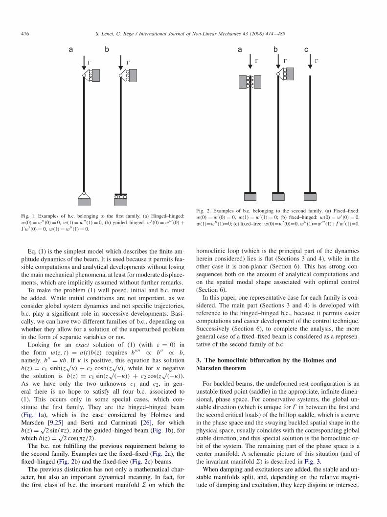
Fig. 1. Examples of b.c. belonging to the first family. (a) Hinged–hinged:w(0) = w′′(0) = 0, w(1) = w′′(1) = 0; (b) guided–hinged: w′(0) = w′′′(0) +�w′(0) = 0, w(1) = w′′(1) = 0.

Eq. (1) is the simplest model which describes the finite am-plitude dynamics of the beam. It is used because it permits fea-sible computations and analytical developments without losingthe main mechanical phenomena, at least for moderate displace-ments, which are implicitly assumed without further remarks.

To make the problem (1) well posed, initial and b.c. mustbe added. While initial conditions are not important, as weconsider global system dynamics and not specific trajectories,b.c. play a significant role in successive developments. Basi-cally, we can have two different families of b.c., depending onwhether they allow for a solution of the unperturbed problemin the form of separate variables or not.

Looking for an exact solution of (1) (with � = 0) inthe form w(z, t) = a(t)b(z) requires b′′′′ ∝ b′′ ∝ b,namely, b′′ = b. If is positive, this equation has solutionb(z) = c1 sinh(z

√) + c2 cosh(z

√), while for negative

the solution is b(z) = c1 sin(z√

(−)) + c2 cos(z√

(−)).As we have only the two unknowns c1 and c2, in gen-eral there is no hope to satisfy all four b.c. associated to(1). This occurs only in some special cases, which con-stitute the first family. They are the hinged–hinged beam(Fig. 1a), which is the case considered by Holmes andMarsden [9,25] and Berti and Carminati [26], for whichb(z) = √

2 sin(�z), and the guided–hinged beam (Fig. 1b), forwhich b(z) = √

2 cos(�z/2).The b.c. not fulfilling the previous requirement belong to

the second family. Examples are the fixed–fixed (Fig. 2a), thefixed–hinged (Fig. 2b) and the fixed-free (Fig. 2c) beams.

The previous distinction has not only a mathematical char-acter, but also an important dynamical meaning. In fact, forthe first class of b.c. the invariant manifold on which the

Γ Γ Γ

Fig. 2. Examples of b.c. belonging to the second family. (a) Fixed–fixed:w(0) = w′(0) = 0, w(1) = w′(1) = 0; (b) fixed–hinged: w(0) = w′(0) = 0,w(1)=w′′(1)=0; (c) fixed–free: w(0)=w′(0)=0, w′′(1)=w′′′(1)+�w′(1)=0.

homoclinic loop (which is the principal part of the dynamicsherein considered) lies is flat (Sections 3 and 4), while in theother case it is non-planar (Section 6). This has strong con-sequences both on the amount of analytical computations andon the spatial modal shape associated with optimal control(Section 6).

In this paper, one representative case for each family is con-sidered. The main part (Sections 3 and 4) is developed withreference to the hinged–hinged b.c., because it permits easiercomputations and easier development of the control technique.Successively (Section 6), to complete the analysis, the moregeneral case of a fixed–fixed beam is considered as a represen-tative of the second family of b.c.

3. The homoclinic bifurcation by the Holmes andMarsden theorem

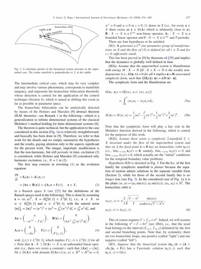
For buckled beams, the undeformed rest configuration is anunstable fixed point (saddle) in the appropriate, infinite dimen-sional, phase space. For conservative systems, the global un-stable direction (which is unique for � in between the first andthe second critical loads) of the hilltop saddle, which is a curvein the phase space and the swaying buckled spatial shape in thephysical space, usually coincides with the corresponding globalstable direction, and this special solution is the homoclinic or-bit of the system. The remaining part of the phase space is acenter manifold. A schematic picture of this situation (and ofthe invariant manifold ) is described in Fig. 3.

When damping and excitations are added, the stable and un-stable manifolds split, and, depending on the relative magni-tude of damping and excitation, they keep disjoint or intersect.


invariant manifold Σ

stable manifold

unstable manifold

saddle x=0homoclinic orbit

Fig. 3. A schematic picture of the dynamical system structure in the unper-turbed case. The center manifold is perpendicular to at the saddle.

The intermediate critical case, which may be very complexand may involve various phenomena, corresponds to manifoldstangency, and represents the homoclinic bifurcation threshold,whose detection is central for the application of the controltechnique (Section 4), which is aimed at shifting this event asfar as possible in parameter space.

The homoclinic bifurcation can be analytically detectedby means of the Holmes and Marsden [9] abstract theorem(H.M. theorem)—see Remark 1 in the following—which is ageneralization to infinite dimensional systems of the classicalMelnikov’s method holding for finite dimensional systems [6].

The theorem is quite technical, but the application to the caseconsidered in this section (Fig. 1a) is relatively straightforward,and basically has been done in [9]. Therefore, we refer to thatwork for the details and we simply summarize the hypothesesand the results, paying attention only to the aspects significantfor the present work. The unique, important, modification isthat the non-harmonic, but still periodic in time, excitation (2)is considered, while Holmes and Marsden [9] considered onlyharmonic excitation, i.e., N = 1 in (2).

The first step consists in rewriting (1) as the evolutionequation

dxdt

= f0(x) + �f1(x, t)

= [Ax + B(x)] + �[A1x + f(t)], x ∈ X, (3)

in a Banach space X (see [27] for the definitions of theBanach spaces used in the following). This is done by assumingx = (w, u)T, X = H 2

0 [0, 1] × L2[0, 1], i.e., x ∈ X ⇔w ∈ H 2

0 [0, 1] and u ∈ L2[0, 1], with the natural norm

‖x‖2X = ‖x‖2 = |w′′|2 + |u|2 = ∫ 1

0 (w′′)2 d� + ∫ 10 u2 d�, and

Ax =(

u

−w′′′′ − �w′′

), B(x) =

( 0

kw′′ ∫ 10 (w′)2 d�

),

A1x =( 0

−�u

), f(t) =

( 0

F(z, t)

), (4)

with fn(z) ∈ L2[0, 1], which implies F(z, t) ∈ L2[0, 1] for allt. Note that A : X ⊃ D(A) → X is an unbounded linear oper-ator (i.e., there not exists a constant c such that ‖Ax‖ < c‖x‖,∀x ∈ D(A)) with domain D(A)={(w, u) ∈ H 4 × H 2|w = 0,

w′′ = 0 and u = 0 at z = 0, 1} dense in X (i.e., for every x ∈X there exists an y ∈ D(A) which is arbitrarily close to x),B : X → X is a C∞ non-linear operator, A1 : X → X is abounded linear operator and f : R → X is C∞ and T-periodic.

There are four hypotheses to be satisfied.(H1). A generates a C0 one parameter group of transforma-

tions on X and the flow of (3) is defined for all t ∈ R and for� > 0 sufficiently small.

This has been proved in [9] by theorems of [25] and impliesthat the dynamics is globally well defined in time.

(H2a). Assume that the unperturbed system is Hamiltonianwith energy H : X → R [� : X × X → R is the weakly non-degenerate (i.e., �(u, v)= 0 for all v implies u = 0) associatedsymplectic form, such that �(f0(x), u) = dH(x) · u].

The symplectic form and the Hamiltonian are

�(x1, x2) = �[(w1, u1), (w2, u2)]

=∫ 1

0(w1u2 − w2u1) d�, (5a)

H(x) = H(w, u) = 1

2|u|2−�

2|w′|2+1

2|w′′|2+k

4|w′|4. (5b)

Note that the symplectic form will play a key role in theMelnikov function derived in the following, which is centralfor the purposes of this work.

(H2b). Assume there exists a symplectic 2-manifold ⊂X invariant under the flow of the unperturbed system andthat on the fixed point x = 0 has an homoclinic orbit xh(t)

(i.e., limt→±∞ xh(t) = 0, namely, limt→±∞ wh(t) = 0 andlimt→±∞ wh(t)= 0, which actually are the “initial” conditionsfor the temporal boundary value problem).

Hypothesis H2b is sketched in Fig. 3. For the b.c. of the firstfamily the symplectic manifold is planar because the equa-tion of motion admits solutions in the separate variable form(Section 2), while for those of the second family this is nolonger true (see Fig. 3). In the considered case of Fig. 1a it isthe plane (w, u) = (a1 sin(�z), a2 sin(�z)), (a1, a2) ∈ R2. Thehomoclinic orbit is

wh(z, t) = ±2

�

√� − �2

k

sin(�z)

cosh(t�√

� − �2),

uh(z, t) = wh(z, t). (6)

This of course requires � > �cr =�2. Indeed, we will assumein the following �2 < � < 4�2 (see (H4)), i.e., that the axialload belongs to the interval [�cr,1, �cr,2] delimited by the firstand second branching points. Note that, by symmetry, thereare two homoclinic loops, one positive (called “right”) and onenegative (called “left”).

(H3). Suppose that the linearized system dxL/dt = [A +�A1]xL + f(t) has a T-periodic solution xL(t, �) such thatxL(t, �) = O(�).


In this case xL(t, �) can be computed exactly:

wL(z, t) =∞∑

j=1

[(N∑

n=1

dnj sin(n�t + �n)

)sin(j�z)

],

uL(z, t) = wL(z, t), (7a)

dnj = � nj√[j2�2(j2�2 − �) − n2�2]2 + (n��)2

,

nj = 2∫ 1

0fn(�) sin(j��) d�,

�n = �n(�n, �, �). (7b)

Eq. (7b) shows that (H3) is satisfied if and only if all the non-resonance conditions

n2�2 �= j2�2(j2�2 − �)

for all n=1, 2, . . ., N, j=2, 3, . . ., ∞ such that nj �=0

(8)

hold. We remark that: (i) There is no non-resonance condi-tion only for j = 1, because of the next assumption (H4)�2 < � < 4�2, namely, the linear stiffness is negative on the firstbuckling mode, positive on the others. This explains why thereis no non-resonance conditions for 1 d.o.f. models based on thefirst buckling mode [9]. (ii) There is a non-resonance conditionto be satisfied only if nj �= 0, i.e., only if the jth buckling modesin(j�z) is excited by the nth term fn(z) of the excitation.

(H4a). For �=0, eT A has a spectrum consisting in two simplereal eigenvalues e±�T , � �= 0, with the rest of the spectrum onthe unit circle.

(H4b). For � > 0, eT (A+�A1) has a spectrum consisting intwo simple real eigenvalues eT �±

� with the rest of the spectrum,��

R , inside the unit circle |z| = 1 and verifying the estimatesC2��dist(��

R, |z| = 1)�C1�, C1, C2 > 0.(H4c). The spectrum of A does not accumulate on 0.A direct computation shows that the eigenvalues of eT (A+�A1)

are eT ��j , where

��j = 1

2 [−�� ±√

(��)2 + j2�2(� − j2�2)]. (9)

The eigenvalues of eT A are eT �0j , while the eigenvalues of A

are �0j . Thus, for the hinged–hinged beam, (H4) is satisfied

if and only if �2 < � < 4�2. Generalizing to other b.c., thishypothesis is satisfied if and only if �cr,1 < � < �cr,2, where�cr,j is the value of � for which �0

j vanishes. Note that the

eigenvalues of A are the complex numbers � satisfying �2w +w′′′′+�w′′=0+b.c. for w(z) �= 0 [9]. Note also that a slightlydifferent, but equivalent, definition of eigenvalues is usedin [28].

This hypothesis implies that for the unperturbed system thesaddle (rest position) has a one dimensional stable and a one-dimensional unstable manifolds, which indeed coincide on thehomoclinic loop, and an infinite dimensional center manifold(see Fig. 3). When the perturbations are added, the stable and

unstable manifolds split, as said, and remain a one dimensionalstrongly stable and a one dimensional unstable manifolds. Thecenter manifold, on the other hand, perturbs to a weakly stablemanifold, so that the whole perturbed stable manifold becomesinfinite dimensional.

The physical interpretation is that the system is dissipativeoutside W u

� (the perturbation of the unstable invariant mani-fold W u), at least in the neighborhood of the saddle, and there-fore it is expected that, if the excitation amplitude is not toohigh, the steady-state dynamics contracts on W s

� (the unionof the perturbation W ss

� of the stable invariant manifold W s

and of the perturbation of the center manifold) due to damp-ing. Thus, the steady state should be “similar” to that of the1 d.o.f. model based on the first buckling mode, at least if theexcitation amplitude is low. It will be proved in the follow-ing that this conjecture is mathematically exact for the b.c. ofthe first family, while it is engineering acceptable for the otherfamily.

Once all the hypotheses have been verified, we are in a po-sition of stating and applying the H.M. theorem.

Let hypotheses (H1–4) hold. Let M(m) = ∫ +∞−∞ �(f0(xh(t)),

f1(xh(t), t +m/�)) dt be the Melnikov’s function. Suppose thatM(m) has a simple zero as a function of m. Then for � suffi-ciently small, the stable W s

� and the unstable W u� manifolds of

the saddle xL(0, �) of the stroboscopic Poincarè map associ-ated with the flow intersect transversally.

Before calculating the Melnikov function, we observethat, roughly speaking, the theorem says that simple zerosof M(m) imply the so-called “Melnikov chaos,” i.e., fractalbasins boundaries, transient chaos, sensitivity to initial con-ditions, onset of the chaotic saddle possibly representing theskeleton for chaotic attractors, etc., which are direct con-sequences of the stable and unstable manifolds intersection[6,7]. The existence of the chaotic attractor is however notguaranteed.

Remark 1. In this paper we identify the homoclinic bifurca-tion, i.e. the first tangency between the perturbed stable andunstable manifolds of the saddle ensuing from the rest position,with the threshold at which the Melnikov function M(m) hasits first (double, and thus non-simple) zero. Technically speak-ing, in many cases we can have Melnikov chaos even belowthis threshold, because when x = 0 has a homoclinic tangle onone side (say, the intersection of W s,l and W u,l is non-trivial),the manifold W u,l winds itself around W u,r, intersecting W s,r

before W u,r does. Thus, the “first” homoclinic tangency on theother side, which would actually correspond to the relevant ho-moclinic bifurcation, does no longer exist. However, it is diffi-cult to estimate the size of this effect, which is typically small,and we consider acceptable our identification from a practicalpoint of view.

With respect to the purposes of control, on the other hand,this fact is unessential. In fact, above the Melnikov thresholdthere certainly exists Melnikov chaos, and thus increasing thisthreshold is worthy in any case, even if some (spurious) chaosmay occur for values of the excitation slightly lower than thiscritical threshold.


After some computations we obtain that the Melnikov func-tions for right and left homoclinic loops are given by

Mr,l(m) = − �∫ ∞

−∞

∫ 1

0w2

h(z, t) dz dt

+∫ ∞

−∞

∫ 1

0wh(z, t)F (z, t + m/�) dz dt

= − 4

3

(� − �2)3/2

k�� ∓

N∑n=1

n1

�√

k

n� cos(nm + �n)

cosh

(n�

2√

� − �2

) .

(10)

It is worth to note that only the terms n1 = 2∫ 1

0 fn(�) sin(��) d� are involved in (10). This is due to the flatness of theinvariant manifold and no longer holds for the second familyof b.c. (see Eq. (41)).

In the following it is convenient to rewrite (10) in the form

Mr,l(m) = const.

[1 ± 11

h11,cr(�)

h(m)

], (11)

where

h11,cr(�) = �

4(� − �2)3/2

3�√

kcosh

(�

2√

� − �2

),

h(m) =N∑

n=1

hn cos(nm + �n),

hn = n1

11

n cosh

(�

2√

� − �2

)

cosh

(n�

2√

� − �2

) . (12)

We prefer to use the representation (11) because we assign 11 the role of overall excitation amplitude, while the relativeamplitudes of the superharmonics n1/ 11 and the phases �n

determine the (temporal) shape of the excitation [12,16]. Theeffects of the superharmonics on the Melnikov functions areinstead governed by the parameters hn, n = 2, 3, . . . , N (notethat h1 = 1, and that the amplitude-free, oscillating part h(m)

of Mr,l(m) is 2�-periodic with zero mean value).According to the H.M. theorem, we have homoclinic inter-

section of the right (left) manifolds if there exists m ∈ [0, 2�]such that Mr,l(m) have simple zeros, respectively. As in [17],we see that the equation Ml(m) = 0 has a simple solution ifand only if

11 > h

11,cr(�)

M l= l

11,cr(�), M l = maxm∈[0,2�]{h(m)}, (13)

while the equation Mr(m) = 0 has a simple solution if andonly if

11 > h

11,cr(�)

M r = r11,cr(�), M r = − min

m∈[0,2�]{h(m)}. (14)

ω

region withhomoclinicintersections

savedregion

γ11,cr

glob

al

one-

side

γ11,cr

2√(Γ−π2)

3√k

2( Γ

−π2 )

δγ 11

7

6

5

4

3

2

1

00

0.5 1 1.5 2.5 3 3.5 42

r,l

h

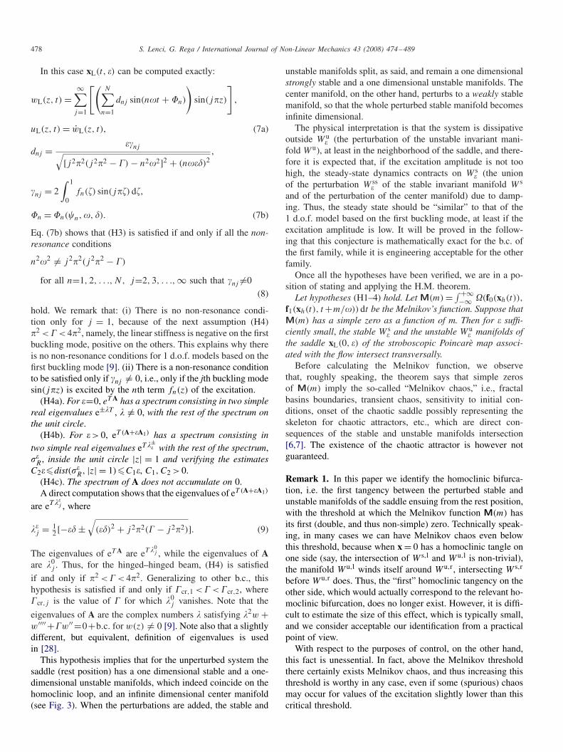
Fig. 4. The curves h11,cr(�) and r,l

11,cr(�) for Gr,l = 1.2732 (optimal global

control with infinite superharmonics) and Gr,l = 2 (optimal one-side controlwith infinite superharmonics).

According to Remark 1, r,l11,cr(�), which are depicted in

Fig. 4 in the frequency/amplitude parameter space (�, 11), areidentified as the homoclinic bifurcation thresholds for the right(left) homoclinic loop. Above these critical curves right (left)homoclinic intersections certainly occur.

In general r11,cr(�) and l

11,cr(�) are distinct (although

they are proportional, being r11,cr(�)/ l

11,cr(�) = M l/M r =const.), and coincide only for the excitations satisfyingM l = max{h(m)} = − min{h(m)} = M r, like, for example, theharmonic excitation (N = 1), for which h(m) = cos(�t + �1)

and M r = M l = 1. These last equalities and (13)–(14) furthershow that the curve h

11,cr(�), which is illustrated in Fig. 4,represents the coinciding right and left homoclinic bifurcationthresholds in the case of harmonic excitation, which is consid-ered as a reference to measure the improvement obtained withcontrol in the next sections.

The strip above h11,cr(�) and below r,l

11,cr(�) is calledsaved (i.e., controlled) region (Fig. 4), and represents the zonewhere the unharmonic excitation is theoretically effective. Itsmaximum enlargement constitutes the objective of the controlmethod.

To quantitatively measure the increment of the critical thresh-olds of the unharmonic excitations with respect to the harmonicreference case we introduce the gains [12,18], which are theratios

Gl = l11,cr(�)

h11,cr(�)

= 1

M l, Gr = r

11,cr(�)

h11,cr(�)

= 1

M r , (15)

and which will be useful in the following.

4. Optimal control

In this section we apply to the buckled beam a method forcontrolling non-linear dynamics and chaos developed by theauthors [12,18] and previously applied only to single d.o.f.


mechanical systems [11,16,17]. Those analyses are herein ex-tended to the infinite dimensional system (1).

The idea of the method is to increase the r,l11,cr(�) thresh-

olds or, equivalently, to enlarge the saved region or increasethe gain. This result is pursued by optimally varying both thespatial (Section 4.1) and temporal (Section 4.2) shapes of theexcitation, and it is what we call “optimal control of homo-clinic bifurcation.” In fact, the two problems can be analyzedseparately.

4.1. “Optimizing” the spatial shape of the excitation

Still referring to the first family of b.c., the optimal choice ofspatial shapes fn(z) of the excitation is based on the observa-tion that, because of the flatness of , only the coefficients n1are involved in the expression of the Melnikov function (10).Accordingly, only the spatial shape of the excitation parallel tothe invariant manifold plays a role in the Melnikov analysis,and then on control. This agrees with the physical considera-tions suggesting that, due to damping, the significant part ofthe dynamics occurs near .

As a consequence, if we assume fn(z) orthogonal to ,i.e., fn(z) = ∑∞

j=2 nj sin(j�z), we have no homoclinic bi-furcation at all, and the problem is meaningless. Thus, fn(z)

must contain at least the term sin(�z). Indeed, we just assumefn(z) = n1 sin(�z), which implies that the useless coefficients nj = 2

∫ 10 fn(�) sin(j��) d�, j = 2, 3, . . . ,∞, vanish identi-

cally. This entails two meaningful circumstances:(i) Being sin(�z) the only spatial component of fn(z) able

to modify the homoclinic bifurcation, this choice permits tominimize the cost of control, because we only use what iseffective.

(ii) Having nj = 0, j = 2, 3, . . . ,∞, the non-resonanceconditions (8) become meaningless, so that the control, whichwould not hold in the present form for the frequencies not sat-isfying Eqs. (8), is applicable everywhere. This is practicallyimportant, because if N is large enough (i.e., if we use a lotof superharmonics, which provide the best optimal gains (seeTables A1 and A2 in Appendix)), the resonant frequencies arealmost dense in R and the control would not be applicableat all.

The previous points show why we consider practically“optimal” the assumption fn(z) = n1 sin(�z). In fact, contraryto what happens with the temporal shape (see Section 4.2), herethe choice does not ensue from a mathematical optimizationproblem, but just from mainly qualitative considerations.

From a practical point of view, the assumption fn(z) = n1 sin(�z) means that we do not excite the vibrating modes;from a theoretical point of view, on the other hand, it meansthat the perturbed manifold � remains planar and coincideswith .

4.2. Optimizing the temporal shape of the excitation

The issues of choosing the optimal temporal shape, i.e. theoptimal superharmonics, is now addressed. It is quite clear from

(13)–(14) that if we want to enlarge as much as possible thesaved region we have to increase the gains (15). However, asshown in [12,17], this requires some care, because the pres-ence of two homoclinic orbits permits to choose among dif-ferent control strategies. Indeed, we can control only the right(left) homoclinic bifurcation, irrespective of what happens tothe other, or we can control simultaneously the right and theleft homoclinic bifurcations.

The two approaches are complementary rather than com-peting [12,17]: the first is aimed at obtaining a topologically“localized” control and provides “large” optimal gains (seeTable A1), whereas the second is aimed at controlling, on av-erage, the “whole” phase space, but provides smaller optimalgains (see Table A2).

4.2.1. “One-side” control of the right (left) homoclinicbifurcation

If we want to increase as much as possible r11,cr ( l

11,cr)

we have to solve the following mathematical problem ofoptimization:

Maximize Gr(Gl) by varying the coefficients hj and �j ,

j = 2, 3, . . . of h(m). (16)

These problems have been solved in [12,16], and the solutionis �j = 0, while the optimal gains and the optimal hj forincreasing number N of added superharmonics are given inTable A1, which refers to the “right” case. The solution ofthe “left” case is that of Table A1 with even coefficients h2j

changed of sign.Table A1 shows that, as expected, the optimal gain is an in-

creasing function of the number N of controlling superharmon-ics. It is bounded from above by 2, which corresponds to the(mostly theoretical) case of infinite superharmonics and showsthat it is possible to double the critical excitation threshold.This limit case is reported in Fig. 4. From a practical point ofview, very satisfactory optimal gains can be obtained with evenfew controlling terms.

Using the coefficients of Table A1 in Eq. (12)2 gives thephysical �-dependent optimal excitations, which for N =2 and3 and in the “right” case are reported below:

F(z, t) = 11 sin(�z)

[sin(�t)

+0.3535cosh[2�/(2

√� − �2)]

2 cosh[�/(2√

� − �2)] sin(2�t)

], (17)

F(z, t)

= 11 sin(�z)

[sin(�t) + 0.5528

cosh[2�/(2√

� − �2)]2 cosh[�/(2

√� − �2)]

× sin(2�t) + 0.1708cosh[3�/(2

√� − �2)]

3 cosh[�/(2√

� − �2)] sin(3�t)

].

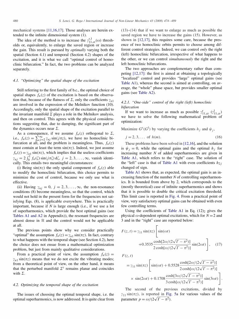
The second of the previous excitations, divided by 11 sin(�z), is reported in Fig. 5a for various values of theparameter p = �/(2

√� − �2).


p=0.1

p=1

p=1.5

p=0.1

p=1

p=1.53

2

1

0

-1

-2

-3

3

2

1

0

-1

-2

0 1 2 3 4 5 6 0 1 2 3 4 5 6

-3

ωt ωt

Fig. 5. The functions F(z, t)/ 11 sin(�z) for various values of the parameter p = �/(2√

� − �2) and for N = 3. (a) Optimal one-side “right” excitation, i.e.,(17)2. Note that in this case there are two controlling superharmonics added to the reference basic harmonic. (b) Optimal global excitation, i.e., (19)1. In thiscase there is only one added superharmonic.

4.2.2. “Global” controlTo control simultaneously the right and the left homoclinic

bifurcations, the right and the left gains, Gr and Gl, must beincreased at the same time. Mathematically, this entails to in-crease their minimum value, namely, to solve the followingoptimization problem:

Maximize G = min{Gr, Gl} by varying the coefficients hj

and �j , j = 2, 3, . . . of h(m). (18)

The solution of (18) is given by �j = 0, h2j = 0 (which auto-matically guarantees that max{h(m)} = − min{h(m)}, i.e., thatGr = Gl) and by the coefficients reported in Table A2 [12,17].

As in the “one-side” control, the optimal gains are still in-creasing functions of N, but now they are strongly lesser thanthose of Table A1, showing how global control is theoreticallyless performant, even in the limit case N = ∞ (see Fig. 4).The counterpart of this drawback is the possibility to controlsimultaneously both homoclinic bifurcations.

By the coefficients of Table A2 and by Eq. (12)2 we cancompute the first two �-dependent optimal physical excitations(N = 3 and 5, respectively):

F(z, t) = 11 sin(�z)

[sin(�t)

−0.1667cosh[3�/(2

√� − �2)]

3 cosh[�/(2√

� − �2)] sin(3�t)

], (19)

F(z, t)

= 11 sin(�z)

[sin(�t) − 0.2323

cosh[3�/(2√

� − �2)]3 cosh[�/(2

√� − �2)]

× sin(3�t) + 0.0610cosh[5�/(2

√� − �2)]

5 cosh[�/(2√

� − �2)] sin(5�t)

].

The first of the previous excitations, divided by 11 sin(�z),is reported in Fig. 5b for various values of the parameter

p = �/(2√

� − �2). By comparing the two pictures of Fig. 5it is possible to note how the one-side optimal excitation has sli-ghtly more pronounced peaks, and that for increasing values ofp the third order superharmonic tends to become predominant.

5. Comparison with the single d.o.f. reduced model

In [17] the control method has been applied to the singled.o.f. approximation of the dynamics of a buckled beam. In thissection we compare the present much more general analysiswith that reported therein.

The single d.o.f. approximation is obtained by the Galerkinmethod by projecting the dynamics onto the planar manifoldspanned by the local stable and unstable directions, which forthe first class of b.c. coincide with . Therefore, we assume

w(z, t) = a(t) sin(�z), (20)

substitute this in (1), multiply by sin(�z) and integrate from 0to 1. This yields the following ODE:

a−�2(�−�2)a+k�4

2a3=�

[N∑

n=1

n1 sin(n�t+�n)−�a

],

n1 = 2∫ 1

0fn(�) sin(��) d�. (21)

Eq. (21) is the classical Duffing equation with negative linearstiffness (being � > �2) which, in a different notation, has beeninvestigated in [17], where it has been shown that the right andleft homoclinic orbits are given by

ah(t) = ±2

�

√� − �2

k

1

cosh(t�√

� − �2). (22)

Eq. (22), together with (20), gives exactly (6). The classical,two-dimensional, Melnikov function [6] can then be computed,which is shown [17] to be exactly given by (10). This provesthat, in the present case, even the single d.o.f. reduced ordermodel is able to exactly capture the homoclinic bifurcation, and


thus the theoretical developments and the practical implemen-tations of the control method are identical for the finite andinfinite dimensional models.

This is a consequence of the flatness of , and no longer holdsfor the second family of b.c. (Section 6). In any case, it must beemphasized that “the full power of the (Holmes and Marsden)theorem is necessary since in the infinite dimensional case,the perturbed manifolds . . . do not lie in ” [9], and thereforethey are only approximated by the single d.o.f. model. Theseperturbations are generic and can be due to external excitationand/or non-linear coupling between different modes, and theirnegligibility, now rigorously proved by the H.M. theorem, couldnot be easily guessed a priori.

Since in the specific case of Fig. 1a, and more generally forthe first family of b.c., the application of the control methodis identical for finite and infinite models, we can take advan-tage of the results in [17], where some numerical simulationsare reported aimed at checking the theoretical predictions andthe practical performance of control. In particular, the one-sideand global controls are numerically compared, and it has beenshown:

(1) The numerical reliability of the Melnikov prediction ofhomoclinic bifurcations, which can be usefully applied inspite of its perturbative nature.

(2) The control induced regularization of fractal basin bound-aries, which confirms the first predicted effect of elimina-tion of the homoclinic bifurcation.

(3) The reduction of fractal erosion of the basins of attractionof confined attractors, which is very useful for reducing thesensitivity to initial conditions.

(4) The effect of control also beyond theoretical expectations,permitting, for example, the delay of the in-well to cross-well chaos transition in the case of one-side control.

6. Different boundary conditions—non-planar manifold �

In this section the more general case of b.c. belonging tothe second family is considered to complete the application ofthe control method to infinite dimensional dynamical systems.The analysis herein developed is general, but to fix ideas, andto make explicit computations, we refer to the fixed–fixed caseof Fig. 2a. Furthermore, we choose � = 40, which belongs tothe interval [�cr,1, �cr,2] = [4�2, 8.183�2] = [39.478, 80.763](Hypothesis (H4) of the H.M. theorem).

6.1. Non-linear normal mode technique for homoclinicsolution

The main difficulty is that the invariant manifold of Hy-pothesis (H2b) is not planar and it is difficult to be handled.To overcome this point, the non-linear normal modes techniqueis used [3,29,30]. Together with other related methods, suchas the approximate inertial manifold and the proper orthogo-nal modes, it is one powerful technique developed to obtainreliable reduced order models, which is a matter of intensiveon-going research (see also a recently published Special Issue

0 0.1 0.2 0.3 0.4 0.5 0.6 0.7 0.8 0.9 1-2

-1.5

-1

-0.5

0

0.5

1

1.5

2

z

wj (z

)

Fig. 6. The first five normalized eigenfunctions wj (z) of the fixed–fixed casefor � = 40. Continuous lines are odd eigenfunctions, and dashed lines areeven eigenfunctions.

[22]). Although these techniques were originally developed todeal with non-linear oscillations, in this paper their applicationis concerned with homoclinic orbits [28].

To apply the method, the first N eigenfunctions of the linearoperator A are required. Because A is self-adjoint and its do-main is dense, we get the exact manifold in the limit N →∞. For w(0) = w′(0) = w(1) = w′(1) = 0 and for � = 40 thefirst five eigenvalues of A are

�1 = 2.620687, �2 = 44.085549i, �3 = 103.232438i,

�4 = 181.871769i, �5 = 280.309519i, (23)

while the expressions of the associated eigenfunctions are givenin Appendix (Eq. (A.1)), and are depicted in Fig. 6. Theyhave been normalized with

∫ 10 [wj(�)]2 d� = 1, which simpli-

fies the inertial terms in the following expression (25) of theHamiltonian.

Note that, according to � ∈ [�cr,1, �cr,2], only the first eigen-value is real, while the others are purely imaginary. This prop-erty, in particular, guarantees that the infinite non-resonanceconditions n2�2

1 �= �2n, n = 2, 3, 4 . . . , which are required for

the validity of the procedure, as shown in [28], are automati-cally satisfied.

Due to symmetric b.c., eigenfunctions with odd index aresymmetric (i.e., w(0.5 + �) = w(0.5 − �), see the continuouslines in Fig. 6), while those with even index are anti-symmetric(i.e., w(0.5 + �) = −w(0.5 − �), see the dashed curves inFig. 6). Consequently, the odd eigenfunctions span the sym-metric part of the domain of A, while the even eigenfunctionsspan its complement, i.e., the anti-symmetric part of the config-uration space. As the homoclinic solutions are expected to bespatially symmetric, because they approach the unstable sym-metric eigenfunction w1(z) for t → ∞, we neglect the eveneigenfunctions. This has no consequences on the expected so-lution since even and odd terms are not coupled in the reduced


order Hamiltonian, so that a solution initially symmetric re-mains symmetric for all times.

Accordingly, we directly assume a2j = 0, j = 1, 2, . . . , andlook for the solution in the form

w(z, t) = a1(t)w1(z) + a3(t)w3(z) + a5(t)w5(z) + · · · ,

u(z, t) = w(z, t). (24)

In the following we consider terms only up to w5(z) to limitthe computations, but of course the analysis can be triviallyextended. By substituting (24) in the Hamilton function (5b)we get

H = 0.5(a21 + a2

3 + a25) + (−3.43400a2

1 + 5328.47013a23

+ 39296.0690a25) + k(6.58790a2

1 + 49.53020a23

+ 132.04221a25 − 12.58343a1a3 − 7.67163a1a5

− 26.57427a3a5)2

= 0.5(a21 + a2

3 + a25) + V (a1, a3, a5). (25)

The equation of motion can then be obtained by the classicalHamiltonian formalism from (25)

aj = − �V

�aj

, (26)

and it is trivial to show that they admit the saddle equilibriumpoint aj = 0 with H = 0.

Generalizing the treatment of [31] (see also the introductorypaper in [22] for an overall framework), we identify a main,or master, variable (i.e. modal amplitude) x and consider theothers as secondary, or slave, variables (higher order modalamplitudes) yi . Because in the buckled beam problem the un-stable direction triggering the homoclinic orbit is just along thefirst eigenfunction, it is natural to assume x = a1 and y1 = a3,y2 = a5 and so on. Eq. (26) then become

x = −�V

�x, yi = −�V

�yi

. (27)

The key idea of the method consists in assuming that theslave variables can be expressed as time-independent functionsof the master one:

yi = yi(x). (28)

If we use only N terms in (24), relation (28) provides anapproximation of the searched manifold (approximate man-ifold), while for N → ∞ it exactly gives (exact manifold).We will see that, in general, few terms are indeed sufficient topractically give an adequate approximation of .

Differentiating (28) with respect to time we get, by the chainrule,

yi = dyi

dt= dyi

dx

dx

dt= y′

i x, yi = y′′i x2 + y′

i x. (29)

Combining (29)2 with (27) yields

�V

�yi

= −y′′i x2 + y′

i

�V

�x. (30)

To apply the previous general treatment to the homoclinicorbit, we note that on these solutions we have H = 0, namely,

0 =(

x2 +N−1∑i=1

y2i

)+ 2V (x, yi(x))

= x2

[1 +

N−1∑i=1

(y′i )

2

]+ 2V (x, yi(x)). (31)

From (30) and (31) we can eliminate x and finally get thestrongly non-linear ODEs permitting to determine the unknownfunctions (28):

2Vy′′i +

[1 +

N−1∑i=1

(y′i )

2

](y′i

�V

�x− �V

�yi

)= 0. (32)

Eq. (32) are the slave amplitudes equations which particu-larize the modal equations of Rand [31]. Indeed, they are muchmore complex than the original system (27), and its introductionmay appear useless. Notwithstanding, it contains only polyno-mial terms, and it is natural to look for a relevant solution inthe Taylor series form [28]

yi = 1√k[yi,1(x

√k) + yi,3(x

√k)3 + yi,5(x

√k)5

+ yi,7(x√

k)7 + · · ·], (33)

where even terms have not been considered because of thesymmetry of the system, which requires that if w(z, t) is asolution of (1), so is −w(z, t). Moreover, the constant termvanishes also because the manifold contains the trivial saddle,i.e., yi(0) = 0. The parameter k has been explicitly singled outin (33) to have k independent numbers yi,l .

To determine the unknowns yi,l , we substitute (33) in (32)and expand in Taylor series. Equating to zero the coefficientsof x we get

ci

⎡⎣1 +

N−1∑j=1

(yj,1)2

⎤⎦ yi,1 = 0 (34)

(ci are constants different from zero). Since complex values ofyi,1 cannot be accepted, the unique solution of (34) is yi,1 = 0.This shows that, in a neighborhood of x =0, a unique manifold is detected by this technique, and that it cubically approachesits tangent manifold at x = 0. Thus, the non-flatness of isexpected to be engineering important only “far enough” fromthe saddle.

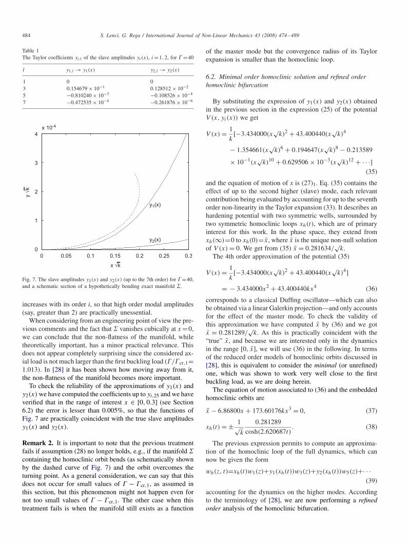
Equating to zero the coefficients of the successive powersof x we get a recursive series of linear algebraic equationspermitting to determine the remaining constants yi,l . The firstfew of them are reported in Table 1, and they are used inFig. 7 to draw the solutions y1(x) and y2(x).

Several conclusions can be drawn from Table 1 and Fig. 7.The most important is that, at least for the considered valueof �, the slave variables are orders of magnitude lesser thanthe master one. Furthermore, the degree of smallness of yi(x)


Table 1The Taylor coefficients yi,l of the slave amplitudes yi(x), i =1, 2, for �=40

l y1,l → y1(x) y2,l → y2(x)

1 0 03 0.154679 × 10−1 0.128512 × 10−2

5 −0.810240 × 10−3 −0.108526 × 10−4

7 −0.472535 × 10−4 −0.261876 × 10−6

0 0.05 0.1 0.15 0.2 0.25 0.3

0

1

2

3

4

x 10-4

y1(x)

y2(x)

y √

k

x √k

Fig. 7. The slave amplitudes y1(x) and y2(x) (up to the 7th order) for �=40,and a schematic section of a hypothetically bending exact manifold .

increases with its order i, so that high order modal amplitudes(say, greater than 2) are practically unessential.

When considering from an engineering point of view the pre-vious comments and the fact that vanishes cubically at x =0,we can conclude that the non-flatness of the manifold, whiletheoretically important, has a minor practical relevance. Thisdoes not appear completely surprising since the considered ax-ial load is not much larger than the first buckling load (�/�cr,1=1.013). In [28] it has been shown how moving away from it,the non-flatness of the manifold becomes more important.

To check the reliability of the approximations of y1(x) andy2(x) we have computed the coefficients up to yi,25 and we haveverified that in the range of interest x ∈ [0, 0.3] (see Section6.2) the error is lesser than 0.005%, so that the functions ofFig. 7 are practically coincident with the true slave amplitudesy1(x) and y2(x).

Remark 2. It is important to note that the previous treatmentfails if assumption (28) no longer holds, e.g., if the manifold containing the homoclinic orbit bends (as schematically shownby the dashed curve of Fig. 7) and the orbit overcomes theturning point. As a general consideration, we can say that thisdoes not occur for small values of � − �cr,1, as assumed inthis section, but this phenomenon might not happen even fornot too small values of � − �cr,1. The other case when thistreatment fails is when the manifold still exists as a function

of the master mode but the convergence radius of its Taylorexpansion is smaller than the homoclinic loop.

6.2. Minimal order homoclinic solution and refined orderhomoclinic bifurcation

By substituting the expression of y1(x) and y2(x) obtainedin the previous section in the expression (25) of the potentialV (x, yi(x)) we get

V (x) = 1

k[−3.434000(x

√k)2 + 43.400440(x

√k)4

− 1.354661(x√

k)6 + 0.194647(x√

k)8 − 0.213589

× 10−1(x√

k)10 + 0.629506 × 10−3(x√

k)12 + · · ·](35)

and the equation of motion of x is (27)1. Eq. (35) contains theeffect of up to the second higher (slave) mode, each relevantcontribution being evaluated by accounting for up to the seventhorder non-linearity in the Taylor expansion (33). It describes anhardening potential with two symmetric wells, surrounded bytwo symmetric homoclinic loops xh(t), which are of primaryinterest for this work. In the phase space, they extend fromxh(∞)=0 to xh(0)= x, where x is the unique non-null solutionof V (x) = 0. We get from (35) x = 0.281634/

√k.

The 4th order approximation of the potential (35)

V (x) = 1

k[−3.434000(x

√k)2 + 43.400440(x

√k)4]

= − 3.434000x2 + 43.400440kx4 (36)

corresponds to a classical Duffing oscillator—which can alsobe obtained via a linear Galerkin projection—and only accountsfor the effect of the master mode. To check the validity ofthis approximation we have computed x by (36) and we gotx = 0.281289/

√k. As this is practically coincident with the

“true” x, and because we are interested only in the dynamicsin the range [0, x], we will use (36) in the following. In termsof the reduced order models of homoclinic orbits discussed in[28], this is equivalent to consider the minimal (or unrefined)one, which was shown to work very well close to the firstbuckling load, as we are doing herein.

The equation of motion associated to (36) and the embeddedhomoclinic orbits are

x − 6.86800x + 173.60176kx3 = 0, (37)

xh(t) = ± 1√k

0.281289

cosh(2.620687t). (38)

The previous expression permits to compute an approxima-tion of the homoclinic loop of the full dynamics, which cannow be given the form

wh(z, t)=xh(t)w1(z)+y1(xh(t))w3(z)+y2(xh(t))w5(z)+· · ·(39)

accounting for the dynamics on the higher modes. Accordingto the terminology of [28], we are now performing a refinedorder analysis of the homoclinic bifurcation.


Using this expression in the Melnikov function of the H.M.theorem we get, after some computations

Mr,l(m) = − �∫ ∞

−∞

∫ 1

0w2

h(z, t) dz dt

+∫ ∞

−∞

∫ 1

0wh(z, t)F (z, t + m/�) dz dt

= − �

k�0 ∓

N∑n=1

n� cos(nm + �n)

× n1�1(n�) + n3�3(n�) + n5�5(n�) + · · ·√k

,

(40)

where

�0 = k

{∫ ∞

−∞x2

h(t) dt +∫ ∞

−∞x2

h(t)[y′1(xh(t))]2 dt

+∫ ∞

−∞x2

h(t)[y′2(xh(t))]2 dt + · · ·

}

nj =∫ 1

0fn(�)wj (�) d�,

�1(�) = √k

∫ ∞

−∞xh(t) cos(�t) dt ,

�3(�) = √k

∫ ∞

−∞y1(xh(t)) cos(�t) dt ,

�5(�) = √k

∫ ∞

−∞y2(xh(t)) cos(�t) dt, . . . . (41)

Note that the constant �0 and the functions �j (�) do not ac-tually depend on k. They are even functions of �, and in theinterval [0, +∞[ they are monotonically decreasing and expo-nentially approach zero for � → ∞.

6.3. Comparisons: flat vs non-flat manifolds, infinite vs finitedimensional models

Expressions (40) and (41) make explicit the contribution ofnon-flatness of to the homoclinic bifurcation, which is takeninto account by the terms containing yi(x), which are missingin (10). There are contributions both in the constant part �0 andin the oscillating part of the Melnikov functions, due to �3(�),�5(�), . . . , and measured by the coefficients n3, n5, . . . .

To quantitatively measure these contributions, expressions(41) must be determined explicitly. �0 and �1(�) can becomputed exactly, and in the reference case � = 40 they aregiven by

�0 = {0.603839 × 10−1 + 0.428994 × 10−6

+ 0.299111 × 10−8 + · · ·}

�1(�) = 0.337200

cosh(0.599383�). (42)

The coefficients �j (�), j > 2, on the other hand, can be eval-uated only numerically. Therefore, supported by the fact that�j (�) are monotonically decreasing in [0, +∞[, we consideronly the maximum values �j (0) of each function �j (�), whichare given below (�1(0) is reported for comparison):

�1(0) = 0.337200, �3(0) = 0.205702 × 10−3,

�5(0) = 0.171352 × 10−4. (43)

Once more, we have found that the non-flatness of ,while having theoretical relevance, gives contributions to theMelnikov functions which are orders of magnitude smallerthan its flat approximation (given by the dominant terms andobtained by the one d.o.f. linear Galerkin approximation),and it is negligible from an engineering point of view for theconsidered parameters.

The previous considerations not only permit to conclude thatthe non-flatness of can be neglected, but also that the bifurca-tion analysis based on the 1D reduced order model (accountingfor only the first term of �0 and for �1) gives the “same” re-sults as the infinite dimensional analysis. This conclusion wasobtained also in Section 5 for the case of flat , but here, likethere, it is important to stress that the full powerfulness of theH.M. theorem is necessary to take into account out of mani-fold perturbations, even if it has been shown a posteriori thatthey are practically negligible, a fact that could not easily beguessed a priori.

The difference is that for flat the one d.o.f. model givesmathematically correct results in terms of Melnikov functions(Section 5), while for non-flat it gives practically correct re-sults, so that the theoretical background is different. However,it can be expected that, moving away from the first bucklingload—which would entail considering a refined homoclinic or-bit [28]—could evidence more marked differences of homo-clinic bifurcation herein considered with respect to the linearGalerkin approximation.

6.4. Optimal control

Following the guidelines of Section 4, the application of theoptimal control method to the second family of b.c. is nowdiscussed.

The influence of the spatial shape of the excitation isconsidered first. As in Section 4.1, we assume the spatialshape of each time component equal to the first eigenfunc-tion, fn(z) = n1w1(z). This implies that the coefficients nj = ∫ 1

0 fn(�)wj (�) d�, j = 3, 5, . . . , vanish, and permits toexactly (i.e. irrespective of engineering considerations) elimi-nate the influence of the non-flatness of on the oscillatingpart of the Melnikov functions. The influence of the non-flatness of , however, has not been completely removed bythis choice, because it remains in the constant part �0, whereit is unavoidable.

In addition to the previous properties, and as in Section 4.1,the choice nj = 0, j = 3, 5, . . . , permits to get rid of thenon-resonance conditions (8) of hypothesis (H3), and thus con-tributes to enlarge the range of applicability of the method.


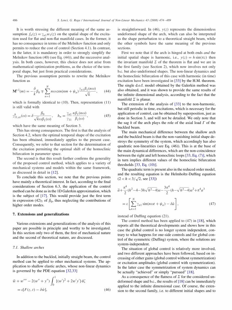
It is worth stressing the different meaning of the same as-sumption fn(z) = n1w1(z) on the spatial shape of the excita-tion used for flat and non-flat manifold cases. In the former, ithas no consequence in terms of the Melnikov function and onlypermits to reduce the cost of control (Section 4.1). In contrast,in the latter, it is mandatory in order to strongly simplify theMelnikov function (40) (see Eq. (44)), and the successive anal-ysis. In both cases, however, this choice does not arise frommathematical optimization problems, as the choice of the tem-poral shape, but just from practical considerations.

The previous assumption permits to rewrite the Melnikovfunction as

Mr,l(m) = −�

k�0 ∓

N∑n=1

n� cos(nm + �n) n1�1(n�)√

k, (44)

which is formally identical to (10). Then, representation (11)is still valid with

h11,cr(�) = �

�0√k��1(�)

, hn = n1

11

n�1(n�)

�1(�), (45)

which have the same meaning of Section 3.This has strong consequences. The first is that the analysis of

Section 4.2, where the optimal temporal shape of the excitationhas been obtained, immediately applies to the present case.Consequently, we refer to that section for the determination ofthe excitation permitting the optimal shift of the homoclinicbifurcation in parameter space.

The second is that this result further confirms the generalityof the proposed control method, which applies to a variety ofmechanical systems and models within the same framework,as discussed in detail in [12].

To conclude this section, we note that the previous pointshave mainly a theoretical interest. In fact, according to the finalconsiderations of Section 6.3, the application of the controlmethod can be done as in the 1D Galerkin approximation, whichis the subject of [17]. This would provide just the first termin expression (42)1 of �0, thus neglecting the contributions ofhigher order modes.

7. Extensions and generalizations

Various extensions and generalizations of the analysis of thispaper are possible in principle and worthy to be investigated.In this section only two of them, the first of mechanical natureand the second of theoretical nature, are discussed.

7.1. Shallow arches

In addition to the buckled, initially straight beam, the controlmethod can be applied to other mechanical systems. The ap-plication to shallow elastic arches, whose non-linear dynamicsis governed by the PDE equation [32,33]

w + w′′′′ − 2(w′′ + y′′)∫ 1

0[(w′)2 + 2w′y′] d�

= �[F(z, t) − �w], (46)

is straightforward. In (46), y(z) represents the dimensionlessundeformed shape of the arch, which can also be interpretedas the shape perturbation to a theoretical straight beam, whilethe other symbols have the same meaning of the previoussections.

First we note that if the arch is hinged at both ends and theinitial spatial shape is harmonic, i.e., y(z) = h sin(�z) thenthe invariant manifold of the theorem is flat and we are inthe first family (see Section 2), which now involves not onlyb.c. but also undeformed shapes. The non-linear dynamics andthe homoclinic bifurcation of this case with harmonic (in time)excitation have been investigated in [33] by the H.M. theorem.The single d.o.f. model obtained by the Galerkin method wasalso obtained, and it was shown to provide the same results ofthe infinite dimensional analysis, according to the fact that themanifold is planar.

The extension of the analysis of [33] to the non-harmonic,but still periodic in time, excitations, which is necessary for theapplication of control, can be obtained by superposition, just asdone in Section 3, and will not be detailed. We only note thatthe sag h of the arch plays the role of the axial load � of thebuckled beam.

The main mechanical difference between the shallow archand the buckled beam is that the non-vanishing initial shape de-stroys the symmetry of the system, which accordingly has alsoquadratic non-linearities (see Eq. (46)). This is at the base ofthe main dynamical differences, which are the non-coincidencebetween the right and left homoclinic loops [33, Eq. (7)], whichin turn implies different values of the homoclinic bifurcationthresholds [33, Eq. (10)].

The quadratic term is present also in the reduced order model,and the resulting equation is the Helmholtz-Duffing equation(2 < h < 3/

√2, see [33])

a+�4

2(h2−4−3h

√h2−4)a−3�4

2(h−

√h2−4)a2+�4a3

= �

[N∑

n=1

n1 sin(n�t + �n) − �a

], (47)

instead of Duffing equation (21).The control method has been applied to (47) in [18], which

reports all the theoretical developments and shows how in thiscase the global control is no longer system independent, con-trary to what happens for one-side controls and for global con-trol of the symmetric (Duffing) system, where the solutions aresystem-independent.

The situation of global control is relatively more involved,and two different approaches have been followed, based on in-creasing of either gains (global control without symmetrization)or excitation amplitudes (global control with symmetrization).In the latter case the symmetrization of system dynamics canbe actually “achieved” or simply “pursued” [18].

As a consequence of the flatness of for the considered un-deformed shape and b.c., the results of [18] can be immediatelyapplied to the infinite dimensional case. Of course, the exten-sion to the second family, i.e. to different initial shapes and to


different b.c., requires an analysis similar to that of Section 6,and will not be pursued here.

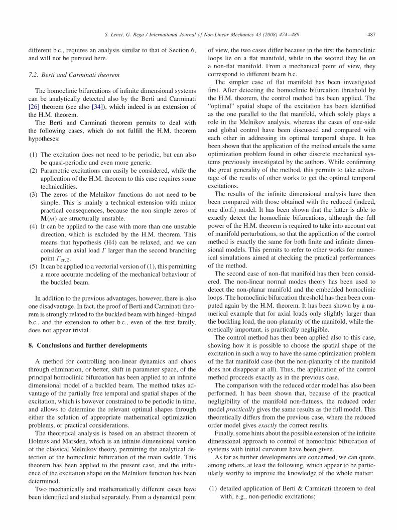
7.2. Berti and Carminati theorem

The homoclinic bifurcations of infinite dimensional systemscan be analytically detected also by the Berti and Carminati[26] theorem (see also [34]), which indeed is an extension ofthe H.M. theorem.

The Berti and Carminati theorem permits to deal withthe following cases, which do not fulfill the H.M. theoremhypotheses:

(1) The excitation does not need to be periodic, but can alsobe quasi-periodic and even more generic.

(2) Parametric excitations can easily be considered, while theapplication of the H.M. theorem to this case requires sometechnicalities.

(3) The zeros of the Melnikov functions do not need to besimple. This is mainly a technical extension with minorpractical consequences, because the non-simple zeros ofM(m) are structurally unstable.

(4) It can be applied to the case with more than one unstabledirection, which is excluded by the H.M. theorem. Thismeans that hypothesis (H4) can be relaxed, and we canconsider an axial load � larger than the second branchingpoint �cr,2.

(5) It can be applied to a vectorial version of (1), this permittinga more accurate modeling of the mechanical behaviour ofthe buckled beam.

In addition to the previous advantages, however, there is alsoone disadvantage. In fact, the proof of Berti and Carminati theo-rem is strongly related to the buckled beam with hinged–hingedb.c., and the extension to other b.c., even of the first family,does not appear trivial.

8. Conclusions and further developments

A method for controlling non-linear dynamics and chaosthrough elimination, or better, shift in parameter space, of theprincipal homoclinic bifurcation has been applied to an infinitedimensional model of a buckled beam. The method takes ad-vantage of the partially free temporal and spatial shapes of theexcitation, which is however constrained to be periodic in time,and allows to determine the relevant optimal shapes througheither the solution of appropriate mathematical optimizationproblems, or practical considerations.

The theoretical analysis is based on an abstract theorem ofHolmes and Marsden, which is an infinite dimensional versionof the classical Melnikov theory, permitting the analytical de-tection of the homoclinic bifurcation of the main saddle. Thistheorem has been applied to the present case, and the influ-ence of the excitation shape on the Melnikov function has beendetermined.

Two mechanically and mathematically different cases havebeen identified and studied separately. From a dynamical point

of view, the two cases differ because in the first the homoclinicloops lie on a flat manifold, while in the second they lie ona non-flat manifold. From a mechanical point of view, theycorrespond to different beam b.c.

The simpler case of flat manifold has been investigatedfirst. After detecting the homoclinic bifurcation threshold bythe H.M. theorem, the control method has been applied. The“optimal” spatial shape of the excitation has been identifiedas the one parallel to the flat manifold, which solely plays arole in the Melnikov analysis, whereas the cases of one-sideand global control have been discussed and compared witheach other in addressing its optimal temporal shape. It hasbeen shown that the application of the method entails the sameoptimization problem found in other discrete mechanical sys-tems previously investigated by the authors. While confirmingthe great generality of the method, this permits to take advan-tage of the results of other works to get the optimal temporalexcitations.

The results of the infinite dimensional analysis have thenbeen compared with those obtained with the reduced (indeed,one d.o.f.) model. It has been shown that the latter is able toexactly detect the homoclinic bifurcations, although the fullpower of the H.M. theorem is required to take into account outof manifold perturbations, so that the application of the controlmethod is exactly the same for both finite and infinite dimen-sional models. This permits to refer to other works for numer-ical simulations aimed at checking the practical performancesof the method.

The second case of non-flat manifold has then been consid-ered. The non-linear normal modes theory has been used todetect the non-planar manifold and the embedded homoclinicloops. The homoclinic bifurcation threshold has then been com-puted again by the H.M. theorem. It has been shown by a nu-merical example that for axial loads only slightly larger thanthe buckling load, the non-planarity of the manifold, while the-oretically important, is practically negligible.

The control method has then been applied also to this case,showing how it is possible to choose the spatial shape of theexcitation in such a way to have the same optimization problemof the flat manifold case (but the non-planarity of the manifolddoes not disappear at all). Thus, the application of the controlmethod proceeds exactly as in the previous case.

The comparison with the reduced order model has also beenperformed. It has been shown that, because of the practicalnegligibility of the manifold non-flatness, the reduced ordermodel practically gives the same results as the full model. Thistheoretically differs from the previous case, where the reducedorder model gives exactly the correct results.

Finally, some hints about the possible extension of the infinitedimensional approach to control of homoclinic bifurcation ofsystems with initial curvature have been given.

As far as further developments are concerned, we can quote,among others, at least the following, which appear to be partic-ularly worthy to improve the knowledge of the whole matter:

(1) detailed application of Berti & Carminati theorem to dealwith, e.g., non-periodic excitations;


(2) physical experiments;(3) more involved mechanical models of the beam;(4) parametric excitations.

Appendix A

In this appendix some results used in the text are reported.Tables A1 and A2 have been obtained in [12,17].The normalized eigenfunctions of Section 6.1, depicted in

Fig. 6, are analytically given by

w1(z) = − 0.011200 sin(6.31091z) − 0.80798 cos(6.31091z)

+ 0.17021 sin(0.41526z) + 0.80798 cos(0.41526z),

w2(z) = 0.72180 sin(8.27104z) − 1.10927 cos(8.27104z)

−1.12007 sinh(5.33011z)+1.10927 cosh(5.33011z),

w3(z) = 0.88169 sin(11.18713z) − 1.06911 cos(11.18713z)

−1.06890 sinh(9.22778z)+1.06911 cosh(9.22778z),

w4(z) = 0.93579 sin(14.24669z) − 1.04433 cos(14.24669z)

− 1.04434 sinh(12.76590z)

+ 1.04433 cosh(12.76590z),

Table A1The numerical results of various optimization problems with increasing finite number of superharmonics in the case of one-side right control

N GN h2 h3 h4 h5 h6 h7 h8 h9

2 1.4142 0.3535533 1.6180 0.552756 0.1707894 1.7321 0.673525 0.333274 0.0961755 1.8019 0.751654 0.462136 0.215156 0.0596326 1.8476 0.807624 0.567084 0.334898 0.153043 0.0424227 1.8794 0.842528 0.635867 0.422667 0.237873 0.103775 0.0273238 1.9000 0.872790 0.706011 0.527198 0.355109 0.205035 0.091669 0.0244749 1.9130 0.877014 0.705931 0.518632 0.341954 0.195616 0.091497 0.031316 0.005929. . . . . . . . . . . . . . . . . . . . . . . . . . . . . .

∞ 2 1 1 1 1 1 1 1 1

Table A2The numerical results of various optimization problems with increasing finite number of superharmonics in the case of global control of symmetric systems

N GN h3 h5 h7 h9 h11 h13 h15

3 1.1547 −0.1666675 1.2071 −0.232259 0.0609877 1.2310 −0.264943 0.100220 −0.0288979 1.2440 −0.284314 0.125257 −0.053460 0.016365

11 1.2518 −0.296177 0.141769 −0.071125 0.031854 −0.00996913 1.2568 −0.304101 0.153247 −0.083936 0.044376 −0.020352 0.00642015 1.2597 −0.307322 0.156798 −0.087358 0.047836 −0.024047 0.010154 −0.002998. . . . . . . . . . . . . . . . . . . . . . . . . . .

∞ 1.2732 −1/3 1/5 −1/7 1/9 −1/11 1/13 −1/15

w5(z) = 0.95954 sin(17.34999z) − 1.03044 cos(17.34999z)

− 1.03044 sinh(16.15618z)

+ 1.03044 cosh(16.15618z). (A.1)

References

[1] G. Rega, W. Lacarbonara, A.H. Nayfeh, C.M. Chin, Multiple resonancesin suspended cables: direct versus reduced-order models, Int. J. Non-linear Mech. 45 (5) (1999) 901–924.

[2] I. Blekhman, Vibrational Mechanics, World Scientific, Singapore,London, Hong Kong, 2000.

[3] A.H. Nayfeh, Nonlinear Interactions, Wiley Interscience, New York,2000.

[4] A. Steindl, H. Troger, Methods for dimension reduction and theirapplication in nonlinear dynamics, Int. J. Solids Struct. 38 (2001)2131–2147.

[5] D.E. Kirk, Optimal Control Theory: An Introduction, Dover Publications,Mineola, New York, 2004.

[6] J. Guckenheimer, P. Holmes, Nonlinear Oscillations, Dynamical Systemsand Bifurcation of Vector Fields, Springer, New York, 1983.

[7] P.J. Holmes, F.C. Moon, Strange attractors and chaos in nonlinearmechanics, ASME J. Appl. Mech. 50 (1983) 1021–1032.

[8] J.M.T. Thompson, H.B. Stewart, Nonlinear Dynamics and Chaos, Wiley,New York, 1986.

[9] P. Holmes, J. Marsden, A partial differential equation with infinitelymany periodic orbits: chaotic oscillations of a forced beam, Arch. Ration.Mech. Anal. 76 (1981) 135–165.

[10] S. Wiggins, Global Bifurcation and Chaos: Analytical Methods, Springer,New York, Heidelberg, Berlin, 1988.

[11] S. Lenci, G. Rega, Controlling nonlinear dynamics in a two-well impactsystem. Parts I & II, Int. J. Bifurcat. Chaos 8 (1998) 2387–2424.


[12] S. Lenci, G. Rega, A unified control framework of the nonregulardynamics of mechanical oscillators, J. Sound Vibr. 278 (2004)1051–1080.

[13] G. Chen, X. Dong, From Chaos to Order: Methodologies Perspectivesand Applications, World Scientific, Singapore, 1998.

[14] E. Ott, C. Grebogi, J.A. Yorke, Controlling chaos, Phys. Rev. Lett. E64 (1990) 1196–1199.

[15] A.L. Fradkov, Chaos Control Bibliography (1997–2000), Russian Sys-tems and Control Archive (RUSYCON), 2000, 〈www.rusycon.ru/chaos-control.html/〉.

[16] S. Lenci, G. Rega, Optimal control of homoclinic bifurcation: theoreticaltreatment and practical reduction of safe basin erosion in the Helmholtzoscillator, J. Vibr. Control 9 (2003) 281–316.

[17] S. Lenci, G. Rega, Optimal control of nonregular dynamics in a Duffingoscillator, Nonlinear Dyn. 33 (2003) 71–86.

[18] S. Lenci, G. Rega, Global optimal control and system-dependentsolutions in the hardening Helmholtz–Duffing oscillator, Chaos SolitonsFractals 21 (2004) 1031–1046.

[19] S. Lenci, G. Rega, Control of pull-in dynamics in a nonlinearthermoelastic electrically actuated microbeam, J. Micromech. Microeng.16 (2006) 390–401.

[20] H. Cao, Primary resonant optimal control for homoclinic bifurcations insingle-degree-of-freedom nonlinear oscillators, Chaos Solitons Fractals24 (5) (2005) 1387–1398.

[21] H. Troger, A. Steindl, Nonlinear Stability and Bifurcation Theory,Springer, Wien, 1991.

[22] G. Rega, H. Troger, Dimension reduction of dynamical systems: methods,models, applications, Nonlinear Dyn. 41 (Special issue) (2005).

[23] H.N. Arafat, A.H. Nayfeh, Non-linear responses of suspended cables toprimary resonance excitations, J. Sound Vibr. 266 (2003) 325–354.

[24] P. Villaggio, Mathematical Models for Elastic Structures, CambridgeUniversity Press, Cambridge, 1997.

[25] P. Holmes, J. Marsden, Bifurcation to divergence and flutter in flowinduced oscillations: an infinite dimensional analysis, Automatica 14(1978) 367–384.

[26] M. Berti, C. Carminati, Chaotic dynamics for perturbations of infinitedimensional Hamiltonian systems, Nonlinear Anal. 48 (2002) 481–504.

[27] H. Brezis, Analyse fonctionnelle. Théorie et Applications, Masson, Paris,1983.

[28] S. Lenci, G. Rega, Dimension reduction of homoclinic orbits of buckledbeams via nonlinear normal modes technique, Int. J. Non-Linear Mech.42 (3) (2007) 515–528.

[29] S.W. Shaw, C. Pierre, Normal modes for nonlinear vibratory systems,J. Sound Vibr. 164 (1993) 85–124.

[30] A.F. Vakakis, L.I. Manevitch, Y.V. Mikhlin, V.N. Pilipchuck, A.A. Zevin,Normal Modes and Localization in Nonlinear Systems, Wiley, New York,1996.

[31] H.R. Rand, Lecture Notes on Nonlinear Vibrations, Cornell University,Available on line at 〈www.tam.cornell.edu/randdocs/〉, 2003.

[32] Y.C. Fung, A. Kaplan, Buckling of low arches or curved beams of smallcurvature, U.S. National Advisory Committee for Aeronautics, TechnicalNote 2840, 1952.

[33] S. Lenci, A.M. Tarantino, Dynamics of shallow elastic arches. Part I:chaotic response of harmonically shaped arches, Eur. J. Mech. A/Solids15 (1996) 513–528.

[34] F. Alessio, C. Carminati, P. Montecchiari, Heteroclinic motions joiningalmost periodic solutions for a class of Lagrangian systems, DiscreteContin. Dyn. Syst. 5 (1999) 569–584.

http://www.rusycon.ru/chaos-control.html/

http://www.rusycon.ru/chaos-control.html/

http://www.tam.cornell.edu/randdocs/

Control of the homoclinic bifurcation in buckled beams: Infinite dimensional vs reduced order...

Documents

Transcript of Control of the homoclinic bifurcation in buckled beams: Infinite dimensional vs reduced order...