C

Consiglio Nazionale delle Ricerche

Iterative image restoration with non negativity constraints

PP..FFaavvaattii,, GG.. LLoottttii,, OO..MMeenncchhii,, FF.. RRoommaannii

IIT TR-10/2006

Technical report

Ottobre 2006

Iit

Istituto di Informatica e Telematica

Iterative image restoration with nonnegativity

constraints

P. Favati G. Lotti O. Menchi F. Romani

Abstract

In many image restoration applications the nonnegativity of thecomputed solution is required. General regularization methods, such asiterative semiconvergent methods, seldom compute nonnegative solu-tions even when the data are nonnegative. Some methods can be mod-ified in order to enforce the nonnegativity constraint. Other methods,which can be derived from the Kuhn-Tucker conditions of a constrainedmaximization problem, naturally embed nonnegativity. In this note weaim to compare the performances of different iterative regularizationmethods which produce nonnegative images from various point of view,i.e. the computational cost, the efficiency and consistency with thediscrepancy principle as standard technique for choosing the best reg-ularization parameter and the sensitivity to this choice. An extensiveexperimentation on both 1D and 2D images has shown that the mostnoteworthy methods are truncated CGLS from the point of view ofthe computational cost and EM for the reconstruction efficiency. Bothmethods appear to be consistent with the discrepancy principle andnot too sensitive to the choice of the number of iterations suggestedby this principle.

Keywords: Image Restoration, Ill-posed Problems, Nonnegativity Con-straints.

1 Introduction

A Fredholm integral equation of the first kind

g(s) =

∫K(s, t)f(t) dt (1)

is often used for modeling the image formation process, where f(t) andg(s) represent a real object and its image, respectively. The kernel K(s, t),which is called the point spread function (PSF) and is assumed to be squareintegrable, represents the imaging system and is responsible for the blurring

1

of the image. In many applications the blurred image g(s) is not available,being replaced by a finite set g of measured quantities, and is degraded bythe noise which affects the process of image recording. Hence the problem ofrestoring f(t) from g is an ill-posed problem. The linear system obtained bythe discretization of (1) inherits this feature, in the sense that the resultingmatrix is highly ill-conditioned, and regularization methods must be usedto solve it [12].

Two important examples of this problem are the deconvolution of as-tronomical images taken by a telescope and the reconstruction of medicalimages taken by a scannering device. In both cases a counting process isinvolved, of photons in the first case and of the rays emitted by body organsor by some injected substance in the second case. The noise is mainly due tothe fluctuations in this counting process, which obeys to Poisson statistics.But there is also the readout noise, due to imperfections of the recordingdevice, which obeys Gaussian statistics.

One of the main features of the problem is the nonnegativity of thefunctions involved in (1). When discretized, the equation leads to a linearproblem whose solution is constrained to be nonnegative. Enforcing sucha constraint is not an easy task. Iterative methods, often applied as reg-ularization techniques, may give solutions with negative entries. Then, aprojection onto the nonnegative quadrant is required, which may have pooreffects on the accuracy of the reconstructed image. Another technique whichproduces nonnegative solutions transforms the constrained linear probleminto a nonlinear one embedding the nonnegativity constraint. The nonlin-ear problem can then be solved by applying the popular method EM, ora more recently proposed steepest descent, modified in order to producenonnegative iterates [21].

In this note we propose to study the regularizing properties of variousiterative methods coupled with different strategies for enforcing nonnegativ-ity. In particular, we want to compare the performance of the methods fromthe point of view of the computational cost, of the efficiency and consistencywith the discrepancy principle as standard technique for choosing the bestregularization parameter and the sensitivity to this choice.

2 The problem

Letb∗ = Ax∗ (2)

be the discretized version of equation (1). In image restoration problems theN -vector x∗ stores columnwise the pixels of the n× n object, with N = n2,and b∗ stores analogously the blurred image. Matrix A, which represents theimaging system, is a large matrix often severely ill-conditioned with singularvalues decaying to zero without significant gap to indicate numerical rank.

2

Vector b∗ is not exactly known, due to the noise introduced by the recordingprocess and only the noisy image

b = b∗ + η

is available. Therefore, finding a good approximation of x∗ by means of thesystem

Ax = b (3)

is an ill-posed problem.Matrix A is defined by the PSF. In many imaging system the PSF is

space invariant with respect to translation (i.e. the PSF is determined bythe image of a single point source) and has a local action (the PSF is ban-dlimited). In this case the PSF is represented by a mask of finite size 2m+1,normalized in such a way that the sum of all its elements is equal to 1. Ma-trix A turns out to have a 2-level band N × N Toeplitz structure withbandwidth m. But there are cases where the PSF is space variant, for ex-ample when the object moves with a different velocity with respect to therecording device.

In the examples considered in the introduction, the ith component ofthe vectors x∗, b∗ and b represents respectively the light intensity or theradiation emitted by the ith pixel of the object, arriving at the ith pixelof the blurred image and recorded in the ith pixel of the noisy image. Thecomponent aij of matrix A measures the fraction of the light or of the raysemitted by the ith pixel of the object which arrives at the jth pixel of theimage. Then all the quantities involved, A, x∗, b∗ and b, are assumedcomponentwise nonnegative and (3) is replaced by the constrained problem

{Ax = b,x ≥ 0.

(4)

Images are shown only in a finite region, but points near the boundary ofa blurred image are likely to have been affected by information outside thefield of view. Different assumptions can be made about the boundary condi-tions (see [20]). The simplest ones are the zero boundary conditions, whichassume that the borders of the image are all zeros, and the periodic bound-ary conditions, which assume that the image repeats itself in all directions.In the latter case, if the PSF is space invariant, matrix A turns out to be2-level circulant with all the columns summing to 1.

In some application matrix A might not be explicitly available and onlythe product of A and AT by a vector x might be computable. In any casewe assume that both Ax 6= 0 and AT x 6= 0 for any x ≥ 0 with x 6= 0.Moreover we assume that Ae > 0 and AT e > 0, where e is the vector of allones (i.e. the sums by rows and columns of A are all nonzero).

Since we do not want to go into details about the structure of A, we willconsider the computation of Ax or AT x as the unit of cost measurement.

3

Discretized problems of the form (4) arise also in one dimensional con-texts, for example in signal processing and in the computation of inversetransformations. In this case the coefficient matrix may have different struc-tures. The size of the problem can be smaller than in the standard twodimensional case of the image restoration, but the ill-conditioning can beeven larger. In the experiments we will consider also some examples of thiskind.

Because of the presence of the noise, the solution xη = A†b of system(3) may differ much from x∗ = A†b∗. Hence special techniques, calledregularization methods, must be used to obtain acceptable approximationsof x∗. In our context, where the dimension of the problem is large, iterativemethods are employed. They must enjoy the semiconvergence property.According to this property, the initially computed vectors are minimallyaffected by the noise and approach solution x∗. After some iterations, thenoise starts to contaminate the computed vectors, which go away from x∗.A good terminating procedure is hence needed to stop the iteration.

Vector xη may even have large negative components. In this case generalregularization methods may not preserve nonnegativity. Various techniquescan be applied to get nonnegative solutions, as it is required in the presentcase.

3 The statistical approach to regularization

When the problem of image restoration is formulated in a statistical frame,the recorded image is seen as the realization of a random process, where thenature of the noise is taken into account. Of course the noise η is in generalnot known, but the knowledge of some basic statistical property may beassumed.

We assume then that each component bk of b is the realization of arandom variable zk with unknown expectation value E(zk) = b∗k = (Ax∗)k.For any index k, consider the family of random variables

zk(y), varying y ≥ 0,

whose realizations are (Ay)k +ηk. The probability that zk = bk when y = x

is given by the density function pzk(bk|x).

Once the observed value bk is given, pzkbecomes a function of the un-

known parameter x alone and is called the likelihood function. In simplewords, the likelihood function expresses the probability that bk is obtainedwhen y = x. If a maximum of the likelihood exists for a certain x, thenx is the object which maximizes the probability of obtaining bk, hence theclosest to x∗, since the expected value of bk is b∗k = (Ax∗)k.

In the hypothesis that the zk(x) are independent random variables, thelikelihood function, which is the density function of the whole vector z(x),

4

whose components are zk(x), results

L(x) = pz(b |x) =∏

k

pzk(bk|x).

The maximum-likelihood estimate of x∗ is the object x which maximizesL(x) on the admissible set, in our case x ≥ 0.

Since maximizing a positive function is the same as maximizing its log-arithm, we will maximize on the admissible set the logarithmic likelihoodfunction

ℓ(x) =∑

k

log(pzk

(bk|x)).

In the case of an additive white Gaussian noise η with zero mean value wehave

pzk(bk|x) =

1√2πσ2

exp(− (b − Ax)2k

2σ2

),

where σ2 is a known variance. Then the likelihood function is

L(x) =1√

2πσ2

∏

k

exp(− (b − Ax)2k

2σ2

)(5)

and the logarithmic likelihood function is

ℓ(x) = −1

2

∑

k

(b − Ax)2k (6)

(the factor σ2 and the term − log(√

2πσ2) have been omitted because theyare ininfluent).

In the case of a Poisson noise η we have

pzk(bk|x) =

(Ax)bk

k

bk!exp ( − (Ax)k),

then the likelihood function is

L(x) =∏

k

(Ax)bk

k

bk!exp ( − (Ax)k) (7)

and the logarithmic likelihood function is

ℓ(x) =∑

k

(bk log(Ax)k − (Ax)k

)(8)

(the term log(bk!) has been omitted because it is ininfluent).We have then to find the solution of the constrained problem

{max ℓ(x),

x ≥ 0.(9)

5

where the objective function ℓ(x) is either (6) or (8). Let gradxℓ(x) andH(ℓ(x)) be its gradient and its Hessian matrix in the point x. AssumeH(ℓ(x)) to be negative semidefinite for any x. Being concave, ℓ(x) has atleast one maximum point. Moreover, all the maxima of ℓ(x) are global andany convex combination of maxima is also a maximum.

Since ℓ(x) is concave, then the necessary Kuhn-Tucker conditions foroptimality are also sufficient. The Kuhn-Tucker conditions for a point x tobe optimal are

∂ℓ(x)

∂xi

∣∣∣x=bx + λi = 0

λi ≥ 0,

λi xi = 0,

xi ≥ 0,

for i = 1, . . . ,N.

The Lagrangian parameters λi can be eliminated by replacing these condi-tions with the following ones

xi∂ℓ(x)

∂xi

∣∣∣x=bx = 0 for i = 1, . . . ,N,

∂ℓ(x)

∂xi

∣∣∣x=bx ≤ 0 if xi = 0

xi ≥ 0,

(10)

Then x is a maximum if and only if (10) holds.In the literature various different approaches are described to solve (9).

In the general optimization problems for example, the nonnegativity con-straints can be enforced by modifying the objective function with a penaltyfunction which depends on a parameter. A sequence of problems is thensolved while decreasing the parameter towards zero. Simpler alternativesare also proposed: among them we consider the two following ones, denotedalternative A and alternative B.

In alternative A, a standard descent method is used, with the aim ofsolving the equation

gradxℓ(x) = 0, (11)

but the point computed at the end is projected onto the nonnegative quad-rant, or the method is adapted in such a way to preserve nonnegativity ateach iteration.

In details, the descent methods have the general form

x(h+1) = x(h) + αhp(h), (12)

where αh and p(h) are a constant and a direction chosen in such a way thatℓ(x(h+1)) > ℓ(x(h)). The first and most used method of this kind is the

6

steepest descent method, where p(h) = −gradxℓ(x) and αh maximizes ℓ(x)along the direction p(h), i.e. αh solves the equation

p(h)T gradxℓ(x(h) + αp(h)) = 0.

Other choices of p(h) and αh give different, often more efficient, methods.In general, such a method would solve system (11), but two adaptationsare required: a regularized solution of the system should be computed, andthe computation should start and be carried out in such a way to preservenonnegativity. The first requirement can be met if the chosen method enjoysthe semiconvergence property, for the second one a nonnegative x(0) mustbe used and a special strategy must be employed. Three simple strategiescan be devised:

T project the final iteration onto the nonnegative quadrant, by settingto zero its negative components (the corresponding method will becalled truncated). This technique reduces the global error and cangive acceptable results with normal photographs. But in astronomicalimaging, where most of the background is zero, it might yield restoredimages with missing details and with artifacts [23].

P apply the projection to each computed vector x(h) (the correspondingmethod will be called projected),

M modify p(h) and reduce the step length αh in order to obtain pointsx(h+1) which satisfy the constraints of (10) (the corresponding methodwill be called modified) in the following way

(a) if x(h)i = 0 and p

(h)i < 0, set p

(h)i = 0,

(b) impose that

0 < αh ≤ mini : p

(h)i

<0

−x(h)i

p(h)i

. (13)

Statement (a) guarantees that the second constraint (10) holds, since

∂ℓ(x)

∂xi

∣∣∣x=x(h)

= −p(h)i = 0 when x

(h)i = 0,

and statement (b) guarantees that the third constraint holds, since

x(h+1)i ≥ 0.

Statement (a) of strategy M avoids that αh becomes zero due to a zero

component x(h)i corresponding to a p

(h)i < 0. But if a small αh induces a

small variation of x(h), the same situation may occur at the next iteration,and a near stall situation may occur if αh ∼ 0. It follows that strategy Mmay become very slow.

7

Typically, strategy P produces at each iteration a greater number of zerocomponents of x(h+1) than strategy M. Then we expect that the final vectorproduced by strategy M have less zero components than those producedby the two other strategies. Hence from the point of view of the visualperception, strategy M is considered more efficacious because more positivecomponents allow more detailed images when the numbers are convertedinto gray levels.

In alternative B, the problem (9) is transformed into an unconstrainedproblem by applying the elementwise parametrization x = ez, as suggestedin [11]. The transformed problem is

max ℓ(ez). (14)

By the chain rule, the i-th component of the gradient gradz ℓ(ez) is

∂ℓ(ez)

∂zi

=∂ℓ(x)

∂xi

∂xi

∂zi

= xi∂ℓ(x)

∂xi

.

Then the solutions of the system

xi

∂ℓ(x)

∂xi

= 0, for i = 1 . . . ,N, (15)

satisfy the first condition (10), but they are not guaranteed to satisfy alsothe two other conditions. It follows that not all the solutions of (15) are alsomaxima of (9) (in particular the nonnegativity is not guaranteed, becausethe parametrization x = ez has disappeared from (15)). Since the set ofsolution of (11) is a subset of the set of solutions of (15), there is a greaterprobability that a solution of (15) also verifies the two other conditions.

System (15) is solved by applying an iterative method which preservesnonnegativity. This feature is enjoyed in a natural way by the widely usedmethods EM and ISRA. In [21] a modified steepest descent method, calledMRNSD, is proposed and tested. Of course, other methods can be used.At any rate, the methods should enjoy semiconvergence and produce non-negative iterates. Moreover, they should be simple to implement, in thesense that they should have a large convergence set and should not rely onparameters to be tuned ad hoc.

In the following section both alternatives A and B are examined forGaussian noise, while only alternative B is taken into consideration for Pois-son noise.

3.1 The case of the Gaussian noise

In the case of the Gaussian noise, problem (9) can be written in terms ofthe residual Euclidean norm

{min φ(x), where φ(x) =

1

2‖r‖2, r = b − Ax,

x ≥ 0.(16)

8

The first and second derivatives of φ(x) are

∂φ

∂xi

=∑

k,j

ak,iak,jxj −∑

k

ak,ibk,∂2φ

∂xi∂xj

=∑

k,j

ak,iak,j.

Then the gradient and the Hessian of φ(x) are

gradx φ(x) = AT Ax − AT b, H(φ(x)) = AT A.

Hence H(φ(x)) is positive semidefinite and φ(x) is convex.For alternative A, the minimum points of φ(x) are found by solving the

systemgradx φ(x) = 0,

i.e. the so-called system of the normal equations

AT Ax = AT b. (17)

The iterative methods we consider are Landweber method, steepest descentand CGLS. To each one a proper nonnegativity strategy is associated (seeSection 4). The choice is based on the literature and on the result of an adhoc experimentation.

For alternative B, when the parametrization x = ez is applied to function(6), system (15) becomes

xi (AT Ax − AT b)i = 0, for i = 1 . . . ,N,

or, in matrix form,XAT Ax = XAT b, (18)

where X = diag(x). Unlike system (17), this system is nonlinear and onlysteepest descent, out of the three method considered above, can be ap-plied (see the residual norm steepest descent method in [24]). We notethat the zero components of x(h) produced at iteration h are kept at allthe subsequent iterations. This may have a bad effect if the correspondingcomponents of the original image are far from zero. Strategy P, producingmore zero components, is affected by this drawback more than the otherstrategies.

System (18) can be solved also by the fixed point method

x(h)i = x

(h−1)i

(AT b)i

(AT Ax(h−1))i, i = 1, 2, . . . (19)

which is known as ISRA (Iterative Space Reconstruction Algorithm). It wasfirst proposed by Daube-Witherspoon and Muehllehner in 1986 [8].

If AT b > 0 and x(0) > 0, the sequence x(h) computed by the iterativemethod (19) satisfies the following properties (for a proof see [9]):

9

1. x(h) > 0 for any h ≥ 1,

2. φ(x(h)) ≤ φ(x(h−1)) for any h ≥ 2,

3. the sequence x(h) converges to a fixed point x of (18), which is aminimum of φ(x).

3.2 The case of the Poisson noise

In this case the logarithmic likelihood function ℓ(x) has the expression givenin (8). While expression (7), thanks to the ordinary notation conventions,has sense also for indices k such that (Ax)k = 0 or bk = 0, this is not truewith expression (8). For this reason, and to avoid troubles in what follows,we assume that a small quantity is added to the null components of b inorder to ensure that b > 0. This is sufficient to guarantee that (Ax) > 0

for all the vectors x which enter into the computation.The first and second derivatives of ℓ(x) are

∂ℓ(x)

∂xi

=∑

k

aki

bk

(Ax)k−

∑

k

aki, (20)

and∂2ℓ(x)

∂xi∂xj

= −∑

k

aki akj

bk

(Ax)2k.

For any vector y, let z = Ay. Then we have

yT Hy =∑

i,j

∑

k

hijyiyj = −∑

i,j

∑

k

aki akj

bk

(Ax)2kyiyj = −

∑

k

bkz2k

(Ax)2k≤ 0,

since b > 0. It follows that H(ℓ(x)) is semidefinite negative.We now apply the parametrization x = ez. For simplicity sake, in the

following equations all the arithmetic operations between vectors are definedcomponentwise. Let c = AT e (which has been assumed nonzero). Using (20)we see that system (15) is written in the form

xi =xi

ci

(AT b

Ax

)i, for i = 1, . . . ,N.

i.e.

x = M(x), where M(x) =x

c

(AT b

Ax

). (21)

Note that, in addition to the solutions of (3), many points on the boundaryof the admissible set solve (21), as for example the points ξj of components

(ξj)i =

1

cj

∑

i

bi for i = j,

0 otherwise.

10

Most points ξj are not maximizers of (8).The fixed point method to solve iteratively (21)

x(h) = M(x(h−1)), (22)

known as “Expectation Maximization” (EM), was introduced by Richardson[22] and Lucy [17] for the deconvolution of astronomical images. It is alsoknown as “Lucy-Richardson” (LR). In 1982 this method was applied byShepp and Vardi to emission tomography with images affected by Poissonnoise. Thanks to its simplicity, EM is applied to a variety of problems.

If b > 0 and x(0) > 0, the sequence x(h) computed by the iterativemethod (22) satisfies the following properties (for a proof see [7]):

1. x(h) > 0 for any h ≥ 1,

2. ℓ(x(h)) ≥ ℓ(x(h−1)) for any h ≥ 2,

3. the sequence x(h) converges to a fixed point x of (21), which is amaximum of ℓ(x).

4 The methods

Nearly all the papers and the books that deal with image restoration presentresults comparing the performances of different methods. For example, com-parisons of the methods we are considering can be found in [1], [2], [4], [5],[15], [21]. In general, the comparison takes into account the relative error ofthe best reconstructed image, and the cost required to obtain it, for some se-lected problem. But the results of different papers do not always agree. Wefeel that the subject deserves a more systematic investigation, taking intoconsideration also different aspects, as for instance the possibility to usea stopping rule based on the discrepancy principle, which is an importantelement of the success of a method.

The first three methods considered in the experimentation are appliedto the normal equations (17) and correspond to alternative A. They are herecollectively called Class A methods. The other three methods correspondto alternative B and are called Class B methods. For both classes theregularized solution xreg is computed by suitably stopping the iteration.

1. For steepest descent we have

p(h) = −gradx φ(x) = AT r(h), where r(h) = b − Ax(h),

and αh minimizes φ(x) along the direction p(h), i.e.

αh =p(h)T AT r(h)

p(h)T AT Ap(h). (23)

11

When x(h+1) is computed according to (12), we have

r(h+1) = r(h) − αhAp(h). (24)

Since Ap(h) has already been computed for (23), no further matrix-vectorproduct is required for the updating of the residual and only two matrix-vector products are required at each iteration. This observation appliesonly to strategies T and M. In fact, with strategy P equation (24) does nothold and another matrix-vector product must be performed for computingthe new residual. A preliminary experimentation has shown that the threestrategies for nonnegativity produce substantially equivalent optimal recon-structions, and that the intrinsic low convergence rate of steepest descent isoften worsened by strategy M. Hence a cost consideration suggests to adoptstrategy T.

2. For Landweber method we have again p(h) = −gradx φ(x) = AT r(h),but αh is equal to a constant parameter ω chosen in such a way to assureconvergence (in practice ω = 1/σ1, where σ1 is the first singular value ofAT A). In the literature strategy P is the one associated with Landwebermethod. The projected Landweber method can be written in the form

x(h+1) = P (h)(x(h) + ωAT r(h)

),

where the projection matrix P (h) is the diagonal matrix with 1 only in cor-respondence of nonnegative components of x(h) + αhp(h). The experimentsdescribed in [2] show that this method still enjoys the semiconvergence. Onthe basis of this consideration and of the results of the ad hoc experimenta-tion, strategy P is chosen for Landweber method.

3. For CGLS, i.e. the conjugate gradient method applied to system (17),p(h) is a direction computed in such a way to be AT A−orthogonal to thedirection of the previous step and αh satisfies (23). To find the best strategyfor CGLS, we note that if we apply the method with strategies P or M,the directions p(h) lose their orthogonality, i.e. the method loses its mostimportant feature, which is the basis of its success, and no convergence canbe guaranteed. For this reason (and because of poor performances in theexperiments) both projected and modified CGLS are abandoned.

4. RNSD (residual norm steepest descent) is the steepest descent appliedto system (18). In this case we have

p(h) = −gradz φ(ez) = X(h)AT r(h),

where X(h)=diag(x(h)), while αh has still expression (23). In [21] thismethod is proposed with strategy M. On the other hand, as already pointedout, strategy P may affect badly the behaviour because of the persistence

12

of more zero components of the vector computed at each iteration. Hence,

following literature, strategy M is chosen. Since in this case p(h)i = 0 if

x(h)i = 0, statement (a) of strategy M is no longer required.

5. ISRA does not require any special nonnegativity strategy if x(0) > 0.In fact, all the components of the vectors Ax(h) computed by the iterationresult to be positive.

6. EM, as the previous method, does not require any special nonnegativitystrategy if x(0) > 0.

Other methods which have shown to possess regularizing properties, suchas the Krylov subspace methods GMRES and QMR [6], could be takeninto consideration. But a preliminary experimentation has indicated thatthey react badly to the implementation of nonnegativity strategies. For thisreason they have been discarded.

4.1 The stopping condition

The semiconvergence property is fundamental for the use of an iterativemethod as a regularization tool. Hence a good terminating procedure isneeded to stop the iteration before the noise starts to contaminate the re-stored image. Of course the quality of the restored image can be judged vi-sually, by examining the details and taking care of the presence of artifacts,due to the noise. But a more algorithmically based procedure is preferablewhen we aim at comparing the performances of different methods.

If an estimate of the magnitude η = ‖η‖ of the noise is available, thediscrepancy principle suggests to stop the iteration when the correspondingresidual norm is approximately equal to η, i.e.

‖r(h)‖ ∼ α η, (25)

for an α independent from η and close to 1 (here and hereafter the Euclideannorm is used).

For an effective use of this principle, the residual norm should have adecreasing behaviour. It is known that certain methods, as for instanceLandweber method, allow the use of the discrepancy principle, but no sys-tematic study of the efficacy of this stopping rule has been made for the casewhere nonnegativity constraints are present. We expect that the methodswhich derive from the minimization of the residual norm take advantageof a stopping condition which exploits it. It is less obvious that the samething might hold also with EM, which derives from a different likelihoodfunction. Hence we will pay a special attention to monitor the efficacy ofthe discrepancy principle for all the methods listed above.

13

4.2 Convergence rate

A high convergence rate is one of the most appreciated feature of iterativemethods. Unfortunately all the methods considered here, except CGLS,have a very low convergence rate, especially when the noise is small. More-over Landweber method requires the knowledge of the parameter ω whichmust be chosen in advance. An incorrect estimate of σ1 may result into afurther decrease of the convergence rate.

Of course other methods with better convergence rates could be em-ployed to solve (18), but in general they require a carefully selected initialguess of the solution and may need the tuning of some parameters to guar-antee or improve the convergence (see for example a quasi-Newton methodsuggested in [11]).

The convergence rate can be improved through the use of suitable pre-conditioners. However we do not take this aspect into consideration, be-cause a preconditioned method can show very different feature from thecorresponding unpreconditioned one.

4.3 The choice of the initial point

For Class B methods, which are applied to nonlinear systems (18) and (21),the initial vector x(0) should not have zero components. In the literature anonzero uniform point is suggested. Since for ISRA and EM any uniformvector produce the same x(1), the point x(0) = e is chosen.

The same thing does not hold for Class A and RNSD methods, whosebehaviour is affected by different choices of the initial point. An ad-hocexperimentation has shown that SD and Landweber methods are affectedmore for what concerns the optimal iteraton numbers than the regularizingefficiency, due to the slow convergence which allows correcting a bad initialguess. On the contrary, the fast convergence of CGLS does not allow such acorrection and its regularizing efficiency can suffer from a bad initial guess.

Anyway, to compare all the methods on a fair basis, we choose the samex(0) = e for all the methods, also for Class A methods instead of x(0) = 0

which is frequently used.

4.4 Codes

Rough sketches of the methods are given below. A Boolean function stop condspecifies when the iteration must be stopped. A function project, applied toa vector v, gives the vector whose ith component is vi if positive, 0 otherwise.

14

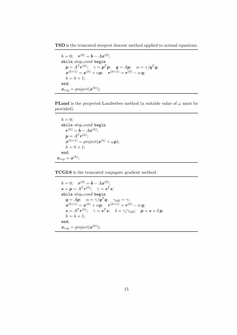
TSD is the truncated steepest descent method applied to normal equations.

h = 0; r(0) = b − Ax(0);while stop cond begin

p = AT r(h); γ = pT p; q = Ap; α = γ/qT q;

x(h+1) = x(h) + αp; r(h+1) = r(h) − α q;h = h + 1;

end;

xreg = project(x(h));

PLand is the projected Landweber method (a suitable value of ω must beprovided).

h = 0;while stop cond begin

r(h) = b − Ax(h);

p = AT r(h);

x(h+1) = project (x(h) + ωp);h = h + 1;

end;

xreg = x(h);

TCGLS is the truncated conjugate gradient method.

h = 0; r(0) = b − Ax(0);

s = p = AT r(0); γ = sT s;while stop cond begin

q = Ap; α = γ/qT q; γold = γ;

x(h+1) = x(h) + αp; r(h+1) = r(h) − α q;

s = AT r(h); γ = sT s; δ = γ/γold; p = s + δ p;h = h + 1;

end;

xreg = project(x(h));

15

MRNSD is the modified steepest descent method applied to system (18).

h = 0; r(0) = b − Ax(0);while stop cond begin

X = diag(x(h)); s = AT r(h); p = Xs;γ = sT p; q = Ap; β = γ/qT q;

α = min(β,minpi<0(−x(h)i /pi));

x(h+1) = x(h) + αp; r(h+1) = r(h) − α q;h = h + 1;

end;

xreg = x(h);

ISRA

h = 0; c = AT b;while stop cond begin

v = Ax(h); s = AT v;for i = 1 to N do ui = ci/si;

for i = 1 to N do x(h+1)i = x

(h)i ui;

h = h + 1;end;

xreg = x(h);

EM

h = 0; c = AT e;while stop cond begin

s = Ax(h);

for i = 1 to N do ui = x(h)i /ci;

for i = 1 to N do vi = bi/si;z = AT v;

for i = 1 to N do x(h+1)i = uizi;

h = h + 1;end;

xreg = x(h);

4.5 The error histories

Numerical simulation is essential when we want to compare the performancesof different methods. When performing a simulation, the exact solution x∗

16

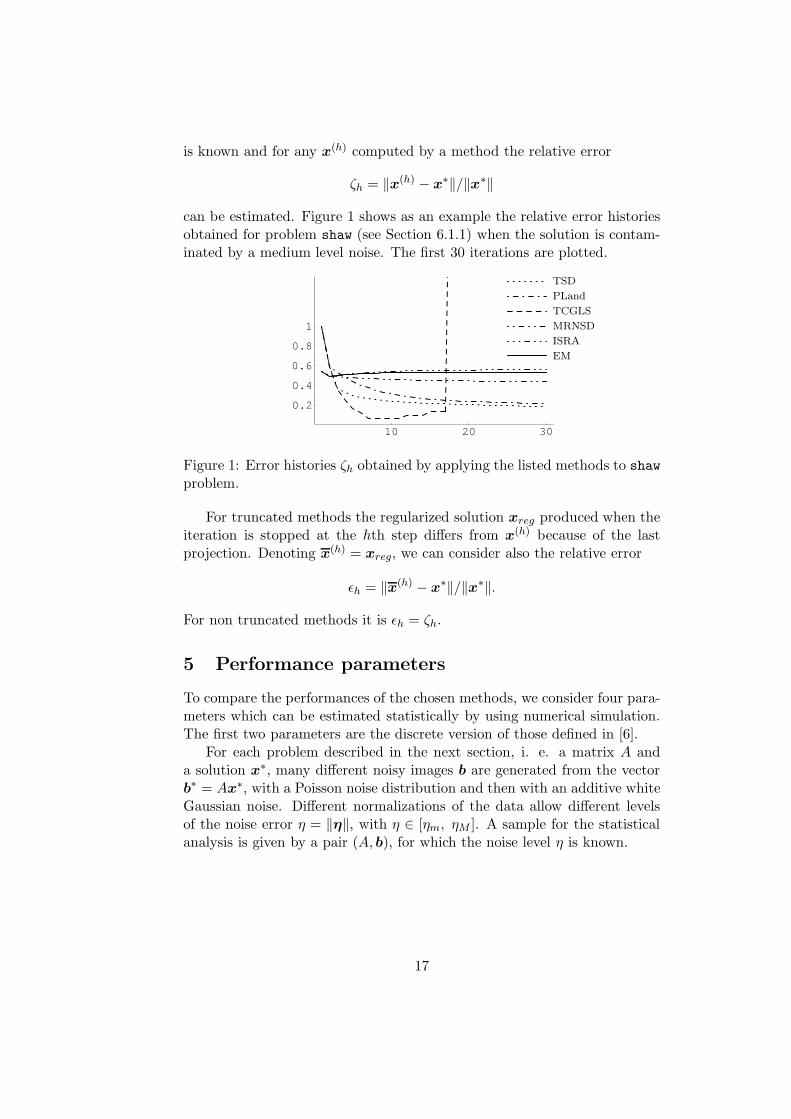
is known and for any x(h) computed by a method the relative error

ζh = ‖x(h) − x∗‖/‖x∗‖

can be estimated. Figure 1 shows as an example the relative error historiesobtained for problem shaw (see Section 6.1.1) when the solution is contam-inated by a medium level noise. The first 30 iterations are plotted.

10 20 30

0.2

0.4

0.6

0.8

1

TSD

PLand

TCGLS

MRNSD

ISRA

EM

Figure 1: Error histories ζh obtained by applying the listed methods to shaw

problem.

For truncated methods the regularized solution xreg produced when theiteration is stopped at the hth step differs from x(h) because of the lastprojection. Denoting x(h) = xreg, we can consider also the relative error

ǫh = ‖x(h) − x∗‖/‖x∗‖.

For non truncated methods it is ǫh = ζh.

5 Performance parameters

To compare the performances of the chosen methods, we consider four para-meters which can be estimated statistically by using numerical simulation.The first two parameters are the discrete version of those defined in [6].

For each problem described in the next section, i. e. a matrix A anda solution x∗, many different noisy images b are generated from the vectorb∗ = Ax∗, with a Poisson noise distribution and then with an additive whiteGaussian noise. Different normalizations of the data allow different levelsof the noise error η = ‖η‖, with η ∈ [ηm, ηM ]. A sample for the statisticalanalysis is given by a pair (A, b), for which the noise level η is known.

17

Each method is applied to a sample and the following elements are com-puted:

– the relative error history ǫh = ‖x(h)−x∗‖/‖x∗‖ and the residual historyδh = ‖r(h)‖,

– the minimum ǫmin of ǫh and the corresponding iteration number hmin

– the value δmin = ‖r(hmin)‖ of the residual norm in hmin and the differ-ence gmin = log10 δmin − log10 η,

– the stopping iteration number hstop according to the discrepancy prin-

ciple, i.e. the smallest index h such that ‖r(h)‖ < η, the correspondingstopping error ǫstop and the ratio smin = ǫstop/ǫmin.

The behaviour of the jth method applied to the ith problem will be analyzedby means of the following indicators, obtained applying the method on allthe samples of the given problem.

– the optimal error Eij, computed by averaging the errors ǫmin. By thisquantity we can estimate the regularizing efficiency of the method.

– the consistency measure Cij, given by the standard deviation of theset of the gmin, says how much the points gmin lie close to their mean.By this quantity we can estimate if the method is consistent with thediscrepancy principle, i.e. if the condition

δmin ∼ α η

holds for a constant α. Graphically, this means that a plot of δmin

versus η would be nearly rectilinear.

– the sensitivity measure Sij, computed by averaging the ratios smin. Bythis quantity we can estimate how much the method is sensitive to anincorrect determination of hmin due to the discrepancy principle. Inpractice, low sensitivity means that the error ǫstop is sufficiently closeto ǫhmin

.

– the optimal iteration number Nij , computed by averaging the iterationnumbers hmin. By this quantity we can estimate the computationalcost of the method, equal to the product of the optimal iteration num-ber by the cost of each iteration, expressed in terms of matrix-vectormultiplications. The cost of each iteration is two matrix-vector multi-plications for all the methods. Actually, Landweber and ISRA meth-ods can have a lower cost if the matrix B = AT A is computed once forall and the vectors AT Ax(h) are computed by means of B. But in thisway the vector Ax(h) is not available for computing the residual normand the discrepancy principle cannot be used without an additionalmatrix-vector product.

18

6 Numerical experimentation

The numerical experimentation has been conducted on both 1D and 2Dtest problems. The 1D problems are obtained from the discretization ofFredholm integral equations of the first kind, while the 2D experimentationdeals with image restoration.

6.1 1D experiments

6.1.1 Test problems

The first set is formed by 1D problems taken from [13], namely baart,

foxgood, ilaplace, phillips, shaw. For problem ilaplace all the ex-amples listed in [13] have been considered, because the various solutions,having a different smoothness degree and a different asymptotic behaviour,lead to problems which respond to the regularization in a different way. Inthe tables the results of this problem are shown under the names ilaplace1,..., ilaplace4. In general the matrices of these problems are severely ill-conditioned, with more than half the singular values below the machineprecision. The size of all the 8 problems is n = 64 and for each problem500 samples have been generated, gathered in 5 relative noise levels from0.087% to 7.6%. An approximation of σ1 for Landweber method has beenfound by a preliminary analysis.

6.1.2 Performance results

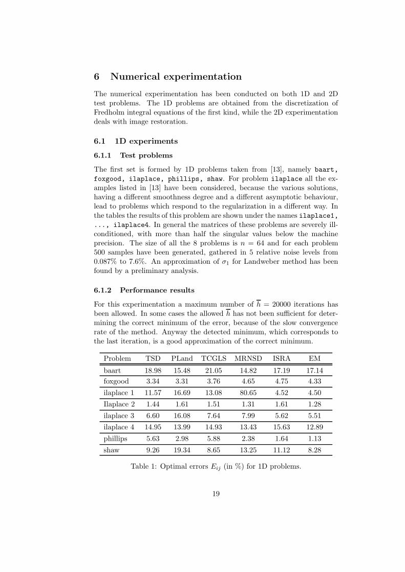
For this experimentation a maximum number of h = 20000 iterations hasbeen allowed. In some cases the allowed h has not been sufficient for deter-mining the correct minimum of the error, because of the slow convergencerate of the method. Anyway the detected minimum, which corresponds tothe last iteration, is a good approximation of the correct minimum.

Problem TSD PLand TCGLS MRNSD ISRA EM

baart 18.98 15.48 21.05 14.82 17.19 17.14

foxgood 3.34 3.31 3.76 4.65 4.75 4.33

ilaplace 1 11.57 16.69 13.08 80.65 4.52 4.50

Ilaplace 2 1.44 1.61 1.51 1.31 1.61 1.28

ilaplace 3 6.60 16.08 7.64 7.99 5.62 5.51

ilaplace 4 14.95 13.99 14.93 13.43 15.63 12.89

phillips 5.63 2.98 5.88 2.38 1.64 1.13

shaw 9.26 19.34 8.65 13.25 11.12 8.28

Table 1: Optimal errors Eij (in %) for 1D problems.

19

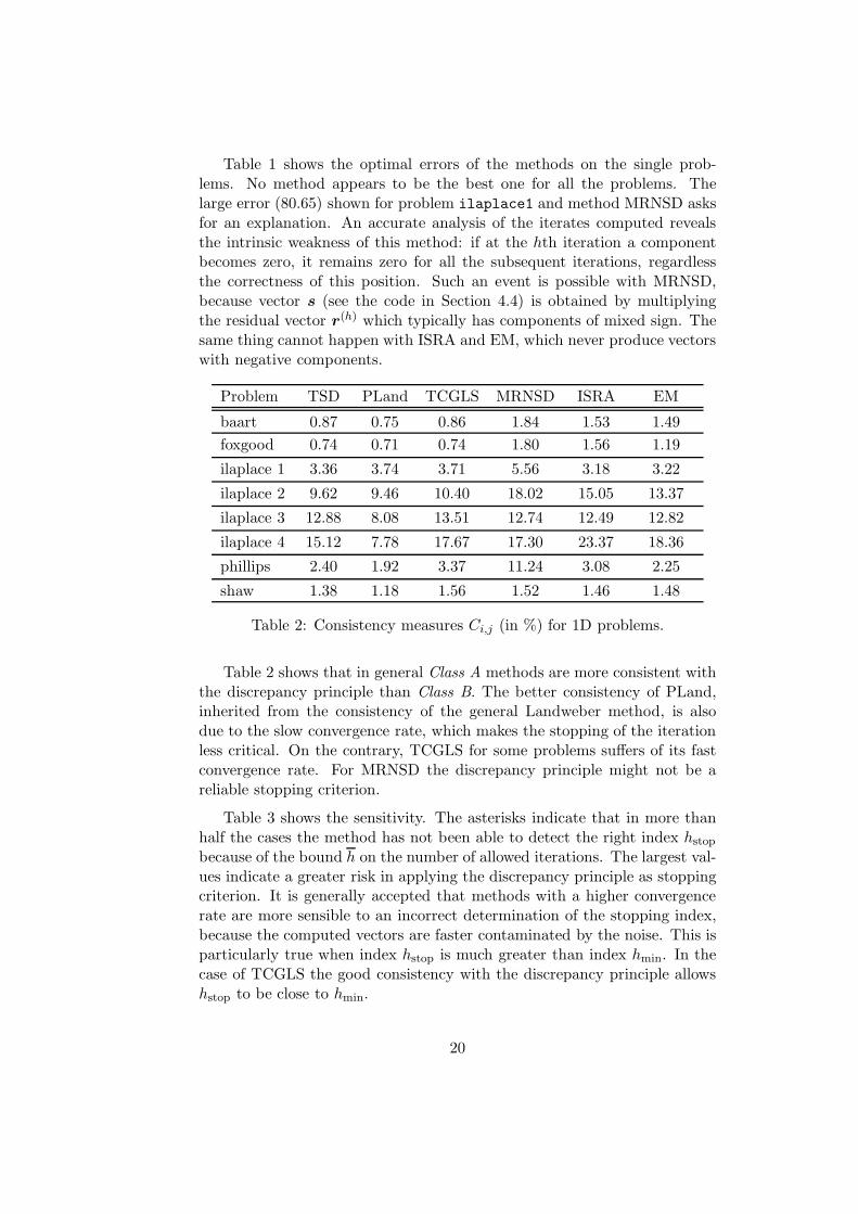
Table 1 shows the optimal errors of the methods on the single prob-lems. No method appears to be the best one for all the problems. Thelarge error (80.65) shown for problem ilaplace1 and method MRNSD asksfor an explanation. An accurate analysis of the iterates computed revealsthe intrinsic weakness of this method: if at the hth iteration a componentbecomes zero, it remains zero for all the subsequent iterations, regardlessthe correctness of this position. Such an event is possible with MRNSD,because vector s (see the code in Section 4.4) is obtained by multiplyingthe residual vector r(h) which typically has components of mixed sign. Thesame thing cannot happen with ISRA and EM, which never produce vectorswith negative components.

Problem TSD PLand TCGLS MRNSD ISRA EM

baart 0.87 0.75 0.86 1.84 1.53 1.49

foxgood 0.74 0.71 0.74 1.80 1.56 1.19

ilaplace 1 3.36 3.74 3.71 5.56 3.18 3.22

ilaplace 2 9.62 9.46 10.40 18.02 15.05 13.37

ilaplace 3 12.88 8.08 13.51 12.74 12.49 12.82

ilaplace 4 15.12 7.78 17.67 17.30 23.37 18.36

phillips 2.40 1.92 3.37 11.24 3.08 2.25

shaw 1.38 1.18 1.56 1.52 1.46 1.48

Table 2: Consistency measures Ci,j (in %) for 1D problems.

Table 2 shows that in general Class A methods are more consistent withthe discrepancy principle than Class B. The better consistency of PLand,inherited from the consistency of the general Landweber method, is alsodue to the slow convergence rate, which makes the stopping of the iterationless critical. On the contrary, TCGLS for some problems suffers of its fastconvergence rate. For MRNSD the discrepancy principle might not be areliable stopping criterion.

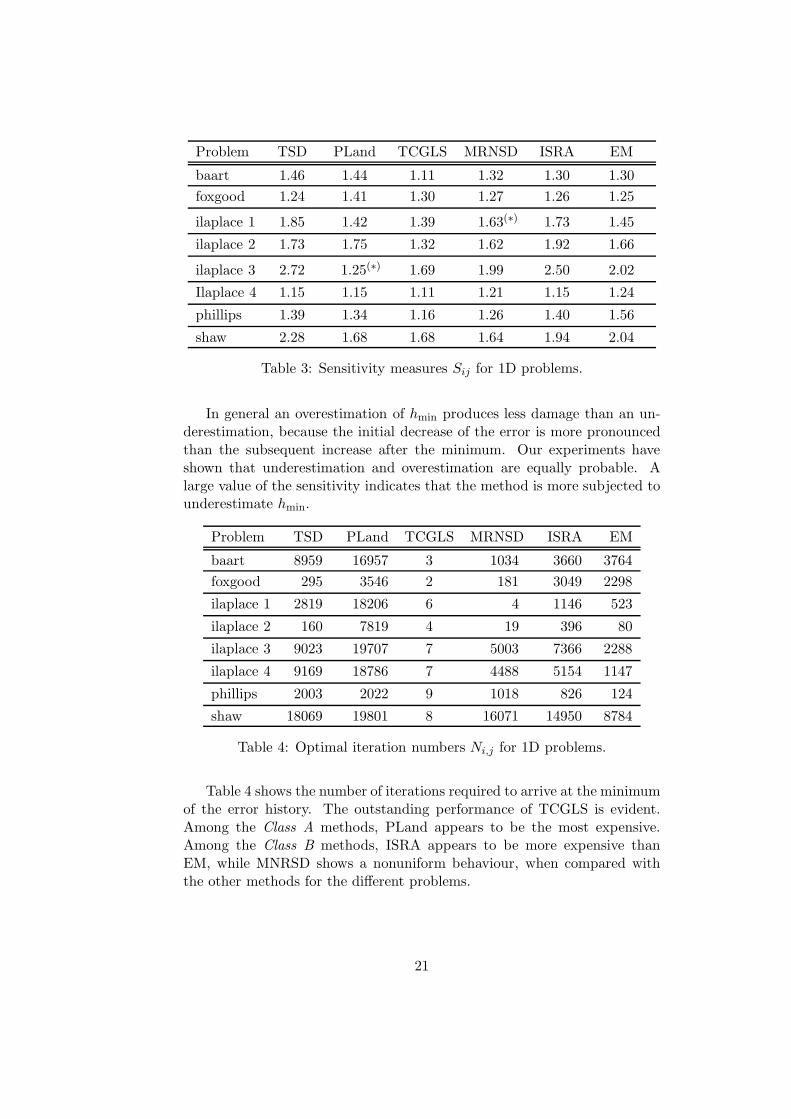
Table 3 shows the sensitivity. The asterisks indicate that in more thanhalf the cases the method has not been able to detect the right index hstop

because of the bound h on the number of allowed iterations. The largest val-ues indicate a greater risk in applying the discrepancy principle as stoppingcriterion. It is generally accepted that methods with a higher convergencerate are more sensible to an incorrect determination of the stopping index,because the computed vectors are faster contaminated by the noise. This isparticularly true when index hstop is much greater than index hmin. In thecase of TCGLS the good consistency with the discrepancy principle allowshstop to be close to hmin.

20

Problem TSD PLand TCGLS MRNSD ISRA EM

baart 1.46 1.44 1.11 1.32 1.30 1.30

foxgood 1.24 1.41 1.30 1.27 1.26 1.25

ilaplace 1 1.85 1.42 1.39 1.63(∗) 1.73 1.45

ilaplace 2 1.73 1.75 1.32 1.62 1.92 1.66

ilaplace 3 2.72 1.25(∗) 1.69 1.99 2.50 2.02

Ilaplace 4 1.15 1.15 1.11 1.21 1.15 1.24

phillips 1.39 1.34 1.16 1.26 1.40 1.56

shaw 2.28 1.68 1.68 1.64 1.94 2.04

Table 3: Sensitivity measures Sij for 1D problems.

In general an overestimation of hmin produces less damage than an un-derestimation, because the initial decrease of the error is more pronouncedthan the subsequent increase after the minimum. Our experiments haveshown that underestimation and overestimation are equally probable. Alarge value of the sensitivity indicates that the method is more subjected tounderestimate hmin.

Problem TSD PLand TCGLS MRNSD ISRA EM

baart 8959 16957 3 1034 3660 3764

foxgood 295 3546 2 181 3049 2298

ilaplace 1 2819 18206 6 4 1146 523

ilaplace 2 160 7819 4 19 396 80

ilaplace 3 9023 19707 7 5003 7366 2288

ilaplace 4 9169 18786 7 4488 5154 1147

phillips 2003 2022 9 1018 826 124

shaw 18069 19801 8 16071 14950 8784

Table 4: Optimal iteration numbers Ni,j for 1D problems.

Table 4 shows the number of iterations required to arrive at the minimumof the error history. The outstanding performance of TCGLS is evident.Among the Class A methods, PLand appears to be the most expensive.Among the Class B methods, ISRA appears to be more expensive thanEM, while MNRSD shows a nonuniform behaviour, when compared withthe other methods for the different problems.

21

6.1.3 Choice of the best method

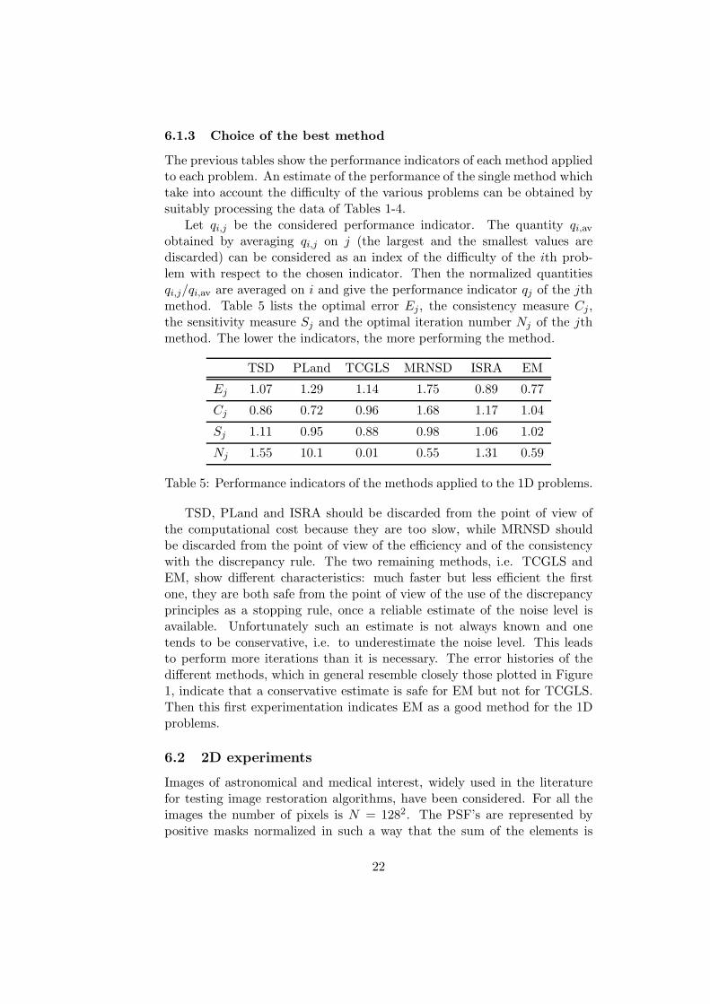
The previous tables show the performance indicators of each method appliedto each problem. An estimate of the performance of the single method whichtake into account the difficulty of the various problems can be obtained bysuitably processing the data of Tables 1-4.

Let qi,j be the considered performance indicator. The quantity qi,av

obtained by averaging qi,j on j (the largest and the smallest values arediscarded) can be considered as an index of the difficulty of the ith prob-lem with respect to the chosen indicator. Then the normalized quantitiesqi,j/qi,av are averaged on i and give the performance indicator qj of the jthmethod. Table 5 lists the optimal error Ej, the consistency measure Cj,the sensitivity measure Sj and the optimal iteration number Nj of the jthmethod. The lower the indicators, the more performing the method.

TSD PLand TCGLS MRNSD ISRA EM

Ej 1.07 1.29 1.14 1.75 0.89 0.77

Cj 0.86 0.72 0.96 1.68 1.17 1.04

Sj 1.11 0.95 0.88 0.98 1.06 1.02

Nj 1.55 10.1 0.01 0.55 1.31 0.59

Table 5: Performance indicators of the methods applied to the 1D problems.

TSD, PLand and ISRA should be discarded from the point of view ofthe computational cost because they are too slow, while MRNSD shouldbe discarded from the point of view of the efficiency and of the consistencywith the discrepancy rule. The two remaining methods, i.e. TCGLS andEM, show different characteristics: much faster but less efficient the firstone, they are both safe from the point of view of the use of the discrepancyprinciples as a stopping rule, once a reliable estimate of the noise level isavailable. Unfortunately such an estimate is not always known and onetends to be conservative, i.e. to underestimate the noise level. This leadsto perform more iterations than it is necessary. The error histories of thedifferent methods, which in general resemble closely those plotted in Figure1, indicate that a conservative estimate is safe for EM but not for TCGLS.Then this first experimentation indicates EM as a good method for the 1Dproblems.

6.2 2D experiments

Images of astronomical and medical interest, widely used in the literaturefor testing image restoration algorithms, have been considered. For all theimages the number of pixels is N = 1282. The PSF’s are represented bypositive masks normalized in such a way that the sum of the elements is

22

equal to 1. By Grenander and Szego theorem [10], the largest singular valueσ1 of AT A is bounded from above by 1. Since all images have sufficientlylarge zero background along the boundary, the coefficient matrix can besafely approximated by a 2-level circulant matrix. In this way the matrix-vector product can be easily computed by means of FFT. The blurred imageshave been corrupted by both Poisson and read-out noise of various relativelevels.

6.2.1 Test problems

The first problem deals with an image of the spiral galaxy NGC 1288 shownin Figure 2 (upper left) blurred by a diffraction-limited PSF. The problemhas been considered in [3], [4], [5]. Noise level varies from 1.5% (low level) to14.9% (high level). The second problem deals with the image of a satelliteshown in Figure 2 (upper right). It can be found in the package RestoreTools[16]. The blur is performed by the exponential mask

mi,j = γ exp(−0.019 (i + j)2 − 0.017(i − j)2), i, j = −8, . . . , 8,

where γ is the normalization factor. Noise level varies from 1.7% (low level)to 17.8% (high level).

The medical images are models of the human brain used in testing theaccuracy of the reconstruction algorithms for emission tomography. Thethird problem deals with a Hoffman phantom [14], shown in Figure 2 (lowerleft), which is used for simulating cerebral blood-flow. The blur is performedby the Gaussian PSF

mij = γ exp(−0.4 i2 − 0.2 j2), i, j = −11, . . . , 11,

where γ is the normalization factor. Noise level varies from 1.5% (low level)to 15.9% (high level). The fourth problem deals with the Shepp-Loganphantom [26], shown in Figure 2 (lower right), which contains ellipsis withdifferent absorption properties. The blur is performed by the Gaussian PSF

mij = γ exp(−0.1 i2 − 0.5 j2), i, j = −15, . . . , 15,

where γ is the normalization factor. Noise level varies from 2.1% (low level)to 21.6% (high level).

6.2.2 Performance results

For these experiments the maximum allowed number for iterations is h =5000 (in the experiments this bound has never been reached).

Tables 6 to 9 list the values of the performance parameters obtainedby the methods for the 2D problem. The differences among the three first

23

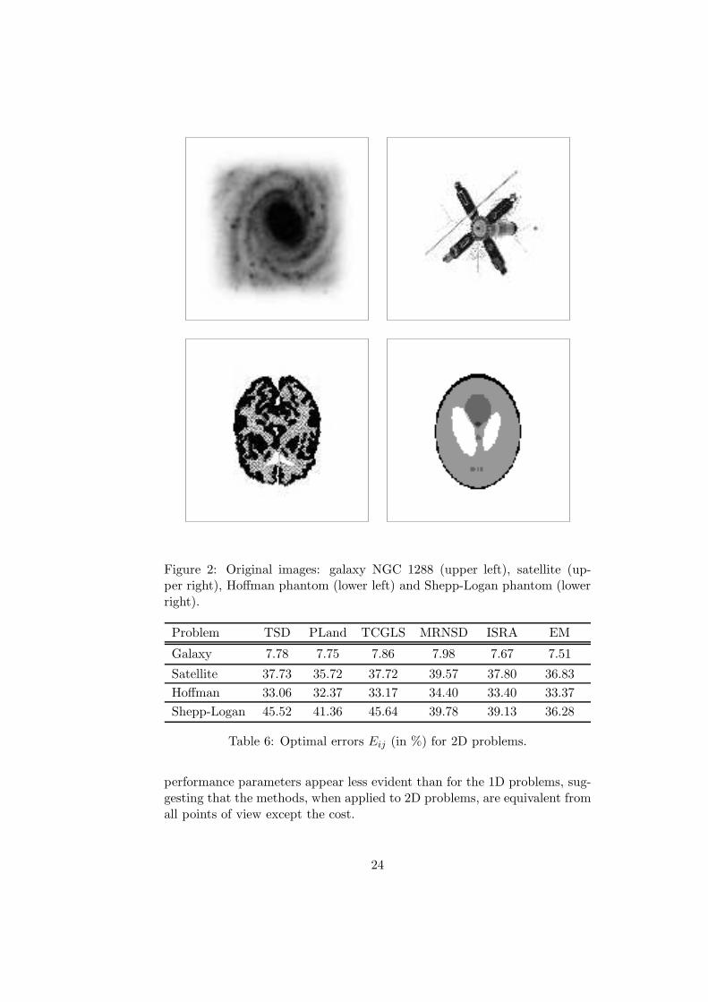
Figure 2: Original images: galaxy NGC 1288 (upper left), satellite (up-per right), Hoffman phantom (lower left) and Shepp-Logan phantom (lowerright).

Problem TSD PLand TCGLS MRNSD ISRA EM

Galaxy 7.78 7.75 7.86 7.98 7.67 7.51

Satellite 37.73 35.72 37.72 39.57 37.80 36.83

Hoffman 33.06 32.37 33.17 34.40 33.40 33.37

Shepp-Logan 45.52 41.36 45.64 39.78 39.13 36.28

Table 6: Optimal errors Eij (in %) for 2D problems.

performance parameters appear less evident than for the 1D problems, sug-gesting that the methods, when applied to 2D problems, are equivalent fromall points of view except the cost.

24

Problem TSD PLand TCGLS MRNSD ISRA EM

Galaxy 0.33 0.33 0.32 0.44 0.33 0.29

Satellite 0.25 0.25 0.21 1.84 0.40 0.42

Hoffman 1.66 1.63 1.64 1.74 1.57 1.48

Shepp-Logan 1.44 1.42 1.39 1.37 1.32 1.16

Table 7: Consistency measures Cij (in %) for 2D problems.

Problem TSD PLand TCGLS MRNSD ISRA EM

Galaxy 1.06 1.07 1.04 1.01 1.06 1.07

Satellite 1.02 1.03 1.02 1.02 1.02 1.03

Hoffman 1.05 1.06 1.04 1.02 1.04 1.04

Shepp-Logan 1.05 1.09 1.03 1.07 1.09 1.14

Table 8: Sensitivity measures Sij (in %) for 2D problems.

Problem TSD PLand TCGLS MRNSD ISRA EM

Galaxy 47 100 10 74 95 81

Satellite 296 913 26 395 823 542

Hoffman 118 257 16 90 210 197

Shepp-Logan 186 627 20 264 442 351

Table 9: Optimal iteration numbers Nij (in %) for 2D problems.

To get a more synthetic view of the performance of the methods, thesetables are processed as already made in the case of the 1D problems. Theresults are shown in Table 10.

TSD PLand TCGLS MRNSD ISRA EM

Ej 1.03 0.98 1.03 1.02 0.99 0.96

Cj 0.96 0.95 0.91 2.25 1.04 0.98

Sj 1.00 1.01 0.98 0.98 1.00 1.02

Nj 0.64 1.70 0.01 0.80 1.42 1.14

Table 10: Performance indicators of the methods applied to the 2D prob-lems.

PLand and MRNSD should be discarded from the point of view of thecomputational cost and the consistency with the discrepancy rule, respec-tively. TSD is outperformed by TCGLS and ISRA is outperformed by EM,

25

with respect to each indicator. For the two remaining methods, i.e. TCGLSand EM, considerations similar to those made in the 1D case hold. Notethat in this case the gap between the reconstruction efficiencies of the twomethods is not very large.

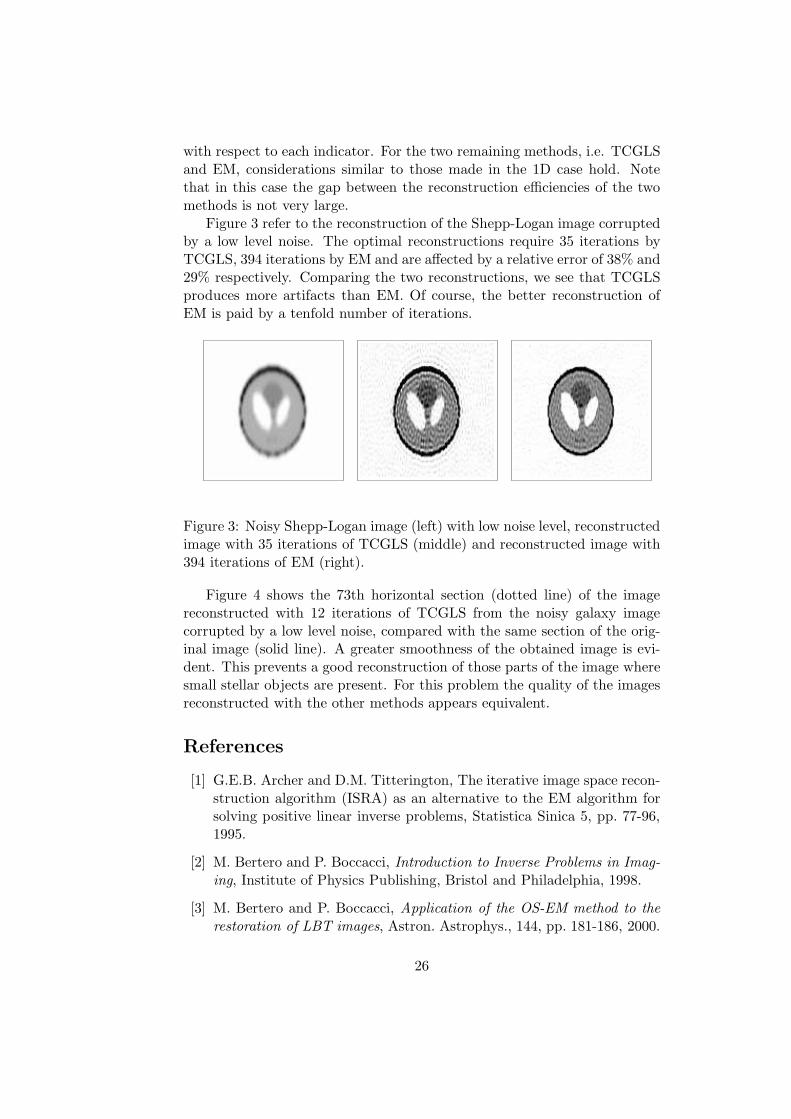
Figure 3 refer to the reconstruction of the Shepp-Logan image corruptedby a low level noise. The optimal reconstructions require 35 iterations byTCGLS, 394 iterations by EM and are affected by a relative error of 38% and29% respectively. Comparing the two reconstructions, we see that TCGLSproduces more artifacts than EM. Of course, the better reconstruction ofEM is paid by a tenfold number of iterations.

Figure 3: Noisy Shepp-Logan image (left) with low noise level, reconstructedimage with 35 iterations of TCGLS (middle) and reconstructed image with394 iterations of EM (right).

Figure 4 shows the 73th horizontal section (dotted line) of the imagereconstructed with 12 iterations of TCGLS from the noisy galaxy imagecorrupted by a low level noise, compared with the same section of the orig-inal image (solid line). A greater smoothness of the obtained image is evi-dent. This prevents a good reconstruction of those parts of the image wheresmall stellar objects are present. For this problem the quality of the imagesreconstructed with the other methods appears equivalent.

References

[1] G.E.B. Archer and D.M. Titterington, The iterative image space recon-struction algorithm (ISRA) as an alternative to the EM algorithm forsolving positive linear inverse problems, Statistica Sinica 5, pp. 77-96,1995.

[2] M. Bertero and P. Boccacci, Introduction to Inverse Problems in Imag-ing, Institute of Physics Publishing, Bristol and Philadelphia, 1998.

[3] M. Bertero and P. Boccacci, Application of the OS-EM method to therestoration of LBT images, Astron. Astrophys., 144, pp. 181-186, 2000.

26

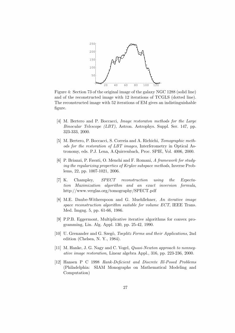
20 40 60 80 100 120

50

100

150

200

250

Figure 4: Section 73 of the original image of the galaxy NGC 1288 (solid line)and of the reconstructed image with 12 iterations of TCGLS (dotted line).The reconstructed image with 52 iterations of EM gives an indistinguishablefigure.

[4] M. Bertero and P. Boccacci, Image restoraton methods for the LargeBinocular Telescope (LBT), Astron. Astrophys. Suppl. Ser. 147, pp.323-333, 2000.

[5] M. Bertero, P. Boccacci, S. Correia and A. Richichi, Tomographic meth-ods for the restoration of LBT images, Interferometry in Optical As-tronomy, eds. P.J. Lena, A.Quirrenbach, Proc. SPIE, Vol. 4006, 2000.

[6] P. Brianzi, P. Favati, O. Menchi and F. Romani, A framework for study-ing the regularizing properties of Krylov subspace methods, Inverse Prob-lems, 22, pp. 1007-1021, 2006.

[7] K. Champley, SPECT reconstruction using the Expecta-tion Maximization algorithm and an exact inversion formula,http://www.verglas.org/tomography/SPECT.pdf

[8] M.E. Daube-Witherspoon and G. Muehllehner, An iterative imagespace reconstruction algorithm suitable for volume ECT, IEEE Trans.Med. Imgng. 5, pp. 61-66, 1986.

[9] P.P.B. Eggermont, Multiplicative iterative algorithms for convex pro-gramming, Lin. Alg. Appl. 130, pp. 25-42, 1990.

[10] U. Grenander and G. Szego, Toeplitz Forms and their Applications, 2ndedition (Chelsea, N. Y., 1984).

[11] M. Hanke, J. G. Nagy and C. Vogel, Quasi-Newton approach to nonneg-ative image restoration, Linear algebra Appl., 316, pp. 223-236, 2000.

[12] Hansen P C 1998 Rank-Deficient and Discrete Ill-Posed Problems(Philadelphia: SIAM Monographs on Mathematical Modeling andComputation)

27

[13] Hansen P C 1994 Regularization tools: a Matlab package for analysisand solution of discrete ill-posed problems Numerical Algorithms 6 1-35

[14] E.J. Hoffman, P.D. Cutler, W.M. Digby, J.C. Mazziotta, 3-D phantomto simulate cerebral blood flow and metabolic images for PET, IEEETrans. Nucl. Sci., 37 (1990), pp. 616-620.

[15] K. P. Lee and J. G. Nagy, Steepest descent, CG, and iterative regular-ization of ill-posed problems, BIT, vol. 40, no. 4, pp. 001-004, 2000.

[16] K.P.Lee, J.G.Nagy, L.Perrone, Iterative methods or image restoration:a Matlab object oriented approach. http://www.mathcs.emory.edu/∼nagy/RestoreTools, 2002.

[17] L. B. Lucy, An Iteration Technique for the Rectification of ObservedDistributions, Astron. Journal, 79, pp. 745-754, 1974.

[18] J. G. Nagy, K. Lee and L. Perrone, An object approach to image restora-tion in Matlab, www.mathcs.emory.edu/ nagy.

[19] J. G. Nagy and D. P. O’Leary, Fast iterative image restoration witha spatially-varying PSF, F. T. Luk, Advanced signal processing algo-rithms, architectures, and implementations VII, vol. 3162, pp. 388-399,SPIE, 1997.

[20] J. G. Nagy, K. Palmer and L. Perrone, Iterative methods for imagedeblurring: a Matlab object oriented approach, Numerical algorithms,36, 2003.

[21] J. Nagy and Z. Strakos, Enforcing nonnegativity in image reconstructionalgorithms, in Math. Model., Estim., and Imag., D.C. Wilson, et.al.,Eds., 4121, pp. 182-190, 2000.

[22] W. Richardson, Bayesian-based iterative method of image restoration,Journal of the Optical Society of America, 62, pp. 55-59, 1972.

[23] M. Rojas and T. Steihaug, An interior-point trust-region-based methodfor large-scale nonnegative regularization, 2001.

[24] Y. Saad, Iterative Methods for Sparse Linear Systems, PWS PublishingCo., Boston, 1996.

[25] L.A. Shepp and Y. Vardi, Maximum likelihood reconstruction for emis-sion tomography, IEEE Trans. Med. Imag., vol. MI-1, no. 2, pp. 113-122,1982.

[26] http://www.oersted.dtu.dk/ftp/jaj/31655/ct programs/

28