COMPUTATION OF WIND FIELD FROM ENVISAT ASAR WIDE SWATH AND ERS SARIMAGES WITHOUT ANY A PRIORI INFORMATION

Stefano Zecchetto1 and Francesco De Biasio2

1Istituto Scienze dell’Atmosfera e del Clima (ISAC) Consiglio Nazionale delle Ricerche, Padova, Italy2Istituzione Centro Previsioni e Segnalazioni Maree (ICPSM), Comune di Venezia, Venezia, Italy

ABSTRACT

A wavelet based methodology has been developed to re-trieve the wind field over the sea surface from SAR im-ages without any a-priori information of the wind di-rection. The method relies on the ability of the two-dimensional continuous wavelet technique to detect thespatial structure of the Marine Atmospheric BoundaryLayer (MABL). The analysis of the geometric and radio-metric characteristics of the backscatter structures definesthe wind direction allowing the computation of the windspeed through the available algorithms. Twenty SARimages (Envisat ASAR Wide Swath and ERS) over theMediterranean Sea have been analysed, and the resultscompared both with the NASA QuikSCAT satellite andthe ECMWF analysis wind fields. These images covera wide range of meteorological conditions, from low (2m/s) to moderate winds (12 m/s), presenting many kindsof signature, i. e. wind cells, atmospheric gravity waves,convective structures and radiometric flatness.

The main difference of this method with respect to thosealready proposed is that the wind direction is not sup-posed a priori, but derived only from the SAR imagesignature. The local scale structure of the wind fieldis thus retrieved with a resolution finer than that of allthe existing other sources (atmospheric models and satel-lite scatterometers).A statistical comparison of the SARderived wind speed and direction has been performedagainst QuikSCAT satellite winds (for Envisat images)or ECMWF analysis winds. Results for Envisat ASARindicate a good score (≈ 75 %) in detecting the wind di-rection.

Key words: SAR; wavelet; MABL; sea wind.

1. INTRODUCTION

At present, many efforts are devoted to set up usefulmethodologies to extract the wind field at the sea surfacefrom Synthetic Aperture Radar (SAR) images. The Ad-vanced SAR instrument of Envisat and the near futureSAR payload of the the Canadian commercial satellite

RADARSAT-2 will enhance the coverage of the sea sur-face greatly. This situation will offer an unique oppor-tunity of investigating the geophysical characteristics ofthe sea wind at meso- and small-scales, provided reliableand robust methodologies for wind extraction from SARimages are available.

The estimation of the wind vector direction at the sea sur-face from SAR images can be done essentially in twoways: using co-located wind measurements (from buoys,in situ measurements, scatterometers data or model sim-ulations), or deriving the wind direction from featurespresent in the image itself. In the last case, the knownmethods yield a 180◦ ambiguous determination of thewind direction which needs, to be resolved, either exter-nal co-located data or some parameter derived from theimage itself.

Besides Alpers & Brummer (1994), more recent deriva-tion of high resolution wind fields from SAR images relyon co-located data to define the true wind direction. InKortcheva et al. (2002) a co-located data set of buoysand NSCAT measurements is used to define the winddirection in the geophysical transfer function. In Mon-aldo & Thompson (2002) the wind direction field is ob-tained by interpolating the atmospheric model estimatesup to the pixels position in the RADARSAT SAR im-ages. Co-located measurements of wind direction fromERS-2 scatterometer and atmospheric global model datawere used by Horstmann & Lehner (2002) to obtain thesurface wind field from ERS-2 SAR wave mode data.

An interesting approach to this problem, followed by themethodologies belonging to the second category, is thederivation of the wind direction directly from the SARsignature. This is done by extracting the local wind direc-tion on the basis of the features in the image: these can bethe quasi-periodic streaks of lower and higher backscattercells, produced by atmospheric wind roll vortices (Alpers& Brummer 1994), or the lee signatures induced by is-lands. The dominant, local direction of the streaks iseasily retrieved by using spectral methods (Gerling 1986;Vachon & Dobson 2000). The wind direction is obtained,with an inherent 180◦ ambiguity, by measuring the orien-tation of the Fourier image spectrum in the wavelengthrange 500-1500 m, which has well defined direction, ifthe signature of wind roll vortices is present in the im-

_____________________________________________________

Proc. ‘Envisat Symposium 2007’, Montreux, Switzerland 23–27 April 2007 (ESA SP-636, July 2007)

age. It is indeed assumed that the energy in that range ofwavelength is aligned with the wind direction.

An alternative method is based on the derivation of the lo-cal gradient of the image signature in the spatial domain,which should evidence the directionality of the windstreaks features (Koch 2002; Horstmann et al. 2002).They are supposed to be locally parallel to the wind vec-tor, which results to be perpendicular to the directionof the local gradient, still with an inherent ambiguity of180◦. In Staples & Mendoza (2002) a comparison of thewind derivation from both the local gradient method andthe co-located data is reported.

The third approach to this problem, which forms thecontribution of this paper, uses the two dimensionalContinuous Wavelet Transform (CWT2) to isolate theSAR backscatter structures (Zecchetto & De Biasio 2001,2002). It carries out a decomposition of the image at var-ious spatial scales, the elementary components being thewavelet coefficients of the transform. A partial recon-struction of the image, in the domain of the transformparameters, is done by adding only the components ofthe decomposition which carry the highest energy in therange of the predefined scales. This method analyses theradar backscatter at local scales, and does not require anyperiodicity of the radar structures.

Others interesting papers about wind retrieval from SARimages are by Wackerman et al. (1996); Vachon & Dob-son (1996); Vachon et al. (1998); Fetterer et al. (1998);Lehner et al. (1998); Korsbakken et al. (1998); Furevik &Korsbakken (2000).

The paper is structured as follows: in section 2 themethodology to extract the wind from SAR images is il-lustrated. Section 3 reports, as example, two of the resultsobtained, and provides a statistic comparison of the SARderived winds with the QuikSCAT scatterometer data andthe analysis fields produced by the ECMWF. Section 4ends the paper with a discussion of the results and theconclusions.

2. THE METHODOLOGY FOR WIND EXTRAC-TION

The CWT2 methodology followed to analyse the SARimages is exhaustively described in Zecchetto & De Bi-asio (2002), which the interested reader is addressed to.For sake of shortness, we draw here only a brief sum-mary. The SAR images, obtained as backscatter imagesusing the ESA BEST software, have been pre-processedbefore undergoing the CWT2 analysis: their size hasbeen reduced by compression of factor ten (ERS) andtwo (Envisat), the land and islands have been masked andthe effects introduced by the variation of the radar inci-dence angle in range mitigated, to avoid that the struc-tures present on the inner part of the images, wherethe backscatter is higher due to the smaller radar inci-dence angle, prevail on the others. The image com-

km

km

50 100 150 200 250 300

50

100

150

200

250

300

350

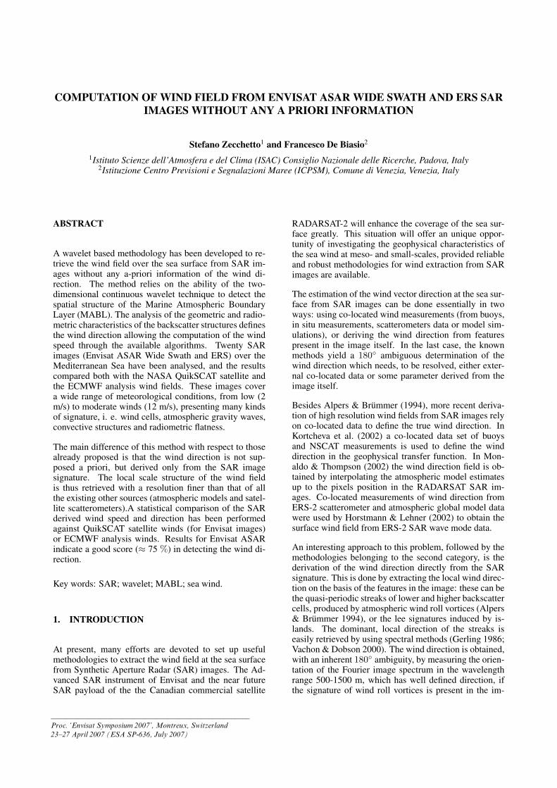
Figure 1. An example of Envisat ASAR Wide Swath im-age showing atmospheric phenomena at different spa-tial scales, as wind rolls (transversal wavelength ≈ 1km) and gravity waves (wavelength ≈ 30 km). Or-bit=3346, track=286, frame=1, 20 October 2002, 20:00GMT. Eastern Mediterranean Sea (Longitude: 27◦ to 31◦E; Latitude: 33◦ to 36.5◦ N)

pression filters out geophysical phenomena with spatialscales shorter than ≈ 150 m as, for instance, sea gravitywaves, without hiding the backscatter structures relatedto atmospheric phenomena of interest. It is frequent tohave backscatter structures of different spatial scales inthe same SAR image. Fig. 1 shows an Envisat ASARWide Swath image taken in the eastern MediterraneanSea (Karpathos and Rhodos islands are visible in the up-per left, while the southern coast of Turkey in the upperright of the image): it clearly shows the presence of windrolls (transversal wavelength ≈1 km) as well as of atmo-spheric gravity waves of wavelength ≈30 km. Since weare interested in the small scale features of SAR images,we have restricted our analysis to scales from 300 m to4 km, a choice which implicitly defines the geophysicalphenomena to study. A total of sixty four combinationsof scales, eight over the image rows and eight over thecolumns (sr, sc) have been taken, thus obtaining 64 mapsfor each SAR image. The energy of each of these mapshas been derived to build the wavelet variance map.

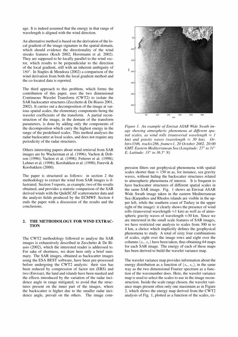
The wavelet variance map provides information about theenergy distribution as a function of (sr, sc), in the sameway as the two dimensional Fourier spectrum as a func-tion of the wavenumber does. Here, the wavelet variancemap is used to select the scales to use in the image recon-struction. Inside the scale range chosen, the wavelet vari-ance maps present often only one maximum as in Figure2, which shows the energy map derived from the CWT2analysis of Fig. 1, plotted as a function of the scales, ex-

km

km

1 2 3

1

2

3

0.5

1

1.5

2

2.5

3

3.5

Figure 2. An example of energy map deriving from theASAR image of Fig. 1. The energy map is plotted as afunction of (sr, sc) in km and in logarithmic scale.

pressed in km and in logarithmic scale. The scales used toreconstruct the images are those falling around the maxi-mum peak. This yields a reconstruction of an image withonly a fraction of the overall energy, which strictly de-pends on the phenomenology imaged by SAR. In aver-age, the reconstruction uses more than 50% of the totalSAR image energy.

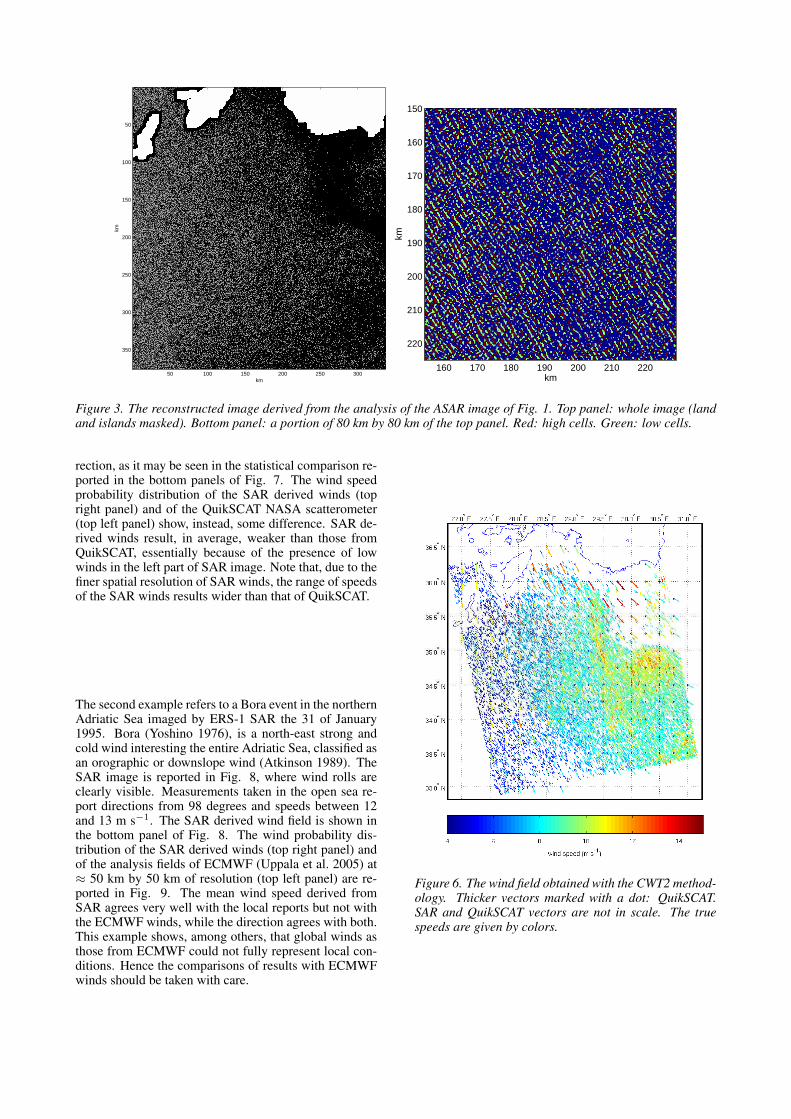
The resulting reconstructed image maps underwent to athreshold procedure to isolate the structures and to sortthem according to their amplitude value. The cells withvalues greater or lower than the reconstructed map meanby σ are referred to as high and low cells respectively,where σ is the reconstructed map standard deviation. Fig-ure 3 reports the reconstructed map of Fig. 1 after thethreshold. The top panel reports the whole image, thebottom panel shows a portion of 80 km by 80 km of thewhole map. Up structures are red, low green, while theremaining areas are blue. This map is then used as a maskover the original SAR image to extract the real backscat-ter value of the cells.

2.1. Choice of the wind directions

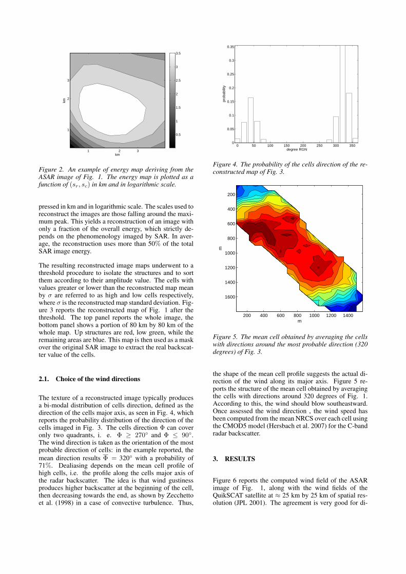
The texture of a reconstructed image typically producesa bi-modal distribution of cells direction, defined as thedirection of the cells major axis, as seen in Fig. 4, whichreports the probability distribution of the direction of thecells imaged in Fig. 3. The cells direction Φ can coveronly two quadrants, i. e. Φ ≥ 270◦ and Φ ≤ 90◦.The wind direction is taken as the orientation of the mostprobable direction of cells: in the example reported, themean direction results Φ = 320◦ with a probability of71%. Dealiasing depends on the mean cell profile ofhigh cells, i.e. the profile along the cells major axis ofthe radar backscatter. The idea is that wind gustinessproduces higher backscatter at the beginning of the cell,then decreasing towards the end, as shown by Zecchettoet al. (1998) in a case of convective turbulence. Thus,

0 50 100 150 200 250 300 3500

0.05

0.1

0.15

0.2

0.25

0.3

0.35

degree RGN

prob

abili

ty

Figure 4. The probability of the cells direction of the re-constructed map of Fig. 3.

m

m

200 400 600 800 1000 1200 1400

200

400

600

800

1000

1200

1400

1600

Figure 5. The mean cell obtained by averaging the cellswith directions around the most probable direction (320degrees) of Fig. 3.

the shape of the mean cell profile suggests the actual di-rection of the wind along its major axis. Figure 5 re-ports the structure of the mean cell obtained by averagingthe cells with directions around 320 degrees of Fig. 1.According to this, the wind should blow southeastward.Once assessed the wind direction , the wind speed hasbeen computed from the mean NRCS over each cell usingthe CMOD5 model (Hersbach et al. 2007) for the C-bandradar backscatter.

3. RESULTS

Figure 6 reports the computed wind field of the ASARimage of Fig. 1, along with the wind fields of theQuikSCAT satellite at ≈ 25 km by 25 km of spatial res-olution (JPL 2001). The agreement is very good for di-

km

km

50 100 150 200 250 300

50

100

150

200

250

300

350

km

km

160 170 180 190 200 210 220

150

160

170

180

190

200

210

220

Figure 3. The reconstructed image derived from the analysis of the ASAR image of Fig. 1. Top panel: whole image (landand islands masked). Bottom panel: a portion of 80 km by 80 km of the top panel. Red: high cells. Green: low cells.

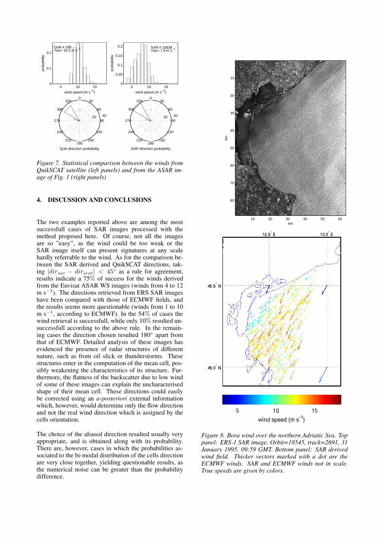
rection, as it may be seen in the statistical comparison re-ported in the bottom panels of Fig. 7. The wind speedprobability distribution of the SAR derived winds (topright panel) and of the QuikSCAT NASA scatterometer(top left panel) show, instead, some difference. SAR de-rived winds result, in average, weaker than those fromQuikSCAT, essentially because of the presence of lowwinds in the left part of SAR image. Note that, due to thefiner spatial resolution of SAR winds, the range of speedsof the SAR winds results wider than that of QuikSCAT.

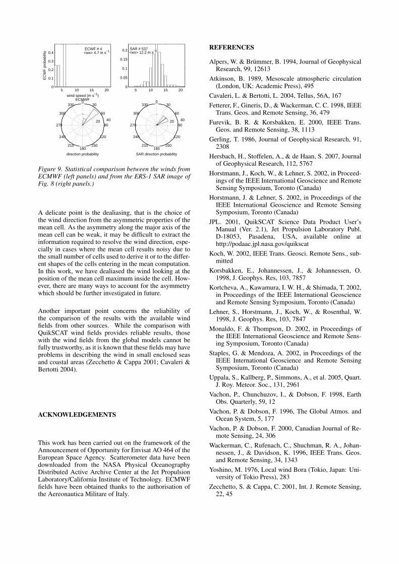
The second example refers to a Bora event in the northernAdriatic Sea imaged by ERS-1 SAR the 31 of January1995. Bora (Yoshino 1976), is a north-east strong andcold wind interesting the entire Adriatic Sea, classified asan orographic or downslope wind (Atkinson 1989). TheSAR image is reported in Fig. 8, where wind rolls areclearly visible. Measurements taken in the open sea re-port directions from 98 degrees and speeds between 12and 13 m s−1. The SAR derived wind field is shown inthe bottom panel of Fig. 8. The wind probability dis-tribution of the SAR derived winds (top right panel) andof the analysis fields of ECMWF (Uppala et al. 2005) at≈ 50 km by 50 km of resolution (top left panel) are re-ported in Fig. 9. The mean wind speed derived fromSAR agrees very well with the local reports but not withthe ECMWF winds, while the direction agrees with both.This example shows, among others, that global winds asthose from ECMWF could not fully represent local con-ditions. Hence the comparisons of results with ECMWFwinds should be taken with care.

Figure 6. The wind field obtained with the CWT2 method-ology. Thicker vectors marked with a dot: QuikSCAT.SAR and QuikSCAT vectors are not in scale. The truespeeds are given by colors.

5 10 150

0.1

0.2

wind speed (m s−1)

prob

abili

tyQuik # 188<ws> 10.3 m s−1

5 10 150

0.05

0.1

0.15

0.2

wind speed (m s−1)

prob

abili

ty

SAR # 15638<ws> 7.9 m s−1

20 40

30

210

60

240

90270

120

300

150

330

180

0

Quik direction probability

20 40

30

210

60

240

90270

120

300

150

330

180

0

SAR direction probability

Figure 7. Statistical comparison between the winds fromQuikSCAT satellite (left panels) and from the ASAR im-age of Fig. 1 (right panels)

4. DISCUSSION AND CONCLUSIONS

The two examples reported above are among the mostsuccessfull cases of SAR images processed with themethod proposed here. Of course, not all the imagesare so ”easy”, as the wind could be too weak or theSAR image itself can present signatures at any scalehardly referrable to the wind. As for the comparison be-tween the SAR derived and QuikSCAT directions, tak-ing |dirsar − dirscat| < 45◦ as a rule for agreement,results indicate a 75% of success for the winds derivedfrom the Envisat ASAR WS images (winds from 4 to 12m s−1). The directions retrieved from ERS SAR imageshave been compared with those of ECMWF fields, andthe results seems more questionable (winds from 1 to 10m s−1, according to ECMWF). In the 54% of cases thewind retrieval is successfull, while only 10% resulted un-successfull according to the above rule. In the remain-ing cases the direction chosen resulted 180◦ apart fromthat of ECMWF. Detailed analysis of these images hasevidenced the presence of radar structures of differentnature, such as from oil slick or thunderstorms. Thesestructures enter in the computation of the mean cell, pos-sibly weakening the characteristics of its structure. Fur-thermore, the flatness of the backscatter due to low windof some of these images can explain the uncharacterisedshape of their mean cell. These directions could easilybe corrected using an a-posteriori external informationwhich, however, would determine only the flow directionand not the real wind direction which is assigned by thecells orientation.

The choice of the aliased direction resulted usually veryappropriate, and is obtained along with its probability.There are, however, cases in which the probabilities as-sociated to the bi-modal distribution of the cells directionare very close together, yielding questionable results, asthe numerical noise can be greater than the probabilitydifference.

kmkm

10 20 30 40 50 60

10

20

30

40

50

60

70

80

Figure 8. Bora wind over the northern Adriatic Sea. Toppanel: ERS-1 SAR image, Orbit=18545, track=2691, 31January 1995, 09:59 GMT. Bottom panel: SAR derivedwind field. Thicker vectors marked with a dot are theECMWF winds. SAR and ECMWF winds not in scale.True speeds are given by colors.

20 40

30

210

60

240

90270

120

300

150

330

180

0ECMWF

direction probability

20 40

30

210

60

240

90270

120

300

150

330

180

0

SAR direction probability

5 10 15 200

0.1

0.2

0.3

0.4

wind speed (m s−1)

EC

WF

pro

babi

lity

ECWF # 4<ws> 4.7 m s−1

5 10 15 200

0.05

0.1

0.15

0.2 SAR # 537<ws> 12.2 m s−1

Figure 9. Statistical comparison between the winds fromECMWF (left panels) and from the ERS-1 SAR image ofFig. 8 (right panels.)

A delicate point is the dealiasing, that is the choice ofthe wind direction from the asymmetric properties of themean cell. As the asymmetry along the major axis of themean cell can be weak, it may be difficult to extract theinformation required to resolve the wind direction, espe-cially in cases where the mean cell results noisy due tothe small number of cells used to derive it or to the differ-ent shapes of the cells entering in the mean computation.In this work, we have dealiased the wind looking at theposition of the mean cell maximum inside the cell. How-ever, there are many ways to account for the asymmetrywhich should be further investigated in future.

Another important point concerns the reliability ofthe comparison of the results with the available windfields from other sources. While the comparison withQuikSCAT wind fields provides reliable results, thosewith the wind fields from the global models cannot befully trustworthy, as it is known that these fields may haveproblems in describing the wind in small enclosed seasand coastal areas (Zecchetto & Cappa 2001; Cavaleri &Bertotti 2004).

ACKNOWLEDGEMENTS

This work has been carried out on the framework of theAnnouncement of Opportunity for Envisat AO 464 of theEuropean Space Agency. Scatterometer data have beendownloaded from the NASA Physical OceanographyDistributed Active Archive Center at the Jet PropulsionLaboratory/California Institute of Technology. ECMWFfields have been obtained thanks to the authorisation ofthe Aereonautica Militare of Italy.

REFERENCES

Alpers, W. & Brummer, B. 1994, Journal of GeophysicalResearch, 99, 12613

Atkinson, B. 1989, Mesoscale atmospheric circulation(London, UK: Academic Press), 495

Cavaleri, L. & Bertotti, L. 2004, Tellus, 56A, 167Fetterer, F., Gineris, D., & Wackerman, C. C. 1998, IEEE

Trans. Geos. and Remote Sensing, 36, 479Furevik, B. R. & Korsbakken, E. 2000, IEEE Trans.

Geos. and Remote Sensing, 38, 1113Gerling, T. 1986, Journal of Geophysical Research, 91,

2308Hersbach, H., Stoffelen, A., & de Haan, S. 2007, Journal

of Geophysical Research, 112, 5767Horstmann, J., Koch, W., & Lehner, S. 2002, in Proceed-

ings of the IEEE International Geoscience and RemoteSensing Symposium, Toronto (Canada)

Horstmann, J. & Lehner, S. 2002, in Proceedings of theIEEE International Geoscience and Remote SensingSymposium, Toronto (Canada)

JPL. 2001, QuikSCAT Science Data Product User’sManual (Ver. 2.1), Jet Propulsion Laboratory Publ.D-18053, Pasadena, USA, available online athttp://podaac.jpl.nasa.gov/quikscat

Koch, W. 2002, IEEE Trans. Geosci. Remote Sens., sub-mitted

Korsbakken, E., Johannessen, J., & Johannessen, O.1998, J. Geophys. Res, 103, 7857

Kortcheva, A., Kawamura, I. W. H., & Shimada, T. 2002,in Proceedings of the IEEE International Geoscienceand Remote Sensing Symposium, Toronto (Canada)

Lehner, S., Horstmann, J., Koch, W., & Rosenthal, W.1998, J. Geophys. Res, 103, 7847

Monaldo, F. & Thompson, D. 2002, in Proceedings ofthe IEEE International Geoscience and Remote Sens-ing Symposium, Toronto (Canada)

Staples, G. & Mendoza, A. 2002, in Proceedings of theIEEE International Geoscience and Remote SensingSymposium, Toronto (Canada)

Uppala, S., Kallberg, P., Simmons, A., et al. 2005, Quart.J. Roy. Meteor. Soc., 131, 2961

Vachon, P., Chunchuzov, I., & Dobson, F. 1998, EarthObs. Quarterly, 59, 12

Vachon, P. & Dobson, F. 1996, The Global Atmos. andOcean System, 5, 177

Vachon, P. & Dobson, F. 2000, Canadian Journal of Re-mote Sensing, 24, 306

Wackerman, C., Rufenach, C., Shuchman, R. A., Johan-nessen, J., & Davidson, K. 1996, IEEE Trans. Geos.and Remote Sensing, 34, 1343

Yoshino, M. 1976, Local wind Bora (Tokio, Japan: Uni-versity of Tokio Press), 283

Zecchetto, S. & Cappa, C. 2001, Int. J. Remote Sensing,22, 45

Zecchetto, S. & De Biasio, F. 2001, Il Nuovo Cimento,24, 81

Zecchetto, S. & De Biasio, F. 2002, IEEE Trans. of Geo-science and Remote Sensing, 40, 2257

Zecchetto, S., Trivero, P., Fiscella, B., & Pavese, P. 1998,Boundary Layer Meteorol., 86, 1