Beyond blacklists:Learning to Detect Malicious

Web Sites from Suspicious URLsJustin Ma, Lawrence K. Saul, Stefan Savage, Geoffrey M. Voelker

Claudio BozzatoLorenzo Simionato

Problematiche

• Evitare lo spam ed il phishing

• Necessario un metodo automatizzato per rilevare le pagine pericolose

• Le blacklist non permettono di rilevare nuovi attacchi

• Metodo dinamico per identificare siti web maligni

• Quali informazioni utilizzare?

• Come estrarle?

2

State of the art

• All’attuale stato dell’arte esistono diversi approcci per l’estrazione delle features a partire da un URL

• URL based

• Content based

• Informazioni indirette

3

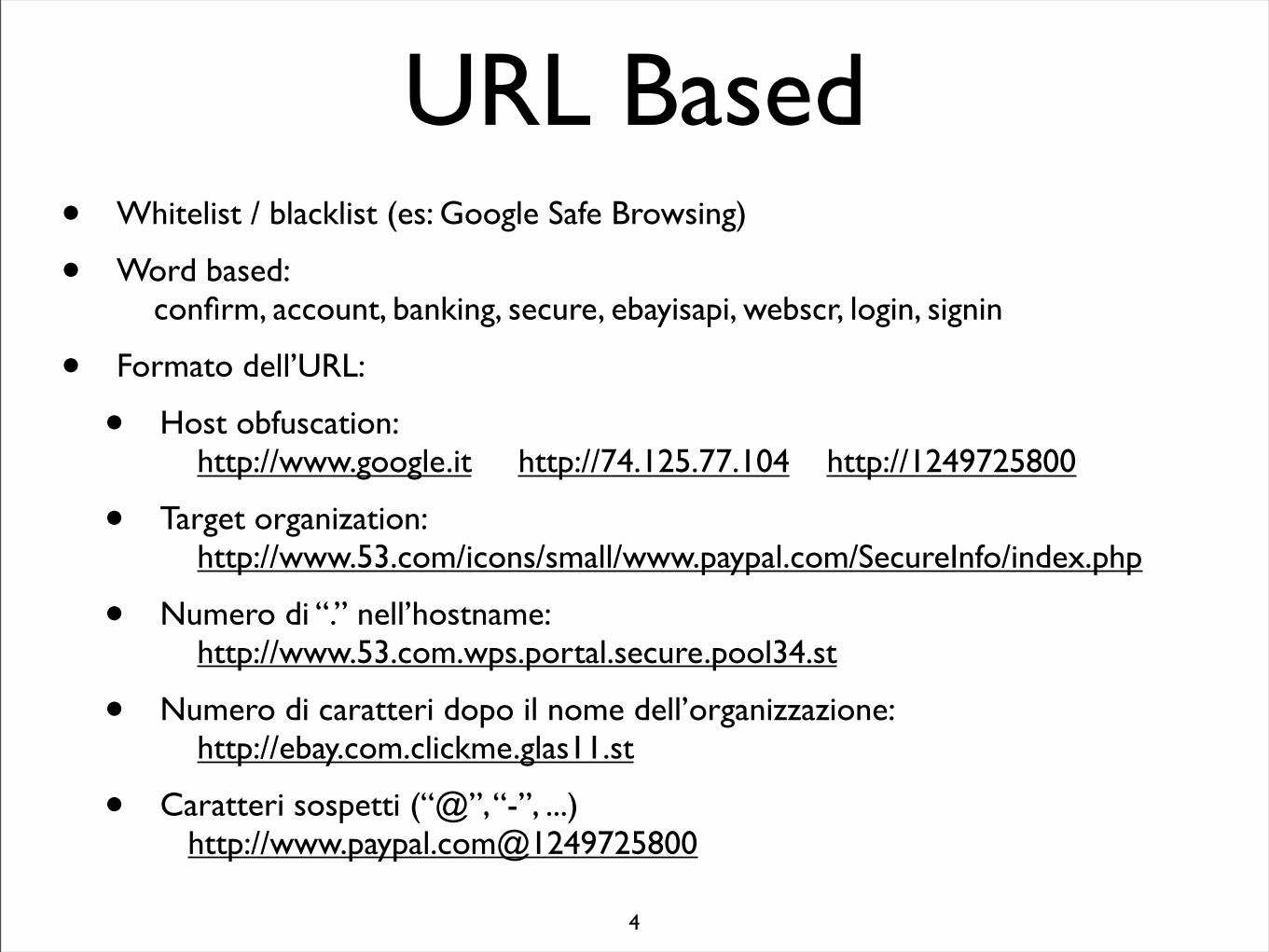
URL Based• Whitelist / blacklist (es: Google Safe Browsing)

• Word based: confirm, account, banking, secure, ebayisapi, webscr, login, signin

• Formato dell’URL:

• Host obfuscation: http://www.google.it http://74.125.77.104 http://1249725800

• Target organization: http://www.53.com/icons/small/www.paypal.com/SecureInfo/index.php

• Numero di “.” nell’hostname: http://www.53.com.wps.portal.secure.pool34.st

• Numero di caratteri dopo il nome dell’organizzazione: http://ebay.com.clickme.glas11.st

• Caratteri sospetti (“@”, “-”, ...) http://www.paypal.com@1249725800

4

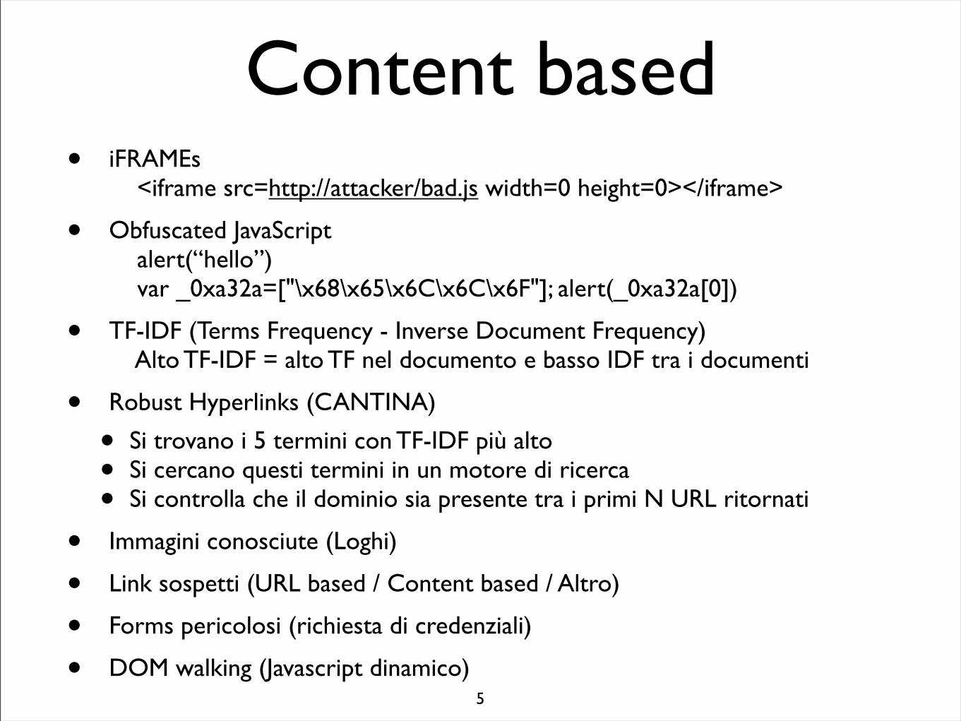
Content based• iFRAMEs

<iframe src=http://attacker/bad.js width=0 height=0></iframe>

• Obfuscated JavaScript alert(“hello”) var _0xa32a=["\x68\x65\x6C\x6C\x6F"]; alert(_0xa32a[0])

• TF-IDF (Terms Frequency - Inverse Document Frequency) Alto TF-IDF = alto TF nel documento e basso IDF tra i documenti

• Robust Hyperlinks (CANTINA)

• Si trovano i 5 termini con TF-IDF più alto• Si cercano questi termini in un motore di ricerca• Si controlla che il dominio sia presente tra i primi N URL ritornati

• Immagini conosciute (Loghi)

• Link sospetti (URL based / Content based / Altro)

• Forms pericolosi (richiesta di credenziali)

• DOM walking (Javascript dinamico)5

Informazioni indirette

• PageRank: in genere le pagine web di questo tipo non rimangono online per un tempo sufficiente da ottenere un PageRank alto

• PageRank dell’URL e dell’host

• Popolarità in Netcraft

• Data di registrazione del dominio

6

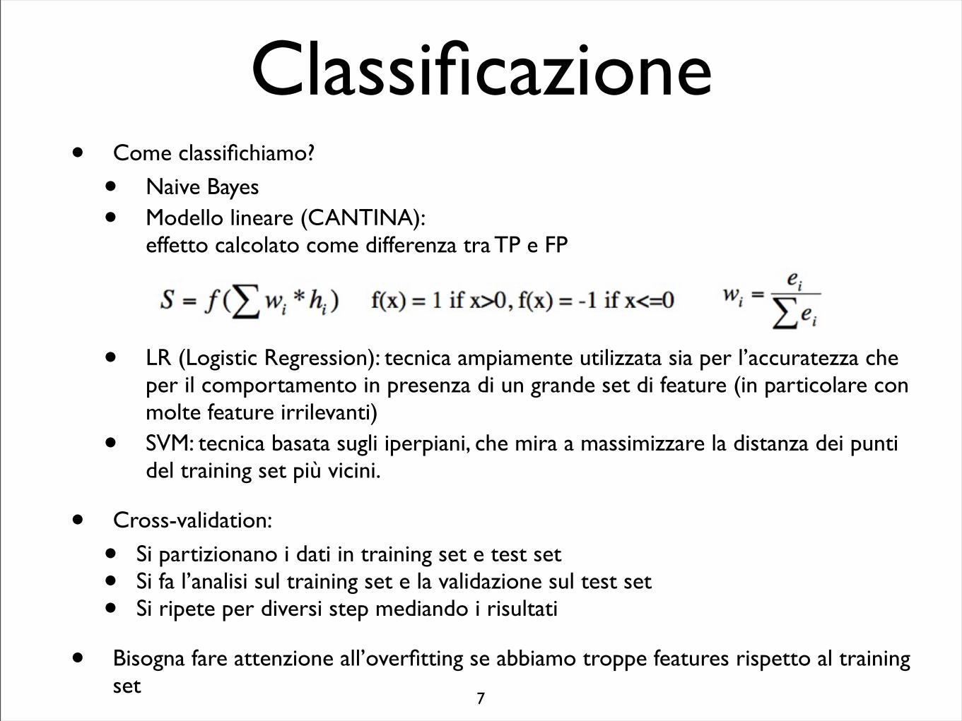
Classificazione• Come classifichiamo?

• Naive Bayes

• Modello lineare (CANTINA):effetto calcolato come differenza tra TP e FP

• LR (Logistic Regression): tecnica ampiamente utilizzata sia per l’accuratezza che per il comportamento in presenza di un grande set di feature (in particolare con molte feature irrilevanti)

• SVM: tecnica basata sugli iperpiani, che mira a massimizzare la distanza dei punti del training set più vicini.

• Cross-validation:

• Si partizionano i dati in training set e test set• Si fa l’analisi sul training set e la validazione sul test set• Si ripete per diversi step mediando i risultati

• Bisogna fare attenzione all’overfitting se abbiamo troppe features rispetto al training set

7

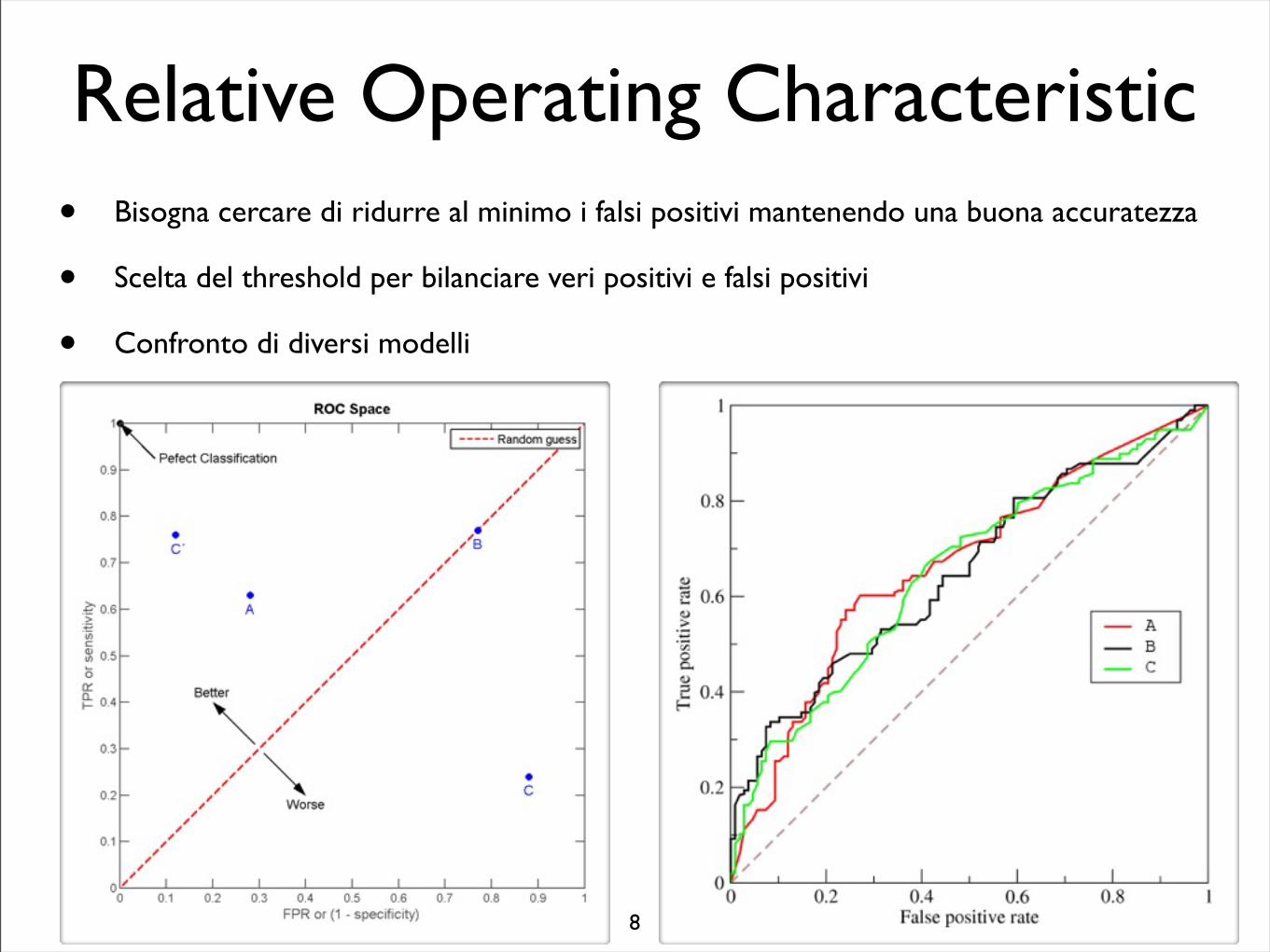
Relative Operating Characteristic• Bisogna cercare di ridurre al minimo i falsi positivi mantenendo una buona accuratezza

• Scelta del threshold per bilanciare veri positivi e falsi positivi

• Confronto di diversi modelli

8

Risultati

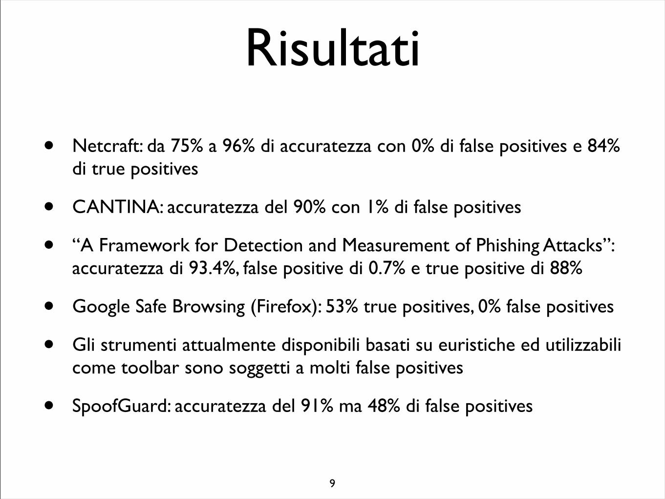
• Netcraft: da 75% a 96% di accuratezza con 0% di false positives e 84% di true positives

• CANTINA: accuratezza del 90% con 1% di false positives

• “A Framework for Detection and Measurement of Phishing Attacks”:accuratezza di 93.4%, false positive di 0.7% e true positive di 88%

• Google Safe Browsing (Firefox): 53% true positives, 0% false positives

• Gli strumenti attualmente disponibili basati su euristiche ed utilizzabili come toolbar sono soggetti a molti false positives

• SpoofGuard: accuratezza del 91% ma 48% di false positives

9

L’articolo

• Approccio esclusivamente URL based

• Non si controlla il contenuto delle pagine (rischio per l’utente e overhead)

• Non si considera il contesto in cui si trova il link (pagina web, e-mail, mittente dell’e-mail)

• Raccoglie un grande insieme di features

• E’ il metodo stesso a scegliere le features più importanti

• Accuratezza del 95-99% (sul test set)

10

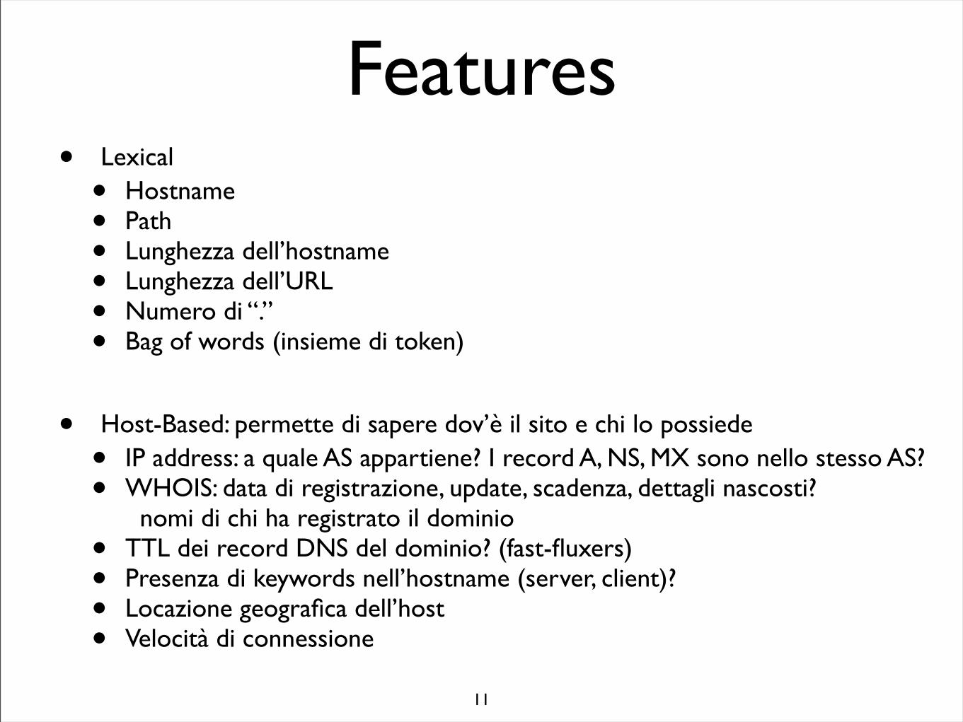
Features• Lexical

• Hostname• Path• Lunghezza dell’hostname• Lunghezza dell’URL• Numero di “.”• Bag of words (insieme di token)

• Host-Based: permette di sapere dov’è il sito e chi lo possiede

• IP address: a quale AS appartiene? I record A, NS, MX sono nello stesso AS?• WHOIS: data di registrazione, update, scadenza, dettagli nascosti?

nomi di chi ha registrato il dominio• TTL dei record DNS del dominio? (fast-fluxers)• Presenza di keywords nell’hostname (server, client)?• Locazione geografica dell’host• Velocità di connessione

11

Features

12

Classificazione

13

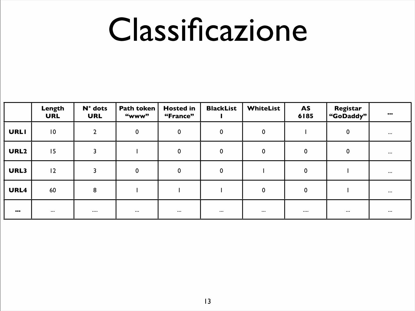
LengthURL

N° dotsURL

Path token“www”

Hosted in “France”

BlackList1

WhiteList AS6185

Registar“GoDaddy” ...

URL1 10 2 0 0 0 0 1 0 ...

URL2 15 3 1 0 0 0 0 0 ...

URL3 12 3 0 0 0 1 0 1 ...

URL4 60 8 1 1 1 0 0 1 ...

... ... .... ... ... ... ... .... ... ...

Logistic regression

14

z = b +d�

i=1

wixi

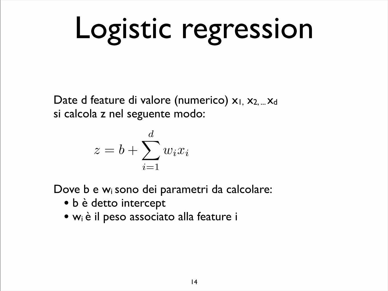
Date d feature di valore (numerico) x1, x2, ... xd si calcola z nel seguente modo:

Dove b e wi sono dei parametri da calcolare:• b è detto intercept• wi è il peso associato alla feature i

Logistic regression

15

σ(z) =1

1 + e−z

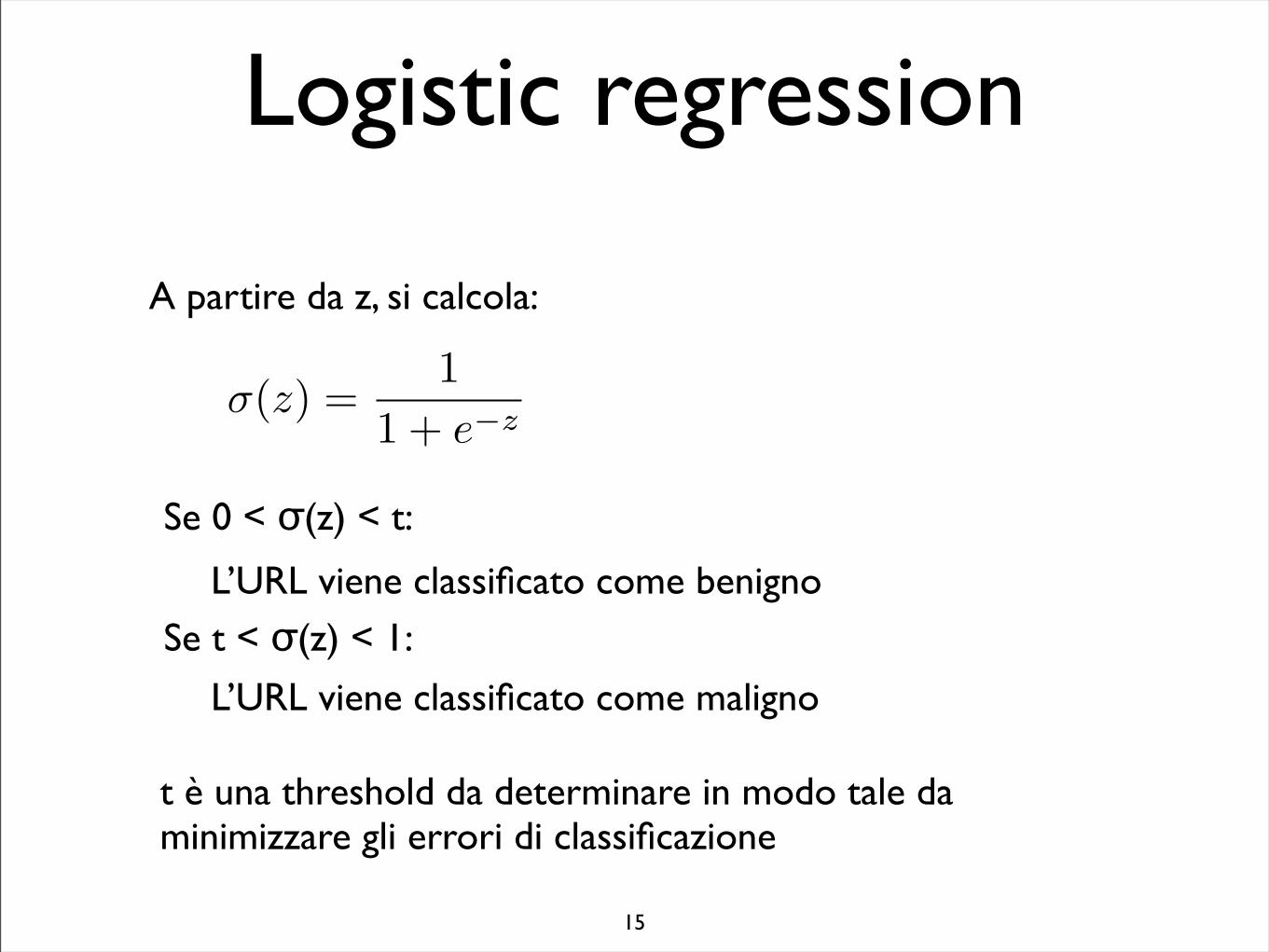
A partire da z, si calcola:

Se 0 < σ(z) < t:

Se t < σ(z) < 1:

t è una threshold da determinare in modo tale da minimizzare gli errori di classificazione

L’URL viene classificato come benigno

L’URL viene classificato come maligno

l1-norm regularization

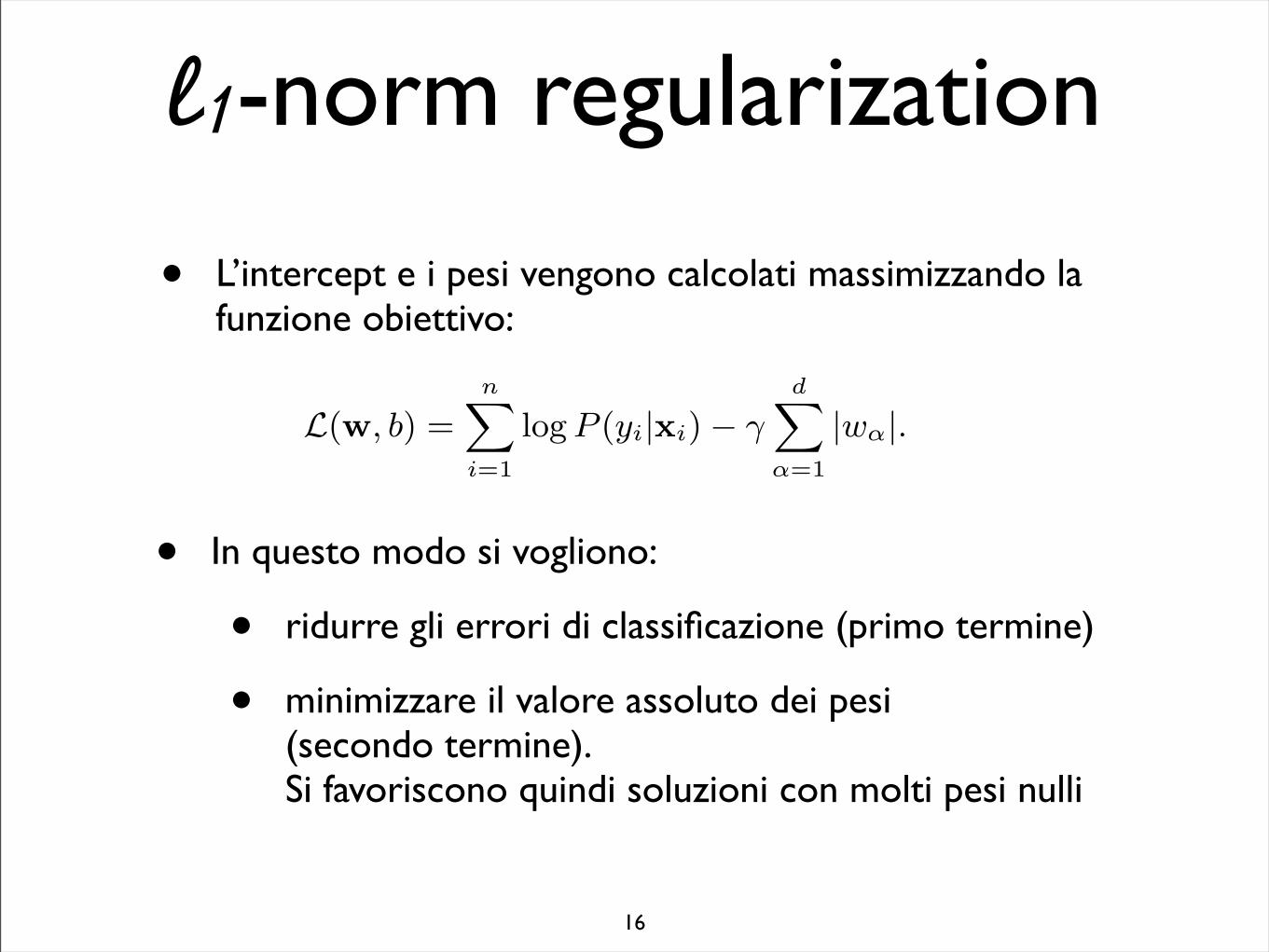
• L’intercept e i pesi vengono calcolati massimizzando la funzione obiettivo:

16

distributed independently of the values of other features [5]. Let-ting P (x|y) denote the conditional probability of the feature vec-

tor given its label, the model assumes P (x|y) =Qd

j=1P (xj |y).

Then, from Bayes rule, assuming that malicious and benign Websites occur with equal probability, we compute the posterior proba-bility that the feature vector x belongs to a malicious URL as:

P (y=1|x) =P (x|y = 1)

P (x|y=1) + P (x|y=0). (1)

Finally, the right hand side of eq. (1) can be thresholded to predicta binary label for the feature vector x.A Naive Bayes classifier is most easily trained by computing the

conditional probabilities P (xj |y) from their maximum likelihoodestimates [5]. For real-valued features, we model P (xj |y) by aGaussian distribution whose mean and standard deviation are com-puted over the jth component of feature vectors in the training setwith label y. For binary-valued features, we estimate P (xj =1|y)as the fraction of feature vectors in the training set with label y forwhich the jth component is one.The model parameters in the Naive Bayes classifier are estimated

to maximize the joint log-likelihood of URL features and labels,as opposed to the accuracy of classification. Optimizing the lat-ter typically leads to more accurate classifiers, notwithstanding theincreased risk of overfitting.Support Vector Machine (SVM): SVMs are widely regarded

as state-of-the-art models for binary classification of high dimen-sional data. SVMs are trained to maximize the margin of cor-rect classification, and the resulting decision boundaries are robustto slight perturbations of the feature vectors, thereby providing ahedge against overfitting. The superior generalization abilities ofSVMs have been borne out by both theoretical studies and experi-mental successes [23].The decision rule in SVMs is expressed in terms of a kernel

functionK(x,x′) that computes the similarity between two featurevectors and non-negative coefficients {αi}

ni=1 that indicate which

training examples lie close to the decision boundary. SVMs classifynew examples by computing their (signed) distance to the decisionboundary. Up to a constant, this distance is given by:

h(x) =n

X

i=1

αi(2yi−1)K(xi,x), (2)

where the sum is over all training examples. The sign of this dis-tance indicates the side of the decision boundary on which the ex-ample lies. In practice, the value of h(x) is thresholded to predicta binary label for the feature vector x.SVMs are trained by first specifying a kernel function K(x,x′)

and then computing the coefficients αi that maximize the marginof correct classification on the training set. The required optimiza-tion can be formulated as an instance of quadratic programming, aproblem for which many efficient solvers have been developed [6].In our study, we experimented with both linear and radial basisfunction (RBF) kernels.Logistic Regression: This is a simple parametric model for bi-

nary classification where examples are classified based on their dis-tance from a hyperplane decision boundary [11]. The decision ruleis expressed in terms of the sigmoid function σ(z) = [1 + e−z]−1,which converts these distances into probabilities that feature vec-tors have positive or negative labels. The conditional probabilitythat feature vector x has a positive label y=1 is the following:

P (y=1|x) = σ(w·x + b), (3)

where the weight vector w∈#d and scalar bias b are parameters tobe estimated from training data. In practice, the right hand side of

eq. (3) is thresholded to obtain a binary prediction for the label ofthe feature vector x.

We trained models for logistic regression using a regularizedform of maximum likelihood estimation. Specifically, we chosethe weight vector w and bias b to maximize the objective function:

L(w, b) =n

X

i=1

log P (yi|xi) − γ

dX

α=1

|wα|. (4)

The first term computes the conditional log-likelihood that the modelcorrectly labels all the examples in the training set. The secondterm in eq. (4) penalizes large magnitude values of the elements inthe weight vectorw. Known as $1-norm regularization, this penaltynot only serves as a measure against overfitting, but also encouragessparse solutions in which many elements of the weight vector areexactly zero. Such solutions emerge naturally in domains where thefeature vectors contain a large number of irrelevant features. Therelative weight of the second term in eq. (4) is determined by theregularization parameter. We selected the value of γ in our experi-ments by cross validation.

We included $1-regularized logistic regression for its potentialadvantages over Naive Bayes and SVMs in our particular domain.Unlike Naive Bayes classification, the parameters in logistic regres-sion are estimated by optimizing an objective function that closelytracks the error rate. Unlike SVMs, $1-regularized logistic regres-sion is especially well suited to domains with large numbers of ir-relevant features. (In large numbers, such features can drown outthe similarities between related examples that SVMs expect to bemeasured by the kernel function.) Finally, because $1-regularizedlogistic regression encourages sparse solutions, the resulting mod-els often have decision rules that are easier to interpret in terms ofrelevant and irrelevant features.

3. DATA SETSThis section describes the data sets that we use for our evalu-

ation. For benign URLs, we used two data sources. One is theDMOZ Open Directory Project [19]. DMOZ is a directory whoseentries are vetted manually by editors. The editors themselvesgo through a vetting process, with editors given responsibility forlarger portions of the directory as they gain trust and experience.The second source of benign URLs was the random URL selectorfor Yahoo’s directory. A sample of this directory can be generatedby visiting http://random.yahoo.com/bin/ryl.

We also drew from two sources for URLs to malicious sites:PhishTank [21] and Spamscatter [3]. PhishTank is a blacklist ofphishing URLs consisting of manually-verified user contributions.Spamscatter is a spam collection infrastructure from which we ex-tract URLs from the bodies of those messages. Note that the ma-licious URL data sets have different scopes. PhishTank focuses onphishing URLs, while Spamscatter includes URLs for a wide rangeof scams advertised in email spam (phishing, pharmaceuticals, soft-ware, etc.). Both sources include URLs crafted to evade automatedfilters, while phishing URLs in particular may be crafted to visuallytrick users as well.

Table 1 summarizes the number and types of features in thedata sets that we use in our evaluations. The four data sets con-sist of pairing 15,000 URLs from a benign source (either Yahoo orDMOZ) with URLs from a malicious source (5,500 from Phish-Tank and 15,000 from Spamscatter). We refer to these sets as theDMOZ-PhishTank (DP), DMOZ-Spamscatter (DS), Yahoo-Phish-Tank (YP), and Yahoo-Spamscatter (YS) sets. We collected URLfeatures between August 22, 2008 – September 1, 2008.

We normalized the real-valued features in each feature set to

1247

• In questo modo si vogliono:

• ridurre gli errori di classificazione (primo termine)

• minimizzare il valore assoluto dei pesi(secondo termine).Si favoriscono quindi soluzioni con molti pesi nulli

Data sets

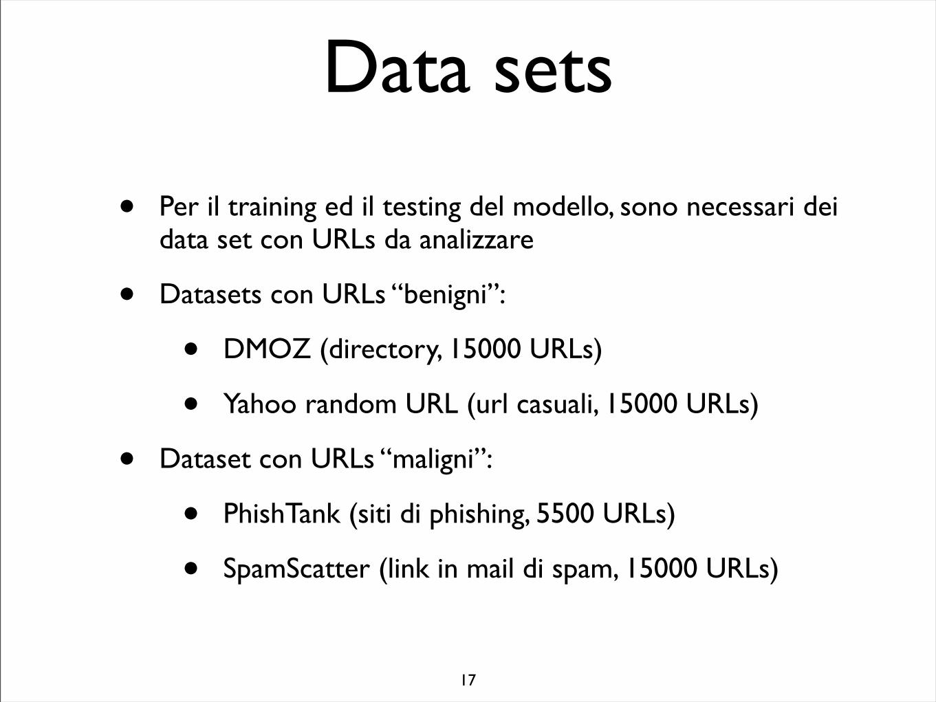
• Per il training ed il testing del modello, sono necessari dei data set con URLs da analizzare

• Datasets con URLs “benigni”:

• DMOZ (directory, 15000 URLs)

• Yahoo random URL (url casuali, 15000 URLs)

• Dataset con URLs “maligni”:

• PhishTank (siti di phishing, 5500 URLs)

• SpamScatter (link in mail di spam, 15000 URLs)

17

Esperimenti

• Combinazione di dataset benigni e maligni: se ne ottengono quattro: DP, DS, YP, YSD: DMOZ, Y:Yahoo, S: Spamscatter, P: PhishTank

• Esperimenti separati per ciascun dataset

• In ciascun esperimento si divide il dataset in 10 parti casuali

• Il 50% di ciascuna parte è usato per il training, l’altro 50% per il testing

• Il risultato della classificazione è calcolato come media dei risultati ottenuti nelle 10 parti

18

Risultati

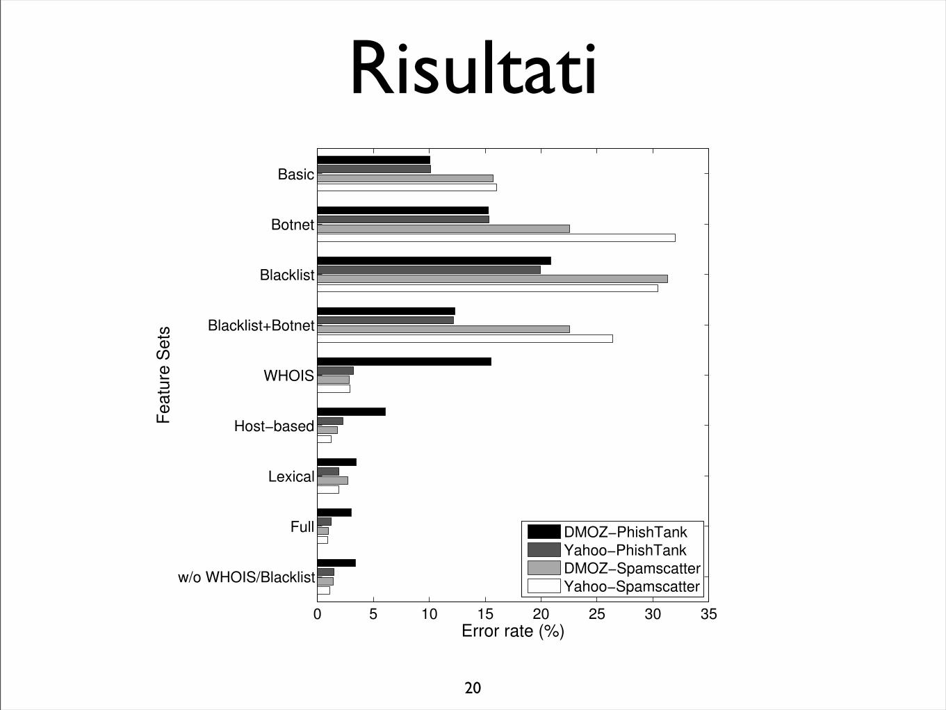
• Dai risultati ottenuti, l’utilizzo di un gran numero di feature produce errori molto piccoli (<5%)

• Si ottengono errori simili anche senza l’utilizzo delle feature delle blacklist

• Utilizzando invece solamente feature relative all’URL gli errori sono ben più grandi (>10%)

• Si nota come ci siano differenze, anche significative, variando i dataset. Ad esempio gli URLs raccolti da PhishTank hanno parecchi campi WHOIS non disponibili

19

Risultati

20

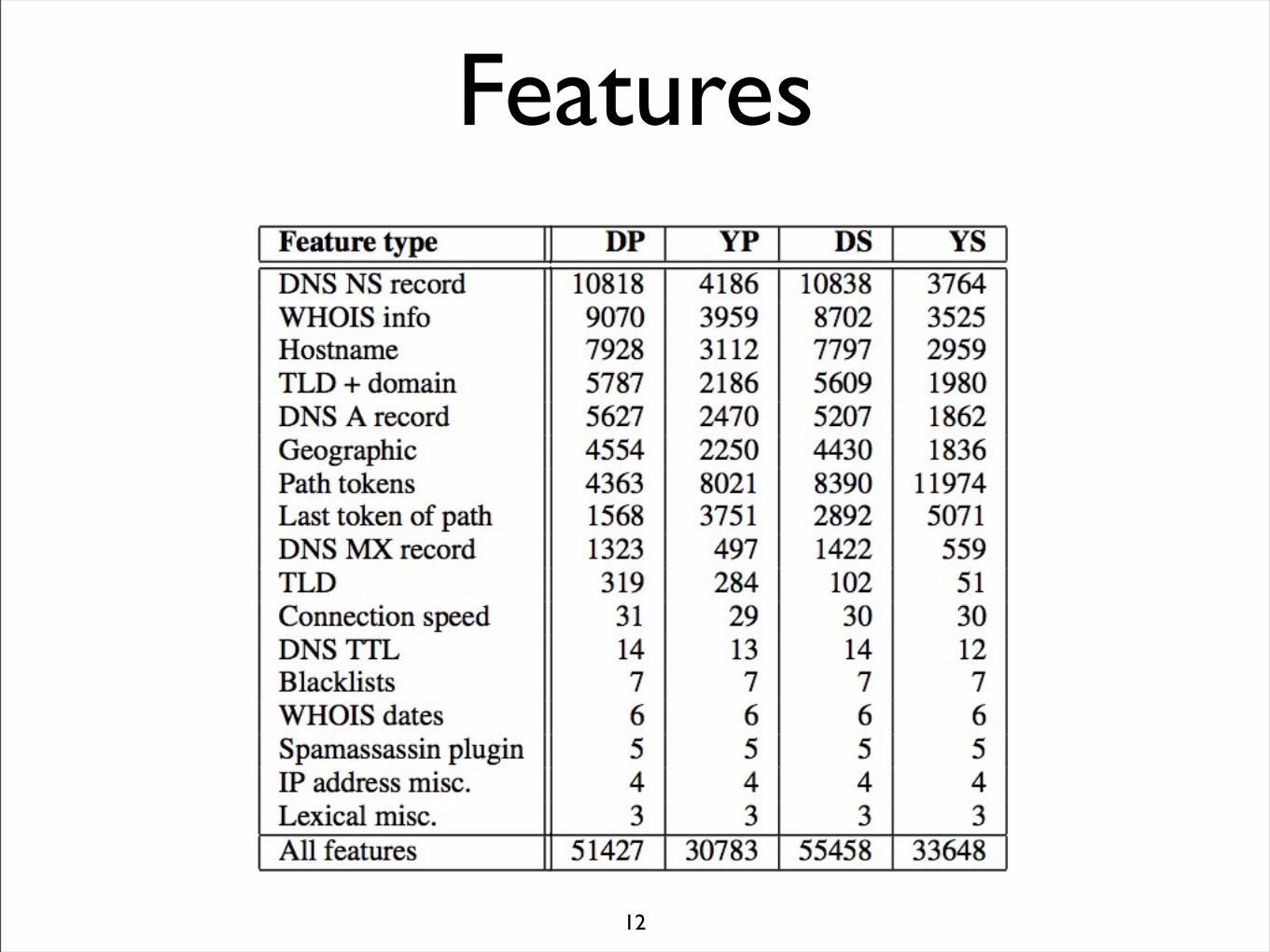
Feature type DP YP DS YS

DNS NS record 10818 4186 10838 3764WHOIS info 9070 3959 8702 3525Hostname 7928 3112 7797 2959TLD + domain 5787 2186 5609 1980DNS A record 5627 2470 5207 1862Geographic 4554 2250 4430 1836Path tokens 4363 8021 8390 11974Last token of path 1568 3751 2892 5071DNS MX record 1323 497 1422 559TLD 319 284 102 51Connection speed 31 29 30 30DNS TTL 14 13 14 12Blacklists 7 7 7 7WHOIS dates 6 6 6 6Spamassassin plugin 5 5 5 5IP address misc. 4 4 4 4Lexical misc. 3 3 3 3All features 51427 30783 55458 33648

Table 1: Breakdown of feature types for data sets used in eval-uations.

lie between zero and one, shifting and rescaling each real-valuedfeature so that zero and one corresponded to the minimum andmaximum values observed in the training set. Values outside thisrange in the testing set were clipped to zero or one as appropriate.The normalization served to equalize the range of the features ineach feature set, both real-valued and binary. Intuitively, it reflectsour prior belief that the real-valued and binary-valued features areequally informative and therefore should be calibrated on the samemeasurement scales.One further complication arises due to undefined, or missing,

features. Many real-valued features are undefined for large num-bers of examples in the data set (e.g., DNS time-to-live values).We handled missing values using the following heuristic: for eachreal-valued feature, we defined an extra binary feature indicatingwhether the feature was defined. This heuristic enables the classi-fiers to learn how to treat missing features from the way they appearin the training set.

4. EVALUATIONIn this section, we evaluate the effectiveness of the classifiers

on identifying URLs to malicious sites. Specifically, we want toanswer the following questions: Does using more features lead tomore accurate classification? What is the most appropriate classifi-cation model to use? What is the impact on accuracy if we tune theclassifier for lower false positives? Can we effectively classify datafrom once source with a model that was trained on a different datasource? What trends do we see among the relevant features? Andwhat do the misclassified examples have in common?

4.1 MethodologyWe start by describing our experimental methodology. For each

feature set and data set in our experiments, we perform classifi-cation over 10 random splits of the data, and the splits are 50/50between training and testing. We learn a decision threshold t thatwill minimize the overall classification error (see Section 2.2 formethodology of learning t). We show the average classificationresults of those 10 splits.We ran our experiments on a machine with 2 dual-core 2.33 GHz

Xeon processors with 4 GB memory. Memory exhaustion wasnot an issue, but typical usage was on the order of a few hundredmegabytes. We implemented a Naive Bayes solver in MATLAB.For the SVM solvers, we used the .mex implementations of LIB-SVM [6] and LIBLINEAR [7] that interface with MATLAB. We

0 5 10 15 20 25 30 35

Basic

Botnet

Blacklist

Blacklist+Botnet

WHOIS

Host−based

Lexical

Full

w/o WHOIS/Blacklist

Error rate (%)

Fe

atu

re S

ets

DMOZ−PhishTankYahoo−PhishTankDMOZ−SpamscatterYahoo−Spamscatter

Figure 1: Error rates for LR with nine features sets on each ofthe four URL data sets. Overall, using more features improvesclassification accuracy.

implemented a custom optimizer for !1-regularized logistic regres-sion in MATLAB using multiplicative updates [24].

4.2 Feature ComparisonOur first experiments on URL classification were designed to

explore the potential benefits of considering large numbers of auto-matically generated features as opposed to small numbers of man-ually chosen features. Fig. 1 compares the classification error rateson the four data sets described in Section 3 using nine differentsets of features. The different feature sets involve combinations offeatures reflecting various practical considerations. For brevity, weonly show detailed results from !1-regularized logistic regression(LR), which yields both low error rates (see Section 4.3) and alsohighly interpretable models (see Section 4.6). However, the otherclassifiers also produce qualitatively similar results.

Table 2 shows the total number of features in each feature set forthe Yahoo-PhishTank data set. For these experiments, we also re-port the number of relevant features that received non-zero weightfrom !1-regularized logistic regression. (The other three data setsyield qualitatively similar results.) The feature sets are listed in as-cending order of the total number of features. In what follows, wedescribe the detailed compositions of these feature sets, as well astheir effects on classification accuracy.

We start with a “Basic” feature set that corresponds to the set ofURL-related (not content-related) heuristics commonly chosen byvarious anti-phishing studies, including Fette et al. [8], Bergholzet al. [4] and CANTINA [28]. This set consists of four features:the number of dots in a URL, whether the hostname contains an IPaddress, the WHOIS registration date (a real-valued feature), andan indicator variable for whether the registration date is defined.Under this scheme, the classifier achieves a 10% error rate.

The next three feature sets (Botnet, Blacklist, and Blacklist +Botnet) represent the use of current spam-fighting techniques forpredicting malicious URLs. The features for “Botnet” are from theSpamAssassin Botnet plugin (Section 2.1). These consist of fivebinary features indicating the presence of certain client- or server-specific keywords, whether the hostname contains an IP address,and two more features involving the PTR record of the host. Withthese features, we obtain a 15% error rate at best.

1248

Analisi

• Con il classificatore LR, siamo in grado di analizzare il “peso” di ciascuna feature, in maniera da trovare quelle più o meno rilevanti

• Se il peso relativo ad una feature è

• positivo: allora essa “penalizza” l’URL

• negativo: allora essa “premia” l’URL

• zero: allora essa non è considerata

• In questo modo possiamo sia verificare quello che già sappiamo sugli URLs maligni, sia imparare nuove cose

21

Analisi

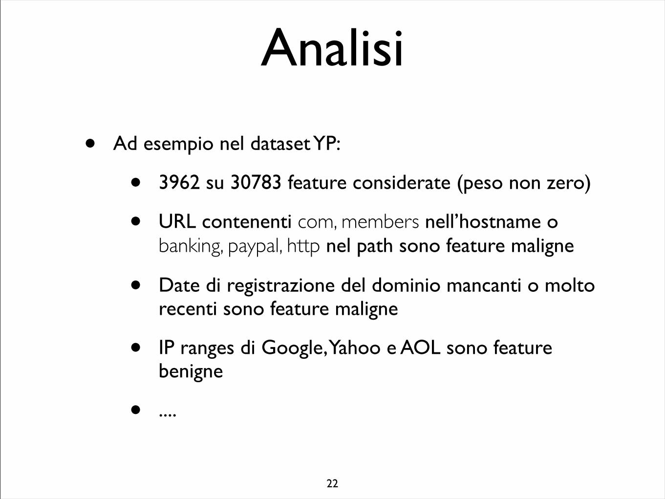
• Ad esempio nel dataset YP:

• 3962 su 30783 feature considerate (peso non zero)

• URL contenenti com, members nell’hostname o banking, paypal, http nel path sono feature maligne

• Date di registrazione del dominio mancanti o molto recenti sono feature maligne

• IP ranges di Google, Yahoo e AOL sono feature benigne

• ....

22

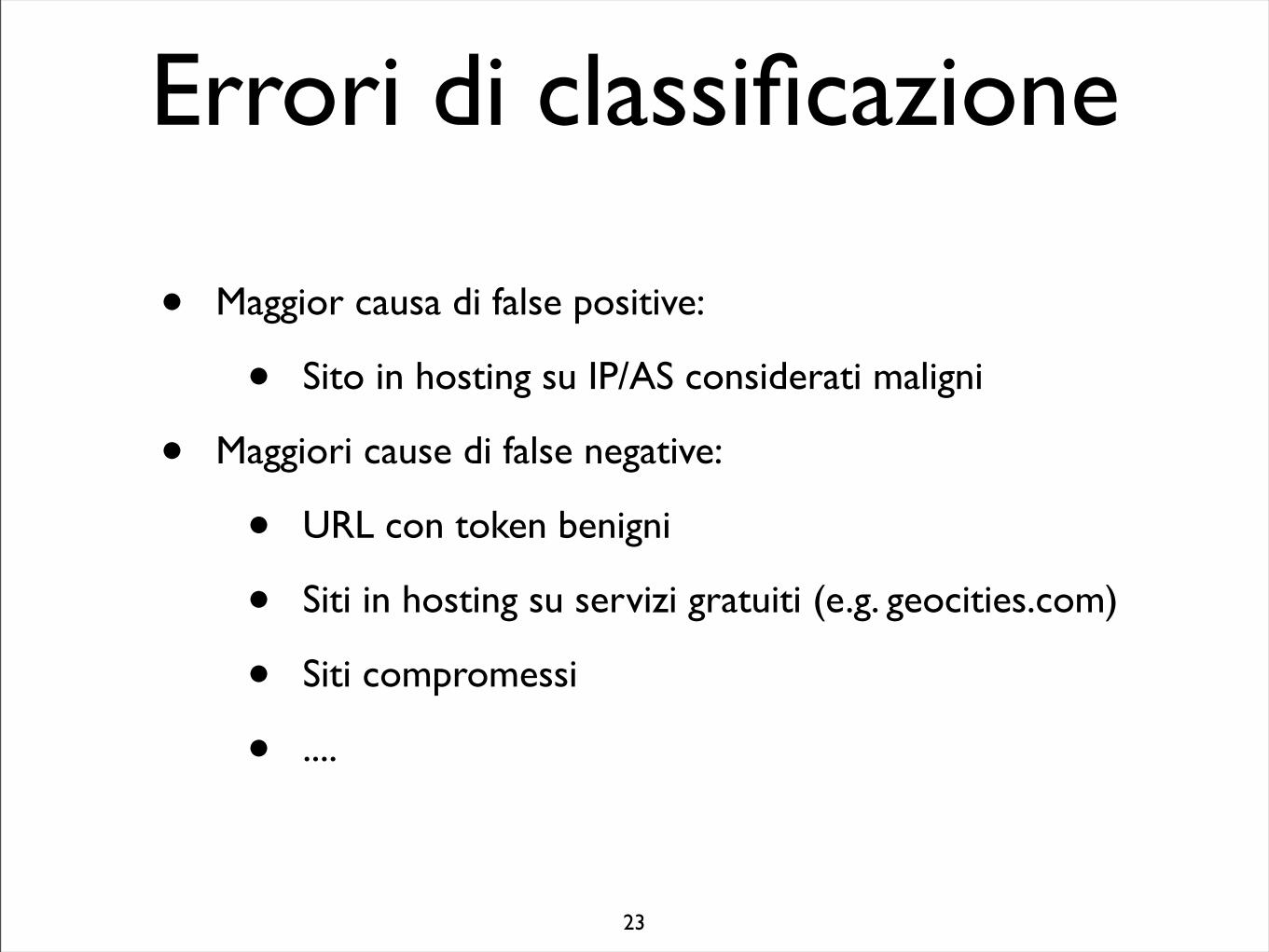
Errori di classificazione

• Maggior causa di false positive:

• Sito in hosting su IP/AS considerati maligni

• Maggiori cause di false negative:

• URL con token benigni

• Siti in hosting su servizi gratuiti (e.g. geocities.com)

• Siti compromessi

• ....

23

Limitazioni

• Conoscendo le feature ed i pesi ad esse associati, un attaccante potrebbe tentare di ingannare il classificatore:URL con poche informazioni (e.g. TinyURL), registrazione su domini benigni (e.g. .org), ecc.

• Problema dei falsi positivi rispetto ad un approccio tradizionale tramite Blacklist (dove i falsi positivi sono praticamente zero).Possibile soluzione per ridurli: calcolare i pesi in maniera tale da da minimizzare i falsi positivi, invece degli errori complessivi (naturalmente aumenteranno i falsi negativi).

24

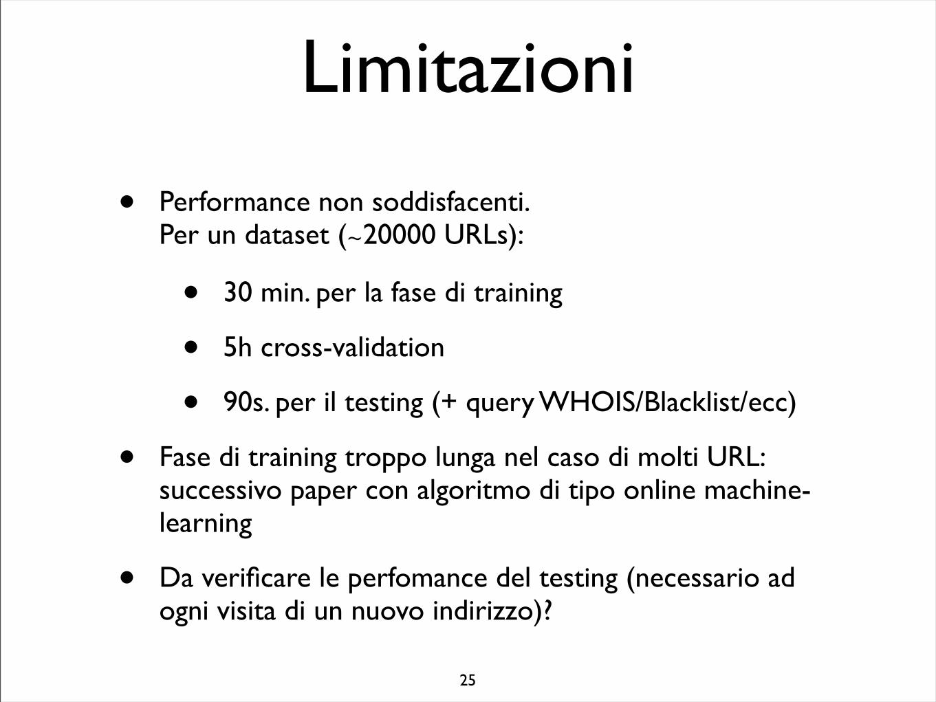
Limitazioni

• Performance non soddisfacenti.Per un dataset (∼20000 URLs):

• 30 min. per la fase di training

• 5h cross-validation

• 90s. per il testing (+ query WHOIS/Blacklist/ecc)

• Fase di training troppo lunga nel caso di molti URL: successivo paper con algoritmo di tipo online machine-learning

• Da verificare le perfomance del testing (necessario ad ogni visita di un nuovo indirizzo)?

25

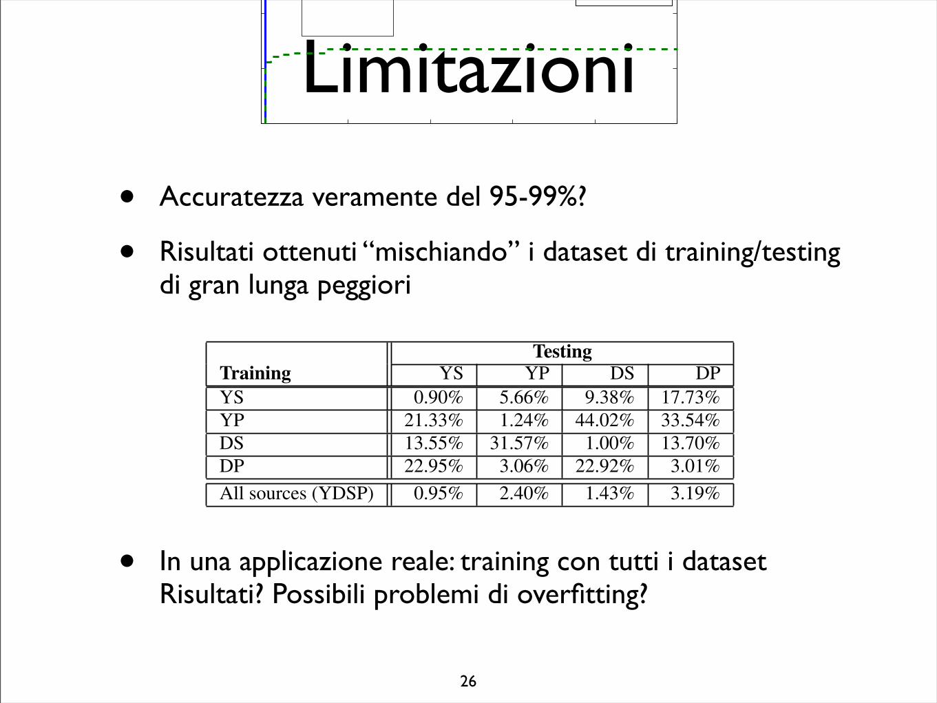
Limitazioni

• Accuratezza veramente del 95-99%?

• Risultati ottenuti “mischiando” i dataset di training/testing di gran lunga peggiori

26

times for each classifier. The cross-validation time refers specifi-cally to the cross-validation process used in LR to choose a regu-larization constant. Although expensive, it can be effectively amor-tized when training over time.

Bayes SVM-lin SVM-rbf LR

Train 51 s 50 s 63 s 30 minTest 87 s 91 s 170 s 90 sCross-validation — — — 5 hrs

Table 3: Training and testing times for the Yahoo-PhishTankdata set.

The SVM and LR classifiers have at least half of the error ofNaive Bayes, which is not surprising given the models that wechose. Naive Bayes is a classifier that sees wide-spread use in spamfilters and related security applications, in part because the trainingand testing performance of Naive Bayes is fast. However, the bene-fit of reduced training time is outweighed in this case by the benefitof using classifiers whose explicit goal is to minimize errors. Thistradeoff is particularly worthwhile when we are dealing with a largefeature set.As mentioned in Section 2.2, SVM classifiers can perform poorly

if irrelevant features in a large feature set make the kernel functionspoor measures of similarity. Given that the difference in error be-tween SVM and LR is so small, though, this problem did not mate-rialize in our data set. As such, we continue to show the results forLR for the remaining experiments because of its interpretability,which is useful for understanding how the model performs (Sec-tion 4.6) and how it might be improved (Section 4.7).

4.4 Tuning False Positives & NegativesAn advantage of using these models is that they can tradeoff false

positives and false negatives. We have seen in the previous sectionsthat classifying with the “Full” feature set yields very low overallerror rates. For policy reasons, however, we may not want to choosea decision threshold t to minimize the overall error rate. Instead,we may want to tune the threshold to have very low false positivesat the expense of more false negatives (or vice versa).Consider blacklisting as a motivating example. Blacklisting has

the intrinsic advantage that it will have very low false positives.Suppose a network administrator wants to take advantage of thebenefits of classifying over a full feature set while maintaining thelow false positives of a blacklist-only policy as applied to URLclassification. To do so, we can select a threshold for the full featureset that will yield a false positive rate competitive with blacklistingwhile having a much lower false negative rates.Figure 3 shows the results of this experiment as an ROC graph

with respect to the decision threshold t. We see that even if wetune the decision threshold of the full-featured classifier to the samefalse positives as a blacklist-only classifier, the full-featured classi-fier still predicts malicious URLs with much better accuracy thanwith blacklists alone.

4.5 Mismatched Data SourcesCoupling the appropriate classifier with a large feature set can

yield a highly accurate classifier when trained and tested on disjointsets of the same data source. But do these results hold when train-ing and testing examples are drawn from different data sources?To answer this question, we experiment with training and testingon various combinations of benign and malicious sources of URLs.(We use the abbreviations defined in Section 3 to refer to each com-bination of data sources, e.g. YP for Yahoo-PhishTank).Table 4 shows classification results using !1-regularized logistic

0 0.2 0.4 0.6 0.8 10

20

40

60

80

100

False positive rate (%)

Tru

e p

osi

tive

ra

te (

%)

↑FP = 0.1%FN = 7.6%

↓

FP = 0.1%FN = 74.3%

FullBlacklist

Figure 3: Tradeoff between false positives and false negatives:ROC graph for LR over an instance of the Yahoo-PhishTankdata set using (1) the “Full” feature set and (2) blacklists only.We highlight the points where the false positives are tuned to0.1%.

TestingTraining YS YP DS DPYS 0.90% 5.66% 9.38% 17.73%YP 21.33% 1.24% 44.02% 33.54%DS 13.55% 31.57% 1.00% 13.70%DP 22.95% 3.06% 22.92% 3.01%

All sources (YDSP) 0.95% 2.40% 1.43% 3.19%

Table 4: Overall error rates when training on one data sourceand testing on another (possibly different) data source using theLR classifier.

regression. Each row represents a pairing of benign and maliciousURL training sources, and each column represents a pairing of be-nign and malicious URL testing sources. As expected, the entriesalong the NW-SE diagonal yield the lowest classification errors be-cause they represent matching similar data sources (these numbersare repeated from previous experiments). When only the benignURL source is mismatched (e.g., YS and DS), error increases dueto higher false positives. And if only the malicious URL source ismismatched (e.g., YS and YP), error increases due to higher falsenegatives. Nevertheless, we note that training on the Spamscatterset — which includes URLs advertising a wide range of scam sites— generally performs better on a mismatched source (YS-YP at6%, DS-DP at 14%) than the PhishTank set (YP-YS at 21%, DP-DS at 23%) — which focuses only on phishing sites (Section 3).

Finally, if the training and testing sources are completely mis-matched (SW-NE diagonal), the error ranges between 18–44%. Al-though better than random, the disparity in accuracy emphasizesthe judicious selection of training data. This selection is of partic-ular importance for use in a deployment: the training data shouldreflect the “testing” environment in which the system is used. Tothat end, if we use all four training sources, the generalization abil-ity of the classifier is strong across all testing sources (last row).Thus, in a deployed system practitioners will want to pay specialattention to collecting training data that is representative.

4.6 Model AnalysisBesides high classification accuracy, LR has the advantages of

performing automatic feature selection as well as providing an in-terpretable linear model of the training data. In particular, becausethe output of a linear model depends on the weighted sum of thefeatures, the sign and magnitude of the individual parameter vectorcoefficients can tell us how individual features contribute to a “ma-licious” prediction or a “benign” prediction. Positive coefficients

1250

• In una applicazione reale: training con tutti i datasetRisultati? Possibili problemi di overfitting?

Conclusioni

• Approccio interessante per la classificazione degli URLs

• L’utilizzo di LR consente un’analisi delle caratteristiche dei siti maligni, utile anche per scoprire nuovi trend

• Problemi di scalabilità rilevanti

• Da verificare l’accuratezza del modello nei casi reali

27

Riferimenti“Beyond Blacklists: Learning to Detect Malicious Web Sites from Suspicious URLs”Justin Ma, Lawrence K. Saul, Stefan Savage, Geoffrey M. VoelkerIn Proc. of the 15th ACM SIGKDD Conference on Knowledge Discovery and Data Mining, Paris 2009

“A Framework for Detection and Measurement of Phishing Attacks”Niels Provos, Sujata Garera, Monica Chew, Aviel D. RubinIn Proc. of the 2007 ACM workshop on Recurring malcode, Alexandria 2007

“All Your iFRAMEs Point to Us”Niels Provos, Panayiotis Mavrommatis, Moheeb Abu Rajab, Fabian MonroseIn Proc. of the 17th conference on Security symposium, San Jose 2008

“CANTINA: A Content-Based Approach to Detecting Phishing Web Sites”Yue Zhang, Jason Hong, Lorrie CranorIn Proc. of the Sixteenth International World Wide Web Conference (WWW2007), Banff 2007

“The elements of statistical learning: data mining, inference, and prediction”Trevor Hastie,Robert Tibshirani,Jerome FriedmanSpringer, 2003

“Identifying Suspicious URLs: An Application of Large-Scale Online Learning”Justin Ma, Lawrence K. Sault, Stefan Savage, Geoffrey M. VoelkerIn Proc. of the International Conference on Machine Learning (ICML), Montreal 2009

28