Analisi del profilo NACA 63012A · - Generazione di un report e di un grafico - Impostazione dei...
82
Seminario nell’ambito del corso di Aerodinamica degli Aeromobili Analisi del profilo NACA 63012A con il solutore STAR-CCM+ Ing. Giuseppe Calise Ph.D. Student e-mail: [email protected]
Transcript of Analisi del profilo NACA 63012A · - Generazione di un report e di un grafico - Impostazione dei...
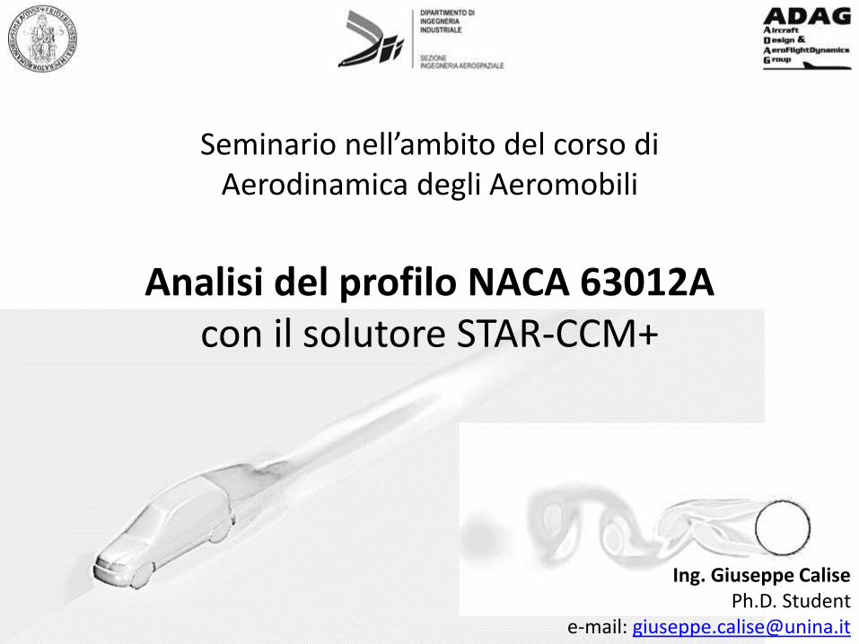
Seminario nell’ambito del corso di Aerodinamica degli Aeromobili
Analisi del profilo NACA 63012A
con il solutore STAR-CCM+
Ing. Giuseppe Calise Ph.D. Student
e-mail: [email protected]

Analisi del profilo NACA 63012A con il solutore STAR-CCM+
SOMMARIO
• Parte 1 - Introduzione al software CFD - Importazione geometria CAD - Generazione griglia di calcolo
• Parte 2 - Impostazione della fisica del problema - Generazione di un report e di un grafico - Impostazione dei criteri di convergenza e avvio del calcolo
• Parte 3 - Confronto dei risultati ottenuti con altri metodi - Variazione della geometria e/o delle condizioni fisiche - Avvio di un nuovo calcolo e confronto dei risultati
Analisi del profilo NACA 63012A con il solutore STAR-CCM+
Introduzione al software CFD
Analisi del profilo NACA 63012A con il solutore STAR-CCM+
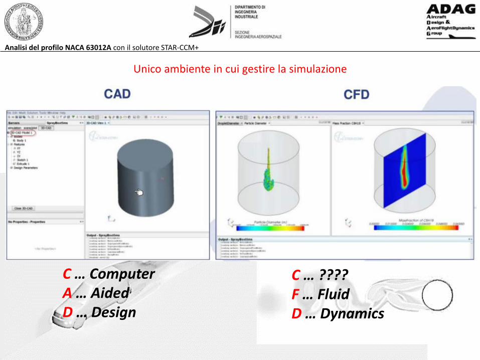
Unico ambiente in cui gestire la simulazione
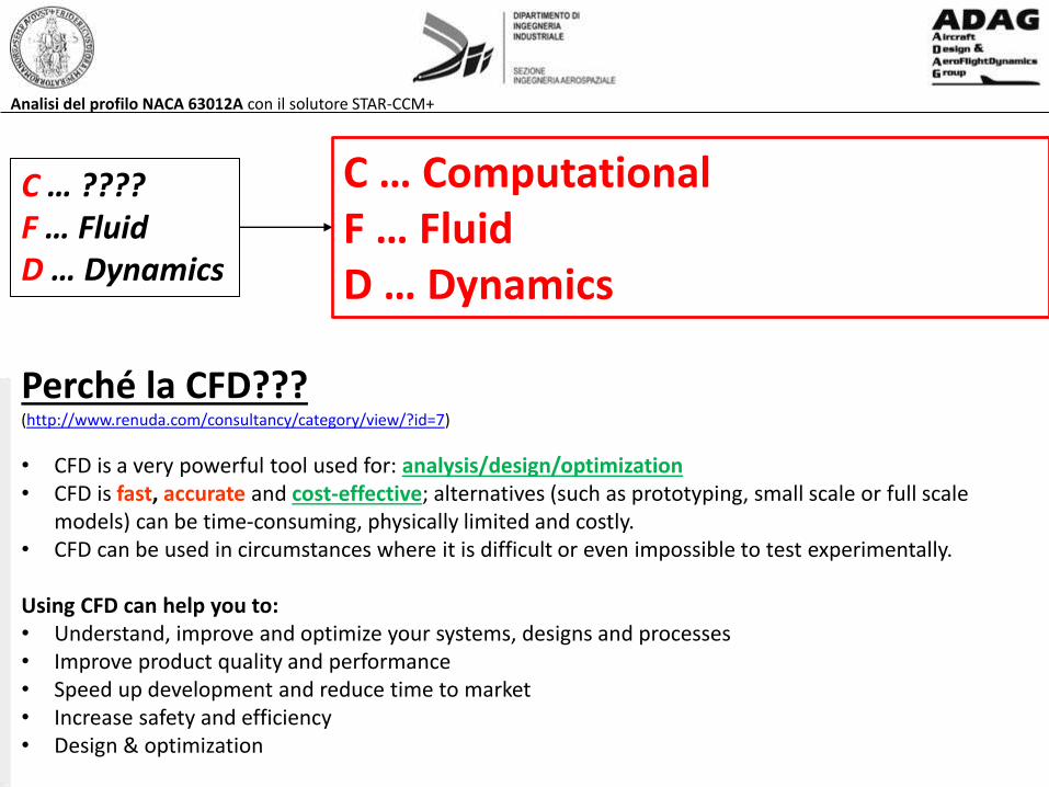
C … Computer A … Aided D … Design
C … ???? F … Fluid D … Dynamics
Analisi del profilo NACA 63012A con il solutore STAR-CCM+
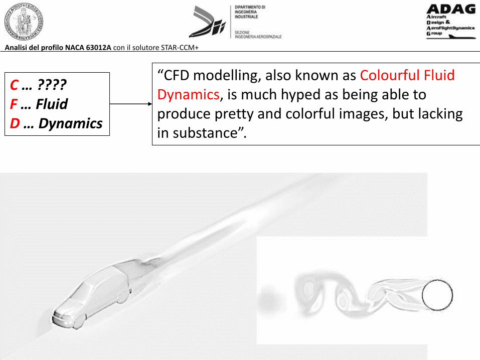
C … ???? F … Fluid D … Dynamics
“CFD modelling, also known as Colourful Fluid Dynamics, is much hyped as being able to produce pretty and colorful images, but lacking in substance”.
Analisi del profilo NACA 63012A con il solutore STAR-CCM+
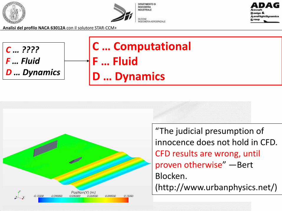
C … ???? F … Fluid D … Dynamics
“CFD modelling, also known as Colourful Fluid Dynamics, is much hyped as being able to produce pretty and colorful images, but lacking in substance”.
“The judicial presumption of innocence does not hold in CFD. CFD results are wrong, until proven otherwise” —Bert Blocken. (http://www.urbanphysics.net/)
C … Computational F … Fluid D … Dynamics
Analisi del profilo NACA 63012A con il solutore STAR-CCM+
C … ???? F … Fluid D … Dynamics
“CFD modelling, also known as Colourful Fluid Dynamics, is much hyped as being able to produce pretty and colorful images, but lacking in substance”.
C … Computational F … Fluid D … Dynamics
Perché la CFD??? (http://www.renuda.com/consultancy/category/view/?id=7)
• CFD is a very powerful tool used for: analysis/design/optimization • CFD is fast, accurate and cost-effective; alternatives (such as prototyping, small scale or full scale
models) can be time-consuming, physically limited and costly. • CFD can be used in circumstances where it is difficult or even impossible to test experimentally. Using CFD can help you to: • Understand, improve and optimize your systems, designs and processes • Improve product quality and performance • Speed up development and reduce time to market • Increase safety and efficiency • Design & optimization
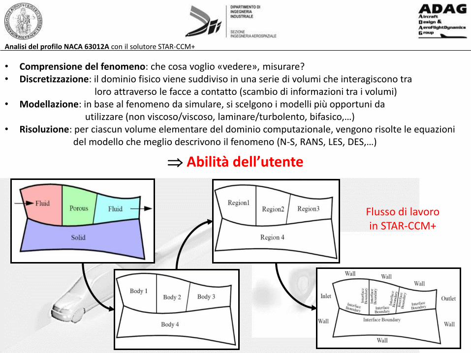
• Comprensione del fenomeno: che cosa voglio «vedere», misurare? • Discretizzazione: il dominio fisico viene suddiviso in una serie di volumi che interagiscono tra
loro attraverso le facce a contatto (scambio di informazioni tra i volumi) • Modellazione: in base al fenomeno da simulare, si scelgono i modelli più opportuni da utilizzare (non viscoso/viscoso, laminare/turbolento, bifasico,…) • Risoluzione: per ciascun volume elementare del dominio computazionale, vengono risolte le equazioni del modello che meglio descrivono il fenomeno (N-S, RANS, LES, DES,…)
Abilità dell’utente
Flusso di lavoro in STAR-CCM+
Analisi del profilo NACA 63012A con il solutore STAR-CCM+
Analisi del profilo NACA 63012A con il solutore STAR-CCM+
Analisi del profilo NACA 63012A con il solutore STAR-CCM+


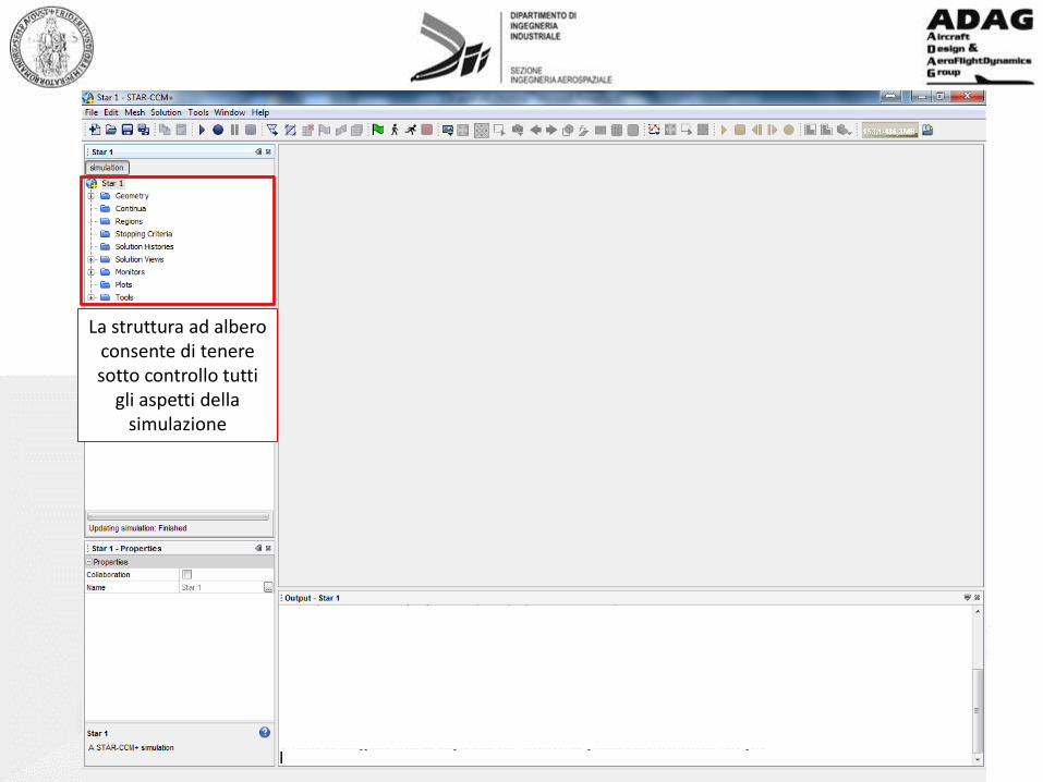
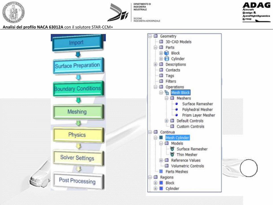
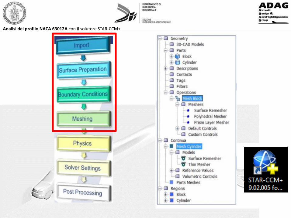
La struttura ad albero consente di tenere sotto controllo tutti
gli aspetti della simulazione
Analisi del profilo NACA 63012A con il solutore STAR-CCM+
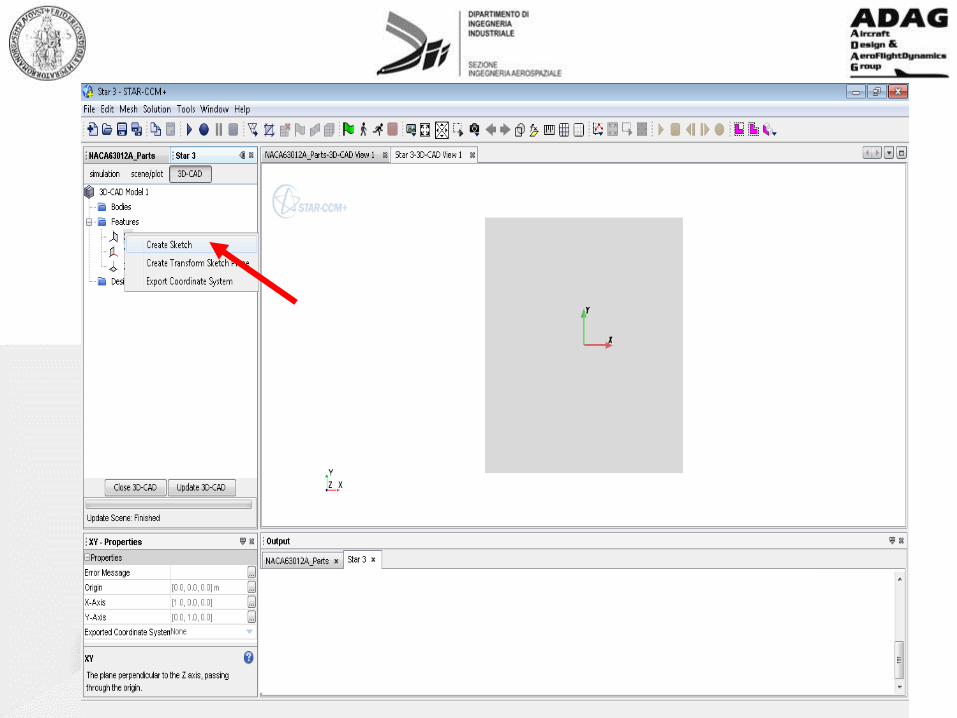
Importazione geometria CAD


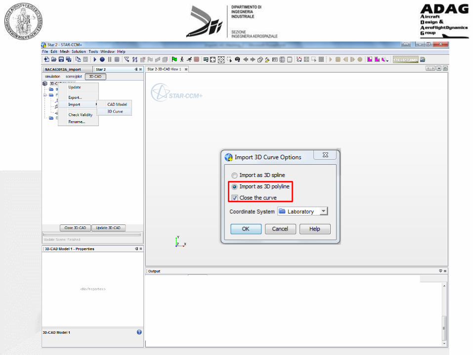

Il file *.csv della geometria deve essere nel formato:
x,y,z
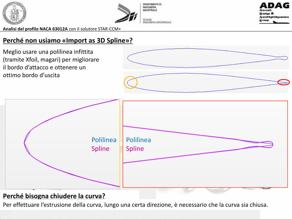
Perché non usiamo «Import as 3D Spline»?
Analisi del profilo NACA 63012A con il solutore STAR-CCM+
Polilinea Spline
Polilinea Spline
Meglio usare una polilinea infittita (tramite Xfoil, magari) per migliorare il bordo d’attacco e ottenere un ottimo bordo d’uscita
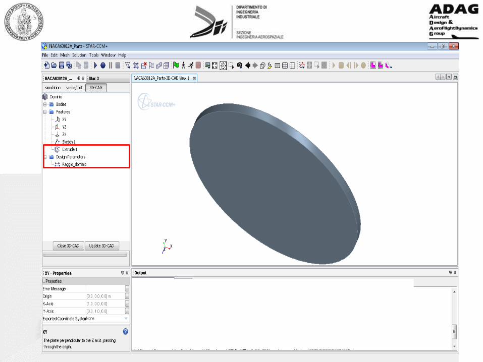
Perché bisogna chiudere la curva? Per effettuare l’estrusione della curva, lungo una certa direzione, è necessario che la curva sia chiusa.

Analisi del profilo NACA 63012A con il solutore STAR-CCM+
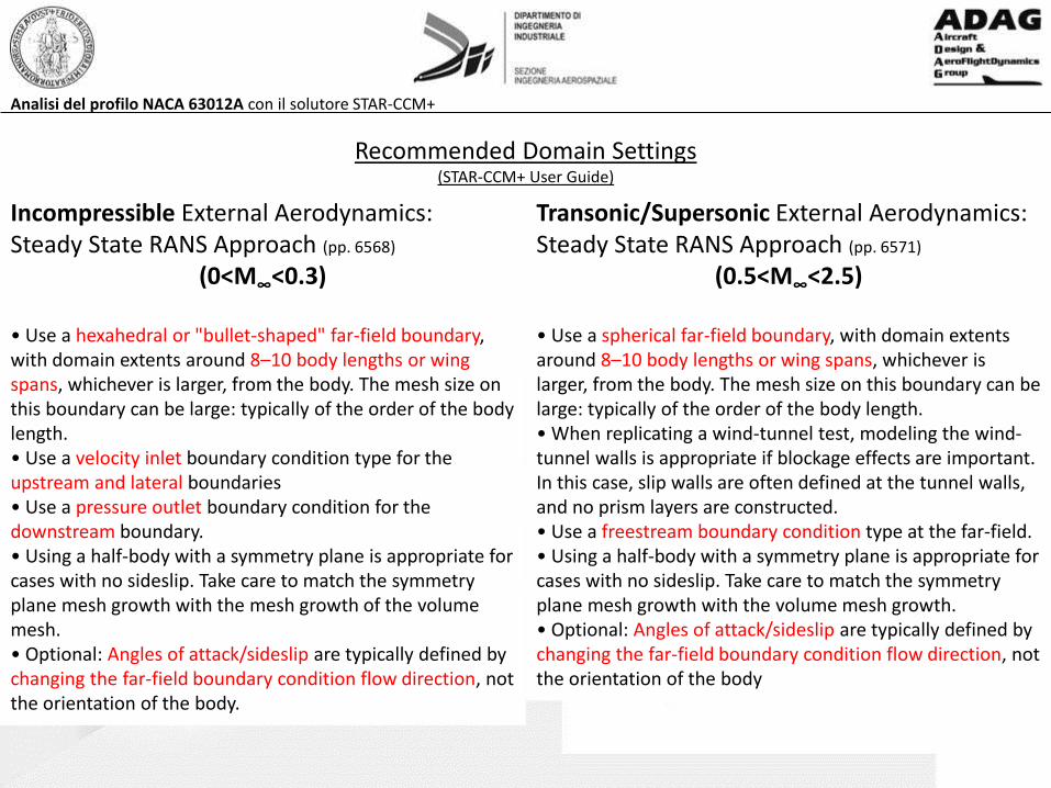
Transonic/Supersonic External Aerodynamics: Steady State RANS Approach (pp. 6571)
(0.5<M∞<2.5)
• Use a spherical far-field boundary, with domain extents around 8–10 body lengths or wing spans, whichever is larger, from the body. The mesh size on this boundary can be large: typically of the order of the body length. • When replicating a wind-tunnel test, modeling the wind-tunnel walls is appropriate if blockage effects are important. In this case, slip walls are often defined at the tunnel walls, and no prism layers are constructed. • Use a freestream boundary condition type at the far-field. • Using a half-body with a symmetry plane is appropriate for cases with no sideslip. Take care to match the symmetry plane mesh growth with the volume mesh growth. • Optional: Angles of attack/sideslip are typically defined by changing the far-field boundary condition flow direction, not the orientation of the body
Incompressible External Aerodynamics: Steady State RANS Approach (pp. 6568)
(0<M∞<0.3)
• Use a hexahedral or "bullet-shaped" far-field boundary, with domain extents around 8–10 body lengths or wing spans, whichever is larger, from the body. The mesh size on this boundary can be large: typically of the order of the body length. • Use a velocity inlet boundary condition type for the upstream and lateral boundaries • Use a pressure outlet boundary condition for the downstream boundary. • Using a half-body with a symmetry plane is appropriate for cases with no sideslip. Take care to match the symmetry plane mesh growth with the mesh growth of the volume mesh. • Optional: Angles of attack/sideslip are typically defined by changing the far-field boundary condition flow direction, not the orientation of the body.
Recommended Domain Settings (STAR-CCM+ User Guide)

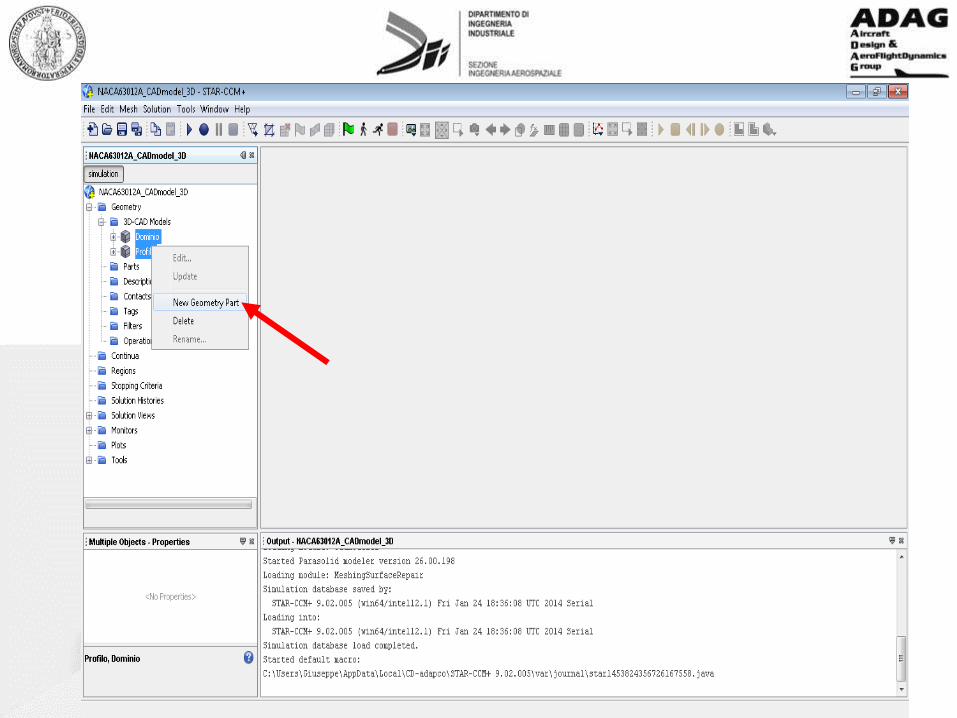
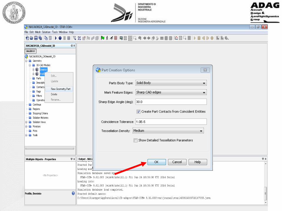

Dopo aver creato le parti, si predispone un’operazione booleana di sottrazione: il profilo viene sottratto dal dominio, producendo una nuova parte in cui il profilo è descritto dalla sola superficie esterna («dominio bucato»).
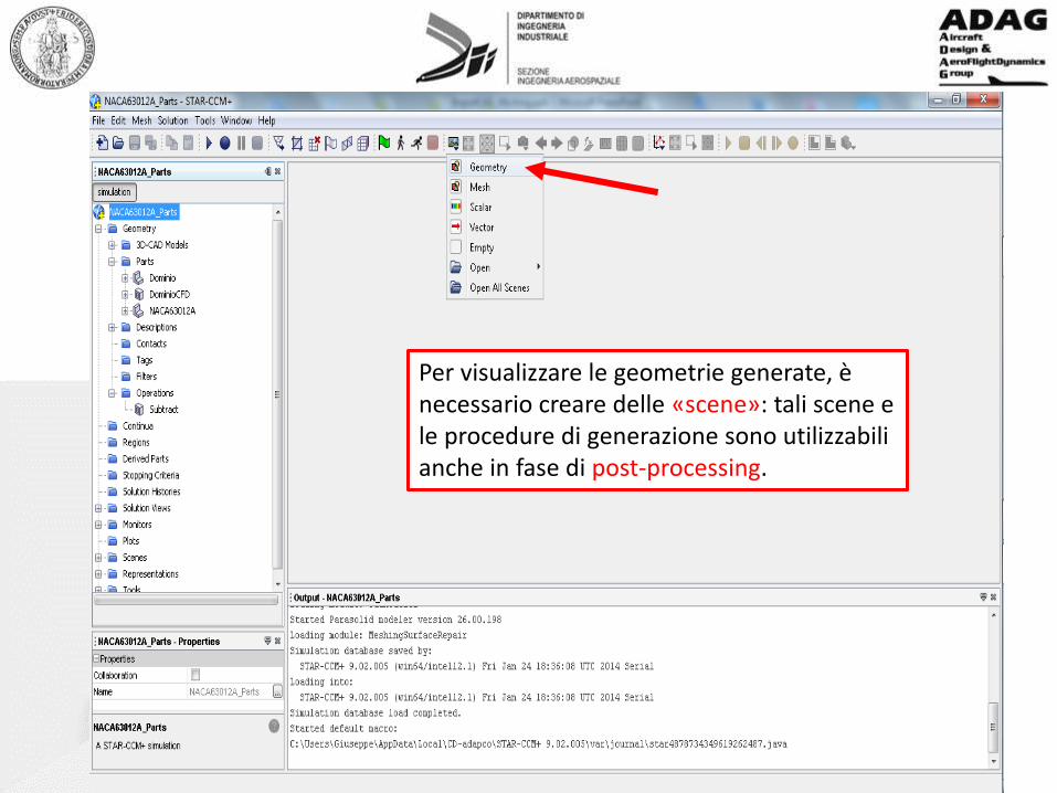
Per visualizzare le geometrie generate, è necessario creare delle «scene»: tali scene e le procedure di generazione sono utilizzabili anche in fase di post-processing.

drag&drop


Analisi del profilo NACA 63012A con il solutore STAR-CCM+
Generazione griglia di calcolo
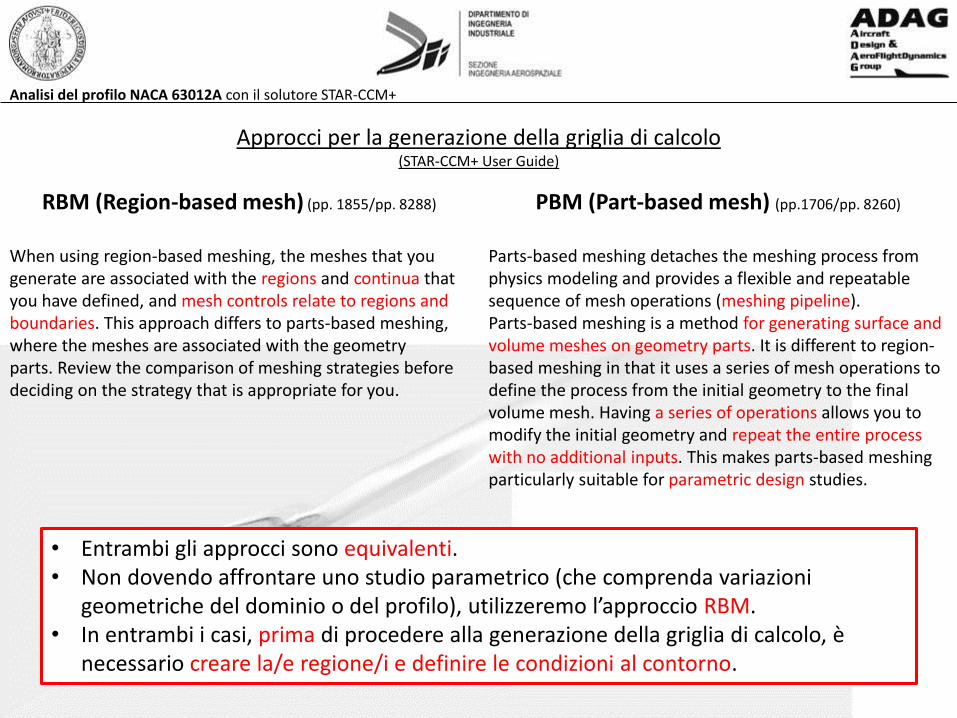
RBM (Region-based mesh) (pp. 1855/pp. 8288)
When using region-based meshing, the meshes that you generate are associated with the regions and continua that you have defined, and mesh controls relate to regions and boundaries. This approach differs to parts-based meshing, where the meshes are associated with the geometry parts. Review the comparison of meshing strategies before deciding on the strategy that is appropriate for you.
Analisi del profilo NACA 63012A con il solutore STAR-CCM+
Approcci per la generazione della griglia di calcolo (STAR-CCM+ User Guide)
PBM (Part-based mesh) (pp.1706/pp. 8260)
Parts-based meshing detaches the meshing process from physics modeling and provides a flexible and repeatable sequence of mesh operations (meshing pipeline). Parts-based meshing is a method for generating surface and volume meshes on geometry parts. It is different to region-based meshing in that it uses a series of mesh operations to define the process from the initial geometry to the final volume mesh. Having a series of operations allows you to modify the initial geometry and repeat the entire process with no additional inputs. This makes parts-based meshing particularly suitable for parametric design studies.
• Entrambi gli approcci sono equivalenti. • Non dovendo affrontare uno studio parametrico (che comprenda variazioni
geometriche del dominio o del profilo), utilizzeremo l’approccio RBM. • In entrambi i casi, prima di procedere alla generazione della griglia di calcolo, è
necessario creare la/e regione/i e definire le condizioni al contorno.

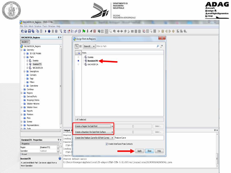
Tutte le operazioni che riguardano la simulazione CFD (mesh, soluzione, post-processing,…), in STAR-CCM+, vengono effettuate sulle regioni.
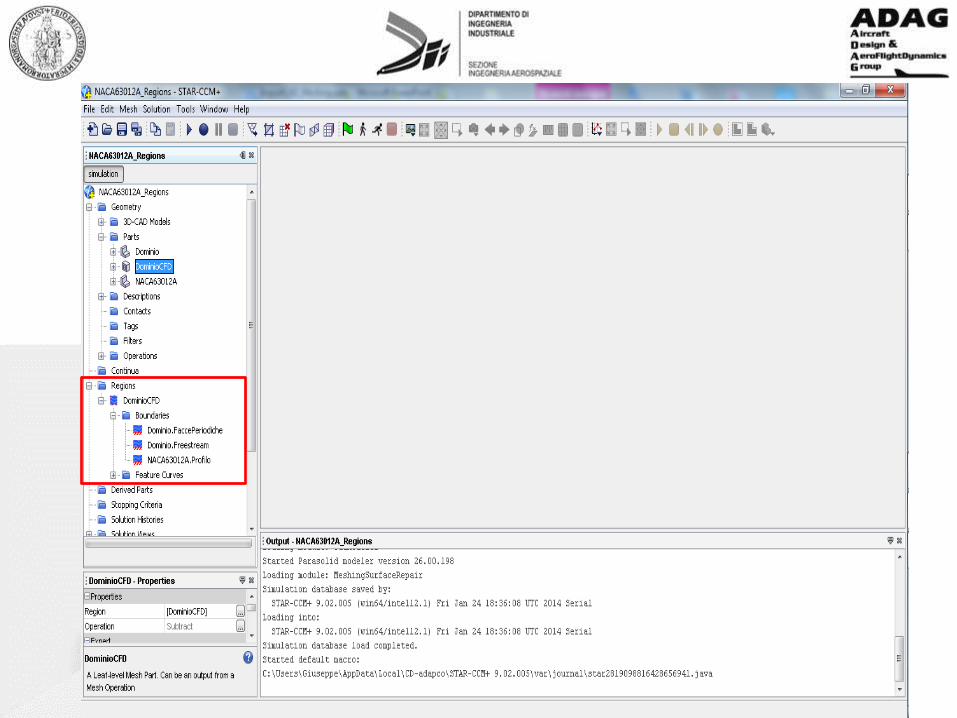
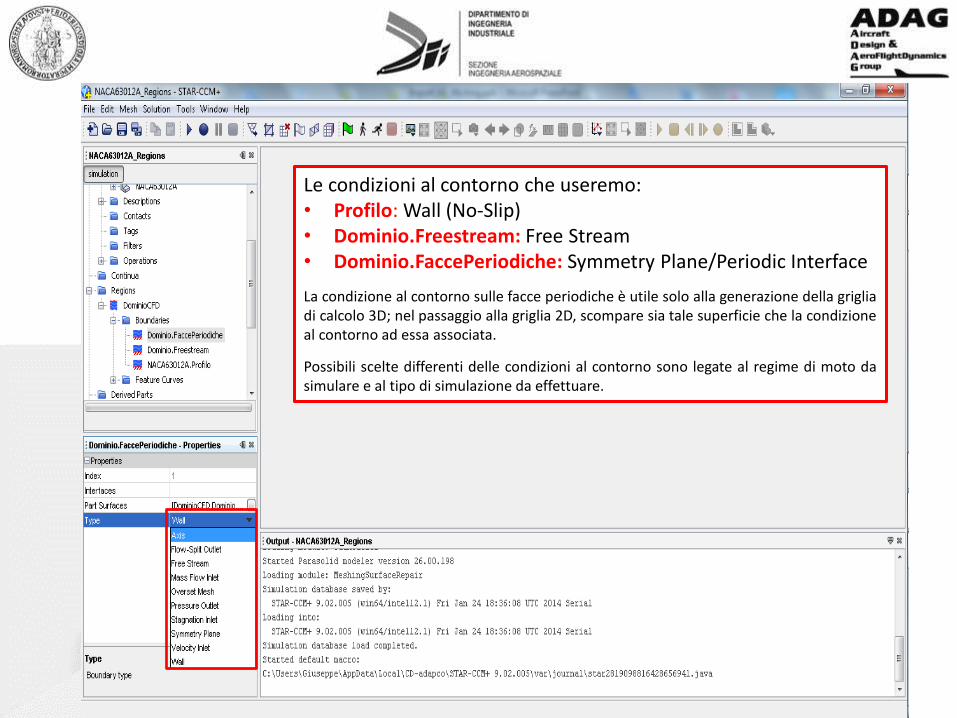
Le condizioni al contorno che useremo: • Profilo: Wall (No-Slip) • Dominio.Freestream: Free Stream • Dominio.FaccePeriodiche: Symmetry Plane/Periodic Interface
La condizione al contorno sulle facce periodiche è utile solo alla generazione della griglia di calcolo 3D; nel passaggio alla griglia 2D, scompare sia tale superficie che la condizione al contorno ad essa associata.
Possibili scelte differenti delle condizioni al contorno sono legate al regime di moto da simulare e al tipo di simulazione da effettuare.
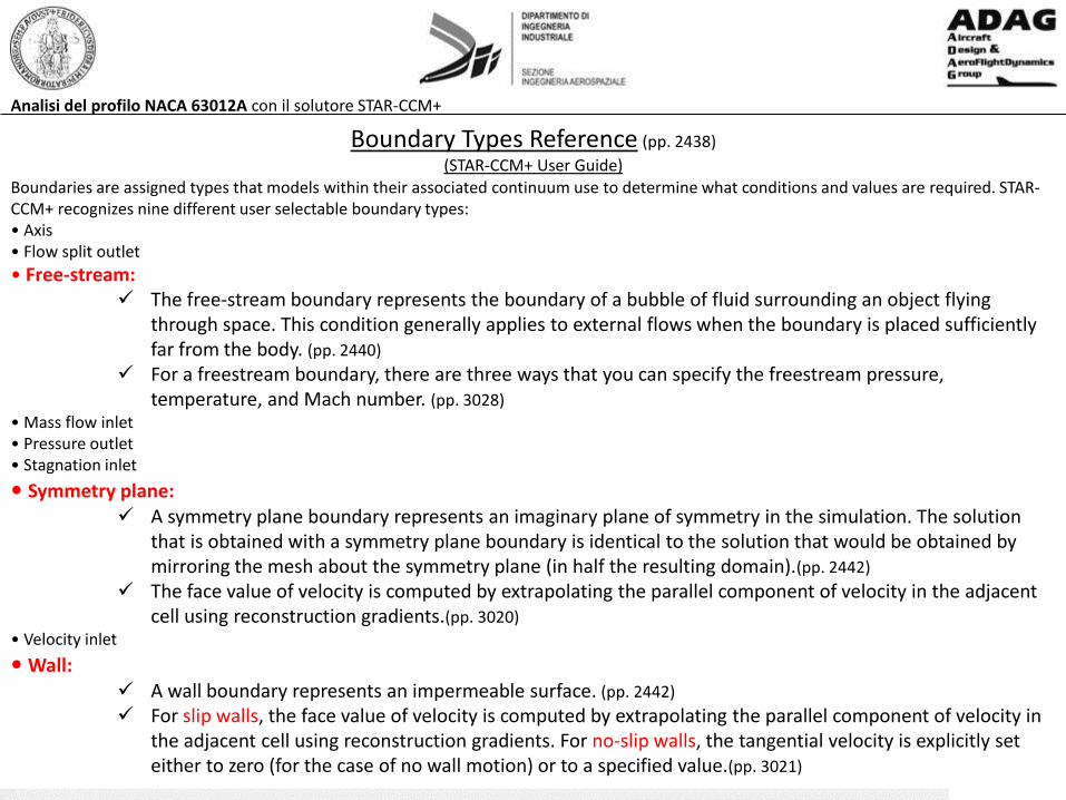
Boundaries are assigned types that models within their associated continuum use to determine what conditions and values are required. STAR-CCM+ recognizes nine different user selectable boundary types: • Axis • Flow split outlet
• Free-stream: The free-stream boundary represents the boundary of a bubble of fluid surrounding an object flying
through space. This condition generally applies to external flows when the boundary is placed sufficiently far from the body. (pp. 2440)
For a freestream boundary, there are three ways that you can specify the freestream pressure, temperature, and Mach number. (pp. 3028)
• Mass flow inlet • Pressure outlet • Stagnation inlet
• Symmetry plane: A symmetry plane boundary represents an imaginary plane of symmetry in the simulation. The solution
that is obtained with a symmetry plane boundary is identical to the solution that would be obtained by mirroring the mesh about the symmetry plane (in half the resulting domain).(pp. 2442)
The face value of velocity is computed by extrapolating the parallel component of velocity in the adjacent cell using reconstruction gradients.(pp. 3020)
• Velocity inlet
• Wall: A wall boundary represents an impermeable surface. (pp. 2442)
For slip walls, the face value of velocity is computed by extrapolating the parallel component of velocity in the adjacent cell using reconstruction gradients. For no-slip walls, the tangential velocity is explicitly set either to zero (for the case of no wall motion) or to a specified value.(pp. 3021)
Boundary Types Reference (pp. 2438)
(STAR-CCM+ User Guide)
Analisi del profilo NACA 63012A con il solutore STAR-CCM+


• Tetrahedral - tetrahedral cell shape based core mesh • Polyhedral - arbitrary polyhedral cell shape based core mesh • Trimmed - trimmed hexahedral cell shape based core mesh • Thin Mesh - tetrahedral or polyhedral based prismatic thin mesh • Advancing Layer Mesh - polyhedral core mesh, with in-built prismatic layers that advance inward from a
polygonal surface mesh. • Prismatic near wall layers can be included with the first three types of mesh that are listed above by
including the prism meshing model as part of the volume meshing process.
Volume Meshers (pp. 1982)
(STAR-CCM+ User Guide)
Analisi del profilo NACA 63012A con il solutore STAR-CCM+
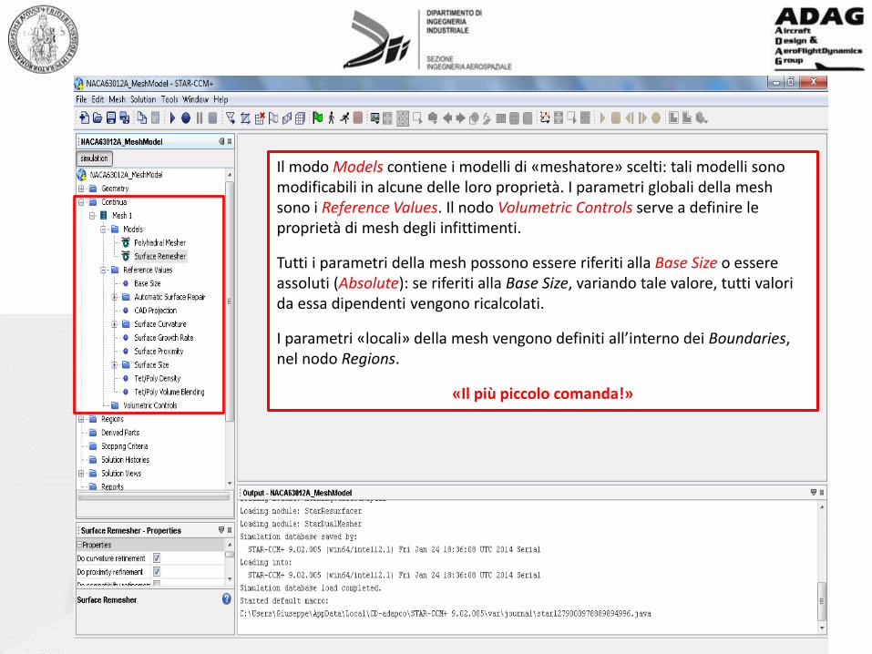
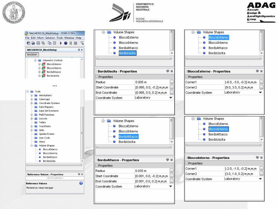
Il modo Models contiene i modelli di «meshatore» scelti: tali modelli sono modificabili in alcune delle loro proprietà. I parametri globali della mesh sono i Reference Values. Il nodo Volumetric Controls serve a definire le proprietà di mesh degli infittimenti.
Tutti i parametri della mesh possono essere riferiti alla Base Size o essere assoluti (Absolute): se riferiti alla Base Size, variando tale valore, tutti valori da essa dipendenti vengono ricalcolati.
I parametri «locali» della mesh vengono definiti all’interno dei Boundaries, nel nodo Regions.
«Il più piccolo comanda!»

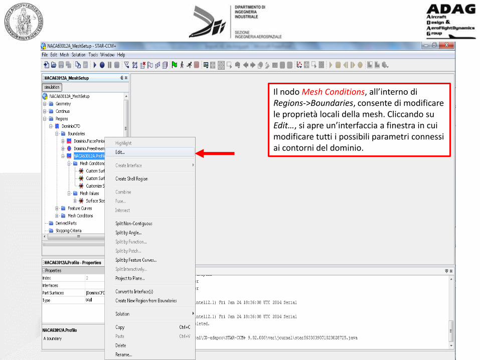
Il nodo Mesh Conditions, all’interno di Regions->Boundaries, consente di modificare le proprietà locali della mesh. Cliccando su Edit…, si apre un’interfaccia a finestra in cui modificare tutti i possibili parametri connessi ai contorni del dominio.

…


Una volta definiti i valori dei parametri della mesh, si può procedere alla generazione della mesh di volume.
N.B.: usare valori troppo stringenti per i parametri della mesh, può letteralmente «bloccare» il vostro PC (saturazione della RAM disponibile). Non osare troppo, soprattutto se non necessario…
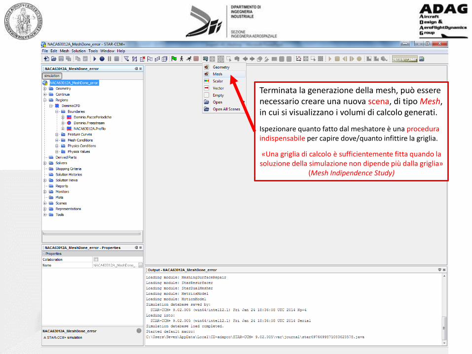
Terminata la generazione della mesh, può essere necessario creare una nuova scena, di tipo Mesh, in cui si visualizzano i volumi di calcolo generati.
Ispezionare quanto fatto dal meshatore è una procedura indispensabile per capire dove/quanto infittire la griglia.
«Una griglia di calcolo è sufficientemente fitta quando la soluzione della simulazione non dipende più dalla griglia»
(Mesh Indipendence Study)

It is important to remember that your solution is the numerical solution to
the problem that you posed by defining your mesh and boundary
conditions. The more accurate your mesh and boundary conditions, the
more accurate your “converged” solution will be.
CONVERGENCE
Convergence is something that all CFD Engineers talk about, but we must
remember that the way we generally define convergence (by looking at
Residual values) is only a small part of ensuring that we have a valid
solution. For a Steady State simulation we need to ensure that the
solution satisfies the following three conditions:
- Residual RMS Error values have reduced to an acceptable value
(typically 10-4 or 10-5)
- Monitor points for our values of interest have reached a steady solution
- The domain has imbalances of less than 1%.
MESH INDEPENDENCE STUDY
Although we are happy that this has “converged” based on RMS Error values,
monitor points and imbalances, we need to make sure that the solution is also
independent of the mesh resolution. Not checking this is a common cause of
erroneous results in CFD, and this process should at least be carried out once for
each type of problem that you deal with so that the next time a similar problem
arises, you can apply the same mesh sizing. In this way you will have more
confidence in your results.
- Step 1
Run the initial simulation on your initial mesh and ensure convergence; if not,
refine the mesh and repeat.
- Step 2
Once you have met the convergence criteria, refine the mesh globally so that you
have finer cells throughout the domain. Run the simulation and ensure
convergence again. Then, compare the monitor point values: if they are the same
(within your own allowable tolerance), then the mesh at Step 1 was accurate
enough to capture the result; otherwise, this means that your solution is changing
because of your mesh resolution, and hence the solution is not yet independent of
the mesh.
- Step 3
Because your solution is changing with the refinements, you need to refine the
mesh more, and repeat the process until you have a solution that is independent of
the mesh. You should then always use the smallest mesh that gives you this mesh
independent solution (to reduce your simulation run time).
Convergence vs. Mesh Indipendence (http://www.computationalfluiddynamics.com.au/convergence-and-mesh-independent-study/)
Analisi del profilo NACA 63012A con il solutore STAR-CCM+
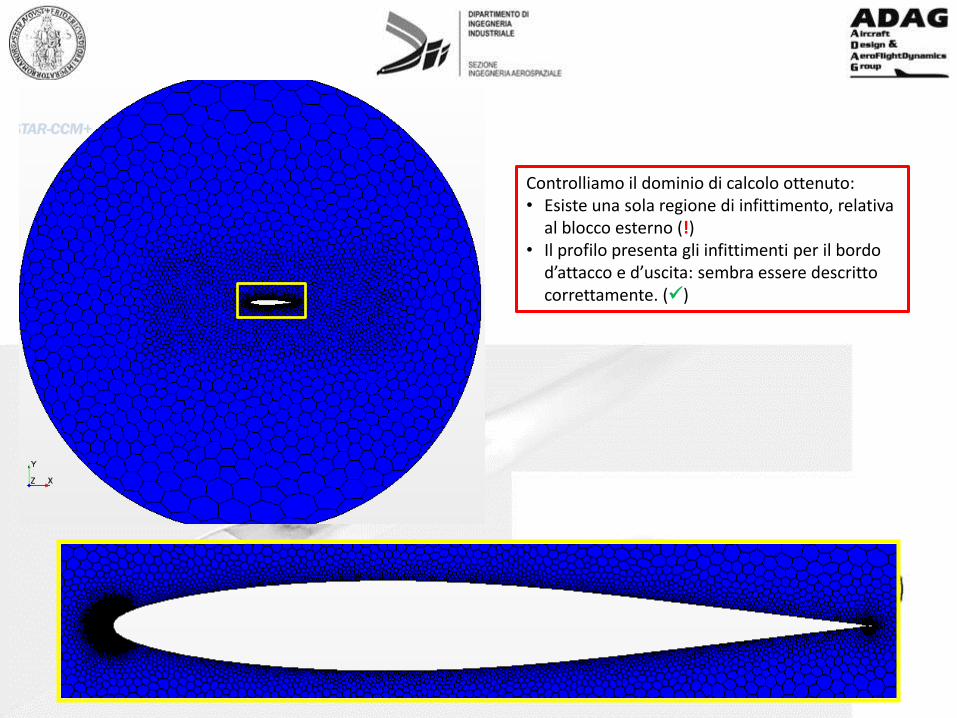
Controlliamo il dominio di calcolo ottenuto: • Esiste una sola regione di infittimento, relativa
al blocco esterno (!) • Il profilo presenta gli infittimenti per il bordo
d’attacco e d’uscita: sembra essere descritto correttamente. ()

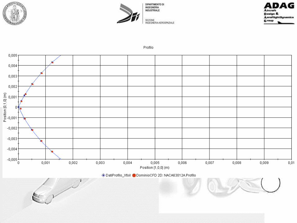
Controlliamo il dominio di calcolo ottenuto: • La curvatura del bordo d’attacco sembra
essere presa correttamente () • L’infittimento del bordo d’attacco è
sufficientemente grande per prendere il picco del Cp? (?)

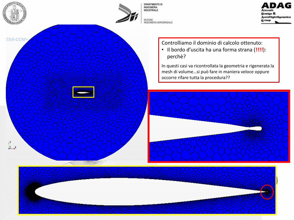
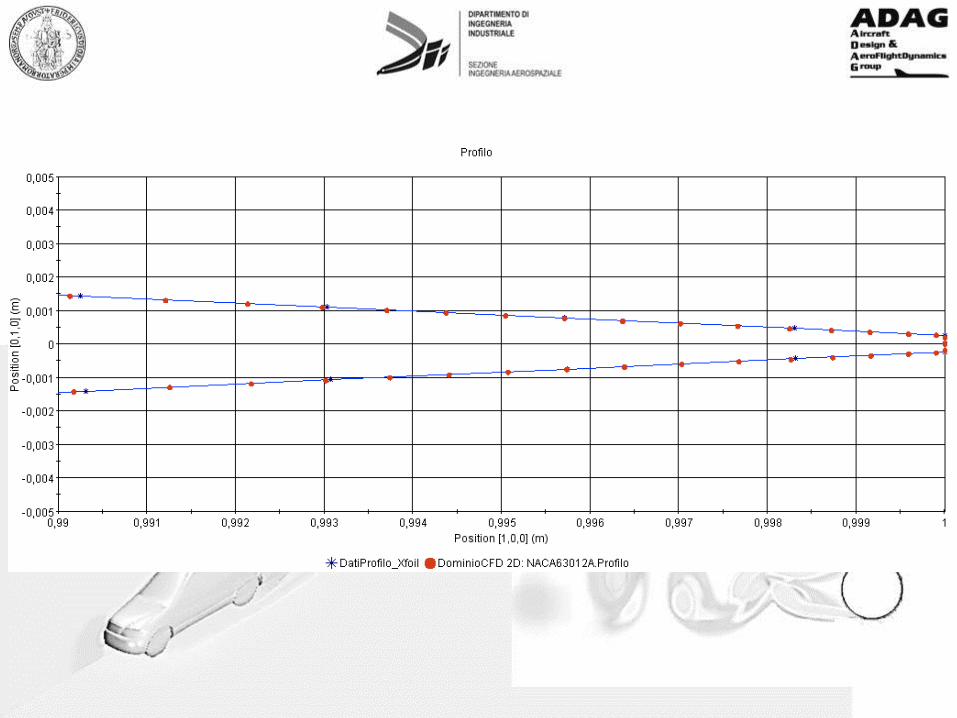
Controlliamo il dominio di calcolo ottenuto: • Il bordo d’uscita ha una forma strana (!!!!):
perchè?
In questi casi va ricontrollata la geometria e rigenerata la mesh di volume…si può fare in maniera veloce oppure occorre rifare tutta la procedura??
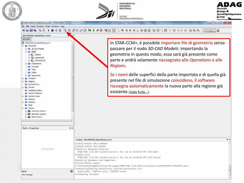
In STAR-CCM+, è possibile importare file di geometria senza passare per il nodo 3D-CAD Models: importando la geometria in questo modo, essa sarà già presente come parte e andrà solamente riassegnata alle Operations e alle Regions.
Se i nomi delle superfici della parte importata e di quella già presente nel file di simulazione coincidono, il software riassegna automaticamente la nuova parte alla regione già esistente (siate furbi…).


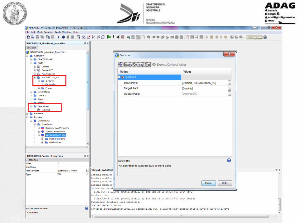

Una volta verificato che la nuova parte è stata correttamente assegnata alla regione corrispondente, si può procedere ad eseguire nuovamente la generazione della mesh di volume.

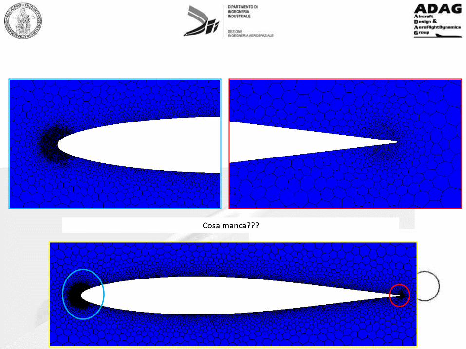
Cosa manca???
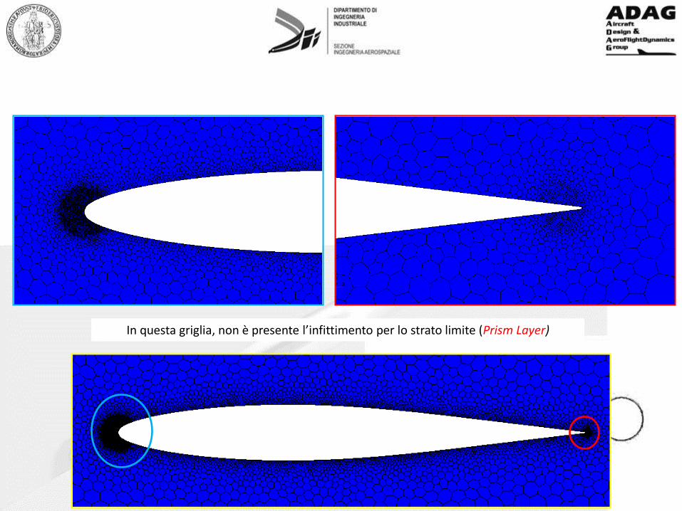
In questa griglia, non è presente l’infittimento per lo strato limite (Prism Layer)


The prism layer mesh model is used with a core volume mesh to generate orthogonal prismatic cells next to wall surfaces or boundaries. This layer of cells is necessary to improve the accuracy of the flow solution.
A prism layer is defined in terms of: • Its thickness • The number of cell layers within it • The size distribution of the layers • The function that is used to generate the distribution -either by geometric progression or hyperbolic tangent.
Analisi del profilo NACA 63012A con il solutore STAR-CCM+
Prism Layer Mesher (pp. 2020)
(STAR-CCM+ User Guide)
Why Is a Prism Layer Mesh Required?
Prism layers allow the solver to resolve near wall flow accurately, which is critical in determining not only the forces and heat transfer on walls, but also flow features such as separation. Separation in turn affects integral results such as drag or pressure drop.
Depending on the Reynolds number, a turbulent shear layer requires in excess of 10-20 cells in the cross-stream direction for accurate resolution of the turbulence flow profiles.
Prism Layers Best Practice (pp. 6574)
• Proper resolution of the boundary layer is critical. Choose the thickness of the prism layer such that the entire boundary layer is contained within it.
• The use of wall functions rather than integrating to the wall can be appropriate for the SST K-Omega turbulence model depending on several factors, including:
o Desired accuracy o Relative importance of skin friction drag o Importance of transition o Existence/importance of separation/reattachment on smooth boundaries
• For integrating to the wall, 20–30 prism layers are typically used, with the near-wall y+ being of the order 1. • For wall functions, 5–8 prism layers are typically used, with the near-wall y+ being of the order 50–150. • When using the Spalart-Allmaras Turbulence model, integrate to the wall (do not use wall functions).
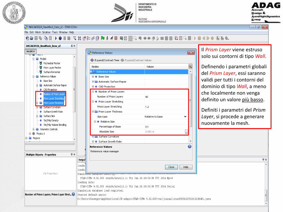
Il Prism Layer viene estruso solo sui contorni di tipo Wall.
Definendo i parametri globali del Prism Layer, essi saranno validi per tutti i contorni del dominio di tipo Wall, a meno che localmente non venga definito un valore più basso.
Definiti i parametri del Prism Layer, si procede a generare nuovamente la mesh.
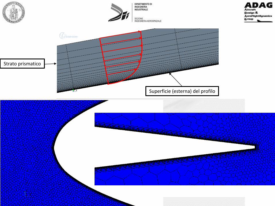
Superficie (esterna) del profilo
Strato prismatico

STAR-CCM+ è orientato a lavorare principalmente con geometrie tridimensionali. Poiché siamo interessati a studiare il comportamento di un profilo (bidimensionale), al solo scopo di ridurre il tempo di calcolo delle simulazioni, convertiamo il dominio 3D in 2D. Questa operazione è possibile SOLO se esiste una superficie del dominio posta sul piano z=0.
DOMINIO 3D: DOMINIO 2D:
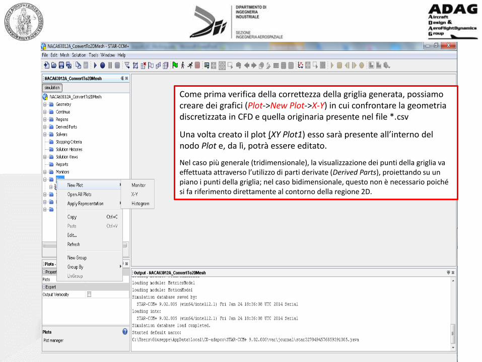
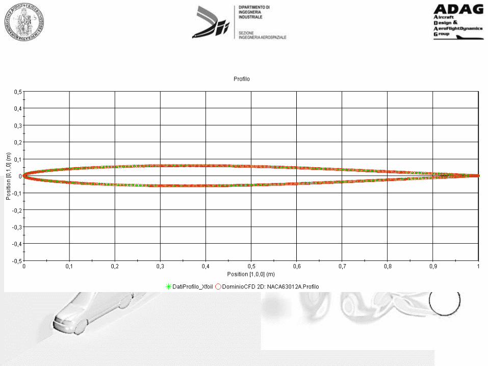
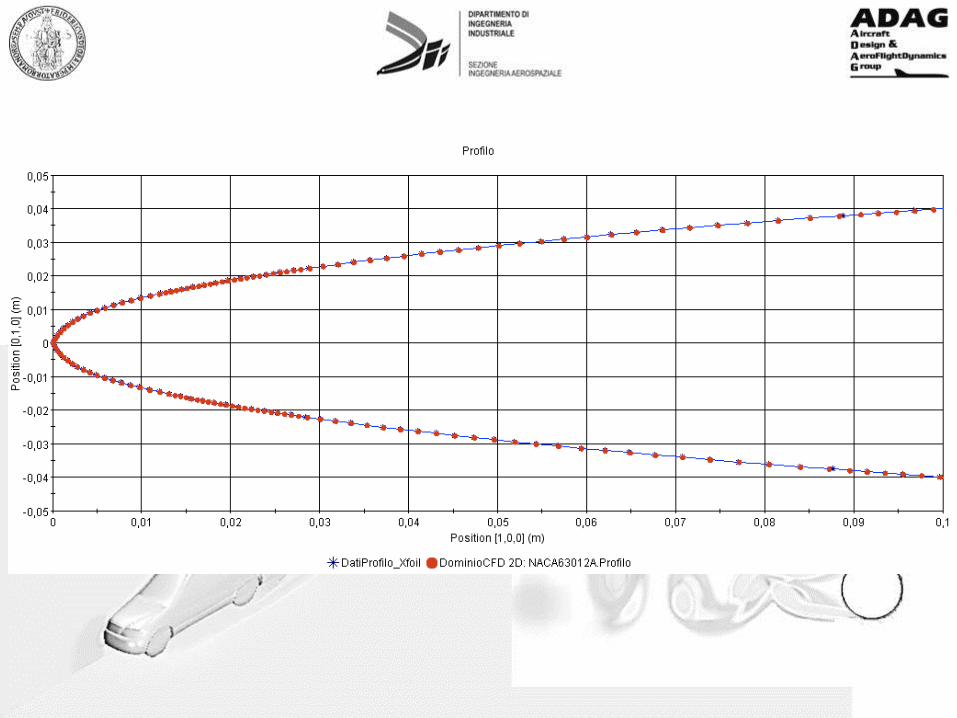
Come prima verifica della correttezza della griglia generata, possiamo creare dei grafici (Plot->New Plot->X-Y) in cui confrontare la geometria discretizzata in CFD e quella originaria presente nel file *.csv
Una volta creato il plot (XY Plot1) esso sarà presente all’interno del nodo Plot e, da lì, potrà essere editato.
Nel caso più generale (tridimensionale), la visualizzazione dei punti della griglia va effettuata attraverso l’utilizzo di parti derivate (Derived Parts), proiettando su un piano i punti della griglia; nel caso bidimensionale, questo non è necessario poiché si fa riferimento direttamente al contorno della regione 2D.

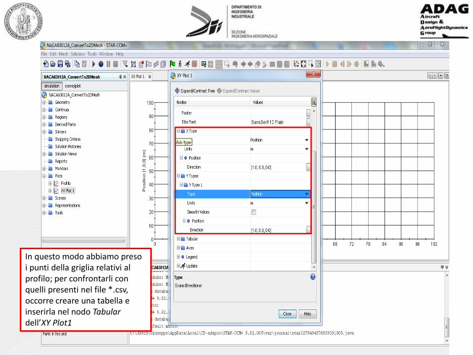
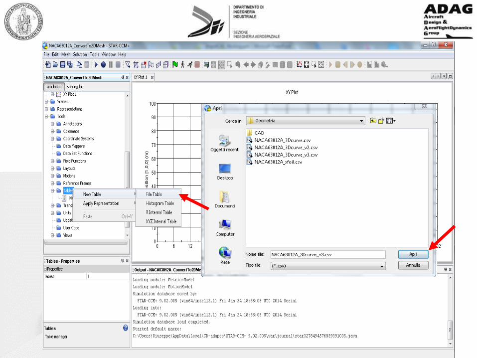
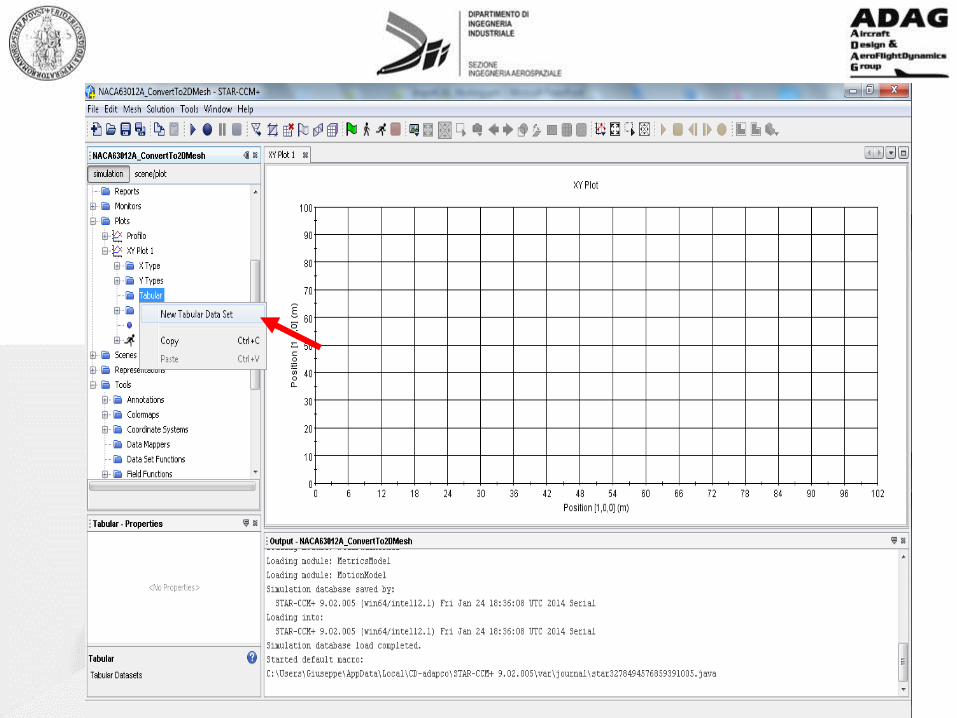
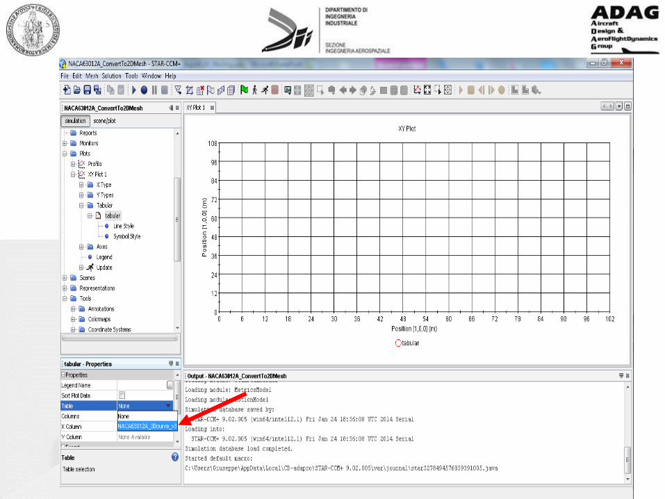
In questo modo abbiamo preso i punti della griglia relativi al profilo; per confrontarli con quelli presenti nel file *.csv, occorre creare una tabella e inserirla nel nodo Tabular dell’XY Plot1


![area delle figure piane [modalità compatibilità]Figure piane poligoni cerchi figure a contorno curvilineo figure a contorno mistilineo ... per altezza rispettivamente le due diagonali](https://static.fdocumenti.com/doc/165x107/6067fdc1654c23023f66c12e/area-delle-figure-piane-modalit-compatibilit-figure-piane-poligoni-cerchi.jpg)