1

AAllmmaa MMaatteerr SSttuuddiioorruumm –– UUnniivveerrssiittàà ddii BBoollooggnnaa

DOTTORATO DI RICERCA IN

SCIENZE AMBIENTALI:

TUTELA E GESTIONE DELLE RISORSE NATURALI

Ciclo XXV

Settore Concorsuale di afferenza: 05/B1 - ZOOLOGIA E ANTROPOLOGIA

Settore Scientifico disciplinare: BIO/05 - ZOOLOGIA

Wide-scale population genomics of Atlantic bluefin

tuna (Thunnus thynnus) inferred by novel high-

throughput technology

Presentata da: Dott.ssa Eleonora Pintus

Coordinatore Dottorato Relatore Prof. Enrico Dinelli Prof. Fausto Tinti

Esame finale anno 2013

2

3

INDEX

ABSTRACT.......................................................................................................5

CHAPTER 1……………………………………………………………………………………………………9

GBYP PROJECT

1.1 State of world fisheries……………………………………………………………………….9

1.2 Aim of the project….…………………………………………………………………………13

1.3 SNP……………………………………………………………………………………………………14

CHAPTER 2………………………………………………………………………………………………….19

TARGET SPECIES: ATLANTIC BLUEFIN TUNA

2.1 Taxonomy and……..…………………………………………………………………………..19

2.2 Geographic distribution, habitat and ecology……………………………………20

2.3 Reproduction and spawning……………………………………………………………..25

2.4 Movement and stock structure…………………………………………………………27

CHAPTER 3………………………………………………………………………………………………….32

STATE OF THE ART

3.1 Fishery genetics………………………………………………………………………………..32

3.2 Fishery and management of Atlantic bluefin tuna…………………………….36

3.2.1 Fishery……………………………………………………………………………………………………….36

3.2.2 Management……………………………………………………………………………………………..39

4

3.3 Population genetic studies of Atlantic bluefin tuna …………………..……..44

3.4 Research aims…………………………………………………………………………………..47

CHAPTER 4………………………………………………………………………………………………….49

HIGH-THROUGHPUT SNP DEVELOPMENT IN ATLANTIC BLUEFIN TUNA USING

A COMBINED GDNA AND CDNA SEQUENCING STRATEGY

CHAPTER 5....................................................................................................92

ASSESSING THE ACCURACY AND POWER OF SNPS MARKERS FOR

POPULATION GENETICS, INDIVIDUAL ASSIGNMENT AND MIXTURE STOCK

ANALYSIS IN THUNNUS THYNNUS

CHAPTER 6..................................................................................................141

CONCLUSIONS

REFERENCES................................................................................................143

AKNOWLEDGEMENTS ................................................................................161

5

ABSTRACT

Il mio progetto di dottorato è focalizzato sul tonno rosso, Thunnus thynnus,

appartenente all’ordine dei Perciformes, e alla famiglia degli Scombridae. Questa specie,

distribuita nell’Oceano Atlantico settentrionale e centrale e nel Mar Mediterraneo, presenta

due principali aree di riproduzione (il Golfo del Messico per lo stock occidentale e il Mar

Mediterraneo per quello orientale) e compie ampie migrazioni transatlantiche tra le zone di

alimentazione e quelle di riproduzione, mostrando alta fedeltà alle zone di nascita, dove

torna per riprodursi (natal homing). Benché il tonno rosso sia stato pescato in modo

continuativo nel Mar Mediterraneo per migliaia di anni, questa specie ha subito un forte

incremento dello sfruttamento negli ultimi decenni, a causa del miglioramento delle

tecniche di pesca, dello sviluppo del mercato giapponese e della nascita delle tuna farm. Si è

infatti passati da una pesca di tipo artigianale ad una di tipo industriale, raggiungendo livelli

che secondo alcune recenti valutazioni del WWF non consentirebbero la sostenibilità della

risorsa. Questo sta portando a rischio di collasso la pesca e gli stock, tanto che il comitato

scientifico ICCAT (Commissione Internazionale per la Gestione del Tonno Atlantico) ha

avviato, attraverso un regolamento comunitario, un piano quindicinale per il ripristino dello

stock (CE N.643/2007). Il mio progetto di ricerca si inserisce all’interno del progetto ICCAT-

GBYP 06/2011 (Atlantic-wide Bluefin Tuna Research Program), sviluppato in collaborazione

con diversi partner italiani e stranieri, in cui ci si è avvalsi di metodiche molecolari innovative

come le nuove tecnologie genomiche, Next Generation Sequencing (NGS). Sono stati

sviluppati e utilizzati marcatori SNPs (Single Nucleotide Polymorphisms) legati o inclusi a geni

espressi che, potenzialmente soggetti a processi di selezione, possono permettere di

studiare i meccanismi di adattamento delle popolazioni ai cambiamenti delle condizioni

ambientali, al prelievo, all’inquinamento ed ad altri disturbi antropici.

Il primo step della ricerca ha visto la costruzione di librerie di cDNA specifiche per

dieci individui rappresentativi del polimorfismo interspecifico nel Mediterraneo e

nell’Atlantico (4 provenienti dal Golfo del Messico, 3 dal Mediterrraneo Occidentale e 3 da

quello Orientale). La scelta dei campioni è stata fatta valutando i requisiti necessari per il

sequenziamento 454 (come quantità e qualità dell’ RNA totale, ricchezza in mRNA). Queste

librerie sono state ottenute mediante retrotrascrizione di mRNA isolato da tessuto

6

muscolare, e il sequenziamento è stato condotto mediante tecnica di pirosequenziamento

implementata dalla tecnologia 454. Queste librerie sono state successivamente purificate e

filtrate per eliminare trascritti mitocondriali e ribosomiali, vettori e adapter. Oltre all’utilizzo

del trascrittoma, è stata utilizzata anche la risorsa genomica per costruire una sequenza di

riferimento (dato che il tonno rosso non è una specie modello e quindi non si hanno

informazioni relative al suo genoma in banche dati), partendo da 4 individui provenienti

dalle due principali regioni dell’areale del tonno rosso (2 dal Golfo del Messico e 2 dalle

Baleari). Il sequenziamento è stato condotto avvalendosi di uno strumento di ultima

generazione, l’ HiSeq 2000 dell’Illumina. Una volta ottenuto questo genoma di riferimento,

tutte le cDNA reads, derivate dal trascrittoma, sono state mappate contro tale genoma, e,

utilizzando diversi software bioinformatici e diversi parametri restrittivi, è stato ottenuto un

pool di 4000 contigs, usato come riferimento per la successiva fase di SNP detection.

Mappando nuovamente le cDNA reads contro questi 4000 contigs selezionati, sono stati

identificati 5412 SNPs candidati, in 1350 contigs.

A questo punto è stato necessario validare gli SNPs identificati, per essere sicuri che

non fossero dovuti ad errori di sequenziamento, in modo tale da ottenere il pannello

definitivo dei 384 SNPs rispondenti ai criteri di selezione in silico. Per fare ciò sono stati

applicati diversi criteri, 2 dei quali richiesti dalla piattaforma Illumina che verrà utilizzata per

la genotipizzazione, che sono la presenza di una regione fiancheggiante lo SNP di almeno

60bp e un Illumina ADT score (Assay Design Tool) > 0,6. In aggiunta a questi parametri, sono

stati scelti SNPs che presentano il polimorfismo anche a livello genomico (in modo tale da

avere sovrapposizione di informazioni tra cDNA e gDNA) e che, a livello del cDNA, siano

presenti in almeno in un individuo con una minima copertura (4 reads presenti in quella data

posizione, 2 delle quali portanti l’allele alternativo).

Il pannello di 384 SNP così ottenuto è stato genotipizzato in 960 individui di diversa

taglia (larve, age 0, juveniles, medium e large), campionati lungo l’intero range di

distribuzione del tonno rosso (Golfo del Messico, Nord-Est Atlantico, Mediterraneo

occidentale, centrale e orientale). Il campionamento è stato effettuato principalmente nel

corso del 2011, ma sono state aggiunte alle analisi anche diverse repliche temporali, in modo

da ottenere un ampio dataset composto da 23 campioni di popolazione. Sei di questi sono

stati identificati come campioni di riferimento, in quanto costituiti da larve e age 0, per le

quali quindi si è certi dell’origine geografica e della diretta correlazione con le unità

7

riproduttive. Sono stati utilizzati 40 individui per ogni “strata” di tonno rosso, campione

definito dalla combinazione della taglia e dell’area di provenienza, e il DNA genomico di tutti

gli individui è stato estratto dal tessuto muscolare, dalla pinna o direttamente dalle larve, e

successivamente è stato sottoposto ad un controllo qualitativo e quantitativo. Tutti gli

individui sono stati genotipizzati mediante il saggio Illumina Golden Gate Assay e i risultati

ottenuti sono stati visualizzati e analizzati mediante un software specifico. Per ottenere una

selezione di loci e di individui rappresentativi e idonei alle analisi successive, è stato

effettuato un accurato controllo qualitativo, mirato ad eliminare gli SNPs non funzionanti e

monomorfici e gli individui non genotipizzati per almeno l’80% dei loci disponibili. Si è così

raggiunto un dataset finale costituito da 848 individui e 287 SNPs.

Una volta completata la genotipizzazione, è iniziata l’analisi dei dati ottenuti,

finalizzata a valutare la diversità genetica e la struttura di popolazione nel tonno rosso. Sono

stati calcolati quindi i principali indici di diversità genetica, come le frequenze alleliche,

l’eterozigosità attesa e osservata, la percentuale di loci polimorfici e l’indice di fissazione;

sono stati inoltre valutati sia la deviazione dall’equilibrio di Hardy Weinberg che il linkage

disequilibrium. Sono stati effettuati successivamente studi sulla struttura di popolazione

attraverso il calcolo degli FST, per valutare la distanza genetica mediante un confronto tra

coppie di popolazioni. Le analisi sono state condotte sia utilizzando l’intero pannello di SNPs

che un pannello ridotto di loci che presentano indici di differenziamento sopra la soglia dello

0,1%, per riuscire ad avere un maggior potere risolutivo e riuscire a individuare un segnale di

differenziazione genetica tra i campioni analizzati. Inoltre la distanza genetica tra i campioni

è stata testata attraverso la PCoA, Principal Coordinate Analysis, condotta con il pannello

selezionato di SNPs, e sono state anche effettuate analisi filogeografiche per valutare le

relazioni tra i campioni esaminati. Tutte queste analisi sono state eseguite sia sulle 23

popolazioni che sulle 6 popolazioni di riferimento. Continuando ad avvalersi dei due pannelli

di SNPs e dei due dataset di popolazioni, lo studio è stato approfondito tramite la DAPC

(Discriminant Analysis of Principal Components) e utilizzando un approccio Bayesiano, per

valutare la presenza di diversi gruppi all’interno dei nostri campioni, non ottenendo però

chiare evidenze di struttura genetica. Un debole segnale di differenziazione è stato trovato

soltanto nell’analisi condotta utilizzando le 6 popolazioni di riferimento e il pannello ristretto

di loci, suggerisce la presenza di 3 cluster genetici corrispondenti alle tre possibili aree di

riproduzione del tonno rosso (Golfo del Messico, Mediterraneo occidentale e orientale).

8

Infine, utilizzando il pannello ristretto di loci, sono stati assegnati tutti gli individui del nostro

dataset alle grandi aree riproduttive del Mediterraneo e del Golfo del Messico, non

ottenendo però un assegnamento con alti valori di significatività statistica, ma

un’indicazione di un maggiore contributo del mar Mediterraneo alle popolazioni adulte. Si è

cercato anche di individuare i loci outlier, che, potenzialmente sotto selezione divergente,

possono essere in correlazione con le variabili ambientali. Le analisi, condotte con due

diversi software, non hanno però prodotto nessun risultato, mettendo in luce l’assenza di

loci potenzialmente sotto selezione, dato che si riflette anche nell’assenza di marcata

differenziazione genetica.

La mia attività di ricerca ha portato quindi allo sviluppo di risorse genomiche e

trascrittomiche per il tonno rosso e alla identificazione e genotipizzazione di un ampio

pannello di marcatori SNPs. Attraverso lo studio condotto si è ottenuto un segnale di basso

differenziamento nelle popolazioni riproduttrici, associato alla mancanza di struttura

genetica tra le popolazioni adulte campionate, portando ad ipotizzare la presenza di una

popolazione panmittica nel Mediterraneo e non una strutturazione in meta popolazioni

distinte come suggerito dagli studi precedenti.

9

CHAPTER 1

GBYP PROJECT

1.1 STATE OF WORLD FISHERIES

Sea fishing is a productive old reality characterized by a globally strong complexity

which makes it particularly difficult to manage, requiring a multidisciplinary and often

multinational approach. The marine biotic resources are classified as potentially renewable,

however renewable resources can run out if the rate of exploitation exceeds the rate at

which they are regenerated by natural processes. Fishing takes part in natural balance of fish

populations, that, in the absence of withdrawal, depends exclusively on the biological

properties of the populations and the characteristics of the environment in which they live.

Over-exploitation of the fish resource may affect its ability to regenerate and therefore the

possibility of using it in the future. Thus, it’s necessary to reconcile the expansion of human

activities with the need not to alter the natural asset, using the resources in a balanced way

without affecting their availability for future generations and maintaining the exploitation at

sustainable levels.

Data provided by the Food and Agriculture Organization of the United Nations (FAO),

which monitors the state of world fisheries, showed that global capture fisheries supplied

the world with about 90.4 million tons of fish in 2011 although there have been some

considerable changes in catch trends by country, fishing area and species. World fish food

supply has grown dramatically in the last five decades, with an average growth rate of 3.2%

per year in the period 1961-2009.

The Northwest Pacific is still by far the most productive fishing area with 20.9 million

tons (27% of the global marine catch) in 2010. Catch peaks in the Northwest Atlantic,

Northeast Atlantic and Northeast Pacific temperate fishing areas were reached many years

ago, and afterwards total production had declined continuously from the early and mid-

2000s, but in 2010 this trend was reversed in all three areas. As for mainly tropical areas,

total catches grew in the Western and Eastern Indian Ocean and in the Western Central

Pacific. In contrast, the 2010 production in the Western Central Atlantic decreased, with a

10

reduction in United States catches by about 100000 tons, probably mostly attributable to

the oil spill in the Gulf of Mexico. Since 1978, the Eastern Central Pacific has shown a series

of fluctuations in capture production with a cycle of about 5-9 years. The latest peak was in

2009, and a declining phase has started in 2010. Both the Mediterranean-Black Sea and the

Southwest Atlantic have seen declining catches, with decreases of 15 and 30%, respectively,

since 2007.

Total global capture production in inland waters has increased dramatically since the

mid-2000s with reported and estimated total production at 11.2 million tons in 2010, an

increase of 30% since 2004. Inland waters are considered as being overfished in many parts

of the world, human pressure and changes in the environmental conditions have seriously

degraded important bodies of freshwater. Growth in the global inland water catch is entirely

attributable to Asian countries. Asia’s share is approaching 70% of global production, with

the remarkable increases reported for 2010 production by India, China and Myanmar.

The world’s marine fisheries increased markedly from 16.8 million tons in 1950 to a

peak of 86.4 million tons in 1996, and then declined before stabilizing at about 80 million

tones, ranging between 72.1 and 73.3 million tons in the last seven years (2004-2010).

The relationship between the spawned biomass and the fishing mortality is

commonly used to the connection between the stock, recruitment, natural mortality, and

growth, and to assess the status of a stock (Figure 1) (Beddington et al. 2007).

Figure 1. Stock status definitions for stock biomass and fishing mortality. F extinction is the limit of fishing

mortality that generates biological extinction (Beddington et al. 2007).

11

The proportion of non-fully exploited stocks has decreased gradually since 1974

when the first FAO assessment was completed. In contrast, the percentage of overexploited

stocks has increased, especially in the late 1970s and 1980s, from 10% in 1974 to 26% in

1989. After 1990, the number of overexploited stocks continued to increase, although at a

slower rate. Most fish stocks are fully exploited at a level very close to their maximum

sustainable yield (MSY), the optimal volume of catches that can be taken each year without

threatening the future reproductive capacity; these stocks have no room for further

expansion and require effective management to avoid decline. The fraction of these stocks

has shown the smallest change over time, with its percentage stable at about 50% from

1974 to 1985, then falling to 43% in 1989 before gradually increasing to 57% in 2009. Among

the remaining stocks, 29.9% were overexploited and 12.7% non-fully exploited in 2009

(Figure 2). Overexploited stocks produced lower yields than their biological and ecological

potential and required strict management plans to restore their full and sustainable

productivity in accordance with the Johannesburg Plan of Implementation that resulted from

the World Summit on Sustainable Development (Johannesburg, 2002), which demands all

overexploited stocks to be restored to the level that can produce maximum sustainable yield

by 2015. The Mediterranean and Black Sea had 33% of assessed stocks fully exploited, 50%

overexploited, and the remaining 17% non-fully exploited in 2009 (FAO 2012).

Figure 2. Global trends in the state of world marine fish stocks since 1974 (FAO 2012).

12

The declining global marine catch over the last few years, the increased percentage

of overexploited fish stocks and the decreased proportion of non-fully exploited species

around the world convey the strong message that the state of world marine fisheries is

worsening and has had a negative impact on fishery production. Overexploitation not only

causes negative ecological consequences, but it also reduces fish production, which further

leads to negative social and economic consequences. To increase the contribution of marine

fisheries to the food security, economies and well-being of the coastal communities,

effective management plans must be put in place to rebuild overexploited stocks. Regional

fishery bodies (RFBs) are the primary organizational mechanism through which States can

work together to ensure the long-term sustainability of shared fishery resources, and they

embraces regional fisheries management organizations (RFMOs), which have the

competence to establish proper conservation and management measures. The most

significant action is the setting of Total Allowable Catches (TAC) for the year and the

consequent closure of the fishery when the year’s cumulative catch has reached this TAC.

Other effective measures adopted as a supplement to TAC are restrictions on fishing gears,

fishing seasons, and fishing areas (Beddington et al. 2007).

Efforts to ensure long-term sustainable fisheries and promote healthier and more

robust ecosystems are weakened by Illegal, Unreported and Unregulated (IUU) fishing and

fraudulent activities, as fishing without permission, catching in protected areas, ignoring

catch quotas and fishing undersize products. IUU fishing is a serious global problem and one

of the main impediments to the achievement of sustainable world fisheries. This business

depletes fish stocks, increases fish mortality, destroys marine habitats, penalizes honest

fishers and impairs coastal communities, particularly in developing countries. Most RFBs

promote and implement measures to fight IUU fishing, that range from more passive

activities, such as awareness and dissemination of information, to aggressive programs as

surveillance of ports, air and surface. The European Union and the United States of America,

as leaders in the global fish trade, in 2011 started a bilateral cooperation in order to fight

IUU fishing by keeping illegally caught fish out of the world market. The European

Commission (EC) is working hard to prevent any illegal operators from making money out of

legal activities, establishing that only marine fisheries products validated as legal by the

relevant flag state or exporting state can be imported to or exported from the EU, and fixing

13

substantial penalties for everyone who fish illegally anywhere in the world, that are

proportionate to the economic value of their catch, so that they deprive them of any profit.

An effective reduction in fishing effort, the participation of fishers and state

authorities in the science and decision-making process, and a deep knowledge of species

biology are important factors affecting successful recovery of depleted fish stocks.

1.2 AIM OF THE PROJECT

The Atlantic-wide research program on bluefin tuna, conventionally ICCAT-GBYP, is

an international research project adopted by the Standing Committee on Research and

Statistics (SCRS) and Commission of ICCAT in 2008. It’s structured as a six years program,

divided in several phases, beginning in 2010, and has the purpose to provide fishery

independent data to overcame several limits and uncertainties of the current system of the

bluefin tuna assessments and management.

Main aims of this project are to enhance knowledge about Atlantic bluefin tuna

population structure and the mixing between fish of eastern and western Atlantic origin, and

to focus on age and reproductive dynamics. To achieve these objectives, the first goal was

aimed at mining historical data sets and at recovering data missing, in order to improve basic

data collection through information from traps, observers and vessel management system.

Another goal was to set-up an aerial surveys on bluefin tuna spawning aggregation for

obtaining indices for the spawning stock biomass and for recruitment. These studies was

based on a statistical survey design covering the most relevant areas for spawners in the

Mediterranean Sea with a fleet of aircraft and a real time monitoring of the oceanographic

conditions. A intense tagging program was also included in the GBYP since the beginning,

using conventional, electronic satellite pop-up and internal electronic archival tags, with the

aim of updating some essential population parameters necessary for the assessment.

To fulfill purposes of the project, it’s also important to enhance understanding of key

biological and ecological processes, determining habitat and migration routes, developing

methods to estimate sizes of caged fish, implementing a large scale of genetic tagging

experiment, carrying out histological analyses to determine bluefin tuna reproductive state

and potential, and biological and genetic analyses to investigate population structure.

Therefore, the GBYP Phase 2, begun on 22 December 2010, covered a wide range of

14

activities, based on broad and hard biological samplings that are an essential part of the

project, particularly to understand the origin of the various individuals and the potential

presence of sub-populations within the ICCAT convention area.

The population structure is of higher hierarchical importance, but several other

important uncertainties in biological parameters and processes have been identified for

ABFT, as maturity, growth and recruitment success, age composition of the catches

(Fromentin and Powers 2005) and they need to be estimated within each new potential

management unit (or sub-population). Therefore, GBYP activities included ageing

determinations from the portion of the otolith corresponding to the first year of life and the

first dorsal fin rays (spines), identification of spawning grounds along the Mediterranean and

fecundity through study of gonads, and sophisticated microchemistry analyses on various

tissues for defining the origin of each fish.

Population structure and individual assignment to the origin population have the

highest priority in marine fish species with high potential for dispersal, as the careful

identification and monitoring of population diversity can make possible to develop strategies

to maximize and preserve genetic resources for adaption to natural and human-induced

environmental alteration. To do this, many efforts of GBYP Phase 2 have focused on genetic

sampling and related analyses, through the discovery of novel DNA polymorphisms and the

use of new high-throughput technologies.

1.3 SNP

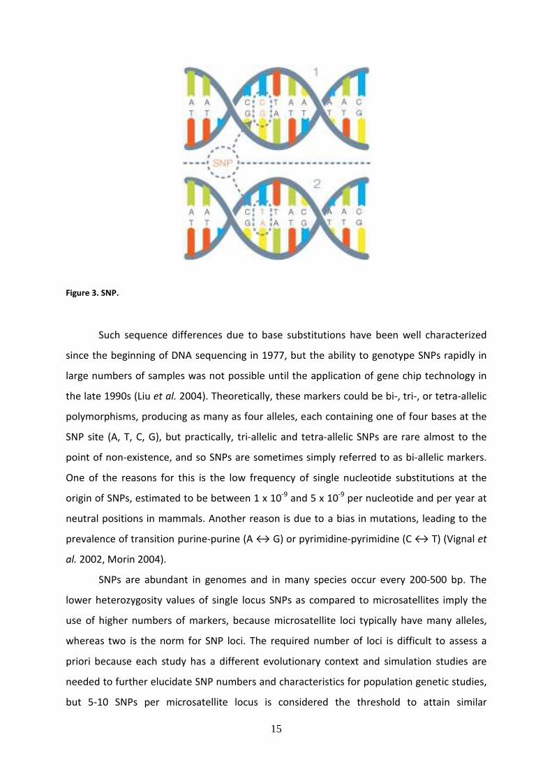
SNPs (Single Nucleotide Polymorphisms) are co-dominant markers and represent

polymorphisms caused by point mutations that give rise to different alleles containing

alternative bases at a given nucleotide position within a locus (Figure 3). For such a base

position with sequence alternatives in genomic DNA to be considered as a SNP, it’s

considered that the least frequent allele should have a frequency of 1% or greater.

15

Figure 3. SNP.

Such sequence differences due to base substitutions have been well characterized

since the beginning of DNA sequencing in 1977, but the ability to genotype SNPs rapidly in

large numbers of samples was not possible until the application of gene chip technology in

the late 1990s (Liu et al. 2004). Theoretically, these markers could be bi-, tri-, or tetra-allelic

polymorphisms, producing as many as four alleles, each containing one of four bases at the

SNP site (A, T, C, G), but practically, tri-allelic and tetra-allelic SNPs are rare almost to the

point of non-existence, and so SNPs are sometimes simply referred to as bi-allelic markers.

One of the reasons for this is the low frequency of single nucleotide substitutions at the

origin of SNPs, estimated to be between 1 x 10-9 and 5 x 10-9 per nucleotide and per year at

neutral positions in mammals. Another reason is due to a bias in mutations, leading to the

prevalence of transition purine-purine (A ↔ G) or pyrimidine-pyrimidine (C ↔ T) (Vignal et

al. 2002, Morin 2004).

SNPs are abundant in genomes and in many species occur every 200-500 bp. The

lower heterozygosity values of single locus SNPs as compared to microsatellites imply the

use of higher numbers of markers, because microsatellite loci typically have many alleles,

whereas two is the norm for SNP loci. The required number of loci is difficult to assess a

priori because each study has a different evolutionary context and simulation studies are

needed to further elucidate SNP numbers and characteristics for population genetic studies,

but 5-10 SNPs per microsatellite locus is considered the threshold to attain similar

16

discriminatory power. However, there are several advantages in the use of SNPs compared

to microsatellites. One technical problem with microsatellites is that it isn’t always possible

to compare data produced by different laboratories, due to the eventuality of

inconsistencies in allele size calling caused by a variety in sequencing machine, fluorescent

dye and allele calling software. On the other hand SNPs can be transferred between

laboratories easily, because SNP genotypes are based on detection of nucleotide sequence

differences rather than PCR product size differences, so that genotype data are universally

comparable and portable. Moreover, allele definition for microsatellites is done by assuming

that size variation of PCR products is directly correlated with differences in repeat numbers

of the simple motif. Although this is generally true, in some instances, size variations can be

due to small deletions or insertions in flanking sequences and two PCR products of identical

sizes can in reality be different alleles. The allele nomenclature problem is much simpler in

the case of SNPs, for which the results can just be coded as a YES/NO problem, where each

of the two alleles can be simply considered as being present or absent (Vignal et al. 2002).

Thus, the many advantages of SNP markers include abundance in any organism,

increased accuracy and ease of automation and transferability of data sets across national

and international laboratories. Another asset of using SNPs as population-level markers is

the ability to efficiently target coding and non-coding regions of the genome simultaneously

and even to predict the functional importance of the SNP depending on the position of the

polymorphism (i.e. amino acid changing, silent, regulatory mutation). SNPs can be found in

coding and non-coding areas, whereas most of the microsatellites used in population

genetics, for example, are typically in non-coding regions of the genome that is expected to

be less influenced by selection.

SNP discovery is the process of finding the polymorphic sites in the genome of the

species and populations of interest. In humans and in model organisms, most of SNP

discovery procedures have been realized “in silico”, meaning that genomic information from

multiple individuals in the public databases is screened for the identification of putative

polymorphisms. As concern non-model organisms, for which genomic resources are lacking

or insufficient, another approach needs to be used: SNPs can be found by sequencing and

comparing genome-wide regions from multiple individuals. Genomic resources from which

SNPs can be derived include Expressed Sequence Tags (EST), sequences of expressed genes,

which have been identified from partial sequencing of a messenger RNA (mRNA) pool that

17

has subsequently been reverse transcribed into cDNA. In the last years, the growing

availability of EST resources made possible to detect SNPs through direct alignment of ESTs

obtained from multiple individuals representing different geographical regions. By

generating SNPs from coding sequences, it’s possible to find polymorphisms in functional

genes, to identify loci under selection and to study the dynamics of these genes in natural

populations. This approach is now becoming easier with the advent of next-generation

sequencing methods that provide access to a wealth of sequence information on non-model

organisms (Margulies et al. 2005; Seeb et al. 2011). Transcriptome sequencing provides rich

sources of SNPs (Barbazuk et al. 2007), facilitating identification and study of the genes

involved in adaptive change (Renaut et al. 2010; Hemmer-Hansen et al. 2011; Williams and

Oleksiak 2011).

These new markers can be used in many types of researches. SNPs have in fact been

employed for individual identification and paternity; studies of Anderson and Garza (2006)

showed that 60-100 SNPs may allow accurate pedigree reconstruction, even in situations

involving thousands of potential mothers, fathers, and offspring, while Hauser et al. (2011)

demonstrated that a panel of 80 SNPs is sufficient to determine parentage in a wild

population.

SNPs have also the great power to detect population structure at several levels, as

proved in a study of Morin et al. (2009) where it was demonstrated that 30 SNPs should be

sufficient to detect moderate (FST = 0.01) levels of differentiation, but 80 or more SNPs may

be required to reveal demographic independence (FST < 0.005) and that increasing the

sample size has a strong effect on power rather than the number of SNP loci. Also, including

loci suspected to be under selection may increase the power to detect differentiation.

The power of SNPs concerning the assignment of individuals to the population of

origin has been widely investigated and, for example, it has been demonstrated that

indicated that as few as 22 SNPs for wolves (Seddon et al. 2005) and 51 SNPs for chum

salmon (Smith and Seeb 2008) provide high probability of correct population assignment,

similar to sets of 12 and 15 microsatellites, respectively. Smith et al. (2005) showed that 9

polymorphic SNPs are sufficient to assign Chinook salmon to a country of origin with more

than 95% accuracy, but their precision decrease when resolving fine-scale relationships. A

more recent study on Chinook salmon proved that between 100 and 200 highly informative

SNP loci are required to meet management standards (correct assignment > 90%) for

18

resolving genetic stock identification in finer-scale scenarios (Hess et al. 2011). In a study

carried out by Glover et al. (2010) on wild and domesticated strains of Atlantic salmon,

assignment was best (80% correct) when at least 100 SNP loci were used. In the last years,

researchers have been using outlier loci (loci more highly differentiated than could be

expected under a neutral model), potentially under diversifying selection, to increase the

accuracy of assignment tests. This was demonstrated in a recent study on Atlantic salmon,

where Freamo et al. (2011) obtained 85% of correct assignment with 14 outlier loci against

67% with neutral loci.

Many studies and researches have been carried out to detect SNPs possibly involved

in local adaptation in various fish species, as herring (Limborg et al. 2012), threespine

stickleback (Deagle et al. 2012), cod (Hemmer-Hansen et al. 2011; Nielsen et al. 2009a;

Poulsen et al. 2011), lake whitefish (Renaut et al. 2010; Renaut et al. 2011) and several

salmonid species (Freamo et al. 2011; Gomez-Uchida et al. 2011; Limborg et al. 2011; Seeb

et al. 2011). The improvement of genome scan techniques increases the chance to identify

candidate loci subject to selection, providing a more direct way of linking genotypes to

physiological functions.

19

CHAPTER 2

TARGET SPECIES: ATLANTIC BLUEFIN TUNA

2.1 TAXONOMY AND DESCRIPTION

The Atlantic Bluefin tuna (Thunnus thynnus, Linnaeus 1758) is the largest tuna

species, belonging to the Family Scombridae, which includes 15 genera and approximately

48 species of epipelagic fish. Seven species belong to the genus Thunnus, included T. thynnus

(Figure 4).

PHYLUM: CHORDATA

SUBPHYLUM: VERTEBRATA

SUPERCLASS: GNATHOSTOMATA

CLASS: OSTEICHTHYES

SUBCLASS: ACTINOPTERYGII

ORDER: PERCIFORMES

SUBORDER: SCOMBROIDEI

FAMILY: SCOMBRIDAE

TRIBE: THUNNINI

GENUS: THUNNUS

SPECIES: THUNNUS THYNNUS

The Atlantic bluefin Tuna grows to over 300 cm and it can reach a maximum length of

4 m. Its official maximum weight is 726 kg, but weights up to 900 kg have been reported in

various fisheries of the West Atlantic and Mediterranean Sea (Mather et al. 1995). Its

physical characteristics make it an excellent swimmer with speeds up to 90 km/h. It has a

fusiform body, deepest near the middle of the first dorsal fin base, with a triangular

pyramid-shaped head and a small mouth compared to the development of the skull. Its skin

Figure 4. Thunnus thynnus.

20

is very hard, resistant, and covered by small scales that decrease in size going from front to

rear of the body. The skin is also lubricated by a mucus which reduces friction with water.

Bluefin tuna displays 39 vertebrae and 12 to 14 dorsal spines and 13 to 15 dorsal soft rays. It

has two dorsal fins separated by a small space: the front is triangular with spines and the

rear is sickle cell and followed by small fins to the tail. The thin caudal peduncle, with a wide

and symmetrical tail at the end, is used as rudder and as a means of propulsion. Dorsal,

pectoral and small ventral thoracic fins are flattened allowing aerodynamic and fast

swimming. The back is dark blue or black, the sides are a silvery gray-blue and belly is white

with translucent patches. The first dorsal fin is yellow, the second, which is higher than the

first, is red, small fins are yellowish with brown edges and the caudal fin is dark blue. Fish

larvae (around 3-4 mm) are typically pelagic with a yolk sac and a relatively undeveloped

body form. The yolk sac is desorbed within few days, then the larvae have to feed on their

own.

2.2 GEOGRAPHIC DISTRIBUTION, HABITAT AND ECOLOGY

Atlantic bluefin tuna occurs throughout the North Atlantic, including the Gulf of

Mexico and the Mediterranean Sea (Walli et al. 2009) (Figure 5).

Its distribution extends over an extraordinarily large area, ranging off the Atlantic

coasts of Europe and Africa, from the North Cape to the Cape of Good Hope, and off the

North American coasts from Newfoundland to a latitude of 40°S (Mather et al. 1995).

Among the tuna, ABFT has the widest geographical distribution and is the only large

pelagic fish living permanently in temperate Atlantic waters (Bard et al. 1998; Fromentin and

Fonteneau 2001).

21

Figure 5. Distribution of Thunnus thynnus.

Archival tagging and tracking information confirmed that ABFT can sustain cold

(down to 3°C) as well as warm (up to 30°C) temperatures while maintaining stable internal

body temperature (Block et al. 2001). Data collected by Walli et al. (2009) with electronic

archival tags on western Atlantic bluefin from ages 7.1 to 14.2 years showed that they spent

87% of occupancy in waters ranging from 10° to 23°C with peak times at 13°-20°C.

T. thynnus is an endothermic fish, so it generates heat as a byproduct of metabolism

and maintains its body temperature above that of the surrounding environment. The

internal body temperatures for bluefin reporting timeseries data showed a mean of 23.9°C

(Walli et al. 2009).

The spatial distribution and movement of ABFT are hypothesized to be controlled by

preferential ranges and gradients of temperature, similar to Pacific bluefin and other tuna

species (Laurs et al. 1984; Lehodey et al. 1997; Bard 2001; Inagake et al. 2001). More works

appears to converge toward the opinion that juvenile and adult ABFT frequent and

aggregate along ocean fronts (Humston et al. 2000; Lutcavage et al. 2000; Royer et al. 2004).

This association is also likely to be related to foraging, ABFT feeding on the abundant

vertebrate and invertebrate prey concentrations of these areas. Juvenile and adult ABFT

spend the majority of their time in waters less than 200 m but frequently dive to depth of

22

500-1000 m (Lutcavage et al. 2000; Block et al. 2001; Stokesbury et al. 2004; De Metrio et al.

2005). The mean diving depths of bluefin tuna was 34.5 m, with most of their time spent

between the surface and 50 meters and an exponential decrease in time spent at greater

depths. Maximum depth of 1200 m was recorded by one fish (Walli et al. 2009); a similar

behaviour has also been reported for southern bluefin tuna, bigeye tuna and swordfish and

is generally related to foraging in deep scattering layers or to physiological constraints to

cool the body temperature (Carey and Robinson 1981; Holland et al. 1992; Musyl et al.

2003). During spawning runs, T. thynnus shows deep-diving behaviors in the Gulf of Mexico,

which likely provide access to cool, oxygen-rich waters as the fish travel to breeding grounds

(Stokesbury et al. 2004; Teo et al. 2007). Once on the spawning area, T. thynnus make

shallow oscillatory dives at night with frequent visits to the surface. Similar behaviors have

been observed for T. orientalis (Kitagawa et al. 2006) and T. albacares (Schaefer 2001)

during the breeding phase. Thunnus thynnus maintains this behavior for approximately 20

days. Maximum diving depths of T. thynnus are significantly less (< 200 m versus > 500 m)

during the spawning phase than observed during entry to and exit from spawning grounds in

the west.

As larvae and small juveniles, their diet is probably similar to that of T. orientalis in

the Pacific Ocean, which is comprised primarily of zooplankton with copepods as the main

stomach item (Uotani et al. 1990). The diet of adults is comprised mainly of fishes,

cephalopods (mostly squid) and crustaceans (Sarà and Sarà 2007). These categories may

include numerous species, and the particular composition is determined principally by

location. In the western Atlantic, the diet is primarily composed of Atlantic herring Clupea

harengus, Atlantic mackerel Scomber scombrus, sand lances Ammodytes spp., and silver

hake Merluccius bilinearis (Nichols 1922; Crane 1936; Dragovich 1970; Mason 1976; Holliday

1978; Eggleston and Bochenek 1990; Chase 2002). In the eastern Atlantic and Mediterranean

Sea, ABFT feed on European sprat Clupea sprattus, European anchovy Engraulis

encrasicholus and European pilchard Sardina pilchardus (Oren et al. 1959; De Jager et al.

1963). At tropical latitudes, porcupinefish Diodon sp. and flying gurnard Dactylopterus sp.

are the dominate items observed in the stomachs of T. thynnus (Krumholz 1959; Dragovich

1970). No clear relationship has been demonstrated between prey length and the size of

ABFT: both small and large ABFT display similar prey-size spectra. Chase (2002) noted that

23

the largest prey (those > 40 cm) were only consumed by giant ABFT > 230 cm, while Logan et

al. (2011) observed that prey length was not significantly correlated with ABFT length.

ABFT has a long life span of 40 years. Methods used to estimate age and growth of T.

thynnus have been based on the examination of calcified structures, length-frequency data

or mark-recapture data. Mark-recapture method is limited due to uncertainties in the initial

age of a fish at release and the lack of observations and high variability in growth for these

sizes. This method used for ageing do not perform well for fish > 200 cm (approximately 10

years old) (Fromentin and Powers 2005). Several different calcified structures have been

used to estimate the age and growth of T. thynnus: otoliths have the advantage that the

central nucleus is not resorbed with age, so they have been used to estimate growth during

larval, juveniles and adult phase (Brothers et al. 1983; Foreman 1986; Itoh et al. 2000;

Megalofonou 2006), while the use of spines is limited by the resorption of the medular

cavity from age 3 (Compeán-Jimenez and Bard 1983; Mather et al. 1995). Growth and

mortality of T. thynnus during the larval phase has been determined from age data from

otolith microstructure analysis (Rooker et al. 2007). Scott et al. (1993) reported that growth

was linear during the larval phase (∼2-10 days) at a rate of 0.3-0.4 mm d-1. Similar rates have

been reported for congeners from temperate and tropical regions: T. orientalis (0.33 mm d-1;

Miyashita et al. 2001), T. albacares (0.47 mm d-1; Lang et al. 1994), and T. maccoyii (0.28-

0.36 mm d-1; Jenkins and Davis 1990; Jenkins et al. 1991). Brothers et al. (1983) reported a

growth rate of 1.4 mm d-1 for juveniles in the western Atlantic (267-413 mm FL; ca. 70-200

d). Estimates of growth for juvenile T. thynnus (85-555 mm FL) from the Mediterranean Sea

are markedly higher, with a mean growth rate of 4.7 mm d-1 (Megalofonou 2006). Juvenile

growth is rapid for a teleost fish (about 30 cm year-1), but somewhat slower than other tuna

and billfish species (Fromentin and Fonteneau 2001, Fromentin and Powers 2005). Fish born

in June attain a length of about 30-40 cm long and a weight of about 1 kg by October. After

one year, fish reach about 4 kg and 60 cm long (Mather et al. 1995). Growth in length tends

to be lower for adults than juveniles, but growth in weight increases. Therefore, juveniles

are relatively slim, whereas adults are thicker and larger, so at 10 years, an ABFT is about

200 cm and 150 kg and at 20 years reaches about 300 cm and 400 kg. West ABFT grow faster

after maturity and attain larger sizes than the East and Mediterranean ABFT.

Age structure of adult T. thynnus has been studied in both the eastern and western

Atlantic, and estimated growth rates are relatively similar between and within regions during

24

the first five years of life. After age 5, growth trajectories of T. thynnus show marked

differences between the eastern and western Atlantic, with the length at age being greater

in the western Atlantic than the eastern Atlantic. At age 10, mean size in the western

Atlantic was 212 cm FL compared to 200 cm FL for the eastern Atlantic (Rooker et al. 2007).

Also seasonal growth patterns have been better documented, so both juveniles

(Mather and Schuck 1960; Furnestin and Dardignac 1962; Farrugio 1980) and adults ABFT

(Tiews 1963; Butler et al. 1977) grow rapidly during summer and early autumn (up to 10%

per month), while growth is negligible in winter. The existence of a slowdown in growth

during the winter has been confirmed for the southern bluefin tuna (Evenson et al. 2004)

and the pacific bluefin tuna (Bayliff 1993). Seasonal variations in length and growth rates of

older T. thynnus are less apparent, probably due to the weak relationship between age and

length for individuals more than 15 years of age (Hurlbut and Clay 1988).

Sex-specific differences both in length at age and weight at age have been reported,

with differential growth in weight being more pronounced between males and females. Past

studies shown that males grow more rapidly than females and reach a slightly greater size at

a given age, with these differences becoming apparent by approximately age 10 (Rivas 1976;

Caddy et al. 1976). In the recent study of Santamaria et al. (2009), based on sampled over an

8-year period from 1998 to 2005 in several central Mediterranean Sea sites (North Ionian,

South Adriatic, South Tyrrhenian seas and Ionian waters around Malta), is shown that after

sexual maturity, reached above 135 cm FL, the female weight-at-length is higher than the

male’s.

Natural mortality rates (M) of ABFT are poorly known. However, the mortality rates is

lower and less variable in long-lived fish, such as ABFT, than in short-lived ones; it’s higher

during juvenile stages than during the adult phase and it also varies with population density,

size, sex, predation and environment (Fromentin and Powers 2005). Scott et al. (1993)

estimated a natural mortality rate of 0.20 d-1 for larvae from the western stock, and rates are

lower than values reported for more tropical tunas during comparable periods: T. albacares

(M = 0.33 d-1; Lang et al. 1994) and T. maccoyii (M = 0.66 d-1; Davis et al. 1991). Tagging from

Southern bluefin tuna (Thunnus maccoyii) tends to confirm that M is higher for juveniles

(between 0.49 and 0.24) compared to that of adults (around 0.1). In the absence of direct

and consistent estimates of M for Atlantic bluefin tuna, the natural mortality vector of the

Southern bluefin tuna is generally used for the East-Atlantic and Mediterranean stock

25

assessment, whereas a constant M of 0.14 is assumed for the West Atlantic bluefin tuna

(ICCAT 1999; ICCAT 2003a).

2.3 REPRODUCTION AND SPAWNING

Bluefin tuna is oviparous and iteroparous like all tuna species (Schaefer 2001).

Ovaries of T. thynnus consist of ovigerous lamellae with follicles at different stages of

development (Corriero et al. 2003). The simultaneous presence of all oocyte developmental

stages during the spawning period (Medina et al. 2002; Corriero et al. 2003) indicates that T.

thynnus has asynchronous oocyte development and, similar to other temperate and tropical

tunas, is a multiple or batch spawner (Wallace and Selman 1981). Spawning frequency or

interval for T. thynnus has been estimated at 1.2 days (Medina et al. 2002). This interval is

similar to the observed frequencies of other members of the genus Thunnus: yellowfin tuna

T. albacares (1.27 to 1.99; Schaefer 1998; Itano 2000), bigeye tuna T. obesus (1.05; Chu

1999), and southern bluefin tuna T. maccoyii (1.62; Farley and Davis 1998). It is generally

assumed that bluefin tuna spawns every year, but electronic tagging experiments, as well as

experiments in captivity, suggest that individual spawning might occur only once every two

or three years (Lutcavage et al. 1999).

The testis of T. thynnus is comprised of lobules radiating from the longitudinal main

sperm duct toward the periphery (Abascal et al. 2003). The testicular structure is cystic, each

cyst being comprised of a clone of germ cells branched by the cytoplasm of Sertoli cells.

Egg production appears to be age (or size) dependent: a 5 years old female produces

an average of 5 million eggs (approximately 1 mm), while a 15-20 years female can carry up

to 45 million eggs (Rodríguez-Roda 1967). Estimated relative batch fecundity of T. thynnus is

greater (> 90 oocytes g-1 of body weight) than those estimated for other tunas in the genus

Thunnus, which are typically less than 70 oocytes g-1 of body weight: T. obesus 31 oocytes g-1

(Nikaido et al. 1991), T. maccoyii 57 oocytes g-1 (Farley and Davis 1998), and T. albacares 67

oocytes g-1 (Schaefer 1998).

Rodriguez-Roda (1967) estimated that 50% of female T. thynnus in the

Mediterranean Sea were reproductively active at approximately 103 cm (age 3) and 100%

maturity was reached between 115 and 121 cm (age 4 or age 5). Corriero et al. (2005)

confirmed results of this study, reporting that 50% of T. thynnus in the Mediterranean Sea

26

reached sexual maturity at 104 cm (age 3 or age 4) and 100% at 130 cm (age5). Instead

Heinesh et al. (2008) studied the growth of the gonads in adults tuna in several areas of the

Mediterranean Sea, verifying a mean body length of 200 cm (age 8). In the western Atlantic,

histological examination of ovaries from females showed delayed maturation schedules, and

individuals were unlikely to reach sexual maturity before age 8 (Baglin 1982). More recent

studies indicate that juvenile tuna, tagged in North Carolina and that return in the

Mediterranean during the spawning season, didn’t pass the Strait of Gibratar before 9-10

years old (Block et al. 2005).

The reproductive cycle of T. thynnus has been reconstructed on the basis of the

histological descriptions of the gonads of fish captured in different periods. In the central

and western Mediterranean, T. thynnus is reproductively inactive from August to April, when

only unyolked oocytes are present in the ovaries, and mainly spermatogonia and meiotic

cells have been found in the seminiferous epithelium. Active non-spawning individuals have

been observed in May, with yolked oocytes in the ovaries and seminiferous lobules

progressively filled with spermatozoa. Hydrated oocytes and post-ovulatory follicles, signs of

imminent and recent ovulation, respectively, have been found in actively spawning

individuals captured in late June to early July. From late July to September, T. thynnus are

reproductively inactive, as ovaries show unyolked oocytes and late stages of atresia of

yolked oocytes; only residual spermatozoa are present in the testes. The presence of actively

spawning fish, with hydrated oocytes and post-ovulatory follicles, was reported in the

eastern Mediterranean Sea from mid May to mid June (Karakulak et al. 2004b), while

spawning occurs in the central and western Mediterranean from mid June to early July

(Susca et al. 2001; Corriero et al. 2003).

There are two regional spawning areas for T. thynnus, one in the east and one in the

west (Mediterranean Sea and Gulf of Mexico, respectively), as confirmed by electronic

tagging studies (Stokesbury et al. 2004; Block et al. 2005; Teo et al. 2007). The timing of

spawning in both the east and west is linked to temperature. Sea surface temperatures

reported for T. thynnus on putative spawning grounds in the Gulf of Mexico and

Mediterranean Sea range from approximately 22.6°C-27.5°C and 22.5°C-25.5°C, respectively

(Karakulak et al. 2004a, 2004b; Garcia et al. 2005; Teo et al. 2007). Because the waters of the

Gulf of Mexico are above the 24°C spawning threshold in early spring (Block et al. 2001,

2005; Teo et al. 2007), T. thynnus begin spawning earlier in the Gulf of Mexico than in the

27

Mediterranean Sea (April versus May) (Baglin 1982; Nishida et al. 1998; Medina et al. 2002;

Corriero et al. 2003; Karakulak et al. 2004a).

In the Mediterranean Sea there are three spawning areas: the waters of southern

Italy around Sicily, nearby the Sicilian Channel and the Malta Channel (Sella 1929; Sanzo

1932; Piccinetti and Manfrin 1970; Nishida et al. 1998), the Balearic Islands, a transitional

zone between Mediterranean and eastern Atlantic waters, mostly in the Mallorca Channel

and in the south of Menorca (Rodriguez-Roda 1975; Nishida et al. 1998; Garcia et al. 2005)

and areas north of Cyprus along the coast of Turkey (Karakulak et al. 2004a, 2004b; Oray and

Karakulak 2005).

In the west, the spawning grounds of T. thynnus in the Gulf are located along the

northern slope waters between the 200 m and 3000 m contours from 85°W and 95°W (Block

et al. 2005; Teo et al. 2007). Apart from the northern Gulf, T. thynnus larvae have been

reported from the southern Gulf to the Yucatan Channel (Richards and Potthoff 1980;

McGowan and Richards 1986) and from the Straits of Florida to the Bahamas (Rivas 1954;

Richards 1976; Richards and Potthoff 1980; Brothers et al. 1983).

2.4 MOVEMENT AND STOCK STRUCTURE

The interest on the behavior of bluefin tuna and its migration goes back to the past.

Bluefin tuna migration in the Mediterranean Sea has been described long ago by the ancient

Greek and Latin philosophers, especially Aristotle (IV B.C.) and Pliny the Elder (Ith A.C.). A

migratory connection between oceans was first mentioned by Cetti (1777), who suggested

that bluefin tuna come into the Mediterranean from the North Atlantic to spawn around

Sicily and then go back by the same routes. The first works are attributed to M. Sella (1926,

1927, 1929; cited by Brunenmeister 1980): he suggested that tuna had moved from the east

of the Atlantic to the Mediterranean, and that after breeding they had moved from South of

Spain to Norway.

New innovative tools promoted a better knowledge of migratory behaviors of this

species. Mark-recapture studies with identification tags (“conventional tagging”) have

provided valuable information on key aspects of the biology of T. thynnus, focusing more on

the western North Atlantic than on the eastern Atlantic. From several studies it emerged

that juveniles tuna (< 4 years) didn’t move out of the place where they were tagged, while

28

adults tuna performed long distance movement across the ocean (trans atlantic movement)

(Rooker et al. 2005). Similar evidence of movement were reported in the eastern Atlantic

(Magnuson et al. 1994; Fromentin 2001). Conventional tags provide valuable data on a range

of life history parameters, but their utility is limited by the lack of information on locations

between release and recapture. Alternatively, electronic tags, recording ambient light level,

water and body temperature, and pressure at frequent intervals throughout the deployment

duration, allowing estimation of position in association with diving behavior and thermal

physiology, yielded important insights about bluefin seasonal movements, aggregations and

diving behaviors (Teo et al. 2004; Block et al. 2005; Walli et al. 2009). Studies of Block et al.

(2001, 2005) have highlighted the phenomenon of "spawning site fidelity" (fidelity of

individuals to the breeding site), demonstrating that adolescent and mature western Atlantic

bluefin tuna (with size > 200 cm) move to the Gulf of Mexico and the eastern Mediterranean

Sea during the known breeding season. The observed pattern of migration supports the

hypothesis of "homing behavior", according to which bluefin tuna would migrate in specific

and well-defined areas, returning to the same spawning area of origin, both in the

Mediterranean and in the Gulf of Mexico. In particular, for bluefin tuna would seem more

plausible theory the "repeat homing", a process related to spatial learning of young

individuals from those adults, rather than the "natal homing", in which the fidelity to the site

of birth is due imprinting, during the early stages of life, of specific environment (Fromentin

and Powers 2005) (Figura 6). Ravier and Fromentin suggested in their work of 2004 a

reproductive strategy, known as "opportunistic homing", halfway between the idea of strict

loyalty to origin breeding site and the reproductive opportunism, according to which

individuals choose the site of deposition in relation to optimal environmental conditions:

during periods when temperatures rise, bluefin tuna may be able to reproduce in areas

other than those traditionally described (for example in North Atlantic), where you could

create environmental conditions favorable to the course of last stages of gametogenesis,

whereas during periods of low temperatures the activity reproduction would be limited to

the permanent sites of deposition (Mediterranean and the Gulf of Mexico).

29

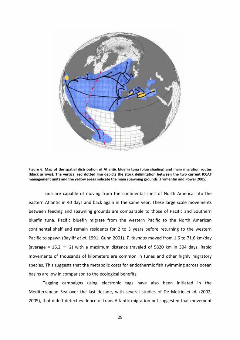
Figure 6. Map of the spatial distribution of Atlantic bluefin tuna (blue shading) and main migration routes

(black arrows). The vertical red dotted line depicts the stock delimitation between the two current ICCAT

management units and the yellow areas indicate the main spawning grounds (Fromentin and Power 2005).

Tuna are capable of moving from the continental shelf of North America into the

eastern Atlantic in 40 days and back again in the same year. These large scale movements

between feeding and spawning grounds are comparable to those of Pacific and Southern

bluefin tuna. Pacific bluefin migrate from the western Pacific to the North American

continental shelf and remain residents for 2 to 5 years before returning to the western

Pacific to spawn (Bayliff et al. 1991; Gunn 2001). T. thynnus moved from 1.6 to 71.6 km/day

(average = 16.2 ± 2) with a maximum distance traveled of 5820 km in 304 days. Rapid

movements of thousands of kilometers are common in tunas and other highly migratory

species. This suggests that the metabolic costs for endothermic fish swimming across ocean

basins are low in comparison to the ecological benefits.

Tagging campaigns using electronic tags have also been initiated in the

Mediterranean Sea over the last decade, with several studies of De Metrio et al. (2002,

2005), that didn’t detect evidence of trans-Atlantic migration but suggested that movement

30

patterns or displacement distance were linked to size, with larger individuals (> 150 kg)

being more likely to move out of the Mediterranean. Yamashita and Miyabe (2001) also

reported that young T. thynnus tagged with archival tags in the Adriatic Sea remained close

to the deployment area within the Mediterranean. Movements of T. thynnus tagged in the

central and western Mediterranean Sea were more pronounced than in the east. Electronic

tagging also revealed that the Northwest Atlantic (especially the area being delimited by the

Gulf of Maine, Newfoundland and the Gulf Stream) has become a key feeding ground for

bluefin tuna of both Western and Eastern origins during the 1990s and early 2000s (Block et

al. 2001; Block et al. 2005; Royer et al. 2008). Moreover, Stokesbury et al. (2007) reported

that giant T. thynnus tagged in the eastern Atlantic off Ireland moved from these areas

across the 45th W stock boundary over short periods of time, demonstrating connectivity

between eastern foraging grounds and western Atlantic fisheries.

A recent work of Walli et al. (2009) has shown clear evidence of mixing between

eastern and western populations in foraging aggregation zones in the North Atlantic,

dependent on the productivity and high abundance of prey species in a given area. This is

well supported by results of analysis based on carbon and oxygen stable isotope in otolith

(δ13C and δ18O). Otolith material deposited during the first year of life serves as a natural tag

of the individual’s place of origin or nursery habitat, it varies regionally and reflects water

composition differences in nurseries. Stable δ18O signatures in otoliths of yearlings from

each nursery were distinct, with enriched δ18O values observed for T. thynnus from the

cooler, more evaporative Mediterranean basin relative to the western Atlantic. (Rooker et

al. 2007, 2008; Schloesser et al. 2010). Rooker and Secor (2004) demonstrated that the

discriminatory power of stable isotopes in otoliths of yearling T. thynnus was high, with well

over 90% of individuals classified correctly to eastern and western Atlantic nurseries. In a

followup study, Rooker et al. (2006a) compared otolith core material (corresponding to the

first year of life) of large school, medium, and giant T. thynnus collected in both the western

Atlantic and the Mediterranean Sea. Results from this preliminary assessment indicated that

a large fraction (> 50%) of the adolescent T. thynnus collected in the western Atlantic fishery

originated from nurseries in the Mediterranean Sea. Alternatively, adult T. thynnus collected

in the Mediterranean Sea were almost entirely of eastern Atlantic origin (> 90%), indicating

strong natal homing to spawning/nursery grounds in the Mediterranean Sea. Experiments

carried out using eight microsatellite in the eastern North Atlantic Ocean south of Iceland for

31

ABFT collected during 1999 and 2002 demonstrated genetic divergence between collections

of fish caught early and late in the fishing season over the two years. These results

confirmed that the northeast Atlantic fishery represents a mixed-stock fishery including

animals migrating from different areas and recruited from different spawning grounds

(Carlsson et al. 2007).

32

CHAPTER 3

STATE OF THE ART

3.1 FISHERY GENETICS

Fisheries management is currently considered a necessity to ensure the long-term

stability of this activity, recovery of fish stocks, sustainability of resources and to avoid the

collapse of natural populations. To manage economically important marine species it’s

necessary to define individual units, as stocks with specific mortality and recruitment levels.

Scientific information represent the focus for a correct management of living marine

resources, thus a variety of international organizations have been established to facilitate

collection and interpretation of scientific data for marine species in a management context,

as International Council for the Exploration of the Sea (ICES), International Whaling

Commission (IWC), and International Commission for the Conservation of Atlantic Tunas

(ICCAT). It’s important to preserve the population diversity, needful for a sustainable

utilization of exploited stocks and for adaption to environmental changes. The field of fishery

genetics has greatly expanded in recent decades (Sweijd et al. 2000; Ward 2000; Hauser and

Carvalho 2008), in parallel with rapidly developing technologies in the field of human

genetics, changed the understanding of population dynamics and structuring in marine fish.

Genetic tools are widely used in many aspects of global biodiversity conservation, including

phylogenetic classification, species identification, genetic structure of natural populations

and identification of management units for conservation, assessment of genetic diversity

within species or population, especially of small ones or at risk, and interactions between

environmental contamination and biology and health of organisms.

Whereas classical fisheries approaches are typically focused on factors driving short-

term demographic changes in populations (quantitative changes), genetic approaches

examine the extent to which changes in the composition of populations (qualitative change)

influence both short-term alterations in phenotypic traits and longer-term response to

natural and anthropogenic perturbations (Frankham 2005). Better integration of genetic

33

information and traditional methods of fisheries stock assessment could substantially

improve the quality of management advice.

The aim of sustainable fisheries management is to identify the spatial and temporal

scale of population structuring, to devise tools to monitor its dynamics and to contribute to

overall fisheries production. Even apparently small genetic differences among populations of

marine fishes could translate into important adaptive variation distributed among

populations (Conover et al. 2006). Genetic diversity is required for populations to adapt to

environmental changes. Large populations have a significant proportion of genetic diversity,

but this is considerably reduced in species and overexploited populations, that may lead to a

decline in their capacity to adapt to new circumstances and to the environmental changes

(Hauser et al. 2002).

The first studies on the structure of fish populations with molecular genetics initiated

around 1950 with the study of blood groups, of tuna, salmon and cod (Ligny 1969). Thanks to

the development of new techniques, as the DNA polymerase chain reaction, in the last

decade of the 20th century different molecular markers are increasingly being used, playing

an important role in animal genetics studies. Now large amounts of genetic data from many

marine species have been generated, focusing on fish species harvested by humans and

overfished, and relevant information for efficient management of fish stocks was provided.

Allozymes are allelic variants of proteins produced by a single gene locus and have long been

used due to the ease of use across species (Nevo 1990), but their statistical power is shrink

by the limited number of loci and low variability. Mitochondrial DNA (mtDNA) was the first

widely used DNA marker and has been employed extensively to investigate stock structure in

a variety of fishes including eels (Avise et al. 1986), bluefish (Graves et al. 1992), red drum

(Gold et al. 1993), snappers (Chow et al. 1993), and sharks (Heist and Gold 1999), providing

many insights into the demography of natural populations thanks to its power for

genealogical and evolutionary studies. However, due to its non-Mendelian mode of

inheritance (it’s maternally inherited), it must be considered a single locus and its ability to

resolve population structure is relatively restricted (Avise 1994). Most recent genetic studies

of natural populations have used microsatellites, multiple copies of tandemly arranged

simple sequence repeats. Microsatellites are inherited in a Mendelian fashion as codominant

markers, they are very abundant, occurring as often as once every 10 kb in fishes, have an

evenly genomic distribution, being in the genome on all chromosomes and all regions of the

34

chromosome, have small locus size, and showed a high polymorphism, based on size

differences due to varying numbers of repeat units contained by alleles at a given locus (Liu

and Cordes 2004). Due to its easy use by simple PCR, followed by a denaturing gel

electrophoresis for allele size determination, and to the high degree of information provided

by its large number of alleles per locus, microsatellites provides high statistical power for

population genetics ability to detect population-genetic structure, to test parentage and

relatedness, to assess genetic diversity, and to study recent population history. They suffer

from two drawbacks: first, they require species-specific marker development, and second,

they undergo a high potential for null alleles and are prone to genotyping errors due to their

size-based nature (homoplasy) (Jarne and Lagoda 1996; Vignal et al. 2002; Oleksiak 2010).

Amplified fragment length polymorphisms (AFLP) have been largely used since first

described (Vos et al. 1995) due to their ease of use in species with no prior sequence

information: many AFLP markers can be easily amplified and scored. AFLP analyses,

however, require high-quality DNA and provide dominant markers so that heterozygotes

cannot be directly measured (Campbell et al. 2003; Oleksiak 2010).

A new marker type, named SNP (Single Nucleotide Polymorphism) is now on the

scene and has gained high popularity (Vignal et al. 2002; Morin 2004). Neutral DNA markers

have been extensively used for elucidating demographic population relationships, but the

distribution of neutral variation among populations reveals little about the adaptive genetic

variation, critical in order to define management units and setting priorities for conservation

(Nielsen et al. 2009). So now there is an increasing interest in identifying molecular genetic

markers under selection that can detect adaptive local events and define different units of

population with greater resolution than neutral markers (Nielsen 2001; Beaumont 2005;

Schlötterer & Dieringer 2005; Storz 2005; Joost et al. 2007). Analysis of variation in or around

genes is specifically targeted by expressed sequence tag (EST) sequencing, providing a more

focused effort at describing functional genomic variation (Bouck and Vision 2007; Bonin

2008). ESTs are single-pass sequences generated from random sequencing of cDNA clones

and represent a partial sequence of the much longer RNA expressed in a cell. Because the

mRNAs have been processed and edited in the cell, ESTs encode genes that are actively

transcribed without intervening intron sequences and so can be more informative about the

ultimate function of the gene. They offer a rapid and valuable first look at genes expressed in

specific tissue types, under specific physiological conditions, or during specific

35

developmental stages (Liu and Cordes 2004). In teleosts fishes, three-dozen species in

diverse orders have EST collections that contain more than 10000 sequences: D. rerio have

the most ESTs, followed by O. latipes, then the salmoniformes (S. salar and O. mykiss) and

finally three-spine stickleback. ESTs often are sequenced with the end goal of using them for

gene expression analyses, but also are a rich source for discovering microsatellites and SNPs.

However, it’s necessary be cautious, because one cannot always be certain that a particular

SNP in an EST is due to true polymorphism or to sequence error. EST-derived microsatellites

have been used for linkage mapping in P. maxima, S. salar, O. mykiss (Rexroad et al. 2005;

Bouza et al. 2008; Moen et al. 2008), and, more recently, Kucuktas et al. (2009) combined

both microsatellites and SNPs derived from ESTs, to construct a genetic linkage map of the

Ictalurus punctatus (Rafinesque) genome. Other uses for these EST-derived microsatellites

and SNPs include population-genomic analyses thanks to the advent of whole genome

sequencing projects.

Genomics is a field of science that deals with the structure, function and evolution of

genomes. Genomics often simply implies the use of high throughput DNA- or RNA- based

methods. It comprises comparative, functional and environmental genomics. Comparative

genomics examines whole genomes, their gene content, gene order, structure, evolution

and taxonomy. Functional genomics investigates the biochemical and physiological role of

gene products and their interactions on a large or small scale. Environmental genomics

encompasses studies molecular variation in natural or artificial populations of different taxa

and their response to environmental conditions such as temperature or pollutants (Wenne

et al. 2007). Previously, fish genomics was restricted to fish species like Japanese pufferfish

(Takifugu rubripes) and zebrafish (Danio rerio), both well-known model species, with

reference genomes, for comparative and developmental genomics. Although marine fish

genomics is still in its infancy, now other species have been sequenced, as medaka, Oryzias

latipes, spotted green pufferfish, Tetraodon nigroviridis, and three-spined stickleback,

Gasterosteus aculeatus.

A genome-wide coverage would provide a powerful tool to explore the balance

between selection and gene flow, and its significance to population connectivity and local

adaptation, and to establish selective effects caused by natural and anthropogenic

environmental changes (Hauser and Seeb 2008). Concomitant with advances in molecular

technology and development of new tools, statistical approaches were also strengthened,

36

mainly because of higher information content of more variable genetic markers, but also

because of the increase in computing power (Beaumont and Rannala 2004; Pearse and

Crandall 2004). In the last period there was an increase in sequencing speed and a reduction

of sequencing cost achieved by enhancing automation and removing human input. Once

limited primarily to model organisms and humans, these techniques are now readily

available to fisheries genetics laboratories (Hauser and Seeb 2008).

3.2 FISHERY AND MANAGEMENT OF ATLANTIC BLUEFIN TUNA

3.2.1 Fishery

The oldest method of catching tuna consists of the traditional trap fishery (tonnara).

They were used in the Mediterranean and along the coasts of the North Atlantic from the

14th century in Sicily, from 16th century in Sardinia and Portugal since the 19th century in

Tunisia, Morocco and Spain. The traditional trap fishery were placed along the migration

routes of tuna that came in May in the Mediterranean from the North Atlantic for breeding

and then resumed in mid-July the way back. Depending on their location along their

migration routes, these traps were divided into two categories: the outward and return. The

first caught tuna at the beginning or during the period of breeding, the second at the end of

such period. Both traps could be of gulf or tip depending on whether they are, within a bay

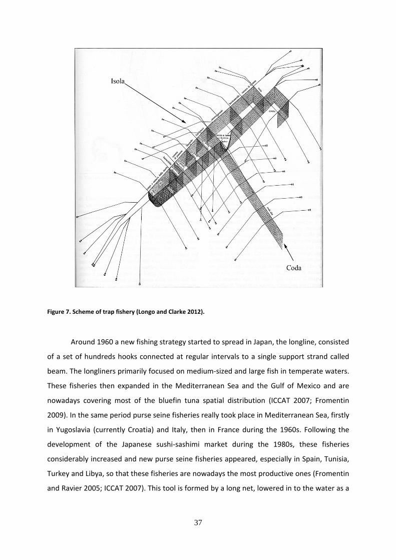
or the end of a promontory. The tonnara is formed by a complex system of nets, placed as

the barrier to guide and trap the tuna. The trap consisted of two essential structural

elements, the coda and the isola; the coda, or the tail, is a long series of nets placed

perpendicular to the coast, guiding bluefin toward the trap, and the isola, or island, is

formed by an elaborate construction of nets that create an elongated rectangular structure.

It is made up of many camera, or chambers, that divide the large structure into multiple

squared pens, where fishes are captured, contained and moved towards final chamber, the

camera della morte (the chamber of death) (Figure 7) (Longo and Clark 2012). Until the first

half of the 20th century, there were hundreds of traps in the Mediterranean, but now they

are about ten, due to expansion of exploited areas and evolution of fishing systems.

37

Figure 7. Scheme of trap fishery (Longo and Clarke 2012).

Around 1960 a new fishing strategy started to spread in Japan, the longline, consisted

of a set of hundreds hooks connected at regular intervals to a single support strand called

beam. The longliners primarily focused on medium-sized and large fish in temperate waters.

These fisheries then expanded in the Mediterranean Sea and the Gulf of Mexico and are

nowadays covering most of the bluefin tuna spatial distribution (ICCAT 2007; Fromentin

2009). In the same period purse seine fisheries really took place in Mediterranean Sea, firstly

in Yugoslavia (currently Croatia) and Italy, then in France during the 1960s. Following the

development of the Japanese sushi-sashimi market during the 1980s, these fisheries

considerably increased and new purse seine fisheries appeared, especially in Spain, Tunisia,

Turkey and Libya, so that these fisheries are nowadays the most productive ones (Fromentin

and Ravier 2005; ICCAT 2007). This tool is formed by a long net, lowered in to the water as a

38

curtain and closed in a circle around a school of fish. Yet, these fishing methods catch many

immature and undersized tunas and fish of other species.

This high increase in purse seine catches is related to the growth of tuna fattening

farms, since the purse seine is the best gear type for ensuring the capture and transfer of live

tuna (Sumalia and Huang 2012). Bluefin tuna ranching began in earnest in the

Mediterranean in the mid-1990s. Up until that time, this practice had been used minimally in

the Mediterranean, but the experience of Australian tuna ranches with southern bluefin

tuna prompted the expansion of these methods in the Mediterranean. Bluefin ranching saw

enormous growth during the 1990s and early 2000s (Miyake et al. 2003). Atlantic bluefin

tuna farming and fattening in the Mediterranean Sea is a seasonal activity and it involves the

capture of fish from the wild and their rearing in sea cages for periods ranging between 3

months to 2 years. According to ICCAT, the Atlantic bluefin tuna rearing operations are

classified as “fattening” if rearing is done for a short period (3-7 months) using mature fish (>

30 kg in body weight) to achieve a greater fat percentage in the muscle, which is desirable by

the sushi and sashimi markets in Japan, or “farming” if rearing is done for a longer period of

time (up to 2 years) and involves juvenile fish (8-30 kg in body weight), reaching a harvest

size between 30 and 50 Kg (ICCAT 2008; Mylonas et al. 2010). The countries involved in

Atlantic bluefin tuna fattening are Cyprus, Greece, Italy, Malta, Spain, Tunisia, and Turkey,

while farming takes place only in Croatia. The highest volumes of production in recent years

are coming from Malta, Tunisia, Croatia, Italy, and Turkey (Mylonas et al. 2010). Yet, this

method of production has faced challenges due to its continued reliance on live fish from

wild stocks. In addition, the metabolism of bluefin tuna requires high inputs of energy

(calories) in order to increase body size and weight. Furthermore, the production and

transport of fresh and frozen bluefin tuna to wealthy markets require a big energy

expenditures (Longo and Clark 2012).

Development of a proper aquaculture industry for the Atlantic bluefin tuna could be

the only way to both satiate the great demand for sushi and conserve the wild stocks of this

fish. One of the prerequisites for domestication and the establishment of a sustainable

aquaculture industry is the capacity to control reproductive processes of fish in captivity, and

to acquire high quality eggs and sperm for grow-out of the marketable product (Mylonas et

al. 2010). Reproduction in captivity of the bluefin tuna was first accomplished in Japan with

the Pacific bluefin tuna (Kumai 1998; Lioka et al. 2000; Sawada et al. 2005; Masuma et al.

39

2006). Fish are maintained in large cages or enclosures and are allowed to spawn naturally.

In June of 2002, artificially bred Pacific bluefin tuna broodstock produced 1 million eggs for

the first time. Several studies have been undertaken to develop methods for the control of

reproductive maturation in captive-reared Atlantic bluefin tuna (Corriero et al. 2007;

Mylonas et al. 2007; Corriero et al. 2009; DeMetrio et al. 2010), capturing migrating Atlantic

bluefin tuna (5-12 years old) in the Mediterranean Sea. During the natural spawning period

(June-July) of two consecutive years, fish were implanted underwater with a controlled-

release delivery system loaded with gonadotropin-releasing hormone agonist (GnRHa),

demonstrating that it is possible to induce maturation, ovulation/spermiation, and spawning

in captivereared Atlantic bluefin tuna using a GnRHa-based therapy. (Mylonas et al. 2007,

2010).

3.2.2 Management

Archaeological excavations have shown that fishing on bluefin tuna has occurred in

the Mediterranean since the 7th millennium BC (Desse and Desse-Berset 1994). The

popularity of Japanese sushi and sashimi worldwide during the 1980s made T. thynnus much

more economically attractive than before. As the western stock has already been extensively

depleted, the eastern Atlantic stock has remained a major source of Atlantic bluefin tuna to

supply the global market. Now bluefin tuna is heavily exploited over its whole spatial

distribution for a decade, there is thus no more refuge and all the potential sub-populations

are currently exploited (Fromentin and Powers 2005; ICCAT 2007). Specific natural

characteristics, such as late reproduction, large size at reproduction, long lifespan and the

aggregation of the fish that occurs during spawning, make bluefin tuna extremely vulnerable

to overexploitation (Safina 2001; Ottolenghi et al. 2004). Bluefin tuna are also sensitive to

oceanic conditions and disturbances such as those caused by industrial pollution. For an

effective management and conservation, it is crucial to know about bluefin tuna population

structure and spatial dynamics and their interactions with fishing and environmental

conditions (Fromentin 2009).

Observing the BFT historic catch by gear type in the Mediterranean Sea from 1950 to

2010, it has been noted that from the 1950s to the early 1970s, total catches were stable at

around 5000 to 8000 t per year, while there was a peak in the mid-1970s (over 15000 t per

40

year), followed by an unusual drop by the early 1980s. From then on to the mid-1990s, the

catches increased steadily from 9000 to 40000 t per year. After that, there was a substantial

decrease in catch to 24000 t per year in the most recent decade, which seems to serve as an

indication of effective management (Figure 8). So, due to its commercial importance, bluefin

tuna is intensely fished and actually overexploited. Since 1970 the biomass of bluefin tuna

broodstocks declined by 77% and 14% in the western and eastern populations, respectively

(ICCAT 2005). Western Atlantic bluefin spawning stock biomass (adult-aged fish) has

declined to about 20-29 per cent of 1970 levels (ICCAT 2010). Eastern Atlantic stocks are

between 40% and 57% of spawning stock biomass of the highest known levels in the late

1950s (MacKenzie et al. 2009; ICCAT 2010).

Figure 8. Catch for the East Atlantic and Mediterranean from 1950 to 2010 by gears; LL: longline; BB: bait

boat; TP: tuna trap; PS: purse seine; TAC: Total Annual Catch (ICCAT 2012).

To deal with the common-property and shared stock problem of tunas, the

International Commission for the Conservation of Atlantic Tunas (ICCAT) was established in

1969 to manage more than 30 tuna and tuna-like species in the Atlantic Ocean and adjacent

seas, including the Mediterranean bluefin tuna. The Commission, composed of 48

Contracting Parties (countries/political entities), is a Regional Fisheries Management

Organization (RFMO) responsible for combining a wide array of scientific and socio-

41

economic information into setting the annual total allowable catch (TAC) of Atlantic Tuna

species. ICCAT also includes the Standing Commitee on Research and Statistics (SCRS),

composed of scientists from various countries, that is responsible for producing models of

catch statistics and trends of populations and for providing scientific advice to ICCAT on the

TAC and quota allocation among countries’ members (Sumalia and Huang 2012). The quota

set by ICCAT is then split among member countries who are individually responsible, but not

obliged, to manage their fleet in accordance with the TAC. How the shares are divided has

undergone changes in two different periods. From 1983 to 1991, ICCAT allocated the TAC

among countries mainly according to their historical catches. In addition, the spatial

distribution of stock, proximity to coastal states, especially in small and developing

countries, have also been taken into consideration. However, CPs (Contracting Parties)

without large historical catches argued for changes in the allocation formula in the 1990s

and succeeded in getting ICCAT to increase their share in 2001. The allocated quota is

transferrable among countries’ members, though transfers have to be made under the

approval of ICCAT (Grafton et al. 2006).

The ICCAT, based on spawning sites of bluefin tuna, recognizes two stocks: those of

the west and the east Atlantic (the latter including the Mediterranean Sea), separated by the

45th W meridian (Nemerson et al. 2000) although mixing between the two units is known to

occur (ICCAT 2002). Both stocks are estimated to be strongly overfished and continue to be

overexploited; the 2006 stock assessment points out a substantial risk of fisheries and

population collapse (ICCAT 2007). Current advice for bluefin tuna is based upon Virtual

Population Analysis (VPA), which assumes that the 2 stocks Eastern and Western considered

since 1981 are homogeneous and that there is no sub stock structure within them (Kell et al.

2012).Recent evidence indicates, however, that the two populations overlap in the North

Atlantic foraging grounds (Block et al. 2005).

Illegal, Unreported and Unregulated (IUU) fishing is widely recognized as one of the

biggest concerns with BFT management in the Mediterranean Sea and other Atlantic Ocean

areas. WWF found huge gaps between national reports on BFT trade and official catch

reports to ICCAT, indicating that a large amount of IUU fishing place in the region (WWF

2006). It estimated that the total BFT catches in the Eastern Atlantic Ocean and the

Mediterranean Sea recorded through international trade were approximately 45000 t in

both 2004 and 2005, which were 40% above the total annual catch (TAC) of 32000 t set by

42

ICCAT. For 2006-2010, declared catch was 30689 t, 34516 t, 23849 t, 19701 t and 11294 t for

the East Atlantic and Mediterranean, of which 23154 t, 26479 t, 16205 t, 13016 t and 6949 t

were declared for the Mediterranean for those same years (Figure 9).

Figure 9. Catches divided by main geographical areas and catches not reported; MED: Mediterranean Sea;

ATE: East Atlantic; TAC: Total Annual Catch (ICCAT 2012).

Catches of bluefin tuna from the east Atlantic and Mediterranean were under-

reported between the mid-1990s through 2007. During this period, based on the number of

vessels operating in the Mediterranean Sea and their catch rates, ICCAT estimated total

catches to be close on the order of 50000 t to 61000 in the Mediterranean Sea. Estimates for

2008 and 2009 showed a substantial decrease in the catch, and declared catches in 2010

(11294 t) were significantly below the 2010 TAC of 13500 t (ICCAT 2012).

The pattern of catch at age in the Mediterranean Sea from 1955 to 2010 showed that

the catch of age 0 ABFT has decreased since the 1960s and is barely observed today. The

catches of other age groups have all increased in weight in 2006 compared to 1950.

Increasing BFT catches have led to rapid stock declines over years. According to the stock

assessment analyses reported by ICCAT, the spawning stock biomass (SSB), one of the most

important indicators of stock abundance and health, is about 57% of the highest estimated

SSB levels (1957-1959). Trend in fishing mortality (F) displayed a continuous increase over

43

the time period for the younger ages (ages 2-5) while for oldest fish (ages 10+) it had been

decreasing during the first 2 decades and then rapidly increased during the 1990s.

Bluefin tuna, like other species of fish, are increasingly commodified under the

capitalist global market. The lifecycles of bluefin are subsumed under market demands to

enhance profit, resulting in unsustainable interactions with bluefin tuna populations. The

consequences of this growth imperative include drastic reductions in bluefin populations

and the collapse of a sustainable fishing system (Longo and Clark 2012). With the intention

of better managing this fishery and protecting the wild stock from over-fishing, during the

last decade, the ICCAT adopted a series of measures to control the fishery in the

Mediterranean Sea, as an increase in the minimum catch size from 10 to 30 Kg, a reduction

in the number of permissible fishing days from 11 to 6 months, the presence of observers at

cage facilities, and the prohibition of at-sea transshipment (Commission 2007). Since 2010

ICCAT reduced total allowable catches to 13500 tons (from 32000 tons three years ago),

lowered this quota to 12900 tons in 2011, and restricted the purse seine fishing period to

only one month. However, it remains to be seen whether the efforts will have the intended

consequences of returning the state of the stock to sustainable levels, as, by ICCAT’s own

estimates, this gives the stock a 60% chance at recovery by 2022 (ICCAT 2010).

Atlantic US. fisheries for tuna are managed by the National Oceanic and Atmospheric

Administration's (NOAA's) National Marine Fisheries Service (NMFS) under the authority of

the Atlantic Tunas Convention Act (ATCA) and the Magnuson-Stevens Fisheries Conservation

and Management Act (Magnuson-Stevens Act). ATCA authorizes the promulgation of

regulations, as may be necessary and appropriate, to implement conservation and

management recommendations adopted by the ICCAT. Directed fishing for bluefin on their

Gulf of Mexico spawning ground was prohibited by ICCAT in 1982 (NMFS 2006). Western

Atlantic catches peaked in 1964 at 18679 t, due to annually fishing of 5000-12000 t mature

bluefin off Brazil by Japanese boats from 1962 to 1967, and declining since 2002 until 1523 t

in 2005 for a unavailability of fish (Figure 10). In 1998 the commission’s scientific committee

determined the annual west-Atlantic catch of 2500 t could not be sustained, 2000 t was

likely sustainable, and a quota near zero was necessary to restore the population to 1970s

levels within 20 years (Safina and Klinger 2008). In recent years, however, there appears to

have been a gradual increase in SSB from the low of 21% in 2003 to an estimated 29% in

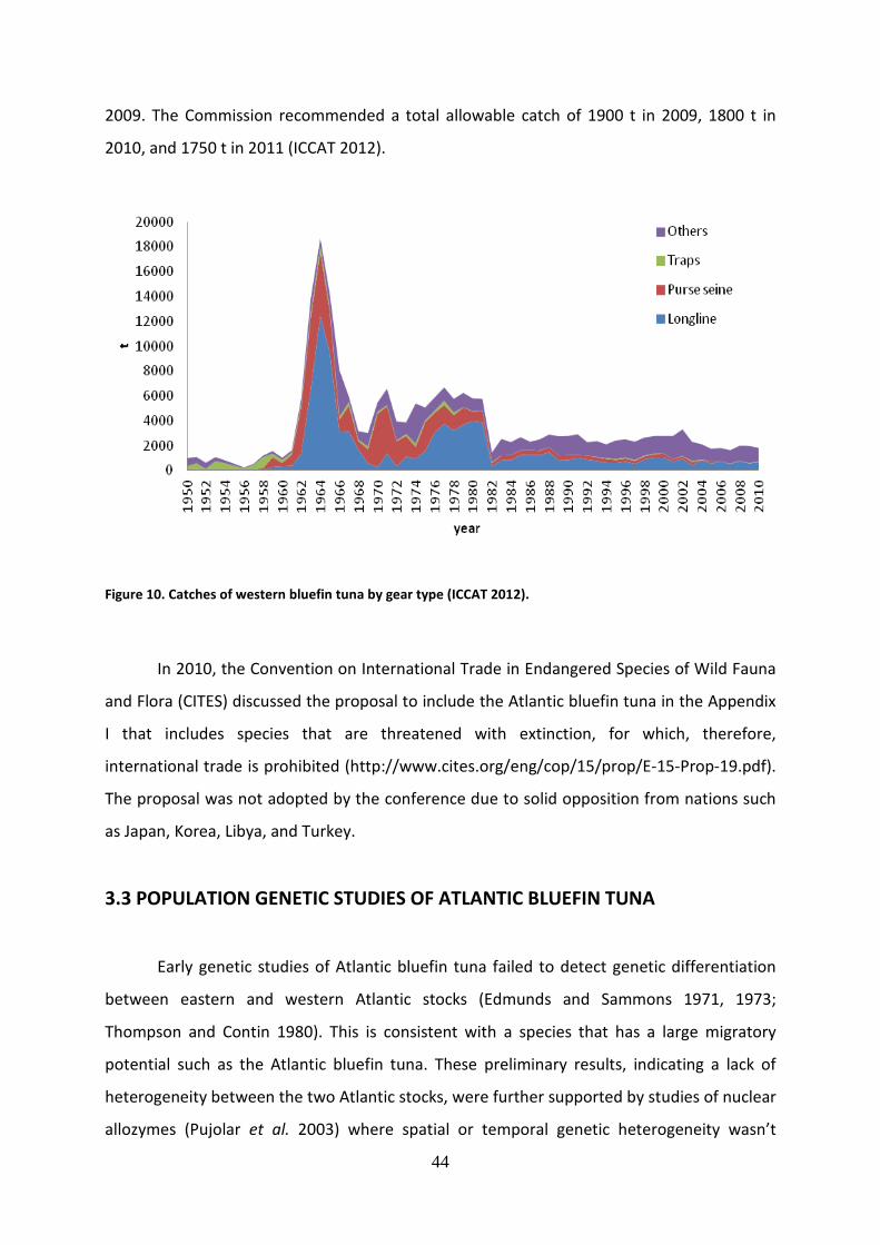
44

2009. The Commission recommended a total allowable catch of 1900 t in 2009, 1800 t in

2010, and 1750 t in 2011 (ICCAT 2012).

Figure 10. Catches of western bluefin tuna by gear type (ICCAT 2012).

In 2010, the Convention on International Trade in Endangered Species of Wild Fauna

and Flora (CITES) discussed the proposal to include the Atlantic bluefin tuna in the Appendix

I that includes species that are threatened with extinction, for which, therefore,

international trade is prohibited (http://www.cites.org/eng/cop/15/prop/E-15-Prop-19.pdf).

The proposal was not adopted by the conference due to solid opposition from nations such

as Japan, Korea, Libya, and Turkey.

3.3 POPULATION GENETIC STUDIES OF ATLANTIC BLUEFIN TUNA

Early genetic studies of Atlantic bluefin tuna failed to detect genetic differentiation

between eastern and western Atlantic stocks (Edmunds and Sammons 1971, 1973;

Thompson and Contin 1980). This is consistent with a species that has a large migratory

potential such as the Atlantic bluefin tuna. These preliminary results, indicating a lack of

heterogeneity between the two Atlantic stocks, were further supported by studies of nuclear

allozymes (Pujolar et al. 2003) where spatial or temporal genetic heterogeneity wasn’t

45

observed within the Mediterranean Sea or between the East Atlantic and Mediterranean,

indicating the existence of a single genetic grouping on the eastern side of the Atlantic

Ocean. No evidence of genetic differentiation between northeast Atlantic and the

Mediterranean samples was also found in a study of Alvarado Bremer et al. (2005) using the

mitochondrial DNA control region (mtDNA CR). This result agrees with the study by Ely et al.

(2002) that failed to find genetic differences between several temporal Mediterranean

samples. Pujolar et al. (2003) and Alvarado Bremer et al. (2005) analyzed a combination of

adult and young individuals using either nuclear allozymes or a short segment of the mtDNA

CR respectively, which in both cases might not have the resolution to observe genetic

differentiation for such closely related populations. However, one of the major limitations of

these studies was that the samples representing the western stock were collected along the

United States where mixing of the two stocks may occur and weren’t collected in the Gulf of

Mexico, the spawning ground for the western stock (Rooker et al.2007). A recent study

(Viñas et al. 2011) conform to the hypothesis of a single panmictic unit of Atlantic bluefin

tuna throughout the Mediterranean. This lack of differentiation within the Mediterranean

conforms to the general pattern that population structure for large pelagic species, such as

the Atlantic bluefin tuna, is only observed on a transoceanic, rather than a local scale

(Palumbi 1994; Graves 1998).

Different results were obtained when more representative samples of the stocks

were analyzed, including samples from the breeding grounds in the Gulf of Mexico and

Mediterranean Sea, so the differentiation between these two populations gained more

support (Carlsson et al. 2007; Boustany et al. 2008). These later findings were in agreement

with the natal homing fidelity observed from recent tagging studies (Block et al. 2005),

microchemical signatures (Rooker et al. 2008), and the clear differentiated biology between

the eastern and western Atlantic bluefin tunas (Fromentin and Powers 2005). Carlsson et al.

(2004) observed low levels of genetic differentiation among three regions within the

Mediterranean using mtDNA CR sequence data and eight microsatellites. Differentiation was

found only between samples in the Ionian Sea and the Tyrrhenian Sea, and it wasn’t

detected between the Balearic Sea and Ionian Sea. In a second study, Carlsson et al. (2007)

used the same sample from the Ionian as a reference for the eastern Mediterranean,

involving only young of the year (YOY) individuals, and compared them to YOYs from the

western Mediterranean and Gulf of Mexico. Significant genetic differentiation at eight

46

nuclear microsatellite loci (FST = 0.0059, P = 0.0005) and at the mitochondrial control region

(ΦST = 0.0129, P = 0.0139) was detected among YOY Atlantic bluefin tuna captured on

spawning grounds in the Gulf of Mexico versus the western and eastern basins of the

Mediterranean Sea. In a more recent study, Boustany et al. (2008) combined mtDNA CR

sequences and electronic tracking data and found significant population subdivision among

the Gulf of Mexico, western Mediterranean and eastern Mediterranean Sea. Finally, in a

study by Riccioni et al. (2010), the authors analyzed 8 microsatellite loci variation from six

contemporary and two historical (80-96 years old) samples of Atlantic bluefin tuna located in

the western Mediterranean, detecting significant genetic differentiation. This study also

showed that genetic differences between ABFT populations were present long before the

development of industrial fisheries and apparently persisted across approximately the past

century and several generations. Despite the overexploitation of the Mediterranean

population has drastically reduced the census size and changed the population age structure

and reproductive demographics (ICCAT 2008; MacKenzie et al. 2009), the genetic diversity of

the Mediterranean population has been retained over the years and the effective population

size (Ne) estimated for Mediterranean populations is about of 500 individuals, a number that

is considered to be above the minimum threshold necessary to maintain the genetic

diversity and evolutionary potential across generations in natural populations. The same

significant differentiation signal (FST = 0.015) was observed between the two most distant

(Alboran Sea and Adriatic Sea) and the two nearest samples (Alboran Sea and Algerian

coast). The differentiation pattern between the Alboran Sea and the Adriatic Sea may be

related to the fact that the location of the Adriatic Sea belongs to the eastern Mediterranean

basin. However, it is very difficult to find a plausible explanation involving life history traits

for the genetic differentiation observed between the Alboran Sea and Algerian coast

samples. These two locations are part of the same Mediterranean basin and probably share

the same breeding ground. In conclusion, although slight evidence of population

differentiation within the Mediterranean cannot be denied, in some cases it is very difficult

to reconcile the present knowledge of the biology of the species with the results suggesting

genetic differentiation (Viñas et al. 2011). Moreover, including historical samples from

juveniles and adults, the work of Riccioni et al. (2010) confirm that the differences that they

find in Atlantic bluefin tuna inhabiting the Mediterranean Sea are temporally stable, and not

a artifact of high fecundity, so great reproductive success of only a few individuals could

47

cause genetic variance (FST’s) to fluctuate widely each generation (commonly called “genetic

sweepstakes”) (Waples 1998).

Chini et al. (2008) started an EST project on T. thynnus, developed 10163 sequences,

obtained from ovary, testis and liver. They have identified several sequences with known

function in other organisms, but not previously described in this species. Among the new

genes, 712 were found only in the expression library of the ovary, 613 in that of the testis

and 318 in that of the liver, while 324 additional genes were shared by two or more

expression libraries; other 127 genes not found in the expression libraries were obtained

from the ovary normalized library. Starting from 10163 Expressed Sequence Tags, Ferrara et

al. (2010) developed 16 EST-linked microsatellite loci for Thunnus thynnus, for understanding

population structure and investigating the dynamics of local adaptation in Atlantic bluefin

tuna.

3.4 RESEARCH AIMS

The changes in fishing rules and the increasing demand of Atlantic bluefin tuna, due

to the expansion of Japanese market since the early 80, have driven to need of the adoption

of suitable measures for the maintenance of this species.

In the last decades, the exploitation of Thunnus thynnus is greatly above the

sustainable level, so ICCAT decided to start a plan for the restoration of stocks, in order to

get better management of this species and to avoid a collapse of these important

commercial resource.

My PhD project was focused on developing new genetic tools for Atlantic bluefin

tuna (Thunnus thynnus) within the Phase 2 of ICCAT/GBYP project, performed with a

consortium of several italian and foreign partners. The research carried out during these

three years was aimed at improving the knowledge of population structure of this species,

shifting from a neutral variation-based approach to a new concept for population genetic

with high-resolution power, based on markers developed in coding regions, so potentially

under selection.

I have used novel high-throughput genomic technologies, as Next Generation

Sequencing (NGS) and a large number of Single Nucleotide Polymorphisms (SNP) markers,

developed from a collection of Expressed Sequence Tags (EST) employing both

48

transcriptomic and genomic resources. Analysis of population genetic structure was

performed between Gulf of Mexico and Mediterranean samples, and within Mediterranean

basin, in order to identify different separates genetic units, needing to be manage

independently.

Methodologies and results related to these two main research topic are illustrated in

chapter 4 and 5, that are manuscripts in preparation to be submitted.

49

CHAPTER 4

HIGH-THROUGHPUT SNP DEVELOPMENT IN ATLANTIC BLUEFIN

TUNA USING A COMBINED GDNA AND CDNA SEQUENCING

STRATEGY

50

High-Throughput SNP development in Atlantic Bluefin Tuna using a

combined gDNA and cDNA sequencing strategy

Authors:

Eleonora Pintus1, Alessia Cariani1, Fausto Tinti1, Jeroen van Houdt2, Gregory Maes2, Aitor

Albaina3, Pablo Markaide3, Andone Estonba3, Rita Cannas4, Urtzi Laconcha5, Nicolas Goñi5,

Haritz Arrizabalaga5.

Affiliations:

1 Department of Biological, Geological & Environmental Sciences (BiGeA) School of Sciences,

University of Bologna, Via Selmi 3, 40126, Bologna, Italy.

2 Katholieke Universiteit Leuven, Laboratory of Biodiversity and Evolutionary Genomics Fish

Genomics Group/BioGenomics division, Ch. Deberiotstraat, 32 B-3000, Leuven, Belgium.

3 Department of Genetics, Physical Anthropology & Animal Physiology, University of the

Basque Country (UPV/EHU), Bº Sarriena s/n 48940, Leioa, Bilbao, Spain.

4 Department of Life and Enviromental Science, University of Cagliari, Via T. Fiorelli 1, 09126

Cagliari, Italy.

5 AZTI-Tecnalia / Unidad de Investigación Marina, Herrera kaia portualdea z/g, 20110 Pasaia

(Gipuzkoa), Spain.

51

Introduction

The Atlantic bluefin tuna (Thunnus thynnus) is a highly valued, long-lived, and large-

bodied marine fish, with geographically restricted spawning sites, as well as relatively short

spawning periods of 1 or 2 months (Fromentin and Powers 2005; Rooker et al. 2007), all life

history traits that make the species susceptible to collapse under continued excessive fishing

pressure (De Roos and Persson 2002). Thunnus thynnus is an important economic resource

that sustains artisanal (with historical and cultural associated value) as well as high capacity

fisheries constituting the main resource for a huge number of fishermen and manufacturers

(Collette et al. 2011). A decline of at least 50% since the 1970s has been estimated and the

species is considered overexploited (MacKenzie et al. 2009; Juan-Jordá et al. 2011) placing T.

thynnus close to resource collapse. Therefore, improving the management of this resource is

a priority and this has to begin by improving the population/stock assessment.

Complex population dynamics, over both spatial and temporal range, and highly

migratory behavior, with documented transoceanic and large-scale movements for feeding

and reproduction, have been reported from classic tagging experiments and fishery data

along with more recently develop methods: otoliths chemistry and molecular marker

analyses (Fromentin and Powers 2005; Block et al. 2005; Carlsson et al. 2007; Rooker et al.

2007; Walli et al. 2009; Galuardi and Lutcavage 2012). Two main spawning areas were

identified, eastern (Mediterranean Sea) and western (Gulf of Mexico) Atlantic, and,

currently, Thunnus thynnus is managed separately as two stocks, divided by a conventional

border in the mid-Atlantic, at 45th W meridian (ICCAT 2002). Further means of assessment of

tuna populations are needed (Collette et al. 2011) and in this sense an improved

understanding of connectivity between individuals from the two main spawning areas is

required to properly manage fisheries (Rooker et al. 2008). Genetic studies using molecular

markers with relatively low resolution (nuclear microsatellites loci and mitochondrial

sequences) didn’t lead to a definitive conclusion about the T. thynnus Mediterranean

population structure that still remains undetermined. Recent studies have shown that

Mediterranean T. thynnus do not represent a single panmictic population thus suggesting

genetic structure in the Mediterranean area (Carlsson et al. 2004, 2007; Boustany et al.

2008; Riccioni et al. 2010; Viñas et al. 2011). It is therefore necessary to develop and apply

more resolving molecular markers to really improve T. thynnus management, because

52

clarifying the population structure as well as achieving the origin traceability of individuals,

will allow contrasting fishery frauds and reach the demanded sustainable management of

the resource. A molecular tool providing high informative power would contribute to

improve the resource management by assessing with certainty the genetic diversity

(resilience capacity) of the species, a key factor when determining the species vulnerability

to extinction based in its evolutionary potential, as well as by clarifying the stock

delimitation. To date the most applied molecular markers when facing genetic diversity and

stock delimitation have been microsatellite loci due to the high informative status that can

be obtained from a few tens of highly polymorphic loci. However, microsatellites present

several drawbacks, mainly of technical nature (Guichoux et al. 2011; Ogden 2011) and,

nowadays, SNPs (Single Nucleotide Polymorphisms) type markers have become the marker

of choice when facing population genetics questions (Helyar et al. 2011; Ogden 2011). SNPs

are less informative per locus but can overcome microsatellites capacities when enough loci

are available, and 5-10 SNPs per microsatellite locus is considered the threshold to attain

similar discriminatory power. The avoidance of microsatellite technical associated problems

and the cost reduction with recently developed SNP genotyping platforms along with the

availability of a large number of SNPs due to the advent of the so-called Next Generation

Sequencing (NGS) technologies (Garvin et al. 2010), makes designing a panel of SNPs the

best selection when trying to produce a highly informative molecular tool.

SNP discovery has experimented a revolution with the advent of NGS technologies,

such as Roche´s 454 or Illumina´s HiSeq platforms, allowing exploring genetic variation at a

genome-wide scale even in non-model organisms (organisms lacking a reference genome, as

most of wild living organisms do) (Garvin et al. 2010; Ekblom and Galindo 2011; Nielsen et al.

2011; Ogden 2011; Seeb et al. 2011a) thanks to the discovery of thousands of SNP markers

via NGS, currently possible given a relatively low budget provided. When performing SNPs

discovery applying NGS technologies, a common problem is to have enough coverage

(number of times each genome position is sequenced) in order to differentiate a real

polymorphism from a sequencing error. Different types of errors arise from distinct

technologies (insertions and deletions (InDels) more common in 454, substitutions in HiSeq),

in order to overcame this drawback and to provide accurate variant calling, a minimum

average coverage of 10x to 30-50x per individual, for respectively 454 and HiSeq (due to

shorter read lengths in the latter), is generally recommended for a good

53

transcriptome/genome assembly (Harismendy et al. 2009; Kim et al. 2011). There are several

strategies aiming to obtain validated SNPs in non-model organisms without involving the

costs of sequencing the whole genome at a high coverage. One of the most applied is

sequencing the transcriptome, that is the very small percentage of the genome but

represents the DNA sequences transcribed into RNA molecules. So, SNPs discovered in

expressed sequences are located in functionally relevant regions of the genome and

probably they are more discriminating between populations than markers found in genomic

DNA sequencing. SNPs developed in transcriptome are prone to be under selection

(conserved), so they are more informative than neutral ones when aiming the

population/origin assignment of individuals (Andre et al. 2010; Freamo et al. 2011; Gómez-

Uchida 2011). It is also possible to annotate the transcripts where SNPs are discovered and

thus allowing to associate SNPs to a gene function providing useful information to address

adaptation-evolution questions (Stapley et al. 2010). This approach was successfully used in

the last years in several non model fish species, as lake sturgeon (Hale et al. 2009), rainbow

trout (Sanchez et al. 2009), lake whitefish (Renault et al. 2010), catfish (Liu et al. 2011), hake

(Milano et al. 2011), chum salmon (Seeb et al. 2011b), turbot (Vera et al. 2011), herring

(Helyar et al. 2012) and common carp (Xu et al. 2012), thanks to progress in high-throughput

technologies, to improvement of bioinformatic software and to reduction of costs. The main

drawback associated to SNPs discovered from transcriptome sequencing is the correct

prediction of Intron Exon Boundaries (IEB) proximity that is considered a major cause of

genotyping failure (Wang et al. 2008). To overcome this issue, in this work we used a

combined approach for the discovery and validation of a large set of SNP loci in Atlantic

bluefin tuna. We used Roche 454 FLX sequencing to obtain muscle transcriptome sequences,

and HiSeq platform, that yield more large output per run and shorter sequences of 100 base

pairs, to produce a shallow sequencing (in terms of coverage) of the genome of Thunnus

thynnus. The availability of this reference allowed us to map the resulting cDNA SNPs on the

genome as to avoid the Intron Exon Boundaries trouble.

Thanks to these combined approach, we discovered and validated a large set of SNPs,

that could be used to reach the knowledge of genetic structure of Atlantic bluefin tuna and

improve its management, with the aim of developing a sustainable fishery of this important

commercial species.

54

Materials and Methods

Atlantic Bluefin Tuna sample

Tuna samples were collected from three geographical regions considered

representative of the species putative reproduction areas: Western Mediterranean (Balearic

Island), Eastern Mediterranean (Cyprus Island) and Western Atlantic (Gulf of Mexico).

Muscle tissue samples were taken from individual belonging to the Young of the Year age

class except for the Eastern Mediterranean where adult individuals from fattening cages

were available to our study.

Muscle tissues for cDNA sequencing were stored in RNA later at -80°C until RNA

extraction, and additional aliquots were preserved in EtOH 96% at -20°C for DNA extraction.

RNA extraction, cDNA library construction and 454 sequencing

Total RNA was extracted with TRIZOL reagent (Invitrogen), and dissolved in Rnase-

Free Water from RNeasy Kit (Qiagen). Quantification was performed with the NanoDrop ND-

1000 UV/VIS spectrophotometer (Thermo Scientific) and RNA integrity check was assessed

on the 2100 Bioanalyzer (Agilent Technologies) using the RNA 6000 Nano assay. Suitable

samples for concentration and integrity were selected for mRNA isolation, after a DNAse

treatment of samples showing a gDNA contamination on the Bioanalizer profile.

Total mRNA was obtained with the mRNA Isolation Kit (Roche) from 10 individuals (3

from Western Mediterranean, 3 from Eastern Mediterranean and 4 from Gulf of Mexico)

and used as template for cDNA libraries synthesis according to Clontech's SMARTer cDNA kit.

Two series of libraries were produced starting from 100ng of total RNA and 10 ng of isolated

mRNA to compare results. Following manufacturer’s protocols, optimization of cDNA

amplification condition was performed for each of the ten samples separately, in order to

assess the optimal number of cycles ensuring that ds cDNA amplification remains in the

exponential phase, as overcycled cDNA might results in concatemerization artifacts due to

SMARTer kit reverse transcriptase enzyme activity. Normalization of cDNA libraries was

performed with Trimmer Kit (Evrogen) following manufacturer’s guidelines. Libraries were

purified with the QiaQuick PCR purification kit (Qiagen) and quantified before being

processed according to the Roche protocol for cDNA Rapid Library preparation.

55

A preliminary test run was performed using only 2 individuals on a ¼ of Roche GS-FLX

plate to assess the optimal conditions to be applied on the full run. The test run was

performed to i) compare the sequencing outcome of libraries produced from total RNA and

mRNA as starting material; ii) evaluate the influence of cycling conditions in the ds cDNA

amplification step and iii) compare native to normalized cDNA libraries. To assess the

influence of different starting material for cDNA synthesis reads were screened for

ribosomal genes by a BLAST search against a local database of Scombridae rDNA sequences.

Libraries produced from mRNA showed a considerable lower content of ribosomal

transcripts; therefore the synthesis of cDNA from isolated mRNA was preferred. Libraries

produced applying different cycling conditions were inspected for the occurrence of PCR

oligos in the reads, expecting them only at 5’ or 3’ ends. In the libraries obtained with higher

number of amplification cycles occurrences of SMARTer primers were detected also within

the sequence reads, with several repeats, reflecting the production of PCR artifacts due to

overcycling. According to these results new libraries were produced with fewer amplification

cycles. The normalized samples sequencing didn’t produced satisfactory length classes

distribution, while the non-normalized ones yielded the expected pattern of reads lengths

distributed around 450bp, therefore non-normalized libraries produced from isolated mRNA

were used to continue.

The new set of cDNA libraries was produced following the results of the test run. In

addition a modified oligo-dT primer (5’-

AAGCAGTGGTATCAACGCAGAGTTTTCTTTTTTCTTTTTTV–3’) was used for first strand synthesis

as described in Meyer et al. (2009) and Beldade et al. (2006). The poly-T stretch is broken by

the inclusion of an internal C to minimize the potential for Roche-454 sequencing problems

in this homopolymer stretch. High-throughput sequencing of 10 individual libraries was

performed on a full plate run of the Roche GS-FLX DNA Sequencer with Titanium chemistry.

DNA extraction, gDNA library construction and HiSeq2000 sequencing

DNA extraction was performed using the NucleoSpin® 96 Tissue Kit (Machery-Nagel)

according to the manufacturer’s instructions and DNA quantity and quality were measured

using the Nanodrop ND-1000. Four suitable samples (2 from Western Mediterranean and 2

from Gulf of Mexico) were processed following the TruSeq DNA sample preparation protocol

56

from Illumina. The genomic libraries were sequenced with 2 × 75-bp paired-end module on

3.25 lanes of a HiSeq2000 (Illumina).

Sequence processing (cDNA and gDNA)

Reads produced from the cDNA sequencing were de-multiplexed based on the

specific barcoding tags using sff-file tools from the Roche-454 analysis software and binned

per individual sample. Reads were trimmed using CLC Genomic Workbench (CLCbio)

according to quality value and removing adapter from Roche-454 and SMARTer libraries

construction using default settings.

To identify and remove mitochondrial transcripts, trimmed cDNA reads were mapped

against complete mitochondrial Thunnus thynnus genomes retrieved from NCBI (Accession

Numbers GU256522 and AY302574), using gsMapper 2.5 software applying default settings.

Local BLAST search was utilized to identify and isolate ribosomal transcripts. The reference

database was constituted by all ribosomal sequences available on GenBank for T. thynnus

and for other Scombridae species when a ribosomal gene was not available for the target

species.

Data produced from the gDNA sequencing on the HiSeq2000 were processed with

CLC Genomic Workbench to trim reads according to quality value and removing TrueSeq

adapters using default settings. No filtering for mitochondrial and ribosomal sequences was

performed on this dataset. A two-step approach for de-novo assembly of ABFT genome was

performed with CLC (default settings): first reads of each of the sequenced individuals were

assembled separately, and then all resulting contigs were de-novo assembled again into a

“second order contig” dataset, to be used as reliable genomic reference for ABTF.

SNP discovery procedure

For computational reason it was necessary to select a suitable subset of the genomic

reference, to reduce the memory requirements of the transcriptomic data mapping step

needed for variants calling. This genomic subset was generated by mapping cDNA reads

(filtered for mitochondrial and ribosomal transcripts) to the complete genomic reference

using CLC. Genomic contigs were selected applying two criteria: i) a minimum of 10 cDNA

reads mapping onto, and ii) a minimum length of 200 bp covered by the mapped reads.

57

Mapping of cDNA reads to the reduced genomic subset was performed with

gsMapper 2.6 (release May 2011), which algorithm can output BAM files. However the BAM

file produced is not transferable to any other SNP detection tool, due to the Roche unique

way of coding SNP variants. For this reason cDNA reads from each of the ten sequenced

individuals were mapped separately and then results pooled to obtain a unique list of not

redundant cDNA variants.

Mapping of gDNA reads was performed with CLC to identify genomic SNP for each of

the four sequenced individuals, with modified settings of Insertion cost (long reads) = 1,

Mismatch cost (long reads) = 3, Similarity = 0.9.

For all candidate cDNA and gDNA SNPs summary statistics at the variant position (i.e.

total depth, reference base, alternative allele and frequency/depth of each allele) were

obtained for each individual from the cDNA and gDNA mapping output BAM files with

custom Perl scripts, as well as ± 60 bp up/down-stream flanking genomic region masking

occurring polymorphism with N.

SNP selection procedure

The list of not redundant cDNA variants produced by the cDNA reads mapping was

mined to select the best 384 candidate SNPs to be included in the genotyping panel.

Different criteria were assessed and evaluated as:

- the coverage of each candidate SNP in each individual (that carries the variant). The

minimum coverage for a SNP to be considered reliable was set to at least 4 reads present at

the position and the alternative allele present in at least 2 reads. The higher the number of

individuals carrying the variant that accomplished this criterion the more trustworthy as real

polymorphism the candidate SNP was considered;

- the presence of the polymorphism in both cDNA and gDNA datasets (i.e. cDNA-

gDNA overlap). If a polymorphism is found in two completely independent datasets and

approaches the robustness of being a real variant and not a sequencing error or artifact is

well supported;

- exclusion of SNP with nucleotidic incongruence between the different individuals

analyzed, due to presence of multiple bases (SNP with 3 or 4 allele cannot be scored with the

Illumina GoldenGate assay) or indels.

58

Since the Illumina GoldenGate assay on the VeraCode BeadXpress format was chosen

for genotyping, the requirements needed for this assay were properly taken into account in

the SNP selection procedure. The main criteria requested for non model organism by the

Illumina GoldenGate genotyping assay design are:

1. distance of at least 60 bp between each SNP included in the assay, to

avoid interaction and steric hindrance of the genotyping oligos annealing on the

same genomic region.

2. conserved flanking region surrounding the SNP position, because

suitable stretches are required for oligos design, to avoid mis-annealing on

polymorphic sequences.

3. Illumina Assay Design Tool Score (ADT score) > 0.6. This value (assigned

between 0 and 1) is obtained submitting the list of variants and 60 bp up/down-

stream flanking region to Illumina, which evaluate them with proprietary software.

ADT score utilizes factors including template GC content, melting temperature,

sequence uniqueness, and self-complementarity to filter the candidates SNP prior to

further inspection. The score is indicative of the expected success of the assay when

genotyped with the Illumina GoldenGate chemistry.

To accomplish Illumina genotyping assay criteria for non model organism we properly

evaluated polymorphism in the genomic region surrounding each candidate cDNA variant to

be included in the GoldenGate assay in order to avoid the design of genotyping oligos in a

variable portion, which could hamper oligos annealing and resulting in assay fail. When

retrieving the flanking regions (± 60 bp) for ADT score evaluation each variant detected by

the mapping of both gDNA and cDNA reads was masked with N.

Available SNPs developed for T. alalunga and already validated on T. thynnus

individuals (Albaina et al, in press), accomplishing with the requirements needed for the

Illumina GoldenGate assay, were included in the genotyping panel.

SNP genotyping procedure

A total of 384 SNPs were selected to be genotyped in 120 T. thynnus individuals, 40

from each of three SNP discovery geographical populations (Eastern Mediterranean,

Western Mediterranean and Gulf of Mexico).

59

To assess the performance of developed markers in a closely related species, 30

individuals of T. alalunga (which global distribution was covered by including five individuals

from each of the six management units currently accepted) were genotyped for the full 384

SNP panel.

Samples tissue (fin clip, muscle or full larvae) was processed for genomic DNA

extraction using the Nucleospin Tissue DNA extraction kit according to manufacturer’s

conditions (Machery-Nagel GmBH, Düren, Germany) with the semiautomatic 96-well plate

equipment Tecan Freedom Evo 150E. PicoGreen (Invitrogen) dsDNA quantification was

performed to assess DNA quantity and quality, and DNA was normalized at 50 ng/ul in order

to fulfill the requirements of the Illumina assay. Genotyping was performed with the

GoldenGate assay on the VeraCode BeadXpress format. Results were visualized and analyzed

with the GenomeStudio Data Analysis Software package.

Individual samples with a call rate lower than 0.8 and loci showing poor amplification

or clustering were excluded. Accepted SNPs were reviewed and manually re-clustered, to

correct errors in allele calling due to inappropriate automatic cluster identification.

Statistical analysis

After removing monomorphic loci applying threshold criteria of Minor Allele

Frequency (MAF) and observed heterozygosity (HO) ≥ 0.01 over the entire dataset. For the

successful polymorphic SNP values of observed (HO) and expected (HE) heterozygosity were

estimated using GenAlEx 6.5 (Peakall and Smouse 2006, 2012). Deviations from Hardy-

Weinberg equilibrium (HWE) was assesses using Genepop 4.2 (Rousset 2008). Significance

levels for HWE tests were estimated using an MCMC chain of 10000 demorizations, 20

batches and 5000 iterations per batch. Evidence of linkage disequilibrium (LD) was explored

using FSTAT 2.9.4 (Goudet 1995) and p-values were adjusted for multiple tests using the

algorithm implemented in SGoF+ software (Carvajal-Rodriguez and Uña-Alvarez 2011).

Lastly, ascertainment bias, resulting from the non-random exclusion of SNPs with a low

Minor Allele Frequency (MAF) from the marker panel, may occur due to the small size (n =

10) of the ascertainment panel. To assess the magnitude of a potential bias, the distribution

of MAF in the markers panel was assessed across the data set to check for an elevated non-

random exclusion of SNPs with a low MAF. An un-biased SNP panel should exhibit a

distribution of MAF categories indicating adequate representation of all MAF categories.

60

Functional annotation and Gene Ontology

The functional annotation was restricted to the reduced genomic subset and to the

contigs, included within the formers, where SNPs were selected for genotyping in order to

look for putative biases in the SNP selection procedure. Java web version of Blast2GO suite

(Conesa et al. 2005; version 2.5.0; http://www.blast2go.com/b2ghome) was selected for

functional annotation. Due to the long genomic contigs to be analyzed and the fact that

Blast2GO is better suited for cDNA annotation than for gDNA sequences, the ab initio gene

predictor Augustus (Stanke et al. 2004; version 2.5.5; http://augustus.gobics.de/) was used

to predict proteins in both the data sets. The program was set to find complete or partial

coding sequences (CDS) on both strands of the contigs, using human (Homo sapiens) as

nearest species for software training. The predicted amino acid sequence was then

annotated usingBlast2GO. Blastp, implemented in Blast2GO, was applied to recover Gene

Ontology (GO) terms by searching against the NCBI non-redundant protein database (e-value

< 10e-6, low complexity filter ON and Hit Sequence Percentage HSP length cutoff set to 33).

For long proteins where Blastp search failed, the NCBI Blast web tool results (applying same

parameters) were added to the Blast2GO project. Blast2GO annotation step was carried out

with default parameters (e-value 10e-6, annotation cutoff 55 and GO weight 5) except for

setting a 30% cutoff for HSP-Hit coverage. The annotated terms obtained with InterProScan,

ANNEX and KEGG analysis, as implemented in Blast2GO tool, were added to previously

obtained GO terms. Finally, an Enrichment Analysis (Fisher Exact Test corrected for False

Discovery Rate, two tailed) was run in order to look for GO terms enrichment bias when

comparing the genomic subset and the SNP containing contigs set.

Synonimous/Non-synonimous SNP classification

For the dataset of polymorphic SNPs, the variants putative effect on protein

sequence was predicted. Briefly, two contig datasets were created to include both allelic

variants for each SNP. Proteins were predicted from these two datasets applying Augustus

software with previous parameters and inferred proteins and coding sequences were then

compared. Intron/exon boundaries defined in the Augustus gff file were used to detect SNPs

located on putative intron/UTR regions. Amino acid changes reported by the two datasets

comparison where classified as Minor or Mayor changes, depending whether the

corresponding amino acid change corresponded to the same group or not (based on the

61

polarity of the R group classification). While SNPs located within exons were classified as

Non-Synonimous (NS), or Synonimous (S) depending on the SNP resulting in an amino acid

change or not, Intronic (I) or Untraslated (UTR) categories applied to the remaining SNPs.

The proteins inferred from the different haplotype combinations were taking into account

when dealing with contigs containing more than one SNP.

62

Results

Sequence processing (cDNA and gDNA)

After evaluation of the preliminary test run to assess optimal conditions for cDNA

library preparation and sequencing as described in the Methods section, transcriptome

sequencing of the selected 10 individuals was carried out using 10 ng of non normalized

mRNA and reduced cycling condition (number of cDNA amplification cycles ranging from 17

to a maximum of 20).

From a full 454 sequencing plate run 1182738 cDNA sequences were obtained using

GS FLEX Titanium sequencing technology. Reads were assigned to each one of 10 sequenced

individuals ranging from 17402 to 264784 reads per individual. After trimming according to

quality value and removing adapter from Roche-454 and SMARTer libraries construction,

1021388 reads were retained. Mitochondrial transcripts were removed by mapping trimmed

cDNA reads against complete mitochondrial T. thynnus genomes, excluding 7.8% of available

sequences. Filtering for ribosomal transcripts was performed by local BLAST search and

954599 filtered reads were retrieved for downstream analyses (Table 1).

Sample

name Region reads

reads

after

trimming

reads after

mitochondrial

and

ribosomial

filtering

reads

mapped

for variant

calling

variant

detected

WMED2 Western Mediterranean 78131 67372 63467 46741 1572

WMED4 Western Mediterranean 213680 171303 156492 123222 1483

WMED5 Western Mediterranean 186034 155624 144076 115895 1554

EMED1 Eastern Mediterranean 17402 16093 15097 12429 359

EMED2 Eastern Mediterranean 123670 115483 106886 84972 1749

EMED5 Eastern Mediterranean 23799 6759 5813 3655 162

GOM5 Gulf of Mexico 33567 24118 23022 17444 539

GOM41 Gulf of Mexico 264784 240872 226628 184599 2186

GOM44 Gulf of Mexico 200850 186007 177615 140202 1935

GOM20 Gulf of Mexico 40821 37757 35503 26627 891

Total 1182738 1021388 954599 709045 12430

Table 1. Summary of reads data for the transcriptome sequencing: sequences numbers for each of the ten

individuals are reported for each processing step as well as the number of variants detected.

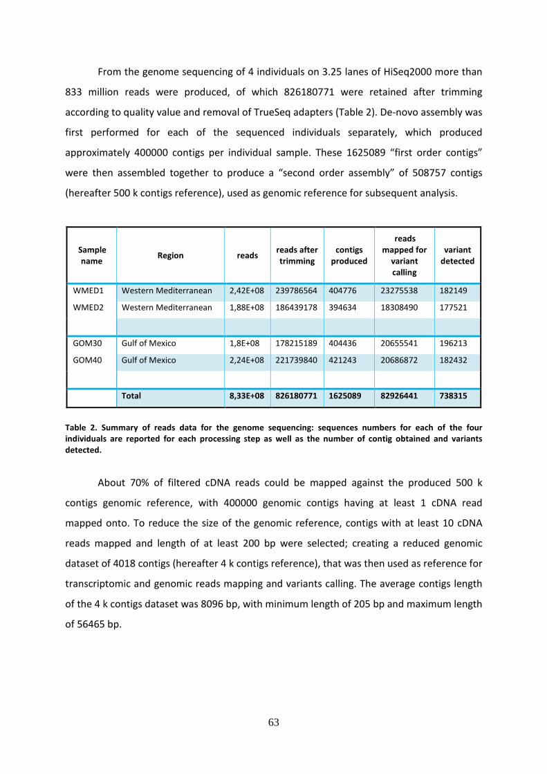
63

From the genome sequencing of 4 individuals on 3.25 lanes of HiSeq2000 more than

833 million reads were produced, of which 826180771 were retained after trimming

according to quality value and removal of TrueSeq adapters (Table 2). De-novo assembly was

first performed for each of the sequenced individuals separately, which produced

approximately 400000 contigs per individual sample. These 1625089 “first order contigs”

were then assembled together to produce a “second order assembly” of 508757 contigs

(hereafter 500 k contigs reference), used as genomic reference for subsequent analysis.

Sample

name Region reads

reads after

trimming

contigs

produced

reads

mapped for

variant

calling

variant

detected

WMED1 Western Mediterranean 2,42E+08 239786564 404776 23275538 182149

WMED2 Western Mediterranean 1,88E+08 186439178 394634 18308490 177521

GOM30 Gulf of Mexico 1,8E+08 178215189 404436 20655541 196213

GOM40 Gulf of Mexico 2,24E+08 221739840 421243 20686872 182432

Total 8,33E+08 826180771 1625089 82926441 738315

Table 2. Summary of reads data for the genome sequencing: sequences numbers for each of the four

individuals are reported for each processing step as well as the number of contig obtained and variants

detected.

About 70% of filtered cDNA reads could be mapped against the produced 500 k

contigs genomic reference, with 400000 genomic contigs having at least 1 cDNA read

mapped onto. To reduce the size of the genomic reference, contigs with at least 10 cDNA

reads mapped and length of at least 200 bp were selected; creating a reduced genomic

dataset of 4018 contigs (hereafter 4 k contigs reference), that was then used as reference for

transcriptomic and genomic reads mapping and variants calling. The average contigs length

of the 4 k contigs dataset was 8096 bp, with minimum length of 205 bp and maximum length

of 56465 bp.

64

SNP detection and selection of candidate SNPs for genotyping

Mapping of cDNA reads from each sequenced individuals against the 4 k contigs

reference was performed separately and then results pooled to obtain a unique list of 5412

not redundant biallelic SNP variants in 1350 separate genomic contigs. All candidate SNPs

positions were also retrieved from the gDNA reads mapping output. Flanking regions of 60

pb were extracted from the contigs sequences, masking occurring polymorphism with N. The

list of candidate SNPs was mined to select the best 384 loci to be included in the genotyping

panel for validation. The first two criteria applied were those mandatory for the Illumina

GoldenGate genotyping assay, i.e. Illumina Assay Design Tool Score (ADT score) > 0.6 and at

least 60 bp between SNPs, reducing the number of suitable variants to 1594. Then SNPs

were further selected if having i) the same polymorphism detected in both cDNA and gDNA

dataset (cDNA and gDNA overlap) and ii) present in at least 1 individual with minimal

coverage of 4X (2X for the alternative allele). This combination led to 299 SNPs.

To this subset of 299 SNPs, we added loci selected following less restrictive criteria:

iii) 41 variants detected in at least 2 individuals with minimal coverage of 4X (to increase the

robustness and therefore the reliability of the locus); iv) 33 SNPs detected in only 1

individual with minimal coverage, but having the highest ADT score.

Moreover, 11 SNPs developed for T. albacore and already validated on T. thynnus

individuals were scored for inclusion in the genotyping panel of 384 loci, after mapping the

markers in the 500 k contigs genomic reference and retrieving the corresponding flanking

region from the T. thynnus genomic data.

The selected 384 SNPs are evenly spread between 277 different contigs, most of

them being unique SNP per contig, with a distribution of 212 contigs with 1 SNP, 61 contigs

with 2 SNPs, 8 contigs with 3 SNPs, 4 contigs with 4 SNPs and only 2 contigs containing 5

SNPs (Figure 1).

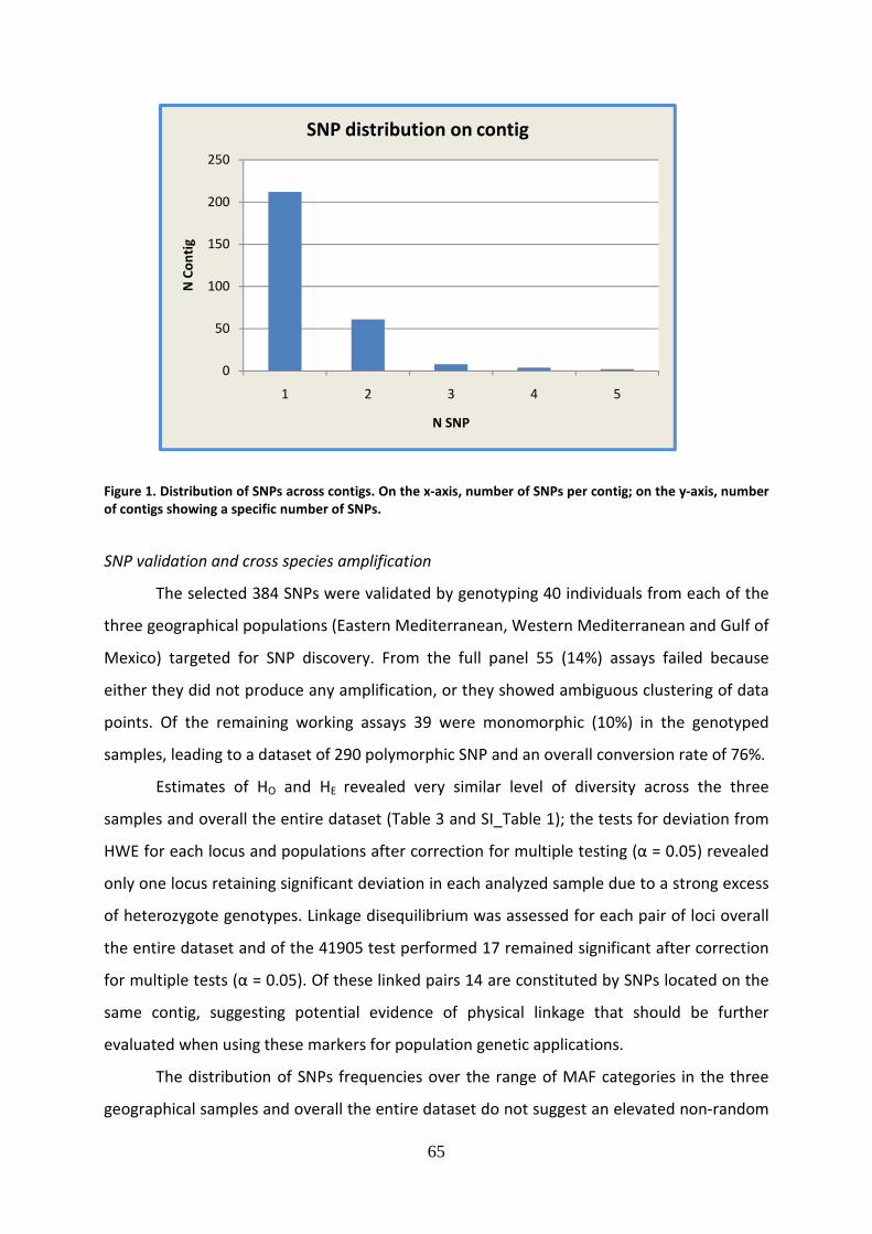
65

Figure 1. Distribution of SNPs across contigs. On the x-axis, number of SNPs per contig; on the y-axis, number

of contigs showing a specific number of SNPs.

SNP validation and cross species amplification

The selected 384 SNPs were validated by genotyping 40 individuals from each of the

three geographical populations (Eastern Mediterranean, Western Mediterranean and Gulf of

Mexico) targeted for SNP discovery. From the full panel 55 (14%) assays failed because

either they did not produce any amplification, or they showed ambiguous clustering of data

points. Of the remaining working assays 39 were monomorphic (10%) in the genotyped

samples, leading to a dataset of 290 polymorphic SNP and an overall conversion rate of 76%.

Estimates of HO and HE revealed very similar level of diversity across the three

samples and overall the entire dataset (Table 3 and SI_Table 1); the tests for deviation from

HWE for each locus and populations after correction for multiple testing (α = 0.05) revealed

only one locus retaining significant deviation in each analyzed sample due to a strong excess

of heterozygote genotypes. Linkage disequilibrium was assessed for each pair of loci overall

the entire dataset and of the 41905 test performed 17 remained significant after correction

for multiple tests (α = 0.05). Of these linked pairs 14 are constituted by SNPs located on the

same contig, suggesting potential evidence of physical linkage that should be further

evaluated when using these markers for population genetic applications.

The distribution of SNPs frequencies over the range of MAF categories in the three

geographical samples and overall the entire dataset do not suggest an elevated non-random

0

50

100

150

200

250

1 2 3 4 5

N C

on

tig

N SNP

SNP distribution on contig

66

exclusion of SNPs with low MAF (Figure 2), showing adequate even representation over the

entire MAF range.

High percentage of the 290 validated SNPs in T. thynnus individuals amplified

successfully also in T. alalunga samples (272 SNPs) and from this list 107 loci (37%) were

polymorphic in the tested individuals (see SI_Table 2).

HO HE

EMED 0.34332 0.34208

WMED 0.35412 0.34952

GOM 0.34774 0.34535

Overall 0.34840 0.34548

Table 3. Estimates of mean observed (HO) and expected (HE) heterozygosity in the three geographical

samples and overall the entire dataset at the 290 polymorphic SNPs ; EMED: Eastern Mediterranean; WMED:

Western Mediterranean; GOM: Gulf of Mexico.

Figure 2. Distribution of Minor Allele Frequency (MAF) of the 290 validated and polymorphic SNPs typed in

the three geographical samples and overall the entire dataset; EMED: Eastern Mediterranean; WMED:

Western Mediterranean; GOM: Gulf of Mexico.

Protein identification and functional annotation

The functional annotation was restricted to the reduced genomic subset (4 k contigs

reference) and to the 277 contigs, included within the formers, where SNPs were selected

for genotyping in order to look for putative biases in the SNP selection procedure.

0,00

2,00

4,00

6,00

8,00

10,00

12,00

14,00

16,00

0.0

0-0

.05

0.0

5-0

.10

0.1

0-0

.15

0.1

5-0

.20

0.2

0-0

.25

0.2

5-0

.30

0.3

0-0

.35

0.3

5-0

.40

0.4

0-0

.45

0.4

5-0

.50

Fre

qu

en

cy o

f S

NP

s (%

)

MAF

EMED

WMED

GOM

Overall

67

Analysis of the 277 contigs dataset

After running an ab initio gene prediction with Augustus software, at least one

protein was predicted for 82% of the contigs (229), yielding a total of 279 predicted proteins

(mean of 1.21 ± 0.47 proteins per contig), with average length of 270 AA (length range of 25

to 3409 AA).

After running Blast2GO with the predicted proteins as input, a total of 267 proteins

(95.6%) showed a significant Blast match against nr protein database, with a majority of the

hits presenting e-value scores above 10e-176. Visual inspection of the Blast results showed

that the majority of the hits corresponded to teleost species (Dario rerio, Oreochromis

niloticus, Salmo salar and Tetraodon nigroviridis); apart from this, as expected, hits against

well annotated genome species, like Homo sapiens and Mus musculus, were reported. While

O. niloticus represented the best match species for 49.8% of the proteins, the first non-

teleost species appeared in thirteen place (H. sapiens).

Annotation by similarity was successful for 216 of the 267 proteins presenting a

significant Blast match (82%), and yielded a total of 2046 GO terms (9.8 GO terms per

protein) annotated, with 1047 of them being unique. An average GO term level of 5.9

(standard deviation 1.7) correspond to the Blast2GO GO term categories (Biological Process

(BP), Molecular Function (MF) and Cellular Component (CC)). Among the GO terms

corresponding to the BP category, metabolic process, cellular process and biological

regulation were the most abundant ones followed by multicellular organismal process and

developmental process (Figure 3). Although the presence of GO terms related to Viral

reproduction and immune system process could suggest that at least one of the sequenced

individuals was under viral infection, manual inspection of the proteins related to those

terms showed that all of them were ribosomal proteins with a viral related term associated

in the Gene Ontology database. While cell, organelle and macromolecular complex were the

most common GO terms corresponding to the CC category, binding and catalytic activity

represented the 74.1% of the MF category.

A)

B)

C)

Figure 3. Gene Ontology (GO) assignment (2nd level GO terms) for 277 contig subset. A) Biological Process; B)

Cellular Component; C) Molecular Function.

68

. Gene Ontology (GO) assignment (2nd level GO terms) for 277 contig subset. A) Biological Process; B)

Cellular Component; C) Molecular Function.

. Gene Ontology (GO) assignment (2nd level GO terms) for 277 contig subset. A) Biological Process; B)

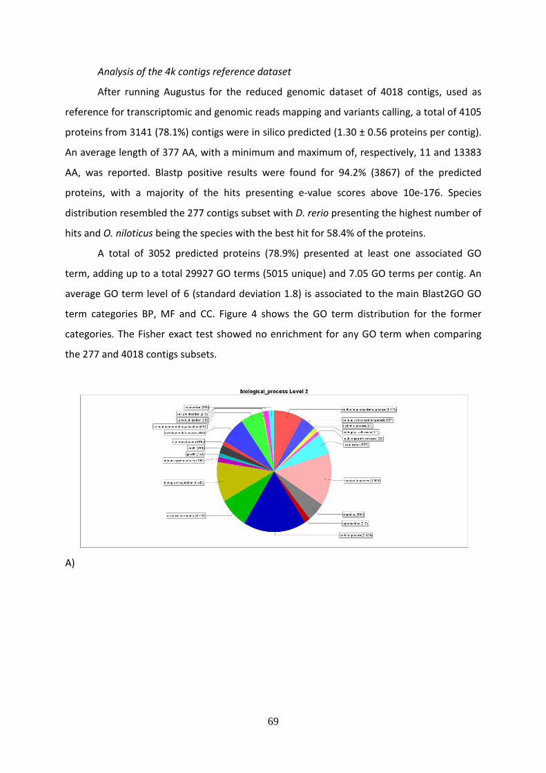
Analysis of the 4k contigs reference dataset

After running Augustus for the reduced genomic dataset of 4018 contigs, used as

reference for transcriptomic and genomic reads mapping and variants calling, a total of 4105

proteins from 3141 (78.1%) contigs were in silico predicted (1.30 ± 0.56 proteins per contig).

An average length of 377 AA, with a minimum and maximum of, respectively, 11 and 13383

AA, was reported. Blastp positive results were found for 94.2% (3867) of the predicted

proteins, with a majority of the hits presenting e

distribution resembled the 277 contigs subset with

hits and O. niloticus being the species with the best hit for 58.4% of the proteins.

A total of 3052 predicted proteins (78.9%) presented at least one as

term, adding up to a total 29927 GO terms (5015 unique) and 7.05 GO terms per contig. An

average GO term level of 6 (standard deviation 1.8) is associated to the main Blast2GO GO

term categories BP, MF and CC. Figure

categories. The Fisher exact test showed no enrichment for any GO term when comparing

the 277 and 4018 contigs subsets.

A)

69

Analysis of the 4k contigs reference dataset

Augustus for the reduced genomic dataset of 4018 contigs, used as

reference for transcriptomic and genomic reads mapping and variants calling, a total of 4105

proteins from 3141 (78.1%) contigs were in silico predicted (1.30 ± 0.56 proteins per contig).

average length of 377 AA, with a minimum and maximum of, respectively, 11 and 13383

AA, was reported. Blastp positive results were found for 94.2% (3867) of the predicted

proteins, with a majority of the hits presenting e-value scores above 10

distribution resembled the 277 contigs subset with D. rerio presenting the highest number of

being the species with the best hit for 58.4% of the proteins.

A total of 3052 predicted proteins (78.9%) presented at least one as

term, adding up to a total 29927 GO terms (5015 unique) and 7.05 GO terms per contig. An

average GO term level of 6 (standard deviation 1.8) is associated to the main Blast2GO GO

term categories BP, MF and CC. Figure 4 shows the GO term distribution for the former

categories. The Fisher exact test showed no enrichment for any GO term when comparing

the 277 and 4018 contigs subsets.

Augustus for the reduced genomic dataset of 4018 contigs, used as

reference for transcriptomic and genomic reads mapping and variants calling, a total of 4105

proteins from 3141 (78.1%) contigs were in silico predicted (1.30 ± 0.56 proteins per contig).

average length of 377 AA, with a minimum and maximum of, respectively, 11 and 13383

AA, was reported. Blastp positive results were found for 94.2% (3867) of the predicted

value scores above 10e-176. Species

presenting the highest number of

being the species with the best hit for 58.4% of the proteins.

A total of 3052 predicted proteins (78.9%) presented at least one associated GO

term, adding up to a total 29927 GO terms (5015 unique) and 7.05 GO terms per contig. An

average GO term level of 6 (standard deviation 1.8) is associated to the main Blast2GO GO

ution for the former

categories. The Fisher exact test showed no enrichment for any GO term when comparing

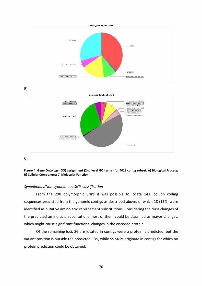
B)

C)

Figure 4: Gene Ontology (GO) assignment (2nd level GO terms) for 4018 contig subset. A) Biological

B) Cellular Component; C) Molecular Function.

Synonimous/Non-synonimous SNP classification

From the 290 polymorphic SNPs it was possible to locate 141 loci on coding

sequences predicted from the genomic contigs as described above, of which 18

identified as putative amino acid replacement substitutions. Considering the class changes of

the predicted amino acid substitutions most of them could be classified as mayor changes,

which might cause significant functional changes in the encod

Of the remaining loci, 86 are located in contigs were a protein is predicted, but the

variant position is outside the predicted CDS, while 59 SNPs originate in contigs for which no

protein prediction could be obtained.

70

: Gene Ontology (GO) assignment (2nd level GO terms) for 4018 contig subset. A) Biological

B) Cellular Component; C) Molecular Function.

synonimous SNP classification

From the 290 polymorphic SNPs it was possible to locate 141 loci on coding

sequences predicted from the genomic contigs as described above, of which 18

identified as putative amino acid replacement substitutions. Considering the class changes of

the predicted amino acid substitutions most of them could be classified as mayor changes,

which might cause significant functional changes in the encoded protein.

Of the remaining loci, 86 are located in contigs were a protein is predicted, but the

variant position is outside the predicted CDS, while 59 SNPs originate in contigs for which no

protein prediction could be obtained.

: Gene Ontology (GO) assignment (2nd level GO terms) for 4018 contig subset. A) Biological Process;

From the 290 polymorphic SNPs it was possible to locate 141 loci on coding

sequences predicted from the genomic contigs as described above, of which 18 (13%) were

identified as putative amino acid replacement substitutions. Considering the class changes of

the predicted amino acid substitutions most of them could be classified as mayor changes,

Of the remaining loci, 86 are located in contigs were a protein is predicted, but the

variant position is outside the predicted CDS, while 59 SNPs originate in contigs for which no

71

Discussion

Before next generation sequencing technology advent in the field of evolutionary

biology, large-scale marker discovery studies have usually concentrated on a restricted

number of organisms for which sequenced genomes were available. The currently ongoing

technological revolution, that is driving decreasing costs for DNA sequencing and

genotyping, allow moving rapidly toward large-scale marker discovery in organisms for

which few genomic resources currently exist (Braütigam and Gowik 2010; Seeb et al.2011a).

With the advent of the new generation of sequencing technologies, genetic⁄genomic

resources for nonmodel species have become far more accessible and transcriptome

sequencing is becoming one of the most important applications of next-generation

sequencing in evolutionary biology (Galindo et al. 2010; Metzker 2010).

In this study we provided the de novo discovery of 5412 putative SNPs based on 454

transcriptome sequencing of ten individuals covering the species putative reproduction

areas, coupled with shallow genome sequencing. Applying a single step approach of

validation and genotyping step for a selected panel of 384 assays, we could evaluate 290 loci

as polymorphic in the tested samples. The data generated constitute a relevant

improvement for genetic analysis in Atlantic bluefin tuna, significantly increasing the omic

resources (genomic and transcriptomic) available for this species, as well as novel SNP that

could be used to assess genetic structure and improve management, with the aim of

developing a sustainable fishery of this important commercial species.

SNPs can be derived by genome or transcriptome resources and, in the latter case,

selected from more abundant or rarer expressed transcripts. The clustering and assembly

step is critical for SNP mining as it generates the reference for variant detection by mapping

reads to the contigs. Not having a validated reference genomes might hamper the

correctness of contig assembly and therefore variants calling by mapping, because

homologous or paralogous genes sequence potential mis-assemblies cannot be directly

sorted out by back-mapping to the species-specific genome. Atlantic bluefin tuna lacks of

genome reference and this increases the likelihood of misidentifying polymorphisms

between paralogous sequence variants (PSVs) as SNPs. In fact, the occurrence of genome

duplication resulted in many assemblies of paralogous sequences that resulted in the

identification of a large proportion of false positives (Sanchez et al. 2009).

72

In our work, we use for the first time a combined approach of transcriptome

sequencing coupled with shallow genome sequencing to achieve more robust results and

overcome the issue of SNPs flanking sequences quality. We use GS FLEX Titanium sequencing

technology to obtain more than 1 million of cDNA sequences of ten individuals of Atlantic

bluefin tuna from different geographic locations. After adapters trimming and filtering for

mitochondrial and ribosomal transcripts, more than 70% of these sequences were available

for subsequent analyses. We also generated more than 833 million reads of DNA sequence

data by four individuals of Thunnus thynnus using Illumina HiSeq2000 and de-novo assembly

of these reads was performed to produce a reference genome of more than 500000 contigs.

The first mapping of cDNA reads against this genomic dataset was aimed to reduce

this reference, selecting contigs complementary to cDNA sequences, that are most likely

coding regions of the genome. We used stringent criteria, as at least 10 cDNA reads mapped

and length of at least 200 bp, in order to obtain a final genomic reference of 4000 contig

associated to expressed sequences, used for subsequent in silico SNP discovery. SNP

identification can proceed either from in vitro or in silico approaches. In vitro methods, such

as the re-sequencing of targeted amplicons, are costly and time consuming and generally

more appropriate when sequence data is limited or when interested in specific

polymorphisms or candidate genes. In contrast, in silico discovery is the most obvious

method for de novo SNP identification, offering a low cost source of abundant SNPs

(Lepoittevin et al. 2010). In this work, after high-throughput sequence generation, basic SNP

discovery was performed mapping cDNA reads against the reference genome dataset,

identifying 5412 putative loci. Sequence accuracy is a crucial point to make sure the

observed polymorphisms are actually true SNPs and not false positives resulting from

sequencing or alignment errors. A robust diagnosis of sequence variation in the vicinity of

the target SNPs is also necessary, especially for the GoldenGate assay, which relies on

hybridization of allele and locus-specific oligonucleotides on both sides of a given SNP; any

sequence ambiguity might compromise their annealing and the subsequent OPA genotyping

success. The genomic reference produced in this study allowed to provide reliable 60 bp on

either side of the SNP, the minimal requirement of flanking sequence for the Illumina

GoldenGate genotyping assay, moreover the masking of occurring polymorphisms in the

region allowed to avoid the design of genotyping oligos in variable portion.

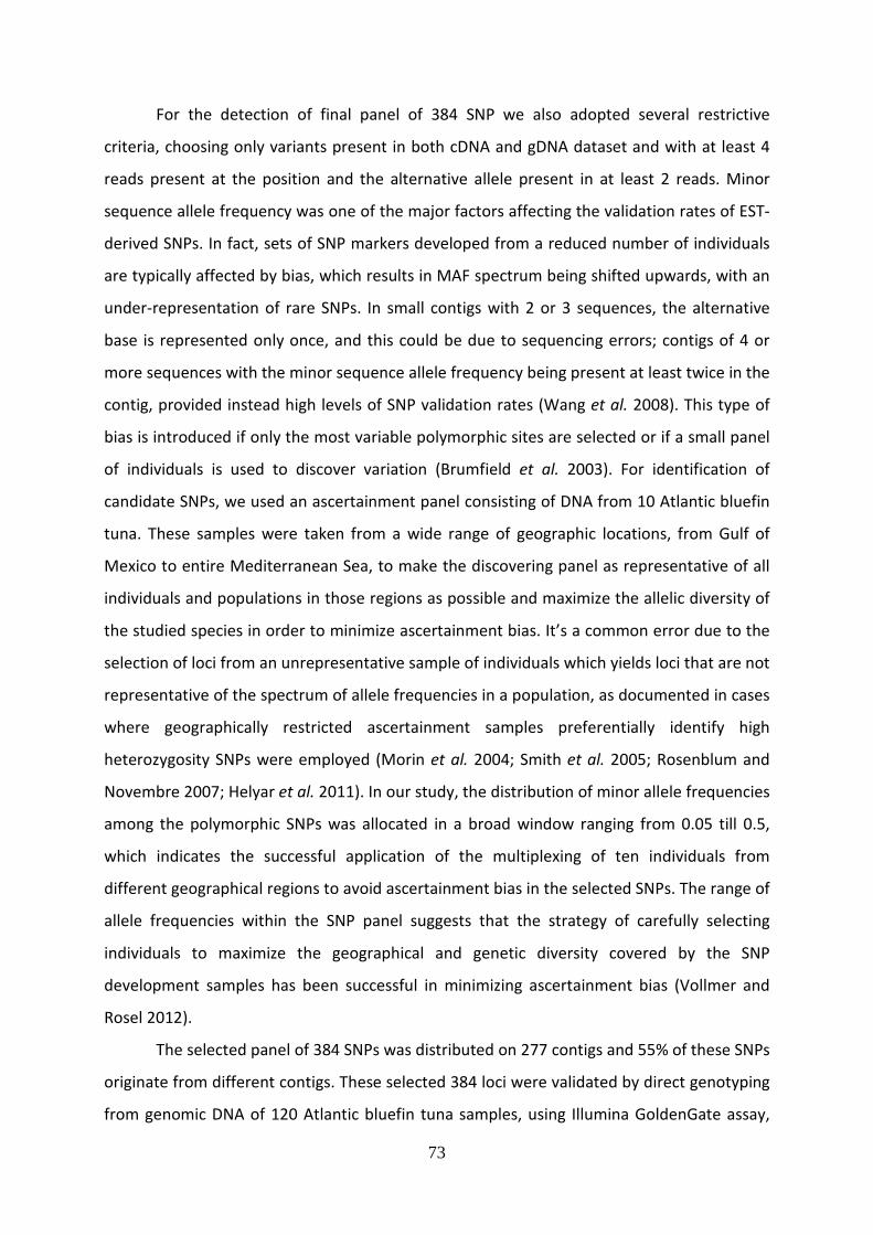
73

For the detection of final panel of 384 SNP we also adopted several restrictive

criteria, choosing only variants present in both cDNA and gDNA dataset and with at least 4

reads present at the position and the alternative allele present in at least 2 reads. Minor

sequence allele frequency was one of the major factors affecting the validation rates of EST-

derived SNPs. In fact, sets of SNP markers developed from a reduced number of individuals

are typically affected by bias, which results in MAF spectrum being shifted upwards, with an

under-representation of rare SNPs. In small contigs with 2 or 3 sequences, the alternative

base is represented only once, and this could be due to sequencing errors; contigs of 4 or

more sequences with the minor sequence allele frequency being present at least twice in the

contig, provided instead high levels of SNP validation rates (Wang et al. 2008). This type of

bias is introduced if only the most variable polymorphic sites are selected or if a small panel

of individuals is used to discover variation (Brumfield et al. 2003). For identification of

candidate SNPs, we used an ascertainment panel consisting of DNA from 10 Atlantic bluefin

tuna. These samples were taken from a wide range of geographic locations, from Gulf of

Mexico to entire Mediterranean Sea, to make the discovering panel as representative of all

individuals and populations in those regions as possible and maximize the allelic diversity of

the studied species in order to minimize ascertainment bias. It’s a common error due to the

selection of loci from an unrepresentative sample of individuals which yields loci that are not

representative of the spectrum of allele frequencies in a population, as documented in cases

where geographically restricted ascertainment samples preferentially identify high

heterozygosity SNPs were employed (Morin et al. 2004; Smith et al. 2005; Rosenblum and

Novembre 2007; Helyar et al. 2011). In our study, the distribution of minor allele frequencies

among the polymorphic SNPs was allocated in a broad window ranging from 0.05 till 0.5,

which indicates the successful application of the multiplexing of ten individuals from

different geographical regions to avoid ascertainment bias in the selected SNPs. The range of

allele frequencies within the SNP panel suggests that the strategy of carefully selecting

individuals to maximize the geographical and genetic diversity covered by the SNP

development samples has been successful in minimizing ascertainment bias (Vollmer and

Rosel 2012).

The selected panel of 384 SNPs was distributed on 277 contigs and 55% of these SNPs

originate from different contigs. These selected 384 loci were validated by direct genotyping

from genomic DNA of 120 Atlantic bluefin tuna samples, using Illumina GoldenGate assay,

74

and we obtained a conversion rate of 76% (290 successful polymorphic SNPs over 384).

Similar proportions of high-quality genotype calls were reported in Wang et al.(2008) and

Hubert et al. (2010), that achieved a 69.2% and 74.5% conversion rate for the channel catfish

and the Atlantic cod respectively. In these studies, SNP validation carried out using Illumina

GoldenGate technology, but SNP discovery was based on EST libraries produced with Sanger

sequencing, that have higher read quality than 454 sequencing technology, and therefore

the results aren’t completely comparable. Another works on Atlantic cod and Atlantic

herring showed instead a percentage of successful assay conversion of 43% and 38%

respectively (Milano et al. 2011; Helyar et al. 2012), due to lack of reference genome of

these species and use of only transcriptome resource, that didn’t allow to overcame the

Intron Exon Boundaries trouble.

A very high proportion of validated SNPs also amplified in T. alalunga even if with a

lower polymorphism rate (37%), which is likely to be downwardly biased due to the smaller

sample size tested (n= 30). However greater percentage of success was obtained in this

study than the reverse amplification test developed by Albaina and colleagues (loci

developed in T. alalunga cross amplified in T. thynnus), which obtained 18% of success

(Albaina et al. in press). Current results of cross-species amplification support the potential

for population genomic studies on T. alalunga increasing the number of markers and

samples analyzed from each of the six management units currently accepted for the species:

North Atlantic, South Atlantic, Indian, North Pacific, South Pacific and Mediterranean

(Montes et al. 2013). Furthermore, the SNPs validated in Bluefin tuna and Albacore could be

tested in other endangered Thunnus species to have a “common” genetic tool developed in

the genus.

The functional annotation led to an over-representation of ribosomal/translation

components as well as cytoskeletal proteins, that is expected when sequencing non-

normalized cDNA libraries from skeletal muscle (Milano et al. 2011), because protein

synthesis is the major cellular process ongoing. This annotation pattern is translated into a

larger proportion of SNPs being correlated to these specific functional groups of genes.

Additionally, the newly developed transcriptome data resources can be used to develop

further tools for gene expression studies such as oligonucleotide microarray or RNA-seq

approaches

75

Resolving the genetic structure of ABFT as well as determining the degree of

connectivity (trans oceanic migrations, homing behavior, mix stock aggregates in feeding

grounds) between individuals from the main spawning areas are two key questions to

understand the ecological and evolutionary dynamics of populations across the entire

distribution in order to improve the management of this endangered fishery resource.

Population genomics approaches for identifying adaptive population divergences in non-

model organisms have become a field of interest as the current high-throughput sequencing

technologies allow a genome-wide analysis of genetic variation across populations. Marine

fish provide good models for studying adaptive evolution (Nielsen et al. 2009) and since

genomes have been completely sequenced for only a handful of fish species the

establishment of genomic resources like a genome-wide set of genetic markers will provide

important contributions for marine genetics and the management of natural and

populations.

We demonstrated de novo discovery of 5412 putative SNPs based on large-scale

transcriptome sequencing of non-normalized muscle samples coupled with shallow genome

sequencing, resulting in a set of 290 validated polymorphic and randomly distributed

genomic markers. The omic resources and markers developed in this study will foster a

broad range of future studies and applications focusing on the ABFT aimed at promoting

sustainable fishery management and preventing overexploitation and illegal fishing

activities.

76

References

Albaina A, Iriondo M, Velado I, Laconcha U, Zarraonaindia I, et al. SNP discovery in albacore

and Atlantic bluefin tuna provides insights into world-wide population structure

(accepted in Animal Genetics).

Beldade P, Rudd S, Gruber JD, Long AD (2006) A wing expressed sequence tag resource for

Bicyclus anynana butterflies, an evo-devo model. BMC Genomics 7,130.

Block BA, Teo SL, Walli A, Boustany A, Stokesbury MJ, et al. (2005) Electronic tagging and

population structure of Atlantic bluefin tuna. Nature 434, 1121-1127.

Boustany AM, Reeb CA, Block BA (2008) Mitochondrial DNA and electronic tracking reveal

population structure of Atlantic bluefin tuna (Thunnus thynnus). Marine Biology

156,13-24.

Braütigam A, Gowik U (2010) What can next generation sequencing do for you? Next

generation sequencing as a valuable tool in plant research. Plant Biology 12, 831-841.

Brumfield RT, Beerli P, Nickerson DA, Edwards SV (2003) The utility of single nucleotide

polymorphisms in inferences of population history. Trends in Ecology & Evolution 18,

249-256.

Carlsson J, McDowell JR, Díaz-Jaimes P, Carlsson JEL, Boles SB, et al. (2004) Microsatellite and

mitochondrial DNA analyses of Atlantic bluefin tuna (Thunnus thynnus thynnus)

population structure in the Mediterranean sea. Molecular Ecology 13, 3345-3356.

Carlsson J, McDowell JR, Carlsson L, Graves JE (2007) Genetic identity of YOY bluefin tuna

from the eastern and western Atlantic spawning areas. Heredity 98, 23-28.

Carvajal-Rodriguez A, de Uña-Alvarez J (2011) Assessing Significance in High-Throughput

Experiments by Sequential Goodness of Fit and q-Value Estimation. PLoS ONE 6(9),

e24700.

Collette BB, Carpenter KE, Polidoro BA, Juan-Jordá MJ, Boustany A, et al. (2011) High Value

and Long Life-Double Jeopardy for Tunas and Billfishes. Science 333, 291-292.

Conesa A, Götz S, Garcia-Gomez JM, Terol J, Talon M, et al. (2005) "Blast2GO: a universal

tool for annotation, visualization and analysis in functional genomics research".

Bioinformatics 21, 3674-3676.

De Roos AM, Persson L (2002) Size-dependent life-history traits promote catastrophic

collapses of top predators. PNAS 99, 12907-12912.

77

Ekblom R, Galindo J (2011) Application of next generation sequencing in molecular ecology

of non-model organism. Heredity 107, 1-15.

Fromentin JM, Powers JE (2005) Atlantic bluefin tuna: population dynamics, ecology,

fisheries and management. Fish and Fisheries 6, 281-306.

Galindo J, Grahame JW, Butlin RK (2010) An EST-based genome scan using 454 sequencing in

the marine snail Littorina saxatilis. Journal of Evolutionary Biology 23, 2004-2016.

Galuardi B, Lutcavage M (2012) Dispersal Routes and Habitat Utilization of Juvenile Atlantic

Bluefin Tuna, Thunnus thynnus, Tracked with Mini PSAT and Archival Tags. PLoS ONE

7(5): e37829. doi:10.1371/journal.pone.0037829.

Garvin MR, Saitoh K, Gharrett AJ (2010) Application of single nucleotide polymorphisms to

non-model species: a technical review. Molecular Ecology Resources 10, 915-934.

Goudet J (1995) FSTAT (Version 1.2): A Computer Program to Calculate F-Statistics. Journal of

Heredity 86, 485-486.

Guichoux E, Lagache L, Wagner S, Chaumeil P, Léger P, et al. (2011) Current trends in

microsatellite genotyping. Molecular Ecology Resources 11, 591-611.

Hale M, McCormick C, Jackson J, DeWoody JA (2009) Next-generation pyrosequencing of

gonad transcriptomes in the polyploid lake sturgeon (Acipenser fulvescens): the

relative merits of normalization and rarefaction in gene discovery. BMC Genomics 10.

203.

Harismendy O, Ng PC, Strausberg RL, Wang X, Stockwell TB, et al. (2009) Evaluation of next

generation sequencing platforms for population targeted sequencing studies.

Genome Biology 10, R32.

Helyar SJ, Hemmer-Hansen J, Bekkevold D, Taylor MI, Ogden R, et al. (2011) Application of

SNPs for population genetics of nonmodel organisms: new opportunities and

challenges. Molecular Ecology Resources 11, 123-136.

Helyar SJ, Limborg MT, Bekkevold D, Babbucci M, van Houdt J, et al. (2012) SNP Discovery

Using Next Generation Transcriptomic Sequencing in Atlantic Herring (Clupea

harengus). PLoS ONE 7(8): e42089. doi:10.1371/journal.pone.0042089.

Hubert S, Higgins B, Borza T, Bowman S (2010) Development of a SNP resource and a genetic

linkage map for Atlantic cod (Gadus morhua). BMC Genomics 11, 191.

Juan-Jordá MJ, Mosqueirad I, Cooperf AB, Freirea J, Dulvyc NK (2011) Global population

trajectories of tunas and their relatives. PNAS 108, 20650-20655.

78

Lepoittevin C, Frigerio JM, Garnier-Géré P, Salin F, Cervera MT, et al. (2010) In Vitro vs In

Silico Detected SNPs for the Development of a Genotyping Array: What Can We Learn

from a Non-Model Species? PloS ONE 5, e11034.

Liu SK, Zhou ZC, Lu JG, Sun FY, Wang SL, et al. (2011) Generation of genome-scale gene-

associated SNPs in catfish for the construction of a highdensity SNP array. BMC

Genomics 12, 13.

MacKenzie BR, Mosegaard H, Rosenberg AA (2009) Impending Collapse of Bluefin Tuna in

the Northeast Atlantic and Mediterranean. Conservation Letters 2 (1), 25-34.

Margulies M, Egholm M, Altman WE, Attiya S, Bader JS, et al. (2005) Genome sequencing in

microfabricated high-density picolitre reactors. Nature 437, 376-380.

Martinsohn JTh, Ogden R, FishPopTrace Consortium (2009) FishPopTrace-Developing SNP-

based population genetic assignment methods to investigate illegal fishing. Forensic

Science International: Genetics Supplement Series 2, 294-296.

Metzker ML (2010) Sequencing technologies - the next generation. Nature Reviews Genetics

11, 31-46.

Meyer E, Aglyamova GV, Wang S, Buchanan-Carter J, Abrego D, et al. (2009) Sequencing and

de novo analysis of a coral larval transcriptome using 454 GSFlx. BMC Genomics

10,219.

Milano I, Babbucci M, Panitz F, Ogden R, Nielsen RO, et al. (2011) Novel Tools for

Conservation Genomics: Comparing Two High-Throughput Approaches for SNP

Discovery in the Transcriptome of the European Hake. PLoS ONE 6, e28008.

Montes I, Iriondo M, Manzano C, Arrizabalaga H, Jiménez E, et al. (2013) Worldwide genetic

structure of albacore Thunnus alalunga revealed by microsatellite DNA markers

Marine Ecology Progress Series, doi: 10.3354/meps09991.

Morin PA, Luikart G, Wayne RK, the Snp wg (2004) SNPs in ecology, evolution and

conservation. Trends in Ecology & Evolution 19, 208-216.

Nielsen EE, Hemmer-Hansen J, Larsen PF, Bekkevold D (2009) Population genomics of marine

fishes: identifying adaptive variation in space and time. Molecular Ecology 18, 3128-

3150.

Nielsen R, Paul SJ, Albrechtsen A, Song YS (2011) Genotype and SNP calling from next-

generation sequencing data. Nature Review Genetics 12, 443-451.

79

Odgen R (2011) Unlocking the potential of genomic technologies for wildlife forensics.

Molecular Ecology resources 11 (Suppl.1), 109-116.

Peakall R, Smouse PE (2006) GENALEX 6: genetic analysis in Excel. Population genetic

software for teaching and research. Molecular Ecology Notes 6, 288-295.

Peakall R, Smouse PE (2012) GenAlEx 6.5: genetic analysis in Excel. Population genetic

software for teaching and research-an update. Bioinformatics 28, 2537-2539.

Renaut S, Nolte AW, Bernatchez L (2010) Mining transcriptome sequences towards

identifying adaptive single nucleotide polymorphisms in lake whitefish species pairs

(Coregonus spp. Salmonidae). Molecular ecology 19, 115-131.

Riccioni G, Landi M, Ferrara G, Milano I, Cariani A, et al. (2010) Spatio-temporal population

structuring and genetic diversity retention in depleted Atlantic bluefin tuna of the

Mediterranean sea. PNAS 107, 2102-2107.

Rooker JR, Alvarado Bremer JR, Block BA, Dewarc H, de Metrio G, et al. (2007) Life history

and stock structure of Atlantic Bluefin Tuna (Thunnus thynnus). Reviews in Fisheries

Science 15, 265-310.

Rooker JR, Secor DH, Metrio G, Schloesser R, Block BA, et al. (2008) Natal Homing and

Connectivity in Atlantic Bluefin Tuna Populations. Science 322, 742.

Rosenblum EB, Novembre J (2007) Ascertainment Bias in Spatially Structured Populations: A

Case Study in the Eastern Fence Lizard. Journal of Heredity 98 (4), 331-336.

Sanchez C, Smith T, Wiedmann R, Vallejo R, Salem M, et al. (2009) Single nucleotide

polymorphism discovery in rainbow trout by deep sequencing of a reduced

representation library. BMC Genomics 10, 559.

Seeb JE, Carvalho G, Hauser L, Naish K, Roberts S, et al. (2011a) Single-nucleotide

polymorphism (SNP) discovery and applications of SNP genotyping in nonmodel

organisms. Molecular Ecology Resources 11(Suppl. 1), 1-8.

Seeb JE, Pascal CE, Grau ED, Seeb LW, Templin WD, et al. (2011b) Transcriptome sequencing

and high-resolution melt analysis advance single nucleotide polymorphism discovery

in duplicated salmonids. Molecular Ecology Resources 11, 335-348.

Seeb LW, Templin WD, Sato S, Abe S, Warheit K, et al. (2011) Single nucleotide

polymorphisms across a species’ range: implications for conservation studies of

Pacific salmon. Molecular Ecology Resources 11, 195-217.

80

Smith CT, Templin WD, Seeb JE, Seeb LW (2005) Single Nucleotide Polymorphisms Provide

Rapid and Accurate Estimates of the Proportions of U.S. and Canadian Chinook

Salmon Caught in Yukon River Fisheries. North American Journal of Fisheries

Management 25, 944-953.

Stanke M, Steinkamp R, Waack S, Morgenstern B (2004) AUGUSTUS: a web server for gene

finding in eukaryotes. Nucleic Acids Research 32, W309-W312.

Stapley J, Reger J, Feulner PGD, Smadja C, Galindo J, et al. (2010) Adaptation genomics: the

next generation. Trends in Ecology & Evolution 25, 705-712.

Vera M, Alvarez-Dios JA, Milian A, Pardo BG, Bouza C, et al. (2011) Validation of single

nucleotide polymorphism (SNP) markers from an immune Expressed Sequence Tag

(EST) turbot, Scophthalmus maximus, database. Aquaculture 313, 31-41.

Viñas J, Gordoa A, Fernández-Cebrián R, Pla C, Vahdet Ü, et al. (2011) Facts and uncertainties

about the genetic population structure of Atlantic bluefin tuna (Thunnus thynnus) in

the Mediterranean. Implications for fishery management. Reviews in Fish Biology and

Fisheries 21, 527-541.

Vollmer NL, Rosel PE (2012) Developing genomic resources for the common bottlenose

dolphin (Tursiops truncatus): isolation and characterization of 153 single nucleotide

polymorphisms and 53 genotyping assays. Molecular Ecology Resources 12, 1124-

1132.

Xu J, Ji P, Zhao Z, Zhang Y, Feng J, et al. (2012) Genome-Wide SNP Discovery from

Transcriptome of Four Common Carp Strains. PLoS ONE 7(10), e48140.

Walli A, Teo SLH, Boustany A, Farwell CJ, Williams T, et al. (2009) Seasonal movements,

aggregations and diving behavior of Atlantic bluefin tuna (Thunnus thynnus) revealed

with archival tags. PLoS ONE 4, 1-18.

Wang S, Sha Z, Sonstegard TS, Liu H, Xu P, et al. (2008) Quality assessment parameters for

EST-derived SNPs from catfish. BMC Genomics 9, 450.

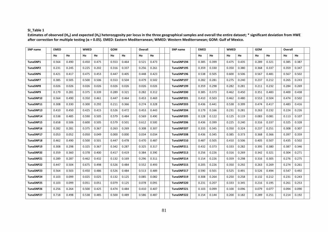
81

SI_Table 1

Estimates of observed (HO) and expected (HE) heterozygosity per locus in the three geographical samples and overall the entire dataset; * significant deviation from HWE

after correction for multiple testing (α = 0.05). EMED: Eastern Mediterranean; WMED: Western Mediterranean; GOM: Gulf of Mexico.

SNP name EMED WMED GOM Overall SNP name EMED WMED GOM Overall

Ho He Ho He Ho He Ho He Ho He Ho He Ho He Ho He

TunaSNP1 0.564 0.490 0.450 0.475 0.553 0.464 0.521 0.473 TunaSNP194 0.385 0.399 0.475 0.435 0.289 0.321 0.385 0.387

TunaSNP2 0.231 0.245 0.225 0.202 0.316 0.337 0.256 0.261 TunaSNP195 0.359 0.330 0.350 0.380 0.368 0.337 0.359 0.347

TunaSNP6 0.421 0.417 0.475 0.453 0.447 0.405 0.448 0.423 TunaSNP196 0.538 0.505 0.600 0.506 0.567 0.481 0.567 0.502

TunaSNP7 0.385 0.505 0.500 0.506 0.553 0.504 0.479 0.502 TunaSNP197 0.282 0.281 0.275 0.240 0.237 0.212 0.265 0.243

TunaSNP8 0.026 0.026 0.026 0.026 0.026 0.026 0.026 0.026 TunaSNP199 0.359 0.298 0.282 0.281 0.211 0.232 0.284 0.269

TunaSNP9 0.179 0.281 0.375 0.339 0.289 0.321 0.282 0.312 TunaSNP200 0.385 0.373 0.462 0.450 0.351 0.483 0.400 0.438

TunaSNP10 0.564 0.490 0.350 0.461 0.447 0.464 0.453 0.469 TunaSNP201 0.410 0.503 0.462 0.480 0.553 0.504 0.474 0.502

TunaSNP11 0.308 0.330 0.300 0.292 0.211 0.366 0.274 0.328 TunaSNP203 0.436 0.441 0.538 0.399 0.474 0.417 0.483 0.416

TunaSNP13 0.410 0.450 0.425 0.415 0.526 0.472 0.453 0.443 TunaSNP204 0.179 0.166 0.231 0.281 0.263 0.232 0.224 0.226

TunaSNP14 0.538 0.485 0.590 0.505 0.579 0.484 0.569 0.490 TunaSNP205 0.128 0.122 0.125 0.119 0.083 0.081 0.113 0.107

TunaSNP15 0.658 0.506 0.600 0.505 0.579 0.501 0.612 0.500 TunaSNP206 0.436 0.399 0.225 0.240 0.316 0.337 0.325 0.328

TunaSNP16 0.282 0.281 0.375 0.367 0.263 0.269 0.308 0.307 TunaSNP207 0.333 0.345 0.350 0.324 0.237 0.251 0.308 0.307

TunaSNP17 0.053 0.052 0.050 0.049 0.000 0.000 0.034 0.034 TunaSNP208 0.436 0.345 0.385 0.373 0.368 0.366 0.397 0.359

TunaSNP18 0.462 0.490 0.500 0.501 0.447 0.478 0.470 0.487 TunaSNP210 0.487 0.505 0.410 0.506 0.405 0.507 0.435 0.502

TunaSNP19 0.308 0.298 0.325 0.367 0.342 0.287 0.325 0.317 TunaSNP211 0.432 0.373 0.333 0.282 0.395 0.380 0.387 0.346

TunaSNP20 0.359 0.360 0.378 0.400 0.417 0.419 0.384 0.390 TunaSNP213 0.256 0.226 0.316 0.269 0.342 0.321 0.304 0.271

TunaSNP21 0.289 0.287 0.462 0.432 0.132 0.169 0.296 0.311 TunaSNP214 0.154 0.226 0.359 0.298 0.316 0.305 0.276 0.275

TunaSNP22 0.447 0.504 0.675 0.498 0.526 0.484 0.552 0.493 TunaSNP215 0.205 0.226 0.350 0.292 0.263 0.269 0.274 0.261

TunaSNP23 0.564 0.503 0.450 0.486 0.526 0.484 0.513 0.489 TunaSNP217 0.590 0.501 0.525 0.491 0.526 0.494 0.547 0.492

TunaSNP24 0.103 0.099 0.025 0.025 0.132 0.125 0.085 0.082 TunaSNP219 0.308 0.264 0.250 0.258 0.132 0.212 0.231 0.243

TunaSNP25 0.103 0.099 0.051 0.051 0.079 0.125 0.078 0.091 TunaSNP220 0.231 0.207 0.333 0.345 0.216 0.195 0.261 0.253

TunaSNP26 0.256 0.264 0.500 0.425 0.474 0.484 0.410 0.407 TunaSNP221 0.103 0.099 0.100 0.096 0.079 0.077 0.094 0.090

TunaSNP27 0.718 0.498 0.538 0.485 0.500 0.489 0.586 0.487 TunaSNP222 0.154 0.144 0.200 0.182 0.289 0.251 0.214 0.192

82

TunaSNP30 0.359 0.386 0.275 0.367 0.342 0.321 0.325 0.357 TunaSNP223 0.487 0.421 0.500 0.444 0.421 0.438 0.470 0.431

TunaSNP31 0.385 0.345 0.564 0.498 0.368 0.337 0.440 0.413 TunaSNP225 0.436 0.345 0.500 0.475 0.342 0.352 0.427 0.399

TunaSNP32 0.282 0.399 0.425 0.367 0.368 0.366 0.359 0.374 TunaSNP226 0.487 0.485 0.550 0.475 0.474 0.472 0.504 0.473

TunaSNP33 0.410 0.410 0.308 0.264 0.342 0.287 0.353 0.324 TunaSNP228 0.128 0.122 0.175 0.240 0.184 0.212 0.162 0.192

TunaSNP34 0.385 0.345 0.325 0.367 0.474 0.417 0.393 0.374 TunaSNP229 * 0.923 0.503 * 0.950 0.505 * 0.892 0.501 * 0.922 0.499 *

TunaSNP35 0.590 0.495 0.579 0.472 0.342 0.504 0.504 0.496 TunaSNP230 0.154 0.144 0.128 0.122 0.278 0.243 0.184 0.168

TunaSNP36 0.179 0.207 0.231 0.207 0.189 0.257 0.200 0.221 TunaSNP232 0.077 0.122 0.075 0.119 0.158 0.147 0.103 0.128

TunaSNP37 0.359 0.410 0.385 0.441 0.421 0.456 0.388 0.433 TunaSNP235 0.282 0.245 0.150 0.222 0.316 0.269 0.248 0.243

TunaSNP40 0.462 0.450 0.541 0.477 0.447 0.489 0.482 0.470 TunaSNP238 0.282 0.315 0.325 0.276 0.378 0.311 0.328 0.298

TunaSNP41 0.333 0.345 0.500 0.475 0.526 0.438 0.453 0.425 TunaSNP239 0.308 0.386 0.250 0.324 0.421 0.393 0.325 0.366

TunaSNP42 0.026 0.026 0.050 0.049 0.026 0.077 * 0.034 0.050 TunaSNP240 0.051 0.051 0.075 0.073 0.079 0.077 0.068 0.066

TunaSNP44 0.051 0.051 0.075 0.073 0.184 0.169 0.103 0.098 TunaSNP241 0.385 0.345 0.375 0.367 0.368 0.393 0.376 0.366

TunaSNP46 0.385 0.501 0.410 0.490 0.417 0.488 0.404 0.498 TunaSNP242 0.231 0.315 0.400 0.380 0.368 0.366 0.333 0.352

TunaSNP48 0.385 0.421 0.436 0.421 0.622 0.454 0.478 0.429 TunaSNP243 0.487 0.495 0.475 0.491 0.500 0.447 0.487 0.477

TunaSNP49 0.231 0.245 0.359 0.360 0.447 0.405 0.345 0.340 TunaSNP244 0.051 0.051 0.100 0.096 0.079 0.077 0.077 0.074

TunaSNP50 0.359 0.498 0.333 0.485 0.395 0.498 0.362 0.490 TunaSNP245 0.205 0.186 0.125 0.119 0.079 0.125 0.137 0.143

TunaSNP51 0.436 0.441 0.436 0.441 0.526 0.456 0.466 0.442 TunaSNP246 0.462 0.466 0.400 0.425 0.500 0.428 0.453 0.437

TunaSNP52 0.436 0.399 0.425 0.415 0.270 0.344 0.379 0.385 TunaSNP248 0.513 0.506 0.590 0.505 0.622 0.507 0.574 0.502

TunaSNP54 0.132 0.169 0.308 0.264 0.216 0.195 0.219 0.210 TunaSNP249 0.256 0.298 0.250 0.222 0.405 0.359 0.302 0.292

TunaSNP55 0.564 0.480 0.436 0.399 0.500 0.405 0.500 0.430 TunaSNP250 0.103 0.099 0.103 0.099 0.053 0.052 0.086 0.083

TunaSNP59 0.231 0.245 0.179 0.245 0.105 0.101 0.172 0.200 TunaSNP251 0.692 0.505 0.550 0.501 0.526 0.494 0.590 0.502

TunaSNP60 0.410 0.480 0.282 0.373 0.368 0.417 0.353 0.427 TunaSNP252 0.026 0.026 0.128 0.122 0.053 0.052 0.069 0.067

TunaSNP62 0.000 0.000 0.075 0.073 0.053 0.052 0.043 0.042 TunaSNP253 0.231 0.245 0.200 0.182 0.447 0.380 0.291 0.273

TunaSNP63 0.179 0.166 0.175 0.162 0.211 0.191 0.188 0.171 TunaSNP254 0.237 0.287 0.333 0.345 0.486 0.373 0.351 0.334

TunaSNP64 0.462 0.450 0.333 0.485 0.526 0.438 0.440 0.456 TunaSNP256 0.103 0.099 0.150 0.141 0.158 0.191 0.137 0.143

TunaSNP65 0.342 0.352 0.300 0.353 0.395 0.321 0.345 0.340 TunaSNP257 0.128 0.122 0.175 0.162 0.211 0.269 0.171 0.185

TunaSNP67 0.564 0.480 0.550 0.505 0.368 0.494 0.496 0.492 TunaSNP258 0.487 0.473 0.385 0.485 0.432 0.489 0.435 0.478

TunaSNP68 0.487 0.373 0.375 0.309 0.447 0.352 0.436 0.342 TunaSNP259 0.179 0.166 0.225 0.202 0.158 0.147 0.188 0.171

TunaSNP70 0.410 0.466 0.625 0.491 0.421 0.507 0.487 0.490 TunaSNP262 0.459 0.470 0.450 0.495 0.658 0.498 0.522 0.485

83

TunaSNP71 0.308 0.298 0.325 0.339 0.237 0.321 0.291 0.317 TunaSNP263 0.256 0.298 0.425 0.392 0.474 0.366 0.385 0.352

TunaSNP72 0.282 0.245 0.150 0.182 0.289 0.251 0.239 0.224 TunaSNP264 0.513 0.506 0.564 0.506 0.447 0.498 0.509 0.501

TunaSNP73 0.410 0.450 0.400 0.353 0.368 0.393 0.393 0.399 TunaSNP265 0.231 0.315 0.350 0.380 0.263 0.393 0.282 0.361

TunaSNP74 0.462 0.432 0.425 0.392 0.447 0.447 0.444 0.421 TunaSNP266 0.410 0.386 0.375 0.339 0.395 0.321 0.393 0.347

TunaSNP76 0.333 0.345 0.256 0.264 0.289 0.287 0.293 0.298 TunaSNP268 0.128 0.122 0.158 0.147 0.053 0.052 0.113 0.107

TunaSNP77 0.077 0.166 0.300 0.258 0.263 0.232 0.214 0.218 TunaSNP269 0.513 0.432 0.436 0.495 0.553 0.447 0.500 0.459

TunaSNP78 0.077 0.075 0.150 0.141 0.211 0.191 0.145 0.135 TunaSNP270 0.385 0.441 0.400 0.425 0.421 0.472 0.402 0.443

TunaSNP79 0.282 0.245 0.250 0.292 0.105 0.101 0.214 0.218 TunaSNP271 0.231 0.207 0.205 0.226 0.316 0.269 0.250 0.233

TunaSNP80 0.538 0.495 0.436 0.506 0.395 0.478 0.457 0.494 TunaSNP272 0.128 0.122 0.000 0.000 0.250 0.222 0.122 0.115

TunaSNP81 0.462 0.410 0.400 0.380 0.395 0.428 0.419 0.403 TunaSNP273 0.359 0.298 0.375 0.309 0.237 0.212 0.325 0.273

TunaSNP82 0.395 0.506 0.361 0.504 0.447 0.506 0.402 0.501 TunaSNP274 0.436 0.441 0.500 0.425 0.579 0.456 0.504 0.437

TunaSNP83 0.308 0.298 0.350 0.292 0.237 0.287 0.299 0.290 TunaSNP276 0.256 0.298 0.150 0.292 0.421 0.337 0.274 0.307

TunaSNP84 0.103 0.099 0.100 0.096 0.053 0.052 0.085 0.082 TunaSNP277 0.132 0.212 0.308 0.264 0.132 0.169 0.191 0.215

TunaSNP86 0.359 0.386 0.325 0.392 0.263 0.366 0.316 0.379 TunaSNP279 0.205 0.186 0.450 0.425 0.389 0.318 0.348 0.321

TunaSNP87 0.179 0.166 0.200 0.324 0.368 0.305 0.248 0.267 TunaSNP280 0.410 0.450 0.450 0.461 0.500 0.447 0.453 0.449

TunaSNP89 0.641 0.485 0.436 0.495 0.500 0.498 0.526 0.489 TunaSNP281 0.564 0.466 0.450 0.495 0.541 0.504 0.517 0.487

TunaSNP90 0.462 0.506 0.650 0.505 0.526 0.505 0.547 0.501 TunaSNP282 0.436 0.421 0.475 0.392 0.421 0.472 0.444 0.428

TunaSNP91 0.590 0.495 0.450 0.486 0.421 0.484 0.487 0.484 TunaSNP283 0.410 0.410 0.333 0.441 0.263 0.366 0.336 0.405

TunaSNP94 0.359 0.330 0.385 0.421 0.324 0.400 0.357 0.383 TunaSNP285 0.051 0.051 0.026 0.026 0.152 0.142 0.072 0.070

TunaSNP95 0.359 0.330 0.150 0.182 0.395 0.380 0.299 0.301 TunaSNP286 0.410 0.386 0.450 0.380 0.342 0.321 0.402 0.361

TunaSNP96 0.359 0.330 0.225 0.240 0.421 0.417 0.333 0.333 TunaSNP288 0.231 0.315 0.538 0.441 0.342 0.287 0.371 0.354

TunaSNP97 0.487 0.485 0.459 0.483 0.526 0.505 0.491 0.490 TunaSNP290 0.256 0.264 0.225 0.202 0.237 0.212 0.239 0.224

TunaSNP98 0.333 0.315 0.275 0.240 0.316 0.305 0.308 0.285 TunaSNP291 0.231 0.245 0.300 0.258 0.105 0.191 0.214 0.231

TunaSNP99 0.154 0.186 0.125 0.119 0.263 0.232 0.179 0.178 TunaSNP292 0.564 0.450 0.579 0.456 0.378 0.424 0.509 0.440

TunaSNP100 0.308 0.360 0.325 0.392 0.289 0.287 0.308 0.347 TunaSNP294 0.333 0.506 0.300 0.475 0.361 0.504 0.330 0.496 *

TunaSNP101 0.359 0.360 0.462 0.410 0.459 0.387 0.426 0.383 TunaSNP297 0.282 0.281 0.375 0.367 0.237 0.251 0.299 0.301

TunaSNP103 0.410 0.330 0.231 0.245 0.105 0.147 0.250 0.245 TunaSNP298 0.526 0.507 0.500 0.495 0.432 0.504 0.487 0.499

TunaSNP105 0.487 0.495 0.436 0.501 0.421 0.501 0.448 0.501 TunaSNP299 0.622 0.470 0.513 0.432 0.459 0.454 0.531 0.448

TunaSNP106 0.231 0.207 0.205 0.186 0.162 0.151 0.200 0.181 TunaSNP300 0.513 0.498 0.500 0.486 0.405 0.412 0.474 0.489

84

TunaSNP107 0.538 0.441 0.450 0.486 0.316 0.456 0.436 0.460 TunaSNP301 0.436 0.399 0.300 0.425 0.526 0.456 0.419 0.425

TunaSNP109 0.282 0.345 0.400 0.324 0.395 0.380 0.359 0.347 TunaSNP302 0.103 0.144 0.300 0.292 0.211 0.269 0.205 0.237

TunaSNP110 0.026 0.026 0.179 0.207 0.079 0.077 0.095 0.106 TunaSNP303 0.385 0.485 0.450 0.461 0.500 0.478 0.444 0.471

TunaSNP111 0.154 0.264 0.250 0.258 0.263 0.269 0.222 0.261 TunaSNP305 0.436 0.495 0.538 0.506 0.526 0.494 0.500 0.497

TunaSNP114 0.513 0.410 0.333 0.399 0.237 0.287 0.362 0.368 TunaSNP307 0.179 0.166 0.150 0.222 0.158 0.191 0.162 0.192

TunaSNP115 0.487 0.501 0.538 0.501 0.395 0.506 0.474 0.502 TunaSNP308 0.462 0.450 0.289 0.352 0.421 0.438 0.391 0.415

TunaSNP116 0.564 0.498 0.436 0.421 0.553 0.447 0.517 0.459 TunaSNP309 0.462 0.450 0.375 0.503 0.526 0.501 0.453 0.487

TunaSNP117 0.564 0.506 0.513 0.498 0.316 0.484 0.466 0.497 TunaSNP311 0.487 0.421 0.475 0.481 0.421 0.366 0.462 0.428

TunaSNP118 0.333 0.281 0.375 0.392 0.474 0.393 0.393 0.357 TunaSNP313 0.462 0.490 0.525 0.491 0.556 0.507 0.513 0.495

TunaSNP119 0.487 0.485 0.500 0.506 0.447 0.428 0.479 0.483 TunaSNP314 0.590 0.485 0.425 0.468 0.500 0.478 0.504 0.473

TunaSNP122 0.359 0.298 0.350 0.324 0.342 0.287 0.350 0.301 TunaSNP315 0.359 0.360 0.263 0.366 0.306 0.441 0.310 0.388

TunaSNP123 0.333 0.315 0.359 0.360 0.368 0.393 0.353 0.354 TunaSNP316 0.385 0.399 0.400 0.380 0.237 0.287 0.342 0.357

TunaSNP125 0.385 0.345 0.436 0.399 0.474 0.366 0.431 0.368 TunaSNP318 0.371 0.506 0.425 0.481 0.237 0.498 0.345 0.492

TunaSNP126 0.256 0.226 0.275 0.276 0.158 0.147 0.231 0.218 TunaSNP319 0.256 0.410 0.410 0.330 0.316 0.417 0.328 0.385

TunaSNP127 0.538 0.485 0.625 0.506 0.526 0.501 0.564 0.496 TunaSNP320 0.256 0.360 0.275 0.276 0.289 0.287 0.274 0.307

TunaSNP129 0.128 0.122 0.100 0.096 0.158 0.191 0.128 0.135 TunaSNP321 0.231 0.207 0.150 0.182 0.316 0.269 0.231 0.218

TunaSNP131 0.308 0.466 0.462 0.450 0.368 0.417 0.379 0.442 TunaSNP323 0.487 0.441 0.225 0.309 0.368 0.366 0.359 0.374

TunaSNP132 0.282 0.315 0.275 0.276 0.184 0.169 0.248 0.255 TunaSNP324 0.154 0.186 0.125 0.119 0.158 0.147 0.145 0.150

TunaSNP134 0.538 0.459 0.487 0.506 0.541 0.477 0.522 0.485 TunaSNP325 0.436 0.473 0.667 0.506 0.500 0.489 0.534 0.493

TunaSNP137 0.103 0.099 0.128 0.122 0.054 0.053 0.096 0.091 TunaSNP326 0.538 0.501 0.550 0.501 0.395 0.504 0.496 0.501

TunaSNP139 0.462 0.386 0.385 0.399 0.395 0.428 0.414 0.401 TunaSNP327 0.487 0.506 0.590 0.506 0.342 0.464 0.474 0.498

TunaSNP140 0.436 0.501 0.525 0.481 0.395 0.478 0.453 0.484 TunaSNP328 0.333 0.315 0.325 0.276 0.395 0.321 0.350 0.301

TunaSNP141 0.282 0.281 0.300 0.324 0.395 0.380 0.325 0.328 TunaSNP329 0.487 0.441 0.308 0.410 0.474 0.456 0.422 0.433

TunaSNP143 0.487 0.459 0.600 0.461 0.263 0.269 0.453 0.410 TunaSNP330 0.385 0.399 0.410 0.360 0.263 0.232 0.353 0.335

TunaSNP144 0.462 0.466 0.450 0.461 0.579 0.494 0.496 0.471 TunaSNP332 0.368 0.337 0.350 0.444 0.421 0.438 0.379 0.409

TunaSNP145 0.256 0.226 0.275 0.309 0.263 0.232 0.265 0.255 TunaSNP333 0.077 0.075 0.075 0.073 0.079 0.077 0.077 0.074

TunaSNP147 0.077 0.075 0.075 0.073 0.081 0.079 0.078 0.075 TunaSNP334 0.026 0.026 0.100 0.096 0.053 0.052 0.060 0.058

TunaSNP148 0.474 0.494 0.500 0.475 0.553 0.504 0.509 0.489 TunaSNP335 0.333 0.441 0.475 0.435 0.395 0.447 0.402 0.437

TunaSNP149 0.308 0.330 0.333 0.373 0.421 0.393 0.353 0.363 TunaSNP336 0.103 0.099 0.075 0.119 0.053 0.052 0.077 0.090

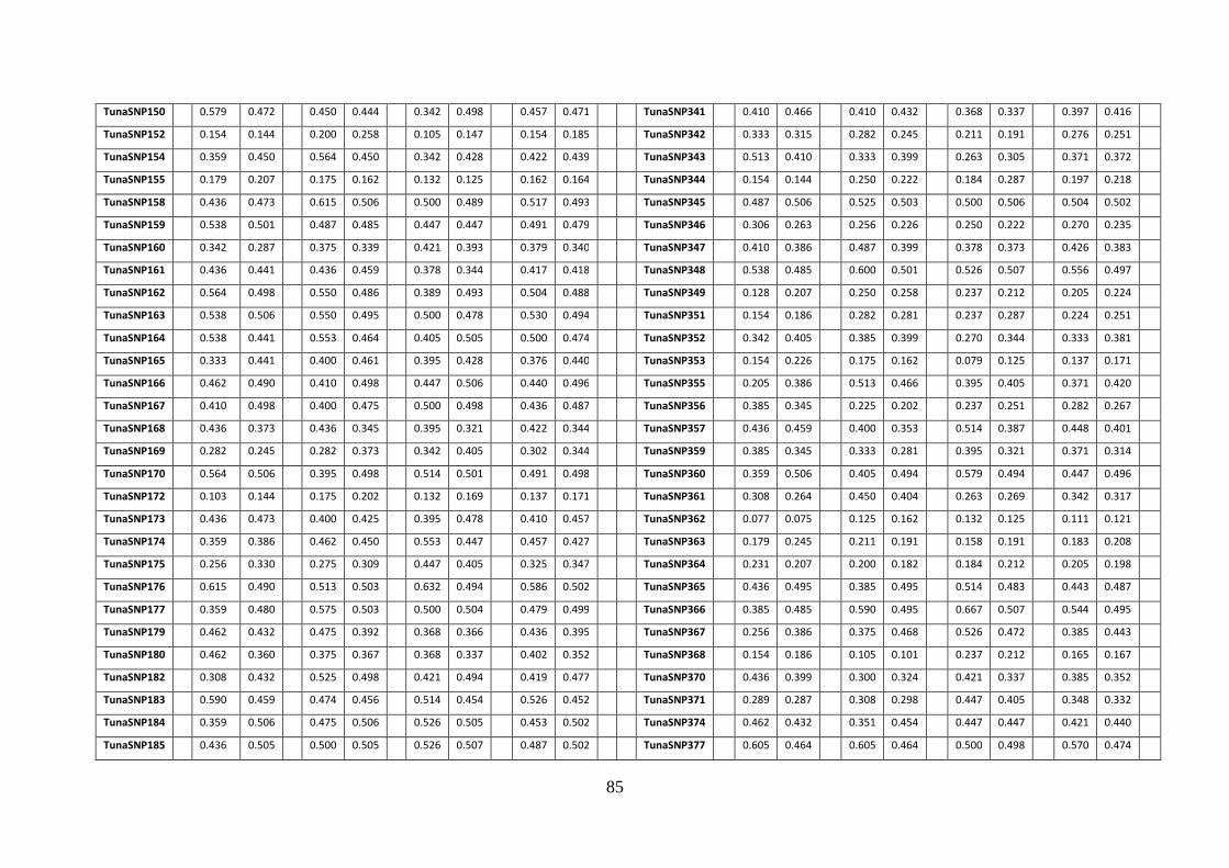
85

TunaSNP150 0.579 0.472 0.450 0.444 0.342 0.498 0.457 0.471 TunaSNP341 0.410 0.466 0.410 0.432 0.368 0.337 0.397 0.416

TunaSNP152 0.154 0.144 0.200 0.258 0.105 0.147 0.154 0.185 TunaSNP342 0.333 0.315 0.282 0.245 0.211 0.191 0.276 0.251

TunaSNP154 0.359 0.450 0.564 0.450 0.342 0.428 0.422 0.439 TunaSNP343 0.513 0.410 0.333 0.399 0.263 0.305 0.371 0.372

TunaSNP155 0.179 0.207 0.175 0.162 0.132 0.125 0.162 0.164 TunaSNP344 0.154 0.144 0.250 0.222 0.184 0.287 0.197 0.218

TunaSNP158 0.436 0.473 0.615 0.506 0.500 0.489 0.517 0.493 TunaSNP345 0.487 0.506 0.525 0.503 0.500 0.506 0.504 0.502

TunaSNP159 0.538 0.501 0.487 0.485 0.447 0.447 0.491 0.479 TunaSNP346 0.306 0.263 0.256 0.226 0.250 0.222 0.270 0.235

TunaSNP160 0.342 0.287 0.375 0.339 0.421 0.393 0.379 0.340 TunaSNP347 0.410 0.386 0.487 0.399 0.378 0.373 0.426 0.383

TunaSNP161 0.436 0.441 0.436 0.459 0.378 0.344 0.417 0.418 TunaSNP348 0.538 0.485 0.600 0.501 0.526 0.507 0.556 0.497

TunaSNP162 0.564 0.498 0.550 0.486 0.389 0.493 0.504 0.488 TunaSNP349 0.128 0.207 0.250 0.258 0.237 0.212 0.205 0.224

TunaSNP163 0.538 0.506 0.550 0.495 0.500 0.478 0.530 0.494 TunaSNP351 0.154 0.186 0.282 0.281 0.237 0.287 0.224 0.251

TunaSNP164 0.538 0.441 0.553 0.464 0.405 0.505 0.500 0.474 TunaSNP352 0.342 0.405 0.385 0.399 0.270 0.344 0.333 0.381

TunaSNP165 0.333 0.441 0.400 0.461 0.395 0.428 0.376 0.440 TunaSNP353 0.154 0.226 0.175 0.162 0.079 0.125 0.137 0.171

TunaSNP166 0.462 0.490 0.410 0.498 0.447 0.506 0.440 0.496 TunaSNP355 0.205 0.386 0.513 0.466 0.395 0.405 0.371 0.420

TunaSNP167 0.410 0.498 0.400 0.475 0.500 0.498 0.436 0.487 TunaSNP356 0.385 0.345 0.225 0.202 0.237 0.251 0.282 0.267

TunaSNP168 0.436 0.373 0.436 0.345 0.395 0.321 0.422 0.344 TunaSNP357 0.436 0.459 0.400 0.353 0.514 0.387 0.448 0.401

TunaSNP169 0.282 0.245 0.282 0.373 0.342 0.405 0.302 0.344 TunaSNP359 0.385 0.345 0.333 0.281 0.395 0.321 0.371 0.314

TunaSNP170 0.564 0.506 0.395 0.498 0.514 0.501 0.491 0.498 TunaSNP360 0.359 0.506 0.405 0.494 0.579 0.494 0.447 0.496

TunaSNP172 0.103 0.144 0.175 0.202 0.132 0.169 0.137 0.171 TunaSNP361 0.308 0.264 0.450 0.404 0.263 0.269 0.342 0.317

TunaSNP173 0.436 0.473 0.400 0.425 0.395 0.478 0.410 0.457 TunaSNP362 0.077 0.075 0.125 0.162 0.132 0.125 0.111 0.121

TunaSNP174 0.359 0.386 0.462 0.450 0.553 0.447 0.457 0.427 TunaSNP363 0.179 0.245 0.211 0.191 0.158 0.191 0.183 0.208

TunaSNP175 0.256 0.330 0.275 0.309 0.447 0.405 0.325 0.347 TunaSNP364 0.231 0.207 0.200 0.182 0.184 0.212 0.205 0.198

TunaSNP176 0.615 0.490 0.513 0.503 0.632 0.494 0.586 0.502 TunaSNP365 0.436 0.495 0.385 0.495 0.514 0.483 0.443 0.487

TunaSNP177 0.359 0.480 0.575 0.503 0.500 0.504 0.479 0.499 TunaSNP366 0.385 0.485 0.590 0.495 0.667 0.507 0.544 0.495

TunaSNP179 0.462 0.432 0.475 0.392 0.368 0.366 0.436 0.395 TunaSNP367 0.256 0.386 0.375 0.468 0.526 0.472 0.385 0.443

TunaSNP180 0.462 0.360 0.375 0.367 0.368 0.337 0.402 0.352 TunaSNP368 0.154 0.186 0.105 0.101 0.237 0.212 0.165 0.167

TunaSNP182 0.308 0.432 0.525 0.498 0.421 0.494 0.419 0.477 TunaSNP370 0.436 0.399 0.300 0.324 0.421 0.337 0.385 0.352

TunaSNP183 0.590 0.459 0.474 0.456 0.514 0.454 0.526 0.452 TunaSNP371 0.289 0.287 0.308 0.298 0.447 0.405 0.348 0.332

TunaSNP184 0.359 0.506 0.475 0.506 0.526 0.505 0.453 0.502 TunaSNP374 0.462 0.432 0.351 0.454 0.447 0.447 0.421 0.440

TunaSNP185 0.436 0.505 0.500 0.505 0.526 0.507 0.487 0.502 TunaSNP377 0.605 0.464 0.605 0.464 0.500 0.498 0.570 0.474

86

TunaSNP186 0.333 0.373 0.359 0.330 0.316 0.337 0.336 0.344 TunaSNP379 0.128 0.166 0.175 0.162 0.105 0.101 0.137 0.143

TunaSNP189 0.051 0.051 0.100 0.096 0.053 0.052 0.068 0.066 TunaSNP380 0.205 0.330 0.300 0.353 0.368 0.393 0.291 0.357

TunaSNP190 0.359 0.450 0.325 0.392 0.429 0.401 0.368 0.413 TunaSNP381 0.256 0.226 0.385 0.345 0.211 0.191 0.284 0.257

TunaSNP191 0.333 0.281 0.300 0.292 0.316 0.366 0.316 0.312 TunaSNP382 0.205 0.186 0.154 0.226 0.211 0.191 0.190 0.200

TunaSNP192 0.385 0.399 0.333 0.345 0.368 0.393 0.362 0.377 TunaSNP383 0.385 0.501 0.425 0.491 0.579 0.494 0.462 0.492

TunaSNP193 0.282 0.245 0.205 0.186 0.132 0.169 0.207 0.200 TunaSNP384 0.103 0.099 0.158 0.147 0.158 0.191 0.139 0.145

87

SI_Table 2

Results of cross-species testing of the 290 validated and polymorphic SNPs in T. alalunga individuals.

SNP name Locus ID Cross species validation

SNP name Locus ID Cross species validation

TunaSNP1 tuna04_contig108622_4256 Working in T. alalunga Polymorphic in T. alalunga

TunaSNP194 tuna_contig1807_1464 Working in T. alalunga

TunaSNP2 tuna02_contig129997_405 Working in T. alalunga Polymorphic in T. alalunga

TunaSNP195 tuna_contig113966_5180 Working in T. alalunga

TunaSNP6 tuna_contig74714_929 Working in T. alalunga

TunaSNP196 tuna_contig228262_2189

TunaSNP7 tuna_contig52293_1028 Working in T. alalunga Polymorphic in T. alalunga

TunaSNP197 tuna_contig220997_1104 Working in T. alalunga

TunaSNP8 tuna_contig56694_2291 Working in T. alalunga Polymorphic in T. alalunga

TunaSNP199 tuna_contig156245_270 Working in T. alalunga

TunaSNP9 tuna02_contig122979_2582 Working in T. alalunga Polymorphic in T. alalunga

TunaSNP200 tuna_contig104549_3250 Working in T. alalunga Polymorphic in T. alalunga

TunaSNP10 tuna_contig149883_1983 Working in T. alalunga

TunaSNP201 tuna01_contig101905_4360 Working in T. alalunga Polymorphic in T. alalunga

TunaSNP11 tuna_contig56436_2296 Working in T. alalunga

TunaSNP203 tuna_contig27279_824 Working in T. alalunga

TunaSNP13 tuna02_contig122146_3467 Working in T. alalunga Polymorphic in T. alalunga

TunaSNP204 tuna_contig154550_3420 Working in T. alalunga Polymorphic in T. alalunga

TunaSNP14 tuna02_contig128705_3411 Working in T. alalunga Polymorphic in T. alalunga

TunaSNP205 tuna_contig224177_3068 Working in T. alalunga

TunaSNP15 tuna_contig81111_1351

TunaSNP206 tuna01_contig191719_2339 Working in T. alalunga Polymorphic in T. alalunga

TunaSNP16 tuna_contig154550_3037 Working in T. alalunga Polymorphic in T. alalunga

TunaSNP207 tuna_contig114273_1588 Working in T. alalunga

TunaSNP17 tuna02_contig92196_1257

TunaSNP208 tuna04_contig151428_1789 Working in T. alalunga

TunaSNP18 tuna02_contig122979_107 Working in T. alalunga Polymorphic in T. alalunga

TunaSNP210 tuna_contig103799_348 Working in T. alalunga Polymorphic in T. alalunga

TunaSNP19 tuna_contig45879_1468 Working in T. alalunga

TunaSNP211 tuna_contig225169_2908 Working in T. alalunga Polymorphic in T. alalunga

TunaSNP20 tuna_contig66558_2260 Working in T. alalunga

TunaSNP213 tuna_contig63575_3883 Working in T. alalunga

TunaSNP21 tuna04_contig267259_10949 Working in T. alalunga Polymorphic in T. alalunga

TunaSNP214 tuna_contig45275_16096 Working in T. alalunga

TunaSNP22 tuna_contig23724_3855 Working in T. alalunga Polymorphic in T. alalunga

TunaSNP215 tuna_contig133101_4816 Working in T. alalunga Polymorphic in T. alalunga

TunaSNP23 tuna01_contig115709_2224 Working in T. alalunga Polymorphic in T. alalunga

TunaSNP217 tuna01_contig93658_346 Working in T. alalunga Polymorphic in T. alalunga

TunaSNP24 tuna_contig54349_593 Working in T. alalunga

TunaSNP219 tuna_contig60806_190 Working in T. alalunga

TunaSNP25 tuna_contig155323_1999 Working in T. alalunga Polymorphic in T. alalunga

TunaSNP220 tuna_contig167626_2260 Working in T. alalunga

TunaSNP26 tuna_contig57535_921 Working in T. alalunga

TunaSNP221 tuna_contig47828_2787 Working in T. alalunga Polymorphic in T. alalunga

TunaSNP27 tuna_contig121382_2923 Working in T. alalunga

TunaSNP222 tuna_contig25320_4698 Working in T. alalunga Polymorphic in T. alalunga

TunaSNP30 tuna_contig222172_1461 Working in T. alalunga Polymorphic in T. alalunga

TunaSNP223 tuna01_contig151302_4649 Working in T. alalunga Polymorphic in T. alalunga

TunaSNP31 tuna_contig115192_1122 Working in T. alalunga Polymorphic in T. alalunga

TunaSNP225 tuna_contig74714_993 Working in T. alalunga

TunaSNP32 tuna_contig23848_5959 Working in T. alalunga Polymorphic in T. alalunga

TunaSNP226 tuna_contig21470_954 Working in T. alalunga

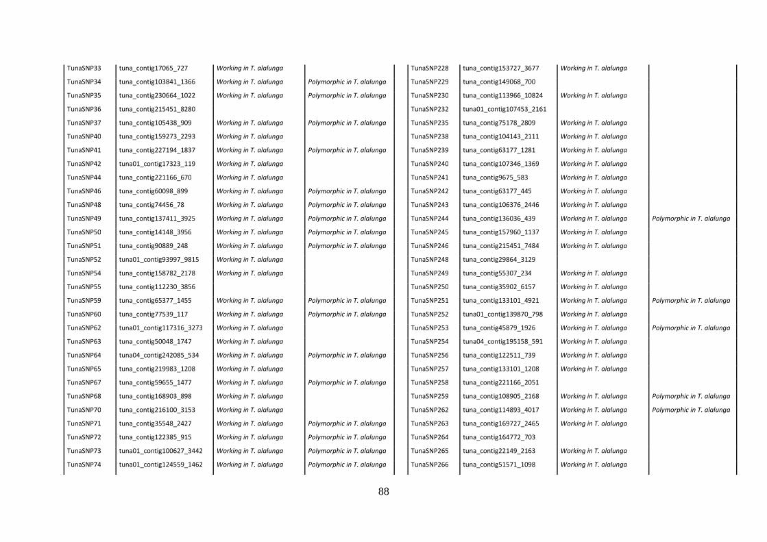
88

TunaSNP33 tuna_contig17065_727 Working in T. alalunga

TunaSNP228 tuna_contig153727_3677 Working in T. alalunga

TunaSNP34 tuna_contig103841_1366 Working in T. alalunga Polymorphic in T. alalunga

TunaSNP229 tuna_contig149068_700

TunaSNP35 tuna_contig230664_1022 Working in T. alalunga Polymorphic in T. alalunga

TunaSNP230 tuna_contig113966_10824 Working in T. alalunga

TunaSNP36 tuna_contig215451_8280

TunaSNP232 tuna01_contig107453_2161

TunaSNP37 tuna_contig105438_909 Working in T. alalunga Polymorphic in T. alalunga

TunaSNP235 tuna_contig75178_2809 Working in T. alalunga

TunaSNP40 tuna_contig159273_2293 Working in T. alalunga

TunaSNP238 tuna_contig104143_2111 Working in T. alalunga

TunaSNP41 tuna_contig227194_1837 Working in T. alalunga Polymorphic in T. alalunga

TunaSNP239 tuna_contig63177_1281 Working in T. alalunga

TunaSNP42 tuna01_contig17323_119 Working in T. alalunga

TunaSNP240 tuna_contig107346_1369 Working in T. alalunga

TunaSNP44 tuna_contig221166_670 Working in T. alalunga

TunaSNP241 tuna_contig9675_583 Working in T. alalunga

TunaSNP46 tuna_contig60098_899 Working in T. alalunga Polymorphic in T. alalunga

TunaSNP242 tuna_contig63177_445 Working in T. alalunga

TunaSNP48 tuna_contig74456_78 Working in T. alalunga Polymorphic in T. alalunga

TunaSNP243 tuna_contig106376_2446 Working in T. alalunga

TunaSNP49 tuna_contig137411_3925 Working in T. alalunga Polymorphic in T. alalunga

TunaSNP244 tuna_contig136036_439 Working in T. alalunga Polymorphic in T. alalunga

TunaSNP50 tuna_contig14148_3956 Working in T. alalunga Polymorphic in T. alalunga

TunaSNP245 tuna_contig157960_1137 Working in T. alalunga

TunaSNP51 tuna_contig90889_248 Working in T. alalunga Polymorphic in T. alalunga

TunaSNP246 tuna_contig215451_7484 Working in T. alalunga

TunaSNP52 tuna01_contig93997_9815 Working in T. alalunga

TunaSNP248 tuna_contig29864_3129

TunaSNP54 tuna_contig158782_2178 Working in T. alalunga

TunaSNP249 tuna_contig55307_234 Working in T. alalunga

TunaSNP55 tuna_contig112230_3856

TunaSNP250 tuna_contig35902_6157 Working in T. alalunga

TunaSNP59 tuna_contig65377_1455 Working in T. alalunga Polymorphic in T. alalunga

TunaSNP251 tuna_contig133101_4921 Working in T. alalunga Polymorphic in T. alalunga

TunaSNP60 tuna_contig77539_117 Working in T. alalunga Polymorphic in T. alalunga

TunaSNP252 tuna01_contig139870_798 Working in T. alalunga

TunaSNP62 tuna01_contig117316_3273 Working in T. alalunga

TunaSNP253 tuna_contig45879_1926 Working in T. alalunga Polymorphic in T. alalunga

TunaSNP63 tuna_contig50048_1747 Working in T. alalunga

TunaSNP254 tuna04_contig195158_591 Working in T. alalunga

TunaSNP64 tuna04_contig242085_534 Working in T. alalunga Polymorphic in T. alalunga

TunaSNP256 tuna_contig122511_739 Working in T. alalunga

TunaSNP65 tuna_contig219983_1208 Working in T. alalunga

TunaSNP257 tuna_contig133101_1208 Working in T. alalunga

TunaSNP67 tuna_contig59655_1477 Working in T. alalunga Polymorphic in T. alalunga

TunaSNP258 tuna_contig221166_2051

TunaSNP68 tuna_contig168903_898 Working in T. alalunga

TunaSNP259 tuna_contig108905_2168 Working in T. alalunga Polymorphic in T. alalunga

TunaSNP70 tuna_contig216100_3153 Working in T. alalunga

TunaSNP262 tuna_contig114893_4017 Working in T. alalunga Polymorphic in T. alalunga

TunaSNP71 tuna_contig35548_2427 Working in T. alalunga Polymorphic in T. alalunga

TunaSNP263 tuna_contig169727_2465 Working in T. alalunga

TunaSNP72 tuna_contig122385_915 Working in T. alalunga Polymorphic in T. alalunga

TunaSNP264 tuna_contig164772_703

TunaSNP73 tuna01_contig100627_3442 Working in T. alalunga Polymorphic in T. alalunga

TunaSNP265 tuna_contig22149_2163 Working in T. alalunga

TunaSNP74 tuna01_contig124559_1462 Working in T. alalunga Polymorphic in T. alalunga

TunaSNP266 tuna_contig51571_1098 Working in T. alalunga

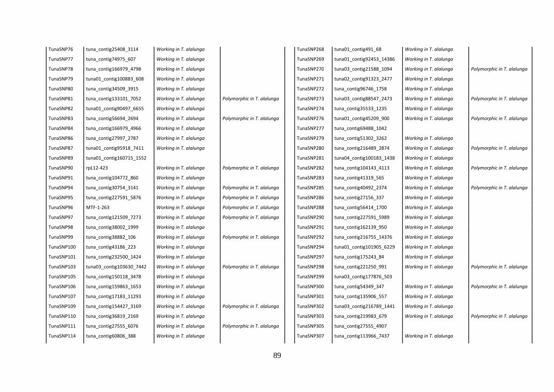
89

TunaSNP76 tuna_contig25408_3114 Working in T. alalunga

TunaSNP268 tuna01_contig491_68 Working in T. alalunga

TunaSNP77 tuna_contig74975_607 Working in T. alalunga

TunaSNP269 tuna01_contig92453_14386 Working in T. alalunga

TunaSNP78 tuna_contig166979_4798 Working in T. alalunga

TunaSNP270 tuna03_contig21588_1094 Working in T. alalunga Polymorphic in T. alalunga

TunaSNP79 tuna01_contig100883_608 Working in T. alalunga

TunaSNP271 tuna02_contig91323_2477 Working in T. alalunga

TunaSNP80 tuna_contig34509_3915 Working in T. alalunga

TunaSNP272 tuna_contig96746_1758 Working in T. alalunga

TunaSNP81 tuna_contig133101_7052 Working in T. alalunga Polymorphic in T. alalunga

TunaSNP273 tuna03_contig88547_2473 Working in T. alalunga Polymorphic in T. alalunga

TunaSNP82 tuna01_contig90497_6655 Working in T. alalunga

TunaSNP274 tuna_contig35533_1235 Working in T. alalunga

TunaSNP83 tuna_contig56694_2694 Working in T. alalunga Polymorphic in T. alalunga

TunaSNP276 tuna01_contig45209_900 Working in T. alalunga Polymorphic in T. alalunga

TunaSNP84 tuna_contig166979_4966 Working in T. alalunga

TunaSNP277 tuna_contig69488_1042

TunaSNP86 tuna_contig27997_2787 Working in T. alalunga

TunaSNP279 tuna_contig51302_3262 Working in T. alalunga

TunaSNP87 tuna01_contig95918_7411 Working in T. alalunga

TunaSNP280 tuna_contig216489_2874 Working in T. alalunga Polymorphic in T. alalunga

TunaSNP89 tuna01_contig160715_1552

TunaSNP281 tuna04_contig100183_1438 Working in T. alalunga

TunaSNP90 rpL12-423 Working in T. alalunga Polymorphic in T. alalunga

TunaSNP282 tuna_contig104143_4113 Working in T. alalunga Polymorphic in T. alalunga

TunaSNP91 tuna_contig104772_860 Working in T. alalunga

TunaSNP283 tuna_contig41319_565 Working in T. alalunga

TunaSNP94 tuna_contig30754_3141 Working in T. alalunga Polymorphic in T. alalunga

TunaSNP285 tuna_contig40492_2374 Working in T. alalunga Polymorphic in T. alalunga

TunaSNP95 tuna_contig227591_5876 Working in T. alalunga Polymorphic in T. alalunga

TunaSNP286 tuna_contig27156_337 Working in T. alalunga

TunaSNP96 MTF-1-263 Working in T. alalunga Polymorphic in T. alalunga

TunaSNP288 tuna_contig56414_1700 Working in T. alalunga

TunaSNP97 tuna_contig121509_7273 Working in T. alalunga Polymorphic in T. alalunga

TunaSNP290 tuna_contig227591_5989 Working in T. alalunga

TunaSNP98 tuna_contig38002_1999 Working in T. alalunga

TunaSNP291 tuna_contig162139_950 Working in T. alalunga

TunaSNP99 tuna_contig38882_106 Working in T. alalunga Polymorphic in T. alalunga

TunaSNP292 tuna_contig216755_14376 Working in T. alalunga

TunaSNP100 tuna_contig43186_223 Working in T. alalunga

TunaSNP294 tuna01_contig101905_6229 Working in T. alalunga

TunaSNP101 tuna_contig232500_1424 Working in T. alalunga

TunaSNP297 tuna_contig175243_84 Working in T. alalunga

TunaSNP103 tuna03_contig103630_7442 Working in T. alalunga Polymorphic in T. alalunga

TunaSNP298 tuna_contig221250_991 Working in T. alalunga Polymorphic in T. alalunga

TunaSNP105 tuna_contig150118_3478 Working in T. alalunga

TunaSNP299 tuna03_contig177876_503

TunaSNP106 tuna_contig159863_1653 Working in T. alalunga

TunaSNP300 tuna_contig54349_347 Working in T. alalunga Polymorphic in T. alalunga

TunaSNP107 tuna_contig17183_11293 Working in T. alalunga

TunaSNP301 tuna_contig135906_557 Working in T. alalunga

TunaSNP109 tuna_contig154427_3169 Working in T. alalunga Polymorphic in T. alalunga

TunaSNP302 tuna03_contig216789_1441 Working in T. alalunga

TunaSNP110 tuna_contig36819_2169 Working in T. alalunga

TunaSNP303 tuna_contig219983_679 Working in T. alalunga Polymorphic in T. alalunga

TunaSNP111 tuna_contig27555_6076 Working in T. alalunga Polymorphic in T. alalunga

TunaSNP305 tuna_contig27555_4907

TunaSNP114 tuna_contig60806_388 Working in T. alalunga

TunaSNP307 tuna_contig113966_7437 Working in T. alalunga

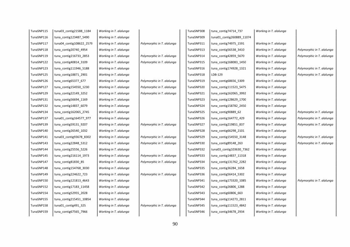
90

TunaSNP115 tuna03_contig21588_1184 Working in T. alalunga

TunaSNP308 tuna_contig74714_737 Working in T. alalunga

TunaSNP116 tuna_contig123487_5490 Working in T. alalunga

TunaSNP309 tuna01_contig260889_11074

TunaSNP117 tuna04_contig108622_2579 Working in T. alalunga Polymorphic in T. alalunga

TunaSNP311 tuna_contig74975_1591 Working in T. alalunga

TunaSNP118 tuna_contig20740_4954 Working in T. alalunga

TunaSNP313 tuna_contig56538_3410 Working in T. alalunga Polymorphic in T. alalunga

TunaSNP119 tuna_contig216733_2853 Working in T. alalunga Polymorphic in T. alalunga

TunaSNP314 tuna_contig42859_5670 Working in T. alalunga Polymorphic in T. alalunga

TunaSNP122 tuna_contig40814_3109 Working in T. alalunga Polymorphic in T. alalunga

TunaSNP315 tuna_contig168083_1450 Working in T. alalunga

TunaSNP123 tuna_contig111946_5188 Working in T. alalunga

TunaSNP316 tuna_contig174928_1321 Working in T. alalunga Polymorphic in T. alalunga

TunaSNP125 tuna_contig18871_2901 Working in T. alalunga

TunaSNP318 LDB-129 Working in T. alalunga Polymorphic in T. alalunga

TunaSNP126 tuna_contig65377_677 Working in T. alalunga Polymorphic in T. alalunga

TunaSNP319 tuna_contig68656_5309 Working in T. alalunga

TunaSNP127 tuna_contig154550_1230 Working in T. alalunga Polymorphic in T. alalunga

TunaSNP320 tuna_contig111523_5475 Working in T. alalunga

TunaSNP129 tuna_contig22149_3252 Working in T. alalunga Polymorphic in T. alalunga

TunaSNP321 tuna_contig162065_3992 Working in T. alalunga

TunaSNP131 tuna_contig56694_1169 Working in T. alalunga

TunaSNP323 tuna_contig128629_1700 Working in T. alalunga

TunaSNP132 tuna_contig14837_6079 Working in T. alalunga

TunaSNP324 tuna_contig158782_2450 Working in T. alalunga

TunaSNP134 tuna_contig162065_2745 Working in T. alalunga

TunaSNP325 tuna_contig90889_62 Working in T. alalunga Polymorphic in T. alalunga

TunaSNP137 tuna01_contig164577_977 Working in T. alalunga

TunaSNP326 tuna_contig164772_429 Working in T. alalunga Polymorphic in T. alalunga

TunaSNP139 tuna_contig59131_9207 Working in T. alalunga Polymorphic in T. alalunga

TunaSNP327 tuna_contig219851_837 Working in T. alalunga Polymorphic in T. alalunga

TunaSNP140 tuna_contig26540_1032 Working in T. alalunga

TunaSNP328 tuna_contig66298_2101 Working in T. alalunga

TunaSNP141 tuna03_contig93678_8302 Working in T. alalunga Polymorphic in T. alalunga

TunaSNP329 tuna_contig154550_3148 Working in T. alalunga Polymorphic in T. alalunga

TunaSNP143 tuna_contig22848_5312 Working in T. alalunga Polymorphic in T. alalunga

TunaSNP330 tuna_contig89148_263 Working in T. alalunga Polymorphic in T. alalunga

TunaSNP144 tuna_contig25556_5226 Working in T. alalunga

TunaSNP332 tuna03_contig103630_7362 Working in T. alalunga

TunaSNP145 tuna_contig216114_1973 Working in T. alalunga Polymorphic in T. alalunga

TunaSNP333 tuna_contig14837_11318 Working in T. alalunga

TunaSNP147 tuna_contig81830_85 Working in T. alalunga Polymorphic in T. alalunga

TunaSNP334 tuna_contig131762_2282 Working in T. alalunga

TunaSNP148 tuna_contig154768_3030 Working in T. alalunga

TunaSNP335 tuna_contig36284_1658 Working in T. alalunga

TunaSNP149 tuna_contig224622_723 Working in T. alalunga Polymorphic in T. alalunga

TunaSNP336 tuna_contig56414_5302 Working in T. alalunga

TunaSNP150 tuna_contig121813_4643 Working in T. alalunga

TunaSNP341 tuna_contig173320_1085 Working in T. alalunga Polymorphic in T. alalunga

TunaSNP152 tuna_contig17183_11458 Working in T. alalunga

TunaSNP342 tuna_contig26806_1288 Working in T. alalunga

TunaSNP154 tuna_contig52955_2028 Working in T. alalunga

TunaSNP343 tuna_contig60806_663 Working in T. alalunga

TunaSNP155 tuna_contig215451_10854 Working in T. alalunga

TunaSNP344 tuna_contig114273_2811 Working in T. alalunga

TunaSNP158 tuna01_contig491_325 Working in T. alalunga Polymorphic in T. alalunga

TunaSNP345 tuna_contig111523_4842 Working in T. alalunga

TunaSNP159 tuna_contig67565_7966 Working in T. alalunga

TunaSNP346 tuna_contig34678_2934 Working in T. alalunga

91

TunaSNP160 tuna_contig40138_3002 Working in T. alalunga

TunaSNP347 tuna_contig74714_1068

TunaSNP161 tuna_contig29338_778 Working in T. alalunga Polymorphic in T. alalunga

TunaSNP348 tuna_contig22149_3357 Working in T. alalunga

TunaSNP162 tuna_contig221038_1952

TunaSNP349 tuna_contig24563_365 Working in T. alalunga

TunaSNP163 tuna_contig162065_2811 Working in T. alalunga

TunaSNP351 tuna_contig164201_1037 Working in T. alalunga

TunaSNP164 tuna_contig221038_1562 Working in T. alalunga Polymorphic in T. alalunga

TunaSNP352 tuna_contig224399_1755 Working in T. alalunga Polymorphic in T. alalunga

TunaSNP165 tuna_contig92628_3851 Working in T. alalunga

TunaSNP353 tuna_contig222995_505 Working in T. alalunga

TunaSNP166 tuna_contig60564_6105 Working in T. alalunga Polymorphic in T. alalunga

TunaSNP355 tuna_contig167840_2640 Working in T. alalunga

TunaSNP167 tuna_contig169746_1876 Working in T. alalunga

TunaSNP356 tuna_contig60098_2850

TunaSNP168 tuna_contig154550_773 Working in T. alalunga Polymorphic in T. alalunga

TunaSNP357 tuna_contig26181_3568 Working in T. alalunga

TunaSNP169 tuna_contig103947_3022 Working in T. alalunga

TunaSNP359 tuna_contig227194_2648 Working in T. alalunga Polymorphic in T. alalunga

TunaSNP170 tuna02_contig94719_12363 Working in T. alalunga Polymorphic in T. alalunga

TunaSNP360 tuna_contig106376_2098 Working in T. alalunga

TunaSNP172 tuna_contig24268_592 Working in T. alalunga

TunaSNP361 tuna01_contig253978_1075 Working in T. alalunga

TunaSNP173 tuna_contig217806_1113 Working in T. alalunga

TunaSNP362 tuna_contig104143_4176 Working in T. alalunga

TunaSNP174 tuna_contig108670_3117 Working in T. alalunga

TunaSNP363 tuna_contig152711_844 Working in T. alalunga

TunaSNP175 CITRA5-395 Working in T. alalunga Polymorphic in T. alalunga

TunaSNP364 tuna_contig33239_1303 Working in T. alalunga

TunaSNP176 tuna04_contig101753_2386 Working in T. alalunga

TunaSNP365 tuna_contig149102_3038 Working in T. alalunga

TunaSNP177 tuna_contig12328_390 Working in T. alalunga

TunaSNP366 tuna_contig123661_1240 Working in T. alalunga Polymorphic in T. alalunga

TunaSNP179 tuna_contig114055_2490 Working in T. alalunga Polymorphic in T. alalunga

TunaSNP367 tuna_contig220997_1396 Working in T. alalunga

TunaSNP180 tuna_contig122189_1042 Working in T. alalunga

TunaSNP368 tuna_contig231022_192 Working in T. alalunga

TunaSNP182 tuna02_contig122146_2581 Working in T. alalunga

TunaSNP370 tuna_contig114893_4160 Working in T. alalunga

TunaSNP183 tuna_contig45092_1603 Working in T. alalunga

TunaSNP371 tuna01_contig96873_2098 Working in T. alalunga

TunaSNP184 tuna02_contig238606_1899 Working in T. alalunga

TunaSNP374 tuna_contig71405_1764 Working in T. alalunga Polymorphic in T. alalunga

TunaSNP185 tuna_contig111946_1396 Working in T. alalunga

TunaSNP377 tuna_contig122511_821 Working in T. alalunga

TunaSNP186 tuna_contig51571_840 Working in T. alalunga

TunaSNP379 tuna_contig228326_2077 Working in T. alalunga

TunaSNP189 tuna_contig225235_1907 Working in T. alalunga

TunaSNP380 tuna_contig21470_885 Working in T. alalunga

TunaSNP190 tuna_contig16636_17148 Working in T. alalunga Polymorphic in T. alalunga

TunaSNP381 tuna_contig34220_1259 Working in T. alalunga Polymorphic in T. alalunga

TunaSNP191 tuna02_contig85098_13011 Working in T. alalunga

TunaSNP382 tuna_contig148347_2296 Working in T. alalunga

TunaSNP192 tuna_contig148017_7280 Working in T. alalunga Polymorphic in T. alalunga

TunaSNP383 tuna_contig111523_3798 Working in T. alalunga

TunaSNP193 tuna_contig59655_1718 Working in T. alalunga Polymorphic in T. alalunga

TunaSNP384 tuna_contig76689_116 Working in T. alalunga

92

CHAPTER 5

ASSESSING THE ACCURACY AND POWER OF SNPS MARKERS FOR

POPULATION GENETICS, INDIVIDUAL ASSIGNMENT AND MIXTURE

STOCK ANALYSIS IN THUNNUS THYNNUS

93

Assessing the accuracy and power of SNPs markers for population genetics,

individual assignment and mixture stock analysis in Thunnus thynnus

Authors:

Eleonora Pintus1, Alessia Cariani1, Fausto Tinti1, Rita Cannas2, Gregory Maes3, Aitor Albaina4,

Andone Estonba4, Urtzi Laconcha5, Haritz Arrizabalaga5.

Affiliations:

1 Department of Biological, Geological & Environmental Sciences (BiGeA) School of Sciences,

University of Bologna, Via Selmi 3, 40126, Bologna, Italy.

2 Department of Life and Enviromental Science, University of Cagliari, Via T. Fiorelli 1, 09126

Cagliari, Italy.

3 Katholieke Universiteit Leuven, Laboratory of Biodiversity and Evolutionary Genomics Fish

Genomics Group/BioGenomics division, Ch. Deberiotstraat, 32 B-3000, Leuven, Belgium.

4 Department of Genetics, Physical Anthropology & Animal Physiology, University of the

Basque Country (UPV/EHU), Bº Sarriena s/n 48940, Leioa, Bilbao, Spain.

5 AZTI-Tecnalia / Unidad de Investigación Marina, Herrera kaia portualdea z/g, 20110 Pasaia

(Gipuzkoa), Spain.

94

Introduction

The persistence of many marine fish is threatened by rapid declines; indeed few

populations with extensive gene flow and infinite population size recover rapidly but most

exhibit little or no change in abundance up to 15 years after a collapse. Reductions in fishing

pressure, although clearly necessary for population recovery, are often insufficient.

Persistence and recovery are also influenced by life history, habitat alteration, changes to

species assemblages, genetic responses to exploitation, and reductions in population

growth. In the late twenty years the interest on fishery genetic is enhanced with a large

amount of data produced, thanks to rapidly developing technologies in the field of human

genetics then applied to others species; so its role on fisheries management and assessment

is become prominent, because loss of genetic diversity can lead species to a decline in

capacity of adaptation. Progress in the knowledge of ecology of marine species is important

not only for improving our basic understanding of natural as well as human-induced

evolutionary processes, but also to define management units and setting priorities for

conservation. A key aim of sustainable fisheries management is to identify the spatial scale

of population structuring, and to find tools to monitor its dynamics. Even apparently small

genetic differences among populations of marine fishes at neutral genetic markers could

translate into important adaptive variation distributed among populations (Hauser and

Carvalho 2008; Nielsen et al. 2009).

The Atlantic bluefin tuna (Thunnus thynnus) is one of the major components of

pelagic ecosystems, being both important predators and forage species that are widely

distributed throughout the temperate and tropical epipelagic waters of the world’s oceans

(Mather et al. 1995; Walli et al. 2009). Much like the other large tunas, the ABFT shows

highly migratory behavior, with well-documented trans-oceanic and large-scale movements

for feeding and spawning, high fecundity, large population size and high potential for

dispersal during early life stages (Block et al. 2005; Fromentin and Power 2005; Rooker et al.

2007; Teo et al. 2007). Currently, ABTF is managed by the International Commission for the

Conservation of Atlantic Tunas (ICCAT) as two stocks, divided at the 45th meridian in the mid-

Atlantic (ICCAT 2008), with separated spawning areas in the Gulf of Mexico and the

Mediterranean Sea, identified as spawning grounds by the presence of larvae during certain

times of the year and adult fish in reproductive condition (National Research Council 1994;

95

Rooker et al. 2007). The two stocks actually mix. All sizes have been documented crossing

the hypothetical line of separation among stocks (the 45th W meridian). Data on fisheries

and satellite tags provide information on movements that reveal the eastern and western

populations of T. thynnus share common foraging grounds in different areas of the Atlantic

Ocean mainly as adolescent, but sort as adults to the respective breeding grounds (Gulf of

Mexico and Mediterranean) a behavior termed natal homing (Rooker et al. 2007).

Tuna is a critical worldwide food resource and, although it was caught for thousands

of years, only in recent decades, particularly after expansion and growth of Japanese market

during 1980s, its use is far above the sustainable level, risking collapse of the fishery and the

stock (ICCAT 2010). Both western than eastern Atlantic bluefin spawning stock biomass (SSB)

(adult-aged fish) has critically declined in the last fifty years (MacKenzie et al. 2009; Juan-

Jordá et al. 2011). SSB spawning stock biomass peaked over 300000 tons in the late 1950s

and early 1970s and then declined to about 150000 tons until the mid-2000s. However, in

the most recent period, the SSB showed clear signs of increase, indicating that the stocks are

slowly recovering (ICCAT 2012). A main objective of fisheries management is to maintain

populations at levels where the spawning stock biomass does not limit the production of

new young fish (MacKenzie et al. 2009; ICCAT 2010; Reeb 2010). Specific natural

characteristics, such as late reproduction, long lifespan and the aggregation of the fish that

occurs during spawning, make ABFT extremely vulnerable to overexploitation. Bluefin tuna

are also sensitive to oceanic conditions and disturbances such as those caused by industrial

pollution (Safina 2001; Ottolenghi et al. 2004).

The delineation of population structure in highly migratory pelagic fishes has

traditionally been difficult. A highly migratory lifestyle and the lack of clear barriers to gene

flow has made the detection of population subdivision within ocean basins difficult (Waples

1998). Currently, the degree of genetic structure among stocks is largely unknown. The

differentiation between eastern and western Atlantic stocks is recognized by genetic studies,

tagging experiments and microchemical signatures in otoliths of young of the years, in

agreement with the spawning site fidelity (Block et al. 2005; Carlsson et al. 2007; Boustany

et al. 2008; Rooker et al. 2008). However, satellite tags studies (Lutcavage et al. 1999;

Galuardi et al. 2010; Wilson et al. 2010) questioned the existence of a unique spawning site

for the western population. In fact, adult bluefin tuna have been observed in the central

Atlantic and off Bahamas during the spawning season when they were supposed to be in the

96

Gulf of Mexico. Possible explanations for these ‘unexpected’ sightings were given: the

existence alternative spawning areas and/or the adoption by some mature specimens a

skipped spawning strategy (remaining in the foraging ground and skipping spawning in that

year) (Lutcavage et al. 1999; Goldstein et al. 2007; Galuardi et al. 2010).

As concerns the Mediterranean Sea, three spawning grounds are traditionally known

in the Western basin: around the Balearic Islands, Sicily and Malta (Rooker et al. 2007).

Recently, the occurrence of a further spawning site in the Levantine Sea has been

demonstrated in eastern Mediterranean. Biological data (different spawning times) and

tagging studies provided indications for the existence of substructuring within the

Mediterranean, with the independence of eastern and western Mediterranean populations

(Rooker et al. 2007). None of the fish tagged in the Atlantic (Block et al. 2005) was ever

located east of Malta or as far as the Levantine Sea, hence the spawning migration from the

Atlantic did not reach the eastern med basin. Moreover, the fish tagged in east

Mediterranean stay confined in that basin (De Metrio et al. 2005) leading to hypothesize the

existence of a separate, local or resident eastern Mediterranean.

Despite the plethora of studies, the population structure within the Mediterranean

Sea is still unclear. Conflicting results were obtained in the genetic studies dealing with the

issue of genetic differentiation of stocks (Viñas et al. 2011). For instance, Boustany et al.

(2008) and Carlsson et al. (2004, 2007) found significant genetic differentiation between

west and east Mediterranean populations, and Riccioni et al. (2010) detected structure also

within the western basin. On the contrary, Ely et al. (2002) and Pujolar et al. (2003) did not

found significant differentiation, in agreement to the hypothesis of a single panmictic unit of

Atlantic bluefin tuna in the Mediterranean basin. Probably these contradictory results could

be due to the use of reduced number of molecular markers, differential sampling design and

methodological techniques (Viñas et al. 2011).

Following many useful suggestions by Viñas et al 2011, in this study we tried to go

over these previous inconsistencies, improving the sampling design and testing new

powerful markers and analytic approaches.

In particular, a large panel of SNP markers recently derived from Atlantic bluefin tuna

transcriptomic and genomic sequences (see chapter 4 of this thesis) was used to genotype to

a wide-scale of samples across the entire range of Thunnnus thynnus. Single-nucleotide

polymorphisms (SNPs) are the more abundant polymorphism in the genome, are

97

codominant, are usually biallelic, represent a more stable nuclear marker than

microsatellites, and are amenable to automation and increasingly cost-effective (Vignal et al.

2002; Morin et al. 2004; Helyar et al. 2011; Odgen 2011). These features have made SNP a

marker of choice in modern genomics research and in studies of the ecology and

conservation of natural populations because of their capacity to access variability across the

genome. Until a short time ago development and genotyping of these markers were not

easy for species without reference genome, but now this gap was overcame by next-

generation sequencing technologies, that provide access to a wealth of sequence

information on non model organisms, thanks to exponentially reduction of DNA-sequencing

costs that has led to rapid increase in throughput, allowing sequencing the entire expressed

genome of a non-model organism with standard project budgets. (Morin and McCarthy

2007; Hauser and Seeb 2008; Seeb et al. 2011; Esteras et al. 2012). We use the Illumina

Golden Gate assays that genotype 384, 768 or 1536 SNP in parallel and have been the most

widely used for high-throughput applications. This genotyping technique has been used

extensively in humans (The International HapMap Consortium 2003) and several animal

species (McKay et al. 2008; Kijas et al. 2009; Malhi et al. 2011).

In summary, considering that the stock structure of Atlantic bluefin tuna is probably

much more complex than originally described, and that more spatially explicit management

plans than the simple two stock structure are urgently required, we aimed at an accurate

description of its population structure, crucial information required for the sustainable

utilization of this important species (Viñas et al. 2011; Kell et al. 2012). Our study is included

in the framework of a wide scientific research program (GBYP “Biological Sampling and

Analysis” program) launched in 2010 by ICCAT to obtain new biological and ecological

information that can be used to upgrade models for stock assessment, which is the most

sensitive process for the conservation of this important resource.

Materials and Methods

Population sampling and SNP

A broad spatial and multi strata sampling has been realized in 2011 and during the

GBYP project phase 2 several temporal replicates, provided by the partners from other

projects or private collections, were been added to the analyses. A total of

were chosen, collected from the most part of the whole range of Atlantic bluefin tuna. We

selected 23 bluefin tuna population samples, 1 from Gulf of Mexico, 4 from Eastern

Mediterranean, 4 from Central Mediterranean, 10 from Western Medit

North East Atlantic, each composed by 40 individuals (except EMED

0-2010 that have 39 and 35 individuals respectively). Six of these were identified as

reference samples of spawning populations (EMED

WMED-BA-0-2010, WMED-BA

aggregates in the regions/areas (Figure 1). Abbreviations cited in the text referred to the

code sampling specified in Table 1.

Figure. Geographical representation of sampling locations of Mediterranean Sea, listed in Table 1. Reference

samples are in bold and underlined.

98

Population sampling and SNP genotyping

A broad spatial and multi strata sampling has been realized in 2011 and during the

GBYP project phase 2 several temporal replicates, provided by the partners from other

projects or private collections, were been added to the analyses. A total of

chosen, collected from the most part of the whole range of Atlantic bluefin tuna. We

23 bluefin tuna population samples, 1 from Gulf of Mexico, 4 from Eastern

Mediterranean, 4 from Central Mediterranean, 10 from Western Mediterranean and 4 from

North East Atlantic, each composed by 40 individuals (except EMED-LS-LA+0 and

that have 39 and 35 individuals respectively). Six of these were identified as

reference samples of spawning populations (EMED-LS-LA+0, WMED-TY-0, WMED

BA-0 and GOM-LA+0) and 17 represented feeding/breeding

aggregates in the regions/areas (Figure 1). Abbreviations cited in the text referred to the

code sampling specified in Table 1.

representation of sampling locations of Mediterranean Sea, listed in Table 1. Reference

samples are in bold and underlined.

A broad spatial and multi strata sampling has been realized in 2011 and during the

GBYP project phase 2 several temporal replicates, provided by the partners from other

projects or private collections, were been added to the analyses. A total of 919 individuals

chosen, collected from the most part of the whole range of Atlantic bluefin tuna. We

23 bluefin tuna population samples, 1 from Gulf of Mexico, 4 from Eastern

erranean and 4 from

LA+0 and WMED-BA-

that have 39 and 35 individuals respectively). Six of these were identified as

0, WMED-BA-0-2009,

LA+0) and 17 represented feeding/breeding

aggregates in the regions/areas (Figure 1). Abbreviations cited in the text referred to the

representation of sampling locations of Mediterranean Sea, listed in Table 1. Reference

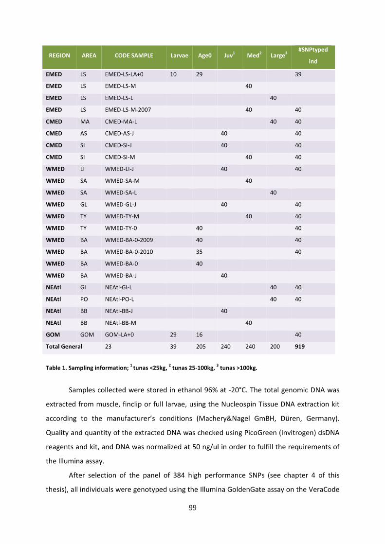
99

REGION AREA CODE SAMPLE Larvae Age0 Juv1 Med

2 Large

3

#SNPtyped

ind

EMED LS EMED-LS-LA+0 10 29 39

EMED LS EMED-LS-M 40

EMED LS EMED-LS-L 40

EMED LS EMED-LS-M-2007 40 40

CMED MA CMED-MA-L 40 40

CMED AS CMED-AS-J 40 40

CMED SI CMED-SI-J 40 40

CMED SI CMED-SI-M 40 40

WMED LI WMED-LI-J 40 40

WMED SA WMED-SA-M 40

WMED SA WMED-SA-L 40

WMED GL WMED-GL-J 40 40

WMED TY WMED-TY-M 40 40

WMED TY WMED-TY-0 40 40

WMED BA WMED-BA-0-2009 40 40

WMED BA WMED-BA-0-2010 35 40

WMED BA WMED-BA-0 40

WMED BA WMED-BA-J 40

NEAtl GI NEAtl-GI-L 40 40

NEAtl PO NEAtl-PO-L 40 40

NEAtl BB NEAtl-BB-J 40

NEAtl BB NEAtl-BB-M 40

GOM GOM GOM-LA+0 29 16 40

Total General 23 39 205 240 240 200 919

Table 1. Sampling information;

1 tunas <25kg,

2 tunas 25-100kg,

3 tunas >100kg.

Samples collected were stored in ethanol 96% at -20°C. The total genomic DNA was

extracted from muscle, finclip or full larvae, using the Nucleospin Tissue DNA extraction kit

according to the manufacturer’s conditions (Machery&Nagel GmBH, Düren, Germany).

Quality and quantity of the extracted DNA was checked using PicoGreen (Invitrogen) dsDNA

reagents and kit, and DNA was normalized at 50 ng/ul in order to fulfill the requirements of

the Illumina assay.

After selection of the panel of 384 high performance SNPs (see chapter 4 of this

thesis), all individuals were genotyped using the Illumina GoldenGate assay on the VeraCode

100

BeadXpress format. Results were visualized and analyzed with the GenomeStudio Data

Analysis Software package and then manually re-clustered to obtain highly accurate

genotype data.

In order to select a better panel of loci, we excluded SNPs that didn’t work, didn’t

cluster or had a percentage of missing value > 10% and that were monomorphic. We

eliminated loci with Minor Allele Frequency (MAF) < 0.01 and observed heterozygosity (HO) >

0.9, in the 919 bluefin tuna individuals. A quality check was also carried out on individuals

and the ones with low-quality results (percentage of missing value over all loci > 20%) were

deleted from dataset. Identity analysis, as implemented in Cervus v3.0.5 (Kalinowski et al.

2007), was used to find matching genotypes in a genotype file. This analysis is particularly

useful in studies where large datasets are used and individuals can be inadvertently

resampled. The same software was used to estimate the frequency of null alleles for each

locus. The minor allele frequency of loci was calculated with Powermarker v3.25 (Liu and

Muse 2005).

Genetic diversity and Hardy-Weinberg Equilibrium

Basic descriptive statistics of genetic diversity in the 23 population samples were

calculated over the dataset obtained after the quality check. We calculated allele

frequencies, expected (HE) and observed (HO) heterozygosity and percentage of polymorphic

loci using the package GenAlEx 6.5 (Peakall and Smouse 2006, 2012). Allelic richness was

estimated using the method implemented in Fstat 2.9.4 (Goudet 1995). The departure from

the Hardy Weinberg Equilibrium (HWE) of each locus in each population was tested using

exact probability test implemented in Genepop 4.1.4 (Rousset 2008) with the complete

enumeration method, as described by Louis and Dempster (1987), recommended in studies

with less than 1000 individuals per sample. In addition, the U tests, both for heterozygote

deficiency and heterozygote excess for each locus in each population, were performed. We

tested the departure from the Hardy Weinberg Equilibrium (HWE) with the multisample

score U test of Rousset and Raymond (1995), which defines a global test across loci and

across samples. The Markov chain (MC) algorithm is used (10000 dememorizations, 100

batches and 5000 iterations per batch) to estimate without bias the exact P-value of the U

tests (Guo and Thompson 1992). The false discovery rate (FDR) correction, based on

Benjamini-Hochberg method (Benjamini and Yekutieli 2001) and implemented in the SGoF+

101

software (Carvajal-Rodriguez and Uña-Alvarez 2011) was applied to adjust significance levels

for multiple simultaneous comparisons.

Linkage disequilibrium (LD) for each pair of SNPs in each population was tested in

Genepop 4.1.4 (Rousset 2008). P-values of HWE tests were corrected for multiple tests,

using SGoF+ software (Carvajal-Rodriguez and Uña-Alvarez 2011) and the false discovery

rate (FDR) correction, based on Benjamini-Hochberg method (Benjamini and Yekutieli 2001),

that is expected to provide a large increase in power to identify differentiated populations

relative to the Bonferroni method (Narum 2006). FIS values (Weir and Cockerham 1984) were

calculated with Fstat 2.9.4 (Goudet 1995) and the significance level was tested with

bootstraping over loci.

Outlier loci detection

To identify loci under selection, we availed of two different complementary

approaches, implemented in two software, and we performed analyses both for all

populations than for six reference samples of the spawning populations.

BayeScan 2.1 (Foll and Gaggiotti 2008) aims at identifying candidate outlier loci using

differences between population allele frequencies and a common gene pool. This method

based on a scission of locus-population FST in two component, one shared of all loci and

population-specific and other shared of all populations and locus-specific. When the latter is

necessary to explain the observed pattern of genetic diversity, we can assume departure

from neutrality at a given locus. So, there are two alternative models for each locus,

including or not this locus-specific component to model selection. The program calculates a

posterior probability for the model including selection, allowing the control of the False

Discovery Rate (FDR), defined as the expected proportion of false positives among outlier

markers (Foll and Gaggiotti 2008). It has been found that this approach have lower type I

(false positive) error rates for divergent selection compared to other outlier detection

methods (Narum and Hess 2011).

We performed analyses setting up 20 pilot runs each consisting of 5000 iterations,

followed by 5000 iterations with a burn-in of 50000 iterations; the thinning interval, that

represent the number of iterations between two samples, was 10, and the prior odds for the

neutral model was set to 10, as suggested for the identification of candidate loci with a few

hundreds of markers. Posterior Odds (PO), indicating how more likely the model including

102

selection is compared to the neutral model, were interpreted according to the Jeffreys' scale

of evidence for Bayes Factors (Jeffreys 1961).

The other method based on FDIST approach (Beaumont and Nichols 1996) evaluated

the relationship between FST and HE (expected heterozygosity) in an island model of

migration with neutral markers. So, this was possible to identify outlier loci that have higher

values of genetic distance than expected from a neutral distribution. We applied this

method implemented in Lositan (Looking for Selection In a TANgled dataset), a selection

detection workbench constructed around FDIST (Antao et al. 2008), with 50000 simulations.

The weakness of this process is the incorrect identification of several neutral markers as

outlier, and much of this type I error for balancing selection. We used a confidence interval

of 0.95 for the expected null differentiation meaning that loci over this interval had to be in

the upper 0.025 tail of the distribution to be considered as potentially under directional or

divergent selection or in the lower 0.025 tail of the distribution to be considered as

potentially under balancing selection (Bourret et al. 2012). Lositan also implements a

multitest correction based on false discovery rates (FDR) that is fundamental to avoid high

overestimation of the percentage of outliers.

Population genetic structure

Genetic distances among samples were also explored by Principal Coordinate

Analysis (PCoA) based on the pairwise FST matrix using GenAlEx 6.5 (Peakall and Smouse

2006, 2012).

Analysis of molecular variance (AMOVA) was used to calculate locus-by-locus FST and

to partition the genetic variance between populations between populations (FST) within

groups within groups (FSC) and among groups (FCT) using Arlequin 3.5 (Excoffier and Lischer

2010).

In particular, individual locus FST values were calculated for the reference samples

(pooling together the ones from the western Mediterranean) and used to rank SNPs in order

to select a subpanel of markers with the highest power in discriminating tunas from the

three spawning areas. The subpanel of SNPs with FST > 0.01 were compared with the full set

of markers for accuracy.

To assess genetic diversity among populations pairwise FST were calculated with the

software Arlequin 3.5 (Excoffier and Lischer 2010) (10000 permutations); a matrix of

103

pairwise FST was generated by R-script implemented in the software. The significance level of

multiple comparisons was adjusted with the FDR method as described above.

To investigate on the genetic similarity of the 23 population samples, DA genetic

distances (Nei et al. 1983) between all pairs of populations were computed with

Powermarker v3.25 (Liu and Muse 2005), and a neighbor-joining tree was produced to

visualize their relationships using Splitstree4 (Huson 1998; Huson and Bryant 2006). The

pattern of phylogeographic structure was visualized with GenGIS v2.02, an application that

provides a 3D graphical interface for the merging of information on molecular diversity with

the geographic location from which the sequences were collected (Parks et al. 2009).

We used also the method successfully adopted by Willing et al. (2010) and Kraus et

al. (2013) to display reticulate relationships among individuals using SNP data: the

NEIGHBOUR-NET algorithm. The phylogeographic analysis uses the method Neighbor-net

(Bryant and Moulton 2004) implemented in Splitstree4 (Huson 1998; Huson and Bryant

2006). According to Kraus et al. (2013) for each individual, the genotype at each SNP was

collapsed into a single base character and concatenated to a sequence of nucleotides.

Heterozygote genotypes were coded according to IUPAC and missing data denoted ‘N’.

Uncorrected_P distance was used as metric.

Detection of genetic clusters

Discriminant analysis of principal components (DAPC; Jombart et al. 2010) from

Adegenet (Jombart 2008) was used to detect the number of genetic clusters and assignment

of individuals.

This method transforms data using principle component analysis (PCA) to create

uncorrelated variables for input into Discriminant Analysis (DA). DA maximizes between-

group variation and minimizes within-group variation for assessment of between-group

variation. DAPC is free of assumptions about Hardy-Weinberg equilibrium or linkage

disequilibrium and provides graphical representation of divergence among populations.

DAPC was implemented using the Adegenet R package (Jombart 2008) version 1.2.8 in R (R

Development Core Team 2009). DAPC allowed the search for the most likely number of

clusters/groups in the dataset. This can be achieved using k-means, a clustering algorithm

which finds a given number (k) of groups maximizing the variation between groups, B(X). To

identify the optimal number of clusters, k-means is run sequentially with increasing values of

104

k, and different clustering solutions are compared using Bayesian Information Criterion (BIC).

Ideally, the optimal clustering solution should correspond to the lowest BIC. In practice, the

’best’ BIC is often indicated by an elbow in the curve of BIC values as a function of k.

Moreover, being based on the Discriminant Analysis, DAPC also provides membership

probabilities of each individual for the different groups based on the retained discriminant

functions, giving indications of how clear-cut genetic clusters are. Loose clusters will result in

fairly flat distributions of membership probabilities of individuals across clusters, pointing to

possible admixture.

We used the function ‘find.clusters’ to determine the most likely number of genetic

clusters in the data, using all available principal components (PCs). To calculate the

probability of assignment of individuals to each of these clusters using DAPC, we determined

the optimal number of PCs. In a preliminary DAPC run we retained only a limited number of

PCs (sample size divided by three) used all discriminant functions, in order to avoid unstable

assignments of individuals to clusters. The ‘optim.a.score’ function determined the optimal

number of PCs, that were used in the final DAPC.

In addition to DAPC, the cluster analyses were also performed with another approach

based on the Bayesian algorithm, implemented in Structure 2.3.4 (Pritchard et al. 2000). This

software, in contrast to DAPC, assumes Hardy-Weinberg and Linkage Equilibrium and

estimates the number of k clusters of individuals. To estimate the more likely number of

clusters, a posterior probability is calculated for each inferred k. The algorithm was run

assuming the admixture model and correlated allele frequencies among populations, and

providing the sampling information as prior with the option LOCPRIOR, in order to improve

accuracy in detecting population structure. For each analysis we used 5 iterations per k

value, for values of k between 1 and 8, a burnin period length of 10000, and 50000 MCMC

repetitions. The optimal k was selected according to the two criteria: the ΔK (Evanno et al.

2005), and the ΔFST (Campana et al. 2011) both implemented in the R package CorrSieve

(Campana et al. 2011). When a K was selected, Clumpp v.1.1 (Jakobsson and Rosenberg,

2007) was used to average the assignment scores over the 5 runs. Results were displayed

using Distruct v.1.1 (Rosenberg 2004).

105

Assignment tests

Assignment tests were used to estimate the origin of each individual fish.

In general Bayesian and maximum likelihood-based methods have proven to be

significantly more effective at assignment than previous distance-based methods (Cornuet et

al. 1999).

The reference sample populations (that comprise larvae and age-0 of known origin)

were considered as baseline populations to assign the other 17 samples, made up of

juvenile/adults of unknown origin. Due to the lack of differentiation among the four

reference samples of Western Mediterranean origin (see Results section), they were put

together and only three reporting groups were considered (EMED, WMED and GOM).

The performance of different panels of SNPs (that is the ability to increase the

percentage of correct assignment of individuals to the baseline populations) were

compared.

In first instance, the ‘leave one out’ test of the accuracy of assignment tests was

performed in Oncor (Anderson et al. 2008). This test evaluates how well individuals can be

assigned to their population of origin. During the test each individual in each baseline is

sequentially removed from the baseline and its origin is estimated using the rest of the

baseline. Tunas with incomplete genotypes (because of missing data) were dropped from

the analysis but remained in the baseline in order to estimate the origin of other individuals.

Oncor records the fraction of assignments for each population that were correct and the

population to which individuals were most often incorrectly assigned to. The accuracy of

assignment was assessed through self-assignment of larvae and age-0 individuals to their

respective reference populations by using the ‘leave-one-out’ cross-validation test. Since the

origin of assigned individuals was known, the probability of assignment to the population of

origin was reported for assignment accuracy (Storer et al. 2012).

The second step was to perform the genetic assignment of the juvenile/adult tunas

to the reference populations using the programs Oncor (Anderson et al. 2008) and

Geneclass2 (Piry et al. 2004).

Classic genetic assignment tests were performed in Geneclass2 (Piry et al. 2004)

according to the methods of Rannala and Mountain (1997). Each fish was assigned to the

reference population with the highest assignment score, and assignment probabilities for

each individual were recorded for reference of assignment confidence. To determine

106

whether any individuals should be excluded from the stock to which they were assigned, we

used an exclusion-based counterpart method based on simulations (Manel et al. 2005). We

used the resampling method of Paetkau et al. (2004) in Geneclass2 to simulate 10000

individuals; this procedure allowed to determine whether the probability of assigning a given

fish fell into the tail of the distribution (P < 0.05), which would indicate that the individual

should be excluded from the population to which it was previously assigned by the classic

tests. This is important to counteract the possibility of false assignment in the case of a

potentially incomplete baselines.

Assignment tests were performed by means of the conditional maximum likelihood

approach in Oncor (Millar 1987; Anderson et al. 2008). Oncor assigns individuals in a mixture

sample to the baseline population that would have the highest probability of producing the

given genotype in the mixture. Oncor uses the method of Rannala and Mountain (1997) to

estimate this probability. The program uses both genotype frequencies and mixture

proportions when estimating the origin of individuals thus is expected to yield more realistic

estimates of assignment accuracy than Geneclass2. In our study the ability of SNPs to assign

individuals to the most likely population was assessed based on the ‘best-estimate’ reporting

group to which individuals were assigned, that is the reporting group to which a given

individual had the highest proportional assignment.

Mixture analysis

Mixture analysis uses baseline genetic data to estimate the composition of a sample, that is

the proportion of fish that belong to different ‘stocks’. Due to the lack of differentiation

among the four reference samples of Western Mediterranean origin, they were pooled

together, therefore the mixture analysis was used to assign proportions of the

feeding/breeding aggregates to the 3 spawning reporting groups (EMED, WMED and GOM).

To examine how accurate mixture analysis Is likely to be, the 100% simulation feature was

used. The effect of population size on average accuracy of estimated mixture was

investigated for different baseline sample sizes along with the empirical baseline sample

sizes. The closer the probability was to 1.0 and the lower the variance, the greater was the

reliability of the reference for mixed-stock analysis. In simulations with sample sizes as

empirical baselines Oncor uses the method of Anderson et al. (2008) to simulate mixture

107

genotypes and to estimate their probability of occurrence in baseline populations. When a

different sample size is employed the method of Kalinowski et al. (2007) is used. The method

of Anderson et al. (2008) is currently preferred for examining the accuracy because the other

method has not been tested extensively, and therefore they should be used with some

caution. To estimate mixture proportions of the 23 samples, Oncor used conditional

maximum likelihood (Millar 1987). Genotype probabilities were calculated using the method

of Rannala and Mountain (1997). Ninety-five per cent confidence intervals (CIs) of mixture

proportions were determined through 1000 bootstraps.

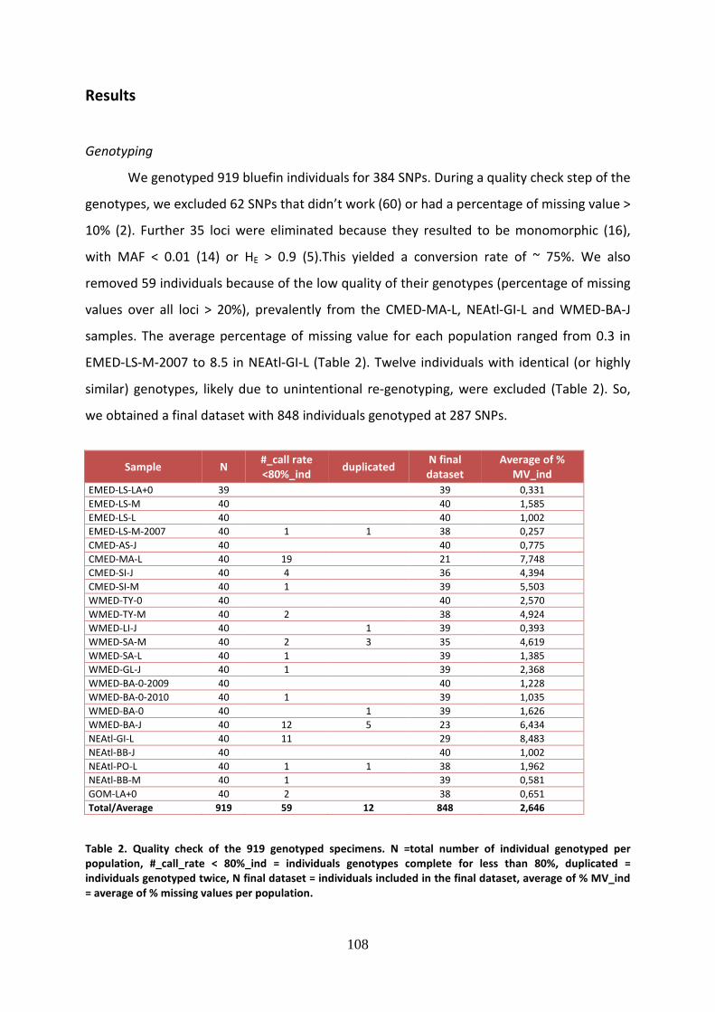
108

Results

Genotyping

We genotyped 919 bluefin individuals for 384 SNPs. During a quality check step of the

genotypes, we excluded 62 SNPs that didn’t work (60) or had a percentage of missing value >

10% (2). Further 35 loci were eliminated because they resulted to be monomorphic (16),

with MAF < 0.01 (14) or HE > 0.9 (5).This yielded a conversion rate of ~ 75%. We also

removed 59 individuals because of the low quality of their genotypes (percentage of missing

values over all loci > 20%), prevalently from the CMED-MA-L, NEAtl-GI-L and WMED-BA-J

samples. The average percentage of missing value for each population ranged from 0.3 in

EMED-LS-M-2007 to 8.5 in NEAtl-GI-L (Table 2). Twelve individuals with identical (or highly

similar) genotypes, likely due to unintentional re-genotyping, were excluded (Table 2). So,

we obtained a final dataset with 848 individuals genotyped at 287 SNPs.

Sample N #_call rate

<80%_ind duplicated

N final

dataset

Average of %

MV_ind

EMED-LS-LA+0 39

39 0,331

EMED-LS-M 40

40 1,585

EMED-LS-L 40

40 1,002

EMED-LS-M-2007 40 1 1 38 0,257

CMED-AS-J 40

40 0,775

CMED-MA-L 40 19

21 7,748

CMED-SI-J 40 4

36 4,394

CMED-SI-M 40 1

39 5,503

WMED-TY-0 40

40 2,570

WMED-TY-M 40 2

38 4,924

WMED-LI-J 40

1 39 0,393

WMED-SA-M 40 2 3 35 4,619

WMED-SA-L 40 1

39 1,385

WMED-GL-J 40 1

39 2,368

WMED-BA-0-2009 40

40 1,228

WMED-BA-0-2010 40 1

39 1,035

WMED-BA-0 40

1 39 1,626

WMED-BA-J 40 12 5 23 6,434

NEAtl-GI-L 40 11

29 8,483

NEAtl-BB-J 40

40 1,002

NEAtl-PO-L 40 1 1 38 1,962

NEAtl-BB-M 40 1

39 0,581

GOM-LA+0 40 2

38 0,651

Total/Average 919 59 12 848 2,646

Table 2. Quality check of the 919 genotyped specimens. N =total number of individual genotyped per

population, #_call_rate < 80%_ind = individuals genotypes complete for less than 80%, duplicated =

individuals genotyped twice, N final dataset = individuals included in the final dataset, average of % MV_ind

= average of % missing values per population.

109

Genetic diversity and Hardy-Weinberg Equilibrium

We obtained a very high percentage of polymorphic loci, the proportion of

polymorphic loci averaged 99.1% and varied from 97.2% in NEAtl-GI-L to 100% in WMED-SA-

L. Estimates of HO and HE across the samples ranged from 0.272 to 0.352 (mean 0.332) and

0.326-0.344 (mean 0.335), respectively. Observed heterozygosity within the reference

populations revealed similar levels of diversity to the 17 feeding/breeding samples, with

WMED-BA-J, CMED-MA-L and NEAtl-GI-L having the lowest HO values while WMED-BA-0-

2009 the highest (Table 3). Global multisample score test of Rousset and Raymond (1995),

over all loci and populations revealed, after FDR correction for multiple tests, 14 loci were

out of equilibrium (9 loci for heterozygotes deficiency and 4 for heterozygotes excess).

However, the “exact HW test" for deviation from equilibrium for each locus in each

population revealed none was significant after FDR correction. Global U test showed that,

after FDR correction for multiple tests, four samples (CMED-MA-L, NEAtl-GI-L, WMED-BA-J,

WMED-SA-M) had significant deviations from HWE. The same populations showed

significantly value of FIS > 0 (Table 3).

Population sample %P HE HO AR FIS P

FIS>observed

P HWE

deficit

EMED-LS-LA+0 99,30% 0,333 0,335 1,930 0,008 0,232 0,3297

EMED-LS-M 98,95% 0,329 0,342 1,931 -0,027 0,995 0,994

EMED-LS-L 98,26% 0,335 0,335 1,932 0,014 0,082 0,1286

EMED-LS-M-2007 99,65% 0,337 0,342 1,939 -0,001 0,526 0,4168

CMED-AS-J 99,65% 0,335 0,336 1,935 0,01 0,1568 0,1876

CMED-MA-L 97,91% 0,328 0,276 1,932 0,185 0 0

CMED-SI-J 98,95% 0,340 0,345 1,939 -0,002 0,5716 0,5276

CMED-SI-M 99,30% 0,332 0,338 1,931 -0,006 0,718 0,4956

WMED-TY-0 99,30% 0,335 0,331 1,936 0,024 0,0093 0,0325

WMED-TY-M 99,30% 0,328 0,338 1,930 -0,018 0,9527 0,9648

WMED-LI-J 99,30% 0,338 0,338 1,941 0,013 0,0968 0,1415

WMED-SA-M 98,26% 0,328 0,318 1,927 0,047 0 0,0003

WMED-SA-L 100,00% 0,339 0,342 1,946 0,003 0,3687 0,2615

WMED-GL-J 99,65% 0,336 0,345 1,940 -0,014 0,9157 0,8975

WMED-BA-0-2009 99,65% 0,344 0,352 1,947 -0,01 0,8385 0,8371

WMED-BA-0-2010 98,95% 0,332 0,333 1,936 0,012 0,1312 0,1208

WMED-BA-0 99,30% 0,337 0,345 1,937 -0,012 0,8783 0,8554

WMED-BA-J 97,91% 0,333 0,293 1,921 0,14 0 0

NEAtl-GI-L 97,21% 0,326 0,272 1,913 0,184 0 0

NEAtl-BB-J 98,95% 0,333 0,332 1,935 0,018 0,0382 0,0522

NEAtl-PO-L 99,65% 0,339 0,348 1,941 -0,012 0,8813 0,7494

NEAtl-BB-M 99,65% 0,339 0,342 1,944 0,004 0,363 0,557

GOM-LA+0 99,65% 0,340 0,345 1,944 -0,004 0,6329 0,5186

110

Table 3. Descriptive statistics of genetic diversity in the 23 population samples at the 287 SNP loci. HE =

expected heterozygosity, HO = observed heterozygosity, AR = allelic richness, FIS = inbreeding fixation index

and relative P- value, P HWE deficit = probability associated to the HWE test for heterozygotes deficiency. FIS

values significantly > 0 are in bold underlined.

Twenty-eight pairs of loci showed significant linkage disequilibrium (p < 0.05) in all

the reference populations. Due to the high number of tests (i.e., 41041 for each population),

no correction for multiple tests was performed since this approach would be overly

conservative and likely underestimate truly significant relationships (Limborg et al. 2012a).

None of these loci pairs were isolated from the same contig, suggesting that distinct

demographic or selective forces may be associated with the observed linkage disequilibrium

rather than merely physical associations (Helyar et al. 2012; Zakas et al. 2012). In many

cases, linked loci appear to provide redundant information, measuring the same allele

frequencies across populations (i.e. providing the power to differentiate between the same

populations) (Storer et al. 2012), and hence potentially leading to upward bias in assignment

success.

However, because we wanted testing all available loci for the species and there are

only limited pairs of loci which were not in linkage equilibrium and not in all populations, we

retained all of them in downstream analyses, and treated them as independent markers.

Outlier loci detection

We searched for outlier loci, that are loci showing higher levels of interspecific

genetic differentiation than expected under neutrality, by two complementary and

exhaustive methods. First, we used the hierarchical Bayesian method described in Beaumont

and Balding (2004), implemented in Bayescan software (Foll and Gaggiotti 2008). Secondly,

we used the Beaumont and Nichols (1996) FDIST approach, implemented in Lositan (Antao

et al. 2008).

Eleven outlier loci under selection were detected by FDIST (Lositan) (Figure 2, Table

4); none was significant after FDR correction. Preliminary analyses did not revealed

differences in allele frequencies among the populations studied at any of these loci.

Figure 2. Comparison of FST and heterozygosity (

candidates for selection using Lositan. Loci highlighted in red are candidates for positive selection (loci

highlighted in grey are selectively neutral).

Locus HE

TunaSNP31 0,37988

TunaSNP54 0,15236

TunaSNP76 0,263474

TunaSNP119 0,489827

TunaSNP196 0,474801

TunaSNP263 0,336313

TunaSNP277 0,215053

TunaSNP285 0,0526

TunaSNP292 0,447185

TunaSNP294 0,468699

TunaSNP326 0,495753

Table 4. Outlier loci detected in Lositan.

Bayescan analysis (Figure 3) pointed out the occurrence

(TunaSNP196).

111

and heterozygosity (HE) in polymorphic loci to identify outliers and potential

candidates for selection using Lositan. Loci highlighted in red are candidates for positive selection (loci

highlighted in grey are selectively neutral).

E FST P(Simul FST < sample F

0,37988 0,021216 0,997291

0,15236 0,023948 0,99924

0,263474 0,02051 0,996211

0,489827 0,016331 0,985804

0,474801 0,027128 0,999686

0,336313 0,014131 0,979717

0,215053 0,015913 0,991643

0,0526 0,015026 0,981575

0,447185 0,013011 0,981883

0,468699 0,019748 0,996564

0,495753 0,015245 0,981053

Table 4. Outlier loci detected in Lositan.

Bayescan analysis (Figure 3) pointed out the occurrence of one differentiation locus

polymorphic loci to identify outliers and potential

candidates for selection using Lositan. Loci highlighted in red are candidates for positive selection (loci

< sample FST)

of one differentiation locus

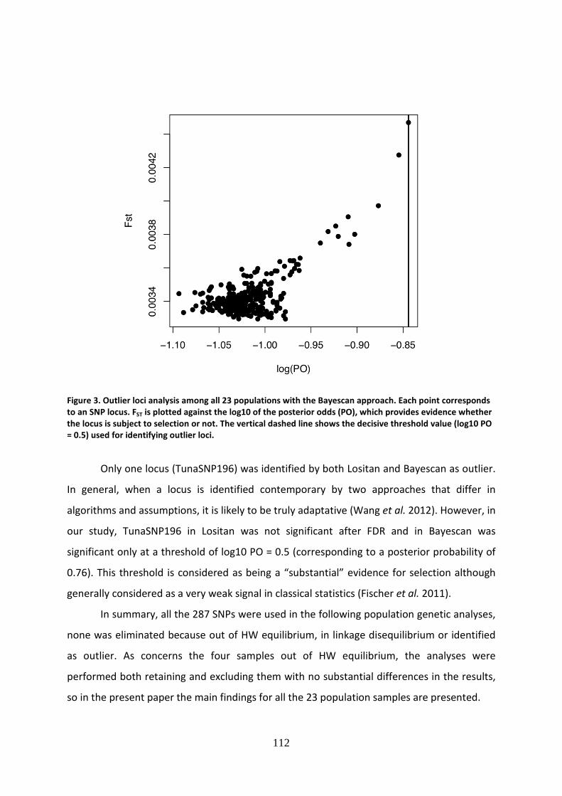
112

Figure 3. Outlier loci analysis among all 23 populations with the Bayescan approach. Each point corresponds

to an SNP locus. FST is plotted against the log10 of the posterior odds (PO), which provides evidence whether

the locus is subject to selection or not. The vertical dashed line shows the decisive threshold value (log10 PO

= 0.5) used for identifying outlier loci.

Only one locus (TunaSNP196) was identified by both Lositan and Bayescan as outlier.

In general, when a locus is identified contemporary by two approaches that differ in

algorithms and assumptions, it is likely to be truly adaptative (Wang et al. 2012). However, in

our study, TunaSNP196 in Lositan was not significant after FDR and in Bayescan was

significant only at a threshold of log10 PO = 0.5 (corresponding to a posterior probability of

0.76). This threshold is considered as being a “substantial” evidence for selection although

generally considered as a very weak signal in classical statistics (Fischer et al. 2011).

In summary, all the 287 SNPs were used in the following population genetic analyses,

none was eliminated because out of HW equilibrium, in linkage disequilibrium or identified

as outlier. As concerns the four samples out of HW equilibrium, the analyses were

performed both retaining and excluding them with no substantial differences in the results,

so in the present paper the main findings for all the 23 population samples are presented.

113

Population genetic structure

The genetic differentiation measured among all population samples at the 287 loci

was not significant, with an overall FST value of -0.00024 (P-value > 0.05). The pairwise FST

values among samples calculated over the 287 SNP loci were very low, with only one

significant pairwise value after FDR correction (FST = 0.00448) between CMED-SI-J and EMED-

LS-M. According to these results, the distribution of locus-by-locus AMOVA FST estimates

showed that about half of the 287 loci (145 SNPs) displayed negative values and only 54 loci

were above a value FST > 0.005.

As for all 23 samples, the distribution of locus-by-locus FST estimates considering only

the six reference samples of the spawning populations (i.e. EMED-LS-LA+0, WMED-TY-0,

WMED-BA-0-2009, WMED-BA-0-2010, WMED-BA-0 and GOM-LA+0) showed that more than

half of the 287 loci (155 SNPs) displayed negative values, 68 loci were with FST > 0.005 and 35

loci had a value of FST > 0.01. When the four reference samples of Western Mediterranean

origin were pooled together, 62 loci had FST > 0.005 and 31 loci FST > 0.01. All these different

panels of loci (54, 68, 35, 62, 31 loci with the highest individual FST values) were tested for

their capacity in differentiating among the three known spawning areas (Eastern

Mediterranean, Western Mediterranean, Gulf of Mexico, henceforth indicated as EMED,

WMED and GOM). The 31 SNPs allowed to measure the highest overall value of FST (0.00945,

with P-value = 0.04106 ± 0.00572) among the reference samples with almost all significant

pairwise FST values between EMED-LS-LA+0, GOM-LA+0 and the other Western

Mediterranean reference samples (Table 5, Figure 4).

EMED-LS-

LA+0

WMED-

BA-0

WMED-BA-0-

2009

WMED-BA-0-

2010

WMED-

TY-0

GOM-

LA+0

EMED-LS-LA+0 0 0,0001 0,04297 0 0

WMED-BA-0 0,02006 0,73211 0,66439 0,96773 0,0002

WMED-BA-0-2009 0,01636 -0,00253 0,7126 0,50718 0

WMED-BA-0-2010 0,0072 -0,00162 -0,00249 0,7322 0,00396

WMED-TY-0 0,02032 -0,00592 -0,00077 -0,00249 0,0001

GOM-LA+0 0,01817 0,01758 0,0199 0,0141 0,0184

Table 5. Matrix of pairwise FST values (below the diagonal) and P-values (above the diagonal) among

reference populations using the 31 SNPs. Significant values after FDR correction are in bold underlined.

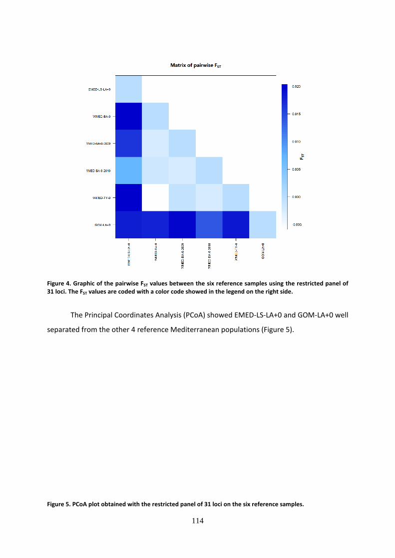
Figure 4. Graphic of the pairwise F

31 loci. The FST values are coded with a color code showed in the legend on the right side.

The Principal Coordinates Analysis (PCoA) showed EMED

separated from the other 4 reference Mediterranean populations (Figure 5).

Figure 5. PCoA plot obtained with the restricted panel of 31 loci on the six reference samples.

114

Figure 4. Graphic of the pairwise FST values between the six reference samples using the restricted panel of

values are coded with a color code showed in the legend on the right side.

The Principal Coordinates Analysis (PCoA) showed EMED-LS-LA+0 and GOM

rom the other 4 reference Mediterranean populations (Figure 5).

Figure 5. PCoA plot obtained with the restricted panel of 31 loci on the six reference samples.

values between the six reference samples using the restricted panel of

values are coded with a color code showed in the legend on the right side.

LA+0 and GOM-LA+0 well

rom the other 4 reference Mediterranean populations (Figure 5).

Figure 5. PCoA plot obtained with the restricted panel of 31 loci on the six reference samples.

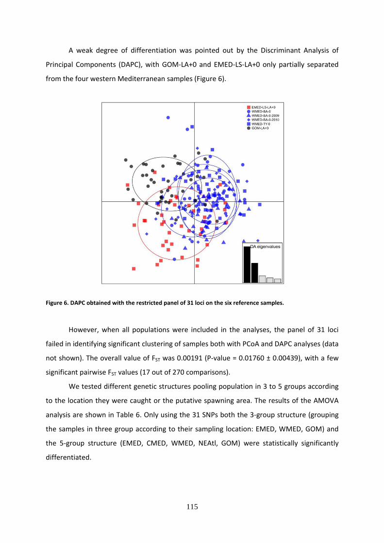
115

A weak degree of differentiation was pointed out by the Discriminant Analysis of

Principal Components (DAPC), with GOM-LA+0 and EMED-LS-LA+0 only partially separated

from the four western Mediterranean samples (Figure 6).

Figure 6. DAPC obtained with the restricted panel of 31 loci on the six reference samples.

However, when all populations were included in the analyses, the panel of 31 loci

failed in identifying significant clustering of samples both with PCoA and DAPC analyses (data

not shown). The overall value of FST was 0.00191 (P-value = 0.01760 ± 0.00439), with a few

significant pairwise FST values (17 out of 270 comparisons).

We tested different genetic structures pooling population in 3 to 5 groups according

to the location they were caught or the putative spawning area. The results of the AMOVA

analysis are shown in Table 6. Only using the 31 SNPs both the 3-group structure (grouping

the samples in three group according to their sampling location: EMED, WMED, GOM) and

the 5-group structure (EMED, CMED, WMED, NEAtl, GOM) were statistically significantly

differentiated.

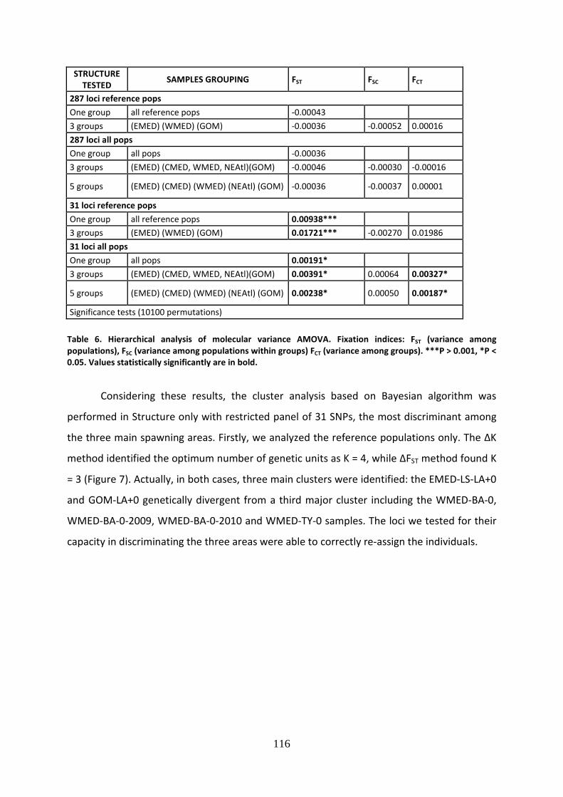
116

STRUCTURE

TESTED SAMPLES GROUPING FST FSC FCT

287 loci reference pops

One group all reference pops -0.00043

3 groups (EMED) (WMED) (GOM) -0.00036 -0.00052 0.00016

287 loci all pops

One group all pops -0.00036

3 groups (EMED) (CMED, WMED, NEAtl)(GOM) -0.00046 -0.00030 -0.00016

5 groups (EMED) (CMED) (WMED) (NEAtl) (GOM) -0.00036 -0.00037 0.00001

31 loci reference pops

One group all reference pops 0.00938***

3 groups (EMED) (WMED) (GOM) 0.01721*** -0.00270 0.01986

31 loci all pops

One group all pops 0.00191*

3 groups (EMED) (CMED, WMED, NEAtl)(GOM) 0.00391* 0.00064 0.00327*

5 groups (EMED) (CMED) (WMED) (NEAtl) (GOM) 0.00238* 0.00050 0.00187*

Significance tests (10100 permutations)

Table 6. Hierarchical analysis of molecular variance AMOVA. Fixation indices: FST (variance among

populations), FSC (variance among populations within groups) FCT (variance among groups). ***P > 0.001, *P <

0.05. Values statistically significantly are in bold.

Considering these results, the cluster analysis based on Bayesian algorithm was

performed in Structure only with restricted panel of 31 SNPs, the most discriminant among

the three main spawning areas. Firstly, we analyzed the reference populations only. The ΔK

method identified the optimum number of genetic units as K = 4, while ΔFST method found K

= 3 (Figure 7). Actually, in both cases, three main clusters were identified: the EMED-LS-LA+0

and GOM-LA+0 genetically divergent from a third major cluster including the WMED-BA-0,

WMED-BA-0-2009, WMED-BA-0-2010 and WMED-TY-0 samples. The loci we tested for their

capacity in discriminating the three areas were able to correctly re-assign the individuals.

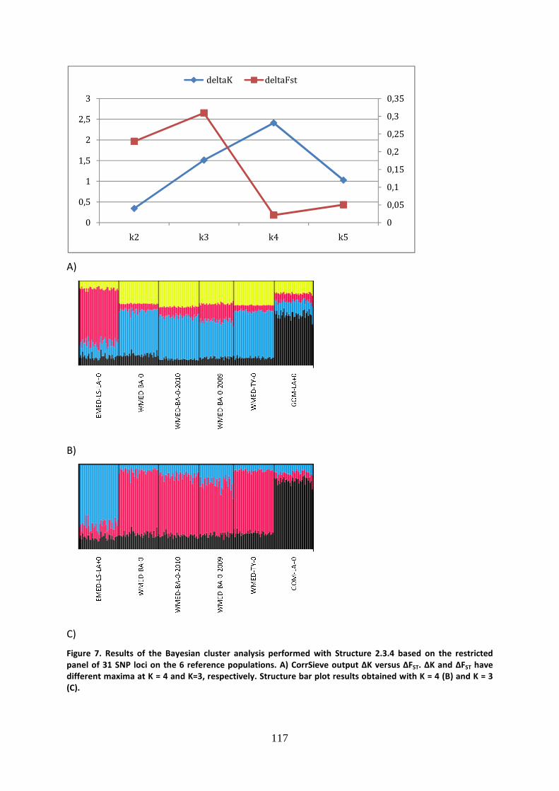
A)

B)

C)

Figure 7. Results of the Bayesian cluster analysis performed with Structure 2.3.4 based on the restricted

panel of 31 SNP loci on the 6 reference populations. A) CorrSieve output

different maxima at K = 4 and K=3, respectiv

(C).

0

0,5

1

1,5

2

2,5

3

k2 k3

117

Figure 7. Results of the Bayesian cluster analysis performed with Structure 2.3.4 based on the restricted

panel of 31 SNP loci on the 6 reference populations. A) CorrSieve output ΔK versus Δ

different maxima at K = 4 and K=3, respectively. Structure bar plot results obtained with K = 4 (B) and K = 3

0

0,05

0,1

0,15

0,2

0,25

0,3

0,35

k3 k4 k5

deltaK deltaFst

Figure 7. Results of the Bayesian cluster analysis performed with Structure 2.3.4 based on the restricted

ΔFST. ΔK and ΔFST have

ely. Structure bar plot results obtained with K = 4 (B) and K = 3

However, when the 31 SNPs were used to identify clusters on the 17

breeding/feeding aggregates the results didn’t provide any signal of genetic structuring.

The relative genetic

phylogenetic analyses using the D

are shown schematically in Figure 8, using the whole dataset of 287 SNPs and the restricted

panel of 31 loci, respectively. No geographical clustering of populations is evident.

Analogously, no groups composed of genetically similar individuals could be detected in the

phylogenetic network obtained in Splitstree (data not shown).

A)

B)

118

However, when the 31 SNPs were used to identify clusters on the 17

breeding/feeding aggregates the results didn’t provide any signal of genetic structuring.

The relative genetic similarity among the 23 samples was investigated also by

phylogenetic analyses using the DA distances (Nei 1983). The relationships among samples

are shown schematically in Figure 8, using the whole dataset of 287 SNPs and the restricted

panel of 31 loci, respectively. No geographical clustering of populations is evident.

composed of genetically similar individuals could be detected in the

phylogenetic network obtained in Splitstree (data not shown).

However, when the 31 SNPs were used to identify clusters on the 17

breeding/feeding aggregates the results didn’t provide any signal of genetic structuring.

similarity among the 23 samples was investigated also by

distances (Nei 1983). The relationships among samples

are shown schematically in Figure 8, using the whole dataset of 287 SNPs and the restricted

panel of 31 loci, respectively. No geographical clustering of populations is evident.

composed of genetically similar individuals could be detected in the

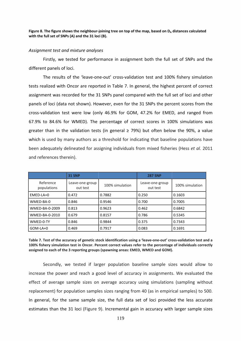
119

Figure 8. The figure shows the neighbour-joining tree on top of the map, based on DA distances calculated

with the full set of SNPs (A) and the 31 loci (B).

Assignment test and mixture analyses

Firstly, we tested for performance in assignment both the full set of SNPs and the

different panels of loci.

The results of the ‘leave-one-out’ cross-validation test and 100% fishery simulation

tests realized with Oncor are reported in Table 7. In general, the highest percent of correct

assignment was recorded for the 31 SNPs panel compared with the full set of loci and other

panels of loci (data not shown). However, even for the 31 SNPs the percent scores from the

cross-validation test were low (only 46.9% for GOM, 47.2% for EMED, and ranged from

67.9% to 84.6% for WMED). The percentage of correct scores in 100% simulations was

greater than in the validation tests (in general ≥ 79%) but often below the 90%, a value

which is used by many authors as a threshold for indicating that baseline populations have

been adequately delineated for assigning individuals from mixed fisheries (Hess et al. 2011

and references therein).

31 SNP

287 SNP

Reference

populations

Leave-one-group

out test 100% simulation

Leave-one-group

out test 100% simulation

EMED-LA+0 0.472 0.7882 0.250 0.1603

WMED-BA-0 0.846 0.9546 0.700 0.7005

WMED-BA-0-2009 0.813 0.9623 0.462 0.6842

WMED-BA-0-2010 0.679 0.8157 0.786 0.5345

WMED-0-TY 0.846 0.9844 0.375 0.7343

GOM-LA+0 0.469 0.7917 0.083 0.1691

Table 7. Test of the accuracy of genetic stock identification using a ‘leave-one-out’ cross-validation test and a

100% fishery simulation test in Oncor. Percent correct values refer to the percentage of individuals correctly

assigned to each of the 3 reporting groups (spawning areas: EMED, WMED and GOM).

Secondly, we tested if larger population baseline sample sizes would allow to

increase the power and reach a good level of accuracy in assignments. We evaluated the

effect of average sample sizes on average accuracy using simulations (sampling without

replacement) for population samples sizes ranging from 40 (as in empirical samples) to 500.

In general, for the same sample size, the full data set of loci provided the less accurate

estimates than the 31 loci (Figure 9). Incremental gain in accuracy with larger sample sizes

was measured. The average correct re

threshold of the 90% (critical level to determine whether the reference population is

acceptably identifiable, Seeb

per populations for the full data set and the 31 SNPs, respectively

A)

B)

Figure 9. Results of 100% simulations test in Oncor comparing the effect on the accuracy of self

of increasing baseline sample sizes using (A) the full data

Considering the findings previously described, for the assignment and mixture

analyses of all populations only the ‘best performing’ panel of 31 SNPs panel was tested.

120

verage correct re-assignment in the 100% simulation tests reached the

threshold of the 90% (critical level to determine whether the reference population is

acceptably identifiable, Seeb et al. 2000) with a sample size of 100 fish and 50 fish sampled

pulations for the full data set and the 31 SNPs, respectively (Figure 9)

Figure 9. Results of 100% simulations test in Oncor comparing the effect on the accuracy of self

of increasing baseline sample sizes using (A) the full data set of 287 loci and (B) the 31 selected SNPs.

Considering the findings previously described, for the assignment and mixture

analyses of all populations only the ‘best performing’ panel of 31 SNPs panel was tested.

assignment in the 100% simulation tests reached the

threshold of the 90% (critical level to determine whether the reference population is

2000) with a sample size of 100 fish and 50 fish sampled

(Figure 9).

Figure 9. Results of 100% simulations test in Oncor comparing the effect on the accuracy of self-assignment

set of 287 loci and (B) the 31 selected SNPs.

Considering the findings previously described, for the assignment and mixture

analyses of all populations only the ‘best performing’ panel of 31 SNPs panel was tested.

121

The assignment test performed in Geneclass2 with the 31 SNPs indicated a prevalent

contribution of the WMED reference samples to the feeding/breeding aggregates, except, as

expected, in the reference populations from the Levantine Sea and Gulf of Mexico (Table 8).

Exclusion analysis found that for 4 tunas, the probability of their assigning to the

reference population was less than 0.05, indicating that they are to be excluded from the

population to which they were assigned. However, the fishes that exceeded the assignment

probability threshold of 90% was only 84 (9.9% of the total individuals in the dataset)

confirming the low performance (accuracy) of the select SNPs.

Similarly, the assignment analyses performed in Oncor assigned the majority of tunas

from the breeding/feeding samples to the WMED area. Still, the individuals with > 90%

probability of assignment to their ‘best-estimate’ reporting group were only 191 (21% of the

total individuals in the dataset) (Figure 10).

Sample N EMED WMED GOM EMED% WMED% GOM%

EMED-LS-LA+0 39 34 3 2 87,18 7,69 5,13

EMED-LS-M 40 6 30 4 15,00 75,00 10,00

EMED-LS-L 40 10 25 5 25,00 62,50 12,50

EMED-LS-M-2007 38 4 26 8* 10,53 68,42 21,05

CMED-AS-J 40 8 25 7 20,00 62,50 17,50

CMED-MA-L 21 13 8 0,00 61,90 38,10

CMED-SI-J 36 3 28 5 8,33 77,78 13,89

CMED-SI-M 39 6 23 10 15,38 58,97 25,64

WMED-TY-0 40 5 35 12,50 87,50 0,00

WMED-TY-M 38 7 27 4 18,42 71,05 10,53

WMED-LI-J 39 6 26 7 15,38 66,67 17,95

WMED-SA-M 35 7 26 2 20,00 74,29 5,71

WMED-SA-L 39 7 24 8* 17,95 61,54 20,51

WMED-GL-J 39 4* 26 9 10,26 66,67 23,08

WMED-BA-0-2009 40 5 31 4 12,50 77,50 10,00

WMED-BA-0-2010 34 5 26 3 14,71 76,47 8,82

WMED-BA-0 39 2 35 2 5,13 89,74 5,13

WMED-BA-J 28 7 18 3 25,00 64,29 10,71

NEAtl-GI-L 29 3 21 5 10,34 72,41 17,24

NEAtl-BB-J 40 5 29 6 12,50 72,50 15,00

NEAtl-PO-L 38 9* 21 8 23,68 55,26 21,05

NEAtl-BB-M 39 8 25 6 20,51 64,10 15,38

GOM-LA+0 38 1 3 34 2,63 7,89 89,47

Total 848 152 546 150 17,92 64,39 17,69

Table 8. Geneclass assignment test. Individual assignment analysis of the 23 population samples towards the

geographical reference populations. In this analysis, the four reference samples from the WMED were

pooled. * indicates that 1 individual has to be excluded (see text for details).

A)

B)

Figure 10. Percentage of tunas assigned by the as

areas EMED, WMED, GOM. A) individuals assigned to their ‘best

assigned with < 90% of probability of correct assignment are reported as unassigned. See text for

details.

Finally, a mixture analysis on our samples was performed in Oncor; Table 9 illustrates

the main results. On the overall, the vast majority of juveniles/adults were assigned to the

122

Figure 10. Percentage of tunas assigned by the assignment test performed by Oncor to the three spawning

areas EMED, WMED, GOM. A) individuals assigned to their ‘best-estimate’ reporting group. B) individuals

assigned with < 90% of probability of correct assignment are reported as unassigned. See text for

Finally, a mixture analysis on our samples was performed in Oncor; Table 9 illustrates

the main results. On the overall, the vast majority of juveniles/adults were assigned to the

signment test performed by Oncor to the three spawning

estimate’ reporting group. B) individuals

assigned with < 90% of probability of correct assignment are reported as unassigned. See text for further

Finally, a mixture analysis on our samples was performed in Oncor; Table 9 illustrates

the main results. On the overall, the vast majority of juveniles/adults were assigned to the

123

WMED reference population (~ 69%), ~ 19% of individuals were assigned to EMED and ~ 12%

to GOM. The very broad confidence intervals for these assignments (often including 0% and

hence to be regarded as not significant according to Habicht et al. 2010) confirm that the loci

have a very low resolutive power also for this application.

Population sample EMED % (95% CI) WMED % (95% CI) GOM % (95% CI)

EMED-LS-M 0.0045 (0.111, 0.829) 0.9457 (0, 0.556) 0.0497 (0.001, 0.652)

EMED-LS-L 0.2943 (0.196, 0.831) 0.595 (0, 0.432) 0.1108 (0.023, 0.665)

EMED-LS-M-2007 0.0736 (0.085, 0.68) 0.6168 (0, 0.421) 0.3097 (0.203, 0.787)

CMED-AS-J 0.235 (0.183, 0.761) 0.7018 (0, 0.503) 0.0633 (0.069, 0.673)

CMED-MA-L 0.1669 (0.004, 0.794) 0.6479 (0, 0.596) 0.1852 (0.042, 0.866)

CMED-SI-J 0.1135 (0.091, 0.82) 0.6977 (0, 0.503) 0.1888 (0.088, 0.712)

CMED-SI-M 0.2131 (0.082, 0.661) 0.4811 (0, 0.381) 0.3057 (0.221, 0.874)

WMED-TY-M 0.3613 (0.217, 0.846) 0.637 (0, 0.503) 0.0017 (0, 0.653)

WMED-LI-J 0.0107 (0.062, 0.695) 0.8927 (0, 0.617) 0.0966 (0.039, 0.68)

WMED-SA-M 0.3168 (0.329, 0.988) 0.6832 (0.001, 0.634) 0 (0, 0.264)

WMED-SA-L 0.2827 (0.153, 0.718) 0.4613 (0, 0.384) 0.256 (0.126, 0.774)

WMED-GL-J 0.1267 (0.058, 0.769) 0.7395 (0, 0.474) 0.1338 (0.119, 0.798)

WMED-BA-J 0.3217 (0.219, 0.905) 0.6777 (0, 0.579) 0.0006 (0, 0.639)

NEAtl-GI-L 0.1301 (0.001, 0.663) 0.8386 (0.005, 0.75) 0.0313 (0, 0.72)

NEAtl-BB-J 0.0004 (0, 0.586) 0.719 (0, 0.524) 0.2807 (0.214, 0.882)

NEAtl-PO-L 0.0863 (0.043, 0.728) 0.7936 (0, 0.574) 0.1201 (0.031, 0.75)

NEAtl-BB-M 0.438 (0.342, 0.951) 0.5616 (0.001, 0.474) 0.0003 (0, 0.421)

EMED-LS-LA+0 0.998 (0.771, 1) 0.0019 (0, 0.066) 0.0001 (0, 0.218)

WMED-TY-0 0 (0, 0.494) 0.9998 (0.286, 0.975) 0.0002 (0, 0.496)

WMED-BA-0-2009 0.0004 (0.001, 0.571) 0.9996 (0.291, 0.965) 0 (0, 0.433)

WMED-BA-0-2010 0.099 (0.019, 0.734) 0.901 (0.082, 0.812) 0 (0, 0.52)

WMED-BA-0 0.0276 (0, 0.47) 0.9724 (0.232, 0.898) 0.0001 (0.001, 0.537)

GOM-LA+0 0 (0, 0.24) 0.0111 (0, 0.041) 0.9889 (0.752, 1)

Table 9. Percentage and 95% confidence intervals of juvenile/adult samples assigned by mixture analysis

performed in Oncor to the three reporting areas (EMED, WMED, GOM). Reference population samples are in

red.

124

Discussion

The Atlantic bluefin tuna (Thunnus thynnus) is one of the most depleted species of

tunas; even though it has been continually exploited for thousands of years, only in these

last decades the exploitation rate was reported to be far beyond the sustainable level, with a

quite high risk of fisheries and stock collapse (Safina 2008).

The species used to be distributed widely throughout the north Atlantic Ocean,

Mediterranean Sea and Black Sea, but its biogeographic range has contracted since the

1950s (MacKenzie and Mariani 2012). After large catches in the 1960s, the species collapsed

from the coasts off Norway and Brazil (Fromentin and Powers 2005; MacKenzie and Myers

2007; ICCAT 2012) and, in the late 1980s, it disappeared also from the Black Sea (MacKenzie

and Mariani 2012). According to these authors, this population should had peculiar

phenotypic (genetic) adaptations in order to reproduce successfully in the specific

hydrographic (estuarine) conditions of the Black Sea. The disappearance of past fisheries

suggest that important changes in the spatial dynamics of bluefin tuna may have resulted

from fishing but also from interactions between biological factors and environmental

variations (ICCAT 2012). In general, the loss of this locally-adapted reproducing populations

is alarming because it represents a dangerous decline in population richness and an increase

in species vulnerability to human-driven perturbations (exploitation and environmental

change) (MacKenzie and Mariani 2012).

The identification of substructuring and local populations is of paramount importance

for the proper management of T. thynnus, but it is a very complex task. The need to

elucidate appropriate management units for ABFT and the actual existence of separate

stocks led to several genetic studies. The genetic structure of Atlantic bluefin tuna was early

studied using molecular markers with low discriminating power, as allozymes (Pujolar et al.

2003) and mithocondrial sequences (Ely et al. 2002; Alvarado Bremer et al. 2005), unsuitable

to detect population differentiation. More recently, markers more used to investigate

population structure of this species were microsatellites (Carlsson et al. 2004, 2007), that

present a high polymorphism degree but have the technical drawback because it isn’t always

possible to compare data produced by different laboratories, due to the eventuality of

inconsistencies in allele size calling caused by variety in sequencing machine, fluorescent dye

and allele calling software (Vignal et al. 2002; Guichoux et al. 2011). In recent years, SNPs

125

have demonstrated more suitable markers in studies of population genetics and they are

already applied to research in various fish species (Poulsen et al. 2011; Deagle et al. 2012;

Hess et al. 2012; Limborg et al. 2012b). A single multiallelic microsatellites has more

statistical power than one bi-allelic SNP, so it’s necessary to use a large numbers of these

markers to obtain a comparable power to detect divergences between populations. The aim

of this work was to examine a wide set of 384 SNP markers newly developed for Atlantic

bluefin tuna (see chapter 4 of this thesis) to choose a panel of high informative loci that

provide enough statistical power to detect fine-scale population differences and that could

be used to a better management of stocks.

Previous studies on population dynamics of Atlantic bluefin tuna were often

conducted on a restricted number of individuals, and this may have been another limiting

factor in the identification of a population structure (see Viñas et al. 2011 and references

therein). To overcome this limits, in our study an intensive sampling effort was performed

and we analyzed a total of 919 individuals (23 population samples), collected from Gulf of

Mexico to entire Mediterranean basin, including individuals of all size/age classes, from

larvae to adults, in order to have a more robust and complete dataset of the reproductive

populations and ecological aggregates of the Atlantic bluefin tuna. To avoid the confounding

effect of mixed populations (typically occurring at foraging grounds) adult spawners at

advanced maturation stage were collected during the spawning season in 2011. Larvae and

age-0 from the EMED, WMED and GOM were analyzed, because they are unlikely to have

undertaken long distance movements and thus they are representative of their respective

spawning populations. Juveniles, medium-sized as well as large adult specimens were also

collected from various locations.

As regards the molecular markers, we used a set of species-specific high performance

genetic loci developed by novel Next Generation Sequencing (NGS) technologies, that

offered the opportunity to obtain several hundreds/thousands of Single Nucleotide

Polymorphisms (SNPs) in expressed gene sequences in non-model species with cheaper and

more reliable high throughput genotyping technologies (Garvin et al. 2010; Ekblom and

Galindo 2011; Nielsen et al. 2011). Using a combined approach of transcriptomic and

genomic resources, we can obtained a conversion rate (number of working and polymorphic

SNPs) of 70%, more higher than that achieved in previous studies for non validated SNPs

126

developed from EST-sequencing of non model organism, where the result was

approximately 30% (Milano et al. 2011).

In our study the analysis of 848 individual with 287 SNP led to detect an extremely

low and not significant level of genetic differentiation among all bluefin tuna population

samples. The adult samples resulted genetically undifferentiated between them and from

the reference samples of the spawning populations, using both entire set of loci than the

restricted panel of SNP. The pairwise Fst values observed were very low, and ranged between

-0.5% to 0.5%. These results are consistent with the values found in previous studied on

Thunnus thynnus, with mitochondrial sequences (0.2% < Fst > 3%) and microsatellites, both

neutral (0.5% < Fst > 2%) and EST-linked (-0.5% < Fst > 0.3%) (Carlsson et al. 2004, 2007;

Boustany et al. 2008; Ferrara et al. 2010; Riccioni et al. 2010). The lack of genetic

differentiation is expected in T. thynnus, a highly vagile species with large populations size

(Ely et al. 2002; Palumbi 2003; Viñas et al. 2011,). Atlantic bluefin tuna, similar to other large

pelagic fishes, have in fact the potential to migrate over extensive distances (Mather et al.

1995; Block et al. 2001) and sampling in a location may be composed of individuals

originating from more than one spawning area, preventing the detection of genetic

population structure. The occurrence of even very low levels of mixing among supposed

isolated regions, that can be under noticed due to the limits in resolution power of tagging

studies and other techniques, are enough to genetically homogenize the populations (Viñas

et al. 2011).

Our results pointed out also the lack of significant genetic differences among

temporal replicate samples of age-0 and larvae from the western Mediterranean. This is

indicative of an absence of family effect (Allendorf-Phelps effect), validating the assumption

that the samples were not the progeny of a few breeding adults rather than entire

population (Allendorf and Phelps 1981; Waples 1998).

Loci influenced by selection could have provide a more precise indication of genetic

structure than other loci. Such loci could have been particularly helpful for assessing relative

differences in levels of gene flow, especially in high gene flow species and highly migratory

behavior, as showed in several papers (Renaut et al. 2010; Freamo et al. 2011; Hess et al.

2011; Guichoux et al. 2012; Renaut et al. 2012). In fact, if overall gene flow is high,

differences in levels of diversity or in allele frequencies among populations might be slight

and error-prone (Waples 1998; Neigel 2002). In contrast, as selection can reduce effective

127

gene flow and increase divergence, the signature of asymmetric gene flow should be strong

at loci under divergent selection (Guichoux et al. 2012). However, in our study, the different

used approaches demonstrated an insufficient sensitivity to identify loci that were under

weak selection, that can cause small differences in allele frequencies of candidate loci

among populations, resulting in lower values of FST (Narum and Hess 2011). Our scenario

could have been worse by presence of loci under balancing selection, that drive to

homogenize differences between population more than neutral loci (Helyar et al. 2011;

Narum and Hess 2011).

According to Kalinowski et al. (2011), when the goal of a genetic study is to

summarize genetic differences among populations, traditional methods can be very effective

for displaying population structure, even when populations have not had a hierarchical

history of population fragmentation. Phylogenetic trees can contain much more information

about population structure than results from more popular approaches such as those

implemented in Structure (Kalinowski et al. 2011). In our study, we used the method

Neighbor-net, successfully adopted by Willing et al. (2010) and Kraus et al. (2013) to display

reticulate relationships among individuals and populations using SNP data. If populations are

differentiated from each other, the Neighbor-net algorithm would display reticulate

relationships more densely within less differentiated groups and less densely in more

differentiated groups (Kraus et al. 2013). The networks obtained from our data were ‘bush-

like’ (sensu Kraus et al. 2013) and confirmed once more the lacking of any population

genetic structure.

Finally, because individual assignment tests based on genetic data have proven to be

effective stock identification tools in many studies (Habicht et al. 2010; Beacham et al. 2011;

Hess et al. 2011; Templin et al. 2011), this approach was also tested.

At present, two main classes of genetic markers are commonly used in genetic stock

identification (GSI) applications: microsatellites and SNPs. High resolution of stock

composition estimation is a function of accurate estimation of allele frequencies of the

genetic markers used (‘‘sampling error’’), and of the degree of genetic differentiation among

populations in the suite of genetic markers applied in estimation of stock composition

(‘‘genetic error’’). Both factors influence the accuracy of estimates of stock composition

when applied to mixed-stock fishery samples compositions (Beacham et al. 2011). Previous

studies have shown that for populations with very low FST (< 0.1), assignment programs can

128

be unreliable (Latch et al. 2006). A value of FST = 0.05 is recommended by the same authors

for 97% accuracy of assignment even if most GSI (Genetic Stock Identification) applications

demand a lower level of accuracy (e.g. 90% correct assignment) to be useful in management

decisions (Beacham et al. 2011).

In our study the low level of differentiation observed for the markers used (see

results) resulted in insufficient power to apply such methods adequately (Vasemägi and

Primmer 2005). Our panel of SNP loci lacks this accuracy; in fact, even if we consider the

most resolutive panel (31 SNPs), the overall FST for all samples included in the baseline was

0.0094 and 0.0019 for the overall dataset. Furthermore, the sample sizes of our baseline

collections (especially EMED and GOM) were relatively small (< 50 individuals), which may

have decreased the accuracy of estimates of allele frequencies.

In general, if genetic differentiation among populations is limited, larger baseline

population sample sizes may be required and more markers incorporated in the panel for

stock identification to provide the maximum differentiation possible (Beacham et al. 2011).

The slight differences measured with the restricted panel of 31 SNPs among the

reference populations between western and eastern spawning samples, partially confirm the

genetic results obtained by Carlsson et al. (2004, 2007) and Boustany et al. (2008), and,

combined with the finding of mature bluefin tuna in this latter area (Karakulak et al. 2004a)

and the presence of a resident tuna component in the eastern Mediterranean throughout

the year (Di Natale et al. 2005; Oray and Karakulak 1997), suggests the presence of a

genetically independent stock of bluefin tuna in the eastern basin of the Mediterranean Sea.

Differences in spawning times among Mediterranean regions could also support the

existence of distinct populations within this sea, in fact spawning occur in June-July in the

western Mediterranean (Susca et al. 2001; Corriero et al. 2003), and on May-June in the

eastern basin (Karakulak et al. 2004b). This hypothesis could be confirmed by tagging data,

as none of the individuals tagged in the western Atlantic and western Mediterranean were

ever spotted in the Levantine, Aegean or Adriatic Seas, and the most eastern locations were

found in the central Mediterranean (Block et al. 2005; De Metrio et al. 2005).

Currently, Atlantic bluefin tuna was managed by ICCAT as two different stocks,

divided in the Atlantic ocean at 45th W meridian. This separation was supported by

identification of two spawning area, one in the Gulf of Mexico e one in the Mediterranean

sea (Mather et al. 1995; ICCAT 2002; Rooker et al. 2008). The Mediterranean basin is treated

129

as a single unit, but our preliminary results could be suggested a possible division in two

different areas that may require a separate approach to avoid the impact of a type II error

that could lead to the possible loss of the regional subpopulations. Future studies of bluefin

tuna population genetics are essentials to go deeper in the structure of this important

commercial species for a better understanding of strategies that will be adopted for its

conservation. It should be necessary to incorporate more samples from eastern

Mediterranean, that is the area less investigate of entire range of Atlantic bluefin tuna. If the

existence of one or more genetically independent bluefin tuna stocks in the eastern basin of

the Mediterranean Sea will be confirmed, this should be taken into consideration when

making decisions concerning the management and conservation of the species.

130

References

Allendorf FW, Phelps SR (1981) Use of allelic frequencies to describe population-structure.

Canadian Journal of Fisheries and Aquatic Sciences 38,1507-1514.

Alvarado-Bremer JR, Viñas J, Mejuto J, Ely B, Pla C (2005) Comparative phylogeography of

Atlantic bluefin tuna and swordfish: the combined effects of vicariance, secondary

contact, introgression, and population expansion on the regional phylogenies of two

highly migratory pelagic fishes. Molecular Phylogenetics and Evolution 36, 169-187.

Anderson EC, Waples RS, Kalinowski ST (2008). An improved method for estimating the

accuracy of genetic stock identification. Canadian Journal of Fisheries and Aquatic

Sciences 65, 1475-1486.

Antao T, Lopes A, Lopes RJ, Beja-Pereira A, Luikart G (2008) LOSITAN: A workbench to detect

molecular adaptation based on a FST-outlier method. BMC Bioinformatics 9, 323.

Beacham TD, McIntosh B, Wallace CG (2011) A comparison of polymorphism of genetic

markers and population sample sizes required for mixed-stock analysis of sockeye

salmon (Oncorhynchus nerka) in British Columbia. Canadian Journal of Fisheries and

Aquatic Sciences 68(3), 550-562.

Beaumont MA, Nichols RA (1996) Evaluating Loci for Use in the Genetic Analysis of

Population Structure. Proceedings of the Royal Society of London. Series B: Biological

Sciences 263, 1619-1626.

Beaumont MA, Balding DJ (2004) Identifying adaptive genetic divergence among populations

from genome scans. Molecular Ecology 13, 969-980.

Benjamini Y, Yekutieli D (2001) The Control of the False Discovery Rate in Multiple Testing

under Dependency. The Annals of Statistics 29, 1165-1188.

Block BA, Dewar H, Blackwell SB, Williams TD, Prince ED, et al. (2001) Migratory movements,

depth preferences, and thermal biology of Atlantic bluefin tuna. Science 293, 1310-

1314.

Block BA, Teo SL, Walli A, Boustany A, Stokesbury MJ, et al. (2005) Electronic tagging and

population structure of Atlantic bluefin tuna. Nature 434, 1121-1127.

131

Bourret V, Kent MP, Primmer CR, Vasemägi A, Karlsson S, et al. (2012) SNP-array reveals

genome-wide patterns of geographical and potential adaptive divergence across the

natural range of Atlantic salmon (Salmo salar). Molecular ecology DOI:

10.1111/mec.12003.

Boustany AM, Reeb CA, Block BA (2008) Mitochondrial DNA and electronic tracking reveal

population structure of Atlantic bluefin tuna (Thunnus thynnus). Marine Biology 156,

13-24.

Bryant D, Moulton V (2004) Neighbor-Net: An Agglomerative Method for the Construction of

Phylogenetic Networks. Molecular Biology and Evolution 21, 255-265.

Campana MG, Hunt HV, Jones H, White J (2011) CorrSieve: software for summarizing and

evaluating Structure output. Molecular Ecology Resources 11, 349-352.

Carlsson J, McDowell JR, Díaz-Jaimes P, Carlsson JEL, Boles SB, et al. (2004) Microsatellite and

mitochondrial DNA analyses of Atlantic bluefin tuna (Thunnus thynnus thynnus)

population structure in the Mediterranean sea. Molecular Ecology 13, 3345-3356.

Carlsson J, McDowell JR, Carlsson L, Graves JE (2007) Genetic identity of YOY bluefin tuna

from the eastern and western Atlantic spawning areas. Heredity 98, 23-28.

Carvajal-Rodriguez A, de Uña-Alvarez J (2011) Assessing Significance in High-Throughput

Experiments by Sequential Goodness of Fit and q-Value Estimation. PLoS ONE 6(9),

e24700.

Cornuet JM, Piry S, Luikart G, Estoup A, Solignac M (1999) New Methods Employing

Multilocus Genotypes to Select or Exclude Populations as Origins of Individuals.

Genetics 153, 1989-2000.

Corriero A, Desantis S, Deflorio M, Acone F, Bridges CR, et al. (2003) Histological

investigation on the ovarian cycle of the bluefin tuna in the western and central

Mediterranean. Journal of Fish Biology 63, 108-119.

Deagle BE, Jones FC, Chan YF, Absher DM, Kingsley DM, et al. (2012) Population genomics of

parallel phenotypic evolution in stickleback across stream-lake ecological transitions.

Proceedings of the Royal Society B:Biological Sciences 279, 1277-1286.

De Metrio G, Arnold GP, De la Serna JM, Block BA, Megalofonou P, et al. (2005) Movements

of bluefin tuna (Thunnus thynnus L.) tagged in the Mediterranean Sea with pop-up

satellite tags. ICCAT Col. Vol. Sci. Pap. 58, 1337-1340.

132

Di Natale A, Mangano A, Asaro B, Bacone B, Celona A, et al. (2005) Bluefin tuna (Thunnus

thynnus L.) catch composition in the Tyrrhenian sea and in the straits of Sicily in 2002

and 2003. ICCAT Coll Vol Sci Pap 58, 1296-1336.

Ekblom R, Galindo J (2011) Application of next generation sequencing in molecular ecology

of non-model organism. Heredity 107, 1-15.

Ely B, Stoner DS, Alvarado-Bremer JR, Dean JM, Addis P, et al. (2002) Analyses of Nuclear

ldhA Gene and mtDNA Control Region Sequences of Atlantic Northern Bluefin Tuna

Populations. Marine Biotechnology 4, 583-588.

Esteras C, Gómez P, Monforte AJ, Blanca J, Vicente-Dólera N, et al. (2012) High-throughput

SNP genotyping in Cucurbita pepo for map construction and quantitative trait loci

mapping. BMC Genomics 13, 80.

Evanno G, Regnaut S, Goudet J (2005) Detecting the number of clusters of individuals using

the software structure: a simulation study. Molecular Ecology 14, 2611-2620.

Excoffier L, Lischer HEL (2010) Arlequin suite ver 3.5: a new series of programs to perform

population genetics analyses under Linux and Windows. Molecular Ecology Resources

10, 564-567.

Ferrara G, Zane L, Van Houdt J, Milano I, Cariani A, et al. (2010) Isolation, characterization

and multiplex genotyping of 16 EST-SSR loci for the Atlantic bluefin tuna, Thunnus

thynnus. Molecular Ecology Resources 10, 576-579.

Fischer MC, Foll M, Excoffier L, Heckel G (2011) Enhanced AFLP genome scans detect local

adaptation in high-altitude populations of a small rodent (Microtus arvalis).

Molecular Ecology 20, 1450-1462.

Foll M, Gaggiotti O (2008) A Genome-Scan Method to Identify Selected Loci Appropriate for

Both Dominant and Codominant Markers: A Bayesian Perspective. Genetics 180, 977-

993.

Freamo H, O’Reilly P, Berg PR, Lien S, Boulding EG (2011) Outlier SNPs show more genetic

structure between two Bay of Fundy metapopulations of Atlantic salmon than do

neutral SNPs. Molecular Ecology Resources 11, 254-267.

Fromentin JM, Powers JE (2005) Atlantic bluefin tuna: population dynamics, ecology,

fisheries and management. Fish and Fisheries 6, 281-306.

133

Galuardi B, Royer F, Golet W, Logan J, Neilson J, et al. (2010) Complex migration routes of

Atlantic bluefin tuna (Thunnus thynnus) question current population structure

paradigm. Canadian Journal of Fisheries and Aquatic Sciences 67(6), 966-976.

Garvin MR, Saitoh K, Gharrett AJ (2010) Application of single nucleotide polymorphisms to

non-model species: a technical review. Molecular Ecology Resources 10, 915-934.

Goldstein J, Heppell S, Cooper A, Brault S, Lutcavage M (2007) Reproductive status and body

condition of Atlantic bluefin tuna in the Gulf of Maine, 2000-2002. Marine Biology

151, 2063-2075.

Goudet J (1995) FSTAT (Version 1.2): A Computer Program to Calculate F-Statistics. Journal of

Heredity 86, 485-486.

Guichoux E, Lagache L, Wagner S, Chaumeil P, Léger P, et al. (2011) Current trends in

microsatellite genotyping. Molecular Ecology Resources 11, 591-611.

Guichoux E, Garnier-Géré P, Lagache L, Lang T, Boury C, et al. (2012) Outlier loci highlight the

direction of introgression in oaks. Molecular Ecology 22, 450-462.

Guo SW, Thompson EA (1992) Performing the Exact Test of Hardy-Weinberg Proportion for

Multiple Alleles. Biometrics 48, 361-372.

Habicht C, Seeb LW, Myers KW, Farley EV, Seeb JE (2010) Summer-Fall Distribution of Stocks

of Immature Sockeye Salmon in the Bering Sea as Revealed by Single-Nucleotide

Polymorphisms. Transactions of the American Fisheries Society 139, 1171-1191.

Hauser L, Carvalho GR (2008) Paradigm shifts in marine fisheries genetics: ugly hypotheses

slain by beautiful facts. Fish and Fisheries 9, 333-362.

Hauser L, Seeb JE (2008) Advances in molecular technology and their impact on fisheries

genetics Fish and Fisheries 9, 473-486.

Helyar SJ, Hemmer-Hansen J, Bekkevold D, Taylor MI, Ogden R, et al. (2011) Application of

SNPs for population genetics of nonmodel organisms: new opportunities and

challenges. Molecular Ecology Resources 11, 123-136.

Helyar SJ, Limborg MT, Bekkevold D, Babbucci M, van Houdt J, et al. (2012) SNP Discovery

Using Next Generation Transcriptomic Sequencing in Atlantic Herring (Clupea

harengus). PLoS ONE 7(8): e42089. doi:10.1371/journal.pone.0042089.

Hess JE, Matala AP, Narum SR (2011) Comparison of SNPs and microsatellites for fine-scale

application of genetic stock identification of Chinook salmon in the Columbia River

Basin. Molecular Ecology Resources 11 (Suppl. 1), 137-149.

134

Hess JE, Campbell NR, Close DA, Docker MF, Narum SR (2012) Population genomics of Pacific

lamprey: adaptive variation in a highly dispersive species. Molecular Ecology doi:

10.1111/mec.12150.

Huson DH (1998) SplitsTree: analyzing and visualizing evolutionary data. Bioinformatics 14

(1),68-73.

Huson DH, Bryant D (2006) Application of Phylogenetic Networks in Evolutionary Studies.

Molecular Biology and Evolution 23(2), 254-267.

ICCAT (2002) ICCAT workshop on bluefin tuna mixing. Collective Volume of Scientific Papers

ICCAT 54, 261-352.

ICCAT (2008) Report of the 2008 Atlantic Bluefin Stock Assessment Session (SCRS/2008/019).

(International Commission for the Conservation of Atlantic Tunas, Madrid).

ICCAT (2010) Report of the Standing Committee on Research and Statistics (SCRS). Madrid:

International Commission for the Conservation of Atlantic Tuna.

ICCAT (2012) Report for Biennial Period, 2010-11, Part II (2011), Vol. 2. Madrid, Spain: SCRS,

2012.

Jakobsson M, Rosenberg NA (2007) CLUMPP: a cluster matching and permutation program

for dealing with label switching and multimodality in analysis of population structure.

Bioinformatics 23 (14), 1801-1806.

Jeffreys H (1961) Theory of probability Clarendon Press, Oxford.

Jombart T (2008) adegenet: a R package for the multivariate analysis of genetic markers.

Bioinformatics 24, 1403-1405.

Jombart T, Devillard S, Balloux F (2010) Discriminant analysis of principal components: a new

method for the analysis of genetically structured populations. BMC Genetics 11, 94.

Juan-Jordá MJ, Mosqueirad I, Cooperf AB, Freirea J, Dulvyc NK (2011) Global population

trajectories of tunas and their relatives. PNAS 108, 20650-20655.

Kalinowski ST, Taper ML, Marshall TC (2007) Revising how the computer program CERVUS

accommodates genotyping error increases success in paternity assignment.

Molecular Ecology 16, 1099-1006.

Kalinowski ST, Novak BJ, Drinan DP, DeM Jennings R, Vu NV (2011) Diagnostic single

nucleotide polymorphisms for identifying westslope cutthroat trout (Oncorhynchus

clarki lewisi), Yellowstone cutthroat trout (Oncorhynchus clarkii bouvieri) and rainbow

trout (Oncorhynchus mykiss). Molecular Ecology Resources 11, 389-393.

135

Karakulak S, Oray I, Corriero A, Aprea A, Spedicato D, et al. (2004a) First information the

reproductive biology of the bluefin tuna (Thunnus thynnus) in the Eastern

Mediterranean. ICCAT Col. Vol. Sci. Pap. 56, 1158-1162.

Karakulak S, Oray I, Corriero A, Deflorio M, Santamaria N, et al. (2004b) Evidence of a

spawning area for the bluefin tuna (Thunnus thynnus L.) in the Eastern

Mediterranean. Journal of Applied Ichthyology 20, 318-320.

Kell LT, Fromentin JM, Bonhommeau S (2012) An evaluation of the implications of

population structure on the current bluefin tuna advice framework. ICCAT Col. Vol.

Sci. Pap 68(1), 370-378.

Kijas JW, Townley D, Dalrymple BP, Heaton MP, Maddox JF, et al. (2009) A genome wide

survey of SNP variation reveals the genetic structure of sheep breeds. PLoS ONE 4(3),

e4668.

Kraus RHS, Van Hooft P, Megens HJ, Tsvey A, Fokin SY, et al. (2013) Global lack of flyway

structure in a cosmopolitan bird revealed by a genome wide survey of single

nucleotide polymorphisms. Molecular Ecology 22, 41-55.

Latch EK, Dharmarajan G, Glaubitz JC, Rhodes Jr. OE (2006) Relative performance of Bayesian

clustering software for inferring population substructure and individual assignment at

low levels of population differentiation. Conservation Genetics 7, 295-302.

Limborg MT, Blankenship SM, Young SF, Utter FM, Seeb LW, et al. (2012a) Signatures of

natural selection among lineages and habitats in Oncorhynchus mykiss. Ecology and

Evolution 2, 1-18.

Limborg MT, Helyar SJ, De Bruyn M, Taylor MI, Nielsen EE, et al. (2012b) Environmental

selection on transcriptome-derived SNPs in a high gene flow marine fish, the Atlantic

herring (Clupea harengus). Molecular Ecology 21, 3686-3703.

Liu K, Muse SV (2005) PowerMarker: an integrated analysis environment for genetic marker

analysis. Bioinformatics 21, 2128-2129.

Louis EJ, Dempster ER (1987) An Exact Test for Hardy-Weinberg and Multiple Alleles.

Biometrics 43, 805-811.

Lutcavage ME, Brill WR, Skomal GB, Chase BC, Howey PW (1999) Results of pop-up satellite

tagging of spawning size class fish in the Gulf of Maine: do North Atlantic bluefin tuna

spawn in the mid-Atlantic? Canadian Journal of Fisheries and Aquatic Sciences 56(2),

173-177.

136

MacKenzie BR, Myers RA (2007) The development of the northern European fishery for

north Atlantic bluefin tuna Thunnus thynnus during 1900–1950. Fisheries Research

87, 229-239.

MacKenzie BR, Mosegaard H, Rosenberg AA (2009) Impending Collapse of Bluefin Tuna in

the Northeast Atlantic and Mediterranean. Conservation Letters 2 (1), 25-34.

MacKenzie BR, Mariani P (2012) Spawning of Bluefin Tuna in the Black Sea: Historical

Evidence, Environmental Constraints and Population Plasticity. PLoS ONE 7(7),

e39998.

Malhi RS, Trask JS, Shattuck M, Johnson J, Chakraborty D, et al. (2011) Genotyping single

nucleotide polymorphisms (SNPs) across species in Old World Monkeys. American

Journal of Primatology 73, 1031-1040.

Manel S, Gaggiotti OE, Waples RS (2005) Assignment methods: matching biological questions

with appropriate techniques. Trends in Ecology & Evolution 20, 136-142.

Mather FJ, Mason JM, Jones AC (1995) Historical document: life history and fisheries of

Atlantic bluefin tuna. U.S. Dep. Comm., NOAA Technical Memorandum, NMFS-SEFSC

370.

McKay SD, Schnabel RD, Murdoch BM, Matukumalli LK, Aerts J, et al. (2008) An assessment

of population structure in eight breeds of cattle using a whole genome SNP panel.

BMC Genetics 9, 37.

Milano I, Babbucci M, Panitz F, Ogden R, Nielsen RO, et al. (2011) Novel Tools for

Conservation Genomics: Comparing Two High-Throughput Approaches for SNP

Discovery in the Transcriptome of the European Hake. PLoS ONE 6, e28008.

Millar RB (1987) Maximum Likelihood Estimation of Mixed Stock Fishery Composition.

Canadian Journal of Fisheries and Aquatic Sciences 44, 583-590.

Morin PA, Luikart G, Wayne RK, the Snp wg (2004) SNPs in ecology, evolution and

conservation. Trends in Ecology & Evolution 19, 208-216.

Morin PA, McCarthy M (2007) Highly accurate SNP genotyping from historical and low-

quality samples. Molecular Ecology Notes 7, 937-946.

Narum SR (2006) Beyond Bonferroni: Less conservative analyses for conservation genetics.

Conservation Genetics 7, 783-787.

Narum SR, Hess JE (2011) Comparison of FST outlier tests for SNP loci under selection.

Molecular Ecology Resources 11, 184-194.

137

National Research Council (1994) An assessment of Atlantic bluefin tuna. National

Academies Press, Washington, 148 pp.

Nei M, Tajima F, Tateno Y (1983) Accuracy of estimated phylogenetic trees from molecular

data. Journal of Molecular Evolution 19, 153-170.

Neigel JE (2002) Is FST obsolete? Conservation Genetics 3, 167-173.

Nielsen EE, Hemmer-Hansen J, Larsen PF, Bekkevold D (2009) Population genomics of marine

fishes: identifying adaptive variation in space and time. Molecular Ecology 18, 3128-

3150.

Nielsen R, Paul SJ, Albrechtsen A, Song YS (2011) Genotype and SNP calling from next-

generation sequencing data. Nature Review Genetics 12, 443-451.

Odgen R (2011) Unlocking the potential of genomic technologies for wildlife forensics.

Molecular Ecology resources 11 (Suppl.1), 109-116.

Oray IK, Karakulak FS (2005) Further evidence of spawning of bluefin tuna (Thunnus thynnus

L., 1758) and the tuna species (Auxis rochei Ris., 1810, Euthynnus alletteratus Raf.,

1810) in the Eastern Mediterranean Sea: preliminary results of TUNALEV larval survey

in 2004. Journal of Applied Ichthyology 21, 236-240.

Ottolenghi F, Silvestri C, Giordano P, Lovatelli A, New MB (2004) Capture-Based Aquaculture.

Rome: Food and Agriculture Organization.

Paetkau D, Slade R, Burden M, Estoup A (2004) Genetic assignment methods for the direct,

real-time estimation of migration rate: a simulation-based exploration of accuracy

and power. Molecular Ecology 13, 55-65.

Palumbi SR (2003) Population genetics, demographic connectivity, and the design of marine

reserves. Ecological Applications 13(1), S146-S158.

Parks DH, Porter M, Churcher S, Wang S, Blouin C, et al. (2009) GenGIS: A geospatial

information system for genomic data. Genome Research 19, 1896-1904.

Peakall R, Smouse PE (2006) GENALEX 6: genetic analysis in Excel. Population genetic

software for teaching and research. Molecular Ecology Notes 6, 288-295.

Peakall R, Smouse PE (2012) GenAlEx 6.5: genetic analysis in Excel. Population genetic

software for teaching and research-an update. Bioinformatics 28, 2537-2539.

Piry S, Alapetite A, Cornuet JM, Paetkau D, Baudouin L, et al. (2004) GeneClass2: A Software

for Genetic Assignment and First-Generation Migrant Detection. Journal of Heredity

95, 536-539.

138

Poulsen N, Hemmer-Hansen J, Loeschcke V, Carvalho G, Nielsen E (2011) Microgeographical

population structure and adaptation in Atlantic cod Gadus morhua: spatio-temporal

insights from geneassociated DNA markers. Marine Ecology Progress Series 436, 231-

243.

Pritchard JK, Stephens M, Donnelly P (2000) Inference of Population Structure Using

Multilocus Genotype Data. Genetics 155, 945-959.

Pujolar JM, Roldán MI, Pla C (2003) Genetic analysis of tuna populations, Thunnus thynnus

thynnus and T. alalunga. Marine Biology 143, 613-621.

Rannala B, Mountain JL (1997) Detecting immigration by using multilocus genotypes. PNAS

94, 9197-9201.

Reeb CA (2010) Genetic discontinuity of big fish in a small sea. PNAS 107, 2377-2378.

Renaut S, Nolte AW, Bernatchez L (2010) Mining transcriptome sequences towards

identifying adaptive single nucleotide polymorphisms in lake whitefish species pairs

(Coregonus spp. Salmonidae). Molecular Ecology 19 (Suppl. 1), 115-131.

Renaut S, Maillet N, Normandeau E, Sauvage C, Derome N, et al. (2012) Genome-wide

patterns of divergence during speciation: the lake whitefish case study. Philosophical

Transactions of the Royal Society B 367, 354-363.

Riccioni G, Landi M, Ferrara G, Milano I, Cariani A, et al. (2010) Spatio-temporal population

structuring and genetic diversity retention in depleted Atlantic bluefin tuna of the

Mediterranean sea. PNAS 107, 2102-2107.

Rooker JR, Alvarado Bremer JR, Block BA, Dewarc H, de Metrio G, et al. (2007) Life history

and stock structure of Atlantic Bluefin Tuna (Thunnus thynnus). Reviews in Fisheries

Science 15, 265-310.

Rooker JR, Secor DH, Metrio G, Schloesser R, Block BA, et al. (2008) Natal Homing and

Connectivity in Atlantic Bluefin Tuna Populations. Science 322, 742.

Rosenberg NA (2004) Distruct: a program for the graphical display of population structure.

Molecular Ecology Notes 4, 137-138.

Rousset F, Raymond M (1995) Testing heterozygote excess and deficiency. Genetics 140,

1413-1419.

Rousset F (2008) Genepop’007: a complete reimplementation of the Genepop software for

Windows and Linux. Molecular Ecology Resources 8, 103-106.

139

Safina C (2001) ‘Tuna Conservation’. In Tuna. Physiology, Ecology, and Evolution, ed. Block

BA and Stevens ED, 414-57. New York: Academic Press.

Safina C, Klinger DH (2008) Collapse of Bluefin Tuna in the Western Atlantic. Conservation

Biology 22, 243-246.

Seeb LW, Habicht C, Templin WD, Tarbox KE, Davis RZ, et al. (2000) Genetic diversity of

sockeye salmon of Cook Inlet, Alaska, and its application to management of

populations affected by the Exxon Valdez oil spill. Transactions of the American

Fisheries Society 129,1223-1249.

Seeb LW, Templin WD, Sato S, Abe S, Warheit K, et al. (2011) Single nucleotide

polymorphisms across a species’ range: implications for conservation studies of

Pacific salmon. Molecular Ecology Resources 11, 195-217.

Storer CG, Pascal CE, Roberts SB, Templin WD, Seeb LW, et al. (2012) Rank and Order:

Evaluating the Performance of SNPs for Individual Assignment in a Non-Model

Organism. PLoS ONE 7: e49018.

Susca V, Corriero A, Bridges CR, De Metrio G (2001) Study of the sexual maturity of female

bluefin tuna: Purification and partial characterization of vitellogenin and its use in an

enzyme-linked immunosorbent assay. Journal of Fish Biology 58, 815-831.

Templin WD, Seeb JE, Jasper JR, Barclay AW, Seeb LW (2011) Genetic differentiation of

Alaska Chinook salmon: the missing link for migratory studies. Molecular Ecology

Resources 11 (Suppl 1), 226-246.

Teo SLH, Boustany A, Dewar H, Stokesbury M, Weng KC, et al. (2007) Annual migrations,

diving behavior and thermal biology of Atlantic bluefin tuna, Thunnus thynnus, to

breeding grounds in the Gulf of Mexico. Marine Biology 151, 1-18.

The International HapMap Consortium (2003) The International HapMap Project. Nature

426, 789-796.

Vasemägi A, Primmer CR (2005) Challenges for identifying functionally important genetic

variation: the promise of combining complementary research strategies. Molecular

Ecology 14, 3623-3642.

Vignal A, Milan D, SanCristobal M, Eggen A (2002) A review on SNP and other types of

molecular markers and their use in animal genetics. Genetics Selection Evolution 34,

275-305.

140

Viñas J, Gordoa A, Fernández-Cebrián R, Pla C, Vahdet Ü, et al. (2011) Facts and uncertainties

about the genetic population structure of Atlantic bluefin tuna (Thunnus thynnus) in

the Mediterranean. Implications for fishery management. Reviews in Fish Biology and

Fisheries 21, 527-541.

Walli A, Teo SLH, Boustany A, Farwell CJ, Williams T, et al. (2009) Seasonal movements,

aggregations and diving behavior of Atlantic bluefin tuna (Thunnus thynnus) revealed

with archival tags. PLoS ONE 4, 1-18.

Wang T, Chen G, Zan Q, Wang C, Su YJ (2012) AFLP Genome Scan to Detect Genetic Structure

and Candidate Loci under Selection for Local Adaptation of the Invasive Weed

Mikania micrantha. PLoS ONE 7, e41310.

Waples RS (1998) Separating the wheat from the chaff: Patterns of genetic differentiation in

high gene flow species. Journal of Heredity 89, 438-450.

Weir BS, Cockerham CC (1984) Estimating F-Statistics for the Analysis of Population

Structure. Evolution 38, 1358-1370.

Willing EM, Bentzen P, Van Oosterhout C, Hoffmann M, Cable J, et al. (2010) Genome-wide

single nucleotide polymorphisms reveal population history and adaptive divergence

in wild guppies. Molecular Ecology 19, 968-984.

Wilson SG, Lawson GL, Stokesbury MJW, Spares A, Boustany AM, et al. (2011) Movements of

Atlantic bluefin tuna from the gulf of St. Lawrence to their spawning grounds. Collect.

Vol. Sci. Pap. ICCAT 66(3), 1247-1256.

Zakas C, Schult N, Mchugh D, Jones KL, Wares JP (2012) Transcriptome Analysis and SNP

Development Can Resolve Population Differentiation of Streblospio benedicti, a

Developmentally Dimorphic Marine Annelid. PLoS ONE 7, e31613.

141

CHAPTER 6

CONCLUSIONS

My PhD project, carried out during these three years, allowed to gain knowledge

about genetic structure of Atlantic bluefin tuna (Thunnus thynnus). Indeed, a wide and

thorough sampling has been realized for this work on this valuable commercial species. This

sampling had several strengths: the large number of individuals collected, close to thousand

samples of tuna, much higher than that reported in previous studies carried out until now,

the wide coverage of the range of T. thynnus, since the sampling is extended from Gulf of

Mexico to the most part of Mediterranean Sea, and the presence of both feeding/breeding

aggregate and reference population samples.

Moreover, the work presented in my PhD thesis has showed the great potential of

high-throughput sequencing technologies to facilitate the access to genomic resources of

non-model species as Atlantic bluefin tuna. New genomic technologies were applied

combining two different approach, both transcriptomic and genomic; so, we can develop

and validate a large panel of 384 Single Nucleotide Polymorphisms (SNPs), nowadays the

most widely used markers in population genetics and conservation studies, thanks to their

high statistical power and to possibility to overcame restrictions related to the previous

marker.

The absence of significant differences between adult samples and the weak signal of

structure between reference populations emerged by our studies suggest the presence of a

panmictic population of adults bluefin tuna and genetically independent reproductive

populations in the Mediterranean Sea. Also, we didn’t detect outlier loci and this occurrence

could be contribute to lack of genetic differentiation founded. In fact, loci under divergent

selection, with FST values higher than loci under neutrality, can provide more information

about population structure and local adaptation, and can be applied in study of traceability,

especially in high migratory fish with a low gene flow and highly migratory behavior, as T.

thynnus.

Novel genetic strategies and bioinformatic tools are in continuous development,

allowing an ever greater decrease of costs for DNA sequencing and genotyping and a growth

142

of efficiency and accuracy of the results. Currently, studies on Atlantic bluefin tuna are in

progress, within the project ICCAT-GBYP Phase 3, that have the aim to go more in depth in

the knowledge about Atlantic bluefin tuna population structure and mixing. To do this, the

project aimed to extend the sampling design, including new spawning and feeding/breeding

population samples from new areas of Mediterranean Sea and new temporal replicates for a

better assessment of interannual variation, and increasing the size of samples analyzed, in

order to have a statistically more robust representation of genetic variation.

To achieve the best results, new sequencing technologies were employed, as the

Reduced Representation Sequencing and Genotyping (RRSG), that permit to develop

thousand SNPs and to select a large panel of outlier and high-divergent loci, useful to the

identification of evolutionary units and to the correct assignment of all individuals to the

geographic basin of origin.

Future results of these works on Thunnus thynnus could be led to an effective

improvement to fisheries control and traceability of this species, because the resolution of

population structure is essential to the identification and preservation of local populations

and adaptive diversity. These kind of approach can be also applied to other species heavily

damaged by intensive exploitation, demonstrating the applicability of these new molecular

and genetic technologies to real-world problems, and providing a considerable contribution

to management, persistence and stability of fish species.

143

REFERENCES

Abascal FJ, Megina C, Medina A (2003) Testicular development in migrant and spawning

bluefin tuna (Thunnus thynnus (L.) from the eastern Atlantic and Mediterranean.

Fishery Bulletin 102, 407-417.

Alvarado-Bremer JR, Viñas J, Mejuto J, Ely B, Pla C (2005) Comparative phylogeography of

Atlantic bluefin tuna and swordfish: the combined effects of vicariance, secondary

contact, introgression, and population expansion on the regional phylogenies of two

highly migratory pelagic fishes. Molecular Phylogenetics and Evolution 36, 169-187.

Anderson EC, Garza JC (2006) The power of Single-Nucleotide Polymorphisms for large-scale

parentage inference. Genetics 172, 2567-2582.

Avise JC, Helfman GS, Saunders NC, Hales LS (1986) Mitochondrial DNA differentiation in

North Atlantic eels: population genetic consequences of an unusual life history

pattern. PNAS 83, 4350-4354.

Avise J (1994) Molecular Markers, Natural History, and Evolution. New York, NY: Chapman

and Hall.

Baglin REJ (1982) Reproductive biology of western Atlantic bluefin tuna. Fishery Bulletin 80,

121-134.

Barbazuk WB, Emrich SJ, Chen HD, Li L, Schnable PS (2007) SNP discovery via 454

transcriptome sequencing. The Plant Journal 51, 910-918.

Bard FX (2001) Extension of geographical and vertical habitat of albacore (Thunnus alalunga)

in the north atlantic. Possible consequences on true rate of exploitation of this stock.

SCRS/00/119, ICCAT Col Vol Sci. Pap 52 (4), 1447-1456.

Bayliff WH, Ishizuka Y, Deriso RB (1991) Growth, movement, and attrition of northern bluefin

tuna (Thunnus thynnus) in the Pacific Ocean as determined by tagging. Inter-Amer.

Trop. Tuna Comm Bull. 20, 1-94.

Bayliff WH (1993) Growth and age composition of northern bluefin tuna, Thunnus thynnus,

caught in the eastern Pacific Ocean, as estimated from length-frequency data, with

comments on trans-Pacific migration. Inter-American Tropical Tuna Commission.

Special Report 20, 523-540.

144

Beaumont MA (2005) Adaptation and speciation: what can FST tell us? Trends in Ecology &

Evolution 20, 435-440.

Beddington JR, Agnew DJ, Clark CW (2007) Current problems in the management of marine

fisheries. Science 316, 1713-1716.

Block BA, Dewar H, Blackwell SB, Williams TD, Prince ED, et al. (2001) Migratory movements,

depth preferences, and thermal biology of Atlantic bluefin tuna. Science 293, 1310-

1314.

Block BA, Teo SL, Walli A, Boustany A, Stokesbury MJ, et al. (2005) Electronic tagging and

population structure of Atlantic bluefin tuna. Nature 434, 1121-1127.

Bonin A (2008) Population genomics: a new generation of genome scans to bridge the gap

with functional genomics. Molecular Ecology 17, 3583-3584.

Bouck A, Vision T (2007) The molecular ecologist’s guide to expressed sequence tags.

Molecular Ecology 16, 907-924.

Boustany AM, Reeb CA, Block BA (2008) Mitochondrial DNA and electronic tracking reveal

population structure of Atlantic bluefin tuna (Thunnus thynnus). Marine Biology 156,

13-24.

Bouza C, Hermida M, Millan A, Vilas R, Vera M, et al. (2008) Characterization of EST-derived

microsatellites for gene mapping and evolutionary genomics in turbot. Animal

Genetics 39, 666-670.

Brothers EB, Prince ED, Lee DW (1983) Age and growth of young-of-the-year bluefin tuna,

Thunnus thynnus, from otolith microstructure. In: Proceedings of the International

Workshop on Age Determination of Oceanic Pelagic Fishes: Tunas, Billfishes, and

Sharks, 49-59 (Prince EE and Pulos LM, Eds.). U.S. Dep. Comm., NOAA Tech. Rep.

NMFS 8.

Bruneinmeister S (1980) A summary and discussion of technical information pertaining to

the geographical discreteness of Atlantic bluefin tuna resources. SCRS/79/95 ICCAT

Col Vol Sci Pap IX(2), 506-527.

Butler MJA, Caddy JF, Dickson CA, Hunt JJ, Burnett CD (1977) Apparent age and growth,

based on otolith analysis of giant bluefin tuna (Thunnus thynnus thynnus) in the 1975-

1976 Canadian catch. ICCAT Col. Vol. Sci. Pap. 5, 318-330.

145

Caddy JF, Dickson CA, Butler JA (1976) Age and growth of giant bluefin tuna (Thunnus

thynnus thynnus) taken in Canadian waters in 1975. Journal of the Fisheries Research

Board of Canada MS Rep. No. 1395.

Campbell D, Duchesne P, Bernatchez L (2003) AFLP utility for population assignment studies:

analytical investigation and empirical comparison with microsatellites. Molecular

Ecology 12, 1979-1991.

Carey FG, Robinson BH (1981) Daily patterns in the activities of swordfish, Xiphias gladius,

observed by acoustic telemetry. Fishery Bulletin 79, 277-292.

Carlsson J, McDowell JR, Díaz-Jaimes P, Carlsson JEL, Boles SB, et al. (2004) Microsatellite and

mitochondrial DNA analyses of Atlantic bluefin tuna (Thunnus thynnus thynnus)

population structure in the Mediterranean sea. Molecular Ecology 13, 3345-3356.

Carlsson J, McDowell JR, Carlsson L, Graves JE (2007) Genetic identity of YOY bluefin tuna

from the eastern and western Atlantic spawning areas. Heredity 98, 23-28.

Chase BC (2002) Differences in the diet of Atlantic bluefin tuna (Thunnus thynnus) at five

seasonal feeding grounds on the New England continental shelf. Fishery Bulletin 100,

168-180.

Chini V, Cattaneo AG, Rossi F, Bernardini G, Terova G, et al. (2008) Genes expressed in Blue

Fin Tuna (Thunnus thynnus) liver and gonads. Gene 410, 207-213.

Chow S, Clarke ME, Walsh PJ (1993) PCR-RFLP analysis on thirteen western Atlantic snappers

(subfamily Lutjaninae): A simple method for species and stock identification. Fishery

Bulletin 91, 619-627.

Chu SL (1999) Reproductive biology of bigeye tuna Thunnus obesus in the western Pacific

Ocean. MS thesis, Institute of Oceanography, National Taiwan University.

Commission E (2007) Establishing a multi-annual recovery plan for bluefin tuna in the

Eastern Atlantic and Mediterranean (a proposal to the Commision for a Council

Regulation). COM (2007) 169 final.

Compeán-Jiménez G, Bard FX (1983) Growth increments on dorsal spines of eastern Atlantic

bluefin tuna (Thunnus thynnus (L.)) and their possible relation to migration patterns.

In: Proceedings of the International Workshop on Age Determination of Oceanic

Pelagic Fishes: Tunas, Billfishes, and Sharks, pp. 77-86 (E. E. Prince and L. M. Pulos,

Eds.). U.S. Dep. Comm., NOAA Tech.Rep. NMFS 8.

146

Conover DO, Clarke LM, Munch SB, Wagner GN (2006) Spatial and temporal scales of

adaptive divergence in marine fishes and the implications for conservation. Journal of

Fish Biology 69, 21-47.

Corriero A, Desantis S, Deflorio M, Acone F, Bridges CR, et al. (2003) Histological

investigation on the ovarian cycle of the bluefin tuna in the western and central

Mediterranean. Journal of Fish Biology 63, 108-119.

Corriero A, Karakulak S, Santamaria N, Deflorio M, Spedicato D, et al. (2005) Size and age at

sexual maturity of female bluefin tuna (Thunnus thynnus L. 1758) from the

Mediterranean Sea. Journal of Applied Ichthyology 21, 483-486.

Corriero A, Medina A, Mylonas CC, Abascal FJ, Deflorio M, et al. (2007) Histological study of

the effects of treatment with gonadotropin-releasing hormone agonist (GnRHa) on

the reproductive maturation of captive-reared Atlantic bluefin tuna (Thunnus thynnus

L.). Aquaculture 272, 675-686.

Corriero A, Medina A, Mylonas CC, Bridges CR, Santamaria N, et al. (2009) Proliferation and

apoptosis of male germ cells in captive Atlantic bluefin tuna (Thunnus thynnus L.)

treated with gonadotroping releasing hormone agonist (GnRHa). Animal

Reproduction Science 116, 346-357.

Crane J (1936) Notes on the biology and ecology of giant tuna Thunnus thynnus, L., observed

at Portland, Maine. Zoologica 21, 207-212.

Davis TLO, Lyne V, Jenkins GP (1991) Advection, dispersion, and mortality of a patch of

southern bluefin tuna larvae Thunnus maccoyii in the East Indian Ocean. Marine

Ecology Progress Series 73, 33-45.

Deagle BE, Jones FC, Chan YF, Absher DM, Kingsley DM, et al. (2012) Population genomics of

parallel phenotypic evolution in stickleback across stream-lake ecological transitions.

Proceedings of the Royal Society B:Biological Sciences 279, 1277-1286.

De Jager B, Van D, de V. Nepgen CS, Van Wyk RJ (1963) A preliminary report on tuna in west

coast waters of South Africa. Part II. S. Afr. Shipp. News Fish. Ind. Rev. 18, 61-69.

De Metrio G, Arnold GP, Block BA, de la Serna JM, Deflorio M, et al. (2002) Behaviour of

post-spawning Atlantic bluefin tuna tagged with pop-up satellite tags in the

Mediterranean and eastern Atlantic. ICCAT Col. Vol. Sci. Pap. 54, 415-424.

147

De Metrio G, Arnold GP, De la Serna JM, Block BA, Megalofonou P, et al. (2005) Movements

of bluefin tuna (Thunnus thynnus L.) tagged in the Mediterranean Sea with pop-up

satellite tags. ICCAT Col. Vol. Sci. Pap. 58, 1337-1340.

De Metrio G, Bridges CR, Mylonas CC, Caggiano M, Deflorio M, et al. (2010) Spawning

induction and large-scale collection of fertilized eggs in captive Atlantic bluefin tuna

(Thunnus thynnus L.) and the first larval rearing efforts. Journal of Applied Ichthyology

26, 596-599.

Desse J, Desse-Berset N (1994) Stratégies de pêche au 8ème millénaire : les poissons de Cap

Andreas Kastros (Chypre), Pages 335-360 in Le Brun, A., ed. Fouilles récentes à

Khirokitia. Paris, Editions Recherche sur Civilisations.

Dragovich A (1970) The food of bluefin tuna (Thunnus thynnus) in the western North Atlantic

Ocean. Transactions of the American Fisheries Society 99, 723-731.

Edmunds PH, Sammons JI (1971) Genic polymorphism of tetrazolium oxidase in bluefin tuna,

Thunnus thynnus, from western north Atlantic. Journal of the Fisheries Research

Board of Canada 28, 1053-1055.

Edmunds PH, Sammons JI (1973) Similarity of genic polymorphism of tetrazolium oxidase in

bluefin tuna (Thunnus thynnus) from Atlantic coast of France and western north

Atlantic. Journal of the Fisheries Research Board of Canada 30, 1031-1032.

Eggleston DB, Bochenek EA (1990) Stomach contents and parasite infestation of school

bluefin tuna, Thunnus thynnus, collected from the middle Atlantic bight, Virginia.

Fishery Bulletin 88, 389-395.

Ely B, Stoner DS, Alvarado-Bremer JR, Dean JM, Addis P, et al. (2002) Analyses of Nuclear

ldhA Gene and mtDNA Control Region Sequences of Atlantic Northern Bluefin Tuna

Populations. Marine Biotechnology 4, 583-588.

Eveson JP, Laslett GM, Polacheck T (2004) An integrated model for growth incorporating tag-

recapture, length-frequency, and direct aging data. Canadian Journal of Fisheries and

Aquatic Sciences 61, 292-306.

FAO (2012) The state of world fisheries and aquaculture 2012.

Farley JH, Davis TLO (1998) Reproductive dynamics of southern bluefin tuna, Thunnus

maccoyii. Fishery Bulletin 96, 223-236.

Farrugio H (1980) Age et croissance du thon rouge (Thunnus thynnus) dans la pecherie

Francaise de surface en Mediterranee. Cybium 9, 45-59.

148

Ferrara G, Zane L, Van Houdt J, Milano I, Cariani A, et al. (2010) Isolation, characterization

and multiplex genotyping of 16 EST-SSR loci for the Atlantic bluefin tuna, Thunnus

thynnus. Molecular Ecology Resources 10, 576-579.

Foreman TJ (1986) An assessment of age determination techniques of northern bluefin tuna

Thunnus thynnus L. from the eastern Pacific Ocean. MS Thesis, San Diego State

University, San Diego, CA.

Frankham R (2005) Stress and adaptation in conservation genetics. Journal of Evolutionary

Biology 18, 750-755.

Freamo H, O’Reilly P, Berg PR, Lien S, Boulding EG (2011) Outlier SNPs show more genetic

structure between two Bay of Fundy metapopulations of Atlantic salmon than do

neutral SNPs. Molecular Ecology Resources 11, 254-267.

Fromentin JM (2001) Descriptive analysis of the ICCAT bluefin tuna tagging database. ICCAT

Col. Vol. Sci. Pap. 54, 353-362.

Fromentin JM, Fonteneau A (2001) Fishing effects and life history traits: a case study

comparing tropical versus temperate tunas. Fisheries Research 53, 133-150.

Fromentin JM, Powers JE (2005) Atlantic bluefin tuna: population dynamics, ecology,

fisheries and management. Fish and Fisheries 6, 281-306.

Fromentin JM, Ravier C (2005) The East Atlantic and Mediterranean Bluefin Tuna Stock:

Looking for Sustainability in a Context of Large Uncertainties and Strong Political

Pressures. Bulletin of Marine Science 76(2), 353-361.

Fromentin JM (2009) Lessons from the past: investigating historical data from bluefin tuna

fisheries. Fish and Fisheries 10, 197-216.

Furnestin J, Dardignac J (1962) Le thon rouge de Maroc Atlantic (Thunnus thynnus). Revue

des Travaux de l'Institut des Peches Maritimes 26, 381-397.

Garcia A, Alemany F, De la Serna JM, Oray I, Karakulak S, et al. (2005) Preliminary results of

the 2004 bluefin tuna larval surveys off different Mediterranean sites (Balearic

Archipelago, Levantine Sea, and the Sicilian Channel). ICCAT Col. Vol. Sci. Pap. 58,

1420-1428.

Glover K, Hansen M, Lien S, Als TD, Høyheim B, et al. (2010) A comparison of SNP and STR

loci for delineating population structure and performing individual genetic

assignment. BMC Genetics 11, 2.

149

Gold JR, Richardson LR, Furman C, King TL (1993) Mitochondrial DNA differentiation and

population structure in red drum (Sciaenops ocellatus) from the Gulf of Mexico and

Atlantic Ocean. Marine Biology 116, 175-185.

Gomez-Uchida D, Seeb JE, Smith MJ, Habicht C, Quinn TP, et al. (2011) Single nucleotide

polymorphisms unravel hierarchical divergence and signatures of selection among

Alaskan sockeye salmon (Oncorhynchus nerka) populations. BMC Evolutionary

Biology 11, 48.

Grafton RQ, Hannesson R, Shallard B, Sykes D, Terry J (2006) The economics of allocation in

Tuna Regional Fisheries Management Organizations (RFMOs). Economics and

Environment Network Working Paper EEN0612. Australian National University.

Graves JE, McDowell JR, Jones ML (1992). A genetic analysis of weakfish Cynoscion regalis

stock structure along the mid-Atlantic coast. Fishery Bulletin 90, 469-475.

Graves JE (1998) Molecular insights into the population structures of cosmopolitan marine

fishes. Journal of Heredity 89, 427-437.

Gunn J, Block BA (2001) Advances in acoustic, archival and satellite telemetry. In: Tuna:

Physiology, Ecology and Evolution, 167-224 (Block BA, Stevens ED, Eds.). New York:

Academic Press.

Hauser L, Adcock GJ, Smith PJ, Ramírez JHB, Carvalho GR (2002) Loss of microsatellite

diversity and low effective population size in an overexploited population of New

Zealand snapper (Pagrus auratus). PNAS 99, 11742-11747.

Hauser L, Carvalho GR (2008) Paradigm shifts in marine fisheries genetics: ugly hypotheses

slain by beautiful facts. Fish and Fisheries 9, 333-362.

Hauser L, Seeb JE (2008) Advances in molecular technology and their impact on fisheries

genetics Fish and Fisheries 9, 473-486.

Hauser L, Baird M, Hilborn RAY, Seeb LW, Seeb JE (2011) An empirical comparison of SNPs

and microsatellites for parentage and kinship assignment in a wild sockeye salmon

(Oncorhynchus nerka) population. Molecular Ecology Resources 11, 150-161.

Heinisch G, Corriero A, Medina A, Abascal FJ, de la Serna JM, et al. (2008) Spatial-temporal

pattern of bluefin tuna (Thunnus thynnus L. 1758) gonad maturation across the

Mediterranean Sea. Marine Biology 154, 623-630.

150

Heist EJ, Gold JR (1999) Microsatellite DNA variation in sandbar sharks (Carcharhinus

plumbeus) from the Gulf of Mexico and mid-Atlantic bight. Copeia 1, 182-186,

published by: American Society of Ichthyologists and Herpetologists (ASIH).

Hemmer-Hansen J, Nielsen EE, Meldrup D, Mittelholzer C (2011) Identification of single

nucleotide polymorphisms in candidate genes for growth and reproduction in a

nonmodel organism; the Atlantic cod, Gadus morhua. Molecular Ecology Resources

11 (Suppl. 1), 1-10.

Hess JE, Matala AP, Narum SR (2011) Comparison of SNPs and microsatellites for fine-scale

application of genetic stock identification of Chinook salmon in the Columbia River

Basin. Molecular Ecology Resources 11 (Suppl. 1), 137-149.

Holland KN, Brill RW, Chang RKC, Sibert JR, Fournier DA (1992) Physiological and behavioural

thermoregulation in bigeye tuna (Thunnus obesus). Nature 358, 410-412.

Humston R, Olson DB, Ault JS (2004) Behavioral Assumptions in Models of Fish Movement

and Their Influence on Population Dynamics. Transactions of the American Fisheries

Society 133.

Hurlbut T, Clay D (1988) A review of age and growth of Canadian giant bluefin as estimated

from otoliths. ICCAT Col. Vol. Sci. Pap. 28, 192-195.

ICCAT (1999) 1998 SCRS detailed report on bluefin tuna. Collective Volume of Scientific

Papers ICCAT 49, 1-191.

ICCAT (2002) ICCAT workshop on bluefin tuna mixing. Collective Volume of Scientific Papers

ICCAT 54, 261-352.

ICCAT (2003) Basic Texts, 3rd revision. International Commission for the Conservation of

Atlantic Tuna (ICCAT), Madrid, 113 pp.

ICCAT (2005) Report for biennial period, 2004–05, Part I (2004), Vol. 2. Madrid, Spain: SCRS,

2005.

ICCAT (2007) Report of the 2006 Atlantic Bluefin Tuna Stock Assessment Session. Collective

Volume of Scientific Papers ICCAT 60, 652-880.

ICCAT (2008) Report of the 2008 Atlantic Bluefin Stock Assessment Session (SCRS/2008/019).

(International Commission for the Conservation of Atlantic Tunas, Madrid).

ICCAT (2010) Report of the Standing Committee on Research and Statistics (SCRS). Madrid:

International Commission for the Conservation of Atlantic Tuna.

151

ICCAT (2012) Report for Biennial Period, 2010-11, Part II (2011), Vol. 2. Madrid, Spain: SCRS,

2012.

Inagake D, Segawa K, Okazaki M, Mitta A, Itoh T (2001) Migration of Young Bluefin Tuna,

Thunnus orientalis Temminck et Schlegel, through Archival Tagging Experiments and

its relation with oceanographic condition in the western north Pacific. Bulletin of the

National Research Institute of Far Seas Fisheries 38, 53-81.

Itano DG (2000) The reproductive biology of yellowfin tuna (Thunnus albacares) in Hawaiian

waters and the western tropical Pacific Ocean: Project summary. SOEST 00-01, JIMAR

Contribution 00-328.

Itoh T, Shiina Y, Tsuji S, Endo F, Tezuka N (2000) Otolith daily increment formation in

laboratory reared larval and juvenile bluefin tuna Thunnus thynnus. Fishery Science

66, 834-839.

Jarne P, Lagoda PJL (1996) Microsatellites, from molecules to populations and back. Trends

in Ecology & Evolution 11, 424-429.

Jenkins GP, Davis TLO (1990) Age, growth rate, and growth trajectory determined from

otolith microstructure of southern bluefin tuna Thunnus maccoyii larvae. Marine

Ecology Progress Series 63, 93-104.

Jenkins GP, Young JW, Davis TLO (1991) Density dependence of larval growth of a marine

fish, the southern bluefin tuna, Thunnus maccoyii. Canadian Journal of Fisheries and

Aquatic Sciences 48, 1358-1363.

Joost S, Bonin A, Bruford W, Després L, Conord C, et al. (2007) A spatial analysis method

(SAM) to detect candidate loci for selection: towards a landscape genomics approach

to adaptation. Molecular Ecology 16, 3955-3969.

Karakulak S, Oray I, Corriero A, Aprea A, Spedicato D, et al. (2004a) First information the

reproductive biology of the bluefin tuna (Thunnus thynnus) in the Eastern

Mediterranean. ICCAT Col. Vol. Sci. Pap. 56, 1158-1162.

Karakulak S, Oray I, Corriero A, Deflorio M, Santamaria N, et al. (2004b) Evidence of a

spawning area for the bluefin tuna (Thunnus thynnus L.) in the Eastern

Mediterranean. Journal of Applied Ichthyology 20, 318-320.

Kell LT, Fromentin JM, Bonhommeau S (2012) An evaluation of the implications of

population structure on the current bluefin tuna advice framework. ICCAT Col. Vol.

Sci. Pap 68(1), 370-378.

152

Kitagawa T, Kimura S, Nakata H, Yamada H (2006) Thermal adaptation of Pacific bluefin tuna

Thunnus orientalis to temperate waters. Fisheries Science 72, 149-156.

Krumholz LA (1959) Stomach contents and organ weights of some bluefin tuna, Thunnus

thynnus (Linneaus), near Bimini, Bahamas. Zoologica 44, 127-131.

Kucuktas H, Wang S, Li P, Li C, Xu P, et al. (2009) Construction of Genetic Linkage Maps and

Comparative Genome Analysis of Catfish Using Gene-Associated Markers. Genetics

181, 1649-1660.

Kumai H (1998) Studies on bluefin tuna artificial hatching, rearing and reproduction. Nipp.

SuisanGakk. 64, 601-605 (in Japanese, with English abstract).

Lang KL, Grimes CB, Shaw RF (1994) Variations in the age and growth of yellowfin tuna

larvae, Thunnus albacares, collected about the Mississippi River plume.

Environmental Biology of Fishes 39, 259-270.

Laurs RM, Fiedler PC, Montgomery DR (1984) Albacore tuna catch distributions relative to

environmental features observed from satellites, Deep Sea Research Part A.

Oceanographic Research Papers 31, 1085-1099.

Lehodey P, Bertignac M, Hampton J, Lewis A, Picaut J (1997) El Niño Southern Oscillation and

tuna in the western Pacific. Nature 389, 715-718.

Ligny W (1969) Serological and biochemical studies in fish populations. Marine Biology

Annual Review 7, 411-513.

Limborg MT, Blankenship SM, Young SF, Utter FM, Seeb LW, et al. (2011) Signatures of

natural selection among lineages and habitats in Oncorhynchus mykiss. Ecology and

Evolution 2, 1-18.

Limborg MT, Helyar SJ, De Bruyn M, Taylor MI, Nielsen EE, et al. (2012) Environmental

selection on transcriptome-derived SNPs in a high gene flow marine fish, the Atlantic

herring (Clupea harengus) Molecular Ecology 21, 3686-3703.

Lioka C, Kani K, Nhhala H (2000) Present status and prospects of technical development of

tuna sea-farming, pp. 275–285. In: Cahiers Options Méditerranéennes, vol. 47:

Mediterranean Marine Aquaculture Finfish Species Diversification (Basurco, B., Ed.).

Zaragoza, Spain, CIHEAM, Instituto Agronomico de Zaragoza.

Liu ZJ, Cordes JF (2004) DNA marker technologies and their applications in aquaculture

genetics. Aquaculture 238, 1-37.

153

Logan JM, Rodríguez-Marín E, Goñi N, Barreiro S, Arrizabalaga H, et al. (2011) Diet of young

Atlantic bluefin tuna (Thunnus thynnus) in eastern and western Atlantic foraging

grounds. Marine Biology 158, 73-85.

Longo SB, Clark B (2012) The Commodification of Bluefin Tuna: The Historical Transformation

of the Mediterranean Fishery. Journal of Agrarian Change 12, 204-226.

Lutcavage ME, Brill RW, Skomal GB, Chase BC, Goldstein JL, et al. (1999) Tracking adult North

Atlantic bluefin tuna (Thunnus thynnus) in the northwestern Atlantic using ultrasonic

telemetry. Marine Biology 137, 347-358.

MacKenzie BR, Mosegaard H, Rosenberg AA (2009) Impending Collapse of Bluefin Tuna in

the Northeast Atlantic and Mediterranean. Conservation Letters 2 (1), 25-34.

Magnuson JJ, Block BA, Deriso RB, Gold JR, Grant WS, et al. (1994) An assessment of Atlantic

bluefin tuna, National Academy Press.

Margulies M, Egholm M, Altman WE, Attiya S, Bader JS, et al. (2005) Genome sequencing in

microfabricated high-density picolitre reactors. Nature 437, 376-380.

Masuma S, Tezuka N, Koiso M, Jinbo T, Takebe T, et al. (2006) Effects of water temperature

on bluefin tuna spawning biology in captivity. Bull. Fish. Res. Agen., Supplement 4,

157-172 (in Japanese, with English abstract).

Mather FJ, Shuck HA (1960) Growth of bluefin tuna of the western North Atlantic. Fishery

Bulletin 179, 39-52.

Mather FJ, Mason JM, Jones AC (1995) Historical document: life history and fisheries of

Atlantic bluefin tuna. U.S. Dep. Comm., NOAA Technical Memorandum, NMFS-SEFSC

370.

McGowan MF, Richards WJ (1986) Distribution and abundance of bluefin tuna (Thunnus

thynnus) larvae in the Gulf of Mexico in 1982 and 1983 with estimates of the biomass

and population size of the spawning stock for 1977, 1978, and 1981-1983. ICCAT Col.

Vol. Sci. Pap. 24, 182-195.

Medina A, Abascal FJ, Megina C, Garcia A (2002) Stereological assessment of the

reproductive status of female Atlantic northern bluefin tuna during migration to

Mediterranean spawning grounds through the Strait of Gibraltar. Journal of Fish

Biology 60, 203-217.

Megalofonou P (2006) Comparison of otolith growth and morphology with somatic growth

and age in young-of-the-year bluefin tuna. Journal of Fish Biology 68, 1867-1878.

154

Miyake PM, de la Serna JM, Di Natale A, Farrugia A, Katavic I, et al. (2003) General Review of

Bluefin Tuna Farming in the Mediterranean Area. Madrid: ICCAT.

Miyashita S, Sawada Y, Okada T, Murata O, Kumai H (2001) Morphological development and

growth of laboratory-reared larval and juvenile Thunnus thynnus (Pisces:

Scombridae). Fishery Bulletin 99, 601-616.

Moen T, Hayes B, Baranski M, Berg PR, Kjoglum S, et al. (2008) A linkage map of the Atlantic

salmon (Salmo salar) based on EST-derived SNP markers. BMC Genomics 9, 223.

Morin PA, Luikart G, Wayne RK, the Snp wg (2004) SNPs in ecology, evolution and

conservation. Trends in Ecology & Evolution 19, 208-216.

Morin PA, Martien KK, Taylor BL (2009) Assessing statistical power of SNPs for population

structure and conservation studies. Molecular Ecology Resources 9, 66-73.

Musyl MK, Brill RW, Bogg CH, Curran DS, Kazama TK, et al. (2003) Vertical movements of

bigeye tuna (Thunnus obesus) associated with islands, buoys, and seamounts near

the main Hawaiian Islands from archival tagging data. Fisheries Oceanography 12,

152-169.

Mylonas C, Bridges CR, Gordin H, Belmonte Ríos A, García A, et al. (2007) Preparation and

administration of gonadotropin-releasing hormone agonist (GnRHa) implants for the

artificial control of reproductive maturation in captive-reared Atlantic bluefin tuna

(Thunnus thynnus thynnus). Reviews in Fisheries Science 15, 183-210.

Mylonas C, De La Gándara F, Corriero C, Belmonte Ríos A (2010) Atlantic Bluefin Tuna

(Thunnus Thynnus) Farming and Fattening in the Mediterranean Sea. Reviews in

Fisheries Science 18(3), 266-280.

Nemerson D, Berkely S, Safina C (2000) Spawning site fidelity in Atlantic bluefin

tuna,Thunnus thynnus: the use of size-frequency analysis to test for the presence of

migrant east Atlantic bluefin tuna on Gulf of Mexico spawning grounds. Fishery

Bulletin 98, 118-126.

Nevo E (1990) Molecular evolutionary genetics of isozymes: pattern, theory, and application.

Progress in Clinical and Biological Research 344, 701-742.

Nichols JT (1922) Color of the tuna. Copeia 1922, 74-75.

Nielsen EE, Hemmer-Hansen J, Larsen PF, Bekkevold D (2009) Population genomics of marine

fishes: identifying adaptive variation in space and time. Molecular Ecology 18, 3128-

3150.

155

Nielsen R (2001) Statistical tests of selective neutrality in the age of genomics. Journal of

Heredity 86, 641-647.

Nikaido H, Miyabe N, Ueyanagi S (1991) Spawning time and frequency of bigeye tune,

Thunnus obesus. Bulletin of the National Research Institute of Far Seas Fisheries 28,

47-73.

Nishida T, Tsuji S, Segawa K (1998) Spatial data analyses of Atlantic bluefin tuna larval

surveys in the 1994 ICCAT BYP. ICCAT Col. Vol. Sci. Pap. 48, 107-110.

Oleksiak MF (2010) Genomic approaches with natural fish populations. Journal of Fish

Biology 76, 1067-1093.

Oray IK, Karakulak FS (2005) Further evidence of spawning of bluefin tuna (Thunnus thynnus

L., 1758) and the tuna species (Auxis rochei Ris., 1810, Euthynnus alletteratus Raf.,

1810) in the Eastern Mediterranean Sea: preliminary results of TUNALEV larval survey

in 2004. Journal of Applied Ichthyology 21, 236-240.

Oren OH, Ben-Tuvia A, Gottleib E (1959) Experimental tuna fishing cruise in the eastern

Mediterranean. Proc. Gen. Fish. Conc. Mediterranean 5, 269-279.

Ottolenghi F, Silvestri C, Giordano P, Lovatelli A, New MB (2004) Capture-Based Aquaculture.

Rome: Food and Agriculture Organization.

Palumbi SR (1994) Genetic-divergence, reproductive isolation, and marine speciation. Annual

Review of Ecology, Evolution, and Systematics 25, 547-572.

Pearse DE, Crandall KA (2004) Beyond FST: Analysis of population genetic data for

conservation. Conservation Genetics 5, 585-602.

Piccinetti C, Manfrin GP (1970) Osservazioni sulla biologia dei primi stadi giovanili del tonno

(Thunnus thynnus L.). Boll. Pesca Piscic. Idrobiol. 25, 223-247.

Poulsen N, Hemmer-Hansen J, Loeschcke V, Carvalho G, Nielsen E (2011) Microgeographical

population structure and adaptation in Atlantic cod Gadus morhua: spatio-temporal

insights from geneassociated DNA markers. Marine Ecology Progress Series 436, 231-

243.

Pujolar JM, Roldán MI, Pla C (2003) Genetic analysis of tuna populations, Thunnus thynnus

thynnus and T. alalunga. Marine Biology 143, 613-621.

Ravier C, Fromentin JM (2001) Long-term fluctuations in the eastern Atlantic and

Mediterranean bluefin tuna population. ICES Journal of Marine Science 58, 1299-

1317.

156

Renaut S, Nolte AW, Bernatchez L (2010) Mining transcriptome sequences towards

identifying adaptive single nucleotide polymorphisms in lake whitefish species pairs

(Coregonus spp. Salmonidae). Molecular Ecology 19, 115-131.

Renaut S, Nolte AW, Rogers SM, Derome N, Bernatchez L (2011) SNP signatures of selection

on standing genetic variation and their association with adaptive phenotypes along

gradients of ecological speciation in lake whitefish species pairs (Coregonus spp.).

Molecular Ecology 20, 545-559.

Rexroad CE, Rodriguez MF, Coulibaly I, Gharbi K, Danzmann RG, et al. (2005) Comparative

mapping of expressed sequence tags containing microsatellites in rainbow trout

(Oncorhynchus mykiss). BMC Genomics 6, 54.

Riccioni G, Landi M, Ferrara G, Milano I, Cariani A, et al. (2010) Spatio-temporal population

structuring and genetic diversity retention in depleted Atlantic bluefin tuna of the

Mediterranean sea. PNAS 107, 2102-2107.

Richards WJ (1976) Spawning of bluefin tuna (Thunnus thynnus) in the Atlantic Ocean and

adjacent seas. ICCAT Col. Vol. Sci. Pap. 5, 267-278.

Richards WJ, Potthoff T (1980) Distribution and abundance of bluefin tuna larvae in the Gulf

of Mexico in 1977 and 1978. ICCAT Col. Vol. Sci. Pap. 9, 433-441.

Rivas LR (1954) A preliminary report on the spawning of the western North Atlantic bluefin

tuna (Thunnus thynnus) in the Straits of Florida. Bull. Mar. Sci. Gulf Carib. 4, 302-321.

Rivas LR (1976) Variation in sex ratio, size differences between sexes, and change in size and

age composition in western North Atlantic giant bluefin tuna (Thunnus thynnus).

ICCAT Col. Vol. Sci.Pap. 5, 297-301.

Rodríguez-Roda J (1967) Fecundidad del atún, Thunnus thynnus (L.), de la costa sudatlántica

de España. Investigacion Pesquera (Spain) 31, 33-52.

Rodríguez-Roda J (1969) Resultados de nuestras marcaciones de atúnes en el Golfo de Cadiz

durante lo años 1960 a 1967. Publ. Téc. Junta Est. Pesca, Dir. Gen. Pesca Mar. 8, 153-

158.

Rooker JR, Secor DH (2004) Stock structure and mixing of Atlantic bluefin tuna: evidence

from stable δ13C and δ18O isotopes in otoliths. ICCAT Col. Vol. Sci. Pap. 56, 1115-1120.

Rooker JR, Secor DH, De Metrio G, Rodriquez-Marin E (2006) Evaluation of population

structure and mixing rates of Atlantic bluefin tuna from chemical signatures in

otoliths. ICCAT Col. Vol.Sci. Pap. 59, 813-818.

157

Rooker JR, Alvarado Bremer JR, Block BA, Dewarc H, de Metrio G, et al. (2007) Life history

and stock structure of Atlantic Bluefin Tuna (Thunnus thynnus). Reviews in Fisheries

Science 15, 265-310.

Rooker JR, Secor DH, Metrio G, Schloesser R, Block BA, et al. (2008) Natal Homing and

Connectivity in Atlantic Bluefin Tuna Populations. Science 322, 742.

Royer F, Fromentin JM, Gaspar P (2004) The association between bluefin tuna schools and

oceanic features in the Western Mediterranean Sea. Marine Ecology Progress Series

269, 249-263.

Safina C (2001) ‘Tuna Conservation’. In Tuna. Physiology, Ecology, and Evolution, ed. Block

BA and Stevens ED, 414-57. New York: Academic Press.

Safina C, Klinger DH (2008) Collapse of Bluefin Tuna in the Western Atlantic. Conservation

Biology 22, 243-246.

Santamaria N, Bello G, Corriero A, Deflorio M, Vassallo-Agius R, et al. (2009) Age and growth

of Atlantic bluefin tuna, Thunnus thynnus (Osteichthyes: Thunnidae), in the

Mediterranean Sea. Journal of Applied Ichthyology 25, 38-45.

Sanzo L (1932) Uova e primi stadi larvali di tonno (Orcynus thynnus Ltkn.). Mem. R. Com.

Talass. Ital. 189, 1-16.

Sarà G, Sarà R (2007) Feeding habits and trophic levels of bluefin tuna (Thunnus thynnus) of

different size classes in the Mediterranean Sea. Journal of Applied Ichthyology 23,

122-127.

Sawada Y, Okada T, Miyashita S, Murata O, Kumai H (2005) Completion of the Pacific bluefin

tuna Thunnus orientalis (Temmich et Schlegel) life cycle. Aquaculture Research 36,

413-421.

Schaefer KM (1998) Reproductive biology of yellowfin tuna (Thunnus albacares) in the

eastern Pacific Ocean. IATTC Bull. 21, 201-272.

Schaefer KM (2001) Reproductive biology of tunas. In: Barbara Block and E. Stevens,

Editor(s), Fish Physiology 19, 225-270.

Schloesser RW, Neilson JD, Secor DH, Rooker JR (2010) Natal origin of Atlantic bluefin tuna

(Thunnus thynnus) from Canadian waters based on otolith δ13C and δ18O. Canadian

Journal of Fisheries and Aquatic Sciences 67, 563-569.

158

Schlötterer C, Dieringer D (2005) A novel test statistics for the identification of local selective

sweeps based on microsatellite gene diversity. In: Selective Sweep (ed. Nurminski D),

55-64. Eurekah.com and Klüwer Academic/Plenum Publishers, Georgetown, TX, USA.

Scott GP, Turner SC, Grimes CB, Richards WJ, Brothers EB (1993) Indices of larval bluefin

tuna, Thunnus thynnus, in the Gulf of Mexico; Modeling variability in growth,

mortality, and gear selectivity. Bulletin of Marine Science 53, 912-929.

Seddon JM, Parker HG, Ostrander EA, Ellegren H (2005) SNPs in ecological and conservation

studies: a test in the Scandinavian wolf population. Molecular Ecology 14, 503-511.

Seeb JE, Carvalho G, Hauser L, Naish K, Roberts S, et al. (2011) Single-nucleotide

polymorphism (SNP) discovery and applications of SNP genotyping in nonmodel

organisms. Molecular Ecology Resources 11, 1-8.

Seeb LW, Templin WD, Sato S, Abe S, Warheit K, et al. (2011) Single nucleotide

polymorphisms across a species’ range: implications for conservation studies of

Pacific salmon. Molecular Ecology Resources 11, 195-217.

Sella M (1929) Biologia e pesca del tonno (Thunnus thynnus L.). Atti Conv. Biol. Mar. Appl.

Pesca, Messina, Giugno 1928, 1-32.

Smith CT, Templin WD, Seeb JE, Seeb LW (2005) Single Nucleotide Polymorphisms Provide

Rapid and Accurate Estimates of the Proportions of U.S. and Canadian Chinook

Salmon Caught in Yukon River Fisheries. North American Journal of Fisheries

Management 25, 944-953.

Smith CT, Seeb LW (2008) Number of Alleles as a Predictor of the Relative Assignment

Accuracy of Short Tandem Repeat (STR) and Single-Nucleotide-Polymorphism (SNP)

Baselines for Chum Salmon. Transactions of the American Fisheries Society 137, 751-

762.

Stokesbury MJW, Teo SLH, Seitz A, O’Dor RK, Block BA (2004) Movement of Atlantic bluefin

tuna (Thunnus thynnus) as determined by satellite tagging experiments initiated off

New England. Canadian Journal of Fisheries and Aquatic Sciences. 61, 1976-1987.

Stokesbury M, Cosgrove R, Boustany A, Browne D, Teo S, et al. (2007) Results of satellite

tagging of Atlantic bluefin tuna, Thunnus thynnus , off the coast of Ireland.

Developments in Hydrobiology 195, 91-97.

Storz JF (2005) Using genome scans of DNA polymorphism to infer adaptive population

divergence. Molecular Ecology 14, 671-688.

159

Sumalia UR, Huang L (2012) Managing Bluefin Tuna in the Mediterranean Sea. Marine Policy

36, 502-511.

Susca V, Corriero A, Bridges CR, De Metrio G (2001) Study of the sexual maturity of female

bluefin tuna: Purification and partial characterization of vitellogenin and its use in an

enzyme-linked immunosorbent assay. Journal of Fish Biology 58, 815-831.

Sweijd NA, Bowie RCK, Evans BS, Lopata AL (2000) Molecular genetics and the management

and conservation of marine organisms. Hydrobiologia 420, 153-164.

Teo SLH, Blackwell SB, Boustany A, Walli A, Weng K, et al. (2004) Validation of geolocation

estimates based on light level and sea surface temperature from electronic tags.

Marine Ecology Progress Series 283, 81-98.

Teo SLH, Boustany A, Dewar H, Stokesbury M, Weng KC, et al. (2007) Annual migrations,

diving behavior and thermal biology of Atlantic bluefin tuna, Thunnus thynnus, to

breeding grounds in the Gulf of Mexico. Marine Biology 151, 1-18.

Thompson HC, Contin RF (1980) Electrophoretic study of Atlantic bluefin tuna (Thunnus

thynnus) from the eastern and western north Atlantic ocean. Bulletin of Marine

Science 30, 727-731.

Tiews K (1963) Synopsis of biological data on bluefin tuna, Thunnus thynnus (Linnaeus) 1758

(Atlantic and Mediterranean). FAO Fish. Rep. 6, 422-481.

Uotani I, Saito T, Hiranuma K, Nishikawa Y (1990) Feeding habit of bluefin tuna Thunnus

thynnus larvae in the western North Pacific Ocean. Bulletin of the Japanese Society of

Science and Fisheries 56, 713-717.

Vignal A, Milan D, SanCristobal M, Eggen A (2002) A review on SNP and other types of

molecular markers and their use in animal genetics. Genetics Selection Evolution 34,

275-305.

Viñas J, Gordoa A, Fernández-Cebrián R, Pla C, Vahdet Ü, et al. (2011) Facts and uncertainties

about the genetic population structure of Atlantic bluefin tuna (Thunnus thynnus) in

the Mediterranean. Implications for fishery management. Reviews in Fish Biology and

Fisheries 21, 527-541.

Vos P, Hogers R, Bleeker M, Reijans M, Van de Lee T, et al. (1995) AFLP: a new technique for

DNA fingerprinting. Nucleic Acids Research 23, 4407-4414.

Wallace RA, Selman K (1981) Cellular and dynamic aspects of oocyte growth in teleosts.

American Zoologist 21, 325-343.

160

Walli A, Teo SLH, Boustany A, Farwell CJ, Williams T, et al. (2009) Seasonal movements,

aggregations and diving behavior of Atlantic bluefin tuna (Thunnus thynnus) revealed

with archival tags. PloS ONE 4, 1-18.

Waples RS (1998) Separating the wheat from the chaff: Patterns of genetic differentiation in

high gene flow species. Journal of Heredity 89, 438-450.

Ward RD (2000) Genetics in fisheries management. Hydrobiologia 420, 191-201.

Wenne R, Boudry P, Hemmer-Hansen J, Lubieniecki KP, Was A, et al. (2007) What role for

genomics in fisheries management and aquaculture? Aquatic Living Resources 20,

241-255.

Williams LM, Oleksiak MF (2011) Ecologically and evolutionarily important SNPs identified in

natural populations. Molecular Biology and Evolution 28(6), 1817-1826.

WWF (2006) The Plunder of Bluefin Tuna in the Mediterranean and East Atlantic in 2004 and

2005. WWF Mediterranean Programme Office.

Yamashita H, Miyabe N (2001) Report of bluefin tuna archival tagging conducted by Japan in

1999 in the Adriatic Sea. ICCAT Col. Vol. Sci. Pap. 52, 809-823.

161

AKNOWLEDGEMENTS

Innanzitutto voglio ringraziare Fausto per avermi dato l’opportunità di inserirmi

all’interno del mondo della ricerca e avermi permesso di partecipare ad un importante

progetto europeo, che mi ha consentito di lavorare in modo costruttivo con partner italiani e

stranieri.

Ringrazio anche tutti i ragazzi del laboratorio, soprattutto Ilaria e Alessia per l’aiuto

ricevuto e il costante supporto offerto anche nei momenti meno positivi. Un grazie

particolare va anche ai ragazzi degli altri gruppi, soprattutto Filippo per l’amicizia costruita in

questi anni e Fabione per le mille risate capaci di tirarmi su anche quando non avevo

nessuna voglia di ridere.

Non posso non ringraziare tutti i miei amici per averli sempre avuti accanto in tutti

questi anni, per avermi fatto dimenticare qualsiasi preoccupazione quando era necessario ed

essermi stati vicini in ogni occasione.

Un grazie immenso va a Fabio, che mi ha accompagnato anche in questa avventura e

mi ha sopportato anche quando io stessa facevo fatica a farlo. Non sarei arrivata qua senza

di lui, senza il suo sostegno e senza la forza che è sempre riuscito a trasmettermi.

Per finire un ringraziamento speciale va ai miei genitori che mi hanno sempre

incoraggiato e hanno sempre dimostrato di avere una grande fiducia in me e in ogni mia

scelta, sperando sempre di non deluderli mai.