


Le lingue
Pagine
Legale

MINIMALLY INVASIVE MONITORING OF SOIL-
PLANT INTERACTIONS:
NEW PERSPECTIVES
Giorgio Cassiani
Dipartimento di Geoscienze, Università di Padova, Italy
SUMMARY q Soil-plant-atmosphere interactions
q Characterization of the Earth’s critical zone: the role of non-invasive monitoring
q Large-scale monitoring
q Small-scale monitoring
q Outlook: assimilate data and models, with a vision
q Conclusions
SUMMARY q Soil-plant-atmosphere interactions
q Characterization of the Earth’s critical zone: the role of non-invasive monitoring
q Large-scale monitoring
q Small-scale monitoring
q Soil – plant interaction modelling
q Conclusions and outlook
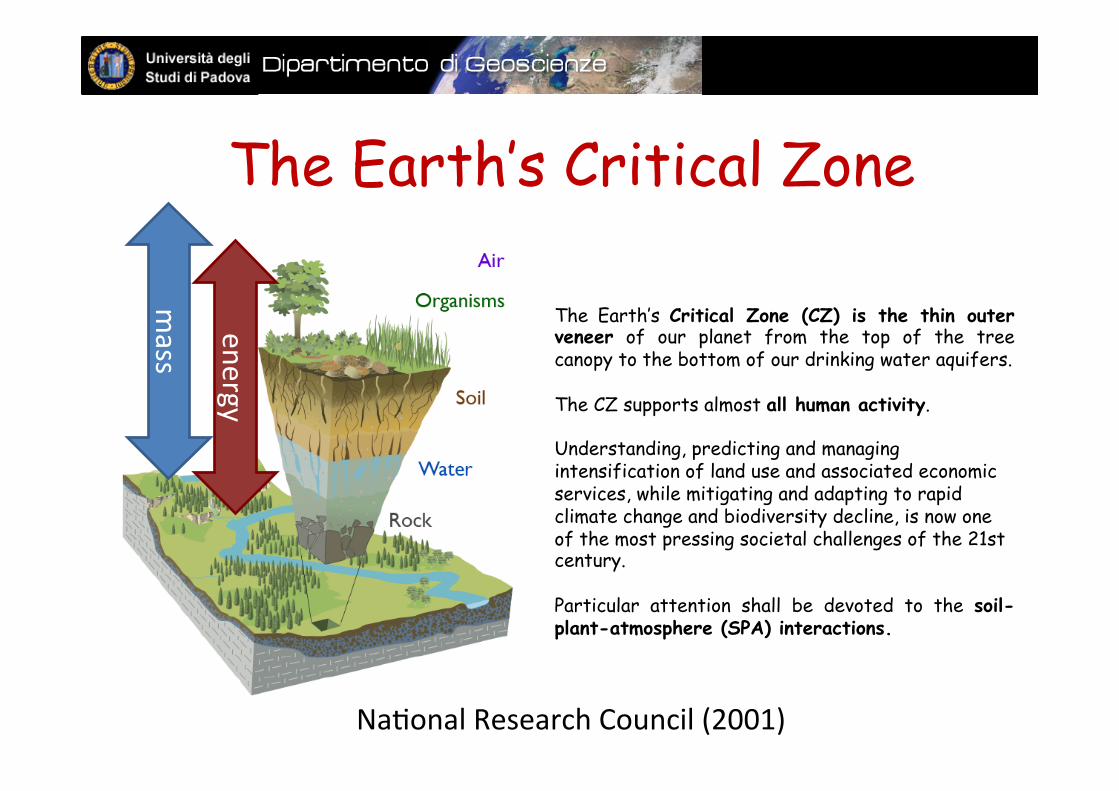
The Earth’s Critical Zone
Na#onal Research Council (2001)
The Earth’s Critical Zone (CZ) is the thin outer veneer of our planet from the top of the tree canopy to the bottom of our drinking water aquifers. The CZ supports almost all human activity. Understanding, predicting and managing intensification of land use and associated economic services, while mitigating and adapting to rapid climate change and biodiversity decline, is now one of the most pressing societal challenges of the 21st century. Particular attention shall be devoted to the soil-plant-atmosphere (SPA) interactions.
mass
energy
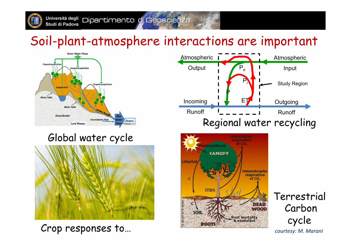
Soil-plant-atmosphere interactions are important
Pe
Pi
P
ET
Atmospheric
Input
Atmospheric
Output
Incoming
Runoff
Outgoing
Runoff
Study Region
Global water cycle Regional water recycling
Terrestrial Carbon cycle
Crop responses to… courtesy: M. Marani
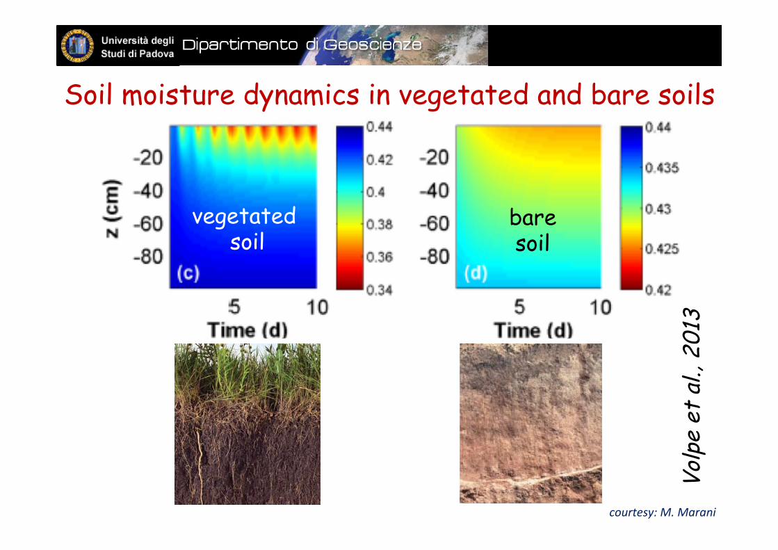
vegetated soil
Soil moisture dynamics in vegetated and bare soils
Volp
e et
al.,
201
3
bare soil
courtesy: M. Marani
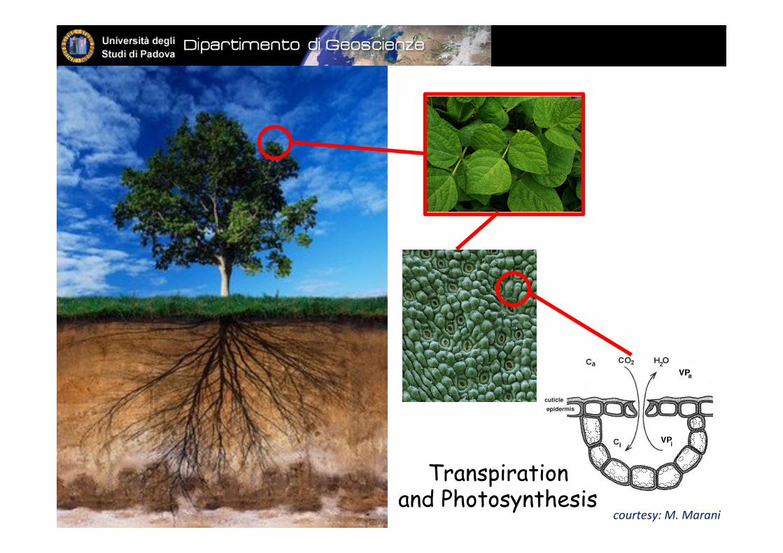
Transpiration and Photosynthesis
courtesy: M. Marani
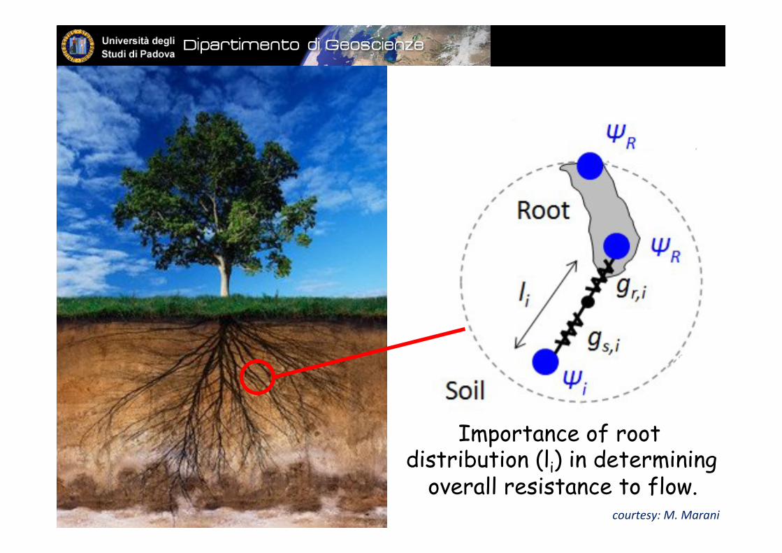
Importance of root distribution (li) in determining
overall resistance to flow. courtesy: M. Marani
Geophysical techniques, combined with flow and transport models, can provide a major step
forward in the ECZ characterization
Key idea
SUMMARY q Soil-plant-atmosphere interactions
q Characterization of the Earth’s critical zone: the role of non-invasive monitoring
q Large-scale monitoring
q Small-scale monitoring
q Outlook: assimilate data and models, with a vision
q Conclusions

water table
aquifer confining layer
impermeable bedrock
small scale large scale
What geophysical methods can help define
q structure / texture

water table
spring evapo-transpiration
water table
aquifer confining layer
impermeable bedrock
small scale large scale
q structure / texture
q fluid-dynamics
What geophysical methods can help define
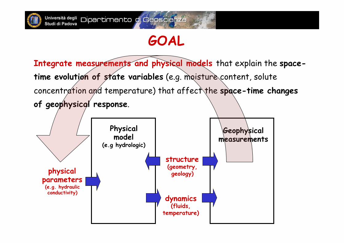
Geophysical measurements
Physical model
(e.g hydrologic)
physical parameters (e.g. hydraulic conductivity)
dynamics (fluids,
temperature)
structure (geometry, geology)
Integrate measurements and physical models that explain the space-time evolution of state variables (e.g. moisture content, solute concentration and temperature) that affect the space-time changes of geophysical response.
GOAL
SUMMARY q Soil-plant-atmosphere interactions
q Characterization of the Earth’s critical zone: the role of non-invasive monitoring
q Large-scale monitoring
q Small-scale monitoring
q Outlook: assimilate data and models, with a vision
q Conclusions
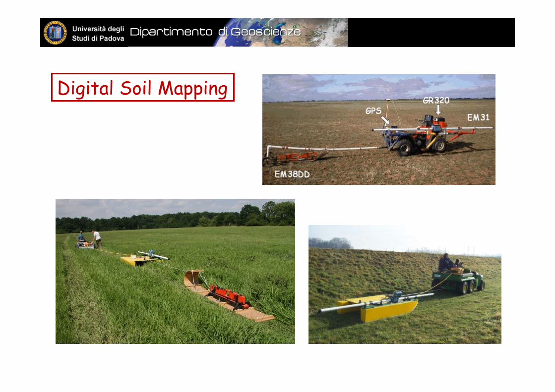
Digital Soil Mapping
Bregonze Hills
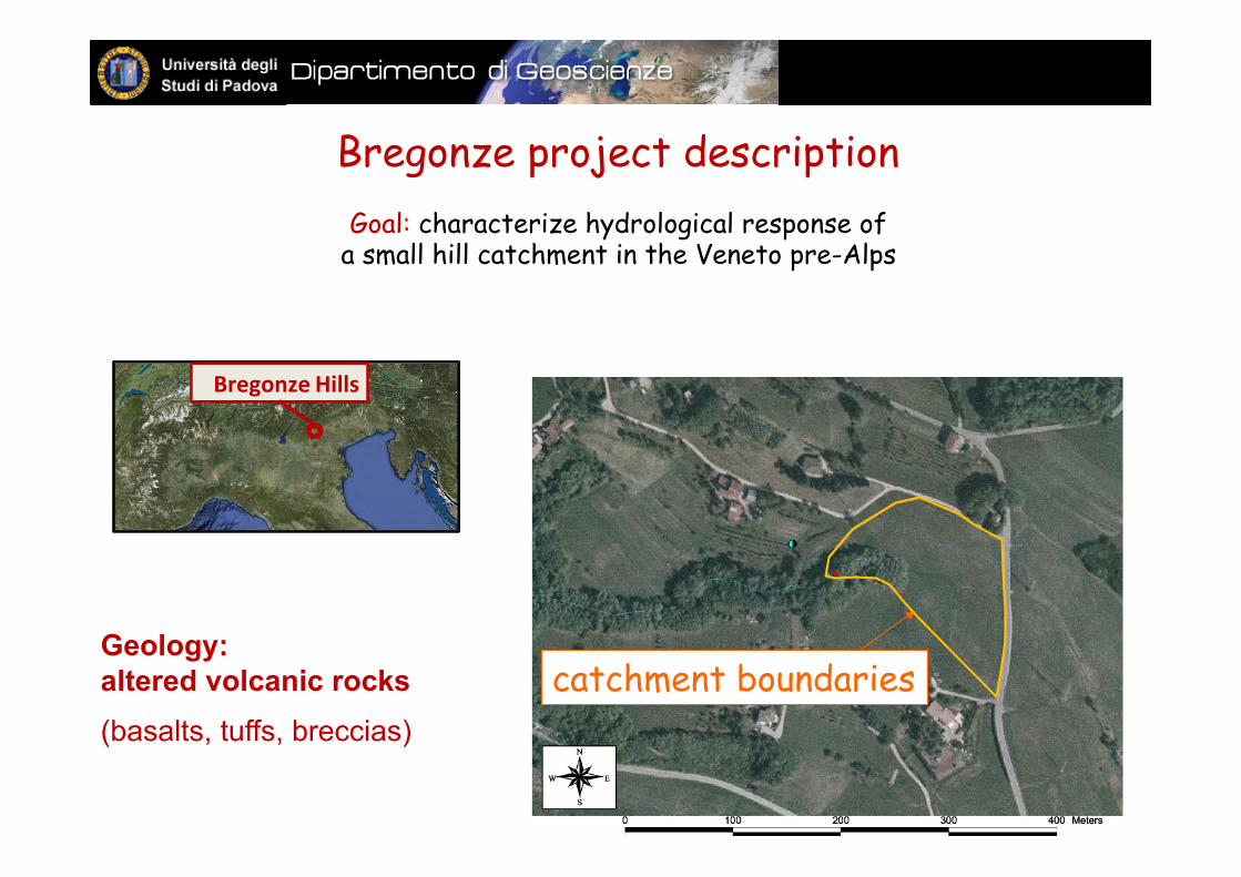
Bregonze project description
Goal: characterize hydrological response of a small hill catchment in the Veneto pre-Alps
Geology: altered volcanic rocks
(basalts, tuffs, breccias)
catchment boundaries
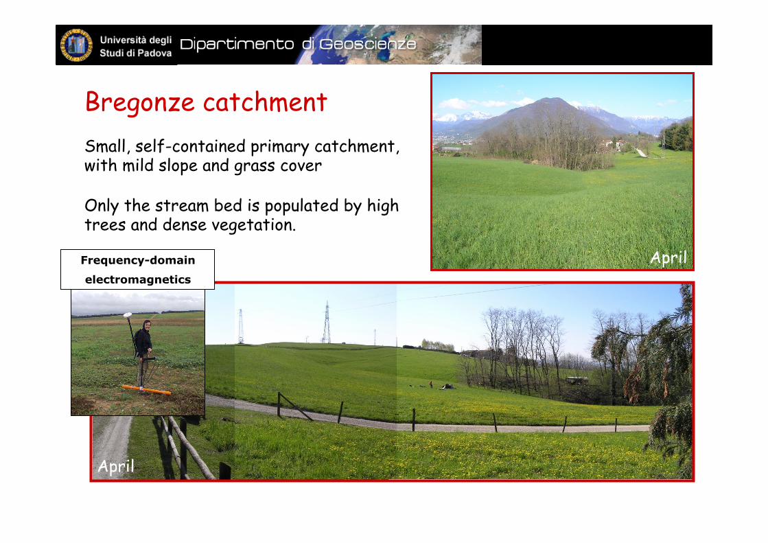
Bregonze catchment Small, self-contained primary catchment, with mild slope and grass cover Only the stream bed is populated by high trees and dense vegetation.
April
April
Frequency-domain
electromagnetics
18/08/2014
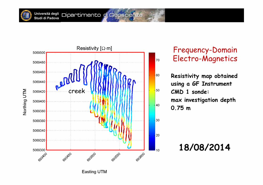
creek
Frequency-Domain Electro-Magnetics
Resistivity map obtained using a GF Instrument CMD 1 sonde: max investigation depth 0.75 m
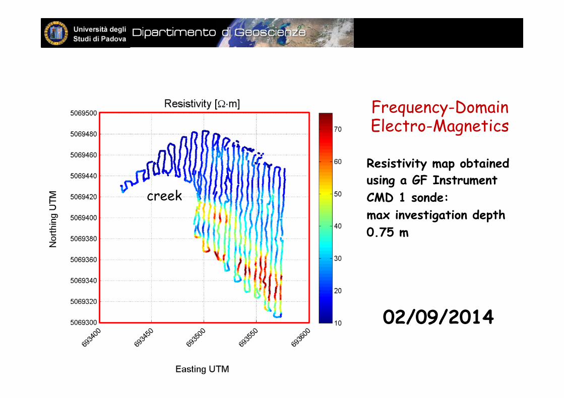
02/09/2014
Frequency-Domain Electro-Magnetics
Resistivity map obtained using a GF Instrument CMD 1 sonde: max investigation depth 0.75 m
creek
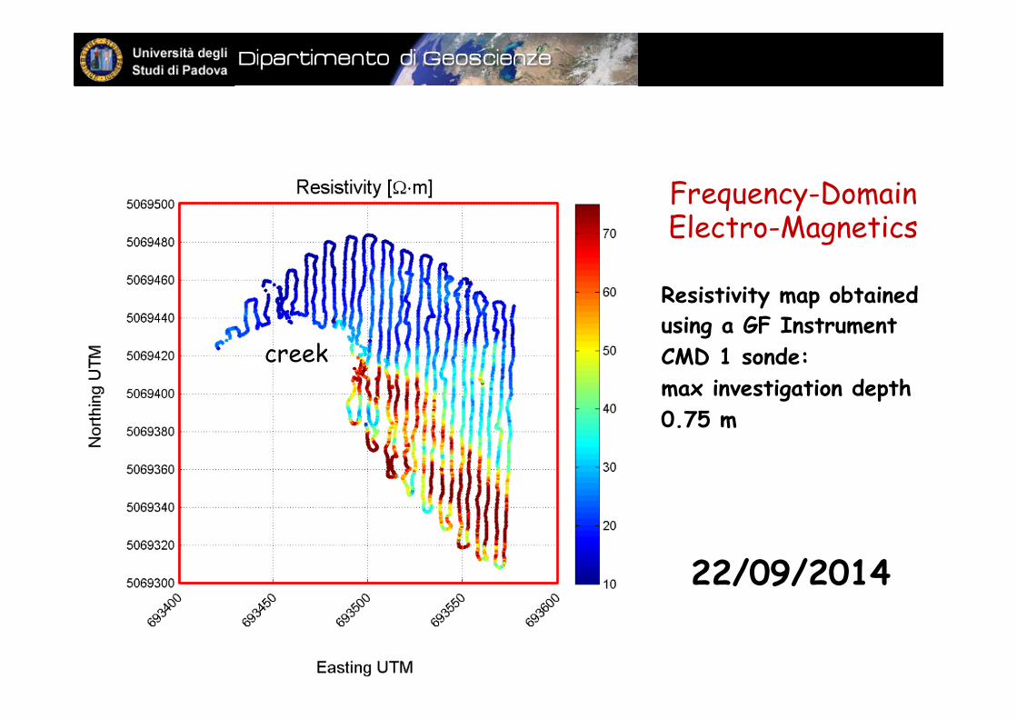
22/09/2014
Frequency-Domain Electro-Magnetics
Resistivity map obtained using a GF Instrument CMD 1 sonde: max investigation depth 0.75 m
creek
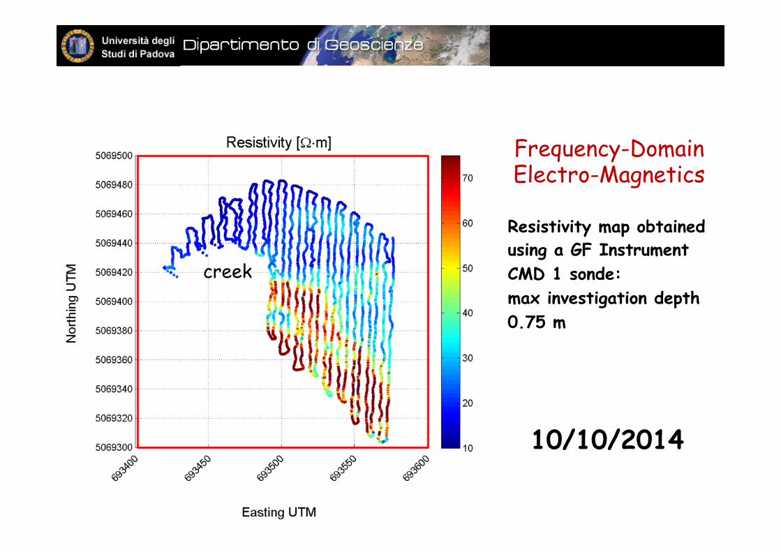
10/10/2014
Frequency-Domain Electro-Magnetics
Resistivity map obtained using a GF Instrument CMD 1 sonde: max investigation depth 0.75 m
creek
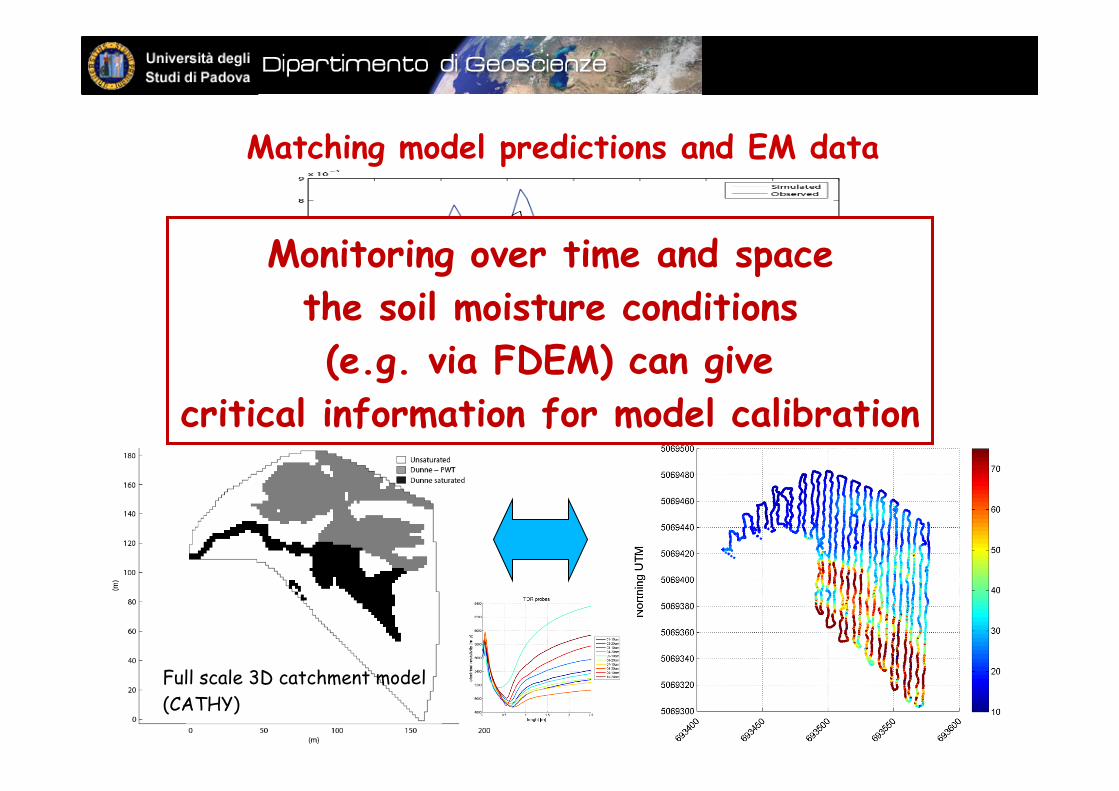
Matching model predictions and EM data
Monitoring over time and space the soil moisture conditions (e.g. via FDEM) can give
critical information for model calibration
Full scale 3D catchment model (CATHY)
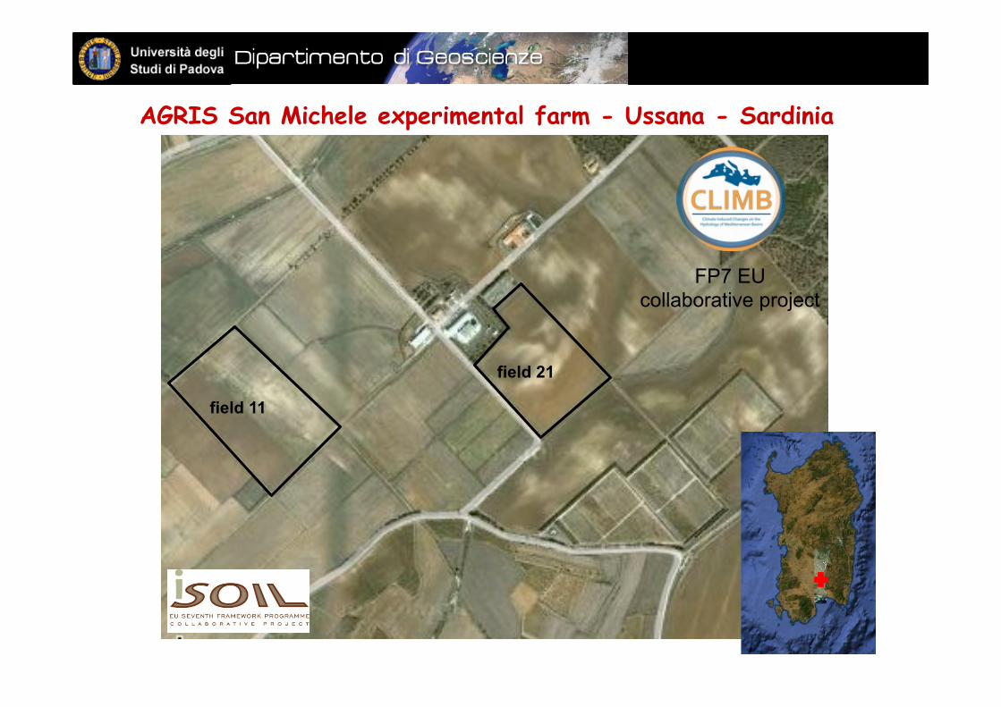
AGRIS San Michele experimental farm - Ussana - Sardinia
field 21
field 11
FP7 EU collaborative project
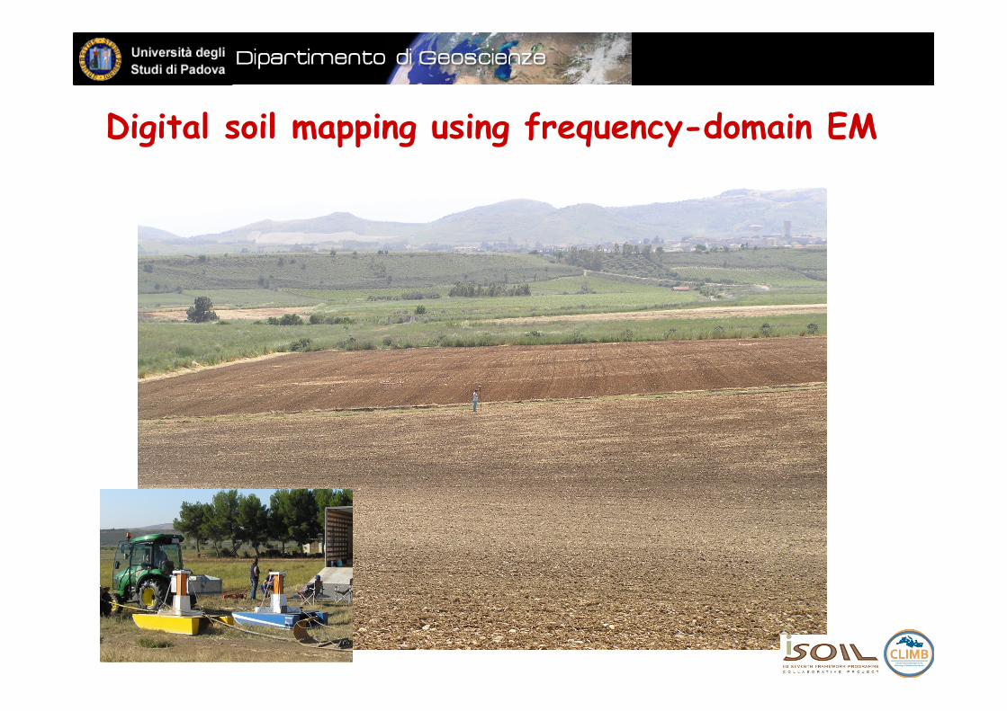
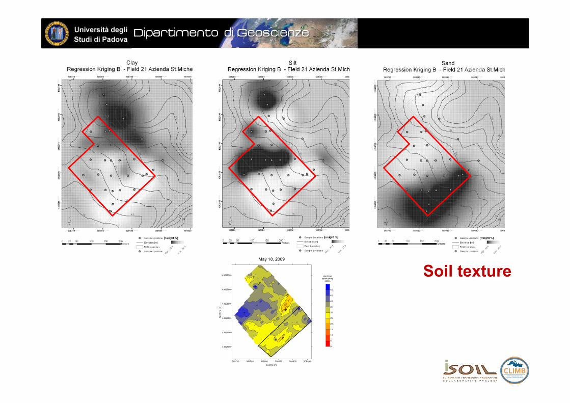
Digital soil mapping using frequency-domain EM
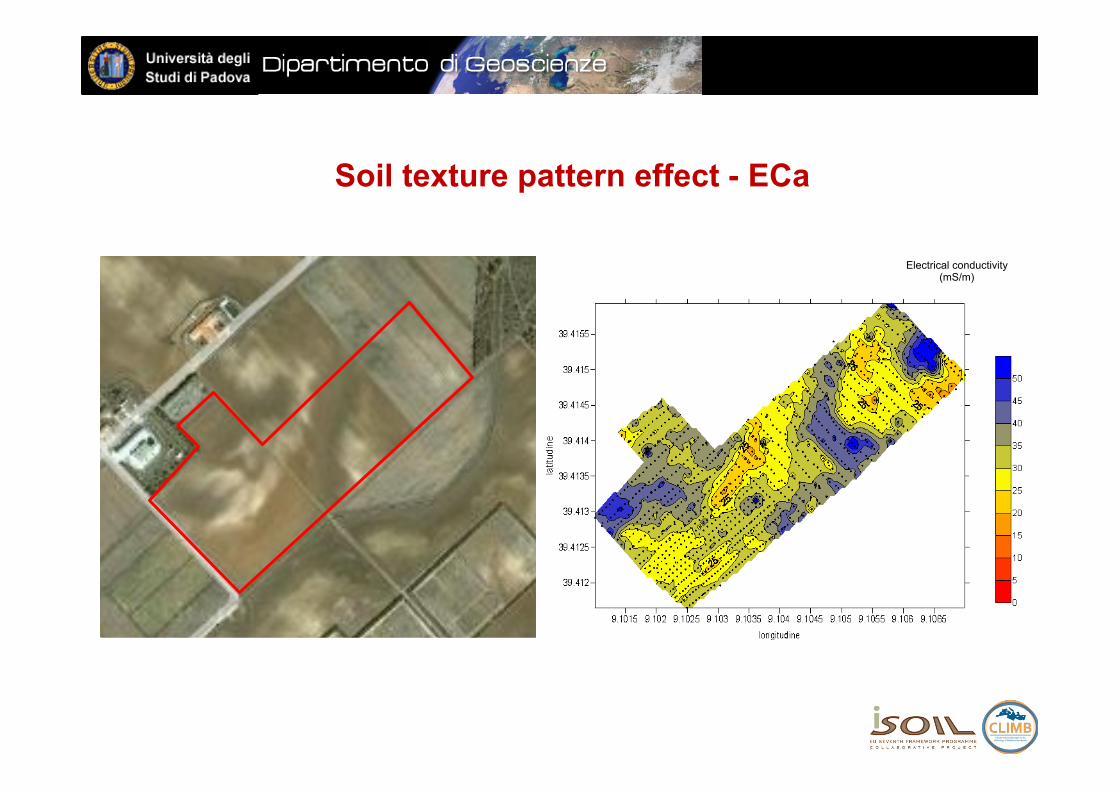
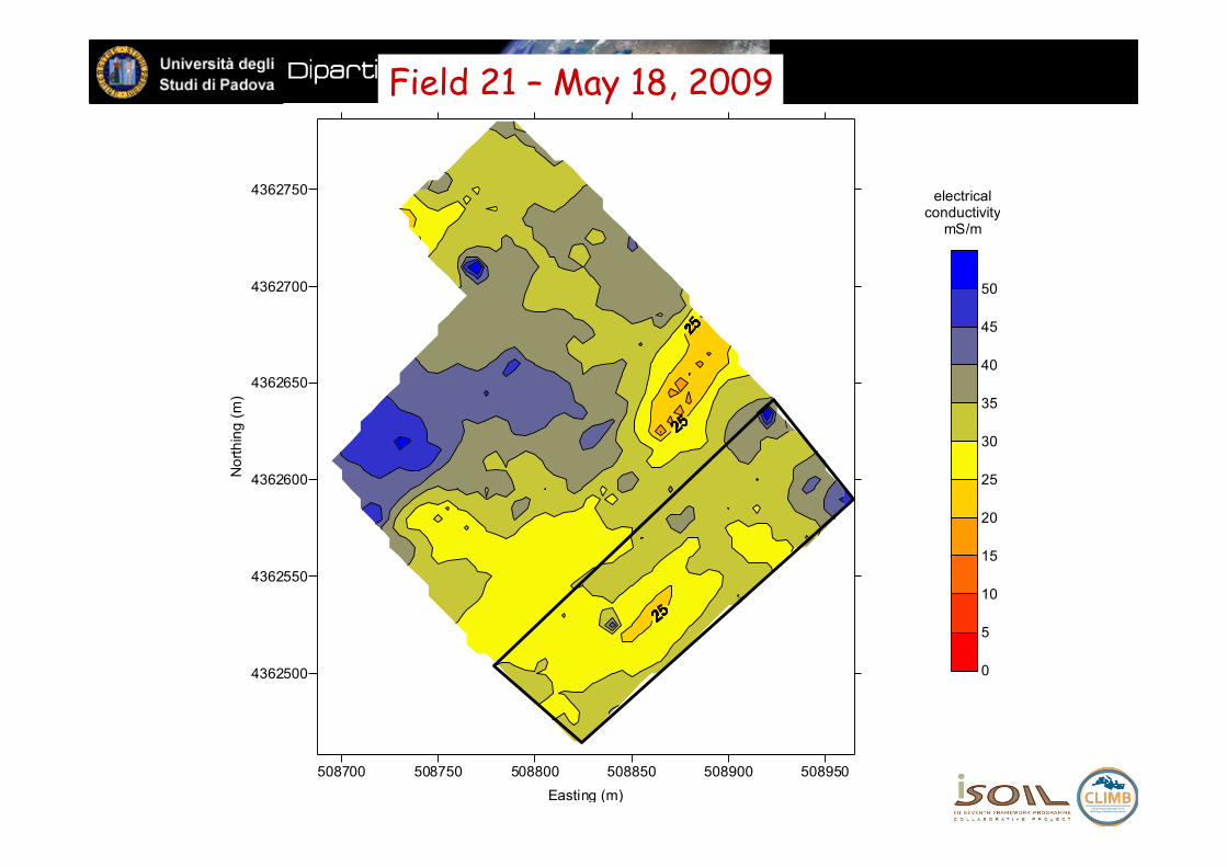
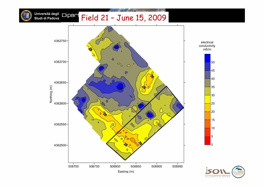
Soil texture pattern effect - ECa
Electrical conductivity (mS/m)
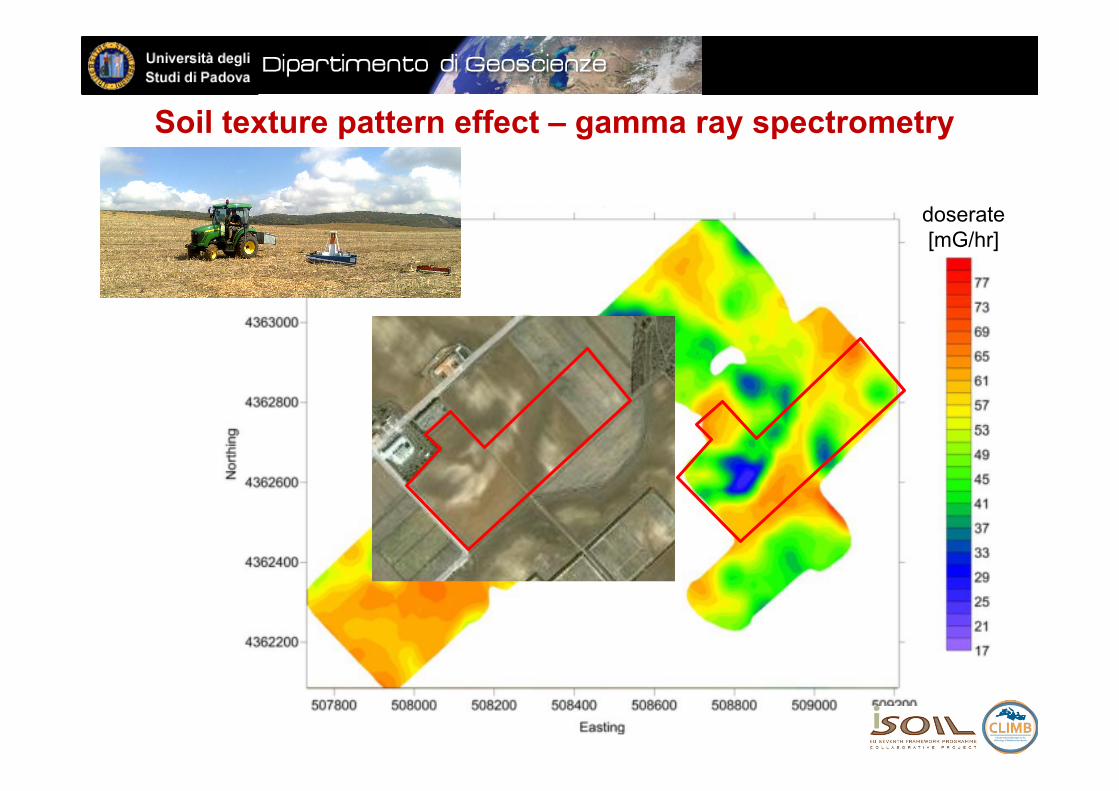
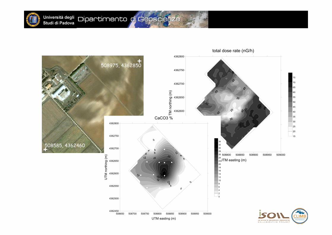
Soil texture pattern effect – gamma ray spectrometry
doserate [mG/hr]
508700 508750 508800 508850 508900 508950Easting (m)
May 18, 2009
4362500
4362550
4362600
4362650
4362700
4362750
Nor
thin
g (m
)
0
5
10
15
20
25
30
35
40
45
50
electricalconductivity
mS/m
Soil texture
508650 508700 508750 508800 508850 508900 508950 509000
UTM easting (m)
total dose rate (nG/h)
4362450
4362500
4362550
4362600
4362650
4362700
4362750
4362800
UTM
nor
thin
g (m
)
15
20
25
30
35
40
45
50
55
60
65
70
75
field 21
508975, 4362850
508585, 4362460 +
+
508650 508700 508750 508800 508850 508900 508950 509000
UTM easting (m)
CaCO3 %
4362450
4362500
4362550
4362600
4362650
4362700
4362750
4362800
UTM
nor
thin
g (m
)
0246810121416182022242628303234
508700 508750 508800 508850 508900 508950Easting (m)
May 18, 2009
4362500
4362550
4362600
4362650
4362700
4362750
Nor
thin
g (m
)
0
5
10
15
20
25
30
35
40
45
50
electricalconductivity
mS/m
Field 21 – May 18, 2009
508700 508750 508800 508850 508900 508950Easting (m)
June 15, 2009
4362500
4362550
4362600
4362650
4362700
4362750
Nor
thin
g (m
)
0
5
10
15
20
25
30
35
40
45
50
electricalconductivity
mS/m
Field 21 – June 15, 2009
508700 508750 508800 508850 508900 508950Easting (m)
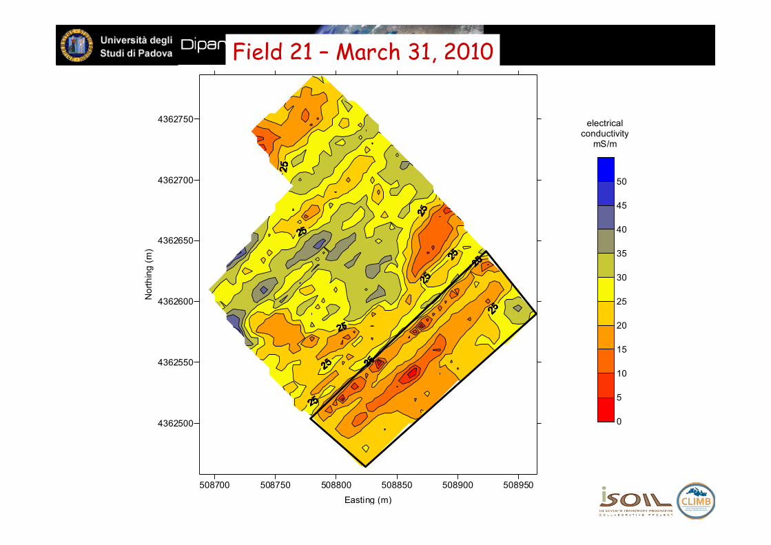
March 31, 2010
4362500
4362550
4362600
4362650
4362700
4362750
Nor
thin
g (m
)
0
5
10
15
20
25
30
35
40
45
50
electricalconductivity
mS/m
Field 21 – March 31, 2010
508700 508750 508800 508850 508900 508950Easting (m)
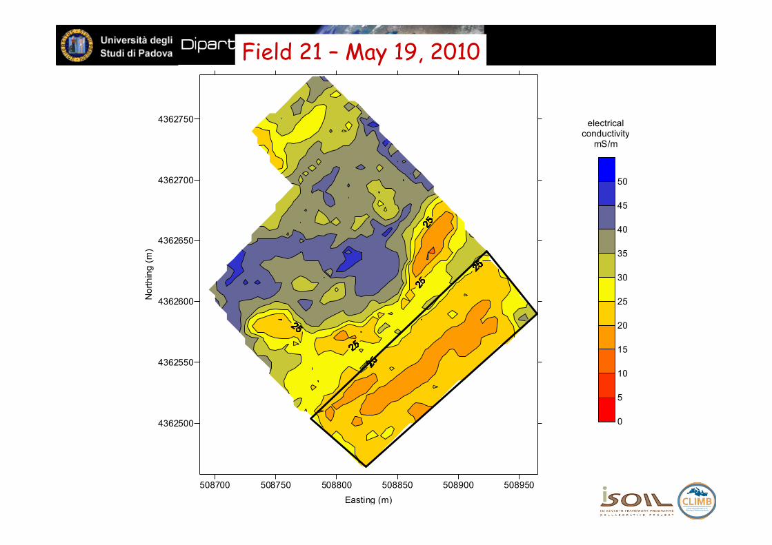
May 19, 2010
4362500
4362550
4362600
4362650
4362700
4362750
Nor
thin
g (m
)
0
5
10
15
20
25
30
35
40
45
50
electricalconductivity
mS/m
Field 21 – May 19, 2010
508700 508750 508800 508850 508900 508950Easting (m)
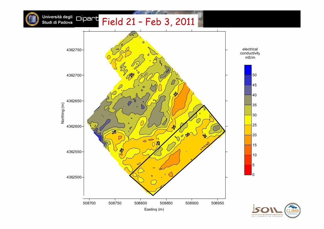
February 3, 2011
4362500
4362550
4362600
4362650
4362700
4362750
Nor
thin
g (m
)
0
5
10
15
20
25
30
35
40
45
50
electricalconductivity
mS/m
Field 21 – Feb 3, 2011
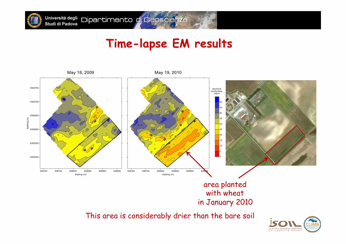
Time-lapse EM results
508700 508750 508800 508850 508900 508950Easting (m)
May 19, 2010
4362500
4362550
4362600
4362650
4362700
4362750
Nor
thin
g (m
)
0
5
10
15
20
25
30
35
40
45
50
electricalconductivity
mS/m
508700 508750 508800 508850 508900 508950Easting (m)
May 18, 2009
4362500
4362550
4362600
4362650
4362700
4362750
Nor
thin
g (m
)
0
5
10
15
20
25
30
35
40
45
50
electricalconductivity
mS/m
508700 508750 508800 508850 508900 508950Easting (m)
May 19, 2010
4362500
4362550
4362600
4362650
4362700
4362750
Nor
thin
g (m
)
0
5
10
15
20
25
30
35
40
45
50
electricalconductivity
mS/m
This area is considerably drier than the bare soil
area planted with wheat
in January 2010
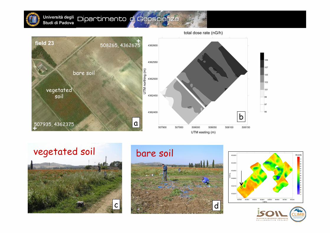
bare soil
bare soil
vegetated soil
vegetated soil
a 507900 507950 508000 508050 508100 508150
UTM easting (m)
total dose rate (nG/h)
4362400
4362450
4362500
4362550
4362600
UTM
nor
thin
g (m
)
95
97
99
101
103
105
107
109
b
c d
field 23 508265, 4362675
507935, 4362375 +
+
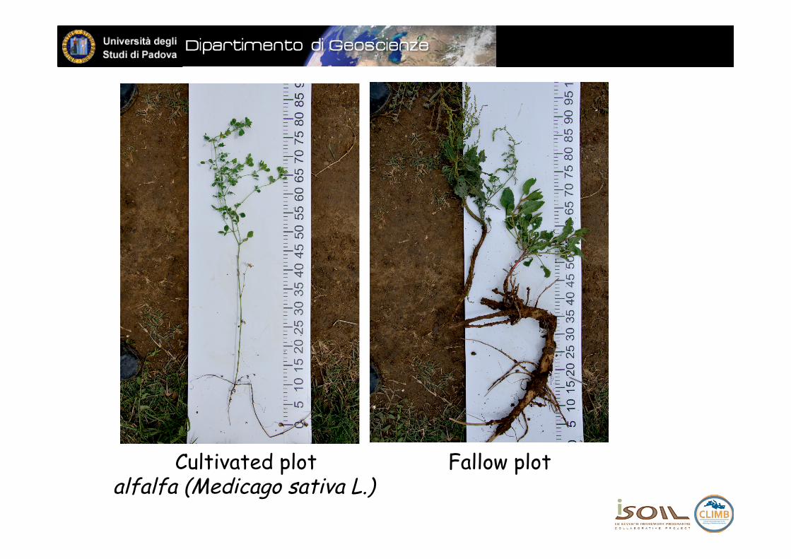
Fallow plot Cultivated plot alfalfa (Medicago sativa L.)
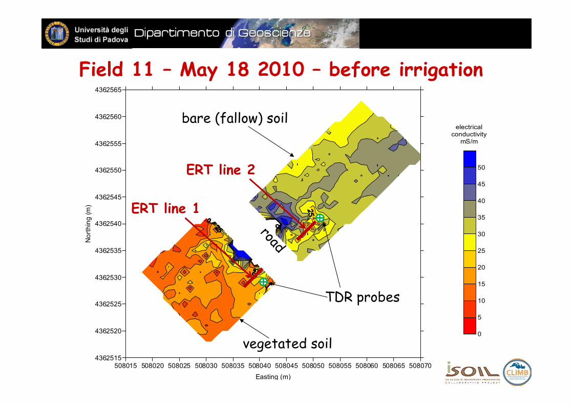
Field 11 – May 18 2010 – before irrigation
508015 508020 508025 508030 508035 508040 508045 508050 508055 508060 508065 508070Easting (m)
Twin fields - background - May 18 2010
4362515
4362520
4362525
4362530
4362535
4362540
4362545
4362550
4362555
4362560
4362565N
orth
ing
(m)
0
5
10
15
20
25
30
35
40
45
50
0
5
10
15
20
25
30
35
40
45
50
bare (fallow) soil
vegetated soil
508700 508750 508800 508850 508900 508950Easting (m)
May 19, 2010
4362500
4362550
4362600
4362650
4362700
4362750N
orth
ing
(m)
0
5
10
15
20
25
30
35
40
45
50
electricalconductivity
mS/m
ERT line 2
TDR probes
ERT line 1
0.5 1 1.5 2 2.5 3 3.5 4 4.5
P0
-0.5
10
15
20
25
30
35
40
45
50
55
60
65
70
75
80
0.5 1 1.5 2 2.5 3 3.5 4 4.5
P1
-0.5
0.5 1 1.5 2 2.5 3 3.5 4 4.5
P2
-0.5
0.5 1 1.5 2 2.5 3 3.5 4 4.5
P5
-0.5
0.5 1 1.5 2 2.5 3 3.5 4 4.5
P12
-0.5
0.5 1 1.5 2 2.5 3 3.5 4 4.5
NA0
-0.5
10
15
20
25
30
35
40
45
50
55
60
65
70
75
80
0.5 1 1.5 2 2.5 3 3.5 4 4.5
NA1
-0.5
0.5 1 1.5 2 2.5 3 3.5 4 4.5
NA2
-0.5
0.5 1 1.5 2 2.5 3 3.5 4 4.5
NA5
-0.5
0.5 1 1.5 2 2.5 3 3.5 4 4.5
NA12
-0.5
0.5 1 1.5 2 2.5 3 3.5 4 4.5
NA0
-0.5
10
15
20
25
30
35
40
45
50
55
60
65
70
75
80
0.5 1 1.5 2 2.5 3 3.5 4 4.5
NA1
-0.5
0.5 1 1.5 2 2.5 3 3.5 4 4.5
NA2
-0.5
0.5 1 1.5 2 2.5 3 3.5 4 4.5
NA5
-0.5
0.5 1 1.5 2 2.5 3 3.5 4 4.5
NA12
-0.5
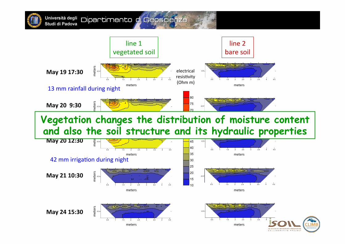
electrical resis#vity (Ohm m)
May 24 15:30
May 19 17:30
May 20 9:30
42 mm irriga#on during night
13 mm rainfall during night
May 20 12:30
May 21 10:30
line 2 bare soil
line 1 vegetated soil
meters
meters
meters
meters
meters
meters
meters
meters
meters
meters
meters
meters
meters
meters
meters
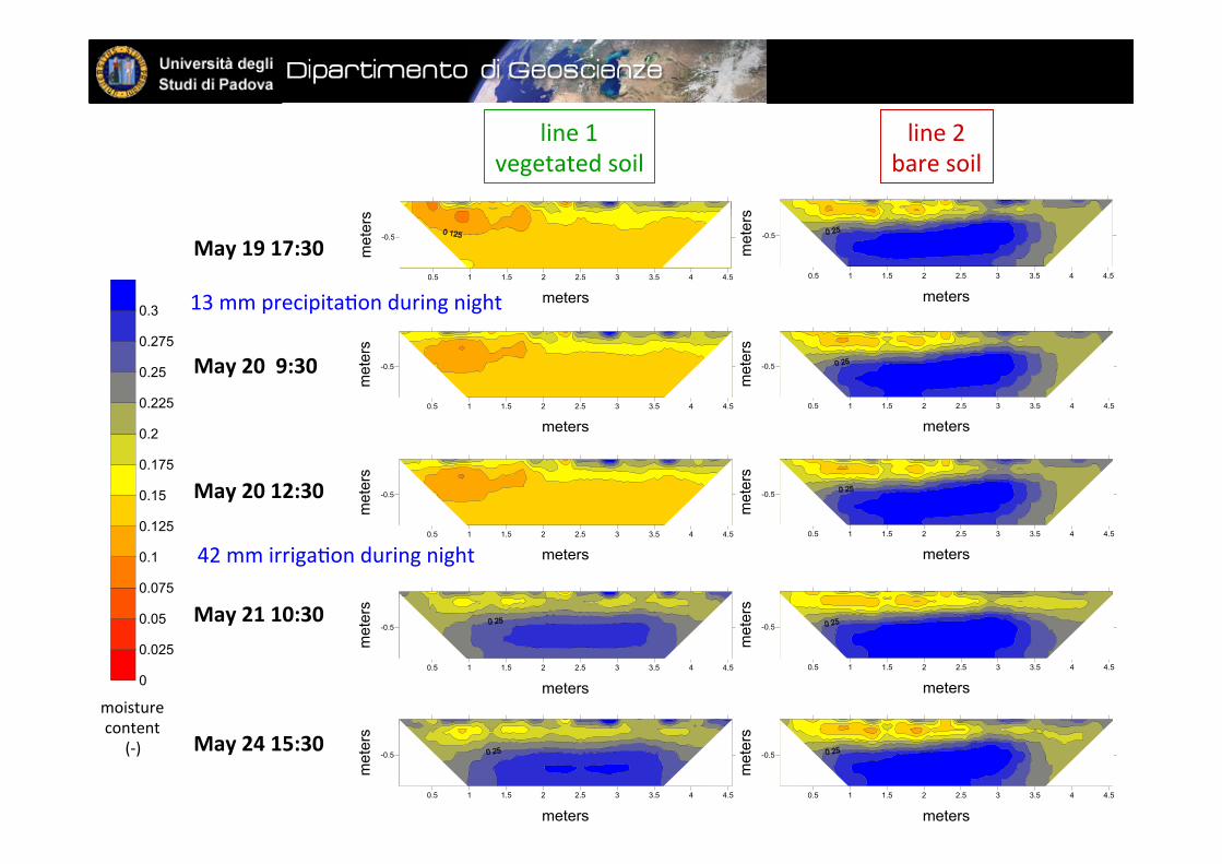
Vegetation changes the distribution of moisture content and also the soil structure and its hydraulic properties
0.12 0.16 0.2 0.24 0.28 0.32
theta (-)
-1
-0.8
-0.6
-0.4
-0.2
0de
pth
(m)
TDRs on May 19TDRs on May 24TRASE on May 19ERT calibrated on May 19 ERT calibrated on May 24
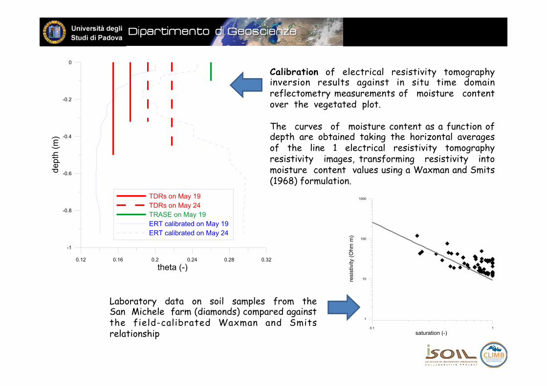
Calibration of electrical resistivity tomography inversion results against in situ time domain reflectometry measurements of moisture content over the vegetated plot. The curves of moisture content as a function of depth are obtained taking the horizontal averages of the line 1 electrical resistivity tomography resistivity images, transforming resistivity into moisture content values using a Waxman and Smits (1968) formulation.
0.1 1
saturation (-)
1
10
100
1000
resi
stiv
ity (O
hm m
)
Laboratory data on soil samples from the San Michele farm (diamonds) compared against the field-calibrated Waxman and Smits relationship
0.5 1 1.5 2 2.5 3 3.5 4 4.5
P12
-0.5
0.5 1 1.5 2 2.5 3 3.5 4 4.5
P12 entire sintetico
-0.5
0.5 1 1.5 2 2.5 3 3.5 4 4.5
P12 65 cm sintetico
-0.5
10
15
20
25
30
35
40
45
50
55
60
65
70
75
80
Line 1: synthe<c (b) May 24 15:30
Line 1: measured May 24 15:30
Line 1: synthe<c (a) May 24 15:30
12 16 20 24 28
resistivity (Ohm m)
-2
-1.6
-1.2
-0.8
-0.4
0
dept
h (m
)
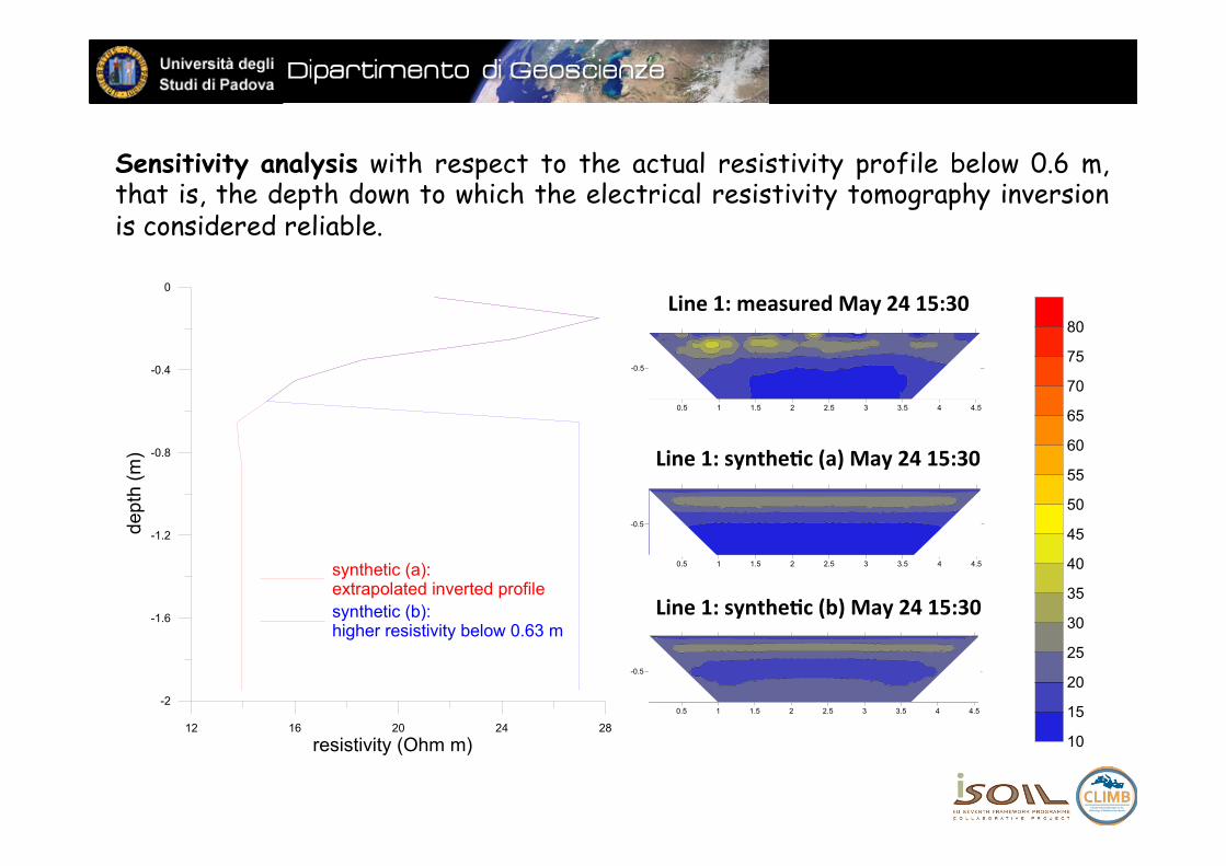
synthetic (a): extrapolated inverted profile synthetic (b):higher resistivity below 0.63 m
Sensitivity analysis with respect to the actual resistivity profile below 0.6 m, that is, the depth down to which the electrical resistivity tomography inversion is considered reliable.
moisture content
(-‐)
May 19 17:30
May 20 9:30
May 20 12:30
May 21 10:30
May 24 15:30
13 mm precipita#on during night
42 mm irriga#on during night
0.5 1 1.5 2 2.5 3 3.5 4 4.5
meters
P0
-0.5
meters
0
0.025
0.05
0.075
0.1
0.125
0.15
0.175
0.2
0.225
0.25
0.275
0.3
0.5 1 1.5 2 2.5 3 3.5 4 4.5
meters
P0
-0.5
meters
0
0.025
0.05
0.075
0.1
0.125
0.15
0.175
0.2
0.225
0.25
0.275
0.3
0.5 1 1.5 2 2.5 3 3.5 4 4.5
meters
P1
-0.5meters
0.5 1 1.5 2 2.5 3 3.5 4 4.5
meters
P2
-0.5
meters
0.5 1 1.5 2 2.5 3 3.5 4 4.5
meters
P5
-0.5
meters
0.5 1 1.5 2 2.5 3 3.5 4 4.5
meters
P12
-0.5
meters
0.5 1 1.5 2 2.5 3 3.5 4 4.5
meters
NA0
-0.5
meters
0.5 1 1.5 2 2.5 3 3.5 4 4.5
meters
NA1
-0.5
meters
0.5 1 1.5 2 2.5 3 3.5 4 4.5
meters
NA2
-0.5
meters
0.5 1 1.5 2 2.5 3 3.5 4 4.5
meters
NA5
-0.5
meters
0.5 1 1.5 2 2.5 3 3.5 4 4.5
meters
NA12
-0.5meters
line 2 bare soil
line 1 vegetated soil
0.51
1.52
2.53
3.54
4.5
NB
5 over 0 - 1%
-0.5
50 55 60 65 70 75 80 85 90 95 100
105
110
115
120
125
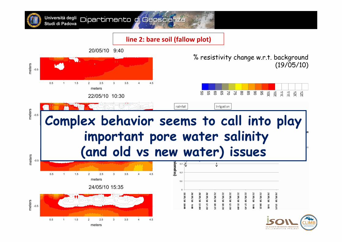
% resistivity change w.r.t. background (19/05/10)
0.5 1 1.5 2 2.5 3 3.5 4 4.5
meters
line NA: 24/05/10 15:35
-0.5
met
ers
0.5 1 1.5 2 2.5 3 3.5 4 4.5
meters
line NA: 23/05/10 9:40
-0.5
met
ers
0.5 1 1.5 2 2.5 3 3.5 4 4.5
meters
line NA: 22/05/10 10:30
-0.5
met
ers
0.5 1 1.5 2 2.5 3 3.5 4 4.5
meters
line NA: 20/05/10 9:40
-0.5
met
ers
line 2: bare soil (fallow plot)
Complex behavior seems to call into play important pore water salinity (and old vs new water) issues
SUMMARY q Soil-plant-atmosphere interactions
q Characterization of the Earth’s critical zone: the role of non-invasive monitoring
q Large-scale monitoring
q Small-scale monitoring
q Outlook: assimilate data and models, with a vision
q Conclusions
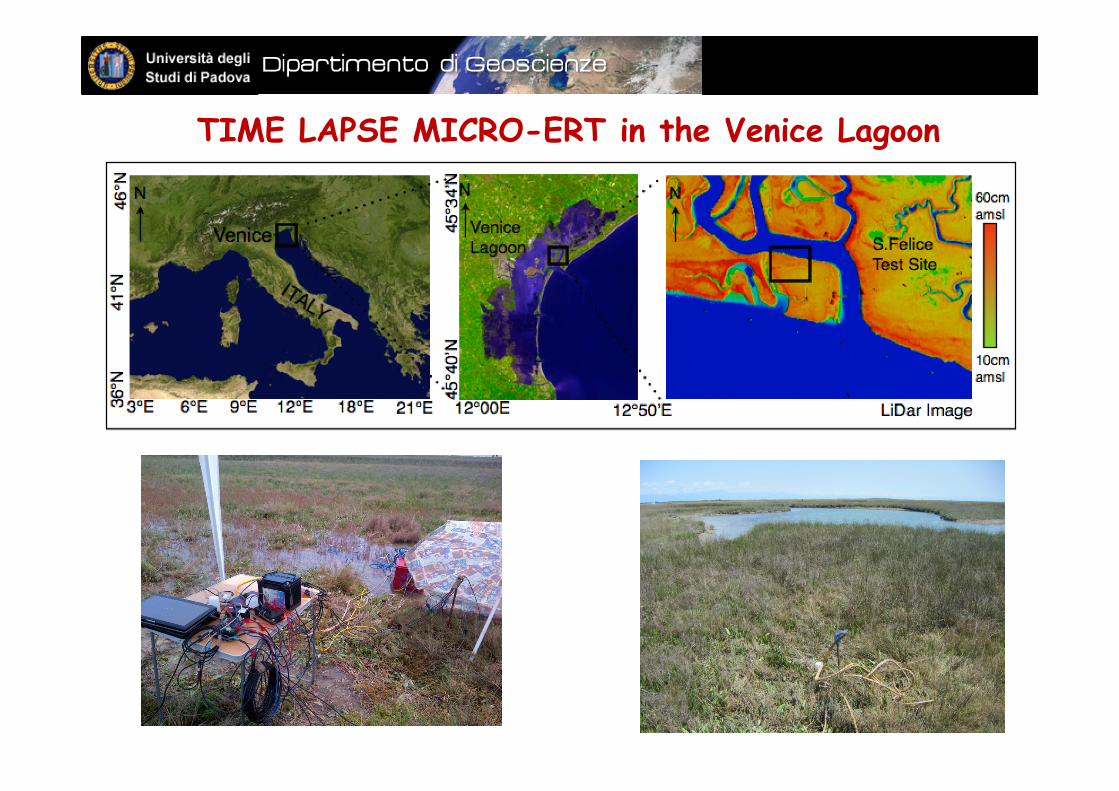
TIME LAPSE MICRO-ERT in the Venice Lagoon
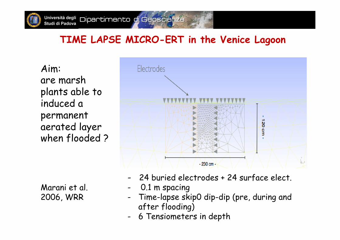
Aim: are marsh plants able to induced a permanent aerated layer when flooded ? Marani et al. 2006, WRR
- 24 buried electrodes + 24 surface elect. - 0.1 m spacing - Time-lapse skip0 dip-dip (pre, during and
after flooding) - 6 Tensiometers in depth
TIME LAPSE MICRO-ERT in the Venice Lagoon
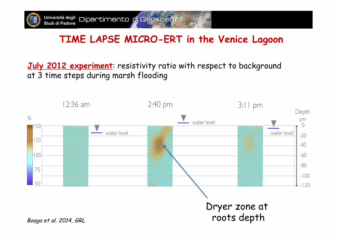
July 2012 experiment: resistivity ratio with respect to background at 3 time steps during marsh flooding
Dryer zone at roots depth Boaga et al. 2014, GRL
TIME LAPSE MICRO-ERT in the Venice Lagoon
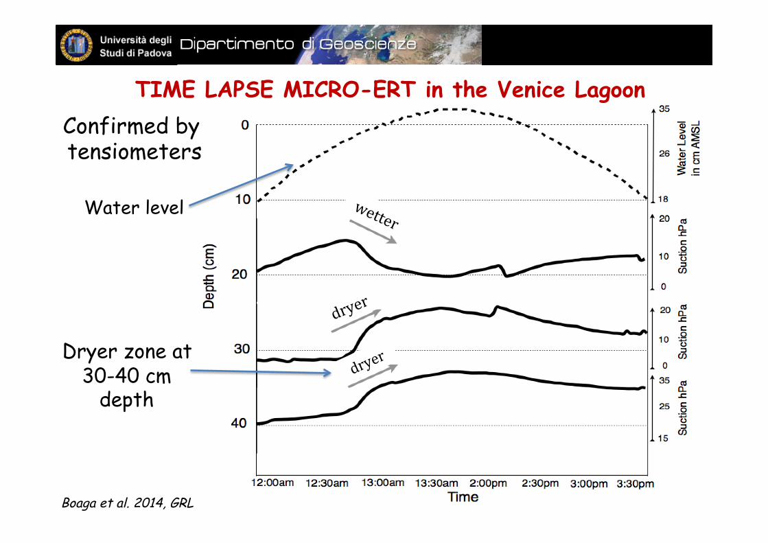
Dryer zone at 30-40 cm
depth
Water level
Confirmed by tensiometers
TIME LAPSE MICRO-ERT in the Venice Lagoon
Boaga et al. 2014, GRL

Dryer zone at roots depth
TIME LAPSE MICRO-ERT in the Venice Lagoon
Boaga et al. 2014, GRL
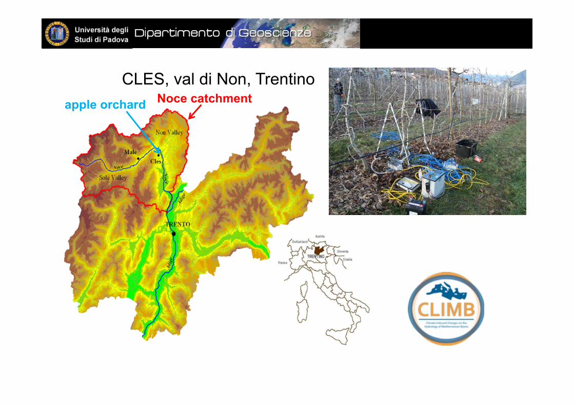
CLES, val di Non, Trentino Noce catchment apple orchard
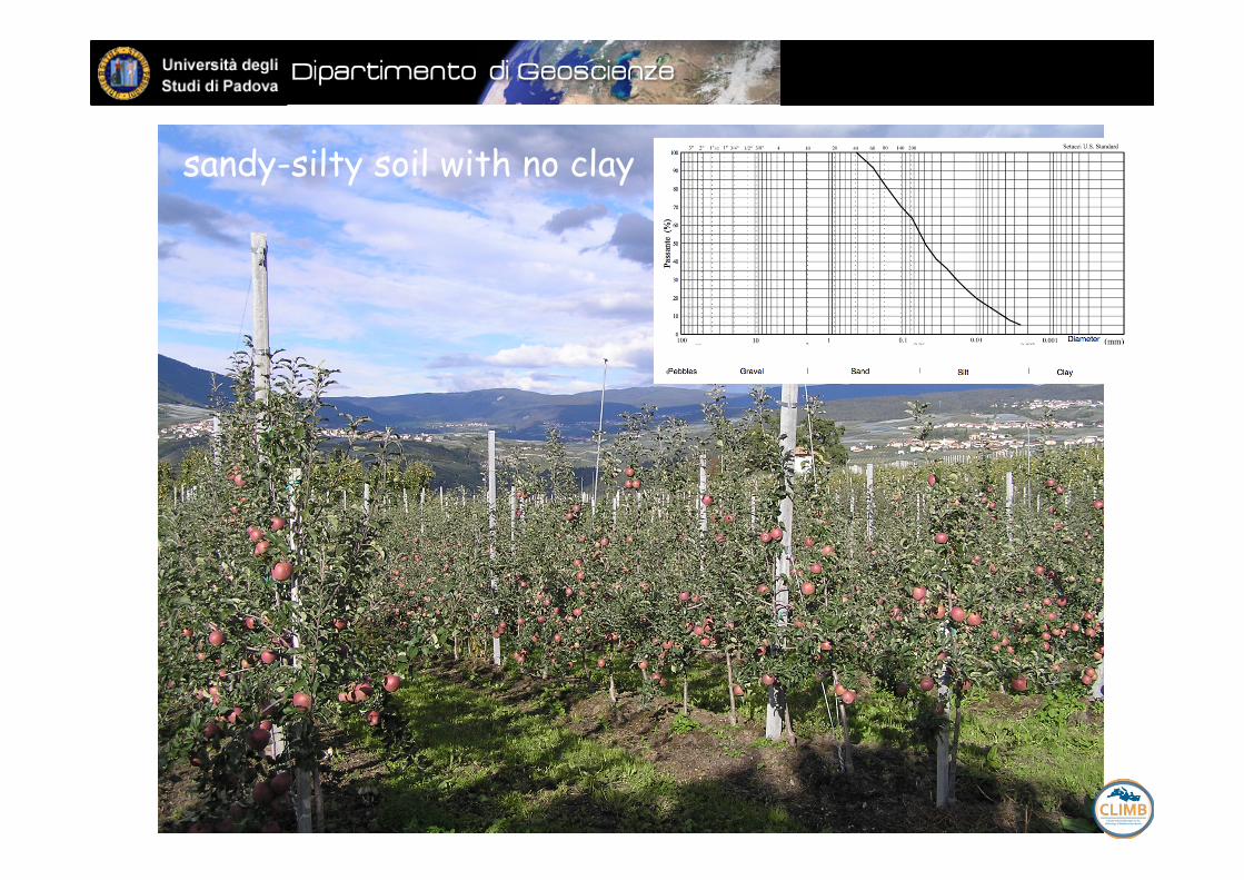
sandy-silty soil with no clay
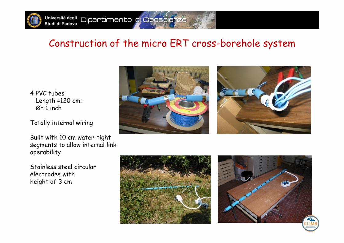
4 PVC tubes Length =120 cm; Ø= 1 inch Totally internal wiring Built with 10 cm water-tight segments to allow internal link operability Stainless steel circular electrodes with height of 3 cm
Construction of the micro ERT cross-borehole system
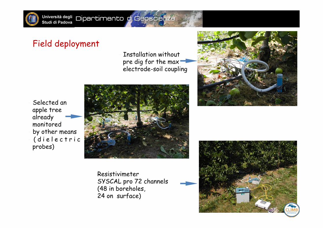
Resistivimeter SYSCAL pro 72 channels (48 in boreholes, 24 on surface)
Field deployment - Installation without
pre dig for the max electrode-soil coupling
- Selected an apple tree already monitored
- by other means - ( d i e l e c t r i c
probes)
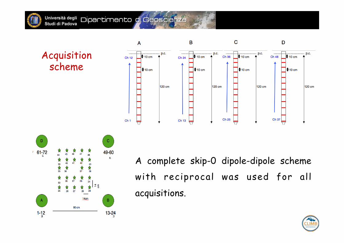
Acquisition scheme
A complete skip-0 dipole-dipole scheme
with reciprocal was used for al l
acquisitions.
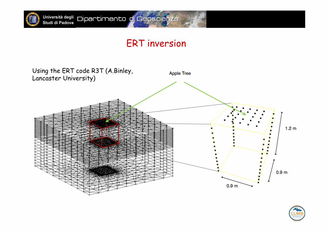
ERT inversion
Using the ERT code R3T (A.Binley, Lancaster University)
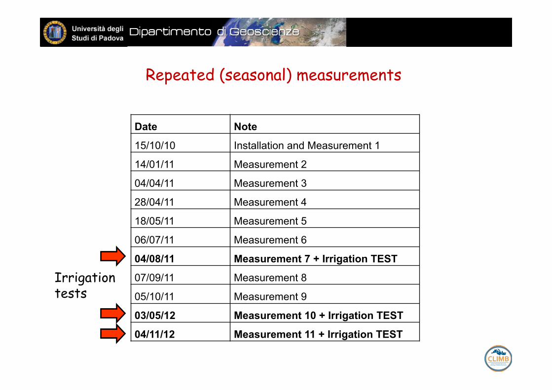
Date Note
15/10/10 Installation and Measurement 1
14/01/11 Measurement 2
04/04/11 Measurement 3
28/04/11 Measurement 4
18/05/11 Measurement 5
06/07/11 Measurement 6
04/08/11 Measurement 7 + Irrigation TEST
07/09/11 Measurement 8
05/10/11 Measurement 9
03/05/12 Measurement 10 + Irrigation TEST
04/11/12 Measurement 11 + Irrigation TEST
Repeated (seasonal) measurements
Irrigation tests
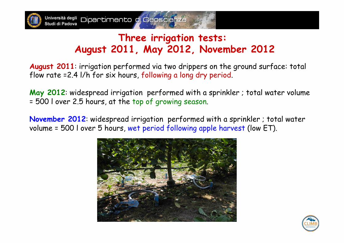
Three irrigation tests: August 2011, May 2012, November 2012
August 2011: irrigation performed via two drippers on the ground surface: total flow rate =2.4 l/h for six hours, following a long dry period. May 2012: widespread irrigation performed with a sprinkler ; total water volume = 500 l over 2.5 hours, at the top of growing season. November 2012: widespread irrigation performed with a sprinkler ; total water volume = 500 l over 5 hours, wet period following apple harvest (low ET).

August 2011 experiment: resistivity ratio with respect to background at four time steps. The iso-surface equal to 60 % of the background resistivity does not penetrate any deeper than 30-40 cm below ground surface.
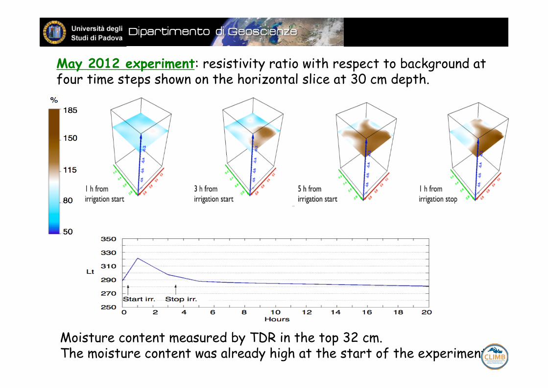
May 2012 experiment: resistivity ratio with respect to background at four time steps shown on the horizontal slice at 30 cm depth.
Moisture content measured by TDR in the top 32 cm. The moisture content was already high at the start of the experiment.
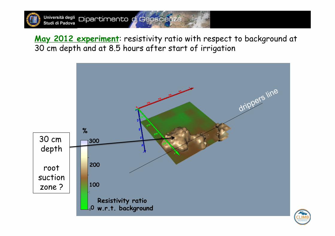
May 2012 experiment: resistivity ratio with respect to background at 30 cm depth and at 8.5 hours after start of irrigation
%
0 Resistivity ratio w.r.t. background
100
200
300 30 cm depth
root
suction zone ?
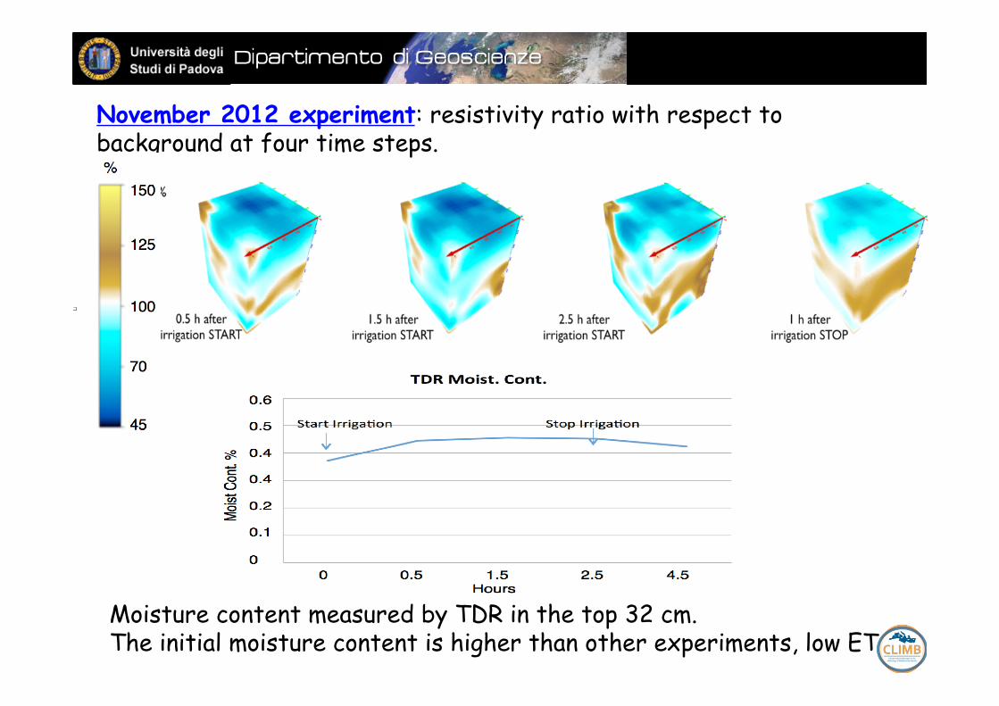
November 2012 experiment: resistivity ratio with respect to background at four time steps.
Moisture content measured by TDR in the top 32 cm. The initial moisture content is higher than other experiments, low ET
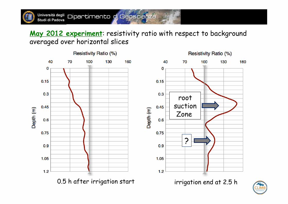
May 2012 experiment: resistivity ratio with respect to background averaged over horizontal slices
0.5 h after irrigation start irrigation end at 2.5 h
root suction Zone
?
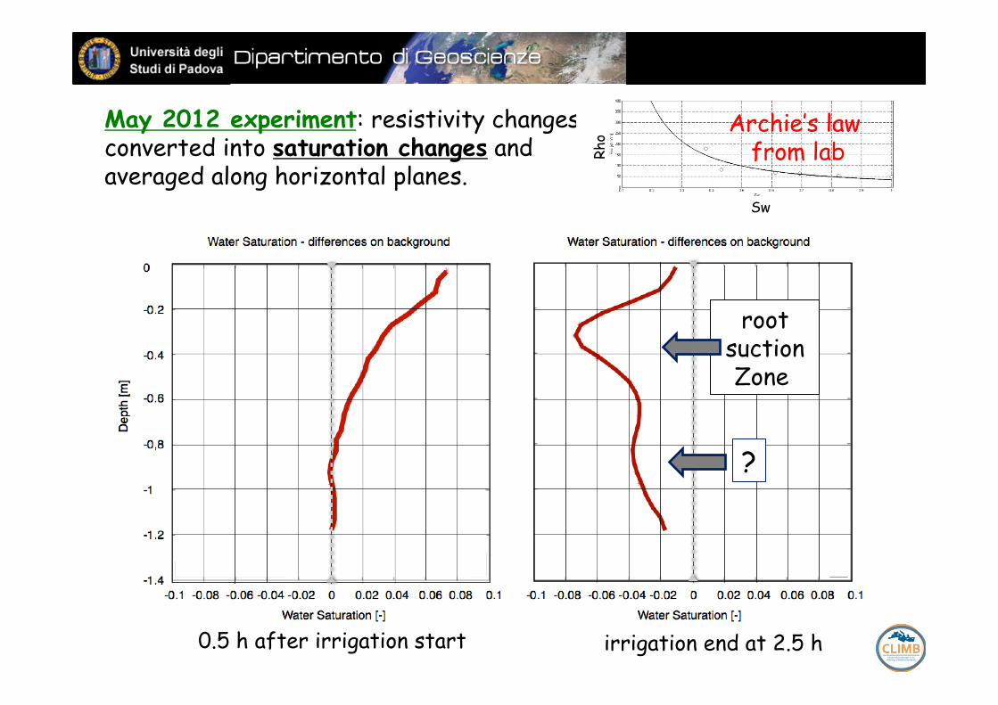
May 2012 experiment: resistivity changes converted into saturation changes and averaged along horizontal planes.
0.5 h after irrigation start irrigation end at 2.5 h
Archie’s law from lab
root suction Zone
?
Rho
Sw
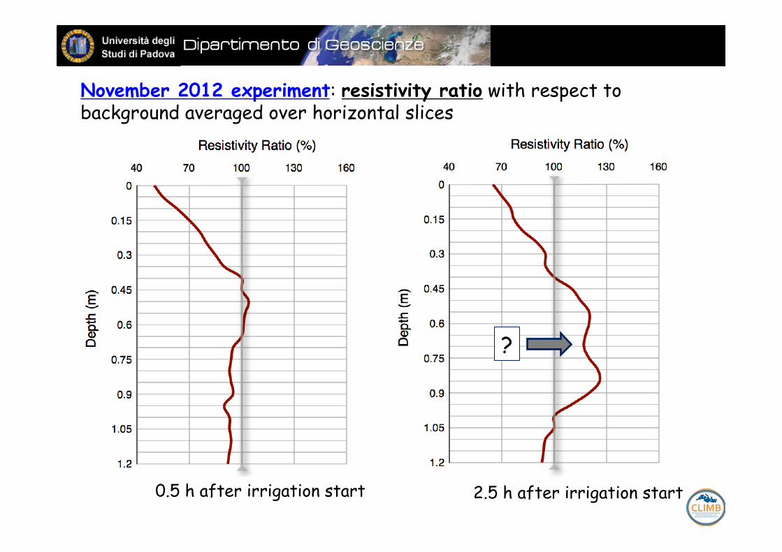
November 2012 experiment: resistivity ratio with respect to background averaged over horizontal slices
0.5 h after irrigation start 2.5 h after irrigation start
?
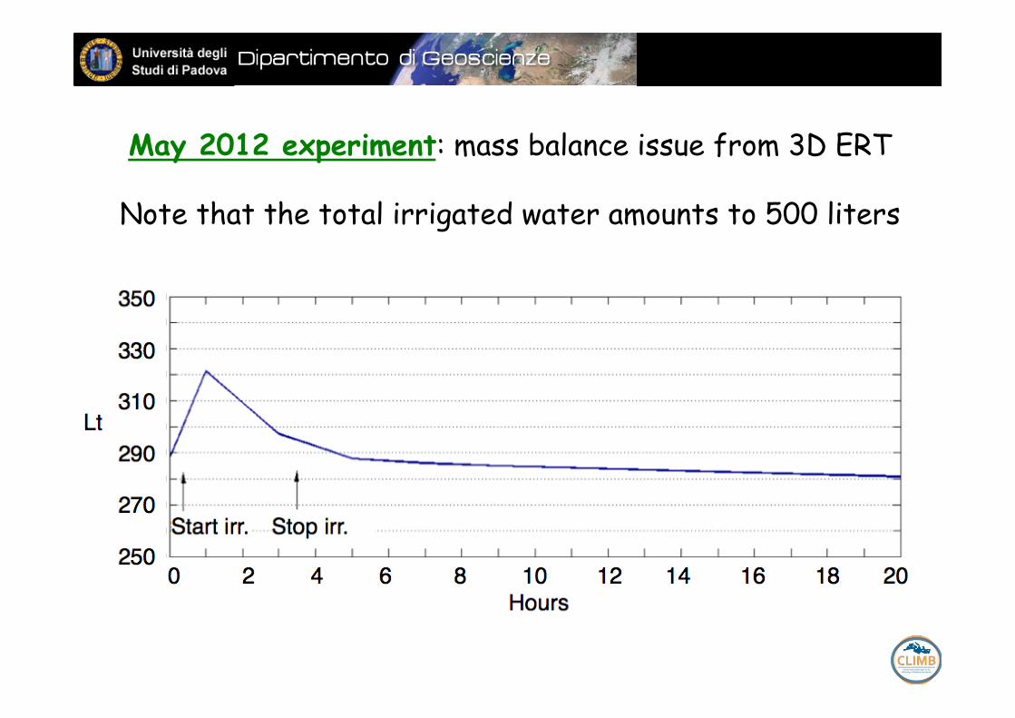
May 2012 experiment: mass balance issue from 3D ERT
Note that the total irrigated water amounts to 500 liters
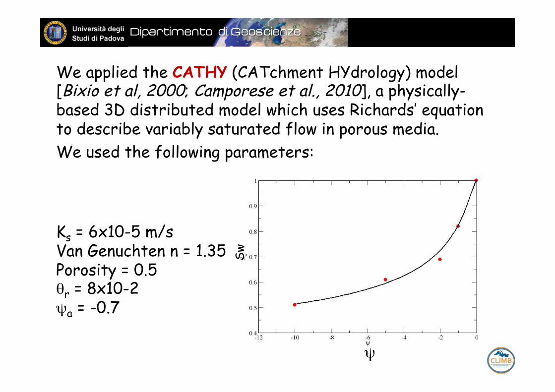
We applied the CATHY (CATchment HYdrology) model [Bixio et al, 2000; Camporese et al., 2010], a physically-based 3D distributed model which uses Richards’ equation to describe variably saturated flow in porous media. We used the following parameters: Ks = 6x10⁻⁵ m/s Van Genuchten n = 1.35 Porosity = 0.5 θr = 8x10⁻² ψa = -0.7
Sw
ψ
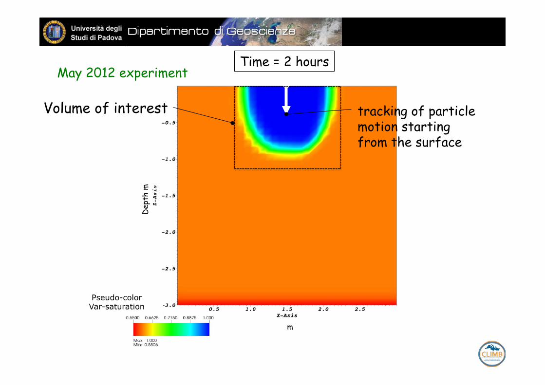
Time = 2 hours
tracking of particle motion starting from the surface
May 2012 experiment
Volume of interest
Pseudo-color Var-saturation
Dep
th m
m
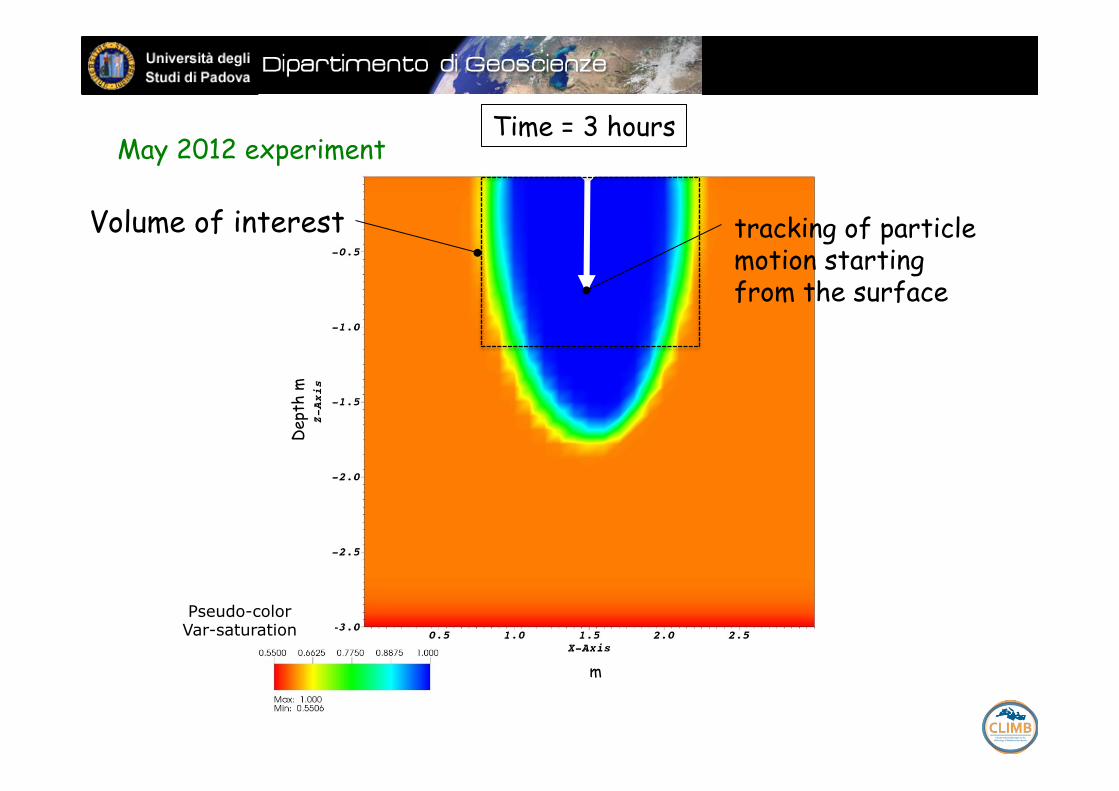
Time = 3 hours
tracking of particle motion starting from the surface
May 2012 experiment
Pseudo-color Var-saturation
Dep
th m
m
Volume of interest
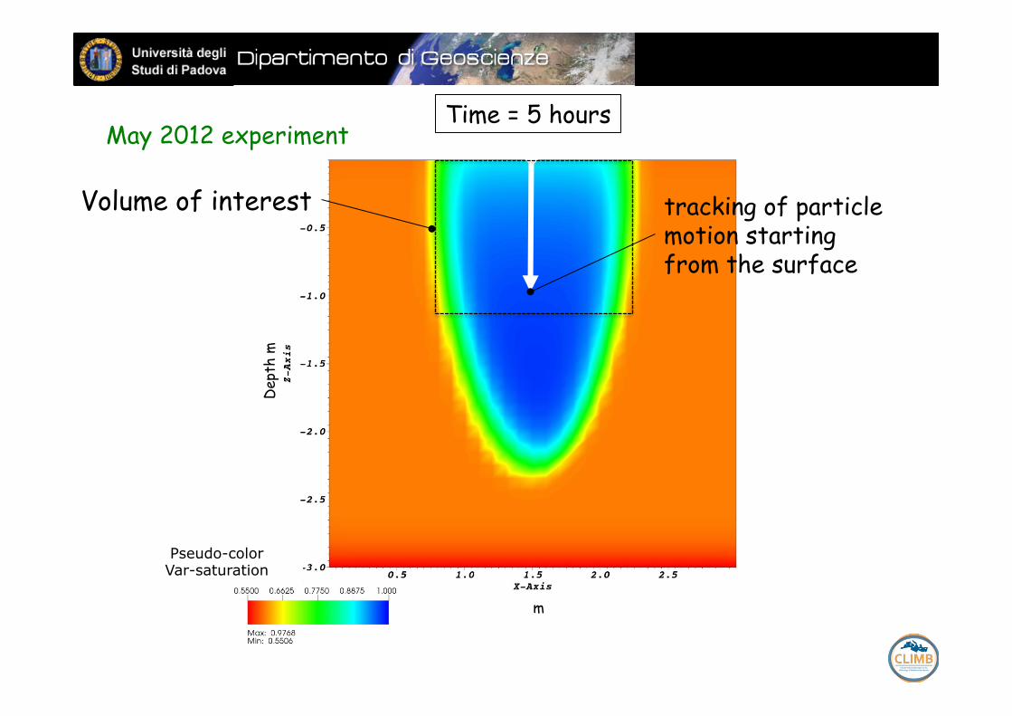
Time = 5 hours
tracking of particle motion starting from the surface
May 2012 experiment
Pseudo-color Var-saturation
Dep
th m
m
Volume of interest
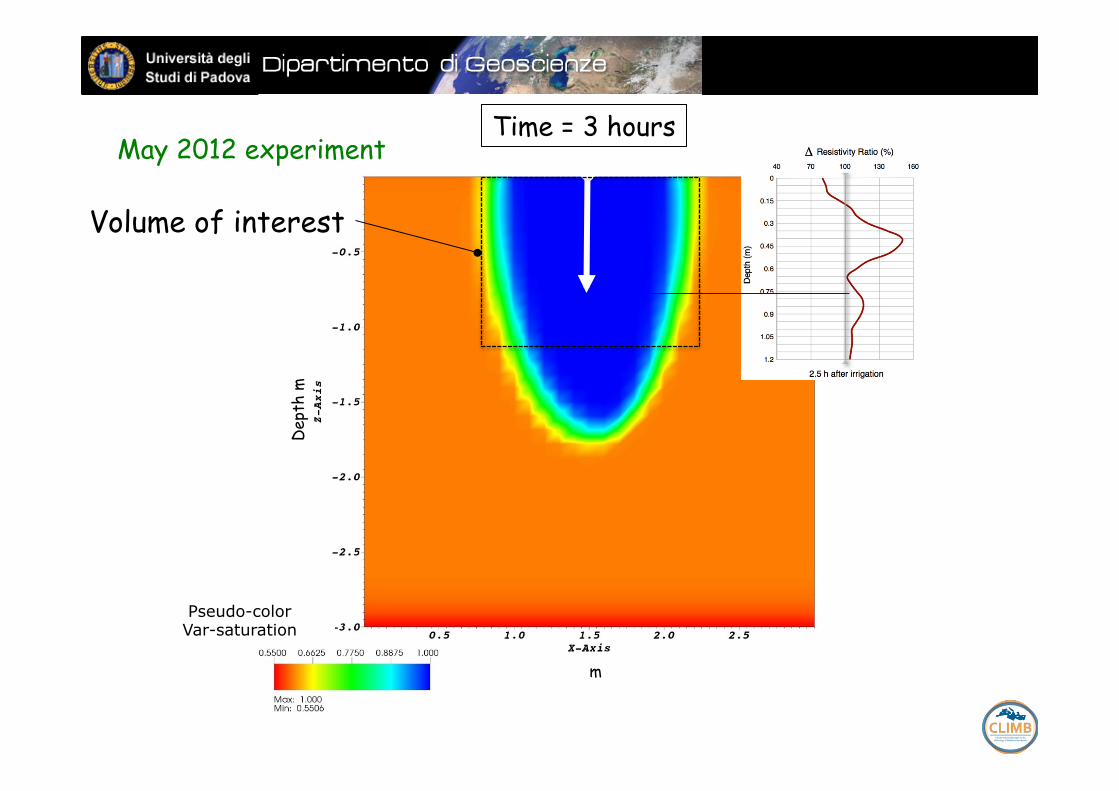
Time = 3 hours May 2012 experiment
Pseudo-color Var-saturation
Dep
th m
m
Volume of interest
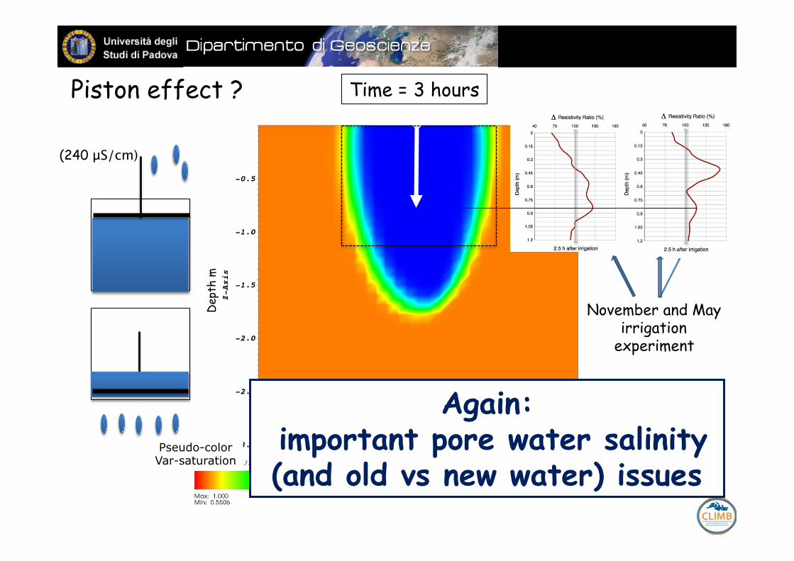
Time = 3 hours
November and May irrigation
experiment
Dep
th m
m
(240 μS/cm)
Pseudo-color Var-saturation
Piston effect ?
Again: important pore water salinity (and old vs new water) issues
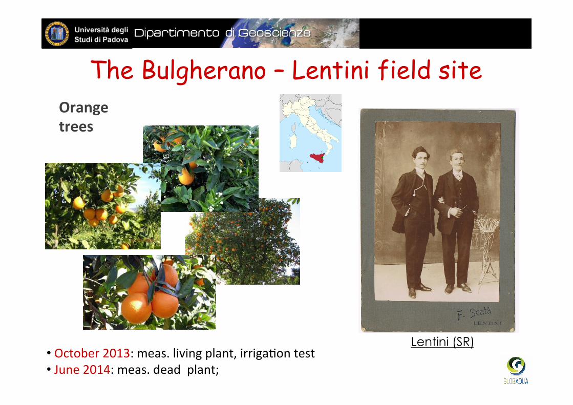
The Bulgherano – Lentini field site
Orange trees
Lentini (SR) • October 2013: meas. living plant, irriga#on test • June 2014: meas. dead plant;
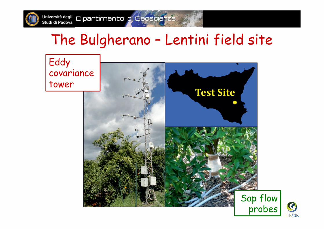
Eddy covariance tower
Sap flow probes
The Bulgherano – Lentini field site
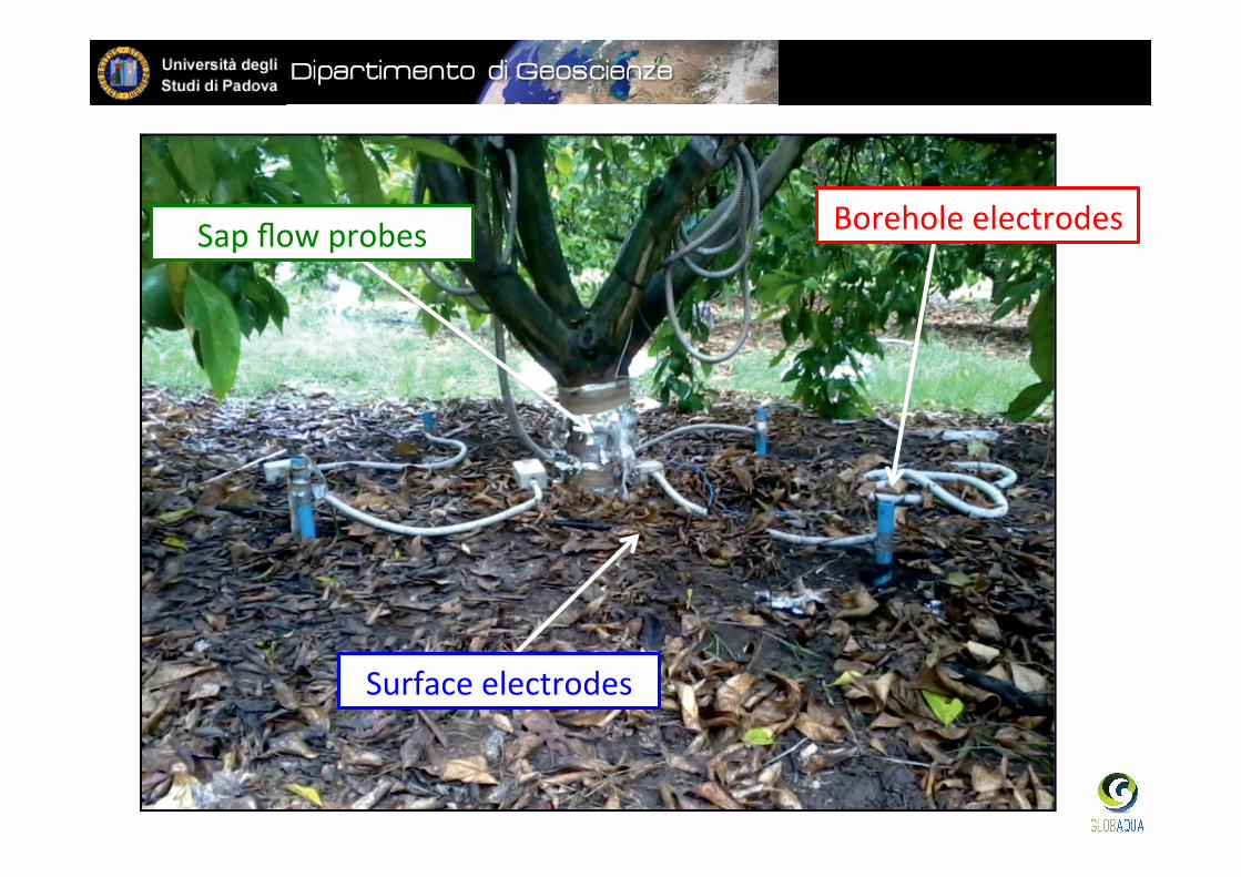
Surface electrodes
Borehole electrodes Sap flow probes
Surface electrodes
Borehole electrodes
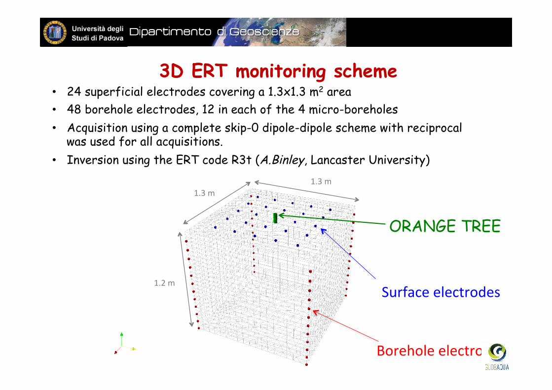
3D ERT monitoring scheme • 24 superficial electrodes covering a 1.3x1.3 m2 area • 48 borehole electrodes, 12 in each of the 4 micro-boreholes • Acquisition using a complete skip-0 dipole-dipole scheme with reciprocal
was used for all acquisitions. • Inversion using the ERT code R3t (A.Binley, Lancaster University)
1.3 m 1.3 m
1.2 m
ORANGE TREE
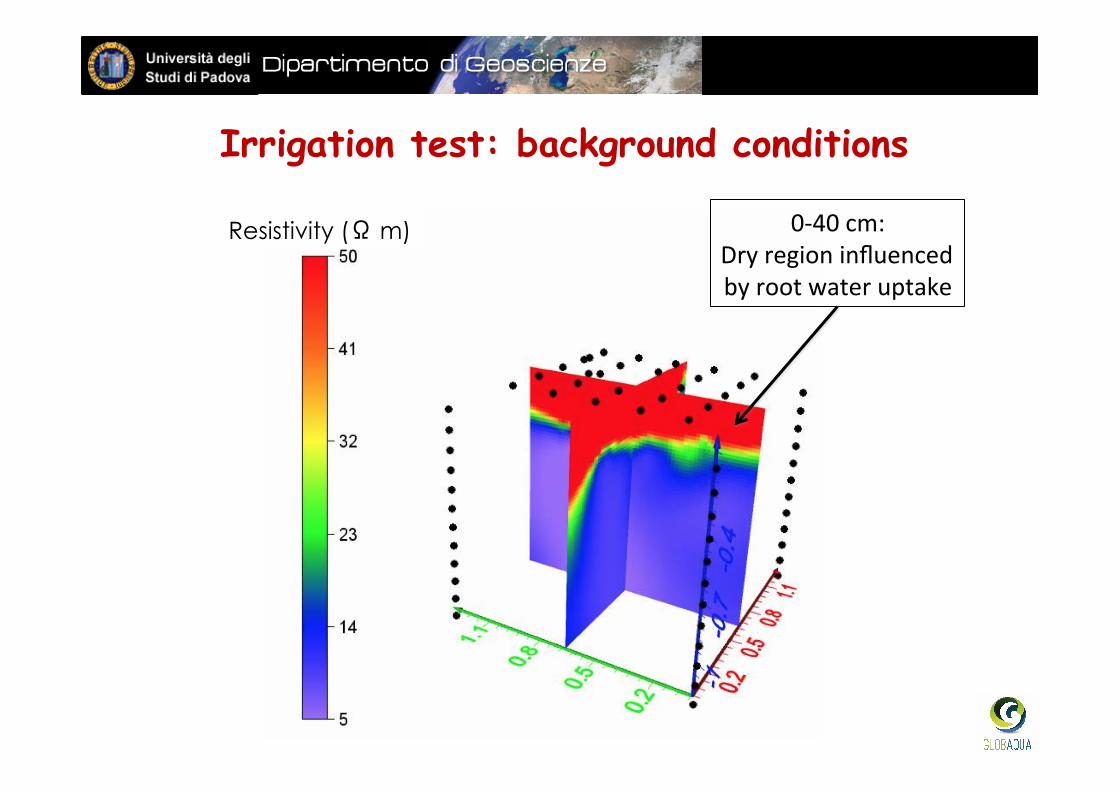
0-‐40 cm: Dry region influenced by root water uptake
Resistivity (Ω m)
Irrigation test: background conditions
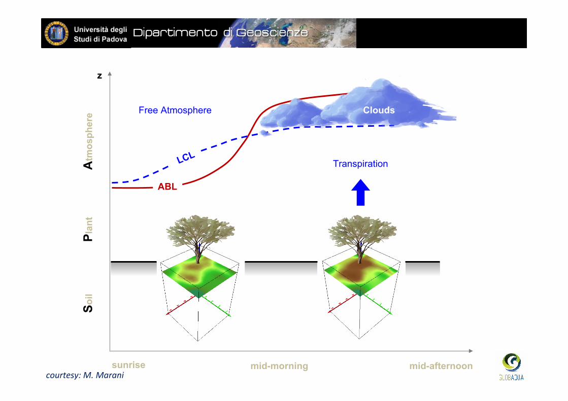
Clouds
Transpiration
z
ABL
Free Atmosphere
sunrise mid-morning
Soil
Plan
t A
tmos
pher
e
mid-afternoon courtesy: M. Marani
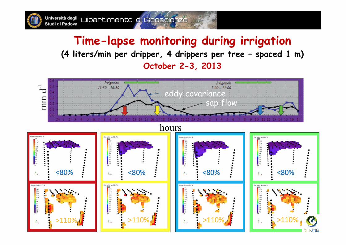
hours
Time-lapse monitoring during irrigation (4 liters/min per dripper, 4 drippers per tree – spaced 1 m)
October 2-3, 2013
eddy covariance sap flow
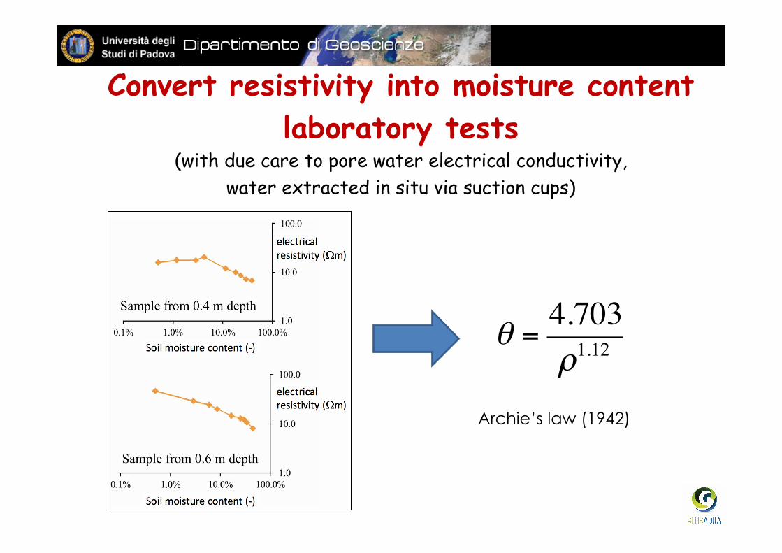
Convert resistivity into moisture content laboratory tests
(with due care to pore water electrical conductivity, water extracted in situ via suction cups)
θ =4.703ρ1.12
Archie’s law (1942)
Resistivity ratio with respect to background(%)
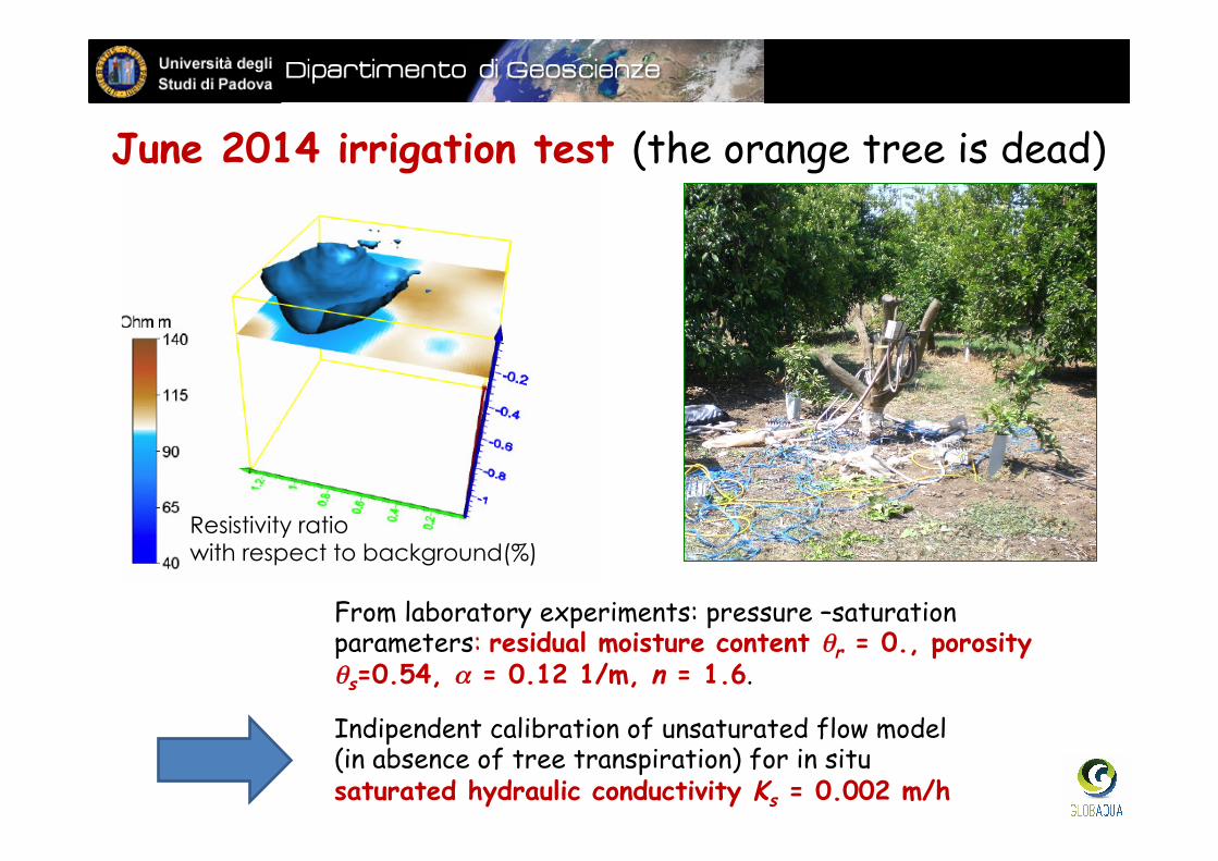
June 2014 irrigation test (the orange tree is dead)
Indipendent calibration of unsaturated flow model (in absence of tree transpiration) for in situ saturated hydraulic conductivity Ks = 0.002 m/h
From laboratory experiments: pressure –saturation parameters: residual moisture content θr = 0., porosity θs=0.54, α = 0.12 1/m, n = 1.6.
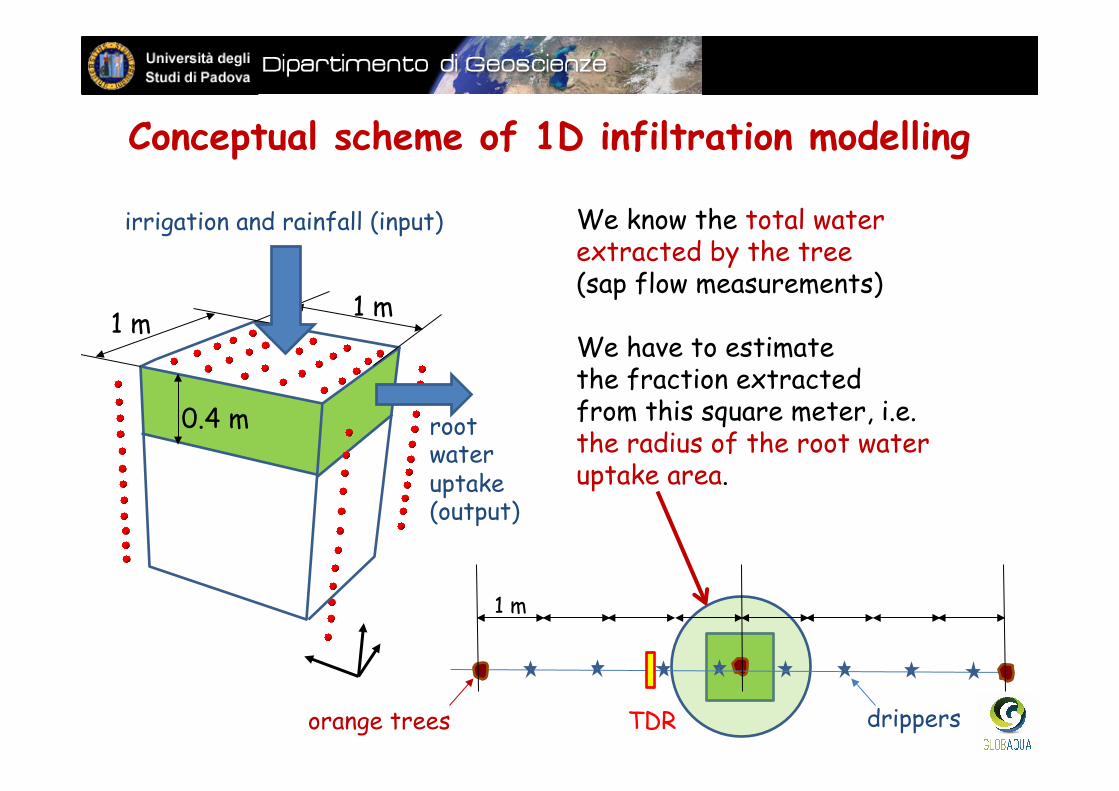
We know the total water extracted by the tree (sap flow measurements) We have to estimate the fraction extracted from this square meter, i.e. the radius of the root water uptake area.
irrigation and rainfall (input)
1 m 1 m
0.4 m root water uptake (output)
Conceptual scheme of 1D infiltration modelling
1 m
drippers orange trees TDR
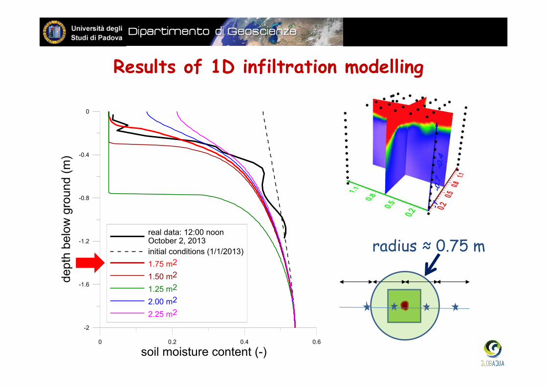
0 0.2 0.4 0.6
soil moisture content (-)
-2
-1.6
-1.2
-0.8
-0.4
0
dept
h be
low
gro
und
(m)
real data: 12:00 noonOctober 2, 2013initial conditions (1/1/2013)1.75 m2
1.50 m2
1.25 m2
2.00 m2
2.25 m2
Results of 1D infiltration modelling
radius ≈ 0.75 m
0.300
0.320
0.340
0.360
0.380
0.400
0.420
0.440
27/09/20
13
28/09/20
13
29/09/20
13
30/09/20
13
01/10/20
13
02/10/20
13
03/10/20
13
04/10/20
13
05/10/20
13
06/10/20
13
07/10/20
13
08/10/20
13
Soilmoistureconten
t(-‐)
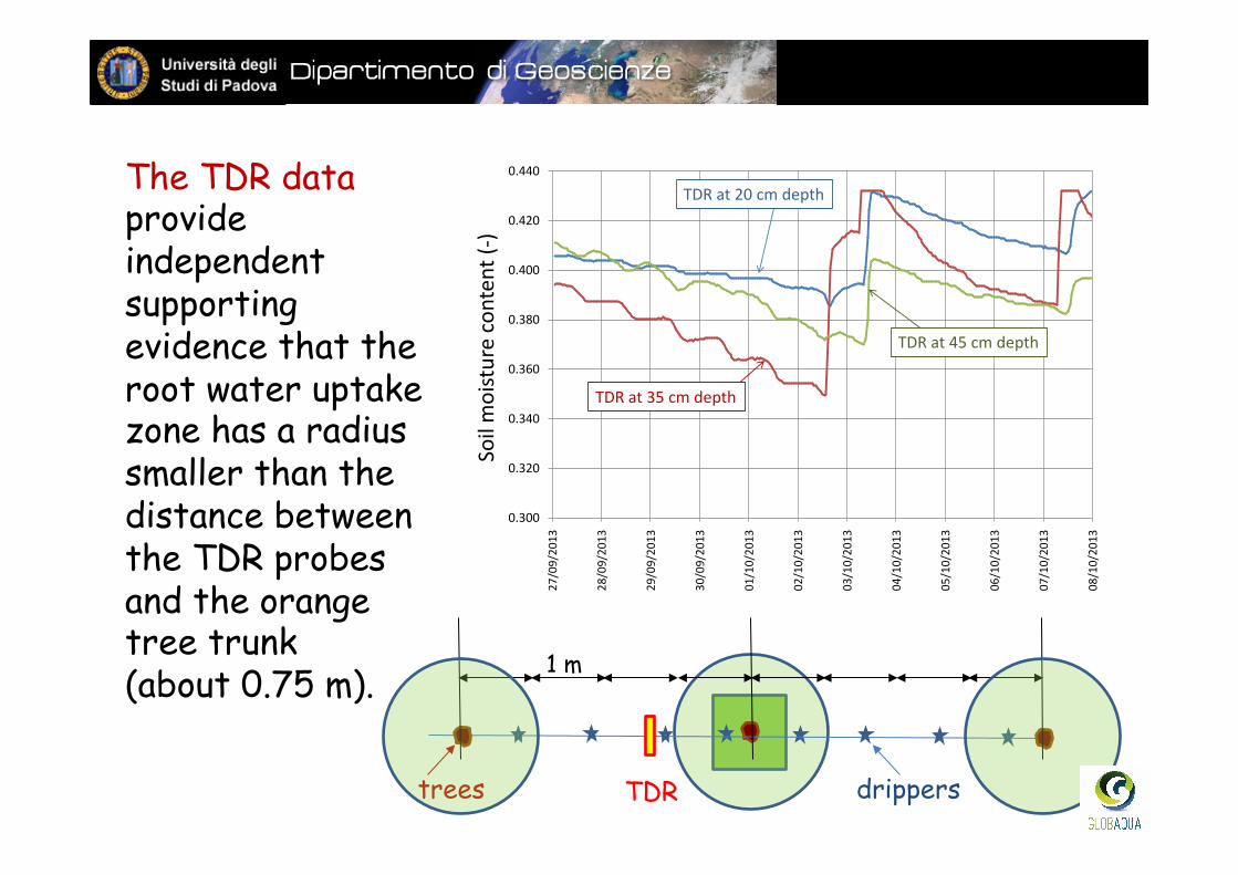
TDR at 20 cm depth
TDR at 35 cm depth
TDR at 45 cm depth
1 m
drippers trees TDR
The TDR data provide independent supporting evidence that the root water uptake zone has a radius smaller than the distance between the TDR probes and the orange tree trunk (about 0.75 m).
SUMMARY q Soil-plant-atmosphere interactions
q Characterization of the Earth’s critical zone: the role of non-invasive monitoring
q Large-scale monitoring
q Small-scale monitoring
q Outlook: assimilate data and models, with a vision
q Conclusions
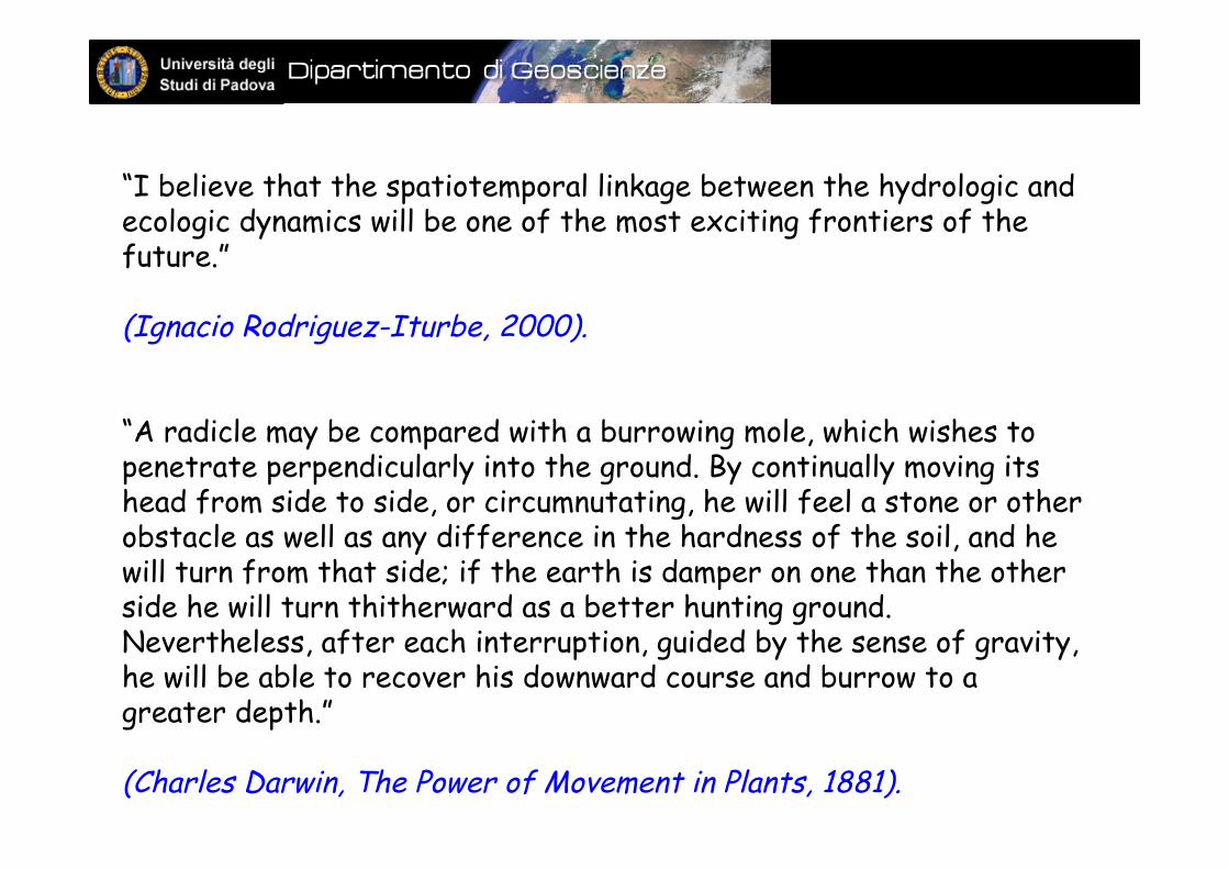
“I believe that the spatiotemporal linkage between the hydrologic and ecologic dynamics will be one of the most exciting frontiers of the future.” (Ignacio Rodriguez-Iturbe, 2000). “A radicle may be compared with a burrowing mole, which wishes to penetrate perpendicularly into the ground. By continually moving its head from side to side, or circumnutating, he will feel a stone or other obstacle as well as any difference in the hardness of the soil, and he will turn from that side; if the earth is damper on one than the other side he will turn thitherward as a better hunting ground. Nevertheless, after each interruption, guided by the sense of gravity, he will be able to recover his downward course and burrow to a greater depth.” (Charles Darwin, The Power of Movement in Plants, 1881).
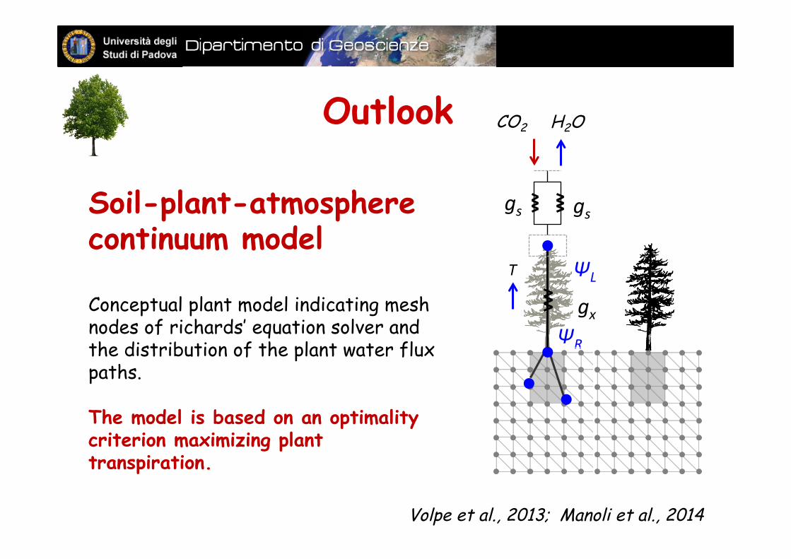
Conceptual plant model indicating mesh nodes of richards’ equation solver and the distribution of the plant water flux paths. The model is based on an optimality criterion maximizing plant transpiration.
Outlook
Soil-plant-atmosphere continuum model
ΨR
ΨL
CO2
gx
gs gs
T
H2O
Volpe et al., 2013; Manoli et al., 2014
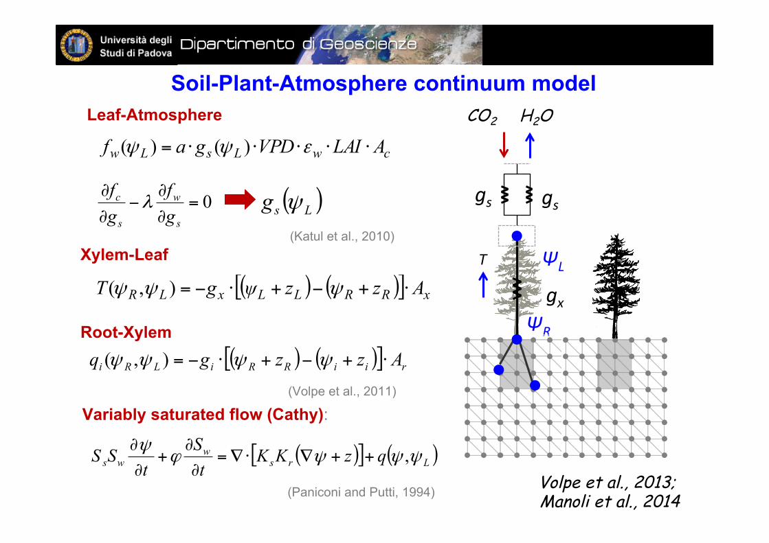
( ) ( )[ ] xRRLLxLR AzzψgT ⋅+−+⋅−= ψψψ ),(
( ) ( )[ ] riiRRiLRi Azzgq ⋅+−+⋅−= ψψψψ ),(
cwLsLw ALAIVPDgaf ⋅⋅⋅⋅⋅= εψψ )()(
Soil-Plant-Atmosphere continuum model Leaf-Atmosphere
Xylem-Leaf
Root-Xylem ΨR
ΨL
CO2
gx
gs gs
T
0=∂
∂−
∂
∂
s
w
s
c
gf
gf
λ
(Katul et al., 2010)
( )Lsg ψ
( )[ ] ( )Lrsw
ws qzKKtS
tSS ψψψϕ
ψ ,++∇⋅∇=∂
∂+
∂
∂
Variably saturated flow (Cathy):
H2O
(Volpe et al., 2011)
Volpe et al., 2013; Manoli et al., 2014 (Paniconi and Putti, 1994)
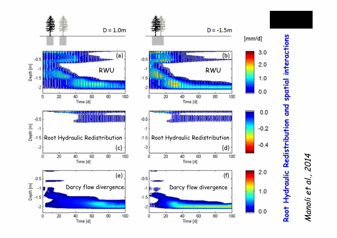
RWU RWU
Root Hydraulic Redistribution Root Hydraulic Redistribution
Darcy flow divergence Darcy flow divergence
Root
Hyd
raulic R
edistr
ibut
ion
and
spat
ial inte
ract
ions
Man
oli e
t al
., 20
14
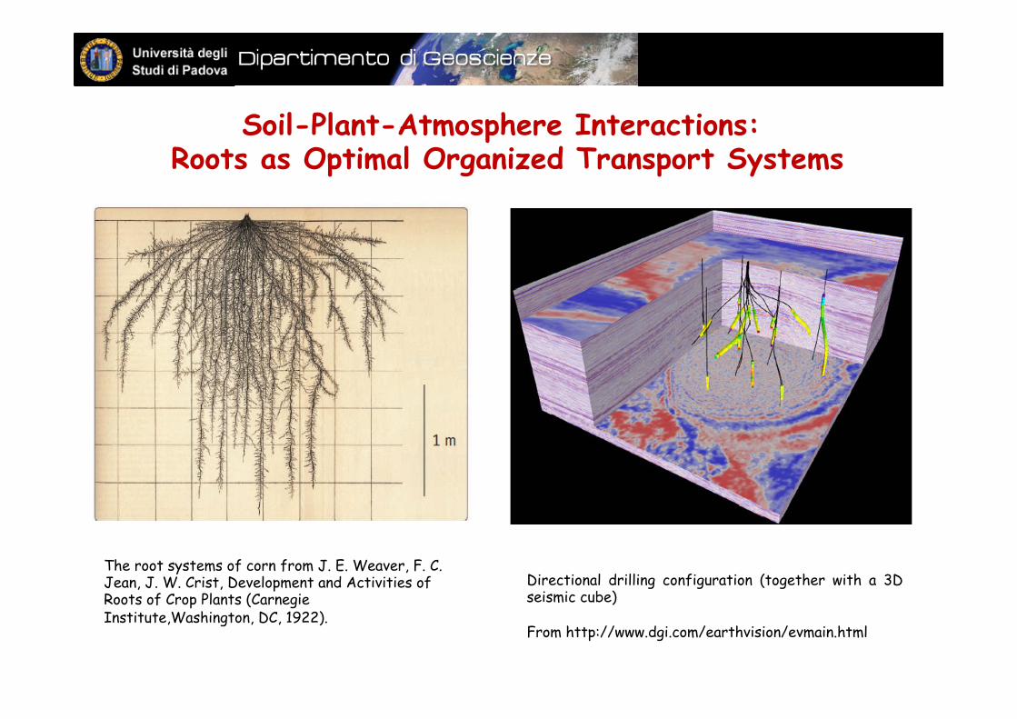
Soil-Plant-Atmosphere Interactions: Roots as Optimal Organized Transport Systems
The root systems of corn from J. E. Weaver, F. C. Jean, J. W. Crist, Development and Activities of Roots of Crop Plants (Carnegie Institute,Washington, DC, 1922).
Directional drilling configuration (together with a 3D seismic cube) From http://www.dgi.com/earthvision/evmain.html
courtesy: M. Pu7
12.5 m
8 m
2 m1.3 m2.5 m
soildrain (gravel)
soildrain (gravel)
12.5 m
12.5 m
5.5m x 2.5m 5.5m x 2.5m
5.5m x 2.5m
2m x
2.5m
3m x 2.5m
2m x
2.5m
3m x 2.5m
2m x
2.5m
3m x 2.5m
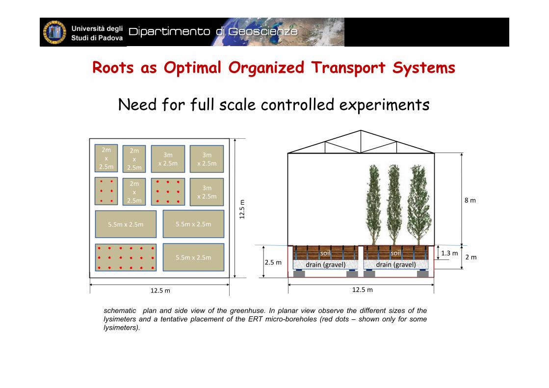
schematic plan and side view of the greenhuse. In planar view observe the different sizes of the lysimeters and a tentative placement of the ERT micro-boreholes (red dots – shown only for some lysimeters).
Roots as Optimal Organized Transport Systems
Need for full scale controlled experiments
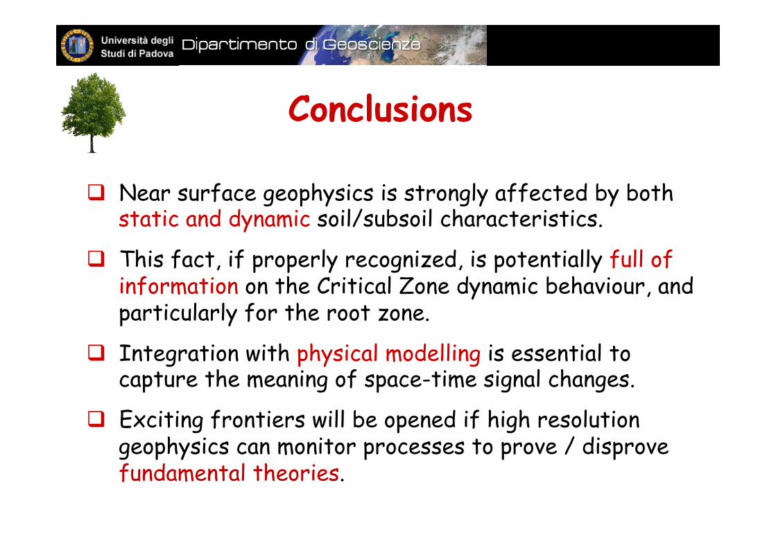
q Near surface geophysics is strongly affected by both static and dynamic soil/subsoil characteristics.
q This fact, if properly recognized, is potentially full of information on the Critical Zone dynamic behaviour, and particularly for the root zone.
q Integration with physical modelling is essential to capture the meaning of space-time signal changes.
q Exciting frontiers will be opened if high resolution geophysics can monitor processes to prove / disprove fundamental theories.
Conclusions
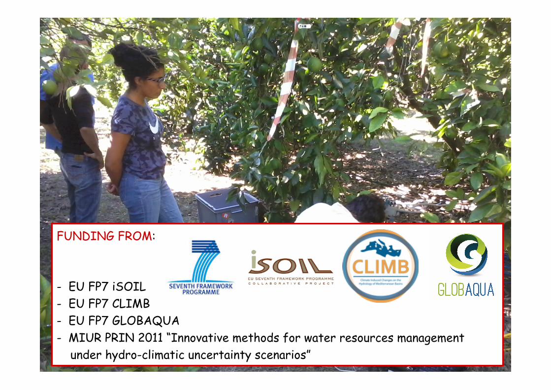
FUNDING FROM: - EU FP7 iSOIL - EU FP7 CLIMB - EU FP7 GLOBAQUA - MIUR PRIN 2011 “Innovative methods for water resources management
under hydro-climatic uncertainty scenarios”
Acknowledgements MARCO MARANI, MARTA ALTISSIMO, PAOLO SALANDIN, MATTEO CAMPORESE, MARIO PUTTI, NADIA URSINO, RITA DEIANA, JACOPO BOAGA, MATTEO ROSSI, MARIATERESA PERRI Università di Padova ALBERTO BELLIN, BRUNO MAJONE Università di Trento
SIMONA CONSOLI, DANIELA VANELLA Università di Catania STEFANO FERRARIS Università di Torino
ANDREW BINLEY Lancaster University
Thanks for your attention
Top Related