Windows 95-98, NT, 2000)web.tiscali.it/epaulesu/spedizione1.pdfEraldo Paulesu ps Gran parte delle...

Eraldo Paulesu Bicocca

From: "Paulesu Eraldo - Dip. di Psicologia" <[email protected]>To: <[email protected]>Sent: martedì 19 marzo 2002 16.19Attach: mrinstall.exe; MRI.hdr; MRI.img.gzSubject: Mailng List Fondamenti. Software per la visualizzazione della risonanza magnetica di un

cervello normale adulto.

of 34

19/03/2002

Buongiorno. Allego qui di seguito la pagina che descrive il software per la visualizzazione di immagini di risonanza magnetica del cervello. Il software è stato scritto da Chris Rorden. In allegato aggiungo il programma stesso ( mrinstall.exe compatibile con Windows 95-98, NT, 2000): copiate il file in un nuovo direttorio e fate doppio click sul file. il programma si installerà automaticamente. Ho anche allegato un file di risonanza magnetica (composto di due parti entrambe indispensabili:MRI.hdr e MRI.img.gz) Il fiel MRI.img.gz è compresso e deve essere espanso (es. con programmi come Winzip o con gzip www.gzip.org) Una volta decompresso il file MRI.img.gz, questo può essere caricato dal software di visualizzazione nè più nè meno di un file di word. Scegliere se vedere i dati in proiezione assiale, sagittale o coronale, in tre proiezioni ortogonali o come rendering 3D è quindi facilissimo. Cordiali saluti Eraldo Paulesu ps Gran parte delle istruzioni qui sotto elencate vanno oltre i vostri scopi dato che il software e' pensato per applicazioni di ricerca. Gli interessati approfondiranno l'uso di questo ed altri software per neuroimmagini nel corso di Psicologia Fisiologica (corso avanzato) ed eventualmente per la tesi di laurea.

System requirements: Windows 95-98, NT, 2000, Linux x86, Solaris

x86Hardware requirements: 16 or 24-bit colour

Current version: 1.33Price: Free (see installation section to download)

Author: Chris Rorden ([email protected])

Index

1. Introduction 2. Installation 3. Loading images and the header information panel 4. Slice viewer panel 5. Region of interest panel 6. Rotation and clipping panel 7. Overlays [Statistical Maps] 8. Selecting Coordinates 9. Other commands

10. Viewing medical images 11. Converting medical images to Analyze format 12. Uninstalling 13. Technical details

Introduction Return to Index

MRIcro allows Windows PCs to view medical images. It is a standalone program, but includes tools to complement SPM (software that allows neuroimagers to normalise and analyse MRI, fMRI and PET images). MRIcro allows efficient viewing and exporting of brain images. In addition, it allows neuropsychologists to identify regions of interest (ROIs, e.g. lesions). MRIcro can create Analyze format headers for exporting brain images to other platforms.

Users familiar with other Windows programs will find that this software is fairly straightforward to use. Resting the mouse cursor over a button will cause a text hint to appear over the button. As a last resort, I have included this brief manual that describes the basic features.

A tutorial with a sample MRI scan and a step by step guide of how to use MRIcro with SPM is available from www.psychology.nottingham.ac.uk/staff/cr1/mritut.html [the tutorial is also available from www.icn.ucl.ac.uk/groups/JD/mricro/mritut.html].

Installation Return to Index

This section describes how to install MRIcro on a computer with the Windows operating system.

Features:

Converts medical images to SPM friendly Analyze format. View Analyze format images (big or little endian). Create Analyze format headers (big or little endian). Create 3D regions of interest (with computed volume & intensity). Overlap multiple regions of interest. Rotate images to match SPM template images. Export images to BMP, JPEG, PNG or TIF format. Yoked images: linked viewing of multiple images (e.g. view same coordinates of PET and MRI scans).

of 34

19/03/2002

There is a separate web page that describes the installation of the Linux version of MRIcro.

1. With your computer connected to the web, shift+click here. This will download the 1.2Mb installer program www.psychology.nottingham.ac.uk/staff/cr1/mrinstall.exe.

2. Double click on the "mrinstall" icon. The installer will give you the option to install the manuals, a sample MRI image and other files. By default, the files will be installed in "C:\Program Files\MRIcro". Note: with Windows 2000/NT, only adminstrators can copy files into the "Program Files" folder. If you are using 2000 or NT, either log in as an administrator or choose a different folder to install the files (e.g. "C:\username\mricro").

3. To run MRIcro, click on the "Start" menu, select "Programs", point to the "MRIcro" folder and click on the "MRIcro" icon.

Note: You can also get MRIcro from "http://www.icn.ucl.ac.uk/groups/JD/mricro/mricro.html". If you want to manually install the software, you can download the zip file, and read the zip file install notes.

Loading images and the header information panel Return to Index

MRIcro can view various medical image formats, including the Analyze format used by SPM. Analyze format images have two components: the image file (*.img) that contains the raw image data and a header file (*.hdr) that describes the image dimensions, data format and comments. MRIcro's header information panel displays the header file's information and includes a series of buttons that allow you to open and save headers. These buttons will be described from left to right as they appear on the screen.

The 'open Analyze format hdr/img pair' button (it looks like an open folder) allows you to view an Analyze format image. When you press this button, a dialog will appear that allows you to select a header file to open. MRIcro will then attempt to open an image file of with the same name (e.g. if you select a header 'C:\17.hdr', MRIcro will attempt to open the image file 'C:\17.img').

Use the 'open Analyze format header' button (it looks like an open folder with the letters 'hdr') to read an Analyze format header. The information will be displayed in the header information panel (e.g. the dimensions of the image).

The 'open Analyze format image' button (it looks like an open folder with the letters 'img') allows you to read an Analyze format image using the header settings currently being displayed in the header information panel. If successful, the selected image will be displayed.

The 'show extended header information' button (it looks like a stack of books) will open a window showing additional information about the currently open header (e.g. Scan comments, patient ID, etc).

Figure 1. The header information panel.

of 34

19/03/2002

The rightmost button in the Header Information panel allows you to save the current header. The new header will contain all of the properties set on the panel as well as the extended header information (it can be displayed by pressing the 'show extended header information' button). Depending on the panel's byte-rder drop down list, the header will be saved in either 'big-endian' or 'little-endian' format. Big-endian is the native format for Sun and Silicon Graphics computers. The Little-endian is the native format for Intel computers (Note that MRIcro, recent versions of Analyze, SPM99 and SPM96 for Windows will automatically read either format [as long as the complementary header and image files have the same byte-order]). For more information about big-endian and little-endian formats, refer to the technical section.

Slice viewer panel Return to Index

The slice viewer panel allows you to select the appearance of the loaded image file. The top slider selects which slice is displayed (alternately, you can select the slice in the edit box located directly to the right of the slider, or pressing Fn1/Fn2 to view the next successively lower/higher slice).

The lower sliders control the contrast of the image. You can adjust these until the image appears at the desired brightness. Note: MRIcro only displays 255 levels of grey. Analyze images with more than 8-bits per voxel can potentially show many more than 255 levels of grey. Therefore, adjusting the contrast sliders for these high-depth images will cause a 'contrast' button to appear directly to the left of the contrast sliders. Pressing this contrast button will optimise the grey scale display (the contrast icon is shown in the Figure above). The contrast sliders allow quick adjustment of the contrast. In addition, MRIcro has two other tools for adjusting image contrast. First, clicking the 'auto contrast' button (it is at the bottom-right of the panel, showing a white arrow on a mostly black circle) sets 1% of the image to be maximum black and 1% to be maximum white. The autobalance works well for MRI scans, but often is not appropriate for CT scans, where the bones appear much brighter than the background and brain tissue. Right clicking the autocontrast balance displays the precise contrast window (shown in the diagram below). This tool uses the DICOM-standard window-center and window-width controls to allow calibrated adjustments of CT images (the window center describes the middle of the gradient, and the window width describes the total width of the gradient, so setting the center/width of an image to 50/100 will create a graded brightness between 0 and 100 [voxels with an intensity <=0 will be black, those>=100 will be white]).This control is also useful for precise brightness control of MRI scans.

Figure 2. Two views of the slice viewer panel. When viewing axial, sagittal or coronal views, a slider appears that allows you to set which slice is displayed (left panel). When projection views are displayed, you can set the X, Y and Z coordinates independently by adjusting the three edit boxes (right panel). Note that the right panel has an 'optimize contrast' button (the icon of a black and white circle), as described in the text.

of 34

19/03/2002

The histogram button (located at the bottom-left of the panel) displays the voxel brightness distribution in the currently open image (see figure, above).

Six icons appear on the lower right of the Slice viewer panel that allow you to select which view of the image is displayed: axial, sagittal, coronal or projection (axial, sagittal and coronal simultaneously), free rotate, multislice and 3D rendering. If the image does not correspond with the selected button, the image was not saved in axial format. In the projection view, three edit boxes appear at the top of the slice viewer, allowing you to independently set the X, Y and Z coordinates you wish to view (alternately, click on the image to jump to the mouse coordinates). The projection view can be displayed with or without cross bars and file information by setting the check boxes that appear in the slice viewer panel.

If you are viewing more than one image simultaneously (having launched MRIcro more than once) you can 'yoke' the views, so that the same view is mirrored for each image (for this feature to work, make sure that the 'yoke' check box is selected). Yoking will try to match the slices based on the origin and size coordinates. This allows you to compare normalisation between an image and its template, as well as localising structures on a PET scan by comparing the PET scan with its coregistered T1 MRI scan.

To see a series of transverse or coronal slices simultaneously press the 'multislice' button (it has an icon showing three axial slices next to a sagittal slice). In order to function, an image must be loaded. The slices can be selected in the 'options' window, as described in other commands section.

Selecting the free rotate button causes a new window titled 'Free Rotate' to appear (see the figure below). This window allows you to select which oblique section you wish to view. You can independently set the yaw, roll, and pitch of the scan. Furthermore, you can select which slice you wish to view. The 'pivot' settings allow you to set the axis for the image rotations. You can also 'nudge' the image (center the image in the frame). Finally, you can set new image dimensions.

Figure 3. The custom intensity window allows users precise control of the image brightness. This feature is described in the MRIcro FAQ

Figure 4. This histogram shows the image intensity profile for the image 'IconT1'. Histograms can also be created for user defined regions of interest (see the ROI section for more details). Note the Threshold Mn value is listed, this can be used to set the image intensity scale of a target image to match an SPM template (see the tutorial for more details).

of 34

19/03/2002

Custom views can be saved as graphic pictures (using the 'file/save as picture' command), printed, or press the 'Save' button at the bottom of the Free Rotate window to create a new 8-bit Analyze format image described by your rotations. Note that the free rotate tools mix viewer centered and object centered coordinates, which can become somewhat disorienting. Also, when free rotating multiple Regions of interest with the 'interpolate' box checked, you may see a slight white halo around the regions.

You can generate 3D volume renderings by pressing the '3D' button. This feature is described in more detail on my volume rendering page.

The Mirror button (it displays the letter 'LR' in either standard or mirrored text, depending on whether mirroring is selected) allows you to flip the image's left and right. If you select mirroring, a message will appear reminding you that it is best not to edit regions of interest while in the mirror mode (as the ROI will be stored in a different orientation than the original image).

A drop-down box selects the color lookup table (LUT) used. By default, MRIcro can show images in the 'black & white' or 'hot metal' color schemes. However, MRIcro can also read Osiris format LUTs, which allow you to view images in different color schemes. MRIcro ships with several LUTs from the Osiris distribution, and you can create your own custom LUTs. If MRIcro finds any *.LUT files in its directory, the drop-down box will list the file names. Select the color scheme you want from the drop down box.

A drop down box allows you to select how MRIcro displays images with voxels of unequal dimensions (e.g. an image slice where voxels are 2mm in theX dimension but 1mm in the Y dimension). First, images can be viewed in the 'square' mode, where all voxels are displayed as being square, irregardless of interslice dimensions. Second, you can view images 'stretch'ed, where the size of voxels is proportional to the interslice dimensions, using a nearest neighbor approximation (though projection and multislice views are NOT scaled). Finally, you can view images as 'smooth'ed: voxel size is proportional and uses a nearest neighbor approximation (this creates 24-bit images, projection views are shown correctly scaled).

Use the zoom factor box (located at the lower right of the slice viewer panel) to set the image scale, MRIcro allows you to view images in x1-x6 scale. Depending on the size and scale of your images, you may want to adjust the size of the MRIcro window (by dragging the lower right corner of the viewer).

Region of interest panel Return to Index

MRIcro allows you to draw three-dimensional regions of interest (ROIs). This is useful for illustrating regions of the brain that have sustained damage. In addition, the volume of the ROI is computed. Moreover, ROIs from different individuals can be overlapped (on brain images that have been normalised to the same template) allowing neuropsychologists to assess common areas of

Figure 5. The free rotation view allows you to create a custom view.

of 34

19/03/2002

damage.

ROIs can be saved to disk for future reference. All ROIs are drawn on top of the MRI image, rather than directly on it. This means that the brain images can be viewed with or without corresponding ROIs.

MRIcro provides a number of tools for creating and viewing ROIs. These tools are displayed as a series of buttons in the 'Region of interest' panel. These buttons will be described sequentially from left to right.

Use the 'open hdr + img + roi' button (it looks like an open folder with a brain image on it) to display a brain image. This command works when the header, image and ROI all share the same name and are located in the same folder (e.g. if the header is named '17.hdr', then the image is '17.img' and the roi is '17.roi').

The 'open roi' button (the bottom, left button that looks like an open folder with a ROI) allows you to select ROI[s] to open. If you want to open multiple ROIs simultaneously, depress the control key as you select the ROI names.

The 'save ROI' button (it has an icon of a disk with a ROI superimposed on it) allows you to save a ROI that you have created to disk.

In order to remove all current ROI[s] from memory, click the 'delete entire ROI' button (it looks like a waste basket). If you have opened multiple ROIs, you will need to select this before creating a new ROI (you can only write to one ROI at a time).

Use the 'delete ROI on this slice' button (it shows a pencil erasing information) to remove the ROI only from the slice you are currently viewing. This button is useful if you make a mistake outlining or filling a ROI that you are drawing.

The ROI information button (it displays an 'i'nformation icon) displays the mean image intensity of a region of interest as well as generating an image intensity histogram (similar to the histogram depicted in the slice viewer section).

Next, there is a small drop down box that defines the colour that single ROIs will be drawn in (when viewing multiple ROIs simultaneously a rainbow colour set is automatically used). The choices are Red, Green, Blue, White or Black. This allows you to choose a salient colour. You can set the ROI to black or white before printing the image to a black and white printer.

After loadingmultiple ROIs, you can select the 'ROI density colorbar' item from the 'ROI' menu to draw graphic of the overlap between ROIs. The colours indicate the number of overlapping ROIs. The leftmost (dark violet) colour indicates the index for a single ROI, while the rightmost (bright red) colour shows the index for all the ROIs overlapping. This feature is demonstrated in the figure below:

Figure 6. The Region of Interest panel contains tools for marking lesion locations or specific areas. In this example, the label '17.7 cc' indicates that an ROI is currently loaded with a volume of 17.7 cubic centimeters.

Figure 7. These figures show MRI multislices with four overlapping ROIs. The colour bar in the upper

of 34

19/03/2002

Select one of the pens for creating ROI outlines. There are two pens: the 'closed' pen (shortcut key Fn6) automatically closes any outline you have drawn. The 'open' pen (shortcut key Fn7) does not automatically close the outline. The 'fill button' (paint can icon, shortcut Fn8) can be used to fill a ROI that has been outlined by the pen (alternative: right click with the pen selected). Before beginning to create a new ROI you should load the image, clear any previous ROIs (using the 'save ROI' or 'delete entire ROI' buttons described above), and set the view to transverse, coronal or sagittal slices (you can not draw ROIs on the free rotate, projection and multiple views). Holding the shift key down while using a pen or fill will erase ROIs in the designated region.

In practice, ROIs can be drawn rapidly by selecting the closed pen (shortcut key Fn6) and then using Fn1 and Fn2 to move up and down to the desired slices. Using the pen with the shift key down is useful for trimming unwanted edges from a ROI. Use the left mouse button to outline the ROI, and then move to the centre of the ROI and right-click to fill the region. Once the ROI is drawn, use the 'Save ROI' button to store the ROI. Note that the ROI volume is listed in the Region of interest panel (computed in either cc or voxels, updated when you change slices or save the ROI).

The wizard's cap icon allows you to temporarily hide a region of interest (shortcut key Fn9). By rapidly hiding and showing the ROI, you can see whether the ROI you have drawn correctly maps the region you are interested in.

Two useful bits of information are displayed immediately below the region of interest panel. Text on the left side shows the image intensity immediately beneath the mouse. Text on the right side displays the mouse position in Talaraich space.

Rotation and clipping panel Return to Index

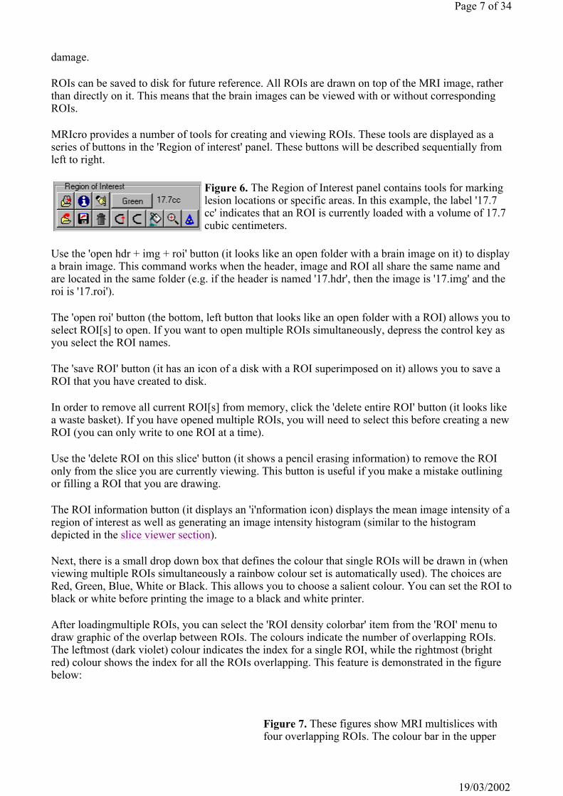
The file menu contains a command labelled 'Save as...'. When this command is selected, a floating panel appears in the lower left corner of program's window. The rotation and clipping panel can be used to prepare image files for normalisation (coregistering an image to a standard template) with SPM.

right corners indicates the ROI density (dark violet for one ROI, bright red for four overlapping ROIs). These figures also demonstrates the option window's 'show right hemisphere' function -where successive slices overlap each other. Multislices can be generated either for transverse slices (top panel) or coronal slices (bottom panel).

Figure 8. The rotation and clipping panel.

of 34

19/03/2002

The clip top and clip bottom fields allow you to choose the number of slices that you want to shave off of the top or bottom of a scan (for example, trimming scans that include too much spinal cord to avoid problems with SPM normalisations). The 'Format' list box allows you to convert coronal or sagittal Analyze format images to axial format (this is the natural preference for SPM). To determine the original format of your image, click on the 'axial [flat] view' button in the slice viewer panel, this will display the scan in its native format (e.g. if the flat format displays a sagittal image, the file is in sagittal format). The 'flip left/right' checkbox mirrors the image.

You can also set the 'data' type for the saved image. Usually it is wise to save the data in the same format as the source image. Down-sampling an image (e.g. saving a 16-bit integer file as an 8-bit data file) will save disk space (potentially at the expense of image intensity quality). Up-sampling an image (e.g. saving a 16-bit file as a 32-bit file) can be useful for when other programs require data of a specific type. If you have adjusted the 'black' or 'white' contrast sliders in the slice viewer panel, you will be asked if you wish to clip the brightest and/or darkest voxels, allowing you to customise the contrast of the output.

Before saving an image that you wish to rotate, you can check your settings by pressing the 'preview' button. The preview will show you two slices of how the image will appear after being rotated. If your settings are correct, the preview should show two transverse slices (with the left slice being more ventral than the right slice). Make sure to check that the left/right mirroring is correct.

When you have selected the desired clipping and check box options, press one of the three file save buttons that are located at the bottom of the window. The buttons 'Save [Sun]' and 'Save [Intel]' will save the files as Analyze format images. SPMwin, SPM99 and MRIcro can all read either big or little-endian Analyze files, while SPM96 requires the images to be in the same format as the machine used. For more information, see the technical section.If the original image is a multi-volume image (i.e. the img file contains multiple MRI scans, which are all the same dimension), MRIcro will rotate each volume and save it as a separate Analyze format header/image (this is useful, as SPM can not read multiple volume files). The 'Save Dicom' button will save the image as a DICOM format image (as described in the DICOM section of this manual). Note that the DICOM format image will either be in 8-bit integer (if that is the data type of the source image) or 16-bit integer format irregardless of the data type seleted.

Overlays [Statistical Maps] Return to Index

The 'Overlay' menu allows you to select an image which is superimposed on top of another image. This is useful for displaying functional statistical maps (generated by SPM from PET, fMRI or SPECT data). Overlays can also be used to check the coregistration of two images. To display an overlay, you should first choose the primary image you want to use (e.g. use the 'Open' command from the file menu to select your anatomical image). Next, use the 'Load overlay' command in the Overlay menu to select the image you wish to superimpose. The overlay does NOT need to be the resliced to the same dimensions as the anatomical image: MRIcro will correctly reslice the data (as long as the image dimensions and origin are correctly specified for each image). The overlay menu also allows you to select the color of the overlay and whether the overlay is shown as opaque or transparent. The images below show overlays of functional data (left) and the use of the overlay function to check normalization. For more details, visit my overlay and volume rendering pages.

Figure 9. MRIcro automatically displays the amount of clipping selected, in this example the top five and bottom ten slices are about to be clipped. This figure also shows the 'Hot Metal' color lookup table.

of 34

19/03/2002

Selecting coordinates Return to Index

The 'Select MNI/Talairach Coordinates' command in the 'View' menu allows you to specify which region of the brain you want to view. With the slice viewer panel, you choose which slice in the image you wish to view. In contrast, the coordinates command allows you to type in the steotactic coordinates used by neuroimagers. This command only makes sense if your image has been normalized (stretched, rotated and centered to match a standard neurological frame of reference). There are two popular frames of reference for brain imaging: MNI space (used by SPM99) and Talairach space (used in the atlases of Talairach and Torneaux). A check box in the coordinates window allows you to set which frame of reference you wish to use (the Talairach coordinates are estimated used Matthew Brett's handy mni2tal routine). These two methods are illustrated below. When looking at an image from the Talairach and Tournoux atlas (left) you should make sure the 'mni2tal' box is checked (shown in red). On the other hand, when looking at SPM99 results, make sure this feature is switched off.

Other commands Return to Index

The 'File' menu contains the command 'save as picture', which allows you to save the currently displayed image as a 2D graphic image. Supported formats include the popular BMP, JPEG, PNG

Left: functional results can be overlayed. Above: you can use overlays to check alignment after normalization.

of 34

19/03/2002

and TIF formats. The File menu's 'Print' item allows you to print the currently displayed image.

The ROI menu contains commands that allow you to export ROIs as big-endian (Sun) or little-endian (Intel) Analyze format images. These commands save the currently displayed region of interest as an 8-bit Analyze format image, which can be used in SPM as a mask (allowing sensible normalization of brain images that have large lesions). Note that the only values on the mask image are 0 (unmasked) and 100 (masked), and that the mask's image intensity scale value is set to 0.01 (so from SPM's point of view, the Mask has voxels of the values 0 and 1).

The ROI menu's 'Export Image as ROI' converts an Analyze format image in MRIcro's custom ROI format. Note that the ROI format is binary -the ROI does not store intensity information. Load the image you wish to convert before selecting this command. When you select this item, a window appears that allows you to set the intensity ROI's threshold. As you adjust the threshold, the image will will preview the portions of the image will be included in the ROI. When you are happy with the selection, press the 'Save as ROI' button to create the new ROI.

In addition, you can transfer a region of interest between two images that have different dimensions. One example of the utility of this command is identifying cortical regions on a PET scan. Using the 'File/Transfer ROI' command you can create a ROI on the individuals T1 anatomical MRI scan and then copy the ROI to the corresponding PET scan(s).

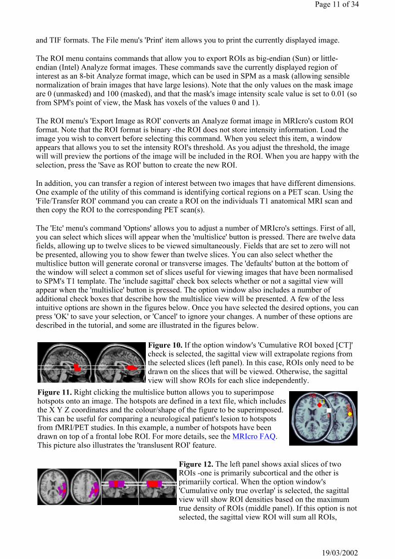
The 'Etc' menu's command 'Options' allows you to adjust a number of MRIcro's settings. First of all, you can select which slices will appear when the 'multislice' button is pressed. There are twelve data fields, allowing up to twelve slices to be viewed simultaneously. Fields that are set to zero will not be presented, allowing you to show fewer than twelve slices. You can also select whether the multislice button will generate coronal or transverse images. The 'defaults' button at the bottom of the window will select a common set of slices useful for viewing images that have been normalised to SPM's T1 template. The 'include sagittal' check box selects whether or not a sagittal view will appear when the 'multislice' button is pressed. The option window also includes a number of additional check boxes that describe how the multislice view will be presented. A few of the less intuitive options are shown in the figures below. Once you have selected the desired options, you can press 'OK' to save your selection, or 'Cancel' to ignore your changes. A number of these options are described in the tutorial, and some are illustrated in the figures below.

Figure 10. If the option window's 'Cumulative ROI boxed [CT]' check is selected, the sagittal view will extrapolate regions from the selected slices (left panel). In this case, ROIs only need to be drawn on the slices that will be viewed. Otherwise, the sagittal view will show ROIs for each slice independently.

Figure 11. Right clicking the multislice button allows you to superimpose hotspots onto an image. The hotspots are defined in a text file, which includes the X Y Z coordinates and the colour/shape of the figure to be superimposed. This can be useful for comparing a neurological patient's lesion to hotspots from fMRI/PET studies. In this example, a number of hotspots have been drawn on top of a frontal lobe ROI. For more details, see the MRIcro FAQ. This picture also illustrates the 'translusent ROI' feature.

Figure 12. The left panel shows axial slices of two ROIs -one is primarily subcortical and the other is primariily cortical. When the option window's 'Cumulative only true overlap' is selected, the sagittal view will show ROI densities based on the maximum true density of ROIs (middle panel). If this option is not selected, the sagittal view ROI will sum all ROIs,

of 34

19/03/2002

Viewing medical images Return to Index

In addition to Analyze format files, MRIcro can also view a wide range of standard medical image formats. A full list of these formats is listed in the Technical Details section of this manual. MRIcro will automatically detect the format of your image regardless of whether it is Analyze, DICOM, etc. format. The easiest way to open a medical image is to simplay drag and drop its icon onto MRIcro. Alternatively, select the 'Open foreign...' command from the 'Import' menu and select your image. One exception to this rule is ECAT images: MRIcro will not detect ECAT6 files and can only automatically view some ECAT7 files. For ECAT files, one should first convert the file to Analyze format (as described in the next section).

Converting medical images to Analyze format Return to Index

SPM, Analyze, mri3dX and MRIcro all use the Analyze format as their native image format. However, many scanners save images to DICOM or proprietary file formats. The technical section describes the formats that MRIcro and other programs can convert to Analyze format.

When you convert medical images to Analyze format, you can select a series of 2D images that will be stacked and saved as a single unified 3D Analyze format file. Selecting 'Convert foreign to Analyze' from the 'Import' menu will create a new window that allows you to describe your images. My tutorial describes this process in detail. ECAT images can be converted selecting the 'Convert ECAT to Analyze' command from the import menu. ECAT images can be saved as the raw data or as scaled data (taking into account the calibration and scaling factors) - the conversion format can be selected in by choosing 'Etc/Options' and setting the 'ECAT convert' values. Finally, you can convert SPMwin headers to SPM headers using the 'Import/SPMwin VHD to Analyze' command.

MRIcro can also convert Analyze format images to the DICOM format. The command 'Save as...' allows you to save an convert an image to DICOM. The *.img file that is created when you press 'Save DICOM' will be in the DICOM format. The image may not strictly obey the guidelines of the DICOM standard. However, the images should be compatible with most DICOM image viewers. The DICOM file will be either 8-bit (if the source file uses 8-bits per voxel) or 16-bit (if the source file uses 16-bits or greater per voxel). The DICOM file that is created is 'anonymized' -and will contain no private details from the Analyze header (e.g. patient name, scan date, etc).

Uninstalling Return to Index

To uninstall MRIcro for Windows, select the "Add/Remove Programs" control panel (to access the control panel, select StartMenu/Settings/ControlPanel). Simply select "MRIcro [remove only]" from the "Add/Remove Programs" control panel and press "Add/Remove".

In order to remove MRIcro for Linux from your computer, delete the folder "/usr/local/bin/mricro". You will need root permissions to do this.

MRIcro normally remembers the recent files you used, your preferred views, and other information. If you want to reset MRIcro to the default settings, run the program and select the 'Uninstall' command from the 'Etc' menu. Then quit MRIcro and relaunching the program.

independent of their location on the X axis (right panel). Note that this will sum ROIs irrespective of whether they are both cortical/subcortical or even in the same hemisphere.

of 34

19/03/2002

Technical Details Return to Index

Referencing. Scientific publications can refer to Rorden, C., Brett, M. (2001). Stereotaxic display of brain lesions. Behavioural Neurology, 12, 191-200. Trouble shooting.

If MRIcro initially shows an image correctly but does not update the display when the slice is changed, turn off the 'graphics acceleration' option found in the 'Etc' menu's 'option' window (graphics acceleration greatly speeds image display, but is not compatible with all graphics cards). When loading multiple regions of interest (in order to show mutual regions of overlap) some Windows NT users may find that not all of the ROIs are loaded. Some versions of NT will only report the first 255 characters of file names. A quick workaround is to shorten the length of the file names (e.g. instead of 'roiforfile1.roi', name the file '1.roi'). To check the number of ROIs that are loaded, choose 'ROI density colorbar' ('ROI' menu), the number of colours displayed shows the number of ROIs loaded. In addition to this manual, the MRIcro FAQ, volume rendering page and the tutorial resolve most questions. Please check these resources carefully before e-mailing me questions: this software is downloaded more than 24,000 times per year. I am happy to help, but it is easy to feel overwhelmed by questions. Having said that, if all else fails e-mail me at [email protected]

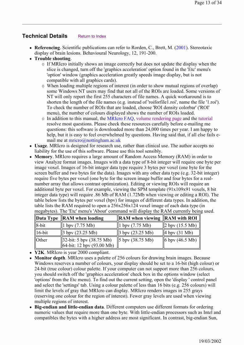
Usage. MRIcro is designed for research use, rather than clinical use. The author accepts no liability for the use of this software. Please use this tool sensibly. Memory. MRIcro requires a large amount of Random Access Memory (RAM) in order to view Analyze format images. Images with a data type of 8-bit integer will require one byte per image voxel. Images of 16-bit integer data type require 3 bytes per voxel (one byte for the screen buffer and two bytes for the data). Images with any other data type (e.g. 32-bit integer) require five bytes per voxel (one byte for the screen image buffer and four bytes for a real-number array that allows contrast optimization). Editing or viewing ROIs will require an additional byte per voxel. For example, viewing the SPM template (91x109x91 voxels, 8 bit integer data type) will require .86 Mb of RAM (1.72Mb when viewing or editing a ROI). The table below lists the bytes per voxel (bpv) for images of different data types. In addition, the table lists the RAM required to open a 256x256x124 voxel image of each data type (in megabytes). The 'Etc' menu's 'About' command will display the RAM currently being used.

Y2K. MRIcro is year 2000 compliant. Monitor depth. MRIcro uses a palette of 256 colours for drawing brain images. Because Windows reserves a number of colours, your display should be set to a 16-bit (high colour) or 24-bit (true colour) colour palette. If your computer can not support more than 256 colours, you should switch off the 'graphics acceleration' check box in the options window (select 'options' from the Etc menu). To find out the current setting, open the 'display ' control panel and select the 'settings' tab. Using a colour palette of less than 16 bits (e.g. 256 colours) will limit the levels of gray that MRIcro can display. MRIcro renders images in 255 grays (reserving one colour for the region of interest). Fewer gray levels are used when viewing multiple regions of interest. Big-endian and little-endian data. Different computers use different formats for ordering numeric values that require more than one byte. With little-endian processors such as Intel and compatibles the bytes with a higher address are most significant. In contrast, big-endian Sun,

Data Type RAM when loading RAM when viewing RAM with ROI8-bit 1 bpv (7.75 Mb) 1 bpv (7.75 Mb) 2 bpv (15.5 Mb)16-bit 3 bpv (23.25 Mb) 3 bpv (23.25 Mb) 4 bpv (31 Mb)Other 32-bit: 5 bpv (38.75 Mb)

64-bit: 12 bpv (93.00 Mb)5 bpv (38.75 Mb) 6 bpv (46.5 Mb)

of 34

19/03/2002

Silicon Graphics, Motorola and HP processors use the opposite byte order. Alpha and PowerPC processors can use either depending on a compiler switch. This means that Analyze format headers and some Analyze format data files (those with more than one byte per voxel, e.g. data type greater than 8-bit integer) may be different between different computers. MRIcro, SPMwin and SPM99 automatically detect the endian-ness of the headers files. When using MRIcro to create header files, you should save them to the same format as the image file. Region of Interest. ROIs are saved as 'filename.ROI'. This is a proprietary binary format that uses run-length encoding (a simple compression algorithm) to store a relatively compact image of the region of interest. Credits. MRIcro was programmed using Delphi (object-oriented Pascal). The sophisticated sliders and real-number edit boxes are components from the free RXlib component collection. SPM guru Matthew Brett suggested and helped test a number of useful enhancements (Matthew has written a number of great web pages that describe how SPM works, which are available at www.mrc- cbu.cam.ac.uk/Imaging/). Tom Womack added the SSE support for faster viewing of 32 and 64-bit images. Chris Rorden wrote MRIcro while working on a project grant from The Wellcome Trust. Header information used by SPM. During loading and saving of header files, MRIcro will show an alert message if it detects an error that might cause SPM difficulty. SPM requires the header to accurately describe the image file: the image dimensions, data type and byte offset all need to be correct. In addition, SPM will use the origin information to select the voxel deemed to be the 'centre' of the image, which in normalised images is the centre of the anterior commissure. If the origin is set to 0,0,0, then SPM will assume that the centre has not been set, which usually works pretty well. SPM also uses the 'scale' factor (the last item displayed in the extended header information window) to compute the true image intensity. For more information on these topics, search the SPM archives. To learn more about the Analyze file format, view the Mayo Clinic's extensive guide (www.mayo.edu/bir) or read Medical Image Format FAQ . For further details on SPM's specific and nonstandard usage of the Analyze format, visit the SPM home or www.mrc-cbu.cam.ac.uk/Imaging/. Supported 2D picture formats. MRIcro can open, save and print BMP, JPEG, PNG and TIF images. Free viewers such as IrfanView can batch convert images to other formats such as GIF. JPG images are very compact, but some of the image quality is lost. BMP and TIF retain the image quality, but the files are large. PNG (portable network graphics) format is both lossless and compressed, combining the best features of TIF and JPG. A number of PNG viewers are available to support virtually every major operating system, see www.libpng.org/pub/png/pngapvw.html for details. My web graphics page describes the relative merits of these formats. Converting images to Analyze format. The table below lists free software for converting images to Analyze format: Viewer Formats, Notes

MRIcro [Windows, Linux]

DICOM (uncompressed, XA and JPEG), NEMA, GE (LX, Genesis, 4.X, 5.X, compressed), Interfile, CTI ECAT6/7, Picker CT, Siemens (Magnetom Vision, Somatom, Somatom Plus), Elscint 2400, Philips .PAR/.REC, SPMwin (*.vhd), VFF, VoxBo, raw

see my conversion tutorial. Bru2Anz [Windows] Bruker Paravision

BMP, TIFF, stacked TIFF, JPEG, GIF, Raw

Choose File/Open to open your images (if you

of 34

19/03/2002

Unsupported 3D formats. If you a working with raw data, or a medical format which is not listed in the table above, you can try this desperate measure to convert the image to Analyze format:

First, give the raw data file name the extension '.img'. Next, create an Analyze format header using MRIcro's header information panel. The bare minimum is to specify the number of voxels in each dimension (the X, Y, and Z dimensions), the number of bytes per voxel (the type drop down menu, e.g. 32-bit real type specifies 4 bytes [a 'byte' is 8 bits] per voxel), the image offset in bytes (usually zero). If you are unsure of your image dimensions, read Dave Clunie's Quick and Dirty Tricks for viewing medical images. If your raw data file contains multiple MRI scans in the same file, you need to specifiy

ImageJ with Analyze plugin installed [Windows, Mac, Unix]

want to stack multiple images, place them alone in a folder and use File/Import/AllAsStack). If your image is 24-bit RGB (e.g. most JPEGs), you need to convert the image to grayscale. First, you may want to optimize the contrast using the functions in the Process menu. Then use the Image/Type/8bitGreyscale function. Select Plugins/AnalyzeWriter to convert your images to Analyze format. If the color-intensity of the new Analyze image is inverted, use Plugins/Inverter before using Plugins/AnalyzeWriter.

XMedCon [Windows, Unix]

DICOM (uncompressed), NEMA, GIF, ECAT6

Mosaic to Analyze [Matlab: Windows, Unix]

Siemens Magnetom Vision

Syngo Converter [Matlab: Windows, Unix]

Siemens Syngo DICOM

exp2ana3d.m (for 256x256 images), exp2ana3dt.m (for 64x64 EPI)[Matlab+SPM99: Windows, Unix]

Giuseppe Pagnoni's Matlab script for converting Philips .PAR/.REC export files.

GE to Analyze [Matlab: Windows, Unix]

GE LX, GE 4.X, GE 5.X format

stim2analyze volume_mri_convert [Unix]

GE Genesis

ge2spm [Unix] GE Genesisana2mnc [ Perl script: Windows, Unix, Macintosh]

MINC, Bruker Paravision, GE 4.x, GE 5.x, DICOM (uncompressed), Scanditronix, ECAT, Siemens Magnetom, Phillips

Image Converter [Windows]

Siemens System 7, Shimadzu HeadTome IV, Hamamatsu Photonics SHR2000, GEMS 2048-15B

of 34

19/03/2002

the number of 'Volumes'. The size of the raw data in bytes should be at least X*Y*Z*N*V+O. Where X,Y and Z are the image dimensions, N is the number of bytes per voxel, V is the number of volumes and O is the offset (if the offset is set to a negative value, each indvidual volume will have its own offset, so the image size will be X*Y*Z*N*V*-1*O). If you are dealing with raw data, set the 'offset' value in the header information panel to zero. If your file is in an unknown filetype instead of raw data, you can usually assume that the file contains a header at the start of the image. For example, if your image is a 256x256x1 voxel scan, with 2 bytes per voxel, the raw image data should be 131072 bytes long - if your file is 131224 bytes long, set the header offset to 152 (131224 - 131072). Save this header by pressing the floppy disk icon in the header information panel. Give the header the same name as your image, but using the extension ".hdr" for your header. Now open your image by pressing on the "open image with displayed header" button (it is in the header information panel, and shows a folder with the letters "img"). Note that most image formats store their data starting from the upper left corner, storing data in the same way we read English (left to right, top to bottom). However, the Analyze format stores the data starting with the bottom right (going right to left, bottom to top). Therefore, you may need to use MRIcro's "Save as..." function to find the correct orientation.

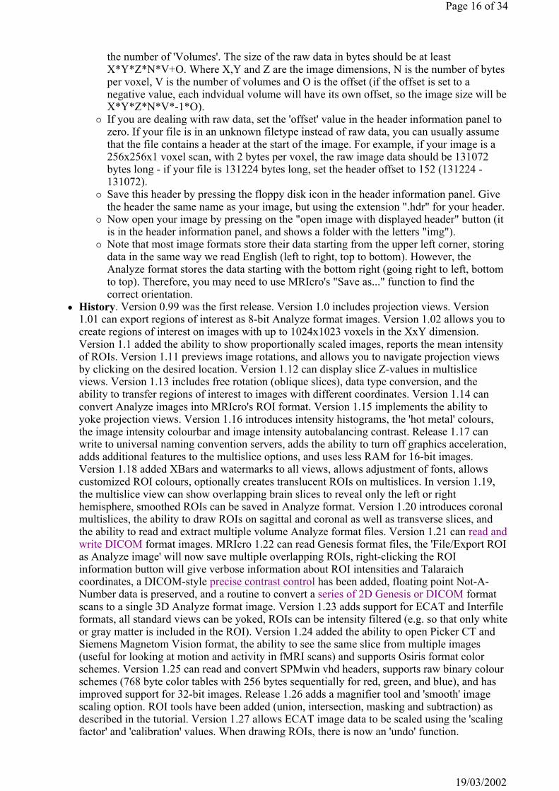
History. Version 0.99 was the first release. Version 1.0 includes projection views. Version 1.01 can export regions of interest as 8-bit Analyze format images. Version 1.02 allows you to create regions of interest on images with up to 1024x1023 voxels in the XxY dimension. Version 1.1 added the ability to show proportionally scaled images, reports the mean intensity of ROIs. Version 1.11 previews image rotations, and allows you to navigate projection views by clicking on the desired location. Version 1.12 can display slice Z-values in multislice views. Version 1.13 includes free rotation (oblique slices), data type conversion, and the ability to transfer regions of interest to images with different coordinates. Version 1.14 can convert Analyze images into MRIcro's ROI format. Version 1.15 implements the ability to yoke projection views. Version 1.16 introduces intensity histograms, the 'hot metal' colours, the image intensity colourbar and image intensity autobalancing contrast. Release 1.17 can write to universal naming convention servers, adds the ability to turn off graphics acceleration, adds additional features to the multislice options, and uses less RAM for 16-bit images. Version 1.18 added XBars and watermarks to all views, allows adjustment of fonts, allows customized ROI colours, optionally creates translucent ROIs on multislices. In version 1.19, the multislice view can show overlapping brain slices to reveal only the left or right hemisphere, smoothed ROIs can be saved in Analyze format. Version 1.20 introduces coronal multislices, the ability to draw ROIs on sagittal and coronal as well as transverse slices, and the ability to read and extract multiple volume Analyze format files. Version 1.21 can read and write DICOM format images. MRIcro 1.22 can read Genesis format files, the 'File/Export ROI as Analyze image' will now save multiple overlapping ROIs, right-clicking the ROI information button will give verbose information about ROI intensities and Talaraich coordinates, a DICOM-style precise contrast control has been added, floating point Not-A-Number data is preserved, and a routine to convert a series of 2D Genesis or DICOM format scans to a single 3D Analyze format image. Version 1.23 adds support for ECAT and Interfile formats, all standard views can be yoked, ROIs can be intensity filtered (e.g. so that only white or gray matter is included in the ROI). Version 1.24 added the ability to open Picker CT and Siemens Magnetom Vision format, the ability to see the same slice from multiple images (useful for looking at motion and activity in fMRI scans) and supports Osiris format color schemes. Version 1.25 can read and convert SPMwin vhd headers, supports raw binary colour schemes (768 byte color tables with 256 bytes sequentially for red, green, and blue), and has improved support for 32-bit images. Release 1.26 adds a magnifier tool and 'smooth' image scaling option. ROI tools have been added (union, intersection, masking and subtraction) as described in the tutorial. Version 1.27 allows ECAT image data to be scaled using the 'scaling factor' and 'calibration' values. When drawing ROIs, there is now an 'undo' function.

of 34

19/03/2002

Individual slices and regions can have their ROIs segmented based on image intensity (as described in the tutorial). Release 1.28 can convert JPEG-compressed (lossless, lossful and XA) DICOM images to Analyze format, can invert colors, and can save images as JPEG format. Version 1.29 views/converts Elscint, Par/Rec and Somatom images. Version 1.30: New installer/uninstaller, Linux version, SSE support. Release 1.31 adds PNG support and can save a 2D bitmap graphic for each slice of a 3D image, hotspots can be added to coronal or axial slices. Version 1.32 can display volume renderings, "Select MNI/Talairach Coordinates" command in "View" menu and supports image overlays (e.g. statistical maps of functional data). Volume 1.33 adds improved quality surface rendering, improved statistical overlays and includes support for VoxBo CUB1 format images. Additional color schemes: MRIcro can display images in the "black and white" as well as "hot metal" color schemes. Additional Osiris-format color lookup tables (LUTs) can also be displayed. The Osiris format is a text format, so you can create your own custom LUTs. In addition, MRIcro can support 768-byte binary data LUTs (NIH Image, XMedcon format). MRIcro expects the *.LUT look-up tables to be placed in the same directory as the MRIcro.exe program. Additional color schemes are available by downloading the free XMedcon 'extra stuff' software. Platforms, limitations, alternatives: MRIcro supports the Windows and Linux platforms. Here is a short list of some freeware Analyze format image viewers that are currently available for the Windows PC (for a list of Linux software, see the MRIcro for Linux web page. A more extensive list of DICOM viewers for Unix, Macintosh and PCs is available at my DICOM page):

Linux. A native Linux-native version of MRIcro is available. Updates. The latest versions of the MRIcro software and help manual are available from www.psychology.nottingham.ac.uk/staff/cr1/mricro.html [this information is mirrored at www.icn.ucl.ac.uk/groups/jd/mricro/mricro.html].

Viewer Platforms Formats [Notes]SPM Unix/Windows NT Analyze [requires Matlab]Slice Overlay Unix/Windows NT Analyze [requires Matlab]

SPMwin Windows AnalyzeACTIV 2000 Windows Analyze/DICOM/GE/GIS/PAR/Siemens

Medal Windows Analyze/DICOMetdips Windows Analyze/DICOM/TIFFSpamalize Unix/Windows/Macintosh Analyze/GE/TIFF [requires IDL]XMedCon Unix/Windows Analyze/DICOM/ECAT6/Interfile

ezDICOM Windows Analyze/ECAT/Interfile/Siemens/Picker/GE/DICOM/V(standard, color, & compressed)

ImageJ w. Analyze plugin

Unix/Windows/Macintosh Analyze/DICOM

MRIcro tutorial

of 34

19/03/2002

This guide gives is a brief description of how you can use MRIcro and SPM to work with patient scans. For the MRIcro manual and software, visit the MRIcro home page (also available at www.icn.ucl.ac.uk/groups/jd/mricro/mricro.html). I also keep a have a FAQ that describes some of the more unusual features of MRIcro. Information about SPM can be found at www.fil.ion.bpmf.ac.uk/spm/, or at www.mrc-cbu.cam.ac.uk/Imaging/. This tutorial will describe the following features:

1. Download this tutorial 2. Viewing images 3. Creating regions of interest (marking and viewing lesions) 4. Segmenting a region of interest 5. Linear and nonlinear normalization functions 6. Normalizing patient (or EPI) scans in stereotactic space ( SPM99 ) 7. Normalizing patient scans in stereotactic space ( SPMwin ) 8. Creating multislice images 9. Creating multiple slices that only show one hemisphere

10. Working with multiple regions of interest 11. Yoking images to check registration 12. Displaying a rendered image of the brain's surface 13. Batch processing scanner images

Downloading this tutorial

Windows users can download this tutorial and the sample MRI image by downloading the Windows installer. Linux users can download a zip file: shift+click here. You can also get the file from the mirror site at www.icn.ucl.ac.uk/groups/JD/mricro/mritut.zip. This will copy a compressed version of the MRIcro tutorial ('mritut.zip') to your computer (The zipped file requires around 820 kb). The tutorial includes a 2x2x2mm MRI scan ('BETicon.img' and 'BETicon.hdr': this is skull-stripped version of the average of 27 T1-weighted scans of the same individual as displayed at www.bic.mni.mcgill.ca/cgi/icbm_view). A 1x1x1mm version of this image is also available. Note that this MNI image does not exactly match the Talairach atlas.However, an MNI atlas is available. You can now delete the mritut.zip file (or save you can as a backup).

Viewing an image

1. Select 'Open Analyze Format hdr+img...' from the 'File' menu. You will be asked to select the MRI you wish to view. At the Medical Research Council, the (normalized) T1 scans have the name 'n'+scan number (e.g. n12345) while the T2 ('pathological') scans have the name 'p'+ scan number (e.g. p12345).

2. The 'slice viewer' panel has three sliders: the top slider determines the scan slice you will be shown.

Left: Two views of the 'Slice viewer panel'. On the left, the slice viewer when viewing axial/transverse slices (notice that the transverse icon is selected in the lower left of this panel). On the right, the slice viewer when displaying

of 34

19/03/2002

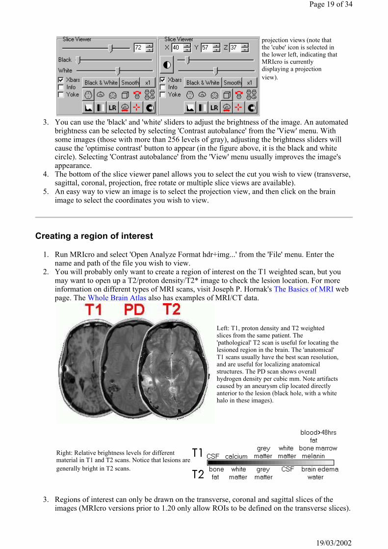
3. You can use the 'black' and 'white' sliders to adjust the brightness of the image. An automated brightness can be selected by selecting 'Contrast autobalance' from the 'View' menu. With some images (those with more than 256 levels of gray), adjusting the brightness sliders will cause the 'optimise contrast' button to appear (in the figure above, it is the black and white circle). Selecting 'Contrast autobalance' from the 'View' menu usually improves the image's appearance.

4. The bottom of the slice viewer panel allows you to select the cut you wish to view (transverse, sagittal, coronal, projection, free rotate or multiple slice views are available).

5. An easy way to view an image is to select the projection view, and then click on the brain image to select the coordinates you wish to view.

Creating a region of interest

1. Run MRIcro and select 'Open Analyze Format hdr+img...' from the 'File' menu. Enter the name and path of the file you wish to view.

2. You will probably only want to create a region of interest on the T1 weighted scan, but you may want to open up a T2/proton density/T2* image to check the lesion location. For more information on different types of MRI scans, visit Joseph P. Hornak's The Basics of MRI web page. The Whole Brain Atlas also has examples of MRI/CT data.

3. Regions of interest can only be drawn on the transverse, coronal and sagittal slices of the images (MRIcro versions prior to 1.20 only allow ROIs to be defined on the transverse slices).

projection views (note that the 'cube' icon is selected in the lower left, indicating that MRIcro is currently displaying a projection view).

Left: T1, proton density and T2 weighted slices from the same patient. The 'pathological' T2 scan is useful for locating the lesioned region in the brain. The 'anatomical' T1 scans usually have the best scan resolution, and are useful for localizing anatomical structures. The PD scan shows overall hydrogen density per cubic mm. Note artifacts caused by an aneurysm clip located directly anterior to the lesion (black hole, with a white halo in these images).

Right: Relative brightness levels for different material in T1 and T2 scans. Notice that lesions are generally bright in T2 scans.

of 34

19/03/2002

In the slice viewer panel, click on the button that shows a minature axial view of the brain. If the image does not appear to be sliced axially when the transverse button is selected (e.g. the scan looks coronal), then you may want to rotate the image, as described in the next section.

4. Press F3 to select the closed pen (or click on this tool in the region of interest panel).

5. Go to the slice you wish to edit (you can use the F1 and F2 keys to go to the next lower or higher slice, respectively)

6. Draw the region of interest by dragging the mouse cursor around the border while depressing the left mouse button.

7. Go to the center of the region, an click the right mouse button to fill the region. 8. If you make a mistake, press the icon of the hand holding an upside down pencil (it is in the

region of interest panel). This will erase your region of interest from this slice only. You can also shift-click to delete a region of a ROI. For example, shift-left-clicking deletes a region of interest beneath the mouse's movements, while shift-right clicking deletes a filled-region underneath the mouse's position.

9. Repeat steps 5-8 until you have drawn the lesion on all of the slices. 10. Choose 'Save ROI...' from the 'RO' menu. It is often useful to give the ROI the same name as

the image file (e.g. if the image file is n12345.img then the roi should be as n12345.roi). 11. Open the next image you wish to view. Repeat until you have created region of interest

information for all of the images you want to process.

Segmenting a region of interest

MRIcro can also be used to filter a region of interest based on the image intensity of the scan. For example, consider an fMRI study of auditory cortex. The experimenter has drawn a region of interest to delineate this region of the cortex, but is specifically interested if the activity of the gray matter is modulated with the task. To solve this problem, the experimenter could filter the ROI of auditory cortex in order to remove white matter from the analysis. Note that SPM99 has a series of sophisticated segmenting algorithms that may be more accurate than MRIcro in many instances. MRIcro can apply an intensity filter to the entire volume (so the same contrast levels are applied to all of the slices in the entire image), to a single slice or to a region within a single slice.

Here is a step-by-step guide for segmenting an ROI using MRIcro:

1. Draw your ROI as described in the previous section. 2. Make sure to adjust the contrast of your image so that the different tissues appear visually

distinctive. For images with more than 8 bits per voxel you may want to use the precision contrast tool (select 'Precise contrast' from the 'Viewer' menu).

3. Select 'Apply intensity filter to slice/region...' from the 'ROI' menu. You will then be asked if

Left: Drawing a region of interest on a scan.

of 34

19/03/2002

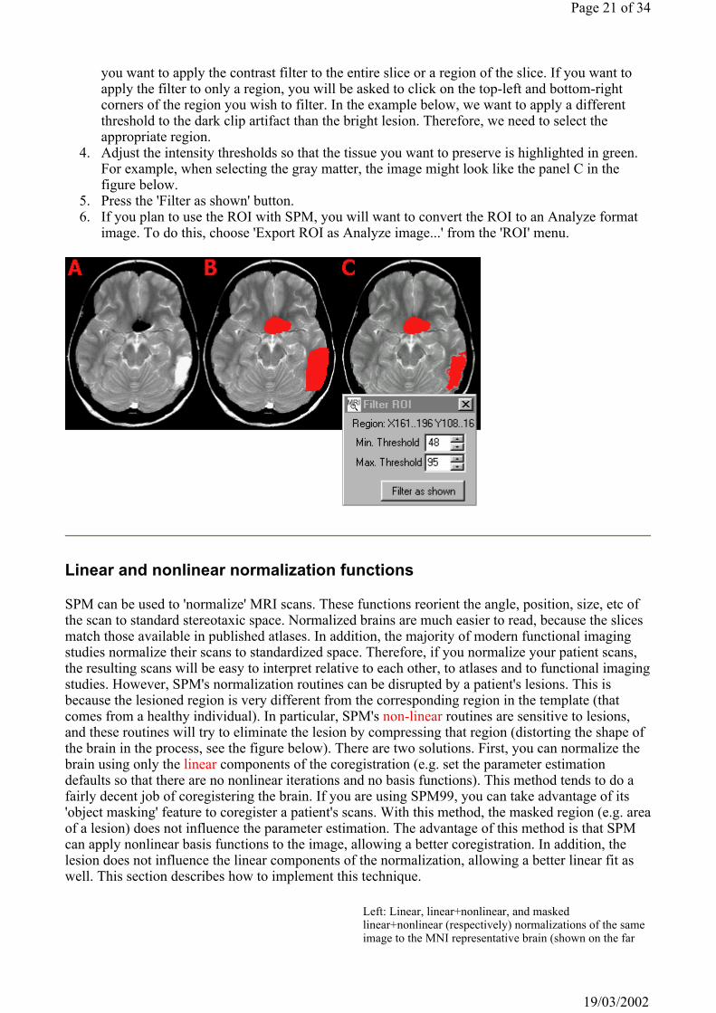
you want to apply the contrast filter to the entire slice or a region of the slice. If you want to apply the filter to only a region, you will be asked to click on the top-left and bottom-right corners of the region you wish to filter. In the example below, we want to apply a different threshold to the dark clip artifact than the bright lesion. Therefore, we need to select the appropriate region.

4. Adjust the intensity thresholds so that the tissue you want to preserve is highlighted in green. For example, when selecting the gray matter, the image might look like the panel C in the figure below.

5. Press the 'Filter as shown' button. 6. If you plan to use the ROI with SPM, you will want to convert the ROI to an Analyze format

image. To do this, choose 'Export ROI as Analyze image...' from the 'ROI' menu.

Linear and nonlinear normalization functions

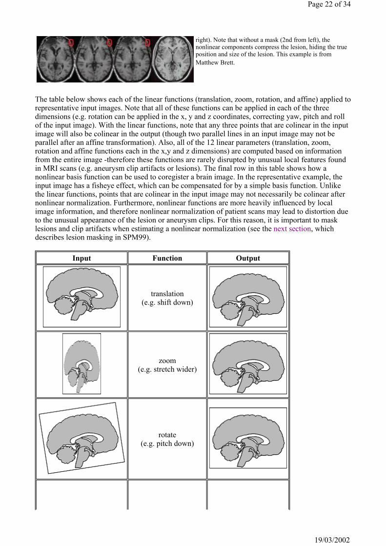
SPM can be used to 'normalize' MRI scans. These functions reorient the angle, position, size, etc of the scan to standard stereotaxic space. Normalized brains are much easier to read, because the slices match those available in published atlases. In addition, the majority of modern functional imaging studies normalize their scans to standardized space. Therefore, if you normalize your patient scans, the resulting scans will be easy to interpret relative to each other, to atlases and to functional imaging studies. However, SPM's normalization routines can be disrupted by a patient's lesions. This is because the lesioned region is very different from the corresponding region in the template (that comes from a healthy individual). In particular, SPM's non-linear routines are sensitive to lesions, and these routines will try to eliminate the lesion by compressing that region (distorting the shape of the brain in the process, see the figure below). There are two solutions. First, you can normalize the brain using only the linear components of the coregistration (e.g. set the parameter estimation defaults so that there are no nonlinear iterations and no basis functions). This method tends to do a fairly decent job of coregistering the brain. If you are using SPM99, you can take advantage of its 'object masking' feature to coregister a patient's scans. With this method, the masked region (e.g. area of a lesion) does not influence the parameter estimation. The advantage of this method is that SPM can apply nonlinear basis functions to the image, allowing a better coregistration. In addition, the lesion does not influence the linear components of the normalization, allowing a better linear fit as well. This section describes how to implement this technique.

Left: Linear, linear+nonlinear, and masked linear+nonlinear (respectively) normalizations of the same image to the MNI representative brain (shown on the far

of 34

19/03/2002

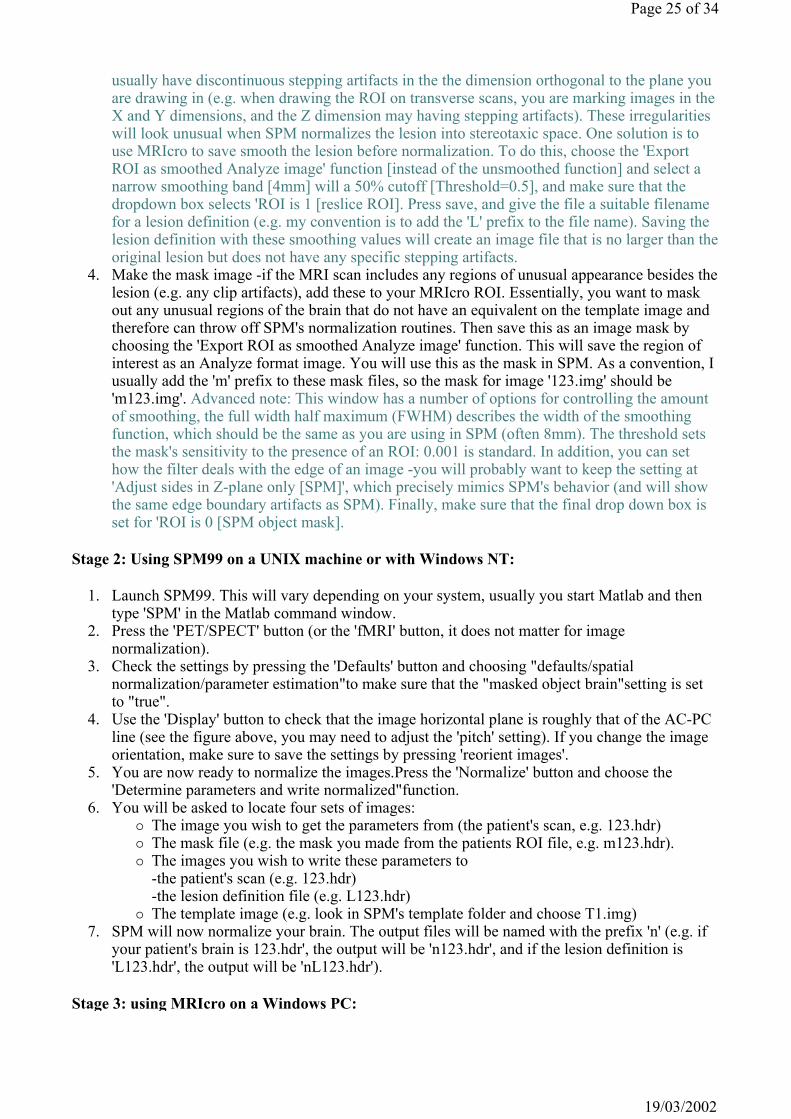
The table below shows each of the linear functions (translation, zoom, rotation, and affine) applied to representative input images. Note that all of these functions can be applied in each of the three dimensions (e.g. rotation can be applied in the x, y and z coordinates, correcting yaw, pitch and roll of the input image). With the linear functions, note that any three points that are colinear in the input image will also be colinear in the output (though two parallel lines in an input image may not be parallel after an affine transformation). Also, all of the 12 linear parameters (translation, zoom, rotation and affine functions each in the x,y and z dimensions) are computed based on information from the entire image -therefore these functions are rarely disrupted by unusual local features found in MRI scans (e.g. aneurysm clip artifacts or lesions). The final row in this table shows how a nonlinear basis function can be used to coregister a brain image. In the representative example, the input image has a fisheye effect, which can be compensated for by a simple basis function. Unlike the linear functions, points that are colinear in the input image may not necessarily be colinear after nonlinear normalization. Furthermore, nonlinear functions are more heavily influenced by local image information, and therefore nonlinear normalization of patient scans may lead to distortion due to the unusual appearance of the lesion or aneurysm clips. For this reason, it is important to mask lesions and clip artifacts when estimating a nonlinear normalization (see the next section, which describes lesion masking in SPM99).

right). Note that without a mask (2nd from left), the nonlinear components compress the lesion, hiding the true position and size of the lesion. This example is from Matthew Brett.

Input Function Output

translation (e.g. shift down)

zoom (e.g. stretch wider)

rotate (e.g. pitch down)

of 34

19/03/2002

Normalize patient MRI scans with MRIcro and SPM99

This section describes how to mask lesions so they do not disrupt the automated normalization functions of SPM. This technique is also useful for EPI fMRI images from healthy individuals (where EPI artifacts can also disrupt normalization). The MRC-CBU has a page devoted to EPI masking.

SPM99 can compute normalize patient scans to a stereotaxi standard template using both linear and nonlinear functions. Allowing SPM to apply nonlinear transformations will generally result in a more accurate normalization. However, with patient scans, nonlinear functions can effectively squash the region of a lesion (as it has no equivalent in the healthy template brain), causing considerable distortion of the brain. This section describes how to create and apply a lesion mask with SPM99, which allows accurate linear and nonlinear normalization of scans that have large lesions.

You will require SPM 99 beta (or later) and MRIcro version 1.19 or later (to get the latest version of MRIcro, go to the MRIcro home page).

Stage 1: using MRIcro on a Windows PC:

1. Open your scan and check the image orientation and the amount of neck presented in the image: when the slice viewer panel is set to display transverse slices, you should see transverse slices with the anterior portion of the brain (and the nose) toward the top of the screen and the posterior regions of the brain toward the bottom of your computer screen. Furthermore, the amount of neck displayed in your image should roughly match the amount of spinal cord shown in the template image. If your image is not in the correct format, choose the 'Save as...[rotate/format/clip/4D->3D]' from the 'File' menu. A window will appear which allows you to describe the current orientation of the brain and the amount of the spinal cord you wish to clip

affine (e.g. perspective)

nonlinear basis function (e.g. shrink middle, expand edges)

This section presents a step-by-step guide for implementing the technique described by Brett et al. For a reprint of this article, please contact Chris Rorden. For references, please cite:

Brett, M., Leff, A.P., Rorden, C., Ashburner, J. (2001). Spatial normalization of brain images with focal lesions using cost function masking. NeuroImage, 14, 486-500.

of 34

19/03/2002

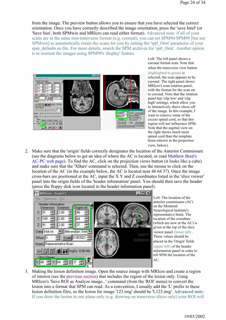
from the image. The preview button allows you to ensure that you have selected the correct orientation. Once you have correctly described the image orientation, press the 'save Intel' (or 'Save Sun', both SPMwin and MRIcro can read either format). Advanced note: if all of your scans are in the same non-transverse format (e.g. coronal), you can set SPM96/SPM99 [but not SPMwin] to automatically rotate the scans for you by setting the 'sptl_Ornt' parameter of your spm_defaults.m file. For more details, search the SPM archives for 'sptl_Ornt'. Another option is to reorient the images using SPM99's 'display' feature.

2. Make sure that the 'origin' fields correctly designates the location of the Anterior Commissure (see the diagrams below to get an idea of where the AC is located, or read Matthew Brett's AC-PC web page). To find the AC, click on the projection views button (it looks like a cube) and make sure that the 'XBars' command is selected. Then, use the mouse to click on the location of the AC (in the example below, the AC is located near 46 64 37). Once the image cross-bars are positioned at the AC, input the X Y and Z coordinates listed in the 'slice viewer' panel into the origin fields of the 'header information' panel. You should then save the header (press the floppy disk icon located in the header information panel).

3. Making the lesion definition image. Open the source image with MRIcro and create a region of interest (see the previous section) that includes the region of the lesion only. Using MRIcro's 'Save ROI as Analyze image...' command (from the 'ROI' menu) to convert the lesion into a format that SPM can read. As a convention, I usually add the 'L' prefix to these lesion definition files, so the lesion for image '123.img' should be 'L123.img'. Advanced note: If you draw the lesion in one plane only (e.g. drawing on transverse slices only) your ROI will

Left: The left panel shows a coronal format scan. Note that when the transverse view button (highlighted in green) is selected, the scan appears to be coronal. The right panel shows MRIcro's scan rotation panel, with the format for the scan set to coronal. Note that the rotation panel has 'clip low' and 'clip high' settings, which allow you to interactively shave slices off of the image. In this example, I want to remove some of the excess spinal cord, so that this region will not influcence SPM. Note that the sagittal view on the right shows much more spinal cord than the template brain (shown in the projection view, below).

Left: The location of the anterior commissure (AC) on the Montreal Neurological Institute's representative brain. The location of the crossbars (which are now at the AC) is given at the top of the slice viewer panel (lower left) . These values should be placed in the 'Origin' fields (upper left) of the header information panel in order to tell SPM the location of the AC.

of 34

19/03/2002

usually have discontinuous stepping artifacts in the the dimension orthogonal to the plane you are drawing in (e.g. when drawing the ROI on transverse scans, you are marking images in the X and Y dimensions, and the Z dimension may having stepping artifacts). These irregularities will look unusual when SPM normalizes the lesion into stereotaxic space. One solution is to use MRIcro to save smooth the lesion before normalization. To do this, choose the 'Export ROI as smoothed Analyze image' function [instead of the unsmoothed function] and select a narrow smoothing band [4mm] will a 50% cutoff [Threshold=0.5], and make sure that the dropdown box selects 'ROI is 1 [reslice ROI]. Press save, and give the file a suitable filename for a lesion definition (e.g. my convention is to add the 'L' prefix to the file name). Saving the lesion definition with these smoothing values will create an image file that is no larger than the original lesion but does not have any specific stepping artifacts.

4. Make the mask image -if the MRI scan includes any regions of unusual appearance besides the lesion (e.g. any clip artifacts), add these to your MRIcro ROI. Essentially, you want to mask out any unusual regions of the brain that do not have an equivalent on the template image and therefore can throw off SPM's normalization routines. Then save this as an image mask by choosing the 'Export ROI as smoothed Analyze image' function. This will save the region of interest as an Analyze format image. You will use this as the mask in SPM. As a convention, I usually add the 'm' prefix to these mask files, so the mask for image '123.img' should be 'm123.img'. Advanced note: This window has a number of options for controlling the amount of smoothing, the full width half maximum (FWHM) describes the width of the smoothing function, which should be the same as you are using in SPM (often 8mm). The threshold sets the mask's sensitivity to the presence of an ROI: 0.001 is standard. In addition, you can set how the filter deals with the edge of an image -you will probably want to keep the setting at 'Adjust sides in Z-plane only [SPM]', which precisely mimics SPM's behavior (and will show the same edge boundary artifacts as SPM). Finally, make sure that the final drop down box is set for 'ROI is 0 [SPM object mask].

Stage 2: Using SPM99 on a UNIX machine or with Windows NT:

1. Launch SPM99. This will vary depending on your system, usually you start Matlab and then type 'SPM' in the Matlab command window.

2. Press the 'PET/SPECT' button (or the 'fMRI' button, it does not matter for image normalization).

3. Check the settings by pressing the 'Defaults' button and choosing "defaults/spatial normalization/parameter estimation"to make sure that the "masked object brain"setting is set to "true".

4. Use the 'Display' button to check that the image horizontal plane is roughly that of the AC-PC line (see the figure above, you may need to adjust the 'pitch' setting). If you change the image orientation, make sure to save the settings by pressing 'reorient images'.

5. You are now ready to normalize the images.Press the 'Normalize' button and choose the 'Determine parameters and write normalized"function.

6. You will be asked to locate four sets of images: The image you wish to get the parameters from (the patient's scan, e.g. 123.hdr) The mask file (e.g. the mask you made from the patients ROI file, e.g. m123.hdr). The images you wish to write these parameters to -the patient's scan (e.g. 123.hdr) -the lesion definition file (e.g. L123.hdr) The template image (e.g. look in SPM's template folder and choose T1.img)

7. SPM will now normalize your brain. The output files will be named with the prefix 'n' (e.g. if your patient's brain is 123.hdr', the output will be 'n123.hdr', and if the lesion definition is 'L123.hdr', the output will be 'nL123.hdr').


of 34

19/03/2002

1. Save the lesion in MRIcro's compressed ROI format. Open the lesion defintion scan (e.g. 'nL123.hdr') select 'Export Analyze image as ROI...' ('ROI' menu). You will be asked to set a threshold for accepting a region as a lesion: you should set this value to 50 (50% of the maximum image intensity). Give this the same name as the patients normalized image (the ROI for image 'n123.hdr' should be 'n123.roi'.

2. Open the normalized patient image with 'Open Analyze format .hdr + .img' ('File' menu). This should load both the normalized image and (if you have successfully completed the previous step) the normalized ROI. Notice that the volume of the lesion is displayed in the region of interest panel. Make sure to save your ROI. You can now view the lesion from any view and get a good idea of the size/position of the lesion (all in standardized stereotactic space).

Normalize patient MRI scans with MRIcro and SPMwin

SPM for windows (SPMwin) is a freely available standalone implementation of SPM96. Unlike other versions of SPM, SPMwin does not require Matlab. Therefore the software is completely free and many users find the user interface friendlier than Matlab versions of SPM. However, the current release of SPMwin does not implement SPM99's ability to create object masks for normalization of patient scans (see the previous section for details). However, for the majority of patient scans, SPMwin can do a reasonable job of coregistration, with the caveat that the normalization should only include linear transformations. The nonlinear transformations will often distort patient scans in an attempt to eliminate the region of the lesion. See the section on linear and nonlinear transformationsfor more details on the advantages and disadvantages of applying nonlinear transformations to patient scans.

You will require SPMwin and MRIcro version 1.19 or later (to get the latest version of MRIcro, go to the MRIcro home page)


1. Open your scan and check the image orientation and the amount of neck presented in the image. The previous section explains this step in detail .

2. Make sure that the 'origin' fields correctly designate the location of the Anterior Commissure. The previous section explains this step in detail .

Stage 2: Using SPMwin on a Windows PC:

1. Run SPMwin. From the 'File' menu choose the 'new/normalization' command. Once you have told the computer how many scans you wish to normalize, you will see a window named 'spatial normalization' with the icon of a small book. Double click on the icon, you will see four small icons labelled 'template','image to estimate parameters' and 'image to normalize'.

2. Double click on the template icon. Make sure that the listed template is the correct one for your patient's scan (e.g. if you are normalizing a T1 scan, make sure that the template is 'T1.hdr'). If it is incorrect, click on the filename and press delete, then drag and drop the correct template header to SPMwin's template icon.

3. Drag and drop the patient scan's header file to both the 'image to estimate parameters' and 'image to normalize' icons.

4. You may want to check the settings by choosing the 'settings' command from the 'calculate' menu. If so, make sure that 'sync' interpolation is selected in the 'general' tab. Makesure that the 'Number of nonlinear iterations' and 'Number of basis functions' are both set to zero (parameter estimation tab). Also check the reslicing dimensions in the 'reslicing' tab.

5. Choose 'start' from the calculate menu. When the normalization is complete a new image file will be created, which will have the prefix 'n' (e.g. if your patient's scan had the name

of 34

19/03/2002

'12345.img', the normalized scan will be named 'n12345.img').


1. Open the normalized scan (e.g. n12345.vhd and n12345.img). Press the floppy disk icon in the header informtion window to create an Analyze format header (n12345.hdr).

2. Create region of interest that marks the region of the lesion (as described in the 'Create ROI' section). This region of interest should only include the regions of the lesion. Notice that the volume of the lesion is displayed in the region of interest panel. Make sure to save your ROI. You can now view the lesion from any view and get a good idea of the size/position of the lesion (all in standardized stereotactic space).

Creating multislice views

MRIcro allows you to quickly create 'multislice' images that show a number of preselected cuts from an scan. This can be useful for presenting similar slices from a number of patients. This section describes how to generate a multislice view.

1. Open the image you wish to view by choosing "Open analyze format hdr+img". If you want to superimpose a region of interest [ROI, e.g. an outline of a lesion] there are two options. First, if the ROI has the same name as your image (e.g. the image is named "mr1.img" and the ROI is "mr1.roi", the ROI will have been opened automatically when you loaded the image. If the ROI has a different name, or if you want to superimpose multiple ROIs, select "Open ROIs..." from the 'ROI' menu. A dialog box will appear and you can control+click on each ROI you wish to open [e.g. for the tutorial, you can open "a.roi","b.roi" and "c.roi" simultaneously].

2. Open the Etc menu's 'Option' window and select the slices that you want to view (these values are shown outlined by yellow in the figure below). You can display up to twelve slices, but if you wish to show fewer slices enter a zero into the unused fields. For this stage you must enter the slice number rather than the Talairach position (e.g. in the image that comes with this tutorial, Z of 0mm is on the 37th slice, so to show Z=0mm enter the number 37). An easy way to find the corresponding slice number is to show the projection view of an image. You can then adjust the slice number (using the boxes in the slice viewer panel) and see the corresponding Talairach coordinate (if the slice viewer's 'info' button is selected).

of 34

19/03/2002

3. At the CBU, we typically display slices 25, 29, 33, 37, 41, 45, 49, 53, 57, 62 and 67 (for

normalized images with 2mm slices, like the image that is downloaded with this tutorial) or slices 48, 56, 64, 72, 80, 88, 96, 104, 112, 122, 132 (for 1mm slices). These slices correspond to Talairach slices -24, -16, -8, 0, 8, 16, 24, 32, 40, 50, 60mm, which are common transverse slices.

4. The options window has a number of additional settings that control the multislice view. Once you have selected your desired settings, press the 'OK' button. (MRIcro will remember your preferred settings, so you usually only have to set these up once). There are a number of options that you can choose:

Select whether you want to view Transverse or Coronal slices. I usually show tranverse views, but for some images (e.g. showing hippocampal lesions), the coronal view may be more appropriate. Select whether you want to see a sagittal view. Select from the various options for the sagittal view.

5. To generate a multislice view, click the multislice view in the Slice Viewer panel. You should see a multislice image similar to the one displayed below.

Creating multiple slices that only show one hemisphere

1. Open the Etc menu's 'Option' window and make sure that multislice options are set for 'Show right hemisphere' (this box is outlined in green below in the diagram of the Options window shown in the previous section) , or 'Show left hemisphere' if you wish to show the left hemisphere. You can also set the other multislice options by setting the approriate check boxes

of 34

19/03/2002

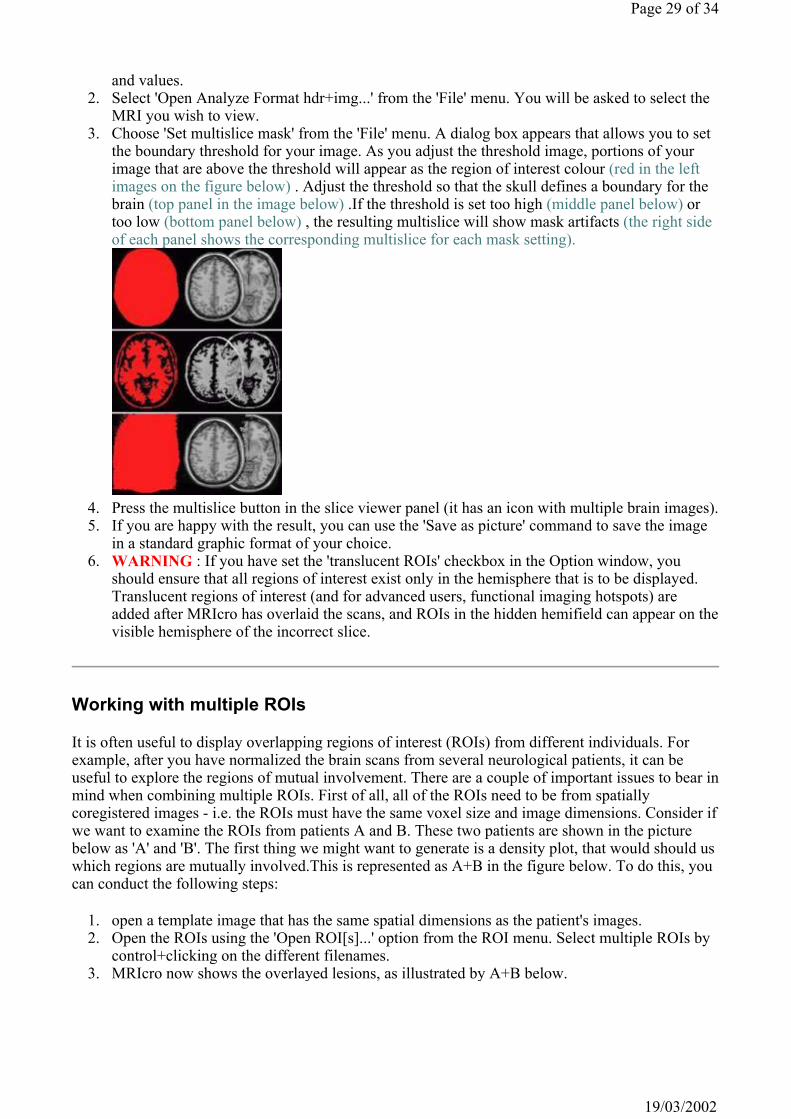
and values. 2. Select 'Open Analyze Format hdr+img...' from the 'File' menu. You will be asked to select the

MRI you wish to view. 3. Choose 'Set multislice mask' from the 'File' menu. A dialog box appears that allows you to set

the boundary threshold for your image. As you adjust the threshold image, portions of your image that are above the threshold will appear as the region of interest colour (red in the left images on the figure below) . Adjust the threshold so that the skull defines a boundary for the brain (top panel in the image below) .If the threshold is set too high (middle panel below) or too low (bottom panel below) , the resulting multislice will show mask artifacts (the right side of each panel shows the corresponding multislice for each mask setting).

4. Press the multislice button in the slice viewer panel (it has an icon with multiple brain images). 5. If you are happy with the result, you can use the 'Save as picture' command to save the image

in a standard graphic format of your choice. 6. WARNING : If you have set the 'translucent ROIs' checkbox in the Option window, you

should ensure that all regions of interest exist only in the hemisphere that is to be displayed. Translucent regions of interest (and for advanced users, functional imaging hotspots) are added after MRIcro has overlaid the scans, and ROIs in the hidden hemifield can appear on the visible hemisphere of the incorrect slice.

Working with multiple ROIs

It is often useful to display overlapping regions of interest (ROIs) from different individuals. For example, after you have normalized the brain scans from several neurological patients, it can be useful to explore the regions of mutual involvement. There are a couple of important issues to bear in mind when combining multiple ROIs. First of all, all of the ROIs need to be from spatially coregistered images - i.e. the ROIs must have the same voxel size and image dimensions. Consider if we want to examine the ROIs from patients A and B. These two patients are shown in the picture below as 'A' and 'B'. The first thing we might want to generate is a density plot, that would should us which regions are mutually involved.This is represented as A+B in the figure below. To do this, you can conduct the following steps:

1. open a template image that has the same spatial dimensions as the patient's images. 2. Open the ROIs using the 'Open ROI[s]...' option from the ROI menu. Select multiple ROIs by

control+clicking on the different filenames. 3. MRIcro now shows the overlayed lesions, as illustrated by A+B below.

of 34

19/03/2002

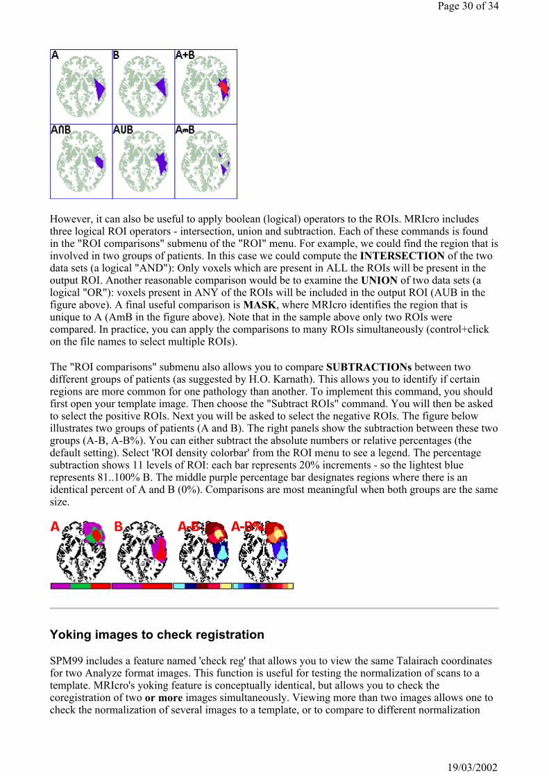
However, it can also be useful to apply boolean (logical) operators to the ROIs. MRIcro includes three logical ROI operators - intersection, union and subtraction. Each of these commands is found in the "ROI comparisons" submenu of the "ROI" menu. For example, we could find the region that is involved in two groups of patients. In this case we could compute the INTERSECTION of the two data sets (a logical "AND"): Only voxels which are present in ALL the ROIs will be present in the output ROI. Another reasonable comparison would be to examine the UNION of two data sets (a logical "OR"): voxels present in ANY of the ROIs will be included in the output ROI (AUB in the figure above). A final useful comparison is MASK, where MRIcro identifies the region that is unique to A (AmB in the figure above). Note that in the sample above only two ROIs were compared. In practice, you can apply the comparisons to many ROIs simultaneously (control+click on the file names to select multiple ROIs).

The "ROI comparisons" submenu also allows you to compare SUBTRACTIONs between two different groups of patients (as suggested by H.O. Karnath). This allows you to identify if certain regions are more common for one pathology than another. To implement this command, you should first open your template image. Then choose the "Subtract ROIs" command. You will then be asked to select the positive ROIs. Next you will be asked to select the negative ROIs. The figure below illustrates two groups of patients (A and B). The right panels show the subtraction between these two groups (A-B, A-B%). You can either subtract the absolute numbers or relative percentages (the default setting). Select 'ROI density colorbar' from the ROI menu to see a legend. The percentage subtraction shows 11 levels of ROI: each bar represents 20% increments - so the lightest blue represents 81..100% B. The middle purple percentage bar designates regions where there is an identical percent of A and B (0%). Comparisons are most meaningful when both groups are the same size.

Yoking images to check registration

SPM99 includes a feature named 'check reg' that allows you to view the same Talairach coordinates for two Analyze format images. This function is useful for testing the normalization of scans to a template. MRIcro's yoking feature is conceptually identical, but allows you to check the coregistration of two or more images simultaneously. Viewing more than two images allows one to check the normalization of several images to a template, or to compare to different normalization

of 34

19/03/2002

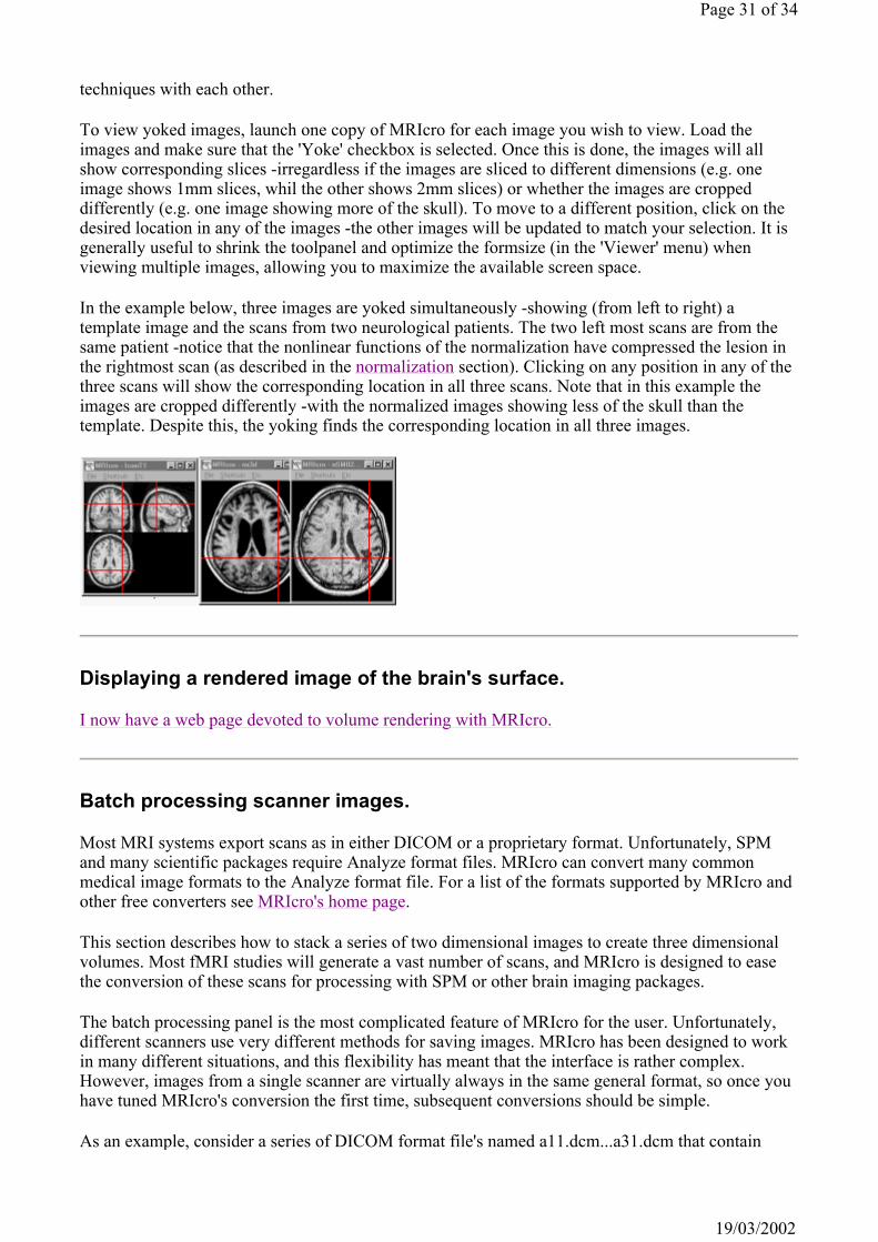
techniques with each other.

To view yoked images, launch one copy of MRIcro for each image you wish to view. Load the images and make sure that the 'Yoke' checkbox is selected. Once this is done, the images will all show corresponding slices -irregardless if the images are sliced to different dimensions (e.g. one image shows 1mm slices, whil the other shows 2mm slices) or whether the images are cropped differently (e.g. one image showing more of the skull). To move to a different position, click on the desired location in any of the images -the other images will be updated to match your selection. It is generally useful to shrink the toolpanel and optimize the formsize (in the 'Viewer' menu) when viewing multiple images, allowing you to maximize the available screen space.

In the example below, three images are yoked simultaneously -showing (from left to right) a template image and the scans from two neurological patients. The two left most scans are from the same patient -notice that the nonlinear functions of the normalization have compressed the lesion in the rightmost scan (as described in the normalization section). Clicking on any position in any of the three scans will show the corresponding location in all three scans. Note that in this example the images are cropped differently -with the normalized images showing less of the skull than the template. Despite this, the yoking finds the corresponding location in all three images.

Displaying a rendered image of the brain's surface.

I now have a web page devoted to volume rendering with MRIcro.

Batch processing scanner images.

Most MRI systems export scans as in either DICOM or a proprietary format. Unfortunately, SPM and many scientific packages require Analyze format files. MRIcro can convert many common medical image formats to the Analyze format file. For a list of the formats supported by MRIcro and other free converters see MRIcro's home page.

This section describes how to stack a series of two dimensional images to create three dimensional volumes. Most fMRI studies will generate a vast number of scans, and MRIcro is designed to ease the conversion of these scans for processing with SPM or other brain imaging packages.

The batch processing panel is the most complicated feature of MRIcro for the user. Unfortunately, different scanners use very different methods for saving images. MRIcro has been designed to work in many different situations, and this flexibility has meant that the interface is rather complex. However, images from a single scanner are virtually always in the same general format, so once you have tuned MRIcro's conversion the first time, subsequent conversions should be simple.

As an example, consider a series of DICOM format file's named a11.dcm...a31.dcm that contain

of 34

19/03/2002

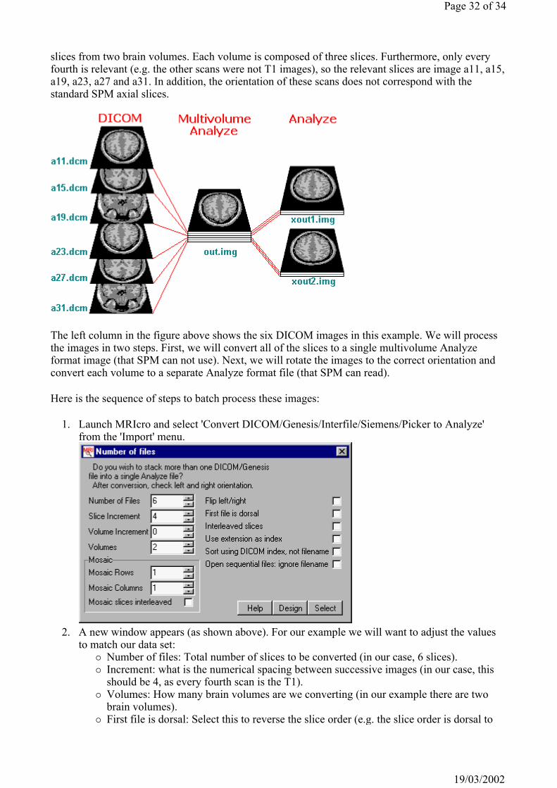
slices from two brain volumes. Each volume is composed of three slices. Furthermore, only every fourth is relevant (e.g. the other scans were not T1 images), so the relevant slices are image a11, a15, a19, a23, a27 and a31. In addition, the orientation of these scans does not correspond with the standard SPM axial slices.

The left column in the figure above shows the six DICOM images in this example. We will process the images in two steps. First, we will convert all of the slices to a single multivolume Analyze format image (that SPM can not use). Next, we will rotate the images to the correct orientation and convert each volume to a separate Analyze format file (that SPM can read).

Here is the sequence of steps to batch process these images:

1. Launch MRIcro and select 'Convert DICOM/Genesis/Interfile/Siemens/Picker to Analyze' from the 'Import' menu.

2. A new window appears (as shown above). For our example we will want to adjust the values

to match our data set: Number of files: Total number of slices to be converted (in our case, 6 slices). Increment: what is the numerical spacing between successive images (in our case, this should be 4, as every fourth scan is the T1). Volumes: How many brain volumes are we converting (in our example there are two brain volumes). First file is dorsal: Select this to reverse the slice order (e.g. the slice order is dorsal to

of 34

19/03/2002

ventral). In our example, slice order is ventral to dorsal (the first slice [a11] is ventral), so we will leave this button unchecked. Interleaved slices: Check this if the slices from the different volumes are interleaved, rather than sequential. In our example, the volumes are sequentially stored (the first slices [a11, a15, a19] belong to the first volume followed by the slices for the next volume [a23, a27, a31]). If the slices for the first volume were a11, a19, a27 and slices from the second volume were a15, a23, a31 we would want to select this checkbox. Use extension as index: select this if the image index number is in the extension, e.g. a.11,a.15,...a.31. On our files, the extension (.dcm) is not the index, so we leave this option unchecked. Sort Using DICOM index, not filename: Some scanners name slices based somewhat randomly (e.g. saving the files as file1.dcm, file6.dcm,file2.dcm,file5.dcm,file3.dcm,file4.dcm). These scanners often save the true sequence in the DICOM header (group/element 0020h/0013h). This option will reorder the slices based on information in the DICOM header. Our files are indexed correctly by the filename, so we can leave this unchecked. Open sequential files: ignore filename: Unfortunately, some scanners save images with a very complicated file naming system that MRIcro will not be aware of (e.g. fileA-1,fileB-2,fileC-3,etc). In this case, I suggest that you write a simple program to rename the files to a numerical sequence that MRIcro can interpret (e.g. file1,file2,file3). However, as a last resort you can have MRIcro ignore the filename altogether and open sequential files in a folder. Important: Before using this option, place the image files you want to convert into a folder that has no other files of any type in it. This option may or may not work- your images may end up in a scrambled order. It works best best when used in conjunction with the "Sort Using DICOM Index" option. In our example, we will [thankfully] leave this option unchecked.

3. Press the 'Design' button to check that you have correctly described the slice order. A window appears that shows the slice order, indexed from one. In our example, the design window will list: Volume 1: 1, 5, 9 Volume 2: 13, 17, 21 This accurately describes our data with the first volume storing the 1st, 5th and 9th slices (a11, a15, a19) and the second volume storing the 13th, 17th and 21st slices (a23, a27, a31).

4. Once you have described the slices, choose 'Select' and find the first DICOM (or NEMA, Genesis) file in the series (i.e. the slice with the lowest numerical value, in our example this is a11.dcm). The file names must end with the numberical index (a11.dcm is valid, 11a.dcm is not). Optionally, the file index may be padded by zeros (e.g. file008.dcm, file009.dcm, file010.dcm is valid, as is file8.dcm, file9.dcm, file10.dcm).

5. Give a name for the output Analyze format image (e.g. lets call it 'out.img'). 6. MRIcro should now process all of the slices and create a multivolume Analyze format image.

If successful, you can close the DICOM conversion window. 7. You will now be able to open the image by selecting 'Open analyze img+hdr...' from the 'File'

menu. You can only view volumes one at a time, so MRIcro will ask you to name the volume you want to view.

8. You should now check the header information panel and make sure all of the information is correct.

You may want to adjust the image intensity value shown in the header information panel. SPM will use this scale for determining the signal level. This is especially crucial for SPM99b (the final release of SPM99 should do this automatically). See the SPM99 normalization section of this tutorial for details on how to automatically adjust the image intensity. Check to make sure that the slice thickness (Z size [mm]) is correct.

9. To extract the individual brain volumes, select 'Save as...' from the 'File' menu. A new window

of 34

19/03/2002

appears. You may want to adjust the orientation by selecting the 'format' and checking the results with the preview. In my example, the images need to be rotated 180 degrees in the Z plane, so the format needs to be set to 'axial down'. Click the 'Save Intel' button to extract and rotate all of the volumes. You will be asked to give the output a name, for example if you name the output 'xout.img', the files will be called 'xout1.img', 'xout2.img'...etc.

10. You can now delete the multivolume image if you wish (in our example, out.img).

In our example, each DICOM file contained one image. Furthermore, the two volumes were stored sequentially rather than being stored with 'interleaved slices' (that is, all the slices for the first volume had lower numbers than the scans for the second volume). Note that the design window allows you to adjust these features.

Interleaving:

In the figure on the left, slice interleaving is shown on the right panel. In our example, the volumes were saved sequentially (e.g. all of the first volume's slices had lower indexes [a11, a15,a19] than the second volume [a23, a27, a31]). However, some scanners save volumes in an 'interleaved' format. Selecting the 'slice interleaving' option will tell MRIcro that the slices are interleaved (e.g. the first volume is a11, a19, a27, and the second volume is a15, a23, a31).

Mosaics:

The NEMA format only specifies image size in two dimensions, so 3D volumes are stored as 'mosaics', which show various cuts on the same plane. The figure aboveshows a 2x3 NEMA mosaic. One way to test whether your images are a mosaic is to select 'Open foreign' from the 'Import' menu. If you see multiple cuts simultaneously, you will have to manually set the mosaic height and width when converting the images to Analyze format. Note that the more recent DICOM format does describe images in three dimensions, so quick opening these files will show only one slice per plane (and for conversion purposes, you should set the mosaic height/width both to 1).

Interleaved Mosaics:

Most mosaic files store slices in the same order we read English: starting from the top left and reading from left to right. However, some Siemens scanners create mosaics where the slice order is interleaved within the mosaic. If you select 'mosaic slice interleave', MRIcro will try to correctly read the order of Siemens mosaics.

of 34

19/03/2002

Windows 95-98, NT, 2000)web.tiscali.it/epaulesu/spedizione1.pdfEraldo Paulesu ps Gran parte delle...

Documents

Transcript of Windows 95-98, NT, 2000)web.tiscali.it/epaulesu/spedizione1.pdfEraldo Paulesu ps Gran parte delle...