
Weiergräber, Stefan: Network Effects and Switching Costs ...
58
Weiergräber, Stefan: Network Effects and Switching Costs in the US Wireless Industry Munich Discussion Paper No. 2014-512 Department of Economics University of Munich Volkswirtschaftliche Fakultät Ludwig-Maximilians-Universität München Online at https://doi.org/10.5282/ubm/epub.25094
Transcript of Weiergräber, Stefan: Network Effects and Switching Costs ...
Weiergräber, Stefan:
Network Effects and Switching Costs in the US Wireless
Industry
Munich Discussion Paper No. 2014-512
Department of Economics
University of Munich
Volkswirtschaftliche Fakultät
Ludwig-Maximilians-Universität München
Online at https://doi.org/10.5282/ubm/epub.25094

Sonderforschungsbereich/Transregio 15 · www.sfbtr15.de
Universität Mannheim · Freie Universität Berlin · Humboldt-Universität zu Berlin · Ludwig-
Maximilians-Universität München
Rheinische Friedrich-Wilhelms-Universität Bonn · Zentrum für Europäische Wirtschaftsforschung
Mannheim
Speaker: Prof. Dr. Klaus M. Schmidt · Department of Economics · University of Munich · D-80539
Munich,
Phone: + 49(89)2180 2250 · Fax: + 49(89)2180 3510
* University of Mannheim
November 2014
Discussion Paper No. 512
Network Effects and Switching Costs in the US Wireless
Industry
Stefan Weiergräber*

Sonderforschungsbereich/Transregio 15 · www.sfbtr15.de
Universität Mannheim · Freie Universität Berlin · Humboldt-Universität zu Berlin · Ludwig-
Maximilians-Universität München
Rheinische Friedrich-Wilhelms-Universität Bonn · Zentrum für Europäische Wirtschaftsforschung
Mannheim
Speaker: Prof. Dr. Klaus M. Schmidt · Department of Economics · University of Munich · D-80539
Munich,
Phone: + 49(89)2180 2250 · Fax: + 49(89)2180 3510
Financial support from the Deutsche Forschungsgemeinschaft through SFB/TR 15 is gratefully
acknowledged.
Network Effects and Switching
Costs in the US Wireless IndustryDisentangling sources of consumer inertia
Stefan Weiergräber∗
November 17, 2014
Abstract
I develop an empirical framework to disentangle different sources of consumer
inertia in the US wireless industry. The use of a detailed data set allows me to
identify preference heterogeneity from consumer type-specific market shares and
switching costs from churn rates. Identification of a localized network effect comes
from comparing the dynamics of distinct local markets. The central condition for
identification is that neither the characteristics defining consumer heterogeneity nor
the characteristics defining reference groups are a (weak) subset of the other. Being
able to separate switching costs and network effects is important as both can lead to
inefficient consumer inertia, but depending on its sources policy implications may
be very different. Estimates of switching costs range from US-$ 316 to US-$ 630.
The willingness to pay for a 20%-point increase in an operator’s market share is
on average US-$ 22 per month. My counterfactuals illustrate that both effects are
important determinants of consumers’ price elasticities potentially translating into
market power that helps large carriers in defending their dominant position.
∗Center for Doctoral Studies in Economics, University of Mannheim; E-mail: stefan.
weiergraeber[at]gess.uni-mannheim[dot]de. This paper was previously circulated asQuantifying network effects in dynamic consumer decisions. For the most recent versionplease check my webpage. I would like to thank my advisors Philipp Schmidt-Dengler andMartin Peitz for continuous support and guidance. I gratefully acknowledge financial supportfrom the Deutsche Forschungsgemeinschaft (SFB TR/15). I thank Isis Durrmeyer, Tim Lee,Christian Michel, Volker Nocke, Kathleen Nosal, Chris Nosko, Paul Scott, Alex Shcherbakov,Nicolas Schutz, Yuya Takahashi, Tommaso Valletti, Naoki Wakamori as well as participants ofthe 2014 CEPR Applied IO School in Athens, the 16th ZEW ICT Conference and the Ph.D. IOSeminar at the University of Mannheim for valuable comments.

Draft: November 17, 2014
1. Introduction
In many high-tech consumer goods industries purchase decisions are characterized by
the presence of both switching costs and network effects. The individual importance
of both effects has been studied extensively, cf. Farrell and Klemperer (2007).
While switching costs create consumer lock-in via a consumer’s own previous choice,
network effects make a consumer prefer a product that many other consumers already
use. Although not necessarily the case, this often leads to inefficient outcomes and
substantially alters the nature of competition generally favoring large incumbent
firms.
The interaction between switching costs and network effects is much less studied.
However, it is exactly this interplay that can be particularly problematic. In fast-
changing industries like the wireless service industry, consumers are usually not able
to forecast the technology evolution well over a longer horizon. When switching
costs impede consumers from re-optimizing quickly, network effects and switching
costs may amplify each other giving large firms not only extensive but also very
persistent market power. In these types of industries, the typical concentrated
market structure with only few firms and heavy consumer inertia constantly raises
regulators’ concern. In order to design effective policies, it is crucial to know where
consumer inertia comes from. For example, policies reducing switching costs, such
as number portability in the wireless industry, may not have a big effect on customer
mobility if inertia is mostly due to network effects.
By only looking at the aggregate industry structure, it is usually hard to empirically
disentangle whether consumers stick with a dominant firm because of preference
heterogeneity, switching costs or network effects. In this context, the identification
of network effects is particularly problematic, especially when only aggregate data
are available. These problems are very similar to Manski (1993)’s reflection problem:
the fact that market shares occur on both sides of an regression equation requires
additional model structure and more sophisticated identification arguments compared
to analyzing demand dynamics in non-network industries. These difficulties have led
most of the literature to make restrictive assumptions or to ignore one of the effects
in order to quantify the others. Restricted models are likely to result in confounded
estimates and wrong conclusions for economic policy, however.
To tackle these problems, I develop an empirical framework that allows me to
separately identify preference heterogeneity from direct network effects and state-
2

Draft: November 17, 2014
dependence due to switching costs. Throughout the paper, the term network effect
denotes a direct, anonymous, firm-specific network effect. It measures the effect of a
product’s aggregate market share within a consumer’s reference group, i.e. the group
of individuals a consumer cares about, on this consumer’s flow utility from using
that product. I model heterogeneous consumers in a discrete-choice framework with
decisions being driven by products’ observed and unobserved quality characteristics,
an individual consumer’s choice in the previous period as well as the contemporaneous
average behavior of her reference group.
In the identification section, I demonstrate under what assumptions the reflection
problem can be transformed into a well-studied endogeneity problem and how
switching costs and certain kinds of network effects - especially those that are similar
to a local spillover - can be separately identified from preference heterogeneity. I
argue that the reflection problem and the associated endogeneity problem can be
overcome as long as neither the determinants of consumer heterogeneity nor the
determinants of the reference group are a weak subset of the other. The implications
of this condition are twofold. First, it enables me observe individuals with identical
preferences in different network environments yielding the necessary variation in the
data. Second, demand shifters that affect different consumer types within a reference
group differently can serve as exclusion restrictions and the basis for instruments for
a product’s market share.
I estimate the model analyzing demand for wireless services in the US focusing on
geographically localized network effects. For the estimation, I use a panel of group-
specific market shares constructed from a large-scale survey. The detailed group-level
data contain market shares separately for different demographic types and different
local markets which allows me to identify consumers’ preference heterogeneity from
type-specific market shares. Aggregate churn rates, i.e. the fraction of consumers
who cancel their contract within a period, identify the switching cost parameters.
In my model, the switching cost measures a one-time utility loss associated with the
switching process. Differences in the evolution of separated local markets identify a
localized network effect. As long as consumers’ preference heterogeneity does not
systematically differ across local markets and time and consumers’ reference groups
consists of at least 2 different types, the model can be estimated using an extension
of the classical framework by Berry, Levinsohn, Pakes (1995, henceforth BLP).
My estimates of both switching costs and network effects are large and significant.
Switching costs vary across consumer types from US-$ 316 to US-$ 630 revealing
3
Draft: November 17, 2014
substantial heterogeneity. The willingness to pay for a 20%-point increase in an
operator’s market share within a consumer’s reference group is around US-$ 22 per
month varying across consumer types from US-$ 18 to US-$ 25. Estimating the model
ignoring either switching costs or network effects results in implausibly large estimates
of the other effect and a substantially worse model fit. In counterfactual simulations,
I demonstrate that network effects and switching costs are important determinants of
consumers’ price elasticities. Implementing perfect network compatibility results in
lower own-price elasticities and much more homogeneous cross-price elasticities. Not
surprisingly, decreasing switching costs results in significantly larger price elasticities.
Short-run elasticities almost triple and the difference between medium-run and
long-run elasticities diminishes. In both simulations, the smaller operators (Sprint
and T-Mobile) would gain substantial market share with T-Mobile generally profiting
most.
This paper is related to several strands of literature. There is a wide range of
studies on switching cost and network effects in the wireless industry most of which
follow a static and reduced-form approach. Moreover, almost all studies focus only
on either switching costs or network effects, but not both simultaneously. In contrast
to the reduced-form studies, e.g. by Kim and Kwon (2003) and Kim et al. (2004), I
follow a structural approach that allows me to conduct counterfactual analysis and
explicitly take the dynamic nature of subscription decisions into account. Grajek
(2010) estimates product-specific network effects and compatibility in the Polish
wireless market. While he follows a structural approach his model is restrictive as
he does not allow consumers to switch operators. Cullen and Shcherbakov (2010)
estimate a structural demand model for bundles of handsets and service provider,
but abstract from consumer heterogeneity and the presence of network effects. Yang
(2011) is to the best of my knowledge the only study that considers direct network
effects and switching costs simultaneously in a dynamic model. However, he does
not take into account consumer heterogeneity and the reflection problem is not dealt
with.
In contrast, I provide identification arguments for a structural demand model
with consumer heterogeneity, switching costs and direct network effects exploiting
detailed group-level data. My model allows me to estimate network effects within
an extension of the methodology by Berry et al. (1995) complemented with dynamic
panel techniques and elements from the dynamic demand literature. For example,
Shcherbakov (2013) and Nosal (2012) quantify consumer switching costs in non-
network industries (cable TV and health plan choice). The structural identification
4

Draft: November 17, 2014
of network effects shares some features with the sorting problems dealt with in the
housing market literature. For example Bayer and Timmins (2007) quantify local
spillovers in a static model of location choice. Identification issues in their model
arise because all variation in choices can be explained by a vector of location fixed
effects. Similar to my method, they apply an instrumental variable approach in the
style of BLP to decompose the location-fixed effects into spillovers and unobserved
quality characteristics. Lee (2013) quantifies indirect network effects in the video
game industry. For estimating direct network effects, I rely on similar moment
conditions as his paper.
The remainder of this paper is structured as follows: The next section describes
important characteristics of the US wireless industry. Section 3 presents the economic
model. Section 4 describe the data used for the estimation. Section 5 develops the
identification arguments and outlines the estimation strategy. Estimation results and
counterfactual experiments are presented in Sections 6 and 7. Section 8 concludes.
2. Industry characteristics
During my sample period (2006-2010), the US wireless industry was a prime example
of an industry in which switching costs and network effects interact. Two large
mergers in 2004 (AT&T and Cingular) and 2005 (Sprint and Nextel) led to an
oligopolistic market structure with 4 dominant players and constant scrutiny by
the FCC. The two biggest operators (AT&T and Verizon) still have a joint market
share of almost 70 %, while each of the two smaller operators (Sprint and T-Mobile)
controls 10-15 % of the market. The remaining market is shared by several smaller
operators often with limited regional coverage mostly in rural areas. While the
smaller operators usually sell more specialized products, the four major carriers offer
only slightly differentiated service bundles with respect to contract types, payment
schemes, tariff structure, handsets subsidized and customer service. However, carriers
can differ significantly in local coverage quality.1
Operator market shares vary significantly across local markets, but are very
persistent over time. In addition, my micro data indicate that the vast majority of
cellphone users has not switched their provider for more than 3 years. The FCC
has been concerned about this consumer inertia and attributed it to the presence
1For a detailed description of variation in local coverage quality see the discussion in Sinkinson(2011).
5
Draft: November 17, 2014
of switching costs. Policy measures, such as number portability in 2003, have been
undertaken to reduce switching costs. However, customer mobility across operators
remains low with average monthly churn rates mostly below 1-2 %. In addition, large
carriers generally have substantially lower churn rates than smaller ones. Switching
costs in the wireless industry can be explicit, e.g. in the form of early-termination-fees
or implicit through hassle costs that consumers incur when switching their operator.
During my sample period all post-paid contracts specified an early-termination-fee
of up to US-$ 350 that a consumer had to pay to end her contract prematurely.
Implicit hassle costs constitute an additional component of switching costs because
consumers in general have to find out how to cancel a contract and incur opportunity
costs of time, e.g. for filling out the necessary paper work.
Network effects in modern wireless communications services are largely tariff-
mediated, i.e. generated by the predominant contract structures. Postpaid contracts
in the US typically take the form of 24-months contracts specifying a monthly fee
plus some included number of anytime minutes that can be used to make calls
at any time to any network (e.g. a 400-anytime-minute package for 40 US-$ per
month). During my sample period, most of these contracts included unlimited night
and weekend minutes as well as free calls to an operator’s own network.2 My data
reveals that at the beginning of my sample period (January 2006) the majority of
consumers (more than 75%) had plans with free on-net calls. This number decreased
to continuously to slightly above 50% at the end of my sample period (December
2010). After the end of my sample period, network effects in the form of on-net call
discounts have continued to decline as wireless carriers shifted their business models
from selling phone services to data plans bundled with unlimited anytime-minutes.
Given the historical contract structures and the fact that many consumers stick to
their old contracts for years, on-net discounts should still have played a substantial
role during my sample period.
The mere presence of on-net discounts however need not generate network effects as
operators could adjust their prices in such a way that small operators compensate for
their smaller network by lower prices. Interestingly, several papers found that even
after controlling for price differentials, consumers perceive networks as incompatible,
i.e. they seem to appreciate being on a larger network per se (Grajek 2010; Kim
and Kwon 2003; Birke and Swann 2006). This may be due to several reasons. First,
it is not clear, that operators really charge fully off-setting prices. Second, there
2For an overview of typical contract features during my sample period see Section D in theAppendix.
6

Draft: November 17, 2014
can be more subtle contract features from which consumers benefit more easily if
they are on the same network. For example, under a receiving-party-pays regime3 as
in the US, consumers can have an incentive to coordinate on symmetric contract
features, e.g. on identical relative prices for voice minutes and text messages as this
facilitates coordinating on a preferred mode of communication. These features are
usually slightly different across operators but are identical across contracts within
an operator. In addition, consumers may appreciate a large network as an insurance
against having to buy more expensive off-net minutes in case of unanticipated calls.
Finally, they may simply derive psychological utility from conforming with their
peers (Grajek 2010).
3. Model
In this section, I present a structural discrete-choice model in which consumer
decisions are driven by both switching costs and network effects. The framework
extends the literature on estimating demand models with state-dependence by
incorporating direct network effects. Although in general applicable to a broad range
of network industries, I tailor the model towards the US wireless industry.
Each period consumers can choose a wireless network to subscribe to. There are
4 major operators and a fringe of smaller operators which constitute the outside
option. This yields a choice set with 5 different products in total. Modeling the
technology adoption decision as in Grajek and Kretschmer (2009) or Goolsbee and
Klenow (2002) is conceptually straightforward and can be done by splitting up the
choice not subscribing to the major 4 into subscribing to a small operator and no
wireless service at all. Given that the wireless penetration rate was already very
high (over 90%) during my sample period, I abstract from the adoption decision
and assume that every consumer is subscribed to a wireless carrier. In contrast to
Cullen and Shcherbakov (2010), I abstract from consumers’ specific handset choice.
In addition, I do not model the decision of which specific plan to choose. Each
consumer is assigned to a local market based on his residency. I classify geographic
markets similarly to Nielsen’s DMA-definition. A DMA (designated market area) is
defined as a collection of counties of similar magnitude as a metropolitan statistical
area. The time period of observation is a quarter.
3While in a receiving-party-pays regime both, the caller and the receiver, are charged for airtime,under a calling-party-pays regime, only the caller is charged for making a call.
7

Draft: November 17, 2014
Consumers have heterogeneous preferences as a function of their individual demo-
graphic characteristics d. This results in a discrete number of consumer types which
may e.g. be defined by age and income. The flow utility of consumer i belonging to
demographic group d in geographic market m from being subscribed to operator j
in quarter t is given by a multiplicative function in usage quantity qdjmt and quality.
I treat usage quantity as fixed and exogenously given. Quality is modeled as a linear
function in observable product characteristics (X) and unobserved demand shocks
(ξ). Due to the presence of network effects, a large network size (srdj ) increases
consumers’ utility of being subscribed to operator j. Here, rd indexes a consumer’s
reference group which need not be equal to her type d, i.e. consumers are allowed
to also care about other types than their own. I assume that consumes are myopic
so that they do not form explicit beliefs about the future evolution of the industry.
However, the model has a dynamic component as consumers incur a switching cost
(ψ) when choosing a different provider today than in the previous period. The
per-period utility function is specified as follows:
uijmt = (Xdjmtβ
d + γdpdjt + ξdjmt + αdsrdjmt)qdjmt
︸ ︷︷ ︸
δdjmt
+ψd1ait−1 6=ait + ǫijmt
where Xdjmt contains operator-fixed effects and observed product quality characteris-
tics varying by local market m and consumer type d, pjt denotes the average price
per unit of phone service of operator j in period t. The structural parameters (β,γ,
α, ψ, ξ) differ across demographic types, but are constant within a group d. In
order to reduce the number of parameters to be estimated, I impose that the price
coefficient is a decreasing function of a type’s income. More specifically, the price
coefficient of type d is modeled as γd = αlog(yd)
Across time and local markets, wireless carriers can differ substantially in various
quality dimensions. Such differences are often observed by the agents, but not by
the econometrician. In the model, they are captured by ξdjmt which is a real-valued
unobserved vertical characteristic. I assume that ξ evolves according to an exogenous
AR(1)-process with a mean-zero innovation ν:
ξdjmt = ιξdjmt−1 + νdjmt
where ι is a nuisance parameter to be estimated. Such a specification is justified by
noting that typical components of ξ, like brand-reputation, customer service and
8

Draft: November 17, 2014
unobserved components of carriers’ infrastructure are very persistent across quarters.
ǫijmt is an iid logit shock drawn from a type-1 extreme value distribution capturing
individual-specific shocks to the utility from each product.
ψd represents a consumer’s switching cost that has to be paid once she decides
to be on a different network in the current period than in the previous period. It
comprises all hassle costs associated with the switching process, i.e. transaction costs
for canceling a subscription, explicit early termination and start-up fees, costs of
buying new equipment and potential learning costs. If applicable, poaching payments,
i.e. one-time payments made by an operator to whom a consumer switches, e.g. in
the form of handset subsidies, reduce the switching costs. Therefore, ψd should be
interpreted as a net switching costs. Moreover, I do not distinguish between quitting
and start-up costs. As the definition of my outside good does not allow consumers
to be in a switching cost free state, I assume that all switching costs are paid when
quitting an operator’s service. Although ψd may in principle differ across markets
and products, I treat it as constant in those dimensions.
The network effect operates through srdj , the market share of operator j in the
reference group of consumer d. If affects a consumers utility in two ways. First, it
explicitly lowers a consumer’s monthly bill because a higher network size generally
implies a lower need for buying more expensive off-net minutes. Second, as argued
in Section 2, consumers may derive explicit additional utility from being on a larger
network. The parameter αd will capture the sum of all these effects after controlling
for the average price per minute and usage quantity. In Appendix A, I show how
the price effect associated with network size can be disentangled from other network
effect components when additional data are available.
In the context of network effects, the specification of the reference group is crucial.
In principle, the reference group can be specified by an arbitrary interaction of local
market and observed demographic characteristics. Identifying restrictions on the
composition of the reference group to overcome the reflection problem are discussed
in Section 5.1. For the empirical application, I assume that a consumer’s reference
group consists of all consumers in her local market m. This assumption is plausible
as for many people, their social network is likely to be localized within their home
region.4 There is also empirical evidence on the local market being an important
reference group. For example, a report from Teletruth, a consumer advocacy group,
indicates that in 2008 local calls made up two thirds of an average phone bill.
4Similar ideas underlie Hoernig et al. (2014), Birke and Swann (2006) and Maicas et al. (2009).
9

Draft: November 17, 2014
As I analyze anonymous network effects, I assume that each demographic group d
consists of a continuum of consumers so that individuals do not act strategically but
take the equilibrium as given. The timing of consumer decisions between periods
t− 1 and t is as follows:
1. Each consumer i observes the industry structure Ωt = (Xt, ξt, st−1) and his
idiosyncratic shock ǫit.5
2. Given (1), consumers form rational expectations on the choices of consumers
in their reference group: E[srdjt |Ωt] =∫
i′∈rPr(ai′t = j)dG(i′). Given the
assumption of a continuum of consumers, there is no uncertainty in the
aggregate so that rational expectations are equivalent to perfect foresight
consumers.
3. Based on their expectations from (2) consumers simultaneously choose their
utility maximizing alternative. Market shares st and churn rates ct are realized
such that the observed market shares are the outcome of a self-consistent
equilibrium (Brock and Durlauf 2003) and one of possibly several fixed points
of a mapping Ψ that maps the industry structure and expectations on market
shares into realized market shares (st = Ψ(Ωt,E[st]))
This timing and information structure provides a justification for using observed
market shares as measures for consumers’ expectations on network size. The presence
of social effects is likely to result in the existence of multiple equilibria which can
be a severe problem for identification and estimation. Therefore, I assume that
within each reference group, consumers coordinate on a single equilibrium. In my
application, this assumption can be justified: I analyze the industry in a mature
stage, so that consumers plausibly had enough time to learn about the market
environment and coordinate successfully. This assumption is less restrictive than
the often-used single-equilibrium in the data assumption as my framework allows
different reference groups, e.g. different local markets, to play different equilibria.
The structure of the model and the distribution of the iid error term result in
closed-form solutions for consumers’ conditional choice probabilities as a function of
5Implicitly, this specification abstracts from problems of limited information as in Sovinsky Go-eree (2008). In my model, people are perfectly informed about product characteristics andprices.This information structure can be justified by noting that wireless carriers heavily engagein advertising and marketing so that consumers can get an accurate picture of the marketenvironment easily.
10

Draft: November 17, 2014
mean flow utilities δ and the switching cost parameters ψ:
Pri(not switch) = Pri(j|j) =exp(δijt)
exp(δijt) +∑
l 6=j exp(δilt − ψi)
Pri(switch from k to j) = Pri(j|k) =exp(δijt − ψi)
exp(δikt) +∑
l 6=k exp(δilt − ψi)
Consequently, market share predictions can be solved for recursively:
sijt =∑
j′
P i(j|j′)sij′t−1
These market share and (analogously churn rate) predictions can be taken to the
data to form moment conditions.
4. Data
To estimate the model, I combine group-level panel data constructed from a large-
scale repeated cross-section survey and operator-level statistics from the Global
Wireless Matrix, an industry report by Merrill Lynch Research. The sample period
is from January 2006 to December 2010.
Global Wireless Matrix The Global Wireless Matrix contains quarterly data on
operational and accounting figures for the major 4 carriers as well as the most
important regional operators. These are not broken down by regional market,
but only available on the national level. Most importantly, I use these data to
construct average price indices for each operator and quarter from usage and revenue
data. In addition, I consider information on the cost side, e.g. EBITDA (earnings
before interest, taxes, depreciation, and amortization) and revenue data to construct
instruments for the subscription prices charged by operators.
Survey data My main data source is a survey conducted quarterly by Comscore,
a market research firm. It surveys more than 30,000 cellphone users throughout
the US each quarter. The survey is stratified in order to allow for a representative
11
Draft: November 17, 2014
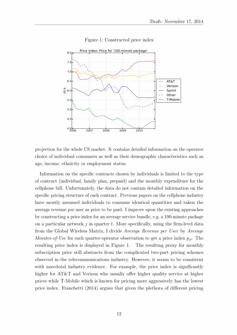
Figure 1: Constructed price index
2006 2007 2008 2009 20104.0
4.5
5.0
5.5
6.0
6.5
7.0
7.5
8.0
US-$
Price Index: Price for '100-minute package'
AT&TVerizonSprintOtherT-Mobile
projection for the whole US market. It contains detailed information on the operator
choice of individual consumers as well as their demographic characteristics such as
age, income, ethnicity or employment status.
Information on the specific contracts chosen by individuals is limited to the type
of contract (individual, family plan, prepaid) and the monthly expenditure for the
cellphone bill. Unfortunately, the data do not contain detailed information on the
specific pricing structure of each contract. Previous papers on the cellphone industry
have mostly assumed individuals to consume identical quantities and taken the
average revenue per user as price to be paid. I improve upon the existing approaches
by constructing a price index for an average service bundle, e.g. a 100-minute package
on a particular network j in quarter t. More specifically, using the firm-level data
from the Global Wireless Matrix, I divide Average Revenue per User by Average
Minutes-of-Use for each quarter-operator observation to get a price index pjt. The
resulting price index is displayed in Figure 1. The resulting proxy for monthly
subscription price still abstracts from the complicated two-part pricing schemes
observed in the telecommunications industry. However, it seems to be consistent
with anecdotal industry evidence. For example, the price index is significantly
higher for AT&T and Verizon who usually offer higher quality service at higher
prices while T-Mobile which is known for pricing more aggressively has the lowest
price index. Franchetti (2014) argues that given the plethora of different pricing
12
Draft: November 17, 2014
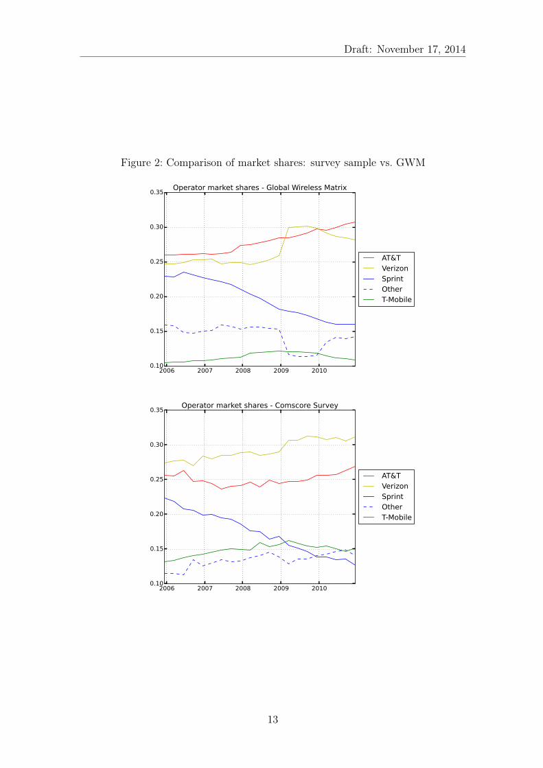
Figure 2: Comparison of market shares: survey sample vs. GWM
2006 2007 2008 2009 20100.10
0.15
0.20
0.25
0.30
0.35Operator market shares - Global Wireless Matrix
AT&TVerizonSprintOtherT-Mobile
2006 2007 2008 2009 20100.10
0.15
0.20
0.25
0.30
0.35Operator market shares - Comscore Survey
AT&TVerizonSprintOtherT-Mobile
13
Draft: November 17, 2014
structures, an average price index may actually be what consumers take into account.
Assuming that every consumer faces the same average price, I can compute the
average usage quantity of each consumer by dividing total expenditure by the price
index. For simplicity, I treat this usage quantity as fixed throughout the estimation
and the counterfactuals. One could extend the model to a continuous-discrete choice
framework as in Schiraldi et al. (2011) by modeling usage quantity as the outcome
of a static optimization problem over quantity.
Consumers are also asked about their switching behavior, in particular how long a
consumer has been subscribed to her current operator. If a respondent reports being
subscribed to her operator for less than 3 months, I treat this consumer as having
switched in this period. There is also a question about their previous operator.
Unfortunately, only very few consumers respond to this question. Consequently, I
cannot reliably construct the full matrix of conditional choice probabilities. Therefore,
I develop an estimation strategy that relies only on unconditional choice probabilities
contained in the market shares and a subset of the conditional choice probabilities
contained in the churn rates.
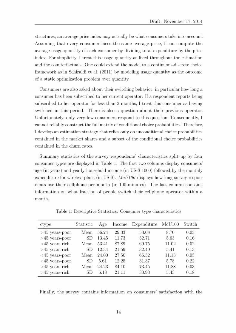
Summary statistics of the survey respondents’ characteristics split up by four
consumer types are displayed in Table 1. The first two columns display consumers’
age (in years) and yearly household income (in US-$ 1000) followed by the monthly
expenditure for wireless plans (in US-$). MoU100 displays how long survey respon-
dents use their cellphone per month (in 100-minutes). The last column contains
information on what fraction of people switch their cellphone operator within a
month.
Table 1: Descriptive Statistics: Consumer type characteristics
ctype Statistic Age Income Expenditure MoU100 Switch
>45 years-poor Mean 56.24 29.33 53.08 8.70 0.03>45 years-poor SD 13.45 11.73 32.71 5.63 0.16>45 years-rich Mean 53.41 87.89 69.75 11.02 0.02>45 years-rich SD 12.34 21.59 32.49 5.41 0.13<45 years-poor Mean 24.00 27.50 66.32 11.13 0.05<45 years-poor SD 5.61 12.25 31.37 5.78 0.22>45 years-rich Mean 24.23 84.10 73.45 11.88 0.03>45 years-rich SD 6.18 21.11 30.93 5.43 0.18
Finally, the survey contains information on consumers’ satisfaction with the
14

Draft: November 17, 2014
quality of the provided wireless service rated on a scale from 1 to 10. In my
estimation, operator fixed effects control for differences in the national mean of
quality characteristics. To control for variation in local coverage quality, I use
information on the average satisfaction level of all customers of an operator within a
local market as proxy for this operator’s network quality in this region. This variable
does not necessarily capture physical signal quality but rather an aggregate index
of perceived service quality by a particular type of consumer. Kim et al. (2004)
and Kim and Yoon (2004) provide evidence that in the Korean market customer
satisfaction and call quality are highly correlated.
In using these variables, I cannot rule out biased reporting due to consumer
selection. For example, more demanding consumers may choose higher quality
operators but may also be more critical in rating service quality. To solve this
problem, I do not use the absolute level of satisfaction, but take the normalized
deviation of the average rating within a region by a specific consumer type d from
the national average rating of this type-operator combination. As the fixed-effects
capture operators’ mean quality level, the satisfaction deviation measure should
appropriately control for regional variation in service quality. Descriptive statistics
of the original satisfaction variable and the constructed proxy for local coverage
quality are summarized in Table 17 in the Appendix.
Unfortunately, the survey is not a panel, but a repeated cross-section. This
limits the possibilities for using the individual-level data directly to analyze demand
dynamics. Therefore, I construct a panel of demographic group-specific market
shares. For data availability reasons, I focus on four consumer types (see Table 2)
and the biggest local markets (see Table 18 in the Appendix). This leaves me with
20 geographically separated markets consisting mostly of the urban areas around
the largest US cities. These markets differ in several respects, e.g. in their local age
or income distribution. However, they are relatively similar in other dimensions, like
the degree of urbanity, the wireless penetration rate (of almost 100%) or market size.
Therefore, I expect market size effects not to play a significant role. As I exclude very
rural areas, the market shares constructed from the survey differ slightly from the
market shares reported in aggregate industry reports. However, the differences are
plausible, e.g. AT&T which is relatively strong in some less densely populated areas
has a lower market share in my sample while T-Mobile which focuses on densely
populated urban markets has a higher market share in my sample. The geographical
size and distribution of the local markets is illustrated in Figure 3.
15

Draft: November 17, 2014
Figure 3: Overview of local markets used in the estimation
5. Identification and Estimation
5.1. Identification
In this subsection, I show under which assumptions the parameters of the demand
model are identified. In particular, I show how switching costs and localized network
effects can be disentangled from preference heterogeneity and that the reflection
problem does not occur under certain conditions.
Consumer heterogeneity in the form of consumer type-specific coefficients is
identified by differences in type-specific market shares. As in Berry et al. (1995),
variation in the choice sets across local markets and time identifies type-specific
price and quality coefficients. For separately identifying switching costs and network
effects, I rely on two key assumptions that are implicit in my model:
Assumption 5.1. Conditional on a consumer type d, consumers have homogeneous
preferences. Preferences are constant across time or local markets (or both).
Assumption 5.2. Each consumer has one reference group rd the average behavior
of which she takes into account. Neither the determinants of rd nor the determinants
of d are a (weak) subset of the other.
As in Yang (2010), the key data to identify switching costs are churn rates. The
model’s churn rate predictions are given by one minus the conditional choice proba-
bilities of sticking to a product. This subset of the conditional choice probabilities
16

Draft: November 17, 2014
contains more detailed information than the unconditional choice probabilities im-
plicit in the market shares. Under Assumption 5.1, this allows for comparing the
choice probabilities of consumers with identical preferences but different choices in
the previous period: If switching costs are zero, the unconditional choice probabilities
should be identical to the conditional choice probabilities. Positive switching costs
will drive a wedge between the two which will identify switching costs.
The identification of network effects is more complicated and runs into several
problems. First, similar to the well-known endogeneity problem of price, reference
group market shares will be correlated with the unobservable demand shocks which
requires finding appropriate instruments. After normalizing for usage quantity and
redefining the mean flow utility per unit, δdjmt =δdjmt
qdjmt
can be decomposed as:
δdjmt = Xdjmtβ
d + γdpdjt + αdsrdjmt + ξdjmt(1)
where d, j, m and t index consumer type, operator, local market and time respectively.
Valid instruments for srdjmt have to be correlated with the endogenous regressor but
uncorrelated with the unobserved error term. An additional problem arises, because
mean utilities are not observed in the data. Very similarly to the literature on pure
switching cost models (Shcherbakov 2013; Nosal 2012), they have to be inferred from
market share data. Knowing the contemporaneous market shares smt and previous
period’s market shares for type d is sufficient for computing the values of type d’s
mean utilities in market m and period t (δdmt) so that δdjmt = f(smt, sdmt−1). The
instruments for reference group market shares must not enter equation 1 directly,
in particular the market share variables needed to back out δdmt cannot be used as
instruments. If these were the only available shifters of srdjmt, the reflection problem
would occur in equation 1 and network effects could not be identified.
My key assumption for identifying a localized network effect is Assumption 5.2.
Intuitively, this assumption requires two things: First, a reference group characteristic
that allows one to observe individuals with identical preferences in different network
environments. The prime example for such a characteristic is the local market.
The second requirement is that there is some heterogeneity across the consumers
within a reference group. This heterogeneity can be used to construct the necessary
exclusion restrictions and instruments: With −d denoting all consumer types within
d’s reference group except for d itself, the reference group market share for type d is
a function of the lagged market shares of types d and −d as well the weights (Dmt)
of the different demographic types in her market.
17

Draft: November 17, 2014
While s−dmt shifts the mean utility for type d in period t directly, srdmt−1 is excluded
from the utility of type d in period t. Lagged market shares of type d affect sdmt and
δdmt through both the switching costs as well as the network effect. Therefore, looking
at own-type lagged market shares will not be sufficient to separately identify the
network effect α. In contrast, s−dmt−1, will affect sdmt only if there is a network effect.
This motivates using lagged market shares of types −d as instruments for current
period’s reference group market shares for type d. These variables are correlated
with srdmt as long as there is some sort of state-dependence in consumer choices.
Lagged market shares of types −d would be uncorrelated with ξdmt if the ξ-terms
were either uncorrelated across demographic groups or time periods. However, it is
likely that the unobserved quality characteristics are correlated in both dimensions.
To construct valid moment conditions, I exploit the dynamic panel data structure
by interacting the instruments from lagged periods with contemporaneous values of
ν, the exogenous innovation in the ξ-process, instead of its levels.
Intuitively, one can think of the identification strategy as comparing the behavior
of the same consumer types d under the dynamics of different network environments.
In my application the variation in networks occurs over time and local markets.
Local markets differ with respect to the initial conditions, the evolution of local
service quality and the distribution of demographic characteristics Dmt.
The initial conditions reflect different market histories that cause operators to
start the sample period with different network sizes in different markets. These
different histories contain variation due to exogenous differences across operators
and local markets, e.g. in spectrum availability, tower and antenna locations or
regulation of land use.
Furthermore, local markets differ in the evolution of operators’ local service
quality. I assume that this evolution is determined by an exogenous technological
process. Across different markets, different operators roll out specific service features
differently across time. This may result in different consumer types evaluating the
stand-alone service quality of an operator within a market differently. As described
in Section 4, I capture type-specific perceived quality with a proxy based on the
survey’s satisfaction measure. While the effect of a type’s own perceived quality will
be informative about her valuation for quality, the perceived quality of other types
in her reference group will help identifying the magnitude of the network effect. To
consider an illustrative example, assume that only younger consumers care about
high data speed. If AT&T can roll out its LTE network in New York, but not in
18
Draft: November 17, 2014
Georgia, comparing the reaction of the older consumers in the two markets should
contain information on the strength of the network effect.
Finally, demographic distributions Dmt, such as the age and income distribution,
are plausibly exogenous and vary across local markets and time. Variation in the
demographic composition will lead to different weightings of the distinct types
within a reference group. These weightings make two markets with the same quality
characteristics different and so introduces additional exogenous variation which shifts
reference group market shares.
A few remarks on the potential breakdown of my identification strategy are
in order. The second part of Assumption 5.1 states that consumers’ preferences
do not change either over time or across local markets. If my model allowed
for systematically different consumer preferences in both dimensions, one could
perfectly explain a higher market share in some market by a change or differences in
preferences for a particular operator in that market. This implies that I can allow
for market- or time-specific preferences but not both. In my application, I control
for consumer heterogeneity in the arguably most important dimensions, age and
income.6 Therefore the assumption that consumers have identical preferences across
local markets and time can be justified.
Moreover, my identification approach would fail, if consumers’ reference groups
consisted only of their own type as then the set of exclusion restrictions and
instruments based on types −d would be empty. This is a restrictive assumption
that prohibits me from identifying all potential kinds of network effects.
A particularly delicate issue is to separate network effects from the effects of
unobserved quality differences. Even though I control for local service quality in a
broad sense, one may argue that there are additional unobserved characteristics that
I am not able capture in the data. Such attributes may also comprise advertising
intensity or promotion activities. In that case, one may worry that my estimates
of the network coefficients pick up the effects of these unobservables. To see how I
mitigate this problem, note that any unobserved quality attribute, call it υdjmt, will
enter into the structural demand error ξ.
δdjmt = Xdjmtβ
d + γdpjt + αdsrdjmt + υdjmt + ξdjmt︸ ︷︷ ︸
ξdjmt
6My data is rich enough to conduct additional robustness checks in this dimension. For exampleone could have preferences differ across ethnicities, education or employment status.
19

Draft: November 17, 2014
Consequently, srdjmt will be correlated with ξdjmt. Using moments based on the
first-differenced equation will control for all persistent differences in unobserved
quality across local markets, e.g. a constantly high advertising intensity of some
operators in some markets.
∆δdjmt+1 = ∆Xdjmt+1β
d + αd∆srdjmt+1 + νdjmt+1︸ ︷︷ ︸
∆ξdjmt+1+∆υd
jmt+1
While ∆srdjmt+1 will still be correlated with νdjmt+1, lags in levels and first-differences
of other types’ market share distributions can be used as instruments. Due to the
sequential exogeneity assumption on ν, the instruments will be uncorrelated with
the error term νt+1.
The implications of the sequential exogeneity of ν are twofold. First, it is crucial
that νt contains only factors that cannot be anticipated by consumers before t. In the
wireless industry, this is not unreasonable. Typical components of ξ and ν are brand
reputation and the introduction of new service features that often have properties of
experience goods. Innovations to these characteristics are usually hard to evaluate
before they are actually realized. In contrast, easily verifiable characteristics like
information on coverage quality (towers and antennas), new handsets or subscription
prices are captured by the observables X which are explicitly controlled for.
A second assumption is that ν cannot be chosen or influenced by firms based
on market characteristics. This would however be the case if firms react to their
market position by adjusting any (unobserved) component of ν. For example,
identification would break down if one allows firms to adjust unobserved quality
levels or advertising intensity based on the instruments used for network size. This
would lead to a correlation between the instruments and the unobserved error
term even in first-differences, as then ∆vdjmt+1 = f(s−djmt−1, Dmt−1). In general, one
can alleviate this problem by imposing an additional timing assumption on firms’
strategies. One could assumes that firms choose νt+1 only based on the most recent
realization of the state variables in period t. Using instruments based on realizations
of the state variables in period t− 1, will then deliver valid moment conditions. If
one is concerned about the effects of advertising or store infrastructure specifically,
one could incorporate explicit data on operator’s marketing intensity across different
local markets and over time.7
7These data are e.g. available in the Ad$pender data base by Kantar Media.
20

Draft: November 17, 2014
5.2. Estimation
The estimation routine consists of three steps. In the first step, I back out the mean
utilities similarly to BLP by matching predicted to observed market shares. The
type-specific market shares in my model can be written as:
sdjmt =∑
j′
Prd(j|δdmt, adt−1 = j′) · sdj′mt−1
where at−1 denotes a consumer’s choice in the previous period. The conditional
choice probabilities for type d are a function only of the mean utilities of type d (δd)
and the switching cost parameter ψd:
Prd(j|δdmt, adt−1 = j) =
exp(δdjmt − j 6=jψd)
∑
j′ exp(δdj′mt − j′ 6=jψ
d)∀d, j,m, t
When implementing the estimation, I use an iterative mapping similar to BLP.
Conditional on the structural parameters θ, I solve for a fixed point of:
f(st, st−1, θ) [δt] = δt + log (st)− log (St(st−1, θ, δt))(2)
where st and St denote observed and predicted market shares respectively. In
contrast to the standard BLP-mapping, I take into account the presence of switching
costs and network effects. Switching costs imply that I have to solve for market share
predictions recursively period-by-period. In addition, I ensure that upon convergence
of the predicted and observed market shares, market share predictions are consistent
with the structure of the mean utilities decomposed into a standalone utility δ and
utility from the network effect: δdjmt = δdjmt + αdsrdjmt with srdjmt =∑
d′∈rdwd′
mtsd′
jmt
being a weighted average of the actual predicted market shares of the different
types in a market. As upon convergence of the mapping, observed and predicted
market shares are identical, this is equivalent to plugging in observed market shares.
The classical proof of BLP can be extended to prove the existence of fixed point
of equation 2. However, as in the literature on dynamic demand estimation, one
cannot formally prove uniqueness using BLP’s arguments.8
Conditional on the resulting vector of mean utilities, I compute a churn rate
8In robustness checks, I searched for fixed points of equation 2 starting from several differentstarting values and always converged to the same solution.
21

Draft: November 17, 2014
prediction error ζ, i.e. the difference between predicted and observed churn rates:
cdjmt − Cdjmt(δt, ψ) = ζdjmt(3)
Afterwards, I directly form moment conditions based on ζ and include them into
the criterion function. Consequently, I treat ζ as a nonstructural error term that
comprises structural parts as well econometric overfitting error. I choose this
specification because in my data churn rates are likely to be measured with error.
Most problematic is that on a very disaggregated level some churn rates in the data
are zero. The structural model will never predict this unless switching costs are
infinity.9
In the second step, I decompose the mean utilities to back out the structural error
terms ξ and ν:
→ ξdjmt = δdjmt −Xdjmtβ
d − γdpdjmt − αdsrdjmt(4)
→ νdjmt = ξdjmt − ιξdjmt−1(5)
In the final step, I use the method of GMM to estimate the parameters. The set
of moments used is based on interacting the error terms ξ, ν and ζ with appropriate
instruments Z:
E[G1(ξ, Z1)|Θ0] = 0
E[G2(ν, Z2)|Θ0] = 0
E[G3(ζ, Z3)|Θ0] = 0
Moments based on ξ will identify quality and price coefficients with Z1 containing
operator dummies, exogenous product characteristics as well as instruments for
subscription prices. The network effect will be backed out interacting ν with
instruments (Z2) based on the exclusion restrictions discussed in the previous
subsection. The last set of moments exploits the churn rate prediction error ζ.
Because of its nonstructural character ζ can be interacted with the superset of all
9Two ad-hoc solutions for this measurement error or zero-problem would be to treat the zeroobservations as missing values and impute these values or to simply aggregate the observedchurn rates up to a level where the zero-problem does not occur anymore. This would allow meto proceed as in Yang (2010). He uses a double contraction mapping to back-out mean utilitiesand the switching cost for each observation.
22

Draft: November 17, 2014
instruments used in Z1 and Z2.
To solve the typical endogeneity problem of price, I instrument subscription prices
pjt using cost side information. Similar to Yang (2010) I use firms’ revenue and
EBITDA to compute a proxy for short-run variable costs. As instrument I use
short-run variable cost per subscriber. A drawback of cost side data is that it is only
available on the national level, and does not exhibit a lot of variation. Therefore,
I include additional instruments based on the average characteristics of operators’
subsidized handset portfolio (BLP-instruments). The attractiveness of competitors’
handset portfolios shifts an operator’s price-cost margins and is therefore a valid
instrument for price.
Based on the logic of the exclusion restrictions discussed in the previous subsection,
I instrument the reference group market share relevant for type d (srdjmt) with the
lagged market shares among other types than d in d’s reference group, weighted by
their demographic mass:
Zdjmt =
∑
d′∈rd,d′ 6=d
sd′
jmt−1 ·Dd′
mt−1
In a myopic model, the values of Zdjmt are fully determined in t− 1. So by definition
they must be uncorrelated with νt+1. Moment conditions in the form of E[Zdjmt ·
νdjmt+1]|θ0] = 0, should therefore be valid and be sufficient to identify the network
effect. Similar moment conditions are used in Lee (2013) and Schiraldi (2011) in
slightly different contexts. Arellano and Bover (1995) and Blundell and Bond (1998)
demonstrate that using both lagged variables in levels as well as first-differences
is much more powerful than relying on instruments in levels alone. Therefore, I
use first (pseudo-)differences in Zdjmt additionally. Analogously, I could include the
perceived quality ratings of other types as instruments. Controlling for the perceived
quality of type d directly, the ratings of other types should only affect the mean
utility of types −d through the network effect. In my application, adding these
moments did not significantly alter the results.
Specification details For the main estimation I choose the following specification:
d = age × income, both measured in a binary way. Consequently, I allow
for four different consumer types as describd in Table 2. A consumer’s reference
group consists of all individuals in her home region, i.e. rd = (local market) and
so comprises 4 different consumer types and each consumer within a local market
23

Draft: November 17, 2014
Table 2: Overview of consumer types
d Age Income
1 >45 below median income2 >45 above median income3 <45 below median income4 <45 above median income
faces the same reference group. One can narrow down the definition of the reference
group by defining it on an interaction of local market and either age or income
characteristics.10 Refining consumers’ reference groups further to a narrowly-defined
demographic group, e.g. to an interaction of age, income and ethnicity can lead to
two problems. First, from an empirical perspective it is hard to construct reliable
estimates of narrow demographic-group specific market shares even with an enormous
amount of observations. Second, one may question that an individual’s reference
group consists only of consumers that are of exactly the same type. For example,
family members might be in a different age group, friends may have a different
ethnicity or fall into a different income group.
I treat preferences as constant across time and local markets. The set of observable
product characteristics Xdjmt includes nation-wide operator-fixed effects, an iPhone
fixed effect that is equal to one for the quarters in which AT&T exclusively offered
the iPhone on its network. In addition, proxies for local service quality and the
number of exclusively available smartphones on an operator’s network are used.
The latter variable should capture the attractiveness of an operator’s subsidized
handset portfolio. As I have only limited pricing and contract data I have to make
simplifying assumptions on the composition of consumers’ monthly expenditure: I
assume that consumers pay according to a linear pricing scheme. As discussed in
Section 4, I construct the price index such that monthly expenditure is perfectly
explained by Rijt = pjt ·q
ijt. Throughout the estimation and the counterfactuals, I use
the observation weights to correct for the survey’s stratification when aggregating
across types and markets.
Multiplicity of equilibria A well-known problem with models of social interactions
is that there may be multiple equilibria. My setup differs from the multiplicity issues
10Qualitatively, the results for these specifications did not differ from the baseline specification.
24

Draft: November 17, 2014
that typically occur when dynamic games are estimated using two-step methods or
when choice probabilities are used directly to construct likelihood functions. In my
estimation routine, I back out a vector of mean utilities by inverting the market
share equation market-by-market. I do not pool market shares before doing the
inversion step: In case of equilibrium multiplicity, the market share mapping may
be a correspondence with multiple predictions for smt. However, each of these
predictions will be associated with a different mean utility vector.
As I assume that there is no coordination failure and that the observed market
shares comes from an equilibrium, I know from the data which equilibrium is
played in each market. I back out only the mean utility vector associated with the
equilibrium actually played. I pool the mean utilities of all markets only in the
second step when decomposing the mean utilities in the effect of the different factors
such as quality, price or network effects conditional on a particular equilibrium being
played. In this step, multiplicity of equilibria may actually help in identifying the
network effect because it introduces an additional source of variation into the model.
Therefore, multiplicity of equilibria across different markets will not be problematic
for the estimation. However, for doing counterfactual analysis, the issue persists.
A computational intensive, but feasible solution is to try to compute all equilibria
starting from different consumer beliefs and so get bounds on measures such as
welfare gains or simulated market share distributions.
6. Results
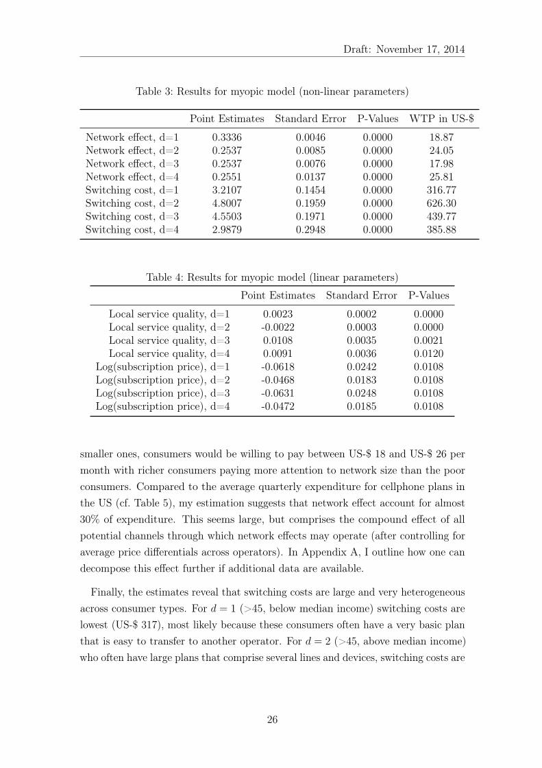
Tables 3 and 4 display the results for the model specified in the previous section.
The last column translates the coefficients into monetary willingness-to-pay using
the marginal utility of money derived from the estimated price coefficient. For the
switching costs, the last column displays the monetary equivalent of a one-time
utility loss from switching operators once. For the network effects, it displays the
average monthly willingness to pay for an increase of an operator’s market share
within a consumer’s reference group by 20%-points. Almost all coefficients have the
expected sign and are highly significant. Local service quality enters with a positive
coefficient for all types except for type d = 2 (>45, above median income). The
estimates for network effects imply reasonable magnitudes in terms of willingness-
to-pay: For an increase in an operator’s local market share by 20%-points, which is
the typical difference in market shares between one of the two big operators and the
25
Draft: November 17, 2014
Table 3: Results for myopic model (non-linear parameters)
Point Estimates Standard Error P-Values WTP in US-$
Network effect, d=1 0.3336 0.0046 0.0000 18.87Network effect, d=2 0.2537 0.0085 0.0000 24.05Network effect, d=3 0.2537 0.0076 0.0000 17.98Network effect, d=4 0.2551 0.0137 0.0000 25.81Switching cost, d=1 3.2107 0.1454 0.0000 316.77Switching cost, d=2 4.8007 0.1959 0.0000 626.30Switching cost, d=3 4.5503 0.1971 0.0000 439.77Switching cost, d=4 2.9879 0.2948 0.0000 385.88
Table 4: Results for myopic model (linear parameters)
Point Estimates Standard Error P-Values
Local service quality, d=1 0.0023 0.0002 0.0000Local service quality, d=2 -0.0022 0.0003 0.0000Local service quality, d=3 0.0108 0.0035 0.0021Local service quality, d=4 0.0091 0.0036 0.0120
Log(subscription price), d=1 -0.0618 0.0242 0.0108Log(subscription price), d=2 -0.0468 0.0183 0.0108Log(subscription price), d=3 -0.0631 0.0248 0.0108Log(subscription price), d=4 -0.0472 0.0185 0.0108
smaller ones, consumers would be willing to pay between US-$ 18 and US-$ 26 per
month with richer consumers paying more attention to network size than the poor
consumers. Compared to the average quarterly expenditure for cellphone plans in
the US (cf. Table 5), my estimation suggests that network effect account for almost
30% of expenditure. This seems large, but comprises the compound effect of all
potential channels through which network effects may operate (after controlling for
average price differentials across operators). In Appendix A, I outline how one can
decompose this effect further if additional data are available.
Finally, the estimates reveal that switching costs are large and very heterogeneous
across consumer types. For d = 1 (>45, below median income) switching costs are
lowest (US-$ 317), most likely because these consumers often have a very basic plan
that is easy to transfer to another operator. For d = 2 (>45, above median income)
who often have large plans that comprise several lines and devices, switching costs are
26

Draft: November 17, 2014
Table 5: Overview on consumer types and average expenditure
d Age Income Monthly expenditure
1 >45 below median income US-$ 532 >45 above median income US-$ 703 <45 below median income US-$ 664 <45 above median income US-$ 73
highest (US-$ 626). For younger consumers, switching costs are more homogeneous
and on average a bit lower. Interestingly, d = 3 (<45, below median income) have
lower switching costs than d = 4 (<45, above median income). This may be due to
consumers of the latter type often having the most expensive handsets. The fact
that subsidies for handsets effectively reduce the switching costs, can explain the
higher switching cost for poorer young consumers. Relatively speaking switching
costs are roughly on the order of 6 to 9 months’ average expenditure.
To get an idea on how the magnitudes of switching cost and network effects relate
to each other, consider the following back-of-the-envelope calculation: A customer
of one of the large providers compares her current operator with another operator
with the same quality but 20 %-points lower market share. In order to switch to the
small operator this customer will require a discount that compensates for switching
costs to be paid immediately and the accumulated benefits from network size over
the consumer’s time horizon. Assuming that the consumer cares about the next 2
years, my estimation results imply that this discount would range between US-$
700 and US-$ 1200 depending on the consumer type. Roughly 50% of the discount
would compensate for the switching costs, the other half for the foregone network
effect.
6.1. Price elasticities
Both switching costs and network effects are likely to result in consumer lock-in and
potentially make consumers insensitive to price increases. Because of the presence
of switching costs and network effects, there does not exist a closed-form formula
for the price elasticities. Computing these requires re-solving the model at different
levels of prices. Tables 6-8 describe the implied price elasticities in the short run
(6 months), medium run (2 years) and long run (5 years). These results are based
on recomputing market shares for every period after an operator has increased its
27

Draft: November 17, 2014
price index by 10% in every period. In principle, the price elasticities may depend
on which specific time periods are compared. Robustness checks looking at different
time periods did not result in significantly different elasticities.
Table 6: Short-run price elasticities
Other AT&T Verizon Sprint T-Mobile
pAT&T 0.1071 -0.1679 0.0353 0.0585 0.0743pVerizon 0.1053 0.0464 -0.1614 0.0530 0.0704pSprint 0.1127 0.0585 0.0423 -0.2484 0.0848
pT-Mobile 0.1010 0.0444 0.0310 0.0552 -0.3146
Table 7: Medium-run price elasticities
Other AT&T Verizon Sprint T-Mobile
pAT&T 0.0909 -0.6830 0.2387 0.2662 0.2305pVerizon 0.0952 0.2758 -0.6144 0.3039 0.2776pSprint 0.0723 0.2585 0.2462 -0.9551 0.2337
pT-Mobile 0.0594 0.2106 0.1983 0.2220 -1.0536
Table 8: Long-run price elasticities
Other AT&T Verizon Sprint T-Mobile
pAT&T 0.1305 -1.9168 1.1146 0.5416 0.4813pVerizon 0.2362 1.3067 -2.0908 0.8968 0.9393pSprint -0.1188 0.3949 0.6252 -2.1111 0.0698
pT-Mobile -0.0919 0.4556 0.7741 0.1451 -2.4705
As expected, switching costs lead to very low own-price elasticities (-0.16 to -0.31)
in the short-run with elasticities for the smaller operators being larger than for
the big ones. On a two-year horizon elasticities become larger (-0.61 to -1.05). In
the long-run consumers react strongly to price increases with elasticities around -2.
These fairly large elasticities suggest, that in the long-run consumer lock-in may
actually not be as strong as suggested by the large point estimates for switching
costs. The long-run cross-price elasticities are largest for the bigger operators, i.e. no
matter which carrier raises its price, consumers are much more likely to substitute
to one of the two large firms.
28
Draft: November 17, 2014
6.2. Comparison with restricted models
Table 9: Comparison with restricted models - point estimates
Full Model No network effects No switching costs
Log(subscription price), d=1 -0.0618 -0.0760 0.6759Log(subscription price), d=2 -0.0468 -0.0575 0.5112Log(subscription price), d=3 -0.0631 -0.0776 0.6900Log(subscription price), d=4 -0.0472 -0.0580 0.5164
Network effect, d=1 0.3336 - 1.8618Network effect, d=2 0.2537 - 3.6584Network effect, d=3 0.2537 - 1.9800Network effect, d=4 0.2551 - 2.1315Switching cost, d=1 3.2107 8.8927 -Switching cost, d=2 4.8007 8.8677 -Switching cost, d=3 4.5503 6.7558 -Switching cost, d=4 2.9879 8.4559 -
J-statistic 0.0478 0.8730 1.7745
Table 10: Comparison with restricted models - WTP
Full Model No network effects No switching costs
Network effect, d=1 18.8711 - -9.6357Network effect, d=2 24.0523 - -31.7323Network effect, d=3 17.9812 - -12.8395Network effect, d=4 25.8078 - -19.7294Switching cost, d=1 316.7690 714.1376 -Switching cost, d=2 626.2952 941.6527 -Switching cost, d=3 439.7651 531.4504 -Switching cost, d=4 385.8769 888.8896 -
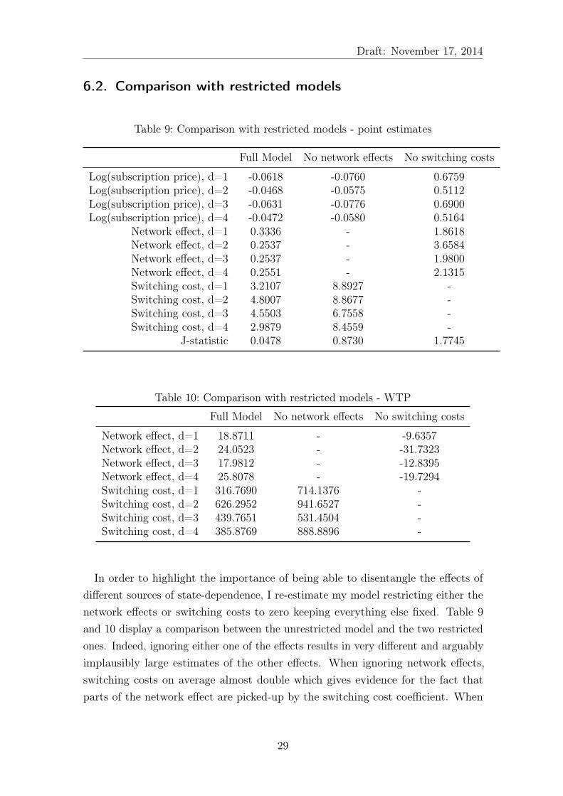
In order to highlight the importance of being able to disentangle the effects of
different sources of state-dependence, I re-estimate my model restricting either the
network effects or switching costs to zero keeping everything else fixed. Table 9
and 10 display a comparison between the unrestricted model and the two restricted
ones. Indeed, ignoring either one of the effects results in very different and arguably
implausibly large estimates of the other effects. When ignoring network effects,
switching costs on average almost double which gives evidence for the fact that
parts of the network effect are picked-up by the switching cost coefficient. When
29
Draft: November 17, 2014
ignoring switching costs, the coefficients on network size increase by a factor of
10. In addition, the price coefficients become positive so that comparing monetary
magnitudes becomes meaningless. Moreover, the GMM J-statistic, a measure of the
violation of the moment conditions increases dramatically by a factor of 20 to 40
when estimating models that focus only on one of the two effects.
7. Counterfactual Analyses
In a series of counterfactuals I analyze how network effects and switching costs affect
consumer behavior. In particular, I evaluate consumers’ price elasticities, when
switching costs are regulated with the level of network effects unchanged. I contrast
this setting with a situation in which switching costs remain constant, but perfect
network compatibility is implemented, i.e. consumers enjoy the network effect based
on the joint network size of all inside goods.
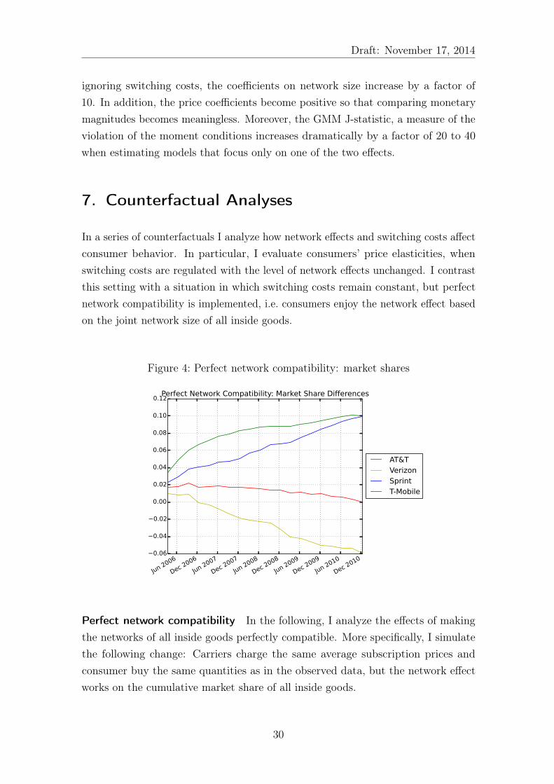
Figure 4: Perfect network compatibility: market shares
Jun 2006
Dec 2006
Jun 2007
Dec 2007
Jun 2008
Dec 2008
Jun 2009
Dec 2009
Jun 2010
Dec 2010
−0.06
−0.04
−0.02
0.00
0.02
0.04
0.06
0.08
0.10
0.12Perfect Network Compatibility: Market Share Differences
AT&TVerizonSprintT-Mobile
Perfect network compatibility In the following, I analyze the effects of making
the networks of all inside goods perfectly compatible. More specifically, I simulate
the following change: Carriers charge the same average subscription prices and
consumer buy the same quantities as in the observed data, but the network effect
works on the cumulative market share of all inside goods.
30
Draft: November 17, 2014
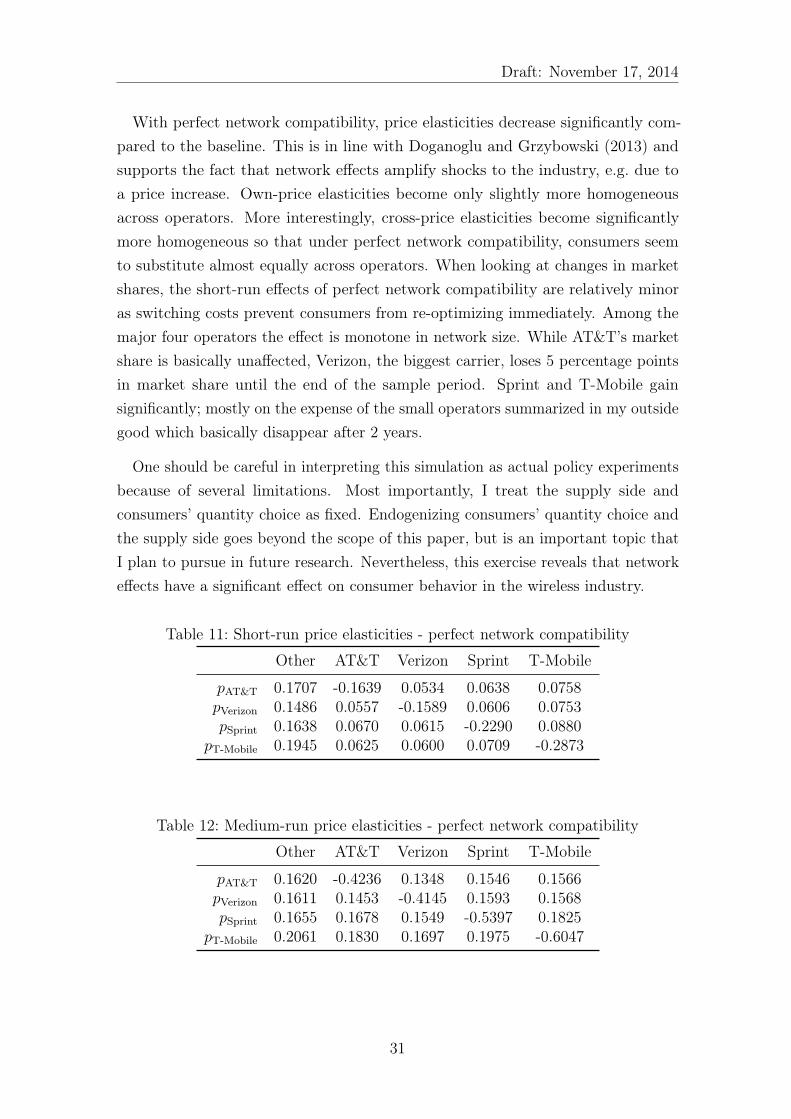
With perfect network compatibility, price elasticities decrease significantly com-
pared to the baseline. This is in line with Doganoglu and Grzybowski (2013) and
supports the fact that network effects amplify shocks to the industry, e.g. due to
a price increase. Own-price elasticities become only slightly more homogeneous
across operators. More interestingly, cross-price elasticities become significantly
more homogeneous so that under perfect network compatibility, consumers seem
to substitute almost equally across operators. When looking at changes in market
shares, the short-run effects of perfect network compatibility are relatively minor
as switching costs prevent consumers from re-optimizing immediately. Among the
major four operators the effect is monotone in network size. While AT&T’s market
share is basically unaffected, Verizon, the biggest carrier, loses 5 percentage points
in market share until the end of the sample period. Sprint and T-Mobile gain
significantly; mostly on the expense of the small operators summarized in my outside
good which basically disappear after 2 years.
One should be careful in interpreting this simulation as actual policy experiments
because of several limitations. Most importantly, I treat the supply side and
consumers’ quantity choice as fixed. Endogenizing consumers’ quantity choice and
the supply side goes beyond the scope of this paper, but is an important topic that
I plan to pursue in future research. Nevertheless, this exercise reveals that network
effects have a significant effect on consumer behavior in the wireless industry.
Table 11: Short-run price elasticities - perfect network compatibility
Other AT&T Verizon Sprint T-Mobile
pAT&T 0.1707 -0.1639 0.0534 0.0638 0.0758pVerizon 0.1486 0.0557 -0.1589 0.0606 0.0753pSprint 0.1638 0.0670 0.0615 -0.2290 0.0880
pT-Mobile 0.1945 0.0625 0.0600 0.0709 -0.2873
Table 12: Medium-run price elasticities - perfect network compatibility
Other AT&T Verizon Sprint T-Mobile
pAT&T 0.1620 -0.4236 0.1348 0.1546 0.1566pVerizon 0.1611 0.1453 -0.4145 0.1593 0.1568pSprint 0.1655 0.1678 0.1549 -0.5397 0.1825
pT-Mobile 0.2061 0.1830 0.1697 0.1975 -0.6047
31

Draft: November 17, 2014
Table 13: Long-run price elasticities - perfect network compatibility
Other AT&T Verizon Sprint T-Mobile
pAT&T 0.1634 -0.5699 0.2041 0.2098 0.2079pVerizon 0.1501 0.2146 -0.6412 0.2162 0.2159pSprint 0.1981 0.2281 0.2298 -0.7679 0.2426
pT-Mobile 0.2721 0.3025 0.3019 0.3247 -0.9405
Figure 5: Regulation of switching costs
Jun 2006
Dec 2006
Jun 2007
Dec 2007
Jun 2008
Dec 2008
Jun 2009
Dec 2009
Jun 2010
Dec 2010
−0.15
−0.10
−0.05
0.00
0.05
0.10
0.15
0.20Regulation of Switching Costs: Market Share Differences
AT&TVerizonSprintT-Mobile
Reduction of switching costs There are several ways one could think of policy
measures to reduce consumer switching costs. A regulator could prohibit early-
termination fees, or force operators to provide a transparent switching procedure.
From an operator’s point of view, consumer switching costs could be overcome
by subsidizing switching, e.g. in the form of poaching payments. A scenario in
which switching costs are completely eliminated is very unrealistic as consumers will
always incur hassle costs and opportunity costs of time when switching providers.
Therefore, I analyze the effect of a reduction of switching costs by 50% which would
be equivalent to a switching subsidy of roughly US-$ 150 to US-$ 300 (depending
on the consumer type).
Compared to the baseline elasticities, consumers react much more strongly and
quickly to a price increase. Short-run elasticities triple, while medium-run elasticities
almost double. The difference between medium- and long-run elasticities basically
32
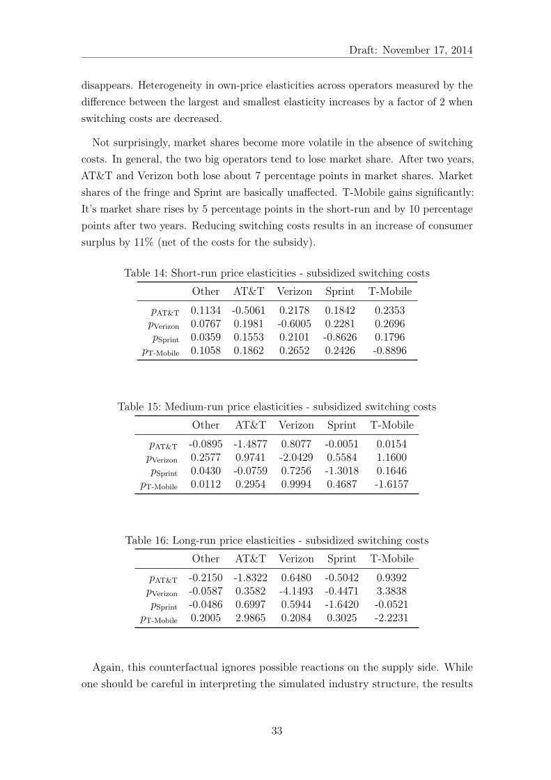
Draft: November 17, 2014
disappears. Heterogeneity in own-price elasticities across operators measured by the
difference between the largest and smallest elasticity increases by a factor of 2 when
switching costs are decreased.
Not surprisingly, market shares become more volatile in the absence of switching
costs. In general, the two big operators tend to lose market share. After two years,
AT&T and Verizon both lose about 7 percentage points in market shares. Market
shares of the fringe and Sprint are basically unaffected. T-Mobile gains significantly:
It’s market share rises by 5 percentage points in the short-run and by 10 percentage
points after two years. Reducing switching costs results in an increase of consumer
surplus by 11% (net of the costs for the subsidy).
Table 14: Short-run price elasticities - subsidized switching costs
Other AT&T Verizon Sprint T-Mobile
pAT&T 0.1134 -0.5061 0.2178 0.1842 0.2353pVerizon 0.0767 0.1981 -0.6005 0.2281 0.2696pSprint 0.0359 0.1553 0.2101 -0.8626 0.1796
pT-Mobile 0.1058 0.1862 0.2652 0.2426 -0.8896
Table 15: Medium-run price elasticities - subsidized switching costs
Other AT&T Verizon Sprint T-Mobile
pAT&T -0.0895 -1.4877 0.8077 -0.0051 0.0154pVerizon 0.2577 0.9741 -2.0429 0.5584 1.1600pSprint 0.0430 -0.0759 0.7256 -1.3018 0.1646
pT-Mobile 0.0112 0.2954 0.9994 0.4687 -1.6157
Table 16: Long-run price elasticities - subsidized switching costs
Other AT&T Verizon Sprint T-Mobile
pAT&T -0.2150 -1.8322 0.6480 -0.5042 0.9392pVerizon -0.0587 0.3582 -4.1493 -0.4471 3.3838pSprint -0.0486 0.6997 0.5944 -1.6420 -0.0521
pT-Mobile 0.2005 2.9865 0.2084 0.3025 -2.2231
Again, this counterfactual ignores possible reactions on the supply side. While
one should be careful in interpreting the simulated industry structure, the results
33

Draft: November 17, 2014
highlight once more the importance of consumer switching costs in the US wireless
industry.
8. Conclusion
In this paper, I developed an empirical framework to disentangle different sources of
consumer inertia in the US wireless industry. The use of detailed group-level panel
data allows me to identify preference heterogeneity from type-specific market shares
and switching costs by matching the model’s churn rate predictions to the observed
counterparts. Identification of a localized network effect comes from comparing the
dynamics of distinct local markets. The central condition for identification is that
neither the characteristics defining consumer heterogeneity nor the characteristics
defining reference groups are a weak subset of the other. The prime example of such
a setting is looking at geographically separated markets with reference groups that
consist of at least two types of heterogeneous consumers. If this condition is fulfilled,
network effects can be estimated using a combination of the seminal framework by
Berry et al. (1995) and dynamic panel techniques.
Even though the model was tailored towards the US wireless industry, my model is
general enough to be applied to other industries where switching costs and network
effects interact. In addition, my setup can be extended in several dimensions. First,
in a companion paper (work in progress) I show how the framework can be generalized
to a model in which consumers are forward-looking and have dynamic beliefs about
the future industry evolution as in Gowrisankaran and Rysman (2012). Second,
my model and my data are rich enough to be extended to a continuous-discrete
choice model that allows for endogenous quantity choice in the style of Schiraldi
et al. (2011).
A framework that allows for separately identifying switching costs and network
effects is not only necessary for obtaining correct estimates of price elasticities.
Reliable demand side estimates are also essential when analyzing firms’ pricing
strategies in the spirit of Cabral (2011) and Chen (2014). I plan to investigate the
empirics of dynamic platform competition in future research. Supplementing my
demand model with a full supply side model will allow for additional and much
richer counterfactuals.
Estimation results from my demand model reveal that during my sample period
34
Draft: November 17, 2014
(2006-2010) the market was characterized by the presence of both significant network
effects and large switching costs. Switching costs range from US-$ 320 to US-$ 630.
My estimates of network effects illustrate that on average consumers are willing to
pay around US-$ 22 per month to be on one of the larger networks compared to a
smaller one. I highlight the importance of being able to disentangle network effects
and switching costs by comparing my results to models that ignore either one of
the effects. When network effects are ignored, estimates of switching costs more
than double. When switching costs are ignored, the magnitude of network effects
increases by a factor of 10. To evaluate the importance of both effects further, I
investigated the short- and long-run effects of reducing switching costs and perfect
network compatibility. The counterfactuals confirm that both switching costs and
network effects are extremely important determinants of consumers’ price elasticities
and the market structure in the US wireless industry.
References
Arellano, M. and O. Bover (1995): “Another look at the instrumental variable
estimation of error-components models,” Journal of Econometrics, 68, 29–51.
Bayer, P. and C. Timmins (2007): “Estimating equilibrium models of sorting
across locations,” The Economic Journal, 117, 353–374.
Berry, S., J. Levinsohn, and A. Pakes (1995): “Automobile prices in market
equilibrium,” Econometrica: Journal of the Econometric Society, 841–890.
Birke, D. and G. P. Swann (2006): “Network effects and the choice of mobile
phone operator,” Journal of Evolutionary Economics, 16, 65–84.
Blundell, R. and S. Bond (1998): “Initial conditions and moment restrictions
in dynamic panel data models,” Journal of Econometrics, 87, 115–143.
Brock, W. and S. N. Durlauf (2003): “Multinomial choice with social interac-
tions,” NBER Working Paper t0288.
Cabral, L. (2011): “Dynamic price competition with network effects,” The Review
of Economic Studies, 78, 83–111.
Chen, J. (2014): “How do switching costs affect market concentration and prices in
network industries?” Unpublished manuscript, UC Irvine.
35
Draft: November 17, 2014
Cullen, J. and O. Shcherbakov (2010): “Measuring consumer switching costs
in the wireless industry,” Unpublished Manuscript.
Doganoglu, T. and L. Grzybowski (2013): “Dynamic duopoly competition
with switching costs and network externalities,” Review of Network Economics,
12, 1–25.
Farrell, J. and P. Klemperer (2007): “Coordination and lock-in: Competition
with switching costs and network effects,” Handbook of Industrial Organization, 3,
1967–2072.
Franchetti, F. (2014): “Essays on dynamic games,” Ph.D. thesis, The University
of Wisconsin-Madison.
Goolsbee, A. and P. J. Klenow (2002): “Evidence on learning and network
externalities in the diffusion of home computers,” Journal of Law and Economics,
45, 317–344.
Gowrisankaran, G. and M. Rysman (2012): “Dynamics of consumer demand
for new durable goods,” Journal of Political Economy, 120, 1173–1219.
Grajek, M. (2010): “Estimating network effects and compatibility: Evidence from
the Polish mobile market,” Information Economics and Policy, 22, 130–143.
Grajek, M. and T. Kretschmer (2009): “Usage and diffusion of cellular tele-
phony, 1998–2004,” International Journal of Industrial Organization, 27, 238–249.
Hoernig, S., R. Inderst, and T. Valletti (2014): “Calling circles: network
competition with nonuniform calling patterns,” The RAND Journal of Economics,
45, 155–175.
Kim, H.-S. and N. Kwon (2003): “The advantage of network size in acquiring new
subscribers: a conditional logit analysis of the Korean mobile telephony market,”
Information Economics and Policy, 15, 17–33.
Kim, H.-S. and C.-H. Yoon (2004): “Determinants of subscriber churn and
customer loyalty in the Korean mobile telephony market,” Telecommunications
Policy, 28, 751–765.
Kim, M.-K., M.-C. Park, and D.-H. Jeong (2004): “The effects of customer
satisfaction and switching barrier on customer loyalty in Korean mobile telecom-
munication services,” Telecommunications Policy, 28, 145–159.
36

Draft: November 17, 2014
Lee, R. S. (2013): “Vertical integration and exclusivity in platform and two-sided
markets,” The American Economic Review, 103, 2960–3000.
Maicas, J. P., Y. Polo, and F. J. Sese (2009): “The role of (personal) network
effects and switching costs in determining mobile users’ choice,” Journal of
Information Technology, 24, 160–171.
Manski, C. F. (1993): “Identification of endogenous social effects: The reflection
problem,” The Review of Economic Studies, 60, 531–542.
Nosal, K. (2012): “Estimating switching costs for Medicare advantage plans,”
Unpublished manuscript, University of Mannheim.
Schiraldi, P. (2011): “Automobile replacement: a dynamic structural approach,”
The RAND Journal of Economics, 42, 266–291.
Schiraldi, P., S. Seiler, and H. Smith (2011): “Supermarket choice with multi-
store shopping: measuring the effect of format regulation,” Tech. rep., working
paper.
Shcherbakov, O. (2013): “Measuring consumer switching costs in the television
industry,” Unpublished manuscript, University of Mannheim.
Sinkinson, M. (2011): “Pricing and entry incentives with exclusive contracts:
Evidence from smartphones,” Available at SSRN 1969855.
Sovinsky Goeree, M. (2008): “Limited information and advertising in the US
personal computer industry,” Econometrica, 76, 1017–1074.
Teletruth (2009): “Phone Bill Survey of UCAN customers,” Tech. rep., Teletruth
New Networks Institute and LTC Consulting.
Yang, Y. (2010): “Identification of consumer switching behavior with market level
data,” PhD Thesis Chapter, UCLA.
——— (2011): “Switching costs and network effects in the telephone industry,” PhD
Thesis Chapter, UCLA.
A. Modeling network effects with additional data
If one has more detailed data on usage behavior and prices, one can allow consumers
to buy different quantities of on-net and off-net minutes (qdjmt = qd,offjmt + q
d,onjmt ) at
37

Draft: November 17, 2014
different prices ponjt and poff
jt :
δdjmt = (Xdjmtβ
d + γdponjt + αdsrdjmt + ξdjmt)q
djmt + γd(poff
jt − ponjt )q
d,offjmt
α should be interpreted as the pure network effect, that consumers get from simply
being on a larger network net of the price effect on the monthly bill through a higher
fraction of cheaper on-net minutes.
When on- and off-net quantities as well as on- and off-net prices are observed, one
can re-write the total flow utility into a flow utility per service-unit:
δdjmt = (Xdjmtβ
d + γdponjt + αdsrdjmt + ξdjmt)q
djmt + γd(poff
jt − ponjt )q
d,offjmt(6)
δdjmt
qdjmt
= (Xdjmtβ
d + γdponjt + αdsrdjmt + ξdjmt) + γd(poff
jt − ponjt )(1− f(srdjmt))(7)
δdjmt = Xdjmtβ
d + γdpoffjt + αdsrdjmt − γd((poff
jt − ponjt ))f(s
rdjt ) + ξdjmt(8)
f(srdjt ) =qd,offjmt
qdjmt
denotes the ratio of off-net to total minutes and can be explicitly
computed for any given calling pattern. In the most simple case of a random calling
pattern, equation 8 simplifies to:
δdjmt = Xdjmtβ
d + γdpoffjt + (αd − γd(poff
jt − ponjt ))
︸ ︷︷ ︸
αd
srdjmt + ξdjmt(9)
Equation 9 is similar to the linear regression equation which I use after having
backed-out the mean utilities δ and normalized for usage quantity. If detailed data
on prices and quantities were available, one could take the more structural equation
8 to the data instead of the equation used in my estimation.
38
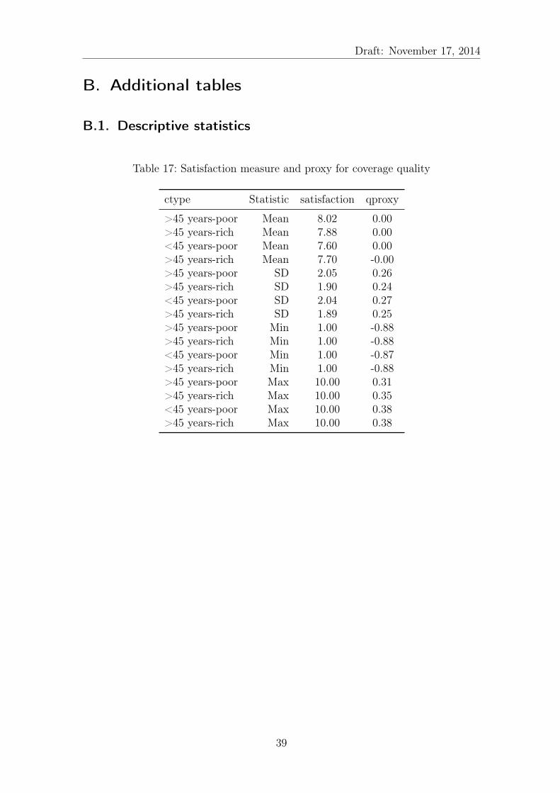
Draft: November 17, 2014
B. Additional tables
B.1. Descriptive statistics
Table 17: Satisfaction measure and proxy for coverage quality
ctype Statistic satisfaction qproxy
>45 years-poor Mean 8.02 0.00>45 years-rich Mean 7.88 0.00<45 years-poor Mean 7.60 0.00>45 years-rich Mean 7.70 -0.00>45 years-poor SD 2.05 0.26>45 years-rich SD 1.90 0.24<45 years-poor SD 2.04 0.27>45 years-rich SD 1.89 0.25>45 years-poor Min 1.00 -0.88>45 years-rich Min 1.00 -0.88<45 years-poor Min 1.00 -0.87>45 years-rich Min 1.00 -0.88>45 years-poor Max 10.00 0.31>45 years-rich Max 10.00 0.35<45 years-poor Max 10.00 0.38>45 years-rich Max 10.00 0.38
39
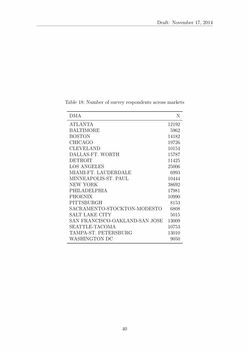
Draft: November 17, 2014
Table 18: Number of survey respondents across markets
DMA N
ATLANTA 12192BALTIMORE 5962BOSTON 14182CHICAGO 19726CLEVELAND 10154DALLAS-FT. WORTH 15787DETROIT 11425LOS ANGELES 25006MIAMI-FT. LAUDERDALE 6993MINNEAPOLIS-ST. PAUL 10444NEW YORK 38692PHILADELPHIA 17981PHOENIX 10990PITTSBURGH 8153SACRAMENTO-STOCKTON-MODESTO 6808SALT LAKE CITY 5015SAN FRANCISCO-OAKLAND-SAN JOSE 13009SEATTLE-TACOMA 10753TAMPA-ST. PETERSBURG 13010WASHINGTON DC 9050
40
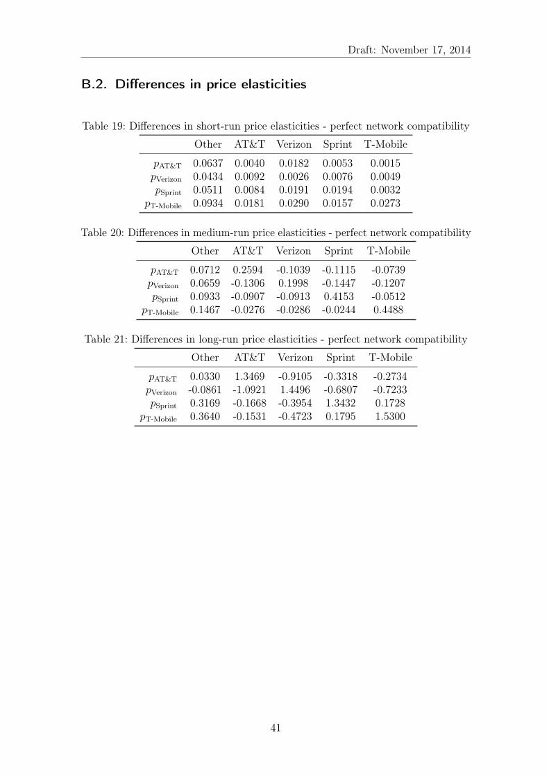
Draft: November 17, 2014
B.2. Differences in price elasticities
Table 19: Differences in short-run price elasticities - perfect network compatibility
Other AT&T Verizon Sprint T-Mobile
pAT&T 0.0637 0.0040 0.0182 0.0053 0.0015pVerizon 0.0434 0.0092 0.0026 0.0076 0.0049pSprint 0.0511 0.0084 0.0191 0.0194 0.0032
pT-Mobile 0.0934 0.0181 0.0290 0.0157 0.0273
Table 20: Differences in medium-run price elasticities - perfect network compatibility
Other AT&T Verizon Sprint T-Mobile
pAT&T 0.0712 0.2594 -0.1039 -0.1115 -0.0739pVerizon 0.0659 -0.1306 0.1998 -0.1447 -0.1207pSprint 0.0933 -0.0907 -0.0913 0.4153 -0.0512
pT-Mobile 0.1467 -0.0276 -0.0286 -0.0244 0.4488
Table 21: Differences in long-run price elasticities - perfect network compatibility
Other AT&T Verizon Sprint T-Mobile
pAT&T 0.0330 1.3469 -0.9105 -0.3318 -0.2734pVerizon -0.0861 -1.0921 1.4496 -0.6807 -0.7233pSprint 0.3169 -0.1668 -0.3954 1.3432 0.1728
pT-Mobile 0.3640 -0.1531 -0.4723 0.1795 1.5300
41

Draft: November 17, 2014
Table 22: Differences in short-run price elasticities - subsidized switching costs
Other AT&T Verizon Sprint T-Mobile
pAT&T 0.0064 -0.3382 0.1825 0.1256 0.1610pVerizon -0.0286 0.1516 -0.4390 0.1750 0.1991pSprint -0.0768 0.0968 0.1678 -0.6142 0.0948
pT-Mobile 0.0048 0.1418 0.2342 0.1875 -0.5750
Table 23: Differences in medium-run price elasticities - subsidized switching costs
Other AT&T Verizon Sprint T-Mobile
pAT&T -0.1803 -0.8047 0.5690 -0.2713 -0.2151pVerizon 0.1626 0.6982 -1.4286 0.2545 0.8824pSprint -0.0293 -0.3344 0.4793 -0.3467 -0.0691
pT-Mobile -0.0482 0.0848 0.8011 0.2467 -0.5621
C. Market share graphs and tables
42

Draft: November 17, 2014
Table 24: Differences in long-run price elasticities - subsidized switching costs
Other AT&T Verizon Sprint T-Mobile
pAT&T -0.3455 0.0846 -0.4666 -1.0458 0.4580pVerizon -0.2949 -0.9485 -2.0585 -1.3439 2.4446pSprint 0.0702 0.3048 -0.0308 0.4691 -0.1219
pT-Mobile 0.2923 2.5309 -0.5657 0.1573 0.2475
D. Empirical evidence on contract structure and
calling patterns
Figure 9 and 11 display information on postpaid cellphone contracts in the US at
various years during and shortly after my sample period (2006, 2008 and 2011).
This information was crawled from the Internet by using the Internet Archive-
Waybackmachine (http://web.archive.org). The term mobile-to-mobile minutes
denotes the minutes available for making and receiving calls from people with
the same provider. Although not every contract offers unlimited mobile-to-mobile
minutes, many operators do have at least some contract with on-net discounts in
some form throughout my sample period and beyond. My survey data does not
contain explicit information on the number of consumers that are subscribed to
contracts with free mobile-to-mobile minutes. In order to get an idea on these
numbers, I obtain information on the characteristics of the most common contracts
from Internet archives. A lower bound for the number of people who have on-net
discounts in their contract would be those who pay less for their plan that the costs
of the most basic unlimited-minutes plan. At the beginning of my sample period
these unlimited plans started at around US-$ 70-80 while at the end of the sample
period these contracts were already available for around US-$ 50.11 Based on these
numbers, I conjecture that at the beginning of my sample period, at least 75% of
consumers had contracts with on-net discounts in some form, while at the end of
my sample, still more than 50% should have had contracts with on-net discounts.
This supports the claim that tariff-mediated network effects have played a role in
the US wireless market during my sample period.
11Source: http://www.costhelper.com/cost/electronics/cell-phone-plans.html
43
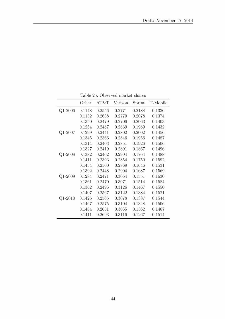
Draft: November 17, 2014
Table 25: Observed market shares
Other AT&T Verizon Sprint T-Mobile
Q1-2006 0.1148 0.2556 0.2771 0.2188 0.13360.1132 0.2638 0.2779 0.2078 0.13740.1350 0.2479 0.2706 0.2063 0.14030.1254 0.2487 0.2839 0.1989 0.1432
Q1-2007 0.1299 0.2441 0.2802 0.2002 0.14560.1345 0.2366 0.2846 0.1956 0.14870.1314 0.2403 0.2851 0.1926 0.15060.1327 0.2419 0.2891 0.1867 0.1496
Q1-2008 0.1382 0.2462 0.2904 0.1764 0.14880.1411 0.2393 0.2854 0.1750 0.15920.1454 0.2500 0.2869 0.1646 0.15310.1392 0.2448 0.2904 0.1687 0.1569
Q1-2009 0.1284 0.2471 0.3064 0.1551 0.16300.1361 0.2470 0.3071 0.1514 0.15840.1362 0.2495 0.3126 0.1467 0.15500.1407 0.2567 0.3122 0.1384 0.1521
Q1-2010 0.1426 0.2565 0.3078 0.1387 0.15440.1467 0.2575 0.3104 0.1348 0.15060.1484 0.2631 0.3055 0.1362 0.14670.1411 0.2693 0.3116 0.1267 0.1514
44

Draft: November 17, 2014
Table 26: Predicted market shares
Other AT&T Verizon Sprint T-Mobile
Q1-2006 0.1144 0.2557 0.2773 0.2189 0.13370.1136 0.2637 0.2777 0.2077 0.13730.1348 0.2479 0.2707 0.2063 0.14030.1264 0.2483 0.2835 0.1987 0.1430
Q1-2007 0.1299 0.2441 0.2802 0.2002 0.14560.1347 0.2366 0.2845 0.1955 0.14870.1318 0.2402 0.2850 0.1925 0.15050.1325 0.2420 0.2892 0.1867 0.1496
Q1-2008 0.1376 0.2464 0.2906 0.1765 0.14890.1408 0.2394 0.2855 0.1750 0.15920.1458 0.2499 0.2866 0.1646 0.15310.1391 0.2448 0.2904 0.1687 0.1569
Q1-2009 0.1286 0.2470 0.3064 0.1551 0.16290.1359 0.2471 0.3072 0.1514 0.15840.1359 0.2496 0.3128 0.1467 0.15500.1409 0.2566 0.3121 0.1383 0.1520
Q1-2010 0.1432 0.2563 0.3076 0.1387 0.15430.1466 0.2575 0.3105 0.1348 0.15060.1484 0.2631 0.3055 0.1362 0.14670.1411 0.2693 0.3115 0.1267 0.1513
45
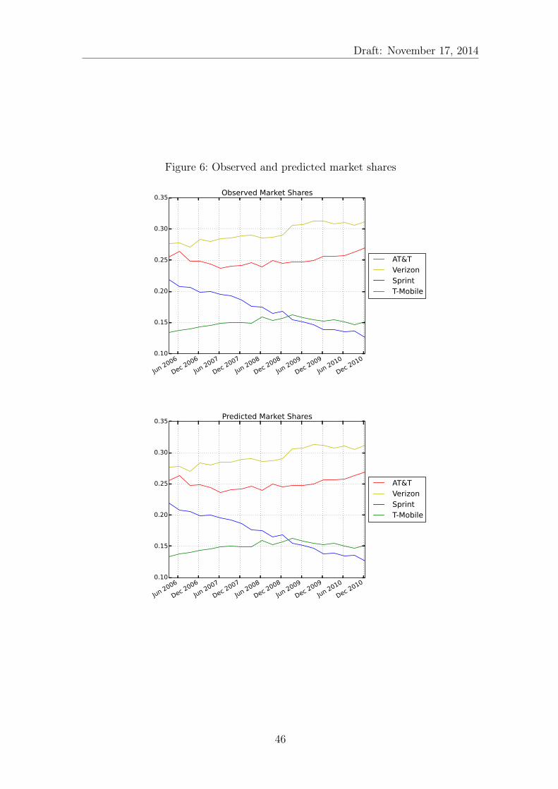
Draft: November 17, 2014
Figure 6: Observed and predicted market shares
Jun 20
06
Dec 2
006
Jun 20
07
Dec 2
007
Jun 20
08
Dec 2
008
Jun 20
09
Dec 2
009
Jun 20
10
Dec 2
010
0.10
0.15
0.20
0.25
0.30
0.35Observed Market Shares
AT&TVerizonSprintT-Mobile
Jun 20
06
Dec 2
006
Jun 20
07
Dec 2
007
Jun 20
08
Dec 2
008
Jun 20
09
Dec 2
009
Jun 20
10
Dec 2
010
0.10
0.15
0.20
0.25
0.30
0.35Predicted Market Shares
AT&TVerizonSprintT-Mobile
46
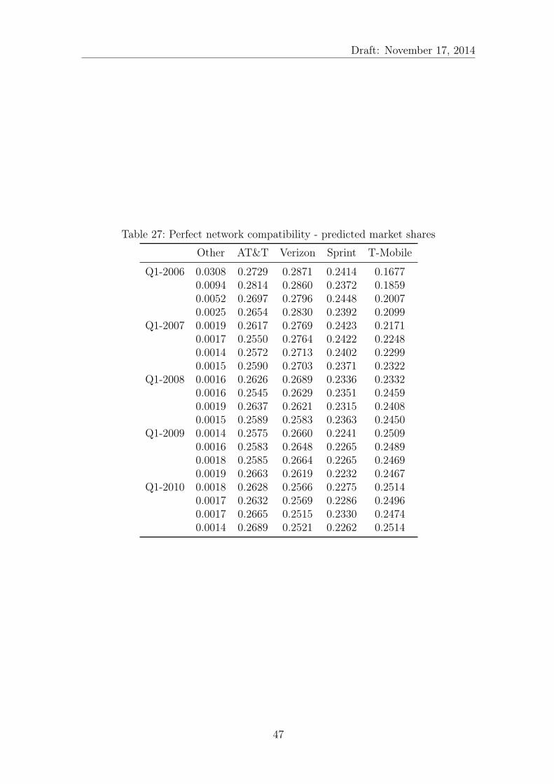
Draft: November 17, 2014
Table 27: Perfect network compatibility - predicted market shares
Other AT&T Verizon Sprint T-Mobile
Q1-2006 0.0308 0.2729 0.2871 0.2414 0.16770.0094 0.2814 0.2860 0.2372 0.18590.0052 0.2697 0.2796 0.2448 0.20070.0025 0.2654 0.2830 0.2392 0.2099
Q1-2007 0.0019 0.2617 0.2769 0.2423 0.21710.0017 0.2550 0.2764 0.2422 0.22480.0014 0.2572 0.2713 0.2402 0.22990.0015 0.2590 0.2703 0.2371 0.2322
Q1-2008 0.0016 0.2626 0.2689 0.2336 0.23320.0016 0.2545 0.2629 0.2351 0.24590.0019 0.2637 0.2621 0.2315 0.24080.0015 0.2589 0.2583 0.2363 0.2450
Q1-2009 0.0014 0.2575 0.2660 0.2241 0.25090.0016 0.2583 0.2648 0.2265 0.24890.0018 0.2585 0.2664 0.2265 0.24690.0019 0.2663 0.2619 0.2232 0.2467
Q1-2010 0.0018 0.2628 0.2566 0.2275 0.25140.0017 0.2632 0.2569 0.2286 0.24960.0017 0.2665 0.2515 0.2330 0.24740.0014 0.2689 0.2521 0.2262 0.2514
47
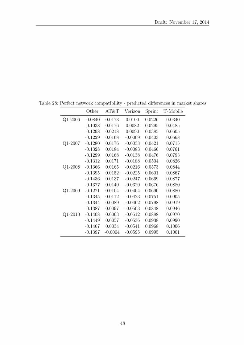
Draft: November 17, 2014
Table 28: Perfect network compatibility - predicted differences in market shares
Other AT&T Verizon Sprint T-Mobile
Q1-2006 -0.0840 0.0173 0.0100 0.0226 0.0340-0.1038 0.0176 0.0082 0.0295 0.0485-0.1298 0.0218 0.0090 0.0385 0.0605-0.1229 0.0168 -0.0009 0.0403 0.0668
Q1-2007 -0.1280 0.0176 -0.0033 0.0421 0.0715-0.1328 0.0184 -0.0083 0.0466 0.0761-0.1299 0.0168 -0.0138 0.0476 0.0793-0.1312 0.0171 -0.0188 0.0504 0.0826
Q1-2008 -0.1366 0.0165 -0.0216 0.0573 0.0844-0.1395 0.0152 -0.0225 0.0601 0.0867-0.1436 0.0137 -0.0247 0.0669 0.0877-0.1377 0.0140 -0.0320 0.0676 0.0880
Q1-2009 -0.1271 0.0104 -0.0404 0.0690 0.0880-0.1345 0.0112 -0.0423 0.0751 0.0905-0.1344 0.0089 -0.0462 0.0798 0.0919-0.1387 0.0097 -0.0503 0.0848 0.0946
Q1-2010 -0.1408 0.0063 -0.0512 0.0888 0.0970-0.1449 0.0057 -0.0536 0.0938 0.0990-0.1467 0.0034 -0.0541 0.0968 0.1006-0.1397 -0.0004 -0.0595 0.0995 0.1001
48
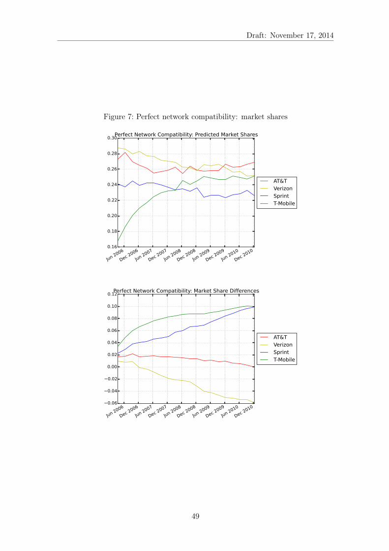
Draft: November 17, 2014
Figure 7: Perfect network compatibility: market shares
Jun 20
06
Dec 2
006
Jun 20
07
Dec 2
007
Jun 20
08
Dec 2
008
Jun 20
09
Dec 2
009
Jun 20
10
Dec 2
010
0.16
0.18
0.20
0.22
0.24
0.26
0.28
0.30Perfect Network Compatibility: Predicted Market Shares
AT&TVerizonSprintT-Mobile
Jun 2006
Dec 2006
Jun 2007
Dec 2007
Jun 2008
Dec 2008
Jun 2009
Dec 2009
Jun 2010
Dec 2010
−0.06
−0.04
−0.02
0.00
0.02
0.04
0.06
0.08
0.10
0.12Perfect Network Compatibility: Market Share Differences
AT&TVerizonSprintT-Mobile
49
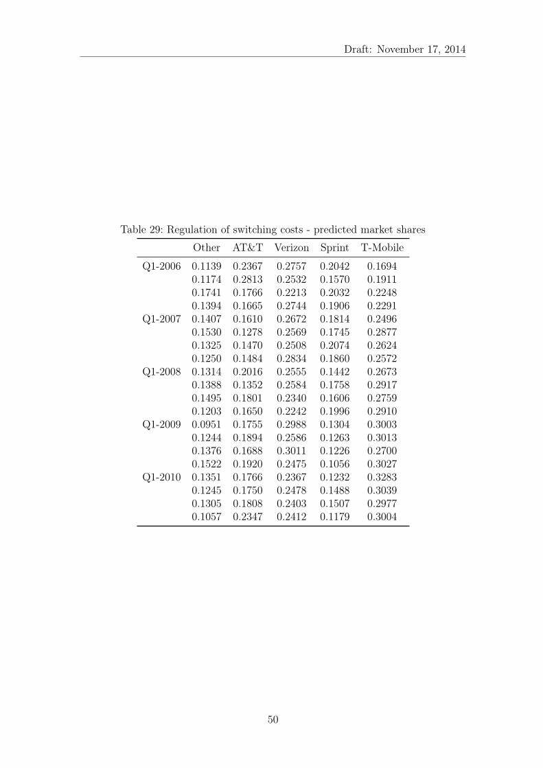
Draft: November 17, 2014
Table 29: Regulation of switching costs - predicted market shares
Other AT&T Verizon Sprint T-Mobile
Q1-2006 0.1139 0.2367 0.2757 0.2042 0.16940.1174 0.2813 0.2532 0.1570 0.19110.1741 0.1766 0.2213 0.2032 0.22480.1394 0.1665 0.2744 0.1906 0.2291
Q1-2007 0.1407 0.1610 0.2672 0.1814 0.24960.1530 0.1278 0.2569 0.1745 0.28770.1325 0.1470 0.2508 0.2074 0.26240.1250 0.1484 0.2834 0.1860 0.2572
Q1-2008 0.1314 0.2016 0.2555 0.1442 0.26730.1388 0.1352 0.2584 0.1758 0.29170.1495 0.1801 0.2340 0.1606 0.27590.1203 0.1650 0.2242 0.1996 0.2910
Q1-2009 0.0951 0.1755 0.2988 0.1304 0.30030.1244 0.1894 0.2586 0.1263 0.30130.1376 0.1688 0.3011 0.1226 0.27000.1522 0.1920 0.2475 0.1056 0.3027
Q1-2010 0.1351 0.1766 0.2367 0.1232 0.32830.1245 0.1750 0.2478 0.1488 0.30390.1305 0.1808 0.2403 0.1507 0.29770.1057 0.2347 0.2412 0.1179 0.3004
50
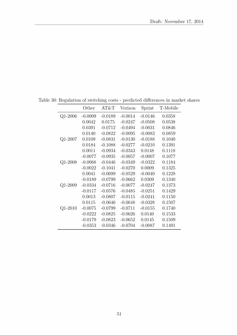
Draft: November 17, 2014
Table 30: Regulation of switching costs - predicted differences in market shares
Other AT&T Verizon Sprint T-Mobile
Q1-2006 -0.0009 -0.0189 -0.0014 -0.0146 0.03580.0042 0.0175 -0.0247 -0.0508 0.05380.0391 -0.0712 -0.0494 -0.0031 0.08460.0140 -0.0822 -0.0095 -0.0083 0.0859
Q1-2007 0.0109 -0.0831 -0.0130 -0.0188 0.10400.0184 -0.1088 -0.0277 -0.0210 0.13910.0011 -0.0934 -0.0343 0.0148 0.1118-0.0077 -0.0935 -0.0057 -0.0007 0.1077
Q1-2008 -0.0068 -0.0446 -0.0349 -0.0322 0.1184-0.0022 -0.1041 -0.0270 0.0009 0.13250.0041 -0.0699 -0.0529 -0.0040 0.1228-0.0189 -0.0799 -0.0662 0.0309 0.1340
Q1-2009 -0.0334 -0.0716 -0.0077 -0.0247 0.1373-0.0117 -0.0576 -0.0485 -0.0251 0.14290.0013 -0.0807 -0.0115 -0.0241 0.11500.0115 -0.0646 -0.0648 -0.0328 0.1507
Q1-2010 -0.0075 -0.0799 -0.0711 -0.0155 0.1740-0.0222 -0.0825 -0.0626 0.0140 0.1533-0.0179 -0.0823 -0.0652 0.0145 0.1509-0.0353 -0.0346 -0.0704 -0.0087 0.1491
51
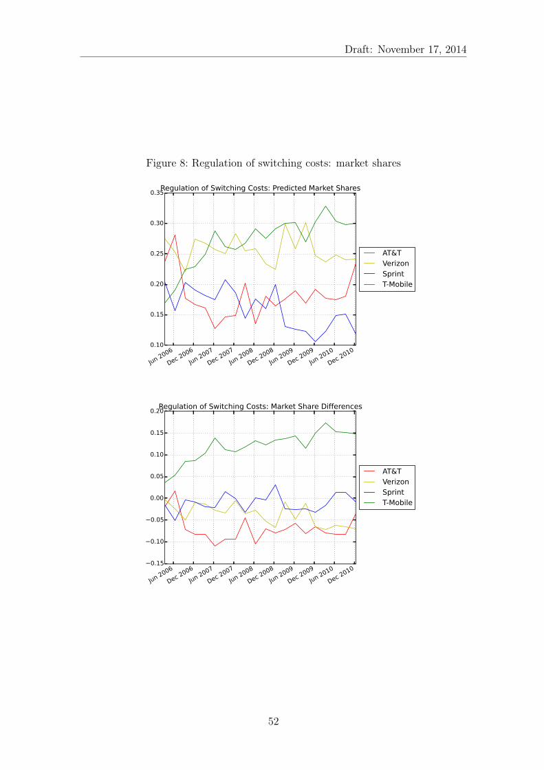
Draft: November 17, 2014
Figure 8: Regulation of switching costs: market shares
Jun 2006
Dec 2006
Jun 2007
Dec 2007
Jun 2008
Dec 2008
Jun 2009
Dec 2009
Jun 2010
Dec 20100.10
0.15
0.20
0.25
0.30
0.35Regulation of Switching Costs: Predicted Market Shares
AT&TVerizonSprintT-Mobile
Jun 2006
Dec 2006
Jun 2007
Dec 2007
Jun 2008
Dec 2008
Jun 2009
Dec 2009
Jun 2010
Dec 2010
−0.15
−0.10
−0.05
0.00
0.05
0.10
0.15
0.20Regulation of Switching Costs: Market Share Differences
AT&TVerizonSprintT-Mobile
52

Draft: November 17, 2014
Figure 9: Information on wireless contracts from 2006
Source: http://cell-phone-providers-review.toptenreviews.com
53
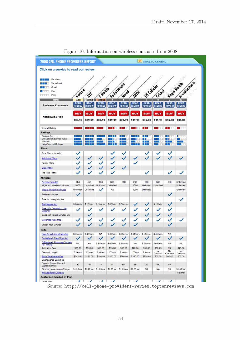
Draft: November 17, 2014
Figure 10: Information on wireless contracts from 2008
Source: http://cell-phone-providers-review.toptenreviews.com
54

Draft: November 17, 2014
Figure 11: Information on wireless contracts from 2011
Source: http://www.phonearena.com
55