Universita degli Studi di PisaFacolta di Ingegneria

Corso di Laurea Specialistica in

Ingegneria Informatica

Adaptive Data Parallelism for InternetClients on Heterogeneous Platforms

Relatori Candidato

Prof. Paolo Ancilotti Alessandro Pignotti

Prof. Giuseppe Lipari

Anno Accademico 2011/12

i

Sommario

Il Web moderno ha da molto superato le pagine statiche, limi-

tate alla formattazione HTML e poche immagini. Siamo entrati

i un era di Rich Internet Applications come giochi, simulazioni

fisiche, rendering di immagini, elaborazione di foto, etc eseguite

localmente dai programmi client. Nonostante questo gli attuali

linguaggi lato client hanno limitatissime capacita di utilizzare le

capacita computazionali della piattaforma, tipicamente eterogenea,

sottostante. Presentiamo un DSL (Domain Specific Language)

chiamato ASDP (ActionScript Data Parallel) integrato in Action-

Script, uno dei linguaggi piu popolari per la programmazione lato

client e un parente prossimo di JavaScript. ASDP e molto simile

ad ActionScript e permette frequentemente di utilizzare la pro-

grammazione parallela con minime modifiche al codice sorgente.

Presentiamo anche un prototipo di un sistema in cui computazioni

data parallel possono essere eseguite su CPU o GPU. Il sistema

runtime si occupera di selezionare in modo trasparente la miglior

unita computazionale a seconda del calcolo, dell’architettura e del

carico attuale del sistema. Vengono inoltre valutate le performance

del sistema su diversi benchmark, rappresentativi dei seguenti tipi

di applicazioni: fisica, elaborazione di immagini, calcolo scientifico

e crittografia.

ii

Abstract

Today’s Internet is long past static web pages full of HTML-

formatted text sprinkled with an occasional image or animation.

We have entered an era of Rich Internet Applications executed

locally on Internet clients such as web browsers: games, physics

engines, image rendering, photo editing, etc. And yet today’s

languages used to program Internet clients have limited ability

to tap to the computational capabilities of the underlying, often

heterogeneous, platforms. We present how a Domain Specific Lan-

guage (DSL) can be integrated into ActionScript, one of the most

popular scripting languages used to program Internet clients and

a close cousin of JavaScript. Our DSL, called ASDP (ActionScript

Data Parallel), closely resembles ActionScript and often only min-

imal changes to existing ActionScript programs are required to

enable data parallelism. We also present a prototype of a system,

where data parallel workloads can be executed on either CPU

or a GPU, with the runtime system transparently selecting the

best processing unit, depending on the type of workload as well

as the architecture and current load of the execution platform.

We evaluate performance of our system on a variety of bench-

marks, representing different types of workloads: physics, image

processing, scientific computing and cryptography.

iii

Per Francesca, che pur non credendo nelle

mie scritte bianche su sfondo nero continua

comunque a volermi bene

iv

Ringraziamenti

A mamma e papa, che hanno saputo accettare che lasciassi Roma cosı presto.

A Francesco e Daniele, che nonostante questo non mi hanno dimenticato.

A Vomere, per il confronto quotidiano.

A Cinzia e Catta, coppia di amici.

Ad Elisa, amica e basta.

Ad Alberto, per tre anni di paziente convivenza.

A Dragoni, sempre primo.

A Bauletto, compagno di puzzle.

E a Cecchi e Brancatello, allenatori.

A Baulone, cuoco e ottimizzatore.

A Corbetta, Kaka, Guillo, Cazzaro, Fonseca, Marino e Il Brigo, che mi hanno

guidato nel labirinto accademico, salvandomi da un sacco di sfavo.

A Tarzan, che mi ha fatto scoprire la Notte.

E a Dyno, che l’ha scoperta ancor prima.

A Sbabbi e Paolone, che mi hanno spinto a capire meglio cose che credevo di

sapere.

A Tommy, Jacopone, Zanetti, Vladimir e gli altri giovani Casti, degni eredi.

E a tutti gli altri che mi hanno supportato, (ri)sollevato e rinfrancato in questi

anni cosı densi.

Grazie mille

v

Contents

1 Introduction 1

1.1 Heterogeneous Devices . . . . . . . . . . . . . . . . . . . . . . 1

1.2 Data Parallel Computing . . . . . . . . . . . . . . . . . . . . . 3

1.3 Web Clients Programming . . . . . . . . . . . . . . . . . . . . 5

1.3.1 ActionScript . . . . . . . . . . . . . . . . . . . . . . . . 5

2 Related Work 8

2.1 RiverTrail . . . . . . . . . . . . . . . . . . . . . . . . . . . . . 8

2.2 Qilin . . . . . . . . . . . . . . . . . . . . . . . . . . . . . . . . 10

2.3 DynoCL . . . . . . . . . . . . . . . . . . . . . . . . . . . . . . 11

3 ActionScript Data Parallel 12

3.1 Motivations . . . . . . . . . . . . . . . . . . . . . . . . . . . . 13

3.1.1 Regular workflow for data parallel programming . . . . 14

3.2 Data parallelism support overview . . . . . . . . . . . . . . . . 16

3.2.1 ActionScript Data Parallel (ASDP) . . . . . . . . . . . 17

3.2.2 ActionScript extensions . . . . . . . . . . . . . . . . . . 19

3.3 Example . . . . . . . . . . . . . . . . . . . . . . . . . . . . . . 21

4 Implementation 24

vi

4.1 Compilation . . . . . . . . . . . . . . . . . . . . . . . . . . . . 24

4.1.1 OpenCL . . . . . . . . . . . . . . . . . . . . . . . . . . 25

4.1.2 ActionScript bytecode . . . . . . . . . . . . . . . . . . 26

4.2 Adaptivity . . . . . . . . . . . . . . . . . . . . . . . . . . . . . 26

4.2.1 Initial sampling runs optimization . . . . . . . . . . . . 29

4.3 Proof of predictably bounded overhead of sampling in steady

conditions . . . . . . . . . . . . . . . . . . . . . . . . . . . . . 29

5 Performance evaluation 32

5.1 Average Performance . . . . . . . . . . . . . . . . . . . . . . . 35

5.2 Adaptive Performance . . . . . . . . . . . . . . . . . . . . . . 38

6 Conclusions & future work 43

vii

Chapter 1

Introduction

Supporting high performance computation on modern platforms and having

it fully integrated in a modern, dynamic programming language requires

deep knowledge of a large number of components, from the hardware to the

compiler to the runtime support engine. We will briefly introduce a few

concept that may be useful in understanding the scope and the behaviour of

our work.

1.1 Heterogeneous Devices

Moore’s Law, introduced in 1965 by Gordon E. Moore [19] describes that

the amount of transistors that can be inexpensively placed on a integrated

circuit doubles roughly every two years. This empiric law has been, up to now,

fairly accurate in predicting the technological advances of electronic devices.

Especially since the silicon industry has invested an enormous amount of

resources to keep up with this prophecy. It’s definitely possible that Moore’s

Law has been one the most sustained and large scale exponential growth

phenomenon of history. 1

Until 2003 the growing transistor density was employed to increase the size

1Only surpassed in recent years by the hyper-exponential decrease of DNA sequencingcost http://www.genome.gov/sequencingcosts/

1

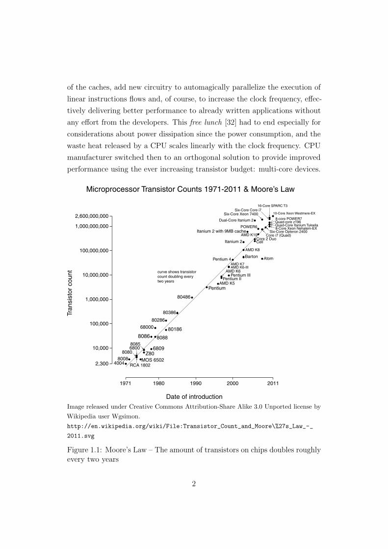
of the caches, add new circuitry to automagically parallelize the execution of

linear instructions flows and, of course, to increase the clock frequency, effec-

tively delivering better performance to already written applications without

any effort from the developers. This free lunch [32] had to end especially for

considerations about power dissipation since the power consumption, and the

waste heat released by a CPU scales linearly with the clock frequency. CPU

manufacturer switched then to an orthogonal solution to provide improved

performance using the ever increasing transistor budget: multi-core devices.

Image released under Creative Commons Attribution-Share Alike 3.0 Unported license by

Wikipedia user Wgsimon.

http://en.wikipedia.org/wiki/File:Transistor_Count_and_Moore\%27s_Law_-_

2011.svg

Figure 1.1: Moore’s Law – The amount of transistors on chips doubles roughlyevery two years

2

Today we are in the midst of the multi-core era, but evolution of computa-

tional platforms did not stop with the introduction of multi-core. Processing

units that have been previously only used for graphics processing, namely

GPUs, are rapidly evolving towards supporting general-purpose computa-

tions. Consequently, even a modestly priced and equipped modern machine

constitutes a heterogeneous computational platform where execution of what

has been traditionally viewed as CPU workloads can be potentially delegated

to a GPU.

Moreover, the Cell Broadband Engine by IBM has introduced an hetero-

geneous device based on a regular multi-core central unit and 8 Synergistic

Processing Units that are not intended to be used as a GPU, demonstrating

that the introduction of heterogeneous devices allows for innovative designs

of computing architectures.

1.2 Data Parallel Computing

The multi-core revolution has brought a new level of complexity to high

performance computing. How to handle such complexity has been extensively

discussed in the scientific community and a multitude of proposals has arisen,

from basic Inter Process Communication features, to Threads to advanced

techniques such as Software Transactional Memory [30].

The even more extended capabilities and innovative architectural designs

that are possible on heterogeneous devices has made the problem worse, since

the developer has to reason about systems that may have an unspecified

number of co-processors, each one potentially having different performance

characteristics and even different instruction sets, memory models and endi-

anness.

A proposed model to simplify the programming of systems with such

properties is Data Parallel Computing. Such model assumes that the compu-

tation is based on a single algorithm that needs to be executed over a very

large amount of data. This model makes it possible to take advantage of

3

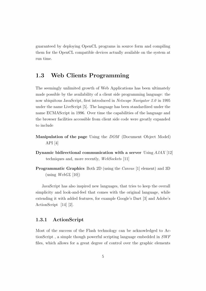
Figure 1.2: A tipical MMX instruction. The operation is carried on in parallellon many values stored in a single register

a1 a2 a3 a4

add

b1 b2 b3 b4

⇓a1 + b1 a2 + b2 a3 + b3 a4 + b4

128 bit

parallel architectures is a very easy way, since the computation can be trivially

parallelized by splitting the data set in subsets and assigning each one to a

different unit. This simplicity comes with a cost, as not every computation

can be expressed by this limited model. Nevertheless it is powerful enough

for many multimedia and physics related algorithm, which are naturally data

driven.

On the smallest scale, Data Parallel Computing has been available even

on classical, single core, CPUs for several years in the form of SIMD (Single

Instruction Multiple Data) instructions. For the x86 they were introduced

by the MMX extensions in 1996 [6] and expanded afterwards with the SSE

family of extensions. Even the low power ARM architecture has his own

SIMD instructions provided by the NEON extension [7]. Such instructions

are usually powered by very wide (128-bit, 256 bit) registers (See Figure

1.2) that stores more than a single value and specific support by the ALU

(Arithmetic and Logic Unit) to execute operations on each element in parallel.

As mentioned before, heterogeneous devices are composed of multiple

computing unit that supports different instructions sets, which are often not

known during development. To overcome such difficulty a few data parallel

languages as been developed. The most important of those is definitely

OpenCL (maintained by the Khronos Group [8]), which is a portable C-based

language now supported by many CPU and GPU vendors. Portability is

4

guaranteed by deploying OpenCL programs in source form and compiling

them for the OpenCL compatible devices actually available on the system at

run time.

1.3 Web Clients Programming

The seemingly unlimited growth of Web Applications has been ultimately

made possible by the availability of a client side programming language: the

now ubiquitous JavaScript, first introduced in Netscape Navigator 2.0 in 1995

under the name LiveScript [5]. The language has been standardized under the

name ECMAScript in 1996. Over time the capabilities of the language and

the browser facilities accessible from client side code were greatly expanded

to include

Manipulation of the page Using the DOM (Document Object Model)

API [4]

Dynamic bidirectional communication with a server Using AJAX [12]

techniques and, more recently, WebSockets [11]

Programmatic Graphics Both 2D (using the Canvas [1] element) and 3D

(using WebGL [10])

JavaScript has also inspired new languages, that tries to keep the overall

simplicity and look-and-feel that comes with the original language, while

extending it with added features, for example Google’s Dart [3] and Adobe’s

ActionScript [14] [2].

1.3.1 ActionScript

Most of the success of the Flash technology can be acknowledged to Ac-

tionScript , a simple though powerful scripting language embedded in SWF

files, which allows for a great degree of control over the graphic elements

5

and interactivity features of the movie. ActionScript was first introduced in

version 2 of Macromedia Flash Player. At first only basic playback control

such as play, stop, getURL and gotoAndPlay was offered, but over time new

features were introduced as conditional branches, looping construct and class

inheritance, and the language evolved to a general purpose though primitive

one. To overcome several limitations in the original design Adobe introduced

ActionScript 3 in 2006 with the release of version 9 of the Flash player and

development tools. The new design it’s quite different from the previous

versions and extremely expressive. The language is mostly based on EC-

MAScript 3 (which is also the base for the popular JavaScript language),

but several new features are added to the standard, such as optional static

typing for variables. The ActionScript specification defines a binary format

and bytecode to encode the scripts so that no language parsing has to be

done on the clients. Moreover a huge runtime library is provided, integrated

with the graphics and multimedia features of the Flash player.

It is useful to define now a few data types that are crucial for the operation

of our system to represent arrays and typed arrays:

Array This type comes firectly from ECMAScript and inherits all its pitfalls

and flexibility. It’s a fully generic associative container of objects.

Object instances are stored by reference and they can be of any type.

The Array is allowed to be sparse, meaning that there is no need to fill

eventually unused indices. Accessing them does not generate an error,

but just return undefined. Moreover, the Array dynamically enlarges

itself when needed and can be considered unlimited in practice (memory

limits obviously holds though)

ByteArray This type is a specialized container of bytes (8-bit unsigned

integers), optimized for performance. The data is stored in packed form

to increase locality and reduce the overhead, making ByteArray very

similar to a buffer of C-style unsigned chars. It’s possible to access

data contained in a ByteArray using the regular [] operator, but also

using instance methods such as readFloat, readInt, writeDouble and so

6

on, to interpret the stored data as various types. Finally, ByteArray

also feature native support for ZLib [13] compression/decompression,

configurable endianness and serialization on ActionScript objects

Vector<BaseType> This is a generic type that is designed to reduce the

overhead caused by using Array. V ector is a dense array of a specified

length, this means that whatever the length of it, memory is allocated

to store all elements from 0 to length − 1. Moreover, V ector is type

safe since it’s only able to store elements of a single type. If objects

of any type other than BaseType are assigned to the V ector they are

automatically converted to BaseType. The implementation of V ector

for primitive types such as int, float and Number is specialized to store

data by value instead of by reference to improve performance.

7

Chapter 2

Related Work

There is a large body of related work in the area of data parallel programming,

including what are arguably the closest approaches to our work, that is

attempts to introduce data parallelism to high level languages. Examples

include CopperHead (Python) [16], Accelerator (.NET) [31], Lime (Java) [18]

and Data Parallel Haskell [17]. The data parallelism support provided by the

RiverTrail project [24] seems to be the closest to our proposal and can be

considered equivalent in terms of expressiveness to our own solution.

Despite also compiling the data parallel constructs to OpenCL, their

system currently does not support execution on a GPU [22]. Some other

approaches mentioned above do support execution on a GPU, but to the best

of our knowledge none of them supports automatic selection of the optimal

processing unit or adaptive switching of processing unit.

2.1 RiverTrail

RiverTrail, developed by Intel Labs, expresses data parallelism in “pure”

JavaScript, using a new data type called ParallelArray. ParallelArray is

a read-only immutable container of data. It can only be created from a

constructor or generated from other data using one of the few available data

parallel methods described below.

8

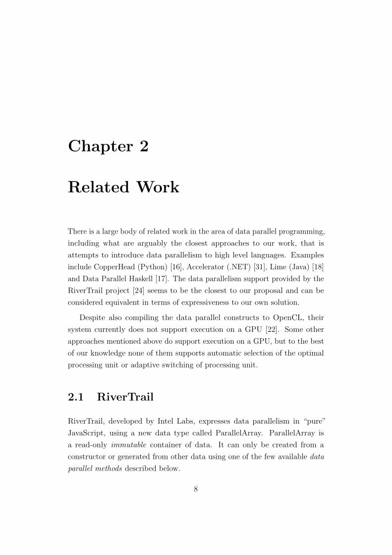
(a) Map (b) Combine

(c) Filter (d) Scatter

Figure 2.1: Graphical interpretation of data parallel methods available inRiverTrail

All the methods are semantically members of a ParallelArray instance.

map The final ParallelArray contains the result of invoking a specified

elemental function over each member of the source ParallelArray. This

is the most basic method.

combine A generalization of map: an index argument is provided and it

makes it possible to access other elements of the source array relative

to the current one or even elements from other ParallelArrays

filter This method evaluates the elemental function over each element of the

source ParallelArray. If the evaluation result is true the element will be

added to the final ParallelArray otherwise it will be ignored

scatter This method shuffles the data in the source ParallelArray. Each

element is moved to the position described by another ParallelArray. If

9

more than an element is moved to the same position a custom conflict

resolution function is invoked to determine the winner

scan The final ParallelArray contains at element N the result of the reduce

method (described below) executed from element 1 to N

Moreover, there is a method to generate a scalar from the source ParallelArray:

reduce A reduction function is a function accepting two scalar arguments

and returning a single scalar. Such function is conceptually invoked on

each element sequentially to accumulate the final result. It’s possible to

get a large speedup by using a divide-and-conquer approach on the data,

although the result is guaranteed to be the same only if the reduction

function is associative. The reduce method does not offer any guarantee

on the order of the calls that will be used to get the final result.

2.2 Qilin

Another notable piece of the related work is the Qilin system [26]. Qilin

introduces an API for C++ that allows programmers to specify parallel

computations and supports utilization of multiple processing units for a given

workload, including adaptivity to the hardware changes. Although Qilin is

based on a very different context (C++), a few details of the system are

interesting.

Qilin capabilities are based on two backends: CUDA [27] and Intel’s

Threading Building Blocks (TBB) [9].

Qilin offers two different approaches to parallelism:

Stream API The parallel code must be written exclusively using Qilin APIs.

Qilin at runtime will construct a DAG (Direct Acyclic Graph) of the

needed operations and translate it to a source code compatible with the

aforementioned backends. The source will then be compiled to native

code using the system provided compilers.

10

Threading API In this case the user has to manually provide the source

code for both TBB and CUDA and Qilin will take care of optimally

splitting the load between the units.

As we have seen Qilin, at the current stage of development, requires

manual coding in the languages of the underlying backends or the usage of

it’s own API. This arguably makes it’s deployment, especially in an already

existing code base, quite invasive. Moreover, as any adaptive system, it

requires training runs on a representative subset of the problem domain to

optimally schedule future executions. But such adaptiveness is only limited

to physical swapping of hardware components and the scheduler is incapable

of reacting to changes in machine load. Overall, this system might be more

suited for batched computations (eg. scientific workloads) than for typical

code running in web clients.

2.3 DynoCL

Finally, Binotto et al. [15] describe a system where OpenCL is used as

the primary programming model, and which does support automatic co-

scheduling between a CPU and a GPU. Their approach, however, targets

mainly scientific computing. Moreover, it focuses on utilization of the entire

platform rather than selection of the optimal processing unit, and similarly

to Qilin is incapable of reacting to changes in machine load.

11

Chapter 3

ActionScript Data Parallel

Today’s Internet clients, such as various web browsers, despite growing de-

mand for computational capabilities triggered by the rise of Rich Internet

Applications and Social Games, have very limited ability to utilize the com-

putational power available on modern heterogeneous architectures. Attempts

have been made to enable utilization of multiple cores, via task parallelism

[21] or data parallelism [24], but our system is the first solution in this context

where the same data parallel workload can be transparently scheduled on

either a CPU or a GPU, depending on the type of workload as well as on the

architecture and the current load of the underlying platform. We introduce a

Domain Specific Language, that integrates seamlessly with ActionScript, one

of the most popular languages used to program Internet clients. Our DSL,

called ASDP (ActionScriptData Parallel) gets compiled down to OpenCL,

enabling execution on a GPU or CPU on platforms that support execution of

OpenCL programs on these processing units. ASDP gets also compiled back

to ActionScript to provide a baseline execution mode and to support execution

of data parallel programs on platforms that do not support OpenCL. While

our solution is based on ActionScript, it can be adapted to other languages

used to program Internet clients, such as JavaScript, as it does not rely on

any language features that are specific only to ActionScript.

12

In summary, we will propose the following contributions:

• We present a domain specific language, ASDP (ActionScript Data

Parallel) that closely resembles ActionScript and that can be used to

express data parallel computations in the context of ActionScript. We

also discuss ActionScript extensions required to integrate ASDP code

• We describe the implementation of a prototype system responsible for

compiling and executing ASDP code fragments. A modified version of

the upcoming ActionScript Falcon compiler [28] translates ASDP code

fragments to OpenCL (for efficient execution on both a CPU and a

GPU) and back to ActionScript (baseline execution mode). A modified

version of Tamarin, an open source ActionScript virtual machine, profiles

execution of the ASDP code fragments and chooses the best processing

unit to execute a give fragment, depending on the type of workload as

well as the architecture and current load of the underlying platform

• We present performance evaluation of our system and demonstrate its

ability to both achieve execution times that are close to those of the

best execution unit on a given platform, and to modify processing unit

selection whenever the system load changes

3.1 Motivations

Data parallelism seems like one of the more natural ways of introducing

parallelism in the context of scripting languages, such as ActionScript, as

support for data parallelism can also be restricted to automatically prevent

problems related to managing access to shared memory, such as data races,

resulting in safer and more robust programs, which preserves the spirit

of scripting languages used to program Internet clients. It is also often

easy to parallelize sequential loops using data parallel constructs, with little

modifications to the existing code. One of our main goals when developing

our solution was to make it convenient to use by “scripters” and yet powerful

13

__kernel void opencl_sum(__global float* out,

__global float* in1,

__global float* in2)

{

size_t index=get_global_id();

out[index] = in1[index] + in2[index];

}

Figure 3.1: An example kernel written in the OpenCL language that computesthe sum of each element of the input arrays

enough to deliver significant performance gains at the cost of relatively

little effort. We argue the first point, the ease of use, below by describing

modifications required to parallelize one of the benchmarks used for our

performance evaluation. Clearly, the number of modifications vary depending

on the specifics of a given program as, for example, not all data types

available in ActionScript are supported in ASDP. We argue the second point,

performance, in Section 5.

3.1.1 Regular workflow for data parallel programming

We will briefly introduce what are the required steps to execute a computation

using regular OpenCL. First of all a kernel must be written in the OpenCL

language (eg. Figure 3.1). The kernel must be stored in a file or as a literal

string inside the source.

Accessing OpenCL capabilities is done at runtime using a system provided

OpenCL library. A few library calls are first needed to initialize the system.

In the next code snippets error checking and handling is omitted to reduce

verbosity.

cl_device_id deviceId;

int err;

err = clGetDeviceIDs(NULL, CL_DEVICE_TYPE_GPU, 1,

14

&deviceId, NULL);

cl_context context = clCreateContext(0, 1, &deviceId,

NULL, NULL, &err);

cl_command_queue queue = clCreateCommandQueue(context,

device_id, 0, &err);

\end{verbatim}

Let’s assume the OpenCL source code of the kernel has been loaded in memory

and is accessible through the pointer sourcePtr.

cl_program program = clCreateProgramWithSource(context, 1,

(const char**) &sourcePtr, NULL, &err);

err = clBuildProgram(program, 0, NULL, NULL, NULL, NULL);

cl_kernel kernel = clCreateKernel(program, "opencl_sum", &err);

The kernel has been now loaded, parsed and compiled by the OpenCL runtime.

A reference to the kernel code we are interested in is also stored in the kernel

variable. Let’s now assume that the two arrays of length elementsNum we

want to sum are already defined and called buf1 and buf2

cl_mem input1 = clCreateBuffer(context, CL_MEM_READ_ONLY,

sizeof(float)*elementsNum, NULL, NULL);

cl_mem input2 = clCreateBuffer(context, CL_MEM_READ_ONLY,

sizeof(float)*elementsNum, NULL, NULL);

cl_mem output = clCreateBuffer(context, CL_MEM_WRITE_ONLY,

sizeof(float)*elementsNum, NULL, NULL);

err = clEnqueueWriteBuffer(queue, input1, CL_TRUE, 0,

sizeof(float)*elementsNum, buf1, 0, NULL, NULL);

err = clEnqueueWriteBuffer(queue, input2, CL_TRUE, 0,

sizeof(float)*elementsNum, buf2, 0, NULL, NULL);

Now the data has been loaded in device memory and it’s ready to be used.

We will now set the arguments and schedule the kernel for execution.

err = clSetKernelArg(kernel, 0, sizeof(cl_mem), &output);

15

err = clSetKernelArg(kernel, 1, sizeof(cl_mem), &input1);

err = clSetKernelArg(kernel, 2, sizeof(cl_mem), &input2);

err = clEnqueueNDRangeKernel(queue, kernel, 1, NULL,

&elementsNum, NULL, 0, NULL, NULL);

Since the execution is asynchronous we have to wait for the end of it before

reading the results in the finalResults array.

clFinish(queue);

err = clEnqueueReadBuffer(queue, output, CL_TRUE, 0,

sizeof(float)*elementsNum, finalResults, 0, NULL, NULL);

It’s pretty clear that the boilerplate needed to use OpenCL is quite a

lot and the syntax is far from immediate. Moreover, the developer has to

manually select what computation unit will be used since the beginning.

3.2 Data parallelism support overview

The style of data parallelism supported in our system is similar to that

defined by OpenCL [20] or CUDA [27], though it is tailored to better suit

the requirements of a scripting language setting, as OpenCL’s and CUDA’s

formulation is quite low level and thus, arguably, somewhat difficult to use.

Parallel computation is defined by a special data parallel function called

kernel. In our system, kernel definitions are distinguished from definitions

of other functions by a dot preceding their name (e.g. .Function). Kernel’s

code is executed in parallel for each point in a single-dimensional index space –

conceptually it is equivalent to executing the kernel’s code inside of a parallel

loop with the number of iterations equal to the size of the index space. A

given point in the index space is identified by a built-in variable index of

type int, ranging from 0 to the size of the index space. We say that a kernel

is evaluated after its code is executed for all points in the index-space. Even

though a return type of the kernel presented in Figure 3.4 is defined as float,

the actual result of the kernel’s evaluation is a vector of float values, with

16

each separate float value representing the result of a computation at a given

point in the index space.

Kernel invocation is, as well, strongly similar to a regular function call:

.Function[indexSpaceSize, outputArray](arg1, arg2)

Between square brackets two special argument are available: the first one

is compulsory and describes the size of the index space, the second one is

optional and specifies a Vector or ByteArray that will be populated with the

returned data. This second parameter can be omitted to get a freshly allocated

ByteArray, using it is advantageous to reduce the overhead of allocating new

memory for each parallel call.

3.2.1 ActionScript Data Parallel (ASDP)

Data parallel computations supported in our system are expressed in a Domain

Specific Language (DSL) we call ASDP (ActionScript Data Parallel). The

description of ASDP and of the extensions required to embed ASDP kernels

into ActionScript programs, building on an overview presented in Section 3.2,

is presented below.

The basic units of data parallel execution in our system, that is kernels, are

written in ASDP, which has been designed to closely resemble ActionScript,

making embedding of ASDP kernels into ActionScript source code feel natural.

In order to enable efficient execution of ASDP kernels on GPUs, ASDP

removes certain features of ActionScript, while trying to preserve the overall

ActionScript look and feel. ASDP supports ActionScript-style control-flow

constructs (such as loop or conditionals), local variable declarations, function

invocations and equivalents of ActionScript primitive types with the exception

of Number (i.e. uint, int, Boolean, float, float4). On the other hand, ASDP

does not support dynamic memory allocation, recursion, objects, closures or

global variables. Despite these restrictions, as demonstrated by successful

parallelization of our benchmarks, ASDP is fully capable of expressing realistic

workloads. Similarly to other data parallel languages such as OpenCL or

17

CUDA, ASDP also includes support for additional vector types that allow

programmers to take direct advantage of vector processing support often

available on modern architectures. Generally, the following types are available

in ASDP :

• primitive types: char and uchar (signed and unsigned 8-bit integer),

short and ushort (signed and unsigned 16-bit integer, int and uint

(signed and unsigned 32-bit integer), float (single-precision floating

point number)

• vector types: vectors of 2, 4, 8, or 16 values of every supported primitive

type – the name of each such type consists of the name of the primitive

type value followed by the number of values in a given vector, for

example: char2, float4 or ushort8 or int16, etc.

• array types: arrays containing either primitive values or vector values –

the name of each such type consists of the the name of the primitive or

vector type value followed by the word “Array”, for example: uintArray,

char2Array, float4Array, etc.

A return value of the kernel, that is a value resulting from executing

kernel’s code for a single point in the index space, can be of any type

supported by ASDP. These separate values are assembled together into a

single data structure containing the result of the entire kernel evaluation and

then made available to the ActionScript code as described in Section 3.2.2.

It’s possible to say that the resulting array is generated by executing

the kernel over each element of the output array. This approach is actually

closer to the semantics exposed by OpenCL and is actually dual to RiverTrail

since the parallel methods provided by the latter operates over the input

ParallelArray. Most RiverTrail methods are easily emulated using our system:

map The kernel computes the returned value using a single input array and

using the index argument to access the current element.

18

combine It’s the closest match to our approach, since the index argument

can still be used like in RiverTrail

scatter It’s actually easier to implement using our approach. Since we are

iterating over the output array it’s not possible to have any conflicts

when choosing which value will be put in the current position.

3.2.2 ActionScript extensions

Scheduling execution of ASDP kernels from the level of ActionScript resembles

strongly invocation of standard ActionScript functions. In the simplest form,

one has to only specify one additional “special” parameter, the size of the index

space, which is specified between square brackets preceding the argument list.

Let us consider a very simple kernel, .init kernel, as an example:

function .init_kernel():int

{

return 42;

}

The following invocation of .init kernel schedules execution of the kernel’s

code for every point in 1000-element index space – its evaluation results in a

byte array allocated internally by the runtime containing 1000 integers, each

equal to the value 42:

var output:ByteArray = .init_kernel[1000]();

The reason that the kernel evaluation result is a byte array is that ByteArray

is the only ActionScript-level data type that is capable of encoding all ASDP

vector and array types described in Section 3.2.1. Clearly, this can be

suboptimal as further data transformations can be required at the ActionScript

level, for example to transform a byte array to a typed ActionScript array.

For that reason, to at least partially ease the programming burden due to

possible subsequent data transformations, for the kernel return types that

19

have their direct ActionScript equivalents (i.e. float, float4, int and uint)

we also support kernel evaluation yielding a result that is of ActionScript

Vector type. This functionality is supported by explicitly passing the output

vector as the second “special” parameter:

var output:Vector.<int> = new Vector.<int>(1000);

output = .init_kernel[1000, output]();

Similarly to the previous example, this invocation of .init kernel schedules

execution of the kernel’s code for every point in 1000-element index space,

but this time its evaluation results in a 1000-element ActionScript Vector of

integers, each equal to the value 42. The same notation, utilizing the second

“special” parameter, can also be used with byte arrays, for example to reuse

the same data structure to store output across multiple kernel invocation and

avoid the cost of per-invocation output byte array allocation.

In order to understand how parameters are passed to kernels, let us

consider another simple kernel, .sum kernel, that takes two arguments of

type intArray, which have no equivalents at the ActionScript level:

function .sum_kernel(in1:intArray, in2:intArray ):int

{

return in1[index] + in2[index];

}

We handle parameter passing similarly to how we handle kernel evaluation

results – at the ActionScript level the input parameters are represented by

appropriately populated byte arrays. When invoking .sum kernel, at the

ActionScript level the arguments will be represented by two byte arrays

containing an amount of integer values equal to the size of the index space

specified at the kernel’s invocation:

var in1:ByteArray = new ByteArray();

var in2:ByteArray = new ByteArray();

20

for (var i:uint = 0; i < 1000; i++)

{

in1.writeInt(42); in2.write(42);

}

output:ByteArray = .sum_kernel[1000](in1, in2);

This invocation yields a byte array containing 1000 integers, each equal to

the value 84.

3.3 Example

We demonstrate how a sequential program can be parallelized using data

parallel constructs available in our system using as an example the Series

benchmark from Tamarin’s performance suite [34], computing a series of

Fourier coefficients. Even though data parallel computations in our system

are expressed in ASDP and not in “full” ActionScript, due to close similarity

between these two languages, the data parallel version of the Series benchmark

is almost identical to the sequential one. The difference between the two ver-

sions includes replacement of the original version’s sequential loop responsible

for performing a trapezoid integration (Figure 3.2) with a definition (Figure

3.4) and an invocation (Figure 3.3) of a data parallel function implementing

the same functionality.

A total of 4 code lines have been removed and 11 code lines added, with

over 200 remaining lines of code left intact.

The kernel example presented in Figure 3.4 uses only variables and passed-

by-value arguments of types that are also available in ActionScript – we

use an upcoming version of the language that features the float type with

a standard IEEE 754 [23] semantics. Please note, that the kernel utilizes

unmodified original function used to perform trapezoid integration, which

significantly contributes to the ease of the parallelization effort. The reason

for introducing the special case for index 0 in the first line of the kernel is

21

CHAPTER 3. ACTIONSCRIPT DATA PARALLEL 22

for (var i:int = 1; i < array_rows; i++)

{

TestArray[0][i] = TrapezoidIntegrate(0.0f, 2.0f,

1000, omega * i, 1);

TestArray[1][i] = TrapezoidIntegrate(0.0f, 2.0f,

1000, omega * i, 2);

}

Figure 3.2: Series sequential – main loop

TestArray[0] = .TrapezoidIntegrateDP[array_rows, TestArray[0]]

(0.0f, 2.0f, 1000, omega, 1, TestArray[0][0]);

TestArray[1] = .TrapezoidIntegrateDP[array_rows, TestArray[1]]

(0.0f, 2.0f, 1000, omega, 2, TestArray[1][0]);

Figure 3.3: Series data parallel – parallel call

function .TrapezoidIntegrateDP(x0:float, x1:float, nsteps:int,

omega:float, select:int, firstElement:float):float

{

if (index == 0) return firstElement;

var omegan:float = omega * index;

return TrapezoidIntegrate(x0, x1, nsteps, omegan, select);

}

Figure 3.4: Series data parallel – kernel definition

that the first element of the result is computed outside of the original loop –

we simply assign it here to the appropriate element of the kernel’s output.

The invocation of the .TrapezoidIntegrateDP kernel from the Action-

Script level is presented in Figure 3.3. It strongly resembles a regular function

call, but takes two special additional arguments specified between the square

brackets – the first describes the size of the index space and the second

specifies a vector of float values 1 to be used to store the output of the kernel’s

evaluation.

1TestArray is defined in the original benchmark as a vector of vectors of float values.

23

Chapter 4

Implementation

Our solution is fully integrated into the existing ActionScript tool chain. We

modified the upcoming ActionScript Falcon compiler [28], soon to be open-

sourced, to translate programs containing ASDP kernels to abcFiles [14], which

store ActionScript Byte Code (ABC ), and are loaded and executed by the

ActionScript virtual machine. We also modified the open-source production

ActionScript virtual machine, Tamarin [33], to support execution of ASDP

kernels and to dynamically choose the optimal processing. Consequently,

programmers can keep using tools already familiar to them and a linear

workflow that avoids multi step compilation processes. This should have a

great positive effect on their productivity.

4.1 Compilation

As the ASDP language closely resembles ActionScript, only moderate changes

to the compiler’s code have been necessary. Clearly, we had to modify

the existing ActionScript parser to support kernel definitions (special “dot”

symbol preceding the name of the kernel) and their invocations (specification

of “special” parameters described in Section 3.2.2).

Falcon compiles an ASDP kernel into two different formats: OpenCL (so

that it can be executed by either a CPU OpenCL driver or a GPU OpenCL

24

driver) and ABC (so that it can be executed sequentially like any other

ActionScript function).

4.1.1 OpenCL

From one point of view, ASDP can be considered as a variant of OpenCL

lifted to a higher level of abstraction, with a lot of low-level aspects of OpenCL

simply omitted. Consequently, compilation from ASDP to OpenCL is rather

straightforward, as all ASDP types have their direct OpenCL equivalents

(e.g char, int2, float16), possibly with different names (e.g. ASDP’s intArray

is OpenCL’s array). ASDP’s built in variable index, described in Section

3.2, is translated into OpenCL’s get global id(0), which is used to identify

a position in the single-dimensional index space during OpenCL execution.

Finally, evaluation of an OpenCL kernel, similarly to an evaluation of an

ASDP kernel, returns a set of values, each representing result of kernel’s

execution at a given point in the index space, which makes translation of the

evaluation results pretty straightforward as well.

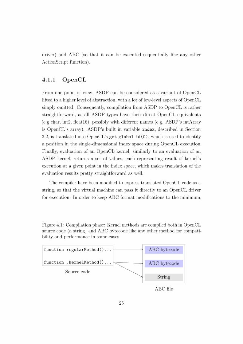
The compiler have been modified to express translated OpenCL code as a

string, so that the virtual machine can pass it directly to an OpenCL driver

for execution. In order to keep ABC format modifications to the minimum,

Figure 4.1: Compilation phase: Kernel methods are compiled both in OpenCLsource code (a string) and ABC bytecode like any other method for compati-bility and performance in some cases

function regularMethod()...

function .kernelMethod()...

Source code

ABC bytecode

ABC bytecode

String

ABC file

25

we embed the strings representing OpenCL kernels into the ABC’s constant

pool that is directly referred to from the modified ABC’s MethodBodyInfo

descriptor, and can be easily found during ABC parsing by the virtual machine.

4.1.2 ActionScript bytecode

From another point of view, ASDP is a language similar to “standard” Ac-

tionScript . Consequently, translation of ASDP kernels back to ActionScript

was not very complicated either. A kernel gets translated to a “standard”

ActionScript function, that gets executed by the virtual machine in a loop,

and takes the index variable as an explicit parameter. The ASDP array and

vector types (see Section 3.2.1) that do not exist in ActionScript get trans-

lated to ActionScript’s ByteArray and to appropriate ActionScript’s Vector

types, respectively, with all array and vector operations translated accordingly.

Unfortunately, at this point we cannot completely soundly translate all ASDP

primitive types to their ActionScript equivalents, as ActionScript support

for integer types is somewhat non-standard (e.g. a result of an operation

on two ints can overflow to a Number), but we have not experienced any

problems related to this fact when translating our sample applications. The

ActionScript function compiled from a given kernel retains the kernel’s type.

As a result, the final kernel evaluation result in this case must be assembled

by the virtual machine from individual function executions inside the loop.

4.2 Adaptivity

Our modified version of Tamarin, Adobe’s open source virtual machine, can

choose to execute a given kernel in three different modes: sequentially using

kernel’s code translated back to ActionScript (SEQUENTIAL), in parallel

using the OpenCL CPU driver (OpenCL-CPU) and in parallel using the

OpenCL GPU driver (OpenCL-GPU).

The first time a given kernel is invoked for a given index space size, no

information about its previous runs is available. Consequently, during the

26

first three executions, Tamarin schedules execution of the kernel in each of

the three different modes to gather initial profiling data.

Based on the data gathered during the first three runs, the optimal mode

(i.e. the one that executed the kernel the fastest) is chosen to evaluate the

kernel in the future, but all modes are periodically sampled to detect changes

in the execution environment. Our system takes into consideration that

effectiveness of non-optimal modes may be orders of magnitude worse than

that of the optimal mode, and chooses sample ratios for non-optimal units

such that the total overhead compared with the execution in the optimal

mode does not cross a certain threshold. There is a trade-off between the

threshold size and the time the scheduler needs to react to changes in the

execution environment – the smaller the threshold, the less frequently the

non-optimal modes are sampled, which makes the reaction time longer. We

currently use threshold equal to 10%. The process of re-evaluating the optimal

mode and re-calculating a sampling ratio is repeated after each sampling run

– the remaining runs are executed in optimal mode and do not require any

additional computations.

As the execution of a given kernel progresses, the scheduler no longer

has to rely on just the execution time from the previous run, but can utilize

historical data to compute an estimated time that would help reducing the

noise. Current estimated time data is stored per-kernel in a separate bucket

for each index space size range. Buckets are of non-uniform capacity with

the capacity growing exponentially with the index space size. The freshly

measured execution time information is combined with the current estimated

time, which an aggregate of all previous execution times (α = 0.5):

estimatedT ime = α ∗measuredT ime+ (1− α) ∗ estimatedT ime

Timing data is acquired using high resolution timers provided by the

processor. Since acquiring new timing data and combining it with the historic

one can be done inexpensively, measurements are done opportunistically after

each evaluation, not only after the sampling runs.

27

Buckets: 1-10 10-100 100-1000 1000-10000 10000-100000

Figure 4.2: Buckets that stores historical timing data are of exponentiallygrowing capacity to guarantee a low memory consumption even for largepossible index space ranges

Since timing data is acquired opportunistically at each execution and the

unit used most often is the best one, the algorithm shows an asymmetric

behavior when dealing with changes in the load of the currently best unit:

Increasing load Since the best unit is sampled most often the system is

able to react quickly to the increasing execution time and, whenever it

gets worse than the predicted time of another unit, the kernel will be

rescheduled

Decreasing load Since sampling runs happens every once in a while the

system has no chance to detect that another unit has got better right

away. Eventually, though, a sampling run will happen and the kernel

will be rescheduled

The scheduler computes the sampling ratios by calculating how many

executions in the optimal mode should happen before doing a profiling run in

any of the modes. This number of executions, incremented by one to account

for the sampling run itself, N is computed for a given execution mode after

its respective sampling run computes its current estimated time (and thus

current best time is known as well), using the following formula:

overhead← estimatedT ime− bestT ime

N ← max

(⌈overhead

bestT ime ∗ (10%/2)

⌉, 2

)

Intuitively, the larger the overhead in the fraction’s numerator, the larger

the number of iterations before a given mode will be sampled again. The

formula uses half of the specified overhead since there are two units, out of

the three supported (SEQUENTIAL, OpenCL-CPU, OpenCL-GPU), that

have a suboptimal execution time. Effectively an equal share of the overhead

28

is assigned to each unit. This approach can be used to scale the assignment

to an arbitrary number of modes. The max operator is used to make sure

at least a run is waited between each sampling run so that the algorithm

progresses. It is straightforward to prove that using this formula we can

indeed bound the total overhead over a certain number of executions to 10%.

The proof is extensively described in Section 4.3.

4.2.1 Initial sampling runs optimization

Since the kernel evaluation times in different modes can differ by orders of

magnitude, initial sampling performed during the first three kernel runs may

incur the amount of overhead that will not be amortized until thousands of

subsequent kernel evaluations are finished. Therefore, instead of sampling

the first three whole kernel evaluations, for kernels executing in sufficiently

large index space, we sample only a part of the whole kernel evaluation, that

occurs over a subset of the entire index space. We then extrapolate the

total evaluation time for each mode and use the resulting data to initialize

the scheduling algorithm. Clearly, additional modifications were required

to support partial kernel evaluations, but they were moderate – the main

concept is to pass an additional parameter to the kernel that specifies the

offset in the kernel’s index space.

4.3 Proof of predictably bounded overhead of

sampling in steady conditions

The formula used to compute how many executions in the optimal mode

should happen before doing a profiling run in any of the modes (see Section

4.2) is derived from the following equation:

(N−1)∗bestT ime+estimatedT ime < N ∗bestT ime+N ∗bestT ime∗(10%/2)

29

Intuitively, the time to execute N − 1 runs in optimal mode plus the time

to execute one run in the non-optimal mode should be smaller than N

executions in optimal mode plus certain overhead (in this case 10%). As

already mentioned in Section 4.2, the formula assign half of the specified

overhead to each of the non-optimal execution modes. This equation is

easily converted into the following form, which directly represents the formula

presented in Section 4.2 (the formula chooses smallest such N):

N >estimatedT ime− bestT ime

bestT ime ∗ (10%/2)

Let us have ti (for i = 1 : 3) represent current estimated execution times

for each execution mode. Let us assume, without loss of generality, that

min(t1, t2, t3) == t1 == bestT ime. Let us have Oi = (ti − bestT ime)

represent execution overhead for each execution mode (and let us assume

that overheads are non-zero). We can now express the number of executions

that should happen before doing a profiling run in mode i as follows:

Ni ← max(⌈

Oi

bound

⌉, 2), where bound← bestT ime ∗ (10%/2)

We will now show that the total overhead compared to the execution in

optimal mode, for a certain period P is indeed no larger than 10%.

Let us choose period P = N2 ∗ N3. The total execution time over this

period is equal to the time spent in sampling runs plus the time spent executing

the remaining runs in the optimal mode (the number of sampling runs for

a given mode is equal to the length of period P divided by the number of

optimal runs between each sampling run for a given mode):

totalT ime =P

N2

t2 +P

N3

t3 +(P − P

N2

− P

N3

)bestT ime

Let us have optimalT ime = (P ∗ bestT ime) represent the time to execute

P runs in the optimal mode. Then, the total overhead can be expressed as

30

follows:

totalOverhead =totalT ime− optimalT ime

optimalT ime=

PN2t2 + P

N3t3− P

N2bestT ime− P

N3bestT ime

P ∗ bestT ime=

PN2

(t2− bestT ime) + PN3

(t3− bestT ime)P ∗ bestT ime

=PN2O2 + P

N3O3

P ∗ bestT ime=

O2N2

+ O3N3

bestT ime=

O2

max(d O2bounde,2)

+ O3

max(d O3bounde,2)

bestT ime

If⌈

Oi

bound

⌉≥ 2 then

Oi

max(⌈

Oi

bound

⌉, 2)

=Oi⌈Oi

bound

⌉ ≤ Oi

Oi

bound

= bound

If⌈

Oi

bound

⌉< 2 then

Oi

max(⌈

Oi

bound

⌉, 2)

=Oi

2<

2 ∗ bound2

= bound

In both cases:

O2

max(d O2bounde,2)

+ O3

max(d O3bounde,2)

bestT ime≤ 2bound

bestT ime=

2 ∗ bestT ime ∗ 10%

2 ∗ bestT ime= 10%

31

Chapter 5

Performance evaluation

When evaluating our system we focus on two important performance char-

acteristics. The first one is the average performance of the adaptive scheme

with the runtime dynamically choosing the best execution scheme from the

available options. The second one is the behavior of our system under varying

machine load.

We evaluate our system using four different benchmarks:

1. CRYPT (cryptography) – a benchmark from Tamarin’s performance

suite [34] implementing the IDEA encryption algorithm

2. PARTICLES (physics) – a benchmark adapted from the “RGB Sinks

and Springs” [25] application implementing particle simulation

3. BLUR (image processing) – a benchmark adapted from the blur algo-

rithm implemented as part of the PIXASTIC image processing library

[29]

4. SERIES (scientific) – a benchmark from Tamarin’s performance suite

[34] computing a series of Fourier coefficients

For each benchmark, initially only sequential, a data parallel portion of the

code has been identified and translated into a definition and an invocation

32

CRYPT SERIES PARTICLES BLUR

0.00

0.10

0.20

0.30

0.40

Nor

mal

ized

tim

e

OpenCL-CPUOpenCL-DYNOpenCL-GPU

(a) SMALL

CRYPT SERIES PARTICLES BLUR

0.00

0.05

0.10

0.15

Nor

mal

ized

tim

e

OpenCL-CPUOpenCL-DYNOpenCL-GPU

(b) MEDIUM

CRYPT SERIES PARTICLES BLUR

0.00

0.02

0.04

0.06

0.08

0.10

0.12

Nor

mal

ized

tim

e

OpenCL-CPUOpenCL-DYNOpenCL-GPU

(c) LARGE

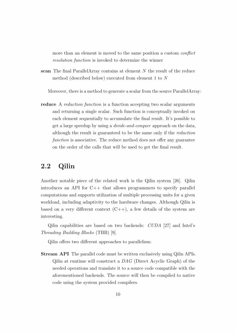
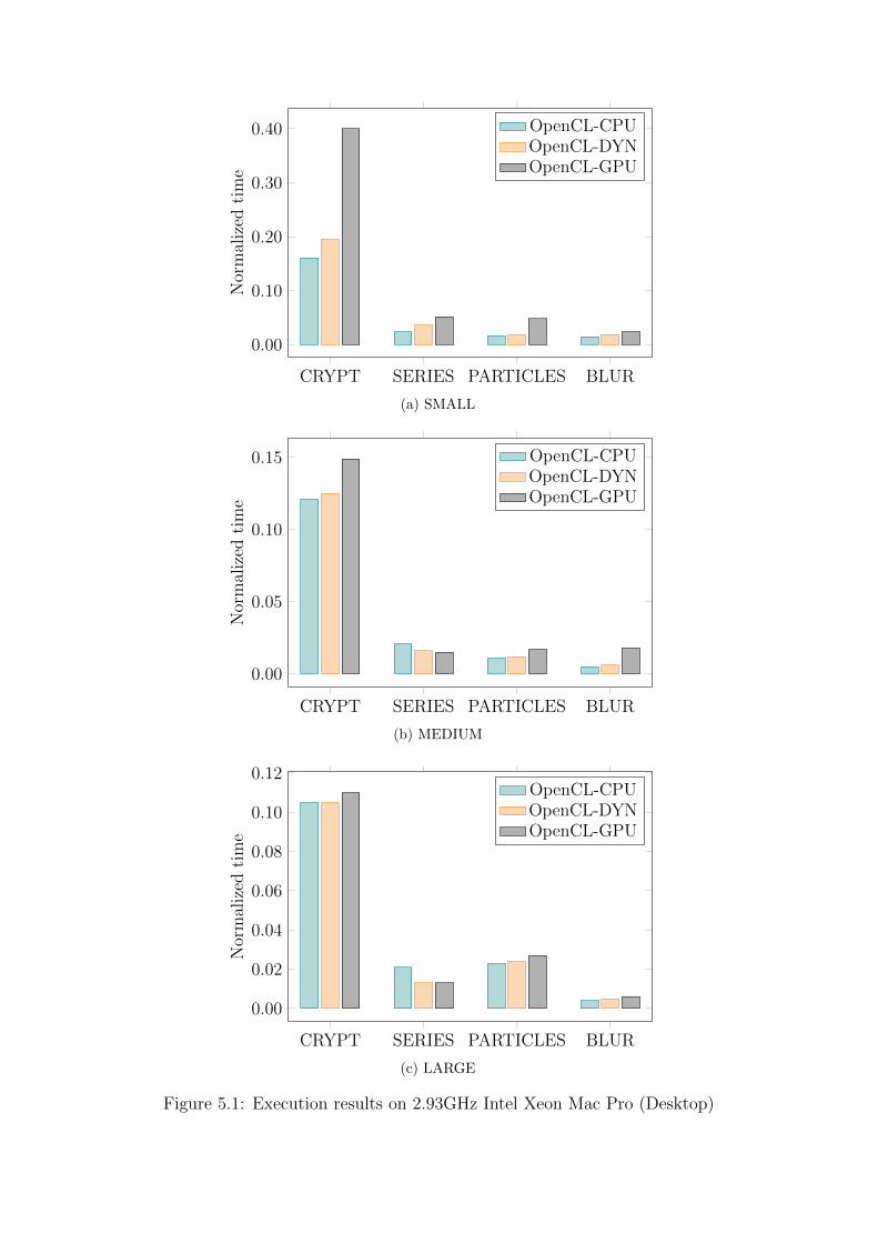
Figure 5.1: Execution results on 2.93GHz Intel Xeon Mac Pro (Desktop)

of an ASDP kernel. In some cases the translation process was extremely

straightforward, for example in the case of the SERIES benchmark described

in Section 3.3, in some others it was more elaborate but never very complicated.

For example, the original version of the “RGB Sinks and Springs” application

(and thus the sequential version of the PARTICLES benchmark), the input

data was encoded as ActionScript objects that are not supported in ASDP

– the data parallel version has been modified to encode the input data as

byte arrays. The two versions of each benchmark (original and data parallel)

enabled 5 different execution configurations:

1. ORG – sequential execution of the original benchmark

2. SEQ – sequential execution of the parallelized benchmark (as described

in Section 4, ASDP kernels are translated back to “pure” ActionScript

code)

3. O-CPU – parallel execution of the parallelized benchmark utilizing

OpenCL CPU driver only

4. O-GPU – parallel execution of the parallelized benchmark utilizing

OpenCL GPU driver only

5. DYN – parallel execution of the parallelized benchmark where the

runtime dynamically and automatically chooses the best execution

mode between SEQ, O-CPU and O-GPU

All benchmarks use only single-precision floating point data (all versions of

the benchmarks have been modified accordingly) as our Domain Specific

Language does not support double-precision at this point, mostly because

the support in OpenCL compilers and runtimes is still quite limited. Each

benchmark features only a single execution of a kernel during its timed run

so that during executions in the DYN configuration we can determine if the

kernel was executed sequentially or in OpenCL (GPU or CPU). This required

modifying the CRYPT and SERIES benchmarks to remove the second kernel

invocation (along with the respective portion of the computation in the

34

original sequential version of the benchmark), which does change the result

computed by the benchmarks, but does not lead to the loss of generality in

terms of performance results generated.

We use two different machines to evaluate our system, each with quite

dramatically different performance characteristics. The first one is a 2.93GHz

Intel Xeon Mac Pro (2 CPUs x 6 cores) desktop machine with a discrete AMD

Radeon HD 5770 GPU card, running Mac OS X 10.6.8 on 32GB of RAM.

The second one is a laptop featuring AMD Fusion E-450 APU consisting of

a single 1.54GHz CPU (two cores) and the AMD Radeon HD 6320 GPU

integrated on on the same die, running Windows 7 Home Premium on 4GB

of RAM.

We will now present evaluation of the dynamic execution mode (DYN)

by comparing its average performance across multiple execution for different

benchmarks and input sizes, and also by demonstrating how the dynamic

execution mode adapts to varying machine load.

5.1 Average Performance

In Figures 5.1a-5.2c we plot execution times (averaged over 100 iterations) for

the O-CPU, O-GPU and DYN configurations, normalized with respect to the

execution time of the ORG configuration. Figures 5.1a-5.1c plot execution

times on the desktop and Figures 5.2a-5.2c plot execution times on the laptop

for different sizes of the index space (and thus of the output): small, medium

and large – each larger by an order of magnitude from the preceding one.

We omit the execution times for the SEQ configurations as they were never

faster than either O-CPU, O-GPU or DYN configurations ,sometimes being

slower and sometimes faster than the ORG configurations, and thus do not

add much to the performance evaluation discussion.

The execution time for the SEQ configurations, omitted here 1 and execu-

1The SEQ configuration have been omitted to enable “zooming” into physically parallelconfigurations.

35

CRYPT SERIES PARTICLES BLUR

0.00

0.10

0.20

0.30

Nor

mal

ized

tim

e

OpenCL-CPUOpenCL-DYNOpenCL-GPU

(a) SMALL

CRYPT SERIES PARTICLES BLUR

0.00

0.10

0.20

0.30

Nor

mal

ized

tim

e

OpenCL-CPUOpenCL-DYNOpenCL-GPU

(b) MEDIUM

CRYPT SERIES PARTICLES BLUR

0.00

0.05

0.10

0.15

0.20

0.25

Nor

mal

ized

tim

e

OpenCL-CPUOpenCL-DYNOpenCL-GPU

(c) LARGE

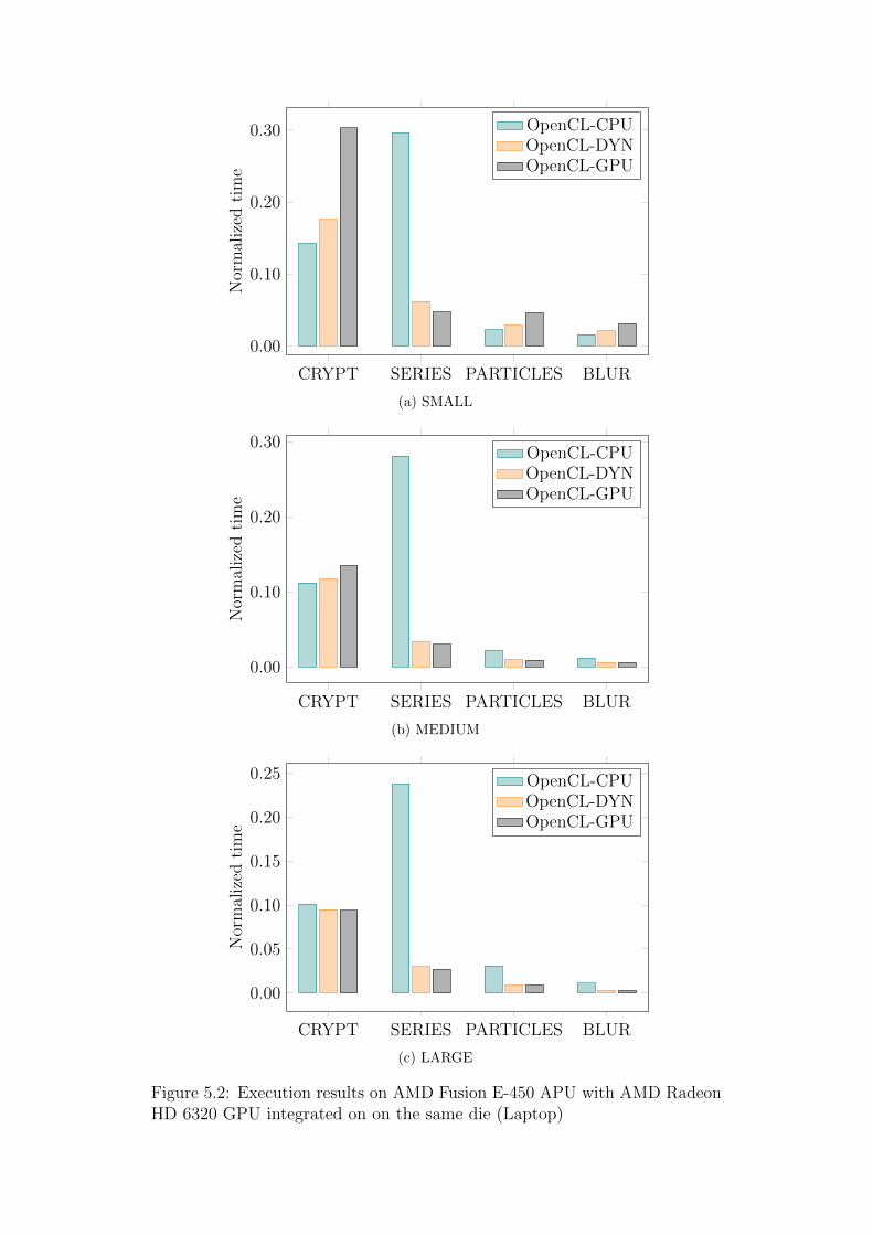
Figure 5.2: Execution results on AMD Fusion E-450 APU with AMD RadeonHD 6320 GPU integrated on on the same die (Laptop)

tion times for the ORG configurations are sometime very similar (SERIES

benchmark), higher (CRYPT and BLUR benchmarks) or lower (PARTICLES

benchmark), depending on the details of sequential-to-parallel translation

process, that may involve use of different data structures and thus yield

different performance characteristics. We leave the task of better matching

the execution times for these two configurations to future work, as it may

require exploring a possibility of modifying the ActionScript language (eg. by

introducing ActionScript Vector support for types such as byte or short so

that translations from/to a byte array can be avoided) or further extending

ASDP (eg. by introducing structs to at least partially emulate ActionScript

objects).

The first conclusion that can be drawn from analyzing Figures 5.1a-5.2c

is that all OpenCL configurations are much faster than the execution of the

original sequential benchmarks (ORG) they have been normalized against.

On the desktop they are at least 6x faster and on the laptop, they are at

least 3x faster. Other than introduction of parallelism, the main reason for

the performance difference is that ASDP is stripped down from virtually all

dynamic features of ActionScript , which results in much faster code. Similar

trend, to a varying degree, would be likely observable in case of other dynamic

languages embedding ASDP , such as JavaScript.

The second conclusion is that different OpenCL configurations fixed to the

same processing unit behave differently on different hardware configurations.

On the desktop, in most cases the O-CPU configuration is faster than the

O-GPU configuration, as the GPU card is a discrete component of the system

and the cost of moving data between the CPU and the GPU is significant.

The only exception from that rule is the SERIES benchmark, as the size of

its input data is very small, and the benefit of higher degree of parallelism

on a GPU outweighs the communication costs for larger sizes of the index

space. On the other hand, on the laptop, in many cases the same O-CPU

configuration is slower than the O-GPU configuration, as both the CPU

and the GPU are integrated on the same die which significantly reduces the

communication cost. The O-CPU configuration can still be faster than the

37

O-GPU configuration, even on the laptop, whenever the benefit of higher

degree of parallelism available on a GPU has a lower impact (ie. for smaller

index space sizes).

Finally, we can easily observe that in all cases the dynamic configuration

(DYN), that automatically chooses the best processing unit to execute a

given workload, closely trails the best configuration for a given machine,

benchmark, and the index space size. The reason why we not always meet the

10% overhead threshold is that the cost of the initial sampling run does not

always get amortized over the 100 kernel evaluations. Moreover, such upper

bound, is technically only guaranteed to hold over a sufficiently large number

of kernel evaluations, as described in section 4. As we only execute 100 kernel

evaluations here, the initial profiling run that samples O-CPU, O-GPU and

SEQ executions, despite being optimized, may increase the average overhead

for benchmarks where the difference between sequential (SEQ) and OpenCL

(O-CPU and O-GPU) executions is unusually high. The BLUR benchmark,

for example, exhibits this kind of behavior.

5.2 Adaptive Performance

Ideally, in addition to choosing the best processing unit for a given workload on

a given hardware platform in a “steady” state (where a given workload had a

chance to execute a least a few times to obtain the initial profiling information),

our system would also adapt to varying machine load by switching between

processing units depending on how heavily (or lightly) loaded they are at any

given point.

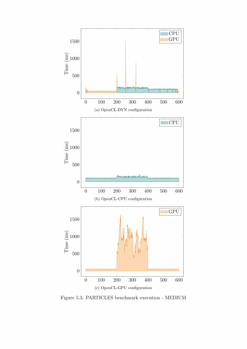
We use the PARTICLES benchmark executing on a laptop as our case

study to demonstrate that our system is indeed capable 2 of this kind of

behavior.

Clearly, the switch should only happen when it is actually beneficial to

2For some benchmarks is never convenient to switch execution unit, especially forthose executed on the desktop, but some others (eg. BLUR) exhibit very similar dynamicbehavior.

38

0 100 200 300 400 500 600

0

500

1000

1500

Tim

e(m

s)

CPUGPU

(a) OpenCL-DYN configuration

0 100 200 300 400 500 600

0

500

1000

1500

Tim

e(m

s)

CPU

(b) OpenCL-CPU configuration

0 100 200 300 400 500 600

0

500

1000

1500

Tim

e(m

s)

GPU

(c) OpenCL-GPU configuration

Figure 5.3: PARTICLES benchmark execution - MEDIUM

0 100 200 300 400 500 600

0

500

1000

1500

2000

Tim

e(m

s)

CPUGPU

(a) OpenCL-DYN configuration

0 100 200 300 400 500 600

0

500

1000

1500

2000

Tim

e(m

s)

CPU

(b) OpenCL-CPU configuration

0 100 200 300 400 500 600

0

500

1000

1500

2000

Tim

e(m

s)

GPU

(c) OpenCL-GPU configuration

Figure 5.4: PARTICLES benchmark execution - LARGE

move from executing on the current processing unit (that has been initially

chosen as optimal) to executing on a different processing unit. As a result,

the switch does not have to happen for each benchmark run. In particular, on

the desktop machine that generally favors executions on a CPU, we suspected

(and then confirmed experimentally) that it would be virtually impossible to

load all cores of the CPU to the extent where the execution on a GPU (which

is a discrete component) would yield a better result. On the other hand, on

the laptop that generally favors GPU executions and where the CPU and the

GPU are integrated on the same die, the adaptive algorithm should be able to

move executions from the GPU to CPU and back, especially for benchmarks

where the difference between CPU execution and GPU execution is moderate

(eg. PARTICLES or BLUR).

In our experimental setup the PARTICLES benchmark is executed for 600

iterations, with the GPU load changing from light to heavy and then back to

light. The GPU load is created by executing the GPU Tropics benchmark

[36] based on the Unigine 3D engine [35]. It is worth noting, that while

the Tropics demo mostly increases the load on the GPU, it also affects the

CPU execution by increasing its load by 10-15%. It is virtually impossible to

design a load that only affects the GPU, as the CPU is still responsible for

scheduling work and creating command buffers. Besides, it would also not be

a very realistic use-case scenario.

The execution time and the processing unit3 is recorded separately for

every iteration. After the first 200 iterations the execution of the Tropics

demo is triggered by the runtime, and after the following 200 iterations the

execution of the demo is terminated, both actions implemented utilizing

OS-level facilities available to the runtime. An additional amount of wait time

is given after the execution of the demo is triggered and after it is terminated,

to make sure that these actions have sufficient time to complete, but please

note that this wait time has no effect on the benchmark execution times as

these are measured individually.

3In the first iteration it is actually the fastest execution unit that is reported as thisprocessing unit is chosen to finalize execution of the first optimized profiling run, asdescribed in Section 4.2.1.

41

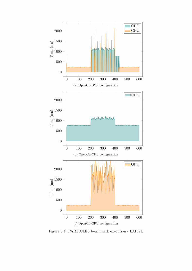
In Figures 5.3a and 5.4a we plot execution times for each of the 600

iterations (the number of iterations constitutes the “timeline” for the entire

execution) of the DYN configuration of the PARTICLES benchmark for the

MEDIUM and LARGE sizes of the index space. The blue portions of the

plot represent execution on a CPU and the red ones represent execution

on a GPU. We omit the plot for the SMALL size of the index space, as

the PARTICLES benchmark on the laptop executes faster on the CPU for

this index space size in the first place (see Figure 5.2a) and increasing the

GPU load has no chance of triggering any processing unit switch. As we

can observe in both cases, the execution moves from the GPU to the CPU

shortly after it is detected that the GPU is heavy loaded (ie. after the first

200 iterations). After the GPU load comes back to normal (ie. after the first

400 iterations), the execution eventually switches back to the GPU – faster

if the difference between CPU and GPU execution is larger (Figure 5.4a —

right before iteration 450) and slower if the difference is smaller (Figure 5.3a –

close to iteration 600). For comparison, we present equivalent graphs (under

the same load) for the O-CPU configuration in Figures 5.3b-5.4b and for the

O-GPU configuration in Figures 5.3c-5.4c.

The conclusion here is that our system is not only capable of adapting to

the varying machine load, but also that under a varying machine load the

adaptive DYN configuration is on average faster than both the O-CPU and

O-GPU configurations (respectively 102ms, 120ms, 337ms for the MEDIUM

index space size and 573ms, 873ms, 708ms for the LARGE index space

size).

42

Chapter 6

Conclusions & future work

We have presented an integrated system that makes it possible to seamlessly

integrate data parallel kernels in an application to take advantage of the

powerful computational capabilities of modern, heterogeneous platform that

are already and increasingly widespread even at the consumer level.

The system features a compile-time conversion of source code to OpenCL

code. This cross-platform intermediate representation is then compiled at

run-time for each OpenCL device available on the platform (most usually the

CPU and GPU) using the system provided libraries. A dynamic adaptive

scheduler is then able to efficiently select the best execution unit for a given

kernel using profiling. The scheduler is also able to update it’s choice when the

system load varies by sampling previously non optimal units. Such sampling

is scheduled while still guaranteeing no more than a specified overhead (10%

in our prototype) from always scheduling on the best unit.

The system has been prototyped in the context of the ActionScript pro-

gramming language and has been designed to be easy to use and robust,

coherently with the spirit of scripting languages for modern Web clients.

Although the system is feature complete and robust enough to require

a relatively small effort to be production ready, we believe there are a few

points where improvements are possible and desirable to improve performance

or flexibility of the system. Possible enhancements are:

43

Extend the supported language features As we said currently only a

subset of the ActionScript 3 language is supported, including most nu-

meric types, Vectors, Arrays and ByteArrays, function calls, conditional

and looping constructs. It would be greatly useful to add support for

ActionScript objects, at least for those simple enough to be implemented

efficiently using the struct OpenCL construct.

Asynchronous execution Since OpenCL code may run on a completely

independent device (like the GPU) it would be interesting to schedule

the execution of the kernel when the invocation happens, but delay the

reading back of the results until them are really accessed by the user

code (ie. a Promise like semantics). Such optimization would reduce

the amount of time spent blocked while the selected device compute

the results, at least in cases when the returned data is not immediately

used.

Kernel composition Currently there is no support for invoking an inner

kernel from another kernel. It would be trivial to support such inner

kernels by translating them to sequential execution using a for loop.

More interesting would be to try multiple parallelism strategies (eg.

parallelize over the outer kernel or over the inner kernel) and profile the

execution time of each strategy to choose the optimal one.

Kernel concatenation The current implementation does not attempt to

optimize data passing when the output of a kernel is immediately passed

to another one. Extending on the Promise solution mentioned before it

could be possible to keep data on the device memory and use it directly

from there when executing the second kernel. Such optimization would

completely skip two heavy weight data transfers in such scenario.

44

Bibliography

[1] 2DContext specification from w3c.

http://www.w3.org/TR/2dcontext/.

[2] ActionScript 3.0 specification by adobe.

http://livedocs.adobe.com/specs/actionscript/3/wwhelp/

wwhimpl/js/html/wwhelp.htm?href=as3_specification.html.

[3] Dart language specification by google.

http://www.dartlang.org/docs/spec/.

[4] DOM Level 3 specification from w3c.

http://www.w3.org/TR/2004/REC-DOM-Level-3-Core-20040407/.

[5] JavaScript article on wikipedia.

http://en.wikipedia.org/wiki/JavaScript.

[6] MMX article on wikipedia.

http://en.wikipedia.org/wiki/MMX_(instruction_set).

[7] NEON article on arm.com.

http://infocenter.arm.com/help/index.jsp?topic=/com.arm.

doc.ddi0409f/Chdceejc.html.

[8] OpenCL official site by khronos group.

http://www.khronos.org/opencl/.

[9] Threading Building Block home by intel.

http://threadingbuildingblocks.org/.

45

[10] WebGL specification by khronos group.

http://www.khronos.org/registry/webgl/specs/latest/.

[11] WebSockets specification from w3c.

http://www.w3.org/TR/websockets/.

[12] XMLHttpRequest specification from w3c.

http://www.w3.org/TR/XMLHttpRequest/.

[13] ZLib compression library.

http://www.zlib.net/.

[14] Adobe. The ActionScript byte code (abc) format.

http://learn.adobe.com/wiki/display/AVM2/4.+The+

ActionScript+Byte+Code+(abc)+format.

[15] Alecio P. D. Binotto, Carlos E. Pereira, Arjan Kuijper, Andre Stork, and

Dieter W. Fellner. An effective dynamic scheduling runtime and tuning

system for heterogeneous multi and many-core desktop platforms. In

HPCC, 2011.

[16] Bryan C. Catanzaro, Michael Garland, and Kurt Keutzer. Copperhead:

compiling an embedded data parallel language. In PPoPP, 2011.

[17] Manuel M. T. Chakravarty, Roman Leshchinskiy, Simon Peyton Jones,

Gabriele Keller, and Simon Marlow. Data parallel haskell: a status

report. In DAMP, 2007.

[18] Christophe Dubach, Perry Cheng, Rodric Rabbah, David F. Bacon, and

Stephen Fink. Compiling a high-level language for gpus (via language

support for architectures and compilers). In PLDI, 2012.

[19] E.M. Gordon. Cramming more components onto integrated circuits.

Electronics Magazine, 4, 1965.

[20] Khronos Group. OpenCL - the open standard for parallel programming

of heterogeneous systems, 2011.

http://www.khronos.org/opencl/.

46

[21] Web Hypertext Application Technology Working Group. Web workers

draft recommendation, 2011.

http://www.whatwg.org/specs/web-apps/current-work/complete/

workers.html.

[22] Stephan Herhut. Building a computing highway for web applications,

2011.

http://blogs.intel.com/research/2011/09/15/pjs/.

[23] IEEE. IEEE standard for floating-point arithmetic. IEEE Std 754-2008,

2008.

[24] Intel. River trail: Bringing parallelism to web applications on top of

intel opencl sdk, 2011.

http://software.intel.com/en-us/articles/

opencl-river-trail/.

[25] Barbara Kaskosz and Dan Gries. RGB sinks and springs.

http://www.flashandmath.com/advanced/rgbsinks/.

[26] Chi-Keung Luk, Sunpyo Hong, and Hyesoon Kim. Qilin: exploiting

parallelism on heterogeneous multiprocessors with adaptive mapping. In

MICRO, 2009.

[27] NVIDIA. CUDA – parallel programming made easy, 2012.

http://www.nvidia.com/object/cuda\_home\_new.html.

[28] Michael Schmalle. Apacheflex :: Falcon compiler update, 2012.

http://blog.teotigraphix.com/2012/01/19/

apacheflex-falcon-compiler-update/.

[29] Jacob Seidelin. PIXASTIC – JavaScript image processing library.

http://www.pixastic.com/.

[30] N. Shavit and D. Touitou. Software transactional memory. In Proceedings

of the fourteenth annual ACM symposium on Principles of distributed

computing, pages 204–213. ACM, 1995.

47

[31] Satnam Singh. Declarative data-parallel programming with the accelera-

tor system. In DAMP, 2010.

[32] H. Sutter. The free lunch is over: A fundamental turn toward concurrency

in software. Dr. Dobb’s Journal, 30(3):202–210, 2005.

[33] Tamarin Team. Tamarin virtual machine, 2011.

http://hg.mozilla.org/tamarin-redux.

[34] Tamarin VM team. jsbench.

http://hg.mozilla.org/tamarin-redux/file/9e56a8e5b17c/test/

performance/jsbench.

[35] Unigine. Unigine – engine of virtual worlds.

http://unigine.com/.

[36] Unigine. Tropics benchmark 1.3, 2010.

http://unigine.com/products/tropics/.

48