
UNIVERSITA' DEGLI STUDI DI PADOVA - Benvenuti su Padua...
182
UNIVERSITA' DEGLI STUDI DI PADOVA Sede Amministrativa: Università degli Studi di Padova Dipartimento di Innovazione Meccanica e Gestionale SCUOLA DI DOTTORATO DI RICERCA IN INGEGNERIA INDUSTRIALE INDIRIZZO: INGEGNERIA DELLA PRODUZIONE INDUSTRIALE CICLO XX INVESTIGATION OF THERMAL, MECHANICAL AND MICROSTRUCTURAL PROPERTIES OF QUENCHENABLE HIGH STRENGTH STEELS IN HOT STAMPING OPERATIONS Direttore della Scuola : Ch.mo Prof. Paolo F. Bariani Supervisore : Ch.mo Prof. Paolo F. Bariani Correlatore : Prof. Stefania Bruschi Dottorando : Alberto Turetta DATA CONSEGNA TESI 31 gennaio 2008
Transcript of UNIVERSITA' DEGLI STUDI DI PADOVA - Benvenuti su Padua...
UNIVERSITA' DEGLI STUDI DI PADOVA
Sede Amministrativa: Università degli Studi di Padova
Dipartimento di Innovazione Meccanica e Gestionale
SCUOLA DI DOTTORATO DI RICERCA IN INGEGNERIA INDUSTRIALE
INDIRIZZO: INGEGNERIA DELLA PRODUZIONE INDUSTRIALE
CICLO XX
INVESTIGATION OF THERMAL, MECHANICAL AND MICROSTRUCTURAL
PROPERTIES OF QUENCHENABLE HIGH STRENGTH STEELS
IN HOT STAMPING OPERATIONS
Direttore della Scuola : Ch.mo Prof. Paolo F. Bariani
Supervisore : Ch.mo Prof. Paolo F. Bariani
Correlatore : Prof. Stefania Bruschi
Dottorando : Alberto Turetta
DATA CONSEGNA TESI 31 gennaio 2008

I
TABLE OF CONTENTS
TABLE OF CONTENTS .......................................................................................... I
PREFACE ..............................................................................................................V
ABSTRACT..........................................................................................................VII
SOMMARIO ..........................................................................................................IX
1 CHAPTER 1 .................................................................................................... 1
INTRODUCTION .................................................................................................... 1
1.1 The industrial problem .............................................................................. 3
1.2 Objective and organization of work ......................................................... 6
2 CHAPTER 2 .................................................................................................... 7
LITERATURE REVIEW.......................................................................................... 7
2.1 Hot stamping process description and technology................................ 9 2.1.1 Base material properties and process design ..................................... 11
2.2 Modelling and simulation of hot stamping ............................................ 14 2.2.1 Thermo-mechanical properties ........................................................... 17 2.2.2 Phase transformation kinetics............................................................. 18
2.2.2.1 Phase transformation modelling .................................................. 19 2.2.2.2 Transformation plasticity.............................................................. 21
2.2.3 Heat transfer ....................................................................................... 23 2.2.3.1 Heat transfer coefficient determination ........................................ 25
2.3 Inverse analysis theoretical bases ......................................................... 28
2.4 Formability................................................................................................ 31

II
3 CHAPTER 3...................................................................................................39
THERMO-MECHANICAL PROPERTIES .............................................................39
3.1 Microstructural process window.............................................................41
3.2 Flow curves in temperature .....................................................................45 3.2.1 Experimental apparatus.......................................................................45
3.2.1.1 Tensile test optimization...............................................................48 3.2.2 Experiments and results ......................................................................50
3.3 Plastic anisotropy evolution....................................................................53 3.3.1 Analysis procedure..............................................................................53 3.3.2 Results and discussion........................................................................55
3.4 Elastic properties .....................................................................................58 3.4.1 Testing procedure ...............................................................................58 3.4.2 Results ................................................................................................59
3.5 Conclusions..............................................................................................62
4 CHAPTER 4...................................................................................................63
PHASE TRANSFORMATION KINETICS .............................................................63
4.1 Transformation plasticity.........................................................................65 4.1.1 Testing procedure ...............................................................................65 4.1.2 Ferrite + pearlite ..................................................................................68
4.1.2.1 Determination of transformation plasticity ....................................69 4.1.3 Bainite .................................................................................................73
4.1.3.1 Determination of transformation plasticity ....................................74 4.1.4 Martensite............................................................................................78
4.1.4.1 Determination of transformation plasticity ....................................79
4.2 Shift of TTT curves due to applied stress ..............................................82 4.2.1 Preliminary results...............................................................................83 4.2.2 Ferritic transformation..........................................................................87 4.2.3 Bainitic transformation.........................................................................88
4.3 Conclusions..............................................................................................92
5 CHAPTER 5...................................................................................................95
MATERIAL FORMABILITY ..................................................................................95
5.1 Experimental apparatus...........................................................................97 5.1.1 Lighting system optimization .............................................................100
III
5.1.2 Punch and die equipment heating system ........................................ 101 5.1.3 Induction heating optimization .......................................................... 102
5.2 Physical simulation experiments ......................................................... 104
5.3 Forming limit curves determination ..................................................... 108 5.3.1 Forming limit curves at elevated temperature ................................... 108 5.3.2 Design of the thermal cycle............................................................... 109
5.3.2.1 Natural air cooling...................................................................... 109 5.3.2.2 Forced air cooling ...................................................................... 111
5.3.3 Results and discussions ................................................................... 114
5.4 Conclusions ........................................................................................... 117
6 CHAPTER 6 ................................................................................................ 119
NUMERICAL MODEL CALIBRATION............................................................... 119
6.1 Numerical model .................................................................................... 121 6.1.1 The FEM code .................................................................................. 121 6.1.2 Rheology........................................................................................... 122 6.1.3 Microstructural behaviour.................................................................. 123 6.1.4 Thermal computation ........................................................................ 123 6.1.5 Modelling of friction........................................................................... 125 6.1.6 Thermo-mechanical-metallurgical coupling....................................... 126
6.2 Calibration of the numerical model ...................................................... 128 6.2.1 Rheological behaviour characterisation ............................................ 129 6.2.2 Microstructural behaviour characterization ....................................... 130 6.2.3 Heat transfer coefficient determination ............................................. 130
6.2.3.1 Experimental apparatus............................................................. 130 6.2.3.2 Experimental results .................................................................. 132 6.2.3.3 Inverse analysis application....................................................... 132 6.2.3.4 Numerical model of the case study............................................ 133 6.2.3.5 Results....................................................................................... 137
6.3 Numerical model validation .................................................................. 139 6.3.1 Physical simulation of the deformation phase................................... 139 6.3.2 Numerical simulation of the deformation phase ................................ 140 6.3.3 Results and discussions ................................................................... 142
7 CHAPTER 7 ................................................................................................ 147
CONCLUSIONS ................................................................................................. 147
IV
APPENDIX A ......................................................................................................151
Ferritic/pearlitic transformation plasticity test curves...................................151
Bainitic transformation plasticity test curves.................................................153
Martensitic transformation plasticity test curves...........................................155
APPENDIX B ......................................................................................................159
Experimental and numerical temperature profiles .........................................159
REFERENCES....................................................................................................163

V
PREFACE
First of all, I would like to thank Prof. Paolo F. Bariani that gave me the possibility to
perform my PhD at DIMEG, and Stefania and Andrea for their valuable advices,
suggestions and teachings.
I also acknowledge Mrs Merklein for having organized my stay at the LFT, University of
Erlangen-Nuremberg, and Jurgen for his wholehearted hospitality and friendship that
transformed this period into a really nice experience.
I express my grateful thanks to all my colleagues, for the friendly and bright atmosphere
that was always present at DIMEG, and to the students that worked with me.
A big thank you to my wonderful family and, last but not least, to my Ultra High Strength
Girlfriend Elena for her loving support.

VI

VII
ABSTRACT
Sheet metal working operations at elevated temperature have gained in the last years
even more importance due to the possibility of producing parts characterized by high
strength-to-mass ratio. In particular, the hot stamping of ultra high strength quenchenable
steels is nowadays widely used in the automotive industry to produce body-in-white
structural components with enhanced crash resistance and geometrical accuracy. The
optimization of the process, where deformation takes place simultaneously with cooling,
and of the final component performances requires the utilization of FE-based codes where
the forming and quenching phases have to be represented by fully thermo-mechanical-
metallurgical models. The accurate calibration of such models, in terms of material
behaviour, tribology, heat transfer, phase transformation kinetics and formability, is
therefore a strong requirement to gain reliable results from the numerical simulations and
offer noticeable time and cost savings to product and process engineers.
The main target of this PhD thesis is the development of an innovative approach based on
the design of integrated experimental procedures and modelling tools in order to
accurately investigate and describe both the mechanical and microstructural material
properties and the interface phenomena due to the thermal and mechanical events that
occur during the industrial press hardening process.
To this aim, a new testing apparatus was developed to evaluate the influence of
temperature and strain rate on the sheet metal elasto-plastic properties and to study the
influence of applied stress and strain of the material phase transformation kinetics.
Furthermore, an innovative experimental setup, based on the Nakazima concept, was
designed and developed to evaluate sheet formability at elevated temperature by
controlling the thermo-mechanical parameters of the test and reproducing the conditions
that govern the microstructural evolution during press hardening. This equipment was
utilized both to determine isothermal forming limit curves at high temperature and to
perform a physical simulation of hot forming operations. Finally, a thermo-mechanical-
metallurgical model was implemented in a commercial FE-code and accurately calibrated
to perform fully coupled numerical simulations of the reference process.

VIII
The material investigated in this work is the Al-Si pre-coated quenchenable steel 22MnB5,
well known with the commercial name of USIBOR 1500P®, and the developed approach
proves to be suitable to proper evaluate high strength steels behaviour in terms of
mechanical, thermal and microstructural properties, and to precisely calibrate coupled
numerical models when they are applied to this innovative manufacturing technology.
The work presented in this thesis has been carried out at DIMEG labs, University of
Padova, Italy, from January 2005 to December 2007 under the supervision of Prof. Paolo
F. Bariani.
IX
SOMMARIO
Negli ultimi anni le lavorazioni di lamiera ad elevate temperature hanno acquisito sempre
più importanza grazie alla possibilità di produrre componenti caratterizzati da un elevato
rapporto resistenza-peso. In particolare lo stampaggio a caldo di acciai alto resistenziali
da tempra è oggigiorno ampiamente utilizzato nell’industria automobilistica per realizzare
parti strutturali con più elevate resistenza agli urti e accuratezza geometrica.
L’ottimizzazione delle prestazioni del processo, in cui le fasi di deformazione e tempra
avvengono in contemporanea, e del prodotto finale richiede l’utilizzo di codici agli elementi
finiti in cui le fasi di formatura e raffreddamento siano implementate in modelli termici,
meccanici e metallurgici accoppiati. L’accurata calibrazione di tali modelli, in termini di
comportamento reologico, tribologia, scambio termico, cinetica di trasformazione di fase e
formabilità, rappresenta un requisito fondamentale per ottenere risultati affidabili dalle
simulazioni numeriche e consentire agli ingegneri di processo e di prodotto di ottenere un
sensibile risparmio di costi e tempi.
L’obiettivo principale di questa tesi di dottorato è lo sviluppo di un approccio innovativo
basato sulla definizione di prove sperimentali e di modelli per l’analisi e la descrizione del
comportamento meccanico e microstrutturale del materiale e dei fenomeni all’interfaccia
che si presentano nelle condizioni meccaniche e termiche tipiche delle operazioni
industriali di stampaggio a caldo.
Con questo obiettivo finale, è stata sviluppata una nuova attrezzatura di prova per
valutare l’influenza di temperatura e velocità di deformazione sulle proprietà elasto-
plastiche di lamiere metalliche e per studiare l’influenza di carichi e deformazioni applicati
sulla cinetica di trasformazione di fase del materiale. Inoltre è stata progettata e messa a
punto una nuova apparecchiatura sperimentale per valutare la formabilità di lamiere ad
elevate temperature assicurando un controllo accurato dei parametri di prova termici e
meccanici e riproducendo le condizioni che governano le trasformazioni microstrutturali
durante le lavorazioni a caldo. Questa attrezzatura è stata utilizzata per determinare curve
limite di formabilità isoterme ad elevata temperatura e, al tempo stesso, per effettuare una
X
simulazione fisica delle operazioni di formatura a caldo. Un modello accoppiato dal punto
di vista termico, meccanico e metallurgico è stato accuratamente calibrato e implementato
in un codice FE commerciale per effettuare simulazione del processo di riferimento.
Il materiale indagato in questo lavoro è l’acciaio da tempra 22MnB5, commercialmente
noto col nome di USIBOR 1500 P®, e l’approccio sviluppato dimostra di essere adatto a
studiare il comportamento di acciai alto resistenziali ad elevate temperature in termini di
proprietà meccaniche, termiche e microstrutturali per poter calibrare modelli numerici
accoppiati utilizzati nell’ottimizzazione di questa innovativa tecnologia di produzione.
Il lavoro presentato in questa tesi è stato svolto presso i laboratori del DIMEG, Università
degli Studi di Padova, da Gennaio 2005 a Dicembre 2007, sotto la supervisione del Prof.
Paolo F. Bariani.

Chapter 1
1
1 CHAPTER 1 INTRODUCTION

Introduction
2

Chapter 1
3
In the last years the main targets of the automotive industries are represented by the
reduction of fuel consumption and environmental impact, the increase of crash
performance and safety and the increase of accuracy and quality of final components.
These requirements force car manufacturers to a continuous search of new solutions, in
direction of new products features and novel manufacturing processes. Different types of
materials, both metallic and non-metallic, are used. Regarding metallic materials,
aluminium alloys and different steels grades are the most common in body components
and reinforcements beams and the introduction of ultra high strength quenchenable steels
represents an innovative solution to increase the strength-to-mass ratio of sheet
components. However, as the forming of such steels at room temperature is almost
impossible, the utilization of sheet working operations at elevated temperature is
increasing more and more. In the hot stamping or press hardening process the steel blank
is heated up above austenitization, then transferred into the press where deformation
takes place simultaneously with quenching in order to achieve a fully martensitic
microstructure in the formed component at room temperature. Compared with traditional
sheet metal forming operation, the proper design of hot stamping process chains requires
a deep knowledge of both interface phenomena and material behaviour at high
temperature. In particular, the choice of the most suitable process parameters of the
forming and the cooling phases requires the utilization of FE-based codes where the
process has to be represented by a fully thermo-mechanical-metallurgical model. Such a
model has to be accurately calibrated and validated, by means of experimental techniques
and numerical inverse analysis approaches, in order to obtain reliable results from the
numerical simulations and achieve the desired mechanical and microstructural properties
on final product.
1.1 The industrial problem Sheet metal working operations at elevated temperatures have gained in the last few
years even more importance due to the possibility of producing components characterized
by high strength-to-mass ratio. Besides the worm forming of aluminium alloys, whose
main target is to increase the material formability limits, the hot stamping of ultra high
strength quenchenable steels is nowadays widely utilized in the automotive industry to
produce components like bumpers and pillar with enhanced crash characteristic and
geometrical accuracy due to reduced springback [1].
Introduction
4
Weight and cost reduction in body-in-white components is mainly driven by the use of
advanced sheet material in combination with optimized production technologies adapted
to the particular material concept [2]. Matching exact mechanical properties of the
intended steel grade against the critical forming mode in the stamping not only requires an
added level of knowledge by steel suppliers and steel users, but also mandates an
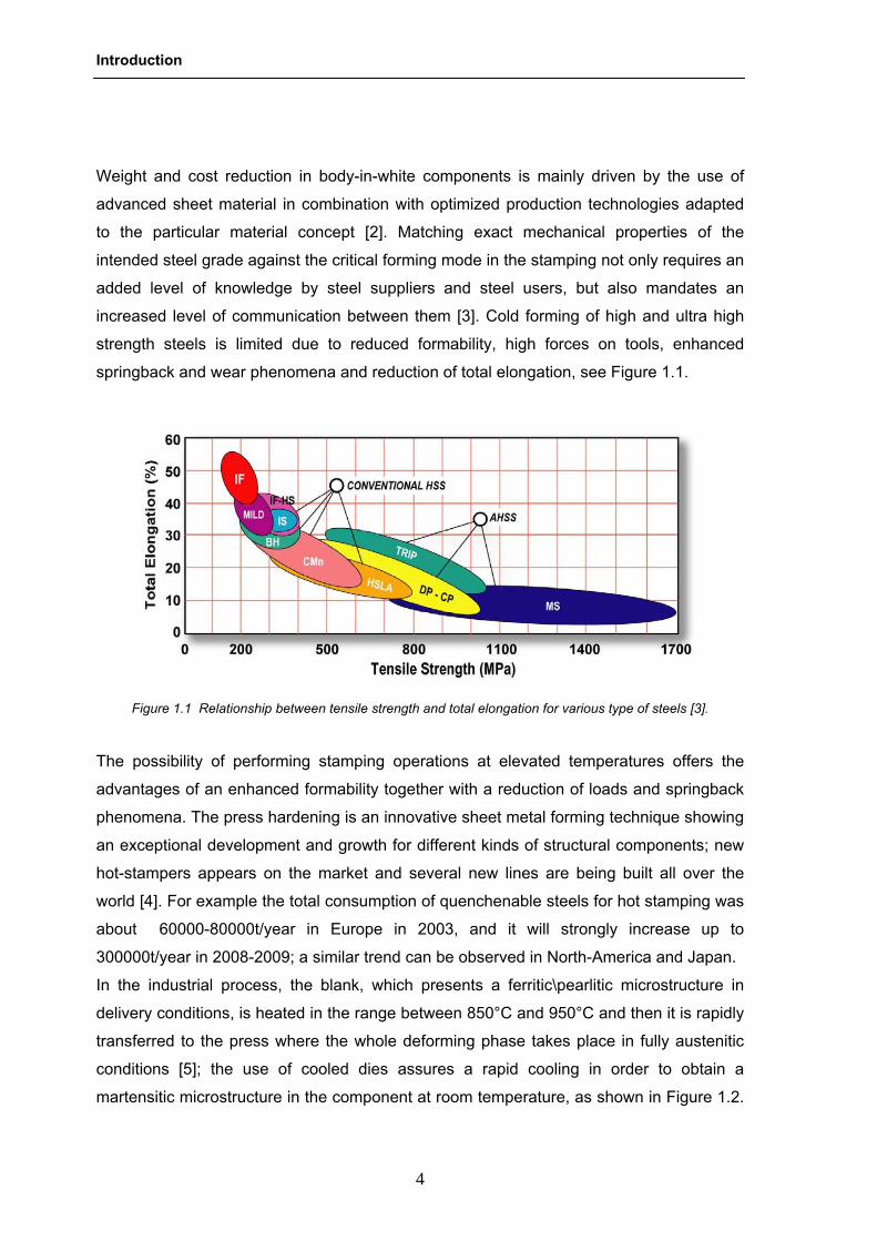
increased level of communication between them [3]. Cold forming of high and ultra high
strength steels is limited due to reduced formability, high forces on tools, enhanced
springback and wear phenomena and reduction of total elongation, see Figure 1.1.
Figure 1.1 Relationship between tensile strength and total elongation for various type of steels [3].
The possibility of performing stamping operations at elevated temperatures offers the
advantages of an enhanced formability together with a reduction of loads and springback
phenomena. The press hardening is an innovative sheet metal forming technique showing
an exceptional development and growth for different kinds of structural components; new
hot-stampers appears on the market and several new lines are being built all over the
world [4]. For example the total consumption of quenchenable steels for hot stamping was
about 60000-80000t/year in Europe in 2003, and it will strongly increase up to
300000t/year in 2008-2009; a similar trend can be observed in North-America and Japan.
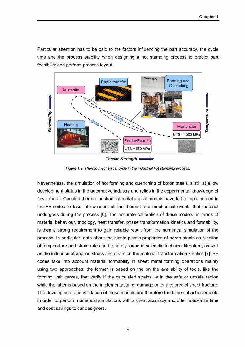
In the industrial process, the blank, which presents a ferritic\pearlitic microstructure in
delivery conditions, is heated in the range between 850°C and 950°C and then it is rapidly
transferred to the press where the whole deforming phase takes place in fully austenitic
conditions [5]; the use of cooled dies assures a rapid cooling in order to obtain a
martensitic microstructure in the component at room temperature, as shown in Figure 1.2.
Chapter 1
5
Particular attention has to be paid to the factors influencing the part accuracy, the cycle
time and the process stability when designing a hot stamping process to predict part
feasibility and perform process layout.
Figure 1.2 Thermo-mechanical cycle in the industrial hot stamping process.
Nevertheless, the simulation of hot forming and quenching of boron steels is still at a low
development status in the automotive industry and relies in the experimental knowledge of
few experts. Coupled thermo-mechanical-metallurgical models have to be implemented in
the FE-codes to take into account all the thermal and mechanical events that material
undergoes during the process [6]. The accurate calibration of these models, in terms of
material behaviour, tribology, heat transfer, phase transformation kinetics and formability,
is then a strong requirement to gain reliable result from the numerical simulation of the
process. In particular, data about the elasto-plastic properties of boron steels as function
of temperature and strain rate can be hardly found in scientific-technical literature, as well
as the influence of applied stress and strain on the material transformation kinetics [7]. FE
codes take into account material formability in sheet metal forming operations mainly
using two approaches: the former is based on the on the availability of tools, like the
forming limit curves, that verify if the calculated strains lie in the safe or unsafe region
while the latter is based on the implementation of damage criteria to predict sheet fracture.
The development and validation of these models are therefore fundamental achievements
in order to perform numerical simulations with a great accuracy and offer noticeable time
and cost savings to car designers.
Introduction
6
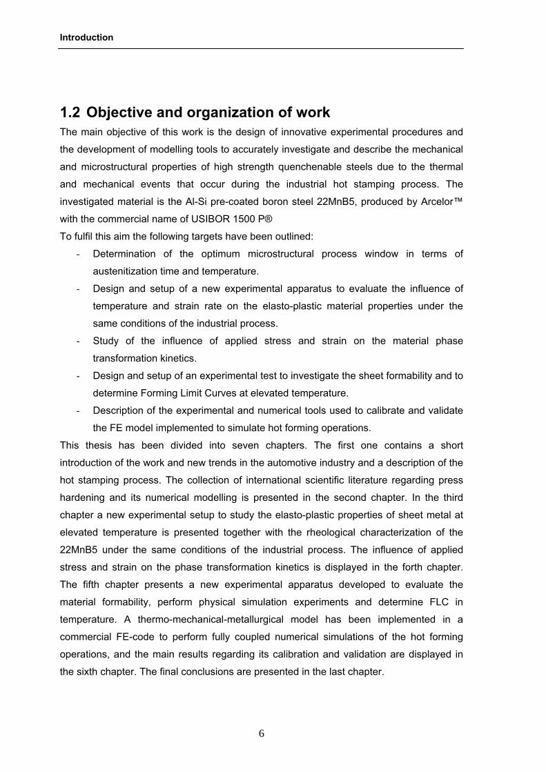
1.2 Objective and organization of work The main objective of this work is the design of innovative experimental procedures and
the development of modelling tools to accurately investigate and describe the mechanical
and microstructural properties of high strength quenchenable steels due to the thermal
and mechanical events that occur during the industrial hot stamping process. The
investigated material is the Al-Si pre-coated boron steel 22MnB5, produced by Arcelor™
with the commercial name of USIBOR 1500 P®
To fulfil this aim the following targets have been outlined:
- Determination of the optimum microstructural process window in terms of
austenitization time and temperature.
- Design and setup of a new experimental apparatus to evaluate the influence of
temperature and strain rate on the elasto-plastic material properties under the
same conditions of the industrial process.
- Study of the influence of applied stress and strain on the material phase
transformation kinetics.
- Design and setup of an experimental test to investigate the sheet formability and to
determine Forming Limit Curves at elevated temperature.
- Description of the experimental and numerical tools used to calibrate and validate
the FE model implemented to simulate hot forming operations.
This thesis has been divided into seven chapters. The first one contains a short
introduction of the work and new trends in the automotive industry and a description of the
hot stamping process. The collection of international scientific literature regarding press
hardening and its numerical modelling is presented in the second chapter. In the third
chapter a new experimental setup to study the elasto-plastic properties of sheet metal at
elevated temperature is presented together with the rheological characterization of the
22MnB5 under the same conditions of the industrial process. The influence of applied
stress and strain on the phase transformation kinetics is displayed in the forth chapter.
The fifth chapter presents a new experimental apparatus developed to evaluate the
material formability, perform physical simulation experiments and determine FLC in
temperature. A thermo-mechanical-metallurgical model has been implemented in a
commercial FE-code to perform fully coupled numerical simulations of the hot forming
operations, and the main results regarding its calibration and validation are displayed in
the sixth chapter. The final conclusions are presented in the last chapter.

Chapter 2
7
2 CHAPTER 2 LITERATURE REVIEW

Literature review
8

Chapter 2
9
In the Introduction, it has been pointed out that the manufacturing technology based on
sheet metal forming at elevated temperature proves today to have great potentiality of
competitiveness in the automotive industry. The improvement of the quality and reliability
of numerical simulations is the main prerequisite to optimize the hot stamping operations
and obtain the desired mechanical and microstructural properties on final components.
When addressing to the hot stamping process, the FE simulations face many challenges
such as the temperature and strain rate dependent material behaviour, the heat transfer at
the workpiece-die interface and the coupled thermo-mechanical-metallurgical calculations.
For an accurate description of these phenomena, it is therefore necessary to correctly
understand and model all the aspects involved in hot forming operations, in order to
determine experimentally material characteristics and thermal parameters and to model
through an accurate mathematical transcription the coupling between the thermal,
mechanical and metallurgical issues.
The literature review has thus been focused on the description of the hot stamping
process in § 2.1 and on the state-of-the-art regarding the modelling and simulation of the
hot forming operations in § 2.2. The inverse analysis theoretical principles used in this
work for the heat transfer coefficient determination have been summarized in § 2.3. Finally
the sheet metal formability evaluation at elevated temperature has been studied in § 2.4.
2.1 Hot stamping process description and technology Nowadays, the demand of coupling performances with cost reduction and the respect of
environment have represented the most challenging targets for the automotive industry,
such as the increase of crash resistance and safety, the reduction of fuel consumption
and emissions and the increase of accuracy and quality for easier, cheaper and more
reliable joining and assembly of final components. These requirements force the car
manufactures to a continuous research of new solutions, in direction of new product
features and new manufacturing processes, leading the most significant evolution and
innovation in sheet metal forming technologies [2, 8]. With regards to these aspects, the
introduction of quenchenable high strength steels represents the solution to enhance the
strength-to-mass ratio of body-in-white components, thus reducing the thickness of
stamped parts, maintaining safety requirements and mechanical strength as well.
Literature review
10
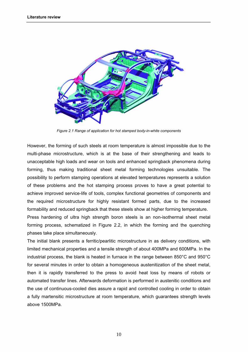
However, the forming of such steels at room temperature is almost impossible due to the
multi-phase microstructure, which is at the base of their strengthening and leads to
unacceptable high loads and wear on tools and enhanced springback phenomena during
forming, thus making traditional sheet metal forming technologies unsuitable. The
possibility to perform stamping operations at elevated temperatures represents a solution
of these problems and the hot stamping process proves to have a great potential to
achieve improved service-life of tools, complex functional geometries of components and
the required microstructure for highly resistant formed parts, due to the increased
formability and reduced springback that these steels show at higher forming temperature.
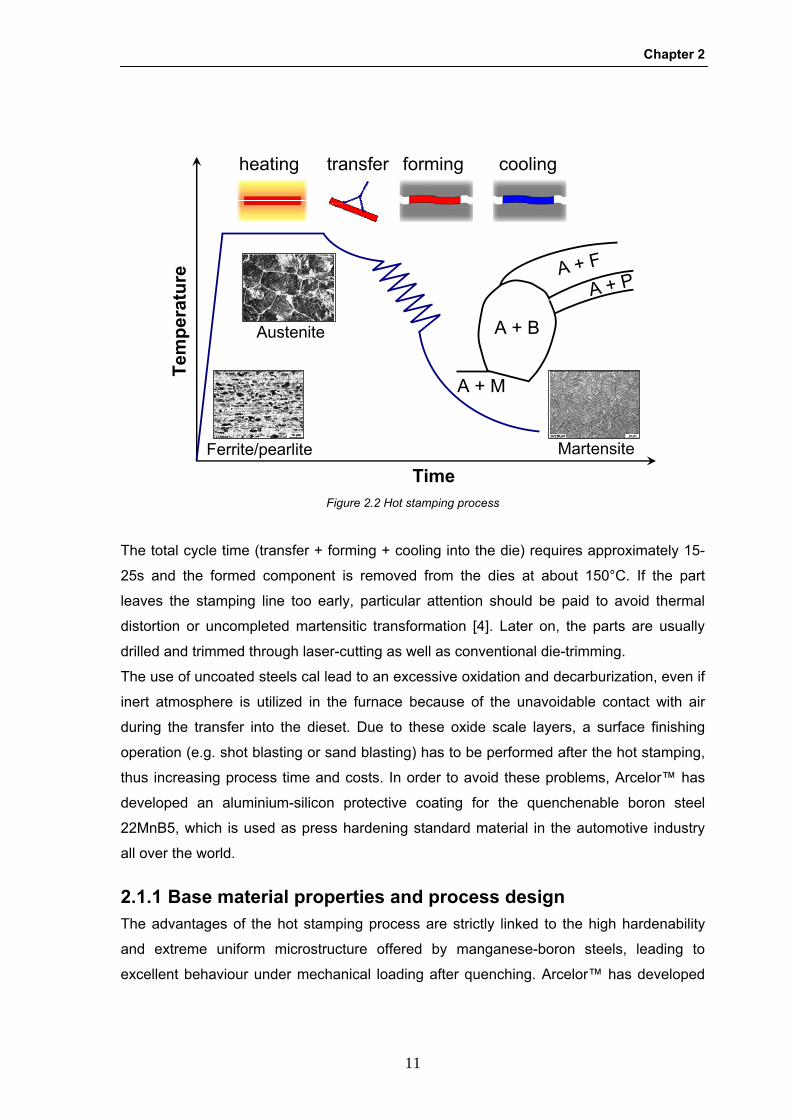
Press hardening of ultra high strength boron steels is an non-isothermal sheet metal
forming process, schematized in Figure 2.2, in which the forming and the quenching
phases take place simultaneously.
The initial blank presents a ferritic/pearlitic microstructure in as delivery conditions, with
limited mechanical properties and a tensile strength of about 400MPa and 600MPa. In the
industrial process, the blank is heated in furnace in the range between 850°C and 950°C
for several minutes in order to obtain a homogeneous austenitization of the sheet metal,
then it is rapidly transferred to the press to avoid heat loss by means of robots or
automated transfer lines. Afterwards deformation is performed in austenitic conditions and
the use of continuous-cooled dies assure a rapid and controlled cooling in order to obtain
a fully martensitic microstructure at room temperature, which guarantees strength levels
above 1500MPa.
Figure 2.1 Range of application for hot stamped body-in-white components
Chapter 2
11
The total cycle time (transfer + forming + cooling into the die) requires approximately 15-
25s and the formed component is removed from the dies at about 150°C. If the part
leaves the stamping line too early, particular attention should be paid to avoid thermal
distortion or uncompleted martensitic transformation [4]. Later on, the parts are usually
drilled and trimmed through laser-cutting as well as conventional die-trimming.
The use of uncoated steels cal lead to an excessive oxidation and decarburization, even if
inert atmosphere is utilized in the furnace because of the unavoidable contact with air
during the transfer into the dieset. Due to these oxide scale layers, a surface finishing
operation (e.g. shot blasting or sand blasting) has to be performed after the hot stamping,
thus increasing process time and costs. In order to avoid these problems, Arcelor™ has
developed an aluminium-silicon protective coating for the quenchenable boron steel
22MnB5, which is used as press hardening standard material in the automotive industry
all over the world.
2.1.1 Base material properties and process design The advantages of the hot stamping process are strictly linked to the high hardenability
and extreme uniform microstructure offered by manganese-boron steels, leading to
excellent behaviour under mechanical loading after quenching. Arcelor™ has developed
Time
Tem
pera
ture
heating transfer forming cooling
A + M
A + B
A + FA + P
Ferrite/pearlite
Austenite
Martensite
Figure 2.2 Hot stamping process
Literature review
12
the well known boron micro-alloyed steel USIBOR 1500 P®, with the alloying composition
22MnB5 summarized in Table 2.1.
Table 2.1 Chemical composition of 22MnB5
C Mn Si Cr Ti B
0.25 1.40 0.35 0.30 0.05 0.005
The USIBOR® mechanical properties before and after the quenching are reported in
Table 2.2, according to the steel supplier indications.
Table 2.2 Tensile properties of 22MnB5 before and after quenching
22MnB5 Yield strength
[MPa] Tensile strength
[MPa] Elongation
[%]
Precoated 370 - 490 ~550 ~21
Quenched 1200 1600 4.5
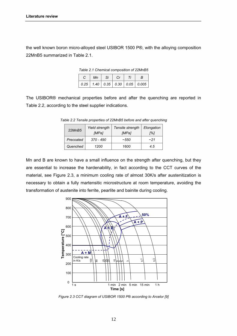
Mn and B are known to have a small influence on the strength after quenching, but they
are essential to increase the hardenability, in fact according to the CCT curves of the
material, see Figure 2.3, a minimum cooling rate of almost 30K/s after austenitization is
necessary to obtain a fully martensitic microstructure at room temperature, avoiding the
transformation of austenite into ferrite, pearlite and bainite during cooling.
1 s 1 min 2 min 5 min 15 min 1 hTime [s]
Tem
pera
ture
[°C
]
A + M
A + B
A + FA + P
50%
Cooling ratein K/s 10
0
80 2025 10 8 6 5 3 0.7
0.2
25
900
800
700
600
500
400
300
200
100
0
Figure 2.3 CCT diagram of USIBOR 1500 P® according to Arcelor [9]
Chapter 2
13
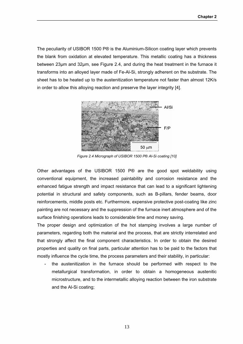
The peculiarity of USIBOR 1500 P® is the Aluminium-Silicon coating layer which prevents
the blank from oxidation at elevated temperature. This metallic coating has a thickness
between 23μm and 32μm, see Figure 2.4, and during the heat treatment in the furnace it
transforms into an alloyed layer made of Fe-Al-Si, strongly adherent on the substrate. The
sheet has to be heated up to the austenitization temperature not faster than almost 12K/s
in order to allow this alloying reaction and preserve the layer integrity [4].
Other advantages of the USIBOR 1500 P® are the good spot weldability using
conventional equipment, the increased paintability and corrosion resistance and the
enhanced fatigue strength and impact resistance that can lead to a significant lightening
potential in structural and safety components, such as B-pillars, fender beams, door
reinforcements, middle posts etc. Furthermore, expensive protective post-coating like zinc
painting are not necessary and the suppression of the furnace inert atmosphere and of the
surface finishing operations leads to considerable time and money saving.
The proper design and optimization of the hot stamping involves a large number of
parameters, regarding both the material and the process, that are strictly interrelated and
that strongly affect the final component characteristics. In order to obtain the desired
properties and quality on final parts, particular attention has to be paid to the factors that
mostly influence the cycle time, the process parameters and their stability, in particular:
- the austenitization in the furnace should be performed with respect to the
metallurgical transformation, in order to obtain a homogeneous austenitic
microstructure, and to the intermetallic alloying reaction between the iron substrate
and the Al-Si coating;
Figure 2.4 Micrograph of USIBOR 1500 P® Al-Si coating [10]

Literature review
14
- the transfer time should be reduced as much as possible in order to limit the heat
loss because at lower forming temperature the material formability is reduced and
undesirable local phase transformations could occur;
- the forming phase should be fast enough to reduce the heat exchange between
blank and dies during deformation, thus considering the influence of strain rate and
temperature on the material rheological behaviour;
- the dies have to be designed to evacuate a big amount of heat by means of
integrated cooling device in order to form and quench the blank at the same time,
and obtain a fully martensitic microstructure at the end of the process, therefore
the material phase transformation kinetics has to be taken into account.
2.2 Modelling and simulation of hot stamping In the sheet metal forming industry, FE codes are widely used to predict and optimize
manufacturing operations and to assess the forming feasibility of a part, reducing lead
times and costs. At present, two main formulations are implemented in commercial codes:
explicit and implicit approaches. Explicit formulations allow to reduce computation times
and grant acceptable accuracy in the solution but may present instabilities in the analysis
and exhibit significant limitations in the prediction of thermal aspects and microstructural
evolution during hot stamping operations (e.g. Autoform, Pam-Stamp 2G). On the other
hand, implicit codes (e.g. Forge, Marc, LS-Dyna, Abaqus) are characterized by higher
accuracy in the results and, due to the non-linearity of the problem, they require long
computation times that make them not suitable for industrial applications, furthermore
reliable material and process data have to be evaluated more in detail [11, 12]. The
introduction of temperature as an additional variable strongly influence the constitution of
the finite element models and enhance their complexity compared to traditional sheet
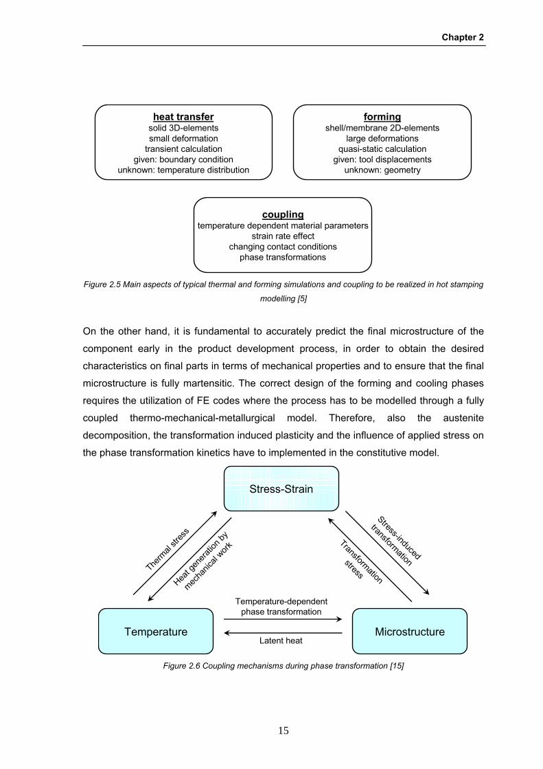
metal forming at room temperature [6, 13], as shown in Figure 2.5.
The main targets of press hardening simulations are the part geometry and the process
parameters which guarantee a successful forming avoiding excessive wrinkling and
thinning. In particular, the thickness distribution is used as input data in further crash
simulations and the thermo-mechanical history of the material model is of great
importance to capture the residual stress state that is responsible for the distortion of the
final component [14].
Chapter 2
15
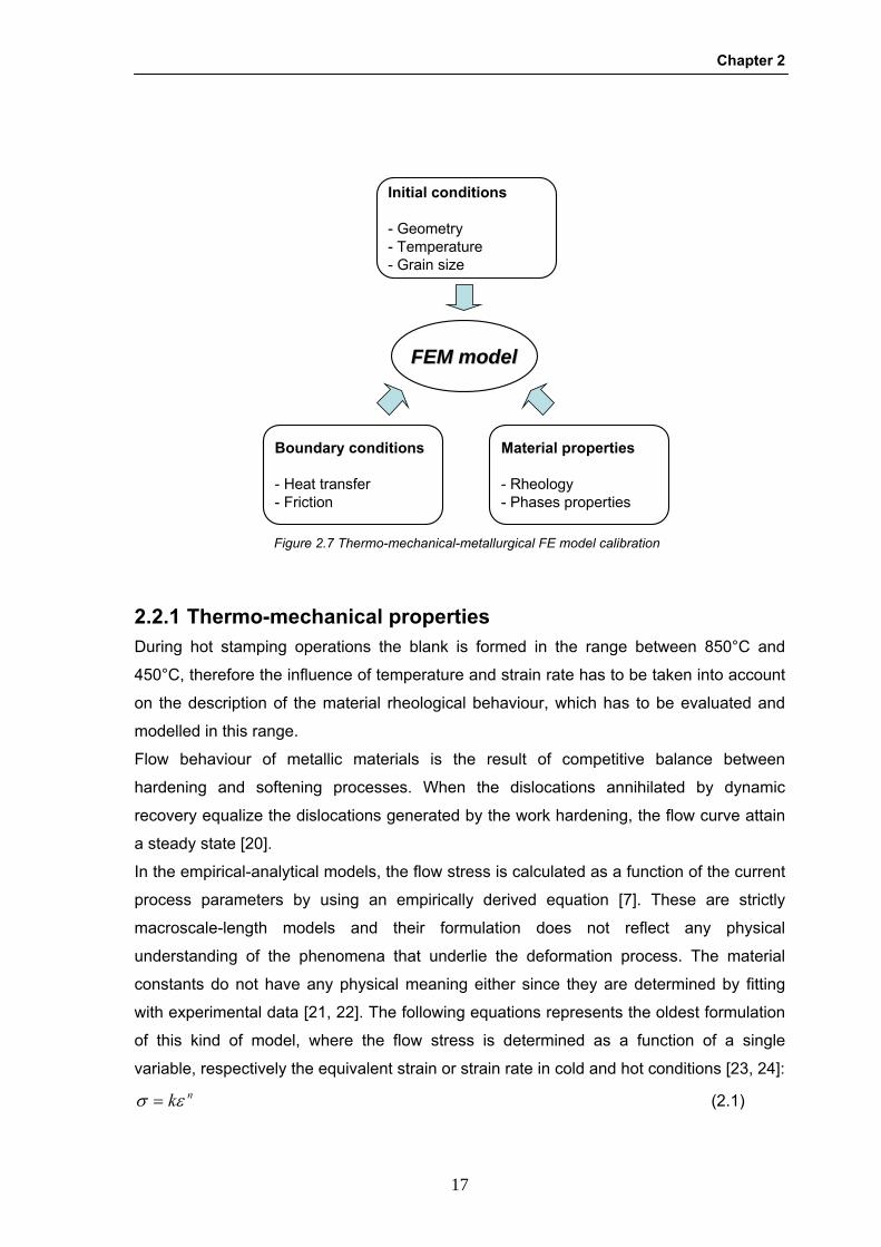
On the other hand, it is fundamental to accurately predict the final microstructure of the
component early in the product development process, in order to obtain the desired
characteristics on final parts in terms of mechanical properties and to ensure that the final
microstructure is fully martensitic. The correct design of the forming and cooling phases
requires the utilization of FE codes where the process has to be modelled through a fully
coupled thermo-mechanical-metallurgical model. Therefore, also the austenite
decomposition, the transformation induced plasticity and the influence of applied stress on
the phase transformation kinetics have to implemented in the constitutive model.
heat transfersolid 3D-elementssmall deformation
transient calculationgiven: boundary condition
unknown: temperature distribution
formingshell/membrane 2D-elements
large deformationsquasi-static calculation
given: tool displacementsunknown: geometry
couplingtemperature dependent material parameters
strain rate effectchanging contact conditions
phase transformations
Figure 2.5 Main aspects of typical thermal and forming simulations and coupling to be realized in hot stamping
modelling [5]
Stress-Strain
Temperature Microstructure
Temperature-dependentphase transformation
Latent heat
Stress-induced
transformation
Transformation
stressHea
t gen
eratio
n by
mecha
nical
work
Therm
al str
ess
Figure 2.6 Coupling mechanisms during phase transformation [15]

Literature review
16
The reliability of the numerical results depends not only on the models and the methods
that are used, but also on the accuracy and applicability of the input data [16]. The
material model and the related material properties data must be consistent with the
conditions of the workpiece in the process of interest. The accurate calibration of such a
model represents a strong requirement to gain reliable results from the FE simulations of
the hot stamping process, and besides the parameters that are necessary for the
simulation of conventional stamping, several material and process parameters and
boundary conditions need to be additionally considered. In particular, data about the
elasto-plastic properties of the material as function of temperature and strain rate, the
sheet formability as well as the influence of applied stress and strain on the phase
transformation kinetics have to be properly evaluated and implemented [17, 18].
Considering the complexity of the virtual model, several problems need to be solved to
improve the simulation reliability and decrease input costs [19]:
- evaluation of which parameters have to be precisely modelled in order to improve
the quality of numerical simulations;
- determination of which material characteristics need to be experimentally tested
and which ones are not crucial for the numerical results;
- identification of the process parameters to be accurately considered already during
the feasibility step in the die planning department.
An accurate and reliable analysis of the coupled thermo-mechanical-metallurgical process
requires efficient simulation tools as well as good quality and relevant material data. The
phenomena during hot stamping process can be divided into plastic deformation of blank,
heat transfer between hot sheet and cold dies and phase transformation of sheet due to
the cooling. Consequently, the simulation of the simultaneous forming and cooling should
consider interactions between the mechanical and temperature field and the
microstructure (Figure 2.7).
Chapter 2
17
2.2.1 Thermo-mechanical properties During hot stamping operations the blank is formed in the range between 850°C and
450°C, therefore the influence of temperature and strain rate has to be taken into account
on the description of the material rheological behaviour, which has to be evaluated and
modelled in this range.
Flow behaviour of metallic materials is the result of competitive balance between
hardening and softening processes. When the dislocations annihilated by dynamic
recovery equalize the dislocations generated by the work hardening, the flow curve attain
a steady state [20].
In the empirical-analytical models, the flow stress is calculated as a function of the current
process parameters by using an empirically derived equation [7]. These are strictly
macroscale-length models and their formulation does not reflect any physical
understanding of the phenomena that underlie the deformation process. The material
constants do not have any physical meaning either since they are determined by fitting
with experimental data [21, 22]. The following equations represents the oldest formulation
of this kind of model, where the flow stress is determined as a function of a single
variable, respectively the equivalent strain or strain rate in cold and hot conditions [23, 24]: nkεσ = (2.1)
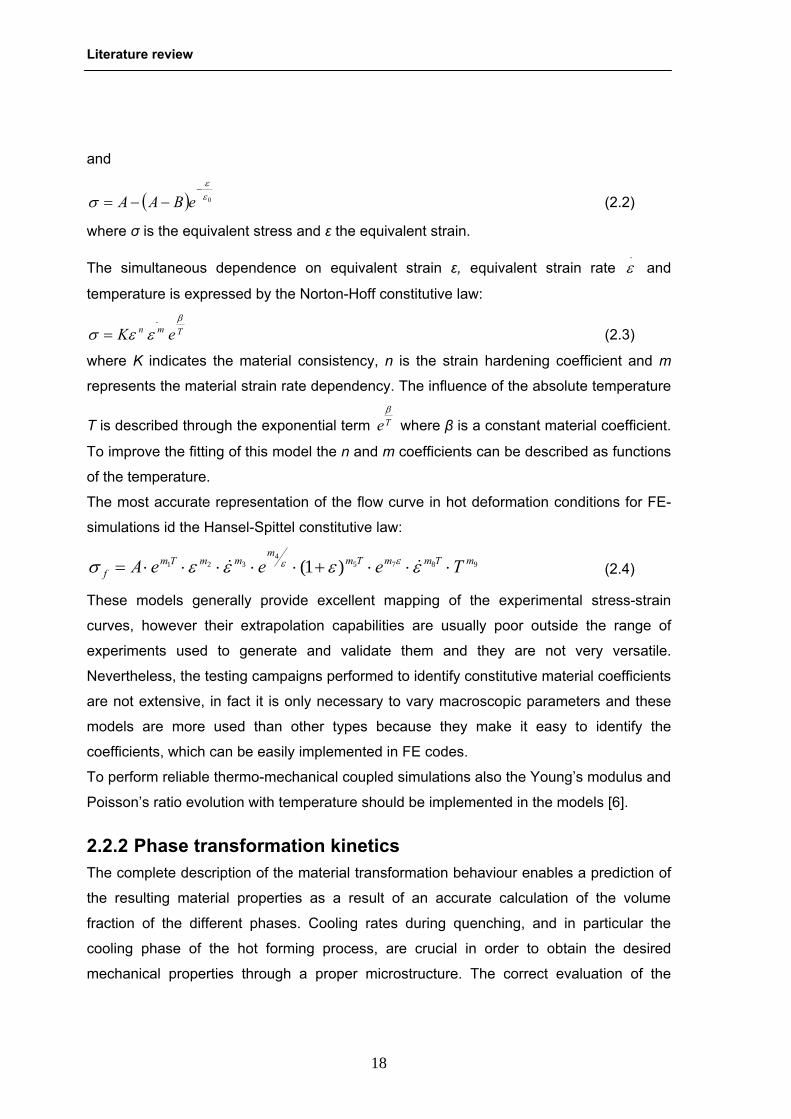
FEM modelFEM model
Material properties
- Rheology- Phases properties
Boundary conditions
- Heat transfer- Friction
Initial conditions
- Geometry- Temperature- Grain size
Figure 2.7 Thermo-mechanical-metallurgical FE model calibration
Literature review
18
and
( ) 0εε
σ−
−−= eBAA (2.2)
where σ is the equivalent stress and ε the equivalent strain.
The simultaneous dependence on equivalent strain ε, equivalent strain rate .ε and
temperature is expressed by the Norton-Hoff constitutive law:
Tmn eKβ
εεσ.
= (2.3)
where K indicates the material consistency, n is the strain hardening coefficient and m
represents the material strain rate dependency. The influence of the absolute temperature
T is described through the exponential term Teβ
where β is a constant material coefficient.
To improve the fitting of this model the n and m coefficients can be described as functions
of the temperature.
The most accurate representation of the flow curve in hot deformation conditions for FE-
simulations id the Hansel-Spittel constitutive law:
98754
321 )1( mTmmTmm
mmTmf TeeeA ⋅⋅⋅+⋅⋅⋅⋅⋅= εεεεσ εε && (2.4)
These models generally provide excellent mapping of the experimental stress-strain
curves, however their extrapolation capabilities are usually poor outside the range of
experiments used to generate and validate them and they are not very versatile.
Nevertheless, the testing campaigns performed to identify constitutive material coefficients
are not extensive, in fact it is only necessary to vary macroscopic parameters and these
models are more used than other types because they make it easy to identify the
coefficients, which can be easily implemented in FE codes.
To perform reliable thermo-mechanical coupled simulations also the Young’s modulus and
Poisson’s ratio evolution with temperature should be implemented in the models [6].
2.2.2 Phase transformation kinetics The complete description of the material transformation behaviour enables a prediction of
the resulting material properties as a result of an accurate calculation of the volume
fraction of the different phases. Cooling rates during quenching, and in particular the
cooling phase of the hot forming process, are crucial in order to obtain the desired
mechanical properties through a proper microstructure. The correct evaluation of the
Chapter 2
19
phase transformation kinetics analysis is therefore essential to couple microstructural
transformation and thermo-mechanical related phenomena.
Microstructural models describe the during- and post-deformation aspects of material
response in terms of microstructure parameters. The phenomena covered by these
models are dynamic and static phenomena, both of which are caused by deformation [25].
Some statistical models based on continuous curve transformation (CCT) permitting to
point out the critical cooling rate for quenching depending on chemical composition and
austenitization conditions have been proposed, but they are not accurate enough to be
used to couple metallurgical and mechanical effect [26]. Phase transformations at
constant temperature are investigated through the temperature-time-transformation (TTT)
curves, indicating on a temperature vs. time logarithmic scale the starting and the ending
transformation point at different constant temperatures.
According to the 22MnB5 CCT diagram (Figure 2.3), a minimum cooling rate of almost
27K/s has to be used to obtain a fully martensitic microstructure at the end of the hot
stamping process. However, it has been shown that applied stress and strain can
accelerate the austenite transformation [27, 28], thus a safety margin should be taken for
this limit. Information about CCT and TTT diagrams of quenchenable boron steels can be
found in the literature [29], but their correlation with the process parameters (e.g. stress
and strain states) has not been investigated in depth yet and its evaluation represents a
basic requirement to obtain reliable results from the numerical simulations of the hot
stamping process.
2.2.2.1 Phase transformation modelling The mathematical formulation for diffusion-controlled transformations is based on the
nucleon-grain-growth theory. First publications about the kinetics of this kind diffusion-
processes were made by Avrami [30]. The Avrami equation is widely used in the form:
( ) ( ) ( ) ( )TntTket ηξ −−= 1 (2.5)
where ( )tξ is the volume fraction at the growing phase at time t, n is the Avrami
coefficient depending on the germination mode and nuclei form, k is function of
temperature and η is:
( ) ( )∫=t
duuqt0
η (2.6)

Literature review
20
where q represents the probability of a germ in the time unit to be active. This law is
general enough to be utilized in both isothermal and anisothermal cases. It is possible to
follow any cooling path and determine the correspondent transformed fraction by knowing
k, n and η. The accessibility to experimental data necessary to determine those
parameters force to a simplification of Avrami equation (2.5) and to deal with distinct
approach to isothermal and anisothermal cases. In addition, the theoretical formulation of
phase evolution was confirmed by experimental investigation of Johnson and Mehl [31].
The anisothermal kinetics theory is based on the subdivision of the thermal path in basic
steps in order to reconstruct the anisothermal kinetics from the knowledge of isothermal
one by applying the additivity principle, which is based on the theory advanced by Scheil
[32] and can be mathematically stated as:
( )∫ =t
Tdt
0
1τ
(2.7)
where dt is the increment of time during continuous cooling and ( )Tτ represents the
isothermal time required to initiate transformation at a specific temperature T. The
additivity rule states that a transformation occurring while the temperature is changing can
be considered as a series of isothermal events, with each increment of transformation
being a function only of the fraction transformed and temperature.
The martensitic transformation requires a different mathematical approach, because it is
very fast and without diffusion of carbon. The kinetics of this phase transformation is often
modelled by the following equation, which was firstly formulated by Koistinen and
Marburger [33]:
( ) ( )καξ TMSet −−−= 1 (2.8)
where ( )tξ is the volume fraction of martensite, Ms is the martensite-start temperature
and α and t are material coefficients.
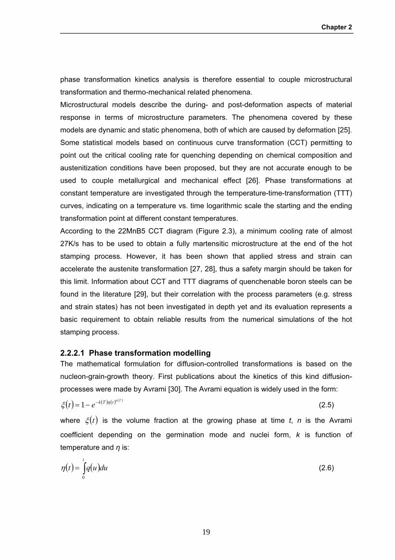
Some preliminary studies have been carried out in order to simulate the 22MnB5 phase
transformation behaviour through the model expressed by the Johnson-Mehl-Avrami (2.6)
and Koistinen-Marburger (2.8) equations, as shown in Figure 2.8, but further
investigations are necessary to validate that model due to the lack of information about
the 22MnB5 isotherm TTT diagram [34] and the influence of applied stresses on the
material phase transformation kinetics.
Chapter 2
21
The martensitic transformation causes a release of latent heat of approximately 85kJ/kg,
therefore this phenomena has to be taken into account for a correct simulation of the
quenching phase.
2.2.2.2 Transformation plasticity Solid state phase transformations do not only change the mechanical and thermal
properties of the material, but result also in volumetric and deviatoric strains. If the phase
transformation occurs without applied stress, the material response is purely volumetric
and an increase in volume is observed due to the compactness differences between the
parent and product phase. Transformation induced plasticity (TRIP) is an irreversible
strain observed when metallurgical transformations occur under external stress that is
lower than the yield stress of the parent phase. In technological applications, TRIP plays
an important role in many problems, in particular for the understanding of residual
stresses and distortions of the final component resulting from anisothermal forming
operations.
Two mechanisms are usually considered to explain this phenomenon from a
microstructural poi of view: the Magee mechanism [35] and the Greenwood-Johnson
mechanism [36]. According to Magee, transformation plasticity is due to an orientation of
the newly formed phase by the applied stress. This mechanism is particularly related to
martensitic transformation during which martensite develops in the form of plates which
generate high shearing in the austenitic phase. It is important to underline that if no
Figure 2.8 Resultant phase fraction of austenite, martensite and bainite after the cooling process simulation
considering both elastic tools and heat transfer into the tools [34].

Literature review
22
external stress is applied, this orientation is random and the resultant micro-stresses can
be considered negligible. On the contrary, an applied load favours a particular orientation
of martensitic plates with a consequent non nil resultant for micro-stresses [37]. According
to Greenwood and Johnson transformation plasticity is due to the compactness difference
between parent and product phase. Therefore, micro-stresses are introduced and
generate plastic strains in the soft austenite when an applied deviatoric stress is applied. If
no external load is applied, no transformation plasticity is observed, due to the nil volume
average of the micro-plasticity [38].
It has been found that the linearity between applied load and final transformation plasticity
surely exists only if the applied load is inferior to the half of the yield stress of austenite at
the considered temperature, as shown in Figure 2.9.
More results can be found in the work published by Coret [15]. In addition, Taleb found
that transformation plasticity strain increases for low fraction of transformed phase while a
sort of saturation arises when about 70% of new phase is formed [38].
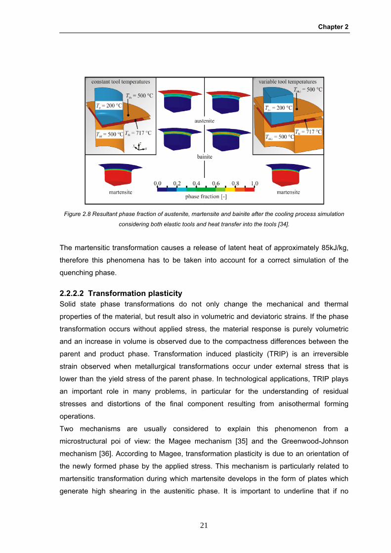
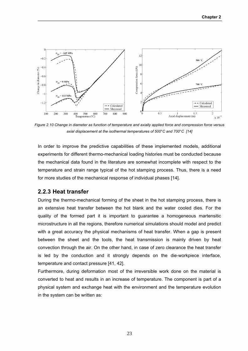
Åkerström developed a constitutive model taking into account austenite decomposition
and transformation induced plasticity in order to increase the accuracy of numerical
simulations of the hot stamping process [40], and Figure 2.10 shows some results
regarding the validation of the implemented model.
Figure 2.9 Transformation plasticity as function of applied load at three different temperatures [39]
Chapter 2
23
In order to improve the predictive capabilities of these implemented models, additional
experiments for different thermo-mechanical loading histories must be conducted because
the mechanical data found in the literature are somewhat incomplete with respect to the
temperature and strain range typical of the hot stamping process. Thus, there is a need
for more studies of the mechanical response of individual phases [14].
2.2.3 Heat transfer During the thermo-mechanical forming of the sheet in the hot stamping process, there is
an extensive heat transfer between the hot blank and the water cooled dies. For the
quality of the formed part it is important to guarantee a homogeneous martensitic
microstructure in all the regions, therefore numerical simulations should model and predict
with a great accuracy the physical mechanisms of heat transfer. When a gap is present
between the sheet and the tools, the heat transmission is mainly driven by heat
convection through the air. On the other hand, in case of zero clearance the heat transfer
is led by the conduction and it strongly depends on the die-workpiece interface,
temperature and contact pressure [41, 42].
Furthermore, during deformation most of the irreversible work done on the material is
converted to heat and results in an increase of temperature. The component is part of a
physical system and exchange heat with the environment and the temperature evolution
in the system can be written as:
Figure 2.10 Change in diameter as function of temperature and axially applied force and compression force versus
axial displacement at the isothermal temperatures of 500°C and 700°C [14]

Literature review
24
( )( ) {
ndissipatioInternalnductionInternalco
evolutioneTemperatur
WTgradkdivtTc
.+⋅=
∂∂
44 344 21321
ρ (2.9)
In the area boundary the temperature evolution depends on the imposed temperature and
radiation, conduction and convection exchange.
The radiation affect the area boundary with a flux exchange term rΦ given by:
( )40
4 TTr −=Φ σε (2.10)
where ε is the material emissivity in its current conditions, σ is the Stefan constant, T0 is
the exterior area temperature and T the area boundary local temperature.
The area boundary is affected by the conduction and the convection with the flux
exchange conductionΦ and convectionΦ that can be expressed as:
( )0TTcconduction −=Φ (2.11)
( )0TThcconvection −=Φ (2.12)
where c is the thermal conductivity of the material and hc is the convection coefficient.
In a metal forming process, the physical system is composed of a workpiece, a set of dies
and sometimes a lubricant. On a microscopic scale both the die and the workpiece reveal
real surfaces which are not perfectly smooth, showing small peaks, asperities and valleys,
as shown in Figure 2.11.
Due to the unevenness of the contact, the heat flux is altered and a temperature
difference occurs at the interface of the two solids. This temperature difference is at the
Figure 2.11 Die-workpiece interface on a micro-scale (a) [43] and heat flow through a joint (b) [44]
Chapter 2
25
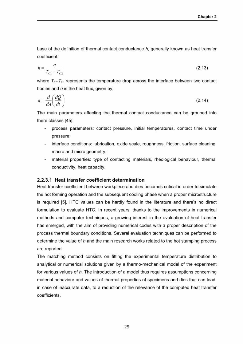
base of the definition of thermal contact conductance h, generally known as heat transfer
coefficient:
21 CC TTqh−
= (2.13)
where Tc1-Tc2 represents the temperature drop across the interface between two contact
bodies and q is the heat flux, given by:
⎟⎠⎞
⎜⎝⎛=dtdQ
dAdq (2.14)
The main parameters affecting the thermal contact conductance can be grouped into
there classes [45]:
- process parameters: contact pressure, initial temperatures, contact time under
pressure;
- interface conditions: lubrication, oxide scale, roughness, friction, surface cleaning,
macro and micro geometry;
- material properties: type of contacting materials, rheological behaviour, thermal
conductivity, heat capacity.
2.2.3.1 Heat transfer coefficient determination Heat transfer coefficient between workpiece and dies becomes critical in order to simulate
the hot forming operation and the subsequent cooling phase when a proper microstructure
is required [5]. HTC values can be hardly found in the literature and there’s no direct
formulation to evaluate HTC. In recent years, thanks to the improvements in numerical
methods and computer techniques, a growing interest in the evaluation of heat transfer
has emerged, with the aim of providing numerical codes with a proper description of the
process thermal boundary conditions. Several evaluation techniques can be performed to
determine the value of h and the main research works related to the hot stamping process
are reported.
The matching method consists on fitting the experimental temperature distribution to
analytical or numerical solutions given by a thermo-mechanical model of the experiment
for various values of h. The introduction of a model thus requires assumptions concerning
material behaviour and values of thermal properties of specimens and dies that can lead,
in case of inaccurate data, to a reduction of the relevance of the computed heat transfer
coefficients.

Literature review
26
Lechler et al. [1] studied the heat transfer coefficient evolution with contact pressure
through an analytical approach based on the following equation:
( )⎟⎟⎠
⎞⎜⎜⎝
⎛−−
−=∞
∞
TTTtT
AtVcp
0
lnρ
α (2.15)
where T0 and T(t) represent the initial and the actual temperature of the blank measured
during the experiments and ∞T indicates the temperature of the contact plates, which is
assumed to be constant. Figure 2.12 shows some results for the USIBOR 1500 P® heat
transfer coefficient evolution with respect to the applied contact pressure.
The inverse analysis method is based on the solution of an inverse problem and may be
applied to determine heat transfer coefficients under both steady-state and transient
conditions. The main advantage of this approach is that the inverse analysis can be
based on complex analytical and numerical models, making it possible to carry out
experiments closer to the industrial conditions, however the drawbacks are the same
outlined for the previous method, with a reduction in the relevance of the computed values
in the case of inaccurate input data.
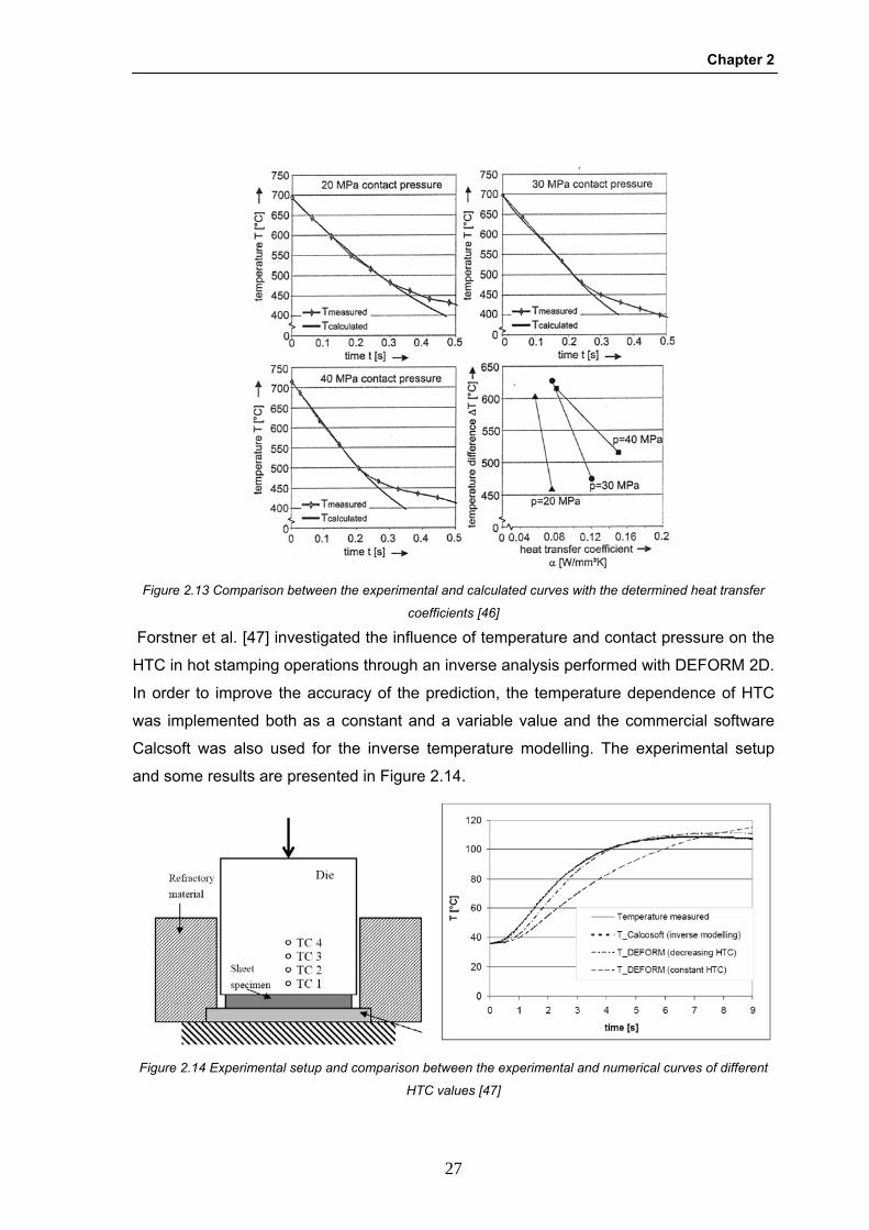
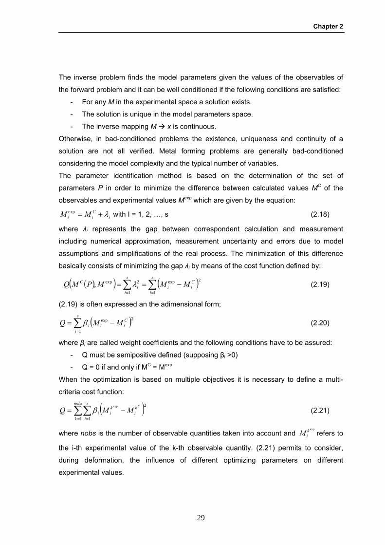
Geiger et al. [46] simulated with ABAQUS the cooling experiments with the USBOR 1500
P® in order to determine the heat transfer coefficients for different contact pressures
through inverse analysis. Two interpolation points of the HTC were inserted in the
simulation in order to interpolate linearly between the data points, as shown in Figure
2.13.
Figure 2.12 Heat transfer coefficient between workpiece and dies as function of the temperature and of the
applied contact pressure [18]
Chapter 2
27
Forstner et al. [47] investigated the influence of temperature and contact pressure on the
HTC in hot stamping operations through an inverse analysis performed with DEFORM 2D.
In order to improve the accuracy of the prediction, the temperature dependence of HTC
was implemented both as a constant and a variable value and the commercial software
Calcsoft was also used for the inverse temperature modelling. The experimental setup
and some results are presented in Figure 2.14.
Figure 2.13 Comparison between the experimental and calculated curves with the determined heat transfer
coefficients [46]
Figure 2.14 Experimental setup and comparison between the experimental and numerical curves of different
HTC values [47]

Literature review
28
2.3 Inverse analysis theoretical bases In this work an inverse analysis technique will be used to determine the heat transfer
coefficient, therefore its theoretical bases are briefly introduced.
A physical system can be described through a mathematical model able to express the
system response MC taking into account the boundary conditions. This direct model can
be given as:
( )xSM C = (2.16)
where x represents the parameters describing the system under study and S is called
forward operator.
On the contrary, the inverse analysis consists in determining the condition x leading a
physical system to describe the experimental value Mexp, and can be expressed as the
determination of:
( )CMSx 1−= so that expMM C = (2.17)
The complexity of most direct models commonly adopted is sometime so elaborate that a
simple inversion of the model results impossible, therefore regression methods are
instead used, in order to predict an experimental state Mexp closer as possible to the
predicted value MC [48]. Only in the last years a systematic study for a general formulation
and resolution of inverse problems has been performed involving several fields such as
electronic [49], structural analysis [50], heat engineering [51, 52], geometrical optimization
[53, 54] and rheological parameters identification [55, 56].
DIRECT MODELDIRECT MODEL
Experimental measurement of variables
or parameters
System response
INVERSE MODELINVERSE MODEL
Evaluation variables or parameters
Experimental measurements of the
system response
Identified parameters
Figure 2.15 Comparison between forward and inverse problems
Chapter 2
29
The inverse problem finds the model parameters given the values of the observables of
the forward problem and it can be well conditioned if the following conditions are satisfied:
- For any M in the experimental space a solution exists.
- The solution is unique in the model parameters space.
- The inverse mapping M x is continuous.
Otherwise, in bad-conditioned problems the existence, uniqueness and continuity of a
solution are not all verified. Metal forming problems are generally bad-conditioned
considering the model complexity and the typical number of variables.
The parameter identification method is based on the determination of the set of
parameters P in order to minimize the difference between calculated values MC of the
observables and experimental values Mexp which are given by the equation:
iCii MM λ+=exp with I = 1, 2, …, s (2.18)
where λi represents the gap between correspondent calculation and measurement
including numerical approximation, measurement uncertainty and errors due to model
assumptions and simplifications of the real process. The minimization of this difference
basically consists of minimizing the gap λi by means of the cost function defined by:
( )( ) ( )∑ ∑= =
−==s
i
s
i
Ciii
C MMMPMQ1 1
2exp2exp, λ (2.19)
(2.19) is often expressed an the adimensional form;
( )∑=
−=s
i
Ciii MMQ
1
2expβ (2.20)
where βi are called weight coefficients and the following conditions have to be assured:
- Q must be semipositive defined (supposing βi >0)
- Q = 0 if and only if MC = Mexp
When the optimization is based on multiple objectives it is necessary to define a multi-
criteria cost function:
( )∑∑= =
−=nobs
k
s
i
ki
kii
C
MMQ1 1
2exp
β (2.21)
where nobs is the number of observable quantities taken into account and expkiM refers to
the i-th experimental value of the k-th observable quantity. (2.21) permits to consider,
during deformation, the influence of different optimizing parameters on different
experimental values.

Literature review
30
A more general form of the cost function employs a statistical approach [49] where the
optimization problem is lead to the determination of the parameters which maximize the
prediction probability of the experimentally evaluated measure. For a Gaussian
distribution, the cost function depends on the mean value of the experimental measure
( )exp~kiMm , which are supposed to be equal to the calculated ones
CkiM , and the quadratic
deviation of measurement errors 2kiσ .
The cost function can be expressed as:
∑∑∑== =
⎥⎦⎤
⎢⎣⎡ −+⎥⎦
⎤⎢⎣⎡ −=
r
ijijj
nobs
k
s
i
kii
ki PPMmQ
C2_
1
2
1
_γλ (2.22)
where 2
/1 ki
ki σλ = with k=1,2,…,nobs and 2/1 pjj σγ =
Several methods can be used for the minimization problem [57-59] and the Gauss-
Newton method, used in this investigation, will be described more in detail.
The Gauss-Newton method introduces a linearization of the non-linear expression of
terms representing the computed observables CiM neglecting the second order
derivative. This method is based on the first order Taylor series expansion of Q in the
quadratic form:
( ) ( ) ( ) ( )22
2
PPPdPQdP
dPdQPP
dPdQ
Δ+Δ⋅+=Δ+ θ (2.23)
An extreme of the Q function is obtained imposing:
( ) 0=Δ+ PPdPdQ
(2.24)
and neglecting terms grater than first order the equation (2.23) can be expressed as a
linear system:
( )
( )⎪⎪⎪
⎩
⎪⎪⎪
⎨
⎧
=
=
=+Δ⋅
PdPdQB
PdPQdA
BPA
2
20
(2.24)
where:
( ) ( )∑=
−==s
iiki
Cii
kk SMM
dPPdQB
1
exp2 β (2.25)
Chapter 2
31
( ) ( ) ∑∑==
+−==s
ijk
j
ci
i
s
i kj
ci
iCii
kjjk S
dPdM
dPdPMd
MMdPdPPQdA
11
2exp
2
22 ββ (2.26)
k
Ci
jk dPdM
S = (2.27)
and S is called sensibility matrix.
The peculiarity of this method consists in neglecting the second order derivatives of the
calculated observables of the direct model in (2.26) which becomes:
( ) ∑=
≅=s
iik
j
Ci
ikj
jk SdPdM
dPdPPQdA
1
2
2 β
The solution of the linear system (2.24) leads thus to the determination of the components
of the matrix S.
The sensitivity matrix allows to determine the matrix A and the gradient B of the linear
system (2.24). It is therefore necessary to calculate the derivatives of MC respect to each
parameter to be determined and the sensitivity analysis may be performed [60]:
- by finite differences;
- by means of analytic direct calculation;
- with the formulation of a conjugate problem;
- with a semi-analytical evaluation.
2.4 Formability The formability of sheet metal depends on both material characteristics (e.g. anisotropy
and microstructure) and on forming process conditions (e.g. temperature, friction, strain
rate and strain path). Sheet metal formability is generally estimated using several tests
(e.g. uni-axial and bi-axial tests, bulging test, FLC, LDH, flange insertion test, etc). Each
type of test has some advantages and some disadvantages in its application both at room
and at elevate temperature.
The concept of the forming limit curve has been introduced by Keller [61] and Goodwin
[62] in order to represents comprehensively sheet metal formability and it has been widely
used both in factories and research laboratories as one of the criteria for optimizing
stamping processes and in the design of dies. Such curves indicate both the principal
strains at diffuse or localized instability for different strain paths.

Literature review
32
At room temperature two main methods are generally used to obtain limit curves, the
Marciniak and the Nakazima, and they effectively constitute the state-of-the-art. The main
differences between these tests is the shape of the punch which is respectively flat and
hemispherical. The Nakazima setup is simpler to perform but a special lubrication system
(e.g. oil, Teflon foil, elastic pad, etc.) has to be used to reduce friction, while the Marciniak
test is equipped with carrier blanks to prevent the contact between the punch and the
tested specimen, thus reducing the difficulties caused by friction. Specimens of various
width are used to determine a complete FLC [63].
Figure 2.16 Standard forming limit curve including scatter band
(a) (b) Figure 2.17 Typical Nakazima (a) and Marciniak (b) setups
Chapter 2
33
Because of the complexity of the experimental determination of FLC, several theoretical
calculating models have been proposed on the basis of the classical or modified Swift and
Hill instability criteria [64, 65] to calculate the limit strains: diffuse necking, localised
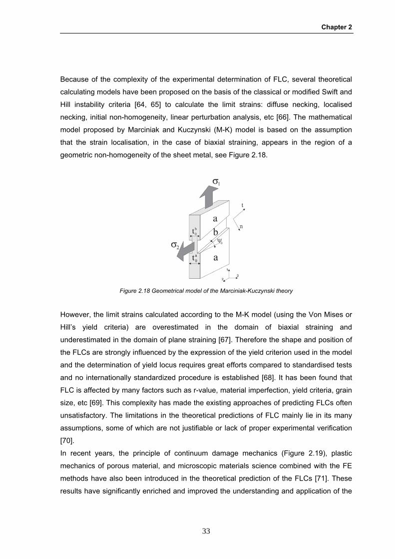
necking, initial non-homogeneity, linear perturbation analysis, etc [66]. The mathematical
model proposed by Marciniak and Kuczynski (M-K) model is based on the assumption
that the strain localisation, in the case of biaxial straining, appears in the region of a
geometric non-homogeneity of the sheet metal, see Figure 2.18.
However, the limit strains calculated according to the M-K model (using the Von Mises or
Hill’s yield criteria) are overestimated in the domain of biaxial straining and
underestimated in the domain of plane straining [67]. Therefore the shape and position of
the FLCs are strongly influenced by the expression of the yield criterion used in the model
and the determination of yield locus requires great efforts compared to standardised tests
and no internationally standardized procedure is established [68]. It has been found that
FLC is affected by many factors such as r-value, material imperfection, yield criteria, grain
size, etc [69]. This complexity has made the existing approaches of predicting FLCs often
unsatisfactory. The limitations in the theoretical predictions of FLC mainly lie in its many
assumptions, some of which are not justifiable or lack of proper experimental verification
[70].
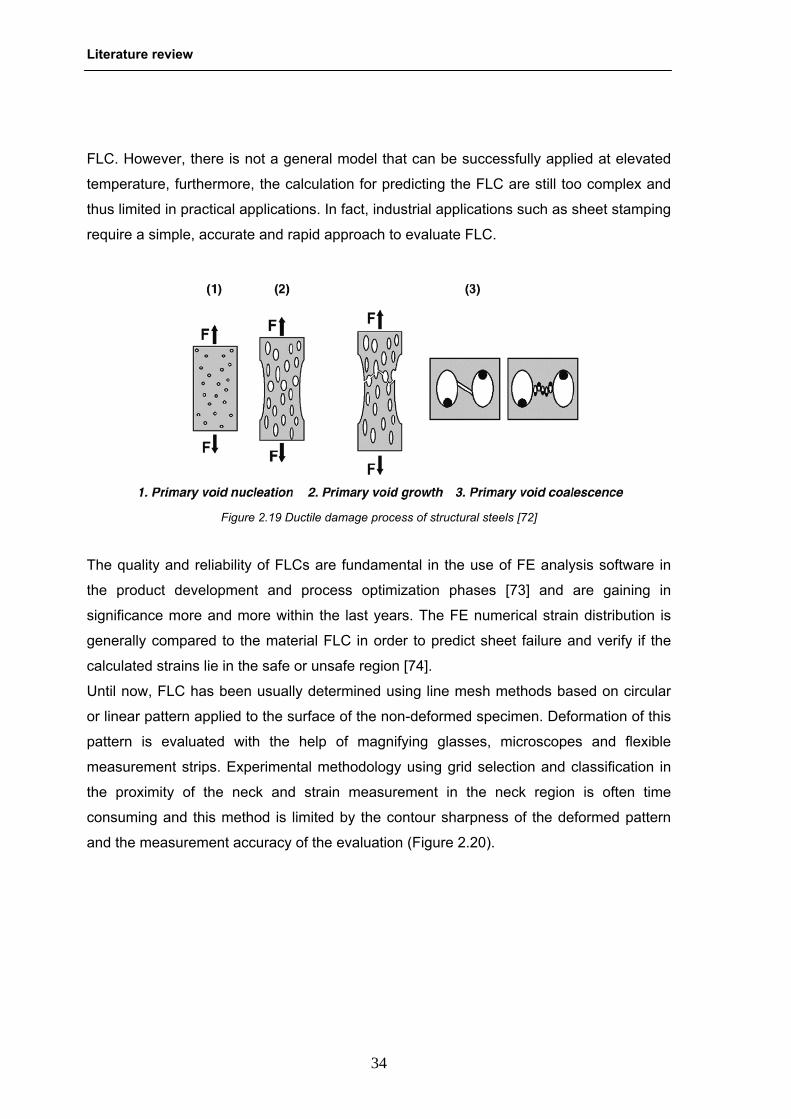
In recent years, the principle of continuum damage mechanics (Figure 2.19), plastic
mechanics of porous material, and microscopic materials science combined with the FE
methods have also been introduced in the theoretical prediction of the FLCs [71]. These
results have significantly enriched and improved the understanding and application of the
Figure 2.18 Geometrical model of the Marciniak-Kuczynski theory
Literature review
34
FLC. However, there is not a general model that can be successfully applied at elevated
temperature, furthermore, the calculation for predicting the FLC are still too complex and
thus limited in practical applications. In fact, industrial applications such as sheet stamping
require a simple, accurate and rapid approach to evaluate FLC.
The quality and reliability of FLCs are fundamental in the use of FE analysis software in
the product development and process optimization phases [73] and are gaining in
significance more and more within the last years. The FE numerical strain distribution is
generally compared to the material FLC in order to predict sheet failure and verify if the
calculated strains lie in the safe or unsafe region [74].
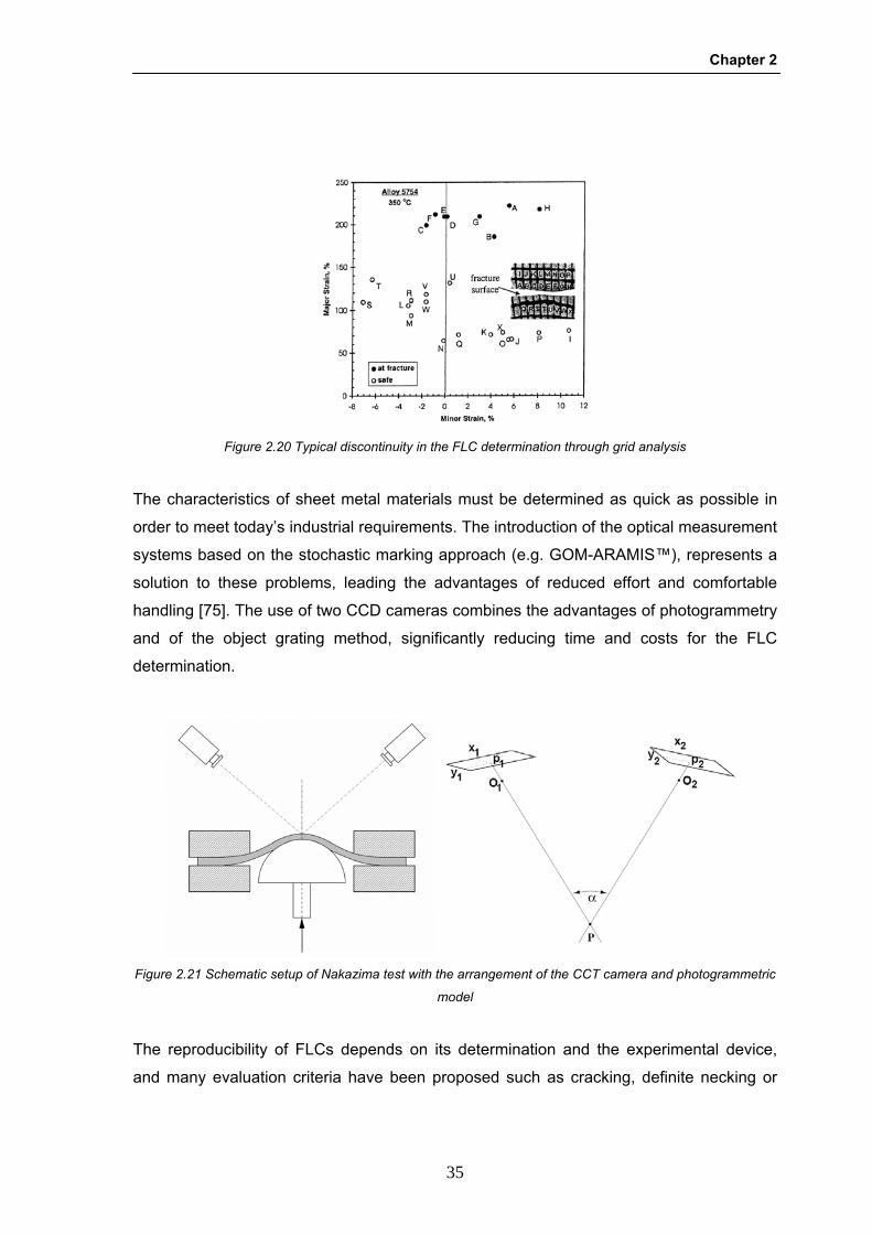
Until now, FLC has been usually determined using line mesh methods based on circular
or linear pattern applied to the surface of the non-deformed specimen. Deformation of this
pattern is evaluated with the help of magnifying glasses, microscopes and flexible
measurement strips. Experimental methodology using grid selection and classification in
the proximity of the neck and strain measurement in the neck region is often time
consuming and this method is limited by the contour sharpness of the deformed pattern
and the measurement accuracy of the evaluation (Figure 2.20).
Figure 2.19 Ductile damage process of structural steels [72]
Chapter 2
35
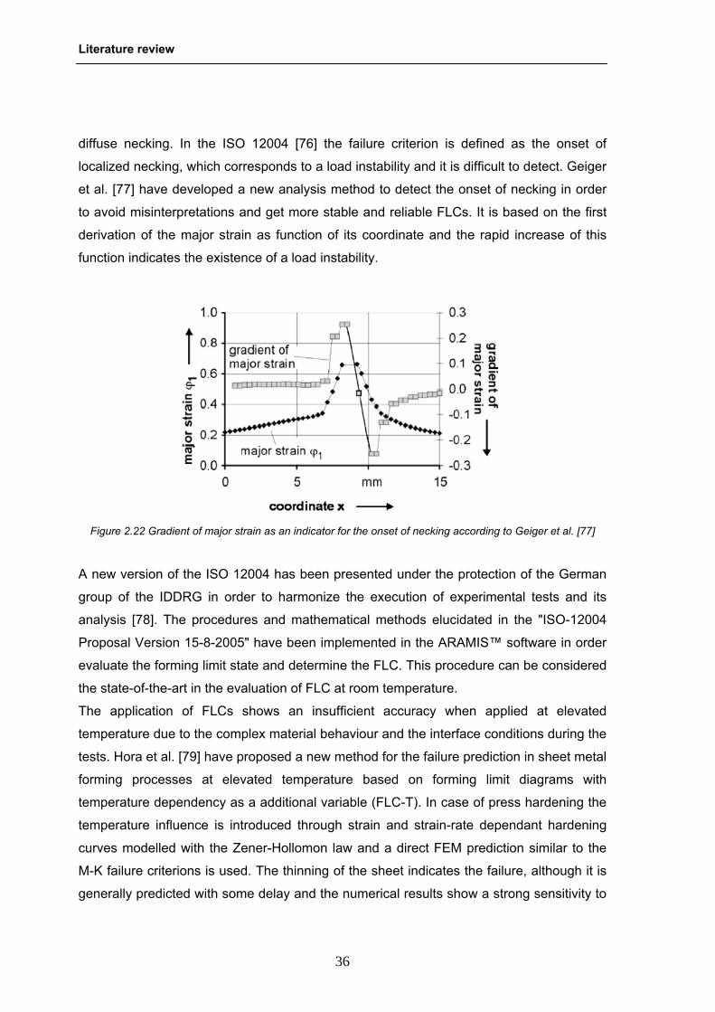
The characteristics of sheet metal materials must be determined as quick as possible in
order to meet today’s industrial requirements. The introduction of the optical measurement
systems based on the stochastic marking approach (e.g. GOM-ARAMIS™), represents a
solution to these problems, leading the advantages of reduced effort and comfortable
handling [75]. The use of two CCD cameras combines the advantages of photogrammetry
and of the object grating method, significantly reducing time and costs for the FLC
determination.
The reproducibility of FLCs depends on its determination and the experimental device,
and many evaluation criteria have been proposed such as cracking, definite necking or
Figure 2.20 Typical discontinuity in the FLC determination through grid analysis
Figure 2.21 Schematic setup of Nakazima test with the arrangement of the CCT camera and photogrammetric
model
Literature review
36
diffuse necking. In the ISO 12004 [76] the failure criterion is defined as the onset of
localized necking, which corresponds to a load instability and it is difficult to detect. Geiger
et al. [77] have developed a new analysis method to detect the onset of necking in order
to avoid misinterpretations and get more stable and reliable FLCs. It is based on the first
derivation of the major strain as function of its coordinate and the rapid increase of this
function indicates the existence of a load instability.
A new version of the ISO 12004 has been presented under the protection of the German
group of the IDDRG in order to harmonize the execution of experimental tests and its
analysis [78]. The procedures and mathematical methods elucidated in the "ISO-12004
Proposal Version 15-8-2005" have been implemented in the ARAMIS™ software in order
evaluate the forming limit state and determine the FLC. This procedure can be considered
the state-of-the-art in the evaluation of FLC at room temperature.
The application of FLCs shows an insufficient accuracy when applied at elevated
temperature due to the complex material behaviour and the interface conditions during the
tests. Hora et al. [79] have proposed a new method for the failure prediction in sheet metal
forming processes at elevated temperature based on forming limit diagrams with
temperature dependency as a additional variable (FLC-T). In case of press hardening the
temperature influence is introduced through strain and strain-rate dependant hardening
curves modelled with the Zener-Hollomon law and a direct FEM prediction similar to the
M-K failure criterions is used. The thinning of the sheet indicates the failure, although it is
generally predicted with some delay and the numerical results show a strong sensitivity to
Figure 2.22 Gradient of major strain as an indicator for the onset of necking according to Geiger et al. [77]
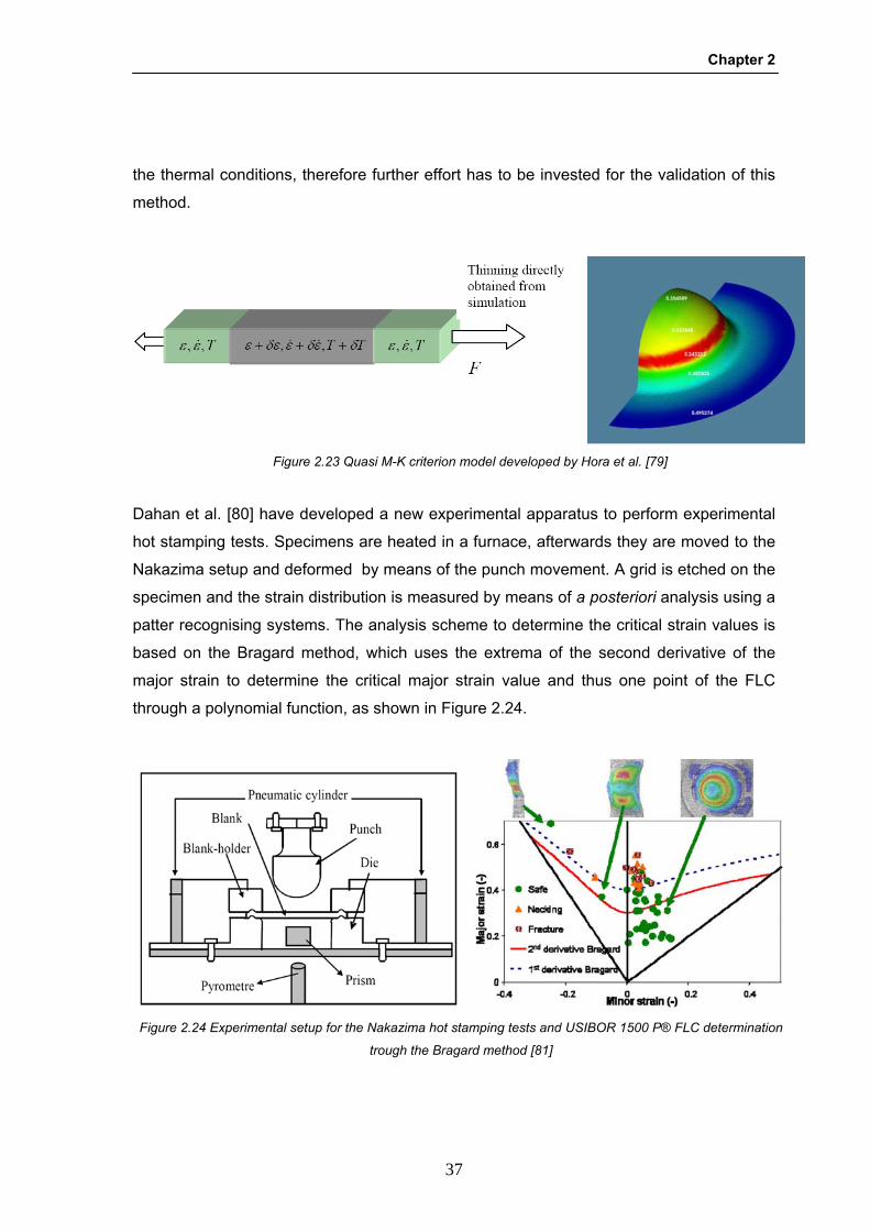
Chapter 2
37
the thermal conditions, therefore further effort has to be invested for the validation of this
method.
Dahan et al. [80] have developed a new experimental apparatus to perform experimental
hot stamping tests. Specimens are heated in a furnace, afterwards they are moved to the
Nakazima setup and deformed by means of the punch movement. A grid is etched on the
specimen and the strain distribution is measured by means of a posteriori analysis using a
patter recognising systems. The analysis scheme to determine the critical strain values is
based on the Bragard method, which uses the extrema of the second derivative of the
major strain to determine the critical major strain value and thus one point of the FLC
through a polynomial function, as shown in Figure 2.24.
Figure 2.23 Quasi M-K criterion model developed by Hora et al. [79]
Figure 2.24 Experimental setup for the Nakazima hot stamping tests and USIBOR 1500 P® FLC determination
trough the Bragard method [81]
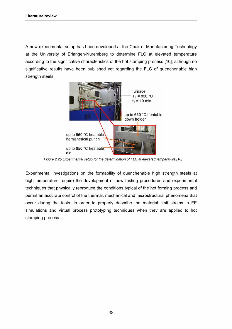
Literature review
38
A new experimental setup has been developed at the Chair of Manufacturing Technology
at the University of Erlangen-Nuremberg to determine FLC at elevated temperature
according to the significative characteristics of the hot stamping process [10], although no
significative results have been published yet regarding the FLC of quenchenable high
strength steels.
Experimental investigations on the formability of quenchenable high strength steels at
high temperature require the development of new testing procedures and experimental
techniques that physically reproduce the conditions typical of the hot forming process and
permit an accurate control of the thermal, mechanical and microstructural phenomena that
occur during the tests, in order to properly describe the material limit strains in FE
simulations and virtual process prototyping techniques when they are applied to hot
stamping process.
Figure 2.25 Experimental setup for the determination of FLC at elevated temperature [10]

Chapter 3
39
3 CHAPTER 3 THERMO-MECHANICAL PROPERTIES

Thermo-mechanical properties
40
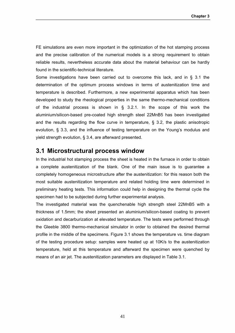
Chapter 3
41
FE simulations are even more important in the optimization of the hot stamping process
and the precise calibration of the numerical models is a strong requirement to obtain
reliable results, nevertheless accurate data about the material behaviour can be hardly
found in the scientific-technical literature.
Some investigations have been carried out to overcome this lack, and in § 3.1 the
determination of the optimum process windows in terms of austenitization time and
temperature is described. Furthermore, a new experimental apparatus which has been
developed to study the rheological properties in the same thermo-mechanical conditions
of the industrial process is shown in § 3.2.1. In the scope of this work the
aluminium/silicon-based pre-coated high strength steel 22MnB5 has been investigated
and the results regarding the flow curve in temperature, § 3.2, the plastic anisotropic
evolution, § 3.3, and the influence of testing temperature on the Young’s modulus and
yield strength evolution, § 3.4, are afterward presented.
3.1 Microstructural process window In the industrial hot stamping process the sheet is heated in the furnace in order to obtain
a complete austenitization of the blank. One of the main issue is to guarantee a
completely homogeneous microstructure after the austenitization: for this reason both the
most suitable austenitization temperature and related holding time were determined in
preliminary heating tests. This information could help in designing the thermal cycle the
specimen had to be subjected during further experimental analysis.
The investigated material was the quenchenable high strength steel 22MnB5 with a
thickness of 1.5mm; the sheet presented an aluminium/silicon-based coating to prevent
oxidation and decarburization at elevated temperature. The tests were performed through
the Gleeble 3800 thermo-mechanical simulator in order to obtained the desired thermal
profile in the middle of the specimens. Figure 3.1 shows the temperature vs. time diagram
of the testing procedure setup: samples were heated up at 10K/s to the austenitization
temperature, held at this temperature and afterward the specimen were quenched by
means of an air jet. The austenitization parameters are displayed in Table 3.1.
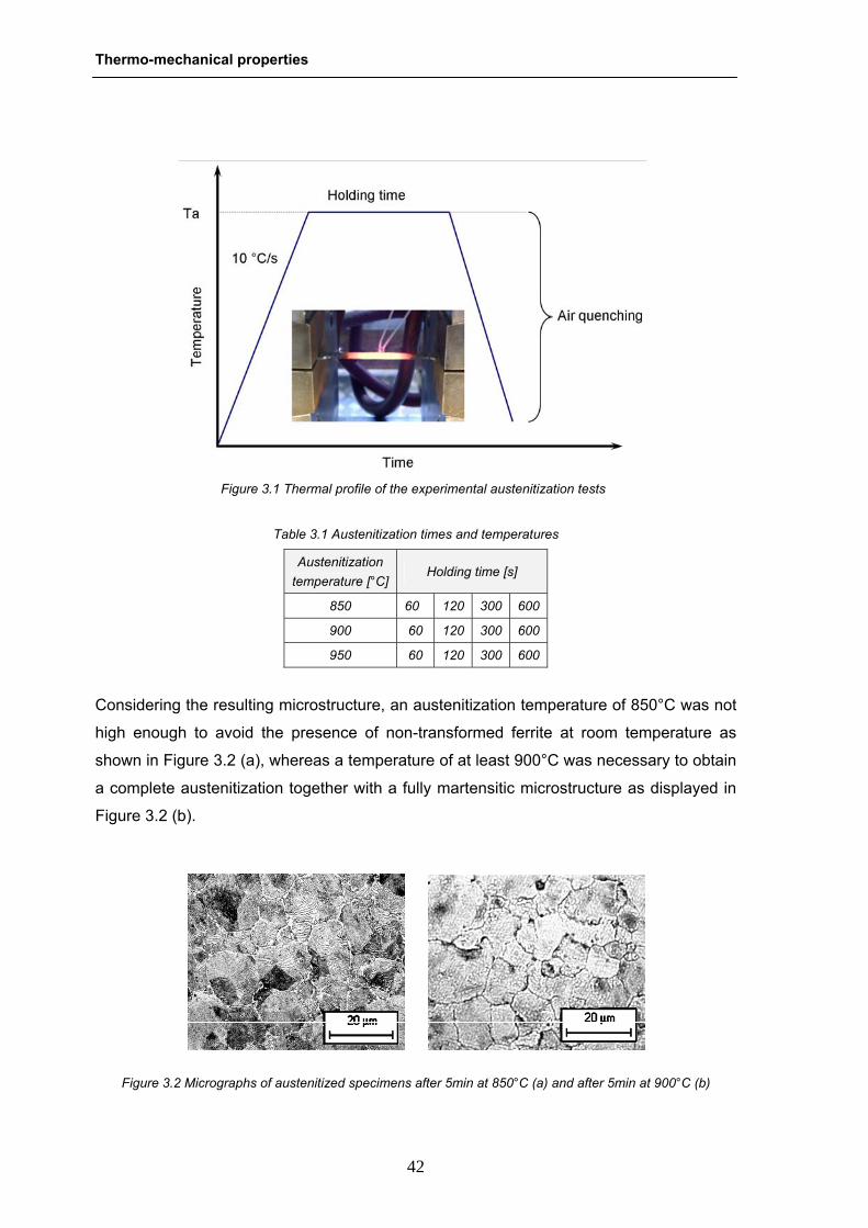
Thermo-mechanical properties
42
Table 3.1 Austenitization times and temperatures
Austenitization temperature [°C]
Holding time [s]
850 600 120 300 600
900 60 120 300 600
950 60 120 300 600
Considering the resulting microstructure, an austenitization temperature of 850°C was not
high enough to avoid the presence of non-transformed ferrite at room temperature as
shown in Figure 3.2 (a), whereas a temperature of at least 900°C was necessary to obtain
a complete austenitization together with a fully martensitic microstructure as displayed in
Figure 3.2 (b).
Figure 3.2 Micrographs of austenitized specimens after 5min at 850°C (a) and after 5min at 900°C (b)
Figure 3.1 Thermal profile of the experimental austenitization tests
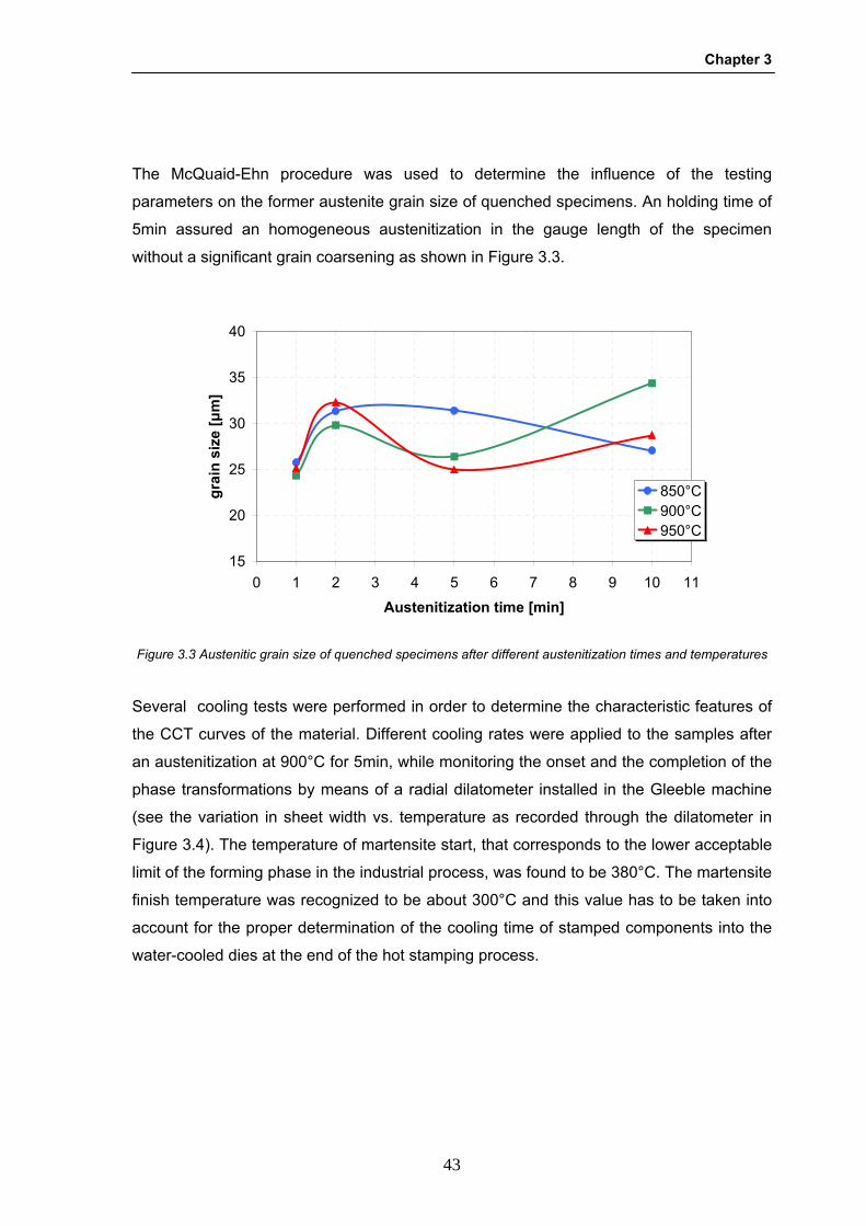
Chapter 3
43
The McQuaid-Ehn procedure was used to determine the influence of the testing
parameters on the former austenite grain size of quenched specimens. An holding time of
5min assured an homogeneous austenitization in the gauge length of the specimen
without a significant grain coarsening as shown in Figure 3.3.
15
20
25
30
35
40
0 1 2 3 4 5 6 7 8 9 10 11
Austenitization time [min]
grai
n si
ze [μ
m]
850°C900°C950°C
Figure 3.3 Austenitic grain size of quenched specimens after different austenitization times and temperatures
Several cooling tests were performed in order to determine the characteristic features of
the CCT curves of the material. Different cooling rates were applied to the samples after
an austenitization at 900°C for 5min, while monitoring the onset and the completion of the
phase transformations by means of a radial dilatometer installed in the Gleeble machine
(see the variation in sheet width vs. temperature as recorded through the dilatometer in
Figure 3.4). The temperature of martensite start, that corresponds to the lower acceptable
limit of the forming phase in the industrial process, was found to be 380°C. The martensite
finish temperature was recognized to be about 300°C and this value has to be taken into
account for the proper determination of the cooling time of stamped components into the
water-cooled dies at the end of the hot stamping process.

Thermo-mechanical properties
44
-0.36
-0.34
-0.32
-0.3
-0.28
-0.26
-0.24
-0.22
0 100 200 300 400 500 600 700 800 900 1000
Temperature [°C]
Wid
th re
duct
ion
[%]
Figure 3.4 Dilatometer curve with a cooling rate of 50 K/s
Hardness measurements at room temperature were performed on the specimens used for
the cooling tests in order to determine the resultant percentage of martensite, which is
proportional to the hardness value. The trend displayed in Figure 3.5 allows to identify the
critical cooling rate to avoid bainitic\ferritic transformation, that was recognized to be about
30K/s, as suggested by the steel supplier.
15
20
25
30
35
40
45
0 10 20 30 40 50 60
Cooling rate [K/s]
Vick
ers
Har
dnes
s
Figure 3.5 Vickers hardness at room temperature for different cooling rates
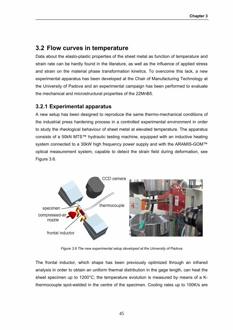
Chapter 3
45
3.2 Flow curves in temperature Data about the elasto-plastic properties of the sheet metal as function of temperature and
strain rate can be hardly found in the literature, as well as the influence of applied stress
and strain on the material phase transformation kinetics. To overcome this lack, a new
experimental apparatus has been developed at the Chair of Manufacturing Technology at
the University of Padova and an experimental campaign has been performed to evaluate
the mechanical and microstructural properties of the 22MnB5.
3.2.1 Experimental apparatus A new setup has been designed to reproduce the same thermo-mechanical conditions of
the industrial press hardening process in a controlled experimental environment in order
to study the rheological behaviour of sheet metal at elevated temperature. The apparatus
consists of a 50kN MTS™ hydraulic testing machine, equipped with an inductive heating
system connected to a 30kW high frequency power supply and with the ARAMIS-GOM™
optical measurement system, capable to detect the strain field during deformation, see
Figure 3.6.
Figure 3.6 The new experimental setup developed at the University of Padova
The frontal inductor, which shape has been previously optimized through an infrared
analysis in order to obtain an uniform thermal distribution in the gage length, can heat the
sheet specimen up to 1200°C; the temperature evolution is measured by means of a K-
thermocouple spot-welded in the centre of the specimen. Cooling rates up to 100K/s are
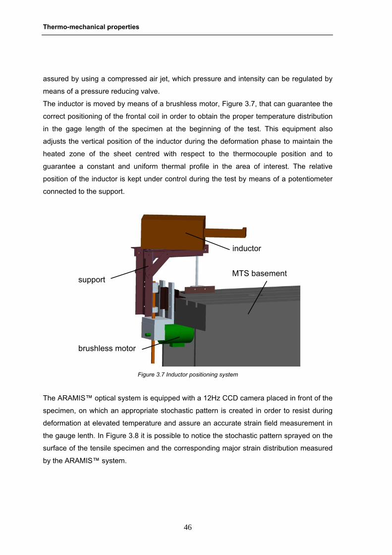
Thermo-mechanical properties
46
assured by using a compressed air jet, which pressure and intensity can be regulated by
means of a pressure reducing valve.
The inductor is moved by means of a brushless motor, Figure 3.7, that can guarantee the
correct positioning of the frontal coil in order to obtain the proper temperature distribution
in the gage length of the specimen at the beginning of the test. This equipment also
adjusts the vertical position of the inductor during the deformation phase to maintain the
heated zone of the sheet centred with respect to the thermocouple position and to
guarantee a constant and uniform thermal profile in the area of interest. The relative
position of the inductor is kept under control during the test by means of a potentiometer
connected to the support.
brushless motor
MTS basement
inductor
support
Figure 3.7 Inductor positioning system
The ARAMIS™ optical system is equipped with a 12Hz CCD camera placed in front of the
specimen, on which an appropriate stochastic pattern is created in order to resist during
deformation at elevated temperature and assure an accurate strain field measurement in
the gauge lenth. In Figure 3.8 it is possible to notice the stochastic pattern sprayed on the
surface of the tensile specimen and the corresponding major strain distribution measured
by the ARAMIS™ system.
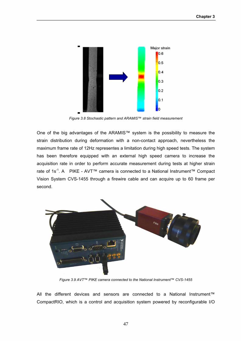
Chapter 3
47
Figure 3.8 Stochastic pattern and ARAMIS™ strain field measurement
One of the big advantages of the ARAMIS™ system is the possibility to measure the
strain distribution during deformation with a non-contact approach, nevertheless the
maximum frame rate of 12Hz representes a limitation during high speed tests. The system
has been therefore equipped with an external high speed camera to increase the
acquisition rate in order to perform accurate measurement during tests at higher strain
rate of 1s-1. A PIKE - AVT™ camera is connected to a National Instrument™ Compact
Vision System CVS-1455 through a firewire cable and can acquire up to 60 frame per
second.
Figure 3.9 AVT™ PIKE camera connected to the National Instrument™ CVS-1455
All the different devices and sensors are connected to a National Instrument™
CompactRIO, which is a control and acquisition system powered by reconfigurable I/O
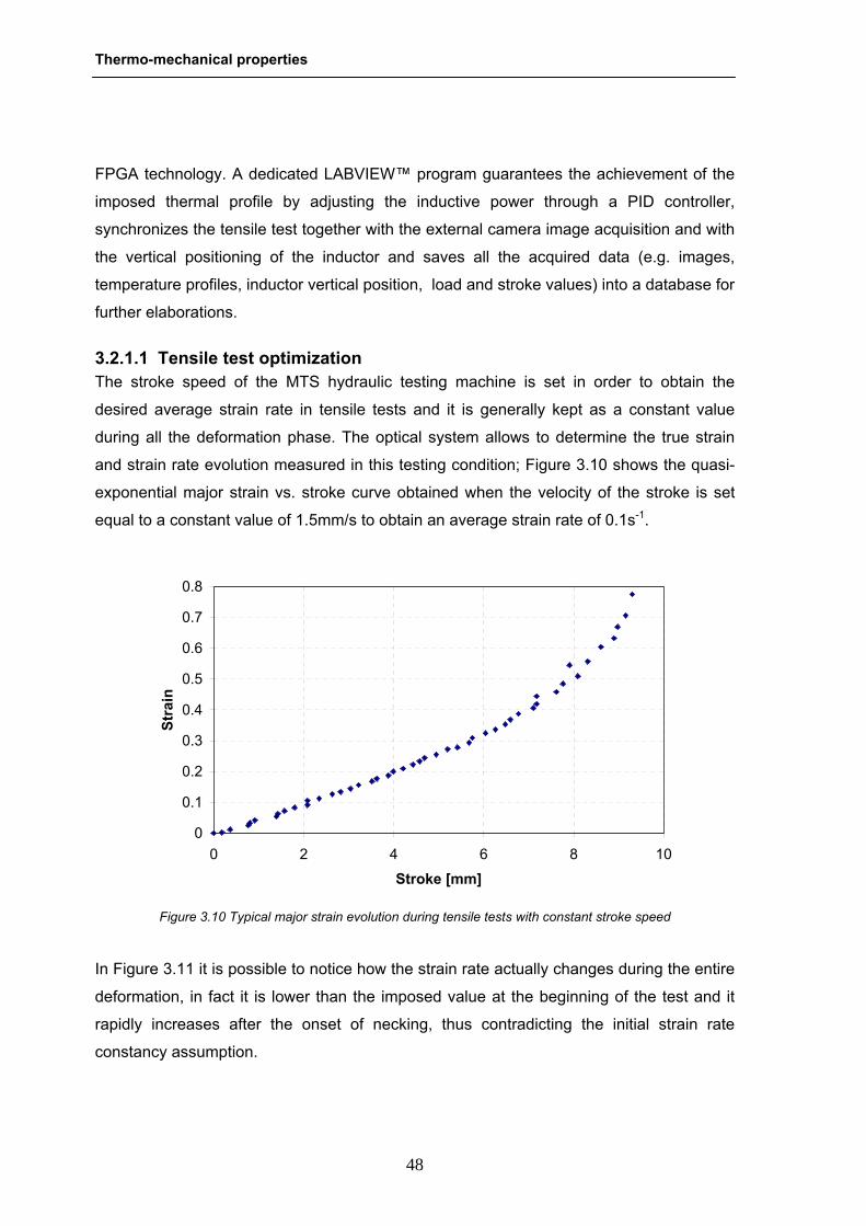
Thermo-mechanical properties
48
FPGA technology. A dedicated LABVIEW™ program guarantees the achievement of the
imposed thermal profile by adjusting the inductive power through a PID controller,
synchronizes the tensile test together with the external camera image acquisition and with
the vertical positioning of the inductor and saves all the acquired data (e.g. images,
temperature profiles, inductor vertical position, load and stroke values) into a database for
further elaborations.
3.2.1.1 Tensile test optimization The stroke speed of the MTS hydraulic testing machine is set in order to obtain the
desired average strain rate in tensile tests and it is generally kept as a constant value
during all the deformation phase. The optical system allows to determine the true strain
and strain rate evolution measured in this testing condition; Figure 3.10 shows the quasi-
exponential major strain vs. stroke curve obtained when the velocity of the stroke is set
equal to a constant value of 1.5mm/s to obtain an average strain rate of 0.1s-1.
0
0.1
0.2
0.3
0.4
0.5
0.6
0.7
0.8
0 2 4 6 8 10
Stroke [mm]
Stra
in
Figure 3.10 Typical major strain evolution during tensile tests with constant stroke speed
In Figure 3.11 it is possible to notice how the strain rate actually changes during the entire
deformation, in fact it is lower than the imposed value at the beginning of the test and it
rapidly increases after the onset of necking, thus contradicting the initial strain rate
constancy assumption.

Chapter 3
49
0
0.05
0.1
0.15
0.2
0.25
0.3
0.35
0 2 4 6 8 10
Stroke [mm]
Stra
in ra
te [s
¯¹]
Figure 3.11 Typical strain rate evolution during tensile tests with constant stroke speed
In order to avoid this phenomenon and obtain an almost constant strain rate during the
entire tensile test, the stroke speed was modified for all the different strain rate values
(e.g. 0.01, 0.1 and 1s-1) through a trial-and-error approach by increasing the velocity in the
first part of the tensile test and by reducing it at the end. The result obtained for the 0.1s-1
testing procedure optimization is shown in Figure 3.12.
0
0.05
0.1
0.15
0.2
0.25
0.3
0.35
0 2 4 6 8 10
Stroke [mm]
Stra
in ra
te [s
¯¹]
Figure 3.12 Strain rate evolution with the modified testing procedure (0.1s-1)

Thermo-mechanical properties
50
3.2.2 Experiments and results Uniaxial tensile tests were performed by means of the new apparatus in order to
determine the influence of cooling rate, temperature and strain rate on the flow curves of
the 22MnB5 under the typical conditions of the industrial hot stamping process. The
specimen geometry was chosen according to the recommendation of ISO 10130.
140
12
80
18
Figure 3.13 Tensile test specimen geometry
The same thermo-mechanical cycle that material undergoes during press hardening
operations was therefore reproduced by means of the new experimental setup. The
specimens were austenitized at 950°C for 3min, afterwards two different cooling rates
equal to 30K/s and 50K/s were applied until the desired temperature Ti was reached as
shown in Figure 3.14; isothermal tensile tests were afterwards performed at different
temperatures and strain rates as summarized in Table 3.2. The stroke speed were set
according to procedure described in the previous paragraph in order obtain a constant
strain rate during the entire deformation. At least two test runs were carried out for each
test condition to assure the repeatability of the results.
Table 3.2 Experimental parameters used for the tensile tests
Deformation temperature [°C]
Strain rate [s-1]
500 0.01 .0.1. 010
650 0.01 0.1 1
800 0.01 0.1 1
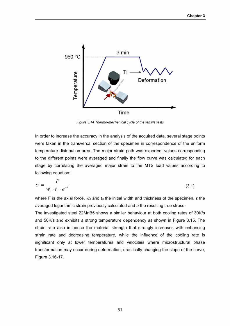
Chapter 3
51
Figure 3.14 Thermo-mechanical cycle of the tensile tests
In order to increase the accuracy in the analysis of the acquired data, several stage points
were taken in the transversal section of the specimen in correspondence of the uniform
temperature distribution area. The major strain path was exported, values corresponding
to the different points were averaged and finally the flow curve was calculated for each
stage by correlating the averaged major strain to the MTS load values according to
following equation:
εσ −⋅⋅=
etwF
00 (3.1)
where F is the axial force, w0 and t0 the initial width and thickness of the specimen, ε the
averaged logarithmic strain previously calculated and σ the resulting true stress.
The investigated steel 22MnB5 shows a similar behaviour at both cooling rates of 30K/s
and 50K/s and exhibits a strong temperature dependency as shown in Figure 3.15. The
strain rate also influence the material strength that strongly increases with enhancing
strain rate and decreasing temperature, while the influence of the cooling rate is
significant only at lower temperatures and velocities where microstructural phase
transformation may occur during deformation, drastically changing the slope of the curve,
Figure 3.16-17.

Thermo-mechanical properties
52
0
100
200
300
400
500
0 0.05 0.1 0.15 0.2 0.25 0.3 0.35Strain
Stre
ss [M
Pa]
500 °C650 °C800 °C
Figure 3.15 22MnB5 temperature sensitivity (strain rate of 1s-1 and cooling rate of 50K/s)
0
50
100
150
200
250
0 0.1 0.2 0.3 0.4 0.5
True strain
True
str
ess
[MPa
]
0.01 s⎯¹0.1 s⎯¹1 s⎯¹
Figure 3.16 22MnB5 strain rate sensitivity (temperature of 800°C and cooling rate of 30K/s)
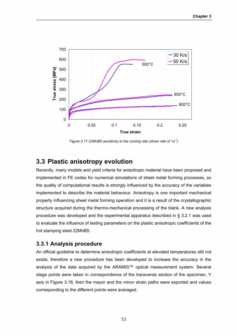
Chapter 3
53
0
100
200
300
400
500
600
700
0 0.05 0.1 0.15 0.2 0.25
True strain
True
str
ess
[MPa
]
800°C
650°C
500°C
30 K/s50 K/s
Figure 3.17 22MnB5 sensitivity to the cooling rate (strain rate of 1s-1)
3.3 Plastic anisotropy evolution Recently, many models and yield criteria for anisotropic material have been proposed and
implemented in FE codes for numerical simulations of sheet metal forming processes, so
the quality of computational results is strongly influenced by the accuracy of the variables
implemented to describe the material behaviour. Anisotropy is one important mechanical
property influencing sheet metal forming operation and it is a result of the crystallographic
structure acquired during the thermo-mechanical processing of the blank. A new analysis
procedure was developed and the experimental apparatus described in § 3.2.1 was used
to evaluate the influence of testing parameters on the plastic anisotropic coefficients of the
hot stamping steel 22MnB5.
3.3.1 Analysis procedure An official guideline to determine anisotropic coefficients at elevated temperatures still not
exists, therefore a new procedure has been developed to increase the accuracy in the
analysis of the data acquired by the ARAMIS™ optical measurement system. Several
stage points were taken in correspondence of the transverse section of the specimen, Y
axis in Figure 3.18, then the mayor and the minor strain paths were exported and values
corresponding to the different points were averaged.

Thermo-mechanical properties
54
Normal anisotropy r was calculated for each stage according (3.2) where ε1 is the
longitudinal true strain, ε2 the true strain in width direction and ε3 the true strain in
thickness direction, calculated by assuming the volume constancy during plastic
deformation.
21
2
3
2 -εε
εεε
+==r (3.2)
A common trend was noticed in the evolution of normal anisotropy during the entire tensile
test: the values considerably fluctuated in correspondence of the initial part of the tensile
curve, then they approached nearly a constant value. Plastic anisotropy was therefore
calculated averaging the data in that one characterized by uniform deformation before the
onset of necking, corresponding the reaching of the maximum force value, as shown in
Figure 3.19.
The r-values were determined for tensile specimens cut at 0°, 45° and 90° with respect to
the rolling direction of the sheet in order to investigate the material anisotropic behaviour.
The coefficients of the normal anisotropy nr and the planar anisotropy rΔ were therefore
calculated according to the following equations:
)2(41
45900 rrrr n ++= (3.3)
)2-(21
45900 rrrr +=Δ (3.4)
Figure 3.18 True strain field measured through the ARAMIS™ optical system

Chapter 3
55
3.3.2 Results and discussion Uniaxial tensile tests were performed by means of the new setup in order to evaluate the
influence of cooling rate, temperature and strain rate on the plastic anisotropy evolution of
the 22MnB5. The tensile specimens were austenitized at 950°C for 3min, chilled down at
the desired temperature with cooling rate of 30K/s and 50K/s and deformed at constant
strain rate. The testing parameters are given in the following Table 3.3
Table 3.3 Experimental parameters used for the tensile tests
Deformation temperature [°C]
Strain rate [s-1]
500 0.01 0.10 010
650 0.01 0.1 1
800 0.01 0.1 1
In Figure 3.20 it is possible to notice the normal anisotropy evolution for specimens cut at
0°, 45° and 90° with respect to the rolling direction of the sheet during deformation at
0.1s-1 and 800°C.
0
0.2
0.4
0.6
0.8
1
1.2
0 0.05 0.1 0.15 0.2 0.25 0.3 0.35
Strain
Nor
mal
ani
sotro
py
Figure 3.19 Independency of the normal anisotropy r from the true strain (deformation at 800°C – 0.01s-1)
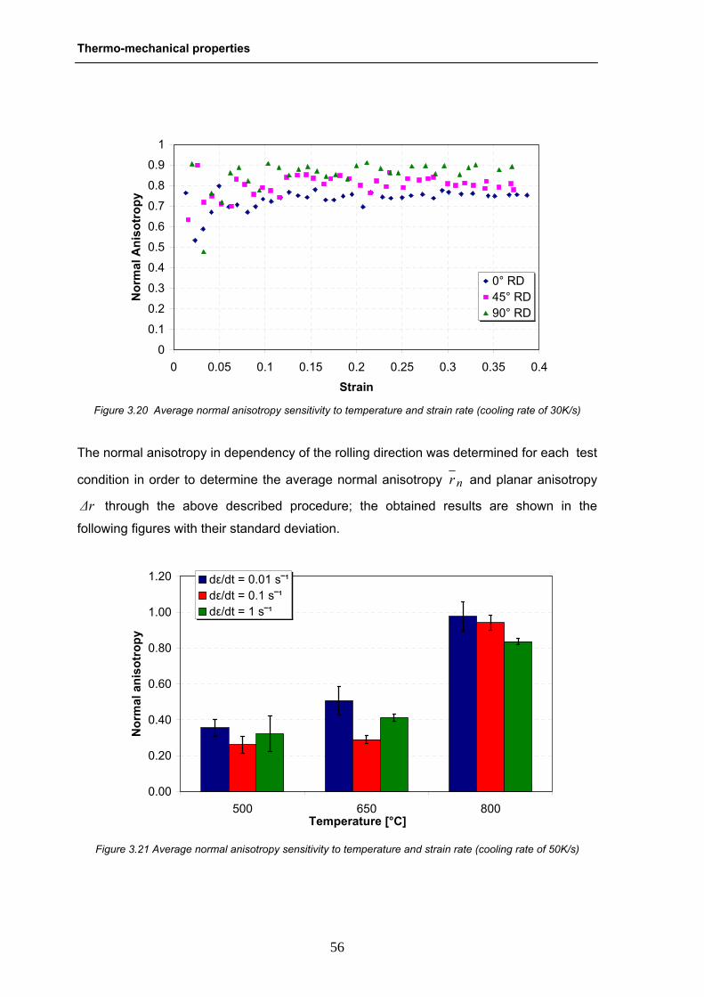
Thermo-mechanical properties
56
The normal anisotropy in dependency of the rolling direction was determined for each test
condition in order to determine the average normal anisotropy nr and planar anisotropy
rΔ through the above described procedure; the obtained results are shown in the
following figures with their standard deviation.
0
0.1
0.2
0.3
0.4
0.5
0.6
0.7
0.8
0.9
1
0 0.05 0.1 0.15 0.2 0.25 0.3 0.35 0.4
Strain
Nor
mal
Ani
sotr
opy
0° RD45° RD90° RD
Figure 3.20 Average normal anisotropy sensitivity to temperature and strain rate (cooling rate of 30K/s)
0.00
0.20
0.40
0.60
0.80
1.00
1.20
500 650 800Temperature [°C]
Nor
mal
ani
sotr
opy
dε/dt = 0.01 s⎯¹dε/dt = 0.1 s⎯¹dε/dt = 1 s⎯¹
Figure 3.21 Average normal anisotropy sensitivity to temperature and strain rate (cooling rate of 50K/s)

Chapter 3
57
The average normal anisotropy was strongly affected by the deformation temperature, in
fact at 800°C the material showed an almost isotropic behaviour, while the anisotropic
tendency increased with decreasing temperature. Normal anisotropy sensitivity to strain
rate was less pronounced and the influence of microstructural evolution should be
considered for a better comprehension of this phenomenon because of the possible
bainitic phase transformation during deformation at lower strain rates. The material
exhibited a similar trend with both cooling rates of 30K/s and 50K/s.
The planar anisotropy was approximately equal to zero in all testing condition, as shown
in Tables 3.4 and 3.5, because the crystallographic grain orientation due to the sheet
rolling practically disappeared after austenitization.
Table 3.4 Influence of temperature and strain rate on planar anisotropy with a cooling rate of 30K/s
Temperature [°C] 30 K/s
500 650 800
0.01 0.13 -0.07 0.05
0.1 -0.02 0.06 0.06 Strain rate [s-1]
1 -0.06 0.14 0.02
0.00
0.20
0.40
0.60
0.80
1.00
1.20
500 650 800Temperature [°C]
Nor
mal
ani
sotr
opy
dε/dt = 0.01 s⎯¹dε/dt = 0.1 s⎯¹dε/dt = 1 s⎯¹
Figure 3.22 Average normal anisotropy sensitivity to temperature and strain rate (cooling rate of 30K/s)

Thermo-mechanical properties
58
Table 3.5 Influence of temperature and strain rate on planar anisotropy with a cooling rate of 50K/s
Temperature [°C] 50 K/s
500 650 800
0.01 0.13 -0.11 -0.06
0.1 0.10 0.03 -0.07 Strain rate [s-1]
1 0.01 0.01 -0.12
Considering these results, the forming of the blank in the industrial process should be
performed as soon as possible after austenitization in order to avoid the sheet cooling and
to form the component at the highest temperature, combining the advantages of lower
loads on tools and increased formability. In fact the higher normal anisotropy at elevated
temperature allows deeper parts to be drawn due to the greater resistance to thinning and
strength in the through-thickness direction, and may reduce the chance of wrinkling or
ripples in the component. In addition the disappearance of planar anisotropy after
austenitization strongly reduces the importance of the orientation of the sheet with respect
to the die or the part to be formed and decreases asymmetric forming and earing.
3.4 Elastic properties The experimental device described in § 3.2.1 was modified in order to evaluate the
influence of testing temperature on the 22MnB5 elastic properties by means of an axial
extensometer.
3.4.1 Testing procedure The apparatus previously described was modified to study the Young’s modulus and yield
strength evolution of sheet metal at elevated temperature through the data analysis of
extensometer measurements. In this new configuration, the optical system was replaced
by an air-cooled MTS 632.52 high temperature axial extensometer, appropriately adapted
to reduce the distance between the extension rods to 11mm in order to obtain a gage
length with a uniform temperature distribution, as shown in Figure 3.23.
The 22MnB5 specimens were austenitized at 900°C for 3 minutes, afterward a cooling
rate of 50K/s was applied and tensile tests were performed at constant temperature in the
range between 900°C and 20°C.
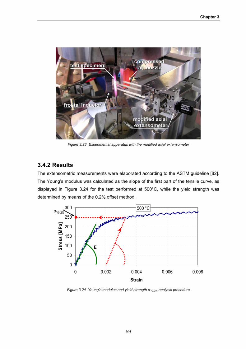
Chapter 3
59
3.4.2 Results The extensometric measurements were elaborated according to the ASTM guideline [82].
The Young’s modulus was calculated as the slope of the first part of the tensile curve, as
displayed in Figure 3.24 for the test performed at 500°C, while the yield strength was
determined by means of the 0.2% offset method.
Figure 3.23 Experimental apparatus with the modified axial extensometer
0
50
100
150
200
250
300
0 0.002 0.004 0.006 0.008
Strain
Stre
ss [M
Pa]
E
500 °CσY0.2%
Figure 3.24 Young’s modulus and yield strength σY0.2% analysis procedure
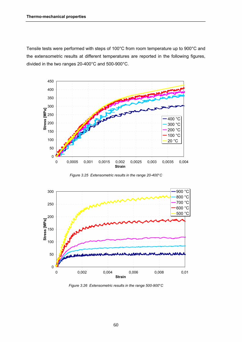
Thermo-mechanical properties
60
Tensile tests were performed with steps of 100°C from room temperature up to 900°C and
the extensometric results at different temperatures are reported in the following figures,
divided in the two ranges 20-400°C and 500-900°C.
0
50
100
150
200
250
300
350
400
450
0 0,0005 0,001 0,0015 0,002 0,0025 0,003 0,0035 0,004Strain
Stre
ss [M
Pa]
400 °C300 °C200 °C100 °C20 °C
Figure 3.25 Extensometric results in the range 20-400°C
0
50
100
150
200
250
300
0 0,002 0,004 0,006 0,008 0,01Strain
Stre
ss [M
Pa]
900 °C800 °C700 °C600 °C500 °C
Figure 3.26 Extensometric results in the range 500-900°C
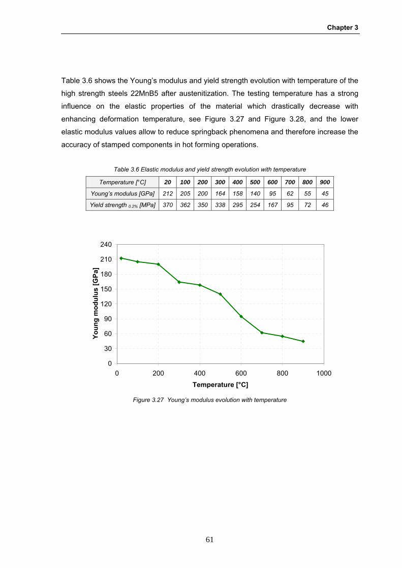
Chapter 3
61
Table 3.6 shows the Young’s modulus and yield strength evolution with temperature of the
high strength steels 22MnB5 after austenitization. The testing temperature has a strong
influence on the elastic properties of the material which drastically decrease with
enhancing deformation temperature, see Figure 3.27 and Figure 3.28, and the lower
elastic modulus values allow to reduce springback phenomena and therefore increase the
accuracy of stamped components in hot forming operations.
Table 3.6 Elastic modulus and yield strength evolution with temperature
Temperature [°C] 20 100 200 300 400 500 600 700 800 900
Young’s modulus [GPa] 212 205 200 164 158 140 95 62 55 45
Yield strength 0.2% [MPa] 370 362 350 338 295 254 167 95 72 46
0
30
60
90
120
150
180
210
240
0 200 400 600 800 1000
Temperature [°C]
Youn
g m
odul
us [G
Pa]
Figure 3.27 Young’s modulus evolution with temperature
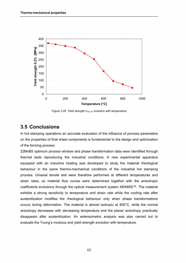
Thermo-mechanical properties
62
3.5 Conclusions In hot stamping operations an accurate evaluation of the influence of process parameters
on the properties of final sheet components is fundamental to the design and optimization
of the forming process.
22MnB5 optimum process window and phase transformation data were identified through
thermal tests reproducing the industrial conditions. A new experimental apparatus
equipped with an inductive heating was developed to study the material rheological
behaviour in the same thermo-mechanical conditions of the industrial hot stamping
process. Uniaxial tensile test were therefore performed at different temperatures and
strain rates, so material flow curves were determined together with the anisotropic
coefficients evolutions through the optical measurement system ARAMIS™. The material
exhibits a strong sensitivity to temperature and strain rate while the cooling rate after
austenitization modifies the rheological behaviour only when phase transformations
occurs during deformation. The material is almost isotropic at 800°C, while the normal
anisotropy decreases with decreasing temperature and the planar anisotropy practically
disappears after austenitization. An extensometric analysis was also carried out to
evaluate the Young’s modulus and yield strength evolution with temperature.
[1] "N.N.; ASTM 03.01."
0
50
100
150
200
250
300
350
400
0 200 400 600 800 1000
Temperature [°C]
Yiel
d st
reng
th 0
.2%
[M
Pa]
Figure 3.28 Yield strength σY0.2% evolution with temperature

Chapter 4
63
4 CHAPTER 4 PHASE TRANSFORMATION KINETICS

Phase transformation kinetics
64
Chapter 4
65
Press hardening is a non-isothermal process where deformation takes place
simultaneously with quenching, therefore particular attention has to be paid to the
evaluation of the influence of applied stress and strain on the phase transformation
kinetics in order to gain more reliable results from the numerical simulations of the hot
stamping operations.
The new experimental apparatus, described in the previous chapter, was used to
determine the 22MnB5 transformation plasticity of phases occurring from austenitization
to room temperature by means of extensometric analyses, as displayed in § 4.1. The
influence of applied stress and strain on the microstructural transformation kinetics of the
material was also investigated and the results regarding the shift of the TTT curves for the
ferritic and bainitic transformation are presented in § 4.2.
4.1 Transformation plasticity The transformation plasticity strain is a plastic strain which arises when a phase
transformation occurs in presence of an applied load, even if this load is lower than the
yield strength of the weaker phase [38]. A permanent strain can appear during phase
transformation due to the differences in the phases specific volumes [83] and this
phenomenon can become more and more relevant when thermal stresses are
superimposed. From this standpoint, it can be deduced that transformation plasticity
appears each time the stress which arises can be considered external with reference to
the growing-up phase.
The 22MnB5 transformation plasticity strain has been therefore evaluated in order to be
implemented in the thermo-mechanical-metallurgical FE models and to increase the
accuracy of the hot forming numerical simulations.
4.1.1 Testing procedure The testing procedure suggested by Taleb [38] was adapted to the new experimental
equipment configuration, described in § 3.4.1, in order to accurately evaluate the
transformation plasticity strain for each phase transformation occurring to 22MnB5 from
austenitization to room temperature. All the tests were carried out on the new apparatus
capable to perform coupled thermal and mechanical cycles and to assure an accurate
control of all testing parameters, during the tests the phase transformation starting and
ending where monitored through the modified axial extensometer.

Phase transformation kinetics
66
The procedure consists of two cycles. In the firs cycle, a free dilatometric test is performed
on the tensile specimen, which is austenitized at 900°C, held in temperature for 3min and
then cooled down until room temperature; the cooling rate is chosen according to the CCT
curves to obtain the desired microstructure. Then the transformation plasticity test is
performed by superimposing a mechanical cycle to the thermal one, by applying a load
just before the onset of the phase transformation to investigate, see Figure 4.1. At the
end, metallographic analyses are performed to be sure that the desired transformation is
achieved and to check the effectiveness of the applied thermal cycle.
The total strain can be calculated as: vptppelthtot εεεεεε ++++= (4.1)
where εtot is the total strain, while εth, εel, εp, εtp, εvp are, respectively, the thermal, elastic,
plastic, transformation plasticity and viscoplastic components of the strain.
Some assumption permit to simplify the calculation by neglecting some contributions in
(4.1). If the applied stress external to the growing-up phase is lower than the yield stress
of the weaker phase present at the beginning of the structural transformation, it can be
supposed that the classic plastic strain εp is negligible. As regards εvp, it seems important
to underline that viscoplasticity is a very complex phenomenon which depends both from
the temperature at which the load is applied and on its duration; moreover its contribution
Time
T [°C]
Ti
Controlledcooling
3 minutes
ti
900
F [MPa]
Time
Time
T [°C]
Ti
Controlledcooling
3 minutes
ti
900
F [MPa]
Time(a) (b)
Figure 4.1 Testing procedure: free dilatometric test (a) and transformation plasticity test (b)
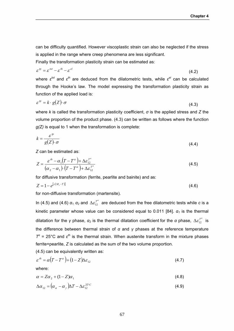
Chapter 4
67
can be difficulty quantified. However viscoplastic strain can also be neglected if the stress
is applied in the range where creep phenomena are less significant.
Finally the transformation plasticity strain can be estimated as: elthtottp εεεε −−= (4.2)
where εtot and εth are deduced from the dilatometric tests, while εel can be calculated
through the Hooke’s law. The model expressing the transformation plasticity strain as
function of the applied load is:
( ) σε ⋅⋅= Zgktp (4.3)
where k is called the transformation plasticity coefficient, σ is the applied stress and Z the
volume proportion of the product phase. (4.3) can be written as follows where the function
g(Z) is equal to 1 when the transformation is complete:
( ) σε
⋅=
Zgk
tp
(4.4)
Z can be estimated as:
( )( ) ( ) α
α
εααεαε
α
α
T
Tth
TTTT
Z1212
121
Δ+−⋅−
Δ+−−= (4.5)
for diffusive transformation (ferrite, pearlite and bainite) and as: ( )[ ]TMc seZ −−= 1 (4.6)
for non-diffusive transformation (martensite).
In (4.5) and (4.6) α1, α2 and α
ε T12Δ are deduced from the free dilatometric tests while c is a
kinetic parameter whose value can be considered equal to 0.011 [84]. α1 is the thermal
dilatation for the γ phase, α2 is the thermal dilatation coefficient for the α phase, α
ε T12Δ is
the difference between thermal strain of α and γ phases at the reference temperature
Tα = 25°C and εth is the thermal strain. When austenite transform in the mixture phases
ferrite+pearlite, Z is calculated as the sum of the two volume proportion.
(4.5) can be equivalently written as:
( ) ( ) 121 εαε α Δ−+−= ZTTth (4.7)
where:
12 )1( ααα ZZ −+= (4.8)
( ) CT °Δ−Δ−=Δ 251212 εααα γα (4.9)

Phase transformation kinetics
68
It is important to underline that the definition of the plasticity coefficients previously
described is valid only for mono-axial tests, in case of multi-axial loads this definition has
to be modified [85].
In the following paragraphs, the experiments carried out to determine the transformation
plasticity of phases in which 22MnB5 can transform during cooling from austenitization
conditions will be described and main results will be discussed.
4.1.2 Ferrite + pearlite The tests were performed on new specimen of 22MnB5 prepared following the ISO 10130
recommendations. The cooling rate was chosen in order to maximize the percentage of
ferrite+pearlite at room temperature, according to the CCT curves of the material (Figure
2.3). The parameters characterizing the thermal cycle are summarized in Table 4.1.
Table 4.1 Thermal cycle parameters
Heating rate [K/s]
Austenitization temp. [°C]
Soaking time [s]
Cooling rate [K/s]
10 900 180 1.5
The occurring of phase transformation can be observed in Figure 4.2. During the heating
phase the dilatation of the specimen and the transformation from α-iron and γ-iron could
be seen.
0
0.002
0.004
0.006
0.008
0.01
0.012
0 200 400 600 800 1000
Temperature [°C]
Axi
al s
trai
n [%
]
Figure 4.2 Stress-free curve
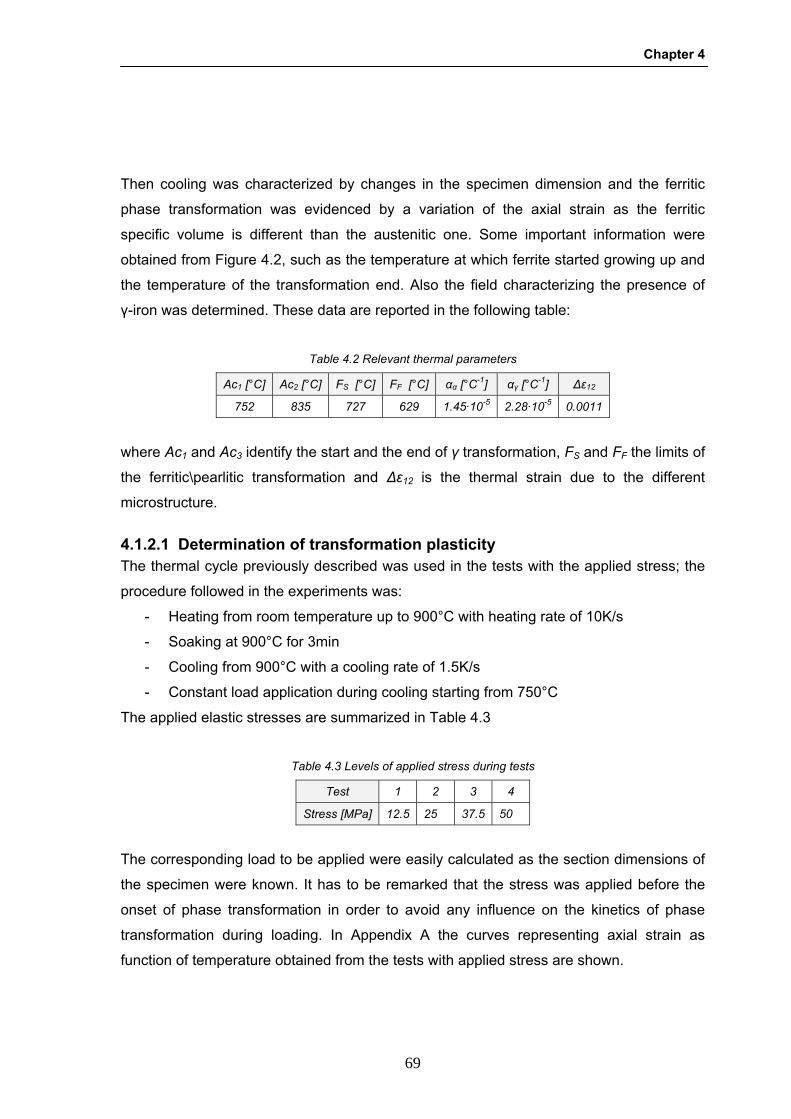
Chapter 4
69
Then cooling was characterized by changes in the specimen dimension and the ferritic
phase transformation was evidenced by a variation of the axial strain as the ferritic
specific volume is different than the austenitic one. Some important information were
obtained from Figure 4.2, such as the temperature at which ferrite started growing up and
the temperature of the transformation end. Also the field characterizing the presence of
γ-iron was determined. These data are reported in the following table:
Table 4.2 Relevant thermal parameters
Ac1 [°C] Ac2 [°C] FS [°C] FF [°C] αα [°C-1] αγ [°C-1] Δε12
752 835 727 629 1.45·10-5 2.28·10-5 0.0011
where Ac1 and Ac3 identify the start and the end of γ transformation, FS and FF the limits of
the ferritic\pearlitic transformation and Δε12 is the thermal strain due to the different
microstructure.
4.1.2.1 Determination of transformation plasticity The thermal cycle previously described was used in the tests with the applied stress; the
procedure followed in the experiments was:
- Heating from room temperature up to 900°C with heating rate of 10K/s
- Soaking at 900°C for 3min
- Cooling from 900°C with a cooling rate of 1.5K/s
- Constant load application during cooling starting from 750°C
The applied elastic stresses are summarized in Table 4.3
Table 4.3 Levels of applied stress during tests
Test 1 2 3 4
Stress [MPa] 12.5 25.3 37.5 50.3
The corresponding load to be applied were easily calculated as the section dimensions of
the specimen were known. It has to be remarked that the stress was applied before the
onset of phase transformation in order to avoid any influence on the kinetics of phase
transformation during loading. In Appendix A the curves representing axial strain as
function of temperature obtained from the tests with applied stress are shown.
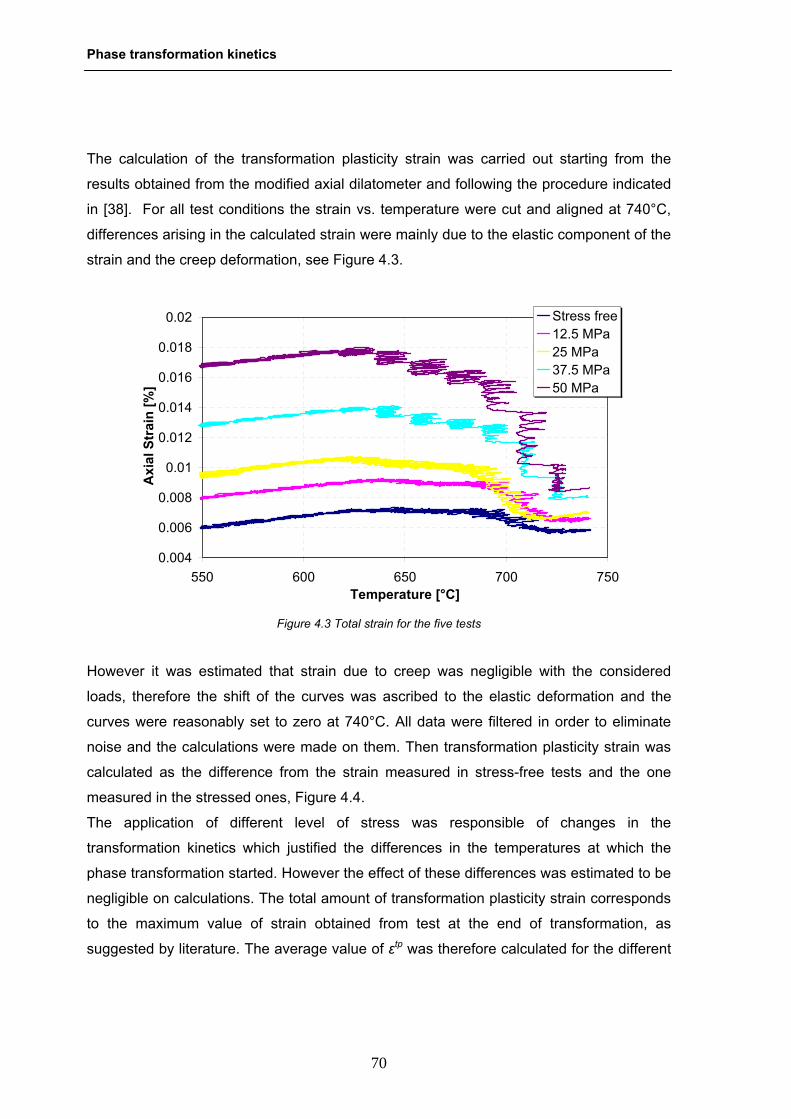
Phase transformation kinetics
70
The calculation of the transformation plasticity strain was carried out starting from the
results obtained from the modified axial dilatometer and following the procedure indicated
in [38]. For all test conditions the strain vs. temperature were cut and aligned at 740°C,
differences arising in the calculated strain were mainly due to the elastic component of the
strain and the creep deformation, see Figure 4.3.
However it was estimated that strain due to creep was negligible with the considered
loads, therefore the shift of the curves was ascribed to the elastic deformation and the
curves were reasonably set to zero at 740°C. All data were filtered in order to eliminate
noise and the calculations were made on them. Then transformation plasticity strain was
calculated as the difference from the strain measured in stress-free tests and the one
measured in the stressed ones, Figure 4.4.
The application of different level of stress was responsible of changes in the
transformation kinetics which justified the differences in the temperatures at which the
phase transformation started. However the effect of these differences was estimated to be
negligible on calculations. The total amount of transformation plasticity strain corresponds
to the maximum value of strain obtained from test at the end of transformation, as
suggested by literature. The average value of εtp was therefore calculated for the different
0.004
0.006
0.008
0.01
0.012
0.014
0.016
0.018
0.02
550 600 650 700 750Temperature [°C]
Axi
al S
trai
n [%
]
Stress free12.5 MPa25 MPa37.5 MPa50 MPa
Figure 4.3 Total strain for the five tests

Chapter 4
71
loads in the plateau zone, as summarized in Table 4.4, and the influence of the applied
true stress on εtp is displayed in Figure 4.5.
0
0.001
0.002
0.003
0.004
0.005
0.006
0.007
0.008
0.009
600 620 640 660 680 700 720 740Temperature [°C]
Tran
sfor
mat
ion
plas
ticity
str
ain
12.5 MPa25 MPa37.5 MPa50 MPa
Figure 4.4 Transformation plasticity strain
0
0.001
0.002
0.003
0.004
0.005
0.006
0.007
0.008
0.009
0 10 20 30 40 50 60
Stress [MPa]
Tran
sfor
mat
ion
plas
ticity
str
ain
Figure 4.5 Transformation plasticity strain as function of the applied load
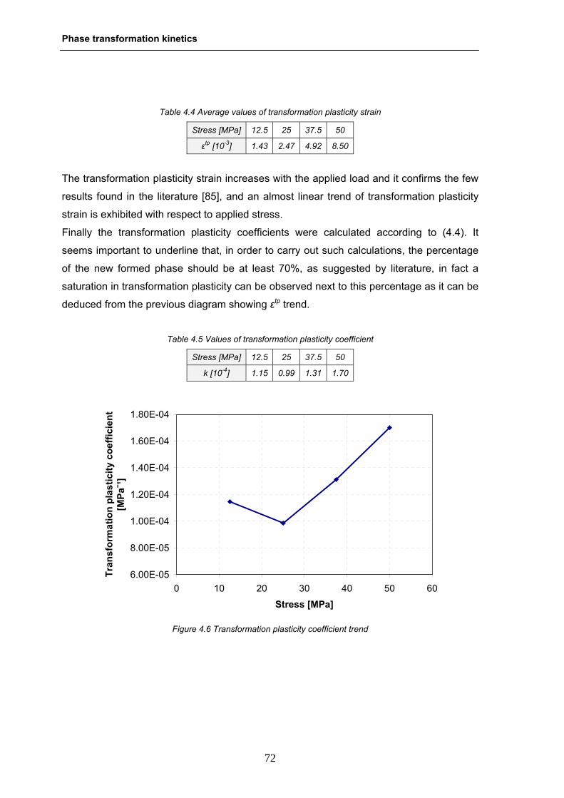
Phase transformation kinetics
72
Table 4.4 Average values of transformation plasticity strain
Stress [MPa] 12.5 25 37.5 50
εtp [10-3] 1.43 2.47 4.92 8.50
The transformation plasticity strain increases with the applied load and it confirms the few
results found in the literature [85], and an almost linear trend of transformation plasticity
strain is exhibited with respect to applied stress.
Finally the transformation plasticity coefficients were calculated according to (4.4). It
seems important to underline that, in order to carry out such calculations, the percentage
of the new formed phase should be at least 70%, as suggested by literature, in fact a
saturation in transformation plasticity can be observed next to this percentage as it can be
deduced from the previous diagram showing εtp trend.
Table 4.5 Values of transformation plasticity coefficient
Stress [MPa] 12.5 25 37.5 50
k [10-4] 1.15 0.99 1.31 1.70
6.00E-05
8.00E-05
1.00E-04
1.20E-04
1.40E-04
1.60E-04
1.80E-04
0 10 20 30 40 50 60
Stress [MPa]
Tran
sfor
mat
ion
plas
ticity
coe
ffici
ent
[MPa
¯¹]
Figure 4.6 Transformation plasticity coefficient trend
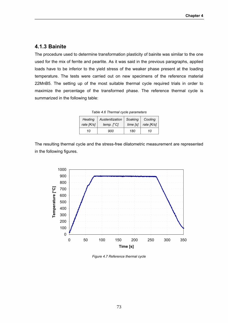
Chapter 4
73
4.1.3 Bainite The procedure used to determine transformation plasticity of bainite was similar to the one
used for the mix of ferrite and pearlite. As it was said in the previous paragraphs, applied
loads have to be inferior to the yield stress of the weaker phase present at the loading
temperature. The tests were carried out on new specimens of the reference material
22MnB5. The setting up of the most suitable thermal cycle required trials in order to
maximize the percentage of the transformed phase. The reference thermal cycle is
summarized in the following table:
Table 4.6 Thermal cycle parameters
Heating rate [K/s]
Austenitization temp. [°C]
Soaking time [s]
Cooling rate [K/s]
10 900 180 10
The resulting thermal cycle and the stress-free dilatometric measurement are represented
in the following figures.
0
100
200
300
400
500
600
700
800
900
1000
0 50 100 150 200 250 300 350
Time [s]
Tem
pera
ture
[°C
]
Figure 4.7 Reference thermal cycle

Phase transformation kinetics
74
The most significant thermal parameters can be obtained from the previous diagram and
they are summarized in Table 4.7. The bainitic transformation starts about 680°C and it
seems to finish about 530°C, while the ferritic and martensitic transformation don’t appear
in the curve. It can be remarked that the initial and the final parts of the curve are not
coincident due to the different specific volume of the microstructures at the two conditions.
Table 4.7 Relevant thermal parameters
Ac1 [°C] Ac2 [°C] BS [°C] BF [°C] αα [°C-1] αγ [°C-1] Δε12
758 842 675 530 1.51·10-5 2.37·10-5 0.0012
where Ac1 and Ac3 identify the start and the end of γ transformation, BS and BF represent
the limit of the bainitic transformation and Δε12 is the thermal strain due to the different
microstructure.
4.1.3.1 Determination of transformation plasticity The thermal cycle previously described was used in the tests with the applied stress and it
was estimated that the most appropriate temperature for the load application was about
700°C; the procedure followed in the experiments was:
- Heating from room temperature up to 900°C with heating rate of 10K/s
- Soaking at 900°C for 3min
0
0.002
0.004
0.006
0.008
0.01
0.012
0 200 400 600 800 1000
Temperature [°C]
Axi
al s
trai
n [%
]
Figure 4.8 Stress-free dilatometric curve
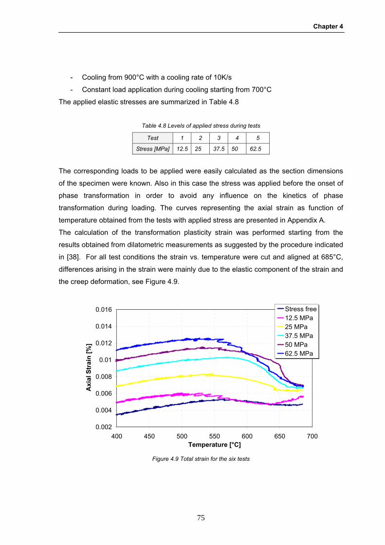
Chapter 4
75
- Cooling from 900°C with a cooling rate of 10K/s
- Constant load application during cooling starting from 700°C
The applied elastic stresses are summarized in Table 4.8
Table 4.8 Levels of applied stress during tests
Test 1 2 3 4 5
Stress [MPa] 12.5 25.3 37.5 50.3 62.5.3
The corresponding loads to be applied were easily calculated as the section dimensions
of the specimen were known. Also in this case the stress was applied before the onset of
phase transformation in order to avoid any influence on the kinetics of phase
transformation during loading. The curves representing the axial strain as function of
temperature obtained from the tests with applied stress are presented in Appendix A.
The calculation of the transformation plasticity strain was performed starting from the
results obtained from dilatometric measurements as suggested by the procedure indicated
in [38]. For all test conditions the strain vs. temperature were cut and aligned at 685°C,
differences arising in the strain were mainly due to the elastic component of the strain and
the creep deformation, see Figure 4.9.
0.002
0.004
0.006
0.008
0.01
0.012
0.014
0.016
400 450 500 550 600 650 700Temperature [°C]
Axi
al S
trai
n [%
]
Stress free12.5 MPa25 MPa37.5 MPa50 MPa62.5 MPa
Figure 4.9 Total strain for the six tests
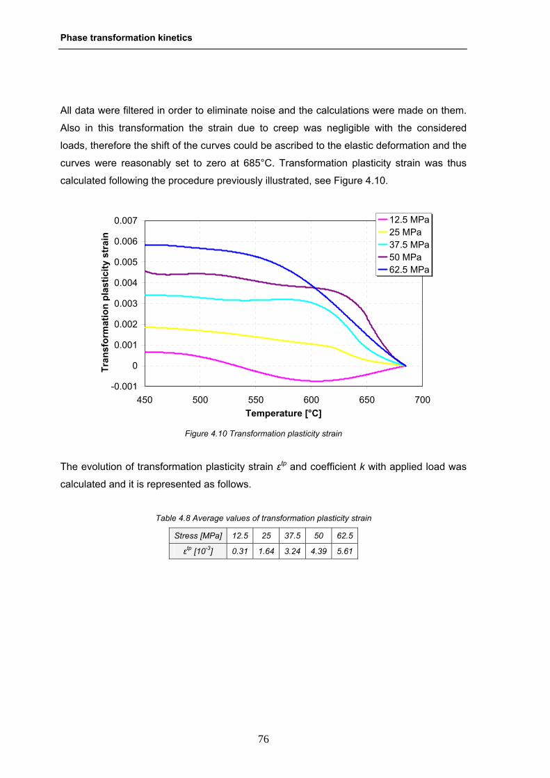
Phase transformation kinetics
76
All data were filtered in order to eliminate noise and the calculations were made on them.
Also in this transformation the strain due to creep was negligible with the considered
loads, therefore the shift of the curves could be ascribed to the elastic deformation and the
curves were reasonably set to zero at 685°C. Transformation plasticity strain was thus
calculated following the procedure previously illustrated, see Figure 4.10.
The evolution of transformation plasticity strain εtp and coefficient k with applied load was
calculated and it is represented as follows.
Table 4.8 Average values of transformation plasticity strain
Stress [MPa] 12.5 25 37.5 50 62.5
εtp [10-3] 0.31 1.64 3.24 4.39 5.61
-0.001
0
0.001
0.002
0.003
0.004
0.005
0.006
0.007
450 500 550 600 650 700Temperature [°C]
Tran
sfor
mat
ion
plas
ticity
str
ain
12.5 MPa25 MPa37.5 MPa50 MPa62.5 MPa
Figure 4.10 Transformation plasticity strain
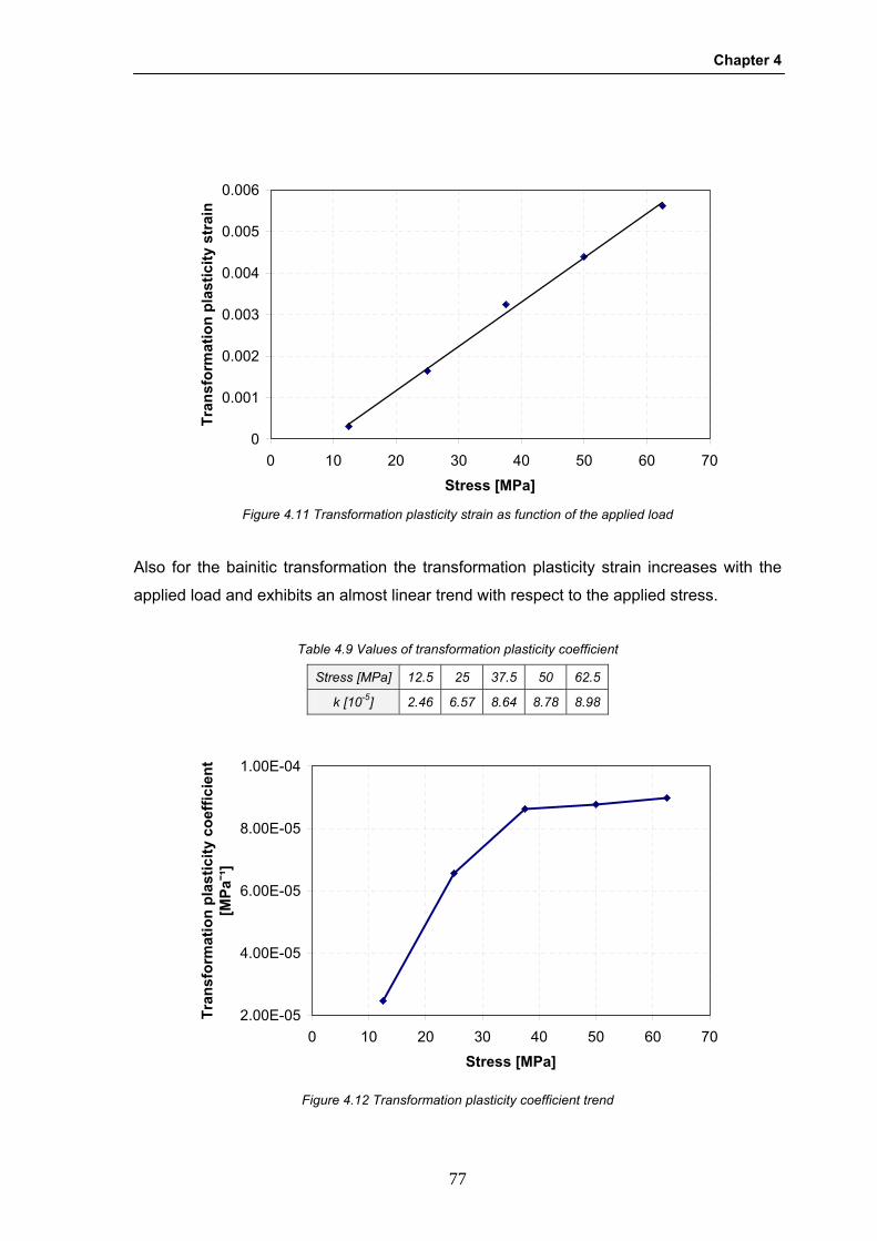
Chapter 4
77
Also for the bainitic transformation the transformation plasticity strain increases with the
applied load and exhibits an almost linear trend with respect to the applied stress.
Table 4.9 Values of transformation plasticity coefficient
Stress [MPa] 12.5 25 37.5 50 62.5
k [10-5] 2.46 6.57 8.64 8.78 8.98
0
0.001
0.002
0.003
0.004
0.005
0.006
0 10 20 30 40 50 60 70
Stress [MPa]
Tran
sfor
mat
ion
plas
ticity
str
ain
Figure 4.11 Transformation plasticity strain as function of the applied load
2.00E-05
4.00E-05
6.00E-05
8.00E-05
1.00E-04
0 10 20 30 40 50 60 70
Stress [MPa]
Tran
sfor
mat
ion
plas
ticity
coe
ffici
ent
[MPa
¯¹]
Figure 4.12 Transformation plasticity coefficient trend
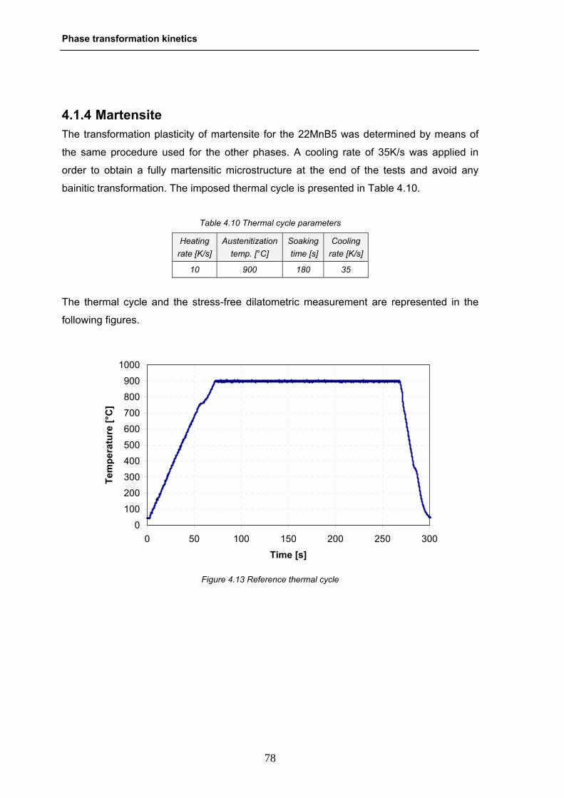
Phase transformation kinetics
78
4.1.4 Martensite The transformation plasticity of martensite for the 22MnB5 was determined by means of
the same procedure used for the other phases. A cooling rate of 35K/s was applied in
order to obtain a fully martensitic microstructure at the end of the tests and avoid any
bainitic transformation. The imposed thermal cycle is presented in Table 4.10.
Table 4.10 Thermal cycle parameters
Heating rate [K/s]
Austenitization temp. [°C]
Soaking time [s]
Cooling rate [K/s]
10 900 180 35
The thermal cycle and the stress-free dilatometric measurement are represented in the
following figures.
0
100
200
300
400
500
600
700
800
900
1000
0 50 100 150 200 250 300
Time [s]
Tem
pera
ture
[°C
]
Figure 4.13 Reference thermal cycle
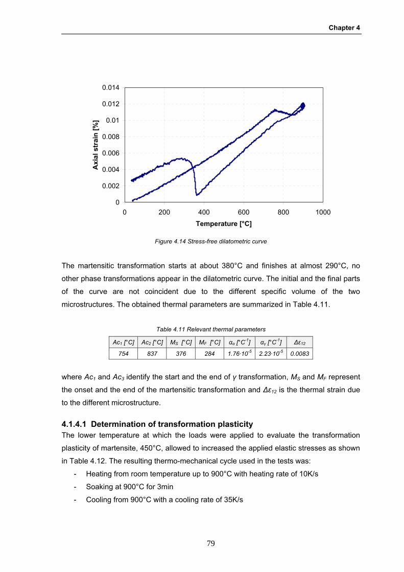
Chapter 4
79
The martensitic transformation starts at about 380°C and finishes at almost 290°C, no
other phase transformations appear in the dilatometric curve. The initial and the final parts
of the curve are not coincident due to the different specific volume of the two
microstructures. The obtained thermal parameters are summarized in Table 4.11.
Table 4.11 Relevant thermal parameters
Ac1 [°C] Ac2 [°C] MS [°C] MF [°C] αα [°C-1] αγ [°C-1] Δε12
754 837 376 284 1.76·10-5 2.23·10-5 0.0083
where Ac1 and Ac3 identify the start and the end of γ transformation, MS and MF represent
the onset and the end of the martensitic transformation and Δε12 is the thermal strain due
to the different microstructure.
4.1.4.1 Determination of transformation plasticity The lower temperature at which the loads were applied to evaluate the transformation
plasticity of martensite, 450°C, allowed to increased the applied elastic stresses as shown
in Table 4.12. The resulting thermo-mechanical cycle used in the tests was:
- Heating from room temperature up to 900°C with heating rate of 10K/s
- Soaking at 900°C for 3min
- Cooling from 900°C with a cooling rate of 35K/s
0
0.002
0.004
0.006
0.008
0.01
0.012
0.014
0 200 400 600 800 1000
Temperature [°C]
Axi
al s
trai
n [%
]
Figure 4.14 Stress-free dilatometric curve
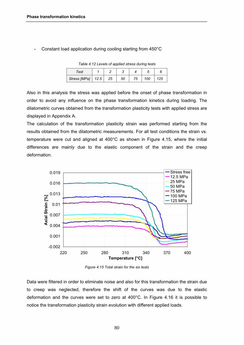
Phase transformation kinetics
80
- Constant load application during cooling starting from 450°C
Table 4.12 Levels of applied stress during tests
Test 1 2 3 4 5 6
Stress [MPa] 12.5 1251 1501 1751 1001 1253
Also in this analysis the stress was applied before the onset of phase transformation in
order to avoid any influence on the phase transformation kinetics during loading. The
dilatometric curves obtained from the transformation plasticity tests with applied stress are
displayed in Appendix A.
The calculation of the transformation plasticity strain was performed starting from the
results obtained from the dilatometric measurements. For all test conditions the strain vs.
temperature were cut and aligned at 400°C as shown in Figure 4.15, where the initial
differences are mainly due to the elastic component of the strain and the creep
deformation.
Data were filtered in order to eliminate noise and also for this transformation the strain due
to creep was neglected, therefore the shift of the curves was due to the elastic
deformation and the curves were set to zero at 400°C. In Figure 4.16 it is possible to
notice the transformation plasticity strain evolution with different applied loads.
-0.002
0.001
0.004
0.007
0.01
0.013
0.016
0.019
220 250 280 310 340 370 400Temperature [°C]
Axi
al S
trai
n [%
]
Stress free12.5 MPa25 MPa50 MPa75 MPa100 MPa125 MPa
Figure 4.15 Total strain for the six tests
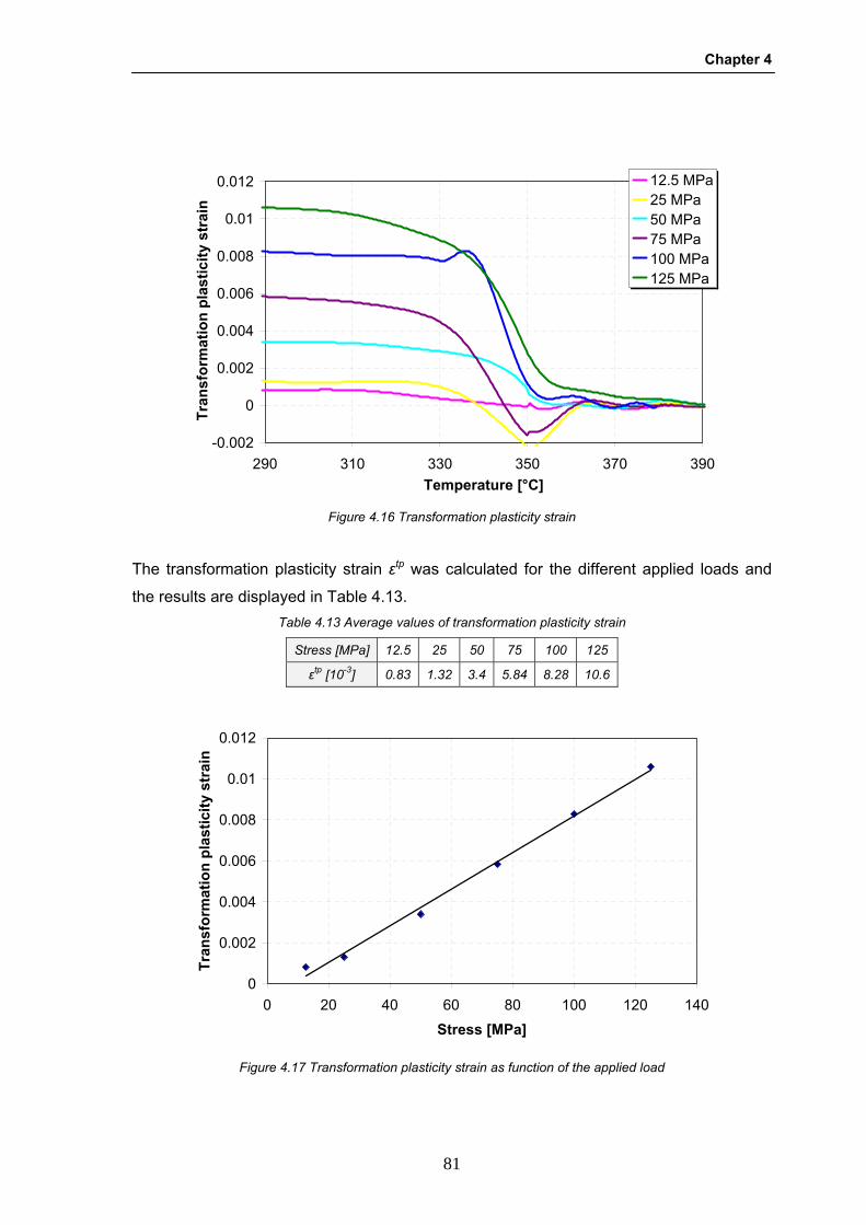
Chapter 4
81
The transformation plasticity strain εtp was calculated for the different applied loads and
the results are displayed in Table 4.13. Table 4.13 Average values of transformation plasticity strain
Stress [MPa] 12.5 25 50 75 100 125
εtp [10-3] 0.83 1.32 3.4 5.84 8.28 10.6
-0.002
0
0.002
0.004
0.006
0.008
0.01
0.012
290 310 330 350 370 390Temperature [°C]
Tran
sfor
mat
ion
plas
ticity
str
ain
12.5 MPa25 MPa50 MPa75 MPa100 MPa125 MPa
Figure 4.16 Transformation plasticity strain
0
0.002
0.004
0.006
0.008
0.01
0.012
0 20 40 60 80 100 120 140
Stress [MPa]
Tran
sfor
mat
ion
plas
ticity
str
ain
Figure 4.17 Transformation plasticity strain as function of the applied load

Phase transformation kinetics
82
The transformation plasticity strain increases with the applied load for martensite as well
as for the other investigated phases and exhibits an almost linear trend with respect to the
applied stress. The transformation plasticity coefficients were finally calculated.
Table 4.14 Values of transformation plasticity coefficient
Stress [MPa] 12.5 25 50 75 100 125
k [10-3 MPa] 6.60 5.28 6.80 7.80 8.28 8.49
4.2 Shift of TTT curves due to applied stress The hot stamping of quenchenable high strength steels is a non-isothermal sheet metal
forming process, in which the final part is produced by combining both the forming and the
hardening stages in a single step through continuous-cooled dies. Thus information given
by CCT and TTT diagrams found in the literature isn’t useful, as they are obtained through
stress-free experiments, because the stress state during deformation may modify the
phase transformation kinetics. The new experimental apparatus described in § 3.4.1 was
therefore used to perform phase transformation tests in order to identify the shift of
22MnB5 TTT curves due to applied stress. After some preliminary tests to evaluate the
most influencing parameters, the influence of applied stresses on the ferritic and bainitic
5.00E-05
5.50E-05
6.00E-05
6.50E-05
7.00E-05
7.50E-05
8.00E-05
8.50E-05
9.00E-05
0 20 40 60 80 100 120 140
Stress [MPa]
Tran
sfor
mat
ion
plas
ticity
coe
ffici
ent
[MPa
¯¹]
Figure 4.18 Transformation plasticity coefficient trend

Chapter 4
83
phase transformation kinetics has been studied in the same range of temperatures typical
of the industrial hot stamping process, as described in the following paragraphs.
4.2.1 Preliminary results The experimental setup used to evaluate the material transformation plasticity was also
utilized to impose coupled thermo-mechanical cycles in order to study the influence of
applied stress and strain on phase transformation kinetics of the 22MnB5. Some
preliminary experiments were carried out in order to evaluate the influence of load
application temperature on the shift of the microstructural transformation onset, and its
sensitivity to both elastic and plastic stresses applied during cooling. To detect the phase
transformation onset the high temperature axial extensometer was used and appropriately
adapted to work as a dilatometer. Specimens were austenitized at 900°C for 3min, then
they were applied a cooling rate of approximately 100K/s down to the testing temperature
to avoid any phase transformation and to assure the holding phase starting with a still fully
metastable austenite. The holding temperature was set equal to 700°C for all the tests
(ferritic transformation) and the reference thermal cycle is summarized in Table 4.15.
Table 4.15 Reference thermal cycle parameters
Heating rate [K/s]
Austenitization temp. [°C]
Soaking time [s]
Cooling rate [K/s]
Holding temp. [°C]
Holding time [s]
15 900 180 100 700 60
In the following figures the thermal cycle and the stress-free dilatometric measurement are
presented, where the change in the slope of the dilatometric curve indicates the onset of
the microstructural transformation (the austenite-to-ferrite one in the this case).
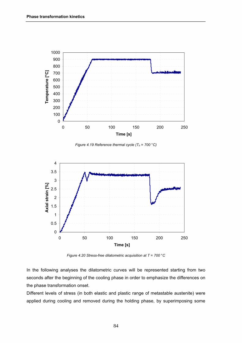
Phase transformation kinetics
84
In the following analyses the dilatometric curves will be represented starting from two
seconds after the beginning of the cooling phase in order to emphasize the differences on
the phase transformation onset.
Different levels of stress (in both elastic and plastic range of metastable austenite) were
applied during cooling and removed during the holding phase, by superimposing some
0
100
200
300
400
500
600
700
800
900
1000
0 50 100 150 200 250
Time [s]
Tem
pera
ture
[°C
]
Figure 4.19 Reference thermal cycle (Th = 700 °C)
0
0.5
1
1.5
2
2.5
3
3.5
4
0 50 100 150 200 250
Time [s]
Axi
al s
trai
n [%
]
Figure 4.20 Stress-free dilatometric acquisition at T = 700 °C
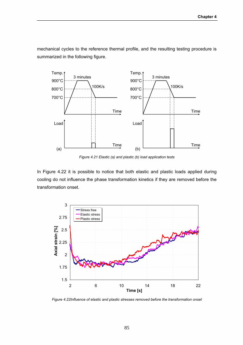
Chapter 4
85
mechanical cycles to the reference thermal profile, and the resulting testing procedure is
summarized in the following figure.
In Figure 4.22 it is possible to notice that both elastic and plastic loads applied during
cooling do not influence the phase transformation kinetics if they are removed before the
transformation onset.
Time
Temp.
800°C 100K/s
3 minutes900°C
Load
Time
700°C
Time
Temp.
800°C 100K/s
3 minutes900°C
Load
Time
700°C
(a) (b) Figure 4.21 Elastic (a) and plastic (b) load application tests
1.5
1.75
2
2.25
2.5
2.75
3
2 6 10 14 18 22Time [s]
Axi
al s
trai
n [%
]
Stress freeElastic stressPlastic stress
Figure 4.22Influence of elastic and plastic stresses removed before the transformation onset
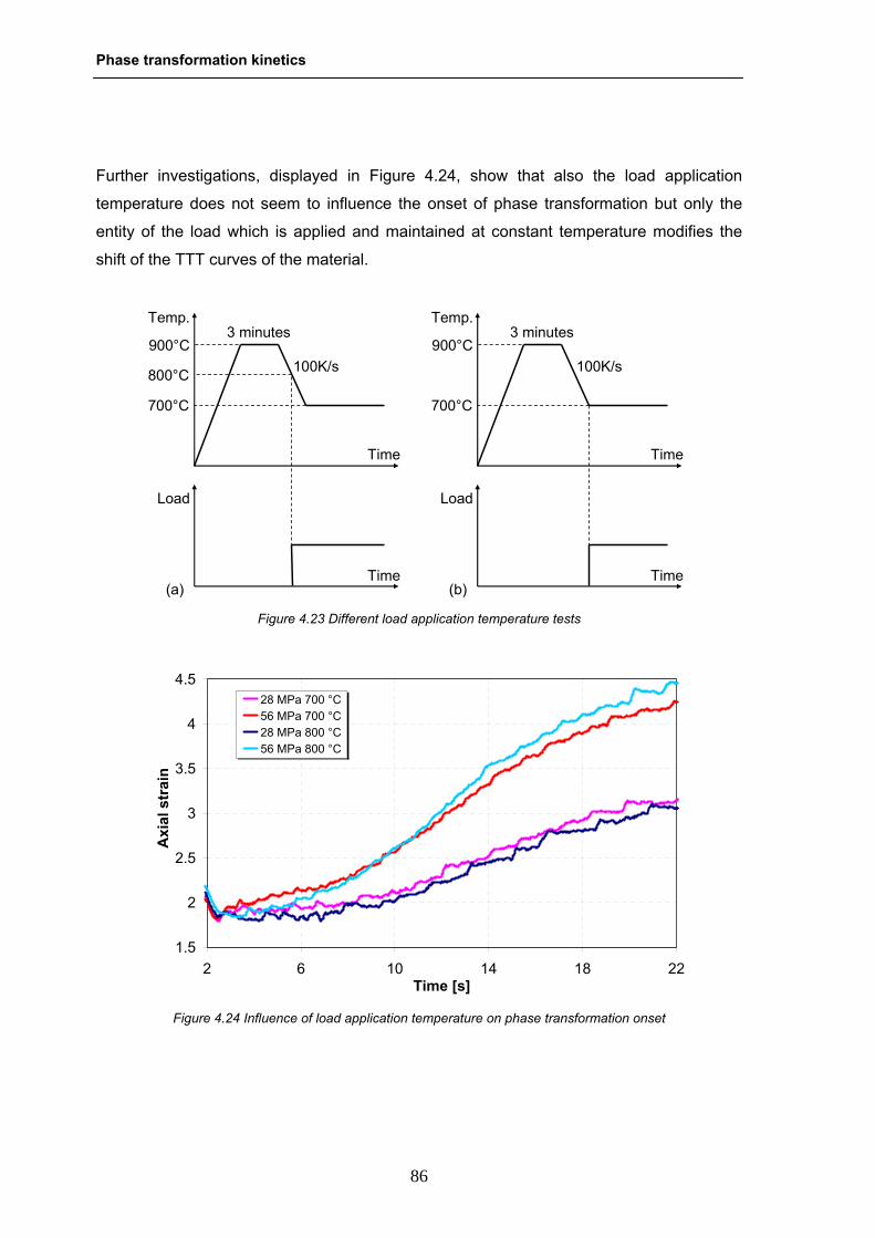
Phase transformation kinetics
86
Further investigations, displayed in Figure 4.24, show that also the load application
temperature does not seem to influence the onset of phase transformation but only the
entity of the load which is applied and maintained at constant temperature modifies the
shift of the TTT curves of the material.
Time
Temp.
800°C 100K/s
3 minutes900°C
Load
Time
700°C
(a)
Time
Temp.
100K/s
3 minutes900°C
Load
Time
700°C
(b) Figure 4.23 Different load application temperature tests
1.5
2
2.5
3
3.5
4
4.5
2 6 10 14 18 22Time [s]
Axi
al s
trai
n
28 MPa 700 °C56 MPa 700 °C28 MPa 800 °C56 MPa 800 °C
Figure 4.24 Influence of load application temperature on phase transformation onset

Chapter 4
87
4.2.2 Ferritic transformation The influence of applied stresses on the 22MnB5 ferritic phase transformation kinetics has
been studied. Specimens were austenitized at 900°C for 3min and cooled down to 700°C
by applying a cooling rate of 100K/s in order to assure the test starting in fully austenitic
conditions. Different σa loads, both elastic and plastic, were applied at 800°C and
maintained during the entire tests and the shift of the onset of the ferritic transformation
were measured by means of the modified axial extensometer. The thermo-mechanical
reference cycle is shown in the next table. The thermal cycle and the stress-free
dilatometric curve are displayed in Figures 4.19-20.
Table 4.16 Thermo-mechanical reference cycle parameters
Heating rate [K/s]
Austenitization temp. [°C]
Soaking time [s]
Cooling rate [K/s]
Holding temp. [°C]
Holding time [s]
Load application temperature [°C]
15 900 180 100 700 60 800
The values of stresses chosen for the experimental campaign are shown in Table 4.17,
where the last value (84MPa) corresponds to a plastic deformation induced in the
specimen.
Table 4.17 Experimental plan for the ferritic phase transformation tests
Test 1 2 3 4
σa [MPa] .0. 28 56 84
Time
Temp.
800°C100K/s
3 minutes900°C
Load
Time
700°C
σa
1 minute
Figure 4.25 Thermo-mechanical reference cycle
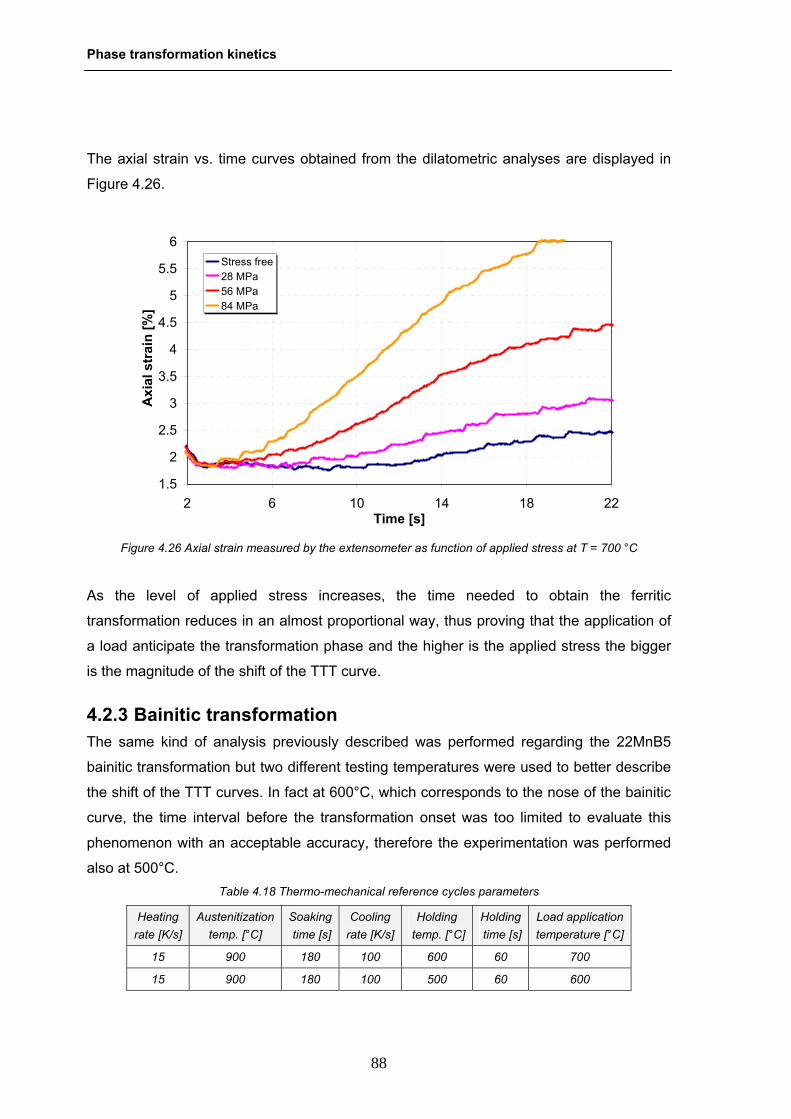
Phase transformation kinetics
88
The axial strain vs. time curves obtained from the dilatometric analyses are displayed in
Figure 4.26.
As the level of applied stress increases, the time needed to obtain the ferritic
transformation reduces in an almost proportional way, thus proving that the application of
a load anticipate the transformation phase and the higher is the applied stress the bigger
is the magnitude of the shift of the TTT curve.
4.2.3 Bainitic transformation The same kind of analysis previously described was performed regarding the 22MnB5
bainitic transformation but two different testing temperatures were used to better describe
the shift of the TTT curves. In fact at 600°C, which corresponds to the nose of the bainitic
curve, the time interval before the transformation onset was too limited to evaluate this
phenomenon with an acceptable accuracy, therefore the experimentation was performed
also at 500°C. Table 4.18 Thermo-mechanical reference cycles parameters
Heating rate [K/s]
Austenitization temp. [°C]
Soaking time [s]
Cooling rate [K/s]
Holding temp. [°C]
Holding time [s]
Load application temperature [°C]
15 900 180 100 600 60 700
15 900 180 100 500 60 600
1.5
2
2.5
3
3.5
4
4.5
5
5.5
6
2 6 10 14 18 22Time [s]
Axi
al s
trai
n [%
]
Stress free28 MPa56 MPa84 MPa
Figure 4.26 Axial strain measured by the extensometer as function of applied stress at T = 700 °C

Chapter 4
89
The values of stresses chosen for the experimental campaign are shown in Table 4.19,
where for each testing temperature the last stress value correspond to a plastic induced
deformation.
Table 4.19 Experimental plan for the bainitic phase transformation tests
T [°C] 600 500
σa [MPa] 28-56-84-112 28-56-84-140
Time
Temp.
700°C100K/s
3 minutes900°C
Load
Time
600°C
σa
1 minute
(a)
Time
Temp.
600°C
100K/s
3 minutes900°C
Load
Time
500°C
σa
1 minute
(b) Figure 4.27 Thermo-mechanical reference cycles for the bainitic transformation kinetics investigation
0
100
200
300
400
500
600
700
800
900
1000
0 50 100 150 200 250
Time [s]
Tem
pera
ture
[°C
]
Figure 4.28 Reference thermal cycle at T = 600 °C
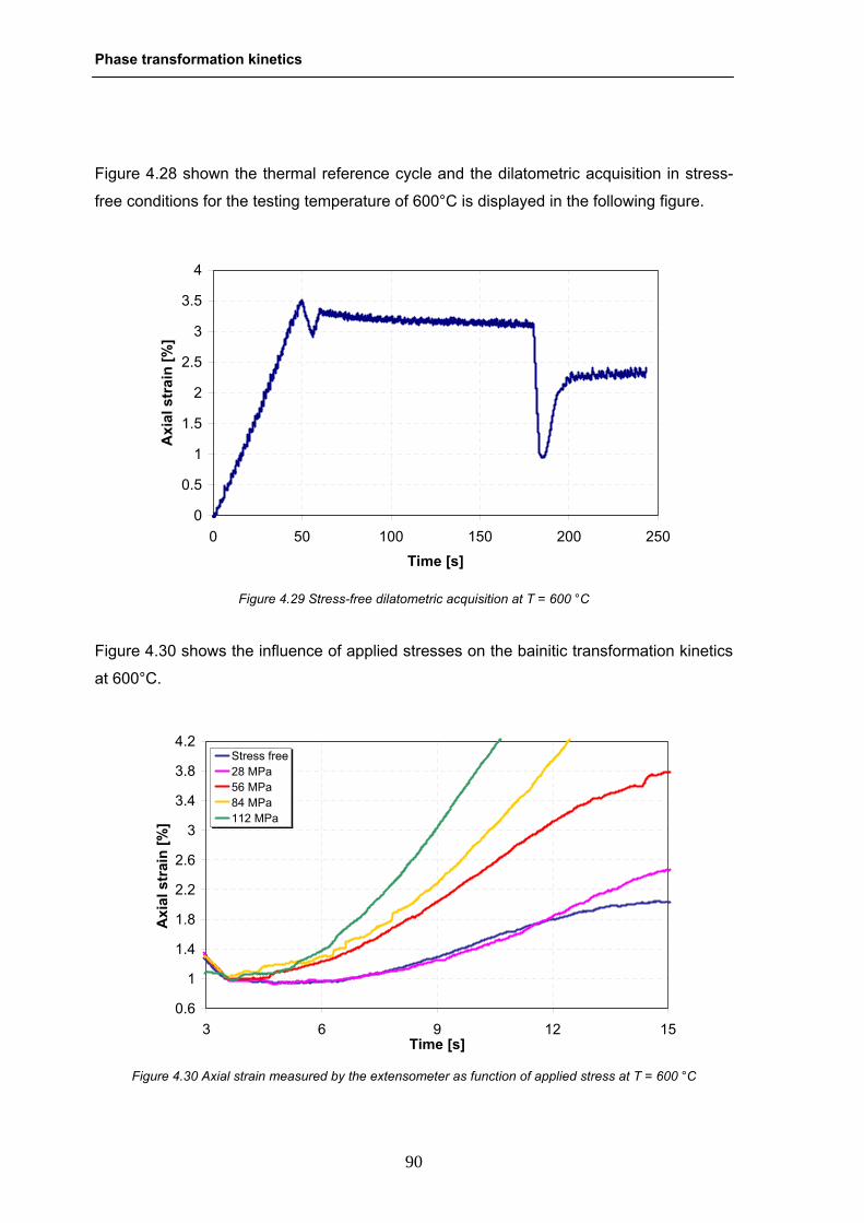
Phase transformation kinetics
90
Figure 4.28 shown the thermal reference cycle and the dilatometric acquisition in stress-
free conditions for the testing temperature of 600°C is displayed in the following figure.
Figure 4.30 shows the influence of applied stresses on the bainitic transformation kinetics
at 600°C.
0
0.5
1
1.5
2
2.5
3
3.5
4
0 50 100 150 200 250
Time [s]
Axi
al s
trai
n [%
]
Figure 4.29 Stress-free dilatometric acquisition at T = 600 °C
0.6
1
1.4
1.8
2.2
2.6
3
3.4
3.8
4.2
3 6 9 12 15Time [s]
Axi
al s
trai
n [%
]
Stress free28 MPa56 MPa84 MPa112 MPa
Figure 4.30 Axial strain measured by the extensometer as function of applied stress at T = 600 °C
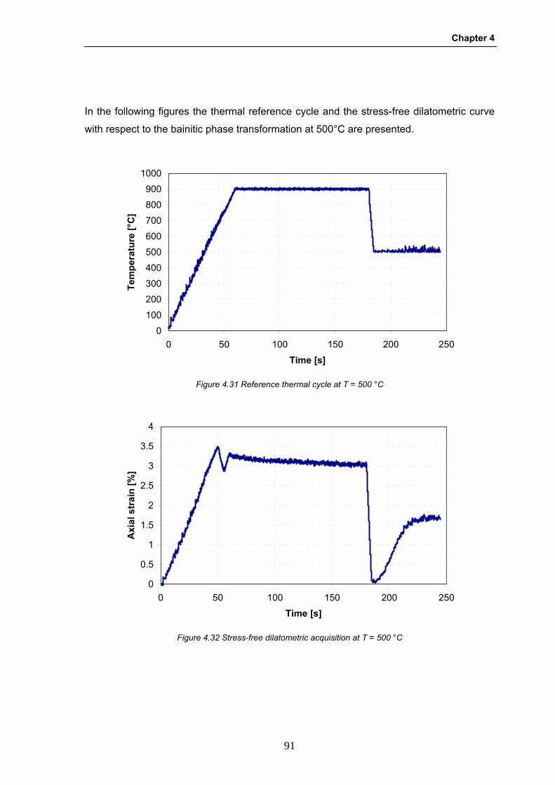
Chapter 4
91
In the following figures the thermal reference cycle and the stress-free dilatometric curve
with respect to the bainitic phase transformation at 500°C are presented.
0
100
200
300
400
500
600
700
800
900
1000
0 50 100 150 200 250
Time [s]
Tem
pera
ture
[°C
]
Figure 4.31 Reference thermal cycle at T = 500 °C
0
0.5
1
1.5
2
2.5
3
3.5
4
0 50 100 150 200 250
Time [s]
Axi
al s
trai
n [%
]
Figure 4.32 Stress-free dilatometric acquisition at T = 500 °C
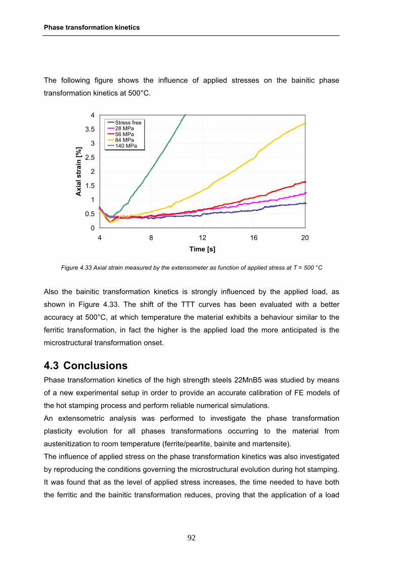
Phase transformation kinetics
92
The following figure shows the influence of applied stresses on the bainitic phase
transformation kinetics at 500°C.
Also the bainitic transformation kinetics is strongly influenced by the applied load, as
shown in Figure 4.33. The shift of the TTT curves has been evaluated with a better
accuracy at 500°C, at which temperature the material exhibits a behaviour similar to the
ferritic transformation, in fact the higher is the applied load the more anticipated is the
microstructural transformation onset.
4.3 Conclusions Phase transformation kinetics of the high strength steels 22MnB5 was studied by means
of a new experimental setup in order to provide an accurate calibration of FE models of
the hot stamping process and perform reliable numerical simulations.
An extensometric analysis was performed to investigate the phase transformation
plasticity evolution for all phases transformations occurring to the material from
austenitization to room temperature (ferrite/pearlite, bainite and martensite).
The influence of applied stress on the phase transformation kinetics was also investigated
by reproducing the conditions governing the microstructural evolution during hot stamping.
It was found that as the level of applied stress increases, the time needed to have both
the ferritic and the bainitic transformation reduces, proving that the application of a load
0
0.5
1
1.5
2
2.5
3
3.5
4
4 8 12 16 20
Time [s]
Axi
al s
trai
n [%
]
Stress free28 MPa56 MPa84 MPa140 MPa
Figure 4.33 Axial strain measured by the extensometer as function of applied stress at T = 500 °C

Chapter 4
93
anticipates the transformation onset and this phenomenon is more pronounced the higher
is the applied stress. When the load, even if plastic, is instead applied before reaching the
testing temperature, but not keep at constant temperature, no shift in the transformation
onset is observed. It must be remarked that stresses were applied at constant
temperature, then the analysed shift regards the TTT curves of the material.

Phase transformation kinetics
94

Chapter 5
95
5 CHAPTER 5 MATERIAL FORMABILITY

Material formability
96
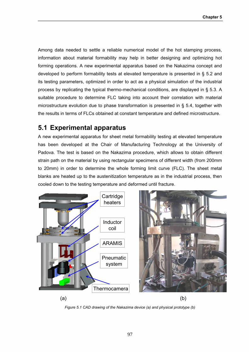
Chapter 5
97
Among data needed to settle a reliable numerical model of the hot stamping process,
information about material formability may help in better designing and optimizing hot
forming operations. A new experimental apparatus based on the Nakazima concept and
developed to perform formability tests at elevated temperature is presented in § 5.2 and
its testing parameters, optimized in order to act as a physical simulation of the industrial
process by replicating the typical thermo-mechanical conditions, are displayed in § 5.3. A
suitable procedure to determine FLC taking into account their correlation with material
microstructure evolution due to phase transformation is presented in § 5.4, together with
the results in terms of FLCs obtained at constant temperature and defined microstructure.
5.1 Experimental apparatus A new experimental apparatus for sheet metal formability testing at elevated temperature
has been developed at the Chair of Manufacturing Technology at the University of
Padova. The test is based on the Nakazima procedure, which allows to obtain different
strain path on the material by using rectangular specimens of different width (from 200mm
to 20mm) in order to determine the whole forming limit curve (FLC). The sheet metal
blanks are heated up to the austenitization temperature as in the industrial process, then
cooled down to the testing temperature and deformed until fracture.
Cartridge heaters
Inductorcoil
ARAMIS
Pneumatic system
Thermocamera
(a) (b)
Figure 5.1 CAD drawing of the Nakazima device (a) and physical prototype (b)
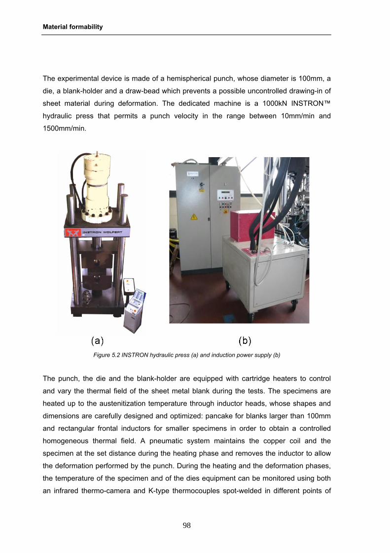
Material formability
98
The experimental device is made of a hemispherical punch, whose diameter is 100mm, a
die, a blank-holder and a draw-bead which prevents a possible uncontrolled drawing-in of
sheet material during deformation. The dedicated machine is a 1000kN INSTRON™
hydraulic press that permits a punch velocity in the range between 10mm/min and
1500mm/min.
The punch, the die and the blank-holder are equipped with cartridge heaters to control
and vary the thermal field of the sheet metal blank during the tests. The specimens are
heated up to the austenitization temperature through inductor heads, whose shapes and
dimensions are carefully designed and optimized: pancake for blanks larger than 100mm
and rectangular frontal inductors for smaller specimens in order to obtain a controlled
homogeneous thermal field. A pneumatic system maintains the copper coil and the
specimen at the set distance during the heating phase and removes the inductor to allow
the deformation performed by the punch. During the heating and the deformation phases,
the temperature of the specimen and of the dies equipment can be monitored using both
an infrared thermo-camera and K-type thermocouples spot-welded in different points of
Figure 5.2 INSTRON hydraulic press (a) and induction power supply (b)
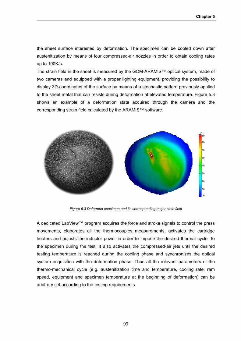
Chapter 5
99
the sheet surface interested by deformation. The specimen can be cooled down after
austenitization by means of four compressed-air nozzles in order to obtain cooling rates
up to 100K/s.
The strain field in the sheet is measured by the GOM-ARAMIS™ optical system, made of
two cameras and equipped with a proper lighting equipment, providing the possibility to
display 3D-coordinates of the surface by means of a stochastic pattern previously applied
to the sheet metal that can resists during deformation at elevated temperature. Figure 5.3
shows an example of a deformation state acquired through the camera and the
corresponding strain field calculated by the ARAMIS™ software.
A dedicated LabView™ program acquires the force and stroke signals to control the press
movements, elaborates all the thermocouples measurements, activates the cartridge
heaters and adjusts the inductor power in order to impose the desired thermal cycle to
the specimen during the test. It also activates the compressed-air jets until the desired
testing temperature is reached during the cooling phase and synchronizes the optical
system acquisition with the deformation phase. Thus all the relevant parameters of the
thermo-mechanical cycle (e.g. austenitization time and temperature, cooling rate, ram
speed, equipment and specimen temperature at the beginning of deformation) can be
arbitrary set according to the testing requirements.
Figure 5.3 Deformed specimen and its corresponding major stain field
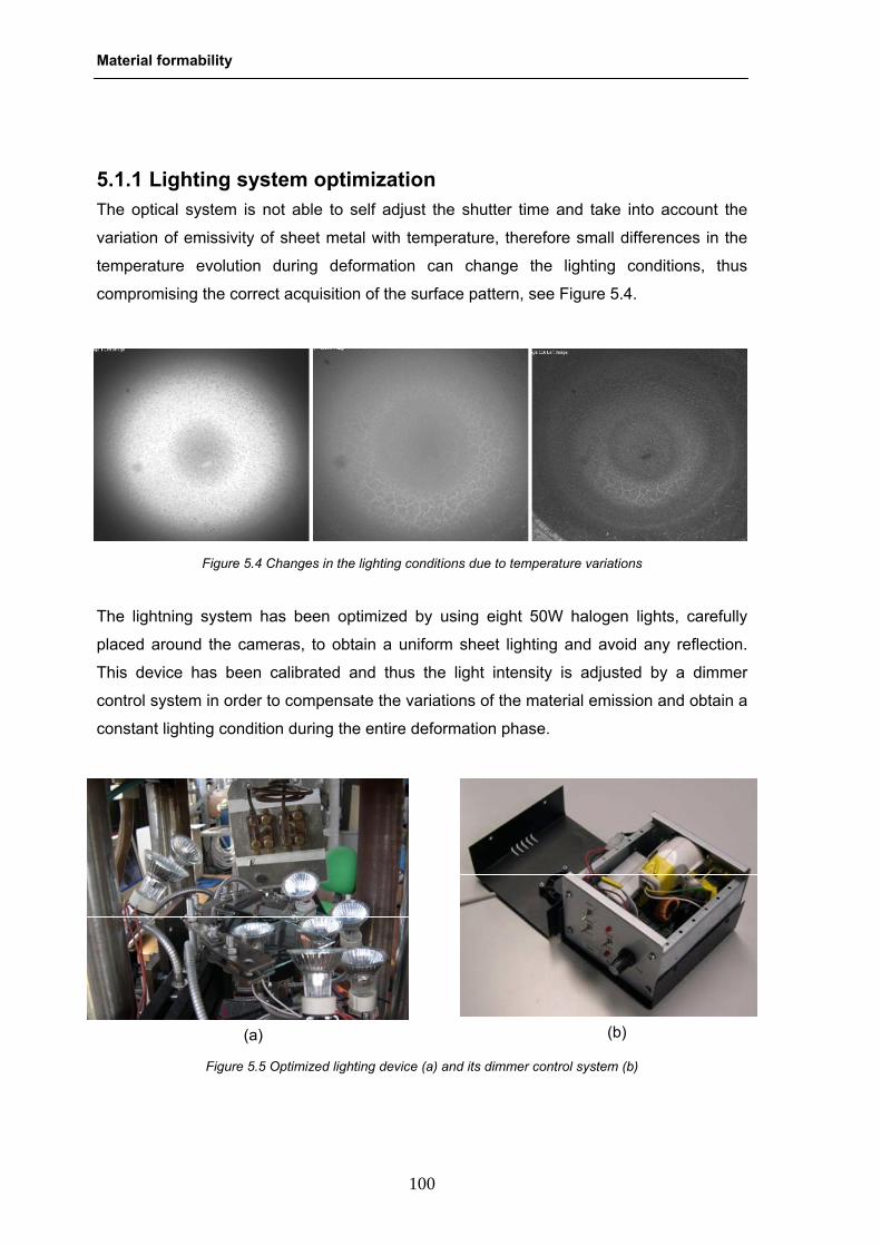
Material formability
100
5.1.1 Lighting system optimization The optical system is not able to self adjust the shutter time and take into account the
variation of emissivity of sheet metal with temperature, therefore small differences in the
temperature evolution during deformation can change the lighting conditions, thus
compromising the correct acquisition of the surface pattern, see Figure 5.4.
The lightning system has been optimized by using eight 50W halogen lights, carefully
placed around the cameras, to obtain a uniform sheet lighting and avoid any reflection.
This device has been calibrated and thus the light intensity is adjusted by a dimmer
control system in order to compensate the variations of the material emission and obtain a
constant lighting condition during the entire deformation phase.
Figure 5.4 Changes in the lighting conditions due to temperature variations
(a) (b)
Figure 5.5 Optimized lighting device (a) and its dimmer control system (b)
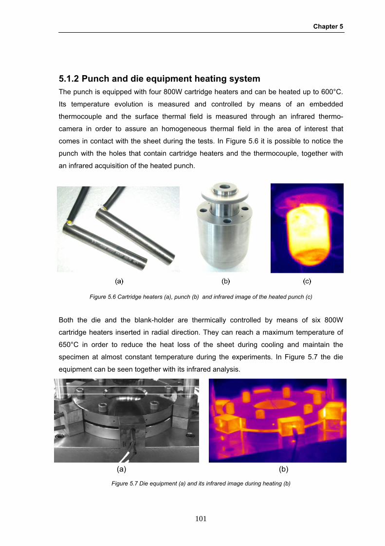
Chapter 5
101
5.1.2 Punch and die equipment heating system The punch is equipped with four 800W cartridge heaters and can be heated up to 600°C.
Its temperature evolution is measured and controlled by means of an embedded
thermocouple and the surface thermal field is measured through an infrared thermo-
camera in order to assure an homogeneous thermal field in the area of interest that
comes in contact with the sheet during the tests. In Figure 5.6 it is possible to notice the
punch with the holes that contain cartridge heaters and the thermocouple, together with
an infrared acquisition of the heated punch.
Both the die and the blank-holder are thermically controlled by means of six 800W
cartridge heaters inserted in radial direction. They can reach a maximum temperature of
650°C in order to reduce the heat loss of the sheet during cooling and maintain the
specimen at almost constant temperature during the experiments. In Figure 5.7 the die
equipment can be seen together with its infrared analysis.
Figure 5.6 Cartridge heaters (a), punch (b) and infrared image of the heated punch (c)
(a) (b)
Figure 5.7 Die equipment (a) and its infrared image during heating (b)
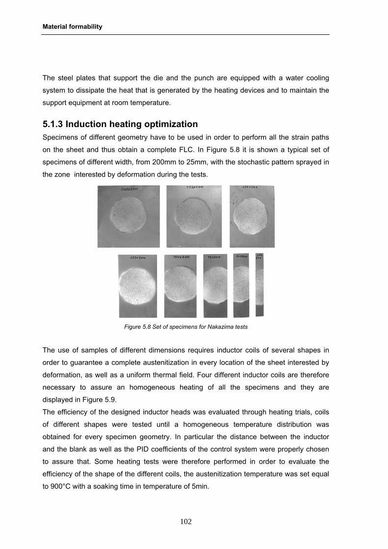
Material formability
102
The steel plates that support the die and the punch are equipped with a water cooling
system to dissipate the heat that is generated by the heating devices and to maintain the
support equipment at room temperature.
5.1.3 Induction heating optimization Specimens of different geometry have to be used in order to perform all the strain paths
on the sheet and thus obtain a complete FLC. In Figure 5.8 it is shown a typical set of
specimens of different width, from 200mm to 25mm, with the stochastic pattern sprayed in
the zone interested by deformation during the tests.
The use of samples of different dimensions requires inductor coils of several shapes in
order to guarantee a complete austenitization in every location of the sheet interested by
deformation, as well as a uniform thermal field. Four different inductor coils are therefore
necessary to assure an homogeneous heating of all the specimens and they are
displayed in Figure 5.9.
The efficiency of the designed inductor heads was evaluated through heating trials, coils
of different shapes were tested until a homogeneous temperature distribution was
obtained for every specimen geometry. In particular the distance between the inductor
and the blank as well as the PID coefficients of the control system were properly chosen
to assure that. Some heating tests were therefore performed in order to evaluate the
efficiency of the shape of the different coils, the austenitization temperature was set equal
to 900°C with a soaking time in temperature of 5min.
Figure 5.8 Set of specimens for Nakazima tests
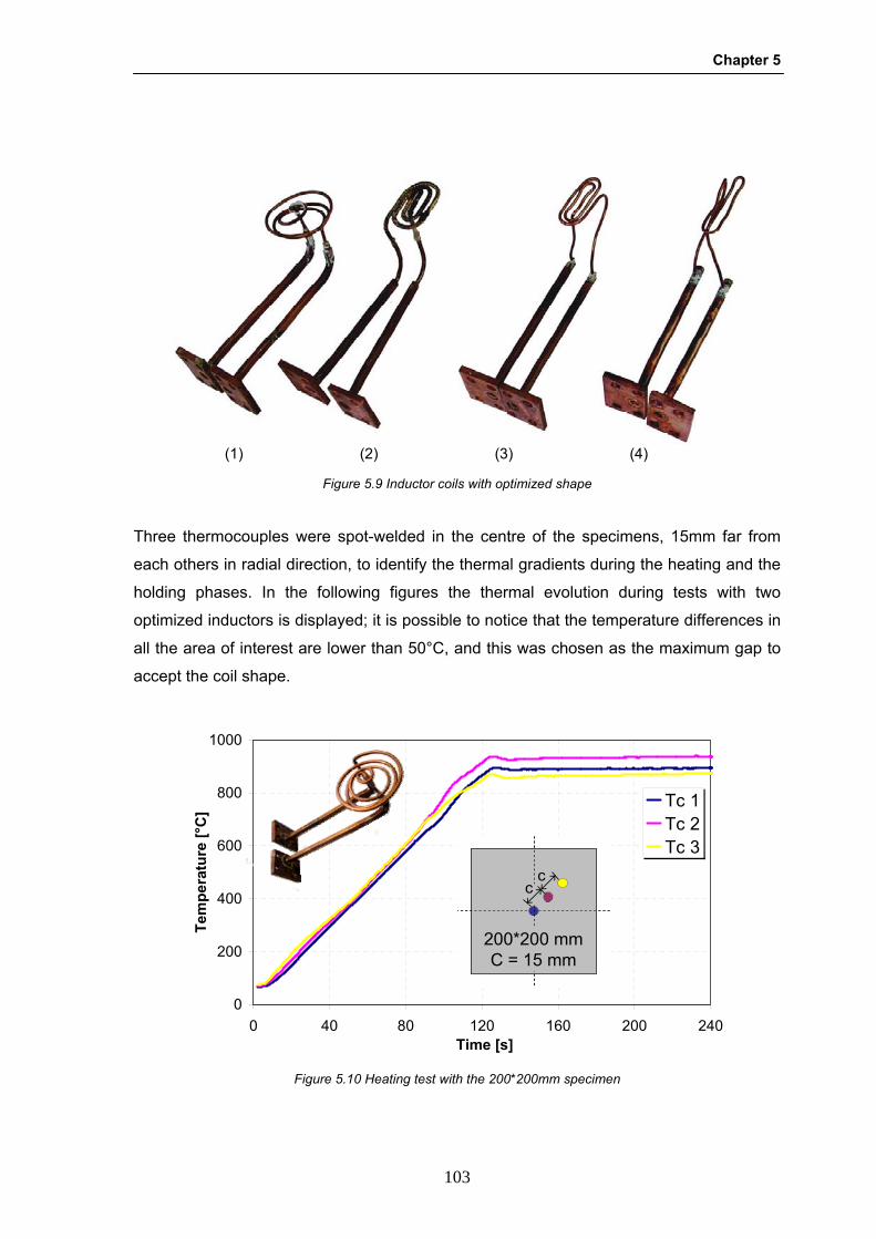
Chapter 5
103
Three thermocouples were spot-welded in the centre of the specimens, 15mm far from
each others in radial direction, to identify the thermal gradients during the heating and the
holding phases. In the following figures the thermal evolution during tests with two
optimized inductors is displayed; it is possible to notice that the temperature differences in
all the area of interest are lower than 50°C, and this was chosen as the maximum gap to
accept the coil shape.
(1) (2) (3) (4) Figure 5.9 Inductor coils with optimized shape
0
200
400
600
800
1000
0 40 80 120 160 200 240Time [s]
Tem
pera
ture
[°C
] Tc 1Tc 2Tc 3
cc
cc
200*200 mmC = 15 mm
Figure 5.10 Heating test with the 200*200mm specimen

Material formability
104
This kind of test was performed for all the samples of different width and Table 5.1 shows
the specimen geometries that can be heated with each inductor coil in order to obtain a
homogeneous temperature distribution.
Table 5.1Inductor types and corresponding specimen widths
Inductor type 1 2 3 4
Specimen width [86] 200, 175 150, 125
100, 75 50 25
5.2 Physical simulation experiments In hot stamping operations an accurate evaluation of the influence of process parameters
on the properties of stamped components is fundamental in the design and optimization of
the forming process. The modified Nakazima device, designed and setup with the above
described features, enabled to carry out physical simulation experiments whose aim was
to reproduce in a controlled environment those variations of the process parameters that
are likely to affect both the material formability and the resulting microstructure of the
component at room temperature. In particular, the influence of punch temperature and
0
200
400
600
800
1000
0 40 80 120 160 200 240Time [s]
Tem
pera
ture
[°C
] Tc 1Tc 2Tc 3
cc
200*75 mmC = 15 mm
Figure 5.11 Heating test with the 200*75mm specimen
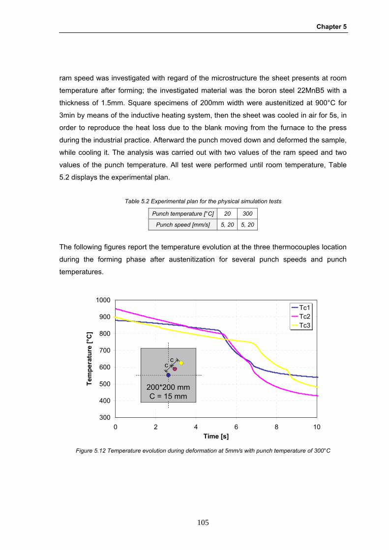
Chapter 5
105
ram speed was investigated with regard of the microstructure the sheet presents at room
temperature after forming; the investigated material was the boron steel 22MnB5 with a
thickness of 1.5mm. Square specimens of 200mm width were austenitized at 900°C for
3min by means of the inductive heating system, then the sheet was cooled in air for 5s, in
order to reproduce the heat loss due to the blank moving from the furnace to the press
during the industrial practice. Afterward the punch moved down and deformed the sample,
while cooling it. The analysis was carried out with two values of the ram speed and two
values of the punch temperature. All test were performed until room temperature, Table
5.2 displays the experimental plan.
Table 5.2 Experimental plan for the physical simulation tests
Punch temperature [°C] 20 300
Punch speed [mm/s] 5, 20 5, 20
The following figures report the temperature evolution at the three thermocouples location
during the forming phase after austenitization for several punch speeds and punch
temperatures.
300
400
500
600
700
800
900
1000
0 2 4 6 8 10Time [s]
Tem
pera
ture
[°C
]
Tc1Tc2Tc3
cc
cc
200*200 mmC = 15 mm
Figure 5.12 Temperature evolution during deformation at 5mm/s with punch temperature of 300°C

Material formability
106
Different test conditions produced various cooling rates and thus different microstructure
at room temperature. Some micrographs were carried out in the area affected by
deformation and Figure 5.15 shows the resulting microstructure in correspondence of the
thermocouple positioned 15mm far from the centre (Tc2) .
300
400
500
600
700
800
900
1000
0 2 4 6 8 10
Time [s]
Tem
pera
ture
[°C
]
Tc1Tc2Tc3
cc
cc
200*200 mmC = 15 mm
Figure 5.13 Temperature evolution during deformation at 5mm/s with punch temperature of 20°C
300
400
500
600
700
800
900
1000
0 2 4 6 8
Time [s]
Tem
pera
ture
[°C
]
Tc1Tc2Tc3
cc
cc
200*200 mmC = 15 mm
Figure 5.14 Temperature evolution during deformation at 20mm/s with punch temperature of 20°C
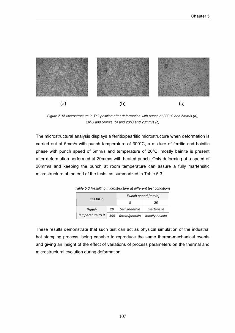
Chapter 5
107
The microstructural analysis displays a ferritic/pearlitic microstructure when deformation is
carried out at 5mm/s with punch temperature of 300°C, a mixture of ferritic and bainitic
phase with punch speed of 5mm/s and temperature of 20°C, mostly bainite is present
after deformation performed at 20mm/s with heated punch. Only deforming at a speed of
20mm/s and keeping the punch at room temperature can assure a fully martensitic
microstructure at the end of the tests, as summarized in Table 5.3.
Table 5.3 Resulting microstructure at different test conditions
Punch speed [mm/s] 22MnB5
5 20
20 bainite/ferrite martensite Punch temperature [°C] 300 ferrite/pearlite mostly bainite
These results demonstrate that such test can act as physical simulation of the industrial
hot stamping process, being capable to reproduce the same thermo-mechanical events
and giving an insight of the effect of variations of process parameters on the thermal and
microstructural evolution during deformation.
Figure 5.15 Microstructure in Tc2 position after deformation with punch at 300°C and 5mm/s (a),
20°C and 5mm/s (b) and 20°C and 20mm/s (c)

Material formability
108
5.3 Forming limit curves determination The investigations described in the previous chapters were performed to evaluate the
material behaviour during press hardening in terms of elastoplastic properties (e.g. flow
curves, anisotropy evolution, Young’s modulus), as function of temperature and strain
rate, and phase transformation kinetics, such as transformation plasticity and shift of the
TTT curves due to applied stress, but their correlation with the process parameters and
the formability characteristics have not been investigated yet. As reliable FE models of the
hot stamping process should require the implementation of Forming Limit Curves at
constant temperature, a new approach is proposed to evaluate material formability and
determine FLC in isothermal conditions taking into account the effects of microstructural
transformation kinetics.
5.3.1 Forming limit curves at elevated temperature in hot stamping operations the material formability is strongly influenced not only by the
stress and strain states, but also by temperature, strain rate and microstructural evolution
during deformation, therefore the well-established approach to determine FLC at room
temperature can be followed only partially. In conventional sheet metal forming at room
temperature material formability is generally described through FLCs obtained by
changing the stress state from balanced biaxial to pure shear. Different kinds of test have
been developed and applied [77] and the Nakazima and the Marciniak are the more
widespread among them. The ISO 12004 [76] standard has been recently improved to
guarantee repeatability in tests conduction and results analysis, but the procedures to
apply this standard to sheet forming at elevated temperature are far from being
established. In particular the FLCs have to be determined at constant temperature and to
be relevant only to one microstructural constituent, when applied to press hardening. The
use of heated tools at testing temperature can assure the uniform thermal profile on the
sheet metal during the test, while the possibility to have only one steel phase during
deformation can be fulfilled only if the material phase transformation kinetics is completely
understood. Particular attention must therefore be paid to properly identify the cooling rate
assuring the whole deformation taking place before phase transformation, in order to
obtain FLCs in fully metastable austenite, which is the most critical condition to be
reproduced. This cannot prescind from an accurate evaluation of the phase transformation
onset as function of both cooling rates and stress conditions characterizing the hot
stamping process.
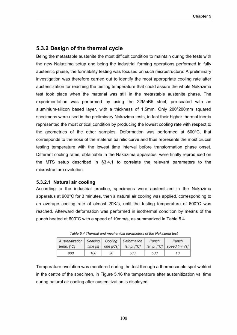
Chapter 5
109
5.3.2 Design of the thermal cycle Being the metastable austenite the most difficult condition to maintain during the tests with
the new Nakazima setup and being the industrial forming operations performed in fully
austenitic phase, the formability testing was focused on such microstructure. A preliminary
investigation was therefore carried out to identify the most appropriate cooling rate after
austenitization for reaching the testing temperature that could assure the whole Nakazima
test took place when the material was still in the metastable austenite phase. The
experimentation was performed by using the 22MnB5 steel, pre-coated with an
aluminium-silicon based layer, with a thickness of 1.5mm. Only 200*200mm squared
specimens were used in the preliminary Nakazima tests, in fact their higher thermal inertia
represented the most critical condition by producing the lowest cooling rate with respect to
the geometries of the other samples. Deformation was performed at 600°C, that
corresponds to the nose of the material bainitic curve and thus represents the most crucial
testing temperature with the lowest time interval before transformation phase onset.
Different cooling rates, obtainable in the Nakazima apparatus, were finally reproduced on
the MTS setup described in §3.4.1 to correlate the relevant parameters to the
microstructure evolution.
5.3.2.1 Natural air cooling According to the industrial practice, specimens were austenitized in the Nakazima
apparatus at 900°C for 3 minutes, then a natural air cooling was applied, corresponding to
an average cooling rate of almost 20K/s, until the testing temperature of 600°C was
reached. Afterward deformation was performed in isothermal condition by means of the
punch heated at 600°C with a speed of 10mm/s, as summarized in Table 5.4.
Table 5.4 Thermal and mechanical parameters of the Nakazima test
Austenitization temp. [°C]
Soaking time [s]
Cooling rate [K/s]
Deformation temp. [°C]
Punch temp. [°C]
Punch speed [mm/s]
900 180 20 600 600 10
Temperature evolution was monitored during the test through a thermocouple spot-welded
in the centre of the specimen, in Figure 5.16 the temperature after austenitization vs. time
during natural air cooling after austenitization is displayed.
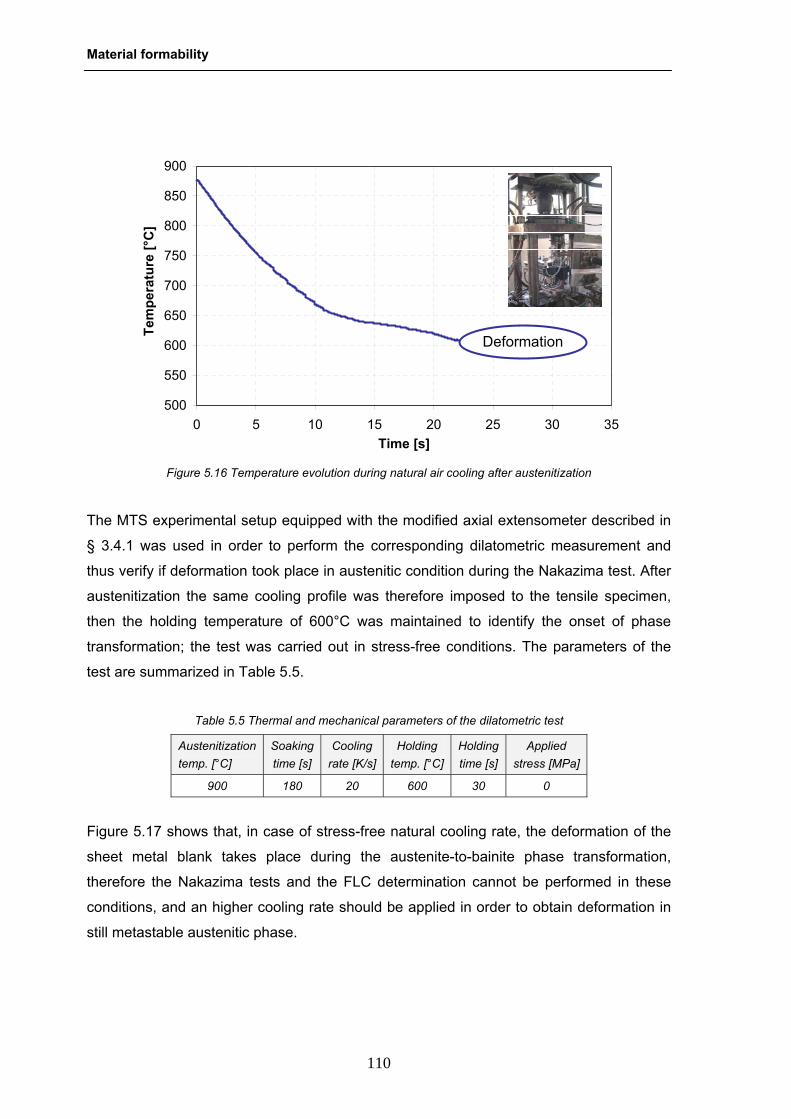
Material formability
110
The MTS experimental setup equipped with the modified axial extensometer described in
§ 3.4.1 was used in order to perform the corresponding dilatometric measurement and
thus verify if deformation took place in austenitic condition during the Nakazima test. After
austenitization the same cooling profile was therefore imposed to the tensile specimen,
then the holding temperature of 600°C was maintained to identify the onset of phase
transformation; the test was carried out in stress-free conditions. The parameters of the
test are summarized in Table 5.5.
Table 5.5 Thermal and mechanical parameters of the dilatometric test
Austenitization temp. [°C]
Soaking time [s]
Cooling rate [K/s]
Holding temp. [°C]
Holding time [s]
Applied stress [MPa]
900 180 20 600 30 0
Figure 5.17 shows that, in case of stress-free natural cooling rate, the deformation of the
sheet metal blank takes place during the austenite-to-bainite phase transformation,
therefore the Nakazima tests and the FLC determination cannot be performed in these
conditions, and an higher cooling rate should be applied in order to obtain deformation in
still metastable austenitic phase.
500
550
600
650
700
750
800
850
900
0 5 10 15 20 25 30 35Time [s]
Tem
pera
ture
[°C
]
Deformation
Figure 5.16 Temperature evolution during natural air cooling after austenitization
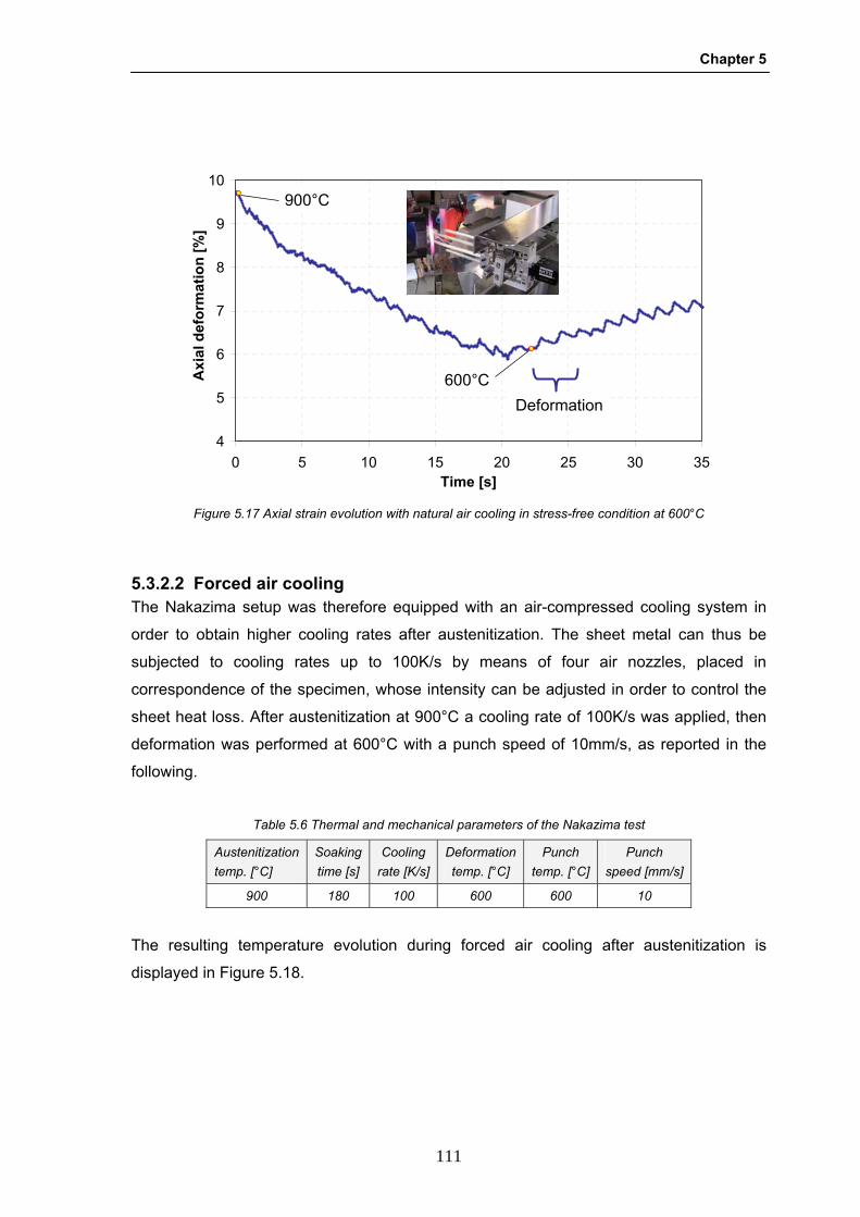
Chapter 5
111
5.3.2.2 Forced air cooling The Nakazima setup was therefore equipped with an air-compressed cooling system in
order to obtain higher cooling rates after austenitization. The sheet metal can thus be
subjected to cooling rates up to 100K/s by means of four air nozzles, placed in
correspondence of the specimen, whose intensity can be adjusted in order to control the
sheet heat loss. After austenitization at 900°C a cooling rate of 100K/s was applied, then
deformation was performed at 600°C with a punch speed of 10mm/s, as reported in the
following.
Table 5.6 Thermal and mechanical parameters of the Nakazima test
Austenitization temp. [°C]
Soaking time [s]
Cooling rate [K/s]
Deformation temp. [°C]
Punch temp. [°C]
Punch speed [mm/s]
900 180 100 600 600 10
The resulting temperature evolution during forced air cooling after austenitization is
displayed in Figure 5.18.
4
5
6
7
8
9
10
0 5 10 15 20 25 30 35Time [s]
Axi
al d
efor
mat
ion
[%]
Deformation600°C
900°C
Figure 5.17 Axial strain evolution with natural air cooling in stress-free condition at 600°C

Material formability
112
The same thermal profile was reproduced in the MTS setup, maintaining the specimen at
600°C after cooling, and the thermo-mechanical parameters of the test are summarized in
Table 5.7.
Table 5.7 Thermal and mechanical parameters of the dilatometric tests
Austenitization temp. [°C]
Soaking time [s]
Cooling rate [K/s]
Holding temp. [°C]
Holding time [s]
Applied stress [MPa]
900 180 100 600 30 0, 112
If a punch speed of 10mm/s is set, then the deformation to failure takes about 2.5s,
therefore the phase transformation at the testing temperature must start after this time
interval. According to the stress-free dilatometric curve displayed in Figure 5.19, the
deformation to failure took place in the constant condition of metastable austenite, before
the bainitic phase transformation onset that corresponds to the increase of the axial strain.
500
550
600
650
700
750
800
850
900
0 2 4 6 8 10Time [s]
Tem
pera
ture
[°C
]
Deformation
Figure 5.18 Temperature evolution during forced air cooling after austenitization
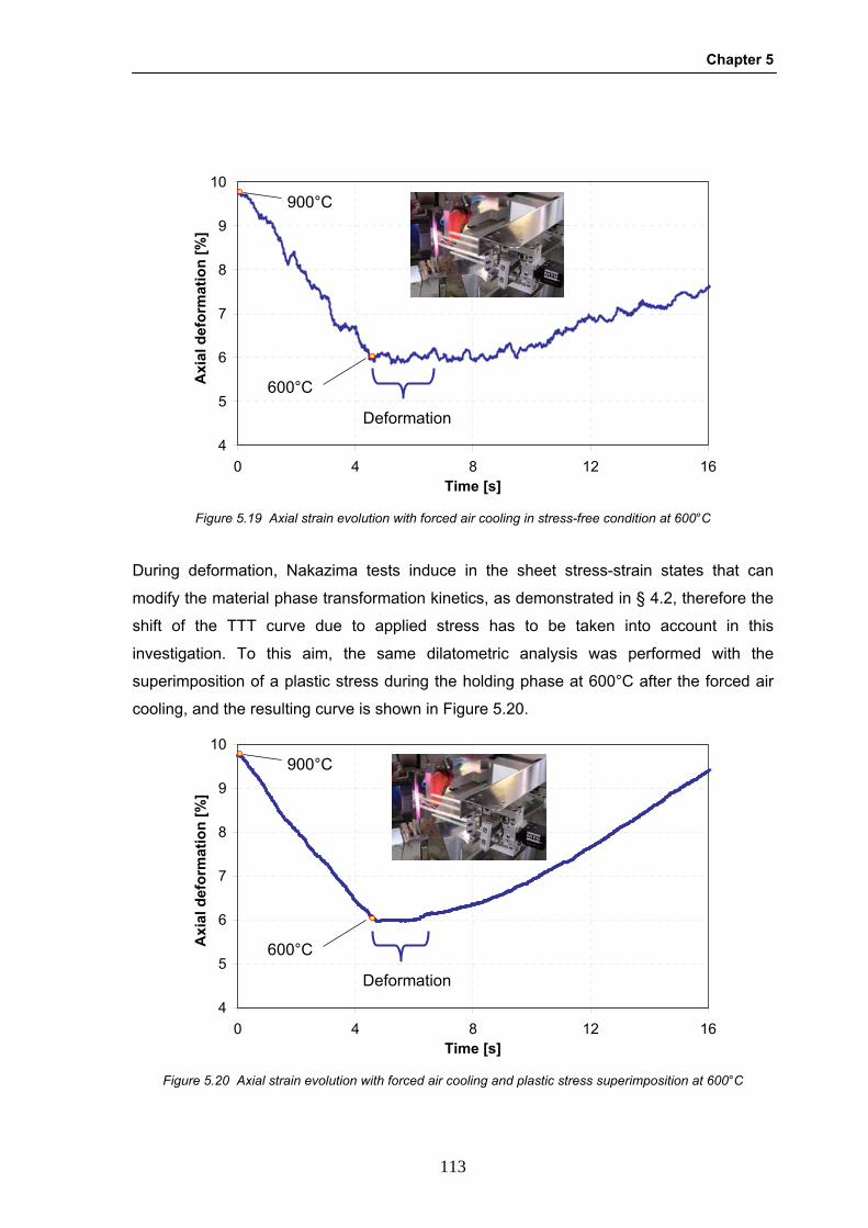
Chapter 5
113
During deformation, Nakazima tests induce in the sheet stress-strain states that can
modify the material phase transformation kinetics, as demonstrated in § 4.2, therefore the
shift of the TTT curve due to applied stress has to be taken into account in this
investigation. To this aim, the same dilatometric analysis was performed with the
superimposition of a plastic stress during the holding phase at 600°C after the forced air
cooling, and the resulting curve is shown in Figure 5.20.
4
5
6
7
8
9
10
0 4 8 12 16Time [s]
Axi
al d
efor
mat
ion
[%]
Deformation
600°C
900°C
Figure 5.19 Axial strain evolution with forced air cooling in stress-free condition at 600°C
4
5
6
7
8
9
10
0 4 8 12 16Time [s]
Axi
al d
efor
mat
ion
[%]
Deformation
600°C
900°C
Figure 5.20 Axial strain evolution with forced air cooling and plastic stress superimposition at 600°C

Material formability
114
Also in this case the dilatometric analysis confirmed that the deformation was performed
in the Nakazima test before the bainitic phase transformation onset, in condition of
metastable austenite. It was then recognized that a cooling rate of 100K/s is suitable to
perform the tests in fully austenite state at the testing temperature of 600°C, and thus also
at lower and higher temperatures where, according to the TTT curves, the transformation
onset is delayed.
5.3.3 Results and discussions The above described Nakazima setup was used to perform tests at high temperature and
obtain FLD in isothermal conditions with the material in a fully metastable austenite state.
The investigated material was the quenchenable high strength steel 22MnB5, 1.5mm
thick. Specimens of different width (from 200mm to 25mm) were austenitized at 900°C for
3min by using inductor coils of different shape, then a rapid cooling rate of 100K/s was
applied, by means of compressed-air jets, until the testing temperature of 600°C was
reach; deformation was therefore carried out with a punch speed of 10mm/s. The surface
punch temperature was set equal to 600°C and it was controlled through a infrared
thermo-camera in order to assure a homogeneous thermal profile in the area of interest;
graphite foils were used to reduce friction at the punch-sheet interface during deformation
and to obtain fracture in correspondence of the apex of the dome. The acquisition rate of
the optical strain measurement system was set equal to 12Hz and the lighting system
candlepower was adjusted to guarantee a good acquisition at the testing temperature. At
least two test runs were performed for each test condition in order to verify the
repeatability. The parameters of the experimental campaign are summarized in Table 5.8.
Table 5.8 Testing parameters of the Nakazima tests
Austenitization temp. [°C]
Soaking time [s]
Cooling rate [K/s]
Testing temp. [°C]
Punch temp. [°C]
Punch speed [mm/s]
Lubricant Frame
rate [Hz]
900 180 100 600 600 10 graphite 12
Figure 5.219 shows the uniformity of temperature profile in the area interested by
deformation of a 200*200mm sheet metal sample acquired through the infrared thermo-
camera just before the beginning of deformation.

Chapter 5
115
Figure 5.22 presents the major and minor logarithmic strains in correspondence of a cross
section of the failure zone, just before fracture occurs. The very pronounced peak in the
major strain represents the post-necking deformation due to the high material sensitivity to
strain rate at elevated temperature and this phenomenon was observed in all tests
conditions.
Formability data were determined for different strain paths, whose range goes from
uniaxial to biaxial tension. One possible representation of these values is represented by
the traditional Forming Limit Curve, elaborated with the indications of the standard ISO
500
540
580
620
660
700
0 15 30 45 60 75
Section Length [mm]
Tem
pera
ture
[°C
]
Figure 5.21 Temperature profile monitored at the end of the cooling phase
0
0.05
0.1
0.15
0.2
0.25
0.3
0.35
0.4
0 10 20 30 40 50 60 70Section Length [mm]
True
Str
ain
Major strainMinor strain
Figure 5.20 Major and minor true strains across the failure zone (200*200mm specimen)

Material formability
116
12004. The standard analysis procedure is implemented in the ARMAIS™ software and it
can be summarized as follows:
- only the last load stage before the crack is computed;
- 3 parallel section, each 2mm apart;
- sections as long as possible, but not up to the edge of the specimen;
- position of the sections for minor strain >0: perpendicular to subsequent crack;
- position of the sections for minor strain <0: as parallel as possible to the edge of
the specimen.
The strain across the deformed test piece is determined and the measured strains are
processed in such way that the necked or failed area is eliminated from the results. The
maximum strain that can be imposed on the material without failing is therefore
determined through interpolation. This maximum of the interpolated curve is thus defined
as the forming limit. Figure 5.23 displays the FLCs determined in isothermal conditions at
600°C, with a punch speed of 10mm/s, and when the material is in a fully metastable
austenite state, together with a set of deformed specimens.
The blue dots represent the FLC obtained through the ISO 12004 procedure, while the
purple ones represent the strains computed at failure. The significant enhancement of
formability in the post-necking is demonstrated by the comparison between the two
0
0.1
0.2
0.3
0.4
0.5
0.6
0.7
-0.2 -0.1 0 0.1 0.2 0.3Minor strain
Maj
or s
trai
n
ISO 12004Failure
Figure 5.21 Forming Limit Curves of 22MnB5 at 600°C in metastable austenite condition

Chapter 5
117
curves. Therefore the increased material formability allowed by deforming at elevated
temperatures during the industrial process can be utilized only in the post-necking
deformation.
A new standard to determine FLC at elevated temperatures should de therefore taken into
account in order to consider the increased post-necking deformation that sheet metal can
undergo during hot forming operations.
5.4 Conclusions The formability of high strength steels, formed and quenched at the same time during
press hardening, has to be investigated under the same process conditions the sheet
experiences during the forming phases. On the other hand, the evaluation of the blank
thinning and eventually fracture through numerical simulation based on FE models
requires the implementation of Forming Limit Curves as function of the various process
parameters. To this aim, a innovative apparatus was developed and the new formability
testing procedure for the investigation of material formability and microstructure
phenomena has been presented. The developed experimental setup can act as a physical
simulation of the industrial hot stamping process, being capable to reproduce the same
thermal and mechanical events and to offer the possibility to evaluate the influence of
testing parameters on thermal and microstructural evolution during deformation. An
accurate methodology for the calibration of the phase transformation parameters and the
temperature control was implemented and the approach was successfully applied to the
determination of the 22MnB5 FLC in metastable austenite state.

Material formability
118

Chapter 6
119
6 CHAPTER 6 NUMERICAL MODEL CALIBRATION

Numerical model calibration
120
Chapter 6
121
Numerical simulations are even more important in the optimization of the hot stamping
operations to obtain the desired mechanical and microstructural properties on final
product. In order to compute reliable FE simulations, a coupled thermo-mechanical-
metallurgical model has to be used.
In § 6.1 the numerical code and the implemented model utilized to take into account the
coupling mechanisms are presented. Particular attention has to be paid to the input data
related to material behaviour and interface phenomena necessary to accurately calibrate
such a model, thus in § 6.2 these data have been determined by combining experimental
techniques and FE inverse analysis. Finally, in § 6.3 the FE model has been validated
through an accurate comparison between the results of physical and numerical
simulations of a formability test.
6.1 Numerical model A fully coupled thermo-mechanical-metallurgical FE model was defined to investigate and
accurately describe phenomena due to the events that occur during industrial hot forming
operations and that significantly influence material behaviour, process performances an
final product features. Details on the code, material rheological and microstructural
behaviour and inter-object interface conditions are given in the following paragraphs.
6.1.1 The FEM code The numerical model developed in this work is a thermo-mechanical-metallurgical model
implemented in the implicit FE code FORGE®. This software enables coupled modelling
of deformation, heat transfer and microstructural evolution for simulation of hot forming
operations, and its main features are briefly described.
All material exhibit a characteristic stress-strain curve that determines how the material
behaves structurally in FE codes. As a material is deformed plastically, the amount of
stress required to incur an incremental amount of deformation is given by the flow stress
curve, which corresponds to the plastic region of the true stress-true-strain curve. Flow
stress is strongly dependent on several parameters, such as temperature, strain rate and
accumulated strain.
The minimum work rate principle is used for accurate calculation of metal flow, thus the
velocity distribution which predicts the lowest work rate is the best approximation of the
actual velocity distribution, and can be expressed mathematically as follows:
Numerical model calibration
122
∫∫ −⋅=S ii
V
dSuFdV.
εσπ (6.1)
∫∫∫ =+−⋅=V
VVS ii
V
dVKdSuFdV 0...
εδεδεσδπ (6.2)
(6.1) is a balance of the body forces versus the surface tractions and it is solved according
to (6.2). The velocities are solved when the variation in the functional is stationary, by
integrating the volumetric strain rate and multiplying by a large constant.
The manner in which the problem is divided into little subproblems that are easier to
formulate is a process called meshing and represents the principle of FEM theory. Bodies
are divided in several elements representing a portion of material and the solutions for
(6.1) and (6.2) are the velocities at each node; FORGE® uses a four nodes tetrahedron
discretization with automatic remeshing procedure. Finally in order to provide a unique
solution to the problem the boundary conditions have to be specified.
6.1.2 Rheology The material rheological behaviour in FORGE® is described by the Norton-Hoff law:
( ) .1.
3,...,2 εεε−
⎟⎟⎠
⎞⎜⎜⎝
⎛=
m
Tks (6.3)
The deviatoric stress tensor s is linked to the strain rate tensor ε through the consistency
K and the strain rate sensitivity m. The consistency forms a function that depends on the
particular thermo-mechanical conditions and various standard functions that are
integrated in the code. When the consistency is established through a function of the
thermo-mechanical conditions, the strain-hardening power law combined with Arrhenius
law for the temperature T, gives the following equation:
( ) ( ) TneKTKβ
εεε 00, += (6.4)
The constant term K0, the term of strain-hardening regulation ε0, the coefficient of
sensitivity to strain-hardening n and the temperature term β have to be defined.
Another type of evolution available in FORGE® is the Hansel-Spittel rheology defined as
follows:
98754
321 )1( mTmmTmm
mmTmf TeeeA ⋅⋅⋅+⋅⋅⋅⋅⋅= εεεεσ εε && (6.5)
Chapter 6
123
where ε is the equivalent deformation (total strain), ε& the equivalent deformation rate, T
the temperature and A, m1, m2, m3, m4, m5, m7, m8, m9 are the regression coefficients.
6.1.3 Microstructural behaviour The microstructural evolution during cooling is represented through the material TTT
diagrams. The FORGE® module uses information of specific material TTT curves along
with thermal and elastic parameters, information about volume change for phase
transformations and phases expansion parameters. Scheil (2.7) and Jhonson-Mehl-
Avrami (2.6) models describe the germination and growing respectively.
Each phase expands and contracts depending on the temperature. A global thermal
expansion coefficient for the material is obtained through a mix law and the global phase
transformation enthalpy is calculated locally from a mix of each phase transformation
enthalpy as function of temperature.
The model takes into account the plastic deformation (transformation plasticity) generated
by the phase change and the influence of applied stresses on the shift of the
transformation times by using the equation:
i
ii
ttt
D'−
= (6.6)
where the characteristic times it are changed in 'it and the parameter D is defined as a
function of the equivalent stress using a point to point or a polynomial law.
6.1.4 Thermal computation Inside a physical system the temperature evolution is the result of the interaction between
the internal heat conduction and the internal heat dissipation, under the constraints
defined on the boundary zone in terms of imposed temperature or in terms of heat
exchange (radiation, conduction, convection). This temperature evolution can be
described by the following equation together with several boundary conditions:
( )( ).WTgradkdiv
tTc +⋅=δδρ (6.7)
The internal dissipation for the system is typically generated by the plastic deformation,
which dissipates the heat power .W , and can be represented using the Norton-Hoff law:
1..3
+
⋅=⋅⋅=m
ijij KW εηεση (6.8)

Numerical model calibration
124
where η represents the efficiency of deformation.
The radiation affects the area boundary with a flux exchange term Фr, described by the
equation:
( )40
4 TTr −⋅=Φ εσ (6.9)
where σ is the Stefan constant and ε is the material emissivity, T represent the area
boundary local temperature and T0 the exterior area temperature.
The area boundary is affected by the conduction and the convection through the flux
exchange Фc which is defined as follows:
( )0TThc −=Φ (6.10)
where h represents the global heat transfer coefficient (HTC) taking into account
conduction and convection.
Also the friction type dissipation process Фfr can generate heat exchanges at the boundary
and the two concerned bodies share the dissipated power at the interface with flux relative
to their respective effusivity, see (6.11).
1
21
1 +Δ⋅⋅+
=Φ pfr vK
bbb
α (6.11)
where α id the friction coefficient, K the consistency of the material, Δv is the relative
velocity between bodies, p the sensitivity to the sliding speed and bi is the effusivity of the
body when a thermal balanced-sheet is processed, calculated as:
ckb ⋅⋅= ρ (6.12)
where k is the conductivity, ρ the density and c the heat capacity.
The thermal phenomena for an area with a part of its boundary thermically regulated and
a part with heat flux exchanges are summarized in Figure 6.1. A plastic deformation is
additionally submitted to this body.
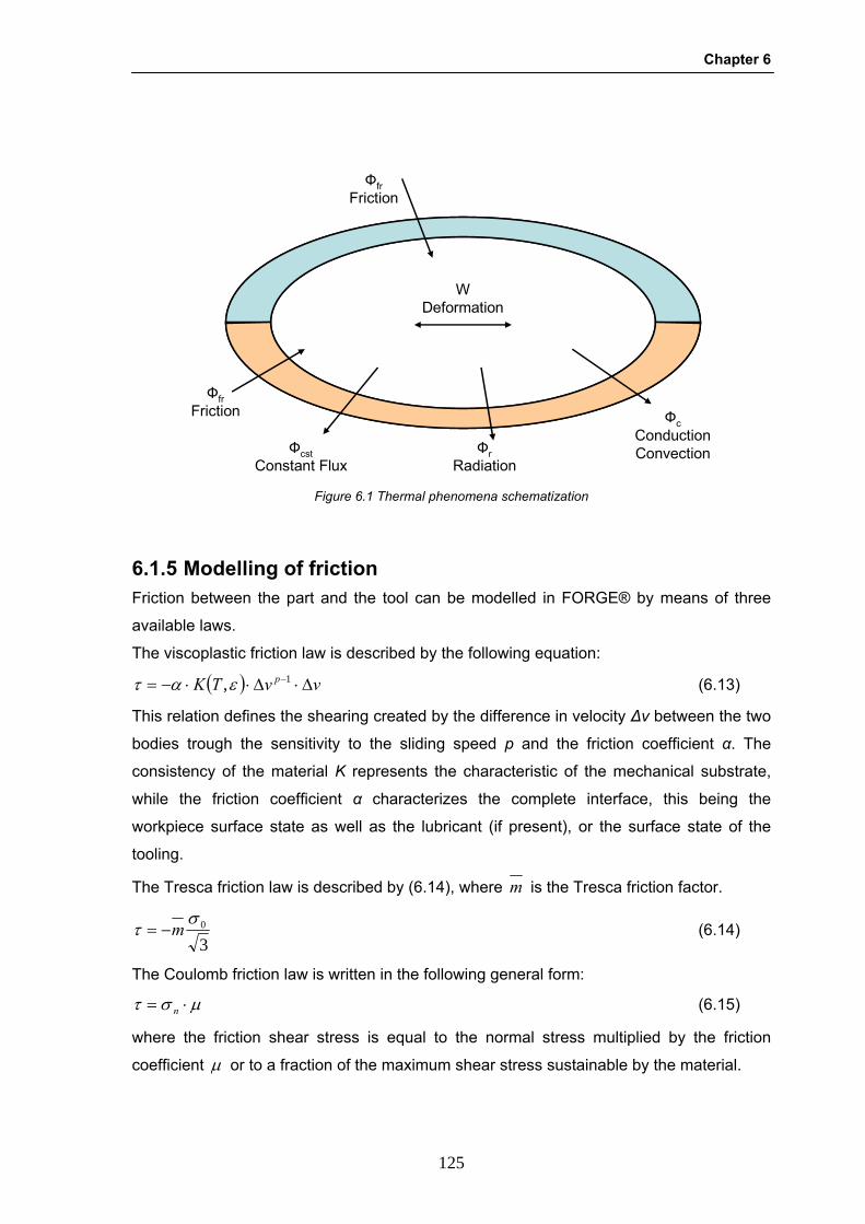
Chapter 6
125
6.1.5 Modelling of friction Friction between the part and the tool can be modelled in FORGE® by means of three
available laws.
The viscoplastic friction law is described by the following equation:
( ) vvTK p Δ⋅Δ⋅⋅−= −1,εατ (6.13)
This relation defines the shearing created by the difference in velocity Δv between the two
bodies trough the sensitivity to the sliding speed p and the friction coefficient α. The
consistency of the material K represents the characteristic of the mechanical substrate,
while the friction coefficient α characterizes the complete interface, this being the
workpiece surface state as well as the lubricant (if present), or the surface state of the
tooling.
The Tresca friction law is described by (6.14), where m is the Tresca friction factor.
30σ
τ m−= (6.14)
The Coulomb friction law is written in the following general form:
μστ ⋅= n (6.15)
where the friction shear stress is equal to the normal stress multiplied by the friction
coefficient μ or to a fraction of the maximum shear stress sustainable by the material.
WDeformation
ФfrFriction
ФfrFriction
ФcstConstant Flux
ФcConductionConvectionФr
Radiation Figure 6.1 Thermal phenomena schematization
Numerical model calibration
126
6.1.6 Thermo-mechanical-metallurgical coupling Most of the mechanical and thermal parameters exhibit a noticeable evolution when the
temperature range is significant. The mechanical equations are generally expressed as
the virtual work principle. A time derivative of the temperature is introduced by a dilatation
term, while the temperature itself is present as result of thermal variation of constitutive
parameters and of boundary conditions. The set of mechanical equations can be therefore
be expressed as:
0,,,.
=⎟⎠⎞
⎜⎝⎛ TTXVR (6.16)
where the array TTXV ,,,.
denote the set of nodal values of velocity, nodal coordinates,
time derivative of temperature and temperature respectively, being:
dtdXV = (6.17)
and
dTdTT =
. (6.18)
The heat equation (6.7) written in integral form can be discretized in finite elements and
the term that contains the velocity is introduced by the heat dissipation of plastic or
viscoplastic work; the heat equation is therefore:
0,,,.
=⎟⎠⎞
⎜⎝⎛ TTXVS (6.19)
The thermal and mechanical coupling is expressed by the ordinary differential equations,
given in implicit form by the nonlinear equations (6.16) and (6.19), and the derivatives in
(6.17) and (6.18).
A Newton-Rapson method is used to resolve simultaneously (6.16) and (6.19). New
values are computed from the increments VΔ and .TΔ starting from the initial value of
V and .T by solving the system:
⎥⎥⎥⎥
⎦
⎤
⎢⎢⎢⎢
⎣
⎡
⎟⎠⎞
⎜⎝⎛−
⎟⎠⎞
⎜⎝⎛−
=⎥⎦
⎤⎢⎣
⎡ΔΔ
⎥⎥⎥⎥
⎦
⎤
⎢⎢⎢⎢
⎣
⎡
.
.
.
.
.
,,,
,,,
TTXVS
TTXVR
TV
T
SVS
T
RVR
δ
δδδ
δ
δδδ
(6.20)

Chapter 6
127
where
VRHδδ
= (6.21)
is the usual matrix derivative for the purely mechanical problem,
.T
SCδ
δ= (6.22)
represents the heat capacity matrix fro the thermal problem, TRδδ
is the thermal coupling in
the mechanical equation and VS
δδ
describes the coupling of mechanics on temperature
distribution.
The use of the Newton-Rapson method on all the nodal unknowns significantly increases
the CPU time, therefore an alternative method is utilized by FORGE®, which solves the
mechanical problem alone, then it uses the new velocity field in the heat equation and
solves the time derivative of temperature, afterward the velocity field is updated tacking
into account the new value of .T . If the coupling terms are smaller than the main matrices
the methods converges rapidly and the time time-integration scheme can be chosen
independently.
The integration of microstructural-mechanical coupling introduces equations taking into
account the elastic and elastoplastic component arising during phases transformations
and a Gauss-Seidel algorithm is used to achieve this coupling.
Figure 6.2 shows the thermo-mechanical-microstructural coupling algorithm where ΔTmax
is set by the user and 0 < q < 1. The thermo-microstructural coupled problem is formerly
solved and the calculated time step is utilized to solve the mechanical problem and the
coupling is achieved by iterating the procedure.

Numerical model calibration
128
6.2 Calibration of the numerical model The accurate calibration of the numerical model previously described is a strong
requirement to improve the quality and reliability of numerical simulations of the hot
stamping process. Such a model was therefore calibrated through both material testing
experiments, to determine the rheological and microstructural parameters, and inverse
analysis method to get a feasible heat transfer description. The investigated material was
the boron steel 22MnB5, pre-coated with an aluminium-silicon protective layer, produced
by ARCELOR with the commercial name of USIBOR 1500 P®.
InitializationV0, X0, T0, T0, Y0
.InitializationV0, X0, T0, T0, Y0
.
Thermal resolutionNew temperature TΔt
Microstructural resolutionKinetic calculation fot TΔt
Time Step CalculationΔt
max1max1 TqTTTq nn Δ≅−≤Δ −
Thermo-microstructuralcalculated time step Δt
.Thermo-microstructuralcalculated time step Δt
.
Mechanical resolutionVΔt, X Δt, T Δt, T Δt, Y Δt
.Mechanical resolutionVΔt, X Δt, T Δt, T Δt, Y Δt
.
no
yes
Figure 6.2 Thermo-mechanical-microstructural coupling algorithm

Chapter 6
129
6.2.1 Rheological behaviour characterisation The material rheological characterization is essential for a proper FE model calibration,
therefore the experimental device described in § 3.2 was used to carry out tensile tests at
elevated temperature and thus generate reliable data as function of temperature and
strain rate. The rheological behaviour of the material was described by means of the
Hansel-Spittel model given by (6.5)
98754
321 )1( mTmmTmm
mmTmf TeeeA ⋅⋅⋅+⋅⋅⋅⋅⋅= εεεεσ εε &&
where σ is the stress tensor, ε the strain tensor, έ the strain rate tensor and T the
temperature of the test. The Hansel-Spittel coefficients for the 22MnB5 were determined
by means of a non-linear regression analysis of the flow curves of the material, previously
presented in § 3.2.2. The results are given in Tables 6.1.
Table 6.1 Hansel-Spittel coefficients for 22MnB5 at elevated temperature
A m1 m2 m3 m4 m5 m7 m8 m9
0.18151 -0.00465 0.35149 -0.02881 0.00281 -0.00179 0.13348 0.000020 1.7299
In Figure 6.3 it is possible to notice the comparison between the experimental flow curves
and the numerical description of the 22MnB5 rheological behaviour through the Hansel-
Spittel model.
0
50
100
150
200
250
300
350
400
450
500
0.0 0.1 0.2 0.3 0.4Strain
Stre
ss [M
pa]
ExperimentalNumerical 500°C
650°C
800°C
0.1s¯¹
Figure 6.3 Comparison between 22MnB5 experimental data and Hansel-Spittel numerical model
Numerical model calibration
130
6.2.2 Microstructural behaviour characterization Microstructural data obtained from the experiment presented in § 3.1 were used to
generate the 22MnB5 metallurgical database necessary to calibrate the FE model; in
particular, an average grain size of 27μm was introduced into the code. To accurately
represent the cooling phase and the 22MnB5 phase transformation kinetics, the material
TTT curves (Figure 2.3) were implemented into the FORGE® TTT modulus, tacking into
account the shift of the TTT curves evaluated in § 4.2 according to (6.6). The martensite
start temperature was set equal to 380°C and a value of 300°C was chosen for the
martensite finish temperature. The transformation plasticity strains as function of applied
stress, determined in § 4.1, were also implemented in the model for all the phase
transformations occurring to austenite during cooling (ferritic, bainitic and martensitic).
6.2.3 Heat transfer coefficient determination Hot stamping is a non-isothermal process where deformation takes place simultaneously
with quenching, thus the time-temperature sequence is essential to determine the final
properties of the formed component. The proper determination of the heat transfer
coefficient is therefore a strong requirement to obtain an accurate calibration of the FE
model and perform reliable simulations of hot forming operations. In press hardening the
thermal exchange depends both on the characteristics of materials in contact and on
interface conditions (e.g. temperature, contact pressure, lubricant, surface quality, sliding
length and velocity, etc.). Phenomena occurring at the sheet-die interface are usually
studied by coupling experimental modelling with inverse analysis techniques or analytical
approaches [46]. The experimental apparatus developed and setup at the Chair of
Manufacturing Technology at the University of Erlangen-Nuremberg [10] was used to
perform some quenching tests and evaluate the influence of contact pressure on the
USIBOR 1500 P® heat transfer coefficient through inverse analysis.
6.2.3.1 Experimental apparatus The experimental device developed at the Chair of Manufacturing Technology at the
University of Erlangen-Nuremberg consists of a universal Schenk-Treble testing machine
with a maximum force of 400kN [10, 46]. The lower and the upper tools are symmetrical
and they are equipped with an exchangeable contact plate fixed on a base plate, which is
water cooled in order to guarantee comparable temperature conditions at each test run,
see Figure 6.4.
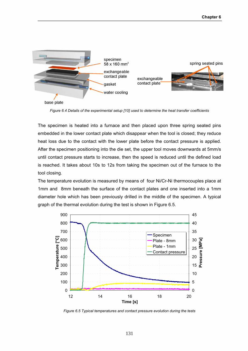
Chapter 6
131
The specimen is heated into a furnace and then placed upon three spring seated pins
embedded in the lower contact plate which disappear when the tool is closed; they reduce
heat loss due to the contact with the lower plate before the contact pressure is applied.
After the specimen positioning into the die set, the upper tool moves downwards at 5mm/s
until contact pressure starts to increase, then the speed is reduced until the defined load
is reached. It takes about 10s to 12s from taking the specimen out of the furnace to the
tool closing.
The temperature evolution is measured by means of four Ni/Cr-Ni thermocouples place at
1mm and 8mm beneath the surface of the contact plates and one inserted into a 1mm
diameter hole which has been previously drilled in the middle of the specimen. A typical
graph of the thermal evolution during the test is shown in Figure 6.5.
Figure 6.4 Details of the experimental setup [10] used to determine the heat transfer coefficients
0
100
200
300
400
500
600
700
800
900
12 14 16 18 20Time [s]
Tem
pera
ture
[°C
]
0
5
10
15
20
25
30
35
40
45
Pres
sure
[MPa
]SpecimenPlate - 8mmPlate - 1mmContact pressure
Figure 6.5 Typical temperatures and contact pressure evolution during the tests

Numerical model calibration
132
6.2.3.2 Experimental results USIBOR 1500 P® sheets produced by ARCELOR, with a thickness of 1.75mm, were used
in this investigation. Specimens were austenitized in the furnace at 950°C for 5min and
then rapidly transferred into the dieset; the experiments were carried out with contact
pressure in the range 5-40MPa. Table 6.2 summarises the main test parameters:
Table 6.2 Testing parameters of the quenching tests
Austenitization temp. [°C]
Soaking time [s]
Contact pressures [MPa]
950 300 5, 10, 20, 30, 40
In Figure 6.6 it is possible to notice the temperature evolutions obtained during cooling by
superimposing different contact pressures.
6.2.3.3 Inverse analysis application The theoretical bases of the inverse analysis approach have been introduce in § 2.2. The
identifications of the parameters is therefore an optimization problem with a final target of
minimizing a cost function Q and needs the following points to be stated:
- a suitable experimental observable choice;
- choice of a proper law describing the physical phenomena;
0
100
200
300
400
500
600
700
800
900
12 13 14 15 16 17 18Time [s]
Tem
pera
ture
[°C
]
5MPa10MPa20MPa30MPa40MPa
Figure 6.6 Experimental thermal evolution with different contact pressures
Chapter 6
133
- definition of the objective function Q;
- definition of a direct model of simulation able to the calculated values Mc by means
of the chosen law starting from a set of parameters;
- definition of a minimizing algorithm;
- choice of a criteria to stop the research.
The method was therefore applied to evaluate the influence of contact pressure on the
heat transfer coefficients at the die-workpiece interface of the experimental results
presented in § 6.2.3.2. Temperature in the centre of the specimen was chosen as
observable entity and a finite element model was used as direct model of simulation. The
least square function (2.20) was chosen as cost function. The minimization algorithm was
a Gauss-Newton method with sensitivity matrix evaluated through finite differences,
jointed to a linear search algorithm inspired to the golden section linear search method.
6.2.3.4 Numerical model of the case study In this investigation the numerical simulations were performed by using the commercial
FE-code FORGE® by TransValor™. This software enables thermo-mechanical-
metallurgical coupled simulations modelling deformation and heat transfer in cold, warm
and hot conditions. The contact plates were modelled as both rigid and deformable bodies
in order to compare the two different approaches.
The rheological behaviour was implemented in the model by means of the 22MnB5
thermo-mechanical parameters described in §6.2.1. The thermal conductivity and specific
heat of the born steel were taken from the literature [87]. The temperature of the dies was
20°C and a specific heat of 461J/kgK was used for the contact plates while modeled as
deformable bodies [13], the thermal and mechanical properties of the tool material were
provided from database, which are shown in Table 6.4. A bilateral-sticking condition was
assumed at the contact plate-specimen interface.
Table 6.3 Mechanical and thermal parameters of the tool material
Young’s modulus [GPa]
Poisson’s ratio
Density [kg/m3]
Conductivity [W/m K)
Specific heat [J/kg K]
210 0.28 7800 23 461

Numerical model calibration
134
Table 6.4 Thermal parameters for 22MnB5
Temperature [°C]
Conductivity [W/m K]
Specific heat [J/kg K]
20 46.1 377
100 46.1 477
200 44.8 511
400 39.8 590
600 34.3 741
800 26.4 821
1000 27.2 821
The simulation was divided into four steps in order to reproduce with a better accuracy the
different phases of the experimental test. The four phases and the corresponding
numerical conditions can be summarized as follows:
1. Natural air cooling, no dies in contact.
2. Upper tool moves downwards, one die in contact.
3. Increasing contact pressure, two dies in contact.
4. Maximum contact pressure, two dies in contact.
The thermal profiles of the specimen and of the dies at the end of each step were
implemented as initial condition in the following step. The initial temperature of the
specimen was assumed to be homogenous and equal to 950°C and the heat loss during
the sheet transfer was simulated by using an heat transfer coefficient with air of 20W/kgK,
reproducing the natural air cooling until the upper die comes in contact with the specimen.
The three-dimensional model of the experimental setup was preliminary compared with
the two-dimensional one in order to evaluate their difference in terms of temperature
evolution. In the following figures the two different models are shown with the contact
plates modelled as deformable dies. In both models a sensor was placed in the middle of
the specimen in order to measure the temperature evolution during the tests.

Chapter 6
135
After the air cooling up to 800°C, the quenching into the dies was simulated assuming
three different heat transfer coefficient for the following steps as reported in Table 6.5.
Table 6.5 Heat transfer coefficients used for the 2D and 3D simulations
Step 1 2 3 4
Heat transfer [MPa]
20 500 2000 4000
The comparison between temperature evolutions with the two models is displayed in
Figure 6.9. The comparison shows a similar temperature evolution during cooling between
the 2D and 3D models, thus the two-dimensional model was used in the investigation to
significantly reduce the simulation time.
Figure 6.7 3D model of the case study
Figure 6.8 2D model of the case study
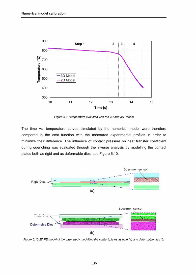
Numerical model calibration
136
The time vs. temperature curves simulated by the numerical model were therefore
compared in the cost function with the measured experimental profiles in order to
minimize their difference. The influence of contact pressure on heat transfer coefficient
during quenching was evaluated through the inverse analysis by modelling the contact
plates both as rigid and as deformable dies, see Figure 6.10.
300
400
500
600
700
800
900
10 11 12 13 14 15
Time [s]
Tem
pera
ture
[°C
]
3D Model2D Model
Step 1 2 3 4
Figure 6.9 Temperature evolution with the 2D and 3D model
(a)
(b) Figure 6.10 2D FE model of the case study modelling the contact plates as rigid (a) and deformable dies (b)
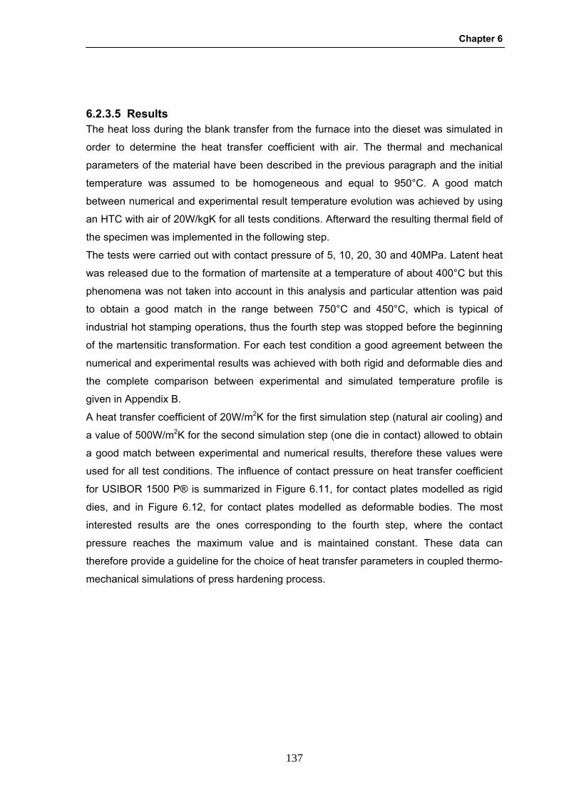
Chapter 6
137
6.2.3.5 Results The heat loss during the blank transfer from the furnace into the dieset was simulated in
order to determine the heat transfer coefficient with air. The thermal and mechanical
parameters of the material have been described in the previous paragraph and the initial
temperature was assumed to be homogeneous and equal to 950°C. A good match
between numerical and experimental result temperature evolution was achieved by using
an HTC with air of 20W/kgK for all tests conditions. Afterward the resulting thermal field of
the specimen was implemented in the following step.
The tests were carried out with contact pressure of 5, 10, 20, 30 and 40MPa. Latent heat
was released due to the formation of martensite at a temperature of about 400°C but this
phenomena was not taken into account in this analysis and particular attention was paid
to obtain a good match in the range between 750°C and 450°C, which is typical of
industrial hot stamping operations, thus the fourth step was stopped before the beginning
of the martensitic transformation. For each test condition a good agreement between the
numerical and experimental results was achieved with both rigid and deformable dies and
the complete comparison between experimental and simulated temperature profile is
given in Appendix B.
A heat transfer coefficient of 20W/m2K for the first simulation step (natural air cooling) and
a value of 500W/m2K for the second simulation step (one die in contact) allowed to obtain
a good match between experimental and numerical results, therefore these values were
used for all test conditions. The influence of contact pressure on heat transfer coefficient
for USIBOR 1500 P® is summarized in Figure 6.11, for contact plates modelled as rigid
dies, and in Figure 6.12, for contact plates modelled as deformable bodies. The most
interested results are the ones corresponding to the fourth step, where the contact
pressure reaches the maximum value and is maintained constant. These data can
therefore provide a guideline for the choice of heat transfer parameters in coupled thermo-
mechanical simulations of press hardening process.
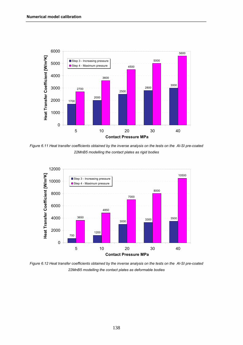
Numerical model calibration
138
1700
25002800
30002700
3600
4500
5000
2000
5600
0
1000
2000
3000
4000
5000
6000
5 10 20 30 40Contact Pressure MPa
Hea
t Tra
nsfe
r Coe
ffici
ent [
W/m
²K]
Step 3 - Increasing pressureStep 4 - Maximum pressure
Figure 6.11 Heat transfer coefficients obtained by the inverse analysis on the tests on the Al-SI pre-coated
22MnB5 modelling the contact plates as rigid bodies
700
3000 3300 35003650
4850
7000
8000
10500
1200
0
2000
4000
6000
8000
10000
12000
5 10 20 30 40Contact Pressure MPa
Hea
t Tra
nsfe
r Coe
ffici
ent [
W/m
²K]
Step 3 - Increasing pressureStep 4 - Maximum pressure
Figure 6.12 Heat transfer coefficients obtained by the inverse analysis on the tests on the Al-SI pre-coated
22MnB5 modelling the contact plates as deformable bodies

Chapter 6
139
6.3 Numerical model validation The numerical model, previously calibrated, was validated through the comparison
between the physical and numerical simulation of a formability test performed on a
USIBOR 1500 P® blank. The thermo-mechanical cycle typical of the hot stamping
process was reproduced by means of the new Nakazima apparatus and the testing
conditions of the deformation phase were implemented in the FE model, in order to
compare the results in terms of stroke vs. force curve and temperature evolution.
6.3.1 Physical simulation of the deformation phase In § 5.2 it has been shown how the new experimental setup, based on the Nakazima
concept, can act as a physical simulation of the hot stamping process by reproducing the
same thermal and mechanical conditions that sheet metal undergoes during hot forming
operations.
Squared specimens of the Al-Si pre-coated boron steel 22MnB5, with a thickness of
1.5mm, were austenitized at 900°C for 3min and cooled in air for 5s to simulate the heat
loos during the blank transfer into the press. Samples were then deformed with the
Figure 6.13 Physical prototype of the experimental setup
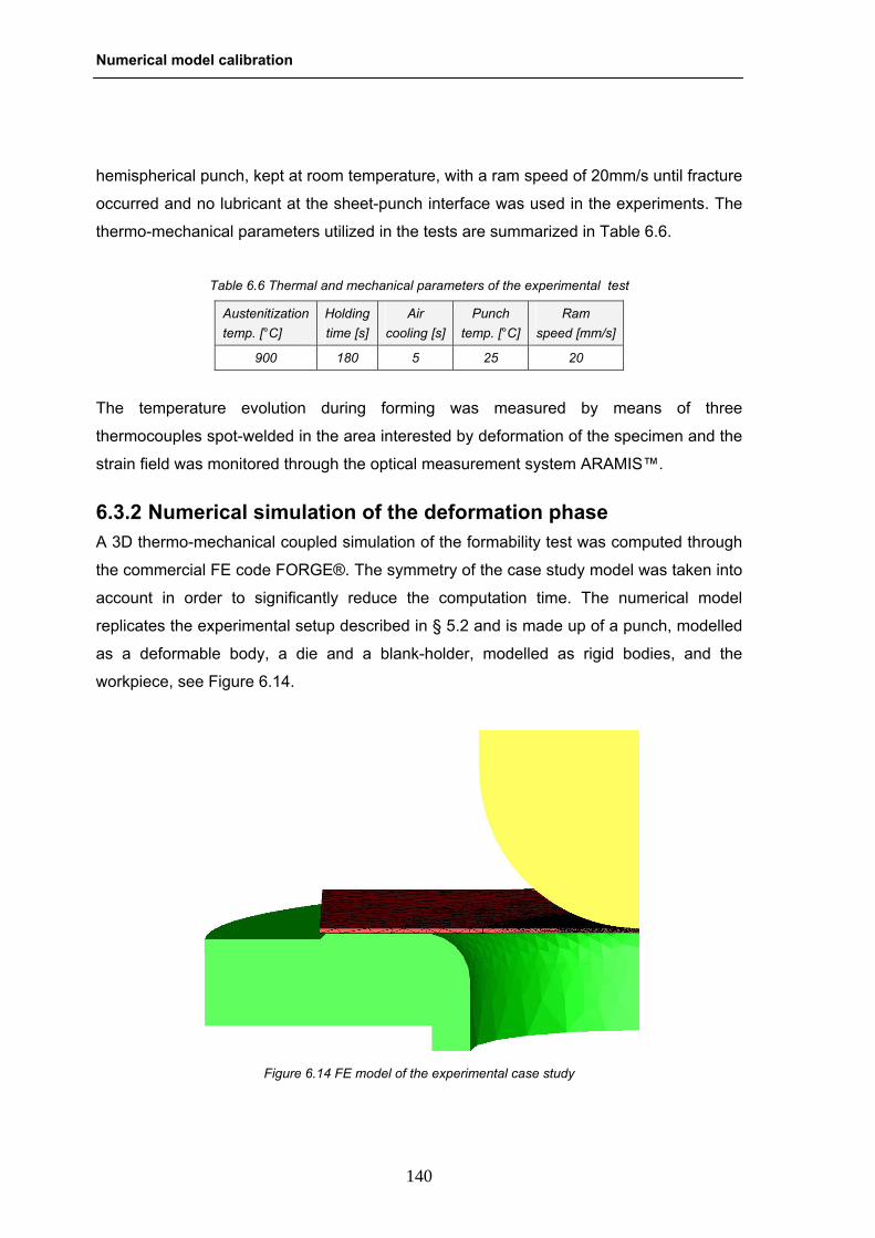
Numerical model calibration
140
hemispherical punch, kept at room temperature, with a ram speed of 20mm/s until fracture
occurred and no lubricant at the sheet-punch interface was used in the experiments. The
thermo-mechanical parameters utilized in the tests are summarized in Table 6.6.
Table 6.6 Thermal and mechanical parameters of the experimental test
Austenitization temp. [°C]
Holding time [s]
Air cooling [s]
Punch temp. [°C]
Ram speed [mm/s]
900 180 5 25 20
The temperature evolution during forming was measured by means of three
thermocouples spot-welded in the area interested by deformation of the specimen and the
strain field was monitored through the optical measurement system ARAMIS™.
6.3.2 Numerical simulation of the deformation phase A 3D thermo-mechanical coupled simulation of the formability test was computed through
the commercial FE code FORGE®. The symmetry of the case study model was taken into
account in order to significantly reduce the computation time. The numerical model
replicates the experimental setup described in § 5.2 and is made up of a punch, modelled
as a deformable body, a die and a blank-holder, modelled as rigid bodies, and the
workpiece, see Figure 6.14.
Figure 6.14 FE model of the experimental case study
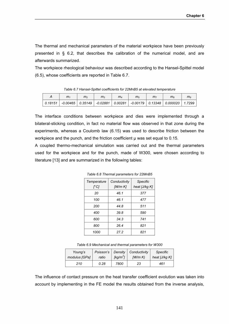
Chapter 6
141
The thermal and mechanical parameters of the material workpiece have been previously
presented in § 6.2, that describes the calibration of the numerical model, and are
afterwards summarized.
The workpiece rheological behaviour was described according to the Hansel-Spittel model
(6.5), whose coefficients are reported in Table 6.7.
Table 6.7 Hansel-Spittel coefficients for 22MnB5 at elevated temperature
A m1 m2 m3 m4 m5 m7 m8 m9
0.18151 -0.00465 0.35149 -0.02881 0.00281 -0.00179 0.13348 0.000020 1.7299
The interface conditions between workpiece and dies were implemented through a
bilateral-sticking condition, in fact no material flow was observed in that zone during the
experiments, whereas a Coulomb law (6.15) was used to describe friction between the
workpiece and the punch, and the friction coefficient μ was set equal to 0.15.
A coupled thermo-mechanical simulation was carried out and the thermal parameters
used for the workpiece and for the punch, made of W300, were chosen according to
literature [13] and are summarized in the following tables:
Table 6.8 Thermal parameters for 22MnB5
Temperature [°C]
Conductivity [W/m K]
Specific heat [J/kg K]
20 46.1 377
100 46.1 477
200 44.8 511
400 39.8 590
600 34.3 741
800 26.4 821
1000 27.2 821
Table 6.9 Mechanical and thermal parameters for W300
Young’s modulus [GPa]
Poisson’s ratio
Density [kg/m3]
Conductivity [W/m K)
Specific heat [J/kg K]
210 0.28 7800 23 461
The influence of contact pressure on the heat transfer coefficient evolution was taken into
account by implementing in the FE model the results obtained from the inverse analysis,
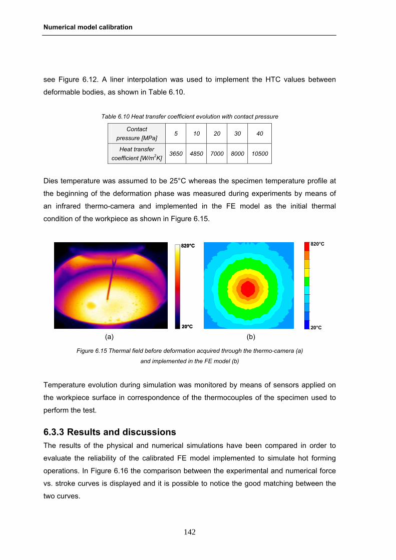
Numerical model calibration
142
see Figure 6.12. A liner interpolation was used to implement the HTC values between
deformable bodies, as shown in Table 6.10.
Table 6.10 Heat transfer coefficient evolution with contact pressure
Contact pressure [MPa]
5 10 20 30 40
Heat transfer coefficient [W/m2K]
3650 4850 7000 8000 10500
Dies temperature was assumed to be 25°C whereas the specimen temperature profile at
the beginning of the deformation phase was measured during experiments by means of
an infrared thermo-camera and implemented in the FE model as the initial thermal
condition of the workpiece as shown in Figure 6.15.
Temperature evolution during simulation was monitored by means of sensors applied on
the workpiece surface in correspondence of the thermocouples of the specimen used to
perform the test.
6.3.3 Results and discussions The results of the physical and numerical simulations have been compared in order to
evaluate the reliability of the calibrated FE model implemented to simulate hot forming
operations. In Figure 6.16 the comparison between the experimental and numerical force
vs. stroke curves is displayed and it is possible to notice the good matching between the
two curves.
820°C
20°C
820°C
20°C
820°C
20°C
(a) (b) Figure 6.15 Thermal field before deformation acquired through the thermo-camera (a)
and implemented in the FE model (b)
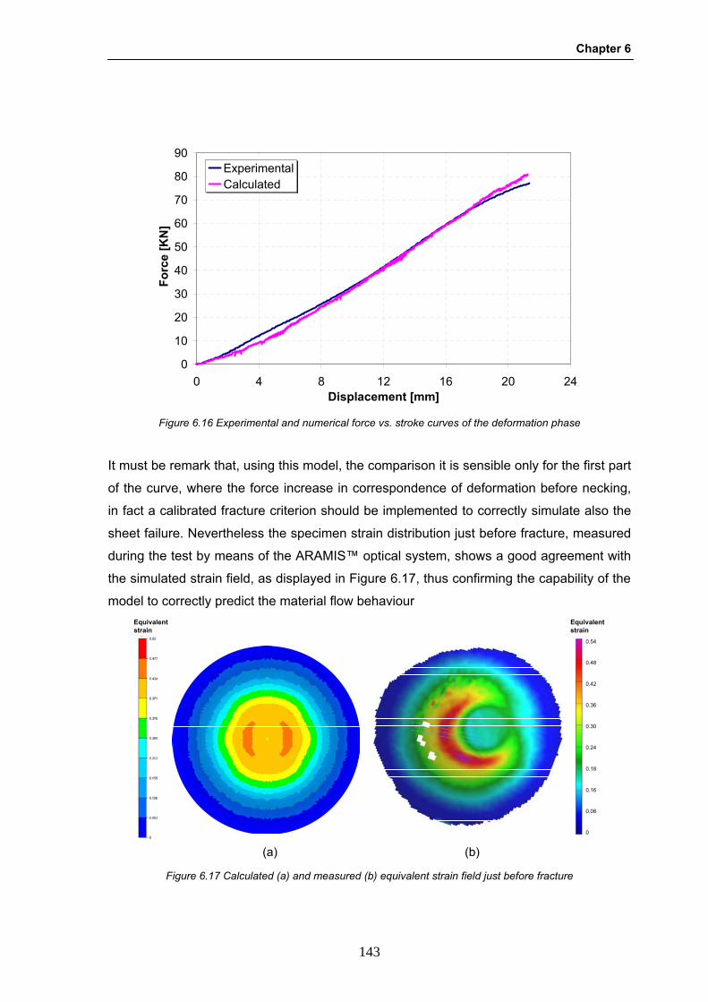
Chapter 6
143
It must be remark that, using this model, the comparison it is sensible only for the first part
of the curve, where the force increase in correspondence of deformation before necking,
in fact a calibrated fracture criterion should be implemented to correctly simulate also the
sheet failure. Nevertheless the specimen strain distribution just before fracture, measured
during the test by means of the ARAMIS™ optical system, shows a good agreement with
the simulated strain field, as displayed in Figure 6.17, thus confirming the capability of the
model to correctly predict the material flow behaviour
0
10
20
30
40
50
60
70
80
90
0 4 8 12 16 20 24Displacement [mm]
Forc
e [K
N]
ExperimentalCalculated
Figure 6.16 Experimental and numerical force vs. stroke curves of the deformation phase
Equivalentstrain
Equivalentstrain
0.54
0.48
0.42
0.36
0.30
0.24
0.18
0.16
0.08
0
(a) (b) Figure 6.17 Calculated (a) and measured (b) equivalent strain field just before fracture
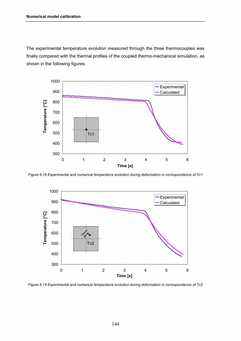
Numerical model calibration
144
The experimental temperature evolution measured through the three thermocouples was
finally compared with the thermal profiles of the coupled thermo-mechanical simulation, as
shown in the following figures.
300
400
500
600
700
800
900
1000
0 1 2 3 4 5 6Time [s]
Tem
pera
ture
[°C
]
ExperimentalCalculated
Tc1
Figure 6.18 Experimental and numerical temperature evolution during deformation in correspondence of Tc1
300
400
500
600
700
800
900
1000
0 1 2 3 4 5 6Time [s]
Tem
pera
ture
[°C
]
ExperimentalCalculated
Tc2
15mm
15mm
Figure 6.19 Experimental and numerical temperature evolution during deformation in correspondence of Tc2
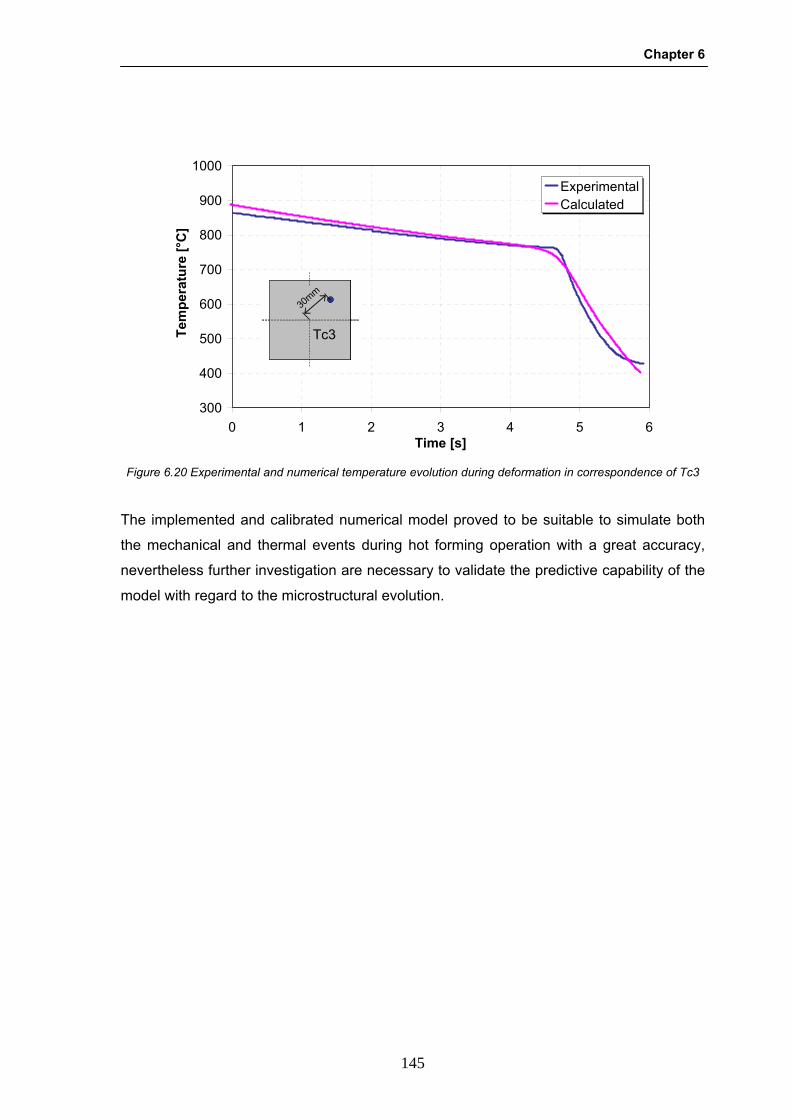
Chapter 6
145
The implemented and calibrated numerical model proved to be suitable to simulate both
the mechanical and thermal events during hot forming operation with a great accuracy,
nevertheless further investigation are necessary to validate the predictive capability of the
model with regard to the microstructural evolution.
300
400
500
600
700
800
900
1000
0 1 2 3 4 5 6Time [s]
Tem
pera
ture
[°C
]ExperimentalCalculated
Tc3
30mm
Figure 6.20 Experimental and numerical temperature evolution during deformation in correspondence of Tc3

Numerical model calibration
146

Chapter 7
147
7 CHAPTER 7 CONCLUSIONS

Conclusions
148
Chapter 7
149
Nowadays the hot stamping of high strength steels is proving to be a challenging
technology gaining the strict requirements of automotive producers. The high formability
and the reduced springback exhibited during deformation at elevated temperature,
together with the controlled microstructural evolution during quenching are the main
issues that make this process suitable to produce complex parts with reduced thickness
maintaining crash and safety requirements, due to the enhanced strength-to-mass ratio.
However, compared to conventional sheet metal forming operation at room temperature,
the optimization of press hardening process chains require a deep knowledge of both
material behaviour and interface phenomena at high temperature. Furthermore, the
correct design of the forming and the cooling phases involves the utilization of numerical
simulation where a coupled thermo-mechanical-metallurgical model has to be properly
implemented and calibrated.
In this PhD thesis, a new approach has been presented, focused on testing and modelling
to analyze and correctly describe the different phenomena that affect material, process
and product performance during and after the thermal, mechanical and microstructural
events in hot stamping operations.
In particular, an experimental setup was designed and developed in order to determine
the elasto-plastic properties of sheet metal at elevated temperature (e.g. flow curves,
plastic anisotropy and Young’s modulus evolution with temperature). This testing
equipment was also modified to study the influence of applied stress and strain on the
phase transformation kinetics together with the material transformation plasticity by means
of an extensometric analysis.
A new testing procedure for the investigation of sheet formability, taking into account the
microstructural aspects in hot stamping of high strength steels, was developed. An
innovative experimental apparatus was designed according to the Nakazima concept,
presenting an accurate methodology for the calibration of the phase transformation
parameters and the temperature control during the test. This formability test acted as a
physical simulation of the industrial press hardening process and, at the same time, it was
used to determine forming limit curves at elevated temperature in isothermal conditions.
A numerical model capable to perform a coupled thermo-mechanical-metallurgical
simulation of the hot stamping process was implemented in a commercial FE-code. The
mechanical and microstructural properties of the Al-Si pre-coated quenchenable high
strength steel 22MnB5 were determined by means of the experimental setups mentioned
above and the heat transfer coefficient at the die-workpiece interface was evaluated by an

Conclusions
150
inverse analysis approach in order to properly calibrate such a model. Finally, the
numerical model was validated through a comparison between a physical and a numerical
simulation of a hot forming operation.
The developed approach can be considered general enough to characterize the thermal,
mechanical and microstructural behaviour of high strength steels and to improve the
quality of FE simulations and virtual process prototyping techniques when they are applied
to analysis and design of the hot stamping process.
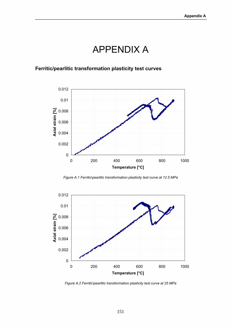
Appendix A
151
APPENDIX A Ferritic/pearlitic transformation plasticity test curves
0
0.002
0.004
0.006
0.008
0.01
0.012
0 200 400 600 800 1000
Temperature [°C]
Axi
al s
trai
n [%
]
Figure A.1 Ferritic\pearlitic transformation plasticity test curve at 12.5 MPa
0
0.002
0.004
0.006
0.008
0.01
0.012
0 200 400 600 800 1000
Temperature [°C]
Axi
al s
trai
n [%
]
Figure A.2 Ferritic\pearlitic transformation plasticity test curve at 25 MPa
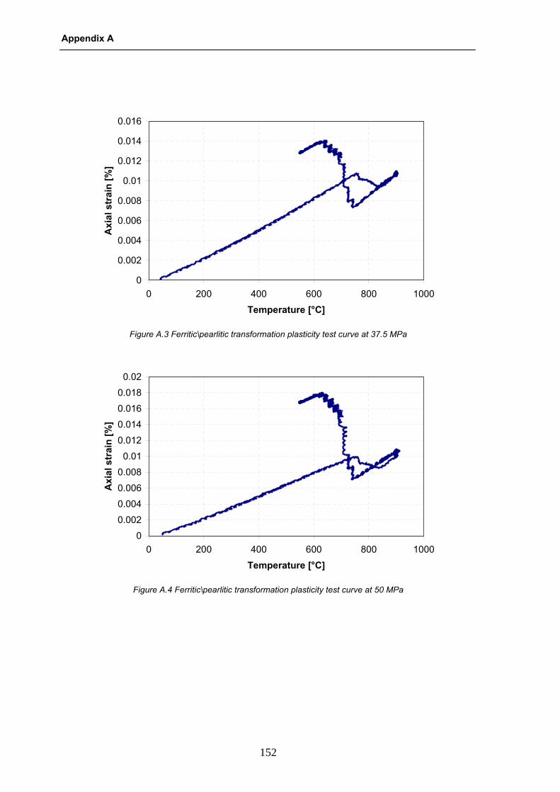
Appendix A
152
0
0.002
0.004
0.006
0.008
0.01
0.012
0.014
0.016
0 200 400 600 800 1000
Temperature [°C]
Axi
al s
trai
n [%
]
Figure A.3 Ferritic\pearlitic transformation plasticity test curve at 37.5 MPa
0
0.002
0.004
0.006
0.008
0.01
0.012
0.014
0.016
0.018
0.02
0 200 400 600 800 1000
Temperature [°C]
Axi
al s
trai
n [%
]
Figure A.4 Ferritic\pearlitic transformation plasticity test curve at 50 MPa
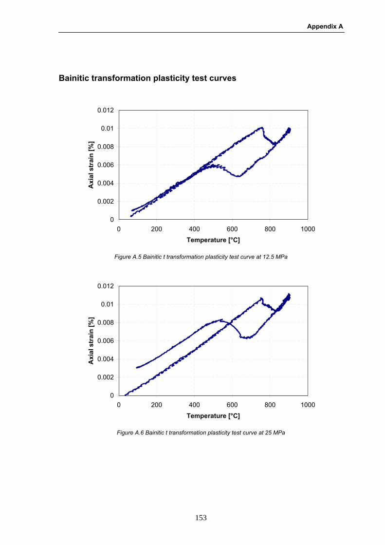
Appendix A
153
Bainitic transformation plasticity test curves
0
0.002
0.004
0.006
0.008
0.01
0.012
0 200 400 600 800 1000
Temperature [°C]
Axi
al s
trai
n [%
]
Figure A.5 Bainitic t transformation plasticity test curve at 12.5 MPa
0
0.002
0.004
0.006
0.008
0.01
0.012
0 200 400 600 800 1000
Temperature [°C]
Axi
al s
trai
n [%
]
Figure A.6 Bainitic t transformation plasticity test curve at 25 MPa
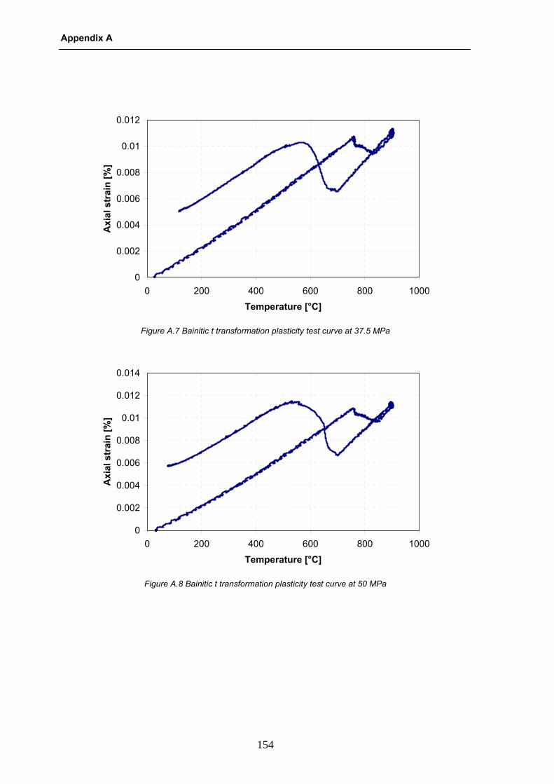
Appendix A
154
0
0.002
0.004
0.006
0.008
0.01
0.012
0 200 400 600 800 1000
Temperature [°C]
Axi
al s
trai
n [%
]
Figure A.7 Bainitic t transformation plasticity test curve at 37.5 MPa
0
0.002
0.004
0.006
0.008
0.01
0.012
0.014
0 200 400 600 800 1000
Temperature [°C]
Axi
al s
trai
n [%
]
Figure A.8 Bainitic t transformation plasticity test curve at 50 MPa
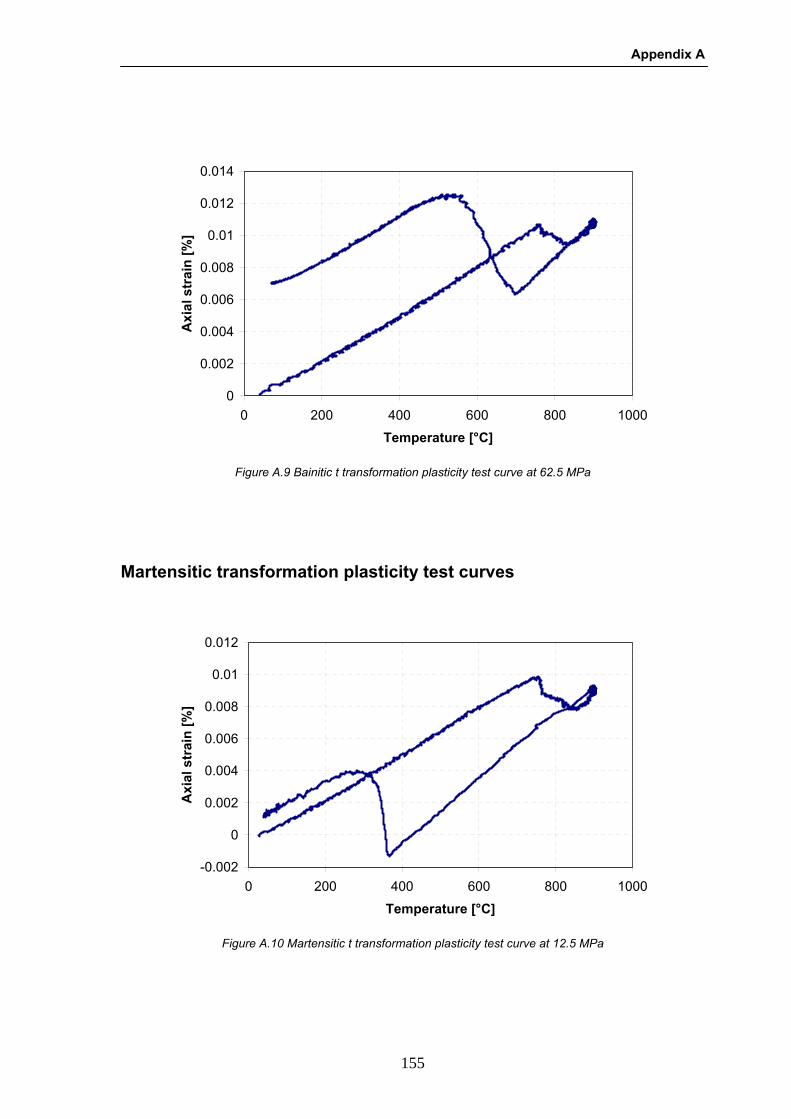
Appendix A
155
Martensitic transformation plasticity test curves
0
0.002
0.004
0.006
0.008
0.01
0.012
0.014
0 200 400 600 800 1000
Temperature [°C]
Axi
al s
trai
n [%
]
Figure A.9 Bainitic t transformation plasticity test curve at 62.5 MPa
-0.002
0
0.002
0.004
0.006
0.008
0.01
0.012
0 200 400 600 800 1000
Temperature [°C]
Axi
al s
trai
n [%
]
Figure A.10 Martensitic t transformation plasticity test curve at 12.5 MPa
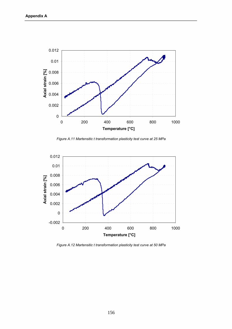
Appendix A
156
0
0.002
0.004
0.006
0.008
0.01
0.012
0 200 400 600 800 1000
Temperature [°C]
Axi
al s
trai
n [%
]
Figure A.11 Martensitic t transformation plasticity test curve at 25 MPa
-0.002
0
0.002
0.004
0.006
0.008
0.01
0.012
0 200 400 600 800 1000
Temperature [°C]
Axi
al s
trai
n [%
]
Figure A.12 Martensitic t transformation plasticity test curve at 50 MPa
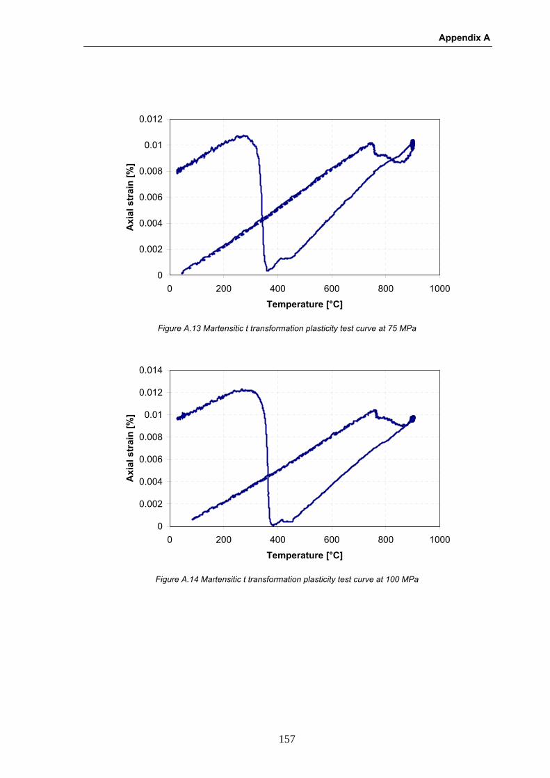
Appendix A
157
0
0.002
0.004
0.006
0.008
0.01
0.012
0 200 400 600 800 1000
Temperature [°C]
Axi
al s
trai
n [%
]
Figure A.13 Martensitic t transformation plasticity test curve at 75 MPa
0
0.002
0.004
0.006
0.008
0.01
0.012
0.014
0 200 400 600 800 1000
Temperature [°C]
Axi
al s
trai
n [%
]
Figure A.14 Martensitic t transformation plasticity test curve at 100 MPa
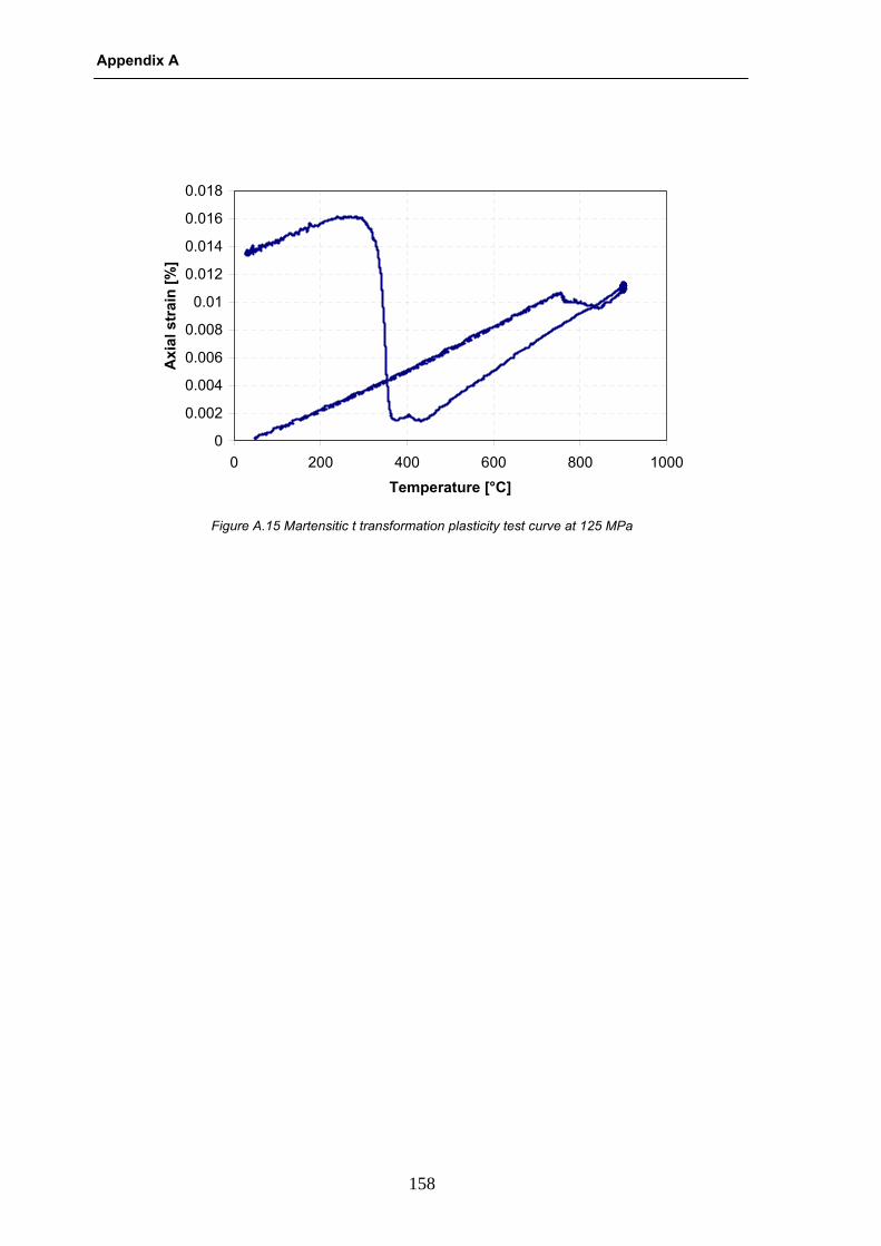
Appendix A
158
0
0.002
0.004
0.006
0.008
0.01
0.012
0.014
0.016
0.018
0 200 400 600 800 1000
Temperature [°C]
Axi
al s
trai
n [%
]
Figure A.15 Martensitic t transformation plasticity test curve at 125 MPa
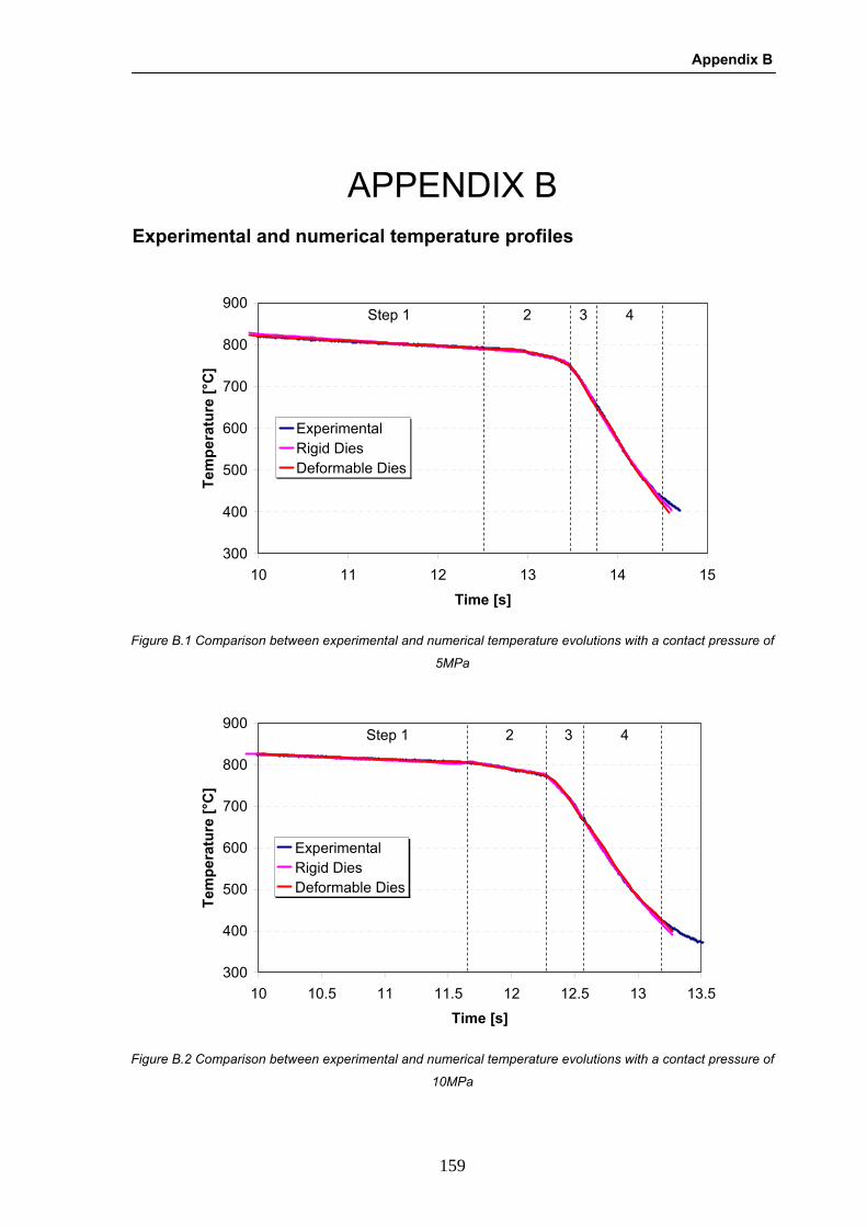
Appendix B
159
APPENDIX B Experimental and numerical temperature profiles
300
400
500
600
700
800
900
10 11 12 13 14 15
Time [s]
Tem
pera
ture
[°C
]
ExperimentalRigid DiesDeformable Dies
Step 1 2 3 4
Figure B.1 Comparison between experimental and numerical temperature evolutions with a contact pressure of
5MPa
300
400
500
600
700
800
900
10 10.5 11 11.5 12 12.5 13 13.5
Time [s]
Tem
pera
ture
[°C
]
ExperimentalRigid DiesDeformable Dies
Step 1 2 3 4
Figure B.2 Comparison between experimental and numerical temperature evolutions with a contact pressure of
10MPa
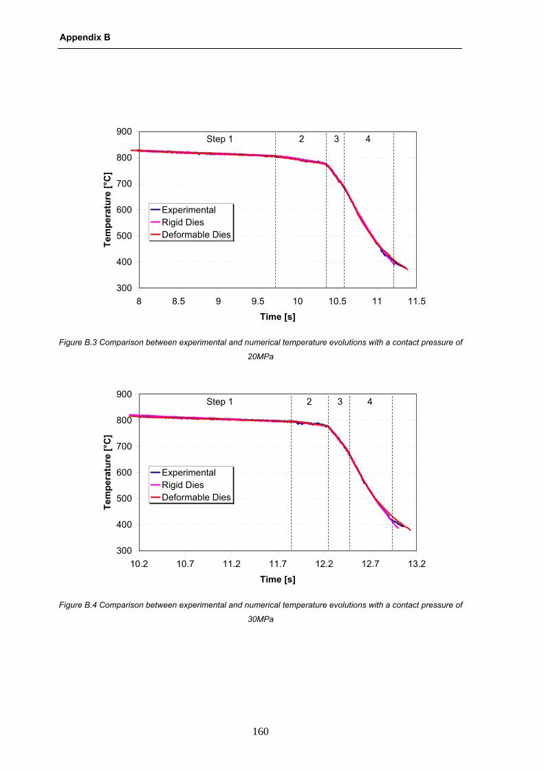
Appendix B
160
300
400
500
600
700
800
900
8 8.5 9 9.5 10 10.5 11 11.5
Time [s]
Tem
pera
ture
[°C
]
ExperimentalRigid DiesDeformable Dies
Step 1 2 3 4
Figure B.3 Comparison between experimental and numerical temperature evolutions with a contact pressure of
20MPa
300
400
500
600
700
800
900
10.2 10.7 11.2 11.7 12.2 12.7 13.2
Time [s]
Tem
pera
ture
[°C
]
ExperimentalRigid DiesDeformable Dies
Step 1 2 3 4
Figure B.4 Comparison between experimental and numerical temperature evolutions with a contact pressure of
30MPa
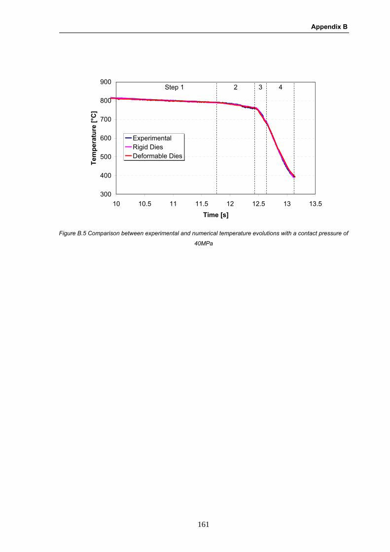
Appendix B
161
300
400
500
600
700
800
900
10 10.5 11 11.5 12 12.5 13 13.5Time [s]
Tem
pera
ture
[°C
]
ExperimentalRigid DiesDeformable Dies
Step 1 2 3 4
Figure B.5 Comparison between experimental and numerical temperature evolutions with a contact pressure of
40MPa

Appendix B
162
References
163
REFERENCES [9] [1] M.Merklein and J. Lechler, "Determination of Influencing Parameters of the Hot
Stamping Process," presented at Proceedings Asia Steel Conference 2006.
[2] D.Lorenz and K. Roll, "Modelling and Analysis of Integrated Hot forming and
quenching Processes," Sheet Metal 2005 Conf.,Proc. (2005), pp. 787-794, 2005.
[3] International Iron and Steel Institute, UltraLight Steel Auto Body - Advanced
Vehicle Concepts (ULSAB-AVC) Overview Report (2002).
[4] J.Wilsius, P. Hein, and R. Kefferstein, "Status and future trends of hot stamping of
USIBOR 1500 P," presented at Erlangen Workshop 2006.
[5] P.Hein, "A Global Approach of the Finite Element Simulation of Hot Stamping,"
Sheet Metal 2005 Conf.,Proc. (2005), pp. 763-770, 2005.
[6] D.Lorenz and K. Roll, "Simulation of Hot Stamping and Quenching of Boron
alloyed Steel.," presented at 7th Int. ESAFORM Conf. on Mat. Forming,
Trondheim, Norway, 2004.
[7] P.F.Bariani, T. D. Negro, and S. Bruschi, "Testing and Modelling of Material
Response to Deformation in Bulk Metal Forming," Annals of the CIRP Vol.
53/2/2004 573-598.
[8] R.Neugebauer, T. Altan, M. Geiger, M. Kleiner, and A. Sterzing, "Sheet metal
forming at elevated temperature," Annals of the CIRP, vol. 55/2/2006, pp. 793-
8166.
[9] "http://www.arcelor.com/."
[10] M.Merklein, J. Lechler, and M. Geiger, "Determination of Thermal and Mechanical
Material Properties for Hot Stamping Processes of Ultra High Strength Steels,"
presented at Proceedings of the 2007 SAE International World Conference.
References
164
[11] L.G.Aranda, P. Ravier, and Y. Chastel, "Hot Stamping of Quenchable Steels:
Material Data and process Simulations," IDDRG 2003 Conf., Proc. (2003), pp.
166-164, 2003.
[12] P.Akerstrom, "Austenite decomposition during press hardening of a boron steel -
Computer simulation test," Journal of Materials Processing Technology, vol. 174,
pp. 399-406, 2006.
[13] H. S. H. Kim, S. Kang, S. Park, "Thermal-Mechanical coupled simulation of the
forming of hot press formed part," presented at Proceedings of the IDDRG 2006
Conference.
[14] P.Akerstrom, G. Bergman, and M. Oldenburg, "Numerical implementation of a
constitutive model for simulation of hot stamping," Modelling and Simulation in
Materials Science and Engineering, vol. 15/2, pp. 105-119, 2007.
[15] M.Coret and A. Combescure, "A mesomodel for the numerical simulation of the
multiphasic behavior of materials under anisothermal loading (application to two
low-carbon steels)," International Journal of Mechanical Sciences, vol. 44/9, pp.
1947-1963, 2002.
[16] P.Akerstrom, B. Wikman, and M. Oldenburg, "Material parameter estimation for
boron steel from simultaneous cooling and compression experiments," Modelling
and Simulation in Materials Science and Engineering, vol. 13, pp. 1291-1308,
2005.
[17] L.G.Aranda, P. Ravier, and Y. Chastel, "Experimental, material data and numerical
model for hot stamping of quenchable steels," 6th ESAFORM Conference on
Material Forming, 2003.
[18] M.Merklein and L. Lechler, "Investigation of the thermo-mechanical properties of
hot stamping steels," Journal of Materials Processing Technology, vol. 117 (2006),
pp. 452-455.
[19] L.Burkhardt and B. Oberpriller, "Sensitivity analysis of process and material
parameters for the efficient simulation of hot forming," presented at Forming
Technology Forum 2007, Zurich (Switzerland).
[20] J.G.Lenard, Modeling hot deformation of steels: Springer-Verlag, 1989.

References
165
[21] L.Anand, "Constitutive equations for the rate�dependent deformation of metals at
elevated temperatures," Journal of engineering materials and technology, pp.
104/13, 1982.
[22] C.S.Hartley and R. Srinivasan, "Constitutive equations for large plastic deformation
of metals," Journal of engineering materials and technology, vol. 105, pp. 162-167,
1983.
[23] J.C.Fisher and J. H. Hollomon, "Dislocation glide as an aid to precipitation at low
temperatures," Acta metallurgica, vol. 3/6:608, 1955.
[24] E.Voce, "A practical strain-hardening function," Acta metallurgica, vol. 51, pp. 219-
226, 1948.
[25] M.A.Meyers and K. K. Chawla, Mechanical metallurgy � Principles and
applications: Prentice-Hall, 1984.
[26] C.Aliaga, "Simulation numérique par éléments finis en 3D du comportment
thermomécanique au couer du traitment thermique d'aciers: application à la
trempe de pièces forgées ou coulées," in L'école nationale supérieure des mines
de Paris, 2000.
[27] M.C.Somani, L. P. Karjalainen, M. Eriksson, and M. Oldenburg, "Dimensional
Changes and Microstructural Evolution in a B-bearing Steel in the Simulated
Forming and Quenching Process," ISIL International, vol. 41, pp. 361-367, 2001.
[28] S.H.Kang and Y. T. Im, "Three-dimensional thermal-elastic-plastic finite element
modeling of quenching process of plain-carbon steel in couple with phase
transformation," International Journal of Mechanical Sciences, vol. 49 (2007), pp.
423-439.
[29] M.Merklein, J. Lechler, and M. Geiger, "Characterisation of the Flow Properties of
the Quenchenable Ultra High Strength Steel 22MnB5," presented at Annals of the
CIRP Vol. 55/1/2006.
[30] W.Avrami, "Kinetics of Phase Change," Journal of chem Physics, vol. 7, pp. 1103-
1112, 1939.
[31] W.A.Johnson and R. F. Mehl, "Reaction kinetics in process of nuceation and
growth," Trans. AIME, vol. 135, pp. 416-458, 1939.

References
166
[32] E.Sheil, "Arch. Eisenhuttenwesen," vol. 12, 1935.
[33] D. P. Koinstinem and R. E. Marburger, "A general equation prescribing the extend
of the austenite-martensite transformation and temperature evolution during
quenching of steels," Acta metallurgica, vol. 7, pp. 59-60, 1950.
[34] B.A.Behrens, P. Olle, F. Schafer, and C. Schaffner, "Numerical simulation of
microstructure evolution during the hot stamping process," presented at
Proceedings of the IDDRG 2007 International Conference.
[35] C.L.Magee, "Transformation kinetics, microplasticity and agening of martensite in
Fe-31-Ni." Pittsburgh: Carnegie Institute of Technologie University, 1966.
[36] G.W.Greenwoog and R.H.Johnson, "The deformation of metal under small
stresses during phase transformations," Proc. Royal Society, vol. 283, pp. 403-
422, 1965.
[37] S.Petit-Grostabussiat, L. Taleb, and J. F. Jullien, "Experimental Results on
Classical plasticity of steels subjected to structural transformation," Journal of
Materials Processing Technology, vol. 20 (2004), pp. 1371-1386, 2003.
[38] L.Taleb, N. Cavallo, and F. Waeckel, "Experimental analysis of transformation
plasticity," International Journal of Plasticity, vol. 17, pp. 1-20, 2001.
[39] E.Gautier, A. Simon, and G. Beck, "Plasticite de transformation durant le
transformation perlitique d'un acier eutectoide," Acta metallurgica, vol. 35, pp.
1367-1375, 1987.
[40] P.Akerstrom, "Modelling and Simulation of Hot Stamping," Lulea University of
Technology, 2006.
[41] Z.Malinowsky, J. G. Lenards, and M. E. Davies, "A Study of the Heat Transfer
Coefficient as a Function of Temperature and Pressure," Journal of Materials
Processing Technology, vol. 42, pp. 125-142, 1994.
[42] P. R. Burte, Y. T. Im, T. Altan, and S. L. Semiation, "Measurement and Analysis of
Heat Transfer and Friction during Hot Forging," J. of Eng. for Ind., vol. 112, pp.
332-339.
[43] K.Lange, Handbook of Metal Forming: Mc Graw Hill.
References
167
[44] C.V.Madhusudana, Thermal contact conductance. Berlin: Springer.
[45] M.Croin, "MODELLING INTERACTIONS AMONG PRESS, TOOLS AND
WORKPIECE IN HOT FORGING OPERATIONS," 2006.
[46] M.Geiger, M. Merklein, and C. Hoff, "Basic Investigation on the Hot Stamping Steel
22MnB5," Sheet Metal 2005 Conference Proceedings (2005), pp. 795-802, 2005.
[47] K.Forstner, S. Strobich, and B. Buchmayr, "Heat transfer during press hardening,"
presented at Proceedings of the IDDRG 2007 International Conference.
[48] A.Tarantola, Inverse problem theory: Elsevier, 1987.
[49] J.P.Norton, An introduction to Identification. London: Ed. Academy Press, 1986.
[50] J.D.Coolins, G. C. Hart, T. K. Hassleman, and B. Kennedy, "Statistical
identification of structures," AAIA Joutnal, vol. 12, pp. 185-190, 1974.
[51] J. V. Beck and K. J. Arnold, Parameter estimation in Engineering and Science:
John Wiley & Sons, 1986.
[52] R.C.Mehta and T. Jayachandran, "Determination of Heat Transfer Coefficient
using transient temperature response chart," Warme und Stoffubertrangung, vol.
26, pp. 1-5, 1990.
[53] A.Badrinarayanan, A. Constantinescu, and N. Zabras, "Preform in metal forming,"
presented at Proceedings of the 1995 Numiform Conference (Balkema).
[54] L.Fourment, T. Balan, and J. L. Chenot, "Shape optimal design in metal forming,"
presented at Proceeding of the 1995 Numiform Conference (Balkema).
[55] D.S.Schnur and N. Zabras, "An inverse method for determining elastic material
properties and a material interface," International Journal for Numerical Methods in
Engineering, vol. 33, pp. 2039-2057, 1992.
[56] C.Caillateaud and P. Pilvin, "Identification and inverse problem: a modular
approach," presented at Winter annual meeting symposium on material parameter
estimation for modern constructive equations, New Orleans, 1993.
[57] D.M.Bates and D. G. Watts, Nonlinear regression Analysis and its Application,
1988.

References
168
[58] P.E.Gill, W. Murray, and M. H. Wright, Pratical Optimization. London, 1981.
[59] W.J.Minkowycz, E. M. Sparrow, and G. E. Schneider, Handbook of heat transfer,
1988.
[60] D.A.Tortorelli and P. Michaleris, "Design sensiticity analysis: overview and review,"
Inverse problem in Engineering 1, pp. 71-105, 1991.
[61] S.P.Keller, "Circular grid system: A valuable aid for evaluation sheet forming,"
Sheet Met. Ind., vol. 45, pp. 633-640, 1969.
[62] G.M.Goodwin, "Application of strin analysis to sheet metal forming problems,"
Metall, Ital., vol. 60, pp. 767-771, 1968.
[63] R.Arrieux, J. M. Chalons, J. M. Bedrin, and M. Bovin, "Computer aided method for
the determination of the FLD at necking," Annals of the CIRP, vol. 33/1, pp. 171-
174, 1984.
[64] H.W.Swift, "Plastic instability under plane stress," J. Mech. Phys. Solids 1, pp. 1-
18, 1952.
[65] R.Hill, "On discontinuus plastic states with special reference to localized neking in
thin sheets," J. Mech. Phys. Solids 1, pp. 19-30, 1952.
[66] D.Banabic, H.-J. Bunge, K. Pohlandt, and A. E. Tekkaya, Formability of Metallic
Materials: Berlin: Springer, 2000.
[67] D.Banabic, "Anisotropy and formability of AA5182-0 aluminium alloy sheets,"
presented at Annals of CIRP, 53, pp. 219-222, 2004.
[68] M.Geiger, G. V. d. Heyd, M. Merklein, and W. Hußnätter, "Novel concept of
Experimental Setup for Characterisation of Plastic Yielding of Sheet Metal at
Elevated Temperatures," Advanced Materials Research, vol. 6-8, pp. 657-664,
2005.
[69] Q.Q.Nie, D. Lee, and J. Matter, "The effect of strain rate sensitivity on history
dependent forming limits of anisotropic sheet metals," Journal of Material Shaping
Technology, vol. 9, pp. 233-240, 1991.

References
169
[70] Q.Situ, M. Bruhis, and M. Jain, "Obtaining Formability Characteristics Of
Automotive Materials Using On-line Strain Imaging System," presented at
Proceedings of the 6th International NUMISHEET Conference (2005).
[71] F.Barlat and A. B. D. Rocha, "Influence of danage on the plastic instability of sheet
metals under complex strain paths," J. Mater. Sci., vol. 19, pp. 4133-4137, 1984.
[72] V.Uthainsangsuk, U. Prahl, S. Munstermann, and W. Bleck, "Experimental and
numerical failure criterion for formability prediction in sheet metal forming,"
Computational Material Science, 2007.
[73] W.Thomas, T. Oenoki, and T. Altan, "Process simulation in stamping - recent
applications for product and process design," International Journal of Materials
Processing Technology, vol. 98 (2000), pp. 232-243.
[74] M.Tolazzi and M. Merklein, "Inlfuence of Pre-forming on the Forming Limit
Diagram of Aluminum and Steel Sheets," presented at Proceedings of the 2007
SHEMET Conference.
[75] M.Merklein and S. Beccari, "Influence of predeformation on the formability of
aluminium alloys," presented at Proceeding of the 8th International Confernce on
Technology of Plasticity, 2005, Verona (Italy).
[76] "Standard ISO 12004-2:1997, TC 164/SC 2."
[77] M.Geiger and M. Merklein, "Determination of forming limit diagrams – a new
analysis method for characterization of materials´ formability," Annals of the CIRP
52/1, 213, 2003.
[78] H.Liebertz, A. Duwel, R. Illig, W. Hotz, S. Keller, A. Koehler, A. Kroeff, M. Merklein,
J. Rauer, L. Staubwasser, G. Steinbeck, and H. Vegter, "Guideline for the
determination of forming linit curves," presented at Proceedings of the IDDRG
2004 Conference.
[79] P.Hora, M. Merklein, L. Tong, and J. Lechler, "Numerical and experimental
evaluation of thermal dependent FLC (FLC-T)," presented at Proceedings of the
IDDRG 2007 International Conference.
References
170
[80] Y.Dahan, Y. Chastel, P. Duroux, P. Hein, E. Massoni, and J. Wilsius, "Formability
investigations fot the hot stamping process," presented at Proceedings of the
IDDRG 2006 International Conference.
[81] Y.Dahan, Y. Chastel, P. Duroux, J. Wlsius, P. Hein, and E. Massoni, "Procedure
for the experimental determination of a forming limit curve for USIBOR 1500 P,"
presented at Proceedings of the IDDRG 2007 International Conference.
[82] "N.N.; ASTM 03.01."
[83] S.Petit-Grostabussiat, L. Taleb, and J. F. Jullien, "Experimental Results on
Classical plasticity of steels subjected to structural transformation," Journal of
Materials Processing Technology, vol. 20 (2004), pp. 1371-1386, 2004.
[84] A.S.Judlin-Denis, "Modèlisation des interactions contrainte-transformation de
phase et calcul par èlèments finis de la gènère des contraintes internes au cours
de la tempre des aciers," in Institut National Polytechnique de Lorraine, France,
2004.
[85] M.Coret, S. Calloch, and A. Combescure, "Experimental study of the phase
transformation plasticity of 16MND5 low carbon steel induced by proportional and
nonproportional biaxial loading paths," European Journal of Mechanics A\Solid,
vol. 23 (2004), pp. 823-842, 2002.
[86] E.Lamm, "Advanced Steel Solutions for Automotive Lightweighting," Windsor
Workshop June 5, 2005.
[87] S.Kobayashi, S. I. Oh, and T. Altan, Metal Forming and Finite Element method,
1989.