Università degli Studi di Napoli - unina.itwpage.unina.it/danilo.ciliberti/doc/Cusati.pdf ·...
123
Università degli Studi di Napoli Federico II Scuola P olitecnica e delle Scienze di base Dipartimento di Ingegneria Industriale Sezione Aerospaziale Corso di Laurea Magistrale in Ingegneria Aerospaziale e Astronautica Master T hesis Development of a new methodology for the prediction of aircraft fuselage aerodynamic characteristics Supervisor: Prof. Eng. Fabrizio Nicolosi Co-supervisor: Eng. Danilo Ciliberti Dr. Eng. Pierluigi Della Vecchia Candidate: Vincenzo Cusati Matr. M53/154 Anno A ccademico 2012/2013
Transcript of Università degli Studi di Napoli - unina.itwpage.unina.it/danilo.ciliberti/doc/Cusati.pdf ·...
Università degli Studi di Napoli
Federico II
Scuola Politecnica e delle Scienze di base
Dipartimento di Ingegneria Industriale
Sezione Aerospaziale
Corso di Laurea Magistrale in
Ingegneria Aerospaziale e Astronautica
Master Thesis
Development of a new methodology for the
prediction of aircraft fuselage
aerodynamic characteristics
Supervisor:Prof. Eng.Fabrizio Nicolosi
Co-supervisor:Eng. Danilo CilibertiDr. Eng. Pierluigi Della Vecchia
Candidate:Vincenzo CusatiMatr. M53/154
Anno Accademico 2012/2013

To invent an airplane is nothing. To build one is something.
But to fly is everything
-Karl Wilhelm Otto Lilienthal
A B S T R A C T
The main aim of this work is to investigate, from aerodynamic pointof view, a modular model of the fuselage of a regional transport turbo-prop aircraft with 90 seats. This approach involves the study of differ-ent fuselage components (nose, cabin and tailcone) to identify trendsin aerodynamic coefficients with geometrical parameters. Usually,in the preliminary design, the aerodynamic studies are conductedwith semi-empirical methods which rely on a huge database of wind-tunnel test results, such as USAF DATCOM, that are based on geome-tries very different from a turboprop. In the present work, the aerody-namic studies were performed by numerical analyses (Reynolds Aver-aged Navier Stokes equations). Therefore the results obtained with anumerical approach are presumably more suitable for a preliminarydesign than those achieved with semi-empirical methods. The numer-ical simulations have been carried out using the commercial softwareStar-CCM+. A large number of simulations have been performed onthe SCoPE grid infrastructure of the University of Naples Federico II,that gave the possibility to simulate complex 3D geometries in a smallamount of time. The only constraint imposed to modifications of thefuselage is the compliance to FAR 25.775 (Windshields and windows).Results of numerical analyses give useful information about trends ofaerodynamic coefficients with geometric parameters. A drag and mo-ment prediction method, accounting for the fuselage shape and wet-ted area, have been developed from these results and are presentedwith some example of application.
ii
A C K N O W L E D G E M E N T S
I am aware that this page can seem too long but I want to thank all thepeople (and there are many) who have contributed to the achievementof this goal.
First of all I would like to express my gratitude to Prof. FabrizioNicolosi for giving me the opportunity of this thesis, transformingit into a great opportunity for professional and human growth. Hispassion for flight and for the aircraft design making me appreciatemore and more the profession that (I hope) I shall make in the future.
If I could accomplish what I hope is a good job, a lot of the creditgoes to Danilo (Eng. Ciliberti) that was my "guardian angel", withwhom I was lucky to deepen the knowledge outside of the workplace.In addition to being an excellent engineer, he has been a great person.Thanks for the time and attention dedicated to me. A similar con-siderations holds for Pierluigi (Eng. Della Vecchia), which often hasshed light on obscure topics for me with simple explanations, whichare not purely limited to engineering. I would also like to thank Sal-vatore (Eng. Corcione) for his willingness to help us to solve any kindof problem.
A special thanks goes to a special person, Amalia, my girlfriend,who has had, has and will have a fundamental role in my life. Shehas been always at my side, in joy and in sorrow, and was helpedme to believe in my qualities even when I didn’t believe anymore (inthis regard I jealously guards a letter that gave me the strength toovercome any trial). I would not be here if you were not by my side.Thank you for everything my love.
I would like also to express my gratitude to my family. I don’t wantto bring everything to a mere economic issue, albeit an importantone. They are the pillars of my life. I want to say thanks to my mumMichela, for having suffered in silence with me when I was about tosuffer, for teaching me humility, and for standing and the supportingme lovingly every day. I want to say thanks to my father Raffaele:his example is for me always a guide. I’ll never forget his words ina "special" moment of my college career, "one stone at a time"...andone stone at a time we built a house! If I am here today, I owe toyou. I want to say thanks to my sisters Grazia and Miriam, which,in addition to their affection, have shown me that the ability andhumility can reach any goal anytime, anywhere and anyhow. I wouldalso like to thank my brother in law, Blair, for language support andhis availability during the writing of the thesis.
An other special thanks goes to Piemonte family, Felice (with whomI share a passion for airplanes), Giovanna and Valeria for the love and
iii

support they have always given me, and Mario, a true friend, withwhom it is always nice to deal with. You welcomed me like a secondfamily and I shall be forever grateful.
Last but not least, I would like to say thanks to all my friends whohave accompanied me during my years spent at university: Pasquale,Angelo, Luigi, Nunzio, Vincenzo D., Vincenzo F., Mino, Aldo, Alessan-dro and many others. It was great to share day-by-day this adventure.I consider myself a very lucky person to have met you.
Vincenzo Cusati
iv
C O N T E N T S
1 introduction 1
1.1 The fuselage design for a transport aircraft 2
1.2 Turboprop aircraft 3
1.2.1 Turboprop Drag and Performance 4
1.3 Aim and structure of thesis work 4
2 semi-empirical methods for prediction of aerody-namic coefficients 8
2.1 Fuselage drag coefficient prediction 8
2.1.1 Effect of fineness ratio 10
2.1.2 Skin friction contribution 11
2.1.3 Fuselage upsweep contribution 13
2.1.4 Fuselage base drag contribution 14
2.1.5 Windshield contribution 14
2.2 Fuselage moment coefficient prediction 16
2.3 Example of application 19
2.3.1 Drag estimation for ATR-72 19
2.3.2 Drag estimation for Dash8-Q400 23
2.3.3 Pitching moment estimation for ATR-72 24
2.3.4 Pitching moment estimation for Dash8-Q400 25
3 a numerical approach 26
3.1 The software Star-CCM+ 28
3.1.1 Simulation workflow 29
3.1.2 Main mesh parameter 31
3.1.3 Convergence 32
3.2 The SCoPE grid infrastructure 32
3.3 Numerical model 33
3.3.1 Test-cases 35
3.4 Processing of geometry with Matlab 37
3.4.1 Modification of the nose 40
3.4.2 Modification of the cabin 42
3.4.3 Modification of the tail 42
3.4.4 Modification of nose height 43
3.4.5 Modification of upsweep angle 45
4 cfd analysis results 48
4.1 Variation of the nose length 48
4.2 Variation of the cabin length 55
4.3 Variation of the tail length 59
4.4 Variation of the nose height 63
4.5 Variation of the upsweep angle 66
5 a new methodology for prediction of aerodynamiccoefficients 68
v
5.1 Methodology for drag prediction 68
5.1.1 The shape factor of the nose 69
5.1.2 The shape factor of the cabin 70
5.1.3 The shape factor of the tail 70
5.1.4 Example of application 72
5.2 Pitching moment prediction 79
5.2.1 Example of application 81
5.3 Prediction of the pitching moment derivative 84
5.3.1 Example of application 87
6 conclusions 90
a far related to windshields and windows 92
b star-ccm+ on scope user guide 94
b.1 Files necessary to the job 94
b.1.1 Java macro example 94
b.1.2 Executable file example 95
b.1.3 Job file example 97
b.2 Transferring files on SCoPE 98
b.3 Copying the simulation file on the LFC 98
b.4 Running, monitoring and retrieving the job 98
c numerical simulation results 100
Bibliography 105
L I S T O F F I G U R E S
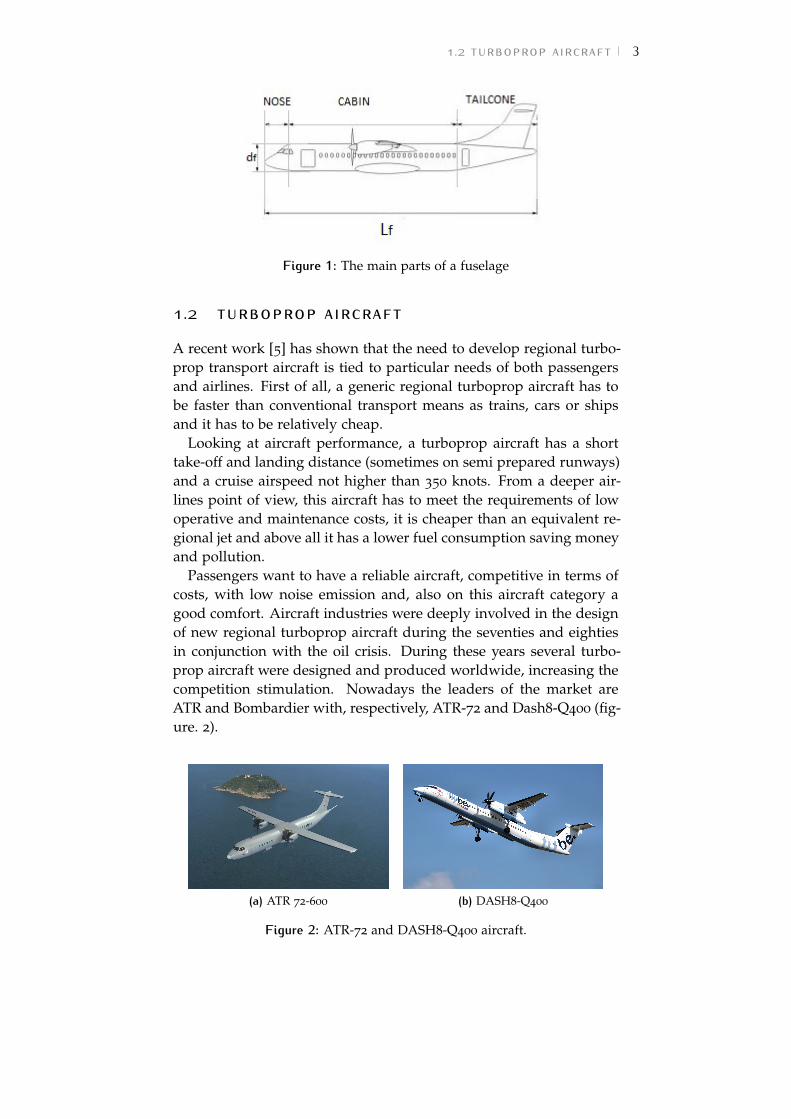
Figure 1 The main parts of a fuselage 3
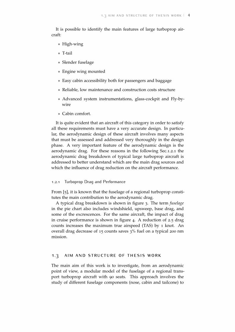
Figure 2 ATR-72 and DASH8-Q400 aircraft. 3
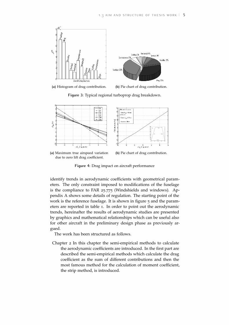
Figure 3 Typical regional turboprop drag breakdown. 5
Figure 4 Drag impact on aircraft performance 5
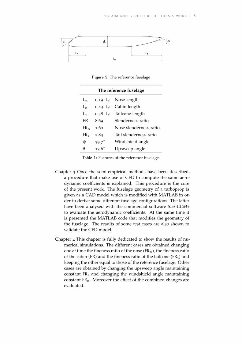
Figure 5 The reference fuselage 6
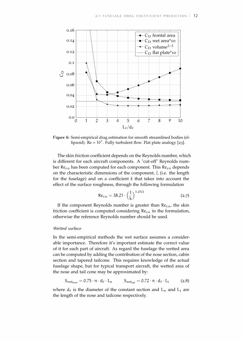
Figure 6 Semi-empirical drag estimation for smooth stream-lined bodies (ellipsoid). Re = 107. Fully turbu-lent flow. Flat plate analogy [23]. 12
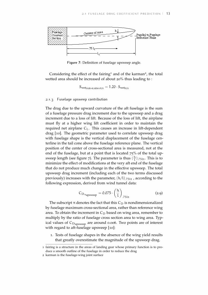
Figure 7 Definition of fuselage upsweep angle. 13
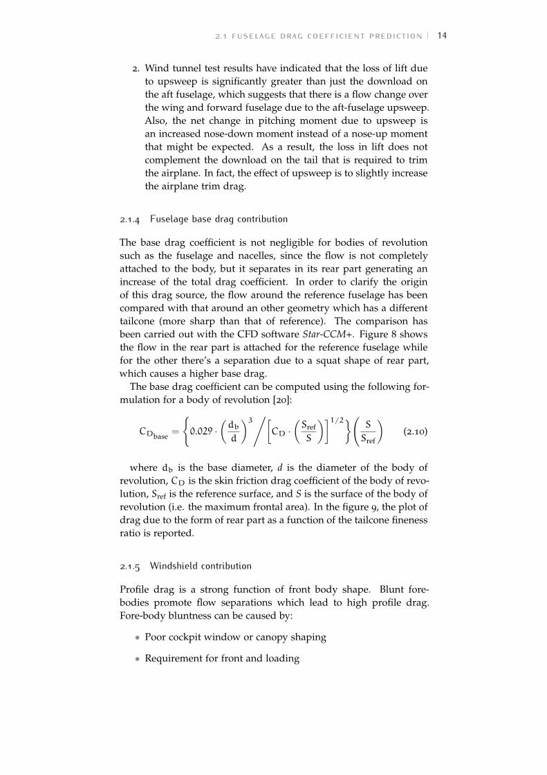
Figure 8 Flow around the rear part of the fuselage. 15
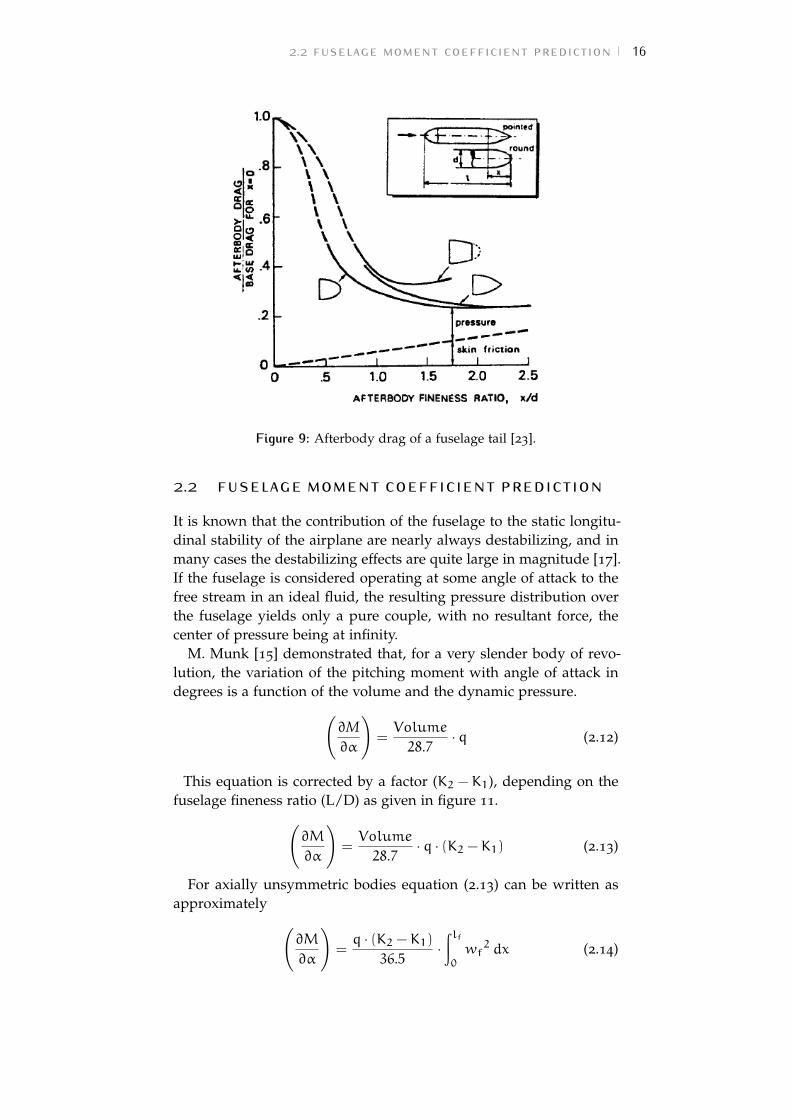
Figure 9 Afterbody drag of a fuselage tail [23]. 16
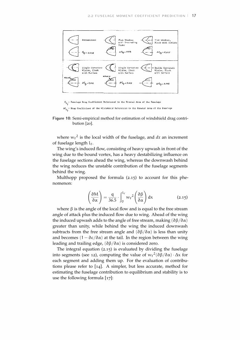
Figure 10 Semi-empirical method for estimation of wind-shield drag contribution [20]. 17
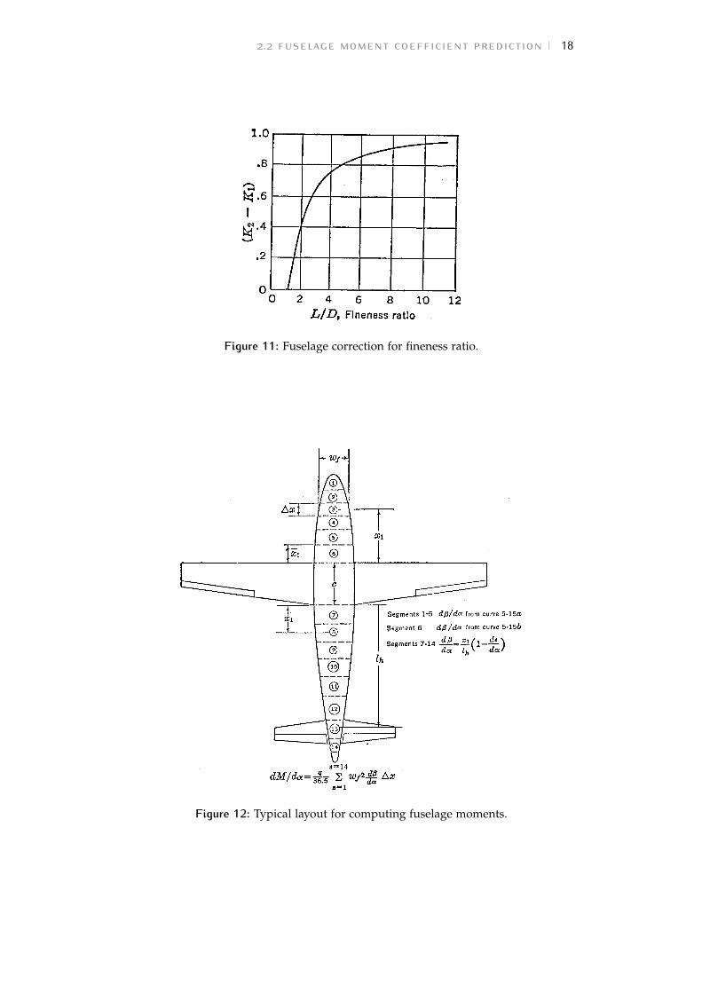
Figure 11 Fuselage correction for fineness ratio. 18
Figure 12 Typical layout for computing fuselage moments. 18
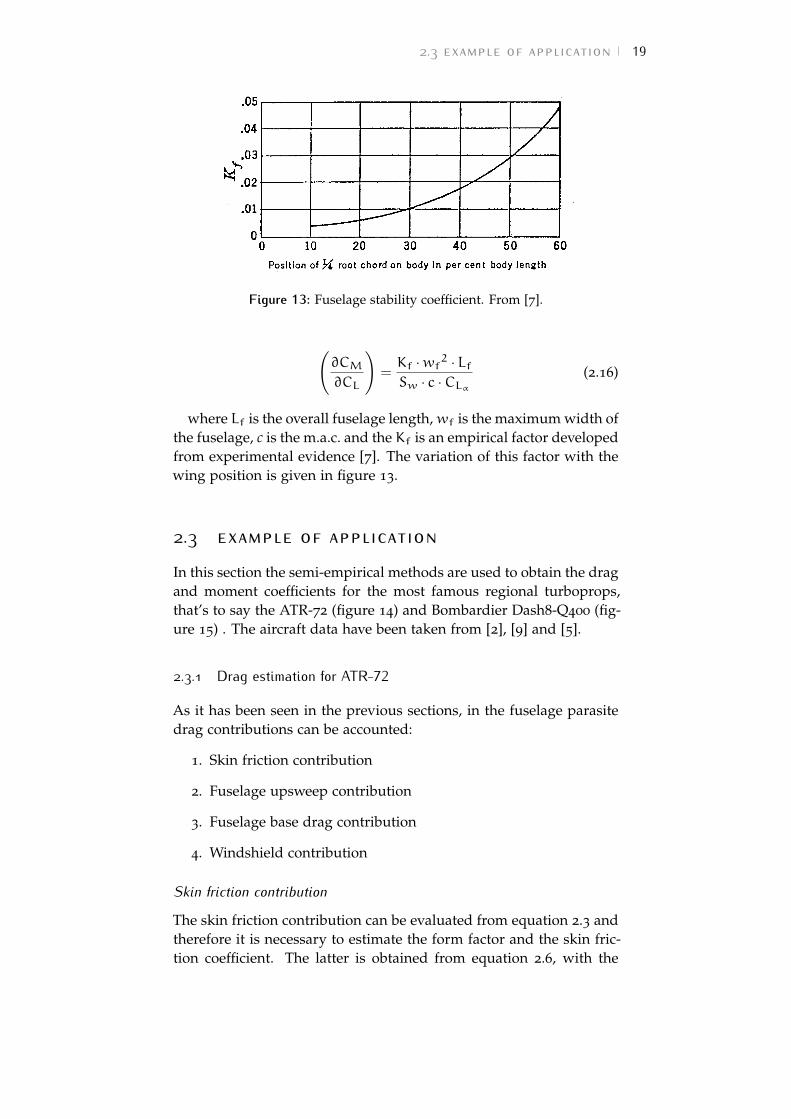
Figure 13 Fuselage stability coefficient. From [7]. 19
Figure 14 ATR-72 dimensions. 20
Figure 15 Bombardier Dash8-Q400 dimensions. 21
vi
List of Figures
Figure 16 Windshield drag contribution for the ATR-72. 22
Figure 17 The comparison of the nose shape. 24
Figure 18 Strips for ATR-72 25
Figure 19 Comparison of analysed geometries experimen-tally with that of reference. 26
Figure 20 The workflow of the proposed methodology. 28
Figure 21 Vertex, face and cell definition in Star-CCM+. 29
Figure 22 General sequence of operations in a Star-CCM+analysis. 30
Figure 23 The SCoPE network infrastructure [22]. 33
Figure 24 Some images of the SCoPE data center 34
Figure 25 Block shape that defines the fluid domain aroundthe model. 34
Figure 26 Aerodynamic comparison between 4 and 5 abreastfuselage. M = 0.52, Re = 11.5×10⁶. 36
Figure 27 Mesh around the reference fuselage. 36
Figure 28 Test case on mesh convergence. M = 0.52, Re =17.4×10⁶. 37
Figure 29 The y+ value for the reference geometry. 37
Figure 30 An example of work window. 38
Figure 31 The fuselage divided in sections. 40
Figure 32 Main geoemtrical parameter. 41
Figure 33 Definition of the windshield angle. 44
Figure 34 Definition of the upsweep angle. 46
Figure 35 Reference center for the calculation of momentcoefficient. 49
Figure 36 Comparison of different nose. 50
Figure 37 Variation of windshield angle due to the varia-tion of nose length. 51
Figure 38 Pressure distribution on the fuselage symmetryplane, due to nose variation,α = 0. 51
Figure 39 Friction and pressure contributions to drag co-efficient due to nose variation, α = 0°. 52
Figure 40 Drag coefficient due to nose variation (sum ofpressure and friction contributions), α = 0°. 52
Figure 41 Fuselage pitching instability due to nose varia-tion. 53
Figure 42 Moment coefficient as function of the nose ge-ometry variation, α = 0° e α = 2° 53
Figure 43 Comparison of the pressure distribution for twonose configurations, α = 0°. 54
Figure 44 Change of the fuselage slenderness by stretch-ing the cabin. 55
Figure 45 Pressure distribution on the fuselage symmetryplane, due to cabin variation, α = 0°. 56
vii
List of Figures
Figure 46 Friction and pressure contributions to drag co-efficient due to cabin variation, α = 0°. 56
Figure 47 Drag coefficient due to cabin variation (sum ofpressure and friction contributions), α = 0°. 57
Figure 48 Fuselage pitching instability due to cabin varia-tion. 57
Figure 49 Moment coefficient as function of the cabin ge-ometry, α = 0° e α = 2° 58
Figure 50 Comparison of different tail. 60
Figure 51 Variation in fuselage tail length and upsweepangle. 60
Figure 52 Pressure distribution on the fuselage symmetryplane, due to tail variation, α = 0°. 60
Figure 53 Friction and pressure contributions to drag co-efficient due to tail variation, α = 0°. 61
Figure 54 Drag coefficient due to tail variation (sum ofpressure and friction contributions), α = 0°. 61
Figure 55 Effect of the upsweep angle on fuselage longi-tudinal stability. 62
Figure 56 Moment coefficient as function of the tail geom-etry variation, α = 0° e α = 2° 62
Figure 57 Comparison of the pressure distribution for twonose configurations, α = 0°. 63
Figure 58 Variation of the windshield angle. 63
Figure 59 Effect of the nose height (and hence windshieldangle) on drag coefficient, α = 0°. 64
Figure 60 Effect of the nose height (and hence windshieldangle) on fuselage longitudinal stability. 65
Figure 61 Effect of the nose height (and hence windshieldangle) on the moment coefficient, α = 0° 65
Figure 62 Variation of the upsweep angle. 66
Figure 63 Effect of the upsweep angle on fuselage longi-tudinal stability. 66
Figure 64 Effect of the upsweep angle on drag coefficient,α = 0°. 67
Figure 65 Effect of the upsweep angle on moment coeffi-cient, α = 0°. 67
Figure 66 Nose shape factor as a function of FRn, α =0°. 71
Figure 67 Nose shape factor as a function of windshieldangle ψ, α = 0°. 72
Figure 68 Cabin shape factor as a function of FR, α = 0°. 73
Figure 69 Tail shape factor as a function of FRt, α = 0°. 74
Figure 70 Scheme of the geometric relationship betweenmaximum value of upsweep angle (θ) and thefineness ratio of the tailcone (FRt). 74
viii
List of Figures
Figure 71 Tail shape factor as a function of upsweep angleθ, α = 0°. 75
Figure 72 The value of the nose shape factor for the "103201"fuselage, α = 0°. 77
Figure 73 The value of the cabin shape factor for the "103201"fuselage, α = 0°. 77
Figure 74 The value of the tailcone shape factor for the"103201" fuselage, α = 0°. 78
Figure 75 Definition of the position of reference center andof the angle of attack α . 79
Figure 76 Moment coefficient (referred to Sfront and Lf) asa function of fineness ratio FR, α = 0°. 80
Figure 77 The nose correction term for the moment co-efficient as a function of windshield angle ψ,α = 0°. 80
Figure 78 The tail correction term for the moment coeffi-cient as a function of upsweep angle θ, α = 0°. 81
Figure 79 Moment coefficient as a function of fineness ra-tio FR, α = 0°. 82
Figure 80 The nose correction term for the moment co-efficient as a function of windshield angle ψ,α = 0°. 82
Figure 81 The tail correction term for the moment coeffi-cient as a function of upsweep angle θ, α = 0°. 83
Figure 82 The curve slope of moment coefficient (referredto Sfront) as a function of fineness ratio FR. 85
Figure 83 The nose correction term for the curve slope ofthe moment coefficient as a function of wind-shield angle ψ. 85
Figure 84 The tail correction term for the moment coeffi-cient as a function of upsweep angle θ. 86
Figure 85 The curve slope of moment coefficient (referredto Sfront ) as a function of fineness ratio FR. 87
Figure 86 The nose correction term for the moment curveslope coefficient as a function of windshield an-gle ψ. 88
Figure 87 The tail correction term for the derivative of mo-ment coefficient as a function of upsweep angleθ. 88
ix

L I S T O F TA B L E S
Table 1 Features of the reference fuselage. 6
Table 2 The parameters of ATR-72 to compute the skinfriction contribution to drag coefficient. 20
Table 3 The parameters of Dash8-Q400 to compute theskin friction contribution to drag coefficient. 23
Table 4 Reasons to not compare CFD and wind-tunnelresults [11]. 27
Table 5 Principal mesh parameters [21]. 31
Table 6 Mesh and physics data for numerical model. 35
Table 7 Fineness ratios of the fuselage components forthe parametric investigation. 40
Table 8 Windshield analysis parameter. 44
Table 9 Upsweep analysis parameter. 46
Table 10 Parameters of the nose investigation. 49
Table 11 Parameters of the cabin investigation. 55
Table 12 Parameters of the tail investigation. 59
Table 13 Main parameter of the proposed method. 69
Table 14 Notations about the fuselage configurations usedto validate the methodology. 76
Table 15 The necessary values to apply the methodologyfor the "103201" fuselage. 76
Table 16 The necessary values to apply the method fordrag coefficient. 78
Table 17 Comparison between the simulation results andthat obtained using the proposed methodologyfor the drag coefficient. 78
Table 18 The necessary values to apply the method forthe moment coefficient. 84
Table 19 Comparison between the simulation results andthat obtained using the proposed methodologyfor moment coefficient. 84
Table 20 The necessary values to apply the method forthe curve slope moment coefficient 89
Table 21 Comparison between the simulation results andthat obtained using the proposed methodologyfor curve slope moment coefficient. 89
Table 22 Results of numerical simulation for the config-uration with nose geometry modifications, M =0.52, ReLf = 2.02×10⁸. 100
x
Table 23 Results of numerical simulation for the configu-ration with cabin geometry modifications, M =0.52, ReLf = 2.02×10⁸. 101
Table 24 Results of numerical simulation for the configu-ration with tailcone geometry modifications, M= 0.52, ReLf = 2.02×10⁸. 102
Table 25 Results of numerical simulation for the configu-ration with windshield geometry modifications,M = 0.52, ReLf = 2.02×10⁸. 103
Table 26 Results of numerical simulation for the config-uration with upsweep geometry modifications,M = 0.52, ReLf = 2.02×10⁸. 104
L I S T I N G S
Listing 1 Part of MATLAB code that rebuild the fuselagegeometry. 38
Listing 2 Part of MATLAB code that modifies the fuse-lage nose. 40
Listing 3 Part of MATLAB code that modifies the fuse-lage cabin. 42
Listing 4 Part of MATLAB code that modifies the fuse-lage tail. 42
Listing 5 Part of MATLAB code that modifies the wind-shield angle. 44
Listing 6 Part of MATLAB code that modifies the upsweepangle. 46
A C R O N Y M S
AIAA American Institute of Aeronautics and Astronautics
ATR Avions de Transport Regional
CAD Computer Aided Design
CFD Computational Fluid Dynamics
CFR Code of Federal Regulations
xi

CLI Command Line Interface
CPU Central Processing Unit
DIAS Dipartimento di Ingegneria AeroSpaziale
DII Dipartimento di Ingegneria Industriale
FAR Federal Aviation Regulations
LFC Local File Catalogue
m.a.c. mean aerodynamic chord
MATLAB Matrix Laboratory
NACA National Advisory Committee for Aeronautics
NASA National Aeronautics and Space Administration
SCoPE Sistema Coperativo Per Elaborazioni ScientificheMultidisciplinari
SFTP Secure File Transfer Protocol
SSH Secure Shell
USAF DATCOM United States Air Force Data Compendium
L I S T O F S Y M B O L
α Angle of attack
ε Downwash angle
φ Shape factor
ψ Windshield angle
θ Upsweep angle
° Degree
AR Aspect Ratio
CD Drag Coefficient
CDbase Base drag coefficient
CDfp Drag coefficient of equivalent flat plate
xii

CDf Friction drag coefficient
CDint Interference drag coefficient
CDp Pressure drag coefficient
CDsf Drag coefficient due to skin friction
CDtrim Trim drag coefficient
CDwave Wave drag coefficient
CDWS Windshield drag coefficient
CDf Friction drag coefficient
Cf Friction coefficient
Cfturb Turbulent skin friction coefficient
C̄f Skin friction coefficient for the equivalent flat plate
CL Lift Coefficient
CLα Lift curve slope
CMαPitching Moment Coefficient derivative
CM Pitching Moment Coefficient
Cp Pressure Coefficient
CG Center of gravity
D Drag
Df Friction drag
db Base diameter
df Fuselage diameter
e Oswald factor
Ff Form factor
f Areas of equivalent flat plat
FR Fineness ratio of the fuselage Lf/df
FRn Fineness ratio of the nose Ln/df
FRt Fineness ratio of the tailcone Lt/df
Kc Cabin shape factor
kf Untreated metal surface roughness
xiii

list of symbols
Kn Nose shape factor
Kt Tail shape factor
Lc Cabin length
Lf Fuselage length
Ln Nose length
Lt Tailcone length
M Pitching moment
M Mach number
q Dynamic pressure
Re Reynolds number
ReLf Reynolds number referred to fuselage length.
Sfront Maximum frontal surface
Sref Reference surface
Swet Wet surface
Swetcabin Wet surface of the cabin
Swetnose Wet surface of the nose
Swettail Wet surface of the tailcone
Swing Wing surface
V Velocity
xiv
1 I N T R O D U C T I O N
Contents1.1 The fuselage design for a transport aircraft 2
1.2 Turboprop aircraft 3
1.2.1 Turboprop Drag and Performance 4
1.3 Aim and structure of thesis work 4
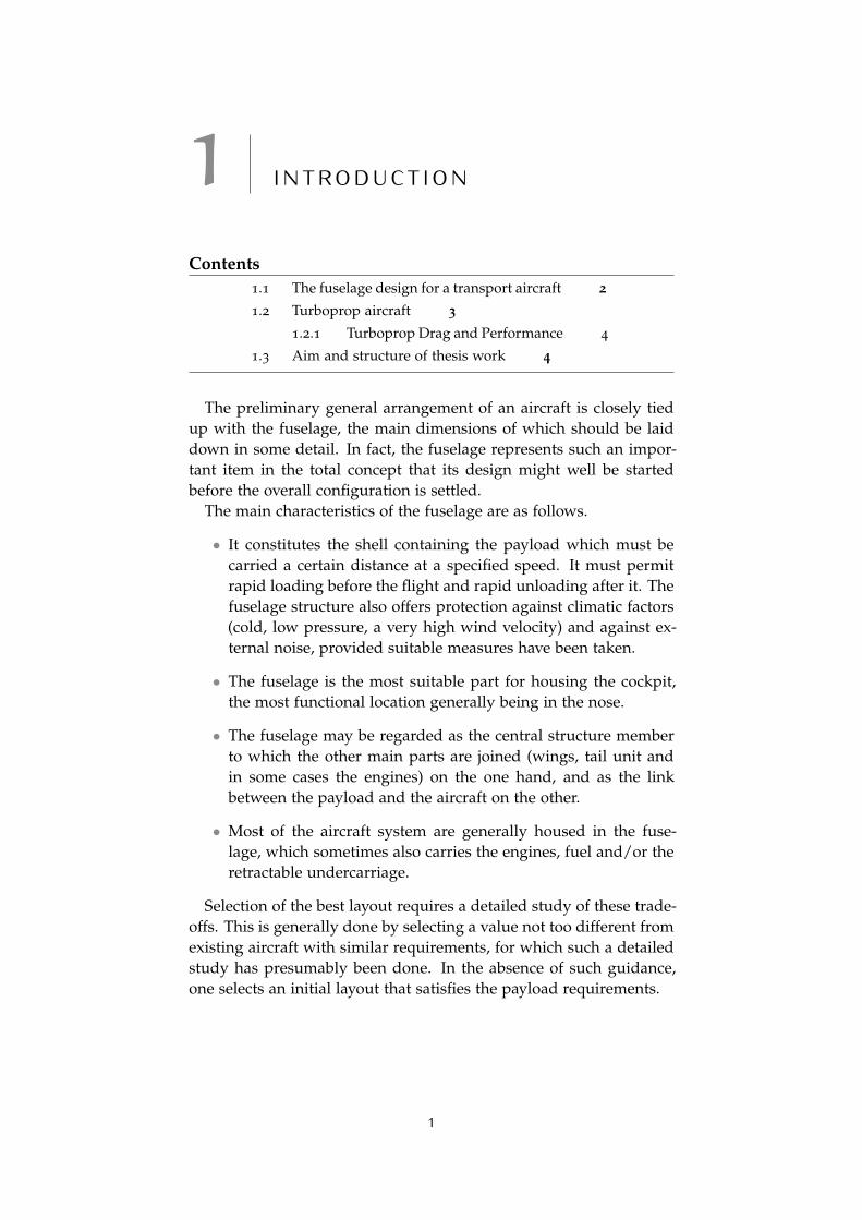
The preliminary general arrangement of an aircraft is closely tiedup with the fuselage, the main dimensions of which should be laiddown in some detail. In fact, the fuselage represents such an impor-tant item in the total concept that its design might well be startedbefore the overall configuration is settled.
The main characteristics of the fuselage are as follows.
• It constitutes the shell containing the payload which must becarried a certain distance at a specified speed. It must permitrapid loading before the flight and rapid unloading after it. Thefuselage structure also offers protection against climatic factors(cold, low pressure, a very high wind velocity) and against ex-ternal noise, provided suitable measures have been taken.
• The fuselage is the most suitable part for housing the cockpit,the most functional location generally being in the nose.
• The fuselage may be regarded as the central structure memberto which the other main parts are joined (wings, tail unit andin some cases the engines) on the one hand, and as the linkbetween the payload and the aircraft on the other.
• Most of the aircraft system are generally housed in the fuse-lage, which sometimes also carries the engines, fuel and/or theretractable undercarriage.
Selection of the best layout requires a detailed study of these trade-offs. This is generally done by selecting a value not too different fromexisting aircraft with similar requirements, for which such a detailedstudy has presumably been done. In the absence of such guidance,one selects an initial layout that satisfies the payload requirements.
1
1.1 the fuselage design for a transport aircraft 2
1.1 the fuselage design for a transportaircraft
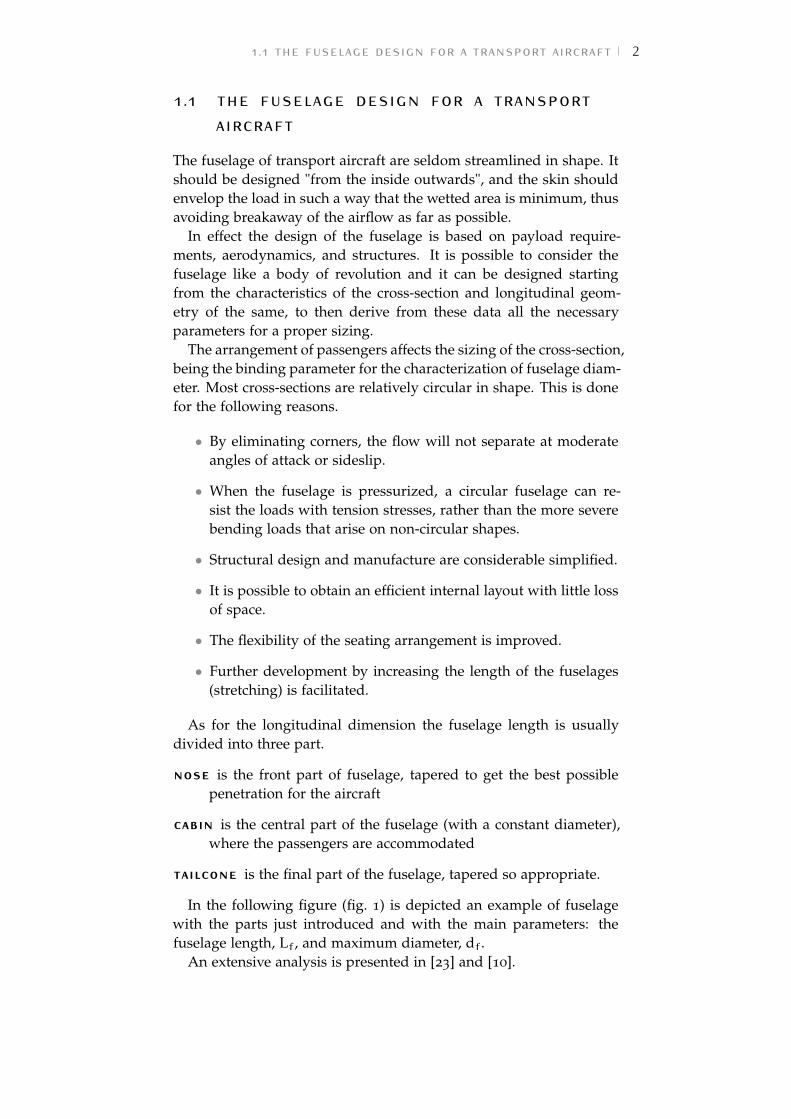
The fuselage of transport aircraft are seldom streamlined in shape. Itshould be designed "from the inside outwards", and the skin shouldenvelop the load in such a way that the wetted area is minimum, thusavoiding breakaway of the airflow as far as possible.
In effect the design of the fuselage is based on payload require-ments, aerodynamics, and structures. It is possible to consider thefuselage like a body of revolution and it can be designed startingfrom the characteristics of the cross-section and longitudinal geom-etry of the same, to then derive from these data all the necessaryparameters for a proper sizing.
The arrangement of passengers affects the sizing of the cross-section,being the binding parameter for the characterization of fuselage diam-eter. Most cross-sections are relatively circular in shape. This is donefor the following reasons.
• By eliminating corners, the flow will not separate at moderateangles of attack or sideslip.
• When the fuselage is pressurized, a circular fuselage can re-sist the loads with tension stresses, rather than the more severebending loads that arise on non-circular shapes.
• Structural design and manufacture are considerable simplified.
• It is possible to obtain an efficient internal layout with little lossof space.
• The flexibility of the seating arrangement is improved.
• Further development by increasing the length of the fuselages(stretching) is facilitated.
As for the longitudinal dimension the fuselage length is usuallydivided into three part.
nose is the front part of fuselage, tapered to get the best possiblepenetration for the aircraft
cabin is the central part of the fuselage (with a constant diameter),where the passengers are accommodated
tailcone is the final part of the fuselage, tapered so appropriate.
In the following figure (fig. 1) is depicted an example of fuselagewith the parts just introduced and with the main parameters: thefuselage length, Lf, and maximum diameter, df.
An extensive analysis is presented in [23] and [10].
1.2 turboprop aircraft 3
Figure 1: The main parts of a fuselage
1.2 turboprop aircraft
A recent work [5] has shown that the need to develop regional turbo-prop transport aircraft is tied to particular needs of both passengersand airlines. First of all, a generic regional turboprop aircraft has tobe faster than conventional transport means as trains, cars or shipsand it has to be relatively cheap.
Looking at aircraft performance, a turboprop aircraft has a shorttake-off and landing distance (sometimes on semi prepared runways)and a cruise airspeed not higher than 350 knots. From a deeper air-lines point of view, this aircraft has to meet the requirements of lowoperative and maintenance costs, it is cheaper than an equivalent re-gional jet and above all it has a lower fuel consumption saving moneyand pollution.
Passengers want to have a reliable aircraft, competitive in terms ofcosts, with low noise emission and, also on this aircraft category agood comfort. Aircraft industries were deeply involved in the designof new regional turboprop aircraft during the seventies and eightiesin conjunction with the oil crisis. During these years several turbo-prop aircraft were designed and produced worldwide, increasing thecompetition stimulation. Nowadays the leaders of the market areATR and Bombardier with, respectively, ATR-72 and Dash8-Q400 (fig-ure. 2).
(a) ATR 72-600 (b) DASH8-Q400
Figure 2: ATR-72 and DASH8-Q400 aircraft.
1.3 aim and structure of thesis work 4
It is possible to identify the main features of large turboprop air-craft:
• High-wing
• T-tail
• Slender fuselage
• Engine wing mounted
• Easy cabin accessibility both for passengers and baggage
• Reliable, low maintenance and construction costs structure
• Advanced system instrumentations, glass-cockpit and Fly-by-wire
• Cabin comfort.
It is quite evident that an aircraft of this category in order to satisfyall these requirements must have a very accurate design. In particu-lar, the aerodynamic design of these aircraft involves many aspectsthat must be assessed and addressed very thoroughly in the designphase. A very important feature of the aerodynamic design is theaerodynamic drag. For these reasons in the following Sec.1.2.1 theaerodynamic drag breakdown of typical large turboprop aircraft isaddressed to better understand which are the main drag sources andwhich the influence of drag reduction on the aircraft performance.
1.2.1 Turboprop Drag and Performance
From [5], it is known that the fuselage of a regional turboprop consti-tutes the main contribution to the aerodynamic drag.
A typical drag breakdown is shown in figure 3. The term fuselagein the pie chart also includes windshield, upsweep, base drag, andsome of the excrescences. For the same aircraft, the impact of dragin cruise performance is shown in figure 4. A reduction of 2.5 dragcounts increases the maximum true airspeed (TAS) by 1 knot. Anoverall drag decrease of 15 counts saves 3% fuel on a typical 200 nmmission.
1.3 aim and structure of thesis work
The main aim of this work is to investigate, from an aerodynamicpoint of view, a modular model of the fuselage of a regional trans-port turboprop aircraft with 90 seats. This approach involves thestudy of different fuselage components (nose, cabin and tailcone) to
1.3 aim and structure of thesis work 5
(a) Histogram of drag contribution. (b) Pie chart of drag contribution.
Figure 3: Typical regional turboprop drag breakdown.
(a) Maximum true airspeed variationdue to zero lift drag coefficient.
(b) Pie chart of drag contribution.
Figure 4: Drag impact on aircraft performance
identify trends in aerodynamic coefficients with geometrical param-eters. The only constraint imposed to modifications of the fuselageis the compliance to FAR 25.775 (Windshields and windows). Ap-pendix A shows some details of regulation. The starting point of thework is the reference fuselage. It is shown in figure 5 and the param-eters are reported in table 1. In order to point out the aerodynamictrends, hereinafter the results of aerodynamic studies are presentedby graphics and mathematical relationships which can be useful alsofor other aircraft in the preliminary design phase as previously ar-gued.
The work has been structured as follows.
Chapter 2 In this chapter the semi-empirical methods to calculatethe aerodynamic coefficients are introduced. In the first part aredescribed the semi-empirical methods which calculate the dragcoefficient as the sum of different contributions and then themost famous method for the calculation of moment coefficient,the strip method, is introduced.
1.3 aim and structure of thesis work 6
Figure 5: The reference fuselage
The reference fuselage
Ln 0.19 ·Lf Nose length
Lc 0.43 ·Lf Cabin length
Lt 0.38 ·Lf Tailcone length
FR 8.69 Slenderness ratio
FRn 1.60 Nose slenderness ratio
FRt 2.83 Tail slenderness ratio
ψ 39.7° Windshield angle
θ 13.6° Upsweep angle
Table 1: Features of the reference fuselage.
Chapter 3 Once the semi-empirical methods have been described,a procedure that make use of CFD to compute the same aero-dynamic coefficients is explained. This procedure is the coreof the present work. The fuselage geometry of a turboprop isgiven as a CAD model which is modified with MATLAB in or-der to derive some different fuselage configurations. The latterhave been analysed with the commercial software Star-CCM+to evaluate the aerodynamic coefficients. At the same time itis presented the MATLAB code that modifies the geometry ofthe fuselage. The results of some test cases are also shown tovalidate the CFD model.
Chapter 4 This chapter is fully dedicated to show the results of nu-merical simulations. The different cases are obtained changingone at time the fineness ratio of the nose (FRn), the fineness ratioof the cabin (FR) and the fineness ratio of the tailcone (FRt) andkeeping the other equal to those of the reference fuselage. Othercases are obtained by changing the upsweep angle maintainingconstant FRt and changing the windshield angle maintainingconstant FRn. Moreover the effect of the combined changes areevaluated.

1.3 aim and structure of thesis work 7
Chapter 5 A new methodology to predict the drag and moment co-efficient have been carried out and are described in this chapter.The method supplies the parametric relationships between theaerodynamic coefficients and the geometry of the fuselage. ThisCFD-born methodology is based on a general turboprop geome-try and this is its strength compared to the semi-empirical meth-ods. It can be very useful in preliminary design phase.
Chapter 6 Finally in this chapter the main achievements of this thesiswork are summarized and some conclusions are drawn.
2 S E M I - E M P I R I C A L M E T H O D SF O R P R E D I C T I O N O FA E R O DY N A M I C C O E F F I C I E N T S
Contents2.1 Fuselage drag coefficient prediction 8
2.1.1 Effect of fineness ratio 10
2.1.2 Skin friction contribution 11
2.1.3 Fuselage upsweep contribution 13
2.1.4 Fuselage base drag contribution 14
2.1.5 Windshield contribution 14
2.2 Fuselage moment coefficient prediction 16
2.3 Example of application 19
2.3.1 Drag estimation for ATR-72 19
2.3.2 Drag estimation for Dash8-Q400 23
2.3.3 Pitching moment estimation for ATR-72 24
2.3.4 Pitching moment estimation for Dash8-Q400 25
In this chapter the methods to calculate the aerodynamic coeffi-cients, that are normally used in the preliminary phase to guide thedesign choices, are introduced. In the first section the semi-empiricalmethods are described and it shows how they predict the drag coeffi-cient. These methods consider the drag coefficient as the sum of dif-ferent contributions that can be evaluated by relations obtained fromwind tunnel test. The content of this chapter is mostly excerpt fromworks of Prof. Roskam [19] and [20], Kroo et al. [10] and Raymer [18].
Afterwards the strip method is reported for the prediction of mo-ment coefficient. It is so called because the fuselage is divided intostrips each of which gives a contribution to pitching moment in afunction of distance from the polo. This method was developed byMunk [15] and Multhopp [14]. Perkins and Hage explained how thefuselage affects the longitudinal stability [17].
2.1 fuselage drag coefficient prediction
Usually, in preliminary design phases, the estimation of drag coef-ficient (CD) is obtained through semi-empirical methods. They arebased on the results of wind-tunnel tests of the past, mainly collected
8
2.1 fuselage drag coefficient prediction 9
in the USAF DATCOM database. The total drag coefficient of an air-craft is given by the sum of the zero lift drag coefficient and the in-duced drag coefficient. This assumption is made when the approxi-mation of a parabolic drag polar is assumed in order to estimate thedrag coefficient for low incidence such as cruise and climb, that isuntil the lift coefficient becomes greater than 1. The approximationleads to the following formulation:
CD = CD0 +CL2
πARe(2.1)
where AR is the aspect ratio of the wing and e is the Oswald factorof the complete aircraft. While the induced drag coefficient can beeasily computed, the zero lift drag coefficient has to be estimated bysemi-empirical approaches in the preliminary design phase.
The zero lift drag coefficient is also known as parasite drag coeffi-cient and it includes skin friction, base, interference, wave, and trimdrag coefficients, thus resulting in the following
CD0 = CDsf +CDbase +CDint +CDwave +CDtrim (2.2)
In the present work it accounts for the contributions to CD0 ofthe fuselage and therefore are taken into account only the CDsf , theCDbase and the CDint (due to the windshield and upsweep angle). Ineffect the fuselage is responsible for a large percentage of the overalldrag (in particular the parasite drag) of the airplanes (about 25% -50% of total drag) and since it is desirable to have as little drag aspossible, the fuselage should be sized and shaped accordingly. Theparasite drag coefficient (see eq. (2.2)) of an aircraft can be computedby adding each contribute of the different components and assumingan interference effect. If CDi and Si are respectively the drag coeffi-cient and the surface of the component i, q the dynamic pressure, thetotal drag given by n components is:
D = q
n∑i=1
CDiSi
Since each component is characterized by a different reference sur-face, it is not possible to sum directly the drag coefficients but it ispossible to sum the products CDiSi . These products are known asthe areas of the equivalent flat plate, that is fi ; since a flat platenormal to the free stream has a drag coefficient equal to 1, fi repre-sents the area of a flat plate that, when it is normal to the free stream,has the same drag coefficient of the component i. Thus, the previousformulation becomes
D = q
n∑i=1
CDiSi = q
n∑i=1
fi = qfTOT
2.1 fuselage drag coefficient prediction 10
Moreover, the skin friction coefficient for a generic component is:
Cf =DfqSwet
where Swet represents the wetted area that is the surface of thatcomponent wetted by the fluid. The skin friction drag coefficient is
CDf =DfqSref
thus, it is easy to find that
CDf =DfSwet
Sref
The link between a generic component and the flat plate is neces-sary since the skin friction coefficient is exactly computed for a flatplate so that, once known Cf for the equivalent flat plate, the skinfriction drag coefficient becomes a function of the geometry of thecomponent. In fact, the skin friction coefficient for a generic compo-nent can be obtained by
Cf = C̄fFf
where C̄f is the skin friction coefficient for the equivalent flat plateand Ff is the form factor that takes into account that the component isnot a flat plate and the boundary layer develops in presence of pres-sure gradients. Finally, the skin friction drag coefficient of a genericcomponent can be computed as follows
CDf = C̄fFfSwet
Sref(2.3)
In order to point out the contributes of the fuselage to parasite drag,it is possible to split up this contribution in 4 parts:
1. Skin friction contribution
2. Fuselage upsweep contribution
3. Fuselage base drag contribution
4. Windshield contribution
2.1.1 Effect of fineness ratio
Before to study how the semi-empirical methods to calculate a vari-ous contributions to CD, it’s important introduce an older approach(reported in [23]) that highlights the effect of one of most importantparameter, the fineness ratio Lf/df (or slenderness ratio).
2.1 fuselage drag coefficient prediction 11
The fuselage is considered a body of revolution (ellipsoid). It’spossible calculate the drag coefficient of the axisymmetric fuselage byevaluating the skin friction coefficient of a flat plate, whose surfaceis equal to the wet surface of the fuselage and the Reynolds numberis evaluated on the fuselage length, and a shape factor to account forpressure drag. The formula is:
CDSref = CfSwet(1+φ) (2.4)
where CD is the drag coefficient, Sref is the reference surface, CF isthe flat plate skin friction coefficient, Swet is the wet surface of thefuselage, and φ is the shape factor that is function of the slendernessratio. The drag coefficient for bodies of different slender ratio andreference area it is represented in figure 6. The slender ratio of 1
represents a sphere, whereas very streamlined bodies are indicatedby high values of the slender ratio. Three reference areas are consid-ered: the body wetted surface, the body frontal area, and the arearepresentative of the body volume. The drag coefficient strongly de-pends from the reference area. The curve that refers to the frontalarea (which is constant with slender ratio) presents a minimum be-tween values of Lf/df between 2 and 3. On the contrary, the curvethat refers to the wetted area (which increases with the slender ratio)presents an asymptote equal to the drag coefficient of the flat platefor high values of the slender ratio. Finally, the curve that refers tothe volume presents a minimum for Lf/df = 5.
By looking at these last two curves it is apparent the convenience ofhigh values of the slender ratio, because of the low value of the dragcoefficient and the availability of space for payload (bigger volumefor a given frontal area).
2.1.2 Skin friction contribution
The fuselage form factor is computed according the following equa-tion
Ff,fus =
[1+
60( ZLFSWF
)2 + 0.0025 ·( ZLFSWF
)](2.5)
where ZLF is the fuselage length and SWF is fuselage equivalentdiameter. The skin friction coefficient depends on the Reynolds andon the Mach number and it is known for the flat plate since this prob-lem has been analytically resolved. A formulation for the turbulentskin friction coefficient is the following, which has been used in thefuselage estimation
Cfturb =
0.455(logRe)2.58 · (1+ 0.144 ·M2)0.58 (2.6)
2.1 fuselage drag coefficient prediction 12
0 1 2 3 4 5 6 7 8 9 100.0
0.02
0.04
0.06
0.08
0.1
0.12
0.14
0.16
Lf/df
CD
CD frontal areaCD wet area*10
CD volume2/3
CD flat plate*10
Figure 6: Semi-empirical drag estimation for smooth streamlined bodies (el-lipsoid). Re = 107. Fully turbulent flow. Flat plate analogy [23].
The skin friction coefficient depends on the Reynolds number, whichis different for each aircraft components. A "cut-off" Reynolds num-ber Reco has been computed for each component. This Reco dependson the characteristic dimensions of the component, l, (i.e. the lengthfor the fuselage) and on a coefficient k that takes into account theeffect of the surface roughness, through the following formulation
Reco = 38.21 ·( lk
)1.053(2.7)
If the component Reynolds number is greater than Reco, the skinfriction coefficient is computed considering Reco in the formulation,otherwise the reference Reynolds number should be used.
Wetted surface
In the semi-empirical methods the wet surface assumes a consider-able importance. Therefore it’s important estimate the correct valueof it for each part of aircraft. As regard the fuselage the wetted areacan be computed by adding the contribution of the nose section, cabinsection and tapered tailcone. This requires knowledge of the actualfuselage shape, but for typical transport aircraft, the wetted area ofthe nose and tail cone may be approximated by:
Swetnose = 0.75 · π · df · Ln Swettail = 0.72 · π · df · Lt (2.8)
where df is the diameter of the constant section and Ln and Lt arethe length of the nose and tailcone respectively.
2.1 fuselage drag coefficient prediction 13
Figure 7: Definition of fuselage upsweep angle.
Considering the effect of the fairing1 and of the karman2, the totalwetted area should be increased of about 20% thus leading to :
SwetFAIR+KARM+FUS = 1.20 · SwetFUS
2.1.3 Fuselage upsweep contribution
The drag due to the upward curvature of the aft fuselage is the sumof a fuselage pressure drag increment due to the upsweep and a dragincrement due to a loss of lift. Because of the loss of lift, the airplanemust fly at a higher wing lift coefficient in order to maintain therequired net airplane CL. This causes an increase in lift-dependentdrag [10]. The geometric parameter used to correlate upsweep dragwith fuselage shape is the vertical displacement of the fuselage cen-terline in the tail cone above the fuselage reference plane. The verticalposition of the center of cross-sectional area is measured, not at theend of the fuselage, but at a point that is located 75% of the total up-sweep length (see figure 7). The parameter is thus (hl ).75lt. This is tominimize the effect of modifications at the very aft end of the fuselagethat do not produce much change in the effective upsweep. The totalupsweep drag increment (including each of the two terms discussedpreviously) increases with the parameter, (h/l).75lt , according to thefollowing expression, derived from wind tunnel data:
CDπupsweep = 0.075 ·(h
l
).75lt
(2.9)
The subscript π denotes the fact that this CD is nondimensionalizedby fuselage maximum cross-sectional area, rather than reference wingarea. To obtain the increment in CD based on wing area, remember tomultiply by the ratio of fuselage cross section area to wing area. Typ-ical values of CDupsweep are around 0.006. Two points are of interestwith regard to aft-fuselage upsweep [10]:
1. Tests of fuselage shapes in the absence of the wing yield resultsthat greatly overestimate the magnitude of the upsweep drag.
1 fairing is a structure in the areas of landing gear whose primary function is to pro-duce a smooth outline of the fuselage in order to reduce the drag
2 karman is the fuselage-wing joint surface
2.1 fuselage drag coefficient prediction 14
2. Wind tunnel test results have indicated that the loss of lift dueto upsweep is significantly greater than just the download onthe aft fuselage, which suggests that there is a flow change overthe wing and forward fuselage due to the aft-fuselage upsweep.Also, the net change in pitching moment due to upsweep isan increased nose-down moment instead of a nose-up momentthat might be expected. As a result, the loss in lift does notcomplement the download on the tail that is required to trimthe airplane. In fact, the effect of upsweep is to slightly increasethe airplane trim drag.
2.1.4 Fuselage base drag contribution
The base drag coefficient is not negligible for bodies of revolutionsuch as the fuselage and nacelles, since the flow is not completelyattached to the body, but it separates in its rear part generating anincrease of the total drag coefficient. In order to clarify the originof this drag source, the flow around the reference fuselage has beencompared with that around an other geometry which has a differenttailcone (more sharp than that of reference). The comparison hasbeen carried out with the CFD software Star-CCM+. Figure 8 showsthe flow in the rear part is attached for the reference fuselage whilefor the other there’s a separation due to a squat shape of rear part,which causes a higher base drag.
The base drag coefficient can be computed using the following for-mulation for a body of revolution [20]:
CDbase =
{0.029 ·
(dbd
)3/[CD ·
(Sref
S
)]1/2}(S
Sref
)(2.10)
where db is the base diameter, d is the diameter of the body ofrevolution, CD is the skin friction drag coefficient of the body of revo-lution, Sref is the reference surface, and S is the surface of the body ofrevolution (i.e. the maximum frontal area). In the figure 9, the plot ofdrag due to the form of rear part as a function of the tailcone finenessratio is reported.
2.1.5 Windshield contribution
Profile drag is a strong function of front body shape. Blunt fore-bodies promote flow separations which lead to high profile drag.Fore-body bluntness can be caused by:
• Poor cockpit window or canopy shaping
• Requirement for front and loading
2.1 fuselage drag coefficient prediction 15
(a) Sharp tail geometry
(b) Reference tail geometry
Figure 8: Flow around the rear part of the fuselage.
The ideal "streamline" nose shape can be achieved only if the wind-shields are integrated into the surface fuselage. Although drag can beconsiderably reduced by these types of windshield fairing, image dis-tortions may be introduced if the "fairing angle" becomes too acute.In the case of transport aircraft the requirement for good visibilityfrom the cockpit becomes a dominant design criterion. This calls fora large canopy. Therefore the canopy drag becomes an import factorin the design of the fuselage. The contribute of the windshield can beestimated as a percentage of the fuselage drag coefficient referred tothe streamlined configuration [20].
If the skin friction drag coefficient (CDsf) of the fuselage is known,the effect of the windshield can be estimated as follows (for ∆CDWSand CDFUS see figure 10):
CDWS =∆CDWSCDFUS
·CDsf (2.11)
2.2 fuselage moment coefficient prediction 16
Figure 9: Afterbody drag of a fuselage tail [23].
2.2 fuselage moment coefficient prediction
It is known that the contribution of the fuselage to the static longitu-dinal stability of the airplane are nearly always destabilizing, and inmany cases the destabilizing effects are quite large in magnitude [17].If the fuselage is considered operating at some angle of attack to thefree stream in an ideal fluid, the resulting pressure distribution overthe fuselage yields only a pure couple, with no resultant force, thecenter of pressure being at infinity.
M. Munk [15] demonstrated that, for a very slender body of revo-lution, the variation of the pitching moment with angle of attack indegrees is a function of the volume and the dynamic pressure.(
∂M∂α
)=Volume
28.7· q (2.12)
This equation is corrected by a factor (K2 − K1), depending on thefuselage fineness ratio (L/D) as given in figure 11.(
∂M
∂α
)=Volume
28.7· q · (K2 −K1) (2.13)
For axially unsymmetric bodies equation (2.13) can be written asapproximately (
∂M
∂α
)=q · (K2 −K1)
36.5·∫ lf0
wf2 dx (2.14)
2.2 fuselage moment coefficient prediction 17
Figure 10: Semi-empirical method for estimation of windshield drag contri-bution [20].
where wf2 is the local width of the fuselage, and dx an incrementof fuselage length lf.
The wing’s induced flow, consisting of heavy upwash in front of thewing due to the bound vortex, has a heavy destabilizing influence onthe fuselage sections ahead the wing, whereas the downwash behindthe wing reduces the unstable contribution of the fuselage segmentsbehind the wing.
Multhopp proposed the formula (2.15) to account for this phe-nomenon: (
∂M
∂α
)=
q
36.5·∫ lf0
wf2
(∂β
∂α
)dx (2.15)
where β is the angle of the local flow and is equal to the free streamangle of attack plus the induced flow due to wing. Ahead of the wingthe induced upwash adds to the angle of free stream, making (∂β/∂α)
greater than unity, while behind the wing the induced downwashsubtracts from the free stream angle and (∂β/∂α) is less than unityand becomes (1− ∂ε/∂α) at the tail. In the region between the wingleading and trailing edge, (∂β/∂α) is considered zero.
The integral equation (2.15) is evaluated by dividing the fuselageinto segments (see 12), computing the value of wf2(∂β/∂α) · ∆x foreach segment and adding them up. For the evaluation of contribu-tions please refer to [14]. A simpler, but less accurate, method forestimating the fuselage contribution to equilibrium and stability is touse the following formula [17]:
2.2 fuselage moment coefficient prediction 18
Figure 11: Fuselage correction for fineness ratio.
Figure 12: Typical layout for computing fuselage moments.
2.3 example of application 19
Figure 13: Fuselage stability coefficient. From [7].
(∂CM∂CL
)=Kf ·wf2 · LfSw · c ·CLα
(2.16)
where Lf is the overall fuselage length,wf is the maximum width ofthe fuselage, c is the m.a.c. and the Kf is an empirical factor developedfrom experimental evidence [7]. The variation of this factor with thewing position is given in figure 13.
2.3 example of application
In this section the semi-empirical methods are used to obtain the dragand moment coefficients for the most famous regional turboprops,that’s to say the ATR-72 (figure 14) and Bombardier Dash8-Q400 (fig-ure 15) . The aircraft data have been taken from [2], [9] and [5].
2.3.1 Drag estimation for ATR-72
As it has been seen in the previous sections, in the fuselage parasitedrag contributions can be accounted:
1. Skin friction contribution
2. Fuselage upsweep contribution
3. Fuselage base drag contribution
4. Windshield contribution
Skin friction contribution
The skin friction contribution can be evaluated from equation 2.3 andtherefore it is necessary to estimate the form factor and the skin fric-tion coefficient. The latter is obtained from equation 2.6, with the
2.3 example of application 20
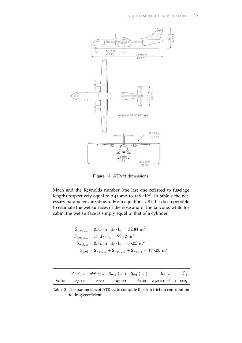
Figure 14: ATR-72 dimensions.
Mach and the Reynolds number (the last one referred to fuselagelength) respectively equal to 0.43 and to 138×106. In table 2 the nec-essary parameters are shown. From equations 2.8 it has been possibleto estimate the wet surfaces of the nose and of the tailcone, while forcabin, the wet surface is simply equal to that of a cylinder.
Swetnose = 0.75 · π · df · Ln = 32.84 m2
Swetcabin = π · df · Lc = 99.10 m2
Swettail = 0.72 · π · df · Lt = 63.05 m2
Swet = Swetnose + Swetcabin + Swettail = 195.00 m2
ZLF (m) SWF (m) Swet (m2 ) Sref ( m2) kf (m) C̄f
Value 27.17 2.70 195.00 61.00 0.405×10⁻⁵ 0.0019
Table 2: The parameters of ATR-72 to compute the skin friction contributionto drag coefficient.
2.3 example of application 21
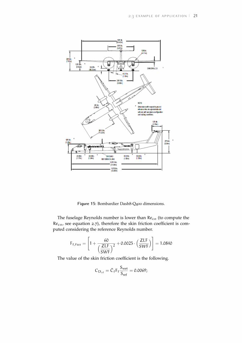
Figure 15: Bombardier Dash8-Q400 dimensions.
The fuselage Reynolds number is lower than Reco (to compute theReco, see equation 2.7), therefore the skin friction coefficient is com-puted considering the reference Reynolds number.
Ff,fus =
[1+
60( ZLFSWF
)2 + 0.0025 ·( ZLFSWF
)]= 1.0840
The value of the skin friction coefficient is the following.
CDsf = C̄fFfSwet
Sref= 0.0069;
2.3 example of application 22
Fuselage upsweep contribution
The contribution of the upsweep angle to drag can be evaluated fromequation 2.9, where h is equal to 0.61 m and l equal to 13.4 m (thesevalues can be pull out graphically from figure 14).
CDupsweep = 0.075 ·(h
l
).75lt = 0.0003
Fuselage base drag contribution
The contribution of the base drag can be evaluated from equation 2.10,where db is equal to 0.35 m (estimated from the figure 14), d is thefuselage diameter (SWF in the table 2), S and Sref are respectively thewet and reference surface, and these are reported in table 2.
CDbase =
{0.029 ·
(dbd
)3/[CD ·
(Sref
S
)]1/2}(S
Sref
)=
= 0.0002
Windshield contribution
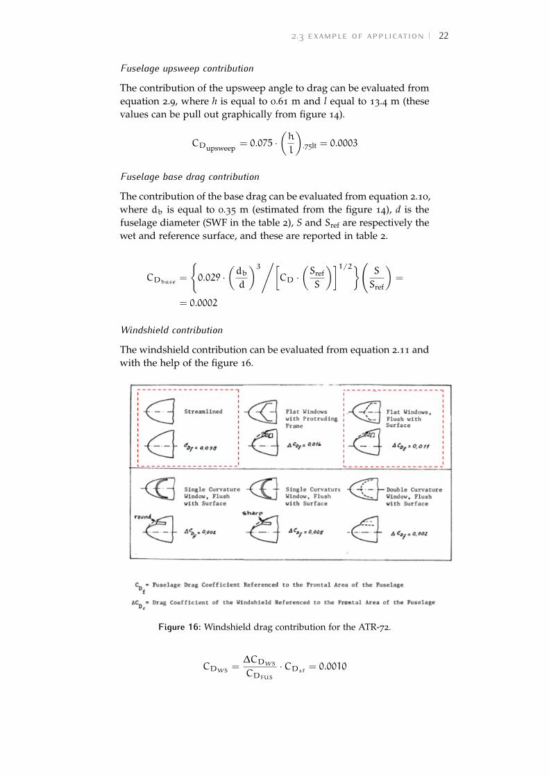
The windshield contribution can be evaluated from equation 2.11 andwith the help of the figure 16.
Figure 16: Windshield drag contribution for the ATR-72.
CDWS =∆CDWSCDFUS
·CDsf = 0.0010
2.3 example of application 23
Once estimated the different contributions, the total drag coeffi-cient is simply the sum of these contributions.
CD = CDsf +CDupsweep +CDbase +CDWS = 0.0085
2.3.2 Drag estimation for Dash8-Q400
In a similar manner to what was done for the ATR-72, in this sec-tion the semi-empirical methods are used to estimate the differentcontributions to drag coefficient for Dash8-Q400. The flight condi-tions are the similar those of ATR-72: Mach number equal to 0.50 andReynolds number (referred to fuselage length) equal to 149×106. Thewet surfaces are estimated with equations 2.8 and in the table 3, thenecessary parameters are reported.
Swetnose = 0.75 · π · df · Ln = 22.04 m2
Swetcabin = π · df · Lc = 149.14 m2
Swettail = 0.72 · π · df · Lt = 60.32 m2
Swet = Swetnose + Swetcabin + Swettail = 231.51 m2
ZLF (m) SWF (m) Swet (m2 ) Sref ( m2) kf (m) C̄f
Value 31.04 2.69 231.51 63.08 0.405×10⁻⁵ 0.0020
Table 3: The parameters of Dash8-Q400 to compute the skin friction contri-bution to drag coefficient.
As before, the fuselage Reynolds number is lower than Reco there-fore the skin friction coefficient is computed considering the referenceReynolds number.
Ff,fus =
[1+
60( ZLFSWF
)2 + 0.0025 ·( ZLFSWF
)]= 1.0679
The value of the skin friction coefficient is the following.
CDsf = C̄fFfSwet
Sref= 0.0078
The contribution of the upsweep angle to drag can be evaluatedfrom equation 2.9, where h is equal to 0.97 m and l equal to 7.43 m(these values can be pull out graphically from figure 15).
CDupsweep = 0.075 ·(h
l
).75lt = 0.0009
2.3 example of application 24
The contribution of the base drag can be evaluated from equa-tion 2.10, where db is equal to 0.35 m (estimated from the figure 14),d is the fuselage diameter (SWF in the table 2), S and Sref are respec-tively the wet and reference surface, and these are reported in table 2.
CDbase =
{0.029 ·
(dbd
)3/[CD ·
(Sref
S
)]1/2}(S
Sref
)=
= 0.0001
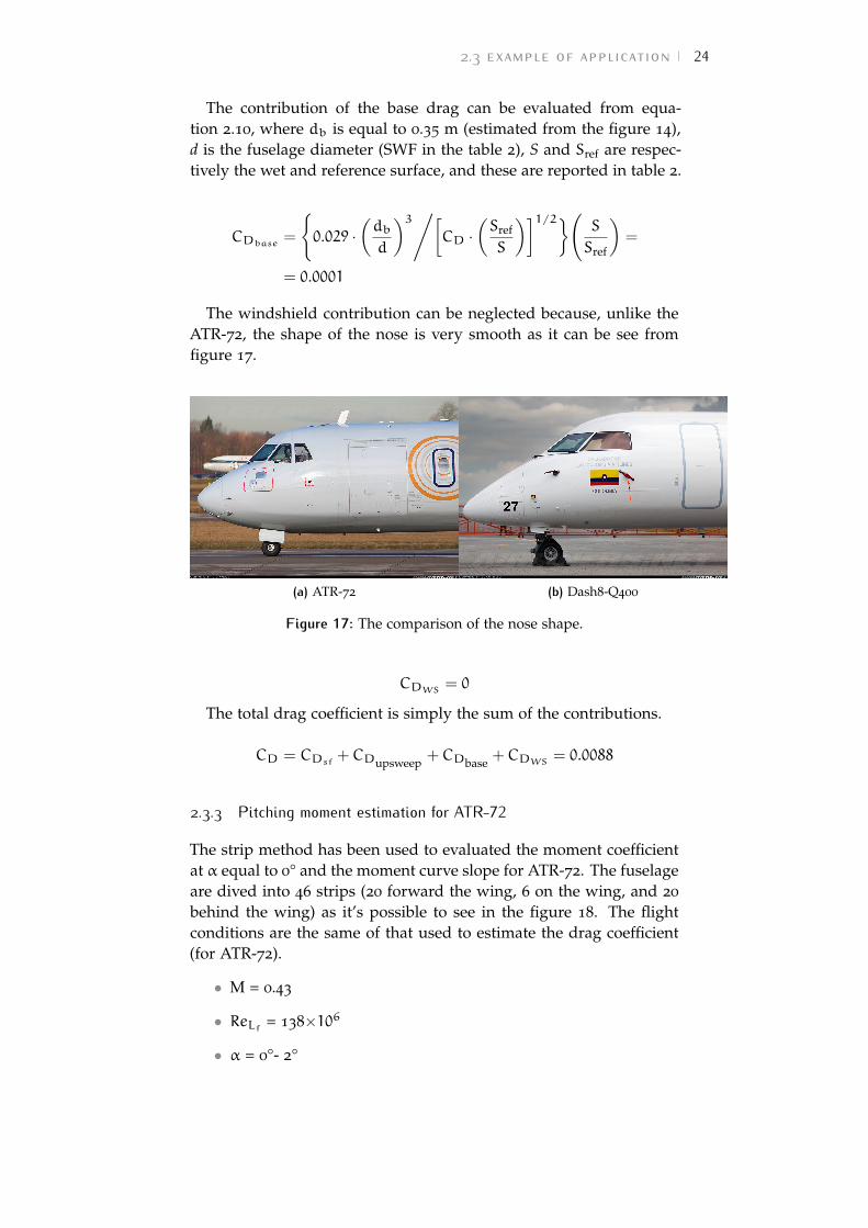
The windshield contribution can be neglected because, unlike theATR-72, the shape of the nose is very smooth as it can be see fromfigure 17.
(a) ATR-72 (b) Dash8-Q400
Figure 17: The comparison of the nose shape.
CDWS = 0
The total drag coefficient is simply the sum of the contributions.
CD = CDsf +CDupsweep +CDbase +CDWS = 0.0088
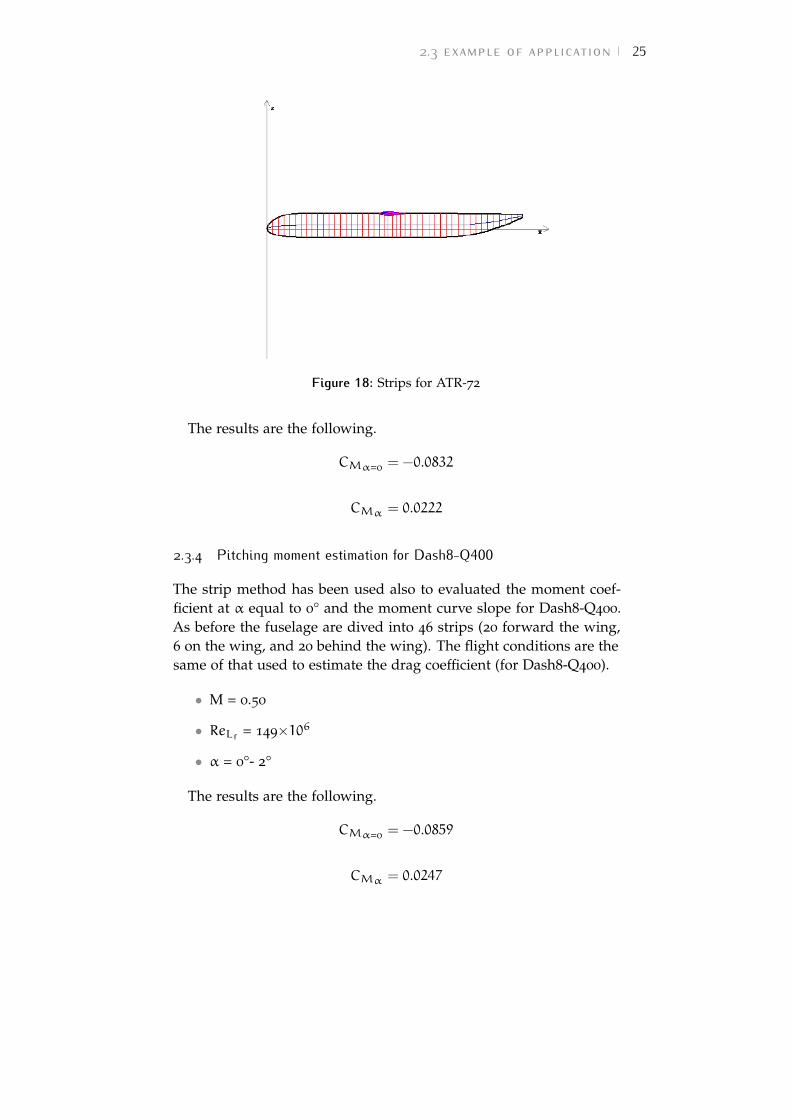
2.3.3 Pitching moment estimation for ATR-72
The strip method has been used to evaluated the moment coefficientat α equal to 0° and the moment curve slope for ATR-72. The fuselageare dived into 46 strips (20 forward the wing, 6 on the wing, and 20
behind the wing) as it’s possible to see in the figure 18. The flightconditions are the same of that used to estimate the drag coefficient(for ATR-72).
• M = 0.43
• ReLf = 138×106
• α = 0°- 2°
2.3 example of application 25
Figure 18: Strips for ATR-72
The results are the following.
CMα=0= −0.0832
CMα = 0.0222
2.3.4 Pitching moment estimation for Dash8-Q400
The strip method has been used also to evaluated the moment coef-ficient at α equal to 0° and the moment curve slope for Dash8-Q400.As before the fuselage are dived into 46 strips (20 forward the wing,6 on the wing, and 20 behind the wing). The flight conditions are thesame of that used to estimate the drag coefficient (for Dash8-Q400).
• M = 0.50
• ReLf = 149×106
• α = 0°- 2°
The results are the following.
CMα=0= −0.0859
CMα = 0.0247
3 A N U M E R I C A L A P P R OA C H
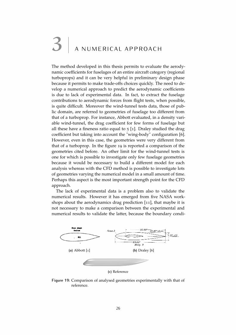
The method developed in this thesis permits to evaluate the aerody-namic coefficients for fuselages of an entire aircraft category (regionalturboprops) and it can be very helpful in preliminary design phasebecause it permits to make trade-offs choices quickly. The need to de-velop a numerical approach to predict the aerodynamic coefficientsis due to lack of experimental data. In fact, to extract the fuselagecontributions to aerodynamic forces from flight tests, when possible,is quite difficult. Moreover the wind-tunnel tests data, those of pub-lic domain, are referred to geometries of fuselage too different fromthat of a turboprop. For instance, Abbott evaluated, in a density vari-able wind-tunnel, the drag coefficient for few forms of fuselage butall these have a fineness ratio equal to 5 [1]. Draley studied the dragcoefficient but taking into account the "wing-body" configuration [6].However, even in this case, the geometries were very different fromthat of a turboprop. In the figure 19 is reported a comparison of thegeometries cited before. An other limit for the wind-tunnel tests isone for which is possible to investigate only few fuselage geometriesbecause it would be necessary to build a different model for eachanalysis whereas with the CFD method is possible to investigate lotsof geometries varying the numerical model in a small amount of time.Perhaps this aspect is the most important strength point for the CFDapproach.
The lack of experimental data is a problem also to validate thenumerical results. However it has emerged from five NASA work-shops about the aerodynamics drag prediction [11], that maybe it isnot necessary to make a comparison between the experimental andnumerical results to validate the latter, because the boundary condi-
(a) Abbott [1] (b) Draley [6]
(c) Reference
Figure 19: Comparison of analysed geometries experimentally with that ofreference.
26
a numerical approach 27
WIND TUNNEL TEST CFD
Walls Free Air
Support System (Sting) Free Air
Laminar/Turbulent (Tripped) "Fully" Turbulent (usually)
Aeroelastic Deformation Rigid
Measurement Uncertainty Numerical Uncertainty & Error
Corrections for known effects No Corrections
Table 4: Reasons to not compare CFD and wind-tunnel results [11].
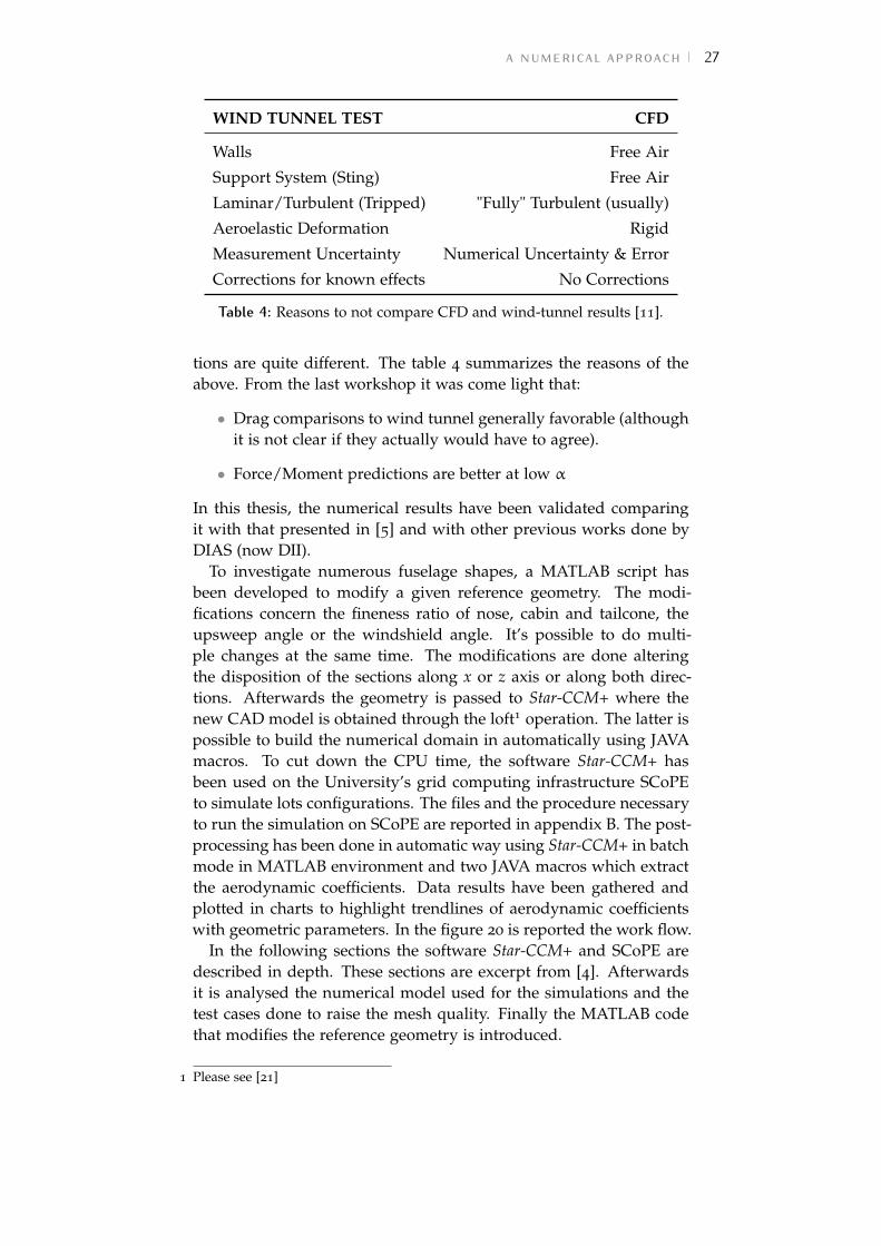
tions are quite different. The table 4 summarizes the reasons of theabove. From the last workshop it was come light that:
• Drag comparisons to wind tunnel generally favorable (althoughit is not clear if they actually would have to agree).
• Force/Moment predictions are better at low α
In this thesis, the numerical results have been validated comparingit with that presented in [5] and with other previous works done byDIAS (now DII).
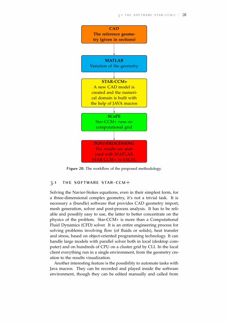
To investigate numerous fuselage shapes, a MATLAB script hasbeen developed to modify a given reference geometry. The modi-fications concern the fineness ratio of nose, cabin and tailcone, theupsweep angle or the windshield angle. It’s possible to do multi-ple changes at the same time. The modifications are done alteringthe disposition of the sections along x or z axis or along both direc-tions. Afterwards the geometry is passed to Star-CCM+ where thenew CAD model is obtained through the loft1 operation. The latter ispossible to build the numerical domain in automatically using JAVAmacros. To cut down the CPU time, the software Star-CCM+ hasbeen used on the University’s grid computing infrastructure SCoPEto simulate lots configurations. The files and the procedure necessaryto run the simulation on SCoPE are reported in appendix B. The post-processing has been done in automatic way using Star-CCM+ in batchmode in MATLAB environment and two JAVA macros which extractthe aerodynamic coefficients. Data results have been gathered andplotted in charts to highlight trendlines of aerodynamic coefficientswith geometric parameters. In the figure 20 is reported the work flow.
In the following sections the software Star-CCM+ and SCoPE aredescribed in depth. These sections are excerpt from [4]. Afterwardsit is analysed the numerical model used for the simulations and thetest cases done to raise the mesh quality. Finally the MATLAB codethat modifies the reference geometry is introduced.
1 Please see [21]
3.1 the software star-ccm+ 28
CADThe reference geome-try (given in sections)
MATLABVariation of the geometry
STAR-CCM+A new CAD model is
created and the numeri-cal domain is built withthe help of JAVA macros
SCoPEStar-CCM+ runs oncomputational grid
POST-PROCESSINGThe results are anal-ysed with MATLAB,
STAR-CCM+ or EXCEL
Figure 20: The workflow of the proposed methodology.
3.1 the software star-ccm+
Solving the Navier-Stokes equations, even in their simplest form, fora three-dimensional complex geometry, it’s not a trivial task. It isnecessary a (bundle) software that provides CAD geometry import,mesh generation, solver and post-process analysis. It has to be reli-able and possibly easy to use, the latter to better concentrate on thephysics of the problem. Star-CCM+ is more than a ComputationalFluid Dynamics (CFD) solver. It is an entire engineering process forsolving problems involving flow (of fluids or solids), heat transferand stress, based on object-oriented programming technology. It canhandle large models with parallel solver both in local (desktop com-puter) and on hundreds of CPU on a cluster grid by CLI. In the localclient everything run in a single environment, from the geometry cre-ation to the results visualization.
Another interesting feature is the possibility to automate tasks withJava macros. They can be recorded and played inside the softwareenvironment, though they can be edited manually and called from
3.1 the software star-ccm+ 29
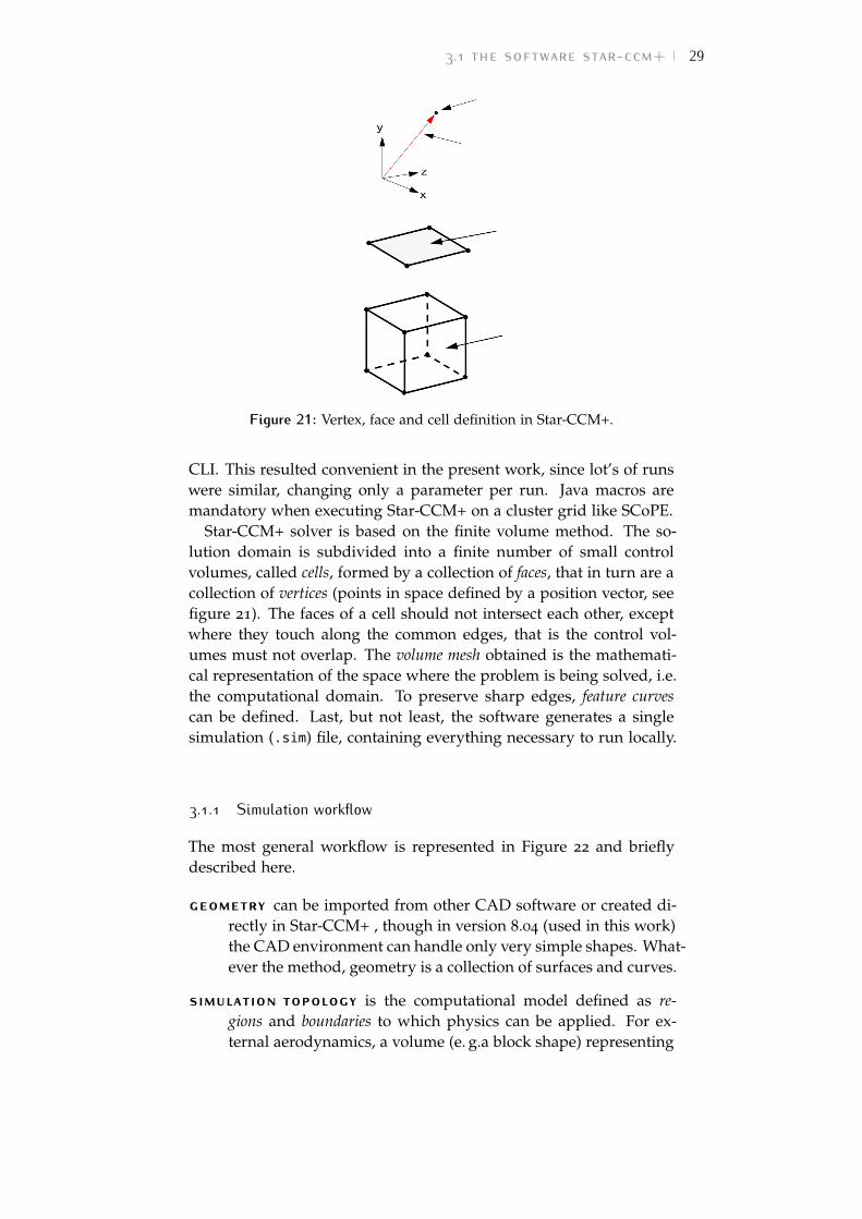
Figure 21: Vertex, face and cell definition in Star-CCM+.
CLI. This resulted convenient in the present work, since lot’s of runswere similar, changing only a parameter per run. Java macros aremandatory when executing Star-CCM+ on a cluster grid like SCoPE.
Star-CCM+ solver is based on the finite volume method. The so-lution domain is subdivided into a finite number of small controlvolumes, called cells, formed by a collection of faces, that in turn are acollection of vertices (points in space defined by a position vector, seefigure 21). The faces of a cell should not intersect each other, exceptwhere they touch along the common edges, that is the control vol-umes must not overlap. The volume mesh obtained is the mathemati-cal representation of the space where the problem is being solved, i.e.the computational domain. To preserve sharp edges, feature curvescan be defined. Last, but not least, the software generates a singlesimulation (.sim) file, containing everything necessary to run locally.
3.1.1 Simulation workflow
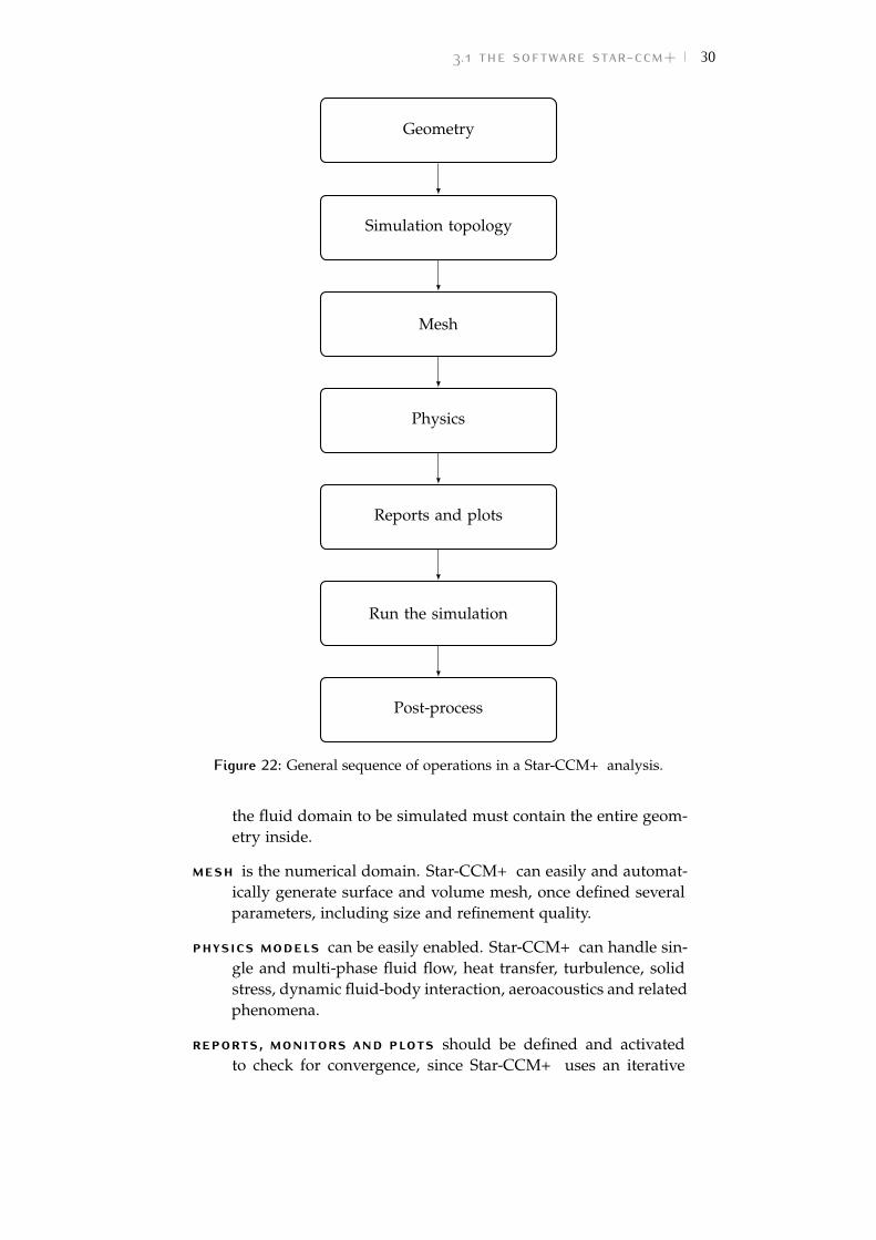
The most general workflow is represented in Figure 22 and brieflydescribed here.
geometry can be imported from other CAD software or created di-rectly in Star-CCM+ , though in version 8.04 (used in this work)the CAD environment can handle only very simple shapes. What-ever the method, geometry is a collection of surfaces and curves.
simulation topology is the computational model defined as re-gions and boundaries to which physics can be applied. For ex-ternal aerodynamics, a volume (e. g.a block shape) representing
3.1 the software star-ccm+ 30
Geometry
Simulation topology
Mesh
Physics
Reports and plots
Run the simulation
Post-process
Figure 22: General sequence of operations in a Star-CCM+ analysis.
the fluid domain to be simulated must contain the entire geom-etry inside.
mesh is the numerical domain. Star-CCM+ can easily and automat-ically generate surface and volume mesh, once defined severalparameters, including size and refinement quality.
physics models can be easily enabled. Star-CCM+ can handle sin-gle and multi-phase fluid flow, heat transfer, turbulence, solidstress, dynamic fluid-body interaction, aeroacoustics and relatedphenomena.
reports, monitors and plots should be defined and activatedto check for convergence, since Star-CCM+ uses an iterative
3.1 the software star-ccm+ 31
procedure to reach the solution to the transport equations thatsatisfies the boundary conditions for a chosen scenario.
run the simulation will automatically initialize the solution andlaunch the solver. For an interactive session, residuals will beplotted in the client workspace and reported in the output win-dow. For batch sessions, residuals will be echoed to the com-mand console. The simulation can be stopped and resumedanytime.
results can be visualized with scenes as contours, vectors and stream-lines. It is possible to create animated scenes. Scatter plots arealso possible. In an interactive session, graphical results can bevisualized as the simulation run, step by step.
3.1.2 Main mesh parameter
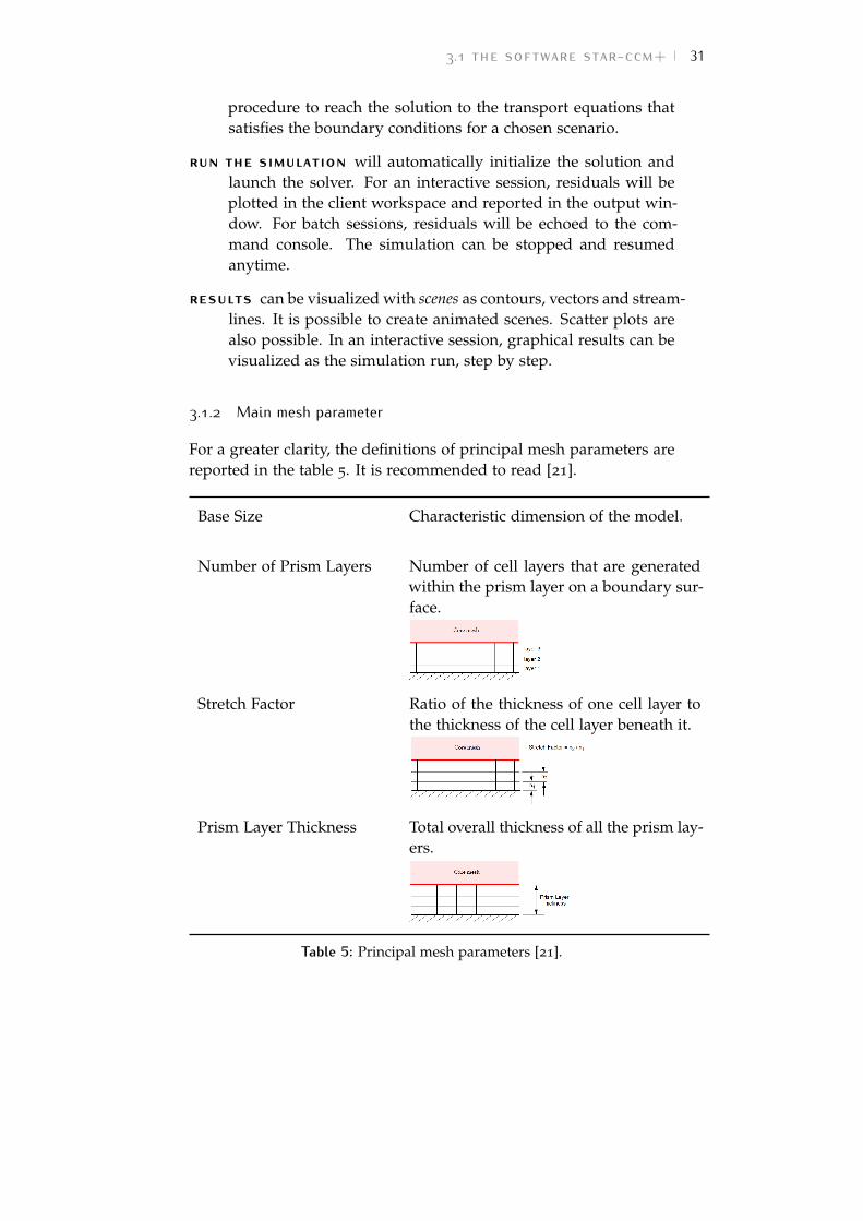
For a greater clarity, the definitions of principal mesh parameters arereported in the table 5. It is recommended to read [21].
Base Size Characteristic dimension of the model.
Number of Prism Layers Number of cell layers that are generatedwithin the prism layer on a boundary sur-face.
Stretch Factor Ratio of the thickness of one cell layer tothe thickness of the cell layer beneath it.
Prism Layer Thickness Total overall thickness of all the prism lay-ers.
Table 5: Principal mesh parameters [21].
3.2 the scope grid infrastructure 32
3.1.3 Convergence
The stopping criterium chosen is a prescribed number of iterativesteps order of magnitude as thousand. Convergence is judged bylooking at the oscillations of the aerodynamic coefficients and thewall y+. The oscillations must be reduced beneath of a certain thresh-old that, in this work, has been fixed equal to ±10−6. Having chosenSpalart-Allmaras as turbulence model, it is important to check thevalue of the dimensionless wall distance
y+ =u∗y
ν(3.1)
where y is the normal distance from the wall to the wall-cell centroid,u∗ is a reference velocity and ν is the kinematic viscosity. Accordingto the model’s formulation, the entire turbulent boundary layer, in-cluding the viscous sublayer, ought to be accurately resolved and themodel can be applied on fine meshes, that is small values, order ofmagnitude as unity, are required [21].
3.2 the scope grid infrastructure
At time of writing, no desktop computer could handle CFD 3D simu-lations of millions of cells in a reasonable amount of time. This worksaw the light also thanks to the availability of the University’s clus-ter grid, since lots of configurations, from wing alone to the wholeairplane, at several angles of incidence and Reynolds numbers hadto be analyzed. Runs with 16, 32 or 64 CPUs per simulation werecommons to get results within a day.
SCoPE is a scientific data center, based on a grid computing infras-tructure, and it is a collaborative system for scientific applications inmany areas of research. It is a project started in 2006 by the Universityof Naples ’Federico II’.
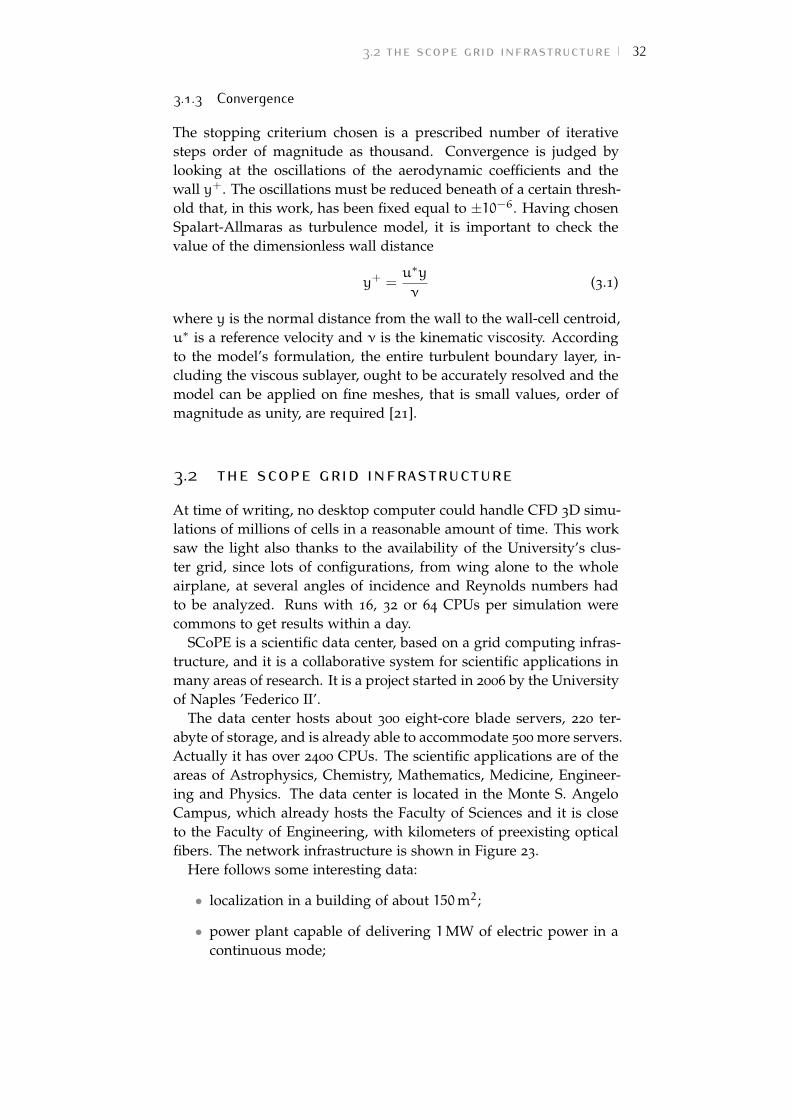
The data center hosts about 300 eight-core blade servers, 220 ter-abyte of storage, and is already able to accommodate 500 more servers.Actually it has over 2400 CPUs. The scientific applications are of theareas of Astrophysics, Chemistry, Mathematics, Medicine, Engineer-ing and Physics. The data center is located in the Monte S. AngeloCampus, which already hosts the Faculty of Sciences and it is closeto the Faculty of Engineering, with kilometers of preexisting opticalfibers. The network infrastructure is shown in Figure 23.
Here follows some interesting data:
• localization in a building of about 150m2;
• power plant capable of delivering 1MW of electric power in acontinuous mode;
3.3 numerical model 33
Figure 23: The SCoPE network infrastructure [22].
• efficient cooling system, capable of dissipating 2000W/m3 and30 000W per rack;
• standard (Gigabit Ethernet) networking infrastructure, with ahigh capacity switching fabric;
• low latency (Infiniband) networking infrastructure, with a sin-gle switching fabric for each group of 256 servers;
• large storage capacity, both nas (Network Attached Storage)working with the iscsi protocol, and san (Storage Area Net-work), working with a Fibre Channel Infrastructure;
• open source (Scientific Linux) for the operating system;
• integrated monitoring system for all the devices of the data cen-ter, able to monitor the most relevant parameters of server, stor-age, networking, as well as all the environmental parameters(as temperature, humidity and power consumption) [13].
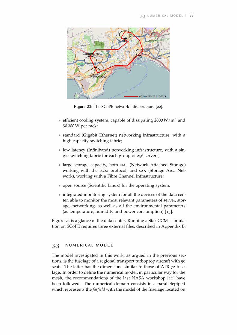
Figure 24 is a glance of the data center. Running a Star-CCM+ simula-tion on SCoPE requires three external files, described in Appendix B.
3.3 numerical model
The model investigated in this work, as argued in the previous sec-tions, is the fuselage of a regional transport turboprop aircraft with 90
seats. The latter has the dimensions similar to those of ATR-72 fuse-lage. In order to define the numerical model, in particular way for themesh, the recommendations of the last NASA workshop [11] havebeen followed. The numerical domain consists in a parallelepipedwhich represents the farfield with the model of the fuselage located on
3.3 numerical model 34
(a) Three rack servers of the data center. (b) Storage devices.
(c) Fiber optic connections. (d) Cables above the racks.
Figure 24: Some images of the SCoPE data center [22].
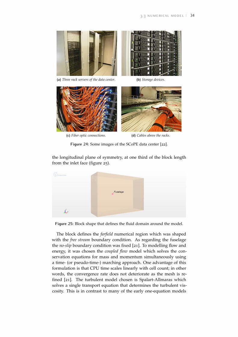
the longitudinal plane of symmetry, at one third of the block lengthfrom the inlet face (figure 25).
Figure 25: Block shape that defines the fluid domain around the model.
The block defines the farfield numerical region which was shapedwith the free stream boundary condition. As regarding the fuselagethe no-slip boundary condition was fixed [21]. To modelling flow andenergy, it was chosen the coupled flow model which solves the con-servation equations for mass and momentum simultaneously usinga time- (or pseudo-time-) marching approach. One advantage of thisformulation is that CPU time scales linearly with cell count; in otherwords, the convergence rate does not deteriorate as the mesh is re-fined [21]. The turbulent model chosen is Spalart-Allmaras whichsolves a single transport equation that determines the turbulent vis-cosity. This is in contrast to many of the early one-equation models
3.3 numerical model 35
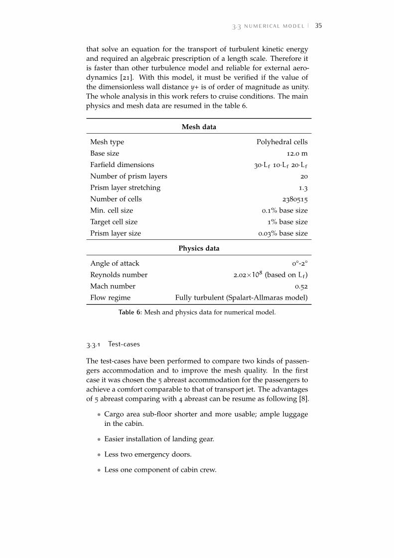
that solve an equation for the transport of turbulent kinetic energyand required an algebraic prescription of a length scale. Therefore itis faster than other turbulence model and reliable for external aero-dynamics [21]. With this model, it must be verified if the value ofthe dimensionless wall distance y+ is of order of magnitude as unity.The whole analysis in this work refers to cruise conditions. The mainphysics and mesh data are resumed in the table 6.
Mesh data
Mesh type Polyhedral cells
Base size 12.0 m
Farfield dimensions 30·Lf 10·Lf 20·LfNumber of prism layers 20
Prism layer stretching 1.3
Number of cells 2380515
Min. cell size 0.1% base size
Target cell size 1% base size
Prism layer size 0.03% base size
Physics data
Angle of attack 0°-2°
Reynolds number 2.02×10⁸ (based on Lf)
Mach number 0.52
Flow regime Fully turbulent (Spalart-Allmaras model)
Table 6: Mesh and physics data for numerical model.
3.3.1 Test-cases
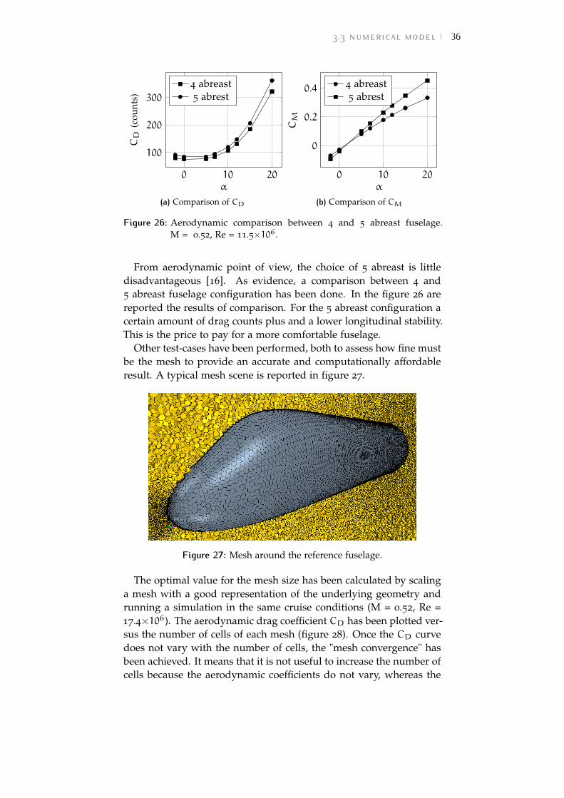
The test-cases have been performed to compare two kinds of passen-gers accommodation and to improve the mesh quality. In the firstcase it was chosen the 5 abreast accommodation for the passengers toachieve a comfort comparable to that of transport jet. The advantagesof 5 abreast comparing with 4 abreast can be resume as following [8].
• Cargo area sub-floor shorter and more usable; ample luggagein the cabin.
• Easier installation of landing gear.
• Less two emergency doors.
• Less one component of cabin crew.
3.3 numerical model 36
0 10 20
100
200
300
α
CD
(cou
nts)
4 abreast5 abrest
(a) Comparison of CD
0 10 20
0
0.2
0.4
α
CM
4 abreast5 abrest
(b) Comparison of CM
Figure 26: Aerodynamic comparison between 4 and 5 abreast fuselage.M = 0.52, Re = 11.5×10⁶.
From aerodynamic point of view, the choice of 5 abreast is littledisadvantageous [16]. As evidence, a comparison between 4 and5 abreast fuselage configuration has been done. In the figure 26 arereported the results of comparison. For the 5 abreast configuration acertain amount of drag counts plus and a lower longitudinal stability.This is the price to pay for a more comfortable fuselage.
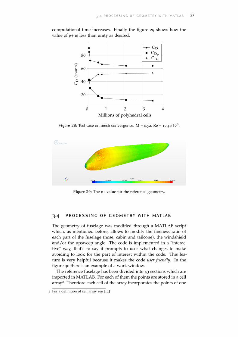
Other test-cases have been performed, both to assess how fine mustbe the mesh to provide an accurate and computationally affordableresult. A typical mesh scene is reported in figure 27.
Figure 27: Mesh around the reference fuselage.
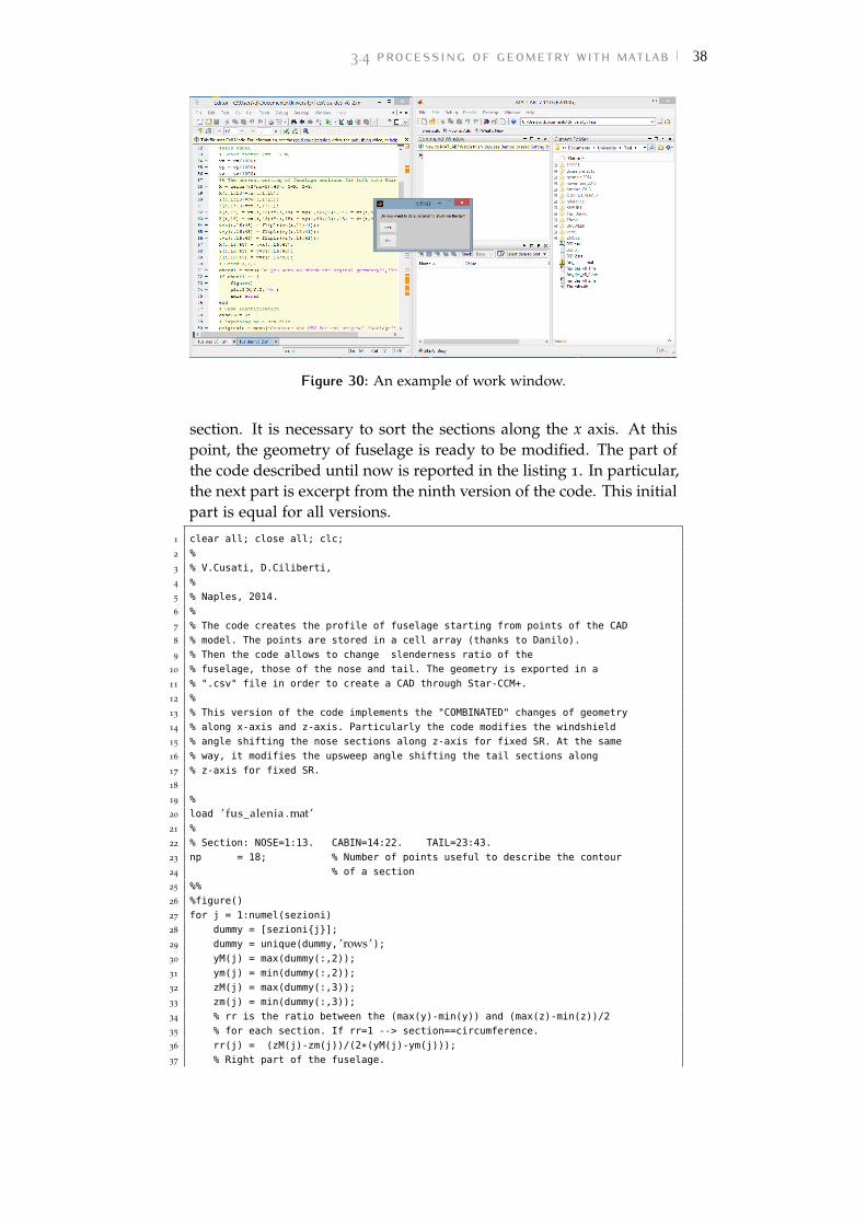
The optimal value for the mesh size has been calculated by scalinga mesh with a good representation of the underlying geometry andrunning a simulation in the same cruise conditions (M = 0.52, Re =17.4×10⁶). The aerodynamic drag coefficient CD has been plotted ver-sus the number of cells of each mesh (figure 28). Once the CD curvedoes not vary with the number of cells, the "mesh convergence" hasbeen achieved. It means that it is not useful to increase the number ofcells because the aerodynamic coefficients do not vary, whereas the
3.4 processing of geometry with matlab 37
computational time increases. Finally the figure 29 shows how thevalue of y+ is less than unity as desired.
0 1 2 3 4
20
40
60
80
Millions of polyhedral cells
CD
(cou
nts)
CDCDpCDf
Figure 28: Test case on mesh convergence. M = 0.52, Re = 17.4×10⁶.
Figure 29: The y+ value for the reference geometry.
3.4 processing of geometry with matlab
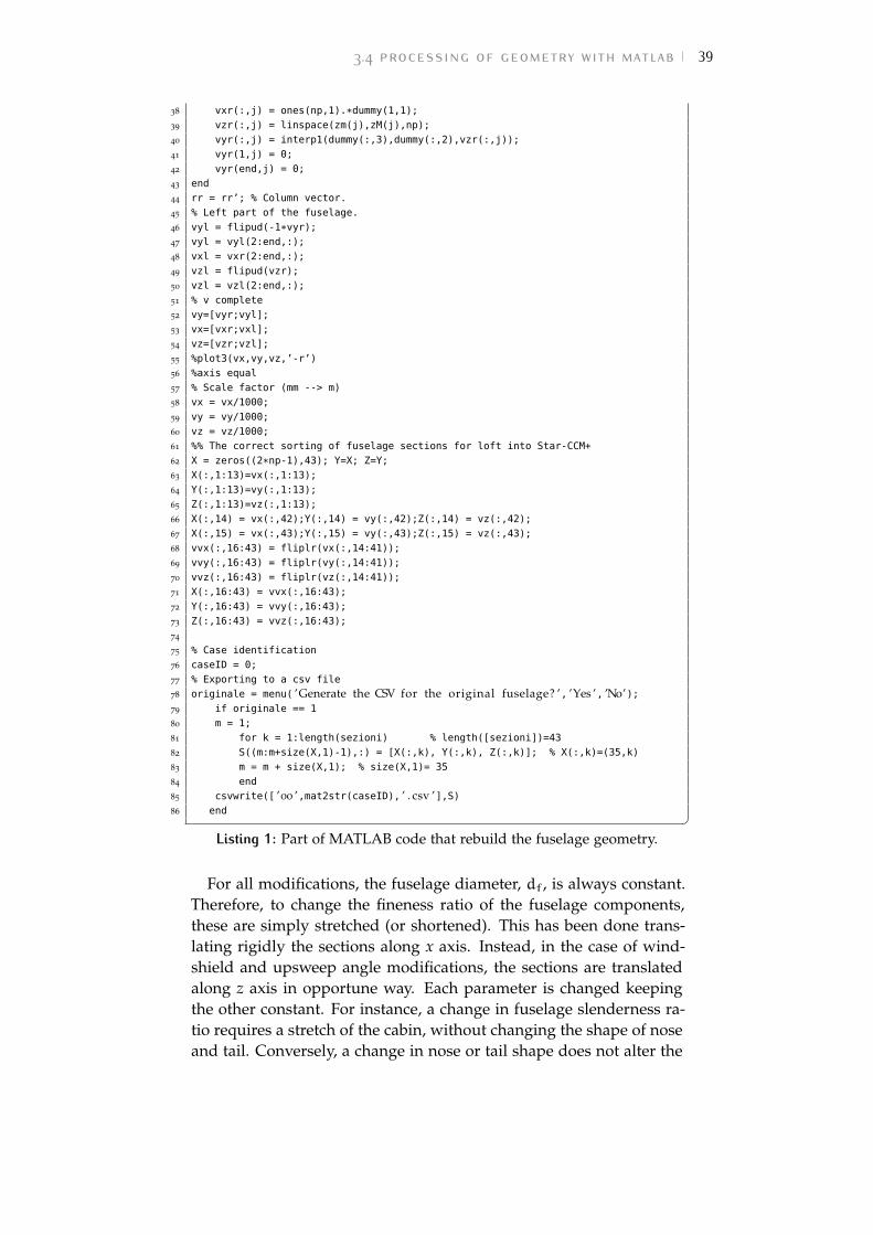
The geometry of fuselage was modified through a MATLAB scriptwhich, as mentioned before, allows to modify the fineness ratio ofeach part of the fuselage (nose, cabin and tailcone), the windshieldand/or the upsweep angle. The code is implemented in a "interac-tive" way, that’s to say it prompts to user what changes to makeavoiding to look for the part of interest within the code. This fea-ture is very helpful because it makes the code user friendly. In thefigure 30 there’s an example of a work window.
The reference fuselage has been divided into 43 sections which areimported in MATLAB. For each of them the points are stored in a cellarray2. Therefore each cell of the array incorporates the points of one
2 For a definition of cell array see [12]
3.4 processing of geometry with matlab 38
Figure 30: An example of work window.
section. It is necessary to sort the sections along the x axis. At thispoint, the geometry of fuselage is ready to be modified. The part ofthe code described until now is reported in the listing 1. In particular,the next part is excerpt from the ninth version of the code. This initialpart is equal for all versions.
1 clear all; close all; clc;
2 %
3 % V.Cusati, D.Ciliberti,
4 %
5 % Naples, 2014.
6 %
7 % The code creates the profile of fuselage starting from points of the CAD
8 % model. The points are stored in a cell array (thanks to Danilo).
9 % Then the code allows to change slenderness ratio of the
10 % fuselage, those of the nose and tail. The geometry is exported in a
11 % ".csv" file in order to create a CAD through Star-CCM+.
12 %
13 % This version of the code implements the "COMBINATED" changes of geometry
14 % along x-axis and z-axis. Particularly the code modifies the windshield
15 % angle shifting the nose sections along z-axis for fixed SR. At the same
16 % way, it modifies the upsweep angle shifting the tail sections along
17 % z-axis for fixed SR.
18
19 %
20 load ’ fus_alenia .mat ’21 %
22 % Section: NOSE=1:13. CABIN=14:22. TAIL=23:43.
23 np = 18; % Number of points useful to describe the contour
24 % of a section
25 %%
26 %figure()
27 for j = 1:numel(sezioni)
28 dummy = [sezioni{j}];
29 dummy = unique(dummy, ’rows ’);30 yM(j) = max(dummy(:,2));
31 ym(j) = min(dummy(:,2));
32 zM(j) = max(dummy(:,3));
33 zm(j) = min(dummy(:,3));
34 % rr is the ratio between the (max(y)-min(y)) and (max(z)-min(z))/2
35 % for each section. If rr=1 --> section==circumference.
36 rr(j) = (zM(j)-zm(j))/(2*(yM(j)-ym(j)));
37 % Right part of the fuselage.
3.4 processing of geometry with matlab 39
38 vxr(:,j) = ones(np,1).*dummy(1,1);
39 vzr(:,j) = linspace(zm(j),zM(j),np);
40 vyr(:,j) = interp1(dummy(:,3),dummy(:,2),vzr(:,j));
41 vyr(1,j) = 0;
42 vyr(end,j) = 0;
43 end
44 rr = rr’; % Column vector.
45 % Left part of the fuselage.
46 vyl = flipud(-1*vyr);
47 vyl = vyl(2:end,:);
48 vxl = vxr(2:end,:);
49 vzl = flipud(vzr);
50 vzl = vzl(2:end,:);
51 % v complete
52 vy=[vyr;vyl];
53 vx=[vxr;vxl];
54 vz=[vzr;vzl];
55 %plot3(vx,vy,vz,’-r’)
56 %axis equal
57 % Scale factor (mm --> m)
58 vx = vx/1000;
59 vy = vy/1000;
60 vz = vz/1000;
61 %% The correct sorting of fuselage sections for loft into Star-CCM+
62 X = zeros((2*np-1),43); Y=X; Z=Y;
63 X(:,1:13)=vx(:,1:13);
64 Y(:,1:13)=vy(:,1:13);
65 Z(:,1:13)=vz(:,1:13);
66 X(:,14) = vx(:,42);Y(:,14) = vy(:,42);Z(:,14) = vz(:,42);
67 X(:,15) = vx(:,43);Y(:,15) = vy(:,43);Z(:,15) = vz(:,43);
68 vvx(:,16:43) = fliplr(vx(:,14:41));
69 vvy(:,16:43) = fliplr(vy(:,14:41));
70 vvz(:,16:43) = fliplr(vz(:,14:41));
71 X(:,16:43) = vvx(:,16:43);
72 Y(:,16:43) = vvy(:,16:43);
73 Z(:,16:43) = vvz(:,16:43);
74
75 % Case identification
76 caseID = 0;
77 % Exporting to a csv file
78 originale = menu( ’Generate the CSV for the original fuselage? ’, ’Yes ’, ’No’);79 if originale == 1
80 m = 1;
81 for k = 1:length(sezioni) % length([sezioni])=43
82 S((m:m+size(X,1)-1),:) = [X(:,k), Y(:,k), Z(:,k)]; % X(:,k)=(35,k)
83 m = m + size(X,1); % size(X,1)= 35
84 end
85 csvwrite([ ’00 ’,mat2str(caseID), ’ . csv ’],S)86 end �
Listing 1: Part of MATLAB code that rebuild the fuselage geometry.
For all modifications, the fuselage diameter, df, is always constant.Therefore, to change the fineness ratio of the fuselage components,these are simply stretched (or shortened). This has been done trans-lating rigidly the sections along x axis. Instead, in the case of wind-shield and upsweep angle modifications, the sections are translatedalong z axis in opportune way. Each parameter is changed keepingthe other constant. For instance, a change in fuselage slenderness ra-tio requires a stretch of the cabin, without changing the shape of noseand tail. Conversely, a change in nose or tail shape does not alter the
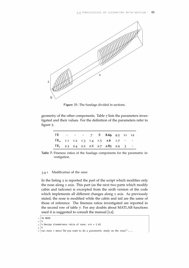
3.4 processing of geometry with matlab 40
x
y
z
Figure 31: The fuselage divided in sections.
geometry of the other components. Table 7 lists the parameters inves-tigated and their values. For the definition of the parameters refer tofigure 5.
FR - - - 7 8 8.69 9.5 11 12
FRn 1.1 1.2 1.3 1.4 1.5 1.6 1.7 - -
FRt 2.3 2.4 2.5 2.6 2.7 2.83 2.9 3 -
Table 7: Fineness ratios of the fuselage components for the parametric in-vestigation.
3.4.1 Modification of the nose
In the listing 2 is reported the part of the script which modifies onlythe nose along x axis. This part (as the next two parts which modifycabin and tailcone) is excerpted from the sixth version of the codewhich implements all different changes along x axis. As previouslystated, the nose is modified while the cabin and tail are the same ofthose of reference. The fineness ratios investigated are reported inthe second row of table 7. For any doubts about MATLAB functionsused it is suggested to consult the manual [12].
1 %% NOSE
2 %
3 % Design slenderness ratio of nose: srn = 1.61
4 %
5 var_nose = menu( ’Do you want to do a parametric study on the nose? ’,...
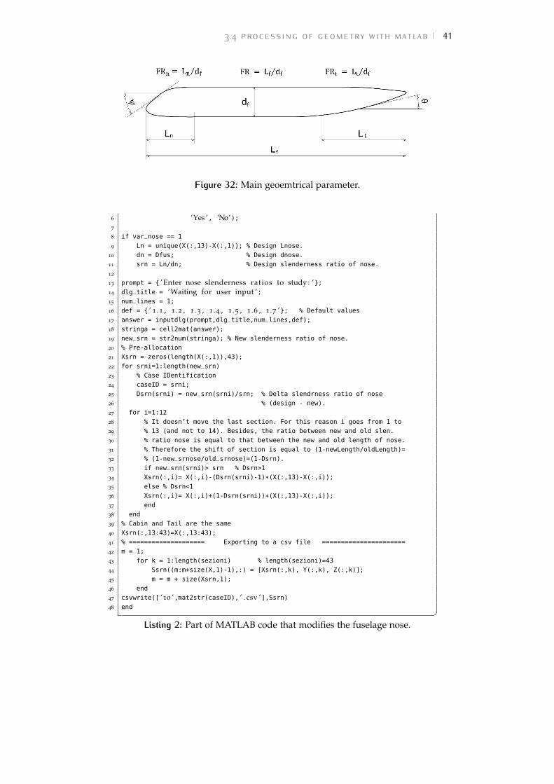
3.4 processing of geometry with matlab 41
Figure 32: Main geoemtrical parameter.
6 ’Yes ’, ’No’);7
8 if var_nose == 1
9 Ln = unique(X(:,13)-X(:,1)); % Design Lnose.
10 dn = Dfus; % Design dnose.
11 srn = Ln/dn; % Design slenderness ratio of nose.
12
13 prompt = { ’Enter nose slenderness ratios to study : ’};14 dlg_title = ’Waiting for user input ’;15 num_lines = 1;
16 def = { ’ 1 .1 , 1 .2 , 1 .3 , 1 .4 , 1 .5 , 1 .6 , 1.7 ’}; % Default values
17 answer = inputdlg(prompt,dlg_title,num_lines,def);
18 stringa = cell2mat(answer);
19 new_srn = str2num(stringa); % New slenderness ratio of nose.
20 % Pre-allocation
21 Xsrn = zeros(length(X(:,1)),43);
22 for srni=1:length(new_srn)
23 % Case IDentification
24 caseID = srni;
25 Dsrn(srni) = new_srn(srni)/srn; % Delta slendrness ratio of nose
26 % (design - new).
27 for i=1:12
28 % It doesn’t move the last section. For this reason i goes from 1 to
29 % 13 (and not to 14). Besides, the ratio between new and old slen.
30 % ratio nose is equal to that between the new and old length of nose.
31 % Therefore the shift of section is equal to (1-newLength/oldLength)=
32 % (1-new_srnose/old_srnose)=(1-Dsrn).
33 if new_srn(srni)> srn % Dsrn>1
34 Xsrn(:,i)= X(:,i)-(Dsrn(srni)-1)*(X(:,13)-X(:,i));
35 else % Dsrn<1
36 Xsrn(:,i)= X(:,i)+(1-Dsrn(srni))*(X(:,13)-X(:,i));
37 end
38 end
39 % Cabin and Tail are the same
40 Xsrn(:,13:43)=X(:,13:43);
41 % ==================== Exporting to a csv file ======================
42 m = 1;
43 for k = 1:length(sezioni) % length(sezioni)=43
44 Ssrn((m:m+size(X,1)-1),:) = [Xsrn(:,k), Y(:,k), Z(:,k)];
45 m = m + size(Xsrn,1);
46 end
47 csvwrite([ ’10 ’,mat2str(caseID), ’ . csv ’],Ssrn)48 end �
Listing 2: Part of MATLAB code that modifies the fuselage nose.
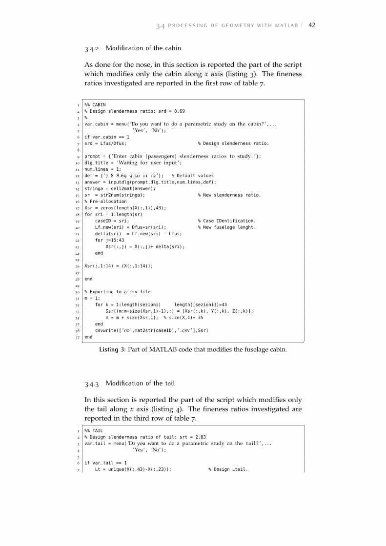
3.4 processing of geometry with matlab 42
3.4.2 Modification of the cabin
As done for the nose, in this section is reported the part of the scriptwhich modifies only the cabin along x axis (listing 3). The finenessratios investigated are reported in the first row of table 7.
1 %% CABIN
2 % Design slenderness ratio: srd = 8.69
3 %
4 var_cabin = menu( ’Do you want to do a parametric study on the cabin? ’,...5 ’Yes ’, ’No’);6 if var_cabin == 1
7 srd = Lfus/Dfus; % Design slenderness ratio.
8
9 prompt = { ’Enter cabin (passengers) slenderness ratios to study : ’};10 dlg_title = ’Waiting for user input ’;11 num_lines = 1;
12 def = { ’7 8 8.69 9.50 11 12 ’}; % Default values
13 answer = inputdlg(prompt,dlg_title,num_lines,def);
14 stringa = cell2mat(answer);
15 sr = str2num(stringa); % New slenderness ratio.
16 % Pre-allocation
17 Xsr = zeros(length(X(:,1)),43);
18 for sri = 1:length(sr)
19 caseID = sri; % Case IDentification.
20 Lf_new(sri) = Dfus*sr(sri); % New fuselage lenght.
21 delta(sri) = Lf_new(sri) - Lfus;
22 for j=15:43
23 Xsr(:,j) = X(:,j)+ delta(sri);
24 end
25
26 Xsr(:,1:14) = (X(:,1:14));
27
28 end
29
30 % Exporting to a csv file
31 m = 1;
32 for k = 1:length(sezioni) length([sezioni])=43
33 Ssr((m:m+size(Xsr,1)-1),:) = [Xsr(:,k), Y(:,k), Z(:,k)];
34 m = m + size(Xsr,1); % size(X,1)= 35
35 end
36 csvwrite([ ’00 ’,mat2str(caseID), ’ . csv ’],Ssr)37 end �
Listing 3: Part of MATLAB code that modifies the fuselage cabin.
3.4.3 Modification of the tail
In this section is reported the part of the script which modifies onlythe tail along x axis (listing 4). The fineness ratios investigated arereported in the third row of table 7.
1 %% TAIL
2 % Design slenderness ratio of tail: srt = 2.83
3 var_tail = menu( ’Do you want to do a parametric study on the t a i l ? ’,...4 ’Yes ’, ’No’);5
6 if var_tail == 1
7 Lt = unique(X(:,43)-X(:,23)); % Design Ltail.
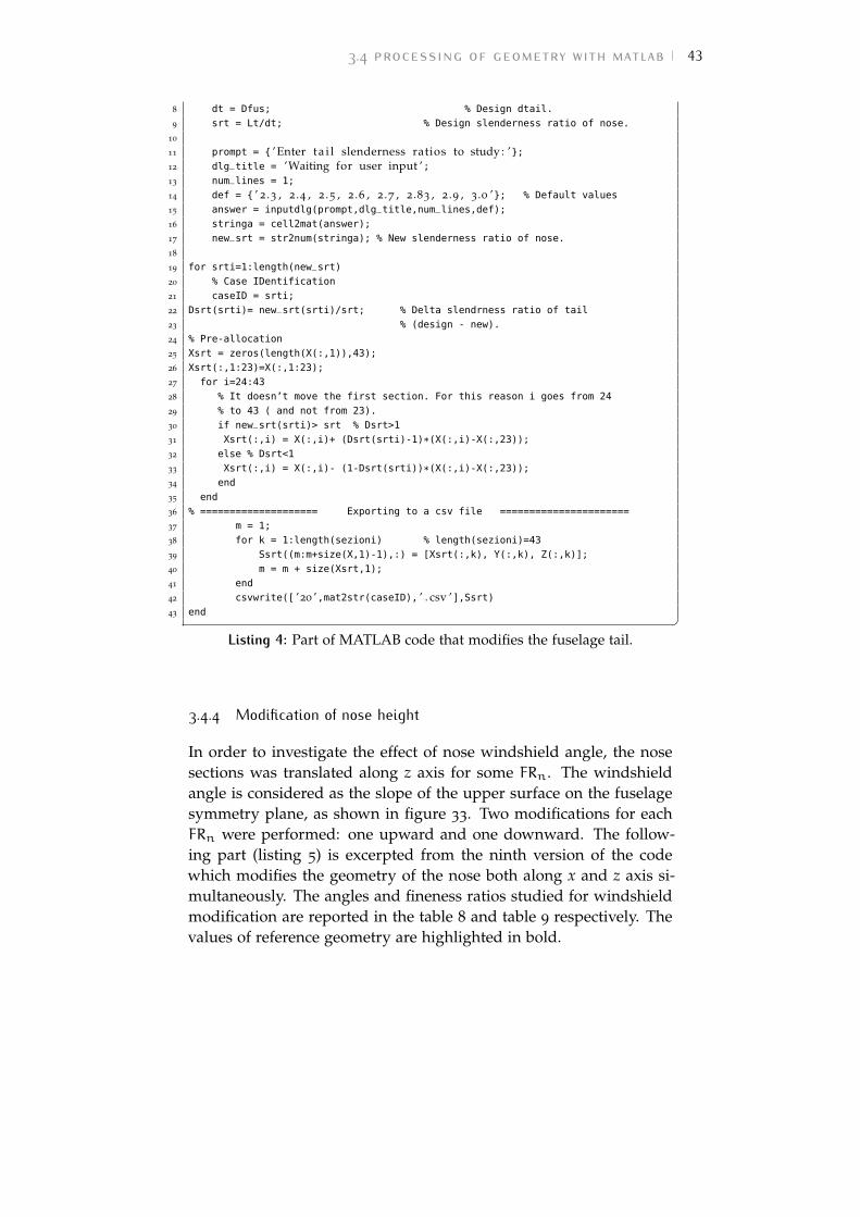
3.4 processing of geometry with matlab 43
8 dt = Dfus; % Design dtail.
9 srt = Lt/dt; % Design slenderness ratio of nose.
10
11 prompt = { ’Enter t a i l slenderness ratios to study : ’};12 dlg_title = ’Waiting for user input ’;13 num_lines = 1;
14 def = { ’ 2 .3 , 2 .4 , 2 .5 , 2 .6 , 2 .7 , 2 .83 , 2 .9 , 3.0 ’}; % Default values
15 answer = inputdlg(prompt,dlg_title,num_lines,def);
16 stringa = cell2mat(answer);
17 new_srt = str2num(stringa); % New slenderness ratio of nose.
18
19 for srti=1:length(new_srt)
20 % Case IDentification
21 caseID = srti;
22 Dsrt(srti)= new_srt(srti)/srt; % Delta slendrness ratio of tail
23 % (design - new).
24 % Pre-allocation
25 Xsrt = zeros(length(X(:,1)),43);
26 Xsrt(:,1:23)=X(:,1:23);
27 for i=24:43
28 % It doesn’t move the first section. For this reason i goes from 24
29 % to 43 ( and not from 23).
30 if new_srt(srti)> srt % Dsrt>1
31 Xsrt(:,i) = X(:,i)+ (Dsrt(srti)-1)*(X(:,i)-X(:,23));
32 else % Dsrt<1
33 Xsrt(:,i) = X(:,i)- (1-Dsrt(srti))*(X(:,i)-X(:,23));
34 end
35 end
36 % ==================== Exporting to a csv file ======================
37 m = 1;
38 for k = 1:length(sezioni) % length(sezioni)=43
39 Ssrt((m:m+size(X,1)-1),:) = [Xsrt(:,k), Y(:,k), Z(:,k)];
40 m = m + size(Xsrt,1);
41 end
42 csvwrite([ ’20 ’,mat2str(caseID), ’ . csv ’],Ssrt)43 end �
Listing 4: Part of MATLAB code that modifies the fuselage tail.
3.4.4 Modification of nose height
In order to investigate the effect of nose windshield angle, the nosesections was translated along z axis for some FRn. The windshieldangle is considered as the slope of the upper surface on the fuselagesymmetry plane, as shown in figure 33. Two modifications for eachFRn were performed: one upward and one downward. The follow-ing part (listing 5) is excerpted from the ninth version of the codewhich modifies the geometry of the nose both along x and z axis si-multaneously. The angles and fineness ratios studied for windshieldmodification are reported in the table 8 and table 9 respectively. Thevalues of reference geometry are highlighted in bold.
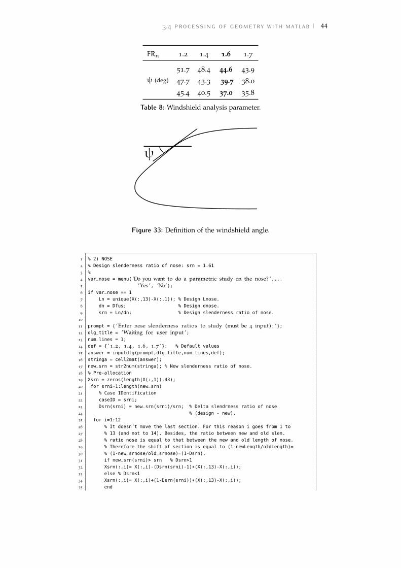
3.4 processing of geometry with matlab 44
FRn 1.2 1.4 1.6 1.7
ψ (deg)
51.7 48.4 44.6 43.9
47.7 43.3 39.7 38.0
45.4 40.5 37.0 35.8
Table 8: Windshield analysis parameter.
Figure 33: Definition of the windshield angle.
1 % 2) NOSE
2 % Design slenderness ratio of nose: srn = 1.61
3 %
4 var_nose = menu( ’Do you want to do a parametric study on the nose? ’,...5 ’Yes ’, ’No’);6 if var_nose == 1
7 Ln = unique(X(:,13)-X(:,1)); % Design Lnose.
8 dn = Dfus; % Design dnose.
9 srn = Ln/dn; % Design slenderness ratio of nose.
10
11 prompt = { ’Enter nose slenderness ratios to study (must be 4 input) : ’};12 dlg_title = ’Waiting for user input ’;13 num_lines = 1;
14 def = { ’ 1 .2 , 1 .4 , 1 .6 , 1.7 ’}; % Default values
15 answer = inputdlg(prompt,dlg_title,num_lines,def);
16 stringa = cell2mat(answer);
17 new_srn = str2num(stringa); % New slenderness ratio of nose.
18 % Pre-allocation
19 Xsrn = zeros(length(X(:,1)),43);
20 for srni=1:length(new_srn)
21 % Case IDentification
22 caseID = srni;
23 Dsrn(srni) = new_srn(srni)/srn; % Delta slendrness ratio of nose
24 % (design - new).
25 for i=1:12
26 % It doesn’t move the last section. For this reason i goes from 1 to
27 % 13 (and not to 14). Besides, the ratio between new and old slen.
28 % ratio nose is equal to that between the new and old length of nose.
29 % Therefore the shift of section is equal to (1-newLength/oldLength)=
30 % (1-new_srnose/old_srnose)=(1-Dsrn).
31 if new_srn(srni)> srn % Dsrn>1
32 Xsrn(:,i)= X(:,i)-(Dsrn(srni)-1)*(X(:,13)-X(:,i));
33 else % Dsrn<1
34 Xsrn(:,i)= X(:,i)+(1-Dsrn(srni))*(X(:,13)-X(:,i));
35 end
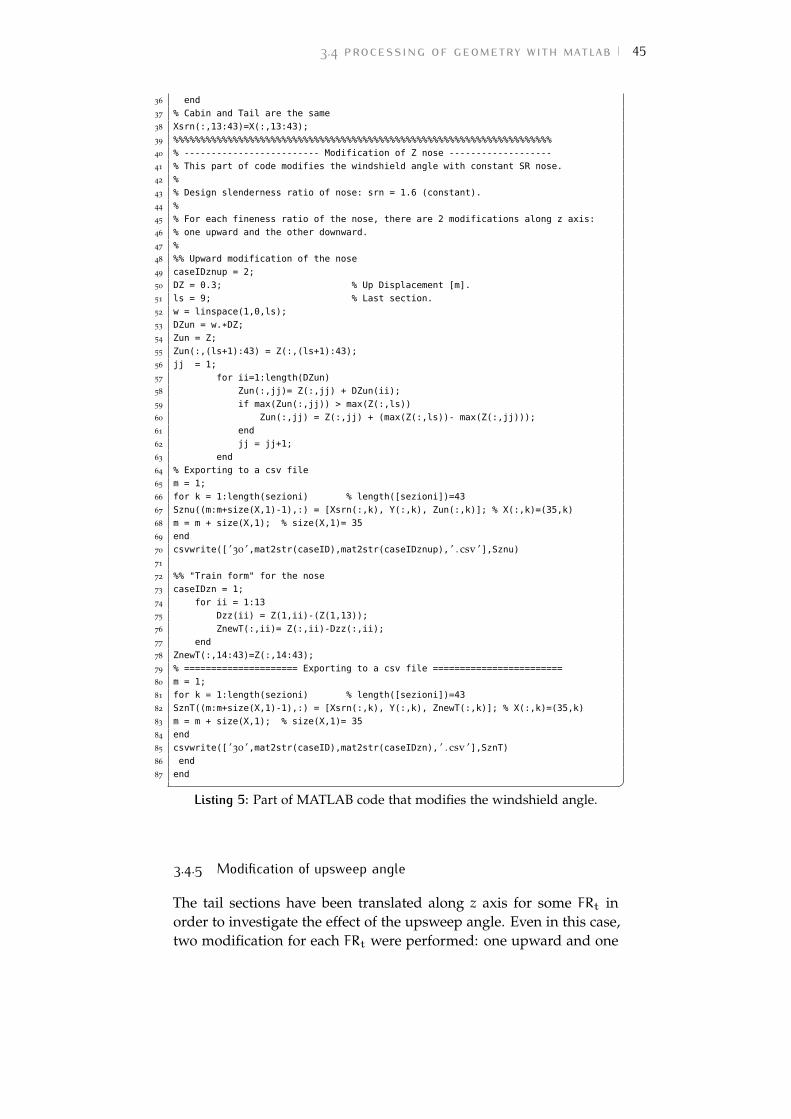
3.4 processing of geometry with matlab 45
36 end
37 % Cabin and Tail are the same
38 Xsrn(:,13:43)=X(:,13:43);
39 %%%%%%%%%%%%%%%%%%%%%%%%%%%%%%%%%%%%%%%%%%%%%%%%%%%%%%%%%%%%%%%%%%%%%%
40 % ------------------------- Modification of Z nose -------------------
41 % This part of code modifies the windshield angle with constant SR nose.
42 %
43 % Design slenderness ratio of nose: srn = 1.6 (constant).
44 %
45 % For each fineness ratio of the nose, there are 2 modifications along z axis:
46 % one upward and the other downward.
47 %
48 %% Upward modification of the nose
49 caseIDznup = 2;
50 DZ = 0.3; % Up Displacement [m].
51 ls = 9; % Last section.
52 w = linspace(1,0,ls);
53 DZun = w.*DZ;
54 Zun = Z;
55 Zun(:,(ls+1):43) = Z(:,(ls+1):43);
56 jj = 1;
57 for ii=1:length(DZun)
58 Zun(:,jj)= Z(:,jj) + DZun(ii);
59 if max(Zun(:,jj)) > max(Z(:,ls))
60 Zun(:,jj) = Z(:,jj) + (max(Z(:,ls))- max(Z(:,jj)));
61 end
62 jj = jj+1;
63 end
64 % Exporting to a csv file
65 m = 1;
66 for k = 1:length(sezioni) % length([sezioni])=43
67 Sznu((m:m+size(X,1)-1),:) = [Xsrn(:,k), Y(:,k), Zun(:,k)]; % X(:,k)=(35,k)
68 m = m + size(X,1); % size(X,1)= 35
69 end
70 csvwrite([ ’30 ’,mat2str(caseID),mat2str(caseIDznup), ’ . csv ’],Sznu)71
72 %% "Train form" for the nose
73 caseIDzn = 1;
74 for ii = 1:13
75 Dzz(ii) = Z(1,ii)-(Z(1,13));
76 ZnewT(:,ii)= Z(:,ii)-Dzz(:,ii);
77 end
78 ZnewT(:,14:43)=Z(:,14:43);
79 % ===================== Exporting to a csv file ========================
80 m = 1;
81 for k = 1:length(sezioni) % length([sezioni])=43
82 SznT((m:m+size(X,1)-1),:) = [Xsrn(:,k), Y(:,k), ZnewT(:,k)]; % X(:,k)=(35,k)
83 m = m + size(X,1); % size(X,1)= 35
84 end
85 csvwrite([ ’30 ’,mat2str(caseID),mat2str(caseIDzn), ’ . csv ’],SznT)86 end
87 end �Listing 5: Part of MATLAB code that modifies the windshield angle.
3.4.5 Modification of upsweep angle
The tail sections have been translated along z axis for some FRt inorder to investigate the effect of the upsweep angle. Even in this case,two modification for each FRt were performed: one upward and one
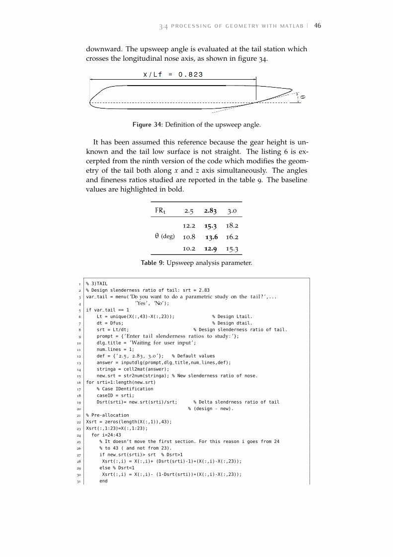
3.4 processing of geometry with matlab 46
downward. The upsweep angle is evaluated at the tail station whichcrosses the longitudinal nose axis, as shown in figure 34.
Figure 34: Definition of the upsweep angle.
It has been assumed this reference because the gear height is un-known and the tail low surface is not straight. The listing 6 is ex-cerpted from the ninth version of the code which modifies the geom-etry of the tail both along x and z axis simultaneously. The anglesand fineness ratios studied are reported in the table 9. The baselinevalues are highlighted in bold.
FRt 2.5 2.83 3.0
θ (deg)
12.2 15.3 18.2
10.8 13.6 16.2
10.2 12.9 15.3
Table 9: Upsweep analysis parameter.
1 % 3)TAIL
2 % Design slenderness ratio of tail: srt = 2.83
3 var_tail = menu( ’Do you want to do a parametric study on the t a i l ? ’,...4 ’Yes ’, ’No’);5 if var_tail == 1
6 Lt = unique(X(:,43)-X(:,23)); % Design Ltail.
7 dt = Dfus; % Design dtail.
8 srt = Lt/dt; % Design slenderness ratio of tail.
9 prompt = { ’Enter t a i l slenderness ratios to study : ’};10 dlg_title = ’Waiting for user input ’;11 num_lines = 1;
12 def = { ’ 2 .5 , 2 .83 , 3.0 ’}; % Default values
13 answer = inputdlg(prompt,dlg_title,num_lines,def);
14 stringa = cell2mat(answer);
15 new_srt = str2num(stringa); % New slenderness ratio of nose.
16 for srti=1:length(new_srt)
17 % Case IDentification
18 caseID = srti;
19 Dsrt(srti)= new_srt(srti)/srt; % Delta slendrness ratio of tail
20 % (design - new).
21 % Pre-allocation
22 Xsrt = zeros(length(X(:,1)),43);
23 Xsrt(:,1:23)=X(:,1:23);
24 for i=24:43
25 % It doesn’t move the first section. For this reason i goes from 24
26 % to 43 ( and not from 23).
27 if new_srt(srti)> srt % Dsrt>1
28 Xsrt(:,i) = X(:,i)+ (Dsrt(srti)-1)*(X(:,i)-X(:,23));
29 else % Dsrt<1
30 Xsrt(:,i) = X(:,i)- (1-Dsrt(srti))*(X(:,i)-X(:,23));
31 end
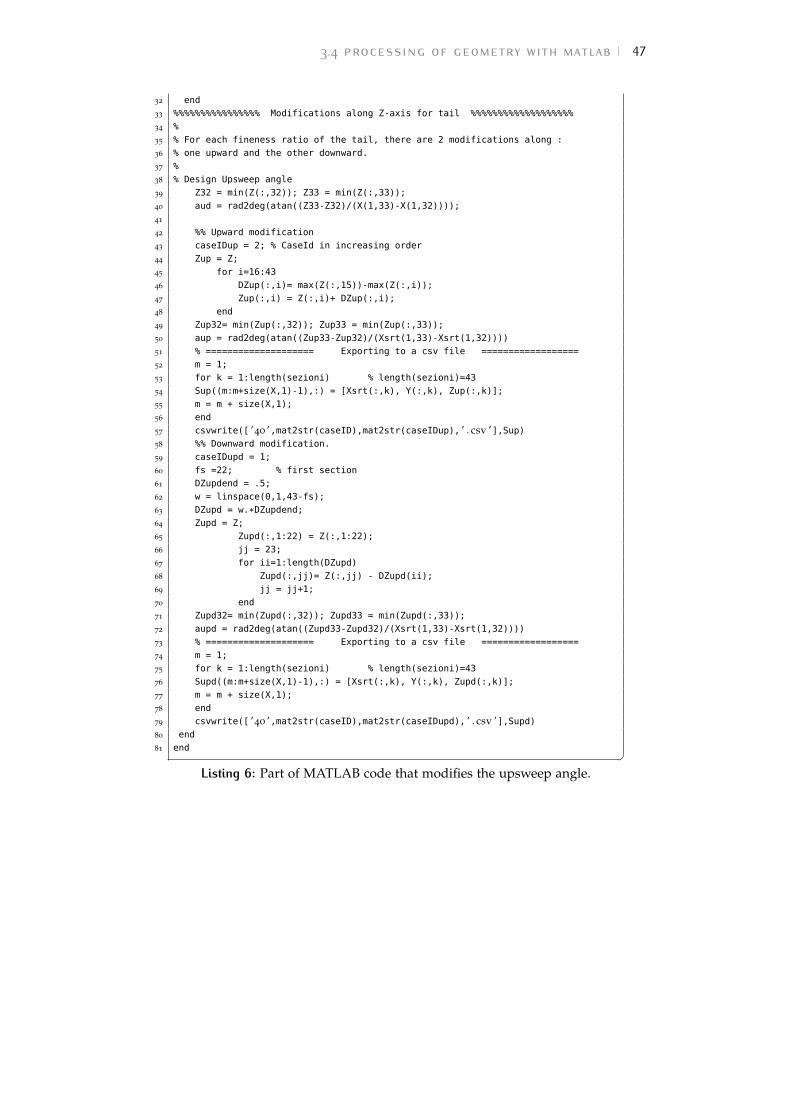
3.4 processing of geometry with matlab 47
32 end
33 %%%%%%%%%%%%%%%% Modifications along Z-axis for tail %%%%%%%%%%%%%%%%%%%
34 %
35 % For each fineness ratio of the tail, there are 2 modifications along :
36 % one upward and the other downward.
37 %
38 % Design Upsweep angle
39 Z32 = min(Z(:,32)); Z33 = min(Z(:,33));
40 aud = rad2deg(atan((Z33-Z32)/(X(1,33)-X(1,32))));
41
42 %% Upward modification
43 caseIDup = 2; % CaseId in increasing order
44 Zup = Z;
45 for i=16:43
46 DZup(:,i)= max(Z(:,15))-max(Z(:,i));
47 Zup(:,i) = Z(:,i)+ DZup(:,i);
48 end
49 Zup32= min(Zup(:,32)); Zup33 = min(Zup(:,33));
50 aup = rad2deg(atan((Zup33-Zup32)/(Xsrt(1,33)-Xsrt(1,32))))
51 % ==================== Exporting to a csv file ==================
52 m = 1;
53 for k = 1:length(sezioni) % length(sezioni)=43
54 Sup((m:m+size(X,1)-1),:) = [Xsrt(:,k), Y(:,k), Zup(:,k)];
55 m = m + size(X,1);
56 end
57 csvwrite([ ’40 ’,mat2str(caseID),mat2str(caseIDup), ’ . csv ’],Sup)58 %% Downward modification.
59 caseIDupd = 1;
60 fs =22; % first section
61 DZupdend = .5;
62 w = linspace(0,1,43-fs);
63 DZupd = w.*DZupdend;
64 Zupd = Z;
65 Zupd(:,1:22) = Z(:,1:22);
66 jj = 23;
67 for ii=1:length(DZupd)
68 Zupd(:,jj)= Z(:,jj) - DZupd(ii);
69 jj = jj+1;
70 end
71 Zupd32= min(Zupd(:,32)); Zupd33 = min(Zupd(:,33));
72 aupd = rad2deg(atan((Zupd33-Zupd32)/(Xsrt(1,33)-Xsrt(1,32))))
73 % ==================== Exporting to a csv file ==================
74 m = 1;
75 for k = 1:length(sezioni) % length(sezioni)=43
76 Supd((m:m+size(X,1)-1),:) = [Xsrt(:,k), Y(:,k), Zupd(:,k)];
77 m = m + size(X,1);
78 end
79 csvwrite([ ’40 ’,mat2str(caseID),mat2str(caseIDupd), ’ . csv ’],Supd)80 end
81 end �Listing 6: Part of MATLAB code that modifies the upsweep angle.
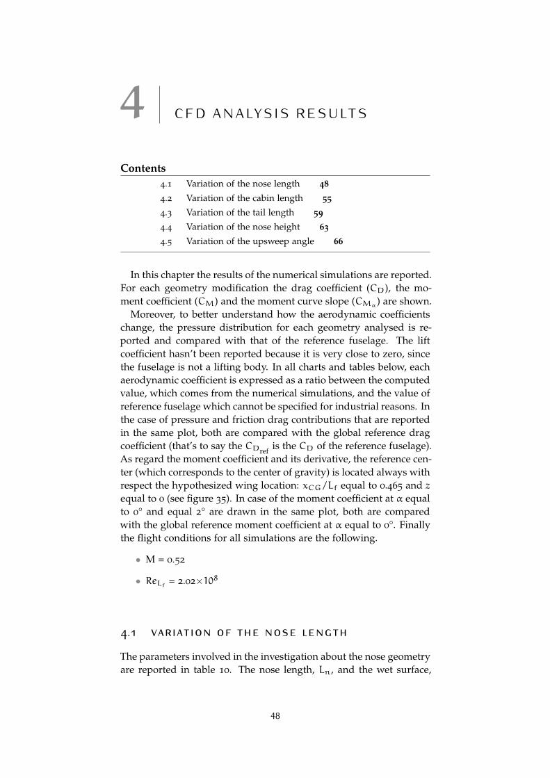
4 C F D A N A LY S I S R E S U LT S
Contents4.1 Variation of the nose length 48
4.2 Variation of the cabin length 55
4.3 Variation of the tail length 59
4.4 Variation of the nose height 63
4.5 Variation of the upsweep angle 66
In this chapter the results of the numerical simulations are reported.For each geometry modification the drag coefficient (CD), the mo-ment coefficient (CM) and the moment curve slope (CMα
) are shown.Moreover, to better understand how the aerodynamic coefficients
change, the pressure distribution for each geometry analysed is re-ported and compared with that of the reference fuselage. The liftcoefficient hasn’t been reported because it is very close to zero, sincethe fuselage is not a lifting body. In all charts and tables below, eachaerodynamic coefficient is expressed as a ratio between the computedvalue, which comes from the numerical simulations, and the value ofreference fuselage which cannot be specified for industrial reasons. Inthe case of pressure and friction drag contributions that are reportedin the same plot, both are compared with the global reference dragcoefficient (that’s to say the CDref is the CD of the reference fuselage).As regard the moment coefficient and its derivative, the reference cen-ter (which corresponds to the center of gravity) is located always withrespect the hypothesized wing location: xCG/Lf equal to 0.465 and zequal to 0 (see figure 35). In case of the moment coefficient at α equalto 0° and equal 2° are drawn in the same plot, both are comparedwith the global reference moment coefficient at α equal to 0°. Finallythe flight conditions for all simulations are the following.
• M = 0.52
• ReLf = 2.02×10⁸
4.1 variation of the nose length
The parameters involved in the investigation about the nose geometryare reported in table 10. The nose length, Ln, and the wet surface,
48
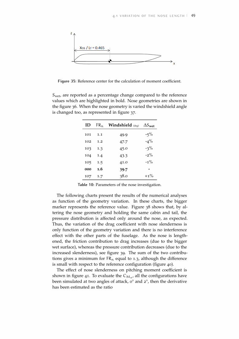
4.1 variation of the nose length 49
Figure 35: Reference center for the calculation of moment coefficient.
Swet, are reported as a percentage change compared to the referencevalues which are highlighted in bold. Nose geometries are shown inthe figure 36. When the nose geometry is varied the windshield angleis changed too, as represented in figure 37.
ID FRn Windshield (deg) ∆Swet
101 1.1 49.9 -5%
102 1.2 47.7 -4%
103 1.3 45.0 -3%
104 1.4 43.3 -2%
105 1.5 41.0 -1%
000 1.6 39.7 -
107 1.7 38.0 +1%
Table 10: Parameters of the nose investigation.
The following charts present the results of the numerical analysesas function of the geometry variation. In these charts, the biggermarker represents the reference value. Figure 38 shows that, by al-tering the nose geometry and holding the same cabin and tail, thepressure distribution is affected only around the nose, as expected.Thus, the variation of the drag coefficient with nose slenderness isonly function of the geometry variation and there is no interferenceeffect with the other parts of the fuselage. As the nose is length-ened, the friction contribution to drag increases (due to the biggerwet surface), whereas the pressure contribution decreases (due to theincreased slenderness), see figure 39. The sum of the two contribu-tions gives a minimum for FRn equal to 1.3, although the differenceis small with respect to the reference configuration (figure 40).
The effect of nose slenderness on pitching moment coefficient isshown in figure 41. To evaluate the CMα
, all the configurations havebeen simulated at two angles of attack, 0° and 2°, then the derivativehas been estimated as the ratio
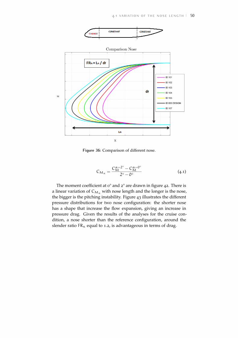
4.1 variation of the nose length 50
Figure 36: Comparison of different nose.
CMα=Cα=2
◦M −Cα=0
◦M
2◦ − 0◦(4.1)
The moment coefficient at 0° and 2° are drawn in figure 42. There isa linear variation of CMα
with nose length and the longer is the nose,the bigger is the pitching instability. Figure 43 illustrates the differentpressure distributions for two nose configuration: the shorter nosehas a shape that increase the flow expansion, giving an increase inpressure drag. Given the results of the analyses for the cruise con-dition, a nose shorter than the reference configuration, around theslender ratio FRn equal to 1.2, is advantageous in terms of drag.
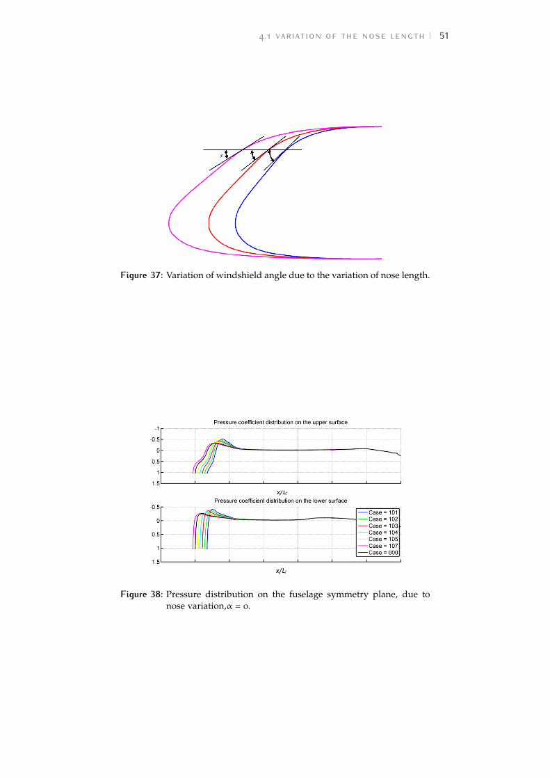
4.1 variation of the nose length 51
Figure 37: Variation of windshield angle due to the variation of nose length.
Figure 38: Pressure distribution on the fuselage symmetry plane, due tonose variation,α = 0.
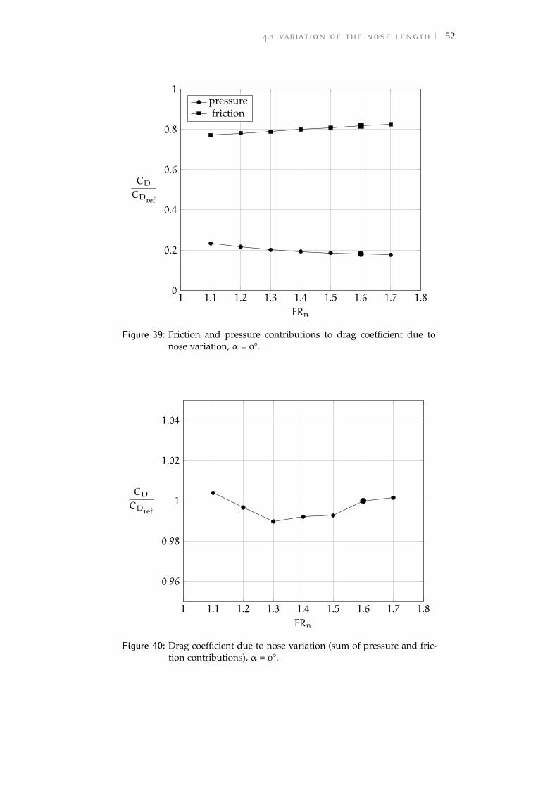
4.1 variation of the nose length 52
1 1.1 1.2 1.3 1.4 1.5 1.6 1.7 1.80
0.2
0.4
0.6
0.8
1
FRn
CDCDref
pressurefriction
Figure 39: Friction and pressure contributions to drag coefficient due tonose variation, α = 0°.
1 1.1 1.2 1.3 1.4 1.5 1.6 1.7 1.8
0.96
0.98
1
1.02
1.04
FRn
CDCDref
Figure 40: Drag coefficient due to nose variation (sum of pressure and fric-tion contributions), α = 0°.
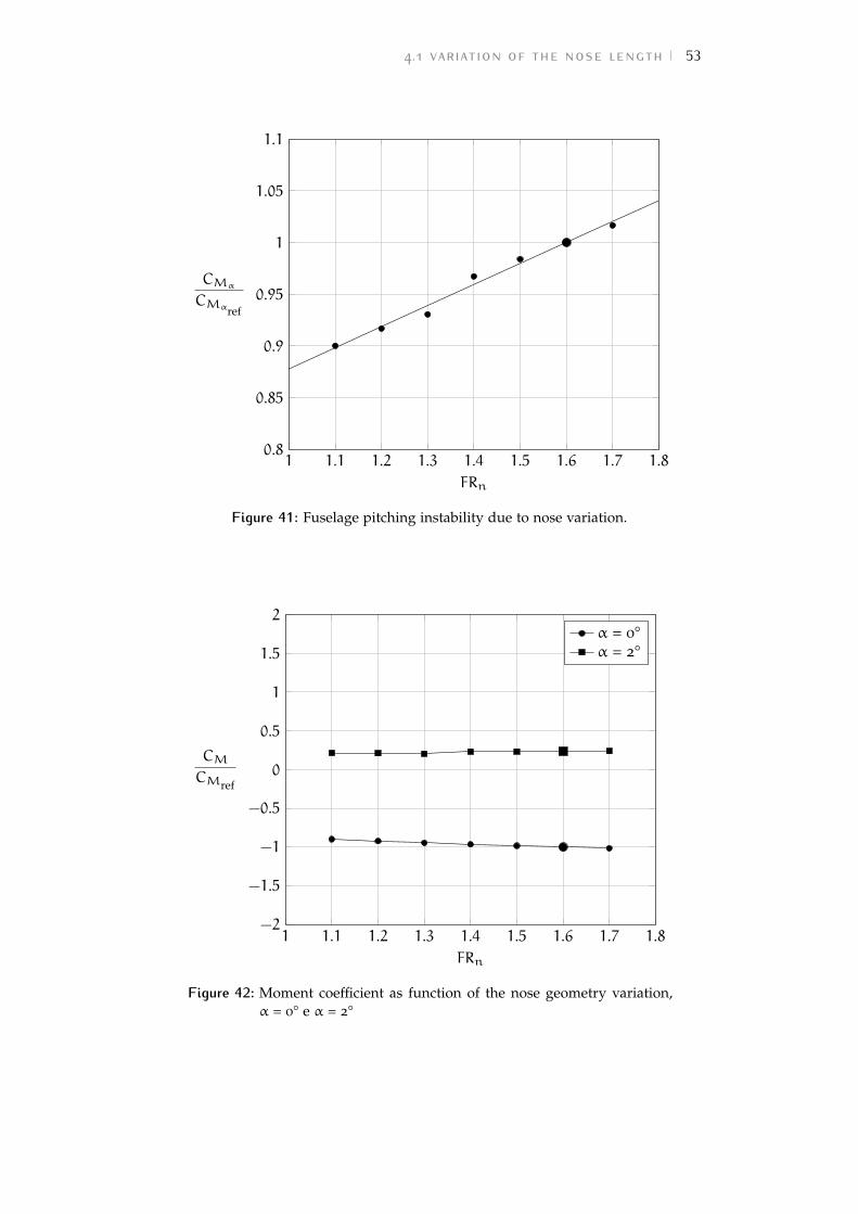
4.1 variation of the nose length 53
1 1.1 1.2 1.3 1.4 1.5 1.6 1.7 1.80.8
0.85
0.9
0.95
1
1.05
1.1
FRn
CMα
CMαref
Figure 41: Fuselage pitching instability due to nose variation.
1 1.1 1.2 1.3 1.4 1.5 1.6 1.7 1.8−2
−1.5
−1
−0.5
0
0.5
1
1.5
2
FRn
CMCMref
α = 0°α = 2°
Figure 42: Moment coefficient as function of the nose geometry variation,α = 0° e α = 2°
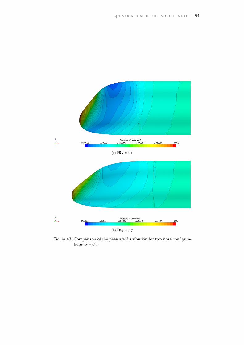
4.1 variation of the nose length 54
(a) FRn = 1.1
(b) FRn = 1.7
Figure 43: Comparison of the pressure distribution for two nose configura-tions, α = 0°.
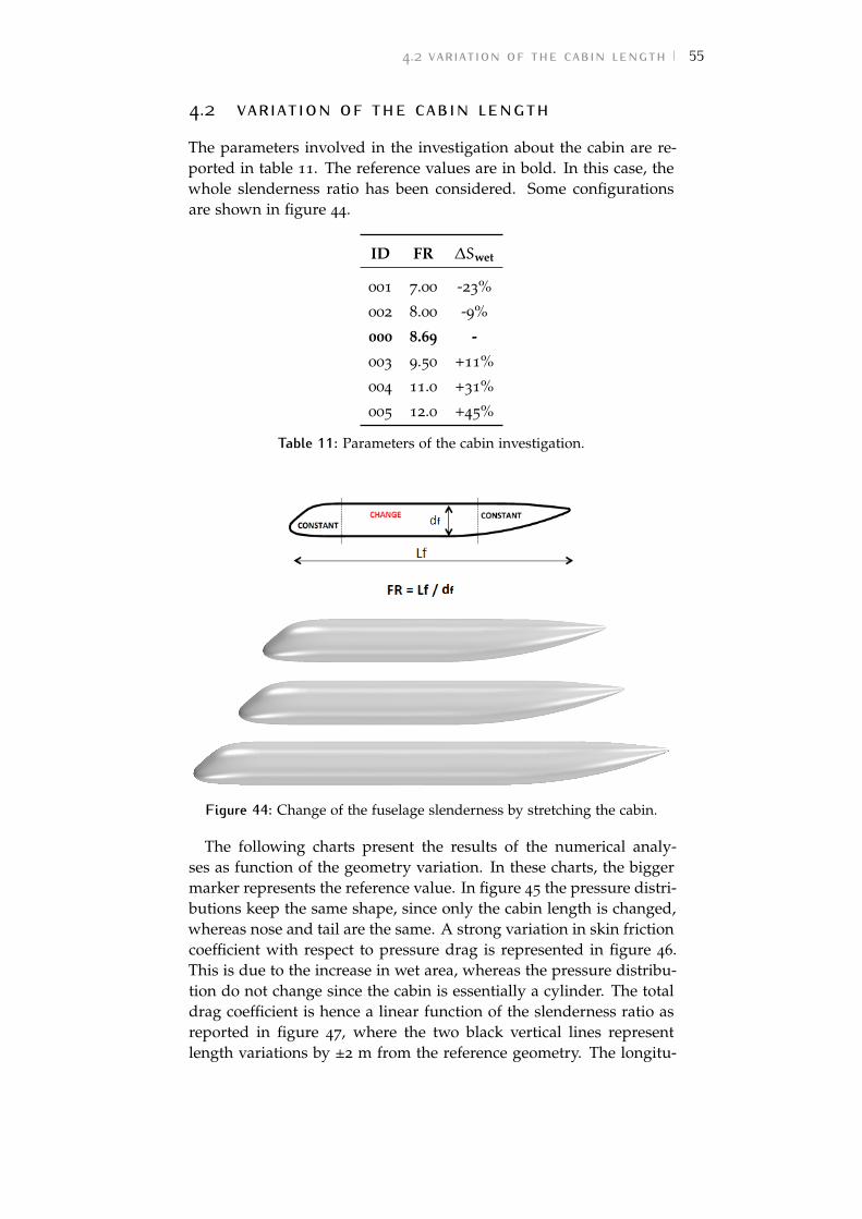
4.2 variation of the cabin length 55
4.2 variation of the cabin length
The parameters involved in the investigation about the cabin are re-ported in table 11. The reference values are in bold. In this case, thewhole slenderness ratio has been considered. Some configurationsare shown in figure 44.
ID FR ∆Swet
001 7.00 -23%
002 8.00 -9%
000 8.69 -
003 9.50 +11%
004 11.0 +31%
005 12.0 +45%
Table 11: Parameters of the cabin investigation.
Figure 44: Change of the fuselage slenderness by stretching the cabin.
The following charts present the results of the numerical analy-ses as function of the geometry variation. In these charts, the biggermarker represents the reference value. In figure 45 the pressure distri-butions keep the same shape, since only the cabin length is changed,whereas nose and tail are the same. A strong variation in skin frictioncoefficient with respect to pressure drag is represented in figure 46.This is due to the increase in wet area, whereas the pressure distribu-tion do not change since the cabin is essentially a cylinder. The totaldrag coefficient is hence a linear function of the slenderness ratio asreported in figure 47, where the two black vertical lines representlength variations by ±2 m from the reference geometry. The longitu-

4.2 variation of the cabin length 56
Figure 45: Pressure distribution on the fuselage symmetry plane, due tocabin variation, α = 0°.
dinal instability is shown in figure 48. The moment reference centerchanges its absolute position to keep the same relative position (atx/Lf equal to 0.465 and z equal to 0). As expected, a longer cabin isless stable in pitch.
6 7 8 9 10 11 12 130
0.2
0.4
0.6
0.8
1
1.2
FR
CDCDref
pressurefriction
Figure 46: Friction and pressure contributions to drag coefficient due tocabin variation, α = 0°.
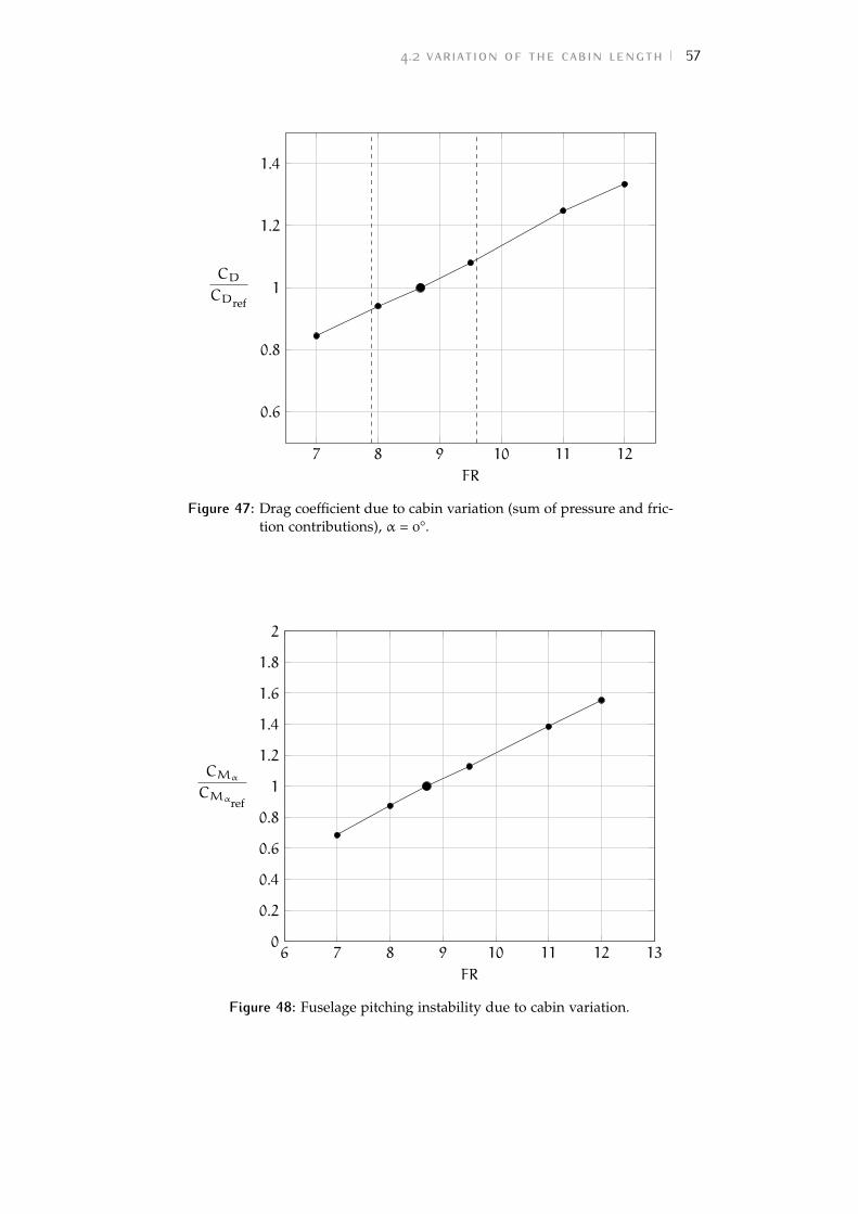
4.2 variation of the cabin length 57
7 8 9 10 11 12
0.6
0.8
1
1.2
1.4
FR
CDCDref
Figure 47: Drag coefficient due to cabin variation (sum of pressure and fric-tion contributions), α = 0°.
6 7 8 9 10 11 12 130
0.2
0.4
0.6
0.8
1
1.2
1.4
1.6
1.8
2
FR
CMα
CMαref
Figure 48: Fuselage pitching instability due to cabin variation.
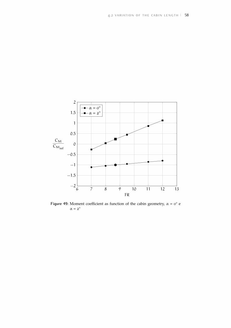
4.2 variation of the cabin length 58
6 7 8 9 10 11 12 13−2
−1.5
−1
−0.5
0
0.5
1
1.5
2
FR
CMCMref
α = 0°α = 2°
Figure 49: Moment coefficient as function of the cabin geometry, α = 0° eα = 2°
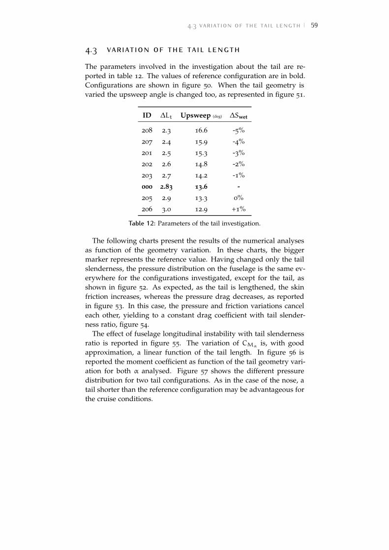
4.3 variation of the tail length 59
4.3 variation of the tail length
The parameters involved in the investigation about the tail are re-ported in table 12. The values of reference configuration are in bold.Configurations are shown in figure 50. When the tail geometry isvaried the upsweep angle is changed too, as represented in figure 51.
ID ∆Lt Upsweep (deg) ∆Swet
208 2.3 16.6 -5%
207 2.4 15.9 -4%
201 2.5 15.3 -3%
202 2.6 14.8 -2%
203 2.7 14.2 -1%
000 2.83 13.6 -
205 2.9 13.3 0%
206 3.0 12.9 +1%
Table 12: Parameters of the tail investigation.
The following charts present the results of the numerical analysesas function of the geometry variation. In these charts, the biggermarker represents the reference value. Having changed only the tailslenderness, the pressure distribution on the fuselage is the same ev-erywhere for the configurations investigated, except for the tail, asshown in figure 52. As expected, as the tail is lengthened, the skinfriction increases, whereas the pressure drag decreases, as reportedin figure 53. In this case, the pressure and friction variations canceleach other, yielding to a constant drag coefficient with tail slender-ness ratio, figure 54.
The effect of fuselage longitudinal instability with tail slendernessratio is reported in figure 55. The variation of CMα
is, with goodapproximation, a linear function of the tail length. In figure 56 isreported the moment coefficient as function of the tail geometry vari-ation for both α analysed. Figure 57 shows the different pressuredistribution for two tail configurations. As in the case of the nose, atail shorter than the reference configuration may be advantageous forthe cruise conditions.
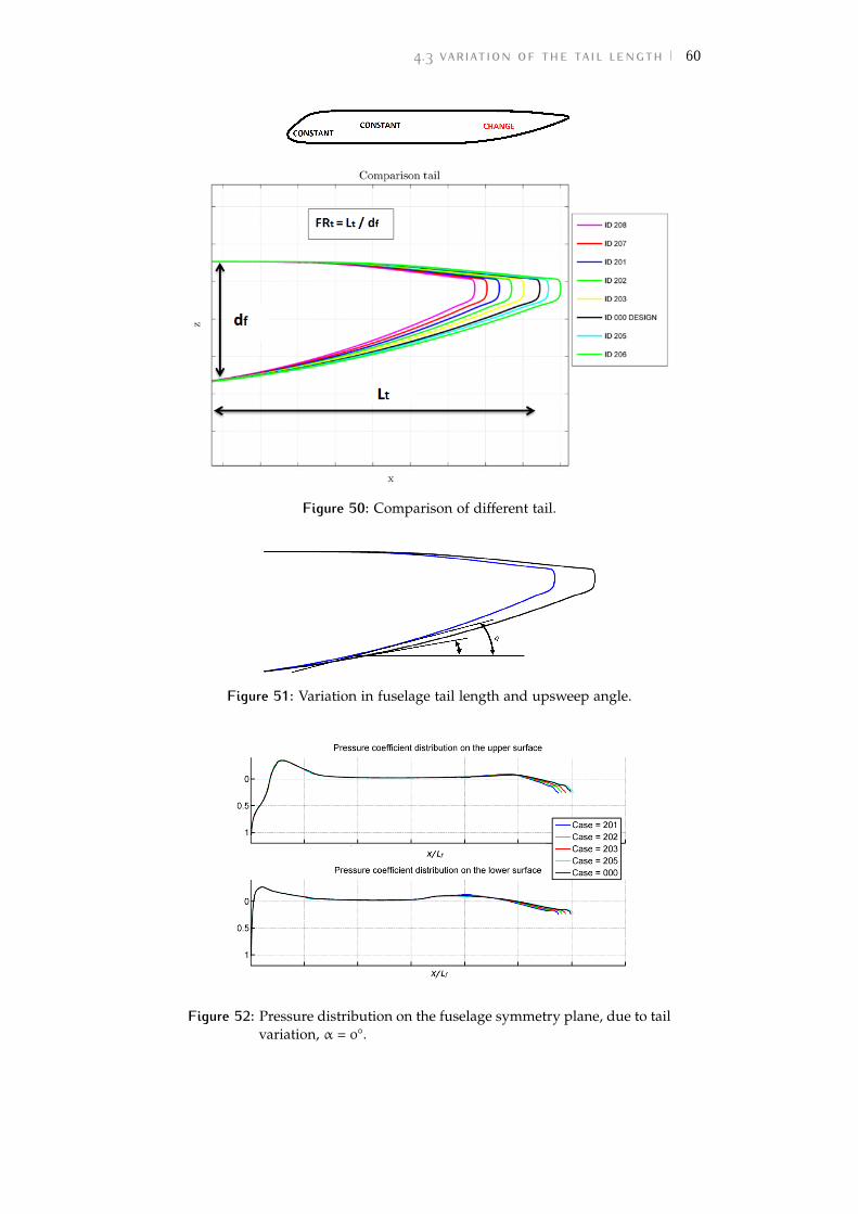
4.3 variation of the tail length 60
Figure 50: Comparison of different tail.
Figure 51: Variation in fuselage tail length and upsweep angle.
Figure 52: Pressure distribution on the fuselage symmetry plane, due to tailvariation, α = 0°.
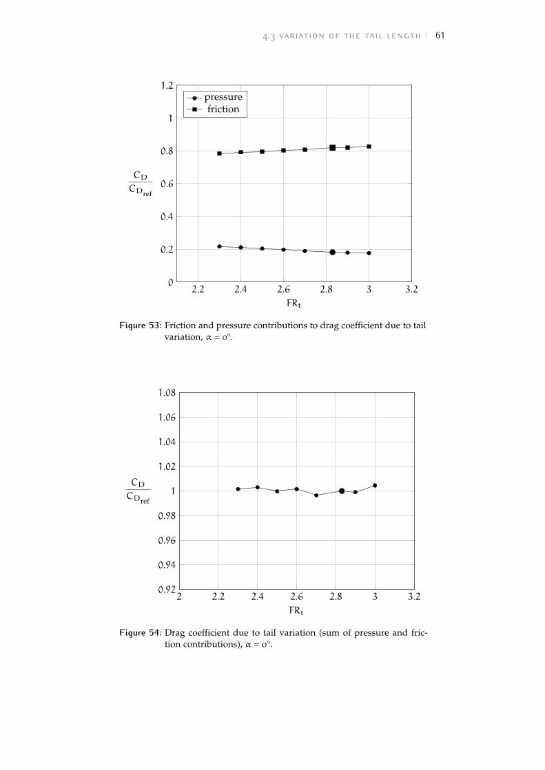
4.3 variation of the tail length 61
2.2 2.4 2.6 2.8 3 3.20
0.2
0.4
0.6
0.8
1
1.2
FRt
CDCDref
pressurefriction
Figure 53: Friction and pressure contributions to drag coefficient due to tailvariation, α = 0°.
2 2.2 2.4 2.6 2.8 3 3.20.92
0.94
0.96
0.98
1
1.02
1.04
1.06
1.08
FRt
CDCDref
Figure 54: Drag coefficient due to tail variation (sum of pressure and fric-tion contributions), α = 0°.
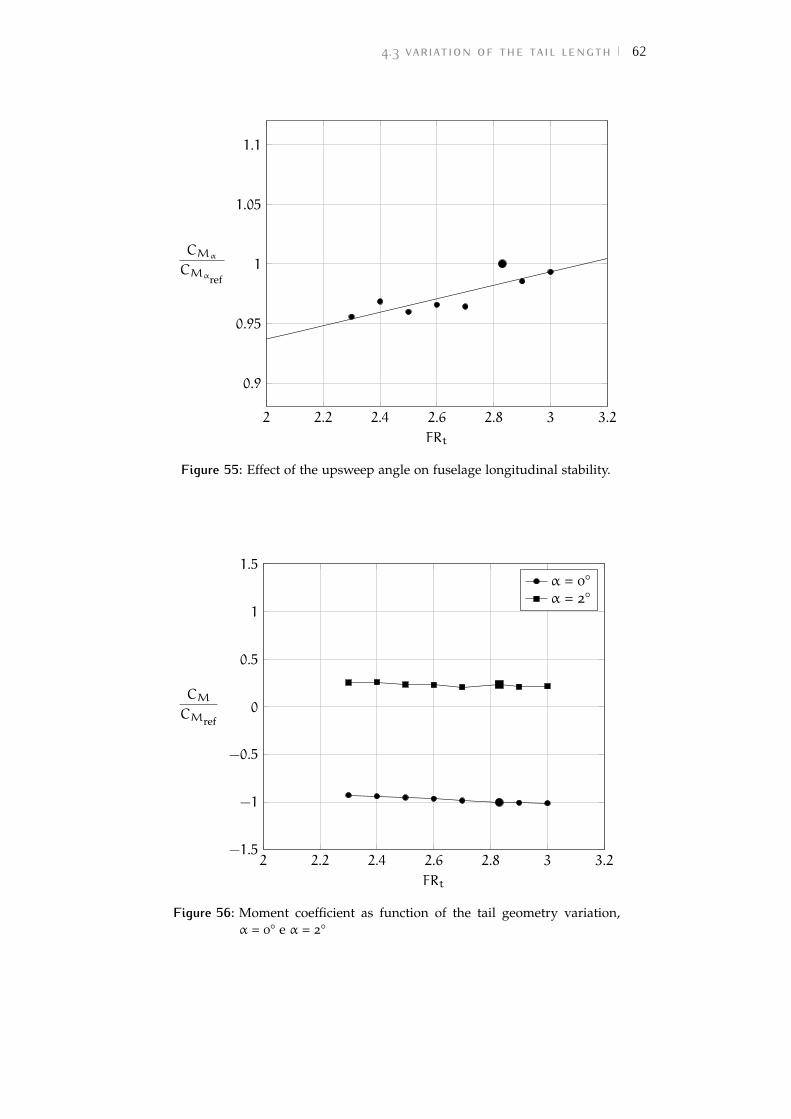
4.3 variation of the tail length 62
2 2.2 2.4 2.6 2.8 3 3.2
0.9
0.95
1
1.05
1.1
FRt
CMα
CMαref
Figure 55: Effect of the upsweep angle on fuselage longitudinal stability.
2 2.2 2.4 2.6 2.8 3 3.2−1.5
−1
−0.5
0
0.5
1
1.5
FRt
CMCMref
α = 0°α = 2°
Figure 56: Moment coefficient as function of the tail geometry variation,α = 0° e α = 2°
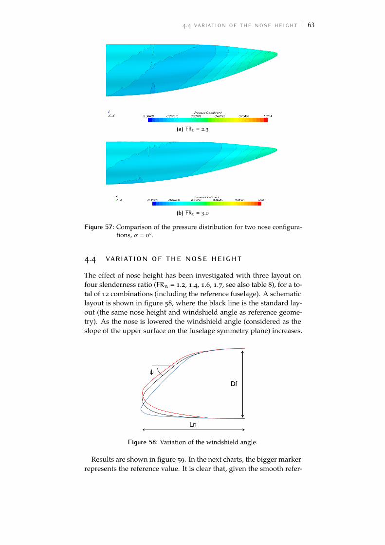
4.4 variation of the nose height 63
(a) FRt = 2.3
(b) FRt = 3.0
Figure 57: Comparison of the pressure distribution for two nose configura-tions, α = 0°.
4.4 variation of the nose height
The effect of nose height has been investigated with three layout onfour slenderness ratio (FRn = 1.2, 1.4, 1.6, 1.7, see also table 8), for a to-tal of 12 combinations (including the reference fuselage). A schematiclayout is shown in figure 58, where the black line is the standard lay-out (the same nose height and windshield angle as reference geome-try). As the nose is lowered the windshield angle (considered as theslope of the upper surface on the fuselage symmetry plane) increases.
Figure 58: Variation of the windshield angle.
Results are shown in figure 59. In the next charts, the bigger markerrepresents the reference value. It is clear that, given the smooth refer-
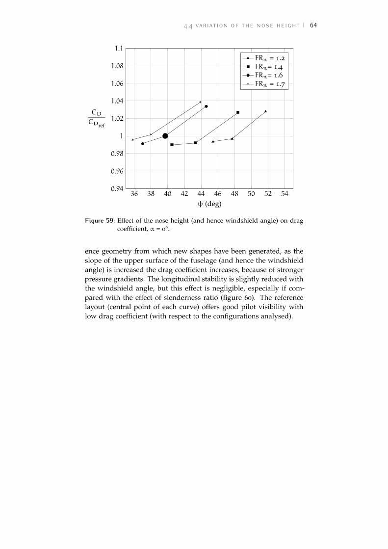
4.4 variation of the nose height 64
36 38 40 42 44 46 48 50 52 540.94
0.96
0.98
1
1.02
1.04
1.06
1.08
1.1
ψ (deg)
CDCDref
FRn = 1.2FRn= 1.4FRn= 1.6FRn = 1.7
Figure 59: Effect of the nose height (and hence windshield angle) on dragcoefficient, α = 0°.
ence geometry from which new shapes have been generated, as theslope of the upper surface of the fuselage (and hence the windshieldangle) is increased the drag coefficient increases, because of strongerpressure gradients. The longitudinal stability is slightly reduced withthe windshield angle, but this effect is negligible, especially if com-pared with the effect of slenderness ratio (figure 60). The referencelayout (central point of each curve) offers good pilot visibility withlow drag coefficient (with respect to the configurations analysed).
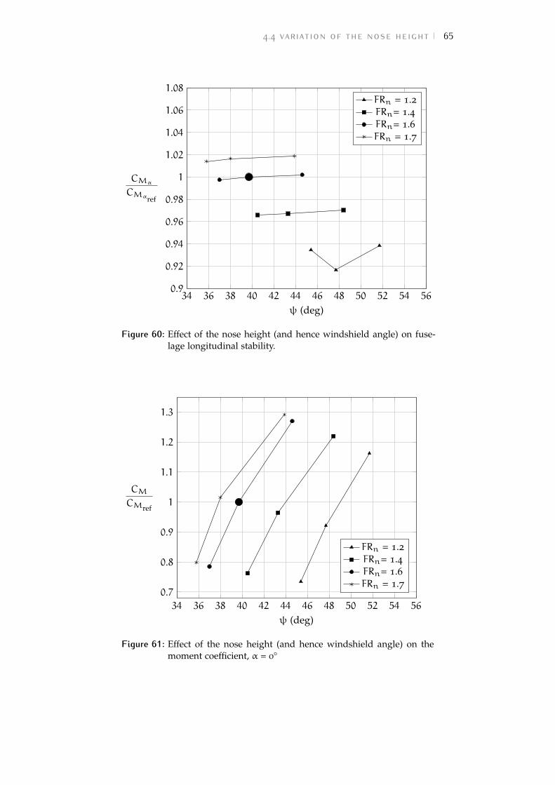
4.4 variation of the nose height 65
34 36 38 40 42 44 46 48 50 52 54 560.9
0.92
0.94
0.96
0.98
1
1.02
1.04
1.06
1.08
ψ (deg)
CMα
CMαref
FRn = 1.2FRn= 1.4FRn= 1.6FRn = 1.7
Figure 60: Effect of the nose height (and hence windshield angle) on fuse-lage longitudinal stability.
34 36 38 40 42 44 46 48 50 52 54 56
0.7
0.8
0.9
1
1.1
1.2
1.3
ψ (deg)
CMCMref
FRn = 1.2FRn= 1.4FRn= 1.6FRn = 1.7
Figure 61: Effect of the nose height (and hence windshield angle) on themoment coefficient, α = 0°
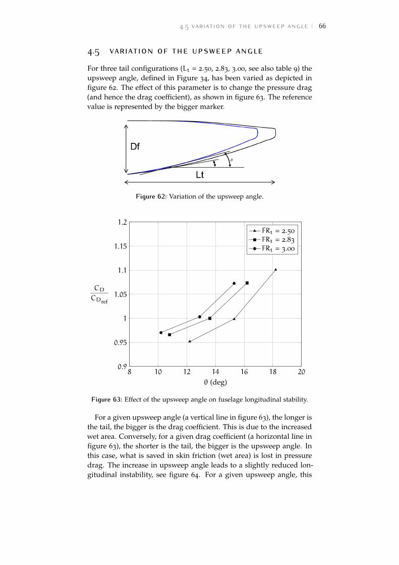
4.5 variation of the upsweep angle 66
4.5 variation of the upsweep angle
For three tail configurations (Lt = 2.50, 2.83, 3.00, see also table 9) theupsweep angle, defined in Figure 34, has been varied as depicted infigure 62. The effect of this parameter is to change the pressure drag(and hence the drag coefficient), as shown in figure 63. The referencevalue is represented by the bigger marker.
Figure 62: Variation of the upsweep angle.
8 10 12 14 16 18 200.9
0.95
1
1.05
1.1
1.15
1.2
θ (deg)
CDCDref
FRt = 2.50
FRt = 2.83
FRt = 3.00
Figure 63: Effect of the upsweep angle on fuselage longitudinal stability.
For a given upsweep angle (a vertical line in figure 63), the longer isthe tail, the bigger is the drag coefficient. This is due to the increasedwet area. Conversely, for a given drag coefficient (a horizontal line infigure 63), the shorter is the tail, the bigger is the upsweep angle. Inthis case, what is saved in skin friction (wet area) is lost in pressuredrag. The increase in upsweep angle leads to a slightly reduced lon-gitudinal instability, see figure 64. For a given upsweep angle, this
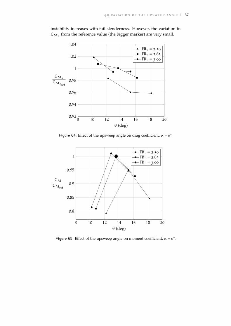
4.5 variation of the upsweep angle 67
instability increases with tail slenderness. However, the variation inCMα
from the reference value (the bigger marker) are very small.
8 10 12 14 16 18 200.92
0.94
0.96
0.98
1
1.02
1.04
θ (deg)
CMα
CMαref
FRt = 2.50
FRt = 2.83
FRt = 3.00
Figure 64: Effect of the upsweep angle on drag coefficient, α = 0°.
8 10 12 14 16 18 20
0.8
0.85
0.9
0.95
1
θ (deg)
CMCMref
FRt = 2.50
FRt = 2.83
FRt = 3.00
Figure 65: Effect of the upsweep angle on moment coefficient, α = 0°.
5 A N E W M E T H O D O LO GY F O RP R E D I C T I O N O FA E R O DY N A M I C C O E F F I C I E N T S
Contents5.1 Methodology for drag prediction 68
5.1.1 The shape factor of the nose 69
5.1.2 The shape factor of the cabin 70
5.1.3 The shape factor of the tail 70
5.1.4 Example of application 72
5.2 Pitching moment prediction 79
5.2.1 Example of application 81
5.3 Prediction of the pitching moment derivative 84
5.3.1 Example of application 87
In this chapter it is proposed a methodology to obtain the valueof drag and pitching moment coefficient as a function of fuselagegeometry and it is suitable for smooth shapes. This approach doesnot allow to evaluate some sources of drag as leakage, wiper, surfaceroughness and excrescences.
5.1 methodology for drag prediction
The methodology allows to compute the fuselage drag coefficient asthe sum of the contributions of each component (nose, cabin, andtailcone), calculated as follows.
SfrontCDi = KiCDfpSwet i (5.1)
In the previous equation i states the geometry part (nose, cabin ortailcone), Sfront is the frontal surface (equal to the maximum area ofcabin section), Swet i is the wet surface of the i-th part, the CDfp is thedrag coefficient of equivalent flat plate and the Ki is the shape factorwhich is the core of the method here presented. It wasn’t chosen theSwing as the reference surface because the wing could be unknownwhen the fuselage is designed. The equation 5.1 is quite similar toequation 2.4 proposed by Torenbeek [23] but there is a fundamentalconceptual difference: the shape factor just introduced, Ki, takes intoaccount the variation of the pressure drag due to the modificationsof the fuselage geometry shape, while the form factor of Torenbeek,
68
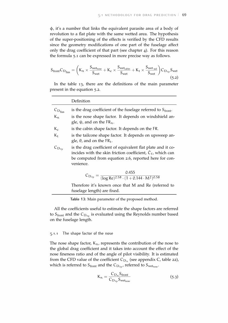
5.1 methodology for drag prediction 69
φ, it’s a number that links the equivalent parasite area of a body ofrevolution to a flat plate with the same wetted area. The hypothesisof the super-positioning of the effects is verified by the CFD resultssince the geometry modifications of one part of the fuselage affectonly the drag coefficient of that part (see chapter 4). For this reasonthe formula 5.1 can be expressed in more precise way as follows.
SfrontCDfus =
(Kn × Swetnose
Swet+Kc ×
Swetcabin
Swet+Kt ×
Swet tail
Swet
)CDfpSwet
(5.2)
In the table 13, there are the definitions of the main parameterpresent in the equation 5.2.
Definition
CDfus is the drag coefficient of the fuselage referred to Sfront.
Kn is the nose shape factor. It depends on windshield an-gle, ψ, and on the FRn.
Kc is the cabin shape factor. It depends on the FR.
Kt is the tailcone shape factor. It depends on upsweep an-gle, θ, and on the FRt.
CDfp is the drag coefficient of equivalent flat plate and it co-incides with the skin friction coefficient, C̄f, which canbe computed from equation 2.6, reported here for con-venience.
CDfp =0.455
(logRe)2.58 · (1+ 0.144 ·M2)0.58
Therefore it’s known once that M and Re (referred tofuselage length) are fixed.
Table 13: Main parameter of the proposed method.
All the coefficients useful to estimate the shape factors are referredto Sfront and the CDfp is evaluated using the Reynolds number basedon the fuselage length.
5.1.1 The shape factor of the nose
The nose shape factor, Kn, represents the contribution of the nose tothe global drag coefficient and it takes into account the effect of thenose fineness ratio and of the angle of pilot visibility. It is estimatedfrom the CFD value of the coefficient CDn (see appendix C, table 22),which is referred to Sfront and the CDfp , referred to Swetnose .
Kn =CDnSfront
CDfpSwetnose
(5.3)
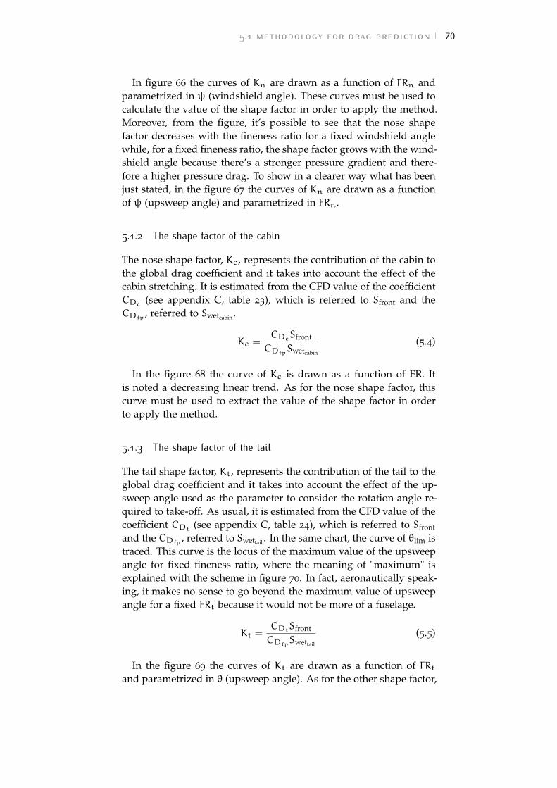
5.1 methodology for drag prediction 70
In figure 66 the curves of Kn are drawn as a function of FRn andparametrized in ψ (windshield angle). These curves must be used tocalculate the value of the shape factor in order to apply the method.Moreover, from the figure, it’s possible to see that the nose shapefactor decreases with the fineness ratio for a fixed windshield anglewhile, for a fixed fineness ratio, the shape factor grows with the wind-shield angle because there’s a stronger pressure gradient and there-fore a higher pressure drag. To show in a clearer way what has beenjust stated, in the figure 67 the curves of Kn are drawn as a functionof ψ (upsweep angle) and parametrized in FRn.
5.1.2 The shape factor of the cabin
The nose shape factor, Kc, represents the contribution of the cabin tothe global drag coefficient and it takes into account the effect of thecabin stretching. It is estimated from the CFD value of the coefficientCDc (see appendix C, table 23), which is referred to Sfront and theCDfp , referred to Swetcabin .
Kc =CDcSfront
CDfpSwetcabin
(5.4)
In the figure 68 the curve of Kc is drawn as a function of FR. Itis noted a decreasing linear trend. As for the nose shape factor, thiscurve must be used to extract the value of the shape factor in orderto apply the method.
5.1.3 The shape factor of the tail
The tail shape factor, Kt, represents the contribution of the tail to theglobal drag coefficient and it takes into account the effect of the up-sweep angle used as the parameter to consider the rotation angle re-quired to take-off. As usual, it is estimated from the CFD value of thecoefficient CDt (see appendix C, table 24), which is referred to Sfront
and the CDfp , referred to Swettail . In the same chart, the curve of θlim istraced. This curve is the locus of the maximum value of the upsweepangle for fixed fineness ratio, where the meaning of "maximum" isexplained with the scheme in figure 70. In fact, aeronautically speak-ing, it makes no sense to go beyond the maximum value of upsweepangle for a fixed FRt because it would not be more of a fuselage.
Kt =CDtSfront
CDfpSwettail
(5.5)
In the figure 69 the curves of Kt are drawn as a function of FRtand parametrized in θ (upsweep angle). As for the other shape factor,
5.1 methodology for drag prediction 71
1.1 1.2 1.3 1.4 1.5 1.6 1.7 1.8 1.9 21.6
1.7
1.8
1.9
2
2.1
2.2
2.3
2.4
FRn
Kn
ψ = 38°ψ = 39°ψ = 40°ψ = 41°ψ = 42°ψ = 43°ψ = 44°ψ = 45°ψ = 46°ψ = 47°ψ = 48°ψ = 49°
ψ
Figure 66: Nose shape factor as a function of FRn, α = 0°.
these curve must be used to extract the value of the shape factorin order to apply the method. The tailcone factor grows with thefineness ratio for a fixed upsweep angle, θ, due to the bigger Swet andit grows with the upsweep angle for a fixed fineness ratio becausethere’s a stronger pressure gradient. To show in a clearer way whathas been just stated, in the figure 71 the curves of Kt are drawn as afunction of θ (upsweep angle) and parametrized in FRt.
5.1 methodology for drag prediction 72
36 38 40 42 44 46 48 50 52 541.4
1.6
1.8
2
2.2
2.4
2.6
ψ
Kn
FRn = 1.2FRn = 1.4FRn = 1.6FRn = 1.7
FRn
Figure 67: Nose shape factor as a function of windshield angle ψ, α = 0°.
5.1.4 Example of application
From previous sections, to calculate the global drag coefficient, itmust be used the equation 5.2, where Kn, Kc and Kt are the shapefactors of different geometry part values of which are extracted fromfigure 66, 68 and 69 respectively.
SfrontCDfus =
(Kn × Swetnose
Swet+Kc ×
Swetcabin
Swet+Kt ×
Swet tail
Swet
)CDfpSwet
(5.6)
Until now the CD has been calculated for each configuration of thefuselage which is different from that of reference only for one geom-etry part. In order to validate the method, some fuselages, whichcharacteristics are reported in table 14, have been simulated.
In order to clarify the different steps of the methodology, the latteris applied to the "103201" fuselage. First of all, the shape factors mustbe evaluated. These can be obtained from the graphs since the FR, ψand θ are known. In particular, for the fuselage under consideration,these parameters are the following.
• FRn = 1.3
• FR = 8.69
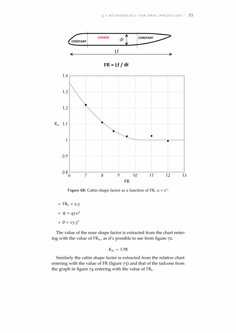
5.1 methodology for drag prediction 73
6 7 8 9 10 11 12 130.8
0.9
1
1.1
1.2
1.3
1.4
FR
Kc
Figure 68: Cabin shape factor as a function of FR, α = 0°.
• FRt = 2.5
• ψ = 45.0°
• θ = 15.3°
The value of the nose shape factor is extracted from the chart enter-ing with the value of FRn, as it’s possible to see from figure 72.
Kn = 1.98
Similarly the cabin shape factor is extracted from the relative chartentering with the value of FR (figure 73) and that of the tailcone fromthe graph in figure 74 entering with the value of FRt.
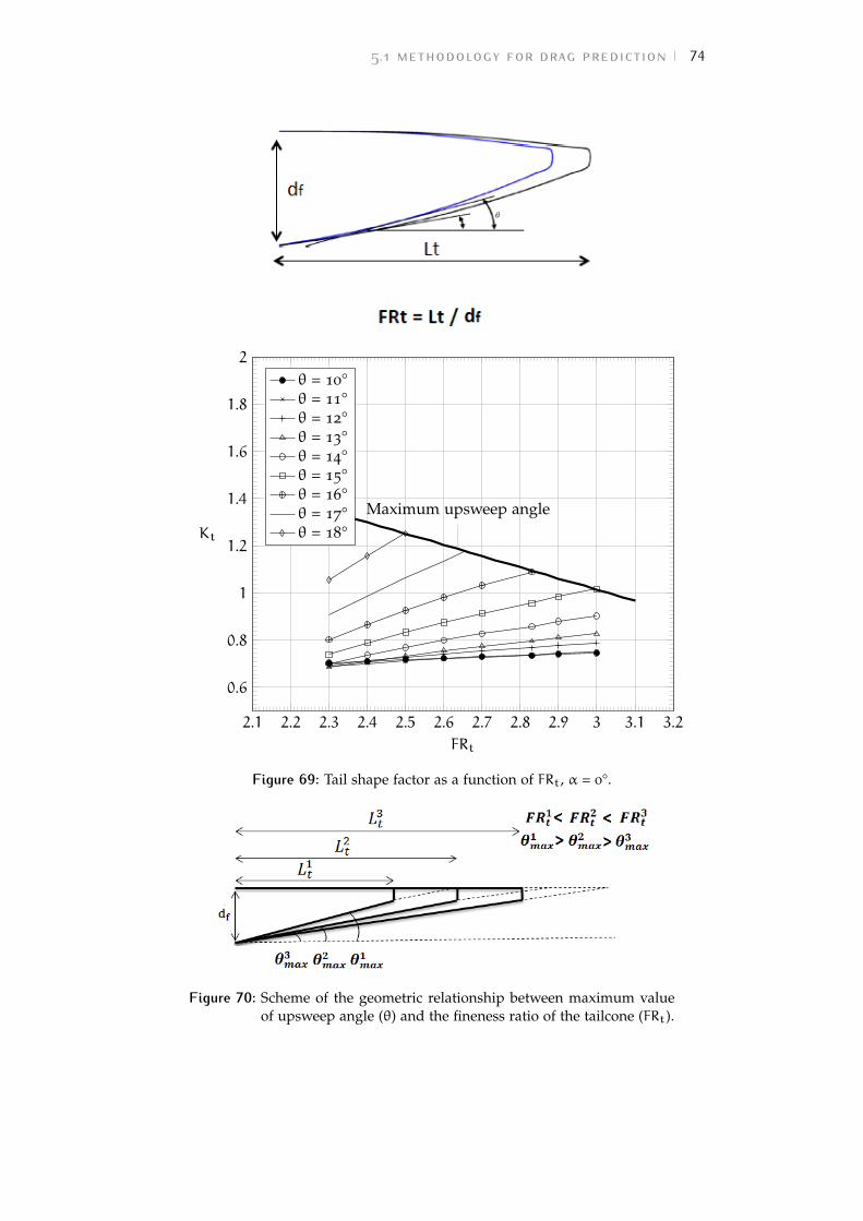
5.1 methodology for drag prediction 74
2.1 2.2 2.3 2.4 2.5 2.6 2.7 2.8 2.9 3 3.1 3.2
0.6
0.8
1
1.2
1.4
1.6
1.8
2
FRt
Kt
θ = 10°θ = 11°θ = 12°θ = 13°θ = 14°θ = 15°θ = 16°θ = 17°θ = 18°
Maximum upsweep angle
Figure 69: Tail shape factor as a function of FRt, α = 0°.
Figure 70: Scheme of the geometric relationship between maximum valueof upsweep angle (θ) and the fineness ratio of the tailcone (FRt).
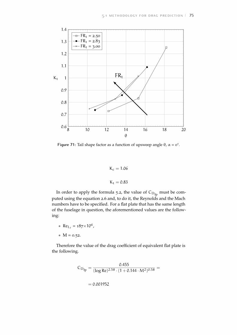
5.1 methodology for drag prediction 75
8 10 12 14 16 18 200.6
0.7
0.8
0.9
1
1.1
1.2
1.3
1.4
θ
Kt
FRt = 2.50
FRt = 2.83
FRt = 3.00
FRt
Figure 71: Tail shape factor as a function of upsweep angle θ, α = 0°.
Kc = 1.06
Kt = 0.83
In order to apply the formula 5.2, the value of CDfp must be com-puted using the equation 2.6 and, to do it, the Reynolds and the Machnumbers have to be specified. For a flat plate that has the same lengthof the fuselage in question, the aforementioned values are the follow-ing:
• ReLf = 187×106,
• M = 0.52.
Therefore the value of the drag coefficient of equivalent flat plate isthe following.
CDfp =0.455
(logRe)2.58 · (1+ 0.144 ·M2)0.58 =
= 0.001952
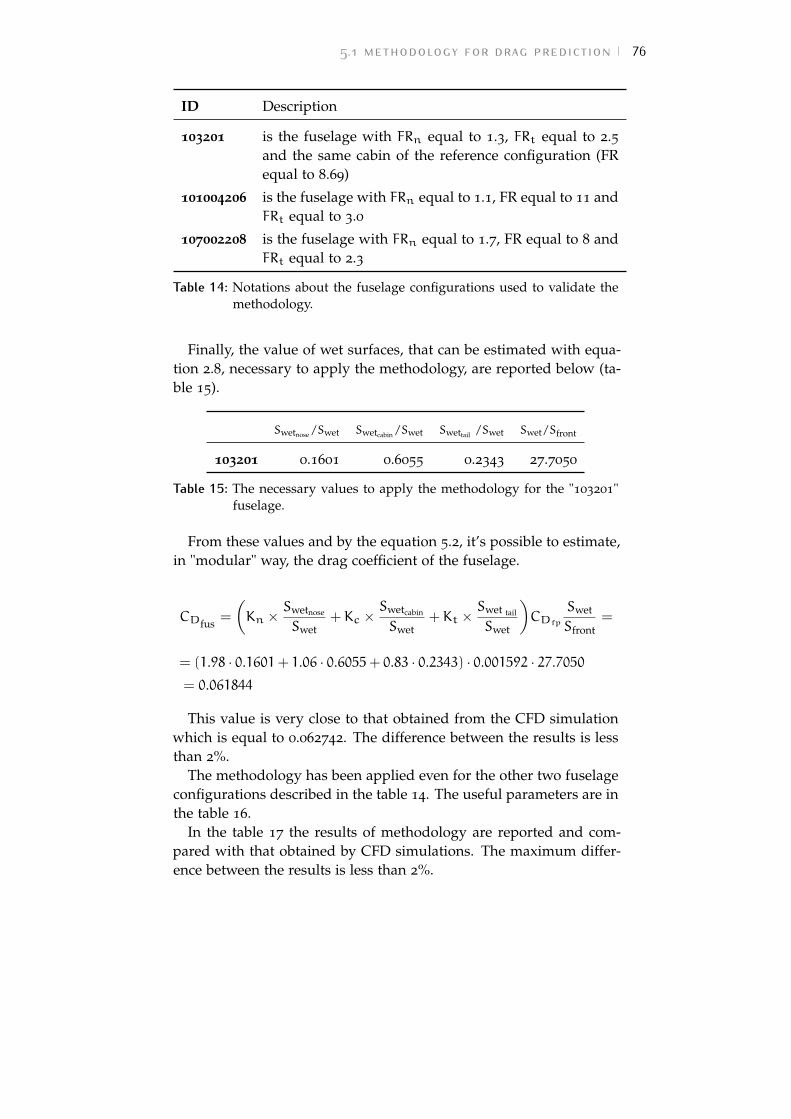
5.1 methodology for drag prediction 76
ID Description
103201 is the fuselage with FRn equal to 1.3, FRt equal to 2.5and the same cabin of the reference configuration (FRequal to 8.69)
101004206 is the fuselage with FRn equal to 1.1, FR equal to 11 andFRt equal to 3.0
107002208 is the fuselage with FRn equal to 1.7, FR equal to 8 andFRt equal to 2.3
Table 14: Notations about the fuselage configurations used to validate themethodology.
Finally, the value of wet surfaces, that can be estimated with equa-tion 2.8, necessary to apply the methodology, are reported below (ta-ble 15).
Swetnose /Swet Swetcabin /Swet Swettail /Swet Swet/Sfront
103201 0.1601 0.6055 0.2343 27.7050
Table 15: The necessary values to apply the methodology for the "103201"fuselage.
From these values and by the equation 5.2, it’s possible to estimate,in "modular" way, the drag coefficient of the fuselage.
CDfus =
(Kn × Swetnose
Swet+Kc ×
Swetcabin
Swet+Kt ×
Swet tail
Swet
)CDfp
Swet
Sfront=
= (1.98 · 0.1601+ 1.06 · 0.6055+ 0.83 · 0.2343) · 0.001592 · 27.7050= 0.061844
This value is very close to that obtained from the CFD simulationwhich is equal to 0.062742. The difference between the results is lessthan 2%.
The methodology has been applied even for the other two fuselageconfigurations described in the table 14. The useful parameters are inthe table 16.
In the table 17 the results of methodology are reported and com-pared with that obtained by CFD simulations. The maximum differ-ence between the results is less than 2%.
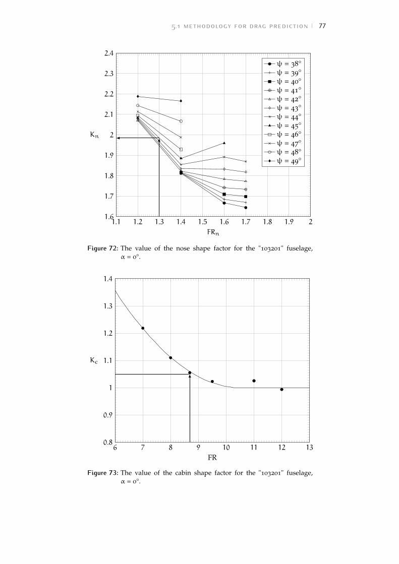
5.1 methodology for drag prediction 77
1.1 1.2 1.3 1.4 1.5 1.6 1.7 1.8 1.9 21.6
1.7
1.8
1.9
2
2.1
2.2
2.3
2.4
FRn
Kn
ψ = 38°ψ = 39°ψ = 40°ψ = 41°ψ = 42°ψ = 43°ψ = 44°ψ = 45°ψ = 46°ψ = 47°ψ = 48°ψ = 49°
Figure 72: The value of the nose shape factor for the "103201" fuselage,α = 0°.
6 7 8 9 10 11 12 130.8
0.9
1
1.1
1.2
1.3
1.4
FR
Kc
Figure 73: The value of the cabin shape factor for the "103201" fuselage,α = 0°.
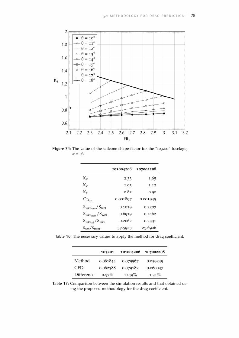
5.1 methodology for drag prediction 78
2.1 2.2 2.3 2.4 2.5 2.6 2.7 2.8 2.9 3 3.1 3.2
0.6
0.8
1
1.2
1.4
1.6
1.8
2
FRt
Kt
θ = 10°θ = 11°θ = 12°θ = 13°θ = 14°θ = 15°θ = 16°θ = 17°θ = 18°
Figure 74: The value of the tailcone shape factor for the "103201" fuselage,α = 0°.
101004206 107002208
Kn 2.33 1.65
Kc 1.03 1.12
Kt 0.82 0.90
CDfp 0.001897 0.001945
Swetnose/Swet 0.1019 0.2207
Swetcabin/Swet 0.6919 0.5462
Swettail/Swet 0.2062 0.2331
Swet/Sfront 37.5923 25.6906
Table 16: The necessary values to apply the method for drag coefficient.
103201 101004206 107002208
Method 0.061844 0.079567 0.059249
CFD 0.062388 0.079182 0.060037
Difference 0.57% -0.49% 1.31%
Table 17: Comparison between the simulation results and that obtained us-ing the proposed methodology for the drag coefficient.
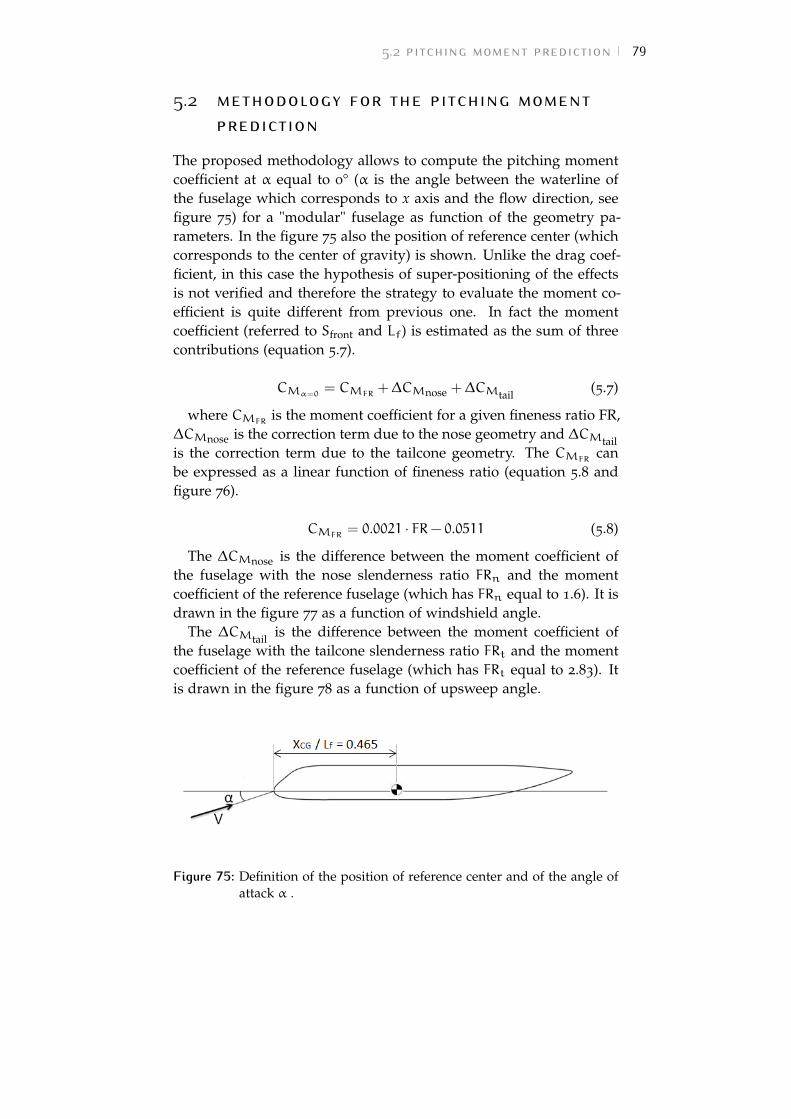
5.2 pitching moment prediction 79
5.2 methodology for the pitching momentprediction
The proposed methodology allows to compute the pitching momentcoefficient at α equal to 0° (α is the angle between the waterline ofthe fuselage which corresponds to x axis and the flow direction, seefigure 75) for a "modular" fuselage as function of the geometry pa-rameters. In the figure 75 also the position of reference center (whichcorresponds to the center of gravity) is shown. Unlike the drag coef-ficient, in this case the hypothesis of super-positioning of the effectsis not verified and therefore the strategy to evaluate the moment co-efficient is quite different from previous one. In fact the momentcoefficient (referred to Sfront and Lf) is estimated as the sum of threecontributions (equation 5.7).
CMα=0= CMFR
+∆CMnose +∆CMtail (5.7)
where CMFRis the moment coefficient for a given fineness ratio FR,
∆CMnose is the correction term due to the nose geometry and ∆CMtailis the correction term due to the tailcone geometry. The CMFR
canbe expressed as a linear function of fineness ratio (equation 5.8 andfigure 76).
CMFR= 0.0021 · FR− 0.0511 (5.8)
The ∆CMnose is the difference between the moment coefficient ofthe fuselage with the nose slenderness ratio FRn and the momentcoefficient of the reference fuselage (which has FRn equal to 1.6). It isdrawn in the figure 77 as a function of windshield angle.
The ∆CMtail is the difference between the moment coefficient ofthe fuselage with the tailcone slenderness ratio FRt and the momentcoefficient of the reference fuselage (which has FRt equal to 2.83). Itis drawn in the figure 78 as a function of upsweep angle.
Figure 75: Definition of the position of reference center and of the angle ofattack α .
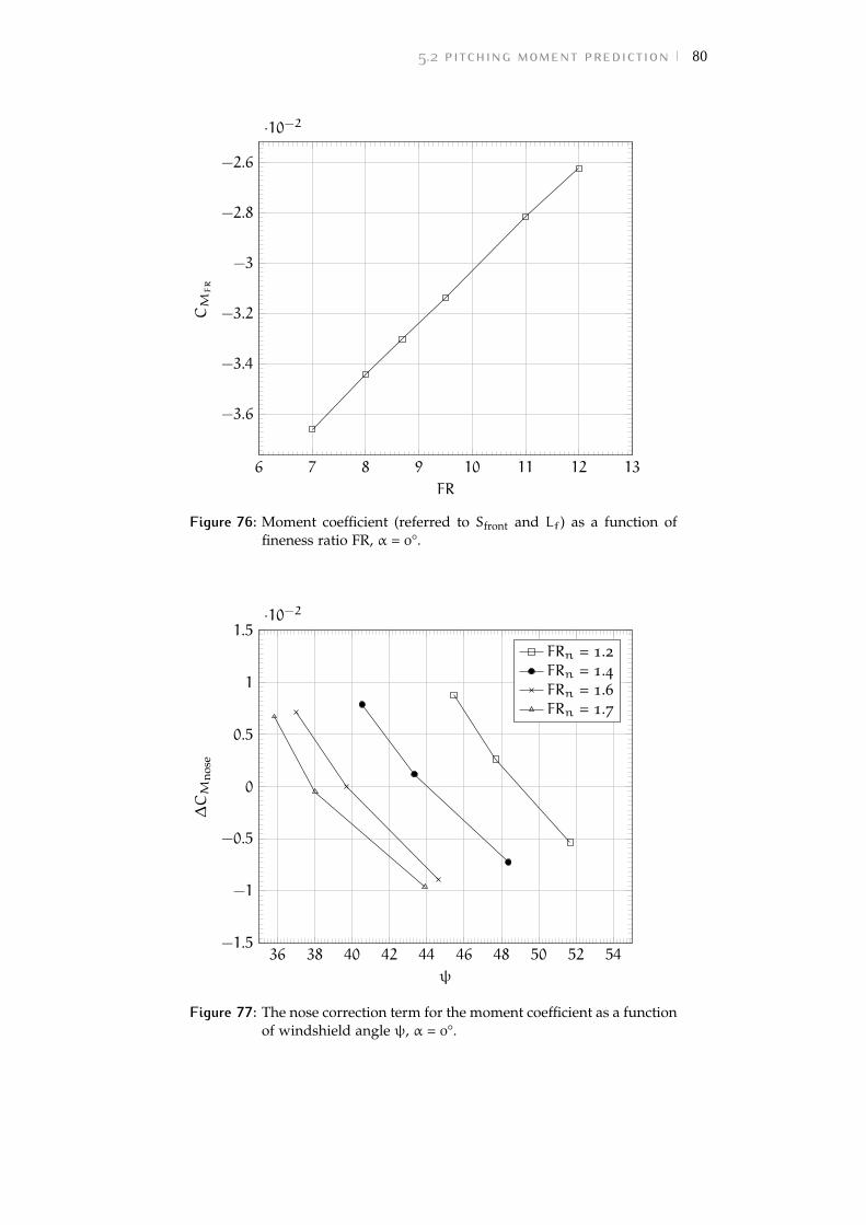
5.2 pitching moment prediction 80
6 7 8 9 10 11 12 13
−3.6
−3.4
−3.2
−3
−2.8
−2.6
·10−2
FR
CMFR
Figure 76: Moment coefficient (referred to Sfront and Lf) as a function offineness ratio FR, α = 0°.
36 38 40 42 44 46 48 50 52 54−1.5
−1
−0.5
0
0.5
1
1.5·10−2
ψ
∆CM
nose
FRn = 1.2FRn = 1.4FRn = 1.6FRn = 1.7
Figure 77: The nose correction term for the moment coefficient as a functionof windshield angle ψ, α = 0°.
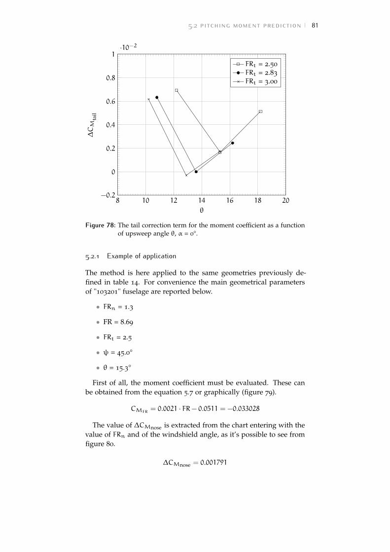
5.2 pitching moment prediction 81
8 10 12 14 16 18 20−0.2
0
0.2
0.4
0.6
0.8
1·10−2
θ
∆CM
tail
FRt = 2.50
FRt = 2.83
FRt = 3.00
Figure 78: The tail correction term for the moment coefficient as a functionof upsweep angle θ, α = 0°.
5.2.1 Example of application
The method is here applied to the same geometries previously de-fined in table 14. For convenience the main geometrical parametersof "103201" fuselage are reported below.
• FRn = 1.3
• FR = 8.69
• FRt = 2.5
• ψ = 45.0°
• θ = 15.3°
First of all, the moment coefficient must be evaluated. These canbe obtained from the equation 5.7 or graphically (figure 79).
CMFR= 0.0021 · FR− 0.0511 = −0.033028
The value of ∆CMnose is extracted from the chart entering with thevalue of FRn and of the windshield angle, as it’s possible to see fromfigure 80.
∆CMnose = 0.001791
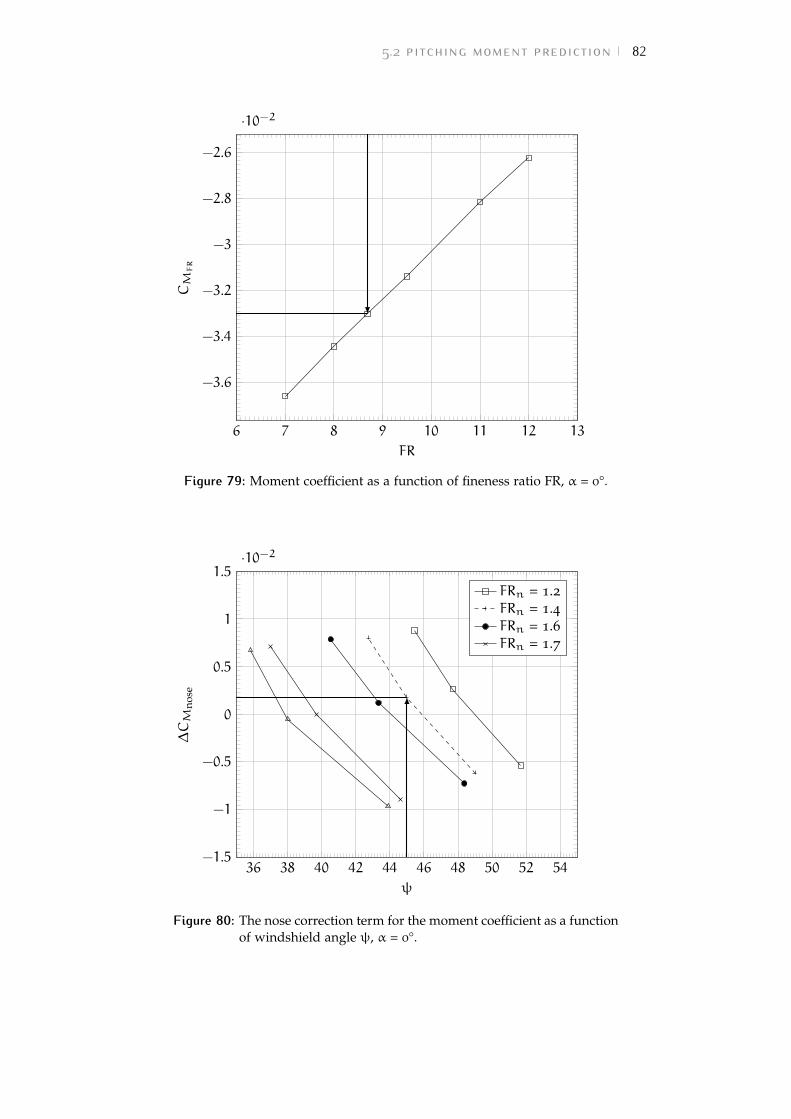
5.2 pitching moment prediction 82
6 7 8 9 10 11 12 13
−3.6
−3.4
−3.2
−3
−2.8
−2.6
·10−2
FR
CMFR
Figure 79: Moment coefficient as a function of fineness ratio FR, α = 0°.
36 38 40 42 44 46 48 50 52 54−1.5
−1
−0.5
0
0.5
1
1.5·10−2
ψ
∆CM
nose
FRn = 1.2FRn = 1.4FRn = 1.6FRn = 1.7
Figure 80: The nose correction term for the moment coefficient as a functionof windshield angle ψ, α = 0°.
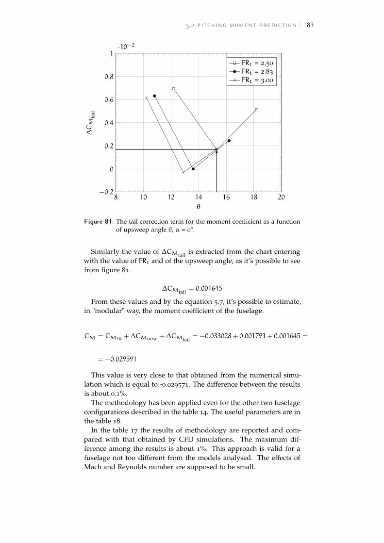
5.2 pitching moment prediction 83
8 10 12 14 16 18 20−0.2
0
0.2
0.4
0.6
0.8
1·10−2
θ
∆CM
tail
FRt = 2.50
FRt = 2.83
FRt = 3.00
Figure 81: The tail correction term for the moment coefficient as a functionof upsweep angle θ, α = 0°.
Similarly the value of ∆CMtail is extracted from the chart enteringwith the value of FRt and of the upsweep angle, as it’s possible to seefrom figure 81.
∆CMtail = 0.001645
From these values and by the equation 5.7, it’s possible to estimate,in "modular" way, the moment coefficient of the fuselage.
CM = CMFR+∆CMnose +∆CMtail = −0.033028+ 0.001791+ 0.001645 =
= −0.029591
This value is very close to that obtained from the numerical simu-lation which is equal to -0.029571. The difference between the resultsis about 0.1%.
The methodology has been applied even for the other two fuselageconfigurations described in the table 14. The useful parameters are inthe table 18.
In the table 17 the results of methodology are reported and com-pared with that obtained by CFD simulations. The maximum dif-ference among the results is about 1%. This approach is valid for afuselage not too different from the models analysed. The effects ofMach and Reynolds number are supposed to be small.
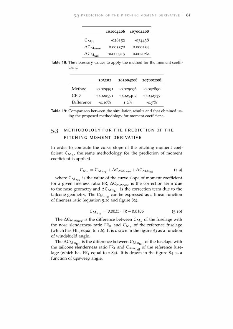
5.3 prediction of the pitching moment derivative 84
101004206 107002208
CMFR-028152 -034438
∆CMnose 0.003370 -0.000534
∆CMtail -0.000315 0.002082
Table 18: The necessary values to apply the method for the moment coeffi-cient.
103201 101004206 107002208
Method -0.029591 -0.025096 -0.032890
CFD -0.029571 -0.025402 -0.032737
Difference -0.10% 1.2% -0.5%
Table 19: Comparison between the simulation results and that obtained us-ing the proposed methodology for moment coefficient.
5.3 methodology for the prediction of thepitching moment derivative
In order to compute the curve slope of the pitching moment coef-ficient CMα
, the same methodology for the prediction of momentcoefficient is applied.
CMα= CMαFR
+∆CMαnose +∆CMαtail (5.9)
where CMαFRis the value of the curve slope of moment coefficient
for a given fineness ratio FR, ∆CMαnose is the correction term dueto the nose geometry and ∆CMαtail is the correction term due to thetailcone geometry. The CMαFR
can be expressed as a linear functionof fineness ratio (equation 5.10 and figure 82).
CMαFR= 0.0035 · FR− 0.0106 (5.10)
The ∆CMαnose is the difference between CMαof the fuselage with
the nose slenderness ratio FRn and CMαof the reference fuselage
(which has FRn equal to 1.6). It is drawn in the figure 83 as a functionof windshield angle.
The ∆CMαtail is the difference between CMαtail of the fuselage withthe tailcone slenderness ratio FRt and CMαtail of the reference fuse-lage (which has FRt equal to 2.83). It is drawn in the figure 84 as afunction of upsweep angle.
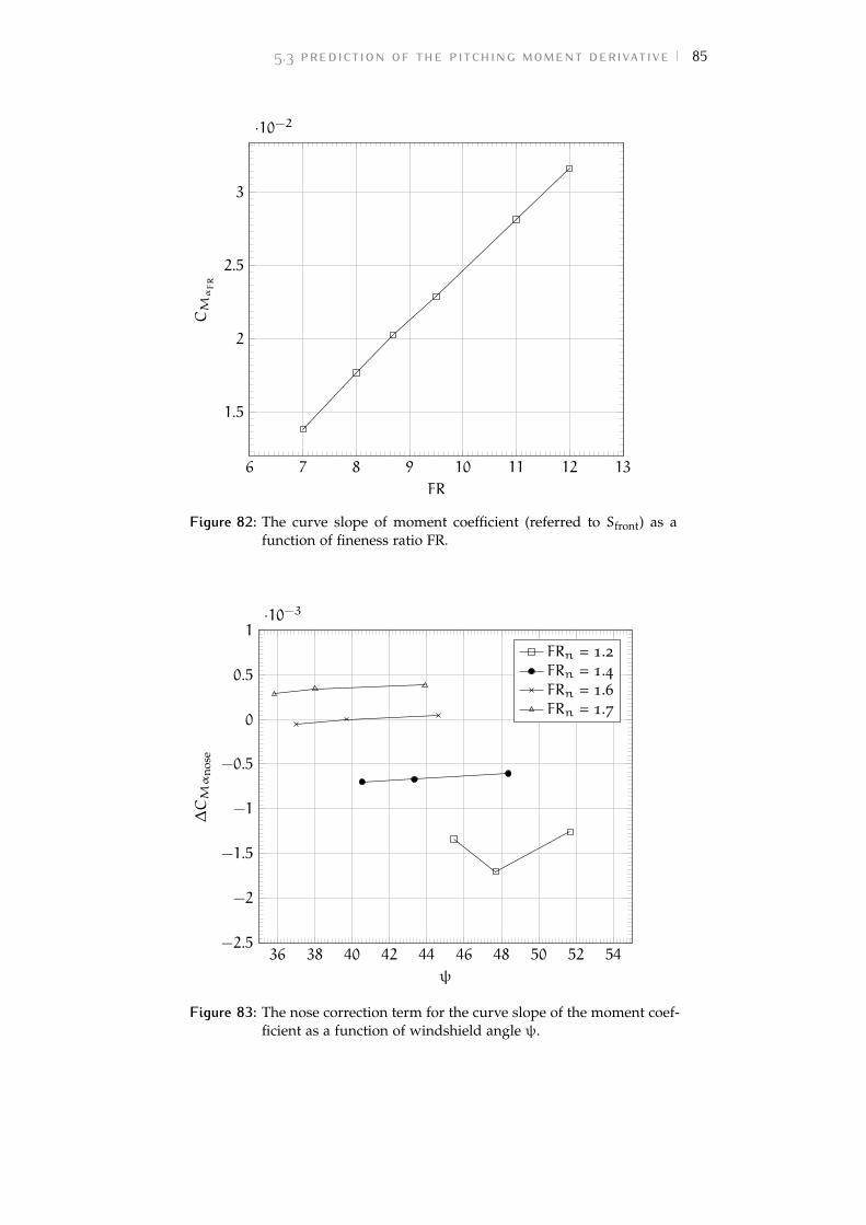
5.3 prediction of the pitching moment derivative 85
6 7 8 9 10 11 12 13
1.5
2
2.5
3
·10−2
FR
CMαFR
Figure 82: The curve slope of moment coefficient (referred to Sfront) as afunction of fineness ratio FR.
36 38 40 42 44 46 48 50 52 54−2.5
−2
−1.5
−1
−0.5
0
0.5
1·10−3
ψ
∆CMα
nose
FRn = 1.2FRn = 1.4FRn = 1.6FRn = 1.7
Figure 83: The nose correction term for the curve slope of the moment coef-ficient as a function of windshield angle ψ.
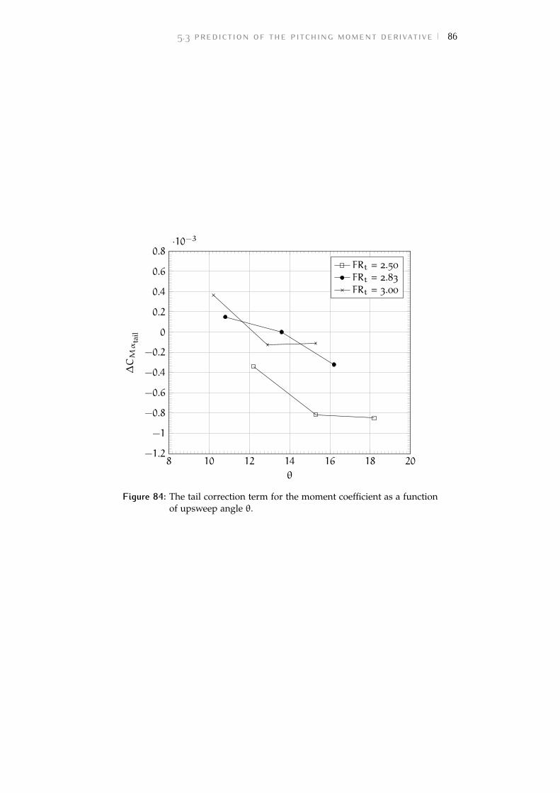
5.3 prediction of the pitching moment derivative 86
8 10 12 14 16 18 20−1.2
−1
−0.8
−0.6
−0.4
−0.2
0
0.2
0.4
0.6
0.8·10−3
θ
∆CMα
tail
FRt = 2.50
FRt = 2.83
FRt = 3.00
Figure 84: The tail correction term for the moment coefficient as a functionof upsweep angle θ.
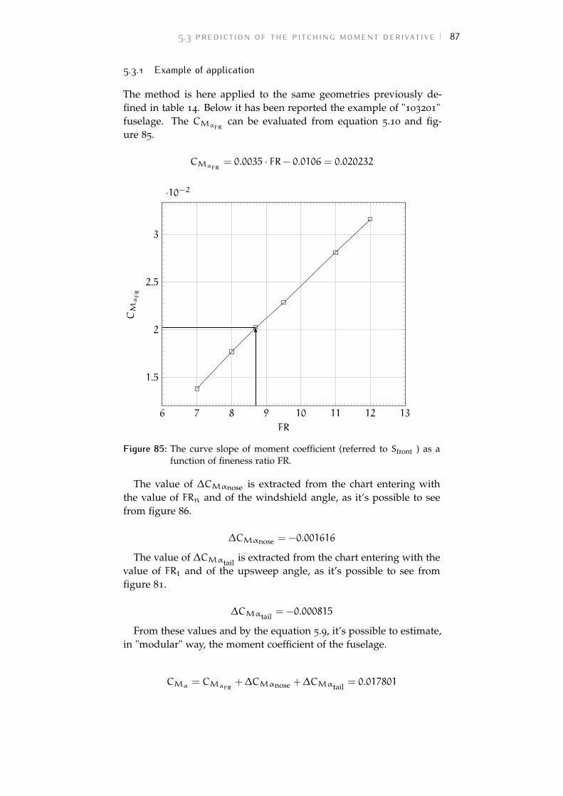
5.3 prediction of the pitching moment derivative 87
5.3.1 Example of application
The method is here applied to the same geometries previously de-fined in table 14. Below it has been reported the example of "103201"fuselage. The CMαFR
can be evaluated from equation 5.10 and fig-ure 85.
CMαFR= 0.0035 · FR− 0.0106 = 0.020232
6 7 8 9 10 11 12 13
1.5
2
2.5
3
·10−2
FR
CMαFR
Figure 85: The curve slope of moment coefficient (referred to Sfront ) as afunction of fineness ratio FR.
The value of ∆CMαnose is extracted from the chart entering withthe value of FRn and of the windshield angle, as it’s possible to seefrom figure 86.
∆CMαnose = −0.001616
The value of ∆CMαtail is extracted from the chart entering with thevalue of FRt and of the upsweep angle, as it’s possible to see fromfigure 81.
∆CMαtail = −0.000815
From these values and by the equation 5.9, it’s possible to estimate,in "modular" way, the moment coefficient of the fuselage.
CMα= CMαFR
+∆CMαnose +∆CMαtail = 0.017801
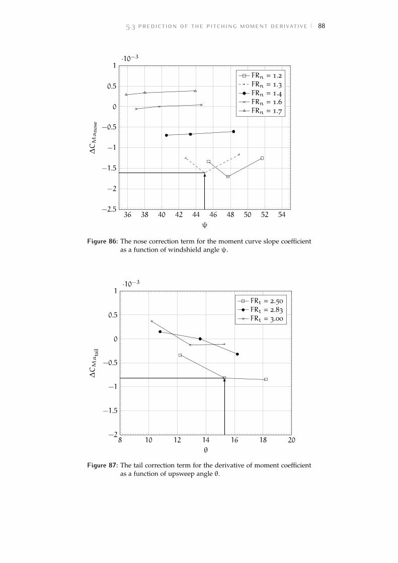
5.3 prediction of the pitching moment derivative 88
36 38 40 42 44 46 48 50 52 54−2.5
−2
−1.5
−1
−0.5
0
0.5
1·10−3
ψ
∆CMα
nose
FRn = 1.2FRn = 1.3FRn = 1.4FRn = 1.6FRn = 1.7
Figure 86: The nose correction term for the moment curve slope coefficientas a function of windshield angle ψ.
8 10 12 14 16 18 20−2
−1.5
−1
−0.5
0
0.5
1·10−3
θ
∆CMα
tail
FRt = 2.50
FRt = 2.83
FRt = 3.00
Figure 87: The tail correction term for the derivative of moment coefficientas a function of upsweep angle θ.
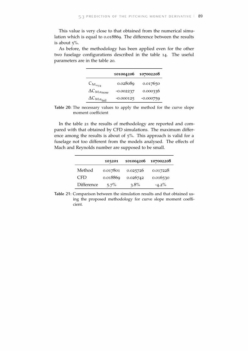
5.3 prediction of the pitching moment derivative 89
This value is very close to that obtained from the numerical simu-lation which is equal to 0.018869. The difference between the resultsis about 5%.
As before, the methodology has been applied even for the othertwo fuselage configurations described in the table 14. The usefulparameters are in the table 20.
101004206 107002208
CMαFR0.028089 0.017650
∆CMαnose -0.002237 0.000336
∆CMαtail -0.000125 -0.000759
Table 20: The necessary values to apply the method for the curve slopemoment coefficient
In the table 21 the results of methodology are reported and com-pared with that obtained by CFD simulations. The maximum differ-ence among the results is about of 5%. This approach is valid for afuselage not too different from the models analysed. The effects ofMach and Reynolds number are supposed to be small.
103201 101004206 107002208
Method 0.017801 0.025726 0.017228
CFD 0.018869 0.026742 0.016530
Difference 5.7% 3.8% -4.2%
Table 21: Comparison between the simulation results and that obtained us-ing the proposed methodology for curve slope moment coeffi-cient.
6 C O N C L U S I O N S
The goal of this work was to develop a new approach for the evalua-tion of aerodynamic characteristics of the fuselage of a generic turbo-prop transport aircraft. For this purpose the fuselage geometry hasbeen conceptually divided into three main components: nose, cabinand tailcone. It has been investigated the relationship between aero-dynamic coefficients and the main geometrical parameters.
Usually, in the preliminary design, the aerodynamic studies areconducted with semi-empirical methods, such as USAF DATCOM.To predict the drag coefficient, these methods consider the sum of dif-ferent contributions due to skin friction, upsweep angle, windshield(or canopy) and base drag. These contributions are estimated with re-sults based on wind-tunnel tests. Unfortunately, the latter are basedon geometries very different from a turboprop.
In order to overcome this issue, the aerodynamic studies have beenperformed with a numerical approach. The reference fuselage hasbeen drawn by a MATLAB script that allows to modify the finenessratio of each part of the fuselage (nose, cabin and tailcone), the wind-shield and/or the upsweep angle. For all modifications, the fuselagediameter is always constant. Therefore, to change the fineness ratioof the fuselage components, these are simply stretched (or shortened).This has been done by translating rigidly the sections along x axis. In-stead, in the case of windshield and upsweep angle modifications, thesections are translated along z axis in opportune way. Each param-eter is changed keeping the other constant. For instance, a changein fuselage slenderness ratio requires a stretch of the cabin, withoutchanging the shape of nose and tail. Conversely, a change in nose ortail shape does not alter the geometry of the other components. Theviscous (to allow for drag prediction), compressible (to include a highspeed cruise at altitude) simulations have been carried out using thecommercial software Star-CCM+ on the SCoPE grid infrastructure ofthe University of Naples Federico II.
The results of the numerical approach are presumably more suit-able for a preliminary design than those achieved with semi-empiricalmethods because they are based on an actual fuselage shape.
From numerical results a new methodology has been developed topredict the drag and pitching moment coefficient. As regard the drag,the methodology allows to compute the coefficient as the sum of thecontributions of each component (nose, cabin, and tailcone) since thehypothesis of the super-positioning of the effects has been verified.The effect of the geometry of each part on the drag coefficient is eval-
90
conclusions 91
uated with a shape factor which is function of fineness ratio of thepart and of windshield angle for the nose or of the upsweep anglefor the tailcone. The results are significant because there is a smalldifference between the results of numerical tests performed on differ-ent geometries and those obtained with the proposed methodology(about of 1%). As regard the moment, the methodology allows toestimate the value of the coefficient at angle of attack equal to 0° andthe moment curve slope coefficient. In this case the hypothesis of thesuper-positioning of the effects is not verified. The moment coeffi-cient is estimated as the sum of three contributions, one of which isthe moment coefficient for a given fineness ratio and the others twoare corrective terms due to the nose and the tailcone geometry. Asjust stated it’s valid both for the pitching moment coefficient and itsderivative. Also in this case the results are significant because thereis a difference between the results of numerical tests performed ondifferent geometries and those obtained with the methodology aboutof 1% for the moment coefficient and less than 6% for the momentcurve slope coefficient.
Thus, it is the author’s opinion that this work gives a new, simple,and reliable approach in the evaluation of the aerodynamic character-istics (drag, pitching moment and static longitudinal stability) of thefuselage of a generic regional turboprop transport airplane. Futureinvestigations may consider sideslip conditions and non-linearities inboth the longitudinal and directional stability curves.
A FA R R E L AT E D TO W I N D S H I E L D SA N D W I N D O W S
The Federal Aviation Regulations, or FARs, are rules prescribed bythe Federal Aviation Administration (FAA) governing all aviation ac-tivities in the United States.
A wide variety of activities are regulated, such as aircraft designand maintenance, typical airline flights, pilot training activities, hot-air ballooning, lighter-than-air aircraft, man-made structure heights,obstruction lighting and marking, and even model rocket launchesand model aircraft operation.
The rules are designed to promote safe aviation, protecting pilots,flight attendants, passengers and the general public from unnecessaryrisk. Since 1958, these rules have typically been referred to as FARsshort for Federal Aviation Regulations.
The FARs are organized into sections, called parts due to their or-ganization within the Code of Federal Regulations (CFR). Each partdeals with a specific type of activity.
The part relating to windshield is 25.775 and it is reported below.
FAR 25.775 Windshields and windows.
a. Internal panes must be made of nonsplintering material.
b. Windshield panes directly in front of the pilots in the normalconduct of their duties, and the supporting structures for thesepanes, must withstand, without penetration, the impact of afour-pound bird when the velocity of the airplane (relative tothe bird along the airplane’s flight path) is equal to the value ofVC, at sea level, selected under § 25.335(a).
c. Unless it can be shown by analysis or tests that the probabilityof occurrence of a critical windshield fragmentation conditionis of a low order, the airplane must have a means to minimizethe danger to the pilots from flying windshield fragments dueto bird impact. This must be shown for each transparent panein the cockpit that —
a) Appears in the front view of the airplane;
b) Is inclined 15 degrees or more to the longitudinal axis ofthe airplane; and
c) Has any part of the pane located where its fragmentationwill constitute a hazard to the pilots.
92
far related to windshields and windows 93
d. The design of windshields and windows in pressurized air-planes must be based on factors peculiar to high altitude oper-ation, including the effects of continuous and cyclic pressuriza-tion loadings, the inherent characteristics of the material used,and the effects of temperatures and temperature differentials.The windshield and window panels must be capable of with-standing the maximum cabin pressure differential loads com-bined with critical aerodynamic pressure and temperature ef-fects after any single failure in the installation or associated sys-tems. It may be assumed that, after a single failure that is ob-vious to the flight crew (established under §25.1523), the cabinpressure differential is reduced from the maximum, in accor-dance with appropriate operating limitations, to allow contin-ued safe flight of the airplane with a cabin pressure altitude ofnot more than 15,000 feet.
e. The windshield panels in front of the pilots must be arrangedso that, assuming the loss of vision through any one panel, oneor more panels remain available for use by a pilot seated at apilot station to permit continued safe flight and landing.
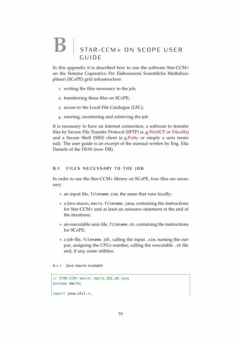
B S TA R - C C M + O N S C O P E U S E RG U I D E
In this appendix it is described how to run the software Star-CCM+on the Sistema Coperativo Per Elaborazioni Scientifiche Multidisci-plinari (SCoPE) grid infrastructure:
1. writing the files necessary to the job;
2. transferring these files on SCoPE;
3. access to the Local File Catalogue (LFC);
4. running, monitoring and retrieving the job.
It is necessary to have an internet connection, a software to transferfiles by Secure File Transfer Protocol (SFTP) (e. g.WinSCP or Filezilla)and a Secure Shell (SSH) client (e. g.Putty or simply a unix termi-nal). The user guide is an excerpt of the manual written by Eng. EliaDaniele of the DIAS (now DII).
b.1 files necessary to the job
In order to use the Star-CCM+ library on SCoPE, four files are neces-sary:
• an input file, filename.sim, the same that runs locally;
• a Java macro, macro_filename.java, containing the instructionsfor Star-CCM+ and at least an autosave statement at the end ofthe iterations;
• an executable unix file, filename.sh, containing the instructionsfor SCoPE;
• a job file, filename.jdl, calling the input .sim, naming the out-put, assigning the CPUs number, calling the executable .sh fileand, if any, some utilities.
b.1.1 Java macro example
// STAR-CCM+ macro: macro_102_a0.java
package macro;
import java.util.*;
94
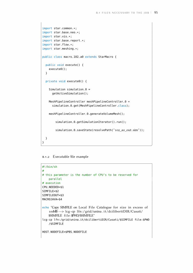
b.1 files necessary to the job 95
import star.common.*;
import star.base.neo.*;
import star.vis.*;
import star.base.report.*;
import star.flow.*;
import star.meshing.*;
public class macro_102_a0 extends StarMacro {
public void execute() {
execute0();
}
private void execute0() {
Simulation simulation_0 =
getActiveSimulation();
MeshPipelineController meshPipelineController_0 =
simulation_0.get(MeshPipelineController.class);
meshPipelineController_0.generateVolumeMesh();
simulation_0.getSimulationIterator().run();
simulation_0.saveState(resolvePath("102_a0_out .sim"));
}
} �b.1.2 Executable file example
#!/bin/sh
#
# this parameter is the number of CPU’s to be reserved for
parallel
# execution
CPU_NEEDED=$1
SIMFILE=$2
SIMFILEOUT=$3
MACROJAVA=$4
echo "Copy SIMFILE on Local File Catalogue for size in excess of100MB−−> lcg−cp lfn :/grid/unina . i t/dcilibertiDIR/Cusati/$SIMFILE f i l e :$PWD/$SIMFILE"
lcg-cp lfn:/grid/unina.it/dcilibertiDIR/Cusati/$SIMFILE file:$PWD
/$SIMFILE
HOST_NODEFILE=$PBS_NODEFILE
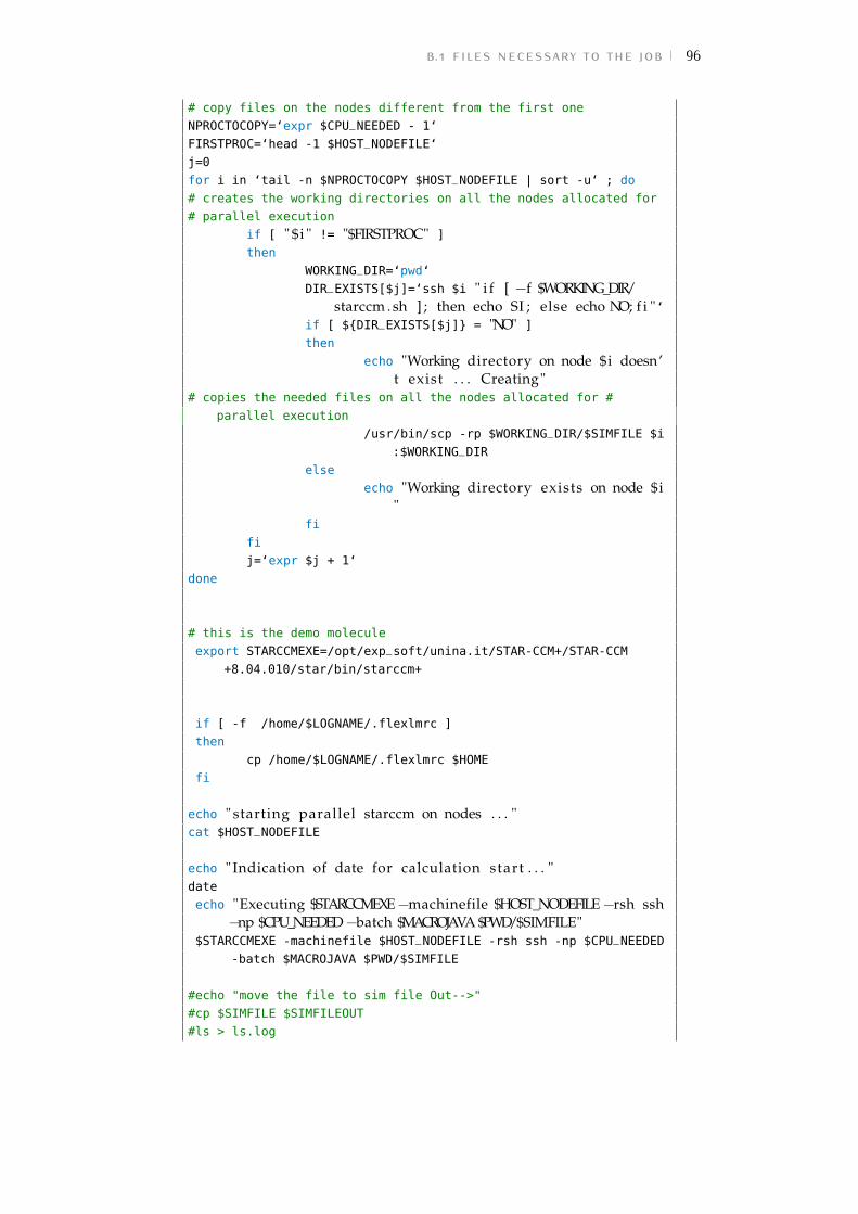
b.1 files necessary to the job 96
# copy files on the nodes different from the first one
NPROCTOCOPY=‘expr $CPU_NEEDED - 1‘
FIRSTPROC=‘head -1 $HOST_NODEFILE‘
j=0
for i in ‘tail -n $NPROCTOCOPY $HOST_NODEFILE | sort -u‘ ; do
# creates the working directories on all the nodes allocated for
# parallel execution
if [ " $i " != "$FIRSTPROC" ]
then
WORKING_DIR=‘pwd‘
DIR_EXISTS[$j]=‘ssh $i " i f [ −f $WORKING_DIR/starccm . sh ] ; then echo SI ; else echo NO; f i "‘
if [ ${DIR_EXISTS[$j]} = "NO" ]
then
echo "Working directory on node $i doesn’t exist . . . Creating"
# copies the needed files on all the nodes allocated for #
parallel execution
/usr/bin/scp -rp $WORKING_DIR/$SIMFILE $i
:$WORKING_DIR
else
echo "Working directory exists on node $i"
fi
fi
j=‘expr $j + 1‘
done
# this is the demo molecule
export STARCCMEXE=/opt/exp_soft/unina.it/STAR-CCM+/STAR-CCM
+8.04.010/star/bin/starccm+
if [ -f /home/$LOGNAME/.flexlmrc ]
then
cp /home/$LOGNAME/.flexlmrc $HOME
fi
echo " starting parallel starccm on nodes . . . "cat $HOST_NODEFILE
echo " Indication of date for calculation start . . . "date
echo "Executing $STARCCMEXE −machinefile $HOST_NODEFILE −rsh ssh−np $CPU_NEEDED −batch $MACROJAVA $PWD/$SIMFILE"
$STARCCMEXE -machinefile $HOST_NODEFILE -rsh ssh -np $CPU_NEEDED
-batch $MACROJAVA $PWD/$SIMFILE
#echo "move the file to sim file Out-->"
#cp $SIMFILE $SIMFILEOUT
#ls > ls.log
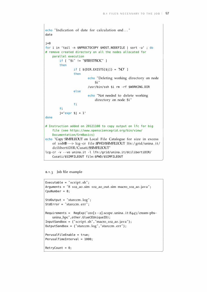
b.1 files necessary to the job 97
echo " Indication of date for calculation end . . . "date
j=0
for i in ‘tail -n $NPROCTOCOPY $HOST_NODEFILE | sort -u‘ ; do
# remove created directory on all the nodes allocated for
parallel execution
if [ " $i " != "$FIRSTPROC" ]
then
if [ ${DIR_EXISTS[$j]} = "NO" ]
then
echo "Deleting working directory on node$i "
/usr/bin/ssh $i rm -rf $WORKING_DIR
else
echo "Not needed to delete workingdirectory on node $i "
fi
fi
j=‘expr $j + 1‘
done
# Instruction added on 20121108 to copy output on lfc for big
file (see https://www.opensciencegrid.org/bin/view/
Documentation/SrmBasics)
echo "Copy SIMFILEOUT on Local File Catalogue for size in excessof 100MB−−> lcg−cr f i l e :$PWD/$SIMFILEOUT lfn :/grid/unina . i t/dcilibertiDIR/Cusati/$SIMFILEOUT"
lcg-cr -v --vo unina.it -l lfn:/grid/unina.it/dcilibertiDIR/
Cusati/$SIMFILEOUT file:$PWD/$SIMFILEOUT �b.1.3 Job file example
Executable = " script . sh";Arguments = "8 102_a0 . sim 102_a0_out .sim macro_102_a0 . java";CpuNumber = 8;
StdOutput = "starccm . log";StdError = "starccm . err ";
Requirements = RegExp("ce0[1−2].scope . unina . i t :8443/cream−pbs−unina_hpc",other.GlueCEUniqueID);
InputSandbox = {" script . sh","macro_102_a0 . java"};OutputSandbox = {"starccm . log","starccm . err "};
PerusalFileEnable = true;
PerusalTimeInterval = 1000;
RetryCount = 0; �
b.2 transferring files on scope 98
b.2 transferring files on scope
The previously mentioned files must be copied on the user’s personaldirectory on SCoPE. To do this, it is necessary a SFTP software asWinSCP, Filezilla or others, connecting to the address
ui01.scope.unina.it
with the credentials provided after the registration. More info areavailable on www.scope.unina.it.
b.3 copying the simulation file on the lfc
First of all, a SSH tunnel must be opened on ui01.scope.unina.it.This can be done with a unix terminal with the command
ssh -l username ui01.scope.unina.it
or by means of an emulator like Putty. Then it is mandatory to createa proxy before giving any command to the jobs, if more than 12 hourshave passed, typing
voms-proxy-init --voms unina.it
The Local File Catalogue is a space dedicated to simulation files big-ger than 100 MB. Every user has his own personal directory on theLFC (to not be confused with the local personal directory). If notexistent, it must be created with the command
lfc-mkdir /grid/unina.it/usernameDIR/folder
and then the filename.sim file can be copied on LFC with the state-ment
lcg-cr -v --vo unina.it file:/home/username/folders/filename.sim
-l lfn:/grid/unina.it/usernameDIR/folders/filename.sim
b.4 running, monitoring and retrieving thejob
From the user’s local folder where there are the previously discussedfiles, a job can be launched from the shell with the command
glite-wms-job-submit -a -o job_ID_filename.txt filename.jdl
that includes the registration of the job. Now any further commandfor that job will refer to its job identifier. For example, the job moni-toring is obtained giving
watch " glite−wms−job−status −i job_ID_filename . txt "
b.4 running, monitoring and retrieving the job 99
and the job status is updated every two seconds. However this tellsthe user only if the run is scheduled, running, completed, aborted orcleared. To get a log file, the same that will be obtained when the jobends, but incomplete for obvious reasons, the perusal option can beenable in the filename.jdl and giving the following commands
glite-wms-job-perusal --set -f starccm.log https://scopedma-ce.
scope.unina.it:9000/U51oobmOGTvXzMKP_pWGZw
to set the perusal and
glite-wms-job-perusal --get -f starccm.log https://scopedma-ce.
scope.unina.it:9000/U51oobmOGTvXzMKP_pWGZw
to get the partial log file. The last string of the command is an internalidentifier displayed on the shell once launched the job.
Once the job is completed, it can be get by typing
glite-wms-job-output -i job_ID_filename.txt
and retrieved from the temporary folder
/root/tmp/jobOutput
with the SFTP client.
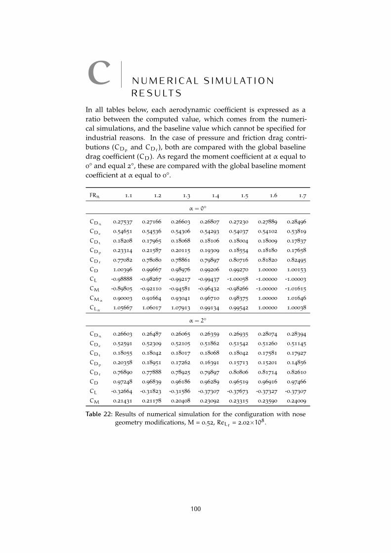
C N U M E R I C A L S I M U L AT I O NR E S U LT S
In all tables below, each aerodynamic coefficient is expressed as aratio between the computed value, which comes from the numeri-cal simulations, and the baseline value which cannot be specified forindustrial reasons. In the case of pressure and friction drag contri-butions (CDp and CDf), both are compared with the global baselinedrag coefficient (CD). As regard the moment coefficient at α equal to0° and equal 2°, these are compared with the global baseline momentcoefficient at α equal to 0°.
FRn 1.1 1.2 1.3 1.4 1.5 1.6 1.7
α = 0◦
CDn 0.27537 0.27166 0.26603 0.26807 0.27230 0.27889 0.28496
CDc 0.54651 0.54536 0.54306 0.54293 0.54037 0.54102 0.53819
CDt 0.18208 0.17965 0.18068 0.18106 0.18004 0.18009 0.17837
CDp 0.23314 0.21587 0.20115 0.19309 0.18554 0.18180 0.17658
CDf 0.77082 0.78080 0.78861 0.79897 0.80716 0.81820 0.82495
CD 1.00396 0.99667 0.98976 0.99206 0.99270 1.00000 1.00153
CL -0.98888 -0.98267 -0.99217 -0.99437 -1.00058 -1.00000 -1.00003
CM -0.89805 -0.92110 -0.94581 -0.96432 -0.98266 -1.00000 -1.01615
CMα0.90003 0.91664 0.93041 0.96710 0.98375 1.00000 1.01646
CLα 1.05667 1.06017 1.07913 0.99134 0.99542 1.00000 1.00038
α = 2◦
CDn 0.26603 0.26487 0.26065 0.26359 0.26935 0.28074 0.28394
CDc 0.52591 0.52309 0.52105 0.51862 0.51542 0.51260 0.51145
CDt 0.18055 0.18042 0.18017 0.18068 0.18042 0.17581 0.17927
CDp 0.20358 0.18951 0.17262 0.16391 0.15713 0.15201 0.14856
CDf 0.76890 0.77888 0.78925 0.79897 0.80806 0.81714 0.82610
CD 0.97248 0.96839 0.96186 0.96289 0.96519 0.96916 0.97466
CL -0.32664 -0.31823 -0.31586 -0.37307 -0.37673 -0.37327 -0.37307
CM 0.21431 0.21178 0.20408 0.23092 0.23315 0.23590 0.24009
Table 22: Results of numerical simulation for the configuration with nosegeometry modifications, M = 0.52, ReLf = 2.02×10⁸.
100
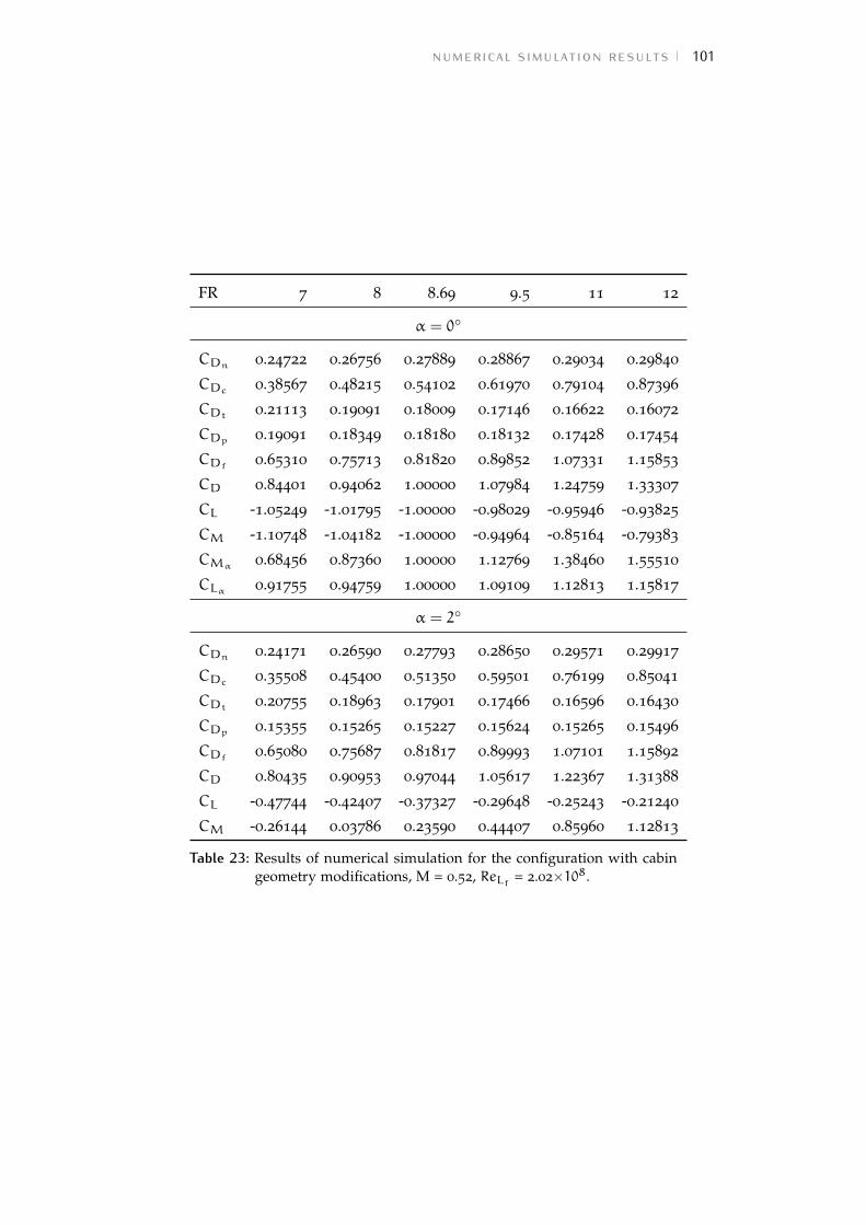
numerical simulation results 101
FR 7 8 8.69 9.5 11 12
α = 0◦
CDn 0.24722 0.26756 0.27889 0.28867 0.29034 0.29840
CDc 0.38567 0.48215 0.54102 0.61970 0.79104 0.87396
CDt 0.21113 0.19091 0.18009 0.17146 0.16622 0.16072
CDp 0.19091 0.18349 0.18180 0.18132 0.17428 0.17454
CDf 0.65310 0.75713 0.81820 0.89852 1.07331 1.15853
CD 0.84401 0.94062 1.00000 1.07984 1.24759 1.33307
CL -1.05249 -1.01795 -1.00000 -0.98029 -0.95946 -0.93825
CM -1.10748 -1.04182 -1.00000 -0.94964 -0.85164 -0.79383
CMα0.68456 0.87360 1.00000 1.12769 1.38460 1.55510
CLα 0.91755 0.94759 1.00000 1.09109 1.12813 1.15817
α = 2◦
CDn 0.24171 0.26590 0.27793 0.28650 0.29571 0.29917
CDc 0.35508 0.45400 0.51350 0.59501 0.76199 0.85041
CDt 0.20755 0.18963 0.17901 0.17466 0.16596 0.16430
CDp 0.15355 0.15265 0.15227 0.15624 0.15265 0.15496
CDf 0.65080 0.75687 0.81817 0.89993 1.07101 1.15892
CD 0.80435 0.90953 0.97044 1.05617 1.22367 1.31388
CL -0.47744 -0.42407 -0.37327 -0.29648 -0.25243 -0.21240
CM -0.26144 0.03786 0.23590 0.44407 0.85960 1.12813
Table 23: Results of numerical simulation for the configuration with cabingeometry modifications, M = 0.52, ReLf = 2.02×10⁸.
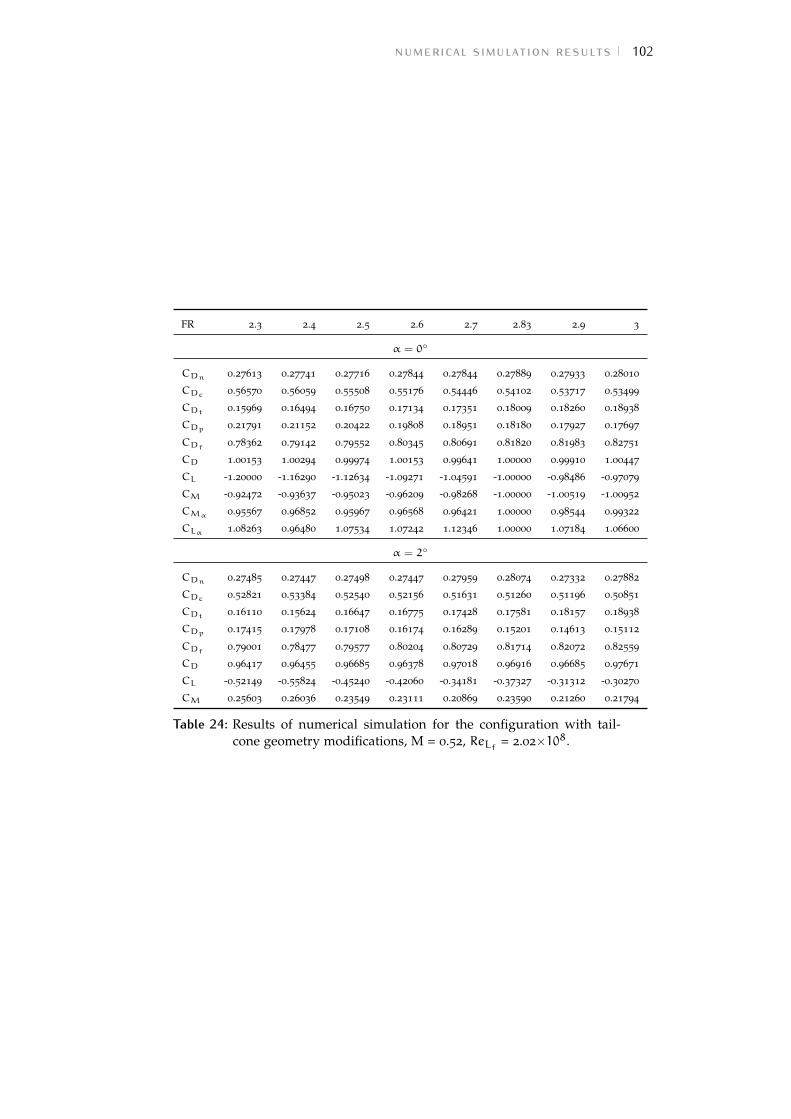
numerical simulation results 102
FR 2.3 2.4 2.5 2.6 2.7 2.83 2.9 3
α = 0◦
CDn 0.27613 0.27741 0.27716 0.27844 0.27844 0.27889 0.27933 0.28010
CDc 0.56570 0.56059 0.55508 0.55176 0.54446 0.54102 0.53717 0.53499
CDt 0.15969 0.16494 0.16750 0.17134 0.17351 0.18009 0.18260 0.18938
CDp 0.21791 0.21152 0.20422 0.19808 0.18951 0.18180 0.17927 0.17697
CDf 0.78362 0.79142 0.79552 0.80345 0.80691 0.81820 0.81983 0.82751
CD 1.00153 1.00294 0.99974 1.00153 0.99641 1.00000 0.99910 1.00447
CL -1.20000 -1.16290 -1.12634 -1.09271 -1.04591 -1.00000 -0.98486 -0.97079
CM -0.92472 -0.93637 -0.95023 -0.96209 -0.98268 -1.00000 -1.00519 -1.00952
CMα 0.95567 0.96852 0.95967 0.96568 0.96421 1.00000 0.98544 0.99322
CLα 1.08263 0.96480 1.07534 1.07242 1.12346 1.00000 1.07184 1.06600
α = 2◦
CDn 0.27485 0.27447 0.27498 0.27447 0.27959 0.28074 0.27332 0.27882
CDc 0.52821 0.53384 0.52540 0.52156 0.51631 0.51260 0.51196 0.50851
CDt 0.16110 0.15624 0.16647 0.16775 0.17428 0.17581 0.18157 0.18938
CDp 0.17415 0.17978 0.17108 0.16174 0.16289 0.15201 0.14613 0.15112
CDf 0.79001 0.78477 0.79577 0.80204 0.80729 0.81714 0.82072 0.82559
CD 0.96417 0.96455 0.96685 0.96378 0.97018 0.96916 0.96685 0.97671
CL -0.52149 -0.55824 -0.45240 -0.42060 -0.34181 -0.37327 -0.31312 -0.30270
CM 0.25603 0.26036 0.23549 0.23111 0.20869 0.23590 0.21260 0.21794
Table 24: Results of numerical simulation for the configuration with tail-cone geometry modifications, M = 0.52, ReLf = 2.02×10⁸.
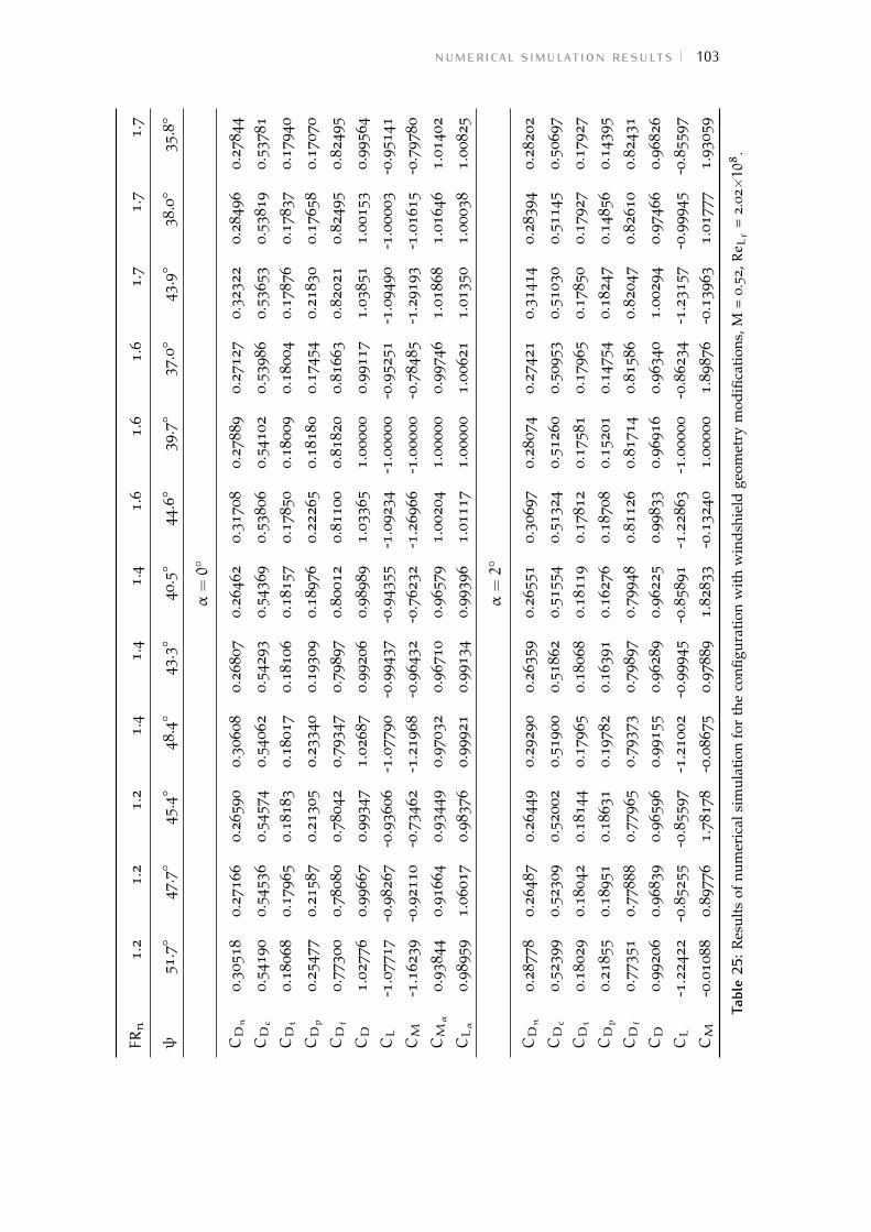
numerical simulation results 103
FRn
1.2
1.2
1.2
1.4
1.4
1.4
1.6
1.6
1.6
1.7
1.7
1.7
ψ51.7
°47.7
°45.4
°48.4
°43.3
°40.5
°44.6
°39
.7°
37.0
°43.9
°38.0
°35.8
°
α=0◦
CDn
0.3
0518
0.2
7166
0.2
6590
0.3
0608
0.2
6807
0.2
6462
0.3
1708
0.2
7889
0.2
7127
0.3
2322
0.2
8496
0.2
7844
CDc
0.5
4190
0.5
4536
0.5
4574
0.5
4062
0.5
4293
0.5
4369
0.5
3806
0.5
4102
0.5
3986
0.5
3653
0.5
3819
0.5
3781
CDt
0.1
8068
0.1
7965
0.1
8183
0.1
8017
0.1
8106
0.1
8157
0.1
7850
0.1
8009
0.1
8004
0.1
7876
0.1
7837
0.1
7940
CDp
0.2
5477
0.2
1587
0.2
1305
0.2
3340
0.1
9309
0.1
8976
0.2
2265
0.1
8180
0.1
7454
0.2
1830
0.1
7658
0.1
7070
CDf
0.7
7300
0.7
8080
0.7
8042
0.7
9347
0.7
9897
0.8
0012
0.8
1100
0.8
1820
0.8
1663
0.8
2021
0.8
2495
0.8
2495
CD
1.0
2776
0.9
9667
0.9
9347
1.0
2687
0.9
9206
0.9
8989
1.0
3365
1.0
0000
0.9
9117
1.0
3851
1.0
0153
0.9
9564
CL
-1.0
7717
-0.9
8267
-0.9
3606
-1.0
7790
-0.9
9437
-0.9
4355
-1.0
9234
-1.0
0000
-0.9
5251
-1.0
9490
-1.0
0003
-0.9
5141
CM
-1.1
6239
-0.9
2110
-0.7
3462
-1.2
1968
-0.9
6432
-0.7
6232
-1.2
6966
-1.0
0000
-0.7
8485
-1.2
9193
-1.0
1615
-0.7
9780
CMα
0.9
3844
0.9
1664
0.9
3449
0.9
7032
0.9
6710
0.9
6579
1.0
0204
1.0
0000
0.9
9746
1.0
1868
1.0
1646
1.0
1402
CLα
0.9
8959
1.0
6017
0.9
8376
0.9
9921
0.9
9134
0.9
9396
1.0
1117
1.0
0000
1.0
0621
1.0
1350
1.0
0038
1.0
0825
α=2◦
CDn
0.2
8778
0.2
6487
0.2
6449
0.2
9290
0.2
6359
0.2
6551
0.3
0697
0.2
8074
0.2
7421
0.3
1414
0.2
8394
0.2
8202
CDc
0.5
2399
0.5
2309
0.5
2002
0.5
1900
0.5
1862
0.5
1554
0.5
1324
0.5
1260
0.5
0953
0.5
1030
0.5
1145
0.5
0697
CDt
0.1
8029
0.1
8042
0.1
8144
0.1
7965
0.1
8068
0.1
8119
0.1
7812
0.1
7581
0.1
7965
0.1
7850
0.1
7927
0.1
7927
CDp
0.2
1855
0.1
8951
0.1
8631
0.1
9782
0.1
6391
0.1
6276
0.1
8708
0.1
5201
0.1
4754
0.1
8247
0.1
4856
0.1
4395
CDf
0.7
7351
0.7
7888
0.7
7965
0.7
9373
0.7
9897
0.7
9948
0.8
1126
0.8
1714
0.8
1586
0.8
2047
0.8
2610
0.8
2431
CD
0.9
9206
0.9
6839
0.9
6596
0.9
9155
0.9
6289
0.9
6225
0.9
9833
0.9
6916
0.9
6340
1.0
0294
0.9
7466
0.9
6826
CL
-1.2
2422
-0.8
5255
-0.8
5597
-1.2
1002
-0.9
9945
-0.8
5891
-1.2
2863
-1.0
0000
-0.8
6234
-1.2
3157
-0.9
9945
-0.8
5597
CM
-0.0
1088
0.8
9776
1.7
8178
-0.0
8675
0.9
7889
1.8
2833
-0.1
3240
1.0
0000
1.8
9876
-0.1
3963
1.0
1777
1.9
3059
Tabl
e25
:Res
ults
ofnu
mer
ical
sim
ulat
ion
for
the
confi
gura
tion
wit
hw
inds
hiel
dge
omet
rym
odifi
cati
ons,
M=
0.5
2,ReLf
=2
.02×108
.
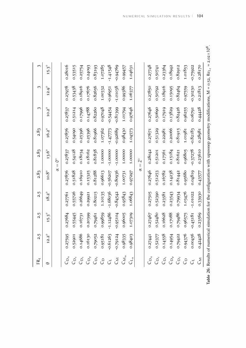
numerical simulation results 104
FRt
2.5
2.5
2.5
2.8
32.8
32.8
33
33
θ12.2
°15.3
°18.2
°10.8
°13.6
°16.2
°10.2
°12.9
°15.3
°
α=0◦
CDn
0.2
7595
0.2
7684
0.2
7761
0.2
7876
0.2
7837
0.2
7876
0.2
7837
0.2
7978
0.2
8016
CDc
0.5
2901
0.5
5445
0.5
5726
0.5
1828
0.5
4128
0.5
4090
0.5
1214
0.5
3438
0.5
3515
CDt
0.1
4686
0.1
6731
0.2
6649
0.1
6910
0.1
8034
0.2
5396
0.1
7996
0.1
8916
0.2
5754
CDp
0.1
6130
0.2
0399
0.2
9921
0.1
5325
0.1
8162
0.2
5396
0.1
4788
0.1
7676
0.2
4093
CDf
0.7
9052
0.7
9461
0.8
0215
0.8
1288
0.8
1838
0.8
1966
0.8
2260
0.8
2656
0.8
3193
CD
0.9
5181
0.9
9859
1.1
0135
0.9
6613
1.0
0000
1.0
7362
0.9
7048
1.0
0332
1.0
7285
CL
-0.6
1263
-1.1
2486
-1.6
8036
-0.5
6207
-1.0
0000
-1.4
7773
-0.5
4454
-0.9
6951
-1.4
1548
CM
-0.7
9124
-0.9
5104
-0.8
4542
-0.8
0936
-1.0
0000
-0.9
2689
-0.8
1399
-1.0
1038
-0.9
4769
CMα
0.9
8335
0.9
6005
0.9
5843
1.0
0731
1.0
0000
0.9
8430
1.0
1794
0.9
9386
0.9
9457
CLα
0.9
8403
1.0
7309
1.0
6843
0.9
7297
1.0
0000
1.0
4573
0.9
7646
1.0
6377
1.0
4631
α=2◦
CDn
0.2
7441
0.2
7467
0.2
7505
0.2
7646
0.2
8042
0.2
7671
0.2
7646
0.2
7850
0.2
7748
CDc
0.5
2377
0.5
2480
0.5
2390
0.5
1253
0.5
1201
0.5
1329
0.5
0690
0.5
0792
0.5
0741
CDt
0.1
4558
0.1
6628
0.2
3581
0.1
6782
0.1
7561
0.2
2981
0.1
7919
0.1
8916
0.2
3364
CDp
0.1
4954
0.1
7088
0.2
3543
0.1
4238
0.1
5184
0.2
0066
0.1
3829
0.1
5095
0.1
8942
CDf
0.7
9422
0.7
9486
0.7
9934
0.8
1442
0.8
1621
0.8
1915
0.8
2426
0.8
2464
0.8
2912
CD
0.9
4376
0.9
6575
1.0
3476
0.9
5680
0.9
6805
1.0
1981
0.9
6255
0.9
7559
1.0
1853
CL
0.0
0456
-0.4
5181
-1.0
1022
0.0
4819
-0.3
7278
-0.8
2183
0.0
6791
-0.3
0230
-0.7
5922
CM
0.4
2428
0.2
3569
0.3
3930
0.4
3577
0.2
3610
0.2
8981
0.4
4428
0.2
1813
0.2
8170
Tabl
e26
:Res
ults
ofnu
mer
ical
sim
ulat
ion
for
the
confi
gura
tion
wit
hup
swee
pge
omet
rym
odifi
cati
ons,
M=
0.5
2,ReLf
=2
.02×108
.
B I B L I O G R A P H Y
[1] I.H. Abbott, Fuselage drag tests in the variable density wind tunnel:streamline bodies of revolution, fineness ratio of 5, NACA tn 614,Washington, 1939.
[2] ATR, The ATR web site, 2014, URL http://www.atraircraft.
com.
[3] CFR, U.S. Government, 2014, URL http://ecfr.gov.
[4] D. Ciliberti, A new vertical tailplane design procedure throughCFD, Master thesis in Aerospace Engineering, Department ofAerospace Engineering, University of Naples Federico II, 2012
[5] P. Della Vecchia, Development of Methodologies for the AerodynamicDesign and Optimization of New Regional Turboprop Aircraft, PhDthesis in Aerospace Engineering, Department of Aerospace En-gineering, University of Naples Federico II, 2013
[6] E.C. Draley, High speed drag test of several fuselage shapes in combi-nation with a wing, NACA wr-l-542, Washington, 1947.
[7] R.R. Gilruth and M.D. White, Analysis and Prediction of Longitudi-nal Stability of Airplanes, NACA TR 711, 1941.
[8] P. Iaia, Verso horizon 2020: il ruolo di nuovi materiali e delletecnologie di manifattura per l’aerospazio:I Materiali e i ProcessiManifatturieri per il Nuovo Velivolo da Trasporto Regionale, associ-azione ARMA aeronautica, CESMA, 2012.
[9] Jane’s. All The World Aircrafts, 2004-2005, Edited by Paul Jackson,MRAeS.
[10] I. Kroo et al., Aircraft Design: Synthesis and Analysis, Stanford Uni-versity, January 2001. URL http://adg.stanford.edu/aa241/
AircraftDesign.html
[11] D.W. Levy, The CFD Drag Prediction Workshop Series: Summaryand Retrospective, Jameson, Roe, van Leer Symposium AIAA, SanDiego (CA), 22-23 June 2013
[12] MATLAB, Matlab R2010b User Guide, Mathworks, 2010
[13] L. Merola, The S.Co.P.E. Project, Università degli Studi di NapoliFederico II.
[14] H. Multhopp, Aerodynamics of the fuselage, NACA TM 1036, Wash-ington, 1942.
105
Bibliography 106
[15] M. Munk, The Aerodynamic forces on airship hulls, NACA TR 184,1924.
[16] F. Nicolosi and P. Della Vecchia, Aerodynamic guidelines in the de-sign and optimization of new regional turboprop aircraft, III CEASAir&Space Conference, XXI AIDAA Congress, Naples, 2011.
[17] C. D. Perkins and R. E. Hage, Airplane performance stability andcontrol., Wiley, New York, 1949.
[18] D. Raymer, Aircraft Design - A Conceptual Approach 2nd ed., 1992.
[19] J. Roskam, Airplane Design, University of Kansas, 1985.
[20] J. Roskam, Methods for estimating drag polars of subsonic airplanes,University of Kansas, 1971.
[21] Star-CCM, Star-CCM+ Version 8.04.007 User Guide, CD-adapco,2013
[22] SCoPE, Università degli Studi di Napoli Federico II, 2014, URLhttp://scope.unina.it.
[23] E. Torenbeek, Synthesis of subsonic airplane design, Delft UniversityPress, 1976.

colophon
This work was realized with LATEXusing arsclassica, a re- style of the ty-pographical look-and-feel classicthesis developed by André Miede.The style was inspired by Robert Bringhurst’s seminal book on typog-raphy “The Elements of Typographic Style”.Charts were generated with pgfplots and graphics were realizedwith TikZ.


![AdR11 lezione 02.ppt [modalità compatibilità] - unina.itwpage.unina.it/rtogna/AdR11_lezione_02.pdf · universita’ degli studi di napoli “federico ii” facolta’ di ingegneria](https://static.fdocumenti.com/doc/165x107/5bcccf8e09d3f2c65e8bafe3/adr11-lezione-02ppt-modalita-compatibilita-unina-universita-degli.jpg)