Università degli Studi di Bologna

Sessione II

Anno Accademico 2001 - 2002

FACOLTA DI SCIENZE MATEMATICHE, FISICHE E NATURALI Corso di Laurea in Informatica

SERVIZIO WEB PER GESTIONE ANAGRAFICA IN AMBITO SANITARIO

Tesi di Laurea di: Relatore: Alessandro Valenti Prof. Danilo Montesi

Correlatore:

Ing. Filippo Di Marco

2

Parole chiave: “Data Integration”, “Health Level 7”,

“Web Services”, “Microsoft .NET framework”

3

Index 1. INTRODUCTION........................................................................... 7 2 SCHEMA INTEGRATION.............................................................. 9

2.1 Introduction .......................................................................... 11 2.1.1 Multidatabase Architecture............................................ 11

2.2 The Schema Integration Problems....................................... 12 2.3 Some approach.................................................................... 14

2.3.1 Model-based Methods................................................... 14 2.3.2 Schema re-engineering/mapping .................................. 16 2.3.3 Metadata approaches ................................................... 17 2.3.4 Object-Oriented Method................................................ 18 2.3.4 Application-Level Integration......................................... 19 2.3.5 Artificial Intelligence Technique..................................... 20 2.3.6 Lexical Semantics ......................................................... 22

2.4 Formal Framework for Schema Transformation................... 25 2.4.1 Schemas Equivalences .................................................... 31

3 DATA INTEGRATION ................................................................. 35

3.1 Introduction .......................................................................... 35 3.2 The Data Integration Problems ............................................ 35 3.3 Models of Data Integration ................................................... 36

3.3.1 Introduction ................................................................... 36 3.3.2 Architecture................................................................... 36 3.3.3 “LOCAL AS VIEW (LAV)” Approaches.......................... 38 3.3.4 “GLOBAL AS VIEW (GAV)” Approaches ...................... 45 3.3.5 “BOTH AS VIEW (BAV)” Approaches ........................... 50

3.4 Data Quality Aspects............................................................ 55 3.4.1 Formalization of Data Quality in MDBS......................... 55 3.4.2 Basic Data Quality Aspects........................................... 56

3.5 Repository ............................................................................ 60

4

4 WEB SERVICES ......................................................................... 65 4.1 Introduction .......................................................................... 65 4.2 What are Web Services........................................................ 68

4.2.1 When to use Web Services........................................... 73 4.2.2 When not to use Web Services..................................... 74

4.3 The Web Service Stack Structure ........................................ 74 4.3.1 Universal Description Discovery Integration (UDDI)...... 76 4.3.2 The Web Service Description Language (WSDL) ......... 78

4.4 SOAP ................................................................................... 80 4.5 Microsoft Implementation “ASP.NET WS”............................ 82

4.5.1 Integration with Visual Studio .NET............................... 82 4.5.2 Security ASP.NET Web Services.................................. 83 4.5.3 Secured Socket Layer (SSL)......................................... 97 4.5.4 Performance ............................................................... 100

5 DATA ACCESS (ADO.NET)...................................................... 103

5.1 Introduction ........................................................................ 103 5.2 ADO.NET ........................................................................... 108

5.2.1 Data Provider .............................................................. 109 5.2.2 .NET Data Provider classes ........................................ 114

5.3 The DataSet ....................................................................... 118 5.3.1 The DataTable ............................................................ 120

5.4 Performance....................................................................... 123 5.4.1 Connection Pooling ..................................................... 123

6 HEALTH LEVEL 7 ..................................................................... 127

6.1 Introduction ........................................................................ 127 6.2 History ................................................................................ 129 6.3 Architecture ........................................................................ 130 6.4 Goals of HL7 ...................................................................... 140 6.5 A Complete Solution .......................................................... 143 6.6 Other Communication Protocols ........................................ 145

6.6.1 ASTM Medical Standard ............................................. 145 6.6.2 ACR-NEMA Standard ................................................. 146 6.6.2 Medical Information Bus Standard IEEE P1073.......... 147

5

6.6.3 Medical Data Interchange Standard IEEE P1157 ....... 148 6.6.4 Comparison of Medical Standards .............................. 149

7 IL SERVIZIO “ANAWEB”........................................................... 151

7.1 Introduzione ....................................................................... 151 7.1.1 Stato Attuale ............................................................... 151 7.1.2 Architettura.................................................................. 153

7.2 Uno schema comune ......................................................... 155 7.3 Modello adottato................................................................. 156 7.4 Configurazione del Servizio................................................ 159 7.5 Implementazione Query Processing .................................. 167

7.5.1 Gestione attributi complessi ........................................ 167 7.5.2 Gestione delle date ..................................................... 168 7.5.3 Gestione delle relazioni............................................... 170 7.5.4 Gestione campi astratti ............................................... 174

7.6 Implementazione Sincronizzazione Dati............................. 175 7.6.1 Sincronizzazione “On Demand” .................................. 176 7.6.2 Sincronizzazione “Schedulata”.................................... 178

7.7 Sicurezza ........................................................................... 179 7.8 Stato dell’Arte..................................................................... 186

7.8.1 Ricerca Semplice ........................................................ 187 7.8.1 Ricerca Avanzata ........................................................ 196

7.9 Lavori Futuri ....................................................................... 200 7.10 Conclusioni......................................................................... 201 7.11 Ringraziamenti ................................................................... 202

APPENDICE..................................................................................... 203

A MAPPING PER OLIVETTI ..................................................... 203 B ESEMPIO DI QUERY DESIGN SIMPLE OLIVETTI .............. 213 C ESEMPIO DI QUERY DESIGN ADVANCE OLIVETTI .......... 216 D STRUMENTI UTILIZZATI E REQUISITI MINIMI ................... 220

BIBLIOGRAFIA................................................................................. 221

6

7

1. INTRODUCTION One of the main problems for a Software House having the aim to operate in the sanitary field is the management of the patient’s identification. Sanitary information started at the beginning of years 80, when healthcare institutions begun to computerize their administration and management systems, this process happened in two different directions, one “horizontal“ and another one “vertical“. The horizontal computerization concerned the administrative management of the hospital, the informatization of GP doctors, the CUP and other generic aspects of medical computerized science. For the administrative management, it was and it is necessary to have a complete and continuously updated identification. The first companies having this type of application were, just to mention some of them, Olivetti®, Finsiel® and Siemens®, who supplied mainframes IBM™. At the same time there was a vertical computerization too, specialized units asked for specific software, such as the management of the analysis laboratories, the informatization of clinical records, the management of radiology departments and many other fields. Also these types of applications require an identification base that until today is not or only partly integrated with the administrative one in spite of that, for any application in sanitary field, it is essential to identify the patient and recover his personal data, this to have a correct running, such as the tax identification number, the date of birth, the sex or the residence. Of course the Software House, suppliers of "horizontal" application who have in charge the administrative process, do not give the possibility to modify the data existing in their registry office, making it as "closed”; they put at disposal of thirds parties their data as only read-mode views. This system obliges the companies who develop "vertical" applications to create their own independent database, which

8

in part repeats the data and in part integrates the available information. For the reason given above, the "vertical" applications strongly depend from the supplied data-structure and, as said previously, they are forced to create themselves and manage their own database; this situation has generated data replication and synchronization problems that can be solved usually just with a manual intervention. In the long run, the market asks for more integration among the various applications that often work with different databases; the minimal pre-qualification of this integration is that the applications must work using a common anagraphical data table. This registry office must be "open", that means supported by documentary evidence, accessible by various applications and with a fixed structure, it must operate as a common base for the present applications and mainly for the future applications, furthermore, it must be as much as possible, synchronized with the hospital correspondent tables and as much as possible coherent "Schema Integration", "Data Integration" and "Data Cleaning". In the clinical realities, where the direct connection to the anagraphical database does not exist, it is necessary to supply a system of "Repository" that allows the creation of a anagraphical database using heterogeneous “disconnected “ data sources, like for instance, from data sources stored on text files into a CD-ROM. Today computer science puts at disposal technologies, development’s instruments, architectures that allow us to easily make what that, years ago, was almost unthinkable, particularly allows the development of services which can be questioned by different applications using different languages and this through the network (both inner or outer network), called "Web Services" that make easy the management of the requested integration.

9

The coming of the Web and of a model of disconnected multi-levels architecture, has made possible, in a reliable and scalable way, the creation of a service for the management of this common anagraphical database. Thanks to the Eurosoft Informatica Medica® (http://www.eim.it) company leader of the field who has put at my disposal basic material for my search and Microsoft® of which Eurosoft Informatica Medica® is a Certified Partner, I am now able to introduce you the project I have realized. This project has involved many innovative aspects of the computer science, among them those already mentioned, "Data Integration", "Repository", using as platform for the development the new framework "Microsoft .NET", having a special attention to the connection to data sources "ADO.NET" and to the implementation of Microsoft of the "Web Services".

10

11

2 SCHEMA INTEGRATION

2.1 Introduction When I started, I found a reality where same data were organized in different ways by using very often different kinds of data which represented at last the same entity. The programmers was frequently obliged, due to the use of these databases, to adapt its source code to the data, by creating therefore different applications but having the same functions. Moreover, due to needs of integration among applications, people had the necessity to have a common registry office base that, as we will see later on, will be a “global view“ on the database given by the producers of “horizontal“ applications. A multidatabase system (MDBS) is a collection of database interconnected to share data. One of the major tasks in building a multidatabase is determining and integrating the data from the component database systems into a “coherent global view”.

2.1.1 Multidatabase Architecture A multidatabase is a collection of autonomous databases participating in a global federation that are capable of exchanging data. The basic multidatabase system (MDBS) architecture consist of a global transaction manager (GTM) which handles the execution of global transaction (GTs) and is responsible for dividing them into subtransactions (STs) for submission the local database system (LDBSs) participating in the MDBS. Each LDBS in the system has an

12

associated global transaction server (GTS) which converts the subtransactions issued by the GTM into a form usable by the local database system.

2.2 The Schema Integration Problems It is often hard to combine different database schemas because of different data models or structural differences in how the data is represented and stored. It is difficult to determine when two schemas represent the same data in different databases, even if they were developed under the same data model. The task of integrating these “views” is as difficult as integrating the knowledge of two humans. There are many factors which may cause schema diversity:

• Equivalence among constructs of the model, e.g., a designer uses an attribute in one schema and an entity in another

• Incompatible design specification, e.g., cardinality constraints, bad name choices

• Common concepts can be represented by different representations which may be identical, equivalent, compatible or incompatible

• Concept may be related by some semantic property which arises only by combining the schemas

There are several features of schema integration which make it difficult. The first problem is that data may be represented using different data models, for example, one database may use the relational model, while another database may use an object-oriented model. Even when two database use the same data model, both naming and structural conflicts may arise.

13

Naming conflict occurs when the same data is stored in multiple databases, but it is referred to by different names, this can introduce the following problems:

• The “homonym” problems, when the same name is used for two different concepts

• The “synonym” problems, when the same concepts is described using two or more different names.

As to me, these are the main problems I faced, problems arisen as I found myself working in a field really heterogeneous, where there are systems that use very different data-sources just to represent the same entity besides this, many problems caused by the “read-only mode view“ that I received, that in some way really gave me many dependence problems. Some common structural conflicts are:

• Type conflicts, using different model constructs to represent the same date

• Dependency conflicts, group of concepts related differently in different schemas, e.g., 1-to-1 participant versus 1-to-N participant

• Key conflicts, different keys for the same entity • Behavioural conflicts, different insertion/deletion policies for the

same entity

14

2.3 Some approach To solve the problems above, there would be some solutions, as follows:

• Model-based methods and heuristic algorithms, including relational, functional, semantic, and canonical models

• Schema re-engineering/mapping, using transformations to convert schemas

• Metadata approaches, adding data about the data and the schema

• Object-oriented methods, using object-oriented models as canonical models

• Application-level integration, no automatic integration technique, the applications are responsible for handling the integration themselves

• AI technique, using artificial intelligence to compare schemas and knowledge bases/ontology to store schema information

• Lexical semantics, expressing data/schema semantics in free-form language which is automatically compared during integration

2.2.1 Model-based Methods The earliest and most common methods of schema integration proposed were based on using semantic models to capture database information. Then, the semantic models were manipulated and interpreted, often with extensive user intervention, to perform the integration. In 1986, a survey of these model-based methods was performed. These methods attempted to define procedures and heuristic

15

algorithms for schema integration in the contexts of database view integration, i.e., producing a global view in one database and database integration, i.e., producing a global view from distributed databases. Their goal was to "produce an integrated schema starting from several application views that have been produced independently." Early pioneers in the integration area were quick to enumerate the potential difficulties in their task. They recognized the problems caused by different user perspectives, using different model constructs, and determining equivalent structures representing an identical concept. The method performed by most algorithms of the time relied on performing the following four steps:

• Pre-integration, analyzes schemas before integration to determine the integration technique, order of integration, and collect additional information

• Schema comparison, compares concepts and looks for conflicts and interschema properties

• Conforming the schemas, resolves schema conflicts • Merging and restructuring, merges and restructures the

schemas so they conform to certain criteria Early integration techniques could generally be classified in one of two schools: relational/functional models or semantic models:

• Relational Models, integrators made the universal relational assumption (every attribute in the database had a unique name) which allowed them to ignore naming conflicts

• Semantic Models, dealt more with conflicts and did not assume certain naming characteristics or design perspectives as in the relational models.

The ER-model is considered a semantic model. Another example of a semantic model is a semantic network which represents real-world

16

knowledge in a graph-like structure. Semantic models have rich techniques for representing data, but were tailored for human use in database design and not specifically for automated database integration.

2.2.2 Schema re-engineering/mapping A logical extension of the semantic modelling idea is schema re-engineering. In schema reengineering, schemas to be integrated are mapped into one canonical model or simply mapped into the same model. Then, the schemas are "compared" by performing semantic preserving transformations on them until the schemas are identical or similar in respect to common concepts. By automating the mapping process and providing a set of suitable transformations, the goal is to compare diverse schemas for similarities and merge them into one schema. Schema re-engineering and mapping methods yield good results when mapping from one model to another, and at the very least, provide techniques for mapping diverse schemas into the same model. Unfortunately, comparisons on schemas mapped to a canonical model are still not possible because of the many possible resulting schemas after the mapping has been completed. Furthermore, the set of equivalence preserving transformations defined is not sufficient to determine if two schemas in the same model are identical. Without the ability to define equivalence, mapping into the same data model does not solve the integration problem, but rather transforms it into the complicated, and no simpler, problem of determining schema equivalence. Schema re-engineering techniques suffer from the same problems as

17

the heuristic, semantic model algorithms on which they are based. Mapping between schema representation models is not a solution to the schema integration problem by itself. The models must map into a schema representation model which allows equivalence comparisons. Thus, these systems resolve no conflicts by themselves, but rather may transform diverse schemas into a single, more usable model. The transformation of schemas is automatic in nature, but no conflicts are resolved and no transparency is provided.

2.2.3 Metadata approaches Schemas specified in legacy systems are hard to integrate because there is no metadata describing the data’s use and semantics. Metadata approaches attempt to solve this problem by defining models which capture metadata. Then, the user or the system, can use schema metadata to simplify the integration task. Metadata is a set of rules on attributes. A rule captures the semantics of an attribute both at the schema level and the instance level. Then, an application could use these rules to determine schema equivalence. This approach is good because it captures some data semantics in the form of machine-processable rules. Unfortunately, the rules must be constructed by the system designer, and the actual integration of the rules must be performed at the application level. That is, the system designer constructs the integration rules, and the applications, using the global system, consult these rules at run-time to provide the necessary schema integration. Thus, applications are not isolated from changes in the semantics or organization of the data, which is the fundamental reason why applications use database systems. There are several other approaches which capture metadata in some manner. However, they all suffer from the fundamental problem of failing to use this captured metadata appropriately.

18

There has been no general solution for capturing metadata in a model such that it can be used to automatically integrate diverse schemas without application or user assistance. Metadata approaches are diverse in terms of the metadata content and the structure in which it is used. However, most systems typically represent metadata using logical rules which can then be used by the application at run-time to determine data equivalence. These rules can be arbitrarily complex and will often resolve most semantic conflicts. This also provides a limited form of transparency as the application is less responsible for the integration as it can use the previously defined integration rules. Metadata approaches based on rules are a combination of application-level integration with a little knowledge-base information added to ease the programming task.

2.3.4 Object-Oriented Method The object-oriented model has grown in popularity because of its simplicity in representing complicated concepts in an organized manner. Using encapsulation, methods, and inheritance, it is possible to define almost any type of data representation. Consequently, object-oriented models have been used not only to model the data, but also to model the data models. That is, object-oriented models have seen increased use as canonical models into which all other data models are transformed into and compared. The object-oriented model has very high expressiveness and is able to represent all common modelling techniques present in other data models. Hence, it is a natural choice for a canonical model. Although this work is a promising first step toward integration using an object-oriented model, the work is still missing a definition of equivalence. Without a definition of equivalence, it is impossible to integrate two schemas, regardless of the power of the schema

19

transformations. The ability to generate an OODBS schema from a high-level language is promising because it may be possible to define equivalence using the high-level language instead of at the schema level. This may eliminate some of the difficulties in defining schema equivalence. The use of an object-oriented model as a canonical model for integration is possible. However, the object-oriented model is very general which makes determining equivalence between schemas quite complex. Current techniques based on object-oriented models are in their infancy and tend to rely on heuristic algorithms similar to semantic models.

2.2.4 Application-Level Integration In application-level integration, applications are responsible for performing the integration. This eliminates the need to perform schema integration at the database level and gives the application more freedom when accessing different data resources. However, applications become more responsible for integration conflicts and no longer are hidden from the complexities of data organization and distribution. Although applications may be able to integrate different data sources easier in certain situations, the applications are no longer independent of data organization or format and become arbitrarily complex. Thus, although application-level integration may have benefits in certain situations, it is not a generally applicable methodology. A variation of application-level integration is integration at the language level. In these systems, applications are developed using a language which masks some of the complexities in the distributed MDBS

20

environment. Many of these systems are based on a form of SQL. The first step in constructing language-based integration systems is determining the types of conflicts that can arise. Typically, semantic conflicts are left to the application programmer to determine. Structural conflicts inherent in the data organization however are captured. How these conflicts are resolved by the language is very important in determining its usefulness. Thus, although the language provides facilities for an administrator to integrate MDBS data sources, the amount of manual work and lack of transparency and automation makes this method no more desirable than the early heuristic algorithms.

2.2.5 Artificial Intelligence Technique When two schemas with limited data semantics are combined, the problem contains both incomplete and inconsistent data. Thus it is natural that AI techniques have been applied to the integration problem with varying success. The major reasoning in AI techniques is that the fundamental database model is insufficient when dealing with diverse information sources. In the Pegasus project at HP, databases are combined into "spheres of knowledge". A sphere of knowledge is data, which may be spread across different databases, that is coherent, correct, and integrated. Thus, differences in data representation or data values only occur when accessing different spheres of knowledge. Another AI approach consists of storing data and knowledge in packets. A global thesaurus maintains a common dictionary of terms and actively works with the user to formulate queries. Each LDBS has its structural and operational semantics captured in an OO domain model and is considered a knowledge source. Users

21

access information in different LDBSs (knowledge sources) by posing a query to the global thesaurus. Query results are posted on a flexible, opportunistic, blackboard architecture from which all knowledge sources access, send and receive query information and results. This blackboard architecture shows promise because it also tackles the operational (transaction management) issue in MDBSs. The only difficulty with the system is the complexity of creating the system and defining how the global thesaurus cooperates with the user to formulate queries. A very good integration system based on a knowledge base was developed for the Carnot project. In this system, each component system is integrated into a global schema defined using the “Cyc knowledge base”. This knowledge base (global schema) contains 50,000 items including entities, relationship, and knowledge of data models. Thus, any information to be integrated into the global schema can either map to an existing entry in the knowledge base or be added to it. Resource integration is achieved by separate mappings between each information resource and the global schema. Since the system maps to a global schema, these mappings can be done individually and as needed. Each new resource is independently compared and integrated into the global schema. The system also uses schema knowledge (data structure, integrity constraints), resource knowledge (designer comments, support systems), and organization knowledge (corporate rules governing use of resource) during the integration process. The transparency of the system is high as it only requires the designer to map an information source to the global view once. An interesting contribution of the work is that the knowledge base is organized into 4 layers: concept layer, view layer, metadata layer, and the database layer. The authors correctly realize that integrating databases occurs at higher levels (conceptual view) than metadata and structural organizations. They then organize the knowledge base to capture and link information at all layers, which simplifies the integration task. Like other knowledge base approaches, the fundamental problem is

22

the imprecision in the knowledge base. Although common concepts are often well integrated by utilizing spanning sub-networks, this is not always guaranteed. Also, the resulting knowledge base does not provide a "unified" global view sufficient for SQL-type querying. Rather, it only supports imprecise queries or can be used as a tool for integrators to construct views over the data.

2.2.6 Lexical Semantics Lexical semantics is the study of the meanings of words. Lexical semantics is a very complicated area because much of human speech is ambiguous, open to interpretation, and dependent on context. Nevertheless, lexical semantics may have a role to play in schema integration. The metadata could be described in free-form language. Using these free-form language descriptions and a suitable lexical analysis tool, it may be possible to automate schema integration. It is our opinion that free-form lexical analysis is too complicated and immature field to be used in schema integration. This opinion is strengthened by the fact that no integration algorithms based on general lexical semantic techniques have been proposed. It is difficult enough to parse free-form language let alone determine its semantics and ambiguity. In the future, lexical semantics may ease the integration task, but further study is needed. However, the use of lexical semantics plays a prominent role in the Summary Schemas Model (SMM) proposed by Bright. The Summary Schemas Model is a combination of adding metadata and intelligent querying based on the semantic meanings of words. This system is not a general lexical semantics parser which takes a free-form description of a query and executes it. Rather, using user supplied words and a global dictionary, the system uses semantic metadata to translate the query into a suitable query for the underlying systems. The SSM provides automated support for identification of semantically similar

23

entities and processes imprecise user queries. It constructs an abstract view of the data using a hierarchy of summary schemas. Summary schemas at higher levels of the hierarchy are more abstract, while those at the leaf nodes represent more specific concepts. The target environment for the system is a MDBS language system which provides the integration. Thus, the SSM is more of a user interface method for dealing with diverse data sources than a method for integrating them. The actual integration is still performed at the MDBS language level. However, the SSM could be used on top of another integration algorithm as its support for imprecise queries is easily extendible. The heart of the SSM is linguistic knowledge stored in an online taxonomy. This taxonomy is a combination of a dictionary and a thesaurus. The authors used an existing taxonomy, the 1965 version of Roget’s thesaurus. The taxonomy contains an entry for each disambiguated definition of each form from a general lexicon of the English language. Each entry also has a precise definition and semantic links to related terms. Links include synonymy links (similar terms) and hpernymy/hyponymy links (related hierarchically). The semantic distance allows the system to translate user-specified words (imprecise terms) into actual database terms using the hierarchy of summary schemas. A leaf node in the hierarchy contains all the terms defined by a DBA for a local database. Local summary schemas are then combined and abstracted into higher-level summary schemas using hierarchal relationship between words. In total, this system allows the user to specify a query using their own key words, and the system translates the query into the best fit semantically from the information provided in summary schemas by every database in the MDBS. It is important to note that no schema integration is actually taking place. The summary schemas (even higher level ones) do not represent integrated schemas but rather an overview of the data in the underlying databases summarized into English-language categories and words. The user interface for the query processor can then translate user queries using the summary schemas from English words

24

provided by the user to database terms provided by the DBAs in the summary schemas. However, the use of a global taxonomy for words and user queries based on words and their meanings may have an important role in schema integration. Related to lexical semantics are integration techniques which construct semantic dictionaries or concept hierarchies to capture knowledge in databases. Similar to knowledge bases, semantic dictionaries and concept hierarchies allow database integrators to capture system knowledge and metadata in a more manageable form. Castano defined concept hierarchies from a set of conceptual (ER) schemas. The concept hierarchies are defined using either an integration based approach, where the integrator maps data sources to a pre-existing concept hierarchy, or using a discovery-based approach, where concept hierarchies can be incrementally defined one schema at a time by integrating with known concepts. The use of a concept hierarchy to define similar concepts is a useful idea. By also defining formulas to determine semantic distance between concepts in the hierarchy, it is possible to estimate semantic equivalence across systems. The authors also presented a mechanism for querying the MDBS based on the concept hierarchy and concept properties. Semantic distance calculations were used to evolve and create the hierarchy by adding new concepts or grouping concepts appropriately as they are integrated. The technique provides a good way of dynamically integrating data sources using ER descriptions. The major problem with this approach is that it does not produce a concept hierarchy which can easily be queried. The authors propose querying the MDBS for entities which are "similar" by virtue of having related structural and behavioural properties. Although this may be sufficient in some cases, the majority of industrial applications require more precise querying using a variant of SQL. Another problem with this approach is that constructing the concept hierarchy in a discovery based approach requires human intervention and decision making. The hierarchy may have been more useful if the structure and the behaviour of the concepts were removed, and it solely focused on

25

identifying similar concepts. In total, using a concept hierarchy to integrate databases is extremely useful insight, but the hierarchy constructed did not allow precises queries essential to most environments.

2.4 Formal Framework for Schema Transformation Conflicts may exist between the export schemas of the component databases, which must be removed by performing on the schema to produce equivalent schemas. In this framework for schema integration we use a variant of the ER model as the CDM, namely a binary ER model with subtypes. This model supports entity types with attributes, subtype relationship between entity types, and binary relationship (without attributes) between entity types. Subtype relationship give sufficient modelling expressiveness for representing object-oriented schemas. The main task of database integration are pre-integration, schema conforming, schema merging e schema restructuring. The last three of these tasks involve a process of schema transformation, and figures below illustrate some of the common transformation used. In practice, schema conforming transformations are applied bi-directionally and schema merging and restructuring ones uni-directionally.

26

Fig. 2.1 Schema Conforming Transformation

Fig. 2.2. Schema Merging Transformation

27

Fig. 2.3 Schema Restructuring Transformation

28

For each of these transformations, the original and resulting schema obey one or more alternate notions o schema equivalence This notion is basic concerning the schema integration and the first aim of this common framework is a rigorous definition of this meaning. Before giving a rigorous notion of the equivalence-concept of ER schemas, is basic that I illustrate other definitions:

1. A ER schema, S, is a quadruple , , ,Ents Incs Atts Assocs where: • Ents Names⊆ is the set of entity type names. • ( )Incs Ents Ents⊆ × , each pair 1 2,e e Incs∈

representing that 1e is a subtype of 2e . We assume that Incs is acyclic.

• Atts Names⊆ is a set of attribute names. • ( )Assocs Names Names Names Cards Cards⊆ × × × × is

the set of associations. For each relationship between two entity 1 2,e e Ents∈ , there is a tuple

1 2 1 2_ , , , ,rel name e e c c Assocs∈ , where 1c indicates the lower and the upper cardinalities of instances of 2e for each instance of 1e and 2c indicates the lower and upper cardinalities of instances of 1e for each instance of 2e . Similarly, for each attribute an associated with an entity type e there is a tuple 1 2, , , ,Null e a c c Assocs∈ , where

1c indicates the lower and upper cardinalities of a for each instance of e, and 2c indicates the lower and the upper cardinalities of instances of e for each value of a.

2. Given an ER schema , , ,S Ents Incs Atts Assocs= , let

{ }0 1 2 0 1 2 1 2, , | , , , ,Schemes n n n n n n c c Assocs= ∈ .

29

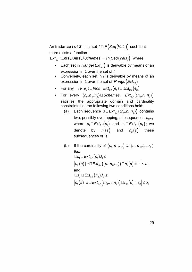
An instance I of S is a set ( )( )I P Seq Vals⊆ such that there exists a function

( )( ), :S IExt Ents Atts Schemes P Seq Vals→∪ ∪ where:

• Each set in ( ),S IRange Ext is derivable by means of an expression in L over the set of I

• Conversely, each set in I is derivable by means of an expression in L over the set of ( ),S IRange Ext

• For any 1 2,e e Incs∈ , ( ) ( ), 1 , 2S I S IExt e Ext e⊆

• For every 0 1 2, ,n n n Schemes∈ , ( ), 0 1 2, ,S IExt n n n satisfies the appropriate domain and cardinality constraints i.e. the following two conditions hold:

(a) Each sequence ( ), 0 1 2, ,S Is Ext n n n∈ contains two, possibly overlapping, subsequences 1 2,s s where ( )1 , 1S Is Ext n∈ and ( )2 , 2S Is Ext n∈ ; we denote by ( )1n s and ( )2n s these subsequences of s

(b) If the cardinality of 0 1 2, ,n n n is 1 1 2 2: , :l u l u

then( )

( ) ( ) ( )1 , 1 1

2 , 0 1 2 1 1 1

.

| , ,S I

S I

s Ext n l

n s s Ext n n n n s s u

∀ ∈ ≤

∈ ∧ = ≤

and( )

( ) ( ) ( )2 , 2 2

1 , 0 1 2 2 2 2

.

| , ,S I

S I

s Ext n l

n s s Ext n n n n s s u

∀ ∈ ≤

∈ ∧ = ≤

30

3. A model is a triple ,, , S IS I Ext where S is a schema, I is an instance of S and ,S IExt an extension mapping from S to I. We denote by Models the set of model. For any schema S, a model of S is a model which has S as its first component.

31

2.4.1 Schemas Equivalences Inst(S) denotes the set of instances of a schema S. A schema S subsumes a schema S’ if Inst(S’) ⊆ Inst(S). Two schemas S and S’ are equivalent if Inst(S’) = Inst(S)

Fig. 2.4 Two equivalent schemas The figure 2.4 illustrate two schemas S and S’. The schema S consisting of an entity “person” with an attribute “dept”, a database instance I consisting of three sets {john, jane, mary}, {compsci, math}

32

and { ⟨ john, compsci ⟩ , ⟨ jane, compsci ⟩ , ⟨ jane, math ⟩ , ⟨mary, math ⟩ } and the function Ext S,I defined as follow:

• ,S IExt (person) = {john, jane, mary} • ,S IExt (dept) = {compsci, maths} • ,S IExt ( ⟨Null, person, depth ⟩ ) = { ⟨ john, compsci ⟩ , ⟨ jane,

compsci ⟩ , ⟨ jane, math ⟩ , ⟨mary, maths ⟩ } The bottom half of figure 2.4 shows another schema S’ consisting of two entities “person” and “dept” and a relationship “works_in” between them. S’ subsumes S in the sense that any instance of S is also an instance of S’ . In particular, we can define Ext S’,I in terms of Ext S,I as follow:

• ',S IExt (person) = ,S IExt (person) • ',S IExt (dept) = ,S IExt (dept) • ',S IExt ( ⟨works_in, person, depth ⟩ ) = ,S IExt ( ⟨Null, person,

depth ⟩ ) By a similar argument, is easy to see that S subsumes S’, and so S and S’ are equivalent. We can generalise the definition of equivalence to incorporate a condition on the instances of one or both schemas. Inst(S, f) denotes the set of instances of a schema S that satisfy a given condition f. A schema S conditionally subsumes (c-subsumes) a schema S’ with respect to f if Inst(S’,f) ⊆ Inst(S,f). Two schemas S, S’ are conditionally equivalent (c-equivalent) with respect to f if Inst(S,f) = Inst(S’,f).

33

Fig. 2.5 Two c-equivalent schemas

The example on top illustrate two schemas S, S’. The schema S and the instance I are as in figure 2.4. The schema S’ now consists of three entities “person”, “mathematician”, “computer scientist”, with the last two being subtypes of the first. The instance I can be shown to be an instance of S’ only if the domain of the “dept” attribute consist of two values. In this case this is indeed so, the two values being compsci and maths and we can define ',S IExt in terms of ,S IExt as follows:

34

• ',S IExt (person) = ,S IExt (person) • ',S IExt (mathematician) = { x | ⟨ x, maths ⟩ ∈ ,S IExt ( ⟨Null, person,

dept ⟩ )} • ',S IExt (computer scientist) = { x | ⟨ x, compsci ⟩ ∈ ',S IExt ( ⟨Null,

person, dept ⟩ )}

Conversely, we con define ,S IExt in terms of ',S IExt as follows: • ,S IExt (person) = ',S IExt (person) • ,S IExt (dept) = {maths, compsci} • ,S IExt ⟨Null, person, dept ⟩ ) = { x | ⟨ x, maths ⟩ ∈ ,S IExt

(mathematician)} U { x | ⟨ x, compsci ⟩ ∈ ',S IExt (computer scientist)}

Thus S and S’ are c-equivalent with respect to the condition that | ,S IExt (dept)| = 2.

35

3 DATA INTEGRATION

3.1 Introduction Data integration is the process of combining data at the entity-level. After schema integration has been completed, a uniform global view has been constructed. However, it may be difficult to combine all the data instances in the combined schemas in a meaningful way. Combining the data instances is the focus of data integration.

3.2 The Data Integration Problems Data integration is difficult because similar data entities in different databases may not have the same key. For example, an employee may be uniquely identified by name in one database, and by social insurance number in another. Determining which employee instances in the two databases are the same is a complicated task if they do not share the same key. Entity identification is the process of determining the correspondence between object instances from more than one database. Combining data instances involves entity identification, i.e., determining which instances are the same, and resolving attribute value conflicts, i.e., two different attribute values for the same attribute. Common methods for determining entity equivalence include:

• key equivalence, assumes a common key • user specified equivalence, user performs matching • probabilistic key equivalence, only use portion of the key, may

make matching errors • probabilistic attribute equivalence, use all of the common

attributes

36

• heuristic rules, knowledge-based approach Data integration is further complicated because attribute values in different databases may disagree or be range values. The description of the date is a classic data-example with different range and different description, very often depending from the system shape this was, in my project, one of the main problems I dealt with.

3.3 Models of Data Integration

3.3.1 Introduction It's basic a search on this integration-model, to understand the reason of my implement choices. Furthermore I have chosen this system because, in the ambit of scientific field, it seemed to me like the most studied, documented, used and probed method of integration.

3.3.2 Architecture At the technological level this task required tools for cooperation and connectivity as ODBC, JDBC, CORBA, CGI, Servlet, ADO, etc. At the conceptual/design level this task is the union of these three parts:

37

• “Global View” represents the abstract entity, on which must be formulated and executed the Query

• “Wrappers” access the source and provide a view in a uniform data model of the data stored in the source.

• “Mediators” combine and reconcile multiple answers coming from wrappers and/or other mediators

In figure following we can see this architecture under a graphical profile.

Fig. 3.1 Data Integration Architecture

38

As we will see better later on, this is the structure when we have a real multidatabase system, with strongly heterogeneous data-sources. My service is easier compared with this reality, easier because the different sources are restricted, on my service there are basically two entities, one representing the client database, the other representing our standard database (see chapter 7.2.). Furthermore, my service same as it is organized, may be used as Backup Server when the customer Server is out of use. The first step of the application designer is to develop a “mediated schema”, often referred to as a “global schema”, that describes the data that exists in the sources, and exposes the aspects of this data that may be of interest to users. Note that the mediated schema does not necessarily contain all the relations and attributes modelled in each of the sources. Users pose queries in terms of the mediated schema, rather than directly in terms of the source schemas. As such, the mediated schema is a set of virtual relations, in the sense that they are not actually stored anywhere. The types of integration are two:

• Virtual integration, data remain at the sources • Materialized integration, data at the sources are replicated in

integration system, typical of Data Warehousing; in this approach, since data at sources change, the problem of refreshment is important

3.3.3 “LOCAL AS VIEW (LAV)” Approaches The integrated database is simply a set of structures (relation, in the relational model), one for each symbol in an alphabet GA .The structure of the global view is specified in the schema language GL over GA .

39

In LAV each source structure is modelled as a view over the global view, expressed in the “view language” VL over the alphabet GA where G represent the global view. For example, we have this Global View: movie(Title, Year, Director) european(Director) review(Title, Recension) and this data source: r1(Title, Year, Director) since 1960, european directors r2(Title, Recension) since 1990 and we want execute the query who returned title and critique of movies in 1998 mr(T, R) movie(T, 1998, D) /\ review(T, R) In LAV the relations at the sources are defined as views over the global view as follow: r1(T, Y, D) movie(T, Y, D) /\ european(D) /\ Y≥ 1960 r2(T, R) movie(T, Y, D) /\ review(T, R) /\ Y ≥ 1990 The mr(T, R) movie(T, 1998, D) /\ review(T, R) is processed by means of an inference mechanism aiming at re-express the atoms of the global view in terms of atoms at the sources. In this case:

mr(T, R) r1(T, 1998, D) /\ r2(T, R)

Note that in this case the resulting query is not equivalent to the original query. This model has the advantage of high modularity and re-usability, when source changes, only its definition is affected. Another

40

characteristic that distinguishes this from GAV, is that in LAV the relations between sources can be inferred. This model has the disadvantage of having a difficult process of query because query reformulation is executed on a run time. 3.3.3.1 Formal Framework In a data integration system I = ⟨G, S, M ⟩ based on the LAV approach, the mapping M associates to each element s of the source schema S a query Gq over G. In other words, the query language ,M SL allows only expressions constituted by one symbol of the alphabet SA . Therefore, a LAV mapping is a set of assertions, one for each element s of S, on the form

Gs q→ To better characterize each source with respect to the global schema, several authors have proposed more sophisticated assertions in the LAV mapping. In particular with the goal of establishing the assumption holding for the various source extension. Formally, this means that in the LAV mapping, a new specification, denoted as(s), is associated to each source element s. The specification as(s) determining how accurate is the knowledge on the data satisfying the sources, i.e., how accurate is the source with respect to the associated view Gq . Three possibilities have been considered, even if in some papers different assumptions on the domain of the database (open vs. closed) are also taken into account:

• Sound views. When a source s is sound (denoted with as(s) = sound), its extension provides any subset of the tuples

41

satisfying the corresponding view Gq . In other words, give a source database D, from the fact that a tuple is in Ds one can conclude that is satisfies the associated view over the global schema, while from the fact that a tuple is no in Ds one cannot conclude that it does not satisfy the corresponding view. Formally, when as(s)= sound, a database B satisfies the assertion Gs q→ with respect to D if Ds ⊆ B

Gq . Note that, from a logical point of view, a sound source s with arity n is modelled through the first order assertion ( ) ( )Gx s x q x∀ → where x denotes variables 1 nx x… .

• Complete views. When a source s is complete (denoted with as(s) = complete), its extension provider any superset of the tuples satisfying the corresponding view. In other words, from the fact that a tuple is in Ds one can conclude that such a tuple does not satisfy the view. On the other hand, from the fact that a tuple is not in Ds one can conclude that such a tuple does not satisfy the view. Formally, when as(s)= complete, a database B satisfies the assertion Gs q→ with respect to D if Ds ⊇ B

Gq . From a logical point of view, a complete source s with arity n is modelled through the first order assertion ( ) ( )Gx s x q x∀ ← .

• Exact views. When a source s is exact (denoted with as(s) =

exact), its extension is exactly the set of tuples of objects satisfying the corresponding view. Formally, when as(s) = exact, a database B satisfies the assertion Gs q→ with respect to D if

Ds = BGq . From a logical point of view, an exact source s with

arity n is modelled through the first order assertion ( ) ( )Gx s x q x∀ ↔ .

42

3.3.3.2 An example, “InfoMaster” Infomaster is an information system developed at the Center for Information Technology of Stanford University. Infomaster has been use since fall 1995 for searching housing rentals in the San Francisco Bay Area, and since 1996 for room scheduling at Stanford. In recent years, there has been a big growth in the number of publicly accessible databases on the Internet, and all indications suggest that this growth will continue in the years come. Access to this data presents several complications. The first complication is distribution. Not every query can be answered by the data in a single database. Useful relations may be broken into fragments that are distributed among distinct databases. Database researchers distinguish among two types of fragmentation; the rows of a database are split across multiple databases. A second complication in database integration is heterogeneity. This heterogeneity may be notational or conceptual. Notational heterogeneity concerns access language and protocol. One source is s Sybase database using SQL while another is an Informix database using SQL and third is an Object Store using OQL. Infomaster is an information integration tool that solves these problems. It provides integrated access to distributed, heterogeneous information sources, thus giving its users the desirable illusion of a centralized, homogeneous information system. Infomaster effectively creates a virtual data warehouse of its sources.

43

The figure below illustrates the architecture.

Fig. 3.2 InfoMaster Architecture There are wrappers for accessing information in a variety of sources. For SQL databases, there is a generic ODBC wrapper. There is also a wrapper for Z39.50 sources. For legacy source and structured information available through the WWW, a custom wrapper is used. Infomaster includes a WWW interface for access through browser such as Netscape’s. This user interface has two levels of access: an easy-to

44

use, forms-based interface, and an advanced interface that support arbitrary constraints applied to multiple information source. Infomaster has a programmatic interface called Magenta, which supports ACL (Agent Communication Language) access. Harmonizing n data sources with m uses does not require m x n sets of rules, or worse. By providing Infomaster whit a reference schema, we allow database users and provide to describe their schemas without regard for the schemas of other users and providers. This strategy is shown in the figure below.

Fig. 3.3 The Reference Schema

These translation rules are bidirectional whenever possible, so information stored in one source’s format may be accessed through another source’s format. Query processing in the Infomaster systems is a three-step process. Assume the user ask a query q. This query is expressed in terms of

45

interface relations. In a first step, query q is rewritten into a query in terms of base relations. We call this step reduction. In a second step, the descriptions of the site relations have to be used to translate the rewritten query in terms of site relations. The second step is called abduction. The query in terms of site relations is an executable query plan, because it only refers to data that is actually available from the information sources. However, the generated query plan might be inefficient. Using the description of the site relations, the query plan can be optimized. The figure below illustrate the three steps of Infomaster’s query planning process.

Fig. 3.4 Steps of Infomaster’s Query Planning Process

3.3.4 “GLOBAL AS VIEW (GAV)” Approaches In this approach each structure in the global view is modelled as a view over the source structures, expressed in the “view language” VL over the alphabet of the source structures SA .

46

To well understand the difference existing on the previous approach, I will show you now how the relations are declared by using the example proposed to define LAV, this time using GAV. The relations in the global view are views over the sources as follow: movie(T, Y, D) r1(T, Y, D) european(D) r1(T, Y, D) review(T, R) r2(T, R) The query mr(T, R) movie(T, 1998, D) /\ review(T, R) is processed by means of unfolding, i.e., by expanding the atoms according to their definitions, until we come up with source relation in this case: mr(T, R) r1(T, 1998, D) /\ r2(T, R) This model is a rigid model, i.e., whenever a source changes or a new one is added, the global view needs to be reconsidered, and it is necessary to understand the relationships among the sources, the query is reformulated at a design time. In this model the task of query process is typically easier. 3.3.4.1 Formal Framework In the GAV approach, the mapping M associates to each element g in G a query sq over S. In other words, the query language ,M GL allows only expressions constituted by one symbol of the alphabet GA . Therefore, a GAV mapping is a set of assertion, one for each element g of G of the form sg q→ . From the modelling point of view, the GAV approach is based on the idea that the content of each element g of the global schema should be characterized in terms f a view sq over the sources. In some sense,

47

the mapping explicitly tells the system how to retrieve the data when one wants to evaluate the various elements of the global schema. This idea is effective whenever the data integration system is based on a set of sources that is stable. Extending the system with a new source is now a problem: the new source may indeed have an impact on the definition of various elements of the global schema, whose associated views need to be redefined. To better characterize each element of the global schema with respect to the sources, more sophisticated assertions in the GAV mapping can be used, in the same spirit as we saw for LAV. Formally, this means that in the GAV mapping, a new specification, denoted as(g) (either sound, complete o exact) is associated to each element g of the global schema. When as(g) = sound (resp., complete, exact), a database B satisfies the assertion sg q→ with respect to a source database D if D

Sq ⊆ Bg (resp. ,D B D B

S Sq g q g⊇ = ). The logical characterization of sound vies and compete views in GAV in therefore through the first order assertion

( ) ( ) ( ) ( ),s sx q x g x x g x q x∀ → ∀ → respectively. It is interesting to observe that the implicit assumption in many GAV proposals is the one of exact views. Indeed, in a setting where all the views are exact, there are no constraints in the global schema, and a first order query language is used as ,M SL , a GAV data integration system enjoys what we can call the “single database property”, i.e., it is characterized by a single database, namely the global database that Is obtained by associating to each element the set of tuples computed by the corresponding view over the sources.

48

3.3.4.2 Un esempio, “TSIMMIS” TSIMMIS - The Stanford-IBM Manager of Multiple Information Sources is a system for integration information. It offers a data model and a common query language that are designed to support the combining of information from many different sources. This represents a typical example of integration system adopting GAV approach. The mediator architecture is one of several that have been proposed to deal with the problem of integration of heterogeneous information. Even as simple a concept as the employees of a single corporation may be represented in different ways by different information source. These sources are “heterogeneous” on many levels.

• Some may be DB relational, others not. Some may not be databases at all, but file system, the Web, or legacy systems.

• The types of data may vary; a salary could be stored as an integer or a character string.

• The underlying units may vary; salaries could be stored on a per-hour or per-month basis, for examples.

• The underling concepts may differ in subtle ways. A payroll database may not regard a retiree as an “employee”, while the benefits department does. Conversely, the payroll department may include consultants in the concept of “employee” while the benefits department does not.

Same as any other data-integration system, TSIMMIS too is composed essentially by three main entities: data-sources, mediator and wrapper. In the figure below is shown in details the architecture of this system:

49

Fig. 3.5 The Components of TSIMMIS

The principal components of TSIMMIS are suggested in fig. 3.5. We use:

• A “lightweight” object model called OEM (Object-Exchange Model) serves to convey information among components. It is “lightweight” because it does not require strong typing of its objects and is flexible in other ways that address desideratum above.

• Mediators are specified with a logic-based object-oriented language called “Mediator Specification Language (MSL)” that can be seen as a view definition language that is targeted to the OEM data model and the functionality needed for integrating heterogeneous sources.

• Wrappers are specified with “Wrapper Specification Language (WSL)” that is an extension to MSL to allow for the description of source contents and querying capabilities. Wrappers allow user queries to be converted into source-specific queries. We do not assume sources are databases, and it is an important goal of the project to cope with radically different information formats in a uniform way.

50

• A “common query language” links components. We are using MSL as both the query language and the specification language for mediators and as the query language for wrappers. The query language LOREL (“Lightweight Object REpostory Language”), an extension of OQL targeted to semistructured data, in oriented toward end user queries and is also the query language of the LORE lightweight database system use for storing OEM objects locally.

• Wrapper and Mediator Generators. We are developing methodologies for generating classes of wrappers and mediators automatically from simple descriptions of their functions.

3.3.5 “BOTH AS VIEW (BAV)” Approaches BAV is a new approach to data integration, which combine the previous approaches of local as view (LAV) and global as view (GAV) into a single method we term “both as view (BAV)”. This method is based on the use of reversible transformation sequences, and combine the respective advantages of GAV and LAV without their disadvantages. One important property of our approach is that it is possible to extract a definition of the global schema as a view over the local schemas, and it is also possible to extract definitions of the local schemas as views over the global schema.

51

3.3.5.1 Framework Formale The framework consists of a low-level hypergraph–based data model (HDM) and a se of primitive schema transformations defined for this model. Higher level data models and primitive schema transformations for them are defined in terms of this lower-level model. In this framework, schemas are incrementally transformed by applying to them a sequence of primitive transformation steps 1, nt t… . Each primitive it make a “delta” change to the scheme, adding, deleting or renaming just one schema construct. Each add or delete step is accompanied by a query specifying the extent of the new or deleted construct in term of the rest of the constructs in the schema. In this simple relational model, schemas are constructed from primary key attributes, non-primary key attributes, and the relationships between them, The underlying graph representation of a relation R with primary key attributes and other attributes is:

Fig. 3.6 Simple relational Model

The set of primitive transformations for schemas expressed in this data model is an follows:

• ( )1Re , , , ,nadd l R k k q… adds to the schema a new relation R

with primary key attribute(s) 1, , , 1nk k n ≥… . The query q

52

specifies the set of primary key values in the extent of R in terms of the already existing schema constructs.

• ( ), ,addAtt R a c q adds to the schema a non primary key attribute a for relation R. The parameter c can be either null or notnull. The query q specifies the extent of the binary relationship between the primary key attribute(s) of R and this new attribute a in terms of the already existing schema constructs.

• ( ), ,delAtt R a c q deletes from schema the non primary key attribute a of relation R. The query q specifies how the extent of the binary relationship between the primary key attribute(s) of R and a can be restored from the remaining schema constructs.

• ( )1Re , , , ,ndel l R k k q… deletes from the schema the relation

R with primary key attribute(s) 1, , nk k… . The query q specifies how the set of primary key values in the extent of R can be restored from the remaining schema constructs.

Each of above primitive transformation, t, has an automatically derivable reverse transformation, t , defined as follows:

: x yt S S→ : y xt S S→

( )( )( )

( )

1

1

Re , , , ,

, , ,

Re , , , ,

, , ,

n

n

add l R k k q

addAtt R a c q

del l R k k q

delAtt R a c q

…

…

( )( )

( )( )

1

1

Re , , , ,

, , ,

Re , , , ,

, , ,

n

n

del l R k k q

delAtt R a c q

add l R k k q

addAtt R a c q

…

…

53

This translation scheme can be applied to each of the constructs of a global schema in order to obtain the derivation of each construct from the set of local schemas; these derivations can then be substituted into any query over the global schema in order to obtain an equivalent query distributed over the local schemas, as n the GAV approach. 3.3.5.2 Un esempio, “AUTOMED” This type of approach is comparatively new as regards to the approaches like LAV and GAV and as to implementations of this system at the present time there is only the project AutoMed. Below we can see the architecture of this project.

Fig. 3.7 AutoMed Architecture

The “Model Definition Tool” allows users to define modelling constructs and primitive transformations of high-level modelling language in terms of those of the lower-level hypergraph data model (HDM). These definitions are stored in the Model Definitions Repository.

54

The Metadata Repository stores schemas of data sources, intermediate schemas, integrated schemas, and the transformation pathways between them. The Schema Transformation and Integration Tool allow the user to apply transformations from the Model Definitions Repository to schemas in the Meta Data Repository. This process creates new intermediate or integrated schemas to be stored in the Metadata Repository, together with the new transformation pathways. The Global Query Processor undertakes execution of global queries, in six main steps:

• Translates a global query over a global schema into the equivalent query expressed in an intermediate query language (IQL) and posed on the HDM representation of the global schema

• Occurrences of global schema constructs in the query are substituted by their definitions as views over local schema constructs

• The Global Query Optimizer is invoked to generate alternative query plans for the query, and select one for execution

• Sub-queries that are to be submitted to data sources are translated into the data model and query language supported by each data source, and submitted for execution

• The returned results are translated back into the IQL type system for any further necessary post-processing

• The query result is translated into the data model of the global schema

Finally, the Schema Evolution Tools allows the user to extend transformations pathways in the Meta Data Repository in order to reflect changes to source or integrated schemas. Query translation with respect to the modified schemas and modified transformation pathways occurs automatically.

55

3.4 Data Quality Aspects In the area of data quality management there has been not particular focus on integrated data or multidatabase systems in general. Most of the paragraph focuses on definition and measurements of data quality aspects in database and information systems.

3.4.1 Formalization of Data Quality in MDBS The quality of data stored at local databases participating in a multidatabase system typically cannot be described or modelled by using discrete values such as “good”, “poor” o “bad”. We suggest a specification of “time-varying” data quality assertion based on comparisons of semantically related classes and class extensions. In order to analyze and determine the conflicts or semantic proximity of two objects, object attributes or even complete classes, one needs to have some kinds of a reference point for comparisons. Such comparisons are based on virtual classes. A virtual class is a description of real world objects or artefacts that all have the same - not necessarily completely instantiated - attributes. The extension of a virtual class is assumed to be always up-to-date, complete and correct, i.e., only current real world objects and data are reflected in the extension of a virtual class. Given a description of real world objects in terms of a virtual class

virtC , local databases 1, , mDB DB… typically employ only a partial mapping of real world data into local data structures, i.e., only information relevant to local applications is mapped into local classes

1, , nC C… . More importantly, the mappings 1, , nα α… adopted by local

56

databases differ in the underlying local data structures (schemata) and how real world data is populated into these structures. Different mappings then result in schematic and semantic heterogeneities among the local classes 1, , nC C… that refer to the same virtual class

virtC . While a local class iC typically maps only a portion of the information associated with virtC , a global class conC integrates all aspects modelled in semantically equivalent or similar local classes.

Fig. 3.8 Relationship between virtual, conceptual and local classes

Determining conceptual classes as components of, e.g., a federated or multidatabase schema, is the main task in database integration. One main goal in database integration of the associated virtual class conC comes as near as possible to the specification of the associated virtual class virtC from which the local classes 1, , nC C… are derived.

3.4.2 Basic Data Quality Aspects A basic property of real world objects is that objects as instances of virtual classes evolve over time. Objects are added and deleted, or properties of objects change. At local sites different organizational activities are performed to map such time-varying information into local

57

classes, thus resulting in a type of heterogeneity among local databases we call operational heterogeneity. We consider operational heterogeneity as a non–uniformity in the frequency, processes, and techniques by which real world information is populated into local data structures. In such cases, operational heterogeneity can lead to the fact that similar data referring to same properties and attributes of real world objects have different quality and thus may have varying reliability. We first give a formal definition of time-varying data quality aspects we considers most important in database integration and resolving semantic data conflicts. For this we make the following simplified assumptions:

• There are two classes 1 1, , nC A A… and 2 1, , nC A A… from two local databases 1DB and 2DB . 1C and 2C refer to the same virtual class virtC and schema integration has been performed for 1C and 2C into the conceptual class 1, ,con nC A A… . We assume that the two classes are represented in the global data model.

• Using the predicate same it is possible to determine whether an object 1o for the extension of 1C , denoted by ( )1Ext C , refers to the same real world object ( )virto Ext C∈ as an object

( )2 2o Ext C∈ . In this model time is interpreted as a set of equally spaced time points, each time point t having a single success. The present point of time, which advances as time goes by, is denoted by nowt . The extension of a class C at time point t is denoted by ( ),Ext C t , the value of an object o for an attribute ( )A schema C∈ at time point t is denoted by ( ), ,CVal o A t . If no time point is explicitly specified, we

58

assume the point nowt . We furthermore assume a function ( ), ,CTime o A t that determines the time point 't t≤ the value A.o of

attribute A of object ( ),o Ext C t∈ was updated the last time before t. The above definitions and assumptions now provide us a suitable framework to define the data quality aspects timeliness, completeness, and accuracy in a formal way. 3.4.2.1 Timeliness Given two classes 1C and 2C with ( ) ( )1 2schema C schema C= . Class

1C is said to be up-to-date than 2C at time point nowt t≤ with respect to attribute ( )1A schema C∈ , denoted by 1 , 2

timeA tC C> , if

( ) ( ) ( ) ( ) ( ){ }( ) ( ) ( ) ( ) ( ){ }

1 1 1 2 2 1 2 1 2

2 1 1 2 2 1 2 2 1

| : , , : , : , , , , ,

| : , , : , : , , , , ,C C

C C

count o o Ext C t o Ext C t same o o time o A t time o A t

count o o Ext C t o Ext C t same o o time o A t time o A t

∧ > ≥

∧ > In other words, the class 1C is more up-to-date than 2C at time point t with respect to attribute A if its extension ( )1,Ext C t contains more recent updates on A then ( )2,Ext C t . 3.4.2.2 Completeness Class 1C is said to be more complete than the class 2C at time point

nowt t≤ , denoted by 1 2comptC C> , if

59

( ) ( ) ( ){ }( ) ( ) ( ){ }

1 1 1 1

2 2 2 2

| , ' , : , '

| , ' , : , 'virt

virt

count o o Ext C t o Ext C t same o o

count o o Ext C t o Ext C t same o o

∈ ∧ ¬ ∈ <

∈ ∧ ¬ ∈

In other words, although the extension of 2C may contain more objects at time point t, this does not necessarily mean that these objects still exist in the corresponding virtual class. 3.4.2.3 Data Accuracy This third data quality aspect, which is orthogonal to timeliness and completeness is the aspect of data accuracy which focuses on how well properties or attributes of real world objects are mapped into local classes. Given two classes 1C and 2C with ( ) ( )1 2schema C schema C= and attribute ( )1A schema C∈ . Class 1C is said to be more accurate than

2C with respect to A at time point t, denoted by 1 , 2accA tC C> , if

( ) ( ) ( ) ( )

( ) ( ) ( ) ( ) ( )

( ) ( ) ( ) ( )

( ) ( )

1 2

1

1 1 1 2 2 1 2

1 1 2

2 1 1 2 2 1 2

2 2

| , , , , , : ,

, , , , , , , , ,

| , , , , , : ,

, , ,

}{

{virt virt

virt

virt

C C C C

virt

C C

count o o Ext C t o Ext C t o Ext C t same o o

same o o Val o A t Val o A t Val o A t Val o A t

count o o Ext C t o Ext C t o Ext C t same o o

same o o Val o A t Val o

∈ ∈ ∈ ∧

∧ ≤

∈ ∈ ∈ ∧

∧

>

( ) ( ) ( )2 1, , , , , , }

virtC CA t Val o A t Val o A t≤

In the above definition − denotes a generic minus operator which is applicable to either a pair of strings, numbers or dates. In order to

60

suitably incorporate the aspect of possible null values, one can define a value maxa that is used if ( ), ,

iC iVal o A t is null. It is even possible to give a definition for data accuracy that takes only the number of objects into account that have the value null for the attribute A. The important point with the above definitions is that they describe orthogonal data quality aspects. That ism in case of data conflict among two objects referring to the same real world object, it is possible to choose either the most accurate or the most up-to-date data about this object, depending on whether respective specifications exist for the two objects.

3.5 Repository “A repository is a place to define, store, access, and manage all the information about an enterprise including its data, and its software systems”. It is not just a passive data dictionary or database. More than information storage, the repository, which is an integrated holding area, should also keep the information up to date by providing processing methods and make it available to a user as needed. A repository, which maintains valuable information about all of the information system assets of an organization and the relationships between them, acts as a central manager of all of the information resources in an enterprise. A repository should provide services such as change notification, modification tracking, version management, configuration management, and user authorization. Several standards have been developed for the repository marketplace. The Information Resource Dictionary System (IRDS) is a

61

standard that describes the requirements and architecture of a repository. The Case Data Interchange Format (CDIF) was initiated by the major CASE (Computer-Aided Software Engineering) vendors and developed as a formal way of transferring data between CASE tools. The Portable Common Tool Environment (PCTE) is a standard for a public tool interface for an open repository. The information technology constitutes logically coherent concepts and is always distributed over several different data sources, which may be from different organizations and are heterogeneous in nature. The widespread availability of XML-capable clients and their flexibility in structuring information make it possible for XML to become the universal data format. Without the help of a repository, it will be difficult to control XML objects in a manageable way and make them available when needed. “An XML repository is a special purpose repository that can manage XML objects in a native format allowing the developer to focus entirely on business logic, instead of database design and programming”. It should provide several basic functions such as importing/exporting XML data from original text files, user check in/check out, version control, as well as searching and querying on XML elements. In the electronic commerce world, XML repositories are the online source for obtaining the appropriate tag, document-type definition, data element, database schema, software code or routines. As a result, companies, especially small enterprises, can speed up processing and expand heir ability to conduct electronic commerce. One major problem is the integration of heterogeneous biological databases, and XML provides an exchange mechanism. XML/EDI (Electronic Data Interchange) developed by the XML/EDI Group represents a new framework for e-business data exchange. It is one of the most important applications of XML, which combines the semantics of EDI with XML. Documents in the XML format can be exchanged across different organizations according to those standards easily, so business and scientific processes can be synchronized from

62

application to application. The XML/EDI group also proposed a standard on public repository for XML message definition. A metadata repository consists of a set of software tools used for storage, search, retrieval, use and management of metadata. The components of a repository system include:

• metadatabase and metadata management system • extensible metamodel and modelling tools, • tools for populating the metadatabase • integrating the metadata • accessing the metadata

The repository includes of metadata and a DBMS to manage it. The repository DBMS provides standard database management facilities, such as persistent storage, data models, keys, certain types of quires, constraints and rules, transactions, data integrity and views, and also provides additional features for dealing with the specific requirements of metadata. Metadata-specific features include built-in complex relationship, navigation, support for long-running transactions, versioning and configuration management. The repository DBMS is a logical system that may be physically instantiated as a single or distributed database. A repository system provides a meta-metamodel describing the things the repository need to know about metadata (e.g., item types, attributes, relationship), and tool for building metamodels to include application-specific metadata description. A repository product usually provides modelling languages and other tools to facilitate creation and modification of these metamodels. The metadata stored in a repository will come from a variety of source, so a repository provides tool for populating the metadatabase with a tool for extracting metadata fro these sources. Some types of metadata sources do not provide an explicit representation of the metadata, so tools may be provided to extract information from each type of source

63

and generate metadata for the repository. For example, description of a legacy file system might be extracted from COBOL code. Repositories support sharing metadata among different components or tools by providing the ability to define global models and integrated views of metadata from heterogeneous systems. Views can be defined to allow access to any item in a metadata repository by any application or user regardless of the originating source’s platform, language, application system, etc. For example, a repository could provide single view of metadata from existing DB2 files on a mainframe database, from old COBOL copybooks, and from a newly designed data model based on CASE tool run on a UNIX system using C++. In addition, model definitions can be used to specify association among repository elements that indicate semantic similarities among elements from heterogeneous sources. A repository product also includes tools to facilitate easy access to metadata and customization of the repository. These typically include a user interface (GUI) , often a Web interface for accessing metadata or Web tools for building such an interface, and ASPs and/or programming language for accessing metadata management functions and building additional, application specific functionality.

64

65

4 WEB SERVICES

4.1 Introduction Distributed computing in the partitioning of application logic into units that are physically distributed among two or more computers in a network. The idea of distributed computing has been around a long time and numerous communication technologies have been developed to allow the distribution and reuse of application logic. There are many reasons for distributing application logic:

• Distributed computing makes it possible to link different organizations and organizational units.

• Often the data accessed by the application is on a different machine. The application logic should be close to the data.

• Distributed application logic may be reused in several applications. Pieces of a distributed application may be upgraded without upgrading the whole application.

• By distributing the application logic, the load is spread out to different machines, giving potentially better performance.

• As new needs arise, application logic may be redistributed or reconnected.

• It is easier to scale one layer than a whole application. If for example the data layer isn’t fast

• Enough, more resources can be added to this layer without affecting the entire application.

The Internet has increased the importance and applicability of distributed computing. The simplicity and ubiquity of the Internet makes it a logical choice as the backbone for distributed applications. The dominant protocols in component-based distributed computing are CORBA (Common Object Request Broker Architecture) from the

66

Object Management Group and Microsoft’s DCOM (Distributed Component Object Model). Although CORBA and DCOM have a lot in common, they differ in the details, making it hard to get the protocols to interoperate. The following table summarizes some similarities and differences between CORBA, DCOM, and Web Services and introduces a slew of acronyms. Characteristic CORBA DCOM Web Services Remote Procedure

Call (RPC)

Internet Inter-ORB Protocol (IIOP)

Distributed Computing

Environment (DCE-RPC)

Hyper Text Transfer Protocol

(HTTP)

Encoding Common Data Representation

(CDR)

Network Data Representation

(NDR)

Extensible Markup Language (XML)

Interface Descriptor

Interface Definition Language (IDL)

Interface Definition Language (IDL)

Web Service Description

Language (WSDL) Discovery Naming service

and trading service Registry Universal

Discovery Description

Language (UDDI) Firewall friendly No No Yes Complexity of

protocols High High Low

Cross-platform Partly No Yes Both CORBA and DCOM allow the invocation of remote objects, CORBA uses a protocol called Internet Inter-ORB Protocol (IIOP); DCOM uses a variation on OSF’s (Open Software Foundation) DCE-RPC. The encoding of data in CORBA is based on a format named Common Data Representation (CDR). In DCOM, the encoding of data is base on a similar but incompatible format named Network Data Representation (NDR).

67

DCOM is often described as “COM with a longer wire”. In the code, a developer does not need to do anything special to invoke a remote object. The code to call a remote object is the same as the code to invoke a local object. This is known as location transparency. This is accomplished by using surrogate objects on both the client and on the server. On the client side the surrogate is called a proxy. The proxy has the same interface as the real object. On the server side, there is a surrogate for the client called a stub. The proxy in CORBA is confusingly called a stub and the stub is called a skeleton. Every object has one or more interfaces and is only callable on an interface. To use an interface a description of it is needed. As shown in the table, both COM and CORBA use ad Interface Definition Language (IDL) to describe the interface. COM and CORBA use different IDLs but they are very similar. The IDL serves as a contract between the server and its clients. IDL is independent of the programming languages used to implement the client and the server. One thing to note about DCOM is that it is connection-oriented. The DCOM client holds on to a connection to the DCOM server. While holding the connection the client may make multiple calls to the DCOM server. The connection-oriented nature of DCOM gives a lot of flexibility; the server may hold state on behalf of the client: it may call back to the client, raise events to notify the client and so on. However, there are technical issues with this, the client may hold on to reference and only make calls when, for example, the user hits a button. For large periods of time, he server is idle waiting for requests from the client. What happens if the client crashes and will never use the server again? Alternatively, imagine an Internet scenario where the DCOM or CORBA server is used by thousands of clients. Since each client has a connection to the server, valuable server resources may be reserved for a client that seldom uses the server or even none longer exists. Although DCOM has ways to deal with these problems, it all adds up to a great deal of complexity. Which is one of the problem Web Services attempts to solve. Let’s now look closer at some of the benefits of Web Services.

68

When writing COM to COM, DCOM was the best solution. When writing .NET to .NET try Remoting. Remoting provides a feature-rich API for an application distributed cross AppDomains, processes or machines. Essentially, it allows the assign of objects fro one system to another, so that “remote” methods calls are performed as though the logic was on the calling system. Although Remoting does allow for SOAP calls like Web Services provide, use of the TCP channel significantly speeds up the process to almost five times as fast. Remoting is designed for communications at the DLL level, and should be used that way.

4.2 What are Web Services A Web Service is application logic accessible to programs via standard web protocols in a platform-independent way. From a technological perspective, Web Services to solve some problem faced when using tightly-coupled technologies such as CORBA and DCOM. These are problem such as getting through firewalls, the complexities of the protocols, and integrating heterogeneous platforms. Web Services are also interesting from an organizational and economic perspective, as they open up doors for new ways of doing business and dealing with organization issues. DCOM and CORBA are fine for building enterprise applications with software running on the same platform and in the same closely administered local network. They are not fine, however, for building

69

applications that span platform, span the Internet and need to achieve Internet scalability; they were simply not designed for this purpose. This in where Web Services come in. Web Services represent the next logical step in the evolution of component-based distributed technologies. Some key features are that:

• Web Services are loosely coupled to the clients. A client makes a request to a Web Service, the Web Service returns the result and the connection is closed. There is no permanent connection, and none of the complexity mentioned above. The Web Service may extend its interface: add new methods and parameters without affecting the clients, as long as it sill services to the old methods and parameters.

• Web Services are stateless: they do not hold on to state on behalf of the client. This makes it easy to scale up and out to many client and use a server farm to serve the Web Services. The underlying HTTP protocol used by Web Services is also stateless. It is possible to achieve some state handling with Web Services the same way it is possible on the Web today using techniques such as cookies.

Many of the concepts from DCOM and CORBA have their offspring in Web Services. That is not surprising since they try to solve the same problem: how to make calls to remote objects.

• The foundation of Web Services is SOAP, the Simple Object Access Protocol. SOAP is much simpler to implement than DCOM and CORBA. DCOM is Microsoft-specific, CORBA is used by many other vendors. SOAP is based on open Internet protocols such as HTTP and bridges the gap between Microsoft and the rest.

• For serialization DCOM and CORBA are based on complex formats. The serialization format for Web Services is based on XML, schema specification, XML, is simple, extensible, and readable, and XML, has already wide acceptance and adoption.

70

• Where DCOM and CORBA use IDL, to describe interfaces, Web Services use the Web Service Description Language, WSDL. WSDL is more flexible and is richer than IDL.

Returning on the first definition we can define the parts of Web Services:

• Application logic – a Web Service exposes some application logic or code. This code can do calculations, if can do database look-ups, anything a computer program can do.

• Accessible to programs – whereas most web sites today are accessed by humans suing a web browser, Web Services will be accessed by computer programs.

• Standard web protocols –the whole concept of Web Services is based on a set of standard web protocols such as HTTP, XML, SOAP, WSD and UDDI.

• Platform independent – Web Services can be implemented on any platform. The standard protocols are not proprietary to a single vendor, and are supported by all major vendors.

A Web Service is accessed by a program. The program may be a web application, a Windows application, or any type of application as indicated in the figure below:

71

Fig. 4.1 Communications among Web Services by SOAP The application may use internal Web Services within the organization or external Web Services provided by partners or as general building block services. A Web Service may also be used by other Web Services. A key factor to the success of Web Services is that to implement Web Services and Web Service infrastructure one can leverage a lot of what is already in place and working on the Internet. One of the design principles behind SOAP has been to avoid inventing a new technology. In an Internet scenario there is a Firewall who are designed to prohibit unauthorized traffic between computers within its control and computers outside its control. When computers communicate with

72

Internet through the firewall, traffic for specific functions travel on designated ports. These ports allow the firewall to restrict traffic to designated protocols, since it can assume that the computers within its control will react in expected ways to that traffic. Traffic for the World Wide Web travels via HTTP on port 80, or 443 if encrypted. In order for a computer to surf the web, firewall between it and the Internet must allow port 80 and 443 traffic. There are the ports, and the protocol, that Web Services use. Therefore, all of this functionally flows conveniently through your corporate firewall, without compromising the security of the rest of the system. Other distributes network architecture like DCOM, CORBA, and RMI use custom ports for their information transfer, often encountering firewall-enforced roadblocks. Here is a list of some key infrastructure and technologies that can be reused when implementing Web Services.

• Web servers – web servers are not required to implement a Web Service but a Web Service can be implemented entirely using existing web servers. For instance, without the .NET Framework, you can implement a Web Service using an XML parser and an ASP script running on IIS. The omnipresence of web servers means that Web Services can be installed everywhere.

• Authentication – a Web Service may need to authenticate the client before using the Web Service. The same mechanisms used for web pages may also be used here, including client certificates, basic authentication, digest authentication and NTLM authentication.

• Encryption – Web Services will often send and receive sensitive business data. Sensitive data exchanged with a Web Service requires encryption. Encryption can be done the same way as for regular web traffic. The Secure Sockets Layer protocol (SSL) may also be used with Web Services.

• Load balancing techniques – since Web Services are stateless, the same load balancing techniques used to load balance web pages may be used to load balance Web

73

Services. Web Services make load balancing a lot easier than using for instance the Component Load Balancing features of Application Center 2000.

• Application servers – Web Services need many of the same services as traditional components behind the scenes: transactional services, object pooling, connection pooling etc. By hosting the Web Services in a component container (COM+/EJB) you can leverage these services from the application server.

If the Web Services standard has tried to implement new technology to handle all these things, they would have ended up on the graveyard alongside large efforts such as the Open System Interconnect (OSI) model and CORBA.

4.2.1 When to use Web Services There are three principal situation in which use Web Service: Internets, Extranets and Intranets.

• Web Services are useful for connecting to information on the Internet that is blocked off by a local or remote firewall, or both.

• Web Services allow you to expose specific portions of your business logic to customers or partners via your extranet.

• Web Service makes an acceptable distributed architecture to share logic between disparate system in the same room, building or organization.

74

4.2.2 When not to use Web Services On the other hand there are times when it doesn’t pay to use Web Services:

• there are some overhead and performance considerations. • there are few existing security models. • there are better ways to solve some of the problems that Web

Services can solve. Web Services aren’t to replace things so much as add a new dimension to interoperability. This is a very fine line, but if it seems that Web Services are missing something intrinsic to be useful, then you are probably trying to use them inappropriately.

4.3 The Web Service Stack Structure The key to the success of Web Services in that they are based on open standards and that major vendors such as Microsoft, IBM, and Sun are behind these standards. Still, open standards do not automatically lead to interoperability. First of all, the standards must be implemented by the vendors. Furthermore they must implement the standards in a compatible way. Telecommunications depend heavily on standards and interoperability. The way this is handled in the telecom industry is by cooperation and interoperability testing, interoperability events where developers come together are commonplace in the telecom industry. We are seeing cooperation also in the Web Service space. There seems to be a lot of commitment in the industry to get Web Services to interoperate. There is a group for implementers of SOAP at

75

http://groups.yahoo.com/group/soapbuilders. They have established suites and interoperability events. Without this commitment to interoperability, Web Services will end up as another technology that failed. There are several specifications that are used when building Web Services. The figure below shows the “Web Services Stack” as it exists today:

Fig. 4.2 Web Service Stack It should be noted that the figure shows a conceptual layering, not a physical. Although there is agreement on several of these specifications, most of them are not all standardized yet. We will see changes in the specifications as they move forward within the standardization process.

76

4.3.1 Universal Description Discovery Integration (UDDI) Universal Description, Discovery, and Integration (UDDI) is a cross-industry initiative to create a global registry of Web Services. UDDI is actually (at least) three things:

• A central registry of Web Services. • Specifications of the structure of the registry, and

specifications of the APIs to access the registry. • An organization, http://www.uddi.org

The specifications are maintained by the UDDI organization. They have not yet been submitted to a standardization organization, but that is the said intention. As a Web Service developer, you can publish your Web Services to the UDDI registry and search for other Web Services in it. The central registry is operated by several companies. Currently Microsoft and IBM host UDDI registries. These registries are synchronized, so if you publish your Web Service in the IBM directory it will also be available in Microsoft directory. To publish or find information in UDDI you can use a web browse to one of the directories. You can also publish and find information programmatically using SOAP. The UDDI API specification describes che SOAP messages to be used when accessing a UDDI registry. By exposing the UDDI directory through SOAP you can find Web Services at runtime in your application. UDDI is that if you have a central repository that all organization can collaborate in populating, it act in a similar way to how a phone book operates, in that we can find and locate organizations either in our area or in a specific category that we interested in.

77

Fig. 4.3 UDDI Registry

The figure on top show the UDDI registry and the structure for publish Web Service. The UDDI registry is not solely run by Microsoft. IBM and Ariba are also controlling repositories for UDDI. This means that if we post information with one, then it’s replicated on all databases help by those companies. Each of the independent repositories have the same interface to give any outside organization or individual the opportunity to post information to UDDI using the UDDI Publish Web Service and search UDDI using UDDI Inquire Web Service. The following are the Web Service server end-point for each of the three holding organizations; this end-point is purely for UDDI inquires only. The publishing end-point will be alternate server locations and usually require HTTPS secure transmission:

• Microsoft inquiry server (http://uddi.microsoft.com/inquire)

• IBM inquiry server (http://www-3.ibm.com/services/uddi/inquiryapi)

78

• Ariba inquiry server (http://uddi.ariba.com/UDDIProcessor.aw/ad/process)

The UDDI Web Service has a SOAP interface, which can be used to send messages to a SOAP server to search or edit the UDDI registry. It also has a WSDL schema definition that defines this Web Service. The UDDI WSDL Schema definition is split into two distinct files:

• Searching (locating business and Web Services) (http://www.uddi.org/wsdl/inquire_v1.wsdl)

• Publishing (adding, updating and removing) (http://www.uddi.org/wsdl/publish_v2.wsdl)

4.3.2 The Web Service Description Language (WSDL) To call Web Services you invoke methods on the service. To do this you need to know what methods it supports, what parameters the Web Service takes, and what it returns. When building applications, you typically read Help files. Lately, I have also become addicted to IntelliSense, in the same way that I can non longer live without a spell checker. IntelliSense relies on the ability to resolve method calls at code time. To use a Web Service, you need a description of that service. You could read a Word document or a Help file documenting the interface and implement according to this document. If you use late-binding techniques you can call the Web Service without any programmatic description or IntelliSense. To be able to use early binding and IntelliSense, the Web Service description must be read by a tool. A Word document or a Help file is not very useful to tools. A structured standardized description format is needed. Structured descriptions can be consumed by tools and used to generate proxy code. When you

79

have a proxy, you can use early binding to the proxy and get full support for IntelliSense. DCOM and CORBA use IDL to describe the interfaces of components. IDL is not suited for Web Services because Web Services need an XML-based description WSDL. The Web Service Description Language (WSDL) defines an XML grammar form describing network services as collections of communications endpoints capable of exchanging messages. Ariba, IBM, and Microsoft have submitted the Web Service Description Language (WSDL) to the W3C. WSDL, replaces earlier specifications such as NASSL from IBM and SCL/SDL from Microsoft. From the specification (http://www.w3.org/TR/WSDL/): The WSDL document is a schema describing a Web Service:

• The WSDL document describes the methods the Web Service understands, including the parameters and the response. The data types of the parameters are defined. This makes it possible for tools such as Visual Studio .NET to generate a strongly-typed proxy.

• The WSDL document describes the protocols supported by the Web Service (SOAP, HTTP-GET, and HTTP-POST).

• The WSDL document specifies the address of the Web Service.

80

4.4 SOAP Simple Object Access Protocol (SOAP) is a protocol that allows not only for remote method invocations in distributed environments, but it also allows for the transfer of rich and complex data types as well as messaging of arbitrary payloads. The first sentence of the specification available from the W3C site at http://www.w3.org/TR/SOAP/ defines what SOAP in: The beauty of SOAP is its simplicity; it does not try to build a complete new infrastructure. As on example, consider the security of Web Services. Security is obviously an important issue, but SOAP does not address it. Instead, it specifies a binding to HTTP and leverages the security mechanism available with HTTP. The SOAP specification is 33 pages including references and appendixes. It is significantly larger than the XML-roc protocol, nut it is still fairly short and simple. The XML-RPC specification is very simple and in only six printed pages long. The following is from the specification available from UserLand Software, Inc. at http://www.xmirpc.com: The XML-RPC specification describes:

- How to encode scalar data types such as integers, strings, Booleans and floating-point numbers.

- How to encode arrays and structs. - How to handle errors. A binding to HTTP

XML-RPC has the advantage of being simpler than SOAP and there are many implementations of XML-RPC available. However, all the major vendors have committed to SOAP and as SOAP support

81

becomes available out-of-the-box in tools and platforms, SOAP will be the dominant protocol. SOAP is similar to XML-RPC, but note the following difference.

• SOAP can be used as an RPC mechanism but can also be used to exchange XML documents

• SOAP uses XML namespaces • SOAP references the XML Schema specification and allows for

encoding of more complex data types and structures than XML-roc

• A SOAP message consists of an envelope. The envelope contains the actual message in the body and may optionally contain additional headers.

The goal of SOAP is to allow for a standardized method of exchanging textual information between clients and applications running on the Internet. It provides for a standard method of encoding data into a portable format, but (in version 1.1) makes no distinction about how data is to be transported from application to application. The original 1.0 specification of SOAP required that SOAP messages be transmitted using only the HTTP protocol. This has since changed with the acceptance of the 1.1 standard, allowing SOAP messages to be sent using other transports such as FTP and SMPT. The main benefit of SOAP is that it is an incredibly lightweight protocol. That is, it doesn’t require an enormous amount of work on the part of either the sender or the recipient to communicate using the protocol. In fact, because SOAP uses conformant XML as its in data encoding format, any system capable of parsing XML should be capable of communicating via SOAP.

82

4.5 Microsoft Implementation “ASP.NET WS”

4.5.1 Integration with Visual Studio .NET When we create a new Web Service project with Visual Studio .NET, quite a number of files are generated:

• WSName.asmx, this file contains the WebService directive • WSName.asmx.cs, this file contains the code-behind for the

Web • Global.asax, can be used for Web Services the same way it

used for web application • Web.config, the configuration file for the Web Service • AssemblyInfo.cs, this file contains information such a title,

description, and version that is added to the assembly • WSDemo.disco, the Web Service discovery file • WSName.dll, the assemblies for our Web Service stored in Bin

directory As developers using ASP.NET, we normally do not need to concern ourselves with WSDL. When we develop a Web Service, ASP.NET automatically generates WSDL for us. To do this, ASP.NET uses a feature of the .NET Framework called Reflection. Reflection is a mechanism by which metadata about code can be examined at runtime. The WSDL file for an ASP.NET Web Service is generated on the fly by the ASP.NET runtime. Visual Studio .NET gives us an integrated development environment where we can develop, debug, test and deploy the Web Service. We also get Intellisense, which completes the code for us. As we have seen, VS.NET also does some of the plumbing for us; it creates files and a virtual directory in IIS where we can develop and test our Web Service.

83

4.5.2 Security ASP.NET Web Services Web Service is as important, in terms of security, as a web site is. Because they are exposed to the public, we have to be on the lookout for many of the same problems as we do for our sites:

• Compromised data • Denial of Service • Unauthorized use • Network level issues • User Privacy

Fortunately, as we are using the sane software we use for those sites many of the solutions are the same. Web Service combines the security problems of the Web with the security problems if a distributed application. This provides quite a challenge for the application architect. While the security within a Web Service, there are other tools ad our disposal of which we should be well aware, including:

• Operating System security • Secure Sockets Layer • Database security • Policy

Class NT Authentication is a very good scenario when security is a must on a Windows 2000 web site. Since the password is never actually sent via clear text through the network – even encrypted – there is little chance of interception and misuse. Web Services don’t make for much use of NT Security in their external interface, but controlling access internally using access control lists it a must. Remember that when we give the world access to a Web Service, we

84

are letting them run a program on our web server. Controlling what that program has access to be a must when considering overall security. In the Favourites Service, the MSDN team decided to pass the logon and password of the licensee directly to the services’ logon sequence, using Secure Sockets Layer, or port 443 of the web server. SSL makes use of Public / Private Key pairs to ensure that clear text like SOAP sent through the Internet is not available for viewing. Since it is an integral part of IIS. In the Methodology section above, we discussed how a database server should be placed in the network for optimum control. This applies in the security scenario too. The database should not have a publicly accessible address under almost any circumstance. Having a Web Service exposed will certainly draw database crackers, and if we don’t have a publicly available database, they don’t have anything to crack. Let your Web Service be the gateway to the database. Finally, as in any good security implementation, policy is our best weapon. Follow the same security procedures that any good administrator follows when designing and maintaining a network or secure facility, Centrally control passwords. Since your users don’t usually have to worry about remembering passwords, make them complex and change them regularly. Remember to watch your log files. Keeping a vigilant eye for crackers is probably the best defence against problems. Those who want to break into systems are never ending in their ingenuity. Don’t expect to be able to plan around and keep a sharp eye our for trouble. The security architecture of a Web Service is somewhat different from that of an ASP.NET application. Typically in an ASP.NET application scenario, there will be one security setting and session management

85

between the ASP.NET client and the server. In the Web Service scenario, it is applications that consume Web Service rather than humans directly. Thus, security and session management considerations should be between applications for Web Services. Consider the following figure:

Fig. 4.4 Web Service Security Architecture

In the Web Service scenario, the server-side ASP.NET page will consume a Web Service and the result will be sent back to the client. In this case, we have to maintain two sets of security settings and session management. The first one is between the ASP.NET application and the client and the next one is between the ASP.NET application and the Web Service. If the Web Service we’re consuming using the proxy is dependent on other Web Service, then the source Web Service has to maintain the session management and the security settings for other Web Services that it is consuming.

86

Web Services support a number of types of security settings for our ASP.NET applications. They are:

• Basic Authentication with or without SSL • Digest Authentication • Integrated Windows Authentication • Client Certificate Authentication • Forms Authentication with or without SSL • Custom Authentication and Authorization

The Basic, Digest and Integrated Windows Authentication methods are provided as a service to Web Services by IIS (Internet Information Server). The .NET Framework classes provide the Form, Passport authentication, and SOAP techniques. ASP.NET and Web Services handle the authentication by using the authentication providers (authentication providers are code modules which have the necessary code to authenticate a user based on their credentials). The current release of ASP.NET is shipped with Windows authentication provider, Passport authentication provider, and Forms authentication. Before we go any further, let’s understand the architecture of APE.NET security. The following figure shows the architecture of an ASP.NET application:

87

Fig. 4.5 ASP.NET Authentication Architecture When a request comes from a web client to the Web Service, it will first reach the web server ( IIS ) as shown above. If the Allow Anonymous option is checked in the IIS Microsoft Management Console ( MMC ) then no authentication will occur at the server-side. If the web application requires any authentication such as Basic, Digest or Integrated Windows then IIS will pop-up a dialog box to collect the

88

username and password from the user. If we’re passing the username, password and domain information using the Web Service proxy then the dialog box will not be shown. If authentication is successful then IIS will pass the web request to the Web Service. If authentication fails then IIS will throw a HTTP status 401: Access Denied error message to the web client. When we use the Basic, Digest or Integrated Windows authentication methods, IIS assumes that the credentials provided by the web client are mapped to a Windows user account. Then the use Web Service will authorize or deny the client based on the credentials presented by the client. 4.5.2.1 IP and DNS Level Security

Web Service administrators take advantage of features that provide Internet protocol ( IP ) address validation to secure content. Since IIS knows the IP address of the computer requesting the Web Service, IIS can use this information to make decisions about security. TPC/IP restrictions are processed before any attempt for authentication is made. The pros of this security lever are:

• Using the IP and DNS restrictions, we can allow or deny access to the web Service based on a single or multiple IP address and DNS names.

• This authentication occurs before any other authentication occurs

The cons of this security lever are:

• If the clients are behind a proxy server or a firewall then all we’ll see is that the connection is originating from the proxy server or the firewall, not from the user’s computer. This means we could only see a single IP address for a set of

89

clients. This will make restricting based on a IP address highly impossible.

• If we’re using domain name-based restrictions, then IIS has to do a DNS lookup to find the IP address, and if the process fails the client will be denied access to the Web Service.

• The DNS lookup process is time consuming and this could become a bottleneck for the performance of the Web Service.

Using TCP/IP restrictions gives us a way to single out a group of users, or a single user, who should have access to our Web Service. We may have, for example, an intranet site that should only be accessible from a group of IP addresses. As a first line of security, we can configure IIS to reject all requests that don’t fit the IP address criteria. We can grant or deny access for the following criteria:

• Any Web Service client connecting from a single IP address • Any Web Service client connecting from a range of IP

addresses ( including subnet mask ) • Any Web Service client connecting from a single host name • Any computer connecting from a particular domain name

(like www.eim.it) 4.5.2.2 Windows Security Before implementing Windows security for ASP.NET applications, it’s important to understand Windows Operating System security. Security is unavoidable on the Windows OS. Anything that we do in Windows is going to involve some kind of security check. For example, if we want to create a text file or delete a Word document we need permission for that. Mostly we don’t notice any security problems with Windows because we are logging in as an administrator has no permission restrictions.

90

The heart of Windows security revolvers around a Windows user account, and user group or roles (a group in Windows, or role in ASP.NET, is a logical name for a set of users grouped together, or rights such as Read, Execute, Write, etc.) In Windows, all user information is stored in a central place called the Windows User Account Database. This database can be stored in the local computer or it can be one a server where it will be called a Domain server or Primary Domain Controller (PDC). The Domain server is the central place to which all the computers in a network will be connected. When you install IIS, it creates a user account called iusr_machinename. For example if your computer name is EURO, then you’ll see a user account in the name of iusr_EURO. IIS uses this account to give anonymous access to web resources. 4.5.2.3 Basic Authentication When basic authentication is used, IIS will ask the web browser to collect credentials from the user if we’re accessing the Web Service without a proxy. Then the web browser will pop-up a dialog box to collect a username and password from the user. If we’re accessing the Web Service using a proxy and we have provided the credentials, then the dialog box will not be shown. In this case, the collected information will be sent back to the server as encoded text. Encoding is not a strong encryption and anyone can read the username and password information over the wire and hack in to the Web Service. Consider the following HTTP Header example: In the HTTP, the word Basic says that we’re using basic authentication and the junk text next to the world Basic is the Base-64 encoded version of the username/password pair.

91

The domain name, username and the password are encoded in “BASIC: Domain|Username:Passoword” format and transmitted with the Authorization HTTP header. The encoded username/password information is sent to the IIS server. The server will compare the username/password against the Windows NT/2000/XP user account database. If the submitted credentials match the Windows NT/2000/XP user account database then IIS will send the requested Web Service result back to the client. Otherwise IIS will send “HTTP status 401 – Access Denied” back to the client. Pros of Basic Authentication:

• Easy to implement and almost all Web Servers support it, including IIS.

• No development required – a few mouse clicks inside the IIS MMC will implement basic authentication

• Supported by almost all browsers. • Supported by all proxies and firewalls.

Cons of Basic Authentication:

• Username and password is sent in encoded format (Clear Text).

• Username and password is passed with every request. • Can’t be used against a custom authority such as a

database Basic authentication is a part of HTTP 1.0 protocol and most of the browsers, proxies and firewalls support this authentication method. In spite of the wide support, basic authentication still sends the username and password in clear text format. Moreover, basic authentication is also very fast when compared with other authentication methods. Therefore, this brings security concerns to the Web Service. If your Web Service is dealing with any highly sensitive data like online banking, or stock trading, you should not use basic authentication.

92

We can fix this problem when we combine basic authentication with SSL. We’ll see more details about this later. 4.5.2.4 Digest Authentication Digest authentication offers the same features as basic authentication, but transmits the credentials in a different way. The authentication credentials pass through a one-way process referred to as hashing. The result of hashing cannot feasibly be decrypted. Additional information is added to the password before hashing so that no one can capture the password hash and reuse it. This is a clear advantage over basic authentication, because the password cannot be intercepted and used by an unauthorised person. Hashing is a set of mathematical calculations (algorithms) that can be used to encrypt and decrypt data safely. The MD5 (Message Digest 5) and SHA1 (Secure Hash Algorithm 1) are two well-known one-way hashing algorithms. When using one-way hashing algorithms the value can’t be rehashed back to the original value. Pros of Digest Authentication:

• Easy to implement, like basic authentication. We’ve already seen how easy it is to implement basic authentication for our Web Service.

• Supported by all proxies and firewalls. • Username/password is never sent as clear text.

Cons of Digest Authentication:

• Only supported by Windows 2000/IIS 5 and above, not available with IIS 4. If you are using the Windows NT operating system then you can’t use this authentication method.

93

• Only supported by modern web browsers such as Internet Explorer 4.0 and above and Netscape 4.0 and above.

• The Windows Serve OS should be using the Active Directory (AD) so store all the Windows user account database information on the server should have access to the Active Directory to look up the user account information.

• Can’t be used against a custom authority such as a database. When we use Digest authentication the credentials will be always compared against the Windows user account database stored in an Active Directory. We can’t compare the credentials against a custom authority such as a text file ore a database.

Digest authentications is a part of HTTP 1.1 protocol and W3C, which addresses the problem faced in the basic authentication. This is a safer authentication option when compared with basic authentication. Since digest authentication uses Active Directory, it is a more scalable solution. We can use this authentication method for slightly more secured applications, such as e-mail accounts or calendar applications, etc. 4.5.2.5 Integrated Windows Authentication Integrated Windows authentication (previously known as NTLM or Windows Challenge/Response authentication) is similar to digest authentication but uses more sophisticated hashing. The beauty of Integrated Windows authentication is that the username and password are not sent over the network. Integrated Windows authentication supports both the Kerberos V5 authentication protocol and the challenge/response protocol. If Active Directory Services is installed on the server and the browser is compatible with the Kerberos V5 authentication protocol, both the Kerberos V5 protocol and the

94

challenge/response protocol are used – otherwise only the challenge/response protocol is used. When we request a web site that consumes Integrated Windows authentication, the web server will send a random number back to the web browser. Then the client will send the username, domain name and a token back to the server. The token contains the encrypted password with the random number. Then the Web server will send the username, domain, and token to the Domain Controller. The Domain Controller will verify the validity of the credentials and sends a response back to IIS. Pros of Using Integrated Windows Authentication:

• Easy to implement and supported by IIS. We’ve already seen how easy it is to implement basic authentication for our Web Service.

• No development required. All we have to do is a couple of mouse clicks here and there and integrated windows authentication is ready to use.

• Password is never sent over the network. The password will be transmitted from the client IIS to the PDC as a hash value, so the privacy of the password is guaranteed.

Cons of Using Integrated Windows Authentication:

• Only supported by Internet Explorer Version 2.0 and above. Other browsers like Netscape and Opera don’t support Windows authentication.

• Integrated Windows authentication doesn’t work proxy servers.

• Additional TCP ports need to be opened in the firewall to use Integrated Windows authentication. (Every protocol uses a port to operate. For example, port 80 is used by the HTTP protocol.)

• Can’t be used against a custom authority such as a database. When we use basic authentication the credentials

95

will always be compared against the Windows user account database. We can’t compare the credentials against a custom authority such as a text file or a database since it uses the Windows user account database to do so.

Integrated Windows authentication in Microsoft’s extension to the HTTP protocol and is only supported by IIS and IE. The Integrated Windows authentication is used in the Intranet scenario in today’s web applications, since it is only supported by IE and other browsers like Netscape don’t support this authentication method. Moreover each corporation has a standard for browsers and if IE happens to be the standard then there is non problem in using this authentication method. However, Web Services are different. Since the Integrated Windows authentication happens at the server side, there is no browser involved in this authentication. Therefore, it is safe to use the Integrated Windows authentication with Web Services, Nevertheless, be aware of the additional TCP pots that need to be opened for this authentication. Most of the companies may hesitate to open these ports. Since they can bring security breach to their internal network. 4.5.2.5 Forms Authentication In your Web Service is going to be used by a large number of users, and if you are concerned about scalability and security then Forms authentication is for you. Forms authentication allows you to authenticate the user against any custom authority such as a database or an Active Directory. Forms authentication is fully customizable, provides built-in features to manage cookies, and takes care of all the complexities involved with encrypting, decrypting, validating, as well as if the user is not authorised then transferring the user to the login page, and so on.

96

When we request a web site that consumes Forms authentication, the web server will pass the request to the ASP.NET runtime. The ASP.NET runtime will check if the web request contains a valid cookie as specified in the web.config file. If the cookie exists in the web request, then the ASP.NET runtime will pass the request to the Web Service page. If the cookie doesn’t exist then the ASP.NET runtime will pass the web request to the login page defined in the web.config file. Pros of Using Forms Authentication:

• Easy to implement – al we have to do is define the web.config file and build the authenticating mechanism using a database or Active Directory, etc.

• No development required – the ASP.NET runtime takes care of all the details of managing the cookie.

• Custom authorities supported – can be used against a custom authority such as a database or Active Directory.

Cons of Using Forms Authentication:

• Cookie needed – Forms authentication uses cookies to authenticate users and the code will fail if the client does not support cookies.

• More memory and processing power – Forms authentication requires more memory and processing power since it is dealing with external authorities such as a database or Active Directory.

Forms authentication is the very popular authentication method used in today’s sites, including Amazon.com, Yahoo.com, etc. Forms authentication brings the flexibility of validating the credentials against any authority such as a database or Active Directory or a simple XML file. Based on your requirements, you can choose the authority and you can scale the Web Service. Therefore, we can use this authentication method with all the applications. If you want more security then consider SSL with these authentication options. The only

97

pitfall in this approach is that the client needs to accept cookies, and if the client has turned off the cookies then the authentication will fail.

4.5.3 Secured Socket Layer (SSL) The Secure Socket Layer 3.0 and Transport Layer Security (TLS) 1.0 protocols (commonly referred to as SSL) are the de facto standard for secure communication over the Web. Using SSL, data that’s passed between server and browser is encrypted using Public Key Infrastructure (PKI) techniques. In that way, no one intercepting TCP/IP packets over the Internet can interpret the transmitted content. To use SSL in a commercial web site we must first obtain a SSL certificate from a Certification Authority (CA) such as a VeriSign or Thawte. Getting a SSL certificate is two-phase process. First, we have to generate a Certificate Signing Request (CSR) from IIS. When we create a CSR using IIS, it will create a certificate-signing request in a file, and a private key. The generated CSR should be sent to the Certification Authority to get an SSL certificate. In the Secure Socket Layer (SSL) 3.0 and Transport Layer Security (TLS) 1.0 protocols, public key certificates and embedded trust points in browsers are the key cornerstones. Client/server applications use the TLS “handshake” protocol to authenticate each other and to negotiate an encryption algorithm and cryptographic keys before an application starts transmitting data. The handshake protocol uses public key cryptography, such as RSA or DSS, to authenticate and transmit data. Once a channel is authenticated, TLS uses symmetric cryptography, such as DES or RC4, to encrypt the application data for transmission over the private or public network. Message transmission

98

includes a message integrity check, using a keyed message authentication code (MAC), computed by applying a secure hash function (such as SHA or MD5). When a user connects to a web site using SSL, they download the server SSL certificate obtained from a CA. The server certificate on the server holds an attribute about the issuing authority. The issuing authority should match with one of the root certificates already installed on the user’s computer by IE or Navigator. When you install IE or Navigator a number of trusted root certificates will be installed into you computer as part of the installation. When the server certificate is downloaded to the client’s computer, it’ll be matched against a root certificate already present in the client’s computer. If the server certificate is form a valid CA and it is trustworthy, then secure communication will begin between the server and the client. If the server certificate is not trustworthy then the browser will prompt a message box and inform the user about the untrustworthiness of the server certificate. From the message, the use may wish to continue browsing the site or leave the site. Pros of SSL:

• Server Identification – when a user wants to use a highly service Web Service that deals with his or her personal data such as medical records or 401K retirement benefit information, the user may or may not trust the online site unless the Web Service has been verified and certified by an independent third party security company. This could give the customer the confidence they need to use the Web Service.

• Data Integrity – data integrity is assurance when transmitting between client and the server when SSL is used.

• Confidentiality – when data is transmitted over an unprotected network, SSL gives the data privacy by assuring the transmitted data can only be read by the specific client.

99

Cons of SSL: • Performance – performance will be the one consideration

that we have to be aware of when we’re planning a SSL implementation. When SSL is used, the whole channel between the client and the server is secured and the data is transmitted in the encrypted format. Therefore the client and server have to process an encrypt and a decrypt operation for each web request ant this well affect performance.

• Need to open SSL port – By default SSL works on the port number 443 and if the user is behind a firewall, then the port 443 needs to be opened for the HTTPS traffic it not already opened.

• HTTP to HTTPS – SSL uses the HTTPS protocol and in the user is trying to access the secured resource using HTTP instead of HTTPS, then the user will receive the “HTTP 403.4 – Forbidden:SSL required” error message. We can fix this writing a custom ASP.NET file that transfers the user from HPPT to HTTPS and install it as the replacement on IIS server for the 403.4 error or we can add the “customErrors” tag in the web.config file. However, these options are very cumbersome.

• Extra Cost – we need to spend some extra money to buy the SSL certificates and to renew the certificate when it expires.

SSL is an excellent way to protect the communication with the server and the client. SSL can be combined with other authentication methods such as basic, Digest, Integrated Windows authentication, Forms authentication, etc., to make it more secure. 100% of today’s secure sites use SSL to protect their communication between the client and the server. SSL can be used with any Web Service that needs bullet-proof security. Nevertheless, we pay a performance penalty when using SSL. Since SSL uses strong encryption and decryption to protect the communication between the server and the client, this is slow. So, make sure you switch on SSL where it is really needed.

100

4.5.4 Performance Finally, we need to consider the performance of a loosely-coupled protocol like SOAP in a tightly-coupled world like .NET. Since Web Services are handled as an XML stream, there are significant performance considerations to even using them. As a general rule of thumb, a method call to a service on the same box runs around five times slower than a call to a .NET object with the same code. Not only are you depending on IIS to broker the transaction, you are forcing XML parsing on both sides of the transaction. Of course, one of the largest performance considerations is the Internet itself. Since we are dependent on so many different points of presence for the connectivity, performance can never be guaranteed. We only have control on the server itself – just as when developing web applications in general. So there are two things we can do to improve the performance on the service side: use caching and not use state, Caching allows us to keep useful information around or when we might need it again. State in interesting new look at state and its potential. 4.5.4.1 State Although state should be avoided in most web applications, Microsoft has provided two ‘stateless’ ways to provide state in .NET. Many of us have built data-driven state tools that use GUIDs to track user existence, then store the GUID in a cookie, or keep it alive in the URL as a Query String Variable. As part of .NET, Microsoft has done this for us, providing both implementations of state as part of the familiar Request and Response objects. These implementations are also available to Web Services.

101

The problem with state in COM was that it required Windows 2000 to track some secret number and store it in the database for its own private use. As most of us know, that simply didn’t work – if you were to load balance your server, it fell apart. Even just using it with a single server added massive overhead. Now, this value assigned to a user is in the open, available to the cookies collection, or merged into the URL. Even though this ends the well-known problems that. ASP Version 3 has with farms and load balancing, there is still a significant performance hit. On every page, .NET objects must make behind the scenes calls to generate or pars the SessionID, a 120 bit unique code. Then database entries must be made to allow .NET namespace access to this session information. Despite the fact the NET Framework does significantly speed up this operation, it still doubles the response time from IIS for an average page. Another option is to use the cookie-based state option, which is even slower – though more invisible to the user. Since the application has to make a second call to che client and request the cookies file, we have network lad added to the parsing and metabase manipulation. What it is important to remember is that state is still to be used only when necessary = like within a shopping cart application for example. Fortunately, it is turned off by default, so a change has to be made in the web.config to even turn it on. On the other hand, the new state objects are good enough that when we do need to use them, we can use the built-in tools, rather than rolling our own.

102

4.5.4.2 Caching On the other side of the performance coin is Caching, which provides a window of tine in which a value in the response of a Web Service method should be held in a memory cache. Caching is used by many technologies in this networked world. For instance, Internet Explorer holds your last 14 days of web sites in a cache, so if you re-quest one, it only needs to check for updates before displaying. In the world of Web Services, this feature can significantly reduce server processing time. For instance, say you are running a weather service. You can set the web method to hold on to the results for 60 seconds, so if it is requested again for that zip code you won’t have to reprocess from the database. Alternatively, you could proactively look up the alerts and cache those results. Knowing that this will be the nest request. CacheDuration in set to 0 as a default, and is a property of the WebMethodAttribute class. The WebMethodAttribute class is inherited by most Web Services and also provides descriptions, sessions and buffet information.

103

5 DATA ACCESS (ADO.NET)

5.1 Introduction At first, programmatic access to databases was performed by native libraries, such as SQLib for SQL Server, and the Oracle Call Interface (OCI) for Oracle. This allowed for fast database access because no extra layer was involved, we simply wrote code that accessed the database directly. However, it also meant that developers had to learn a different set of APIs for every database system they ever needed to access, and if the application had to be updated to run against a different database system, all the data access code would have to be changed. As a solution to this, in the early 1990s Microsoft and other companies developed Open Database Connectivity, or ODBC. This provided a common data access layer, which could be used to access almost any relational database management system (RDBMS). ODBC uses are RDBMS-specific driver to communicate with the data source. The drivers (sometimes no more than a wrapper around native API calls) are loaded and managed by the ODBC Driver Manager. This also provides features such as connection pooling – the ability to reuse connections, rather than destroying connections when they are closed and creating a new connection every time the database is accessed. The application communicates with the Driver Manager through a standard API, so if we wanted to update the application to connect to a different RDBMS, we only needed to change the connection details (in practice, there were often differences in the SQL dialect supported). Perhaps the most important feature of ODBC, however, was the fact that is was an open standard, widely adopted even by the Open Source community. As a result, ODBC drivers have been developed for many database systems that can’t be accessed directly by later

104

data access technologies. As we’ll shortly, this means ODBC still has a role to play in conjunction with ADO.NET.

One of the problems with ODBC is that it was designed to be used from low-level languages such as C++. As the importance of Visual Basic grew, there was a need for a data access technology that could be used more naturally from VB. This need was met in VB 3 with Data Access Objects (DAO). DAO provided a simple object model for talking to Jet, the database engine behind Microsoft’s Access desktop database. As DAO was optimized for Access (although it can also be used to connect to ODBC data sources), it is very fast – in fact, still the fastest way of talking to Access from VB 6. Due to its optimization for Access, DAO was very slow when used with ODBC data sources. To get round this, Microsoft introduced Remote Data Objects (RDO) with the Enterprise Edition of VB 4 (32 bit version only). RDO provides a simple object model, similar to that of DAO, designed specifically for access to ODBC data sources. RDO is essentially a thin wrapper over the ODBC API. The next big shake-up in the world of data access technologies came with to release of OLE DB. Architecturally, OLE DB bears some resemblance to ODBC: communication with the data source takes place through OLE DB providers (similar in concept to ODBC drivers), which are designed for each supported type of data source. OLE DB providers implement a set of COM interfaces, which allow access to the data in a standard row/column format. An application that makes use of this data is know as an OLE DB consumer. As well as these standard data providers, which extract data from a data source and make it available through the OLE DB interfaces, OLE DB also has a number of service providers. These form a “middle tier” of the OLE DB architecture, providing services that are used with the data provider. These services include connection pooling, transaction enlistment (the ability to register MTS/COM+ components automatically within as MTS/COM+ transaction), data persistence, client-side data manipulation (the Client Cursor Engine, or CCE), hierarchical

105

Recordsets (data shaping) and data Remoting (the ability to instantiate an OLE DB data provider on a remote machine). The real innovation behind OLE DB was Microsoft’s strategy for Universal Data Access (UDA). The thinking behind UDA is that data is stored in many places – e-mails, Excel spreadsheets, web pages, and so on, as well as traditional databases – and that we should be able to access all this data programmatically, through a single unified data access technology, OLE DB is the base for Microsoft’s implementation of this strategy. The number of OLE DB providers has been gradually rising to cover both relational database systems, and non-relational data sources such as the Exchange 2000 Web Store, Project 2000 files, and IIS virtual directories. However, even before these providers became available, Microsoft ensured wide-ranging support for OLE DB by supplying an OLE DB provider for ODBC drivers. This meant that right from the start OLE DB could be used to access any data source that had an ODBC driver. As we shall see, this successful tactic has been adopted again for ADO.NET. ActiveX Data Objects (ADO) is the technology that gave its name to ADO.NET (although in reality the differences are far greater than the similarities). ADO is merely an OLE DB consumer, a thin layer allowing users of high-level languages such as VB and script languages to access OLE DB data sources through a simple object model: ADO is to OLE DB more or less what RDO was to ODBC. Its popularity lay in the fact it gave the vast number of Visual Basis, ASP, and Visual J++ developers easy access to data in many different locations. If OLE DB was the foundation on which UDA was built, ADO was the guise in which it appeared to the majority of developers. And, in certain scenarios, ADO still represents a valid choice for developers on the .NET Framework. Moreover, because many of the classes and concepts are similar, knowledge of ADO is a big advantage when learning ADO.NET.

106

Although we’ve presented it as something of an inevitability that .NET would bring a new data access API, we haven’t yet really said why. After all, it’s perfectly possible to carry on using ADO in .NET applications through COM interoperability. However, there are some very good reasons why ADO wasn’t really suited to the new programming environment. We’ll look quickly at some of the ways in which ADO.NET improves upon ADO called from .NET, before looking ad the ADO.NET architecture in more detail. Firstly, and most obviously, if we’re using .NET then COM interoperability adds overhead to our application. .NET communicates with COM components via proxies called Runtime Callable Wrappers, and method calls need to be marshalled from the proxy to the COM object. In addition, COM components can’t take advantage of the benefits of the CLR such as JIT compilation and the managed execution environment, they need to be compiled to native code prior to installation. This makes it essential to have a genuine .NET class library for data access. Another factor is the fact that ADO wasn’t really designed for cross-language use: it was aimed primarily at VB programmers. As a result, ADO makes much use of optional method parameters, which are supported by VB and VB.NET, but not by C-based languages such as C#. As we noted above, ADO is no more than a thin layer over OLE DB. This makes the ADO architecture slightly cumbersome, as extra layers are introduced between the application and the data source. White much ADO.NET code will use OLE DB for the immediate future, this will decrease as more native .NET data providers become available. Where a native provider exists, ADO.NET can be much faster than ADO, as the providers communicate directly with the data source.

107

Fig. 5.1 .NET Framework

One of the key features of the .NET Framework (fig 5.1) is its support for XML. XML is the standard transport and persistence format throughout the .NET Framework. While ADO had some support for XML form version 2.1 onwards, this was very limited, and required XML documents to be in exactly the right format. Finally, it’s important to remember that the .NET Framework is aimed squarely at developing distributed applications, and particularly Internet-enabled applications. In this context, it’s clear that certain types of connection are better than others. In ad Internet application, we don’t want to hold a connection open for a long time, as this could create a bottleneck as the number of open connections to the data source increase, and hence destroy scalability. ADO didn’t encourage disconnected Recordsets, whereas ADO.NET has different classes for

108

connected and disconnected access, and doesn’t permit updateable connected Recorsets.

5.2 ADO.NET The ADO.NET object model consists of two fundamental components:

• DataSet, which is disconnected from the data source and doesn’t need to know where the data it holds came from

• .NET data provider providers allow us to connect to the data source, and to execute SQL commands against it.

Fig. 5.2 ADO.NET Object Model

109

5.2.1 Data Provider .NET data providers available: for SQL Server, for OLE DB Data sources, and for ODBC-compliant data sources. Each provider exists in a namespace within the System.Data namespace, and consists of a number of classes. Each .NET data provider consists of four main components:

• Connection – used to connect to the data source • Command – used to execute a command against the data

source and retrieve a DataReader or DataSet, or to execute an INSERT, UPDATE, or DELETE command against the data source

• DataReader – forward-only, read-only connected resultset • DataAdapter – used to populate a DataSet with data from

the data source, and to update the data source Note that these components are implemented separately by the .NET providers; there isn’t a single Connection class, for example, Instead, the SQL Server and OLE DB providers implement SqlConnection and OleDbConnection classes respectively. These classes derive directly from System.ComponentModel.Component – there isn’t an abstract Connection class – but they implement the same IDbConnection interface (in the System.Data namespace). 5.2.1.1 SQL Data Provider The SqlClient provider ships with ADO.NET and resides in the System.Data.SqlClient namespace. It can (and should) be used to access SQL Server 7.0 or later databases, or MSDE databases. The SqlClient provider can’t be used with SQL Server 6.5 or earlier databases, so you will need to use the OleDb .NET provider with the OLE DB provider for SQL Server (SQLOLEDB) if you want to access

110

an earlier version of SQL Server. However, if you can use the SqlClient provider, it is strongly recommended that you so so – using the OleDb provider adds an extra layer to your data access code, and uses COM interoperability behind the scenes (OLE DB is COM – based). The class within the SqlClient provider all begin with “Sql”, so the connection class is SqlConnection, the command class is SqlCommand, and so on. Let’s take a quick look at the ADO.NET code to open a connection to the pubs database on SQL Server. using System.Data.SqlClient // The Namespace

// Instantiate the connection, passing the// connection string into the constructorSqlConnection conn = new SqlConnection(...);conn.Open() // Open the connection

Notice that if you’re coding in C#, you don’t need to add a reference to System.Data.dll (where the SqlClient and OleDb providers live), even if you’re using the command-line compiler. With the other languages, you will need to add the reference unless you’re using Visual Studio.NET (which adds the reference for you). Next, we instantiate the SqlConnection object – the SqlClient implementation of the IDbConnection interface. We pass the connection information into the constructor for this object, although we could instantiate it using the default (parameter-less) constructor, and then set its ConnectionString property. The connection string itself is almost identical to an ADO connection string, the one difference being that we don’t, of course, need to specify the provider we’re using. We’re already done that by instantiating a SqlConnecion object (rather than an OleDbConnection object). Finally, we call the Open method to open the connection. Unlike the ADO Connection object’s Open

111

method, we can’t pass a connection string into this method as a parameter, so we must specify the connection information before opening the connection. 5.2.1.2 OLEDB Data Provider If you’re not using SQL Server 7.0 or later, it’s almost certain that your best be will be to use the OleDb provider, at least until more .NET providers are released. There are a couple of exceptions to this rule – if your data source has an ODBC driver, but not an OLE DB provider, then you will need to use the Odbc .NET provider. Support for MSDASQL (the OLE DB provider for ODBC drivers) was withdrawn from the OleDb provider somewhere between Beta 1 and Beta 2 of the .NET Framework, so there really is no alternative to this. This was probably done to prevent the use of ODBC Data Source Names (DSNs) with ADO.NET, except where ODBC really is required. Even in ADO, using DSNs involved a substantial performance penalty (particularly when an OLE DB provide was available), but the extra layers would be intolerable under .NET. Think of the architecture involved: ADO.NET – COM interop – (optional) OLE DB services – OLE DB provider – ODBC driver – data source. The second situation where the OleDb provider doesn’t help us has already been mentioned. If you need to access a data source using the Exchange 2000 or Internet Publishing Provider (IPP), then I’m afraid that for the moment there’s no alternative to COM interop and old-fashioned ADO; the OleDb provider doesn’t currently support the IRecord and IStream interfaces used by these providers. The OleDb provider acts much like traditional ADO – it is essentially just a .NET wrapper around OLE DB (except that the OLE DB service providers are now largely obsolete, as this functionality – and more – is provided by ADO.NET). So as well as specifying that we’re going to

112

use the OleDb.NET provider (by instantiating the OleDbConnection etc. Objects), we need to specify the OLE DB data provider that we want to use to connect from OLE DB to the data source. We do this in the same way as in ADO – by including the Provider property in the connection string, or by setting the Provider property of the OleDbConnection object. Like the SqlClient provider, the OleDb provider resides in System.Data.dll, and ships with the .NET Framework. The classes that compose the provider are in the System.Data.OleDb namespace, and all have the prefix “OleDb” (OleDbConnection, OleDbCommand, and so on). using System.Data.OleDb // The Namespace

// Instantiate the connection, passing the// connection string into the constructorOleDbConnection conn = new OleDbConnection(..);conn.Open() // Open the connection

There’s nothing very different here to the previous example, except that we need to include the Provider property in the connection string, as we mentioned above. So, although we’re using different objects, we’ve only changed three things:

• The using directive at the start of the code • The connection string • The prefix “OleDb” whenever we instantiate the provider-specific

objects This is also the natural-choice provider to use to connect to an Oracle database. As with ADO, we pass in the name of the Oracle OLE DB provider (MSDAORA), as the Data Source, and the schema in the Oracle a database as the User ID.

113

The OLE DB provider uses native OLE DB through COM interoperability to access database and execute commands. The following OLE DB providers are compatible with ADO.NET:

• SQLOLEDB, Microsoft OLEDB Provider for SQL Server • MSDAORA, Microsoft OLEDB Provider for Oracle • IBMDADB2, IBM OLEDB Provider for DB2 • IBMDA400, IBM OLEDB Provider for DB2 on AS/400 • Microsoft.Jet.OLEDB.4.0, OLEDB Provider for Microsoft Jet

5.2.1.3 ODBC Data Provider Unlike the other two .NET providers, the Odbc provider isn’t shipped with the .NET Framework. The current beta version can be downloaded as a single .exe file of 503KB from the MSDN site (http://www.microsoft.com/downloads/release.asp?ReleaseID=31125). Simply run this executable to install the classes – this program will install the assembly into the Global Assembly Cache, so the classes will automatically be globally available on the local machine. However, you will need to add a reference to the assembly (System.Data.Odbc.dll) to your projects to use the provider. The Odbc provider should be used whenever you need to access a data source with no OLE DB provider (such as PostegreSQL or older databases such as Paradox or dBase), or if you need to use an OBDC driver for functionality that isn’t available with the OLE DB provider. Architecturally, the Odbc provider is similar to the OleDb provider – it acts a .NET wrapper around the ODBC API, and allows ADO.NET to access a data source through an ODBC driver. The Odbc provider classes reside in the Systen.Data.Odbc namespace, and begin with the prefix “Odbc”. For example, we can connect to a MySQL:

114

using System.Data.Odbc // The Namespace

// Instantiate the connection, passing the// connection string into the constructorOdbcConnection conn = new OdbcConnection(“DRIVER={MySQL};SERVER=...;DATABASE=...;UID=ALEX;PWD=”);

conn.Open() // Open the connection The only difference here is that we use an ODBC rather an OLE DB connection string (exactly as we would connecting to an ODBC data source from ADO). This could be a pre-configured connection in the form of a Data Source Name (DSN), or it could be a full connection string (as above) specifying the ODBC driver to use, the name of the database server and the database on the server, and the user ID (UID) and password (PWD) to use.

5.2.2 .NET Data Provider classes Remember that each .NET data provider consists of four main components:

• Connection – used to connect to the data source • Command – used to execute a command against the data

source and retrieve a DataReader or DataSet, or to execute an INSERT, UPDATE, or DELETE command against the data source

• DataReader – forward-only, read-only connected resultset • DataAdapter – used to populate a DataSet with data from

the data source, and to update the data source

115

5.2.2.1 Connection Class The connection classes are very similar to the ADO Connection object, and like that, they are used to represent a connection to a specific data source. The connection classes store the information that ADO.NET needs to connect to a data source in the form of a familiar connection string (just as in ADO). The IDbConnection interface’s ConnectionString property holds information such as the username and password of the user, the name and location of the data source to connect to, and so on. In addition, the connection classes also have methods for opening and closing connections, and for beginning a transaction, and properties for setting the timeout period of the connection and for returning the current state (open or closed) of the connection. We’ll see how to open connections to specific data sources in the section on the existing .NET providers. 5.2.2.2 Command Class The command classes expose the IDbCommand interface and are similar to the ADO Command object – they are used to execute SQL statements or stored procedures in the data source. Also, like the ADO Command object, the command classes have a CommandText property, which contains the text of the command to be executed against the data source, and a CommandType property, which indicates whether the command is a SQL statement, the name of a stored procedure, or the name of a table. There are three distinct execute methods – ExecuteReader, which returns a DataReader; ExecuteScalar, which returns a single value; and ExecuteNonQuery, for use when no data will be returned from the query (for example, for a SQL UPDATE statement). Again like their ADO equivalent, the command classes have a Parameters collection – a collection of objects to represent the

116

parameters to be passed into a stored procedure. These objects expose the IDataParameter interface, and from part of the .NET provider. That is, each provider has a separate implementation of the IDataParameter (and IDataParameterCollection) interfaces. 5.2.2.3 DataReader Class The DataReader is ADO.NET’s answer to the connected recordset in ADO. However, the DataReader is forward-only and read-only – we can’t navigate through it a random, and we can’t use it to update the data source. It therefore allows extremely fast access to data that we just want to iterate through once, and it is recommended to use the DataReader (rather than the DataSet) wherever possible. A DataReader can only be returned from a call to the ExecuteReader method of a command object; we can’t instantiate it directly, This forces us to instantiate a command object explicitly, unlike in ADO, where we could retrieve a Recordset object without ever explicitly creating a Command object. This makes the ADO.NET object model more transparent than the “flat” hierarchy of ADO. 5.2.2.4 DataAdapter Class The last main component of the .NET data provider is the DataAdapter. The DataAdapter acts as a bridge between the disconnected DataSet and the data source. It exposes two interfaces; the first of these, IDataAdapter, defines methods for populating a DataSet with data from the data source, and for updating the data source with changes made to the DataSet on the client. The second interface, IdbDataAdapter, defines four properties, each of type IdbCommand. These properties each set or return a command object

117

specifying the command to be executed when the data source is to be queried or updated:

Fig. 5.3 DataAdapter Class Note that an error will be generated if we attempt to update a data source and the correct command hasn’t been specified. For example, if we try to call Update for a DataSet where a new row has been added, and don’t specify as InsertCommand for the DataAdapter, we will get this error message:

• UnhandledException:System.IncalidOperationException:Update requires a valid InsertCommand when passed DataRow collection with new rows.

We’ll look briefly at how we avoid this error when we discuss the DataSet.

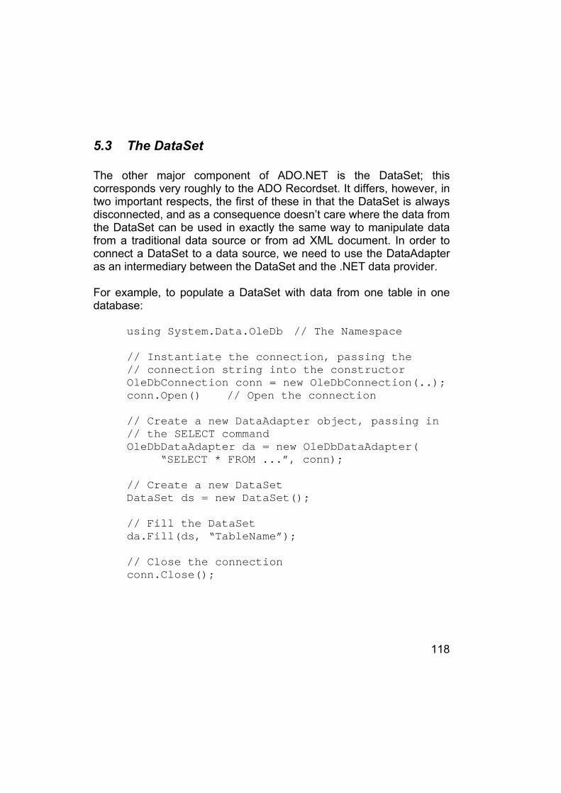
118

5.3 The DataSet The other major component of ADO.NET is the DataSet; this corresponds very roughly to the ADO Recordset. It differs, however, in two important respects, the first of these in that the DataSet is always disconnected, and as a consequence doesn’t care where the data from the DataSet can be used in exactly the same way to manipulate data from a traditional data source or from ad XML document. In order to connect a DataSet to a data source, we need to use the DataAdapter as an intermediary between the DataSet and the .NET data provider. For example, to populate a DataSet with data from one table in one database: using System.Data.OleDb // The Namespace

// Instantiate the connection, passing the// connection string into the constructorOleDbConnection conn = new OleDbConnection(..);conn.Open() // Open the connection

// Create a new DataAdapter object, passing in// the SELECT commandOleDbDataAdapter da = new OleDbDataAdapter(

“SELECT * FROM ...”, conn);

// Create a new DataSetDataSet ds = new DataSet();

// Fill the DataSetda.Fill(ds, “TableName”);

// Close the connectionconn.Close();

119

After opening the connection just as we did before, there are three steps involved do populating the DataSet:

• Instantiate a new DataAdapter object. Before we fill the DataSet, we’ll obviously need to specify the connection information and the data we want to fill it with. There are a number of ways of doing that, but probably the easiest is to pass the command text for the SQL query and either a connection string or an open connection into the DataAdapter’s constructor, as we do above.

• Create the new DataSet. • Call the DataAdapter’s Fill method. We pass the DataSet we

want to populate as a parameter to this method, and also the name of the table within the DataSet we want to fill. If we call the Fill method against a closed connection, the connection will automatically be opened, and then re-closed when the DataSet has been filled.

The DataSet is the centrepiece of a disconnected, data-driven application: it is an in-memory representation of complete set of data, including tables, relationships, and constraints. The DataSet does not maintain a connection to a data source, enabling true disconnected data management. The data in a DataSet can be accessed, manipulated, updated, or deleted, and then reconciled with the original data source. Since the DataSet is disconnected from the data source, there is less contention for valuable resources, such as database connection, and less record locking. The DataSet uses a eXtensible Markup Language (XML) for transmission and persistence. Moving data across application boundaries no longer incurs the expense of COM data type marshalling, since the data is transmitted in text-based XML format. Any application or object that can handle text can deal with a DataSet in some fashion. If the object does not support ADO.NET, but can parse XML, then it can treat the DataSet as an XML file. If the object supports ADO.NET, then the data can be materialized into a DataSet,

120

which will expose all of the properties and methods of the System.Data.DataSet class. The DataSet object model will help us understand the power and usefulness of the DataSet. When we look at the DataSet object model, we see that it is made up of three collections, Tables, Relations, and ExtendedProperties. These collections make up the relational data structure of the DataSet:

• Tables Collection, the DataSet.Tables property is a DataTableCollection object, which contains zero or more DataTable objects. Each DataTable represents a table of data from the data source. Each DataTable is made up of a Columns collection and a Rows collection, which are zero or more DataColumns or DataRows, respectively.

• Relations Collection, the DataSet.Relations property is a DataRelationCollection object, which contains zero or more DataRelation objects. The DataRelation objects define a parent-child relationship between two tables based on foreign key values.

• ExtendetProperties Collection, the DataSet.ExtendedProperties property is a PropertyCollection object, which contains zero or more user-defined properties. The ExtendedProperties collection can be used to store custom data related to the DataSet, such as the time when the DataSet was constructed.

5.3.1 The DataTable A DataTable stores data in a similar form to a database table: data is stored in a set of fields (columns) and records (rows). The DataTable class is a central class in the ADO.NET architecture; it can be used independently, and in DataSet objects. A DataTable consists of a Columns collection, a Rows collection, and a Constraints collection:

121

• The Columns collection is an instance of the DataColumnCollection class, and is a container object for zero or more DataColumn objects. The DataColumn objects define the DataTable column, including the column name, the data type, and any primary key or incremental numbering information.

• Rows Collection, the Rows collection is an instance of the DataRowCollection class, and is a container for zero or more DataRow objects. The DataRow object contains the data in the DataTable, as defined by the DataTable.Columns collection. Each DataRow has one item per DataColumns in the Columns collection.

• Constraints Collection, the Constraints collection is an instance of the ConstraintCollection class, and is a container for zero or more ForeignKeyConstraint objects and/or UniqueConstraint objects. The ForeignKeyConstraint object defines the action to be taken on a column in a primary key/foreign key relationship when a row is update or deleted. The UniqueConstraint is used to force all values in a column to be unique.

Like many of the objects in the .NET Framework, the DataTable exposes a set of events that can be captured and handled. It can be very useful to handle the DataTable event, for instance, we can use the events to update the user interface, or to validate edits, updates, or deletes before they are committed. There are six events, and they all work in nearly the same way: they each have similar arguments, and are invoked when their respective event is fired. The events are:

• ColumChanging, occurs when a value is being changed for the specified DataColumn in a DataRow.

• ColumsChanged, occurs after a value has been changed for the specified DataColumn in a DataRow.

• RowChanging, occurs when a DataRow is changing. This event will fire each time a change is made to the DataRow, after the ColumnChanging event fires.

122

• RowChanged, occurs after a DataRow has been changed successfully.

• RowDeleting, occurs when a DataRow is about to be deleted. • RowDeleted, occurs after a DataRow is successfully deleted.

As we can see, these events are paired; one event fires when something is happening, and one fires after the first finishes successfully. We can handle these events by creating an event handler for each event. The event handlers take arguments as specified for the event: To add the event handler to an instance of a DataTable, create e new event handler object, and pass in the name of the method that will handle the event. Each of the DataTable events works in the same fashion. The ColumnChanging and ColumnChanged events take a DataColumnChangeEventArgs object, while the other events take a DataRowChangeEventArgs object. The DataColumnChangeEventArgs object exposes three properties:

• Column, gets the DataColumn with the changing value. • ProposedValue, gets or sets the proposed value. This is the

new value being assigned to the column. For example, in a ColumnChanging event handler we can evaluate the ProposedValue and accept or reject the change based on uts value. We’ll see how to use this in the following DataTable Events Example.

• Row, gets the DataRow with che changing value. The DataRowChangeEventArgs objects exposes only two properties:

• Action, gets the action that has occurred on the DataRow • Row, gets the DataRow upon which the action occurred

123

5.4 Performance Once we’ve become accustomed to the basics of working with ADO.NET – using the DataSet, DataAdapter, SQL Client and OLE DB data providers, and so on we can focus more on some of the details generally left out of most overview texts on the subject. Among such details are performance and security issues.

In this chapter, we’ll discuss the issues surrounding creating high-performance applications and components for use with ADO.NET in the .NET framework, as well as issues concerning code and data security. Performance is a problem that plagues even the most well-designed and well-programmed solutions. In this chapter, we will see how to take ADO.NET solutions and make them faster and more secure by using some optimization techniques, asynchronous execution, connection pooling, and various security technologies. By the time this chapter is complete, you should have a through understanding of the following topics:

• Various method to optimize data access • Connection Pooling • Message Queuing • Security issues and tradeoffs concerning Data Access.

5.4.1 Connection Pooling

Opening and closing database connections is a very expensive operation. The concept of connection pooling involves preparing connection instances ahead of time in a pool. This has the upshot that multiple requests for the same connection can be served by a pool of available connections, thereby reducing the overhead of obtaining a new connection instance. Connection pooling is handled differently by

124

each data provider: we’ll cover how the SQL Client and OLE DB .NET Data Providers handle connection pooling. The SqlConnection object is implicitly a pooled object. It relies solely on Windows 2000 Component Services (COM+) to provide pooled connections. Each pool of available connections is based on a single, unique connection string. Each time a request for a connection is made with a distinct connection string, a new pool will be created. The pools will be filled with connections up to a maximum defined size. Requests for connections from a full pool will be queued until c connection can be re-allocated to the queued request. If the queued request times out, an exception will be thrown. There are some arguments that can be passed to the connection string to manually configure the pooling behaviour of the connection. Note that these arguments count towards the uniqueness of the string, and two otherwise identical strings with differing pool settings will create two different pools. The following is a list of SQL connection string parameters that affect pooling:

• Connection Lifetime (0) – this is a value that indicates how ling (in seconds) a connection will remain live after having been created and placed in the pool. The default value if 0 indicates that the connection will never time out.

• Connection Reset (true) – this Boolean value indicates whether or not che connection will be reset when removed from the pool. A value of false avoids hitting the database again when obtaining the connection, but may cause unexpected results as the connection state will not be reset. The default value for this option is true, and is set to false only when we can be certain that not resetting connection state when obtaining the connection will not have any adverse effects on code.

• Enlist (true) – this Boolean value indicates whether or not the connection should automatically enlist the connection in

125

the current transaction of the creation thread (if one exists). The default value for this is true.

• Max Pool Size (100) – maximum number of connections that can reside in the pool at any given time.

• Min Pool Size (0) = the minimum number of connections maintained in the pool. Setting this to at least 1 will guarantee that, after the initial start up of your application, there will always be at least one connection available in he pool.

• Pooling (true) – this is the Boolean value that indicates whether or not the connection should be pooled at all. The default is true.

The best thing about SQL connection pooling in that, besides optionally tuning pooling configuration in the connection string, we don’t have to do any additional programming to support it. The OLE DB .NET Data Provider provides connection pooling automatically through the use of OLE DB session pooling. Again, there is no special code that we need to write to take advantage of the OLE DB session pooling; it is simply there for us. We can configure or disable the OLE DB session pooling by using the OLE DB Services connection string argument.

126

127

6 HEALTH LEVEL 7

6.1 Introduction Health Level Seven (HL7) is the Standard for electronic data exchange in all healthcare environments, with special emphasis on inpatient acute care facilities (i.e., hospitals). The term “Level 7” refers to the highest level of the Open System Interconnection (OSI) model of the International Organization for Standardization (ISO). This is not to say that HL7 conforms to ISO defined elements of the OSI’s seventh level. Also, HL7 does not specify a set of ISO approved specifications to occupy layers 1 to 6 under HL7’s abstract message specifications. HL7 does, however, correspond to the conceptual definition of an application-to-application interface placed in the seventh layer of the OSI model. The HL7 Standard is primarily focused on the issues that occur within the seventh, or application level. These are the definition of the data to be exchanged, the timing of the exchanges, and the communication of certain application-specific errors between the applications. However, of necessity, protocols that refer to the lower layers of the OSI model are sometimes mentioned to help implementers understand the context of the Standard. It is generally accepted that the efficacy of healthcare operations is greatly affected by the extent of automation of information management functions. Many believe that healthcare delivery agencies that have not automated their information systems are not able to complete effectively in the healthcare market of the 1990’s. In the past two decades, healthcare institutions, and hospitals in particular, have begun to automate aspects of their information

128

management. Initially, such efforts have been geared towards reducing paper processing, improving cash flow, and improving management decision making. In later years a distinct focus on streamlining and improving clinical and ancillary services has evolved, including bedside and “patient-side” systems. Within the last few years, interest has developed in integrating all information related to the delivery of healthcare to a patient over his or her lifetime (i.e., an electronic medical record). It has also been envisioned that all or part of this electronic medical record should be able to be communicated electronically anywhere as needed. It is not uncommon today for the average hospital to have installed computer systems for admission, discharge, and transfer; clinical laboratories; radiology; billing and accounts receivable to cite a few. Often these applications have been developed by different vendors or in–house groups, with each product having highly specific information formats. As hospitals have gradually expanded information management operation, a concomitant need to share critical data among the systems has emerged. Comprehensive systems that aim at performing most, if not all, healthcare information management are in production by selected vendors. These systems may be designed in a centralized or a distributed architecture. Nevertheless, to the extent that such systems are truly complete, their use would mitigate the need for an external data interchange standard such as HL7. Network technology has emerged as a viable and cost-effective approach to the integration of functionally and technically diverse computer applications in healthcare environments. However, these applications have developed due to market structure rather than through a logical systems approach; they are therefore often ad hoc and idiosyncratic. At the very least, they do not possess a common data architecture and their combined data storage actually constitutes a highly distributed and severely de-normalized database. Expensive site-specific programming and program maintenance are often necessity for interfacing these applications in a network environments. This occurs at considerable expense to the user/purchaser and vendor

129

while often keeping vendor staff from other initiatives such as new product development. The need for extensive site-specific interface work could be greatly reduced if a standard for network interfaces for healthcare environments were available and accepted by vendors and users alike. Finally, the lack of data and process standards between both vendor systems and the many healthcare provider organizations present a significant barrier to application interfaces. In some cases, HL7 becomes an effective template to facilitate negotiations between vendors and users but cannot, by itself, serve as an “off-the-shelf” complete interface. In summary, it is important that both vendors and users not be faced with the problem of supporting incompatible transaction/communications structures. Instead, a framework must be developed for minimizing incompatibly and maximizing the exchange of information between systems. It is proposed that HL7 can act as a superstructure in this environments to facilitate a common specification and specifications methodology. Ii is indeed both practical and economical to develop, and commit to, standard interfaces for computer applications in healthcare institutions.

6.2 History HL7, as an organization, has experienced significant growth over the last several years. Currently, HL7’s membership consists of approximately 1600 members in all memberships categories and regularly attracts 350-400 members and non-members to each of its three yearly meetings. The HL7 Working Group has met approximately every three to four months since March 1987 to develop and review the specification. The group is structured into committees to address each of the functional

130

interfaces under development, with additional committees to address the overall control structure and various administrative aspects of the group. These committees have the responsibility to author and maintain the chapters in the HL7 Interface Standard. In addition, from time to time various special interest groups are formed within HL7 to develop ideas and sponsors particular perspectives that are not covered by any single existing committee. HL7 is operating under bylaws and balloting procedures. These procedures are modelled on the balloting procedures of other relevant healthcare industry computer messaging standards organizations (e.g., ASTM) and designed to conform to the requirements of the American National Standards Institute (ANSI). HL7 is participating in ANSI’s Healthcare Informatics Standards Boards (HISB). In June 1994, HL7 became an ANSI Accredited Standards Developing Organization. Version 2.2 of HL7 was accepted by ANSI as an accredited standard in 1996 and HL7 Version 2.3 revived ANSI approval in May of 1997. HL7 sanctioned national groups also exist in many other countries outside of the United States including Australia, Germany, Japan, the Netherlands, New Zealand and Canada.

6.3 Architecture HL7 does not try to assume a particular architecture with respect to the placement of data within applications but is designed to support a central patient care system as well as a more distributed environment where data resides in departmental system. Instead, HL7 server as a way for inherently disparate applications and data architecture operating in a heterogeneous system environment to communicate with each other.

131

The figure below represents the atmosphere previously explained, and is interesting to notice that the fulcrum of the architecture of this system consists in the structure of the message that we will show subsequently. This message turns in the Bus Software and renders through interface the communication possible.

Fig. 6.1 Software Bus for HL7 Messages We have pointed out previously to the fact that the composition of the message in HL7 is the main process of integration and that this represents the architecture of system HL7. Now we analyzing the fundamental job, the message composing. A message is the atomic unit of data transferred between systems. It is comprised of a group of segments in a defined sequence. Each message has a message type that defines its purpose. For example the ADT Message type is used to transmit portions of a patient’s

132

Patient Administration (ADT) data from one system to another. A three character code contained within each message identifies its type. A segment is a logical groping of data fields. Segments of a message may be required or optional. They many occur only once in a message or the may be allowed to repeat. Each segment is given a name. For example, the ADT message may contain the following segments: Message Header (MSH), Event Type (EVN), Patient ID (PID), and Patient Visit (PV1). Each segment is identified by a unique tree character code know as Segment ID. All segment ID codes beginning with the letter Z are reserved for locally-defined message. A field is a string of characters. HL7 does not care how systems actually store data within application. When fields are transmitted, they are sent as character strings. In defining a segment, the following information is specified about each field:

• Position • Maximum length • Data Type • Optionality • Repetition • Table

Where Position (sequence within the segment) represent the ordinal position of the data field within the segment. This number is used to refer to the data field in the text comments that follow the segment definition table. In the segment attribute tables this information is provided in the column labeled SEQ. The Maximum length represent the maximum number of character that one occurrence of the data field may occupy. The maximum length is not of conceptual importance in the abstract message or the HL7 coding rules. In the segment attribute tables this information is in a column labeled LEN.

133

The Data Type is a restrictions on the contents of the data field. There are a number of data types defined by HL7; this Data Type are defined in the below table, in the segment attribute table this information is provided in the column labeled DT. Data Type Category/

Data type Data Type Name HL7 Section

Reference Notes/Format

Alphanumeric ST String 2.8.40 TX Text data 2.8.45 FT Formatted text 2.8.19

Numerical CQ Composite quantity

with units 2.8.10 <quantity (NM)> ^ <units (CE)>

MO Money 2.8.25 <quantity (NM)> ^ <denomination (ID)> NM Numeric 2.8.27 SI Sequence ID 2.8.38 SN Structured numeric 2.8.39 <comparator (ST)> ^ <num1 (NM)> ^

<separator/suffix> ^ <num2 (NM)> Identifier

ID Coded values for HL7 tables

2.8.21

IS Coded value for user-defined tables

2.8.22

VID Version identifier <version ID (ID)> ^ <internationalization code (CE)> ^ <international version ID (CE)

HD Hierarchic designator

2.8.20 <namespace ID (IS)> ^ <universal ID (ST)> ^ <universal ID type (ID)> Used only as part of EI and other data types.

EI Entity identifier 2.8.17 <entity identifier (ST)> ^ <namespace ID (IS)> ^ <universal ID (ST)> ^ <universal ID type (ID)>

RP Reference pointer 2.8.36 <pointer (ST) > ^ < application ID (HD)> ^ <type of data (ID)> ^ <subtype (ID)>

PL Person location 2.8.28 <point of care (IS )> ^ <room (IS )> ^ <bed (IS)> ^ <facility (HD)> ^ < location status (IS )> ^ <person location type (IS)> ^ <building (IS )> ^ <floor (IS )> ^ <location description (ST)>

PT Processing type 2.8.31 <processing ID (ID)> ^ <processing mode

134

(ID)> Date/Time

DT Date 2.8.15 YYYY[MM[DD]] TM Time 2.8.41 HH[MM[SS[.S[S[S[S]]]]]][+/-ZZZZ] TS Time stamp 2.8.44 YYYY[MM[DD[HHMM[SS[.S[S[S[S]]]]]]]][

+/-ZZZZ] ^ <degree of precision> Code Values

CE Coded element 2.8.3 <identifier (ST)> ^ <text (ST)> ^ <name of coding system (ST)> ^ <alternate identifier (ST)> ^ <alternate text (ST)> ^ <name of alternate coding system (ST)>

CNE Coded with no exceptions

2.8.8 <identifier (ST)> ^ <text (ST)> ^ <name of coding system (ST)> ^ <alternate identifier (ST)> ^ <alternate text (ST)> ^ <name of alternate coding system (ST)> ^ <coding system version ID (ST)> ^ alternate coding system version ID (ST)> ^ <original text (ST) >

CWE Coded with exceptions

2.8.11 <identifier (ST)> ^ <text (ST)> ^ <name of coding system (ST)> ^ <alternate identifier (ST)> ^ <alternate text (ST)> ^ <name of alternate coding system (ST)> ^ <coding system version ID (ST)> ^ alternate coding system version ID (ST)> ^ <original text (ST) >

CF Coded element with formatted values

2.8.4 <identifier (ID)> ^ <formatted text (FT)> ^ <name of coding system (ST)> ^ <alternate identifier (ID)> ^ <alternate formatted text (FT)> ^ <name of alternate coding system (ST)>

CK Composite ID with check digit

2.8.5 <ID number (NM)> ^ <check digit (NM)> ^ <code identifying the check digit scheme employed (ID)> ^ < assigning authority (HD)>

CN Composite ID number and name

2.8.7 <ID number (ST)> ^ <family name (ST)> ^ <given name (ST)> ^ <middle initial or name (ST)> ^ <suffix (e.g., JR or III) (ST)> ^ <prefix (e.g., DR) (ST)> ^ <degree (e.g., MD) (ST)> ^ <source table (IS)> ^ <assigning authority (HD)>

CX Extended composite ID with check digit

2.8.12 <ID (ST)> ^ <check digit (ST)> ^ <code identifying the check digit scheme employed (ID)> ^ < assigning authority (HD)> ^ <identifier type code (IS)> ^ < assigning facility (HD)

XCN Extended composite ID number and name

2.8.49 In Version 2.3, use instead of the CN data type. <ID number (ST)> ^ <family name (ST)> & <last_name_prefix (ST) ^ <given name (ST)> ^ <middle initial or

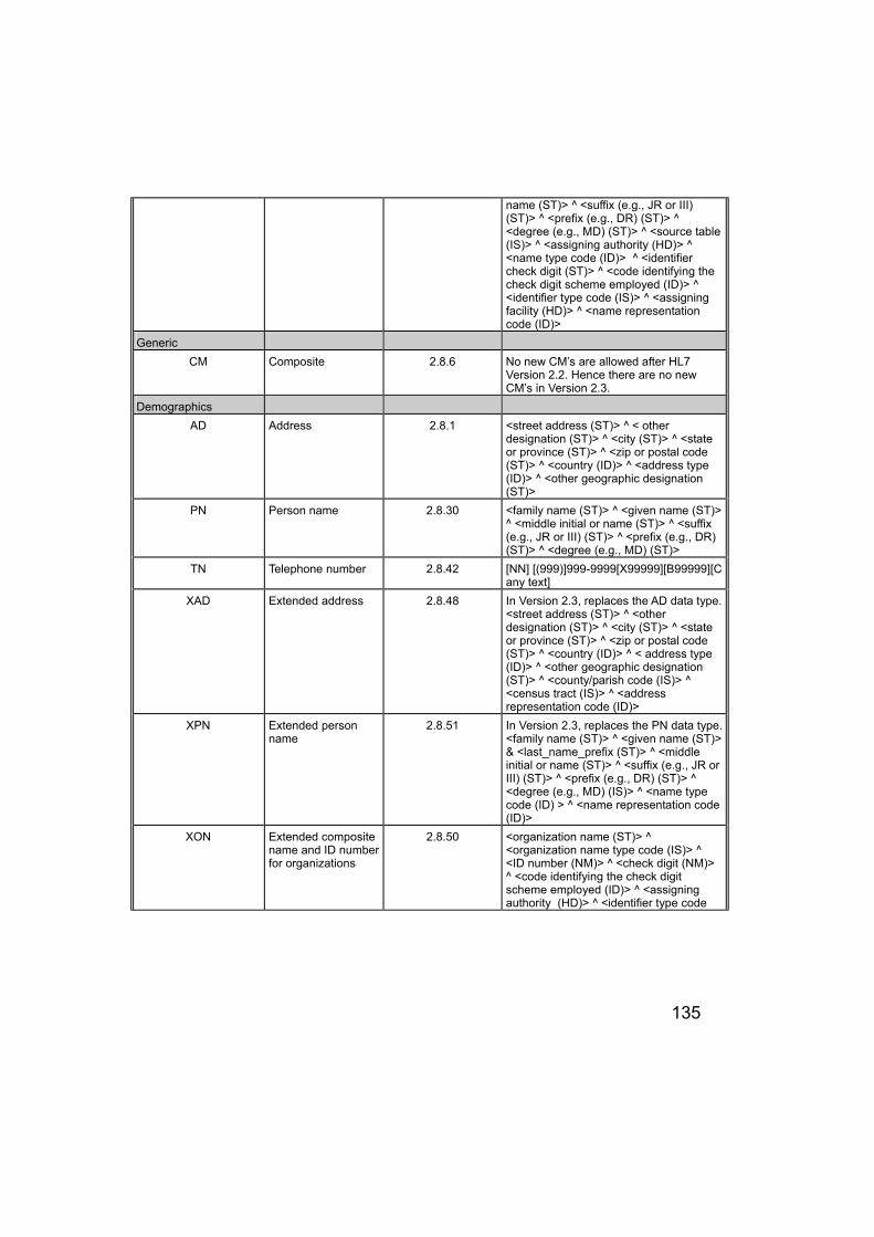
135

name (ST)> ^ <suffix (e.g., JR or III) (ST)> ^ <prefix (e.g., DR) (ST)> ^ <degree (e.g., MD) (ST)> ^ <source table (IS)> ^ <assigning authority (HD)> ^ <name type code (ID)> ^ <identifier check digit (ST)> ^ <code identifying the check digit scheme employed (ID)> ^ <identifier type code (IS)> ^ <assigning facility (HD)> ^ <name representation code (ID)>

Generic CM Composite 2.8.6 No new CM’s are allowed after HL7

Version 2.2. Hence there are no new CM’s in Version 2.3.

Demographics AD Address 2.8.1 <street address (ST)> ^ < other

designation (ST)> ^ <city (ST)> ^ <state or province (ST)> ^ <zip or postal code (ST)> ^ <country (ID)> ^ <address type (ID)> ^ <other geographic designation (ST)>

PN Person name 2.8.30 <family name (ST)> ^ <given name (ST)> ^ <middle initial or name (ST)> ^ <suffix (e.g., JR or III) (ST)> ^ <prefix (e.g., DR) (ST)> ^ <degree (e.g., MD) (ST)>

TN Telephone number 2.8.42 [NN] [(999)]999-9999[X99999][B99999][C any text]

XAD Extended address 2.8.48 In Version 2.3, replaces the AD data type. <street address (ST)> ^ <other designation (ST)> ^ <city (ST)> ^ <state or province (ST)> ^ <zip or postal code (ST)> ^ <country (ID)> ^ < address type (ID)> ^ <other geographic designation (ST)> ^ <county/parish code (IS)> ^ <census tract (IS)> ^ <address representation code (ID)>

XPN Extended person name

2.8.51 In Version 2.3, replaces the PN data type. <family name (ST)> ^ <given name (ST)> & <last_name_prefix (ST)> ^ <middle initial or name (ST)> ^ <suffix (e.g., JR or III) (ST)> ^ <prefix (e.g., DR) (ST)> ^ <degree (e.g., MD) (IS)> ^ <name type code (ID) > ^ <name representation code (ID)>

XON Extended composite name and ID number for organizations

2.8.50 <organization name (ST)> ^ <organization name type code (IS)> ^ <ID number (NM)> ^ <check digit (NM)> ^ <code identifying the check digit scheme employed (ID)> ^ <assigning authority (HD)> ^ <identifier type code

136

(IS)> ^ <assigning facility ID (HD)> ^ <name representation code (ID)>

XTN Extended telecommunications number

2.8.52 In Version 2.3, replaces the TN data type. [NNN] [(999)]999-9999 [X99999] [B99999] [C any text] ^ <telecommunication use code (ID)> ^ <telecommunication equipment type (ID)> ^ <email address (ST)> ^ <country code (NM)> ^ <area/city code (NM)> ^ <phone number (NM)> ^ <extension (NM)> ^ <any text (ST)>

Specialty/Chapter Specific

Waveform CD Channel definition 2.8.2 <channel identifier (*)> ^ <channel

number (NM)> & <channel name (ST)> ^ <electrode names (*) > ^ <channel sensitivity/units (*) > ^ <calibration parameters (*)> ^ <sampling frequency (NM)> ^ <minimum/maximum data values (*)>

MA Multiplexed array 2.8.24 <sample 1 from channel 1 (NM)> ^ <sample 1 from channel 2 (NM)> ^ <sample 1 from channel 3 (NM)> ...~<sample 2 from channel 1 (NM)> ^ <sample 2 from channel 2 (NM)> ^ <sample 2 from channel 3 (NM)> ...~

NA Numeric array 2.8.26 <value1 (NM)> ^ <value2 (NM)> ^ <value3 (NM)> ^ <value4 (NM)> ^ ...

ED Encapsulated data 2.8.16 Supports ASCII MIME-encoding of binary data. <source application (HD) > ^ <type of data (ID)> ^ <data subtype (ID)> ^ <encoding (ID)> ^ <data (ST)>

Price Data CP Composite price 2.8.9 In Version 2.3, replaces the MO data

type. <price (MO)> ^ <price type (ID)> ^ <from value (NM)> ^ <to value (NM)> ^ <range units (CE)> ^ <range type (ID)>

Patient Administration /Financial Information

FC Financial class

2.8.18 <financial class (ID)> ^ <effective date (TS)>

Extended Queries QSC

Query selection criteria

2.8.33 <name of field (ST)> ^ <relational operator (ID)> ^ <value (ST)> ^ <relational conjunction (ID)>

137

QIP

Query input parameter list

2.8.32 <field name (ST) > ^ <value1 (ST) & value2 (ST) & value3 (ST) ...>

RCD

Row column definition

2.8.34 <HL7 item number (ST)> ^ <HL7 data type (ST)> ^ <maximum column width (NM)>

Master Files

DLN Driver’s license number

2.8.13 <license number (ST)> ^ <issuing state, province, country (IS)> ^ <expiration date (DT)

JCC

Job code/class 2.8.23 <job code (IS)> ^ <job class (IS)>

VH Visiting hours 2.8.46 <start day range (ID)> ^ <end day range (ID)> ^ <start hour range (TM)> ^ <end hour range (TM)>

Medical Records/Information Management

PPN

Performing person time stamp

2.8.29 <ID number (ST)> ^ <family name (ST)> ^ & <last name prefix (ST)> ^ <given name (ST)> ^ <middle initial or name (ST)> ^ <suffix (e.g., JR or III) (ST)> ^ <prefix (e.g., DR) (ST)> ^ <degree (e.g., MD) (ST)> ^ <source table (IS)> ^ <assigning authority (HD)> ^ <name type code(ID)> ^ <identifier check digit (ST)> ^ <code identifying the check digit scheme employed (ID )> ^ <identifier type code (IS)> ^ <assigning facility (HD)> ^ < date/time action performed (TS)> ^ <name representation code (ID)>

Time Series: DR

Date/time range 2.8.14 <range start date/time (TS)> ^ <range

end date/time (TS)>

RI Repeat interval 2.8.35 <repeat pattern (IS)> ^ <explicit time interval (ST)>

SCV Scheduling class value pair

2.8.37 <parameter class (IS)> ^ <parameter value (ST)>

TQ Timing/quantity 2.8.43 <quantity (CQ)> ^ <interval (*)> ^ <duration (*)> ^ <start date/time (TS)> ^ <end date/time (TS)> ^ <priority (ST)> ^ <condition (ST)> ^ <text (TX)> ^ <conjunction (ID)> ^ <order sequencing (*)> ^ <performance duration (CE)> ^ <total occurrences (NM)>

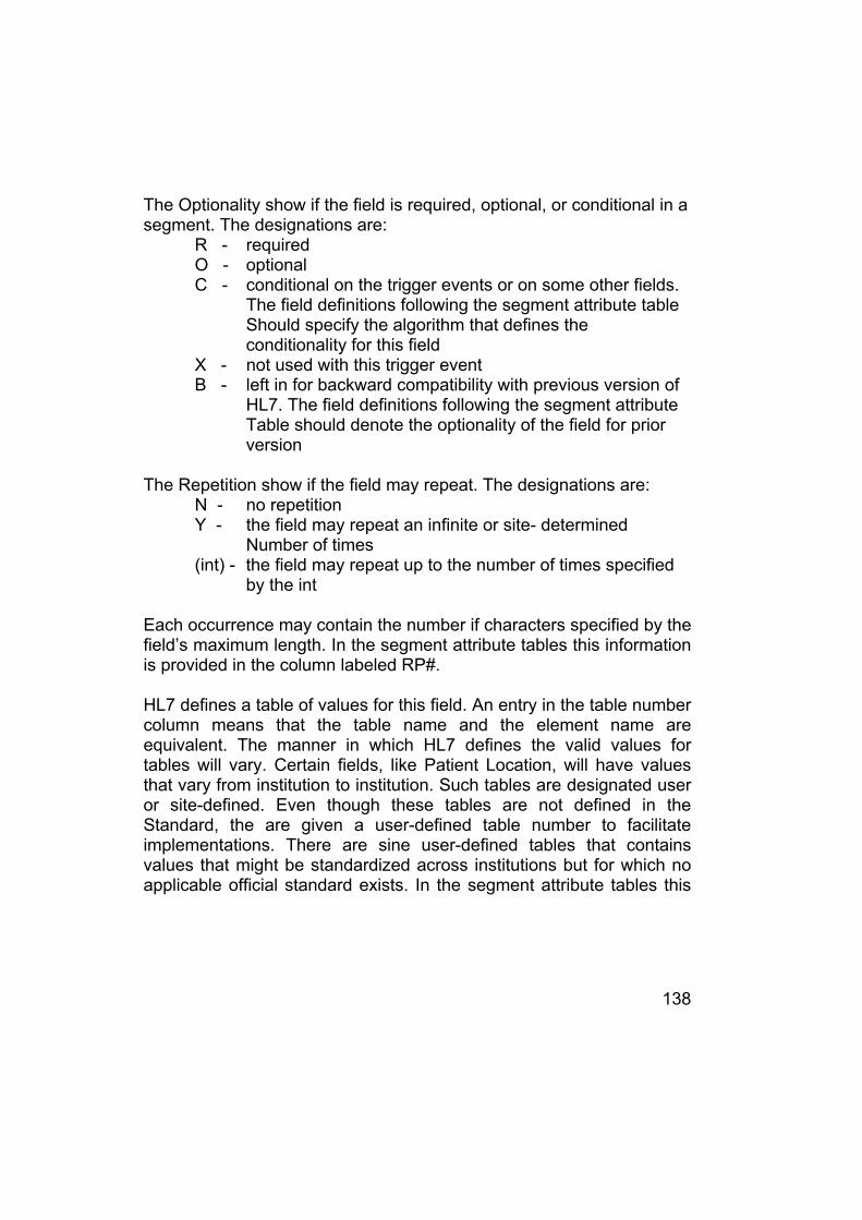
138

The Optionality show if the field is required, optional, or conditional in a segment. The designations are:

R - required O - optional C - conditional on the trigger events or on some other fields. The field definitions following the segment attribute table Should specify the algorithm that defines the conditionality for this field X - not used with this trigger event B - left in for backward compatibility with previous version of HL7. The field definitions following the segment attribute Table should denote the optionality of the field for prior version

The Repetition show if the field may repeat. The designations are: N - no repetition Y - the field may repeat an infinite or site- determined Number of times (int) - the field may repeat up to the number of times specified by the int Each occurrence may contain the number if characters specified by the field’s maximum length. In the segment attribute tables this information is provided in the column labeled RP#. HL7 defines a table of values for this field. An entry in the table number column means that the table name and the element name are equivalent. The manner in which HL7 defines the valid values for tables will vary. Certain fields, like Patient Location, will have values that vary from institution to institution. Such tables are designated user or site-defined. Even though these tables are not defined in the Standard, the are given a user-defined table number to facilitate implementations. There are sine user-defined tables that contains values that might be standardized across institutions but for which no applicable official standard exists. In the segment attribute tables this

139

information is provided in the column labeled TBL#, the only exceptions are the CE and CF data types, witch contain the table identifiers as part of the data type definition. In constructing a message, certain special characters are used. They are the segment terminator, the field separator, the component separator, subcomponent separator, repetition separator, and escape character. The segment terminator is always a carriage return (in ASCII, a hex 0D). The other delimiters are defined in the MSH segment, with the field delimiter in the 4th character position, and the other delimiters occurring as in the field called Encoding Characters, which is the first field after the segment ID. The delimiter values used in the MSH segment are the delimiter values used throughout the entire message. In the absence of other considerations, HL7 recommends the suggested values found in Figure 2-1 delimiter values. At any given site, the subset of the possible delimiters may be limited by negotiations between applications. This implies that the receiving applications will use the agreed upon delimiters, as they appear in the Message Header segment (MSH), to parse the message.

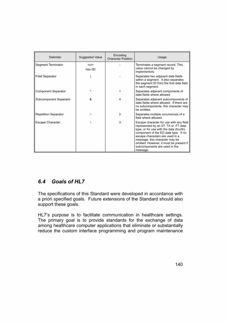
140

Delimiter Suggested Value Encoding Character Position Usage

Segment Terminator <cr> hex 0D

- Terminates a segment record. This value cannot be changed by implementors.

Field Separator | - Separates two adjacent data fields within a segment. It also separates the segment ID from the first data field in each segment.

Component Separator ^ 1 Separates adjacent components of data fields where allowed.

Subcomponent Separator & 4 Separates adjacent subcomponents of data fields where allowed. If there are no subcomponents, this character may be omitted.

Repetition Separator ~ 2 Separates multiple occurrences of a field where allowed.

Escape Character \ 3 Escape character for use with any field represented by an ST, TX or FT data type, or for use with the data (fourth) component of the ED data type If no escape characters are used in a message, this character may be omitted. However, it must be present if subcomponents are used in the message.

6.4 Goals of HL7 The specifications of this Standard were developed in accordance with a priori specified goals. Future extensions of the Standard should also support these goals. HL7’s purpose is to facilitate communication in healthcare settings. The primary goal is to provide standards for the exchange of data among healthcare computer applications that eliminate or substantially reduce the custom interface programming and program maintenance

141

that may otherwise be required. This primary goal can be delineated as a set of goals:

• the Standard should support exchanges among systems implemented in the widest variety of technical environments. Its implementation should be practical in a wide variety of programming languages and operating systems. It should also support communications in a wide variety of communications environments, ranging from a full, OSI-compliant, 7-level network “stack” to less complete environments including primitive point-to-point RS-232C interconnections and transfer of data by batch media such as floppy disk and tape.

• immediate transfer of single transactions should be supported along with file transfers of multiple transactions.

• the greatest possible degree of standardization should be achieved, consistent with site variations in the usage and format of certain data elements. The Standard should accommodate necessary site-specific variations. This will include, at least, site-specific tables, code definitions and possibly site-specific message segments (i.e., HL7 Z-segments).

• the Standard must support evolutionary growth as new requirements are recognized. This includes support of the process of introducing extensions and new releases into existing operational environments.

• the Standard should be built upon the experience of existing production protocols and accepted industry-wide standard protocols. It should not, however, favor the proprietary interests of specific companies to the detriment of other users of the Standard. At the same time, HL7 seeks to preserve the unique attributes that an individual vendor can bring to the marketplace.

142

• while it is both useful and pertinent to focus on information systems within hospitals, the long-term goal should be to define formats and protocols for computer applications in all healthcare environments.

• the very nature of the diverse business processes that exist within the healthcare delivery system prevents the development of either a universal process or data model to support a definition of HL7’s target environments. In addition, HL7 does not make a priori assumptions about the architecture of healthcare information systems nor does it attempt to resolve architectural differences between healthcare information systems. For at least these reasons, HL7 cannot be a true “plug and play” interface standard. These differences at HL7 sites will most likely require site negotiated agreements.

• a primary interest of the HL7 Working Group has been to employ the Standard as soon as possible. Having achieved this, HL7 has also developed an infrastructure that supports a consensus balloting process and has been recognized by the American National Standards Institute (ANSI) as an Accredited Standards Organization (ASO).

• cooperation with other related healthcare standards efforts (e.g., ACR/NEMA DICOM, ASC X12, ASTM, IEEE/MEDIX, NCPDP, etc.) has become a priority activity of HL7. HL7 has participated in the ANSI HISPP (Health Information Systems Planning Panel) process since its inception in 1992.

143

6.5 A Complete Solution HL7 is not, in itself, a complete systems integration solution. The issue directly addresses the so-called goal for “plug-and-play.” There are several barriers in today’s healthcare delivery environment that make it difficult, it not impossible, for HL7 to create a complete ”plug-and-play” solution. Two of these barriers include:

a) the lack or process conformity within healthcare delivery environments and

b) the resulting requirement for “negotiation” between users and vendors.

There is little, if any, process conformity within healthcare delivery environments. As a consequence, healthcare information solutions vendors are required to create very flexible systems with a very wide range of data and process flow options. HL7 attempts to address the superset of all known process (i.e., trigger) and data (i.e., segment and field) requirements. In doing this, it has attempted to be “all things to systems and users.” In fact, there is no one user nor any system that users would elect to use that would use all that HL7 attempts to offer. This “excess” of features typically requires some level of “negotiation” to take place between a user and his/her vendors to come up with the set of triggers and data items necessary to affect the solution for the user. In effect, this creates a unique use of the Standard at that site. The current version of HL7 has no intrinsic way to tailor a pre-determinable view of the Standard for each possible use. Future versions of HL7 will likely address this shortcoming.

144

A true integrated healthcare information systems solution addresses an integrated database, or at least what appears to be a virtual integrated database. In fact, however, as a practical matter, information solutions still need to be installed and operated in environments where no other, or only a subset of other, systems are available. In any case, all systems today are designed and implemented to process using their own local copies of data. HL7, to this date, has not attempted to prescribe the architecture, functionality, data elements or data organization of healthcare applications. Rather, HL7 has attempted to accommodate all application requirements that have been brought to its attention by volunteers willing and able to address them. Future versions of HL7 may choose to alter HL7’s historic approach to these issues. Recent efforts by HL7 and other ANSI Standards Developers to produce Data Meta Models have created a framework that both standards and applications developers can use as a common basis for defining and using both data and data organizations. Widespread acceptance of these concepts may allow HL7 and other Standards Groups to be more prescriptive in their approach with a smaller set of choices that must be made when interfaces are implemented. For now, however, users should be aware that HL7 provides a common framework for implementing interfaces between disparate vendors. In all cases, if an existing application interface is not available, HL7 reduces (but does not eliminate) the time and cost required to implement an application interface between two or more healthcare information systems. If a user chooses to implement a set of homogeneous solutions from a single vendor, HL7 is typically not necessary even applicable.

145

6.6 Other Communication Protocols This is an overview of evolving medical information exchange standards showing their primary goals, and their relation to network protocols.

6.6.1 ASTM Medical Standard American Society of Testing and Materials (ASTM) committee E-31 was started in 1970 as the “committee on computerized laboratory system” and was originally constrained to write standards for computer automation f laboratory instruments. Later the name was changed to “committee on computerized systems” and the scope broadened to include other kind of computerized systems. In 1975, a subcommittee to deal with clinical laboratory systems was formed, beginning E-31’s interest in medical computer systems. There are now six active subcommittees dealing with different aspects of computer applications in medicine. The primary goal of the subcommittee on data exchange for clinical result E-31.11 is as stated in the mission statement: “the specification for transferring clinical laboratory data messages between independent computer systems E1238”. In relationship to networking protocols this ASTM standard deals with the application layer, the seventh layer in the ISO/OSI model. The lower layers can be any set or reliable protocols (TCP/IP, X.400, Kermit, RS 232). However, the messages are composed of a restricted ASCII character set. Furthermore, the message consist of an unlimited number or lines. However, each line can’t be longer than 220 characters.

146

6.6.2 ACR-NEMA Standard The American College of Radiology (ACR) and the National Electrical Manufacturers Association (NEMA) formed the ACR-NEMA Digital Imaging and Communication Standards Committee (DICSC) in 1983. The primary goal as stated in the charter of this committee was to develop an interface standard for the interconnection of two pieces of imaging equipment. The standard was created so that a group of devices, each of witch meets this standard, may be organized into a system to meet user need. The standardization process has produced three versions to date. Version 1 was published in 1985. It specifies data formatting and provides a data dictionary, a set of commands and hardware interface. It supports transmission of data between two pieces of medical imaging equipment. It provides for a variety of functions such as data integrity checking, media access, flow control as well as fragmenting and reconstruction. ACR-NEMA is patterned after the ISO/OSI Reference Model. However, it is a six layer protocol since the transport layer and the network layer were consolidated. The transport/network layer, data link layer and physical layer all follow very specific protocols. These protocols where defined by state transitions, timing, and cable activity diagrams. Version 2 id an expanded of Version 1 but still supports only point-to-point message exchange. The data dictionary syntax rules are identical to those of Version 1. It added some features like controlling display devices. Version 3 is know as digital imaging and communications in medicine (DICOM) and was published in 1992. This version is a complex standard structured in a multi-part document (9 parts) using a pseudo-

147

object oriented description. It attempts to maintain compatibility with Version 2 where possible.

6.6.2 Medical Information Bus Standard IEEE P1073 In 1984, the P1073 Committee of the Institute of Electrical and Electronics Engineers (IEEE) Engineering in Medicine and Biology Society (EMBS) started developing he Medical Information Bus (MIB) standard. The primary goal as started in the mission of the P1073 Committee is to: “provide an international standard for open systems communication in healthcare applications, primarily between bedside medical devices and clinical information system, optimized for the acute care setting”. In relationship to networking protocols the MIB standard specifies local area network through a family of three network communication standard. These standards were modelled after the ISO/OSI reference model. The presentation layer is a subset of ISO 8822/23 standard, the session layer is a subset of ISO 8326 standard. The transport layer provides simple transport service, but does not strictly comply with it as many parameters are defaulted. The network layer is a functionally inactive layer, while the data link layer offers a subset of HDLC services: a connection-oriented, point-to-point data transfer. The physical layer uses the EIA-485 specification with non-return to zero inverted (NRZI) encoding at 375 Kbps.

148

6.6.3 Medical Data Interchange Standard IEEE P1157 In November 1987, the P1157 Working Group of the IEEE EMBS started developing the Medical Fata Interchange (MEDIX) standard. The primary goal as defined in the charter of the P1157 Committee is to: “specify and establish a robust and flexible communication standard for the exchange of data between heterogeneous healthcare information system”. The relation between MEDIX and network protocols is outlined in he Communication Profiles. A Communication Profiles is a set of protocols or communication options that supports a certain functionality or service to the user. The MEDIX standard is based upon and will confirm to the ISO/OSI reference model. Nonetheless, realizing that different applications have various communication needs, the standard attempts to allow both flexibility and interoperability.

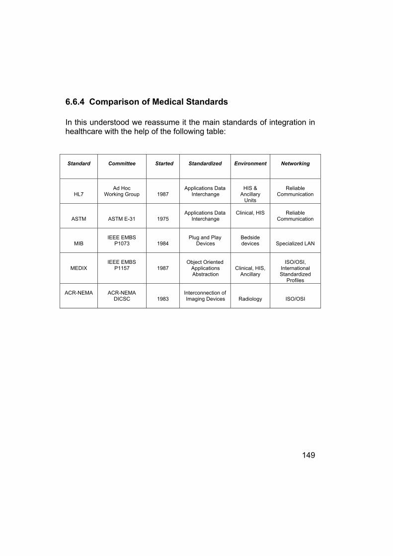
149

6.6.4 Comparison of Medical Standards In this understood we reassume it the main standards of integration in healthcare with the help of the following table:

Standard

Committee

Started

Standardized

Environment

Networking

HL7

Ad Hoc

Working Group

1987

Applications Data

Interchange

HIS &

Ancillary Units

Reliable

Communication

ASTM

ASTM E-31

1975

Applications Data

Interchange

Clinical, HIS

Reliable

Communication

MIB

IEEE EMBS

P1073

1984

Plug and Play

Devices

Bedside devices

Specialized LAN

MEDIX

IEEE EMBS

P1157

1987

Object Oriented

Applications Abstraction

Clinical, HIS, Ancillary

ISO/OSI,

International Standardized

Profiles

ACR-NEMA

ACR-NEMA DICSC

1983

Interconnection of Imaging Devices

Radiology

ISO/OSI

150

151

7 IL SERVIZIO “ANAWEB”

7.1 Introduzione L’obiettivo di questo “Web Services” è quello di fornire una risposta comune alla necessità di vari applicativi per accedere alla base dati anagrafica comune. Questa base di dati non sarà direttamente accessibile con i classici sistemi di accesso ai dati, ma sarà consultata tramite il servizio che provvederà a elaborare la richiesta, aggiornare i dati e restituire al richiedente una struttura dati (DataSet) uguale a quella che il richiedente avrebbe ricevuto se avesse interrogato direttamente la base di dati. Questo servizio vuole essere un middleware il più possibile trasparente tra le richieste client e la base di dati. Particolare attenzione è stata rivolta agli aspetti di sicurezza in quanto i dati trattati sono dati sensibili, soggetti alla legge sulla Privacy. Questo servizio ha come principali compiti mantenere sempre una base anagrafica aggiornata con l’anagrafe ospedaliera ed un meccanismo efficiente di ricerca assistito.

7.1.1 Stato Attuale Lo stato che mi si è presentato all’inizio del progetto è stato uno scenario molto interessante, uno scenario che grazie alla spinta delle nuove tecnologie prova a svincolarsi dai vecchi modelli (Client – Server) per tentare di migrare a nuovi modelli che promettono maggiore scalabilità e maggiore flessibilità. Oggi nell’Informatica Medica si sente la reale necessità di integrare applicativi nati separatamente. Il primo passo per questa integrazione

152

si basa su un requisito minimo; gli applicativi devono identificare lo stesso paziente nello stesso modo, devono essere aggiornati sulle variazioni anagrafiche fatte da altri in tempo reale. La realtà odierna è per diversi motivi avversa a questo tipo di unificazione. L’Informatica Medica che mi si è presentata è un mercato che ha visto la crescita delle medie Software House che dapprima creando software specializzato, che successivamente si sono trovare a progettare vere e proprie Suite Mediche. Queste Suite nate come indipendenti sotto il profilo anagrafico hanno presto sentito la necessità di “Integrarsi” con l’anagrafica centralizzata ospedaliera, dapprima con un’integrazione statica, cioè, con aggiornamenti programmati; ora le nuove tecnologie permettono di creare un sistema efficiente in grado di integrare le informazioni anagrafiche fornite dai produttori di software “orizzontale” ed in grado di fornirci un sistema che ci metta nelle condizioni di essere sempre aggiornate con esse.

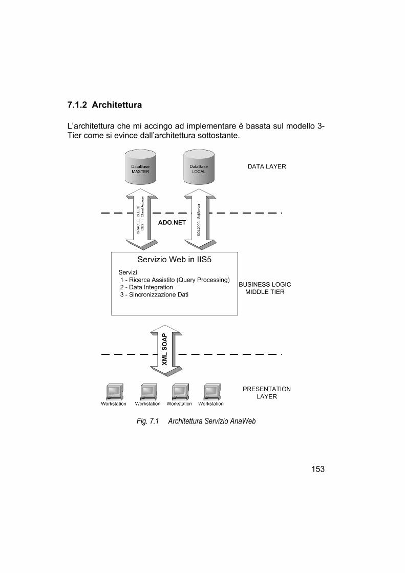
153

7.1.2 Architettura L’architettura che mi accingo ad implementare è basata sul modello 3-Tier come si evince dall’architettura sottostante.

Fig. 7.1 Architettura Servizio AnaWeb

154

Come si vede dalla figura il Servizio Web è uno strato che si pone tra i dati e i client. Particolarmente interessante notare come i client nel livello di presentazione comunichino con un protocollo non proprietario dando la possibilità a qualsiasi client scritto in qualsiasi linguaggio di utilizzare il servizio. Il servizio riceve una richiesta ben formattata, elabora la richiesta e restituisce con lo stesso protocollo una struttura dati che rappresenta la risposta. Come spiegato nel capitolo riguardante i Web Services il tutto opera in modo disconnesso al contrario delle tecnologie DCOM o RMI per garantire la massima scalabilità. L’efficienza sarà da verificare in quanto il servizio ha bisogno di essere ospitato da IIS per funzionare ed in attesa di provider diretti per Oracle e DB2 si è costretti a utilizzare provider OLE DB che come spiegato nel capitolo ADO.NET non hanno la stessa efficienza rispetto a un accesso diretto. Per questi motivi ho deciso di effettuare sincronizzazioni “On Demand”, cioè, sarà il client a decidere la ricerca, se opta per una ricerca nel database locale gli aggiornamenti potrebbero non essere disponibili, adottando l’altro approccio, cioè, la ricerca effettuata sul database orizzontale si ottengono dati aggiornati in tempo reale e simultaneamente un aggiornamento di questi nel database locale, naturalmente questo ultimo processo risulta penalizzato in termini di prestazioni. Per quanto riguarda il DBMS adottato per ospitare l’anagrafica locale le regole di mercato, la sua semplicità di utilizzo, la sua efficienza e soprattutto la sua forte integrazione con il nuovo framework .NET hanno fatto si che la scelta ideale fosse Microsoft SQL Server 2000.

155

7.2 Uno schema comune Come enunciato precedentemente lo scenario in cui mi sono trovato ad operare sono principalmente due, l’ospedale e le piccole realtà mediche che spesso condividono gli stessi applicativi adattati alle varie sorgenti anagrafiche. Sorgenti anagrafiche che spesso sono legate alle anagrafiche ospedaliere o nella piccola realtà è l’applicativo stesso che gestisce una propria anagrafica locale di minori dimensioni. Le due anagrafiche pur compiendo lo stesso compito adottano spesso schemi completamente differenti e persino tipi di dati differenti per memorizzare le stesse informazioni. Ci si trova nella situazione in cui quando una Software House intende vendere un applicativo in una nuova realtà è spesso costretta a dover modificare la struttura anagrafica in base ad una struttura già presente dal cliente con le conseguenze di dover applicare modifiche al sorgente distribuendo cosi diversi software replicando eventuali bug che una volta scoperti dovranno essere sistemati su tutte le versioni vendute. Per questo motivo si è giunti al punto in cui si è reso necessaria una struttura anagrafica completa, rigida che garantisca una base certa per gli sviluppatori, sarà compito del servizio tramite tecniche di “Data Integration” fare si che tutte le anagrafiche concorrano con questa per creare una “Vista Globale” su cui sviluppare gli applicativi futuri e su cui aggiornare gli applicativi esistenti. Lo schema comune adottato per questo progetto è stato formalizzato nel diagramma ER in figura 7.2.

156

Fig. 7.2 ER Schema Comune

7.3 Modello adottato Essendo l’anagrafe una delle strutture principali sia per i processi verticali che per quelli orizzontali e sullo schema di questa si appoggiano numerosi applicativi la struttura è ben definita a priori e poco incline a variazioni. Inoltre una successiva aggiunta di database esterni alla federazione formata dal database locale e dal database master è improbabile, quindi, la necessità di adottare un modello di tipo LAV risultava una forzatura che avrebbe enormemente complicato il processo di Query Processing.

157

Per questi motivi è stato scelto un modello di tipo GAV che grazie alla sua chiarezza e semplicità mi ha permesso di realizzare questo progetto. Come detto in precedenza il modello GAV necessita di una definizione per ogni elemento della vista globale, questo processo di mappatura tra la vista globale e le sorgenti dati è stato implementato in un file XML (FileMappingCfg.xml) che racchiude tutte le informazioni per la conversione della richiesta espresso sulla vista globale trasformandola in n richieste sui database che contengono le informazioni. In sostanza questo file configura il mediator. In particolare è stato adottato un file XML in quanto è un formato chiaro e soprattutto standard. Inoltre Microsoft nel suo ambiente .NET mette a disposizione un parser DOM che mi rappresenta in memoria sotto forma di albero quello definito in un file facilmente editabile dall’utente. . Il servizio alla partenza carica in memoria questo file che funge da “Mediator” tra i due database e la vista globale. La Query viene espressa sulla vista globale e tramite il “Mediator” viene formattata SQL per il database selezionato e successivamente eseguita. In dettaglio questo file è composto da quattro nodi:

• ServiceDef, in questo nodo vengono specificate le caratteristiche dei database partecipanti alla federazione ed in particolare si definisce la stringa di connessione per ADO e si definisce il database a cui ci si riferisce. Da notare che per ora sono specificabili esclusivamente due entità ConnectionMaster e ConnectionLocal.

• TablesDef, in questo nodo vengono definite le tabelle che verranno integrate nella vista globale, per ognuna di queste tabelle viene specificato in nome, lo schema a cui appartengono e viene specificato inoltre a che database sono connessi, cioè, se appartengono al database Master o Local.

• GLOBALVIEW, questo è il nodo cruciale per la definizione del mapping, qui ogni elemento della vista globale viene associato

158

a un campo di uno o più database appartenenti alla federazione siano questi Master o Local

• TabsLocalDef, questo nodo serve principalmente per dare una definizione alle tabelle accessorie del database locale che vogliamo aggiornare con dati provenienti dai database master, qui non vengono definite le regole di aggiornamento ma esclusivamente la struttura di esse.

Quando parleremo dell’implementazione del Query Processing entreremo nel dettaglio dell’implementazione del mapping per determinati tipi di dati. Ora entriamo nel dettaglio generale dei vari nodi figli del file di configurazione. Come enunciato precedentemente il file FileMappingCfg.xml è il configuratore per il “mediator”, nel nodo GLOBALVIEW troviamo la definizione della vista globale. Nel mio progetto questa vista globale è composta dai principali campi presenti in una qualsiasi anagrafica. Per il momento la nostra vista globale è definita da un’unica tabella ma in seguito questo verrà ampliato, per ora un corretto funzionamento del sistema è garantito anche con questa limitazione, la definizione di questa vista globale è la seguente: GLOBALVIEW(Id, IdEsterno, Nome, Cognome, Sesso, DataNascita, IdComuneNascita, DescrComuneNascita, TesseraSanitaria, IdStatoCivile, IdGradoIstruzione, IdNazionalita,…., Percentuale) Questa vista viene espressa nel file XML di configurazione in questo modo:

<GLOBALVIEW><Id> SourcesDefs </Id><IdEsterno> SourcesDefs </IdEsterno><Nome> SourcesDefs </Nome>

159

<Cognome> SourcesDefs </Cognome><Sesso> SourcesDefs </Sesso><DataNascita> SourcesDefs </DataNascita>. . .<Percentuale> SourcesDefs </Percentuale>

<GLOBALVIEW> Un approfondimento sulla configurazione del servizio verrà affrontata nel capitolo successivo, per ora è stato introdotto questo esempio di sintassi per mostrare l’approccio adottato nella definizione della vista globale. In effetti come impone il modello GAV ogni attributo appartenente alla vista globale rappresentato da un tag XML, viene espresso nel tag SourcesDefs che rappresenta le definizioni sui database partecipanti. Come vedremo meglio nei successivi capitoli, in particolar modo nel capitolo in cui parleremo del query processing la definizione degli attributi della vista globale è fondamentale nel processo di integrazione. Abbiamo precedentemente accennato che ogni attributo della vista globale può essere mappato su più database (GAV), inoltre lo stesso dato può differire per tipo o per rappresentazione, queste differenze vengono risolte al momento di integrazione nella vista globale.

7.4 Configurazione del Servizio In questo capitolo verrà data illustrato il sistema per configurare il servizio. Come detto precedentemente per configurare il servizio è necessario un file XML che contenga le regole per mappare i database appartenenti alla federazione sulla vista globale anch’essa definita nel file. Questo file è composto da una radice come imposto dallo standard W3C e da quattro nodi figli che rappresentano le impostazioni

160

principali per il servizio. Queste impostazioni verranno spiegate in questo e nel successivo capitolo. La struttura sottostante rappresenta lo scheletro del servizio già spiegato precedentemente.

<ConfigAnaWeb><ServiceDef>ServiceDef</ServiceDef><TablesDef>TabsDef</TablesDef ><GLOBALVIEW>GlobalDef<GLOBALVIEW><TablesLocalDef>TabsLocal<TablesLocalDef>

</ConfigAnaWeb> Ora entriamo nel dettaglio della configurazione analizzando il primo tag ServiceDef in cui si definiscono le caratteristiche dei database partecipanti alla federazione. Le informazioni fondamentali sono definite in questo tag che contiene le stringhe di connessione ADO che il servizio utilizzerà per collegarsi alle sorgenti dati e definisce il tipo di DBMS che il fornitore dati utilizza per poi poter generare query compatibili con tale sistema. Ad esempio nell’implementazione di una query SQL che richiede solo n tuple viene risolta su un databse SQLServer con l’istruzione SELECT TOP n, mentre su un database Oracle viene implementate con la clausola ROWNUM < n nella WHERE condition, o nel sistema DB2 tramite l’istruzione FETCH n ROWS ONLY. Per questo motivo risulta fondamentale sapere con che DBMS si interagisce.

<ServiceDef><ConnectionMaster> ConnDef</ConnectionMaster><ConnectionLocal> ConnDef</ConnectionLocal>

</ServiceDef> ConnDef::=

[<DataBaseVendor>AS400DB2|ORACLE|ACCESS

161

</DataBaseVendor>][<AllowFisicTop>

TRUE | FALSE</AllowFisicTop>][<AllowSoundex>

TRUE | FALSE</AllowSoundex>]

<ConnectionString>ADO ConnectionString

</ConnectionString>

L’opzione DataBaseVendor potrebbe risultare ridondante in quanto nella definizione di ADO ConnectionString è presente la definizione del Provider, ma questo verrà implementato in una versione futura. Il tag ADO ConnectionString richiede una connessione con Provider compatibile con OleDb e non accetta connessioni ODBC. Le definizioni AllowFisicTop e AllowSoundex specificano se il DBMS supporta le funzioni di SOUNDEX e la TOP, se queste funzioni non sono supportate direttamente dal DBMS come nelle vecchie versioni di DB2 su AS400 vengono simulate via software da ADO, per quanto riguarda la simulazione della TOP questa soluzione non minimizza ne il traffico di rete ne diminuisce il lavoro del mainframe. Il secondo tag TablesDef risulta fondamentale in quanto specifica le tabelle del database che partecipano all’integrazione definendone il nome e gli schemi a cui appartengono, per ora il progetto definisce esclusivamente due schemi a cui le tabelle possono essere collegate, il database Master e il database Local.

< TablesDef ><Table name= “Name”> TableDef</Table >

162

...<Table name=“Name”> TableDef</Table >

</ TablesDef > Il nome fisico della tabella viene riportato nell’attributo Name e le sue caratteristiche vengono specificate nel tag TableDef in questo modo:

TableDef ::=<SchemaName> Nome_Schema </SchemaName><Type> Master | Local </Type>

Prima di entrare nel punto cruciale della configurazione GLOBALVIEW già accennata nel capitolo precedente, analizzeremo il tag TablesLocalDef che vedremo elemento fondamentale nel processo di JOIN in fase di selezione, aggiornamento ed inserimento, in sostanza in questo tag vengono definite le tabelle del database locale che vengono utilizzate dal servizio. Queste tabelle sono molto importanti in quanto consentono al database locale che replica i dati del database master di essere normalizzato e quindi di evitare un’inutile replicazione dei dati. Una delle tabelle fondamentali rappresentate in questo tag è la tabella TComuni che racchiude le principali informazioni sui comuni italiani come il nome, la descrizione, il CAP e la provincia, questa tabella viene posta in relazione con la tabella Assistiti per diverse rappresentazioni come ad esempio per il comune di nascita, di residenza e di domicilio. Ecco come viene definito il tag:

< TablesLocalDef ><Table name=“TableName”

[schema=“SchemaName”]>FieldLocalDef...

163

FieldLocalDef</Table >...<Table name=“TableName”

[schema=“SchemaName”]>FieldLocalDef...FieldLocalDef

</Table ></ TablesLocalDef >

La definizione FieldsLocalDef avviene tramite un tag vuoto definito da attributi in questo modo:

FieldLocalDef ::=<Name_Field

type = “alpha | numeric | date”size = “Field_Size”[iskey = “0 | 1”][iskeyextern = “0 | 1”]/>

In questo tag vengono espressi due attributi fondamentali di questo servizio, attributi che ritroveremo anche nella definizione delle relazioni tra i campi della vista globale, questi attributi sono iskey eiskeyextern, sostanzialmente questi attributi sono fondamentali nel processo di inserimento e di aggiornamento / sincronizzazione dati. In particolare gioca un ruolo fondamentale nell’integrazione l’attributo iskeyextern che mantiene il legame dell’oggetto tra la sua rappresentazione nel database master e la corrispettiva rappresentazione nel database locale. Spesso il tag con l’attributo iskeyextern = “1” viene nominato IdEsterno in cui viene memorizzata la chiave della tupla originaria presente sul database

164

master, la tupla replicata in locale viene identificata dal campo con l’attributo iskey = “1” generalmente nominato Id di tipo contatore. Ora nel resto di questo capitolo approfondiremo la configurazione del tag GLOBALVIEW analizzando la struttura generale del mapping entrando nel dettaglio della configurazione semplice lasciando al capitolo successivo 7.5 il compito di analizzare alcuni aspetti particolari del processo di integrazione. Come detto precedentemente in questo tag viene definita la vista globale e le relazioni con database partecipanti. Questo tag è definito secondo la seguente sintassi:

< GLOBALVIEW >FieldDef...FieldDef

</ GLOBALVIEW >

FieldDef ::=<Name_GlobalField

[type = “alpha | numeric | date”][size = “Field_Size”][defaultdata = “Default_Data”]

TableFieldTypeDef...TableFieldTypeDef

</Name_GlobalField>

Sin da questo punto è fondamentale capire che ogni tag figlio di GLOBALVIEW rappresenta un campo della nostra vista globale, questo campo può esprimere un tipo nell’attributo type e può definire una dimensione nell’attributo size e infine può definire un valore di ritorno

165

espresso in defaultdata nel caso in cui il valore nel database sia NULL. Entrando nel cuore della configurazione definiamo il tag TableFieldTypeDef che rappresenta l’associazione tra l’elemento della vista globale e la rispettiva rappresentazione nel database; ogni elemento rappresenta una diversa rappresentazione in diverse tabelle.

TableFieldTypeDef ::=<Table

name=”TableName”[iskey = “0 | 1”][iskeyextern = “0 | 1”][localupdate = “0 | 1”][type = “alpha | numeric | date”][size = “Field_Size”][defaultdata = “Default_Data”]>FieldTypeDef

</Table>

FieldTypeDef ::=FieldDef | FieldMappingDef | FieldSplitDefFieldDateDef|FieldJoinDef| FieldAbstactDef

Alcune di queste definizioni verranno esposte nel successivo capitolo riguardante la fase di Query Processing, ora prenderemo in considerazione le definizioni meno complesse FieldDef eFieldMappingDef. Prima di questo è comunque bene soffermarci sulla definizione di TableFieldTypeDef e analizzare ogni singolo attributo, in particolare, nell’attributo name=”Name”, Name deve essere definito nel tag TablesDef. I tag facoltativi diventano obbligatori quando si definisce il database locale in quanto questi tag definiscono i parametri per una corretta operazione di INSERT o di

166

UPDATE. I due tag iskey e iskeyextern come nella definizione precedente servono per identificare la chiave nei database partecipanti e nella definizione del database locale la definizione di iskeyexternè fondamentale per tenere una relazione tra la chiave del database master e la sua rappresentazione nel database locale. A questo punto analizziamo il primo tipo di rappresentazione dati definito nel tag FieldDef, questa definizione potrebbe risultare forviante in quanto questa definizione viene applicata dal servizio quando non viene definita una corrispondenza sul database e in questo caso la vista globale riceve sempre un valore NULL o il valore espresso dal tag defaultdata se definito.

La prima vera definizione di mapping tra la vista globale e il database sorgente la troviamo nel tag FieldMappingDef dove si assume una corrispondenza biunivoca tra il campo della vista globale e la rappresentazione sul database, ad esempio il caso più ricorrente nelle varie configurazioni finora testate risulta nel tag IdEsterno mappato di volta in volta con la chiave dei database master e con il tag omonimo nel database locale. Ecco qui di seguito la definizione di questo tag: FieldMappingDef ::=

<DataMapping><SourceField>FieldName</SourceField>

</DataMapping>

Questa semplice definizione ha come unico requisito il fatto che il campo con nome FieldName deve esistere nella tabella definita dal tag padre nell’attributo TableName. L’eventuale conversione del tipo avviene implicitamente. Fino ad ora abbiamo analizzato la struttura principale della configurazione del servizio, questo progetto di integrazione anagrafica ha posto ulteriori problematiche di integrazione dovute principalmente ad alcune rappresentazioni di entità. Queste problematiche sono state

167

risolte definendo alcune specifiche di mapping particolari che vi saranno esposte nel prossimo capitolo, specifiche fondamentali per completare una corretta configurazione del servizio.

7.5 Implementazione Query Processing Nell’architettura implementata e avendo adottato un modello di tipo GAV, e come in ogni sistema di integrazioni questo processo è uno degli aspetti più delicati. Fortunatamente il mio sistema MDBMS è un sistema ridotto e formato da due entità, il database orizzontale del cliente e il nostro database verticale che corrisponde alla vista globale. I principali conflitti sorti sono esclusivamente conflitti di nome e raramente conflitti di tipo, in particolare i principali problemi nel adattare il database orizzontale a quello verticale sono stati:

• Problema gestione attributi complessi • Problema gestione date • Problema gestione relazioni

Il processo di mappatura per risolvere questi problemi consiste nell’editare un file XML definito nel capitolo precedente, il file che contiene le regole di mapping tra il database del cliente e la vista globale. Ora tenterò di spiegare l’approccio adottato per risolvere i problemi sopraelencati.

7.5.1 Gestione attributi complessi In alcune realtà non è stata rispettata la 1 NF in quanto non è vero che ogni componente di una tupla ha un valore atomico. In quasi tutti i database che ho avuto a disposizione il nome ed il cognome

168

dell’assistito erano memorizzati nello stesso attributo separati da un carattere speciale, invece, nella vista globale si è voluto come di consuetudine tenerli separati. Questa anomalia mi ha indotto a definire una nuova regola di mapping che rappresenti questa situazione e viene definita nel tag FieldSplitDef definito come segue:

FieldSplitDef ::=<Split>

<SourceField>FieldName</SourceField><CharSplitter>SpitChar</CharSplitter><Part>LEFT | RIGHT</Part>

</Split> Questa definizione definisce tre tag fondamentali, il primo SourceField che come per la definizione del mapping semplice identifica il nome del campo appartenente alla tabella definita dal tag padre che partecipa all’integrazione, il secondo e il terzo tag definiscono la rappresentazione del dato complesso e di conseguenza le regole per trasformare il dato e l’eventuale query associata sul campo. In particolare il tag CharSplitter identifica il carattere che divide le due informazioni definite erroneamente in un unico campo, e di conseguenza il tag Part definisce quale parte del dato complesso tenere in considerazione.

7.5.2 Gestione delle date Questa particolare regola di mapping si è resa necessaria esclusivamente nell’analisi della vista fornita dalla Siemens in cui i campi data come DataNascita vengono rappresentati da più campi numerici che rappresentano rispettivamente il giorno, il mese e l’anno.

169

Nella vista globale si è voluto utilizzare un singolo campo per definire le date utilizzando il tipo di dato più appropriato, il tipo DateTime definito in tutti i DBMS. In sostanza questo tag risolve il principale conflitto di tipo a me presentatomi risolto nel seguente tag: FieldDateDef ::=

<Date><Year>

<SourceField>FName</SourceField></Year><Month>

<SourceField>FName</SourceField></Month><Day>

<SourceField>FName</SourceField></Day>

</Date> Anche per questa regola FName abbreviazione di FieldName deve esistere nella tabella di appartenenza ed identificano rispettivamente il campo che rappresenta l’anno, il campo che rappresenta il mese e infine quello che rappresenta il giorno, all’interno della configurazione del servizio avviene una conversione del tipo al momento dell’aggiornamento del database locale e della raffigurazione nella vista globale, in particolare il servizio effettua la query sul database trattando la data come tre campi separati come da rappresentazione, successivamente al momento della risposta da parte del DBMS elabora le tuple ricevute, crea un nuova istanza System.DateTime del .NET framework inizializzata dalle informazioni ricevute, istanza poi utilizzata per aggiornare il database locale e utilizzata per rappresentare il responso della query nella vista globale. Facendo un breve riassunto, la query viene effettuata sulla vista globale che vede il campo DataNascita come un campo di tipo DateTime, la query riformulata sul master trasformando il tipo in tre

170

parametri di tipo numerico, effettua la query e riceve la risposta ritrasformando i tre campi in un unico campo di tipo DateTime. Se il tipo data non è valido viene ritornato un valore NULL.

7.5.3 Gestione delle relazioni Questo è il processo di mapping più delicato ed introduce due tipi di regole definite rispettivamente da FieldJoinDef eFieldAbstactDef, l’una diretta conseguenza dell’altra. Questa regola si è resa fondamentale in quanto generalmente la tabella sorgente non è sufficientemente espressiva per definire una vista globale utile allo sviluppatore, in particolare questo problema si è verificato nel momento in cui oltre a conoscere l’identificativo del paese di nascita IdComuneNascita si vuole ottenere anche il nome di questo comune, nome memorizzato in una tabella esterna in relazione con la tabella originaria. Inoltre anche nel database locale per mantenere la normalizzazione queste informazioni devono essere memorizzate in tabelle accessorie grazie alle quali si evitano i classici problemi di ridondanza dei dati. Iniziamo con la definizione formale del tag principale:

FieldJoinDef ::=<Join>

<DestTableName>TableExternName

</DestTableName><DestMatchField>

TableExternFieldName</DestMatchField>

171

<SourKeyField>TableFieldName

</SourKeyField>

[<LocalJoinTableMatch>TableLocalName

</LocalJoinTableMatch><LocalJoinFieldMatch>

FieldKeyMasterName</LocalJoinFieldMatch><LocalJoinReturn>

FieldKeyLocalName</LocalJoinReturn>]

[<TableReturn>FieldTableReturn...FieldTableReturn

</TableReturn>]

[<TableUpdate name="TableLocalName”>FieldTableUpdate...FieldTableUpdate

</TableUpdate>]</Join>

FieldTableReturn ::=<Field>

<FieldName>FieldMasterName

</FieldName>

172

<Alias>FieldAliasName

</Alias></Field>

FieldTableUpdate ::=<Field>

<FieldDest>FieldLocalName

</FieldDest><FieldSource>

FieldAliasName |FieldMasterName

</FieldSource></Field>

Si nota immediatamente che la configurazione di questa regola non è particolarmente intuitiva, anzi, necessita di un’approfondita analisi. Si nota come prima cosa che la metà dei tag risultano facoltativi nella forma, ma vedremo in fine che sono fondamentali per un corretto processo di integrazione. I primi tre tag DestTableName, DestMatchField, SourKeyField sono obbligatori e definiscono rispettivamente la tabella accessoria definita nello schema di appartenenza della tabella definita nel tag padre, il secondo tag identifica la chiave della tabella che andrà in JOIN 1:1 con il campo definito nel terzo tag appartenente alla tabella definita nel tag padre. I tre tag LocalJoinTableMatch, LocalJoinFieldMatch,LocalJoinReturn risultano non obbligatori ma sono fondamentali in quanto unificano in caso di difformità di chiave nelle tabelle accessorie. Per spiegare meglio questo concetto mi aiuterò con un esempio; la

173

rappresentazione della tabella accessoria dei comuni appare sia nel database master RCODCOM con chiave RCOM6 sia nel database locale TComuni con chiave IdComune, IdComune e RCOM6 possono coincidere rendendo di fatto inutile la definizione di questi tre tag, nel caso che queste due chiavi differiscano nel valore vengono mantenute in relazione da un terzo attributo IdEsterno che mappa uno ad uno gli elementi presenti in RCODCOM. In questo caso definendo in LocalJoinTableMatch il nome della tabella locale, in LocalJoinFieldMatch il nome del campo appartenente alla tabella locale che mantiene la relazione con la tabella definita nel master, nel nostro caso IdEsterno e per finire in LocalJoinReturn definire il nome del campo che restituisce il valore da restituire alla vista globale. Questo processo è fondamentale nel caso in cui la chiave nel database master differisca dalla vista globale nel tipo, cioè, se ad esempio vogliamo che nella vista globale l’identificativo del comune di nascita sia di tipo numerico e nel database master sia rappresentato da un tipo di tipo alfanumerico, allora possiamo nella copia locale TComuni definiame IdEsterno come alfanumerico, IdComune come numerico e definire la regola in caso di ricerca su master di convertire il valore di ritorno alfanumerico espresso nella chiave di RCODCOM mappato nell’attributo IdEsterno di TComuni, ritornando il valore numerico espresso in IdComune coerentemente con la definizione della vista globale. Questo processo di conversione di valore di chiave risulta pesante ma necessario, pesante perché per ogni valore del risultato della query si deve eseguire una query su TComuni per ottenere la conversione della chiave. Ora passeremo a definire gli ulteriori tag non obbligatori definiti in FieldTableReturn e in FieldTableUpdate, nel primo tag vengono definite le ulteriori informazioni che vogliamo importare dalla tabella accessoria partecipante all’integrazione rendendo di fatto questi campi di tipo astratto, nel secondo tag si definiscono le eventuali sincronizzazioni tra la tabella accessoria mastrer e la tabella accessoria locale.

174

Approfondendo FieldTableReturn si capisce come questo tag crea un insieme di attributi astratti fondamentali in tutto il contesto di integrazione. Questo tag definisce un insieme di campi appartenenti alle tabelle accessorie che devono far parte dell’integrazione come ad esempio la denominazione del comune di nascita. In particolare questo tag definisce tanti tag figli, tanti come il numero di campi della tabella accessoria che partecipano all’integrazione nella vista globale o partecipano alla sincronizzazione della tabella accessoria locale. Per ognuno di questi tag figli vengono definiti due tag FieldName eAlias che rappresentano rispettivamente il nome del campo appartenente alla tabella accessoria definita in DestTableName e in Alias viene definito il nome univoco che verrà utilizzato sotto forma di campo astratto. Il tag TableUpdate definisce l’attributo name in cui viene definito il nome della tabella locale da sincronizzare, la struttura della tabella deve essere definita nel tag TablesLocalDef spiegato nel capitolo precedente, inoltre questo tag definisce la lista dei campi della tabella accessoria nel database locale da aggiornare, campi definiti nel tag FieldDest associandoli uno ad uno con un campo appartenente al database master o ad un campo definito astratto nel tag FieldSource.

7.5.4 Gestione campi astratti Un accenno di questo tipo è già stato affrontato nel capitolo riguardante la gestione delle relazioni. Questo tipo di campo è il risultante di un processo di JOIN per la definizione di un determinato tipo di campo e viene identificato univocamente dal nome definito nel tag Alias. Questo campo risultante da un processo di JOIN con una tabella accessoria può essere utilizzato per definire un elemento della vista globale in questo modo:

175

FieldAbstactDef ::=

<Abstract><SourceField>FieldName</SourceField>

</Abstract> Nel tag SourceField viene definito FieldName che rappresenta il nome del campo astratto che contiene il valore da inviare alla vista globale. Il valore di FieldName deve esistere e può essere un nome definito in un tag Alias o può contenere il valore Percentuale che è un campo definito nel servizio e serve per indicizzare la qualità della risposta nel caso si faccia una ricerca di tipo avanzato spiegata nel capitolo 7.8.

7.6 Implementazione Sincronizzazione Dati Il sistema sanitario è eterogeneo non solo nei tipi dati ma anche nei metodi in cui questi dati si aggiornano. In alcune realtà i dati aggiornati sono riconoscibili tramite il campo “Progressivo Modifica”, in altre realtà non abbiamo a disposizione nessuna informazione che questa modifica sia avvenuta. Inoltre la sincronizzazione dei dati richiede più tempo rispetto ad una normale scansione sul disco locale, quindi minimizzare gli accessi OLE DB al database master è da preferire, purtroppo a volte questo processo è essenziale. Ho implementato due metodi per aggiornare il database locale:

• “On Demand”, utilizzato in particolar modo quando vogliamo dati sempre aggiornati

• “Schedulato”, quando siamo in presenza di un sistema lento e non vogliamo sovraccaricare la rete.

176

7.6.1 Sincronizzazione “On Demand” Questo tipo di sincronizzazione viene utilizzato principalmente quando non abbiamo a disposizione informazioni che ci mettano nella possibilità di capire se un record è stato cambiato, oppure, quando vogliamo essere sicuri che i dati siano il più possibile aggiornati. Questo processo è computazionalmente pesante in quanto il processo si svolge principalmente in quattro fasi:

• Il servizio riceve una richiesta basata sulla “Vista Globale” • Il servizio implementa il “wrappers” generando due query

compatibili con gli schemi dei database che contengono i dati • Esegue le query sui database • Il servizio implementa il “mediators” combinando le risposte

ottenute dalle query ed aggiorna il database locale. Questo processo è rappresentato graficamente nello schema sottostante.

177

Fig.7.3 UML Sincronizzazione

Alla fine di questo processo il Client riceve un oggetto DataSet in XML (vedi Capitolo 5.3) il più possibile sincronizzato con il database messo a disposizione dai software orizzontali, inoltre otteniamo una sincronizzazione del database locale.

178

7.6.2 Sincronizzazione “Schedulata” Al contrario del metodo “On Demand” questo metodo è implementato in modo indiretto, cioè, un demone esterno a intervalli stabiliti esegue una richiesta particolare che aggiorni il database locale. Questo approccio è da preferirsi quando si vuole salvaguardare le prestazioni e quando si hanno a disposizione attributi che identifichino i record da aggiornare. Gli scenari che si possono presentare sono principalmente due, il primo già enunciato, quando abbiamo a disposizione dati che ci identifichino in maniera precisa quali record sono stati modificati e invece il secondo scenario in cui non sappiamo a priori quali sono stati modificati. Lo scenario in cui ci si trova cambia il modo di schedulare l’aggiornamento. Nella prima ipotesi essendo a conoscenza dei record modificati si può fare un demone che memorizzi l’ultimo progressivo di modifica e a tempi regolari (15 minuti ad esempio ) esegua una query sul database del cliente chiedendo una sincronizzazione per quei record che hanno il progressivo di modifica maggiore di quello memorizzato, una volta eseguita questa sincronizzazione nel demone verrà memorizzato il progressivo maggiore. Questo metodo risulta l’ideale compromesso tra sovraccarico della rete e validità dei dati. Purtroppo senza l’informazione di progressivo modifica questo metodo è inapplicabile. Nel secondo scenario essendo all’oscuro di eventuali modifiche si dovrebbe verificare l’intero database. Si comprende benissimo che è inaccettabile eseguire questa sincronizzazione ad intervalli brevi e soprattutto durante le ore in cui le reti sanitarie sono più sovraccaricate, questa sincronizzazione arresterebbe completamente tutto il sistema quindi fino ad oggi queste sincronizzazioni vengono effettuate durante gli orari notturni quando nessun utente ha necessità di utilizzare il servizio. Questa situazione inoltre non garantisce una

179

validità dei dati completa, anche per questo è l’opzione da tenere per ultima privilegiando eventualmente un approccio “On Demand”.

7.7 Sicurezza Nel capitolo 4.3 abbiamo analizzato i principali metodi di autenticazione per limitare l’utilizzo del servizio a coloro che ne hanno i permessi per farlo. Per implementare la sicurezza di utilizzo viene sfruttata la gestione integrata in IIS, questo ci permette di modificare le modalità di accesso senza modificare il sorgente del servizio. Per quanto riguarda la sicurezza sulla comunicazione tra il client e il servizio sappiamo che l’architettura utilizza il protocollo SOAP per scambiarsi le informazioni, sappiamo inoltre che il protocollo SOAP è strutturato su XML. Purtroppo utilizzando XML sul canale di comunicazione passano pacchetti contenenti le informazioni in chiaro, informazioni anagrafiche soggette alla normativa sulla privacy, una situazione di questo tipo è inaccettabile per questo si è dovuto implementare un meccanismo di criptaggio e decriptaggio delle informazioni. Fino ad ora W3C non ha definito per SOAP uno standard per la sicurezza ma si possono implementare tecniche custom per raggiungere un livello di sicurezza adeguato. In una prima analisi si potrebbe utilizzare le potenzialità di IIS utilizzando un certificato SSL per garantire un canale sicuro, questa soluzione potrà risultare la scelta definitiva in un secondo momento, per ora la sicurezza è stata implementata utilizzando l’algoritmo DES che utilizza una coppia di chiavi simmetriche, chiavi che devono essere a conoscenza dei vari client. Il .NET framework mette a disposizione una infrastruttura ideale per applicare questo tipo di sicurezza. In particolare il framework mette a disposizione una classe SoapExtension che può essere utilizzata per estendere SOAP, questa classe permette di leggere o modificare il

180

messaggio SOAP in un preciso momento come ad esempio prima della serializzazione. Tutte le estensioni a SOAP come quella implementata per la sicurezza deve ereditare la classe sopra citata. Inoltre in .NET framework mette a disposizione nel namespace System.Security.Cryptography l’implementazione dei principali algoritmi di crittografia, la scelta dell’algoritmo DES è stata dettata da un buon livello di sicurezza ed ad una elevata efficienza. Il processo di conversione tra oggetti e XML è conosciuto con il nome di serializzazione, ed il processo di ricostruzione dell’oggetto da XML è detto deserializzazione. Il modulo che esegue questa conversione è XmlSerializer. Utilizzando questo modello raffigurato nella figura sottostante mostro come ho implementato un livello di sicurezza adeguato. DES Data Encryption Standard è tra gli algoritmi disponibili uno dei più apprezzati per la codifica e decodifica dei dati. DES è una cifratura sviluppata dal governo degli Stati Uniti negli anni 70 per essere l’algoritmo ufficiale di crittografia degli Stati Uniti. Triple DES codifica il dato in tre passaggi usando l’algoritmo DES. DES è veloce ed efficiente per trasferimenti di dati in grosse quantità e cosi risulta una eccellente scelta per uso in dispositivi di crittografia della rete.

Fig. 7.4 Serializzazione SOAP

181

Come accennato precedentemente grazie alle SOAP Extension possiamo avere accesso prima e dopo che l’oggetto venga convertito in e da XML. Questo meccanismo ha permesso di implementare le due funzioni Enctypt e Decrypt e di inserirle nel punto ottimale, cioè, prima che il flusso dei dati passi attraverso la rete. Successivamente ci soffermeremo brevemente sulle due funzioni, ora verrà mostrato il grafico UML fra la comunicazione tra client e middleware mostrando la sequenza di metodi invocati tra i partecipanti quando viene invocata una richiesta di ricerca.

182

Fig. 7.5 Ruolo PROXY per implementare la Sicurezza

183

Come si può dedurre dal grafico e come precedentemente detto per utilizzare le SOAP Extension si deve implementare una classe che la erediti. Questa classe come si evince anche dalla figura viene inizializzata e passa per le due funzioni virtuali ChainStream e ProcessMessage che verranno sottoposte a ovveride in questo modo:

public override Stream ChainStream(Stream stream) {oldStream = stream;newStream = new MemoryStream();return newStream;

}

In questo override di funzione prendo il flusso di dati originario e lo rendo globale assegnandolo alla variabile oldStream, allo stesso momento istanzio un nuovo stream newStream che servirà ad accogliere i dati risultanti dalla criptazione o dalla decriptazione. La seconda funzione in ordine di tempo è la seguente anch’essa sottoposta ad override in questo modo:

public override void ProcessMessage(SoapMessage message){

switch (message.Stage) {case SoapMessageStage.BeforeSerialize:

break;

case SoapMessageStage.AfterSerialize:// Encrypt the data before serializing// it to the clientEncrypt();break;

case SoapMessageStage.BeforeDeserialize:// Decrypt the data before Deserializing// it as .NET Objects

184

Decrypt();break;

case SoapMessageStage.AfterDeserialize:break;

default:throw new Exception("Invalid Stage");

}}

Questa funzione ci permette di implementare la sicurezza in quanto intercetta il messaggio dandoci informazioni sullo stato, informazioni che ci danno la possibilità di operare sullo stream precedentemente istanziato. Le funzioni Encrypt() e Decrypt() possono essere implementate a piacimento, è invece a mio avviso interessante notare la facilità con cui l’ambiente .NET nel suo pacchetto Cryptography ci metta a disposizione classi per implementare la crittografia, nel seguito le due funzioni principali da me implementate per trasformare una stringa in un array di byte criptati e per ritrasformare questo array in stringa:

//Decrypt Dataprivate byte[] DecryptData(string stringToDecrypt) {

//Create a new DES Crypto providerDESCryptoServiceProvider des = new

DESCryptoServiceProvider();

//Convert the input string into byte array for decryptionbyte[] inputByteArray =

CovertStringToByteArray(stringToDecrypt);

MemoryStream ms = new MemoryStream();

//Create a crypto stream and pass the new memory//stream and new decrypter object using then custom key//and vector

185

Byte[] IV = { 0x01, 0x23, 0x45, 0x67, 0x89, 0xab,0xcd, 0xef};

Byte[] key = { 0x12, 0x34, 0x56, 0x78, 0x90, 0xab,0xcd, 0xef};

CryptoStream cs = new CryptoStream(ms,des.CreateDecryptor( key, IV ),CryptoStreamMode.Write);

//Write the decrypted stream into the crypto streamcs.Write(inputByteArray, 0, inputByteArray.Length);cs.FlushFinalBlock();

//Return the decrypted byte array backreturn ms.ToArray();

}

//Encrypt Dataprivate byte[] EncryptData(string stringToEncrypt) {

//Create a new DES Crypto providerDESCryptoServiceProvider des = new

DESCryptoServiceProvider();

//Convert the string into byte array for encryptionbyte[] inputByteArray =

Encoding.UTF8.GetBytes(stringToEncrypt);

MemoryStream ms = new MemoryStream();

//Create a crypto stream and pass the new memory stream//and new decrypter object using then custom key and//vector

Byte[] IV = { 0x01, 0x23, 0x45, 0x67, 0x89, 0xab,0xcd, 0xef};

Byte[] key = { 0x12, 0x34, 0x56, 0x78, 0x90, 0xab,0xcd, 0xef};

CryptoStream cs = new CryptoStream(ms,des.CreateEncryptor( key, IV ),CryptoStreamMode.Write);

186

cs.Write(inputByteArray, 0, inputByteArray.Length);cs.FlushFinalBlock();

//Return the Encrypted byte array backreturn ms.ToArray();

}

La semplicità e la chiarezza di questa implementazione è tale grazie al framework che ci mette a disposizione CryptoStream, una speciale classe che gestisce stream crittografati il cui costruttore è costituito da tre parametri, un stream di tipo MemoryStream in cui memorizza i dati elaborati dal provider, il provider fornisce una funzione che implementa l’interfaccia di trasformazione ICryptoTransformpassatagli come secondo parametro, nel nostro caso è un metodo appartenente all’istanza di DESCryptoServiceProvider, il terzo parametro specifica se si ha un accesso in lettura o in scrittura ad un oggetto stream crittografato. La principale limitazione di questo approccio alla sicurezza riguarda l’obbligo per ogni client di avere l’implementazione di questa classe, classe in cui devono essere anche definite le chiavi simmetriche utilizzate dall’algoritmo DES.

7.8 Stato dell’Arte Fino a questo punto è stato esposto il servizio da un punto di vista riguardante esclusivamente gli aspetti di integrazione dati, un breve accenno alla ricerca assistito è stata trattata nel capitolo riguardante la sincronizzazione dati in cui si faceva riferimento all’aggiornamento “OnDemand”, come ricorderete la sincronizzazione avveniva tramite una ricerca mirata sul database master e la risposta integrata nella vista globale concorreva al processo del database locale. L’intera architettura è basata sul processo di ricerca che scatena il servizio, in

187

effetti l’interfaccia pubblica del servizio è sostanzialmente formato da due funzioni che hanno come parametri i criteri per una individuazione del paziente. In particolare sono state implementate due modalità di ricerca:

• Ricerca Semplice • Ricerca Avanzata

Entrambe queste ricerche avvengono sui campi definiti nella vista globale, il primo tipo di ricerca avviene specificando tutti le clausole della ricerca ottenendo una ricerca mirata come ad esempio per sapere chi è nato in un determinato giorno o a chi appartiene un determinato identificativo; la seconda ricerca che come vedremo in seguito si appoggia sulla prima richiede solo i campi su cui effettuare la ricerca ed i valori associati a questi campi, il servizio cerca in modo intelligente, modificando i criteri, partendo da criteri molto restrittivi per giungere in casi di necessità ai criteri più lassi escludendo volta per volta i record già individuati nelle ricerche precedenti. Nei prossimi capitoli entreremo nel dettaglio di questi tipi di ricerche.

7.8.1 Ricerca Semplice In questo capitolo si fonda la struttura principale del servizio, in questo capitolo verrà mostrato il “mediator” tra la vista globale e la reale rappresentazione dei dati. Il metodo migliore per spiegare questo processo é quello di iniziare mostrando la funzione che implementa questa ricerca:

[WebMethod]public DataSet SimpleSearch(FieldRequestSimple req){...}

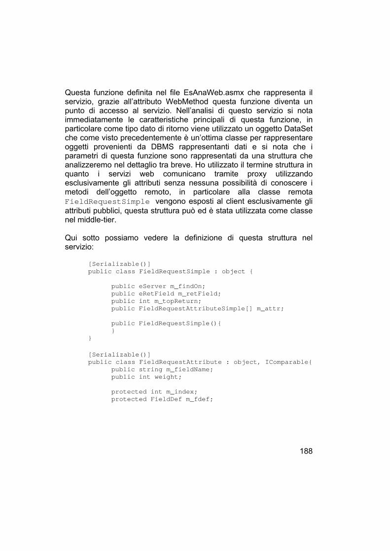
188

Questa funzione definita nel file EsAnaWeb.asmx che rappresenta il servizio, grazie all’attributo WebMethod questa funzione diventa un punto di accesso al servizio. Nell’analisi di questo servizio si nota immediatamente le caratteristiche principali di questa funzione, in particolare come tipo dato di ritorno viene utilizzato un oggetto DataSet che come visto precedentemente è un’ottima classe per rappresentare oggetti provenienti da DBMS rappresentanti dati e si nota che i parametri di questa funzione sono rappresentati da una struttura che analizzeremo nel dettaglio tra breve. Ho utilizzato il termine struttura in quanto i servizi web comunicano tramite proxy utilizzando esclusivamente gli attributi senza nessuna possibilità di conoscere i metodi dell’oggetto remoto, in particolare alla classe remota FieldRequestSimple vengono esposti al client esclusivamente gli attributi pubblici, questa struttura può ed è stata utilizzata come classe nel middle-tier. Qui sotto possiamo vedere la definizione di questa struttura nel servizio:

[Serializable()]public class FieldRequestSimple : object {

public eServer m_findOn;public eRetField m_retField;public int m_topReturn;public FieldRequestAttributeSimple[] m_attr;

public FieldRequestSimple(){}

}

[Serializable()]public class FieldRequestAttribute : object, IComparable{

public string m_fieldName;public int weight;

protected int m_index;protected FieldDef m_fdef;

189

protected TableFieldsDef m_tableDef;

public FieldRequestAttribute(){ }

public FieldRequestAttribute(TableFieldsDeftableDef, int index){...

}

...

public int CompareTo(object obj) {...}}

[Serializable()]public class FieldRequestAttributeSimple :

FieldRequestAttribute {public eOperation m_op;public eBOperation m_bop;public object arg1;public object arg2;

public FieldRequestAttributeSimple() : base (){...

}

public FieldRequestAttributeSimple(TableFieldsDeftableDef, int index) : base(tableDef, index){...

}

...}

Della definizione di questa classe viene serializzata e mostrata al client in questo modo:

<?xml version="1.0" encoding="utf-8"?><soap:Envelopexmlns:xsi="http://www.w3.org/2001/XMLSchema-instance"

190

xmlns:xsd="http://www.w3.org/2001/XMLSchema"xmlns:soap="http://schemas.xmlsoap.org/soap/envelope/"><soap:Body><SimpleSearch xmlns="http://tempuri.org/"><request><m_findOn>LOCAL or MASTER</m_findOn><m_topReturn>int</m_topReturn><m_attr><FieldRequestAttributeSimple><m_fieldName>string</m_fieldName><m_bop>AND or OR</m_bop><m_op>operation</m_op><arg1 /><arg2 />

</FieldRequestAttributeSimple><FieldRequestAttributeSimple><m_fieldName>string</m_fieldName><m_bop>AND or OR</m_bop><m_op>operation</m_op><arg1 /><arg2 />

</FieldRequestAttributeSimple></m_attr>

</request></SimpleSearch>

</soap:Body></soap:Envelope>

operation ::= EQUAL or GREATER or GREATER_EQUAL or LESS

or LESS_EQUAL or BETWEEN or LIKE or ISNULLor DIFFERENT or SOUNDEX or BEGINNODEor ENDNODE

Da questa struttura si notano immediatamente le tre caratteristiche principali che sono alla base del servizio e che ne indirizzano il comportamento, questa struttura risponde alle domande che il servizio pone:

• Dove vuoi cercare? • Quanti record ti devo restituire? • In base a che criteri devo cercare?

191

Le risposte a queste domande completano con dati la struttura che viene inviata al servizio che la elabora, verifica eventuali errori e tramite il GAV query processing crea le query sugli schemi delle sorgenti dati, esegue le query, le fonde nella vista globale e restituisce il risultato di questa fusione. In particolare il nodo principale di questo progetto è quello di disegnare le query espresse sulla vista globale in query sui dati e di riconvertire questi risultati nella vista globale. Per ottenere questo processo è stata fondamentale la precedente definizione della vista globale trattata nel capitolo 7.5. Il resto del capitolo spiegherà il processo di conversione tra la richiesta del client e la creazione della query. In particolare questo processo consiste in due parti:

• Disegnare la query rispetto allo schema delle sorgenti dati • Passare i parametri alla query precedentemente calcolata

Disegnare la query rispetto allo schema delle sorgenti dati è un processo relativamente facile avendo utilizzato il modello GAV in quanto la creazione della struttura portante della query avviene a Design Time nel file di definizione FileMappingCfg.xml mentre a Run Time avviene l’integrazione delle clausole di ricerca inviati dalla struttura creando di fatto una query pronta da essere inviata. Da questo si capisce che il processo di design della query avviene in due momenti distinti:

• La struttura portane a Design Time • Il completamento con l’integrazione delle clausole a Run Time

Il processo di Design della struttura avviene grazie alla struttura in memoria del servizio, struttura generata dal file FileMappingCfg.xml che come visto precedentemente definisce il mapping tra ogni singola

192

voce della vista globale e la rappresentazione nelle sorgenti dati in particolare la struttura in memoria è formata da un’istanza della classe GlobalView la quale contiene a sua volta l’insieme delle definizioni dei campi della vista globale gestite nell’istanza della classe FieldGlobalList ereditata dalla classe ArrayList specializzata per gestire istanze del tipo FieldGlobalDef che rappresentano i singoli campi della vista globale (vedi capitolo 7.3 nella definizione del tag GLOBALVIEW). A sua volta ogni istanza di FieldGlobalDef definisce al suo interno un Array con le definizioni per ogni singola sorgente dati, definizioni che possono essere quelle espresse nel capitolo 7.4 e 7.5. La rappresentazione di questa struttura viene espressa graficamente dal seguente diagramma UML.

193

Fig. 7.6 UML delle Classi Principali

194

Con l’aiuto del grafico UML nella figura 7.6 tenterò di spiegare il processo di Query Design. Innanzi tutto una parte della query viene fatta a Design Time, questo processo avviene nella funzione CalcolaSELECT() definita nella classe TableFieldsDef seguendo i seguenti passi; per ogni elemento TableFieldsDef in TablesFieldsDef viene creata una classe temporanea GlobalRequest la quale contiene una propria definizione di TablesFieldsDef che contiene solo le definizione dei campi appartenenti alla tabella, a questo punto invocando la funzione CalcolaSELECT() vengono invocati i metodi polimorfici delle istanze delle classi rappresentanti i singoli campi, i metodi GetStr_SELECT(), GetStr_FROM(), GetStr_WHERE() combinati formano la struttura della query. Una volta creato questo scheletro si deve adattare la query alle richieste provenienti dal client ed in particolare le restrizioni da apportare alla query. Prima di entrare in questo delicato processo si noti che questo processo risponde alla domanda che chiedeva dove cercare, in effetti grazie al parametro m_islocal in TableFieldsDef possiamo filtrare la nostra classe temporanea GlobalRequest solo sulle tabelle che rappresentano il database locale o il database master. Alla domanda quanti record vuoi che ti vengano restituiti si risponde facilmente applicando la clausola TOP n o ROWNUM < n o FETCH n ROWS ONLY in base al tipo di DBMS che ospita la tabella. Il processo che trasforma l’array m_attr in clausole compatibili con lo standard SQL avviene grazie alla funzione polimorfica SqlWriteAttribute() definita nella classe FieldDef la quale viene invocata per ogni elemento definito in m_attr. Come accennato precedentemente ogni elemento di m_attr è una istanza della struttura FieldRequestAttributeSimple nella quale viene definito in m_fieldName il nome del campo appartenente alla vista globale, in m_op l’operazione da compiere, in m_bop il vincolo booleano con l’attributo precedente e in arg1 e arg2 i valori per la query, esistono due valori speciali BEGINNODE ed ENDNODE che rappresentano rispettivamente parentesi aperta e parentesi chiusa.

195

Una volta compiuto questo processo di trasformazione otteniamo una query completa e parametrizzata (vedi appendice C), il nome del parametro viene calcolato a RunTime e nella funzione polimorfica SqlSetParameter() vengono legati i valori tipizzati espressi in arg1 e arg2. Una volta legati i parametri alla classe SqlCommand o OleDbCommand dove è stata espressa la query completa di vincoli può essere invocato il metodo Fill() della classe DataAdapter ed ottenere così i dati desiderati. Una volta eseguito il metodo, il servizio ottiene un oggetto DataSet contenente i dati espressi sullo schema della fonte dati, ora il passo successivo consiste nella trasformazione dello schema di questo oggetto per renderlo compatibile con la vista globale, di questo processo se ne fa carico la classe temporanea GlobalRequest che per ogni elemento FieldDef in FieldList chiama la funzione polimorfica GetGlobalSynkValue() la quale si incarica di trasformare il dato e di copiarlo nell’attributo della vista globale. Ora abbiamo ottenuto una risposta espressa sulla vista globale il passo successivo non obbligatorio è la sincronizzazione del database locale che avviene tramite la funzione ExecuteSyncGlobal2Local() appartenente all’istanza della classe GlobalView. A questo punto l’istanza della classe temporanea GlobalRequest viene disallocata in quanto il processo di interrogazione è concluso e il servizio può restituire l’oggetto DataSet contenente i dati contenuti nello schema della vista globale. Nel successivo capitolo verrà mostrato il processo di interrogazione avanzato che si basa interamente su questo tipo di ricerca con qualche aggiunta.

196

7.8.1 Ricerca Avanzata Questo tipo di ricerca nasce per risolvere uno dei principali problemi dei sistemi sanitari, l’identificazione di un paziente in un sistema non privo di errori, per questo si è voluto un metodo che nonostante i possibili errori di inserimento dati o di interrogazione restituisse un determinato numero di assistiti che rispondessero nel miglior modo possibile ai parametri inseriti ed alla fine del processo restituisse un insieme di assistiti con la relativa percentuale di assonanza alla richiesta. Questa ricerca può essere considerata intelligente in quanto non richiede a priori le operazioni sugli attributi ne il legame booleano tra essi, il servizio in modo “intelligente” cerca di combinare gli attributi per generare query partendo da un criterio ristretto per giungere ad un criterio ampio. Questo modello di ricerca si fonda totalmente sul modello di ricerca semplice; prima di addentrarci nella spiegazione di questo tipo di ricerca può essere utile, come fatto precedentemente, mostrare la funzione che implementa questa ricerca e mostrare la definizione della classe che questa funzione accetta come parametro:

[WebMethod]public DataSet AdvancedSearch(FieldRequestAdvanced req){

...}

[Serializable()]public class FieldRequestAdvanced : object {

public eServer m_findOn;public int m_topReturn;public FieldRequestAttributeAdvance[] m_attr;public FieldRequestAttributeSimple[] m_attrsimple;

public FieldRequestAdvanced(){}

}

[Serializable()]public class FieldRequestAttributeAdvance :

197

FieldRequestAttribute {public object arg1;

public FieldRequestAttributeAdvance() : base (){...

}

public FieldRequestAttributeAdvance(TableFieldsDeftableDef, int index) : base(tableDef, index){...

}}

La prima cosa da notare analizzando queste strutture consiste nell’osservare che anche la ricerca avanzata chiede dove cercare, quanti valori restituire e specifica su che campi cercare, ma la cosa che differenzia maggiormente questo approccio dal precedente consiste nella definizione dell’attributo avanzato definito in FieldRequestAttributeAdvance, in questa definizione viene specificato esclusivamente su che attributo cercare con m_fieldNameereditato dalla classe padre ed il valore in arg1; è inoltre stato inserito un array di attributi semplici che seguono il comportamento della ricerca precedente. Di seguito ecco riportato la serializzazione dell’oggetto contenente i parametri di richiesta:

<?xml version="1.0" encoding="utf-8"?><soap:Envelopexmlns:xsi="http://www.w3.org/2001/XMLSchema-instance"xmlns:xsd="http://www.w3.org/2001/XMLSchema"xmlns:soap="http://schemas.xmlsoap.org/soap/envelope/"><soap:Body><AdvancedSearch xmlns="http://tempuri.org/">

<request><m_findOn>LOCAL or MASTER</m_findOn><m_topReturn>int</m_topReturn><m_attr>

<FieldRequestAttributeAdvance><m_fieldName>string</m_fieldName>

198

<weight>int</weight><arg1 /></FieldRequestAttributeAdvance><FieldRequestAttributeAdvance><m_fieldName>string</m_fieldName><weight>int</weight><arg1 />

</FieldRequestAttributeAdvance></m_attr><m_attrsimple><FieldRequestAttributeSimple>

<m_fieldName>string</m_fieldName><m_bop>AND or OR</m_bop><m_op>operation</m_op><arg1 /><arg2 />

</FieldRequestAttributeSimple><FieldRequestAttributeSimple>

<m_fieldName>string</m_fieldName><m_bop>AND or OR</m_bop><m_op>operation</m_op><arg1 /><arg2 />

</FieldRequestAttributeSimple></m_attrsimple>

</request></AdvancedSearch>

</soap:Body></soap:Envelope>

Ora che abbiamo analizzato i parametri di ricerca possiamo addentrarci nel cuore dell’algoritmo che ricerca l’assistito. Per non appesantire eccessivamente la ricerca sono stati definiti cinque combinazioni di query che eseguite successivamente trovano un insieme di assistiti il più possibile attinente alla richiesta formulata. Come specificato nei capitoli precedenti ho definito quattro tipi di dati generici a cui i miei attributi possono appartenere, il tipo alfanumerico, il tipo numerico, il tipo data ed il tipo booleano, la definizione di questi tipi influenzerà il comportamento della ricerca. In appendice C viene mostrato un esempio dell’applicazione dell’algoritmo che mi accingerò

199

a presentarvi. Anche per questo algoritmo la classe temporanea GlobalRequest gioca un ruolo fondamentale, è proprio questa classe che implementa la ricerca. Come detto precedentemente questo algoritmo si basa sull’esecuzione in sequenza delle cinque query, query che seguono il seguente modello:

L Alpha Op Num Op Date Op Bool1 = (and) AND =(and) AND =(and) AND =(and)2 LIKE(and) AND =(or) AND =(or)3 SOUNDEX(and) OR =(or) OR BETWEEN(or) OR =(or)4 LIKE(or) OR =(or)5 SOUNDEX(or) OR =(or)

Questo schema tenta di rappresentare l’algoritmo che ho implementato, da questo schema si evince che le richieste vengono raggruppate per tipo, il quale viene definito dalla vista globale, vengono applicati le regole esposte dalla tabella precedente, cioè, una volta raggruppati per tipo viene applicato l’operatore booleano rappresentato tra parentesi e tra un raggruppamento di attributi dello stesso tipo viene applicato l’operatore definito in Op. Per ora questo elenco di combinazioni mi ha permesso una buona identificazione dell’utente, comunque, risulta particolarmente semplice definire nuove regole di assegnazione degli operatori in quanto queste assegnazioni vengono assegnate da una funzione ModifyRequestForFind() che prende in input un intero che rappresenta il livello di interrogazione, applica le clausole, passa i parametri ed esegue le query. Tutto questo processo viene monitorato dalla classe temporanea GlobalRequest che contiene la definizione di ModifyRequestForFind(); una volta eseguita la query memorizza le chiavi dei risultati in un’apposita struttura, al passaggio al livello successivo applica la clausola NOT IN all’SQL generato mettendo come parametri i valori

200

delle chiavi precedentemente individuate, questo processo mi ha garantito che i dati non venissero replicati durante la richiesta. Questa è la struttura generale di questo algoritmo di ricerca, un’ulteriore funzionalità di questa ricerca consiste nel calcolo a Run Time della percentuale di somiglianza tra il record restituito ed i parametri di interrogazione in particolare per quanto riguarda le stringhe questo calcolo si avvale dell’algoritmo SOUNDEX in questo modo; una volta ottenuto l’oggetto DataSet con i dati prelevati dal DBMS viene calcolato nel middle-tier il corrispettivo codice risultante dalla funzione SOUNDEX, questo valore viene confrontato con il codice SOUNDEX del parametro di richiesta e grazie all’attributo weight siamo in grado di esprimere una percentuale pesata di assonanza. Il risultato di questo processo può essere visualizzato nell’appendice E.

7.9 Lavori Futuri Uno dei principali aspetti da implementare sarà il già citato sistema di “repository”, sistema che deve essere in grado di prendere i dati memorizzati in file di testo e aggiornare il database locale, questo processo non avrà grosse difficoltà a livello di integrazione di schemi e di query processing ma dovrò affrontare con molta attenzione il problema della rappresentazione dei tipi di dati. Una delle prossime estensioni al servizio sarà quella di fornirgli di un sistema che permetta all’utente di esprimere la query sulla vista globale con un linguaggio simile all’SQL da definire. Questo linguaggio deve poi preparare la struttura dati da inviare al servizio ed eventualmente prima verificare la correttezza della query.

201

7.10 Conclusioni Questo interessante progetto mi ha permesso di conoscere le complesse realtà presenti nel mondo reale, problemi di rappresentazioni dati eterogenee in una realtà importante come quella sanitaria. Il sistema risultante da questo lavoro consiste in un progetto che seppure partito con scopi specifici come l’integrazione dell’anagrafe sanitaria in determinati ambienti, si è tramutato grazie alla sua flessibilità in un sistema che, con qualche modifica, è in grado di integrare schemi generici. Durante la stesura di questo progetto mi sono imbattuto con altri sistemi di integrazione come HL7 (Capitolo 6) ed è fondamentale fare alcune precisazioni; prima di tutto è importante ribadire che questo progetto consiste in un’implementazione semplificata del processo di Data Integration adottando un modello di tipo GAV, questo non significa assolutamente che questo sistema sia in opposizione con lo standard HL7 in quanto i due sistemi operano in ambienti diversi. Un progetto di Data Integration mira ad offrire un’interfaccia comune, global view, tra l’applicativo e le sorgenti dati appartenenti al sistema MDBMS mentre come si è visto dal capitolo precedente HL7 mira a fornire un’interfaccia comune basata sui messaggi per la comunicazione tra applicativi. Purtroppo ad oggi HL7 non è ancora pronto per entrare con forza nella sanità Italiana essendo ancora privo di alcune tipologie di messaggi tipici del nostro sistema sanitario come il messaggio per il pronto soccorso, mentre abbiamo visto adattarsi molto bene nei paesi anglosassoni, nonostante ciò per come è strutturato il progetto l’integrazione con questo standard non dovrebbe essere molto gravoso.

202

7.11 Ringraziamenti Un sentito e sincero ringraziamento all’Ing. Filippo di Marco che mi ha messo a disposizione materiale per lo sviluppo oltre ad una grande esperienza nel settore dell’Informatica Medica, informazioni fondamentali per la buona riuscita dell’applicativo, inoltre, un ringraziamento all’Ing. Enrico Lucchi per avermi messo a disposizione strumenti e suggerimenti per la realizzazione di questo progetto. Infine un grande ringraziamento al Prof. Danilo Montesi che mi ha indirizzato verso questo settore dell’IT a me precedentemente sconosciuto.

203

APPENDICE

A MAPPING PER OLIVETTI Come anagrafica di riferimento ho utilizzato la vista in sola lettura che l’AUSL di Reggio Emilia mette a disposizione; la vista si chiama AD_ANAGRA residente sul DBMS Oracle 8i. PAZ_CPAZ VARCHAR2(16) NOT NULL Codice PazientePAZ_COGN VARCHAR2(35) Cognome*NomePAZ_TSAN VARCHAR2(16) Tessera SanitariaPAZ_DNAS DATE Data nascitaPAZ_SESS VARCHAR2(1) SessoPAZ_STC_SCIV VARCHAR2(8) Stato civilePAZ_COM_CNAS VARCHAR2(8) Cod. Com. NascitaCOM_DESC VARCHAR2(30) Desc.NascitaPAZ_CIT_CITT VARCHAR2(8) Cod. CittadinanzaCIT_DESC VARCHAR2(30) Desc. CittadinanzaPAZ_IRES VARCHAR2(35) Indirizzo Resid.PAZ_CAPR VARCHAR2(5) Cap ResidenzaPAZ_COM_CRES VARCHAR2(8) Cod.Com.Resid.RES_DESC VARCHAR2(30) Desc.ResidenzaPAZ_IDOM VARCHAR2(35) Indirizzo Domic.PAZ_CAPD VARCHAR2(5) Cap DomicilioPAZ_COM_CDOM VARCHAR2(8) Cod. Com. DomDOM_DESC VARCHAR2(30) Descr. DomicilioPAZ_USL_USL VARCHAR2(8) USL ResidenzaUSL_DESC VARCHAR2(30) Desc. USLPAZ_SCE_MED_CMED VARCHAR2(16) Medico SceltoOPE_NOME VARCHAR2(35) Nome MedicoOPE_TMD_CODI VARCHAR2(8) Tipo MedicoMED_CFIS VARCHAR2(16) Codice Fiscale

204

La chiave di questa tabella è PAZ_CPAZ di tipo VARCHAR2(16), nel mio progetto questa informazione viene memorizzata nel campo IdEsterno del database locale SQL Server 2000 nel tipo equivalente VARCHAR(16) in quanto si è stabilito a priori che l’identificativo nel database locale deve essere di tipo intero e in questo caso utilizzando il tipo intero contatore. Per avere la certezza di non replicare i pazienti sul database locale viene inserito un indice univoco sul campo IdEsterno.

Ora mostrerò il file FileMappingCfg.xml per questa configurazione: <ConfigAnaWeb><ServiceDef><ConnectionMaster>

<DataBaseVendor>ORACLE</DataBaseVendor><AllowFisicTop>TRUE</AllowFisicTop><AllowSoundex>TRUE</AllowSoundex><ConnectionString>Provider=MSDAORA.1;Password=MANAGER;

User ID=SYSTEM;Persist Security Info=True</ConnectionString>

</ConnectionMaster><ConnectionLocal>

<ConnectionString>Persist Security Info=False;User ID=sa; Initial Catalog = EsAnaWeb;Data Source=LOCAL

</ConnectionString></ConnectionLocal></ServiceDef>

<TablesDef><Table name="TAssistiti">

<SchemaName>dbo</SchemaName><Type>Local</Type>

</Table><Table name="AD_ANAGRA">

<SchemaName>OLIVETTI</SchemaName><Type>Master</Type>

</Table></TablesDef>

205

<GLOBALVIEW><Id>

<Table name="TAssistiti" iskey="1" type="numeric"><DataMapping>

<SourceField>Id</SourceField></DataMapping>

</Table></Id><IdEsterno>

<Table name="TAssistiti" iskeyextern="1" type="alpha"size="25">

<DataMapping><SourceField>IdEsterno</SourceField>

</DataMapping></Table><Table name="AD_ANAGRA" iskey="1" type="alpha">

<DataMapping><SourceField>PAZ_CPAZ</SourceField>

</DataMapping></Table>

</IdEsterno><Cognome>

<Table name="TAssistiti" defaultdata="" type="alpha"size="25">

<DataMapping><SourceField>Cognome</SourceField>

</DataMapping></Table><Table name="AD_ANAGRA">

<Split><Part>LEFT</Part><SourceField>PAZ_COGN</SourceField><CharSplitter>*</CharSplitter>

</Split></Table>

</Cognome><Nome>

<Table name="TAssistiti"><DataMapping>

<SourceField>Nome</SourceField></DataMapping>

</Table>

206

<Table name="AD_ANAGRA"><Split>

<Part>RIGHT</Part><SourceField>PAZ_COGN</SourceField><CharSplitter>*</CharSplitter>

</Split></Table>

</Nome><Sesso>

<Table name="TAssistiti"><DataMapping>

<SourceField>Sesso</SourceField></DataMapping>

</Table><Table name="AD_ANAGRA" type="alpha">

<DataMapping><SourceField>PAZ_SESS</SourceField>

</DataMapping></Table>

</Sesso><DataNascita>

<Table name="TAssistiti" type="date"><DataMapping>

<SourceField>DataNascita</SourceField></DataMapping>

</Table><Table name="AD_ANAGRA" type="date">

<DataMapping><SourceField>PAZ_DNAS</SourceField>

</DataMapping></Table>

</DataNascita><IdComuneNascita defaultdata="0" type="numeric" size="4">

<Table name="TAssistiti" type="numeric"><Join>

<DestTableName>TComuni</DestTableName><DestMatchField>Id</DestMatchField><SourKeyField>IdComuneNacita</SourKeyField><TableReturn>

<Field><FieldName>Descrizione</FieldName><Alias>ComDescrNasc</Alias></Field>

207

</TableReturn></Join>

</Table><Table name="AD_ANAGRA" type="numeric">

<DataMapping><SourceField>PAZ_COM_CNAS</SourceField>

</DataMapping></Table>

</IdComuneNascita><ComuneNascita>

<Table name="TAssistiti"><Abstract>

<SourceField>ComDescrNasc</SourceField></Abstract>

</Table><Table name="AD_ANAGRA">

<DataMapping><SourceField>COM_DESC</SourceField>

</DataMapping></Table>

</ComuneNascita><IdStatoCivile>

<Table name="TAssistiti"><DataMapping>

<SourceField>IdStatoCivile</SourceField></DataMapping>

</Table><Table name="AD_ANAGRA">

<DataMapping><SourceField>PAZ_STC_CIV</SourceField>

</DataMapping></Table>

</IdStatoCivile><IdGradoIstruzione>

<Table name="TAssistiti"><DataMapping>

<SourceField>IdGradoIstruzione</SourceField></DataMapping>

</Table></IdGradoIstruzione><IdNazionalita>

<Table name="TAssistiti"><DataMapping>

208

<SourceField>IdNazionalita</SourceField></DataMapping>

</Table></IdNazionalita><IndirizzoResidenza>

<Table name="TAssistiti"><DataMapping>

<SourceField>IndirizzoResidenza</SourceField></DataMapping>

</Table></IndirizzoResidenza><CircoscrizioneResidenza>

<Table name="TAssistiti"><DataMapping><SourceField>CircoscrizioneResidenza</SourceField></DataMapping>

</Table></CircoscrizioneResidenza><DistrettoResidenza>

<Table name="TAssistiti"><DataMapping>

<SourceField>DistrettoResidenza</SourceField></DataMapping>

</Table></DistrettoResidenza><IdComuneResidenza>

<Table name="TAssistiti"><DataMapping>

<SourceField>IdComuneResidenza</SourceField></DataMapping>

</Table></IdComuneResidenza><IdRegioneResidenza>

<Table name="TAssistiti"><DataMapping>

<SourceField>IdRegioneResidenza</SourceField></DataMapping>

</Table></IdRegioneResidenza><CapResidenza>

<Table name="TAssistiti"><DataMapping>

<SourceField>CapResidenza</SourceField>

209

</DataMapping></Table>

</CapResidenza><IdComuneDomicilio>

<Table name="TAssistiti"><DataMapping>

<SourceField>IdComuneDomicilio</SourceField></DataMapping>

</Table></IdComuneDomicilio><IndirizzoDomicilio>

<Table name="TAssistiti"><DataMapping>

<SourceField>IndirizzoDomicilio</SourceField></DataMapping>

</Table></IndirizzoDomicilio><CircoscrizioneDomicilio>

<Table name="TAssistiti"><DataMapping><SourceField>CircoscrizioneDomicilio</SourceField></DataMapping>

</Table></CircoscrizioneDomicilio><DistrettoDomicilio>

<Table name="TAssistiti"><DataMapping>

<SourceField>DistrettoDomicilio</SourceField></DataMapping>

</Table></DistrettoDomicilio><CapDomicilio>

<Table name="TAssistiti"><DataMapping>

<SourceField>CapDomicilio</SourceField></DataMapping>

</Table></CapDomicilio><Telefono>

<Table name="TAssistiti"><DataMapping>

<SourceField>Telefono</SourceField></DataMapping>

210

</Table></Telefono><Cellulare>

<Table name="TAssistiti" localupdate="0"><DataMapping>

<SourceField>Cellulare</SourceField></DataMapping>

</Table></Cellulare><Fax>

<Table name="TAssistiti"><DataMapping>

<SourceField>Fax</SourceField></DataMapping>

</Table></Fax><AltroTelefono>

<Table name="TAssistiti"><DataMapping>

<SourceField>AltroTelefono</SourceField></DataMapping>

</Table></AltroTelefono><eMail>

<Table name="TAssistiti"><DataMapping>

<SourceField>eMail</SourceField></DataMapping>

</Table></eMail><IdMedicoMG>

<Table name="TAssistiti"><DataMapping>

<SourceField>IdMedicoMG</SourceField></DataMapping>

</Table></IdMedicoMG><CFMedicoMG>

<Table name="TAssistiti"><DataMapping>

<SourceField>CFMedicoMG</SourceField></DataMapping>

</Table>

211

</CFMedicoMG><CFCalcolato>

<Table name="TAssistiti"><DataMapping>

<SourceField>CFCalcolato</SourceField></DataMapping>

</Table></CFCalcolato><AslResidenza>

<Table name="TAssistiti"><DataMapping>

<SourceField>AslResidenza</SourceField></DataMapping>

</Table></AslResidenza><AslAssistenza>

<Table name="TAssistiti"><DataMapping>

<SourceField>AslAssistenza</SourceField></DataMapping>

</Table></AslAssistenza><IdRegioneAssistenza>

<Table name="TAssistiti"><DataMapping><SourceField>IdRegioneAssistenza</SourceField></DataMapping>

</Table></IdRegioneAssistenza><IdRiservatezza>

<Table name="TAssistiti"><DataMapping>

<SourceField>IdRiservatezza</SourceField></DataMapping>

</Table></IdRiservatezza><DataInserimento type="date" size="8"/><DataModifica type="date" size="8"/><DataAllineamento type="date" size="8"/><DataSceltaMedico type="date" size="8"/><ProgressivoModifica type="numeric" size="4"/><IdMotivoTerminazione type="numeric" size="4"/><DataTerminazione type="date" size="8"/>

212

<NuovoId type="numeric" size="4"/><Cancellato type="bool" size="1"/><HDN_CODE type="alpha" size="4"/><HDN_DATE type="alpha" size="4"/><Percentuale type="numeric" size="4">

<Table name="TAssistiti"><Abstract>

<SourceField>Percentuale</SourceField></Abstract>

</Table></Percentuale></GLOBALVIEW>

<TablesLocalDef><Table name="TComuni" schema="dbo">

<IdComune iskey="1" type="numeric" size="4"/><IdEsterno iskeyextern="1" type="alpha" size="25"/><Comune type="alpha" size="50"/><Descrizione type="alpha" size="50"/>

</Table><Table name="TProfessioni" schema="dbo">

<Id iskey="1" type="numeric" size="4"/><Codice type="numeric" size="4"/><Descrizione type="alpha" size="50"/>

</Table><Table name="TStatoCivile" schema="dbo">

<Id iskey="1" type="numeric" size="4"/><Codice type="numeric" size="4"/><Descrizione type="alpha" size="50"/>

</Table><Table name="TGradoIstruzione" schema="dbo">

<Id iskey="1" type="numeric" size="4"/><Codice type="numeric" size="4"/><Descrizione type="alpha" size="50"/>

</Table></TablesLocalDef></ConfigAnaWeb>

213

B ESEMPIO DI QUERY DESIGN SIMPLE OLIVETTI Per lo sviluppo di questo progetto avevo la necessità di testare il processo di “design query” sui due database ed il relativo processo di query, il processo di “query design” avviene seguendo il mapping definito in appendice A. Per un veloce realizzo di questa interfaccia ho utilizzato il framework .NET utilizzando come IDE Visual Studio .NET che, oltre a creare un’infrastruttura per agevolare la realizzazione del servizio vero e proprio, agevola il collegamento a riferimenti Web per gli applicativi Win32; inoltre permette di eseguire il debug del servizio invocato dall’applicativo Win32. Nella figura qui sotto viene presentata l’interfaccia grafica di questo strumento di debug per la richiesta semplice:

214

Fig. A Programma Ricerca Semplice Questo applicativo prende in input il Nome ed il Cognome, questi dati vengono messi in OR tra di loro, l’operazione di confronto tra i dati inseriti e quelli nel database sono in LIKE come si vede nelle query successive. Sul database locale SQL Server 2000:

SELECT DISTINCT TOP 10 dbo.TAssistiti.Id,dbo.TAssistiti.IdEsterno, dbo.TAssistiti.Cognome,dbo.TAssistiti.Nome, dbo.TAssistiti.Sesso,

215

dbo.TAssistiti.DataNascita, dbo.TAssistiti.IdStatoCivile,dbo.TAssistiti.IdGradoIstruzione,dbo.TAssistiti.IdNazionalita,dbo.TAssistiti.IndirizzoResidenza,dbo.TAssistiti.CircoscrizioneResidenza,dbo.TAssistiti.DistrettoResidenza,dbo.TAssistiti.IdComuneResidenza,dbo.TAssistiti.IdRegioneResidenza,dbo.TAssistiti.CapResidenza, dbo.TAssistiti.IdComuneDomicilio,dbo.TAssistiti.IndirizzoDomicilio,dbo.TAssistiti.CircoscrizioneDomicilio,dbo.TAssistiti.DistrettoDomicilio,dbo.TAssistiti.CapDomicilio, dbo.TAssistiti.Telefono,dbo.TAssistiti.Cellulare, dbo.TAssistiti.Fax,dbo.TAssistiti.AltroTelefono, dbo.TAssistiti.eMail,dbo.TAssistiti.IdMedicoMG, dbo.TAssistiti.CFMedicoMG,dbo.TAssistiti.CFCalcolato, dbo.TAssistiti.AslResidenza,dbo.TAssistiti.AslAssistenza,dbo.TAssistiti.IdRegioneAssistenza,dbo.TAssistiti.IdRiservatezza FROM dbo.TAssistitiWHERE ( dbo.TAssistiti.Nome LIKE @arg1_TAssistiti1 ORdbo.TAssistiti.Cognome LIKE @arg1_TAssistiti2 )

Sul database Oracle 8.0.5: SELECT DISTINCT OLIVETTI.AD_ANAGRA.PAZ_CPAZ,OLIVETTI.AD_ANAGRA.PAZ_COGN, OLIVETTI.AD_ANAGRA.PAZ_SESS,OLIVETTI.AD_ANAGRA.PAZ_DNASFROM OLIVETTI.AD_ANAGRAWHERE ( OLIVETTI.AD_ANAGRA.PAZ_COGN LIKE ? OROLIVETTI.AD_ANAGRA.PAZ_COGN LIKE ? )AND ROWNUM < 11

Nei DataGrid appaiono i risultati delle query di cui sopra espressi sullo schema della vista globale, nell’oggetto DataGrid sotto appare l’integrazione tra i due risultati anch’esso in forma di vista globale.

216

C ESEMPIO DI QUERY DESIGN ADVANCE OLIVETTI Una volta verificato il funzionamento del processo di query semplice vi mostrerò l’interfaccia utilizzata per la ricerca di tipo avanzato. Anche per questo approccio ho dovuto sviluppare un’interfaccia Win32 per aiutarmi nel processo di debug. Qui sotto nella figura B possiamo vedere questo applicativo. Come vedremo successivamente questa interfaccia differisce lievemente dall’applicativo precedente; come spiegato nell’approccio avanzato ora le relazioni tra i dati inseriti ed i valori non vengono specificati ma vengono espressi secondo la tabella indicata nel capitolo 7.8.1; a questo punto si generano cinque query che vengono eseguite in sequenza. Ecco le query generate per il database locale: SELECT DISTINCT TOP 100 dbo.TAssistiti.Id,dbo.TAssistiti.IdEsterno, dbo.TAssistiti.Cognome,dbo.TAssistiti.Nome, dbo.TAssistiti.Sesso,dbo.TAssistiti.DataNascita, dbo.TAssistiti.IdStatoCivile,dbo.TAssistiti.IdGradoIstruzione,dbo.TAssistiti.IdNazionalita,dbo.TAssistiti.IndirizzoResidenza, dbo.TAssistiti.CircoscrizioneResidenza,dbo.TAssistiti.DistrettoResidenza,dbo.TAssistiti.IdComuneResidenza,dbo.TAssistiti.IdRegioneResidenza, dbo.TAssistiti.CapResidenza,dbo.TAssistiti.IdComuneDomicilio,dbo.TAssistiti.IndirizzoDomicilio,dbo.TAssistiti.CircoscrizioneDomicilio,dbo.TAssistiti.DistrettoDomicilio,dbo.TAssistiti.CapDomicilio, dbo.TAssistiti.Telefono,dbo.TAssistiti.Cellulare, dbo.TAssistiti.Fax,dbo.TAssistiti.AltroTelefono, dbo.TAssistiti.eMail,dbo.TAssistiti.IdMedicoMG, dbo.TAssistiti.CFMedicoMG,dbo.TAssistiti.CFCalcolato, dbo.TAssistiti.AslResidenza,dbo.TAssistiti.AslAssistenza,dbo.TAssistiti.IdRegioneAssistenza, dbo.TAssistiti.IdRiservatezzaFROM dbo.TAssistiti

217

WHERE (dbo.TAssistiti.Cognome = @arg1_TAssistiti1 ANDdbo.TAssistiti.Nome = @arg1_TAssistiti0 )SELECT DISTINCT TOP 100 dbo.TAssistiti.Id,...FROM dbo.TAssistitiWHERE (dbo.TAssistiti.Cognome LIKE @arg1_TAssistiti1 ANDdbo.TAssistiti.Nome LIKE @arg1_TAssistiti0 )

SELECT DISTINCT TOP 100 dbo.TAssistiti.Id,...FROM dbo.TAssistitiWHERE (SOUNDEX(@arg1_TAssistiti1) = SOUNDEX(dbo.TAssistiti.Cognome)AND SOUNDEX(@arg1_TAssistiti0) = SOUNDEX(dbo.TAssistiti.Nome))

SELECT DISTINCT TOP 100 dbo.TAssistiti.Id,...FROM dbo.TAssistitiWHERE (dbo.TAssistiti.Cognome LIKE @arg1_TAssistiti1 ORdbo.TAssistiti.Nome LIKE @arg1_TAssistiti0 ) )

Mentre sul database master vengono generate le seguenti query compatibilmente alla sintassi Oracle: SELECT DISTINCT OLIVETTI.AD_ANAGRA.PAZ_CPAZ,OLIVETTI.AD_ANAGRA.PAZ_COGN, OLIVETTI.AD_ANAGRA.PAZ_SESS,OLIVETTI.AD_ANAGRA.PAZ_DNASFROM OLIVETTI.AD_ANAGRAWHERE ( OLIVETTI.AD_ANAGRA.PAZ_COGN LIKE ? ANDOLIVETTI.AD_ANAGRA.PAZ_COGN LIKE ? )AND ROWNUM < 101

SELECT DISTINCT OLIVETTI.AD_ANAGRA.PAZ_CPAZ,OLIVETTI.AD_ANAGRA.PAZ_COGN, OLIVETTI.AD_ANAGRA.PAZ_SESS,OLIVETTI.AD_ANAGRA.PAZ_DNASFROM OLIVETTI.AD_ANAGRAWHERE ( ( SOUNDEX(SUBSTR(OLIVETTI.AD_ANAGRA.PAZ_COGN, 1,INSTR(OLIVETTI.AD_ANAGRA.PAZ_COGN, '*') - 1)) = SOUNDEX(?)

218

AND SOUNDEX(SUBSTR(OLIVETTI.AD_ANAGRA.PAZ_COGN,INSTR(OLIVETTI.AD_ANAGRA.PAZ_COGN, '*') + 1,LENGTH(OLIVETTI.AD_ANAGRA.PAZ_COGN) -INSTR(OLIVETTI.AD_ANAGRA.PAZ_COGN, '*'))) = SOUNDEX(?) ) )AND ROWNUM < 101

SELECT DISTINCT OLIVETTI.AD_ANAGRA.PAZ_CPAZ,OLIVETTI.AD_ANAGRA.PAZ_COGN, OLIVETTI.AD_ANAGRA.PAZ_SESS,OLIVETTI.AD_ANAGRA.PAZ_DNASFROM OLIVETTI.AD_ANAGRAWHERE ( OLIVETTI.AD_ANAGRA.PAZ_COGN LIKE ? OROLIVETTI.AD_ANAGRA.PAZ_COGN LIKE ? )AND ROWNUM < 101

La risultante di queste query espresse sugli schemi proprietari vengono convertiti nello schema globale e dopo aver aggiornato i dati nel database locale viene calcolata a run-time la percentuale di assonanza in base al peso dato in input e ritorna l’oggetto DataSet associato al DataGrid in fondo all’interfaccia; il DataSet viene ordinato in base alla percentuale calcolata per presentare un risultato ottimo.

219

Fig. B Programma Ricerca Avanzata

220

D STRUMENTI UTILIZZATI E REQUISITI MINIMI Per la realizzazione di questo progetto e la stesura di questa tesi ho utilizzato i seguenti strumenti:

• Microsoft Visual Studio .NET, per lo sviluppo del servizio e la realizzazione dei programmi per testarlo.

• Microsoft SQL Server 2000, utilizzato come database locale • Oracle 8.0.5, utilizzato per simulare il database del master • DB2 su AS/400, utilizzato per simulare il database del master

Per la stesura di questo documento ho utilizzato i seguenti programmi:

• Microsoft Word 2000 • Microsoft Visio 2002, per la realizzazione dei grafici

I requisiti minimi per l’installazione del software sono:

• Microsoft Windows 2000 • .NET Framework • Internet Information Services (IIS) 5 • SQL Server 2000

Inoltre se si accede a database Oracle sul server è necessario installare Oracle Client che mette a disposizione il driver OLEDB; per utilizzare DB2 su AS/400 è necessario installare sul server IBM Client Access il quale mette a disposizione il driver OLEDB.

221

BIBLIOGRAFIA [1] Batini C., Lenzerini M. and Navate S. B., A comparative analysis of methodologies for schema integration. ACM Computing Surveys, 18(4):323-364, December 1986. [2] Lawrence R. Schema Integration Methodologies for Multidatabases and the Relational Integration Model, March 1999 [3] McBrien P., Poulovassilis A., A Formal Framework for ER Schema Transformation. Proceedings of ER’97, volume 1131 of LNCS, pages 408-421, 1997. [4] McBrien P., Poulovassilis A., A General Framework for Schema Trasformation. May 1998. [5] Levy A.Y., Logic-Based Techniques in Data Integration. In J. Minker, Logic Based Artificial Intelligence. Kluwer Academic Publishers, 2000. [6] McBrien P., Poulovassilis A., Data Integration by Bi-Directional Schema Trasformation Rules. [7] Lenzerini M., Data Integration: A Theoretical Perspective. [8] Lenzerini M., Calvanese D., De Giacomo G., Vardi M.Y., Query Answering Using Views for Data Integration over the Web. [9] McBrien P., Poulovassilis A., A Formalization of Semantic Schema Integration. Information System, volume 23 nr 5, pages 307-334, 1998.

222

[10] Garcia-Molina H., Papakonstantinou Y., Quass D., Rajaraman A., Savig Y., Ullman J., Vassalos V., Widom J., The TSIMMIS Approach to Mediation: Data Models and Langages. [11] Manolescu I., Florescu D., Kossmann D., Xhumari F., Olteanu D., Agora: Living with XML and Relational. [12] Manolescu I., Florescu D., Kossmann D., Answering XML Queries over Heterogeneous Data Sources. [13] Gertz M., Schmitt I., Data Integration Techniques based on Data Quality Aspects. [14] Genesereth M.R., Keller A.M., Duschka O.M., Infomaster: An Information Integration System. [15] Genesereth M.R., Duschka O.M., Infomaster - An Information Integration Tool. [16] Papakonstantinou Y., Query Processing In Heterogeneous Information Sources, January 1997 [17] Song M., Miller J.A., Arpinar I.B., REPOX: An XML Repository for Workflow Designs and Specifications, August 2001 [18] Heiler S., Lee W., Mitchell G., Repository Support for Metadata-based Legacy Migration, Data Engineering, volume 22 nr 1, pages 37-42, 1999. [19] Health Level Seven, Version 2.3.1 Final Standard. http://www.hl7.org, May 1999 [20] HL7 Version 3 Statement of Priciples. http://www.hl7.org, January 1998

223

[21] Thoughts on a Publication Format for V3 Messaging. http://www.hl7.org, April 1999 [22] HL7 Version 3-METL Description. . http://www.hl7.org, January 1999 [23] Kuhn K,, Reichert M., Nathe M., Beuther T., Heinlein C., Dadam P, A Conceptual Approach to an Open Hospital Information System, 1994 [24] Hasselbring W., Extending the Schema Architecture of Federated Database Systems for Replicating Information in Hospital Information System [25] Alsafadi Y., Liu Sheng O.R., Martinez R., Comparison of Communication Protocols in Medical Information Exchange Standards [26] Basiura R., Batongbacal M., Bohling B., Clark M., Eide A., Eisenberg R., Lee D., Loesgen B., Miller C.L., Reynolds M., Sempf B., Sivakumar S., PROFESSIONAL ASP.NET Web Services, USA, Wrox Press, ISBN 1-861005-45-8, 2001 [27] Joshi B., Dickinson P., Ferracchiati F.C., Hoffman K., McTainsh J., Mack D., Milner M., Narkewicz J.D., Seven D., Skinner J., PROFESSIONAL ADO.NET Programming, USA, Wrox Press, ISBN 1-861005-27-X, 2001 [28] Fowler M., Scott K., UML Distilled, Second Edition, Italy, Addison Wesley, ISBN 88-7192-087-2, 2000