UNIVERSITÀ DEGLI STUDI DI PADOVA Scuola di Ingegneria...
114
UNIVERSITÀ DEGLI STUDI DI PADOVA Scuola di Ingegneria Dipartimento di Ingegneria Industriale Laurea Magistrale in Ingegneria dell’Energia Elettrica A Study of the Impact of Integrating Energy Storage and PV Systems into Domestic Distribution Networks in Ireland Relatore: Prof. Roberto Turri Co-Relatore: Prof. Michael Farrell Laureando: Laura Beccari Data: 7/12/2018 A.A. 2017/2018 Firma del Laureando Firma del Relatore
Transcript of UNIVERSITÀ DEGLI STUDI DI PADOVA Scuola di Ingegneria...
UNIVERSITÀ DEGLI STUDI DI PADOVA
Scuola di Ingegneria Dipartimento di Ingegneria Industriale
Laurea Magistrale in Ingegneria dell’Energia Elettrica
A Study of the Impact of Integrating Energy Storage and PV Systems into Domestic Distribution Networks in Ireland
Relatore: Prof. Roberto Turri Co-Relatore: Prof. Michael Farrell
Laureando: Laura Beccari
Data: 7/12/2018 A.A. 2017/2018
Firma del Laureando Firma del Relatore


Alla mia famiglia e a Luca, con immensa riconoscenza e amore.

i
Index Acronyms ................................................................................................................................... i
Index of Figures ........................................................................................................................ ii
Index of Tables ........................................................................................................................ iv
Abstract ..................................................................................................................................... 5
1 System and technologies for electricity storage .................................................................. 6
1.1 Introduction ................................................................................................................. 6
1.2 Traditional electrical system ........................................................................................ 7
1.3 Storage ......................................................................................................................... 7
1.3.1 Power services ...................................................................................................... 8
1.3.2 Energy services .................................................................................................. 11
1.4 Peak shaving vs Load levelling ................................................................................. 12
1.4.1 Peak Shaving ...................................................................................................... 13
1.4.2 Load levelling ..................................................................................................... 14
1.5 Energy storage classification ..................................................................................... 14
1.6 Overview of energy storage System .......................................................................... 17
1.6.1 Introduction ........................................................................................................ 17
1.6.2 Mechanical Storage Systems (MSS) .................................................................. 17
1.6.3 Electrochemical Storage Systems (EcSS) .......................................................... 21
1.6.4 Electrolyte circulation batteries .......................................................................... 27
1.7 Chemical storage systems .......................................................................................... 29
1.8 Electrical storage systems .......................................................................................... 30
1.8.1 Superconducting Magnetic Energy Storage ....................................................... 31
1.8.2 Supercapacitor .................................................................................................... 31
2 Battery characteristics ....................................................................................................... 33
2.1 Voltage....................................................................................................................... 33
2.2 Capacity ..................................................................................................................... 34
2.3 State quantities ........................................................................................................... 35
2.4 Energy quantities ....................................................................................................... 36
2.5 Efficiency quantities .................................................................................................. 37
2.6 Life quantities ............................................................................................................ 37
3 Data, profiles and case studies .......................................................................................... 38
3.1 Introduction ............................................................................................................... 38
3.2 Smart Metering Method............................................................................................. 39
3.3 ISSDA introduction ................................................................................................... 39
3.4 Network considered ................................................................................................... 40
3.5 Data consumers.......................................................................................................... 43
3.5.1 Matlab Code ....................................................................................................... 44
3.5.2 Matlab Plot and Graphs ...................................................................................... 48
3.6 Case Studies ............................................................................................................... 53
4 Simulink Model ................................................................................................................ 56
4.1 Introduction ............................................................................................................... 56
4.2 Simulink Model ......................................................................................................... 56
4.2.1 Three Phase Load Block .................................................................................... 59
4.2.2 Battery model ..................................................................................................... 61
4.2.3 Distributed Batteries on Cumulative Loads ....................................................... 62
5 Distribution network losses ............................................................................................... 64
5.1 Theoretical Basis ....................................................................................................... 64
5.1.1 Matlab Code ....................................................................................................... 69
5.2 Comparing losses scenarios without PV ................................................................... 73
5.3 Rooftop PV in Residential Distribution Network ...................................................... 77
5.3.1 PV Generation .................................................................................................... 78
6 Voltage .............................................................................................................................. 86
6.1.1 Voltage without Battery ..................................................................................... 87
6.1.2 Voltage with battery on MV side of the transformer ......................................... 88
6.1.3 Voltage with battery on LV side of the transformer .......................................... 89
6.1.4 Voltage with distributed battery on each load .................................................... 89
6.1.5 Voltage 1 kW PV panel installed on half number of houses - Without Battery 90
6.1.6 Voltage 1 kW PV panel installed on half number of houses – With Battery and original SP ......................................................................................................................... 91
6.1.7 Voltage 1 kW PV panel installed on half number of houses – With Battery and new SP 91
6.1.8 Voltage 1 kW PV panel installed on each house - Without Battery .................. 91
6.1.9 Voltage 1 kW PV panel installed on each house – With Battery and Original SP 92
6.1.10 Voltage 1 kW PV panel installed on each house – With Battery and New SP .. 93
6.1.11 Voltage 2 kW PV panel installed on each house - Without Battery .................. 93
6.1.12 Voltage 2 kW PV panel installed on each house – With Battery and Original SP 94
6.1.13 Voltage 2 kW PV panel installed on each house – With Battery and New SP .. 94
7 Costs and Sizing ................................................................................................................ 95
7.1 Energy Storage System Costs .................................................................................... 95
7.2 Battery Capacity ........................................................................................................ 97
7.2.1 Battery parameter - Matlab Code ....................................................................... 97
7.3 Results ..................................................................................................................... 101
8 Conclusions and Future Works ....................................................................................... 103
8.1 Conclusions ............................................................................................................. 103
8.2 Future works ............................................................................................................ 103
Acknowledgment .................................................................................................................. 104
References ............................................................................................................................. 106
i
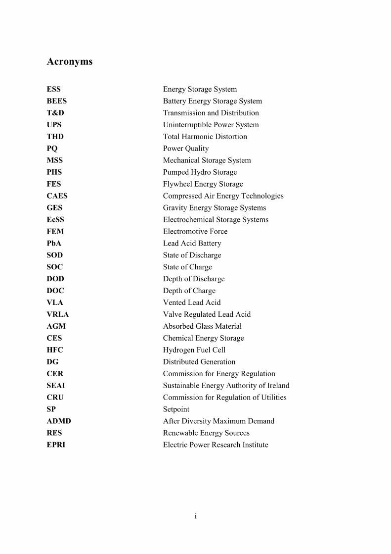
Acronyms
ESS Energy Storage System BEES Battery Energy Storage System T&D Transmission and Distribution UPS Uninterruptible Power System THD Total Harmonic Distortion PQ Power Quality MSS Mechanical Storage System PHS Pumped Hydro Storage FES Flywheel Energy Storage CAES Compressed Air Energy Technologies GES Gravity Energy Storage Systems EcSS Electrochemical Storage Systems FEM Electromotive Force PbA Lead Acid Battery SOD State of Discharge SOC State of Charge DOD Depth of Discharge DOC Depth of Charge VLA Vented Lead Acid VRLA Valve Regulated Lead Acid AGM Absorbed Glass Material CES Chemical Energy Storage HFC Hydrogen Fuel Cell DG Distributed Generation CER Commission for Energy Regulation SEAI Sustainable Energy Authority of Ireland CRU Commission for Regulation of Utilities SP Setpoint ADMD After Diversity Maximum Demand RES Renewable Energy Sources EPRI Electric Power Research Institute

ii
Index of Figures Figure 1-1 Traditional Electric System with five dimensions.................................................... 7
Figure 1-2 Classification of Energy Storage application ........................................................... 8
Figure 1-3 Peak Shaving .......................................................................................................... 13
Figure 1-4 Load Levelling ........................................................................................................ 14
Figure 1-5 Classification of Energy Storage Systems .............................................................. 15
Figure 1-6 Classification of Energy Storage technologies - Types, Energy formation and materials ................................................................................................................................... 16
Figure 1-7 Pumped Hydro Energy Storage Plant layout .......................................................... 18
Figure 1-8 Flywheels Technology ............................................................................................ 19
Figure 1-9 Compressed Air energy Storage ............................................................................. 20
Figure 1-10 Gravity Energy Storage System ........................................................................... 21
Figure 1-11 NaS charging and discharging .............................................................................. 26
Figure 1-12 Mechanism of HFC ............................................................................................. 30
Figure 1-13 Principal diagram of SMES system ...................................................................... 31
Figure 1-14 Principal structure of a supercapacitor ................................................................. 32
Figure 2-1 Simple Battery Equivalent Circuit .......................................................................... 33
Figure 3-1 Network used in the simulation .............................................................................. 41
Figure 3-2 Power 72 houses with 3 bedrooms - Summer ........................................................ 49
Figure 3-3 Power 72 houses with 4 bedrooms - Summer ........................................................ 49
Figure 3-4 Power 24 houses with 3 and 4 bedrooms - Summer .............................................. 50
Figure 3-5 Power 24 houses with 3 and 4 bedrooms 3D - Summer ......................................... 50
Figure 3-6 Power tot in each feeder - Summer ........................................................................ 51
Figure 3-7 Power 72 houses with 3 bedrooms - Winter ........................................................... 51
Figure 3-8 Power 72 houses with 4 bedrooms - Winter ........................................................... 52
Figure 3-9 Power 24 houses with 3 and 4 bedrooms - Winter ................................................. 52
Figure 3-10 Power 24 houses with 3 and 4 bedrooms 3D - Winter ......................................... 53
Figure 3-11 Power tot in each feeder – Winter ........................................................................ 53
Figure 3-12 Topologies of BESS: a) centralised BESS b) distributed BESS .......................... 54
Figure 4-1 Simulink Model ...................................................................................................... 57
Figure 4-2 Single Feeder Simulink Model ............................................................................... 58
Figure 4-3 Single Load Model ................................................................................................. 59
Figure 4-4 Vector Parameter .................................................................................................... 60
Figure 4-5 Battery Model ......................................................................................................... 61
Figure 4-6 Distributed Batteries Model ................................................................................... 63
iii
Figure 5-1 Simple diagram with ESS on MV or LV side ........................................................ 66
Figure 5-2 Currents with ESS on MV or LV side .................................................................... 66
Figure 5-3 SimPowerSystem Power measurement block ........................................................ 68
Figure 5-4 Compared Transformer Losses 4 Scenarios ........................................................... 73
Figure 5-5 Compared Feeder Losses 4 Scenarios .................................................................... 74
Figure 5-6 Compared Total Losses 4 Scenarios ....................................................................... 75
Figure 5-7 Compared Losses 4 Scenarios - Separated Columns ............................................. 75
Figure 5-8 Compared Losses 4 Scenarios – Stacked ............................................................... 76
Figure 5-9 Compared MV side losses 4 Scenarios .................................................................. 76
Figure 5-10 Load and PV trend with 1 kW panel on half houses - Without Battery ............... 80
Figure 5-11 Load, PV and Battery trend with 1 kW panel on half houses – Original SP........ 80
Figure 5-12 Load, PV and Battery trend with 1 kW panel on half houses - New SP .............. 81
Figure 5-13 Loa and PV trend with 1 kW panel on each house – No Battery ......................... 81
Figure 5-14 Load, PV and Battery trend with 1 kW panel on each house - Original SP ......... 81
Figure 5-15 Load, PV and Battery trend with 1 kW panel on each house - New SP .............. 82
Figure 5-16 Load and PV trend with 2 kW panel on each house - No Battery ........................ 82
Figure 5-17 Load, PV and Battery trend with 2 kW panel on each house - Original SP ......... 82
Figure 5-18 Load, PV and Battery trend with 2 kW panel on each house - New SP .............. 83
Figure 5-19 Comparing Transformer Losses ........................................................................... 83
Figure 5-20 Comparing Feeder Losses .................................................................................... 84
Figure 6-1 Load Voltage Without Battery ............................................................................... 88
Figure 6-2 Load Voltage with battery on MV side of the transformer .................................... 88
Figure 6-3 Load Voltage with battery on LV side of the transformer ..................................... 89
Figure 6-4 Voltage with distributed battery on each cumulative load ..................................... 89
Figure 6-5 Voltage 1 kW PV panel installed on half houses - Without Battery ...................... 90
Figure 6-6 Voltage 1 kW PV panel installed on half houses - Original SP ............................. 91
Figure 6-7 Voltage 1 kW PV panel installed on half houses - New SP ................................... 91
Figure 6-8 Voltage 1 kW PV panel on each house - Without Battery ..................................... 92
Figure 6-9 Voltage 1 kW PV panel on each house - Original SP ............................................ 92
Figure 6-10 Voltage 1 kW PV panel on each house - New SP ................................................ 93
Figure 6-11 Voltage 2 kW PV panel on each house - Without battery .................................... 93
Figure 6-12 Voltage 2 kW PV panel on each house - Original SP .......................................... 94
Figure 6-13 Voltage 2 kW PV panel on each house - New SP ................................................ 94
Figure 7-1 Battery capacity .................................................................................................... 102
Figure 7-2 Minimum Battery Costs ....................................................................................... 102
Figure 7-3 Maximum battery Costs ....................................................................................... 102
iv
Index of Tables Table 1-1 Classification of Control Power Reserves ............................................................... 10
Table 1-2 Classification of possible size and functions of energy storage .............................. 15
Table 1-3 Characteristics of electrochemical energy storage technologies in modern grids ... 29
Table 3-1 Network values ........................................................................................................ 42
Table 5-1 Energy Losses Values 4 Scenarios – Summer Day ................................................. 77
Table 5-2 Energy Losses Values 4 Scenarios - Winter Day .................................................... 77
Table 5-3 Comparing losses 13 scenarios - Summer ............................................................... 84
Table 5-4 Comparing losses 13 scenarios - Winter .................................................................. 84
Table 7-1 Energy Storage Characteristics by Application (MW scale) ................................... 96
Table 7-2 Energy Storage Characteristics by Application (kW scale) ..................................... 97
Abstract
5
Abstract The increased deployment of renewable generation, the high capital cost of managing grid peak demands, and large capital investments in grid infrastructure for reliability is creating new interest in electric energy storage systems. Consequently, the use of stored energy to support and optimize the generation, transmission, and distribution subsystems has been grown up worldwide. One of the ESS applications is using them for load levelling. Since network losses are a square function of current, shifting load from peak to off-peak periods can potentially reduce system losses. In the present work the application of concentrated or distributed accumulation in low and medium voltage grids, for losses reduction and peak shaving has been evaluated. Various factors governing loss reduction such as transformer side installation (MV/LV), distributed ESS and the presence of PV generation are analysed with several scenarios. Voltage profiles on loads in all scenarios have also been evaluated, paying attention to the case where there were many rooftop Photovoltaics (PVs) that have turned from traditional passive networks into active networks with intermittent and bidirectional power flow. The capacity values necessary to store the energy and the costs related to three electrochemical storage technologies were finally assessed.
Chapter 1 System and technologies for electricity storage
6
Chapter 1
1 System and technologies for electricity storage
1.1 Introduction The increasing use of renewable sources, on the one hand improves pollution problem related to the techniques used to produce energy, but on the other hand it imposes to the grid a massive revision and adaptation to all the industries involved both for production and for transmission of energy. These changes introduce a completely new model of system with several interconnected systems and is need the maximum efficiency. The nature of renewable, with intermittent and non-programmable sources, requires a substantial modification of electric network and must adapt itself to the places and time of these sources and, at the same time, guarantee the supply of power and energy requested by users. This new concept needs an intelligent control of energy flows and power. Another important point is that now, the final user could become an active player, therefore a producer and not just a consumer, thus creating the figure of the "prosumer". The process of change taking place is not only leading an infrastructural modification of the electricity grids, with the addition of new lines and stations towards a distributed generation, but it is transforming itself with the overlap of a form of active intelligence, able to manage in real time the flows of energy and power between the systems generation and loads, in a smart-grid logic, that is a new electric network intelligent, economical, sustainable and with an advanced management, control and protection system with an increasing share of non-programmable generation. The liberalization of the electricity market improves the ability of produce and manage with efficiency and flexibility generation plants, transmission, distribution and final using of electricity energy. About network electrical system development, energy storage systems are a growing interest topic, to improve energy efficiency, support the introduction of renewable sources, separate production from use of energy time, postpone the creation of new generation plants and allow more diversified use of electricity. For the future is use more of electricity mobility with the possibility to develop the technology V2G (vehicle to grid). In this way, thanks to an aggregator, the batteries of the cars could support the network during peak hours and be recharged during low-load hours. These qualities are particularly useful to give flexibility to electricity grids.

Chapter 1 System and technologies for electricity storage
7
1.2 Traditional electrical system We can think about the traditional electricity system as a passive grid with an energy unidirectional flow. As shown in the Figure 1-1, there are five main components:
• Energy source next transformed into electricity. It includes both conventional sources and renewable.
• Energy generation. It, at least in the industrialized countries, is generally realized in large concentrated plants and with great advantages of efficiency, but with significant losses in long distance transmissions, that cause impacts on the environment and on the quality of the supply. Alternatively, there is the generation distributed which is closer to the final use point: it is better for transmission efficiency but suffers from intermittence of non-programmable sources.
• Transmission: the energy is transported to the substations where, through step-down transformers, the voltage is reduced before distribution to final users. The transmission system is created on the shortest path to follow economy principles and to guarantee security and continuity of service, it is a redundant system.
• Distribution system joins primary substations with the final user. • Final user.
Figure 1-1 Traditional Electric System with five dimensions
1.3 Storage In the new concept of network, we can think about the storage as the “sixth” dimension. The energy and power storage, as we will see later, might improve electrical system making it more flexible, intelligent and available for bidirectional flow and information exchange. There are a lot of storage possible applications and they are often not easily recognizable because a storage function could cover different aspects. Energy storage technologies cover a wide spectrum of power system applications, ranging from power quality to energy management [1] as we can see in Figure 1-2. The storage can provide “Power” and “Energy” services. The first concerns the aspects related to the power of the system, response speed to the electricity grid to which is connected. The latter concerns energetic aspects, so they are distributed over a quantity of power in a longer time.

Chapter 1 System and technologies for electricity storage
8
In this work we want to focus our attention on the value analysis of high-energy side, considering the effects of energy storage on load levelling, peak shaving and control power (minutes – hours regulation).
Figure 1-2 Classification of Energy Storage application
1.3.1 Power services • Security. Regarding electrical system security, the storage system can carry significant
benefits in terms of: o Peak shaving. The storage system can deliver power for short time to supply load
peaks trying to keep as flat as possible the power provided from power plants. This is an important aspect of system security since the storage allows the system to work properly. Today the electricity buyers can install the BESS capable of discharging for short periods of time at peak periods and charging during the low demand periods, hence reducing the peak demand charge. The valley filling phenomenon has more interest in services of load levelling.
o UPS (Uninterruptible Power System). When a short-term interruption occurs, an accumulation system can work as a UPS for sensitive loads which can’t be disconnected so this functionality became important for devices security.
o Island. “Island” means a portion of the electrical system disconnected from the rest of the grid where is necessary to maintain the perfect balance between generation and load. The stability depends on island capacity to keep this balance in a short time end with the minimum load loss. The risk is to create a grid portion where there isn’t enough generation capacity and this situation could lead to a frequency degradation causing the collapse of the system. With storage devices, able to develop primary frequency control and load shedding, is it possible and easier to keep the balance, helping the island grid to come back in parallel with the main grid. In this case the
Chapter 1 System and technologies for electricity storage
9
priority is the security regarding the balance between load and generation and Power Quality aspects are less important so, on this, we can accept larger tolerance.
o Ramp. The ramp service opposes itself against rapid increases and decreases of load the cannot be followed by thermoelectric units. This service is very easy to carry out with storage systems since their speed of response.
o Black start. Providing plant power sources with storage system, it is possible to launch the engine-generator suitable for the Black Start or, to allow the start, directly all the auxiliary services of the production group.
• Power quality. It can be enhanced thank to a well sized storage system:
o Short-term interruptions. The first aim regarding power quality is, using storage, to reduce short-term interruptions, also called voltage dips, caused by faults or energizations. This can be achieved using a UPS for the loads powered or using storage system in series with feeders that feed sensitive loads.
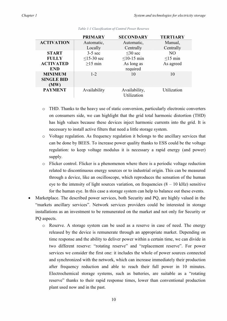
o Control power for frequency regulation. The storage can help frequency regulation in island systems that are imagined working all the time separately from the main grid (in this case island condition is structural and not for emergency). These systems have low value of regulating energy, so they are subject to great frequency variations. Two problems are considered: on the one hand security problem discussed above and in the other hand frequency quality that can be kept between narrower oscillation band. Control power, also known as spinning reserve, consists of generating units which are on-line but operate below their full capacity. This is necessary to provide power on short notice for balancing purpose when a load or generator in service experiences an unexpected outage. Control power, actually, is made by thermal and hydro generators that are synchronized and can be ramped up quickly. Power systems typically keep enough reserves available to compensate for the worst credible contingency (ex. loss of the largest generator). BESS is composed only of static elements; hence its response time to changing conditions in the power system is very fast. Full response is typically completed in few milliseconds as compared with a 15-30 seconds lag for different types of generators. BESS is discharging when the system frequency is below the regulating dead-band and is charging when the frequency is above the limit. In accordance to the UCTE rules there are three types of reserves available (Table 1-1).[1][2]
Chapter 1 System and technologies for electricity storage
10
Table 1-1 Classification of Control Power Reserves
PRIMARY SECONDARY TERTIARY ACTIVATION Automatic,
Locally Automatic, Centrally
Manual, Centrally
START FULLY
ACTIVATED END
3-5 sec ≤15-30 sec
≥15 min
≤30 sec ≤10-15 min As long as required
NO ≤15 min
As agreed
MINIMUM SINGLE BID
(MW)
1-2 10 10
PAYMENT Availability Availability, Utilization
Utilization
o THD. Thanks to the heavy use of static conversion, particularly electronic converters
on consumers side, we can highlight that the grid total harmonic distortion (THD) has high values because these devices inject harmonic currents into the grid. It is necessary to install active filters that need a little storage system.
o Voltage regulation. As frequency regulation it belongs to the ancillary services that can be done by BEES. To increase power quality thanks to ESS could be the voltage regulation: to keep voltage modulus it is necessary a rapid energy (and power) supply.
o Flicker control. Flicker is a phenomenon where there is a periodic voltage reduction related to discontinuous energy sources or to industrial origin. This can be measured through a device, like an oscilloscope, which reproduces the sensation of the human eye to the intensity of light sources variation, on frequencies (8 – 10 kHz) sensitive for the human eye. In this case a storage system can help to balance out these events.
• Marketplace. The described power services, both Security and PQ, are highly valued in the “markets ancillary services”. Network services providers could be interested in storage installations as an investment to be remunerated on the market and not only for Security or PQ aspects.
o Reserve. A storage system can be used as a reserve in case of need. The energy released by the device is remunerate through an appropriate market. Depending on time response and the ability to deliver power within a certain time, we can divide in two different reserve: “rotating reserve” and “replacement reserve”. For power services we consider the first one: it includes the whole of power sources connected and synchronized with the network, which can increase immediately their production after frequency reduction and able to reach their full power in 10 minutes. Electrochemical storage systems, such as batteries, are suitable as a “rotating reserve” thanks to their rapid response times, lower than conventional production plant used now and in the past.
Chapter 1 System and technologies for electricity storage
11
o Load shed. A storage system can carry benefits for example avoiding load shedding: when a power source is not available it can temporarily replace the source. In this application it is possible to recognize two different type of storage: external one, designed and sized to avoid load detachment, and the internal one also called “process storage”. The “process storage” term, indicates an amount of energy intrinsically present in production process and which ca be used to support the process itself for short periods without degeneration of performance.
• Grid connections. The availability of the storage on a network, can cut power peaks and therefore allows to not use all the feeders’ capacity, increasing the possibility to connect other users avoiding to size again the line. This logic can also be applied on users’ side: the customer can employ on his network internal storage which can cut the peaks and then he can ask for less power, saving even on bills. If the user is an active user, installing a BEES can allow it to be less variable and even less random, improving acceptability on network managing authority side and with the benefit of being remunerated if the conditions provides for its.[3]
1.3.2 Energy services
• Security. Regarding Energy services security an energy storage system can be useful for: o Load levelling. This term means a levelling of the load profile during a range of long
time, which can be a day, a week or a month. BESS involves storing power during periods of light loading (night time) and discharge it during periods of heavy demand (day time). This application usually uses predetermined charge/discharge daily cycles. This storage system certainly produces a daily load levelling, but the same way of thinking can be extended to longer periods varying charging and discharging parameters. Later in the dissertation the differences between load levelling and peak shaving will be debated.
o Valley filling. When, during the night, the load suddenly drops under an allowable value for generation power groups, there are over generation problems.
• Power quality. Regarding power quality from an energy point of view, storage systems can avoid long interruptions and increase the quality of the system, subsequently. In this case power performances and speed response are not required to the storage system, but performances of energetic nature. These last will establish the design constrains of the storage system itself.
• Marketplace. The vision on energy side rather than in power allow to highlight another advantage that the storage could have on the market. Storage allows a form of flexibility that can allow advantages for supply and demand.
Chapter 1 System and technologies for electricity storage
12
• Grid connection. Certainly, a storage system could support the acceptability of a load in a network allowing to defer or even delete the costly investments aimed at adapting weak networks with new impulsive or temporary loads. A very simple example can be a user who needs an exceeding power of the available power line. A ESS could recharge itself during the night a release energy needed during the day, avoiding sizing again the insufficient feeders. ESS systems evaluation of capital investment costs and financial evaluation related to different type of storage technologies is extremely difficult and it depends on variable considerations, such as territorial configuration, political constrains or incentives, size of the systems and geographical area.
New form of energy generation, strongly variable according to the period of the year, the hours of the day and the location, could produce not dispatchable power in a precise moment. The need for a greater modulation will arise, and it will be based on a “just-in-time” criterion. In this context, the contribution that comes from storage systems is the introduction of an important form of flexibility which is expressed with the possibility to temporally and spatially decouple generation and load. Conventional power grids have always used large ESS to better support the centralized generation system but in this work, we will evaluate the possibility of insert BEES small or medium sizes, depending on the location, to improve the daily load profile.[4]
1.4 Peak shaving vs Load levelling As said before, in recent years, Distributed Generation (DG) has become increasingly common and different solutions have been proposed to solve integration of renewable power generations problems. One type of solution is using hybrid systems: they combine the use of power generation, with storage or generation source. BESS involves improvements in the electrical system such as load levelling, peak shaving, reduction of losses on feeders, power quality improvement, frequency control, load balancing. Utilities employing the use of BESS hybrid systems can mitigate the problem of congestion, lower the cost of locational marginal pricing, shave loads, and decrease the thermal unit commitment. In this work enhancement will be taken into account. Let us consider what are peak shaving and load levelling and their main difference. Peak shaving and load levelling are very similar process: an ESS store electrical energy when the load is low and discharge itself when the load is high. In peak shaving case, the battery (or energy storage in general) stores energy when the load is low and discharges itself to only remove the peaks of the load and not to obtain a completely flat trend. Regarding the load levelling, the same process takes place, but the air is to obtain an as flat as possible curve rather than just remove the peak.
Chapter 1 System and technologies for electricity storage
13
Usually in a day there are two periods where the energy demand is high and there I have the peak: in midday and evening hours. In this period of time the battery will be discharged, while in the early hours of the day and during the night the battery will be charged, so that the power plants will not have to provide for required power peaks.[5]
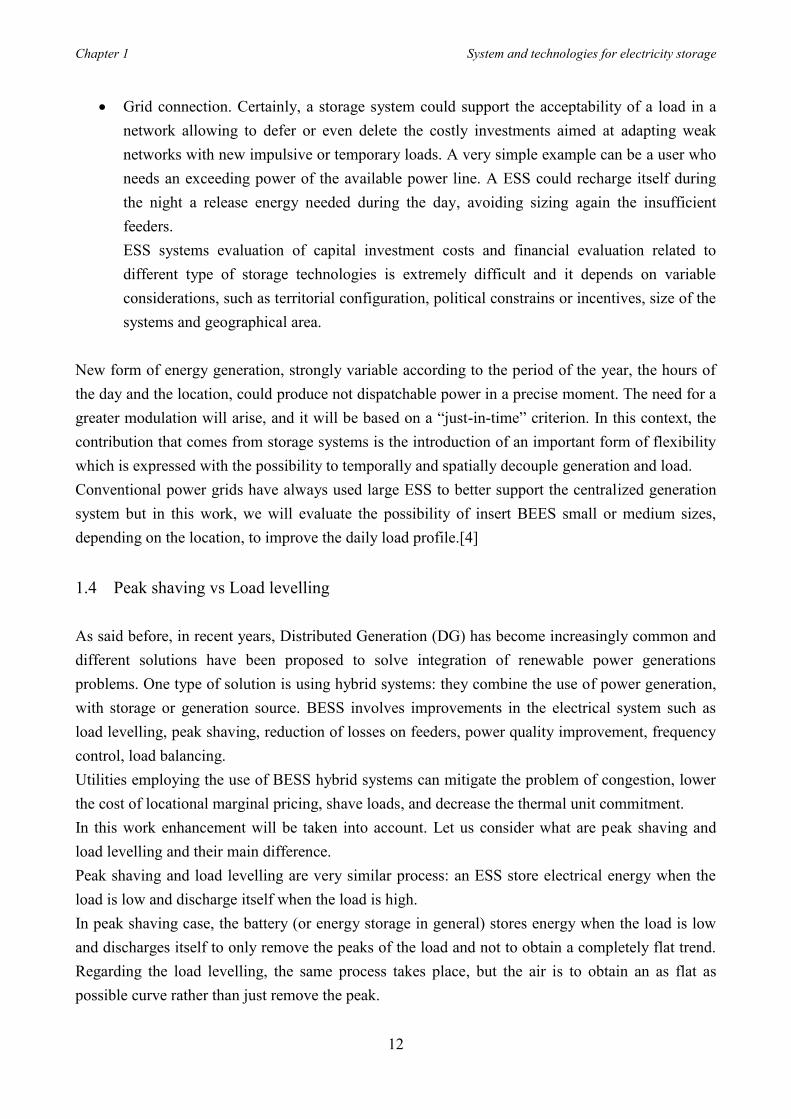
1.4.1 Peak Shaving The practise of peak shaving consists of several different ways to eliminate the peak and valleys in the load profile. As said before, it is done, reducing, or better compensating for the demand request using local energy storage systems. The figure below illustrates the use of energy storage for the application of peak shaving.
During the early morning hours from about midnight to 08:00, the load is slightly raised while the storage is charging. The storage is then discharged when load’s peaks are removed. Often industrial customers run devices that requires significant amount of power over relatively short time intervals during a day. Another consequence of peak period is that the transmission and distribution systems must be dimensioned for this short time and they are not fully utilized for the rest of the day. During peak hours the prices of electricity per kilowatt used increase due to the increase in location marginal pricing due to the energy production in power plants and they include these extra costs to correctly size the transmission system. There are many applications that can be used for peak shaving, regarding both consideration on plant equipment and economic gain. Peak shaving has been used for many years using on-site diesel generators and gas turbines to reduce the load, thus reducing power production costs. Storage type, size, capacity and characteristics are chosen according to the application in which the peak shaving is used.
Figure 1-3 Peak Shaving
Chapter 1 System and technologies for electricity storage
14
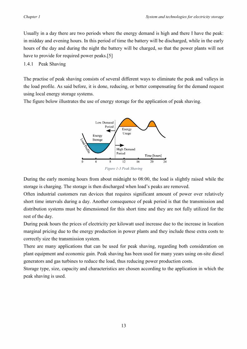
1.4.2 Load levelling The practise of peak shaving, sometimes is referred to as load levelling and it is very useful when it can yield economic benefits. The goal of load levelling is to make the load as flat as possible during the day. The figure below shows the idea of load levelling compared with peak shaving deal with before.
Optimal operation of the system is done with coordination of charging and discharging periods. The ESS is charged during off peak hours, when power price is low and uniformly discharged during the peak hours, starting around noon. The charging raises the load when it “falls” during the early hours of the morning and reduces its when it “jumps” during the middle day hours. About the value to set for the load levelled, the average of the daily load can be chosen as a first approximation. However, it should be considered that this value could change according to the characteristics and especially about ESS costs. Taking the average of the load as the initial value it will be decided later if choosing a value of the flat curve greater or smaller than the average. It can be noted that for load levelling applications, much more energy storage is required. It can also be seen from Figure 1-4 that the load has two peaks, and this is a problem because it must be decided when discharge the storage device. One solution to this problem is to discharge half of the storage device during the first peak and the discharge the other half during the second peak. However, it’s very difficult to have two equal peaks in magnitude and the load might remain uneven after both discharges. A solution to this problem is to use multiple storage devices and allocate a greater amount of stored energy for the larger peak and less amount for the smaller peak.[5]
1.5 Energy storage classification New functions and applications of energy storage systems must be differentiated into technical and economic terms. The growing interest in the use of storage systems has encouraged researchers and industries to develop different technologies and methods, to respond on several requests in terms of performances and costs. Characterization, optimization and localization activities have been added
Figure 1-4 Load Levelling
Chapter 1 System and technologies for electricity storage
15
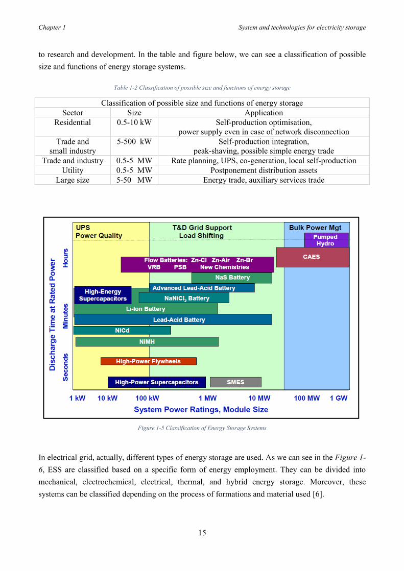
to research and development. In the table and figure below, we can see a classification of possible size and functions of energy storage systems.
Table 1-2 Classification of possible size and functions of energy storage
Classification of possible size and functions of energy storage Sector Size Application
Residential 0.5-10 kW Self-production optimisation, power supply even in case of network disconnection
Trade and small industry
5-500 kW Self-production integration, peak-shaving, possible simple energy trade
Trade and industry 0.5-5 MW Rate planning, UPS, co-generation, local self-production Utility 0.5-5 MW Postponement distribution assets
Large size 5-50 MW Energy trade, auxiliary services trade
Figure 1-5 Classification of Energy Storage Systems
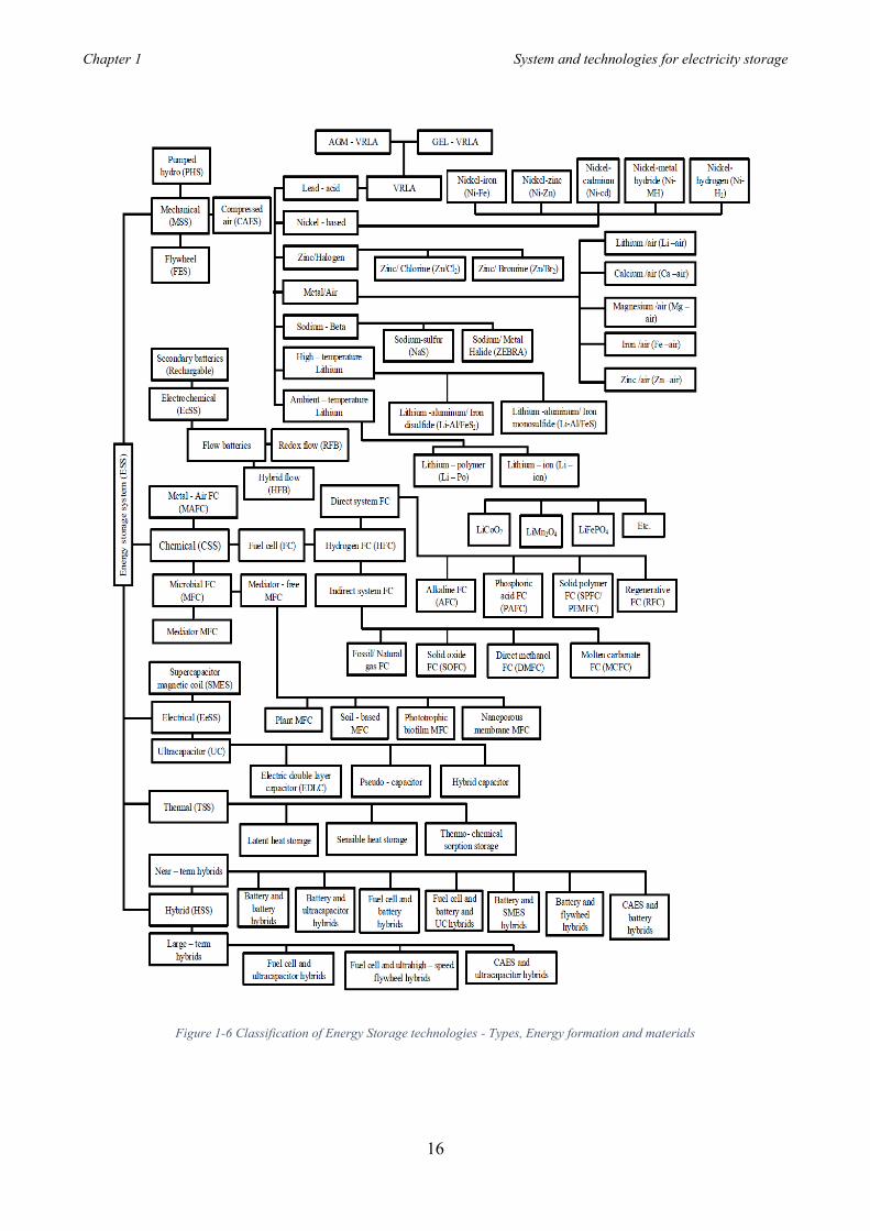
In electrical grid, actually, different types of energy storage are used. As we can see in the Figure 1-6, ESS are classified based on a specific form of energy employment. They can be divided into mechanical, electrochemical, electrical, thermal, and hybrid energy storage. Moreover, these systems can be classified depending on the process of formations and material used [6].
Chapter 1 System and technologies for electricity storage
16
Figure 1-6 Classification of Energy Storage technologies - Types, Energy formation and materials

Chapter 1 System and technologies for electricity storage
17
1.6 Overview of energy storage System
1.6.1 Introduction ESS technologies can be categorized by various criteria such as: suitable storage duration (short-term, mid-term or long-term), response time (rapid or not), scale (small-scale, medium-scale or large-scale) or based on the form of stored energy. Depending on the form in which the electrical energy can be stored, ESS systems are divides into mechanical, electrochemical, chemical, electrical, thermal, and hybrid energy storage system. A description regarding each storage technology is shown below [7].
1.6.2 Mechanical Storage Systems (MSS) These ESS are usually big size storage systems with a hundred of discharge power and autonomy around several hours; they are advantageous in transmission system for their flexibility to convert and store energy from sources and deliver it when required for mechanical work. Based on the working principle, MSS can be classified as pressurized gas, forced spring, kinetic energy, and potential energy. However, mechanical storage systems consist of three techniques: flywheel, pumped hydro storage (PHS), and compressed air energy technologies (CAES). [6] [7]
1.6.2.1 Pumped hydro storage Pumped hydro energy storage (PHES) is the most widely adopted technology for large scale (>100 MW) plants. PHS store energy in the form of water in an upper reservoir, pumped from another reservoir at a lower level. During high electricity demand periods, power is generated by releasing the stored water through turbines in the same manner as a conventional hydropower station. During periods of low demand (usually nights or weekends when electricity is also lower cost), the upper reservoir is recharged by using lower-cost electricity from the grid to pump the water back to the upper reservoir. The amount of stored energy is proportional to the height difference between the reservoirs and the mass of water stored according to equation (1.1): 𝐸 = 𝑚𝑔ℎ (1.1) Among the three systems, PHS contribute the most in the world electricity storage capacity because this technology offers long life in the range of 30-50 years, low operation and maintenance (O&M)
Chapter 1 System and technologies for electricity storage
18
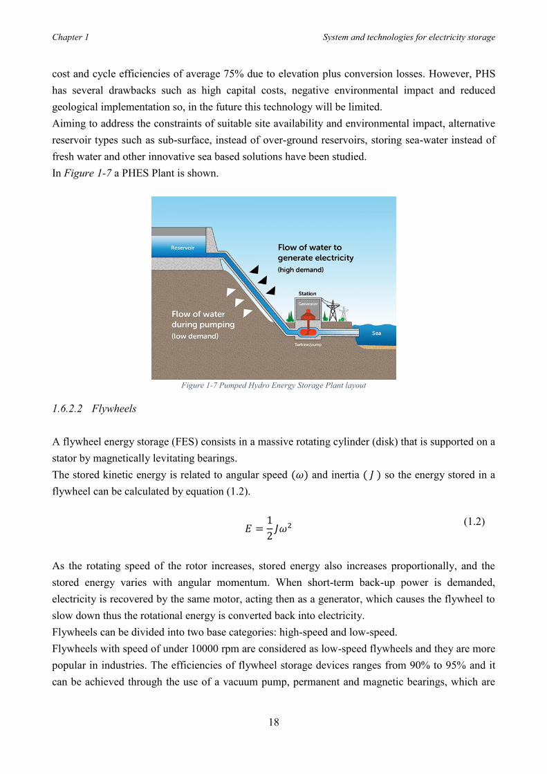
cost and cycle efficiencies of average 75% due to elevation plus conversion losses. However, PHS has several drawbacks such as high capital costs, negative environmental impact and reduced geological implementation so, in the future this technology will be limited. Aiming to address the constraints of suitable site availability and environmental impact, alternative reservoir types such as sub-surface, instead of over-ground reservoirs, storing sea-water instead of fresh water and other innovative sea based solutions have been studied. In Figure 1-7 a PHES Plant is shown.
Figure 1-7 Pumped Hydro Energy Storage Plant layout
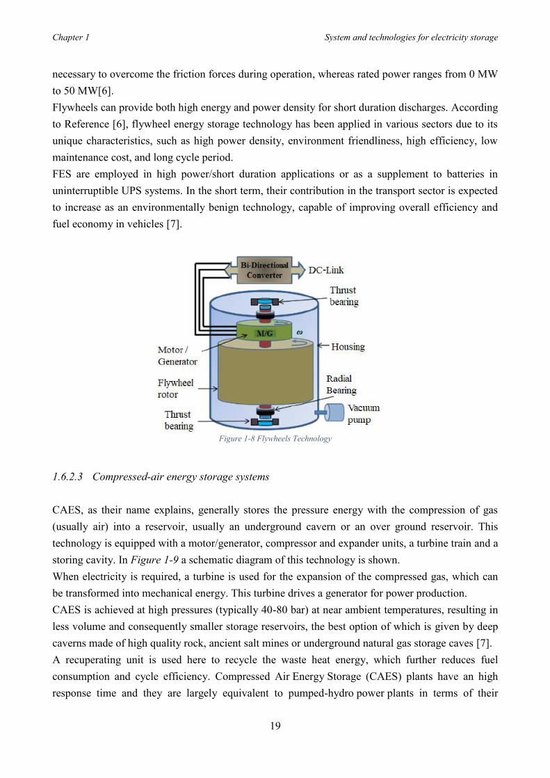
1.6.2.2 Flywheels A flywheel energy storage (FES) consists in a massive rotating cylinder (disk) that is supported on a stator by magnetically levitating bearings. The stored kinetic energy is related to angular speed (𝜔) and inertia ( 𝐽 ) so the energy stored in a flywheel can be calculated by equation (1.2).
𝐸 =1
2𝐽𝜔2 (1.2)
As the rotating speed of the rotor increases, stored energy also increases proportionally, and the stored energy varies with angular momentum. When short-term back-up power is demanded, electricity is recovered by the same motor, acting then as a generator, which causes the flywheel to slow down thus the rotational energy is converted back into electricity. Flywheels can be divided into two base categories: high-speed and low-speed. Flywheels with speed of under 10000 rpm are considered as low-speed flywheels and they are more popular in industries. The efficiencies of flywheel storage devices ranges from 90% to 95% and it can be achieved through the use of a vacuum pump, permanent and magnetic bearings, which are
Chapter 1 System and technologies for electricity storage
19
necessary to overcome the friction forces during operation, whereas rated power ranges from 0 MW to 50 MW[6]. Flywheels can provide both high energy and power density for short duration discharges. According to Reference [6], flywheel energy storage technology has been applied in various sectors due to its unique characteristics, such as high power density, environment friendliness, high efficiency, low maintenance cost, and long cycle period. FES are employed in high power/short duration applications or as a supplement to batteries in uninterruptible UPS systems. In the short term, their contribution in the transport sector is expected to increase as an environmentally benign technology, capable of improving overall efficiency and fuel economy in vehicles [7].
Figure 1-8 Flywheels Technology
1.6.2.3 Compressed-air energy storage systems CAES, as their name explains, generally stores the pressure energy with the compression of gas (usually air) into a reservoir, usually an underground cavern or an over ground reservoir. This technology is equipped with a motor/generator, compressor and expander units, a turbine train and a storing cavity. In Figure 1-9 a schematic diagram of this technology is shown. When electricity is required, a turbine is used for the expansion of the compressed gas, which can be transformed into mechanical energy. This turbine drives a generator for power production. CAES is achieved at high pressures (typically 40-80 bar) at near ambient temperatures, resulting in less volume and consequently smaller storage reservoirs, the best option of which is given by deep caverns made of high quality rock, ancient salt mines or underground natural gas storage caves [7]. A recuperating unit is used here to recycle the waste heat energy, which further reduces fuel consumption and cycle efficiency. Compressed Air Energy Storage (CAES) plants have an high response time and they are largely equivalent to pumped-hydro power plants in terms of their
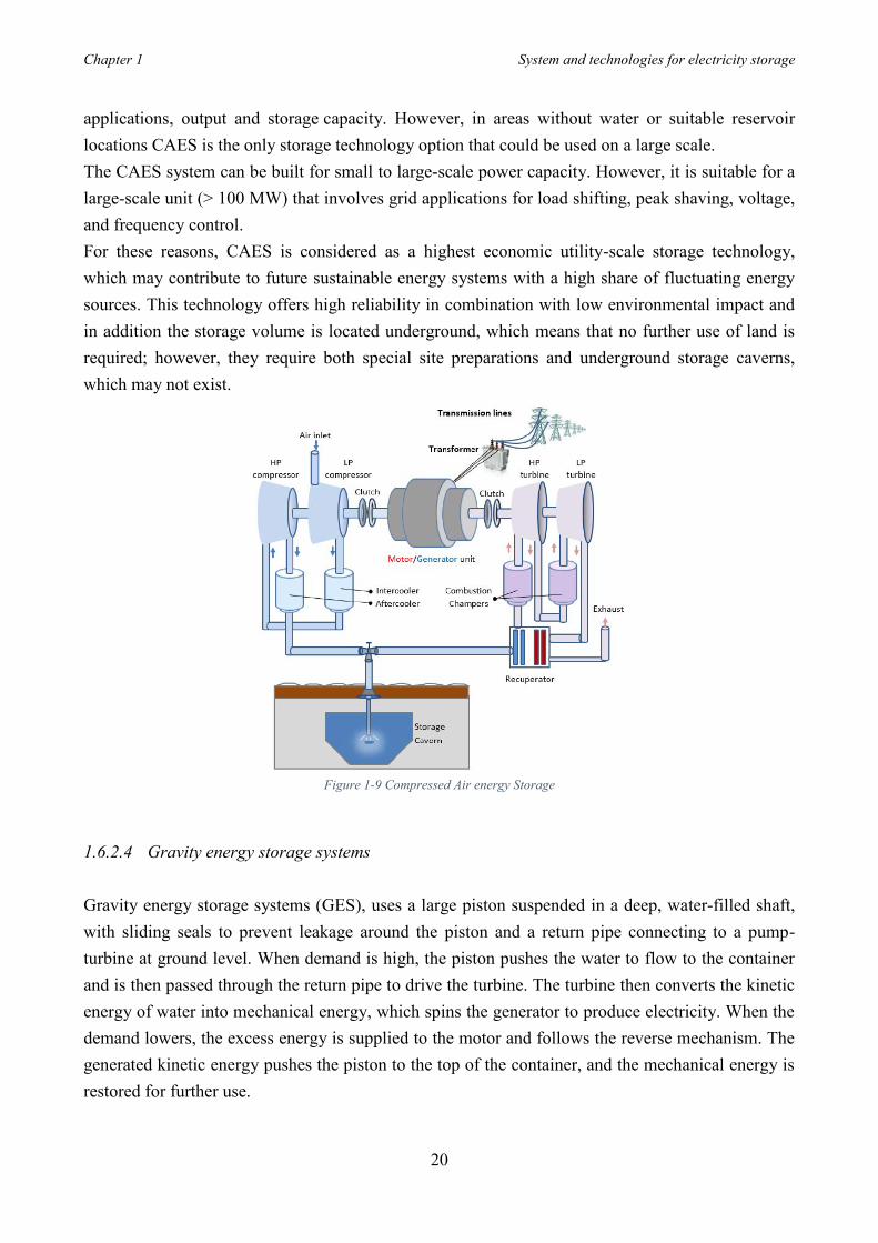
Chapter 1 System and technologies for electricity storage
20
applications, output and storage capacity. However, in areas without water or suitable reservoir locations CAES is the only storage technology option that could be used on a large scale. The CAES system can be built for small to large-scale power capacity. However, it is suitable for a large-scale unit (> 100 MW) that involves grid applications for load shifting, peak shaving, voltage, and frequency control. For these reasons, CAES is considered as a highest economic utility-scale storage technology, which may contribute to future sustainable energy systems with a high share of fluctuating energy sources. This technology offers high reliability in combination with low environmental impact and in addition the storage volume is located underground, which means that no further use of land is required; however, they require both special site preparations and underground storage caverns, which may not exist.
Figure 1-9 Compressed Air energy Storage
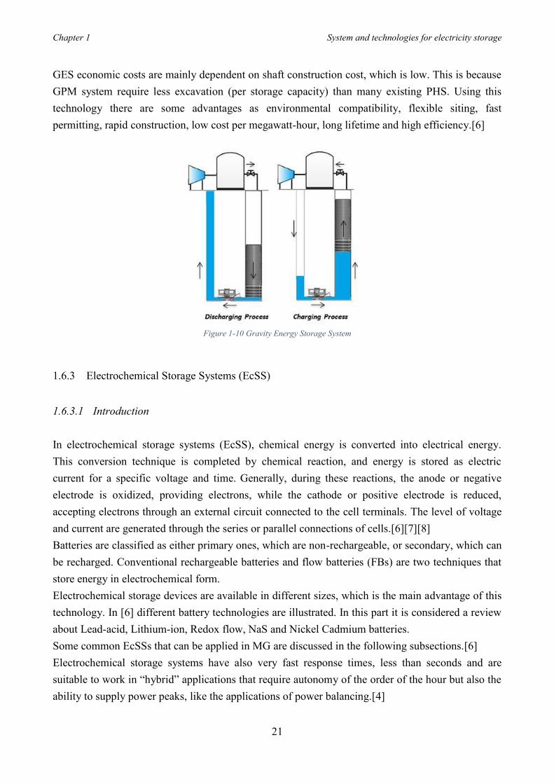
1.6.2.4 Gravity energy storage systems Gravity energy storage systems (GES), uses a large piston suspended in a deep, water-filled shaft, with sliding seals to prevent leakage around the piston and a return pipe connecting to a pump-turbine at ground level. When demand is high, the piston pushes the water to flow to the container and is then passed through the return pipe to drive the turbine. The turbine then converts the kinetic energy of water into mechanical energy, which spins the generator to produce electricity. When the demand lowers, the excess energy is supplied to the motor and follows the reverse mechanism. The generated kinetic energy pushes the piston to the top of the container, and the mechanical energy is restored for further use.
Chapter 1 System and technologies for electricity storage
21
GES economic costs are mainly dependent on shaft construction cost, which is low. This is because GPM system require less excavation (per storage capacity) than many existing PHS. Using this technology there are some advantages as environmental compatibility, flexible siting, fast permitting, rapid construction, low cost per megawatt-hour, long lifetime and high efficiency.[6]
Figure 1-10 Gravity Energy Storage System
1.6.3 Electrochemical Storage Systems (EcSS)
1.6.3.1 Introduction In electrochemical storage systems (EcSS), chemical energy is converted into electrical energy. This conversion technique is completed by chemical reaction, and energy is stored as electric current for a specific voltage and time. Generally, during these reactions, the anode or negative electrode is oxidized, providing electrons, while the cathode or positive electrode is reduced, accepting electrons through an external circuit connected to the cell terminals. The level of voltage and current are generated through the series or parallel connections of cells.[6][7][8] Batteries are classified as either primary ones, which are non-rechargeable, or secondary, which can be recharged. Conventional rechargeable batteries and flow batteries (FBs) are two techniques that store energy in electrochemical form. Electrochemical storage devices are available in different sizes, which is the main advantage of this technology. In [6] different battery technologies are illustrated. In this part it is considered a review about Lead-acid, Lithium-ion, Redox flow, NaS and Nickel Cadmium batteries. Some common EcSSs that can be applied in MG are discussed in the following subsections.[6] Electrochemical storage systems have also very fast response times, less than seconds and are suitable to work in “hybrid” applications that require autonomy of the order of the hour but also the ability to supply power peaks, like the applications of power balancing.[4]
Chapter 1 System and technologies for electricity storage
22
The main features of an EcSS concern essentially the specific and operational storage properties as density of energy and power, energy efficiency during charging and discharging, self-discharge, charging and discharging time, behaviour in different conditions of state of charge, life time (in years and cycles), realization time, reliability, material used, costs and safety in the use. These characteristics become evaluation criteria during the design and selection of the accumulation system, which mainly aim to promote economic and environmental aspects of the identified system.
1.6.3.2 Lead-acid storage systems Due to their energetic characteristics (energy and power density) and low costs, Lead-acid batteries (PbA) represent the most used solution for electrochemical storage both in industrial applications and in distributed generation. Their success is essentially due to the low cost and the wide availability of lead, in addition to a relatively simple and widespread technology. Finally, very important are the advantages of good reliability and well-established recycling infrastructures. Among all electrolyte batteries, the PbA battery shows high efficiency (70% – 80%) and possesses the highest cell voltage. PbA provides an excellent charge retention end energy density with fast response and long-life cycle, around 5-15 years. On the other hand, they have several negative aspects, such as a short-life cycle (500-2000cycle), not excessively high density of energy and power, which result is the need of a large surface, appropriate ventilation systems because during recharge it is possible hydrogen production at the terminals. Another disadvantage is the premature failure due to sulphating. To overcome all the limitations mentioned, advanced PbA batteries have been developed. The cathode and anode are made of 𝑃𝑏𝑂2 and 𝑃𝑏, respectively and Sulfuric acid is used as the electrolyte. The main reactions encountered in a battery of this type during charging and discharging processes are the following: 2𝑃𝑏𝑆𝑂4 + 2𝐻2𝑂
𝐶ℎ𝑎𝑟𝑔𝑖𝑛𝑔→ 𝑃𝑏𝑂2 + 𝑃𝑏 + 2𝐻
+ + 2𝐻𝑆𝑂4−
(1.3)
𝑃𝑏𝑂2 + 𝑃𝑏 + 2𝐻
+ + 2𝐻𝑆𝑂4−𝐷𝑖𝑠𝑐ℎ𝑎𝑟𝑔𝑖𝑛𝑔→ 2𝑃𝑏𝑆𝑂4 + 2𝐻2𝑂
(1.4)
There are many types of PbA accumulators, which can be gathered into flooded and valve regulators batteries categories:
• Open accumulators or Vented Lead Acid (VLA) • Hermetic accumulators or Valve Regulated Lead Acid (VRLA)
The VLA accumulators, still the most common in stationary and traction applications, are characterized with some openings that allow gases (essentially hydrogen and oxygen) exit. These are produced during charging.
Chapter 1 System and technologies for electricity storage
23
VRLA accumulators has become increasingly popular due to its high specific power, relatively low installation and maintenance cost, and rapid charging characteristics. However, they are widespread due to less space used and for limited quantities of hydrogen emitted. In these, the hydrogen produced on the negative pole, is conveyed to the positive one where it recombines itself with oxygen, forming water again. VRLA technologies include adsorbed glass material (AGM) and GEL. The first have compact volume and during the charging mode they recombine hydrogen and oxygen to form water; in this case water usage is limited. In GEL batteries, during the charging mode, gas bubbles may be produced, and they could damage permanently the battery so in this type mechanism for charging must be controlled. VRLA use, initially limited to UPS installations, has also be extended to other stationary applications, such as security and emergency services. Regarding the performances, generally, type VLA accumulators have specific energy values between 15 and 25 𝑊ℎ/𝑘𝑔 (corresponding to an energy density of 30-50 𝑊ℎ/𝑙) and specific power peaks of 20-40 𝑊/𝑘𝑔 (40-80 𝑊/𝑙). In special realizations for electric traction they reach specific powers of 70-80 𝑊/𝑘𝑔. The VRLA hermetic accumulators, being more compact, have better performance in fact specific energy values are between 20-45 𝑊ℎ/𝑘𝑔 (40-90 𝑊ℎ/𝑙), with peak power of 60-150 𝑊/ 𝑘𝑔 (120-300 𝑊/𝑙). The electromotive force (FEM) of Lead-acid cells in nominally 2 V. This value depends on several external factors, such as electrolyte density, temperature, state of charge, current, state of ageing. Another phenomenon to be considered is self-discharge. Self-discharge in lead-acid batteries it is due to parasitical reactions that slowly consume the present charges and cause the complete discharge of the battery. Under normal conditions the self-discharge determines a reduction of the battery charge of about 2-3% per month. The expected life of a Lead accumulator may vary according to type and management. A SLI type, which is a battery for engines internal combustion starting, has an expected life of about 5 years, while a stationary accumulator, managed in a correct way can reach a lifetime of over 20 years. The number of charge / discharge cycles of a lead cell, considering DOD of 80%, is between 500 and 800. Despite the lead battery has reached a good maturity both technological and commercial, research activities are still underway to improve their performances and specially to increase life battery.
1.6.3.3 Nickel batteries Until few years ago, nickel-cadmium accumulator was widely diffused thanks to some advantages compared to lead batteries including longer life, reliability and best behaviour at low temperatures. This type is replaced by nickel-metal hydride for economic reasons and due to environmental
Chapter 1 System and technologies for electricity storage
24
problems related to the presence of cadmium, the scarcity of disposal centres and for several European directives which are dedicated towards the prohibition of the use of cadmium.
1.6.3.3.1 Nickel-Cadmium batteries The positive electrode consists of nickel hydroxide (𝑁𝑖𝑂(𝑂𝐻)), while the negative electrode is cadmium. The electrolyte is an aqueous solution of alkaline type, containing potassium hydroxide, sodium or lithium. As for the lead-acid battery, there are also some parasitic reactions, which generate gas during charging. In particular, the development of oxygen to the positive electrode and the production of hydrogen to the negative electrode occurs close to full charge conditions. These parasitic reactions involve charge and energy and periodic filling need of water in non-hermetic accumulators. The reaction involved are the following 2𝑁𝑖(𝑂𝐻)2 +𝐶𝑑(𝑂𝐻)2
𝐶ℎ𝑎𝑟𝑔𝑖𝑛𝑔→ 2𝑁𝑖𝑂(𝑂𝐻) + 𝐶𝑑 + 2𝐻2𝑂 (1.5)
2𝑁𝑖𝑂(𝑂𝐻) + 𝐶𝑑 + 2𝐻2𝑂
𝐷𝑖𝑠𝑐ℎ𝑎𝑟𝑔𝑖𝑛𝑔→ 2𝑁𝑖(𝑂𝐻)2 +𝐶𝑑(𝑂𝐻)2
(1.6)
Nickel cadmium batteries have a nominal voltage of 1.2 V and they have capacity values from fractions of 𝐴ℎ to several hundreds of 𝐴ℎ. It is also possible to find single units with several elementary cells in series, typically up to 12 cells, with a nominal voltage of 14.4 V. This type of batteries is made according to two main construction technologies: - with "pocket" electrodes, in which the active materials of both electrodes are included inside a perforated steel leaf pocket to allow electrolyte penetration; - with "sintered" electrodes, which allow better performance such as greater specific energy, higher power and reduction of internal resistance. The ability to supply strong powers is obtained creating a large surface of the electrodes. As lead accumulator, nickel / cadmium batteries can be open or hermetic type. The total energy efficiency of charge / discharge is lower than lead batteries and generally has a value around 60-70%. Regarding specific energy is around 50 - 60 𝑊ℎ / 𝑘𝑔 (60-100 𝑊ℎ / 𝑙) and it has higher values than lead batteries. The specific power that can be supplied by these batteries varies from a few tens up to 500 𝑊 / 𝑘𝑔 (in some case can reach 800 𝑊/𝑘𝑔) depending on the construction technology. Self-discharge of this battery is less than 5% per month, while hermetic batteries can reach 25% per month. This accumulator is very robust and can achieve 1500-2000 cycles of work with 80% of DOD. Compared with the others, this type can be completely discharged without great damages.
Chapter 1 System and technologies for electricity storage
25
Despite environmental problems and high costs, it still finds a lot of application in space, military, traction field and as UPS or photovoltaic systems isolated from the network. However, there is no interest in the development of this technology.
1.6.3.3.2 Nickel/metal hydride batteries This type of accumulator comes from nickel/cadmium one with the substitution of cadmium electrode with a mixture of metal hydrides. This replacement allows to delete environmental problems related to the use of cadmium. The technology of metal hydrides involves the use of expensive raw materials so, for this reason, these accumulators are widely employed in the field of small size portable applications where the little volumes partially compensate for the higher costs. The positive electrode is made of hydrated nickel oxide, as in the nickel / cadmium cell, while the negative electrode is instead made of metal alloys (𝑀𝑒) capable of absorbing and accumulate hydrogen with hydride formation (𝑀𝑒𝐻). The electrolyte is alkaline (an aqueous solution of potassium, sodium or lithium hydroxide). The reactions involved on the anode are shown in formula (1.7),(1.8). 𝐻2𝑂 +𝑀 + 𝑒
−𝐶ℎ𝑎𝑟𝑔𝑖𝑛𝑔→ 𝑂𝐻− +𝑀𝐻 (1.7)
𝑂𝐻− +𝑀𝐻𝐷𝑖𝑠𝑐ℎ𝑎𝑟𝑔𝑖𝑛𝑔→ 𝐻2𝑂 +𝑀 + 𝑒
− (1.8)
1.6.3.4 High temperature batteries The "high temperature" battery family includes the sodium / sulphur battery and the sodium / nickel chloride battery (ZEBRA). The main feature of this technology is the cell working temperature which is around 300°C, and it is necessary both to maintain in the molten state the electrodes, both to increase the conductivity of the electrolyte. These new types of cells were developed to identify electrochemical couples able to supply very high specific energies without using excessively precious and rare materials.
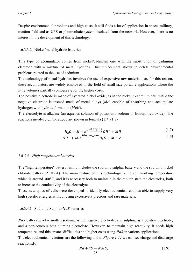
1.6.3.4.1 Sodium / Sulphur 𝑁𝑎𝑆 batteries 𝑁𝑎𝑆 battery involve molten sodium, as the negative electrode, and sulphur, as a positive electrode, and a non-aqueous beta alumina electrolyte. However, to maintain high reactivity, it needs high temperature, and this creates difficulties and higher costs using 𝑁𝑎𝑆 in various applications. The electrochemical reactions are the following and in Figure 1-11 we can see charge and discharge reactions.[6] 𝑁𝑎 + 𝑥𝑆 = 𝑁𝑎2𝑆𝑥 (1.9)
Chapter 1 System and technologies for electricity storage
26
This technology is widely applicable for load levelling, voltage conservation and stabilizing energy power generation. 𝑁𝑎𝑆 batteries could be used in microgrid applications due to high efficiency, long cycle period up to 15 years and fast response, around millisecond during full charging and discharging operation; for these reason, the research is moving forward to overcome limits of this technology, especially high temperature control.
1.6.3.4.2 Sodium batteries / nickel chloride (ZEBRA) The ZEBRA battery (Zero Emission Battery Research Activity) is, from the point of view of the performance, substantially like sodium / sulphur but is safer. For this reason, as said previously, sodium / sulphur battery is currently designed and used in stationary applications, generally large (for peak-shaving, load-levelling), in which there are no risks of mechanical crashes, while the ZEBRA battery is currently used mainly in electric road traction and it is being tested for stationary applications. In these batteries the two electrodes are in molten state and are separated by a ceramic material, β-alumina which allows ionic transfer. The positive electrode consists of nickel chloride, and it is immersed in an electrolyte liquid consisting of a sodium tetra chloroaluminate solution while, the negative electrode is formed by sodium. The electrochemical reactions are the following: 2𝑁𝑎𝐶𝑙 + 𝑁𝑖
𝐶ℎ𝑎𝑟𝑔𝑖𝑛𝑔→ 𝑁𝑖𝐶𝑙2 + 2𝑁𝑎 (1.10)
𝑁𝑖𝐶𝑙2 + 2𝑁𝑎
𝐷𝑖𝑠𝑐ℎ𝑎𝑟𝑔𝑖𝑛𝑔→ "𝑁𝑎𝐶𝑙 + 𝑁𝑖 (1.11)
Figure 1-11 NaS charging and discharging
Chapter 1 System and technologies for electricity storage
27
1.6.4 Electrolyte circulation batteries The electrolyte circulation batteries, also known by the term "redox", can accumulate electricity using coupled oxidation-reduction reactions in which both reagents, both the reaction products, in ionic form, are completely dissolved in water solution. Positive and negative electrolyte solutions are stored in tanks, and their circulation is made by pumps. The two electrolytes interface themselves through a membrane (separator) that allows ions exchange, and therefore the charge / discharge reactions, but prevents mixing of solutions. The most important feature of this storage technology is the total decoupling between power and energy. The power that the battery can deliver or absorb depends on the quantity of electrolyte that takes part in the reaction (clearly compatibly with the speed of the reaction) and, therefore, on the membrane surface and the speed of the pumps. The storage capacity is instead linked to the total quantity of liquid and therefore to the capacity of the tanks. Therefore, with the same installed power, it is possible to increase the capacity of the battery increasing the size of the tanks. These types of accumulators are particularly suitable for applications of very large size (around MWh), such as load-levelling. Some types of batteries belonging to this category can be mentioned such as:
• Zinc-bromine batteries • Vanadium Salts batteries • Lithium batteries
1.6.4.1 Lithium batteries Lithium is the metal with the lowest atomic weight, high absolute value of electrode potential, small size and a very high specific capacity. These features make it one of the most suitable elements for batteries with high energy density and specific energy, which allow to storage a large amount of storable energy compared to other batteries, for equal weight or volume. Lithium batteries are divided into three main categories. The first type is the most widespread and technically mature one. In this category we can find lithium ion batteries with liquid electrolyte (commonly called lithium-ions) which are commercially available especially in small size (from fractions of 𝐴ℎ up to about ten of 𝐴ℎ) and they were commonly used for small portable devices electricity supply. These types of cells are finding more interest in the perspective of development and use for the propulsion of electric vehicles and in electric system. Lithium ion rechargeable batteries can store energy at MW scale. The significant advancement of this technology is due to the characteristics of high efficiency (> 90%), high energy density, rapid response time (in milliseconds), lack of memory effect and a reduced self-discharge phenomenon.

Chapter 1 System and technologies for electricity storage
28
The continuous evolution is aimed to overcome safety problems related to the high Lithium reactivity. Li-ion cells don’t have Lithium in metallic form in either of the two electrodes, so this guarantees greater security even if with partially reduced performances. The second type is spreading because presents fewer risks in terms of security and these cells are called lithium-ion-polymers, which have a solid electrolyte of a polymeric type. The third type is the Polymer Metal Lithium cells belonging to the metal-air battery family, in which the lithium is in metallic form and in the liquid state. However, they have a limited development because they present greater security problems. Lithium-ion cells operate with an electrochemical process in which lithium ions migrate from one electrode to another during the charge and discharge processes, due to redox processes of the electrodes. In lithium ion cells is possible to use different types of electrode and electrolyte materials without changing basic operating principle. The use of different materials has an influence on the characteristics of the cell, depending on the electrochemical characteristics of the materials used. Charging and discharging cell reactions are described below. Cathode and anode of a Li-ion battery are made from lithium metal oxide (𝐿𝑖𝐶𝑜𝑂2) and graphite carbon cell, respectively. During the charging period, Li-ion passes from cathode to anode and the reverse during discharge process.
𝐿𝑖𝑀𝑒𝑂2 + 𝐶
𝐶ℎ𝑎𝑟𝑔𝑖𝑛𝑔𝐷𝑖𝑠𝑐ℎ𝑎𝑟𝑔𝑖𝑛𝑔↔ 𝐿𝑖1−𝑥𝑀𝑒𝑂2 + 𝐿𝑖𝑥𝐶
(1.12)
Li-ion can be the best suited storage technology for the islanded operation of microgrid thank to their efficiency (90%-95%), high power capacity, extended lifetime (of approximately 20 years), prolonged cycle operation (8000 full cycles) and a wide temperature range (-20 °C to 55 °C). A schematic table with a summary of the main characteristics of electrochemical energy storage technology in modern grids are shown in Table 1-3.
Chapter 1 System and technologies for electricity storage
29
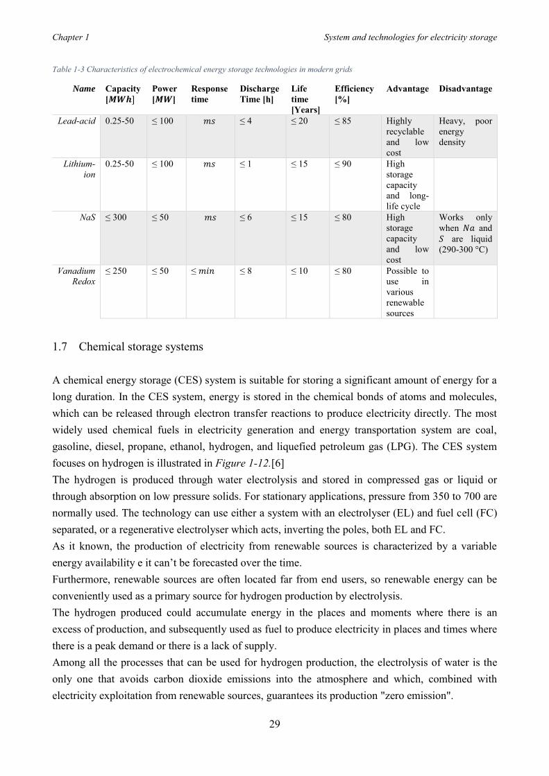
Table 1-3 Characteristics of electrochemical energy storage technologies in modern grids
Name Capacity [𝑴𝑾𝒉]
Power [𝑴𝑾]
Response time
Discharge Time [h]
Life time [Years]
Efficiency [%]
Advantage Disadvantage
Lead-acid 0.25-50 ≤ 100 𝑚𝑠 ≤ 4 ≤ 20 ≤ 85 Highly recyclable and low cost
Heavy, poor energy density
Lithium-ion
0.25-50 ≤ 100 𝑚𝑠 ≤ 1 ≤ 15 ≤ 90 High storage capacity and long-life cycle
NaS ≤ 300 ≤ 50 𝑚𝑠 ≤ 6 ≤ 15 ≤ 80 High storage capacity and low cost
Works only when 𝑁𝑎 and 𝑆 are liquid (290-300 °C)
Vanadium Redox
≤ 250 ≤ 50 ≤ 𝑚𝑖𝑛 ≤ 8 ≤ 10 ≤ 80 Possible to use in various renewable sources
1.7 Chemical storage systems A chemical energy storage (CES) system is suitable for storing a significant amount of energy for a long duration. In the CES system, energy is stored in the chemical bonds of atoms and molecules, which can be released through electron transfer reactions to produce electricity directly. The most widely used chemical fuels in electricity generation and energy transportation system are coal, gasoline, diesel, propane, ethanol, hydrogen, and liquefied petroleum gas (LPG). The CES system focuses on hydrogen is illustrated in Figure 1-12.[6] The hydrogen is produced through water electrolysis and stored in compressed gas or liquid or through absorption on low pressure solids. For stationary applications, pressure from 350 to 700 are normally used. The technology can use either a system with an electrolyser (EL) and fuel cell (FC) separated, or a regenerative electrolyser which acts, inverting the poles, both EL and FC. As it known, the production of electricity from renewable sources is characterized by a variable energy availability e it can’t be forecasted over the time. Furthermore, renewable sources are often located far from end users, so renewable energy can be conveniently used as a primary source for hydrogen production by electrolysis. The hydrogen produced could accumulate energy in the places and moments where there is an excess of production, and subsequently used as fuel to produce electricity in places and times where there is a peak demand or there is a lack of supply. Among all the processes that can be used for hydrogen production, the electrolysis of water is the only one that avoids carbon dioxide emissions into the atmosphere and which, combined with electricity exploitation from renewable sources, guarantees its production "zero emission".

Chapter 1 System and technologies for electricity storage
30
There are two methods to produce hydrogen and both don’t have environmental impact. The first one concerns the construction of large plants, located in areas where energy from renewable sources it is more abundant and can be more conveniently exploited; from here the hydrogen can be "transported" to the point of final use. The second provides the distribution with small generation units which, taking advantage on the environmental energy potential present locally, produce more hydrogen close to the end use point. Fuel cells are a system for hydrogen energy electrochemical conversion and there are three types of electrolysis technology: alkaline, polymer electrolyte membrane (PEM) and high-temperature solid oxide electrolysis. The most suitable are the alkaline because of its maturity and low costs. Figure 1-12 shows a schematic representation of HFC (Hydrogen Fuel Cell).
The overall chemical reaction in a HFC is the following
2𝐻2𝑂 + 𝑂2
𝐸𝑙𝑒𝑐𝑡𝑟𝑖𝑐𝑖𝑡𝑦 𝑝𝑟𝑜𝑑𝑢𝑐𝑡𝑖𝑜𝑛𝐸𝑙𝑒𝑐𝑡𝑟𝑜𝑙𝑦𝑠𝑖𝑠
↔ 2𝐻2𝑂 + 𝑒𝑙𝑒𝑐𝑡𝑟𝑖𝑐𝑖𝑡𝑦 (1.13)
When hydrogen fuel reaches the surface of the electrode it dissociated into 𝐻+ and 𝑒−. Hydrogen ions, oxygen, and electrons are combined to form water.
1.8 Electrical storage systems In EESS (Electrical Energy Storage Systems) energy can be stored by modifying the electrical or magnetic fields with the help of capacitors or superconducting magnets: ultracapacitors (UCs) and SMES systems are examples of EESS. These features may help the power system network improving the power quality, load balancing, supporting the MG, and reducing the necessity of importing electrical energy in the peak demand periods.
Figure 1-12 Mechanism of HFC
Chapter 1 System and technologies for electricity storage
31
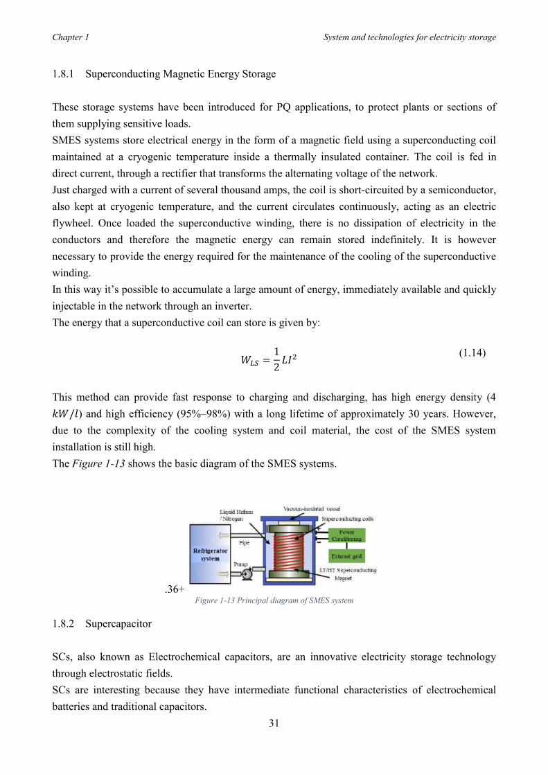
1.8.1 Superconducting Magnetic Energy Storage These storage systems have been introduced for PQ applications, to protect plants or sections of them supplying sensitive loads. SMES systems store electrical energy in the form of a magnetic field using a superconducting coil maintained at a cryogenic temperature inside a thermally insulated container. The coil is fed in direct current, through a rectifier that transforms the alternating voltage of the network. Just charged with a current of several thousand amps, the coil is short-circuited by a semiconductor, also kept at cryogenic temperature, and the current circulates continuously, acting as an electric flywheel. Once loaded the superconductive winding, there is no dissipation of electricity in the conductors and therefore the magnetic energy can remain stored indefinitely. It is however necessary to provide the energy required for the maintenance of the cooling of the superconductive winding. In this way it’s possible to accumulate a large amount of energy, immediately available and quickly injectable in the network through an inverter. The energy that a superconductive coil can store is given by:
𝑊𝐿𝑆 =1
2𝐿𝐼2 (1.14)
This method can provide fast response to charging and discharging, has high energy density (4 𝑘𝑊/𝑙) and high efficiency (95%–98%) with a long lifetime of approximately 30 years. However, due to the complexity of the cooling system and coil material, the cost of the SMES system installation is still high. The Figure 1-13 shows the basic diagram of the SMES systems.
.36+ Figure 1-13 Principal diagram of SMES system
1.8.2 Supercapacitor SCs, also known as Electrochemical capacitors, are an innovative electricity storage technology through electrostatic fields. SCs are interesting because they have intermediate functional characteristics of electrochemical batteries and traditional capacitors.
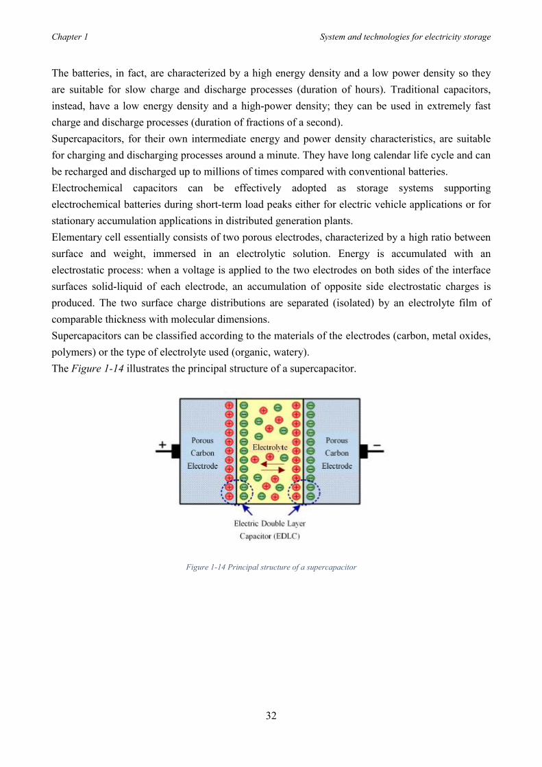
Chapter 1 System and technologies for electricity storage
32
The batteries, in fact, are characterized by a high energy density and a low power density so they are suitable for slow charge and discharge processes (duration of hours). Traditional capacitors, instead, have a low energy density and a high-power density; they can be used in extremely fast charge and discharge processes (duration of fractions of a second). Supercapacitors, for their own intermediate energy and power density characteristics, are suitable for charging and discharging processes around a minute. They have long calendar life cycle and can be recharged and discharged up to millions of times compared with conventional batteries. Electrochemical capacitors can be effectively adopted as storage systems supporting electrochemical batteries during short-term load peaks either for electric vehicle applications or for stationary accumulation applications in distributed generation plants. Elementary cell essentially consists of two porous electrodes, characterized by a high ratio between surface and weight, immersed in an electrolytic solution. Energy is accumulated with an electrostatic process: when a voltage is applied to the two electrodes on both sides of the interface surfaces solid-liquid of each electrode, an accumulation of opposite side electrostatic charges is produced. The two surface charge distributions are separated (isolated) by an electrolyte film of comparable thickness with molecular dimensions. Supercapacitors can be classified according to the materials of the electrodes (carbon, metal oxides, polymers) or the type of electrolyte used (organic, watery). The Figure 1-14 illustrates the principal structure of a supercapacitor.
Figure 1-14 Principal structure of a supercapacitor
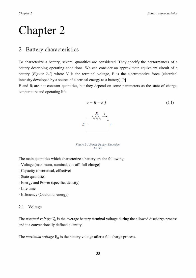
Chapter 2 Battery characteristics
33
Chapter 2
2 Battery characteristics To characterize a battery, several quantities are considered. They specify the performances of a battery describing operating conditions. We can consider an approximate equivalent circuit of a battery (Figure 2-1) where V is the terminal voltage, E is the electromotive force (electrical intensity developed by a source of electrical energy as a battery).[9] E and Ri are not constant quantities, but they depend on some parameters as the state of charge, temperature and operating life. 𝑣 = 𝐸 − 𝑅𝑖𝑖 (2.1)
The main quantities which characterize a battery are the following: - Voltage (maximum, nominal, cut-off, full-charge) - Capacity (theoretical, effective) - State quantities - Energy and Power (specific, density) - Life time - Efficiency (Coulomb, energy)
2.1 Voltage The nominal voltage 𝑉𝑛 is the average battery terminal voltage during the allowed discharge process and it a conventionally defined quantity. The maximum voltage 𝑉𝑚 is the battery voltage after a full charge process.
Figure 2-1 Simple Battery Equivalent Circuit
Chapter 2 Battery characteristics
34
The voltage at the end of the discharge, called cut-off voltage or discharge-end voltage 𝑉𝑐𝑜 is the minimum allowable battery voltage. This value is dictated by technical and/or economic reasons. Going down this value, the life of the battery can be appreciably shortened, and/or its performance can be permanently impaired. The working voltage is the terminal voltage of the battery when it delivers current. For a given current, the working voltage decreases as the battery discharges due to decrease of the emf and increase of the internal resistance. After a full charge, the initial discharge voltage is the battery voltage after a low-level discharge (conventionally 10% of the maximum capacity).[9]
2.2 Capacity Battery capacity is an important determinant in selecting a storage device. The capacity of a battery may be defined as the total quantity of electrical charges that can be delivered in a single discharge by the cell. The capacity 𝐶, measured in Amp-hour [𝐴ℎ], is the charge delivered from the battery discharging under specified conditions. The theoretical capacity 𝐶𝑇 is the battery capacity for a discharge from the fully charged condition up to completely exhausted reactants. The effective capacity 𝐶𝐸 is the battery capacity for a discharge from the fully charged condition up to the cut-off voltage where at the time 𝑡 = 0 the battery is fully charged and at the time 𝑡𝑐𝑜 it reaches the cut-off voltage. In practice, the effective capacity is used.
𝐶𝐸 = ∫ 𝑖(𝑡)𝑑𝑡𝑡𝑐𝑜
0
(2.2)
The capacity of a battery depends on several parameters. The most important one is the discharge current. Regarding its, as smaller it is and as higher the battery capacity is. Common battery specifications assume that the current is constant during the discharge. After deciding battery capacity, it is necessary to specify the discharge current or the discharge time. The nominal capacity 𝐶𝑁 is the effective capacity obtained for a discharge time equal to the standard time value 𝑇𝑑 (it must be specified) which is tied to the type of battery. The ratio 𝐶𝑁 𝑇𝑑⁄ gives the standard discharging current (C-rate). If discharged with a higher current, the capacity of the battery is lower.

Chapter 2 Battery characteristics
35
𝑇𝑑 is typically of: 5 or 10 h for Pb batteries, 5 h for NiMH batteries and of 2 h for Li batteries.[9]
2.3 State quantities The state of discharge (SOD) is the capacity delivered during a partial discharge process from the fully charge condition. It is generally calculated using integration of the delivered current and gives the reduction in the battery capacity over the time.
𝑆𝑂𝐷(𝑡) = ∫ 𝑖(𝑡)𝑑𝑡𝑡
0
(2.3)
The state of charge (SOC) is the remaining capacity of a battery after a partial discharge process from the fully charged condition. It is generally calculated using integration of the delivered current and it is subtracted to the capacity in the fully charged condition.
𝑆𝑂𝐶(𝑡) = 𝐶𝐸 −∫ 𝑖(𝑡)𝑑𝑡𝑡
0
(2.4)
The following relationship exists between SOC and SOD 𝑆𝑂𝐶(𝑡) + 𝑆𝑂𝐷(𝑡) = 𝐶𝐸 (2.5) The degree or depth of discharge (DOD) is the capacity delivered during a partial discharge process from the fully charged condition, expressed as a percentage of the capacity in the fully charged condition.
𝐷𝑂𝐷(𝑡) =𝑆𝑂𝐷(𝑇)
𝐶∙ 100 =
𝐶 − 𝑆𝑂𝐶(𝑡)
𝐶∙ 100 (2.6)
The degree or depth of charge (DOC) is the remaining capacity of a battery after a partial discharge process from the fully charged condition, expressed as a percentage of the capacity in the fully charged condition.
𝐷𝑂𝐶(𝑡) =𝑆𝑂𝐶(𝑡)
𝐶∙ 100 (2.7)
A discharge is said deep when the DOD, computed for 𝐶 = 𝐶𝐸, is equal to al 100%. However, this corresponds to a DOD of 80%, computed for 𝐶 = 𝐶𝑇.[9]
Chapter 2 Battery characteristics
36
2.4 Energy quantities Considering nominal voltage 𝑉𝑁 and theoretical capacity of the battery 𝐶𝑇 , The theoretic energy 𝐸𝑇 is conventionally defined as: 𝐸𝑇 = 𝑉𝑁𝐶𝑇 (2.8) The effective energy 𝐸𝐸 is defined as:
𝐸𝐸 = ∫ (𝑣𝑖)𝑑𝑡𝑡𝑐𝑜
0
(2.9)
where at the time 𝑡 = 0 the battery is fully charged and at the time 𝑡𝑐𝑜 it reaches the cut-off voltage. By convention, the effective energy is obtained multiplying the nominal voltage by the effective capacity. 𝐸𝐸 = 𝑉𝑁𝐶𝐸 (2.10)
In turn, the nominal energy is obtained by multiplying the nominal voltage by the nominal capacity. 𝐸𝑁 = 𝑉𝑁𝐶𝑁 (2.11)
The energy delivered from a battery is given in 𝑊ℎ. Energy and power of a battery are commonly given in terms of specific values (for unit of mass) 𝑊ℎ 𝑘𝑔⁄ obtainable from the ratio between the extractable energy of an accumulator during a given power discharge and the storage system weight in 𝑘𝑔 or in terms of densities (for unit of volume). This parameter doesn’t have a constant value but changes in function of the working use (i.e. the discharge power) and the ambient temperature. We can take the nominal energy as a reference, which is the energy that can be extracted from the accumulator in nominal conditions, in a discharge at nominal power and temperature reference environment, typically 20 or 25 ° C. The power delivered by a battery is conventionally given by the product of the nominal voltage by the standard discharge current (C-rate) 𝐼𝑁. 𝑃 = 𝐼𝑁𝑉𝑁 (2.12) The specific power, expressed in 𝑊 𝑘𝑔⁄ , obtainable from the ratio of the power and the weight in kg of the battery. As for energy, even power doesn’t have a unique value because it depends on the applied load. However, define a nominal power for each accumulator is useful because it corresponds to the most representative discharge capacity.
Chapter 2 Battery characteristics
37
2.5 Efficiency quantities Energy efficiency is defined as the ratio between the extracted energy from the accumulation system during a discharge 𝑊𝑑 to a given power and the energy spent to bring back the system into the initial state of charge (energy absorbed during the preceding charge process 𝑊𝑐).
𝜂𝑒 =∫ 𝑣𝑑𝑖𝑑𝑑𝑡𝑡𝑑0
∫ 𝑣𝑐𝑖𝑐𝑑𝑡𝑡𝑐0
=𝑊𝑑𝑊𝑐
(2.13)
The Coulomb efficiency is the ratio between the charge 𝑄𝑑 delivered from the battery during the discharge process (effective capacity) and the charge 𝑄𝑐 absorbed during the preceding charge process.
𝜂𝑎 =∫ 𝑖𝑑𝑑𝑡𝑡𝑑0
∫ 𝑖𝑐𝑑𝑡𝑡𝑐0
=𝑄𝑑𝑄𝑐
(2.14)
The values of Coulomb efficiency are between the range 0.95-1 and decrease when the charge is done quickly. The Coulomb efficiency is 1 when all the absorbed charges take part to the process of formation of the electrodes and then are released during the discharge process. It is less than 1 when a portion of the absorbed charges produces substances that do not participate in the successive discharge process. The energy efficiency is between the range 0.85-0.9 and it is lower than the Coulomb efficiency due to the presence of the internal resistance of the battery that wastes energy during both the discharge and the charge process.
2.6 Life quantities The life time, expressed in years or cycles, defines the total time of exercise of an accumulator. This time ends when the system performances degrade below operating limits, for example when the capacity is lower than a fixed percentage. Life duration of an accumulator depends heavily on the conditions of use and is reduced if the battery works with high temperatures and with incorrect management. The working temperature is the temperature range in which the accumulator can work without damages or excessive decays of performances. If the life time is expressed in cycles, it represents the number of cycles discharge, up to a prefixed percentage of DOD, and complete charge that a battery can complete before its performances falls below a minimum limit (typically before its capacity is reduced by 20%). This value changes according to the DOD value chosen, typical work and temperature.[9]
Chapter 3 Data profiles and case studies
38
Chapter 3
3 Data, profiles and case studies
3.1 Introduction In these last years the European Union has been a move towards smarter electricity networks where Advanced Metering Infrastructure (AMI) has been installed. Smart metering is considered an important part to achieve EU 20 20 20 energy policy goal by the year 2020. These rules set defines three main objectives: 20% cut in greenhouse gas emissions (compared to 1990 levels), 20% of the energy needs obtained from renewable sources and 20% improvement in energy efficiency. The objectives of the strategy were set by EU leaders in 2007 and were incorporated into national legislation in 2009. They are also the main objectives of the Europe 2020 strategy for smart, sustainable and inclusive growth. The electronic meters are located between the energy distribution networks and the user. This position offers the opportunity to add useful functionalities to distributors and sellers improving the service offered by suppliers and the management of electrical absorption for the users. However, to fully exploit this potential and involve the final consumer in the smart grid paradigm, a bidirectional communication channel between the electronic meter and the data management centre is required. The bidirectional nature of the communications allows both the absorption monitoring and the significant network parameters, and to transfer the characteristic signals of the smart grids to the consumer as market and system signals (electricity tariffs and electrical parameters). As just mentioned, particularly residential sector was involved in smart metering pilot programmes and this gave a lot of detailed data about electricity consumption. This information can be used to create electricity load profile Classes (PC) [10] and subsequently to forecast the maximum peak of power demand according to: the hours of the day, the day of the week and the season. With the traditional methods of meter data analysis, it has been noted that user characteristics key information is often lost, particularly when the average or aggregation calculation processes are applied. Therefore, other methods of analysing data need to be used so that this information is not lost. For the later SimPowerSystem model used, different residential load profiles were evaluated (PC) and obtained through a characterization concerning the aggregation of many dissimilar patterns of electricity used together. The smart metering method was carried out by Commission for Energy Regulation (CER) between 2009 and 2010 (over the period 1st July to 31st December) and consisted to installing smart meters in over 4000 residential dwellings in Ireland.
Chapter 3 Data profiles and case studies
39
3.2 Smart Metering Method As said above, the smart metering method was carried out by Commission for Energy Regulation (CER). The Commission for Energy Regulation (CER) is the regulator for the electricity and natural gas sectors in Ireland. The CER was first set up in 1999 and works within the framework of national and EU energy policy which aim to create a single European electricity market that best meets the needs of Europe’s energy consumers. The energy absorbed data were recorded every half hour and a series of tests were submitted to end users to detect their habits. The data provided was in anonymized format to protect personal and confidential customer information. It was used a clustering method to identify similar patterns of electricity. In the reality, this approach doesn’t exactly reflect how energy is used by different dwellings during the day but is useful to understand the power trend absorbed. Regarding clustering method, the clustering or group analysis is a set of multivariate data analysis techniques aimed at the selection and grouping of homogeneous elements in a group of data. Clustering techniques are based on measures related to the similarity between the elements. In many approaches this similarity, or rather dissimilarity, is conceived in terms of distance in a multidimensional space. The goodness of the analysis obtained from the clustering algorithms depends on the choice of the metric, and therefore on how the distance is calculated. The clustering algorithms gather the elements based on their mutual distance, and therefore whether or not belonging to a set depends on how much the element taken into consideration is distant from the whole itself.[11]
3.3 ISSDA introduction The data used for the case study was obtained from the project carried out by CER Smart Metering Project. The demand of residents was measured using a detailed survey conducted in the community and a modelling tool that considers the household occupancy levels, and consumer behaviour thanks to a series of submitted questionnaire. It is based on probability models that predict the possibility of each household to operate a certain number of appliances on a certain time of the day for different end users, i.e. occupancy types.[11] CER Smart Metering Project The CER initiated the Smart Metering Project in 2007 with the purpose of undertaking trials to assess the performance of Smart Meters, their impact on consumers’ energy consumption and the economic case for a wider national rollout. It is a collaborative energy industry-wide project managed by the CER and actively involving energy industry participants including the Sustainable Energy Authority of Ireland (SEAI), the Department of Communications, Energy and Natural
Chapter 3 Data profiles and case studies
40
Resources (DCENR), ESB Networks, “Bord Gáis” Networks, Electric Ireland, “Bord Gáis” Energy and other energy suppliers. The Smart Metering Electricity Customer Behaviour Trials (CBTs) took place during 2009 and 2010 with over 5,000 Irish homes and businesses participating. The purpose of the trials was to assess the impact on consumer’s electricity consumption to inform the cost-benefit analysis for a national rollout. Electric Ireland residential and business customers, and Bord Gáis Energy business customers, who participated in the trials had an electricity smart meter installed in their homes/premises and agreed to take part in research to help establish how smart metering can help shape energy usage behaviours across a variety of demographics, lifestyles and home sizes. The trials produced positive results, the reports for which are available on from CER along with further information on the Smart Metering Project. The detailed data underlying the electricity customer behaviour trial results is now being made available in anonymised format to facilitate further research and the development of competitive products and services following the anticipated rollout of Smart Meters in Ireland. No personal or confidential information is contained in the data set, which instead gives anonymised behavioural and usage patterns.[11] About CRU The Commission for Regulation of Utilities (CRU) is Ireland’s independent energy and water regulator. The CRU was originally established as the Commission for Energy Regulation (CER) in 1999. The CER changed its name to the CRU in 2017 to better reflect the expanded powers and functions of the organisation. The CRU has a wide range of economic, customer protection and safety responsibilities in energy and water. The CRU’s mission is to regulate water, energy and energy safety in the public interest. The work of the CRU impacts every Irish home and business, by ensuring safe, secure and sustainable energy and water supplies at a reasonable cost. The sectors we regulate underpin Irish economic competitiveness, investment and growth, while also contributing to our international obligations to address climate change.[11]
3.4 Network considered The generic urban model used for the simulations is shown in Figure 3-1. Table 3-1 summarises the data used.
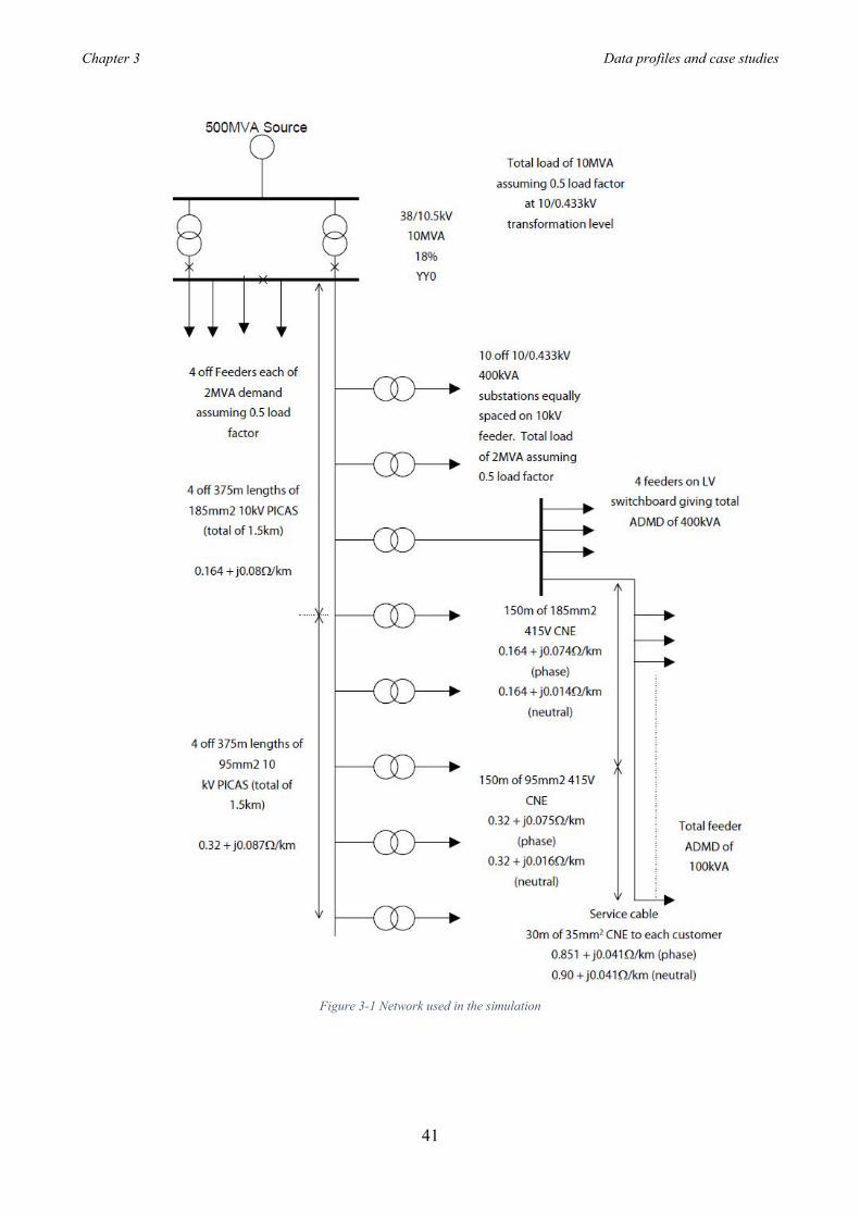
Chapter 3 Data profiles and case studies
41
Figure 3-1 Network used in the simulation
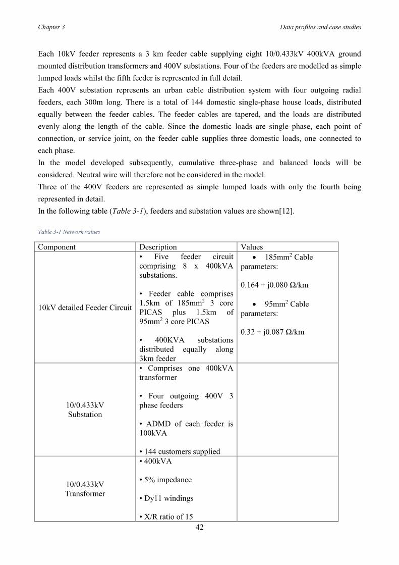
Chapter 3 Data profiles and case studies
42
Each 10kV feeder represents a 3 km feeder cable supplying eight 10/0.433kV 400kVA ground mounted distribution transformers and 400V substations. Four of the feeders are modelled as simple lumped loads whilst the fifth feeder is represented in full detail. Each 400V substation represents an urban cable distribution system with four outgoing radial feeders, each 300m long. There is a total of 144 domestic single-phase house loads, distributed equally between the feeder cables. The feeder cables are tapered, and the loads are distributed evenly along the length of the cable. Since the domestic loads are single phase, each point of connection, or service joint, on the feeder cable supplies three domestic loads, one connected to each phase. In the model developed subsequently, cumulative three-phase and balanced loads will be considered. Neutral wire will therefore not be considered in the model. Three of the 400V feeders are represented as simple lumped loads with only the fourth being represented in detail. In the following table (Table 3-1), feeders and substation values are shown[12]. Table 3-1 Network values
Component Description Values
10kV detailed Feeder Circuit
• Five feeder circuit comprising 8 x 400kVA substations. • Feeder cable comprises 1.5km of 185mm2 3 core PICAS plus 1.5km of 95mm2 3 core PICAS • 400KVA substations distributed equally along 3km feeder
• 185mm2 Cable parameters: 0.164 + j0.080 Ω/km
• 95mm2 Cable parameters: 0.32 + j0.087 Ω/km
10/0.433kV Substation
• Comprises one 400kVA transformer • Four outgoing 400V 3 phase feeders • ADMD of each feeder is 100kVA • 144 customers supplied
10/0.433kV Transformer
• 400kVA • 5% impedance • Dy11 windings • X/R ratio of 15
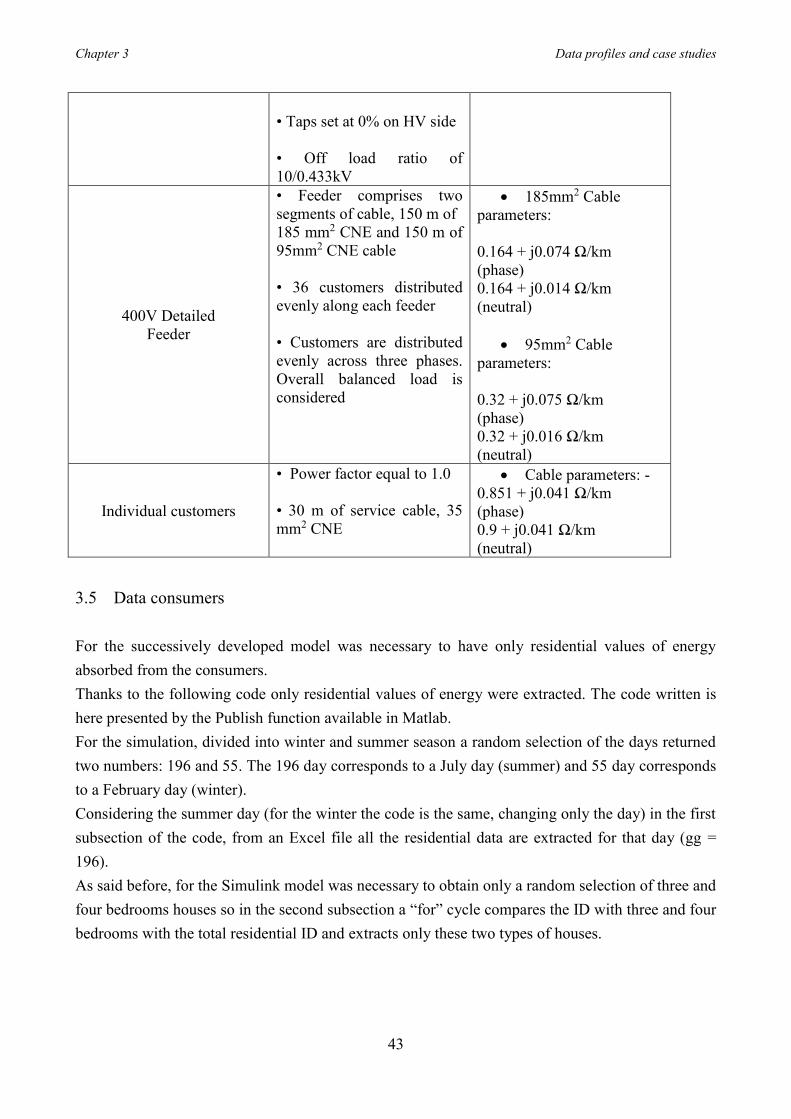
Chapter 3 Data profiles and case studies
43
• Taps set at 0% on HV side • Off load ratio of 10/0.433kV
400V Detailed Feeder
• Feeder comprises two segments of cable, 150 m of 185 mm2 CNE and 150 m of 95mm2 CNE cable • 36 customers distributed evenly along each feeder • Customers are distributed evenly across three phases. Overall balanced load is considered
• 185mm2 Cable parameters: 0.164 + j0.074 Ω/km (phase) 0.164 + j0.014 Ω/km (neutral)
• 95mm2 Cable parameters: 0.32 + j0.075 Ω/km (phase) 0.32 + j0.016 Ω/km (neutral)
Individual customers
• Power factor equal to 1.0 • 30 m of service cable, 35 mm2 CNE
• Cable parameters: - 0.851 + j0.041 Ω/km (phase) 0.9 + j0.041 Ω/km (neutral)
3.5 Data consumers For the successively developed model was necessary to have only residential values of energy absorbed from the consumers. Thanks to the following code only residential values of energy were extracted. The code written is here presented by the Publish function available in Matlab. For the simulation, divided into winter and summer season a random selection of the days returned two numbers: 196 and 55. The 196 day corresponds to a July day (summer) and 55 day corresponds to a February day (winter). Considering the summer day (for the winter the code is the same, changing only the day) in the first subsection of the code, from an Excel file all the residential data are extracted for that day (gg = 196). As said before, for the Simulink model was necessary to obtain only a random selection of three and four bedrooms houses so in the second subsection a “for” cycle compares the ID with three and four bedrooms with the total residential ID and extracts only these two types of houses.
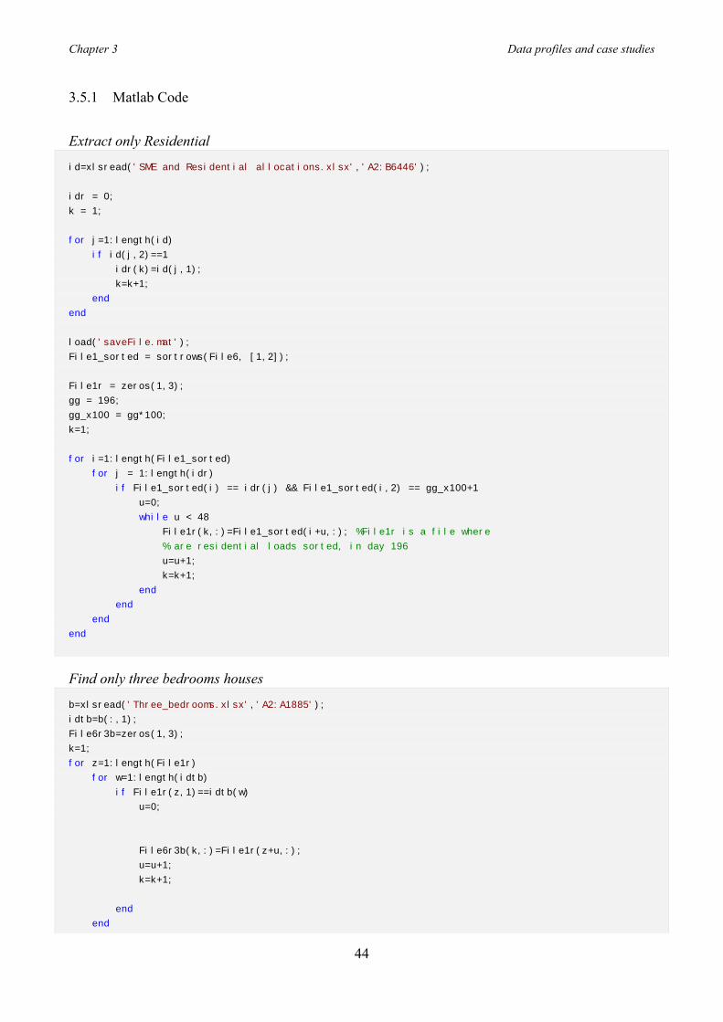
Chapter 3 Data profiles and case studies
44
3.5.1 Matlab Code Extract only Residential
id=xlsread('SME and Residential allocations.xlsx','A2:B6446');
idr = 0;
k = 1;
for j=1:length(id)
if id(j,2)==1
idr(k)=id(j,1);
k=k+1;
end
end
load('saveFile.mat');
File1_sorted = sortrows(File6, [1,2]);
File1r = zeros(1,3);
gg = 196;
gg_x100 = gg*100;
k=1;
for i=1:length(File1_sorted)
for j = 1:length(idr)
if File1_sorted(i) == idr(j) && File1_sorted(i,2) == gg_x100+1
u=0;
while u < 48
File1r(k,:)=File1_sorted(i+u,:); %File1r is a file where
% are residential loads sorted, in day 196
u=u+1;
k=k+1;
end
end
end
end
Find only three bedrooms houses
b=xlsread('Three_bedrooms.xlsx','A2:A1885');
idtb=b(:,1);
File6r3b=zeros(1,3);
k=1;
for z=1:length(File1r)
for w=1:length(idtb)
if File1r(z,1)==idtb(w)
u=0;
File6r3b(k,:)=File1r(z+u,:);
u=u+1;
k=k+1;
end
end
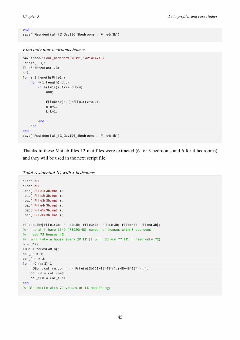
Chapter 3 Data profiles and case studies
45
end
save('Residential_ID_Day196_3bedrooms','File6r3b')
Find only four bedrooms houses
b=xlsread('Four_bedrooms.xlsx','A2:A1471');
idtb=b(:,1);
File6r4b=zeros(1,3);
k=1;
for z=1:length(File1r)
for w=1:length(idtb)
if File1r(z,1)==idtb(w)
u=0;
File6r4b(k,:)=File1r(z+u,:);
u=u+1;
k=k+1;
end
end
end
save('Residential_ID_Day196_4bedrooms','File6r4b')
Thanks to these Matlab files 12 mat files were extracted (6 for 3 bedrooms and 6 for 4 bedrooms) and they will be used in the next script file. Total residential ID with 3 bedrooms
clear all
close all
load('File1r3b.mat');
load('File2r3b.mat');
load('File3r3b.mat');
load('File4r3b.mat');
load('File5r3b.mat');
load('File6r3b.mat');
Filetot3b=[File1r3b; File2r3b; File3r3b; File4r3b; File5r3b; File6r3b];
% In total I have 1540 (73920/48) number of houses with 3 bedrooms
% I need 72 houses ID
% I will take a house every 20 ID (I will obtain 77 ID. I need only 72)
n = 3*72;
ID3b = zeros(48,n);
col_in = 1;
col_fin = 3;
for i=0:(n/3)-1
ID3b(:,col_in:col_fin)=Filetot3b((1+19*48*i):(48+48*19*i),:);
col_in = col_in+3;
col_fin = col_fin+3;
end
% ID3b matrix with 72 values of ID and Energy

Chapter 3 Data profiles and case studies
46
Total residential ID with 4 bedrooms
load('File1r4b.mat');
load('File2r4b.mat');
load('File3r4b.mat');
load('File4r4b.mat');
load('File5r4b.mat');
load('File6r4b.mat');
Filetot4b=[File1r4b; File2r4b; File3r4b; File4r4b; File5r4b; File6r4b];
m= 3*72;
ID4b=zeros(48,m);
col_in = 1;
col_fin = 3;
for j=0:(m/3)-1
ID4b(:,col_in:col_fin)=Filetot4b((1+15*48*j):(48+48*15*j),:);
col_in = col_in+3;
col_fin = col_fin+3;
end
%%Extract only 3rd and multiple columns to a matrix containing only
%%energies of the 3 bedrooms ID
energy3b=zeros(48,72);
for w=1:72
energy3b(:,w)=ID3b(:,3*w);
end
%I have to sum 3 by 3 to obtain 24 houses (24*3=72)
houses3b=zeros(48,24);
k=0;
for u=1:24
houses3b(:,u)=energy3b(:,1+k)+energy3b(:,2+k)+energy3b(:,3+k);
k=k+3;
end
%%Extract only 3rd and multiple columns to a matrix containing only
% Energies of the 4 bedrooms ID
energy4b=zeros(48,72);
for v=1:72
energy4b(:,v)=ID4b(:,3*v);
end
%I have to sum 3 by 3 to obtain 24 houses (24*3=72)
houses4b=zeros(48,24);
k=0;
for z=1:24
houses4b(:,z)=energy4b(:,1+k)+energy4b(:,2+k)+energy4b(:,3+k);
k=k+3;
end
% Each house includes 3 houses with 3 bedrooms and 3 with 4 bedrooms. I
% have 24 blocks because 6 blocks oh houses each feeder multiplied by 4
% feeders
ehousetot=houses3b+houses4b; %values of energy in 24 hours [kWh]
phousetot=ehousetot/0.5; %to obtain the power I divide by 0.5 because each value
%corrispond to half an hour [kW].
phousetotW=phousetot*(10^3);%THIS IS THE POWER IN kW TO USE IN SIMULINK MODEL
% I have to find the power peak in each feeders. They are sized on 100kVA
% ADMD
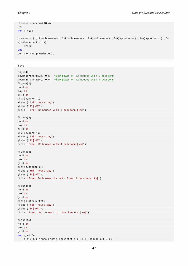
Chapter 3 Data profiles and case studies
47
pfeedertot=zeros(48,4);
k=0;
for ii=1:4
pfeedertot(:,ii)=phousetot(:,1+k)+phousetot(:,2+k)+phousetot(:,3+k)+phousetot(:,4+k)+phousetot(:,5+
k)+phousetot(:,6+k);
k=k+6;
end
col_max=max(pfeedertot);
Plot
h=[1:48]';
power3b=energy3b./0.5; %[kW]power of 72 houses with 3 bedrooms
power4b=energy4b./0.5; %[kW]power of 72 houses with 4 bedrooms
figure(1)
hold on
box on
grid on
plot(h,power3b)
xlabel('half hours day');
ylabel('P [kW]');
title('Power 72 houses with 3 bedrooms [kw]');
figure(2)
hold on
box on
grid on
plot(h,power4b)
xlabel('half hours day');
ylabel('P [kW]');
title('Power 72 houses with 4 bedrooms [kw]');
figure(3)
hold on
box on
grid on
plot(h,phousetot)
xlabel('Half hours day');
ylabel('P [kW]');
title('Power 24 houses mix with 3 and 4 bedrooms [kw]');
figure(4)
hold on
box on
grid on
plot(h,pfeedertot)
xlabel('half hours day');
ylabel('P [kW]');
title('Power tot in each of four feeders [kw]');
figure(5)
hold on
box on
grid on
for jj=1:24
plot3(h,jj*ones(length(phousetot(:,jj)),1),phousetot(:,jj));
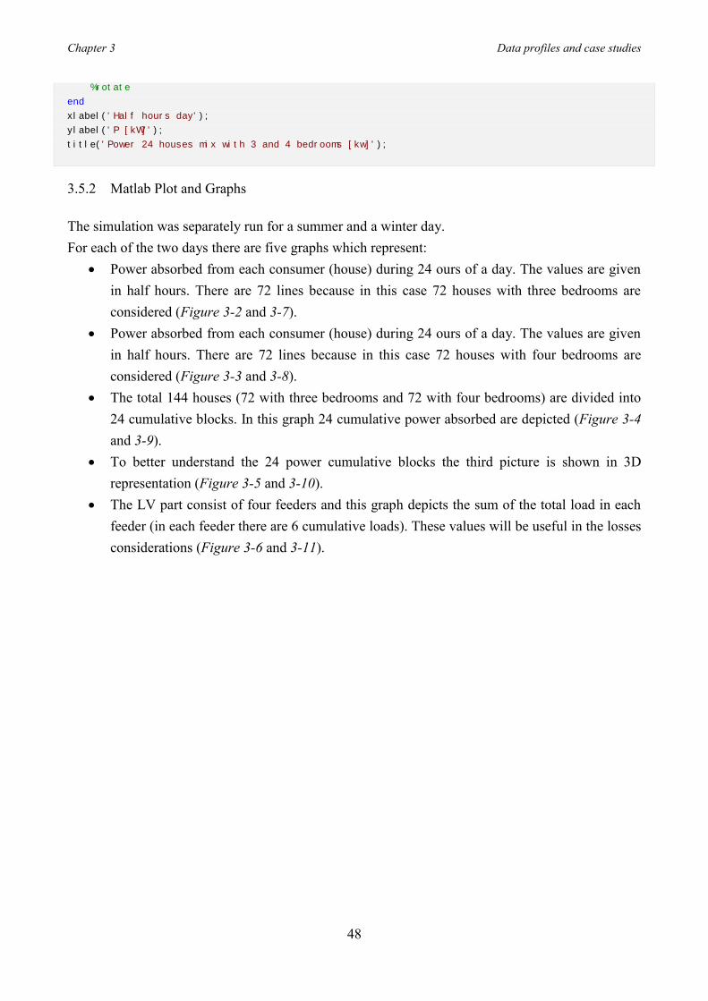
Chapter 3 Data profiles and case studies
48
%rotate
end
xlabel('Half hours day');
ylabel('P [kW]');
title('Power 24 houses mix with 3 and 4 bedrooms [kw]');
3.5.2 Matlab Plot and Graphs The simulation was separately run for a summer and a winter day. For each of the two days there are five graphs which represent:
• Power absorbed from each consumer (house) during 24 ours of a day. The values are given in half hours. There are 72 lines because in this case 72 houses with three bedrooms are considered (Figure 3-2 and 3-7).
• Power absorbed from each consumer (house) during 24 ours of a day. The values are given in half hours. There are 72 lines because in this case 72 houses with four bedrooms are considered (Figure 3-3 and 3-8).
• The total 144 houses (72 with three bedrooms and 72 with four bedrooms) are divided into 24 cumulative blocks. In this graph 24 cumulative power absorbed are depicted (Figure 3-4 and 3-9).
• To better understand the 24 power cumulative blocks the third picture is shown in 3D representation (Figure 3-5 and 3-10).
• The LV part consist of four feeders and this graph depicts the sum of the total load in each feeder (in each feeder there are 6 cumulative loads). These values will be useful in the losses considerations (Figure 3-6 and 3-11).
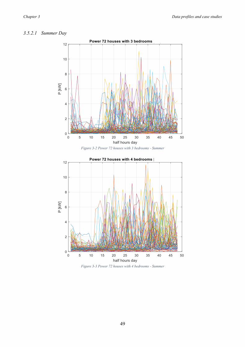
Chapter 3 Data profiles and case studies
49
3.5.2.1 Summer Day
Figure 3-2 Power 72 houses with 3 bedrooms - Summer
Figure 3-3 Power 72 houses with 4 bedrooms - Summer
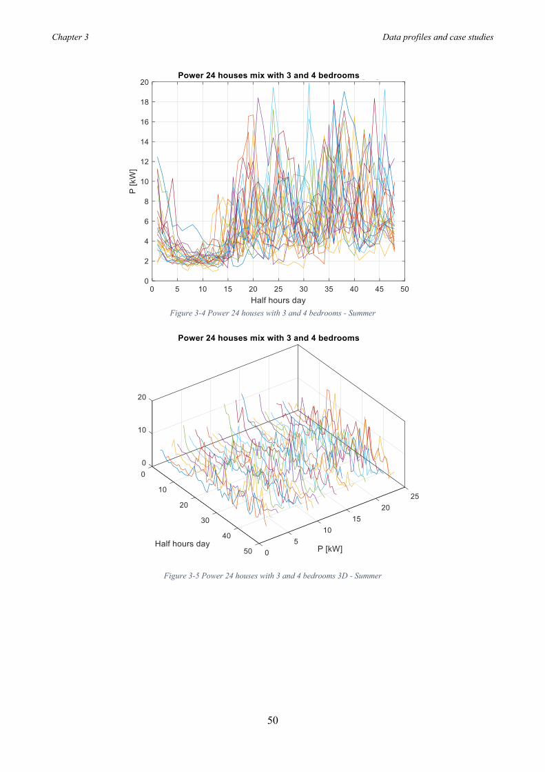
Chapter 3 Data profiles and case studies
50
Figure 3-4 Power 24 houses with 3 and 4 bedrooms - Summer
Figure 3-5 Power 24 houses with 3 and 4 bedrooms 3D - Summer
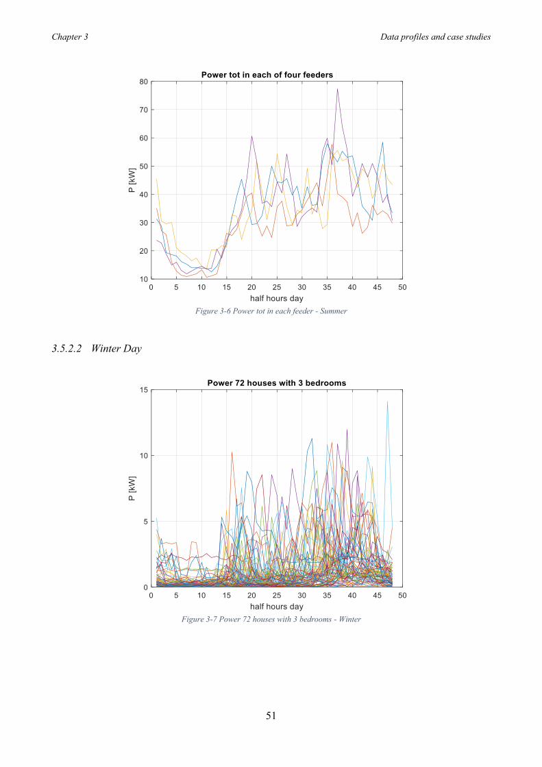
Chapter 3 Data profiles and case studies
51
Figure 3-6 Power tot in each feeder - Summer
3.5.2.2 Winter Day
Figure 3-7 Power 72 houses with 3 bedrooms - Winter
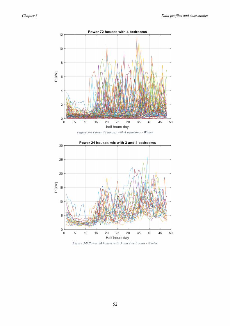
Chapter 3 Data profiles and case studies
52
Figure 3-8 Power 72 houses with 4 bedrooms - Winter
Figure 3-9 Power 24 houses with 3 and 4 bedrooms - Winter
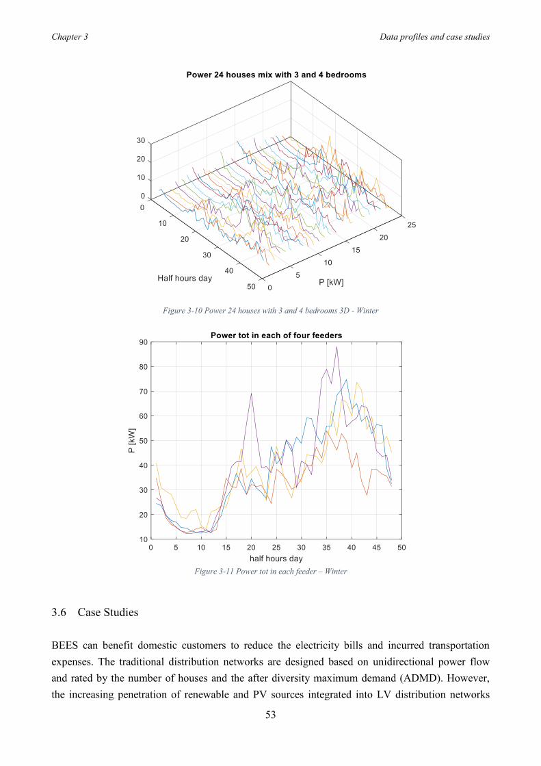
Chapter 3 Data profiles and case studies
53
Figure 3-10 Power 24 houses with 3 and 4 bedrooms 3D - Winter
Figure 3-11 Power tot in each feeder – Winter
3.6 Case Studies BEES can benefit domestic customers to reduce the electricity bills and incurred transportation expenses. The traditional distribution networks are designed based on unidirectional power flow and rated by the number of houses and the after diversity maximum demand (ADMD). However, the increasing penetration of renewable and PV sources integrated into LV distribution networks
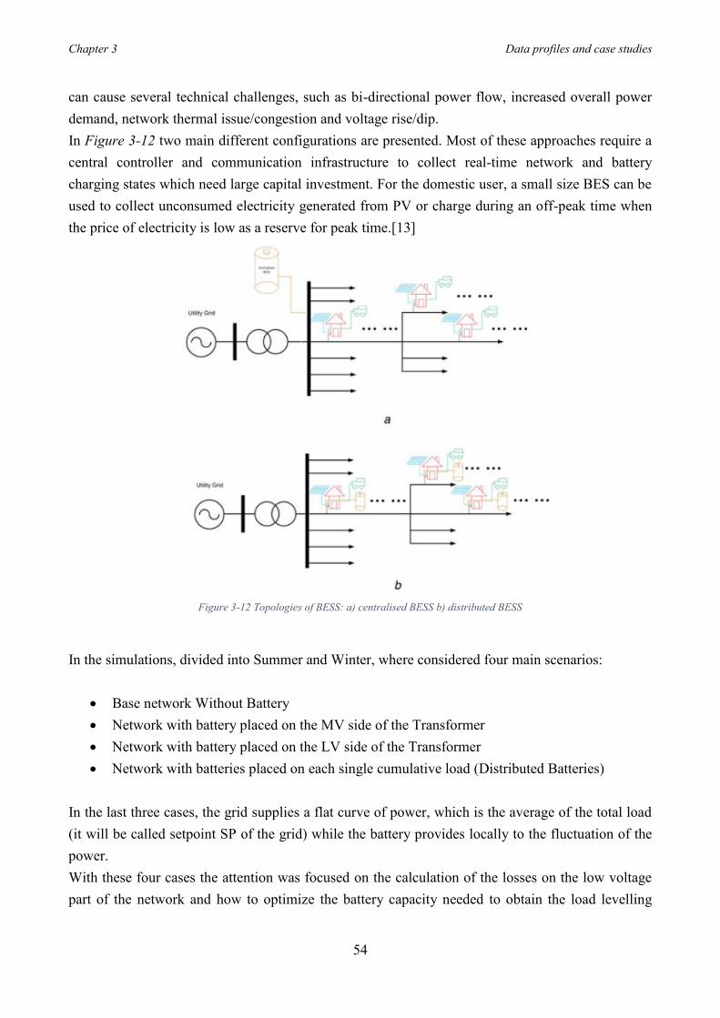
Chapter 3 Data profiles and case studies
54
can cause several technical challenges, such as bi-directional power flow, increased overall power demand, network thermal issue/congestion and voltage rise/dip. In Figure 3-12 two main different configurations are presented. Most of these approaches require a central controller and communication infrastructure to collect real-time network and battery charging states which need large capital investment. For the domestic user, a small size BES can be used to collect unconsumed electricity generated from PV or charge during an off-peak time when the price of electricity is low as a reserve for peak time.[13]
Figure 3-12 Topologies of BESS: a) centralised BESS b) distributed BESS
In the simulations, divided into Summer and Winter, where considered four main scenarios:
• Base network Without Battery • Network with battery placed on the MV side of the Transformer • Network with battery placed on the LV side of the Transformer • Network with batteries placed on each single cumulative load (Distributed Batteries)
In the last three cases, the grid supplies a flat curve of power, which is the average of the total load (it will be called setpoint SP of the grid) while the battery provides locally to the fluctuation of the power. With these four cases the attention was focused on the calculation of the losses on the low voltage part of the network and how to optimize the battery capacity needed to obtain the load levelling

Chapter 3 Data profiles and case studies
55
during the day. On the medium part of the grid where considered the same four scenarios to investigate how the battery existence could influence the losses on the MV part. In the second part of the evaluation, to consider the impact of residential PV generation other 9 cases divided into 3 main scenarios where considered:
• The first scenario considered half houses number (72 houses) with 1 kW PV panel installed and for this case where divided three sub-cases:
o Without battery installed o With battery considering the original setpoint of the grid o With battery considering a new setpoint of the grid which takes into account the total
load of the grid and the presence of PV generation • The second one considered the total number of houses (144) with 1 kW PV panel installed
and for this case where divided three sub-cases: o Without battery installed o With battery considering the original setpoint of the grid o With battery considering a new setpoint of the grid which takes into account the total
load of the grid and the presence of PV generation • The third one considered the total number of houses (144) with 2 kW PV panel installed and
for this case where divided three sub-cases: o Without battery installed o With battery considering the original setpoint of the grid o With battery considering a new setpoint of the grid which takes into account the total
load of the grid and the presence of PV generation.
Chapter 4 Simulink Model
56
Chapter 4
4 Simulink Model
4.1 Introduction The following study was developed using a part of Simulink, Simscape Electrical (formerly SimPowerSystems and SimElectronics). It provides component libraries for modelling and simulating electronic, mechatronic, and electrical power systems. It includes models of semiconductors, motors, and components for applications such as electromechanical actuation, smart grids, and renewable energy systems. In this case it was used to analyse the transmission and distribution of electrical power at the grid level.
4.2 Simulink Model The figure below (Figure 4-1) depicts the whole Simulink model used. In this figure it is possible to see and to have an idea of the general model and the configuration of the network shown in Figure 3-1. The specific part will be will be explained in detail in this paragraph. Even if many scenarios and different input values for winter and summer day will be considered, the same model was used for all the simulations changing only the input values of the loads. In the model properties part there is a window to initialize the model functions. Thanks to this, it was possible to recall the Matlab scripts, seen in the previous chapter, containing vectors in “mat” files format to be supplied as input to the load blocks. For model simulations, a phasor type simulation was used with a simulation time of 48 seconds. This time has been chosen to correspond each second to a value of power supplied to the load block relative by means of a vector; as previously said, the data are provided in half hours during the day. However, it was necessary to fix a time interval between samples that was set equal to 𝑇𝑠 = 2 ∙10−3. Starting from the left side of the figure, it is possible to identify the 38 kV power source, the HV/MV transformer and five derived feeders. Four of the feeders are modelled as simple lumped loads whilst the fifth feeder is represented in full detail. Regarding the blocks containing the line values, a Three-Phase Series RLC branch block was used where an RL branch type was selected. It was assumed that only balanced load was present. In the Figure 4-2 it is possible to see one feeder on the right part of the model which depicts the core of the whole study.

Chapter 4 Simulink Model
57
Figure 4-1 Simulink Model
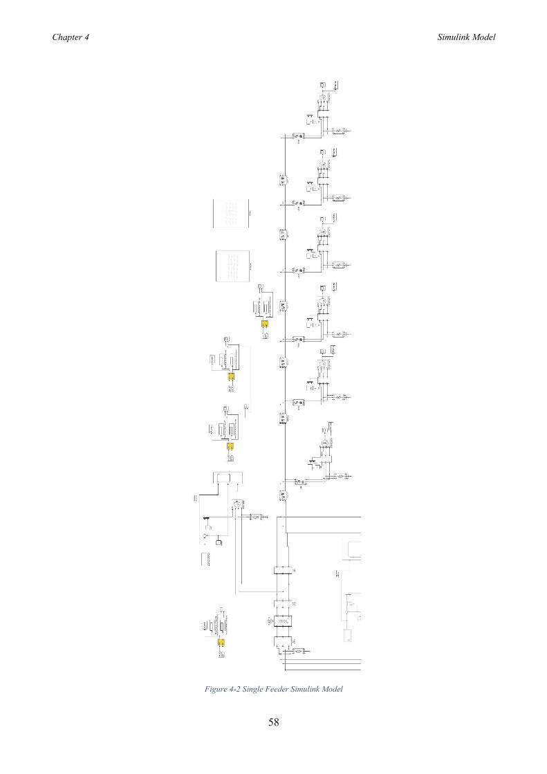
Chapter 4 Simulink Model
58
Figure 4-2 Single Feeder Simulink Model

Chapter 4 Simulink Model
59
4.2.1 Three Phase Load Block In Figure 4-2 a feeder is shown in detail. Starting from the right it is possible to see a transformer MV/LV between two three phase measurement blocks. After the battery connection, there is another three-phase measurement block. These “Three-Phase V-I Measurement” block is used to measure instantaneous three-phase voltages and currents in a circuit. When connected in series with three-phase elements, it returns the three phase-to-ground or phase-to-phase peak voltages and currents. The block can output the voltages and currents in per unit (pu) values or in volts and amperes. In this case the phase-to-ground voltage measure was chosen. The output voltage and current values achieved, have been reprocessed to obtain the values of power passing through that portion of the line in order to perform the calculations concerning to the feeders’ losses; they will be dealt with in the next chapter. In Figure 4-3 a single load of the feeder is represented.
Figure 4-3 Single Load Model
The “Three-Phase Dynamic Load” block implements a three-phase, three-wire dynamic load whose active power P and reactive power Q vary as function of positive-sequence voltage. Negative and zero-sequence currents are not simulated. The three load currents are therefore balanced, even under unbalanced load voltage conditions. There is the possibility to implement an external control of the block. If selected, the active power and reactive power of the load are defined by an external Simulink vector of two signals and an input, labelled PQ, appears. This input is used to control the active and reactive powers of the load from a vector of two signals [P, Q]. In this case a “Repeating Sequence Interpolated” block was used. It outputs a periodic discrete-time sequence based on the values in “Vector of time values” and “Vector of output values” parameters. In Figure 4-4 the blocks parameters are shown.
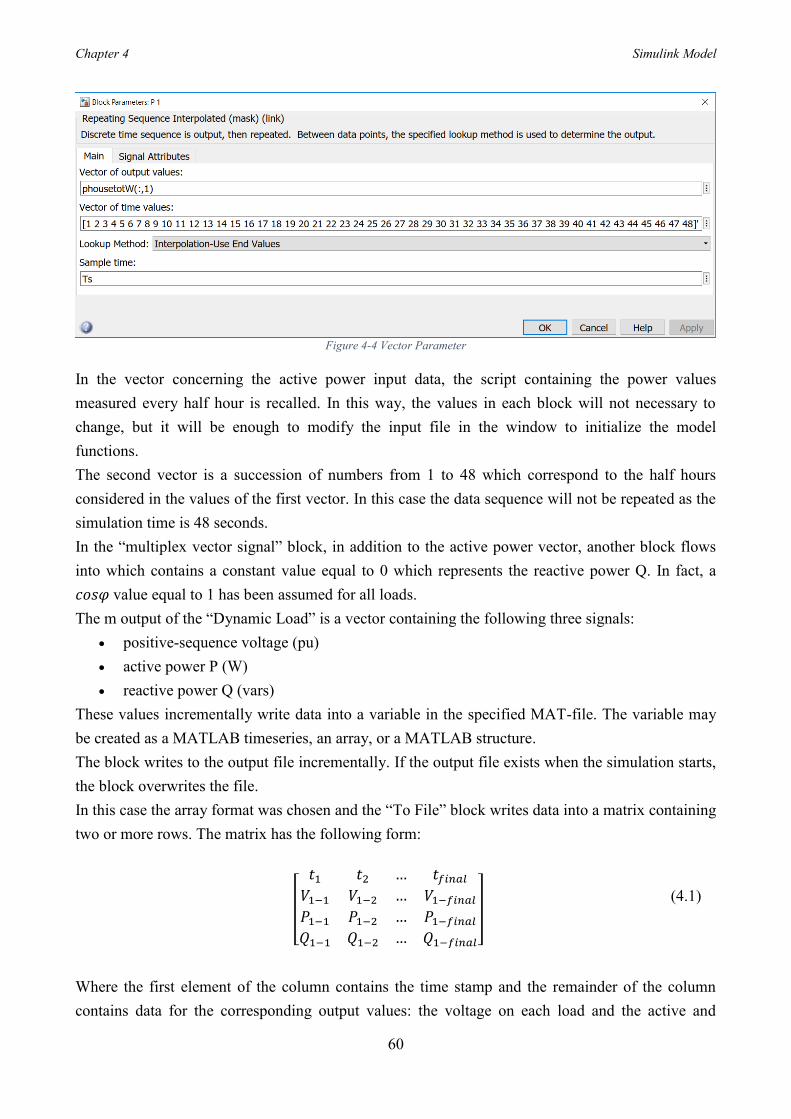
Chapter 4 Simulink Model
60
Figure 4-4 Vector Parameter
In the vector concerning the active power input data, the script containing the power values measured every half hour is recalled. In this way, the values in each block will not necessary to change, but it will be enough to modify the input file in the window to initialize the model functions. The second vector is a succession of numbers from 1 to 48 which correspond to the half hours considered in the values of the first vector. In this case the data sequence will not be repeated as the simulation time is 48 seconds. In the “multiplex vector signal” block, in addition to the active power vector, another block flows into which contains a constant value equal to 0 which represents the reactive power Q. In fact, a 𝑐𝑜𝑠𝜑 value equal to 1 has been assumed for all loads. The m output of the “Dynamic Load” is a vector containing the following three signals:
• positive-sequence voltage (pu) • active power P (W) • reactive power Q (vars)
These values incrementally write data into a variable in the specified MAT-file. The variable may be created as a MATLAB timeseries, an array, or a MATLAB structure. The block writes to the output file incrementally. If the output file exists when the simulation starts, the block overwrites the file. In this case the array format was chosen and the “To File” block writes data into a matrix containing two or more rows. The matrix has the following form:
[ 𝑡1 𝑡2 … 𝑡𝑓𝑖𝑛𝑎𝑙𝑉1−1 𝑉1−2 … 𝑉1−𝑓𝑖𝑛𝑎𝑙𝑃1−1 𝑃1−2 … 𝑃1−𝑓𝑖𝑛𝑎𝑙𝑄1−1 𝑄1−2 … 𝑄1−𝑓𝑖𝑛𝑎𝑙]
(4.1)
Where the first element of the column contains the time stamp and the remainder of the column contains data for the corresponding output values: the voltage on each load and the active and

Chapter 4 Simulink Model
61
reactive power flowing into each load. As said before, the reactive power row is always fluctuating around 0 due to 𝑐𝑜𝑠𝜑 = 1 chosen for the loads.
4.2.2 Battery model The model considered is illustrated in Figure 4-5. The idea behind this model is that the network has to provide constant power throughout the day while a battery can be charged or discharged in discrete steps supplying the variable part of the loads. However, due to the general nature of the model, this model can also be used to describe other storage devices that can buy and sell a commodity with restricted storage.
Figure 4-5 Battery Model
The model includes several blocks:
• A “Repeating Sequence Interpolated” block called “Total Power at B3 bus”. In this block all the 24 cumulative loads are summed and a vector of 48 rows is created. This is the total power of the LV part of the network seen from bus located after the MV/LV transformer.
• A “Constant” block called “Setpoint”. The setpoint is the constant value of the power supplied by the grid and it is obtained from the sum of the daily total load and the losses (feeders + transformers). The basic idea is the following: the network, and consequently the production plants, must supply the network with a constant power value during the day while the batteries must provide the variable part. They will be charged when the power plants produce a surplus of energy while they will be discharged during peak hours. This operation allows not having to size the plants units for peak values but for a constant and lower power value.
Chapter 4 Simulink Model
62
• The values coming from the sum of the loads and the average power value supplied by the network converge into a "Sum" block. This type of blocks adds or subtracts inputs. In this case the following signs were used: "- +". The setpoint enters the block with a positive sign while the sum of the loads enters with a minus sign as the battery must supply or absorb the difference of power. When the battery has to supply the LV network, the resulting sign will be negative because the storage must deliver power (the setpoint is less than the power that is actually require by the loads) and the battery is discharged. On the other hand, when the storage has to absorb power, and then the battery is charging, the resulting sign will be positive because the network is producing more power than required by the loads.
• The power value supplied or absorbed from the battery flows into a "Mux" block. This block has a fixed number of scalar or vector inputs. In this case there will be two inputs: a constant value equal to 0 of reactive power and the value of active power coming from the sum block.
• The actual model of the battery is a "Three Phase Dynamic Load" block equal to the load model. The operation is the following: when the battery is charged, the input power vector is positive, while when the battery is discharged, i.e. it is powering the LV network, the output power will have a negative sign. An external control of the PQ is implemented. As previously said, the reactive power vector is set to 0 throughout the day while the power value comes from the sum block.
4.2.3 Distributed Batteries on Cumulative Loads In the scenario where distributed batteries are considered, and positioned exactly on the cumulative loads, which include 6 units each, the basic Simulink model is modified. The network upstream of the MV / LV transformer remains unchanged to the Figure 4-1 while the individual loads will be modified as in the Figure 4-6. In this case the sum block has three inputs: two equal vectors containing the powers absorbed in the 48 half hours of the day and a constant setpoint block provided by the network. This value is the average of the power vector and therefore changes for each cumulative load. The sum of the average values of the 24 cumulative loads assembles the setpoint that the network must supply; it will be the same value obtained and used in previous simulations. The power exchange, charging and discharge of the battery occur locally while the upstream network provides a constant value throughout the day.
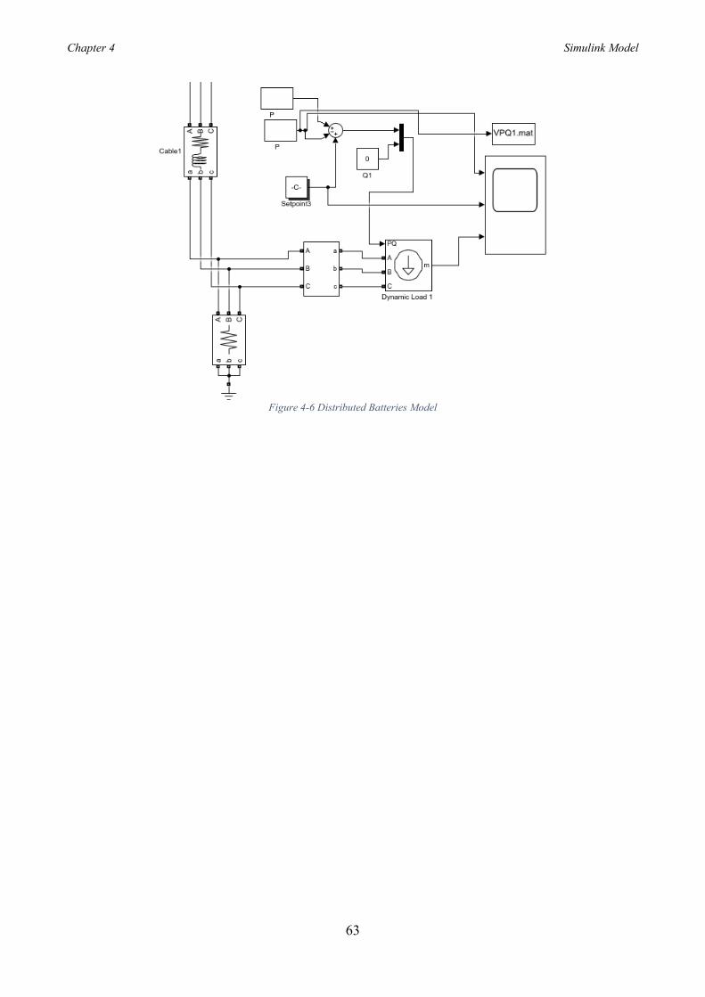
Chapter 4 Simulink Model
63
Figure 4-6 Distributed Batteries Model

Chapter 5 Distribution network losses
64
Chapter 5
5 Distribution network losses
In this new electric context where the price of energy increases, and renewable sources become more important over total generation, it is necessary to study components that improve the supply of the power to the load, managing voltage quality and trying to minimize losses, increasing the overall energy efficiency of the system. Losses reduction in distribution network is one of the the most important topics especially in medium (MV) and low voltage (LV) grid. The variable load during a day and the increasing input of energy by private household, suggest the use of storage to reduce daily load peak and improve energy distribution. Using batteries as an instrument to reduce the losses is the main topic of this chapter and it will be considered the losses amount during all time interval. As will be dealt later, four simulations scenarios will be considered: the first is a distribution network without batteries, second and third with localized battery while the last one with distributed storage provided by the user, which in the future could be electric vehicles.
5.1 Theoretical Basis The main purpose of this thesis is to use BESS to level the daily load profile. Since network losses are directly proportional to the square of the current, shifting load from peak to off-peak periods, can potentially reduce system losses. Power losses cause production of heat which increase the temperature on the feeders, so lifetime and reliability of the system decrease if the losses increase. Losses reduction depends on several factors such as ESS transformer side installation (MV or LV side) or distributed BEES on each load. According to [14] losses in the distribution network may be resulted from various technical and non-technical reasons. Technical losses are caused by active and reactive energy that flows through distribution network while non-technical losses are produced by errors in metering, reading, accounting and invoicing processes. Many techniques for loss minimization such as automating the distribution reconfiguration, optimal design and planning of the distribution system and demand side management are considered in research but one of the effective ways to reduce distribution losses is flattening the load curve thanks to BEES. Load levelling consist in shaving the peak load and filling the load valley.
There are three factors that help loss reduction:
Chapter 5 Distribution network losses
65
• As said before, ohmic losses are a square function of current flow, so shifting some currents from peak to off-peak period decrease the net losses.
• The resistance of distribution wires and transformers is lower in off-peak periods when the temperature is lower.
• The cost of energy, and subsequently of the losses, is generally lower during off-peak periods.
In general, the total losses in a time period with and without load levelled are shown below[14]. In this study it is considered a period 𝑇 of simulation of 48 seconds which corrispond to 24 half hours in a day.
𝐿𝑜𝑠𝑠 =∑𝑅(𝑡) ∙ 𝐼(𝑡)2𝑇
𝑡=1
(5.1)
𝐿𝑜𝑠𝑠𝐿𝑒𝑣𝑒𝑙𝑒𝑑 =∑𝑅(𝑡) ∙ [𝐼(𝑡) + 𝐼𝐸𝑆𝑆(𝑡)]2
𝑇
𝑡=1
(5.2)
Where: 𝐿𝑜𝑠𝑠 Network losses 𝐿𝑜𝑠𝑠𝐿𝑒𝑣𝑒𝑙𝑒𝑑 Network losses with BEES (current leveled) 𝑅(𝑡) & 𝐼(𝑡) Resistance and current at time t Starting from the total power of the loads, ideal load levelling can be achieved finding the average of the power. This produce a single value of power that will be provided from the grid while the ESS should balance out the fluctuation between this value, that in the future will be called “setpoint”, and the trend of the daily load power. This same way of thinking can be expressed in current terms. Considering the average of current (derived from the power values), load currents below the straight line will be increase to reach average value by charging ESS and load currents above average will be compensate discharging the battery.
𝐼𝐿𝑜𝑎𝑑𝐴𝑣𝑒𝑟 =
∑ 𝐼𝐿𝑜𝑎𝑑(𝑡)𝑇𝑡=1
𝑇
(5.3)
𝐼𝐸𝑆𝑆(𝑡) = 𝐼𝐿𝑜𝑎𝑑(𝑡) − 𝐼𝐿𝑜𝑎𝑑𝐴𝑣𝑒𝑟 = 𝐼𝐿𝑜𝑎𝑑(𝑡) −
∑ 𝐼𝐿𝑜𝑎𝑑(𝑡)𝑇𝑡=1
𝑇
(5.4)
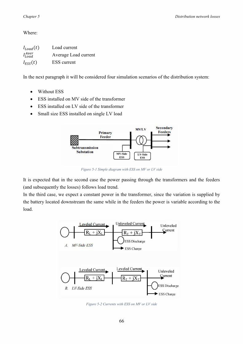
Chapter 5 Distribution network losses
66
Where: 𝐼𝐿𝑜𝑎𝑑(𝑡) Load current 𝐼𝐿𝑜𝑎𝑑𝐴𝑣𝑒𝑟 Average Load current 𝐼𝐸𝑆𝑆(𝑡) ESS current In the next paragraph it will be considered four simulation scenarios of the distribution system:
• Without ESS • ESS installed on MV side of the transformer • ESS installed on LV side of the transformer • Small size ESS installed on single LV load
Figure 5-1 Simple diagram with ESS on MV or LV side
It is expected that in the second case the power passing through the transformers and the feeders (and subsequently the losses) follows load trend. In the third case, we expect a constant power in the transformer, since the variation is supplied by the battery located downstream the same while in the feeders the power is variable according to the load.
Figure 5-2 Currents with ESS on MV or LV side
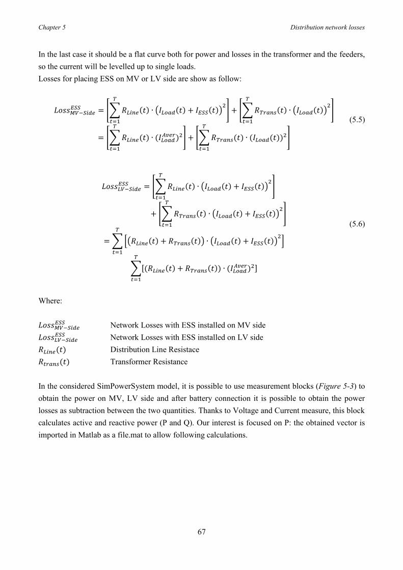
Chapter 5 Distribution network losses
67
In the last case it should be a flat curve both for power and losses in the transformer and the feeders, so the current will be levelled up to single loads. Losses for placing ESS on MV or LV side are show as follow:
𝐿𝑜𝑠𝑠𝑀𝑉−𝑆𝑖𝑑𝑒𝐸𝑆𝑆 = [∑𝑅𝐿𝑖𝑛𝑒(𝑡) ∙ (𝐼𝐿𝑜𝑎𝑑(𝑡) + 𝐼𝐸𝑆𝑆(𝑡))
2𝑇
𝑡=1
] + [∑𝑅𝑇𝑟𝑎𝑛𝑠(𝑡) ∙ (𝐼𝐿𝑜𝑎𝑑(𝑡))2
𝑇
𝑡=1
]
= [∑𝑅𝐿𝑖𝑛𝑒(𝑡) ∙ (𝐼𝐿𝑜𝑎𝑑𝐴𝑣𝑒𝑟)2
𝑇
𝑡=1
] + [∑𝑅𝑇𝑟𝑎𝑛𝑠(𝑡) ∙ (𝐼𝐿𝑜𝑎𝑑(𝑡))2
𝑇
𝑡=1
]
(5.5)
𝐿𝑜𝑠𝑠𝐿𝑉−𝑆𝑖𝑑𝑒𝐸𝑆𝑆 = [∑𝑅𝐿𝑖𝑛𝑒(𝑡) ∙ (𝐼𝐿𝑜𝑎𝑑(𝑡) + 𝐼𝐸𝑆𝑆(𝑡))
2𝑇
𝑡=1
]
+ [∑𝑅𝑇𝑟𝑎𝑛𝑠(𝑡) ∙ (𝐼𝐿𝑜𝑎𝑑(𝑡) + 𝐼𝐸𝑆𝑆(𝑡))2
𝑇
𝑡=1
]
=∑[(𝑅𝐿𝑖𝑛𝑒(𝑡) + 𝑅𝑇𝑟𝑎𝑛𝑠(𝑡)) ∙ (𝐼𝐿𝑜𝑎𝑑(𝑡) + 𝐼𝐸𝑆𝑆(𝑡))2]
𝑇
𝑡=1
∑[(𝑅𝐿𝑖𝑛𝑒(𝑡) + 𝑅𝑇𝑟𝑎𝑛𝑠(𝑡)) ∙ (𝐼𝐿𝑜𝑎𝑑𝐴𝑣𝑒𝑟)2]
𝑇
𝑡=1
(5.6)
Where: 𝐿𝑜𝑠𝑠𝑀𝑉−𝑆𝑖𝑑𝑒
𝐸𝑆𝑆 Network Losses with ESS installed on MV side 𝐿𝑜𝑠𝑠𝐿𝑉−𝑆𝑖𝑑𝑒
𝐸𝑆𝑆 Network Losses with ESS installed on LV side 𝑅𝐿𝑖𝑛𝑒(𝑡) Distribution Line Resistace 𝑅𝑡𝑟𝑎𝑛𝑠(𝑡) Transformer Resistance In the considered SimPowerSystem model, it is possible to use measurement blocks (Figure 5-3) to obtain the power on MV, LV side and after battery connection it is possible to obtain the power losses as subtraction between the two quantities. Thanks to Voltage and Current measure, this block calculates active and reactive power (P and Q). Our interest is focused on P: the obtained vector is imported in Matlab as a file.mat to allow following calculations.
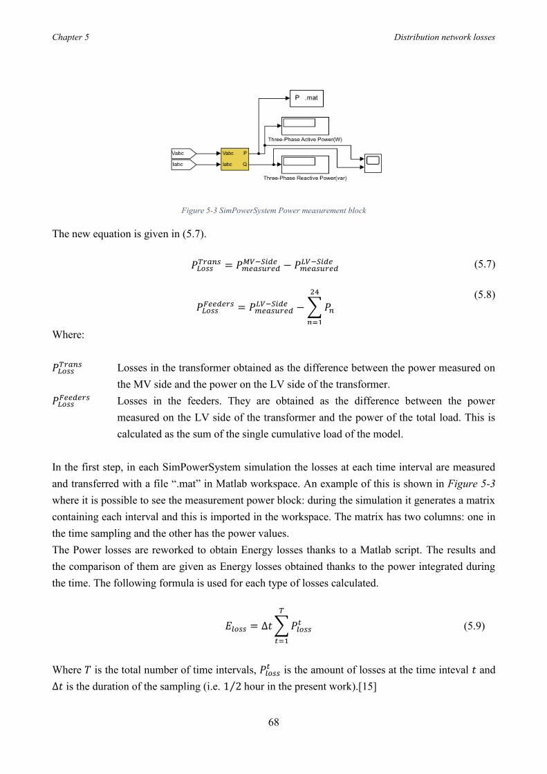
Chapter 5 Distribution network losses
68
Figure 5-3 SimPowerSystem Power measurement block
The new equation is given in (5.7). 𝑃𝐿𝑜𝑠𝑠
𝑇𝑟𝑎𝑛𝑠 = 𝑃𝑚𝑒𝑎𝑠𝑢𝑟𝑒𝑑𝑀𝑉−𝑆𝑖𝑑𝑒 − 𝑃𝑚𝑒𝑎𝑠𝑢𝑟𝑒𝑑
𝐿𝑉−𝑆𝑖𝑑𝑒 (5.7)
𝑃𝐿𝑜𝑠𝑠𝐹𝑒𝑒𝑑𝑒𝑟𝑠 = 𝑃𝑚𝑒𝑎𝑠𝑢𝑟𝑒𝑑
𝐿𝑉−𝑆𝑖𝑑𝑒 −∑𝑃𝑛
24
𝑛=1
(5.8)
Where: 𝑃𝐿𝑜𝑠𝑠𝑇𝑟𝑎𝑛𝑠 Losses in the transformer obtained as the difference between the power measured on
the MV side and the power on the LV side of the transformer. 𝑃𝐿𝑜𝑠𝑠𝐹𝑒𝑒𝑑𝑒𝑟𝑠 Losses in the feeders. They are obtained as the difference between the power
measured on the LV side of the transformer and the power of the total load. This is calculated as the sum of the single cumulative load of the model.
In the first step, in each SimPowerSystem simulation the losses at each time interval are measured and transferred with a file “.mat” in Matlab workspace. An example of this is shown in Figure 5-3 where it is possible to see the measurement power block: during the simulation it generates a matrix containing each interval and this is imported in the workspace. The matrix has two columns: one in the time sampling and the other has the power values. The Power losses are reworked to obtain Energy losses thanks to a Matlab script. The results and the comparison of them are given as Energy losses obtained thanks to the power integrated during the time. The following formula is used for each type of losses calculated.
𝐸𝑙𝑜𝑠𝑠 = ∆𝑡∑𝑃𝑙𝑜𝑠𝑠𝑡
𝑇
𝑡=1
(5.9)
Where 𝑇 is the total number of time intervals, 𝑃𝑙𝑜𝑠𝑠𝑡 is the amount of losses at the time inteval 𝑡 and ∆𝑡 is the duration of the sampling (i.e. 1 2⁄ hour in the present work).[15]

Chapter 5 Distribution network losses
69
5.1.1 Matlab Code First Scenario: Without battery. A Matlab script was built to calculate the Energy losses in the feeders, in the transformers, the values of the voltage in p.u. on each cumulative load and the efficiency of the feeders, the transformer and the total grid. Losses without battery In this first part the values of time, active and reactive power are recalled which have been calculated from the Simulink measurement blocks placed directly on the loads. 24 𝑛 × 3 matrices are created where the first column represents all the time values coming from the sampling, the second the power values in a given instant while the third column has a series of values that oscillate around zero since there is no exchange of reactive power. Since it is necessary to obtain a single vector sum of all the powers (ptot vector), the 24 columns relative to the active power are added. Regarding the time vector that will then be necessary to plot the graphs, the first column of the matrix is extracted (time).
clear all
close all
%From Simulink, I import the values of the file .mat
for n=25:48
filename=sprintf('VPQ%0.5g.mat',n);
S(n)=load(filename); %it is a struct. I have to convert it in a matrix
end
cc=struct2cell(S);
aa=cell2mat(cc);
%size(aa)
bb=permute(aa,[2 1 3]); % to obtain values in column and not in rows
% The fist column is the time, second the voltage, third the Active Power and
% the fourth reactive power
% I need to extract the third column of each matrix and sum toghether to
% have the total power absorbed from the 24 houses.
p=zeros(length(bb),24);
for m=1:24
p(:,m)=bb(:,2,m); %This values are the same of phousetotW [W] present
% HouseSelection_Day196 script
end
%i want the power tot on LV side. I sum the 24 column of each row
ptot=sum(p,2); %POWER TOT OF THE 24 HOUSES
time=bb(:,1); %vector of the time. to plot use this value
Total power in LV side
figure(1)
hold on
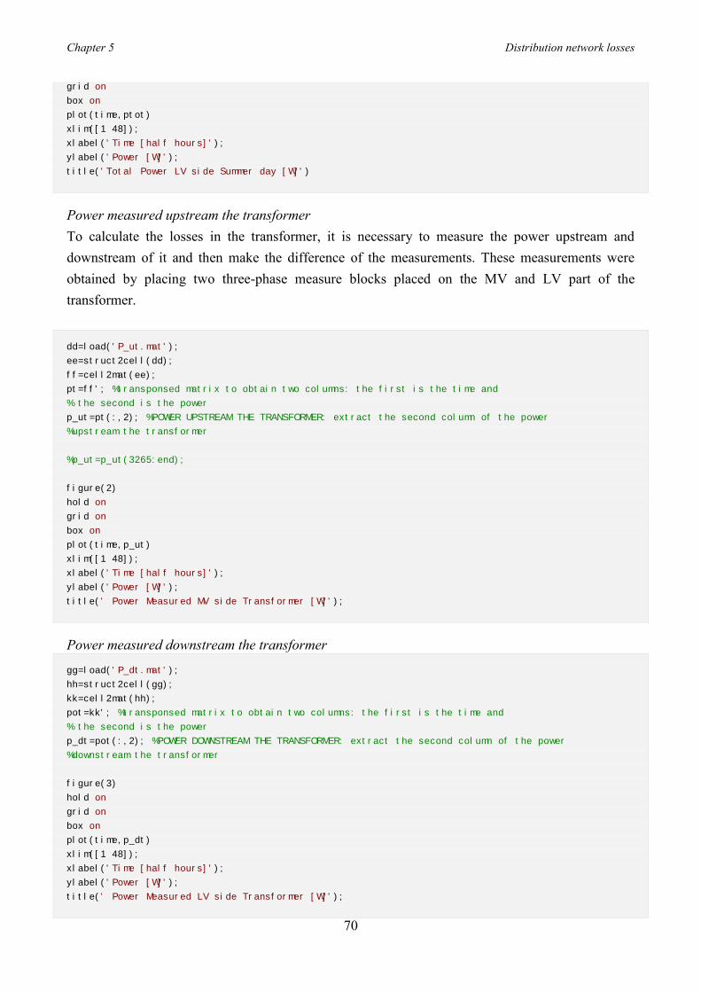
Chapter 5 Distribution network losses
70
grid on
box on
plot(time,ptot)
xlim([1 48]);
xlabel('Time [half hours]');
ylabel('Power [W]');
title('Total Power LV side Summer day [W]')
Power measured upstream the transformer To calculate the losses in the transformer, it is necessary to measure the power upstream and downstream of it and then make the difference of the measurements. These measurements were obtained by placing two three-phase measure blocks placed on the MV and LV part of the transformer.
dd=load('P_ut.mat');
ee=struct2cell(dd);
ff=cell2mat(ee);
pt=ff'; %transponsed matrix to obtain two columns: the first is the time and
% the second is the power
p_ut=pt(:,2); %POWER UPSTREAM THE TRANSFORMER: extract the second column of the power
%upstream the transformer
%p_ut=p_ut(3265:end);
figure(2)
hold on
grid on
box on
plot(time,p_ut)
xlim([1 48]);
xlabel('Time [half hours]');
ylabel('Power [W]');
title(' Power Measured MV side Transformer [W]');
Power measured downstream the transformer
gg=load('P_dt.mat');
hh=struct2cell(gg);
kk=cell2mat(hh);
pot=kk'; %transponsed matrix to obtain two columns: the first is the time and
% the second is the power
p_dt=pot(:,2); %POWER DOWNSTREAM THE TRANSFORMER: extract the second column of the power
%downstream the transformer
figure(3)
hold on
grid on
box on
plot(time,p_dt)
xlim([1 48]);
xlabel('Time [half hours]');
ylabel('Power [W]');
title(' Power Measured LV side Transformer [W]');

Chapter 5 Distribution network losses
71
Losses calculation - Losses transformer As mentioned above, the losses in the transformer are obtained by making the difference between the measured power values respectively on the MV and LV parts of the transformer.
p_tl=p_ut-p_dt; %POWER LOSSES OF THE TRANSFORMER
figure(5)
hold on
box on
grid on
plot(time,p_tl);
xlim([1 48]);
xlabel('Time [half hours]')
ylabel('Power [W]')
title('Power Losses Transformer [W]')
figure(6)
hold on
box on
grid on
area(time,p_tl);
energylossestrasf=(trapz(time,p_tl))/2;
xlim([1 48]);
xlabel('Time [half hours]')
ylabel('Power [W]')
title('Energy Losses Transformer [Wh]')
energylossestrasf %Energy losses in the transformer
Losses feeders Regarding the calculation of online losses, the measurement performed by the measurement block on the LV side of the transformer to which the total power of the loads was subtracted was used. From these calculations the power losses are obtained while to calculate the losses in energy, the "trapz" command of Matlab is used which calculates the area through the integral of the infinitesimal trapezoids.
plt=p_dt-ptot; % POWER LOSSES FEEDERS
figure(7)
hold on
grid on
box on
plot(time,plt);
xlim([1 48]);
xlabel('Time [half hours]');
ylabel('Power [W]');
title('Power Losses Feeders [W]');
figure(8)
hold on
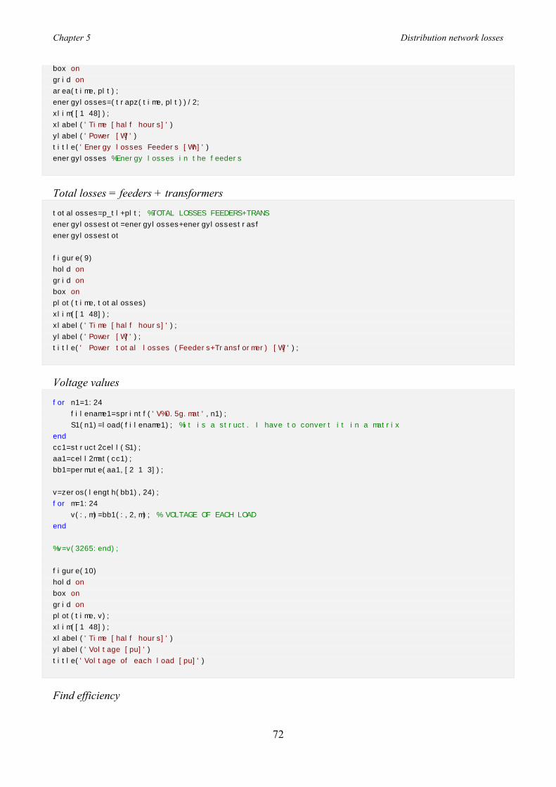
Chapter 5 Distribution network losses
72
box on
grid on
area(time,plt);
energylosses=(trapz(time,plt))/2;
xlim([1 48]);
xlabel('Time [half hours]')
ylabel('Power [W]')
title('Energy losses Feeders [Wh]')
energylosses %Energy losses in the feeders
Total losses = feeders + transformers
totalosses=p_tl+plt; %TOTAL LOSSES FEEDERS+TRANS
energylossestot=energylosses+energylossestrasf
energylossestot
figure(9)
hold on
grid on
box on
plot(time,totalosses)
xlim([1 48]);
xlabel('Time [half hours]');
ylabel('Power [W]');
title(' Power total losses (Feeders+Transformer) [W]');
Voltage values
for n1=1:24
filename1=sprintf('V%0.5g.mat',n1);
S1(n1)=load(filename1); %it is a struct. I have to convert it in a matrix
end
cc1=struct2cell(S1);
aa1=cell2mat(cc1);
bb1=permute(aa1,[2 1 3]);
v=zeros(length(bb1),24);
for m=1:24
v(:,m)=bb1(:,2,m); % VOLTAGE OF EACH LOAD
end
%v=v(3265:end);
figure(10)
hold on
box on
grid on
plot(time,v);
xlim([1 48]);
xlabel('Time [half hours]')
ylabel('Voltage [pu]')
title('Voltage of each load [pu]')
Find efficiency

Chapter 5 Distribution network losses
73
epsilontrasf=sum(p_dt)/sum(p_ut) % TRANSFORMER EFFICIENCY IN A DAY
epsilonfeeders=sum(ptot)/sum(p_dt) % FEEDERS EFFICIENCY
epsilongrid=sum(ptot)/sum(p_ut) % EFFICIENCY FEEDERS+TRANSF
percentagefeederslosses=sum(plt)/sum(ptot)
percentagetransflosses=sum(p_tl)/sum(ptot)
%save('AA_LossesWithoutBattery','time','ptot','p_ut','p_dt','p_tl','v','plt',...
%'energylosses','energylossestrasf','energylossestot','epsilongrid','epsilontrasf',...
%'epsilonfeeders','percentagefeederslosses','percentagetransflosses');
5.2 Comparing losses scenarios without PV In this paragraph the losses, in a Summer and Winter day, are presented both in the LV and MV lines and their comparison in the first four scenarios:
1. Without battery 2. Battery on the MV part of the transformer 3. Battery on the LV part of the transformer 4. Batteries distributed on individual cumulative loads
In each chart, this numeration will be maintained for the four different cases. Let's start by graphically comparing the four trends of losses in the transformer. It can be noted that both in the absence of a battery and in the case of a battery located on the MV part of the transformer (cases 1 and 2) the losses follow the trend of the load absorption in the day. The two trends are practically overlapping and this means that in these two scenarios the losses in the transformer do not vary so much. Regarding the last two cases (3 and 4), the power flowing through the transformer during the day is constant and equal, except for losses, to the setpoint supplied by the power supply network.
a) Summer Day b) Winter Day
Figure 5-4 Compared Transformer Losses 4 Scenarios
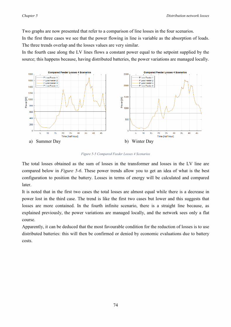
Chapter 5 Distribution network losses
74
Two graphs are now presented that refer to a comparison of line losses in the four scenarios. In the first three cases we see that the power flowing in line is variable as the absorption of loads. The three trends overlap and the losses values are very similar. In the fourth case along the LV lines flows a constant power equal to the setpoint supplied by the source; this happens because, having distributed batteries, the power variations are managed locally.
a) Summer Day b) Winter Day
Figure 5-5 Compared Feeder Losses 4 Scenarios
The total losses obtained as the sum of losses in the transformer and losses in the LV line are compared below in Figure 5-6. These power trends allow you to get an idea of what is the best configuration to position the battery. Losses in terms of energy will be calculated and compared later. It is noted that in the first two cases the total losses are almost equal while there is a decrease in power lost in the third case. The trend is like the first two cases but lower and this suggests that losses are more contained. In the fourth infinite scenario, there is a straight line because, as explained previously, the power variations are managed locally, and the network sees only a flat course. Apparently, it can be deduced that the most favourable condition for the reduction of losses is to use distributed batteries: this will then be confirmed or denied by economic evaluations due to battery costs.
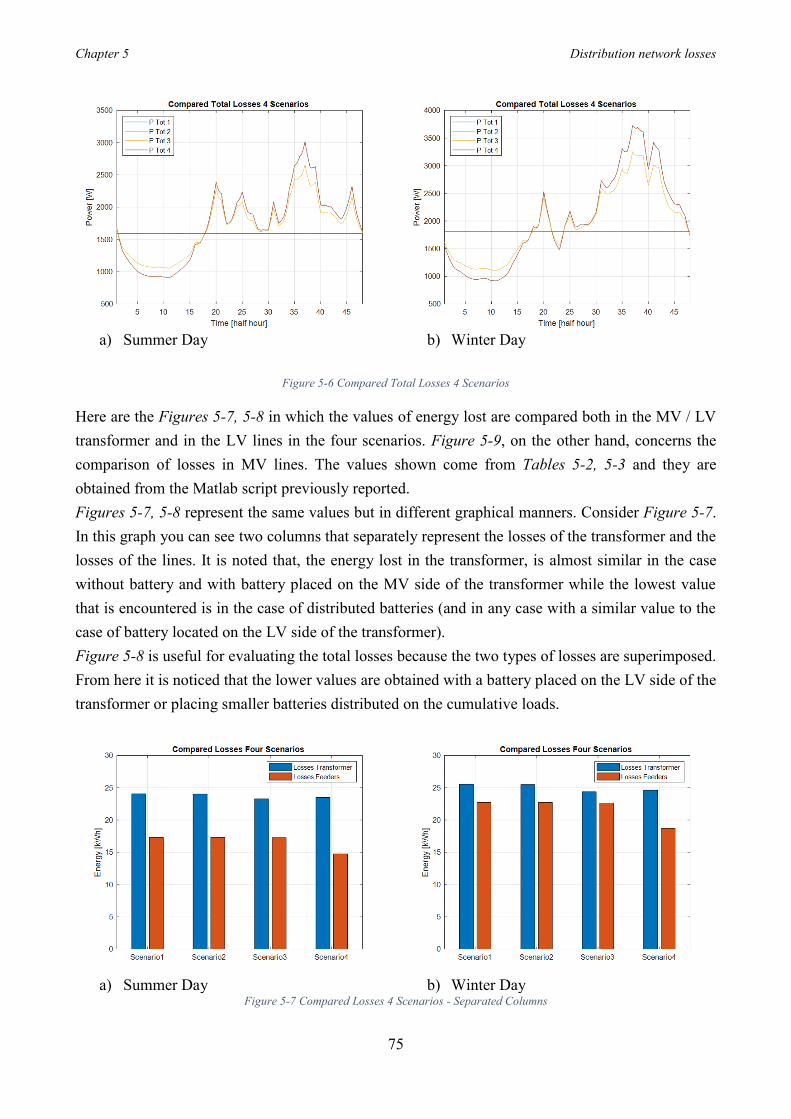
Chapter 5 Distribution network losses
75
a) Summer Day b) Winter Day
Figure 5-6 Compared Total Losses 4 Scenarios
Here are the Figures 5-7, 5-8 in which the values of energy lost are compared both in the MV / LV transformer and in the LV lines in the four scenarios. Figure 5-9, on the other hand, concerns the comparison of losses in MV lines. The values shown come from Tables 5-2, 5-3 and they are obtained from the Matlab script previously reported. Figures 5-7, 5-8 represent the same values but in different graphical manners. Consider Figure 5-7. In this graph you can see two columns that separately represent the losses of the transformer and the losses of the lines. It is noted that, the energy lost in the transformer, is almost similar in the case without battery and with battery placed on the MV side of the transformer while the lowest value that is encountered is in the case of distributed batteries (and in any case with a similar value to the case of battery located on the LV side of the transformer). Figure 5-8 is useful for evaluating the total losses because the two types of losses are superimposed. From here it is noticed that the lower values are obtained with a battery placed on the LV side of the transformer or placing smaller batteries distributed on the cumulative loads.
a) Summer Day b) Winter Day
Figure 5-7 Compared Losses 4 Scenarios - Separated Columns
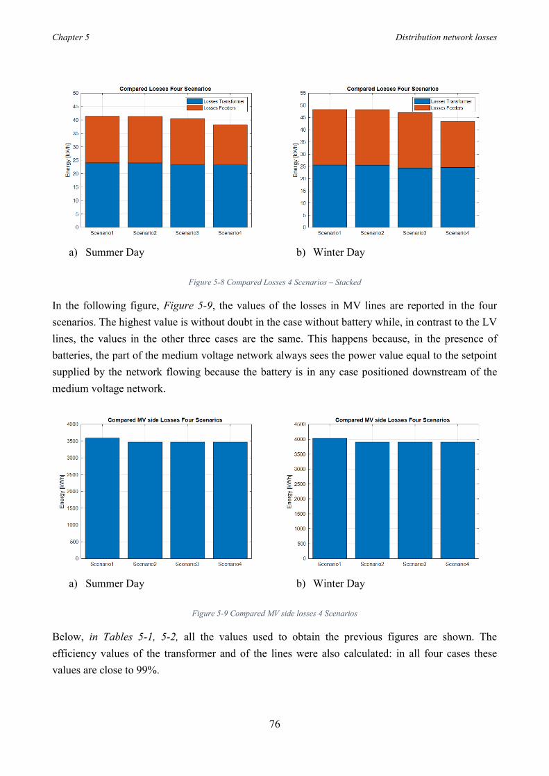
Chapter 5 Distribution network losses
76
a) Summer Day b) Winter Day
Figure 5-8 Compared Losses 4 Scenarios – Stacked
In the following figure, Figure 5-9, the values of the losses in MV lines are reported in the four scenarios. The highest value is without doubt in the case without battery while, in contrast to the LV lines, the values in the other three cases are the same. This happens because, in the presence of batteries, the part of the medium voltage network always sees the power value equal to the setpoint supplied by the network flowing because the battery is in any case positioned downstream of the medium voltage network.
a) Summer Day b) Winter Day
Figure 5-9 Compared MV side losses 4 Scenarios
Below, in Tables 5-1, 5-2, all the values used to obtain the previous figures are shown. The efficiency values of the transformer and of the lines were also calculated: in all four cases these values are close to 99%.

Chapter 5 Distribution network losses
77
Table 5-1 Energy Losses Values 4 Scenarios – Summer Day
SUMMER Transformer Losses [kWh]
LV Feeder Losses [kWh]
MV Feeder Losses [kWh]
Transformer Efficiency
[adim]
Feeder Efficiency
[adim]
Without Battery
24.062 17.325 3589.5 0.9927 0.9946
Battery MV side
24.028 17.323 3472.5 0.9927 0.9946
Battery LV side
23.292 17.285 3472.5 0.9929 0.9947
Distribuited Batteries
23.499 14.7 3472.5 0.9928 0.9954
Table 5-2 Energy Losses Values 4 Scenarios - Winter Day
WINTER Transformer Losses [kWh]
Feeder Losses [kWh]
MV Feeder Losses [kWh]
Transformer Efficiency
[adim]
Feeder Efficiency
[adim]
Without Battery
25.556 22.738 4031.9 0.9930 0.9937
Battery MV side
25.511 22.735 3906.7 0.9930 0.9937
Battery LV side
24.379 22.652 3906.7 0.9933 0.9938
Distribuited Batteries
24.635 18.725 3906.7 0.9933 0.9948
5.3 Rooftop PV in Residential Distribution Network With recent technology advanced solar photovoltaic has become one of the fastest-growing renewable sourced in Europe. However, high penetration of PV systems into the distribution networks may arise undesirable issues such as voltage fluctuation and reverse power flows. These issue may be mitigated with onsite energy storage systems.[16][17] Since photovoltaic generation takes place mainly in the city areas, if urban renewable energy strategies are to be successful, we need a far greater understanding of the resource that is available locally. In this regard, the deployment of consumer-level grid-tied PV systems could provide localised generation to support the local distribution network while increased efficiency would result from shorter transmission distances. It is in this context that there is particular focus on understanding bidirectionality of energy flows at the LV consumer level.[18].
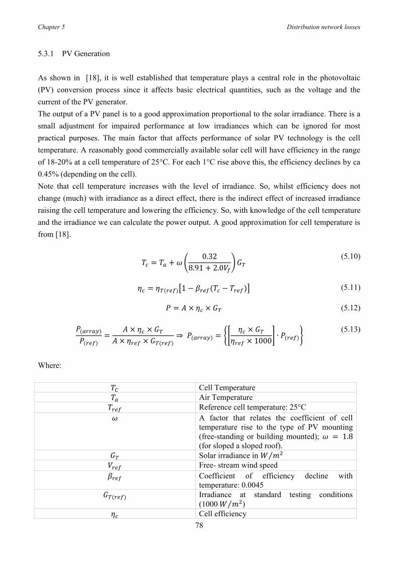
Chapter 5 Distribution network losses
78
5.3.1 PV Generation As shown in [18], it is well established that temperature plays a central role in the photovoltaic (PV) conversion process since it affects basic electrical quantities, such as the voltage and the current of the PV generator. The output of a PV panel is to a good approximation proportional to the solar irradiance. There is a small adjustment for impaired performance at low irradiances which can be ignored for most practical purposes. The main factor that affects performance of solar PV technology is the cell temperature. A reasonably good commercially available solar cell will have efficiency in the range of 18-20% at a cell temperature of 25°C. For each 1°C rise above this, the efficiency declines by ca 0.45% (depending on the cell). Note that cell temperature increases with the level of irradiance. So, whilst efficiency does not change (much) with irradiance as a direct effect, there is the indirect effect of increased irradiance raising the cell temperature and lowering the efficiency. So, with knowledge of the cell temperature and the irradiance we can calculate the power output. A good approximation for cell temperature is from [18].
𝑇𝑐 = 𝑇𝑎 + 𝜔(0.32
8.91 + 2.0𝑉𝑓)𝐺𝑇
(5.10)
𝜂𝑐 = 𝜂𝑇(𝑟𝑒𝑓)[1 − 𝛽𝑟𝑒𝑓(𝑇𝑐 − 𝑇𝑟𝑒𝑓)]
(5.11)
𝑃 = 𝐴 × 𝜂𝑐 × 𝐺𝑇 (5.12) 𝑃(𝑎𝑟𝑟𝑎𝑦)
𝑃(𝑟𝑒𝑓)=
𝐴 × 𝜂𝑐 × 𝐺𝑇𝐴 × 𝜂𝑟𝑒𝑓 × 𝐺𝑇(𝑟𝑒𝑓)
⇒ 𝑃(𝑎𝑟𝑟𝑎𝑦) = [𝜂𝑐 × 𝐺𝑇
𝜂𝑟𝑒𝑓 × 1000] ∙ 𝑃(𝑟𝑒𝑓)
(5.13)
Where:
𝑇𝐶 Cell Temperature 𝑇𝑎 Air Temperature 𝑇𝑟𝑒𝑓 Reference cell temperature: 25°C 𝜔 A factor that relates the coefficient of cell
temperature rise to the type of PV mounting (free-standing or building mounted); 𝜔 = 1.8 (for sloped a sloped roof).
𝐺𝑇 Solar irradiance in 𝑊 𝑚2⁄ 𝑉𝑟𝑒𝑓 Free- stream wind speed 𝛽𝑟𝑒𝑓 Coefficient of efficiency decline with
temperature: 0.0045 𝐺𝑇(𝑟𝑒𝑓) Irradiance at standard testing conditions
(1000 𝑊 𝑚2⁄ ) 𝜂𝑐 Cell efficiency

Chapter 5 Distribution network losses
79
𝜂𝑇(𝑟𝑒𝑓) A reference cell efficiency measured at standard testing conditions (1000 𝑊 𝑚2⁄ irradiance and 25°C cell temperature)
𝐴 Area (𝑚2) 𝑃(𝑟𝑒𝑓) Panel output under test conditions 𝑃(𝑎𝑟𝑟𝑎𝑦) PV panel output
Thanks to the formulas obtained from [18], the power output values of a 1kW panel were calculated as a function of the irradiation. Three main cases will be considered:
• 1 PV panel of 1 kW placed on half number of houses • 1 PV panel of 1 kW positioned on each house • 2 PV panels of 1 kW (equivalent to 2 kW) placed on each house.
Each scenario is then divided into 3 sub-areas: • Without battery • With battery positioned on the LV part of the transformer using the original setpoint
considered in the 4 basic scenarios • With battery positioned on the LV part of the transformer, using the setpoint obtained
considering the production of photovoltaics consumed locally by the loads. In the graphs in which the cases without batteries are represented, Figure 5-10, 5-13, 5-16, the production of photovoltaics is shown in yellow (1 kW multiplied by 3 houses present in each cumulative load and then multiplied by 24, total number of cumulative loads), in red the total demand for power by the loads while in blue, obtained by subtracting the red and yellow curve, there is the power that will be required to the network. In the following figures, Figure 5-11, 5-12, 5-14, 5-15, 5-17, 5-18 as there is the presence of the battery, its behaviour was also plotted. Four curves can be identified as follows: in blue you can see the absorption of loads without PV, in yellow there is the setpoint set on the network, in red there is the production of photovoltaic while in purple there is the behaviour of the battery. In this case, when there is a peak of absorption by the loads, the battery will take negative values as it is being discharged while when there is a surplus of photovoltaic production compared to the load demand the battery will take positive values which means that it's charging. As in all the scenarios considered, there is the presence of a summer and winter “type” day; the values of irradiation and therefore of power produced by the panel were chosen exactly equal to the days considered for the absorption of load (day 196 for summer and 55 days for winter). It can be seen that there is a difference between summer and winter: on the first day there is a higher production from PV while a lower power absorption while on the winter day the roles are reversed. This, from a logical point of view, is normal because during the winter the hours of light are lower

Chapter 5 Distribution network losses
80
than in the summer. What is expected from the sizing of the battery is that you get a greater capacity if it is calculated from the summer data. Another aspect to note is related to the setpoint value. It changes both in relation to the season and in relation to the quantity of photovoltaic production. As photovoltaic production grows, in extreme cases when we have 2 kW installed on each home, the setpoint decreases as the main network will have to provide less power as it is produced and consumed locally. In the case of the 2 kW installed on each house, it is also noted that in the central part of the day (between 10 and 15) there is a surplus of production and this means that there will be an inverse flow of power in the network. In this case the battery must be larger to avoid this type of flow.
a) Summer Day b) Winter Day
Figure 5-10 Load and PV trend with 1 kW panel on half houses - Without Battery
a) Summer Day b) Winter Day
Figure 5-11 Load, PV and Battery trend with 1 kW panel on half houses – Original SP
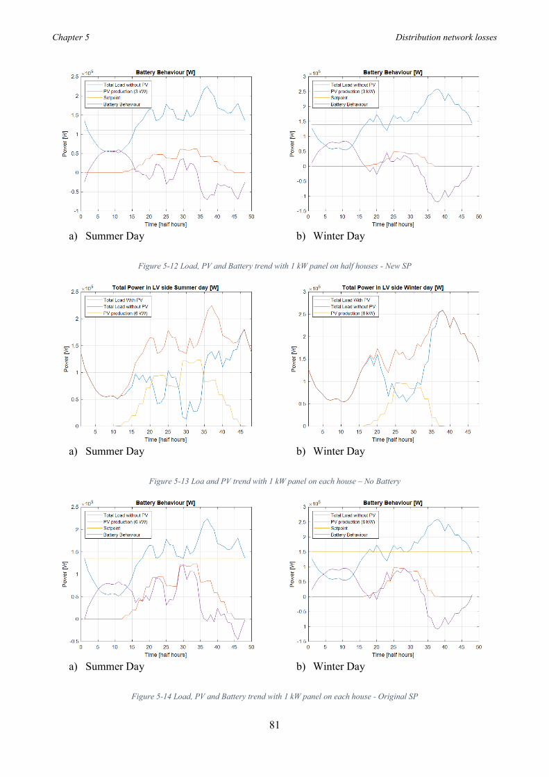
Chapter 5 Distribution network losses
81
a) Summer Day b) Winter Day
Figure 5-12 Load, PV and Battery trend with 1 kW panel on half houses - New SP
a) Summer Day b) Winter Day
Figure 5-13 Loa and PV trend with 1 kW panel on each house – No Battery
a) Summer Day b) Winter Day
Figure 5-14 Load, PV and Battery trend with 1 kW panel on each house - Original SP
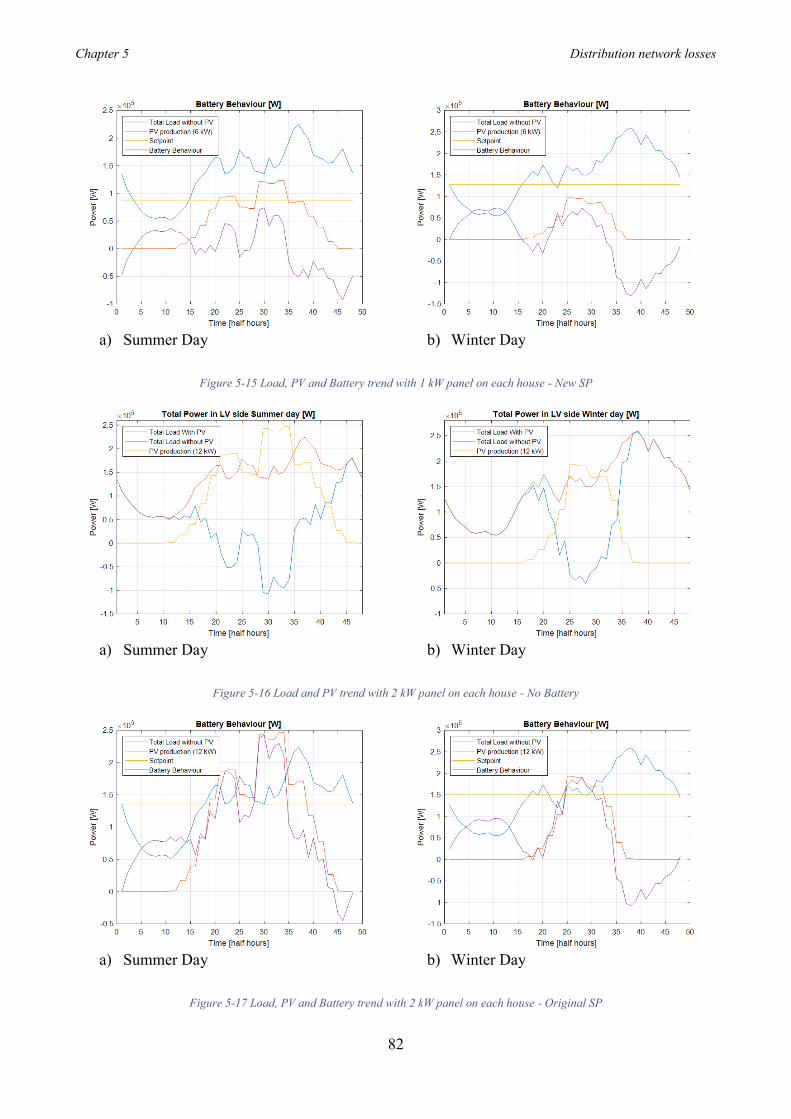
Chapter 5 Distribution network losses
82
a) Summer Day b) Winter Day
Figure 5-15 Load, PV and Battery trend with 1 kW panel on each house - New SP
a) Summer Day b) Winter Day
Figure 5-16 Load and PV trend with 2 kW panel on each house - No Battery
a) Summer Day b) Winter Day
Figure 5-17 Load, PV and Battery trend with 2 kW panel on each house - Original SP
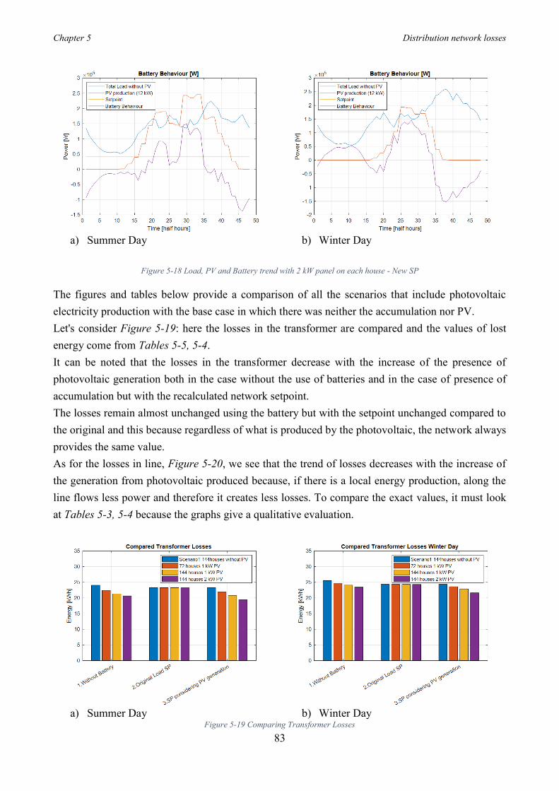
Chapter 5 Distribution network losses
83
a) Summer Day b) Winter Day
Figure 5-18 Load, PV and Battery trend with 2 kW panel on each house - New SP
The figures and tables below provide a comparison of all the scenarios that include photovoltaic electricity production with the base case in which there was neither the accumulation nor PV. Let's consider Figure 5-19: here the losses in the transformer are compared and the values of lost energy come from Tables 5-5, 5-4. It can be noted that the losses in the transformer decrease with the increase of the presence of photovoltaic generation both in the case without the use of batteries and in the case of presence of accumulation but with the recalculated network setpoint. The losses remain almost unchanged using the battery but with the setpoint unchanged compared to the original and this because regardless of what is produced by the photovoltaic, the network always provides the same value. As for the losses in line, Figure 5-20, we see that the trend of losses decreases with the increase of the generation from photovoltaic produced because, if there is a local energy production, along the line flows less power and therefore it creates less losses. To compare the exact values, it must look at Tables 5-3, 5-4 because the graphs give a qualitative evaluation.
a) Summer Day b) Winter Day
Figure 5-19 Comparing Transformer Losses
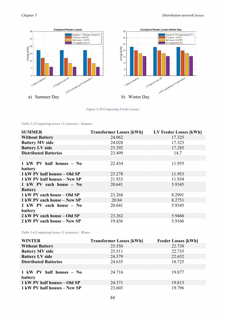
Chapter 5 Distribution network losses
84
a) Summer Day b) Winter Day
Figure 5-20 Comparing Feeder Losses
Table 5-3 Comparing losses 13 scenarios - Summer
SUMMER Transformer Losses [kWh] LV Feeder Losses [kWh] Without Battery 24.062 17.325 Battery MV side 24.028 17.323 Battery LV side 23.292 17.285 Distributed Batteries 23.499 14.7 1 kW PV half houses – No battery
22.434 11.955
1 kW PV half houses – Old SP 23.278 11.953 1 kW PV half houses – New SP 21.933 11.934 1 kW PV each house – No Battery
20.641 5.9345
1 kW PV each house – Old SP 23.268 8.2991 1 kW PV each house – New SP 20.84 8.2751 2 kW PV each house – No battery
20.641 5.9345
2 kW PV each house – Old SP 23.262 5.9460 2 kW PV each house – New SP 19.436 5.9166 Table 5-4 Comparing losses 13 scenarios - Winter
WINTER Transformer Losses [kWh] Feeder Losses [kWh] Without Battery 25.556 22.738 Battery MV side 25.511 22.735 Battery LV side 24.379 22.652 Distributed Batteries 24.635 18.725 1 kW PV half houses – No battery
24.716 19.877
1 kW PV half houses – Old SP 24.371 19.813 1 kW PV half houses – New SP 23.603 19.796
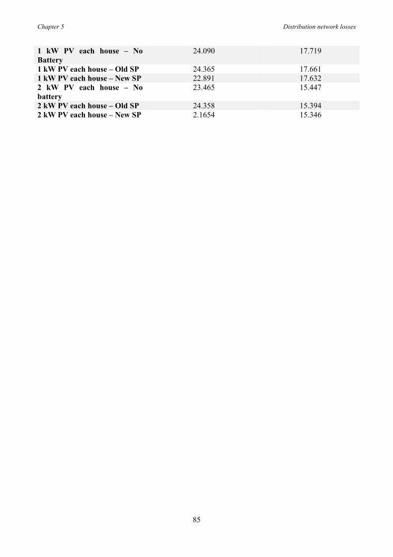
Chapter 5 Distribution network losses
85
1 kW PV each house – No Battery
24.090 17.719
1 kW PV each house – Old SP 24.365 17.661 1 kW PV each house – New SP 22.891 17.632 2 kW PV each house – No battery
23.465 15.447
2 kW PV each house – Old SP 24.358 15.394 2 kW PV each house – New SP 2.1654 15.346
Chapter 6 Voltage
86
Chapter 6
6 Voltage The regulation and the conservation of a certain sufficiently uniform voltage profile, represents one of the important technical constraints. The maintenance of the voltage modulus goes supported by a rapid and transient supply of energy (and power) so, for this reason, it may be useful to use storage systems that can cope with rapid variations. Considering active electricity networks, the maintaining of the voltage represents a constraint that usually limit power generation installable by users / producers in electrical networks. Indeed, the presence of distributed generation (GD) changes the regulation criterion that acts on the tap changer of the AT/MT transformer of the primary substations, which reduces or increases the voltage according to the magnitude of the load overall absorbed, measured through the total current flowing through the transformer. This system cannot consider the peculiarities of each departure supplied by the transformer and is therefore not useful with the presence of distributed GD generation. On the other hand, GD can easily turn into a good opportunity, if exploited to provide a regulation support: this is one of the main reasons for which we are started to feel the need to introduce in the management of distribution networks the concept of active electric networks. The following paragraphs summarize the graphs of the different scenarios:
1. Voltage without battery. 2. Voltage with battery on MV side of the transformer. 3. Voltage with battery on LV side of the transformer. 4. Voltage with distributed battery on each load.
5. Voltage with 1 kW PV panel without battery considering the installation of panels on half
the number of houses. 6. Voltage with 1 kW PV panel with battery on LV side of the transformer considering the
original Setpoint of the grid and the installation of panels on half the number of houses. 7. Voltage with 1 kW PV panel with battery on LV side of the transformer considering the
Setpoint of the grid with the impact of the PV and the installation of panels on half the number of houses.
8. Voltage with 1 kW PV panel without battery considering the installation of panels on the
total number of houses. 9. Voltage with 1 kW PV panel with battery on LV side of the transformer considering the
original Setpoint of the grid and the installation of panels on the total number of houses.

Chapter 6 Voltage
87
10. Voltage with 1 kW PV panel with battery on LV side of the transformer considering the Setpoint of the grid with the impact of the PV and the installation of panels on the total number of houses.
11. Voltage with 2 kW PV panel without battery considering the installation of panels on the
total number of houses. 12. Voltage with 2 kW PV panel with battery on LV side of the transformer considering the
original Setpoint of the grid and the installation of panels on half the number of houses. 13. Voltage with 2 kW PV panel with battery on LV side of the transformer considering the
Setpoint of the grid with the impact of the PV and the installation of panels on half the number of houses.
In each of the different scenarios the two cases concerning the summer type day (to the left) and the winter type day (to the right) are presented. The voltage values are shown in pu values (per unit). In each chart we see 24 different colours trends which represent the voltage trends in the 24 cumulative loads. As is known from the literature, for technical reasons (voltage drop on the power line) the voltage value is not always equal to the nominal value (230 or 400 V), but this can vary within the limit of ±10% of its nominal value.
6.1.1 Voltage without Battery In this scenario the basic case that represents the low voltage distribution network without the use of batteries is presented. From the graph, the loads closest to the transformer have a slightly higher voltage than those farther away and this is due to voltage drops present in line. However, both in this first scenario and in all the others considered, the voltage values remain within the range established by the standards. Another aspect to note is how voltage trends are reversed with respect to load absorption. In moments of the day when there is a peak of power absorption, mainly in the mid-morning (h 10) and towards evening (h 18/19), we see that the voltage tends to fall while the hours of low load tend to go towards an overvoltage, remaining however in the allowed values.
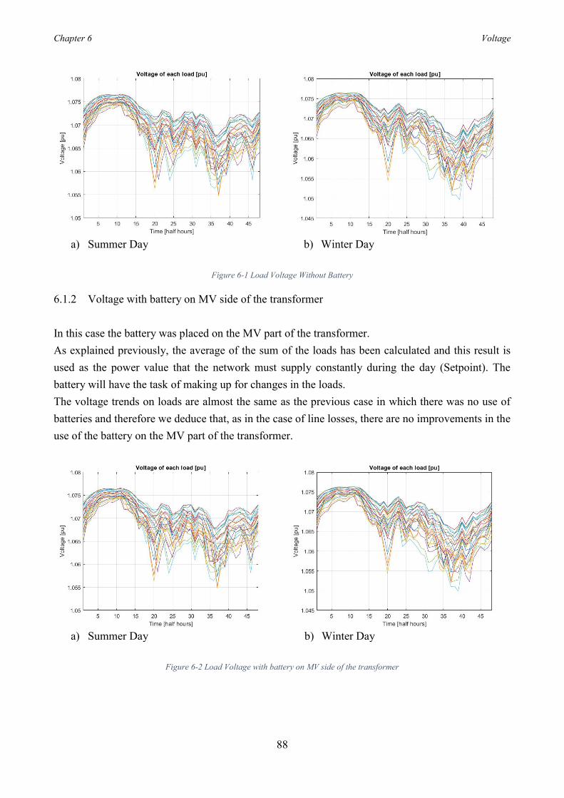
Chapter 6 Voltage
88
a) Summer Day b) Winter Day
Figure 6-1 Load Voltage Without Battery
6.1.2 Voltage with battery on MV side of the transformer In this case the battery was placed on the MV part of the transformer. As explained previously, the average of the sum of the loads has been calculated and this result is used as the power value that the network must supply constantly during the day (Setpoint). The battery will have the task of making up for changes in the loads. The voltage trends on loads are almost the same as the previous case in which there was no use of batteries and therefore we deduce that, as in the case of line losses, there are no improvements in the use of the battery on the MV part of the transformer.
a) Summer Day b) Winter Day
Figure 6-2 Load Voltage with battery on MV side of the transformer
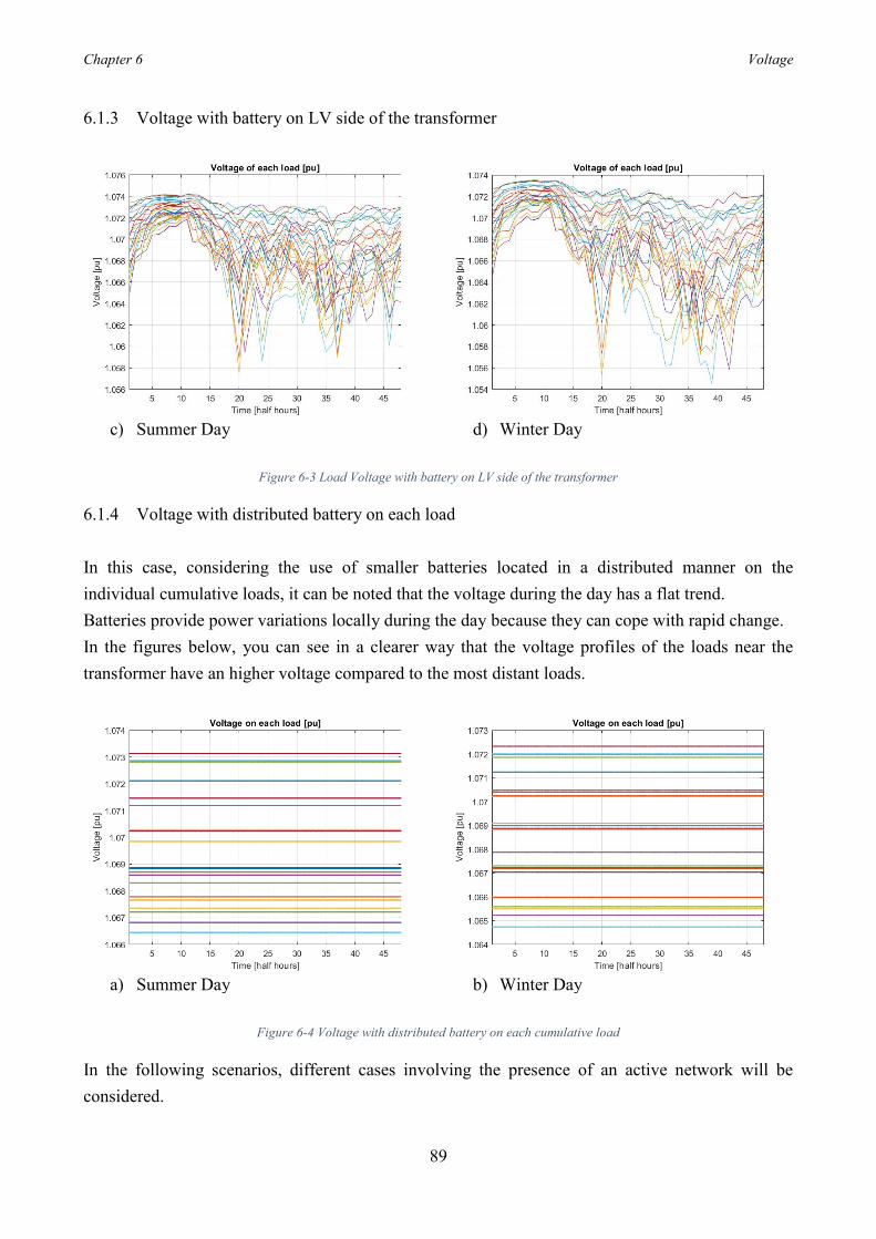
Chapter 6 Voltage
89
6.1.3 Voltage with battery on LV side of the transformer
c) Summer Day d) Winter Day
Figure 6-3 Load Voltage with battery on LV side of the transformer
6.1.4 Voltage with distributed battery on each load In this case, considering the use of smaller batteries located in a distributed manner on the individual cumulative loads, it can be noted that the voltage during the day has a flat trend. Batteries provide power variations locally during the day because they can cope with rapid change. In the figures below, you can see in a clearer way that the voltage profiles of the loads near the transformer have an higher voltage compared to the most distant loads.
a) Summer Day b) Winter Day
Figure 6-4 Voltage with distributed battery on each cumulative load
In the following scenarios, different cases involving the presence of an active network will be considered.

Chapter 6 Voltage
90
Times with high PV generation and low load demand, leads to the problem of reverse power flow in the LV residential feeder which then subsequently lead to over-voltage problem. Simple result is to put a limitation on the amount of PV that can be installed on LV feeders. In overvoltage study, the residential feeders are considered as a critical case regarding overvoltage problem due to their characteristics. The load profile of residential feeders shows a peak value during evening in the absence of PV generation. However, the commercial and industrial feeders load profiles have a good correlation with the PV power profile, which tends to reduce the possibility of overvoltage. In addition, there is more possibility for overvoltage problem in rural feeders, due to their length which increases the impedance value [19]. Analysing the overvoltage issue, the effect of substation transformer’s short circuit resistance and the feeder layout must also to be considered. [19] shows that the voltage rise rate is higher when the transformer has larger resistance. So, reducing the transformer short circuit resistance make system’s efficiency higher and the possibility to incur a voltage rise problem lower. For each scenario considered it is possible to distinguish three cases: the first one analyses the impact of the PV on the voltage without the use of storage, in the second and third case there is the presence of a battery concentrated in the LV part of the transformer. The difference between second and third cases is the choice of the setpoint considered for the network. In the second, the same SP is used for the initial scenarios without photovoltaics and will be classified as the “Original Setpoint”. In the third, the setpoint is recalculated, subtracting the photovoltaic power output from the absorbed load and it will be named “New Setpoint”.
6.1.5 Voltage 1 kW PV panel installed on half number of houses - Without Battery In these first three cases the installation of 1 kW panels is evaluated on half of the number of houses considered (72) and this means that locally, on each cumulative load, consisting of 6 residential units, we will have a production of 3 kW PV.
a) Summer Day b) Winter Day
Figure 6-5 Voltage 1 kW PV panel installed on half houses - Without Battery
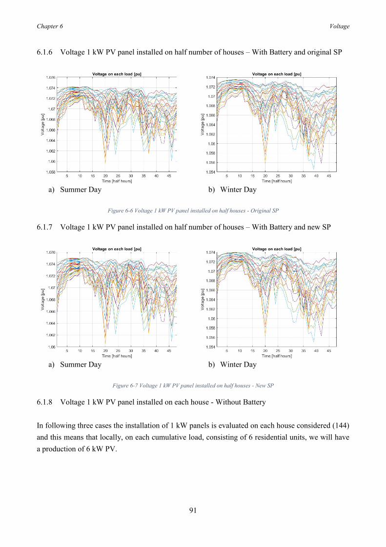
Chapter 6 Voltage
91
6.1.6 Voltage 1 kW PV panel installed on half number of houses – With Battery and original SP
a) Summer Day b) Winter Day
Figure 6-6 Voltage 1 kW PV panel installed on half houses - Original SP
6.1.7 Voltage 1 kW PV panel installed on half number of houses – With Battery and new SP
a) Summer Day b) Winter Day
Figure 6-7 Voltage 1 kW PV panel installed on half houses - New SP
6.1.8 Voltage 1 kW PV panel installed on each house - Without Battery In following three cases the installation of 1 kW panels is evaluated on each house considered (144) and this means that locally, on each cumulative load, consisting of 6 residential units, we will have a production of 6 kW PV.
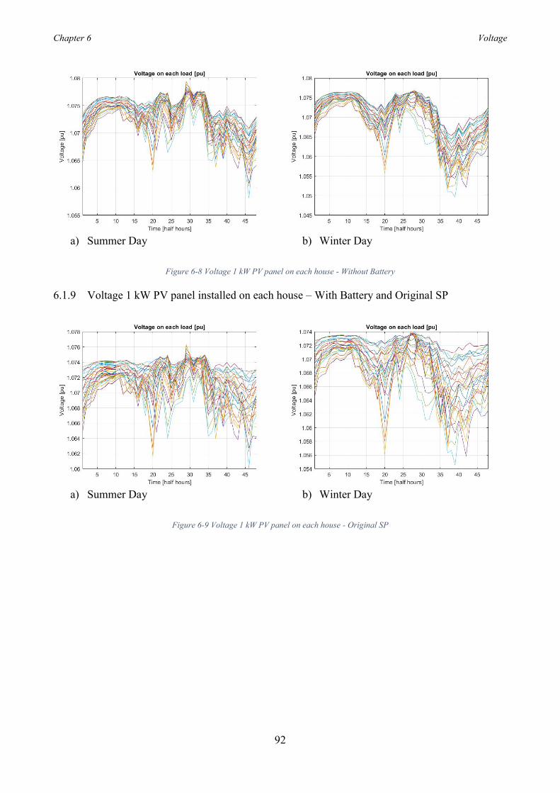
Chapter 6 Voltage
92
a) Summer Day b) Winter Day
Figure 6-8 Voltage 1 kW PV panel on each house - Without Battery
6.1.9 Voltage 1 kW PV panel installed on each house – With Battery and Original SP
a) Summer Day b) Winter Day
Figure 6-9 Voltage 1 kW PV panel on each house - Original SP
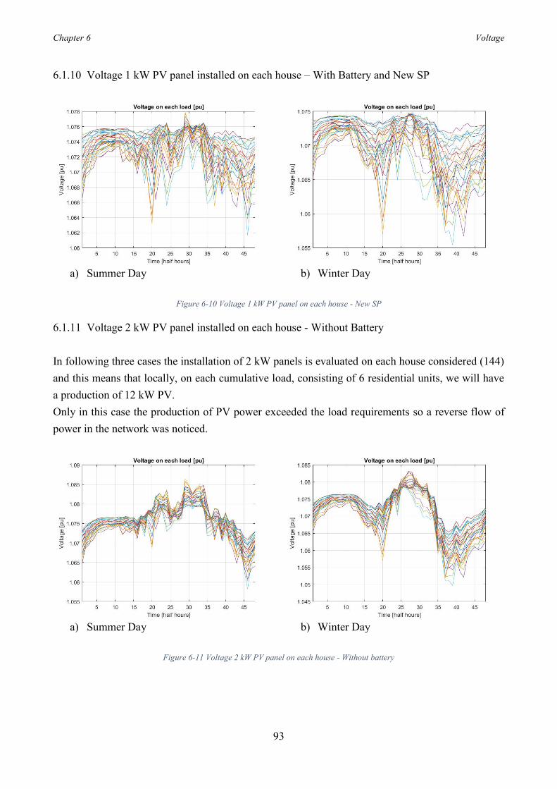
Chapter 6 Voltage
93
6.1.10 Voltage 1 kW PV panel installed on each house – With Battery and New SP
a) Summer Day b) Winter Day
Figure 6-10 Voltage 1 kW PV panel on each house - New SP
6.1.11 Voltage 2 kW PV panel installed on each house - Without Battery In following three cases the installation of 2 kW panels is evaluated on each house considered (144) and this means that locally, on each cumulative load, consisting of 6 residential units, we will have a production of 12 kW PV. Only in this case the production of PV power exceeded the load requirements so a reverse flow of power in the network was noticed.
a) Summer Day b) Winter Day
Figure 6-11 Voltage 2 kW PV panel on each house - Without battery
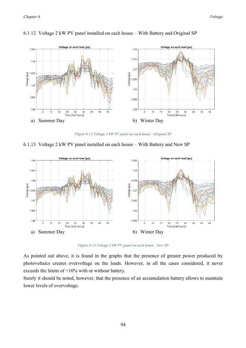
Chapter 6 Voltage
94
6.1.12 Voltage 2 kW PV panel installed on each house – With Battery and Original SP
a) Summer Day b) Winter Day
Figure 6-12 Voltage 2 kW PV panel on each house - Original SP
6.1.13 Voltage 2 kW PV panel installed on each house – With Battery and New SP
a) Summer Day b) Winter Day
Figure 6-13 Voltage 2 kW PV panel on each house - New SP
As pointed out above, it is found in the graphs that the presence of greater power produced by photovoltaics creates overvoltage on the loads. However, in all the cases considered, it never exceeds the limits of +10% with or without battery. Surely it should be noted, however, that the presence of an accumulation battery allows to maintain lower levels of overvoltage.

Chapter 7 Costs and Sizing
95
Chapter 7
7 Costs and Sizing The increasing number of renewable energy resources results in a need of additional electric energy storage systems [20]. Stationary grid-connected batteries can facilitate a system integration of RES and can provide ancillary services, load levelling, system backup etc. However, within the future liberalized European energy market, there are several other energy-generation and storage technologies competing each other in various application fields. The market success of a technology and the initial investment decision is determined by its electricity production costs in €ct./kWh. [20].
7.1 Energy Storage System Costs The status of energy storage technology options and updated estimated ranges for their total installed costs, performance, and availability for key applications are presented below. Estimates are based on technology assessments, discussions with vendors and utilities, and experience with operating systems. The estimates include process and project contingencies to account for technology and application uncertainties. Tables 7-1, 7-2 provide estimates by application for megawatt-scale and kilowatt-scale energy storage systems, respectively. Distributed energy storage systems smaller than 100 kW are sometimes called “community energy storage systems. These cost values of storage technologies were taken from a research conducted by EPRI [21]; the Electric Power Research Institute (EPRI) conducts research, development, and demonstration projects for the benefit of the public in the United States and internationally. Refer to [21], all systems are modular and can be configured in both smaller and larger sized not represented. Figures are estimated ranges for the total capital installed cost estimates of “current” systems based on 2010 inputs from vendors and system integrators. Included are the costs of power electronics if applicable, all costs for installation, step-up transformer, and grid interconnection to utility standards. Smart-grid communication and controls are also assumed to be included. For batteries, values are reported at rated conditions based on reported depth of discharge. Costs include process and project contingency depending on technical maturity. The cost in $/kW-h is calculated by dividing the total cost by the hours of storage duration. Note that the technological and commercial maturity of these energy storage technologies also varies greatly. Some systems, such as lead-acid batteries and sodium sulphur batteries, are proven
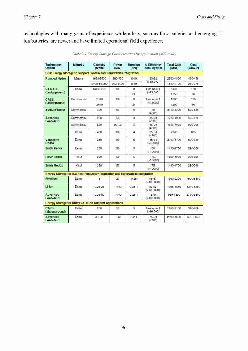
Chapter 7 Costs and Sizing
96
technologies with many years of experience while others, such as flow batteries and emerging Li-ion batteries, are newer and have limited operational field experience.
Table 7-1 Energy Storage Characteristics by Application (MW scale)

Chapter 7 Costs and Sizing
97
Table 7-2 Energy Storage Characteristics by Application (kW scale)
7.2 Battery Capacity Battery capacity defines the storable energy of the accumulator, and therefore is the parameter that represents the amount of electrical charge stored by the battery. It is usually expressed in [Ah], but if it is multiplied by the nominal voltage of the battery, the capacity is obtained in watt hours [Wh].
7.2.1 Battery parameter - Matlab Code To calculate the capacity of the battery needed to accumulate energy, a script for all the scenarios considered was used. The files related to the load and production of total PV are initially loaded (always separating the summer and winter cases).
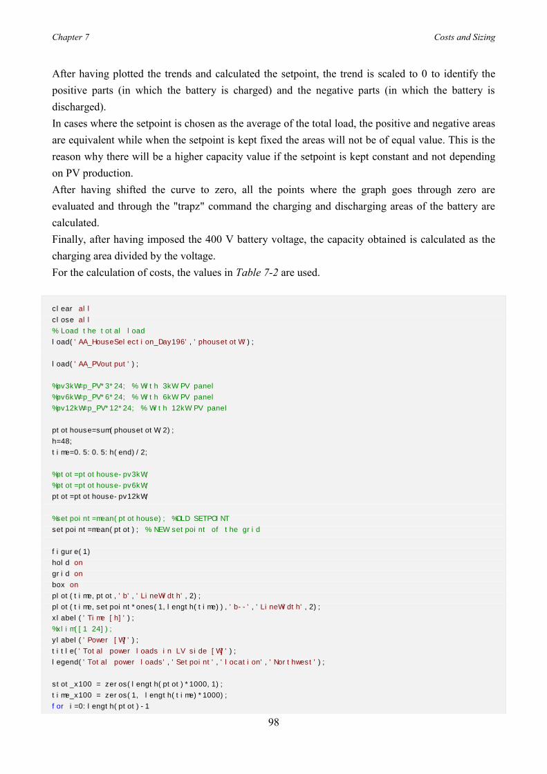
Chapter 7 Costs and Sizing
98
After having plotted the trends and calculated the setpoint, the trend is scaled to 0 to identify the positive parts (in which the battery is charged) and the negative parts (in which the battery is discharged). In cases where the setpoint is chosen as the average of the total load, the positive and negative areas are equivalent while when the setpoint is kept fixed the areas will not be of equal value. This is the reason why there will be a higher capacity value if the setpoint is kept constant and not depending on PV production. After having shifted the curve to zero, all the points where the graph goes through zero are evaluated and through the "trapz" command the charging and discharging areas of the battery are calculated. Finally, after having imposed the 400 V battery voltage, the capacity obtained is calculated as the charging area divided by the voltage. For the calculation of costs, the values in Table 7-2 are used.
clear all
close all
% Load the total load
load('AA_HouseSelection_Day196','phousetotW');
load('AA_PVoutput');
%pv3kW=p_PV*3*24; % With 3kW PV panel
%pv6kW=p_PV*6*24; % With 6kW PV panel
%pv12kW=p_PV*12*24; % With 12kW PV panel
ptothouse=sum(phousetotW,2);
h=48;
time=0.5:0.5:h(end)/2;
%ptot=ptothouse-pv3kW;
%ptot=ptothouse-pv6kW;
ptot=ptothouse-pv12kW;
%setpoint=mean(ptothouse); %OLD SETPOINT
setpoint=mean(ptot); % NEW setpoint of the grid
figure(1)
hold on
grid on
box on
plot(time,ptot,'b','LineWidth',2);
plot(time,setpoint*ones(1,length(time)),'b--','LineWidth',2);
xlabel('Time [h]');
%xlim([1 24]);
ylabel('Power [W]');
title('Total power loads in LV side [W]');
legend('Total power loads','Setpoint','location','Northwest');
stot_x100 = zeros(length(ptot)*1000,1);
time_x100 = zeros(1, length(time)*1000);
for i=0:length(ptot)-1

Chapter 7 Costs and Sizing
99
if i < length(ptot)-1
stot_x100(1000*i+1:1000*(i+1))=linspace(ptot(i+1),ptot(i+2),1000);
time_x100(1000*i+1:1000*(i+1))=linspace(time(i+1),time(i+2),1000);
end
end
%Shifted power to 0 to obtain charging and discharging power of the battery
figure(2)
hold on
box on
grid on
time_x100 = time_x100(1:47000);
stot_x100 = stot_x100(1:47000);
plot(time_x100,stot_x100-setpoint,'bx');
plot(time_x100,setpoint*ones(1,length(time_x100))-setpoint,'b--')
xlabel('Time [h]');
ylabel('Power [W]');
title('Power charging and discharging battery [W]');
hold off
area1 = trapz(time_x100,stot_x100-setpoint);
figure(3)
box on
grid on
area1_col = area(stot_x100-setpoint);
xlabel('Time [h]');
ylabel('Power [W]');
xlim([1 48000]);
title('Energy charging and discharging battery');
figure(4)
hold on
box on
grid on
begin_change = 1;
area_carica = 0;
area_scarica = 0;
for i = 1:length(stot_x100)-1
if (stot_x100(i)> setpoint && stot_x100(i+1)< setpoint)
area_temp_carica = trapz(time_x100(begin_change:i+1),stot_x100(begin_change:i+1)-setpoint);
area_carica = area_carica+area_temp_carica; %USE THIS VALUE TO CALCULATE BATTERY CAPACITY
[Wh]
plot(time_x100(i), stot_x100(i)-setpoint, 'ro', 'MarkerSize',10)
begin_change = i+1;
end
if (stot_x100(i)> setpoint && stot_x100(i+1)==stot_x100(end))
area_temp_carica = trapz(time_x100(begin_change:i+1),stot_x100(begin_change:i+1)-setpoint);
area_carica = area_carica+area_temp_carica;
plot(time_x100(i+1), stot_x100(i+1)-setpoint, 'rx', 'MarkerSize',10)
begin_change = i+1;
end
if (stot_x100(i)< setpoint && stot_x100(i+1)> setpoint)
area_temp_scarica = trapz(time_x100(begin_change:i+1),stot_x100(begin_change:i+1)-
setpoint);
area_scarica = area_scarica+area_temp_scarica;
plot(time_x100(i), stot_x100(i)-setpoint, 'go', 'MarkerSize',10)
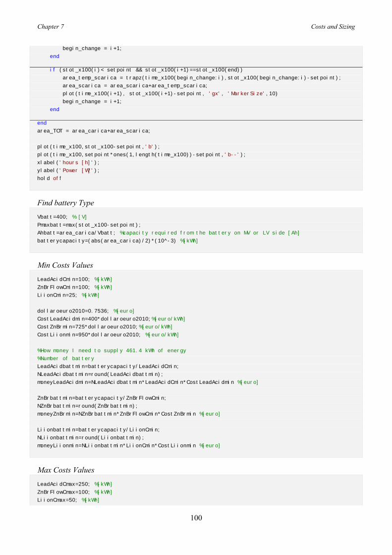
Chapter 7 Costs and Sizing
100
begin_change = i+1;
end
if (stot_x100(i)< setpoint && stot_x100(i+1)==stot_x100(end))
area_temp_scarica = trapz(time_x100(begin_change:i),stot_x100(begin_change:i)-setpoint);
area_scarica = area_scarica+area_temp_scarica;
plot(time_x100(i+1), stot_x100(i+1)-setpoint, 'gx', 'MarkerSize',10)
begin_change = i+1;
end
end
area_TOT = area_carica+area_scarica;
plot(time_x100,stot_x100-setpoint,'b');
plot(time_x100,setpoint*ones(1,length(time_x100))-setpoint,'b--');
xlabel('hours [h]');
ylabel('Power [W]');
hold off
Find battery Type
Vbatt=400; % [V]
Pmaxbatt=max(stot_x100-setpoint);
Ahbatt=area_carica/Vbatt; %capacity required from the battery on MV or LV side [Ah]
batterycapacity=(abs(area_carica)/2)*(10^-3) %[kWh]
Min Costs Values
LeadAcidCmin=100; %[kWh]
ZnBrFlowCmin=100; %[kWh]
LiionCmin=25; %[kWh]
dollaroeuro2010=0.7536; %[euro]
CostLeadAcidmin=400*dollaroeuro2010;%[euro/kWh]
CostZnBrmin=725*dollaroeuro2010;%[euro/kWh]
CostLiionmin=950*dollaroeuro2010; %[euro/kWh]
%How money I need to supply 461.4 kWh of energy
%Number of battery
LeadAcidbattmin=batterycapacity/LeadAcidCmin;
NLeadAcidbattmin=round(LeadAcidbattmin);
moneyLeadAcidmin=NLeadAcidbattmin*LeadAcidCmin*CostLeadAcidmin %[euro]
ZnBrbattmin=batterycapacity/ZnBrFlowCmin;
NZnBrbattmin=round(ZnBrbattmin);
moneyZnBrmin=NZnBrbattmin*ZnBrFlowCmin*CostZnBrmin %[euro]
Liionbattmin=batterycapacity/LiionCmin;
NLiionbattmin=round(Liionbattmin);
moneyLiionmin=NLiionbattmin*LiionCmin*CostLiionmin %[euro]
Max Costs Values
LeadAcidCmax=250; %[kWh]
ZnBrFlowCmax=100; %[kWh]
LiionCmax=50; %[kWh]

Chapter 7 Costs and Sizing
101
%dollaroeuro2010=0.7536 %[euro]
CostLeadAcidmax=950*dollaroeuro2010;%[euro/kWh]
CostZnBrmax=1950*dollaroeuro2010;%[euro/kWh]
CostLiionmax=3600*dollaroeuro2010; %[euro/kWh]
%How money I need to supply 461.4 kWh of energy
%Number of battery
LeadAcidbattmax=batterycapacity/LeadAcidCmax;
NLeadAcidbattmax=round(LeadAcidbattmax);
moneyLeadAcidmax=NLeadAcidbattmax*LeadAcidCmax*CostLeadAcidmax %[euro]
ZnBrbattmax=batterycapacity/ZnBrFlowCmax;
NZnBrbattmax=round(ZnBrbattmax);
moneyZnBrmax=NZnBrbattmax*ZnBrFlowCmax*CostZnBrmax %[euro]
Liionbattmax=batterycapacity/LiionCmax;
NLiionbattmax=round(Liionbattmax);
moneyLiionmax=NLiionbattmax*LiionCmax*CostLiionmax %[euro]
7.3 Results Thanks to the Matlab code just mentioned, the capacity values for the necessary batteries and consequently the costs have been calculated. From the Figure 7-1 we note that the highest value of capacity that is obtained is in the case in which we have a production of 2 kW of PV on each house, using the original setpoint of the network: this is because the network setpoint is too high and the battery needs a large capacity to accumulate surplus energy. This behaviour can be seen in a more contained way in all cases in which, in the presence of PV, the original setpoint calculated in the base cases is used without the presence of PV. As mentioned earlier, we see a greater capacity in the calculation with data coming from a typical summer day as there is less demand for loading but more production of PV. This is directly reflected on the costs of the battery itself. The costs used are derived from Table 7-2 and they have been reported from dollars to euro using the dollar/euro conversion coming from the average of the values of the year 2010. As the table shows a range of costs, the extreme values of the interval are considered, and they are characterized as minimum and maximum cost of batteries. In Figures 7-2, 7-3, the values on the y-axis must be multiplied by 105 for minimum cost values and for 106 for maximum cost values, respectively.
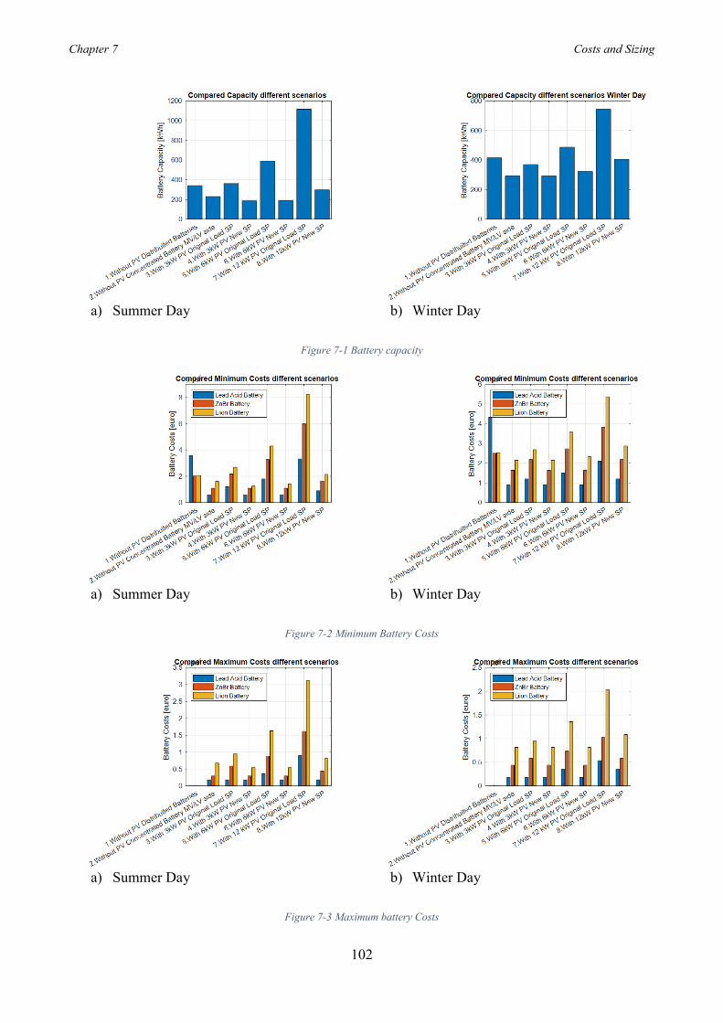
Chapter 7 Costs and Sizing
102
a) Summer Day b) Winter Day
Figure 7-1 Battery capacity
a) Summer Day b) Winter Day
Figure 7-2 Minimum Battery Costs
a) Summer Day b) Winter Day
Figure 7-3 Maximum battery Costs
Chapter 8 Conclusions and Future Works
103
Chapter 8
8 Conclusions and Future Works
8.1 Conclusions In this paper, results show that both centralised and distributed BES can mitigate the network losses and voltage issues. In scenarios with the presence of PV generation, the case in which there are fewer losses in the transformer is equivalent to both the battery concentrated on the LV part and with distributed batteries. For LV feeder losses, the best case is with distributed batteries because there is less current flowing in line, having a local power exchange. Losses on MV lines are mitigated in the same way. Considering the presence of PV, the losses in the transformer decrease varying the network setpoint according to the generation quantity of PV while they remain constant if a single setpoint value is used, but still lower than those obtained without the presence of a battery. As expected at the beginning, line losses decrease in the presence of storage and higher local PV output. However, it is necessary to establish a maximum generation limit from PV not to create problems of reverse flow of power in the network and overvoltage. Costs increase as installed capacity increases and higher prices occur with Li-ion batteries. Investing in the installation of concentrated batteries allows to not overload the network during peak hours, to not have to size the power plants for the peaks of demand while for the distributed batteries, the individual user can accumulate energy in the hours when it costs lesser and then use it in the peak of consumption, when it would be a greater cost.
8.2 Future works This study could be fully developed in the Matlab environment without considering an exact residential scheme but using all the starting data of the users without making a random choice. It is possible to evaluate the whole year without extracting a typical summer and winter day and connecting it directly with the PV measurements. This would allow to get an overview of the whole year and make a load forecast for the following years to evaluate the savings in energy terms of energy losses due to feeder and transformer losses.
Ringraziamenti
104
Ringraziamenti Alla fine di questo percorso di studi desidero porgere la mia gratitudine al Prof. Roberto Turri, per avermi dato la possibilità di fare questa esperienza internazionale presso il Dublin Institute of Technology e al Prof. Michael Farrell (capo dipartimento di ingegneria elettrica del DIT) per l’aiuto che mi ha dato e poiché mi ha permesso di lavorare su un argomento proiettato al futuro. Un grande ringraziamento va ai miei genitori Lorella e Milco che mi hanno permesso di raggiungere questo meraviglioso traguardo, appoggiandomi e sostenendomi in ogni mia scelta e nei momenti di difficoltà e a mio fratello Giulio che è capace di ascoltarmi e tranquillizzarmi in ogni momento. Un ringraziamento speciale va a Luca, abbiamo percorso questo cammino insieme e sei stato capace di capirmi e di sostenermi nei momenti difficili. Un ringraziamento va a LEDS e a tutti i soci, per aver reso unica la esperienza universitaria e per aver suscitato in me l’interesse nella ricerca e nel miglioramento. Un grandissimo ringraziamento va ai miei compagni di corso (ormai più amici che compagni!!!), ai miei amici e amiche del CAI di Feltre, alle mie coinquiline negli anni vissuti a Padova e a chi ho conosciuto a Dublino: siete le persone con cui ho condiviso momenti di gioia e tristezza e mi siete stati accanto in questi anni di Università. Acknowledgment At the end of this academic pathway I would like to extend my gratitude to Prof. Roberto Turri, for giving me the opportunity to make this international experience at the Dublin Institute of Technology and to Prof. Michael Farrell (Head of Electrical Engineering at DIT) for the help he gave me and because he allowed me to work on a topic projected into the future. A big thank you is for my parents Lorella and Milco who have allowed me to reach this wonderful goal, supporting me in all my choices and moments of difficulties and to my brother Giulio who is always able to listen and reassure me. Special thanks are for Luca, we have walked along this path together and you have been able to understand me and support me in difficult moments. Thanks to LEDS and to all the members, for making my university experience unique and for having aroused my interest in research and improvement.

Ringraziamenti
105
A big thank you to my classmates (now more friends than mates!!!), to my friends of the CAI of Feltre, to my roommates in the years lived in Padua and who I met in Dublin: you are the people with whom I shared moments of joy and sadness and you have been with me during these years of University.

References
106
References [1] A. Oudalov, D. Chartouni, C. Ohler, and G. Linhofer, “Value analysis of battery energy
storage applications in power systems BT”, IEEE PES Power Systems Conference and
Exposition, pp. 2206–2211, 2006.
[2] M. Zarghami, M. Y. Vaziri, A. Rahimi, and S. Vadhva, “Applications of battery storage to
improve performance of distribution systems,” IEEE Green Technol. Conf., pp. 345–350,
2013.
[3] X. Xu, M. Bishop, O. Donna G, and H. Chen, “Application and modeling of battery energy
storage in power systems,” CSEE J. Power Energy Syst., vol. 2, no. 3, pp. 82–90, 2016.
[4] A. Bregolin, F. Bignucolo, “RESS: sistemi di accumulo dell’energia elettrica in ambito
residenziale - Valutazioni tecnico-economiche,” 2011.
[5] R. J. Kerestes, “Economic Analysis of Grid Level Energy Storage fo the Application of Load
Levelling,” Mycol. Res., vol. 106, no. 11, pp. 1323–1330, 2002.
[6] M. Faisal, M. A. Hannan, P. J. Ker, A. Hussain, M. Bin Mansor, and F. Blaabjerg, “Review
of energy storage system technologies in microgrid applications: Issues and challenges,”
IEEE Access, vol. 6, no. 1, pp. 35143–35164, 2018.
[7] P. Nikolaidis and A. Poullikkas, “A comparative review of electrical energy storage systems
for better sustainability,” Open Access J. J. Power Technol., vol. 97, no. 3, pp. 220–245,
2017.
[8] M. Daghi, M. Sedghi, and M. Aliakbar-Golkar, “Optimal battery planning in grid connected
distributed generation systems considering different technologies,” 20th Electr. Power
Distrib. Conf. EPDC 2015, no. April, pp. 138–142, 2015.
[9] E. Bertoluzzo, “Batteries: Part I,” pp. 1–28, 2014.
[10] F. McLoughlin, A. Duffy, and M. Conlon, “A clustering approach to domestic electricity
load profile characterisation using smart metering data,” Appl. Energy, vol. 141, pp. 190–
199, 2015.
[11] “ISSDA, Irish Social Science Data Archive” [Online]. Available: https://www.ucd.ie/issda/
[Accessed: August 2018].
[12] “Cost and Benefits of Embedded Generation in Ireland”, PB Power, no. September, 2004.
[13] Z. Qiao and J. Yang, “Comparison of centralised and distributed battery energy storage
systems in LV distribution networks on operational optimisation and financial benefits,” J.
Eng., vol. 2017, no. 13, pp. 1671–1675, 2017.
[14] H. Saboori and H. Abdi, “Application of a grid scale energy storage system to reduce
References
107
distribution network losses,” 18th Conf. Electr. Power Distrib. Networks, pp. 1–5, 2013.
[15] M. Farrokhifar, S. Grillo, and E. Tironi, “Optimal placement of energy storage devices for
loss reduction in distribution networks,” 4th IEEE/PES Innov. Smart Grid Technol. Eur.
ISGT Eur. 2013, pp. 9–13, 2013.
[16] G. Naveen, B. P. Kumar, and M. L. Sudheer, “Demand side load leveling using distributed
micro energy and storage systems with the establishment of micro grids,” IEEE Innov. Smart
Grid Technol. - Asia, ISGT Asia 2013, pp. 1–6, 2013.
[17] H. Sadeghian, Z. Wang, “Decentralized demand side management with rooftop PV in
residential distribution network”, IEEE ISGT, pp. 5–9, 2018.
[18] E. Skoplaki, A. G. Boudouvis, and J. A. Palyvos, “A simple correlation for the operating
temperature of photovoltaic modules of arbitrary mounting,” Sol. Energy Mater. Sol. Cells,
vol. 92, no. 11, pp. 1393–1402, 2008.
[19] M. Aghahassani, S. Grillo, “Voltage regulation by means of storage device in LV feeder
using OpenDSS interfacing with MATLAB”, 2017.
[20] M. Baumann, B. Zimmermann, H. Dura, B. Simon, and M. Weil, “A comparative
probabilistic economic analysis of selected stationary battery systems for grid applications,”
4th Int. Conf. Clean Electr. Power Renew. Energy Resour. Impact, ICCEP 2013, pp. 87–92,
2013.
[21] Electric Power Research Institute, “Electricity Energy Storage Technology Options,” Power,
vol. 64, no. 2–3, p. 170, 2010.


![quantum battery arXiv:2005.05068v1 [cond-mat.mes-hall] 11 ...](https://static.fdocumenti.com/doc/165x107/625047fe873c387914110699/quantum-battery-arxiv200505068v1-cond-matmes-hall-11-.jpg)


![PART C1 ISOSINT SENSOR · Electronic SYSTEMS spa - DOMINO System - OPERATION MANUAL [ML14036A159.docx] C1.1.2 Intended Use The ISOSINT measure sensor is designed to be installed exclusively](https://static.fdocumenti.com/doc/165x107/5e6d36c3d58b6c20922e5040/part-c1-isosint-sensor-electronic-systems-spa-domino-system-operation-manual.jpg)