UNIVERSITà DEGLI STUDI DI TORINO

Facoltà di Economia

Corso di Laurea in Finanza Aziendale e Mercati Finanziari

TESI DI LAUREA

Agent-based models review for option pricing

Relatore: Prof. Pietro TernaCorrelatore: Prof. Marina Marena

Candidato: Eni Rrema

Anno Accademico: 2009 - 2010

Contents

Introduction 4

1 Agent-based models 61.1 Social Science, Complexity, Models, and ABMs . . . . . . . . 61.2 ABMs: a new way of doing science . . . . . . . . . . . . . . . 101.3 On the motivations for using agent computing in social sci-

ence. . . . . . . . . . . . . . . . . . . . . . . . . . . . . . . . 121.3.1 ABMs construction in financial economic system . . . 13

1.4 System dynamics, Discrete Events and ABMs . . . . . . . . . 141.4.1 Differences between System Dynamics and ABMs . . . 171.4.2 Which approach to use? . . . . . . . . . . . . . . . . . 18

1.5 Tools for ABMs . . . . . . . . . . . . . . . . . . . . . . . . . . 191.5.1 Swarm . . . . . . . . . . . . . . . . . . . . . . . . . . . 191.5.2 JAS . . . . . . . . . . . . . . . . . . . . . . . . . . . . 201.5.3 NetLogo . . . . . . . . . . . . . . . . . . . . . . . . . . 201.5.4 A tool comparison . . . . . . . . . . . . . . . . . . . . 21

2 On the protocol to describe ABMs 222.1 Overview . . . . . . . . . . . . . . . . . . . . . . . . . . . . . 232.2 Design Concepts . . . . . . . . . . . . . . . . . . . . . . . . . 252.3 Details . . . . . . . . . . . . . . . . . . . . . . . . . . . . . . . 272.4 Complaints and benefits from using ODD . . . . . . . . . . . 28

2.4.1 Complaints about ODD . . . . . . . . . . . . . . . . . 282.4.2 Benefits of using ODD . . . . . . . . . . . . . . . . . 29

3 Black and Scholes model and parameter uncertainty 313.1 Black and Scholes model . . . . . . . . . . . . . . . . . . . . . 313.2 Option pricing under unknown volatility . . . . . . . . . . . . 343.3 Is the Black and Scholes formula used in practice? Criticism

and appreciation. . . . . . . . . . . . . . . . . . . . . . . . . . 37

2

4 Option Pricing under unknown volatility: an agent basedmodel 404.1 Model assumptions . . . . . . . . . . . . . . . . . . . . . . . . 404.2 ODD model description . . . . . . . . . . . . . . . . . . . . . 434.3 Model replication . . . . . . . . . . . . . . . . . . . . . . . . . 46

Conclusions 47

References 48

3

Introduction

Options are one of the most used derivative contracts in financial markets.They can be used by speculators to generate profits or by hedgers to protecttheir positions. Trying to find the real value of these derivative contracts it’sa hard task.

Since the introduction of the Black-Scholes formula, things become easier.With a mathematical formula it was possible to link option’s value to theparameters it depends on. Unfortunately, the assumptions on which theformula is based are very strong and it put doubts on its accuracy to find thereal value of options. In the original framework the volatility is assumed tobe constant. Concerns arise around this assumptions. Empirical observationshows that volatility during option’s life changes especially for options withlong expiration. Thus, researchers started studying models, still based onBlack-Scholes formula, to account for non constant volatility. This producedthe construction of new models that were used by practioners in the valuationof options.

The natural question that arises is how wrong is the original Black-Scholes formula from its further developments? Zhang et al. (2009) pro-posed in their work an original way to make this comparison. They valuatedfirst the option with the original Black-Scholes formula (to compute thetheoretical price) and then they used the ABMs (Agent-based modelings)methodology to compute the formula with stochastic volatility. This is anoriginal idea to use ABMs methodology in finance and so far is the first workthat apply it to option pricing. To study a complex phenomenon such as thegeneration of option prices requires, indeed, tools that can handle complexitymore efficiently. ABMs serve to this scope.

The aim of this work is to review the ABMs methodology and see anapplication of it in option pricing. In chapter 1 the ABMs methodology ispresented with a comparison with other models. Moreover, a description oftools and their comparison is presented as well. ABMs is a very powerfultool but it is very difficult to explain the model clearly once it is constructed.Therefore, a standard protocol for model description is needed. The most

4

natural and easy way to describe ABMs is the ODD. In chapter 2 is presentedthe ODD: description, advantages and disadvantages. Chapter 3 explainshow the Black-Scholes formula is obtained. In this chapter it is also explainedthe uncertain volatility framework. In Chapter 4 is presented the model ofoption pricing with uncertain volatility using ABMs. An ODD prospect ofthe model is presented as well.

5

1 Agent-based models

1.1 Social Science, Complexity, Models, and ABMs

Social science is the field that mainly study human nature. It covers manyareas such as demography, sociology, economics, anthropology, politics andso on. It is considered to be a complex science. We refer to it as a so-cial complexity that is the study of social phenomena in a complex systemenvironment. What is a complex system? Flake (1998) describe it as:

“A collection of many simple units that operate in parallel andinteract locally with each other so as to produce emergent be-havior.”

Complex system, therefore, must have the following two characteristics:

• It is composed of interacting units that operate in parallel.

• The system has emergent proprieties. It is not possible to deducesystem features by summing up the characteristics of the units thatcompose the system.

Therefore, when studying social sciences we cannot decompose it into sepa-rate subprocess, that the aggregate analysis will give us insights about theprocess as a whole. In other words, to understand it we cannot just have asimple look at the single individuals that constitute the system and pretendto understand the characteristics of the whole system. We need to analyzethe interactions among individuals and try to explain how the output ispossible. We can distinguish between reductionism that allows us to startfrom a system as a whole and find the simple micro rules that make thesystem possible and constructivism, that is not applicable to social scienceas it starts from simple rules and tell about the proprieties of the system asa whole.

Experiments in social science are also very difficult to be implemented. Itis difficult to test hypothesis concerning the individual’s behavior related tomacro regularities. Moreover, social scientists have to deal with a perfectly

6

informed individual that has infinite computing capacity who maximizes afixed exogenous utility function. Unfortunately, this is not what in the realworld happens. Individuals do not have all the available information andtheir computing capacity is limited.

Regarding social science, equilibrium is one of the biggest issue that theyhave to face. Equilibrium is studied only in a static way as there is no otherapproach to see the effects of the time on it. To overcome these major issuesa new way of treating social science is needed.

Models can be considered as an interesting and very powerful tool forrepresenting real systems. They are constructed to answer questions aboutreal systems. In this way, model purpose depends on the question we wantto answer. The question serves as a filter for selecting the criteria in whatway the model will be constructed. If we want to represent a certain partof a real system then different parameters will be considered and other willbe ignored. Thus, model parameters will depend on the purpose of themodel. The parameter choice is not easy. At the beginning a simple modelwill be constructed. This simple model should represent a simplified versionof observed patterns in real systems. Simplified model can be constructedstarting from theory, previous models, empirical evidence, or imagination.Then, to say if a parameter is important or not, researchers have to testthem and compare the results with the observed patterns. Thus, startingfrom simple model researchers can add more details to obtain what theyoriginally had in mind.

“Agent Based Models” are a new way of treating social science. It consistsof population set of agent implemented on computers. Running an ABMsconsists in letting the agents population interact with each other and observethe results. This new way of doing science has been considered favorably inthe last years.

The use of ABM can be tracked in the late 1940 to the Von Neumannmachine capable of reproduction. The idea was later improved thanks thesuggestion made by Stanislaw Ulam to construct the famous cellular au-tomata. Improvements to the model were made by John Conway to buildthe well-known “Game of life.”

7

One of the first agent based model was the Thomas Schellings’s segrega-tion model. In his model agents with simple rules interact with each otherand emergent behavior is observed.

Later in the early 1980, Robert Axelord contributed to ABM trying tosolve the Prisoners Dilemma using ABM. Axelord developed many othermodels in political science. In the late 1980, Christopher Langton coined theterm artificial life meaning the field that study the systems related to lifeand its processes and its evolution using computer models and simulations.Langton can be considered one major author that contributed in the field ofABM (his famous model is called Langton’s ant).

The first scientists to use the term “agent” were John Holland and JohnH. Miller in their famous paper “Artificial Adaptive Agents in EconomicTheory.” Holland and Miller contributed as well in developing the field.

Epstein and Axtell (1996) developed the first large scale ABM the “Sug-arscape” to model the role of social phenomena.

With the appearance of programs such as StarLogo, NetLogo, SWARM,and RePast, ABM becomes a very used tool to do science and its applicabilityspread among many fields.

The main feature of artificial society model (ABM applied to social sci-ence) is that:

“fundamental social structures and group behaviors emerge fromthe interaction of individual agents operating on artificial envi-ronment under rules that place only bounded demands on eachagent’s information and computational capacity” Epstein andAxtell (1996) .

This allows the social scientist to recreate social phenomena and study iton computers. Simply creating agents with simple rules and an artificialenvironment where they interact, social scientist can study very complexphenomena. Complex phenomena emerge by simply letting agents interact-ing with each other.

Agents are the “peoples” of artificial societies. Each agent understandshis situation and based on his internal rules makes decisions. Agents may

8

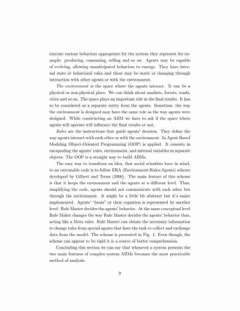
execute various behaviors appropriate for the system they represent for ex-ample: producing, consuming, selling and so on. Agents may be capableof evolving, allowing unanticipated behaviors to emerge. They have inter-nal state or behavioral rules and these may be static or changing throughinteraction with other agents or with the environment.

The environment is the space where the agents interact. It can be aphysical or non-physical place. We can think about markets, forests, roads,cities and so on. The space plays an important role in the final results. It hasto be considered as a separate entity from the agents. Sometime, the waythe environment is designed may have the same role as the way agents weredesigned. While constructing an ABM we have to ask if the space whereagents will operate will influence the final results or not.

Rules are the instructions that guide agents’ decision. They define theway agents interact with each other or with the environment. In Agent BasedModeling Object-Oriented Programming (OOP) is applied. It consists inencapsuling the agents’ rules, environment, and internal variables in separateobjects. The OOP is a straight way to build ABMs.

The easy way to transform an idea, that social scientists have in mind,to an executable code is to follow ERA (Environment-Rules-Agents) schemedeveloped by Gilbert and Terna (2000). The main feature of this schemeis that it keeps the environment and the agents at a different level. Thus,simplifying the code, agents should not communicate with each other butthrough the environment. It might be a little bit abstract but it’s easierimplemented. Agents’ “brain” or their cognition is represented by anotherlevel. Rule Master decides the agents’ behavior. At the same conceptual levelRule Maker changes the way Rule Master decides the agents’ behavior thus,acting like a Meta ruler. Rule Master can obtain the necessary informationto change rules from special agents that have the task to collect and exchangedata from the model. The scheme is presented in Fig. 1. Even though, thescheme can appear to be rigid it is a source of better comprehension.

Concluding this section we can say that whenever a system presents thetwo main features of complex system ABMs becomes the most practicablemethod of analysis.

9

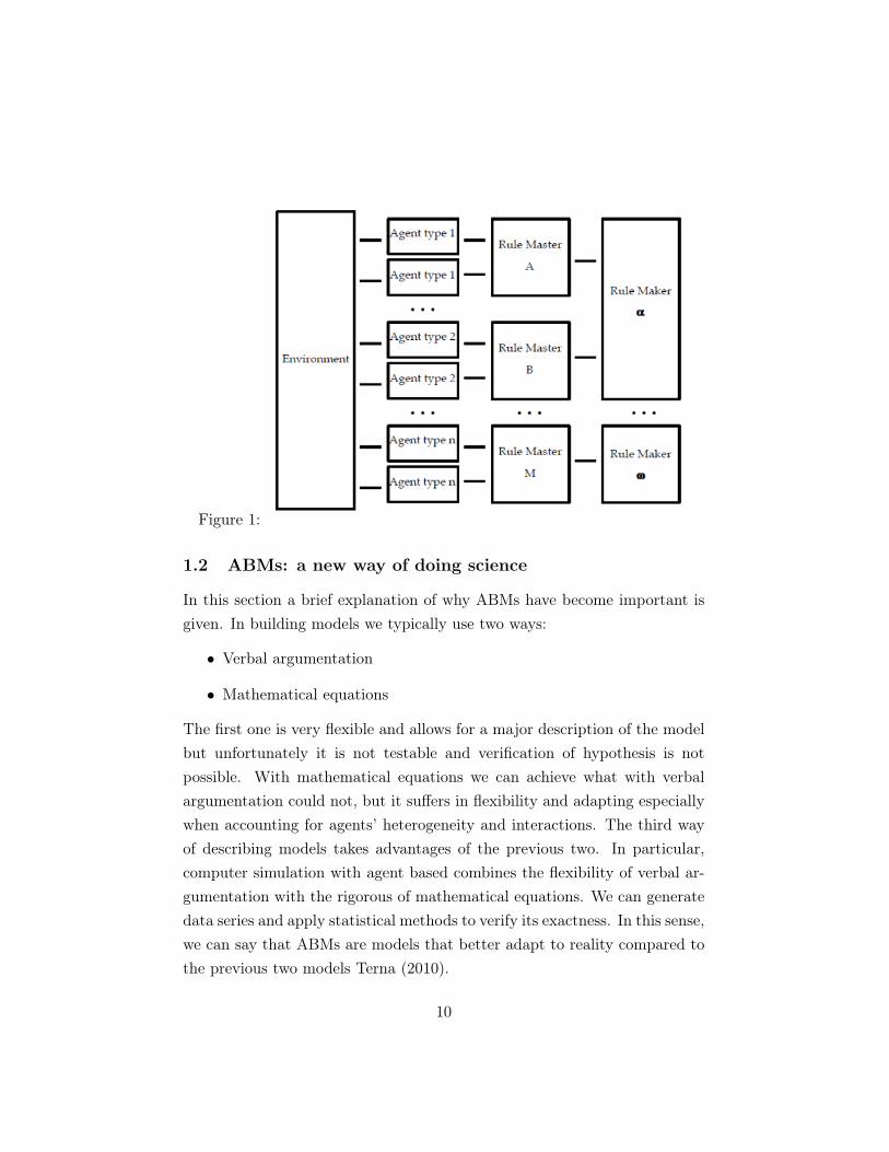
Figure 1:

1.2 ABMs: a new way of doing science

In this section a brief explanation of why ABMs have become important isgiven. In building models we typically use two ways:

• Verbal argumentation

• Mathematical equations

The first one is very flexible and allows for a major description of the modelbut unfortunately it is not testable and verification of hypothesis is notpossible. With mathematical equations we can achieve what with verbalargumentation could not, but it suffers in flexibility and adapting especiallywhen accounting for agents’ heterogeneity and interactions. The third wayof describing models takes advantages of the previous two. In particular,computer simulation with agent based combines the flexibility of verbal ar-gumentation with the rigorous of mathematical equations. We can generatedata series and apply statistical methods to verify its exactness. In this sense,we can say that ABMs are models that better adapt to reality compared tothe previous two models Terna (2010).

10

Now let see the role of ABMs compared to the traditional deduction andinduction. This is best explained by Axelrod and Tesfatsion in the followingstatement:

“Simulation in general, and ABMs in particular, is a third way ofdoing science in addition to deduction and induction. Scientistsuse deduction to derive theorems from assumptions, and induc-tion to find patterns in empirical data. Simulation, like deduc-tion, starts with a set of explicit assumptions. However, unlikededuction, simulation does not prove theorems with generality.Instead, simulation generates data suitable for analysis by in-duction. Nevertheless, unlike typical induction, the simulateddata come from a rigorously specified set of assumptions regard-ing an actual or proposed system of interest rather than directmeasurements of the real world. Consequently, simulation differsfrom standard deduction and induction in both its implementa-tion and its goals. Simulation permits increased understanding ofsystems through controlled computational experiments.” Axelrodand Tesfatsion (2005)

Traditionally with deduction we mean the process of deriving b from a whereb is a formal consequence of a. With induction we are allowed to infer bfrom a where b does not follow necessarily from a. The quote cited abovecan be conducted to abduction. Abduction is a method of reasoning whereone chooses the hypothesis that if realized give the best explanation of theactual evidence.

Let’s see the position that ABMs has compared to the classical and con-structive mathematics. Generally classical mathematics is ruled by the Lawof Excluded Middle (LEM). It says that for any proposition P, either P istrue or its negation is true. Thus, classical mathematicians accept existenceproofs based on proof by contradiction. In contrast, constructive mathemati-cians require a direct proof that P is true in as a computational procedure torule out both the falseness and the undecidability of P. Constructive proofscan, in principle, be realized with computer programs.

11

ABMs combine both constructive and classical approaches. Agents canacquire new data constructively through interactions and this is the samefor real people. Moreover, like real people, agents can have “uncomputablebeliefs”. It means that they can have unexpected behavior and this mightbe possible due to interactions with other agents or inborn rules.

The choice between a more classical or constructive approach in ABMsdepend on the purpose of the model. For descriptive purposes, it permitshuman behavior to be captured with greater fidelity than simple algorith-mic representations. For optimization purposes, it permits a deeper andmore creative exploration of large domains, a melding of experience-temperedguesswork with step-by-step computation that could vastly extend the powerof traditional finite search methods. In conclusion ABMs can be expressed asfinite systems of discrete time recursive equations over finite state domains.Nevertheless, they can be data-driven dynamic applications systems. Thus,it is true that ABMs can be considered as a new form of mathematics. Borrilland Tesfatsion (2010)

1.3 On the motivations for using agent computing in socialscience.

Many models rely on strong assumptions such as ideal condition or idealagents. The main goal of these models is to understand the relationship be-tween key variables and it can turn out to be useful as a good approximationof the reality. However, in reality departure from ideal world is the rule morethan the exception. To better understand the real world we need to adoptmodels that can try to explain such departures.

The reasons for using Agent Based Modeling (ABMs) in social sciencecan be enveloped in three main blocks depending on the solubility of theunderlying mathematical equations. The first one derives when the equationsis completely solvable analytically or numerically. ABMs can be used topresent results or as a new method of Monte Carlo Simulation. The othermotivation derives when the underlying equations cannot be solved. In thiscase, ABMs can help understating the proprieties of the model structure, test

12

results on parameters and assumptions, and illustrate dynamical proprieties.The third reason derives when writing equations is not useful. In this caseABMs can help in understanding better the structure of the model.

Several are the advantages that arise from using the ABMs in social sci-ence. In particular, it is easy to limit agents’ rationality and even if onewould use complete rational agents that would result in a tricky operation.In most contest both social and spatial matters and this is difficult to ac-count in a mathematical framework while in ABMs it is easier. There is adisadvantage in using ABMs. In particular, in order to obtain robust resultsone needs to compute several runs. Thus, the single run itself cannot saymuch about the general results and explain the dynamic. Axtell (2000)

An important point in favor of ABMs comes from the Nobel price winnerE. Ostrom. In her nobel lecture work Ostrom (2010) she stated:

“To explain the world of interactions and outcomes occurring atmultiple levels, we also have to be willing to deal with complex-ity instead of rejecting it. Some mathematical models are veryuseful for explaining outcomes in particular settings. We shouldcontinue to use simple models where they capture enough of thecore underlying structure and incentives that they usefully pre-dict outcomes. When the world we are trying to explain andimprove, however, is not well described by a simple model, wemust continue to improve our frameworks and theories so as tobe able to understand complexity and not simply reject it.”

Even though, it is not stated explicitly the need of ABMs by accepting thecomplexity paradigm it is accepted the need of models that can handle itproperly.

1.3.1 ABMs construction in financial economic system

In this section, I will explain what are the positive aspects of using ABMs ina particular field of social science: financial economics. ABMs can be usefulto explain the connection between micro-simulation properties of financial

13

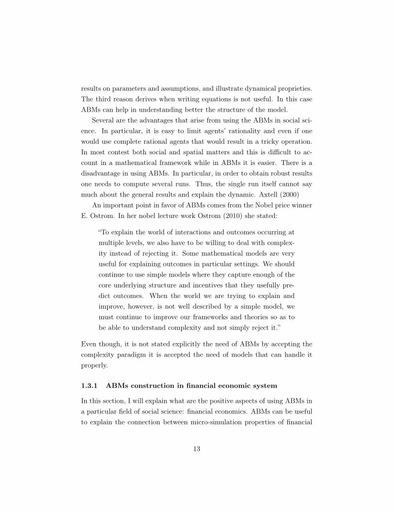
Figure 2:

system with its macro or statistical properties Fig. 2. Explaining macro-levelthings in micro-simulation is the aim of using ABMs in social science.

In financial markets events such as fat tails, jumps, volatility grouping,etc., have become an important issue that need to find a solution. Theuse of ABMs can spread light through such a puzzles. Several importantmodels have achieved important results so far. The Artificial Stock Marketdeveloped by Santa Fe Institute is one of those. Why is that possible? Thisis possible mainly because the ABMs is bottom-up approach. We can modelinvestors the way we want to operate. This can generate unexpected resultsand perhaps explain results that were not explained with other models. Forexample in their work, Situngkir and Surya show how to explain phenomenasuch as:

• Volatility grouping

• Excess kurtosis

• Multifractality character

present in Indonesian market using ABMs Situngkir and Surya (2005) .

1.4 System dynamics, Discrete Events and ABMs

Modeling is a way of solving problems that occur in real life. Throughmodeling it is possible to test systems before it is implemented. In general,

14

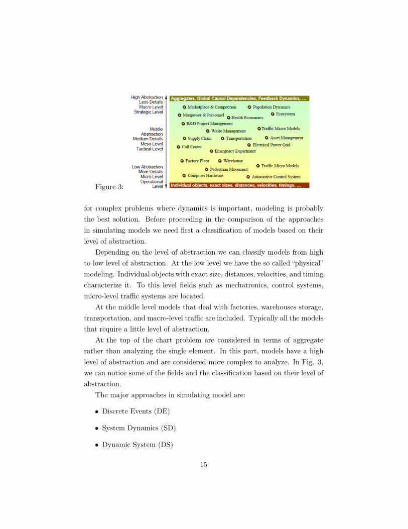
Figure 3:

for complex problems where dynamics is important, modeling is probablythe best solution. Before proceeding in the comparison of the approachesin simulating models we need first a classification of models based on theirlevel of abstraction.

Depending on the level of abstraction we can classify models from highto low level of abstraction. At the low level we have the so called “physical”modeling. Individual objects with exact size, distances, velocities, and timingcharacterize it. To this level fields such as mechatronics, control systems,micro-level traffic systems are located.

At the middle level models that deal with factories, warehouses storage,transportation, and macro-level traffic are included. Typically all the modelsthat require a little level of abstraction.

At the top of the chart problem are considered in terms of aggregaterather than analyzing the single element. In this part, models have a highlevel of abstraction and are considered more complex to analyze. In Fig. 3,we can notice some of the fields and the classification based on their level ofabstraction.

The major approaches in simulating model are:

• Discrete Events (DE)

• System Dynamics (SD)

• Dynamic System (DS)

15

• Agent Based Modeling (ABMs)

Technically, SD and DS work mainly in continuous process whereas DE andABMs work in discrete time. If we consider the level of abstraction usedin the model we can notice that: System Dynamic is at the bottom levelwhile Dynamic Systems dealing with aggregates is located at the top level.Discrete Events is located at the low to middle level and Agent Based Model,due to its flexibility, can be located across all the three levels. ABMs is arelatively new subject. It started being used as an increasing demand forplatforms that could combine the main characteristics of the three modelstogether.

System Dynamics developed by electrical engineer Jay W. Forester is

“The study of information-feedback characteristics of industrialactivity to show how organizational structure, amplification (inpolicies), and time delays (in decisions and actions) interact toinfluence the success of the enterprise”.

The range of SD applications includes urban, social, ecological types of sys-tems. In SD, the real-world processes are represented in terms of stocks,flows between these stocks, and information that determines the values ofthe flows. To approach the problem in SD style one has to describe thesystem behavior as a number of interacting feedback. Mathematically is asystem of differential equations.

Dynamic Systems modeling may be considered as the ancestor of SystemDynamics. It is used in mechanical, electrical, chemical, and other technicalengineering disciplines. The underlying mathematical model of a dynamicsystem would consist of a number of state variables and algebraic differentialequations of various forms over these variables. In contrast with the SD,variables here have direct meaning: location, velocity, acceleration, pressure,concentration, etc., they are inherently continuous, and are not aggregates ofany entities. The mathematical diversity and complexity in dynamic systemsdomain can be much higher than in system dynamics. The tools used fordynamic system simulation could easily solve any SD problem with evenmuch better accuracy than SD tools.

16

Discrete Event is the modeling approach based on the concept of entities,resources, and block charts describing entity flow and resource sharing. Thisapproach is dated to 1960s developed by Geoffrey Gordon. Entities are pas-sive objects that represent people, parts, documents, tasks, messages, etc.They travel through the blocks of the flowchart where they stay in queues,are delayed, processed, seize and release resources, split, combined, etc. DEmodeling may be considered as definition of a global entity-processing algo-rithm, typically with stochastic elements.

Agent Based Modeling has its roots in different disciplines like artificialintelligence, complexity science, game theory, etc. There is no a universallyaccepted definition in this area, and people still discuss what kind of proper-ties an object should have to “deserve” to be called an “agent.” Compared toSD or DE models, the modeler defines the behavior at individual level, andthe global behavior emerges as a result of many individuals, each followingits own behavior rules, living together in some environment and communi-cating with each other and with the environment. That is why AB modelingis also called bottom-up modeling. Borshchev and Filippov (2004)

1.4.1 Differences between System Dynamics and ABMs

The major differences between the two modeling techniques represent alsotheir relative strengths and weaknesses. Agent-based modeling focuses onindividuals who interact based on of simple rules. The resulting emergentbehavior of such agents as a complex system is the basic unit of analysis. Theresearcher may modify rules and environmental parameters and then try tounderstand what the outcomes are with regard to the emergent behavior ofthe overall system. As long as rules are known or can be discovered by somesort of observation, the modeling and testing of such emergent structures isa relatively straightforward process. However, once the reverse direction ofstudy is employed, that is, a complex aggregate behavior of a system hasbeen observed, and now its agents and the rules by which they interact shallbe identified, the process can be very complicated. Discovering agents andrules and then building a model, which is capable of mimicking the previously

17

observed dynamic behavior, is a very complicated task.In SD, modeling the feedback loop is the unit of analysis. Individual

agents or events do not matter much in SD models, since the dynamics of theunderlying structures are seen as dominant. Feedback structures, for exam-ple in social-science fields of study, can become subject to controversy sinceperspectives on a problem and perceptions may differ widely. Construct-ing models is a process in which expert consensus regarding the feedbackstructure is essential to the credibility of any given model. If the feedbackstructure of a model captures the structure of a system insufficiently, theresulting insights may be faulty. On the other hand, if the model does rep-resent the systemic problem sufficiently, leverage points for intervention canbe identified effectively. This, however, is not possible at an individual butat an aggregate level.

Both techniques aim at discovering leverage points in complex aggregatesystems, modelers of agent-based models seek them in rules and agents, whileSD modelers do so in the feedback structure of a system. Jochen (2009)

1.4.2 Which approach to use?

In general, using AB approach allows capturing more real life phenomenathan with SD or DE approach. However, AB is not always a replacement forSD or DE modeling. There are a lot of applications where SD or DE modelcan efficiently solve the problems and agent based modeling will result in aless efficient approach, harder to develop, or simply not matching the natureof the problem. Whenever this is the case, traditional approaches should beused.

Agent based modeling is for those who wish to go beyond the limitsof SD and DE approaches, especially in the case the system being modeledcontains active objects (people, business units, animals, vehicles, or projects,stocks, products, etc.) with timing, event ordering or other kind of individualbehavior. We should also consider using different modeling paradigms fordifferent parts of the simulation model.

18

1.5 Tools for ABMs

The number of products that can be used now days for doing ABMs has in-creased considerably. Each of these products has potentially and limitationsdepending on the work that the research has in mind. Three main programsare mostly used in the simulation field Terna et al. (2006):

• Swarm

• JAS

• NetLogo (StarLogo)

1.5.1 Swarm

Swarm is one of the most consolidated project and environment for agentsimulation. It was originally developed by the Santa Fe Institute as a univer-sal simulation language to be applied not only in economic simulation butalso in every field.

Swarm has been developed as a library written in Objective C, whichis a similar language to C but object oriented one. Many years after aversion that reads Java was available. Summarizing the characteristics andthe advantages in using Swarm:

• Swarm can use both Objective C and Java. The first one is moresuitable to optimize models on computer and the other one let the userto more freedom in use and the possibility to use the major knowledgeof Java.

• The tool is comprehensive of software for scheduling, GUI with basicinstruments for numerical and graphical analysis.

• The simulation run with Swarm allows saving the results in file or in agraphic mode where it is possible to access the single agent and modifyhis internal parameters.

• It is very easy to add on more tools especially if we are using Swarmwith Java.

19

• It has a powerful community where doubts are solved altogether andupdates are issued frequently.

1.5.2 JAS

JAS (Java Agent-based Simulation) was developed my Michele Sonnessa. Itconsists in a library of object-oriented functions that has as objective thecreation of a simulation model in discrete time using a standard programinglanguage. Other than the library it has a standard protocol that allows theusers to create their own code. This allow other users to easily understandthe code and thus to reproduce it. Below a description of the main featuresof JAS is provided.

• JAS is an easily tools for discrete event simulation.

• It has an easily and highly intuitive graphical representation.

• It has a library for artificial neural network and genetic algorithm.

• The network library can be very easily implemented and allows theusers to implement complicated simulation on networks.

• An object oriented model very flexible that allows the users to havedifferent statistics during the simulation and the possibility to save theresults in a database.

1.5.3 NetLogo

NetLogo offers a simplified language for the realization of simulating model.Initially was introduced as StarLogo. It is based on Logo language intro-duced in the 1970s. In NetLogo, the main features are the turtles. Turtlescan become agents, they can communicate with each other and with theenvironment surrounding them. The turtles moves around an environmentcalled patches that can have different states each described by internal vari-ables. The interactions between turtles and patches allow the writing ofcomplicated and enriched programs in a short time.

20

1.5.4 A tool comparison

NetLogo has the advantage of being user friendly. It has very short learningtime compared to Swarm or JAS that requires a previous programing knowl-edge. Obviously, the things that we can do with NetLogo are less powerfulcompared to the other two programs. It is useful at the beginning to firstbuild the model in NetLogo and then proceed in a further implementationof the model in more complicated program such as Swarm or JAS.

21

2 On the protocol to describe ABMs

The agent-based simulation has become a very popular tool in many fields.However, the great potential of ABMs comes at a cost. ABMs are morecomplex in structure than analytical models. They have to be implementedand run on computers. Thus, they are more difficult to analyze, understand,and communicate than traditional analytical models Grimm et al. (1999).The results obtained from ABMs are not easily reproduced. A standardprotocol for the description of ABMs would make reading and understandingthem easier because readers would be guided through their expectationsGopen and Swan (1990).

Grimm et al. proposed a standard protocol for describing ABMs calledODD. This is the acronym for Overview, Design, and Details. The ODDwas primary designed to give ABMs a standard description structure. Inthis way, the reading and the comprehension of these models will be easier.The protocol other than being widely used by researchers combines two fun-damental features that are necessary to explain a model Grim et al. (2006,2009) :

• A general structure for describing the model

• Mathematical language necessary to explain the agent rules, schedules,etc.

Having a standard structure models will result very easy to replicate andthus, being more scientific. Since it was introduced in 2006, the ODD proto-col has seen an increase in the number of researchers that use the protocol.This makes the ODD the primary source to refer when describing a model.The protocol has been updated and some aspects of it have been improvedbased on the experience and suggestions of hundreds of researchers. TheODD is defined by its seven elements, its identifiers, and its sequences. Us-ing ODD means using all those elements described by the protocol in theorder they have been described.

When the ODD is used it should be referred to it as:

22

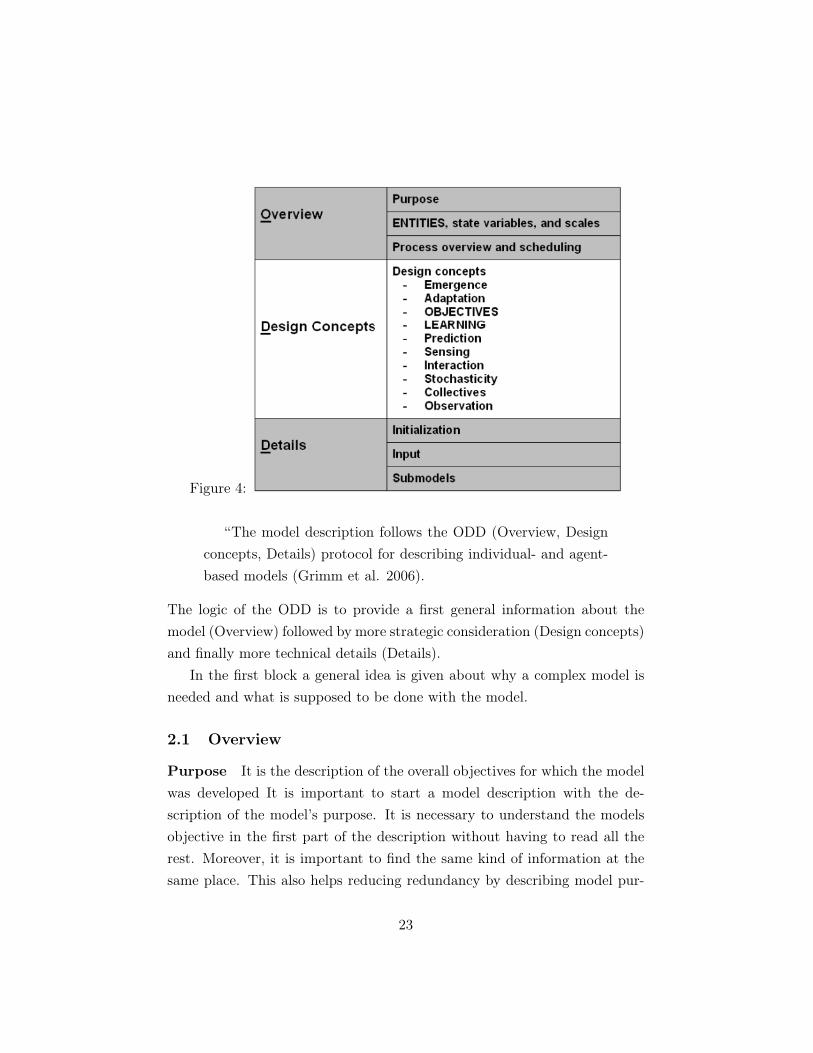
Figure 4:

“The model description follows the ODD (Overview, Designconcepts, Details) protocol for describing individual- and agent-based models (Grimm et al. 2006).

The logic of the ODD is to provide a first general information about themodel (Overview) followed by more strategic consideration (Design concepts)and finally more technical details (Details).

In the first block a general idea is given about why a complex model isneeded and what is supposed to be done with the model.

2.1 Overview

Purpose It is the description of the overall objectives for which the modelwas developed It is important to start a model description with the de-scription of the model’s purpose. It is necessary to understand the modelsobjective in the first part of the description without having to read all therest. Moreover, it is important to find the same kind of information at thesame place. This also helps reducing redundancy by describing model pur-

23

pose in few sentences, which also forces the modeler to clearly specify themodel purpose.

Entities, state variables, and scales By entity is meant the actors,objects, or things that interact with other actors or with the environmentfactors. Its current state is characterized by state variables. State variablescharacterize individuals from others. They records values that have changedthrough interactions, movements and other actions. State variables shouldintended as “low level” or “elementary” one. In this sense, state variablescannot be calculated by other variables and thus, they represent the basicinformation that we can have looking at them. Typically, ABMs includesthe following entities:

• Agents or individuals. Models can include different type of agent andin the same model different types of sub-agents. Each of these agentsusually has state variables that are helpful to understand the evolutionof the simulation.

• Spatial units. These are usually state variables that indicate environ-mental conditions that vary over space.

• Environment. These are variables that influence the whole space wherethe agent behave.

• Collectives. It is useful sometime to distinguish between group of agentthat have the same behavior but are different from the rest of thepopulation. It is represented by a list of agent that altogether performsthe same action. It is important to specify what model’s spatial andtemporal units represent in reality.

Process overview and scheduling In this subsection only a list of“things” that agent do should be written. The detailed description of itshould later be done in the “Submodels” section. Moreover, we should ex-plain both the order in which process happen and the way they are executedby agents. The problem of when variables are updated depends on whether

24

the new value is stored as it is calculated (asynchronous updating) or whenthe new value is stored until all the agents have executed the process andthen all update at once (synchronous updating). Defining a model’s sched-ule includes stating how time is modeled if it not done in the Entities, StateVariables, and Scales element. Verbal description is not very well suited forschedule description. To decide whether a schedule description is good ornot we should ask ourselves if from the description we could rebuild all theschedule process.

2.2 Design Concepts

In this section, a list of common framework concepts is provided. By describ-ing each of these it may be helpful for the reader to understand the generalconcepts underlying the design of the model. The purpose of this element isto link model design to general concepts identified in the field of ComplexAdaptive Systems.

1. Emergence. Explain the general outcome that emerges from the in-teraction of individuals. It also can be explained by changes in anunpredictable way of the general outcome due to changes in individu-als’ rules.

2. Adaption. Rules that individuals have to make decision as a responseto changes in environment conditions or other individuals behavior.It should be cited whether or not these particular traits are made toincrease individuals success compared to other individuals.

3. Objectives. Once explained the adaptive characteristics of the agentsit is therefore, necessary to explain what the goal of this individuals is.The criteria that agents use to make decision when choosing betweenalternatives should be explained in this subsection.

4. Learning. Here all the rules that allow individuals to change theiradaptive rules as consequence of learning should be stated in this sub-section.

25

5. Prediction. Prediction is important in successful decision-making. Inthis subsection all the rules that allow the agents to evaluate theircurrent situation and thus, to make predictions should be listed here.

6. Sensing. These are the rules that allow agents to perceive signals,situations and other parameters that allow them to make decision. Itshould be explained if these rules are modeled explicitly or are agentssupposed to know by themselves.

7. Interactions. Here the interactions between agents and agents and en-vironment should be stated. It should also, be stated whether theseinteractions are direct or indirect. Moreover, if interactions are repre-sented by communications how this is done.

8. Stochasticity. If there is any process that is random then, this processshould be listed here. Moreover, it should be cited here the effect ofthe stochasticity on the general result.

9. Collectives. Agents may belong to groups or form groups during thesimulation. If this is the case then, the rules that allow it should bestated here.

10. Observation. In this subsection all the data that come as output shouldbe listed here. Moreover, if this data are used for tests then it shouldbe notified what kind of test are run on these data.

These ODD elements do not describe the model entirely as this is not theirgoal. It is important to note that through these elements important conceptsare not left unsaid. These elements make particular the ODD as it onlyrequires a verbal explanation and does not need equation of flow charts.Most models include the major part of these elements but many others maynot have all of them included.

This part of the ODD is also the most critiqued one. In particular, cri-tiques focus on the redundancy of the information provided here. Moreover,as it does not describe the model per se this element should not be put intothe protocol.

26

2.3 Details

In the third block details omitted in the previous blocks are presented. Adescription of the initial conditions is presented in Initialization. In the sub-section Input a description of the variables is given. Readers need to knowwhat input data are used, how they are used, how they can be generatedand the influence that these variables have on the model. In the last part ofthe ODD the subsection Submodels presents the skeleton of the underlyingmodel. In particular, both a mathematical formulation of the decision mak-ing of agents is presented and a full verbal model description is presented aswell.

Initialization In this section, the initial value of the model should be cited.In particular the number of initial agents, their initial state values, time andspatial values. It should be reported whether the initialization changes withsimulation or is always the same. Initial conditions is important as it mayaffect the results. Thus, in order to replicate the model it is important thatall the initial conditions values and how they change should be reported.

Input Data In order to obtain realistic results real data, in case they areused should be reported. In order to replicate the model the data and themodel should be provided.

Submodels The submodels are presented in detail and completely. Equa-tion and algorithms, should come first and be separated from additionalinformation. However, presenting only the factual description of submodels,separate from their justification and explanation, creates the risk of makingthe model design appear arbitrary. Many ABMs include submodels that arealgorithms rather than equations. Verbal descriptions are a limited mediumfor describing schedules and algorithms exactly.

27

2.4 Complaints and benefits from using ODD

2.4.1 Complaints about ODD

ODD can be redundant The three elements of the ODD are seen asbeing redundant:

• Purpose: can be presented in a paper’s introduction

• Design Concept: can be included, more or less explicitly, in submodels’descriptions.

• Submodels: submodels are also listed in Process Overview and Schedul-ing.

Indeed some redundancy exists but it’s necessary if we want to have andordered hierarchical protocol. The protocol makes descriptions easier tounderstand by providing an overview before all the details. The Purposeredundancy can be reduced by keeping the description of the model’s pur-pose very short. The Design Concepts redundancy often does not exist. Thedescriptions of the submodels typically do not explicitly refer to design con-cepts. Any details needed to describe design concepts can be left out of theSubmodels element. Finally, the minor redundancy introduced by first pro-viding the Process Overview and Schedule before all the submodel details isin fact needed if we want to know and understand the context of each sub-model. It is also particularly appropriate if submodel details are publishedin an appendix or separately.

ODD is overdone for simple models Some ABMs are extremely simple,and describing them in ODD could use considerably more space than a com-plete description not in ODD. The format of ODD can be shortened, whenappropriate, such as by using continuous text instead of separate documentsubsections for each ODD element.

ODD is too technical ODD has been criticized for making model de-scriptions too technical. Providing technical details is the primary goal of

28

the ODD protocol. In this way model can be described completely and canbe replicated by a reader. It is obvious that writing down the entire storyand the ultimate purpose of a model, for example motivations and goals ofhuman actors, functions, and emergent phenomena of ecosystems, or self-organization in tissues and cells, to a skeleton of attributes can be long.

Modeling is all about finding a simplified representation of things andprocesses that captures key characteristics of the real systems.

The Overview includes the framework and purpose of the model, a briefdescription of the model entities, their properties, and what they do in themodel world. Using self-explanatory names for variables and processes isessential for communicating the scope of the model at once. The ProcessOverview and Scheduling element should be intended as a summary of themodel while also providing a technical description of its schedule.

ODD separates units of object-oriented implementations In object-oriented programming (OOP), model entities and their behaviors is one unit.However, the ODD requires the properties and methods to be presentedseparately. OOP certainly is natural for implementing ABMs, but ODD wasdesigned to be independent of software platforms. Presenting entities firstand then what these entities can do has the advantage that we get a completeoverview of what the model world is.

The principle of encapsulation in OOP is designed to promote sourcecode that is easier to maintain through collecting the data and methods thatoperate on them in one place.

2.4.2 Benefits of using ODD

The ODD protocol was originally designed just to promote an efficient andcomplete communication and, thereby, replication, of ABMs. However, theprotocol has turned out to be much more interesting. There are benefits thatwere forecasted by the ODD developers and which are very important.

ODD promotes rigorous model formulation When it was introduced,the ODD was seen as a new rigorous way to write ABMs. It was a response

29

to the need of more rigor in describing models and made possible modelreplication. Therefore, after it was introduced, people developed experiencein describing models and consequently new ABMs were formulated.

ODD provides what is called “design patterns.” This means that theODD has all the necessary elements to provide a full and comprehensibledescription.

ODD spotlights incomplete or poor model descriptions When us-ing ODD frequently it becomes easy later when reading the description ofother models to recognize the missing parts (if any!). This is one of the goalsof the protocol, to easily understand models. Moreover, when you use theODD frequently it becomes natural way of thinking. This could be on thesuccess factor of the ODD.

ODD facilitates reviews and comparisons of ABMs When compar-ing two or more models for similarities the ODD turns to be very useful.Since the ODD is divided in parts it turns to be quite an easy task to docomparison between similar models.

30

3 Black and Scholes model and parameter uncer-tainty

3.1 Black and Scholes model

In the early 1970s Fisher Black, Myron Scholes, and Robert Merton achieveda major breakthrough in the pricing of stock options. They introduced thefamous Black and Scholes (or Black, Scholes and Merton) formula. Blackand Scholes (1973). The model was a huge change in the way options werepriced and put the basis for the development of financial engineering.

Clearly, when evaluating the characteristics of an option we need to havein mind what are the characteristics of the underlying asset itself.

Thus, we know that the value of an option will depend on:

• S and t: the current stock price and current time.

• sv and m: parameters associated with the stock indicating the volatilityand the drift parameter

• E and T: parameters associated with the particular contract indicatingthe strike price and the expiration date

• r: the risk-free interest rate.

We will start by constructing a portfolio of financial securities and from thatwe will derive the famous Black and Scholes formula to price options. Thederivation will be shown in the case of a European Call option but similarlyit can be shown for a European Put option. Suppose we have a portfoliowhich its value is given by:

P = V (S, t)−DS

This portfolio consists in a long position in the derivative contract andin D short position in the underlying asset. For now, we set the quantity Dequal to some constant. Now we assume that the underlying asset has thefollowing form and follows a lognormal random walk:

31

dS = mSdt + svSdX

At this point we ask what the change in value of the portfolio is if wechange time from t to t+dt. The change will be given partially by changesin the value of the underlying asset and partially in changes in the value ofthe derivative contract. In particular:

dP = dV − dDS

We know that the parameters that influence the derivative contract arethe time and the underlying asset. Thus applying the Ito’s lemma, we get afunction for the derivative contract:

dV =∂V

∂tdt +

∂V

∂SdS +

1

2sv2S2∂

2V

∂S2dt

The second order term for the time is omitted since it is very small andwill have no influence if we consider it. In this way, changes in portfoliosubstituting are given by:

dP =∂V

∂tdt +

∂V

∂SdS +

1

2sv2S2∂

2V

∂S2dt−DdS

By observing the equation we can notice that there are deterministicterms and stochastic ones. Deterministic terms are those with the dt whilerandom terms are those with the dS. Our goal is to eliminate the risk asso-ciated to the random term. We can do it by choosing the right quantity ofD. In particular if we choose D to be:

D =∂V

∂S

then the random term is reduced to zero. This operation is called deltahedging. It consists in eliminating the risk connected to any derivative con-tract by opportunely selecting the right amount of underlying to hold. Byselecting the right D we now hold a portfolio that has the following form:

32

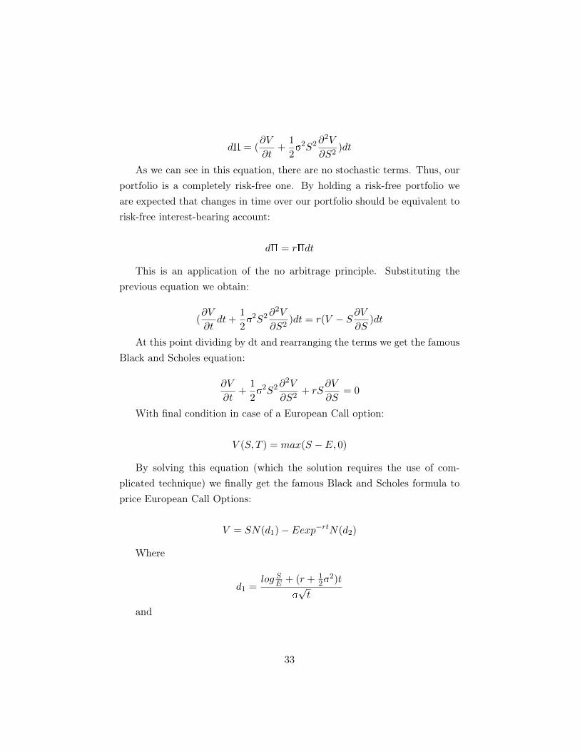
dP = (∂V

∂t+

1

2sv2S2∂

2V

∂S2)dt

As we can see in this equation, there are no stochastic terms. Thus, ourportfolio is a completely risk-free one. By holding a risk-free portfolio weare expected that changes in time over our portfolio should be equivalent torisk-free interest-bearing account:

dP = rPdt

This is an application of the no arbitrage principle. Substituting theprevious equation we obtain:

(∂V

∂tdt +

1

2sv2S2∂

2V

∂S2)dt = r(V − S

∂V

∂S)dt

At this point dividing by dt and rearranging the terms we get the famousBlack and Scholes equation:

∂V

∂t+

1

2sv2S2∂

2V

∂S2+ rS

∂V

∂S= 0

With final condition in case of a European Call option:

V (S, T ) = max(S − E, 0)

By solving this equation (which the solution requires the use of com-plicated technique) we finally get the famous Black and Scholes formula toprice European Call Options:

V = SN(d1)− Eexp−rtN(d2)

Where

d1 =log S

E + (r + 12sv

2)t

sv√t

and

33

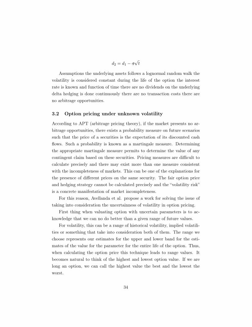
d2 = d1 − sv√t

Assumptions the underlying assets follows a lognormal random walk thevolatility is considered constant during the life of the option the interestrate is known and function of time there are no dividends on the underlyingdelta hedging is done continuously there are no transaction costs there areno arbitrage opportunities.

3.2 Option pricing under unknown volatility

According to APT (arbitrage pricing theory), if the market presents no ar-bitrage opportunities, there exists a probability measure on future scenariossuch that the price of a securities is the expectation of its discounted cashflows. Such a probability is known as a martingale measure. Determiningthe appropriate martingale measure permits to determine the value of anycontingent claim based on these securities. Pricing measures are difficult tocalculate precisely and there may exist more than one measure consistentwith the incompleteness of markets. This can be one of the explanations forthe presence of different prices on the same security. The fair option priceand hedging strategy cannot be calculated precisely and the “volatility risk”is a concrete manifestation of market incompleteness.

For this reason, Avellanda et al. propose a work for solving the issue oftaking into consideration the uncertainness of volatility in option pricing.

First thing when valuating option with uncertain parameters is to ac-knowledge that we can no do better than a given range of future values.

For volatility, this can be a range of historical volatility, implied volatili-ties or something that take into consideration both of them. The range wechoose represents our estimates for the upper and lower band for the esti-mates of the value for the parameter for the entire life of the option. Thus,when calculating the option price this technique leads to range values. Itbecomes natural to think of the highest and lowest option value. If we arelong an option, we can call the highest value the best and the lowest theworst.

34

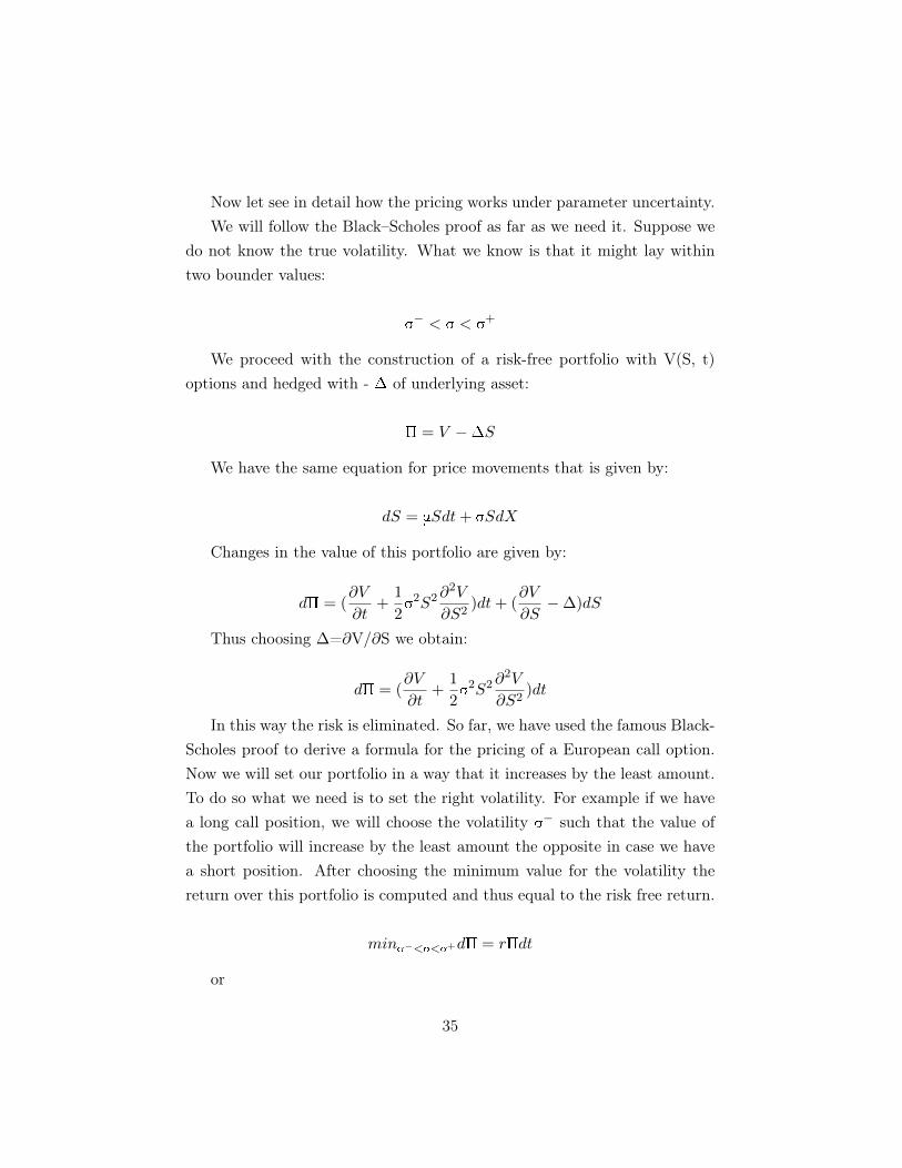
Now let see in detail how the pricing works under parameter uncertainty.We will follow the Black–Scholes proof as far as we need it. Suppose we

do not know the true volatility. What we know is that it might lay withintwo bounder values:

sv− < sv < sv+

We proceed with the construction of a risk-free portfolio with V(S, t)options and hedged with - D of underlying asset:

P = V −DS

We have the same equation for price movements that is given by:

dS = mSdt + svSdX

Changes in the value of this portfolio are given by:

dP = (∂V

∂t+

1

2sv2S2∂

2V

∂S2)dt + (

∂V

∂S−∆)dS

Thus choosing ∆=∂V⁄∂S we obtain:

dP = (∂V

∂t+

1

2sv2S2∂

2V

∂S2)dt

In this way the risk is eliminated. So far, we have used the famous Black-Scholes proof to derive a formula for the pricing of a European call option.Now we will set our portfolio in a way that it increases by the least amount.To do so what we need is to set the right volatility. For example if we havea long call position, we will choose the volatility sv− such that the value ofthe portfolio will increase by the least amount the opposite in case we havea short position. After choosing the minimum value for the volatility thereturn over this portfolio is computed and thus equal to the risk free return.

minsv−<sv<sv+dP = rPdt

or

35

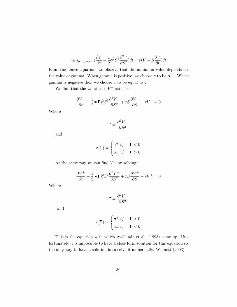
minsv−<sv<sv+(∂V

∂t+

1

2sv2S2∂

2V

∂S2)dt = r(V − S

∂V

∂t)dt

From the above equation, we observe that the minimum value depends onthe value of gamma. When gamma is positive, we choose sv to be sv− . Whengamma is negative then we choose sv to be equal to sv+.

We find that the worst case V − satisfies:

∂V −

∂t+

1

2sv(G)2S2∂

2V −

∂S2+ rS

∂V −

∂S− rV − = 0

Where

G =∂2V −

∂S2

and

sv(G) =

sv+ if G < 0

sv− if G > 0

At the same way we can find V + by solving:

∂V +

∂t+

1

2sv(G)2S2∂

2V +

∂S2+ rS

∂V +

∂S− rV + = 0

Where

G =∂2V +

∂S2

and

sv(G) =

sv+ if G > 0

sv− if G < 0

This is the equation with which Avellanda et al. (1993) came up. Un-fortunately it is impossible to have a close form solution for this equation sothe only way to have a solution is to solve it numerically. Wilmott (2003)

36

3.3 Is the Black and Scholes formula used in practice? Crit-icism and appreciation.

In this paragraph I will describe the point of view of two of the major practi-tioners and researchers in the field. Nicolas Nasrim Taleb and Paul Wilmott.Taleb argues that the Black and Scholes formula is not an important ar-gument nowadays while Wilmott gives some arguments in defense of theformula.

The critique by Taleb and Haug (2007) goes beyond the well known issuesabout the formula and focuses mainly on three points:

• It’s not used (even by those who think that they use it).

• It wasn’t needed.

• It wasn’t original.

Most textbook assumes that Black and Scholes enjoys a huge success and iswidely used by practitioners. There are two main reasons why Black-Scholesis not used. First, option prices (at least for liquid contracts) may be simplythe result of supply and demand interaction, with no model involved at all.Options often are priced via other options, through the well known put-callparity, which allows a trader or investor to derive the price of a call from aput and vice versa. No mathematical modeling and no partial differentialequations is required.

When Black and Scholes is used, it’s not really Black-Scholes. The Black-Scholes formula is like a black box: certain inputs must be inserted in orderto obtain some output, only one is not directly available: the underlyingasset’s volatility. Traders must estimate such a number before putting itinto the Black-Scholes.

The basic version of Black-Scholes assumes that volatility should be con-stant. Valuating options of different strikes one is expecting to obtain thesame volatility. Instead, what we get is something similar to a “smile” theso called volatility smile. At-the-money options tend to have lower impliedvolatilities than in- or out-of-the-money options.

37

Assuming that traders are using Black-Scholes, this reflects the fact thatthe volatility input is being manipulated in order to obtain more realisticoption prices, essentially to correct for the formula’s unrealistic assumptionsand to allow traders to freely express their opinions.

The insight from Taleb is to point out that once you manipulate thevolatility, you are no longer using Black-Scholes, even if such manipulationhappens to take place within a Black-Scholes framework.

The model may have not been needed at all. Taleb and Haug show howbefore 1973 traders had very sophisticated knowledge about how optionsshould be traded, priced and risk-managed, even as far back as the 1800s.Taleb and Haug produce a chronological list of technical and academic workon option pricing pre-dating Black-Scholes, including basically identical for-mulas.

According to Taleb and Haug, the acceptance of this tool is really theresult of an "academic marketing exercise" rather than the appearance of ainnovative piece of work.

We already knew that Black-Scholes was unrealistic. What we didn’tknow is that it’s not really used, it wasn’t truly needed and it wasn’t entirelyoriginal.

This is the view of Paul Wilmott which goes in the oposite direction ofthat of Taleb and Haug. Black-Scholes is a robust model that behaves verywell even when its underlying assumptions are violated, as they inevitablyare in practice. It just needed a minor adjustments. Sometimes it is neededto work with something that while not perfect is good enough and is un-derstandable enough that you don’t do more harm than good. And that’sBlack-Scholes.

It is well accepted that the Black-Scholes formulae were around wellbefore 1973. Ed Thorp plays a large role in that history. Ed wrote a seriesof articles “What I Knew and When I Knew it” to clarify his role in thediscovery, including his argument for what is now called risk-neutral pricing.

They say traders don’t use Black-Scholes because traders use an impliedvolatility skew and smile that is inconsistent with the model. Sometimestraders use the model in ways not originally intended but they are still using

38

a model that is far simpler than modern-day improvements. Black-Scholesperforms better compared with many of these improvements. For example,the deterministic volatility model is an attempt by quants to make Black-Scholes consistent with the volatility smile. But the complexity of the cali-bration of this model, its sensitivity to initial data and ultimately its lack ofstability make this far more dangerous in practice.

Transaction costs may be large or small, depending on which market youare in and who you are, but Black-Scholes doesn’t need much modificationto accommodate them. The Black-Scholes equation can often be treated asthe foundation to which you add new terms to incorporate corrections toallow for dropped assumptions.

Discrete hedging is a good example of robustness. It’s easy to show thathedging errors can be very large. But even with hedging errors Black-Scholesis correct on average. If you only trade one option per year then, yes, worryabout this. But if you are trading thousands then don’t. It also turns outthat you can get many of the benefits of (impossible) continuous dynamichedging by using static hedging with other options. Even continuous hedgingis not as necessary as people think.

As for volatility modelling, the average profit you make from an option isvery insensitive to what volatility you actually use for hedging. That aloneis enough of a reason to stick with the uncomplicated Black-Scholes model,it shows just how robust the model is to changes in volatility. You cannotsay that a calibrated stochastic volatility model is similarly robust.

When it comes to fat tails, it would be nice to have a theory to accom-modate them but why use a far more complicated model that is harder tounderstand and that takes much longer to compute just to accommodate anevent that probably won’t happen during the life of the option? Keepingit simple and pricing quickly and often, using a simpler model and focusingmore on diversification and risk management.

The many improvements on Black-Scholes are rarely improvements, thebest that can be said for many of them is that they are just better at hidingtheir faults. Black-Scholes also has its faults, but at least you can see them.Wilmott (2008)

39

4 Option Pricing under unknown volatility: an agentbased model

In Black-Scholes world the full knowledge of the asset price model rulesout the model risk. It means that if we are able to define a model for theunderlying asset there will be no uncertainty about the pricing model of thederivative contract. The goal of this paper is to understand how the priceof the option depends on the unknown parameter m, how to model traders’behavior reasonably with unknown volatility and how these parameters canbe integrated in option pricing. Therefore, we are questioning whether thereis a considerable difference between market prices and theoretical prices givenby the Black-Scholes formula. With agent based model and simulation it ispossible to shed light on the proprieties of this parameters. Zhang et al.(2009).

4.1 Model assumptions

We start assuming that option price is determined ultimately by supply anddemand that results from trader’s behavior. Moreover, everyone knows anduses the Black-Scholes model. We put ourselves in an observing contest aswe know the true volatility but the market participant doesn’t know it. Theunderlying stock follows a Geometric Brownian Motion (GBM) with drift mand volatility sv:

dSt

St= modt + sv0dWt

moand sv0are the true ones but they are unknown to market participants.Therefore, they might agree or not but basically everyone has his personalview on the parameters:

dSt

St= midt + svidWt

The subscript i indicates that the equation is valid for each investorfrom i = 1...10000. According to his personal view of the parameters each

40

investor calculates his own valuation of the option according to Black andScholes formula:

V = StN(d1)−Kexp(−rt)N(d2)

with

d1 =log S

E + (r + 12sv

2)t

sv√t

and

d2 = d1 − sv√t

In d1 and d2 we can notice that sv has the subscript i to indicate thatthis equation is valid for each single investor according to his personal viewof the volatility.

Investors’ personal view of the volatility could become relevant to optionpricing and so can the implied volatility influence the price of the option.Therefore, our goal is to model investors view on volatility and include themin the option pricing formula.

Following the approach proposed by Avellanda et al. one way to dealwith uncertainty is to specify a band. Thus, each investor has its own viewof the volatility band as:

svmini < svi < svmax

i

Traders are modeled as heterogeneous and autonomous agents character-ized by:

• Patience: is the minimum length of days to calculate historical volatil-ity, given by a uniform random integer between 5 and 45 days

• Judgments: is traders’ personal adjustment of his experience in histor-ical volatility band. It is given by a random uniform number between0.5 and 1.5.

41

The volatility band thus, is calculated for example as: trader i has patienceequal to 30, he calculate the volatility band of the underlying asset with 30days of historical prices and then he multiplies it with his judgment. In thisway, traders obtain a range of options evaluations with their volatility band.

Our final goal is to verify if the price that will emerge from the market isthe same as predicted theoretically by Black and Scholes. Once the investorshave their own subjective volatility valuation they proceed to calculate theoption price with Black and Scholes. They obtain a range of prices since theyuse a volatility band. Thus, they have to adopt a trading strategy. Theirstrategy is buying low and selling high. This means that traders will sell theoption with the highest value and will buy the one with lowest value. Theywill put both buy and sell orders in the market. The market will record theorders submitted by traders and will match them with the orders of othertraders.

We need to model the market for the underlying asset. In particular, wecan use simulation to provide a series of prices. Using the following formulato generate price we have:

Sit+Dt = Si

texp(m0−sv20/2)Dt+sv0Zi(Dt)1/2

The simulation is organized in two stages. In the first one the stockmarket and the simulation of the stock prices start. The simulation willrun for 250 days so we will generate each simulation 250 stock prices. Afterthe stock market is open the traders start collecting data. Based on theirpersonal settings they start calculate the volatility and thus consequently theoption price. After 50 days of stock prices the option market starts. In thisway, all the traders have the chance to calculate their volatilities and updatethem every day. Once the valuation is done, they enter the market and starttrading. Every day option price is calculated as the average between theminimum ask quote and maximum bid quote. After calculating the price ofthe option it is possible to compute the implied volatility.

The simulation is run with 10000 agents for 1000 runs for each condition.

42

4.2 ODD model description

Purpose. Option pricing is one of the biggest issues in modern finance.Since the introduction of the Black and Scholes formula, new models havebeen constructed. Related to option pricing the constant volatility is onesuch a major problem. Should volatility be considered constant throughthe life of the option? Many practitioners use new formula with stochasticvolatility and many others uses the formula with constant volatility (wayfaster and easy to understand). The purpose of this paper is to understandwhether there is a significant difference in prices using the Black and Scholesformula with certain and uncertain volatility. Moreover, it is important toverify the role of the uncertain parameter m. The particularity of this workis that it is implemented in an ABMs contest. Theoretical price throughBlack and Scholes formula will be computed and the market price will becalculated as the interactions of the agents.

Entities, state variables, and scales. In this simulation, agents arerepresented by investors and the market is the place where they operate.Agents will have different state variables. Judgment and patience are param-eters that will characterize all the agents. In particular, patience representsthe minimum length of day for them to calculate the volatility. It will becalculated as a random integer between 4 and 45 days. Judgment representsthe adjustments that investors do the historical volatility based on their ex-perience. It will be calculated as a uniform random variable between 0.5and 1.5. The market is represented by “the book.” In this book bid and askoffers will be recorded and operations with the same sign will be matched.The market is a virtual place so no concrete interaction through agents willoccur. The spatial dimension thus, will be insignificant. Regarding time,each simulation will represent 1 day. After 250 days the simulation will beconcluded.

Process overview and scheduling The investors do the main activityin this model. They calculate the volatility and then based on their valuation

43

proceed to put an order in the option marker. Chronological order of theoperations goes like this:

1. Simulation begins.

2. At day 1 the stock market starts and run until the end of the simulation.

3. At day 50 agents can calculate their estimations of the volatility andthen after their option prices.

4. Option market opens the same day. Agents are allowed to put theirbid and ask offers.

5. The market book records all the operations and matches the operationwith the same sign.

6. At the end of the day, the daily price is computed and compared withthe theoretical price.

7. Investors can compute the implied volatility and adjust the volatilityestimations.

8. After 250 runs the simulation is over and a new one can be started.

9. The results are presented.

The order in which agents make their offer in the market is random.

Design concepts

Emergence Through simple interactions of agents, buy and sell options,we should be able to find complex results. We do not know whether the resultwill be the same according to Black and Scholes or not. The unexpectedelement is thus, given by the uncertainty in the result.

Adaption Agents do not have any adaptive rules. The model proposedby the authors is quite simple and the only rules that govern the investorsare investment rules.

44

Objectives Investor’s goal is to make a sure profit driven by their optionvaluation. They will present a bid and an ask offer to the market and whentheir offer is matched then the transaction will be concluded. This simplerule is represented by the option valuation formula.

Learning In the original work of the authors, agents do not have anycomplex rule to learn from past situation. It would be very interesting todevelop kind of agent capable of creating strategies based on their experience.

Prediction This is the same as the previous rule. Inserting some rulesthat will make agents capable of forecasts will make the model more realisticand probably will have a different impact on the results.

Interactions Interactions through agents occur in indirect way. They donot see each other but they just place orders in the market. Is the marketitself that will match the orders.

Stochasticity The randomness is presented in the choice of the numbersof days to calculate the volatility and on judgment the investors do, based ontheir past experience, of the historical volatility. The stochasticity is presentalso in the simulation of the path of the underlying asset.

Initialization & Input data The initial inputs are the option parameters.These parameters are choose by the user to make test on them. In particular:

• The variance sv.

• The drift parameter m.

Moreover, the user can choose the number of simulation and the number ofagents. In a more complex work, the user can also have the possibility tomodify investors’ strategy to verify the effects on the result.

45

4.3 Model replication

Our final goal will be that of recreating the model proposed by the authorand further complicating the agents’ behavior. We want to verify if theresults, found by the author, hold in a more complicated agents’ behavior.We suspect that the work proposed by the author is not an ABMs in thewhole sense of the word.

In particular, we think that agents need more complicated rules such as:having their own strategy, the possibility to make forecasts and so on. Thismay be more realistic and perhaps brings some unexpected results.

To do so we think that the model should follow the author’s idea andthen have a different development as regarding the agents’ behavior.

At the beginning we should develop the stock market. We will use theunderlying asset price model as the one proposed by the authors to simulatethe stock path.

The second step consists in creating agents. To have an easy task the useof OOP (Object-Oriented-Programming) is a natural way to model agents.Agents will be encapsulated as object with their state variables. These par-ticular investors will be able to estimate the variance, will have scheduledaction, and will be capable of learning from past history.

After, the option market will be created. In the option market all theoffers will be recorded and the option market price will be calculated daily.

In conclusion, we think that the work of the original authors is a verynice attempt to evaluate options under uncertain volatility but to have arealistic and more precise ABMs a further extension is needed.

46

Conclusions

In this review, I analyzed the ABMs methodology in option pricing view.From this, we can understand that this methodology is the most suitablefor social sciences. This is due to the fact the ABMs can well capture theemergent behavior that emerge from individuals interaction. Moreover, com-paring the ABMs to other paradigms (System Dynamics, discrete Events andDynamic Systems) we notice that ABMs generally better perform in all thelevel of abstractions of the models under analyze. This can be explained bythe fact that ABMs better combine the main features of the other paradigms.

ABMs can also represent a new form of mathematic. In the traditionalcomparison between classical and constructive mathematics ABMs place inthe between of the two approaches. In fact we can present ABMs as finitesystems of discrete time recursive equations over finite state domains or asdata-driven dynamic applications systems.

ABMs, as said, have great potentials but it comes at a cost. ABMs arevery hard to read when they are not written in a standard way. To solve thisproblem a standard protocol was introduced by Grim. The main featuresof this protocol were shown in Chapter 2. ODD is standard protocol thatmakes things easier to understand and makes the model way easy to beimplemented again.

A mathematical proof of the Black-Scholes formula was introduced andas well the unknown volatility framework. This serves to us as a backgroundfor developing our work.

Packed with all the necessary tools, finally, the option pricing under un-known volatility studied with agent-based methodology was introduced. An-alyzing the paper under the ODD protocol it emerges that the work doesn’tlook like an ABM model. This leads to a further implementation of thismodel taking inspiration from the original work. Especially, the further im-plementation should go in the way of modifying agents behavior. We areexpected to reach more realistic results.

47

References

Axelrod R., Tesfatsion L. (2005) A guide for newcomers to Agent-Based-Modeling in social sciences.

Axtell, R. L. (2000) Why Agents? On the varied motivations for agentcomputing in the social sciences.

Avellanda, M. Levy, A. and Paras A. (1995) Pricing and HedgingDerivative Securities in Markets with Uncertain Volatility.

Black, F. and Scholes M. (1973) The Pricing of Options and CorporateLiabilities.

Borrill, P. L. and Tesfatsion, L (2010) Agent-based modeling: the rightmathematics for the social sciences?

Borshchev, A. and Filippov, A. (2004) From System Dynamics and Dis-crete Event to Practical Agent Based Modeling: Reasons, Techniques,Tools

Epstein J.M. and Axtell R. L. (1996) Growing Artificial Societies.

Flake, G.W. (1998), The Computational Beauty of Nature: Computer Ex-plorations of Fractals, Chaos, Complex Systems, and Adaptation.

Gilbert, N. and Terna, P. (2000) How to build and use Agent-based mod-els in social science.

Grimm et al. (1999) Individual-based modelling and ecological theory: syn-thesis of a workshop

Grimm et al. (2006) A standard protocol for describing individual-basedand agent-based models

Grimm et al. (2009) The ODD protocol for describing individual-basedand agent-based models: a first update

Gopen, G. and Swan, J. (1990) The sciene of scientific writing. Am Sci

48

Situngkir, H and Surya, Y. (2005) Agent-based Model Construction InFinancial Economic System.

Scholl, H. (2009) Agent-based and System Dynamics Modeling: A Call forCross Study and Joint Research

Taleb, N. and Haug, E.G. (2007) Why We Have Never Used the Black-Scholes-Merton Option Pricing Formula

Terna, P. (2010) Complexity and Economics, reading notes for a discussion

Terna, P. et al. (2006) Modelli per la complessità

Wilmott, P. (2003) On quantitative finance

Wilmott, P. (2008) Science in Finance IX: In defense of Black, Scholesand Merton

Zhang, S., Feng, D. and Wang S. (2009) Option Pricing under UnknownVolatility: An Agent-Based Modeling and Simulation Approach.

49