Spatial Characterisation of Spectrum Occupancy in...
80
Universit ` a degli Studi di Padova Facolt ` a di Ingegneria Corso di Laurea in Ingegneria delle telecomunicazioni Spatial Characterisation of Spectrum Occupancy in Urban Environment for Cognitive Radio Laureando: Emanuele Tassinello Relatore: Ch.mo Prof. Michele Zorzi Correlatore: Miguel L ´ opez Ben ´ ıtez Anno accademico 2009/2010
Transcript of Spatial Characterisation of Spectrum Occupancy in...
Universita degli Studi di Padova
Facolta di IngegneriaCorso di Laurea in Ingegneria delle
telecomunicazioni
Spatial Characterisation ofSpectrum Occupancy in Urban
Environment for Cognitive Radio
Laureando:Emanuele Tassinello
Relatore:Ch.mo Prof. Michele Zorzi
Correlatore:Miguel Lopez Benıtez
Anno accademico 2009/2010

Abstract
Cognitive Radio (CR) has been proposed to solve the so-called spectrumscarcity problem. CR uses opportunistically the licensed bands when theyare temporarily unused. The realization of spectrum models and the statis-tical characterization of spectrum occupancy is an important point to assistthe study and the development of various features required to CR. In thiscontext we conducted a measurement campaign in the DCS and UMTS cel-lular bands in an urban environment. We collected spectral occupation datain order to analyze and characterize the behavior of spatial correlation ofthe spectrum occupancy. We analyze the spatial correlation by calculatingsome metrics as a function of the distance. Finally we propose a differentapproach to the calculation of the metrics, that is to characterize spatialcorrelation as a function of the SNR-difference at the receiver instead of thedistance.
i

ii
Contents
Acronyms vii
1 Introduction 1
2 Cognitive Radio Basics 32.1 Introduction . . . . . . . . . . . . . . . . . . . . . . . . . . . . 32.2 Cognitive Radio Technology . . . . . . . . . . . . . . . . . . . 42.3 Cognitive Radio Network Architecture . . . . . . . . . . . . . 52.4 Cognitive Radio Functions . . . . . . . . . . . . . . . . . . . . 7
2.4.1 Spectrum Sensing . . . . . . . . . . . . . . . . . . . . 82.4.2 Spectrum Management . . . . . . . . . . . . . . . . . 102.4.3 Spectrum Sharing . . . . . . . . . . . . . . . . . . . . 122.4.4 Spectrum Mobility . . . . . . . . . . . . . . . . . . . . 14
2.5 Summary . . . . . . . . . . . . . . . . . . . . . . . . . . . . . 15
3 Spectrum Analysis Basics 173.1 Introduction . . . . . . . . . . . . . . . . . . . . . . . . . . . . 173.2 Super-heterodyne Spectrum Analyzers . . . . . . . . . . . . . 19
3.2.1 RF attenuator . . . . . . . . . . . . . . . . . . . . . . 203.2.2 Low-pass filter . . . . . . . . . . . . . . . . . . . . . . 213.2.3 Mixer and local oscillator . . . . . . . . . . . . . . . . 213.2.4 IF gain amplifier . . . . . . . . . . . . . . . . . . . . . 233.2.5 Resolution filter . . . . . . . . . . . . . . . . . . . . . 233.2.6 Envelope detector . . . . . . . . . . . . . . . . . . . . 273.2.7 Video filter . . . . . . . . . . . . . . . . . . . . . . . . 283.2.8 Display . . . . . . . . . . . . . . . . . . . . . . . . . . 29
3.3 Summary . . . . . . . . . . . . . . . . . . . . . . . . . . . . . 32
4 Measurement Setup 334.1 Measurement scheme . . . . . . . . . . . . . . . . . . . . . . . 33
4.1.1 Antennas . . . . . . . . . . . . . . . . . . . . . . . . . 354.1.2 Filters . . . . . . . . . . . . . . . . . . . . . . . . . . . 354.1.3 Switch . . . . . . . . . . . . . . . . . . . . . . . . . . . 374.1.4 Pre-amplifier . . . . . . . . . . . . . . . . . . . . . . . 37
iii
iv CONTENTS
4.1.5 Spectrum Analyzer . . . . . . . . . . . . . . . . . . . . 394.1.6 Other components . . . . . . . . . . . . . . . . . . . . 40
4.2 Spurious Free Dynamic Range (SFDR) . . . . . . . . . . . . . 404.3 Measurement scenario . . . . . . . . . . . . . . . . . . . . . . 414.4 Measurement methodology . . . . . . . . . . . . . . . . . . . 444.5 Summary . . . . . . . . . . . . . . . . . . . . . . . . . . . . . 48
5 Measurement Results 495.1 Introduction . . . . . . . . . . . . . . . . . . . . . . . . . . . . 495.2 Spectral occupancy . . . . . . . . . . . . . . . . . . . . . . . . 49
5.2.1 Analysis of Spectrum Occupancy . . . . . . . . . . . . 525.3 Evaluation Criteria . . . . . . . . . . . . . . . . . . . . . . . . 54
5.3.1 Cooperative sensing and spatial statistics . . . . . . . 545.3.2 Correlation metrics . . . . . . . . . . . . . . . . . . . . 55
5.4 Results . . . . . . . . . . . . . . . . . . . . . . . . . . . . . . . 575.4.1 Correlation metrics vs. distance . . . . . . . . . . . . . 575.4.2 Correlation metrics vs. SNR difference . . . . . . . . . 57
5.5 Summary . . . . . . . . . . . . . . . . . . . . . . . . . . . . . 66
6 Conclusions and future work 67
Bibliography 68

List of Figures
2.1 Spectrum Utilization. . . . . . . . . . . . . . . . . . . . . . . 4
2.2 Spectrum hole concept. . . . . . . . . . . . . . . . . . . . . . 5
2.3 Cognitive Radio network architecture. . . . . . . . . . . . . . 6
2.4 Cognitive cycle. . . . . . . . . . . . . . . . . . . . . . . . . . . 8
2.5 Transmitter detection problem: a) receiver uncertainty; b)shadowing uncertainty. . . . . . . . . . . . . . . . . . . . . . . 10
2.6 Channel structure of the multi-spectrum decision. . . . . . . . 12
2.7 Inter-network and intra-network spectrum sharing in CR net-works. . . . . . . . . . . . . . . . . . . . . . . . . . . . . . . . 14
3.1 Relationship between time and frequency domain. . . . . . . 18
3.2 Block diagram of a classic superheterodyne spectrum analyzer. 20
3.3 RF input attenuator circuitry. . . . . . . . . . . . . . . . . . . 21
3.4 The LO must be tuned to fIF + fsig to produce a responseon the display. . . . . . . . . . . . . . . . . . . . . . . . . . . 22
3.5 As a mixing product sweeps past the IF filter, the filter shapeis traced on the display. . . . . . . . . . . . . . . . . . . . . . 24
3.6 Two equal-amplitude sinusoids separated by the 3 dB BW ofthe selected IF can be resolved. . . . . . . . . . . . . . . . . . 25
3.7 A low-level signal can be lost under skirt of the response to alarger signal. . . . . . . . . . . . . . . . . . . . . . . . . . . . 25
3.8 Displayed noise is a function of IF filter bandwidth. . . . . . 27
3.9 Displayed noise level change with the ratio of resolution andvideo bandwidth. . . . . . . . . . . . . . . . . . . . . . . . . . 27
3.10 Envelope detector. . . . . . . . . . . . . . . . . . . . . . . . . 28
3.11 Spectrum analyzers display signal plus noise. . . . . . . . . . 29
3.12 Display of Figure 3.11 after full smoothing. . . . . . . . . . . 30
3.13 Trace point saved in memory is based on detector type algo-rithm. . . . . . . . . . . . . . . . . . . . . . . . . . . . . . . . 31
4.1 Measurement Scheme. . . . . . . . . . . . . . . . . . . . . . . 34
4.2 Types of interference. . . . . . . . . . . . . . . . . . . . . . . 38
4.3 Campus Nord of UPC. . . . . . . . . . . . . . . . . . . . . . . 42
v
vi LIST OF FIGURES
4.4 Location of the measurement points. . . . . . . . . . . . . . . 434.5 Measurement setup available at UPC (Antenna subsystem). . 454.6 Measurement setup available at UPC (RF subsystem). . . . . 464.7 Measurement setup available at UPC (spectrum analyzer). . . 47
5.1 Occupation results between 1800 and 1880MHz for location 1. 515.2 Occupation results between 1880 and 2290MHz for location 1. 515.3 Values of the mean PSD for f=1812 MHz as function of the
location of the measurement point. The distribution of thepoints in this figure corresponds to the measurement locationsshown in Figure 4.3. . . . . . . . . . . . . . . . . . . . . . . . 53
5.4 Values of the mean PSD for f=2117 MHz as function of thelocation of the measurement point. The distribution of thepoints in this figure corresponds to the measurement locationsshown in Figure 4.3. . . . . . . . . . . . . . . . . . . . . . . . 53
5.5 Cross-correlation vs distance for DCS. . . . . . . . . . . . . . 585.6 Covariance vs distance for DCS. . . . . . . . . . . . . . . . . 585.7 Normalized Covariance vs distance for DCS. . . . . . . . . . . 595.8 Semivariance vs distance for DCS. . . . . . . . . . . . . . . . 595.9 Cross-correlation vs distance for UMTS. . . . . . . . . . . . . 605.10 Covariance vs distance for UMTS. . . . . . . . . . . . . . . . 605.11 Normalized Covariance vs distance for DCS. . . . . . . . . . . 615.12 Semivariance vs distance for UMTS. . . . . . . . . . . . . . . 615.13 Cross-correlation vs SNR difference for DCS. . . . . . . . . . 635.14 Covariance vs SNR difference for DCS. . . . . . . . . . . . . . 635.15 Normalized covariance vs SNR difference for DCS. . . . . . . 645.16 Semivariance vs SNR difference for DCS. . . . . . . . . . . . 645.17 Cross-correlation vs SNR difference for UMTS. . . . . . . . . 655.18 Covariance vs SNR difference for UMTS. . . . . . . . . . . . . 655.19 Normalized covariance vs SNR difference for UMTS. . . . . . 66
Acronyms
BS Base Station
CDMA Code Division Multiple-Access
CR Cognitive Radio
CRN Cognitive Radio Network
CV Continous Wave
DANL Displayed Average Noise Level
DC Direct Current
DCS Digital Cellular System
DECT Digital Enhanced Cordless Telecommunication
DSA Dynamic Spectrum Access
DSP Digital Signal Processing
DTV Digital Television
EMC ElectroMagnetic Compatibility
EMI ElectroMagnetic Interference
FCC Federal Communications Commission
FFT Fast Fourier Transform
FM Frequency Modulation
GSM Global System for Mobile Communications
IF Intermediate Frequency
LO Local Oscillator
MAC Medium Access Control
vii
viii ACRONYMS
PSD Power Spectral Density
QoS Quality of Service
RBW Resolution BandWidth
RF Radio Frequency
RMS Root Mean Square
SFDR Spurious Free Dynamic Range
SNR Signal-to-Noise Ratio
SPDT Single Pole Double Throw
UMTS Universal Mobile Telecommunications System
USB Universal Serial Bus
UWB Ultra Wide Band
VBW Video BandWidth
VSA Vector Signal Analyzer
xG NeXt Generation
Chapter 1
Introduction
The work done is part of current research for the development of CognitiveRadio (CR) technology. CR has been proposed to solve the so-called spec-trum scarcity problem; the increasing success of wireless services has rapidlyrun out the free frequencies below 3GHz, that is those one with the morecommercially interesting propagation characteristics. Furthermore severalresearches show that the actual technologies made an inefficient use of theirresources: multiple services are active only for a fraction of time or in afraction of the spatial area where their license is valid for.
CR’s main idea is to use opportunistically the licensed bands when theyare temporarily unused. When a primary user, that is a user that has a li-cense to operate in that band, requires these resources CR user immediatelyvacates the band and moves to another one. It is clear that the developmentof such technology requires special features for correctly managing the vari-ous spectrum bands without causing harmful interference to licensed users.
Several measurement campaigns have been conducted to estimate thereal spectrum usage by actual technologies. In general the results of thesestudies show the presence of a number of technologies that make an ineffi-cient use of their resources. Therefore, there exists the margin for CR tooperate in those bands that present interesting properties. Furthermore,the vast amount of data generated by various campaigns has been used toanalyze the statistical characteristic of spectrum utilization. The realizationof spectrum models for CR is an important point to assist the study andthe development of various features required to CR.
In this context we conducted a measurement campaign in the bands1800-1880MHz and 1880-2190MHz; these bands are mainly allocated to Dig-ital Cellular System (DCS) and Universal Mobile Telecommunications Sys-tem (UMTS) cellular technologies. The campaign was performed at CampusNord of UPC, in Barcelona. We collected spectral occupation data in vari-ous points of the measurement location. Our main objective was to analyzeand characterize the behavior of spatial correlation of the spectrum occu-
1
2 CHAPTER 1. INTRODUCTION
pation, which may result of significant importance and usefulness on thedevelopment of the CR technology.
In chapter 1 we give a general introduction to CR technology, focusing onthe spectrum management tasks required to CR. In chapter 2 we introducespectrum analysis and the instrument that permit us to measure spectrumoccupancy, that is the spectrum analyzer. In particular we focus on super-heterodyne spectrum analyzer, giving the theoretical basics of its operatingprinciples. In chapter 3 we describe our measurement equipment, givinga description of each component; we talk about the configuration adoptedexplaining how it was obtained. Then we describe the measurement locationand the methodology used to realize the measurement campaign. In chapter4 we analyze the data gathered during the campaign. After briefly showingthe spectrum occupancy results we introduce the correlation metrics we usein our analysis. Based on such correlation metrics, we then analyze thespatial correlation of spectrum occupancy and derive the main conclusions.
This thesis has been developed within the European Erasmus program(Ref. E -BARCELO 03) between University of Padua and UniversitatPolitecnica de Catalunya (UPC) and developed at the Mobile Communi-cation Research Group, under the supervision of Prof. Dr. F. Casadevalland M. Lopez-Benıtez. A special thank goes to Miguel Lopez Benıtez forhis incomparable help in the realization of this thesis.
Chapter 2
Cognitive Radio Basics
The measurement campaign and the results described in this thesis must beinserted in the context of CR networks (or Dynamic Spectrum Access (DSA)networks or NeXt Generation (xG) networks). To provide a better under-standing, in this chapter we provide a brief introduction to the argumentin order to correctly set in context the work done. First we describe whatCR is and the motivations that led to its development, i.e. the so-calledspectrum scarcity problem. Then we focus on CR technology and CR net-work architecture. Finally we discuss on some spectrum management issuesrequired from CR: spectrum sensing, spectrum decision, spectrum sharingand spectrum mobility.
2.1 Introduction
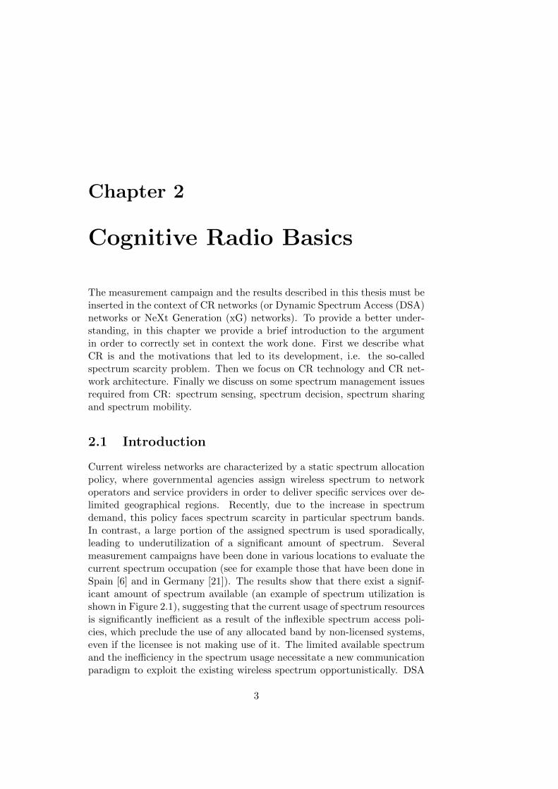
Current wireless networks are characterized by a static spectrum allocationpolicy, where governmental agencies assign wireless spectrum to networkoperators and service providers in order to deliver specific services over de-limited geographical regions. Recently, due to the increase in spectrumdemand, this policy faces spectrum scarcity in particular spectrum bands.In contrast, a large portion of the assigned spectrum is used sporadically,leading to underutilization of a significant amount of spectrum. Severalmeasurement campaigns have been done in various locations to evaluate thecurrent spectrum occupation (see for example those that have been done inSpain [6] and in Germany [21]). The results show that there exist a signif-icant amount of spectrum available (an example of spectrum utilization isshown in Figure 2.1), suggesting that the current usage of spectrum resourcesis significantly inefficient as a result of the inflexible spectrum access poli-cies, which preclude the use of any allocated band by non-licensed systems,even if the licensee is not making use of it. The limited available spectrumand the inefficiency in the spectrum usage necessitate a new communicationparadigm to exploit the existing wireless spectrum opportunistically. DSA
3

4 CHAPTER 2. COGNITIVE RADIO BASICS
Figure 2.1: Spectrum Utilization.
has been proposed to solve these current spectrum inefficiency problems.
The key technology of the DSA paradigm is CR, which provides the capa-bility to share the wireless channel with licensed users in an opportunisticmanner. CR networks are envisioned to provide high bandwidth to CRterminals via heterogeneous wireless architectures and DSA techniques.
2.2 Cognitive Radio Technology
The key enabling technology of DSA networks are the CR techniques thatprovide the capability to share the spectrum in an opportunistic manner.Formally, a CR is defined as a radio that can change its transmitter parame-ters based on interaction with its environment [3]. From this definition, twomain characteristics of CR can be defined:
Cognitive capability. It refers to the ability of the radio technology tocapture or sense the information from its radio environment. Thiscapability cannot simply be realized by monitoring the power in somefrequency band but more sophisticated techniques are required in orderto capture the temporal and spatial variations in the radio environmentand avoid interference to other users.
Reconfigurability. It enables the radio to be dynamically programmedaccording to the radio environment. More specifically, CR can be pro-grammed to transmit and receive on a variety of frequencies and to use
2.3. COGNITIVE RADIO NETWORK ARCHITECTURE 5
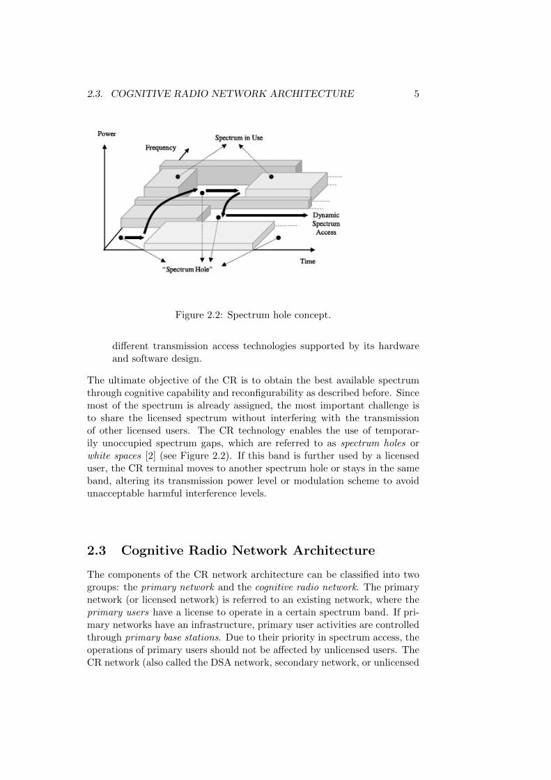
Figure 2.2: Spectrum hole concept.
different transmission access technologies supported by its hardwareand software design.
The ultimate objective of the CR is to obtain the best available spectrumthrough cognitive capability and reconfigurability as described before. Sincemost of the spectrum is already assigned, the most important challenge isto share the licensed spectrum without interfering with the transmissionof other licensed users. The CR technology enables the use of temporar-ily unoccupied spectrum gaps, which are referred to as spectrum holes orwhite spaces [2] (see Figure 2.2). If this band is further used by a licenseduser, the CR terminal moves to another spectrum hole or stays in the sameband, altering its transmission power level or modulation scheme to avoidunacceptable harmful interference levels.
2.3 Cognitive Radio Network Architecture
The components of the CR network architecture can be classified into twogroups: the primary network and the cognitive radio network. The primarynetwork (or licensed network) is referred to an existing network, where theprimary users have a license to operate in a certain spectrum band. If pri-mary networks have an infrastructure, primary user activities are controlledthrough primary base stations. Due to their priority in spectrum access, theoperations of primary users should not be affected by unlicensed users. TheCR network (also called the DSA network, secondary network, or unlicensed
6 CHAPTER 2. COGNITIVE RADIO BASICS
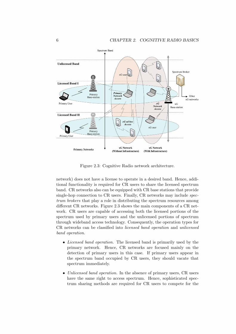
Figure 2.3: Cognitive Radio network architecture.
network) does not have a license to operate in a desired band. Hence, addi-tional functionality is required for CR users to share the licensed spectrumband. CR networks also can be equipped with CR base stations that providesingle-hop connection to CR users. Finally, CR networks may include spec-trum brokers that play a role in distributing the spectrum resources amongdifferent CR networks. Figure 2.3 shows the main components of a CR net-work. CR users are capable of accessing both the licensed portions of thespectrum used by primary users and the unlicensed portions of spectrumthrough wideband access technology. Consequently, the operation types forCR networks can be classified into licensed band operation and unlicensedband operation.
• Licensed band operation. The licensed band is primarily used by theprimary network. Hence, CR networks are focused mainly on thedetection of primary users in this case. If primary users appear inthe spectrum band occupied by CR users, they should vacate thatspectrum immediately.
• Unlicensed band operation. In the absence of primary users, CR usershave the same right to access spectrum. Hence, sophisticated spec-trum sharing methods are required for CR users to compete for the
2.4. COGNITIVE RADIO FUNCTIONS 7
unlicensed band.
According to Figure 2.3, we can notice that CR users have the opportunityto perform three different access types:
• CR network access: CR users can access their own CR base station, onboth licensed and unlicensed spectrum bands. Because all interactionsoccur inside the CR network, their spectrum sharing policy can beindependent of that of the primary network.
• CR ad hoc access: CR users can communicate with other CR usersthrough an ad hoc connection on both licensed and unlicensed spec-trum bands.
• Primary network access: CR users can also access the primary basestation through the licensed band. Unlike for other access types, thisrequires an adaptive Medium Access Control (MAC) protocol, whichenables roaming over multiple primary networks with different accesstechnologies.
According to the xG architecture described above, new spectrum manage-ment functions are required, to satisfy the following critical design chal-lenges:
• Interference avoidance: CR networks should avoid interference withprimary networks.
• Quality of Service (QoS) awareness: to decide on an appropriate spec-trum band, CR networks should support QoS-aware communication,considering the dynamic and heterogeneous spectrum environment.
• Seamless communication: CR networks should provide seamless com-munication regardless of the spectrum occupancy patterns of the pri-mary users.
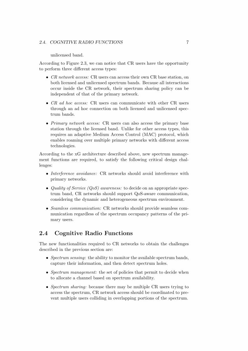
2.4 Cognitive Radio Functions
The new functionalities required to CR networks to obtain the challengesdescribed in the previous section are:
• Spectrum sensing : the ability to monitor the available spectrum bands,capture their information, and then detect spectrum holes.
• Spectrum management: the set of policies that permit to decide whento allocate a channel based on spectrum availability.
• Spectrum sharing: because there may be multiple CR users trying toaccess the spectrum, CR network access should be coordinated to pre-vent multiple users colliding in overlapping portions of the spectrum.
8 CHAPTER 2. COGNITIVE RADIO BASICS
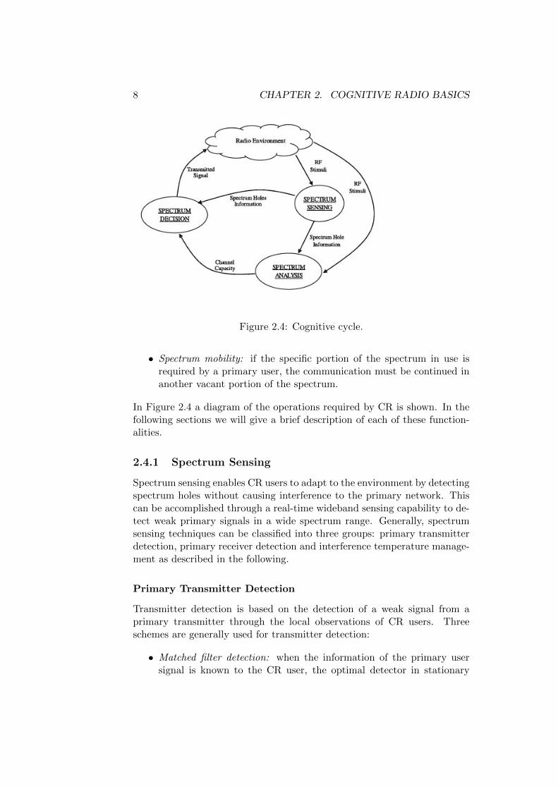
Figure 2.4: Cognitive cycle.
• Spectrum mobility: if the specific portion of the spectrum in use isrequired by a primary user, the communication must be continued inanother vacant portion of the spectrum.
In Figure 2.4 a diagram of the operations required by CR is shown. In thefollowing sections we will give a brief description of each of these function-alities.
2.4.1 Spectrum Sensing
Spectrum sensing enables CR users to adapt to the environment by detectingspectrum holes without causing interference to the primary network. Thiscan be accomplished through a real-time wideband sensing capability to de-tect weak primary signals in a wide spectrum range. Generally, spectrumsensing techniques can be classified into three groups: primary transmitterdetection, primary receiver detection and interference temperature manage-ment as described in the following.
Primary Transmitter Detection
Transmitter detection is based on the detection of a weak signal from aprimary transmitter through the local observations of CR users. Threeschemes are generally used for transmitter detection:
• Matched filter detection: when the information of the primary usersignal is known to the CR user, the optimal detector in stationary

2.4. COGNITIVE RADIO FUNCTIONS 9
gaussian noise is the matched filter. This requires a priori knowledgeof the characteristics of the primary user signal.
• Energy detection: if the receiver has no sufficient information aboutthe primary transmitter the optimal detector is an energy detector.However, the performance of this detector is susceptible to the un-certainty in noise power and also generates false alarms triggered byunintended signals because they cannot differentiate among intendedprimary transmissions and man-made noise sources or other undesiredsignal components.
• Feature Detection: in general, modulated signals are characterized bybuilt-in periodicity or cyclostationarity. This feature can be detectedby analyzing a spectral correlation function. The main advantage ofthis kind of signal detection is robustness to uncertainty in noise power.However, it is computationally complex and requires significantly longobservation times.
The main problem of primary transmitter detection techniques are:
• Receiver uncertainly: transmitter detection techniques alone cannotavoid interference to primary receivers in some cases because of theinability to detect of passive primary receivers that do not transmit(e.g., TV receivers) as depicted in Figure 2.5a.
• Hidden terminal problem: a CR user (transmitter) can have a goodline of sight to a CR receiver but may not be able to detect the primarytransmitter due to shadowing, as shown in Figure 2.5b.
In order to overcome the above mentioned problems, the sensing infor-mation from several CR terminals can be gathered and combined for moreaccurate primary transmitter detection, which is referred to as cooperativespectrum sensing of cooperative detection. However, cooperative approachescause adverse effects on resource constrained networks due to the overheadtraffic required for cooperation.
Primary Receiver Detection
Although cooperative detection reduces the probability of interference, themost efficient way to detect spectrum holes is to detect the primary usersthat are receiving data within the communication range of a CR user. Usu-ally, the Local Oscillator (LO) leakage power emitted by the Radio Fre-quency (RF) front-end of the primary receiver is exploited. However, be-cause the LO leakage signal is typically weak, implementation of a reliabledetector may have to face important problems in practice. This detectionapproach was firstly proposed for the detection of passive TV receivers [22].

10 CHAPTER 2. COGNITIVE RADIO BASICS
Figure 2.5: Transmitter detection problem: a) receiver uncertainty; b) shad-owing uncertainty.
Interference Temperature Management
Traditionally, interference can be controlled at the transmitter through theradiated power and location of individual transmitters. However, interfer-ence actually takes place at the receivers, as shown in Figure 2.5. Therefore,a model for measuring interference, referred to as interference temperature,was introduced by the Federal Communications Commission (FCC). Thismodel limits the interference at the receiver through an interference tem-perature limit, which is the amount of new interference the receiver couldtolerate. As long as CR users do not exceed this limit, they can use thespectrum band. Although this model is the best fit for the objective ofspectrum sensing, the difficulty of this model lies in accurately determiningthe interference temperature limit. This model was finally discarded by theFCC due to the its practical implementation problems.
2.4.2 Spectrum Management
CR networks require the capability to decide which is the best spectrumband among the available bands according to the QoS requirements of theapplications. This notion is called spectrum management and constitutesconstitutes and important but yet rather unexplored topic in CR networks.Spectrum management is closely related to the channel characteristics andoperations of primary users. Furthermore, spectrum decision is affected bythe activities of other CR users in the network. Spectrum decision usuallyconsists of two steps: first, each spectrum band is characterized, based onnot only local observations of CR users but also on statistical informationof primary networks, if available. Then, based on this characterization,the most appropriate spectrum band can be chosen. In the following weinvestigate the channel characteristics and decision procedures.
2.4. COGNITIVE RADIO FUNCTIONS 11
Spectrum Characterization
Because available spectrum holes show different characteristics that varyover time, each spectrum hole should be characterized considering both thetime-varying radio environment and spectrum parameters, such as operatingfrequency and bandwidth. Hence, it is essential to define parameters thatcan represent a particular spectrum band as follows:
Interference From the amount of interference at the primary receiver, thepermissible power of a CR user can be derived, which is used for theestimation of channel capacity.
Path loss The path loss is closely related to distance and frequency. As theoperating frequency increases, the path loss increases, which results ina decrease in the transmission range. If transmission power is increasedto compensate for the increased path loss, interference at other usersmay increase.
Wireless link errors Depending on the modulation scheme and the in-terference level of the spectrum band, the error rate of the channelchanges.
Link layer delay To address different path loss, wireless link error, andinterference, different types of link layer protocols are required at dif-ferent spectrum bands. This results in different link layer delays. Itis desirable to identify the spectrum bands that combine all the char-acterization parameters described previously for accurate spectrumdecision. However, a complete analysis and modeling of spectrum inCR networks has not been developed yet.
Decision Procedure
After the available spectrum bands are characterized, the most appropriatespectrum band should be selected, considering the QoS requirements andspectrum characteristics. Accordingly, the transmission mode and band-width for the transmission can be reconfigured. To describe the dynamicnature of CR networks, the primary user activity, which is defined as theprobability that a primary user appears during a CR user transmission,can be used. Because there is no guarantee that a spectrum band will beavailable during the entire communication of a CR user, it is important toconsider how often the primary user appears on the spectrum band. How-ever, because of the operation of primary networks, CR users cannot obtain areliable communication channel for a long time period. Moreover, CR usersmight not detect any single spectrum band to meet the users requirements.Therefore, multiple noncontiguous spectrum bands can be simultaneouslyused for transmission in CR networks, as shown in Figure 2.6. This method
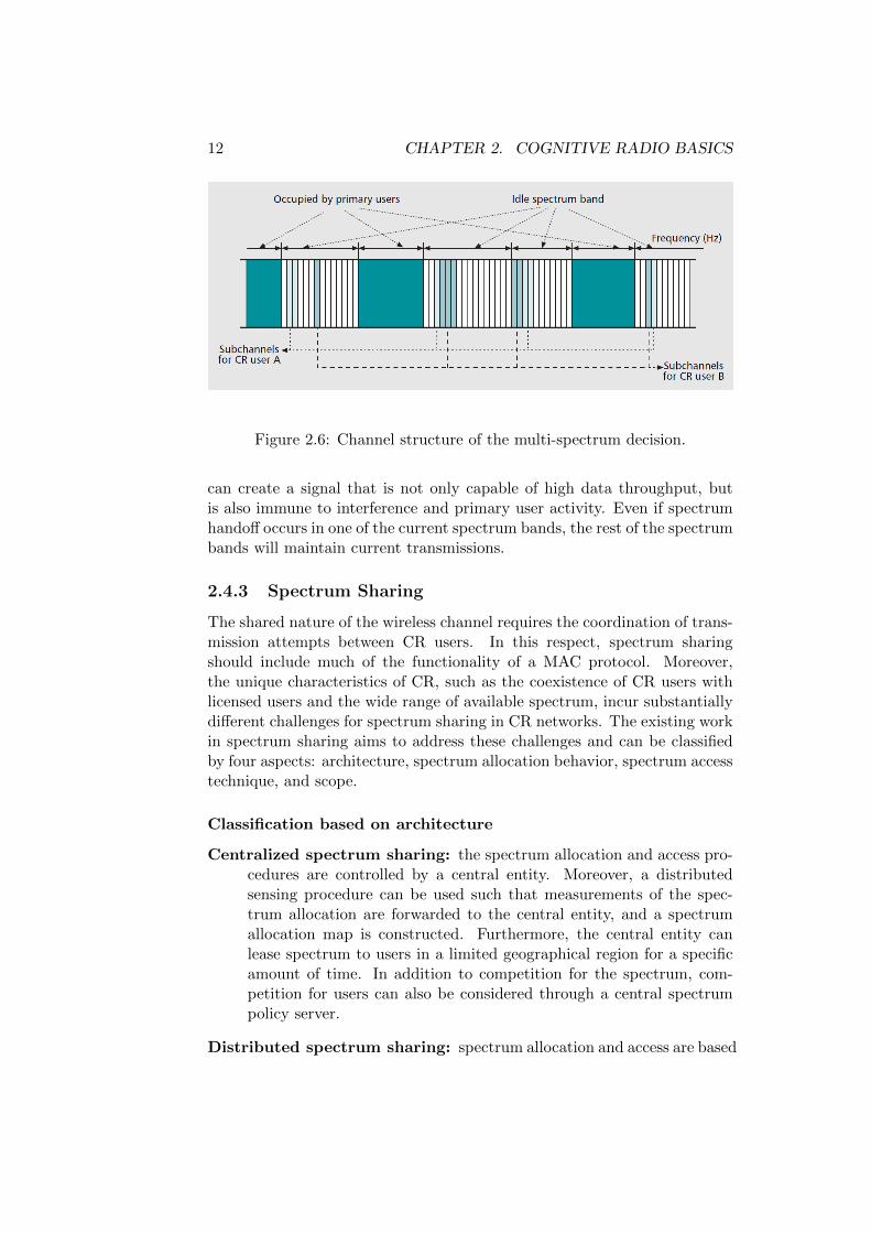
12 CHAPTER 2. COGNITIVE RADIO BASICS
Figure 2.6: Channel structure of the multi-spectrum decision.
can create a signal that is not only capable of high data throughput, butis also immune to interference and primary user activity. Even if spectrumhandoff occurs in one of the current spectrum bands, the rest of the spectrumbands will maintain current transmissions.
2.4.3 Spectrum Sharing
The shared nature of the wireless channel requires the coordination of trans-mission attempts between CR users. In this respect, spectrum sharingshould include much of the functionality of a MAC protocol. Moreover,the unique characteristics of CR, such as the coexistence of CR users withlicensed users and the wide range of available spectrum, incur substantiallydifferent challenges for spectrum sharing in CR networks. The existing workin spectrum sharing aims to address these challenges and can be classifiedby four aspects: architecture, spectrum allocation behavior, spectrum accesstechnique, and scope.
Classification based on architecture
Centralized spectrum sharing: the spectrum allocation and access pro-cedures are controlled by a central entity. Moreover, a distributedsensing procedure can be used such that measurements of the spec-trum allocation are forwarded to the central entity, and a spectrumallocation map is constructed. Furthermore, the central entity canlease spectrum to users in a limited geographical region for a specificamount of time. In addition to competition for the spectrum, com-petition for users can also be considered through a central spectrumpolicy server.
Distributed spectrum sharing: spectrum allocation and access are based
2.4. COGNITIVE RADIO FUNCTIONS 13
on local (or possibly global) policies that are performed by each nodedistributively. Distributed solutions can also be used between differentnetworks such that a Base Station (BS) competes with its interfererBSs according to the QoS requirements of its users to allocate a portionof the spectrum.
Classification based on spectrum allocation behavior
Cooperative spectrum sharing: cooperative (or collaborative) solutionsexploit the interference measurements of each node such that the effectof the communication of one node on other nodes is considered. Acommon technique used in these schemes is forming clusters to shareinterference information locally. This localized operation provides aneffective balance between a fully centralized and a distributed scheme.
Non-cooperative spectrum sharing: only a single node is considered innon-cooperative (or non-collaborative, selfish) solutions. Because in-terference in other CR nodes is not considered, non-cooperative so-lutions may result in reduced spectrum utilization. However, thesesolutions do not require frequent message exchanges between neigh-bors as in cooperative solutions.
Classification based on spectrum access technique
Overlay spectrum sharing: nodes access the network using a portion ofthe spectrum that has not been used by licensed users. This minimizesthe interference to the primary network since primary and secondarytransmissions overlap neither in frequency nor time.
Underlay spectrum sharing: overlapping secondary transmissions are al-lowed as long as their resulting interference level at the primary re-ceiver is regarded as noise. To this end, the aggregated interferencesfrom several CR nodes should not exceed the primary user’s noise floorpower. In order to achieve such low interference levels, efficient spreadspectrum techniques, such as Code Division Multiple-Access (CDMA)and Ultra Wide Band (UWB), need to be employed.
Classification based on scope
Intranetwork spectrum sharing: these solutions focus on spectrum al-location between the entities of a CR network, as shown in Figure2.7. Accordingly, the users of a CR network try to access the availablespectrum without causing interference to the primary users. Intranet-work spectrum sharing poses unique challenges that have not beenconsidered previously in wireless communication systems.

14 CHAPTER 2. COGNITIVE RADIO BASICS
Figure 2.7: Inter-network and intra-network spectrum sharing in CR net-works.
Internetwork spectrum sharing: the CR architecture enables multiplesystems to be deployed in overlapping locations and spectrum, asshown in Figure 2.7. So far the internetwork spectrum sharing so-lutions provide a broader view of the spectrum sharing concept byincluding certain operator policies.
2.4.4 Spectrum Mobility
After a CR captures the best available spectrum, primary user activity onthe selected spectrum may necessitate that the user changes its operatingspectrum band, which is referred to as spectrum mobility. Spectrum mobil-ity gives rise to a new type of handoff in CR networks, spectrum handoff. Thepurpose of the spectrum mobility management in CR networks is to ensuresmooth and fast transition leading to minimum performance degradationduring a spectrum handoff. Spectrum handoff mechanisms in a CR networkmay be triggered by the CR user mobility (i.e., as a result of the changeof location, the available spectrum bands may also change, thus requiring aspectrum handoff) as well as a change in the operating conditions (i.e., theCR user may be best served in a different frequency band). Although themobility-based handoff mechanisms that have been investigated in cellularnetworks may lay the groundwork in this area, there are still open researchtopics to be investigated.
2.5. SUMMARY 15
2.5 Summary
By exploiting the existing wireless spectrum opportunistically, CR networksare being developed to solve current wireless network problems resultingfrom the limited available spectrum and the inefficiency in spectrum usage.DSA networks, equipped with the intrinsic capabilities of CR, will providean ultimate spectrum-aware communication paradigm in wireless communi-cations. In this chapter intrinsic properties of CR networks are presented.In particular, we have described the functions required by a DSA/CR net-work, namely spectrum sensing, spectrum management, spectrum sharing,and spectrum mobility.A more detailed description of CR networks can befound in [2] and [3].

16 CHAPTER 2. COGNITIVE RADIO BASICS
Chapter 3
Spectrum Analysis Basics
The aim of this chapter is to introduce spectrum analysis and particulary theinstrument that permit us to perform spectral measurements: the spectrumanalyzer. A basic knowledge of this instrument is important as it will beused intensively for the measure of spectrum occupancy in the context of thecognitive radio. Therefore, this chapter presents the fundamentals of spec-trum analysis, including the motivations of spectral analysis, the existingtypes of spectrum analyzers, their main parameters and how their variationaffects the measured signals. This chapter places the emphasis on the oper-ating principles of swept-tuned, superheterodyne spectrum analyzers sincethis is the type of spectrum analyzer employed in this work.
3.1 Introduction
The theoretical foundation of spectrum analysis is the Fourier transforma-tion. The theory tells us that a time-domain signal can be decomposedinto a set of sine waves, referred to as spectral components, of differentamplitude, frequency and phase as it can be seen in Figure 3.1. At themost basic level, the spectrum analyzer can be described as a frequency-selective, peak-responding voltmeter calibrated to display the Root MeanSquare (RMS) value of the measured spectral components. The main pointof the frequency analysis is that it gives us different information with respectto the time-domain analysis. If we are interested in the transient period ofa signal or on its peak response then the time analysis would be the mostsuitable alternative. However, there are many fields in which spectrum anal-ysis is important, in particular in the area of radio communications. Someexamples include, but are not limited to:
• Out-of-band and spurious emissions;
• Spectrum monitoring;
• ElectroMagnetic Interference (EMI).
17

18 CHAPTER 3. SPECTRUM ANALYSIS BASICS
Figure 3.1: Relationship between time and frequency domain.
To make the transformation from the time domain to the frequency do-main the signal must be evaluated over all time; in practice a finite timeperiod is used when making a measurement. Generally spectrum analyzersdo not give us a complete information about the amplitude and the phaseof the spectral components. They only tell us how much energy is presentat a particular frequency (or its effective value, they are proportional). Alarge group of measurements can be made without knowing the phase rela-tionships among the spectral components of a signal, including the kind ofstudies performed in this work. However, some measurements require thatwe preserve complete information about the signal (frequency, amplitudeand phase). For this type of studies, other signal analysis architectures arerequired. We can distinguish three main types of signal analyzers:
• Fourier Analyzer - it digitizes the time-domain signal and then usesDigital Signal Processing (DSP) techniques to perform a Fast FourierTransform (FFT) and display the signal in the frequency domain. Oneadvantage of the FFT approach is its ability to characterize single-shotphenomena. Another is that phase as well as magnitude can be mea-sured. However, Fourier analyzers do have some limitations relativeto the superheterodyne spectrum analyzer, particularly in the areas offrequency range, sensitivity, and dynamic range. Fourier analyzers aretypically used in baseband signal analysis applications up to 40 MHz.
• Vector Signal Analyzer - VSAs also digitize the time domain signal

3.2. SUPER-HETERODYNE SPECTRUM ANALYZERS 19
like Fourier analyzers and preserve complete information about thesignal (frequency, amplitude and phase), but extend the capabilitiesto the Radio Frequency (RF) frequency range using downconverters infront of the digitizer. They offer fast, high-resolution spectrum mea-surements, demodulation, and advanced time-domain analysis. Theyare especially useful for characterizing complex signals such as burst,transient or modulated signals used in communications.
• Swept-tuned super-heterodyne Spectrum Analyzer - measures the powerof the various spectral components of the signal using the super-heterodyne technique which uses the frequency mixing to translatethe received signal to an Intermediate Frequency (IF), more suitablefor the signal processing.
Among the three signal analyzer types described above, vector signalanalyzers are able to perform the widest variety of measurements and signalanalyses. However, due to the offered high capabilities, their economicalcost usually is significantly high. Since the objectives pursued in this workcan be fulfilled with lower-cost analyzers, this type of signal analyzer hasbeen discarded. Among the remaining alternatives, the swept-tuned super-heterodyne analyzer is the most attractive option because of its improvedcapabilities in terms of sensitivity and dynamic range. It is worth notingthat the objective of this work is to assess the degree to which spectrum isused in real wireless communications systems, and to this end it becomesnecessary to detect signals of the most diverse nature, from weak signals re-ceived near the noise floor that may be difficult to detect, to strong signalsthat may overload the receiving system. Hence, sensitivity and dynamicrange are two key requirements. On one hand, higher sensitivities enablethe detection of weaker signals, received with low power levels. On theother hand, higher dynamic ranges enable the detection of weaker signals inpresence of strong ones. Since superheterodyne spectrum analyzers provideimproved performance figures in terms of sensitivity and dynamic range withrespect to Fourier analyzers, the former type of analyzers represent a moreappropriate choice and have therefore been selected in this work. In the nextsection we discuss in more detail the superheterodyne spectrum analyzer.
3.2 Super-heterodyne Spectrum Analyzers
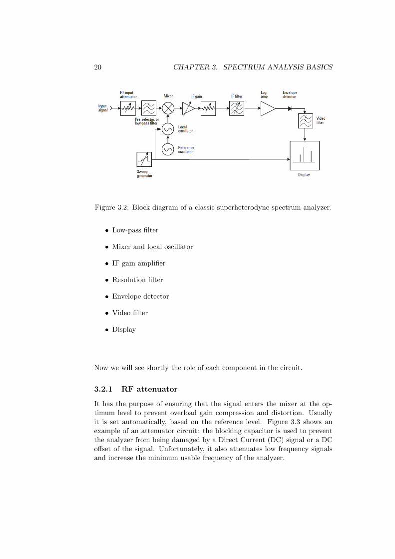
This part will focus on the fundamental theory of how a superheterodynespectrum analyzer works. In Figure 3.2 a simplified block diagram of asuper-heterodyne spectrum analyzer is shown. This ideal diagram is aimedat showing the main components of a spectrum analyzer and how and whythey affect the measure of a signal. The main components of the circuit are:
• RF attenuator
20 CHAPTER 3. SPECTRUM ANALYSIS BASICS
Figure 3.2: Block diagram of a classic superheterodyne spectrum analyzer.
• Low-pass filter
• Mixer and local oscillator
• IF gain amplifier
• Resolution filter
• Envelope detector
• Video filter
• Display
Now we will see shortly the role of each component in the circuit.
3.2.1 RF attenuator
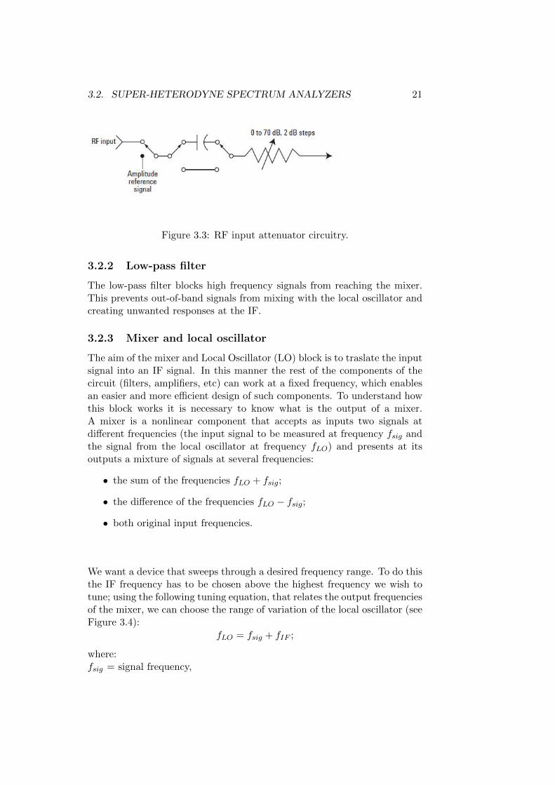
It has the purpose of ensuring that the signal enters the mixer at the op-timum level to prevent overload gain compression and distortion. Usuallyit is set automatically, based on the reference level. Figure 3.3 shows anexample of an attenuator circuit: the blocking capacitor is used to preventthe analyzer from being damaged by a Direct Current (DC) signal or a DCoffset of the signal. Unfortunately, it also attenuates low frequency signalsand increase the minimum usable frequency of the analyzer.
3.2. SUPER-HETERODYNE SPECTRUM ANALYZERS 21
Figure 3.3: RF input attenuator circuitry.
3.2.2 Low-pass filter
The low-pass filter blocks high frequency signals from reaching the mixer.This prevents out-of-band signals from mixing with the local oscillator andcreating unwanted responses at the IF.
3.2.3 Mixer and local oscillator
The aim of the mixer and Local Oscillator (LO) block is to traslate the inputsignal into an IF signal. In this manner the rest of the components of thecircuit (filters, amplifiers, etc) can work at a fixed frequency, which enablesan easier and more efficient design of such components. To understand howthis block works it is necessary to know what is the output of a mixer.A mixer is a nonlinear component that accepts as inputs two signals atdifferent frequencies (the input signal to be measured at frequency fsig andthe signal from the local oscillator at frequency fLO) and presents at itsoutputs a mixture of signals at several frequencies:
• the sum of the frequencies fLO + fsig;
• the difference of the frequencies fLO − fsig;
• both original input frequencies.
We want a device that sweeps through a desired frequency range. To do thisthe IF frequency has to be chosen above the highest frequency we wish totune; using the following tuning equation, that relates the output frequenciesof the mixer, we can choose the range of variation of the local oscillator (seeFigure 3.4):
fLO = fsig + fIF ;
where:fsig = signal frequency,

22 CHAPTER 3. SPECTRUM ANALYSIS BASICS
Figure 3.4: The LO must be tuned to fIF + fsig to produce a response onthe display.
fLO = local oscillator frequency, andfIF = IF frequency;
For example, if we want a frequency range from 0 Hz to 3 GHz, choosingan IF of 3.9 GHz, our oscillator has to vary from 3.9 GHz to 6.9 GHz.Depending on the frequency range to be measured, the local oscillator variestemporally its frequency fLO so that the desired range of frequencies fsigis sequentially swept 1 and the energy level measured at each frequency isshown in the display. Since the ramp generator controls both the horizontalposition of the trace on the display and the LO frequency, the horizontalaxis of the display can be calibrated in terms of the input signal frequencyin order to show each measured energy level at the proper frequency pointin the horizontal axis.
One major disadvantage to the superheterodyne receiving structure isthe well-know image frequency problem. Let’s assume that we want to receivea signal at fsig′ . In this case, the local oscillator is tuned to fLO = fsig′ +fIF .When this oscillator frequency fLO is selected, a response is generated atfIF due to the desired signal at fsig′ . Unfortunately, signals at fsig′ + 2fIF(known as the image frequency fimage) also cause a response at fIF , evenif no signal is present at fsig′ . In effect, one of the output frequencies inthe mixer would be the difference between the input frequency fsig′ + 2fIFand the local oscillator frequency fLO. Since the local oscillator is tunedto fLO = fsig′ + fIF , a response is obtained at (fimage) − (fLO) = (fsig′ +2fIF )−(fsig′ +fIF ) = fIF , i.e. the IF. This response would be observed as if
1The superheterodyne spectrum analyzer is also referred to as swept-tuned spectrumanalyzer.
3.2. SUPER-HETERODYNE SPECTRUM ANALYZERS 23
a signal was present at fsig′ , when it actually is not. To avoid this problem,a low-pass filter is placed before the mixer as shown in Figure 3.2 in orderto prevent such high-frequency signals from reaching the mixing stage. Insummary, we can say that for a single-band RF spectrum analyzer, an IFabove the highest frequency of the tuning range is chosen, the local oscillatoris made tunable from the IF to the IF plus the upper limit of the tuningrange, and a low-pass filter is included in front of the mixer that cuts offbelow the IF.
To separate closely spaced signals, some spectrum analyzers have IFbandwidths as narrow as 1 kHz; others, 10 Hz; still others, 1 Hz. Suchnarrow filters are difficult to achieve at a center frequency of e.g. 3.9 GHz.In practice, this problem can be solved by adding additional mixing stages,typically two to four stages, to down-convert from the first to the final IF.
3.2.4 IF gain amplifier
After the input signal is converted to an IF, it passes through the IF gainamplifier and IF attenuator which are adjusted to compensate for changesin the RF attenuator setting and mixer conversion loss. Input signal am-plitudes are thus referenced to the top line of the graticule on the display,known as the reference level. When the IF gain is changed, the value of thereference level is changed accordingly to retain the correct indicated valuefor the displayed signals. Generally, we do not want the reference level tochange when we change the input attenuator, so the settings of the inputattenuator and the IF gain are coupled together. A change in input attenu-ation will automatically change the IF gain to offset the effect of the changein input attenuation, thereby keeping the signal at a constant position onthe display.
3.2.5 Resolution filter
After the IF gain amplifier we find the IF section which consists of the analogand/or digital Resolution BandWidth (RBW) filters.
Frequency Resolution
Frequency resolution is the ability of a spectrum analyzer to separate twoinput sinusoids into distinct responses, i.e. the smallest frequency intervalthat can be resolved.
Two signals, no matter how close in frequency, should appear as two lineson the display. But a closer look at our superheterodyne receiver shows whysignal responses have a definite width on the display. The output of a mixerincludes the sum and difference products plus the two original signals (inputand LO). A bandpass filter determines the IF, and this filter selects thedesired mixing product and rejects all other signals. Because the input signal
24 CHAPTER 3. SPECTRUM ANALYSIS BASICS
Figure 3.5: As a mixing product sweeps past the IF filter, the filter shapeis traced on the display.
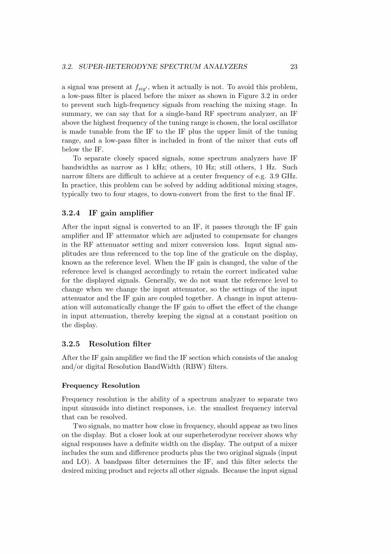
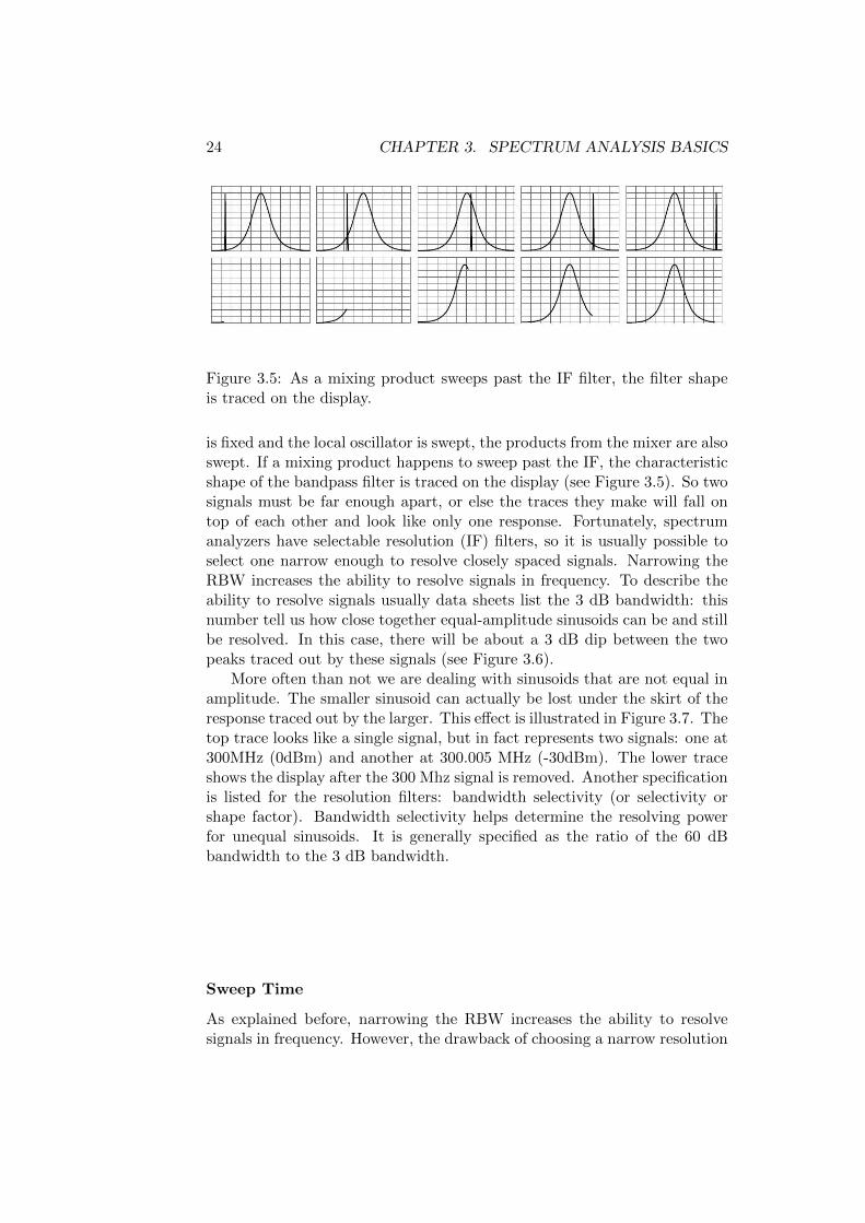
is fixed and the local oscillator is swept, the products from the mixer are alsoswept. If a mixing product happens to sweep past the IF, the characteristicshape of the bandpass filter is traced on the display (see Figure 3.5). So twosignals must be far enough apart, or else the traces they make will fall ontop of each other and look like only one response. Fortunately, spectrumanalyzers have selectable resolution (IF) filters, so it is usually possible toselect one narrow enough to resolve closely spaced signals. Narrowing theRBW increases the ability to resolve signals in frequency. To describe theability to resolve signals usually data sheets list the 3 dB bandwidth: thisnumber tell us how close together equal-amplitude sinusoids can be and stillbe resolved. In this case, there will be about a 3 dB dip between the twopeaks traced out by these signals (see Figure 3.6).
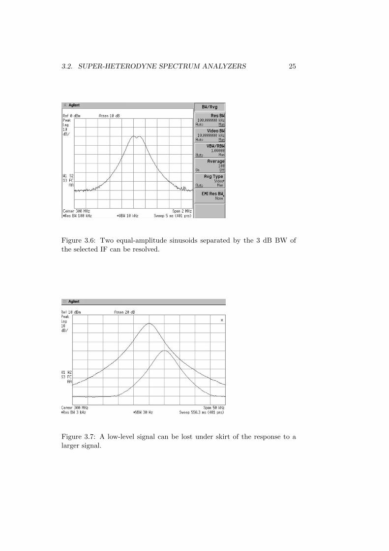
More often than not we are dealing with sinusoids that are not equal inamplitude. The smaller sinusoid can actually be lost under the skirt of theresponse traced out by the larger. This effect is illustrated in Figure 3.7. Thetop trace looks like a single signal, but in fact represents two signals: one at300MHz (0dBm) and another at 300.005 MHz (-30dBm). The lower traceshows the display after the 300 Mhz signal is removed. Another specificationis listed for the resolution filters: bandwidth selectivity (or selectivity orshape factor). Bandwidth selectivity helps determine the resolving powerfor unequal sinusoids. It is generally specified as the ratio of the 60 dBbandwidth to the 3 dB bandwidth.
Sweep Time
As explained before, narrowing the RBW increases the ability to resolvesignals in frequency. However, the drawback of choosing a narrow resolution
3.2. SUPER-HETERODYNE SPECTRUM ANALYZERS 25
Figure 3.6: Two equal-amplitude sinusoids separated by the 3 dB BW ofthe selected IF can be resolved.
Figure 3.7: A low-level signal can be lost under skirt of the response to alarger signal.
26 CHAPTER 3. SPECTRUM ANALYSIS BASICS
filter is that this increases sweep time that directly affects how long it takesto complete a measurement.
In the analog case, resolution comes into play because the IF filters areband-limited circuits that require finite times to charge and discharge. If wethink about how long a mixing product stays in the passband of the IF filter,that time is directly proportional to bandwidth and inversely proportionalto the sweep in hertz per unit time, or:
Time in passband =RBWSpanST
(3.1)
where RBW = resolution bandwidth, and ST = sweep time.The rise time of a filter is inversely proportional to its bandwidth, and
if we include a constant of proportionality, k, then
RiseTime =k
RBW(3.2)
ST =k · SpanRBW 2
(3.3)
The important message here is that a change in resolution has a dramaticeffect on sweep time (e.g., reducing the RBW by a factor of 10 increases thesweep time by a factor of 100). Spectrum analyzers automatically couplesweep time to the span and resolution bandwidth settings. Sweep time isadjusted to maintain a calibrated display.
Some spectrum analyzers use digital techniques to realize their RBWfilters. Digital filters can provide important benefits, such as dramaticallyimproved bandwidth selectivity. Another important advantage is that digitalfilters are from 2 to 4 times faster, due to the fact that the signal beinganalyzed is processed into frequency blocks.
Noise Floor
The selection of different RBWs has an impact not only on the ability toresolve signals in frequency and the sweep time but also on the system’snoise floor and thus on the ability to detect the presence of weak signal.When modifying the RBW, the noise floor observed in the spectrum ana-lyzer changes. Although there are various noise sources inside a spectrumanalyzer, this variation is mainly due to the effect of the thermal noise. Thethermal noise power PN of a receiver can be expressed as PN = kTB, wherek is the Boltzmann’s constant, T is the absolute temperature in Kelvin,and B is the system bandwidth (the resolution bandwidth in the case ofa spectrum analyzer). From the previous expression, it is clear that if weincrease the RBW, the captured noise power also increases, thus degradingthe receiving Signal-to-Noise Ratio (SNR). This effect is clearly appreciated
3.2. SUPER-HETERODYNE SPECTRUM ANALYZERS 27
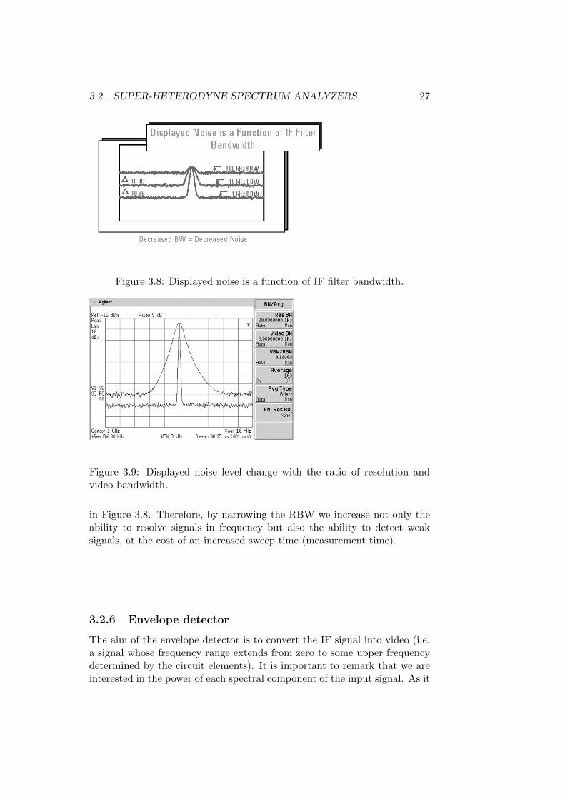
Figure 3.8: Displayed noise is a function of IF filter bandwidth.
Figure 3.9: Displayed noise level change with the ratio of resolution andvideo bandwidth.
in Figure 3.8. Therefore, by narrowing the RBW we increase not only theability to resolve signals in frequency but also the ability to detect weaksignals, at the cost of an increased sweep time (measurement time).
3.2.6 Envelope detector
The aim of the envelope detector is to convert the IF signal into video (i.e.a signal whose frequency range extends from zero to some upper frequencydetermined by the circuit elements). It is important to remark that we areinterested in the power of each spectral component of the input signal. As it
28 CHAPTER 3. SPECTRUM ANALYSIS BASICS
Figure 3.10: Envelope detector.
can be seen in Figure 3.10 the response of the detector follows the changesin the envelope of the IF signal, but not the instantaneous value of the IFsine wave itself. For most measurements, we choose a RBW narrow enoughto resolve the individual spectral components of the input signal. If we fixthe frequency of the LO so that our analyzer is tuned to one of the spectralcomponents of the signal, the output of the IF is a steady sine wave witha constant peak value. The output of the envelope detector will then be aconstant (DC) voltage, and there is no variation for the detector to follow.So the envelope detector follows the changing amplitude values of the peaksof the signal from the IF chain but not the instantaneous values, resultingin the loss of phase information.
The logarithmic amplifier in front of the envelope detector in Figure 3.2can be enabled in order to display the detected signal in logarithmic scale(decibels).
3.2.7 Video filter
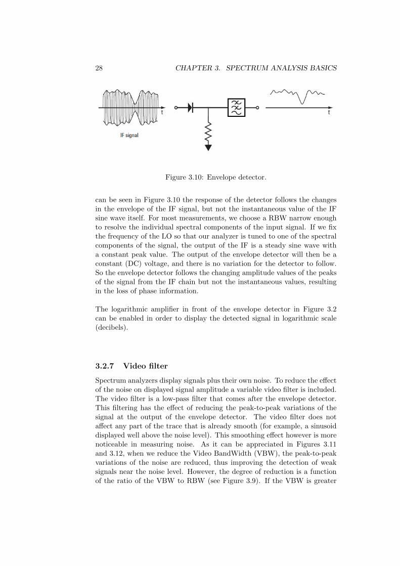
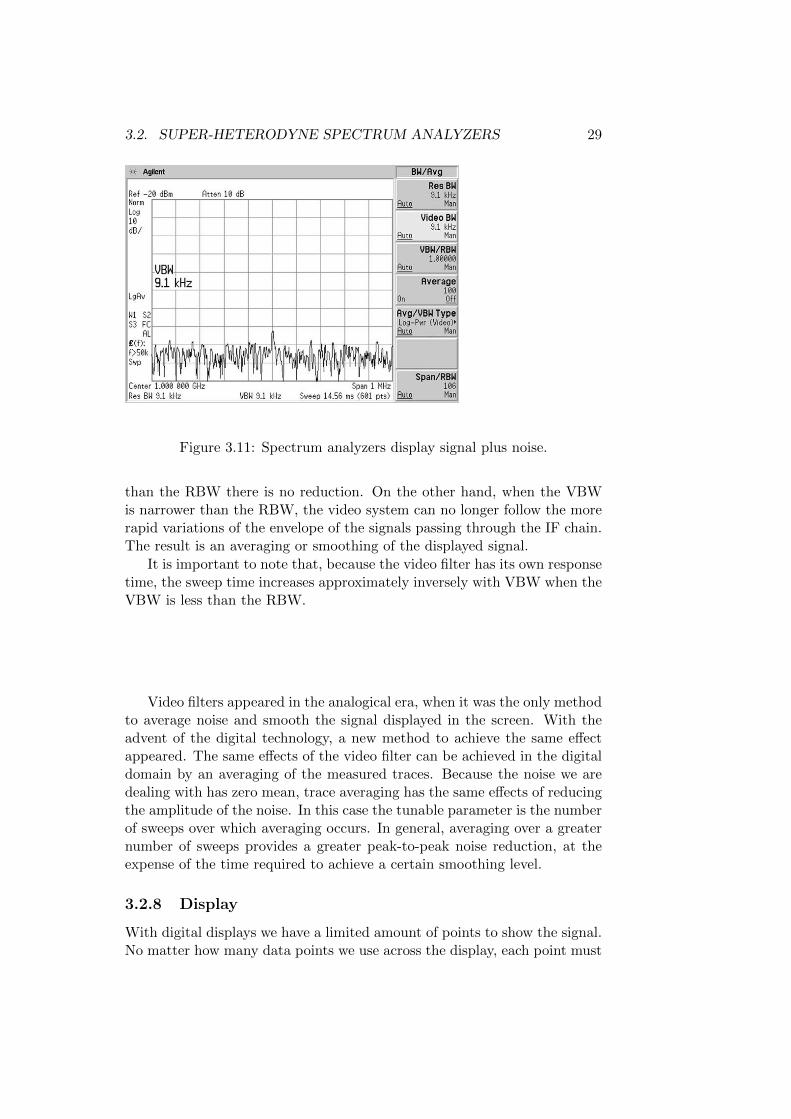
Spectrum analyzers display signals plus their own noise. To reduce the effectof the noise on displayed signal amplitude a variable video filter is included.The video filter is a low-pass filter that comes after the envelope detector.This filtering has the effect of reducing the peak-to-peak variations of thesignal at the output of the envelope detector. The video filter does notaffect any part of the trace that is already smooth (for example, a sinusoiddisplayed well above the noise level). This smoothing effect however is morenoticeable in measuring noise. As it can be appreciated in Figures 3.11and 3.12, when we reduce the Video BandWidth (VBW), the peak-to-peakvariations of the noise are reduced, thus improving the detection of weaksignals near the noise level. However, the degree of reduction is a functionof the ratio of the VBW to RBW (see Figure 3.9). If the VBW is greater
3.2. SUPER-HETERODYNE SPECTRUM ANALYZERS 29
Figure 3.11: Spectrum analyzers display signal plus noise.
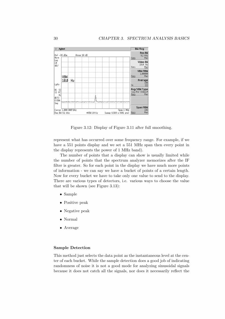
than the RBW there is no reduction. On the other hand, when the VBWis narrower than the RBW, the video system can no longer follow the morerapid variations of the envelope of the signals passing through the IF chain.The result is an averaging or smoothing of the displayed signal.
It is important to note that, because the video filter has its own responsetime, the sweep time increases approximately inversely with VBW when theVBW is less than the RBW.
Video filters appeared in the analogical era, when it was the only methodto average noise and smooth the signal displayed in the screen. With theadvent of the digital technology, a new method to achieve the same effectappeared. The same effects of the video filter can be achieved in the digitaldomain by an averaging of the measured traces. Because the noise we aredealing with has zero mean, trace averaging has the same effects of reducingthe amplitude of the noise. In this case the tunable parameter is the numberof sweeps over which averaging occurs. In general, averaging over a greaternumber of sweeps provides a greater peak-to-peak noise reduction, at theexpense of the time required to achieve a certain smoothing level.
3.2.8 Display
With digital displays we have a limited amount of points to show the signal.No matter how many data points we use across the display, each point must
30 CHAPTER 3. SPECTRUM ANALYSIS BASICS
Figure 3.12: Display of Figure 3.11 after full smoothing.
represent what has occurred over some frequency range. For example, if wehave a 551 points display and we set a 551 MHz span then every point inthe display represents the power of 1 MHz band).
The number of points that a display can show is usually limited whilethe number of points that the spectrum analyzer memorizes after the IFfilter is greater. So for each point in the display we have much more pointsof information - we can say we have a bucket of points of a certain length.Now for every bucket we have to take only one value to send to the display.There are various types of detectors, i.e. various ways to choose the valuethat will be shown (see Figure 3.13):
• Sample
• Positive peak
• Negative peak
• Normal
• Average
Sample Detection
This method just selects the data point as the instantaneous level at the cen-ter of each bucket. While the sample detection does a good job of indicatingrandomness of noise it is not a good mode for analyzing sinusoidal signalsbecause it does not catch all the signals, nor does it necessarily reflect the

3.2. SUPER-HETERODYNE SPECTRUM ANALYZERS 31
Figure 3.13: Trace point saved in memory is based on detector type algo-rithm.
true peak values of the displayed signals. When RBW is narrower than thesample interval (i.e., the bucket width), the sample mode can give erroneousresults.
Positive Peak Detection
One way to insure that all sinusoids are reported at their true amplitudes isto display the maximum value encountered in each bucket. This is the posi-tive peak detection mode. It ensures that no sinusoid is missed, regardless ofthe ratio between resolution bandwidth and bucket width. However peak de-tection does not give a good representation of random noise because it onlydisplays the maximum value in each bucket and ignore the true randomnessof the noise.
Negative Peak Detection
Negative peak detection displays the minimum value encountered in eachbucket. It is generally available in most spectrum analyzers, though itis not used as often as other types of detection. Differentiating Continu-ous Wave(CW) from impulsive signals in Electro-Magnetic Compatibility(EMC) testing is one application where negative peak detection is valuable.
Normal Detection
The normal detection provides a better visual display of random noise thanpeak and avoide the missed-signal problem of the sample mode.The normal detection algorithm:
If the signal rises and falls within a bucket:
Even numbered buckets display the minimum (negative peak)
32 CHAPTER 3. SPECTRUM ANALYSIS BASICS
value in the bucket. The maximum is remembered.
Odd numbered buckets display the maximum (positive peak)
value determined by comparing the current bucket peak with
the previous (remembered) bucket peak.
If the signal only rises or only falls within a bucket, the peak
is displayed.
Peak detection is best for locating CW signals well out of the noise, sampledetection is best for looking at noise, and normal detection is best for viewingsignals and noise.
Average Detection
While spectrum analyzers usually collect amplitude data many times in eachbucket, sample detection keeps only one of those values and throws awaythe rest. An averaging detector uses all the data collected within the time(and frequency) interval of a bucket. Averaging detector is usually referredto as Root Mean Square (RMS) detector when it averages power (basedon the RMS of voltage). Average detection is an improvement over usingsample detection for the determination of power. Sample detection requiresmultiple sweeps to collect enough data points to give us accurate averagepower information.
3.3 Summary
This chapter has presented the basic operating principles of a superhetero-dyne spectrum analyzer, also referred to as swept-tuned spectrum analyzer.This kind of spectrum analyzer constitutes the key element of the measure-ment setup employed in this work to measure and characterize the degree towhich spectrum is currently used. Therefore, it becomes necessary to have ageneral picture of spectrum analysis basics for a better understanding of thematerial presented in next chapters, especially in the areas of configurationparameters and obtained results.
Chapter 4
Measurement Setup
There are many factors that need to be considered when defining a strategyto meet a particular radio spectrum occupancy measurement need. Thereare some basic dimensions that every spectrum occupancy measurementstrategy should clearly specify, namely frequency (frequency span and fre-quency points to be measured), location (measurement site selection), direc-tion (antenna pointing angle), polarization (receiving antenna polarization)and time (sampling rate and measurement period). The measurement setupemployed in the evaluation of spectrum occupancy should be designed takinginto account the previous factors since they play a key role in the accuracy ofthe obtained results. In the next sections we will describe the measurementscheme employed with detailed information about every component, theSpurious Free Dynamic Range (SFDR), the locations and the measurementmethod.
4.1 Measurement scheme
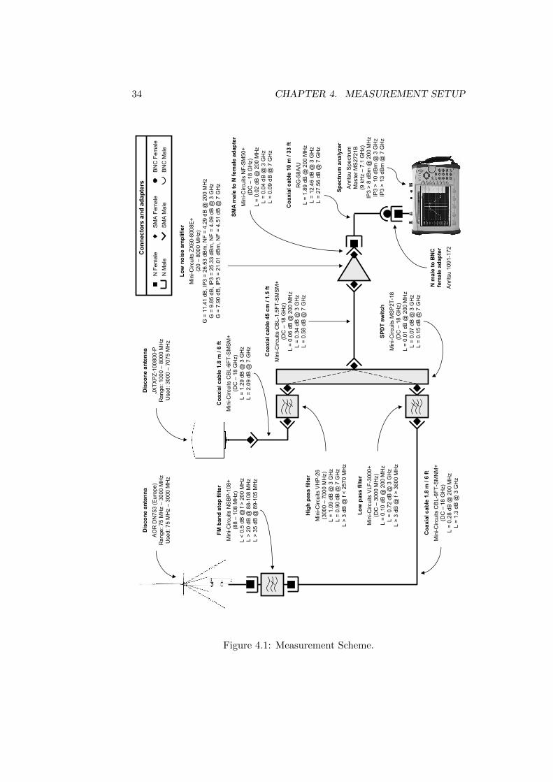
The measurement setup should be able to detect, over a wide range of fre-quencies, a large number of transmitters of the most diverse nature, fromnarrow band to wide band systems and from weak signals received near thenoise floor to strong signals that may overload the receiving system. Ourstudy is based on a spectrum analyzer setup where different external de-vices have been added in order to improve the detection capabilities of thesystem and hence obtain more accurate and reliable results. A simplifiedscheme of the measurement configuration is shown in Figure 3.1. The designis composed of:
• two broadband antennas;
• a switch to select the desired antenna;
33
34 CHAPTER 4. MEASUREMENT SETUP
Dis
cone
ante
nna
AOR
DN
753
(Eur
ope)
Ran
ge: 7
5 M
Hz
–
3000
MH
zU
sed:
75
MH
z –
3000
MH
z
Spec
trum
ana
lyze
rA
nrits
u S
pect
rum
Mas
ter M
S27
21B
(9 k
Hz
–
7.1
GH
z)IP
3 >
8 dB
m
@ 2
00 M
Hz
IP3
> 10
dB
m
@ 3
GH
zIP
3 >
13 d
Bm
@ 7
GH
z
Dis
cone
ante
nna
JXTX
PZ-1
0080
0-P
Ran
ge: 1
000
–
8000
MH
zU
sed:
300
0 –
7075
MH
z
SPD
T sw
itch
Min
i-Circ
uits
MS
P2T
-18
(DC
–
18 G
Hz)
L =
0.01
dB
@ 2
00 M
Hz
L =
0.07
dB
@ 3
GH
zL
= 0.
15 d
B @
7 G
Hz
Coa
xial
cab
le 1
.8 m
/ 6
ftM
ini-C
ircui
ts C
BL-
6FT-
SM
NM
+
(DC
–
18 G
Hz)
L =
0.28
dB
@ 2
00 M
Hz
L =
1.3
dB @
3 G
Hz
FM b
and
stop
filte
rM
ini-C
ircui
ts N
SB
P-1
08+
(88
–
108
MH
z)L
< 0.
5 dB
@ f
> 20
0 M
Hz
L >
20 d
B @
88-
108
MH
zL
> 35
dB
@ 8
9-10
5 M
Hz
Con
nect
ors
and
adap
ters
Coa
xial
cab
le 1
.8 m
/ 6
ftM
ini-C
ircui
ts C
BL-
6FT-
SM
SM
+
(DC
–
18 G
Hz)
L =
1.29
dB
@ 3
GH
zL
= 2.
09 d
B @
7 G
Hz
Low
pas
s fil
ter
Min
i-Circ
uits
VLF
-300
0+(D
C –
3000
MH
z)L
= 0.
10 d
B @
200
MH
z
L =
0.72
dB
@ 3
GH
zL
> 3
dB @
f >
3600
MH
z
Hig
h pa
ss fi
lter
Min
i-Circ
uits
VH
P-2
6(3
000
–
7000
MH
z)L
= 1.
09 d
B @
3 G
Hz
L =
0.90
dB
@ 7
GH
zL
> 3
dB @
f <
2570
MH
z
Low
noi
se a
mpl
ifier
Min
i-Circ
uits
ZX6
0-80
08E
+(2
0 –
8000
MH
z)G
= 1
1.41
dB
, IP
3 =
26.5
3 dB
m, N
F =
4.29
dB
@ 2
00 M
Hz
G =
9.8
5 dB
, IP
3 =
25.3
3 dB
m, N
F =
4.09
dB
@ 3
GH
zG
= 7
.90
dB, I
P3
= 21
.01
dBm
, NF
= 4.
51 d
B @
7 G
Hz
N F
emal
eN
Mal
eS
MA
Fem
ale
SM
A M
ale
BN
C F
emal
eBN
C M
ale
N m
ale
to B
NC
fem
ale
adap
ter
Anrit
su 1
091-
172
Coa
xial
cab
le 1
0 m
/ 33
ftR
G-5
8A/U
L =
1.89
dB
@ 2
00 M
Hz
L =
12.4
6 dB
@ 3
GH
zL
= 27
.56
dB @
7 G
Hz
Coa
xial
cab
le 4
5 cm
/ 1.
5 ft
Min
i-Circ
uits
CB
L-1.
5FT-
SM
SM
+
(DC
–
18 G
Hz)
L =
0.06
dB
@ 2
00 M
Hz
L =
0.34
dB
@ 3
GH
zL
= 0.
58 d
B @
7 G
Hz
SMA
mal
e to
N fe
mal
e ad
apte
rM
ini-C
ircui
ts N
F-S
M50
+(D
C –
18 G
Hz)
L =
0.02
dB
@ 2
00 M
Hz
L =
0.04
dB
@ 3
GH
zL
= 0.
09 d
B @
7 G
Hz
Figure 4.1: Measurement Scheme.
4.1. MEASUREMENT SCHEME 35
• several filters;
• a low noise amplifier;
• high performance spectrum analyzer.
In the next subsections we will see the technical characteristics of everycomponent and we will explain their role in the measurement setup.
4.1.1 Antennas
When covering small frequency ranges or specific licensed bands a singleantenna may suffice. However, in broadband spectrum measurements froma few megahertzs up to several gigahertzs two or more broadband antennasare required in order to cover the whole frequency range. Most of spec-trum measurement campaigns are based on omni-directional measurementsin order to detect primary signals coming for any directions. To this end,omni-directional vertically polarized antennas are the most common choice.Our antenna system comprises two broadband discone-type antennas, whichare vertically polarized antennas with omni-directional receiving pattern inthe horizontal plane. Even though some transmitters are horizontally polar-ized, they usually are high-power stations (e.g., TV stations) that can stillbe detected with vertically polarized antennas. The antennas employed inthe measurement were:
• AOR DA753G Compact Discone Aerial; vertically polarized, designedto receive across the frequency range of 75MHz to 3000MHz (3GHz)and with an impedance of 50Ω [7].
• JXTXPZ-100800/P 1.0 8.0GHz Discone-type Antenna; vertically po-larized, designed to receive the frequency range of 1GHz to 8Ghz andwith an impedance of 50Ω [1].
4.1.2 Filters
The filters employed in our setup are:
• high-pass filter Mini-Circuits VHP-26 with pass-band 3000-7000 MHz[17];
• low-pass filter Mini-Circuits VLF-3000+ with pass-band DC-3000 MHz[10];
• a band-stop filter Mini-Circuits NSBP-108+ with stop-band 88108MHz [11];
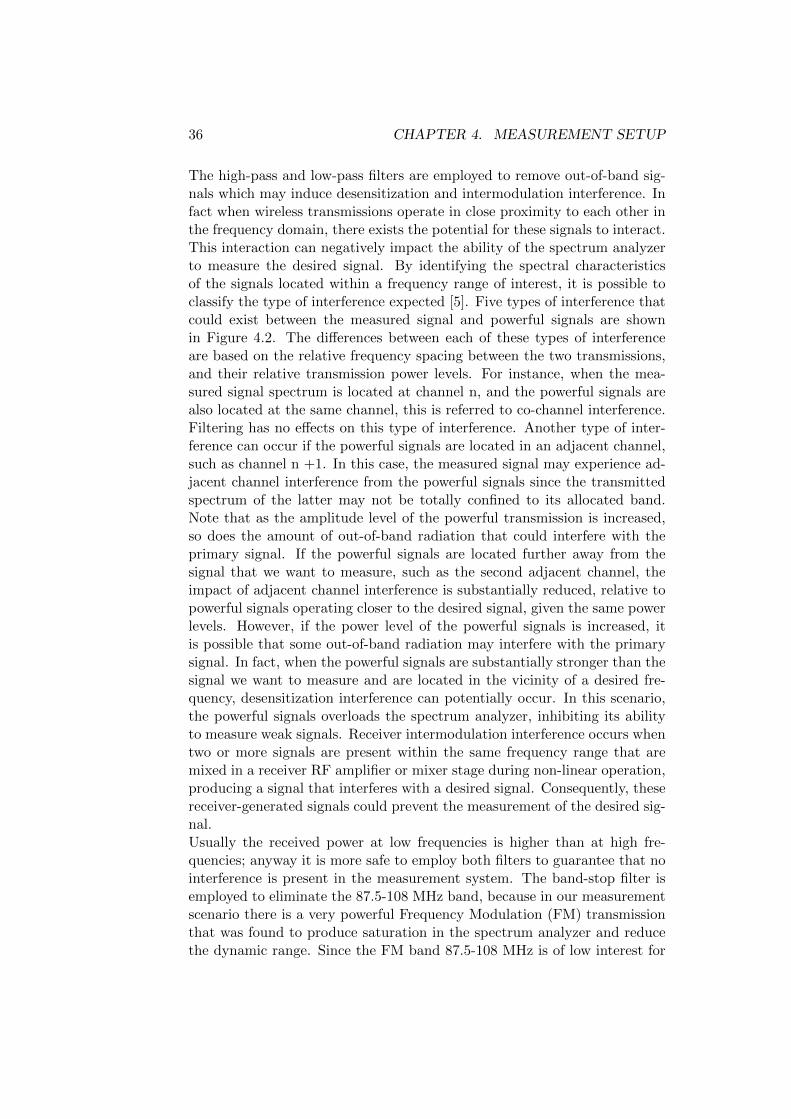
36 CHAPTER 4. MEASUREMENT SETUP
The high-pass and low-pass filters are employed to remove out-of-band sig-nals which may induce desensitization and intermodulation interference. Infact when wireless transmissions operate in close proximity to each other inthe frequency domain, there exists the potential for these signals to interact.This interaction can negatively impact the ability of the spectrum analyzerto measure the desired signal. By identifying the spectral characteristicsof the signals located within a frequency range of interest, it is possible toclassify the type of interference expected [5]. Five types of interference thatcould exist between the measured signal and powerful signals are shownin Figure 4.2. The differences between each of these types of interferenceare based on the relative frequency spacing between the two transmissions,and their relative transmission power levels. For instance, when the mea-sured signal spectrum is located at channel n, and the powerful signals arealso located at the same channel, this is referred to co-channel interference.Filtering has no effects on this type of interference. Another type of inter-ference can occur if the powerful signals are located in an adjacent channel,such as channel n +1. In this case, the measured signal may experience ad-jacent channel interference from the powerful signals since the transmittedspectrum of the latter may not be totally confined to its allocated band.Note that as the amplitude level of the powerful transmission is increased,so does the amount of out-of-band radiation that could interfere with theprimary signal. If the powerful signals are located further away from thesignal that we want to measure, such as the second adjacent channel, theimpact of adjacent channel interference is substantially reduced, relative topowerful signals operating closer to the desired signal, given the same powerlevels. However, if the power level of the powerful signals is increased, itis possible that some out-of-band radiation may interfere with the primarysignal. In fact, when the powerful signals are substantially stronger than thesignal we want to measure and are located in the vicinity of a desired fre-quency, desensitization interference can potentially occur. In this scenario,the powerful signals overloads the spectrum analyzer, inhibiting its abilityto measure weak signals. Receiver intermodulation interference occurs whentwo or more signals are present within the same frequency range that aremixed in a receiver RF amplifier or mixer stage during non-linear operation,producing a signal that interferes with a desired signal. Consequently, thesereceiver-generated signals could prevent the measurement of the desired sig-nal.Usually the received power at low frequencies is higher than at high fre-quencies; anyway it is more safe to employ both filters to guarantee that nointerference is present in the measurement system. The band-stop filter isemployed to eliminate the 87.5-108 MHz band, because in our measurementscenario there is a very powerful Frequency Modulation (FM) transmissionthat was found to produce saturation in the spectrum analyzer and reducethe dynamic range. Since the FM band 87.5-108 MHz is of low interest for
4.1. MEASUREMENT SCHEME 37
secondary usage (high occupancy and high transmission power) we filter thisband in order avoid any potential problems.
4.1.3 Switch
The switch employed in our scheme was Single Pole Double Throw (SPDT)switch Mini-Circuits MSP2T-18 [12] that can be used in the DC-18 GHzfrequency range. The function of the switch is to select what antenna wewant to use without the need of changing the setup manually. The switchemployed is a SPDT that is a switch with one output that can be connectedto one of the two inputs while the other one is isolated. This device requiresa power supply of 24V Direct Current (DC). When the switch is not fed thelow-frequency (75-3000 MHz) antenna is selected while when it is fed thehigh-frequency (3000-7000 MHz) antenna is selected.
4.1.4 Pre-amplifier
In our measurement setup the antenna is connected to the spectrum analyzerby means of a 10-meter coaxial cable. This cable introduces relevant losseswhich make the detection of weak signals difficult. To compensate for thislosses and to improve the capabilities of our system we could use the built-in high-gain pre-amplifier of the spectrum analyzer. Nevertheless, due tothe high length between the antenna and the built-in pre-amplifier a betteroption is to place a external low-noise pre-amplifier right after the antennasystem. To reach this conclusion four possible configurations have beenanalyzed:
• without external pre-amplifier and without internal pre-amplifier;
• without external pre-amplifier and with internal pre-amplifier;
• with external pre-amplifier and without internal pre-amplifier;
• with external pre-amplifier and with internal pre-amplifier;
For every configuration the noise figure has been calculated using the param-eters of every component. The best configuration is the one with externalpre-amplifier and with internal pre-amplifier. In Table 4.1 we report theresults of the calculation of the noise figure for the selected configuration:the upper 3 GHz value is in the upper-limit of the low-frequency branchof the measurement setup, while the lower 3 GHz value corresponds to thelower-limit of the high-frequency branch of the measurement setup. Thehigh NF! (NF!) value observed at FM is due to the high attenuation in-troduced by the FM band, while the high NF value at 7 GHz is due to thehigh attenuation introduced by the 10-meter cable at high frequencies.

38 CHAPTER 4. MEASUREMENT SETUP
Figure 4.2: Types of interference.
4.1. MEASUREMENT SCHEME 39
NF [linear] NF [dB]
FM 302.34 24.80
200 MHz 3.39 5.30
3 GHz 8.48 9.28
3 GHz 8.21 9.14
7 GHz 233.26 23.68
Table 4.1: Noise Figure results for the adopted configuration.
In our setup we have utilized a Mini-Circuits ZX60-8008E+ [8] amplifierwith a frequency range from 20 MHz to 8 GHz. It is worth noting thatchoosing an amplifier with the highest possible gain is not always the bestoption in broadband spectrum surveys, where very different signal levelsmay be present. The existing tradeoff between sensitivity and dynamic rangemust be taken into account. To choose the correct preamplifier, we must lookat our measurement needs. If we want absolutely the best sensitivity andare not concerned about measurement range, we would choose a high-gain,low-noise pre-amplifier. If we want better sensitivity but cannot afford togive up any measurement range, we must choose a lower-gain pre-amplifier.A reasonable design criterion is to guarantee that the received signals liewithin the overall systems SFDR, which is defined as the difference betweena threshold or lower limit at which signals can be detected without excessiveinterference by noise (constrained by the systems noise floor) and the inputlevel that produces spurs at levels equal to the noise power. If the maximumlevel is exceeded, some spurs might arise above the systems noise floor andwould be detected as signals in truly unoccupied bands, thus resulting ininaccurate results and erroneous conclusions about the primary activity.
4.1.5 Spectrum Analyzer
The spectrum analyzer is the main component of the measurement setup.In the first chapter we described the general operation of a super-heterodynespectrum analyzer. The one we utilized for our measurements is a AnritsuSpectrum Master MS2721B [4]. It is a high-performance handheld spectrumanalyzer with frequency range from 9 KHz to 7.1 GHz, low noise floor (Dis-played Average Noise Level (DANL) of -163dBm with a Resolution Band-Width (RBW) of 1kHz) that permits a reliable detection of weak signals. Ithas tunable RBW and Video BandWidth (VBW) from 1 Hz to 3MHz. Thesweep speed is automatically changed by the analyzer to the fastest sweepspeed that will yield accurate results. It has an internal pre-amplifier andthe possibility to store the measured data into an external Universal SerialBus (USB) device, that permits a more comfortable data analysis.

40 CHAPTER 4. MEASUREMENT SETUP
4.1.6 Other components
To connect the antennas, the spectrum analyzers and the amplifier we useseveral cables and connectors. Following there is a list of the componentsutilized in our measurement scheme.
• Test Cable CBL-1.5FT-SMSM+ [13]; used to connect the switch withthe pre-amplifier.
• Test Cable CBL-6FT-SMSM+ [15]; used to connect the discone an-tenna JXTXPZ-100800-P to the switch.
• Test Cable CBL-6FT-SMNM+ [14]; used to connect the discone AORDN753 antenna to the switch.
• Test Cable RG-58A/U [16]; used to connect the pre-amplifier to thespectrum analyzer.
• Coaxial Adapter N male to BNC female NF-SM50+ [9] used to connectthe coaxial cable to the spectrum analyzer.
• Coaxial Adapter SMA male to N female NF-SM50+ [9] used to connectthe pre-amplifier to the coaxial cable.
4.2 Spurious Free Dynamic Range (SFDR)
As previously explained the SFDR is defined as the difference between thepower of signals that generate spurious responses and the power of the noisefloor at the input. It is necessary to calculate the SFDR to guarantee that thereceived signals will not exceed the maximum allowed level; if this happened,then the measurement setup might work in non-linear regime, thus yieldingto spurious responses.
To calculate the SFDR we use the following equations:
SFDR(dB) =m− 1
m[IPi(dBm)− PNi(dBm)]
with m = i = 3, where PNi is the noise power and the IPi is the interceptpoint of order i. Here we consider the third-order intercept point because itis the more constraining one. The calculation of the total SFDR has beenmade splitting our setup scheme into two quadripoles: the first one includesthe antenna, the filters, the switch, the coaxial cable, the amplifier and theadaptor; the second one includes the coaxial cable, the adaptor and thespectrum analyzer. To calculate the noise power we could use the followingequation:
PNi = KT0FBN ;
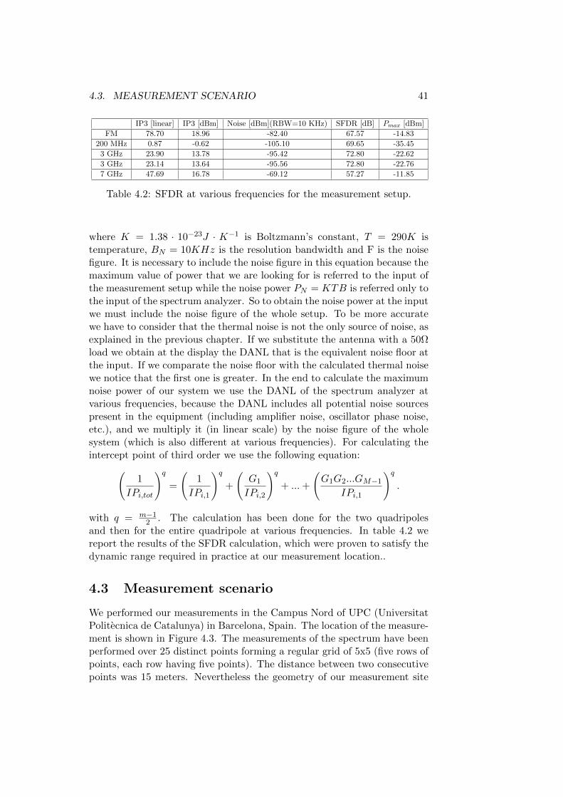
4.3. MEASUREMENT SCENARIO 41
IP3 [linear] IP3 [dBm] Noise [dBm](RBW=10 KHz) SFDR [dB] Pmax [dBm]
FM 78.70 18.96 -82.40 67.57 -14.83
200 MHz 0.87 -0.62 -105.10 69.65 -35.45
3 GHz 23.90 13.78 -95.42 72.80 -22.62
3 GHz 23.14 13.64 -95.56 72.80 -22.76
7 GHz 47.69 16.78 -69.12 57.27 -11.85
Table 4.2: SFDR at various frequencies for the measurement setup.
where K = 1.38 · 10−23J · K−1 is Boltzmann’s constant, T = 290K istemperature, BN = 10KHz is the resolution bandwidth and F is the noisefigure. It is necessary to include the noise figure in this equation because themaximum value of power that we are looking for is referred to the input ofthe measurement setup while the noise power PN = KTB is referred only tothe input of the spectrum analyzer. So to obtain the noise power at the inputwe must include the noise figure of the whole setup. To be more accuratewe have to consider that the thermal noise is not the only source of noise, asexplained in the previous chapter. If we substitute the antenna with a 50Ωload we obtain at the display the DANL that is the equivalent noise floor atthe input. If we comparate the noise floor with the calculated thermal noisewe notice that the first one is greater. In the end to calculate the maximumnoise power of our system we use the DANL of the spectrum analyzer atvarious frequencies, because the DANL includes all potential noise sourcespresent in the equipment (including amplifier noise, oscillator phase noise,etc.), and we multiply it (in linear scale) by the noise figure of the wholesystem (which is also different at various frequencies). For calculating theintercept point of third order we use the following equation:(
1
IPi,tot
)q
=
(1
IPi,1
)q
+
(G1
IPi,2
)q
+ ...+
(G1G2...GM−1
IPi,1
)q
.
with q = m−12 . The calculation has been done for the two quadripoles
and then for the entire quadripole at various frequencies. In table 4.2 wereport the results of the SFDR calculation, which were proven to satisfy thedynamic range required in practice at our measurement location..
4.3 Measurement scenario
We performed our measurements in the Campus Nord of UPC (UniversitatPolitecnica de Catalunya) in Barcelona, Spain. The location of the measure-ment is shown in Figure 4.3. The measurements of the spectrum have beenperformed over 25 distinct points forming a regular grid of 5x5 (five rows ofpoints, each row having five points). The distance between two consecutivepoints was 15 meters. Nevertheless the geometry of our measurement site
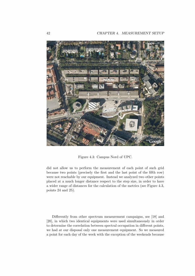
42 CHAPTER 4. MEASUREMENT SETUP
Figure 4.3: Campus Nord of UPC.
did not allow us to perform the measurement of each point of such gridbecause two points (precisely the first and the last point of the fifth row)were not reachable by our equipment. Instead we analyzed two other pointsplaced at a much longer distance respect to the step size, in order to havea wider range of distances for the calculation of the metrics (see Figure 4.3,points 24 and 25).
Differently from other spectrum measurement campaigns, see [18] and[20], in which two identical equipments were used simultaneously in orderto determine the correlation between spectral occupation in different points,we had at our disposal only one measurement equipment. So we measureda point for each day of the week with the exception of the weekends because
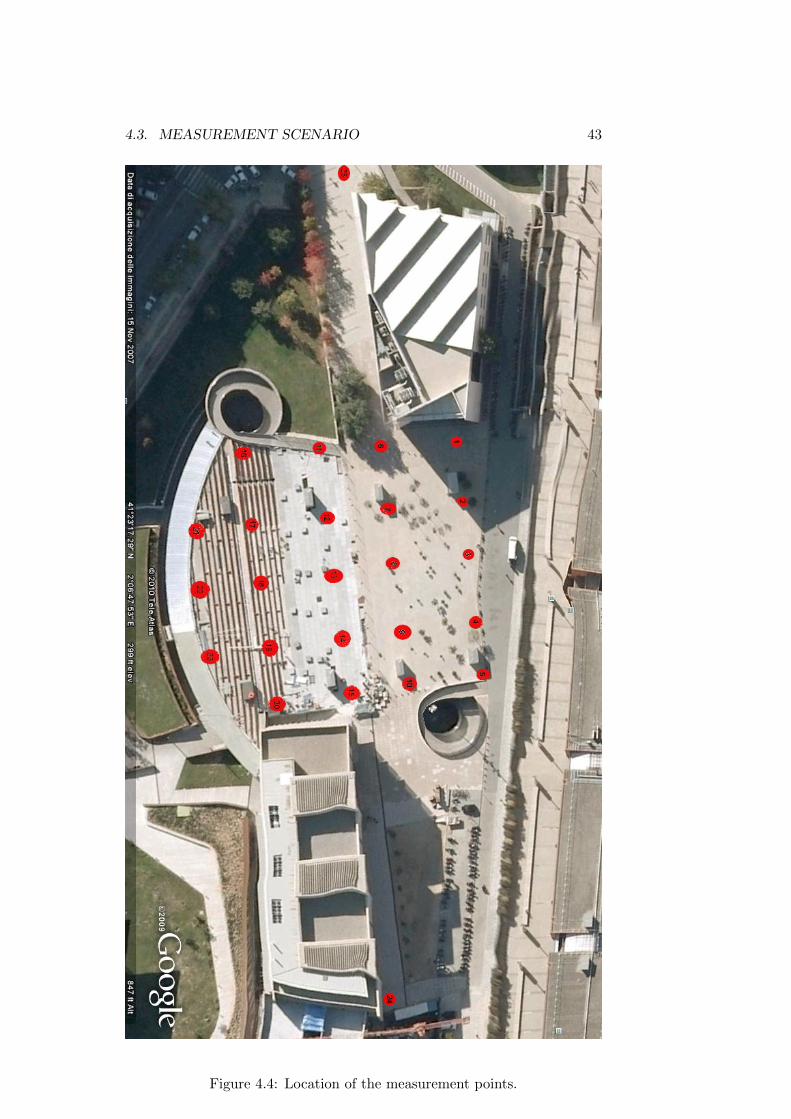
4.3. MEASUREMENT SCENARIO 43
Figure 4.4: Location of the measurement points.
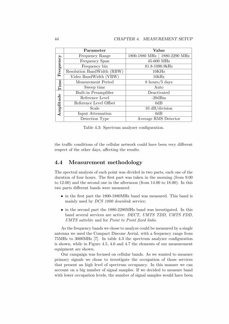
44 CHAPTER 4. MEASUREMENT SETUP
Parameter Value
Fre
qu
en
cy Frequency Range 1800-1880 MHz 1880-2290 MHz
Frequency Span 45-600 MHzFrequency bin 81.8-1090.9kHz
Resolution BandWidth (RBW) 10KHzVideo BandWidth (VBW) 10kHz
Tim
e Measurement Period 8 hours/5 daysSweep time Auto
Am
plitu
de
Built-in Preamplifier DeactivatedReference Level -20dBm
Reference Level Offset 0dBScale 10 dB/division
Input Attenuation 0dBDetection Type Average RMS Detector
Table 4.3: Spectrum analyzer configuration.
the traffic conditions of the cellular network could have been very differentrespect of the other days, affecting the results.
4.4 Measurement methodology
The spectral analysis of each point was divided in two parts, each one of theduration of four hours. The first part was taken in the morning (from 9.00to 12.00) and the second one in the afternoon (from 14.00 to 18.00). In thistwo parts different bands were measured:
• in the first part the 1800-1880MHz band was measured. This band ismainly used by DCS 1800 downlink service;
• in the second part the 1880-2280MHz band was investigated. In thisband several services are active: DECT, UMTS TDD, UMTS FDD,UMTS sattelite and for Point to Point fixed links.
As the frequency bands we chose to analyze could be measured by a singleantenna we used the Compact Discone Aerial, with a frequency range from75MHz to 3000MHz [7]. In table 4.3 the spectrum analyzer configurationis shown, while in Figure 4.5, 4.6 and 4.7 the elements of our measurementequipment are shown.
Our campaign was focused on cellular bands. As we wanted to measureprimary signals we chose to investigate the occupation of those servicesthat present an high level of spectrum occupancy. In this manner we canaccount on a big number of signal samples. If we decided to measure bandwith lower occupation levels, the number of signal samples would have been
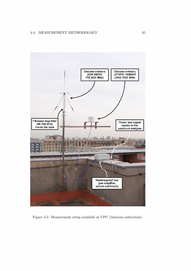
4.4. MEASUREMENT METHODOLOGY 45
Figure 4.5: Measurement setup available at UPC (Antenna subsystem).
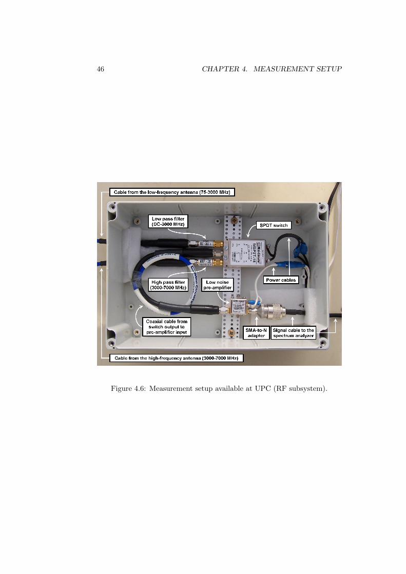
46 CHAPTER 4. MEASUREMENT SETUP
Figure 4.6: Measurement setup available at UPC (RF subsystem).
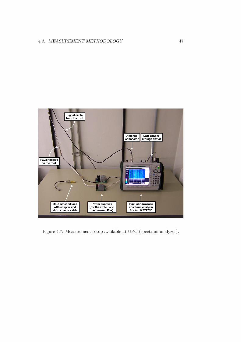
4.4. MEASUREMENT METHODOLOGY 47
Figure 4.7: Measurement setup available at UPC (spectrum analyzer).
48 CHAPTER 4. MEASUREMENT SETUP
lower within the same measurement period. Moreover this choice permittedus to perform our measurement campaign in a relatively small are. If weconsidered for example TV bands, which are also subject to an intensiveusage (TV channels are active 100% of the time), due to the large coveragearea of TV transmitters and their high power level, we would have to performour study over a large area, in the order of several square kilometers. Theselected bands therefore allow us to capture a high number of primary signalsamples within practical measurement periods in a practical reduced area.
At the end of every measurement the data were saved in a USB pen andpost-processed offline with MATLAB and appropriate analysis scripts thatwere developed to this end.
4.5 Summary
In this chapter we described every component of the equipment used to per-form the spectrum occupancy measurement. We also illustrated the criteriaused to find the optimal configuration for our needs, i.e. the analysis ofthe SFDR. We showed the site where the campaign was carried out, thefrequency bands measured and the methodology that we used to performthe measurement campaign.
Chapter 5
Measurement Results
5.1 Introduction
In this chapter we discuss the results obtained from the analysis of thedata of our measurement campaign. First we take a look at the spectraloccupation of the measured bands. Then we introduce and describe thecorrelation metrics used to analyze the data. After that we illustrate theresults obtained applying these metrics to our data and explain the observedbehavior.
5.2 Spectral occupancy
Before introducing the main results we give a look to the spectral occupancyresults obtained in our measurement campaign. We analyzed the 1800-1880MHz band and the 1880-2290 MHz band, which comprise the DCS and theUMTS, respectively. There are several reasons that support our decisionto analyze these spectrum bands. The main objective is to analyze spec-trum occupancy and its correlation. In order to obtain reliable estimates ofthe spectral occupancy and its correlation, it is necessary to capture a suffi-ciently high number of primary signal samples. If we select channels with lowoccupancy levels, most of the captured samples would correspond to noise,meaning that the measurement sessions would then need to be extended tolong measurement periods in order to capture a high number of signal sam-ples. By selecting channels with high occupancy levels, the measurementperiod required to capture a sufficiently high number of primary signal sam-ples then reduces to feasible values. Although some parts of the selectedbands remain unused, the channels being actually used in such bands are, ingeneral, subject to significant occupancy levels. According to this criterion,it would also be possible to select TV bands, since the channels employed inthe TV bands are used virtually 100% of the time. However, in this case itis important to note that TV transmitters are normally intended to provide
49
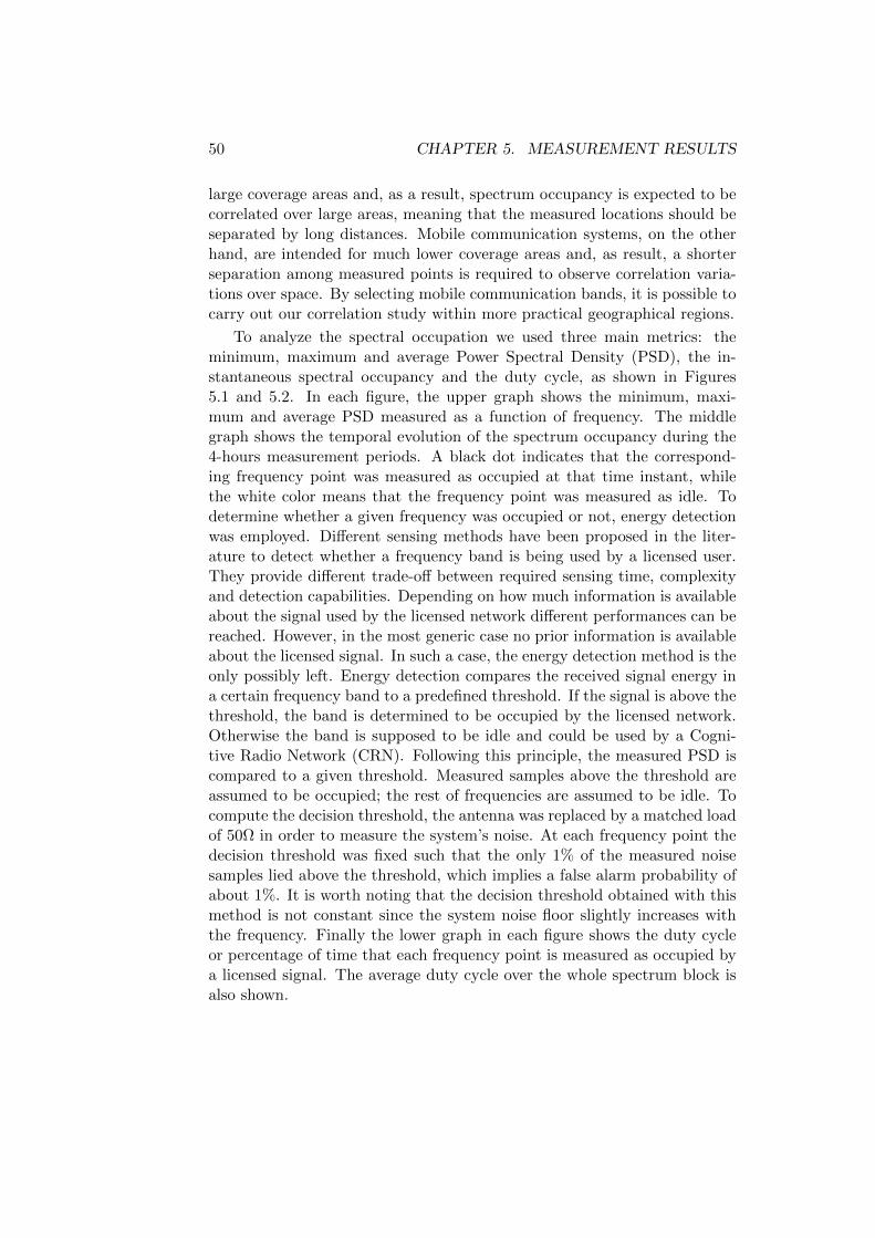
50 CHAPTER 5. MEASUREMENT RESULTS
large coverage areas and, as a result, spectrum occupancy is expected to becorrelated over large areas, meaning that the measured locations should beseparated by long distances. Mobile communication systems, on the otherhand, are intended for much lower coverage areas and, as result, a shorterseparation among measured points is required to observe correlation varia-tions over space. By selecting mobile communication bands, it is possible tocarry out our correlation study within more practical geographical regions.
To analyze the spectral occupation we used three main metrics: theminimum, maximum and average Power Spectral Density (PSD), the in-stantaneous spectral occupancy and the duty cycle, as shown in Figures5.1 and 5.2. In each figure, the upper graph shows the minimum, maxi-mum and average PSD measured as a function of frequency. The middlegraph shows the temporal evolution of the spectrum occupancy during the4-hours measurement periods. A black dot indicates that the correspond-ing frequency point was measured as occupied at that time instant, whilethe white color means that the frequency point was measured as idle. Todetermine whether a given frequency was occupied or not, energy detectionwas employed. Different sensing methods have been proposed in the liter-ature to detect whether a frequency band is being used by a licensed user.They provide different trade-off between required sensing time, complexityand detection capabilities. Depending on how much information is availableabout the signal used by the licensed network different performances can bereached. However, in the most generic case no prior information is availableabout the licensed signal. In such a case, the energy detection method is theonly possibly left. Energy detection compares the received signal energy ina certain frequency band to a predefined threshold. If the signal is above thethreshold, the band is determined to be occupied by the licensed network.Otherwise the band is supposed to be idle and could be used by a Cogni-tive Radio Network (CRN). Following this principle, the measured PSD iscompared to a given threshold. Measured samples above the threshold areassumed to be occupied; the rest of frequencies are assumed to be idle. Tocompute the decision threshold, the antenna was replaced by a matched loadof 50Ω in order to measure the system’s noise. At each frequency point thedecision threshold was fixed such that the only 1% of the measured noisesamples lied above the threshold, which implies a false alarm probability ofabout 1%. It is worth noting that the decision threshold obtained with thismethod is not constant since the system noise floor slightly increases withthe frequency. Finally the lower graph in each figure shows the duty cycleor percentage of time that each frequency point is measured as occupied bya licensed signal. The average duty cycle over the whole spectrum block isalso shown.
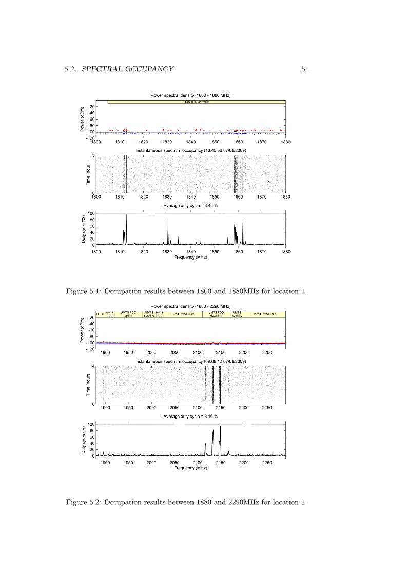
5.2. SPECTRAL OCCUPANCY 51
Figure 5.1: Occupation results between 1800 and 1880MHz for location 1.
Figure 5.2: Occupation results between 1880 and 2290MHz for location 1.
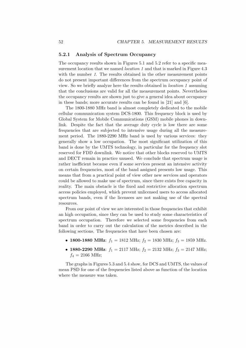
52 CHAPTER 5. MEASUREMENT RESULTS
5.2.1 Analysis of Spectrum Occupancy
The occupancy results shown in Figures 5.1 and 5.2 refer to a specific mea-surement location that we named location 1 and that is marked in Figure 4.3with the number 1. The results obtained in the other measurement pointsdo not present important differences from the spectrum occupancy point ofview. So we briefly analyze here the results obtained in location 1 assumingthat the conclusions are valid for all the measurement points. Neverthelessthe occupancy results are shown just to give a general idea about occupancyin these bands; more accurate results can be found in [21] and [6].
The 1800-1880 MHz band is almost completely dedicated to the mobilecellular communication system DCS-1800. This frequency block is used byGlobal System for Mobile Communications (GSM) mobile phones in down-link. Despite the fact that the average duty cycle is low there are somefrequencies that are subjected to intensive usage during all the measure-ment period. The 1880-2290 MHz band is used by various services: theygenerally show a low occupation. The most significant utilization of thisband is done by the UMTS technology, in particular for the frequency slotreserved for FDD downlink. We notice that other blocks reserved to UMTSand DECT remain in practice unused. We conclude that spectrum usage israther inefficient because even if some services present an intensive activityon certain frequencies, most of the band assigned presents low usage. Thismeans that from a practical point of view other new services and operatorscould be allowed to make use of spectrum, since there exists free capacity inreality. The main obstacle is the fixed and restrictive allocation spectrumaccess policies employed, which prevent unlicensed users to access allocatedspectrum bands, even if the licensees are not making use of the spectralresources.
From our point of view we are interested in those frequencies that exhibitan high occupation, since they can be used to study some characteristics ofspectrum occupation. Therefore we selected some frequencies from eachband in order to carry out the calculation of the metrics described in thefollowing sections. The frequencies that have been chosen are:
• 1800-1880 MHz: f1 = 1812 MHz; f2 = 1830 MHz; f3 = 1859 MHz.
• 1880-2290 MHz: f1 = 2117 MHz; f2 = 2132 MHz; f3 = 2147 MHz;f4 = 2166 MHz;
The graphs in Figures 5.3 and 5.4 show, for DCS and UMTS, the values ofmean PSD for one of the frequencies listed above as function of the locationwhere the measure was taken.
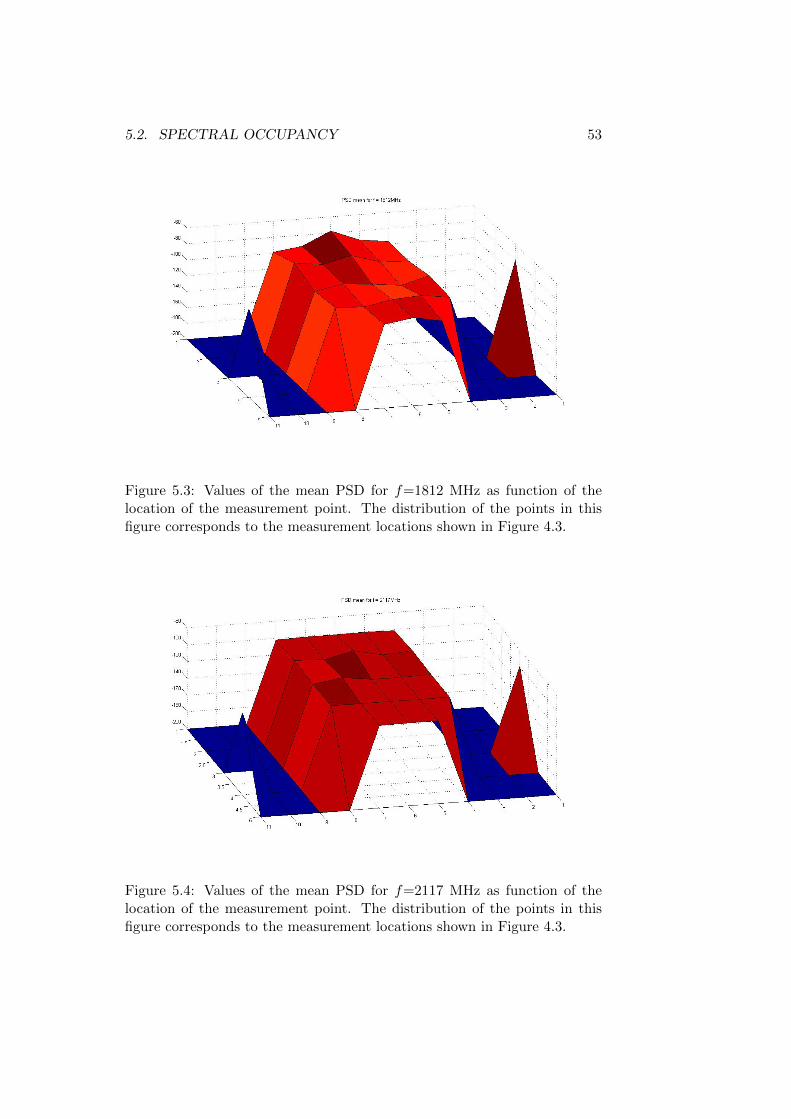
5.2. SPECTRAL OCCUPANCY 53
Figure 5.3: Values of the mean PSD for f=1812 MHz as function of thelocation of the measurement point. The distribution of the points in thisfigure corresponds to the measurement locations shown in Figure 4.3.
Figure 5.4: Values of the mean PSD for f=2117 MHz as function of thelocation of the measurement point. The distribution of the points in thisfigure corresponds to the measurement locations shown in Figure 4.3.
54 CHAPTER 5. MEASUREMENT RESULTS
5.3 Evaluation Criteria
Given the results of the measurement campaign, our aim was to investigatethe behavior of the spectral occupancy as function of the distance by thecalculation and the comparison of appropriate metrics. Before introducingthese metrics, and to understand the reasons behind this choice, in thefollowing we give a brief introduction about spatial statics and its relationwith cooperative sensing.
5.3.1 Cooperative sensing and spatial statistics
In chapter 2 we gave an introduction to cognitive radio. The main idea ofCongitive Radio (CR) is to permit its users to access those parts of the spec-trum licensed to other services but that are temporarily unused. As soon asa primary user (an user who has a license to operate in the band considered)shows up, CR user immediately vacates the spectrum and moves to anotherfree location. In this context it is clear that detection of the primary usersby CR is a fundamental task, in order to avoid harmful interference withlicensed users. This task takes the name of spectrum sensing. However thereare several scenarios in which a single secondary user is likely to miss a pri-mary transmission and mistakenly assumes a spectrum band to be free. Aspreviously told in section 2.4.1, several methods have been proposed to en-sure a reliable detection. One of the most interesting detection methods, dueto its ability to overcome practical spectrum sensing limitations, is coopera-tive sensing. The basic idea behind cooperative sensing is that if two or moreCR users, located in the area of the same primary network, exchange eachother their information about spectral occupation, then their probability totake a right decision is increased. This method helps to prevent detectionerrors of primary users that might be caused by various problems, amongwhich the most important are the hidden terminal problem and fading andshadowing effects.
In the hidden terminal problem the secondary user is either too far awayfrom the primary transmitter or the signal is attenuated because of buildingsor other obstacles in the propagation path. This could lead a CR user toconsider free a frequency that is actually used. The use of cooperativesensing coupled with the presence of another secondary user that that doesnot suffer from the same problem can avoid this kind of situations.
Fast fading may cause a severe drop in the received signal and and hencea missed detection. Cooperative sensing can help to solve this problem be-cause fast fading is only correlated over distances of the order of the usedwavelength. The case of shadowing is more complicated because shadowingis correlated over longer distances. There are several studies on the charac-teristics of these correlations, but they have been developed in the contextof cellular networks and therefore present several drawbacks when applied
5.3. EVALUATION CRITERIA 55
to DSA networks. As a consequence, more suitable statistical models areneeded for better understand the spatial behavior of spectrum utilization.More in general, the analysis of several aspects of DSA systems requiresgood spatial models of spectrum usage: the development of this aspects willreceive a great benefit from the development of a spectrum model with thepossibility to generate synthetic data for testing purposes.
In this context we focused our attention on the spatial correlation of thespectral occupancy. Differently from the work in [20], in which two pointswere measured simultaneously, our equipment allowed us to measure just onesingle location per measurement session. Therefore our analysis could notbe based on instantaneous PSD, because the data were taken sequentiallyat different times. Instead we considered the average PSD obtained duringthe measurement period. We considered only the frequencies cited in theprevious section as they presented a high occupation and therefore ensuremore reliable results.
5.3.2 Correlation metrics
Before introducing the metrics used we give a short explanation of themethod used to treat the gathered data. In section 4.3 we explained thatthe measurements of the spectrum have been performed over 25 distinctpoints forming a regular grid of 5x5 (five rows of points, each row havingfive points). At the end of the campaign for each point measured we hadinformation about the instantaneous power spectral density during the timethat the measure was performed. The locations on which we performed ourmeasurement formed a regular grid (with the exception of two points), witha step of 15 meters. As showed in Figure 4.3 we marked each point witha number. The following step was to group all pair of locations having thesame distance. For example, if we consider a 15 meters length, we have togroup location 1 and 2, location 2 and 3, location 4 and 5 and so on, that isall the pairs of points 15 meters apart from each other. We did this for eachdistance that we could find from the grid. In the calculation of the pairs ofpoints far-between the same length we used a binning procedure: we consid-ered two pairs of points to belong to the same set if h−∆ ≤‖ xj−xi ‖≤ h+∆where we h denotes the length considered, ‖ xj − xi ‖ the distance betweenthe two points and ∆ an appropriate margin included in order to grouppoints that are separated by a similar, but not exactly the same, distance.In this way we also assured vectors to have a significant number of elements.Therefore, for each considered length, we could create two vectors U(h) andV(h). These vectors contained the average PSD of all the pairs of pointsfor the considered length h. For example, previously we considered a 15meters length: in this case the first element of vector U was the averagePSD measured in location 1. The corresponding element (that is the onehaving the same index) for the vector V was the average PSD of the location
56 CHAPTER 5. MEASUREMENT RESULTS
2. Therefore, each couple of points having the same distance were placed inthe same position/index within the two vectors. In the following we presentthe employed correlation metrics.
Cross correlation
The cross-correlation between two independent processes is defined as
R(U,V) =1
Ns
Ns∑t=1
Ut · Vt (5.1)
where Ns is the number of samples, U and V are the vectors to be compared,and Ut and Vt are their components, respectively. In our case U and Vcorrespond to the vectors previously defined, containing the average PSD ofthe pairs of points located at a certain distance.
Covariance
The covariance is obtained from the cross-correlation by subtracting fromeach vector its mean (which is the average of the various mean powers)
cov(U, V ) =1
Ns
Ns∑t=1
(Ut − U) · (Vt − V ) (5.2)
where U and V denote the average of the vectors U and V , respectively.
Normalized covariance
The covariance is often extended by normalization:
ρ(U, V ) =1
Ns
Ns∑t=1
Ut − UσU
· Vt − VσV
(5.3)
where σU and σV are the standard deviations of the vectors U and V , re-spectively.
Semivariance
The empirical semivariance is described as
γ(h) =1
2|N(h)|
Ns∑t=1
(Ut − Vt)2 (5.4)
where we denote with |N(h)| the cardinality of the vector U (or equivalentlyV ), where we emphasized the dependence by the distance h. A plot ofsemivariances versus distances between ordered data in a graph is known asa semivariogram.

5.4. RESULTS 57
5.4 Results
5.4.1 Correlation metrics vs. distance
In Figure 5.5, 5.6, 5.7 and 5.8 we show the metrics calculated for the selectedfrequencies of DCS band. In Figure 5.9, 5.10, 5.11 and 5.12 we show themetrics calculated for the selected frequencies of UMTS band.
Previous studies suggest that the expected behavior for cross-correlation,covariance and normalized covariance is to decrease as the distance increases,while we expected the semivariance to increase with distance. The resultsobtained with our data do not show in general a well defined trend. In somecases, as for example the cross-correlation in Figure 5.5, the cross-correlationseems to increase with the distance, that is the opposite behavior with re-spect to the expected one. As the shape of the metrics graphs could be dueto a few pairs of points having an abnormal behavior (that might happen,for example, if during the measurement our equipment was subject to somenoise source causing an alteration in the measured PSD) we analyzed thecomputed graphs. We checked for each distance that the values considered,that is, using the above notation, the products Ut · Vt for each value of t,lied near the average. If we had found some couples of points laying faraway from the average then we could explain the strange behavior of thecorrelation metrics. As in our analysis we did not find any anomaly weconcluded that the correlation metrics as a function of the distance had arandom behavior. The more likely hypothesis explaining the random behav-ior versus distance is that different locations separated by the same distancemay experience significantly dissimilar primary signals. The primary powerlevel observed at each location is the result of the constructive/destructivecombination of all the primary signal components received through differentpropagation paths, which depend on the particular measured location andits surrounding propagation environment (buildings, walls, etc.). Therefore,various points separated by the same distance may observe dissimilar pri-mary power levels depending on the particular location of each point. Thiscan explain the random behavior observed for the analyzed correlation met-rics as a function of the distance. In the following we analyze a differentapproach for analyzing spatial correlation of spectrum occupancy.
5.4.2 Correlation metrics vs. SNR difference
The results obtained for the correlation parameters as a function of the dis-tance did not show the expected trend. Therefore we thought to compute thecorrelation parameters as a function of the SNR difference. The calculation
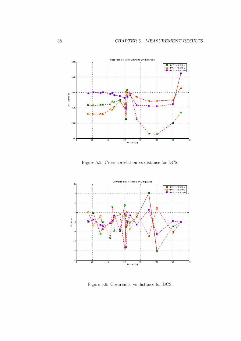
58 CHAPTER 5. MEASUREMENT RESULTS
Figure 5.5: Cross-correlation vs distance for DCS.
Figure 5.6: Covariance vs distance for DCS.

5.4. RESULTS 59
Figure 5.7: Normalized Covariance vs distance for DCS.
Figure 5.8: Semivariance vs distance for DCS.
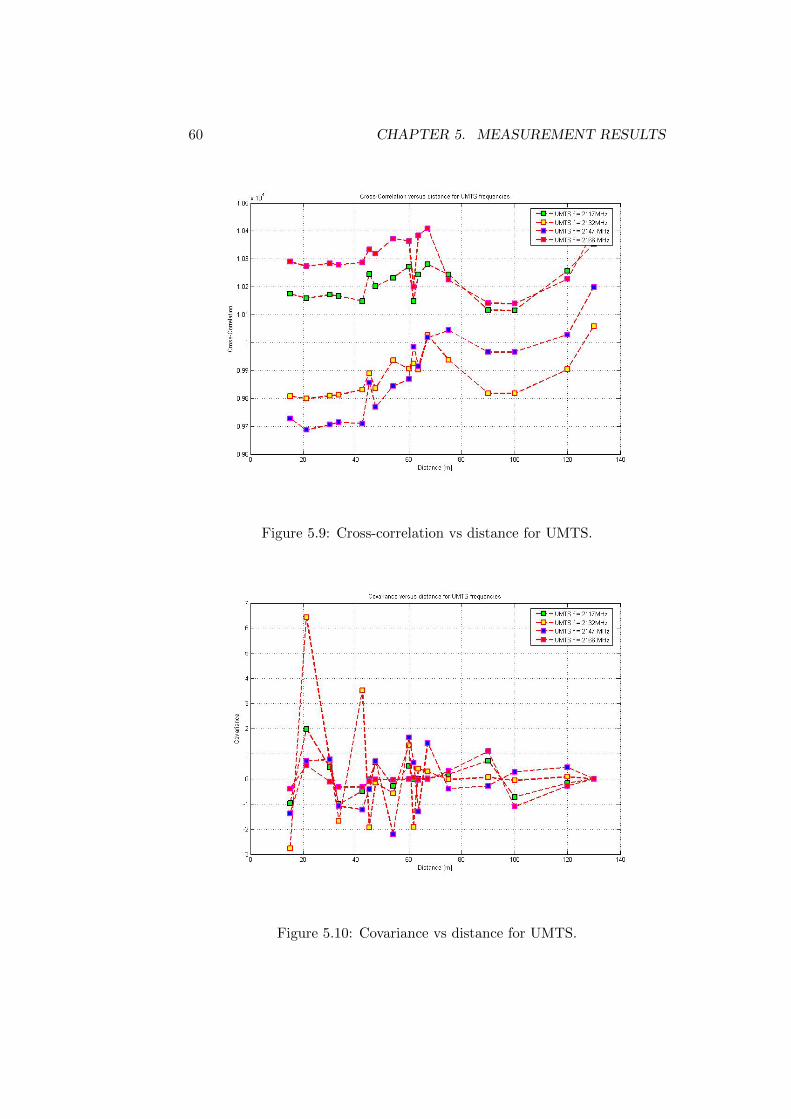
60 CHAPTER 5. MEASUREMENT RESULTS
Figure 5.9: Cross-correlation vs distance for UMTS.
Figure 5.10: Covariance vs distance for UMTS.
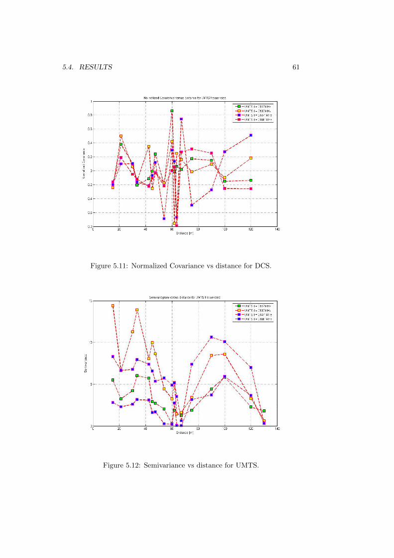
5.4. RESULTS 61
Figure 5.11: Normalized Covariance vs distance for DCS.
Figure 5.12: Semivariance vs distance for UMTS.
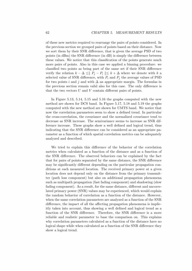
62 CHAPTER 5. MEASUREMENT RESULTS
of these new metrics required to rearrange the pairs of points considered. Inthe previous section we grouped pairs of points based on their distance. Nowwe sort them by their SNR difference, that is given the average PSD of twopoints (in dBm) the SNR difference (in dB) is simply the difference betweenthese values. We notice that this classification of the points generate muchmore pairs of points. Also in this case we applied a binning procedure: weclassified two points as being part of the same set if their SNR differenceverify the relation k − ∆ ≤‖ Pj − Pi ‖≤ k + ∆ where we denote with k aselected value of SNR difference, with Pi and Pj the average values of PSDfor two points i and j and with ∆ an appropriate margin. The formulas inthe previous section remain valid also for this case. The only difference isthat the two vectors U and V contain different pairs of points.
In Figure 5.13, 5.14, 5.15 and 5.16 the graphs computed with the newmethod are shown for DCS band. In Figure 5.17, 5.18 and 5.19 the graphscomputed with the new method are shown for UMTS band. We notice thatnow the correlation parameters seem to show a defined trend. In particularthe cross-correlation, the covariance and the normalized covariance tend todecrease as SNR increase. The semivariance seems to increase as SNR dif-ference increase. These graphs show a well defined and logical trend, thusindicating that the SNR difference can be considered as an appropriate pa-rameter as a function of which spatial correlation metrics can be adequatelyanalyzed and described.
We tried to explain this difference of the behavior of the correlationmetrics when calculated as a function of the distance and as a function ofthe SNR difference. The observed behaviors can be explained by the factthat for pairs of points separated by the same distance, the SNR differencemay be significantly different depending on the particular propagation con-ditions at each measured location. The received primary power at a givenlocation does not depend only on the distance from the primary transmit-ter (path loss component) but also on additional propagation phenomenasuch as multipath propagation (fast fading component) and shadowing (slowfading component). As a result, for the same distance, different and uncorre-lated primary power (SNR) values may be experienced, which would explainthe random behavior of correlation as a function of the distance. However,when the same correlation parameters are analyzed as a function of the SNRdifference, the impact of all the affecting propagation phenomena is implic-itly taken into account, thus showing a well defined and logical trend as afunction of the SNR difference. Therefore, the SNR difference is a morereliable and realistic parameter to base the comparison on. This explainswhy correlation parameters calculated as a function of the distance have nological shape while when calculated as a function of the SNR difference theyshow a logical trend.
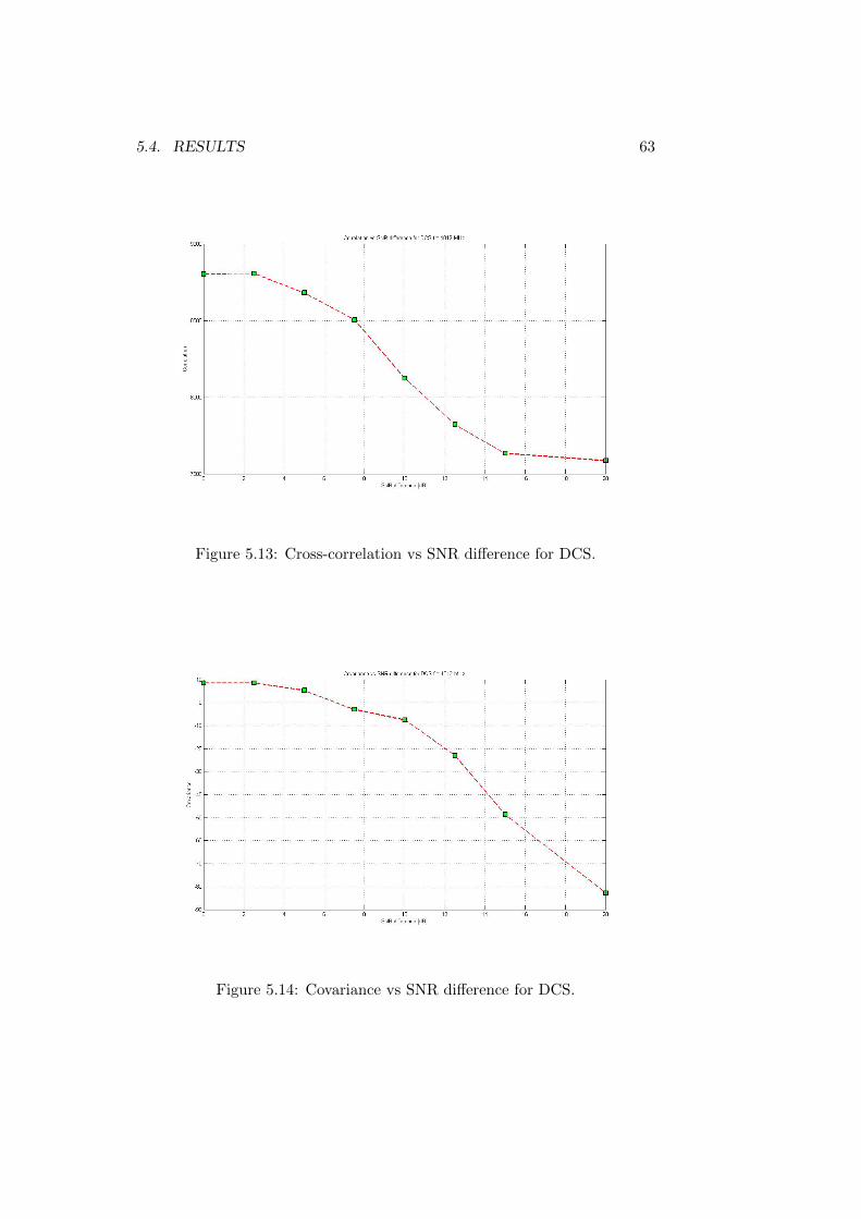
5.4. RESULTS 63
Figure 5.13: Cross-correlation vs SNR difference for DCS.
Figure 5.14: Covariance vs SNR difference for DCS.

64 CHAPTER 5. MEASUREMENT RESULTS
Figure 5.15: Normalized covariance vs SNR difference for DCS.
Figure 5.16: Semivariance vs SNR difference for DCS.
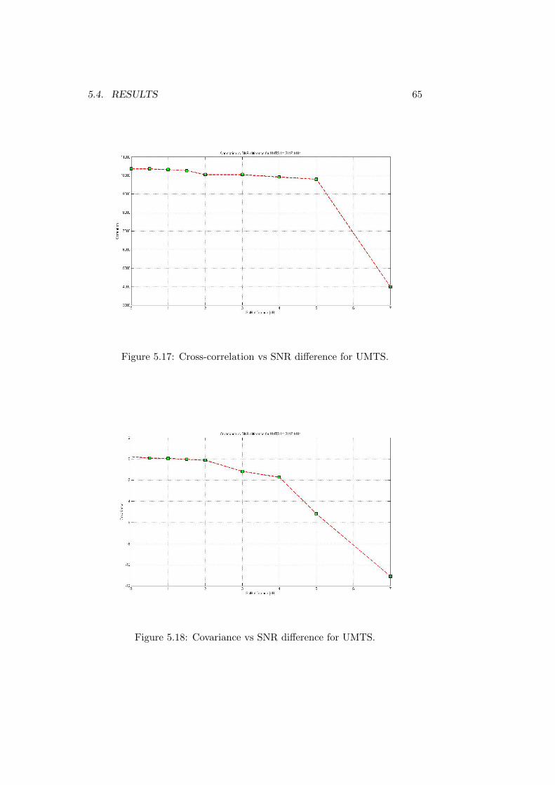
5.4. RESULTS 65
Figure 5.17: Cross-correlation vs SNR difference for UMTS.
Figure 5.18: Covariance vs SNR difference for UMTS.
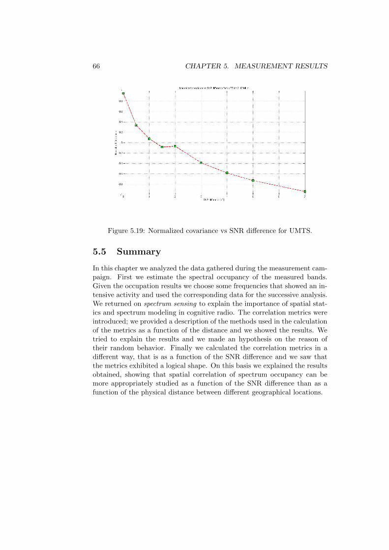
66 CHAPTER 5. MEASUREMENT RESULTS
Figure 5.19: Normalized covariance vs SNR difference for UMTS.
5.5 Summary
In this chapter we analyzed the data gathered during the measurement cam-paign. First we estimate the spectral occupancy of the measured bands.Given the occupation results we choose some frequencies that showed an in-tensive activity and used the corresponding data for the successive analysis.We returned on spectrum sensing to explain the importance of spatial stat-ics and spectrum modeling in cognitive radio. The correlation metrics wereintroduced; we provided a description of the methods used in the calculationof the metrics as a function of the distance and we showed the results. Wetried to explain the results and we made an hypothesis on the reason oftheir random behavior. Finally we calculated the correlation metrics in adifferent way, that is as a function of the SNR difference and we saw thatthe metrics exhibited a logical shape. On this basis we explained the resultsobtained, showing that spatial correlation of spectrum occupancy can bemore appropriately studied as a function of the SNR difference than as afunction of the physical distance between different geographical locations.
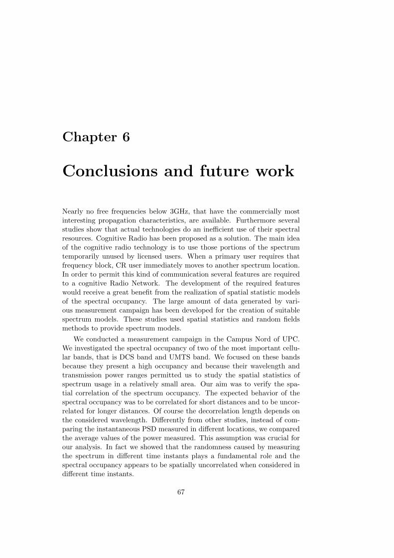
Chapter 6
Conclusions and future work
Nearly no free frequencies below 3GHz, that have the commercially mostinteresting propagation characteristics, are available. Furthermore severalstudies show that actual technologies do an inefficient use of their spectralresources. Cognitive Radio has been proposed as a solution. The main ideaof the cognitive radio technology is to use those portions of the spectrumtemporarily unused by licensed users. When a primary user requires thatfrequency block, CR user immediately moves to another spectrum location.In order to permit this kind of communication several features are requiredto a cognitive Radio Network. The development of the required featureswould receive a great benefit from the realization of spatial statistic modelsof the spectral occupancy. The large amount of data generated by vari-ous measurement campaign has been developed for the creation of suitablespectrum models. These studies used spatial statistics and random fieldsmethods to provide spectrum models.
We conducted a measurement campaign in the Campus Nord of UPC.We investigated the spectral occupancy of two of the most important cellu-lar bands, that is DCS band and UMTS band. We focused on these bandsbecause they present a high occupancy and because their wavelength andtransmission power ranges permitted us to study the spatial statistics ofspectrum usage in a relatively small area. Our aim was to verify the spa-tial correlation of the spectrum occupancy. The expected behavior of thespectral occupancy was to be correlated for short distances and to be uncor-related for longer distances. Of course the decorrelation length depends onthe considered wavelength. Differently from other studies, instead of com-paring the instantaneous PSD measured in different locations, we comparedthe average values of the power measured. This assumption was crucial forour analysis. In fact we showed that the randomness caused by measuringthe spectrum in different time instants plays a fundamental role and thespectral occupancy appears to be spatially uncorrelated when considered indifferent time instants.
67

68 CHAPTER 6. CONCLUSIONS AND FUTURE WORK
We showed that a more reliable parameter on which base a statisticalanalysis of the spectral occupancy, when not considering the instant values,could be the SNR difference. In fact when we consider the distance as anevaluating parameter, in the time between two measurements, very differ-ent propagation conditions could be present; this cause the spectrum to beuncorrelated over the distance. The received power depends instead on theSNR in the measurement location, which also depends on the distance, butnot in a linear manner because of the great variability of the propagationconditions. This conclusion was supported by the results of the correlationmetrics calculated as a functions of the SNR difference, which showed a welldefined trend, as we expected, thus indicating that the spatial correlationcharacteristics of spectrum occupancy in the context of DSA/CR can bemore appropriately analyzed and characterized in terms of the SNR differ-ence, instead of in terms of the distance between different locations as it hasbeen considered in previous studies on spatial correlation.
Bibliography
[1] A-Info. Test Report for JXTXPZ-100800/P.http://www.ainfoinc.com/en/pro_pdf/new_products/antenna/.
[2] I.F. Akyildiz, W.-Y. Lee, M.C. Vuran, and S. Mohanty. Next gener-ation/dynamic spectrum access/cognitive radio wireless networks: Asurvey.
[3] I.F. Akyildiz, W.-Y. Lee, M.C. Vuran, and S. Mohanty. A survey onspectrum management in cognitive radio networks.
[4] Anritsu. Spectrum Master MS2721B, MS2723B, and MS2724B User’sGuide. http://www.anritsu.com/.
[5] V.R. Petty et al. Feasibility of dynamic spectrum access in underutilizedtelevision bands.
[6] M. Lopez-Benitez, A. Umbert, and F. Casadevall. Evaluation of spec-trum occupancy in spain for cognitive radio applications.
[7] AOR Ltd. DA753G Compact Discone Aerial.http://www.aoruk.com/pdf/da753g_leaflet.pdf.
[8] Mini-Circuits. Amplifier ZX60-8008E+.http://www.minicircuits.com/.
[9] Mini-Circuits. Coaxial Adapter N-F to SMA-M NF-SM50+.http://www.minicircuits.com/.
[10] Mini-Circuits. Coaxial Low-Pass Filter VLF-3000.http://www.minicircuits.com/.
[11] Mini-Circuits. Connectorized Band-Stop Filter NSBP-108+.http://www.minicircuits.com/.
[12] Mini-Circuits. SPDT Switch MSP2T-18.http://www.minicircuits.com/.
[13] Mini-Circuits. Test Cable CBL-1.5FT-SMSM+.http://www.minicircuits.com/.
69
70 BIBLIOGRAPHY
[14] Mini-Circuits. Test Cable CBL-6FT-SMNM+.http://www.minicircuits.com/.
[15] Mini-Circuits. Test Cable CBL-6FT-SMSM+.http://www.minicircuits.com/.
[16] Mini-Circuits. Test Cable RG-58A/U.http://www.minicircuits.com/.
[17] Mini-Circuits. Ultra Reliable High-Pass Filter VHP-26.http://www.minicircuits.com/.
[18] J. Riihijarvi, P. Mahonen, M. Wellens, and M. Gordziel. Character-ization and modelling of spectrum for dynamic spectrum access withspatial statistics and random fields.
[19] Agilent Technology. Spectrum Analysis Basics.http://cp.literature.agilent.com/litweb/pdf/5952-0292.pdf.
[20] M. Wellens, J. Riihijarvi, M. Gordziel, and P. Mahonen. Evaluation ofcooperative spectrum sensing based on large scale measurements.
[21] M. Wellens, J. Wu, and P. Mahonen. Evaluation of spectrum occupancyin indoor and outdoor scenario in the context of cognitive radio.
[22] B. Wild and K. Ramchandran. Detecting primary receivers for cognitiveradio applications.