Alma Mater Studiorum – Università di Bologna

DOTTORATO DI RICERCA IN

Scienze Ambientali: Tutela e Gestione Delle Risorse Naturali

Ciclo XXVI

Settore Concorsuale di afferenza: 03/A1 – CHIMICA ANALITICA

Settore Scientifico disciplinare: CHIM/12 - CHIMICA DELL’AMBIENTE E DEI

BENI CULTURALI

TITOLO TESI

CHEMISTRY OF AEROSOL PARTICLES AND FOG

DROPLETS DURING FALL - WINTER SEASON IN THE PO VALLEY

Presentata da: Dott.ssa Lara Giulianelli

Coordinatore Dottorato

Prof. Enrico Dinelli Tutore Relatore

Prof. Emilio Tagliavini Dott.ssa M. Cristina Facchini

Esame finale anno 2014

i 

 

Summary 

Abstract ...................................................................................................................................... 1 

1. Introduction ............................................................................................................................ 3 

1.1 Tropospheric aerosol ........................................................................................................ 3 

1.1.1 Aerosol size distribution ............................................................................................. 4 

1.1.2 Aerosol sources and chemical composition ............................................................... 5 

1.2 Fog ..................................................................................................................................... 7 

1.2.1 Fog formation ............................................................................................................. 7 

1.2.2 Fog chemical composition .......................................................................................... 9 

1.3 Aerosol/clouds interactions ............................................................................................ 11 

1.3.1 Effects of aerosol on cloud properties ..................................................................... 11 

1.3.2 Effects of clouds on aerosol composition and lifecycle ........................................... 12 

1.4 Fogs in polluted environments ....................................................................................... 14 

1.5 Aerosol composition in wintertime in continental areas ............................................... 15 

1.6 Air quality and fogs in the Po Valley, Italy ...................................................................... 16 

2. Experimental setup .............................................................................................................. 21 

2.1 Sampling sites ................................................................................................................. 21 

2.2 Aerosol sampling ............................................................................................................. 22 

2.3 Fog sampling ................................................................................................................... 24 

2.4 Analytical methods ......................................................................................................... 25 

2.4.1 Sample handling ....................................................................................................... 25 

2.4.2 Ion Chromatography ................................................................................................. 27 

2.4.3 Water‐soluble organic carbon (WSOC) .................................................................... 28 

2.4.4 Total Carbon (TC) ...................................................................................................... 28 

ii 

 

2.4.5  WSOC  characterization  by  Proton  Nuclear  Magnetic  Resonance  (1H‐NMR) 

spectroscopy ...................................................................................................................... 29 

2.4.6 On‐line aerosol chemical characterization ............................................................... 29 

2.4.7 Evaluation of the random uncertainties associated to the measurements ............. 30 

3. Aerosol chemical composition in the Po Valley ................................................................... 33 

3.1 November 2011 field campaign ...................................................................................... 34 

3.2 February 2013 field campaign ........................................................................................ 37 

3.3 Size segregated chemical characterization of aerosol particles ..................................... 40 

4. Fog chemical composition in the Po Valley .......................................................................... 49 

4.1 Fog frequency ................................................................................................................. 49 

4.2 Chemical composition of fog droplets ............................................................................ 52 

4.3 Liquid water content (LWC) ............................................................................................ 60 

4.4 Fog water acidity ............................................................................................................. 62 

4.5 Organic fraction of fog droplets ...................................................................................... 64 

5. Aerosol – fog interaction ...................................................................................................... 69 

5.1 Fog scavenging ................................................................................................................ 70 

5.1.1 Influence of fog on aerosol mass size distribution ................................................... 71 

5.1.2 Influence of fog on aerosol chemical composition .................................................. 77 

5.2 Organic fraction of aerosol particles and fog droplets ................................................... 80 

5.3 High time resolution characterization of a nocturnal fog episode ................................. 85 

6. Conclusions ........................................................................................................................... 91 

Acknowledgments .................................................................................................................... 95 

Bibliography .............................................................................................................................. 97 

List of frequently used abbreviations..................................................................................... 111 

 

 

1 

 

Abstract 

Air quality represents a key issue in the so‐called pollution “hot spots”: environments in which 

anthropogenic sources are concentrated and dispersion of pollutants is limited. One of these 

environments,  the  Po  Valley,  normally  experiences  exceedances  of  PM10  and  PM2.5 

concentration  limits,  especially  in winter when  the  ventilation  of  the  lower  layers  of  the 

atmosphere is reduced. 

This  thesis  provides  a  highlight  of  the  chemical  properties  of  particulate matter  and  fog 

droplets in the Po Valley during the cold season, when fog occurrence is very frequent. Fog‐

particles interactions were investigated with the aim to determine their impact on the regional 

air quality. 

Size‐segregated  aerosol  samples  were  collected  in  Bologna,  urban  site,  and  San  Pietro 

Capofiume  (SPC), rural site, during two campaigns  (November 2011; February 2013)  in the 

frame of Supersito project. The comparison between particles size‐distribution and chemical 

composition in both sites showed the relevant contribution of the regional background and 

secondary processes in determining the Po Valley aerosol concentration. 

Occurrence of fog in November 2011 campaign in SPC allowed to investigate the role of fog 

formation and fog chemistry in the formation, processing and deposition of PM10. Nucleation 

scavenging  was  investigated  with  relation  to  the  size  and  the  chemical  composition  of 

particles. We found that PM1 concentration is reduced up to 60% because of fog scavenging. 

Furthermore,  aqueous‐phase  secondary  aerosol  formation mechanisms were  investigated 

through time‐resolved measurements. 

In SPC fog samples have been systematically collected and analysed since the nineties; a 20 

years long database has been assembled. This thesis reports for the first time the results of 

this  long  time  series  of  measurements,  showing  a  decrease  of  sulphate  and  nitrate 

concentration  and  an  increase  of  pH  that  reached  values  close  to  neutrality.  A  detailed 

discussion  about  the  occurred  changes  in  fog  water  composition  over  two  decades  is 

presented. 

 

 

2 

 

 

Papers on the international refereed literature originating from this thesis: 

 

Gilardoni, S., Massoli, P., Giulianelli, L., Rinaldi, M., Paglione, M., Pollini, F., Lanconelli, 

C., Poluzzi, V., Carbone,  S., Hillamo, R., Russell,  L. M.,  Facchini, M. C.  and  Fuzzi,  S. 

(2014). Fog Scavenging of Organic and Inorganic Aerosol in the Po Valley. Atmospheric 

Chemistry and Physics Discussion 14, 4787‐4826. 

 

Giulianelli L., Tarozzi L., Gilardoni S., Rinaldi M., Decesari S., Carbone C., Facchini M.C., 

Fuzzi S. Fog occurrence and chemical composition in the Po Valley over the last twenty 

years (to be submitted). 

 

3 

 

1. Introduction 

 

Air pollution represents a real threat to human health in Europe. Air quality is a key issue of 

the European environmental policy to guarantee a sufficient  level of protection against air 

pollutants, such as particulate matter, whose harmful effect has been reported in numerous 

recent studies (Brunekreef, 2013; Fuzzi and Gilardoni, 2013). 

This doctoral thesis set the objective to highlight the properties of particulate matter and fog 

droplets in fall and winter in the Po Valley, where fog occurrence is very frequent during the 

cold season. The interactions between particles and fog droplets will be also investigated with 

the aim to determine their impact on the air quality of this region. 

The  following  sections will  introduce  the  general  definitions  of  aerosol  particles  and  fog 

droplets as well as a brief illustration of their physical and chemical properties. Sections 1.4 

and 1.5 will describe the specific field of this study and its principal purposes. 

 

1.1 Tropospheric aerosol 

An aerosol is properly defined as a suspension of fine solid or liquid particles in a gas, even 

though in atmospheric science common usage refers to the aerosol as the solid or deliquesced 

(concentrated liquid) particulate component only, while specific terms are used for the liquid 

or ice particles in fogs and clouds (droplets, drops, crystals, hydrometeors etc.) (Seinfeld and 

Pandis, 1998). 

Atmospheric aerosol particles consist of a large variety of species, arising from natural sources 

such as volcanoes, sea spray, plant evapotranspiration or soil erosion and from anthropogenic 

activities like agricultural practises, industrial and combustion processes. 

Particulate matter can be classified also as primary and secondary aerosol. Primary particles 

are directly emitted  into  the atmosphere,  from sources such as  incomplete combustion of 

fossil  fuels, biomass burning, mechanical erosion of dry  soils,  resuspension of particles by 

vehicular  traffic,  sea  spray,  volcanic  eruptions  and  biological  debris  (pollen,  spores,  plant 

fragments,  etc.).  By  contrast,  secondary  particles  are  formed  in  the  atmosphere  by  the 

4 

 

transformation  of  reactive  gases  into  particulate matter  through  chemical  reactions  and 

condensation processes (gas‐to‐particle conversion). 

Particles are removed  from the atmosphere by gravitational settling and diffusion to Earth 

surfaces  (dry  deposition)  and  by  incorporation  of  particles  into  cloud  droplets  during  the 

formation of precipitation  (wet deposition).  These  removal mechanisms  lead  to  relatively 

short residence times of aerosol particles in the troposphere, ranging from a few hours to a 

couple of weeks. Due to their short residence times and to the non‐homogeneous distribution 

of  the  sources,  tropospheric  aerosols  composition  and  concentration  are  temporally  and 

spatially highly variable. 

 

1.1.1 Aerosol size distribution 

The aerodynamic diameter (Da) is usually used in order to classify particles according to their 

size. It is defined as the diameter of a spherical particle with density = 1 g cm‐3 having the same 

gravitational settling velocity as the particle in question. 

The atmospheric aerosol particles size distribution ranges from a few nanometres to about a 

hundred micrometres,  even  if  particles with  aerodynamic  diameters  smaller  than  10  μm 

account  for  most  of  the  total  aerosol  particles  (on  both  number  and  mass  basis).  The 

atmospheric aerosol size distribution  is characterized by modes, corresponding to different 

populations of particles, classified as nucleation (Da < 0.01 μm), Aitken mode (0.01 µm < Da < 

0.1 μm); accumulation (0. 1 μm < Da < 1 μm) and coarse mode (Da > 1 μm) (Fig.1.1). The first 

three modes, that is particles with Da < 1 µm, are also referred to as fine aerosol. 

A  fundamental distinction between  fine and coarse aerosol has  to be  found  in  the  source 

mechanisms of particles production. For this reason, the experimental work of this thesis is 

discussed separating particles according to their size. 

Coarse particles are  formed mainly by mechanical processes  such as dust  suspension and 

resuspension, and sea spray. They never account for more than a few percent of the particles 

by number concentration, even if they can account for a large fraction of particulate mass. 

5 

 

 

Figure 1.1: ideal size distribution with their four principal modes. The diagram also shows the main mechanisms 

of formation of particles acting in the various size ranges. 

 

 

Fine  particles  are  mainly  produced  by  combustion  processes  (open  burning,  vehicular 

emissions, etc.) and by secondary processes such as gas‐to‐particle conversion mechanisms. 

More  in detail, the nucleation mode arises from nucleation of new particles from rapid gas 

condensation, the Aitken mode results from condensation of vapours onto nucleation mode 

particles and from their coagulation, as well as from primary combustion emissions. Finally, 

the  accumulation  mode  particles  usually  form  from  prolonged  (several  hours  to  days) 

condensation of vapours on Aitken particles and from the formation of particles by chemical 

reactions in non‐precipitating cloud droplets. 

 

1.1.2 Aerosol sources and chemical composition 

Due to the relative low residence time in atmosphere, tropospheric aerosol exhibits a chemical 

composition characterized by a great spatial and temporal variability, reflecting the variety of 

6 

 

sources,  transformation, and  removal processes. That  is why  the  chemical  composition of 

tropospheric aerosol is usually referred to a specific environment and size interval. 

In general, aerosol particles consist of complex mixtures of inorganic water‐soluble salts such 

as  sulphates,  nitrates,  ammonium  salts  and  sea  salt,  soluble  and  insoluble  carbonaceous 

material  (organic  species,  black  carbon,  carbonates)  and  insoluble  inorganic  compounds 

including mineral soil particles and combustion ash. 

The submicron inorganic mass fraction is prevalently composed by species derived from gas‐

to‐particle conversion processes, as in the case of sulphate, produced in the atmosphere by 

the oxidation of sulphur dioxide (SO2). Sulphuric acid (H2SO4) produced by the oxidation of SO2 

can  further  react with  ammonia  (NH3)  to  produce  ammonium  bisulphate  (NH4HSO4)  and 

ammonium sulphate (NH4)2SO4 (Hazi et al., 2003). 

Similarly, nitrogen oxides (NOx) are oxidized in the atmosphere to nitric acid (HNO3) which can 

form both non‐volatile and semivolatile salts in the aerosol phase. Most common semivolatile 

nitrate salts, such as NH4NO3, exist in the troposphere in a dynamic equilibrium with the gas 

phase precursors and  the actual partitioning between  the gas and  the aerosol phases can 

change continuously following the diurnal cycle of temperature and relative humidity. Since 

the fine fraction of the aerosol is more rich in acidic species (e.g., ammonium bisulfate) than 

the coarse fraction where conversely alkaline species may occur (sea salt, calcium carbonate), 

nitric acid often partitions efficiently into coarse particles. 

Organic compounds are produced by both anthropogenic and natural sources (Fuzzi, et al., 

2006) and represent a relevant fraction of atmospheric fine particles, accounting for 20‐90% 

of aerosol mass in the lower troposphere (Kanakidou et al., 2005). In the fine fraction, organic 

aerosol  originates  either  from  primary  emissions  due  to  combustion  processes  at  high 

temperature, or from the oxidation of volatile organic compounds (VOC) and gas‐to‐particle 

conversion mechanisms (Kroll and Seinfeld, 2008; Zhang et al., 2007). In the coarse fraction, it 

can result also from biological debris (Jaenicke, 2005). 

Black carbon (BC) accounts for insoluble carbonaceous material showing absorbance across 

all  the  spectrum  of  visible  light.  It  overlaps  with  the  so  called  elemental  carbon  (EC), 

characterized  by  very  low  hydrogen  and  oxygen  contents,  and  which  is  refractory  at 

temperatures below 350 °C. BC in the fine fraction is typically emitted by high‐temperature 

7 

 

combustion processes (traffic, open combustion, etc.). In the coarse mode, BC can originate 

by resuspended dust containing soot. 

Sea salt mass is mainly distributed in the coarse fraction and is produced by the mechanical 

mechanisms at the sea surface (breaking waves and whitecaps) (Blanchard, 1983). 

Mineral  dust  is  produced  by  natural weathering  processes,  and  is  enriched  in  the  coarse 

aerosol mode. 

 

1.2 Fog 

Fog is physically a cloud that forms close to the ground or in contact with it and is associated 

with visibility lower than 1km.  Fogs are classified according to their formation process. Some 

continental areas, such as the Po Valley, are usually affected in the cold season by phenomena 

named  “radiation  fogs”.  This  type  of  fog  forms  at  night  under  clear  sky  and  stagnant  air 

conditions. Nightly,  heat  absorbed  by  the  earth  during  the  day  is  radiated  back  to  space 

cooling the air close to the surface. In presence of moisture, humidity will soon reach 100% 

allowing condensation and fog to occur. 

Another type of fog  is advection fog.  It  is also the result of condensation, but occurs when 

warm moist  air passes over  a  cold  surface  and  is  cooled  down  to  the dew point.  Typical 

examples are sea fogs that form when warm air drifts over a cool oceanic current. Advection 

fog may also form when moist maritime air drifts over a cold inland area. Other types of fog 

are upslope fog, ice fog, evaporation fog, but a detailed description of their characteristics is 

beyond the purpose if this thesis. 

 

1.2.1 Fog formation 

Fog droplets, as well as clouds, are formed in the atmosphere by the condensation of water 

vapour on aerosol particles when the relative humidity (RH) exceeds 100% and a slight degree 

of  supersaturation  (typically  1%)  is achieved. Not all particles will grow  to  real droplets. 

Particles that enable droplets to form at supersaturation levels found in the atmosphere are 

called cloud condensation nuclei (CCN). 

8 

 

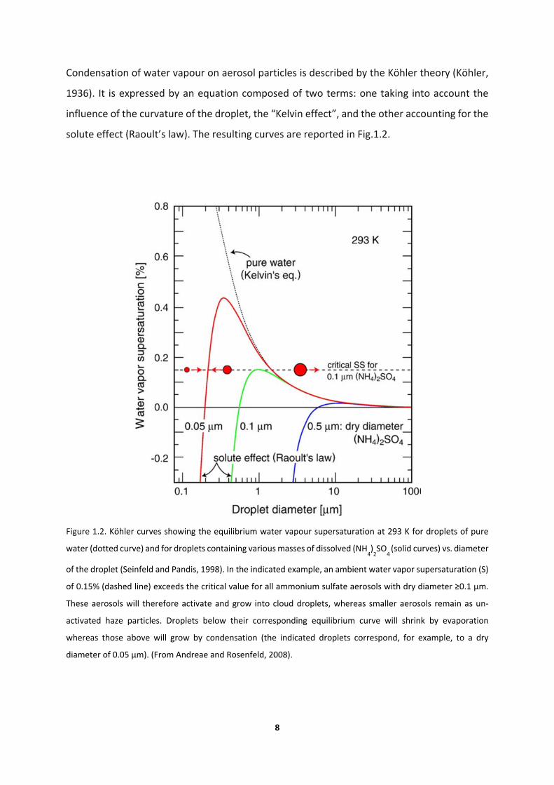
Condensation of water vapour on aerosol particles is described by the Köhler theory (Köhler, 

1936).  It  is expressed by an equation composed of two terms: one taking  into account the 

influence of the curvature of the droplet, the “Kelvin effect”, and the other accounting for the 

solute effect (Raoult’s law). The resulting curves are reported in Fig.1.2. 

 

 

 

Figure 1.2. Köhler curves showing the equilibrium water vapour supersaturation at 293 K for droplets of pure 

water (dotted curve) and for droplets containing various masses of dissolved (NH4)2SO

4 (solid curves) vs. diameter 

of the droplet (Seinfeld and Pandis, 1998). In the indicated example, an ambient water vapor supersaturation (S) 

of 0.15% (dashed line) exceeds the critical value for all ammonium sulfate aerosols with dry diameter ≥0.1 μm. 

These aerosols will  therefore activate and grow  into cloud droplets, whereas smaller aerosols  remain as un‐

activated  haze  particles.  Droplets  below  their  corresponding  equilibrium  curve  will  shrink  by  evaporation 

whereas  those  above will  grow  by  condensation  (the  indicated  droplets  correspond,  for  example,  to  a  dry 

diameter of 0.05 μm). (From Andreae and Rosenfeld, 2008). 

 

9 

 

With increasing RH, the particle will absorb water and grow until saturation is reached. If the 

air becomes enough supersaturated to enable the particle to reach a diameter  just beyond 

the maximum (critical supersaturation), the particle enters a region of instability and grows 

continuously limited only by the availability of water vapour and by the kinetic of diffusion: 

the particle has been activated to a real cloud (or fog) droplet. The supersaturation required 

for aerosol activation depends on  the  size and  the composition of  the particle. As a  large 

amount  of  the  supersaturated water  vapour  concentration  is  used  for  the  growth  of  the 

droplets originated by  the  first‐nucleated particles,  the  supersaturation  level will decrease 

rapidly unless it is compensated by the cooling rate. Particles which have not yet grown above 

their critical diameter will then re‐evaporate to dimensions where the Raoult effect prevails 

over the Kelvin term and the aerosol liquid water content is in equilibrium with the ambient 

RH. The non‐activated particles form the so‐called “interstitial aerosol”. Large sizes and large 

water solubility correspond to lower critical supersaturations that is a better attitude for the 

particles to act as CCN. Since ambient aerosols are very often polydisperse with respect to size 

and composition, nucleation scavenging is a very selective process, and only a fraction of the 

total number of aerosol particles present in the air is able to serve as CCN (Arends, 1996; Fuzzi, 

1994). 

 

1.2.2 Fog chemical composition 

The initial composition of fog droplets depends mainly on the nature of the particles that acted 

as CCN. During the fog lifetime, many concurrent physical and chemical processes take place 

that will cause change in the fog droplets composition, such as the dissolution of trace gases 

into droplets, chemical reactions within  fog droplets and the capture of  interstitial aerosol 

particles by droplets, although this is expected to be of minor importance (Fuzzi et al., 2002). 

Fog  chemical  composition  reflects  the  chemical  properties  of  the  air  in  which  it  forms, 

therefore is highly variable in time and space. In general, the major compounds of fog droplets 

are  soluble  inorganic  species  like  sulphate  (SO42‐), nitrate  (NO3

‐), chloride  (Cl‐), ammonium 

(NH4+),  sodium  (Na+),  potassium  (K+), magnesium  (Mg2+)  and  calcium  (Ca2+).  Sodium  and 

chloride are major compounds especially in marine areas, because sea‐salt particles are very 

efficient CCN. Also the presence of K+, Ca2+ and Mg2+ ions can originate from marine sources 

10 

 

(Keene et al., 1986), but  it mostly depends on  the mineral component of aerosol particles 

originating  from  soil  dust.  NH4+,  NO3

‐  and  SO42‐  derive  both  from  the  incorporation  of 

atmospheric aerosol and from the scavenging of gaseous ammonia (NH3), nitric acid (HNO3) 

and sulphur dioxide (SO2). H2SO4 and HNO3 produced from the oxidation of SO2 and NOx are 

the dominant strong acids in fog water, while NH3 is the only alkaline gaseous species in the 

atmosphere. NH3 is therefore the main buffering agent of fog acidity. The balance between 

acid  and  basic  components  scavenged  from  the  air  or  produced  within  the  droplets 

determines the actual pH of fog water (Fuzzi, 1994). However, since the Henry coefficients of 

nitric acid and of sulphuric acid are much greater than that of ammonia, alkaline pH are rarely 

found in fog water, while strong acidic pH values have been recorded in some polluted areas 

(Fuzzi et al., 1985; Hileman, 1983). 

Although  inorganic  ions account  for the major  fraction of  fog water chemical components, 

organic matter concentrations are by no means negligible, accounting for up to more than 

30%  of  the  total  solute mass  (Fuzzi  et  al.,  2002).  Organic  concentrations  show  a  great 

variability depending on the environment, as shown in Fig.1.3. As expected, the highest values 

are found in polluted urbanized areas and the lowest in marine fogs. However, organic matter 

concentrations can be fairly high also at continental rural sites because of the scavenging of 

biogenic organic particles and gases (Herckes et al., 2013). 

It should be noticed that, contrary to the chemistry of fog inorganic constituents is relatively 

well known, especially in respect to the species involved in the acid‐base equilibria, the current 

knowledge of fog organic components is based on a rather sparse literature (Herckes et al., 

2013). In our study, we will present one of the longest measurement record of fog dissolved 

organic carbon concentrations currently available. 

 

 

11 

 

 

Figure 1.3. Dissolved organic carbon (DOC) mg C/L concentrations reported for fogs and ground based clouds. 

Bars represent average values, while the error bars represent the range of observations (min–max). Absence of 

a solid bar means no average/median was provided. Marine clouds and fogs are depicted in blue, hill or mountain 

intercepted clouds in green (except if heavily marine influenced, then in dark blue), radiation fogs or polluted 

urban fogs in grey (Herckes et al., 2013). 

 

 

1.3 Aerosol/clouds interactions 

1.3.1 Effects of aerosol on cloud properties 

For a given cloud liquid water content and cloud depth, an increase in aerosol particle number 

concentration (hence in CCN) leads to an increase in cloud droplet number concentration, and 

a concurrent reduction of droplet diameter, which can cause an increase of cloud albedo. Such 

effect is generally referred to as first indirect effect of aerosol on climate. The increase in cloud 

albedo would lead to cooling and partially counteract the warming due to greenhouse gases. 

A  second  indirect  effect  of  aerosol  particles  concerns  the  increase  in  clouds  lifetime  and 

extent: for a given liquid water content, the increase in cloud droplet number concentration 

produces smaller droplets,  therefore  reducing  the probability  that droplets collide  to  form 

precipitating  droplets.  Since  precipitations  are  hindered,  cloud  lifetime  is  prolonged  and 

12 

 

clouds are more abundant. Additional feedback mechanisms potentially responsible for the 

uncertainty in the prediction of the indirect effects, include changes in precipitation regimes 

and in increases or decreases in cloud cover due to pollution and smoke aerosol (Kaufman and 

Koren, 2006; Rosenfeld et al., 2008). 

This indirect aerosol effect is presently considered the most uncertain of the known forcing 

mechanisms in the prediction of climate change over the industrial period. Due to the scales 

involved,  it  is  one  of  the major  challenges  in  understanding  and  predicting  the  indirect 

radiative effect of aerosols: while the effect itself is global, the processes causing it occur on 

spatial  scales as  small as micrometres and  temporal  scales as  short as  seconds. Thus,  the 

global‐scale  phenomenon  cannot  be  understood  and  predicted  quantitatively  without 

adequate understanding of the microscale processes. 

 

1.3.2 Effects of clouds on aerosol composition and lifecycle 

Nucleation  scavenging  is  the  process  by which  CCN  particles  activate  to  form  cloud/fog 

droplets. Once  the  droplet  are  formed,  interstitial  particles  can  be  incorporated  into  the 

droplet by  in‐cloud  scavenging due  to Brownian diffusion,  inertial  impaction  and phoretic 

effects, but their contribution in terms of mass is generally small (Flossmann et al., 1985). By 

contrast, gas absorption and chemical reactions in the aqueous phase can affect substantially 

the chemical composition of fog solutes. In‐cloud aqueous phase reactions play a major role 

in  the  atmospheric  cycling  of  many  trace  gases.  For  example,  gas  phase  SO2  oxidation 

reactions are much slower than corresponding reactions  in the  liquid phase  (Calvert et al., 

1986;  Hoffmann,  1986).  Eventually,  the  evaporation  of  cloud  and  fog  droplets  produces 

aerosol particles with different chemical and physical characteristics compared to the original 

particles, which acted as CCN for cloud/fog droplets. Such effects are generally referred to as 

cloud (or fog) processing. Since submicron aerosols account for the greatest fraction of CCN 

number concentrations, most of the material that  is produced by aqueous‐phase reactions 

increased fine particle mass (Collett et al., 1993; Fuzzi et al., 1992a; Wobrock et al., 1994). 

Since  the  eighties, many  studies  investigated  the  effects  of  cloud  processing  on  aerosol 

particles.  For  example,  (Laj  et  al.,  1997)  reported  a  significant  increase  in  sulphate 

concentration in an aerosol population passing through a cloud. The increase in sulphur (IV) 

13 

 

oxidation was promoted by the radicals produced by peroxides (H2O2) dissolved in the cloud 

droplets. Eventually, the uptake of NH3 from the gas phase  led to evaporating cloud drops 

forming  aerosol  particles  enriched  in  ammonium  sulphate.  Clearly,  by  modifying  the 

dimension of the particles and the content of soluble  inorganic salts, cloud processing can 

impact  the hygroscopic  properties of  the  aerosols,  and  consequently  their CCN  efficiency 

(Hallberg et al., 1992; Svenningsson et al., 1992). 

Clouds and fog also determine the residence time of particles in the atmosphere through “wet 

deposition” processes. It should be noticed that, beside the removal of aerosol particles via 

incorporation in raindrops, the deposition of fog and low‐level cloud droplets to the ground 

and  other  surfaces  can  also  occur  in  the  absence  of  precipitations.  This  process  is  often 

referred to as “occult deposition”  (Dollard et al., 1983). Deposition occurs both due to the 

settling of large droplets and to turbulent impaction on surfaces. This removal mechanism can 

be  relevant  in  certain  areas where  the  amount  of water  deposited  through  cloud water 

interception was  found  to  be  comparable  or  even  larger  than  the  amount  deposited  by 

precipitation. This is especially true in the case of forested mountain areas where vegetation 

is an efficient collector of cloud water. (Waldman and Hoffmann, 1987); (Fuzzi, 1994; Fuzzi et 

al., 1992a; Fuzzi et al., 1985). 

Fogs  and  clouds  cause  changes  in  airborne  particle  concentrations, with  different  effects 

depending on aerosol size distribution. During a fog cycle, big particles are more efficiently 

scavenged then the smaller ones, and, upon evaporation, their average size  is even greater 

than  the  original  one  because  of  the  accretion  caused  by  the  sulphates  and  the  other 

components formed by aqueous phase reactions. Consequently, fog cycles tend to generate 

bimodal  aerosol  size  distributions  by  exacerbating  the  difference  in  size  between  the  big 

particles  which  undergo  a  progressive  growth  and  the  smaller,  interstitial  particles,  left 

untouched. However, the growth of “droplet mode” particles is limited by the enhanced dry 

and wet deposition. In fact, depositional losses of aerosol particles are much more effective 

in the large size fraction of the aerosol distribution (Pandis et al., 1990). 

Finally,  (Fuzzi  et  al.,  1997a),  reported  the  influence  of  fog  on  biological  particles.  They 

observed an enrichment of the concentration of bacteria and yeasts in air in foggy conditions 

compared  to clear air conditions: acting as culture media  for viable particles,  fog droplets 

represent an atmospheric source of secondary biological aerosol particles. These findings are 

14 

 

relevant for the possibility of transmission of pathogenic airborne microorganisms and also 

for the possible impact on the atmospheric CCN population (Casareto et al., 1996). 

 

1.4 Fogs in polluted environments 

Many studies investigated the effects of aerosol‐clouds interactions and the related impacts 

on the ecosystems and human health (Fowler et al., 2009;  Isaksen et al., 2009). This thesis 

work wants  to  focus  the attention on aerosol  interactions with  fog droplets, which play a 

major role in the frame of air quality, being formed close to the Earth’s surface. 

The interest on fog and aerosol interaction began in the middle of the XX century (Houghton, 

1955), but raised in the eighties, after the discovery of the acid fog (Waldman et al., 1982). In 

those years, the research was mainly focused on fog and cloud acidification, especially in the 

industrialized  northern  hemisphere  (Barrie,  1985; Hoffmann,  1986; Munger  et  al.,  1983). 

Many  studies  investigated  the  deposition  processes  of  water  and  the  environmental 

consequences on interception of cloud‐borne solutes by vegetation (Fuzzi et al., 1985; Lovett, 

1984;  Schemenauer,  1986;  Waldman  et  al.,  1985).  Soon  it  became  clear  that  fogs  are 

characterized  by  a  much  higher  solute  concentration  compared  to  precipitations,  and 

therefore  understanding  the  chemistry  of  wet  depositions  is  particularly  important  in 

geographical regions characterized by high fog occurrence and high level of pollutants in the 

atmosphere.  

During the nineties, the research was extended to the investigation of aerosol processing by 

clouds  and  fog.  (Facchini  et  al.,  1999)  reported  a  study  regarding  the  highly  polluted 

environment of  the Po Valley  (Italy), where  they  showed how  fog  can  act  as  an  efficient 

separator  for  carbonaceous  species,  with  polar  water‐soluble  compounds  efficiently 

scavenged into fog, while water‐insoluble carbonaceous species preferentially remain in the 

interstitial particles. 

During the 2000s, the development of modern analytical techniques for trace‐level organic 

compound  determination  allowed  to  face  the  challenging  issue  of  the  chemical 

characterization of organic matter  in  cloud and  fog water. Specifically, many  studies have 

focused  on  the  formation  of  secondary  organic  aerosol  species  through  fog  and  cloud 

15 

 

processing of volatile organic precursors (Ervens et al., 2011; Herckes et al., 2013; Lim et al., 

2013; Tan et al., 2012). 

All these studies show how atmospheric pollutants are affected by the presence of fogs. The 

processes  responsible  for  the  formation  and  transformation  of  aerosol  constituents  and 

soluble trace gases must be studied in connection with the chemistry of cloud and fog water 

in  order  to  adopt  effective  pollution  abatement  strategies  at  the  regional  scale.  This  is 

particularly true for many continental areas at the mid‐latitudes, where air pollutants typically 

show peak concentrations in wintertime, when fogs occur. 

 

1.5 Aerosol composition in wintertime in continental areas 

Composition  and  concentration  of  aerosol  particles  change  from  place  to  place  and 

differences can occur from season to season within the same observation site. In this section, 

I  present  an  overview  of  field  studies  focusing  on  wintertime  aerosol  in  mid‐latitude 

continental areas, which is the type of aerosol we are interested in within this doctoral thesis, 

being it impacted by radiation fog occurrence to the greatest extent. 

In winter, high pressure conditions  in continental areas are characterised by  temperatures 

frequently dropping below the dew point, stagnant air and a reduced height of the Planetary 

Boundary  Layer  (PBL). Winter  season  is  the  period  in which  the most  serious  particulate 

matter (PM) pollution episodes (PM10 > 50 mg m‐3) occur. In these cases nitrate becomes the 

main contributor to PM10 and PM2.5 together with organic matter (OM) in sites affected by 

local  emissions.  Anthropogenic  sources  of  NOx  lead  to  the  formation  of  nitrate,  whose 

condensation  in  the particulate phase as NH4NO3  is  favoured  in cold conditions  (Ge et al., 

2012; Putaud et al., 2004; Watson and Chow, 2002). 

Organic aerosol (OA) is composed by both primary organic particulate (POA) and secondary 

organic particulate (SOA). Primary emission sources of OA in this period of the year include 

mainly vehicular traffic and domestic heating. Wood combustion as domestic heating can be 

the most  important  source  for particulate matter at  rural  location  (Puxbaum et al., 2007; 

Weimer et al., 2009). The transport of wood burning particles also  impact air quality  in the 

cities (Favez, et al., 2010). Contribution of ~20%, ~30% and ~40% of wood combustion to total 

16 

 

organic carbon were measured in in Vienna (Austria), Oslo (Norway) and Zürich (Switzerland), 

respectively (Caseiro et al., 2009); (Yttri et al., 2009) (Szidat et al., 2006). 

A revision of the European emission inventories for POA performed in the frame of the project 

EUCAARI (European Aerosol Cloud Climate and Air Quality Interactions) has shown that the 

emission of organic carbon in the fine fraction of aerosol particles in Europe is dominated by 

the  residential  combustion  of  wood  and  coal.  Transport  (diesel  use)  and  residential 

combustion also represent the largest sources of submicron elemental carbon (EC) (Kulmala 

et  al.,  2011).  Organic  aerosol  originating  from  biomass  burning  is  rich  in  carcinogenetic 

compounds, such as polycyclic aromatic hydrocarbons (Ge et al., 2012; Lewtas, 2007). It also 

has  a  significant  climate  impact,  representing  a  significant  source  of  light‐absorbing 

carbonaceous aerosols (Andreae and Gelencser, 2006).  

Even though in winter conditions most of OA is of primary origin, a non‐negligible amount of 

SOA can be produced. Low mixing height and stagnant conditions favour the accumulation of 

SOA  precursors  and  despite  the  low  photochemical  activity,  low  temperatures  and  high 

relative humidity favour the partitioning of the gaseous precursors to the particle phase (Chen 

et al., 2010; Ge et al., 2012).  In addition, the occurrence of  fog events  in cold season may 

enhance SOA production via aqueous‐phase reactions. (Ge et al., 2012) reported a positive 

correlation between SOA and sulphate, suggesting that aqueous‐phase reactions, which are 

known to regulate the production of sulphate, also affect the formation of organic particles. 

 

1.6 Air quality and fogs in the Po Valley, Italy 

The Po Valley is located in Northern Italy and represents the largest flat region of Italy and one 

of the most extended in the Mediterranean Europe. It is surrounded by mountains on three 

sides, the Alps in the North and West sides and the Apennines in the South, only the East side 

is delimited by the Adriatic Sea (Fig.1.4).  

 

17 

 

 

Figure 1.4. Satellite view of haze in the Po Valley (Credit: Jeff Schmaltz). MODIS NASA 

 

 

Together  with  the  Rhine‐Ruhr  (Germany),  the  region  has  been  included  into  the  list  of 

European “megacities”, owning megacity features (population  10 millions), even if it can be 

better described as an urban conglomeration rather than as a single metropolitan area. 

Po  Valley  is  the most  industrialised  area  of  the  peninsula  and  it  is  also  characterised  by 

intensive livestock and agricultural activities. The Po Valley suffers bad air quality conditions, 

with  frequent  exceedances  of  the  PM10  concentration  limits  in  the  cold  season, mainly 

because  of  the  strong  anthropogenic  sources  of  VOC  and  aerosols  and  of  the  adverse 

meteorological  conditions.  In  wintertime,  the  low  mixing  layer  heights  and  the  weak 

atmospheric circulation promote stagnation of air masses at the low altitudes, and does not 

allow to the pollutants to disperse in the atmosphere, favouring the development of critical 

pollution episodes. 

18 

 

For these reasons, despite the application of legislation pointed to air pollution control, the 

Po valley has been  identified as an area  in Europe where pollutant  levels are expected  to 

remain problematic in the years to come(Pernigotti et al., 2012). 

 

 

 

Figure 1.5. Loss in life expectancy (months) attributable to exposure to anthropogenic PM2.5 for year 2000 

emissions (Source: EC, IIASA). 

 

 

Air quality is therefore one of the most urgent and challenging problem to solve in this region, 

considering  the  consequences of pollution on people health  (Fig.1.5). Within  the  complex 

issue of air quality in the Po Valley, this thesis aims to strengthen the knowledge of processes 

involving  atmospheric  pollutants.  Among  these  processes,  interactions  between  aerosol 

particles and fog droplets play a relevant role in the Po Valley, because of the high frequency 

of fog events during the cold season. These interactions will be investigated in the following 

chapters, to better clarify their effects on air pollutants. 

19 

 

Furthermore, a long time series of data regarding fog chemical and physical properties will be 

presented in chapter 4. Long time series represent a useful tool to appreciate the effectiveness 

of the adopted environmental policy strategies. 

A more detailed scientific knowledge and a deeper comprehension of atmospheric chemistry 

and processes is fundamental to support the legislation in making effective choices pointed to 

the abatement of pollutants. 

 

21 

 

2. Experimental setup 

 

The present thesis work reports data from two field campaigns set up in the Po Valley during 

the fall‐winter season by CNR‐ISAC,  in collaboration with ARPA Emilia Romagna (within the 

Supersito project,  see chapter 3), with  the purpose of getting an  insight  into atmospheric 

particulate matter physico‐chemical properties. Data from routine sampling and analysis of 

Po Valley fog water, in the period November ‐ March, will be also presented and discussed. 

The Po Valley fog sampling and characterization activity has been carried out since the nineties 

and the results of this long‐term database will be also discussed in the following chapters. 

Sampling sites description and analytical protocols of both aerosol particles and fog droplets 

analysis will be reported in the following sections. 

 

2.1 Sampling sites 

Samples  have  been  collected  in  two  different  sites:  Bologna  and  San  Pietro  Capofiume 

(Molinella). 

Bologna is a city located in the south‐eastern part of the Po Valley, at the foot of the Tosco‐

Emiliano Apennines. The inhabitants are approximately 380.000 in an urban area of 140.000 

km2,  even  though  the whole metropolitan  area  reaches  roughly  980.000  inhabitants.  The 

sampling was carried out at the Institute of Atmospheric Sciences and Climate (ISAC) building, 

in the northern outskirts, 3.5 km far away from the city centre. 

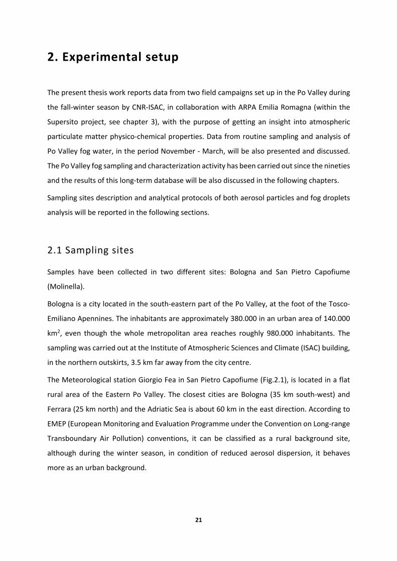
The Meteorological station Giorgio Fea in San Pietro Capofiume (Fig.2.1), is located in a flat 

rural area of  the Eastern Po Valley. The closest cities are Bologna  (35 km south‐west) and 

Ferrara (25 km north) and the Adriatic Sea is about 60 km in the east direction. According to 

EMEP (European Monitoring and Evaluation Programme under the Convention on Long‐range 

Transboundary  Air  Pollution)  conventions,  it  can  be  classified  as  a  rural  background  site, 

although during  the winter  season,  in  condition of  reduced aerosol dispersion,  it behaves 

more as an urban background. 

22 

 

 

Figure 2.1. Measurement station of San Pietro Capofiume (BO) during a foggy winter day. 

 

 

2.2 Aerosol sampling 

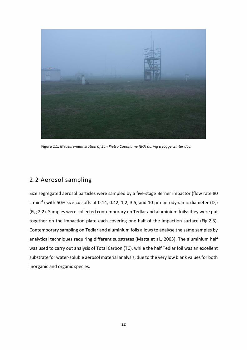
Size segregated aerosol particles were sampled by a five‐stage Berner impactor (flow rate 80 

L min‐1) with 50% size cut‐offs at 0.14, 0.42, 1.2, 3.5, and 10 µm aerodynamic diameter (Da) 

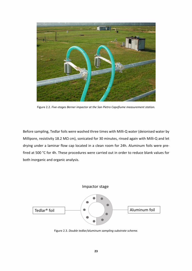
(Fig.2.2). Samples were collected contemporary on Tedlar and aluminium foils: they were put 

together on  the  impaction plate each covering one half of  the  impaction surface  (Fig.2.3). 

Contemporary sampling on Tedlar and aluminium foils allows to analyse the same samples by 

analytical techniques requiring different substrates (Matta et al., 2003). The aluminium half 

was used to carry out analysis of Total Carbon (TC), while the half Tedlar foil was an excellent 

substrate for water‐soluble aerosol material analysis, due to the very low blank values for both 

inorganic and organic species. 

23 

 

 

Figure 2.2. Five‐stages Berner impactor at the San Pietro Capofiume measurement station. 

 

 

Before sampling, Tedlar foils were washed three times with Milli‐Q water (deionised water by 

Millipore, resistivity 18.2 MΩ cm), sonicated for 30 minutes, rinsed again with Milli‐Q and let 

drying under a  laminar flow cap  located  in a clean room for 24h. Aluminum foils were pre‐

fired at 500 °C for 4h. These procedures were carried out in order to reduce blank values for 

both inorganic and organic analysis. 

 

 

 

Figure 2.3. Double tedlar/aluminum sampling substrate scheme. 

 

Aluminum foilTedlar® foil

Impactor stage

24 

 

Simultaneously with Berner  impactor sampling, aerosol particles were also collected with a 

dichotomous high volume sampler from MSP Corporation (Universal Air Sampler, model 310) 

working at a constant nominal airflow rate of 300 L/min. The dichotomous sampler allowed 

the collection of atmospheric aerosols  in their PM1 (particles with Da < 1 µm) and PM1‐10 

(particles with 1 µm < Da < 10 µm) fractions. PALL quartz‐fibre filters were used as substrates. 

To reduce their blank values, filters for fine fraction were washed with 500 mL of Milli‐Q water 

and then fired at 800 °C for 1 h. Filters for the collection of the coarse fraction were only fired 

at 800°C for 1h. Samples collected by the dichotomous sampler were addressed to 1H‐NMR 

analysis for the characterization of the water‐soluble organic fraction. 

 

2.3 Fog sampling 

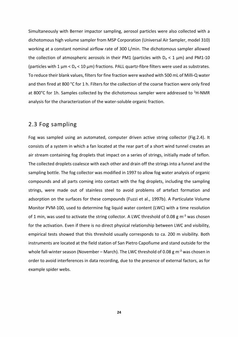
Fog was  sampled using  an  automated,  computer driven  active  string  collector  (Fig.2.4).  It 

consists of a system in which a fan located at the rear part of a short wind tunnel creates an 

air stream containing fog droplets that impact on a series of strings, initially made of teflon. 

The collected droplets coalesce with each other and drain off the strings into a funnel and the 

sampling bottle. The fog collector was modified in 1997 to allow fog water analysis of organic 

compounds and all parts coming  into contact with the fog droplets,  including the sampling 

strings,  were  made  out  of  stainless  steel  to  avoid  problems  of  artefact  formation  and 

adsorption on the surfaces for these compounds (Fuzzi et al., 1997b). A Particulate Volume 

Monitor PVM‐100, used to determine fog liquid water content (LWC) with a time resolution 

of 1 min, was used to activate the string collector. A LWC threshold of 0.08 g m‐3 was chosen 

for the activation. Even if there is no direct physical relationship between LWC and visibility, 

empirical tests showed that this threshold usually corresponds to ca. 200 m visibility. Both 

instruments are located at the field station of San Pietro Capofiume and stand outside for the 

whole fall‐winter season (November – March). The LWC threshold of 0.08 g m‐3 was chosen in 

order to avoid interferences in data recording, due to the presence of external factors, as for 

example spider webs. 

 

25 

 

 

Figure 2.4. Fog string collector and PVM in the background. 

 

 

2.4 Analytical methods 

2.4.1 Sample handling 

Size segregated aerosol samples from the Berner impactors were put in Petri dishes and stored 

in freezer at ‐15°C until analysis were performed. Quartz filters were stored in freezer as well. 

Before  analysis,  both  quartz‐fibre  filters  and  tedlar  foils were  extracted  in  10 mL Milli‐Q 

deionised water and sonicated for 30 minutes. Liquid extract of quartz‐fibre filters was filtered 

before analysis  in order to remove quartz residues. A summary of the analytical procedure 

performed on aerosol samples is shown in Fig.2.5. 

 

 

26 

 

 

Figure 2.5. Scheme of analytical procedure performed on aerosol samples. 

 

 

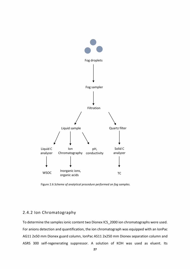
Fog water samples were filtered on 47 mm quartz‐fibre filters (Whatman, QMA grade) within 

a  few  hours  after  collection  to  remove  suspended  particulate  and  conductivity  and  pH 

measurements were  carried  out  immediately.  The  samples were  then  stored  frozen  until 

analysis. A schematic summary of the analytical procedure performed on fog samples is shown 

in Fig.2.6. 

Aerosol 

Berner impactor Dichotomous sampler

Tedlar foil Al foil

Solid C analyzer

TC

Liquid C analyzer

WSOC

WINC

Ion Chromatography

Inorganic ions, organic acids

Water extractionWater extraction

1H ‐ NMR

Functional groups

Quartz filter

27 

 

 

 

 

Figure 2.6 Scheme of analytical procedure performed on fog samples. 

 

 

2.4.2 Ion Chromatography 

To determine the samples ionic content two Dionex ICS_2000 ion chromatographs were used. 

For anions detection and quantification, the ion chromatograph was equipped with an IonPac 

AG11 2x50 mm Dionex guard column, IonPac AS11 2x250 mm Dionex separation column and 

ASRS  300  self‐regenerating  suppressor.  A  solution  of  KOH  was  used  as  eluent.  Its 

Fog droplets

Fog sampler

Filtration

Liquid sample Quartz filter

Solid C analyzer

Liquid C analyzer

Ion Chromatography

Inorganic ions, organic acids

WSOC TC

pH, conductivity

28 

 

concentration increased from 0.8 mM to 38 mM, in a 35 minutes long run (0.8 mM for 10 min, 

5 mM reached at 15 min, 10 mM at 20 min and 38 mM at 35 min). The flow rate was 0.25 

mL/min. The  chromatographic equipment  for  cation analysis  consisted of an  IonPac CG16 

3x50 mm Dionex guard column, IonPac CS16 3x250 mm Dionex separation column and CSRS 

300 self‐regenerating suppressor. The analysis were performed using a solution of MSA as 

eluent with a  flow rate of 0.36 mL/min. The  following separation method was used:  initial 

eluent concentration 6 mM, increase to 15 mM in 20 minutes, then 30 mM reached at 30 min 

and 50 mM from 31 min until 42 min. This program allows to separate both inorganic cations 

(sodium,  ammonium,  potassium, magnesium,  calcium)  and methyl‐,  dimethyl‐,  trimethyl‐, 

ethyl‐ and diethylammonium. 

 

2.4.3 Water‐soluble organic carbon (WSOC) 

Two  instruments were used to determine the WSOC content  in fog and aerosol samples: a 

carbon analyser Shimadzu TOC‐5000A and a nitrogen/carbon analyser Analitik Jena Multi N/C 

2100S. The two  instruments follow the same analysis procedure: parallel measurements of 

inorganic carbon (IC) and total soluble carbon (TSC) are carried out. The measurement of the 

TSC  is  performed  by  catalytic  high  temperature  combustion  (800  °C,  in  presence  of  a  Pt 

catalyst) in a pure carrier gas (oxygen for the Analitik Jena and air for the Shimadzu) and an 

Infrared Detector (NDIR) to measure the evolved CO2.  IC content  is provided acidifying the 

solution and measuring the generated CO2. WSOC is determined by difference (WSOC = TSC – 

IC) (Rinaldi et al., 2007). 

Standard calibration curves obtained with potassium hydrogen phthalate and with a mixture 

of  sodium  carbonate  and  sodium  hydrogen  carbonate were  used  to  quantify  TSC  and  IC 

respectively. Replicate measurements of standard solutions showed a reproducibility within 

5% for concentration range typically encountered in samples extracts. 

 

2.4.4 Total Carbon (TC) 

The  total carbon  (TC) content of  the samples was determined by  the Analitik  Jena Multi N/C 

2100S analyser equipped with a furnace for solid analysis. A small portion (about 1 cm2) of 

29 

 

aluminium foils (for aerosol samples) or quartz filters (for fog samples) is introduced into the 

furnace where it is exposed to a constant temperature 950 °C in a pure oxygen atmosphere, 

in presence of a catalyst (CeO2). All the carbonaceous matter (both organic, carbonate and 

elemental carbon) evolves in CO2 under these conditions. A non‐dispersive infrared detector 

(NDIR) is used to measure the evolved CO2. The instrument was calibrated using pre‐muffled 

quartz  filter  or  aluminium  foils  soaked  with  different  volumes  of  potassium  hydrogen 

phthalate 100 or 1000 ppm solution. The instrumental detection limit is 0.2 μg of carbon and 

the accuracy of the TC measurement resulted better than 5% for 1 μg of carbon. 

By  subtracting WSOC  from TC  the water‐insoluble carbon  (WINC) content of  the collected 

aerosol samples was calculated. 

 

2.4.5 WSOC characterization by Proton Nuclear Magnetic Resonance 

(1H‐NMR) spectroscopy 

Proton Nuclear Magnetic  Resonance  (1H‐NMR)  spectroscopy was  applied  to  quantify  the 

functional groups of WSOC, following the procedure described in Decesari et al. 2000. 1H‐NMR 

spectroscopy  provides  information  about main  structural  units  and  it  is  able  to  identify 

individual  compounds.  Another  important  characteristic  of  NMR  spectroscopy  is  that 

quantitative  analysis  is  straightforward,  since  the  integrated  area  of  the  spectra  is 

proportional to the moles of organic hydrogen atoms present in the sample (Derome, 1987); 

(Braun et al., 1998) . Aliquots of fog water samples and quartz filters extracts were vacuum 

dried  and  redissolved  in  650  μL D2O  in order  to be  subjected  to  the  analyses;  sodium  3‐

trimethylsilyl‐(2,2,3,3‐d4) propionate (TSPd4) was added to the solution as internal standard. 

1HNMR spectra were acquired by a Varian MERCURY 400 spectrometer working at 400 MHz 

in a 5 mm probe. In order to obtain a good signal‐to‐noise ratio, the carbon content of the 

analysed aliquot should not be lower than 80 μgC. 

 

2.4.6 On‐line aerosol chemical characterization 

Besides  the  previously  described  off‐line  analysis  of  collected  filters,  aerosol  chemical 

composition and size distribution of chemical constituents were characterized on‐line by a 

30 

 

High Resolution Time of Flight Aerosol Mass Spectrometer (HR‐ToF‐AMS). Even though HR‐

ToF‐AMS measurements are not the main topic of this thesis,  it  is worth to provide here a 

general  information  on  the  AMS  set  up,  because  AMS measurements  accompanied  filter 

sampling during all the field campaigns described in this study and some results are reported 

in chapter 5 to support off‐line analysis data. 

A detailed description of the HR‐ToF‐AMS can be found in (DeCarlo et al., 2006). Briefly, the 

instrument provides size resolved atmospheric concentrations of the non‐refractory fraction 

of  PM1  particles,  i.e.,  sulphate,  nitrate,  ammonium,  chloride,  and  organics,  with  a  time 

resolution of the order of 5 minutes. The AMS has an effective 50% cut‐off for particle sizes 

below 80 and above 600 nm  in vacuum aerodynamic diameter, Dva, as determined by  the 

transmission characteristics of the standard aerodynamic  lens (Zhang et al., 2002; Zhang et 

al., 2004). All the AMS data were analysed using standard AMS software (SQUIRREL v1.51 and 

PIKA v1.10) within Igor Pro 6.2.1 (WaveMetrics, Lake Oswego, OR) (DeCarlo et al., 2006). To 

obtain PM1 mass closure HR‐ToF‐AMS analysis were integrated with online black carbon (BC) 

measurements, carried out by a Soot Particle Aerosol Mass Spectrometer (SP‐AMS). The SP‐

AMS provide measurements of the refractory component of the submicron aerosol, nominally 

rBC, and of the non‐refractory coating material associated with it (Onasch et al., 2012). 

 

2.4.7 Evaluation of the random uncertainties associated to the 

measurements 

The random uncertainty associated to each aerosol component atmospheric concentration 

and  each  size  range was  computed  using  the  standard  procedure  for  error  propagation, 

considering:  

1. the uncertainty in the sampled air volume (± 3% for Berner impactor and ± 10% for high 

volume sampler);  

2. the precision of the extraction water volume (± 0.04 mL);  

3. the uncertainties in ion chromatography, WSOC and TC measurements (± 5%);  

4. the uncertainty associated to the blank variability, in order to take into account the error 

due to the subtraction of an average blank value.  

31 

 

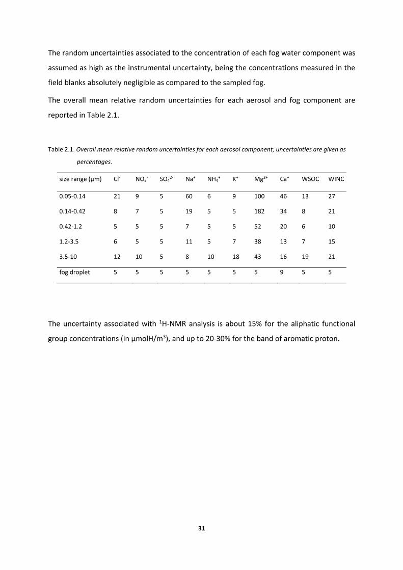
The random uncertainties associated to the concentration of each fog water component was 

assumed as high as the instrumental uncertainty, being the concentrations measured in the 

field blanks absolutely negligible as compared to the sampled fog. 

The  overall mean  relative  random  uncertainties  for  each  aerosol  and  fog  component  are 

reported in Table 2.1.  

 

Table 2.1. Overall mean relative random uncertainties for each aerosol component; uncertainties are given as 

percentages. 

size range (µm)  Cl‐  NO3‐  SO4

2‐  Na+  NH4+  K+  Mg2+  Ca+  WSOC  WINC

0.05‐0.14  21 9  5  60 6 9 100 46  13  27

0.14‐0.42  8  7  5  19 5 5 182 34  8  21

0.42‐1.2  5  5  5  7 5 5 52 20  6  10

1.2‐3.5  6  5  5  11 5 7 38 13  7  15

3.5‐10  12 10  5  8 10 18 43 16  19  21

fog droplet  5  5  5  5 5 5 5 9 5  5 

 

 

The uncertainty associated with  1H‐NMR analysis  is about 15%  for  the aliphatic  functional 

group concentrations (in μmolH/m3), and up to 20‐30% for the band of aromatic proton. 

 

33 

 

3. Aerosol chemical composition in the Po Valley  

 

“Supersito” is a project promoted by Emilia Romagna region and coordinate by the Regional 

Environmental Agency of Emilia Romagna (ARPA‐EMR). The goal of the project  is to furnish 

complete  and  detailed  observations  of  physical,  chemical  and  toxicological  atmospheric 

parameters  and  integrating  environmental  and  health  data.  Numerous  recent  studies 

demonstrate  a  correlation  between  high  concentration  of  particulate matter  and  health 

effects (Brunekreef, 2013; Pope and Dockery, 2006). The project aspires to reach a deeper 

knowledge about primary and secondary aerosol particles, their chemical composition and 

their formation mechanisms, in order to drive the governance towards incisive policies for the 

environmental and health protection. 

Within this project, the Institute of Atmospheric Science and Climate (ISAC) – CNR of Bologna 

participates  investigating  chemical  composition of aerosol particles. Online measurements 

and samples are collected during Intensive Observation Period (IOP) scheduled over the three 

years of experimental work (2011‐2014). 

Five  different  places  located  all  over  the  region  have  been  chosen  as  sampling  and 

measurement sites. The study reported in this chapter deals with data recorded during two 

intensive  field campaigns  in the  frame of Supersito project carried out  in Bologna and San 

Pietro Capofiume. A detailed description of both sites is reported in chapter 2. Bologna (BO) 

represents the Main Site of the project. Due to the high population of the Bologna urban area, 

it  is representative and significative  for  future epidemiological studies.  In  the  frame of  the 

project, San Pietro Capofiume (SPC) has been classified as Rural Satellite site. 

The interest of this Ph.D. thesis is focused on the characterization of atmospheric chemistry 

during the fall‐winter season in the Po Valley. For this purpose November 2011 and February 

2013 field campaigns were chosen to be analysed. 

 

 

 

 

34 

 

3.1 November 2011 field campaign 

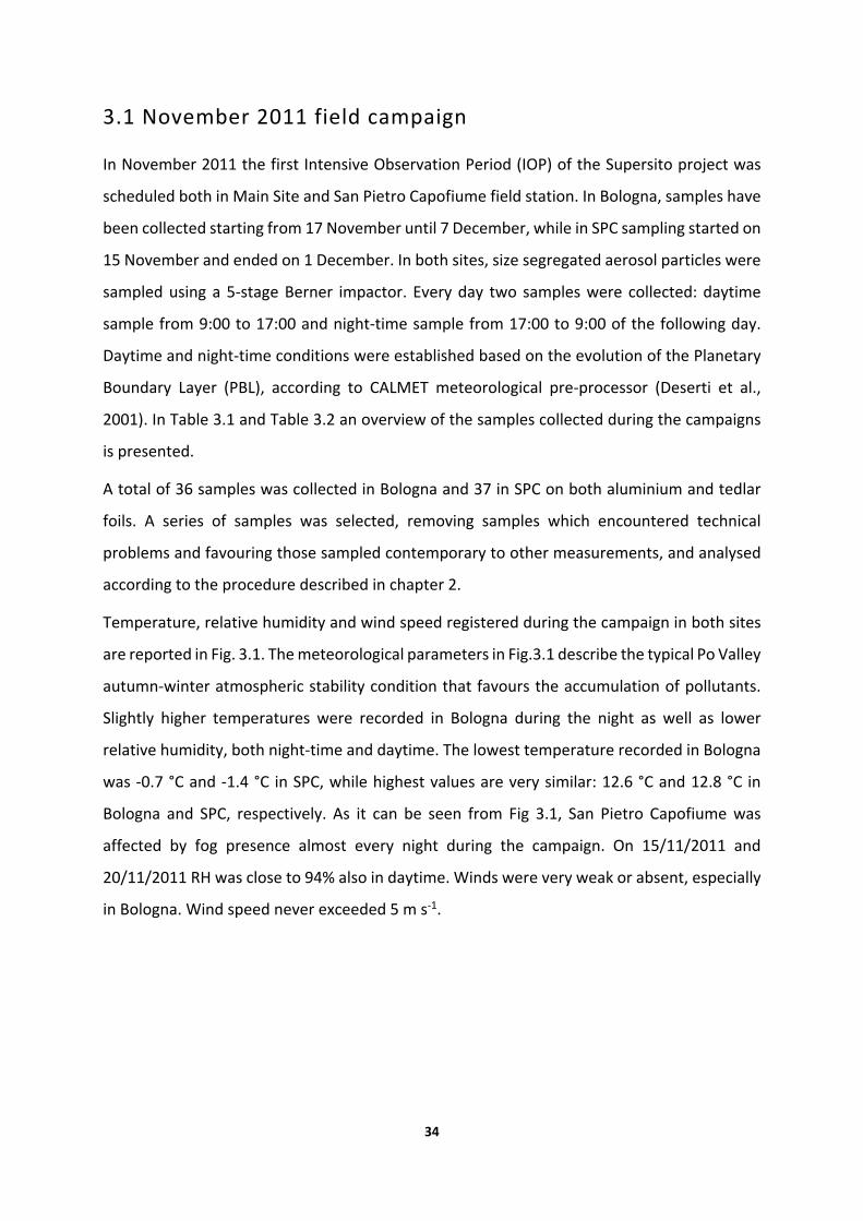
In November 2011 the first Intensive Observation Period (IOP) of the Supersito project was 

scheduled both in Main Site and San Pietro Capofiume field station. In Bologna, samples have 

been collected starting from 17 November until 7 December, while in SPC sampling started on 

15 November and ended on 1 December. In both sites, size segregated aerosol particles were 

sampled using a 5‐stage Berner  impactor. Every day  two  samples were collected: daytime 

sample from 9:00 to 17:00 and night‐time sample from 17:00 to 9:00 of the following day. 

Daytime and night‐time conditions were established based on the evolution of the Planetary 

Boundary  Layer  (PBL),  according  to  CALMET meteorological  pre‐processor  (Deserti  et  al., 

2001). In Table 3.1 and Table 3.2 an overview of the samples collected during the campaigns 

is presented. 

A total of 36 samples was collected in Bologna and 37 in SPC on both aluminium and tedlar 

foils.  A  series  of  samples  was  selected,  removing  samples  which  encountered  technical 

problems and favouring those sampled contemporary to other measurements, and analysed 

according to the procedure described in chapter 2. 

Temperature, relative humidity and wind speed registered during the campaign in both sites 

are reported in Fig. 3.1. The meteorological parameters in Fig.3.1 describe the typical Po Valley 

autumn‐winter atmospheric stability condition that favours the accumulation of pollutants. 

Slightly  higher  temperatures were  recorded  in Bologna  during  the  night  as well  as  lower 

relative humidity, both night‐time and daytime. The lowest temperature recorded in Bologna 

was  ‐0.7 °C and  ‐1.4 °C  in SPC, while highest values are very similar: 12.6 °C and 12.8 °C  in 

Bologna  and  SPC,  respectively. As  it  can be  seen  from  Fig 3.1,  San Pietro Capofiume was 

affected  by  fog  presence  almost  every  night  during  the  campaign.  On  15/11/2011  and 

20/11/2011 RH was close to 94% also in daytime. Winds were very weak or absent, especially 

in Bologna. Wind speed never exceeded 5 m s‐1. 

 

 

 

 

 

35 

 

Table 3.1. Aerosol sampling schedule at Main Site. * = local time. ** = analysed samples. 

 

Bologna 

Sample  Classification  Start date*  Stop date* Time of 

sampling (min) 

BO171111_D**  day  17/11/2011 12.31  17/11/2011 17.01  270 

BO171111_N**  night  17/11/2011 17.05 18/11/2011 09.01 956 

BO181111_D**  day  18/11/2011 09.07 18/11/2011 17.00 473 

BO181111_N**  night  18/11/2011 22.45 19/11/2011 09.00 615 

BO191111_D  day  19/11/2011 09.03 19/11/2011 17.00 477 

BO191111_N  night  19/11/2011 17.40  20/11/2011 09.00  920 

BO201111_D  day  20/11/2011 09.45 20/11/2011 17.14 449 

BO201111_N  night  20/11/2011 18.03 21/11/2011 09.05 902 

BO211111_D  day  21/11/2011 09.08 21/11/2011 17.01 473 

BO211111_N  night  21/11/2011 17.04 22/11/2011 09.00 956 

BO221111_D  day  22/11/2011 09.04 22/11/2011 17.00 476 

BO221111_N  night  22/11/2011 18.00 23/11/2011 09.00 900 

BO231111_D  day  23/11/2011 09.06 23/11/2011 16.59 473 

BO231111_N  night  23/11/2011 17.30  24/11/2011 09.05  935 

BO241111_D  day  24/11/2011 09.07 24/11/2011 17.00 473 

BO241111_N  night  24/11/2011 17.34 25/11/2011 09.00 926 

BO251111_D**  day  25/11/2011 09.03 25/11/2011 17.03 480 

BO251111_N**  night  25/11/2011 17.47 26/11/2011 09.02 915 

BO261111_D**  day  26/11/2011 09.07  26/11/2011 17.02  475 

BO261111_N**  night  26/11/2011 17.34 27/11/2011 09.00 926 

BO271111_D**  day  27/11/2011 09.04 27/11/2011 17.04 480 

BO271111_N**  night  27/11/2011 17.33 28/11/2011 09.00 927 

BO281111_D**  day  28/11/2011 09.03 28/11/2011 17.00 477 

BO281111_N**  night  28/11/2011 17.35  29/11/2011 09.00  925 

BO291111_D**  day  29/11/2011 09.03 29/11/2011 17.00 477 

BO291111_N**  night  29/11/2011 17.33 30/11/2011 09.03 930 

BO301111_D**  day  30/11/2011 09.05 30/11/2011 17.00 475 

BO301111_N**  night  30/11/2011 17.28 01/12/2011 09.00 932 

BO011211_D**  day  01/12/2011 09.03 01/12/2011 17.00 477 

BO011211_N**  night  01/12/2011 17.38 02/12/2011 09.03 925 

BO021211_D**  day  02/12/2011 09.06 02/12/2011 17.04 478 

BO051211_D**  day  05/12/2011 09.07  05/12/2011 17.00  473 

BO051211_N**  night  05/12/2011 17.28 06/12/2011 09.00 932 

BO061211_D**  day  06/12/2011 09.03 06/12/2011 17.00 477 

BO061211_N**  night  06/12/2011 17.00 07/12/2011 09.02 962 

BO071211_D**  day  07/12/2011 09.06 07/12/2011 17.00 474 

36 

 

Table 3.2. Aerosol sampling schedule at San Pietro Capofiume field station. * = local time. ** = analysed samples. 

 

 

San Pietro Capofiume 

Sample  Classification  Start date *  Stop date * Time of 

sampling (min) 

SPC151111_D**  day  15/11/2011 09.23 15/11/2011 17.00 457 

SPC151111_Na** night  15/11/2011 18.03 15/11/2011 22.03 240 

SPC151111_Nb**  night  15/11/2011 22.40  16/11/2011 02.40  240 

SPC151111_Nc** night  16/11/2011 03.15 16/11/2011 07.15 240 

SPC151111_Nd**  night  16/11/2011 07.35  16/11/2011 11.18  223 

SPC161111_D**  day  16/11/2011 11.46  16/11/2011 16.55  309 

SPC161111_N**  night  16/11/2011 18.12  17/11/2011 09.00  888 

SPC171111_D**  day  17/11/2011 09.33  17/11/2011 17.00  447 

SPC171111_Na**  night  17/11/2011 17.25  17/11/2011 21.25  240 

SPC171111_Nb**  night  17/11/2011 21.47  18/11/2011 01.47  240 

SPC171111_Nc**  night  18/11/2011 02.07  18/11/2011 05.50  223 

SPC181111_D**  day  18/11/2011 09.25  18/11/2011 17.00  455 

SPC181111_N**  night  18/11/2011 17.45  19/11/2011 08.35  890 

SPC191111_D  day  19/11/2011 09.10 19/11/2011 17.00 470 

SPC191111_N  night  19/11/2011 17.37 20/11/2011 08.30 893 

SPC201111_D  day  20/11/2011 09.00 20/11/2011 17.06 486 

SPC201111_N  night  20/11/2011 18.02 21/11/2011 09.00 898 

SPC211111_D  day  21/11/2011 09.28 21/11/2011 17.00 452 

SPC211111_N  night  21/11/2011 17.31 22/11/2011 08.54 923 

SPC221111_D  day  22/11/2011 09.26 22/11/2011 17.00 454 

SPC221111_N  night  22/11/2011 17.48 23/11/2011 09.00 912 

SPC231111_D  day  23/11/2011 09.20 23/11/2011 17.00 460 

SPC231111_N  night  23/11/2011 17.35 24/11/2011 09.07 932 

SPC241111_D  day  24/11/2011 09.42 24/11/2011 17.00 438 

SPC241111_N  night  24/11/2011 17.38 25/11/2011 08.27 889 

SPC251111_D**  day  25/11/2011 09.00 25/11/2011 16.59 479 

SPC251111_N**  night  25/11/2011 17.59 26/11/2011 09.18 919 

SPC261111_D**  day  26/11/2011 09.45 26/11/2011 16.59 434 

SPC261111_N**  night  26/11/2011 17.29 27/11/2011 09.02 933 

SPC271111_D**  day  27/11/2011 09.33 27/11/2011 17.01 448 

SPC271111_N**  night  27/11/2011 17.28  28/11/2011 09.12  944 

SPC281111_D**  day  28/11/2011 09.55 28/11/2011 17.00 425 

SPC281111_N**  night  28/11/2011 17.41  29/11/2011 09.10  929 

SPC291111_D**  day  29/11/2011 09.33  29/11/2011 16.59  446 

SPC291111_N**  night  29/11/2011 17.31  30/11/2011 09.18  947 

SPC301111_D**  day  30/11/2011 09.52  30/11/2011 17.00  428 

SPC301111_N**  night  30/11/2011 17.32  01/12/2011 09.00  928 

37 

 

 

 

 

 

 

Figure 3.1. Meteorological parameters recorded during in Bologna and in San Pietro Capofiume from 15/11/2011 

to 02/12/2011. 

 

 

3.2 February 2013 field campaign 

Another field campaign was scheduled in Bologna and San Pietro Capofiume in February 2013. 

In both sites samples have been collected starting from 4 until 15 February. As for the previous 

campaign, size segregated aerosol particles were sampled using a 5‐stage Berner  impactor 

twice a day (9:00  ‐ 18:00, 18:00  ‐ 9:00 of the  following day).  In Table 3.3 and Table 3.4 an 

overview of the samples collected during the campaigns is presented. 

12

8

4

0

T (

°C)

16/11/2011 21/11/2011 26/11/2011 01/12/2011

dat

90

80

70

60

50

RH

(%

)

T_BO T_SPC

RH_BO RH_SPC

0

1

2

3

4

5

6

15/11/2011

 00.00

15/11/2011

 12.00

16/11/2011

 00.00

16/11/2011

 12.00

17/11/2011

 00.00

17/11/2011

 12.00

18/11/2011

 00.00

18/11/2011

 12.00

19/11/2011

 00.00

19/11/2011

 12.00

20/11/2011

 00.00

20/11/2011

 12.00

21/11/2011

 00.00

21/11/2011

 12.00

22/11/2011

 00.00

22/11/2011

 12.00

23/11/2011

 00.00

23/11/2011

 12.00

24/11/2011

 00.00

24/11/2011

 12.00

25/11/2011

 00.00

25/11/2011

 12.00

26/11/2011

 00.00

26/11/2011

 12.00

27/11/2011

 00.00

27/11/2011

 12.00

28/11/2011

 00.00

28/11/2011

 12.00

29/11/2011

 00.00

29/11/2011

 12.00

30/11/2011

 00.00

30/11/2011

 12.00

01/12/2011

 00.00

01/12/2011

  12.00

02/12/2011

 00.00

m s‐1

wind BO wind SPC

38 

 

 

 

 

Table 3.3. Aerosol sampling schedule at Main Site. * = local time. ** = analysed samples. 

 

 

 

 

 

 

 

 

 

Bologna 

Sample  Classification  Start date *  Stop date * Time of 

sampling (min) 

 BO040213_D  day  04/02/2013 09.28 04/02/2013 18.00 512 

 BO040213_N**  night  04/02/2013 18.18  05/02/2013 09.00  882 

 BO050213_D** day  05/02/2013 09.04 05/02/2013 18.00 536 

 BO050213_N** night  05/02/2013 18.22 06/02/2013 08.55 873 

 BO060213_D  day  06/02/2013 09.21  06/02/2013 17.57  516 

 BO060213_N  night  06/02/2013 18.20 07/02/2013 09.00 880 

 BO070213_D  day  07/02/2013 09.18 07/02/2013 18.01 523 

 BO070213_N**  night  07/02/2013 18.03  08/02/2013 09.00  897 

 BO080213_D** day  08/02/2013 09.20 08/02/2013 17.58 518 

 BO080213_N  night  08/02/2013 18.21 09/02/2013 09.00 879 

 BO110213_D  day  11/02/2013 09.28  11/02/2013 18.00  512 

 BO110213_N  night  11/02/2013  ??? 12/02/2013 09.05 n.a. 

 BO120213_D** day  12/02/2013 09.06 12/02/2013 18.00 534 

 BO120213_N**  night  12/02/2013 18.19  13/02/2013 09.00  881 

 BO130213_D** day  13/02/2013 09.27 13/02/2013 18.00 513 

 BO130213_N** night  13/02/2013 18.23 14/02/2013 09.00 877 

 BO140213_D**  day  14/02/2013 09.20  14/02/2013 18.07  527 

 BO140213_N** night  14/02/2013 18.10 15/02/2013 09.00 890 

 BO150213_D** day  15/02/2013 09.20 15/02/2013 18.00 520 

 BO150213_N  night  15/02/2013 18.23 16/02/2013 09.01 878 

39 

 

Table3.4. Aerosol sampling schedule at San Pietro Capofiume field station. * = local time. ** = analysed samples. 

 

 

 

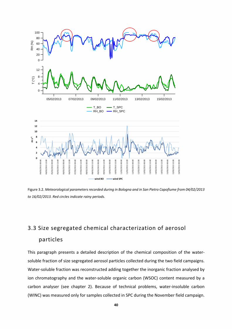
Fig.3.2 shows meteorological parameters (T, RH and wind speed) of the two sites during the 

campaign. Conditions met during this campaign are more variable than  in November 2011, 

with low pressure systems bringing occasional rain over the sampling sites. Temperature are 

similar in the two sites with values ranging from ‐1.3 °C to 12.2 °C in Bologna and from ‐0.7°C 

to 12.3 °C in SPC. Trend of RH is the same for both sites, with values usually slightly lower in 

Bologna. Red circles indicate rainy periods in both sites: 06/02/2013 6:00 – 9:00, 11/02/2013 

9:00 – 12/02/2013 15:00 and 13/02/2013 21:00 – 22:00 in Bologna and 06/02/2013 06:00 – 

08:00, 11/02/2013 09:00 –23:00 and 13/02/2013 21:00 – 22:00 in SPC. In this campaign, winds 

are weaker in SPC and are slightly faster than the previous campaign, with values reaching 12 

m s‐1 in Bologna on 11/02/2013. 

San Pietro Capofiume 

Sample  Classification  Start date *  Stop date * Time of 

sampling (min) 

 SPC040213_D  day  04/02/2013 09.00 04/02/2013 18.00 540 

 SPC040213_N**  night  04/02/2013 18.00  05/02/2013 09.00  900 

 SPC050213_D** day  05/02/2013 09.00 05/02/2013 18.00 540 

 SPC050213_N** night  05/02/2013 18.00 06/02/2013 09.00 900 

 SPC060213_D  day  06/02/2013 09.14  06/02/2013 18.00  526 

 SPC060213_N  night  06/02/2013 18.00 07/02/2013 09.00 900 

 SPC070213_D  day  07/02/2013 09.07 07/02/2013 18.00 533 

 SPC070213_N**  night  07/02/2013 18.00  08/02/2013 09.00  900 

 SPC080213_D** day  08/02/2013 09.05 08/02/2013 18.00 535 

 SPC080213_N  night  08/02/2013 18.00 09/02/2013 09.00 900 

 SPC110213_D  day  11/02/2013 09.05  11/02/2013 18.00  535 

 SPC110213_N  night  11/02/2013 18.00 12/02/2013 09.00 900 

 SPC120213_D** day  12/02/2013 09.02 12/02/2013 18.00 538 

 SPC120213_N**  night  12/02/2013 18.00  13/02/2013 09.00  900 

 SPC130213_D** day  13/02/2013 09.02 13/02/2013 18.00 538 

 SPC130213_N** night  13/02/2013 18.00 14/02/2013 09.00 900 

 SPC140213_D**  day  14/02/2013 09.00  14/02/2013 18.00  540 

 SPC140213_N** night  14/02/2013 18.00 15/02/2013 09.00 900 

 SPC150213_D** day  15/02/2013 09.02 15/02/2013 18.00 538 

 SPC150213_N  night  15/02/2013 18.03 16/02/2013 09.03 900 

40 

 

 

 

Figure 3.2. Meteorological parameters recorded during in Bologna and in San Pietro Capofiume from 04/02/2013 

to 16/02/2013. Red circles indicate rainy periods. 

 

 

3.3 Size segregated chemical characterization of aerosol 

particles 

This paragraph presents a detailed description of  the  chemical  composition of  the water‐

soluble fraction of size segregated aerosol particles collected during the two field campaigns. 

Water‐soluble fraction was reconstructed adding together the inorganic fraction analysed by 

ion chromatography and the water‐soluble organic carbon  (WSOC) content measured by a 

carbon  analyser  (see  chapter  2).  Because  of  technical  problems,  water‐insoluble  carbon 

(WINC) was measured only for samples collected in SPC during the November field campaign. 

12

8

4

0

T (

°C)

05/02/2013 07/02/2013 09/02/2013 11/02/2013 13/02/2013 15/02/2013

dat

100

80

60

40

20

0

RH

(%

)

T_BO T_SPC RH_BO RH_SPC

0

2

4

6

8

10

12

14

04/02/2013 00:00

04/02/2013 12:00

05/02/2013 00:00

05/02/2013 12:00

06/02/2013 00:00

06/02/2013 12:00

07/02/2013 00:00

07/02/2013 12:00

08/02/2013 00:00

08/02/2013 12:00

09/02/2013 00:00

09/02/2013 12:00

10/02/2013 00:00

10/02/2013 12:00

11/02/2013 00:00

11/02/2013 12:00

12/02/2013 00:00

12/02/2013 12:00

13/02/2013 00:00

13/02/2013 12:00

14/02/2013 00:00

14/02/2013 12:00

15/02/2013 00:00

15/02/2013 12:00

16/02/2013 00:00

m s‐1

wind BO wind SPC

41 

 

Therefore, data are not included in the following discussion and will be presented in detail in 

chapter 5. 

Fig.3.3 shows the concentration of water‐soluble compounds of PM10 collected  in the two 

campaigns. Total mass concentrations are obtained summing up the five Berner stages. 

 

 

 

Figure  3.3.  Concentration  of  PM10  water‐soluble  fraction  during  the  November  2011  and  February  2013 

campaigns. 

 

 

In November2011, PM10 water‐soluble  fraction concentration  is comparable between San 

Pietro Capofiume and Bologna. Soluble mass showed low concentrations in the first period, 

then particles accumulated at the end of November and at the beginning of December  (in 

December data are available only for Bologna). Concentrations range between 24 – 75 µgm‐3 

in Bologna and 14 – 76 µg m‐3 in SPC. These values do not account for the insoluble matter 

0

10

20

30

40

50

60

70

80

151111_D

151111_N

161111_D

161111_N

171111_D

171111_N

181111_D

181111_N

191111_D

191111_N

201111_D

201111_N

251111_D

251111_N

261111_D

261111_N

271111_D

271111_N

281111_D

281111_N

291111_D

291111_N

301111_D

301111_N

011211_D

011211_N

021211_D

051211_D

051211_N

061211_D

061211_N

071211_D

µgm

‐3

Nov 2011

0

10

20

30

40

50

60

70

80

040213_N

050213_D

050213_N

070213_N

080213_D

120213_D

120213_N

130213_D

130213_N

140213_D

140213_N

150213_D

µg m‐3

FEB _ 2011

SPC BO

42 

 

present  in aerosol particles  that was not analysed. Nevertheless,  in  the second half of  the 

campaign PM10 soluble fraction concentrations exceed the 50 µg m‐3 PM10 threshold. 

In  February  2013  concentrations  are  also  very  similar  between  the  two  sites  and  are 

comparable  to  those measured  in  the  first  half  of  November  2011, with  values  ranging 

between 3.2 ‐ 58 µg m‐3 in Bologna and 18 – 38 µg m‐3 in San Pietro Capofiume. 

Soluble mass concentration remains almost constant all over the measuring period, without 

any daily trend, as it is expected, given the scarce evolution of the PBL during daytime in winter 

(Carbone  et  al.,  2010).  Conversely,  for  the  November  campaign,  a  clear  diurnal  trend  is 

observed, especially for samples collected in SPC: PM10 concentration decreases during the 

night and increases again during the day. This trend is linked with the presence of fog in night 

hours and will be further discussed in chapter 5. 

We expected higher particles concentration in an urban site compared to a rural background, 

while similar concentrations are observed in the two sites. The water‐soluble fraction is the 

most influenced by secondary processes and less affected by local source emissions as traffic 

and domestic heating (Seinfeld and Pandis, 1998). The above data indicate that concentrations 

of  secondary  aerosol  particles  is  rather  homogeneous  across  the  region. We  expect  that 

adding  the water‐insoluble  components  (especially  elemental  carbon  and water‐insoluble 

organic carbon), mass concentrations will be higher in Bologna, according to what reported in 

literature. Carbone et al. (2010) showed that aerosol collected in Milan (Po Valley urban site) 

differed  from  the  rural  site of SPC  for  the  larger amount of water  insoluble carbonaceous 

matter (WINCM), and its enrichment in small particles confirms the important role of domestic 

heating and traffic‐related sources at the urban site. 

In November, fine particles (PM1.2) account on average for 86 (±8) % and 86 (±5) % of the 

total water‐soluble mass in Bologna in daytime and night‐time conditions, respectively. In SPC 

they contribute for 79 (±21) % and 49 (±13) %. In February, PM1.2 accounts on average for 89 

(±4) % and 81 (±7) % in Bologna, while in SPC on average for 86 (±11) % and 79 (±12) %. Fine 

concentrations are obtained summing up stage 1, 2 and 3 of Berner impactor (size range 0.05‐

1.2 µm). Hereafter  in the chapter,  I will refer to fine particles as particles  in the size range 

between 0.05 and 1.2 µm and coarse particles will be those in the size range between 1.2 and 

10 µm (the sum of stage 4 and 5). 

43 

 

A  detailed  size  segregated  average  chemical  composition  of  aerosol  particles  collected  in 

November  2011  and  February  2013  in  the  two  sites  is  reported  in  Fig.3.4,  and  Fig.3.5, 

respectively. 

 

 

 

 

Figure 3.4. Average size segregated absolute and relative chemical composition of aerosol particles collected in 

November 2011 in Bologna and San Pietro Capofiume. Samples have been divided between nocturnal and diurnal. 

 

0.0

5.0

10.0

15.0

20.0

25.0

30.0

0.05‐0.14 0.14‐0.42 0.42‐1.2 1.2‐3.5 3.5‐10

µg m

‐3

NOV ‐ BO day

Na Ca Cl Mg K NO3 SO4 NH4 WSOM

0.0

5.0

10.0

15.0

20.0

25.0

30.0

0.05‐0.14 0.14‐0.42 0.42‐1.2 1.2‐3.5 3.5‐10

NOV ‐ BO night

Na Ca Cl Mg K NO3 SO4 NH4 WSOM

0%

20%

40%

60%

80%

100%

0.05‐0.14 0.14‐0.42 0.42‐1.2 1.2‐3.5 3.5‐10

Na Ca Cl Mg K NO3 SO4 NH4 WSOM

0%

20%

40%

60%

80%

100%

0.05‐0.14 0.14‐0.42 0.42‐1.2 1.2‐3.5 3.5‐10

Na Ca Cl Mg K NO3 SO4 NH4 WSOM

0.0

5.0

10.0

15.0

20.0

25.0

0.05‐0.14 0.14‐0.42 0.42‐1.2 1.2‐3.5 3.5‐10

µg m

‐3

NOV ‐ SPC day

Na Ca Cl Mg K NO3 SO4 NH4 WSOM

0.0

5.0

10.0

15.0

20.0

25.0

0.05‐0.14 0.14‐0.42 0.42‐1.2 1.2‐3.5 3.5‐10

NOV ‐ SPC night

Na Ca Cl Mg K NO3 SO4 NH4 WSOM

0%

20%

40%

60%

80%

100%

0.05‐0.14 0.14‐0.42 0.42‐1.2 1.2‐3.5 3.5‐10

Na Ca Cl Mg K NO3 SO4 NH4 WSOM

0%

20%

40%

60%

80%

100%

0.05‐0.14 0.14‐0.42 0.42‐1.2 1.2‐3.5 3.5‐10

Na Ca Cl Mg K NO3 SO4 NH4 WSOM

44 

 

 

 

Figure 3.5. Average size segregated absolute and relative chemical composition of aerosol particles collected in 

February 2013 in Bologna and San Pietro Capofiume. Samples have been divided between nocturnal and diurnal. 

 

 

The size range between 0.42 and 1.2 µm is always the most abundant in terms of mass, except 

for one case: nocturnal samples collected in SPC in Nov 2011. As stated above, this campaign 

was characterised by the occurrence of  fog during the night. Fog scavenging depleted  fine 

particles  (0.14  <  Da  <  1.2  µm),  thus  affecting  aerosol  mass  size  distribution.  Average 

concentration of the third stage of Berner  impactor reached a value close to that of fourth 

0.0

5.0

10.0

15.0

20.0

0.05‐0.14 0.14‐0.42 0.42‐1.2 1.2‐3.5 3.5‐10

µg m

‐3

FEB ‐ BO day

Na Ca Cl K Mg NO3 SO4 NH4 WSOM

0%

20%

40%

60%

80%

100%

0.05‐0.14 0.14‐0.42 0.42‐1.2 1.2‐3.5 3.5‐10

Na Ca Cl K Mg NO3 SO4 NH4 WSOM

0.0

5.0

10.0

15.0

20.0

0.05‐0.14 0.14‐0.42 0.42‐1.2 1.2‐3.5 3.5‐10

FEB ‐ BO night

Na Ca Cl K Mg NO3 SO4 NH4 WSOM

0%

20%

40%

60%

80%

100%

0.05‐0.14 0.14‐0.42 0.42‐1.2 1.2‐3.5 3.5‐10

Na Ca Cl K Mg NO3 SO4 NH4 WSOM

0.0

5.0

10.0

15.0

20.0

0.05‐0.14 0.14‐0.42 0.42‐1.2 1.2‐3.5 3.5‐10

µg m

‐3

FEB ‐ SPC day

Na Ca Cl K Mg NO3 SO4 NH4 WSOM

0.0

5.0

10.0

15.0

20.0

0.05‐0.14 0.14‐0.42 0.42‐1.2 1.2‐3.5 3.5‐10

FEB ‐ SPC night

Na Ca Cl K Mg NO3 SO4 NH4 WSOM

0%

20%

40%

60%

80%

100%

0.05‐0.14 0.14‐0.42 0.42‐1.2 1.2‐3.5 3.5‐10

Na Ca Cl K Mg NO3 SO4 NH4 WSOM

0%

20%

40%

60%

80%

100%

0.05‐0.14 0.14‐0.42 0.42‐1.2 1.2‐3.5 3.5‐10

Na Ca Cl K Mg NO3 SO4 NH4 WSOM

45 

 

stage. The effects of fog droplets and aerosol particles interaction will be discussed in detail 

in chapter 5. 

Chemical composition of  fine  fraction  is very similar  in Bologna and San Pietro Capofiume, 

confirming that the water‐soluble fraction of particulate matter over the Po Valley is mainly 

related to regional sources.  Inorganic species  in the fine fraction are dominated by nitrate, 

sulphate and ammonium that, in November, account together for 50 (±10) % and 51 (±9) % of 

the total soluble mass in Bologna and SPC, respectively. In February they account on average 

for 63 (±14) % and 65 (±10) % in BO and SPC. These three species are mainly distributed in the 

fine fraction peaking in the accumulation mode (0.14 μm < Da <1.2 μm). These ionic species 

accumulate into fine particles in the form of ammonium salts. This is confirmed by the high 

correlation between the sum of nitrate and sulphate with ammonium: R2 = 0.98 and R2 = 0.99 

in BO and SPC November samples, respectively, and R2 = 0.95 and R2 = 0.98  in BO and SPC 

February samples. Furthermore, this hypothesis  is supported by the  ionic balance (Fig.3.6), 

showing that ammonium is fully neutralised by the sum of nitrate and sulphate. 

Ammonium nitrate dominates  the  chemical  composition  of  fine  aerosol  in  the  fall winter 

season, in agreement with previous studies carried out in the Po Valley (Carbone et al., 2010; 

Lonati et al., 2007; Putaud et al., 2004; Rodriguez et al., 2007). 

Water‐soluble organic matter constitutes a significant fraction of fine particles soluble mass, 

in November accounting on average  for 42  (±11) % and 44  (±10) %  in BO and SPC, and  in 

February 33 (±13) % and 32 (±9) % in BO and SPC. The homogeneous distribution of WSOM 

between BO and SPC is indicative of secondary processes as the main source of WSOM over 

the Po Valley during the investigated period. Finest particles in the size range between 0.05 

and 0.14 µm are the most enriched in organic compounds, with WSOM accounting up to 86% 

of the total soluble mass. 

Aerosol mass concentration of coarse fraction is much lower than fine fraction, accounting for 

14 (±7) % and 33 (±21) % of the total soluble mass in November BO and SPC samples, and 15 

(±7) % and 18 (±12) % in February BO and SPC samples. 

 

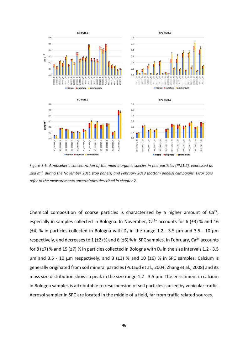
46 

 

 

 

Figure 3.6. Atmospheric concentration of the main  inorganic species  in fine particles (PM1.2), expressed as 

µeq m‐3, during the November 2011 (top panels) and February 2013 (bottom panels) campaigns. Error bars 

refer to the measurements uncertainties described in chapter 2. 

 

 

Chemical  composition  of  coarse  particles  is  characterized  by  a  higher  amount  of  Ca2+, 

especially  in samples collected  in Bologna.  In November, Ca2+ accounts for 6 (±3) % and 16 

(±4) %  in particles collected  in Bologna with Da  in  the  range 1.2  ‐ 3.5 µm and 3.5  ‐ 10 µm 

respectively, and decreases to 1 (±2) % and 6 (±6) % in SPC samples. In February, Ca2+ accounts 

for 8 (±7) % and 15 (±7) % in particles collected in Bologna with Da in the size intervals 1.2 ‐ 3.5 

µm and 3.5  ‐ 10 µm  respectively, and 3  (±3) % and 10  (±6) %  in  SPC  samples. Calcium  is 

generally originated from soil mineral particles (Putaud et al., 2004; Zhang et al., 2008) and its 

mass size distribution shows a peak in the size range 1.2 ‐ 3.5 µm. The enrichment in calcium 

in Bologna samples is attributable to resuspension of soil particles caused by vehicular traffic. 

Aerosol sampler in SPC are located in the middle of a field, far from traffic related sources. 

0.0

0.1

0.2

0.3

0.4

0.5

0.6

171111_D

171111_N

181111_D

181111_N

251111_D

251111_N

261111_D

261111_N

271111_D

271111_N

281111_D

281111_N

291111_D

291111_N

301111_D

301111_N

011211_D

011211_N

021211_D

051211_D

051211_N

061211_D

061211_N

071211_D

µeq

 l‐1

BO PM1.2

nitrate sulphate ammonium

0.0

0.1

0.2

0.3

0.4

0.5

0.6

151111_D

151111_N

161111_D

161111_N

171111_D

171111_N

181111_D

181111_N

191111_D

191111_N

201111_D

201111_N

251111_D

251111_N

261111_D

261111_N

271111_D

271111_N

281111_D

281111_N

291111_D

291111_N

301111_D

301111_N

µeq

 l‐1

SPC PM1.2

nitrate sulphate ammonium

0.0

0.1

0.2

0.3

0.4

0.5

0.6

BO_040213_N

BO_050213_D

BO_050213_N

BO_070213_N

BO_080213_D

BO_120213_D

BO_120213_N

BO_130213_D

BO_130213_N

BO_140213_D

BO_140213_N

BO_150213_D

µeq m

‐3

BO PM1.2

nitrate sulphate ammonium

0.0

0.1

0.2

0.3

0.4

0.5

0.6

SPC_040213_N

SPC_050213_D

SPC_050213_N

SPC_070213_N

SPC_080213_D

SPC_120213_D

SPC_120213_N

SPC_130213_D

SPC_130213_N

SPC_140213_D

SPC_140213_N

SPC_150213_D

µeq l‐1

SPC PM1.2

nitrate sulphate ammonium

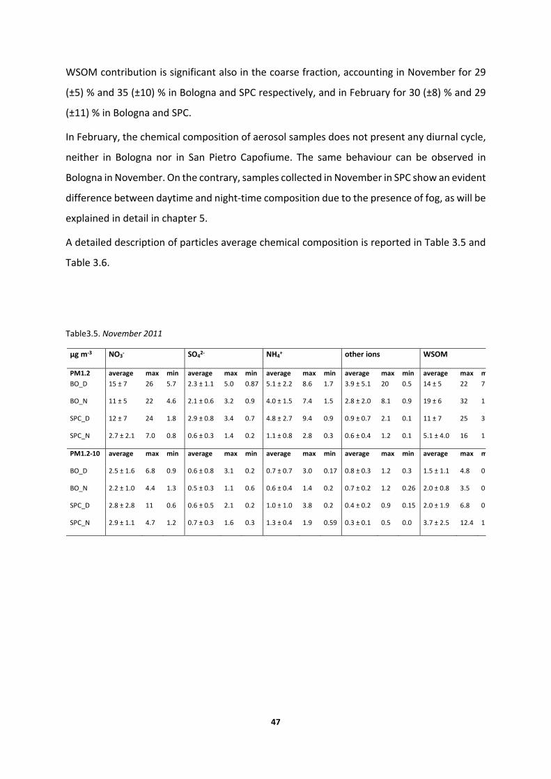
47 

 

WSOM contribution is significant also in the coarse fraction, accounting in November for 29 

(±5) % and 35 (±10) % in Bologna and SPC respectively, and in February for 30 (±8) % and 29 

(±11) % in Bologna and SPC. 

In February, the chemical composition of aerosol samples does not present any diurnal cycle, 

neither  in Bologna nor  in  San Pietro Capofiume.  The  same behaviour  can be observed  in 

Bologna in November. On the contrary, samples collected in November in SPC show an evident 

difference between daytime and night‐time composition due to the presence of fog, as will be 

explained in detail in chapter 5. 

A detailed description of particles average chemical composition is reported in Table 3.5 and 

Table 3.6. 

 

 

Table3.5. November 2011 

 

 

 

 

 

 

 

 

µg m‐3  NO3‐  SO4

2‐  NH4+  other ions  WSOM 

PM1.2  average  max  min  average  max min average max min average max  min  average  max m

BO_D  15 ± 7  26  5.7  2.3 ± 1.1  5.0 0.87 5.1 ± 2.2 8.6 1.7 3.9 ± 5.1 20 0.5  14 ± 5  22 7.

BO_N  11 ± 5  22  4.6  2.1 ± 0.6  3.2 0.9 4.0 ± 1.5 7.4 1.5 2.8 ± 2.0 8.1  0.9  19 ± 6  32 12

SPC_D  12 ± 7  24  1.8  2.9 ± 0.8  3.4 0.7 4.8 ± 2.7 9.4 0.9 0.9 ± 0.7 2.1  0.1  11 ± 7  25 3.

SPC_N  2.7 ± 2.1  7.0  0.8  0.6 ± 0.3  1.4 0.2 1.1 ± 0.8 2.8 0.3 0.6 ± 0.4 1.2  0.1  5.1 ± 4.0  16 1.

PM1.2‐10  average  max  min  average  max min average max min average max  min  average  max m

BO_D  2.5 ± 1.6  6.8  0.9  0.6 ± 0.8  3.1 0.2 0.7 ± 0.7 3.0 0.17 0.8 ± 0.3 1.2  0.3  1.5 ± 1.1  4.8 0.

BO_N  2.2 ± 1.0  4.4  1.3  0.5 ± 0.3  1.1 0.6 0.6 ± 0.4 1.4 0.2 0.7 ± 0.2 1.2  0.26  2.0 ± 0.8  3.5 0.

SPC_D  2.8 ± 2.8  11  0.6  0.6 ± 0.5  2.1 0.2 1.0 ± 1.0 3.8 0.2 0.4 ± 0.2 0.9  0.15  2.0 ± 1.9  6.8 0.

SPC_N  2.9 ± 1.1  4.7  1.2  0.7 ± 0.3  1.6 0.3 1.3 ± 0.4 1.9 0.59 0.3 ± 0.1 0.5  0.0  3.7 ± 2.5  12.4 1.

 

48 

 

Table3.6. February 2013 

 

 

 

In wintertime, soluble species represent the main compounds of aerosol particles in the Po 

Valley, especially for the fine fraction. In (Matta et al., 2003) they account for more than 70% 

of PM10 mass  and  in  (Carbone et  al., 2010)  their  contribution  ranges  from 40  to 70% of 

submicron aerosol mass. Our results show a rather homogeneous chemical composition of 

this fraction in both urban and rural site, confirming the dominant role of regional secondary 

processes in particles formation under typical winter conditions. Sources of secondary aerosol 

in the whole area of the Po Valley, together with long‐range transport processes (Alves et al., 

2012; Maurizi et al., 2013) should be taken into account in order to adopt effective pollution 

abatement strategies. 

 

µg m‐3  NO3‐  SO4

2‐  NH4+  other ions  WSOM 

PM1.2  average  max  min  average  max min average max min average max min  average  max  min

BO_D  13 ± 7  25  7.0 2.1 ± 1.2  3.9  0.7 4.3 ±  2.3 8.4 2.0 0.9 ± 0.6 1.7 0.3  7.7 ± 3.8  13  3.5

BO_N  7.6 ± 3.7  12  3.3 2.0 ± 1.3  3.9  0.5 3.0 ± 1.7 5.6 0.9 0.9 ± 0.2 1.3 0.6  7.8 ± 2.4  10  3.3

SPC_D  11 ± 2.4  14  7.4 2.5 ± 1.0  3.7  1.1 4.2 ± 0.9 5.1 2.9 0.6 ± 0.4 1.2 0.2  8.2 ± 3.8  13  3.7

SPC_N  8.8 ± 2.4  12  5.1 1.5 ± 0.9  2.8  0.6 3.2 ± 0.9 4.3 1.7 0.7 ± 0.2 0.9 0.3  7.0 ± 1.2  8.3  5.7

PM1.2‐10  average  max  min  average  max min average max min average max min  average  max  min

BO_D  1.1 ± 0.8  2.4  0.2 0.2 ± 0.2  0.5  0.1 0.3 ± 0.3 0.8 0.0 0.9 ± 0.6 1.7 0.2  0.9 ± 0.5  1.7  0.4

BO_N  2.0 ± 1.7  4.3  0.3 0.5 ± 0.5  1.2  0.1 0.7 ± 0.8 2.0 0.0 0.7 ± 0.4 1.4 0.4  1.4 ± 0.7  2.3  0.9

SPC_D  2.0 ± 2.2  5.9  0.6 0.5 ± 0.7  1.7  0.1 0.7 ± 1.0 2.4 0.2 0.3 ± 0.2 0.5 0.1  1.0 ± 0.5  1.7  0.4

SPC_N  3.0 ± 2.9  7.6  0.5 0.7 ± 0.9  2.3  0.06 1.1 ± 1.2 2.9 0.0 0.3 ± 0.1 0.5 0.1  1.6 ± 0.6  2.5  1.0

 

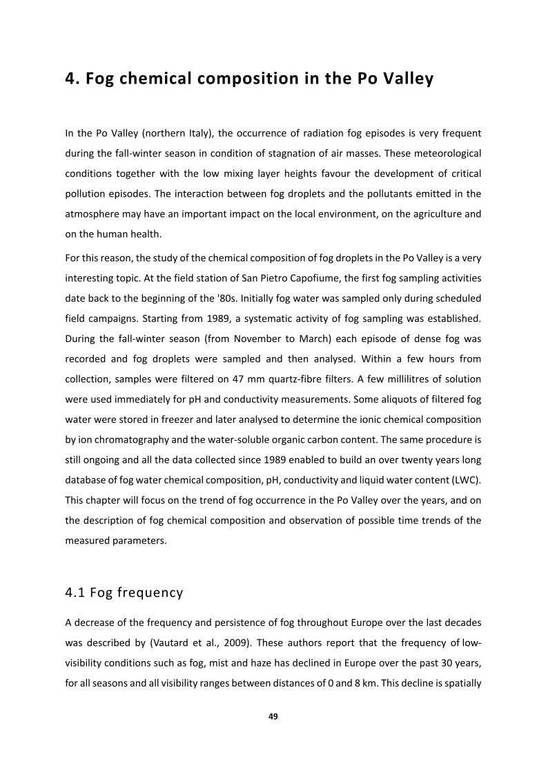
49 

 

4. Fog chemical composition in the Po Valley 

 

In  the Po Valley  (northern  Italy),  the occurrence of  radiation  fog episodes  is very  frequent 

during the fall‐winter season in condition of stagnation of air masses. These meteorological 

conditions  together with  the  low mixing  layer  heights  favour  the  development  of  critical 

pollution episodes. The  interaction between fog droplets and the pollutants emitted  in the 

atmosphere may have an important impact on the local environment, on the agriculture and 

on the human health. 

For this reason, the study of the chemical composition of fog droplets in the Po Valley is a very 

interesting topic. At the field station of San Pietro Capofiume, the first fog sampling activities 

date back to the beginning of the '80s. Initially fog water was sampled only during scheduled 

field campaigns. Starting  from 1989, a systematic activity of  fog sampling was established. 

During  the  fall‐winter  season  (from November  to March)  each  episode  of  dense  fog was 

recorded  and  fog  droplets  were  sampled  and  then  analysed. Within  a  few  hours  from 

collection, samples were  filtered on 47 mm quartz‐fibre  filters. A  few millilitres of solution 

were used immediately for pH and conductivity measurements. Some aliquots of filtered fog 

water were stored in freezer and later analysed to determine the ionic chemical composition 

by ion chromatography and the water‐soluble organic carbon content. The same procedure is 

still ongoing and all the data collected since 1989 enabled to build an over twenty years long 

database of fog water chemical composition, pH, conductivity and liquid water content (LWC). 

This chapter will focus on the trend of fog occurrence in the Po Valley over the years, and on 

the description of fog chemical composition and observation of possible time trends of the 

measured parameters. 

 

4.1 Fog frequency  

A decrease of the frequency and persistence of fog throughout Europe over the last decades 

was  described  by  (Vautard  et  al.,  2009).  These  authors  report  that  the  frequency  of low‐

visibility conditions such as fog, mist and haze has declined in Europe over the past 30 years, 

for all seasons and all visibility ranges between distances of 0 and 8 km. This decline is spatially 

50 

 

and temporally correlated with trends  in sulphur dioxide emissions, suggesting a significant 

contribution of air‐quality improvements, i.e. reduction in the aerosol sulphate loading which 

act  as  condensation  nuclei  for  fog  formation.  Similar  conclusions  were  reached  by  (van 

Oldenborgh  et  al.,  2010), who  restricted  the  study  of  (Vautard  et  al.,  2009)  to  dense  fog 

(visibility < 200 m). This study reported that the relative temporal trends of the number of days 

with dense fog are comparable to the trends of days with presence of haze and mist (2 km 

visibility and higher), although the scatter around the mean values is much larger in the former 

case. These studies address particularly the regions of eastern and central Europe, north of 

the Alps. 

For the Po Valley area, (Mariani, 2009) reported a decreasing frequency of days with fog (in 

this case defined as visibility < 1 km) in the Milan area with a reduction of 73% within the city 

and of 52% at the Linate airport, 7 km from the city centre, over the decade 1991 ‐ 2000 with 

respect to the decade 1960 ‐ 1969. A reduction of fog frequency of about 50% over the period 

1949 ‐ 1990 was also documented by (Sachweh and Koepke, 1995) for the metropolitan area 

of Munich. These authors attribute this reduction to the urban heat island that increases the 

heating of the air and causes a moisture deficit. 

Visibility data collected by the Regional Environmental Agency of Emilia Romagna in the area 

of Bologna  airport  are available  since 1984. Assuming  fog occurrence only during  the fall‐

winter season (November ‐ March), they show a statistically significant reduction of 47% of 

annual  foggy hours  in  the period 2004/05‐2012/13 with  respect  to  the decade 1984/85  ‐ 

1993/94, with fog defined as visibility < 1 km. Visibility data at the field station of San Pietro 

Capofiume are available for a shorter period: fall‐winter season 1986/87 ‐ 1998/99. The trend 

is consistent with that of Bologna airport, even if the absolute values are higher, as expected 

for a rural site, not affected by the urban heat island effect. Both trends are reported in Fig.4.1. 

A reduction in fog occurrence is evident until the first half of the nineties. From then on, the 

percentage of foggy hours during the fall‐winter season is slightly variable around the mean 

value of 10%. These data agree with the results of the studies presented above, where clear 

fog reduction is documented up to 2000, and few data are available for the last decade. 

Due to instrumental limits (see chapter 2) only thick fog events (visibility < 200m) have been 

collected in San Pietro Capofiume and then analysed. For each event, start and end time have 

been registered, supplying information about the hours of dense fog occurred during each fall‐

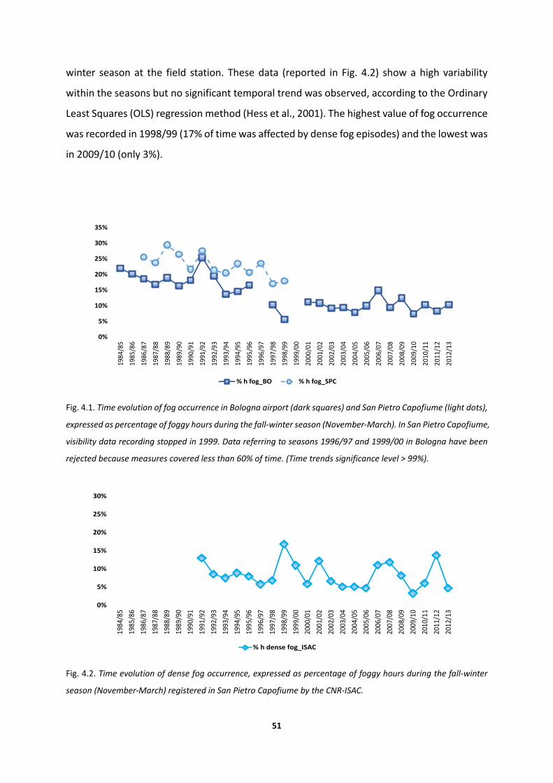
51 

 

winter  season at  the  field  station. These data  (reported  in Fig. 4.2)  show a high variability 

within the seasons but no significant temporal trend was observed, according to the Ordinary 

Least Squares (OLS) regression method (Hess et al., 2001). The highest value of fog occurrence 

was recorded in 1998/99 (17% of time was affected by dense fog episodes) and the lowest was 

in 2009/10 (only 3%). 

 

 

 

Fig. 4.1. Time evolution of fog occurrence in Bologna airport (dark squares) and San Pietro Capofiume (light dots), 

expressed as percentage of foggy hours during the fall‐winter season (November‐March). In San Pietro Capofiume, 

visibility data recording stopped in 1999. Data referring to seasons 1996/97 and 1999/00 in Bologna have been 

rejected because measures covered less than 60% of time. (Time trends significance level > 99%). 

 

 

Fig. 4.2. Time evolution of dense fog occurrence, expressed as percentage of foggy hours during the fall‐winter 

season (November‐March) registered in San Pietro Capofiume by the CNR‐ISAC. 

0%

5%

10%

15%

20%

25%

30%

35%

1984

/85

1985

/86

1986

/87

1987

/88

1988

/89

1989

/90

1990

/91

1991

/92

1992

/93

1993

/94

1994

/95

1995

/96

1996

/97

1997

/98

1998

/99

1999

/00

2000

/01

2001

/02

2002

/03

2003

/04

2004

/05

2005

/06

2006

/07

2007

/08

2008

/09

2009

/10

2010

/11

2011

/12

2012

/13

% h fog_BO % h fog_SPC

0%

5%

10%

15%

20%

25%

30%

1984

/85

1985

/86

1986

/87

1987

/88

1988

/89

1989

/90

1990

/91

1991

/92

1992

/93

1993

/94

1994

/95

1995

/96

1996

/97

1997

/98

1998

/99

1999

/00

2000

/01

2001

/02

2002

/03

2003

/04

2004

/05

2005

/06

2006

/07

2007

/08

2008

/09

2009

/10

2010

/11

2011

/12

2012

/13

% h dense fog_ISAC

52 

 

4.2 Chemical composition of fog droplets 

The first parameters taken into account were conductivity and ionic strength (IS). Conductivity 

has been measured directly (see Chapter 2), while IS has been calculated as a function of the 

concentration of all ions detected by ion chromatography, using the following equation: 

 

IS = ½ Σ ci zi2 

 

where ci is the molar concentration (mol l‐1) and zi is the charge number of the ion i. 

The two parameters are a function of the ionic content of fog water samples, so they both are 

indicative  of  the  total  pollution  loading  of  the  atmosphere where  fog  droplets  form.  The 

volume‐weighted means of conductivity and IS have been calculated for each season (from 

November to March) from 1989/90 to 2010/11 and are reported in Fig.4.3. Panel A shows the 

volume weighted means of ionic strength and panel B refers to conductivity. Coloured areas 

on the plots represent the standard deviations of the calculated averages. Ion content from 

1989/90 to 1992/93 was not available, so IS has not been calculated for those years. 

Both  IS and conductivity trends show a significant decrease: 82% and 80%, respectively  (IS 

from  1993/94  to  2010/11  and  conductivity  from  1989/90  to  2010/11).  The  statistical 

significance of all the trends reported  in this chapter has been calculated according to the 

Ordinary Least Square (OLS) regression method (Hess et al., 2001). 

 

 

53 

 

 

Figure 4.3. Volume weighted averages of  ionic strength  (A) and conductivity  (B). Coloured areas are standard 

deviation of the averages (represented by the dots). (Time trends significance level > 99%). 

 

 

Ionic composition of fog water samples have been determined by ion chromatography. The 

detected  inorganic  ions  are:  sodium  (Na+),  ammonium  (NH4+), potassium  (K+), magnesium 

(Mg2+), calcium (Ca2+), chloride (Cl‐), nitrate (NO32‐) and sulphate (SO4

2‐). A statistical summary 

of their concentration (mmol L‐1)  is reported  in Fig.4.4. Box plots  indicate the 25th, median 

and 75th percentiles and whiskers the 10th and 90th percentiles. Data reported in plots refer 

to the period 1993/94 – 2010/11. Previous chromatographic data are not available, as already 

explained.  It should be noticed that y axes scale (meq L‐1),  is very different from species to 

species. 

Medians, 10° percentile and 90° percentile of all ion concentrations are reported in detail in 

Table 4.1. 

0

200

400

600

800

1000

1989/90

1990/91

1991/92

1992/93

1993/94

1994/95

1995/96

1996/97

1997/98

1998/99

1999/00

2000/01

2001/02

2002/03

 2003/04

2004/05

2005/06

2006/07

2007/08

2008/09

2009/10

2010/11

µS cm

‐1

B

0

2

4

6

8

10

12

14

1989/…

1990/…

1991/…

1992/…

1993/…

1994/…

1995/…

1996/…

1997/…

1998/…

1999/…

2000/…

2001/…

2002/…

2004/…

2005/…

2006/…

2007/…

2008/…

2009/…

2010/…

meq

 L‐1

A

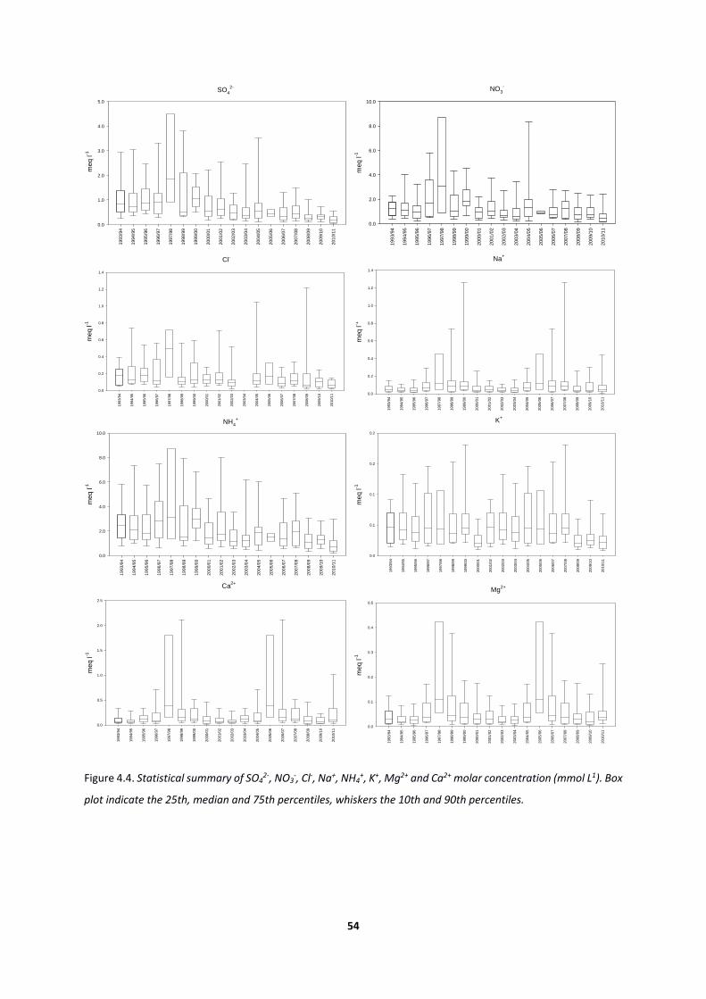
54 

 

 

Figure 4.4. Statistical summary of SO42‐, NO3

‐, Cl‐, Na+, NH4+, K+, Mg2+ and Ca2+ molar concentration (mmol L1). Box 

plot indicate the 25th, median and 75th percentiles, whiskers the 10th and 90th percentiles. 

 

 

 

SO42-

1993

/94

1994

/95

1995

/96

1996

/97

1997

/98

1998

/99

1999

/00

2000

/01

2001

/02

2002

/03

200

3/0

4

2004

/05

2005

/06

2006

/07

2007

/08

2008

/09

2009

/10

2010

/11

meq

l-1

0.0

1.0

2.0

3.0

4.0

5.0

NO3-

1993

/94

1994

/95

1995

/96

1996

/97

1997

/98

1998

/99

1999

/00

2000

/01

2001

/02

2002

/03

200

3/04

2004

/05

2005

/06

2006

/07

2007

/08

2008

/09

2009

/10

2010

/11

meq

l-1

0.0

2.0

4.0

6.0

8.0

10.0

NH4+

19

93

/94

19

94

/95

19

95

/96

19

96

/97

19

97

/98

19

98

/99

19

99

/00

20

00

/01

20

01

/02

20

02

/03

20

03

/04

20

04

/05

20

05

/06

20

06

/07

20

07

/08

20

08

/09

20

09

/10

20

10

/11

meq

l-1

0.0

2.0

4.0

6.0

8.0

10.0

Mg2+

1993

/94

1994

/95

1995

/96

1996

/97

1997

/98

1998

/99

1999

/00

2000

/01

2001

/02

2002

/03

200

3/04

2004

/05

2005

/06

2006

/07

2007

/08

2008

/09

2009

/10

2010

/11

meq

l-1

0.0

0.1

0.2

0.3

0.4

0.5

Ca2+

1993

/94

1994

/95

1995

/96

1996

/97

1997

/98

1998

/99

1999

/00

2000

/01

2001

/02

2002

/03

200

3/04

2004

/05

2005

/06

2006

/07

2007

/08

2008

/09

2009

/10

2010

/11

meq

l-1

0.0

0.5

1.0

1.5

2.0

2.5

K+

1993

/94

1994

/95

1995

/96

1996

/97

1997

/98

1998

/99

1999

/00

2000

/01

2001

/02

2002

/03

200

3/04

2004

/05

2005

/06

2006

/07

2007

/08

2008

/09

2009

/10

2010

/11

meq

l-1

0.0

0.1

0.1

0.2

0.2

Na+

1993

/94

1994

/95

1995

/96

1996

/97

1997

/98

1998

/99

1999

/00

2000

/01

2001

/02

2002

/03

200

3/04

2004

/05

2005

/06

2006

/07

2007

/08

2008

/09

2009

/10

2010

/11

meq

l-1

0.0

0.2

0.4

0.6

0.8

1.0

1.2

1.4

Cl-

1993

/94

1994

/95

1995

/96

1996

/97

1997

/98

1998

/99

1999

/00

2000

/01

2001

/02

2002

/03

2003

/04

2004

/05

2005

/06

2006

/07

2007

/08

2008

/09

2009

/10

2010

/11

meq

l-1

0.0

0.2

0.4

0.6

0.8

1.0

1.2

1.4

55 

 

Table 4.1. Median, 10° percentile and 90° percentile of inorganic ion concentrations (meq L‐1) in fog water from 

fall winter‐season 1993/94 to fall‐winter season 2010/11. 

 

Cl‐ NO3‐ SO4

2‐ Na+

meq L‐1  median  10° perc  90° perc  median  10° perc  90° perc  median  10° perc  90° perc  median  10° perc  90° perc

1993/94  0.18  0.06  0.35  1.2  0.38  2.2  0.82  0.30  2.2  0.04  0.02  0.14 

1994/95  0.12  0.07  0.71  1.1  0.48  3.0  0.74  0.37  2.4  0.04  0.02  0.10 

1995/96  0.18  0.08  0.42  0.95  0.29  2.9  0.87  0.53  2.2  0.03  0.02  0.13 

1996/97  0.12  0.05  0.48  1.7  0.51 5.4 0.91 0.32 2.2 0.06 0.03  0.20 

1997/98  0.50  0.13  5.0  3.1  0.60 15 1.9 0.72 7.9 0.11 0.04  4.4 

1998/99  0.11  0.04  0.41  1.0  0.42  2.9  0.50  0.35  2.8  0.09  0.02  0.55 

1999/00  0.13  0.05  0.48  1.8  0.83  3.7  1.1  0.60  1.7  0.08  0.04  0.38 

2000/01  0.12  0.06  0.25  0.93  0.34  2.2  0.54  0.22  1.9  0.04  0.02  0.16 

2001/02  0.12  0.06  0.35  1.1  0.47 3.0 0.63 0.28 2.2 0.04 0.01  0.29 

2002/03  0.09  0.02  0.34  0.70  0.33 2.3 0.46 0.19 1.2 0.05 0.01  0.25 

2003/04  0.00  0.00  0.00  0.57  0.30  1.5  0.35  0.17  1.3  0.10  0.03  0.15 

2004/05  0.12  0.07  0.35  1.4  0.44  2.6  0.54  0.19  1.5  0.02  0.01  0.09 

2005/06  0.17  0.06  0.48  0.88  0.64  1.2  0.44  0.29  0.6  0.07  0.01  0.41 

2006/07  0.09  0.04  0.20  0.72  0.46 2.2 0.34 0.12 1.1 0.04 0.02  0.15 

2007/08  0.12  0.05  0.28  1.23  0.39 2.3 0.45 0.16 1.2 0.06 0.02  0.29 

2008/09  0.07  0.03  0.71  0.74  0.12  2.2  0.24  0.13  0.8  0.06  0.02  0.67 

2009/10  0.11  0.02  0.21  0.73  0.43  2.2  0.33  0.15  0.5  0.07  0.04  0.13 

2010/11  0.07  0.03  0.15  0.45  0.16  1.5  0.20  0.06  0.5  0.04  0.01  0.12 

  NH4+ K+ Mg2+ Ca2+

meq L‐1 median  10° perc  90° perc  median  10° perc  90° perc  median  10° perc  90° perc  median  10° perc  90° perc

1993/94  2.5  0.84  5.2  0.05  0.02 0.08 0.03 0.01 0.10 0.07 0.03  0.21 

1994/95  2.1  1.1  6.1  0.04  0.02 0.12 0.02 0.01 0.07 0.07 0.03  0.25 

1995/96  1.8  0.93  5.2  0.04  0.01  0.10  0.03  0.01  0.07  0.13  0.04  0.28 

1996/97  2.9  0.68  5.7  0.04  0.02  0.13  0.04  0.02  0.16  0.09  0.04  0.54 

1997/98  3.1  1.1  11  0.04  0.02  0.39  0.11  0.05  2.84  0.39  0.12  6.40 

1998/99  1.5  1.0  6.7  0.04  0.02 0.12 0.04 0.01 0.24 0.15 0.06  0.93 

1999/00  3.0  1.3  5.3  0.05  0.02 0.15 0.04 0.01 0.15 0.12 0.05  0.44 

2000/01  1.5  0.62  4.4  0.02  0.01  0.06  0.03  0.01  0.12  0.08  0.02  0.39 

2001/02  1.8  0.71  5.9  0.02  0.01  0.07  0.02  0.01  0.11  0.06  0.03  0.22 

2002/03  1.2  0.67  2.9  0.02  0.01  0.05  0.04  0.01  0.15  0.10  0.04  0.45 

2003/04  1.2  0.59  3.0  0.01  0.01 0.03 0.04 0.02 0.08 0.11 0.06  0.27 

2004/05  1.9  0.67  2.7  0.02  0.00 0.03 0.02 0.01 0.09 0.07 0.03  0.31 

2005/06  1.5  0.88  2.0  0.01  0.00  0.02  0.04  0.01  0.16  0.12  0.08  0.22 

2006/07  1.3  0.70  4.2  0.01  0.01  0.04  0.02  0.01  0.05  0.09  0.06  0.23 

2007/08  2.0  0.69  4.3  0.02  0.01  0.04  0.04  0.01  0.10  0.10  0.04  0.31 

2008/09  1.1  0.37  3.0  0.01  0.01 0.04 0.03 0.01 0.33 0.10 0.03  0.41 

2009/10  1.3  0.67  2.6  0.01  0.01 0.03 0.03 0.01 0.06 0.04 0.02  0.13 

2010/11  0.73  0.20  1.7  0.02  0.00 0.05 0.02 0.00 0.09 0.04 0.01  0.19 

56 

 

The major chemical constituents of fog water are NO3‐, SO4

2‐ and NH4+ that alone account for 

an average 86 (±12) % of total IS. The mean volume‐weighted concentrations of the three ionic 

species  are  reported  in  Fig.4.5.  NH4+,  NO3

‐  and  SO42‐  concentrations  show  a  significant 

decreasing  trend, as expected  from  the decrease of  ionic strength and conductivity values 

over the considered period. Concentration of SO42‐ in fog water decreased of 76%. NO3

‐ and 

NH4+ underwent a smaller decrease: 43% and 55%, respectively. Ionic load reduction of these 

chemical  species  is  explained  by  a  parallel  reduction  of  the  atmospheric  emission  of  fog 

droplets gas – phase precursors (SO2, NOx and NH3). In order to verify this correlation, emission 

data, provided by the Italian Institute for the Environmental Protection and Research (ISPRA) 

(http://www.isprambiente.gov.it/banche‐dati/aria‐ed‐emissioni‐in‐atmosfera),  were  analysed. 

The results are reported in Fig.4.6. Data refer to total emission in the region Emilia‐Romagna 

from 1990 ‐ 2010. They show a 90% reduction of SO2 emission and smaller reductions for NOx 

emission  (44%)  and  NH3  (31%).  These  trends  agree  with  those  of  fog  chemical  species, 

confirming  the  correlation  between  atmospheric  emissions  and  ionic  load  in  fog  droplets 

composition. 

 

 

 

 

 

 

 

 

 

 

 

 

 

 

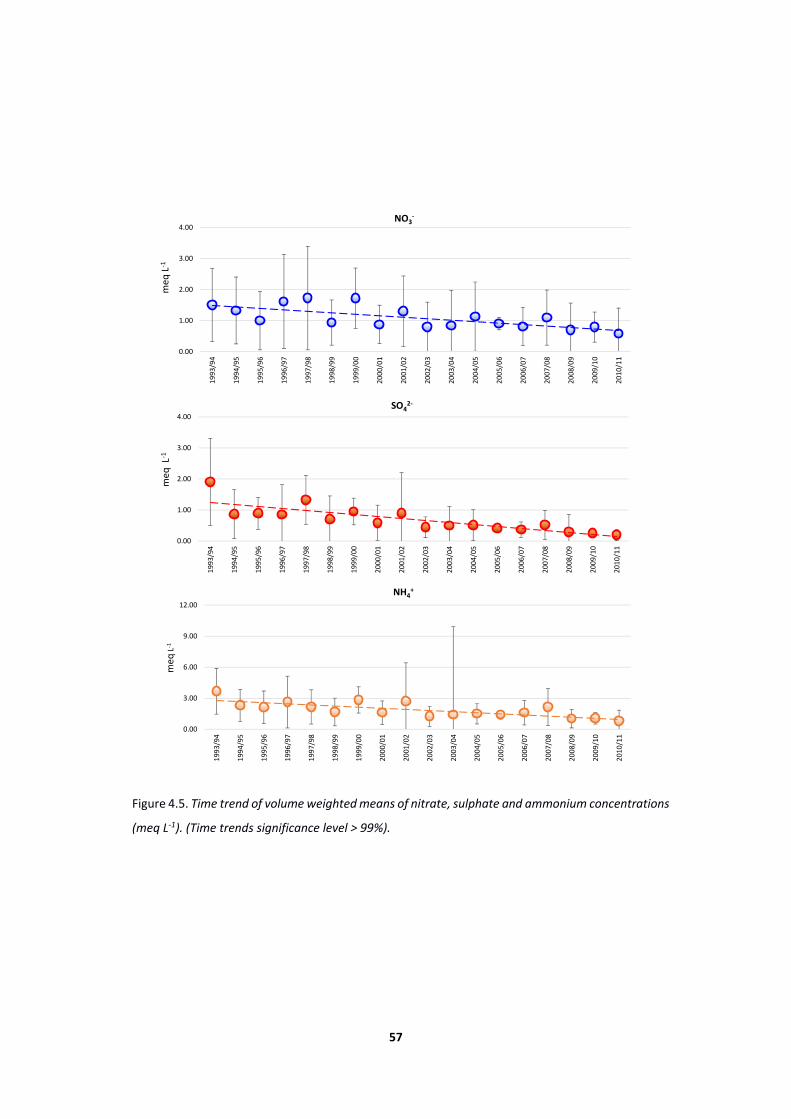
57 

 

 

 

 

 

Figure 4.5. Time trend of volume weighted means of nitrate, sulphate and ammonium concentrations 

(meq L‐1). (Time trends significance level > 99%). 

 

 

0.00

1.00

2.00

3.00

4.00

1993/94

1994/95

1995/96

1996/97

1997/98

1998/99

1999/00

2000/01

2001/02

2002/03

 2003/04

2004/05

2005/06

2006/07

2007/08

2008/09

2009/10

2010/11

meq L‐1

NO3‐

0.00

1.00

2.00

3.00

4.00

1993/94

1994/95

1995/96

1996/97

1997/98

1998/99

1999/00

2000/01

2001/02

2002/03

 2003/04

2004/05

2005/06

2006/07

2007/08

2008/09

2009/10

2010/11

meq  L

‐1

SO42‐

0.00

3.00

6.00

9.00

12.00

1993/94

1994/95

1995/96

1996/97

1997/98

1998/99

1999/00

2000/01

2001/02

2002/03

 2003/04

2004/05

2005/06

2006/07

2007/08

2008/09

2009/10

2010/11

meqL‐1

NH4+

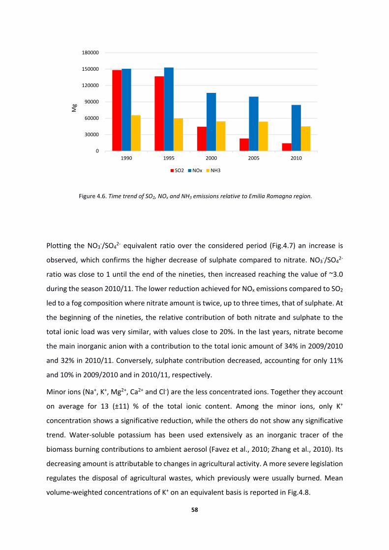
58 

 

 

Figure 4.6. Time trend of SO2, NOx and NH3 emissions relative to Emilia Romagna region. 

 

 

Plotting  the NO3‐/SO4

2‐ equivalent  ratio over  the considered period  (Fig.4.7) an  increase  is 

observed, which confirms  the higher decrease of sulphate compared to nitrate. NO3‐/SO4

2‐ 

ratio was close to 1 until the end of the nineties, then  increased reaching the value of ~3.0 

during the season 2010/11. The lower reduction achieved for NOx emissions compared to SO2 

led to a fog composition where nitrate amount is twice, up to three times, that of sulphate. At 

the beginning of the nineties, the relative contribution of both nitrate and sulphate to the 

total ionic load was very similar, with values close to 20%. In the last years, nitrate become 

the main inorganic anion with a contribution to the total ionic amount of 34% in 2009/2010 

and 32%  in 2010/11. Conversely, sulphate contribution decreased, accounting for only 11% 

and 10% in 2009/2010 and in 2010/11, respectively. 

Minor ions (Na+, K+, Mg2+, Ca2+ and Cl‐) are the less concentrated ions. Together they account 

on  average  for  13  (±11)  %  of  the  total  ionic  content.  Among  the  minor  ions,  only  K+ 

concentration shows a significative reduction, while the others do not show any significative 

trend. Water‐soluble  potassium  has  been  used  extensively  as  an  inorganic  tracer  of  the 

biomass burning contributions to ambient aerosol (Favez et al., 2010; Zhang et al., 2010). Its 

decreasing amount is attributable to changes in agricultural activity. A more severe legislation 

regulates  the disposal of agricultural wastes, which previously were usually burned. Mean 

volume‐weighted concentrations of K+ on an equivalent basis is reported in Fig.4.8. 

0

30000

60000

90000

120000

150000

180000

1990 1995 2000 2005 2010

Mg 

SO2 NOx NH3

59 

 

 

 

Figure 4.7. Time trend of NO3‐/SO4

2‐ ratio. (Time trend significance level > 99%). 

 

 

Figure 4.8. Time trend of volume weighted means of potassium concentration (meq L‐1). (Time trend 

significance level > 99%). 

 

These results are in line with other studies carried out in Europe (Lange et al., 2003), where a 

reduction of ionic concentration in fog water was observed and attributed to an improvement 

of air quality pursued since the 1990s. 

 

 

0.0

1.0

2.0

3.0

4.0

5.0

1989/90

1990/91

1991/92

1992/93

1993/94

1994/95

1995/96

1996/97

1997/98

1998/99

1999/00

2000/01

2001/02

2002/03

 2003

/04

2004/05

2005/06

2006/07

2007/08

2008/09

2009/10

2010/11

NO

3‐/ SO

42‐(m

eq l‐

1)

0.00

0.02

0.04

0.06

0.08

0.10

0.12

0.14

1993/94

1994/95

1995/96

1996/97

1997/98

1998/99

1999/00

2000/01

2001/02

2002/03

 2003/04

2004/05

2005/06

2006/07

2007/08

2008/09

2009/10

2010/11

meq

 l‐1

K+

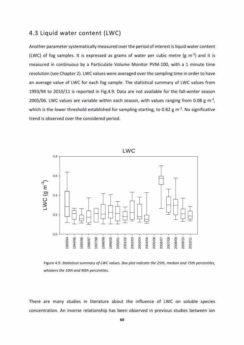
60 

 

4.3 Liquid water content (LWC) 

Another parameter systematically measured over the period of interest is liquid water content 

(LWC) of  fog  samples.  It  is expressed  as  grams of water per  cubic metre  (g m‐3)  and  it  is 

measured  in continuous by a Particulate Volume Monitor PVM‐100, with a 1 minute  time 

resolution (see Chapter 2). LWC values were averaged over the sampling time in order to have 

an average value of LWC for each fog sample. The statistical summary of LWC values from 

1993/94 to 2010/11  is reported  in Fig.4.9. Data are not available for the fall‐winter season 

2005/06. LWC values are variable within each season, with values ranging from 0.08 g m‐3, 

which is the lower threshold established for sampling starting, to 0.82 g m‐3. No significative 

trend is observed over the considered period. 

 

 

 

Figure 4.9. Statistical summary of LWC values. Box plot indicate the 25th, median and 75th percentiles, 

whiskers the 10th and 90th percentiles. 

 

 

There  are  many  studies  in  literature  about  the  influence  of  LWC  on  soluble  species 

concentration. An  inverse  relationship has been observed  in previous studies between  ion 

LWC

1993

/94

1994

/95

1995

/96

1996

/97

1997

/98

1998

/99

1999

/00

2000

/01

2001

/02

2002

/03

200

3/04

2004

/05

2005

/06

2006

/07

2007

/08

2008

/09

2009

/10

2010

/11

LW

C (

g m

-3)

0.0

0.2

0.4

0.6

0.8

61 

 

concentrations and LWC, although with a different trends in different locations (Aleksic and 

Dukett, 2010; Elbert et al., 2000; Elbert et al., 2002; Kasper‐Giebl, 2002; Straub et al., 2012). 

The plot in Fig.4.10 shows the sum of molalities of nitrate and sulphate as a function of LWC 

for the data recorded at San Pietro Capofiume from 1993/94 to 2010/11. 

The best fit for the data was calculated using the following equation: 

 

m = b L‐1 

 

where m is the molality of a substance in fog water (µmol kg‐1), L the liquid water content (g 

m‐3) and b the regression slope obtained plotting measured m versus corresponding L‐1. This 

equation was  chosen  according  to  (Elbert  et  al.,  2000),  that  suggested  its  suitability  for 

samples of different origins, such as marine and polluted continental. 

Best fit is represented by the thick solid line in the plot. Thin lines were calculated the same 

way, but slope values  (b) derive  from  the 5th and 95th percentile molality values. Even  if a 

decreasing anion molality with increasing LWC can be discerned, the power law best fit shows 

a very low correlation (R2 = 0.03), indicating that variation in LWC values only minimally affect 

ions concentrations. This observation  together with  the  fact  that no statistically significant 

trend was found for LWC values, strengthen the hypothesis that the decreasing ionic load in 

fog water is not due to a “dilution” effect, but is connected with lower atmospheric emission 

of gaseous precursors. 

 

62 

 

 

Figure 4.10. Correlation between LWC and the sum of sulphate and nitrate molalities. Thick line is the power 

law best fit, while thin lines were calculated using the 5th and the 95th percentile values of molalities. No 

samples were collected at LWC < 0.08 g m‐3 because of technical limitations (see chapter 2). 

 

 

4.4 Fog water acidity 

Until the eighties, many studies were carried out about the acidity of cloud water, fog water, 

rain and snow, especially  in the  industrialized countries of the northern hemisphere, where 

increasing  combustion  processes  caused  the  acidification  of  the  atmospheric  liquid water 

phase (Jacobson, 1984; Wisniewski, 1982) (Saxena and Lin, 1990). (Fuzzi et al., 1983) focused 

on the pH trend during the evolution of a fog event in the Po Valley, stressing the crucial role 

of NO3‐ and SO4

2‐ in the determination of fog acidity. From then on, fog pH values have been 

regularly measured at the field station of San Pietro Capofiume. Fig.4.11 shows the statistical 

summary of pH value of each season from 1989/90 to 2010/11.  

0

2000

4000

6000

8000

10000

12000

14000

0.0 0.1 0.2 0.3 0.4 0.5 0.6 0.7 0.8

m, µ

mol kg‐1

LWC, g m‐3

63 

 

 

Figure 4.11. Statistical summary of pH values. Box plot indicate the 25th, median and 75th percentiles, 

whiskers  the 10th and 90th percentiles. Regression  line  (red dotted  line)  shows an  increasing  trend 

(significance level > 99%). 

 

 

Despite the variability of pH values within each season (in 2004/05 pH ranged from 3.4 to 7.5), 

pH shows an increasing trend, at a 99% confidence interval. The calculated volume weighted 

means  show  that during  the 90s  the mean pH values never exceeded 5,  ranging  from  the 

lowest average pH  in 1995/96  (3.6) to the highest  in 1998/99  (4.7).  In the  last decade, the 

lowest average pH value was 4.1  in 2001/02 and  the highest  reached 6.9  in 2005/06 with 

values mostly exceeding 5. This reduction of fog acidity is what we expected from the observed 

decrease of NO3‐ and SO4

2‐ concentrations in fog water. 

The pH trend leads to a condition of neutrality in fog water presently collected, even though 

it should be taken into account that these pH values refer to bulk sample and not to single fog 

droplets. Anyway, the achievement of a pH neutral condition is linked to the lower decrease 

of ammonia emissions compared to those of SO2 and NOx that represent the precursors of the 

two major acidic species in solution. 

1989

/90

1990

/91

1991

/92

1992

/93

1993

/94

1994

/95

1996

/97

1997

/98

1998

/99

1999

/00

2000

/01

2001

/02

2002

/03

200

3/04

2004

/05

2005

/06

2006

/07

2007

/08

2008

/09

2009

/10

2010

/11

pH

2

3

4

5

6

7

8

9

64 

 

4.5 Organic fraction of fog droplets 

So  far, only the  inorganic components of  fog water were taken  into account. We saw that 

sulphate, nitrate and ammonium together account for near 90% of the total ionic strength of 

fog water. Besides these three main ionic species, the organic matter must also be evaluated, 

representing  a  significant  fraction  of  the  total mass  of  fog water,  and  playing  a  role  in 

determining  the  physical  ‐  chemical  characteristics  of  fog  droplets  and  residual  aerosol 

particles after water evaporation. 

Starting from fall‐winter season 1997/98, WSOC has been systematically measured with the 

purpose to implement the knowledge about the organic fraction of fog droplets. The average 

chemical composition of fog water over the period 1997/98 ‐ 2010/11 is reported in Fig.4.12. 

 

 

 

Figure 4.12. Average chemical composition of fog water over the period 1997/98 ‐ 2010/11. 

 

 

The three main ionic species together account on average for 67% of the total soluble mass 

and water‐soluble organic matter (WSOM) for 28%. A factor of 1.8 was used to convert water‐

65 

 

soluble organic carbon  (WSOC)  to water‐soluble organic matter  (WSOM), according  to  the 

literature (Matta et al., 2003). 

Fig.4.13  shows a statistical summary of WSOC concentration  in  fog water collected at San 

Pietro Capofiume. Concentrations can be very variable within each season and no significative 

trend  is observed  from 1997/98  to 2010/11. Values  range  from 3 mgC L‐1  to 350 mgC L‐1. 

Seasonal  median  concentration  range  from  15  mgC  L‐1  in  2002/2003,  to  49  mgC  L1  in 

1999/2000. 

 

 

 

Figure 4.13. Statistical summary of WSOC concentration (mgC L‐1). Box plot indicate the 25th, median 

and 75th percentiles, whiskers the 10th and 90th percentiles. 

 

 

Previous studies carried out at  the  field station of San Pietro Capofiume, showed  that  the 

absorption of gases contributes for about 3% to the fog droplets organic fraction, while the 

contribution of  the  coagulation of  interstitial particles  is negligible  (Facchini  et  al.,  1999). 

Nucleation scavenging has been  found to be the most  important source of soluble organic 

compounds in fog droplets in the Po Valley region. 

WSOC

199

7/9

8

199

8/9

9

199

9/0

0

200

0/0

1

200

1/0

2

200

2/0

3

200

3/0

4

200

4/0

5

200

5/0

6

200

6/0

7

200

7/0

8

200

8/0

9

200

9/1

0

201

0/1

1

mg

C L

-1

0

50

100

150

200

250

300

66 

 

Specific studies have been carried out to characterise the organic  fraction of Po Valley  fog 

samples.  (Facchini  et  al.,  1992),  focused  on  the  gas‐liquid  phase  partitioning  of  carbonyl 

compounds, formaldehyde (HCHO), formic acid (HCOOH) and acetic acid (CH3COOH), which in 

the Po Valley mainly originate from anthropogenic sources. Further efforts have been made 

to  implement  the  characterization  of  the  organic  fraction.  An  analytical  method  was 

developed  for  this  purpose,  combining  HPLC  and  HNMR  techniques,  and  described  in 

(Decesari  et  al.,  2000).  This  methodology  classifies  WSOC  into  a  few  major  classes  of 

compounds,  attempting  a  characterization  and  quantification  of  the  functional  groups, 

instead of a definition of individual molecular species. They found that 25% of soluble organic 

carbon derived from neutral and basic compounds, 35% from mono and dicarboxylic acids and 

17% from polyacids, showing that the organic fraction was formed for more than 50% by acidic 

compounds. The unaccounted fraction (23%) was due to losses of material during the different 

phases of the analytical procedure. These results were confirmed in a later study reported in 

(Fuzzi et al., 2002), where a similar relative organic carbon content was determined. They also 

detected a class of polycarboxylic acids similar to fulvic acids. These studies showed that a 

significant  fraction  of  WSOC  in  fog  droplets  is  not  volatile  and  cannot  originate  via 

condensation  from  the  gas  phase.  The most  plausible  source  of  such  non‐volatile water‐

soluble organic matter is nucleation scavenging of aerosol particles, because polyacids are also 

found in submicron particles out of fog conditions (Decesari et al., 2000; Decesari et al., 2001). 

On the other hand, recent laboratory studies indicate that low‐volatility compounds can form 

through aqueous phase reactions starting from volatile precursors (Ervens et al., 2011; Lim et 

al., 2013; Tan et  al., 2012).  These  studies  therefore  suggest  that  complex, high‐molecular 

water‐soluble organic compounds  in fog droplets can form as secondary compounds, along 

with the most common products such as pyruvic acid and oxalate. 

Unfortunately, due to  its time consuming nature, the analytical procedure described above 

was not  applied  to  the whole  series of  available  fog  samples. Only  low molecular weight 

carboxylic  acids,  acetic  acid  (CH3COOH),  formic  acid  (HCOOH),  methanesulfonic  acid 

(CH3SO3H) and oxalic acid (C2H2O4), have been systematically detected and quantified by ion 

chromatography. Concentrations are very variable from sample to sample, ranging from a few 

to several hundreds µmol L‐1. A statistical summary of the data is reported in Table 4.2. The 

contribution of these low molecular weight organic acids to the total organic mass ranges from 

1% to 68%, with median percentages ranging from 4%, in 2010/11, to 25%, in 1998/99. 

67 

 

 

Table 4.2. Median, minimum and maximum of low molecular weight organic acids (µmol L‐1) 

in fog water from fall winter‐season 1997/98 to fall‐winter season 2010/11. 

    Concentration (µmol l‐1)

  Acetate Formate Methanesulfonate Oxalate 

Season  median range  median range median range median  range 

1997/9 100  (43‐163)  116 (43‐314) 1.5 (0‐31) 22 (7.9‐106) 

1998/9 98  (36‐909)  91 (12‐318) n.a. n.a. 8.0 (2.7‐30) 

1999/0 97  (17‐290)  8.0 (0‐174) 68 (0‐191) 21 (3.8‐82) 

2000/0 36  (5.1‐170)  6.8 (0‐146) 47 (0‐416) 12 (4.9‐59) 

2001/0 33  (0‐239)  5.4 (0‐152) 46 (0.2‐358) 13 (4.9‐70) 

2002/0 n.a.  n.a.  n.a. n.a. n.a. n.a. 8.5 (0‐37) 

2003/0 n.a.  n.a.  n.a. n.a. n.a. n.a. 8.2 (0‐60) 

2004/0 59  (1.1‐189)  57 (4.1‐176) 0.5 (0‐165) 14 (0.5‐95) 

2005/0 28  (6.3‐125)  37 (4.2‐67) 0 (0‐4.3) 6.9 (0.7‐13) 

2006/0 4.6  (0.1‐102)  18 (1.2‐78) 0.1 (0‐31) 5.2 (0‐54) 

2007/0 3.1  (0.3‐60)  6.9 (0‐46) 1.9 (0‐13) 6.2 (0‐58) 

2008/0 13  (0.7‐124)  18 (0‐133) 0.4 (0‐11) 3.6 (0‐31) 

2009/1 35  (7.9‐184)  28 (1.6‐79) 0 (0‐35) 8.9 (0‐30) 

2010/1 14  (3.3‐109)  1.7 (0.2‐124) 0.7 (0‐14) 0 (0‐6.8) 

 

69 

 

5. Aerosol – fog interaction 

 

In  the  frame  of  the  Supersito  project  an  intensive  field  campaign  has  been  organized  on 

November 2011, where aerosol samples were collected at the Meteorological station Giorgio 

Fea  in  San  Pietro  Capofiume,  Bologna.  A  detailed  description  of  the  campaign  has  been 

provided in Chapter 3. The routine collection of fog samples at the measurement station in 

San Pietro Capofiume started in November 2011 and lasted until March 2012. The Supersito 

campaign  started  in 15/11/2011 and ended  in 01/12/2011. The measurement period was 

characterized by very frequent fog episodes and 13 fog samples were collected. The list of fog 

samples is reported in Table 5.1. 

 

 

Table 5.1. List of  fog samples collected during the Supersito  field campaign at the 

meteorological station in San Pietro Capofiume (Bo). 

Sample name  Sample start  Sample stop sampling time 

(min) 

SPC141111  14/11/2011 19.30 15/11/2011 09.00 810 

SPC151111  15/11/2011 09.00 15/11/2011 18.03 543 

SPC151111_S 15/11/2011 18.03 16/11/2011 10.39 996 

SPC161111  16/11/2011 18.00 17/11/2011 09.09 909 

SPC171111  17/11/2011 17.23 18/11/2011 05.56 753 

SPC181111  18/11/2011 18.20 19/11/2011 10.50 990 

SPC191111  19/11/2011 17.30 20/11/2011 13.09 1179 

SPC201111  20/11/2011 15.40 21/11/2011 12.30 1250 

SPC211111  21/11/2011 19.00 21/11/2011 21.00 120 

SPC251111  25/11/2011 19.00 25/11/2011 21.20 140 

SPC261111  26/11/2011 19.00 26/11/2011 19.50 50 

SPC271111  27/11/2011 19.40 28/11/2011 10.20 880 

SPC281111  28/11/2011 17.10 28/11/2011 22.10 300 

SPC291111  29/11/2011 18.10 30/11/2011 09.20 910 

 

 

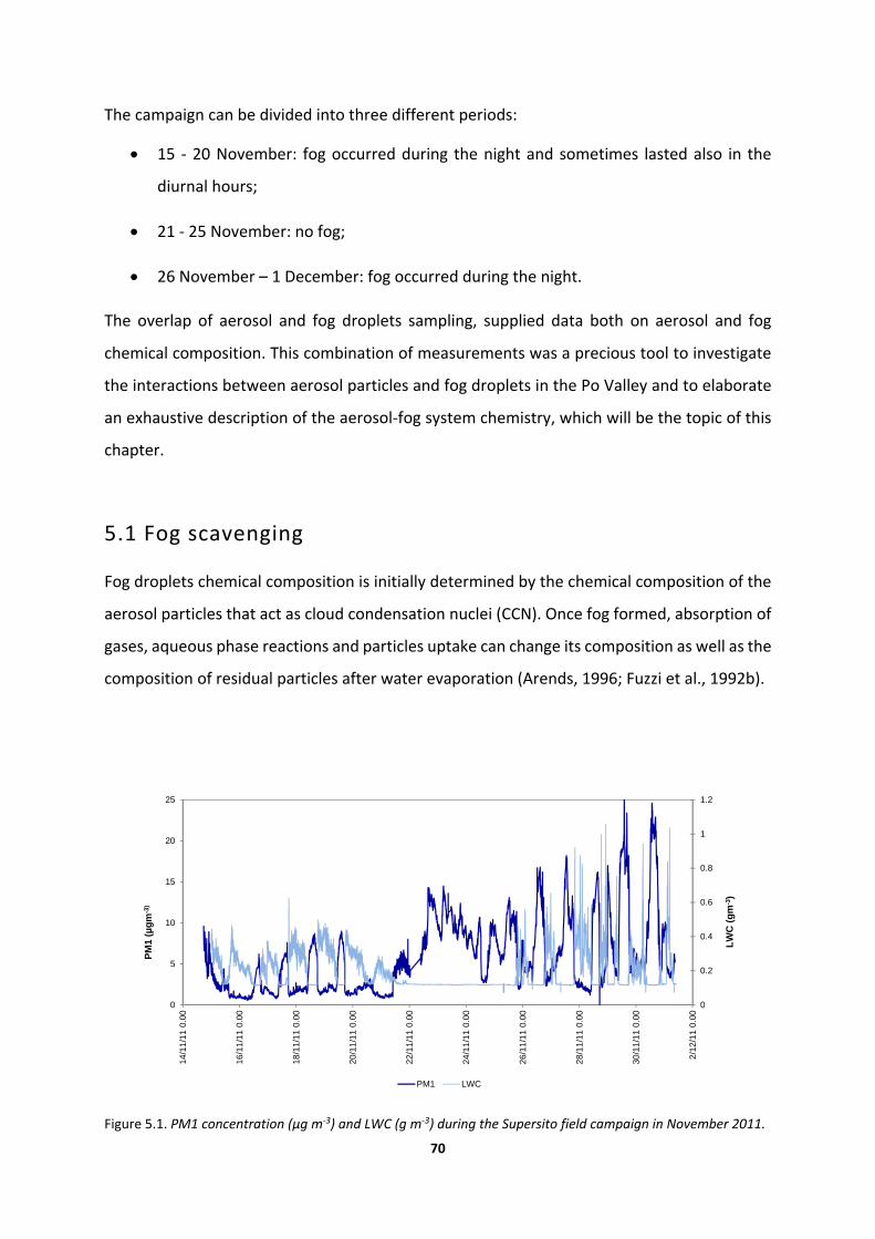
70 

 

The campaign can be divided into three different periods: 

15  ‐ 20 November:  fog occurred during  the night and sometimes  lasted also  in  the 

diurnal hours; 

21 ‐ 25 November: no fog; 

26 November – 1 December: fog occurred during the night. 

The overlap of  aerosol  and  fog droplets  sampling,  supplied data both on  aerosol  and  fog 

chemical composition. This combination of measurements was a precious tool to investigate 

the interactions between aerosol particles and fog droplets in the Po Valley and to elaborate 

an exhaustive description of the aerosol‐fog system chemistry, which will be the topic of this 

chapter. 

 

5.1 Fog scavenging 

Fog droplets chemical composition is initially determined by the chemical composition of the 

aerosol particles that act as cloud condensation nuclei (CCN). Once fog formed, absorption of 

gases, aqueous phase reactions and particles uptake can change its composition as well as the 

composition of residual particles after water evaporation (Arends, 1996; Fuzzi et al., 1992b). 

 

 

 

Figure 5.1. PM1 concentration (µg m‐3) and LWC (g m‐3) during the Supersito field campaign in November 2011. 

0

0.2

0.4

0.6

0.8

1

1.2

0

5

10

15

20

25

14/1

1/1

1 0.

00

16/1

1/1

1 0.

00

18/1

1/1

1 0.

00

20/1

1/1

1 0.

00

22/1

1/1

1 0.

00

24/1

1/1

1 0.

00

26/1

1/1

1 0.

00

28/1

1/1

1 0.

00

30/1

1/1

1 0.

00

2/1

2/1

1 0

.00

LW

C (

gm

-3)

PM

1 (µ

gm

-3)

PM1 LWC

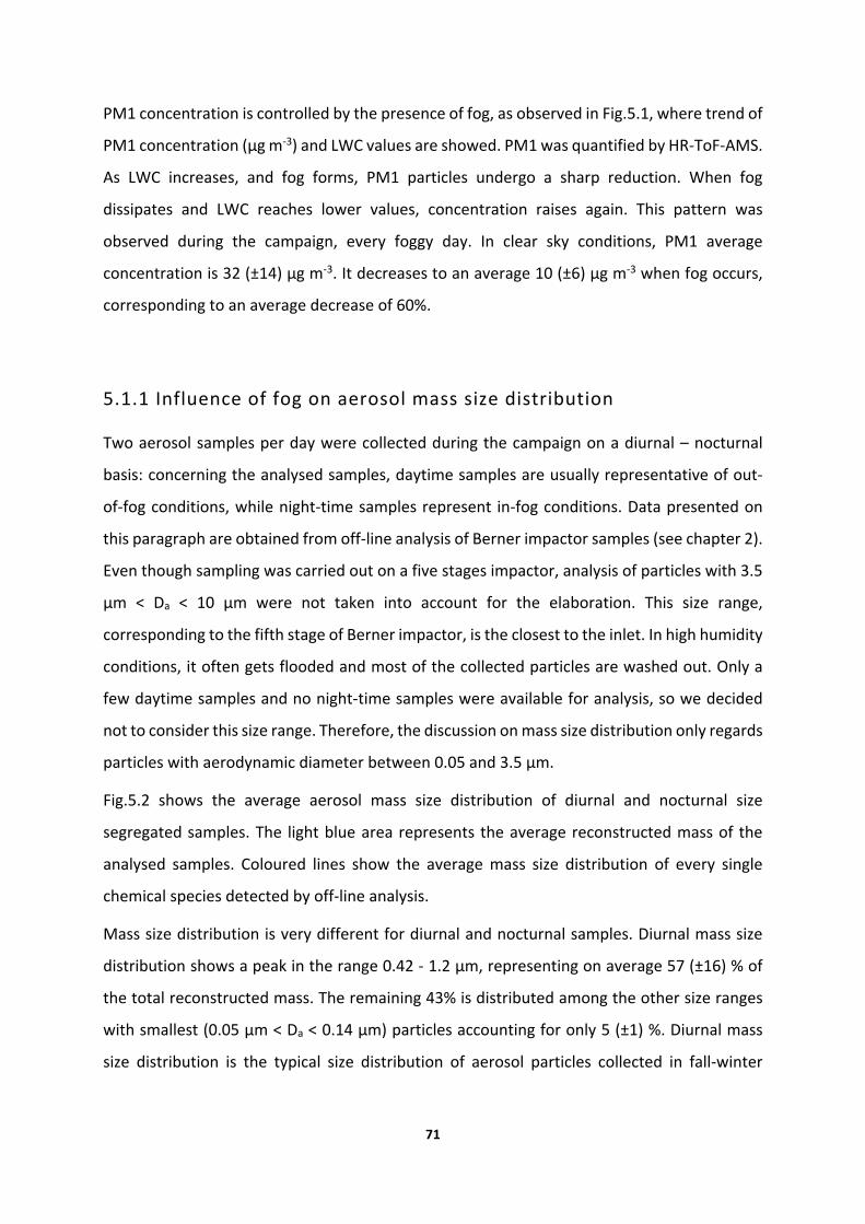
71 

 

PM1 concentration is controlled by the presence of fog, as observed in Fig.5.1, where trend of 

PM1 concentration (µg m‐3) and LWC values are showed. PM1 was quantified by HR‐ToF‐AMS. 

As  LWC  increases,  and  fog  forms,  PM1  particles  undergo  a  sharp  reduction. When  fog 

dissipates  and  LWC  reaches  lower  values,  concentration  raises  again.  This  pattern  was 

observed  during  the  campaign,  every  foggy  day.  In  clear  sky  conditions,  PM1  average 

concentration is 32 (±14) µg m‐3. It decreases to an average 10 (±6) µg m‐3 when fog occurs, 

corresponding to an average decrease of 60%. 

 

5.1.1 Influence of fog on aerosol mass size distribution 

Two aerosol samples per day were collected during the campaign on a diurnal – nocturnal 

basis: concerning the analysed samples, daytime samples are usually representative of out‐

of‐fog conditions, while night‐time samples represent  in‐fog conditions. Data presented on 

this paragraph are obtained from off‐line analysis of Berner impactor samples (see chapter 2). 

Even though sampling was carried out on a five stages impactor, analysis of particles with 3.5 

µm  <  Da  <  10  µm  were  not  taken  into  account  for  the  elaboration.  This  size  range, 

corresponding to the fifth stage of Berner impactor, is the closest to the inlet. In high humidity 

conditions, it often gets flooded and most of the collected particles are washed out. Only a 

few daytime samples and no night‐time samples were available for analysis, so we decided 

not to consider this size range. Therefore, the discussion on mass size distribution only regards 

particles with aerodynamic diameter between 0.05 and 3.5 µm. 

Fig.5.2  shows  the  average  aerosol  mass  size  distribution  of  diurnal  and  nocturnal  size 

segregated samples. The  light blue area represents the average reconstructed mass of the 

analysed  samples. Coloured  lines  show  the  average mass  size distribution  of  every  single 

chemical species detected by off‐line analysis. 

Mass size distribution  is very different for diurnal and nocturnal samples. Diurnal mass size 

distribution shows a peak in the range 0.42 ‐ 1.2 µm, representing on average 57 (±16) % of 

the total reconstructed mass. The remaining 43% is distributed among the other size ranges 

with smallest (0.05 µm < Da < 0.14 µm) particles accounting for only 5 (±1) %. Diurnal mass 

size  distribution  is  the  typical  size  distribution  of  aerosol  particles  collected  in  fall‐winter 

72 

 

season in urban continental environments, as reported in previous studies(Matta et al., 2003; 

Pennanen et al., 2007; Spindler et al., 2012). 

 

 

 

Figure 5.2. Average aerosol total mass size distribution (µg m‐3) of diurnal (a) and nocturnal (b) samples and mass 

size distribution of the main chemical species. 

 

 

During the night, when fog occurs, mass size distribution differs significantly from the diurnal  

one, showing an intense decrease of particles with 0.42 µm < Da < 1.2 µm, whose mass now 

accounts for 38 (±10) % of total reconstructed mass. Particles with 0.14 µm < Da < 0.42 µm 

also show a sharp reduction, representing only 10 (±2) % of the total mass, compared to 23 

(±4) % in daytime samples. 

0

10

20

30

0.05‐0.14 0.14‐0.42 0.42‐1.2 1.2‐3.5

µg m

‐3

a) Day

0

3

6

9

12

0.05‐0.14 0.14‐0.42 0.42‐1.2 1.2‐3.5

µg m

‐3

b) Night

PM3.5 NO3 SO4 NH4 WSOM WINCM other ions

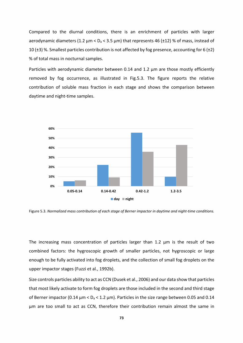
73 

 

Compared  to  the  diurnal  conditions,  there  is  an  enrichment  of  particles  with  larger 

aerodynamic diameters (1.2 µm < Da < 3.5 µm) that represents 46 (±12) % of mass, instead of 

10 (±3) %. Smallest particles contribution is not affected by fog presence, accounting for 6 (±2) 

% of total mass in nocturnal samples. 

Particles with aerodynamic diameter between 0.14 and 1.2 μm are those mostly efficiently 

removed  by  fog  occurrence,  as  illustrated  in  Fig.5.3.  The  figure  reports  the  relative 

contribution  of  soluble mass  fraction  in  each  stage  and  shows  the  comparison  between 

daytime and night‐time samples. 

 

 

 

Figure 5.3. Normalized mass contribution of each stage of Berner impactor in daytime and night‐time conditions. 

 

 

The  increasing mass  concentration  of  particles  larger  than  1.2  μm  is  the  result  of  two 

combined  factors:  the  hygroscopic  growth  of  smaller  particles,  not  hygroscopic  or  large 

enough to be fully activated into fog droplets, and the collection of small fog droplets on the 

upper impactor stages (Fuzzi et al., 1992b). 

Size controls particles ability to act as CCN (Dusek et al., 2006) and our data show that particles 

that most likely activate to form fog droplets are those included in the second and third stage 

of Berner impactor (0.14 µm < Da < 1.2 µm). Particles in the size range between 0.05 and 0.14 

µm  are  too  small  to  act  as  CCN,  therefore  their  contribution  remain  almost  the  same  in 

0%

10%

20%

30%

40%

50%

60%

0.05‐0.14 0.14‐0.42 0.42‐1.2 1.2‐3.5

day night

74 

 

daytime and night‐time conditions. These results are in agreement with previous observations 

reported in literature (McFiggans et al., 2006; Noone et al., 1992; Whiteaker et al., 2002). 

Concerning the single chemical species considered, all of them show a peak at the size range 

0.42 ‐ 1.2 µm in daytime conditions. As fog occurs, inorganic species and water‐soluble organic 

compounds show similar concentration both  in  the third and  fourth stage  (Fig.5.2b), while 

water‐insoluble carbonaceous material still peaks at size range 0.42 ‐ 1.2 µm. The behaviour 

of water‐insoluble carbonaceous material (WINCM)  is the same both  in fog and out of fog, 

demonstrating that  insoluble material  is  less effected by fog water scavenging than soluble 

species.  The  different  behaviour  between  insoluble  carbonaceous  compounds  and more 

soluble species indicates a certain degree of external mixing of the aerosol measured during 

the  fall‐winter season, even  though  the  field station of San Pietro Capofiume represents a 

rural site, far from primary sources of particles. 

 

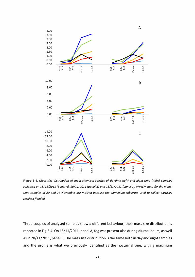
75 

 

 

Figure  5.4. Mass  size  distribution  of main  chemical  species  of  daytime  (left)  and  night‐time  (right)  samples 

collected on 15/11/2011 (panel A), 20/11/2011 (panel B) and 28/11/2011 (panel C). WINCM data for the night‐

time  samples of 20 and 28 November are missing because  the aluminium  substrate used  to  collect particles 

resulted flooded. 

 

 

Three couples of analysed samples show a different behaviour; their mass size distribution is 

reported in Fig.5.4. On 15/11/2011, panel A, fog was present also during diurnal hours, as well 

as in 20/11/2011, panel B. The mass size distribution is the same both in day and night samples 

and  the  profile  is what we  previously  identified  as  the  nocturnal  one, with  a maximum 

0.00

0.50

1.00

1.50

2.00

2.50

3.00

3.50

4.00

0.05‐

0.14

0.14‐

0.42

0.42‐1.2

1.2‐3.5

0.05‐

0.14

0.14‐

0.42

0.42‐1.2

1.2‐3.5

A

0.00

2.00

4.00

6.00

8.00

10.00

0.05‐

0.14

0.14‐

0.42

0.42‐1.2

1.2‐3.5

0.05‐

0.14

0.14‐

0.42

0.42‐1.2

1.2‐3.5

B

0.00

2.00

4.00

6.00

8.00

10.00

12.00

14.00

0.05

‐0.14

0.14

‐0.42

0.42‐1.2

1.2‐3.5

0.05

‐0.14

0.14

‐0.42

0.42‐1.2

1.2‐3.5

C

76 

 

concentration  of  soluble  species  in  the  fourth  size  range  and  the  insoluble  carbonaceous 

material still peaking at 0.42 µm < Da < 1.2 µm. On the contrary, on 28/11/2011, panel C, fog 

lasted only a few hours during the night and the mass size distribution  is typical of diurnal 

conditions for both samples. These examples confirm fog presence as the main factor driving 

the mass size distribution of aerosol particles in fall season in San Pietro Capofiume. 

The above data show that the most interested size range by fog scavenging is that between 

0.14 and 1.2 µm, while smaller and larger particles are only slightly affected. A focus on the 

scavenging effect on submicron aerosol chemical species was elaborated using the HR‐ToF‐

AMS measurements, which produces data with higher size and time resolution. Fig.5.5 reports 

the  average mass  size  distribution  of  nitrate,  sulphate,  ammonium,  chloride  and  organic 

compounds  in  the  two meteorological  conditions:  out‐of‐fog  (left)  and  in‐fog  (right).  Fine 

particles with  vacuum  aerodynamic diameter  (Dva)  larger  than 200 nm  shows  the highest 

scavenging efficiency. All species show a reduction  in concentration. Furthermore, peaks of 

nitrate (blue line) and organics (green line) shifted from 400 nm and 300 nm, respectively, to 

200 nm. The peak of ammonium (yellow line) followed the same behaviour of nitrate and the 

broad sulphate peak (red line) at 400 ‐ 500 nm in out‐of‐fog conditions smoothed over values 

around 200 nm. 

 

 

 

Figure 5.5. Mass size distribution of the main chemical compounds of submicron particles out of fog (left) and in 

fog (right) measured by an HR‐ToF‐AMS and averaged over the entire campaign. 

8

6

4

2

0

dM

/dlo

g 10d

va (µg

m-3)

4 5 6 7 8100

2 3 4 5 6 7 81000

PToF size (nm)

4 5 6 7 8100

2 3 4 5 6 7 81000

PToF size (nm)

no fog in fog

8

6

4

2

0

dM

/dlo

g 10d

va (µg

m-3)

4 5 6 7 8100

2 3 4 5 6 7 81000

PToF size (nm)

4 5 6 7 8100

2 3 4 5 6 7 81000

PToF size (nm)

8

6

4

2

0

dM

/dlo

g 10d

va (µg

m-3)

4 5 6 7 8100

2 3 4 5 6 7 81000

PToF size (nm)

4 5 6 7 8100

2 3 4 5 6 7 81000

PToF size (nm)

no fog in fog

Org NO3‐ SO4

= NH4+ Cl‐

77 

 

5.1.2 Influence of fog on aerosol chemical composition 

The parameters that contribute to determine the attitude of aerosol particles to be scavenged 

by  fog  droplets  are  both  size  and  chemical  composition  (McFiggans  et  al.,  2006).  A  full 

description of  the size  segregated chemical composition of aerosol particles  is  reported  in 

Fig.5.6. The figure shows the relative contribution of the main chemical species to the total 

reconstructed mass of each sample, calculated as the sum of nitrate, sulphate, ammonium, 

other  ions  (potassium,  magnesium,  calcium  and  chloride),  water‐soluble  organic  matter 

(WSOM) and water‐insoluble carbonaceous material (WINCM). A factor of 1.8 (Matta et al., 

2003) and 1.2 (Zappoli et al., 1999) were used to convert, respectively, WSOC in WSOM and 

WINC in WINCM. 

Comparison of daytime and night‐time samples shows that water‐soluble  inorganic species 

are removed more efficiently than carbonaceous species during the night, when fog occurs: 

nitrate, sulphate and ammonium contribution is usually lower in nocturnal samples, while the 

contribution  of  carbonaceous  material  increases  (particularly  that  of  WINCM).  Average 

percentage contributions of the main chemical species are reported  in Table 5.2. The same 

trend is observed for all the four stages, even though to a lower extent for the largest particles 

(1. 2 µm < Da < 3.5 µm). 

78 

 

 

Figure 5.6. Relative chemical composition of all the analysed aerosol size segregated samples. 

 

 

The  percentage  contribution  of  nitrate  to  the  total mass  in  the  first  three  stages  of  the 

nocturnal samples decreases from 24 (±4) % to 9 (±4) %, 31 (±5) % to 12 (±5) % and 35 (±6) % 

0%

20%

40%

60%

80%

100%

0.05‐

0.14

0.14‐

0.42

0.42‐

1.2

1.2‐3.5

0.05‐

0.14

0.14‐

0.42

0.42‐

1.2

1.2‐3.5

15/11/2011day night

0%

20%

40%

60%

80%

100%

0.05

‐0.14

0.14

‐0.42

0.42

‐1.2

1.2‐3.5

0.05

‐0.14

0.14

‐0.42

0.42

‐1.2

1.2‐3.5

16/11/2011 nightday

0%

20%

40%

60%

80%

100%

0.05

‐0.14

0.14

‐0.42

0.42

‐1.2

1.2‐3.5

0.05

‐0.14

0.14

‐0.42

0.42

‐1.2

1.2‐3.5

17/11/2011day night

0%

20%

40%

60%

80%

100%

0.05‐

0.14

0.14‐

0.42

0.42‐

1.2

1.2‐3.5

0.05‐

0.14

0.14‐

0.42

0.42‐

1.2

1.2‐3.5

18/11/2011day night

0%

20%

40%

60%

80%

100%

0.05‐

0.14

0.14‐

0.42

0.42‐

1.2

1.2‐3.5

0.05‐

0.14

0.14‐

0.42

0.42‐

1.2

1.2‐3.5

19/11/2011day night

0%

20%

40%

60%

80%

100%

0.05‐

0.14

0.14‐

0.42

0.42‐

1.2

1.2‐3.5

0.05‐

0.14

0.14‐

0.42

0.42‐

1.2

1.2‐3.5

20/11/2011day night

0%

20%

40%

60%

80%

100%

0.05

‐0.14

0.14

‐0.42

0.42

‐1.2

1.2‐3.5

0.05

‐0.14

0.14

‐0.42

0.42

‐1.2

1.2‐3.5

25/11/2011day night

0%

20%

40%

60%

80%

100%

0.05‐

0.14

0.14‐

0.42

0.42‐

1.2

1.2‐3.5

0.05‐

0.14

0.14‐

0.42

0.42‐

1.2

1.2‐3.5

26/11/2011day night

0%

20%

40%

60%

80%

100%

0.05‐

0.14

0.14‐

0.42

0.42‐

1.2

1.2‐3.5

0.05‐

0.14

0.14‐

0.42

0.42‐

1.2

1.2‐3.5

27/11/2011day night

0%

20%

40%

60%

80%

100%

0.05

‐0.14

0.14

‐0.42

0.42

‐1.2

1.2‐3.5

0.05

‐0.14

0.14

‐0.42

0.42

‐1.2

1.2‐3.5

28/11/2011day night

0%

50%

100%

0.05

‐0.14

0.14

‐0.42

0.42

‐1.2

1.2‐

3.5

0.05

‐0.14

0.14

‐0.42

0.42

‐1.2

1.2‐

3.5

29/11/2011day night

0%

50%

100%

0.05

‐0.14

0.14

‐0.42

0.42

‐1.2

1.2‐

3.5

0.05

‐0.14

0.14

‐0.42

0.42

‐1.2

1.2‐

3.5

30/11/2011day night

79 

 

to 23 (±7) %, respectively. The percentage contribution of sulphate and ammonium also shows 

a depletion with the occurrence of fog, while carbonaceous material, considered as the sum 

of soluble and insoluble carbonaceous compounds, increases its contribution, accounting for 

more than 70% of the total reconstructed mass of the finest particles (first and second stage) 

at night. 

 

 

Table  5.2.  Size  segregated  average  relative  contribution  of  the  main  chemical  species  to  the  total 

reconstructed mass of aerosol samples. 

   other ions  NO3

‐  SO42‐  NH4

+  WSOM  WINCM 

 

0.05 – 0.14 

µm 

day  1% ± 1%  24% ± 4% 4% ± 1% 10% ± 1% 29% ± 9%  32% ± 11%

night  4% ± 4%  9% ± 4%  4% ± 2%  4% ± 2%  45% ± 14%  33% ± 15% 

               

 

0.14 – 0.42 

µm 

day  3% ± 2%  31% ± 5% 6% ± 1% 13% ± 2% 37% ± 4%  11% ± 9%

night  5% ± 6%  12% ± 5%  4% ± 2%  5% ± 2%  43% ± 12%  30% ± 13% 

               

 

0.42 – 1.2 

µm 

day  3% ± 2%  35% ± 6% 7% ± 2% 15% ± 2% 29% ± 6%  12% ± 8%

night  4% ± 3%  23% ± 7%  6% ± 2%  9% ± 2%  36% ± 8%  21% ± 10% 

               

 

1.2 – 3.5  

µm 

day  6% ± 3%  35% ± 6% 10% ± 3% 13% ± 1% 24% ± 6%  13% ± 8%

night 3% ± 1%  29% ± 8%  7% ± 3%  12% ± 3%  35% ± 11%  15% ± 14% 

 

 

The scavenging efficiency (η) can be calculated to determine the attitude of chemical species 

to  be  scavenged  by  fog  droplets.  During  the  November  2011  field  campaign,  online 

measurements were carried out using an HR‐ToF‐AMS that supplies high time resolution data 

of submicron aerosol chemical composition. In Gilardoni et al. (2014) we used the available 

chemical data to calculate η, according to the definition given by (Collett et al., 2008): 

 

80 

 

η = 1‐ [X]interstitial/[X]before fog 

Concentration  of  before‐fog  and  interstitial  species  X  was  calculated  from  HR‐ToF‐AMS 

measurements, averaged over 30 minutes before fog formation and over 30 minutes after fog 

formation.  Scavenging  efficiency  is  found  to  be  related  to  the  water  solubility  of  the 

considered  chemical  species.  The  highest  scavenging  efficiencies  were  observed  for 

ammonium  and  nitrate,  the  most  soluble  components  (on  average  71%  and  68%, 

respectively). Black carbon, the most hydrophobic compound, showed the lowest η value (on 

average 45%). Organic aerosol showed the largest η variability (20 ‐ 60%), as suggested by its 

highly variable composition, including soluble molecules and more hydrophobic compounds. 

(Gilardoni  et  al.,  2014)  supported  the  idea  that  the  observed  differences  among  the 

scavenging efficiencies depend on a  joined effect of both solubility and size distribution of 

chemical species. According to Köhler theory, activation of particles larger than 300 ‐ 400 nm 

Dva  is more  likely  than  activation  of  smaller  particles  especially  at  supersaturation  values 

typical of fog events (0.01 ‐ 0.03%). Nitrate and ammonium size distribution peaks around 400 

‐ 500 nm, while black carbon, besides to be the most insoluble compound, usually dominates 

smaller particles (Dva < 150 nm) (Seinfeld and Pandis, 1998). 

 

5.2 Organic fraction of aerosol particles and fog droplets 

So  far, the study regarded the observation of how chemical and physical characteristics of 

aerosol  particles  are  affected  by  fog  occurrence.  This  paragraph,  instead,  will  compare 

particles chemical composition with  that of  fog droplets, with a particular  interest  for  the 

organic fraction. 

Carbonaceous compounds account for a significant fraction of total mass composition of both 

fog  droplets  and  aerosol  particles  (Fuzzi  et  al.,  2002).  Fig.5.7  shows  the  average  relative 

chemical  composition of  fog and PM10  collected  in San Pietro Capofiume over  the entire 

campaign in November 2011: the carbonaceous material (intended as the sum of soluble and 

insoluble material) accounts on average for 33 (±8) % and 50 (±12) % of total reconstructed 

mass for fog droplets and aerosol particles (PM10), respectively. 

 

 

81 

 

 

Figure 5.7. Relative chemical composition of fog droplets and PM10 averaged over the entire campaign. 

 

 

Except for the contribution of the  insoluble carbonaceous fraction, which will be discussed 

later in this paragraph, the percentage composition of both aerosol and fog is very similar. It 

indicates  that  fog  composition  is  mainly  determined  by  aerosol  particles  that  act  as 

condensation nuclei. Studies carried out  in  the Po Valley  in  the  last decades,  reported  the 

negligible contribution of the coagulation of interstitial particles with fog droplets to the mass 

of fog droplets, leading to a major role of nucleation scavenging in determining the organic 

composition  (Facchini  et  al.,  1999).  Further  studies  reported  high  similarity  between  the 

organic chemical composition of fog droplets and aerosol particles collected during the cold 

season at the field station of San Pietro Capofiume, confirming the nucleation scavenging as 

the main source of organic compounds in fog water (Fuzzi et al., 2002). 

In Fig.5.8 relative contribution of WSOC and WINC to the total carbon content is reported for 

fog water, PM10 out of fog and PM10 in fog conditions (interstitial aerosol). In fog droplets, 

water‐soluble carbon accounts on average for 77 (±6) % and insoluble carbon for 24 (±7) %. 

The partitioning of carbon between soluble and insoluble species is similar in PM10 out of fog: 

soluble C accounts for 62 (±16) %. In interstitial aerosol samples the contribution of insoluble 

carbon increases, reaching 45 (±16) % of total carbon mass, because of the scavenging of part 

of the soluble carbonaceous species in fog water. 

 

0%

20%

40%

60%

80%

100%

fog PM10

other ions NO3 SO4 NH4 WSOM WINCM

82 

 

 

Figure 5.8. Average relative contribution of WSOC and WINC to the total carbon content of fog water, PM10 out‐

of‐fog and PM10 in‐fog conditions. 

 

 

The water‐soluble carbonaceous fraction of both aerosol and fog droplets has been further 

analysed,  to  reach  a better  characterization. By  ion  chromatography  some  low molecular 

weight carboxylic acids can been detected and quantified. Acetic acid (CH3COOH), formic acid 

(HCOOH), methanesulfonic  acid  (CH3SO3H)  and  oxalic  acid  (C2H2O4)  have  been measured. 

Their carbon contribution to the total WSOC is small and variable from sample to sample. They 

accounts on average only for 0.7 (±1.9) %, 1.2 (±1.8) %, 1.5 (±0.6) % and 2.5 (±2.0) % of the 

total WSOC  in  the  four  size  stages  of  size  segregated  aerosol  samples,  respectively.  Low 

molecular weight carboxylic acids contribute  for 4.3  (±2.1) %  to  the water‐soluble organic 

carbon of the fog droplets. 

Using an  individual compound approach to determine the chemical composition of aerosol 

organic fraction, the speciation usually produces a list of individual compounds which together 

account only for a few percent of the OC composition (Fuzzi et al., 2001). A different approach 

aimed to a more general characterization, based on determination of type and concentration 

of functional groups, instead of individual compounds, is more affordable. This strategy was 

pursued using 1H‐NMR spectroscopy (Decesari et al., 2000; Decesari et al., 2001). For these 

analysis aerosol particles were sampled on quartz fibre filter by a dichotomous sampler, with 

0%

20%

40%

60%

80%

100%

FOG PM10‐out of fog PM10‐in fog

WSOC WINC

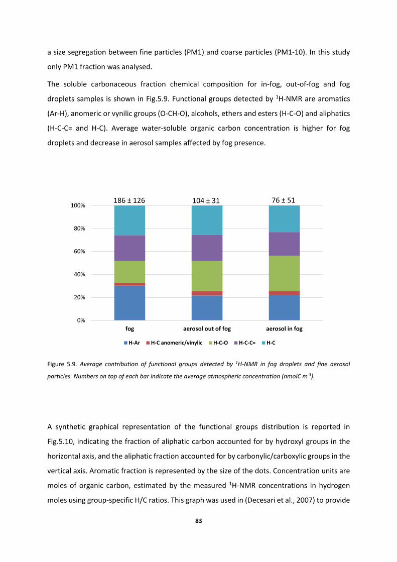
83 

 

a size segregation between fine particles (PM1) and coarse particles (PM1‐10). In this study 

only PM1 fraction was analysed. 

The  soluble  carbonaceous  fraction  chemical  composition  for  in‐fog,  out‐of‐fog  and  fog 

droplets samples  is shown  in Fig.5.9. Functional groups detected by 1H‐NMR are aromatics 

(Ar‐H), anomeric or vynilic groups (O‐CH‐O), alcohols, ethers and esters (H‐C‐O) and aliphatics 

(H‐C‐C=  and  H‐C).  Average  water‐soluble  organic  carbon  concentration  is  higher  for  fog 

droplets and decrease in aerosol samples affected by fog presence. 

 

 

 

Figure  5.9.  Average  contribution  of  functional  groups  detected  by  1H‐NMR  in  fog  droplets  and  fine  aerosol 

particles. Numbers on top of each bar indicate the average atmospheric concentration (nmolC m‐3). 

 

 

A  synthetic  graphical  representation  of  the  functional  groups  distribution  is  reported  in 

Fig.5.10,  indicating the fraction of aliphatic carbon accounted for by hydroxyl groups  in the 

horizontal axis, and the aliphatic fraction accounted for by carbonylic/carboxylic groups in the 

vertical axis. Aromatic fraction is represented by the size of the dots. Concentration units are 

moles of organic  carbon, estimated by  the measured  1H‐NMR  concentrations  in hydrogen 

moles using group‐specific H/C ratios. This graph was used in (Decesari et al., 2007) to provide 

0%

20%

40%

60%

80%

100%

fog aerosol out of fog aerosol in fog

H‐Ar H‐C anomeric/vinylic H‐C‐O H‐C‐C= H‐C

186 ± 126 104 ± 31 76 ± 51

84 

 

source  identification  for water‐soluble organic aerosol based on  1H‐NMR  functional group 

composition. Comparing our results to those reported in the paper, we found that our samples 

are positioned  in  the area assigned  to  samples affected by biomass burning  (black border 

rectangle in Fig.5.10). This result agrees with previous studies indicating that organic aerosol 

in the rural Po Valley in fall is usually dominated by wood burning emissions from residential 

heating and fossil fuel burning from traffic and residential heating (Gilardoni et al., 2011). The 

figure  shows  that  the  compositions of  the  three  sample  subsets object of  this  study  (fog, 

aerosol in‐fog and aerosol out‐of‐fog), beside falling approximately in the same region of the 

functional group diagram, they tend to scatter out  in different directions.  In particular, the 

composition of interstitial aerosol (blue dots) is enriched in aromatic and hydroxyl groups and 

depleted  in  carbonyls/carboxyls with  respect  to  that of out‐of‐fog aerosol  (in green). This 

finding indicates that interstitial aerosols retain the original (“primary”) constituents of wood 

burning products  (e.g., anhydrosugars, phenols) while  they are depleted of  the  secondary 

species (e.g., carboxylic acids). This in turn can be explained by the fact that local sources from 

domestic heating directly impact the composition of aerosol particles in the small size range 

which  is  less  efficiently  scavenged  by  fog  than  larger  particles  (where  biomass  burning 

products  are  more  aged  and  enriched  in  secondary  species).  Conversely,  the  1H‐NMR 

composition of fog WSOC is depleted of primary biomass burning products (hydroxyl groups 

from anhydrosugars), but, unexpectedly, they exhibit a greater aromatic content than out‐of‐

fog aerosols. To explain  this  last  finding, additional sources of aromatic compounds  in  fog 

droplets must be hypothesized, like scavenging of aromatic aldehydes (e.g., benzoaldehyde) 

and acids from the gas phase, or formation of heteroaromatic compounds from the reaction 

of  low‐molecular weight  carbonyls  and  ammonia  (e.g.,  Yu  et  al.,  2011).  These  additional 

mechanisms involving aqueous phase chemical reactions cannot be fully explained based on 

the available set of data and require further attempts for chemical speciation. 

 

85 

 

 

Figure 5.10. Functional group distribution of water‐soluble organic fraction in fog and aerosol samples. 

 

 

5.3 High time resolution characterization of a nocturnal fog 

episode 

Due  to  the presence of very dense  fog on  the  first day of  the campaign, a special  fog and 

aerosol sampling was set up on 15/11/2011. Starting from 18:00, fog samples were collected 

every hour and aerosol samples were collected every four hours using a Berner impactor, until 

the fog dissipation on the following morning (sampling stopped on 16/11/2011 at 11:18). The 

purpose was to collect samples with a higher time resolution in order to observe how both 

aerosol and fog water change during a unique fog event. 

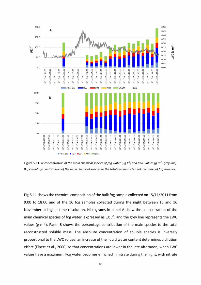
86 

 

 

Figure 5.11. A: concentration of the main chemical species of fog water (µg L‐1) and LWC values (g m‐3, grey line). 

B: percentage contribution of the main chemical species to the total reconstructed soluble mass of fog samples. 

 

 

Fig.5.11 shows the chemical composition of the bulk fog sample collected on 15/11/2011 from 

9:00  to  18:00  and  of  the  16  fog  samples  collected  during  the  night  between  15  and  16 

November at higher time resolution. Histograms  in panel A show the concentration of the 

main chemical species of fog water, expressed as µg L‐1, and the grey line represents the LWC 

values  (g m‐3). Panel B shows the percentage contribution of the main species to the total 

reconstructed  soluble  mass.  The  absolute  concentration  of  soluble  species  is  inversely 

proportional to the LWC values: an increase of the liquid water content determines a dilution 

effect (Elbert et al., 2000) so that concentrations are lower in the late afternoon, when LWC 

values have a maximum. Fog water becomes enriched in nitrate during the night, with nitrate 

1 256 511 766 1021 1276

0.00

0.05

0.10

0.15

0.20

0.25

0.30

0.35

0.40

0.45

0.50

0.0

50.0

100.0

150.0

200.0

15/11/2011 09.00

15/11/2011 10.00

15/11/2011 11.00

15/11/2011 12.00

15/11/2011 13.00

15/11/2011 14.00

15/11/2011 15.00

15/11/2011 16.00

15/11/2011 17.00

15/11/2011 18.00

15/11/2011 19.00

15/11/2011 20.00

15/11/2011 21.00

15/11/2011 22.00

15/11/2011 23.00

16/11/2011 00.00

16/11/2011 01.00

16/11/2011 02.00

16/11/2011 03.00

16/11/2011 04.00

16/11/2011 05.00

16/11/2011 06.00

16/11/2011 07.00

16/11/2011 08.00

16/11/2011 09.00

LWC (g m

‐3)

µg l‐1

other ions NO3 SO4 NH4 WSOM LWC

A

0%

25%

50%

75%

100%

15/11/2011 09.00

15/11/2011 10.00

15/11/2011 11.00

15/11/2011 12.00

15/11/2011 13.00

15/11/2011 14.00

15/11/2011 15.00

15/11/2011 16.00

15/11/2011 17.00

15/11/2011 18.00

15/11/2011 19.00

15/11/2011 20.00

15/11/2011 21.00

15/11/2011 22.00

15/11/2011 23.00

16/11/2011 00.00

16/11/2011 01.00

16/11/2011 02.00

16/11/2011 03.00

16/11/2011 04.00

16/11/2011 05.00

16/11/2011 06.00

16/11/2011 07.00

16/11/2011 08.00

16/11/2011 09.00

other ions NO3 SO4 NH4 WSOM

B

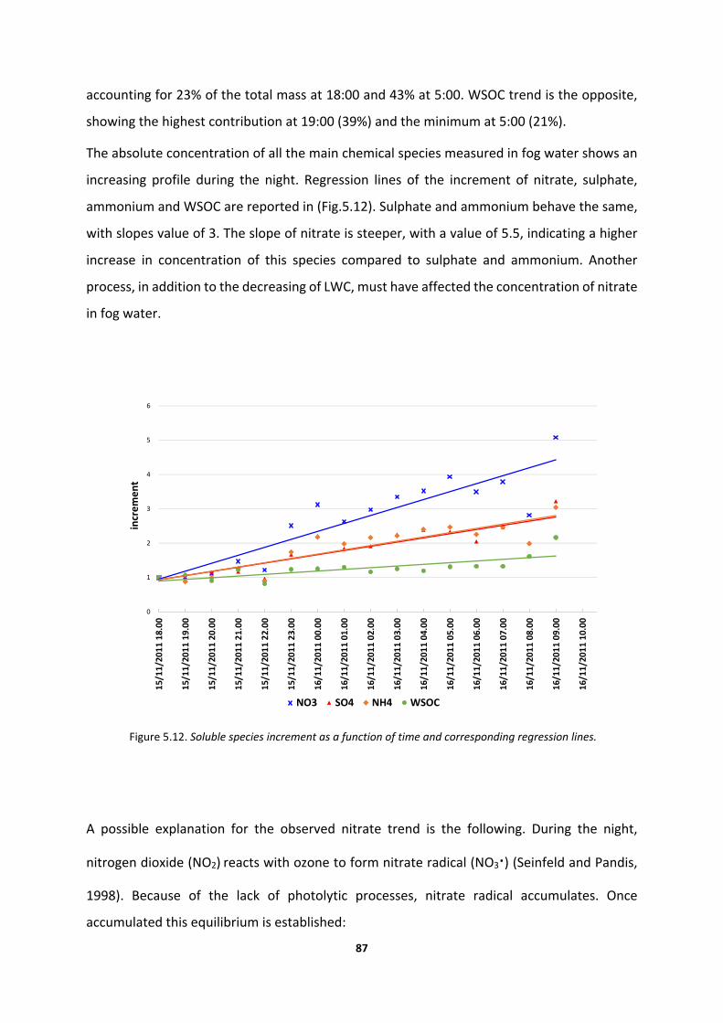
87 

 

accounting for 23% of the total mass at 18:00 and 43% at 5:00. WSOC trend is the opposite, 

showing the highest contribution at 19:00 (39%) and the minimum at 5:00 (21%). 

The absolute concentration of all the main chemical species measured in fog water shows an 

increasing profile during  the night. Regression  lines of  the  increment of nitrate,  sulphate, 

ammonium and WSOC are reported in (Fig.5.12). Sulphate and ammonium behave the same, 

with slopes value of 3. The slope of nitrate is steeper, with a value of 5.5, indicating a higher 

increase  in  concentration  of  this  species  compared  to  sulphate  and  ammonium. Another 

process, in addition to the decreasing of LWC, must have affected the concentration of nitrate 

in fog water. 

 

 

 

Figure 5.12. Soluble species increment as a function of time and corresponding regression lines. 

 

 

A  possible  explanation  for  the  observed  nitrate  trend  is  the  following.  During  the  night, 

nitrogen dioxide (NO2) reacts with ozone to form nitrate radical (NO3∙) (Seinfeld and Pandis, 

1998).  Because  of  the  lack  of  photolytic  processes,  nitrate  radical  accumulates.  Once 

accumulated this equilibrium is established:  

0

1

2

3

4

5

6

15/11/2011 18.00

15/11/2011 19.00

15/11/2011 20.00

15/11/2011 21.00

15/11/2011 22.00

15/11/2011 23.00

16/11/2011 00.00

16/11/2011 01.00

16/11/2011 02.00

16/11/2011 03.00

16/11/2011 04.00

16/11/2011 05.00

16/11/2011 06.00

16/11/2011 07.00

16/11/2011 08.00

16/11/2011 09.00

16/11/2011 10.00

increment

NO3 SO4 NH4 WSOC

88 

 

NO3∙ + NO2 ↔ N2O5 

Dinitrogen pentoxide (N2O5) is very soluble and quickly dissolves in fog water producing nitric 

acid (HNO3). Through this mechanism nitrate is produced directly in the aqueous phase and 

contributes to the accumulation of this ion in fog droplets throughout the night. 

The above data demonstrate that fog chemistry occurring during the night can be responsible 

for the formation of important amounts of aerosol nitrate in the Po Valley, in addition to the 

most  common  process  of  NOX  oxidation  by  the  OH  radical,  occurring  during  the  day. 

Conversely,  the  concentration of WSOC  shows  a  lower  increment  compared  to  the other 

species.  This  behaviour  is  due  to  the  semivolatile  nature  of  a  fraction  of  soluble  organic 

compounds that likely passes into the gas phase with decreasing water content. 

Fig.5.13 shows the soluble fraction chemical composition of the aerosol particles with 0.14 

µm < Da < 0.42 µm and 0.42 µm < Da < 1.2 µm collected from 15/11/2011 at 9:00 to 16/11/2011 

at 11:00. We previously observed that these particles are the most affected by fog scavenging. 

This  statement  is  confirmed  by  the  results  shown  on  the  left  side  of  Fig.5.13, where  the 

absolute mass concentration of each sample is reported. When LWC values start to increase, 

around 18:00, and fog become denser, a reduction of particles occurs. Concentrations remain 

stationary until the early hours in the morning of 16/11/2011 when fog begins to dissipate. At 

11:30, when fog is completely dissipated, aerosol particles accumulate again. Concentrations 

of total soluble mass and of each chemical species are reported in detail in Table 5.3. In size 

range  0.42  µm  <  Da  <  1.2  µm,  nitrate  is  the most  scavenged  species  by  fog  water.  Its 

contribution to the total mass decreases contemporary to its increase in fog water samples 

(compare with Fig.5.11 panel B), passing from 43% in the first sample to 30% in the last one. 

 

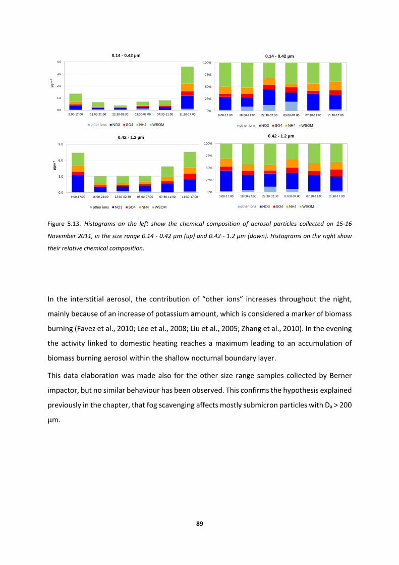
89 

 

 

Figure  5.13.  Histograms  on  the  left  show  the  chemical  composition  of  aerosol  particles  collected  on  15‐16 

November 2011, in the size range 0.14 ‐ 0.42 µm (up) and 0.42 ‐ 1.2 µm (down). Histograms on the right show 

their relative chemical composition. 

 

 

In  the  interstitial aerosol,  the contribution of “other  ions”  increases  throughout  the night, 

mainly because of an increase of potassium amount, which is considered a marker of biomass 

burning (Favez et al., 2010; Lee et al., 2008; Liu et al., 2005; Zhang et al., 2010). In the evening 

the activity  linked  to domestic heating  reaches a maximum  leading  to an accumulation of 

biomass burning aerosol within the shallow nocturnal boundary layer. 

This data elaboration was made also  for  the other size  range samples collected by Berner 

impactor, but no similar behaviour has been observed. This confirms the hypothesis explained 

previously in the chapter, that fog scavenging affects mostly submicron particles with Da > 200 

µm. 

 

 

 

 

 

0.0

3.0

6.0

9.0

9:00‐17:00 18:00‐22:00 22:30‐02:30 03:00‐07:00 07:30‐11:00 11:30‐17:00

µg

m-3

0.42 - 1.2 µm

other ions NO3 SO4 NH4 WSOM

0%

25%

50%

75%

100%

9:00‐17:00 18:00‐22:00 22:30‐02:30 03:00‐07:00 07:30‐11:00 11:30‐17:00

0.42 - 1.2 µm

other ions NO3 SO4 NH4 WSOM

0.0

1.0

2.0

3.0

4.0

9:00‐17:00 18:00‐22:00 22:30‐02:30 03:00‐07:00 07:30‐11:00 11:30‐17:00

µg

m-3

0.14 - 0.42 µm

other ions NO3 SO4 NH4 WSOM

0%

25%

50%

75%

100%

9:00‐17:00 18:00‐22:00 22:30‐02:30 03:00‐07:00 07:30‐11:00 11:30‐17:00

0.14 - 0.42 µm

other ions NO3 SO4 NH4 WSOM

90 

 

Table 5.3. Concentrations of chemical species in aerosol particles collected on 15 ‐ 16 November 

2011, in the size range 0.14 ‐ 0.42 µm and 0.42 ‐ 1.2 µm. 

  µg m‐3 

ID Sample  sampling time total 

mass NO3

‐  SO42‐  NH4

+  other ions  WSOM 

Size: 0.14‐0.42µm     

SPC151111_D2  9:00‐17:00  1.4 0.37 0.08 0.21 0.67  0.03 

SPC151111_NA2  18:00‐22:00  0.66 0.13 0.05 0.08 0.34  0.06 

SPC151111_NB2  22:30‐02:30  0.39 0.13 0.04 0.05 0.12  0.05 

SPC151111_NC2  03:00‐07:00  0.70 0.14 0.07 0.05 0.31  0.13 

SPC151111_ND2  07:30‐11:00  0.81 0.28 0.05 0.12 0.35  0.01 

SPC161111_D2  11:30‐17:00  3.6 1.1 0.36 0.63 1.4  0.12 

Size: 0.42‐1.2 µm 

SPC151111_D3  9:00‐17:00  7.4 3.2 0.61 1.2 2.3  0.14 

SPC151111_NA3  18:00‐22:00  3.1 0.98 0.25 0.43 1.3  0.12 

SPC151111_NB3  22:30‐02:30  3.1 0.86 0.18 0.39 1.4  0.34 

SPC151111_NC3  03:00‐07:00  3.1 1.0 0.34 0.52 1.03  0.21 

SPC151111_ND3  07:30‐11:00  4.9 1.7 0.38 0.81 2.0  0.08 

SPC161111_D3  11:30‐17:00  7.6 2.3 1.1 1.2 2.9  0.20 

91 

 

6. Conclusions 

 

Air pollution is believed to be responsible for more than 400,000 premature deaths in Europe 

(Brunekreef, 2013). The  impact on human health  is exacerbated  in so‐called pollution “hot 

spots”: environments  in which  anthropogenic  sources  are  concentrated  and dispersion of 

pollutants  is  limited.  One  of  these  environments,  the  Po  Valley,  normally  experiences 

exceedances of PM10 and PM2.5 daily concentration limits, especially in the cold season when 

the ventilation of the lower layers of the atmosphere is reduced. Traditionally, air pollution 

studies  in  the  cold  season have  focused on primary  combustion emission  sources  (traffic, 

residential heating) and atmospheric dispersion, while the role of photochemical (secondary) 

processes has been  investigated mainly  in the summer. In this study we were able to show 

that secondary processes are responsible for the formation of the largest fraction of PM10 in 

the Po Valley also in winter, when photochemistry is reduced, and that fog aqueous chemistry 

can play a key role in such processes.  

Size‐segregated  aerosol  samples  (5  size  classes  between  0.05  and  10 µm) were  collected 

simultaneously  in two different sites  (Bologna, urban site, and San Pietro Capofiume, rural 

site)  during  two  different  campaigns  (November  2011  and  February  2013).  The  total 

concentrations  of  the  reconstructed  PM10  mass  and  the  size‐distributions  were  similar 

between the urban and the rural site, confirming the importance of the regional background 

aerosol contribution  in determining the concentrations at the urban scale  in the Po Valley. 

Most  importantly, our results  from  the analysis of the water‐soluble  inorganic and organic 

fraction  show  that  the  chemical  composition  is  dominated  by  ammonium  nitrate  and 

ammonium sulphate, which are known secondary components of  the aerosol. This  finding 

indicates that not only the limited atmospheric dispersion is the cause for the build‐up of the 

regional background aerosol, but also atmospheric reactions occurring in the gas and in the 

particulate  phase  across  the  Po  Valley.  Soluble  organic  compounds  are  also  relevant, 

accounting for more than 80% of the finest particles (size range between 0.05 and 0.14 µm). 

Water‐soluble organic matter (WSOM)  is homogeneously distributed between BO and SPC, 

analogously  to  ammonium  nitrate  and  sulphate,  indicating  that  secondary  processes  also 

contributed to WSOM over the Po Valley during the investigated period. 

92 

 

The role of fog formation and fog chemistry  in the formation, processing and deposition of 

PM10 in the Po Valley has been studied during the field campaign of November 2011 in San 

Pietro Capofiume. Our results show that particles with aerodynamic diameter between 0.14 

and  1.2  μm,  where  most  of  the  PM1  mass  is  found,  are  efficiently  scavenged  by  fog 

occurrence. Therefore, during fog events, the ambient concentration of the finest particles, 

with the highest capacity to penetrate in the human respiratory system, is strongly reduced 

because of fog scavenging (up to 60%). The presence of fog in the Po Valley thus represents a 

relevant  mechanism  of  control  of  the  aerosol  load  in  the  atmosphere,  with  relevant 

implications on the air quality of the region. 

Other potential  impacts of aerosol‐fog  interaction that have been evaluated  in the present 

study are the role of fog droplets in absorbing trace gases like nitric acid, sulphur dioxide and 

ammonia, which can result in increased concentrations of PM10 upon fog evaporation, or, in 

case of an excess of acidic gases, in wet deposition of fogs with low pH, with harmful effects 

on the vegetation and buildings. Time‐resolved measurements of fog composition highlighted 

the  formation  of  particulate  nitrate  through  an  in‐fog  aqueous  phase  reaction:  gaseous 

dinitrogen pentoxide (N2O5) is absorbed into the droplets and then hydrolysed and neutralized 

by ammonia to form ammonium nitrate (NH4NO3). After evaporation of fog droplets, aerosol 

particles result enriched in NH4NO3. This aqueous secondary aerosol formation mechanism is 

very  important  in  wintertime,  when  the  photochemical  activity  is  reduced,  and  so  the 

formation of nitric acid (HNO3) in the gaseous phase is slow. These results indicate that fog 

processing can be responsible  for the enrichment of ammonium nitrate  in PM10  in the Po 

Valley  in wintertime,  and  that  these  reactions  contribute  to  the  build‐up  of  the  regional 

background aerosol concentrations in the region. 

During  the 2011  field campaign,  the absorption of ammonia neutralized  the production of 

nitric acid from the N2O5 channel. The fog water pH during the full 2011/12 season remained 

close  to  neutrality,  in  conflict with  first  observations  at  the  site  dating  back  the  80s  and 

showing  frequent episodes of acidic pH.  In  fact,  the composition of  fog water has evolved 

continuously over the last decades following the changes in atmospheric composition, which 

in  turn  were  dictated  by  several  processes,  including  the  introduction  of  anthropogenic 

emission controls. We present here for the first time the results of the analysis of fog water 

composition from a 20 years record of measurements in San Pietro Capofiume. This long time 

93 

 

series  showed  a  clear  decreasing  trend  of  ionic  strength  and  conductivity  of  fog water, 

indicating a reduction of its ionic load. The ionic species that exhibited the highest decrease 

was  sulphate  (SO42‐).  The  gradual  decrease  of  sulphates,  lead  to  an  increased  relative 

contribution of organic compounds and nitrates, which suffered a less drastic reduction. The 

low correlation between ion concentrations and LWC, and the lack of a statistically significant 

trend for LWC, excluded that the observed decreasing concentrations were due to a “dilution 

effect”. The negative trend of fog water ionic load is mainly due to the reduction in SO2 and 

NOX  atmospheric  emissions  (emission  data  are  reported  by  the  Italian  Institute  for  the 

Environmental Protection and Research –ISPRA), in agreement with other studies carried out 

in Europe (Lange et al., 2003). These results reflect the impact of the implemented air quality 

policies in determining the concentrations of atmospheric constituents. As a consequence of 

the  lower  content  of  the  two main  acidic  species  (NO3‐  and  SO4

2‐)  pH  values  showed  an 

increase  over  the  last  two  decades,  reaching  values  close  to  neutrality.  In  the  today‐

atmosphere,  the  ammonia  concentrations  are  large  enough  to  neutralize  the 

production/absorption of acidic compounds  in fog water, excluding the formation of acidic 

fogs. On the other hand, the neutralization of nitric acid leads to the production of particulate 

ammonium nitrate, which, upon fog evaporation, leads to an increase of PM10 concentrations 

in the region. Introducing a regulation on the emissions of ammonia (mainly from agricultural 

activities, animal husbandry, and waste treatment) can be an agreeable strategy to decrease 

the particulate matter concentrations, but with  the possible  side effect of making  the  fog 

depositions more acidic. 

Even though the results presented  in this doctoral thesis refer to data collected  in Bologna 

and San Pietro Capofiume, they can be extended to the whole Po Valley basin that has been 

classified as a unique megacity (see chapter 1). Therefore, these results could be a valuable 

tool to support integrated future policy actions in the whole region. 

 

95 

 

Acknowledgments 

 

The research work reported in this PhD thesis was carried out at the Institute of Atmospheric 

Sciences and Climate, National Research Council (ISAC‐CNR), Bologna, within the Atmospheric 

Chemistry group headed by Dr. Sandro Fuzzi and Dr. Maria Cristina Facchini. 

Financial  supports was  provided  by  the  Emilia‐Romagna  Region  “SUPERSITO”  Project,  the 

Atmospheric  Composition  Change  European Network  of  Excellence  (ACCENT‐Plus)  and  the 

European project PEGASOS. 

I would like to express, first of all, my gratitude to Dr. Fuzzi e Dr. Facchini for having given me 

this opportunity. I owe to them most of all I learned in these years. 

I gratefully acknowledge Prof. Emilio Tagliavini (University of Bologna) for having supported 

this doctoral project. 

My special thanks to my friend and colleague Dr. Matteo Rinaldi for his supervision and most 

of all  for his  support during  the whole period of  the PhD. My work would not have been 

successful without his help. 

My special thanks also to Dr. Stefano Decesari for his precious and fundamental suggestions 

and supervision during the preparation of the thesis. 

I warmly  thank Dr. Marco Paglione, Dr.  Stefania Gilardoni, Dr. Claudio Carbone, Dr.  Silvia 

Sandrini and Dr. Leone Tarozzi, which all contributed to this work with their constant human 

and professional support. 

 

97 

 

Bibliography 

 

Aleksic, N. and Dukett,  J. E.  (2010). Probabilistic relationship between  liquid water content and  ion 

concentrations in cloud water. Atmospheric Research 98, 400‐405. 

 

Alves, C., Vicente, A., Pio, C., Kiss, G., Hoffer, A., Decesari, S., Prevot, A. S. H., Cruz Minguillon, M., 

Querol, X., Hillamo, R., Spindler, G. and Swietlicki, E. (2012). Organic compounds in aerosols from 

selected European sites ‐ Biogenic versus anthropogenic sources. Atmospheric Environment 59, 

243‐255. 

 

Andreae, M. O. and Gelencser, A. (2006). Black carbon or brown carbon? The nature of light‐absorbing 

carbonaceous aerosols. Atmospheric Chemistry and Physics 6, 3131‐3148. 

 

Andreae, M. O. and Rosenfeld, D. (2008). Aerosol‐cloud‐precipitation interactions. Part 1. The nature 

and sources of cloud‐active aerosols. Earth‐Science Reviews 89, 13‐41. 

 

Arends, B. G. (1996). Aerosol and Cloud Microphysics, Measurements and Interpretations. 

 

Barrie, L. A. (1985). Features of the Atmospheric Cycle of Aerosol Trace‐Elements and Sulfur Dioxide 

revealed‐by Baseline Observations in Canada. Journal of Atmospheric Chemistry 3, 139‐152. 

 

Blanchard, D. (1983). The Production, distribution, and bacterial enrichment of the sea‐salt aerosol, in 

Air‐Sea Exchange of Gases and Particles. D Reidel: Norwell, Mass. 

 

Braun, S., Kalinowski, H. O. and Berber, S. (1998). 150 and more basic NMR Experiments. Wiley‐VHC: 

Weinheim, Germany. 

 

Brunekreef, B. (2013). Air Quality and Health In Union, E. (Ed), Air Quality ‐ Research Findings in support 

of the EU: Luxembourg, pp. 20 ‐ 30. 

 

Calvert, J. G., Heikes, B. G., Stockwell, W. R., Mohnen, V. A. and Kerr, J. A. (1986). Some considerations 

of the important chemical processes in acid deposition In Ed., W. J. (Ed), Chemistry of Multiphase 

Atmospheric Systems, Springer Verlag, berlin: City, pp. 615‐647. 

98 

 

 

Carbone, C., Decesari, S., Mircea, M., Giulianelli, L., Finessi, E., Rinaldi, M., Fuzzi, S., Marinoni, A., Duchi, 

R., Perrino, C., Sargolini, T., Varde, M., Sprovieri, F., Gobbi, G. P., Angelini, F. and Facchini, M. C. 

(2010).  Size‐resolved  aerosol  chemical  composition  over  the  Italian  Peninsula during  typical 

summer and winter conditions. Atmospheric Environment 44, 5269‐5278. 

 

Casareto, B. E., Suzuki, Y., Okada, K. and Morita, M. (1996). Biological micro‐particles  in rain water. 

Geophysical Research Letters 23, 173‐176. 

 

Caseiro, A., Bauer, H., Schmidl, C., Pio, C. A. and Puxbaum, H. (2009). Wood burning impact on PM10 

in three Austrian regions. Atmospheric Environment 43, 2186‐2195. 

 

Chen, J., Ying, Q. and Kleeman, M. J. (2010). Source apportionment of wintertime secondary organic 

aerosol during the California regional PM10/PM2.5 air quality study. Atmospheric Environment 

44, 1331‐1340. 

 

Collett, J. L., Jr., Herckes, P., Youngster, S. and Lee, T. (2008). Processing of atmospheric organic matter 

by California radiation fogs. Atmospheric Research 87, 232‐241. 

 

Collett,  J. L., Oberholzer, B., Mosimann, L., Staehelin,  J. and Waldvogel, A.  (1993). Contributions of 

Cloud Processes to Precipitation Chemistry in Mixed‐phase Clouds. Water Air and Soil Pollution 

68, 43‐57. 

 

DeCarlo, P. F., Kimmel, J. R., Trimborn, A., Northway, M. J., Jayne, J. T., Aiken, A. C., Gonin, M., Fuhrer, 

K., Horvath, T., Docherty, K. S., Worsnop, D. R. and Jimenez, J. L. (2006). Field‐deployable, high‐

resolution, time‐of‐flight aerosol mass spectrometer. Analytical Chemistry 78, 8281‐8289. 

Decesari, S., Facchini, M. C., Fuzzi, S. and Tagliavini, E. (2000). Characterization of water‐soluble organic 

compounds  in  atmospheric  aerosol:  A  new  approach.  Journal  of  Geophysical  Research‐

Atmospheres 105, 1481‐1489. 

 

Decesari, S., Facchini, M. C., Matta, E., Lettini, F., Mircea, M., Fuzzi, S., Tagliavini, E. and Putaud, J. P. 

(2001).  Chemical  features  and  seasonal  variation  of  fine  aerosol  water‐soluble  organic 

compounds in the Po Valley, Italy. Atmospheric Environment 35, 3691‐3699. 

 

99 

 

Decesari, S., Mircea, M., Cavalli, F., Fuzzi, S., Moretti, F., Tagliavini, E. and Facchini, M. C. (2007). Source 

attribution  of  water‐soluble  organic  aerosol  by  nuclear  magnetic  resonance  spectroscopy. 

Environmental Science & Technology 41, 2479‐2484. 

 

Derome, A. E. (1987). Modern NMR Techniques for Chemistry Research. Pergamon Press: Oxford, UK. 

Deserti, M.,  Cacciamani,  C.,  Golinelli,  M.,  Kerschbaumer,  A.,  Leoncini,  G.,  Savoia,  E.,  Selvini,  A., 

Paccagnella,  T.  and  Tibaldi,  S.  (2001).  Operational meteorological  pre‐processing  at  Emilia‐

Romagna ARPA Meteorological Service as a part of a decision support system  for air quality 

management. International Journal of Environment and Pollution 16, 571‐582. 

 

Dollard, G. J., Unsworth, M. H. and Harve, M. J. (1983). Pollutant tranfer in Upland Regions by Occult 

Precipitation. Nature 302, 241‐243. 

 

Dusek, U., Frank, G. P., Hildebrandt, L., Curtius, J., Schneider, J., Walter, S., Chand, D., Drewnick, F., 

Hings, S., Jung, D., Borrmann, S. and Andreae, M. O. (2006). Size matters more than chemistry 

for cloud‐nucleating ability of aerosol particles. Science 312, 1375‐1378. 

 

Elbert, W., Hoffmann, M. R., Kramer, M., Schmitt, G. and Andreae, M. O.  (2000). Control of solute 

concentrations  in cloud and fog water by  liquid water content. Atmospheric Environment 34, 

1109‐1122. 

 

Elbert,  W.,  Kramer,  M.  and  Andreae,  M.  O.  (2002).  Reply  to  discussion  on  "Control  of  solute 

concentrations in cloud and fog water by liquid water content". Atmospheric Environment 36, 

1909‐1910. 

 

Ervens, B., Turpin, B. J. and Weber, R. J. (2011). Secondary organic aerosol formation in cloud droplets 

and aqueous particles  (aqSOA): a review of  laboratory,  field and model studies. Atmospheric 

Chemistry and Physics 11, 11069‐11102. 

 

Facchini, M. C., Fuzzi, S., Lind, J. A., Fierlingeroberlinninger, H., Kalina, M., Puxbaum, H., Winiwarter, 

W., Arends, B. G., Wobrock, W., Jaeschke, W., Berner, A. and Kruisz, C. (1992). Phase Partitioning 

and Chemical Reactions of Low Molecular Weight Organic Compounds  in Fog. Tellus Series B‐

Chemical and Physical Meteorology 44, 533‐544. 

 

100 

 

Facchini, M. C., Fuzzi, S., Zappoli, S., Andracchio, A., Gelencser, A., Kiss, G., Krivacsy, Z., Meszaros, E., 

Hansson, H. C., Alsberg, T. and Zebuhr, Y. (1999). Partitioning of the organic aerosol component 

between  fog droplets and  interstitial  air.  Journal of Geophysical Research‐Atmospheres 104, 

26821‐26832. 

 

Favez, O., El Haddad, I., Piot, C., Boreave, A., Abidi, E., Marchand, N., Jaffrezo, J. L., Besombes, J. L., 

Personnaz, M. B., Sciare, J., Wortham, H., George, C. and D'Anna, B. (2010). Inter‐comparison of 

source apportionment models for the estimation of wood burning aerosols during wintertime in 

an Alpine city (Grenoble, France). Atmospheric Chemistry and Physics 10, 5295‐5314. 

 

Flossmann, A. I., Hall, W. D. and Pruppacher, H. R. (1985). A Theoretical Study of the Wet Removal of 

Atmospheric Pollutants.1. The Redistribution of Aerosol‐particles Captured through Nucleationa 

and Impaction Scavenging by Growing Cloud Drops. Journal of the Atmospheric Sciences 42, 583‐

606. 

 

Fowler, D., Pilegaard, K., Sutton, M. A., Ambus, P., Raivonen, M., Duyzer, J., Simpson, D., Fagerli, H., 

Fuzzi, S., Schjoerring, J. K., Granier, C., Neftel, A., Isaksen, I. S. A., Laj, P., Maione, M., Monks, P. 

S., Burkhardt, J., Daemmgen, U., Neirynck, J., Personne, E., Wichink‐Kruit, R., Butterbach‐Bahl, 

K., Flechard, C., Tuovinen,  J. P., Coyle, M., Gerosa, G., Loubet, B., Altimir, N., Gruenhage, L., 

Ammann, C., Cieslik,  S., Paoletti, E., Mikkelsen, T. N., Ro‐Poulsen, H., Cellier, P., Cape,  J. N., 

Horvath, L., Loreto, F., Niinemets, U., Palmer, P. I., Rinne, J., Misztal, P., Nemitz, E., Nilsson, D., 

Pryor, S., Gallagher, M. W., Vesala, T., Skiba, U., Brueggemann, N., Zechmeister‐Boltenstern, S., 

Williams,  J.,  O'Dowd,  C.,  Facchini, M.  C.,  de  Leeuw,  G.,  Flossman,  A.,  Chaumerliac,  N.  and 

Erisman, J. W. (2009). Atmospheric composition change: Ecosystems‐Atmosphere interactions. 

Atmospheric Environment 43, 5193‐5267. 

 

Fuzzi, S. (1994). Clouds  in Troposphere  In Boutron, C. F. (Ed), Topics  in Atmospheric and  Interstellar 

Physics and Chemistry, Les Editions de Physique: France, pp. 291‐308. 

 

Fuzzi, S., Andreae, M. O., Huebert, B. J., Kulmala, M., Bond, T. C., Boy, M., Doherty, S. J., Guenther, A., 

Kanakidou, M., Kawamura, K., Kerminen, V. M., Lohmann, U., Russell, L. M. and Poschl, U. (2006). 

Critical assessment of the current state of scientific knowledge, terminology, and research needs 

concerning  the  role  of  organic  aerosols  in  the  atmosphere,  climate,  and  global  change. 

Atmospheric Chemistry and Physics 6, 2017‐2038. 

 

101 

 

Fuzzi, S., Decesari, S., Facchini, M. C., Matta, E., Mircea, M. and Tagliavini, E. (2001). A simplified model 

of the water soluble organic component of atmospheric aerosols. Geophysical Research Letters 

28, 4079‐4082. 

 

Fuzzi, S., Facchini, M. C., Decesari, S., Matta, E. and Mircea, M. (2002). Soluble organic compounds in 

fog and cloud droplets: what have we learned over the past few years? Atmospheric Research 

64, 89‐98. 

 

Fuzzi,  S.,  Facchini, M.  C.,  Orsi,  G.  and  Ferri,  D.  (1992a).  Seasonal  Trend  of  Fog Water  Chemical 

Composition in the Po Valley. Environmental Pollution 75, 75‐80. 

 

Fuzzi, S., Facchini, M. C., Orsi, G., Lind, J. A., Wobrock, W., Kessel, M., Maser, R., Jaeschke, W., Enderle, 

K. H., Arends, B. G., Berner, A., Solly, I., Kruisz, C., Reischl, G., Pahl, S., Kaminski, U., Winkler, P., 

Ogren, J. A., Noone, K. J., Hallberg, A., Fierlingeroberlinninger, H., Puxbaum, H., Marzorati, A., 

Hansson, H. C., Wiedensohler, A., Svenningsson, I. B., Martinsson, B. G., Schell, D. and Georgii, 

H. W. (1992b). The Po Valley Fog Experiment 1989 ‐ AN OVERVIEW. Tellus Series B‐Chemical and 

Physical Meteorology 44, 448‐468. 

 

Fuzzi, S. and Gilardoni, S. (2013). Particulate Matter In Union, E. (Ed), Air Quality ‐ Research Findings in 

support of the EU: Luxembourg, pp. 31 ‐ 42. 

 

Fuzzi, S., Mandrioli, P. and Perfetto, A. (1997a). Fog droplets  ‐ An atmospheric source of secondary 

biological aerosol particles. Atmospheric Environment 31, 287‐290. 

 

Fuzzi, S., Orsi, G., Bonforte, G., Zardini, B. and Franchini, P. L. (1997b). An automated fog water collector 

suitable for deposition networks: Design, operation and field tests. Water Air and Soil Pollution 

93, 383‐394. 

 

Fuzzi, S., Orsi, G. and Mariotti, M. (1983). Radiation Fog Liquid Water Acidity at a Field Station in the 

Po Valley. Journal of Aerosol Science 14, 135‐138. 

 

Fuzzi, S., Orsi, G. and Mariotti, M. (1985). Wet Deposition Due to Fog in the Po Valley, Italy. Journal of 

Atmospheric Chemistry 3, 289‐296. 

 

102 

 

Ge, X., Setyan, A., Sun, Y. and Zhang, Q.  (2012). Primary and secondary organic aerosols  in Fresno, 

California during wintertime: Results from high resolution aerosol mass spectrometry. Journal 

of Geophysical Research‐Atmospheres 117. 

 

Gilardoni, S., Massoli, P., Giulianelli, L., Rinaldi, M., Paglione, M., Pollini, F., Lanconelli, C., Poluzzi, V., 

Carbone, S., Hillamo, R., Russell, L. M., Facchini, M. C. and Fuzzi, S. (2014). Fog Scavenging of 

Organic and Inorganic Aerosol in the Po Valley. Atmospheric Chemistry and Physics Discussion 

14, 4787‐4826. 

 

Gilardoni, S., Vignati, E., Cavalli, F., Putaud,  J. P., Larsen, B. R., Karl, M., Stenstrom, K., Genberg,  J., 

Henne, S. and Dentener, F. (2011). Better constraints on sources of carbonaceous aerosols using 

a  combined  C‐14  ‐ macro  tracer  analysis  in  a  European  rural  background  site. Atmospheric 

Chemistry and Physics 11, 5685‐5700. 

 

Hallberg, A., Ogren, J. A., Noone, K. J., Heintzenberg, J., Berner, A., Solly, I., Kruisz, C., Reischl, G., Fuzzi, 

S.,  Facchini, M.  C.,  Hansson, H.  C., Wiedensohler,  A.  and  Svenningsson,  I.  B.  (1992).  Phase 

Partitioning  for  Differernt  Aerosol  Species  in  Fog.  Tellus  Series  B‐Chemical  and  Physical 

Meteorology 44, 545‐555. 

 

Herckes, P., Valsaraj, K. T. and Collett, J. L., Jr. (2013). A review of observations of organic matter in 

fogs and clouds: Origin, processing and fate. Atmospheric Research 132, 434‐449. 

Hess, A., Iyer, H. and Malm, W. (2001). Linear trend analysis: a comparison of methods. Atmospheric 

Environment 35, 5211‐5222. 

 

Hileman, B. (1983). ACID FOG. Environmental Science & Technology 17, A117‐A120. 

Hoffmann, M. R. (1986). Laboratory studies of the Kinetics and Mechanisms of Reactions Important in 

Clouds and Fogs. Abstracts of Papers of the American Chemical Society 192, 4‐CHED. 

 

Houghton, H. G. (1955). On the Chemical Composition of Fog and Cloud Water. Journal of Meteorology 

12, 355‐357. 

 

Isaksen, I. S. A., Granier, C., Myhre, G., Berntsen, T. K., Dalsoren, S. B., Gauss, M., Klimont, Z., Benestad, 

R., Bousquet, P., Collins, W., Cox, T., Eyring, V., Fowler, D., Fuzzi, S., Joeckel, P., Laj, P., Lohmann, 

U., Maione, M., Monks, P., Prevot, A. S. H., Raes, F., Richter, A., Rognerud, B., Schulz, M., Shindell, 

D., Stevenson, D. S., Storelvmo, T., Wang, W. C., van Weele, M., Wild, M. and Wuebbles, D. 

103 

 

(2009).  Atmospheric  composition  change:  Climate‐Chemistry  interactions.  Atmospheric 

Environment 43, 5138‐5192. 

 

Jacobson, J. S. (1984). Effects of Acidic Aerosol, Fog, Mist and Rain on Crops and Trees. Philosophical 

Transactions of the Royal Society of London Series B‐Biological Sciences 305, 327‐338. 

 

Jaenicke, R. (2005). Abundance of cellular material and proteins in the atmosphere. Science 308, 73‐

73. 

 

Kanakidou, M., Seinfeld, J. H., Pandis, S. N., Barnes, I., Dentener, F. J., Facchini, M. C., Van Dingenen, 

R., Ervens, B., Nenes, A., Nielsen, C. J., Swietlicki, E., Putaud, J. P., Balkanski, Y., Fuzzi, S., Horth, 

J., Moortgat, G. K., Winterhalter, R., Myhre, C. E. L., Tsigaridis, K., Vignati, E., Stephanou, E. G. 

and Wilson,  J.  (2005). Organic  aerosol  and  global  climate modelling:  a  review. Atmospheric 

Chemistry and Physics 5, 1053‐1123. 

 

Kasper‐Giebl,  A.  (2002).  Control  of  solute  concentrations  in  cloud  and  fog water  by  liquid water 

content. Atmospheric Environment 36, 1907‐1908. 

 

Kaufman, Y. J. and Koren, I. (2006). Smoke and pollution aerosol effect on cloud cover. Science 313, 

655‐658. 

 

Keene, W. C., Pszenny, A. A. P., Galloway,  J. N. and Hawley, M. E.  (1986). Sea‐salt Corrections and 

Interpretations of Constituent Ratios in Marine Precipitation. Journal of Geophysical Research‐

Atmospheres 91, 6647‐6658. 

 

Kroll, J. H. and Seinfeld, J. H. (2008). Chemistry of secondary organic aerosol: Formation and evolution 

of low‐volatility organics in the atmosphere. Atmospheric Environment 42, 3593‐3624. 

 

Kulmala, M., Asmi, A., Lappalainen, H. K., Baltensperger, U., Brenguier, J. L., Facchini, M. C., Hansson, 

H. C., Hov, O., O'Dowd, C. D., Poeschl, U., Wiedensohler, A., Boers, R., Boucher, O., de Leeuw, 

G., van der Gon, H. A. C. D., Feichter, J., Krejci, R., Laj, P., Lihavainen, H., Lohmann, U., McFiggans, 

G., Mentel, T., Pilinis, C., Riipinen,  I., Schulz, M., Stohl, A., Swietlicki, E., Vignati, E., Alves, C., 

Amann, M., Ammann, M., Arabas, S., Artaxo, P., Baars, H., Beddows, D. C. S., Bergstrom, R., 

Beukes, J. P., Bilde, M., Burkhart, J. F., Canonaco, F., Clegg, S. L., Coe, H., Crumeyrolle, S., D'Anna, 

B., Decesari, S., Gilardoni, S., Fischer, M., Fjaeraa, A. M., Fountoukis, C., George, C., Gomes, L., 

104 

 

Halloran, P., Hamburger, T., Harrison, R. M., Herrmann, H., Hoffmann, T., Hoose, C., Hu, M., 

Hyvarinen, A., Horrak, U., Iinuma, Y., Iversen, T., Josipovic, M., Kanakidou, M., Kiendler‐Scharr, 

A., Kirkevag, A., Kiss, G., Klimont, Z., Kolmonen, P., Komppula, M., Kristjansson, J. E., Laakso, L., 

Laaksonen, A., Labonnote, L., Lanz, V. A., Lehtinen, K. E. J., Rizzo, L. V., Makkonen, R., Manninen, 

H. E., McMeeking, G., Merikanto, J., Minikin, A., Mirme, S., Morgan, W. T., Nemitz, E., O'Donnell, 

D., Panwar, T. S., Pawlowska, H., Petzold, A., Pienaar, J. J., Pio, C., Plass‐Duelmer, C., Prevot, A. 

S. H., Pryor, S., Reddington, C. L., Roberts, G., Rosenfeld, D., Schwarz, J., Seland, O., Sellegri, K., 

et al. (2011). General overview: European Integrated project on Aerosol Cloud Climate and Air 

Quality  interactions  (EUCAARI)  ‐  integrating  aerosol  research  from  nano  to  global  scales. 

Atmospheric Chemistry and Physics 11, 13061‐13143. 

 

Köhler, H. (1936). The Nucleus in and the Growth of Hygroscopic Particles. Transactions of the Faraday 

Society 32, 1152‐1162. 

 

Laj, P., Fuzzi, S., Facchini, M. C., Orsi, G., Berner, A., Kruisz, C., Wobrock, W., Hallberg, A., Bower, K. N., 

Gallagher, M. W., Beswick, K. M., Colvile, R. N., Choularton, T. W., Nason, P. and Jones, B. (1997). 

Experimental evidence for  in‐cloud production of aerosol sulphate. Atmospheric Environment 

31, 2503‐2514. 

 

Lange, C. A., Matschullat, J., Zimmermann, F., Sterzik, G. and Wienhaus, O. (2003). Fog frequency and 

chemical composition of fog water ‐ a relevant contribution to atmospheric deposition  in the 

eastern Erzgebirge, Germany. Atmospheric Environment 37, 3731‐3739. 

 

Lee, S., Liu, W., Wang, Y., Russell, A. G. and Edgerton, E. S. (2008). Source apportionment of PM2.5: 

Comparing PMF and CMB results for four ambient monitoriniz sites in the southeastern United 

States. Atmospheric Environment 42, 4126‐4137. 

 

Lewtas,  J.  (2007).  Air  pollution  combustion  emissions:  Characterization  of  causative  agents  and 

mechanisms  associated  with  cancer,  reproductive,  and  cardiovascular  effects.  Mutation 

Research‐Reviews in Mutation Research 636, 95‐133. 

 

Lim, Y. B., Tan, Y. and Turpin, B. J. (2013). Chemical insights, explicit chemistry, and yields of secondary 

organic aerosol from OH radical oxidation of methylglyoxal and glyoxal in the aqueous phase. 

Atmospheric Chemistry and Physics 13, 8651‐8667. 

 

105 

 

Liu, W., Wang, Y. H., Russell, A. and Edgerton, E. S. (2005). Atmospheric aerosol over two urban‐rural 

pairs  in  the  southeastern  United  States:  Chemical  composition  and  possible  sources. 

Atmospheric Environment 39, 4453‐4470. 

 

Lonati, G., Ozgen, S. and Giugliano, M. (2007). Primary and secondary carbonaceous species in PM2.5 

samples in Milan (Italy). Atmospheric Environment 41, 4599‐4610. 

 

Lovett, G. M.  (1984). Rates and Mechanisms of Cloud Water Deposition  to a Subalpine Balsam Fir 

Forest. Atmospheric Environment 18, 361‐371. 

 

Mariani,  L.  (2009).  Fog  in  the  Po  Valley:some  meteo‐climatic  aspects.  Italian  Journal  of 

Agrometeorology 3, 35‐44. 

 

Matta, E., Facchini, M. C., Decesari, S., Mircea, M., Cavalli, F., Fuzzi, S., Putaud, J. P. and Dell'Acqua, A. 

(2003). Mass closure on the chemical species in size‐segregated atmospheric aerosol collected 

in an urban area of the Po Valley, Italy. Atmospheric Chemistry and Physics 3, 623‐637. 

 

Maurizi, A., Russo, F. and Tampieri, F. (2013). Local vs. external contribution to the budget of pollutants 

in the Po Valley (Italy) hot spot. Science of the Total Environment 458, 459‐465. 

 

McFiggans, G., Artaxo, P., Baltensperger, U., Coe, H., Facchini, M. C., Feingold, G., Fuzzi, S., Gysel, M., 

Laaksonen, A.,  Lohmann, U., Mentel,  T.  F., Murphy, D. M., O'Dowd, C. D.,  Snider,  J. R.  and 

Weingartner, E. (2006). The effect of physical and chemical aerosol properties on warm cloud 

droplet activation. Atmospheric Chemistry and Physics 6, 2593‐2649. 

 

Munger,  J. W.,  Jacob, D.  J., Waldman,  J. M. and Hoffmann, M. R.  (1983). Fogwater chemistry  in an 

Urban Atmosphere. Journal of Geophysical Research‐Oceans and Atmospheres 88, 5109‐5121. 

 

Noone, K. J., Ogren, J. A., Hallberg, A., Heintzenberg, J., Strom, J., Hansson, H. C., Svenningsson, B., 

Wiedensohler, A., Fuzzi, S., Facchini, M. C., Arends, B. G. and Berner, A.  (1992). CHANGES  IN 

AEerosol Size and Phase Distributions Due  to Physical and Chemical Processes  in Fog. Tellus 

Series B‐Chemical and Physical Meteorology 44, 489‐504. 

 

106 

 

Onasch, T. B., Trimborn, A., Fortner, E. C.,  Jayne,  J. T., Kok, G. L., Williams, L. R., Davidovits, P. and 

Worsnop, D. R. (2012). Soot Particle Aerosol Mass Spectrometer: Development, Validation, and 

Initial Application. Aerosol Science and Technology 46, 804‐817. 

 

Pandis, S. N., Seinfeld,  J. H. and Pilinis, C.  (1990). The Smog‐Fog_Smog Cycle and Acid Deposition. 

Journal of Geophysical Research‐Atmospheres 95, 18489‐18500. 

 

Pennanen, A. S., Sillanpaa, M., Hillamo, R., Quass, U., John, A. C., Branis, M., Hunova, I., Meliefste, K., 

Janssen, N. A. H., Koskentalo, T., Castano‐Vinyals, G., Bouso, L., Chalbot, M. C., Kavouras, I. G. 

and Salonen, R. O. (2007). Performance of a high‐volume cascade impactor in six European urban 

environments: Mass measurement and chemical characterization of size‐segregated particulate 

samples. Science of the Total Environment 374, 297‐310. 

 

Pernigotti, D., Georgieva, E., Thunis, P. and Bessagnet, B. (2012). Impact of meteorology on air quality 

modeling over the Po valley in northern Italy. Atmospheric Environment 51, 303‐310. 

 

Pope,  C. A.  and Dockery, D. W.  (2006). Health  effects  of  fine  particulate  air  pollution:  Lines  that 

connect. Journal of the Air & Waste Management Association 56, 709‐742. 

 

Putaud, J. P., Raes, F., Van Dingenen, R., Bruggemann, E., Facchini, M. C., Decesari, S., Fuzzi, S., Gehrig, 

R., Huglin,  C.,  Laj,  P.,  Lorbeer, G., Maenhaut, W., Mihalopoulos, N., Mulller,  K., Querol,  X., 

Rodriguez, S., Schneider, J., Spindler, G., ten Brink, H., Torseth, K. and Wiedensohler, A. (2004). 

European aerosol phenomenology‐2: chemical characteristics of particulate matter at kerbside, 

urban, rural and background sites in Europe. Atmospheric Environment 38, 2579‐2595. 

 

Puxbaum, H., Caseiro, A., Sanchez‐Ochoa, A., Kasper‐Giebl, A., Claeys, M., Gelencser, A., Legrand, M., 

Preunkert, S. and Pio, C. (2007). Levoglucosan levels at background sites in Europe for assessing 

the impact of biomass combustion on the European aerosol background. Journal of Geophysical 

Research‐Atmospheres 112. 

 

Rinaldi, M.,  Emblico,  L.,  Decesari,  S.,  Fuzzi,  S.,  Facchini, M.  C.  and  Librando,  V.  (2007).  Chemical 

characterization and source apportionment of size‐segregated aerosol collected at an urban site 

in sicily. Water Air and Soil Pollution 185, 311‐321. 

 

107 

 

Rodriguez, S., Van Dingenen, R., Putaud, J. P., Dell'Acqua, A., Pey, J., Querol, X., Alastuey, A., Chenery, 

S., Ho, K. F., Harrison, R. M., Tardivo, R., Scarnato, B. and Gemelli, V.  (2007). A study on  the 

relationship between mass concentrations, chemistry and number size distribution of urban fine 

aerosols in Milan, Barcelona and London. Atmospheric Chemistry and Physics 7, 2217‐2232. 

 

Rosenfeld, D., Lohmann, U., Raga, G. B., O'Dowd, C. D., Kulmala, M., Fuzzi, S., Reissell, A. and Andreae, 

M. O. (2008). Flood or drought: How do aerosols affect precipitation? Science 321, 1309‐1313. 

Sachweh, M. and Koepke, P. (1995). Radiation Fog and Urban Climate. Geophysical Research Letters 

22, 1073‐1076. 

 

Saxena, V. K. and Lin, N. H. (1990). Cloud Chemistry Measurements and Estimates of Acidic Deposition 

on an Above Cloudbase Coniferous Forest. Atmospheric Environment Part a‐General Topics 24, 

329‐352. 

 

Schemenauer, R. S.  (1986). Acidic Deposition to Forests: The 1985 Chemistry of High Elevation Fog 

(CHEF) Project. Atmosphere‐Ocean 24, 303‐328. 

 

Seinfeld, J. and Pandis, S. (1998). Atmospheric Chemistry and Physics. John Wiley & Sons: New York, 

USA. 

 

Spindler, G., Gnauk, T., Gruener, A., Iinuma, Y., Mueller, K., Scheinhardt, S. and Herrmann, H. (2012). 

Size‐segregated characterization of PM10 at the EMEP site Melpitz (Germany) using a five‐stage 

impactor: a six year study. Journal of Atmospheric Chemistry 69, 127‐157. 

 

Straub, D. J., Hutchings, J. W. and Herckes, P. (2012). Measurements of fog composition at a rural site. 

Atmospheric Environment 47, 195‐205. 

 

Svenningsson, I. B., Hansson, H. C., Wiedensohler, A., Ogren, J. A., Noone, K. J. and Hallberg, A. (1992). 

Hygroscopic Growth of Aerosol Particles in the Po Valley. Tellus Series B‐Chemical and Physical 

Meteorology 44, 556‐569. 

 

Szidat,  S.,  Jenk,  T.  M.,  Synal,  H.  A.,  Kalberer,  M.,  Wacker,  L.,  Hajdas,  I.,  Kasper‐Giebl,  A.  and 

Baltensperger, U. (2006). Contributions of fossil fuel, biomass‐burning, and biogenic emissions 

to  carbonaceous  aerosols  in  Zurich  as  traced  by  C‐14.  Journal  of  Geophysical  Research‐

Atmospheres 111. 

108 

 

 

Tan,  Y.,  Lim,  Y.  B., Altieri,  K.  E.,  Seitzinger,  S.  P.  and  Turpin,  B.  J.  (2012). Mechanisms  leading  to 

oligomers and SOA through aqueous photooxidation: insights from OH radical oxidation of acetic 

acid and methylglyoxal. Atmospheric Chemistry and Physics 12, 801‐813. 

 

van Oldenborgh, G. J., Yiou, P. and Vautard, R. (2010). On the roles of circulation and aerosols in the 

decline of mist and dense  fog  in Europe over  the  last 30  years. Atmospheric Chemistry and 

Physics 10, 4597‐4609. 

 

Vautard, R., Yiou, P. and van Oldenborgh, G. J. (2009). Decline of fog, mist and haze in Europe over the 

past 30 years. Nature Geoscience 2, 115‐119. 

 

Waldman, J. M. and Hoffmann, M. R. (1987). Depositional Aspects of Pollutant Behavior  in Fog and 

Intercepted Clouds. Advances in Chemistry Series, 79‐129. 

 

Waldman, J. M., Munger, J. W., Jacob, D. J., Flagan, R. C., Morgan, J. J. and Hoffmann, M. R. (1982). 

CHEMICAL‐COMPOSITION OF ACID FOG. Science 218, 677‐680. 

 

Waldman, J. M., Munger, J. W., Jacob, D. J. and Hoffmann, M. R. (1985). Chemical Characterization of 

Stratus Cloudwater and its Role as a Vector for Pollutant Deposition in a Los Angeles Pine Forest. 

Tellus Series B‐Chemical and Physical Meteorology 37, 91‐108. 

 

Watson,  J.  G.  and  Chow,  J.  C.  (2002).  A wintertime  PM2.5  episode  at  the  fresno,  CA,  supersite. 

Atmospheric Environment 36, 465‐475. 

 

Weimer, S., Mohr, C., Richter, R., Keller, J., Mohr, M., Prevot, A. S. H. and Baltensperger, U. (2009). 

Mobile measurements of  aerosol number  and  volume  size distributions  in  an Alpine  valley: 

Influence of traffic versus wood burning. Atmospheric Environment 43, 624‐630. 

 

Whiteaker, J. R., Suess, D. T. and Prather, K. A. (2002). Effects of meteorological conditions on aerosol 

composition and mixing state in Bakersfield, CA. Environmental Science & Technology 36, 2345‐

2353. 

 

Wisniewski, J. (1982). The Potential Acidity Associated with Dews, Frosts and Fogs. Water Air and Soil 

Pollution 17, 361‐377. 

109 

 

 

Wobrock, W., Schell, D., Maser, R., Jaeschke, W., Georgii, H. W., Wieprecht, W., Arends, B. G., Mols, J. 

J., Kos, G. P. A., Fuzzi, S., Facchini, M. C., Orsi, G., Berner, A., Solly, I., Kruisz, C., Svenningsson, I. 

B., Wiedensohler, A., Hansson, H. C., Ogren, J. A., Noone, K. J., Hallberg, A., Pahl, S., Schneider, 

T., Winkler, P., Winiwarter, W., Colvile, R. N., Choularton, T. W., Flossmann, A. I. and Borrmann, 

S. (1994). The Kleiner‐Feldberg Cloud Experiment 1990 ‐ an Overview. Journal of Atmospheric 

Chemistry 19, 3‐35. 

 

Yttri, K. E., Dye, C., Braathen, O. A., Simpson, D. and Steinnes, E.  (2009). Carbonaceous aerosols  in 

Norwegian urban areas. Atmospheric Chemistry and Physics 9, 2007‐2020. 

 

Yu, G., Bayer, A. R., Galloway, M. M., Korshavn, K. J., Fry, C. G. and Keutsch, F. N. (2011). Glyoxal  in 

Aqueous Ammonium Sulfate Solutions: Products, Kinetics and Hydration Effects. Environmental 

Science & Technology 45, 6336‐6342. 

 

Zappoli, S., Andracchio, A., Fuzzi, S., Facchini, M. C., Gelencser, A., Kiss, G., Krivacsy, Z., Molnar, A., 

Meszaros,  E.,  Hansson,  H.  C.,  Rosman,  K.  and  Zebuhr,  Y.  (1999).  Inorganic,  organic  and 

macromolecular components of  fine aerosol  in different areas of Europe  in  relation  to  their 

water solubility. Atmospheric Environment 33, 2733‐2743. 

 

Zhang,  L., Vet, R., Wiebe, A., Mihele,  C.,  Sukloff, B.,  Chan,  E., Moran, M. D.  and  Iqbal,  S.  (2008). 

Characterization of  the  size‐segregated water‐soluble  inorganic  ions  at  eight Canadian  rural 

sites. Atmospheric Chemistry and Physics 8, 7133‐7151. 

 

Zhang, Q., Jimenez, J. L., Canagaratna, M. R., Allan, J. D., Coe, H., Ulbrich, I., Alfarra, M. R., Takami, A., 

Middlebrook, A. M., Sun, Y. L., Dzepina, K., Dunlea, E., Docherty, K., DeCarlo, P. F., Salcedo, D., 

Onasch,  T.,  Jayne,  J.  T., Miyoshi,  T.,  Shimono, A., Hatakeyama,  S.,  Takegawa, N.,  Kondo,  Y., 

Schneider,  J., Drewnick, F., Borrmann, S., Weimer, S., Demerjian, K., Williams, P., Bower, K., 

Bahreini, R., Cottrell, L., Griffin, R. J., Rautiainen, J., Sun, J. Y., Zhang, Y. M. and Worsnop, D. R. 

(2007). Ubiquity and dominance of oxygenated species in organic aerosols in anthropogenically‐

influenced Northern Hemisphere midlatitudes. Geophysical Research Letters 34. 

 

Zhang, X., Hecobian, A., Zheng, M., Frank, N. H. and Weber, R. J. (2010). Biomass burning impact on 

PM2.5  over  the  southeastern  US  during  2007:  integrating  chemically  speciated  FRM  filter 

110 

 

measurements, MODIS  fire counts and PMF analysis. Atmospheric Chemistry and Physics 10, 

6839‐6853. 

 

Zhang, X. F., Smith, K. A., Worsnop, D. R., Jimenez, J., Jayne, J. T. and Kolb, C. E. (2002). A numerical 

characterization of particle beam collimation by an aerodynamic lens‐nozzle system: Part I. An 

individual lens or nozzle. Aerosol Science and Technology 36, 617‐631. 

 

Zhang, X. F., Smith, K. A., Worsnop, D. R., Jimenez, J. L., Jayne, J. T., Kolb, C. E., Morris, J. and Davidovits, 

P.  (2004).  Numerical  characterization  of  particle  beam  collimation:  Part  II  ‐  Integrated 

aerodynamic‐lens‐nozzle system. Aerosol Science and Technology 38, 619‐638. 

111 

 

List of frequently used abbreviations 

 

1H‐NMR = Proton‐Nuclear Magnetic Resonance Spectroscopy 

BC = Black Carbon 

BO = Bologna 

CCN = Cloud Condensation Nuclei 

Da = Aerodynamic Diameter 

Dva = Vacuum Aerodynamic Diameter 

EC = Elemental Carbon 

HR‐ToF‐AMS = High Resolution Time of Flight Aerosol Mass Spectrometer 

IC = Ion Chromatography 

IS = Ionic Strenght 

LWC = Liquid Water Content 

MSA = Methane Sulfonic Acid 

OA = Organic Aerosol 

OM = Organic Matter 

PBL = Planet Boundary Layer 

PM1 = Particulate Matter with Da<1µm 

PM1.2 = Particulate Matter with Da<1.2µm 

PM10 = Particulate Matter with Da<10µm 

POA = Primary Organic Aerosol 

RH = Relative Humidity 

SOA = Secondary Organic Aerosol 

SPC = San Pietro Capofiume 

TC = Total Carbon 

VOC = Volatile Organic Compound 

WINC = Water Insoluble Carbon 

WINCM = Water Insoluble Carbonaceous Matter 

WSOC = Water Soluble Organic Carbon 

WSOM = Water Soluble Organic Matter