RETI OTTICHE -...
70
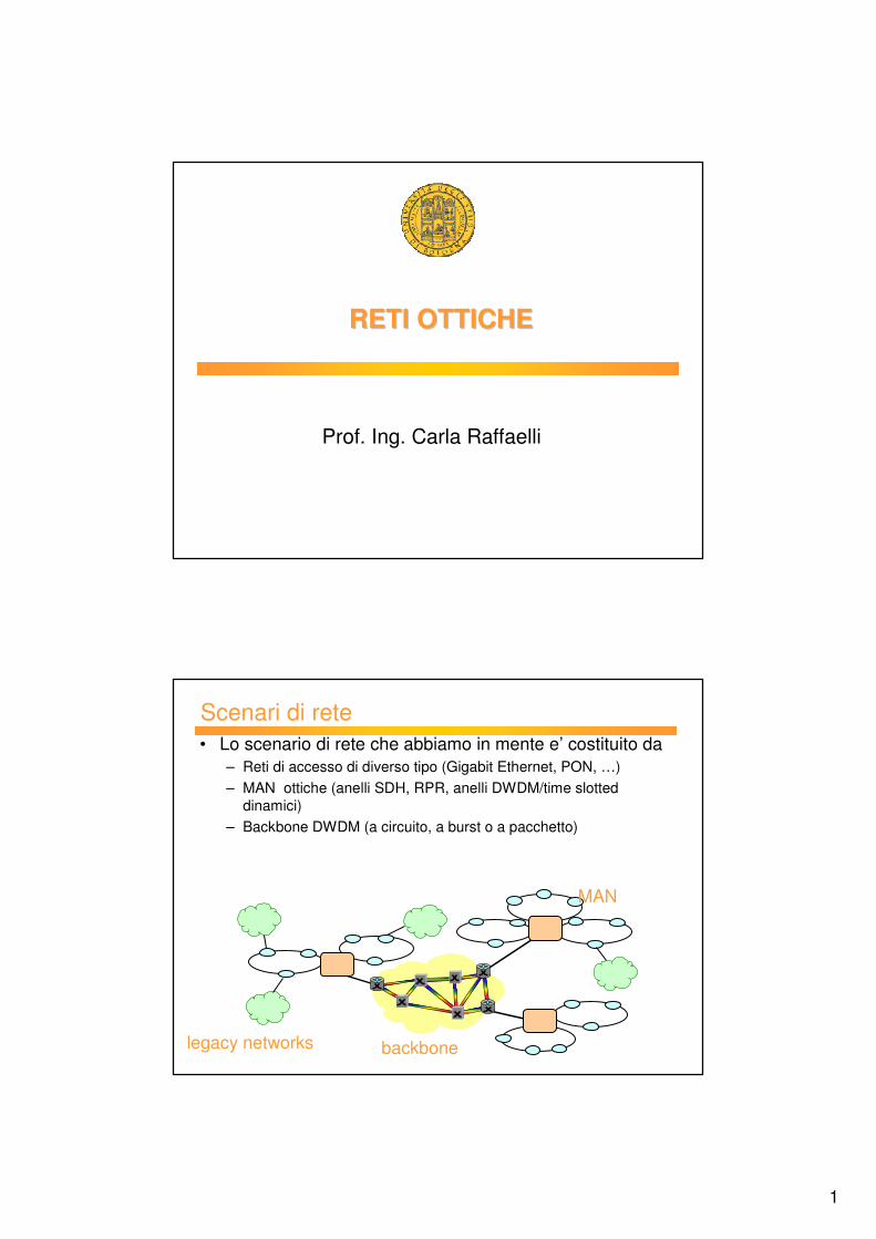
1 RETI OTTICHE RETI OTTICHE Prof. Ing. Carla Raffaelli Scenari di rete • Lo scenario di rete che abbiamo in mente e’ costituito da – Reti di accesso di diverso tipo (Gigabit Ethernet, PON, …) – MAN ottiche (anelli SDH, RPR, anelli DWDM/time slotted dinamici) – Backbone DWDM (a circuito, a burst o a pacchetto) backbone MAN legacy networks
-
Upload
duongkhanh -
Category
Documents
-
view
214 -
download
0
Transcript of RETI OTTICHE -...
1
RETI OTTICHE RETI OTTICHE
Prof. Ing. Carla Raffaelli
Scenari di rete• Lo scenario di rete che abbiamo in mente e’ costituito da
– Reti di accesso di diverso tipo (Gigabit Ethernet, PON, …)– MAN ottiche (anelli SDH, RPR, anelli DWDM/time slotted
dinamici)– Backbone DWDM (a circuito, a burst o a pacchetto)
backbone
MAN
legacy networks
2
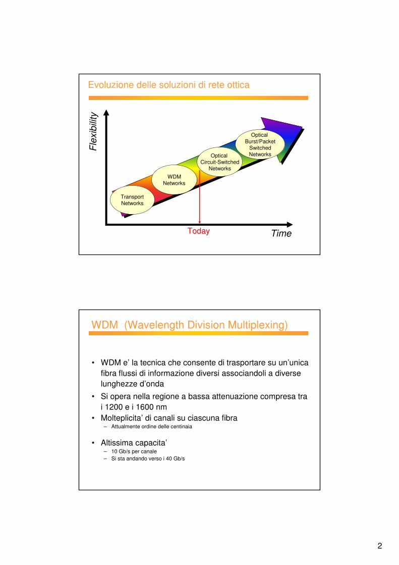
Evoluzione delle soluzioni di rete ottica
TransportNetworks
Optical Circuit-Switched
Networks
OpticalBurst/Packet
SwitchedNetworks
WDMNetworks
Time
Flex
ibili
ty
Today
WDM (Wavelength Division Multiplexing)
• WDM e’ la tecnica che consente di trasportare su un’unicafibra flussi di informazione diversi associandoli a diverse lunghezze d’onda
• Si opera nella regione a bassa attenuazione compresa trai 1200 e i 1600 nm
• Molteplicita’ di canali su ciascuna fibra– Attualmente ordine delle centinaia
• Altissima capacita’– 10 Gb/s per canale– Si sta andando verso i 40 Gb/s
3
Caratteristiche delle reti WDM
• Elevata capacita’
• Trasparenza
• Semplicita’ di gestione
• Scalabilita’
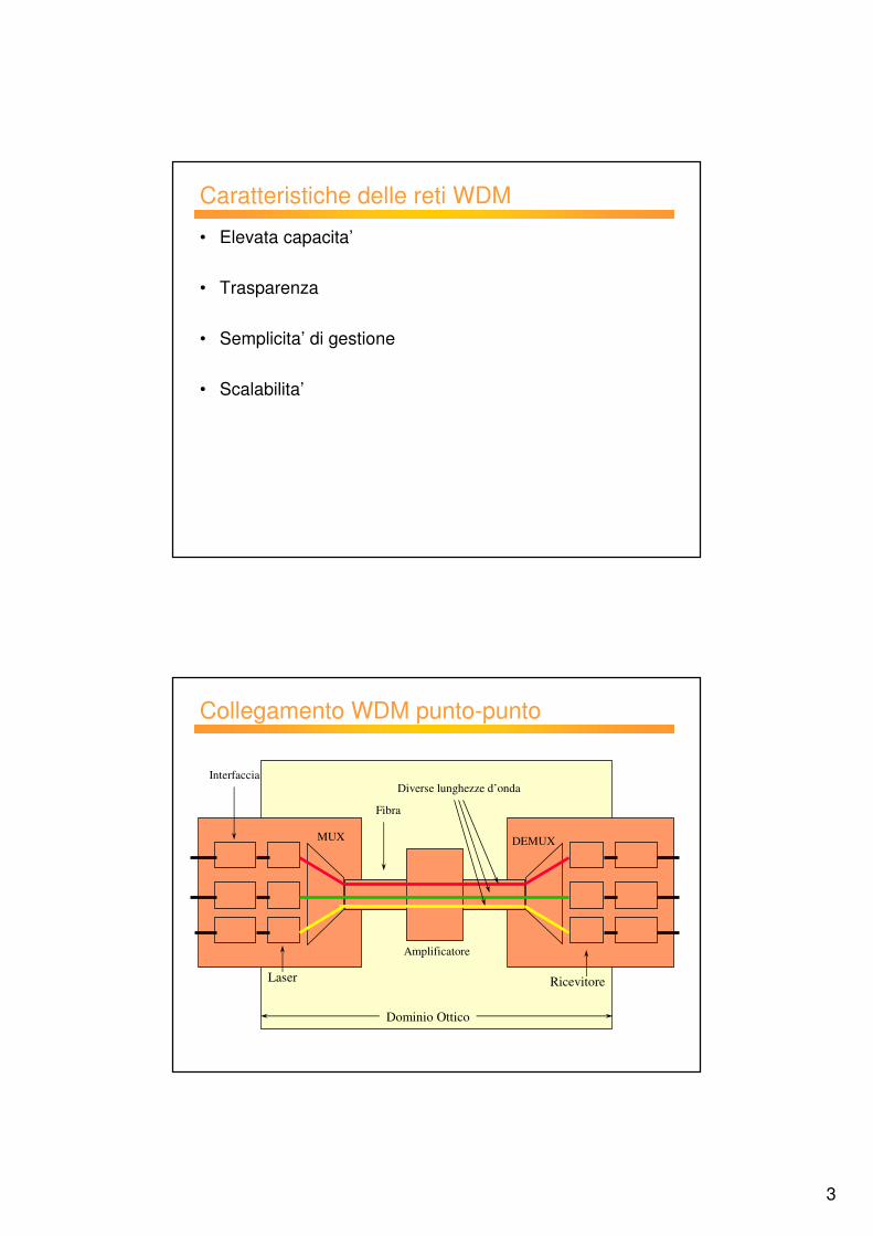
Laser Ricevitore
Amplificatore
Fibra
MUX DEMUX
Interfaccia
Dominio Ottico
Diverse lunghezze d’onda
Collegamento WDM punto-punto
4
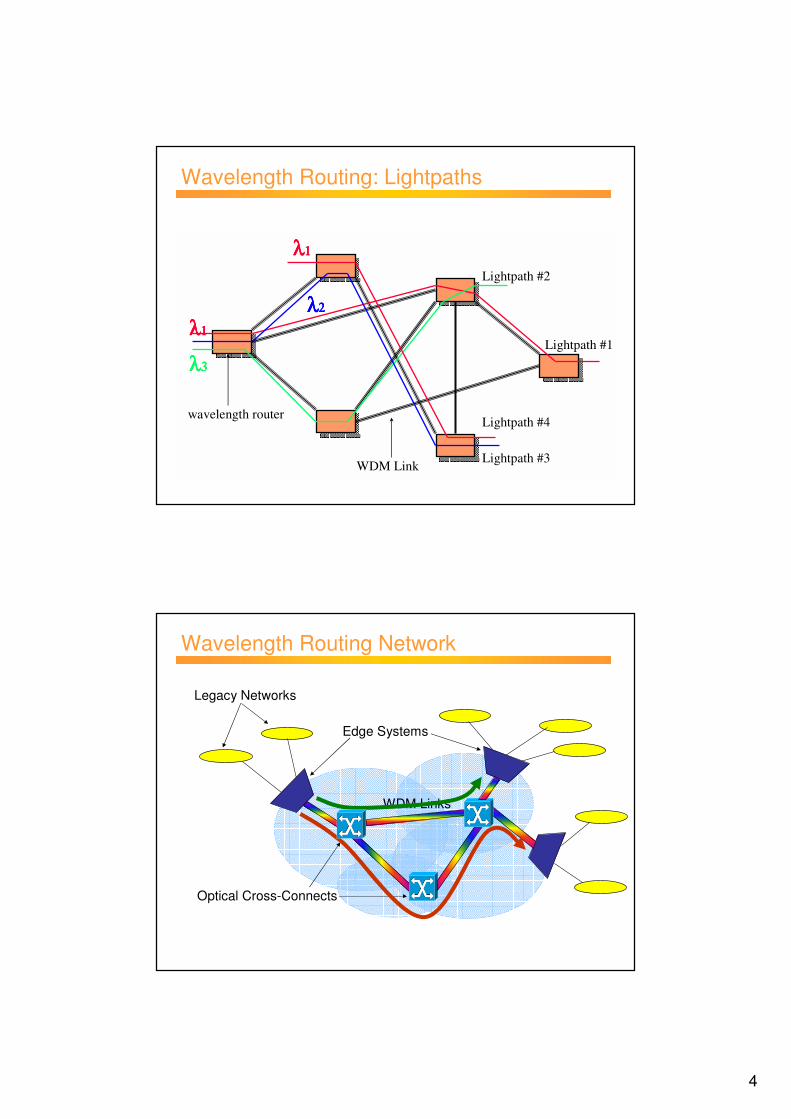
Wavelength Routing: Lightpaths
Lightpath #1
Lightpath #2
Lightpath #3
λλλλ1111
λλλλ3333
λλλλ2222
wavelength router
WDM Link
Lightpath #4
λλλλ1111
Wavelength Routing Network
Legacy Networks
WDM Links
Optical Cross-Connects
Edge Systems
5
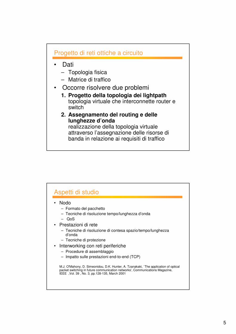
Progetto di reti ottiche a circuito
• Dati– Topologia fisica– Matrice di traffico
• Occorre risolvere due problemi1. Progetto della topologia dei lightpath
topologia virtuale che interconnette router e switch
2. Assegnamento del routing e dellelunghezze d’ondarealizzazione della topologia virtualeattraverso l’assegnazione delle risorse di banda in relazione ai requisiti di traffico
Aspetti di studio
• Nodo– Formato del pacchetto– Tecniche di risoluzione tempo/lunghezza d’onda– QoS
• Prestazioni di rete– Tecniche di risoluzione di contesa spazio/tempo/lunghezza
d’onda– Tecniche di protezione
• Interworking con reti periferiche– Procedure di assemblaggio– Impatto sulle prestazioni end-to-end (TCP)
M.J. O'Mahony, D. Simeonidou, D.K. Hunter, A. Tzanakaki, `The application of optical packet switching in future communication networks', Communications Magazine, IEEE ,Vol. 39 , No. 3, pp.128-135, March 2001
6
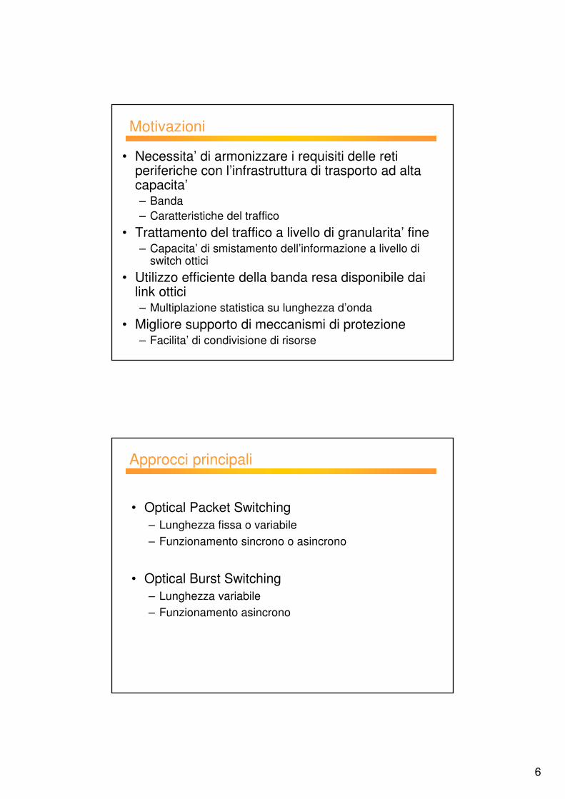
Motivazioni
• Necessita’ di armonizzare i requisiti delle reti periferiche con l’infrastruttura di trasporto ad alta capacita’– Banda– Caratteristiche del traffico
• Trattamento del traffico a livello di granularita’ fine– Capacita’ di smistamento dell’informazione a livello di
switch ottici• Utilizzo efficiente della banda resa disponibile dai
link ottici– Multiplazione statistica su lunghezza d’onda
• Migliore supporto di meccanismi di protezione– Facilita’ di condivisione di risorse
Approcci principali
• Optical Packet Switching– Lunghezza fissa o variabile– Funzionamento sincrono o asincrono
• Optical Burst Switching– Lunghezza variabile– Funzionamento asincrono
7
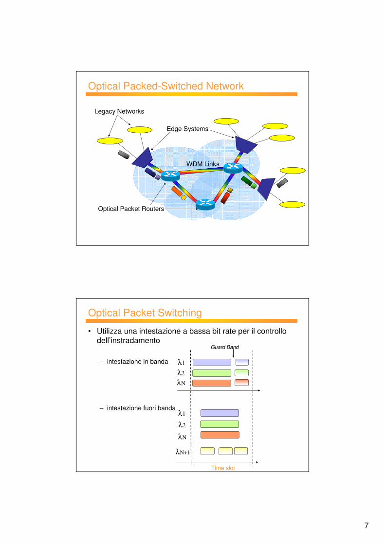
Optical Packed-Switched Network
Legacy Networks
WDM Links
Optical Packet Routers
Edge Systems
Optical Packet Switching
• Utilizza una intestazione a bassa bit rate per il controllo dell’instradamento
– intestazione in banda
– intestazione fuori banda
Guard Band
λ1λ2λN
λ1
λ2
λN
λN+1
Time slot
8
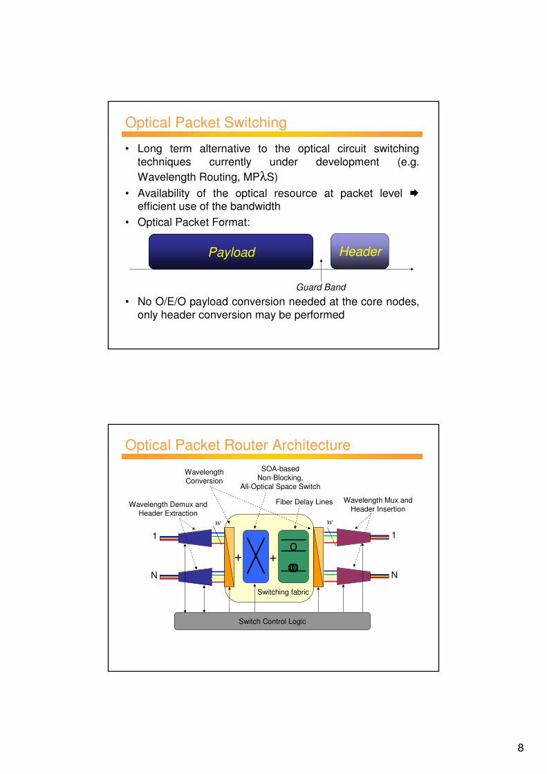
• Long term alternative to the optical circuit switching techniques currently under development (e.g. Wavelength Routing, MPλS)
• Availability of the optical resource at packet level �efficient use of the bandwidth
• Optical Packet Format:
• No O/E/O payload conversion needed at the core nodes, only header conversion may be performed
Optical Packet Switching
Payload Header
Guard Band
Optical Packet Router ArchitectureSOA-based
Non-Blocking, All-Optical Space Switch
Fiber Delay Lines
+
Wavelength Demux and Header Extraction
1w
N
Wavelength Mux and Header Insertion
Switch Control Logic
1
N
w
WavelengthConversion
+
Switching fabric

9
Componenti principali
• Convertitori ottici di lunghezza d’onda– consentono di associare a ciascun pacchetto una
lunghezza d’onda in generale diversa da quella con cui si presenta in ingresso
• Filtri ottici– consentono di selezionare una sola delle lunghezze
d’onda multiplate sulla stessa linea di ritardo
• Interruttori ottici– consentono di associare due linee disgiunte
mediante amplificatori ottici a semiconduttore (SOA)
Buffer ottico• E’ il dispositivo che ritarda il segnale di un numero intero di tempi di
pacchetto• Si realizza secondo lo schema seguente:
• su ciascuna delle Q linee di ritardo sono allocate N lunghezze d’onda
• La lunghezza L della fibra ottica che realizza il ritardo kT e’stimabile mediante
L = c k Tdove c e’la velocita’della luce

10
Buffer ottico: rappresentazione temporale
• Realized with B Fiber Delay Lines (FDL):– the delay must be chosen at packet arrival– packets are delayed until the output wavelength is available– available delays are consecutive multiples of the delay unit D
(different choices are also possible)– packets are lost when the buffer is full, i.e. the required delay is
larger than the maximum delay achievable DM = (B -1)D
0
D
(B -1)Dt0 t0+D t0+2D t0+(B -1)D
t0
…
Pacchetto ottico sincrono di lunghezza fissa
• Necessita di sincronizzazione e allineamento• Consente una piu’ naturale realizzazione delle
memorie con linee di ritardo– Unita’ di tempo = durata del pacchetto
• Nella versione sincrona da’ luogo a migliori prestazioni
• Durate tipiche dell’ordine del microsecondo
11
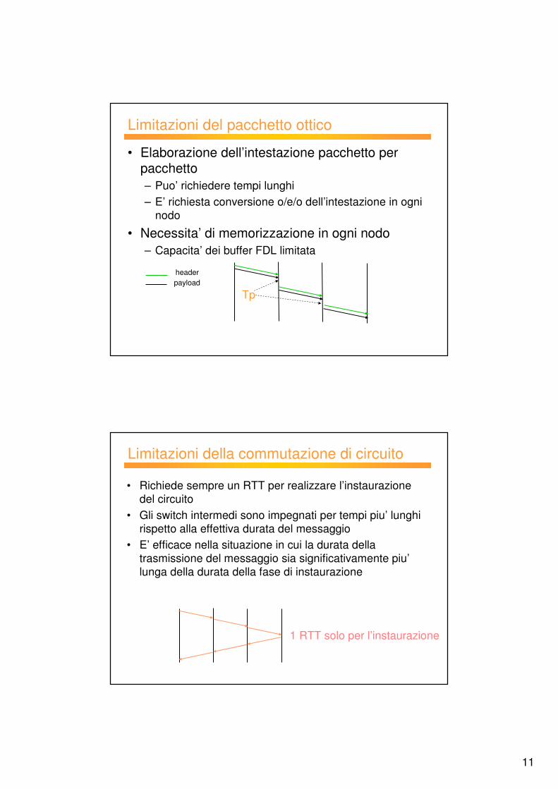
Limitazioni del pacchetto ottico
• Elaborazione dell’intestazione pacchetto per pacchetto– Puo’ richiedere tempi lunghi – E’ richiesta conversione o/e/o dell’intestazione in ogni
nodo
• Necessita’ di memorizzazione in ogni nodo– Capacita’ dei buffer FDL limitata
Tp
headerpayload
Limitazioni della commutazione di circuito
• Richiede sempre un RTT per realizzare l’instaurazione del circuito
• Gli switch intermedi sono impegnati per tempi piu’ lunghi rispetto alla effettiva durata del messaggio
• E’ efficace nella situazione in cui la durata della trasmissione del messaggio sia significativamente piu’lunga della durata della fase di instaurazione
1 RTT solo per l’instaurazione

12
Burst switching
• Cerca di combinare i vantaggi della commutazione di circuito e di pacchetto
• Utilizza segnalazione fuori banda per configurare i nodi lungo il percorso del burst per il trasferimento dell’informazione
• I burst sono di lunghezza variabile• La memorizzazione dei pacchetti avviene
tipicamente all’ingresso della rete
JIT:Just-in-time
• Viene inviato un messaggio di setup per configurare i cross-connect lungo il percorso
• La configurazione del cross connect avviene parallelamente alla propagazione del setup nella rete
• La trasmissione dati inizia con un ritardo opportuno rispetto alla emissione del setup e comunque non si prevede ricezione di una conferma
• Le risorse vengono rilasciate esplicitamente
13
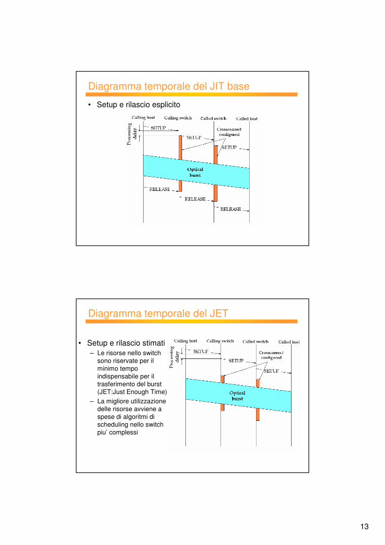
Diagramma temporale del JIT base
• Setup e rilascio esplicito
Diagramma temporale del JET
• Setup e rilascio stimati– Le risorse nello switch
sono riservate per il minimo tempo indispensabile per il trasferimento del burst(JET:Just Enough Time)
– La migliore utilizzazione delle risorse avviene a spese di algoritmi di scheduling nello switchpiu’ complessi
14
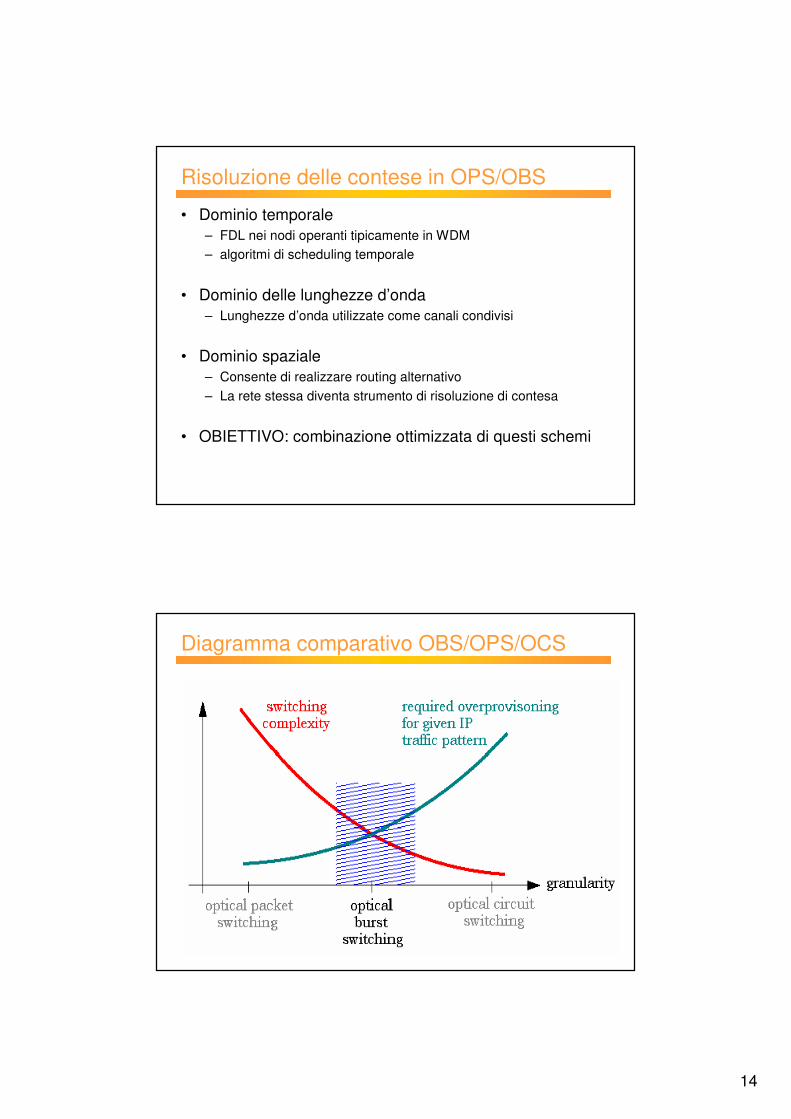
Risoluzione delle contese in OPS/OBS
• Dominio temporale– FDL nei nodi operanti tipicamente in WDM– algoritmi di scheduling temporale
• Dominio delle lunghezze d’onda– Lunghezze d’onda utilizzate come canali condivisi
• Dominio spaziale– Consente di realizzare routing alternativo– La rete stessa diventa strumento di risoluzione di contesa
• OBIETTIVO: combinazione ottimizzata di questi schemi
Diagramma comparativo OBS/OPS/OCS
15
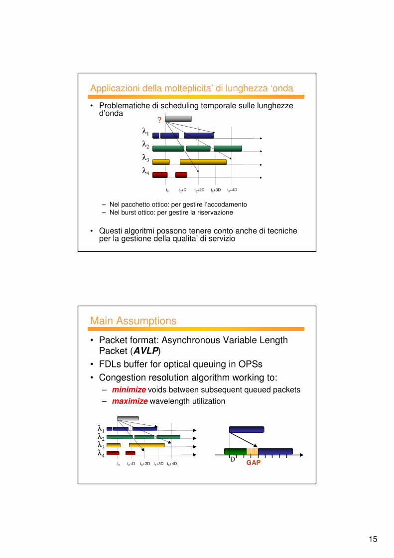
Applicazioni della molteplicita’ di lunghezza ‘onda
• Problematiche di scheduling temporale sulle lunghezze d’onda
– Nel pacchetto ottico: per gestire l’accodamento– Nel burst ottico: per gestire la riservazione
• Questi algoritmi possono tenere conto anche di tecniche per la gestione della qualita’ di servizio
t0 t0+D t0+2D t0+4Dt0+3D
λ1
λ2
λ3
λ4
?
Main Assumptions
• Packet format: Asynchronous Variable Length Packet (AVLP)
• FDLs buffer for optical queuing in OPSs • Congestion resolution algorithm working to:
– minimize voids between subsequent queued packets– maximize wavelength utilization
D GAPt0 t0+D t0+2D t0+4Dt0+3D
λ1λ2λ3λ4
16
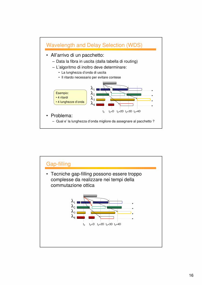
Wavelength and Delay Selection (WDS)
• All’arrivo di un pacchetto:– Data la fibra in uscita (dalla tabella di routing)– L’algoritmo di inoltro deve determinare:
• La lunghezza d’onda di uscita• Il ritardo necessario per evitare contese
• Problema:– Qual e’ la lunghezza d’onda migliore da assegnare al pacchetto ?
Esempio:• 4 ritardi• 4 lunghezze d’onda
t0 t0+D t0+2D t0+4Dt0+3D
λ1λ2λ3λ4
Gap-filling
• Tecniche gap-filling possono essere troppocomplesse da realizzare nei tempi dellacommutazione ottica
t0 t0+D t0+2D t0+4Dt0+3D
λ1λ2λ3λ4
17
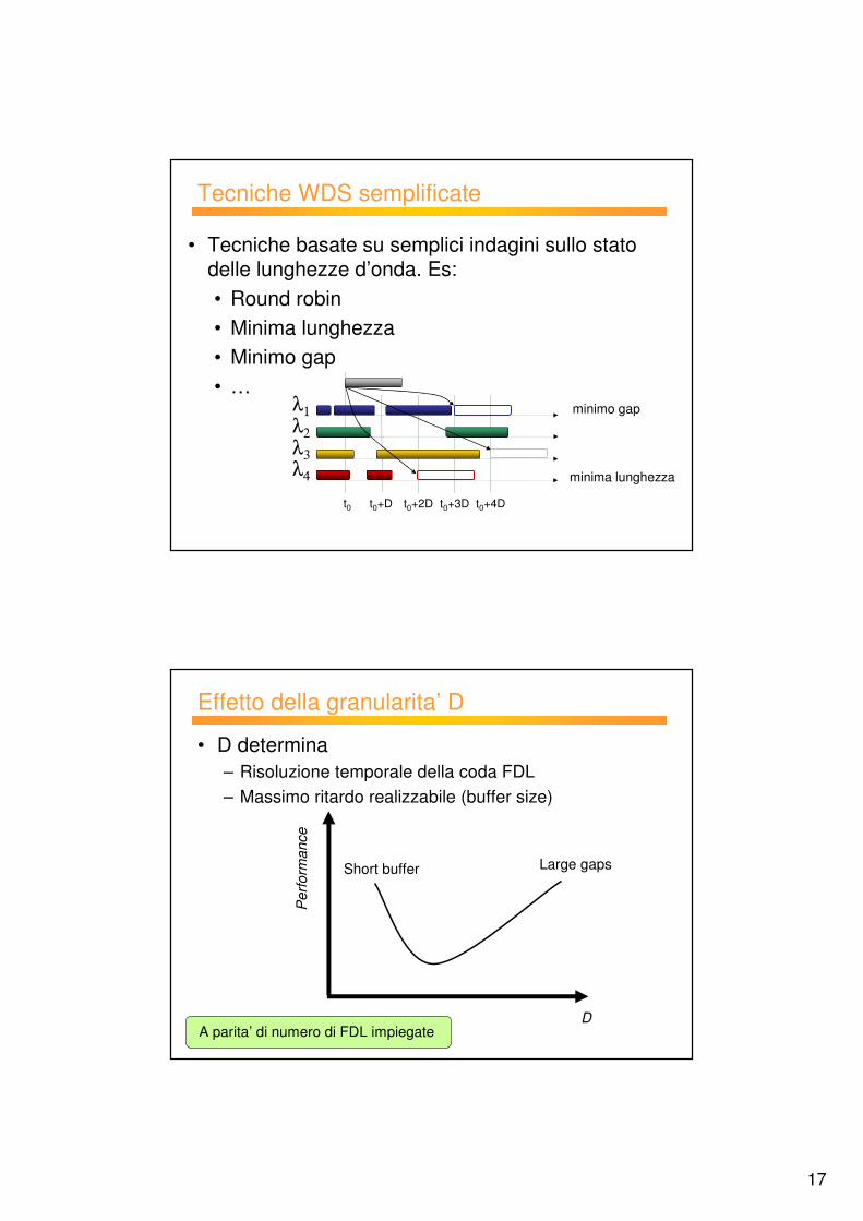
Tecniche WDS semplificate
t0 t0+D t0+2D t0+4Dt0+3D
λ1λ2λ3λ4
• Tecniche basate su semplici indagini sullo statodelle lunghezze d’onda. Es:• Round robin• Minima lunghezza• Minimo gap• …
minima lunghezza
minimo gap
Effetto della granularita’ D
• D determina– Risoluzione temporale della coda FDL– Massimo ritardo realizzabile (buffer size)
D
Per
form
ance
Short buffer Large gaps
A parita’ di numero di FDL impiegate
18
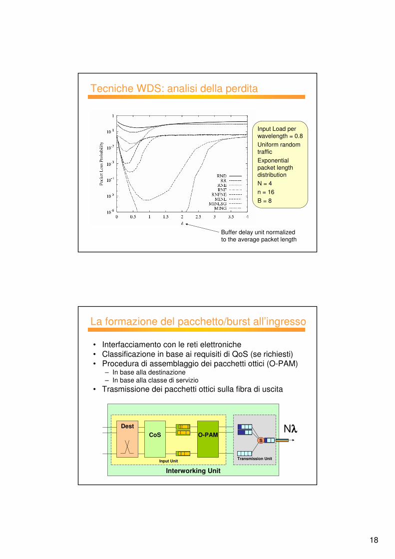
Tecniche WDS: analisi della perdita
Buffer delay unit normalizedto the average packet length
Input Load per wavelength = 0.8Uniform random trafficExponential packet length distributionN = 4n = 16B = 8
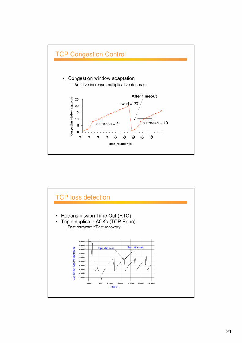
La formazione del pacchetto/burst all’ingresso
Interworking Unit
Input Unit
DestCoS O-PAM
Transmission Unit
S
Nλλλλ
• Interfacciamento con le reti elettroniche • Classificazione in base ai requisiti di QoS (se richiesti)• Procedura di assemblaggio dei pacchetti ottici (O-PAM)
– In base alla destinazione– In base alla classe di servizio
• Trasmissione dei pacchetti ottici sulla fibra di uscita

19
Per-flow aggregation
F1
F2Transmission Queue
Assembly Queues
• Ingress per-flow queuing • Optical packet assembled with segments of the same
flow• An assembly time-out for each active flow is needed• High complexity of assembly mechanism
Fn
Mixed-flow aggregation
• TCP segments from different flows and with the same optical destination address aggregated in the same optical packet
• Only one assembly time-out is needed• Low complexity of the assembly mechanism
F1
F2Transmission Queue
Fn
Assembly Queue

20
TCP over OBS
Studio dell’influenza del processo di formazione dei pacchetti sulle prestazioni del TCP
Basic TCP control functions
• Flow control– the TCP window size is used to prevent the sender
from flooding the receiver
• Congestion control– TCP window is dynamically updated in relation to the
network state as perceived by the sender
21
TCP Congestion Control
• Congestion window adaptation– Additive increase/multiplicative decrease
ssthresh = 8 ssthresh = 10
cwnd = 20
After timeout
0
5
10
15
20
25
0 3 6 9 12 15 20 22 25
Time (round trips)
Con
gest
ion
win
dow
(seg
men
ts)
TCP loss detection
• Retransmission Time Out (RTO)• Triple duplicate ACKs (TCP Reno)
– Fast retransmit/Fast recovery
Con
gest
ion
win
dow
(se
gmen
ts)
fast retransmittriple dup acks
Time (s)
22
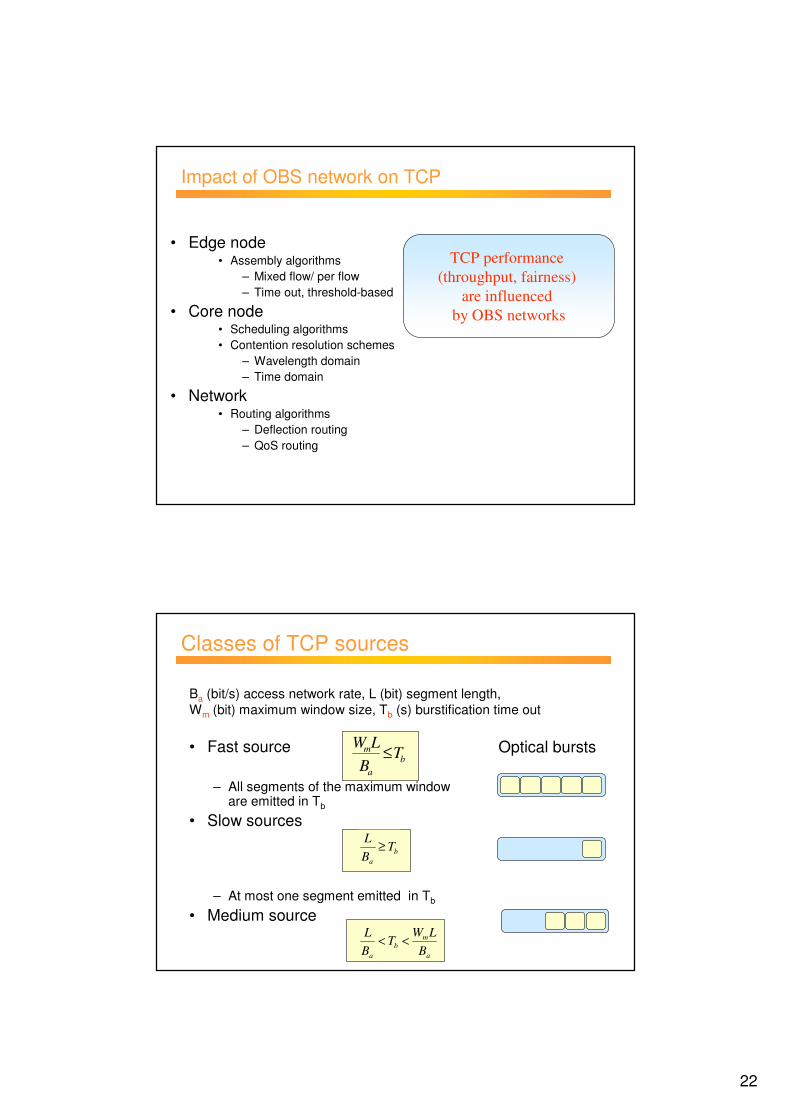
Impact of OBS network on TCP
• Edge node• Assembly algorithms
– Mixed flow/ per flow– Time out, threshold-based
• Core node• Scheduling algorithms• Contention resolution schemes
– Wavelength domain– Time domain
• Network• Routing algorithms
– Deflection routing– QoS routing
TCP performance (throughput, fairness)
are influencedby OBS networks
Classes of TCP sources
• Fast source
– All segments of the maximum window are emitted in Tb
• Slow sources
– At most one segment emitted in Tb
• Medium source
ba
m TB
LW ≤
a
mb
a BLW
TBL <<
ba
TBL ≥
Optical bursts
Ba (bit/s) access network rate, L (bit) segment length, Wm (bit) maximum window size, Tb (s) burstification time out
23
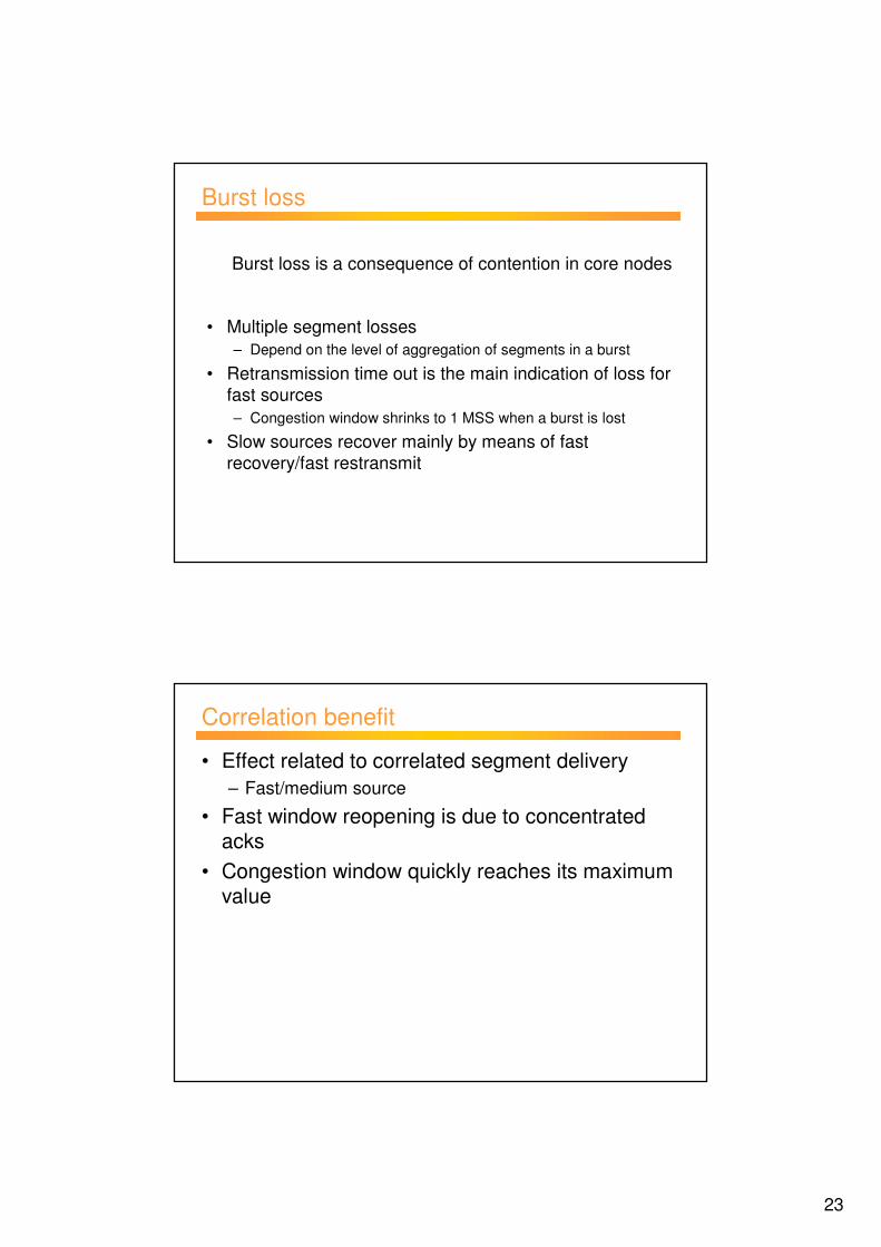
Burst loss
• Multiple segment losses– Depend on the level of aggregation of segments in a burst
• Retransmission time out is the main indication of loss forfast sources– Congestion window shrinks to 1 MSS when a burst is lost
• Slow sources recover mainly by means of fast recovery/fast restransmit
Burst loss is a consequence of contention in core nodes
Correlation benefit
• Effect related to correlated segment delivery– Fast/medium source
• Fast window reopening is due to concentratedacks
• Congestion window quickly reaches its maximumvalue
24
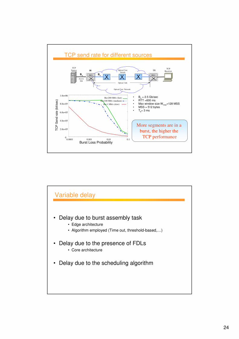
TCP send rate for different sources
• Bo = 2.5 Gb/sec• RTT =600 ms• Max window size Wmax=128 MSS• MSS = 512 bytes• Tb= 3 ms
0.10.0001 0.001 0.01Burst Loss Probability
TCP
Sen
dra
te (b
it/se
c)
0
1.0e+06
8.0e+05
6.0e+05
4.0e+05
2.0e+05
Ba=200 Mb/s (fast)Ba=100 Mb/s (medium)
Ba=1 Mb/s (slow)
IR ERTCP
SourceTCP
Receiver
Access link
Ba Bo
Optical Core Switch
Optical link
Optical Core Network
IWU IWU
More segments are in a burst, the higher the
TCP performance
Variable delay
• Delay due to burst assembly task• Edge architecture• Algorithm employed (Time out, threshold-based,…)
• Delay due to the presence of FDLs• Core architecture
• Delay due to the scheduling algorithm

25
Modeling TCP throughput *
• A simple model is able to calculate throughput as a function of burst loss probability p– p is a Bernoulli r.v.– Aggregation is accounted through the average number of segment in
a burst E[N]• The average TCP throuhput is calculated starting from the formula
– where E[Y] is the average number of segments transmitted in burstsduring during the interval I between two time out periods and E[R] isthe average number of segments transmitted during the time out period ZTO
• The result is
][][][][
TOTCP ZEIEREYE
B++=
)( pFBTCP =p is due to losses
arising in the network and in the core nodes
Core switch architecture
26
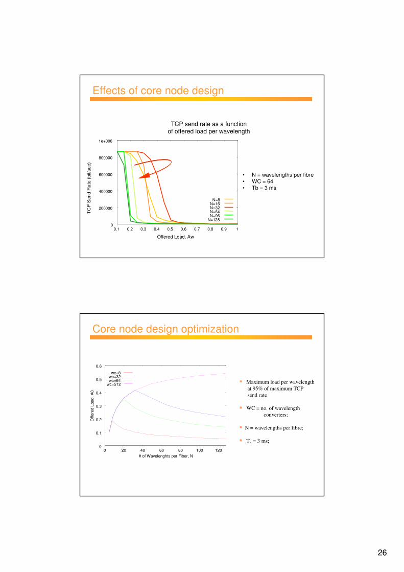
Effects of core node design
TCP send rate as a functionof offered load per wavelength
0
200000
400000
600000
800000
1e+006
0.1 0.2 0.3 0.4 0.5 0.6 0.7 0.8 0.9 1
TC
P S
end
Rat
e (b
it/se
c)
Offered Load, Aw
N=8N=16N=32N=64N=96
N=128
• N = wavelengths per fibre• WC = 64 • Tb = 3 ms
Core node design optimization
� Maximum load per wavelengthat 95% of maximum TCPsend rate
� WC = no. of wavelengthconverters;
� N = wavelengths per fibre;
� Tb = 3 ms;0
0.1
0.2
0.3
0.4
0.5
0.6
0 20 40 60 80 100 120
Offe
red
Load
, A0
# of Wavelenghts per Fiber, N
wc=8wc=32wc=64
wc=512

27
References• A.Detti, M. Listanti, “Impact of Segment Aggregation on TCP Reno Flows in Optical Burst
Switching Networks”, Proc. INFOCOM 2002, Vol.3 pp1803-1812.• J. Padhye, V. Firoiu, D.F. Towsley, J. F. Kurose, “Modeling TCP Reno Performance: a simple
model and its empirical validation”, IEEE/ACM Transaction on Networking, Vol. 8, No.2, pp.133-144, April 2000.
• J. He, S.-H. G. Chan, “TCP and UDP Performance for Internet over Optical Packet-SwitchedNetworks”, Proc. of ICC 2003, pp.1350-1354.
Il ruolo di MPLS
• MPLS consente di definire percorsi virtuali anche per la rete ottica identificati link by link da label
• E’ applicabile sia al packet switching che al burstswitch
• Svolge il ruolo di ridurre i tempi di instradamentonel momento in cui l’informazione deve essere trasmessa
• Consente maggior controllo sui trasferimenti di traffico attraverso la rete
28
GMPLS: Generalized MPLS
• GMPLS is a multipurpose control plane paradigm able to manage not only packet switching devices, but also devices that perform switching in time, wavelength, space domain.
• GMPLS aims at extending the existing MPLS routing and signaling protocols to address the characteristics of optical transport networks.– Improve the RSVP-TE and CR-LDP to allow signaling of optical
channel in optical transport networks and other connection-oriented environments
– Enhancements to OSPF and IGP to manage optical resources in the network, other network attributes and constraints
– A new Link Management Protocol suitable for the optical network scenario
GMPLS: main issues
• GMPLS requires that each LSP starts and ends on devices of the same kind
• In MPLS the control plane is logically separate from the data plane. GMPLS extends these concept, allowing the control plane to be physically diverse from the related data plane.
• GMPLS defines a hierarchical LSPs set up– LSPs may be tunneled inside an existing higher-order
LSP, that acts as a link along the path of the new LSP– Nodes at the border of two regions, different from the
MUX point of view, have the task to form higher-order LSPs by aggregating lower-order LSPs

29
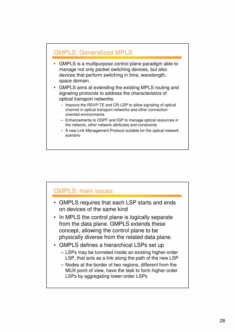
GMPLS: hierarchical LSPs
P4 P5 P6 O7O3S2 S8R1 R9R0 R10Fiber LSP4
λλλλ LSP3
TDM LSP2
Packet LSP1
GbEth
OC-12
OC-192Fiber
R IP-LSR
S SONET switch
O Optical OEO Switch
P Photonic SwitchJ. Drake et al.
“GMPLS: An oveview of sgnalingenhancements and recovery
techniques”,
IEEE Communication Magazine
Algorithms for adaptive routing
• Routing algorithms can be– static or dynamic/adaptive
• Static: routing tables defined once for all• Adaptive: considers alternatives to shortest path
depending on the state of the network• In a DWDM OPS network the aim is to:
– Combine the flexibility of adaptive routing with the power of WDM at various level
– Design routing procedures outperforming the conventional shortest path routing
30
Definition of the routing path sets and routing algorithm actions• By knowing the network topology:
– find the whole set of paths per source/destination pair– calculate the related costs (hops)
• Define:– default set: used at the first attempt to route a packet– alternate set: used when the default set is not
available (congested).• If an available wavelength is not found the packet
is dropped• Wavelength sharing: WDM is applied among a
different number of path according to the diverse routing agorithms
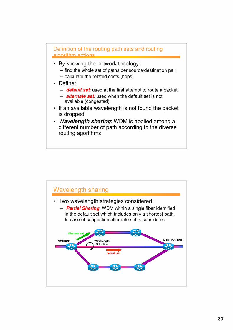
Wavelength sharing
• Two wavelength strategies considered:– Partial Sharing: WDM within a single fiber identified
in the default set which includes only a shortest path. In case of congestion alternate set is considered
Wavelength Selection
default set
alternate set
SOURCE DESTINATION
31
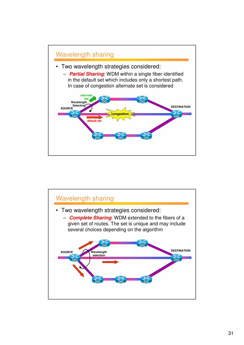
Wavelength sharing
• Two wavelength strategies considered:– Partial Sharing: WDM within a single fiber identified
in the default set which includes only a shortest path. In case of congestion alternate set is considered
Wavelength Selection
default set
congestion congestion
alternate set
SOURCE DESTINATION
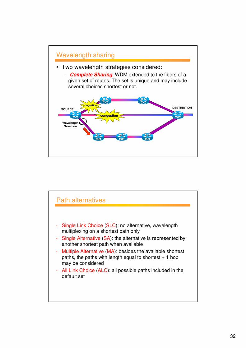
Wavelength sharing
• Two wavelength strategies considered:– Complete Sharing: WDM extended to the fibers of a
given set of routes. The set is unique and may include several choices depending on the algorithm
Wavelength selection
SOURCE DESTINATION
32
Wavelength sharing
• Two wavelength strategies considered:– Complete Sharing: WDM extended to the fibers of a
given set of routes. The set is unique and may include several choices shortest or not.
congestion congestion
congestion congestion
Wavelength Selection
SOURCE DESTINATION
Path alternatives
• Single Link Choice (SLC): no alternative, wavelength multiplexing on a shortest path only
• Single Alternative (SA): the alternative is represented by another shortest path when available
• Multiple Alternative (MA): besides the available shortest paths, the paths with length equal to shortest + 1 hop may be considered
• All Link Choice (ALC): all possible paths included in the default set
33
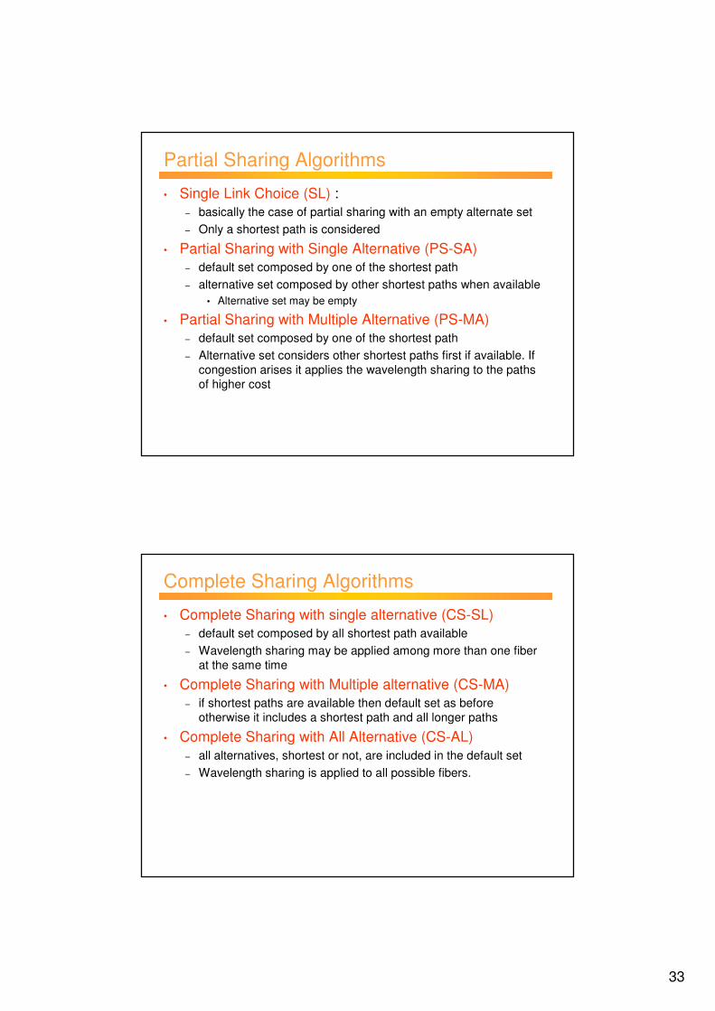
Partial Sharing Algorithms
• Single Link Choice (SL) : – basically the case of partial sharing with an empty alternate set – Only a shortest path is considered
• Partial Sharing with Single Alternative (PS-SA)– default set composed by one of the shortest path– alternative set composed by other shortest paths when available
• Alternative set may be empty
• Partial Sharing with Multiple Alternative (PS-MA) – default set composed by one of the shortest path – Alternative set considers other shortest paths first if available. If
congestion arises it applies the wavelength sharing to the pathsof higher cost
Complete Sharing Algorithms
• Complete Sharing with single alternative (CS-SL) – default set composed by all shortest path available– Wavelength sharing may be applied among more than one fiber
at the same time
• Complete Sharing with Multiple alternative (CS-MA) – if shortest paths are available then default set as before
otherwise it includes a shortest path and all longer paths
• Complete Sharing with All Alternative (CS-AL)– all alternatives, shortest or not, are included in the default set– Wavelength sharing is applied to all possible fibers.
34
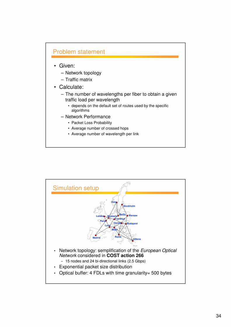
Problem statement
• Given:– Network topology– Traffic matrix
• Calculate:– The number of wavelengths per fiber to obtain a given
traffic load per wavelength• depends on the default set of routes used by the specific
algorithms
– Network Performance• Packet Loss Probability• Average number of crossed hops • Average number of wavelength per link
Simulation setup
• Network topology: semplification of the European Optical Network considered in COST action 266– 15 nodes and 24 bi-directional links (2.5 Gbps)
• Exponential packet size distribution• Optical buffer: 4 FDLs with time granularity= 500 bytes
Oslo
Stockholm
London Brussels
Paris
Madrid
Milan
Berlin
Athens
BudapestVienna
Warsaw
Rome
Lyon
Frankfurt
35
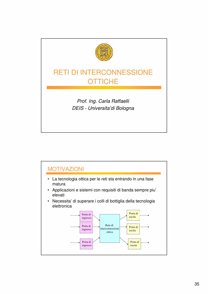
RETI DI INTERCONNESSIONE OTTICHE
Prof. Ing. Carla RaffaelliDEIS - Universita’di Bologna
MOTIVAZIONI
• La tecnologia ottica per le reti sta entrando in una fase matura
• Applicazioni e sistemi con requisiti di banda sempre piu’elevati
• Necessita’ di superare i colli di bottiglia della tecnologia elettronica
Rete di interconnessione
ottica
Porta di ingresso
Porta di ingresso
Porta di ingresso
Porta di uscita
Porta di uscita
Porta di uscita
36
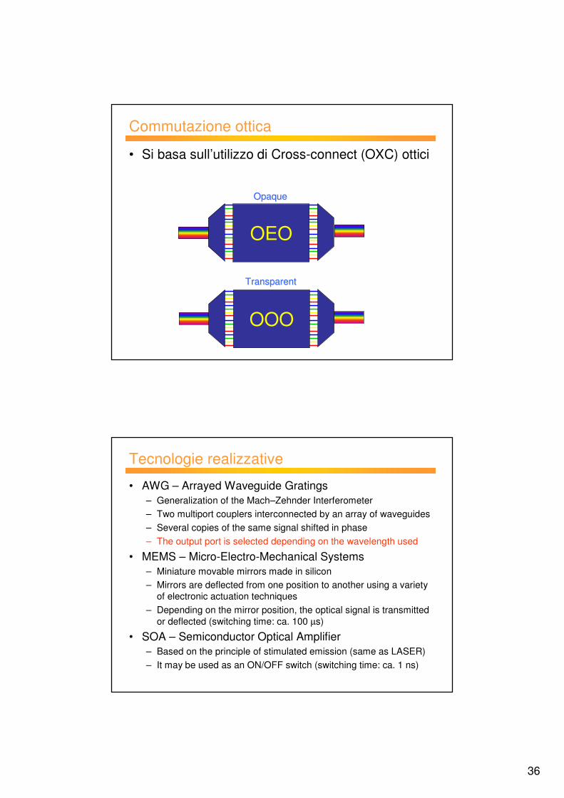
Commutazione ottica
• Si basa sull’utilizzo di Cross-connect (OXC) ottici
OEO
OpaqueOpaque
OOO
TransparentTransparent
Tecnologie realizzative
• AWG – Arrayed Waveguide Gratings– Generalization of the Mach–Zehnder Interferometer– Two multiport couplers interconnected by an array of waveguides– Several copies of the same signal shifted in phase– The output port is selected depending on the wavelength used
• MEMS – Micro-Electro-Mechanical Systems– Miniature movable mirrors made in silicon– Mirrors are deflected from one position to another using a variety
of electronic actuation techniques – Depending on the mirror position, the optical signal is transmitted
or deflected (switching time: ca. 100 µs)
• SOA – Semiconductor Optical Amplifier– Based on the principle of stimulated emission (same as LASER)– It may be used as an ON/OFF switch (switching time: ca. 1 ns)
37
Switch Architectures and Experiments
Switch TechnologiesQueste diapositive sono state preparate dal Prof.
W. Kabacinsky
Switch Technologies and Switching Types (1)
� To construct optical switching elements two different technologies are being used:– guided lightwave based switches – they use fibers or
waveguides for transmitting and switching lightwaves,– free-space switches – lightwaves.
38
Switch Technologies and Switching Types(2)� Each category can be further divided into different
classes, depending on the physical phenomena used to switch lightwaves between inputs and outputs.1. electro-optic switches – they use an electro-optic effect of a
material, i.e. changes of the refractive index due to the application of an electric filed,
2. acousto-optic switches – they use an acousto-optic effect of a material, i.e. changes of the refractive index due to the application of acoustic waves,
Switch Technologies and Switching Types(3)
3. thermo-optic switches – they use thermo-optic effect of a material, i.e. changes of the refractive index due to changes oftemperature,
4. MEMS switches – they use micro-electro-mechanical systems to move fibers, micro-mirrors or prisms,
5. liquid-crystal switches – they use properties of liquid-crystal materials, where the refractive index is determined by molecular alignment controlled by electric fields,
6. switches based on optical semiconductor amplifiers.
39
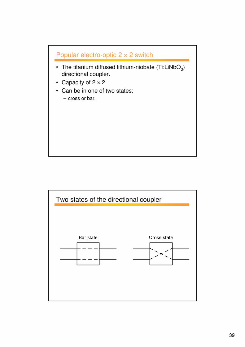
Popular electro-optic 2 × 2 switch
• The titanium diffused lithium-niobate (Ti:LiNbO3) directional coupler.
• Capacity of 2 × 2.• Can be in one of two states:
– cross or bar.
Two states of the directional coupler
40
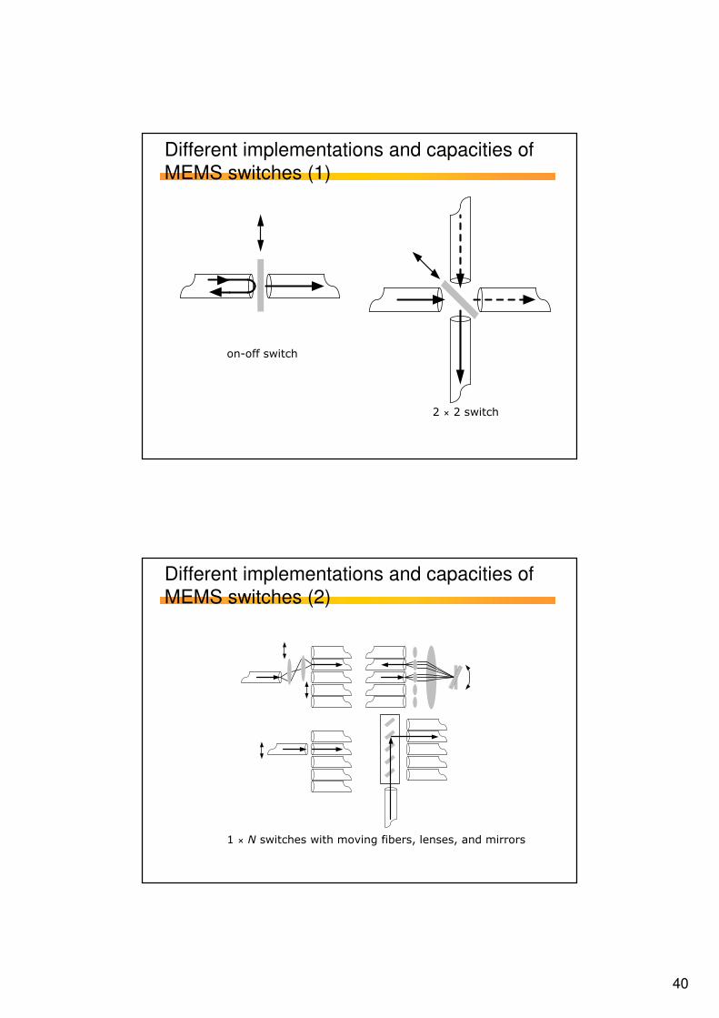
Different implementations and capacities ofMEMS switches (1)
����������
��× ������
Different implementations and capacities ofMEMS switches (2)
�× �������������������������������������������
41
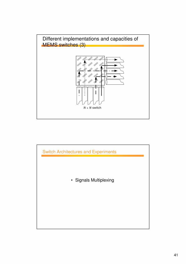
Different implementations and capacities ofMEMS switches (3)
��× ������
Switch Architectures and Experiments
• Signals Multiplexing

42
Multiplexing Techniques
• Information from different users transferred through a switch can be multiplexed in different ways:– space-division multiplexing (SDM) – signals from different users
are sent using separate fibers,– time-division multiplexing systems (TDM) – links are shared in
time, where data from different users are sent in different timeintervals called time slots,
– wavelength-division multiplexing (WDM) – when data are sent through the same fiber using different wavelengths (or frequency).
Space-division switching fabrics
��� ��� ���
����������������������������������������������������������������
43
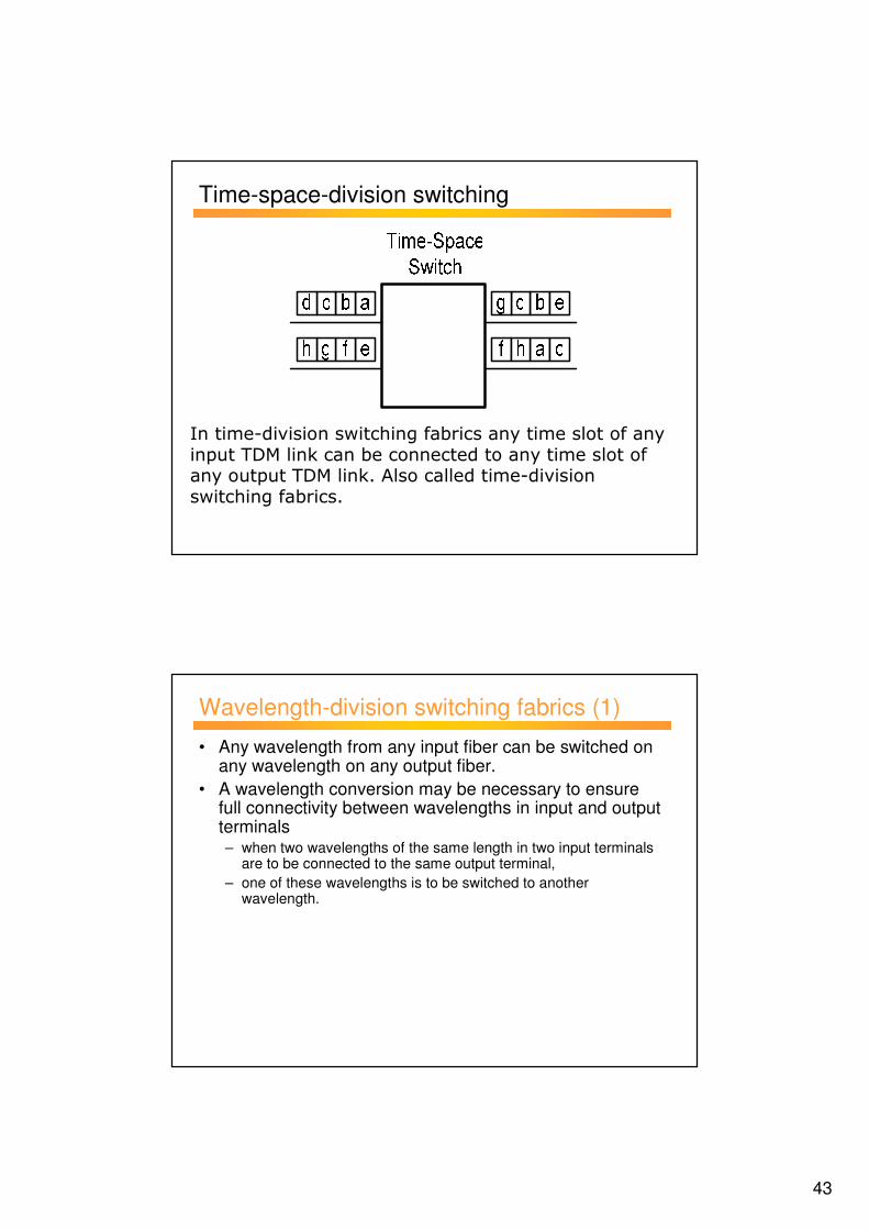
Time-space-division switching
��������������������������������!����������������!��������������"�������������������!����������������!��������������"��#��� ����������������������������������
Wavelength-division switching fabrics (1)
• Any wavelength from any input fiber can be switched on any wavelength on any output fiber.
• A wavelength conversion may be necessary to ensure full connectivity between wavelengths in input and output terminals– when two wavelengths of the same length in two input terminals
are to be connected to the same output terminal,– one of these wavelengths is to be switched to another
wavelength.

44
Wavelength-division switching fabrics (2)
• Waveband switching:– a set of wavelengths (called a waveband) on an
incoming fiber is switched to an outgoing fiber.
Wavelength-division switching fabrics (3)
� �
��
�
�

45
Switching fabric parameters
• The capacity of an optical switch is limited by technology constraints.
• To construct switches of greater capacity, many switches are connected between themselves and form a switching fabric.
• Many parameters has to be taken into account when designing a switching fabric. Important characteristics used in evaluating optical switching fabrics are:– attenuation and – signal-to-noise ratio (SNR).
Attenuation
• Attenuation of light passing through the switching network has several components, but the primary design criterion is the insertion loss in directional couplers. It varies depending on semiconductor technology (generally about 0.5 dB).
46
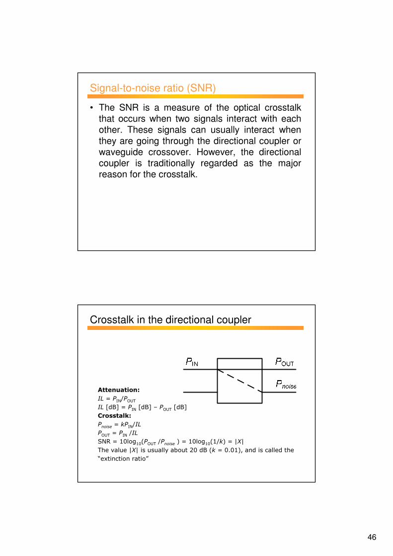
Signal-to-noise ratio (SNR)
• The SNR is a measure of the optical crosstalk that occurs when two signals interact with each other. These signals can usually interact when they are going through the directional coupler or waveguide crossover. However, the directional coupler is traditionally regarded as the major reason for the crosstalk.
Crosstalk in the directional coupler
�����������
���$�� %&�'(����)�*+�$�� % )�*+�, �'(�)�*+�
������ �
����
$��� %&���
�'(�$�� % &���
�%-�$� .��� ./�'(�&����0�$� .��� ./ &�0�$�1�1
���������1�1����������!��������.��*�/� $�.�. 0�����������������
2�3�������������4
47
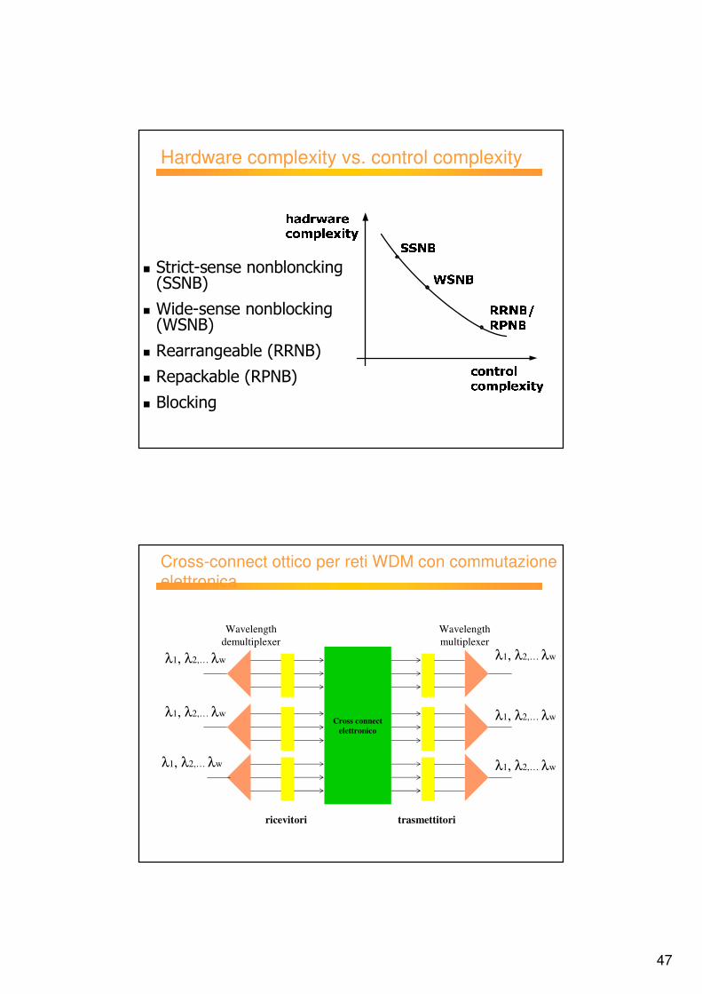
Hardware complexity vs. control complexity
� ������������� �����������
� ����������� �����������
� ���������� �������
� �������� �������
� � �����
Cross-connect ottico per reti WDM con commutazione elettronica
Cross connectelettronico
ricevitori trasmettitori
λ1, λ2,… λw
λ1, λ2,… λw
λ1, λ2,… λw
λ1, λ2,… λw
λ1, λ2,… λw
λ1, λ2,… λw
Wavelengthdemultiplexer
Wavelengthmultiplexer

48
Cross-connect tutto ottico con conversione di lunghezza d’onda
Commutatore ottico
Convertitori di lunghezza d’onda
λ1, λ2,… λw
λ1, λ2,… λw
λ1, λ2,… λw
λ1, λ2,… λw
λ1, λ2,… λw
λ1, λ2,… λw
Wavelengthdemultiplexer
Wavelengthmultiplexer
Cross-connect tutto ottico senza conversione di lunghezza d’onda
λ1, λ2,… λw
λ1, λ2,… λw
λ1, λ2,… λw
λ1, λ2,… λw
λ1, λ2,… λw
λ1, λ2,… λw
Wavelengthdemultiplexer
Wavelengthmultiplexer
λ1
switchottici
λ2
λw

49
Modalita’ di organizzazione dei convertitori
• Shared per output link– I convertitori sono condivisi dal traffico diretto alla
medesima uscita
• Shared per node– I convertitori sono condivisi da tutti gli ingressi
• Shared per wavelength– I convertitori sono condivisi per lunghezza d’onda
Shared per output link architecture
• Ogni fibra in uscita ha un insieme di R convertitori dedicati
• I convertitori dello stesso insiemepossono essere utilizzati solo daipacchetti diretti alla uscitacorrispondente
• I pacchetti in ingresso vengono inviatipossibilmente sulla stessa lunghezzad’onda su cui sono arrivati. Se cio’non e’ possibile utilizzano I convertitori
• Occorre stabilire quanti convertitorisono realmente necessari
Space Switching Matrix(non-blocking)
Fibre 1
Fibre N
Fibre 1
Fibre 2
M
R
M
Fibre 2
Fibre N
50
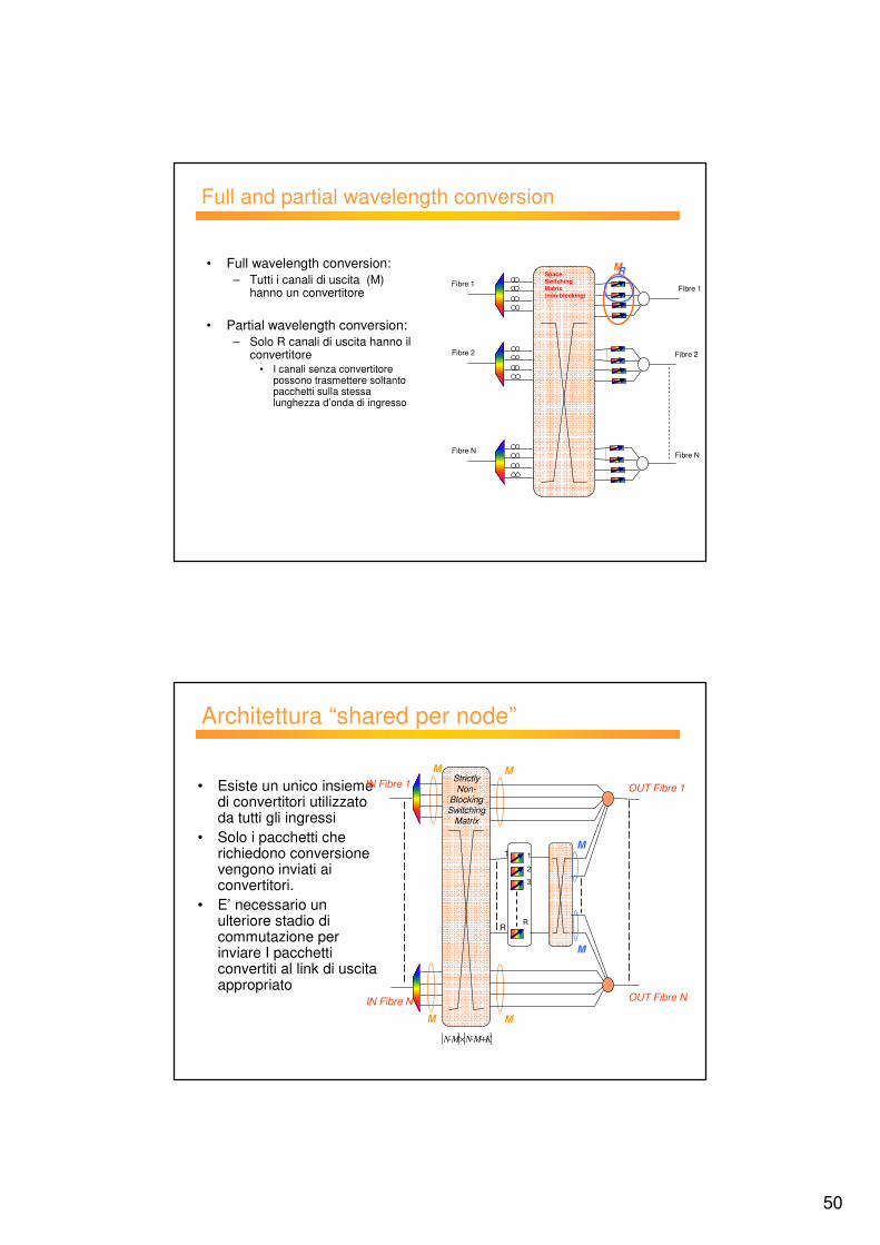
Full and partial wavelength conversion
Space Switching Matrix(non-blocking)
Fibre 1
Fibre 2
Fibre N
Fibre 1
Fibre 2
Fibre N
• Full wavelength conversion:– Tutti i canali di uscita (M)
hanno un convertitore
• Partial wavelength conversion:– Solo R canali di uscita hanno il
convertitore• I canali senza convertitore
possono trasmettere soltantopacchetti sulla stessalunghezza d’onda di ingresso
MR
Architettura “shared per node”
• Esiste un unico insiemedi convertitori utilizzatoda tutti gli ingressi
• Solo i pacchetti cherichiedono conversionevengono inviati aiconvertitori.
• E’ necessario un ulteriore stadio di commutazione per inviare I pacchetticonvertiti al link di uscitaappropriato
Strictly Non-
Blocking Switching
Matrix
IN Fibre 1
IN Fibre N
M
OUT Fibre 1
OUT Fibre N
[ ] [ ]KMNMN +⋅×⋅
M
M
1
2
R
3
1
R
M
M
M

51
Conversione di lunghezza d’onda
IN 1, WL 1
IN 2, WL 3
IN 2, WL 1 Wavelength Conversion
TWC
IN 1, WL 1
IN 2, WL 3
IN 2, WL 1
No Wavelength ConversionLost
Out fibre 1In fibre 1
In fibre 2
In fibre 1
In fibre 2
Out fibre 1
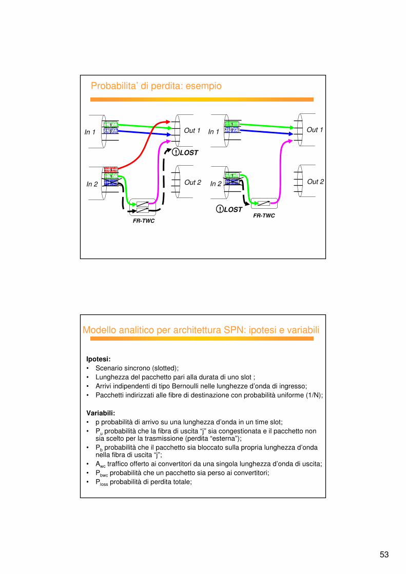
• Pacchetti sulla stessalunghezza d’onda diretti allastessa fibra di uscitacontendono per lo stessocanale
• Uno viene inoltratodirettamente, gli altriconvertiti e poi inoltrati
Convertitori di lunghezza d’onda
• TWCs (tunable wavelength converters):– FR-TWCs (Full Range wavelength converters), possono convertire
una qualsiasi lunghezza d’onda verso ogni altra
– LR-TWCs (Limited Range wavelength converters), possonoconvertire una lunghezza di ingresso verso un sub-set di lunghezzed’onda di uscita
• Convertitori di lunghezza d’onda sono componenti molto costosi– Specialmente FR-TWCs
• Sono state proposte architetture con numero ridotto di convertitori
52
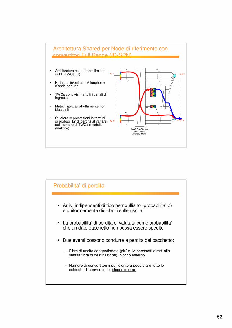
Architettura Shared per Node di riferimento con convertitori Full Range (ID-SPN)
• Architectura con numero limitatodi FR-TWCs (R)
• N fibre di in/out con M lunghezzed’onda ognuna
• TWCs condivisi fra tutti i canali di ingresso
• Matrici spaziali strettamente non bloccanti
• Studiare le prestazioni in termini di probabilita’ di perdita al variaredel numero di TWCs (modelloanalitico)
OUT N
IN 1
IN N
OUT 1
1
R
M
M M
M
Strictly Non-Blocking (SNB) Space
Switching Matrix
Probabilita’ di perdita
• Arrivi indipendenti di tipo bernoulliano (probabilita’ p) e uniformemente distribuiti sulle uscita
• La probabilita’ di perdita e’ valutata come probabilita’che un dato pacchetto non possa essere spedito
• Due eventi possono condurre a perdita del pacchetto:
– Fibra di uscita congestionata (piu’ di M pacchetti diretti alla stessa fibra di destinazione); blocco esterno
– Numero di convertitori insufficiente a soddisfare tutte le richieste di conversione; blocco interno
53
Probabilita’ di perdita: esempio
1
11
1
In 1
Out 2
Out 1
In 2
1
LOST!
1
1
1
In 1
Out 2
Out 1
In 2
1
LOST!
FR-TWCFR-TWC
Modello analitico per architettura SPN: ipotesi e variabili
Ipotesi:• Scenario sincrono (slotted);• Lunghezza del pacchetto pari alla durata di uno slot ;• Arrivi indipendenti di tipo Bernoulli nelle lunghezze d’onda di ingresso;• Pacchetti indirizzati alle fibre di destinazione con probabilità uniforme (1/N);
Variabili:• p probabilità di arrivo su una lunghezza d’onda in un time slot;• Pu probabilità che la fibra di uscita “j” sia congestionata e il pacchetto non
sia scelto per la trasmissione (perdita “esterna”);• Pb probabilità che il pacchetto sia bloccato sulla propria lunghezza d’onda
nella fibra di uscita “j”;• Awc traffico offerto ai convertitori da una singola lunghezza d’onda di uscita;• Pbwc probabilità che un pacchetto sia perso ai convertitori; • Ploss probabilità di perdita totale;
54
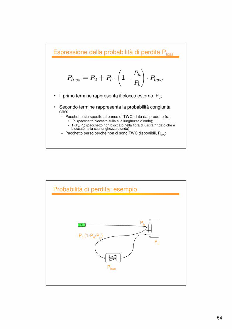
Espressione della probabilità di perdita Ploss
• Il primo termine rappresenta il blocco esterno, Pu;
• Secondo termine rappresenta la probabilità congiuntache:– Pacchetto sia spedito al banco di TWC, data dal prodotto fra:
• Pb (pacchetto bloccato sulla sua lunghezza d’onda);• 1-(Pu/Pb) (pacchetto non bloccato nella fibra di uscita “j” dato che è
bloccato nella sua lunghezza d’onda);– Pacchetto perso perchè non ci sono TWC disponibili, Pbwc;
1
Pu
Pb
Pb (1-Pu/Pb)
Pbwc
Probabilità di perdita: esempio
55
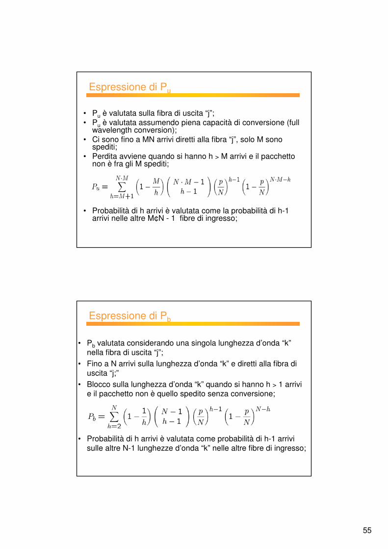
Espressione di Pu
• Pu è valutata sulla fibra di uscita “j”;• Pu è valutata assumendo piena capacità di conversione (full
wavelength conversion);• Ci sono fino a MN arrivi diretti alla fibra “j”, solo M sono
spediti; • Perdita avviene quando si hanno h > M arrivi e il pacchetto
non è fra gli M spediti;
• Probabilità di h arrivi è valutata come la probabilità di h-1 arrivi nelle altre M¢N - 1 fibre di ingresso;
Espressione di Pb
• Pb valutata considerando una singola lunghezza d’onda “k”nella fibra di uscita “j”;
• Fino a N arrivi sulla lunghezza d’onda “k” e diretti alla fibra di uscita “j;”
• Blocco sulla lunghezza d’onda “k” quando si hanno h > 1 arrivie il pacchetto non è quello spedito senza conversione;
• Probabilità di h arrivi è valutata come probabilità di h-1 arrivisulle altre N-1 lunghezze d’onda “k” nelle altre fibre di ingresso;

56
Traffico al banco di TWC
• E necessario valutare il traffico offerto al banco di TWC da ogni lunghezza d’onda di uscita;
– Probabilità che un pacchetto sia inviato albanco di TWC:
– Carico per lunghezza d’onda: p;
• Traffico al banco di TWC:
Espressione di Pbwc
• Assumendo arrivi indipendenti di tipo Bernoulli in ingresso al banco di TWC (solo una ipotesi, in reatà arrividipendenti), si hanno fino a M¢N possibili arrivi, ognunocon probabilità Awc;
• Ci sono R · M¢N TWC nel banco;• Perdita quando si hanno h > R arrivi e il pacchetto non è
scelto per la conversione;
• Probabilità di h arrivi valutata come la probabilità di h-1 arrivi dalle altre MN - 1 lunghezze d’onda di uscita;
57
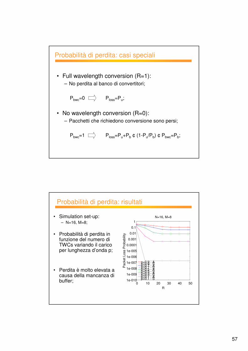
Probabilità di perdita: casi speciali
• Full wavelength conversion (R=1):– No perdita al banco di convertitori;
Pbwc=0 Ploss=Pu;
• No wavelength conversion (R=0):– Pacchetti che richiedono conversione sono persi;
Pbwc=1 Ploss=Pu+Pb ¢ (1-Pu/Pb) ¢ Pbwc=Pb;
Probabilità di perdita: risultati
• Simulation set-up:– N=16, M=8;
• Probabilità di perdita in funzione del numero di TWCs variando il caricoper lunghezza d’onda p;
• Perdita è molto elevata a causa della mancanza di buffer; 1e-010
1e-009
1e-008
1e-007
1e-006
1e-005
0.0001
0.001
0.01
0.1
1
0 10 20 30 40 50
Pac
ket L
oss
Pro
babi
lity
R
N=16, M=8
p=0.9 - Ap=0.9 - Sp=0.7 - Ap=0.7 - Sp=0.5 - Ap=0.5 - Sp=0.3 - Ap=0.3 - Sp=0.1 - Ap=0.1 - S
58
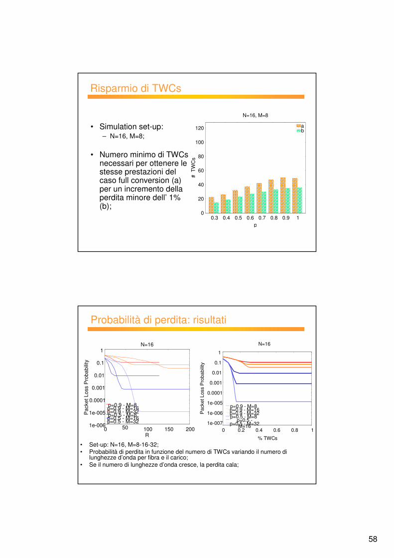
Risparmio di TWCs
• Simulation set-up:– N=16, M=8;
• Numero minimo di TWCsnecessari per ottenere le stesse prestazioni del caso full conversion (a) per un incremento dellaperdita minore dell’ 1% (b);
0
20
40
60
80
100
120
0.3 0.4 0.5 0.6 0.7 0.8 0.9 1
# T
WC
s
p
N=16, M=8
ab
• Set-up: N=16, M=8-16-32;• Probabilità di perdita in funzione del numero di TWCs variando il numero di
lunghezze d’onda per fibra e il carico;• Se il numero di lunghezze d’onda cresce, la perdita cala;
1e-006
1e-005
0.0001
0.001
0.01
0.1
1
0 100 150 200
Pac
ket L
oss
Pro
babi
lity
R
N=16
50
p=0.9 - M=8p=0.9 - M=16p=0.9 - M=32p=0.5 - M=8p=0.5 - M=16p=0.5 - M=32
% TWCs
1e-007
1e-006
1e-005
0.0001
0.001
0.01
0.1
1
0 0.2 0.4 0.6 0.8 1
Pac
ket L
oss
Pro
babi
lity
N=16
p=0.9 - M=8p=0.9 - M=16p=0.9 - M=32p=0.5 - M=8
p=0.5 -M=16p=0.5 - M=32
Probabilità di perdita: risultati
59
• Modello analitico proposto per architettura SPN è molto flessibile;
• Può essere usato in casi particolari;• Qui è usato per valutare la perdita con
architettura MS-SPN;
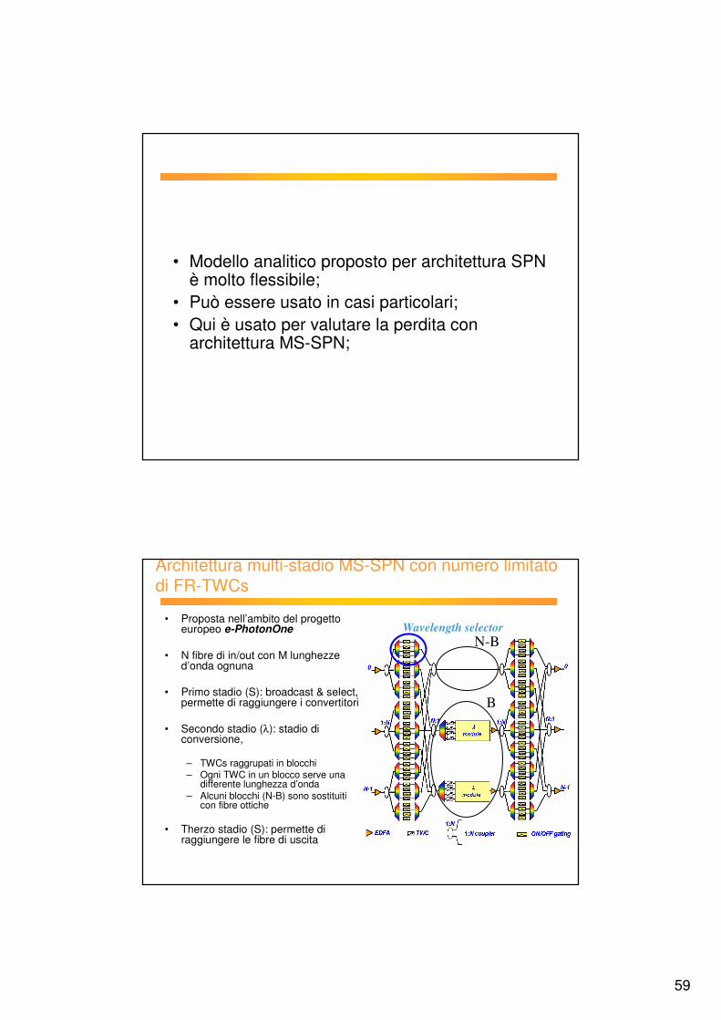
Architettura multi-stadio MS-SPN con numero limitato di FR-TWCs
• Proposta nell’ambito del progettoeuropeo e-PhotonOne
• N fibre di in/out con M lunghezzed’onda ognuna
• Primo stadio (S): broadcast & select, permette di raggiungere i convertitori
• Secondo stadio (λ): stadio di conversione,
– TWCs raggrupati in blocchi– Ogni TWC in un blocco serve una
differente lunghezza d’onda– Alcuni blocchi (N-B) sono sostituiti
con fibre ottiche
• Therzo stadio (S): permette di raggiungere le fibre di uscita
N-B
B
Wavelength selector
60
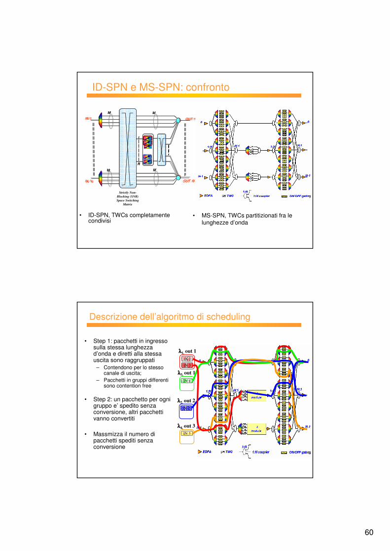
ID-SPN e MS-SPN: confronto
• ID-SPN, TWCs completamentecondivisi
OUT N
IN 1
IN N
OUT 1
1
R
M
M M
M
OUT N
IN 1
IN N
OUT 1
1
R
M
M M
M
Strictly Non-Blocking (SNB) Space Switching
Matrix
• MS-SPN, TWCs partitizionati fra le lunghezze d’onda
Descrizione dell’algoritmo di scheduling
• Step 1: pacchetti in ingressosulla stessa lunghezzad’onda e diretti alla stessauscita sono raggruppati– Contendono per lo stesso
canale di uscita;– Pacchetti in gruppi differenti
sono contention free
• Step 2: un pacchetto per ognigruppo e’ spedito senzaconversione, altri pacchettivanno convertiti
• Massmizza il numero di pacchetti spediti senzaconversione
IN 1
IN 3
IN 1
IN 2
IN 3
λλλλ1, out 1
λλλλ3, out 1
λλλλ2, out 2
λλλλ4, out 3
61
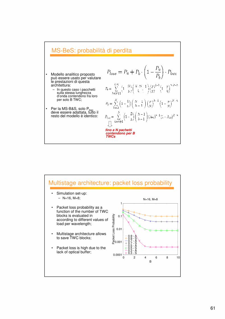
MS-BeS: probabilità di perdita
fino a N pachetticontendono per B TWCs
• Modello analitico propostopuò essere usato per valutarele prestazioni di questaarchitettura:– In questo caso i pacchetti
sulla stessa lunghezzad’onda contendono fra loroper solo B TWC;
• Per la MS-B&S, solo Pbwcdeve essere adattata, tutto ilresto del modello è identico:
Multistage architecture: packet loss probability
• Simulation set-up:– N=16, M=8;
• Packet loss probability as a function of the number of TWC blocks is evaluated in according to different values of load per wavelength;
• Multistage architecture allows to save TWC blocks;
• Packet loss is high due to the lack of optical buffer;
0.0001
0.001
0.01
0.1
1
0 2 4 6 8 10
Pac
ket L
oss
Pro
babi
lity
B
N=16, M=8
0.9 - A0.9 - S0.7 - A0.7 - S0.5 - A0.5 - S0.3 - A0.3 - S
62
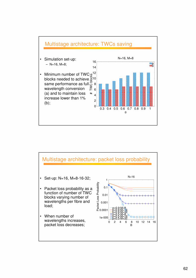
Multistage architecture: TWCs saving
• Simulation set-up:– N=16, M=8;
• Minimum number of TWC blocks needed to achieve same performance as full wavelength conversion (a) and to maintain loss increase lower than 1% (b);
0
2
4
6
8
10
12
14
16
0.3 0.4 0.5 0.6 0.7 0.8 0.9 1
# T
WC
blo
cks
p
N=16, M=8
ab
Multistage architecture: packet loss probability
• Set-up: N=16, M=8-16-32;
• Packet loss probability as a function of number of TWC blocks varying number of wavelengths per fibre and load;
• When number of wavelengths increases, packet loss decreases;
1e-005
0.0001
0.001
0.01
0.1
1
0 2 4 6 8 10 12 14 16
Pac
ket L
oss
Pro
babi
lity
B
N=16
p=0.9-M=8p=0.9-M=16p=0.9-M=32p=0.5-M=8p=0.5-M=16p=0.5-M=32
63
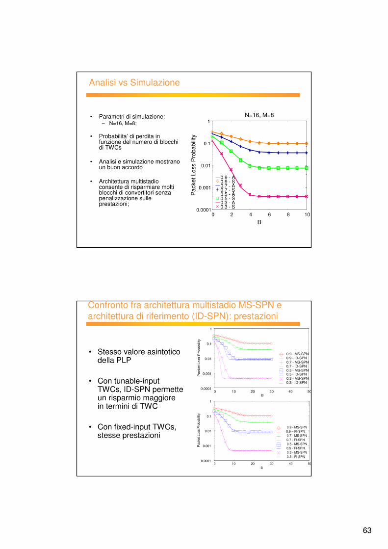
Analisi vs Simulazione
• Parametri di simulazione:– N=16, M=8;
• Probabilita’ di perdita in funzione del numero di blocchidi TWCs
• Analisi e simulazione mostranoun buon accordo
• Architettura multistadioconsente di risparmiare moltiblocchi di convertitori senzapenalizzazione sulleprestazioni;
0.0001
0.001
0.01
0.1
1
0 4 6 8 10
Pac
ket L
oss
Pro
babi
lity
B
N=16, M=8
2
0.9 - A0.9 - S0.7 - A0.7 - S0.5 - A0.5 - S0.3 - A0.3 - S
Confronto fra architettura multistadio MS-SPN e architettura di riferimento (ID-SPN): prestazioni
• Stesso valore asintoticodella PLP
• Con tunable-input TWCs, ID-SPN permetteun risparmio maggiorein termini di TWC
• Con fixed-input TWCs, stesse prestazioni
0.0001
0.001
0.01
0.1
1
0 10 20 30 40 50
Pac
ket L
oss
Pro
babi
lity
0.9 - MS-SPN
0.7 - MS-SPN0.7 - ID-SPN
0.9 - ID-SPN
0.5 - MS-SPN0.5 - ID-SPN0.3 - MS-SPN0.3 - ID-SPN
B
0.0001
0.001
0.01
0.1
1
0 10 20 30 40 50
Pac
ket L
oss
Pro
babi
lity
B
0.3 - FI-SPN
0.9 - MS-SPN0.9 – FI-SPN0.7 - MS-SPN0.7 - FI-SPN0.5 - MS-SPN0.5 - FI-SPN0.3 - MS-SPN
64
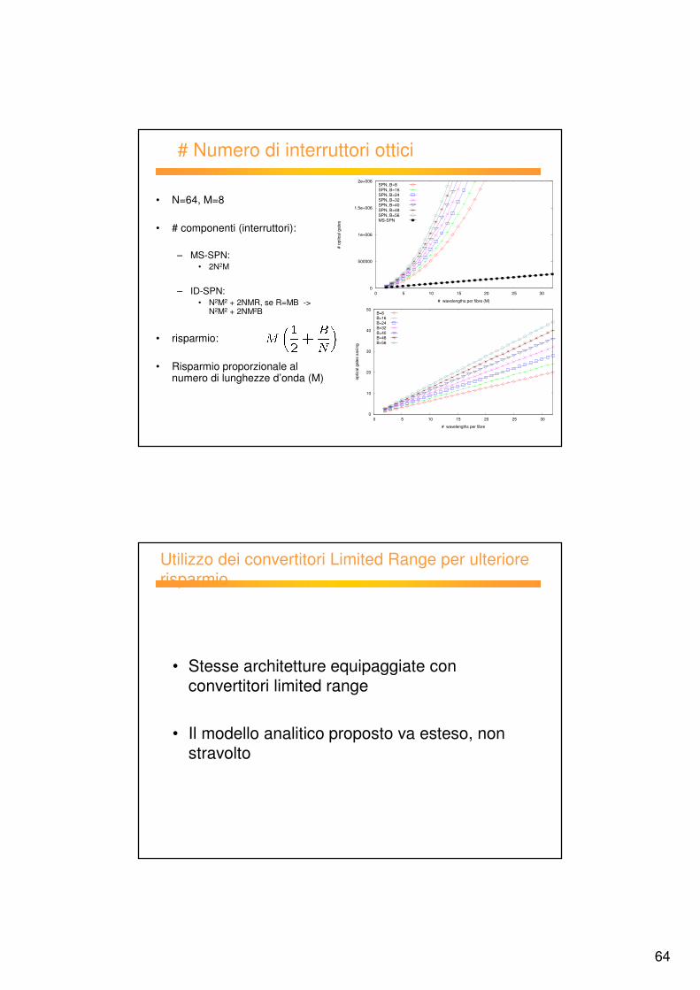
• N=64, M=8
• # componenti (interruttori):
– MS-SPN:• 2N2M
– ID-SPN:• N2M2 + 2NMR, se R=MB ->
N2M2 + 2NM2B
• risparmio:
• Risparmio proporzionale al numero di lunghezze d’onda (M)
0
500000
1e+006
1.5e+006
2e+006
0 5 10 15 20 25 30
# op
tical
gat
es
# wavelengths per fibre (M)
SPN, B=8SPN, B=16SPN, B=24SPN, B=32SPN, B=40SPN, B=48SPN, B=56MS-SPN
0
10
20
30
40
50
0 5 10 15 20 25 30
optic
al g
ates
sav
ing
# wavelengths per fibre
B=8B=16B=24B=32B=40B=48B=56
# Numero di interruttori ottici
Utilizzo dei convertitori Limited Range per ulteriorerisparmio
• Stesse architetture equipaggiate con convertitori limited range
• Il modello analitico proposto va esteso, non stravolto
65
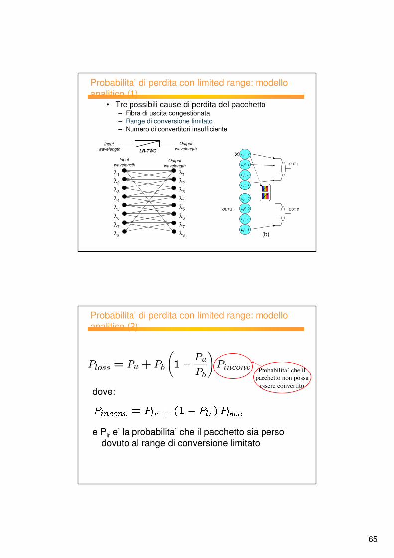
Probabilita’ di perdita con limited range: modelloanalitico (1)
• Tre possibili cause di perdita del pacchetto– Fibra di uscita congestionata– Range di conversione limitato– Numero di convertitori insufficiente
OUT 2
L11, 2
L12, 1
L13, 0
L14, 1
L21, 0
L22, 0
L23, 0
L24, 1
OUT 1
OUT 2
(b)
Input wavelength
Output wavelength
λ1
λ2
λ8
λ7
λ6
λ4
λ5
λ3
λ1
λ2
λ8
λ7
λ6
λ4
λ5
λ3
Input wavelength LR-TWC
Output wavelength
Probabilita’ di perdita con limited range: modelloanalitico (2)
dove:
e Plr e’ la probabilita’ che il pacchetto sia persodovuto al range di conversione limitato
Probabilita’ che ilpacchetto non possa
essere convertito
66
RouterMxM
RouterMxM
RouterMxM
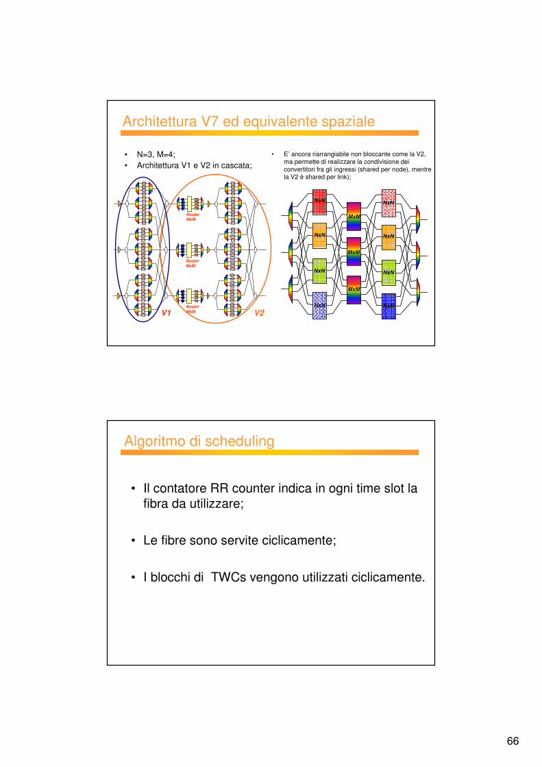
Architettura V7 ed equivalente spaziale
• N=3, M=4; • Architettura V1 e V2 in cascata;
• E’ ancora riarrangiabile non bloccante come la V2, ma permette di realizzare la condivisione dei convertitori fra gli ingressi (shared per node), mentre la V2 è shared per link);
V1 V2
MxM
MxM
MxM
NxN
NxN
NxN
NxN
NxN
NxN
NxN
NxN
Algoritmo di scheduling
• Il contatore RR counter indica in ogni time slot la fibra da utilizzare;
• Le fibre sono servite ciclicamente;
• I blocchi di TWCs vengono utilizzati ciclicamente.
67
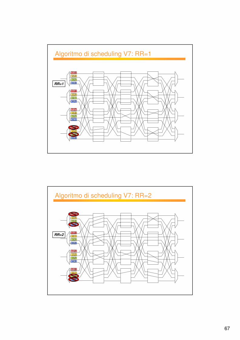
Algoritmo di scheduling V7: RR=1
2,43,24,3
1,32,33,14,2
2,3,3,24,1
1,2
2,43,34,4
1,3
1,4
RR=1
Algoritmo di scheduling V7: RR=2
2,43,44,2
1,32,13,34,2
2,2,3,24,3
1,2
2,13,34,3
1,3
1,2
RR=2
68
RouterMxM
RouterMxM
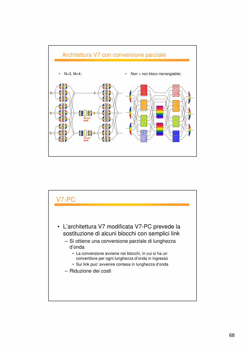
Architettura V7 con conversione parziale
• N=3, M=4; • Non + non blocc riarrangiabile;
V7-PC
• L’architettura V7 modificata V7-PC prevede la sostituzione di alcuni blocchi con semplici link– Si ottiene una conversione parziale di lunghezza
d’onda• La conversione avviene nei blocchi, in cui si ha un
convertitore per ogni lunghezza d’onda in ingresso• Sui link puo’ avvenire contesa in lunghezza d’onda
– Riduzione dei costi

69
Algoritmo di scheduling V7 modificata
2,43,24,3
1,32,33,14,2
2,3,3,24,1
1,2
2,43,34,4
1,3
1,4RR=1
Algoritmo di scheduling
• Il contatore RR counter indica in ogni time slot la fibra da utilizzare;
• Le fibre sono servite ciclicamente;
• I link senza convertitori vengono utilizzati per primi; I blocchi di convertitori vengono utilizzati in caso di contesa sulla lunghezza d’onda
70
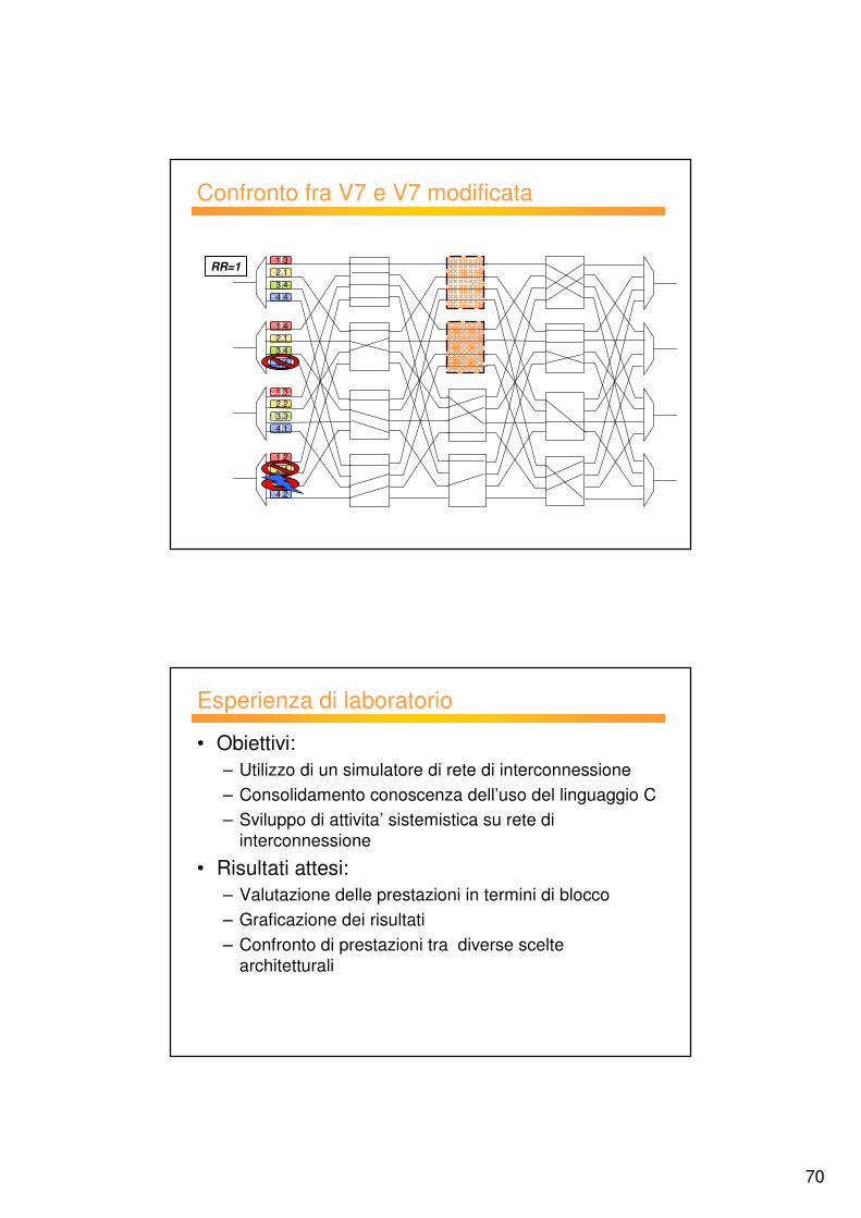
Confronto fra V7 e V7 modificata
2,13,44,4
1,42,13,44,4
2,2,3,34,1
1,3
2,43,34,2
1,2
1,3RR=1
Esperienza di laboratorio
• Obiettivi:– Utilizzo di un simulatore di rete di interconnessione– Consolidamento conoscenza dell’uso del linguaggio C– Sviluppo di attivita’ sistemistica su rete di
interconnessione
• Risultati attesi:– Valutazione delle prestazioni in termini di blocco– Graficazione dei risultati– Confronto di prestazioni tra diverse scelte
architetturali