POLITECNICO DI MILANO - politesi.polimi.it · il calcolo del tasso di crescita delle perturbazioni...
118
Transcript of POLITECNICO DI MILANO - politesi.polimi.it · il calcolo del tasso di crescita delle perturbazioni...
POLITECNICO DI MILANO
Scuola di Ingegneria Industriale e dell'Informazione
Corso di Laurea Magistrale in Ingegneria Aeronautica
Computation of boundary-layer thickness in
RANS code: improvement and eects on the
prediction of transition
Relatore: Prof. Franco AUTERI
Tesi di Laurea di:
Marco LANFRANCHI
Matricola 838180
Anno Accademico 2015 - 2016


4
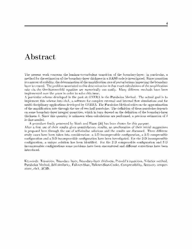
Abstract
The present work concerns the laminar-to-turbulent transition of the boundary-layer: in particular, amethod for the estimation of the boundary-layer thickness in a RANS code is investigated. Since transitionis a matter of stability, the determination of the amplication rate of perturbations impacting the boundarylayer is treated. The problem associated to this determination is that exact calculations of the amplicationrate via the Orr-Sommerfeld equation are numerically too costly. Many dierent methods have beenimplemented over the years in order to solve this issue.A particular scheme developed in the past at ONERA is the Parabolas Method. The actual goal is toimplement this scheme into elsA, a software for complex external and internal ow simulations and formulti-disciplinary applications developed by ONERA. The Parabolas Method relies on the approximationof the amplication rate through the use of two half-parabolas. The denition of these parabolas dependson some boundary-layer integral quantities, which in turn depend on the denition of the boundary-layerthickness δ. Since this quantity is unknown when calculations are performed, a previous estimation of δis thus needed.
A procedure rstly presented by Stock and Haase [30] has been chosen for this purpose.After a rst use of their results gives unsatisfactory results, an amelioration of their initial suggestionsis proposed here through the use of self-similar solutions and the results are discussed. Three dierentstudy cases have been taken into consideration: a 2-D incompressible conguration, a 2-D compressibleconguration and a 3-D incompressible conguration have been investigated. For the 2-D incompressibleconguration, a unique solution has been identied. For the 2-D compressible conguration and 3-Dincompressible congurations some problems have been encountered and dierent corrections have beenintroduced.
Keywords: Transition, Boundary layer, Boundary-layer thickness, Prandtl's equations, N-factor method,Parabolas Method, Self-similarity, Falkner-Skan, Falkner-Skan-Cooke, Compressibility, Recovery temper-ature, elsA, 3C3D.

6
Sommario
La tematica analizzata nel presente lavoro è il problema della transizione dello strato limite da unostato laminare a uno stato turbolento. Il problema della transizione è un problema di stabilità e vienegeneralmente arontato tramite l'utilizzo dell'equazione di Orr-Sommerfeld, che tuttavia presenta costicomputazionali di risoluzione molto elevati. Negli anni, ONERA ha sviluppato un metodo semplicato peril calcolo del tasso di crescita delle perturbazioni che impattano sullo strato limite. L'impegno attuale è disviluppare e integrare tale metodo, noto come Metodo delle Parabole, nel solutore elsA, codice di calcoloRANS sviluppato dalla stessa ONERA. Tale metodo si basa sull'approssimazione del tasso di crescitadelle perturbazioni tramite la denizione di due semi-parabole, le cui espressioni analitiche dipendono daalcune quantità integrali caratteristiche dello strato limite. Il calcolo di tali quantità integrali dipendedirettamente dalla determinazione dello spessore di strato limite. Questa quantità è tuttavia incognita almomento in cui il calcolo viene eettuato: una sua stima preventiva risulta dunque essere necessaria.
Tra i vari metodi possibili per eettuare tale stima, un metodo interessante è stato proposto da Stocke Haase nel 1999 [30].Un primo utilizzo di tale metodo ha condotto a risultati non soddisfacenti: esso è stato dunque ripresoed è stato studiato e proposto un miglioramento. Al ne di realizzare uno studio in tale senso, è statointrodotto l'utilizzo di proli di velocità in similitudine. Tre casi di studio dierenti sono stati considerati:una congurazione 2-D incomprimibile, una congurazione 2-D comprimibile e una congurazione 3-Dincomprimibile. Per il caso 2-D incomprimibile è stato possibile identicare con successo una soluzioneunica. Per il caso 2-D comprimibile e per il caso incomprimibile tridimensionale l'unicità di tale soluzionenon è più garantita. Per queste ultime due ultime congurazioni sono state studiate delle correlazioni infunzione delle caratteristiche principali del usso e sono state proposte delle correzioni.
Parole chiave: Transizione, Strato limite, Spessore di strato limite, Equazioni di Prandtl, Metodo eN ,Metodo delle Parabole, Similitudine, Falkner-Skan, Falkner-Skan-Cooke, Comprimibilità, Temperatura direcupero, elsA, 3C3D.

8
Sinossi
Il presente testo tratta il delicato e importante problema del calcolo della transizione laminare-turbolentadello strato limite in programmi di calcolo RANS. Il lavoro è stato organizzato in due parti principali.Poichè la transizione da uno strato limite laminare ad uno strato limite turbolento è un problema distabilità, la prima parte è stata dedicata alla trattazione matematica del problema. In primo luogosono state descritte le equazioni di Prandtl e sono state introdotte le principali quantità caratteristichedello strato limite. Poichè il presente lavoro è in particolare rivolto alla trattazione del fenomeno dellatransizione naturale, è stata successivamente introdotta e presentata l'analisi modale: infatti, per il casodella transizione naturale, le perturbazioni esterne che impattano sullo strato limite vengono ltrate dalusso medio e solo alcuni modi contaminano il usso nello strato limite. Un metodo per lo studio dellastabilità modale è il cosidetto metodo eN , che risulta particolarmente interessante per l'adabilità dellesue previsioni. Tale metodo consiste nell'integrare il tasso di amplicazione spaziale delle perturbazionilungo la linea di corrente alla frontiera dello strato limite. La determinazione del tasso di amplicazioneviene solitamente arontata tramite la risoluzione dell'equazione di Orr-Sommerfeld, che però presental'inconveniente di avere costi computazionali di risoluzione troppo elevati.Per ovviare a tale problematica, ONERA ha sviluppato, nelle ultime due decadi, un metodo semplicatoper il calcolo del tasso di amplicazione. Tale metodo, noto come Metodo delle Parabole, si basa suuna approssimazione in forma chiusa dei tassi di crescita come funzioni del numero di Reynolds e dellafrequenza ridotta. I diversi coecienti usati per la calibrazione di tale metodo si basano su un databasein cui sono contenute alcune delle quantità caratteristiche principali dello strato limite, tra le quali, adesempio, lo spessore di spostamento e lo spessore di quantità di moto. Inizialmente sviluppato per un ussobidimensionale incomprimibile, è stato successivamente esteso anche a congurazioni tridimensionali, condelle correzioni che tenessero in conto eetti termici alla parete. Il metodo completo è stato quindiinserito nel codice di calcolo di strato limite 3C3D, sempre sviluppato da ONERA, dove è stato validatocon successo.Lo scopo attuale di ONERA è di implementare tale schema in elsA, progamma di calcolo RANS. Poichè, adierenza di un codice di calcolo di strato limite, la conoscenza dello spessore di strato limite in un solutoreRANS non è nota se non quando il calcolo è stato completato, una stima preventiva di tale quantità risultaessere necessaria, sia per poter calcolare le proprietà di strato limite da inserire nel database su cui poggiail Metodo delle Parabole, sia per poter utilizzare successivamente il metodo eN . In un codice RANS,infatti, le quantità alla frontiera dello strato limite vengono estratte dalla soluzione del campo medio auna distanza dalla parete pari allo spessore di strato limite, informazione che tuttavia non si conosceprima di eettuare il calcolo
Denito quindi il contesto nel quale ci si trova ad operare, la seconda parte del lavoro si concentra sulcuore dell'analisi qui presentata, ovvero la stima dello spessore di strato limite.In un articolo del 1999, Stock e Haase [30] propongono, per il calcolo dello spessore di strato limite, dibasarsi sulla denizione di una funzione diagnostica dello stesso genere di quella utilizzata nel modelloalgebrico di turbolenza di Baldwin-Lomax. Tale funzione diagnostica, calcolata lungo ciascuna direzionenormale alla parete, è denita come il prodotto tra la distanza dalla parete e il modulo della vorticità,
9
dove entrambi i termini sono pesati attraverso l'utilizzo di due esponenti indipendenti. La funzione cosìdenita presenta un massimo. Lo spessore di strato limite può quindi essere denito come il prodotto trala distanza dalla parete a cui si trova tale massimo e un terzo coeciente moltiplicativo. Il metodo risultaquindi completo una volta che i tre coecienti sono noti.Stock e Haase proposero dei valori particolari per questi coecienti a completamento del metodo, siaper il caso laminare sia per quello turbolento. Se l'utilizzo dei valori per il caso turbolento in elsA hadato risultati molto promettenti, altrettanto non si può dire per il caso laminare. I valori proposti inquest'ultimo caso conducono infatti a risultati non soddisfacenti. Poiché il caso laminare è quello che piùinteressa, dato che sono le caratteristiche dello strato limite laminare che ne determinano la ricettività,questo studio aronta il problema di determinare i coecienti ottimali.Al ne di diminuire ulteriormente i costi computazionali, si è proceduto inoltre a cercare un insieme dicoecienti universali, ovvero costanti al variare delle condizioni del usso. Per arontare dunque questaanalisi si è scelto di servirsi dell'utilizzo dei proli di velocità in similitudine. Diversi studi condottinegli anni hanno infatti mostrato quanto i proli di similitudine, soluzioni dell'equazione di Falkner-Skan,rappresentino con un buon grado di fedeltà i proli di velocità che si incontrano in geometrie reali. Poichéla funzione diagnostica è calcolata lungo la normale alla parete in una specica posizione, la determinazionedello spessore di strato limite in ogni punto richiede il calcolo di tale funzione su tutta la supercie. L'ideaè quindi di simulare gli eetti dei reali proli di velocità attraverso l'utilizzo di un'ampia gamma di prolidi similitudine e di cercare di estrarre da questi ultimi dei coecienti universali.
Tre casi di studio dierenti sono stati considerati per arontare l'analisi: una congurazione 2-Dincomprimibile, una congurazione 2-D comprimibile ed una congurazione 3-D incomprimibile. Per og-nuna delle tre è stato innanzitutto dettagliato l'approccio teorico, che porta alla scrittura dell'equazione diFalkner-Skan per il caso bidimensionale e dell'equazione di Falkner-Skan-Cooke per il caso tridimensionale.In secondo luogo sono stati implementati, utilizzando il linguaggioMatlabr, degli specici programmi perla determinazione numerica delle soluzioni delle suddette equazioni. In denitiva, la funzione diagnosticaè stata riscritta nei tre casi in funzione delle variabili di similitudine, permettendo così l'utilizzo dei prolidi similitudine precedentemente determinati.Per il caso 2-D incomprimibile è stato possibile identicare con successo un insieme di coecienti univer-sali, tali cioè da permettere una stima dello spessore di strato limite indipendentemente dalla posizionein cui il calcolo viene eettuato. Tale soluzione è già stata provata da Bégou [3] e ha portato a risultatimolto soddisfacenti.Per il caso 2-D comprimibile, l'implicazione delle soluzioni di similitudine è legata all'introduzione di al-cune ipotesi. In particolare, due casistiche di interesse sono state indagate: la prima prevede la presenzadi un usso a numero di Prandtl unitario su parete adiabatica, mentre la seconda prescrive la presenza diuna lastra piana, mentre non impone vincoli sul numero di Prandtl. Per il primo caso si ritrova, come perla congurazione incomprimibile, un insieme di coecienti universali. La presenza di eetti termici sullalastra piana fa invece perdere tale carattere di universalità ai coecienti di interesse. Si è cercato quindi dideterminare una relazione che permettesse l'identicazione dei coecienti in funzione della temperaturaa parete e della temperatura di recupo. Tale espressione è stata quindi proposta come correzione deglieetti termici in rapporto alla condizione adiabatica.L'ultimo caso indagato è stato quello incomprimibile tridimensionale per il caso di un'ala a frecciadi apertura innita. Come già detto, alcune soluzioni di similitudine possono essere trovate anche inquesto frangente. L'utilizzo della similitudine nella formulazione della funzione diagnostica fa comparirenell'analisi un nuovo parametro: la direzione che la linea di corrente alla frontiera dello strato limite formacon la direzione longitudinale. Lo studio ha evidenziato come gli eetti di questo nuovo parametro im-pediscano, come per il caso di eetti termici, l'identicazione di un set di coecienti universali. Sono statedunque cercate e proposte delle relazioni che potessero fornire la determinazione dei coecienti desideratiin funzione del nuovo parametro in gioco.Come già specicato in precedenza, le quantità alla frontiera dello strato limite vengono estratte dalla

10
soluzione del campo medio a una distanza dalla parete pari allo spessore di strato limite, informazione chetuttavia non si conosce prima di eettuare il calcolo. L'informazione sulla direzione della linea di correnteesterna allo strato limite non può dunque essere direttamente utilizzata.L'idea è dunque quella di correlare l'informazione sulla linea di corrente esterna, non accessibile a priori,con un'informazione alla parete, che può invece essere estratta a ogni iterazione del calcolo RANS. Si èdunque cercata una relazione tra l'angolo che la linea di corrente esterna forma con la direzione longitudi-nale e l'angolo tra l'attrito a parete ed il gradiente di pressione, calcolato anch'esso a parete. Ancora unavolta, la relazione cercata è stata espressa in funzione delle variabili di similitudine. Una validazione èstata inne realizzata tramite l'utilizzo di una simulazione ottenuta per mezzo del codice di strato limite3C3D.

12
Acknowledgments
I am really thankful to ONERA for the incredible opportunity of performing an internship in one of itssites. It has been a great experience both for my personal and professional growth.I wish to thank my supervisor, Professor Franco Auteri, for the time, patience and guidance he dedicatedto me in the past months.I express my deepest gratitude to Guillaume Bégou and Lucas Pascal for the chance they accorded me injoining ONERA for my internship. I am grateful for their constant availability in helping me, their guid-ance and expertise provided me the necessary insight to understand and complete my research project.Deep thanks also go to the entire scientic sta of the DMAE department of ONERA, especially toOlivier Vermeersch, Hugues Deniau, Grégoire Casalis and Jean Cousteix, whom I thank for the enrichingsuggestions.
A special, immense and heartfelt thank goes to my mom, my dad and my sister, who constantly supportedme in every situation throughout these years.To my dearest friend Davide, to my comrades Pietro and Luca, to my atmates and to all my life-longfriends in Verona and in Milano, thank you very much.
Je voudrais aussi remercier Marco, Giulia, Aida, Javier et les autres compagnons pour le temps passéà l'ISAE-ENSMA et pour toutes les expériences inoubliables qu'on a vécu ensemble.


14
Contents
I Stability theory 20
1 Introduction to boundary-layer transition 22
1.1 Boundary layer . . . . . . . . . . . . . . . . . . . . . . . . . . . . . . . . . . . . . . . . . . 221.2 Prantl's equations . . . . . . . . . . . . . . . . . . . . . . . . . . . . . . . . . . . . . . . . 23
1.2.1 Incompressible case . . . . . . . . . . . . . . . . . . . . . . . . . . . . . . . . . . . . 241.2.2 2-D compressible case . . . . . . . . . . . . . . . . . . . . . . . . . . . . . . . . . . 251.2.3 Characteristic boundary layer quantities . . . . . . . . . . . . . . . . . . . . . . . . 26
1.2.3.1 Denitions . . . . . . . . . . . . . . . . . . . . . . . . . . . . . . . . . . . 261.2.3.2 Physical interpretation . . . . . . . . . . . . . . . . . . . . . . . . . . . . 27
1.3 Dierent types of transition . . . . . . . . . . . . . . . . . . . . . . . . . . . . . . . . . . . 281.4 Natural transition . . . . . . . . . . . . . . . . . . . . . . . . . . . . . . . . . . . . . . . . 30
1.4.1 Tollmien-Schlichting instabilities . . . . . . . . . . . . . . . . . . . . . . . . . . . . 301.4.2 Crossow instabilities . . . . . . . . . . . . . . . . . . . . . . . . . . . . . . . . . . 301.4.3 Görtler instabilities . . . . . . . . . . . . . . . . . . . . . . . . . . . . . . . . . . . . 31
2 Modal stability analysis and N-factor method 34
2.1 Modal formulation . . . . . . . . . . . . . . . . . . . . . . . . . . . . . . . . . . . . . . . . 342.2 Types of instabilities . . . . . . . . . . . . . . . . . . . . . . . . . . . . . . . . . . . . . . . 35
2.2.1 Viscous instabilities . . . . . . . . . . . . . . . . . . . . . . . . . . . . . . . . . . . 362.2.2 Purely inectional instabilities . . . . . . . . . . . . . . . . . . . . . . . . . . . . . 362.2.3 Viscous-inectional instabilities . . . . . . . . . . . . . . . . . . . . . . . . . . . . . 37
2.3 The N -factor method . . . . . . . . . . . . . . . . . . . . . . . . . . . . . . . . . . . . . . 382.4 Orr-Sommerfeld . . . . . . . . . . . . . . . . . . . . . . . . . . . . . . . . . . . . . . . . . . 40
2.4.1 The Orr-Sommerfeld equation . . . . . . . . . . . . . . . . . . . . . . . . . . . . . . 402.5 Database approach method . . . . . . . . . . . . . . . . . . . . . . . . . . . . . . . . . . . 43
2.5.1 Parabolas Method . . . . . . . . . . . . . . . . . . . . . . . . . . . . . . . . . . . . 432.5.1.1 Purely viscous instabilities . . . . . . . . . . . . . . . . . . . . . . . . . . 432.5.1.2 Viscous-inectional instabilities . . . . . . . . . . . . . . . . . . . . . . . . 44
II Boundary-layer thickness determination 48
3 Self-similar solutions 50
3.1 2D incompressible Falkner-Skan equation . . . . . . . . . . . . . . . . . . . . . . . . . . . 503.1.1 Falkner-Skan-Hartree solution . . . . . . . . . . . . . . . . . . . . . . . . . . . . . . 523.1.2 Numerical implementation . . . . . . . . . . . . . . . . . . . . . . . . . . . . . . . . 543.1.3 Numerical results . . . . . . . . . . . . . . . . . . . . . . . . . . . . . . . . . . . . . 55
3.2 2D compressible Falkner-Skan equations . . . . . . . . . . . . . . . . . . . . . . . . . . . . 59

CONTENTS 15
3.2.1 Unit Prandtl number and adiabatic wall case . . . . . . . . . . . . . . . . . . . . . 613.2.1.1 Numerical implementation . . . . . . . . . . . . . . . . . . . . . . . . . . 613.2.1.2 Numerical results . . . . . . . . . . . . . . . . . . . . . . . . . . . . . . . 62
3.2.2 Flat plate case . . . . . . . . . . . . . . . . . . . . . . . . . . . . . . . . . . . . . . 633.2.2.1 Numerical implementation . . . . . . . . . . . . . . . . . . . . . . . . . . 633.2.2.2 Numerical results . . . . . . . . . . . . . . . . . . . . . . . . . . . . . . . 643.2.2.3 Adiabatic case . . . . . . . . . . . . . . . . . . . . . . . . . . . . . . . . . 643.2.2.4 Non-adiabatic case . . . . . . . . . . . . . . . . . . . . . . . . . . . . . . . 65
3.3 3D incompressible Falkner-Skan equations . . . . . . . . . . . . . . . . . . . . . . . . . . . 693.3.1 Falkner-Skan-Cooke solution . . . . . . . . . . . . . . . . . . . . . . . . . . . . . . 69
3.3.1.1 Numerical implementation . . . . . . . . . . . . . . . . . . . . . . . . . . 703.3.1.2 Numerical results . . . . . . . . . . . . . . . . . . . . . . . . . . . . . . . 70
4 Boundary layer thickness determination 74
4.1 Similarity for the 2-D incompressible case . . . . . . . . . . . . . . . . . . . . . . . . . . . 754.2 Similarity for the 2-D compressible case . . . . . . . . . . . . . . . . . . . . . . . . . . . . 80
4.2.1 Unit Prandtl number and adiabatic case . . . . . . . . . . . . . . . . . . . . . . . . 804.2.2 Flat plate case for Pr = 0.72 . . . . . . . . . . . . . . . . . . . . . . . . . . . . . . 86
4.2.2.1 Adiabatic wall . . . . . . . . . . . . . . . . . . . . . . . . . . . . . . . . . 864.2.2.2 Non-adiabatic wall . . . . . . . . . . . . . . . . . . . . . . . . . . . . . . . 86
4.3 Conclusions on 2D . . . . . . . . . . . . . . . . . . . . . . . . . . . . . . . . . . . . . . . . 884.3.1 Recovery temperature properties . . . . . . . . . . . . . . . . . . . . . . . . . . . . 884.3.2 Correlation between εnon adiabatic and εadiabatic . . . . . . . . . . . . . . . . . . . . 90
4.4 Similarity for the 3-D incompressible case . . . . . . . . . . . . . . . . . . . . . . . . . . . 914.4.1 Application of the 2-D solution . . . . . . . . . . . . . . . . . . . . . . . . . . . . . 934.4.2 b and ε as functions of the ratio We
Ue. . . . . . . . . . . . . . . . . . . . . . . . . . 95
4.4.3 Study on the parameter We
Ue. . . . . . . . . . . . . . . . . . . . . . . . . . . . . . . 100
4.4.3.1 Skin friction - freeow streamline correlation . . . . . . . . . . . . . . . . 1004.4.3.2 Validation . . . . . . . . . . . . . . . . . . . . . . . . . . . . . . . . . . . 102
4.4.4 Conclusions . . . . . . . . . . . . . . . . . . . . . . . . . . . . . . . . . . . . . . . . 107
5 Transition calculation 108
A Runge-Kutta method 116
16
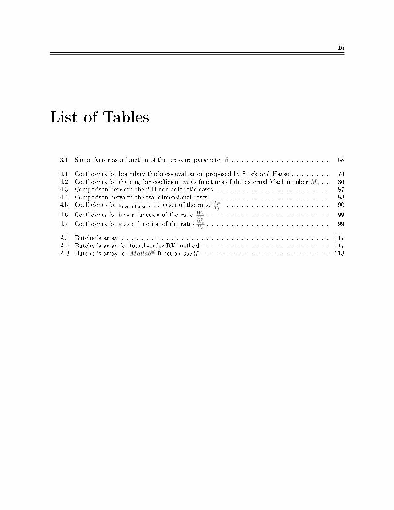
List of Tables
3.1 Shape factor as a function of the pressure parameter β . . . . . . . . . . . . . . . . . . . . 58
4.1 Coecients for boundary thickness evaluation proposed by Stock and Haase . . . . . . . . 744.2 Coecients for the angular coecient m as functions of the external Mach number Me . . 864.3 Comparison between the 2-D non adiabatic cases . . . . . . . . . . . . . . . . . . . . . . . 874.4 Comparison between the two-dimensional cases . . . . . . . . . . . . . . . . . . . . . . . . 884.5 Coecients for εnon adiabatic function of the ratio TP
Tf. . . . . . . . . . . . . . . . . . . . . 90
4.6 Coecients for b as a function of the ratio We
Ue. . . . . . . . . . . . . . . . . . . . . . . . . 99
4.7 Coecients for ε as a function of the ratio We
Ue. . . . . . . . . . . . . . . . . . . . . . . . . 99
A.1 Butcher's array . . . . . . . . . . . . . . . . . . . . . . . . . . . . . . . . . . . . . . . . . . 117A.2 Butcher's array for fourth-order RK method . . . . . . . . . . . . . . . . . . . . . . . . . . 117A.3 Butcher's array for Matlabr function ode45 . . . . . . . . . . . . . . . . . . . . . . . . . 118
17
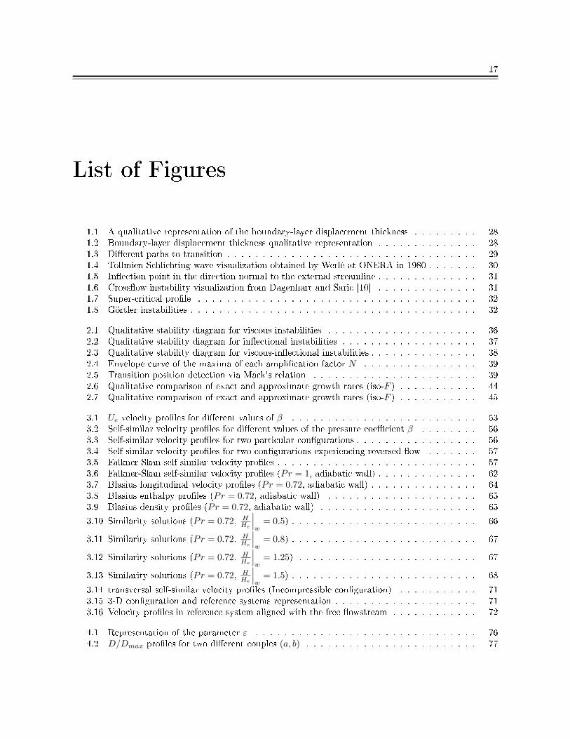
List of Figures
1.1 A qualitative representation of the boundary-layer displacement thickness . . . . . . . . . 281.2 Boundary-layer displacement thickness qualitative representation . . . . . . . . . . . . . . 281.3 Dierent paths to transition . . . . . . . . . . . . . . . . . . . . . . . . . . . . . . . . . . . 291.4 Tollmien-Schlichting wave visualization obtained by Werlé at ONERA in 1980 . . . . . . . 301.5 Inection point in the direction normal to the external streamline . . . . . . . . . . . . . . 311.6 Crossow instability visualization from Dagenhart and Saric [10] . . . . . . . . . . . . . . 311.7 Super-critical prole . . . . . . . . . . . . . . . . . . . . . . . . . . . . . . . . . . . . . . . 321.8 Görtler instabilities . . . . . . . . . . . . . . . . . . . . . . . . . . . . . . . . . . . . . . . . 32
2.1 Qualitative stability diagram for viscous instabilities . . . . . . . . . . . . . . . . . . . . . 362.2 Qualitative stability diagram for inectional instabilities . . . . . . . . . . . . . . . . . . . 372.3 Qualitative stability diagram for viscous-inectional instabilities . . . . . . . . . . . . . . . 382.4 Envelope curve of the maxima of each amplication factor N . . . . . . . . . . . . . . . . 392.5 Transition position detection via Mack's relation . . . . . . . . . . . . . . . . . . . . . . . 392.6 Qualitative comparison of exact and approximate growth rates (iso-F ) . . . . . . . . . . . 442.7 Qualitative comparison of exact and approximate growth rates (iso-F ) . . . . . . . . . . . 45
3.1 Ue velocity proles for dierent values of β . . . . . . . . . . . . . . . . . . . . . . . . . . 533.2 Self-similar velocity proles for dierent values of the pressure coecient β . . . . . . . . 563.3 Self-similar velocity proles for two particular congurations . . . . . . . . . . . . . . . . . 563.4 Self-similar velocity proles for two congurations experiencing reversed ow . . . . . . . 573.5 Falkner-Skan self-similar velocity proles . . . . . . . . . . . . . . . . . . . . . . . . . . . . 573.6 Falkner-Skan self-similar velocity proles (Pr = 1, adiabatic wall) . . . . . . . . . . . . . . 623.7 Blasius longitudinal velocity proles (Pr = 0.72, adiabatic wall) . . . . . . . . . . . . . . . 643.8 Blasius enthalpy proles (Pr = 0.72, adiabatic wall) . . . . . . . . . . . . . . . . . . . . . 653.9 Blasius density proles (Pr = 0.72, adiabatic wall) . . . . . . . . . . . . . . . . . . . . . . 65
3.10 Similarity solutions (Pr = 0.72, HHe
∣∣∣w
= 0.5) . . . . . . . . . . . . . . . . . . . . . . . . . . 66
3.11 Similarity solutions (Pr = 0.72, HHe
∣∣∣w
= 0.8) . . . . . . . . . . . . . . . . . . . . . . . . . . 67
3.12 Similarity solutions (Pr = 0.72, HHe
∣∣∣w
= 1.25) . . . . . . . . . . . . . . . . . . . . . . . . . 67
3.13 Similarity solutions (Pr = 0.72, HHe
∣∣∣w
= 1.5) . . . . . . . . . . . . . . . . . . . . . . . . . . 68
3.14 transversal self-similar velocity proles (Incompressible conguration) . . . . . . . . . . . 713.15 3-D conguration and reference systems representation . . . . . . . . . . . . . . . . . . . . 713.16 Velocity proles in reference system aligned with the free owstream . . . . . . . . . . . . 72
4.1 Representation of the parameter ε . . . . . . . . . . . . . . . . . . . . . . . . . . . . . . . 764.2 D/Dmax proles for two dierent couples (a, b) . . . . . . . . . . . . . . . . . . . . . . . . 77
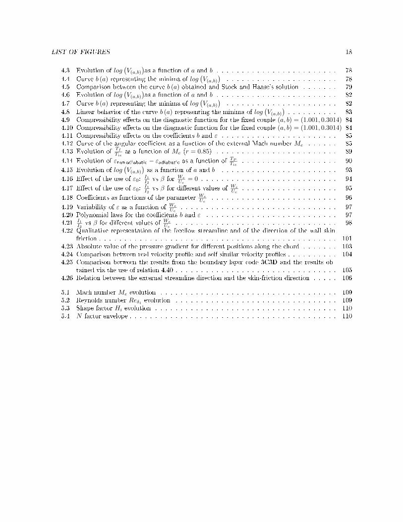
LIST OF FIGURES 18
4.3 Evolution of log(V(a,b)
)as a function of a and b . . . . . . . . . . . . . . . . . . . . . . . . 78
4.4 Curve b (a) representing the minima of log(V(a,b)
). . . . . . . . . . . . . . . . . . . . . . 78
4.5 Comparison between the curve b (a) obtained and Stock and Haase's solution . . . . . . . 794.6 Evolution of log
(V(a,b)
)as a function of a and b . . . . . . . . . . . . . . . . . . . . . . . . 82
4.7 Curve b (a) representing the minima of log(V(a,b)
). . . . . . . . . . . . . . . . . . . . . . 82
4.8 Linear behavior of the curve b (a) representing the minima of log(V(a,b)
). . . . . . . . . . 83
4.9 Compressibility eects on the diagnostic function for the xed couple (a, b) = (1.001, 0.3014) 844.10 Compressibility eects on the diagnostic function for the xed couple (a, b) = (1.001, 0.3014) 844.11 Compressibility eects on the coecients b and ε . . . . . . . . . . . . . . . . . . . . . . . 854.12 Curve of the angular coecient as a function of the external Mach number Me . . . . . . 854.13 Evolution of
TfTie
as a function of Me (r = 0.85) . . . . . . . . . . . . . . . . . . . . . . . . 89
4.14 Evolution of εnon adiabatic − εadiabatic as a function of TPTie
. . . . . . . . . . . . . . . . . . . 90
4.15 Evolution of log(V(a,b)
)as a function of a and b . . . . . . . . . . . . . . . . . . . . . . . 93
4.16 Eect of the use of ε0:I1I2
vs β for We
Ue= 0 . . . . . . . . . . . . . . . . . . . . . . . . . . . 94
4.17 Eect of the use of ε0:I1I2
vs β for dierent values of We
Ue. . . . . . . . . . . . . . . . . . . 95
4.18 Coecients as functions of the parameter We
Ue. . . . . . . . . . . . . . . . . . . . . . . . . 96
4.19 Variability of ε as a function of We
Ue. . . . . . . . . . . . . . . . . . . . . . . . . . . . . . . 97
4.20 Polynomial laws for the coecients b and ε . . . . . . . . . . . . . . . . . . . . . . . . . . 974.21 I1
I2vs β for dierent values of We
Ue. . . . . . . . . . . . . . . . . . . . . . . . . . . . . . . . 98
4.22 Qualitative representation of the freeow streamline and of the direction of the wall skinfriction . . . . . . . . . . . . . . . . . . . . . . . . . . . . . . . . . . . . . . . . . . . . . . . 101
4.23 Absolute value of the pressure gradient for dierent positions along the chord . . . . . . . 1034.24 Comparison between real velocity prole and self-similar velocity proles . . . . . . . . . . 1044.25 Comparison between the results from the boundary-layer code 3C3D and the results ob-
tained via the use of relation 4.40 . . . . . . . . . . . . . . . . . . . . . . . . . . . . . . . . 1054.26 Relation between the external streamline direction and the skin-friction direction . . . . . 106
5.1 Mach number Me evolution . . . . . . . . . . . . . . . . . . . . . . . . . . . . . . . . . . . 1095.2 Reynolds number Reδ1 evolution . . . . . . . . . . . . . . . . . . . . . . . . . . . . . . . . 1095.3 Shape factor Hi evolution . . . . . . . . . . . . . . . . . . . . . . . . . . . . . . . . . . . . 1105.4 N factor envelope . . . . . . . . . . . . . . . . . . . . . . . . . . . . . . . . . . . . . . . . . 110


20
Part I
Stability theory

21

22
Chapter 1
Introduction to boundary-layer
transition
Laminar to turbulent transition is the process through which a ow undergoes a change from laminar toturbulent state. Transition prediction is nowadays one of the most important subject in the aerodynamicseld for many practical applications.
The detection of the transition position is of major importance, for example, in drag reduction ofa wing. Also in the automobile industry, transition prediction is at the base of the improvement ofperformances.
The rst person who made observations about transition was Reynolds in 1880.His experiment consisted in injecting a thin lament of dye into a ow of water through a glass tube andin varying the velocity of this owAt low velocities, the dye lament appeared as straight line through the length of the tube and it stayedparallel to its axis. As the velocity increased, the dye lament became regularly wavy since when, formore increasing values of the velocity, the lament broke up and diused completely.
These three dierent behaviors can be linked to very specic states of the uid. The rst thin andparallel ow line is the manifestation of a laminar state while the fully mixed ow represents a turbulentstate. When the lament still conserves a structured but less regular shape, the ow is encountering atransition process.
From his experiment, many other experiments took place through the years and showed that thisbehavior of the uid could also depend on surface roughness or on the presence of heating of the bodyplunged in the ow.
These experiments show that the change of state is caused by external perturbations. Transition isthus a matter of stability of the boundary layer.
Once the perturbation coming from the external ow are injected in the boundary layer, a rst re-ceptivity phase (Morkovin,1969[22]) takes place and then, depending on the properties of the boundarylayer, dierent scenarios can take place.
The concept of boundary layer will be presented, followed by the description of the dierent scenarios.
1.1 Boundary layer
The concept of boundary layer was rst introduced by Ludwig Prandtl. In his work, Prandtl arms thatthere exist two separated regions in the ow eld around every surface in a uid ow: an external regionand an internal region. The behavior of these two regions is dierent. The behavior of the ow in theouter region can be described using the equations of a perfect ow, and so viscosity can be neglected. On

CHAPTER 1. INTRODUCTION TO BOUNDARY-LAYER TRANSITION 23
the other hand, in the internal region, called boundary layer, viscosity dominates the dynamics of the owitself. This characteristic strongly impacts on the physical proprieties of the ow. If a direction normalto the wall is considered, the longitudinal ow velocity is null at the wall and has to attain very rapidlythe value Ue of the velocity external to the boundary layer. This velocity evolution suggests the denitionof a certain length δ, called boundary layer thickness, which is the distance from the wall at which thelongitudinal velocity value is almost the same as Ue. It is commonly dened as the distance at whichU/Ue = 0.99. The hypotheses of boundary layer are valid as long as the following relation is preserved:
δL (1.1)
where L is the characteristic length of the problem. The previous condition can also be seen as follows:the boundary layer is a region in which the shear stresses due to the strong variation of the velocity are ofthe same order of those related to inertia. This statement is really important, since it links the hypothesesof boundary layer to a condition on the Reynolds number, as it is shown further below. Let's consider aninnitesimal cube of uid of dimensions dxdydz and compare the order of magnitude of shear and inertialstresses inside this control volume. Shear stresses can be expressed as:
Visc =∂τ
∂ydxdydz = µ
∂2u
∂y2dxdydz . (1.2)
where µ is considered constant and Newton's law for shear stresses is applied. Inertial forces are in theorder of magnitude of their longitudinal component and can be instead expressed as:
Inert = ρu∂u
∂xdxdydz . (1.3)
In order to compare the two types of stresses, the following considerations on the order of magnitude haveto be established:
u w U∂u
∂xwU
L
∂2u
∂y2wU
δ2. (1.4)
By substituting relations (1.4) into the expressions (1.2) and (1.3), it can be obtained that:
Inert
Visc=ρu∂u∂xµ∂
2u∂y2
wρU U
L
µ Uδ2=ρUL
µL2
δ2
= ReLδ2
L2. (1.5)
Hence, for the shear stresses and inertial forces to be of the same order of magnitude, the relation
δ
L∼ 1√
ReL(1.6)
must be veried, which means, with hypothesis (1.1), that the Reynolds number ReL must be high.
1.2 Prantl's equations
The eect of a large Reynolds number has a direct impact on the distinction of two separated regions inthe ow eld. As it has already been underlined, the zone external to the boundary layer can be describedby the equations of the perfect uid, that are obtained from Navier-Stokes equations by neglecting theterm linked to the viscosity. Regarding Prandtl's equations, the same sort of reasoning cannot be applied.The idea is, in this case, to do a dimensional analysis of the Navier-Stokes equations and to inject theinformation of high Reynolds number.
CHAPTER 1. INTRODUCTION TO BOUNDARY-LAYER TRANSITION 24
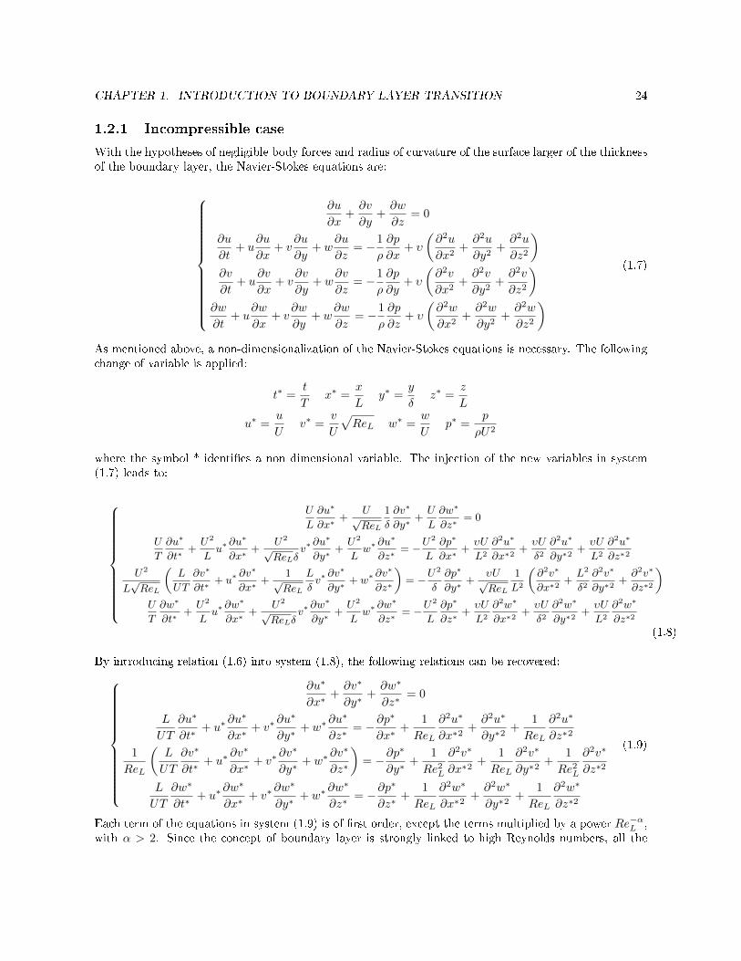
1.2.1 Incompressible case
With the hypotheses of negligible body forces and radius of curvature of the surface larger of the thicknessof the boundary layer, the Navier-Stokes equations are:
∂u
∂x+∂v
∂y+∂w
∂z= 0
∂u
∂t+ u
∂u
∂x+ v
∂u
∂y+ w
∂u
∂z= −1
ρ
∂p
∂x+ υ
(∂2u
∂x2+∂2u
∂y2+∂2u
∂z2
)∂v
∂t+ u
∂v
∂x+ v
∂v
∂y+ w
∂v
∂z= −1
ρ
∂p
∂y+ υ
(∂2v
∂x2+∂2v
∂y2+∂2v
∂z2
)∂w
∂t+ u
∂w
∂x+ v
∂w
∂y+ w
∂w
∂z= −1
ρ
∂p
∂z+ υ
(∂2w
∂x2+∂2w
∂y2+∂2w
∂z2
)(1.7)
As mentioned above, a non-dimensionalization of the Navier-Stokes equations is necessary. The followingchange of variable is applied:
t∗ =t
Tx∗ =
x
Ly∗ =
y
δz∗ =
z
L
u∗ =u
Uv∗ =
v
U
√ReL w∗ =
w
Up∗ =
p
ρU2
where the symbol * identies a non dimensional variable. The injection of the new variables in system(1.7) leads to:
U
L
∂u∗
∂x∗+
U√ReL
1
δ
∂v∗
∂y∗+U
L
∂w∗
∂z∗= 0
U
T
∂u∗
∂t∗+U2
Lu∗∂u∗
∂x∗+
U2
√ReLδ
v∗∂u∗
∂y∗+U2
Lw∗
∂u∗
∂z∗= −U
2
L
∂p∗
∂x∗+υU
L2
∂2u∗
∂x∗2+υU
δ2∂2u∗
∂y∗2+υU
L2
∂2u∗
∂z∗2
U2
L√ReL
(L
UT
∂v∗
∂t∗+ u∗
∂v∗
∂x∗+
1√ReL
L
δv∗∂v∗
∂y∗+ w∗
∂v∗
∂z∗
)= −U
2
δ
∂p∗
∂y∗+
υU√ReL
1
L2
(∂2v∗
∂x∗2+L2
δ2∂2v∗
∂y∗2+∂2v∗
∂z∗2
)U
T
∂w∗
∂t∗+U2
Lu∗∂w∗
∂x∗+
U2
√ReLδ
v∗∂w∗
∂y∗+U2
Lw∗
∂w∗
∂z∗= −U
2
L
∂p∗
∂z∗+υU
L2
∂2w∗
∂x∗2+υU
δ2∂2w∗
∂y∗2+υU
L2
∂2w∗
∂z∗2
(1.8)
By introducing relation (1.6) into system (1.8), the following relations can be recovered:
∂u∗
∂x∗+∂v∗
∂y∗+∂w∗
∂z∗= 0
L
UT
∂u∗
∂t∗+ u∗
∂u∗
∂x∗+ v∗
∂u∗
∂y∗+ w∗
∂u∗
∂z∗= −∂p
∗
∂x∗+
1
ReL
∂2u∗
∂x∗2+∂2u∗
∂y∗2+
1
ReL
∂2u∗
∂z∗2
1
ReL
(L
UT
∂v∗
∂t∗+ u∗
∂v∗
∂x∗+ v∗
∂v∗
∂y∗+ w∗
∂v∗
∂z∗
)= −∂p
∗
∂y∗+
1
Re2L
∂2v∗
∂x∗2+
1
ReL
∂2v∗
∂y∗2+
1
Re2L
∂2v∗
∂z∗2
L
UT
∂w∗
∂t∗+ u∗
∂w∗
∂x∗+ v∗
∂w∗
∂y∗+ w∗
∂w∗
∂z∗= −∂p
∗
∂z∗+
1
ReL
∂2w∗
∂x∗2+∂2w∗
∂y∗2+
1
ReL
∂2w∗
∂z∗2
(1.9)
Each term of the equations in system (1.9) is of rst order, except the terms multiplied by a power Re−αL ,with α > 2. Since the concept of boundary layer is strongly linked to high Reynolds numbers, all the
CHAPTER 1. INTRODUCTION TO BOUNDARY-LAYER TRANSITION 25
terms multiplied by Re−αL can be considered negligible. System (1.9) thus becomes:
∂u∗
∂x∗+∂v∗
∂y∗+∂w∗
∂z∗= 0
L
UT
∂u∗
∂t∗+ u∗
∂u∗
∂x∗+ v∗
∂u∗
∂y∗+ w∗
∂u∗
∂z∗= −∂p
∗
∂x∗+∂2u∗
∂y∗2
∂p∗
∂y∗= 0
L
UT
∂w∗
∂t∗+ u∗
∂w∗
∂x∗+ v∗
∂w∗
∂y∗+ w∗
∂w∗
∂z∗= −∂p
∗
∂z∗+∂2w∗
∂y∗2
(1.10)
A remark on the term LUT should be done. Strongly accelerated ows and ows at high frequencies (such
as pulsed ows) are not the interest of the present study, so it can be inferred that
T ∼ L
U. (1.11)
By performing the opposite change of variables in order to return to physical variables, the Prandtl'sequation system can nally be written:
∂u
∂x+∂v
∂y+∂w
∂z= 0
∂u
∂t+ u
∂u
∂x+ v
∂u
∂y+ w
∂u
∂z= −1
ρ
∂p
∂x+ υ
∂2u
∂y2
∂p
∂y= 0
∂w
∂t+ u
∂w
∂x+ v
∂w
∂y+ w
∂w
∂z= −1
ρ
∂p
∂z+ υ
∂2w
∂y2
(1.12)
A very important remark has to be made: the value of the static pressure does not change in the directionnormal to the wall, thus meaning that it is sucient to know the pressure evolution at the edge of theboundary layer to know the pressure evolution inside the boundary layer.
1.2.2 2-D compressible case
Compressibility starts to be relevant when the Mach number of the ow increases or when the temperaturevariations that the ow experiences are signicant.When this scenario takes place, the ow motion has to be described through the use of ve coupledequations: one for conservation of mass, three for the momentum balance and one for conservation ofenergy.
The set of compressible boundary-layer equations can once again be recovered from the compressibleversion of Navier-Stokes equation. The same set of change of variables presented in Section 1.2.1 ishere applied. Since a new equation has been introduced, two new quantities are dened for the thermalboundary layer, that are
δT ∼1√Pe
with Pe =U∞L
a(1.13)
where a is the thermal diusivity coecient and the Peclet number Pe is the thermal equivalent of theReynolds number.
CHAPTER 1. INTRODUCTION TO BOUNDARY-LAYER TRANSITION 26
By calculating the ratio between the dynamical boundary layer thickness and the thermal boundarylayer thickness, a new non-dimensional number can be introduced, as follows
δ
δT=
1√Pr
with Pr =ν
a(1.14)
where Pr is the Prandtl's number.Prandtl's number is a dimensionless number dened as the ratio of momentum diusivity to thermaldiusivity. In air, Pr ' 0.7 − 0.8, which means that dynamical and thermal phenomena have the sameorder of magnitude. This important characteristic allows one to apply to energy equation the sameapproach used for the momentum equation , thus leading to the system of Prandtl's equations for thecompressible two-dimensional case
∂ρ
∂t+∂ρu
∂x+∂ρv
∂y= 0
ρ∂u
∂t+ ρu
∂u
∂x+ ρv
∂u
∂y= −∂p
∂x+
∂
∂y
(µ∂u
∂y
)∂p
∂y= 0
ρ∂h
∂t+ ρu
∂h
∂x+ ρv
∂h
∂y=
∂
∂y
(µ∂T
∂y
)+∂p
∂t+ u
∂p
∂x+ µ
∂2u
∂y2
. (1.15)
1.2.3 Characteristic boundary layer quantities
1.2.3.1 Denitions
Boundary layer calculation are usually performed in order to determine the contribution of viscous eectsto drag. A suitable parameter that takes this contribution into account is the friction coecient Cf ,dened as
Cf =τw
12ρeu
2e
(1.16)
where τw is the shear stress and can be determined via Newton's law, that states
τw =
(µ∂u
∂y
)y=0
. (1.17)
For the compressible case, the energy equation and momentum equations are coupled. The eects ofcompressibility can thus be taken into account through the dimensionless heat ux, dened as
φwρeuehie
, (1.18)
where hie is the total enthalpy at the edge of the boundary layer and φw is evaluated via the Fourier law
φw = −(λ∂T∂y
)y=0
.
Other relevant quantities can then be dened.The rst really important quantity is the boundary layer thickness. As it has been derived, the hypothesisthat allows one to recover Prandtl's equations is that, for a high Reynolds number, a separation of scalesoccurs and boundary layer's equations are valid up to an arbitrary small distance δ, the boundary layerthickness. The classical way to dene it is to identify δ as the distance at which the velocity in theboundary layer is the 99% of the velocity at the outside of the boundary layer itself.
CHAPTER 1. INTRODUCTION TO BOUNDARY-LAYER TRANSITION 27
The denition of the boundary layer thickness is the base for the denition of some very importantintegral quantities, whose meaning is detailed in next section
Displacement thickness δ1 =
∫ δ
0
(1− ρu
ρeUe
)dy
Momentum thickness ϑ =
∫ δ
0
ρu
ρeUe
(1− u
Ue
)dy
Shape factor H =δ1ϑ
Energy thickness ∆ =
∫ δ
0
ρu
ρeUe
(hi
hie− 1
)dy
Kinetic energy thickness δ3 =
∫ δ
0
ρu
ρeUe
(1−
(u
Ue
)2)dy
Energy shape factor H32 =δ3ϑ.
(1.19)
In the case of an incompressible ow, density ρ is constant and can then be simplied, leading to incom-pressible integral quantities
Displacement thickness δ1i =
∫ δ
0
(1− u
Ue
)dy
Momentum thickness ϑi =
∫ δ
0
u
Ue
(1− u
Ue
)dy
Shape factor Hi =δ1iϑi
.
(1.20)
1.2.3.2 Physical interpretation
The quantities dened in (1.19) can be interpreted as mass and momentum losses with respect to the caseof a perfect uid ow.For what concerns mass ux, its expression is given, for the boundary layer and the case of an inviscidow at the free-ow velocity, by
q =
∫ δ
0
(ρu) dy (1.21)
Qe =
∫ δ
0
(ρeUe) dy (1.22)
and, consequently, the loss of mass is given by
Qe − q =
∫ δ
0
(ρeUe − ρu) dy , (1.23)
that, with the use of the denition of the displacement thickness in (1.19), can be also written as
Qe − q = ρeUeδ1 . (1.24)
A physical interpretation of the relations written above can be given. The displacement thickness δ1 isthe distance by which a surface would have to be moved in the direction perpendicular to its normalvector away from the reference plane in an inviscid uid stream of velocity Ue to give the same ow rate

CHAPTER 1. INTRODUCTION TO BOUNDARY-LAYER TRANSITION 28
as occurs between the surface and the reference plane in a real uid.An illustration of this principle is given in Figure 1.1.
ρe ue
ρu δ
(a) Boundary-layer displacement thickness
ρe ue
δ
δ1Displacement surface
(b) Physical interpretation of the displacementthickness
Figure 1.1: A qualitative representation of the boundary-layer displacement thickness
The same idea can be applied to the momentum thickness.The momentum ow in the real case can be expressed as
m =
∫ δ
0
(ρu2)dy (1.25)
and the momentum ow for a uid as the one represented in Figure 1.1 is
M = Ueq = Ue
∫ δ
0
(ρu) dy =
∫ δ
0
(ρuUe) dy . (1.26)
From (1.25) and (1.26), it can be deduced that
M −m = ρeU2e ϑ . (1.27)
Just as what has been done for the displacement thickness, a real boundary layer conguration can beimagined as a boundary layer in which the momentum is equal to zero up to a distance from the wallequal to ϑ and then it maintains a constant value, equal to ρeU
2e , up to y = δ. Figure (1.2) shows a
visualization of the previous reasoning.
ρe ue²
ρu²δ
(a) Boundary-layer momentum thickness
ρe ue²
δ
δ1Displacement surface
θ
(b) Physical interpretation of the momentumthickness
Figure 1.2: Boundary-layer displacement thickness qualitative representation
1.3 Dierent types of transition
Transition can follow dierent paths. Reshotko [27] has categorized in his work these dierent paths totransition in wall layers. Those scenarios are illustrated in Figure 1.3
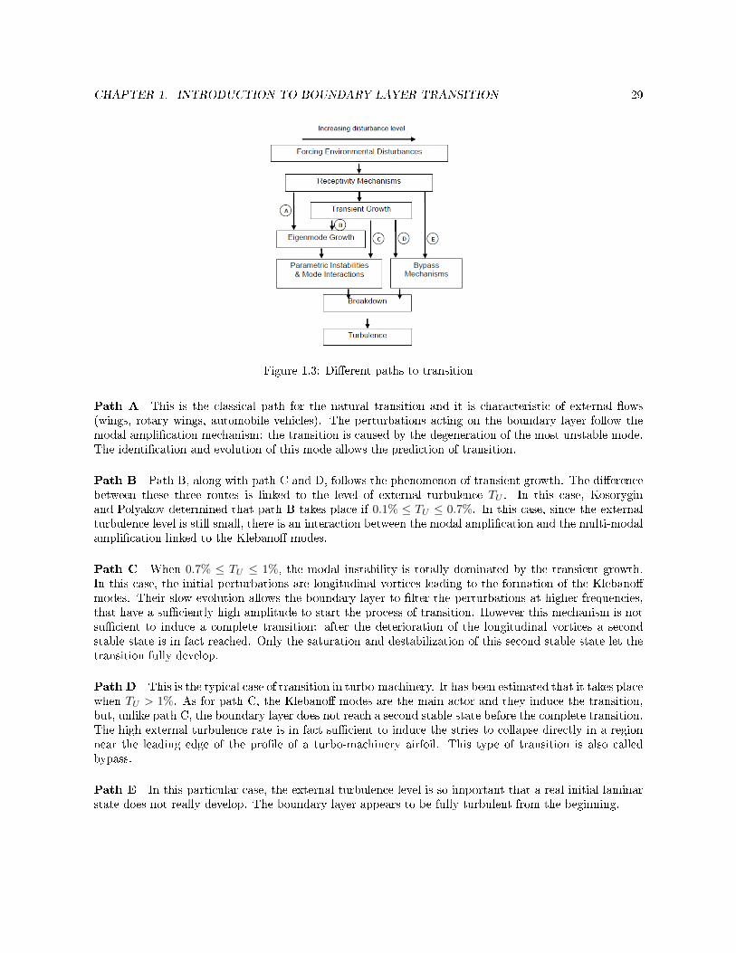
CHAPTER 1. INTRODUCTION TO BOUNDARY-LAYER TRANSITION 29
Figure 1.3: Dierent paths to transition
Path A This is the classical path for the natural transition and it is characteristic of external ows(wings, rotary wings, automobile vehicles). The perturbations acting on the boundary layer follow themodal amplication mechanism: the transition is caused by the degeneration of the most unstable mode.The identication and evolution of this mode allows the prediction of transition.
Path B Path B, along with path C and D, follows the phenomenon of transient growth. The dierencebetween these three routes is linked to the level of external turbulence TU . In this case, Kosoryginand Polyakov determined that path B takes place if 0.1% ≤ TU ≤ 0.7%. In this case, since the externalturbulence level is still small, there is an interaction between the modal amplication and the multi-modalamplication linked to the Klebano modes.
Path C When 0.7% ≤ TU ≤ 1%, the modal instability is totally dominated by the transient growth.In this case, the initial perturbations are longitudinal vortices leading to the formation of the Klebanomodes. Their slow evolution allows the boundary layer to lter the perturbations at higher frequencies,that have a suciently high amplitude to start the process of transition. However this mechanism is notsucient to induce a complete transition: after the deterioration of the longitudinal vortices a secondstable state is in fact reached. Only the saturation and destabilization of this second stable state let thetransition fully develop.
Path D This is the typical case of transition in turbo-machinery. It has been estimated that it takes placewhen TU > 1%. As for path C, the Klebano modes are the main actor and they induce the transition,but, unlike path C, the boundary layer does not reach a second stable state before the complete transition.The high external turbulence rate is in fact sucient to induce the stries to collapse directly in a regionnear the leading edge of the prole of a turbo-machinery airfoil. This type of transition is also calledbypass.
Path E In this particular case, the external turbulence level is so important that a real initial laminarstate does not really develop. The boundary layer appears to be fully turbulent from the beginning.
CHAPTER 1. INTRODUCTION TO BOUNDARY-LAYER TRANSITION 30
1.4 Natural transition
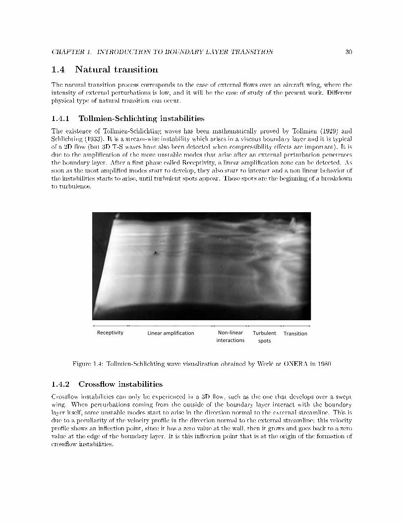
The natural transition process corresponds to the case of external ows over an aircraft wing, where theintensity of external perturbations is low, and it will be the case of study of the present work. Dierentphysical type of natural transition can occur.
1.4.1 Tollmien-Schlichting instabilities
The existence of Tollmien-Schlichting waves has been mathematically proved by Tollmien (1929) andSchlichting (1933). It is a stream-wise instability which arises in a viscous boundary layer and it is typicalof a 2D ow (but 3D T-S waves have also been detected when compressibility eects are important). It isdue to the amplication of the more unstable modes that arise after an external perturbation penetratesthe boundary layer. After a rst phase called Receptivity, a linear amplication zone can be detected. Assoon as the most amplied modes start to develop, they also start to interact and a non linear behavior ofthe instabilities starts to arise, until turbulent spots appear. These spots are the beginning of a breakdownto turbulence.
Receptivity Linear amplification Non-linear
interactions Turbulent
spots Transition
Figure 1.4: Tollmien-Schlichting wave visualization obtained by Werlé at ONERA in 1980
1.4.2 Crossow instabilities
Crossow instabilities can only be experienced in a 3D ow, such as the one that develops over a sweptwing. When perturbations coming from the outside of the boundary layer interact with the boundarylayer itself, some unstable modes start to arise in the direction normal to the external streamline. This isdue to a peculiarity of the velocity prole in the direction normal to the external streamline: this velocityprole shows an inection point, since it has a zero value at the wall, then it grows and goes back to a zerovalue at the edge of the boundary layer. It is this inection point that is at the origin of the formation ofcrossow instabilities.

CHAPTER 1. INTRODUCTION TO BOUNDARY-LAYER TRANSITION 31
UW
xz
y
inflection point
e
e
e
Figure 1.5: Inection point in the direction normal to the external streamline
Crossow instabilities appear as longitudinal periodic vortices in the transversal direction and theyexist for perturbation at zero frequency, thus they correspond to stationary modes.
Figure 1.6 shows a visualization of crossow instabilities that is obtained by coating the wall with awall marker, such as acenaphthene.The change of heat transfer properties between laminar and turbulent states causes the marker to evap-orate.
Figure 1.6: Crossow instability visualization from Dagenhart and Saric [10]
1.4.3 Görtler instabilities
This kind of instabilities are specics to concave geometries. They are typically encountered in critical andsuper-critical airfoils, where the upper wing side is at in order to avoid shocks, and the lower wing sideis concave in the proximity of the trailing edge in order to create a higher pressure dierence that allowslift to be important. A visualization of a super-critical prole is given in Figure 1.7. In this concave zone,counter-rotating longitudinal vortices appear due to the presence of a strong normal pressure gradientand centrifugal forces. It has been demonstrated that there exists a critical radius that makes Görtler

CHAPTER 1. INTRODUCTION TO BOUNDARY-LAYER TRANSITION 32
vortices appear. The relation for the critical radius is the following
δ1R> 1.3 · 10−4 (1.28)
where R is the curvature radius.A schematization and a visualization of Görtler vortices is given in Figures 1.8a and 1.8b.
Figure 1.7: Super-critical prole
(a) Görtler vortices schematization (b) Görtler vortices visualization
Figure 1.8: Görtler instabilities

34
Chapter 2
Modal stability analysis and N-factor
method
In the present study, the interest is directed to the study of natural transition mechanisms.In this case, the laminar boundary layer is subjected to external perturbations, which are turned intonormal modes through receptivity. After a rst linear amplication phase, non linear interactions startto grow since a breakdown of these interactions leads to transition.
Since the external modes grow in a normal way, a modal stability analysis can be performed.
2.1 Modal formulation
A generic dimensionless boundary-layer quantity ϕ∗ can be expressed as the composition of a mean valueϕ and a uctuating part ϕ′, as follows
ϕ∗ = ϕ+ ϕ′ (2.1)
withϕ′ ϕ . (2.2)
A proper form for the perturbation has to be dened. Since for the case of natural transition the pertur-bation are of modal type, it is convenient to write the perturbations as the product of an eigenfunctionand a wave function, as follows:
ϕ′ = ϕ′ (y∗) ei(α∗cx∗+β∗c z
∗−ω∗c t∗) + C.C. (C.C. = complex conjugate) (2.3)
where (α∗c , β∗c , ω
∗c ) ∈ C are constant and ϕ′ is the eigenfunction. The previous quantities are dened by
α∗c = αδ1 and β∗c = βδ1 (2.4)
where δ1 =
∫ δ
0
(1− ρu
ρeue
)dy is the compressible displacement thickness.
The dimensionless angular velocity ω∗c corresponds to the physical frequency f and it is given by
ω∗c = ωδ1ue
= 2πfδ1ue. (2.5)
The quantities (α∗c , β∗c , ω
∗c ) in expression (2.3) are complex numbers, whose real parts are the wave
numbers and the angular velocity and whose imaginary parts represent respectively spatial and temporal
CHAPTER 2. MODAL STABILITY ANALYSIS AND N -FACTOR METHOD 35
amplication rates.Since the present study concerns spatial stability, no temporal amplication rate is taken into considera-tion, thus leading to
ω∗c = ω∗ with ω∗ real . (2.6)
The spatial stability is also studied by considering that the amplication of the perturbation acts onlyin the x-direction. This hypothesis yields
β∗c = β∗ with β∗ real . (2.7)
The form (2.3) for the perturbations thus becomes
ϕ′ = ϕ′ (y∗) ei(α∗cx∗+β∗z∗−ω∗t∗) = ϕ′ (y∗) e−α
∗i ei(α
∗rx∗+β∗z∗−ω∗t∗) (2.8)
where the term e−α∗i is linked to the amplication or dumping of the external perturbation.
By dening the amplication rate σ∗asσ∗ = −α∗i
three dierent scenarios are possible
σ∗ > 0 (α∗i < 0) : unstablemode, amplication of the perturbation
σ∗ < 0 (α∗i > 0) : stablemode, damping
σ∗ = 0 (α∗i = 0) : neutralmode, non linear eectsmust be taken into
account to decide if the ow is stable or unstable .
Therefore, for a given mean ow, the growth rates for several frequencies must be obtained and studiedas functions of both Reδ1 and ω∗.The growth rates σ∗ are determined via the use of Orr-Sommerfeld equation.
A further explication of the choice to put β∗i = 0 can be given.
The perturbations impacting the boundary layer spread in a direction identied by the ratioβ∗rα∗r
while the
amplication direction (with respect to the spreading direction) is given by the ratioβ∗iα∗i
.
It as been shown that in general the perturbation amplication follows the direction of the group velocity,and this last direction can be identied with the external velocity direction, that is a zero-value anglebetween the external streamline and the amplication directions can be inferred, thus
ψki = arctan
(β∗iα∗i
)= 0 . (2.9)
This condition can be expressed as β∗i = 0.In order to perform the stability analysis, an additional parameter is introduced. This quantity is a
characteristic reduced frequency F , dened as
F =2πfνeu2e
=w
Reδ1
δ1ue
=ω∗
Reδ1, (2.10)
where Reδ1 is the Reynolds number based on the displacement thickness.Therefore, in the plane ω vsReδ1 the iso-F lines are straight lines of slope F .
2.2 Types of instabilities
Dierent types of instability can be encountered in a generic ow.For the case of a ow over a wing, three types of instabilities can be identied: viscous instabilities, purelyinectional instabilities and viscous-inectional instabilities. Their characterization is detailed hereafter.

CHAPTER 2. MODAL STABILITY ANALYSIS AND N -FACTOR METHOD 36
2.2.1 Viscous instabilities
This kind of instabilities are due to a destabilizing eect of the viscosity, as it has rstly been demonstratedby Prandtl in 1921. They are mostly encountered for highly accelerated bi-dimensional ows and smallReynolds numbers Reδ1 .A simplied explication to this problem is that, for small Reynolds numbers, viscous forces are comparableto inertial stresses and act against them with a sort of delay. By using a mass-spring-damper system,viscosity can be modeled as a damper with negative damping coecient, thus a destabilizing element.
Stability diagram is shown in gure 2.1a . The black curve is the neutral stability curve, and all thediagrams inside this curve show an unstable behavior. The critical point is marked in Figure 2.1a witha star and it reveals the rst value of the critical Reynolds number for which the rst unstable modesappear.Figure 2.1b shows the evolution of the growth rate σ∗ as a function of the Reynolds number.
Reδ1
ω
R1 R2
F1
(a) Stability diagram
σ
Iso-F1
Reδ1R1 R2
(b) Iso-F growth rate curve
Figure 2.1: Qualitative stability diagram for viscous instabilities
2.2.2 Purely inectional instabilities
Inectional instabilities can be encountered in bi-dimensional ows that experience an adverse pressuregradient, where an inection point is located at a certain distance from the wall (normally y
δ > 0.3).For high Reynolds numbers Reδ1 , the reduced frequency F depends only slightly on Reδ1 , and the inectionpoint leads the instability growth.
Stability diagram is shown in Figure 2.2.
CHAPTER 2. MODAL STABILITY ANALYSIS AND N -FACTOR METHOD 37
Reδ1
ω
R1 R2
F1
(a) Stability diagram
σ
Iso-F1
Reδ1R1 R2
(b) Iso-F growth rate curve
Figure 2.2: Qualitative stability diagram for inectional instabilities
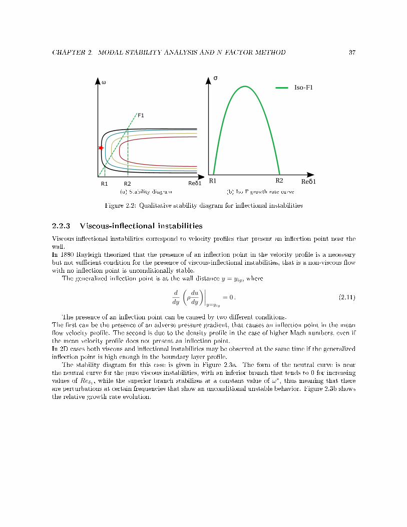
2.2.3 Viscous-inectional instabilities
Viscous-inectional instabilities correspond to velocity proles that present an inection point near thewall.In 1880 Rayleigh theorized that the presence of an inection point in the velocity prole is a necessarybut not sucient condition for the presence of viscous-inectional instabilities, that is a non-viscous owwith no inection point is unconditionally stable.
The generalized inection point is at the wall distance y = yig, where
d
dy
(ρdu
dy
)∣∣∣∣y=yig
= 0 . (2.11)
The presence of an inection point can be caused by two dierent conditions.The rst can be the presence of an adverse pressure gradient, that causes an inection point in the meanow velocity prole. The second is due to the density prole in the case of higher Mach numbers, even ifthe mean velocity prole does not present an inection point.In 2D cases both viscous and inectional instabilities may be observed at the same time if the generalizedinection point is high enough in the boundary layer prole.
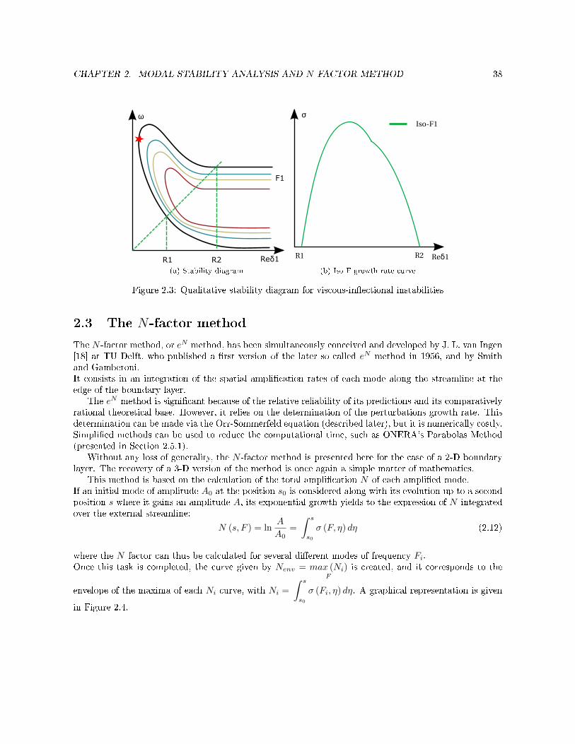
The stability diagram for this case is given in Figure 2.3a. The form of the neutral curve is nearthe neutral curve for the pure viscous instabilities, with an inferior branch that tends to 0 for increasingvalues of Reδ1 , while the superior branch stabilizes at a constant value of ω∗, thus meaning that thereare perturbations at certain frequencies that show an unconditional unstable behavior. Figure 2.3b showsthe relative growth rate evolution.
CHAPTER 2. MODAL STABILITY ANALYSIS AND N -FACTOR METHOD 38
Reδ1
ω
R1 R2
F1
(a) Stability diagram
σIso-F1
Reδ1R1 R2
(b) Iso-F growth rate curve
Figure 2.3: Qualitative stability diagram for viscous-inectional instabilities
2.3 The N-factor method
The N -factor method, or eN method, has been simultaneously conceived and developed by J. L. van Ingen[18] at TU Delft, who published a rst version of the later so called eN method in 1956, and by Smithand Gamberoni.It consists in an integration of the spatial amplication rates of each mode along the streamline at theedge of the boundary layer.
The eN method is signicant because of the relative reliability of its predictions and its comparativelyrational theoretical base. However, it relies on the determination of the perturbations growth rate. Thisdetermination can be made via the Orr-Sommerfeld equation (described later), but it is numerically costly.Simplied methods can be used to reduce the computational time, such as ONERA's Parabolas Method(presented in Section 2.5.1).
Without any loss of generality, the N -factor method is presented here for the case of a 2-D boundarylayer. The recovery of a 3-D version of the method is once again a simple matter of mathematics.
This method is based on the calculation of the total amplication N of each amplied mode.If an initial mode of amplitude A0 at the position s0 is considered along with its evolution up to a secondposition s where it gains an amplitude A, its exponential growth yields to the expression of N integratedover the external streamline:
N (s, F ) = lnA
A0=
∫ s
s0
σ (F, η) dη (2.12)
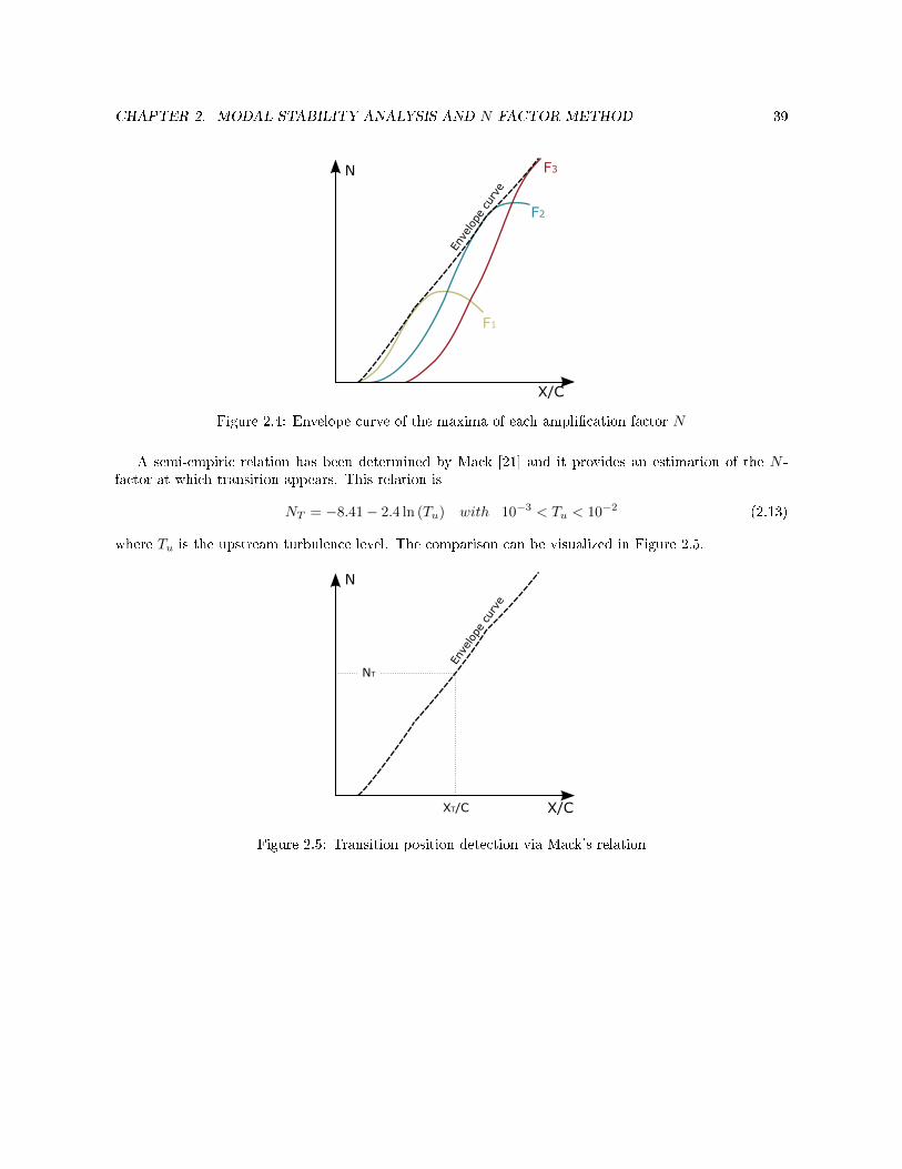
where the N factor can thus be calculated for several dierent modes of frequency Fi.Once this task is completed, the curve given by Nenv = max (Ni)
F
is created, and it corresponds to the
envelope of the maxima of each Ni curve, with Ni =
∫ s
s0
σ (Fi, η) dη. A graphical representation is given
in Figure 2.4.
CHAPTER 2. MODAL STABILITY ANALYSIS AND N -FACTOR METHOD 39
N
X/C
F1
F2
F3
Enve
lope
cur
ve
Figure 2.4: Envelope curve of the maxima of each amplication factor N
A semi-empiric relation has been determined by Mack [21] and it provides an estimation of the N -factor at which transition appears. This relation is
NT = −8.41− 2.4 ln (Tu) with 10−3 < Tu < 10−2 (2.13)
where Tu is the upstream turbulence level. The comparison can be visualized in Figure 2.5.
N
X/C
NT
XT/C
Enve
lope
cur
ve
Figure 2.5: Transition position detection via Mack's relation
CHAPTER 2. MODAL STABILITY ANALYSIS AND N -FACTOR METHOD 40
2.4 Orr-Sommerfeld
2.4.1 The Orr-Sommerfeld equation
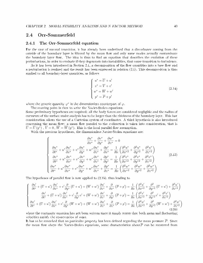
For the case of natural transition, it has already been underlined that a disturbance coming from theoutside of the boundary layer is ltered by the mean ow and only some modes actually contaminatethe boundary layer ow. The idea is thus to nd an equation that describes the evolution of theseperturbations, in order to evaluate if they degenerate into instabilities, that cause transition to turbulence.
As it has been introduced in Section 2.1, a decomposition of the ow quantities into a base ow anda perturbation is realized and the result has been expressed in relation (2.1). This decomposition is thusapplied to all boundary-layer quantities, as follows
u∗ = U + u′
v∗ = V + v′
w∗ = W + w′
p∗ = P + p′
(2.14)
where the generic quantity ϕ∗ is the dimensionless counterpart of ϕ.The starting point is then to write the Navier-Stokes equations.
Some preliminary hypotheses are required: all the body forces are considered negligible and the radius ofcurvature of the surface under analysis has to be larger than the thickness of the boundary layer. This lastconsideration allows the use of a Cartesian system of coordinates. A third hypothesis is also introducedconcerning the mean ow: a mean ow parallel to the x-direction is taken into consideration, that isU = U (y∗) , V = 0 , W = W (y∗). This is the local parallel ow assumption.
With the previous hypotheses, the dimensionless Navier-Stokes equations are:
∂u∗
∂x∗+∂v∗
∂y∗+∂w∗
∂z∗= 0
∂u∗
∂t∗+ u∗
∂u∗
∂x∗+ v∗
∂u∗
∂y∗+ w∗
∂u∗
∂z∗+∂p∗
∂x∗=
1
Re
(∂2u∗
∂x∗2+∂2u∗
∂y∗2+∂2u∗
∂z∗2
)∂v∗
∂t∗+ u∗
∂v∗
∂x∗+ v∗
∂v∗
∂y∗+ w∗
∂v∗
∂z∗+∂p∗
∂y∗=
1
Re
(∂2v∗
∂x∗2+∂2v∗
∂y∗2+∂2v∗
∂z∗2
)∂w∗
∂t∗+ u∗
∂w∗
∂x∗+ v∗
∂w∗
∂y∗+ w∗
∂w∗
∂z∗+∂p∗
∂z∗=
1
Re
(∂2w∗
∂x∗2+∂2w∗
∂y∗2+∂2w∗
∂z∗2
)(2.15)
The hypotheses of parallel ow is now applied to (2.15), thus leading to
∂u′
∂t∗+(U + u′
) ∂u′∂x∗
+ v′∂
∂y∗(U + u′
)+(W + w′
) ∂u′∂z∗
+∂
∂x∗(P + p′
)=
1
Re
(∂2u′
∂x∗2+
∂2
∂y∗2(U + u′
)+∂2u′
∂z∗2
)∂v′
∂t∗+(U + u′
) ∂v′∂x∗
+ v′∂
∂y∗v′ +
(W + w′
) ∂v′∂z∗
+∂
∂y∗(P + p′
)=
1
Re
(∂2v′
∂x∗2+
∂2
∂y∗2v′ +
∂2v′
∂z∗2
)∂w′
∂t∗+(U + u′
) ∂w′∂x∗
+ v′∂
∂y∗(W + w′
)+(W + w′
) ∂w′∂z∗
+∂
∂z∗(P + p′
)=
1
Re
(∂2w′
∂x∗2+
∂2
∂y∗2(W + w′
)+∂2w′
∂z∗2
)(2.16)
where the continuity equation has not been written since it simply states that both mean and uctuatingvelocities satisfy the conservation of mass.It has to be remarked that no particular property has been dened regarding the mean pressure P . Sincethe mean ow obeys the Navier-Stokes equations, some characteristics aboutP can be recovered from

CHAPTER 2. MODAL STABILITY ANALYSIS AND N -FACTOR METHOD 41
there, as presented below
U∂U
∂x∗+ V
∂U
∂y∗+W
∂U
∂z∗+∂P
∂x∗=
1
Re
(∂2U
∂x∗2+∂2U
∂y∗2+∂2U
∂z∗2
)U∂v′
∂x∗+ V
∂V
∂y∗+W
∂V
∂z∗+∂P
∂y∗=
1
Re
(∂2V
∂x∗2+∂2V
∂y∗2+∂2V
∂z∗2
)U∂W
∂x∗+ V
∂W
∂y∗+W
∂W
∂z∗+∂P
∂z∗=
1
Re
(∂2W
∂x∗2+∂2W
∂y∗2+∂2W
∂z∗2
)The previous system, along with parallel ow hypotheses, can be reduced to
∂P
∂x∗=
1
Re
(∂2U
∂y∗2
)∂P
∂y∗= 0
∂P
∂z∗=
1
Re
(∂2W
∂y∗2
) (2.17)
Linearization is now required.The process of linearization consists in eliminating from a given relation all the terms of order 2 or higher,since their values are negligible compared to rst order quantities: this is a direct consequence of (2.2).
So, all the quantities of type ϕ′ ∂ϕ′
∂q∗ can be erased form system (2.16), thus leading to
∂u′
∂x∗+∂v′
∂y∗+∂w′
∂z∗= 0
∂u′
∂t∗+ U
∂u′
∂x∗+ v′
∂
∂y∗U +W
∂u′
∂z∗+∂p′
∂x∗=
1
Re∇2 (u′)
∂v′
∂t∗+ U
∂v′
∂x∗+ W
∂v′
∂z∗+∂p′
∂y∗=
1
Re∇2 (v′)
∂w′
∂t∗+W
∂w′
∂x∗+ v′
∂
∂y∗W +W
∂w′
∂z∗+∂p′
∂z∗=
1
Re∇2 (w′)
(2.18)
Equations in system (2.18) are the ones who describe the evolution of disturbances.A proper form for the perturbation has to be dened. Since for the case of natural transition the pertur-bation are of modal type, it is convenient to write the perturbations as the product of an eigenfunctionand a wave function, as follows:
ϕ′ = ϕ′ (y∗) ei(α∗cx∗+β∗c z
∗−ω∗c t∗) + C.C. (C.C. = complex conjugate) (2.19)
with (α∗c , β∗c , ω
∗c ) ∈ C constant.
This denition of the disturbances can be introduced into system (2.18) as follows
iα∗cu′ +Dv′ + iβ∗cw
′ = 0
−iω∗cu′ + iα∗cUu′ + v′DU + iβ∗cWu′ + iα∗cp
′ =1
Re
((α∗c)
2u′ −D2u′ + (β∗c ) 2u′)
−iω∗cv′ + iα∗cUv′ + iβ∗cWv′ +Dp′ =
1
Re
((α∗c)
2v′ −D2v′ + (β∗c ) 2v′)
−iω∗cw′ + iα∗cUw′ + v′DW + iβ∗cWw′ + iβ∗c p
′ =1
Re
((α∗c)
2w′ −D2w′ + (β∗c ) 2w′)
(2.20)

CHAPTER 2. MODAL STABILITY ANALYSIS AND N -FACTOR METHOD 42
where D is the operator of derivation with respect to y.By dening the parameter k2 = (α∗c)
2 + (β∗c ) 2 and by factoring, the momentum balance equations ofsystem (2.20) become:
i(−ω∗c + α∗cU + β∗cW
)u′ + v′DU + iα∗cp
′ =[D2 − k2
] u′Re
i(−ω∗c + α∗cU + β∗cW
)v′ + Dp′ =
[D2 − k2
] v′Re
i(−ω∗c + α∗cU + β∗cW
)w′ + v′DW + iβ∗c p
′ =[D2 − k2
] w′Re
(2.21)
The following change of variables is introduced
φ = v′ and χ1 = iα∗cu′ + iβ∗cw
′ (2.22)
that, if introduced into continuity equation, gives
χ1 +Dφ = 0 . (2.23)
The next step is then to manipulate the equations for momentum balance in system (1.1). In particular,the rst and third equations are multiplied respectively by iα∗cRe and iβ
∗cRe, and they are then summed
together. At the same time the equation for y-momentum is multiplied by Rek2 . The result is
iRe(−ω∗c + α∗cU + β∗cW
)D2φ+ iRe
(α∗cD
2U + β∗cD2W)φ−Rek2Dp′ +D4φ− k2D2φ = 0
iRe(−ω∗c + α∗cU + β∗cW
)k2φ+ +Rek2Dp′ − k2D2φ+ k4φ = 0
(2.24)
The last step is now to combine the two equations of system (2.24) by means of the term Dp′ to obtain
[D2 − k2
]2φ− iRe
[(−ω∗c + α∗cU + β∗cW
) [D2 − k2
]φ−
(α∗cD
2U + β∗cD2W)φ]
= 0 (2.25)
which is the Orr-Sommerfeld equation. The boundary conditions supplementing this equation are
φ (0) = Dφ (0) = 0 and φ (y∗ →∞) = 0
CHAPTER 2. MODAL STABILITY ANALYSIS AND N -FACTOR METHOD 43
2.5 Database approach method
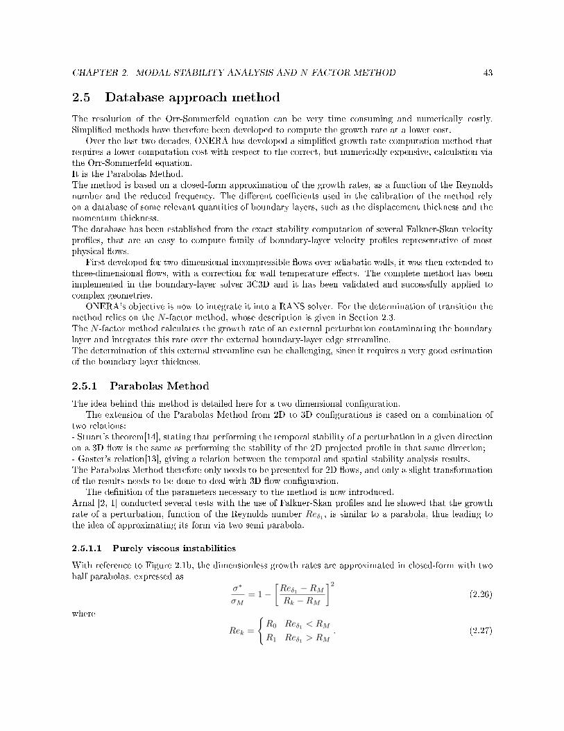
The resolution of the Orr-Sommerfeld equation can be very time consuming and numerically costly.Simplied methods have therefore been developed to compute the growth rate at a lower cost.
Over the last two decades, ONERA has developed a simplied growth-rate computation method thatrequires a lower computation cost with respect to the correct, but numerically expensive, calculation viathe Orr-Sommerfeld equation.It is the Parabolas Method.The method is based on a closed-form approximation of the growth rates, as a function of the Reynoldsnumber and the reduced frequency. The dierent coecients used in the calibration of the method relyon a database of some relevant quantities of boundary layers, such as the displacement thickness and themomentum thickness.The database has been established from the exact stability computation of several Falkner-Skan velocityproles, that are an easy to compute family of boundary-layer velocity proles representative of mostphysical ows.
First developed for two-dimensional incompressible ows over adiabatic walls, it was then extended tothree-dimensional ows, with a correction for wall temperature eects. The complete method has beenimplemented in the boundary-layer solver 3C3D and it has been validated and successfully applied tocomplex geometries.
ONERA's objective is now to integrate it into a RANS solver. For the determination of transition themethod relies on the N -factor method, whose description is given in Section 2.3.The N -factor method calculates the growth rate of an external perturbation contaminating the boundarylayer and integrates this rate over the external boundary-layer edge streamline.The determination of this external streamline can be challenging, since it requires a very good estimationof the boundary layer thickness.
2.5.1 Parabolas Method
The idea behind this method is detailed here for a two dimensional conguration.The extension of the Parabolas Method from 2D to 3D congurations is cased on a combination of
two relations:- Stuart's theorem[14], stating that performing the temporal stability of a perturbation in a given directionon a 3D ow is the same as performing the stability of the 2D projected prole in that same direction;- Gaster's relation[13], giving a relation between the temporal and spatial stability analysis results.The Parabolas Method therefore only needs to be presented for 2D ows, and only a slight transformationof the results needs to be done to deal with 3D ow conguration.
The denition of the parameters necessary to the method is now introduced.Arnal [2, 1] conducted several tests with the use of Falkner-Skan proles and he showed that the growthrate of a perturbation, function of the Reynolds number Reδ1 , is similar to a parabola, thus leading tothe idea of approximating its form via two semi parabola.
2.5.1.1 Purely viscous instabilities
With reference to Figure 2.1b, the dimensionless growth rates are approximated in closed-form with twohalf parabolas, expressed as
σ∗
σM= 1−
[Reδ1 −RMRk −RM
]2
(2.26)
where
Rek =
R0 Reδ1 < RM
R1 Reδ1 > RM. (2.27)
CHAPTER 2. MODAL STABILITY ANALYSIS AND N -FACTOR METHOD 44
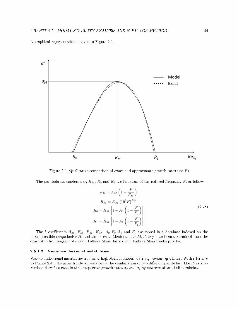
A graphical representation is given in Figure 2.6.
𝑅𝑒𝛿1
𝜎∗
𝜎𝑀
𝑅𝑀
𝑅0
𝑅1
Model
Exact
Figure 2.6: Qualitative comparison of exact and approximate growth rates (iso-F )
The parabola parameters σM , RM , R0 and R1 are functions of the reduced frequency F , as follows
σM = AM
(1− F
FM
)RM = KM
(105F
)EMR0 = RM
[1−A0
(1− F
F0
)]R1 = RM
[1−A1
(1− F
F1
)]. (2.28)
The 8 coecients AM , FM , EM , KM , A0 F0 A1 and F1 are stored in a database indexed on theincompressible shape factor Hi and the external Mach number Me. They have been determined from theexact stability diagram of several Falkner-Skan-Hartree and Falkner-Skan-Cooke proles.
2.5.1.2 Viscous-inectional instabilities
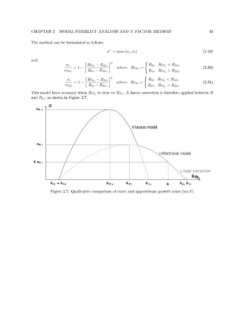
Viscous-inectional instabilities appear at high Mach numbers or strong pressure gradients. With referenceto Figure 2.3b, the growth rate appears to be the combination of two dierent parabolas. The ParabolasMethod therefore models their respective growth rates σv and σi by two sets of two half parabolas.
CHAPTER 2. MODAL STABILITY ANALYSIS AND N -FACTOR METHOD 45
The method can be formulated as follows
σ∗ = max (σv, σi) (2.29)
andσvσMv
= 1−[Reδ1 −RMv
Rkv −RMv
]2
where Rekv =
R0v Reδ1 < RMv
R1v Reδ1 > RMv
(2.30)
σiσMi
= 1−[Reδ1 −RMi
Rki −RMi
]2
where Reki =
R0i Reδ1 < RMi
RPi Reδ1 > RMi
(2.31)
This model loses accuracy when Reδ1 is close to RPi. A linear correction is therefore applied between Rand R1i, as shown in Figure 2.7.
R0i = R 0v RM v RM i R 1v ,R R p i R 1i
K σM i
σM i
σM v
Viscousmodel
Inflectional model
Linear correctionReδ1
σ
R0i = R 0v RM v RM i R 1v ,R R p i R 1i
K σM i
σM i
σM v
Viscousmodel
Inflectional model
Linear correctionReδ1
σ
Figure 2.7: Qualitative comparison of exact and approximate growth rates (iso-F )
46
Summary
This rst part presented a way through which the laminar-to-turbulent transition problem is treatednowadays.
For the transition position determination the N -factor method is used. This method requires theknowledge of the amplication rate of the perturbations impacting the boundary layer.
The determination of the amplication rate can be exploited via the Orr-Sommerfeld equation, whichdetermines precisely what the conditions for hydrodynamic stability are. Even though this equation givesthe solution to the problem, its resolution is numerically too costly. Another way for the calculation ofthe growth rate has to be put in place.
A database approach method developed at ONERA, the Parabolas Method, has already been imple-mented in a boundary-layer solver and it has been successfully tested. The interest is now to implementand to integrate it in a RANS solver.Since the method relies on the calculation of some integral boundary-layer quantities, the problem of thedetermination of the boundary layer thickness δ appears (since the value of the velocity at the edge of theboundary layer −→ue is not known in a RANS solver).In Part II the determination of δ is studied.

48
Part II
Boundary-layer thickness determination

49
50
Chapter 3
Self-similar solutions
This chapter presents a family of boundary-layer proles that have an important common property: self-similarity.The analytical and numerical development of self-similar solutions is here introduced since it will be usedlater as a tool to develop a method to compute the boundary-layer thickness δ.
In mathematics, a self-similar object is an entity that is exactly or approximately equal to a part ofitself.In the case of a boundary layer, self-similarity is the peculiarity of the velocity proles u, at dierent posi-tions along the surface, to dier only by a scale factor. This characteristic of the laminar boundary layeris extremely important, since it is sucient to know the solution at one point to recover information onthe ow in another point. This very important aspect has rstly been studied by Blasius, who found outself-similar solutions for the case of a at innite plate. The study of self-similarity has been continued byFalkner and Skan, who extended the solution given by Blasius to the case of non-null pressure gradients.Since Blasius solution appears to be a particular case of Falkner-Skan solution, it is here presented onlythe development of Falkner-Skan theory and Blasius solution will be retrieved in a second time.The Falkner-Skan solution for a 2D incompressible boundary layer is rstly derived. Then the 2D com-pressible case will be introduced and, at last, the incompressible 3D self-similar solutions will be presented.
Self-similar solutions have been employed by Arnal for the calibration of the Parabolas Method for itsuse in the boundary-layer code 3C3D, and it has been shown that they match with real proles.
Therefore, the idea is to create a database of similarity prole obtained for dierent values of thepressure gradient, and to use them to cover almost all the possible velocity proles that can be found ona real geometry case.
3.1 2D incompressible Falkner-Skan equation
Self-similar solutions have been found by Blasius for the case of a at plate with no pressure gradient,where the velocity at the edge of the boundary layer is constant. When a generic geometry is exploited,such as an airfoil prole, the question is to nd out under which particular distribution of the externalvelocity self-similarity can be recovered.
Prandtl's equations system for the 2D incompressible ow case is here reminded (see Section 1.2.1):∂u∂x + ∂v
∂y = 0∂u∂t + u∂u∂x + v ∂u∂y = − 1
ρ∂p∂x + υ ∂
2u∂y2
∂p∂y = 0
(3.1)
CHAPTER 3. SELF-SIMILAR SOLUTIONS 51
The rst step to recover the Falkner-Skan equation is to work with nondimensional proles. In par-ticular, the velocity u is divided by its value Ue at the edge of the boundary layer. The reduced prole isthus subject to the following boundary conditions
y = 0u
Ue= 0 ; y →∞ u
Ue→ 1 .
The idea is now to introduce a dimensionless variable η through which the velocity prole can be expressedin the following form:
u
Ue= f ′ (η) with η =
y
∆ (x)(3.2)
where ∆ (x) is a function to be determined. If a similitude between proles in two dierent stations x1
and x2 can be found, then there exists an anity of ratio ∆(x1)∆(x2) between the two of them.
It is useful for the following to work in terms of the stream function ψ. This function automaticallysatises the continuity equation, since
u =∂ψ
∂y, v = −∂ψ
∂x.
The stream function can thus be determined by integration of the velocity, as follows
ψ =
∫ y
0
u dy with ψ (0) = 0 . (3.3)
If hypothesis (3.2) is introduced into expression (3.3), the following relation is valid
ψ = Ue(x)∆ (x) f (η) with f =
∫ η
0
f ′ dη and f (0) = 0 . (3.4)
The normal velocity v is then
v = −∂ψ∂x
= −f d
dx(Ue∆) + Ue∆
′ (x) ηf ′ (3.5)
where ∆′ (x) = d∆dx and f ′ = df
dη .
Expressions (3.2) and (3.5) can now be injected in the equation of momentum balance of the system(3.1) and an Ordinary Dierential Equation can be found
f ′′′ + a (x) ff ′′ + b (x)(1− f ′2
)= 0 (3.6)
where a (x) = ∆νddx (∆Ue) , b (x) = ∆2
νdUedx , f ′′ = ∂2f
dη2 and f ′′′ = ∂3fdη3 .
In order for the solution to be dependent only on η, the coecients a and b must depend only on η. Sincea and b are functions of the coordinate x, the only way for self-similarity to exist is that a and b areconstant, thus:
∆
ν
d
dx(∆Ue) = a , (3.7)
∆2
ν
d
dx(Ue) = b . (3.8)
By grouping together equation (3.7) and equation (3.8), the following condition is obtained
1
ν
d
dx
(∆2Ue
)= 2a− b (3.9)
CHAPTER 3. SELF-SIMILAR SOLUTIONS 52
which, once integrated by assuming 2a− b 6= 0 and by putting the x origin at ∆2Ue = 0, gives
∆2Ueν
= (2a− b)x . (3.10)
By arranging Equation (3.7) and Equation (3.8) and by combining them with equation (3.10), the followingrelation can be written
(2a− b) x∆
d∆
dx= a− b (3.11)
Since Ue > 0, two dierent cases can be distinguished from (3.10)
(2a− b) > 0 =⇒ x > 0
(2a− b) < 0 =⇒ x < 0
For the rst one, through integration of equation (3.11), the expression for ∆ (x) and Ue (x) can be nallyretrieved:
∆ = Kx(a−b)(2a−b) (3.12)
Ue =2a− bK2
νxb
(2a−b) (3.13)
For the second case ((2a− b) < 0 ), ∆ (x) and Ue (x) are
∆ = K (−x)(a−b)(2a−b) (3.14)
Ue =b− 2a
K2ν (−x)
b(2a−b) (3.15)
Two particular solutions can be obtained for a = 0 and 2a− b = 0.The rst of this two conditions leads to an external velocity distribution of the type
Ue =c
x(3.16)
that represents the case of a source or a sink, depending on the value of c.The second case leads to an external ow of type
Ue = K1eK2x . (3.17)
These two congurations will not be investigated in this study.
3.1.1 Falkner-Skan-Hartree solution
From the relations regarding the form of the external velocity Ue and of ∆, it can be seen that they onlydepend on the ratio between a and b. It can in fact be written that
a− b2a− b
=b
a
(ab − 1
2− ba
)and
b
2a− b=b
a
(1
2− ba
). (3.18)
Without any lack of generality the constant a can be set equal to 1. The constant b will be called β.The attention will be focused on the case of 2a− b > 0, that is β < 2. The external-velocity distributiontakes then the following form
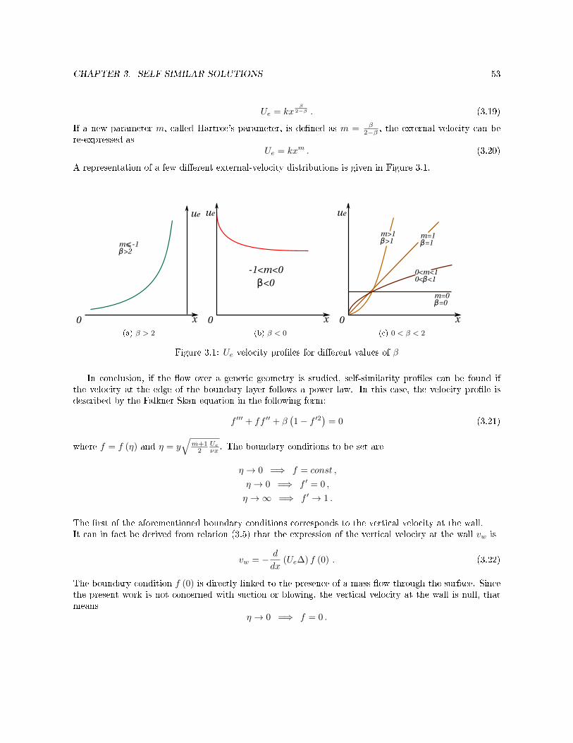
CHAPTER 3. SELF-SIMILAR SOLUTIONS 53
Ue = kxβ
2−β . (3.19)
If a new parameter m, called Hartree's parameter, is dened as m = β2−β , the external velocity can be
re-expressed asUe = kxm . (3.20)
A representation of a few dierent external-velocity distributions is given in Figure 3.1.
0 x
ue
m⩽-1β>2
(a) β > 2
0 x
ue
-1<m<0
β<0
(b) β < 0
0 x
ue
m>1β>1
m=1β=1
0<m<10<β<1
m=0β=0
(c) 0 < β < 2
Figure 3.1: Ue velocity proles for dierent values of β
In conclusion, if the ow over a generic geometry is studied, self-similarity proles can be found ifthe velocity at the edge of the boundary layer follows a power law. In this case, the velocity prole isdescribed by the Falkner-Skan equation in the following form:
f ′′′ + ff ′′ + β(1− f ′2
)= 0 (3.21)
where f = f (η) and η = y√
m+12
Ueνx . The boundary conditions to be set are
η → 0 =⇒ f = const ,
η → 0 =⇒ f ′ = 0 ,
η →∞ =⇒ f ′ → 1 .
The rst of the aforementioned boundary conditions corresponds to the vertical velocity at the wall.It can in fact be derived from relation (3.5) that the expression of the vertical velocity at the wall vw is
vw = − d
dx(Ue∆) f (0) . (3.22)
The boundary condition f (0) is directly linked to the presence of a mass ow through the surface. Sincethe present work is not concerned with suction or blowing, the vertical velocity at the wall is null, thatmeans
η → 0 =⇒ f = 0 .
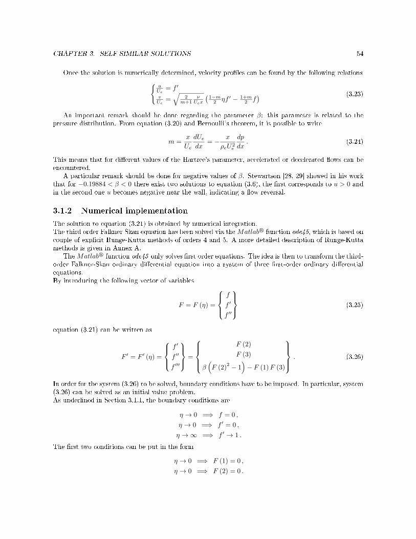
CHAPTER 3. SELF-SIMILAR SOLUTIONS 54
Once the solution is numerically determined, velocity proles can be found by the following relationsuUe
= f ′
vUe
=√
2m+1
νUex
(1−m
2 ηf ′ − 1+m2 f
) (3.23)
An important remark should be done regarding the parameter β: this parameter is related to thepressure distribution. From equation (3.20) and Bernoulli's theorem, it is possible to write
m =x
Ue
dUedx
= − x
ρeU2e
dp
dx. (3.24)
This means that for dierent values of the Hartree's parameter, accelerated or decelerated ows can beencountered.
A particular remark should be done for negative values of β. Stewartson [28, 29] showed in his workthat for −0.19884 < β < 0 there exist two solutions to equation (3.6), the rst corresponds to u > 0 andin the second one u becomes negative near the wall, indicating a ow reversal.
3.1.2 Numerical implementation
The solution to equation (3.21) is obtained by numerical integration.The third order Falkner-Skan equation has been solved via theMatlabr function ode45, which is based oncouple of explicit Runge-Kutta methods of orders 4 and 5. A more detailed description of Runge-Kuttamethods is given in Annex A.
TheMatlabr function ode45 only solves rst order equations. The idea is then to transform the third-order Falkner-Skan ordinary dierential equation into a system of three rst-order ordinary dierentialequations.By introducing the following vector of variables
F = F (η) =
f
f ′
f ′′
(3.25)
equation (3.21) can be written as
F ′ = F ′ (η) =
f ′
f ′′
f ′′′
=
F (2)
F (3)
β(F (2)
2 − 1)− F (1)F (3)
. (3.26)
In order for the system (3.26) to be solved, boundary conditions have to be imposed. In particular, system(3.26) can be solved as an initial value problem.As underlined in Section 3.1.1, the boundary conditions are
η → 0 =⇒ f = 0 ,
η → 0 =⇒ f ′ = 0 ,
η →∞ =⇒ f ′ → 1 .
The rst two conditions can be put in the form
η → 0 =⇒ F (1) = 0 ,
η → 0 =⇒ F (2) = 0 .

CHAPTER 3. SELF-SIMILAR SOLUTIONS 55
Concerning the boundary condition for η →∞, a shooting method is applied.In numerical analysis, a shooting method is a procedure through which a boundary value problem can
be reduced to an initial value problem.In particular, a problem in the general form
y′′ (t) = f (t , y (t) , y′ (t))
y (t0) = y0
y (t1) = y1
(3.27)
can be transformed into y′′ (t) = f (t , y (t) , y′ (t))
y (t0) = y0
y′ (t0) = k
. (3.28)
k is obtained by the denition of a functional G such that
G (k) = y (t1; k)− y1 . (3.29)
If G has a root equal to k then the solution y (t; k) of the corresponding initial value problem is alsosolution of the boundary value problem.
For the particular case under study, the method used for nding the root of (3.29) is Newton's method.Initial condition for F (2) is thus determined as follows
F (2)n+1
= F (2)n
+(F (2)
n − F (2)n−1) F (1)
n∣∣∣η→∞
− 1
F (1)n∣∣∣η→∞
− F (1)n−1∣∣∣η→∞
. (3.30)
The expression (3.30) is then be applied iteratively until a chosen convergence level is attained.The system (3.26) can now be solved via the aforementioned Runge-Kutta method.
3.1.3 Numerical results
The numerical solutions to the Falkner-Skan equation are now presented. As it has already been underlinedin the previous section, such solutions depend on the parameter β. It is recalled that m = β
2−β .For positive values of β the ow encounters a negative pressure gradient with respect to x-direction,according to expression (3.24), thus the pressure gradient accelerates the uid. On the other hand, anegative value of β indicate an adverse pressure gradient, whose eect is to decelerate the uid. The twocases are presented in Figure 3.2.
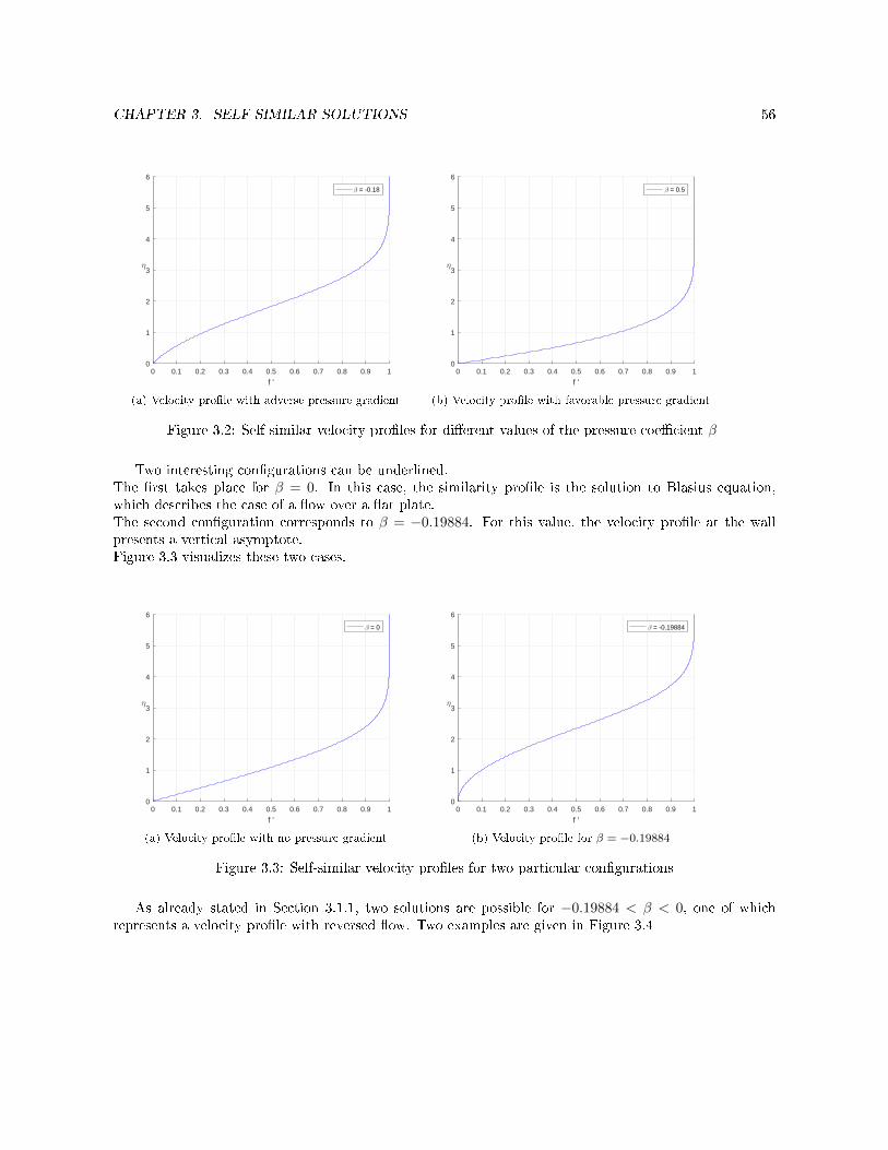
CHAPTER 3. SELF-SIMILAR SOLUTIONS 56
0 0.1 0.2 0.3 0.4 0.5 0.6 0.7 0.8 0.9 1
f '
0
1
2
3
4
5
6
η
β = -0.18
(a) Velocity prole with adverse pressure gradient
0 0.1 0.2 0.3 0.4 0.5 0.6 0.7 0.8 0.9 1
f '
0
1
2
3
4
5
6
η
β = 0.5
(b) Velocity prole with favorable pressure gradient
Figure 3.2: Self-similar velocity proles for dierent values of the pressure coecient β
Two interesting congurations can be underlined.The rst takes place for β = 0. In this case, the similarity prole is the solution to Blasius equation,which describes the case of a ow over a at plate.The second conguration corresponds to β = −0.19884. For this value, the velocity prole at the wallpresents a vertical asymptote.Figure 3.3 visualizes these two cases.
0 0.1 0.2 0.3 0.4 0.5 0.6 0.7 0.8 0.9 1
f '
0
1
2
3
4
5
6
η
β = 0
(a) Velocity prole with no pressure gradient
0 0.1 0.2 0.3 0.4 0.5 0.6 0.7 0.8 0.9 1
f '
0
1
2
3
4
5
6
η
β = -0.19884
(b) Velocity prole for β = −0.19884
Figure 3.3: Self-similar velocity proles for two particular congurations
As already stated in Section 3.1.1, two solutions are possible for −0.19884 < β < 0, one of whichrepresents a velocity prole with reversed ow. Two examples are given in Figure 3.4
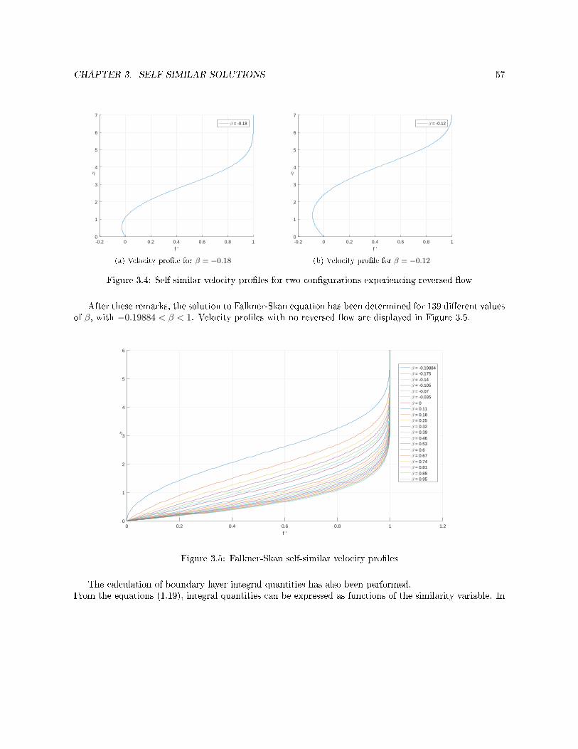
CHAPTER 3. SELF-SIMILAR SOLUTIONS 57
-0.2 0 0.2 0.4 0.6 0.8 1
f '
0
1
2
3
4
5
6
7
η
β = -0.18
(a) Velocity prole for β = −0.18
-0.2 0 0.2 0.4 0.6 0.8 1
f '
0
1
2
3
4
5
6
7
η
β = -0.12
(b) Velocity prole for β = −0.12
Figure 3.4: Self-similar velocity proles for two congurations experiencing reversed ow
After these remarks, the solution to Falkner-Skan equation has been determined for 139 dierent valuesof β, with −0.19884 < β < 1. Velocity proles with no reversed ow are displayed in Figure 3.5.
0 0.2 0.4 0.6 0.8 1 1.2
f '
0
1
2
3
4
5
6
η
β = -0.19884β = -0.175β = -0.14β = -0.105β = -0.07β = -0.035β = 0β = 0.11β = 0.18β = 0.25β = 0.32β = 0.39β = 0.46β = 0.53β = 0.6β = 0.67β = 0.74β = 0.81β = 0.88β = 0.95
Figure 3.5: Falkner-Skan self-similar velocity proles
The calculation of boundary layer integral quantities has also been performed.From the equations (1.19), integral quantities can be expressed as functions of the similarity variable. In

CHAPTER 3. SELF-SIMILAR SOLUTIONS 58
particular, it can be derived that
Displacement thicknessδ1√Rexx
=
∫ ∞0
(1− f ′) dy
Momentum thicknessϑ√Rexx
=
∫ ∞0
f ′ (1− f ′) dy
Shape factor H =δ1ϑ.
(3.31)
All the quantities in (3.31) depend only on β. The calculation performed are summarized in Table 3.1and are in very good accordance with results from Cousteix [8].
β m Hi
- 0.19884 -0.0904 4.0295- 0.175 -0.0805 3.2327- 0.105 -0.0499 2.8174
0 0 2.59130.11 0.0582 2.47280.32 0.1905 2.35390.6 0.4286 2.27480.81 0.6807 2.23961 1 2.2168
Table 3.1: Shape factor as a function of the pressure parameter β
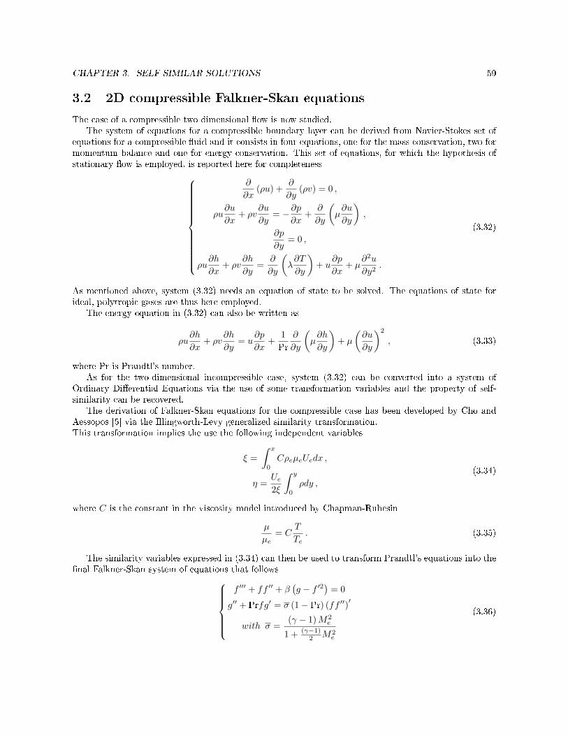
CHAPTER 3. SELF-SIMILAR SOLUTIONS 59
3.2 2D compressible Falkner-Skan equations
The case of a compressible two dimensional ow is now studied.The system of equations for a compressible boundary layer can be derived from Navier-Stokes set of
equations for a compressible uid and it consists in four equations, one for the mass conservation, two formomentum balance and one for energy conservation. This set of equations, for which the hypothesis ofstationary ow is employed, is reported here for completeness
∂
∂x(ρu) +
∂
∂y(ρv) = 0 ,
ρu∂u
∂x+ ρv
∂u
∂y= −∂p
∂x+
∂
∂y
(µ∂u
∂y
),
∂p
∂y= 0 ,
ρu∂h
∂x+ ρv
∂h
∂y=
∂
∂y
(λ∂T
∂y
)+ u
∂p
∂x+ µ
∂2u
∂y2.
(3.32)
As mentioned above, system (3.32) needs an equation of state to be solved. The equations of state forideal, polytropic gases are thus here employed.
The energy equation in (3.32) can also be written as
ρu∂h
∂x+ ρv
∂h
∂y= u
∂p
∂x+
1
Pr
∂
∂y
(µ∂h
∂y
)+ µ
(∂u
∂y
)2
, (3.33)
where Pr is Prandtl's number.As for the two-dimensional incompressible case, system (3.32) can be converted into a system of
Ordinary Dierential Equations via the use of some transformation variables and the property of self-similarity can be recovered.
The derivation of Falkner-Skan equations for the compressible case has been developed by Cho andAessopos [5] via the Illingworth-Levy generalized similarity transformation.This transformation implies the use the following independent variables
ξ =
∫ x
0
CρeµeUedx ,
η =Ue2ξ
∫ y
0
ρdy ,
(3.34)
where C is the constant in the viscosity model introduced by Chapman-Rubesin
µ
µe= C
T
Te. (3.35)
The similarity variables expressed in (3.34) can then be used to transform Prandtl's equations into thenal Falkner-Skan system of equations that follows
f ′′′ + ff ′′ + β(g − f ′2
)= 0
g′′ + Prfg′ = σ (1− Pr) (ff ′′)′
with σ =(γ − 1)M2
e
1 + (γ−1)2 M2
e
(3.36)
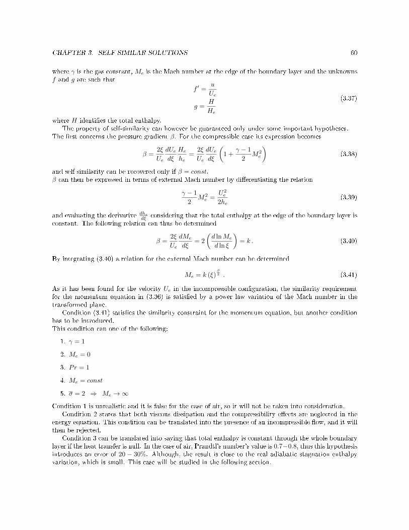
CHAPTER 3. SELF-SIMILAR SOLUTIONS 60
where γ is the gas constant, Me is the Mach number at the edge of the boundary layer and the unknownsf and g are such that
f ′ =u
Ue
g =H
He
(3.37)
where H identies the total enthalpy.The property of self-similarity can however be guaranteed only under some important hypotheses.
The rst concerns the pressure gradient β. For the compressible case its expression becomes
β =2ξ
Ue
dUedξ
He
he=
2ξ
Ue
dUedξ
(1 +
γ − 1
2M2e
)(3.38)
and self similarity can be recovered only if β = const.β can then be expressed in terms of external Mach number by dierentiating the relation
γ − 1
2M2e =
U2e
2he(3.39)
and evaluating the derivative dhedξ considering that the total enthalpy at the edge of the boundary layer is
constant. The following relation can thus be determined
β =2ξ
Ue
dMe
dξ= 2
(d lnMe
d ln ξ
)= k . (3.40)
By integrating (3.40) a relation for the external Mach number can be determined
Me = k (ξ)β2 . (3.41)
As it has been found for the velocity Ue in the incompressible conguration, the similarity requirementfor the momentum equation in (3.36) is satised by a power law variation of the Mach number in thetransformed plane.
Condition (3.41) satises the similarity constraint for the momentum equation, but another conditionhas to be introduced.This condition can one of the following:
1. γ = 1
2. Me = 0
3. Pr = 1
4. Me = const
5. σ = 2 ⇒ Me →∞
Condition 1 is unrealistic and it is false for the case of air, so it will not be taken into consideration.Condition 2 states that both viscous dissipation and the compressibility eects are neglected in the
energy equation. This condition can be translated into the presence of an incompressible ow, and it willthen be rejected.
Condition 3 can be translated into saying that total enthalpy is constant through the whole boundarylayer if the heat transfer is null. In the case of air, Prandtl's number's value is 0.7−0.8, thus this hypothesisintroduces an error of 20 − 30%. Although, the result is close to the real adiabatic stagnation enthalpyvariation, which is small. This case will be studied in the following section.

CHAPTER 3. SELF-SIMILAR SOLUTIONS 61
Condition 4 corresponds to the ow over a at plate, for which β = 0, and sets no limits for thePrandtl number. This case will be detailed hereafter.
Condition 5 represents the case of hypersonic ow and it will not be investigated, since out of thescope of the present study.
3.2.1 Unit Prandtl number and adiabatic wall case
The condition of Pr = 1 simplies consistently system (3.36), which becomesf ′′′ + ff ′′ + β
(g − f ′2
)= 0
g′′ + fg′ = 0(3.42)
with boundary conditionsη = 0 =⇒ f = const , f ′ = 0 , g = const
η →∞ =⇒ f ′ → 1 , g → 1. (3.43)
Once again, no injection nor suction of uid through the wall is considered, that is f (0) = 0.Another important hypothesis has to be introduced in order to set boundary condition g (0) = const.
The presence of an adiabatic wall will be taken into consideration, i.e. no heat ux through the wall ispresent.The hypothesis of an adiabatic wall is widely used in aerodynamics for external ows. It must be precisedthat for the majority of metallic materials thermal conductivity is high and the hypothesis of unitaryPrandtl's number turns out to be inaccurate. Nevertheless, this assumption leads to necessary simplica-tions and results show a good level of accordance to empirical data.For zero heat transfer at the surface, an explicit integral for the second equation in (3.42) subjected toboundary conditions (3.43) is
g (η) = 1 . (3.44)
This shows that, for an adiabatic wall, the stagnation enthalpy is constant throughout the whole boundarylayer. This can be explained considering that the internal heat generated due to viscosity and the heattransferred by diusion and conduction interact in a way that the total enthalpy remains constant. Thisphenomenon is a direct consequence of the hypothesis Pr = 1 .
With the previous considerations, system (3.42) becomesf ′′′ + ff ′′ + β
(1− f ′2
)= 0
g (η) = 1(3.45)
where the rst equation is Falkner-Skan equation for the incompressible two-dimensional case.
3.2.1.1 Numerical implementation
As already done in Section 3.1.2, the solution to system (3.45) is obtained by numerical integration.System (3.42) has been reduced to a system of rst-order dierential equations to which a Runge-Kuttamethod has been applied.As it has been done for the incompressible case, the boundary conditions for η →∞ are applied to f ′′ (0)and to g′ (0) via the use of a shooting method.
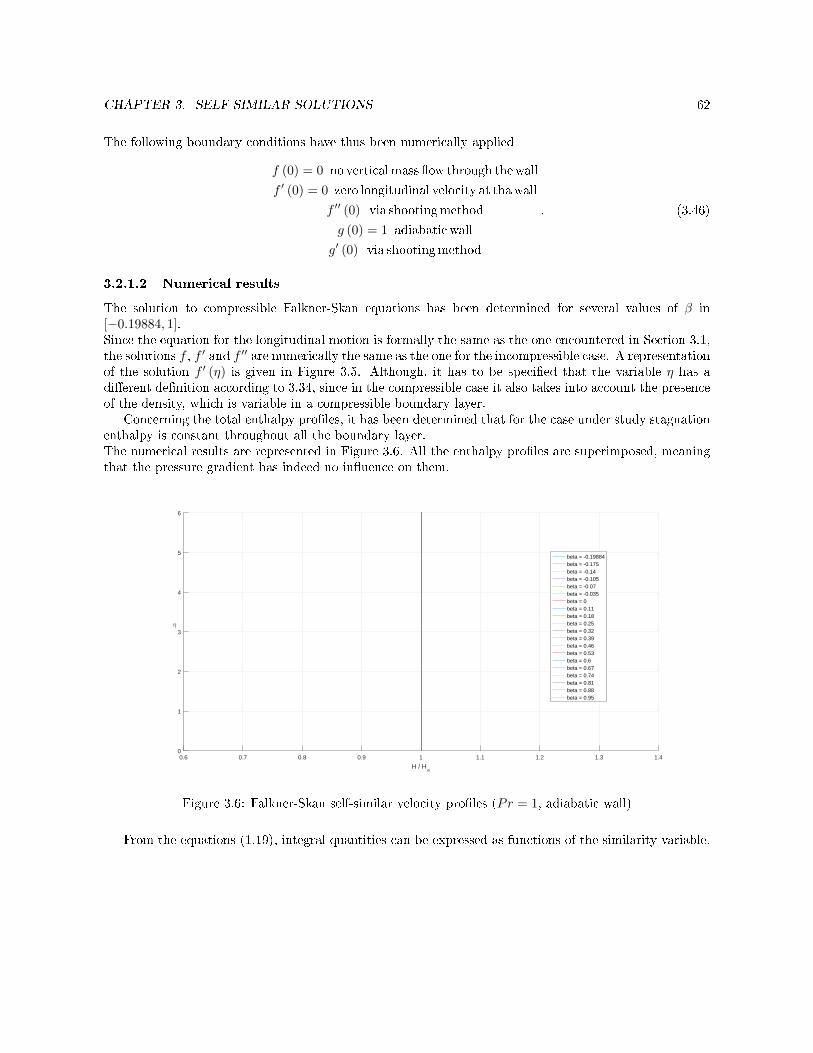
CHAPTER 3. SELF-SIMILAR SOLUTIONS 62
The following boundary conditions have thus been numerically applied
f (0) = 0 no verticalmass ow through thewall
f ′ (0) = 0 zero longitudinal velocity at thawall
f ′′ (0) via shootingmethod
g (0) = 1 adiabaticwall
g′ (0) via shootingmethod
. (3.46)
3.2.1.2 Numerical results
The solution to compressible Falkner-Skan equations has been determined for several values of β in[−0.19884, 1].Since the equation for the longitudinal motion is formally the same as the one encountered in Section 3.1,the solutions f , f ′ and f ′′ are numerically the same as the one for the incompressible case. A representationof the solution f ′ (η) is given in Figure 3.5. Although, it has to be specied that the variable η has adierent denition according to 3.34, since in the compressible case it also takes into account the presenceof the density, which is variable in a compressible boundary layer.
Concerning the total enthalpy proles, it has been determined that for the case under study stagnationenthalpy is constant throughout all the boundary layer.The numerical results are represented in Figure 3.6. All the enthalpy proles are superimposed, meaningthat the pressure gradient has indeed no inuence on them.
0.6 0.7 0.8 0.9 1 1.1 1.2 1.3 1.4
H / He
0
1
2
3
4
5
6
η
beta = -0.19884beta = -0.175beta = -0.14beta = -0.105beta = -0.07beta = -0.035beta = 0beta = 0.11beta = 0.18beta = 0.25beta = 0.32beta = 0.39beta = 0.46beta = 0.53beta = 0.6beta = 0.67beta = 0.74beta = 0.81beta = 0.88beta = 0.95
Figure 3.6: Falkner-Skan self-similar velocity proles (Pr = 1, adiabatic wall)
From the equations (1.19), integral quantities can be expressed as functions of the similarity variable.
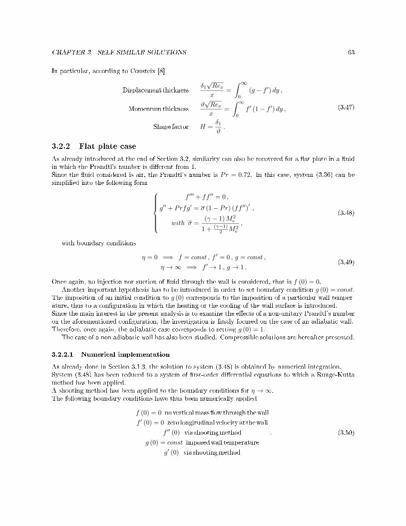
CHAPTER 3. SELF-SIMILAR SOLUTIONS 63
In particular, according to Cousteix [8]
Displacement thicknessδ1√Rexx
=
∫ ∞0
(g − f ′) dy ,
Momentum thicknessϑ√Rexx
=
∫ ∞0
f ′ (1− f ′) dy ,
Shape factor H =δ1ϑ.
(3.47)
3.2.2 Flat plate case
As already introduced at the end of Section 3.2, similarity can also be recovered for a at plate in a uidin which the Prandtl's number is dierent from 1.Since the uid considered is air, the Prandtl's number is Pr = 0.72. In this case, system (3.36) can besimplied into the following form
f ′′′ + ff ′′ = 0 ,
g′′ + Prfg′ = σ (1− Pr) (ff ′′)′,
with σ =(γ − 1)M2
e
1 + (γ−1)2 M2
e
,
(3.48)
with boundary conditions
η = 0 =⇒ f = const , f ′ = 0 , g = const ,
η →∞ =⇒ f ′ → 1 , g → 1 .(3.49)
Once again, no injection nor suction of uid through the wall is considered, that is f (0) = 0.Another important hypothesis has to be introduced in order to set boundary condition g (0) = const.
The imposition of an initial condition to g (0) corresponds to the imposition of a particular wall temper-ature, thus to a conguration in which the heating or the cooling of the wall surface is introduced.Since the main interest in the present analysis is to examine the eects of a non-unitary Prandtl's numberon the aforementioned conguration, the investigation is rstly focused on the case of an adiabatic wall.Therefore, once again, the adiabatic case corresponds to setting g (0) = 1.
The case of a non adiabatic wall has also been studied. Compressible solutions are hereafter presented.
3.2.2.1 Numerical implementation
As already done in Section 3.1.3, the solution to system (3.48) is obtained by numerical integration.System (3.48) has been reduced to a system of rst-order dierential equations to which a Runge-Kuttamethod has been applied.A shooting method has been applied to the boundary conditions for η →∞.The following boundary conditions have thus been numerically applied
f (0) = 0 no verticalmass ow through thewall
f ′ (0) = 0 zero longitudinal velocity at thewall
f ′′ (0) via shootingmethod
g (0) = const imposedwall temperature
g′ (0) via shootingmethod
. (3.50)

CHAPTER 3. SELF-SIMILAR SOLUTIONS 64
3.2.2.2 Numerical results
Since the equation for the longitudinal motion is a particular case of the one encountered in section 3.1.3,the velocity prole can be easily determined and it is displayed in Figure 3.7.
0 0.2 0.4 0.6 0.8 1 1.2
U/Ue
0
1
2
3
4
5
6
η
Mach number = 0Mach number = 0.1Mach number = 0.2Mach number = 0.3Mach number = 0.4Mach number = 0.5Mach number = 0.6Mach number = 0.7Mach number = 0.8Mach number = 0.9Mach number = 1Mach number = 1.1Mach number = 1.2Mach number = 1.3
Figure 3.7: Blasius longitudinal velocity proles (Pr = 0.72, adiabatic wall)
3.2.2.3 Adiabatic case
Concerning the total enthalpy proles, it is true that g (0) = 1. The results are represented in Figure 3.8,along with the density proles in Figure 3.9.It has to be precised that enthalpy proles are not constant anymore because of the eects of a non-unitaryPrandtl's number.

CHAPTER 3. SELF-SIMILAR SOLUTIONS 65
0.992 0.994 0.996 0.998 1 1.002 1.004 1.006 1.008 1.01 1.012
H/He
0
1
2
3
4
5
6
η
Mach number = 0Mach number = 0.1Mach number = 0.2Mach number = 0.3Mach number = 0.4Mach number = 0.5Mach number = 0.6Mach number = 0.7Mach number = 0.8Mach number = 0.9Mach number = 1Mach number = 1.1Mach number = 1.2Mach number = 1.3
Figure 3.8: Blasius enthalpy proles (Pr = 0.72, adiabatic wall)
0.7 0.75 0.8 0.85 0.9 0.95 1 1.05
ρ/ρe
0
1
2
3
4
5
6
η
Mach number = 0Mach number = 0.1Mach number = 0.2Mach number = 0.3Mach number = 0.4Mach number = 0.5Mach number = 0.6Mach number = 0.7Mach number = 0.8Mach number = 0.9Mach number = 1Mach number = 1.1Mach number = 1.2Mach number = 1.3
Figure 3.9: Blasius density proles (Pr = 0.72, adiabatic wall)
3.2.2.4 Non-adiabatic case
Concerning the total enthalpy and the density proles, dierent values of g (0) have been chosen.The imposition of a value for g (0) corresponds to the imposition of a particular value of the ratio H
He,
thus of the ratio TiwTie
= TwTie
. In particular, a value of the ratio HHe
∣∣∣w< 1 is associated to the cooling,
CHAPTER 3. SELF-SIMILAR SOLUTIONS 66
otherwise for HHe
∣∣∣w> 1 the wall is heated. This last case is of interest for practical application as, for
instance, anti-icing and de-icing problems.The results are represented in Figure 3.10, 3.11, 3.12 and 3.13 for dierent values of the wall temperature.
0.5 0.6 0.7 0.8 0.9 1 1.1
H/He
0
1
2
3
4
5
6
η
Mach number = 0Mach number = 0.1Mach number = 0.2Mach number = 0.3Mach number = 0.4Mach number = 0.5Mach number = 0.6Mach number = 0.7Mach number = 0.8Mach number = 0.9Mach number = 1Mach number = 1.1Mach number = 1.2Mach number = 1.3
(a) Enthalpy proles for dierent values of the Mach number
0.8 1 1.2 1.4 1.6 1.8 2
ρ/ρe
0
1
2
3
4
5
6
η
Mach number = 0Mach number = 0.1Mach number = 0.2Mach number = 0.3Mach number = 0.4Mach number = 0.5Mach number = 0.6Mach number = 0.7Mach number = 0.8Mach number = 0.9Mach number = 1Mach number = 1.1Mach number = 1.2Mach number = 1.3
(b) Density proles for dierent values of the Mach number
Figure 3.10: Similarity solutions (Pr = 0.72, HHe
∣∣∣w
= 0.5)
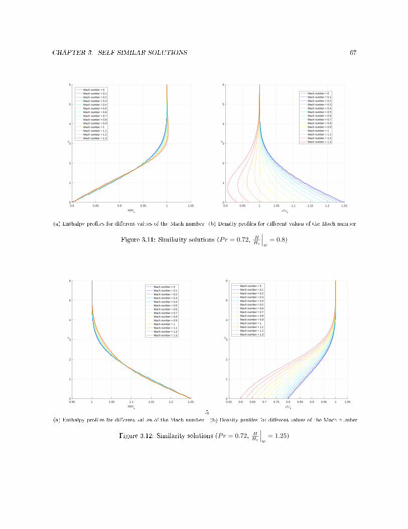
CHAPTER 3. SELF-SIMILAR SOLUTIONS 67
0.8 0.85 0.9 0.95 1 1.05
H/He
0
1
2
3
4
5
6
η
Mach number = 0Mach number = 0.1Mach number = 0.2Mach number = 0.3Mach number = 0.4Mach number = 0.5Mach number = 0.6Mach number = 0.7Mach number = 0.8Mach number = 0.9Mach number = 1Mach number = 1.1Mach number = 1.2Mach number = 1.3
(a) Enthalpy proles for dierent values of the Mach number
0.9 0.95 1 1.05 1.1 1.15 1.2 1.25
ρ/ρe
0
1
2
3
4
5
6
η
Mach number = 0Mach number = 0.1Mach number = 0.2Mach number = 0.3Mach number = 0.4Mach number = 0.5Mach number = 0.6Mach number = 0.7Mach number = 0.8Mach number = 0.9Mach number = 1Mach number = 1.1Mach number = 1.2Mach number = 1.3
(b) Density proles for dierent values of the Mach number
Figure 3.11: Similarity solutions (Pr = 0.72, HHe
∣∣∣w
= 0.8)
0.95 1 1.05 1.1 1.15 1.2 1.25
H/He
0
1
2
3
4
5
6
η
Mach number = 0Mach number = 0.1Mach number = 0.2Mach number = 0.3Mach number = 0.4Mach number = 0.5Mach number = 0.6Mach number = 0.7Mach number = 0.8Mach number = 0.9Mach number = 1Mach number = 1.1Mach number = 1.2Mach number = 1.3
(a) Enthalpy proles for dierent values of the Mach number
5
0.55 0.6 0.65 0.7 0.75 0.8 0.85 0.9 0.95 1 1.05
ρ/ρe
0
1
2
3
4
5
6
η
Mach number = 0Mach number = 0.1Mach number = 0.2Mach number = 0.3Mach number = 0.4Mach number = 0.5Mach number = 0.6Mach number = 0.7Mach number = 0.8Mach number = 0.9Mach number = 1Mach number = 1.1Mach number = 1.2Mach number = 1.3
(b) Density proles for dierent values of the Mach number
Figure 3.12: Similarity solutions (Pr = 0.72, HHe
∣∣∣w
= 1.25)
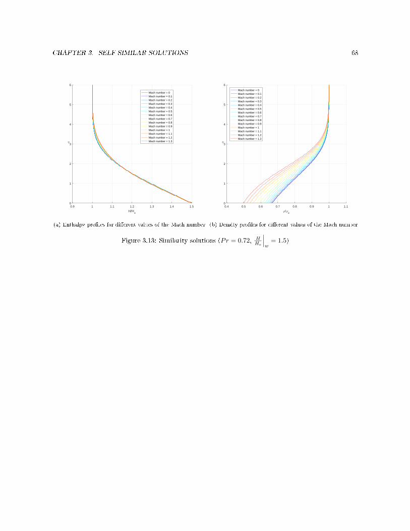
CHAPTER 3. SELF-SIMILAR SOLUTIONS 68
0.9 1 1.1 1.2 1.3 1.4 1.5
H/He
0
1
2
3
4
5
6
η
Mach number = 0Mach number = 0.1Mach number = 0.2Mach number = 0.3Mach number = 0.4Mach number = 0.5Mach number = 0.6Mach number = 0.7Mach number = 0.8Mach number = 0.9Mach number = 1Mach number = 1.1Mach number = 1.2Mach number = 1.3
(a) Enthalpy proles for dierent values of the Mach number
0.4 0.5 0.6 0.7 0.8 0.9 1 1.1
ρ/ρe
0
1
2
3
4
5
6
η
Mach number = 0Mach number = 0.1Mach number = 0.2Mach number = 0.3Mach number = 0.4Mach number = 0.5Mach number = 0.6Mach number = 0.7Mach number = 0.8Mach number = 0.9Mach number = 1Mach number = 1.1Mach number = 1.2Mach number = 1.3
(b) Density proles for dierent values of the Mach number
Figure 3.13: Similarity solutions (Pr = 0.72, HHe
∣∣∣w
= 1.5)
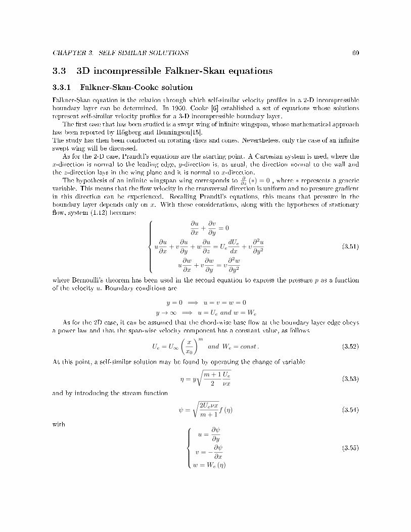
CHAPTER 3. SELF-SIMILAR SOLUTIONS 69
3.3 3D incompressible Falkner-Skan equations
3.3.1 Falkner-Skan-Cooke solution
Falkner-Skan equation is the relation through which self-similar velocity proles in a 2-D incompressibleboundary layer can be determined. In 1950, Cooke [6] established a set of equations whose solutionsrepresent self-similar velocity proles for a 3-D incompressible boundary layer.
The rst case that has been studied is a swept wing of innite wingspan, whose mathematical approachhas been reported by Högberg and Henningson[15].The study has then been conducted on rotating discs and cones. Nevertheless, only the case of an inniteswept wing will be discussed.
As for the 2-D case, Prandtl's equations are the starting point. A Cartesian system is used, where thex-direction is normal to the leading edge, y-direction is, as usual, the direction normal to the wall andthe z-direction lays in the wing plane and it is normal to x-direction.
The hypothesis of an innite wingspan wing corresponds to ∂∂z (∗) = 0 , where ∗ represents a generic
variable. This means that the ow velocity in the transversal direction is uniform and no pressure gradientin this direction can be experienced. Recalling Prandtl's equations, this means that pressure in theboundary layer depends only on x. With these considerations, along with the hypotheses of stationaryow, system (1.12) becomes:
∂u
∂x+∂v
∂y= 0
u∂u
∂x+ v
∂u
∂y+ w
∂u
∂z= Ue
dUedx
+ υ∂2u
∂y2
u∂w
∂x+ v
∂w
∂y= υ
∂2w
∂y2
(3.51)
where Bernoulli's theorem has been used in the second equation to express the pressure p as a functionof the velocity u. Boundary conditions are
y = 0 =⇒ u = v = w = 0
y →∞ =⇒ u = Ue and w = We
As for the 2D case, it can be assumed that the chord-wise base ow at the boundary layer edge obeysa power law and that the span-wise velocity component has a constant value, as follows
Ue = U∞
(x
x0
)mand We = const . (3.52)
At this point, a self-similar solution may be found by operating the change of variable
η = y
√m+ 1
2
Ueνx
(3.53)
and by introducing the stream function
ψ =
√2Ueνx
m+ 1f (η) (3.54)
with u =
∂ψ
∂y
v = −∂ψ∂x
w = We (η)
(3.55)
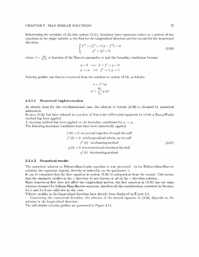
CHAPTER 3. SELF-SIMILAR SOLUTIONS 70
Substituting the variables (3.55) into system (3.51), boundary layer equations reduce to a system of twoequations in the single variable η, the rst for the longitudinal direction and the second for the transversaldirection:
f ′′′ + ff ′′ + β(1− f ′2
)= 0
g′′ + fg′ = 0(3.56)
where β = 2mm+1 is function of the Hartree parameter m and the boundary conditions become:
η = 0 =⇒ f = f ′ = g = 0
η →∞ =⇒ f ′ → 1, g → 1
Velocity proles can thus be recovered from the solution to system (3.56) as follows:
u = f ′ (η)
w =We
Ueg (η)
3.3.1.1 Numerical implementation
As already done for the two-dimensional case, the solution to system (3.56) is obtained by numericalintegration.System (3.56) has been reduced to a system of rst-order dierential equations to which a Runge-Kuttamethod has been applied.A shooting method has been applied to the boundary conditions for η →∞.The following boundary conditions have thus been numerically applied
f (0) = 0 no verticalmass ow through thewall
f ′ (0) = 0 zero longitudinal velocity at thewall
f ′′ (0) via shootingmethod
g (0) = 0 zero transversal velocity at thewall
g′ (0) via shootingmethod
. (3.57)
3.3.1.2 Numerical results
The numerical solution to Falkner-Skan-Cooke equation is now presented. As for Falkner-Skan-Hartreesolution, the equations depend, directly or indirectly, on the parameter β.It can be remarked that the rst equation in system (3.56) is independent from the second. This meansthat the similarity proles in the x-direction do not depend at all on the z-direction solution.Since transversal ow does not aect the longitudinal motion, the rst equation in (3.56) has the samesolution obtained for Falkner-Skan-Hartree equation, therefore all the considerations presented in Sections3.1.1 and 3.1.3 are valid also in this case.Velocity proles in the longitudinal direction have already been displayed in Figure 3.5
Concerning the transversal direction, the solution of the second equation in (3.56) depends on thesolution in the longitudinal direction.The self-similar velocity proles are presented in Figure 3.14.
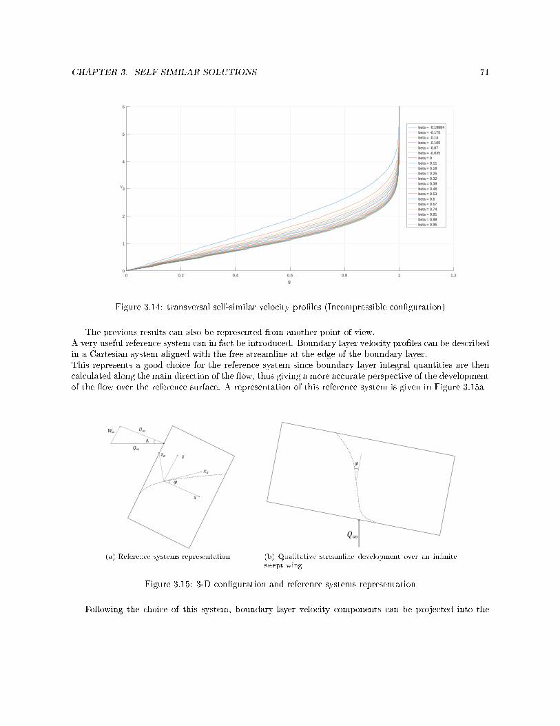
CHAPTER 3. SELF-SIMILAR SOLUTIONS 71
0 0.2 0.4 0.6 0.8 1 1.2
g
0
1
2
3
4
5
6
η
beta = -0.19884beta = -0.175beta = -0.14beta = -0.105beta = -0.07beta = -0.035beta = 0beta = 0.11beta = 0.18beta = 0.25beta = 0.32beta = 0.39beta = 0.46beta = 0.53beta = 0.6beta = 0.67beta = 0.74beta = 0.81beta = 0.88beta = 0.95
Figure 3.14: transversal self-similar velocity proles (Incompressible conguration)
The previous results can also be represented from another point of view.A very useful reference system can in fact be introduced. Boundary layer velocity proles can be describedin a Cartesian system aligned with the free streamline at the edge of the boundary layer.This represents a good choice for the reference system since boundary layer integral quantities are thencalculated along the main direction of the ow, thus giving a more accurate perspective of the developmentof the ow over the reference surface. A representation of this reference system is given in Figure 3.15a
𝑥
𝑥𝑒
𝑧
𝜑
𝑧𝑒 𝑄∞
𝑊∞ 𝑈∞
Λ
(a) Reference systems representation
𝑄∞
𝜑
(b) Qualitative streamline development over an inniteswept wing
Figure 3.15: 3-D conguration and reference systems representation
Following the choice of this system, boundary-layer velocity components can be projected into the

CHAPTER 3. SELF-SIMILAR SOLUTIONS 72
direction of the external ow through the change of variablesue = u cos (ϕ) + w sin (ϕ)
we = −u sin (ϕ) + w cos (ϕ). (3.58)
By expressing the external velocity aligned with the xe-direction as Qe, relations in system (3.58) can beexpressed as functions of similarity variables, as follows
ueQe
=u
Qecos (ϕ) +
w
Qesin (ϕ)
weQe
= − u
Qesin (ϕ) +
w
Qecos (ϕ)
=⇒
ueQe
= f ′ cos2 (ϕ) + g sin2 (ϕ)
weQe
= cos (ϕ) sin (ϕ) (g − f ′). (3.59)
The eect of this projection is visualized in Figure 3.16
0 0.1 0.2 0.3 0.4 0.5 0.6 0.7 0.8 0.9 1
ue/Q
e
0
1
2
3
4
5
6
7
η
(a) Velocity prole in the xe-direction
-14 -12 -10 -8 -6 -4 -2 0 2
we/Q
e ×10-3
0
1
2
3
4
5
6
7
η
(b) Velocity prole in the ze-direction
Figure 3.16: Velocity proles in reference system aligned with the free owstream

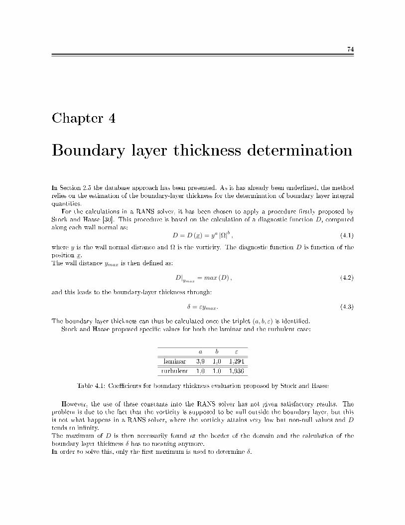
74
Chapter 4
Boundary layer thickness determination
In Section 2.5 the database approach has been presented. As it has already been underlined, the methodrelies on the estimation of the boundary-layer thickness for the determination of boundary layer integralquantities.
For the calculations in a RANS solver, it has been chosen to apply a procedure rstly proposed byStock and Haase [30]. This procedure is based on the calculation of a diagnostic function D, computedalong each wall normal as:
D = D (x) = ya |Ω|b , (4.1)
where y is the wall-normal distance and Ω is the vorticity. The diagnostic function D is function of theposition x.The wall distance ymax is then dened as:
D|ymax = max (D) , (4.2)
and this leads to the boundary-layer thickness through:
δ = εymax. (4.3)
The boundary layer thickness can thus be calculated once the triplet (a, b, ε) is identied.Stock and Haase proposed specic values for both the laminar and the turbulent case:
a b ε
laminar 3,9 1,0 1,294
turbulent 1,0 1,0 1,936
Table 4.1: Coecients for boundary thickness evaluation proposed by Stock and Haase
However, the use of these constants into the RANS solver has not given satisfactory results. Theproblem is due to the fact that the vorticity is supposed to be null outside the boundary layer, but thisis not what happens in a RANS solver, where the vorticity attains very low but non-null values and Dtends to innity.The maximum of D is then necessarily found at the border of the domain and the calculation of theboundary layer thickness δ has no meaning anymore.In order to solve this, only the rst maximum is used to determine δ.

CHAPTER 4. BOUNDARY LAYER THICKNESS DETERMINATION 75
Another problem is that in the laminar case, y is predominant in the diagnostic function (since a = 3.9)but has very low values near the wall.Dmax has thus a very small value that would be contaminated by numerical errors.
The idea is then to determine other constants dierent from the original model.The laminar case will be inspected, since the characteristics of the laminar boundary layer are the onesthat determine the boundary layer receptivity phase.
The idea is to nd a triplet that is unique, that means a value of a, b and ε that does not dependon the actual x position at which the calculation is made. The interest in such a method is that, oncecalibrated, it requires no parameters to be introduced from the user and it avoids high calculation costs.
The value of ε is not independent from the choice of a and b. In fact, the idea is to associate the valueof ε to the maximum of the diagnostic function D. The way pursued to nd the values for (a, b, ε) isdetailed in the next section.
4.1 Similarity for the 2-D incompressible case
As it has already been introduced in Chapter 3, it has been chosen to use similarity proles for theestimation of the boundary layer thickness, since they accurately represent the velocity proles over a realgeometry. The diagnostic function D can thus be expressed as a function of the similarity variables η andf . For a 2-D situation, the vorticity Ω is well approximated by the sole derivative of velocity u in they-direction, as follows:
D = ya |Ω|b = ya∣∣∣∣∂u∂y
∣∣∣∣b . (4.4)
The change of variables can now be applied.It is here recalled for completeness that, for a generic function χ = χ (g (t) , h (t)), the partial derivativeof the function χ with respect to the variable t is equal to
dχ
dt=∂χ
∂g
dg
dt+∂χ
∂h
dh
dt.
Therefore, by expressing the term ∂u∂y in similitude variables and by recalling that u = u (f ′ (η)) = Uef
′ (η),it can be found that
∂u
∂y=∂ (Uef
′)
∂η
∂η
∂y= f ′′Ue
√m+ 1
2
Ueνx
, (4.5)
expression (4.4) becomesD = ηaf ′′bH (x) (4.6)
where H(x) = Ueb(m+1
2Ueνx
) a+b2 depends only on the x-coordinate and f ′′ depend only on the constant
pressure gradient parameter β.The interest is nding the maximum of D
Dmaxfor a xed x position through the use of similarity
variables. This is due to the fact that the estimation of the boundary layer thickness is made locally.Since for a xed chord-wise position the quantity H (x) is xed, the maximum of D
Dmaxreduces to the
maximum of the expression ηa (f ′′) b, function of similarity variables only.The idea is then to search the maximum of D
Dmaxfor all the velocity proles, each of which corresponds
to a dierent value of β, and to trace DDmax
as a function of ηηδ, where ηδ represents the value of η that
corresponds to f ′ = 0.99.By dening ηmax as the value of η at which D
Dmaxhas a maximum, ε can nally be dened as:
ε (a, b) =ηδηmax
. (4.7)

CHAPTER 4. BOUNDARY LAYER THICKNESS DETERMINATION 76
The process can be visualized in Figure 4.1, where the result is obtained for a xed couple (a, b) and fora single self-similar velocity prole.
Figure 4.1: Representation of the parameter ε
As above mentioned, the idea is to nd a unique value of ε that does not depend on the actual velocityprole. A test on each of the self-similar solutions is thus required.
For a xed couple (a, b) the diagnostic function D is evaluated for several dierent self-similar velocityproles, each of them obtained with a dierent value of β in equation (3.21). In order to perform thecalculation, 139 dierent values of β ∈ R have been used, with R = [−0.19884, 1] and NR the number ofelement in R.
Two dierent scenarios can be obtained, as shown in Figure 4.2.
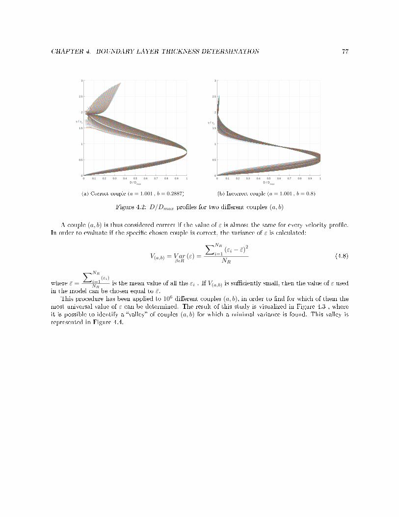
CHAPTER 4. BOUNDARY LAYER THICKNESS DETERMINATION 77
0 0.1 0.2 0.3 0.4 0.5 0.6 0.7 0.8 0.9 1
D / Dmax
0
0.5
1
1.5
2
2.5
3
η / ηδ
(a) Correct couple (a = 1.001 , b = 0.2887)
0 0.1 0.2 0.3 0.4 0.5 0.6 0.7 0.8 0.9 1
D / Dmax
0
0.5
1
1.5
2
2.5
3
η / ηδ
(b) Incorrect couple (a = 1.001 , b = 0.8)
Figure 4.2: D/Dmax proles for two dierent couples (a, b)
A couple (a, b) is thus considered correct if the value of ε is almost the same for every velocity prole.In order to evaluate if the specic chosen couple is correct, the variance of ε is calculated:
V(a,b) = V arβεR
(ε) =
∑NR
i=1(εi − ε)2
NR(4.8)
where ε =
∑NR
i=1(εi)
NRis the mean value of all the εi . If V(a,b) is suciently small, then the value of ε used
in the model can be chosen equal to ε.This procedure has been applied to 106 dierent couples (a, b), in order to nd for which of them the
most universal value of ε can be determined. The result of this study is visualized in Figure 4.3 , whereit is possible to identify a valley of couples (a, b) for which a minimal variance is found. This valley isrepresented in Figure 4.4.

CHAPTER 4. BOUNDARY LAYER THICKNESS DETERMINATION 78
Figure 4.3: Evolution of log(V(a,b)
)as a function of a and b
0.5 1 1.5 2 2.5 3
a
0.1
0.2
0.3
0.4
0.5
0.6
0.7
0.8
0.9
b
Figure 4.4: Curve b (a) representing the minima of log(V(a,b)
)If the couple (a, b) = (1.001, 0.2887) is chosen, it has been determined that ε = 1.36 and its variance
is V(a,b) = V(1.001,0.2887) = 3.97 · 10−5.The standard deviation is now introduced to have a direct meter of judgment of the variability of the
mean value ε.
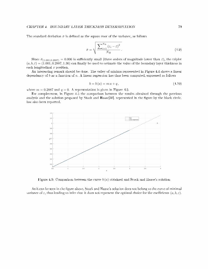
CHAPTER 4. BOUNDARY LAYER THICKNESS DETERMINATION 79
The standard deviation σ is dened as the square root of the variance, as follows
σ =
√√√√∑NR
i=1(εi − ε)2
NR. (4.9)
Since σ(1.001,0.2887) = 0.006 is suciently small (three orders of magnitude lower than ε), the triplet(a, b, ε) = (1.001, 0.2887, 1.36) can nally be used to estimate the value of the boundary layer thickness ineach longitudinal x position.
An interesting remark should be done. The valley of minima represented in Figure 4.4 shows a lineardependency of b as a function of a. A linear regression has thus been computed, expressed as follows
b = b (a) = ma+ q , (4.10)
where m = 0.2887 and q = 0. A representation is given in Figure 4.5.For completeness, in Figure 4.5 the comparison between the results obtained through the previous
analysis and the solution proposed by Stock and Haase[30], represented in the gure by the black circle,has also been reported.
0.5 1 1.5 2 2.5 3 3.5 4
a
0.2
0.3
0.4
0.5
0.6
0.7
0.8
0.9
1
1.1
1.2
b
DataLinear regression
Figure 4.5: Comparison between the curve b (a) obtained and Stock and Haase's solution
As it can be seen in the gure above, Stock and Haase's solution does not belong to the curve of minimalvariance of ε, thus leading to infer that it does not represent the optimal choice for the coecients (a, b, ε).
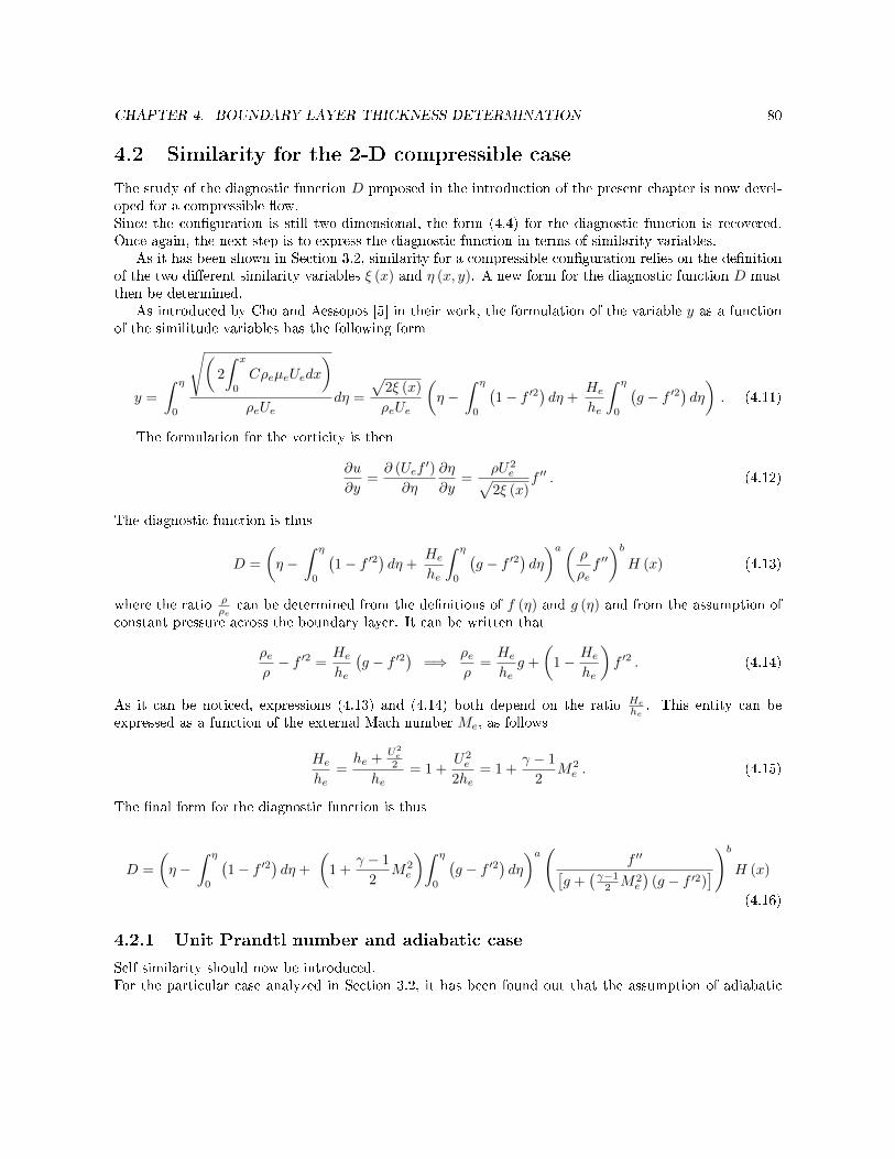
CHAPTER 4. BOUNDARY LAYER THICKNESS DETERMINATION 80
4.2 Similarity for the 2-D compressible case
The study of the diagnostic function D proposed in the introduction of the present chapter is now devel-oped for a compressible ow.Since the conguration is still two-dimensional, the form (4.4) for the diagnostic function is recovered.Once again, the next step is to express the diagnostic function in terms of similarity variables.
As it has been shown in Section 3.2, similarity for a compressible conguration relies on the denitionof the two dierent similarity variables ξ (x) and η (x, y). A new form for the diagnostic function D mustthen be determined.
As introduced by Cho and Aessopos [5] in their work, the formulation of the variable y as a functionof the similitude variables has the following form
y =
∫ η
0
√(2
∫ x
0
CρeµeUedx
)ρeUe
dη =
√2ξ (x)
ρeUe
(η −
∫ η
0
(1− f ′2
)dη +
He
he
∫ η
0
(g − f ′2
)dη
). (4.11)
The formulation for the vorticity is then
∂u
∂y=∂ (Uef
′)
∂η
∂η
∂y=
ρU2e√
2ξ (x)f ′′ . (4.12)
The diagnostic function is thus
D =
(η −
∫ η
0
(1− f ′2
)dη +
He
he
∫ η
0
(g − f ′2
)dη
)a(ρ
ρef ′′)b
H (x) (4.13)
where the ratio ρρe
can be determined from the denitions of f (η) and g (η) and from the assumption ofconstant pressure across the boundary layer. It can be written that
ρeρ− f ′2 =
He
he
(g − f ′2
)=⇒ ρe
ρ=He
heg +
(1− He
he
)f ′2 . (4.14)
As it can be noticed, expressions (4.13) and (4.14) both depend on the ratio Hehe. This entity can be
expressed as a function of the external Mach number Me, as follows
He
he=he +
U2e
2
he= 1 +
U2e
2he= 1 +
γ − 1
2M2e . (4.15)
The nal form for the diagnostic function is thus
D =
(η −
∫ η
0
(1− f ′2
)dη +
(1 +
γ − 1
2M2e
)∫ η
0
(g − f ′2
)dη
)a(f ′′[
g +(γ−1
2 M2e
)(g − f ′2)
])bH (x)
(4.16)
4.2.1 Unit Prandtl number and adiabatic case
Self similarity should now be introduced.For the particular case analyzed in Section 3.2, it has been found out that the assumption of adiabatic

CHAPTER 4. BOUNDARY LAYER THICKNESS DETERMINATION 81
wall leads to the solution g (η) = 1.The injection of this information in equation (4.16) thus gives
D =
(η +
(γ − 1
2M2e
)∫ η
0
(1− f ′2
)dη
)a(f ′′[
1 +(γ−1
2 M2e
)(1− f ′2)
])bH (x) . (4.17)
In the aforementioned equation the integral of the quantity f ′2 appears. This integral can be determinedby recalling the rst equation in system (3.45) and by performing an integration by parts on the termff ′′, that gives ∫ η
0
f ′2dη =1
1 + β(f ′′ + ff ′ + βη) . (4.18)
The nal form for D is then
D =
((1 +
γ − 1
2M2e
)η +
(−γ − 1
2M2e
)(1
1 + β
)(f ′′ + ff ′ + βη)
)a(f ′′
1 +(γ−1
2 M2e
)(1− f ′2)
)bH (x) .
(4.19)As it can be seen in relation (4.19), a new parameter appears in the expression of D for the compress-
ible case: it is the external Mach number Me.The interest is always nding the maximum of D
Dmaxfor all the self-similar velocity proles and to trace
DDmax
as a function of ηηδ, where ηδ represents the value of η that corresponds to f ′ = 0.99. ε is always
dened as ε (a, b) = ηδηmax
.
For a xed couple (a, b) the diagnostic function D is evaluated for several dierent self-similar veloc-ity proles, each of them obtained with a dierent value of the gradient parameter β in equation (3.36).In order to perform the calculation, as for the 2-D incompressible case 139 dierent values of β εB havebeen used, with B = [−0.19884, 1] and Nβ will denote the number of dierent values of β employed.Since for a xed couple (a, b) the function D depends also on the external Mach number, 20 dierentvalues of Me have been taken as additional parameters in M = [0, 1.3], with NM will denote the numberof dierent Mach numbers employed.
In order to evaluate if the specic chosen couple is correct, the variance of ε is now calculated by takinginto account the eect of two dierent and independent parameters, β andMe. By dening N = NB ·NM ,the variance of ε is determined as
V(a,b) = V ar (ε) =
∑N
i=1(εi − ε)2
N(4.20)
whereεi = εjk is the value of ε calculated forβ (j) andMe (k)
ε =
∑N
i=1(εi)
Nis themean value of all the εi
If V(a,b) is suciently small, then the value of ε used in the model can be chosen equal to ε.This procedure has been applied to approximately 106 dierent couples (a, b) and the result is shown inFigure 4.6.
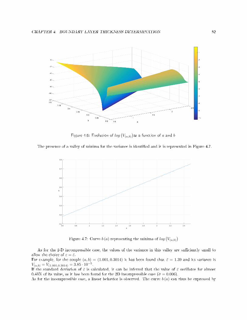
CHAPTER 4. BOUNDARY LAYER THICKNESS DETERMINATION 82
Figure 4.6: Evolution of log(V(a,b)
)as a function of a and b
The presence of a valley of minima for the variance is identied and it is represented in Figure 4.7.
0.6 0.8 1 1.2 1.4 1.6 1.8 2 2.2 2.4
a
0.1
0.2
0.3
0.4
0.5
0.6
0.7
0.8
b
Figure 4.7: Curve b (a) representing the minima of log(V(a,b)
)As for the 2-D incompressible case, the values of the variance in this valley are suciently small to
allow the choice of ε = ε.For example, for the couple (a, b) = (1.001, 0.3014) it has been found that ε = 1.39 and its variance isV(a,b) = V(1.001,0.3014) = 3.85 · 10−5.If the standard deviation of ε is calculated, it can be inferred that the value of ε oscillates for almost0.45% of its value, as it has been found for the 2D incompressible case (σ = 0.006).As for the incompressible case, a linear behavior is observed. The curve b (a) can thus be expressed by
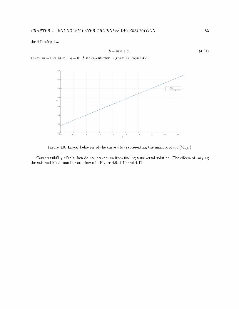
CHAPTER 4. BOUNDARY LAYER THICKNESS DETERMINATION 83
the following law
b = ma+ q , (4.21)
where m = 0.3014 and q = 0. A representation is given in Figure 4.8.
0.6 0.8 1 1.2 1.4 1.6 1.8 2 2.2 2.4
a
0.1
0.2
0.3
0.4
0.5
0.6
0.7
0.8
b
DataLinear regression
Figure 4.8: Linear behavior of the curve b (a) representing the minima of log(V(a,b)
)Compressibility eects then do not prevent us from nding a universal solution. The eects of varying
the external Mach number are shown in Figure 4.9, 4.10 and 4.11
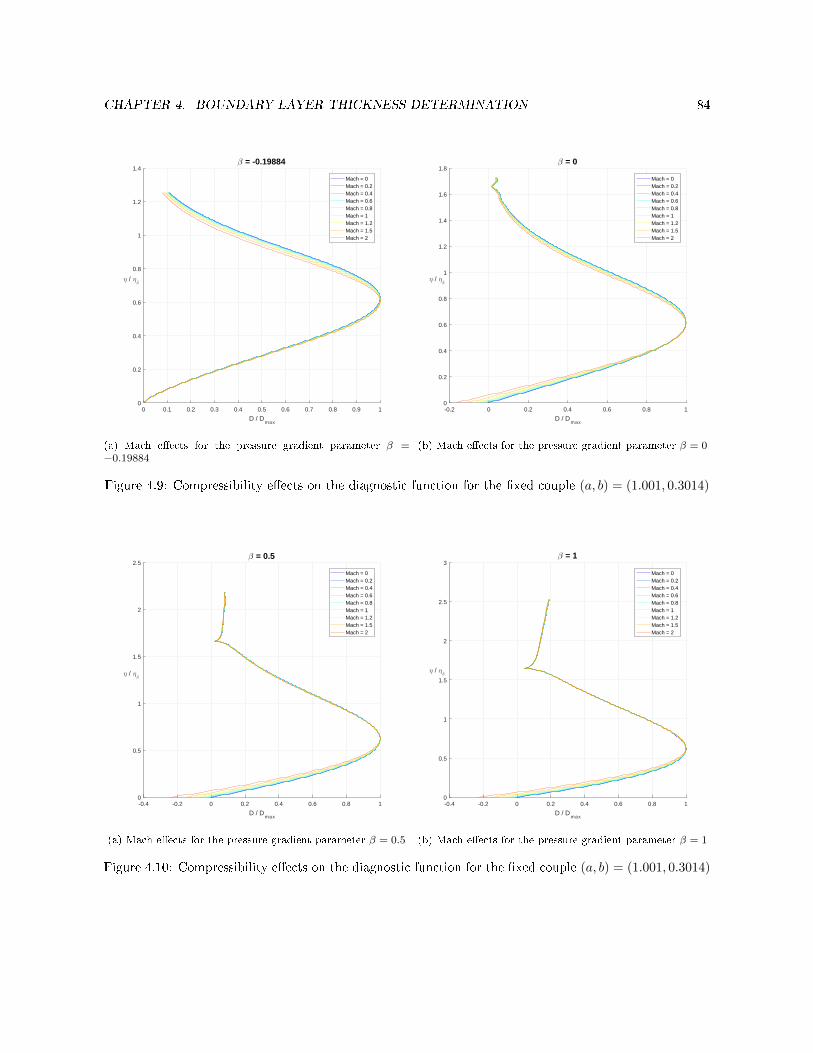
CHAPTER 4. BOUNDARY LAYER THICKNESS DETERMINATION 84
0 0.1 0.2 0.3 0.4 0.5 0.6 0.7 0.8 0.9 1
D / Dmax
0
0.2
0.4
0.6
0.8
1
1.2
1.4
η / ηδ
β = -0.19884
Mach = 0Mach = 0.2Mach = 0.4Mach = 0.6Mach = 0.8Mach = 1Mach = 1.2Mach = 1.5Mach = 2
(a) Mach eects for the pressure gradient parameter β =−0.19884
-0.2 0 0.2 0.4 0.6 0.8 1
D / Dmax
0
0.2
0.4
0.6
0.8
1
1.2
1.4
1.6
1.8
η / ηδ
β = 0
Mach = 0Mach = 0.2Mach = 0.4Mach = 0.6Mach = 0.8Mach = 1Mach = 1.2Mach = 1.5Mach = 2
(b) Mach eects for the pressure gradient parameter β = 0
Figure 4.9: Compressibility eects on the diagnostic function for the xed couple (a, b) = (1.001, 0.3014)
-0.4 -0.2 0 0.2 0.4 0.6 0.8 1
D / Dmax
0
0.5
1
1.5
2
2.5
η / ηδ
β = 0.5
Mach = 0Mach = 0.2Mach = 0.4Mach = 0.6Mach = 0.8Mach = 1Mach = 1.2Mach = 1.5Mach = 2
(a) Mach eects for the pressure gradient parameter β = 0.5
-0.4 -0.2 0 0.2 0.4 0.6 0.8 1
D / Dmax
0
0.5
1
1.5
2
2.5
3
η / ηδ
β = 1
Mach = 0Mach = 0.2Mach = 0.4Mach = 0.6Mach = 0.8Mach = 1Mach = 1.2Mach = 1.5Mach = 2
(b) Mach eects for the pressure gradient parameter β = 1
Figure 4.10: Compressibility eects on the diagnostic function for the xed couple (a, b) = (1.001, 0.3014)
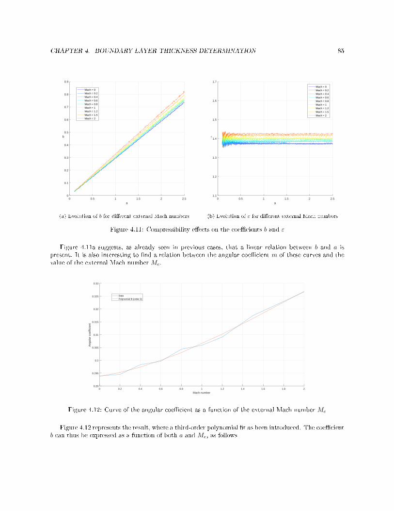
CHAPTER 4. BOUNDARY LAYER THICKNESS DETERMINATION 85
0 0.5 1 1.5 2 2.5
a
0
0.1
0.2
0.3
0.4
0.5
0.6
0.7
0.8
0.9
b
Mach = 0Mach = 0.2Mach = 0.4Mach = 0.6Mach = 0.8Mach = 1Mach = 1.2Mach = 1.5Mach = 2
(a) Evolution of b for dierent external Mach numbers
0 0.5 1 1.5 2 2.5
a
1.1
1.2
1.3
1.4
1.5
1.6
1.7
ǫ
Mach = 0Mach = 0.2Mach = 0.4Mach = 0.6Mach = 0.8Mach = 1Mach = 1.2Mach = 1.5Mach = 2
(b) Evolution of ε for dierent external Mach numbers
Figure 4.11: Compressibility eects on the coecients b and ε
Figure 4.11a suggests, as already seen in previous cases, that a linear relation between b and a ispresent. It is also interesting to nd a relation between the angular coecient m of these curves and thevalue of the external Mach number Me.
0 0.2 0.4 0.6 0.8 1 1.2 1.4 1.6 1.8 2
Mach number
0.29
0.295
0.3
0.305
0.31
0.315
0.32
0.325
0.33
Ang
ular
coe
ffici
ent
DataPolynomial fit (order 3)
Figure 4.12: Curve of the angular coecient as a function of the external Mach number Me
Figure 4.12 represents the result, where a third-order polynomial t as been introduced. The coecientb can thus be expressed as a function of both a and Me, as follows
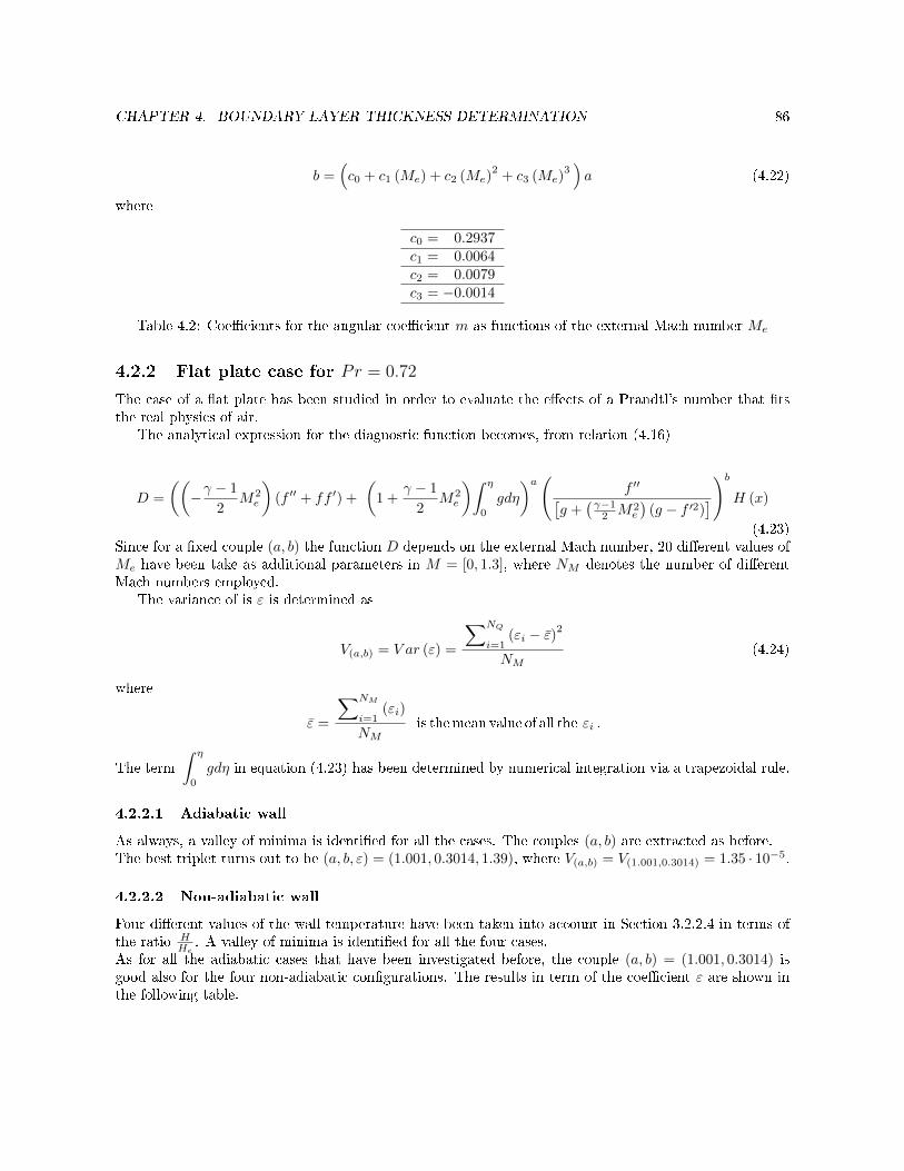
CHAPTER 4. BOUNDARY LAYER THICKNESS DETERMINATION 86
b =(c0 + c1 (Me) + c2 (Me)
2+ c3 (Me)
3)a (4.22)
where
c0 = 0.2937c1 = 0.0064c2 = 0.0079c3 = −0.0014
Table 4.2: Coecients for the angular coecient m as functions of the external Mach number Me
4.2.2 Flat plate case for Pr = 0.72
The case of a at plate has been studied in order to evaluate the eects of a Prandtl's number that tsthe real physics of air.
The analytical expression for the diagnostic function becomes, from relation (4.16)
D =
((−γ − 1
2M2e
)(f ′′ + ff ′) +
(1 +
γ − 1
2M2e
)∫ η
0
gdη
)a(f ′′[
g +(γ−1
2 M2e
)(g − f ′2)
])bH (x)
(4.23)Since for a xed couple (a, b) the function D depends on the external Mach number, 20 dierent values ofMe have been take as additional parameters in M = [0, 1.3], where NM denotes the number of dierentMach numbers employed.
The variance of is ε is determined as
V(a,b) = V ar (ε) =
∑NQ
i=1(εi − ε)2
NM(4.24)
where
ε =
∑NM
i=1(εi)
NMis themean value of all the εi .
The term
∫ η
0
gdη in equation (4.23) has been determined by numerical integration via a trapezoidal rule.
4.2.2.1 Adiabatic wall
As always, a valley of minima is identied for all the cases. The couples (a, b) are extracted as before.The best triplet turns out to be (a, b, ε) = (1.001, 0.3014, 1.39), where V(a,b) = V(1.001,0.3014) = 1.35 · 10−5.
4.2.2.2 Non-adiabatic wall
Four dierent values of the wall temperature have been taken into account in Section 3.2.2.4 in terms ofthe ratio H
He. A valley of minima is identied for all the four cases.
As for all the adiabatic cases that have been investigated before, the couple (a, b) = (1.001, 0.3014) isgood also for the four non-adiabatic congurations. The results in term of the coecient ε are shown inthe following table.
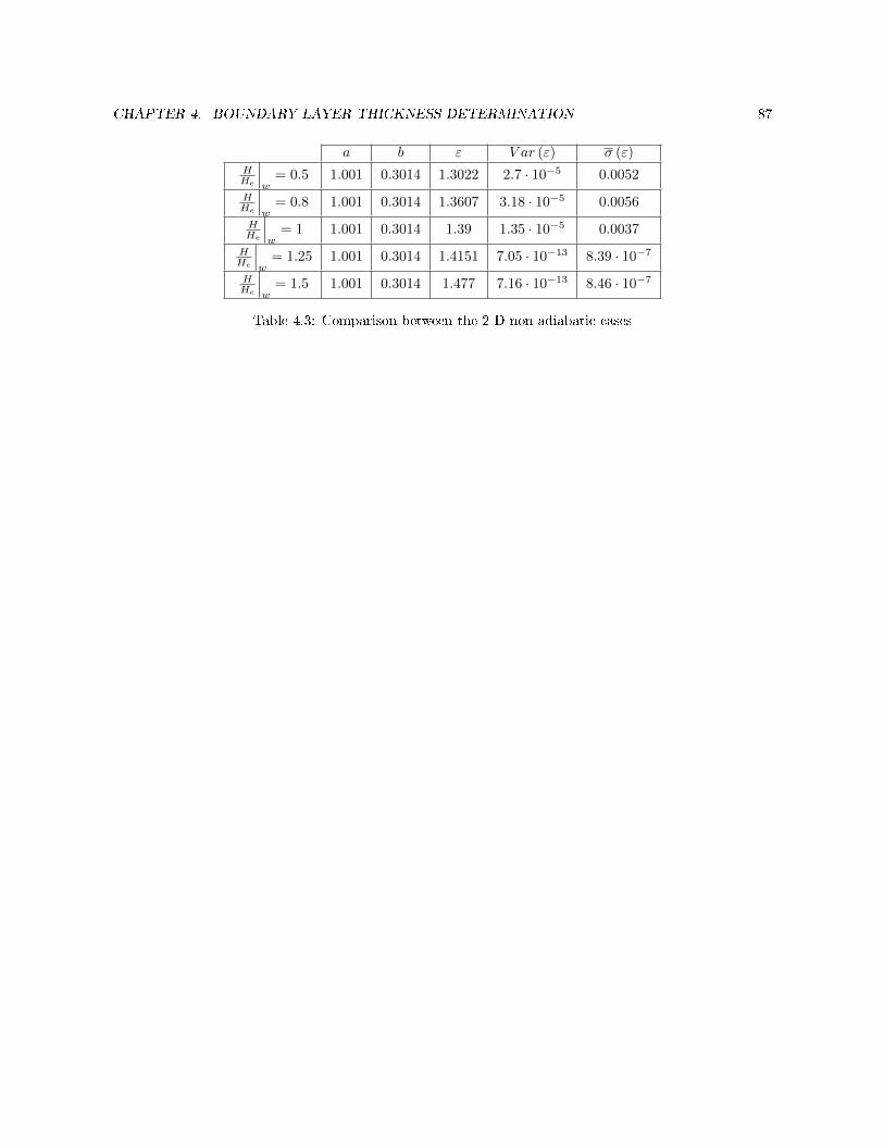
CHAPTER 4. BOUNDARY LAYER THICKNESS DETERMINATION 87
a b ε V ar (ε) σ (ε)HHe
∣∣∣w
= 0.5 1.001 0.3014 1.3022 2.7 · 10−5 0.0052
HHe
∣∣∣w
= 0.8 1.001 0.3014 1.3607 3.18 · 10−5 0.0056
HHe
∣∣∣w
= 1 1.001 0.3014 1.39 1.35 · 10−5 0.0037
HHe
∣∣∣w
= 1.25 1.001 0.3014 1.4151 7.05 · 10−13 8.39 · 10−7
HHe
∣∣∣w
= 1.5 1.001 0.3014 1.477 7.16 · 10−13 8.46 · 10−7
Table 4.3: Comparison between the 2-D non adiabatic cases
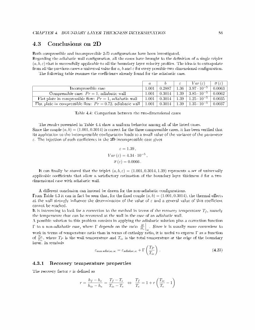
CHAPTER 4. BOUNDARY LAYER THICKNESS DETERMINATION 88
4.3 Conclusions on 2D
Both compressible and incompressible 2-D congurations have been investigated.Regarding the adiabatic wall conguration, all the cases have brought to the denition of a single triplet(a, b, ε) that is successfully applicable to all the boundary-layer velocity proles. The idea is to extrapolatefrom all the previous cases a universal value for a, b and ε for every possible two-dimensional conguration.
The following table resumes the coecients already found for the adiabatic case.
a b ε V ar (ε) σ (ε)Incompressible case 1.001 0.2887 1.36 3.97 · 10−5 0.0063
Compressible case: Pr = 1, adiabatic wall 1.001 0.3014 1.39 3.85 · 10−5 0.0062Flat plate in compressible ow: Pr = 1, adiabatic wall 1.001 0.3014 1.39 1.25 · 10−5 0.0035
Flat plate in compressible ow: Pr = 0.72, adiabatic wall 1.001 0.3014 1.39 1.35 · 10−5 0.0037
Table 4.4: Comparison between the two-dimensional cases
The results presented in Table 4.4 show a uniform behavior among all of the listed cases.Since the couple (a, b) = (1.001, 0.3014) is correct for the three compressible cases, it has been veried thatits application to the incompressible conguration leads to a small value of the variance of the parameterε. The injection of such coecients in the 2D incompressible case gives
ε = 1.39 ,
V ar (ε) = 4.34 · 10−5 ,
σ (ε) = 0.0066 .
It can nally be stated that the triplet (a, b, ε) = (1.001, 0.3014, 1.39) represents a set of universallyapplicable coecients that allow a satisfactory estimation of the boundary-layer thickness δ for a two-dimensional case with adiabatic wall.
A dierent conclusion can instead be drawn for the non-adiabatic congurations.From Table 4.3 it can in fact be seen that, for the xed couple (a, b) = (1.001, 0.3014), the thermal eectsat the wall strongly inuence the determination of the value of ε and a general value of this coecientcannot be reached.It is interesting to look for a correction to the method in terms of the recovery temperature Tf , namelythe temperature that can be recovered at the wall in the case of an adiabatic wall.A possible solution to this problem consists in applying the adiabatic solution plus a correction function
Γ to a non-adiabatic case, where Γ depends on the ratio HHe
∣∣∣w. Since it is usually more convenient to
work in terms of temperature ratio than in terms of enthalpy ratio, it is useful to express Γ as a functionof TP
Tie, where TP is the wall temperature and Tie is the total temperature at the edge of the boundary
layer. In symbols
εnon adiabatic = εadiabatic + Γ
(TPTie
). (4.25)
4.3.1 Recovery temperature properties
The recovery factor r is dened as
r =hf − hehie − he
=Tf − TeTie − Te
⇔ TfTe
= 1 + r
(TieTe− 1
)

CHAPTER 4. BOUNDARY LAYER THICKNESS DETERMINATION 89
where he and Te are, respectively, the enthalpy and the temperature at the edge of the boundary layer,while hie and Tie are the total enthalpy and total temperature at the edge of the boundary layer.The St. Venant equation yields, for an isentropic ow
TieTe
=
(1 +
γ − 1
2M2e
),
the ratioTfTe
thus becomes
TfTe
=
(1 + r
γ − 1
2M2e
)and the relation
TfTie
=TfTe
TeTie
=
(1 + r γ−1
2 M2e
)(1 + γ−1
2 M2e
)is then obtained. A unitary recuperation factor (r = 1) yields the trivial equation
TfTie
= 1 .
A classical approximation isr = Pr
12
yielding r = 0.85 when Pr = 0.725. The evolution ofTfTie
as a function of Me can be examined.
0 0.2 0.4 0.6 0.8 1 1.2 1.4Me
0.96
0.965
0.97
0.975
0.98
0.985
0.99
0.995
1
1.005
Tf/Tie
Figure 4.13: Evolution ofTfTie
as a function of Me (r = 0.85)
This allows the conclusion that r = 1 is an acceptable approximation up to supersonic Mach numbers.
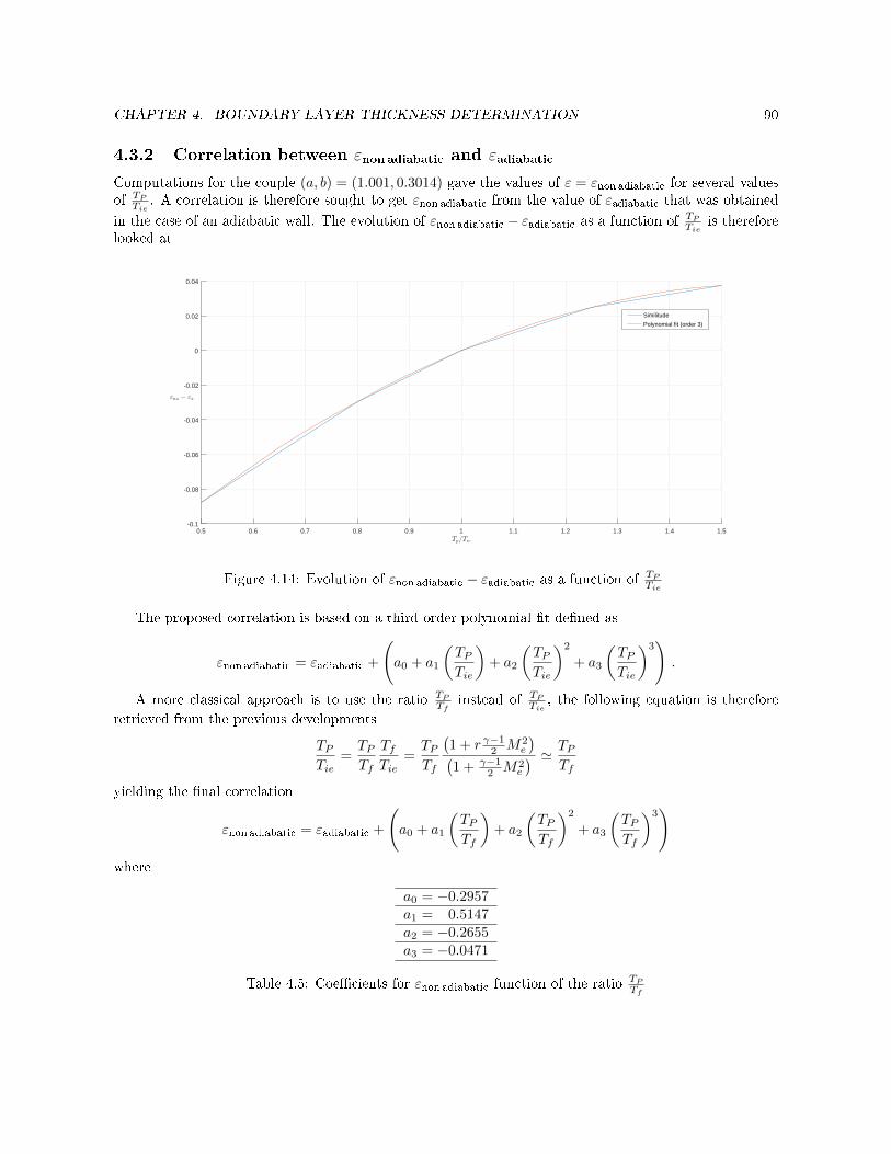
CHAPTER 4. BOUNDARY LAYER THICKNESS DETERMINATION 90
4.3.2 Correlation between εnon adiabatic and εadiabatic
Computations for the couple (a, b) = (1.001, 0.3014) gave the values of ε = εnon adiabatic for several valuesof TP
Tie. A correlation is therefore sought to get εnon adiabatic from the value of εadiabatic that was obtained
in the case of an adiabatic wall. The evolution of εnon adiabatic − εadiabatic as a function of TPTie is thereforelooked at
0.5 0.6 0.7 0.8 0.9 1 1.1 1.2 1.3 1.4 1.5Tp/Tie
-0.1
-0.08
-0.06
-0.04
-0.02
0
0.02
0.04
εna − εa
Similitude
Polynomial fit (order 3)
Figure 4.14: Evolution of εnon adiabatic − εadiabatic as a function of TPTie
The proposed correlation is based on a third-order polynomial t dened as
εnon adiabatic = εadiabatic +
(a0 + a1
(TPTie
)+ a2
(TPTie
)2
+ a3
(TPTie
)3).
A more classical approach is to use the ratio TPTf
instead of TPTie
, the following equation is therefore
retrieved from the previous developments
TPTie
=TPTf
TfTie
=TPTf
(1 + r γ−1
2 M2e
)(1 + γ−1
2 M2e
) ' TPTf
yielding the nal correlation
εnon adiabatic = εadiabatic +
(a0 + a1
(TPTf
)+ a2
(TPTf
)2
+ a3
(TPTf
)3)
where
a0 = −0.2957a1 = 0.5147a2 = −0.2655a3 = −0.0471
Table 4.5: Coecients for εnon adiabatic function of the ratio TPTf
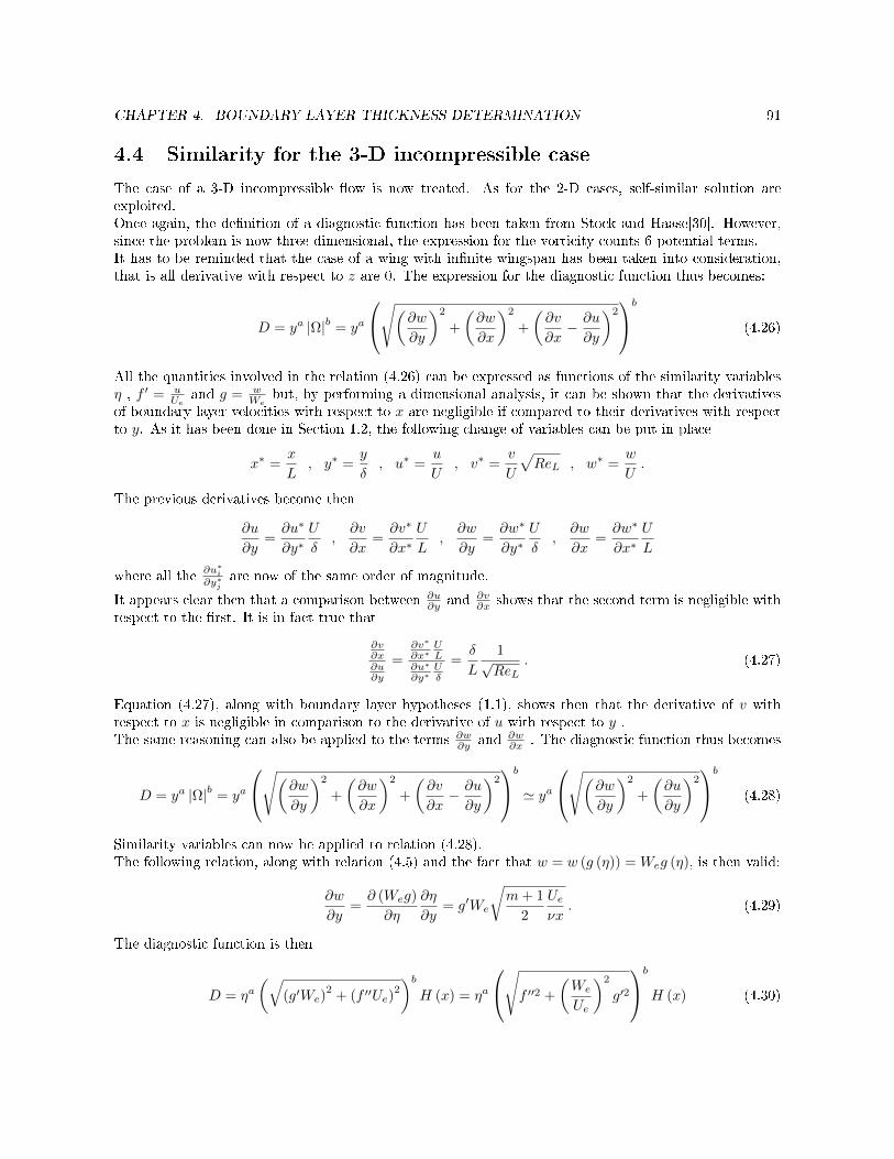
CHAPTER 4. BOUNDARY LAYER THICKNESS DETERMINATION 91
4.4 Similarity for the 3-D incompressible case
The case of a 3-D incompressible ow is now treated. As for the 2-D cases, self-similar solution areexploited.Once again, the denition of a diagnostic function has been taken from Stock and Haase[30]. However,since the problem is now three-dimensional, the expression for the vorticity counts 6 potential terms.It has to be reminded that the case of a wing with innite wingspan has been taken into consideration,that is all derivative with respect to z are 0. The expression for the diagnostic function thus becomes:
D = ya |Ω|b = ya
√(∂w∂y
)2
+
(∂w
∂x
)2
+
(∂v
∂x− ∂u
∂y
)2b
(4.26)
All the quantities involved in the relation (4.26) can be expressed as functions of the similarity variablesη , f ′ = u
Ueand g = w
Webut, by performing a dimensional analysis, it can be shown that the derivatives
of boundary layer velocities with respect to x are negligible if compared to their derivatives with respectto y. As it has been done in Section 1.2, the following change of variables can be put in place
x∗ =x
L, y∗ =
y
δ, u∗ =
u
U, v∗ =
v
U
√ReL , w∗ =
w
U.
The previous derivatives become then
∂u
∂y=∂u∗
∂y∗U
δ,∂v
∂x=∂v∗
∂x∗U
L,∂w
∂y=∂w∗
∂y∗U
δ,∂w
∂x=∂w∗
∂x∗U
L
where all the∂u∗i∂y∗j
are now of the same order of magnitude.
It appears clear then that a comparison between ∂u∂y and ∂v
∂x shows that the second term is negligible withrespect to the rst. It is in fact true that
∂v∂x∂u∂y
=∂v∗
∂x∗UL
∂u∗
∂y∗Uδ
=δ
L
1√ReL
. (4.27)
Equation (4.27), along with boundary layer hypotheses (1.1), shows then that the derivative of v withrespect to x is negligible in comparison to the derivative of u with respect to y .The same reasoning can also be applied to the terms ∂w
∂y and ∂w∂x . The diagnostic function thus becomes
D = ya |Ω|b = ya
√(∂w∂y
)2
+
(∂w
∂x
)2
+
(∂v
∂x− ∂u
∂y
)2b
' ya√(∂w
∂y
)2
+
(∂u
∂y
)2b
(4.28)
Similarity variables can now be applied to relation (4.28).The following relation, along with relation (4.5) and the fact that w = w (g (η)) = Weg (η), is then valid:
∂w
∂y=∂ (Weg)
∂η
∂η
∂y= g′We
√m+ 1
2
Ueνx
. (4.29)
The diagnostic function is then
D = ηa(√
(g′We)2
+ (f ′′Ue)2
)bH (x) = ηa
√f ′′2 +
(We
Ue
)2
g′2
b
H (x) (4.30)
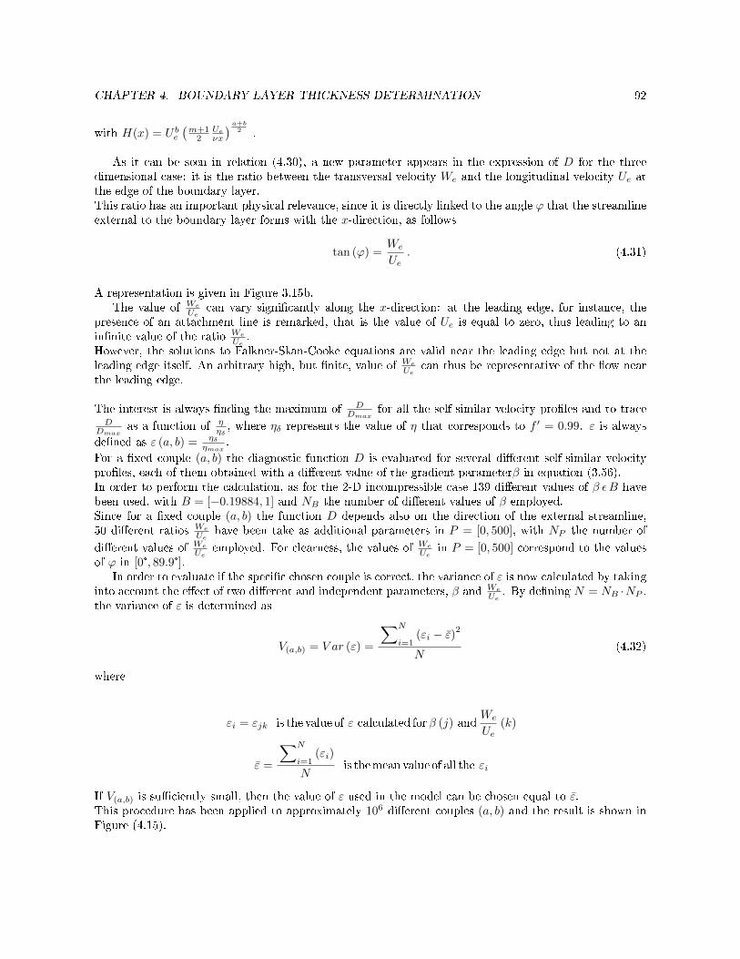
CHAPTER 4. BOUNDARY LAYER THICKNESS DETERMINATION 92
with H(x) = U be(m+1
2Ueνx
) a+b2 .
As it can be seen in relation (4.30), a new parameter appears in the expression of D for the threedimensional case: it is the ratio between the transversal velocity We and the longitudinal velocity Ue atthe edge of the boundary layer.This ratio has an important physical relevance, since it is directly linked to the angle ϕ that the streamlineexternal to the boundary layer forms with the x-direction, as follows
tan (ϕ) =We
Ue. (4.31)
A representation is given in Figure 3.15b.The value of We
Uecan vary signicantly along the x-direction: at the leading edge, for instance, the
presence of an attachment line is remarked, that is the value of Ue is equal to zero, thus leading to aninnite value of the ratio We
Ue.
However, the solutions to Falkner-Skan-Cooke equations are valid near the leading edge but not at theleading edge itself. An arbitrary high, but nite, value of We
Uecan thus be representative of the ow near
the leading edge.
The interest is always nding the maximum of DDmax
for all the self-similar velocity proles and to traceD
Dmaxas a function of η
ηδ, where ηδ represents the value of η that corresponds to f ′ = 0.99. ε is always
dened as ε (a, b) = ηδηmax
.
For a xed couple (a, b) the diagnostic function D is evaluated for several dierent self-similar velocityproles, each of them obtained with a dierent value of the gradient parameterβ in equation (3.56).In order to perform the calculation, as for the 2-D incompressible case 139 dierent values of β εB havebeen used, with B = [−0.19884, 1] and NB the number of dierent values of β employed.Since for a xed couple (a, b) the function D depends also on the direction of the external streamline,50 dierent ratios We
Uehave been take as additional parameters in P = [0, 500], with NP the number of
dierent values of We
Ueemployed. For clearness, the values of We
Uein P = [0, 500] correspond to the values
of ϕ in [0°, 89.9°].In order to evaluate if the specic chosen couple is correct, the variance of ε is now calculated by taking
into account the eect of two dierent and independent parameters, β and We
Ue. By dening N = NB ·NP ,
the variance of ε is determined as
V(a,b) = V ar (ε) =
∑N
i=1(εi − ε)2
N(4.32)
where
εi = εjk is the value of ε calculated forβ (j) andWe
Ue(k)
ε =
∑N
i=1(εi)
Nis themean value of all the εi
If V(a,b) is suciently small, then the value of ε used in the model can be chosen equal to ε.This procedure has been applied to approximately 106 dierent couples (a, b) and the result is shown inFigure (4.15).
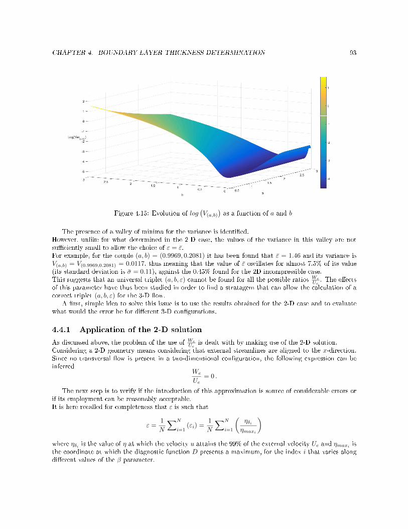
CHAPTER 4. BOUNDARY LAYER THICKNESS DETERMINATION 93
Figure 4.15: Evolution of log(V(a,b)
)as a function of a and b
The presence of a valley of minima for the variance is identied.However, unlike for what determined in the 2-D case, the values of the variance in this valley are notsuciently small to allow the choice of ε = ε.For example, for the couple (a, b) = (0.9969, 0.2081) it has been found that ε = 1.46 and its variance isV(a,b) = V(0.9969,0.2081) = 0.0117, thus meaning that the value of ε oscillates for almost 7.5% of its value(its standard deviation is σ = 0.11), against the 0.45% found for the 2D incompressible case.This suggests that an universal triplet (a, b, ε) cannot be found for all the possible ratios We
Ue. The eects
of this parameter have thus been studied in order to nd a stratagem that can allow the calculation of acorrect triplet (a, b, ε) for the 3-D ow.
A rst, simple idea to solve this issue is to use the results obtained for the 2-D case and to evaluatewhat would the error be for dierent 3-D congurations.
4.4.1 Application of the 2-D solution
As discussed above, the problem of the use of We
Ueis dealt with by making use of the 2-D solution.
Considering a 2-D geometry means considering that external streamlines are aligned to the x-direction.Since no transversal ow is present in a two-dimensional conguration, the following expression can beinferred
We
Ue= 0 .
The next step is to verify if the introduction of this approximation is source of considerable errors orif its employment can be reasonably acceptable.It is here recalled for completeness that ε is such that
ε =1
N
∑N
i=1(εi) =
1
N
∑N
i=1
(ηδiηmaxi
)where ηδi is the value of η at which the velocity u attains the 99% of the external velocity Ue and ηmaxi isthe coordinate at which the diagnostic function D presents a maximum, for the index i that varies alongdierent values of the β parameter.
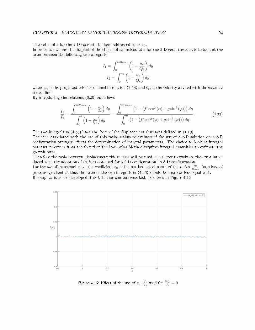
CHAPTER 4. BOUNDARY LAYER THICKNESS DETERMINATION 94
The value of ε for the 2-D case will be here addressed to as ε0.In order to evaluate the impact of the choice of ε0 instead of ε for the 3-D case, the idea is to look at theratio between the following two integrals
I1 =
∫ ε0ηmax
0
(1− ue
Qe
)dy
I2 =
∫ ηδ
0
(1− ue
Qe
)dy
where ue is the projected velocity dened in relation (3.58) and Qe is the velocity aligned with the externalstreamline.By introducing the relations (3.59) as follows
I1I2
=
∫ ε0ymax
0
(1− ue
Qe
)dy∫ δ
0
(1− ue
Qe
)dy
=
∫ ε0ηmax
0
(1−
(f ′ cos2 (ϕ) + g sin2 (ϕ)
))dη∫ ηδ
0
(1−
(f ′ cos2 (ϕ) + g sin2 (ϕ)
))dη
. (4.33)
The two integrals in (4.33) have the form of the displacement thickness dened in (1.19).The idea associated with the use of this ratio is thus to evaluate if the use of a 2-D solution on a 3-Dconguration strongly aects the determination of integral parameters. The choice to look at integralparameters comes from the fact that the Parabolas Method requires integral quantities to estimate thegrowth rates.Therefore the ratio between displacement thicknesses will be used as a meter to evaluate the error intro-duced with the adoption of (a, b, ε) obtained for a 2-D conguration on 3-D conguration.For the two-dimensional case, the coecient ε0 is the mathematical mean of the ratios ηδ
ηmaxfunctions of
pressure gradient β, thus the ratio of the two integrals in (4.33) should be more or less equal to 1.If computations are developed, this behavior can be remarked, as shown in Figure 4.16
-0.2 0 0.2 0.4 0.6 0.8 1
β
0.9
0.95
1
1.05
1.1
1.15
I1 / I
2
We / U
e = 0 - φ = 0 °
Figure 4.16: Eect of the use of ε0:I1I2
vs β for We
Ue= 0
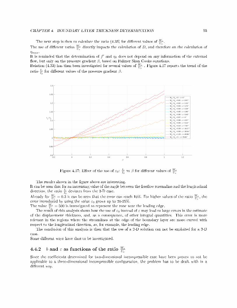
CHAPTER 4. BOUNDARY LAYER THICKNESS DETERMINATION 95
The next step is then to calculate the ratio (4.33) for dierent values of We
Ue.
The use of dierent ratios We
Uedirectly impacts the calculation of D, and therefore on the calculation of
ηmax.It is reminded that the determination of f ′ and ηδ does not depend on any information of the externalow, but only on the pressure gradient β, based on Falkner-Skan-Cooke equations.Relation (4.33) has then been investigated for several values of We
Ue. Figure 4.17 reports the trend of the
ratio I1I2
for dierent values of the pressure gradient β.
-0.2 0 0.2 0.4 0.6 0.8 1 1.2
β
0.9
0.95
1
1.05
1.1
1.15
1.2
1.25
1.3
I1 / I
2
We / U
e = 0 - φ = 0 °
We / U
e = 0.01 - φ = 0.57 °
We / U
e = 0.02 - φ = 1.15 °
We / U
e = 0.03 - φ = 1.72 °
We / U
e = 0.04 - φ = 2.29 °
We / U
e = 0.05 - φ = 2.86 °
We / U
e = 0.06 - φ = 3.43 °
We / U
e = 0.07 - φ = 4 °
We / U
e = 0.08 - φ = 4.57 °
We / U
e = 0.09 - φ = 5.14 °
We / U
e = 0.14 - φ = 7.97 °
We / U
e = 0.29 - φ = 16.17 °
We / U
e = 0.59 - φ = 30.54 °
We / U
e = 1.19 - φ = 49.96 °
We / U
e = 5 - φ = 78.69 °
Figure 4.17: Eect of the use of ε0:I1I2
vs β for dierent values of We
Ue
The results shown in the gure above are interesting.It can be seen that for an increasing value of the angle between the freeow streamline and the longitudinaldirection, the ratio I1
I2deviates from the 2-D case.
Already for We
Ue= 0.3 it can be seen that the error can reach 10%. For higher values of the ratio We
Ue, the
error introduced by using the value ε0 grows up to 20-25%.The value We
Ue= 500 is investigated to represent the zone near the leading edge.
The result of this analysis shows how the use of ε0 instead of ε may lead to large errors in the estimateof the displacement thickness, and, as a consequence, of other integral quantities. This error is morerelevant in the regions where the streamlines at the edge of the boundary layer are more curved withrespect to the longitudinal direction, as, for example, the leading edge.
The conclusion of this analysis is then that the use of a 2-D solution can not be exploited for a 3-Dcase.Some dierent ways have thus to be investigated.
4.4.2 b and ε as functions of the ratio We
Ue
Since the coecients determined for two-dimensional incompressible case have been proven to not beapplicable to a three-dimensional incompressible conguration, the problem has to be dealt with in adierent way.
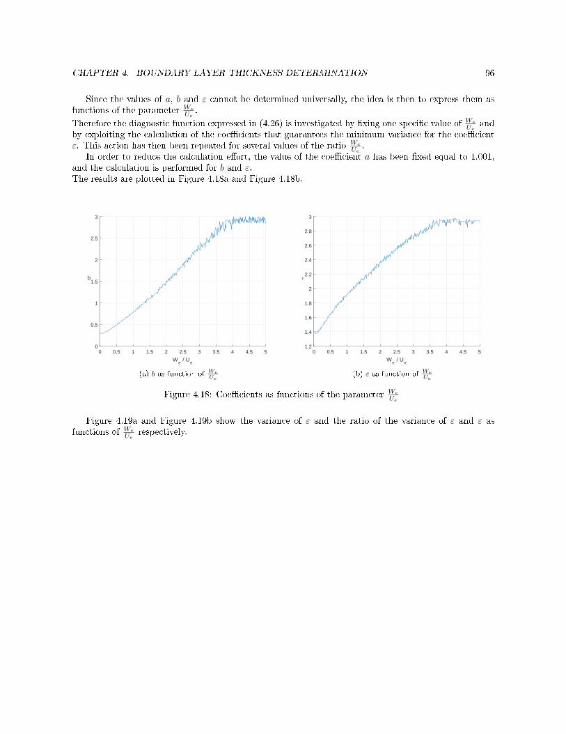
CHAPTER 4. BOUNDARY LAYER THICKNESS DETERMINATION 96
Since the values of a, b and ε cannot be determined universally, the idea is then to express them asfunctions of the parameter We
Ue.
Therefore the diagnostic function expressed in (4.26) is investigated by xing one specic value of We
Ueand
by exploiting the calculation of the coecients that guarantees the minimum variance for the coecientε. This action has then been repeated for several values of the ratio We
Ue.
In order to reduce the calculation eort, the value of the coecient a has been xed equal to 1.001,and the calculation is performed for b and ε.The results are plotted in Figure 4.18a and Figure 4.18b.
0 0.5 1 1.5 2 2.5 3 3.5 4 4.5 5
We / U
e
0
0.5
1
1.5
2
2.5
3
b
(a) b as function of WeUe
0 0.5 1 1.5 2 2.5 3 3.5 4 4.5 5
We / U
e
1.2
1.4
1.6
1.8
2
2.2
2.4
2.6
2.8
3
ǫ
(b) ε as function of WeUe
Figure 4.18: Coecients as functions of the parameter We
Ue
Figure 4.19a and Figure 4.19b show the variance of ε and the ratio of the variance of ε and ε asfunctions of We
Uerespectively.
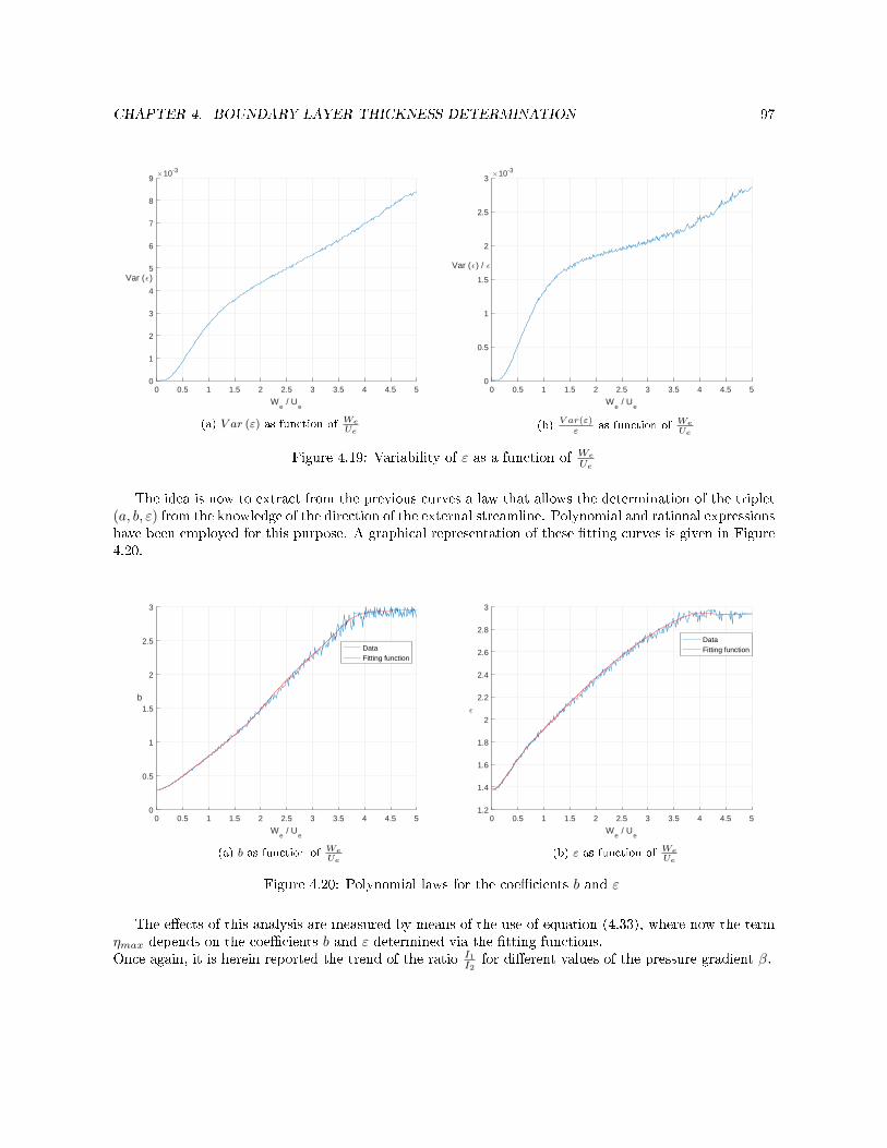
CHAPTER 4. BOUNDARY LAYER THICKNESS DETERMINATION 97
0 0.5 1 1.5 2 2.5 3 3.5 4 4.5 5
We / U
e
0
1
2
3
4
5
6
7
8
9
Var (ǫ)
×10-3
(a) V ar (ε) as function of WeUe
0 0.5 1 1.5 2 2.5 3 3.5 4 4.5 5
We / U
e
0
0.5
1
1.5
2
2.5
3
Var (ǫ) / ǫ
×10-3
(b)V ar(ε)ε
as function of WeUe
Figure 4.19: Variability of ε as a function of We
Ue
The idea is now to extract from the previous curves a law that allows the determination of the triplet(a, b, ε) from the knowledge of the direction of the external streamline. Polynomial and rational expressionshave been employed for this purpose. A graphical representation of these tting curves is given in Figure4.20.
0 0.5 1 1.5 2 2.5 3 3.5 4 4.5 5
We / U
e
0
0.5
1
1.5
2
2.5
3
b
DataFitting function
(a) b as function of WeUe
0 0.5 1 1.5 2 2.5 3 3.5 4 4.5 5
We / U
e
1.2
1.4
1.6
1.8
2
2.2
2.4
2.6
2.8
3
ǫ
DataFitting function
(b) ε as function of WeUe
Figure 4.20: Polynomial laws for the coecients b and ε
The eects of this analysis are measured by means of the use of equation (4.33), where now the termηmax depends on the coecients b and ε determined via the tting functions.Once again, it is herein reported the trend of the ratio I1
I2for dierent values of the pressure gradient β.
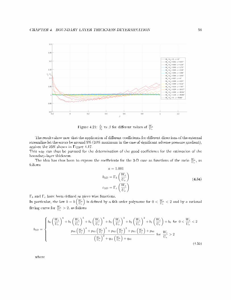
CHAPTER 4. BOUNDARY LAYER THICKNESS DETERMINATION 98
-0.2 0 0.2 0.4 0.6 0.8 1 1.2
β
0.9
0.95
1
1.05
1.1
1.15
1.2
1.25
1.3
I1 / I
2
We / U
e = 0 - φ = 0 °
We / U
e = 0.01 - φ = 0.57 °
We / U
e = 0.02 - φ = 1.15 °
We / U
e = 0.03 - φ = 1.72 °
We / U
e = 0.04 - φ = 2.29 °
We / U
e = 0.05 - φ = 2.86 °
We / U
e = 0.06 - φ = 3.43 °
We / U
e = 0.07 - φ = 4 °
We / U
e = 0.08 - φ = 4.57 °
We / U
e = 0.09 - φ = 5.14 °
We / U
e = 0.14 - φ = 7.97 °
We / U
e = 0.29 - φ = 16.17 °
We / U
e = 0.59 - φ = 30.54 °
We / U
e = 1.19 - φ = 49.96 °
We / U
e = 5 - φ = 78.69 °
Figure 4.21: I1I2
vs β for dierent values of We
Ue
The results show now that the application of dierent coecients for dierent directions of the externalstreamline let the errors be around 5% (10% maximum in the case of signicant adverse pressure gradient),against the 25% shown in Figure 4.17.This way can thus be pursued for the determination of the good coecients for the estimation of theboundary-layer thickness.
The idea has thus been to express the coecients for the 3-D case as functions of the ratio We
Ue, as
followsa = 1.001
b3D = Γb
(We
Ue
)ε3D = Γε
(We
Ue
) (4.34)
Γb and Γε have been dened as piece-wise functions.
In particular, the law b = b(We
Ue
)is dened by a 6th order polynome for 0 < We
Ue< 2 and by a rational
tting curve for We
Ue> 2, as follows
b3D =
b6
(We
Ue
)6
+ b5
(We
Ue
)5
+ b4
(We
Ue
)4
+ b3
(We
Ue
)3
+ b2
(We
Ue
)2
+ b1
(We
Ue
)+ b0 for 0 <
We
Ue< 2
pb4(WeUe
)4+ pb3
(WeUe
)3+ pb2
(WeUe
)2+ pb1
(WeUe
)+ pb0(
WeUe
)2+ qb1
(WeUe
)+ qb0
forWe
Ue> 2
(4.35)
where

CHAPTER 4. BOUNDARY LAYER THICKNESS DETERMINATION 99
b0 = 0.2943 pb0 = −13.9619b1 = 0.0279 pb1 = 29.2044b2 = 1.3480 pb2 = −14.6485b3 = −1.7060 pb3 = 2.6810b4 = 1.1930 pb4 = −0.1528b5 = −0.4307 qb0 = 14.2100b6 = 0.0639 qb1 = −7.4710
Table 4.6: Coecients for b as a function of the ratio We
Ue
The law ε = ε(We
Ue
)is dened by a 6th order polynome for 0 < We
Ue< 1.5 and by a rational tting
curve for We
Ue> 1.5, as follows
ε3D =
ε6
(We
Ue
)6
+ ε5
(We
Ue
)5
+ ε4
(We
Ue
)4
+ ε3
(We
Ue
)3
+ ε2
(We
Ue
)2
+ ε1
(We
Ue
)+ ε0 for 0 <
We
Ue< 1.5
pε5(WeUe
)5+ pε4
(WeUe
)4+ pε3
(WeUe
)3+ pε2
(WeUe
)2+ pε1
(WeUe
)+ pε0(
WeUe
)3+ qε2
(WeUe
)2+ qε1
(WeUe
)+ qε0
forWe
Ue> 1.5
(4.36)
where
ε0 = 1.3770 pε1 = 16.5221ε1 = −7.3090 10−3 pε2 = 9.9819
ε2 = 2.5700 pε3 = −7.7037ε3 = −4.3630 pε4 = 1.4433ε4 = 3.4310 pε5 = −0.0757ε5 = −1.2650 qε0 = −19.0240ε6 = 0.1726 qε1 = 26.2600
pε0 = −21.9991 qε2 = −9.318
Table 4.7: Coecients for ε as a function of the ratio We
Ue
CHAPTER 4. BOUNDARY LAYER THICKNESS DETERMINATION 100
4.4.3 Study on the parameter We
Ue
The ratio between the transversal and longitudinal external velocity is now analyzed.It is reminded that all the present study aims at nding an estimation of δ in a RANS code.
In a RANS code the velocities We and Ue at the edge of the boundary layer are the values of thevelocity extracted from the mean ow at the distance δ from the wall. These quantities can thus berecovered only if the boundary-layer thickness is known.The only available quantities before the determination of δ are located at the wall.The point is therefore to bypass the direct use of We
Ueby using wall characteristic quantities that are known
in a RANS solver.
4.4.3.1 Skin friction - freeow streamline correlation
As already above mentioned, in a RANS code the knowledge of the streamline direction is known onlyonce the calculation is completed, not before.The idea is then to use some information at the lower boundary of the boundary layer, i.e. at the wall.The information about the ow behavior at the wall is in fact accessible at each iteration of the RANScalculation.
Two relevant pieces of information that can be recovered are the wall skin friction and the wall pressuregradient.In particular, the original parameter We
Uerepresents the tangent of the angle ϕ that the freeow streamline
creates with respect to the longitudinal direction.The idea is then to correlate this angle to the angle between the wall skin friction vector and wall pressuregradient, identied as θ.A qualitative representation of those angles is given in Figure 4.22.It must be recalled that the reference case is that of an innite wing with no pressure gradient in thetransversal direction, thus the wall pressure gradient is aligned with the x-direction.
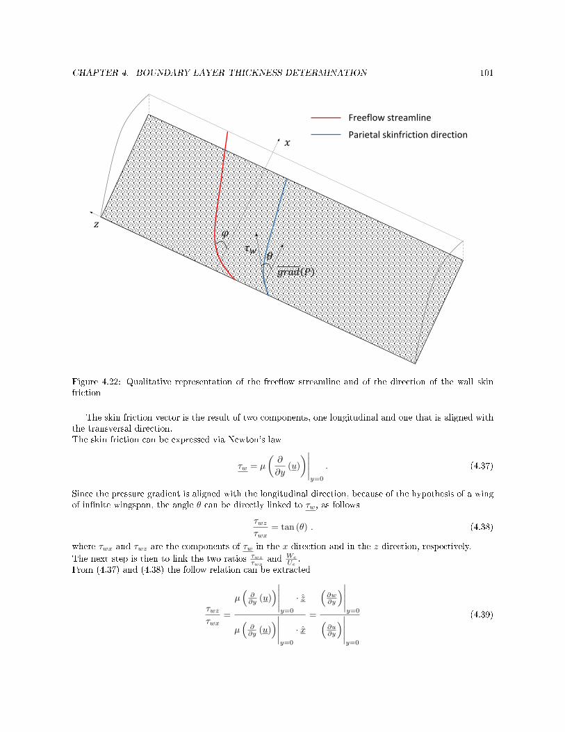
CHAPTER 4. BOUNDARY LAYER THICKNESS DETERMINATION 101
𝜑
𝜃
𝑥
𝑧
Freeflow streamline
Parietal skinfriction direction
𝑔𝑟𝑎𝑑 (𝑃)
𝜏𝑤
Figure 4.22: Qualitative representation of the freeow streamline and of the direction of the wall skinfriction
The skin friction vector is the result of two components, one longitudinal and one that is aligned withthe transversal direction.The skin friction can be expressed via Newton's law
τw = µ
(∂
∂y(u)
)∣∣∣∣∣y=0
. (4.37)
Since the pressure gradient is aligned with the longitudinal direction, because of the hypothesis of a wingof innite wingspan, the angle θ can be directly linked to τw, as follows
τwzτwx
= tan (θ) . (4.38)
where τwx and τwz are the components of τw in the x-direction and in the z-direction, respectively.
The next step is then to link the two ratios τwzτwx
and We
Ue.
From (4.37) and (4.38) the follow relation can be extracted
τwzτwx
=
µ(∂∂y (u)
)∣∣∣∣∣y=0
· z
µ(∂∂y (u)
)∣∣∣∣∣y=0
· x=
(∂w∂y
)∣∣∣∣∣y=0(
∂u∂y
)∣∣∣∣∣y=0
(4.39)
CHAPTER 4. BOUNDARY LAYER THICKNESS DETERMINATION 102
where x and z are the unit vectors directed respectively in the x-direction and z-direction.Once again, self-similarity is exploited.As already introduced in Section 4.1 and 4.4, the derivatives in (4.39) can be expressed as functions ofthe similarity variables.Relations (4.5) and (4.29) are here reported for clearness
∂u
∂y= f ′′Ue
√m+ 1
2
Ueνx
∂w
∂y= g′We
√m+ 1
2
Ueνx
.
Equation (4.39) can nally be written as
We
Ue=
(f ′′)∣∣η=0
(g′)∣∣η=0
τwzτwx
. (4.40)
Equation (4.40) is the desired relation, since it allows the determination of the desired coecients (a, b, ε)from an accessible information at the wall of the geometry that is investigated.In order to evaluate if this relation leads to satisfactory results, a validation is put in place through thesolution of the boundary-layer ow over a wing of innite wingspan generated through the use of 3C3D.This validation is herein presented.
4.4.3.2 Validation
The validation of the relation (4.40) is now attempted.Since this equation involves both quantities at the wall and quantities at the edge of the boundary layer,a complete solution of a boundary-layer ow is needed.The boundary-layer solver 3C3D, developed by ONERA, has thus been employed.
The case of an innite wing with a sweep angle Λ = 60°, at incidence α = −8° and with an incidentvelocity of U∞ = 70 m/s is considered. The reference airfoil is the ONERA D airfoil. This case is widelyused at ONERA for comparisons and validations, since it is known to generate crossow-type instabilities.
The solution is given in terms of the ow properties at several stations along the longitudinal direction.For each station the following quantities can be recovered over the suction side:
the dimensionless coordinate along the chord xc and the dimensionless coordinate over the prole
geometry sc , where is the chord
the three velocity components u, v and w over the whole the boundary-layer thickness
the rst- and second-order derivatives of u, v and w with respect to y
the rst- and second-order derivatives of u, v and w with respect to s, where s is the curvilinearcoordinate along the prole
the density proles ρ over the whole boundary-layer thickness
the absolute value of the velocity vector aligned with the streamline at the edge of the boundarylayer Qe
the external value of µe, ρe, Te, Me and the Reynolds number Reδ1 = Qeδ1ρeµe
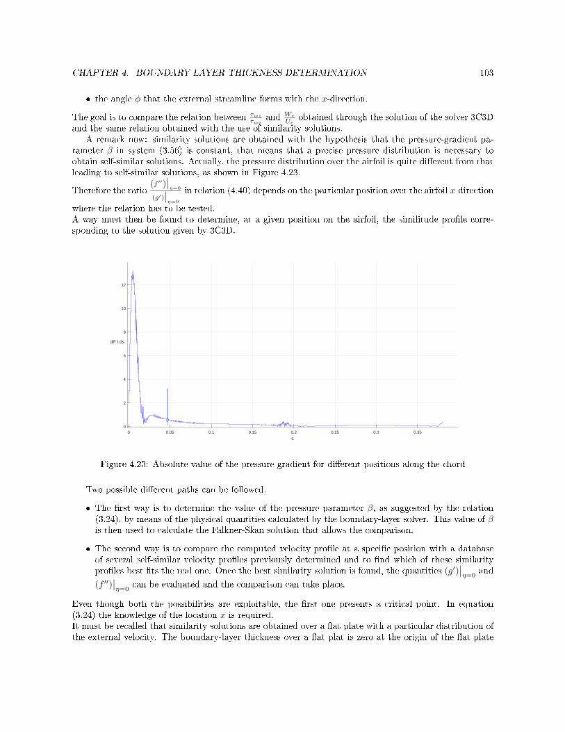
CHAPTER 4. BOUNDARY LAYER THICKNESS DETERMINATION 103
the angle φ that the external streamline forms with the x-direction.
The goal is to compare the relation between τwzτwx
and We
Ueobtained through the solution of the solver 3C3D
and the same relation obtained with the use of similarity solutions.A remark now: similarity solutions are obtained with the hypothesis that the pressure-gradient pa-
rameter β in system (3.56) is constant, that means that a precise pressure distribution is necessary toobtain self-similar solutions. Actually, the pressure distribution over the airfoil is quite dierent from thatleading to self-similar solutions, as shown in Figure 4.23.
Therefore the ratio(f ′′)
∣∣η=0
(g′)∣∣η=0
in relation (4.40) depends on the particular position over the airfoil x-direction
where the relation has to be tested.A way must then be found to determine, at a given position on the airfoil, the similitude prole corre-sponding to the solution given by 3C3D.
0 0.05 0.1 0.15 0.2 0.25 0.3 0.35
s
0
2
4
6
8
10
12
dP / ds
Figure 4.23: Absolute value of the pressure gradient for dierent positions along the chord
Two possible dierent paths can be followed.
The rst way is to determine the value of the pressure parameter β, as suggested by the relation(3.24), by means of the physical quantities calculated by the boundary-layer solver. This value of βis then used to calculate the Falkner-Skan solution that allows the comparison.
The second way is to compare the computed velocity prole at a specic position with a databaseof several self-similar velocity proles previously determined and to nd which of these similarityproles best ts the real one. Once the best similarity solution is found, the quantities (g′)
∣∣η=0
and
(f ′′)∣∣η=0
can be evaluated and the comparison can take place.
Even though both the possibilities are exploitable, the rst one presents a critical point. In equation(3.24) the knowledge of the location x is required.It must be recalled that similarity solutions are obtained over a at plate with a particular distribution ofthe external velocity. The boundary-layer thickness over a at plat is zero at the origin of the at plate
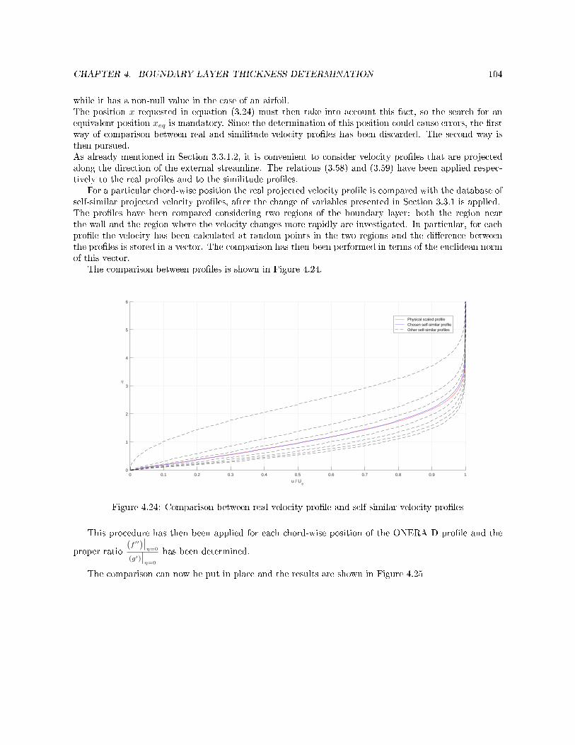
CHAPTER 4. BOUNDARY LAYER THICKNESS DETERMINATION 104
while it has a non-null value in the case of an airfoil.The position x requested in equation (3.24) must then take into account this fact, so the search for anequivalent position xeq is mandatory. Since the determination of this position could cause errors, the rstway of comparison between real and similitude velocity proles has been discarded. The second way isthen pursued.As already mentioned in Section 3.3.1.2, it is convenient to consider velocity proles that are projectedalong the direction of the external streamline. The relations (3.58) and (3.59) have been applied respec-tively to the real proles and to the similitude proles.
For a particular chord-wise position the real projected velocity prole is compared with the database ofself-similar projected velocity proles, after the change of variables presented in Section 3.3.1 is applied.The proles have been compared considering two regions of the boundary layer: both the region nearthe wall and the region where the velocity changes more rapidly are investigated. In particular, for eachprole the velocity has been calculated at random points in the two regions and the dierence betweenthe proles is stored in a vector. The comparison has then been performed in terms of the euclidean normof this vector.
The comparison between proles is shown in Figure 4.24.
0 0.1 0.2 0.3 0.4 0.5 0.6 0.7 0.8 0.9 1
u / Ue
0
1
2
3
4
5
6
η
Physical scaled profile Chosen self-similar profile Other self-similar profiles
Figure 4.24: Comparison between real velocity prole and self-similar velocity proles
This procedure has then been applied for each chord-wise position of the ONERA D prole and the
proper ratio(f ′′)
∣∣η=0
(g′)∣∣η=0
has been determined.
The comparison can now be put in place and the results are shown in Figure 4.25
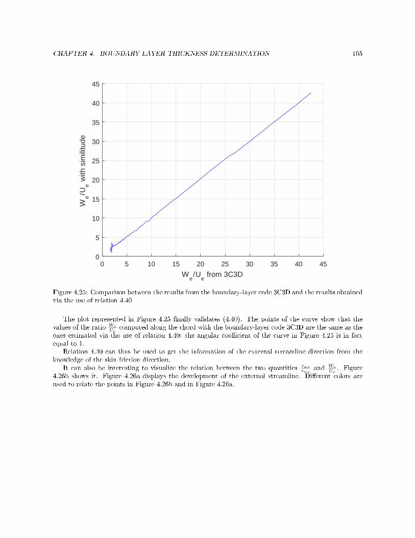
CHAPTER 4. BOUNDARY LAYER THICKNESS DETERMINATION 105
0 5 10 15 20 25 30 35 40 45
We/U
e from 3C3D
0
5
10
15
20
25
30
35
40
45W
e/U
e w
ith s
imili
tude
Figure 4.25: Comparison between the results from the boundary-layer code 3C3D and the results obtainedvia the use of relation 4.40
The plot represented in Figure 4.25 nally validates (4.40). The points of the curve show that thevalues of the ratio We
Uecomputed along the chord with the boundary-layer code 3C3D are the same as the
ones estimated via the use of relation 4.40: the angular coecient of the curve in Figure 4.25 is in factequal to 1.
Relation 4.40 can thus be used to get the information of the external streamline direction from theknowledge of the skin friction direction.
It can also be interesting to visualize the relation between the two quantities τwzτwx
and We
Ue. Figure
4.26b shows it. Figure 4.26a displays the development of the external streamline. Dierent colors areused to relate the points in Figure 4.26b and in Figure 4.26a.
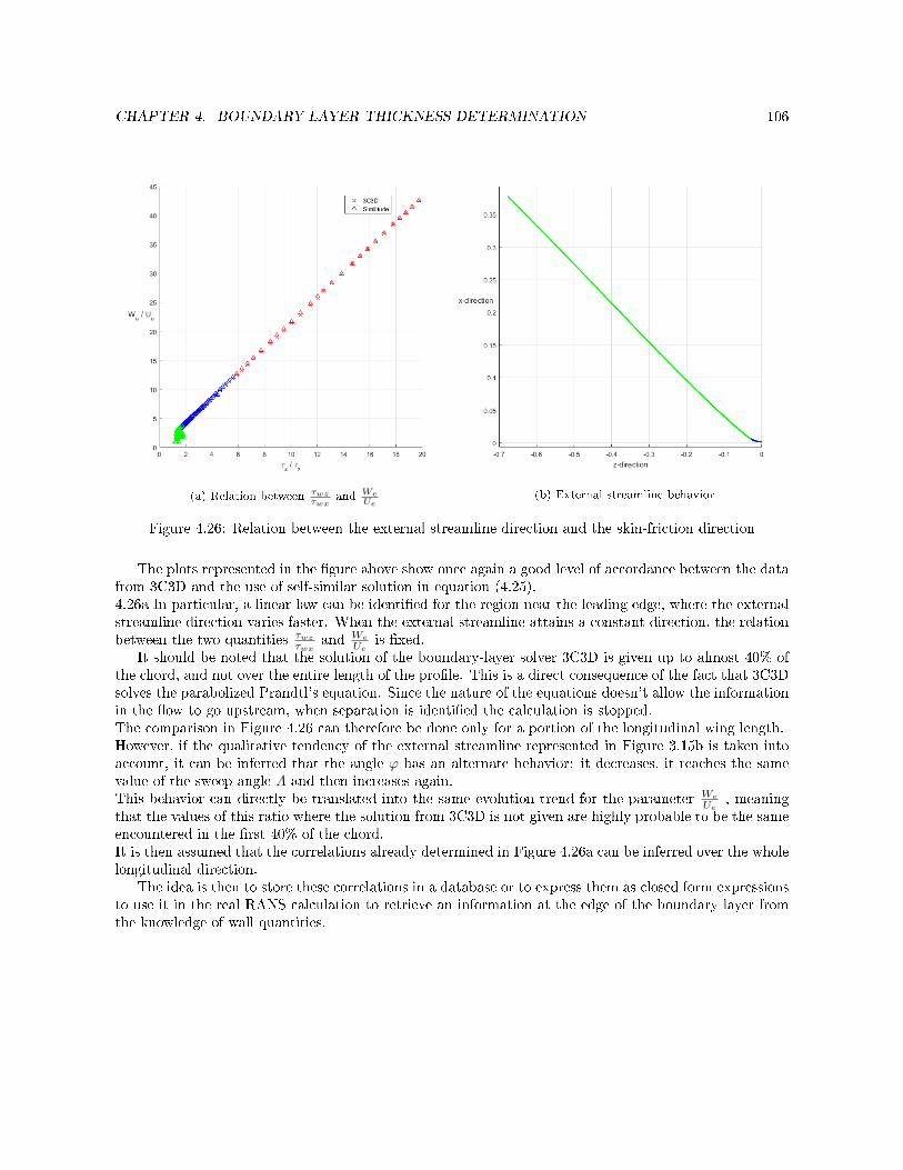
CHAPTER 4. BOUNDARY LAYER THICKNESS DETERMINATION 106
(a) Relation between τwzτwx
and WeUe
(b) External streamline behavior
Figure 4.26: Relation between the external streamline direction and the skin-friction direction
The plots represented in the gure above show once again a good level of accordance between the datafrom 3C3D and the use of self-similar solution in equation (4.25).4.26a In particular, a linear law can be identied for the region near the leading edge, where the externalstreamline direction varies faster. When the external streamline attains a constant direction, the relationbetween the two quantities τwz
τwxand We
Ueis xed.
It should be noted that the solution of the boundary-layer solver 3C3D is given up to almost 40% ofthe chord, and not over the entire length of the prole. This is a direct consequence of the fact that 3C3Dsolves the parabolized Prandtl's equation. Since the nature of the equations doesn't allow the informationin the ow to go upstream, when separation is identied the calculation is stopped.The comparison in Figure 4.26 can therefore be done only for a portion of the longitudinal wing length.However, if the qualitative tendency of the external streamline represented in Figure 3.15b is taken intoaccount, it can be inferred that the angle ϕ has an alternate behavior: it decreases, it reaches the samevalue of the sweep angle Λ and then increases again.This behavior can directly be translated into the same evolution trend for the parameter We
Ue, meaning
that the values of this ratio where the solution from 3C3D is not given are highly probable to be the sameencountered in the rst 40% of the chord.It is then assumed that the correlations already determined in Figure 4.26a can be inferred over the wholelongitudinal direction.
The idea is then to store these correlations in a database or to express them as closed form expressionsto use it in the real RANS calculation to retrieve an information at the edge of the boundary layer fromthe knowledge of wall quantities.

CHAPTER 4. BOUNDARY LAYER THICKNESS DETERMINATION 107
4.4.4 Conclusions
The analysis for the determination of the boundary-layer thickness in a three-dimensional incompressibleconguration has been here conducted. The base idea is always to nd a triplet of values (a, b, ε) that canbe used for the purpose.
Unlike the two-dimensional case, it has been shown that the coecients a, b and ε cannot be foundunivocally for all the possible velocity proles. This result led to the idea that these coecients arenot universal, but they can be expressed as functions of the ratio We
Ue, which indicates the direction of
the streamline at the edge of the boundary layer. Since this quantity is not directly accessible for thedetermination of δ during a RANS calculation, it has been chosen to link it to some recoverable quantitiesat the wall.This hypothesis has then been checked by means of a boundary-layer solver calculation.
Once the problem of the determination of the ratio We
Uehas been solved, the coecients b and ε have
nally been expressed as functions of the free streamline direction and thus, from the present analysis, asfunctions of τwzτwx
.The calculation of the desired triplet (a, b, ε) can nally be exploited.
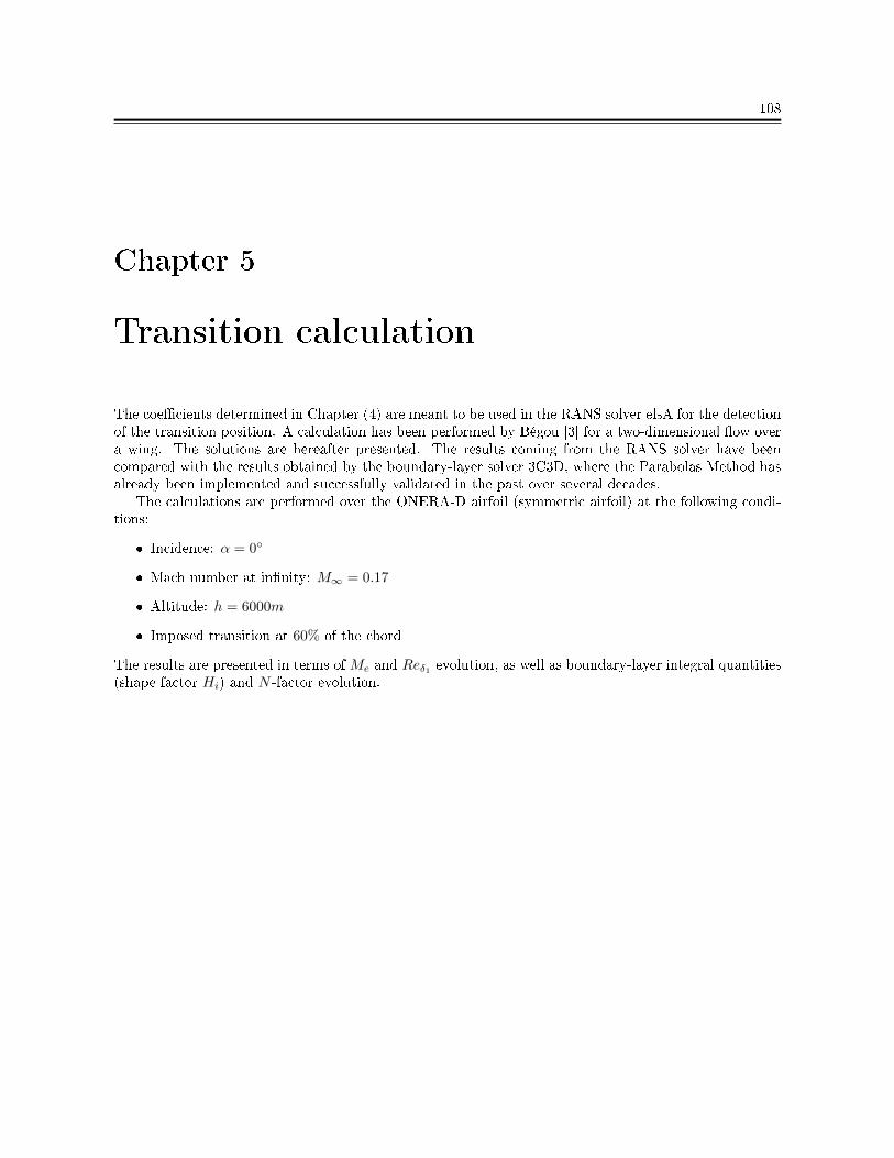
108
Chapter 5
Transition calculation
The coecients determined in Chapter (4) are meant to be used in the RANS solver elsA for the detectionof the transition position. A calculation has been performed by Bégou [3] for a two-dimensional ow overa wing. The solutions are hereafter presented. The results coming from the RANS solver have beencompared with the results obtained by the boundary-layer solver 3C3D, where the Parabolas Method hasalready been implemented and successfully validated in the past over several decades.
The calculations are performed over the ONERA-D airfoil (symmetric airfoil) at the following condi-tions:
Incidence: α = 0
Mach number at innity: M∞ = 0.17
Altitude: h = 6000m
Imposed transition at 60% of the chord
The results are presented in terms ofMe and Reδ1 evolution, as well as boundary-layer integral quantities(shape factor Hi) and N -factor evolution.
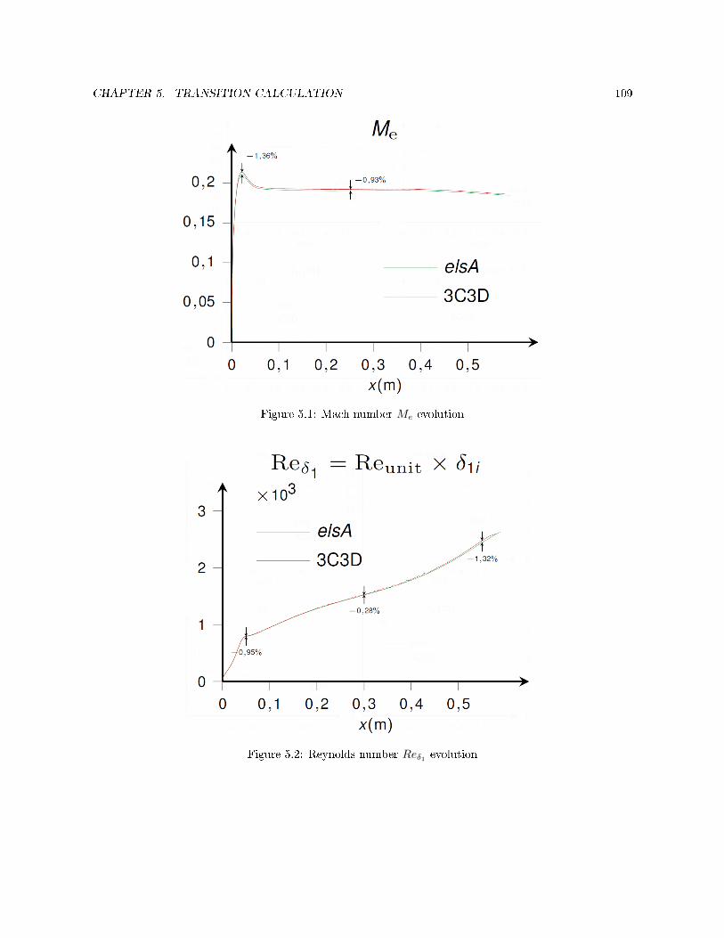
CHAPTER 5. TRANSITION CALCULATION 109
Figure 5.1: Mach number Me evolution
Figure 5.2: Reynolds number Reδ1 evolution
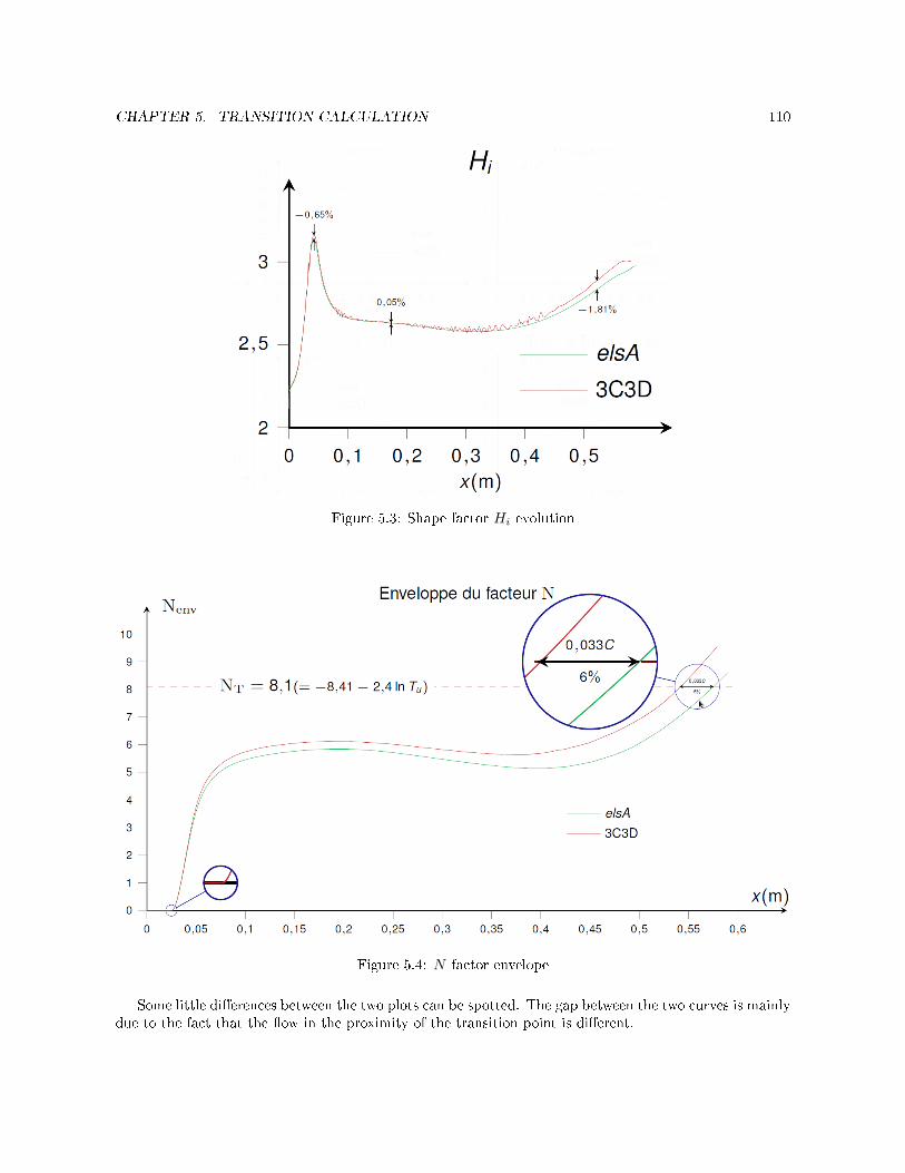
CHAPTER 5. TRANSITION CALCULATION 110
Figure 5.3: Shape factor Hi evolution
Figure 5.4: N factor envelope
Some little dierences between the two plots can be spotted. The gap between the two curves is mainlydue to the fact that the ow in the proximity of the transition point is dierent.
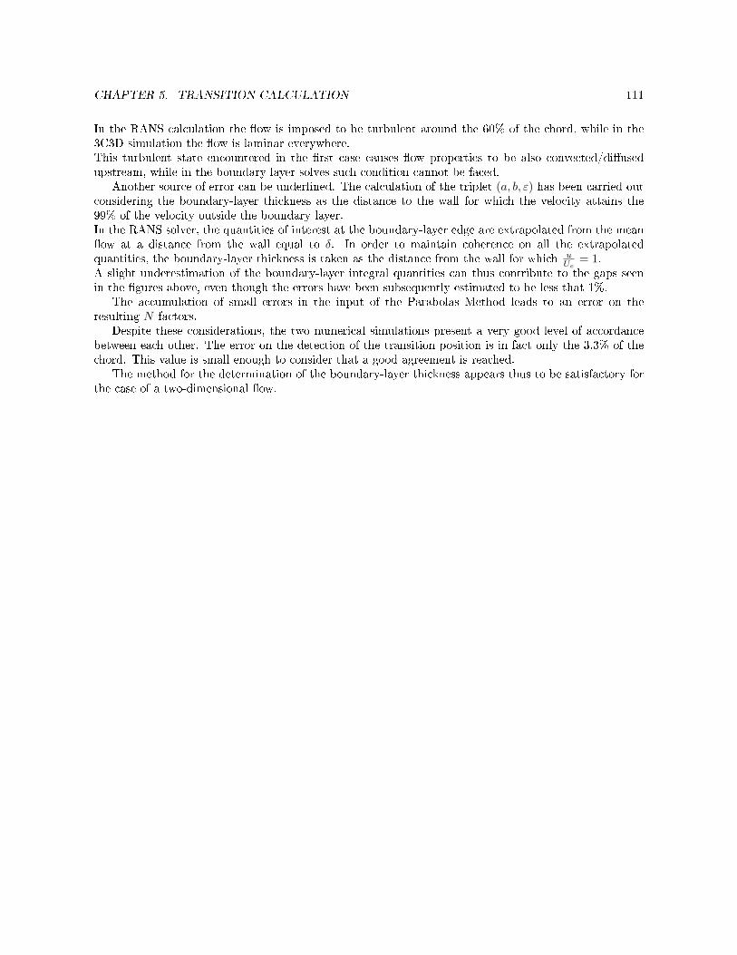
CHAPTER 5. TRANSITION CALCULATION 111
In the RANS calculation the ow is imposed to be turbulent around the 60% of the chord, while in the3C3D simulation the ow is laminar everywhere.This turbulent state encountered in the rst case causes ow properties to be also convected/diusedupstream, while in the boundary-layer solves such condition cannot be faced.
Another source of error can be underlined. The calculation of the triplet (a, b, ε) has been carried outconsidering the boundary-layer thickness as the distance to the wall for which the velocity attains the99% of the velocity outside the boundary layer.In the RANS solver, the quantities of interest at the boundary-layer edge are extrapolated from the meanow at a distance from the wall equal to δ. In order to maintain coherence on all the extrapolatedquantities, the boundary-layer thickness is taken as the distance from the wall for which u
Ue= 1.
A slight underestimation of the boundary-layer integral quantities can thus contribute to the gaps seenin the gures above, even though the errors have been subsequently estimated to be less that 1%.
The accumulation of small errors in the input of the Parabolas Method leads to an error on theresulting N -factors.
Despite these considerations, the two numerical simulations present a very good level of accordancebetween each other. The error on the detection of the transition position is in fact only the 3.3% of thechord. This value is small enough to consider that a good agreement is reached.
The method for the determination of the boundary-layer thickness appears thus to be satisfactory forthe case of a two-dimensional ow.
112
Conclusions
The present work dealt with the problem of computing the boundary layer thickness as a necessary stepto predict the transition position in RANS calculations.Among the many existent numerical schemes for the treatment of this problem, ONERA has developedover the year a simplied method for the determination of the amplication rate of external perturbationpenetrating the boundary layer. This method, called Parabolas Method, has already been successfullyused in a boundary-layer solver (the solver 3C3D, always developed at ONERA). The interest is now toimplement such method for a RANS solver.
This implementation is still in progress and it is developed by Bégou and al. [3]. The analyticformulation for the Parabolas Method relies on the use of integral quantities, which in turn depend onthe denition of a boundary-layer thickness. The calculation of the boundary-layer thickness is then thebasis for this method.
An evaluation procedure for this parameter has been proposed by Stock and Haase [30], but it turnedout to be inaccurate. This procedure has thus been improved in the present work through the use ofself-similarity. Two cases, the two-dimensional and the three-dimensional boundary layer, have beensubsequently investigated.
Concerning the two-dimensional case, the study has been conducted rstly on a incompressible ow andconsequently on a compressible layout. The good accordance between the results for the incompressibleand compressible case shows how a unique triplet of coecients can be found for all the dierent boundarylayer congurations, allowing its implementation in the Parabolas Method. A test on these coecientshas been conducted by Bégou and al. [3] on a Dassault airfoil. The results show the good match betweenexperimental and numerical data, thus allowing one to successfully validate the Parabolas Method for ageneric 2-D case of study.
The three-dimensional incompressible boundary layer has then been explored. Unlike the 2-D case,a new parameter appears in the procedure, and a universal solution cannot be determined. Since thisnew parameter depends on physical quantities that are not directly retrievable for the purpose during aRANS computation, it has been chosen to link this parameter to some recoverable quantities at the wall.A validation of this hypothesis has been carried out, and a nal procedure for the computation of thegood set of parameter for the method has been nally dened. A validation of this procedure when usedin the numerical method has not still been carried out.If its future application to the Parabolas Method will not be judged suciently accurate, other solutionsshould be exploited. If, in contrast, its application will be satisfying, the study could be completed by theinvestigation of a compressible three-dimensional study and, in case of positive results, the boundary-layerthickness determination process can be permanently integrated in the RANS code.
The next step will thus be a test of these results over a general three-dimensional incompressibleconguration.


114
Bibliography
[1] D. Arnal. Transition Prediction in Transonic Flow. In J. Zierep and H. Oertel, editors, Sympo-sium Transsonicum III, International Union of Theoretical and Applied Mechanics, pages 253262.Springer Berlin Heidelberg, 1989.
[2] Daniel Arnal and J.P. Archambaud. Méthode des paraboles en écoulement tridimensionnel général.Rapport technique RF 2/5118.37, ONERA-DMAE, Toulouse, 1999.
[3] Guillaume Bégou, Hugues Deniau, Olivier Vermeersch, and Gregoire Casalis. Database Approachfor 2d Flow Transition Prediction in a RANS Code. In 46th AIAA Fluid Dynamics Conference.American Institute of Aeronautics and Astronautics.
[4] C. B. Blumer and E. R. Van Driest. Boundary layer transition - freestream turbulence and pressuregradient eects. AIAA Journal, 1(6):13031306, 1963.
[5] Yeunwoo Cho and Angelica Aessopos. Similarity transformation methods in the analysis of the twodimensional steady compressible laminar boundary layer. 2004.
[6] J. C. Cooke. The boundary layer of a class of innite yawed cylinders. Mathematical Proceedings ofthe Cambridge Philosophical Society, 46(04):645648, October 1950.
[7] J. C. Cooke. Stewartson's compressibility correlation in three dimensions. Journal of Fluid Mechanics,11(01):5164, August 1961.
[8] J. Cousteix. Aérodynamique - Couche limite laminaire. Editions Cépadués, Toulouse, 1989.
[9] J. Cousteix and C. Gleyzes. Couches limites laminaires bidimensionnelles avec ux de chaleur. Tech-nical report, DERAT, 1974.
[10] J. Ray Dagenhart, W. S. Saric, and Langley Research Center. Crossow stability and transitionexperiments in swept-wing ow. National Aeronautics and Space Administration, Langley ResearchCenter, 1999. Google-Books-ID: Jv4UAQAAIAAJ.
[11] M. Drela and Michael B. Giles. Viscous-inviscid analysis of transonic and low Reynolds numberairfoils. AIAA Journal, 25(10):13471355, 1987.
[12] S. A. Gaponov and B. V. Smorodskii. Linear stability of three-dimensional boundary layers. Journalof Applied Mechanics and Technical Physics, 49(2):157166, March 2008.
[13] M. Gaster. A note on the relation between temporally-increasing and spatially-increasing disturbancesin hydrodynamic stability. Journal of Fluid Mechanics, 14(2):222224, October 1962.
[14] N. Gregory, J. T. Stuart, and W. S. Walker. On the Stability of Three-Dimensional Boundary Layerswith Application to the Flow Due to a Rotating Disk. Philosophical Transactions of the Royal Societyof London A: Mathematical, Physical and Engineering Sciences, 248(943):155199, July 1955.
BIBLIOGRAPHY 115
[15] Markus Hogberg and Dan Henningson. Secondary instability of cross-ow vortices in FalknerCookeboundary layers. Journal of Fluid Mechanics, 368:339357, August 1998.
[16] H. P. Horton. Near-similarity approximation for compressible, laminar boundary layers on adia-batic walls. Proceedings of the Institution of Mechanical Engineers, Part G: Journal of AerospaceEngineering, 211(5):285294, May 1997.
[17] Harry P. Horton and Hans-Werner Stock. Computation of compressible, laminar boundary layers onswept, tapered wings. Journal of Aircraft, 32(6):14021405, 1995.
[18] J. van Ingen. The eN Method for Transition Prediction. Historical Review of Work at TU Delft. In38th Fluid Dynamics Conference and Exhibit. American Institute of Aeronautics and Astronautics.
[19] Roger R. Inger Leblanc. Similar Solutions and Integral Quantities of the Rotating CompressibleLaminar Boundary Layer. AIAA Journal, 22(6):748749, 1984.
[20] P. Luchini and M. Quadrio. Aerodinamica.
[21] L. M. Mack. Boundary-layer linear stability theory. In AGARD Spec. Course on Stability andTransition of Laminar Flow 81 p (SEE N84-33757 23-34), volume -1, June 1984.
[22] Mark V. Morkovin. On the Many Faces of Transition. In C. Sinclair Wells, editor, Viscous DragReduction, pages 131. Springer US, 1969.
[23] L. Quartapelle and F. Auteri. Fluidodinamica incomprimibile. Casa Editrice Ambrosiana, 2013.
[24] A. Quarteroni. Modellistica Numerica per Problemi Dierenziali. Springer-Verlag Mailand, 2008.
[25] Ramy Rashad and David W. Zingg. Laminar-Turbulent Transition Prediction in a Reynolds-AveragedNavier-Stockes Solver. 2012.
[26] Helen L. Reed and William S. Saric. Attachment-line heating in a compressible ow. Journal ofEngineering Mathematics, 84(1):99110, August 2013.
[27] E. Reshotko. Paths to transition in wall layers. In RTO-AVT/VKI Lectures Series "Advances inLaminar-Turbulent Transition Modelling ", 2008.
[28] K. Stewartson. Correlated Incompressible and Compressible Boundary Layers. Proceedings of theRoyal Society of London A: Mathematical, Physical and Engineering Sciences, 200(1060):84100,December 1949.
[29] K. Stewartson. Further solutions of the falkner-skan equation. Mathematical Proceedings of theCambridge Philosophical Society, 50(3):454465, 1954.
[30] Hans W. Stock and Werner Haase. Feasibility Study of en Transition Prediction in Navier-StokesMethods for Airfoils. AIAA Journal, 37(10):11871196, 1999.
[31] Hans W. Stock and Werner Haase. Navier-Stokes Airfoil Computations with e Transition PredictionIncluding Transitional Flow Regions. AIAA Journal, 38(11):20592066, 2000.
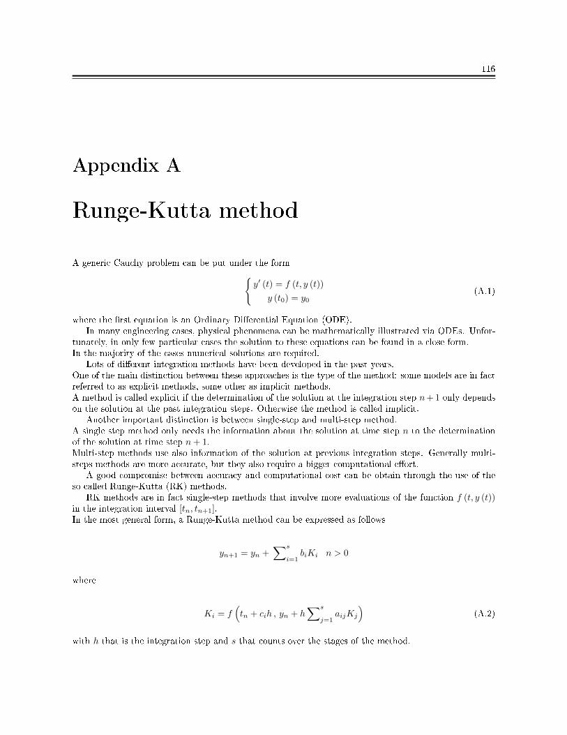
116
Appendix A
Runge-Kutta method
A generic Cauchy problem can be put under the formy′ (t) = f (t, y (t))
y (t0) = y0
(A.1)
where the rst equation is an Ordinary Dierential Equation (ODE).In many engineering cases, physical phenomena can be mathematically illustrated via ODEs. Unfor-
tunately, in only few particular cases the solution to these equations can be found in a close form.In the majority of the cases numerical solutions are required.
Lots of dierent integration methods have been developed in the past years.One of the main distinction between these approaches is the type of the method: some models are in factreferred to as explicit methods, some other as implicit methods.A method is called explicit if the determination of the solution at the integration step n+ 1 only dependson the solution at the past integration steps. Otherwise the method is called implicit.
Another important distinction is between single-step and multi-step method.A single step method only needs the information about the solution at time step n to the determinationof the solution at time step n+ 1.Multi-step methods use also information of the solution at previous integration steps. Generally multi-steps methods are more accurate, but they also require a bigger computational eort.
A good compromise between accuracy and computational cost can be obtain through the use of theso called Runge-Kutta (RK) methods.
RK methods are in fact single-step methods that involve more evaluations of the function f (t, y (t))in the integration interval [tn, tn+1].In the most general form, a Runge-Kutta method can be expressed as follows
yn+1 = yn +∑s
i=1biKi n > 0
where
Ki = f(tn + cih , yn + h
∑s
j=1aijKj
)(A.2)
with h that is the integration step and s that counts over the stages of the method.
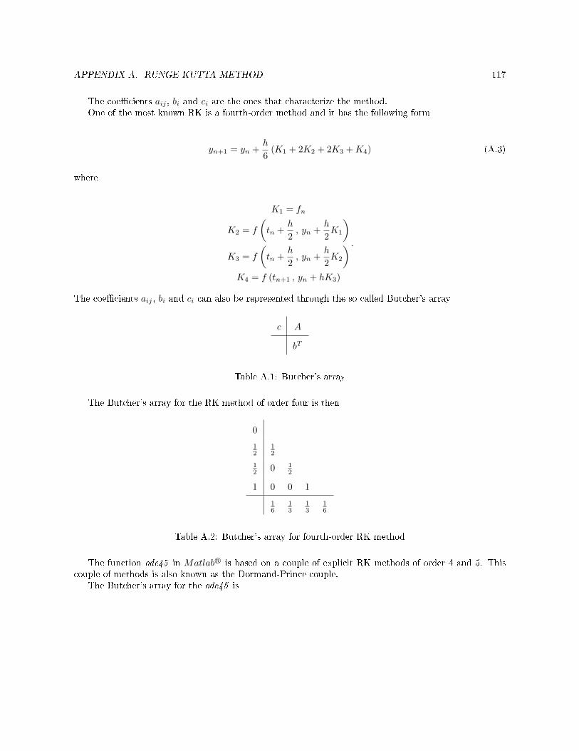
APPENDIX A. RUNGE-KUTTA METHOD 117
The coecients aij , bi and ci are the ones that characterize the method.One of the most known RK is a fourth-order method and it has the following form
yn+1 = yn +h
6(K1 + 2K2 + 2K3 +K4) (A.3)
where
K1 = fn
K2 = f
(tn +
h
2, yn +
h
2K1
)K3 = f
(tn +
h
2, yn +
h
2K2
)K4 = f (tn+1 , yn + hK3)
.
The coecients aij , bi and ci can also be represented through the so called Butcher's array
c A
bT
Table A.1: Butcher's array
The Butcher's array for the RK method of order four is then
0
12
12
12 0 1
2
1 0 0 1
16
13
13
16
Table A.2: Butcher's array for fourth-order RK method
The function ode45 in Matlabr is based on a couple of explicit RK methods of order 4 and 5. Thiscouple of methods is also known as the Dormand-Prince couple.
The Butcher's array for the ode45 is
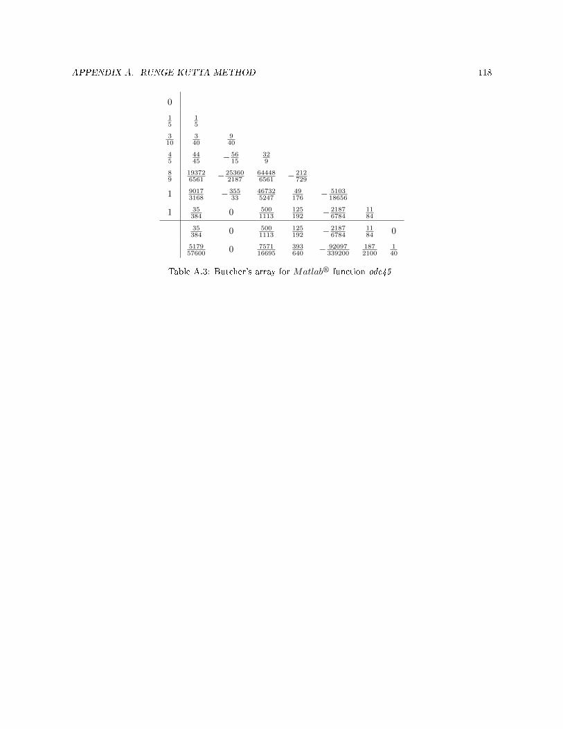
APPENDIX A. RUNGE-KUTTA METHOD 118
0
15
15
310
340
940
45
4445 − 56
15329
89
193726561 − 25360
2187644486561 − 212
729
1 90173168 − 355
33467325247
49176 − 5103
18656
1 35384 0 500
1113125192 − 2187
67841184
35384 0 500
1113125192 − 2187
67841184 0
517957600 0 7571
16695393640 − 92097
3392001872100
140
Table A.3: Butcher's array for Matlabr function ode45