NBER WORKING PAPER SERIES

PROMOTIONS AND THE PETER PRINCIPLE

Alan BensonDanielle LiKelly Shue

Working Paper 24343http://www.nber.org/papers/w24343

NATIONAL BUREAU OF ECONOMIC RESEARCH1050 Massachusetts Avenue

Cambridge, MA 02138February 2018

We thank Lisa Kahn, Steve Kaplan, Eddie Lazear, Inessa Liskovich (discussant), Vladimir Mukharlyamov (discussant), Paige Ouimet (discussant), Michaela Pagel (discussant), Amanda Pallais, Brian Phelan, Thomas Peeters, Lamar Pierce, Felipe Severino (discussant), Kathryn Shaw (discussant), Mike Waldman, and seminar participants at CUHK, FOM Conference, GSU CEAR, Gerzensee ESSFM, Harvard Business School, HKUST, Hong Kong U., ITAM, Melbourne FIRCG, MIT Sloan, Midwest Economics Association Meetings, Nanjing U., NBER (Corporate Finance, Personnel Economics, and Organizational Economics), Purdue, SOLE, Tsinghua PBC, U. of Chicago, U. of Hong Kong, U. of Miami, U. of Minnesota Carlson, Wharton People Analytics Conference, Wharton People \& Organizations conference, and Yale Junior Finance Conference for helpful comments. We thank Menaka Hamplole and Leland Bybee for excellent research assistance. This research was funded in part by the Initiative on Global Markets and the Fama Miller Center at the University of Chicago Booth School of Business. The views expressed herein are those of the authors and do not necessarily reflect the views of the National Bureau of Economic Research.

NBER working papers are circulated for discussion and comment purposes. They have not been peer-reviewed or been subject to the review by the NBER Board of Directors that accompanies official NBER publications.

© 2018 by Alan Benson, Danielle Li, and Kelly Shue. All rights reserved. Short sections of text, not to exceed two paragraphs, may be quoted without explicit permission provided that full credit, including © notice, is given to the source.

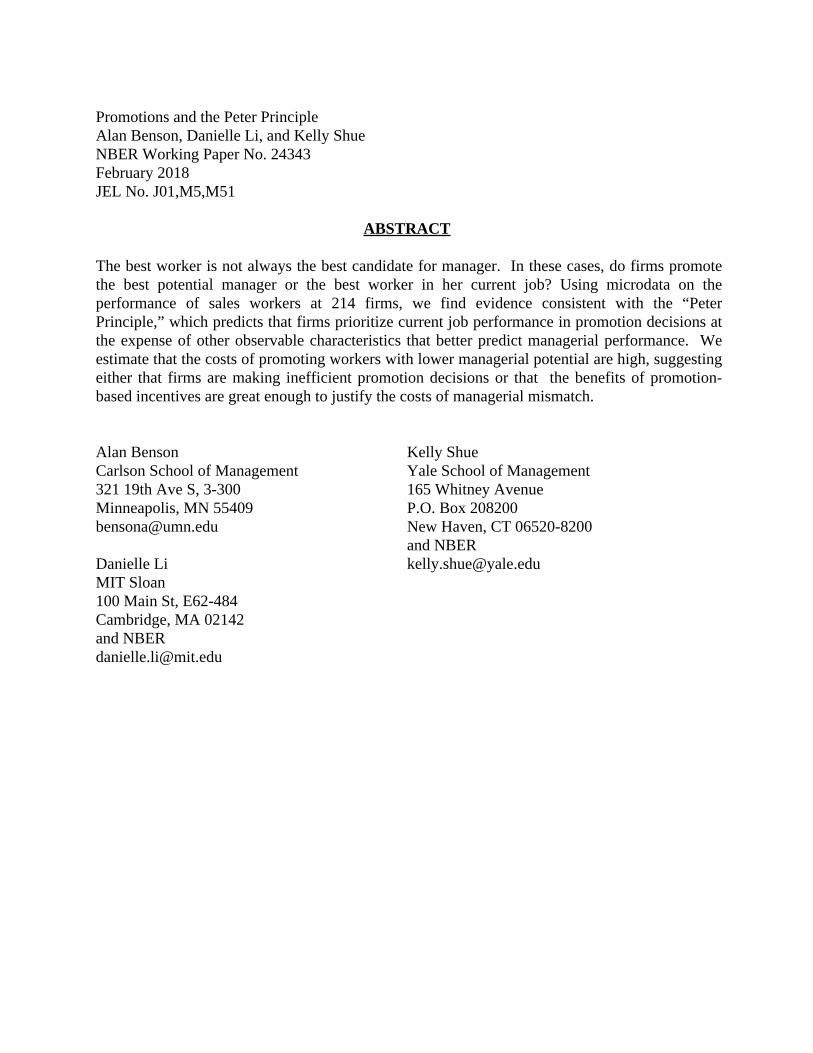
Promotions and the Peter PrincipleAlan Benson, Danielle Li, and Kelly ShueNBER Working Paper No. 24343February 2018JEL No. J01,M5,M51

ABSTRACT

The best worker is not always the best candidate for manager. In these cases, do firms promote the best potential manager or the best worker in her current job? Using microdata on the performance of sales workers at 214 firms, we find evidence consistent with the “Peter Principle,” which predicts that firms prioritize current job performance in promotion decisions at the expense of other observable characteristics that better predict managerial performance. We estimate that the costs of promoting workers with lower managerial potential are high, suggesting either that firms are making inefficient promotion decisions or that the benefits of promotion-based incentives are great enough to justify the costs of managerial mismatch.

Alan BensonCarlson School of Management321 19th Ave S, 3-300Minneapolis, MN 55409bensona@umn.edu

Danielle LiMIT Sloan100 Main St, E62-484Cambridge, MA 02142and NBERdanielle.li@mit.edu

Kelly ShueYale School of Management165 Whitney AvenueP.O. Box 208200New Haven, CT 06520-8200and NBERkelly.shue@yale.edu

When management requires different skills than lower-level work, the best workers may

not make the best managers. In these cases, do firms promote someone who excels in

her current position or someone who is likely to excel as a manager? If firms promote

workers based on their current performance, they may end up with worse managers. Yet

if firms promote workers based on traits that predict managerial potential, they may pass

over higher-performing workers, thereby weakening incentives for workers to perform well in

their current roles. Such promotion policies could also lead to perceptions of favoritism or

unfairness, or the impression that effort in one’s job goes unrewarded.

Using detailed microdata on sales workers in US firms, we provide the first large-scale

empirical evidence showing that firms prioritize current performance in promotion decisions

at the expense of promoting the best potential managers. Our findings are consistent with

the “Peter Principle,” which, in its extreme form, states that firms promote competent

workers until they become incompetent managers (Peter and Hull 1969). In particular, we

show that high-performing sales workers are more likely to be promoted, but that prior

sales performance negatively predicts managerial performance, even after accounting for

selection into the sample of promoted workers. These results suggest either that firms make

mistakes in their promotion decisions or that the incentive benefits of promoting based on

sales performance justify the costs of promoting workers with lower managerial potential.

We provide supportive evidence for the latter possibility by showing that firms appear to

actively manage the trade-off between providing incentives and promoting the best potential

managers: firms place less emphasis on sales performance in promotions where managerial

roles entail greater responsibility and where sales performance is also rewarded by relatively

strong pay-for-performance.

The Peter Principle applies broadly to settings in which the skills required to succeed

at one level in the organizational hierarchy may differ from the skills required in the next

level, e.g., science, engineering, manufacturing, academia, or entrepreneurship (Baker, Jensen

and Murphy 1988). Among such settings, sales is particularly attractive from a research

perspective for several reasons. First, it is an economically important occupation, accounting

for 10.4 percent of the US labor force.1 Second, sales performance is relatively easy to

quantify, allowing us to observe a more reliable measure of worker performance. Finally,

the sales setting allows us to explore an interesting tension. Sales is both widely cited as a

1In 2016, the U.S. labor force had 14.5 million workers in sales and sales-related occupations (Bureau ofLabor Statistics 2016).

1

canonical example of where the Peter Principle is likely to apply2 and a setting in which a

simple economics model would predict that the Peter Principle may be less likely to apply:

pay-for-performance is common in sales, so firms may not need to rely on promotion-based

incentives to induce worker effort. Finding evidence of the Peter Principle in such a setting

would suggest that pay-for-performance cannot fully resolve the tension between providing

incentives and promoting the most qualified managers.

Our analysis uses new transaction-level data that are well suited for the study of firms’

promotion policies.3 These data, provided by a firm that offers sales performance

management software to client firms, include standardized measures of sales transactions

and organizational hierarchy for a panel of 53,035 workers, 1,531 of whom are promoted

into managerial positions during our sample period. Our data cover 214 different US-based

client firms in a range of industries from 2005 to 2011. Data on multiple firms allow us to

study heterogeneity in how much firms prioritize current job performance as a function of

firm organization or pay practices.

For sales workers, we use employment history and sales credit data to examine

promotion as a function of sales performance (the dollar value of sales), sales collaboration

(the number of colleagues with whom a worker shared credit on transactions), and other

observable worker characteristics. For promoted managers, we evaluate their managerial

performance as their “manager value added” in shaping their subordinates’ sales

performance, i.e., each manager’s contribution to improving her subordinates’ sales,

controlling for subordinate and firm-year-month fixed effects, as well as other potentially

confounding factors (following the methods used in, e.g., Abowd, Kramarz and Margolis

1999; Bertrand and Schoar 2003; Lazear, Shaw and Stanton 2016). While this measure of

manager value added has a number of important advantages, it remains imperfect given

that managers may be non-randomly matched to subordinates. Thus, we present a number

2Deutsch (1986) points out that “American companies have always wrestled with ways to keep the PeterPrinciple at bay—to prevent competent salesmen, for example, from rising to become incompetent salesmanagers.” Baker, Jensen and Murphy (1988) state that “in many cases, the best performer at one level inthe hierarchy is not the best candidate for the job one level up—the best salesman is rarely the best manager.”Sevy (2016), in a Forbes article entitled “Why Great Sales People Make Terrible Sales Managers,” arguesthat great sales workers are motivated by a desire for personal—rather than team—achievement: “successin sales is about me while success in sales management is about my team. This is where the downside ofa strong achievement drive makes itself known. If I’m driven to prove my personal ability, I find it hard(nearly impossible sometimes) to step back and let others take the spotlight.”

3We do not observe promotion offers. As such, when we refer to a “promotion policy,” we refer to thecombined impact of the firm’s promotion offer and the worker’s decision to accept the offer.

2

of additional tests in Section 5 to show that non-random matching is unlikely to drive our

findings of evidence consistent with the Peter Principle.

We begin by documenting a strong, positive relation between past sales performance

and promotion to managerial positions. Doubling sales credits increases the probability

that a worker will be promoted by 14.3 percent relative to the base probability of

promotion.4 However, among promoted workers, we find that pre-promotion sales

performance negatively predicts manager value added: doubling the new manager’s

pre-promotion sales corresponds to a 7.5 percent decline in the sales performance of each of

the newly-promoted manager’s subordinates. Equivalently, relatively poor prior sales

performance among newly promoted managers is associated with significant improvements

in subordinate performance. This negative correlation is consistent with the Beckerian

insight about selection and discrimination: if firms’ promotion policies “discriminate”

against poor sales performers, then poor sales performers who are nevertheless promoted

should be better managers.

Our analysis also identifies another observable worker characteristic, sales collaboration

experience, which is positively related to managerial performance but not consistently

correlated with promotions. Sales collaboration may be a measure of a worker’s experience

working in teams or with more complex or customized products that require coordination.

In either case, these results suggest that firms wishing only to maximize managerial quality

could potentially achieve better outcomes by placing more weight on collaboration

experience, rather than sales, when making promotion decisions.5

Next, we show that these findings are robust to selection concerns. Because workers are

not promoted at random, the relation between sales and managerial performance in the

promoted sample may not reflect the true relation in the full sample of workers. To recover

the full-sample predictive relation, we apply a model of promotions based on the Heckman

(1976) selection model. We instrument for promotion, i.e., selection into the sample of

promoted workers, using the average firm- and industry-level promotion rates within each

time period. These average promotion rates reflect time-varyinlg vacancies and firm- and

industry-level demand for managers, which are strongly positively correlated with a

4A doubling of a worker’s relative sales performance is not an unusual occurrence given the wide dispersionin sales across workers. It is equivalent to a worker moving from the 50th to the 67th percentile in terms ofsales relative to others in the same firm-year-month.

5We caution that our results hold in the sense that collaboration experience under the existing set ofpromotion policies positively predicts managerial value added. If firms began to heavily weight collaborationexperience in promotion decisions, workers could potentially add fake collaborators by sharing credits. Recentexamples of the gaming of various evaluation metrics include Benson (2015); Larkin (2014); Oyer (1998).

3

worker’s probability of promotion. To satisfy the exclusion restriction, these average

promotion rates must be uncorrelated with managerial performance. In general, this may

not be true: high average promotion rates may reflect strong consumer demand or other

time-varying firm shocks that affect the performance of all sales workers and may thus be

correlated with managerial performance. In our setting, however, we measure a manager’s

quality as his or her value added to subordinate sales, net of worker and firm-year-month

fixed effects. Because our instruments only vary across firm-year-months, they are—by

construction—orthogonal to our measures of manager value added, which are extracted

from a regression that controls for firm-year-month fixed effects. After accounting for

selection, we continue to find a strong, negative predictive relation between pre-promotion

sales performance and manager value added.

In addition to addressing potential selection biases, we also provide evidence in Section 5

that our results are not driven by other potential measurement issues such as mean reversion,

non-linear relations, or the unwillingness of some top sales workers to accept promotion

offers. We further test whether managers with high pre-promotion sales contribute to the

firm in other ways, such as by retaining more skilled subordinates, and find no evidence that

high-sales managers are better on these dimensions.

We next assess the magnitude of the costs associated with promoting high-performing

sales workers at the expense of promoting the best potential managers. To do this, we

compare the predicted managerial performance of actually promoted workers to the predicted

managerial performance of workers who would have been promoted under a counterfactual

policy in which firms weigh worker observables solely to maximize managerial quality. We

find that average managerial quality, as measured by value added to subordinate sales, is 30

percent higher under the counterfactual policy.

We emphasize here that finding evidence of the Peter Principle does not imply that

firms make mistakes. Alternative promotion policies that maximize managerial match

quality may lead to the loss of incentive benefits associated with existing promotion

policies. Indeed, a promotion policy that favors top sales workers may provide a variety of

incentive benefits that justify the costs of managerial mismatch. For example, such policies

may preserve tournament incentives (Lazear and Rosen 1981), especially if workers

strongly value the security, stature (e.g. DellaVigna and Pope 2016; Larkin 2011), or

external signaling abilities associated with promotions (DeVaro and Waldman 2012).

Prioritizing objective performance measures in promotions may also improve incentives by

avoiding favoritism (Fisman et al. 2017; Prendergast and Topel 1996) and maintaining pay

4

equity and fairness norms (e.g., Larkin, Pierce and Gino 2012). Promotion policies based

on verifiable performance metrics such as sales may also discourage the manipulation of

other, more fungible performance metrics such as credit sharing and collaboration

experience (DeVaro and Gurtler 2015; Fisman and Wang 2017). What our findings do

suggest is that the costs of not promoting the best potential managers are high: firms

appear willing to forgo a 30 percent improvement in subordinate performance to achieve

better incentives or to avoid costly politicking.

Our final two results explore how firms trade off the benefits of using promotion-based

incentives against the costs of managerial mismatch. If firms consciously choose to provide

strong incentives at the expense of selecting the best managers, we would expect to find more

evidence of the Peter Principle in settings in which promotion-based incentives are relatively

important and less evidence in settings where managerial quality is relatively important.

We first examine how promotion policies vary with differences in managerial

responsibility. In particular, the cost of promoting bad managers is likely to be higher

when managers lead large teams, and so we would expect firms with larger teams to place

less weight on sales performance and more weight on collaboration experience in their

promotion choices. This is indeed what we find in our data: when the quality of managers

is relatively more important, firms appear more willing to promote workers who are weaker

in terms of pre-promotion sales but more likely to be effective managers.

Similarly, firms should place less weight on current performance in promotions if they

have chosen to incentivize worker performance in other ways. For a subset of our data, we

observe both variable and fixed worker compensation, which allows us to measure how

much each firm uses explicit pay-for-performance. We find that firms with stronger

pay-for-performance—defined as those in which commissions and bonuses are large on

average relative to fixed compensation—put less weight on sales performance when making

promotion decisions. While this finding suggests that pay-for-performance can partially

substitute for promotion-based incentives, it does not imply that pay-for-performance can

eliminate the costs associated with the Peter Principle. Indeed, relative to other

occupations, sales is associated with high pay-for-performance, and yet we continue to find

evidence consistent with the Peter Principle. This again suggests that the incentive power

of promotions may be quite important in practice. Pay-for-performance may not always be

the most cost-effective way to motivate workers (Cullen and Perez-Truglia 2018),6 and

6Cullen and Perez-Truglia (2018) use experimental evidence in the field to show that horizontal payinequality (which could result from pay-for-performance) can demotivate workers, whereas vertical payinequality (which could result from promotion-related incentives) can motivate workers.

5

workers may additionally value managerial titles associated with promotion because they

confer status and can be readily advertised on resumes (DeVaro and Waldman 2012;

Waldman 2003).

In general, our results do not allow us to reject the possibility that firms make mistakes

in their promotion decisions. However, they do suggest that firms are aware of the trade-off

between providing worker incentives and selecting good managers, and attempt to set their

promotion policies accordingly.

This study offers the first empirical test of the Peter Principle using data on promotions

across a large number of firms. Although theoretical work and reviews have hypothesized

that promotions based on current job performance may yield managerial mismatch (Fairburn

and Malcomson 2001; Lazear 2004; Waldman 2003), there is little empirical work that tests

the Peter Principle directly. Our paper is most closely related to Grabner and Moers (2013),

which shows that a bank places less weight on current job performance when a promotion

would be to a job performing dissimilar tasks. However, Grabner and Moers use data from

a single firm and do not attempt to estimate the overall cost of the Peter Principle.

Our analysis is motivated by research showing that managerial quality is an important

determinant of firm productivity (e.g., Bloom and Reenen 2007). A large related literature

on corruption in leadership dating back to Weber (1947) attributes the existence of bad

leaders to selection policies that are polluted by nepotism and cronyism. However, our

findings suggest that promotion policies that are more meritocratic or “fair” may still be

problematic, as promoting based on merits in the current job—rather than on managerial

potential—may still result in bad leaders.

Our analysis is also related to recent findings in Kaplan, Klebanov and Sorensen (2012)

and Kaplan and Sorensen (2016) showing that execution ability, interpersonal skills, and

other general skills are associated with performance in executive roles. These findings

underscore the possibility that promoting based on lower-level job skills rather than

managerial skills can be extremely costly. Our findings also relate to the literature

exploring the declining popularity of internal promotions and the rising popularity of

external managers or directors (e.g., Murphy and Zabojnik 2004). The decision to hire an

external manager must weigh the benefits of expanding the field of candidates to improve

the quality of an eventual match against the costs of reducing incentives for internal

candidates. The Peter Principle may also be very relevant for entrepreneurial firms, which

must decide whether to keep founders and early team members in leadership roles as the

6

business scales or bring in external talent whose skills may be better suited to management

(Ewens and Marx 2016; Hellmann and Puri 2002).

1 Setting and data

Our data come from a firm that offers sales performance management (SPM) software

over the cloud. The firm’s clients input their employee records, organizational hierarchies,

and sales transactions into the software, which then calculates pay for each individual

worker. Transaction inputs can be entered manually or linked to order management and

customer relationship management software. Pay outputs are typically linked directly to

payroll software. The software also provides reporting and analysis. Sales workers and sales

managers can view their sales credits, progress toward quotas, commissions, and other

data. The software can also generate reports for use in auditing and compliance with

Sarbanes-Oxley.

The data include 214 client firms and 53,035 sales workers, 1,531 of whom are promoted

to managerial roles. The most-represented industries include manufacturing (62 firms),

information technology and services (56 firms), and professional services (38 firms). In

2011, sales workers in the US earned a median monthly wage of $2,070 and about half

worked in retail sales (Bureau of Labor Statistics 2011). By contrast, sales workers in our

data predominantly work in business-to-business sales and earn a median monthly

commission of $3,658, not including base salary and bonuses. Table 1 provides descriptive

statistics for sample coverage. All firms have at least one complete fiscal year of data, and

no one firm constitutes more than 8 percent of person-months.

1.1 Overview of sales positions

Sales workers are typically assigned a market consisting of a territory, a set of products, or

a type of client. Within their market, they are responsible for generating leads on potential

new clients, making first contact, executing the initial sale, cross-selling other products,

selling upgrades, and maintaining relationships. The sales industry refers to this process as

the sales cycle.

The primary measure of a salesperson’s performance is the total dollar value of the sales

to which he or she contributes. Our data include 156 million sales transactions tied to

individual workers. Table 1 describes the distribution of sales generated. Because sales tend

7

to be intermittent and can vary over the year, we report rolling averages of sales credits

in the previous 12 months. The quartiles for monthly worker sales are $49,956, $285,573,

and $1.54 million (in 2010 dollars). Reflecting the wide and skewed distribution of sales

standards across markets in which workers operate, the mean of this figure is $3.62 million.

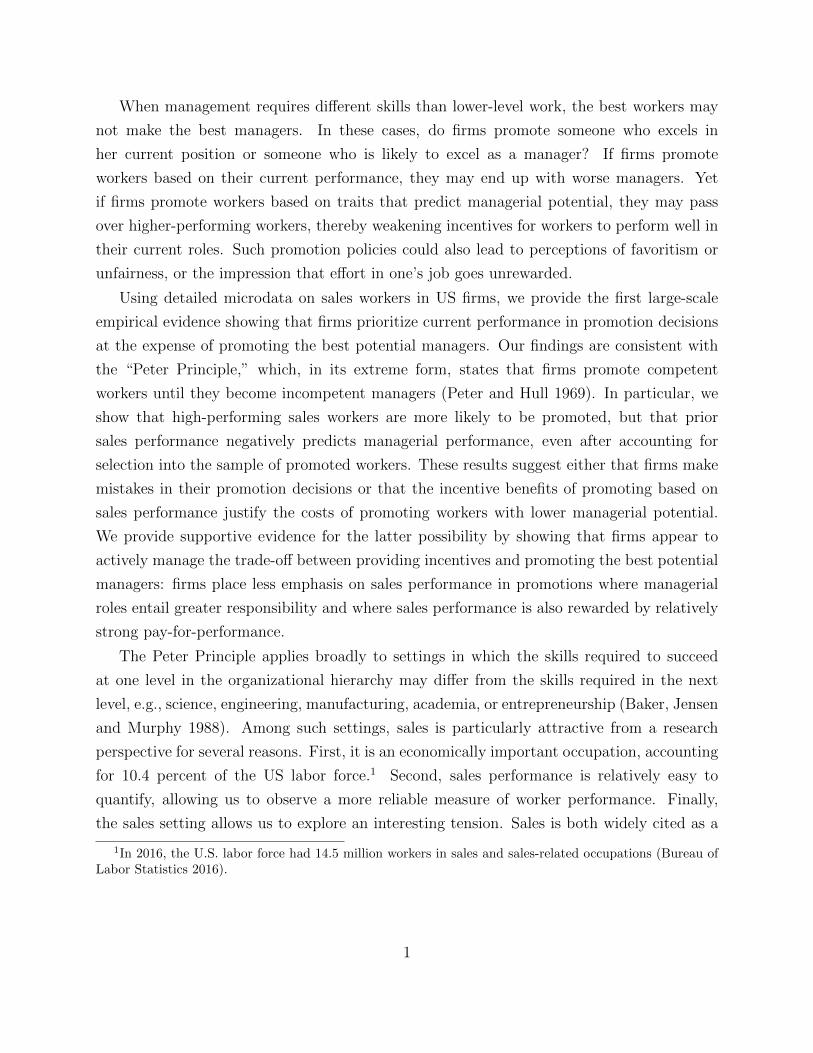
Figure 1 also illustrates the skewness in the distribution of sales. The top left panel

presents a histogram for the raw distribution of worker-level monthly sales (measured as 12

month rolling averages). The middle left panel plots the log of monthly sales, and shows

that this follows a less skewed distribution. The bottom left panel, which reflects our main

measure of sales performance, shows the residual distribution of monthly sales after

controlling for firm-year-month fixed effects. In other words, we measure sales performance

as the recent performance of a sales worker compared to others in her same company at the

same period in time. Even with these fixed effects, we still observe wide variation in sales

credits across workers. The interquartile range of residual log sales is 2.49, meaning that,

among rank and file sales workers in the same firm in the same year-month, a worker in the

75th percentile generates approximately e2.49 = 12.1 times as much revenue as one in the

25th percentile. Although this difference is stark, it’s also consistent with the so-called

“80-20 rule,” a well-known heuristic in the sales industry that states that the top 20

percent of the sales force is responsible for 80 percent of sales.

In addition to total sales, we also observe collaboration experience. In the potentially

complex business-to-business sales settings that constitute the majority of our data, sales

transactions are often credited to more than one worker. For example, a relationship

manager may be a client’s single point of contact. For specialized products and services,

the relationship manager may consult a product specialist, and, if a sale is made, both the

relationship manager and the product specialist would receive a credit. For complex

products and services, a single transaction can involve salespeople across many sales

functions, products, and geographies. In our data, we observe all workers credited on a

transaction and define a salesperson’s collaboration experience as her average number of

distinct colleagues per order over the past 12 months (or for her tenure if less than a year).

A salesperson’s collaboration history can serve as a proxy for both experience in working in

teams and experience with more complex products that require more coordination to sell.

Table 1 presents summary statistics for collaboration, and Figure 1 presents histograms

of the distribution of the mean number of collaborators a sales worker has per order, over

the past year (or her tenure if less than a year). Over 40 percent of workers worked alone

in the past year, while the remainder vary greatly in their number of collaborators. This

8

difference does not merely reflect differences in work organization across firms or over time.

The bottom-right panel of Figure 1 shows that even within the same firm-year-month, there

is substantial variation in the extent to which workers collaborate on sales. The within

firm-year-month interquartile range of sales collaborators is 1.19, signifying that the 75th

percentile worker has e1.19 = 3.28 times as many collaborators as the 25th percentile worker.

This variation highlights two archetypal sales workers: those who are the only person

credited on transactions and those who share sales credits on transactions. Indeed, much of

the practitioner literature emphasizes different performance management practices for these

groups. “Lone wolves” might be recruited for their self-confidence, resilience, and autonomy,

and are stereotypically marked by their reluctance to share leads, best practices, and client

relationship responsibilities with others in the organization. The most effective team players,

by contrast, enable those around them by forwarding leads, crafting sales that include many

others’ territories and products, forwarding established clients to account managers, and

developing team members so they can be effective in these capacities. These lead generation

and origination activities would also generally entitle that salesperson to a portion of the

sales executed by others.7

The correlation between our sales and collaboration measures is 0.21. While positive

and statistically significant, the moderate correlation shows that there is substantial

variation across these measures: workers can be effective salespeople under various models

of collaboration.

Table 1 also provides summary statistics for worker compensation. Because our data

provider’s software is designed to track and distribute pay for sales performance, salary is an

optional field and can be missing or measured with error. Based on these limited data, we

believe that the median worker in our sample receives at most $89,000 in base pay per year,

and more likely $50,000 to $60,000 per year in base pay, which is approximately half that of

managers.8 Given that the software outputs commission data that are often linked to payroll,

7We do not assume that collaboration experience is freely chosen by the worker. Indeed, some workersmay be assigned to work alone or in teams. We instead focus on showing that collaboration experience,which is observable by the firm, positively predicts manager value added.

8The salary figures reported in Table 1 are based on data that are sometimes unclear in terms of units.Given the manner in which the software interprets these fields on online dashboards and other automatedreports, we believe that the majority of salaries are reported in monthly terms. However, some salary fieldsmay be populated with annual salaries, and some workers with missing salary data may have missing salarydata precisely because they work fully on commission. We expect the latter bias to affect workers more thanmanagers, since conversations with our data provider suggest that managers are very rarely paid entirelyon commission. These two biases operate in the same direction and lead us to believe that the true medianmonthly salary is lower than the median $7,443 figure reported in this table.

9

we’re more confident in these measures, although they can still be missing. The median

sales worker earns $3,658 per month in commission pay, slightly less than our estimates of

workers’ base pay, and the 75th percentile sales worker earns the same in commission as in

base pay. These numbers are generally consistent with benchmark data for the relative sizes

of compensation for sales workers. However, total compensation in our data is substantively

greater than BLS estimates for median pay among non-retail sales workers, which ranges

from $48,200 to $71,550 per year. This is unsurprising given that our sample is largely

composed of highly-compensated sales workers who engage in big-ticket business-to-business

sales.

Our analysis uses monthly sales as the measure of pre-promotion sales performance, which

has the advantage of being highly standardized, and after controlling for firm-year-month

fixed effects, has an easy interpretation. A limitation of our sales performance measure is

that we do not observe the profit margins associated with sales transactions. Nevertheless,

we believe that the relative levels of sales credits among workers in the same firm and time

offers a reasonable approximation of relative sales performance, and in the data, these sales

mechanically determine the ultimate commissions. In theory, we could instead use worker

compensation as a measure of sales performance. However, this approach would also have

disadvantages. First, compensation can be difficult to interpret because firms can “pay for

performance” by paying a high base rate and setting high standards for retention. Second,

compensation doesn’t always correspond to recent performance; for example, in a given

month, workers may receive commissions for origination or renewals for sales that were

made in the distant past. Third, the base pay data can be unreliable since they are not

required by the software and not directly linked to payroll. Therefore, we prefer relative

sales credits as our measure of sales performance.

While our data have the unique advantage of offering detailed organizational structure

and worker productivity measures, we unfortunately do not observe employee demographic

characteristics such as age, gender, or education. We do observe worker tenure, which may

affect both worker sales and promotion prospects. The tenure variable is censored by the

date the firm began using the SPM software. Therefore, we control for tenure within the

SPM system and its interaction with whether tenure is potentially censored.

1.2 Overview of managerial positions

In our data, we observe the hierarchical structure linking sales managers to sales

subordinates. For each person in the data, we observe the ID number of at most one direct

10

superior within the hierarchy, as well as the ID numbers of any direct subordinates.

Therefore, we define a worker as someone with zero subordinates and a manager as

someone with at least one subordinate. Some managers are higher up in the hierarchy, and

have subordinates who manage other subordinates. While it would be very interesting to

study promotions from managerial positions into higher level managerial positions, we

observe relatively few promotions into higher levels of management. Therefore, we focus

our analysis on front-line sales workers (those at the bottom of the sales hierarchy), and

managers one level above these front-line sales workers.

Managers typically have titles such as “territory manager,” “sales director,” “regional

director,” “regional manager,” and “regional vice president.” The last panel of Table 1

summarizes the characteristics of managers in our data. On average, each manager has five

subordinates. Conversations with our data provider suggest that managers typically receive

greater total compensation than their subordinates and have a pay mix that favors base

pay rather than commission pay. Consistent with this, managers in our data have

significantly higher reported salaries than workers on average and at each quartile of the

pay distribution. In absolute terms, managers also have greater commissions than workers

at each quartile of the commission pay distribution, though managers’ overall pay mix is

more weighted toward base pay. In addition, nonpecuniary rewards are also likely to favor

managers, who typically enjoy greater prestige, opportunities for career progression inside

and outside the firm, benefits, job security, pay security, and better work conditions than

their subordinates. Nevertheless, the top salespeople in our data earn more in commissions

than the median manager. This raises the possibility that some top sales workers in our

sample may prefer not to be promoted to managerial positions. We’ll return to this

potential selection concern in the empirical section.

Managers also perform substantially different tasks. While sales workers are primarily

engaged in direct sales activities, sales managers are responsible for building a

high-performing sales team and earn commissions as a function of their team’s

performance. A survey of front line sales managers by the Sales Management Association

(2008) reports that sales managers spend the most time on performance management,

followed by company administration, sales planning, selling and market development, and

staff deployment. Performance management requires leadership, coaching, and training

skills that may be imperfectly related to those used in direct sales activities.

Administrative duties require general management knowledge so that the sales manager

can interface with other functions, such as marketing and operations. Sales planning

11

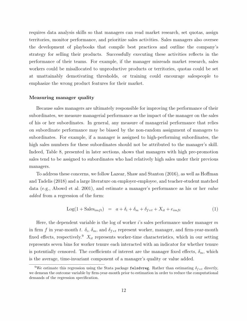
requires data analysis skills so that managers can read market research, set quotas, assign

territories, monitor performance, and prioritize sales activities. Sales managers also oversee

the development of playbooks that compile best practices and outline the company’s

strategy for selling their products. Successfully executing these activities reflects in the

performance of their teams. For example, if the manager misreads market research, sales

workers could be misallocated to unproductive products or territories, quotas could be set

at unattainably demotivating thresholds, or training could encourage salespeople to

emphasize the wrong product features for their market.

Measuring manager quality

Because sales managers are ultimately responsible for improving the performance of their

subordinates, we measure managerial performance as the impact of the manager on the sales

of his or her subordinates. In general, any measure of managerial performance that relies

on subordinate performance may be biased by the non-random assignment of managers to

subordinates. For example, if a manager is assigned to high-performing subordinates, the

high sales numbers for these subordinates should not be attributed to the manager’s skill.

Indeed, Table 8, presented in later sections, shows that managers with high pre-promotion

sales tend to be assigned to subordinates who had relatively high sales under their previous

managers.

To address these concerns, we follow Lazear, Shaw and Stanton (2016), as well as Hoffman

and Tadelis (2018) and a large literature on employer-employee, and teacher-student matched

data (e.g., Abowd et al. 2001), and estimate a manager’s performance as his or her value

added from a regression of the form:

Log(1 + Salesimft) = a+ δi + δm + δf×t +Xit + eimft (1)

Here, the dependent variable is the log of worker i’s sales performance under manager m

in firm f in year-month t. δi, δm, and δf×t represent worker, manager, and firm-year-month

fixed effects, respectively.9 Xit represents worker-time characteristics, which in our setting

represents seven bins for worker tenure each interacted with an indicator for whether tenure

is potentially censored. The coefficients of interest are the manager fixed effects, δm, which

is the average, time-invariant component of a manager’s quality or value added.

9We estimate this regression using the Stata package felsdvreg. Rather than estimating δf×t directly,we demean the outcome variable by firm-year-month prior to estimation in order to reduce the computationaldemands of the regression specification.

12

By including both manager and worker fixed effects, manager value added is identified

from workers whom we observe under multiple managers. A manager’s fixed effect represents

the average change in sales performance across all workers who switch to or from that

manager. As such, a manager with a high value added is one under whom workers perform

above their individual mean across all the managers under whom they have worked. Whether

a manager is assigned to strong or weak subordinates should not impact our measure of value

added because a manager is credited only for changes in the performance of her subordinates.

Further, firm-year-month fixed effects net out macroeconomic, industry-specific, and other

firm-time specific conditions that may impact subordinate sales performance.

Estimating managerial quality as the manager’s value added as in Equation (1) has

clear advantages, as described above. However, we also acknowledge that it is an imperfect

measure. First, our estimates of manager value added are likely to be noisy. In Equation

(1), the dependent variable is worker monthly sales, which varies widely, with some workers

making zero sales in some months and large sales in others.10 Classical measurement error

in worker sales will add noise to our measures of manager value added. However, our tests

of the Peter Principle will regress manager value added on each manager’s pre-promotion

sales experience. Noise in manager value added (the dependent variable in the regression)

will reduce our statistical power but should not bias our estimated coefficients.

One may still be concerned, however, that our estimates of manager value added are

systematically biased. This could happen if managers are non-randomly assigned to

subordinates on the basis of time-varying subordinate performance. For example, if some

types of managers tend to be assigned to subordinates whose sales performance is on an

increasing trend, then Equation (1) may mistakenly attribute subsequent sales gains by

those employees to the manager’s ability. Our estimates may also be biased if workers are

assigned to managers based on match-specific quality; in this case, we could not interpret a

manager’s estimated value added as his or her value added for the average worker. Instead,

the worker’s change in sales could be due to the quality of the match between the worker

and the new manager or team.

However, our tests of the Peter Principle remain valid even with the existence of such

biases in the estimates of manager value added, as long as the biases in value added are not

10In later regressions where we test how sales performance predicts promotions, we used backward rollingaverages of sales to smooth this variation, but we do not use backward rolling averages in Equation (1)because we are interested in measuring changes in performance as workers move across managers; backwardaverages would contaminate measures of manager value added by including worker performance underprevious managers.

13

related to the manager’s pre-promotion sales performance. In particular, our main test of

the Peter Principle will regress estimates of value added on the manager’s pre-promotion

sales performance. For example, non-random assignment of some managers to workers on

upward time trends in performance will not impact our conclusions as long as this

non-random assignment to time-varying worker performance is uncorrelated with a

manager’s pre-promotion sales.

In Section 5, we test for non-random assignment directly and show that managers are

not assigned to workers with trending sales performance on the basis of the managers’

pre-promotion characteristics. Further, if it were the case that we mistakenly assigned

some managers higher value added on the basis of their subordinates’ time-trends in

performance, then we would expect there to be a correlation between a manager’s

estimated value added and the recent prior performance of his or her new subordinates. In

Section 5, we show that this is not the case.

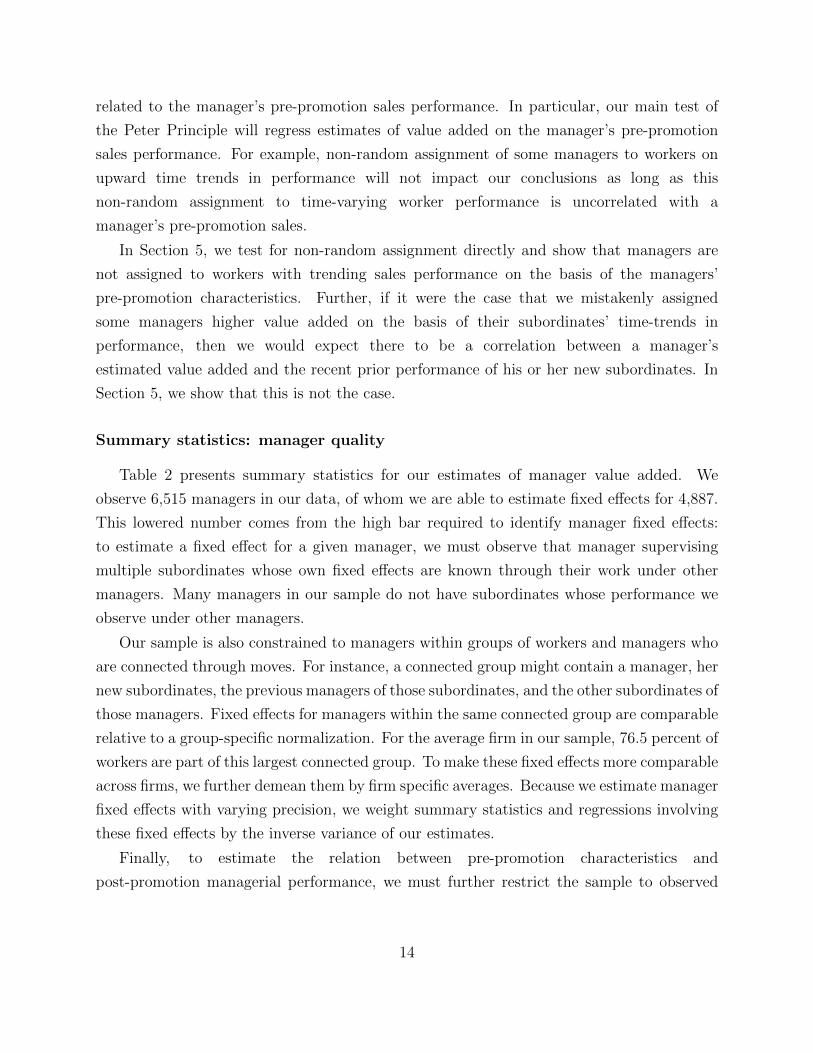
Summary statistics: manager quality

Table 2 presents summary statistics for our estimates of manager value added. We

observe 6,515 managers in our data, of whom we are able to estimate fixed effects for 4,887.

This lowered number comes from the high bar required to identify manager fixed effects:

to estimate a fixed effect for a given manager, we must observe that manager supervising

multiple subordinates whose own fixed effects are known through their work under other

managers. Many managers in our sample do not have subordinates whose performance we

observe under other managers.

Our sample is also constrained to managers within groups of workers and managers who

are connected through moves. For instance, a connected group might contain a manager, her

new subordinates, the previous managers of those subordinates, and the other subordinates of

those managers. Fixed effects for managers within the same connected group are comparable

relative to a group-specific normalization. For the average firm in our sample, 76.5 percent of

workers are part of this largest connected group. To make these fixed effects more comparable

across firms, we further demean them by firm specific averages. Because we estimate manager

fixed effects with varying precision, we weight summary statistics and regressions involving

these fixed effects by the inverse variance of our estimates.

Finally, to estimate the relation between pre-promotion characteristics and

post-promotion managerial performance, we must further restrict the sample to observed

14

promotions. We have information on both manager value added and pre-promotion

characteristics for 1,028 managers who are promoted during our sample period.

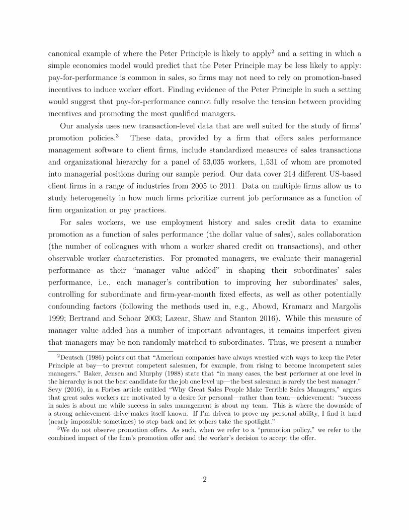
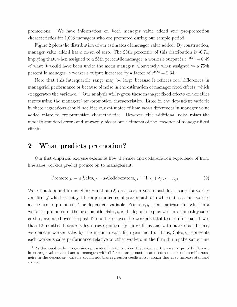
Figure 2 plots the distribution of our estimates of manager value added. By construction,

manager value added has a mean of zero. The 25th percentile of this distribution is -0.71,

implying that, when assigned to a 25th percentile manager, a worker’s output is e−0.71 = 0.49

of what it would have been under the mean manager. Conversely, when assigned to a 75th

percentile manager, a worker’s output increases by a factor of e0.85 = 2.34.

Note that this interquartile range may be large because it reflects real differences in

managerial performance or because of noise in the estimation of manager fixed effects, which

exaggerates the variance.11 Our analysis will regress these manager fixed effects on variables

representing the managers’ pre-promotion characteristics. Error in the dependent variable

in these regressions should not bias our estimates of how mean differences in manager value

added relate to pre-promotion characteristics. However, this additional noise raises the

model’s standard errors and upwardly biases our estimates of the variance of manager fixed

effects.

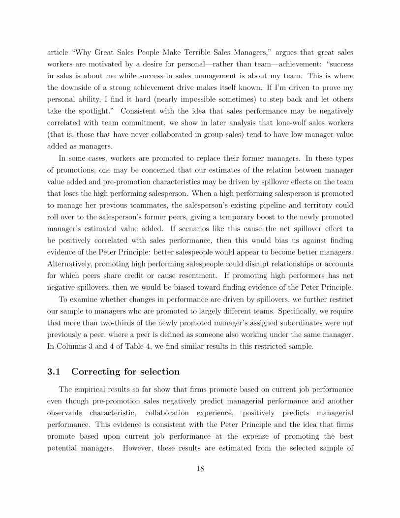
2 What predicts promotion?

Our first empirical exercise examines how the sales and collaboration experience of front

line sales workers predict promotion to management:

Promoteift = a1Salesift + a2Collaboratorsift +Wift + δf×t + eift (2)

We estimate a probit model for Equation (2) on a worker-year-month level panel for worker

i at firm f who has not yet been promoted as of year-month t in which at least one worker

at the firm is promoted. The dependent variable, Promoteift, is an indicator for whether a

worker is promoted in the next month. Salesift is the log of one plus worker i’s monthly sales

credits, averaged over the past 12 months or over the worker’s total tenure if it spans fewer

than 12 months. Because sales varies significantly across firms and with market conditions,

we demean worker sales by the mean in each firm-year-month. Thus, Salesift represents

each worker’s sales performance relative to other workers in the firm during the same time

11As discussed earlier, regressions presented in later sections that estimate the mean expected differencein manager value added across managers with different pre-promotion attributes remain unbiased becausenoise in the dependent variable should not bias regression coefficients, though they may increase standarderrors.

15

period. Collaboratorsift is the log of one plus worker i’s average number of collaborators per

order, again averaged over the past 12 months or over the total tenure if it spans fewer than

12 months. The other covariates Wift include fixed effects for seven bins of worker tenure,

interacted with whether tenure may be censored in the data. Some specifications also control

for the industry-wide and firm-wide promotion rates in the current month.

Equation (2) estimates the determinants of firm “promotion policies,” which we use as an

umbrella term for the ultimate outcome in terms of which workers transition into managerial

positions. We caution that firm “promotion policies” refer to more than the firm’s choice of

which workers to offer promotion opportunities, it also depends on the terms of the promotion

offer and whether workers accept. We present a detailed discussion of non-random selection

into the sample of promoted workers in Section 3.1.

Table 3 reports the regression results. We find that firms are significantly more likely

to promote higher performing salespeople. This result is robust across specifications that

control for a worker’s pre-promotion tenure and the industry- or firm-level promotion rates

in each year-month. The estimate in Column 4 implies that a doubling of a worker’s relative

sales performance corresponds to a 0.030 percentage point increase in a worker’s probability

of being promoted, or a 14.3 percent increase relative to the base rate.12 We also note that

a doubling of a worker’s relative sales performance is not an unusual occurrence in our data

given the wide dispersion in worker sales—it is equivalent to a worker moving from the 50th

to the 67th percentile in terms of relative worker sales.

By contrast, workers with high collaboration experience do not appear, in most

specifications, to be more likely to be promoted—despite, as we will later show,

collaboration experience being predictive of manager value added. In Appendix Table A1,

we present results using an OLS model of promotion instead of a probit model. The OLS

model also accommodates firm-year-month fixed effects as additional control variables. We

continue to find that sales positively predicts promotion, while collaboration experience

insignificantly predicts or negatively predicts promotion probability.

The estimates presented in Columns 3 and 4 of Table 3 additionally control for industry

or firm-level promotion rates in each year month. As expected, industry- and firm-level

promotion rates are highly predictive of worker promotion probability. We will use this

result in later analysis when we instrument for a worker’s probability of promotion.

12A doubling of sales corresponds to a 0.699 log point increase in the independent variable. This leads toa 0.699*0.043=0.030 percentage point increase in the likelihood of promotion, relative to a base rate of 0.21percent, making for a 0.030/0.21=14.3 percentage point increase.

16

3 What predicts managerial performance?

Next, we examine the relation between pre-promotion worker characteristics and

post-promotion manager value added:

Manager Value Addedif = b1Pre-Promotion Salesif + b2Pre-Promotion Collaboratorsif

+Wif + uif (3)

We estimate Equation (3) at the manager level because manager value added is defined

as a time-invariant manager characteristic. Pre-Promotion Salesif is the log of one plus

manager i’s monthly sales credits as a worker, averaged over the 12 months prior to i’s

promotion or over the total tenure if it spans fewer than 12 months. Analogous to the

demeaned measure of worker sales in Equation (2), Pre-Promotion Salesif is also demeaned

by the average sales performance of all workers in the sample in the same firm-year-month

to account for variation in market conditions. Thus, Pre-Promotion Salesif represents each

manager’s pre-promotion sales performance relative to other workers in the firm during the

same time period.

Similarly, Pre-Promotion Collaboratorsif is the log of one plus manager i’s average

number of collaborators per order in the year prior to promotion or over the total tenure if

it spans fewer than 12 months. In some specifications, we also control for manager i’s

tenure in the month prior to the promotion event.

Table 4 shows that, among promoted managers, there is a significant negative relation

between pre-promotion sales performance and subsequent managerial performance.

Column 2 shows that doubling a manager’s pre-promotion sales corresponds to a 7.5

percent decline in manager value added. Since manager value added represents the change

in log subordinate sales, this implies that a manager with double the pre-promotion sales

leads each subordinate’s sales to decline by 7.5 percent. Given that a typical manager is in

charge of five subordinates, our results also imply that a doubling of a manager’s

pre-promotion sales predicts that total team sales under the new manager will decline by

more than one third of one worker. By contrast, collaboration experience is positively

correlated with manager value added. In Column 2, we find that doubling collaboration

experience predicts a 15.8 percent improvement in manager value added.

While it may seem counterintuitive that good sales workers make worse managers because

both roles are likely to require social skills, the business press offers some insights into why

excellence in sales may translate negatively into managerial quality. Sevy (2016), in an Forbes

17

article “Why Great Sales People Make Terrible Sales Managers,” argues that great sales

workers are motivated by a desire for personal—rather than team—achievement: “success

in sales is about me while success in sales management is about my team. This is where

the downside of a strong achievement drive makes itself known. If I’m driven to prove my

personal ability, I find it hard (nearly impossible sometimes) to step back and let others

take the spotlight.” Consistent with the idea that sales performance may be negatively

correlated with team commitment, we show in later analysis that lone-wolf sales workers

(that is, those that have never collaborated in group sales) tend to have low manager value

added as managers.

In some cases, workers are promoted to replace their former managers. In these types

of promotions, one may be concerned that our estimates of the relation between manager

value added and pre-promotion characteristics may be driven by spillover effects on the team

that loses the high performing salesperson. When a high performing salesperson is promoted

to manage her previous teammates, the salesperson’s existing pipeline and territory could

roll over to the salesperson’s former peers, giving a temporary boost to the newly promoted

manager’s estimated value added. If scenarios like this cause the net spillover effect to

be positively correlated with sales performance, then this would bias us against finding

evidence of the Peter Principle: better salespeople would appear to become better managers.

Alternatively, promoting high performing salespeople could disrupt relationships or accounts

for which peers share credit or cause resentment. If promoting high performers has net

negative spillovers, then we would be biased toward finding evidence of the Peter Principle.

To examine whether changes in performance are driven by spillovers, we further restrict

our sample to managers who are promoted to largely different teams. Specifically, we require

that more than two-thirds of the newly promoted manager’s assigned subordinates were not

previously a peer, where a peer is defined as someone also working under the same manager.

In Columns 3 and 4 of Table 4, we find similar results in this restricted sample.

3.1 Correcting for selection

The empirical results so far show that firms promote based on current job performance

even though pre-promotion sales negatively predict managerial performance and another

observable characteristic, collaboration experience, positively predicts managerial

performance. This evidence is consistent with the Peter Principle and the idea that firms

promote based upon current job performance at the expense of promoting the best

potential managers. However, these results are estimated from the selected sample of

18

workers who are actually promoted. Because promotion is not random, the relationship

between sales and managerial performance in the promoted sample may not reflect the true

relationship among all workers. For example, suppose that firms promote to maximize

expected managerial match quality, which is a positive function of sales performance plus

some other unobserved worker characteristic. In this example, strong sales performance can

make up for deficits in the unobserved dimension, meaning that, among promoted workers,

high sales workers will tend be weaker on unobservables than low sales workers. This type

of selection would negatively bias our estimates of the true relation between pre-promotion

sales and managerial quality, and may lead us to mistakenly conclude that sales

performance negatively predicts managerial performance in the overall sample, even if the

true relationship were positive and firms were indeed promoting the best potential

managers. Selection bias can also lead to a positive bias in the estimated relation between

sales and manager value added. Top sales people with weak unobservables may be more

likely to turn down promotion offers because they expect to earn more in their current

positions. If so, sales and unobserved managerial ability will be positively correlated in the

selected sample of workers who are offered and accept promotions. We discuss this type of

selection in more detail in Section 5.

To address this measurement challenge, we apply a two-step selection model in the style

of Heckman (1976), Heckman (1979), Gronau (1974), and Lewis (1974). The goal of this

selection correction is to recover the predictive relationship between sales performance and

latent managerial potential for the full sample of workers, so that we can assess whether firms

indeed promote high performing sales workers even though sales performance negatively

predicts managerial performance.

Suppose that the underlying relationship between latent managerial potential Mi and

worker characteristics is given by:

Mi = β1Salesi + β2Collaboratorsi +Xiβ3 + εi. (4)

However, we only observe Mi if workers are promoted. The firm’s promotion policy is given

by:

Pi = I (τ1Salesi + τ2Collaboratorsi +Xiτ3 + Ziτ4 + µi > 0) (5)

This promotion equation is flexible and allows promotion to depend on observable worker

characteristics that impact managerial potential (Salesi, Collaboratorsi, and Xi) as well as

other factors Zi that affect the probability of promotion but not managerial potential. We

19

do not impose any restrictions on the relation between Equations (4) and (5) other than the

standard assumption in Heckman-style selection models that their respective error terms are

jointly normally distributed with mean zero and correlation ρ, and that there exist variables

Zi that affect promotion but do not relate to managerial performance (discussed shortly).

Our empirical test of the Peter Principle centers on showing that both τ1 > 0 (firms

are more likely to promote high-performing salespeople) and β1 < 0 (higher-performing

salespeople are more likely to be worse managers). If this were the case in the full sample

of workers, it would have to be that better sales performers were receiving some kind of

positive boost in promotion probability unrelated to their managerial potential. We have

already shown τ1 > 0 in the full sample of workers, and we now seek to recover β1 after

correcting for sample selection.

Before continuing, we note that τ1 > 0 and β1 < 0 is a sufficient but not necessary criterion

for the Peter Principle. Firms may be promoting the best sales workers at the expense of

managerial match quality even if the underlying relation between sales and latent managerial

performance is positive. In such cases, firms may simply place too much weight on sales

performance in promotion decisions and thereby overemphasize current job performance at

the expense of promoting the best potential managers. In other words, the Peter Principle

could still apply if τ1 > 0 and β1 > 0, but τ1 were too large relative to the weights on

other characteristics in the promotion rule. In practice, we will show that sales performance

continues to negatively predict managerial performance after correcting for selection, so any

positive weight on sales in the promotion decision represents a promotion policy that does

not maximize managerial match quality.

In our setting, latent managerial performance defined in Equation (4) is observed only

when workers are promoted according to the rule defined in Equation (5). Following the

standard Heckman correction procedure, we first estimate promotion propensity in the full

worker-month level panel using a probit model:

Pr(Pift = 1|Salesift,Collaboratorsift, Xift, Zift)

= Φ(a1Salesift + a2Collaboratorsift +Xifta3 + Zifta4) (6)

This first stage is identical to the probit regression model that was already presented in

Columns 3 and 4 of Table 3. We then recover estimates for the βs in Equation (4) by

estimating a regression similar to Equation (3)—presented earlier—also controlling for the

20

inverse Mills ratio, λi, of the fitted values from the first stage regression:

Mi = b1Salesi + b2Collaboratorsi +Xib3 + b4λi + ei. (7)

This selection model allows us to recover unbiased estimates for the βs in Equation (4).

Here, the inverse Mills ratio is a function of sales, collaborations, and other covariates X and

Z. Crucially, we assume that there exist variables Zi that impact a worker’s probability of

promotion, but not her managerial potential. If this assumption holds, then λi is separately

identified from the other variables in the second stage regression because we assume that Zi

does not directly impact managerial performance and thus would not directly enter into this

regression. This is equivalent to saying that the Zis are instruments for promotion.

For Zi, we use of industry-level or firm-level promotion rates. As shown in Columns 3

and 4 of Table 3, these average promotion rates are strongly positively correlated with a

worker’s probability of promotion. However, one may be concerned that differences in

industry or company conditions captured by promotion rates may also reflect strong

consumer demand and other firm-level factors, which may directly impact the performance

of managers. Formally, industry-level or firm-level average promotion rates must be

orthogonal to latent managerial potential in the full set of workers. While it is impossible

to fully test this exclusion restriction because we do not observe latent managerial

performance for the full sample of workers, we measure managerial quality as the value

added of managers to subordinate sales, after controlling for worker and firm-year-month

fixed effects. As such, our measure of manager quality among promoted workers is—by

construction—orthogonal to our instruments for selection, which do not vary within

year-month for a given firm.

Before continuing, we note that this approach allows us to recover the predictive

relationship between worker characteristics and managerial potential in the full sample of

workers and is not intended to establish a causal relation between these characteristics and

managerial performance. For example, it remains possible that something correlated with

sales performance, rather than sales performance per se, causes lower managerial

performance. The same logic applies to collaboration experience. In addition, workers may

not have the option to choose their level of collaboration if their products and collaborators

are assigned by the firm. In this case, collaboration experience may not reflect a worker’s

underlying preferences for teamwork. Nevertheless, we argue that understanding the

underlying predictive relation between observable worker characteristics and managerial

21

performance can aid firm promotion decisions even absent causality. Firms can still take

these observable characteristics into account to promote the best potential managers.

Table 5 reports the relationship between pre-promotion characteristics and manager

value added, corrected for selection. We continue to find that sales performance negatively

predicts manager value added. Using industry-month level promotion rates as the selection

instruments in Column 1, we estimate that a doubling (0.7 log point increase) in

pre-promotion sales performance predicts a 7.4 percent decline in the sales performance of

subordinates. Controlling for fixed effects in a manager’s pre-promotion tenure in Column

2 does not make a difference. Using firm-month promotion rates in Columns 3 and 4 also

yields nearly identical estimates. Overall, these estimates are similar in magnitude to those

in Table 4, which did not correct for selection issues.

In Appendix Table A2, we restrict our sample to promoted managers that are assigned

to subordinates that were not also their former team members. We find similar results in

this sample, suggesting that our findings are not driven by unusual time trends occurring

when workers are promoted to replace their former managers.

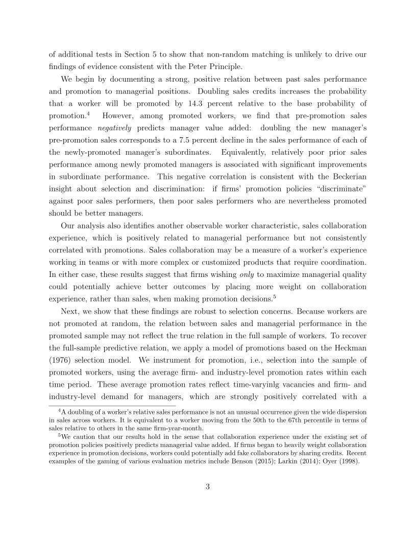
Figure 3 plots the relationship between sales performance, promotion probability, and

manager value added. In the left panel, we see that sales is strongly associated with a

higher probability of promotion, after controlling for firm-year-month fixed effects and

collaboration experience. At the same time, however, this residual sales performance is

negatively correlated with manager value added, even after applying a selection correction.

Further, this figure allows us to look for potential non-monotonicities in the relationship

between pre-promotion characteristics and promotion or manager value added. An inverted

relation for certain parts of the sales distribution would suggest that promoting based on

sales may actually help to maximize managerial match quality, at least within those parts

of the sales distribution. For example, suppose that pre-promotion sales performance

negatively predicts manager value added on average, but positively predicts manager value

added for high values of sales. If so, firms may be maximizing managerial match quality

when they promote based on sales performance, at least among the sample of workers with

high sales. As can been seen in Figure 3, we do not find strong evidence of inversions for

sales.

In Table 5, we also continue to find that collaboration experience positively predicts

manager value added after applying a selection correction. The estimated magnitudes are

economically large, but significant only when using industry-month rather than firm-month

promotion-rates as the instruments for selection. Across all specifications, a doubling of

22

pre-promotion collaboration experience predicts a 12.3 to 16.9 percent increase in subordinate

performance.

We explore the relationship between collaboration experience and manager value added

in more detail in Table 6. We find that workers who never collaborate with others—so

called “lone wolves”—fare particularly poorly when they are promoted into managerial

roles. Anecdotally, lone wolves are known within the sales profession to be “the deeply

self-confident, the rule-breaking cowboys of the sales force who do things their way or not

at all” (Dixon and Adamson 2011). In our setting, whether a salesperson works alone or

collaborates with others may either be a choice or be assigned. Regardless, we find that

lone wolf status negatively predicts manager value added. A manager who was a lone wolf

prior to promotion is associated with a 35 percent decrease in subordinate performance,

relative to managers with collaboration experience. Despite this, lone wolves are not less

likely to be promoted. Appendix Table A4 shows the predictive relation between lone wolf

status and promotion; we find, if anything, a positive relation between the two. Similarly,

Appendix Table A3 shows that this result is robust to considering workers promoted to

manage different teams.

4 Could managers contribute in other ways?

Our results so far show that high-sales managers have lower value added from the

perspective of increasing the average sales performance of their subordinates. It is possible,

however, that managers contribute to firm value in other ways and that high pre-promotion

sales managers may be better at these tasks in a way that justifies their promotion. For

example, managers may play a role in reducing costly worker turnover or in recruiting new

sales employees to expand the operations of the firm.

In Table 7, we show that, to the extent we are able to measure these behaviors in our

data, high sales managers do not appear to be associated with better performance on these

dimensions. To assess whether high-sales managers contribute by managing larger or more

important divisions, we regress a manager’s pre-promotion characteristics on the size of the

team to which he or she is assigned. All team size and retention measures are demeaned by

the average within a firm-year-month so that we can focus on differences across managers

within the same firm-year-month. Column 1 shows that we find no statistically significant

differences along this dimension. Next, Columns 2 and 3 show that high sales managers do

not appear to be better at growing their team size or reducing turnover, respectively. Finally,

23

Column 4 shows that they are not better at retaining good sales workers while letting go

of poor performers: subordinates departing from the teams of high sales managers appear

to come from the same percentile of the performance distribution as those departing teams

managed by those with poorer pre-promotion sales records. In addition to being statistically

insignificant, these estimates are economically close to zero. For example, the coefficient

of 0.049 in Column 1 signifies that a doubling in pre-promotion sales is associated with

0.034 more subordinates (relative to other teams in the same firm-year-month), an increase

of less than one percent relative to the mean team size. In practice, our estimates are

somewhat noisy and we interpret them as showing that there is no significant evidence that

pre-promotion sales are associated with meaningful differences in performance along other

dimensions.

5 Potential alternative explanations

The results above are consistent with the Peter Principle, which we define as promotion

policies that favor higher performing workers at the expense of promoting the best potential

managers. In this section, we explore whether alternative explanations or biases could explain

our findings such that firms in our sample actually are promoting the best potential managers.

Lazear (2004) shows that mean reversion can generate patterns that, on the surface,

look like the Peter Principle. The highest performing sales worker at any point in time may

be a person who is currently selling above her individual mean; if she is promoted at this

point, then her performance as a manager may fall relative to her pre-promotion

performance due to mean reversion. The existence of mean reversion implies that, even if

firms were promoting the best potential managers, we may see a decline in within-person

performance after promotion. Our results cannot be explained by this type of mean

reversion for two fundamental reasons. First, our empirical tests do not exploit

within-person changes in performance after promotion. Instead, we show that sales

negatively predicts potential managerial value added in the cross-section of workers. That

is, regardless of whether individual workers experience mean reversion after promotion, our

results suggest that firms can improve managerial performance by promoting workers with

strong collaboration experience, rather than those with strong sales performance. Second,

our measure of managerial performance is not based on a manager’s own sales, but is

instead based on the value added to the sales performance of his or her subordinates.

24

Thus, mean reversion in the manager’s own sales performance would not affect our measure

of manager value added.

Another potential concern is that newly promoted managers may be assigned to

subordinates in a non-random manner. When a worker is promoted to manager, her new

set of subordinates may be non-randomly drawn from the full sample of workers. In

general, a simple correlation between the pre-promotion sales of newly-promoted managers

and the level of performance of their assigned subordinates should not impact our results

because we estimate manager value added from changes in subordinate performance under

the new manager. However, we remain concerned that managers’ pre-promotion

performance may be correlated with time-varying aspects of a worker’s sales performance.

In particular, managers with high pre-promotion sales may be systematically assigned to

subordinates whose sales are likely to decrease thereafter, for reasons unrelated to that

manager’s quality.

Table 8 explores the assignment of managers to subordinates. The first key pattern

that emerges is that managers are not randomly assigned to subordinates: a doubling of

a manager’s pre-promotion sales is correlated with an approximately 20 percent increase

in the prior sales of the subordinates to whom he or she is assigned. However, managers

with higher pre-promotion sales do not appear to be assigned to subordinates with different

trends in performance. Table 8, Columns 1, 2, and 3 examine subordinates’ sales in the

7-9, 4-6, and 1-3 months prior to the arrival of the new managers. We find that the sales

performance of subordinates in the 7-9 months prior to being assigned a new manager is just

as predictive of that manager’s pre-promotion sales performance as the subordinate’s sales in

the 1-3 months prior. The stability of these estimates over time suggests that managers with

higher pre-promotion sales are not assigned to subordinates with increasing or decreasing

trends in performance. We also find that managers with high pre-promotion collaboration

experience tend to be assigned to subordinates with lower sales, although this relationship

is not statistically significant, and there are no obvious time trends.

We also explore potential biases from non-random assignment by considering how

subordinates’ sales prior to a manager’s promotion are correlated with the new manager’s

estimated value added. For example, high performing sales workers may have less scope for

further improvement. If so, managers who are assigned to high prior sales subordinates

may have low value added simply because these subordinates are already such high

performers. In this case, manager value added should be negatively correlated with a

subordinate’s prior sales. Table 8, Columns 4 and 5 instead show a statistically

25

insignificant relationship between subordinate prior sales and manager value added. In

Column 6, we find a borderline significant positive relationship suggesting that, if anything,

high performing subordinates are associated with higher value added of future managers.

Because managers with high pre-promotion sales are more likely to be assigned to these

high performing subordinates, this positive relation would bias us away from finding

evidence of the Peter Principle.

One may also be concerned about a different type of selection issue in which some top sales

workers prefer not to be promoted. Although most workers enjoy significant pay increases

after promotion, the very top sales workers in our sample earn more than the typical sales

manager. It may be the case that some top sales workers do not want to be promoted and, as

a consequence, we do not observe managers with very high pre-promotion sales in our sample

of promoted workers. This type of selection is likely to be a bias against our findings that

higher pre-promotion sales is associated with lower manager value added. Sales workers who

are offered promotions should compare their expected pay as managers with their expected

pay as sales workers, and then decide whether to accept the promotion. Thus, workers with

strong sales should only accept promotions if they have very good prospects as managers.

In other words, the selection in terms of who accepts promotion should bias toward finding

that better sales workers make better managers, contrary to our finding that better sales

workers become worse managers.

Even if it were the case that the very best sales workers actually made good managers

but preferred to remain in their current roles, our results would still indicate that firms were

not maximizing managerial performance by promoting good sales workers. If firms wish to

maximize managerial match quality, they should promote the best potential managers from

the set of workers who would be willing to accept such a promotion.

Finally, one may also be concerned that our results are influenced by the Great Recession,

which occurs in our sample period. For example, high performing sales workers may be poor

managers in recessions, but good managers otherwise, so that our results may lack external

validity outside of downturns. Tables A5 and A6 provide evidence that this is not the case

by showing that our results are robust to excluding the period of the Great Recession.

6 What are the performance losses from mismatch?

How much do the observed promotion policies cost firms in terms of lost subordinate

sales? To analyze this, we set aside tournament incentives, worker motivation, monitoring

26

constraints, fairness concerns, and other potential benefits of firms’ promotion rules to focus

instead on the costs of managerial mismatch. Our estimates may be interpreted as the match

quality that firms forgo to use promotions for other purposes.

To calculate the cost of mismatch, we examine how predicted managerial performance

differs among three groups of workers: (1) actually promoted salespeople, (2)

non-promoted salespeople among the promoted worker’s peers, and (3) the top predicted

manager among a promoted sales worker’s peers. Peers are defined as other salespeople in

a team managed by the same manager in the same time period. We interpret case (3) to be

the performance-maximizing promotion decision under the restriction that mobility and

other frictions prevent the firm from promoting among the entire organization, so that

firms must promote among the peers of promoted workers. If we relax this restriction, then

the estimated costs of mismatch will further increase. If firms face greater restrictions in

promotions than we impose in our simulation, then we would overestimate the costs of

mismatch.

We predict manager value added for each group using fitted values from the regression

presented in Table 5, Column 2, modified so that pre-promotion sales are measured as an

equally spaced three-part spline to allow for potential non-linearities.13 Figure 4 shows the

distributions of predicted manager value added in the three groups of workers. The mean

predicted improvement in subordinate sales performance is scaled to zero for the sample of

promoted workers.

The mean change in subordinate sales performance for the sample of non-promoted

workers is 0.07, implying that firms’ current promotion policies do slightly worse than

promoting at random. This is expected, as firms’ current promotion policies strongly favor

sales performance, and sales performance negatively predicts manager value added (even

when we allow for nonlinear relationships in the counterfactual simulation). Therefore, a

random promotion policy that does not favor high sales workers outperforms the existing

promotion policy in terms of promoting the best potential managers.

The mean in the sample of best predicted managers is 0.29, implying that subordinate

performance could improve by up to 30 percent if firms pursued an alternative promotion

policy of promoting the best predicted manager within a sales team.14 Our estimate is not

13As discussed previously, the variance of manager value added may be biased upward because ofmeasurement error in the estimation of the manager fixed effects. However, the measurement error associatedwith manager value added should not bias regression coefficients and estimates in this counterfactual, whichuses fitted values from a regression based on Table 5, Column 2.

14We estimate a 30 percent gain in sales if firms switched to a promotion policy in which they promotedthe best potential managers. This number would be even higher if we adjusted for the fact that promoting

27

meant to suggest that firms would actually achieve 30 percent gains in sales if they switched to

a promotion policy in which they promoted the best potential managers. This counterfactual

estimate ignores potentially large productivity declines that could result due to lost incentive

and other morale effects that may occur if firms switched away from the current promotion

policy of rewarding high sales with promotions. Thus, the 30 percent should be viewed as a

lower bound for how large the incentive and other benefits of promoting the top sales workers

would have to be to rationalize the current set of promotion policies.

7 Heterogeneity across firms

In this section, we consider whether firms vary in the extent to which they emphasize sales

performance in promotion decisions. If firms are aware of the trade-off between maximizing

managerial match quality and providing incentives for workers in their current roles, then

we would expect firms to behave differently depending on the specific costs and benefits

they face. For example, firms in which managers have greater responsibility may place more

weight on picking the best managers and may therefore be more willing to promote workers

who are weaker in terms of sales performance. Similarly, firms that have alternative ways

of incentivizing workers to exert effort in their current job roles may prioritize managerial

match quality more in their promotion decisions.

Table 9 considers the first possibility by examining how promotion policies differ across

firms by the supervisory responsibilities assigned to managers. We use the number of

subordinates associated with each manager as a proxy for managerial responsibility and

then take averages to obtain a firm-level measure. We then augment Equation (2), which

examines a worker’s likelihood of promotion, by interacting our measures of worker’s sales

and collaboration experience with the log of average team sizes each firm-year. Our

estimation also controls for the direct effects of all variables.

Our results show that firms with larger subordinate teams tend to place less weight on

sales performance in promotion decisions. A doubling of average team size reduces the

predictive relationship between sales performance and promotion by over 25 percent. By

contrast, firms with larger team sizes place relatively more weight on collaboration

experience. These findings suggest that, when the costs of managerial mismatch are

lower sales workers results in less foregone sales, given that managers are no longer engaged in direct frontline sales.

28

particularly high, firms are more willing to sacrifice possible incentive benefits of

performance-based promotion tournaments in order to promote better managers.

Next, we consider how promotion policies vary with pay-for-performance. Baker, Jensen

and Murphy (1988) suggest that pay-for-performance incentivizes worker effort and may

offer an alternative to the tournament incentives associated with promotion policies that

heavily weight current job performance. To explore this possibility, we construct a firm-level

measure of pay-for-performance as the ratio of commissions and bonuses to base salary,

averaged across all workers in the firm within each calendar year. Before proceeding, we

note that, although we observe commission and bonus compensation for most workers in our

sample, we only observe base salaries for a subsample of firms, leading to an approximate

35 percent decline in sample size for this analysis. Further, as discussed previously, our data

provider’s software is not designed to track or distribute base salaries, which is an optional

field. Therefore, salary data can be missing or measured with error (for example, if they

are not updated or the pay periods are unclear). Nevertheless, we are able to construct a

reasonable, if noisy, proxy for the strength of pay-for-performance incentives across firms in

our data.

As with our team size analysis, we regress whether a worker is promoted on the interaction

between our measure of pay-for-performance and worker sales and collaboration experience.

We find that firms with relatively stronger pay-for-performance tend to implement promotion

policies that are less sensitive to worker sales performance and more sensitive to collaboration

experience. This is consistent with the idea that pay-for-performance incentives can partially

offset the need to provide incentives through promotion tournaments based on current job

performance. However, our results do not necessarily imply that pay-for-performance can

fully substitute for promotion based-incentives. Pay-for-performance may be an expensive

substitute for promotion-based incentives, especially if workers also value the security, stature

(e.g. DellaVigna and Pope 2016; Larkin 2011), or external signaling abilities associated with

promotions (DeVaro and Waldman 2012). The sales positions we study already have strong

pay-for-performance relative to many other occupations. The fact that we still observe

evidence of the Peter Principle in the sales setting suggests that it may be difficult to fully

substitute for promotion-based incentives.

29

8 Conclusion

We use detailed microdata on the performance and promotions of sales workers at a large

number of firms to test the adage that “the best salesperson doesn’t always make the best

manager.” Consistent with the Peter Principle, we find that promotion decisions place more

weight on current performance than would be justified if firms only tried to promote the

best potential managers. The most productive worker is not always the best candidate for

manager, and yet firms are significantly more likely to promote top frontline sales workers

into managerial positions. As a result, the performance of a new manager’s subordinates

declines relatively more after the managerial position is filled by someone who was a strong

salesperson prior to promotion. This is particularly true if the new manager had little

collaboration experience during her tenure as a sales worker.

We caution against interpreting these results as evidence that firms have mistaken beliefs

or behave inefficiently. Rather, consistent with tournament theory, firms may heavily weight

current job performance in promotion decisions to encourage workers to exert effort in their

current job roles and to maintain norms of fairness. In addition, the availability of relatively

clear measures of worker productivity among frontline sales workers may lead organizations

to emphasize these characteristics rather than other, more subjective or fungible employee

characteristics in promotion decisions.

Regardless, our analysis shows that firms do not promote to maximize managerial

match quality. Instead, firms appear to actively manage the trade-off between providing

incentives and promoting the best potential managers: firms place less emphasis on current

job performance in promotions where managerial roles entail greater responsibility and

where current performance is rewarded by relatively strong pay-for-performance. Overall,

our results imply that managerial match quality, tournament incentives, and other

objectives of job promotions are not perfectly aligned. The trade-off between incentives

and match quality is likely to be an important consideration for any firm or institution in

which the skills required to succeed at one level in the organizational hierarchy differ from

the skills necessary to succeed at a higher level.

30

References

Abowd, John M., Francis Kramarz, and David N. Margolis. 1999. “High Wage

Workers and High Wage Firms.” Econometrica, 67(2): 251–333.

Abowd, John M., Francis Kramarz, David N. Margolis, and Kenneth R. Troske.

2001. “The Relative Importance of Employer and Employee Effects on Compensation: A

Comparison of France and the United States.” Journal of the Japanese and International

Economies, 15(4): 419–436.

Baker, George P., Michael C. Jensen, and Kevin J. Murphy. 1988. “Compensation

and Incentives: Practice vs. Theory.” The Journal of Finance, 43(3): 593–616.

Benson, Alan. 2015. “Do Agents Game Their Agents Behavior? Evidence from Sales

Managers.” Journal of Labor Economics, 33(4): 863–890.

Bertrand, Marianne, and Antoinette Schoar. 2003. “Managing with Style: The Effect

of Managers on Firm Policies.” Quarterly Journal of Economics, 118(4): 1169–1208.

Bloom, Nicholas, and John Van Reenen. 2007. “Measuring and Explaining

Management Practices across Firms and Countries.” The Quarterly Journal of Economics,

122(4): 1351–1408.

Bureau of Labor Statistics. 2016. “Occupational Employment Statistics: Sales and

Related Occupations.”

Cullen, Zoe, and Ricardo Perez-Truglia. 2018. “How Much Does Your Boss Make?

The Incentive Effects of Inequality.” Working paper.

DellaVigna, Stefano, and Devin Pope. 2016. “What Motivates Effort? Evidence and

Expert Forecasts.” The Review of Economic Studies.

Deutsch, Claudia. 1986. “Holding on to Technical Talent.” New York Times.

DeVaro, Jed, and Michael Waldman. 2012. “The Signaling Role of Promotions: Further

Theory and Empirical Evidence.” Journal of Labor Economics, 30(1): 91–147.

DeVaro, Jed, and Oliver Gurtler. 2015. “Strategic Shirking in Promotion Tournaments.”

Journal of Law, Economics, and Organization, 507–32.

31

Dixon, Matthew, and Brent Adamson. 2011. The Challenger Sale: Taking Control of

the Customer Conversation. Penguin.

Ewens, Michael, and Matt Marx. 2016. “Founder Replacement and Startup

Performance.”

Fairburn, James A., and James M. Malcomson. 2001. “Performance, Promotion, and

the Peter Principle.” The Review of Economic Studies, 68(1): 45–66.

Fisman, Raymond, and Yongxiang Wang. 2017. “The Distortionary Effects of

Incentives in Government: Evidence from China’s Death Ceiling Program.” American

Economic Journal: Applied Economics, 9(2): 202–218.

Fisman, Raymond, Jing Shi, Yongxiang Wang, and Rong Xu. 2017. “Social Ties

and Favoritism in Chinese Science.” Journal of Political Economy (Forthcoming).

Grabner, Isabella, and Frank Moers. 2013. “Managers’ Choices of Performance

Measures in Promotion Decisions: An Analysis of Alternative Job Assignments.” Journal

of Accounting Research, 51(5): 1187–1220.

Gronau, Reuben. 1974. “Wage Comparisons: A Selectivity Bias.” Journal of Political

Economy, 82: 1119–1143.

Heckman, James J. 1976. “The Common Structure of Statistical Models of Truncation,

Sample Selection and Limited Dependent Variables and a Simple Estimator for Such

Models.” Annals of Economic and Social Measurement, 51: 475–492.

Heckman, James J. 1979. “Sample Selection Bias as a Specification Error.” Econometrica:

Journal of the Econometric Society, 153–161.

Hellmann, Thomas, and Manju Puri. 2002. “Venture Capital and the

Professionalization of Start-up Firms: Empirical Evidence.” The Journal of Finance,

57(1): 169–197.

Hoffman, Mitchell, and Steven Tadelis. 2018. “People Management Skills, Employee

Attrition, and Manager Rewards: An Empirical Analysis.” Working paper.

Kaplan, Steven N., and Morten Sorensen. 2016. “Are CEOs Different? Characteristics

of Top Managers.” Working paper.

32

Kaplan, Steven N., Mark M. Klebanov, and Morten Sorensen. 2012. “Which CEO

Characteristics and Abilities Matter?” The Journal of Finance, 67(3): 973–1007.

Larkin, Ian. 2011. “Paying $30,000 for a Gold Star: An Empirical Investigation into the

Value of Peer Recognition to Software Salespeople.” Working paper.

Larkin, Ian. 2014. “The Cost of High-powered Incentives: Employee Gaming in Enterprise

Software Sales.” Journal of Labor Economics, 32(2): 199–227.

Larkin, Ian, Lamar Pierce, and Francesca Gino. 2012. “The Psychological Costs

of Pay-for-performance: Implications for the Strategic Compensation of Employees.”

Strategic Management Journal, 33(10): 1194–1214.

Lazear, Edward P. 2004. “The Peter Principle: A Theory of Decline.” The Journal of

Political Economy, 112(S1): S141–S163.

Lazear, Edward P., and Sherwin Rosen. 1981. “Rank-Order Tournaments as Optimum

Labor Contracts.” The Journal of Political Economy, 89(5): 841–864.

Lazear, Edward P., Kathryn L. Shaw, and Christopher T. Stanton. 2016. “Who

Gets Hired? The Importance of Finding an Open Slot.” National Bureau of Economic

Research.

Lewis, H. Gregg. 1974. “Comments on Selectivity Biases in Wage Comparisons.” The

Journal of Political Economy, 21: 1145–1155.

Murphy, Kevin J, and Jan Zabojnik. 2004. “CEO Pay and Appointments: A

Market-Based Explanation for Recent Trends.” The American Economic Review,

94(2): 192–196.

Oyer, Paul. 1998. “Fiscal Year Ends and Nonlinear Incentive Contracts: The Effect on

Business Seasonality.” The Quarterly Journal of Economics, 113(1): 149–185.

Peter, Laurence J., and Raymond Hull. 1969. The Peter Principle. New York: William

Morrow & Co.

Prendergast, Canice, and Robert H. Topel. 1996. “Favoritism in Organizations.” The

Journal of Political Economy, 104(5): 958–978.

Sales Management Association. 2008. “How Do Sales Managers Spend Their Time?”

33

Sevy, Bruce. 2016. “Why Great Salespeople Make Terrible Sales Managers.” Forbes.

Waldman, Michael. 2003. “Ex Ante Versus Ex Post Optimal Promotion Rules: The Case

of Internal Promotion.” Economic Inquiry, 41(1): 27–41.

Weber, Max. 1947. “The Theory of Social and Economic Organization.” AM Henderson

and Talcott Parsons (New York, 1947), 132.

34

Figure 1: Distribution of Sales and Number of Collaborators

0%

10%

20%

30%

40%

50%

0 2 4 6

Sales in millions

0%

2%

4%

6%

8%

0 5 10 15 20

Log(sales)

0%

5%

10%

15%

-10 -5 0 5 10

Residualized sales

0%

10%

20%

30%

40%

50%

0 10 20 30

Number of collaborators

0%

10%

20%

30%

40%

0 1 2 3 4 5

Log(collaborators)

0%5%

10%15%20%

-4 -2 0 2 4

Residualized collaborators

Notes: Left and right panels are 12-month moving averages for sales and number ofcollaborators, respectively. The top panels show the untransformed distribution. Themiddle panels show the log-transformed distribution. The bottom panels show theresiduals after the log-transformed variables are regressed on firm-year-month fixed effects.

35

Figure 2: Distribution of Manager Value Added

0

0.1

0.2

0.3

-10 -5 0 5 10Manager Value Added

Notes: The figure shows the kernel density of estimated manager value added, which iscomputed as described in Section 1.2.

36

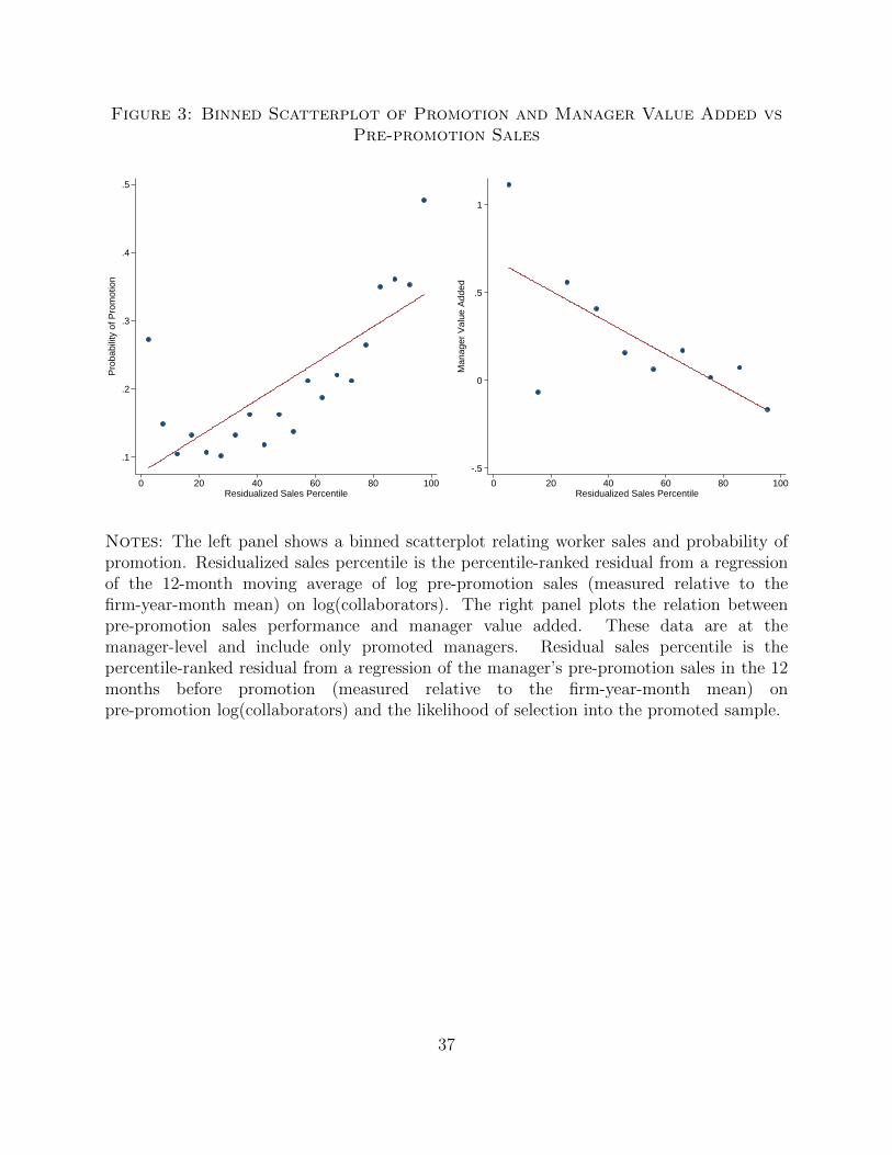
Figure 3: Binned Scatterplot of Promotion and Manager Value Added vsPre-promotion Sales

.1

.2

.3

.4

.5

Pro

babi

lity

of P

rom

otio

n

0 20 40 60 80 100Residualized Sales Percentile

-.5

0

.5

1

Man

ager

Val

ue A

dded

0 20 40 60 80 100Residualized Sales Percentile

Notes: The left panel shows a binned scatterplot relating worker sales and probability ofpromotion. Residualized sales percentile is the percentile-ranked residual from a regressionof the 12-month moving average of log pre-promotion sales (measured relative to thefirm-year-month mean) on log(collaborators). The right panel plots the relation betweenpre-promotion sales performance and manager value added. These data are at themanager-level and include only promoted managers. Residual sales percentile is thepercentile-ranked residual from a regression of the manager’s pre-promotion sales in the 12months before promotion (measured relative to the firm-year-month mean) onpre-promotion log(collaborators) and the likelihood of selection into the promoted sample.

37

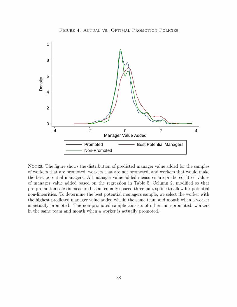
Figure 4: Actual vs. Optimal Promotion Policies

0

.2

.4

.6

.8

1D

ensi

ty

-4 -2 0 2 4Manager Value Added

Promoted Best Potential ManagersNon-Promoted

Notes: The figure shows the distribution of predicted manager value added for the samplesof workers that are promoted, workers that are not promoted, and workers that would makethe best potential managers. All manager value added measures are predicted fitted valuesof manager value added based on the regression in Table 5, Column 2, modified so thatpre-promotion sales is measured as an equally spaced three-part spline to allow for potentialnon-linearities. To determine the best potential managers sample, we select the worker withthe highest predicted manager value added within the same team and month when a workeris actually promoted. The non-promoted sample consists of other, non-promoted, workersin the same team and month when a worker is actually promoted.

38

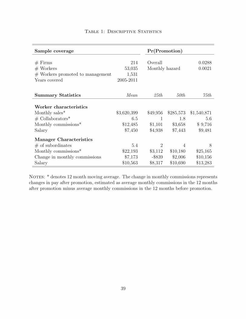
Table 1: Descriptive Statistics

Sample coverage Pr(Promotion)

# Firms 214 Overall 0.0288# Workers 53,035 Monthly hazard 0.0021# Workers promoted to management 1,531Years covered 2005-2011

Summary Statistics Mean 25th 50th 75th

Worker characteristicsMonthly sales* $3,620,399 $49,956 $285,573 $1,540,871# Collaborators* 6.5 1 1.8 5.6Monthly commissions* $12,485 $1,101 $3,658 $ 9,716Salary $7,450 $4,938 $7,443 $9,481

Manager Characteristics# of subordinates 5.4 2 4 8Monthly commissions* $22,193 $3,112 $10,180 $25,165Change in monthly commissions $7,173 -$839 $2,006 $10,156Salary $10,563 $8,317 $10,690 $13,283

Notes: * denotes 12 month moving average. The change in monthly commissions representschanges in pay after promotion, estimated as average monthly commissions in the 12 monthsafter promotion minus average monthly commissions in the 12 months before promotion.

39

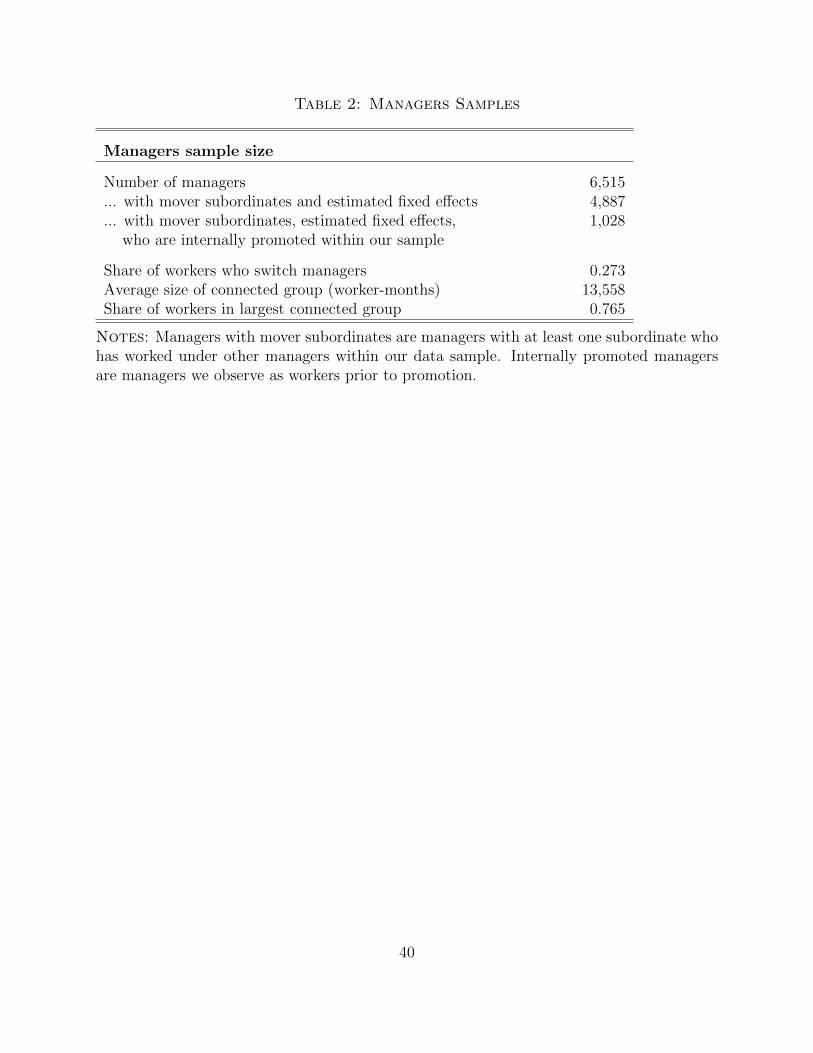
Table 2: Managers Samples

Managers sample size

Number of managers 6,515... with mover subordinates and estimated fixed effects 4,887... with mover subordinates, estimated fixed effects, 1,028

who are internally promoted within our sample

Share of workers who switch managers 0.273Average size of connected group (worker-months) 13,558Share of workers in largest connected group 0.765

Notes: Managers with mover subordinates are managers with at least one subordinate whohas worked under other managers within our data sample. Internally promoted managersare managers we observe as workers prior to promotion.

40

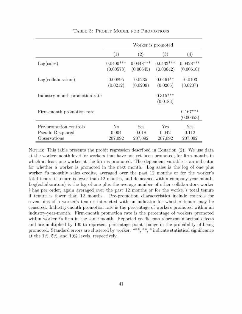
Table 3: Probit Model for Promotions

Worker is promoted

(1) (2) (3) (4)

Log(sales) 0.0400*** 0.0448*** 0.0433*** 0.0428***(0.00578) (0.00645) (0.00642) (0.00610)

Log(collaborators) 0.00895 0.0235 0.0461** -0.0103(0.0212) (0.0209) (0.0205) (0.0207)

Industry-month promotion rate 0.315***(0.0183)

Firm-month promotion rate 0.167***(0.00653)

Pre-promotion controls No Yes Yes YesPseudo R-squared 0.004 0.018 0.042 0.112Observations 207,092 207,092 207,092 207,092

Notes: This table presents the probit regression described in Equation (2). We use dataat the worker-month level for workers that have not yet been promoted, for firm-months inwhich at least one worker at the firm is promoted. The dependent variable is an indicatorfor whether a worker is promoted in the next month. Log sales is the log of one plusworker i’s monthly sales credits, averaged over the past 12 months or for the worker’stotal tenure if tenure is fewer than 12 months, and demeaned within company-year-month.Log(collaborators) is the log of one plus the average number of other collaborators workeri has per order, again averaged over the past 12 months or for the worker’s total tenureif tenure is fewer than 12 months. Pre-promotion characteristics include controls forseven bins of a worker’s tenure, interacted with an indicator for whether tenure may becensored. Industry-month promotion rate is the percentage of workers promoted within anindustry-year-month. Firm-month promotion rate is the percentage of workers promotedwithin worker i’s firm in the same month. Reported coefficients represent marginal effectsand are multiplied by 100 to represent percentage point change in the probability of beingpromoted. Standard errors are clustered by worker. ***, **, * indicate statistical significanceat the 1%, 5%, and 10% levels, respectively.

41

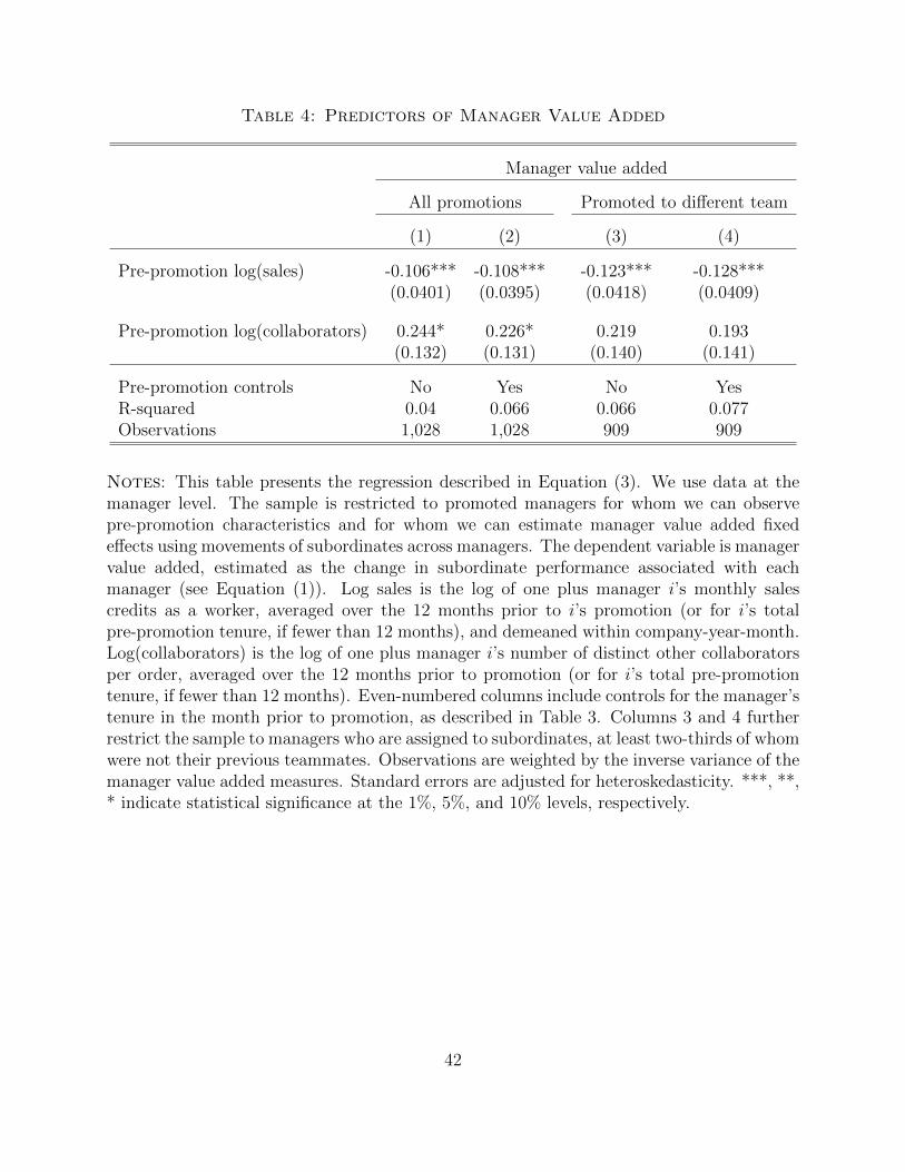
Table 4: Predictors of Manager Value Added

Manager value added

All promotions Promoted to different team

(1) (2) (3) (4)

Pre-promotion log(sales) -0.106*** -0.108*** -0.123*** -0.128***(0.0401) (0.0395) (0.0418) (0.0409)

Pre-promotion log(collaborators) 0.244* 0.226* 0.219 0.193(0.132) (0.131) (0.140) (0.141)

Pre-promotion controls No Yes No YesR-squared 0.04 0.066 0.066 0.077Observations 1,028 1,028 909 909

Notes: This table presents the regression described in Equation (3). We use data at themanager level. The sample is restricted to promoted managers for whom we can observepre-promotion characteristics and for whom we can estimate manager value added fixedeffects using movements of subordinates across managers. The dependent variable is managervalue added, estimated as the change in subordinate performance associated with eachmanager (see Equation (1)). Log sales is the log of one plus manager i’s monthly salescredits as a worker, averaged over the 12 months prior to i’s promotion (or for i’s totalpre-promotion tenure, if fewer than 12 months), and demeaned within company-year-month.Log(collaborators) is the log of one plus manager i’s number of distinct other collaboratorsper order, averaged over the 12 months prior to promotion (or for i’s total pre-promotiontenure, if fewer than 12 months). Even-numbered columns include controls for the manager’stenure in the month prior to promotion, as described in Table 3. Columns 3 and 4 furtherrestrict the sample to managers who are assigned to subordinates, at least two-thirds of whomwere not their previous teammates. Observations are weighted by the inverse variance of themanager value added measures. Standard errors are adjusted for heteroskedasticity. ***, **,* indicate statistical significance at the 1%, 5%, and 10% levels, respectively.

42

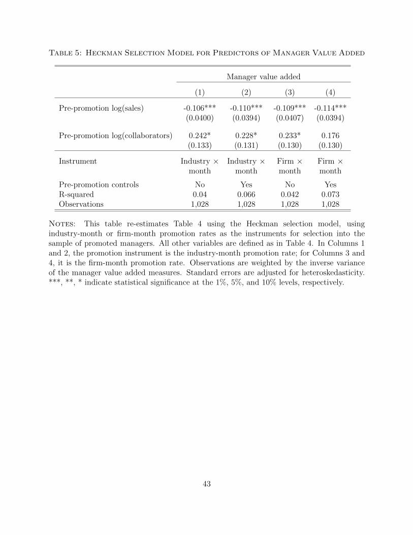
Table 5: Heckman Selection Model for Predictors of Manager Value Added

Manager value added

(1) (2) (3) (4)

Pre-promotion log(sales) -0.106*** -0.110*** -0.109*** -0.114***(0.0400) (0.0394) (0.0407) (0.0394)

Pre-promotion log(collaborators) 0.242* 0.228* 0.233* 0.176(0.133) (0.131) (0.130) (0.130)

Instrument Industry × Industry × Firm × Firm ×month month month month

Pre-promotion controls No Yes No YesR-squared 0.04 0.066 0.042 0.073Observations 1,028 1,028 1,028 1,028

Notes: This table re-estimates Table 4 using the Heckman selection model, usingindustry-month or firm-month promotion rates as the instruments for selection into thesample of promoted managers. All other variables are defined as in Table 4. In Columns 1and 2, the promotion instrument is the industry-month promotion rate; for Columns 3 and4, it is the firm-month promotion rate. Observations are weighted by the inverse varianceof the manager value added measures. Standard errors are adjusted for heteroskedasticity.***, **, * indicate statistical significance at the 1%, 5%, and 10% levels, respectively.

43

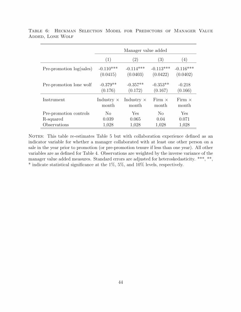
Table 6: Heckman Selection Model for Predictors of Manager ValueAdded, Lone Wolf

Manager value added

(1) (2) (3) (4)

Pre-promotion log(sales) -0.110*** -0.114*** -0.113*** -0.116***(0.0415) (0.0403) (0.0422) (0.0402)

Pre-promotion lone wolf -0.379** -0.357** -0.353** -0.218(0.176) (0.172) (0.167) (0.166)

Instrument Industry × Industry × Firm × Firm ×month month month month

Pre-promotion controls No Yes No YesR-squared 0.039 0.065 0.04 0.071Observations 1,028 1,028 1,028 1,028

Notes: This table re-estimates Table 5 but with collaboration experience defined as anindicator variable for whether a manager collaborated with at least one other person on asale in the year prior to promotion (or pre-promotion tenure if less than one year). All othervariables are as defined for Table 4. Observations are weighted by the inverse variance of themanager value added measures. Standard errors are adjusted for heteroskedasticity. ***, **,* indicate statistical significance at the 1%, 5%, and 10% levels, respectively.

44

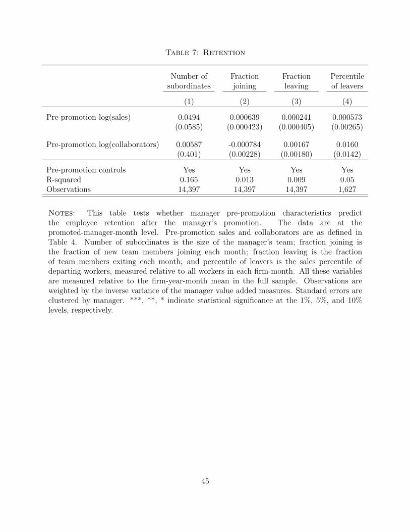
Table 7: Retention

Number of Fraction Fraction Percentilesubordinates joining leaving of leavers

(1) (2) (3) (4)

Pre-promotion log(sales) 0.0494 0.000639 0.000241 0.000573(0.0585) (0.000423) (0.000405) (0.00265)

Pre-promotion log(collaborators) 0.00587 -0.000784 0.00167 0.0160(0.401) (0.00228) (0.00180) (0.0142)

Pre-promotion controls Yes Yes Yes YesR-squared 0.165 0.013 0.009 0.05Observations 14,397 14,397 14,397 1,627

Notes: This table tests whether manager pre-promotion characteristics predictthe employee retention after the manager’s promotion. The data are at thepromoted-manager-month level. Pre-promotion sales and collaborators are as defined inTable 4. Number of subordinates is the size of the manager’s team; fraction joining isthe fraction of new team members joining each month; fraction leaving is the fractionof team members exiting each month; and percentile of leavers is the sales percentile ofdeparting workers, measured relative to all workers in each firm-month. All these variablesare measured relative to the firm-year-month mean in the full sample. Observations areweighted by the inverse variance of the manager value added measures. Standard errors areclustered by manager. ***, **, * indicate statistical significance at the 1%, 5%, and 10%levels, respectively.

45

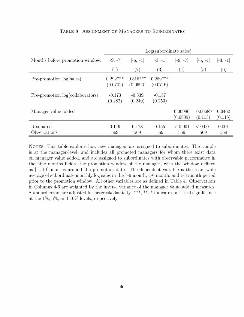
Table 8: Assignment of Managers to Subordinates

Log(subordinate sales)

Months before promotion window: [-9, -7] [-6, -4] [-3, -1] [-9, -7] [-6, -4] [-3, -1]

(1) (2) (3) (4) (5) (6)

Pre-promotion log(sales) 0.292*** 0.316*** 0.289***(0.0702) (0.0696) (0.0716)

Pre-promotion log(collaborators) -0.173 -0.339 -0.157(0.282) (0.249) (0.253)

Manager value added 0.00986 -0.00689 0.0462(0.0809) (0.113) (0.115)

R-squared 0.149 0.178 0.155 < 0.001 < 0.001 0.001Observations 569 569 569 569 569 569

Notes: This table explores how new managers are assigned to subordinates. The sampleis at the manager-level, and includes all promoted managers for whom there exist dataon manager value added, and are assigned to subordinates with observable performance inthe nine months before the promotion window of the manager, with the window definedas [-1,+1] months around the promotion date. The dependent variable is the team-wideaverage of subordinate monthly log sales in the 7-9 month, 4-6 month, and 1-3 month periodprior to the promotion window. All other variables are as defined in Table 4. Observationsin Columns 4-6 are weighted by the inverse variance of the manager value added measures.Standard errors are adjusted for heteroskedasticity. ***, **, * indicate statistical significanceat the 1%, 5%, and 10% levels, respectively.

46

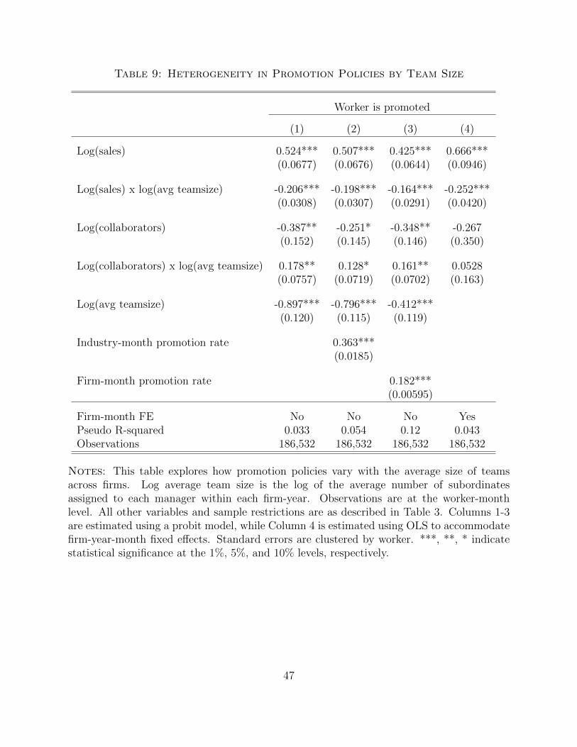
Table 9: Heterogeneity in Promotion Policies by Team Size

Worker is promoted

(1) (2) (3) (4)

Log(sales) 0.524*** 0.507*** 0.425*** 0.666***(0.0677) (0.0676) (0.0644) (0.0946)

Log(sales) x log(avg teamsize) -0.206*** -0.198*** -0.164*** -0.252***(0.0308) (0.0307) (0.0291) (0.0420)

Log(collaborators) -0.387** -0.251* -0.348** -0.267(0.152) (0.145) (0.146) (0.350)

Log(collaborators) x log(avg teamsize) 0.178** 0.128* 0.161** 0.0528(0.0757) (0.0719) (0.0702) (0.163)

Log(avg teamsize) -0.897*** -0.796*** -0.412***(0.120) (0.115) (0.119)

Industry-month promotion rate 0.363***(0.0185)

Firm-month promotion rate 0.182***(0.00595)

Firm-month FE No No No YesPseudo R-squared 0.033 0.054 0.12 0.043Observations 186,532 186,532 186,532 186,532

Notes: This table explores how promotion policies vary with the average size of teamsacross firms. Log average team size is the log of the average number of subordinatesassigned to each manager within each firm-year. Observations are at the worker-monthlevel. All other variables and sample restrictions are as described in Table 3. Columns 1-3are estimated using a probit model, while Column 4 is estimated using OLS to accommodatefirm-year-month fixed effects. Standard errors are clustered by worker. ***, **, * indicatestatistical significance at the 1%, 5%, and 10% levels, respectively.

47

Table 10: Heterogeneity in Promotion Policies by Pay-for-Performance

Worker is promoted

(1) (2) (3) (4)

Log(sales) 0.200*** 0.182*** 0.181*** 0.342***(0.0470) (0.0471) (0.0429) (0.0782)

Log(sales) x ratio variable pay -0.373*** -0.329*** -0.316*** -0.597***(0.110) (0.110) (0.103) (0.180)

Log(collaborators) -0.387*** -0.238** -0.0902 -0.733***(0.111) (0.107) (0.109) (0.255)

Log(collaborators) x ratio variable pay 0.910*** 0.575** 0.135 1.33**(0.276) (0.263) (0.282) (0.639)

Ratio variable pay -1.42*** -0.994** -0.677*(0.403) (0.399) (0.405)

Industry-month promotion rate 0.543***(0.0364)

Firm-month promotion rate 0.175***(0.00783)

Firm-month FE No No No YesPseudo R-squared 0.018 0.037 0.092 0.031Observations 136,083 136,083 136,083 136,083

Notes: This table explores how promotion policies vary with the strength ofpay-for-performance across firms. Ratio variable pay represents the ratio of commissionsplus bonus to salary, averaged across all workers within each firm-year. Observations areat the worker-month level and exclude firms for which we do not have compensation data.All other variables and sample restrictions are as described in Table 3. Columns 1-3 areestimated using a probit model, while Column 4 is estimated using OLS to accommodatefirm-year-month fixed effects. Standard errors are clustered by worker. ***, **, * indicatestatistical significance at the 1%, 5%, and 10% levels, respectively.

48

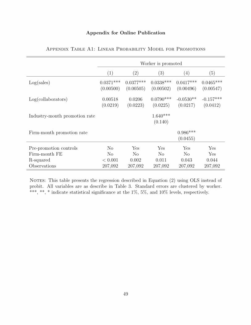
Appendix for Online Publication

Appendix Table A1: Linear Probability Model for Promotions

Worker is promoted

(1) (2) (3) (4) (5)

Log(sales) 0.0371*** 0.0377*** 0.0338*** 0.0417*** 0.0465***(0.00500) (0.00505) (0.00502) (0.00496) (0.00547)

Log(collaborators) 0.00518 0.0206 0.0790*** -0.0530** -0.157***(0.0219) (0.0223) (0.0225) (0.0217) (0.0412)

Industry-month promotion rate 1.640***(0.140)

Firm-month promotion rate 0.986***(0.0455)

Pre-promotion controls No Yes Yes Yes YesFirm-month FE No No No No YesR-squared < 0.001 0.002 0.011 0.043 0.044Observations 207,092 207,092 207,092 207,092 207,092

Notes: This table presents the regression described in Equation (2) using OLS instead ofprobit. All variables are as describe in Table 3. Standard errors are clustered by worker.***, **, * indicate statistical significance at the 1%, 5%, and 10% levels, respectively.

49

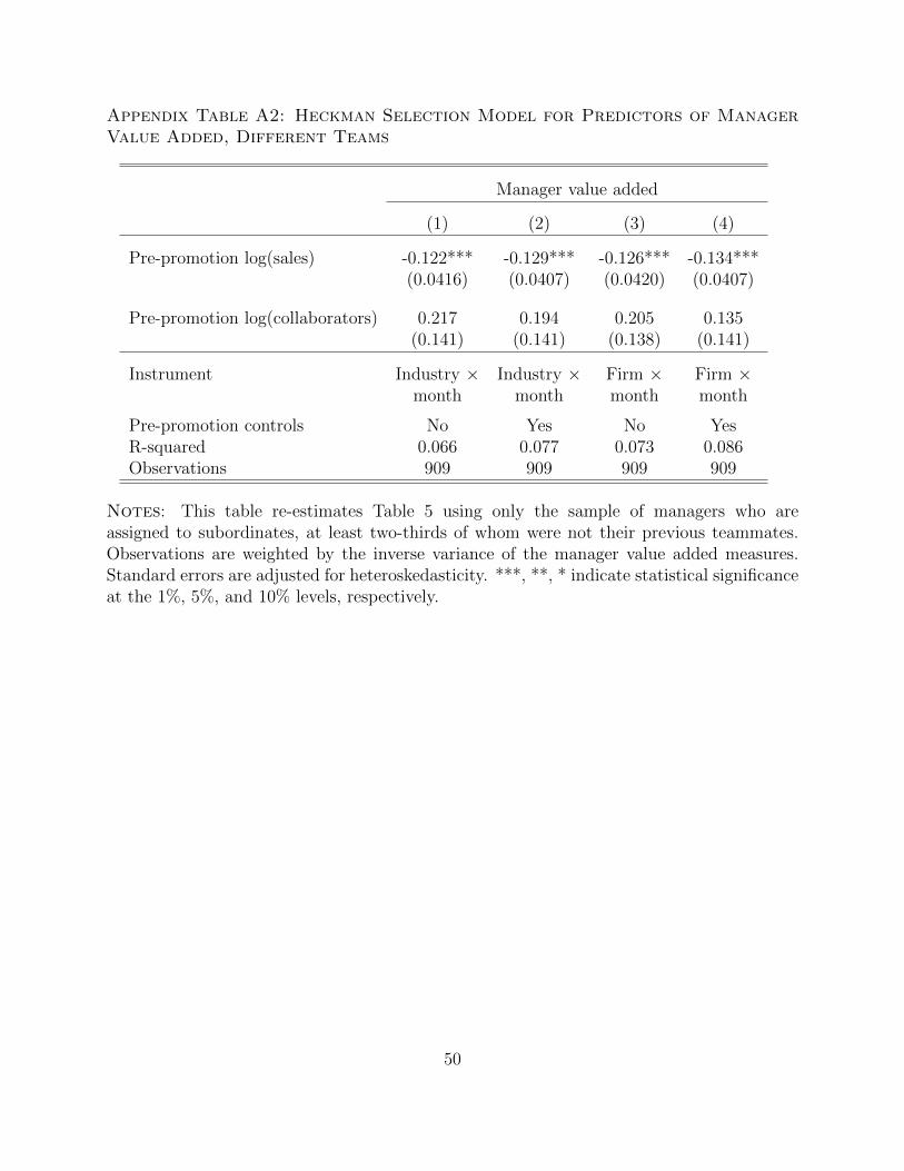
Appendix Table A2: Heckman Selection Model for Predictors of ManagerValue Added, Different Teams

Manager value added

(1) (2) (3) (4)

Pre-promotion log(sales) -0.122*** -0.129*** -0.126*** -0.134***(0.0416) (0.0407) (0.0420) (0.0407)

Pre-promotion log(collaborators) 0.217 0.194 0.205 0.135(0.141) (0.141) (0.138) (0.141)

Instrument Industry × Industry × Firm × Firm ×month month month month

Pre-promotion controls No Yes No YesR-squared 0.066 0.077 0.073 0.086Observations 909 909 909 909

Notes: This table re-estimates Table 5 using only the sample of managers who areassigned to subordinates, at least two-thirds of whom were not their previous teammates.Observations are weighted by the inverse variance of the manager value added measures.Standard errors are adjusted for heteroskedasticity. ***, **, * indicate statistical significanceat the 1%, 5%, and 10% levels, respectively.

50

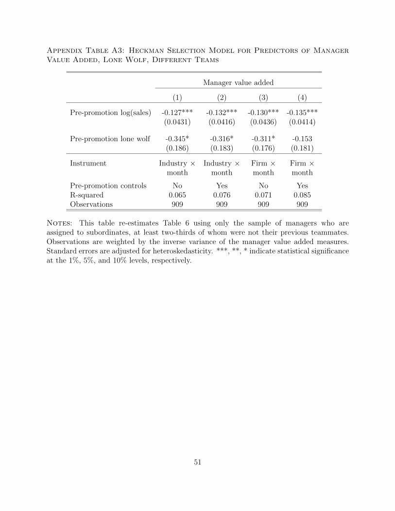
Appendix Table A3: Heckman Selection Model for Predictors of ManagerValue Added, Lone Wolf, Different Teams

Manager value added

(1) (2) (3) (4)

Pre-promotion log(sales) -0.127*** -0.132*** -0.130*** -0.135***(0.0431) (0.0416) (0.0436) (0.0414)

Pre-promotion lone wolf -0.345* -0.316* -0.311* -0.153(0.186) (0.183) (0.176) (0.181)

Instrument Industry × Industry × Firm × Firm ×month month month month

Pre-promotion controls No Yes No YesR-squared 0.065 0.076 0.071 0.085Observations 909 909 909 909

Notes: This table re-estimates Table 6 using only the sample of managers who areassigned to subordinates, at least two-thirds of whom were not their previous teammates.Observations are weighted by the inverse variance of the manager value added measures.Standard errors are adjusted for heteroskedasticity. ***, **, * indicate statistical significanceat the 1%, 5%, and 10% levels, respectively.

51

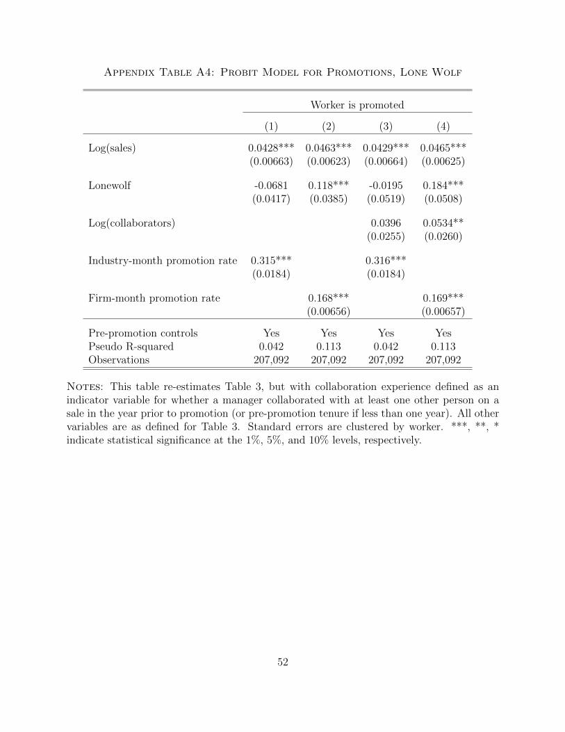
Appendix Table A4: Probit Model for Promotions, Lone Wolf

Worker is promoted

(1) (2) (3) (4)

Log(sales) 0.0428*** 0.0463*** 0.0429*** 0.0465***(0.00663) (0.00623) (0.00664) (0.00625)

Lonewolf -0.0681 0.118*** -0.0195 0.184***(0.0417) (0.0385) (0.0519) (0.0508)

Log(collaborators) 0.0396 0.0534**(0.0255) (0.0260)

Industry-month promotion rate 0.315*** 0.316***(0.0184) (0.0184)

Firm-month promotion rate 0.168*** 0.169***(0.00656) (0.00657)

Pre-promotion controls Yes Yes Yes YesPseudo R-squared 0.042 0.113 0.042 0.113Observations 207,092 207,092 207,092 207,092

Notes: This table re-estimates Table 3, but with collaboration experience defined as anindicator variable for whether a manager collaborated with at least one other person on asale in the year prior to promotion (or pre-promotion tenure if less than one year). All othervariables are as defined for Table 3. Standard errors are clustered by worker. ***, **, *indicate statistical significance at the 1%, 5%, and 10% levels, respectively.

52

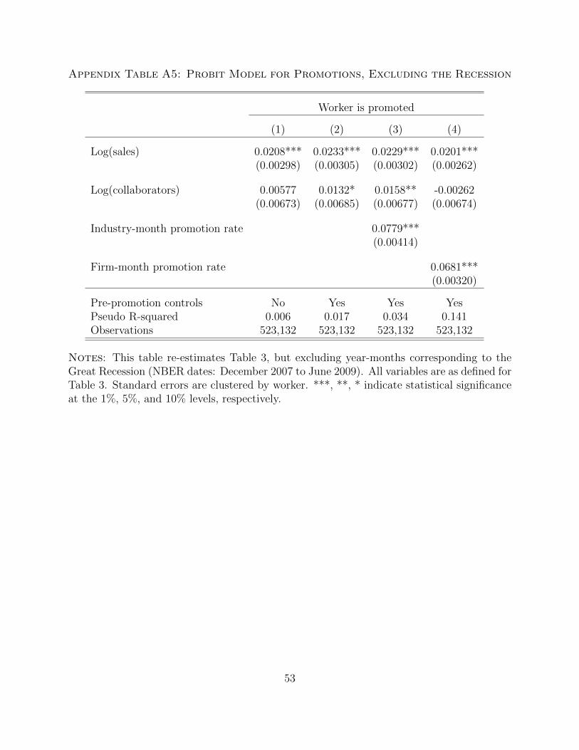
Appendix Table A5: Probit Model for Promotions, Excluding the Recession

Worker is promoted

(1) (2) (3) (4)

Log(sales) 0.0208*** 0.0233*** 0.0229*** 0.0201***(0.00298) (0.00305) (0.00302) (0.00262)

Log(collaborators) 0.00577 0.0132* 0.0158** -0.00262(0.00673) (0.00685) (0.00677) (0.00674)

Industry-month promotion rate 0.0779***(0.00414)

Firm-month promotion rate 0.0681***(0.00320)

Pre-promotion controls No Yes Yes YesPseudo R-squared 0.006 0.017 0.034 0.141Observations 523,132 523,132 523,132 523,132

Notes: This table re-estimates Table 3, but excluding year-months corresponding to theGreat Recession (NBER dates: December 2007 to June 2009). All variables are as defined forTable 3. Standard errors are clustered by worker. ***, **, * indicate statistical significanceat the 1%, 5%, and 10% levels, respectively.

53

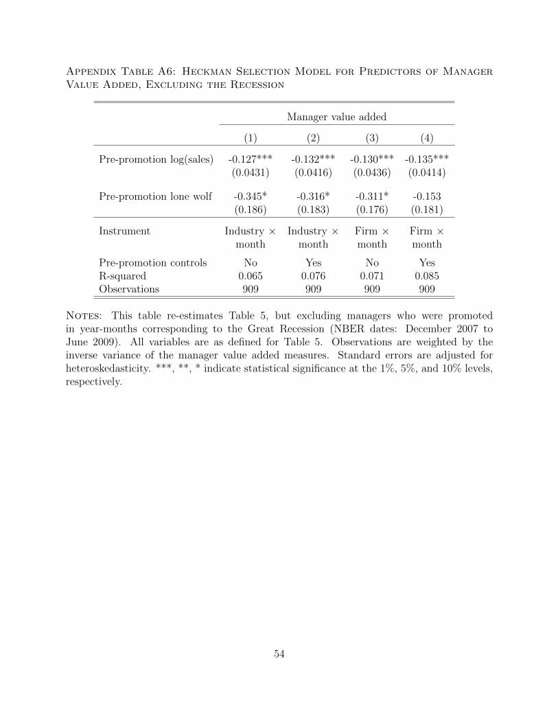
Appendix Table A6: Heckman Selection Model for Predictors of ManagerValue Added, Excluding the Recession

Manager value added

(1) (2) (3) (4)

Pre-promotion log(sales) -0.127*** -0.132*** -0.130*** -0.135***(0.0431) (0.0416) (0.0436) (0.0414)

Pre-promotion lone wolf -0.345* -0.316* -0.311* -0.153(0.186) (0.183) (0.176) (0.181)

Instrument Industry × Industry × Firm × Firm ×month month month month

Pre-promotion controls No Yes No YesR-squared 0.065 0.076 0.071 0.085Observations 909 909 909 909

Notes: This table re-estimates Table 5, but excluding managers who were promotedin year-months corresponding to the Great Recession (NBER dates: December 2007 toJune 2009). All variables are as defined for Table 5. Observations are weighted by theinverse variance of the manager value added measures. Standard errors are adjusted forheteroskedasticity. ***, **, * indicate statistical significance at the 1%, 5%, and 10% levels,respectively.

54