Trabajo fin de másterMáster en Mecánica aplicada

Programa oficial de postgrado en Mecánica computacionalCurso 2011-2012

Métodos multimalla geométricos en mallas semi-estructuradas de Voronoi

Pablo Salinas Cortés

5 de junio de 2012

Director: Francisco José Gaspar Lorenz

Departamento de matemática aplicadaEscuela de Ingeniería y Arquitectura

Universidad de Zaragoza

Métodos multimalla geométricos en mallas semi-estructuradas de Voronoi:

Resumen

Las ecuaciones en derivadas parciales son ampliamente utilizadas para modelizar gran cantidad de problemas físicos, debido a que son el tipo de ecuaciones que se usa para representar la naturaleza. Sin embargo, aunque están ampliamente extendidas en su uso, no siempre se pueden resolver analíticamente, y hay por tanto, que resolverlas numéricamente discretizándolas en una malla. Esta metodología, permite obtener los resultados deseados dentro de un dominio dadas unas condiciones de contorno. Por contra, los sistemas de ecuaciones obtenidos son muy grandes. Esto conlleva escoger muy cuidadosamente qué metodología se va a utilizar para resolverlo si no queremos malgastar recursos y tiempo. Dentro de los posibles algoritmos, el método multimalla destaca por su velocidad y por que el número de iteraciones necesarias para resolver es independiente del número de incógnitas.

Dentro de los métodos multimalla, nos encontramos dos, el geométrico y el algebraico. El primero, es muy rápido pero solo se puede aplicar en dominios simples, el algebraico por otra parte es más lento pero se puede usar en formas complejas. Nosotros, en este trabajo hemos utilizado un método semi-estructurado que consiste en realizar una triangulación no estructurada sobre el dominio, como en el caso algebraico, para captar bien la superficie, y posteriormente dentro de cada triángulo, subdividirlos geométricamente, conectando los puntos medios de los lados cuantas veces sea necesario para obtener la precisión deseada. Además, dentro de cada triángulo de la malla no estructurada se pueden seguir diferentes estrategias dependiendo de las características de este, por ejemplo si es equilátero o isósceles, permitiendo una mayor optimización.

Concretamente, hemos utilizado una malla de Delaunay como triangulación grosera y posteriormente hemos discretizado mediante volúmenes finitos. Como centros de los triángulos hemos usado los centros de Voronoi, toda malla Delaunay tiene asociada una de Voronoi, por sus buenas características; como por ejemplo que este centro es siempre perpendicular a los lados, lo que permite aproximar las derivadas con diferencias finitas. Sin embargo, el uso de estos puntos, a pesar de sus ventajas, introduce anisotropía en la discretización, exige el uso de triángulos acutángulos, así como al ir avanzando a lo largo de la jerarquía de mallas los puntos no están anidados, es decir, al restringir o prolongar los puntos no coinciden en coordenadas. Esto significa, que el método multimalla va a perder rendimiento si no hacemos nada para compensarlo. Para solucionar estos dos problemas hemos diseñado un conjunto de suavizadores que compensan los problemas de anisotropía y de no anidamiento, obteniendo unos resultados muy satisfactorios.

Fijándonos en casos más particulares, podemos tener materiales cuyas propiedades varíen de un punto a otro, por ejemplo, un material compuesto. Si la variación de estas propiedades es de varios órdenes de magnitud, el algoritmo multimalla convencional no va a funcionar correctamente. Sin embargo, este problema puede solventarse si en la malla más fina se utiliza la media harmónica en las zonas de contacto y en las mallas bastas del multimalla se tiene en cuenta que se debe mantener la continuidad en el flujo. Esto se consigue utilizando el operador de Galerkin en las mallas más bastas. A su vez, hemos propuesto un algoritmo que permite obtener este operador en el caso de mallas triangulares, utilizando solamente moléculas en su cálculo.

Los métodos propuestos, tanto los suavizadores, como el operador de Galerkin han sido puestos a prueba en varios ejemplos numéricos para comprobar su eficacia.

Contents

1 Introduction 2

2 Introduction to Multigrid 5

3 Discretization of a diffusion problem on Voronoi grids 93.1 Discretization on triangular unstructured grids . . . . . . . . . . 93.2 Discretization on triangular structured grids . . . . . . . . . . . . 10

3.2.1 Stencil dependence on two angles characterizing the tri-angular grid. . . . . . . . . . . . . . . . . . . . . . . . . . 13

4 Multigrid method 154.1 Coarse-grid correction . . . . . . . . . . . . . . . . . . . . . . . . 154.2 Smoothers . . . . . . . . . . . . . . . . . . . . . . . . . . . . . . . 17

4.2.1 Jacobi smoother. . . . . . . . . . . . . . . . . . . . . . . . 174.2.2 Red-Black smoother. . . . . . . . . . . . . . . . . . . . . . 174.2.3 Diamond smoothers. . . . . . . . . . . . . . . . . . . . . . 184.2.4 Wormy smoothers. . . . . . . . . . . . . . . . . . . . . . . 19

5 Results of the proposed multigrid method on structured grids 20

6 Numerical experiments 246.1 Laplace problem in an A-shaped domain . . . . . . . . . . . . . . 256.2 Convection-diffusion problem on a square domain . . . . . . . . . 25

7 Piecewise discontinuous diffusion coefficient 287.1 Galerkin operator . . . . . . . . . . . . . . . . . . . . . . . . . . . 297.2 Numerical experiments . . . . . . . . . . . . . . . . . . . . . . . . 31

7.2.1 Diffusion problem on the unit square with various diffu-sion coefficients . . . . . . . . . . . . . . . . . . . . . . . . 31

7.2.2 Diffusion problem on a composite material domain . . . . 33

8 Conclusions 35

1

Chapter 1

Introduction

In this work, we are interested in the multigrid solution of the large sparse systemof equations, arising from the cell-centered finite volume discretization of a two-dimensional partial differential equation on acute Delaunay triangulations. Theuse of Delaunay grids is motivated by the good properties of the discretizationsobtained on this type of triangulations; by requiring them to be acute, we achievemonotonicity properties, see [4, 5, 16]. Every Delaunay grid has an associateddual mesh, known as Voronoi tesselation [28], constituted by convex polygons,each one composed of the points closer to a Delaunay vertex (its center) thanto any other.

Voronoi polygons naturally appear in many situations in nature, such as thehottest parts of the sun, ice melting, and even on giraffe skin. Apart from theserelations connected with natural science, not directly related to the numericalsolution of PDEs, more relevant for us is the use of Voronoi grids for the dis-cretization by finite volumes for oil reservoir simulations, oceanographic models,and other complex problems in science and engineering which are derived fromconservation laws.

Finite volume methods are discretizations locally preserving some conserva-tion properties. A first approach to this kind of methods was introduced forone-dimensional problems by Samarskii in 1960, see [24], as a finite differencemethod called balance method (or integro-interpolation method). For manyyears finite volume methods on rectangular and triangular grids were used inheat transfer and computational fluid mechanics [6, 20, 22]. From the theoreticalpoint of view, we refer to the reader to Eymard et al. [9].

One of the most important aspects in the numerical solution of partial dif-ferential equations is the efficient solution of the corresponding large systemsof equations arising from their discretization. Multigrid methods [3, 11, 27] areamong the most powerful techniques for solving such type of algebraic systems,and they have become very popular among the scientific community. Basically,multigrid methods are based on the property of a strong smoothing effect onthe error of many iterative methods, together with the fact that an smoothfunction can be well represented on coarser grids, where its approximation isless expensive. The multigrid performance strongly depends on the choice ofthe components of the algorithm, which are problem dependent, and it is crucialan harmonic interplay between the smoothing and the coarse-grid correction.There are two basic approaches to multigrid solvers: geometric and algebraic

2

multigrid. Whereas in geometric multigrid a hierarchy of grids must be pro-posed, in algebraic multigrid no information is used concerning the grid onwhich the governing PDE is discretized.The focus on this work is to consider geometric multigrid methods. Not manyauthors have applied geometric multigrid methods on cell-centered discretiza-tions. Most of these works have been done in rectangular grids. Historically, thepioneer work is due to Wesseling, [31], in which a multigrid method for interfaceproblems was constructed to simulate oil reservoir problems. This work starteda chain reaction of papers focused on this subject, see [12, 13, 14, 15, 29, 30, 32].The W-cycle convergence of these multigrid methods, in the case of natural in-jection as prolongation, was theoretically analyzed by Bramble et al. [2], and inthe case of V-cycle, the convergence was proved by Kwak et al. in [17] usingcertain weighted prolongation operators. By other hand, on triangular grids,Kwak et al., [18, 19], proposed a new multigrid method, extending their previ-ous works.

For an irregular domain, it is very common to apply regular refinement toan unstructured input grid. In this way, a hierarchy of locally structured gridsis generated. To perform this refinement, each triangle is divided into four con-gruent ones by connecting the midpoints of their edges. In this way, a hierarchyof grids is obtained, where transfer operators between two consecutive levels canbe defined. These grids provide a suitable framework for the implementationof a geometric multigrid algorithm, permitting the use of stencil-based datastructures, see [1], being necessary only a few stencils to represent the discreteoperator, reducing drastically the memory required. In this work, very simplelocal inter-grid transfer operators have been chosen to make easier the com-munication between different input blocks. For this reason, powerful smoothershave to be designed. Different smoothers are used on each input block of the ini-tial unstructured grid, depending on its geometry. Notice that these smootherscouldn’t be implemented on a pure unstructured grid. We are speaking about,for example, the line-type smoothers, very necessary in the case of anisotropicproblems.

Regarding particular applications, the diffusion equation with discontinu-ous coefficients is widely used in computational fluid dynamics. However, it iswell-known that when standard multigrid is applied for solving equations withhighly varying discontinuous coefficients, a deterioration in the convergence ofthe method can be obtained, and even divergence can be observed.

In the case of cell-centered approximations, the main idea to circumvent theproblem is to use Galerkin approximation [32] on coarse grids. The disadvantageusually observed when using this approach, is that the stencils of the coarse-grid operators are often larger than the corresponding fine-grid stencil, what isproblematic especially in three dimensions. However, note that the use of sim-ple transfer operators preserves four-point stencils in the case of cell-centeredschemes on triangular grids.

In the case of composite materials their components have nearly constantdiffusivity, but vary by several orders of magnitude. In these cases, it is quitecommon to idealize the diffusivity by a piecewise constant function. This makessuitable the use of semi-structured grids to deal with these problems.

3

The rest of the work is organized as follows: Chapter 2 presents the ba-sic principles of Multigrid. Chapter 3 is devoted to present the cell-centereddiscretization, deriving the corresponding equations which define the discreteoperator for both unstructured and structured triangular grids. A multigridmethod for this kind of scheme is proposed in Chapter 4. In particular, spe-cial smoothers are designed to overcome troubles arising from some difficultgrid-geometries. In Chapter 5, the good performance of the proposed multigridmethods is demonstrated on structured triangular grids, comparing the behaviorof the considered smoothers for different grid-geometries. In Chapter 6, sometest examples are presented to show the applicability of the strategies followedthroughout all the work. Finally, in Chapter 7, we focus the previous work inthe resolution of diffusion equation with piece-wise discontinuous coefficients.

4

Chapter 2

Introduction to Multigrid

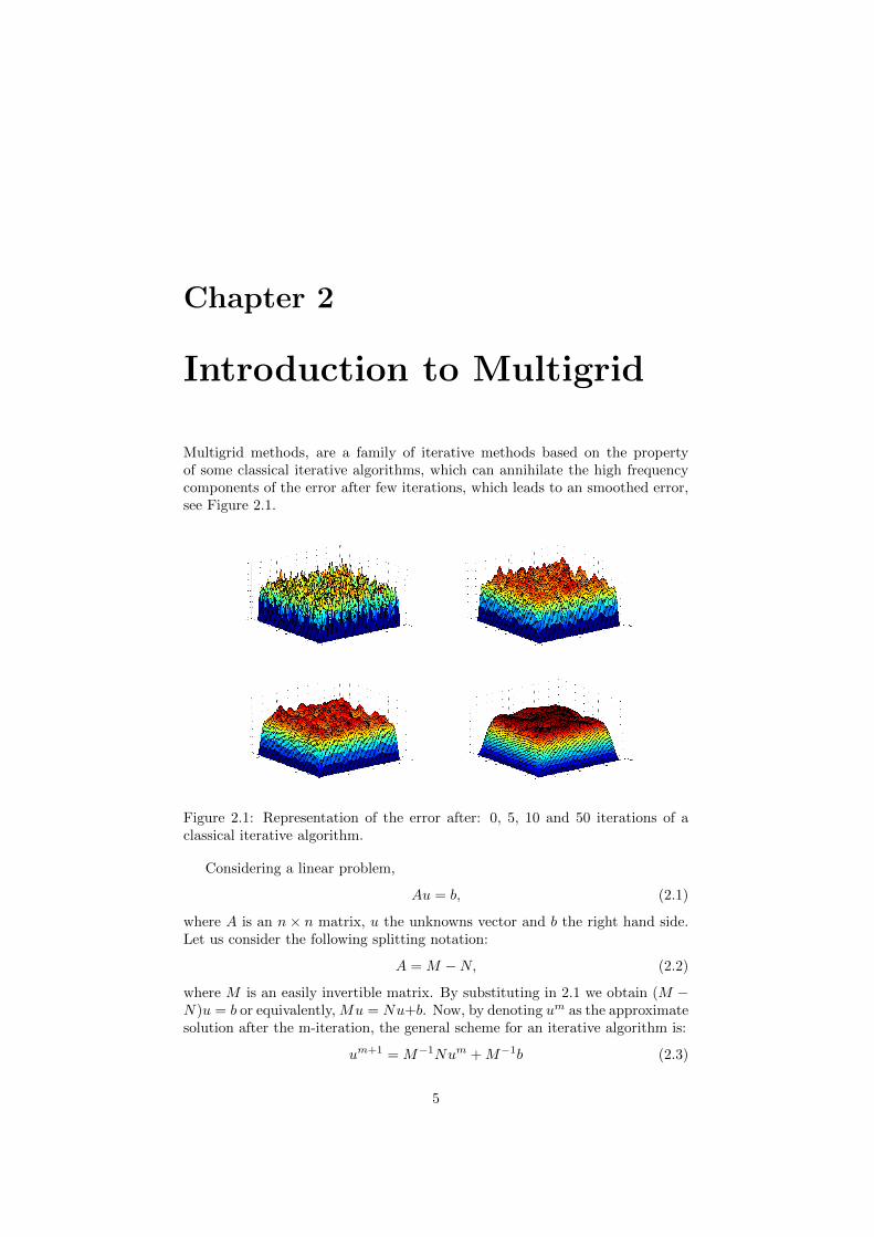
Multigrid methods, are a family of iterative methods based on the propertyof some classical iterative algorithms, which can annihilate the high frequencycomponents of the error after few iterations, which leads to an smoothed error,see Figure 2.1.

Figure 2.1: Representation of the error after: 0, 5, 10 and 50 iterations of aclassical iterative algorithm.

Considering a linear problem,

Au = b, (2.1)

where A is an n× n matrix, u the unknowns vector and b the right hand side.Let us consider the following splitting notation:

A = M −N, (2.2)

where M is an easily invertible matrix. By substituting in 2.1 we obtain (M −N)u = b or equivalently, Mu = Nu+b. Now, by denoting um as the approximatesolution after the m-iteration, the general scheme for an iterative algorithm is:

um+1 = M−1Num +M−1b (2.3)

5

If we call ue to the exact solution, we can define the error in the iterationm, as em = ue − um, and the residual rm = b − Aum. We can combine theseexpressions with (2.1) in order to get a system of equations for the error:

rm = b−Aue +Aem = Aem, (2.4)

therefore, we can solve a system for the error in order to get a better approxi-mation of the solution. If we now combine the smoothing property, that allowsto represent the error in a coarser grid without data loss, with the possibility tosolve an equation for the error, we can define the following strategy:

1 Smooth.

2 Represent the error in a coarser grid.

3 Solve the equation exactly.

4 Use the error calculated to correct the approximation, um.

5 Iterate until obtaining the desired precision.

The above explained method is called two-grids method. Its efficiency isnot a high improvement, however, its convergence rate is constant not matterthe number of nodes, this is also known as h-independence rate. Nevertheless,two-grids method can be improved if, in the third step, we approximate theanalytical solution by using another two-grids method and so on, leading tothe so called multigrid method, which keeps the h-independence rate, and itsnumerical cost is about O(n× n).

Regarding the second and the forth step we can split the inter-grid transferoperators in:

• Restriction: Introduce, the data from a fine grid to a coarse one, it canbe done by simple injection, just introduce in the coarse grid the value ofthe nodes that relies in the same coordinates, or by an average of nodes.

• Prolongation: Interpolate the solution of the coarse grid to the nodes of afiner one. The simplest, the adjoint of the simple injection, is to introducethe data from the coarse grid directly to a cluster of nodes.

One can realize that the performance of the multigrid method relies on thesmoother, coarse grid transfer method and in the interpolation from a coarsergrid to a finer one. The intercourse between the smoother and the inter-gridtransfer operators are the key in multigrid. In fact there are two families ofmultigrid methods, depending on their intercourse:

• Geometric multigrid: The coarsening is fixed, usually the coarser grid istwice the finer, and the smoother must annihilate the half of the frequencyerrors. These methods are fast, but the geometry must be simple.

• Algebraic multigrid: The smoother is fixed, and the coarsening must adaptitself in order to compensate what the smoother cannot smooth. Thesefamily fits very easily complex geometries, but they are slower than thegeometric multigrid.

6

Figure 2.2: Relation, along the grids, between nodes for a simple injection andits adjoint.

Regarding the smoothers, the most common smoothers are the Jacobi iter-ative method with a relaxation parameter, Gauss-Seidel algorithm and a mod-ification of the Gauss-Seidel, in which you apply a Gauss-Seidel step but in achessboard manner, i.e: first the odd nodes and next the even ones, see Fig-ure 2.3.

Figure 2.3: Red-Black smoother on a triangular grid.

There are three kind of multigrid methods depending on the effort to ap-proximate the error on coarser grids, one get three different multigrid methods,V-cycle, W-cycle and F-cycle, see Figure 2.4. V-cycle is the fastest, but theweakest, F-cycle is usually preferred over W-cycle since it achieve similar re-

7

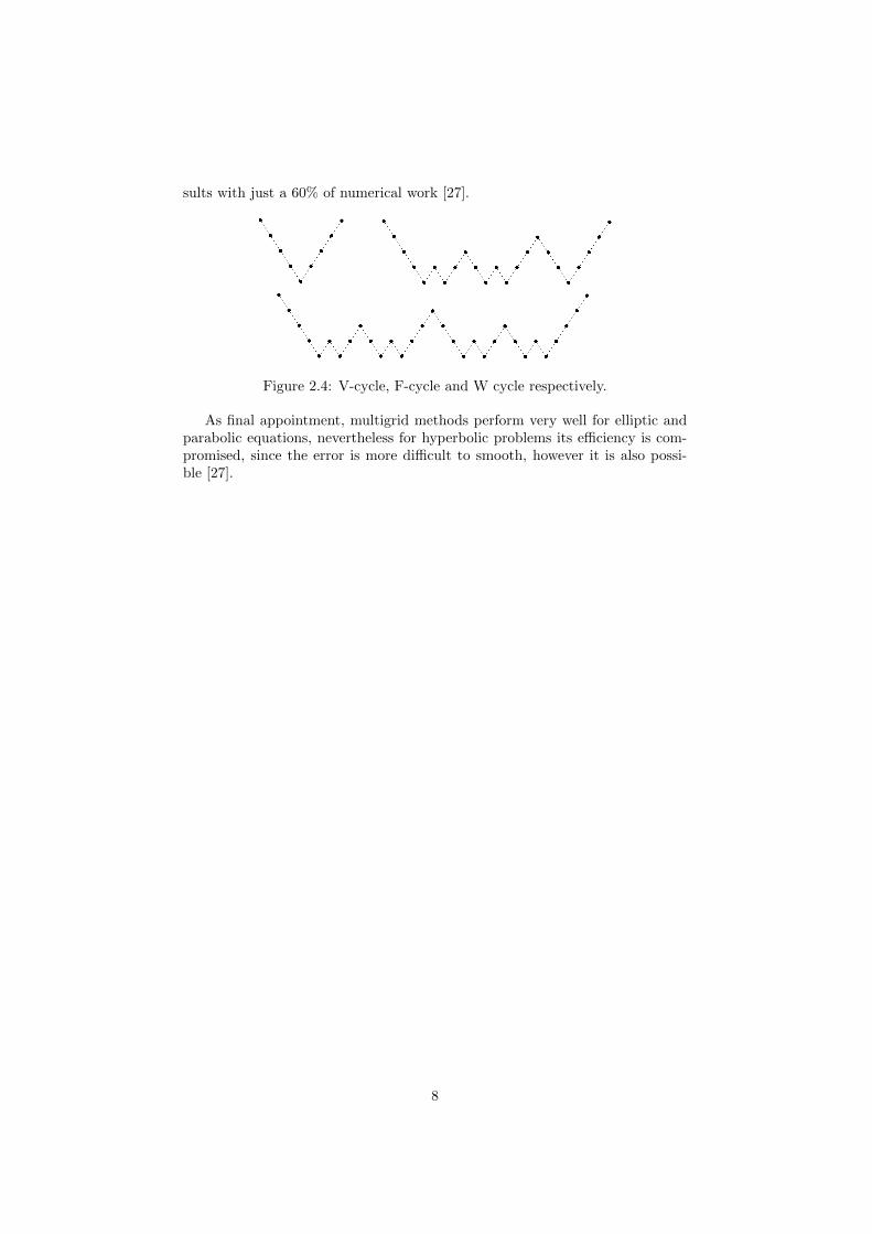
sults with just a 60% of numerical work [27].

Figure 2.4: V-cycle, F-cycle and W cycle respectively.

As final appointment, multigrid methods perform very well for elliptic andparabolic equations, nevertheless for hyperbolic problems its efficiency is com-promised, since the error is more difficult to smooth, however it is also possi-ble [27].

8

Chapter 3

Discretization of a diffusionproblem on Voronoi grids

3.1 Discretization on triangular unstructured grids

We are going to construct a finite volume discretization scheme on the Voronoimesh associated with a Delaunay triangulation for the following boundary valueproblem:

−∆v = f, in Ω, (3.1)

v = 0, on ∂Ω. (3.2)

Firstly, we suppose to have a Delaunay triangulation T on the domain Ω, sat-isfying the usual admissibility assumption (see [5]), i.e. the intersection of twodifferent triangles is either empty, a vertex, or a whole edge. Besides, as com-mented in the introduction, we restrict ourselves to an acute triangulation.The grid points associated with the cell-centered scheme are the centers of the

Figure 3.1: Unstructured mesh and its associated Voronoi grid.

circumscribed circle of each triangle, defining a Voronoi mesh, see Figure 3.1.Notice that from the previous restriction with regard to the angles of the trian-gulation, we are sure that each Voronoi point falls inside of a triangle. More-

9

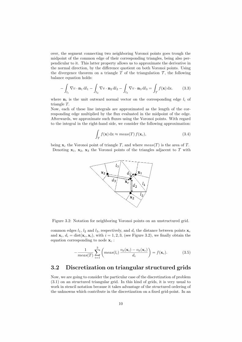
over, the segment connecting two neighboring Voronoi points goes trough themidpoint of the common edge of their corresponding triangles, being also per-pendicular to it. This latter property allows us to approximate the derivative inthe normal direction, by the difference quotient on both Voronoi points. Usingthe divergence theorem on a triangle T of the triangulation T , the followingbalance equation holds:

−∫l1

∇v · n1 dl1 −∫l2

∇v · n2 dl2 −∫l3

∇v · n3 dl3 =

∫T

f(x) dx. (3.3)

where ni is the unit outward normal vector on the corresponding edge li oftriangle T.Now, each of these line integrals are approximated as the length of the cor-responding edge multiplied by the flux evaluated in the midpoint of the edge.Afterwards, we approximate such fluxes using the Voronoi points. With regardto the integral in the right-hand side, we consider the following approximation:∫

T

f(x) dx ≈ meas(T ) f(xc), (3.4)

being xc the Voronoi point of triangle T, and where meas(T ) is the area of T.Denoting x1, x2, x3 the Voronoi points of the triangles adjacent to T with

Figure 3.2: Notation for neighboring Voronoi points on an unstructured grid.

common edges l1, l2 and l3, respectively, and di the distance between points xc

and xi, di = dist(xc,xi), with i = 1, 2, 3, (see Figure 3.2), we finally obtain theequation corresponding to node xc :

− 1

meas(T )

3∑i=1

(meas(li)

vh(xi)− vh(xc)

di

)= f(xc). (3.5)

3.2 Discretization on triangular structured grids

Now, we are going to consider the particular case of the discretization of problem(3.1) on an structured triangular grid. In this kind of grids, it is very usual towork in stencil notation because it takes advantage of the structured ordering ofthe unknowns which contribute in the discretization on a fixed grid-point. In an

10

structured grid, any point is surrounded by the same grid-pattern, and using asuitable numbering of the grid-points it is easy to capture this pattern in a smallmatrix or “stencil” which stores the contributions of the neighboring unknowns.Then, first of all, a suitable numbering of the grid-points is needed. In triangulargrids, a unitary basis of R2, e1, e2, where e1, and e2 are unit vectors definingthe oblique coordinate system, is considered fitting the geometry of the triangle,as can be seen in Figure 3.3. Hence, a local numeration can be fixed according

a) b)

Figure 3.3: a) New basis in R2 fitting the geometry of a triangular grid, andlocal numeration for the regular Delaunay grid obtained on a triangular domain.b) Corresponding Voronoi mesh.

to the definition of the spatial basis. In this way, a manner of numbering nodesvery convenient for identifying the neighboring nodes can be defined.We consider a triangular grid arising on a triangular domain by applying a fixednumber of regular refinement steps `. This is done in the way that, on eachrefinement step every triangle is divided into four congruent ones by connectingthe midpoints of their edges.Then, we can define the corresponding grid in the following way:

G` = x = k1h1 e1 + k2h2 e2 | k1 = 0, . . . , 2`, k2 = 0, . . . , k1, (3.6)

where h = (h1, h2) is the grid spacing associated with the refinement level ` (h1is the grid spacing in the direction of e1, and h2 in the direction of e2), so thatthe grid G` can also be denoted by Gh.Thus, for a refinement level `, a local numeration with double index (k1, k2),k1 = 0, . . . , 2`, k2 = 0, . . . , k1, is used in such a way that the indexes of thevertices of the triangle are (0, 0), (2`, 0), (2`, 2`), as it can also be observed inFigure 3.3a) for ` = 2.

By other hand, the considered discretization is based on the dual Voronoimesh, represented in Figure 3.3b). In the particular case in which an structuredgrid as considered here is used, the obtained finite difference scheme results tobe different depending on the grid point. More concretely, one-half of the gridpoints, those corresponding to an up oriented triangle, have the same equationand the other half, those corresponding to a down oriented triangle, have a“mirror image stencil”, see Figure 3.4. In this sense, the Voronoi mesh, denotedby Vh could be split up into two sub-grids V u

h (associated with the up-orientedtriangles) and V d

h , (corresponding to the down-oriented triangles), as seen inFigure 3.3b). These sub-grids can be defined from the grid Gh, in the following

11

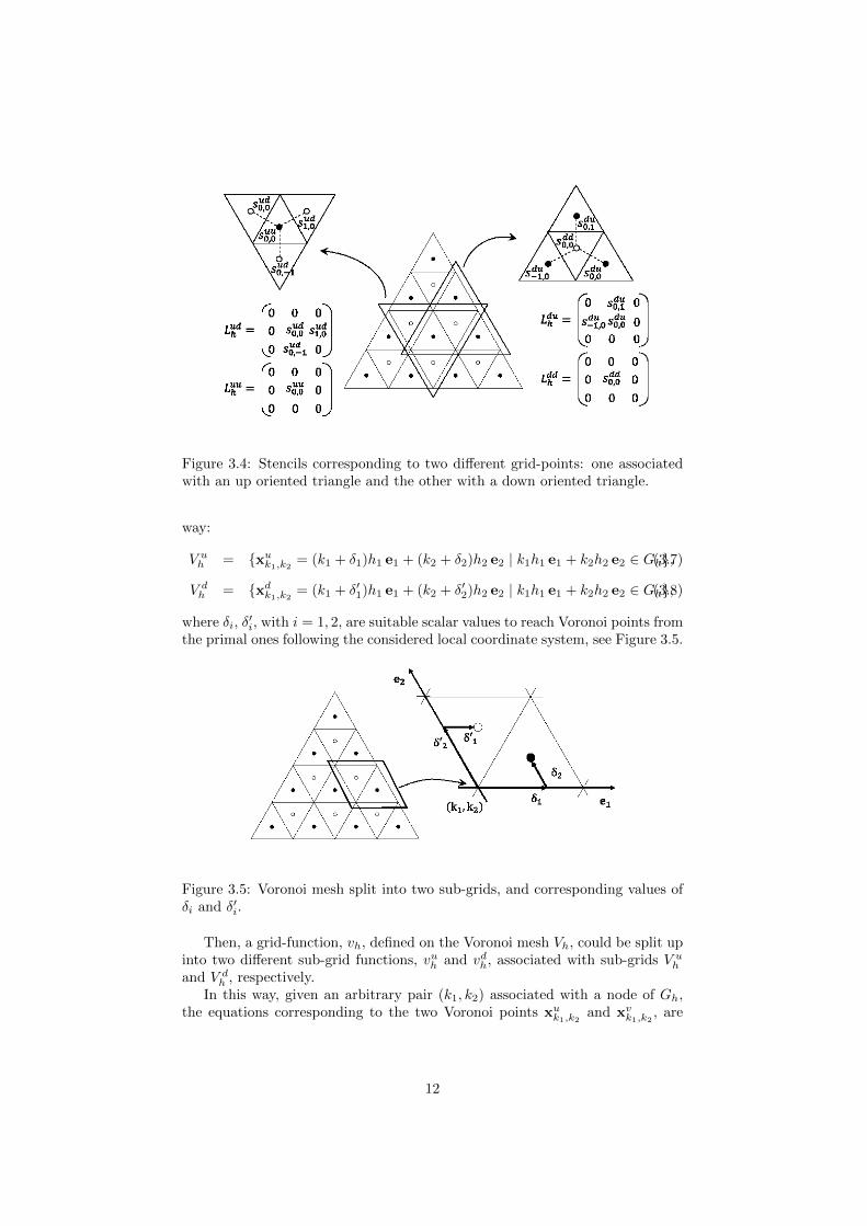
Figure 3.4: Stencils corresponding to two different grid-points: one associatedwith an up oriented triangle and the other with a down oriented triangle.

way:

V uh = xu

k1,k2= (k1 + δ1)h1 e1 + (k2 + δ2)h2 e2 | k1h1 e1 + k2h2 e2 ∈ Gh,(3.7)

V dh = xd

k1,k2= (k1 + δ′1)h1 e1 + (k2 + δ′2)h2 e2 | k1h1 e1 + k2h2 e2 ∈ Gh,(3.8)

where δi, δ′i, with i = 1, 2, are suitable scalar values to reach Voronoi points from

the primal ones following the considered local coordinate system, see Figure 3.5.

Figure 3.5: Voronoi mesh split into two sub-grids, and corresponding values ofδi and δ′i.

Then, a grid-function, vh, defined on the Voronoi mesh Vh, could be split upinto two different sub-grid functions, vuh and vdh, associated with sub-grids V u

h

and V dh , respectively.

In this way, given an arbitrary pair (k1, k2) associated with a node of Gh,the equations corresponding to the two Voronoi points xu

k1,k2and xv

k1,k2, are

12

given by

Luuh vuh(xu

k1,k2) + Lud

h vdh(xdk1,k2

) = fuh (xuk1,k2

), (3.9)

Lduh vuh(xu

k1,k2) + Ldd

h vdh(xd

k1,k2) = fdh(xd

k1,k2), (3.10)

where these “scalar” operators are given in stencil form as:

Luuh =1

meas(T )

0 0 0

0l1

d1

+l2

d2

+l3

d3

0

0 0 0

, Ludh =1

meas(T )

0 0 0

0 −l1

d1

−l3

d3

0 −l2

d2

0

,

Lduh =1

meas(T )

0 −

l2

d2

0

−l3

d3

−l1

d1

0

0 0 0

, Lddh =1

meas(T )

0 0 0

0l1

d1

+l2

d2

+l3

d3

0

0 0 0

.

3.2.1 Stencil dependence on two angles characterizing thetriangular grid.

In order to know a priori the strong and weak connections between neighboringunknowns depending on the grid geometry, we are going to rewrite the stencilsin function of some parameters characterizing the grid, that is, two angles, αand β, and the length l, of one edge of an arbitrary triangle of the grid, seeFigure 3.6. As we will see, this is going to be very useful for the design ofsmoothers for different geometries, taking into account the strong connectionsappearing in the stencils.

Therefore, we are going to describe in detail the computation of the stencil foran arbitrary down-oriented Voronoi grid-point xd

k1,k2in V d

h . With this purpose,we can write the coordinates of the points involved in such stencil (see Figure 3.6)in terms of the previously explained geometric parameters in the following way:

xdk1,k2

=l

2

(sinα cosβ

3 sin(α+ β)+ 2,

cos(α− β)

sin(α+ β)

), (3.11)

xuk1,k2

=l

2(3,− cot(α+ β)) , (3.12)

xuk1−1,k2

=l

2(1,− cot(α+ β)) , (3.13)

xuk1,k2+1 =

l

2

(2 sinα cosβ

sin(α+ β)+ 1,

2 sinα sinβ

sin(α+ β)− cot(α+ β)

). (3.14)

Since all the parameters involved in the stencil (area, distances between Voronoipoints and lengths of the edges) are independent of the chosen coordinate sys-tem, for simplicity, these coordinates have been computed in the Cartesiancoordinate system with respect to the origin, see Figure 3.6.

Due to the fact that the area of an arbitrary triangle T is given in terms ofthe geometric parameters as

meas(T ) =l2 sinα sinβ

2 sin(α+ β), (3.15)

13

Figure 3.6: Notation for neighboring Voronoi points on an structured grid,characterized by angles α and β.

and the lengths of the sides of T are l2 = l, l1 =l sinβ

sin(α+ β), and l3 =

l sinα

sin(α+ β),

after simple calculations, we finally obtain the stencils:

Lduh =

2 sin(α+ β)

l2 sinα sinβ

0 tan(α+ β) 0− tanα − tanβ 0

0 0 0

, (3.16)

Lddh =

2 sin(α+ β)

l2 sinα sinβ

0 0 00 tan(α+ β)− tanα− tanβ 00 0 0

. (3.17)

As previously commented, for an arbitrary up-oriented Voronoi grid-point xuk1,k2

in V uh the stencil would be the “mirror image stencil” of (3.16)-(3.17), that is,

Luuh =

2 sin(α+ β)

l2 sinα sinβ

0 0 00 tan(α+ β)− tanα− tanβ 00 0 0

, (3.18)

Ludh =

2 sin(α+ β)

l2 sinα sinβ

0 0 00 − tanβ − tanα0 tan(α+ β) 0

. (3.19)

Notice that depending on the angles characterizing the grid, some strongconnections appear between unknowns and this fact makes that we will have totake care in the design of the smoothers in a geometric multigrid method, aswill be discussed in next chapter.

14

Chapter 4

Multigrid method

The performance of geometric multigrid methods is strongly dependent on thechoice of adequate components to the considered problem. The main compo-nents are the smoother Sh, inter-grid transfer operators: restriction I2hh andprolongation Ih2h, and the coarse-grid operator L2h. These components have tobe chosen so that they efficiently interplay with each other in order to obtaina good connection between the relaxation and the coarse-grid correction. Inthis chapter the proposed cell-centered multigrid algorithm is described. Allthe attention is focused in the detailed explanation of the considered smoothersand the special features appearing due to the cell-centered character of the dis-cretization.

Although the presentation of such components is done on a regular struc-tured grid, our purpose is to apply the proposed multigrid method in the frame-work of semi-structured grids. Therefore, the choice of the corresponding com-ponents is done also with a view to this application. In this case, we will usea block-wise multigrid algorithm, where each triangle of the coarsest grid istreated as a different block with regard to the smoothing process. This block-wise strategy is suitable thanks to the possibility of choosing different smoothersfor triangles having different geometries, thus resulting in an improvement ofthe characteristics of our algorithm. Besides, we will have to take care in thecommunication among the triangles of the coarsest triangulation. Next, we aregoing to describe the components of the algorithm that we are going to considerthroughout all this work.

4.1 Coarse-grid correction

In the application of geometric multigrid, a hierarchy of grids is needed in orderto accelerate the convergence of the smoother, by using solutions obtained onthe coarser meshes as corrections. As previously commented, in order to obtainsuch hierarchy of grids, we divide the initial triangles into four congruent onesby connecting the midpoints of the edges, and so forth until the mesh has thedesired fine scale to approximate the solution of the problem.When vertex-centered discretizations are considered on triangular grids, gridpoints laying on coarser grids also belong to the finer grids, giving rise to a

15

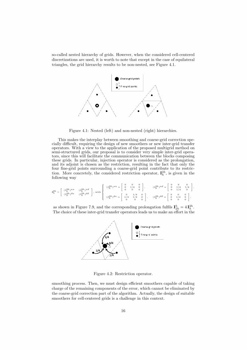
so-called nested hierarchy of grids. However, when the considered cell-centereddiscretizations are used, it is worth to note that except in the case of equilateraltriangles, the grid hierarchy results to be non-nested, see Figure 4.1.

Figure 4.1: Nested (left) and non-nested (right) hierarchies.

This makes the interplay between smoothing and coarse-grid correction spe-cially difficult, requiring the design of new smoothers or new inter-grid transferoperators. With a view to the application of the proposed multigrid method onsemi-structured grids, our proposal is to consider very simple inter-grid opera-tors, since this will facilitate the communication between the blocks composingthese grids. In particular, injection operator is considered as the prolongation,and its adjoint is chosen as the restriction, resulting in the fact that only thefour fine-grid points surrounding a coarse-grid point contribute to its restric-tion. More concretely, the considered restriction operator, I2hh , is given in thefollowing way

I2hh =

(I2hh )uu (I2hh )ud

(I2hh )du (I2hh )dd

, with

(I2hh )uu =

0 0 00 1/4 00 0 0

, (I2hh )ud =

0 0 00 1/4 1/40 1/4 0

,

(I2hh )du =

0 1/4 01/4 1/4 00 0 0

, (I2hh )dd =

0 0 00 1/4 00 0 0

,

as shown in Figure 7.9, and the corresponding prolongation fulfils Ih2h = 4 I2hh .The choice of these inter-grid transfer operators leads us to make an effort in the

Figure 4.2: Restriction operator.

smoothing process. Then, we must design efficient smoothers capable of takingcharge of the remaining components of the error, which cannot be eliminated bythe coarse-grid correction part of the algorithm. Actually, the design of suitablesmoothers for cell-centered grids is a challenge in this context.

16

4.2 Smoothers

The smoother usually plays an important role in multigrid algorithms, mainly inthe geometric approach, resulting the choice of a suitable smoother an importantfeature for the efficiency of these methods. Moreover, as previously commented,in the framework we are working with, this choice is even more relevant.Due to the general observation that errors become smooth if strongly connectedunknowns are collectively updated, appropriate smoothers have been designeddepending on the magnitude of the coefficients of the stencils, given in (3.16)-(3.19). The following smoothers have been considered and tested in order tofulfil the previous requirement.

4.2.1 Jacobi smoother.

For almost equilateral triangles, the magnitude of all the entries of the stencilsis similar, and therefore a point-wise smoother is enough to satisfactorily reducethe components of the error. The easiest smoother to perform is a Jacobi typesmoother, which consists of computing the approximation of each unknown, byusing non-updated values of the rest of the unknowns. Notice that this impliesthat it makes not difference the order in which the grid points are visited, whatmakes Jacobi scheme well-suited for parallel processing. However, for difficultproblems, usually this smoother does not give enough satisfactory results, andsome variants have to be considered.As is the case for Jacobi smoother presented here, some standard smoothers arebased on a decomposition on the positive and negative parts of the operator,which correspond to the updated an non-updated unknowns before the currentstep. Here we are going to present the corresponding decomposition for Jacobismoother. In order to do this, only the positive part of the operator is displayed.Taking into account that only the diagonal blocks of the operator contribute inthis positive part, it holds

(Luuh )+ = Luu

h , (Lddh )+ = Ldd

h . (4.1)

4.2.2 Red-Black smoother.

Due to the fact that unknowns related to up or down-oriented triangles haveno direct connection with each other, it seems natural to simultaneously updateall unknowns associated with equally oriented triangles, giving rise to a patternrelaxation scheme. Since two different types of grid-points are distinguished, atwo-color relaxation process, called here Red-Black smoother, is considered.More concretely, one iteration of this relaxation scheme consists of two partialsteps. In the first one, unknowns corresponding to up-oriented triangles areupdated, and in the second step those associated with the down-oriented tri-angles are relaxed by using the updated values. Thus, the complete smoothingoperator Sh is given by the composition of two partial step operators, Su

h andSdh, which correspond to apply a Jacobi step on each type of grid-points, that

is, Sh = Sdh Su

h. These partial step operators are characterized by a differentdecomposition than the previous Jacobi over all the grid-points, in the way thatfor Su

h, for example, the positive parts of the scalar operators are:

(Luuh )+ = Luu

h , (Lddh )+ = Ih, (4.2)

17

and if Sdh is considered, the identity operator will correspond to (Luu

h )+, and(Ldd

h )+ = Lddh .

4.2.3 Diamond smoothers.

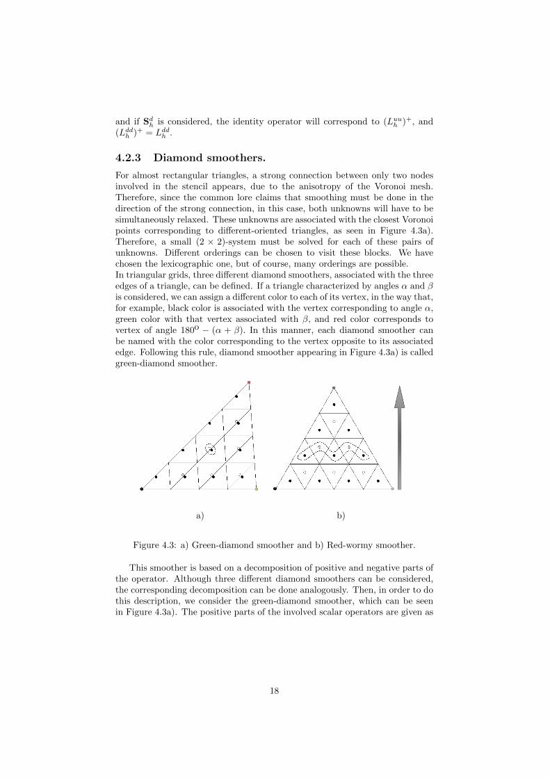
For almost rectangular triangles, a strong connection between only two nodesinvolved in the stencil appears, due to the anisotropy of the Voronoi mesh.Therefore, since the common lore claims that smoothing must be done in thedirection of the strong connection, in this case, both unknowns will have to besimultaneously relaxed. These unknowns are associated with the closest Voronoipoints corresponding to different-oriented triangles, as seen in Figure 4.3a).Therefore, a small (2 × 2)-system must be solved for each of these pairs ofunknowns. Different orderings can be chosen to visit these blocks. We havechosen the lexicographic one, but of course, many orderings are possible.In triangular grids, three different diamond smoothers, associated with the threeedges of a triangle, can be defined. If a triangle characterized by angles α and βis considered, we can assign a different color to each of its vertex, in the way that,for example, black color is associated with the vertex corresponding to angle α,green color with that vertex associated with β, and red color corresponds tovertex of angle 180o − (α + β). In this manner, each diamond smoother canbe named with the color corresponding to the vertex opposite to its associatededge. Following this rule, diamond smoother appearing in Figure 4.3a) is calledgreen-diamond smoother.

a) b)

Figure 4.3: a) Green-diamond smoother and b) Red-wormy smoother.

This smoother is based on a decomposition of positive and negative parts ofthe operator. Although three different diamond smoothers can be considered,the corresponding decomposition can be done analogously. Then, in order to dothis description, we consider the green-diamond smoother, which can be seenin Figure 4.3a). The positive parts of the involved scalar operators are given as

18

follows:

(Luuh )+ = Luu

h , (Ludh )+ =

0 0 00 sud0,0 00 sud0,−1 0

,(Ldu

h )+ =

0 0 0sdu−1,0 sdu0,0 0

0 0 0

, (Lddh )+ = Ldd

h .

(4.3)

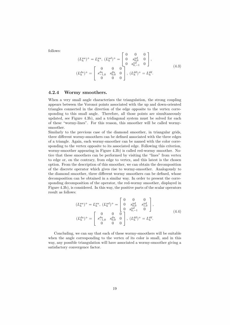
4.2.4 Wormy smoothers.

When a very small angle characterizes the triangulation, the strong couplingappears between the Voronoi points associated with the up and down-orientedtriangles connected in the direction of the edge opposite to the vertex corre-sponding to this small angle. Therefore, all those points are simultaneouslyupdated, see Figure 4.3b), and a tridiagonal system must be solved for eachof these “wormy-lines”. For this reason, this smoother will be called wormy-smoother.Similarly to the previous case of the diamond smoother, in triangular grids,three different wormy-smoothers can be defined associated with the three edgesof a triangle. Again, each wormy-smoother can be named with the color corre-sponding to the vertex opposite to its associated edge. Following this criterion,wormy-smoother appearing in Figure 4.3b) is called red-wormy smoother. No-tice that these smoothers can be performed by visiting the “lines” from vertexto edge or, on the contrary, from edge to vertex, and this latest is the chosenoption. From the description of this smoother, we can obtain the decompositionof the discrete operator which gives rise to wormy-smoother. Analogously tothe diamond smoother, three different wormy smoothers can be defined, whosedecomposition can be obtained in a similar way. In order to present the corre-sponding decomposition of the operator, the red-wormy smoother, displayed inFigure 4.3b), is considered. In this way, the positive parts of the scalar operatorsresult as follows:

(Luuh )+ = Luu

h , (Ludh )+ =

0 0 00 sud0,0 sud1,00 sud0,−1 0

,(Ldu

h )+ =

0 0 0sdu−1,0 sdu0,0 0

0 0 0

, (Lddh )+ = Ldd

h .

(4.4)

Concluding, we can say that each of these wormy-smoothers will be suitablewhen the angle corresponding to the vertex of its color is small, and in thisway, any possible triangulation will have associated a wormy-smoother giving asatisfactory convergence factor.

19

Chapter 5

Results of the proposedmultigrid method onstructured grids

In order to see the suitability of the introduced smoothers in the design ofan efficient multigrid algorithm, we present some experiments comparing theirbehavior in regular structured grids. In particular, model problem (3.1)-(3.2) issolved in the structured grid arising from the regular refinement of a triangulardomain, characterized by two of their angles. In all the presented experiments,an F (2, 2)−cycle is considered. F−cycle is preferred to V−cycle due to the poorchosen inter-grid transfer operators.

We begin by considering an equilateral triangular domain. As any anisotropyarises from the grid resulting of a regular refinement, it could be seen natu-ral to think in applying a simple point-wise smoother, like Jacobi or lexico-graphic Gauss-Seidel, to this kind of triangulations. However, as previouslycommented, for this situation a pattern relaxation scheme could be more ap-propriately. Thus, we are going to present some convergence results on a regularequilateral grid, comparing the behavior of multigrid by considering: undampedJacobi smoother, Red-Black smoother, ω−Red-Black smoother (with ω = 1.15)and diamond smoother. In Figure 5.1a), we show the history of the convergenceon a grid obtained after eight refinement levels, and by considering as stoppingcriterion to reduce the maximum residual until 10−8. First of all, a rather sur-prising observation could be concluded from this figure: the performance of un-damped Jacobi appears to be a satisfactory choice as smoother for cell-centereddiscretizations on triangular grids (as also seen for other type of discretizationson triangular grids, [10], and in the context of full-multigrid on rectangulargrids, [23]), despite the well-known lack of smoothing property of this iterativescheme. Notwithstanding this unusual behavior, the obtained Jacobi resultsare largely improved by Red-Black smoother and diamond smoother. At thesame time, the convergence factors provided by both smoothers are enhancedby the Red-Black smoother with relaxation parameter ω = 1.15, which has beenobtained by experimental tests. This improving effect was pointed out in [21]for cell-centered discretizations on rectangular grids, where it was validated bya local Fourier analysis. Moreover, the good behavior of the multigrid based

20

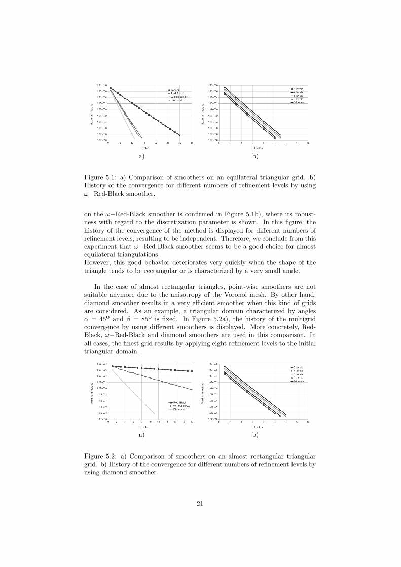
a) b)

Figure 5.1: a) Comparison of smoothers on an equilateral triangular grid. b)History of the convergence for different numbers of refinement levels by usingω−Red-Black smoother.

on the ω−Red-Black smoother is confirmed in Figure 5.1b), where its robust-ness with regard to the discretization parameter is shown. In this figure, thehistory of the convergence of the method is displayed for different numbers ofrefinement levels, resulting to be independent. Therefore, we conclude from thisexperiment that ω−Red-Black smoother seems to be a good choice for almostequilateral triangulations.However, this good behavior deteriorates very quickly when the shape of thetriangle tends to be rectangular or is characterized by a very small angle.

In the case of almost rectangular triangles, point-wise smoothers are notsuitable anymore due to the anisotropy of the Voronoi mesh. By other hand,diamond smoother results in a very efficient smoother when this kind of gridsare considered. As an example, a triangular domain characterized by anglesα = 45o and β = 85o is fixed. In Figure 5.2a), the history of the multigridconvergence by using different smoothers is displayed. More concretely, Red-Black, ω−Red-Black and diamond smoothers are used in this comparison. Inall cases, the finest grid results by applying eight refinement levels to the initialtriangular domain.

a) b)

Figure 5.2: a) Comparison of smoothers on an almost rectangular triangulargrid. b) History of the convergence for different numbers of refinement levels byusing diamond smoother.

21

As we can observe, very poor rates are obtained when both Red-Blacksmoothers are considered, whereas the convergence factors provided by the newdiamond smoother are very satisfactory, achieving the convergence in only elevencycles. Besides, in Figure 5.2b), where the history of the convergence is shownfor different numbers of refinement levels, the robustness of this smoother withrespect to the space discretization parameter is demonstrated.Although convergence factors provided by diamond smoother are very satis-factory for many grid configurations, when a triangulation characterized by avery small angle is used, this smoother gives rise to poor rates. This behaviorcan be seen in Figure 5.3, where asymptotic convergence factors of the dia-mond smoother based multigrid are shown for a wide range of pairs of anglescharacterizing the grid.

Figure 5.3: Experimentally computed convergence factors for the diamondsmoother based multigrid and four smoothing steps, for different triangles infunction of two of their angles.

To overcome these troubles appearing when the primal mesh is anisotropic,wormy-smoother in the direction of the anisotropy is a suitable smoother, largelyimproving the convergence factors provided by the rest of point-wise or block-wise smoothers. To validate this statement, we are going to compare the multi-grid convergence by using each one of the smoothers proposed in this work,when an isosceles triangle with a small angle of 10o is considered as domainof our problem. With this purpose, in Figure 5.4a), the multigrid convergenceprovided by using ω−Red-Black, diamond and wormy smoothers is depicted foreight refinement levels. From this picture, it is clear that wormy-smoother isthe best choice for this type of triangulations. Moreover, an h−independentconvergence is also shown in Figure 5.4b).

Concluding, from the results presented in this chapter, it seems that a reason-able strategy to follow would be to apply the point-wise ω−Red-Black smootherfor almost equilateral triangles, the collective diamond smoother for almost rect-angular triangles, and finally the appropriate block collective wormy smoother

22

a) b)

Figure 5.4: a) Comparison of smoothers on an isosceles triangular grid withsmallest angle 10o. b) History of the convergence for different numbers of re-finement levels by using wormy-smoother.

when triangulations with a small angle appear.

23

Chapter 6

Numerical experiments

From the practical point of view, for any given triangular geometry would benice to be capable of choosing a suitable smoother in order to reach a desiredconvergence factor. Moreover, for semi-structured grids, it is imperative to knowthe smoother to use for each triangle of the input grid, in order to achieve glob-ally a desired convergence factor. In order to reach this, a set-up phase has beenimplemented in the multigrid code; it consists of reading an already calculateddatabase containing the most efficient strategy depending on the triangle angles.The corresponding guideline to reach a global convergence factor about 0.1 isshown in Figure 6.1, and it has been numerically calculated by doing extensivecomputations in regular triangular grids.

Figure 6.1: Guideline to choose suitable smoothers to reach an asymptotic con-vergence factor about 0.1 on different triangles.

Strategy shown in Figure 6.1 has been followed in the two model problemsconsidered here: a Laplace problem in an A-shaped domain, and a convection-diffusion problem in an square domain. In both problems, aCute software, [7,8], which is based on Triangle, [25, 26], has been used to generate the initial

24

unstructured acute Delaunay triangulation.

6.1 Laplace problem in an A-shaped domain

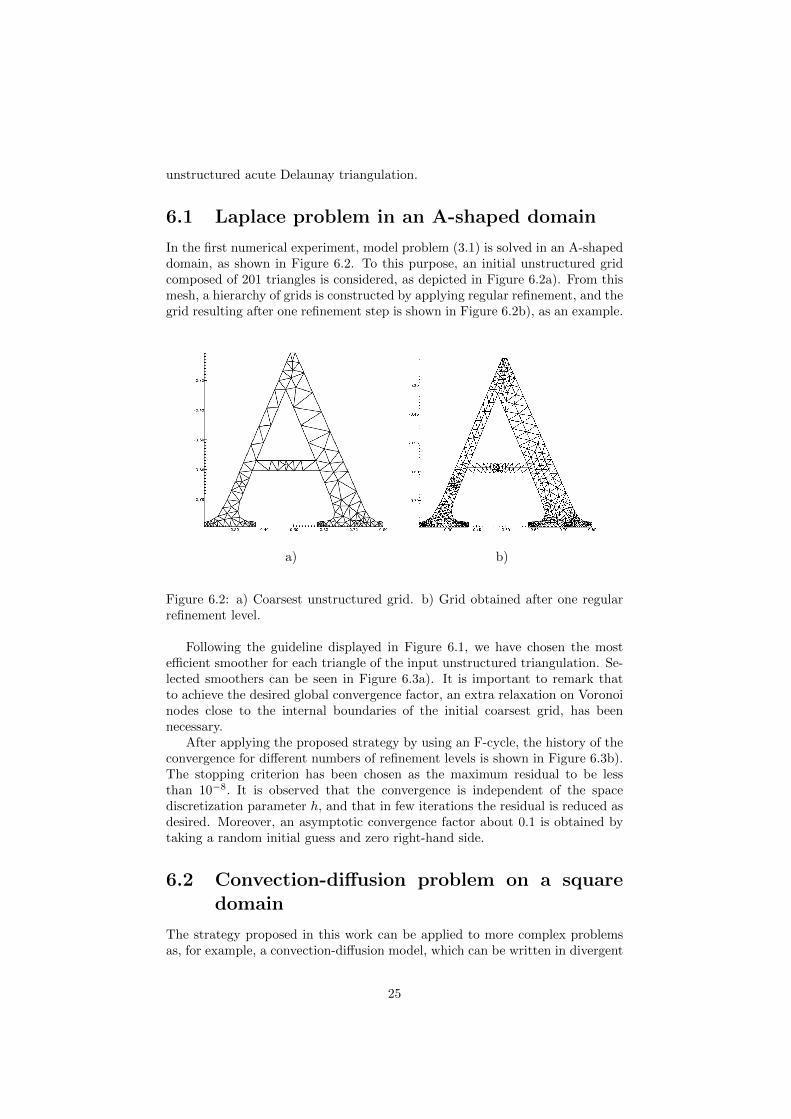
In the first numerical experiment, model problem (3.1) is solved in an A-shapeddomain, as shown in Figure 6.2. To this purpose, an initial unstructured gridcomposed of 201 triangles is considered, as depicted in Figure 6.2a). From thismesh, a hierarchy of grids is constructed by applying regular refinement, and thegrid resulting after one refinement step is shown in Figure 6.2b), as an example.

a) b)

Figure 6.2: a) Coarsest unstructured grid. b) Grid obtained after one regularrefinement level.

Following the guideline displayed in Figure 6.1, we have chosen the mostefficient smoother for each triangle of the input unstructured triangulation. Se-lected smoothers can be seen in Figure 6.3a). It is important to remark thatto achieve the desired global convergence factor, an extra relaxation on Voronoinodes close to the internal boundaries of the initial coarsest grid, has beennecessary.

After applying the proposed strategy by using an F-cycle, the history of theconvergence for different numbers of refinement levels is shown in Figure 6.3b).The stopping criterion has been chosen as the maximum residual to be lessthan 10−8. It is observed that the convergence is independent of the spacediscretization parameter h, and that in few iterations the residual is reduced asdesired. Moreover, an asymptotic convergence factor about 0.1 is obtained bytaking a random initial guess and zero right-hand side.

6.2 Convection-diffusion problem on a squaredomain

The strategy proposed in this work can be applied to more complex problemsas, for example, a convection-diffusion model, which can be written in divergent

25

a) b)

Figure 6.3: a) Different smoothers for the triangles composing the initial trian-gulation of the A-shaped domain. b) Multigrid convergence for Poisson problemon the A-shaped domain.

form as:−∇ · (∇v + b v) = f, in Ω, (6.1)

where b(x) is a given velocity field, whose divergence is assumed to be zero.In order to obtain a difference scheme by the cell-centered finite volume method,we follow the same approach that we have explained in detail in Chapter 3, byusing a central difference scheme to approximate the convective term. In thisnumerical experiment an square domain of unit length and Dirichlet boundaryconditions are considered, and a constant vector b = (1, 0) is fixed in the wholedomain. Thus, the following equation on each of the grid-nodes xc results:

− 1

meas(T )

3∑i=1

(meas(li)

(vh(xi)− vh(xc)

di+ b · ni

vh(xi) + vh(xc)

2

))= f(xc).

(6.2)

Figure 6.4: Coarsest unstructured grid together with the associated Voronoimesh.

26

We consider an initial unstructured grid, composed of 96 triangles, as seen inFigure 6.4, in which, for illustration, the dual Voronoi mesh has been displayed.The hierarchy of grids is obtained by regular refinement. As the convectivepart of the problem is not dominant, and its derivatives are of lower order, thebehavior of the multigrid will be similar to that obtained for a pure diffusiveproblem, and therefore we will follow the guideline given in Figure 6.1 to choosethe suitable local smoother on each input triangle, and this selection is displayedin Figure 6.5. The proposed geometric multigrid method is applied to solve thecorresponding large sparse linear system of equations. An F-cycle is used to testthe independency of the multigrid convergence with regard to the discretizationparameters.

Figure 6.5: Different smoothers considered on each triangular block of the inputgrid.

N. of levels N. of unknowns N. of cycles ρh4 24576 9 0.095 98304 9 0.096 393216 9 0.097 1572864 9 0.108 6291456 9 0.10

Table 6.1: Number of iterations to reduce the initial residual in a factor of10−10, and corresponding asymptotic convergence rates for different numbers ofrefinement levels, by using an F-cycle

In Table 6.1, for different numbers of refinement levels, the asymptotic con-vergence rate, ρh, and the number of iterations necessary to reduce the initialresidual in a factor of 10−10, are displayed.

27

Chapter 7

Piecewise discontinuousdiffusion coefficient

In this chapter we will consider the diffusion problem:

−∇ · (κ(x, y)∇u) = f, in Ω, (7.1)

u = g, on Γ (7.2)

where κ(x, y) is a discontinuous the diffusion coefficient. In particular, here weare interested in problems were κ is piecewise constant. Considering again thecell-centered discretization scheme, equation 3.5 reads now as:

− 1

meas(T )

3∑i=1

(κHi meas(li)

vh(xi)− vh(xc)

di

)= f(xc). (7.3)

Where x1, x2, x3 are the Voronoi points of the triangles adjacent to T withcommon edges l1, l2 and l3, respectively, and di the distance between points xc

and xi, with i = 1, 2, 3, (see Figure 3.2). The coefficient κHi appearing in (7.3)is the harmonic average given by:

κHi =2κcκiκc + κi

, (7.4)

which is the most accurate method of known techniques of averaging, [32, 24].In this way, given an arbitrary pair (k1, k2) associated with a node of Gh,

the equations corresponding to the two Voronoi points xuk1,k2

and xvk1,k2

, aregiven by

Luuh vuh(xu

k1,k2) + Lud

h vdh(xdk1,k2

) = fuh (xuk1,k2

), (7.5)

Lduh vuh(xu

k1,k2) + Ldd

h vdh(xd

k1,k2) = fdh(xd

k1,k2), (7.6)

where “scalar” operators Luuh , Lud

h , Lduh and Ldd

h can be obtained from equa-tion (7.3), and are given in stencil form as:

28

Luuh =1

meas(T )

0 0 0

0 κH1

l1

d1

+ κH2

l2

d2

+ κH3

l3

d3

0

0 0 0

, Ludh =1

meas(T )

0 0 0

0 −κH1l1

d1

−κH3l3

d3

0 −κH2l2

d2

0

,

Lduh =1

meas(T )

0 −κH2

l2

d2

0

−κH3l3

d3

−κH1l1

d1

0

0 0 0

, Lddh =1

meas(T )

0 0 0

0 κH1

l1

d1

+ κH2

l2

d2

+ κH3

l3

d3

0

0 0 0

,

where the distances d1, d2, d3 and the lengths l1, l2, l3 are defined dependingon the orientation of the triangle, as seen in Figure 7.1. For example, for anup-oriented triangle d2 is defined as the distance between xu

k1,k2and xd

k1,k2−1,and l2 as the length of the edge between those Voronoi points.

(a) (b)

Figure 7.1: Notation used to construct the stencil on a Voronoi point at (a) anup-oriented triangle or at (b) a down-oriented triangle.

When the semi-structured grid is considered, different stencils are necessaryto describe the discrete operator on the structured grid arising on a triangle Tof this mesh. Notice that all the down-oriented triangles comprising this gridare “interior”, that is, they only connect with up-oriented triangles of T. Inthis way, the stencils corresponding to their Voronoi nodes will be identical.However, for those grid-points associated with up-oriented triangles, differentstencils appear depending on their location, since it is necessary to take intoaccount the connections with other triangles belonging to other block of thecoarsest grid.

7.1 Galerkin operator

When large jumps in the diffusion coefficient κ occur in the domain, a di-rect discretization on coarse grids may not work properly. However, in mostof the multigrid methods for discontinuous coefficients problems, the Galerkinapproach have been used satisfactorily. This method consists of defining thecoarse-grid operator in terms of the fine-grid operator, Lk, the restriction,Ik−1k

and the prolongation, Ikk−1, in the following way:

Lk−1 = Ik−1k LkIkk−1 (7.7)

With this method, it is not straight to work directly with stencil notationas the operations are matrix multiplications.

29

We propose an easy algorithm to calculate Lk−1 using only stencils. Thismethod must be applied once per stencil operator. Firstly, the notation for thisalgorithm needs to be modified, nevertheless using the following conversion ofthe previously explained stencils, its application is straightforward:

Stencil =

0 0 0Ludh (0, 0) Luu

h (0, 0) Ludh (1, 0)

0 Ludh (0, 1) 0

. (7.8)

Secondly, we have to define an stencil of stencils:

St(j, i) =

0 0 0SE(jj, ii) SC(jj, ii) SW (jj, ii)

0 SN (jj, ii)|SS(jj, ii) 0

, (7.9)

Where the subfix is their position in cardinal coordinates, being SC the center,see Figure 7.2.

Figure 7.2: Stencils notation to be used in the Stencil of Stencils

All the stencils coordinates must be defined from −1 to 1, being the center(0, 0), and the κ must be included. The stencil of stencil, St must be a 4dimensional array in which the two first coordinates are the position of thestencil, and the last two the coordinates the position entries of that stencil. Thealgorithm is as follows:

Program Galerkin_Operator

StencilC = 0

n = 0

center = 1

!Compute A_coarse

do ii = 0 to 1

do jj = 1 to -1 add -1

do i = 0 to 1

do j = 1 to -1 add -1

n = n + 1

if ((ii = 0 and jj = 0) or (i = 0 and j = 0) or

(n = center)) then

StencilC(0,0) = StencilC(0,0) +

+ S_t(j,i,-jj,ii) * R(j,i)

30

else

StencilC(jj,ii) = StencilC(jj,ii) +

+ S_t(-j,i,jj,ii) * R(-j,i)

end do

end do

n = 0

center = center + 1

end do

end do

!Store stencil

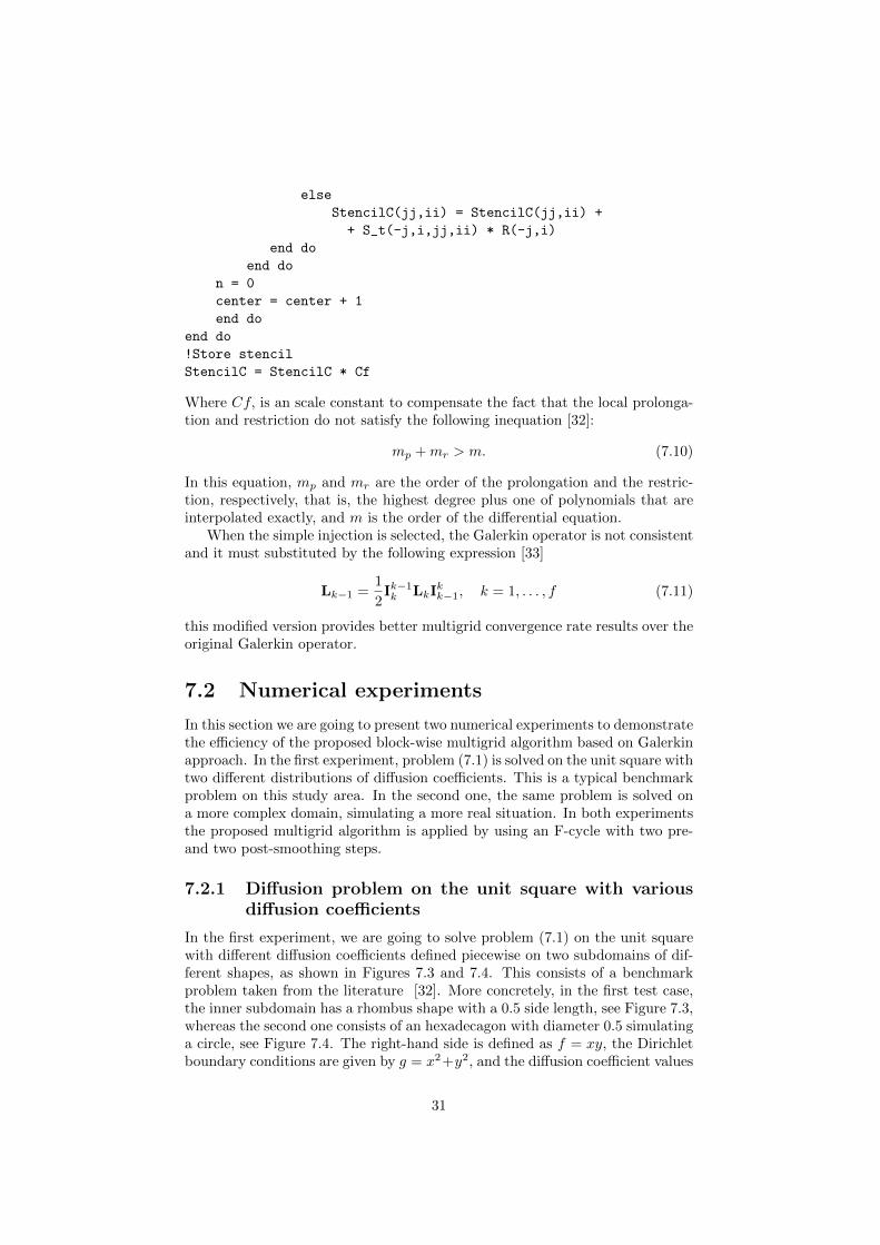
StencilC = StencilC * Cf

Where Cf, is an scale constant to compensate the fact that the local prolonga-tion and restriction do not satisfy the following inequation [32]:

mp +mr > m. (7.10)

In this equation, mp and mr are the order of the prolongation and the restric-tion, respectively, that is, the highest degree plus one of polynomials that areinterpolated exactly, and m is the order of the differential equation.

When the simple injection is selected, the Galerkin operator is not consistentand it must substituted by the following expression [33]

Lk−1 =1

2Ik−1k LkIkk−1, k = 1, . . . , f (7.11)

this modified version provides better multigrid convergence rate results over theoriginal Galerkin operator.

7.2 Numerical experiments

In this section we are going to present two numerical experiments to demonstratethe efficiency of the proposed block-wise multigrid algorithm based on Galerkinapproach. In the first experiment, problem (7.1) is solved on the unit square withtwo different distributions of diffusion coefficients. This is a typical benchmarkproblem on this study area. In the second one, the same problem is solved ona more complex domain, simulating a more real situation. In both experimentsthe proposed multigrid algorithm is applied by using an F-cycle with two pre-and two post-smoothing steps.

7.2.1 Diffusion problem on the unit square with variousdiffusion coefficients

In the first experiment, we are going to solve problem (7.1) on the unit squarewith different diffusion coefficients defined piecewise on two subdomains of dif-ferent shapes, as shown in Figures 7.3 and 7.4. This consists of a benchmarkproblem taken from the literature [32]. More concretely, in the first test case,the inner subdomain has a rhombus shape with a 0.5 side length, see Figure 7.3,whereas the second one consists of an hexadecagon with diameter 0.5 simulatinga circle, see Figure 7.4. The right-hand side is defined as f = xy, the Dirichletboundary conditions are given by g = x2+y2, and the diffusion coefficient values

31

are 0.333× 105 for the internal subdomains and 2 for the rest of the square, seeFigures 7.3 and 7.4. In the same figures the corresponding coarsest grids arealso represented.

a) b)

Figure 7.3: a) Coarsest unstructured mesh for the first test case, and distributionof diffusion coefficients: 0.333×105 at the white region and 2 at the shaded part.b) Different smoothers for the triangles of the coarsest grid: white is Red-Blacksmoother, diamond smoother is represented by light-grey, and wormy smootherby dark-grey.

a) b)

Figure 7.4: a) Coarsest unstructured mesh for the second test case, and dis-tribution of diffusion coefficients: 0.333 × 105 at the white region and 2 atthe shaded part. b) Different smoothers for the triangles of the coarsest grid:white is Red-Black smoother, diamond smoother is represented by light-grey,and wormy smoother by dark-grey.

For these examples, Red-Black, Wormy and Diamond smoothers have beenconsidered, along with some extra-relaxation process on Voronoi nodes close tothe internal boundaries of the initial coarsest grid.

The proposed block-wise multigrid method has been applied to solve bothtest cases. Red-black, wormy and diamond smoothers have been used for dif-ferent triangles of the coarsest grid, as shown in Figures 7.3 7.4. Regardingthe obtained multigrid convergence, in Table 7.2.1, the number of iterationsnecessary to reduce the initial residual in a factor of 10−10 are shown for bothtest cases, together with the asymptotic convergence rates and the number ofunknowns for each number of refinement levels. We observe an h-independentconvergence for both problems, and although these results are slightly worsethan those obtained in the case of constant diffusion coefficients, as expected,

32

Diamond CircleLevels Unknowns Cycles ρh Cycles ρh

4 6912 8 0.15 8 0.135 27648 8 0.18 9 0.176 110592 8 0.22 9 0.197 442368 8 0.24 9 0.208 1769472 9 0.25 9 0.21

Table 7.1: Number of iterations to reduce the residual in a factor of 10−10, andasymptotic convergence rates for both test cases.

the method shows a very satisfactory convergence. On the other hand, whendirect discretization is used on coarse grids, a very poor convergence rate isobtained.

7.2.2 Diffusion problem on a composite material domain

In the second experiment, problem (7.1) is solved on a rectangular domaincomposed of two different materials with different diffusion coefficients: 1 and0.001, as we can see in Figure 7.5a).The considered coarsest grid is also shown in the same figure, and also we canobserve that it is composed of triangles with very disparate geometries. Forthis reason different smoothers are considered for the triangles of the coarsesttriangulation. In particular the smoothers chosen for these triangles are shownin Figure 7.5b). In this way, the block-wise multigrid previously proposed isused for solving the problem. We want to comment that an extra-relaxation onVoronoi nodes close to the internal boundaries of the initial coarsest grid hasbeen necessary.

a) b)

Figure 7.5: a) Diffusion coefficients for the second experiment, white color rep-resents κ = 0, 001 and grey κ = 1. b) Different used smoothers: white isred-black, diamond smoother is represented by light-grey and wormy smootherby dark-grey.

Now we are going to compare the behavior of the multigrid algorithm by con-sidering both, direct discretization on coarse grids and the Galerkin approach.For this purpose, in Figure 7.6, the history of the convergence of the method, fortwo different refinement levels, to reach a final maximum residual below 10−7,is displayed. In this case, the method based on direct discretization leads todivergence, while that based on Galerkin approach yields very satisfactory androbust results. Moreover, we observe that the convergence is independent ofthe discretization parameter, and with only twelve/thirteen cycles the residual

33

reaches the desired value. Note, that in this experiment the use of Galerkincoarse-grid operator is mandatory.

Figure 7.6: Comparison between direct discretization and Galerkin for two dif-ferent refinement levels.

34

Chapter 8

Conclusions

In this work, the design of efficient multigrid methods for cell-centered finitevolume schemes on semi-structured triangular grids has been the main focus.Due to the cell-centered character of the discretization and because of the appli-cation of the proposed strategy on semi-structured grids, very simple inter-gridtransfer operators have been used in the design of these methods, leading tothe requirement of stronger smoothers. Thus, appropriate novel smoothers areproposed depending on the geometry of the grid. Moreover, due to the semi-structured nature of the grid, different smoothers can be used on each structuredregion, giving rise to a block-wise multigrid method. The global behavior relieson its components on each block. Furthermore, the good behavior of the pro-posed multigrid method has been illustrated by some numerical experiments.A fast and h-independent convergence has been obtained, concluding that theadopted strategy yields very efficient solvers on relatively complex domains forcell-centered discretizations. Also, the proposed Galerkin operator gives goodconvergence rates even for high diffusion coefficient jumps, concluding that thismethodology is efficient also for heterogeneous materials, which, in first instanceare prohibitive. Moreover, the algorithm proposed is fast an efficient as it onlyuse the collide stencils to get the Galerkin operator, making the user of thisoperator more plausible than having to multiply three matrices.

35

Bibliography

[1] B. Bergen, T. Gradl, F. Hulsemann, U. Ruede, A massively parallelmultigrid method for finite elements, Comput. Sci. Eng., 8: 56–62, 2006.

[2] J. Bramble, R. Ewing, J. Pasciak, J. Shen, The analysis of multigridalgorithms for cell centered finite difference methods, Adv. Comput. Math.,5: 15-29, 1996.

[3] A. Brandt, Multi–level adaptive solutions to boundary-value problems,Math. Comput., 31: 333–390, 1977.

[4] J. Brandts, S. Korotov, M. Krızek, The discrete maximum principlefor linear simplicial finite element approximations of a reaction–diffusionproblem, Linear Algebra Appl., 429: 2344–2357, 2008.

[5] P.G. Ciarlet, The finite element method for elliptic problems, Series“Studies in Mathematics and its Applications”, North-Holland, Amster-dam, 1978.

[6] P. Colella, E.G. Puckett, Modern Numerical Methods for Fluid Flow,Lecture Notes, Department of Mechanical Engineering, University of Cali-fornia, Berkeley, CA, 1994.

[7] H. Erten, A. Ungor, Quality Triangulations with Locally OptimalSteiner Points, SIAM J. Sci. Comput., 31: 2103–2130, 2009.

[8] H. Erten, A. Ungor, Computing Triangulations without Small and LargeAngles, International Symposium on Voronoi Diagrams (ISVD) 2009.

[9] R. Eymard, T. Gallouet, R. Herbin, Finite volume methods, in:Handbook of Numerical Analysis, Vol.7, North Holland, Amsterdam, 2000,pp. 713–1020.

[10] F.J. Gaspar, J.L. Gracia, F.J. Lisbona, Fourier analysis for multigridmethods on triangular grids, SIAM J. Sci. Comput., 31: 2081–2102, 2009.

[11] W. Hackbusch, Multi–grid methods and applications, Springer, Berlin,1985.

[12] M. Khalil, Analysis of linear multigrid methods for elliptic differentialequations with discontinuous and anisotropic coefficients. PhD thesis, Tech-nical University Delft, The Netherlands, 1989.

36

[13] M. Khalil, P. Wesseling, A cell-centered multigrid method for three-dimensional anisotropic-diffusion and interface problems, in: Mandel, J.,McCormick, S.F. (eds.), Preliminary Proc. of the 4th Copper MountainConference on Multigrid Methods, Vol. 3, pp. 99-117, Denver, 1989. Com-putational Mathematics Group, Univ. of Colorado.

[14] M. Khalil, P. Wesseling, Vertex-centered and cell-centered multigridfor interface problems, in: Mandel, J., McCormick, S.F. (eds.), PreliminaryProc. of the 4th Copper Mountain Conference on Multigrid Methods, Vol.3, pp. 61-97, Denver, 1989. Computational Mathematics Group, Univ. ofColorado.

[15] M. Khalil, P. Wesseling, Vertex–centered and cell–centered multigridfor interface problems, J. Comput. Phys., 98: 1-20, 1992.

[16] J. Karatson, S. Korotov, Discrete maximum principles for finite ele-ment solutions of nonlinear elliptic problems with mixed boundary condi-tions, Numer. Math. 99: 669-698, 2005.

[17] D.Y. Kwak, V–cycle multigrid for cell centered finite differences, SIAM J.Sci. Comput., 21: 552-564, 1999.

[18] D.Y. Kwak, J.S. Lee, Multigrid algorithm for the cell centered finitedifference method II: Discontinuous coefficient case, Numer. Meth. PartialDifferential Eqs., 20(5): 723-741, 2004.

[19] D.Y. Kwak, J.S. Lee, Comparison of V–cycle Multigrid Method for Cell–Centered Finite Difference on Triangular Meshes, Numer. Meth. PartialDifferential Eqs., 22: 1080–1089, 2006.

[20] R.J. Leveque, Finite volume methods for hyperbolic problems, CambridgeTexts in Applied Mathematics. Cambridge: Cambridge University Press.xix, 558, 2002.

[21] M. Mohr, R. Wienands, Cell–centered multigrid revisited, Comput. Vi-sual. Sci., 7: 129–140, 2004.

[22] S.V. Patankar, D.B. Spalding, Heat and mass transfer in boundarylayers, Morgan–Grampian, London, 1967.

[23] C. Rodrigo, F.J. Gaspar, C.W. Oosterlee, I. Yavneh, AccuracyMeasures and Fourier Analysis for the Full Multigrid Algorithm, SIAM J.Sci. Comput., 32: 3108–3129, 2010.

[24] A.A. Samarskii, Parabolic equations and difference methods for their so-lution, in: Proc. of All–Union Conference on Differential Equations, 1958,Publishers of Armenian Ac.Sci., 1960, pp 148–160.

[25] J.R. Shewchuk, Triangle: Engineering a 2D Quality Mesh Generator andDelaunay Triangulator, in “Applied Computational Geometry: TowardsGeometric Engineering” (Ming C. Lin and Dinesh Manocha, editors), vol-ume 1148 of Lecture Notes in Computer Science, pages 203–222, Springer-Verlag, Berlin, May 1996. (From the First ACM Workshop on AppliedComputational Geometry.)

37

[26] J.R. Shewchuk, Delaunay Refinement Algorithms for Triangular MeshGeneration, Comput. Geom., 22: 21–74, 2002.

[27] U. Trottenberg, C.W. Oosterlee, A. Schuller, Multigrid, Aca-demic Press, New York, 2001.

[28] C. Voronoi, Nouvelles applications des parametres continus a la theoriedes forms quadratures, J. Reine Angew Math., 134: 198–287, 1908.

[29] P. Wesseling, Cell–centered multigrid for interface problems, J. Comput.Phys. 79: 85-91, 1988.

[30] P. Wesseling, Cell–centered multigrid for interface problems, in: Mc–Cormick, S.F. (ed.), Multigrid Methods: Theory, Applications, and Super-computing, Vol. 110 of Lecture Notes in Pure and Applied Mathematics.New York: Marcel Dekker 1988, pp. 631-641.

[31] P. Wesseling, A multigrid method for elliptic equations with a discon-tinuous coefficient, in: van der Burgh, A.H.P., Mattheij, R.M.M. (eds.),Proceedings of the First International Conference on Industrial and Ap-plied Mathematics (ICIAM 87). Philadelphia: SIAM 1988, pp. 173–183.

[32] P. Wesseling, An introduction to multigrid methods, John Wiley, Chich-ester, UK, 1992.

[33] D.J. Mavriplis, V.Ventakatrishnan, Agglomeration multigrid for vis-cous turbulent flows, ICASE, 1994

38