Modelli Geometrici per l’apprendimentoautomatico e l’Information Retrieval

R. Basili

Corso diWeb MiningeRetrievala.a. 2008-9

June 26, 2010

OverviewLinear TransformationsEmbeddings

SVD for LSALSA: semantic interpretationLSA, second-order relations and clusteringLSA and MLAn example: LSA and Frame Semantics

LSA and kernels

Beyond LSAIsomapLocally Linear EmbeddingLocality Preserving Projections

References

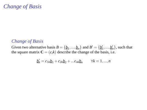
Change of Basis

Change of BasisGiven two alternative basisB = {b1, ...,bn} andB′ = {b′1, ...,b

′n}, such that

the square matrixC = (cik) describe the change of the basis, i.e.

b′k = c1kb1 +c2kb2 + ...cnkbn ∀k = 1, ...,n

Matrix and Change of BasisMatrix and Change of BasisThe effect of the matrixC on a generic vectorx allows to compute thechange of basis according only to the involved basisB andB′. For everyx = ∑n

k=1xkbk such that in the new basisB′, x can be expressed byx = ∑n

k=1x′kb′k, then it follows that:

x =n

∑k=1

x′kb′k = ∑

k

x′k

(

∑i

cikbi

)

=n

∑i,k=1

x′kcikbi

from which it follows that:

xi =n

∑k=1

x′kcik ∀i = 1, ...,n

The above condition suggests thatC is sufficient to describe any change ofbasis through the matrix vector mutliplication operations:

x = Cx′

Matrix and Change of Basis

Matrix and Change of BasisThe effect of the matrixC on a matrixA can be seen by studying the casewherex,y are the expression of two vectors in a baseB while theircounterpart onB′ arex′,y′, respectively. Now ifA andB are such thaty = Ax andy′ = Bx′, then it follows that:

y = Cy′ = Ax = A(Cx′) = ACx′

(this means that)

y′ = C−1ACx′

from which it follows that:

B = C−1AC

The transformation of basisC is asimilarity transformationand matricesAandC are saidsimilar.

Overview

◮ Analisi alle Componenti Principali◮ La Singular Value Decomposition

◮ Definizione◮ Esempi◮ Riduzione della dimensionalita’ del problema

◮ Latent Semantic Analysise SVD◮ Interpretazione◮ Latent Semantic Indexing

◮ Applicazioni di LSA:termedocument clustering

◮ Latent Semantic kernels◮ Embedding non lineari:Isomap, LNN ed LPP

Analisi delle componenti principali

Analisi delle componenti principali

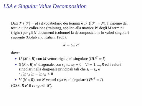
LSA e Singular Value Decomposition

Dati V (|V |= M) il vocabolario dei termini eT (|T |= N), l’insieme deitesti di una collezione (training), applico alla matriceW degliM termini(righe) per gliN documenti (colonne) la decomposizione in valori singolariseguente (Golub and Kahan, 1965):

W = USVT

dove:◮ U (M×R) conM vettori rigaui e’ singolare (UUT = I )◮ S(R×R) e’ diagonale, consij tc. sij = 0 ∀i = 1, ...,R ed i valori

singolari nella diagonale principali tali chesi = sii es1 ≥ s2≥ ...≥ sR > 0

◮ V (N×R) conN vettori rigavi e’ singolare (VVT = I )

(OSS:Re’ il rangodi W).

Le proprieta’ di SVD

La decomposizione in valori singolari traduce la matriceW di partenza in:

W = USVT

dove:◮ U eV sono le matrici deivettori singolari sinistroedestrodi W (cioe’

gli autovettorio eigenvectorsdi WWT e WTW, rispettivamente)◮ le colonne diU e le righe diV definiscono uno spazioortonormale,

cioe’ UUT = I eVVT = I

◮ Se’ la matrice diagonale dei valori singolari diW. I valori singolarisono le radici degli autovalori diWWT o WTW (sono uguali)

Le trasformazioni lineari ottenute ora sono due (come vedremo tra poco):WV e WTU.

LSA: proprieta’ di SVD

La decomposizione in valori singolari

W = USVT

si puo’ approssimare con

W∼W′ = UkSkVTk

trascurando le trasformazioni lineari di ordine superioreak << R in modoche:

◮ Uk (M×k) conM vettori rigaui e’ singolare ed ortonormale(UkUT

k = I )◮ Sk (k×k) e’ diagonale, consij tc. sij = 0 ∀i = 1, ...,k ed i valori

singolari nella diagonale principali tali chesi = sii es1 ≥ s2≥ ...≥ sk > 0

◮ Vk (N×k) conN vettori rigavi e’ singolare ed ortonormale (VkVTk = I )

Riduzione del rango

k e’ il numero di valori singolari scelti per rappresentare i concettinellŠinsieme dei documenti.In genere,k << R (rango iniziale).

LSA: proprieta’ di SVD

La decomposizione in valori singolari

W∼W′ = UkSkVTk

ha un certo insieme di proprieta’◮ la matriceSk e’ unica (anche seU e V non lo sono)◮ per costuzioneW′ e’ la matrice che soddisfa la decomposizione di

ordinek piu’ vicina a W (in norma euclidea)◮ gli si sono le radici degli autovalori diWWT

◮ le componenti principalidel problema sono in relazione aUk eVk

LSA: interpretazione semantica

Si dice che inW = USVT, Scattura lastruttura semantica latentedellospazio di partenza diW, V ×T e che la riduzione aW′ non ha effettosignificativo su questa proprieta’.... Vediamo perche’:

◮ gli autovalori ed autovettori sono direzioni particolari dello spazio dipartenzaV ×T , determinate dalla trasformazioneW.

◮ USsi ottiene daW = USVT: infatti WV= USVTV = US, cioe’ per ogniriga (termine)i-esima diW (o U), uiS= wiV.

◮ QUINDI: rappresentare i vettori dei termini (righewi della matriceW)medianteuiS, SIGNIFICA: combinare linearmente gli elementi (idocumenti,vj) della base ortonormale data daV (dopo il troncamento ak)

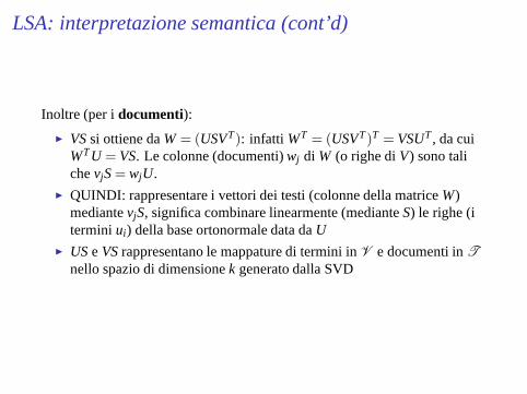
LSA: interpretazione semantica (cont’d)

Inoltre (per idocumenti):

◮ VSsi ottiene daW = (USVT): infatti WT = (USVT)T = VSUT, da cuiWTU = VS. Le colonne (documenti)wj di W (o righe diV) sono talichevjS= wjU.

◮ QUINDI: rappresentare i vettori dei testi (colonne della matriceW)mediantevjS, significa combinare linearmente (medianteS) le righe (iterminiui) della base ortonormale data daU

◮ USe VSrappresentano le mappature di termini inV e documenti inTnello spazio di dimensionek generato dalla SVD

LSA: interpretazione semantica (cont’d)

◮ Le trasformazioni sono date dalle combinazioni lineari sulle kdimensioni che corrispondono a concetti (temi). Infatti:

◮ Le matriciU eV sono basi ortonormali per lo spazio LS di dimensionek generato. Esso sono le direzioni privilegiate della trasformazioneiniziale e quindi sono combinazioni lineari inWWT (o WTW) cioe’concetti determinati dal ricorrere degli stessi termini nei documenti (eviceversa).

◮ Ogni vettore di terminewi dunque e’ rappresentato in tale spaziotramiteWV cioŁ come combinazione dei documenti inziali, il cheequivale a calcolareUS

◮ Analogamente per i documentiwj medianteWTU=VS

LSA: un esempio da una distribuzione artificiale

LSA: un esempio calcolato

LSA: Calcolo UΣVT

LSA: Approssimazione del rango, k= 2

LSA

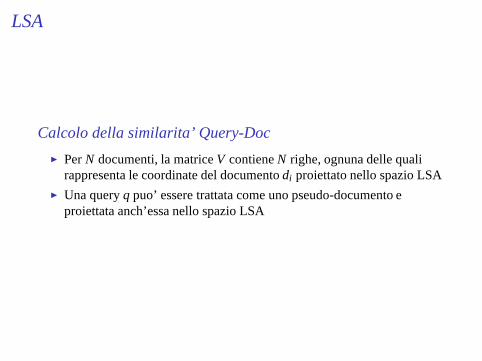
Calcolo della similarita’ Query-Doc

◮ PerN documenti, la matriceV contieneN righe, ognuna delle qualirappresenta le coordinate del documentodi proiettato nello spazio LSA

◮ Una queryq puo’ essere trattata come uno pseudo-documento eproiettata anch’essa nello spazio LSA

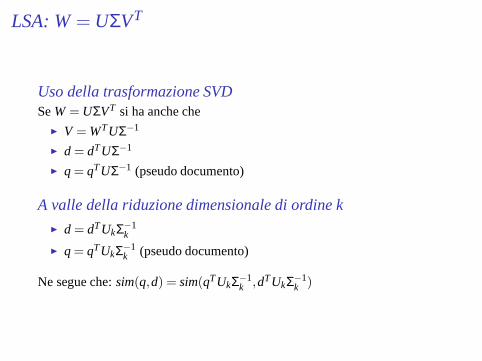
LSA: W= UΣVT

Uso della trasformazione SVDSeW = UΣVT si ha anche che

◮ V = WTUΣ−1

◮ d = dTUΣ−1

◮ q = qTUΣ−1 (pseudo documento)

A valle della riduzione dimensionale di ordine k

◮ d = dTUkΣ−1k

◮ q = qTUkΣ−1k (pseudo documento)

Ne segue che:sim(q,d) = sim(qTUkΣ−1k ,dTUkΣ−1

k )

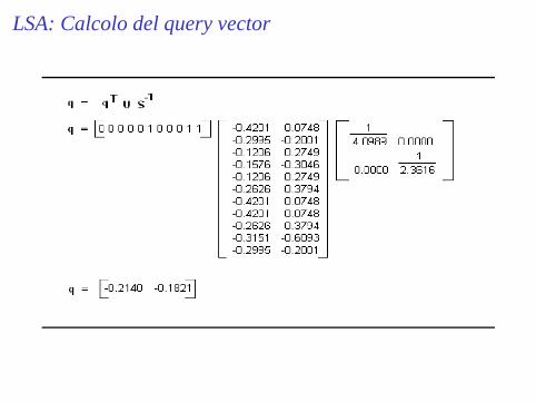
LSA: Calcolo del query vector

LSA: Vettori della query e dei documenti

LSA: Relazioni del secondo ordine

LSA e significato

◮ La rappresentazione in LSA dei termini coglie un numero maggiore diaspetti del significato dei termini, poiche’ contribuiscono alla nuovarappresentazione tutte le co-occorrenze nei diversi contesti descrittidalla matriceW iniziale

◮ La rappresentazione di un terminet nel nuovo spazio non è piu’ ilversore unitario~t ortogonale a (e quindi indipendente da) tutti gli altri

◮ La similitudine tra due terminiti e tj dipende dalla trasformazioneUΣ edipende quindi da tutte le co-occorrenze comuni con altri termini tk(contk 6= ti , tj). Queste dipendenze costituiscono relazioni delsecondoordine.

LSA: SVD e term clustering

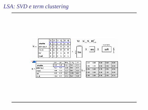
LSA: SVD e term clustering

LSA: SVD e term clustering

LSA: SVD e term clustering

LSA: SVD e term clustering

LSA: SVD e term clustering

LSA: Metriche di pesatura

In LSA i modelli di pesatura possono variare per migliorare la ricerca nellospazio delle trasformazioni lineari possibili

◮ Frequenza.cij (o le sue varianti normalizzatecij|dj |

,cij

maxlkclk)

◮ (Landauer)wij =log(cij +1)

1+∑Nj=1

cijti

logcijti

logN

=log(cij +1)

1+∑Nj=1 Pij logPij

logN

◮ (Bellegarda, LM modeling)wij = (1− εi)cijnj

con

εi =− 1log2N ∑N

j=1cijti

logcijti

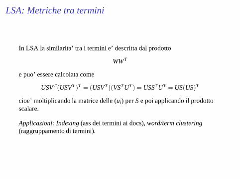
LSA: Metriche tra termini

In LSA la similarita’ tra i termini e’ descritta dal prodotto

WWT

e puo’ essere calcolata come

USVT(USVT)T = (USVT)(VSTUT) = USSTUT = US(US)T

cioe’ moltiplicando la matrice delle (ui) perSe poi applicando il prodottoscalare.

Applicazioni: Indexing(ass dei termini ai docs),word/term clustering(raggruppamento di termini).

LSA: Word Clustering

LSA: Metriche tra documenti

In LSA la similarita’ tra i documenti e’ descritta dal prodotto

WTW

e puo’ essere calcolata come

(USVT)TUSVT = (VSTUT)(USVT) = VSSVT = VS(VS)T

cioe’ moltiplicando la matrice delle (vi) perSe poi applicando il prodottoscalare.

Applicazioni: document clustering(raggruppamento di docs) ecategorizzazione dei testi(associazione di categorie ai documenti).

LSA: Osservazioni

◮ LSA e’ una tecnica per ottenere sistematicamente le rotazioninecessarie nello spazioV ×T ad allineare i nuovi assi con ledimensioni lungo le quali sussite la piu’ ampia variazione tra idocumenti

◮ Il primo asse (s1) fornisce la variazione massima, il secondo quellamassima tra le rimanenti e cosi’ via

◮ Vengono trascurate (scelta dik) le dimensioni le cui variazioni sonotrascurabili

LSA: Osservazioni (2)

◮ LSA e’ una tecnica per ottenere sistematicamente le rotazioninecessarie nello spazioV ×T ad allineare i nuovi assi con ledimensioni lungo le quali sussite la piu’ ampia variazione tra idocumenti

◮ Ipotesi sottostanti:◮ misura la variazione attraverso la norma euclidea (minimizza lo scarto

quadratico)◮ la distribuzione dei pesi legati ai termini nei documenti e’normale(i

sistemi di pesatura tendono a consolidare questa proprieta’)

LSA: Altre Applicazioni

Inferenza Semantica nelAutomatic Call Routing◮ Il taske’ quello di mappare domande (per unCall Center) in una

procedura (azione) direply.◮ Domande di training:

(T1) What is the time, (T2) What is the day, (T3) What time is themeeting, (T4) Cancel the meeting

◮ thee’ irrilevante,timee’ ambiguo (tra 1 e 3)◮ Domanda di ingresso:when is the meeting(classe correttaT3)

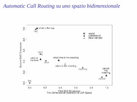
Automatic Call Routing su uno spazio bidimensionale

LSA vs. Machine Learning

Esiste una relazione tra LSA ed i modelli dilearning?

Induction in LSA◮ LSA fornisce un metodo generale per lastima di similarita’quindi e’

utilizzabile in tutti gli algoritmi induttivi per guidare lageneralizzazione (ad es. iperpiano di separazione)

◮ LSA fornisce una trasformazione lineare dei vettori di attributi originaliispirata dalle caratteristiche del data set, quindi produce una nuovametrica guidata dai datistessi. Questo meccanismo e’ particolarmenteimportante quando non esistono modelli analitici (generativi) precisidelle distribuzioni dei dati iniziali (ad es. dati linguistici)

◮ LSA puo’ essere applicato a dati non controllati (per esempio collezionidi documenti tematiche non annotate) e quindi estende il potere digeneralizzazione dei metodisupervisedsfruttando informazioni esterneal task. Questa proprieta’ consente di indurre una conoscenzacomplementare al task stesso

LSA: Machine Learning tasks

LSA in Relevance Feedback◮ Automatic Global Analysis◮ Stimatore di pseudo-rilevanzaprimadella espansione.

LSA and language semantics

◮ SVD in distributional analysis: semantic spaces (see (Padoand Lapata,2007))

◮ Word Sense Discrimination as clustering in LSA-like spaces(seeSchutze, 1998)

◮ Word Sense Disambiguation in LSA spaces (see (Gliozzo et al., 2005),(Basili et al., 2006)

◮ Framenet predicate induction (see (Basili et al., 2008), (Pennacchiotti etal., 2008))

Frames as Conceptual Patterns

An example: theKILLING frame

Frame: KILLING

A K ILLER or CAUSE causes the death of the VICTIM .

CAUSE The rockslide killed nearly half of the climbers.INSTRUMENT It’s difficult to suicidewith only a pocketknife.K ILLER John drownedMartha.MEANS The flood exterminatedthe ratsby cutting off access to food.MEDIUM John drownedMartha.

Fra

me

Ele

me

nts

Pre

dica

tes annihilate.v, annihilation.n, asphyxiate.v,assassin.n, assassinate.v, assassina-

tion.n, behead.v, beheading.n, blood-bath.n, butcher.v,butchery.n, carnage.n,crucifixion.n, crucify.v, deadly.a, decapitate.v, decapitation.n, destroy.v, dis-patch.v, drown.v, eliminate.v, euthanasia.n, euthanize.v, . . .

Harvesting frames in semantic fields

Semantic Spaces (Pado and Lapata, 2007)A Semantic Space for a set ofN targets is 4-tuple< B,A,S,V > where:

◮ B is the set of basic features (e.g. words co-occurring with the targets)◮ A is a lexical association function that weights the correlations between

b∈ B and the targets◮ S is a similarity function between targets (i.e. inℜ|B|×ℜ|B|)◮ V is a linear transformation over the originalN×|B|matrix

Harvesting frames in semantic fields

Semantic Spaces: a definitionA Semantic Space for a set ofN targets is 4-tuple< B,A,S,V > where:

◮ B is the set of basic features (e.g. words co-occurring with the targets)

◮ A is a lexical association function that weights the correlations betweenb∈ B and thetargets

◮ S is a similarity function between targets (i.e. inℜ|B|×ℜ|B|)◮ V is a linear transformation over the originalN×|B|matrix

Examples◮ In IR systems targets are documents,B is the term vocabulary,A is thetf · idf score. TheS

function is usually the cosine similarity, i.e.sim(~t1,~t2) = ∑i t1i ·t2i||~t1||·||~t2||

◮ In Latent Semantic Analysis (Berry et al. 94) targets are documents (or dually words), and theSVD transformation is used asV

Harvesting ontologies in semantic fields

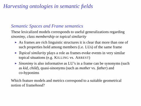
Semantic Spaces and Frame semanticsThese lexicalized models corresponds to useful generalizations regardingsinonimy, class membershipor topical similarity

◮ As frames are rich linguistic structures it is clear that more than one ofsuch properties hold among members (i.e. LUs) of the same frame

◮ Topical similarityplays a role as frames evoke events in very similartopical situations (e.g. KILLING vs. ARREST)

◮ Sinonimyis also informative as LU’s in a frame can be synonyms (suchaskid, child), quasi-sinonyms (such asmothervs. father) andco-hyponims

Which feature models and metrics correspond to a suitable geometricalnotion of framehood?

Latent Semantic Spaces

LSA and Frame semanticsIn our approach SVD is applied to source co-occurrence matrices in order to

◮ Reduce the original dimensionality◮ Capturetopical similarity latent in the original documents, i.e. second

order relations among targets

Harvesting ontologies in semantic fields

Framehood in a semantic space◮ Frames are rich polymorphic classes and clustering is applied for detecting multiple

centroids◮ Regions of the space where LU’s manifest are also useful for detecting the sentences that

express the intended predicate semantics

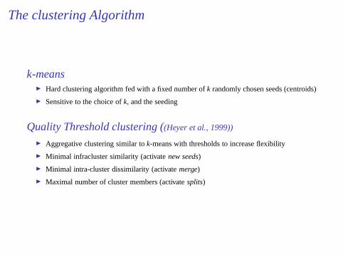
The clustering Algorithm

k-means◮ Hard clustering algorithm fed with a fixed number ofk randomly chosen seeds (centroids)

◮ Sensitive to the choice ofk, and the seeding

Quality Threshold clustering ((Heyer et al., 1999))

◮ Aggregative clustering similar tok-means with thresholds to increase flexibility

◮ Minimal infracluster similarity (activatenew seeds)

◮ Minimal intra-cluster dissimilarity (activatemerge)

◮ Maximal number of cluster members (activatesplits)

The clustering Algorithm

QT-clusteringRequire: QT {Quality Threshold for clusters}

repeatfor all slot fillersw do

SelectCx as the best cluster forw.if sim(w,cx) > QT then

Generate new clusterCw for welse

Acceptw into clusterCx

end ifend for

until No other shift is necessary or the maximum number of iteration is reached

The clustering Algorithm: Different settings

Harvesting ontologies in semantic fields

Framehood in a semantic space◮ Frames are rich polymorphic classes and clustering is applied for detecting multiple

centroids◮ Regions of the space where LU’s manifest are also useful for detecting the sentences that

express the intended predicate semantics

Evaluation: Current experimental set-up

The Corpus◮ TREC 2005 vol. 2

◮ # of docs: about 230,000

◮ # of tokens: about 110,000,000 (more than 70,000types)

◮ Source Dimensionality: 230,000× 49,000

◮ LSA Dimensionality reduction: 7,700× 100

Syntactic and Semantic Analysis◮ Parsing: Minpar (Lin,1998)

◮ Synonimy, hyponimy info: Wordnet 1.7

◮ Semantic Similarity Estimation: CD library (Basili et al„ 2004)

◮ Framenet: 2.0 version

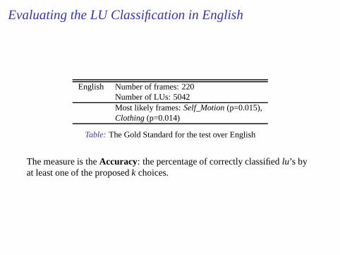
Evaluating the LU Classification in English

English Number of frames: 220Number of LUs: 5042Most likely frames:Self_Motion(p=0.015),Clothing(p=0.014)

Table: The Gold Standard for the test over English

The measure is theAccuracy: the percentage of correctly classifiedlu’s byat least one of the proposedk choices.

The impact of LU Classification on the English data set

Nouns Verbs

Targeted Frames 220 220Involved LUs 2,200 2,180Average LUs per frame 10.0 9.91LUs covered by WordNet 2,187 2,169Number of Evoked Senses 7,443 11,489Average Polysemy 3.62 5.97Represented words (i.e.∑F WF) 2,145 1,270Average represented LUs per frame 9.94 9.85Active Lexical Senses (LF) 3,095 2,282Average Active Lexical Senses(|LF |/|WF |) per word over frames 1.27 1.79Active synsets (SF) 3,512 2,718Average Active synsets (|SF |/|WF |)per word over frames 1.51 2.19

Table: Statistics on nominal and verbal senses in the paradigmaticmodel of theEnglish FrameNet

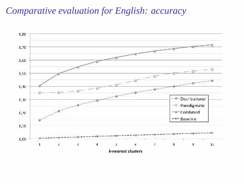
Comparative evaluation for English: accuracy

LSA e metodi Kernel

Le funzioni kernelK(~oi ,~o) possono essere usate per la stima (implicita)della similarita’ tra due termini o documenti,oi eo, in spazi complessi alfine di addestrare una SVM secondo l’equazione:

h(~x) = sgn

(

m

∑i=1

αiK(oi,o)+b

)

dove~x = φ(o)Alcuni modelli che utilizzano LSA per la definizione diK(oi ,o) sono statidefiniti per problemi di

◮ Text Categorization (categorizzazione testi)◮ Word Sense Disambiguation (classificazione occorrenze di una parola

in sensi)

LSA-based Domain Kernels

Assunzioni:◮ oi rappresenta un "termine"~ti◮ Lo spazio di rappresentazione di partenza per i~ti e’ quello di un VSM

tradizionale (pesatura dei termin tramite la loro pesaturaTF× IDF neidocumenti)

◮ La matriceT di partenza e’ quindi termini per doc

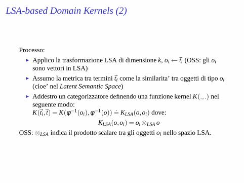
LSA-based Domain Kernels (2)

Processo:◮ Applico la trasformazione LSA di dimensionek, oi ←~ti (OSS: glioi

sono vettori in LSA)◮ Assumo la metrica tra termini~ti come la similarita’ tra oggetti di tipooi

(cioe’ nelLatent Semantic Space)◮ Addestro un categorizzatore definendo una funzione kernelK(., .) nel

seguente modo:K(~ti ,~t) = K(φ−1(oi),φ−1(o))

.= KLSA(o,oi) dove:

KLSA(o,oi) = oi⊗LSAo

OSS:⊗LSA indica il prodotto scalare tra gli oggettioi nello spazio LSA.

LSA-based Domain Kernels (3)

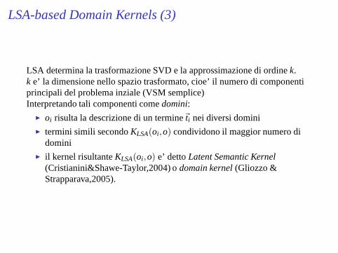
LSA determina la trasformazione SVD e la approssimazione diordinek.k e’ la dimensione nello spazio trasformato, cioe’ il numero di componentiprincipali del problema inziale (VSM semplice)Interpretando tali componenti comedomini:

◮ oi risulta la descrizione di un termine~ti nei diversi domini◮ termini simili secondoKLSA(oi ,o) condividono il maggior numero di

domini◮ il kernel risultanteKLSA(oi ,o) e’ dettoLatent Semantic Kernel

(Cristianini&Shawe-Taylor,2004) odomain kernel(Gliozzo &Strapparava,2005).

LSA-based Domain Kernels:

Applicazione allaText Categorization

◮ un documentoxi (come un termine) puo’ essere mappato in uno spaziodi tipo LSA, oi ←~xi

◮ le k componenti dioi rappresentano la descrizione dixi nel nuovospazio

◮ il kernelKLSA(oi,o) risultante cattura le similarita’ mediante unadescrizione di dominio di~xi

◮ l’addestramento della SVM genera l’equazione dell’iperpiano secondoLSA:

f (~x) =

(

m

∑i=1

αiKLSA(oi ,oj)+b

)

OSS: LSA puo’ essere computato in una collezioneesternaal data set ditraining.

Embeddings in ML

Embedding

◮ Dimensionality reduction is a way to reduce the original spacedimension to a more manageable size that is still highly informative: itaims to prune out irrelevant information and noise from the initial set ofobservations

◮ The idea is to embed the sourceN dimensional space into a smallerddimensional space: this operation is calledembedding

◮ a transformation is suitable for a given feature representation and aspecific task if it optimizes one or more principles or aspects of the task(utility function)

◮ The DR techniques employed make different assumptions on (1) thenature of the original space (domain, range and distributions of attributevalues) and on (2) the optimality criterion to be applied (e.g. manifoldstructure, efficiency, resulting accuracy or cognitive plausibility)

Linear Embeddings: PCA

Embedding

Non-Linear Embeddings

Non-Linear Embeddings

Non-Linear Embeddings

Embedding and UnfoldingAn embedding define a process aiming to unfold the underlyingstructure ofthe data distribution on which linear (such Euclidean) distances are not valid.

Non-Linear Embeddings and manifolds

A manifold is a topological space which is locally Euclidean. In general, anyobject which is nearlyflat on small scales is amanifold. Euclidean space is asimplest example of a manifold.

Concept of submanifoldManifolds arise naturally whenever there is a smooth variation of parameters(like pose of the face in previous example)The dimension of a manifold is the minimum integer number of co-ordinatesnecessary to identify each point in that manifold.

Non-Linear Embeddings and manifolds

In general, the transformation should be make dependent on the local ratherthan on the global structure of the data distributions in theoriginal space inorder to recreate the manifold structure with the smallest number ofdimensions:Unfolding manifolds.

Isomap

Isomap Algorithm

◮ Determine the neighbors. Two methods: (1) All points in a fixedradius; (2)K nearest neighbors

◮ Construct a neighborhood graph. Each point is connected to the otherif it is a K nearest neighbor. Edge Length equals the Euclidean distance

◮ Compute the shortest paths between two nodes through◮ Floyd’s Algorithm◮ Djkstra’s Algorithm

◮ Construct a lower dimensional embedding through ClassicalMultidimensional Scaling (or SVD)

Isomap vs. MDS: Residuals in different problems

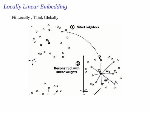
Locally Linear Embedding

Fit Locally , Think Globally

Locally Linear Embedding

Local weightsIn the first phase weights are chosen such that

ε(W) = minW||~Xi−∑j

Wij~Xj ||2

The weights that minimize the reconstruction errors are invariant to rotation,rescaling and translation of the data points

Invariance to translation is enforced by adding the constraint that the weightssum to one, i.e.∑ij Wij = 1

The same weights that reconstruct the data points inD dimensions shouldreconstruct it in the manifold ind dimensions.

Locally Linear Embedding

Reconstruction weightsThe weights derived in the first phase

ε(W) = minW||Xi−∑j

Wij Xj ||2

are used for the reconstruction ind dimensions.

Each high-dimensional representation~Xi is mapped to a low-dimensionalvector~Yj representing the global internal coordinates on the manifold.

This is done by choosing thed-dimensional coordinates~Yi such to minimizethe embedding cost function, i.e.

Ψ(Y) = ∑i

||~Yi−∑j

Wij~Yj ||2

Fix the weights and optimize the coordinates

Locally Linear Embedding

How to compute the reconstruction weightsThe solution to the following problem

Ψ(Y) = ∑i||~Yi−∑

jWij~Yj ||

2

consists in◮ Add constraints to ask for the solutions~Yi to be centered on the origin

(∑i~Yi =~0

◮ Minimize theΨ by solving the corresponding sparseN×N eigenvalueproblem, whose bottomd non zero eigenvalues are the solution

◮ Such setA of the (smallestd non-zero) eigenvalues provide an orderedset of orthogonal coordinates centered in the origin (i.e. the new basisfor the low-dimensional space), i.e.

~Yi = A~Xi

.

Think Globally ...

LLE

The analytical setting

minWΨ(Y) = ∑i ||~Yi−∑j Wij~Yj ||2

∑i~Yi =~0

1N ∑i

~Yi×~Yi = 1

that is equivalent to

minWΨ(Y) = ∑ij M(~Yi ,~Yj)

∑i~Yi =~0

1N ∑i

~Yi×~Yi = 1

whereMij = δij −Wij −Wji + ∑k WkiWkj

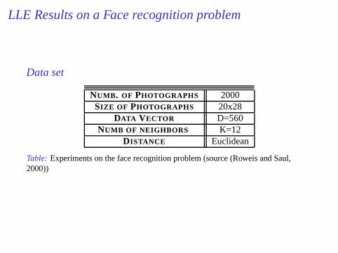
LLE Results on a Face recognition problem

Data set

NUMB. OF PHOTOGRAPHS 2000SIZE OF PHOTOGRAPHS 20x28

DATA VECTOR D=560NUMB OF NEIGHBORS K=12

DISTANCE Euclidean

Table: Experiments on the face recognition problem (source (Roweis and Saul,2000))

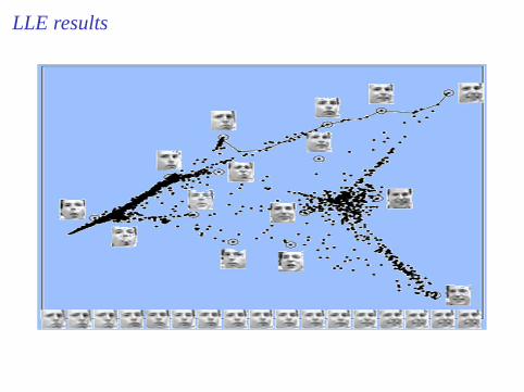
LLE results

LLE Results on Word clustering

Data set

SOURCE Grolier EncyclopediaNUMB. OF DOCUMENTS 31,000SIZE OF VOCABULARY 5,000NUMB OF NEIGHBORS K=20

WEIGHTING word countsDISTANCE normalized inner product

Table: Experiments on word clustering (source (Roweis and Saul, 2000))

LLE results

LLE results

Locality Preserving Projections (LPP)

LPP Embedding

◮ LPP (Cai et al., IEEE on DKE 2005) is the last of this class of non linear embeddingmethods

◮ It is in the class of laplacian methods (such as LLE)◮ Application to image and document clustering, topic modeling (such as

LDA)

LPP as a data-driven metrics

General Idea◮ Determine thebestlinear transformationA that preserves thelocal

properties of the space, without making global assumptions(as in LSA)◮ An adjecency graphG is adopted, based on internal metrics (i.e. the

space inner product) or external ones (e.g. dictionaries)

Formally:

◮ arg min~a∑ij (~a~xi−~a~xj)2Wij

◮ Dii = ∑j Wij and ...L = D−W (Laplacian matrix)

◮ Solve the eingenvector problem:XLXT~a = λXDXT~a◮ Final projection intoℜd: yi = ATxi

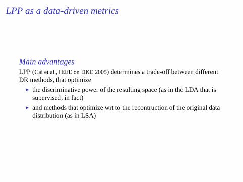
LPP as a data-driven metrics

Main advantagesLPP (Cai et al., IEEE on DKE 2005) determines a trade-off between differentDR methods, that optimize

◮ the discriminative power of the resulting space (as in the LDA that issupervised, in fact)

◮ and methods that optimize wrt to the recontruction of the original datadistribution (as in LSA)

The Adjacency Graph,G

Given two vectorsxi andxj , G defines weightswij , as:

◮ cosinegraph: wij = max{0,cos(xi ,xj)−τ|cos(xi ,xj)−τ| ·cos(xi ,xj)}.

◮ ε-neighborhoodsgraph (gaussian kernel):

wij = max{0,ε−||xi−xj ||

2

|ε−||xi−xj ||2|·e−

||xi−xj ||2

t },

◮ thetopicgraph:

wij = δ (i, j) ·cos(xi ,xj)

whereδ (i, j) = 1 only if a corpus categoryC can be found such thatxi ∈ C andxj ∈C and 0 otherwise.

Evaluation Metrics

NMINormalized mutual information, defined as follows:

NMI(T,C) =∑t∈T,c∈C p(t,c)log2

p(t,c)p(t)·p(c)

min(H(T),H(C))(1)

AccuracyThe accuracyAC is given by:

AC=∑N

i=1 δ (Ai ,Oi)

N(2)

whereN is the total number of documents andδ (Ai ,Oi) is 1 only if Ai = Oi

and 0 otherwise

Results

Topic Graph

REUTERS

METHOD ACC NMI

LSA 0.82 0.79LPP 0.94 0.99

Table: Best LSA vs. upper bound LPP results based on the "topic" graph on Reuters.

Results

Dimensionality reduction effect: LSA vs. LPP

Results

Clustering effect: LSA vs. LPP

Results

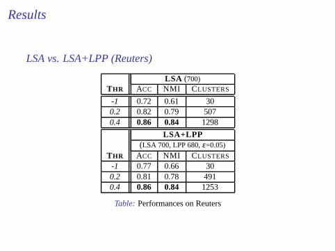
LSA vs. LSA+LPP (Reuters)

LSA (700)THR ACC NMI CLUSTERS

-1 0.72 0.61 300.2 0.82 0.79 5070.4 0.86 0.84 1298

LSA+LPP(LSA 700, LPP 680,ε=0.05)

THR ACC NMI CLUSTERS

-1 0.77 0.66 300.2 0.81 0.78 4910.4 0.86 0.84 1253

Table: Performances on Reuters

Results

LSA vs. LSA+LPP (20Newsgroup)

LSA (500)THR ACC NMI CLUSTERS

-1 0.58 0.57 200.2 0.59 0.59 4300.3 0.63 0.64 720

LSA+LPP(LSA 500, LPP 480,ε=0.05)

THR ACC NMI CLUSTERS

-1 0.54 0.55 200.2 0.59 0.60 4380.3 0.62 0.64 724

Table: Performances on 20Newsgroups

Non linear embedding: summary

ISOMAP LLEDo MDS on the geodesicdistance matrix.

Model local neighborhoods as lin-ear a patches and then embed in alower dimensional manifold

Global approach Local approachDynamic programming ap-proaches

Computationally efficient... sparsematrices

Convergence limited bythe manifold curvature andnumber of points

Good representational capacity

No clustering effect Clustering effect due to the local-ity preserving property of the eigen-value approach

References

SVD and LSA◮ Susan T. Dumais, Michael Berry, Using Linear Algebra for Intelligent

Information Retrieval, SIAM Review, 1995, 37, 573–595

◮ G. W. Furnas, S. Deerwester, S. T. Dumais, T. K. Landauer, R. A. Harshman, L.A. Streeter, K. E. Lochbaum, Information retrieval using a singular valuedecomposition model of latent semantic structure, SIGIR ’88: Proc. of theACM SIGIR conference on Research and development in InformationRetrieval, 1988

Non linear embeddings

◮ S. T. Roweis and L. K. Saul. Nonlinear dimensionality reduction by locallylinear embedding. Science, 2000.

◮ B. J. Tenenbaum, V. Silva, and J. Langford. A Global Geometric Frameworkfor Nonlinear Dimensionality Reduction. Science, pp.2319-2323, 2000

◮ Xiaofei He, Partha Niyogi, Locality Preserving Projections. Proceedings ofAdvances in Neural Information Processing Systems, Vancouver, Canada,2003.

References

LSA in language learning

◮ Hinrich Schutze, Automatic word sense discrimination, ComputationalLinguistics, 24(1), 1998.

◮ Beate Dorow and Dominic Widdows, Discovering Corpus-Specific WordSenses. EACL 2003, Budapest, Hungary. Conference, pages 79-82

◮ Basili Roberto, Marco Cammisa, Alfio Gliozzo, Integrating Domain andParadigmatic Similarity for Unsupervised Sense Tagging, 17th EuropeanConference on Artificial Intelligence (ECAI06), Riva del Garda, Italy, 2006.

◮ Sebastian Pado and Mirella Lapata. Dependency-based Construction ofSemantic Space Models. In Computational Linquistics, Vol.33(2):161-199,2007.

◮ Basili R. Pennacchiotti M., Proceedings of GEMS "Geometrical Models ofNatural Language Semantics",http://www.aclweb.org/anthology/W/W09/#0200