
Incertezza: trattazione elementare - sea.uniroma3.it · Errore e incertezza hanno definizioni e...
26
Enrico Silva - diritti riservati - Non è permessa, fra l’altro, l’inclusione anche parziale in altre opere senza il consenso scritto dell’autore Elementi di Misure Elettriche e Elettroniche E. Silva - a.a. 2016/2017 Errori. Incertezza. Trattazione elementare. Trattazione statistica. Riferimenti: J. R. Taylor, “An Introduction to Error Analysis”, 2nd ed., University Science Book Capp. 1, 2,3 (con esercizi) R. Bartiromo, M. De Vincenzi “Electrical Measurements in the Laboratory Practice”, Springer Cap. 3 (con esercizi). P. Fornasini “The Uncertainty in Physical Measurements”, Springer Cap. 1 (parr. 1.1, 1.2, 1.3, 1.6), Cap. 2, App. B I. G. Hughes, T. P. A. Hase “Measurements and their Uncertainties”, Oxford University Press, 2010 Enrico Silva - diritti riservati - Non è permessa, fra l’altro, l’inclusione anche parziale in altre opere senza il consenso scritto dell’autore Incertezza: trattazione elementare Enrico Silva - diritti riservati - Non è permessa, fra l’altro, l’inclusione anche parziale in altre opere senza il consenso scritto dell’autore Incertezza Ogni misurazione è necessariamente accompagnata da errori, imprecisioni, limitazioni degli strumenti e degli operatori. Non è possibile associare un numero unico al misurando, ma un intervallo di valori. TUTTAVIA questo intervallo può essere stimato, ed esprime l’incertezza della misura. L’incertezza è un parametro quantitativo . Quando l’incertezza non è nota, non è possibile confrontare differenti misure! Il risultato di una misurazione è completo solo quando comprende anche l’incertezza 1 2 3
Transcript of Incertezza: trattazione elementare - sea.uniroma3.it · Errore e incertezza hanno definizioni e...

Enrico Silva - diritti riservati - Non è permessa, fra l’altro, l’inclusione anche parziale in altre opere senza il consenso scritto dell’autore
Elementi di Misure Elettriche e ElettronicheE. Silva - a.a. 2016/2017
Errori. Incertezza. Trattazione elementare.Trattazione statistica.
Riferimenti:
J. R. Taylor, “An Introduction to Error Analysis”, 2nd ed., University Science Book Capp. 1, 2,3 (con esercizi)
R. Bartiromo, M. De Vincenzi “Electrical Measurements in the Laboratory Practice”, Springer Cap. 3 (con esercizi).
P. Fornasini “The Uncertainty in Physical Measurements”, Springer Cap. 1 (parr. 1.1, 1.2, 1.3, 1.6), Cap. 2, App. B
I. G. Hughes, T. P. A. Hase “Measurements and their Uncertainties”, Oxford University Press, 2010
Enrico Silva - diritti riservati - Non è permessa, fra l’altro, l’inclusione anche parziale in altre opere senza il consenso scritto dell’autore
Incertezza: trattazione elementare
Enrico Silva - diritti riservati - Non è permessa, fra l’altro, l’inclusione anche parziale in altre opere senza il consenso scritto dell’autore
IncertezzaOgni misurazione è necessariamente accompagnata da errori,
imprecisioni, limitazioni degli strumenti e degli operatori.
Non è possibile associare un numero unico al misurando,ma un intervallo di valori.
TUTTAVIA questo intervallo può essere stimato,ed esprime l’incertezza della misura.
L’incertezza è un parametro quantitativo.
Quando l’incertezza non è nota, non è possibile confrontare differenti misure!
Il risultato di una misurazione è completo solo quando comprende anche l’incertezza
1
2
3

Enrico Silva - diritti riservati - Non è permessa, fra l’altro, l’inclusione anche parziale in altre opere senza il consenso scritto dell’autore
Errori e incertezza
Linguaggio comune:errore = sbaglio
Contesto scientifico e ingegneristico:differenza fra il valore (“vero”) μ e il valore misurato m: e = | μ -m |
Attenzione! Suppone che un valore “vero” μ esista!Difficoltà concettuale: l’esistenza necessaria di “errori” (a priori sconosciuti!) implica che il valore “vero” sia, in linea di principio, sconosciuto.
La formulazione corretta viene da una trattazione statistica (vedi oltre)
Enrico Silva - diritti riservati - Non è permessa, fra l’altro, l’inclusione anche parziale in altre opere senza il consenso scritto dell’autore
Esempio: stime da lettura di scale (1)
È ragionevole descrivere l’incertezza sul valore da fornire come “mezza divisione”
→ 35.5 mm ≤ ℓ ≤ 36.5 mm
8 Chapter I: Preliminary Description of Error Analysis
ously been tested many times with much more precision than possible in a teaching laboratory. Nonetheless, if you understand the crucial role of error analysis and accept the challenge to make the most precise test possible with the available equip-ment, such experiments can be interesting and instructive exercises.
1.5 Estimating Uncertainties When Reading Scales
Thus far, we have considered several examples that illustrate why every measure-ment suffers from uncertainties and why their magnitude is important to know. We have not yet discussed how we can actually evaluate the magnitude of an uncer-tainty. Such evaluation can be fairly complicated and is the main topic of this book. Fortunately, reasonable estimates of the uncertainty of some simple measurements are easy to make, often using no more than common sense. Here and in Section 1.6, I discuss examples of such measurements. An understanding of these examples will allow you to begin using error analysis in your experiments and will form the basis for later discussions.
The first example is a measurement using a marked scale, such as the ruler in Figure 1.2 or the voltmeter in Figure 1.3. To measure the length of the pencil in
millimeters 0 10 20 30 40 50
Figure 1.2. Measuring a length with a ruler.
Figure 1.2, we must first place the end of the pencil opposite the zero of the ruler and then decide where the tip comes to on the ruler's scale. To measure the voltage in Figure 1.3, we have to decide where the needle points on the voltmeter's scale. If we assume the ruler and voltmeter are reliable, then in each case the main prob-
4
volts 5
6 7
Figure 1.3. A reading on a voltmeter.
Figu
ra d
a J.
R. T
aylo
r, “A
n In
trodu
ctio
n to
Erro
r Ana
lysis
”
ℓ ?
Enrico Silva - diritti riservati - Non è permessa, fra l’altro, l’inclusione anche parziale in altre opere senza il consenso scritto dell’autore
8 Chapter I: Preliminary Description of Error Analysis
ously been tested many times with much more precision than possible in a teaching laboratory. Nonetheless, if you understand the crucial role of error analysis and accept the challenge to make the most precise test possible with the available equip-ment, such experiments can be interesting and instructive exercises.
1.5 Estimating Uncertainties When Reading Scales
Thus far, we have considered several examples that illustrate why every measure-ment suffers from uncertainties and why their magnitude is important to know. We have not yet discussed how we can actually evaluate the magnitude of an uncer-tainty. Such evaluation can be fairly complicated and is the main topic of this book. Fortunately, reasonable estimates of the uncertainty of some simple measurements are easy to make, often using no more than common sense. Here and in Section 1.6, I discuss examples of such measurements. An understanding of these examples will allow you to begin using error analysis in your experiments and will form the basis for later discussions.
The first example is a measurement using a marked scale, such as the ruler in Figure 1.2 or the voltmeter in Figure 1.3. To measure the length of the pencil in
millimeters 0 10 20 30 40 50
Figure 1.2. Measuring a length with a ruler.
Figure 1.2, we must first place the end of the pencil opposite the zero of the ruler and then decide where the tip comes to on the ruler's scale. To measure the voltage in Figure 1.3, we have to decide where the needle points on the voltmeter's scale. If we assume the ruler and voltmeter are reliable, then in each case the main prob-
4
volts 5
6 7
Figure 1.3. A reading on a voltmeter.
Esempio: stime da lettura di scale (2)
È ragionevole interpolare, ma dipende dall’operatore.→ 5.2 V ≤ V ≤ 5.4 V
Figu
ra d
a J.
R. T
aylo
r, “A
n In
trodu
ctio
n to
Erro
r Ana
lysis
”
V ?
4
5
6

Enrico Silva - diritti riservati - Non è permessa, fra l’altro, l’inclusione anche parziale in altre opere senza il consenso scritto dell’autore
Esempio: stime da letture ripetute
È ragionevole assumere che• la stima migliore sia la media aritmetica dei risultati, • il valore corretto si trovi nell’intervallo compreso fra
la minima e massima lettura
→ 22 μA ≤ I ≤ 26 μAcon
Imiglior stima = 24 μA
Figu
ra d
a J.
R. T
aylo
r, “A
n In
trodu
ctio
n to
Erro
r Ana
lysis
”
Supponiamo di leggere più volte la corrente I che scorre in un ramo di un circuito. Otteniamo:
25 μa, 24 μA, 25 μA, 23 μA, 24 μA, 22 μA, 23 μA, 26 μA
Enrico Silva - diritti riservati - Non è permessa, fra l’altro, l’inclusione anche parziale in altre opere senza il consenso scritto dell’autore
Esempio: stime da letture ripetute
È ragionevole assumere che• la stima migliore sia la media aritmetica dei risultati, • il valore corretto si trovi nell’intervallo compreso fra
la minima e massima lettura
→ 22 μA ≤ I ≤ 26 μAcon
Imiglior stima = 24 μA
Figu
ra d
a J.
R. T
aylo
r, “A
n In
trodu
ctio
n to
Erro
r Ana
lysis
”
Attenzione! Le misurazioni sono state eseguite tutte nelle stesse condizioni?(temperatura, alimentazione del circuito, funzionamento dello strumento...)
Enrico Silva - diritti riservati - Non è permessa, fra l’altro, l’inclusione anche parziale in altre opere senza il consenso scritto dell’autore
Errori
Errori casuali: variabili in maniera non prevedibile in misurazioni ripetute.Se ci si aspetta che il valor medio di questi contributi casuali sia nullo, effettuare molte misure e mediarle ne riduce il peso.
Errori sistematici: in misurazioni ripetute rimangono costanti o variano in maniera prevedibile.L’effetto può essere ridotto se se ne conosce l’origine (ad esempio, l’effetto dell’impedenza interna di un voltmetro sui valori di una misura può essere calcolato se si conosce l’impedenza del circuito fra i punti di misura).Calibrazione e offset fanno parte degli effetti sistematici.Errore di offset: la grandezza misurata è m = m0 + μ. Errore di calibrazione: la grandezza misurata è m = f(μ).Nei casi più semplici, m = β μ con β ≠ 1.
... oltre ovviamente agli errori veri e propri: errori di lettura, errori di comunicazione,...
7
8
9

Enrico Silva - diritti riservati - Non è permessa, fra l’altro, l’inclusione anche parziale in altre opere senza il consenso scritto dell’autore
Incertezza
Definizione data dal metodo di stima dell’incertezza:
Incertezza di tipo A, uA: stimata attraverso analisi statistica mediante misure ripetute.
Incertezza di tipo B, uB: non può essere stimata attraverso misure ripetute. Ad esempio precedenti informazioni (datasheets, caratteristiche strumentali), osservazioni sperimentali,...
Una volta stimate le due tipologie di incertezza, l’incertezza complessiva andrà espressa come
u =q
u2a + u2
B
Enrico Silva - diritti riservati - Non è permessa, fra l’altro, l’inclusione anche parziale in altre opere senza il consenso scritto dell’autore
Errori e IncertezzaErrore e incertezza hanno definizioni e origini diverse!
In particolare:gli errori casuali non sono sovrapponibili all’incertezza di tipo Agli errori sistematici non sono sovrapponibili all’incertezza di tipo B
L’incertezza è classificata in base alla metodologia utilizzata per stimarla.Gli errori sono classificati in base alla loro “natura”.
metodo scientifico → la definizione di incertezza è più soddisfacente!
Enrico Silva - diritti riservati - Non è permessa, fra l’altro, l’inclusione anche parziale in altre opere senza il consenso scritto dell’autore
Errori e Incertezza
8 Chapter I: Preliminary Description of Error Analysis
ously been tested many times with much more precision than possible in a teaching laboratory. Nonetheless, if you understand the crucial role of error analysis and accept the challenge to make the most precise test possible with the available equip-ment, such experiments can be interesting and instructive exercises.
1.5 Estimating Uncertainties When Reading Scales
Thus far, we have considered several examples that illustrate why every measure-ment suffers from uncertainties and why their magnitude is important to know. We have not yet discussed how we can actually evaluate the magnitude of an uncer-tainty. Such evaluation can be fairly complicated and is the main topic of this book. Fortunately, reasonable estimates of the uncertainty of some simple measurements are easy to make, often using no more than common sense. Here and in Section 1.6, I discuss examples of such measurements. An understanding of these examples will allow you to begin using error analysis in your experiments and will form the basis for later discussions.
The first example is a measurement using a marked scale, such as the ruler in Figure 1.2 or the voltmeter in Figure 1.3. To measure the length of the pencil in
millimeters 0 10 20 30 40 50
Figure 1.2. Measuring a length with a ruler.
Figure 1.2, we must first place the end of the pencil opposite the zero of the ruler and then decide where the tip comes to on the ruler's scale. To measure the voltage in Figure 1.3, we have to decide where the needle points on the voltmeter's scale. If we assume the ruler and voltmeter are reliable, then in each case the main prob-
4
volts 5
6 7
Figure 1.3. A reading on a voltmeter.
35.5 mm ≤ ℓ ≤ 36.5 mm
8 Chapter I: Preliminary Description of Error Analysis
ously been tested many times with much more precision than possible in a teaching laboratory. Nonetheless, if you understand the crucial role of error analysis and accept the challenge to make the most precise test possible with the available equip-ment, such experiments can be interesting and instructive exercises.
1.5 Estimating Uncertainties When Reading Scales
Thus far, we have considered several examples that illustrate why every measure-ment suffers from uncertainties and why their magnitude is important to know. We have not yet discussed how we can actually evaluate the magnitude of an uncer-tainty. Such evaluation can be fairly complicated and is the main topic of this book. Fortunately, reasonable estimates of the uncertainty of some simple measurements are easy to make, often using no more than common sense. Here and in Section 1.6, I discuss examples of such measurements. An understanding of these examples will allow you to begin using error analysis in your experiments and will form the basis for later discussions.
The first example is a measurement using a marked scale, such as the ruler in Figure 1.2 or the voltmeter in Figure 1.3. To measure the length of the pencil in
millimeters 0 10 20 30 40 50
Figure 1.2. Measuring a length with a ruler.
Figure 1.2, we must first place the end of the pencil opposite the zero of the ruler and then decide where the tip comes to on the ruler's scale. To measure the voltage in Figure 1.3, we have to decide where the needle points on the voltmeter's scale. If we assume the ruler and voltmeter are reliable, then in each case the main prob-
4
volts 5
6 7
Figure 1.3. A reading on a voltmeter.
5.2 V ≤ V ≤ 5.4 V 22 μA ≤ I ≤ 26 μA
In questi esempi si fornisce il cosiddetto errore massimo. Questo è ancora usato in alcuni contesti industriali.
Data una misura A completa di stima dell’intervallo (Amin, Amax) dove è ragionevole che si trovi il valore cercato, allora si esprime:
A ± δAdove δA = (Amax – Amin)/2 è l’errore massimo.
Usiamo il concetto di errore massimo come proxy per l’incertezza (per adesso).
10
11
12

Enrico Silva - diritti riservati - Non è permessa, fra l’altro, l’inclusione anche parziale in altre opere senza il consenso scritto dell’autore
Cifre significativeSi sia eseguita una misura della grandezza α, risultante nel valore A completo di stima dell’incertezza δA
α = A ± δA
L’incertezza sperimentale va arrotondata a una cifra significativa (esempio 1) a meno che tale operazione non dia una significativa perdita
di informazione sull’incertezza stessa (esempio 2).
Esempio 1. Si misura una ddp V0 = 6.386 V con una incertezza stimata δV = 0.056 V. il risultato sarà espresso come (6.39 ± 0.06) V.
Il risultato è dato con tre cifre significative.
Esempio 2. Si misura una resistenza Rc = 3347.5 Ω con una incertezza stimata δΩ = 1.4 Ω. il risultato sarà espresso come (3347.5 ± 1.4) V.
Il risultato è dato comunque con cinque cifre significative.
regola empirica: se l’incertezza sperimentale ha la prima cifra significativa pari a 1 o 2, ha senso esprimerla con due cifre.
Enrico Silva - diritti riservati - Non è permessa, fra l’altro, l’inclusione anche parziale in altre opere senza il consenso scritto dell’autore
Regole di scrittura
Usualmente si scrive l’unità di misura una sola volta:
Rc = (3347.5 ± 1.4) Ω
e non Rc = 3347.5 Ω ± 1.4 Ω
In casi in cui si usi la notazione esponenziale,la potenza di 10 si esprime alla fine:
q = (3.22 ± 0.06) × 10–19 C
Enrico Silva - diritti riservati - Non è permessa, fra l’altro, l’inclusione anche parziale in altre opere senza il consenso scritto dell’autore
Regole di calcolo dell’incertezza
L’incertezza (e il valore dato) vanno calcolati mantenendo almeno una cifra significativa in più rispetto alle cifre signficative del
risultato finale.Non è scorretto mantenere nei calcoli intermedi più cifre.
È scorretto esprimerle in un valore finale!
13
14
15

Enrico Silva - diritti riservati - Non è permessa, fra l’altro, l’inclusione anche parziale in altre opere senza il consenso scritto dell’autore
Discrepanza
discrepanza: differenza fra due valori misurati della stessa quantità
non è detto che quando fra due misure vi sia discrepanza, essa sia signficativa.
Vengono fornite alcune misure di una stessa grandezza attraverso procedure diverse.
Esse forniscono i risultati:x1 ± δx1
x2 ± δx2
x3 ± δx3
...
con x1 ≠ x2 ≠ x3 (discrepanza)
Enrico Silva - diritti riservati - Non è permessa, fra l’altro, l’inclusione anche parziale in altre opere senza il consenso scritto dell’autore
Discrepanza
Le misure non sono significativamente diverse,
essendo le bande di incertezza sovrapposte.
Le misure non sono consistenti. I
I
Enrico Silva - diritti riservati - Non è permessa, fra l’altro, l’inclusione anche parziale in altre opere senza il consenso scritto dell’autore
Accuratezza e precisioneAccuratezza: caratteristica metrologica che indica quanto bene una misura
si avvicina al “valore atteso” . Precisione: caratteristica metrologica che indica la dispersione dei dati
intorno ad un valore.
16
17
18

Enrico Silva - diritti riservati - Non è permessa, fra l’altro, l’inclusione anche parziale in altre opere senza il consenso scritto dell’autore
Accuratezza e precisioneUn’analogia
4.2 Properties of Measuring Instruments 81
(a) (b) (c) (d)
Fig. 4.1 Analogy between various distributions of shots on target and properties of accuracy andprecision of measurements.Ameasures accurate but not precise,Bmeasures precise but not accurate,C measures nor accurate nor precise, and D precise and accurate measurements. On top of eachtarget, we show the parent distribution of the horizontal position of the hits
• Working range. The working range is the interval of measurand values for whichthe instrument is able to perform the measurement. The maximum value is calledfull-scale while the minimum is called threshold.
• Promptness. The promptness is linked to the response time of the instrument tothe input quantity. The lower this time, the higher the promptness of the instrument.The promptness remains a qualitative concept unless it refers to a mathematicalmodel describing the instrumental response as a function of time. For example,the characteristic time of a mercury thermometer is a quantitative definition of itspromptness and makes it possible the comparison of different instruments basedon the same physical principle.
A note on accuracy and precision. In the terminology used in metrology, accu-racy and precision describe two properties of a measurement completely separateand independent: an instrument can be accurate but not precise, and vice versa. Toillustrate the difference between precision and accuracy is helpful to use an analogywith the sport of shooting by interpreting the center of the target as the “true value”of a measurand and the different trials as the measurements. The Fig. 4.1 shows fourdifferent distributions of shots (A, B, C, and D) on the target that can be commentedas follows: (A) averaging the positions of the different shots we come very near to thecenter, on the other hand the individual shots are rather dispersed. We can concludethat in this case, the measures are accurate but not precise, (B) the measures areprecise but not accurate, (C) the measures are neither accurate nor precise, and (D)the measures are accurate and precise.
In conclusions, the accuracy is related to the proximity of the measurement tothe true value while the precision is linked to the dispersion of the measurements.From this discussion, it is obvious that a “good” instrument must be both accurateand precise.
Preciso, non accurato
Accurato, non preciso
Né accurato, né preciso
Accurato e preciso
Il tiratore è stato
Enrico Silva - diritti riservati - Non è permessa, fra l’altro, l’inclusione anche parziale in altre opere senza il consenso scritto dell’autore
Incertezza di somme e differenzeregola provvisoria
(riguarda il “proxy”, l’errore massimo)
Siano date le misure di due grandezze x1 ± δx1, x2 ± δx2 (ad es., le tensioni di due batterie), dove le incertezze rappresentano gli errori massimi.
Incertezza di x+ = x1 + x2: il valore massimo prevedibile sarà dato da(x1 + δx1) + (x2 + δx2) = (x1 + x2) + (δx1 + δx2)
il valore minimo prevedibile sarà dato da(x1 – δx1) + (x2 – δx2) = (x1 + x2) – (δx1 + δx2)
Incertezza di x– = x1 – x2: il valore massimo prevedibile sarà dato da(x1 + δx1) – (x2 – δx2) = (x1 – x2) + (δx1 + δx2)
il valore minimo prevedibile sarà dato da(x1 – δx1) – (x2 + δx2) = (x1 – x2) – (δx1 + δx2)
⇒ δ(x1 ± x2) ≈ δ(x1) + δ(x2)questa regola sarà rivista alla
luce della definizione statistica dell‘incertezza
Enrico Silva - diritti riservati - Non è permessa, fra l’altro, l’inclusione anche parziale in altre opere senza il consenso scritto dell’autore
Incertezza relativa (o frazionaria).regola provvisoria
(riguarda il “proxy”, l’errore massimo)
Data le misura x0 ± δx, l’incertezza frazionaria (o relativa) è:
È una quantità adimensionale.
�x
|x0|
Rappresenta meglio di δx la “bontà” di una misura: indica il valore percentuale dell’incertezza.
Esempio. Una misura di capacità fornisce C0 = (103 ± 2) pF. L’incertezza frazionaria vale 2/103 = 0.019 → 0.02, ovvero 2%. Si può scrivere C0 = 103 pF ± 2%
Sono tipicamente valori “piccoli”: 10% → 0.1�x
|x0|⌧ 1
19
20
21

Enrico Silva - diritti riservati - Non è permessa, fra l’altro, l’inclusione anche parziale in altre opere senza il consenso scritto dell’autore
Incertezza di prodotti.regola provvisoria
(riguarda il “proxy”, l’errore massimo)
Siano date le misure di due grandezze x1 ± δx1, x2 ± δx2 (ad es., carica e ddp di un condensatore).Conviene riscrivere le misure come
Incertezza di x× = x1 · x2. Valore massimo prevedibile:
Valore minimo prevedibile:
x1
✓1± �x1
|x1|
◆, x2
✓1± �x2
|x2|
◆
x1
✓1 +
�x1
|x1|
◆· x2
✓1 +
�x2
|x2|
◆= x1x2
✓1 +
�x1
|x1|+
�x2
|x2|+
�x1
|x1|�x2
|x2|
◆⇡ x1x2
✓1 +
�x1
|x1|+
�x2
|x2|
◆
x1
✓1� �x1
|x1|
◆· x2
✓1� �x2
|x2|
◆= x1x2
✓1� �x1
|x1|� �x2
|x2|+
�x1
|x1|�x2
|x2|
◆⇡ x1x2
✓1� �x1
|x1|� �x2
|x2|
◆
questa regola sarà rivista alla luce della definizione statistica
dell‘incertezza
�(x1 · x2)
|x1||x2|⇡ �x1
|x1|+
�x2
|x2|⇒
In un prodotto, le (piccole) incertezze
frazionarie si sommano
piccole ⇒ secondo ordine
Enrico Silva - diritti riservati - Non è permessa, fra l’altro, l’inclusione anche parziale in altre opere senza il consenso scritto dell’autore
Incertezza di rapporti.regola provvisoria
(riguarda il “proxy”, l’errore massimo)
Siano date le misure di due grandezze x1 ± δx1, x2 ± δx2 (ad es., carica e ddp di un condensatore).Conviene riscrivere le misure come
Incertezza di x÷ = x1 / x2. Valore massimo prevedibile:
Valore minimo prevedibile:
x1
✓1± �x1
|x1|
◆, x2
✓1± �x2
|x2|
◆
questa regola sarà rivista alla luce della definizione statistica
dell‘incertezza
⇒In un rapporto, le
(piccole) incertezze frazionarie si sommano
x1
⇣1 + �x1
|x1|
⌘
x2
⇣1� �x2
|x2|
⌘ ⇡ x1
x2
✓1 +
�x1
|x1|+
�x2
|x2|
◆
Esercizio: dimostrare, usando
1/(1-ε) ≃ 1+εx1
⇣1� �x1
|x1|
⌘
x2
⇣1 + �x2
|x2|
⌘ ⇡ x1
x2
✓1� �x1
|x1|� �x2
|x2|
◆
�(x1/x2)
|x1|/|x2|⇡ �x1
|x1|+
�x2
|x2|
Enrico Silva - diritti riservati - Non è permessa, fra l’altro, l’inclusione anche parziale in altre opere senza il consenso scritto dell’autore
Incertezza per funzioni arbitrarie.
Section 3.7 Arbitrary Functions of One Variable 63
3.7 Arbitrary Functions of One Variable
You have now seen how uncertainties, both independent and otherwise, propagate through sums, differences, products, and quotients. However, many calculations re-quire more complicated operations, such as computation of a sine, cosine, or square root, and you will need to know how uncertainties propagate in these cases.
As an example, imagine finding the refractive index n of glass by measuring the critical angle e. We know from elementary optics that n = 1/sin e. Therefore, if we can measure the angle e, we can easily calculate the refractive index n, but we must then decide what uncertainty on in n = 1/sin e results from the uncertainty 8e in our measurement of e.
More generally, suppose we have measured a quantity x in the standard form xbest ± ox and want to calculate some known function q(x), such as q(x) = 1/sinx or q(x) = -{;:. A simple way to think about this calculation is to draw a graph of q(x) as in Figure 3.3. The best estimate for q(x) is, of course, %est = q(xbesi), and the values xbest and qbest are shown connected by the heavy lines in Figure 3.3.
To decide on the uncertainty oq, we employ the usual argument. The largest probable value of x is xbest + &; using the graph, we can immediately find the largest probable value of q, which is shown as qmax· Similarly, we can draw in the smallest probable value, qmin, as shown. If the uncertainty ox is small (as we always suppose it is), then the section of graph involved in this construction is approxi-mately straight, and qmax and qmin are easily seen to be equally spaced on either side of qbest· The uncertainty oq can then be taken from the graph as either of the lengths shown, and we have found the value of q in the standard form %est ± oq.
Occasionally, uncertainties are calculated from a graph as just described. (See Problems 3.26 and 3.30 for examples.) Usually, however, the function q(x) is known
q q(x)
qmax l oq qbest >----+---------.r
_ _! oq ---------qmin
>---------~--~-~--------..x xbes,-ox Xbest + OX
Figure 3.3. Graph of q(x) vs x. If x is measured as xbest ± ox, then the best estimate for q(x) is qbest = q(xbes,)· The largest and smallest probable values of q(x) correspond to the values Xbest ± OX of X.
64 Chapter 3: Propagation of Uncertainties
q
qmax
Oq I --r----------- I I
qbest >--~------~----I I
--------------~-----1 I I I I I I
'---------~---'-----"-------+-X Xbest - OX t
Xbest
Figure 3.4. If the slope of q(x) is negative, the maximum probable value of q corresponds to the minimum value of x, and vice versa.
explicitly-q(x) = sinx or q(x) = -{;;, for example-and the uncertainty 8q can be calculated analytically. From Figure 3.3, we see that
8q = q(xbest + &) - q(xbest). (3.20)
Now, a fundamental approximation of calculus asserts that, for any function q(x) and any sufficiently small increment u,
dq q(x + u) - q(x) = d.x u.
Thus, provided the uncertainty 8x is small (as we always assume it is), we can rewrite the difference in (3.20) to give
dq 8q = d.x 8x. (3.21)
Thus, to find the uncertainty 8q, we just calculate the derivative dq/d.x and multiply by the uncertainty 8x.
The rule (3.21) is not quite in its final form. It was derived for a function, like that of Figure 3.3, whose slope is positive. Figure 3.4 shows a function with nega-tive slope. Here, the maximum probable value qmax obviously corresponds to the minimum value of x, so that
dq 8q = - d.x 8x. (3.22)
Because dq/d.x is negative, we can write - dq/d.x as Jdq/d.xJ, and we have the follow-ing general rule.
Sia q = ƒ(x). La misura è ottenuta dalla misura di x con incertezza δx. Poiché: �q = q(x
best
+ �x)� q(xbest
) =dq
dx
����xbest
�x purché δx ≪ |x|
Figu
re d
a J.
R. T
aylo
r, “A
n In
trodu
ctio
n to
Erro
r Ana
lysis
”
�q =
����dq
dx
����xbest
�x
Tenendo conto della possibile pendenza positiva o negativa di f:
regola provvisoria(riguarda il “proxy”, l’errore massimo)
22
23
24

Enrico Silva - diritti riservati - Non è permessa, fra l’altro, l’inclusione anche parziale in altre opere senza il consenso scritto dell’autore
Incertezza per funzioni arbitrarie: potenze.
Sia q = ƒ(x). La misura è ottenuta dalla misura di x con incertezza δx.
purché δx ≪ |x|�q =
����dq
dx
����xbest
�x
Per funzioni potenza, q = xα:
da cui:
�q = |↵|x↵�1�x
�q
|q| =�q
x
↵= |↵|�x
x
L’incertezza percentuale per una potenza xα è α volte l’incertezza percentuale su x.
regola provvisoria(riguarda il “proxy”, l’errore massimo)
Enrico Silva - diritti riservati - Non è permessa, fra l’altro, l’inclusione anche parziale in altre opere senza il consenso scritto dell’autore
Incertezza per funzioni arbitrarie.regola provvisoria
(riguarda il “proxy”, l’errore massimo)
Sia q = ƒ(x1, x2, x3...) una grandezza la cui misura è ottenuta da misure di N grandezze x1, ciascuna con incertezza δxi.Come per una funzione di una variabile:
Si ottiene
questa regola sarà rivista alla luce della
definizione statistica dell‘incertezza
�q =
����dq
dx
����xbest
�x
�q =X
i
����dq
dx
i
����xi,best
�x
i
Enrico Silva - diritti riservati - Non è permessa, fra l’altro, l’inclusione anche parziale in altre opere senza il consenso scritto dell’autore
Esercizi.Es.1 La ddp di un generatore può essere mantenuta costante a V = (7.00±0.05) V. In un resistore collegato al generatore scorre una corrente misurata di (35±5) μA. Determinare il valore della resistenza R del resistore e l’errore massimo.
25
26
27

Enrico Silva - diritti riservati - Non è permessa, fra l’altro, l’inclusione anche parziale in altre opere senza il consenso scritto dell’autore
Esercizi.Es.2 In un resistore di resistenza R = (47.0±0.1) kΩ scorre una corrente I = (1.5±0.1) mA. Determinare la potenza dissipata e l’errore massimo..
Enrico Silva - diritti riservati - Non è permessa, fra l’altro, l’inclusione anche parziale in altre opere senza il consenso scritto dell’autore
Esercizi.Es.3 Due resistori di uguale resistenza nominale R = 33 kΩ hanno tolleranze differenti: 20% e 5%, rispettivamente. Calcolare la resistenza serie e l’errore massimo.
Enrico Silva - diritti riservati - Non è permessa, fra l’altro, l’inclusione anche parziale in altre opere senza il consenso scritto dell’autore
Esercizi.Es.4 Due resistori di resistenza nominale R1 = 220 Ω e R2 = 47.5 Ω hanno tolleranze differenti: 5% e 1%, rispettivamente. Calcolare la resistenza serie e l’errore massimo.
28
29
30

Enrico Silva - diritti riservati - Non è permessa, fra l’altro, l’inclusione anche parziale in altre opere senza il consenso scritto dell’autore
Incertezze di somme e differenze: rivisitazionese q=x1 ± x2, dire δ(q) = δ(x1 ± x2) ≈ δx1 + δx2 implica che è ugualmente probabile sovrastimare/sottostimare contemporaneamente x1 e x2.
In molte occasioni ciò non è vero e porta a una sovrastima dell’incertezza (infatti si chiama errore massimo).
Se le misure sono indipendenti (attenzione!) e descrivibili con una distribuzione normale (gaussiana), allora si dimostra
con
�q =p
(�x1)2 + (�x2)2
�q =p
(�x1)2 + (�x2)2 �x1 + �x2 δx1
δx2
p (�x1)2 + (�x
2)2
Enrico Silva - diritti riservati - Non è permessa, fra l’altro, l’inclusione anche parziale in altre opere senza il consenso scritto dell’autore
Sia q=x1 · x2, oppure q = x1/x2 considerare
equivale a dare come ugualmente probabile la contemporanea sovrastima/sottostima di x1 e x2.
Se le misure sono indipendenti (attenzione!) e descrivibili con una distribuzione normale (gaussiana), allora si dimostra
Incertezze di prodotti o rapporti: rivisitazione
�q
|q| =
s✓�x1
|x1|
◆2
+
✓�x2
|x2|
◆2
�q
|q| =�x1
|x1|+
�x2
|x2|
Enrico Silva - diritti riservati - Non è permessa, fra l’altro, l’inclusione anche parziale in altre opere senza il consenso scritto dell’autore
Incertezza per funzioni arbitrarie: rivisitazione.
Sia q = ƒ(x1, x2, x3...) una grandezza la cui misura è ottenuta da misure di N grandezze x1, ciascuna con incertezza δxi.
Se le misure sono indipendenti (attenzione!) e descrivibili con una distribuzione normale (gaussiana), allora si dimostra
�q =
vuutX
i
✓dq
dxi�xi
◆2
31
32
33

Enrico Silva - diritti riservati - Non è permessa, fra l’altro, l’inclusione anche parziale in altre opere senza il consenso scritto dell’autore
Incertezza: trattazione statistica
Enrico Silva - diritti riservati - Non è permessa, fra l’altro, l’inclusione anche parziale in altre opere senza il consenso scritto dell’autore
Trattazione statistica“Se le misure sono indipendenti (attenzione!) e descrivibili con
una distribuzione normale (gaussiana), allora si dimostra...”
Siamo naturalmente portati a una trattazione statistica
Incertezza di tipo A, uA: stimata attraverso analisi statistica mediante misure ripetute.
Incertezza di tipo B, uB: non può essere stimata attraverso misure ripetute. Ad esempio precedenti informazioni (datasheets, caratteristiche strumentali), osservazioni sperimentali,... Tuttavia viene ancora trattata con la statistica
Il risultato di una misurazione rimane sempre una stima del valore del misurando!
Enrico Silva - diritti riservati - Non è permessa, fra l’altro, l’inclusione anche parziale in altre opere senza il consenso scritto dell’autore
Incertezza: definizione della GUM(*)
“Parametro, associato al risultato di una misurazione, che caratterizza la dispersione dei valori ragionevolmente attribuibili al misurando”
Le cause responsabili dell’incertezza sono molteplici (*):
(*) “Guide to the Expression of Uncertainty in Measurement”, Bureau International des Poids et des Mesures (BIPM), http://www.bipm.org/en/publications/guides/gum.html
• Definizione incompleta del misurando.• Realizzazione imperfetta della definizione del misurando (implementazione pratica).• Campioni non rappresentativi.• Conoscenza inadeguata degli effetti delle condizioni ambientali sulla misurazione, o misurazioni imperfette delle condizioni ambientali stesse.• Lettura non corretta di strumenti analogici (esempio tipico: errore di parallasse).• Risoluzione o soglia di discriminazione finite.• Valori inesatti degli standard e dei riferimenti.• Valori inesatti delle costanti e di altri parametri provenienti da sorgenti esterne, utilizzati negli algoritmi.• Approssimazioni e assunzioni presenti nel metodo e nella procedura di misurazione.• Variazioni nelle osservazioni ripetute del misurando in condizioni apparentemente identiche.
34
35
36

Enrico Silva - diritti riservati - Non è permessa, fra l’altro, l’inclusione anche parziale in altre opere senza il consenso scritto dell’autore
Misura: il problema statistico
Come stimare il “valore atteso” e l’incertezza da misure ripetute?
misura di X: (xb ± δx) u.m.
La ripetizione delle misure permette l’accesso a un campione (finito, eventualmente molto numeroso) della (infinita) popolazione delle misure
54 4 Uncertainty in Direct Measurements
Limiting Histogram and Limiting Distribution
It has just been shown that the results of N measurements a↵ected by ran-dom fluctuations can be represented by a histogram, or, in a more syntheticalthough less complete way, by two parameters: sample mean m⇤ and samplestandard deviation �⇤.
Let us now suppose that a new set of N measurements is performed on thesame quantity X; one expects to obtain a di↵erent histogram, with di↵erentvalues m⇤ and �⇤. By repeating other sets of N measurements, one againobtains di↵erent histograms and di↵erent values m⇤ and �⇤. The histogramrelative to N measurements and its statistical parameters m⇤ and �⇤ havethus a random character.
2 4 6 80
0.2
0.4
f*
N=10
2 4 6 80
0.2
0.4
N=100
2 4 6 80
0.2
0.4
N=1000
2 4 6 80
0.2
0.4
N=10000
2 4 6 80
0.2
0.4
f*
X2 4 6 8
0
0.2
0.4
X2 4 6 8
0
0.2
0.4
X2 4 6 8
0
0.2
0.4
X
Fig. 4.7. Eight area-normalized histograms, relative to di↵erent measurementsof the same quantity. The two left histograms (N = 10 measurements) are verydi↵erent. When the number of measurements increases from N = 10 to N = 10000(from left to right), the histograms progressively lose their random character andtend to assume a well-defined shape.
It is, however, a matter of experience that when the number N of mea-surements increases, the histograms tend to assume a similar shape (Fig. 4.7);correspondingly, the di↵erences between the values m⇤ and �⇤ of di↵erent his-tograms tend to reduce. This observed trend leads to the concept of limitinghistogram, towards which the experimental histograms are supposed to tendwhen the number of measurements N increases, ideally for N !1.
The limiting histogram is clearly an abstract idea, whose existence cannotbe experimentally verified (N is necessarily finite). Assuming the existenceof a limiting histogram corresponds to postulating the existence of a regular-ity in natural phenomena, which justifies the enunciation of physical laws of
Numerose misure → dispersione(con sufficiente risoluzione)
Al crescere del num. di misure Nl’istogramma tende a unadistribuzione continua
uguale per diverse serie di misure.
f
f
f: numero di misure/numero totale di misure
Stima di xb ?Stima di δx?
Figu
ra a
datta
ta d
a P.
For
nasin
i “Th
e U
ncer
tain
ty in
Phy
sical
Mea
sure
men
ts”
Enrico Silva - diritti riservati - Non è permessa, fra l’altro, l’inclusione anche parziale in altre opere senza il consenso scritto dell’autore
Distribuzione di probabilitàZ +1
�1f(x)dx = 1
Probabilità che la misura di x cada fra x1 e x2:
Normalizzazione della probabilità:
P (x1 x x2) =
Zx2
x1
f(x)dx
Valore aspettato per xn:x
n =
Z 1
�1f(x) xn
dx
Valore aspettato per x:
�
2 =
Z 1
�1f(x) (x� x)2 dx = x
2 � x
2Varianza:
x =
Z 1
�1f(x) x dx
Enrico Silva - diritti riservati - Non è permessa, fra l’altro, l’inclusione anche parziale in altre opere senza il consenso scritto dell’autore
Misura: il problema statistico
54 4 Uncertainty in Direct Measurements
Limiting Histogram and Limiting Distribution
It has just been shown that the results of N measurements a↵ected by ran-dom fluctuations can be represented by a histogram, or, in a more syntheticalthough less complete way, by two parameters: sample mean m⇤ and samplestandard deviation �⇤.
Let us now suppose that a new set of N measurements is performed on thesame quantity X; one expects to obtain a di↵erent histogram, with di↵erentvalues m⇤ and �⇤. By repeating other sets of N measurements, one againobtains di↵erent histograms and di↵erent values m⇤ and �⇤. The histogramrelative to N measurements and its statistical parameters m⇤ and �⇤ havethus a random character.
2 4 6 80
0.2
0.4
f*
N=10
2 4 6 80
0.2
0.4
N=100
2 4 6 80
0.2
0.4
N=1000
2 4 6 80
0.2
0.4
N=10000
2 4 6 80
0.2
0.4
f*
X2 4 6 8
0
0.2
0.4
X2 4 6 8
0
0.2
0.4
X2 4 6 8
0
0.2
0.4
X
Fig. 4.7. Eight area-normalized histograms, relative to di↵erent measurementsof the same quantity. The two left histograms (N = 10 measurements) are verydi↵erent. When the number of measurements increases from N = 10 to N = 10000(from left to right), the histograms progressively lose their random character andtend to assume a well-defined shape.
It is, however, a matter of experience that when the number N of mea-surements increases, the histograms tend to assume a similar shape (Fig. 4.7);correspondingly, the di↵erences between the values m⇤ and �⇤ of di↵erent his-tograms tend to reduce. This observed trend leads to the concept of limitinghistogram, towards which the experimental histograms are supposed to tendwhen the number of measurements N increases, ideally for N !1.
The limiting histogram is clearly an abstract idea, whose existence cannotbe experimentally verified (N is necessarily finite). Assuming the existenceof a limiting histogram corresponds to postulating the existence of a regular-ity in natural phenomena, which justifies the enunciation of physical laws of
Numerose misure → dispersione(con sufficiente risoluzione)
Se le misurazioni sono caratterizzate solo da fluttuazioni casuali
f
f
f: numero di misure/numero totale di misure
Stima di xb ?Stima di δx?
Figu
ra a
datta
ta d
a P.
For
nasin
i “Th
e U
ncer
tain
ty in
Phy
sical
Mea
sure
men
ts”
↓Al crescere del num. di misure N
l’istogramma tende a una campanauguale per diverse serie di misure.
La distribuzione di probabilitàtende alla
distribuzione normale di Gauss
37
38
39

Enrico Silva - diritti riservati - Non è permessa, fra l’altro, l’inclusione anche parziale in altre opere senza il consenso scritto dell’autore
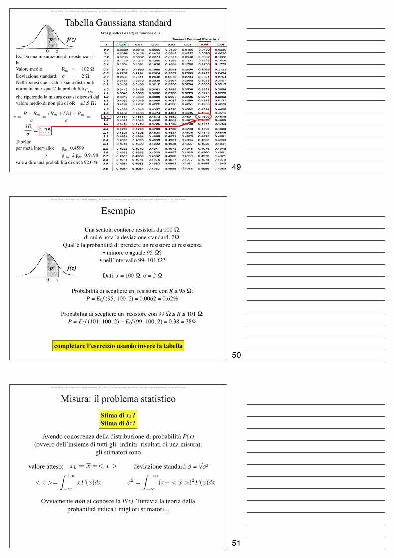
Distribuzione normaleSe gli istogrammi tendono a una curva a campana (sole fluttuazioni casuali), La funzione di distribuzione cui tende l’istogramma delle occorrenze al crescere di N è la distribuzione normale o curva di Gauss, dove il valore medio (in corrispondenza del massimo della “campana”) coincide con il valore atteso m e la larghezza σ è indice della dispersione delle misure (→ incertezza)
f(x) =1
�
p2⇡
e�(x�m)2
2�2
4.3 Random Fluctuations 55
general validity on the grounds of a limited number of experimental observa-tions.
In many cases, although not always, the histograms of measurements af-fected by random fluctuations tend to a symmetric “bell” shape when Nincreases (Fig. 4.7, right). The limiting histogram is then assumed to have abell shape. It is convenient to describe the bell shape of the limiting histogramby a mathematical model, expressed in terms of a continuous function. Tothis aim, the further approximation of shrinking to zero the width of the his-togram columns is made: �x! 0. By that procedure, the limiting histogramis substituted by a limiting distribution, corresponding to a continuous func-tion of continuous variable f(X).
The Normal Distribution
According to both experimental observations and theoretical considerations,the bell-shaped behavior of the limiting distribution is best represented bythe normal distribution, also called Gaussian distribution, after the name ofthe German mathematician C. F. Gauss (1777–1855):
f(x) =1
�p
2⇡exp
� (x�m)2
2�2
�. (4.17)
The parameters m and � in (4.17) have the same dimension of the variable x.It easy to verify that m gives the position of the distribution on the x-axis,whereas � depends on the width of the distribution (Fig. 4.8).
0
0.1
0.2
0.3
0 5 10 15 20
f(x)
x
m=7 m=13
=2
0
0.1
0.2
0.3
0 5 10 15 20
f(x)
x
=1.5
=3
m
Fig. 4.8. Normal distribution (4.17). Left: two distributions with the same standarddeviation � and di↵erent means m. Right: two distributions with the same meanm and di↵erent standard deviations �.
The function f(x) in (4.17) is dimensionally homogeneous to the sampledensity f⇤
j
defined in (4.8). The normal distribution is the limiting distri-bution of an area-normalized histogram (Fig. 4.7) for both N ! 1 (num-ber of measurements) and N ! 1 (number of columns, corresponding to�x
j
! 0). One can show that m and � are the asymptotic values, for N !1,of sample mean m⇤ and sample standard deviation �⇤, respectively. To this
Figu
ra a
datta
ta d
a P.
For
nasin
i “Th
e U
ncer
tain
ty in
Phy
sical
Mea
sure
men
ts”
m valore medioσ deviazione standardσ2 varianza
Enrico Silva - diritti riservati - Non è permessa, fra l’altro, l’inclusione anche parziale in altre opere senza il consenso scritto dell’autore
Importanza della distribuzione normale
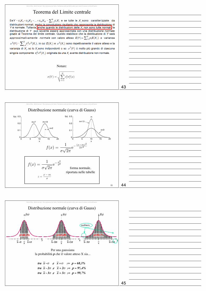
Teorema del Limite centrale
La variabile somma di un grande numero N di variabili casuali indipendenti, ciascuna a media e varianza finite, tende alla distribuzione normale di
Gauss indipendentemente dalla funzione di distribuzione delle variabili casuali.
Enrico Silva - diritti riservati - Non è permessa, fra l’altro, l’inclusione anche parziale in altre opere senza il consenso scritto dell’autore
Teorema del Limite centrale
Ad esempio, anche se la grandezza x non è distribuita secondo una gaussiana, la sua media (ovvero Y = (1/N)∑xi) sarà distribuita
approssimativamente come una gaussiana.
Questo giustifica la scelta degli stimatori (vedi dopo) per xb , δx...
40
41
42
Enrico Silva - diritti riservati - Non è permessa, fra l’altro, l’inclusione anche parziale in altre opere senza il consenso scritto dell’autore
Teorema del Limite centrale
Notare:
�(Y ) =
vuutNX
i=1
c
2i�
2i (x)
Enrico Silva - diritti riservati - Non è permessa, fra l’altro, l’inclusione anche parziale in altre opere senza il consenso scritto dell’autore
11
Distribuzione normale (curva di Gauss)
forma normale, riportata nelle tabelle
f(x) =1
�
p2⇡
e�(x�m)2
2�2
4.3 Random Fluctuations 55
general validity on the grounds of a limited number of experimental observa-tions.
In many cases, although not always, the histograms of measurements af-fected by random fluctuations tend to a symmetric “bell” shape when Nincreases (Fig. 4.7, right). The limiting histogram is then assumed to have abell shape. It is convenient to describe the bell shape of the limiting histogramby a mathematical model, expressed in terms of a continuous function. Tothis aim, the further approximation of shrinking to zero the width of the his-togram columns is made: �x! 0. By that procedure, the limiting histogramis substituted by a limiting distribution, corresponding to a continuous func-tion of continuous variable f(X).
The Normal Distribution
According to both experimental observations and theoretical considerations,the bell-shaped behavior of the limiting distribution is best represented bythe normal distribution, also called Gaussian distribution, after the name ofthe German mathematician C. F. Gauss (1777–1855):
f(x) =1
�p
2⇡exp
� (x�m)2
2�2
�. (4.17)
The parameters m and � in (4.17) have the same dimension of the variable x.It easy to verify that m gives the position of the distribution on the x-axis,whereas � depends on the width of the distribution (Fig. 4.8).
0
0.1
0.2
0.3
0 5 10 15 20
f(x)
x
m=7 m=13
=2
0
0.1
0.2
0.3
0 5 10 15 20
f(x)
x
=1.5
=3
m
Fig. 4.8. Normal distribution (4.17). Left: two distributions with the same standarddeviation � and di↵erent means m. Right: two distributions with the same meanm and di↵erent standard deviations �.
The function f(x) in (4.17) is dimensionally homogeneous to the sampledensity f⇤
j
defined in (4.8). The normal distribution is the limiting distri-bution of an area-normalized histogram (Fig. 4.7) for both N ! 1 (num-ber of measurements) and N ! 1 (number of columns, corresponding to�x
j
! 0). One can show that m and � are the asymptotic values, for N !1,of sample mean m⇤ and sample standard deviation �⇤, respectively. To this
f(x) =1
�
p2⇡
e�z2
22
z =x�m
�
Enrico Silva - diritti riservati - Non è permessa, fra l’altro, l’inclusione anche parziale in altre opere senza il consenso scritto dell’autore
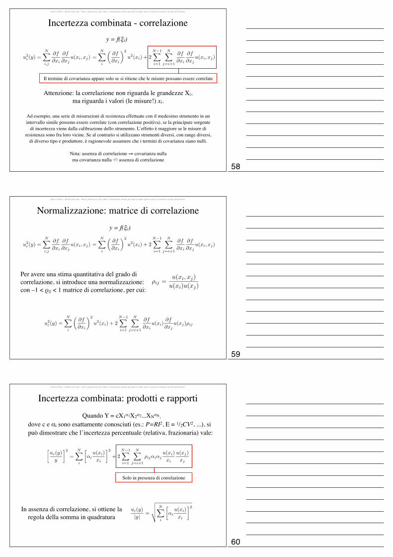
Distribuzione normale (curva di Gauss)
Per una gaussianala probabilità p che il valore atteso X sia...
outliers
43
44
45

Enrico Silva - diritti riservati - Non è permessa, fra l’altro, l’inclusione anche parziale in altre opere senza il consenso scritto dell’autore
Livello e intervallo di confidenzaN: numero totale di misuren
k: numero di misure di valore x
k (occorrenze)
nk/N: frequenza relativa della misura x
k.
Intervallo di confidenza corrispondente al livello di confidenza del 68%
Intervallo di confidenza corrispondente al livello di confidenza del 95%
(calcolati sulla gaussiana limite)
Enrico Silva - diritti riservati - Non è permessa, fra l’altro, l’inclusione anche parziale in altre opere senza il consenso scritto dell’autore
Calcolo di probabilità - distribuzione normaleProbabilità cumulativa
24 Uncertainties as probabilities
(3) The expectation of the nth power of the random variable x is
xn =∞!
−∞PDF (x) xn dx . (3.3)
The mean can be calculated by applying eqn (3.3) with n = 1:
x̄ =∞!
−∞PDF (x) x dx . (3.4)
The variance, σ 2, is defined as:
σ 2 =∞!
−∞PDF (x) (x − x̄)2 dx =
∞!
−∞PDF (x)
"x2 + x̄2 − 2x x̄
#dx . (3.5)
By applying eqn (3.3) with n = 2 and eqn (3.4) we obtain
σ 2 = x2 − x̄2, (3.6)
where x2 is the mean of the squares of the random variable x .
3.2 The Gaussian probabilitydistribution function
As we discussed in Section 2.5 the most important function in error analysisis the Gaussian (or normal) probability density distribution. For the sake ofbrevity we usually refer to it as the Gaussian probability distribution, orsimply the Gaussian distribution. In this chapter we will write the functionas G (x; x̄, σ ), where:
G (x; x̄, σ ) = 1
σ√
2πexp
$
− (x − x̄)2
2σ 2
%
, (3.7)
to emphasise that the function has x as a variable, and has the mean, x̄ , andstandard deviation, σ , as two parameters.
3.2.1 Probability calculationsFig. 3.1 The error function of the ran-dom variable x is the cumulative integral(the area under the curve) of a Gaussianfrom −∞ to x . Here it is plotted for aGaussian with mean x̄ = 10 and standarddeviation σ = 3. The function is antisym-metric about the mean; is equal to 0.159 forx = x̄ − σ , 0.500 for x = x̄ , and 0.841 forx = x̄ + σ ; and the error function tendsasymptotically to 1.
We can use eqn (3.7) to determine the fraction of the data which is expectedto lie within certain limits. For a Gaussian the cumulative probability is thewell-known error function Erf (x1; x̄, σ ):
Erf (x1; x̄, σ ) =! x1
−∞G (x; x̄, σ ) dx . (3.8)
This function has the mean, x̄ , and the standard deviation, σ , as parameters, andis evaluated at x = x1. The error function is plotted in Fig. 3.1 and tabulated in
Figu
ra a
datta
ta d
a H
ughe
s, H
ase,
Mea
sure
men
ts an
d th
eir U
ncer
tain
ties,
Oxf
ord
Uni
vers
ity P
ress
, 201
0
Erf(x0;x,�) =
Zx0
�1f(x)dx =
Zx0
�1
1
�
p2⇡
e�(x�m)2
2�2dx
3.3 Confidence limits and error bars 25
many data-analysis packages. The fractional area under the curve between thebounds x1 and x2 is thus:
P (x1 ≤ x ≤ x2) = 1
σ√
2π
! x2
x1
exp
"
− (x − x̄)2
2σ 2
#
dx
= Erf (x2; x̄, σ ) − Erf (x1; x̄, σ ) . (3.9)
Figure 3.2 shows the relationship between the error function and the area
Fig. 3.2 A Gaussian with mean x̄ = 10 andstandard deviation σ = 3 is shown. In (a)the fraction of the curve within the interval5 ≤ x ≤ 11.5 is shaded; this is equal to thedifference between (b) the error functionevaluated at 11.5 and (c) the error functionevaluated at 5. The relevant values of theerror function are highlighted in (d).
under certain portions of the Gaussian distribution function. For a Gaussianwith mean x̄ = 10 and standard deviation σ = 3, what fraction of the data liesin the interval 5 ≤ x ≤ 11.5? For this Gaussian the probability of obtaining avalue of x ≤ 11.5 is 0.69, and the probability of obtaining a value of x ≤ 5 is0.05; hence 64% of the area under the curve is in the interval 5 ≤ x ≤ 11.5.
3.2.2 Worked example—the error functionA box contains 100 # resistors which are known to have a standard deviationof 2 #. What is the probability of selecting a resistor with a value of 95 # orless? What is the probability of finding a resistor in the range 99–101 #?
Let x represent the value of the resistance which has a mean of x̄ = 100 #.The standard deviation is given as σ = 2 #. The probability of selecting aresistor with a value of 95 # or less can be evaluated from eqn (3.8):
P = Erf (95; 100, 2) = 0.0062.
Applying eqn (3.9) we find the probability of finding a resistor in the range99–101 #
P = Erf (101; 100, 2) − Erf (99; 100, 2) = 0.38.
These integrals can be evaluated numerically, found in look-up tables or foundby using appropriate commands in spreadsheet software.
3.3 Confidence limits and error barsConsider first the fraction of the data expected to lie within one standarddeviation of the mean:
P = 1
σ√
2π
! x̄+σ
x̄−σexp
"
− (x − x̄)2
2σ 2
#
dx
= Erf (x̄ + σ ; x̄, σ ) − Erf (x̄ − σ ; x̄, σ ) . (3.10)
Numerically, this integral is equal to 0.683 (to three significant figures). Inother words, approximately two-thirds of the total area under the curve iswithin a standard deviation of the mean. This is the origin of the two-thirdsterms used extensively in Chapter 2. We can now quantify our statements aboutthe standard deviation of a sample of measurements: we are confident, at the68% level, that, were we to take another measurement, the value would liewithin one standard deviation of the mean.
x0
x
Area sottesa sotto la curva della gaussiana
Notare: Erf(x;x,�) =1
2
Funzione riportata nelle
tabelle
Enrico Silva - diritti riservati - Non è permessa, fra l’altro, l’inclusione anche parziale in altre opere senza il consenso scritto dell’autore
Calcolo di probabilità - distribuzione normale
Probabilità di trovare il dato fra x1 e x2
Figu
ra a
datta
ta d
a H
ughe
s, H
ase,
Mea
sure
men
ts an
d th
eir U
ncer
tain
ties,
Oxf
ord
Uni
vers
ity P
ress
, 201
0
3.3 Confidence limits and error bars 25
many data-analysis packages. The fractional area under the curve between thebounds x1 and x2 is thus:
P (x1 ≤ x ≤ x2) = 1
σ√
2π
! x2
x1
exp
"
− (x − x̄)2
2σ 2
#
dx
= Erf (x2; x̄, σ ) − Erf (x1; x̄, σ ) . (3.9)
Figure 3.2 shows the relationship between the error function and the area
Fig. 3.2 A Gaussian with mean x̄ = 10 andstandard deviation σ = 3 is shown. In (a)the fraction of the curve within the interval5 ≤ x ≤ 11.5 is shaded; this is equal to thedifference between (b) the error functionevaluated at 11.5 and (c) the error functionevaluated at 5. The relevant values of theerror function are highlighted in (d).
under certain portions of the Gaussian distribution function. For a Gaussianwith mean x̄ = 10 and standard deviation σ = 3, what fraction of the data liesin the interval 5 ≤ x ≤ 11.5? For this Gaussian the probability of obtaining avalue of x ≤ 11.5 is 0.69, and the probability of obtaining a value of x ≤ 5 is0.05; hence 64% of the area under the curve is in the interval 5 ≤ x ≤ 11.5.
3.2.2 Worked example—the error functionA box contains 100 # resistors which are known to have a standard deviationof 2 #. What is the probability of selecting a resistor with a value of 95 # orless? What is the probability of finding a resistor in the range 99–101 #?
Let x represent the value of the resistance which has a mean of x̄ = 100 #.The standard deviation is given as σ = 2 #. The probability of selecting aresistor with a value of 95 # or less can be evaluated from eqn (3.8):
P = Erf (95; 100, 2) = 0.0062.
Applying eqn (3.9) we find the probability of finding a resistor in the range99–101 #
P = Erf (101; 100, 2) − Erf (99; 100, 2) = 0.38.
These integrals can be evaluated numerically, found in look-up tables or foundby using appropriate commands in spreadsheet software.
3.3 Confidence limits and error barsConsider first the fraction of the data expected to lie within one standarddeviation of the mean:
P = 1
σ√
2π
! x̄+σ
x̄−σexp
"
− (x − x̄)2
2σ 2
#
dx
= Erf (x̄ + σ ; x̄, σ ) − Erf (x̄ − σ ; x̄, σ ) . (3.10)
Numerically, this integral is equal to 0.683 (to three significant figures). Inother words, approximately two-thirds of the total area under the curve iswithin a standard deviation of the mean. This is the origin of the two-thirdsterms used extensively in Chapter 2. We can now quantify our statements aboutthe standard deviation of a sample of measurements: we are confident, at the68% level, that, were we to take another measurement, the value would liewithin one standard deviation of the mean.
=
3.3 Confidence limits and error bars 25
many data-analysis packages. The fractional area under the curve between thebounds x1 and x2 is thus:
P (x1 ≤ x ≤ x2) = 1
σ√
2π
! x2
x1
exp
"
− (x − x̄)2
2σ 2
#
dx
= Erf (x2; x̄, σ ) − Erf (x1; x̄, σ ) . (3.9)
Figure 3.2 shows the relationship between the error function and the area
Fig. 3.2 A Gaussian with mean x̄ = 10 andstandard deviation σ = 3 is shown. In (a)the fraction of the curve within the interval5 ≤ x ≤ 11.5 is shaded; this is equal to thedifference between (b) the error functionevaluated at 11.5 and (c) the error functionevaluated at 5. The relevant values of theerror function are highlighted in (d).
under certain portions of the Gaussian distribution function. For a Gaussianwith mean x̄ = 10 and standard deviation σ = 3, what fraction of the data liesin the interval 5 ≤ x ≤ 11.5? For this Gaussian the probability of obtaining avalue of x ≤ 11.5 is 0.69, and the probability of obtaining a value of x ≤ 5 is0.05; hence 64% of the area under the curve is in the interval 5 ≤ x ≤ 11.5.
3.2.2 Worked example—the error functionA box contains 100 # resistors which are known to have a standard deviationof 2 #. What is the probability of selecting a resistor with a value of 95 # orless? What is the probability of finding a resistor in the range 99–101 #?
Let x represent the value of the resistance which has a mean of x̄ = 100 #.The standard deviation is given as σ = 2 #. The probability of selecting aresistor with a value of 95 # or less can be evaluated from eqn (3.8):
P = Erf (95; 100, 2) = 0.0062.
Applying eqn (3.9) we find the probability of finding a resistor in the range99–101 #
P = Erf (101; 100, 2) − Erf (99; 100, 2) = 0.38.
These integrals can be evaluated numerically, found in look-up tables or foundby using appropriate commands in spreadsheet software.
3.3 Confidence limits and error barsConsider first the fraction of the data expected to lie within one standarddeviation of the mean:
P = 1
σ√
2π
! x̄+σ
x̄−σexp
"
− (x − x̄)2
2σ 2
#
dx
= Erf (x̄ + σ ; x̄, σ ) − Erf (x̄ − σ ; x̄, σ ) . (3.10)
Numerically, this integral is equal to 0.683 (to three significant figures). Inother words, approximately two-thirds of the total area under the curve iswithin a standard deviation of the mean. This is the origin of the two-thirdsterms used extensively in Chapter 2. We can now quantify our statements aboutthe standard deviation of a sample of measurements: we are confident, at the68% level, that, were we to take another measurement, the value would liewithin one standard deviation of the mean.
–Z
x2
�1
1
�
p2⇡
e�(x�m)2
2�2dx
Zx1
�1
1
�
p2⇡
e�(x�m)2
2�2dx
3.3 Confidence limits and error bars 25
many data-analysis packages. The fractional area under the curve between thebounds x1 and x2 is thus:
P (x1 ≤ x ≤ x2) = 1
σ√
2π
! x2
x1
exp
"
− (x − x̄)2
2σ 2
#
dx
= Erf (x2; x̄, σ ) − Erf (x1; x̄, σ ) . (3.9)
Figure 3.2 shows the relationship between the error function and the area
Fig. 3.2 A Gaussian with mean x̄ = 10 andstandard deviation σ = 3 is shown. In (a)the fraction of the curve within the interval5 ≤ x ≤ 11.5 is shaded; this is equal to thedifference between (b) the error functionevaluated at 11.5 and (c) the error functionevaluated at 5. The relevant values of theerror function are highlighted in (d).
under certain portions of the Gaussian distribution function. For a Gaussianwith mean x̄ = 10 and standard deviation σ = 3, what fraction of the data liesin the interval 5 ≤ x ≤ 11.5? For this Gaussian the probability of obtaining avalue of x ≤ 11.5 is 0.69, and the probability of obtaining a value of x ≤ 5 is0.05; hence 64% of the area under the curve is in the interval 5 ≤ x ≤ 11.5.
3.2.2 Worked example—the error functionA box contains 100 # resistors which are known to have a standard deviationof 2 #. What is the probability of selecting a resistor with a value of 95 # orless? What is the probability of finding a resistor in the range 99–101 #?
Let x represent the value of the resistance which has a mean of x̄ = 100 #.The standard deviation is given as σ = 2 #. The probability of selecting aresistor with a value of 95 # or less can be evaluated from eqn (3.8):
P = Erf (95; 100, 2) = 0.0062.
Applying eqn (3.9) we find the probability of finding a resistor in the range99–101 #
P = Erf (101; 100, 2) − Erf (99; 100, 2) = 0.38.
These integrals can be evaluated numerically, found in look-up tables or foundby using appropriate commands in spreadsheet software.
3.3 Confidence limits and error barsConsider first the fraction of the data expected to lie within one standarddeviation of the mean:
P = 1
σ√
2π
! x̄+σ
x̄−σexp
"
− (x − x̄)2
2σ 2
#
dx
= Erf (x̄ + σ ; x̄, σ ) − Erf (x̄ − σ ; x̄, σ ) . (3.10)
Numerically, this integral is equal to 0.683 (to three significant figures). Inother words, approximately two-thirds of the total area under the curve iswithin a standard deviation of the mean. This is the origin of the two-thirdsterms used extensively in Chapter 2. We can now quantify our statements aboutthe standard deviation of a sample of measurements: we are confident, at the68% level, that, were we to take another measurement, the value would liewithin one standard deviation of the mean.
Erf(x2;x,�)� Erf(x1;x,�)⇒
Zx2
x1
1
�
p2⇡
e�(x�m)2
2�2dx
46
47
48
Enrico Silva - diritti riservati - Non è permessa, fra l’altro, l’inclusione anche parziale in altre opere senza il consenso scritto dell’autore
Tabella Gaussiana standard
Es. Da una misurazione di resistenza si ha:Valore medio: Rm = 102 ΩDeviazione standard: σ = 2 Ω.Nell’ipotesi che i valori siano distribuiti normalmente, qual’è la probabilità p
±δx
che ripetendo la misura essa si discosti dal valore medio di non più di δR = ±3.5 Ω?
Tabella:per metà intervallo: pδx=0.4599 ⇒ p±δx=2·pδx=0.9198vale a dire una probabilità di circa 92.0 %
f(z)Area p sottesa da f(z) in funzione di z
= 1.75=�R
�
z =R�Rm
�=
(Rm + �R)�Rm
�=
p
0 z
Enrico Silva - diritti riservati - Non è permessa, fra l’altro, l’inclusione anche parziale in altre opere senza il consenso scritto dell’autore
Esempio
f(z)p
0 z
Una scatola contiene resistori da 100 Ω,di cui è nota la deviazione standard, 2Ω.
Qual’è la probabilità di prendere un resistore di resistenza• minore o uguale 95 Ω?
• nell’intervallo 99–101 Ω?
Dati: x = 100 Ω; σ = 2 Ω
Probabilità di scegliere un resistore con R ≤ 95 Ω: P = Erf (95; 100, 2) = 0.0062 = 0.62%
Probabilità di scegliere un resistore con 99 Ω ≤ R ≤ 101 Ω:P = Erf (101; 100, 2) − Erf (99; 100, 2) = 0.38 = 38%
completare l’esercizio usando invece la tabella
Enrico Silva - diritti riservati - Non è permessa, fra l’altro, l’inclusione anche parziale in altre opere senza il consenso scritto dell’autore
Misura: il problema statisticoStima di xb ?Stima di δx?
Avendo conoscenza della distribuzione di probabilità P(x)(ovvero dell’insieme di tutti gli -infiniti- risultati di una misura),
gli stimatori sono
< x >=
Z +1
�1xP (x)dx
valore atteso: deviazione standard σ = √σ2
Ovviamente non si conosce la P(x). Tuttavia la teoria della probabilità indica i migliori stimatori...
�
2 =
Z +1
�1(x� < x >)2P (x)dx
xb = x =< x >
49
50
51

Enrico Silva - diritti riservati - Non è permessa, fra l’altro, l’inclusione anche parziale in altre opere senza il consenso scritto dell’autore
Misura: il problema statisticoStima di xb ?Stima di δx?
La teoria della probabilità indica i migliori stimatoria partire dal campione disponibile.
xb : media aritmeticax̄ =
1
N
NX
i=1
xi
Miglior stima della varianza σ2(x):
δx: deviazione standard della media semplices
2(x̄) =s
2(x)
N
u(x̄) = s(x̄)incertezza standard:
s
2(x) =1
N � 1
NX
i=1
(xi � x̄)2 UNI CEI ENV 13005:s(x): scarto tipo
UNI CEI ENV 13005:miglior stima dei
valori attesi
Enrico Silva - diritti riservati - Non è permessa, fra l’altro, l’inclusione anche parziale in altre opere senza il consenso scritto dell’autore
Valutazione dell’incertezza di tipo AIncertezza di tipo A, uA: stimata attraverso analisi statistica mediante misure ripetute
xb : media aritmetica x̄ =1
N
NX
i=1
xi
δx: incertezza standard(scarto tipo)
misura di X: (xb ± δx) u.m.
STATISTICA
u(x̄) = s(x̄) =
vuut 1
N(N � 1)
NX
i=1
(xi � x̄)2
UNI CEI ENV 13005: incertezza tipo di categoria A
Stima di xb ? Stima di δx?
→
→
Enrico Silva - diritti riservati - Non è permessa, fra l’altro, l’inclusione anche parziale in altre opere senza il consenso scritto dell’autore
Valutazione dell’incertezza di tipo BIncertezza di tipo B, uB: non può essere dedotta da misure ripetute,
ma da altre informazioni(dati ottenuti in condizioni simili, conoscenza del comportamento degli strumenti, specifiche tecniche,
calibrazioni, dati di riferimento...)
Anche per uB si tratta di una stima di una deviazione standard,la quale tuttavia non può essere ottenuta da un campione di numerose misure.
Trattandosi ancora di una grandezza statistica, l’incertezza combinata sarà ottenuta in maniera consistente.
52
53
54

Enrico Silva - diritti riservati - Non è permessa, fra l’altro, l’inclusione anche parziale in altre opere senza il consenso scritto dell’autore
Incertezza combinataSi debba dare la misura y di una grandezza Y, funzione di N grandezze Xi
direttamente misurate, le cui misure siano xi con incertezze ui:
Y = f(X1, X2,..., XN)
Trattiamo le variabili y, xi come variabili stocastiche di valore aspettato:η = E(y)ξi = E(xi)
cerchiamo η.Per piccole variazioni Δi (dove Δi = xi – ξi):
⌘ = E(y) = E[f(⇠i +�i)] ' E
"f(⇠i) +
X
i
@f
@⇠i�i + o(�2
i + ...)
#
Poiché (variabili stocastiche) E(Δi) = 0, si haη = f(ξi)
coefficienti di sensibilità(nulla a che vedere con gli strumenti!)
(purché Δi ≪ ξi)
y = f(x1, x2,..., xN)⇒
Enrico Silva - diritti riservati - Non è permessa, fra l’altro, l’inclusione anche parziale in altre opere senza il consenso scritto dell’autore
Incertezza combinata - varianza
dove E[ΔiΔj] = E[(xi – ξi)(xj – ξj)] = cov(xi, xj) è la matrice di covarianza
definizione
�
2y = E[(y � ⌘)2] = E[(f(xi)� f(⇠i))
2] ' E
2
4X
i,j
@f
@⇠i
@f
@⇠j�i�j
3
5 =X
i,j
@f
@⇠i
@f
@⇠jE [�i�j ]
Taylor
si ha subito E[ΔiΔi] = E[(xi – ξi)2] = σxi2
Gli elementi fuori diagonale E[ΔiΔj] danno una quantificazione della correlazione (dipendenza mutua) fra xi e xj.
Enrico Silva - diritti riservati - Non è permessa, fra l’altro, l’inclusione anche parziale in altre opere senza il consenso scritto dell’autore
Incertezza combinata - propagazione
Sostituendo ai valori esatti le stime, otteniamo le stime dei risultati di una misura indiretta, in cui la grandezza di interesse Y è funzione di più grandezze Xi.
y = f(ξi)
con incertezza combinata data dalla stima della varianza
legge della propagazione delle incertezze
in assenza di correlazione u(xi, xj) = 0 (i≠j), da cui:
u
2c(y) =
NX
i,j
@f
@xi
@f
@xju(xi, xj)
u
2c(y) =
NX
i
✓@f
@xi
◆2
u
2(xi) somma delle incertezze in quadratura
55
56
57
Enrico Silva - diritti riservati - Non è permessa, fra l’altro, l’inclusione anche parziale in altre opere senza il consenso scritto dell’autore
Incertezza combinata - correlazioney = f(ξi)
Attenzione: la correlazione non riguarda le grandezze Xi,ma riguarda i valori (le misure!) xi.
u
2c(y) =
NX
i,j
@f
@xi
@f
@xju(xi, xj)
Ad esempio, una serie di misurazioni di resistenza effettuate con il medesimo strumento in un intervallo simile possono essere correlate (con correlazione positiva), se la principare sorgente
di incertezza viene dalla calibrazione dello strumento. L’effetto è maggiore se le misure di resistenza sono fra loro vicine. Se al contrario si utilizzano strumenti diversi, con range diversi,
di diverso tipo e produttore, è ragionevole assumere che i termini di covarianza siano nulli.
Nota: assenza di correlazione ⇒ covarianza nullama covarianza nulla ⇏ assenza di correlazione
Il termine di covarianza appare solo se si ritiene che le misure possano essere correlate
=NX
i
✓@f
@xi
◆2
u
2(xi) + 2N�1X
i=1
NX
j=i+1
@f
@xi
@f
@xju(xi, xj)
Enrico Silva - diritti riservati - Non è permessa, fra l’altro, l’inclusione anche parziale in altre opere senza il consenso scritto dell’autore
Normalizzazione: matrice di correlazioney = f(ξi)
Per avere una stima quantitativa del grado di correlazione, si introduce una normalizzazione:con –1 < ρij < 1 matrice di correlazione, per cui:
u
2c(y) =
NX
i,j
@f
@xi
@f
@xju(xi, xj)
⇢ij =u(xi, xj)
u(xi)u(xj)
=NX
i
✓@f
@xi
◆2
u
2(xi) + 2N�1X
i=1
NX
j=i+1
@f
@xi
@f
@xju(xi, xj)
u
2c(y) =
NX
i
✓@f
@xi
◆2
u
2(xi) + 2N�1X
i=1
NX
j=i+1
@f
@xiu(xi)
@f
@xju(xj)⇢ij
Enrico Silva - diritti riservati - Non è permessa, fra l’altro, l’inclusione anche parziale in altre opere senza il consenso scritto dell’autore
uc(y)
y
�2=
NX
i
↵i
u(xi)
xi
�2+ 2
N�1X
i=1
NX
j=i+1
⇢ij↵i↵ju(xi)
xi
u(xj)
xj
Incertezza combinata: prodotti e rapportiQuando Y = cX1α1X2α2...XNαN,
dove c e αi sono esattamente conosciuti (es.: P=RI2, E = 1/2CV2, ...), si può dimostrare che l’incertezza percentuale (relativa, frazionaria) vale:
Solo in presenza di correlazione
uc(y)
|y| =
vuutNX
i
↵i
u(xi)
xi
�2In assenza di correlazione, si ottiene la regola della somma in quadratura
58
59
60

Enrico Silva - diritti riservati - Non è permessa, fra l’altro, l’inclusione anche parziale in altre opere senza il consenso scritto dell’autore
Incertezza ↔ deviazione standard
Identificazione δx ↔ u(x) ↔ σ(x) →l’incertezza dà una misura della probabilità di trovare il risultato
della misura nell’intervallo x± δx.Quale?
Si assume (spesso implicitamente) che i risultati siano dispersi secondo una gaussiana (i valori medi di gruppi numerosi di campioni lo sono!) (teorema del
limite centrale). Ok per incertezza di tipo A.
Supponiamo comunque di poter applicare i medesimi ragionamenti all’incertezza di tipo B (vedremo oltre come variare il ragionamento).
N.B.: in questo caso assumere che la distribuzione sia gaussiana è un’ipotesi forte (non sono possibili misure ripetute, non si può invocare il limite centrale).
Enrico Silva - diritti riservati - Non è permessa, fra l’altro, l’inclusione anche parziale in altre opere senza il consenso scritto dell’autore
Incertezza estesa e fattore di copertura
dove uc,A e uc,B sono eventualmente incertezze combinate. Tuttavia, nulla dice sulla distribuzione di probabilità associata.
In ambito commerciale, di produzione, normativo etc etc è necessario ricorrere all’ intervallo che contiene con (ragionevole) certezza (ovvero con probabilità p ≃ 100%) il valore del misurando.
→ incertezza estesa: U = k uc
dove k è il fattore di copertura.
Il valore di k necessario a ottenere una certa p (livello di probabilità o livello di confidenza*) dipende dalla funzione di distribuzione del misurando.
L’incertezza standard uc =q
u2c,A + u2
c,B esprime l’incertezza di una misura.
* definizione non raccomandata dalla GUM
UNI CEI ENV 13005: incertezza estesa
Enrico Silva - diritti riservati - Non è permessa, fra l’altro, l’inclusione anche parziale in altre opere senza il consenso scritto dell’autore
Incertezza estesa: distribuzione gaussianaincertezza standard:
incertezza estesa: U = k uc
fattore di copertura: k
uc =q
u2c,A + u2
c,B
k = 1U = uc
p = 68 %
k = 2U = 2 uc
p = 95 %
k = 3U = 3 uc
p ≳ 99 %
61
62
63
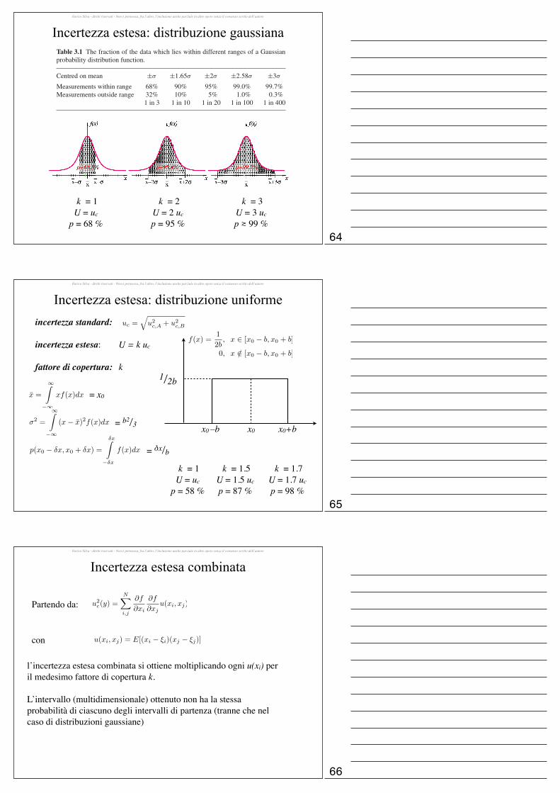
Enrico Silva - diritti riservati - Non è permessa, fra l’altro, l’inclusione anche parziale in altre opere senza il consenso scritto dell’autore
Incertezza estesa: distribuzione gaussiana
k = 1U = uc
p = 68 %
k = 2U = 2 uc
p = 95 %
k = 3U = 3 uc
p ≳ 99 %
26 Uncertainties as probabilities
3.3.1 Extended ranges
Fig. 3.3 The shaded areas of the Gaussiancurves show the fraction of data within (a)one standard deviation of the mean, (b) twostandard deviations, and (c) three standarddeviations. The corresponding points on theerror function, along with those for four stan-dard deviations, are indicated in (d).
By evaluating the error function of eqn (3.9) we can define the probabilitiesthat the data lie within an interval defined by two, three, etc. standard devia-tions from the mean; these values are indicated in Fig. 3.3, and tabulated inTable 3.1.
Table 3.1 The fraction of the data which lies within different ranges of a Gaussianprobability distribution function.
Centred on mean ±σ ±1.65σ ±2σ ±2.58σ ±3σ
Measurements within range 68% 90% 95% 99.0% 99.7%Measurements outside range 32% 10% 5% 1.0% 0.3%
1 in 3 1 in 10 1 in 20 1 in 100 1 in 400
Recalling the interpretation of the standard error as a standard deviation of themean we can also calculate other confidence intervals. Whereas often in thephysical sciences the error bar is taken as one standard deviation of the mean(the standard error), other conventions exist; in other disciplines the 95% con-fidence limit is often used. Evaluating the error function of eqn (3.9) it can beshown that 95.0% of the measurements lie within the range ±1.96σ . Thereforeif a data set of N measurements has a mean x̄ and standard deviation σN−1, wewould report the result at the 95% confidence limit as x̄ ± 1.96 × σN−1√
N. Dif-
ferent confidence limits can be used by scaling the standard error appropriately.It should be noted that in the above discussion it is assumed that the standard
deviation of the Gaussian distribution is precisely and accurately known. WhenσN−1 is ascertained from experimental data, especially from a small numberof repeat measurements, greater care is needed with confidence limits. InChapter 8 we will discuss the Student’s t distribution which is more appropriatefor interval estimation from a small number of data points.
3.3.2 Rejecting outliersHere we discuss a controversial topic in data analysis, that of rejecting outliers.From Table 3.1 we learn that we should not be very surprised if a measure-ment is in disagreement with the accepted value by more then one error bar,α; indeed, for a group of 15 students in a laboratory performing the sameexperiment, we would expect approximately five to report results where themagnitude of the difference between the accepted and measured results isgreater than one error bar. However, as the fractional area under a Gaussiancurve beyond 3σ or 5σ is only 0.3% and 6 × 10⁻⁵%, respectively, we expectsuch large deviations to occur very infrequently.
Enrico Silva - diritti riservati - Non è permessa, fra l’altro, l’inclusione anche parziale in altre opere senza il consenso scritto dell’autore
Incertezza estesa: distribuzione uniformeincertezza standard:
incertezza estesa: U = k uc
fattore di copertura: k
uc =q
u2c,A + u2
c,B
k = 1U = uc
p = 58 %
k = 1.5U = 1.5 uc
p = 87 %
k = 1.7U = 1.7 uc
p = 98 %
x0 x0+bx0 –b
1/2bx̄ =
1Z
�1
xf(x)dx
�
2 =
1Z
�1
(x� x̄)2f(x)dx
p(x0 � �x, x0 + �x) =
�xZ
��x
f(x)dx
= x0
= b2/3
= δx/b
f(x) =1
2b, x 2 [x0 � b, x0 + b]
0, x /2 [x0 � b, x0 + b]
Enrico Silva - diritti riservati - Non è permessa, fra l’altro, l’inclusione anche parziale in altre opere senza il consenso scritto dell’autore
Incertezza estesa combinata
Partendo da: u
2c(y) =
NX
i,j
@f
@xi
@f
@xju(xi, xj)
l’incertezza estesa combinata si ottiene moltiplicando ogni u(xi) per il medesimo fattore di copertura k.
L’intervallo (multidimensionale) ottenuto non ha la stessa probabilità di ciascuno degli intervalli di partenza (tranne che nel caso di distribuzioni gaussiane)
u(xi, xj) = E[(xi � ⇠i)(xj � ⇠j)]con
64
65
66

Enrico Silva - diritti riservati - Non è permessa, fra l’altro, l’inclusione anche parziale in altre opere senza il consenso scritto dell’autore
Compatibilità di due misure
compatibili
Con errore massimo:I
I
non compatibili
Usando statistica? Sì, se possiamo assumere che la distribuzione della differenza di due misure sia gaussiana
misure: m1 ± u1, m2 ± u2 differenza:Δ = (m1 – m2) ± uδ,
Misure compatibili ⇔ Δ compatibile con 0 (zero)Se la variabile x = m1 – m2 è gaussiana → identificando uδ con la deviazione standard e 0 (zero) col valore “vero” di x (ovvero supponendo che m1 e m2 siano compatibili), posso conoscere la probabilità che x non sia contenuto in un certo intervallo [– Δ,+ Δ].
u� =qu21 + u2
2
Enrico Silva - diritti riservati - Non è permessa, fra l’altro, l’inclusione anche parziale in altre opere senza il consenso scritto dell’autore
Outliers: rifiutarli?Misure che cadono fuori dagli andamenti aspettati, o presentano valori
sensibilmente differenti rispetto agli altri in una serie di misure omogenee
Supponiamo che un dato si trovi “parecchie” barre di incertezza distante dalla media di un seti di misure (“outlier”).
Dovrebbe essere scartato, considerato “spurio”?
Criterio di Chauvenet(controverso! usare con cautela)
Un dato proveniente da un campione di N misure è scartato se il numero di eventi che ci si aspetta che sian più lontani dalla media rispetto al punto sospetto, utilizzando per la stima il valor medio e la varianza
provenienti dal campione stesso, è inferiore a 0.5
Enrico Silva - diritti riservati - Non è permessa, fra l’altro, l’inclusione anche parziale in altre opere senza il consenso scritto dell’autore
Outliers: rifiutarli?Criterio di Chauvenet
(controverso! usare con cautela)
Un dato proveniente da un campione di N misure è scartato se il numero di eventi che ci si aspetta che sian più lontani dalla media rispetto al punto sospetto, utilizzando per la stima il valor medio e la varianza
provenienti dal campione stesso, è inferiore a 0.5
1. Si abbiano N misure. Si calcoli la media x e la deviazione standard σN-1. 2. Per il possibile dato spurio, xout, si usi la funzione Errore per trovare la probabilità the un risultato differisca casualmente dalla media quanto o più di xout.
3. Si moltiplichi la probabilità così trovata di un outlier per il numero di dati sperimentali, nout = Pout ·N4. Se nout < 1/2, allora il criterio di Chauvenet richiede che l’outlier xout sia scartato, e che si ricalcoli media e varianza con i restatni N–1 punti
P
out
= 1� P (x� x
out
x x+ x
out
) = 1� [Erf(x+ x
out
;x,�)� Erf(x� x
out
;x,�)]
67
68
69
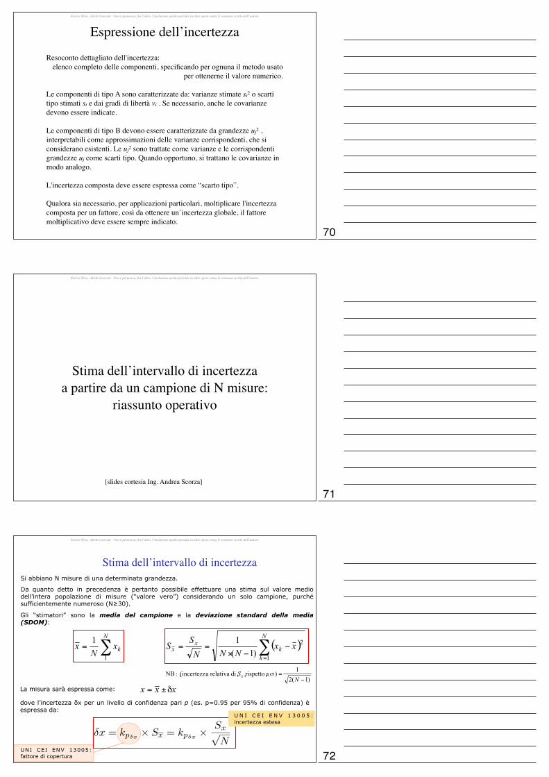
Enrico Silva - diritti riservati - Non è permessa, fra l’altro, l’inclusione anche parziale in altre opere senza il consenso scritto dell’autore
Resoconto dettagliato dell'incertezza: elenco completo delle componenti, specificando per ognuna il metodo usato
per ottenerne il valore numerico.
Le componenti di tipo A sono caratterizzate da: varianze stimate si2 o scarti tipo stimati si e dai gradi di libertà vi . Se necessario, anche le covarianze devono essere indicate.
Le componenti di tipo B devono essere caratterizzate da grandezze uj2 , interpretabili come approssimazioni delle varianze corrispondenti, che si considerano esistenti. Le uj2 sono trattate come varianze e le corrispondenti grandezze uj come scarti tipo. Quando opportuno, si trattano le covarianze in modo analogo.
L'incertezza composta deve essere espressa come “scarto tipo”.
Qualora sia necessario, per applicazioni particolari, moltiplicare l'incertezza composta per un fattore, così da ottenere un’incertezza globale, il fattore moltiplicativo deve essere sempre indicato.
Espressione dell’incertezza
Enrico Silva - diritti riservati - Non è permessa, fra l’altro, l’inclusione anche parziale in altre opere senza il consenso scritto dell’autore
Stima dell’intervallo di incertezzaa partire da un campione di N misure:
riassunto operativo
[slides cortesia Ing. Andrea Scorza]
Enrico Silva - diritti riservati - Non è permessa, fra l’altro, l’inclusione anche parziale in altre opere senza il consenso scritto dell’autore
Stima dell’intervallo di incertezzaSi abbiano N misure di una determinata grandezza.
Da quanto detto in precedenza è pertanto possibile effettuare una stima sul valore medio dell’intera popolazione di misure (“valore vero”) considerando un solo campione, purché sufficientemente numeroso (N≥30).
Gli “stimatori” sono la media del campione e la deviazione standard della media (SDOM):
La misura sarà espressa come:
dove l’incertezza δx per un livello di confidenza pari p (es. p=0.95 per 95% di confidenza) è espressa da:
UNI CEI ENV 13005: fattore di copertura
�x = k
p
�x
⇥ S
x
= k
p
�x
⇥ S
xpN
U N I C E I E N V 1 3 0 0 5 : incertezza estesa
70
71
72
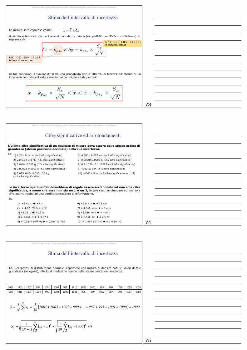
Enrico Silva - diritti riservati - Non è permessa, fra l’altro, l’inclusione anche parziale in altre opere senza il consenso scritto dell’autore
In tali condizioni il “valore di” X ha una probabilità pari a 100·p% di trovarsi all’interno di un intervallo centrato sul valore medio del campione e tale per cui:
Stima dell’intervallo di incertezza
La misura sarà espressa come:
dove l’incertezza δx per un livello di confidenza pari p (es. p=0.95 per 95% di confidenza) è espressa da:
UNI CEI ENV 13005: fattore di copertura
�x = k
p
�x
⇥ S
x
= k
p
�x
⇥ S
xpN
U N I C E I E N V 1 3 0 0 5 : incertezza estesa
x� k
p
�x
⇥ S
xpN
< x < x+ k
p
�x
⇥ S
xpN
Enrico Silva - diritti riservati - Non è permessa, fra l’altro, l’inclusione anche parziale in altre opere senza il consenso scritto dell’autore
6) ±2.5 km è ±2.5 km
7) ± 4.556 mm è ± 5 mm
8) ±3.556 mm è ± 4 mm
9) ± 2.566 nF è ± 2.6 nF
10) ± 1.654 10-19 C è ± 1.6 10-19C
Le incertezze sperimentali dovrebbero di regola essere arrotondate ad una sola cifra significativa, a meno che essa non sia un 1 o un 2, in tale caso arrotondare ad una sola cifra equivarrebbe ad una perdita consistente di informazione.
Es.
Cifre significative ed arrotondamenti
L’ultima cifra significativa di un risultato di misura deve essere dello stesso ordine di grandezza (stessa posizione decimale) della sua incertezza.
Es. 1) 4.25± 0.14 m (n.3 cifre significative)
2) 2345.0± 3.3 °C (n.5 cifre significative)
3) 0.818± 0.002 g (n.3 cifre significative)
4) 0.0002± 0.0001 s (n.1 cifra significativa)
5) 7.035 1019± 0.023 1019 kg (n.4 cifre significative)
6) 4.300± 0.002 km (n.4 cifre significative)
7) 0.0030±0.0008 A (n.2 cifre significative)
8) 0.6 10-12± 0.1 10-12 F (n.1 cifra significativa)
9) 40001± 5 in (n.5 cifre significative)
10) 40000± 5 in (n.5 cifre significative o.. 1!?)
1) ±3.41 m è ±3 m
2) ± 4.62 °C è ± 5 °C
3) ±1.26 g è ±1.3 g
4) ± 0.066 s è ± 0.07 s
5) ± 0.0244 1019 kg è ± 0.024 1019 kg
Enrico Silva - diritti riservati - Non è permessa, fra l’altro, l’inclusione anche parziale in altre opere senza il consenso scritto dell’autore
Es. Nell’ipotesi di distribuzione normale, esprimere una misura di densità noti 30 valori di tale grandezza (in kg/m3), riferiti al medesimo liquido nelle stesse condizioni ambiente.
1001 1003 1002 999 1001 1000 989 1010 1003 1000 993 980 1010 1005 1020
998 1015 1001 1004 999 1000 1006 1001 995 999 1002 987 993 1001 1000
Stima dell’intervallo di incertezza
73
74
75

Enrico Silva - diritti riservati - Non è permessa, fra l’altro, l’inclusione anche parziale in altre opere senza il consenso scritto dell’autore
Stima dell’intervallo di incertezza
La deviazione standard della media risulta pertanto:
L’ampiezza dell’intervallo di incertezza va scelta in funzione del livello di confidenza e del tipo di distribuzione dei dati:
Scegliendo un livello di confidenza del 95% (p=0.95) ed essendo la distribuzione normale, si ricava il coefficiente k in corrispondenza del valore p
δx=0.95/2=0.475 nella tabella
relativa alla distribuzione gaussiana normalizzata:
La misura è pertanto espressa come:
�x = k
p
�x
⇥ S
xpN
= k
p
�x
⇥ 1.5
kp�x
= kp0.475 = 1.96
x = x± k
p
�x
⇥ S
xpN
= (1000± 1.96⇥ 1.5) kg ·m�3 = (1000± 3) kg ·m�3
Sx
=SxpN
=8p30
= 1.46
) Sx
= 1.5
76