
Graphene under Strain - UniCA Eprintsveprints.unica.it/532/1/PhD_Emiliano_Cadelano.pdf ·...
187
UNIVERSITA‘ DEGLI STUDI DI CAGLIARI Facoltà di Scienze Matematiche Fisiche e Naturali Dipartimento di Fisica GRAPHENE UNDER STRAIN A Combined Continuum-Atomistic Approach EMILIANO CADELANO PhD Thesis FIS/03 Novembre 2010 Relatore: Correlatore: Prof. Luciano Colombo Dott. Stefano Giordano
Transcript of Graphene under Strain - UniCA Eprintsveprints.unica.it/532/1/PhD_Emiliano_Cadelano.pdf ·...

UNIVERSITA‘ DEGLI STUDI DI CAGLIARIFacoltà di Scienze Matematiche Fisiche e Naturali
Dipartimento di Fisica
G R A P H E N E U N D E R S T R A I NA Combined Continuum-Atomistic Approach
EMILIANO CADELANO
PhD Thesis FIS/03Novembre 2010
Relatore: Correlatore:
Prof. Luciano Colombo Dott. Stefano Giordano

Emiliano Cadelano: Graphene under Strain,PhD Course in Condensed Matter PhysicsXXIII Cycle., © October 2009
supervisors:Luciano ColomboCagliari October 2009

Famiglia means family.Family means nobody gets left behind, or forgotten.
Emi & Manu
Dedicated to the loving memory of my grandPa and grandMaBenedetto Pinna and Agnese Pisu.


A B S T R A C T
By combining continuum elasticity theory and atomistic simu-lations, we provide a picture of the elastic behavior of graphene,which was addressed as a two-dimensional crystal membrane.Thus, the constitutive nonlinear stress-strain relations for graphene,as well as its hydrogenated conformers, have been derived inthe framework of the two-dimensional elastic theory, and all thecorresponding linear and nonlinear elastic moduli have been com-puted by atomistic simulations. Moreover, we discuss the effectsof an applied stretching on graphene lattice to its electronic bandstructure, in particular regards the concept of strain-inducedband gap engineering. Finally, we focus on the emergence of astretching field induced on a graphene nanoribbon by bending,providing that such an in-plane strain field can be decomposedin a first contribution due to the actual bending of the sheet anda second one due to the edge effects induced by the finite size ofthe nanoribbon.
S U M M A R I O
Combinando la teoria dell‘elasticità del continuo con calcolieseguiti attraverso simulazioni atomistiche, si è affrontato lostudio del comportamento elastico del grafene, ovvero di unastruttura cristallina bidimensionale a base carbonio. In tal modo,nell‘ambito della teoria elastica bidimensionale, sono state derivatele equazioni costitutive non lineari per il grafene e per il suo com-posto con l‘idrogeno, detto grafane; conseguentemente sono statideterminati per mezzo di simulazioni atomistiche tutti i relativimoduli elastici lineari e non lineari. Inoltre, abbiamo discusso glieffetti dovuti a deformazioni omogenee applicate al reticolo digrafene sulle sue bande elettroniche, con particolare attenzioneal concetto di ingegnerizzazione della gap elettronica indottada deformazione. Infine, discutiamo l‘insorgenza di un campodi deformazione su un campione di grafene finito sottoposto apiegamento, evidenziando come tale campo possa essere decom-posto in un contributo causato della flessione reale subita e in unsecondo dovuto ai soli effetti di bordo.
v

P U B L I C AT I O N S
Some ideas and figures have been discussed previosly in thefollowing pubblications
1. Emiliano Cadelano, Pier Luca Palla, Stefano Giordano, andLuciano Colombo, Elastic properties of hydrogenated graphene,Phys. Rev. B 82, 235414 (2010).
2. Giulio Cocco, Emiliano Cadelano, Luciano Colombo Gapopening in graphene by shear strain Phys. Rev. B 81, 241412(R)(2010) (selected for the July 2, 2010 issue of Virtual Journalof Nanoscale Science & Technology) (selected for Editors’Suggestions list in Physical Review B)
3. Emiliano Cadelano, Stefano Giordano, and Luciano Colombo,Interplay between bending and stretching in carbon nanoribbonsPhys. Rev. B 81, 144105 (2010)
4. Emiliano Cadelano, Pier Luca Palla, Stefano Giordano,and Luciano Colombo,Nonlinear elasticity of monolayer graphenePhys. Rev. Lett. 102, 235502 (2009)(selected for the June, 22 2009 issue of Virtual Journal ofNanoscale Science & Technology)
5. Federico Bonelli, Nicola Manini, Emiliano Cadelano, andLuciano Colombo, Atomistic simulations of the sliding frictionof graphene flakes, Eur. Phys. J. B 70, 449,(2009)
6. Stefano Giordano, Pier Luca Palla, Emiliano Cadelano, andMichele Brun, On the behavoir of elastic nano-inhomogeneitieswith size and shape differnt from thier hosting cavities. In prepa-ration
vii

Feymann: “I am Feymann.”Dirac: “I am Dirac.”
. . . (silence) . . .F.: “It must be wounderful to be the discover of that equation.”
D.: “That was a long time ago”. . . (pause) . . .
D.: “What are you working?”F.: “Mesons.”
D.: “are you trying to discover an equation for them?”F.: “It is hard.”
D.: “One must try!”
1961, 12th Solvay.Congress
A C K N O W L E D G M E N T S
This thesis project would not have been possible without thesupport of many people. I would like to express my gratitude tomy supervisor, Luciano Colombo, whose expertise, understand-ing, and patience, added considerably to my graduate experience.I would like to thank the other members of my research group,Stefano Giordano, and Pier Luca Palla for the assistance theyprovided at all levels of the research project, and expecially fortheir friendship. Discussions with Alessandro Mattoni, GiuseppeFadda, Nicola Manini, and Giancarlo Cappellini are gratefullyacknowledged. Appreciation also goes out to Matteo Dessalviand the CASPUR staff for technical support and assistance. Iacknowledge financial support by MIUR and the University ofCagliari and computational support by COSMOLAB (Cagliari,Italy) and CASPUR (Rome, Italy).
I would also like to thank my family for the support theyprovided me through my entire life. In particular, I thank a lot mylovely wife, Manuela, without whose love, and encouragement, Iwould not have finished this thesis.
Many thanks to everybody!
ix


C O N T E N T S
1 the graphene : welcome in flatland. 1
i theoretical background 11
2 the tight-binding semi-empirical scheme 13
2.1 The Tight-Binding method 13
2.2 The Tight-Binding representation of carbon-basesystems 21
3 density functional theory 25
3.1 Density functional theory 25
3.1.1 Exchange and correlation energy approxi-mations 28
3.1.2 Plane waves and Pseudopotentials 31
3.2 Density Functional Pertubation Theory 33
4 continuum mechanics and nonlinear elastic-ity 35
4.1 Lagrangian versus Eulerian formalism 35
4.2 Finite Strain Theory 38
4.3 Stress Theory 41
4.4 The Continuity equation 46
4.5 Balance equations 46
4.5.1 The Euler description 46
4.5.2 The Lagrange description 48
4.6 Nonlinear constitutive equations 50
4.7 The small-strain approximation 53
4.8 The Stiffness tensor and the Elastic moduli in two-dimensional systems. 60
4.9 The virial stress tensor 66
4.9.1 Physical meaning of the virial stress 70
4.9.2 The atomistic nonlinear Cauchy stress 71
4.9.3 Atomic stress for two-body interactions 72
ii elastic behavior of graphene 75
5 the graphene is stretched 77
5.1 Elastic properties of graphene 78
5.2 The computational approach 83
5.3 The stress-strain approach 86
6 elastic properties of graphane 89
6.1 Graphane 89
6.2 Methods and computational setup 92
6.3 Structure and stability of graphane conformers 94
6.4 Linear elasticity 96
6.5 Nonlinear elasticity 103
7 gap opening in graphene by shear strain 109
xi

xii contents
7.1 Introduction and motivation 109
7.2 The electronic structure of graphene 110
7.3 Some detail about the out-of-plane relaxation 117
8 the bending of graphene . 121
8.1 Bending in carbon nanoribbons 121
8.2 The bending rigidity theory 122
8.2.1 Continuum picture 122
8.2.2 Atomistic simulations 126
8.3 Simulation protocol and the calculated bendingfeatures 130
iii appendix 135
a appendix 137
a.1 Derivative of a volume integral 137
a.2 Derivative of a surface integral 139
a.3 Novozhilov formulation of Lagrangian equationsof motion. 141
a.4 Crystal symmetry condition 143
a.5 Virial stress and Periodic Boundary Conditions 145
a.6 Symmetry of the elastic moduli of Graphane con-formers 147
a.6.1 Young Modulus 147
a.6.2 Poisson Ratio 151
a.7 Bending rigidity in nanotubes 153
a.8 Minimal surface of a bended membrane 157
bibliography 163
index 171

A C R O N Y M S
DRY Don’t Repeat Yourself
TB Tigth Binding
TBMD Tigth Binding Molecular Dynamics
DFT Density Functional Theory
DFPT Density Functional Pertubation Theory
LDA Local Density Approximation
GGA Generalized Gradient Approximation
SEOC Second Order Elastic Constant
TEOC Third Order Elastic Constant
LCAO Linear Combination of Atomic Orbitals
KS Kohn-Sham
PP PseudoPotential
PW Plane Waves
PAW Plane Augmented Waves
PBE Perdew-Burke-Ernzerhof
BLYP Becke-Lee-Yang-Parr
PW91 Perdew-Wang Becke
LSD Local Spin Density
xiii

xiv symbols
S Y M B O L S
List of the most important tensor quantities used in the follow-ing capters
F deformation gradient
G inverse deformation gradient
L velocity gradient
J deformation Jacobian
B and C left and right Cauchy tensors
U and V left and right stretching tensors
R rotation tensor
η Green-Lagrange tensor
e Almansi-Eulero tensor
JL Lagrangian displacement gradient
JE Eulerian displacement gradient
D rate of deformation tensor
W spin tensor
T Cauchy stress tensor
T1PK first Piola-Kirchhoff stress tensor
T2PK second Piola-Kirchhoff stress tensor
J small-strain displacement gradient
ε small-strain tensor
Ω local rotation tensor
C stiffness tensor
1T H E G R A P H E N E : W E L C O M E I N F L AT L A N D .
”True” said the Sphere ”it appears to you a Plane because you are notaccustomed to light and shade and perspective just as in Flatland a
Hexagon would appear a Straight Line to one who has not the Art ofSight Recognition But in reality it is a Solid as you shall learn by the
sense of Feeling”Edwin A. Abbott ”Flatland” (1884).
Graphene is the name given to a two-dimensional flat sheetof sp2−hybridized carbon atoms. Its extended honeycomb net- Graphene is the
name given to atwo-dimensional flatsheet ofsp2−hybridizedcarbon atoms.
work is the basic building block of other important allotropes.It can be stacked to form three-dimensional graphite, rolled toform one-dimensional nanotubes, and wrapped to form zero-dimensional fullerenes. Long-range π-conjugation in grapheneyields extraordinary thermal, mechanical, and electrical proper-ties, which have long been the interest of many theoretical studiesand more recently became an exciting area for experimentalists.
Indeed, some extraordinary properties of honeycomb carbonatoms are not really new. Abundant and naturally occurring,graphite has been known as a mineral for nearly 500 years. Even A brief history: from
graphite to graphenein the middle ages, the layered morphology and weak dispersionforces between adjacent sheets were utilized to make markinginstruments, much in the same way that we use graphite inpencils today. More recently, these same properties have madegraphite an ideal material for use as a dry lubricant, along withthe similarly structured but more expensive compounds hexago-nal boron nitride and molybdenum disulfide. High in-plane elec-trical (104 Ω−1 cm−1) and thermal conductivity (3000 W/mK)enable graphite [1] to be used in electrodes and as heating el-ements for industrial blast furnaces. High mechanical stiffnessof the hexagonal network (1060 GPa) is also utilized in carbonfiber reinforced composites [2, 3, 4]. The anisotropy of graphite’smaterial properties continues to fascinate both scientists andtechnologists. The s, px, and py atomic orbitals on each carbonatom hybridize to form strong covalent sp2 bonds, giving rise to120o C-C-C bond angles and the familiar chicken-wire-like layers.The remaining pz orbital on each carbon overlaps with its threeneighboring carbons to form a band of filled π orbitals, knownas the valence band, and a band of empty π∗ orbitals, calledthe conduction band. While three of the four valence electronson each carbon form the σ (single) bonds, the fourth electronforms one-third of a π bond with each of its neighbors producing
1
2 the graphene : welcome in flatland.
a carbon-carbon bond order in graphite of one and one-third.With no chemical bonding in the normal direction, out-of-planeinteractions are extremely weak. This includes the propagation ofcharge and thermal carriers, which leads to out-of-plane electricaland thermal conductivities that are both more than ∼100 timeslower than those of their in-plane analogues. While studies ofgraphite have included those utilizing fewer and fewer layers forsome time, the field was delivered a jolt in 2004 [5, 6], when A.Geim, K. Novoselov, and co-workers at Manchester UniversityThe discover of
graphene first isolated single-layer samples from graphite. For this they areawarded the Nobel Prize in Physics 2010. This led to their NobelDegree in Physics in 2010 and aroused interest in everybody elsesince its discovery.
Initial studies included observations of graphene’s ambipolarfield effect, the quantum Hall effect at room temperature [7],and even the first ever detection of single molecule adsorptionevents. Furthermore, graphene is the thinnest known crystal inthe universe and the strongest ever measured. Its charge carri-ers exhibit giant intrinsic mobility, have zero effective mass, andcan travel for micrometers without scattering at room tempera-ture. Electron transport in graphene is described by a Dirac-likeMain graphene
properties equation, which allows the investigation of relativistic quantumphenomena in a benchtop experiment. Graphene can sustain cur-rent densities six orders of magnitude higher than that of copper,shows record thermal conductivity and stiffness, is impermeableto gases, and reconciles such conflicting qualities as brittlenessand ductility. These properties generated huge interest in the pos-sible implementation of graphene in a myriad of devices. Theseinclude future generations of high-speed and radio frequencylogic devices, thermally and electrically conductive reinforcedcomposites, sensors, and transparent electrodes for displays andsolar cells.
The experimental isolation of single-layer graphene yieldedaccess to a large amount of interesting physics, neverthelesstwo-dimensional crystals were thought to be thermodynamicallyunstable at finite temperatures. In fact, graphene is a materialthat should not exist. More than 70 years ago, Landau and Peierls[8, 9] shown that strictly two-dimensional crystals were thermo-dynamically unstable. Their theory pointed out that a divergentcontribution of thermal fluctuations in low-dimensional crystallattices should lead to such displacements of atoms that theybecome comparable to interatomic distances at any finite tem-perature. The argument was later extended by Mermin- Wagner[10] and it is strongly supported by experimental observations.The Mermin-Wagner
Theorem Indeed, the melting temperature of thin films rapidly decreaseswith decreasing thickness, and the films become unstable (segre-gate into islands or decompose) at a thickness of, typically, dozens
the graphene: welcome in flatland. 3
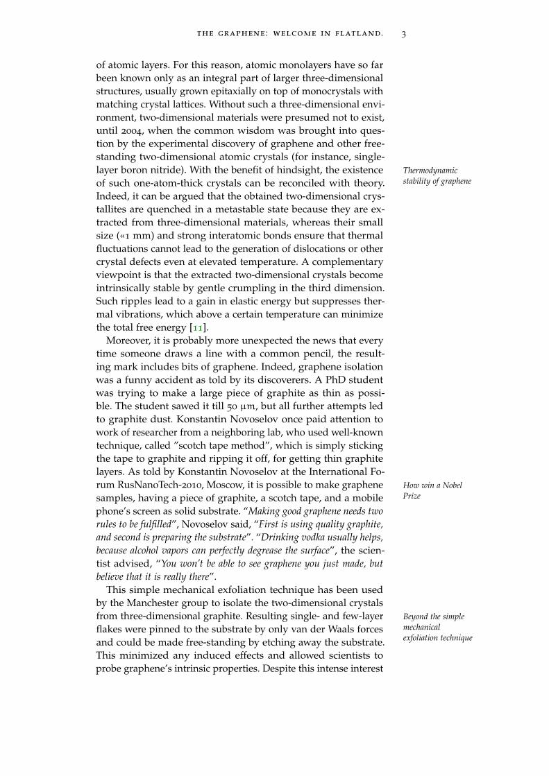
of atomic layers. For this reason, atomic monolayers have so farbeen known only as an integral part of larger three-dimensionalstructures, usually grown epitaxially on top of monocrystals withmatching crystal lattices. Without such a three-dimensional envi-ronment, two-dimensional materials were presumed not to exist,until 2004, when the common wisdom was brought into ques-tion by the experimental discovery of graphene and other free-standing two-dimensional atomic crystals (for instance, single-layer boron nitride). With the benefit of hindsight, the existence Thermodynamic
stability of grapheneof such one-atom-thick crystals can be reconciled with theory.Indeed, it can be argued that the obtained two-dimensional crys-tallites are quenched in a metastable state because they are ex-tracted from three-dimensional materials, whereas their smallsize («1 mm) and strong interatomic bonds ensure that thermalfluctuations cannot lead to the generation of dislocations or othercrystal defects even at elevated temperature. A complementaryviewpoint is that the extracted two-dimensional crystals becomeintrinsically stable by gentle crumpling in the third dimension.Such ripples lead to a gain in elastic energy but suppresses ther-mal vibrations, which above a certain temperature can minimizethe total free energy [11].
Moreover, it is probably more unexpected the news that everytime someone draws a line with a common pencil, the result-ing mark includes bits of graphene. Indeed, graphene isolationwas a funny accident as told by its discoverers. A PhD studentwas trying to make a large piece of graphite as thin as possi-ble. The student sawed it till 50 µm, but all further attempts ledto graphite dust. Konstantin Novoselov once paid attention towork of researcher from a neighboring lab, who used well-knowntechnique, called ”scotch tape method”, which is simply stickingthe tape to graphite and ripping it off, for getting thin graphitelayers. As told by Konstantin Novoselov at the International Fo-rum RusNanoTech-2010, Moscow, it is possible to make graphene How win a Nobel
Prizesamples, having a piece of graphite, a scotch tape, and a mobilephone’s screen as solid substrate. “Making good graphene needs tworules to be fulfilled”, Novoselov said, “First is using quality graphite,and second is preparing the substrate”. “Drinking vodka usually helps,because alcohol vapors can perfectly degrease the surface”, the scien-tist advised, “You won’t be able to see graphene you just made, butbelieve that it is really there”.
This simple mechanical exfoliation technique has been usedby the Manchester group to isolate the two-dimensional crystalsfrom three-dimensional graphite. Resulting single- and few-layer Beyond the simple
mechanicalexfoliation technique
flakes were pinned to the substrate by only van der Waals forcesand could be made free-standing by etching away the substrate.This minimized any induced effects and allowed scientists toprobe graphene’s intrinsic properties. Despite this intense interest

4 the graphene : welcome in flatland.
and continuing experimental success by physicists, widespreadimplementation of graphene has yet to occur. This is primarilydue to the difficulty of reliably producing high quality samples,especially in any scalable fashion. The challenge is double be-cause performance depends on both the number of layers presentand the overall quality of the crystal lattice. So far, the originalapproach of mechanical exfoliation has produced the highestquality samples, but the method is neither high throughput norhigh-yield. In order to exfoliate a single sheet, van der Waalsattraction between exactly the first and second layers must beovercome without disturbing any subsequent sheets. Therefore, anumber of alternative approaches to obtaining single layers havebeen explored, a few of which have led to promising proof-of-concept devices. Alternatives to mechanical exfoliation includeprimarily three general approaches: chemical efforts to exfoliateand stabilize individual sheets in solution, bottom-up methodsto grow graphene directly from organic precursors, and attemptsto catalyze growth in situ on a substrate.Mechanical
properties ofgraphene
Graphene have mainly attracted interest for its unusual elec-tron transport properties, but recently some attention has beenpaid also to mechanical properties of planar graphene sheets. Inparticular, Lee et al. in 2008 [12] measured the mechanical prop-erties of a single graphene layer, demonstrating that graphene isthe hardest material known, since the effective three-dimensionalelastic modulus reaches a huge value of 1.0 TPa.
Moreover, the ultimate use of graphene sheets in integrateddevices will likely require understanding of the mechanical prop-erties that may affect the device performance and reliability aswell as the intriguing morphology [13].
One typically assumes that the in-plane elastic moduli of asingle-layer graphene are identical to those for the base plane ofhexagonal crystal graphite. However, significant discrepancieshave been reported between theoretical predictions for in-planeYoung’s modulus and Poisson’s ratio of graphene and those de-rived from graphite [14]. It has also been noted that bending of aAims and scope of
this thesis graphene sheet of a single atomic layer cannot be simply mod-eled using continuum plate or shell theories [15]. Further studiesare thus necessary in order to develop a theoretically consistentunderstanding for the mechanical properties of graphene as wellas their relationships with corresponding properties of carbonnanotubes and nanoribbons. A theoretical approach is developedin the present Thesis in order to predict the in-plane elastic prop-erties of single- layer graphene based on an interplay betweenan atomistic Tight Binding simulations and a continuum elastictheory approach, providing a link between atomistic interactionsand macroscopic elastic properties of crystals.

the graphene: welcome in flatland. 5
While similar approaches have been developed previously [16],we herein emphasize the nonlinear elastic behavior under homo-geneous deformation. Third-order elastic constants are importantquantities characterizing nonlinear elastic properties of materials,and the interest in them dates back to the beginning of mod-ern solid state physics. Third- and higher-order elastic constantsare useful not only in describing mechanical phenomena whenlarge stresses and strains are involved e.g., in heterostructures ofoptoelectronic devices, but they can also serve as a basis for dis-cussion of other anharmonic properties. The applications includephenomena such as thermal expansion, temperature dependenceof elastic properties, phonon-phonon interactions, etc.
Thus, by combining continuum elasticity theory and tight-binding atomistic simulations, we work out the constitutive non- Non linear elastic
featureslinear stress-strain relation for graphene stretching elasticity andwe calculate all the corresponding nonlinear elastic moduli. Weshow in Chapter 5 some results which represent a robust pictureon the elastic behavior and provide the proper interpretation ofrecent experiments of Lee et al. [12]. In particular, we discussthe physical meaning of the effective nonlinear elastic modulusthere introduced and we predict its value in good agreementwith available data. Moreover, a hyperelastic softening behavioris observed and discussed, so determining the failure propertiesof graphene.
The defect-free and highly ordered, crystals of graphene are thethinnest objects possible and, simultaneously, 100 times strongerthan structural steel, making them the strongest material in na-ture. Such an unusual combination of extreme properties makesthis two-dimensional crystal attractive for a wide variety of appli-cations. However, in terms of electronic applications, sometimes Too conductive for
transistorsgraphene is a little too conductive. Graphene is so highly conduc-tive that it is hard to create graphene-based transistors suitable forapplications in integrated circuits. In order to reduce its conduc-tivity, many efforts have been dedicated to study the electronicproperties of graphene, for instance because creating a gap couldallow the use of graphene in field effect transistors. Many mecha-nisms have been proposed with that purpose: e.g. by quantumconfinement of electrons and holes in graphene nanoribbons [17]or quantum dots. [18] These patterning techniques are unfortu-nately affected by the edge roughness problem, [19] namely: theedges are extensively damaged and the resulting lattice disordercan even suppress the efficient charge transport. The sensitivityto the edge structure has been demonstrated through explicitcalculations of the electronic states in ribbons [20]. More recently,it has been shown experimentally that a band gap as large as0.45 eV can be opened if a graphene sheet is placed on an Ir(111)substrate and exposed to patterned hydrogen adsorption [21]. The graphane is the
fully hydrogenatedgraphene

6 the graphene : welcome in flatland.
Therefore, graphene-like carbon compound that acts as aninsulator could be produce. The simplest and most straight-forward candidate to do this is hydrogen. Exposing grapheneto an atomic hydrogen atmosphere produces a material calledgraphane, which is described as a two-dimensional crystal mappedonto the graphene scaffold, and covalently bonded hydrocarbonwith one to one C:H ratio. Graphane was theoretically predictedby Sofo et al. [22], further investigated by Boukhvalov et al. [23]and eventually was first synthesized by Elias et al. [24] in the2009.
An additional attractive feature of graphane is that by variouslydecorating the graphene atomic scaffold with hydrogen atoms(still preserving periodicity) it is in fact possible to generate aset of two dimensional materials with new physico-chemicalproperties. These systems are all characterized by a sp3 orbitalhybridization instead the sp2 hybridization of graphene. Becauseof in graphane the π−electrons are strongly bound to hydrogenatoms, the π−bands are absent altogether. Thus, a band gap iscreated, separating the highest occupied band from the lowestunoccupied band as in insulators. For instance, it has been calcu-lated [22, 23] that graphane has got an energy gap as large as ∼ 6
eV [25], while in case the hydrogenated sample is disordered, theresulting electronic and phonon properties are yet again different[24]. This simple change in hybridization may open up a wholenew world of graphene-based chemistry, leading to novel two-dimensional crystals with predefined properties, and an ability totune the electronic, optical,and other properties. HydrogenationElastic properties of
graphane likely affects the elastic properties as well. Topsakal et al. [26]indeed calculated that the in-plane stiffness and Poisson ratio ofgraphane are smaller than those of graphene. In addition, thevalue of the yield strain is predicted to vary upon temperatureand stoichiometry.
Among many possible conformers of hydrogenated graphene,as discuss in detail in Chapter 6, we focus our study to threestructures referred to as chair-, boat-, or washboard- graphane.By first principles calculations we determine their structural andphonon properties, as well as we establish their relative stability.Through continuum elasticity we measure by a computer exper-iment their linear and nonlinear elastic moduli, so that we cancompare them with the elastic behavior of graphene. We arguethat all graphane conformers respond to any arbitrarily-orientedextention with a much smaller lateral contraction than the onecalculated for graphene. Furthermore, we provide evidence thatboat-graphane has a small and negative Poisson ratio along thearmchair and zigzag principal directions of the carbon honey-comb lattice (i.e. axially auxetic elastic behavior). Moreover, we

the graphene: welcome in flatland. 7
show that chair-graphane admits both softening and hardeninghyperelasticity, depending on the direction of applied load.
Besides, an alternative technique to open a gap in the electronicstructure of graphene involves the application of mechanicalstress. For instance, an electronic band gap has been obtained bygrowing graphene sheets on an appropriately chosen substrate,inducing a reversible strain field controllable by temperature[27, 28, 29], and it has been experimentally shown that by usingflexible substrates a reversible and controlled strain up to ∼ 18%[29] can be generated with measurable variations in the optical,phonon and electronic properties of graphene [30]. Strain affects the
band structureThis interesting result suggests that gap opening could beengineered by strain, rather than by patterning. The idea hasbeen validated within linear elasticity theory and a tight-bindingapproach by Pereira and Castro Neto [31] showing that straincan generate a spectral gap. However this gap is critical, requir-ing threshold deformations in excess of 23%, approaching thegraphene failure strain (εf = 25%) [12], and only along preferreddirections with respect to the underlying lattice. The same au-thors propose an alternative origami technique [13] aimed atgenerating local strain profiles by means of appropriate geomet-rical patterns in the substrate, rather than by applying straindirectly to the graphene sheet. Shear deformation
could open a gapIn Chapter 7 we exploit this concept of strain-induced bandstructure engineering in graphene through the calculation of itselectronic properties under several deformations, by using linearelasticity theory and a semi-empirical tight-binding approach. Weshow that by combining shear deformations to uniaxial strains itis possible modulate the graphene energy gap value from zeroup to 0.9 eV. Interestingly enough, the use of a shear componentallows for a gap opening at moderate absolute deformation,safely smaller than the graphene failure strain, i.e. in a range ofreversible and more easily accessible deformations, ranging inbetween 12% and 17%.
Among the many studies of graphene, a substantial portionhave been devoted to the physics of graphene edges, whose struc-ture in narrow graphene ribbons is predicted to have a majorimpact on their electronic properties [32]. Recent theoretical stud-ies show that transport effects such as Coulomb blockade [18] ora mobility gap induced by edge disorder may affect the accuracyof bandgaps measured under transport conditions [33]. On theother hand, the free edges of graphene are amenable to edge Rippling, warping
and other bendingissues
instabilities, because of edges are under compressive stress ren-dering a mechanical edge rippling and warping instability [34, 35].Rippling of graphene has been also observed with mesoscopicamplitude and wavelength, both for suspended monolayers [36]and sheets deposited on substrates such as silicon dioxide [37].

8 the graphene : welcome in flatland.
Besides, any bending phenomena, i.e. out-of-plane displacements,are critical in attaining the structural stability and morphologyfor both suspended and supported graphene sheets, and directlyaffect their electronic properties [38]. Moreover, the bending prop-erties play a central role in the design of graphene-based devices,like e.g. mechanical resonators [39, 40]. The bending features offunctionalized graphene sheets have been probed by atomic forcemicroscopy, observing that the folding behavior is dominated bydefects and functional groups [41]. Finally, bending ultimatelygoverns the carbon nanotubes unzipping process, recently used toproduce narrow ribbons for nanoelectronics [42]. With the sametechnique, a new class of carbon-based nanostructures, whichcombine nanoribbons and nanotubes, has been introduced inorder to obtain magnetoresistive devices [43].
Within this scenario, in Chapter 8 we face the problem of thefundamental understanding of the bending properties of a two-dimensional carbon ribbon, and its interplay with the edge effects.The main goal is twofold: to draw a thorough theoretical pictureon bending of two-dimensional structures, fully exploiting theelasticity theory and providing an atomistic quantitative esti-mation of the corresponding bending rigidity; to prove that thebending process of a carbon nanoribbon is always associated withthe emergence of a (small) stretching, particularly close to theedges. These results have been obtained by combining continuumelasticity theory and tight-binding atomistic simulations too.

the graphene: welcome in flatland. 9
outline
The Thesis is organized as follows
• Part IA brief outline of the theoretical framework is shown asfollows
chapter 2 We report the main concepts and formalismof the tight-binding theory, in particular addressed tothe semi-empirical approach
chapter 3 The density functional theory and its pertur-bative version are briefly discussed
chapter 4 We show the continuum mechanics, in partic-ular the main concepts of the two-dimensional non-linear elasticity, and some reference to the atomistictreatment of the elastic continuum theory
• Part IIWe discuss in detail the some meaningful results regard theelastic behavior of graphene
chapter 5 We deal with the constitutive nonlinear stress-strain relation for graphene stretching elasticity, andwith all the corresponding nonlinear elastic moduli
chapter 6 We discuss about the linear and nonlinearelastic behavior of the hydrogenated conformers ofgraphene, namely graphane.
chapter 7 We exploit the concept of strain-induced bandgap engineering in graphene
chapter 8 Some fundamental concepts about the bend-ing properties of a two-dimensional ribbons of graphenehave been discussed


Part I
T H E O R E T I C A L B A C K G R O U N D


2T H E T I G H T- B I N D I N G S E M I - E M P I R I C A LS C H E M E
“Everything should be made as simple as possible, but no simpler. ”Albert Einstein, ’Einstein’s razor’ (1934).
Contents2.1 The Tight-Binding method 132.2 The Tight-Binding representation of carbon-
base systems 21
In Chapter 3, we’ll briefly review the Density Functional Theory.This ab-initio theory offers accuracy, transferability, and reliability.These are undoubtedly three key features to achieve predictiveinvestigation of materials properties, but it is just as certain thatthe corresponding computational workload can became quiteheavy and sometimes overwhelming.
The Tight Binding (TB) method is an intermediate solutionbetween a cheaper, from the computational point of view, totallyempirical potential model and a much more expensive ab-initiocalculation. Tight binding joins the advantage of the accuracyneeded to describe complex systems and of a reduced computa-tional workload.
2.1 the tight-binding method
TB is based on the basic formalism of linear combination ofatomic orbitals (LCAO) and Bloch sums. The Hamiltonian for asolid systam is given by
H = Tn + Te + Uen + Uee + Unn. (2.1)
Here,
Tn = −∑il
h2
2Mi∇2(Ril), kinetic energy operators for each ion
Te = −∑i
h2
2me∇2(ri), kinetic energy operators for each electron
Uen = −∑i,l,j
Zie2∣∣Ril − rj∣∣ , electron-nucleus potential energy
13

14 the tight-binding semi-empirical scheme
Uee =∑i,j>i
e2∣∣ri − rj∣∣ , electron-electron potential energy
Unn =∑
l,l ′,j ′>j
ZjZj ′e2∣∣Rjl − Rj ′l ′∣∣ , nucleus-nucleus potential energy
(2.2)
where the i, j indices count the particles inside the unit cell, the lindex runs over the Bravais lattice sites, and the atomic positionsare Rjl = dj + Rl, with the generic traslational lattice vector Rland dj labels the basis vector for the nuclei in the unit cell. TheCoulomb potential, depending on difference vectors, is invariantas well. Under the assumption of the frozen-core picture forthe electronic system and the Born-Oppenheimer or adiabaticapproximation, the corresponding single-electron Hamiltonian is
hel = Te + Uen + Uee + Unn. (2.3)
describing the energy of the valence electrons in the electrostaticfield of the ions, which are assumed as the nucleus and core-electrons together, where the nuclei are assumed to be stationarywith respect to an inertial frame.The adiabatic
theorem: “Aphysical systemremains in itsinstantaneouseigenstate if a givenperturbation isacting on it slowlyenough and if thereis a gap between theeigenvalue and therest of theHamiltonian’sspectrum."
Assuming the approximation of non-interacting (Hartree-like)electrons and the mean-field approximation, the ith-electron hasbeen described as particle moving in the ground-state of a effec-tive periodic potential Uave due to the other valence electronsand to the ions
h(ri) = − h2
2me∇2(ri) + Uave, (2.4)
invariant by lattice translation h(ri) = h(ri + Rl).The wave functions ψnk(r), provided by the Schrödinger equa-
tion h(r)ψnk(r) = εn(k)ψnk(r), must satisfy the Bloch condictionas well; thus:
ψnk(r + Rl) = ψnk(r) exp(ik · Rl) (2.5)
where k is the electron Bloch wavevector, n is the band index,εn(k) is the one-electron band energy and crystalline periodicsymmetry is assumed. By means of a linear combination of atomicorbitals (LCAO), the electronic wave function ψnk(r) can be ex-panded as Bloch sumBloch sum

2.1 the tight-binding method 15
ψnk(r) =∑αj
Bnαjφαjk(r)
=∑αjl
exp(ik · Rl)Bnαjφα(r − Rl − dj)
=∑αjl
Bnα(jl)(k)φαjl(r)
(2.6)
Here, the label α indicates the full set of atomic quantum numbersdefining the orbital, and we assume that the wave function arenormalized in the volume of crystal. The Bloch sum is defined as
φαjk(r) =∑l
exp(ik · Rl)φα(r − Rl − dj) (2.7)
Despite the simplicity of this formalism, referred to as tight-binding method, it is very hard to carry out, mainly due to thedifficulty in the computation of the overlap integrals betweenatomic functions centred on different lattice points. In fact, be-cause of the basis orbitals φαjl(r) located at different atoms aregenerally not orthogonal, their calculation is numerically incon-venient, and the computational workload increase as well. These Löwdin theorem:
”The problem ofsolving the secularequations includingthe overlap integralsS can be reduced tothe same form as ithas in simplifiedtheory, S neglected,if the Hamiltonian his replaced by thehL”
overlap integrals, defined by
Sα ′(j ′l ′),α(jl) =
∫drφα ′j ′l ′(r)∗φαjl(r) − δαα ′δ(jl)(j ′l ′),
with Sα(jl),α(jl) = 0
(2.8)
are often small compared to unity, but, even if they have almostbeen neglected, overlap effects are often of essential importancefor crystal properties. By joining the normalization condiction,B†n(k)(1 + S)Bn(k) = 1, with the orthogonality theorem, conse-quence of the hermitian character of h and S, the Schrödingerequation can be written in the matrix formalism as
hBn(k) = εn(k)(1 + S)Bn(k) (2.9)
By introducing the substitution
Bn(k) = (1 + S)−1/2Cn(k) (2.10)
where, (1 + S)−1/2 = 1 − 12S + 3
8S2 − 516S3 + . . .
the Eq. (2.9) becomes hLCnk(r) = εn(k)Cnk(r). Here, the hL =
(1 + S)−1/2h(1 + S)−1/2 is the Löwdin transformation [44] thatleads to a new orthogonal set of atomic orbitals ψα ′j ′l ′(r)
ψα ′j ′l ′(r) =∑αjl
(1 + S)−1/2α ′(j ′l ′),α(jl)φα(r − Rl − dj) (2.11)
16 the tight-binding semi-empirical scheme
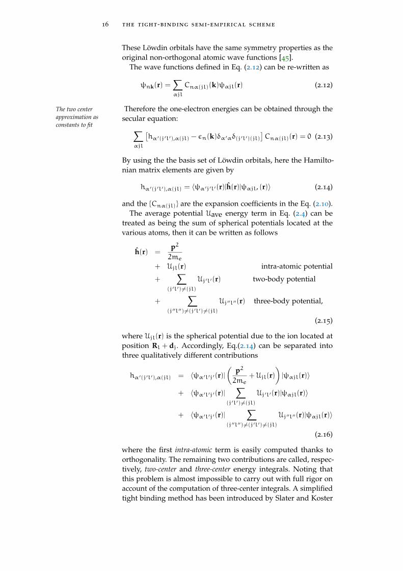
These Löwdin orbitals have the same symmetry properties as theoriginal non-orthogonal atomic wave functions [45].
The wave functions defined in Eq. (2.12) can be re-written as
ψnk(r) =∑αjl
Cnα(jl)(k)ψαjl(r) (2.12)
Therefore the one-electron energies can be obtained through theThe two centerapproximation asconstants to fit
secular equation:∑αjl
[hα ′(j ′l ′),α(jl) − εn(k)δα ′αδ(j ′l ′)(jl)
]Cnα(jl)(r) = 0 (2.13)
By using the the basis set of Löwdin orbitals, here the Hamilto-nian matrix elements are given by
hα ′(j ′l ′),α(jl) = 〈ψα ′j ′l ′(r)|h(r)|ψαjl, (r)〉 (2.14)
and the Cnα(jl) are the expansion coefficients in the Eq. (2.10).The average potential Uave energy term in Eq. (2.4) can be
treated as being the sum of spherical potentials located at thevarious atoms, then it can be written as follows
h(r) =p2
2me+ Ujl(r) intra-atomic potential
+∑
(j ′l ′) 6=(jl)
Uj ′l ′(r) two-body potential
+∑
(j ′′l ′′) 6=(j ′l ′) 6=(jl)
Uj ′′l ′′(r) three-body potential,
(2.15)
where Ujl(r) is the spherical potential due to the ion located atposition Rl + dj. Accordingly, Eq.(2.14) can be separated intothree qualitatively different contributions
hα ′(j ′l ′),α(jl) = 〈ψα ′l ′j ′(r)|(
p2
2me+ Ujl(r)
)|ψαjl(r)〉
+ 〈ψα ′l ′j ′(r)|∑
(j ′l ′) 6=(jl)
Uj ′l ′(r)|ψαjl(r)〉
+ 〈ψα ′l ′j ′(r)|∑
(j ′′l ′′) 6=(j ′l ′) 6=(jl)
Uj ′′l ′′(r)|ψαjl(r)〉
(2.16)
where the first intra-atomic term is easily computed thanks toorthogonality. The remaining two contributions are called, respec-tively, two-center and three-center energy integrals. Noting thatthis problem is almost impossible to carry out with full rigor onaccount of the computation of three-center integrals. A simplifiedtight binding method has been introduced by Slater and Koster

2.1 the tight-binding method 17
[46]. Basically, they suggest to cut the expansion of spherical po-tential in Eq. (2.15) up to the second term, and instead the explicitcomputation of the first and second integrals in Eq. (2.16), theyconsider the two-center hopping integrals as disposable constantsfitted from available experimental measures or from results ofmore accurate techniques, which are available only at a restrictedset of symmetric points of Brillouin zone.
The first approximation is the so-called two center approximationfor energy integrals.
These two-center hopping integrals can be expressed as prod-ucts of a radial wave function and a spherical harmonic Ylm(θ, ϑ)with the atom chosen as the origin. We will denote the vectorgoing from the first atom A, at Rjl, to the second atom B, at Rj ′l ′ ,as t = (Rjl − Rj ′l ′). For both orbitals ψαjl and ψα ′j ′l ′ , we willchoose the coordinate axes such that the z−axes are parallel tot and the azimuthal angles ϑ are the same. In these coordinatesystems the spherical harmonic wave functions of the two atomsA and B are Ylm(θ, ϑ) and Yl ′m ′(θ ′, ϑ), respectively. The Hamilto-nian h has cylindrical symmetry with respect to t and thereforecannot depend on ϑ. Thus the matrix element hα ′(j ′l ′),α(jl), isproportional to the integral of the azimuthal wave functionsexp(i(m ′ −m)). This integral vanishes except when m = m ′.symmetry. The concept of bonding and antibonding orbitals formolecules can be easily extended to crystals if one assumes thatthe orbitals of each atom in the crystal overlap with those of itsnearest neighbors only. This is a reasonable approximation formost solids. The interaction between two atomic orbitals pro-duces one symmetric orbital, with respect to the interchange ofthe two atoms, which is known as the bonding orbital, and oneantisymmetric orbital, which is known as the antibonding orbital.The results of orbital overlap in a solid is that the bonding and an-tibonding orbitals are broadened into bands. Those occupied byelectrons form valence bands while the empty ones form conduc-tion bands. The hopping integrals are usually labeled σ, π, and δfor (l = 2 wave functions), depending on whether m =0, 1, or 2
(in analogy with the s, p, and d atomic wave functions). In thecase of p orbitals there are two ways for them to overlap. Whenthey overlap along the direction of the p orbitals, they are said toform σ bonds. When they overlap in a direction perpendicularto the p orbitals they are said to form π bonds. These hoppingintegrals have a simple physical interpretation as representinginteractions between electrons on adjacent atoms. The fitting pro- Close neighbor
interactionapproximation
cedure is carried out on the basis of some approximations. Firstof all, only interactions into close neighbor shell are taken intoaccount. Therefore only atoms within a certain cut-off distanceinteract with each other. This approximation is validated by thelocalized character of the atomic orbitals. Second approximation Minimal basis set

18 the tight-binding semi-empirical scheme
Two-center Integrals
〈ψs,i|h(t)|ψs,i〉 = Es〈ψp,i|h(t)|ψp,i〉 = Ep〈ψs,i|h(t)|ψs,j〉 = Vssσ〈ψs,i|h(t)|ψpx,j〉 = l(Vspσ)
〈ψpx,i|h(t)|ψpx,j〉 = l2(Vppσ) + (1− l2)(Vppπ)
〈ψpx,i|h(t)|ψpy,j〉 = lm(Vppσ) − lm(Vppπ)
〈ψpx,i|h(t)|ψpz,j〉 = ln(Vppσ) − ln(Vppπ)
Table 2.1: Two-center hopping integrals up to the p-orbital [46]. Herethe vector t = (l, m, n)t is written through its director cosines.
is the choice of a minimal basis set for the LCAO expansion,including only those Löwdin atomic orbitals whose energy isclose to the energy of the electronic states we are interested in.This choice minimizes the size of the TB matrix to be diagonal-ized and, therefore, affects directly the computational workloadassociated to the TB method.
Rewriting the Löwdin wave functions ψαjl(r) of the Eq. (2.12)in form of Bloch functions
ψαjk(r) =∑l
exp(ik · Rl)ψαjl(r), (2.17)
the matrix elements defined in the Eq. (2.14) is now in the form
hα ′j ′,αj(k) = 〈ψα ′j ′k(r)|h(r)|ψαjk(r)〉=∑ll ′
exp(ik · (Rl − Rl ′))〈ψα ′j ′l ′(r)|h(r)|ψαjl(r)〉
(2.18)
where the matrix elements are basically the same hopping inte-grals defined in Eq. (2.14), which can also be expressed in termsof the overlap parameters shown in Table 2.1, and the phasefactors are the geometrical factors containing the k−dependence.Instead of summing over all the unit cells in the crystal, wesum over the nearest neighbors only. If needed, one can easilyinclude second neighbor or even further interactions, applyingsymmetry arguments allows the number of nonzero and linearlyindependent matrix elements to be greatly reduced.Tight Binding
Molecular dynamics(TBMD)
Starting from the previously described TB semi-empirical, two-center, short-ranged and orthogonal scheme, we now introducethe tight-binding molecular dynamics, (TBMD), namely the ap-plication of the above described tight binding TB model to thecalculation of the forces for a molecular dynamics MD scheme.

2.1 the tight-binding method 19
The tight-binding molecular dynamics TBMD ionic trajectoriesare generated by the TBMD Hamiltonian
H =∑j
P2j2Mj
+ Ebs +Urep(R1, R2, · · · , RN), (2.19)
where Pj and Mj represent atomic momenta and masses and εnis the one-electron energy and n the band index. The effective
repulsive potentialBecause of it is not possible to directly compute the Hartreeenergy Uel−el, within the semi-empirical TB scheme, since theelectron density ρ(r) is unknown, the total energy Etot of the(ions+electrons) system is re-written as
Etot = Uion−ion +Uel−ion +Uel−el = Ebs +Urep. (2.20)
Here, the Ebs = Uel−ion+ 2Uel−el is the so-called band-structureenergy, which is calculated by solving the Eq. (2.13)
Ebs = 2
occup∑n
εn, (2.21)
and it can be written as the Fermi-Dirac function
Ebs = 2∑k,n
fFD[εn(k), T ]εn(k),
at the temperature T = 0 evaluated at a single k point in theBrillouin zone, and the Urep = Uion−ion −Uel−el is an effectiverepulsive potential assumed to be short-ranged. Because of thehopping integrals have been fitted on the equilibrium propertiesthat is with the ions at the equilibrium lattice positions, the so-called Harrison rule [47] is introduced . If h(0)
α ′j ′,αj is the matrix The universal TightBinding method:Harrison ruleelements referred to the equilibrium interatomic distance R(0)
jj ′ ,the variation of the matrix element hα ′j ′,αj(Rjj ′) upon the actualdistance Rjj ′ is given by
hα ′j ′,αj(Rjj ′) = h(0)α ′j ′,αj
R(0)jj ′
Rjj ′
n (2.22)
Similarly, the repulsive energy Urep =∑j6=j ′ U(Rjj ′) obeys the
Harrison-like rule
U(Rjj ′) = U(0)
R(0)jj ′
Rjj ′
m (2.23)
where the two-body potential U(0) regards a couple of ions attheir equilibrium distance. The parameters n and m have to bedetermined by fitting. Calculation of the
forces

20 the tight-binding semi-empirical scheme
These assumptions implie that the force Fk acting on the kth
ion is given by
Fk = −∂H
∂Rk= −
∂
∂Rk[Ebs + Urep(R1, R2, · · · , RN)]
=[
FAk + FRk]
(2.24)
where the force Fk is separated in an attractive contribution FAkand in a repulsive term FRk . The FAk depends only on the actualtight binding model, while the FRk depends just on the empiricalrepulsive potential and they require dissimilar numeric treat-ment. The repulsive term FRk is straightforwardly calculated fromUrep(R1, R2, · · · , RN), which is known as an analytic function ofinteratomic distances.
The attractive term FAk is given by
FAk = −2∂
∂Rk
(occup)∑n
εn
= −2∂
∂Rk
(occup)∑n
∑α ′j ′
∑αj
C∗nα ′j ′Cnαjhα ′j ′,αj (2.25)
The derivative with respect to the ionic position has been devel-oped as follow
FAk = −2
(occup)∑n
∑α ′j ′
∑αj
∂C∗nα ′j ′
∂RkCnαjhα ′j ′,αj
+∑α ′j ′
∑αj
C∗nα ′j ′∂Cnαj
∂Rkhα ′j ′,αj+
+∑α ′j ′
∑αj
C∗nα ′j ′Cnαj∂hα ′j ′,αj
∂Rk
= −2
(occup)∑n
∑α ′j ′
∂C∗nα ′l ′
∂Rk
∑αj
Cnαjhα ′j ′,αj
+∑αj
∂Cnαj
∂Rk
∑α ′j ′
C∗nα ′j ′hα ′j ′,αj+
+∑α ′j ′
∑αj
C∗nα ′l ′Cnαj∂hα ′j ′,αj
∂Rk
(2.26)
and imposing the orthogonality condictions∑αj
hα ′j ′,αjCnαj = εnCnα ′j ′ and∑α ′j ′
C∗nα ′j ′hα ′j ′,αj = εnC∗nαj,
(2.27)
2.2 the tight-binding representation of carbon-base systems 21
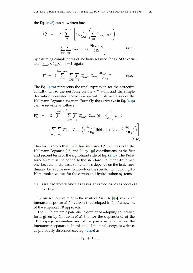
the Eq. (2.26) can be written into
FAk = −2
(occup)∑n
εn ∂
∂Rk
∑αj
C∗nαjCnαj
+∑α ′j ′
∑αj
C∗nα ′l ′Cnαj∂hα ′j ′,αj
∂Rk
(2.28)
by assuming completeness of the basis set used for LCAO expan-sion,
∑αjC
∗nαjCnαj = 1, again
FAk = −2
(occup)∑n
∑α ′j ′
∑αj
C∗nα ′j ′Cnαj∂hα ′j ′,αj
∂Rk(2.29)
The Eq. (2.29) represents the final expression for the attractivecontribution to the net force on the kth atom and the simplederivation presented above is a special implementation of theHellmann-Feynman theorem. Formally the derivative in Eq. (2.29)can be re-write as follows
FAk = −2
(occup)∑n
∑α ′j ′
∑αj
C∗nα ′l ′Cnαj〈ψα ′j ′ |∂h∂Rk
|ψαj〉
+∑α ′j ′
∑αj
C∗nα ′l ′Cnαj
(〈∂ψα ′j ′∂Rk
|h|ψαj〉+ 〈ψα ′j ′ |h|∂ψαj
∂Rk〉)
(2.30)
This form shows that the attractive force FAk includes both theHellmann-Feynman [48] and Pulay [49] contributions, as the firstand second term of the right-hand side of Eq. (2.30). The Pulayforce term must be added to the standard Hellmann-Feynmanone, because of the basis set functions depends on the ionic coor-dinates. Let’s come now to introduce the specific tight binding TBHamiltonian we use for the carbon and hydro-carbon systems.
2.2 the tight-binding representation of carbon-base
systems
In this section we refer to the work of Xu et al. [50], where aninteratomic potential for carbon is developed in the frameworkof the empirical TB approach.
The TB interatomic potential is developed adopting the scalingform given by Goodwin et al. [51] for the dependence of theTB hopping parameters and of the pairwise potential on theinteratomic separation. In this model the total energy is written,as previously discussed (see Eq. (2.20)) as
Etot = Ebs +Urep,
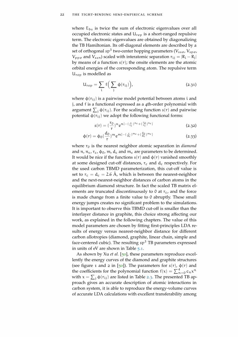
22 the tight-binding semi-empirical scheme
where Ebs is twice the sum of electronic eigenvalues over alloccupied electronic states and Urep is a short-ranged repulsiveterm. The electronic eigenvalues are obtained by diagonalizingthe TB Hamiltonian. Its off-diagonal elements are described by aset of orthogonal sp3 two-center hopping parameters (Vssσ, Vspσ,Vppσ and Vssπ) scaled with interatomic separation rij = |Ri − Rj|
by means of a function s(r); the onsite elements are the atomicorbital energies of the corresponding atom. The repulsive termUrep is modelled as
Urep =∑i
f(∑j
φ(rij))
, (2.31)
where φ(rij) is a pairwise model potential between atoms i andj, and f is a functional expressed as a 4th-order polynomial withargument
∑jφ(rij). For the scaling function s(r) and pairwise
potential φ(rij) we adopt the following functional forms:
s(r) = (r0
r)nen[−( rrc )nc+(
r0rc
)nc ] (2.32)
φ(r) = φ0(d0
r)mem[−( r
dc)mc+(
d0dc
)mc ] (2.33)
where r0 is the nearest neighbor atomic separation in diamondand n, nc, rc, φ0, m, dc and mc are parameters to be determined.It would be nice if the functions s(r) and φ(r) vanished smoothlyat some designed cut-off distances, rc and dc respectively. Forthe used carbon TBMD parameterization, this cut-off value isset to rc = dc = 2.6 Å, which is between the nearest-neighborand the next-nearest-neighbor distances of carbon atoms in theequilibrium diamond structure. In fact the scaled TB matrix el-ements are truncated discontinuously to 0 at rc, and the forceis made change from a finite value to 0 abruptly. These smallenergy jumps creates no significant problem to the simulations.It is important to observe this TBMD cut-off is smaller than theinterlayer distance in graphite, this choice strong affecting ourwork, as explained in the following chapters. The value of thismodel parameters are chosen by fitting first-principles LDA re-sults of energy versus nearest-neighbor distance for differentcarbon allotropies (diamond, graphite, linear chain, simple andface-centered cubic). The resulting sp3 TB parameters expressedin units of eV are shown in Table 5.1.
As shown by Xu et al. [50], these parameters reproduce excel-lently the energy curves of the diamond and graphite structures(see figure 1 and 2 in [50]). The parameters for s(r), φ(r) andthe coefficients for the polynomial function f(x) =
∑4n=0 cnx
n
with x =∑jφ(rij) are listed in Table 2.3. The presented TB ap-
proach gives an accurate description of atomic interactions incarbon system, it is able to reproduce the energy-volume curvesof accurate LDA calculations with excellent transferability among

2.2 the tight-binding representation of carbon-base systems 23
Two-center Integral Xu et al. [50]
Es −2.99
Ep +3.71
Vssσ −5.0
Vspσ +4.7
Vppσ +5.5
Vppπ −1.55
Table 2.2: The sp3 tight-binding parameters expressed in units of eV atthe reference interatomic separation r0 = 1.536 Å of diamondnearest neighbors.
graphite and diamond structures, giving a good description ofthe dynamical and elastic properties of such structures.

24 the tight-binding semi-empirical scheme
Parameter
n 2.0
nc 6.5
rc 2.18 Å
r0 1.536329 Å
r1 2.45 Å
φ0 8.18555(eV)
m 3.30304
mc 8.6655
dc 2.1052 Å
d0 1.64 Å
d1 2.57 Å
c0 −2.5909765118191
c1 0.5721151498619
c2 −1.7896349903396 · 10−3
c3 2.3539221516757 · 10−5
c4 −1.24251169551587 · 10−7
Table 2.3: The parameters defining s(r), φ(r), and the coefficients forthe polynomial function f(x) =
∑4n=0 cnx
n.

3D E N S I T Y F U N C T I O N A L T H E O RY
“ It doesn’t matter how beautiful your theory is, it doesn’t matterhow smart you are. If it doesn’t agree with experiment, it’s wrong.”
Richard P. Feynman (1918 - 1988)
Contents3.1 Density functional theory 25
3.1.1 Exchange and correlation energy ap-proximations 28
3.1.2 Plane waves and Pseudopotentials 31
3.2 Density Functional Pertubation Theory 33
3.1 density functional theory
Density functional theory (DFT) [52, 53] solves the electronicSchröedinger equation
Hψ = Eψ (3.1)
by reducing the quantum mechanical problem for a many-bodyinteracting system to an equivalent problem for non-interactingparticles. This is achieved by using as fundamental variable theelectronic density instead of the many-body electronic wavefunc-tion. Hohenberg and Kohn
lemmaThe theoretical base of DFT is the Hohenberg and Kohn lemma[54, 55] which considers an electronic system subject to an exter-nal potential. This theorem states that any ground state density n(r)of a many-electron system determines uniquely the external potentialVext(r), modulo an uninteresting additive constant. This lemma ismathematically rigorous. Since n(r) determines both the numberof electrons N and Vext(r) , it gives the full Hamiltonian for theelectronic system, and it determines implicitly all physical prop-erties derivable from H through the solutions of the Schrödingerequation (time-dependent or not).Therefore according to this lemma, considering a set of Hamilto-nians that have the same kinetic energy Te and electron-electronoperator Uee but different external potentials, their ground statewill have different densities, or rather two different potentialsacting on the same electronic system cannot give rise to the sameground-state electronic charge density. The external potential isthus a functional of the ground-state density. Therefore once theexternal potential Vext is fixed, the total energy will also be afunctional EV [n(r)] of the electronic charge density n(r).
25
26 density functional theory
Applying the standard Rayleigh-Ritz variational principle ofquantum mechanics, the electronic charge density of the groundstate, corresponding to the external potential Vext, minimizes thefunctional EV [n(r)], under the constraint that the integral of n(r)equals the total number of electrons N. The ground state energycoincides with the minimum of the constrained energy minimumEV [n(r)] = min
(ψ, Hψ
), where the trial function ψ corresponds
to a fixed trial density n
n(r) = N
∫d3r2
∫d3r3 · · ·
∫d3rNψ∗(r, r2, . . . ,~rN)ψ(r, r2, . . . , rN)
(3.2)
The expression for the ground state energy of the electronicsystem is then
EV = minnEV [n] = minn
(F[n] +
∫dr n(r)Vext(r)
)(3.3)
where F[n] is an universal functional of the density n(r) that doesnot require explicit knowledge of Vext(r). It is defined by thekinetic energy Te and by the electron-electron interaction Uee as
F[n(r)] = min(ψ∗, (Te +Uee)ψ
)(3.4)
The functional F[n] is not easy to calculate and represents mostof the total energy EV . Moreover there is no analytic expressionfor F[n]. Nevertheless, significant formal progress has been made,the problem of ground-state densities and energies has beenwell-formulated entirely in terms of the density n and of a well-defined, but explicitly unknown, functional of the density F[n].In the work of Kohn and Sham [55] an approximate expressionfor F[n] was proposed by considering an equivalent problemof non interacting electrons. The core of the Kohn and Shamassumption was that, for every system of interacting electrons,a corresponding system of non-interacting particles, describedby single particle orbitals , exists subject to an external potentialwith the same ground state density as the interacting system.Kohn-Sham
equations The Kohn-Sham functional can be written as [55]
F[n] = Te[n] +1
2
∫drdr ′
n(r)n(r ′)|r − r ′|
+ Exc[n] (3.5)
Here and in the follows, any physical constant are assumedequal to the unit. Te[n] is the kinetic energy of the ground-stateof non-interacting electrons with density n(r), and Exc[n] is theso-called exchange and correlation energy. The last two termsof Eq. (3.5) derive from the decomposition of the Uee operator,whose quantum mechanical effects are contained in Exc[n]. Aconsequence of the Hohenberg and Kohn lemma is that the Eq.

3.1 density functional theory 27
(3.3) is variational with respect to the charge density, under thecondition that the number of electrons is conserved. The solutionof the corresponding variational equation leads to the equation
δEV [n(r)] =
∫δn(r)
δTe[n]
δn(r)
∣∣∣∣n=n
+ VKS − λ
dr = 0 (3.6)
where
VKS = Vext +1
2
∫dr ′
n(r ′)|r − r ′|
+ vxc(r). (3.7)
and λ is a Lagrange multiplier constraining the density to benormalized to the total number of the electrons. In Eq. (3.6),the local exchange-correlation potential vxc(r) is the functionalderivative of exchange and correlation energy
vxc(r) =δExc[n]
δn(r)
∣∣∣∣n=n
(3.8)
depending functionally on the density n(r).Now the Hohenberg-Kohn variational problem for interact-
ing systems becomes formally identically to a correspondingequation for a system of non-interacting electrons subject to aneffective external potential Veff instead Vext, so the ground stateof this system is obtained by solving the single particle equations
(−1
2∇2 + Veff − εj
)ψj(r) = 0 (3.9)
where ψj(r) are orthonormalized single particle orbitals, and theminimizing density n(r) is given by
n(r) =∑j
|ψj(r)|2 (3.10)
It is possible to demonstrate that the two Eqs. (3.6) and (3.9)fulfill the same minimum conditions leading to the same densityif the Kohn-Sham potential VKS is equal to the Veff. Therefore, as-suming that the exchange-correlation energy functional is known,it is possible to treat the many-body problem as an independentparticle problem. The self-consistent Eqs. (3.9) are the so-calledthe Kohn-Sham (KS) equations. The ground-state energy is nowgiven by
E =∑j
εj+Exc[n]−
∫drn(r)vxc(r)−
1
2
∫drdr ′
n(r)n(r ′)|r − r ′|
(3.11)
reducible to the Hartree equations neglecting Exc and vxc. TheKS theory may be regarded as the formal improvement of theHartree theory, indeed with the exact Exc and vxc all many body
28 density functional theory
effects are in principle included. Unfortunately, the practicalusefulness of the ground-state DFT depends entirely on whetherapproximations for the functional Exc[n] could be found, thatat the same time has to be sufficiently simple and sufficientlyaccurate. The next section regards briefly the development andthe current status of such approximations.
3.1.1 Exchange and correlation energy approximations
Dealing with the exchange and correlation energy Exc[n] is themost difficult task in the solutions of the Kohn-Sham equations.The exchange energy derives from Pauli exclusion principle,which imposes the antisymmetry of the many-electron wavefunc-tion. This antisymmetrization produces a spatial separation be-tween electrons with the same spin and thus reduces the Coulombenergy of the electronic system. This energy reduction is calledthe exchange energy. The Hartree-Fock method exactly describesexchange energy; the difference between the energy of an elec-tronic system and the Hartree-Fock energy is called the correlationenergy. It is extremely difficult to calculate the correlation energyof a complex system, although some attempts have been madeby using quantum Monte Carlo simulations.The most important approximation for Exc[n] can be written in aquasi-local form
Exc[n(r)] =
∫drn(r)εxc(r; [n(r ′)]) (3.12)
where the exchange-correlation energy per particle εxc at thepoint r which depending functionally on the density charge n(r ′)at the point r ′ near r, where "near" means at a distance suchas the local Fermi wavelenght |r − r ′| ' λF(r) = (3π2n(r ′))−1/3.The most popular implementations of this quasi-local approachfor the exchange and correlation energy are the Local DensityApproximation (LDA) and the Generalized Gradient Approximation(GGA).Local Density
Approximation LDA was propoded in their original paper by Kohn and Sham[55] as the simplest method to describe the exchange-correlationenergy Exc[n]. They assume that the non-local exchange-correlationenergy εxc(r; [n(r ′)]) in Eq. (3.16) can be equal to the local exchange-correlation energy per particle εxc[n(r)] of a homogeneous elec-tron gas, which has the same density as the electron gas at pointr ∈ (r, –F(r)), if this volume is little enough that the charge den-sity could be assume constant therein. In this assumption, the Eq.(3.16) becomes
ELDAxc [n] =
∫drn(r)εhomoxc [n(r)] (3.13)
3.1 density functional theory 29
and the potential in Eq. (3.8)
vLDAxc [n(r)] =
(εhomoxc [n] +n
dεhomoxc [n]
dn
)n=n(r)
(3.14)
The LDA assumes that the exchange correlation energy func-tional is purely local, ignoring the corrections to the exchangecorrelation energy at a point r due to the nearby inhomogeneitiesin the electron density, but it is exact in the limit of high densityor of a slowly varying charge density. Moreover, the exchange-correlation energy Exc[n] can be separeted in two terms
ELDAxc [n(r)] = ELDAx [n(r)] + ELDAc [n(r)] (3.15)
The exchange term Ex[n] is simply the Fermi-Thomas-Dirac ex-change energy
ELDAx [n(r)] = −3
4
(3
π
)1/3 ∫n(r)4/3dr (3.16)
that comparing ith Eq. (3.13) leads to an elementary form of theexchange part, given by, in atomic units
εhomox [n(r)] ≈ −0.4582
rs(3.17)
where rs is the radius of a sphere containing an electron, namelyradius of Sietz, and given by (4π/3)rs
3 = n−1. The correlationpart was extimated by E.P. Wigner [56]
εhomoc [n(r)] ≈ −0.44
rs + 7.8(3.18)
and using Monte Carlo methods it was calculated with higherprecision for uniform electron gas by D.M. Ceperly and B.J. Alder[57, 58]
εhomoc [n(r)] = λ (1+β√
rs +βrs)−1 , rs > 1
εhomoc [n(r)] = (A ln rs +B+Crs ln rs +Drs) , rs < 1
(3.19)
which has been parametrized by J.P. Perdew and A. Zunger [59]. GeneralizedGradientApproximation
Another useful approximation is the so-called GeneralizedGradient Approximation GGA. The basic concept is the averagexc hole distribution around a given point r
nxc(r, r ′) = g(r, r ′) −n(r ′)∫nxc(r, r ′)dr ′ = −1 (3.20)
with the conditional density g(r, r ′) at r ′ due to an electron atr. It describes the hole dug into the average density n(r ′) by

30 density functional theory
the electron at r, and it reflects the screening of the the electronat r due to the Pauli effect and the electron-electron interation.Introducing a parameter λ, (0 6 λ 6 1), the λ−average xc holedensity nxc(r, r ′) is then defined as
nxc(r, r ′) =
∫nxc(r, r ′; λ)dλ (3.21)
the very physical formally exact espretion of the exchange-correlationenergy εxc(r; [n(r ′)]) in Eq. (3.16) is given by
εxc(r; [n(r ′)]) = −1
2R−1xc (r; [n(r ′)]) (3.22)
where R−1xc (r; [n(r ′)]) is
R−1xc (r; [n(r ′)]) =
∫−nxc(r, r ′)
|r − r ′|dr ′ (3.23)
Since R−1xc is a functional of n(r ′), we can formally use the expan-
sion of the electron density n(r ′) around the point r
n(r ′) = n(r)+ (r − r ′)[∇n(r ′)]r ′=r +1
2(r − r ′)2[∇2n(r ′)]r ′=r + . . .
(3.24)
and we obtain
R−1xc (r) = F0(n(r)) + F21(n(r))∇2n(r) + . . . (3.25)
This leads to the gradient expression for Exc
Exc = ELDAxc +
∫G2(n(r))(∇n(r))2dr + . . .
=
∫n(r)εLDAxc [n(r)]dr +
∫n(r)εGGAxc [n(r), |∇n(r)|]dr + . . .
(3.26)
where G2 is an universal functional of n(r). Generally the GGAmethod stops the expansion at the first derivative, and the exchange-correlation function is expressed as function of the two variablesn(r) e |∇n(r)|
EGGAxc [n] =
∫n(r)εGGAxc (n(r), ∇n(r))dr (3.27)
An important point regard the parametrization of the εGGAxc .Analytical form was proposed by Perdew-Wang [60, 61, 62], andBecke [63], namely (PW91), using the local spin density (LSD)approximation for the exchange-corelation energy, Eq. (3.27),which it can be separated in two terms
EPW91xc [n] = EPW91x [n] + EPW91c [n] (3.28)

3.1 density functional theory 31
The exchange term is given by, using atomic units
EPW91x [n] =
∫n(r)εPW91x (rs,σ)σ=0F
PW91X (s)dr
εGGAx (rs, 0) = −3kF
4π(3.29)
(3.30)
Here, εPW91x (rs,σ) is the exchange-correlation energy per particlefor a uniform electron gas, with rs is the local Seitz radius andσ = (nup −ndown)/n is the local spin polarization,
kF = (3π2n(r))1/3 (3.31)
is the local Fermi wave vector, and
s(r) =|∇n(r)|2kFn(r)
, (3.32)
is a scaled density gradient. The function FPW91X (s) is written as[60]
FPW91X (s(r)) =1+ s(r)A sinh−1(s(r)B) + (C−De−100s2(r))s2(r)
1+ s(r)A sinh−1(s(r)B) + s4(r)E,
(3.33)
The correlation part of Eq. (3.28) is
EPW91c [n] =
∫n(r)[εc(rs, ζ) +H(t, rs, ζ)]dr , (3.34)
where εc(rs, ζ) is the correlation energy per particle of an uniformelectron gas [60], and t is another scaled density gradient
t =|∇n(r)|2gksn(r)
, (3.35)
here, ks = (4kF/π)1/2 is the local screening wave vector, andg = [(1+ ζ)2/3 + (1− ζ)2/3]/2. Analytic representations both forεc(rs, ζ) and for the function H(t, rs, ζ) are available in Ref. [62].Popular GGA implementations include Perdew-Burke-Ernzerhof(PBE) [64], and Becke-Lee-Yang-Parr (BLYP) [63, 65].
3.1.2 Plane waves and Pseudopotentials
As shown previously, DFT reduces a many-body interactingparticle problem to an independent particle problem. Howeversolving single particle equations also presents technical difficul-ties. In particular, if a plane-waves basis set is chosen to expandthe wavefunctions, an extremely large number of plane waves isneeded for expanding the core electron wavefunctions (strongly

32 density functional theory
localized in the region near the nucleus) and for reproducing therapid oscillations of the valence electron wavefunctions in thecore region. For this reason a calculation including all the elec-trons using a plane wave basis set requires a huge computationalcost.The pseudopotential approximation is an effective method toeliminate the core electrons in the calculations of the electronicstructure. It is known that the core electrons are chemical in-ert and that most molecular properties can be calculated withacceptable precision assuming that the core electrons do not mod-ify their state in different chemical configurations (free atom,molecule, solid): this is known as the frozen core approximation.Therefore in the solution of the Schröedinger equation it is pos-sible to distinguish: i) The core region mainly constituted ofelectrons deeply bonded and almost non interacting with thoseof other atoms; ii) the remaining volume, where there are valenceelectrons that are involved in bonds with the neighbor atoms.Although the potential in the core region is strongly attractive,the orthogonality condition between the valence and core elec-tron wavefunctions results in oscillations of the valence electronwavefunctions, which correspond to a kinetic energy that almostbalances the attractive potential. In the pseudopotential methodthis kinetic effect is simulated by a repulsive potential that bal-ances the strong attractive potential in the core region. This resultsin the separation of the electron-electron interaction term Ueeinto a term corresponding to the valence electrons and a termcorresponding to the core electrons that screen the attraction ofthe nuclear potential onto the valence electrons. Therefore thepseudopotential (PP) is
UPP = UeN +Usc +Uval (3.36)
where UeN represents the electron-nuclei interaction, Usc repre-sents the screening due to the core electrons and Uval representthe interaction between valence electrons. The pseudopotential isidentical to the real potential at distance greater than the core ra-dius rc, while for r 6 rc, it is built so as to simulate the combinedaction of the ionic and screening terms on the valence electrons.The eigenfunctions of the corresponding Schroedinger equationare therefore pseudo-eigenfunctions, which coincide with the realeigenfunctions only in the region for r > rc . In the core region,the pseudo-eigenfunctions are continuous and node less. Theyallow a rapid convergence in the plane wave expansion.The main advantages achieved by using the pseudopotentialmethod are: the number of the electrons to deal with is reducedfor a given system; the computational cost is lower due to thesmaller number of plane waves necessary for the calculations.Technical aspects of the implementation of the KS equations in
3.2 density functional pertubation theory 33
plane wave pseudopotential (PW-PP) framework have been foundin Ref. [66].
3.2 density functional pertubation theory : from elec-tronic structure to lattice dynamics
Lattice dynamical properties of a system are determined by thesolution of the Schródinger equation for the ionic part, by usingthe adiabatic approximation of Born-Oppenheimer(
−∑ h2
2Mi
∂2
∂R2i+ E(R)
)φ(R) = Eφ(R) (3.37)
where Ri and Mi are the coordinate of the ith−ion, and its mass,respectively, and E(R) is the ground-staet energy of the elec-tronic system moving in the field of fixed ions. The equilibriumcondiction is achieved when the forces acting in the electronicground-state on each ion vanish
Fi = −∂E(R)
∂Ri=
⟨ψ(R)
∣∣∣∣∂Hel∂Ri
∣∣∣∣ψ(R)
⟩= 0 (3.38)
Here, the Hellmann-Feynman theorem has been appliyed in theframework of the Born-Oppenheimer approximation, the ψ(R) isthe electronic ground-state wave function, and the ion coordinatesact as parameters in the electronic Hamiltonian Hel.
The vibrational frequenciesω are determinated by the eigenval-ues of the Hessian of E(R), namely the matrix of the interatomicforce constants interatomic force
constants
det
∣∣∣∣ (MiMj
)−1/2 ∂2E(R)
∂Ri∂Rj−ω2
∣∣∣∣ = 0 (3.39)
The calculation of the equilibrium configuration and of thevibrational properties of the system need to compute the first andthe second derivative [67], respectively, of the Born-Oppenheimerenergy surface E(R). linear response
∂nR(r)∂Rj∂E(R)
∂Ri=
∫∂VR(r)∂Ri
nR(r)dr , (3.40)
∂2E(R)
∂Ri∂Rj=
∫∂2VR(r)∂Ri∂Rj
nR(r)dr +
∫∂VR(r)∂Ri
∂nR(r)∂Rj
dr (3.41)
where the derivative of the ion-ion electrostatic interation is as-sumed constant. The calculation of the matrix interatomic forceconstants, Eq. (3.39), the calculation of the ground-state elec-tronic charge density nR(r) and its linear response to a distortionof the ion configuration, ∂nR(r)
∂Rj. The linear response can be com-
puted within the perturbative version of the density funtional

34 density functional theory
theory (DFT), usually referred as density funtional perturbation the-ory (DFPT) [68, 69]. Through the liniarization of the Kohn-ShamDensity Funtional
Perturbation Theory(DFPT)
Eqs. (3.9), (3.10), and (3.7) with respect to wave function, density,and potential variations. Linearization of the charge density n(r)leads to
∇Rn(r) = 2Re∑n
ψ∗n(r)∇Rψn(r) (3.42)
By using the standard first-order perturbation theory, the vari-ation of the Kohn-Sham unperturbed orbitals ψn(r) is given by
(−1
2∇2 + VKS − εn
)∇Rψn(r) = − (∇RVKS −∇Rεn)ψn(r)
(3.43)
Here,
∇RVKS(r) = ∇RVext(r)+
1
2
∫dr ′∇Rn(r ′)|r − r ′|
+d vxc(n)
dn
∣∣∣∣n=n(r)
∇Rn(r)
(3.44)
is the first-order correction to the Kohn-Sham potential, and
∇Rεn = 〈ψn|∇RVKS(r)|ψn〉 (3.45)
is the first-order variation of the Kohn-Sham eigenvalues. TheThe (2n+ 1)
theorem knowledge of the first-order derivative of the wave functions is,hence, enough to compute the second-order derivative of theenergy. This is a special case of the (2n+ 1) theorem [70], whichstates that the knowledge of the nth-order derivative of the wavefunctions allows the calculation of derivative of the energy upto the (2n + 1)th-order. The set of self-consinstent Eqs. (3.42),(3.44), and (3.45) for the perturbated system are analogous to theKohn-Sham equation for the unperturbed case, Eqs. (3.9), (3.10),and (3.7).
4C O N T I N U U M M E C H A N I C S A N D N O N L I N E A RE L A S T I C I T Y
“ I try not to break the rules but merely to test their elasticity.”Bill Veeck (American Baseball Player, 1914-1986)
Contents4.1 Lagrangian versus Eulerian formalism 354.2 Finite Strain Theory 384.3 Stress Theory 414.4 The Continuity equation 464.5 Balance equations 46
4.5.1 The Euler description 46
4.5.2 The Lagrange description 48
4.6 Nonlinear constitutive equations 504.7 The small-strain approximation 534.8 The Stiffness tensor and the Elastic moduli
in two-dimensional systems. 604.9 The virial stress tensor 66
4.9.1 Physical meaning of the virial stress 70
4.9.2 The atomistic nonlinear Cauchy stress 71
4.9.3 Atomic stress for two-body interac-tions 72
In this Chapter we introduce the basic formalism of the con-tinuum theory of elasticity, summarizing its foundation and keyconcepts. We also discuss same general features regarding theelastic theory in two dimensional systems.
4.1 lagrangian versus eulerian formalism
The motion of a body is typically referred to a reference configu-ration Ω0 ⊂ R3, which is often chosen to be the undeformed con-figuration. After the deformation the body occupies the currentconfiguration Ωt ⊂ R3. Thus, the current coordinates (x ∈ Ωt)are expressed in terms of the reference coordinates (X ∈ Ω0):
X 7→ x = Ft (X) (4.1)
where Ft is the transformation function at any time t (see Fig.4.1). More explicitly, it means that
x1 = x1 (X1,X2,X3, t)
x2 = x2 (X1,X2,X3, t) (4.2)
x3 = x3 (X1,X2,X3, t)
35

36 continuum mechanics and nonlinear elasticity
P
x1
x2
x3
X
p
x1
x2
x3
x = Ft(X)
Deformation, Ft
reference configuration current configuration
Figure 4.1: Reference configuration and current configuration after adeformation.
We call the set (X and t) Lagrangian coordinates, named afterJoseph Louis Lagrange [1736-1813], or material coordinates, orreference coordinates. The application of these coordinates iscalled Lagrangian description or reference description. We canobtain also the inverse function of Eq. (4.1) in the formLagrangian reference
coordinatesx 7→ X = F−1
t (x) (4.3)
or, in components
X1 = X1 (x1, x2, x3, t)
X2 = X2 (x1, x2, x3, t) (4.4)
X3 = X3 (x1, x2, x3, t)
The set x, t is called Eulerian coordinates, named after Leon-Eulerian spacecoordinate hard Euler [1707-1783], or space coordinates, and their application
is said Eulerian description or spatial description. The Lagrangiancoordinates were introduced by Euler in 1762, while Jean le RondD’Alembert [1717-1783] was the first to use the Eulerian coor-dinates in 1752. In general Continuum Mechanics Lagrangiancoordinates and the reference description are the most common.The same holds true in solid Mechanics. However, in Fluid Me-chanics, due to large displacements and complex deformations,it is usually necessary and most practical to use Eulerian coor-dinates and spatial description. One of the key quantities inDeformation
gradient deformation analysis is the deformation gradient of Ωt relativeto the reference configuration Ω0, denoted F, which gives therelationship of a material line dX before deformation to the linedx (consisting of the same material as dX) after deformation. It isdefined as
x = Ft (X) : F (X, t) = ∇XFt (X)⇒ dx = F (X, t)dX
(4.5)

4.1 lagrangian versus eulerian formalism 37
Its components are given by
FiK =∂xi
∂XK, ∀(i,K) ∈ 1, 2, 32 (4.6)
As before, we can define a deformation gradient G of the inversefunction relating Ω0 to the current configuration Ωt
X = F−1t (x) : G (x, t) = ∇xF
−1t (x)⇒ dX = G (x, t)dx
(4.7)
In components, it assumes the form
GKi =∂XK
∂xi, ∀(i,K) ∈ 1, 2, 32 (4.8)
The tensors F and G are related by the relationships
G (Ft (X) , t) = F−1 (X, t) (4.9)
F(F−1t (x) , t
)= G−1 (x, t) (4.10)
Here, F is a Lagrangian tensor while G is an Eulerian tensor. Thevelocity and acceleration fields, related to the trajectory of the Velocity and
acceleration fieldsparticle starting at X (Lagrangian description) are given by
v (X, t) =∂x∂t
(X, t) (4.11)
a (X, t) =∂2x∂t2
(X, t) (4.12)
On the other hand, the velocity and acceleration fields in theEuler description are given by
v (x, t) =∂x∂t
(F−1t (x) , t
)(4.13)
a (x, t) =∂2x∂t2
(F−1t (x) , t
)(4.14)
Any time-dependent scalar, vector, or tensor field can be regardedas a function of (X, t) (Lagrangian or material variables) or (x, t)(Eulerian or spatial variables) whenever the motion x = Ft (X)
is given. For example, for a scalar field we can write φ (x, t) =
Φ (X, t) where
Φ (X, t) = φ (Ft (X) , t) (4.15)
The time derivative of the field Φ (X, t) can be calculated as
∂Φ
∂t=∂φ
∂t+∂φ
∂x·∂x∂t
=∂φ
∂t+∂φ
∂x· v (4.16)
Instead of using different symbols for the quantities (i.e. φ andΦ) in the Lagrangian and Eulerian descriptions, we can use thedot for the Lagrangian or material derivative (φ) and the partial

38 continuum mechanics and nonlinear elasticity
differentiation symbol (∂φ∂t ) for the Eulerian or spatial derivative.Therefore, Eq. (4.16) assumes the simpler form
φ =∂φ
∂t+∂φ
∂x· v (4.17)
The Eulerian tensor
L =∂v∂x
(4.18)
with components
Lij =∂vi
∂xj(4.19)
satisfies the important relation
˙F = LF (4.20)
It can be proved as follows
˙F =∂
∂t
∂
∂XFt (X) =
∂
∂X∂
∂tFt (X) =
∂v∂X
=∂v∂x∂x∂X
= LF
(4.21)
It is also important an inverse relation given by
˙F−1 = −GL (4.22)
Since ddt
(F−1F
)= 0 we have ˙F−1 = −F−1 ˙FF−1 (where ˙F−1 rep-
resents the Lagrangian time derivative of the inverse of F) and,therefore, we obtain the proof of Eq. (4.22)
˙F−1 = −F−1 ˙FF−1 = −F−1LFF−1 = −F−1L = −GL (4.23)
4.2 finite strain theory
The measure of the deformation between the reference and thecurrent configuration is an important topic in continuum mechan-ics and it can be performed in several ways. The starting quantityis the deformation gradient F(X) (in the Lagrangian formalism) orits inverse G(x) (in the Eulerian formalism). We consider two in-finitesimal vectors dX and dY in Ω0 and their deformed versionsdx and dy in Ωt (see Fig. 4.2 for the deformation of dX). Thechanges of lengths and angles are controlled by the scalar prod-uct of the vectors and, therefore, we define the right and the leftCauchy tensors C and B in order to obtain dx ·dy = dX · CdY ordX ·dY = dx · B−1dy (see Table 4.1). The variations of the scalarproduct (moving from the reference to the current configuration)are described by the Green-Lagrange strain tensor η and by theAlmansi-Eulero strain tensor e as summarized in Table 4.1.
Moreover, the gradients of the displacements field u(X) andu(x) are defined by JL = ∂u
∂X and JE = ∂u∂x in the Lagrangian
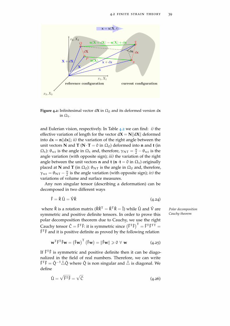
4.2 finite strain theory 39
P
Q
dX
q
p
dx
x1, X1
x2, X2
x3, X3
X
X + dX
x
x + dxu(X)
u(X + dX) = u(X) + du
du
x = x(X, t)
reference configuration current configuration
Figure 4.2: Infinitesimal vector dX in Ω0 and its deformed version dxin Ωt.
and Eulerian vision, respectively. In Table 4.2 we can find: i) theeffective variation of length for the vector dX = N‖dX‖ deformedinto dx = n‖dx‖; ii) the variation of the right angle between theunit vectors N and T (N · T = 0 in Ω0) deformed into n and t (inΩt): θnt is the angle in Ωt and, therefore, γNT = π
2 − θnt is theangle variation (with opposite sign); iii) the variation of the rightangle between the unit vectors n and t (n · t = 0 in Ωt) originallyplaced at N and T (in Ω0): θNT is the angle in Ω0 and, therefore,γnt = θNT − π
2 is the angle variation (with opposite sign); iv) thevariations of volume and surface measures.
Any non singular tensor (describing a deformation) can bedecomposed in two different ways
F = R U = VR (4.24)
where R is a rotation matrix (RRT = RT R = I) while U and V are Polar decompositionCauchy theoremsymmetric and positive definite tensors. In order to prove this
polar decomposition theorem due to Cauchy, we use the rightCauchy tensor C = FT F: it is symmetric since
(FT F
)T= FT FTT =
FT F and it is positive definite as proved by the following relation
wT FT Fw =(Fw)T (
Fw)
= ‖Fw‖ > 0 ∀ w (4.25)
If FT F is symmetric and positive definite then it can be diago-nalized in the field of real numbers. Therefore, we can writeFT F = Q−14Q where Q is non singular and 4 is diagonal. Wedefine
U =√FT F =
√C (4.26)

40 continuum mechanics and nonlinear elasticity
Table 4.1: Strains definitions and properties in Lagrangian and Eulerianformalisms.
Lagrangian vision Eulerian vision
Right Cauchy tensor Left Cauchy tensor
C = FT F B = FFT
C−1 = GGT B−1 = GT G
dx ·dy = dX · CdY dX ·dY = dx · B−1dy
Green-Lagrange tensor Almansi-Eulero tensor
η = 12
(C− I
)e = 1
2
(I− B−1
)dx ·dy − dX ·dY = 2dX · ηdY dx ·dy − dX ·dY = 2dx · edy
Lagrange displacement gradient Eulero displacement gradient
JL = ∂u∂X JE = ∂u
∂x
F = I+ JL F−1 = I− JE
C = I+ JL + JTL + JTL JL B−1 = I− JE − JTE + JTEJE
η = 12
(JL + JTL + JTL JL
)e = 1
2
(JE + JTE − JTEJE
)
The square root of the tensor can be defined (and calculated) asfollows
U =√FT F =
√Q−14Q = Q−1
√4Q (4.27)
in fact(Q−1
√4Q
)2= Q−1
√4QQ−1
√4Q
= Q−1√4√4Q = Q−14Q (4.28)
where√4 = diag(
√λi) if 4 = diag(λi) (the symbol diag explic-
itly indicates the entries of a diagonal matrix). Finally, we defineR = FU−1 and we verify its orthogonality
RT R =(U−1
)TFT FU−1 =
(U−1
)TU2U−1 = U−1UUU−1 = I
(4.29)
This concludes the proof of the first polar decomposition. Wehave to prove the unicity of the right decomposition F = R U. Wecan suppose the two different decompositions F = R U = R∗U∗
exist. It follows that FT F = U2 = U∗2 from which U = U∗ and,therefore, R = R∗. It proves the unicity of the right decomposition.Similarly we can obtain the left decomposition by defining V =

4.3 stress theory 41
Table 4.2: Variations measure in Lagrangian and Eulerian formalisms.
Lagrangian vision Eulerian vision
Lagrangian length variation Eulerian length variation
N = dX‖dX‖ n = dx
‖dx‖
εNN =‖dx‖−‖dX‖‖dX‖ =
√N · CN − 1εnn =
‖dx‖−‖dX‖‖dx‖ = 1−
√n · B−1n
εNN + 12ε2NN = N · ηN εnn − 1
2ε2nn = n · en
Lagrangian angle variation Eulerian angle variation
N · T = 0 n · t = 0
γNT = π2 − θnt γnt = θNT − π
2
sin(γNT ) = 2N · ηT√N · CN
√T · CT
sin(γnt) = 2n · et√n · B−1n
√t · B−1t
Lagrangian volume variation Eulerian volume variation
J = det(F) J−1 = det(G)
ΘV = dv−dVdV = J− 1 Θv = dv−dV
dv = 1− 1J
Lagrangian surface variation Eulerian surface variation
NdS = J−1FTnds nds = JF−TNdS
ΘN =‖nds‖−‖NdS‖‖NdS‖ Θn =
‖nds‖−‖NdS‖‖nds‖
ΘN = J√
N · C−1N − 1 Θn = 1− J−1√
n · Bn
√FFT =
√B: it is possible to prove that it is symmetric and
positive definite and we define R ′ = V−1F, which is orthogonal.To conclude we must verify that R ′ = R. Since R ′
(R ′)T
=
I we have F = VR ′ = R ′(R ′)TVR ′. The unicity of the right
decomposition (F = R U) allows us to affirm that R ′ = R and thatU = RT VR. This completes the proof of the polar decompositionCauchy theorem.
This decomposition implies that the deformation of a lineelement dX in the undeformed configuration onto dx in thedeformed configuration, i.e. dx = FdX may be obtained eitherby first stretching the element by U i.e. dx ′ = UdX, followed bya rotation R, i.e. dx = Rdx ′ or, equivalently, by applying a rigidrotation R first, i.e. dx ′′ = RdX followed later by a stretching V ,i.e. dx = Vdx ′′ (see Fig. 4.3).
4.3 stress theory
In continuum mechanics we must consider two systems offorces acting on a given region of a material body. They are The body forces
dependent on the external fields acting on the elastic body and

42 continuum mechanics and nonlinear elasticity
x1, X1
x2, X2
x3, X3
R V
R
F = RV = UR
U
Figure 4.3: Polar decomposition applied to a given deformation.
they are described by the vector field b(x) representing theirdensity on the volume in the current configuration. The physicalmeaning of such a density of forces can be summed up statingthat the total force dFv applied to a small volume dx centeredon the point x is given by dFv = b(x)dx. A typical example isgiven by the gravitational forces proportional to the mass of theregion under consideration. In this case we can write dFv = gdmwhere g is the gravitational acceleration and dm is the mass ofthe volume dx. If we define ρ = dm
dx as the density of the body,we simply obtain b(x) = ρg. In continuum mechanics we areThe surface forces
additionally concerned with the interaction between neighboringportions of the interiors of deformable bodies. In reality suchan interaction consists of complex interatomic forces, but wemake the simplifying assumption that the effect of all such forcesacross any given surface may be adequately represented by asingle vector field defined over the surface. It is important toobserve that the nature of the forces exerted between two bodiesin contact is identical to the nature of the actions applied betweentwo portions of the same body, separated by an ideal surface.
In order to begin the mathematical descriptions of the forces, itis useful to introduce the following notation for the surface forcedFs applied to the area element ds (with unit normal vector n)of the deformed configuration
dFs = f (x, n, t)ds (4.30)

4.3 stress theory 43
f2f1
f3dA3
dA1
dA2
x1
x2
x3
n
h
fn
P
dAn
Figure 4.4: Cauchy tetrahedron on a generic point P.
where f assumes the meaning of a density of forces distributedover the surface. By definition, the force dFs is applied by theregion where the unit vector n is directed to the other regionbeyond the ideal surface (or interface). We can now recall theCauchy theorem on the existence of the stress tensor describingthe distribution of the surface forces in a given elastic body. More The Cauchy theorem
precisely, we can say that a tensor T exists such that
f (x, n, t) = T(x, t)n (4.31)
where n is the external normal unit vector to the surface de-limiting the portion of body subjected to the force field f. Thequantity T has been called Cauchy stress tensor or simply stresstensor. This very important result has been firstly published by Cauchy stress tensor
Cauchy in 1827 in the text “Exercices de mathématique”. Theforces applied to the area element can be therefore written in thefollowing form
dFs = T(x)nds (4.32)
or, considering the different components, dFs,ids = Tijnj. The proof
of the Cauchy theorem can be performed as follows.We consider a generic point P in the deformed configuration
and a small tetrahedron as described in Fig. 4.4. The obliqueplane is defined by a unit vector n and by the distance dh from P.

44 continuum mechanics and nonlinear elasticity
The faces of the tetrahedron have areas dA1, dA2, dA3 and dAnand the outgoing normal unit vectors are −E1, −E2, −E3 and n(where the vectors Ei belong to the reference base). We define f1,f2, f3 and fn as the surface forces acting on each face and b asthe body force distributed over the volume. The motion equationis
fndAn + f1dA1 + f2dA2 + f3dA3 + b dv = ρadv (4.33)
where a is the acceleration of the tetrahedron with mass ρdv.From Eq. (4.30) we can identify fn = f (n, x, t) and fk = f (−Ek, x, t),∀ k = 1, 2, 3. Moreover, dAi = nidAn ,∀ i = 1, 2, 3 and dv =13dAndh, so we can write Eq. (4.33) as follows (sum over j)
f (n, x, t) + f(−Ej, x, t
)nj +
1
3b dh =
1
3ρ a dh (4.34)
In the limit of dh→ 0 we obtain (sum over j)
f (n, x, t) = −f(−Ej, x, t
)nj (4.35)
We can now use the previous result with n = Ei (for any i =
1, 2, 3), by obtaining
f (Ei, x, t) = −f (−Ei, x, t) (4.36)
This is a sort of third law of the dynamics written in term ofsurface forces. Now, Eq. (4.35) can be simply rewritten as (sumover j)
f (n, x, t) = f(Ej, x, t
)nj (4.37)
This result shows that the surface force f on a given plane isdetermined by the three surface forces on the three coordinateplanes; in components
fi (n, x, t) = f (n, x, t) · Ei = f(Ej, x, t
)· Einj = Tijnj (4.38)
where the Cauchy stress T is represented by Tij = f(Ej, x, t
)· Ei.
To better understand the physical meaning of the stress tensorwe consider the cubic element of volume shown in Fig. 4.5, cor-responding to an infinitesimal portion dV = (dl)3 taken in anarbitrary solid body. The six faces of the cube have been num-bered as shown in Fig. 4.5. We suppose that a stress T is appliedto that region: the Tij component represents the pressure appliedon the jth face along the ith direction.
The Cauchy stress tensor is the most natural and physical mea-sure of the state of stress at a point in the deformed configurationand measured per unit area of the deformed configuration. Itis the quantity most commonly used in spatial or Eulerian de-scription of problems in continuum mechanics. Some other stress

4.3 stress theory 45
x1
x2
x3
T21T22
T23
f2
T11 T12
T13
f1
T31
T32
T33
f3
Figure 4.5: Geometrical representation of the stress tensor T : the Tijcomponent represents the pressure applied on the jth faceof the cubic volume along the ith direction.
measures must be introduced in order to describe continuummechanics in the Lagrangian formalism. From Cauchy formula,we have dFs = Tnds, where T is the Cauchy stress tensor. Ina similar fashion, we introduce a stress tensor T1PK, called thefirst Piola-Kirchhoff stress tensor, such that dFs = T1PKNdS. By 1st Piola-Kirchhoff
stress tensorusing the Nanson formula nds = JF−TNdS we obtain
dFs = T JF−TNdS = T1PKNdS (4.39)
and therefore
T1PK = JT F−T (4.40)
Sometimes it is useful to introduce another state of stress T2PK,called the second Piola-Kirchhoff stress tensor, defined as F−1dFs =
T2PKNdS. We simply obtain 2nd Piola-Kirchhoffstress tensor
F−1dFs = F−1T JF−TNdS = T2PKNdS (4.41)
and therefore
T2PK = JF−1T F−T = F−1T1PK (4.42)
The stress tensors T1PK and T2PK will be very useful for the finiteelasticity theory described within the Lagrangian formalism.

46 continuum mechanics and nonlinear elasticity
4.4 the continuity equation
The first balance equation of the continuum mechanics con-cerns the mass distribution. We define the mass density: we willBalance equation of
the mass distribution use ρ0(X) in the Lagrangian formalism and ρ (x, t) in the Euleriandescription. The total mass of the region Pt is given by
m (Pt) =
∫Pt
ρ(x, t)dx (4.43)
The conservation of the mass gives∫Pt
ρ(x, t)dx =
∫P0
ρ0(X)dX, ord
dt
∫Pt
ρ(x, t)dx = 0 (4.44)
The first equality in Eq. (4.44) can be also written∫P0
ρJdX =
∫P0
ρ0dX, (4.45)
and we simply obtain
ρJ = ρ0 (4.46)
On the other hand, from the second equality in Eq. (4.44) we have∫Pt
(ρ+ ρ∇x · v)dx =
∫Pt
[∂ρ
∂t+∇x · (ρv)
]dx = 0 (4.47)
and therefore we obtain two forms of the continuity equation
ρ+ ρ∇x · v = 0 (4.48)∂ρ
∂t+∇x · (ρv) = 0 (4.49)
It is important for the following applications to evaluate expres-sions of this kind: ddt
∫Ptρ(x, t)Ψ(x, t)dx; to this aim we use the
Reynolds theorem with φ = ρΨ
d
dt
∫Pt
ρΨdx =
∫Pt
(ρΨ+ ρΨ+ ρΨ∇x · v
)dx =
∫Pt
ρΨdx
(4.50)
It means that, when there is the density in the integrand, the timederivative must be applied directly to the function Ψ.
4.5 balance equations
4.5.1 The Euler description
The other two important balance equations can be derived bythe principles of linear and angular momentum. When dealingwith a system of particles, we can deduce from Newton’s laws of
4.5 balance equations 47
motion that the resultant of the external forces is equal to the rateof change of the total linear momentum of the system. By takingmoments about a fixed point, we can also show that the resultantmoment of the external forces is equal to the rate of change ofthe total moment of momentum. Here we define the linear andangular momentum density for a continuum and we introducebalance laws for these quantities. We consider a portion Pt in amaterial body and we define P as its linear momentum, F as theresultant of the applied forces, L as the total angular momentumand, finally, M as the resultant moment of the applied forces. Thestandard principles for a system of particles can be written asfollows
dPdt
= F,dLdt
= M (4.51)
We start with the first principle, applied to the portion of bodycontained to the region Pt, limited by the closed surface ∂Pt
d
dt
∫Pt
ρvdx =
∫∂Pt
Tnds+
∫Pt
bdx (4.52)
where we have utilized the decomposition of the forces (bodyforces and surface forces) as described in the previous section.The previous equation can be simplified by means of Eq. (4.50)and the divergence theorem, by obtaining∫
Pt
ρvdx =
∫Pt
∇x · Tdx +
∫Pt
bdx (4.53)
Since the volume Pt is arbitrary, we easily obtain the first balanceequation for the elasticity theory (Eulerian description) 1st Eulerian balance
equation for theelasticity theory∇x · T + b = ρv (4.54)
This is the basic linear momentum equation of continuum me-chanics. We remark that the divergence of a tensor is applied onthe second index; in fact, in components, we simply obtain
∂Tji
∂xi+ bj = ρvj (4.55)
Further, we observe that
v =∂v∂t
+∂v∂x
· v =∂v∂t
+1
2∇x (v · v) + (∇x ∧ v) ∧ v (4.56)
and, therefore Eq. (4.54) is equivalent to
∇x · T + b = ρ
[∂v∂t
+∂v∂x
· v]
(4.57)
or
∇x · T + b = ρ
[∂v∂t
+1
2∇x (v · v) + (∇x ∧ v) ∧ v
](4.58)

48 continuum mechanics and nonlinear elasticity
Now, we consider the principle of the angular momentum.For the region Pt such a balance equation can be written in thefollowing form
d
dt
∫Pt
x ∧ ρvdx =
∫∂Pt
x ∧(Tn)ds+
∫Pt
x ∧ b dx (4.59)
As before, the surface integral can be simplified with the ap-plication of the divergence theorem, by obtaining, after somestraightforward calculations∫
∂Pt
x× (Tn)ds =
∫Pt
[Tkh + xh
∂Tkp
∂xp
]ηhkjejdx (4.60)
So, the second balance equation assumes the form2nd Eulerianbalance equation ∫
Pt
xh
[ρvk −
∂Tkp
∂xp− bk
]− Tkh
ηhkjejdx = 0 (4.61)
The term in bracket is zero because of the first balance equa-tion. Therefore, we obtain
∫PtTkhηhkjejdx = 0 or, equivalently,
Tkhηhkj = 0. Finally, the second principle leads to
Tij = Tji (4.62)
In other words, we may state that the principle of the angularmomentum assures the symmetry of the Cauchy stress tensor.
4.5.2 The Lagrange description
In finite elasticity theory the Lagrangian description is themost important point of view since it allows to determine theexact transformation x = Ft (X) between the reference and theactual configurations. In the case of finite deformations (arbitrar-ily large), the Piola-Kirchhoff stress tensors above defined areused to express the stress relative to the reference configuration.This is in contrast to the Cauchy stress tensor which expressesthe stress relative to the current configuration. In order to obtainthe Lagrangian equations of motion it is useful to introduce theso-called Piola transformation W(X, t) (which is a LagrangianPiola transformation
vector field) of a given Eulerian vector field w(x, t)
w(x, t) ⇒ W(X, t) = JF−1w(Ft (X) , t) (4.63)
An important relation gives the relationship between the diver-gence of the two fields: of course, the divergence of W(X, t) iscalculated with respect to the Lagrangian variables X while thatof w(x, t) is calculated with respect to the Eulerian variables x
∇X · W(X, t) =∂Wi
∂Xi=
∂
∂Xi
(J∂Xi
∂xsws
)=
∂
∂Xi
(J∂Xi
∂xs
)ws + J
∂Xi
∂xs
∂ws
∂Xi(4.64)
4.5 balance equations 49
The first term is zero for the Piola identity given in Eq. (A.21),and therefore
∇X · W(X, t) = J∂Xi
∂xs
∂ws
∂Xi= J
∂ws
∂xs(4.65)
It means that we have obtained the important relation
∇X · W(X, t) = J∇x · w(x, t) (4.66)
We can also make a Piola transformation on a given index ofa tensor. For example, if Tji the Cauchy stress tensor, we mayuse the above transformation on the last index. We apply thisprocedure to transform the motion equation from the Eulerian tothe Lagrangian coordinates
∂Tji
∂xi+ bj = ρvj ⇒ 1
J
∂
∂Xi
(J∂Xi
∂xsTjs
)+ bj = ρvj (4.67)
or, identifying the deformation gradient
∂
∂Xi
[J(F−1)isTjs
]+ Jbj = ρJvj (4.68)
By using the relation ρ0 = Jρ we obtain
∂
∂Xi
[JTjs(F
−T )si]+ρ0
ρbj = ρ0vj (4.69)
Since we have defined the first Piola-Kirchhoff stress tensor asT1PK = JT F−T we obtain
∇X · T1PK +ρ0
ρb = ρ0v (4.70)
Now, we consider the principle of the angular momentum: sinceT = 1
J T1PKFT and T = TT we obtain
T1PKFT = F)T1PK)T (4.71)
These two important results can be also expressed in terms ofthe second Piola-Kirchhoff stress tensor T2PK = F−1T1PK. Wesimply obtain the linear momentum balance
∇X ·(FT2PK
)+ρ0
ρb = ρ0v (4.72)
and the angular momentum balance
T2PK = (T2PK)T (4.73)
Of course, Eqs. (4.72) and (4.73) must be completed by the consti-tutive equations and by the boundary conditions.

50 continuum mechanics and nonlinear elasticity
4.6 nonlinear constitutive equations
The constitutive equations represent the relation between thestress and the strain and, therefore, they depend on the materialunder consideration. Here we prove that there is a strong con-ceptual connection between the constitutive equations and theenergy balance for a continuum body. We start from the motionequation in the Eulerian formalism and we multiply both sidesto the velocity component vj
vj∂Tji
∂xi+ vjbj = ρvjvj (4.74)
This expression can also be written as
∂(vjTji
)∂xi
− Tji∂vj
∂xi+ vjbj = ρvjvj (4.75)
The Eulerian velocity gradient Lji =∂vj∂xi
can be decomposed inthe symmetric and skew-symmetric parts
Lji =∂vj
∂xi=1
2
(∂vj
∂xi+∂vi
∂xj
)︸ ︷︷ ︸symmetric
+1
2
(∂vj
∂xi−∂vi
∂xj
)︸ ︷︷ ︸skew−symmetric
= Dji +Wji
(4.76)
where D is the rate of deformation tensor and W is the spintensor. Therefore, the energy balance equation assumes the localformThe local form of the
Energy BalanceEquation ∂
(vjTji
)∂xi
− TjiDji + vjbj = ρvjvj (4.77)
By using the property in Eq. (4.50) we also obtain the globalversion on the region Pt
d
dt
∫Pt
1
2ρvjvjdx +
∫Pt
TjiDjidx =
∫∂Pt
Tjinivjdx +
∫Pt
vjbjdx
(4.78)
The second side of this balance represents the power input (prod-uct between force and velocity) consisting of the rate of workdone by external surface tractions Tjini per unit area and bodyforces bj per unit volume of the region Pt bounded by ∂Pt. Sincethe time-rate of change of the total energy is equal to the the rateof work done by the external forces (first principle of thermo-dynamics without thermal effects), we identify the first side asdE/dt, where E is the total energy contained in Pt. Moreover, thetotal energy can be written as E = K + U where K is the kineticenergy and U is the potential energy. Since K =
∫Pt12ρvjvjdx is
the standard kinetic energy, we identify
dU
dt=
∫Pt
TjiDjidx (4.79)

4.6 nonlinear constitutive equations 51
We define the energy density U per unit volume in the reference The strain energydensity function Uconfiguration and therefore ρ
ρ0U is the energy density per unit
volume in the current configuration. We obtain
U =
∫Pt
ρ
ρ0Udx (4.80)
By drawing a comparison between Eqs. (4.79) and (4.80) we obtain∫Pt
TjiDjidx =d
dt
∫Pt
ρ
ρ0Udx (4.81)
By using the property in Eq. (4.50) we obtain
ρ
ρ0U = TjiDji (4.82)
We introduce now a general statement affirming that the strainenergy function U depends upon the deformation gradient F:therefore, we have U = U(F). This relation can be simplified bymeans of the principle of material objectivity (or material frameindifference), which says that the energy (and the stress) in thebody should be the same regardless of the reference frame fromwhich it is measured. If we consider a motion x = Ft(X) we obtaina corresponding deformation gradient F; on the other hand, if weconsider a roto-translated motion x = Q(t)Ft(X) + c(t) (whereQ(t) is an orthogonal matrix and c(t) is an arbitrary vector), thenthe deformation gradient is QF. In both cases we must have thesame energy and therefore
U(F) = U(QF), ∀Q : QQT = I (4.83)
Now, the deformation gradient F can be decomposed throughF = RU by obtaining
U(F) = U(QRU), ∀Q : QQT = I (4.84)
By imposing Q = RT we have U(F) = U(U) and, since U2 = C,we finally obtain the dependence
U(F) = U(C) (4.85)
where C is the right Cauchy tensor. The choice of C as an in-dependent variable is convenient because, from its definition,C = FT F is a rational function of the deformation gradient F. Nowwe can calculate U as follows
U =∂U
∂CijCij =
∂U
∂Cij
(FkiFkj + FkiFkj
)(4.86)
We remember that Fkj = LksFsj (see Eq. (4.20)) and we obtain
U =∂U
∂Cij
(FkiLksFsj + LksFsiFkj
)= tr
[∂U
∂CFT LF+
∂U
∂CFT LT F
]= tr
[2∂U
∂CFT DF
](4.87)

52 continuum mechanics and nonlinear elasticity
where D is the rate of deformation tensor defined as the symmet-ric part of the velocity gradient L. Through the comparison ofEqs. (4.82) and (4.87) we obtain
tr[ρ0
ρTD
]= tr
[2∂U
∂CFT DF
](4.88)
Further, from the commutation rule tr(AB) = tr(BA) of the traceoperation we arrive at the following relationships, which mustbe satisfied for any possible D
tr[ρ0
ρTD
]= tr
[2F∂U
∂CFT D
](4.89)
Therefore, we obtain the formal connection between the consti-tutive equation (giving the Cauchy stress tensor) and the strainenergy function in the form
T = 2ρ
ρ0F∂U
∂CFT (4.90)
Similarly for the first Piola-Kirchhoff stress tensor we obtain
T1PK = JT F−T = 2F∂U
∂C(4.91)
and finally for the second Piola-Kirchhoff stress tensor
T2PK = F−1T1PK = 2∂U
∂C(4.92)
We have proved that an arbitrarily nonlinear constitutive equationcan be always written by means of derivations of the strain energyfunction: it means that the strain energy function contains thecomplete information about the nonlinear elastic response ofa given material. For the particular case of nonlinear isotropicmaterial the strain energy function U must depend only uponNonlinear isotropic
material: the Cauchyinvariants
the invariants of the right Cauchy tensor C. We observe that theyare defined as
IC = tr[C]
(4.93)
IIC =1
2
[(trC)2
− tr(C2)]
(4.94)
IIIC = det C (4.95)
and therefore we have U = U(IC, IIC, IIIC). We remember thatthe three invariants define the characteristic polynomial of thetensor C
det(C− λI
)= −λ3 + λ2IC − λIIC + IIIC (4.96)
and satisfy the so-called Cayley-Hamilton theoremCayley-Hamiltontheorem
0 = −C3 + ICC2 − IICC+ IIICI (4.97)
4.7 the small-strain approximation 53
It is possible to prove that
∂IC
∂C= I;
∂IIC
∂C= ICI− C;
∂IIIC
∂C= IIICC
−1; (4.98)
and therefore we obtain
∂U(IC, IIC, IIIC)
∂C=
∂U
∂IC
∂IC
∂C+∂U
∂IIC
∂IIC
∂C+
∂U
∂IIIC
∂IIIC
∂C
=∂U
∂ICI+
∂U
∂IIC
(ICI− C
)+
∂U
∂IIICIIICC
−1
(4.99)
This expression can be used in the Cauchy and Piola-Kirchhofftensors given in Eqs. (4.90), (4.91) and (4.92) in order to obtaintheir final form in terms of the invariants of the right Cauchytensor C. Sometime the stress tensors can also be expressed interm of the Green-Lagrange strain tensor η = 1
2
(C− I
); since
2dη = dC, we have
T =ρ
ρ0F∂U
∂ηFT ; T1PK = F
∂U
∂η; T2PK =
∂U
∂η(4.100)
In this case the strain energy function U (for unit volume of thereference configuration) may be developed in power series withrespect to the components of η. This leads to the expression
U(η) =1
2CLijkhηijηkh +
1
6CLijkhnmηijηkhηnm + ... (4.101)
Here the CLijkh and the CL
ijkhnm denote the second order elasticconstants (SEOC) and the third order elastic constants (TOEC),respectively (within the Lagrangian formalism).
4.7 the small-strain approximation
In the infinitesimal elasticity theory the extent of the deforma-tions is assumed small. While this notion is rather intuitive, itcan be formalized by imposing that for small deformations F isvery similar to I or, equivalently, that G is similar to I as well. Itmeans that both JL and JE are very small. Therefore, we adopt asan operative definition of small deformation the relations Small deformation: a
deformation will behereafter regarded toas small providedthat the trace of theproduct JLJTL orJEJ
TE is negligible.
Tr(JLJTL) 1 and Tr(JEJTE) 1 (4.102)
i.e., a deformation will be hereafter regarded to as small providedthat the trace of the product JLJTL or JEJTE is negligible. It meansthat we can assume JL = JE = J and that we can interchangethe Eulerian and the Lagrangian variables without problems.Here, we write all the equations with the Eulerian variables x.We observe that the displacement gradient J can be written as the

54 continuum mechanics and nonlinear elasticity
sum of a symmetric and a skew-symmetric (antisymmetric) partas follows
Jij =1
2
(∂ui
∂xj+∂uj
∂xi
)︸ ︷︷ ︸symmetric
+1
2
(∂ui
∂xj−∂uj
∂xi
)︸ ︷︷ ︸skew−symmetric
= εij +Ωij
(4.103)
The meaning of the displacement gradient can be found in Fig.4.6 for a two-dimensional configuration. Accordingly, we definethe (symmetric) infinitesimal strain tensor (or small strain tensor) asThe small strain
tensor
εij =1
2
(∂ui
∂xj+∂uj
∂xi
)(4.104)
and the (antisymmetric) local rotation tensor as
Ωij =1
2
(∂ui
∂xj−∂uj
∂xi
)(4.105)
Such a decomposition is useful to obtain three very importantproperties of the small strain tensor, which is the key quantity todetermine the state of deformation of an elastic body.Small strain tensor
must not affect bypure local rotations,but only by thechanges of shape andsize of the givenelement of volume.
First, for a pure local rotation (a volume element is rotated,but not changed in shape and size) we have J = Ω and thereforeε = 0. This means that the small strain tensor does not take intoaccount any local rotation, but only the changes of shape andsize (dilatation or compression) of that element of volume.
Let us clarify this fundamental result. We consider a pointx inside a volume element which is transformed to x + u(x)
in the current configuration. Under a pure local rotation wehave: x + u(x) = Rx, where R is a given orthogonal rotationmatrix (satisfying RRT = I). We simply obtain u(x) = (R− I)xor, equivalently, J = R− I. Since the applied deformation (i.e.,the local rotation) is small by hypothesis, we observe that thedifference R− I is very small too. The product JJT will be thereforenegligible, leading to the following expression
0 ∼= JJT =(R− I
) (RT − I
)= RRT − R− RT + I
= I− R− RT + I = −J− JT (4.106)
Therefore J = −JT or, equivalently, J is a skew-symmetric tensor.It follows that J = Ω and ε = 0. We have verified that a purerotation corresponds to zero strain. In addition, we remark thatthe local rotation of a volume element within a body cannot becorrelated with any arbitrary force exerted in that region (theforces are correlated with ε and not with Ω): for this reasonthe infinitesimal strain tensor is the only relevant object for theanalysis of the deformation due to applied loads in elasticitytheory.Small strain tensor
determines thelength variation ofany vector from thereference to thecurrentconfiguration.

4.7 the small-strain approximation 55
x1
x2
x3
u1(x1, x2)u
2(x
1,x
2)
u1(x1 + dx1, x2)
u2(x
1,x
2+
dx
2)
∂u2∂x1
dx1
∂u
1∂
x1dx
1
∂u1∂x2
dx2
∂u2∂x2
dx2
dx1
dx2
Figure 4.6: Two-dimensional geometric deformation of an infinitesimalmaterial element.
Second, the infinitesimal strain tensor allows for the determi-nation of the length variation of any vector from the reference tothe current configuration. By defining εnn as the relative lengthvariation in direction n, we have from Table 4.2
εnn = n · εn (4.107)
If n is actually any unit vector of the reference frame, it is straight-forward to attribute a geometrical meaning to the componentsε11, ε22, ε33 of the strain tensor. Since εnn = ei · (ε ei) = εii,they describe the relative length variations along the three axesof the reference frame. Third, the infinitesimal strain tensor al- Small strain tensor
determines the anglevariation betweenany pair of vectorsfrom the reference tothe currentconfiguration.
lows for the determination of the angle variation between anytwo vectors from the reference to the current configuration. Thevariation of the angle defined by the two orthogonal directions nand t can be obtained from Table 4.2
γnt = 2n · εt (4.108)
The present result is also useful for giving a direct geometricalinterpretation of the components ε12, ε23 and ε13 of the infinites-imal strain tensor. As an example, we take into considerationthe component ε12 and we assume that n = e1 and t = e2. Thequantity γnt represents the variation of a right angle lying onthe plane (x1, x2). Since ε12 = e1 · (ε e2), we easily obtain therelationship γnt = 2ε12 = ∂u1
∂x2+ ∂u2∂x1
. In other words, ε12 is halfthe variation of the right angle formed by the axis x1 and x2. Of

56 continuum mechanics and nonlinear elasticity
Table 4.3: The small strain approximation.
Lagrangian vision Eulerian vision
JL = J JE = J
F = G−1 = I+ J F−1 = G = I− J
η = ε e = ε
C = B = I+ 2ε C−1 = B−1 = I− 2ε
U = V = I+ ε U−1 = V−1 = I− ε
R = I+ Ω R−1 = I− Ω
T1PK = T2PK = ∂U∂ε T = ∂U
∂ε
course, the same interpretation is valid for the other componentsε23 and ε13.
The result of the application of the small strain approximationon the main quantities of the continuum mechanics is summa-rized in Table 4.3.
Knowing the ε tensor field within a strained (i.e., deformed)elastic body allows us to calculate the volume change ∆V of agiven region. Reminding that the Lagrangian volume variation(∆V) during a finite deformation is given by ∆V =
∫V(J − 1)dx,
where in the case of infinitesimal deformations, the displacementgradient can be written as
det F = det(1+∇u) = 1+ Tr∇u + O(ε2) = 1+∇ · u + O(ε2)
(4.109)
Here, the quantity ∇ · u = Tr(ε) is the dilatation. We get ∆V =∫V Tr(ε)dx, where V is the reference volume of the unstrained
region.The above discussion states that, given a displacement field
u(x), the components of the infinitesimal strain tensor are easilycalculated by direct differentiation. The inverse problem is muchmore complicated. Given an arbitrary infinitesimal strain tensorε(x) we could search for that displacement field u(x) generatingthe imposed deformation. In general, such a displacement fieldmay not exist. There are, however, suitable conditions underwhich the solution of this inverse problem is actually found.These conditions are written in the very compact formThe Beltrami
Saint-Venantequations.
ηqkiηphj∂2εij
∂xk∂xh= 0 (4.110)
where η’s are the Levi-Civita permutation symbols. Eqs. (4.110)are known as infinitesimal strain compatibility equations or Bel-trami Saint-Venant equations.
4.7 the small-strain approximation 57
The balance equations assume the standard form
∂Tji
∂xi+ bj = ρ
∂2uj
∂t2(4.111)
Tij = Tji (4.112)
The principles of linear and angular momentum, the definition of Constitutiveequationsstrain and its compatibility conditions need to be supplemented
by a further set of equations, known as constitutive equations,which characterize the constitution of the elastic solid body. Inthe case of small deformation we can write
T = T1PK = T2PK =∂U
∂ε(4.113)
where the strain energy function is expressed as U = U(ε). Sucha strain energy function U may be developed in power serieswith respect to the components of ε. This leads to the expression
U(ε) =1
2Cijkhεijεkh +
1
6Cijkhnmεijεkhεnm + ... (4.114)
Here the Cijkh and the Cijkhnm denote the second order elasticconstant (SEOC) and the third order elastic constant (TOEC),respectively, with reference to the small strain tensor. We candetermine the relations with the elastic constants defined in Eq.(4.101): to this aim, we consider an homogeneous deformationwith F = I+ ε (i.e. with Ω = 0 or J = ε) and we obtain η =
ε+ 12 ε2; so, by imposing U(ε) = U(η) we eventually obtain
Cijkh = CLijkh
Cijkhnm = CLijkhnm +
3
2CLimkhδjn +
3
2CLijkmδhn (4.115)
The linear law for the relation between stress and strain is called The generalizedHooke’s lawthe generalized Hooke’s law. The general form of writing Hooke’s
law is as follows
Tij = Cijkhεkh (4.116)
where Cijkh are constants (for homogeneous materials). Equation(4.116) is of general validity, including all the possible crystallinesymmetry or, in other words, any kind of anisotropy.
The tensor of the elastic constants,which is called also stiffnesstensor, must satisfy the following symmetry rules. Since Tij = Tji The stiffness tensor
symmetrieswe have symmetry in the first pair of indices Cijkh = Cjikh, thisreduces the number independent components of Cijkh from 81
(think of a 9× 9 matrix because the stresses and strains havenine components each) to 54 (6 components for the ij term and3 each for the k, l terms. Similarly, using the symmetry of the
58 continuum mechanics and nonlinear elasticity
strain tensor εkh = εhk, we obtain a symmetry in the last pair ofindices Cijkh = Cijhk. These are called the minor symmetries ofthe elasticity tensor and we are then left with only 36 independentcomponents. Since the strain energy function should not changewhen we interchange ij and kl in the quadratic form, it leads toa symmetry between the first pair and the last pair of indicesCijkh = Ckhij. These are known as the major symmetries ofthe stiffness tensor. At the end Cijkh has at most 21 (think of asymmetric 6× 6 matrix) independent components rather thanthe 34 = 81 which, as a general fourth-rank tensor, it might havehad. The inverse relation between the strain and the stress can bedetermined by taking the inverse of stress-strain relation to get
εij = Sijkh Tkh (4.117)
where S is defined as the compliance tensor. The complianceThe compliancetensor tensor has 21 components and the same symmetries as well as
the stiffness tensor.In the case of a linear and isotropic material we have
T =E
1+ νε+
νE
(1+ ν)(1− 2ν)I Tr (ε) (4.118)
where E and ν are the Young modulus and the Poisson ratio,respectively. We can also introduce the Lamé coefficients µ and λas follows
µ =E
2(1+ ν)λ =
νE
(1+ ν)(1− 2ν)(4.119)
Therefore, Eq. (4.118) assumes the standard form
T = 2µε+ λITr(ε) (4.120)
or, in index notation,
Tij = 2 µ εij + λ εkk δij (4.121)
The number of indipendent elastic moduli can be also derivedfrom the Eq. (4.116) and the algebric properties of the forth-rankstiffness tensor, Cijkh. Since the general form of an isotropicforth-rank tensor is
Cijkh = λδijδkh + ζδikδjh + ξδihδjk (4.122)
where λ, ζ, and ξ are constants which do not depend on thechoosing coordinate system. Given the symmetry of the straintensor, the Eq. (4.116) can be rewritten as
Tij = (λδijδkh + ζδikδjh + ξδihδjk)εkh
= λ δij εkk + ζεij + ξεji
= λ δij εkk + (ζ+ ξ)εij
= λ δij εkk + 2µεij

4.7 the small-strain approximation 59
here we have set 2µ = (ζ+ ξ), hence there are only two indepen-dent constants in the constitutive equation for isotropic systems.
The inverse relationship can be derived from Eq. (4.120) bycalculating its trace Tr(T) = 2µTr(ε) + 3λTr(ε), so that
ε =1
2µT −
λ
2µ(2µ+ 3λ)I Tr(T) (4.123)
or, in index notation,
εij =1
2µTij −
λ
2µ(2µ+ 3λ)Tkk δij (4.124)
When we are dealing with a linear, isotropic and homogeneousmaterial the governing equations of the elasticity theory can besummed up as follows The Navier equation
(λ+ µ)∇ (∇ · u) + µ∇2u + b = ρ∂2u∂t2
(4.125)
This is an equation of motion where the displacement field isthe single unknown, which have been called Lamé or Navierequation. Such a motion equation for a isotropic elastic bodycan be also written in a different form by utilizing the generalproperty ∇× (∇× u) = ∇ (∇ · u) −∇2u, which holds for thedifferential operators. The result is
(λ+ µ)∇× (∇× u) + (λ+ 2µ)∇2u + b = ρ∂2u∂t2
(4.126)
Both Eq. (4.125) and Eq. (4.126) are linear partial differentialequations of the second order with a vector field u (r) as unknown.In order to find a solution of Eq. (4.125) or Eq. (4.126) we mustimpose some boundary conditions depending on the physicalproblem under consideration. If we consider a body with anexternal surface S, a first type of boundary condition fixes thevalues of the displacement field on this surface at any time. It The first kind
(Dirichlet) elasticproblem
means that u = u(x, t) for any x ∈ S and for any t in a giveninterval. When the entire external surface is described by theseconditions we say that we are solving an elastic problem of thefirst kind (Dirichlet). A second kind of boundary conditions The second kind
(Neumann) elasticproblem
fixes the stress applied on the external surface. It means thatTijnj = fi(x, t) for any x ∈ S and for any t in a given interval.When the entire external surface is described by these conditionswe say that we are solving an elastic problem of the second kind(Neumann). Finally, a third case can be defined by dividing the The third kind elastic
problemsurface S in two parts and by applying the Dirichlet conditionsto the first part and the Neumann conditions to the second part.In this case we say that we are solving an elastic problem of thethird kind, subjected to mixed boundary conditions.
60 continuum mechanics and nonlinear elasticity
4.8 the stiffness tensor and the elastic moduli in two-dimensional systems.
Voigt notationTo express the general stress-strain relation for a linear elastic
material in terms of matrix elements, we can use the Voigt no-tation. We have seen that both stress and strain tensors involvesix components identifiable by a double subscript notation. Boththe second-rank tensors are symmetric with respect to an inter-change of the subscripts, Tij = Tij, or with the Janh symbols [V2].So it is convenient to abbreviate the notation by using singlesubscript, running from 1 to 6, 11→ 1, 22→ 2, 33→ 3, 23→ 4,13 → 5, and 12 → 6. In this notation, the stress and strain areexpressed as 6× 1 column vectors. The Voigt notation can beadopted also for higher-rank tensor with different internal sym-metries, as in the case of the fourth-rank stiffness and compliancetensors, which are symmetric with respect to the first and secondpair of indices and also with respect to their permutation, ordifferently with respect the [[V2]2] internal symmetry, and for thesixth-rank tensor build with the third-order derivate of energystrain Cijklmn = ∂3U
∂εij ∂εkl ∂εmnin Eq. (4.114) with respect the
[[[V2]]3] internal symmetry.The elasticity tensor can be expressed as a symmetric 6× 6
matrix, and the Eq. 4.116 can be written as
Tλ = Cλµεµ, with (ij)↔ λ, (kh)↔ µ, (4.127)
or equivalently in term of matrix as
T11
T22
T33
T23
T31
T12
=
C1111 C1122 C1133 C1123 C1131 C1112
C2211 C2222 C2233 C2223 C2231 C2212
C3311 C3322 C3333 C3323 C3331 C3312
C2311 C2322 C2333 C2323 C2331 C2312
C3111 C3122 C3133 C3123 C3131 C3112
C1211 C1222 C1233 C1223 C1231 C1212
ε11
ε22
ε33
ε23
ε31
ε12
⇒
T1
T2
T3
T4
T5
T6
=
C11 C12 C13 C14 C15 C16
C21 C22 C23 C24 C25 C26
C31 C32 C33 C34 C35 C36
C41 C42 C43 C44 C45 C46
C51 C52 C53 C54 C55 C56
C61 C62 C63 C64 C65 C66
ε1
ε2
ε3
ε4
ε5
ε6
(4.128)

4.8 the stiffness tensor and the elastic moduli in two-dimensional systems . 61
The inverse relation, defined in Eq. (4.117), is more complicated.Again from the Eq. (4.104) the indices of the compliance tensorcan be written according to the following rules
Sλµ =
Sijkl, if ∀λ, µ = 1, 2, 3,
2Sijkl, if λ = 1, 2, 3, µ = 4, 5, 6,
4Sijkl, if λ = 4, 5, 6, µ = 4, 5, 6,
(4.129)
where each indices λ, or µ greater than 3 leads to doubling thecorresponding matrix element, in order to take in account of thepermutations.
The number of independent stiffness coefficients in Eq. (4.128)can be further reduced by imposing the symmetry operators ofthe respective crystal classes. In all of them, but the triclinic one,the effects of crystal symmetries are reveled by the presence ofnull and repeated elements among the matrix components. Formore detail see the Appendix A.4.
As an example of these effects, we show the stiffness tensorof an isotropic material. In this case only two components areindependent, because of its symmetry group contains all orthog-onal transformations. In Voigt notation the stiffness tensor of anisotropic materials can be written as Isotropic materials
C11 C12 C12 0 0 0
C12 C11 C12 0 0 0
C12 C12 C11 0 0 0
0 0 0 (C11 − C12) 0 0
0 0 0 0 (C11 − C12) 0
0 0 0 0 0 (C11 − C12)
(4.130)
Combining the Eq. (4.116) with the Eq. (4.121)
Cijklεkl = 2µεij + λδijεkk (4.131)
and because of εkk = δklεkl, and εij = δikδjlεkl
Cijklεkl = 2µδikδjlεkl + λδijδklεkl (4.132)
So the stiffness coefficients for an isotropic crystal can be ex-pressed in term of elastic moduli as
Cijkl = 2 µδik δjl + λ δij δkl (4.133)

62 continuum mechanics and nonlinear elasticity
Table 4.4: Relations between different couples of elastic moduli. Here(λ,µ) are the Lamè coefficients, E, µ, and K are the Youngmodulus, the Poisson ratio, and the Bulk modulus, respec-tively.
(λ,µ) (K,µ) (µ,ν) (E,ν) (E,µ)
λ K − 23µ
2µν1−2ν
νE(1+ν)(1−2ν)
µ(E−2µ)3µ−E
µ E2(1+ν)
K 3λ+2µ3
2µ(1+ν)3(1−2ν)
E3(1−2ν)
Eµ3(3µ−E)
Eµ(3λ+2µ)λ+µ
9Kµ3K+µ 2(1+ ν)µ
ν λ2(λ+µ)
3K−µ2(3K+µ)
E−2µ2µ
or, in more explicit way
2µ+ λ λ λ 0 0 0
λ 2µ+ λ λ 0 0 0
λ λ 2µ+ λ 0 0 0
0 0 0 2µ 0 0
0 0 0 0 2µ 0
0 0 0 0 0 2µ
(4.134)
which gives us the direct connection between stiffness coefficientsand elastic moduli.
Another peculiar example regards the transversely isotropicmaterials. A transversely isotropic material is symmetric aboutan axis that is normal to a plane of isotropy. This transverse planehas infinite planes of symmetry and thus, within this plane, thematerial properties are same in all directions. With this type ofmaterial symmetry, the number of independent constants in theelasticity tensor are reduced to 5 from a total of 21 independentconstants in case of fully anisotropic solid. The stiffness tensorTransversely
isotropic materials has the following form
C11 C12 C13 0 0 0
C12 C11 C13 0 0 0
C13 C13 C33 0 0 0
0 0 C44 0 0
0 0 0 0 C44 0
0 0 0 0 0 (C11 − C12)
(4.135)
Starting from the constitutive equation (4.116)
T = 2µε + λTr(ε)I (4.136)
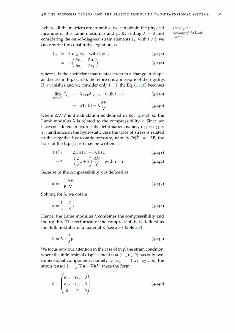
4.8 the stiffness tensor and the elastic moduli in two-dimensional systems . 63
where all the matrices are in rank 3, we can obtain the physical The physicalmeaning of the Lamèmoduli
meaning of the Lamè moduli, λ and µ. By setting λ = 0 andconsidering the out-of-diagonal strain elements εij with i 6= j, wecan rewrite the constitutive equation as
Tij = 2µεij =, with i 6= j, (4.137)
= µ
(∂ui
∂xj+∂uj
∂xi
)(4.138)
where µ is the coefficient that relates stress to a change in shape,as discuss in Eq. (4.108), therefore it is a measure of the rigidity.If µ vanishes and we consider only i = j, the Eq. (4.116) becomes
limµ→0+
Tij = λεkkδij =, with i = j, (4.139)
= λTr(ε) = λ∆V
V(4.140)
where ∆V/V is the dilatation as defined in Eq. (4.109), so theLamè modulus λ is related to the compressibility κ. Since wehave considered an hydrostatic deformation, namely ε11 = ε22 =
ε33,and since in the hydrostatic case the trace of stress is relatedto the negative hydrostatic pressure, namely Tr(T) = −3P, thetrace of the Eq. (4.116) may be written as
Tr(T) = 2µTr(ε) + 3λTr(ε) (4.141)
−P =
(2
3µ+ λ
)∆V
Vwith i = j, (4.142)
Because of the compressibility κ is defined as
κ = −1
P
∆V
V(4.143)
Solving for λ, we obtain
λ =1
κ−2
3µ (4.144)
Hence, the Lamè modulus λ combines the compressibility andthe rigidity. The reciprocal of the compressibility is defined asthe Bulk modulus of a material K (see also Table 4.4)
K = λ+2
3µ (4.145)
We focus now our attention in the case of in plane strain condition,where the infinitesimal displacement u = (u1,u2, 0) has only two-dimensional components, namely u1,u2 = f(x1, x2). So, thestrain tensor ε = 1
2(∇u +∇uT ) takes the form
ε =
ε11 ε12 0
ε12 ε22 0
0 0 0
(4.146)

64 continuum mechanics and nonlinear elasticity
It is easy now to introduce a two dimensional notation, wherePlane straincondition: 3D Vs 2Dnotation
the Eq. (4.116) is rewritten with only matrix in rank 2(T11 T12
T12 T22
)= 2µ
(ε11 ε12
ε12 ε22
)+ λ(ε11 + ε22)I (4.147)
Now, we have obtained the constitutive relation for two-dimensional(2D) systems
T = 2µ2Dε + λ2DTr(ε)I (4.148)
With the same arguments discussed before for the three-dimensionalcase, instead the Eq. (4.145), the two-dimensional Bulk modulusis
K2D = λ2D + µ2D (4.149)
Note that this is a very important issue to study the two-dimensionalelastic properties of a given two-dimensional system. The rela-tions between different two-dimensional elastic moduli is shownin Table 4.5.
Using the two-dimensional version of the Eq. (4.116), we candefine the relations between elastic moduli and the stiffnesscoefficients (see also Table 4.5)T11T22
T12
=
C11 C12 0
C12 C11 0
0 0 (C11 − C12)
ε11ε22ε12
=
=
2µ2D + λ2D λ2D 0
λ2D 2µ2D + λ2D 0
0 0 2µ2D
ε11ε22ε12
(4.150)
Plane stresscondition: 3D Vs 2Dnotation
Imposing the plane stress boundary condition instead the planestrain one, the out-of-plane components of the stress tensor haveto null, namely Tnnn = 0, where n is the normal versor parallell tothe x3−axis. Hence the stress tensor is in the following form
T =
T11 T12 0
T12 T22 0
0 0 0
(4.151)
Therefore, instead the Eq. (4.123) which is reported below
ε =1
2µT −
λ
2µ(2µ + 3λ)III3Tr(σ), (4.152)
we derive the two-dimensional inverse constitutive equation fromthe Eq. (4.148)
ε =1
2µ2DT −
λ2D
4µ2D(µ2D + λ2D)III2Tr(T) (4.153)
where all the matrices are in rank 2.

4.8 the stiffness tensor and the elastic moduli in two-dimensional systems . 65
Tabl
e4.
5:R
elat
ions
betw
een
diff
eren
tco
uple
sof
two-
dim
ensi
onal
elas
tic
mod
uli.
Her
e(λ2D
,µ2D
)ar
eth
eLa
mè
coef
ficie
nts,E2D
,µ2D
,andK2D
are
the
two-
dim
ensi
onal
Youn
gm
odul
us,t
hetw
o-di
men
sion
alPo
isso
nra
tio,a
ndth
etw
o-di
men
sion
alBu
lkm
odul
us,r
espe
ctiv
ely.
Mor
eove
r,w
esh
owth
ere
lati
onbe
twee
nel
asti
cm
odul
iand
stiff
ness
coef
ficie
nts
Cλµ
.
(λ2D
,µ2D
)(K2D
,µ2D
)(µ2D
,ν2D
)(E2D
,ν2D
)(E2D
,µ2D
)Cλµ
λ2D
K2D
−µ2D
2µ2Dν2D
1−ν2D
ν2DE2D
(1+ν2D
)(1
−ν2D
)
2µ2D
(E2D
−2µ2D
)
4µ2D
−E
C12
µ2D
E2D
2(1
+ν2D
)
C11
−C12
2
K2D
λ2D
+µ2D
µ2D
(1+ν2D
)
(1−ν2D
)
E2D
2(1
−ν2D
)
E2Dµ2D
(4µ2D
−E2D
)
C11
+C12
2
E2D
4µ2D
(λ2D
+µ2D
)
λ2D
+2µ2D
4K2Dµ2D
K2D
+µ2D
2(1
+ν2D
)µ2D
C2 11
−C2 12
C11
ν2D
λ2D
(λ2D
+2µ2D
)
K2D
−µ2D
(K2D
+µ2D
)
E2D
−2µ2D
2µ2D
C12
C11

66 continuum mechanics and nonlinear elasticity
4.9 the virial stress tensor
The continuum stress interpretation of atomic force fields isimportant because it allows the intensity and nature of internalinteractions in materials to be measured. In order to obtain theatomic-molecular counterpart of the Cauchy stress tensor definedin Eq. (4.31), we consider a small volume V , with surface S, of agiven elastic body . We suppose that in this region there are Natoms, described by positions xi for i = 1...N. The number of theThe continuum
stress interpretationof atomic force fields
atoms is large enough to allow the definition of the macroscopicelastic fields (stress and strain) in that region, but it is also smallenough to identify the effective stress with its average on thevolume. The components of the position vector xi will be denotedwith (xi,1, xi,2, xi,3). In order to obtain the continuum-molecularequivalence it is useful to introduce the so-called virial form∑Ni=1 xi ⊗ Fi where the symbol ⊗ represents the tensor product
of vectors. The quantity Fi is the total force acting on the ith
atom and, therefore, the equation of motion Fi = miai leads tothe balance
N∑i=1
xi ⊗ Fi =
N∑i=1
mixi ⊗ ai (4.154)
where mi is the mass of the ith atom. The total force Fi can bewritten as the sum of two contributes: the internal force Finti ,which is defined as the force on the ith atom exerted by theother atoms contained in the volume V , and the external forceFesti , i.e. the force on the ith atom exerted by the atoms outsidethe volume V and by any external action. Therefore the balanceequation (4.154) becomes
N∑i=1
xi ⊗ Finti +
N∑i=1
xi ⊗ Festi =
N∑i=1
mixi ⊗ ai (4.155)
Moreover, because of the external force Festi is made by thesurface force Festi (S), that is the force on the ith atom exerted bythe atoms outside the volume V , and by the body force Festi (V),i.e. the force on the ith atom exerted by any external action (e.g.gravity), again we rite the Eq. (4.154) as follows
N∑i=1
xi ⊗ Finti +
N∑i=1
xi ⊗ Festi (V) +
N∑i=1
xi ⊗ Festi (S)
=
N∑i=1
mixi ⊗ dvidt
(4.156)
where vi is the velocity of the ith atom, and the contributeFesti (S) can be different from zero only for atoms very close tothe surface S, i.e. interacting with the atoms outside the volume

4.9 the virial stress tensor 67
V . We observe that the velocity vi of each atom is composed bya term corresponding to an effective macroscopic drift v(0)
i anda statistical (thermal) fluctuation δvi. Therefore, we substitutevi = (v(0)
i + δvi) into Eq. (4.156)
N∑i=1
xi ⊗ Finti +
N∑i=1
xi ⊗ Festi (V) +
N∑i=1
xi ⊗ Festi (S)
=
N∑i=1
mixi ⊗dv(0)i
dt+
N∑i=1
mixi ⊗ dδvidt
(4.157)
If we introduce the time average 〈 · 〉τ = limτ→∞ 1τ
∫τ0 ( · ) dt
and we can develop the average value of the last term of the righthand side of Eq. (4.157) as follows⟨N∑i=1
mixi ⊗ dδvidt
⟩τ
=
⟨N∑i=1
mi
[ddt
(xi ⊗ δvi) − vi ⊗ δvi]⟩τ
= limτ→∞ 1τ
∫τ0
N∑i=1
middt
(xi ⊗ δvi) dt−
⟨N∑i=1
mivi ⊗ δvi⟩τ
= limτ→∞ 1τ
N∑i=1
mixi ⊗ δvi∣∣∣∣∣t=τ
t=0
−
⟨N∑i=1
mivi ⊗ δvi⟩τ
(4.158)The virial theorem
We are dealing with an elastic solid body which is a stablebound system, i.e. a system that hold together. In other words,coordinates and velocities for all particles remain finite. In thiscase, the quantity G(t) =
∑Ni=1mixi ⊗ δvi is a limited function
with extremes, Gmin and Gmax, and its average goes to zero inthe limit of very long times τ
limτ→∞ 1τ
N∑i=1
mixi ⊗ δvi∣∣∣∣∣t=τ
t=0
= limτ→∞ G(τ) −G(0)
τ0 limτ→∞ Gmax −Gmin
τ= 0
(4.159)
Moreover, the last term in Eq. (4.158) can be developed by recall-ing the decomposition of the velocity vi = (v(0)
i + δvi), and byusing the statistical independence of v(0)
i and δvi as follows⟨N∑i=1
mivi ⊗ δvi⟩τ
=
⟨N∑i=1
miv(0)i ⊗ δvi
⟩τ
+
⟨N∑i=1
miδvi ⊗ δvi⟩τ
(4.160)
The first average value in the right hand side is zero, because theaverage value of the velocity fluctuation δvi is null. Conversely,

68 continuum mechanics and nonlinear elasticity
the second average value is a quadratic term in the fluctuation δviand therefore it is not negligible. Hence, this important equalityhas been obtained from Eq. (4.158)⟨
N∑i=1
mixi ⊗ dδvidt
⟩τ
= −
⟨N∑i=1
miδvi ⊗ δvi⟩τ
(4.161)
Summing up, the virial balance in Eq. (4.157) can be written as⟨N∑i=1
xi ⊗ Finti
⟩τ
+
⟨N∑i=1
xi ⊗ Festi (V)
⟩τ
+
⟨N∑i=1
xi ⊗ Festi (S)
⟩τ
=
⟨N∑i=1
mixi ⊗dv(0)i
dt
⟩τ
−
⟨N∑i=1
miδvi ⊗ δvi⟩τ
(4.162)
Here, the term with the body force Festi (V) corresponds to a vol-ume integral, the term with the surface force Festi (S) correspondsto a surface integral and the first sum in the right hand side canbe converted to a volume integral by observing that dv(0)
i /dt isthe macroscopic acceleration field a. By identifying these atomicterms with their continuum counterparts, we can rewritten⟨N∑i=1
xi ⊗ Finti
⟩τ
+
⟨∫V
x⊗ Fest(V)dx⟩τ
+
⟨∫S
x⊗ Fest(S)dS⟩τ
=
⟨∫Vρx⊗ adx
⟩τ
−
⟨N∑i=1
miδvi ⊗ δvi⟩τ
(4.163)
As described in Section 4.3, the body and the surface forces canbe identified as Fest(V) = b, and Fest(S) = Tn, where T is thestress tensor and n is the unit vector normal to S. Therefore, thebalance equation assumes the form⟨
N∑i=1
xi ⊗ Finti
⟩τ
+
⟨∫V
x⊗ bdx⟩τ
+
⟨∫S
x⊗ (Tn)
dS⟩τ
=
⟨∫Vρx⊗ adx
⟩τ
−
⟨N∑i=1
miδvi ⊗ δvi⟩τ
,
(4.164)
or equivalently through its components⟨N∑i=1
xi,kFinti,h
⟩τ
+
⟨∫Vxkbhdx
⟩τ
+
⟨∫SxkThpnpdS
⟩τ
=
⟨∫Vρxkahdx
⟩τ
−
⟨N∑i=1
miδvi,kδvi,h
⟩τ
(4.165)

4.9 the virial stress tensor 69
Applying the divergence theorem (see Appendix A.2) the surfaceintegral can be converted into a volume integral as follows⟨N∑i=1
xi,kFinti,h
⟩τ
+
⟨∫Vxkbhdx
⟩τ
+
⟨∫V
∂
∂xp
(xkThp
)dx⟩τ
=
⟨∫Vρxkahdx
⟩τ
−
⟨N∑i=1
miδvi,kδvi,h
⟩τ
(4.166)
The derivative can be developed by obtaining⟨N∑i=1
xi,kFinti,h
⟩τ
+
⟨∫Vxkbhdx
⟩τ
+
⟨∫V
(δkpThp + xk
∂Thp
∂xp
)dx⟩τ
=
⟨∫Vρxkahdx
⟩τ
−
⟨N∑i=1
miδvi,kδvi,h
⟩τ
(4.167)
Therefore, we can collect the terms as shown in the followingrelation⟨
N∑i=1
xi,kFinti,h
⟩τ
+
⟨∫VThkdx
⟩τ
+
⟨N∑i=1
miδvi,kδvi,h
⟩τ
+
⟨∫Vxk
(∂Thp
∂xp+ bh − ρah
)dx⟩τ
= 0
(4.168)
The quantity in brackets is zero because of the Equation (4.54),∂Tji∂xi
+ bj − ρaj = 0, which describes the motion of any elasticbody. Moreover, we can define the average value of the stresstensor over the volume V , namely Thk = 1
V
∫V Thkdx. It follows
that the balance equation for the virial sum leads to the followingdefinition of stress, based on atomic quantities The virial stress
tensor⟨Thk
⟩τ
= −1
V
⟨N∑i=1
miδvi,kδvi,h
⟩τ
−1
V
⟨N∑i=1
xi,kFinti,h
⟩τ
(4.169)
This very important relation, called virial stress tensor, linksamong microscopic atomic quantities and macroscopic observ-ables and it can be written in tensor form, as follows
⟨¯T⟩τ
= −1
V
⟨N∑i=1
miδvi ⊗ δvi⟩τ
−1
V
⟨N∑i=1
xi ⊗ Finti
⟩τ
(4.170)
This result has innumerable applications in the field of the molec-ular dynamic simulations of mechanical structures. In fact, itenables us to evaluate the macroscopic Cauchy stress in an elas-tic solid system defined at the atomic or molecular level. It is
70 continuum mechanics and nonlinear elasticity
important to observe that the first kinetic term considers thefluctuations of the velocities and not the absolute velocities: itis very important for analyzing thermoelasticity with moleculardynamic simulations [71]. To conclude, we have obtained theatomic-molecular counterpart of the Cauchy stress tensor, asgiven in Eq. (4.170): we point out that this result is exactly correct(at any time) for systems undergoing arbitrary time-dependentdeformations.
4.9.1 Physical meaning of the virial stress
We add some comments on other quantities defined for a sys-tem of particles similar to that above derived. This discussion isuseful to avoid some errors and misunderstandings often encoun-tered in the development of these concepts. The pressure stress⟨Π⟩τ
is the most commonly used definition of stress-like quantityin discrete particle systemsThe pressure tensor
⟨Π⟩τ
= −1
V
⟨N∑i=1
midxidt⊗ dxi
dt
⟩τ
−1
V
⟨N∑i=1
xi ⊗ Finti
⟩τ
(4.171)
This quantity includes two terms [72, 73]. The first part dependson the mass and on the absolute velocity of atomic particles,reflecting the assertion that mass transfer causes pressure tobe applied on stationary spatial surfaces external to an atomic-particle system. The second part depends on interatomic forcesand atomic positions, providing a continuum measure for the in-ternal mechanical interactions between particles. Historic deriva-tions of the pressure stress include generalization from the virialtheorem of Clausius or Maxwell for gas pressure and solution ofthe spatial equation of balance of momentum [74, 75]. However,the pressure stress is not a measure for the Cauchy mechanicalstress in an elastic body [76]. We have proved, in the previousSection 4.9, that the absolute velocities vi = dxi/dt in Eq. (4.171)must be substituted with their fluctuations δvi for obtaining theCauchy stress, as shown in Eq. (4.170).
We also remark that the virial approach or virial theorem (Clau-sius 1870), as applied to gas systems for the evaluation of externalpressure strictly in the statistical average sense, correctly capturesthis effect. The key is that the pressure represents external forcesbetween an atomic system and a container, where the pressureis generated by the collisions of the atoms on the container. Incontrast, stress represents internal forces between particles insidea body, and it is not generated by collisions against a wall. Indeed,Eq. (4.171) correctly describes the macroscopic pressure of a gassystem under the three following conditions: i) the system is instatistical equilibrium, ii) the pressure must be interpreted in atime and volume averaged sense, i.e. fluctuations at the molecular

4.9 the virial stress tensor 71
level are assumed to average out over time and space, and iii)the pressure must be recognized as the average force per unitarea on the wall of a physical container holding the gas system.The pressure stress given in Eq. (4.171) can be correctly applied inmolecular dynamic simulations when one is analyzing the pres-sure (or pressure tensor) of a gas or a fluid at thermodynamicequilibrium.
Furthermore, we remark that Eq. (4.170) represents the atomiccounterpart of the Cauchy stress when it is considered in anEulerian (spatial) reference frame. Andia et al. (see Refs.[77, 78]),have taken a Lagrangian (material) frame of reference to showthat the stress in the atomic system does not contain velocityterm at all, by obtaining the further relation
⟨TL
⟩τ
= −1
V
⟨N∑i=1
xi ⊗ Finti
⟩τ
(4.172)
For example, Gao and Weiner (see Ref.[79]) clearly show that thedynamic term is included only in an Eulerian (spatial) referenceframe and not in a Lagrangian frame of reference. They alsoshow the equivalence between the Eulerian (spatial) and theLagrangian (material) definitions of virial stress [79]. Anyway, inmolecular dynamic simulations the Eulerian point of view mustbe always considered in order to draw coherent comparisonsamong numerical and continuum results [71].
4.9.2 The atomistic nonlinear Cauchy stress
The viral stress defined as in Eq. (4.170) corresponds to theCauchy stress only in the framework of the linear approximation.To achieve also the nonlinear elastic behavior of the system, weneed to derive a different form of the atomistic stress. A relationbetween the atomic stress and the Cauchy stress tensor can bestraightforwardly derived by the strain energy function, as in Eq.(4.113).
In a given system, the strain energy function U(ε) can be iden-tified with the thermodynamic potential of the corresponding Thermodynamical
identification of thestrain energy
statistical ensemble (i.e. the internal energy for an isolated system,the Helmholtz free energy for a system in equilibrium with athermal bath, etc...). By considering the basic case of an isolatedsystem at T = 0 K, the internal energy corresponds to the in-teratomic potential energy U which is a function of the atomicpositions xi i = 1, ...,N, namely: U = U(xi). In absence of anyexternal load, the system lies in the minimum energy configura-tion
x0i
. If a uniform strain field ε is applied, the new atomicpositions can be expressed as xi = (I+ ε)x0i and the correspond-

72 continuum mechanics and nonlinear elasticity
ing internal energy is given by U(
(I+ ε)x0i)
. Thus, the strainenergy density can be written as
U(ε) =1
VU(
(I+ ε)x0i)
(4.173)
where V is the volume of the system. According to Eq. (4.113),the stress tensor is given byThe nonlinear form
of the Cauchy stress
T =∂U(ε)
∂ε=
1
V
N∑i
∂U
∂xi∂xi∂ε
(4.174)
=1
V
N∑i
∂U
∂xi∂
∂ε(I+ ε)x0i
=1
V
N∑i
∂U
∂xi⊗ x0i
= −1
V
N∑i
x0i ⊗ Finti
This expression corresponds to that in Eq. (4.170) but the positionsxi in the deformed configuration are replaced by the positions x0iof the system in the minimum energy state. Note that Eq. (4.170)is coincident with the first-order expansion in ε of Eq. (4.174)Therefore we can obtain that to take in account nonlinear effectof stress up to the second order in the strain, we need to evaluatethe following version of the virial stress tensor instead the Eq.(4.170)
1
V
N∑i
∂U
∂xi⊗ x0i =
1
V
N∑i
∂U
∂xi⊗ xi + o(ε2) (4.175)
x0i = xi + o(ε), and∂V
∂xi= o(ε) (4.176)
4.9.3 Atomic stress for two-body interactions
In this Section we specialize the general result given in Eq.(4.170) to the case of two-body interactions among the atoms ofthe solid elastic body. We remember that the internal force Fintion the ith atom is given by all the forces exerted by other atomscontained into the volume V . Therefore, the quantity Finti canbe written as the sum
∑Nj6=i fij where fij is the force applied on
the ith atom by the jth atom. It follows that Eq. (4.170) can beconverted to
⟨¯T⟩τ
= −1
V
⟨N∑i=1
miδvi ⊗ δvi⟩τ
−1
V
⟨N∑i=1
xi ⊗N∑j6=i
fij
⟩τ
(4.177)

4.9 the virial stress tensor 73
The last term can be split in two identical terms as follows
⟨¯T⟩τ
= −1
V
⟨N∑i=1
miδvi ⊗ δvi⟩τ
−1
2V
⟨N∑i=1
xi ⊗N∑j6=i
fij
⟩τ
+1
2V
⟨N∑i=1
xi ⊗N∑j6=i
fji
⟩τ
(4.178)
where we have utilized the Newton’s third law fji = −fij. Inthe last double sum we can exchange the names of the summedindices, by obtaining
⟨¯T⟩τ
= −1
V
⟨N∑i=1
miδvi ⊗ δvi⟩τ
+1
2V
⟨N∑i=1
(xj − xi
)⊗ N∑j6=i
fij
⟩τ
(4.179)
Moreover, we define the vector from the ith atom to the jth atomwith xij = (xj − xi). It follows that
⟨¯T⟩τ
= −1
V
⟨N∑i=1
miδvi ⊗ δvi⟩τ
+1
2V
⟨N∑i=1
N∑j6=i
xij ⊗ fij
⟩τ
(4.180)
This form is particularly useful for the applications to the molecu-lar dynamic simulations since the force term fij is directly linkedwith the interaction potential energy U2B (r) between two atoms
fij =dU2B (r)
dr
∣∣∣∣r=|xij|
xij|xij|
(4.181)
By substituting Eq. (4.181) into Eq. (4.180) we obtain the finalrelation⟨
¯T⟩τ
= −1
V
⟨N∑i=1
miδvi ⊗ δvi⟩τ
+1
2V
⟨N∑i=1
N∑j6=i
xij ⊗ xij
(1
r
dU2B (r)
dr
)∣∣∣∣r=|xij|
⟩τ
(4.182)
This form is useful since it considers only quantities available instandard molecular dynamic procedures and it is perfectly suitedfor being used under the typical assumption of periodic boundaryconditions. In fact, when the periodic boundary conditions areapplied, the system interacts with the copies of the unit cellwhich are called images. When a molecule passes through oneface of the unit cell, it reappears on the opposite face with the

74 continuum mechanics and nonlinear elasticity
same velocity and, therefore, the definition of internal forces andexternal ones is not applicable. Nevertheless, the stress expressiongiven in Eq. (4.182) solves the problem, being written in terms ofU2B. However, it is important to consider the correct periodicityin the definition of the vectors xij = (xj − xi) by applying thestandard minimum-image convention [80].

Part II
E L A S T I C B E H AV I O R O F G R A P H E N E


5T H E G R A P H E N E I S S T R E T C H E D
“The most exciting phrase to hear in science, the one that heralds newdiscoveries, is not ’Eureka!’ but ’That’s funny...”’
Isaac Asimov (1920-1992)
Contents5.1 Elastic properties of graphene 785.2 The computational approach 835.3 The stress-strain approach 86
The elastic properties of graphene have been recently deter-mined by atomic force microscope nanoindentation [12, 81], mea-suring the deformation of a free-standing monolayer. In particu-lar, in Ref. [12] the experimental force-deformation relation hasbeen expressed as a phenomenological nonlinear scalar relationbetween the applied stress (σ) and the observed strain (ε)
σ = Eε+Dε2 (5.1)
where E and D are, respectively, the Young modulus and aneffective nonlinear (third-order) elastic modulus of the two di-mensional carbon sheet. The reported experimental values are:E = 340± 40 Nm−1 and D = −690± 120Nm−1. While the firstresult is consistent with previous existing data [82, 14, 83, 15], theabove value for D represents so far the only available informationabout the nonlinear elasticity of a one-atom thick carbon sheet.Although nonlinear features are summarized in Eq. (5.1) by one
suspended graphene
substrate
indenter
Scheme of theindentation of a
suspendedmonolayer graphene.
effective parameter D, continuum elasticity theory predicts theexistence of three independent third-order parameters Cijk forgraphene, as reported below. In other words, while Eq. (5.1) rep-resents a valuable effective relation for the interpretation of acomplex experiment [12], it must be worked out a more rigoroustheoretical picture in order to properly define all the nonlinearelastic constants of graphene and to understand the physicalmeaning of D.
This corresponds to the content of the present Chapter wherewe investigate the constitutive nonlinear stress-strain relation ofgraphene for graphene stretching elasticity and we calculate allthe corresponding nonlinear elastic moduli, by combining con-tinuum elasticity and tight-binding atomistic simulation (TB-AS)[84]. Present results represent a robust picture on elastic behaviorand provide the proper interpretation of recent experiments. In
77

78 the graphene is stretched
zz
ac
θ~ey sin θ
~ex cos θ
~n = ~excos
θ + ~eysinθ
Figure 5.1: By applying an axial tension σ along the arbitrary direc-tion ~n (θ = ~zz ∠ ~n), the Cauchy stress tensor T = ∂U/∂ε
is T = σ~n⊗ ~n, where the in-plane stress components aredefined, respectively, as Txx = σ cos2 θ, Txy = σ cos θ sin θ,and Tyy = σ sin2 θ.
particular, we discuss the physical meaning of the effective non-linear elastic modulus there introduced and we predict its valuein good agreement with available data. Finally, a hyperelasticsoftening behavior is observed and discussed, so determining thefailure properties of graphene.
5.1 elastic properties of graphene
To obtain the nonlinear stress-strain relation of an elastic mem-brane, we need at first to elaborate an expression for the corre-sponding strain energy function U (per unit area), which wasdefined in Eq. (4.114) as follows
U(ε) =1
2Cijkhεijεkh +
1
6Cijkhnmεijεkhεnm (5.2)
Riminding that the Cijkh and the Cijkhnm denote the secondorder elastic constant (SEOC) and the third order elastic constant(TOEC), respectively
Cijkh =∂2U
∂εij ∂εkh; Cijkhnm =
∂3U
∂εij ∂εkh ∂εnm(5.3)

5.1 elastic properties of graphene 79
The complexvariables methodSince, as illustrated in Figure 5.1, the graphene lattice is hexag-
onal, it is useful to consider the coordinate set α = (x+ iy) andβ = (x− iy) [85], where the x and y directions are respectivelyidentified with the zig-zag (zz) and the armchair (ac) directions.We introduce the corresponding form for the strain energy func-tion U as follows
2U = λijkhεijεkh +Λijkhnmεijεkhεnm (5.4)
where λijkh and Λijkhnm are parameters analogous to the Cijkhand the Cijkhnm in the Eq. (5.2). Because of the six-fold symmetryof hexagonal lattices, the strain energy function U have to beinvariant under a rotation of π/3 about the z-axis (normal to thegraphene plane).
α = (x+ iy) −→ α e2πi6
β = (x− iy) −→ β e− 2πi6
(5.5)
Since (e±2πi6 )6 = 1 and e
2πi6 e− 2πi
6 = 1, the parameters λijkh A complete set ofelastic moduliand Λijkhnm must have among their indices 6-times α or β,
or an equal number of them to be invariant under these trans-formations. We get the follows complete set of elastic modulifor an hexagonal symmetry which is composed by a couple oflinear moduli λ1 and λ2 and by three nonlinear independentelastic coefficients, namely Λi, i = 1, 2, 3, all expressed in units offorce/length as follows
λ1 = λααββ; λ2 = λαβαβ;
Λ1 = Λαααααα ≡ Λββββββ;
Λ2 = Λααββαβ; Λ3 = Λαβαβαβ
(5.6)
Hence the strain energy function U can be written consideringseparately the quadratic terms and the cubic terms, U = U(2) +
U(3), the Eq. (5.4) is given by
2U(2) = +λ1εααεββ + λ2ε2αβ
6U(3) = +Λ1(ε3αα + ε3ββ) +Λ2εααεββεαβ +Λ3ε
3αβ,
(5.7)
In order to further proceed we must better focus the strain defini-tion which in elasticity theory is twofold: we can introduce the so-called small strain tensor ε = 1
2(~∇~u+ ~∇~uT), being ~u the displace-
ment field, or the Lagrangian strain η = 12(
~∇~u+ ~∇~uT + ~∇~uT ~∇~u).While ε takes into account only the physical nonlinearity features(i.e. a nonlinear stress-strain dependence observed in regime ofsmall deformation), η describes any possible source of nonlinear-ity, including both physical and geometrical (large deformation)

80 the graphene is stretched
ones. To turn back in Cartesian coordinates, x, y, we can derivethe strain elements from their definition
εαβ =1
2
(∂uα
∂β+∂uβ
∂α
)= εxx + εyy
εαα =1
2
(∂uα
∂α+∂uα
∂α
)= εxx − εyy + 2iεxy
εββ =1
2
(∂uβ
∂β+∂uβ
∂β
)= εxx − εyy − 2iεxy
(5.8)
Combining the Eq. (5.7) with the Eq. (5.8) we have a completerelationship for density of energy in a non linear form
2U(2) = + ε2xx(λ1 + λ2) + ε2yy(λ1 + λ2)
+2εxxεyy(−λ1 + λ2) + 4ε2xyλ1
6U(3) = + ε3xx(2Λ1 +Λ2 +Λ3)
+ ε3yy(−2Λ1 +Λ2 +Λ3)
+ ε2xxεyy(−6Λ1 −Λ2 + 3Λ3)
+ εxxε2yy(6Λ1 −Λ2 + 3Λ3)
+ ε2xyεxx(−24Λ1 + 4Λ2)
+ε2xyεyy(24Λ1 + 4Λ2)
(5.9)
Otherwise we can write it also in terms of stiffness tensor coeffi-cients by the complite expantion of the Eq. (5.2)
2U(2) = C11ε2xx + C22ε
2yy + 2C12εxxεyy + 4C66ε
2xy
+ 2C16εxxεxy + 2C26εyyεxy (5.10)
6U(3) = +C111ε3xx + C222 ε
3yy
+ 3C112 ε2xxεyy + 3C122 εxxε
2yy
+ 12C166 εxxε2xy + 12C266 εyyε
2xy
+ 6C116 ε2xxεxy + 6C226 ε
2yyεxy
+ 12C126 εxxεyyεxy + 8C666 ε3xy
(5.11)
By comparing term by term the Eq. (5.9) and the Eq. (5.10), weget the relationships between the linear elastic coefficients λ1,λ2 and the nonlinear elastic coefficients Λ1, Λ2 and Λ3 withthe second order elastic constants and the third order elasticconstants, respectively Thus we obtain that
λ1 =1
2(C11 − C12), λ2 =
1
2(C11 + C12) (5.12)
Λ1 =1
12(C111 − C222), Λ2 =
1
4(C222 − C112),
Λ3 =1
12(2C111 − C222 + 3C112). (5.13)
Furthermore, we obtain that the hexagonal symmetry dictates 2-independent Cijkl (C11, C12) as well as we aspect for an isotropic

5.1 elastic properties of graphene 81
material, and 3-independent Cijklmn (C111, C222, C112). Thereare some linear terms null, C16 = C26 = 0, and some non-linear terms, C116 = C226 = C126 = C666 = 0 as well. For thesame symmetry reasons the follows relations between stiffnesscoefficients have been derived: C11 = C22, 2C66 = C11 − C12,C122 = C111 − C222 + C112, C166 = −2C111 + 3C222 − C112, andC222 = 2C111 − C222 − C112.
The quadratic terms of the density energy U(2) in Eq. (5.9) havebeen derived also as follows
2U(2) = λ1εααεββ + λ2ε2αβ
= λ1(2Tr(ε2) − (Tr(ε))2) + λ2(Tr(ε))2
= 2λ1Tr(ε2) + (λ2 − λ1)(Tr(ε))2(5.14)
where we have used the follows relations, which have been de-rived from the Eq. (5.8)
εααεββ = (εxx − εyy)2 + 4ε2xy
ε2αβ = (εxx + εyy)2
(Tr(ε))2 = (εxx + εyy)2
Tr(ε2) = ε2xx + ε2yy + 2ε2xy
(5.15)
Hence, starting from the Eq. (5.2) and using the tensor stressformulations, Tij = Cijkh εkh and T = 2µε + (K − µ)Tr(ε)I2(see Eq. (4.116) and Eq. (4.148) respectively), the density energyU(2) can be written as
U(2) =1
2Cijkl εij εkl
=1
2Tij εij =
1
2Tr(T ε)
=1
2
[2µTr(ε2) + (K − µ)Tr(ε)2
] (5.16)
Finally, comparing the Eq. (5.16) with the Eq. (5.14), we haveobtained that the two elastic constant λ1, λ2 are directly relatedto the Lamè modulus µ and the Bulk modulus K (see also Table4.5), respectively
λ1 ≡ µ =C11 − C12
2
λ2 ≡ K = µ+ λ =C11 + C12
2
(5.17)
The strain energy function is finally obtained as
2U = 2µTr(ε2)+ λ (Trε)2
+1
3C111ε
3xx +
1
3C222ε
3yy + C112ε
2xxεyy
+(C111 − C222 + C112)εxxε2yy
+(3C222 − 2C111 − C112)εxxε2xy
+(2C111 − C222 − C112)εyyε2xy (5.18)

82 the graphene is stretched
where we set εααεββ = Tr(ε2)
and ε2αβ = (Trε)2.Uniform uniaxialstress in plane stressboundary condition:the stress-strainnonlinearconstitutive equation
The analysis of the experimental data provided in Ref. [12]through Eq. (5.1) is assuming an applied uniaxial stress in planestress boundary condition. Since the stress-strain nonlinear con-stitutive equation for in-plane stretching is straightforwardlyobtained by T = ∂U/∂ε, where T is the Cauchy stress tensordefined in Section 4.3, we can write its components as functionof the strain tensor elements
Txx =∂U
∂εxx= f1(εxx, εyy, εxy) = f1(εxx, εyy, 0)
Tyy =∂U
∂εyy= f2(εxx, εyy, εxy) = f2(εxx, εyy, 0)
Txy =∂U
∂εxy= f3(εxx, εyy, εxy) = 0
(5.19)
Here to achieve the uniaxial stress condition we have to imposethat Txy = 0 and conseguently εxy = 0. We now suppose toapply a uniaxial tension σ~n along the arbitrary direction ~n =
cos θ~ex + sin θ~ey, where ~ex and ~ey are the unit vectors along thezig-zag and the armchair directions, respectively (see Figure 5.1).Under this assumption we get: T = σ~n~n⊗ ~n, with in-plane com-ponents defined as Txx = σ~n cos2 θ, Txy = σ~n cos θ sin θ, andTyy = σ~n sin2 θ. Similarly, by inverting the nonlinear constitu-tive equation we find the corresponding strain tensor and therelative variation of length ε~n = ~n · ε~n along the direction ~n.By combining these results, we obtain the stress-strain relationσ~n = Eε~n +D~nε
2~n along the arbitrary direction ~n (see Figure 1,
bottom), where D~n is given byThe nonlineareffective elasticmodulus D~n =
3
2(1− ν)3Λ3 +
3
2(1− ν) (1+ ν)2Λ2 (5.20)
+3(2 cos2 θ− 1
) (16 cos4 θ− 16 cos2 θ+ 1
)(1+ ν)3Λ1
If we set ~n = ~ex (i.e. θ = 0), we get the nonlinear modulus D(zz)
for stretching along the zig-zag direction
D(zz) = D~ex = 3 (1+ ν)3Λ1 +3
2(1− ν) (1+ ν)2Λ2
+3
2(1− ν)3Λ3 (5.21)
Similarly, by setting ~n = ~ey (i.e. θ = π/2), we obtain the nonlinearmodulus D(ac) for stretching along the armchair direction
D(ac) = D~ey = −3 (1+ ν)3Λ1 +3
2(1− ν) (1+ ν)2Λ2
+3
2(1− ν)3Λ3 (5.22)
We observe that the above expression for D(zz) apply for allstretching directions defined by the angles θ = kπ/3 (k ∈ Z),while D(ac) holds for the angles θ = π/6 + kπ/3. Since the
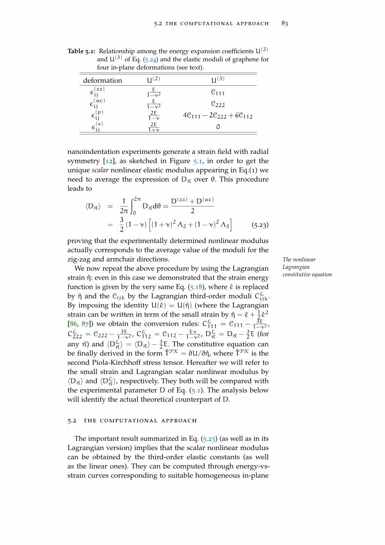
5.2 the computational approach 83
Table 5.1: Relationship among the energy expansion coefficients U(2)
and U(3) of Eq. (5.24) and the elastic moduli of graphene forfour in-plane deformations (see text).
deformation U(2) U(3)
ε(zz)ij
E1−ν2
C111
ε(ac)ij
E1−ν2
C222
ε(p)ij
2E1−ν 4C111 − 2C222 + 6C112
ε(s)ij
2E1+ν 0
nanoindentation experiments generate a strain field with radialsymmetry [12], as sketched in Figure 5.1, in order to get theunique scalar nonlinear elastic modulus appearing in Eq.(1) weneed to average the expression of D~n over θ. This procedureleads to
〈D~n〉 =1
2π
∫2π0D~ndθ =
D(zz) +D(ac)
2
=3
2(1− ν)
[(1+ ν)2Λ2 + (1− ν)2Λ3
](5.23)
proving that the experimentally determined nonlinear modulusactually corresponds to the average value of the moduli for thezig-zag and armchair directions. The nonlinear
Lagrangianconstitutive equation
We now repeat the above procedure by using the Lagrangianstrain η: even in this case we demonstrated that the strain energyfunction is given by the very same Eq. (5.18), where ε is replacedby η and the Cijk by the Lagrangian third-order moduli CL
ijk.By imposing the identity U(ε) = U(η) (where the Lagrangianstrain can be written in term of the small strain by η = ε+ 1
2 ε2
[86, 87]) we obtain the conversion rules: CL111 = C111 − 3E
1−ν2,
CL222 = C222 − 3E
1−ν2, CL
112 = C112 − Eν1−ν2
, DL~n = D~n − 3
2E (forany ~n) and 〈DL
~n〉 = 〈D~n〉− 32E. The constitutive equation can
be finally derived in the form TPK = ∂U/∂η, where TPK is thesecond Piola-Kirchhoff stress tensor. Hereafter we will refer tothe small strain and Lagrangian scalar nonlinear modulus by〈D~n〉 and 〈DL
~n〉, respectively. They both will be compared withthe experimental parameter D of Eq. (5.1). The analysis belowwill identify the actual theoretical counterpart of D.
5.2 the computational approach
The important result summarized in Eq. (5.23) (as well as in itsLagrangian version) implies that the scalar nonlinear moduluscan be obtained by the third-order elastic constants (as wellas the linear ones). They can be computed through energy-vs-strain curves corresponding to suitable homogeneous in-plane

84 the graphene is stretched
−3.23
−3.22
−3.21
−3.20
−3.19
−3.18
−3.17
−3.16
−3.15
0.00 0.01 0.02 0.03 0.04 0.05
0 1 2 3 4 5
Str
ain
Ene
rgy
Den
sity
U(ζ), [
eV/Å
2 ]
Absolute Strain Parameter ζ
Relative Strain Parameter ζ [%]
ε(p)ij
ε(s)ij
ε(ac)ij
ε(zz)ij
Figure 5.2: Strain energy density U, obtained by TB-AS, as function ofthe strain parameter ζ corresponding to the four homoge-neous deformations summarized in Table 5.1.
deformations, thus avoiding a technically complicated simulationof the nanoindentation experiment. Therefore, the following in-plane deformation have been applied: (i) an uniaxial deformationThe uniform
deformation method ζ along the zig-zag direction, corresponding to a strain tensorε
(zz)ij = ζδixδjx; (ii) an uniaxial deformation ζ along the armchair
direction, corresponding to a strain tensor ε(ac)ij = ζδiyδjy; (iii)
an hydrostatic planar deformation ζ, corresponding to the straintensor ε(p)
ij = ζδij; (iv) a shear deformation ζ, corresponding to
an in-plain strain tensor ε(s)ij = ζ
(δixδjy + δiyδjx
).
All the needed energy-vs-strain curves have been determinedby TB-AS, making use of the tight-binding representation by Xu etal. [50]. A periodically repeated square cell containing 400 carbonatoms was deformed as above. For any given applied deforma-tion, full relaxation of the internal degrees of freedom of the simu-lation cell was performed by zero temperature damped dynamicsuntil interatomic forces resulted not larger than 0.5 · 10−11eV/Å.
For the deformations ε(zz)ij , ε(ac)
ij , ε(p)ij and ε
(s)ij the elastic
energy of strained graphene can be written in terms of just thesingle deformation parameter ζPolynomial fitting
method
U(ζ) = U0 +1
2U(2)ζ2 +
1
6U(3)ζ3 +O(ζ4) (5.24)
where U0 is the energy of the unstrained configuration. Since theexpansion coefficients U(2) and U(3) are related to elastic modulias summarized in Table 5.1, a straightforward fit of Eq. (5.24)has provided the full set of linear moduli and third order elasticconstants, while the shear deformation was used to confirm the

5.2 the computational approach 85
isotropy of the lattice in the linear approximation. Each energy-vs-strain curve, shown in Figure 5.2, has been computed by TB-ASas above described, by increasing the magnitude of ζ in stepsof 0.005 up to a maximum strain |ζmax| = 0.055. Arrows inFigure 5.16 indicate the different nonlinear behavior along the zzand ac directions. Nonlinear
anisotripicity ofgraphene
The outputs of the fitting procedure are reported in Table 5.2where the full set of third order elastic constants of monolayergraphene is shown. We remark that C111 is different than C222, i.ea monolayer graphene is isotropic in the linear elasticity approxi-mation, while it is anisotropic when nonlinear features are takeninto account. By inserting the elastic constants Cijk of Table 5.2into Eqs. (5.12), (5.21) and (5.22), we also obtained the nonlinearmoduli for both the zz and ac directions.
In Table 5.3 we report the values of the calculated elastic mod-uli, together with the available experimental and theoretical data.The present TB-AS value for E is in reasonable agreement withliterature [12, 88, 83, 89], while the value of ν is larger than mostof the ab-initio results [83, 89, 90, 91] (but for the result in Ref.[76]). While this disagreement is clearly due to the empiricalcharacter of the adopted TB model (where, however, no elasticdata were inserted in the fitting data base), we remark that thevalues of 〈D~n〉 and 〈DL
~n〉 predicted by means of Eq. (5.23) areaffected by only 10% if we vary ν in the range of values shownin Table 5.3.
Table 5.3 shows that the predicted 〈D~n〉 is much closer tothe experimental value D than its Lagrangian counterpart 〈DL
~n〉.This seems to suggest that measurements in Ref. [12] were per-formed in the physical nonlinearity regime (small strain formal-ism), rather than in the geometrical nonlinearity one (Lagrangianformalism), as also confirmed by the excellent agreement shownin Figure 5.3 commented below. Since Cijk < 0 (and D < 0),graphene is an hyperelastic softening system. Therefore, thepresent model plays a crucial role in determining the failurebehavior of the graphene membrane [92, 93]. Hyperelastic
softening behavior ofgraphene
Table 5.2: Small strain and Lagrangian nonlinear elastic moduli ofgraphene in units of Nm−1.
Small strain Lagrangian
C111 -1689.2 CL111 -2724.7
C222 -1487.7 CL222 -2523.2
C112 -484.1 CL112 -591.1
D(zz) -696.2 DL(zz) -1163.7
D(ac) -469.6 DL(ac) -937.9

86 the graphene is stretched
Table 5.3: Linear and nonlinear elastic moduli of graphene in units ofNm−1 (ν is dimensionless).
E ν D 〈D~n〉 〈DL~n〉
Present 312 0.31 - -582.9 -1050.9
Ref. [12]a 340±40 - -690±120 - -
Ref. [82, 14]b 235 0.413 - - -
Ref. [88]c 384 0.227 - - -
Ref. [83]d 345 0.149 - - -
Ref. [90]d - 0.173 - - -
Ref. [89]d 350 0.186 - - -
Ref. [76]d - 0.32 - - -
Ref. [91]d - 0.12-0.19 - - -a Experimental, b Tersoff-Brenner, c Empirical force-constant
calculations, d Ab-initio
In order to substantiate the above statement, we show in Fig-ure 5.3 the graphene stress-strain curve, as defined in Eq. (5.1).Both the theoretical and experimental curves have been obtainedby using the Young modulus and the scalar nonlinear coefficientas reported in Table 5.3. We remark that in Figure 5.3 the smallstrain 〈D~n〉 value was used. The agreement between the experi-mental curve and the theoretical (small strain) one is remarkable.In addition, by means of Figure 5.3 we can determine the failurestress (maximum of the stress-strain curve) σf = −E2/4〈D~n〉,corresponding to a predicted failure stress as high as 42.4 Nm−1.This result is in excellent agreement with the experimental value42± 4 Nm−1, reported in Ref. [12]. These values correspond toFailure stress
the failure strength of a two-dimensional system. In order to drawa comparison with bulk materials, we define an effective three-dimensional failure stress σ3Df = σf/d, where d is taken as theinterlayer spacing in graphite. By considering d = 0.335 nm [94],we obtain σ3Df ∼= 130 GPa. This very high value, exceeding thatof most materials (even including multi-walled nanotubes [95]),motivates the use of one-atom thick carbon layers as possiblereinforcement in advanced composites.
5.3 the stress-strain approach
The same quantities derived and discussed previously havebeen computed by using the fitting method applied to a setof stress-strin curves instead the energy-strain approach. TheThe stress-strain
approach previous results are confirmed and in Fig. 5.4 we show the stress-strain curves calculated by TB-AS through the implementation ofthe atomic stress tensor version defined in Eq. (4.180). Using the

5.3 the stress-strain approach 87
0
10
20
30
40
50
60
70
0 0.05 0.1 0.15 0.2 0.25 0.3
0 5 10 15 20 25 30
Stre
ss σ
, [N
/m]
Absolute Strain ε
Relative Strain ε [%]
0
10
20
30
40
50
60
70
0 0.05 0.1 0.15 0.2 0.25 0.3
0 5 10 15 20 25 30
Stre
ss σ
, [N
/m]
Absolute Strain ε
Relative Strain ε [%]
TheoreticalExperimental
Figure 5.3: Experimental (see Ref. [12]) and present theoretical stress-strain curves, as defined in Eq. (5.1). Shaded area representsthe experimental error.
Cauchy stress tensor definition (see Eq. (4.113) and the Eq. (4.114),we can derive an expression for the stress tnsor in terms of thestiffness coefficients. Thus we can solve the follows derivative
Tij =∂U
∂εij=
∂
∂εij
(1
2Cijkl εij εkl +
1
6Cijklmn εij εkl εmn
)+1
2Cijkl
(∂εij
∂εijεkl +
∂εkl
∂εijεij
)
+1
6Cijklmn
(∂εij
∂εijεkl εmn + εij
∂εkl
∂εijεmn + εij εkl
∂εmn
∂εij
)
=1
2Cijkl
(εkl +
1
2
(δkiδlj + δkjδli
)εij
)+1
6Cijklmn
(εkl εmn + εij
1
2
(δkiδlj + δkjδli
)εmn
+ εij εkl1
2
(δmiδnj + δmjδni
) )
=1
2Cijkl
(εkl +
1
2( εkl + εlk)
)+1
6Cijklmn
(εkl εmn +
1
2(εkl εmn + εlk εmn + εnm εkl )
)= Cijkl εkl +
1
2Cijklmn εkl εmn
(5.25)

88 the graphene is stretched
0
0.1
0.2
0.3
0.4
0.5
0.0000.0020.0040.0060.0080.0100.0120.014
0 0.2 0.4 0.6 0.8 1 1.2 1.4
Str
ess,
T ij(
ζ) [e
V/Å
2 ]
Absolute Strain Parameter, ζ
Relative Strain Parameter, ζ [%]
T(zz)11
T(zz)22
T(ac)22
T(ac)11
T(p)11
T(zz)22
T(s)12
Figure 5.4: Stress tensor components Tij, obtained by TB-AS, as func-tion of the strain parameter ζ corresponding to the fourhomogeneous deformations summarized in Table 5.1. Notethat couples of curves overlap perfectly as imposed by sym-metry.
or, in more explicit way, we can write
T11 = C11ε11 +C12ε22 + 12(+C111ε
211 + 4C166ε
212
+2C112ε11ε22 +C122ε222)
T22 = C11ε22 +C12ε11 + 12(+C222ε
222 + 4C266ε
212
+2C122ε11ε22 +C112ε211)
T12 = +2C66ε12 + 12( +8C166ε11ε12 + 8C266ε12ε22)
Note that form the computational point of view, the stress-strainapproach is more advantageous than the energy-strain method,because of the number of experiments needed to achieve thesame imformations is smaller. In fact, each deformation leads toa set of three equations, i.e. three curves to fit.
6E L A S T I C P R O P E RT I E S O F G R A P H A N E
“On a piece of paper, a picture’s drawn. It floats on down the street,till the wind is gone. The memory now is like the picture was then;
When the paper’s crumpled up, it can’t be perfect again. ”Linkin Park ’Hybrid Theory’
Contents6.1 Graphane 896.2 Methods and computational setup 926.3 Structure and stability of graphane conform-
ers 946.4 Linear elasticity 966.5 Nonlinear elasticity 103
There exist three conformers of hydrogenated graphene, re-ferred to as chair-, boat-, or washboard-graphane. These systemshave a perfect two-dimensional periodicity mapped onto thegraphene scaffold, but they are characterized by a sp3 orbitalhybridization, have different crystal symmetry, and otherwise be-have upon loading. By first principles calculations we determine The graphane is the
fully hydrogenatedgraphene
their structural and phonon properties, as well as we establishtheir relative stability. Through continuum elasticity we define asimulation protocol addressed to measure by a computer experi-ment their linear and nonlinear elastic moduli and we actuallycompute them by first principles. We argue that all graphaneconformers respond to any arbitrarily-oriented extention witha much smaller lateral contraction than the one calculated forgraphene. Furthermore, we provide evidence that boat-graphanehas a small and negative Poisson ratio along the armchair andzigzag principal directions of the carbon honeycomb lattice (ax-ially auxetic elastic behavior). Moreover, we show that chair-graphane admits both softening and hardening hyperelasticity,depending on the direction of applied load.
6.1 graphane
The hydrogenated form of graphene is referred to as graphane.It is described as a two-dimensional, periodic, and covalentlybonded hydrocarbon with a C:H ratio of 1. Hydrogen atomsdecorate the carbon honeycomb lattice on both the top and bot-tom side (see Fig. 6.1). Graphane was theoretically predictedby Sofo et al., [22] further investigated by Boukhvalov et al. [23]
89

90 elastic properties of graphane
zz
ac
(a)
~a
~b
(b)
~a
~b
(c)
~b
~a
(d)
~b
~a
Figure 6.1: Pictorial representations of the graphane conformers, ob-tained by different hydrogen decorations (the actual atomicpositions are reported in Fig. 6.2). Top hydrogen atoms areindicated by red (dark) circles, while bottom ones by gray(light) circles. Shaded areas represent the unit cell and thecorresponding lattice vectors are indicated by ~a and ~b. Panela: graphene scaffold (full lines) with zigzag (zz) and arm-chair (ac) directions. Panel b, c, and d: chair-, boat-, andwashboard-graphane, respectively.
and eventually grown by Elias et al. [24] The investigation ofgraphane properties was originally motivated by the search fornovel materials with possibly large impact in nanotechnology.
The attractive feature of graphane is that by variously deco-rating the graphene atomic scaffold with hydrogen atoms (stillpreserving periodicity) it is in fact possible to generate a set oftwo dimensional materials with new physico-chemical proper-ties. This is obviously due to change in the orbital hybridizationwhich, because of hydrogenation, is now sp3-like. For instance, ithas been calculated [22, 23] that graphane is an insulator, withan energy gap as large as ∼ 6 eV [96], while graphene is a highlyconductive semi-metal. In case the hydrogenated sample is dis-ordered, the resulting electronic and phonon properties are yetagain different [24]. Hydrogenation likely affects the elastic prop-erties as well. Topsakal et al. [26] indeed calculated that the in-plane stiffness and Poisson ratio of graphane are smaller thanthose of graphene. In addition, the value of the yield strain ispredicted to vary upon temperature and stoichiometry.
As far as the mechanical properties of graphane are concerned,the sp2-to-sp3 change in orbital hybridization causes a major

6.1 graphane 91
ac
zz
z
h C1
C3
C2
C4
H2
H1
H3
(a) C-graphane
ac
zz
z
h
ϕ
C1
C3 C4
C2
H2 H3
H1
(b) B-graphane
ac
zz
z
h
ϕ
C4
C1
C2
C3
H3
H1
H2
(c) W-graphane
Figure 6.2: Perspective representations of fully relaxed graphane con-formers. Gray (light gray) and red (dark gray) spheres rep-resent carbon and hydrogen atoms, respectively. Labels Cnand Hn (with n = 1, 2, 3 and 4) provide the atom identifica-tions used in Table 6.1. Right panels show the orientationwith respect to the armchair (ac) and zigzag (zz) direction,as well as the structural parameters h and ϕ reported inTable 6.1.

92 elastic properties of graphane
difference with respect to graphene. There in fact exist graphaneconformers which are not isotropic, at variance with graphenewhich is so (in linear approximation as shown in Chapter 5). ThisThere exist
anisotropic graphaneconformers
feature stimulates an intriguing change of perspective, namely:hydrogenation could not only affect the actual value of somelinear elastic moduli [26]; it could even dramatically change theoverall mechanical behavior of the system by introducing ananisotropic dependence of its respose to an external load. Thisis in fact what we predict in this work by first principles totalenergy calculations, combined to continuum elasticity: we showthat there is a graphane conformer (i.e., boat graphane as detailedbelow) showing a vanishingly small (possibly negative) Poissonratio upon loading along given directions. In other words, weprovide evidence that upon suitable hydrogenation a graphenesheet behaves as an axially auxetic material [97], namely: it doesnot shrink, but actually slightly elongates perpendicularly toan applied traction force. Nonlinear elastic features show aninteresting anisotropic behavior as well.
This Chapter is organized as follows. In Sec. 6.2, the methodsand the general computational setup adopted in our calculationsare outlined. In Sec. 6.3 we provide a full structural characteriza-tion of three graphane conformers and we discuss their stability.In Sec. 6.4 and Sec. 6.5 we describe their linear and nonlinearelastic properties, respectively, and we compute all the relevantelastic moduli.
6.2 methods and computational setup
All calculations have been performed by Density FunctionalTheory (DFT) (Chapter 3) as implemented in the Quantum
ESPRESSO package [98]. The exchange correlation potentialwas evaluated through the generalized gradient approximation(GGA), using the Vanderbilt ultrasoft pseudopotential PW91 [99].A plane wave basis set with kinetic energy cutoff as high as 50
Ry was used and in most calculations the Brillouin zone (BZ) hasbeen sampled by means of a (18x18x3) Monkhorst-Pack grid. Theatomic positions of the investigated samples have been optimizedby using the quasi-Newton algorithm and periodically-repeatedsimulation cells. Accordingly, the interactions between adjacentatomic sheets in the supercell geometry was hindered by a largespacing greater than 10 Å.
The elastic moduli of the structures under consideration havebeen obtained from the energy-vs-strain curves, correspondingto suitable sets of deformations applied to a single unit cellsample. As discussed in more detail in Sec. 6.4 and Sec. 6.5, forany deformation the magnitude of the strain is represented by asingle parameter ζ. The curves have been carefully generated by

6.2 methods and computational setup 93
Table 6.1: Space groups and structural parameters for each graphaneconformers. The cell parameters a and b are defined inFig. 6.1 while the other quantities are reported in Fig. 6.2.Note that the B-graphane shows two types of C-C bondswhile W-graphane exhibits a large buckling parameter, h.
C-graphane B-graphane W-graphane
Space Group P-3m1 (164) Pmmn (59) Pmna (53)
a 2.54 Å 2.53 Å 2.55 Å
b - 4.31 Å 3.82 Å
C1 −C2 1.54 Å 1.54 Å 1.54 Å
C3 −C4 1.54 Å 1.57 Å 1.54 Å
C−H 1.11 Å 1.11 Å 1.11 Å
h 0.46 Å 0.65 Å 1.14 Å
ϕ 0.0 16.7 30.1
C1C2C3 111.5 110.7 111.2
C2C3C4 111.5 112.3 112.3
H1C2C3 107.4 107.2 106.5
H1C2C3H2 180.0 180.0 51.2
H2C3C4H3 180.0 0.0 0.0
increasing the magnitude of ζ in steps of 0.001 up to a maximumstrain |ζmax| = 0.05. All results have been confirmed by checkingthe stability of the estimated elastic moduli over several fittingranges. The reliability of the above computational set up is provedby the estimated values for the Young modulus and the Poissonratio of graphene, respectively 344 Nm−1 and 0.169, which are inexcellent agreement with recent literature [83, 90, 89]. Similarly,our results for the same moduli in C-graphane (respectively, 246
Nm−1 and 0.08) agree very well with data reported in Ref. [26].The stability of the three graphane conformers has been es-
tablished by calculating the corresponding phonon dispersions.Phonon dispersions, have been obtained by means of Density-Functional Perturbation Theory (DFPT) [69], based on the (2n+
1) theorem (Sec. 3.2). In this case, during the self-consistent fieldcalculation, the BZ has been sampled by a (16x16x3) Monkhorst-Pack grid. The accuracy of the phonon dispersion evaluationshas been tested on a graphene sample.

94 elastic properties of graphane
6.3 structure and stability of graphane conformers
By hydrogenating a honeycomb graphene lattice, three or-dered graphane structures can be generated, namely: the chair(C-graphane), boat (B-graphane) and washboard (W-graphane)conformers [22, 100] shown in Fig. 6.2.structure of trigonal
and orthorhombicgraphane
Each conformer is characterized by a specific hydrogen sub-lattice and by a different buckling of the carbon sublattice. Inparticular: in C-graphane the hydrogen atoms alternate on bothsides of the carbon sheet; in B-graphane pairs of H-atoms alter-nate along the armchair direction of the carbon sheet; finally,in W-graphane double rows of hydrogen atoms, aligned alongthe zigzag direction of the carbon sublattice, alternate on bothsides of the carbon sheet. A perspective view of the conformersis shown in Fig. 6.2 and the corresponding structural data aregiven in Table 6.1. In C-graphane and W-graphane the calculatedC-C bond length of 1.54 Å is similar to the sp3 bond length indiamond and much larger than in graphene. Moreover, we notethat the B-graphane shows two types of C-C bonds, namely: thoseconnecting two carbon atoms bonded to hydrogen atoms eitherlying on opposite sides (bond length 1.57 Å) or lying on the sameside of honeycomb scaffold (bond length 1.54 Å). Finally, the C-Hbond length of 1.1 Å is similar in all conformers and it is typicalof any hydrocarbon.
The stability of the three graphane conformers has been estab-lished by calculating the phonon dispersion curves reported inFig. 6.3. Graphene phonon spectrum is reported as well for com-parison. No soft modes (with negative frequency) correspondingAb-initio phonon
dispersioncalculations
to possible instabilities were found along any high-symmetrydirection of the Brillouin zone. Furthermore, as expected [101],the zone-center longitudinal (LA) and transverse (TA) acousticbranches show a linear dependence upon the wavevector, whilethe acoustic mode ZA (with displacement patterns along thez-direction shown in Fig. 6.2) shows a quadratic dependence. Weobserve that in C-graphane, as well as in graphene, the speed ofsound (i.e. the slope of the acoustic branches at Γ -point) is thesame along the Γ −M and Γ −K directions. On the other hand,the B- and W-graphane conformers are characterized by differentsound velocities along the Γ −X and Γ − Y directions. This is thefingerprint of an unlike elastic behavior: as extensively discussedin Sec. 6.4, C-graphane is elastically isotropic while neither B- norW-graphane are so.
Finally, according to the present first principles total energycalculations we identified C-graphane as the most energeticallyfavorable conformer. W- and B-graphane have higher ground-state energy of 0.05 and 0.10 eV (per C-H unit), respectively. Thesesmall differences in energy demonstrate that all three conform-

6.3 structure and stability of graphane conformers 95
0
20
0
40
0
60
0
80
0
10
00
12
00
14
00
16
00
ΓM
KΓ
frequency (cm-1
)Z
A
TA
LA
(a)
grap
hene
28
00
30
00 0
20
0
40
0
60
0
80
0
10
00
12
00
ΓM
KΓ
frequency (cm-1
)
ZA
TA
LA
(b)
C-g
raph
ane
29
00
30
00 0
20
0
40
0
60
0
80
0
10
00
12
00
14
00
ΓX
SY
Γ
frequency (cm-1
)
ZA
TA
LA
(c)
B-gr
apha
ne
29
00
30
00 0
20
0
40
0
60
0
80
0
10
00
12
00
14
00
ΓX
SY
Γ
frequency (cm-1
)
ZA
TA
LA
(d)
W-g
raph
ane
Figu
re6.
3:Ph
onon
disp
ersi
onre
latio
nsof
grap
hene
(pan
ela)
,C-(
pane
lb),
B-(p
anel
c)an
dW
-(pa
neld
)gra
phan
e.A
cous
tican
dop
tical
mod
esco
rres
pond
,re
spec
tivel
y,to
blue
(dar
kgr
ay)
and
yello
w(li
ghtg
ray)
disp
ersi
ons.
Long
itudi
nala
ndtr
ansv
erse
acou
stic
bran
ches
are
indi
cate
das
LAan
dTA
,re
spec
tive
ly.T
heac
oust
icbr
anch
wit
hdi
spla
cem
ent
patt
erns
alon
gth
ez-d
irec
tion
ofFi
g.6
.2is
mar
ked
asZ
A.

96 elastic properties of graphane
ers are thermodynamically accessible, as indeed experimentallyguessed [100].
6.4 linear elasticity
While C-graphane has trigonal symmetry (and, therefore, iselastically isotropic as hexagonal graphene), the remaining B- andW-conformers show an orthorhombic symmetry, which causesan anisotropic linear elastic behavior. Accordingly, the elasticenergy density (per unit of area) accumulated upon strain can beexpressed as [102]Elastic energy
density for trigonaland orthorhombicsymmetries
Utrigo =1
2C11
(ε2xx + ε2yy + 2ε2xy
)+ C12
(εxxεyy − ε2xy
)(6.1)
for the isotropic structures and as
Uortho =1
2C11ε
2xx +
1
2C22ε
2yy + C12εxxεyy + 2C44ε
2xy(6.2)
for the anisotropic ones. In Eqs.(6.1) and (6.2) we have explicitlymade use of the elastic linear constants C11, C22, C12 and C44.Furthermore, the infinitesimal strain tensor ε = 1
2(~∇~u+ ~∇~uT) is
represented by a symmetric matrix with elements εxx = ∂ux∂x ,
εyy =∂uy∂y and εxy = 1
2
(∂ux∂y +
∂uy∂x
), where the functions
ux(x,y) and uy(x,y) correspond to the planar displacement~u = (ux,uy). It is important to remark that Utrigo can be ob-tained from the Uortho by simply imposing the isotropy con-dition C11 = C22 and the Cauchy relation 2C44 = C11 − C12,holding for both the hexagonal and trigonal symmetry. We willtake profit of this by focussing just on the elastic behavior ofa system described by Eq.(6.2); when needed, the general re-sults so obtained will be applied to the isotropic structures byfully exploiting the above conditions. The constitutive in-planestress-strain equations are straightforwardly derived from Eq.(6.2)through T = ∂U/∂ε, where T is the Cauchy stress tensor [85].They are: Txx = C11εxx + C12εyy, Tyy = C22εyy + C12εxx andTxy = 2C44εxy. We now suppose to apply an axial tension σ toThe anisotropic
elastic moduli any two dimensional hydrocarbon shown in Fig. 6.2 along thearbitrary direction ~n = cos θ~ex + sin θ~ey, where ~ex and ~ey are,respectively, the unit vectors along the zigzag and the armchairdirections of the underlying honeycomb lattice. In this notation,therefore, θ is the angle between ~n and the zigzag direction.Under this assumption we get T = σ~n⊗ ~n, where the in-planestress components are defined, respectively, as Txx = σ cos2 θ,Txy = σ cos θ sin θ, and Tyy = σ sin2 θ. By inverting the consti-tutive equation we find the corresponding strain tensor ε. In
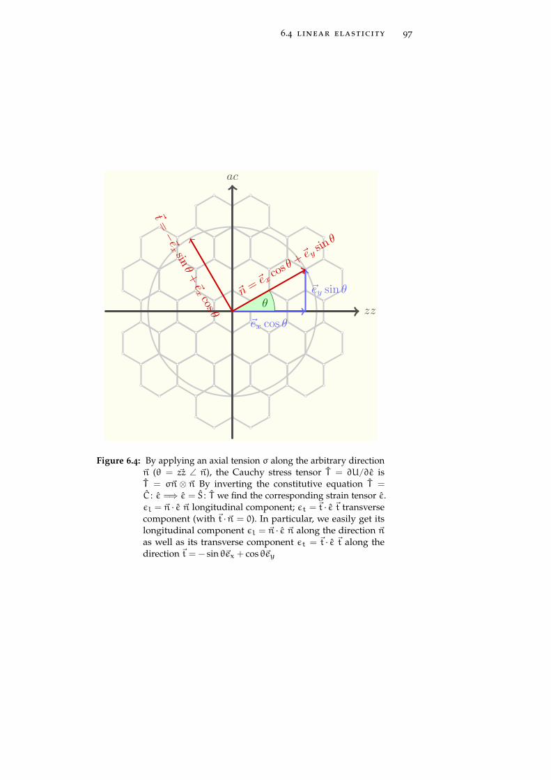
6.4 linear elasticity 97
zz
ac
θ~ey sin θ
~ex cos θ
~n = ~excos
θ + ~eysinθ
~t =−~e
x sinθ+~e
x cos θ
Figure 6.4: By applying an axial tension σ along the arbitrary direction~n (θ = ~zz ∠ ~n), the Cauchy stress tensor T = ∂U/∂ε isT = σ~n ⊗ ~n By inverting the constitutive equation T =
C : ε =⇒ ε = S : T we find the corresponding strain tensor ε.εl = ~n · ε ~n longitudinal component; εt = ~t · ε ~t transversecomponent (with ~t · ~n = 0). In particular, we easily get itslongitudinal component εl = ~n · ε ~n along the direction ~n
as well as its transverse component εt = ~t · ε ~t along thedirection ~t = − sin θ~ex + cos θ~ey

98 elastic properties of graphane
particular, we easily get its longitudinal component εl = ~n · ε ~n
along the direction ~n
εl = σ
[C11
∆s4 +
C22
∆c4 +
(1
C44− 2
C12
∆
)c2s2
](6.3)
as well as its transverse component εt = ~t · ε~t along the direction~t = − sin θ~ex + cos θ~ey (with ~t · ~n = 0)
εt = σ
[(C11 + C22
∆−
1
C44
)c2s2 −
C12
∆
(c4 + s4
)](6.4)
where ∆ = C11C22 − C212, c = cos θ, and s = sin θ. By meansof Eqs.(6.3) and (6.4) we obtain, respectively, the ~n-dependentYoung modulus E~n = σ/εl (i.e. the ratio between the appliedThe ~n-dependent
Young modulus traction and the longitudinal extension) as
E~n =∆
C11s4 + C22c4 +(∆
C44− 2C12
)c2s2
(6.5)
and the ~n-dependent Poisson ratio ν~n = −εt/εl (i.e. the ratiobetween the lateral contraction and the longitudinal extension)asThe ~n-dependent
Poisson ratio
ν~n = −
(C11 + C22 − ∆
C44
)c2s2 − C12
(c4 + s4
)C11s4 + C22c4 +
(∆
C44− 2C12
)c2s2
(6.6)
Eqs.(6.5) and (6.6) are central to our investigation. More detailregard these derivations can be found in the Appendix A.6
First of all, we remark that they allow for the full linear elas-tic characterization of both the anisotropic graphane conform-ers and the trigonal one (as well as graphene), provided thatin the latter case the isotropy and Cauchy conditions are dulyexploited. In this case we in fact obtain the Young modulusE = (C211 − C212)/C11 and the Poisson ratio ν = C12/C11, whichare independent of the angle θ, confirming the planar isotropy.
More importantly, however, Eqs.(6.5) and (6.6) imply that E~n
and ν~n can be directly obtained by the linear elastic constants Cij,in turn computed through energy-vs-strain curves correspondingto suitable homogeneous in-plane deformations. This impliesHomogeneous
in-plane deformationmethod
that there is no actual need to mimic by a computer simulationa traction experiment along the arbitrary direction identified by~n or θ, indeed a technically complicated issue to accomplish.Rather, for the isotropic case (graphene and C-graphane) onlytwo in-plane deformations should be applied in order to obtainall the relevant elastic constants, namely: (i) an axial deformationalong the zigzag direction; and (ii) an hydrostatic planar defor-mation. For the anisotropic case (B- and W-graphane) two morein-plane deformations must be applied: (iii) an axial deformation

6.4 linear elasticity 99
Tabl
e6.
2:D
efor
mat
ions
and
corr
espo
ndin
gst
rain
tens
ors
appl
ied
toco
mpu
teth
eel
astic
cons
tant
sCij
ofgr
apha
ne.T
here
latio
nbe
twee
nsu
chco
nsta
nts
and
the
fitt
ing
term
U(2
)of
Eq.
(6.7
)is
rep
orte
das
wel
l.D
efor
mat
ions
(i)-
(ii)
are
app
lied
toth
eC
-con
form
er,
whi
leth
efu
llse
t(i
)-(i
v)of
defo
rmat
ions
isap
plie
dto
the
B-an
dW
-con
form
ers.ζ
isth
esc
alar
stra
inpa
ram
eter
.
stra
inte
nsor
U(2
)U
(2)
isot
ropi
cst
ruct
ures
anis
otro
pic
stru
ctur
es
(i)
zigz
agax
iald
efor
mat
ion
( ζ0 00)
C11
C11
(ii)
hydr
osta
tic
plan
arde
form
atio
n( ζ0 0ζ
)2(C11
+C12)
C11
+C22
+2C12
(iii)
arm
chai
rax
iald
efor
mat
ion
( 00 0ζ)
C22
(iv)
shea
rde
form
atio
n( 0ζ ζ0
)4C44
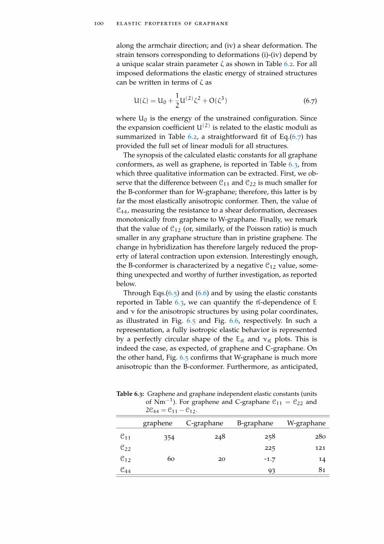
100 elastic properties of graphane
along the armchair direction; and (iv) a shear deformation. Thestrain tensors corresponding to deformations (i)-(iv) depend bya unique scalar strain parameter ζ as shown in Table 6.2. For allimposed deformations the elastic energy of strained structurescan be written in terms of ζ as
U(ζ) = U0 +1
2U(2)ζ2 +O(ζ3) (6.7)
where U0 is the energy of the unstrained configuration. Sincethe expansion coefficient U(2) is related to the elastic moduli assummarized in Table 6.2, a straightforward fit of Eq.(6.7) hasprovided the full set of linear moduli for all structures.
The synopsis of the calculated elastic constants for all graphaneconformers, as well as graphene, is reported in Table 6.3, fromwhich three qualitative information can be extracted. First, we ob-serve that the difference between C11 and C22 is much smaller forthe B-conformer than for W-graphane; therefore, this latter is byfar the most elastically anisotropic conformer. Then, the value ofC44, measuring the resistance to a shear deformation, decreasesmonotonically from graphene to W-graphane. Finally, we remarkthat the value of C12 (or, similarly, of the Poisson ratio) is muchsmaller in any graphane structure than in pristine graphene. Thechange in hybridization has therefore largely reduced the prop-erty of lateral contraction upon extension. Interestingly enough,the B-conformer is characterized by a negative C12 value, some-thing unexpected and worthy of further investigation, as reportedbelow.
Through Eqs.(6.5) and (6.6) and by using the elastic constantsreported in Table 6.3, we can quantify the ~n-dependence of Eand ν for the anisotropic structures by using polar coordinates,as illustrated in Fig. 6.5 and Fig. 6.6, respectively. In such arepresentation, a fully isotropic elastic behavior is representedby a perfectly circular shape of the E~n and ν~n plots. This isindeed the case, as expected, of graphene and C-graphane. Onthe other hand, Fig. 6.5 confirms that W-graphane is much moreanisotropic than the B-conformer. Furthermore, as anticipated,
Table 6.3: Graphene and graphane independent elastic constants (unitsof Nm−1). For graphene and C-graphane C11 = C22 and2C44 = C11 − C12.
graphene C-graphane B-graphane W-graphane
C11 354 248 258 280
C22 225 121
C12 60 20 -1.7 14
C44 93 81

6.4 linear elasticity 101
zigzag
θ=30°
θ=60
°
armchair
grapheneB−graphaneC−graphaneW−graphane
0
100
300
Figure 6.5: Polar diagram for the Young modulus E of graphene andgraphane conformers. The angle θ identifies the extension di-rection with respect to the zigzag one. Isotropic (anisotropic)behavior is associated to a circular (non circular) shape ofthe E~n plot.
Fig. 6.6 provides evidence that the Poisson ratio in any graphaneconformer is much smaller than in pristine graphene, since thecorresponding ν~n polar plots are contained within the graphenecircle.
An intriguing unconventional behavior is observed in Fig. 6.6for B-graphane, namely: for extensions along to the zigzag andarmchair directions, the corresponding Poisson value is vanish-ingly small. This feature appears as a flower petal structure of theν~n plot for such a system. By considering Fig. 6.7, where a zoomof the previous plot nearby the origin has been reported, wecan actually learn more information. It is evident that four smalllobes appear along the zigzag and armchair directions (i.e. alongthe principal axis of the orthorhombic symmetry), correspondingto a Poisson ratio varying in the range −0.0075 < ν < −0.0065.The limiting values are computed for extensions along the zigzagand armchair directions, respectively. It is truly remarkable that νcould be negative in B-graphane. While a negative Poisson ratiovalue is allowed by thermo-elasticity, this peculiar situation is Negative Poisson
ratioonly observed in special systems (i.e. foams, molecular networksor tailored engineering structures) or just rarely in ordinary bulkmaterials (i.e. SiO2, cubic metals, or polymer networks) [103].

102 elastic properties of graphane
0
zigzag
θ =30°
θ =6
0°armchair
grapheneB−graphaneC−graphaneW−graphane
0.1
0.2
Figure 6.6: Polar diagram for the Poisson ratio ν of graphene andgraphane conformers. The angle θ identifies the extension di-rection with respect to the zigzag one. Isotropic (anisotropic)behavior is associated to a circular (non circular) shape ofthe ν~n plot. The special case of B-graphane is enlighten byshading (see text).
zigzag
armchair
ν > 0ν < 0
θ=30°
θ=60
°
0
0.004
0.008
Figure 6.7: The same as Fig. 6.6 zoomed in the region nearby the origin.Positive and negative Poisson ratio values are differentlyshaded as indicated.

6.5 nonlinear elasticity 103
Table 6.4: Strain fields applied to compute the linear (Cij) and nonlin-ear (Cijk) elastic constants of the C-graphane. The relationbetween such constants and the fitting terms U(2) and U(3)
of Eq.(6.11) is reported as well.
Strain U(2) U(3)
tensor(ζ 00 0
)C11 C111(
ζ 00 ζ
)2 (C11 + C12) 2C111 + 6C112(
0 ζζ 0
)2 (C11 − C12) 8C444(
ζ ζζ 0
)3C11 − 2C12 C111 + 12C144 + 6C114 + 8C444(
0 ζζ −ζ
)3C11 − 2C12 −C111 − 12C144 + 6C114 + 8C444(
ζ ζζ −ζ
)4 (C11 − C12) 12C114 − 12C124 + 8C444
6.5 nonlinear elasticity
In this Section we generalize the previous analysis in orderto draw a comparison between the nonlinear elastic behavior ofgraphene, see Chapter 5, and the three conformers of graphane.The nonlinear strain energy function Uhex for an hexagonal twodimensional lattice is (see Chapter 5 ) Nonlinear strain
energy function
Uhex =1
2C11
(ε2xx + ε2yy + 2ε2xy
)+ C12
(εxxεyy − ε2xy
)+
1
6C111ε
3xx +
1
6C222ε
3yy +
1
2C112ε
2xxεyy
+1
2(C111 − C222 + C112)εxxε
2yy
+1
2(3C222 − 2C111 − C112)εxxε
2xy
+1
2(2C111 − C222 − C112)εyyε
2xy (6.8)
where all the nonlinear features are described by the three inde-pendent moduli C111, C222 and C112. Similarly, the strain energyfunction Utrigo for C-graphane depending on the linear (C11 andC12) and nonlinear (C111, C112, C144, C114, C124 and C444) elasticconstants is found to be
Utrigo =1
2C11
(ε2xx + ε2yy + 2ε2xy
)+ C12
(εxxεyy − ε2xy
)+
1
6C111
(ε3xx + ε3yy
)+1
2C112
(ε2xxεyy + εxxε
2yy
)+ 2C144
(εxxε
2xy + εyyε
2xy
)+ C114
(ε2xxεxy + ε2yyεxy
)+ 2C124εxxεxyεyy +
4
3C444ε
3xy (6.9)

104 elastic properties of graphane
Table 6.5: Strain fields applied to compute the linear (Cij) and nonlin-ear (Cijk) elastic constants of the B- and W-graphane. Therelation between such constants and the fitting terms U(2)
and U(3) of Eq.(6.11) is reported as well.
Strain U(2) U(3)
tensor(ζ 00 0
)C11 C111(
0 00 ζ
)C22 C222(
ζ 00 ζ
)C11 + C22 + 2C12 C111 + C222 + 3C112 + 3C122(
0 ζζ 0
)4C44 0(
ζ ζζ 0
)C11 + 4C44 C111 + 12C144(
0 ζζ ζ
)C22 + 4C44 C222 + 12C244(
ζ 00 −ζ
)C11 + C22 − 2C12 C111 − C222 − 3C112 + 3C122
For such a trigonal symmetry we have C111 = C222, C112 = C122and C144 = C244. Nevertheless, it is important to underline thatthe overall nonlinear elastic response is truly anisotropic sincenot all the relevant isotropic conditions are fulfilled.
Finally, the strain energy function Uortho for the B- and W-graphane, expressed through the linear (C11, C22, C12 and C44)and nonlinear (C111, C222, C112, C122, C144 and C244) elastic con-stants, is given by
Uortho =1
2C11ε
2xx +
1
2C22ε
2yy + 2C44ε
2xy + C12εxxεyy
+1
6C111ε
3xx +
1
6C222ε
3yy +
1
2C112ε
2xxεyy
+1
2C122εxxε
2yy + 2C144εxxε
2xy + 2C244εyyε
2xy(6.10)
Eqs.(6.8), (6.9) and (6.10) can be obtained by using the standardtables of the tensor symmetries, found in many crystallographytextbooks (see for instance Ref. [102]).
As above described, in any symmetry the strain energy functiondepends on the third-order elastic constants (as well as the linearones). Once again, they can be computed through energy-vs-strain curves corresponding to suitable homogeneous in-planedeformations. For each deformation the elastic energy of strainedgraphene or graphane can be written in terms of just the singledeformation parameter ζ
U(ζ) = U0 +1
2U(2)ζ2 +
1
6U(3)ζ3 +O(ζ4) (6.11)

6.5 nonlinear elasticity 105
Table 6.6: Graphene and graphane independent nonlinear elastic con-stants (units of Nm−1).
graphene C-graphane B-graphane W-graphane
C111 -1910 ± 11 -1385±18 -1609±31 -1756±33
C222 -1764 ± 3 -1827±7 -487±85
C112 -341 ± 35 -195±41 -20±14 -75±54
C122 -55±22 -296±36
C124 -411±17
C114 530±12
C144 568±7 -161±4 -143±17
C244 -159±3 -287±10
C444 0.0±10−5
Since the expansion coefficients U(2) and U(3) are related toelastic constants, as summarized in Table 6.4 for the C-graphaneand in Table 6.5 for the B- and W-graphane, a straightforwardfit of Eq.(6.11) has provided the full set of third-order elasticconstants.
The results have been reported in Table 6.6 where only thevalues of the independent elastic constants appearing in Eqs.(6.8), (6.9) and (6.10) are reported. We note that graphene andB-graphane are characterized by an inverted anisotropy: whileC111 < C222 for graphene, we found C222 > C111 for B-graphane.On the contrary, W-graphane has the same anisotropy of graphene(C111 < C222), but a larger |C111 − C222| difference. So, it is in-teresting to observe that the different distribution of hydrogenatoms can induce strong qualitative variations for the nonlinearelastic behavior of these structures.
We finally observe that necessarily C444 = 0 for B- and W-graphane because of the orthorhombic symmetry. On the otherhand, this nonlinear shear modulus could assume any valuefor the trigonal lattice. Interesting enough, we have verified thatC444 = 0 also for C-graphane. This is due to the additional(with respect to the trigonal symmetry) mirror symmetry of C-graphane.
As shown in Chapter 5, similarly to the case of graphene [12],a nonlinear stress-strain relation can be derived for the threegraphane conformers:
σ~n = E~nε~n +D~nε2~n (6.12)
where E~n and D~n are, respectively, the Young modulus andan effective nonlinear (third-order) elastic modulus, along thearbitrary direction ~n, as defined in Sec. 6.4. The nonlinear elastic

106 elastic properties of graphane
zigzag
θ=30°
θ=60
°
armchair
C−graphane (D > 0.0)C−graphane (D < 0.0)B−graphane (D < 0.0)C−graphane (D < 0.0)
0 250 500 750 1000 1000 750 500 250 0
Figure 6.8: Polar representation of the nonlinear elastic moduli D~n ofthe three graphane conformers. In the B- and W-graphanecases, D~n ≡ D are everywhere negative (softening hyper-elesticity), while in the C-graphene one the D~n alternatesnegative and positive values (hardening hyperelesticity).
6.5 nonlinear elasticity 107
modulus D(trigo)~n for the C-graphane (as well as for any trigonal
2D lattice) is given by
D(trigo)~n = 1
2
[ν (1− ν) (C111 − 3C112)
+ (1− ν)(1+ ν2
)C111
+6cs (1+ ν)(1+ ν2
)C114 − 12cs (1+ ν)νC124
+3c2s2 (1− ν)(1+ ν2
)(−C111 + 4C144 + C112)
+4c3s3 (1+ ν)(1+ ν2
)(−3C114 + 2C444 + 3C124)
+8c3s3 (1+ ν)ν (−6C114 + 5C444 + 6C124)]
(6.13)
while the corresponding modulus D(ortho)~n B- and W-graphene
is
D(ortho)~n =
1
2∆3E3~n
[C111
(C22c
2 − C12s2)3
+C222(C11s
2 − C12c2)3
+3C112(C11s
2 − C12c2) (
C22c2 − C12s
2)2
+3C122(C22c
2 − C12c2) (
C11s2 − C12c
2)2
−3C166c2s2
(C22c
2 − C12s2)(∆/C44)
2
−3C266c2s2
(C11s
2 − C12c2)(∆/C44)
2](6.14)
where ∆ = C11C22 − C212, c = cos θ, and s = sin θ. Since Cijk < 0,as shown in Tab.6.6, D(ortho)
~n are negative for any direction (see Fig. 6.8), so both B- and W-graphane show an hyperelasticsoftening behavior. The trigonal C-graphane behaves in a verydifferent way instead. Since the C114 and C144 are positive, theC-graphane can show an hyperelastic hardening behavior in theangular sectors 5/12π+ kπ < θ < 1/12+ kπ and 8/12π+ kπ <
θ < 10/12+ kπ (kεZ).In conclusion, present first principles calculations predict that
the class of auxetic materials is larger than reported so far, includ-ing as well two dimensional hydrocarbons like B-graphane. Moreprecisely, since a negative Poisson ratio is observed for extensionsalong the zigzag and armchair principal directions, B-graphaneis better referred to as an axially auxetic atomic sheet. Moreover,we calculated that the other two conformers, namely the C- andW-graphane, exhibit a vanishingly small value of the Poissonratio. The linear moduli values are in agreements with those re-cently reported in literature [25]. The nonlinear elastic behavior ofgraphane shows peculiar features as well. In particular, we havefound that the C-graphane admits both softening and hardeninghyperelasticity, depending on the direction of the applied strain.These features makes graphane a very intriguing material withpotentially large technological impact in nanomechanics.

7G A P O P E N I N G I N G R A P H E N E B Y S H E A RS T R A I N
“The Indians are finding the gaps like a pin in a haystack.”Navjot Singh Sidhu
Contents7.1 Introduction and motivation 1097.2 The electronic structure of graphene 1107.3 Some detail about the out-of-plane relaxation 117
In this Chapter we exploit the concept of strain-induced bandstructure engineering in graphene through the calculation ofits electronic properties under uniaxial, shear, and combineduniaxial-shear deformations. We show that by combining sheardeformations to uniaxial strains it is possible modulate the grapheneenergy gap value from zero up to 0.9 eV. Interestingly enough, theuse of a shear component allows for a gap opening at moderateabsolute deformation, safely smaller than the graphene failurestrain, i.e. in a range of reversible and more easily accessibledeformations, ranging in between 12% and 17%. We also discussthe merging of Dirac points [104], which is involved into the gapopening process.
7.1 introduction and motivation
As report in Chapter 1, graphene exhibits a number of exoticelectronic properties, such as unconventional integer quantumHall effect, ultrahigh electron mobility, electron-hole symmetryand ballistic transport even at room temperature [5, 38, 105]. Fullaccount of these features is provided by the relativistic Diractheory [7] suitably developed within the standard condensedmatter formalism. A key feature of graphene is that its elec-tronic density of states vanishes at the so-called Dirac points,where the valence and the conduction bands cross with a linearenergy-momentum dispersion. Due to the hexagonal symmetryof graphene, the Dirac points are located at two high-symmetrypoints of its Brillouin zone. Dirac points due to
the hexagonalsymmetry
While many other properties of graphene are very promis-ing for nanoelectronics, its zero-gap semiconductor nature isdetrimental, since it prevents the pinch off of charge current asrequested in conventional electronic devices. Different attempts
109

110 gap opening in graphene by shear strain
have been therefore tried in order to induce a gap, for instance byquantum confinement of electrons and holes in graphene nanorib-bons [17] or quantum dots [18]. These patterning techniquesare unfortunately affected by the edge roughness problem [19],namely: the edges are extensively damaged and the resulting lat-tice disorder can even suppress the efficient charge transport. Thesensitivity to the edge structure has been demonstrated throughexplicit calculations of the electronic states in ribbons [20]. Morerecently, it has been shown experimentally that a band gap aslarge as 0.45 eV can be opened if a graphene sheet is placed on anIr(111) substrate and exposed to patterned hydrogen adsorption[21].
Alternatively, an electronic band gap can be obtained by grow-ing graphene sheets on an appropriately chosen substrate, in-ducing a strain field controllable by temperature [27, 28, 29, 30].Recently, it has been experimentally shown that by using flexiblesubstrates a reversible and controlled strain up to ∼ 18% [29] canbe generated with measurable variations in the optical, phononand electronic properties of graphene [30]. This interesting resultsuggests that gap opening could be engineered by strain, ratherthan by patterning. The idea has been theoretically validatedby Pereira and Castro Neto [31] showing that a gap is indeedgenerated by applying an uniaxial strain as large as ∼ 23%, ap-proaching the graphene failure strain εf = 25% [12] (see Chapter5). This large value stands for the high robustness of the gaplessfeature of graphene under deformation. The same authors pro-pose an alternative origami technique [13] aimed at generatinglocal strain profiles by means of appropriate geometrical patternsin the substrate, rather than by applying strain directly to thegraphene sheet.
7.2 the electronic structure of graphene
The electronicstructure ofgraphene by meansof a semi-empiricalsp3 tight-binding(TB) model
The electronic structure of graphene has been computed foreach deformed configuration by means of a semi-empirical sp3
tight-binding (TB) model, making use of the two-center param-eterization by Xu et al. [50]. as discussed in Sec. 2.1. Despite itssemi-empirical character, the present TB model correctly pro-vides the occurrence of Dirac points in the band structure ofgraphene in its equilibrium geometry. Furthermore, the Xu et al.parametrization provides accurate scaling functions for the vari-ation of the TB hopping integrals upon lattice distortions. Thisfeature is instrumental for investigating gap opening in grapheneby strain.
As discuss in Chapter 1, graphene is an hexagonal lattice withtwo carbon atoms per unit cell and a lattice basis defined bythe vectors (a1, a2), as shown in Fig. 7.1, with a nearest-neighbor

7.2 the electronic structure of graphene 111
zig-z
ag
armchair
y
x
~a1
~a2
Figure 7.1: Top view of the hexagonal graphene lattice with its lattice
vectors a1,2 = a0
(32 ,±
√32
), where a0 is the equilibrium
C-C distance. Axis x and y corresponds to the armchair andzig-zag direction, respectively. Shaded area represents theunit cell.
x
(b) (c)
K
MkΓ
(a)
yk
x
’
’
K
M
y
kΓ
kK’
M’K
M
M"K’
yk
xkΓ
K’’M’
K"
Figure 7.2: Brillouin zone of graphene under strain. The shaded ar-eas are the corresponding irreducible part: Panel (a), un-deformed BZ with 6/mmm hexagonal symmetries; Panel(b), BZ deformed by uniaxial strain with mmm rhombicsymmetry; Panel (c), BZ deformed by shear strain with 2/mmonoclinic symmetry.
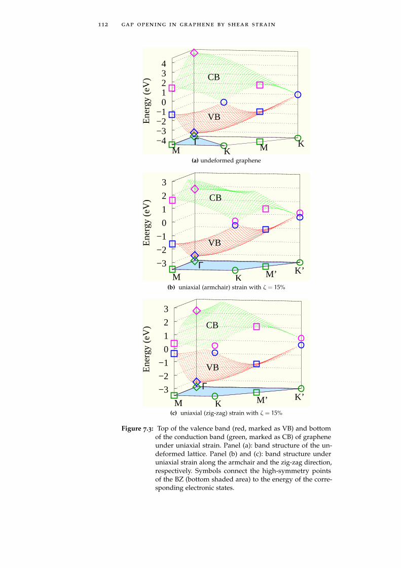
112 gap opening in graphene by shear strain
M K−4−3−2−1 0 1 2 3 4
M KΓ
Ene
rgy
(eV
) CB
VB
(a) undeformed graphene
−3
−2
−1
0
1
2
3
K M’Γ K’
Ene
rgy
(eV
)
M
CB
VB
(b) uniaxial (armchair) strain with ζ = 15%
−3
−2
−1
0
1
2
3
M K M’ K’Γ
Ene
rgy
(eV
) CB
VB
(c) uniaxial (zig-zag) strain with ζ = 15%
Figure 7.3: Top of the valence band (red, marked as VB) and bottomof the conduction band (green, marked as CB) of grapheneunder uniaxial strain. Panel (a): band structure of the un-deformed lattice. Panel (b) and (c): band structure underuniaxial strain along the armchair and the zig-zag direction,respectively. Symbols connect the high-symmetry pointsof the BZ (bottom shaded area) to the energy of the corre-sponding electronic states.

7.2 the electronic structure of graphene 113
carbon-carbon distance as small as a0 = 1.42 Å. The in-planeelastic behavior of the honeycomb lattice is isotropic in the linearregime, but two inequivalent crystallographic directions can benevertheless defined: the so-called armchair and zig-zag direc-tions, shown in Fig. 7.1 as x and y axis, respectively. Accordingto the Cauchy-Born rule, when straining a graphene sample itslattice vectors are affected accordingly, as well as the associatedreciprocal vectors (b1, b2). The deformed metric tensor are given The deformed
reciprocal latticevectors
(b ′1, b ′2
)by a ′iα = (εik + δik)akα, here the vector indices i = 1, 2 andthe Cartesian indices α = x,y, and ε =
εij
is the strain ten-sor describing the deformation and i, j = x,y. The condition(b ′1, b ′2
)T= 2π
(a ′1, a ′2
)−1 allows us to obtain the deformed recip-rocal lattice vectors. The applied in-plane
deformations tohoneycomb latticeunder plane-strainborder conditions
The following in-plane deformations have been applied to theequilibrium honeycomb lattice under plane-strain border condi-tions: i) an uniaxial deformation ζ along the armchair direction,corresponding to a strain tensor ε(ac)
ij = ζδixδjx; ii) an uniaxialdeformation ζ along the zig-zag direction, corresponding to astrain tensor ε(zz)
ij = ζδiyδjy; iii) an hydrostatic planar defor-
mation ζ, corresponding to the strain tensor ε(p)ij = ζδij; iv) a
shear deformation ζ, corresponding to an in-plain strain tensorε
(s)ij = ζ
(δixδjy + δiyδjx
). For any deformend configuration, we
have computed the corresponding electronic band structure anddensity of states. The carbon atoms in graphene shown the sp2
hybridization. Among the four valence orbitals, three (2s, 2px,2py) are combined to form the in-plane σ (bonding or occupated)and σ∗ (anti-bonding or unoccupated) orbitals, while the delocal-ized π (bonding) and π∗ (anti-bonding) are due to the interactionwith neighboring 2pz (where ~z are orthogonal to the graphenesheet). Because of the σ and σ∗ bands are well separeted in energy( 10 eV at Γ ), the π and π∗ bands coincide with the valence andthe conduction bands, respectively. Such that they are enough todescribe the electronic properties of graphene in its equilibriumstatus and also up to an applied strain of 10%, when the σ, σ∗and π, π∗ bands overlap at Γ . In the following we discuss theresults simply in terms of valence and conduction bands.
In order to extend the reliability of the present model to elec-tronic features under strain, our results about the effects of hy-drostatic and uniaxial deformations on the band structure areat first compared with previous data available in literature. Forgraphene under in-plane hydrostatic deformation with ζ 6 15%, In-plane hydrostatic
deformationboth in compression and in traction, we have calculated the bandelectronic structure and the density of states. Since the hydro-static strain does not change the D6h(6/mmm) symmetry of thehexagonal lattice (Fig. 7.2a), we only observe the variation of thepseudogaps at Γ and M points, while the location of the Dirac

114 gap opening in graphene by shear strain
−4−3−2−1 0 1 2 3 4
K’K"
Γ
KK’
Ene
rgy
(eV
)
CB
VB
Figure 7.4: Top of the valence band (red, marked as VB) and bottomof the conduction band (green, marked as CB) of grapheneunder pure shear strain with ζ = 20%. Symbols connect thehigh-symmetry points of the BZ (bottom shaded area) tothe energy of the corresponding electronic states.
points is clamped at the K point. In particular, the pseudogapat M decreases almost linearly from 6 eV (for ζ = −15%) to 1.8eV (for ζ = +15%). We remind that its value for the unstrainedconfiguration is 2.2 eV. These results are in quantitative goodagreement with Ref. [90]. Any other non-hydrostatic deformationlowers the symmetry of the graphene lattice. When an uniaxialstrain is applied, all the 6- and 3-fold rotational symmetries areUniaxial strain
lost: a transition from the hexagonal D6h(6/mmm) to the rhom-bic D2h(mmm) symmetry is observed (Fig. 7.2b). The irreduciblepart of the first Brillouin zone (BZ) is also affected by such defor-mations, since its original triangular shape (Fig. 7.2a) is variedto the polygonal form represented in Fig. 7.2b. The top of thevalence band and the bottom of the conduction band are shownin Fig. 7.3 for the undeformed configuration (panel a), as well asunder uniaxial deformation (panels b and c, corresponding to astrain ζ = 15% along the armchair direction and in the zig-zagdirection respectively). The main effect of strain is the openingof a pseudo-gap at K and K’. Accordingly, the Dirac points areno more located at such high-symmetry points; rather, they driftaway within the BZ, either for deformations along armchair direc-tion or along zig-zag one. Once again this important qualitativefeature is in good agreement with Ref. [31].
Let us now consider the case of an in-plane shear deformation,In-plane sheardeformation described by the following shear strain
ε =
(0 ζ
ζ 0
)(7.1)

7.2 the electronic structure of graphene 115
where ζ is the strain parameter. Such a deformation modifies theoriginal reciprocal lattice vectors b1 and b2 into
b ′1 =2π
a
(1− ζ2
)−1(13
−
√3
3ζ,√3
3−1
3ζ
)
b ′2 =2π
a
(1− ζ2
)−1(+1
3+
√3
3ζ, −
√3
3−1
3ζ
)(7.2)
By applying the shear strain given in Eq. (7.1) to the graphenelattice, its symmetry class is further lowered to monoclinic. Thecorresponding symmetry group is 2/m. Because of this change insymmetry, the irreducible part of the BZ is affected accordinglyas shown in Fig. 7.2c, which has K’, K, K", K’ as corners. Inthe undeformed lattice, a Dirac point is located at each of thesecorners. The scenario under shear strain is quite different fromthe case of uniaxial deformations: at the comparatively smallstrain ζ ' 16%, a gap is indeed opened. The rise of a gap in theelectronic band structure under shear is due to a peculiar processthat involves the merging of two Dirac points, namely D’ andD", which move away from the corners K’ and K" and approacheach other inside the BZ. By “merging“ we mean the following:as shown in Fig. 7.5, at a critical strain ζ ' 15.95% the Diracpoints are so close that they annihilate in a single hybrid Diraccone, which shows a peculiar energy-momentum dispersion: it islinear (quadratic) along (perpendicular) to the direction joiningthe two Dirac points. At ζ = 16.0%, a gap as small as 0.05 eV iseventually opened. More details about the motion of Dirac pointsin two-dimensional crystals under uniaxial stress are reported inRef. [104, 106, 107]. Merging of Dirac
conesIs important to remark that the merging of the two inequivalentDirac points and the opening of a gap, appear for a shear strainvalue ζ ' 16% which is lower than in the case of zig-zag uniaxialdeformation [31]. The gap increases up to a maximum value of0.72 eV for shear strain parameter of ζ ' 20%, as shown in Fig.7.4. Moreover, the same detail is shown in Fig. 7.5b-c: in panel b,at a strain ζ ' 15.9% the couple of Dirac points are very close, butnot yet annihilated and at their middle point D a pseudo-gap ∆can be observed; in panel c, the band structure shows a small gapalready at ζ ' 16%. We conclude that shear strain seems a likelycandidate to achieve gap opening in graphene for a deformationfar enough from failure strain and, therefore, achievable with nodanger for the overall mechanical stability of the two-dimensionalsheet.
Gap opening is predicted by the present TB calculation tooccur at an even smaller strain parameter ζ, provided that acombination of shear and uniaxial strain is considered. By addingan uniaxial component to shear we generate a strain tensor of theform Combining uniaxial
and sheardeformations

116 gap opening in graphene by shear strain
y
x
vM’
M’ c
K c
vKv
cM c
MM"
K"v
K’ v
cK"c
cM"K’
v
Γ
Γ v
K’ c
K’ v
−2 −1 0 1 2−4
−3
−2
−1
0
1
2
3
1 0k
k
Ene
rgy
[eV
]
(a) shear strain ζ =15%
F
y
x
D O
∆D’ E
E
k
k
D "
(b) ζ = 15.9%
∆
oD
(c) ζ = 16.0%
Figure 7.5: (a) Electronic band structure of purely sheared graphene(with the same value of strain parameter ζ = 15%) areshown in the corresponding irreducible zone. The Diraccones (blue ellipse) are enlarged and shown in panels b-c:(b) with ζ = 15.9% the couple of Dirac cones D’ and D" arejust before merging and shown a pseudo-gap ∆ at D equalto 0.15eV; (c) with ζ = 16.0% the merging is occurred andthe gap is equal to 0.05 eV.

7.3 some detail about the out-of-plane relaxation 117
ε =
(ζ ζ
ζ 0
)or ε =
(0 ζ
ζ ζ
)(7.3)
for which the symmetry class of the lattice is not changed withrespect to the pure shear case.
Nevertheless, uniaxial deformations along the armchair or zig-zag direction are found to dissimilarly affect the band structureof graphene. Only in the last case we have observed the mergingof the Dirac points already at ζ ' 12%. The main features of thetransition is the same as described before. The energy gap growsup to a maximum value of 0.95 eV (when the strain parameterachieves a value of ζ ' 17%), reducing again to zero at ζ ' 20%due to the steady decrease of the direct gap at Γ .
In order to quantitatively describe the evolution of the gapopening as function of the applied strain, the density of states(DOS) has been calculated by a two-dimentional 75× 150× 1regular k-point mesh of the (deformed) BZ. As shown in Fig.7.6, for a strain value less then 15% (panel a) or 11% (panel b),the DOS depends linearly on energy close to the Fermi level,showing a slope increasing with the strain. The two characteristicVan Hove singularities into the DOS move closer the Fermi energyand disappear into abrupt gap-edges as soon as the gap is open.After the annihilation of the Dirac points, the DOS shows a ∼
√E
behavior.We conclude by remarking that the two strain contributions (i.e.
uniaxial and shear) could be combined in different ways so as tomodulate the energy gap value. In Fig. 7.7, the electronic bandstructures of graphene under different combinations of shearand uniaxial strain are compared, keeping the same value of thestrain parameter ζ = 15%. While the combination of shear withuniaxial armchair shows a sizable energy gap of about 0.6 eV,the combination of shear with uniaxial zig-zag is associated to agapless band structure.
7.3 some detail about the out-of-plane relaxation
We showed that by combining shear deformations to uniaxialstrains it is possible to affect the gapless electronic structure ofgraphene by opening a gap as large as 0.9 eV. The use of a shearcomponent allows for gap opening at a moderate absolute defor-mation, safely smaller than the graphene failure strain. This resultwas obtained in absence of out-of-plane deformations (as due,e.g., to bending or rippling), a situation corresponding to config-urations where the graphene sheet is supported, i.e. deposited ona suitable substrate [27, 30, 29]. On the other hand out-of-planeatomic relaxations on a free standing graphene monolayer undershear strain can induced ripples. This is consistent with a well

118 gap opening in graphene by shear strain
−0.6 −0.4 −0.2 0 0.2 0.4 0.6
Den
sity
of S
tate
s (a
.u.)
Energy (eV)
ζ=0.00
ζ=0.16
ζ=0.18
ζ=0.20
(a) pure shear deformation
−0.6 −0.4 −0.2 0 0.2 0.4 0.6
Den
sity
of S
tate
s (a
.u.)
Energy (eV)
ζ=0.00
ζ=0.12
ζ=0.14
ζ=0.17
(b) (shear + armchair uniaxial) deformation
Figure 7.6: Density of states around the Fermi level (set convention-ally at 0 eV) as function of the strain parameter ζ . Panel(a): graphene under pure shear deformation. Panel (b):graphene under combined shear and uniaxial deformation(along the armchair direction). The maximum value of theenergy gap is observed for a strain parameter as large asζ ' 20% and ζ ' 17% respectively.
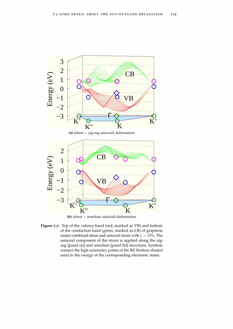
7.3 some detail about the out-of-plane relaxation 119
−3−2−1 0 1 2 3
KK’
K"
ΓK’
Ene
rgy
(eV
)
CB
VB
(a) (shear + zig-zag uniaxial) deformation
−3
−2
−1
0
1
2
KK’
K"K’
Γ
Ene
rgy
(eV
) CB
VB
(b) (shear + armchair uniaxial) deformation
Figure 7.7: Top of the valence band (red, marked as VB) and bottomof the conduction band (green, marked as CB) of grapheneunder combined shear and uniaxial strain with ζ = 15%. Theuniaxial component of the strain is applied along the zig-zag [panel (a)] and armchair [panel (b)] directions. Symbolsconnect the high-symmetry points of the BZ (bottom shadedarea) to the energy of the corresponding electronic states.

120 gap opening in graphene by shear strain
known result of continuum mechanics: shear, as well as uniax-ial, deformations come with reversible corrugations, whetherapplied to a free standing elastic membrane [108, 109]. There-fore the gap opening in graphene under shear deformation (orcombined uniaxial and shear deformations) could be unlikelyinhibited, since ripples should cancel the strain effects we foundfor a flat graphene sheet. While overall interesting, our resultsare addressed to a graphene sheet where out-of-plane relaxationsare inhibited. The first and second configurations correspond,respectively, to a suspended and to a supported sample. In addi-tion, we observe that the ripple geometry of a suspended sheetcan be effectively altered via thermal manipulation, up to a com-plete suppression when temperature is raised to 450-600K, asexperimentally found by Bao al. [110]. We believe that this resultprovides another example of ripple-free, but strained graphenemembrane, making our investigation relevant and physicallysound even for some suspended samples.
Interesting enough, in Ref. [110] it has been also reported thatthe measured wavelength of the ripples ranges from 370 to 5000
nm. Under this respect, once again we believe that our calcula-tions are meaningful: the larger is the wavelength of the ripples,the better is the approximation of a ripple-free graphene sheet(which locally is basically flat). Moreover, Pereira et al. [13] ex-plore the influence of local strain on the electronic structure ofgraphene. They suggest that the graphene electronics can becontrolled by suitable engineering of local strain profiles, a per-spective which is indeed in nice agreement with our conclusions.

8T H E B E N D I N G O F G R A P H E N E .
“Notice that the stiffest tree is most easily cracked, while the bambooor willow survives by bending with the wind.”
Bruce Lee (1940- 1973)
Contents8.1 Bending in carbon nanoribbons 1218.2 The bending rigidity theory 122
8.2.1 Continuum picture 122
8.2.2 Atomistic simulations 126
8.3 Simulation protocol and the calculated bend-ing features 130
In present Chapter we discuss the bending properties of car-bon nanoribbons by combining continuum elasticity theory andtight-binding atomistic simulations. First, we develop a completeanalysis of a given bended configuration through continuum me-chanics. Then, we provide by tight-binding calculations the valueof the bending rigidity in good agreement with recent literature.We discuss the emergence of a stretching field induced by the fullatomic-scale relaxation of the nanoribbon architecture. We furtherprove that such an in-plane strain field can be decomposed in afirst contribution due to the actual bending of the sheet and asecond one due to the edges effects induced by the finite size ofthe nanoribbon.
8.1 bending in carbon nanoribbons
Graphene [111] plays a unique role in materials science sinceit is the mother structure of most carbon sp2 nanosystems ofcurrent interest. By stacking, folding or bending a graphene sheetit is indeed possible to generate, respectively, graphite-like sys-tems, fullerene cages (pentagonal rings are here needed as well)or nanotubes. In particular, the bending properties are criticalin attaining the structural stability and morphology for bothsuspended and supported graphene sheets, and directly affecttheir electronic properties [38]. Rippling of pure graphene hasbeen also observed with mesoscopic amplitude and wavelength,both for suspended monolayers [36] and sheets deposited onsubstrates such as silicon dioxide [37]. Moreover, the bendingproperties play a central role in the design of graphene- or carbon
121

122 the bending of graphene .
nanotube-based devices, like e.g. mechanical resonators [39, 40].The bending features of functionalized graphene sheets have beenprobed by atomic force microscopy, observing that the folding be-havior is dominated by defects and functional groups [41]. Finally,bending ultimately governs the carbon nanotubes unzipping pro-cess, recently used to produce narrow ribbons for nanoelectronics[42]. With the same technique, a new class of carbon-based nanos-tructures, which combine nanoribbons and nanotubes, has beenintroduced in order to obtain magnetoresistive devices [43].
Within this scenario we frame the present investigation, ad-dressed to improve our fundamental understanding of the bend-ing properties of a one-atom thick carbon sheet. The main goalis twofold: i) to draw a thorough theoretical picture on bending,fully exploiting the elasticity theory and providing an atomisticquantitative estimation of the corresponding bending rigidity;ii) to prove that the bending process of a carbon nanoribbon isalways associated with the emergence of a (small) stretching, par-ticularly close to the edges. These results have been obtained bycombining continuum elasticity theory and tight-binding atom-istic simulations (TB-AS).
The conceptual development and actual exploitation of ourtheoretical model proceeds through the following steps. At first,by means of continuum mechanics we have obtained the exactshape for a purely bended nanoribbon, by imposing suitableboundary conditions. The bending rigidity is then evaluated byTB-AS for several nanoribbons differing by length and width. Asa second step, we observed that, under the above assumptionof pure bending, the corresponding rigidity must be a constantindependent of the actual shape of the sheet. Nevertheless byallowing full atomic-scale relaxation during bending, we ratherfound a geometry-dependent rigidity, a feature that we have at-tributed to the onset of stretching phenomena. Therefore, as finalstep, we have developed a procedure to discriminate betweenstretching and bending energy, so providing a complete pictureabout the mechanical behavior of graphene and also reconcilingthe atomistic data with the continuum theory results.
8.2 the bending rigidity theory
8.2.1 Continuum picture
The graphene strain energy density U [eVÅ−2] is defined as[112, 85]
U =1
2
E
1+ νTr(ε2)+1
2
Eν
1− ν2[Tr (ε)]2
+1
2κ (2H)2 − κK (8.1)

8.2 the bending rigidity theory 123
where E [Nm−1] and ν are the two dimensional Young modulusand the Poisson ratio, while κ [eV] and κ [eV] are the bend-ing rigidity and the Gaussian rigidity, respectively. The in-plane Bending rigidity and
the Gaussian rigiditydeformation (stretching) energy [given by the first two termsin Eq. (8.1)] is described by the standard small strain tensorε = 1
2(~∇~u+ ~∇~uT ), being ~u the displacement field. On the other
hand, the out of plane deformation (bending) energy [given bythe last two terms in Eq. (8.1)] is described by the mean curvature Geometric feature of
a surfaceH = k1+k22 [m−1] and by the Gaussian curvature K = k1k2
[m−2], where k1 and k2 are the principal curvatures at a givenpoint on the surface [113], as shown in Fig. 8.1a. They are straight-forwardly given by k1 = 1/R1 and k2 = 1/R2 where R1 and R2are the principal radii of curvature at that point. In the caseof a continuum plate of thickness h made of an isotropic andhomogeneous material, the classical Kirchhoff theory provides The classical
Kirchhoff theoryκ = 112
Eh2
1−ν2and κ = 1
12Eh2
1+ν (note that E = Yh where Y is thethree-dimensional Young modulus) [85]. For an infinitesimallythin graphene monolayer such a theory does not apply, since thethickness h cannot be unambiguously defined and the bendingmoment has simply a different physical origin. While the bendingmoment for the Kirchhoff plate derives from a compression/ex-tension of the different material layers forming the thickness h,in graphene it is due to the interactions among orbitals pz whichare affected by the bending process. Therefore, the determinationof κ and κ for graphene is a well-posed (and, to a large extent,still open) problem, which is independent of the evaluation of Eand ν [114].
To evaluate only the bending energy term, the ribbon has beenbended without stretching (i.e. strain ε = 0) Thus the Eq. (8.1) is The bending energy
of a bended ribbonwithout stretching
reduced to the only bending energy contribution Ub [eVÅ−2] ofa given cylindric surface
Us =1
2
E
1+ νTr(ε2)+1
2
Eν
1− ν2[Tr (ε)]2 = 0
Ub =1
2κ k21 (8.2)
As sketched in Fig. 8.1b, our model system is a rectangular ribbonwith length l and width L. The boundary conditions consist infixing the positions of the two parallel edges (with length l) at agiven distance a, while the attack angles θ is free to relax. Thisconfiguration involves only one curvature k1, leading to H = k1
2
and K = 0, as shown in Fig. 8.1b. By considering different valuesof a in the range (0,L), we obtained a set of differently bendedconfigurations. The elastic problem consists in finding the sheetshape by minimizing the bending energy
Ub =
∫ ∫A
UdA =1
2κl
∫L0k21ds (8.3)

124 the bending of graphene .
x
y
z
b
R2
b
R1
b
tangent plane
principal curvature planes
(a)
x
y
z
R2 →∞
b
R1
b
tangent plane
principal curvature planes
(b)
Figure 8.1: Panel (a) A sketch of the main geometrical features of ageneric surface. At a given point on the surface the princi-pal curvature planes and the corresponding principal radiiR1,R2 are shown. The red lines on the surface represent thegeodesics at the given point, i.e. the intersections betweenthe surface and the principal planes. Panel (b) In cylindricsurfaces one geodesic has to be a straight, here R2 → inf, sothat the Gaussian curvature goes to zero.
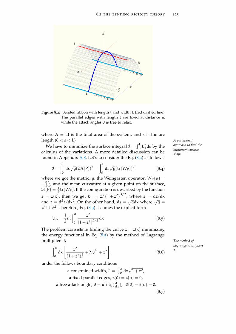
8.2 the bending rigidity theory 125
x
y
z
l
L fixed edges
fixed edges
aθ
Figure 8.2: Bended ribbon with length l and width L (red dashed line).The parallel edges with length l are fixed at distance a,while the attack angles θ is free to relax.
where A = Ll is the total area of the system, and s is the arclength (0 < s < L) A variational
approach to find theminimum surfaceshape
We have to minimize the surface integral I =∫L0 k21ds by the
calculus of the variations. A more detailed discussion can befound in Appendix A.8. Let’s to consider the Eq. (8.3) as follows
I =
∫L0ds√g(2H(P))2 =
∫L0ds√g(tr(WP))2 (8.4)
where we got the metric, g, the Weingarten operator, WP(u) =
−∂n∂u , and the mean curvature at a given point on the surface,H(P) = 1
2tr(WP). If the configuration is described by the function
z = z(x), then we get k1 = z/(1+ z2
)3/2, where z = dz/dx
and z = d2z/dx2. On the other hand, ds =√gdx where
√g =√
1+ z2. Therefore, Eq. (8.3) assumes the explicit form
Ub =1
2κl
∫a0
z2
(1+ z2)5/2
dx (8.5)
The problem consists in finding the curve z = z(x) minimizingthe energy functional in Eq. (8.5) by the method of Lagrangemultipliers λ The method of
Lagrange multipliersλ
∫a0dx
[z2
(1+ z2)52
+ λ√1+ z2
], (8.6)
under the follows boundary conditions
a constrained width, L =∫a0 dx√1+ z2,
a fixed parallel edges, z(0) = z(a) = 0,
a free attack angle, θ = arctg(dzdx), z(0) = z(a) = 0.
(8.7)

126 the bending of graphene .
enforcing the absence of any in-plane stretching. The above inte-gral can be written in the general form G(z) =
∫a0 dxF(z, z, z, x),
which is the solution of the Euler-Poisson differential equationEulero-Poissonequation
∂F
∂z−d
dx
∂F
∂z+d2
dx2∂F
∂z= 0 (8.8)
By the application of the constrained variational calculus weeventually obtain the final geometry in parametric representation[x(s), z(s)]The minimum
surface in parametricrepresentation[x(s), z(s)]
x
L=
E(q) − E(amK(q)
(1− 2 sL
),q)
K(q)−s
L(8.9)
z
L=
q
K(q)cn
K(q)(1− 2
s
L
)(8.10)
where s is the arc length (0 < s < L), q = sin θ2 is the ellipticmodulus and θ is the attack angle given by
a
L= 2
E(q)
K(q)− 1. (8.11)
The quantities E(q) and K(q) are the complete elliptic integrals,defined as [115, 116]The complete elliptic
integralsE(q) = F
(π2
,q)
, K(q) = E(π2
,q)
(8.12)
where the functions F(v,q) and E(v,q) are incomplete ellipticintegrals of the first and second kind, respectively [115, 116]
F(v,q) =
v∫0
dα√1− q2 sin2 α
E(v,q) =
v∫0
√1− q2 sin2 αdα. (8.13)
Moreover, by considering u = F(v,q) we define the inverse re-lation (with fixed modulus q) v = am u, which is called Jacobiamplitude function. Further, cn u = cos v = cos (am u) andsn u = sin v = sin (am u) are the Jacobi elliptic functions [116].Universal value of
the attack angle Interesting enough, one can prove that lima/L→0 θ = 130.709o,an universal value of the attack angle found whenever a = 0 or Lis very large.
8.2.2 Atomistic simulations
The present TB-AS [84] have been performed making use of thesp3, orthogonal, and next-neighbors tight-binding representationby Xu et al. [50]. The present TB total energy model has beenimplemented within the scheme given by Goodwin et al. [117]

8.2 the bending rigidity theory 127
1.38
1.39
1.40
1.41
1.42
0.00 0.25 0.50 0.75 1.00
bend
ing
rigi
dity
κ [
eV]
a/L
L= 4.8 nmL= 7.2 nm
L= 9.7 nmL=12.1 nm
Figure 8.3: Bending rigidity κ obtained for purely ribbons with severalwidths L. The average value is given by κave = 1.4025±0.0025 eV (yellow area shows the error bar)
for the dependence of the TB hopping integrals and the pairwisepotential on the interatomic separation.
Applications to molecular-dynamics studies of liquid carbonand small carbon clusters indicate that this model correctly de-scribes carbon systems over a wide range of environments [50].This approach has been successfully used to show that the surfaceof nanodiamond particles reconstructs in a fullerenelike manner,generating carbon clusters called bucky diamonds [118]. More-over, the growth of nanostructures (linear, ring, and fullerenelikeobjects) in a carbon plasma [119] and the formation of carbonclusters (onion-like and endohedral structures) from the conden-sation of liquid droplets [120] have been simulated by the presenttight-binding model. Simulative protocoll:
Step 1.The previous continuum analysis is useful both to create the in-put configurations for atomistic calculations and to define the sim-ulation protocol. The investigated system consists in a nanoribbonformed by a perfect hexagonal carbon lattice, having width L inthe range 4-12 nm and length l imposed to obtain a simulationbox containing a constant number of ∼ 600 carbon atoms. In Figs.8.2.2, 8.2.2 there are shown some examples of the atomistic sam-ples under bending. Morever, periodic boundary conditions areassumed along the direction of the length l. The length (width)is developed along the armchair (zig-zag) direction of the honey-comb lattice. Each nanoribbon is deformed as defined in Eqs. (8.9)and (8.10) in ten configurations corresponding to different valuesof a. In any bended configuration, all the interatomic distancesare fixed at the equilibrium value for flat graphene (so that nobond stretching is for the moment allowed). The bending rigidityhas been straightforwardly obtained as κ = 2
lIUb with Ub givenby Eq. (8.3), where the integral I =
∫L0 k21ds is computed for the
given configuration. It is important to remark that the obtained
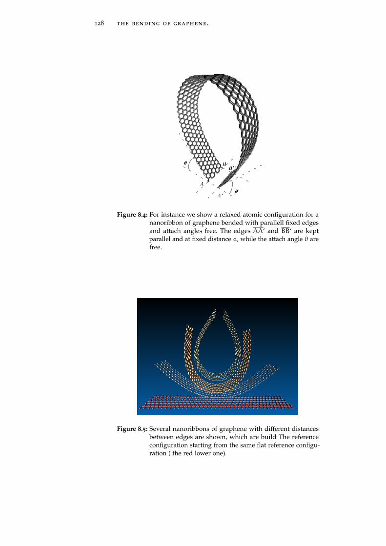
128 the bending of graphene .
Figure 8.4: For instance we show a relaxed atomic configuration for ananoribbon of graphene bended with parallell fixed edgesand attach angles free. The edges AA‘ and BB‘ are keptparallel and at fixed distance a, while the attach angle θ arefree.
Figure 8.5: Several nanoribbons of graphene with different distancesbetween edges are shown, which are build The referenceconfiguration starting from the same flat reference configu-ration ( the red lower one).

8.2 the bending rigidity theory 129
x
y
z
l
L fixed edges
fixed edges
aθ
x
y
z
l
LBending
fixed edges
fixed edges
a=
L
(a) Step 1
x
y
z
l
L” fixed edges
fixed edges
aθ
x
y
z
l
L′Bending
Relaxed
free edges
free edges
a=
L′
(b) Step 2
x
y
z
l
L” fixed edges
fixed edges
aθ
xy
z
l
L′BendingRelaxed
free edges
free edges
a = L′
xy
z
l
L” StraightenedNo Relaxed
fixed edges
fixed edges
a = L”
(c) Step 3
Figure 8.6: Panel(a) In the continuum picture the (pure) bending energyis Ub = Ebendedo − Eflato , here Eflato is the total energy ofthe equilibrium (flat) configuration, and Ebendedo is the totalenergy of the bended unrelaxed configuration. Panel (b)Taking into account full relaxation of the internal degreesof freedom of the bended systems, we evaluate the newbending rigidity κ by means of the energy Ub = Ebendedrelaxed−
Eflatrelaxed,where Eflatrelaxed is the energy of a flat ribbon aftera full relaxation, and Ebendedrelaxed is the energy of a full relaxedbended ribbon. Panel (c) we have defined a virtual processof straightening of a given relaxed and bended ribbon, thusthe bending rigidity κ can be consequently determined byusing Ub = Ebendedrelaxed − Eflatstraightened.
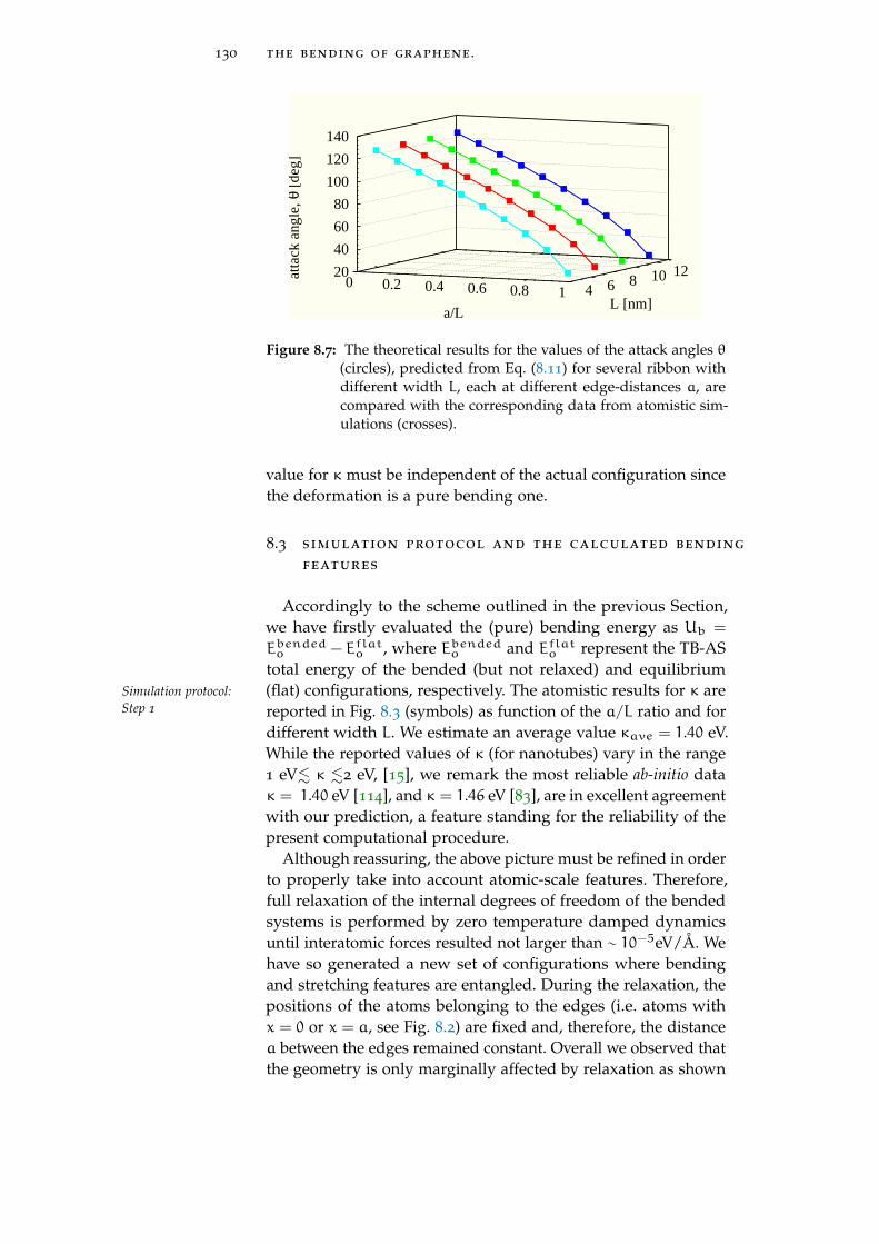
130 the bending of graphene .
0 0.2 0.4 0.6 0.8 1 4 6 8 10 1220
40
60
80
100
120
140
atta
ck a
ngle
, θ [
deg]
a/LL [nm]
Figure 8.7: The theoretical results for the values of the attack angles θ(circles), predicted from Eq. (8.11) for several ribbon withdifferent width L, each at different edge-distances a, arecompared with the corresponding data from atomistic sim-ulations (crosses).
value for κ must be independent of the actual configuration sincethe deformation is a pure bending one.
8.3 simulation protocol and the calculated bending
features
Accordingly to the scheme outlined in the previous Section,we have firstly evaluated the (pure) bending energy as Ub =
Ebendedo − Eflato , where Ebendedo and Eflato represent the TB-AStotal energy of the bended (but not relaxed) and equilibrium(flat) configurations, respectively. The atomistic results for κ areSimulation protocol:
Step 1 reported in Fig. 8.3 (symbols) as function of the a/L ratio and fordifferent width L. We estimate an average value κave = 1.40 eV.While the reported values of κ (for nanotubes) vary in the range1 eV. κ .2 eV, [15], we remark the most reliable ab-initio dataκ = 1.40 eV [114], and κ = 1.46 eV [83], are in excellent agreementwith our prediction, a feature standing for the reliability of thepresent computational procedure.
Although reassuring, the above picture must be refined in orderto properly take into account atomic-scale features. Therefore,full relaxation of the internal degrees of freedom of the bendedsystems is performed by zero temperature damped dynamicsuntil interatomic forces resulted not larger than ∼ 10−5eV/Å. Wehave so generated a new set of configurations where bendingand stretching features are entangled. During the relaxation, thepositions of the atoms belonging to the edges (i.e. atoms withx = 0 or x = a, see Fig. 8.2) are fixed and, therefore, the distancea between the edges remained constant. Overall we observed thatthe geometry is only marginally affected by relaxation as shown
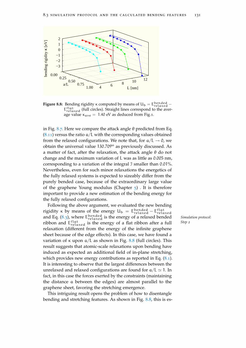
8.3 simulation protocol and the calculated bending features 131
0.000.25
0.500.75
1.00 4 6 8 10 12
−3−2−1 0 1 2
bend
ing
rigid
ity κ
[eV
]
a/LL [nm]
Figure 8.8: Bending rigidity κ computed by means of Ub = Ebendedrelaxed−
Eflatrelaxed (full circles). Straight lines correspond to the aver-age value κave = 1.40 eV as deduced from Fig.1.
in Fig. 8.7. Here we compare the attack angle θ predicted from Eq.(8.11) versus the ratio a/Lwith the corresponding values obtainedfrom the relaxed configurations. We note that, for a/L→ 0, weobtain the universal value 130.709o as previously discussed. Asa matter of fact, after the relaxation, the attack angle θ do notchange and the maximum variation of L was as little as 0.005 nm,corresponding to a variation of the integral I smaller than 0.01%.Nevertheless, even for such minor relaxations the energetics ofthe fully relaxed systems is expected to sizeably differ from thepurely bended case, because of the extraordinary large valueof the graphene Young modulus (Chapter 5) . It is thereforeimportant to provide a new estimation of the bending energy forthe fully relaxed configurations.
Following the above argument, we evaluated the new bendingrigidity κ by means of the energy Ub = Ebendedrelaxed − Eflatrelaxed
and Eq. (8.3), where Ebendedrelaxed is the energy of a relaxed bended Simulation protocol:Step 2ribbon and Eflatrelaxed is the energy of a flat ribbon after a full
relaxation (different from the energy of the infinite graphenesheet because of the edge effects). In this case, we have found avariation of κ upon a/L as shown in Fig. 8.8 (full circles). Thisresult suggests that atomic-scale relaxations upon bending haveinduced as expected an additional field of in-plane stretching,which provides new energy contributions as reported in Eq. (8.1).It is interesting to observe that the largest differences between theunrelaxed and relaxed configurations are found for a/L ' 1. Infact, in this case the forces exerted by the constraints (maintainingthe distance a between the edges) are almost parallel to thegraphene sheet, favoring the stretching emergence.
This intriguing result opens the problem of how to disentanglebending and stretching features. As shown in Fig. 8.8, this is es-

132 the bending of graphene .
0.000.25
0.500.75
1.00 4 6 8 10 12
1.371.381.391.401.411.42
bend
ing
rigi
dity
κ [
eV]
a/LL [nm]
Figure 8.9: Comparison between the bending rigidity κ computedthrough Ub = Ebendedo − Eflato (open circles) and Ub =
Ebendedrelaxed − Eflatstraightened (crosses). The maximum devia-tion is less than the 1.5%.
pecially important in the limit of small deformations, a situationof considerable practical interest. To this aim we have defined aproof-of-concept computational procedure based on the virtualprocess of straightening (or unbending) of a given relaxed andbended ribbon: atoms are projected from such a configurationonto a plane by conserving all the first next neighbor bond lengthsand all the second next neighbor planar angles. The process re-covers a planar configuration, still maintaining all the detailsabout any possible stretching (in-plane strain field); the corre-sponding energy Eflatstraightened is straightforwardly evaluatedby means of TB-AS. The bending rigidity κ can be consequentlySimulation protocol:
Step 3 determined by using Ub = Ebendedrelaxed − Eflatstraightened: the resultsare shown in Fig. 8.9 (crosses) where we also report κ as obtainedby Ub = Ebendedo − Eflato (open circles). The comparison pointsout a good agreement between the two different approaches sincestretching features are either at all non considered (open circles)or included in both the bended and flat configurations (crosses)so as to compensate. It is interesting to note that the constanttrend of κ versus a and L has been found similar to Fig. 8.3. Inother words, we have proved that the evaluation of κ through theenergy term Ub = Ebendedrelaxed − Eflatrelaxed is not correct since it iscorrupted by a strain energy amount which is not directly relatedto the bending process. The energy due to the sole stretchingfield (induced by the bending process) can be accordingly de-fined as Eflatstraightened − Eflatrelaxed. The demonstration that suchan energetic contribution corresponds only to stretching relieson the fact that both the terms Eflatstraightened and Eflatrelaxed havebeen evaluated on flat ribbons through TB atomistic simulations.

8.3 simulation protocol and the calculated bending features 133
0.0
0.5
1.0
-0.04
-0.02
0.00
0.02
ε(b)
ss [
%]
0.0
0.5
1.0
y [n
m]
0.00
0.30
0.60
0.90
ε(e)
ss [
%]
0.0
0.5
1.0
0.00
0.30
0.60
0.90
ε(t)
ss [
%]
0 2 4 6 8 10 12
0 2 4 6 8 10 12
s [nm]
Figure 8.10: ε(b)ss (strain induced by the bending), ε(e)ss (strain induced
by the edges) and ε(t)ss (total strain) versus s (red curves).The gray scale map in background represents the samequantities in the sy-space for L = 12 nm and a/L = 0.95
A further evidence of the stretching emergence can be derivedfrom Fig. 8.10 where the strain is calculated along the arc oflength L (corresponding to the dashed line in Fig. 8.2), labeled Strain field along the
arc of lenghtby the coordinate s. We can calculate three strain fields ε(b)ss ,
ε(e)ss and ε(t)ss which are respectively defined as the relative dif-
ference between: (i) the relaxed and straightened configuration(energy Eflatstraightened) and the flat relaxed configuration (energyEflatrelaxed); (ii) the flat relaxed configuration (energy Eflatrelaxed)and the flat unrelaxed configuration (energy Eflato ); (iii) the re-laxed and straightened configuration (energy Eflatstraightened) andthe flat unrelaxed configuration (energy Eflato ). While the strainε(b)ss is only due to bending, the term ε
(e)ss is induced by the
presence of the edges (finite nanoribbon) in a flat configuration.The quantity ε(t)ss represents the total strain induced by the relax-ation of the bended ribbon with reference to the ideal graphenesheet. We observed with good accuracy the validity of the re-lation ε(t)ss = ε
(b)ss + ε
(e)ss , further proving that the total strain in
a bended ribbon is the sum of two different contributions: thefirst one (ε(b)
ss ) is directly related to the bending process and thesecond one (ε(e)ss ) is originated by edges effects, i.e. by the finitesize of the nanoribbon. Although the first term seems to be quitenegligible with respect to the second one, the previous energeticanalysis reveals that both contributions are essential in orderto explain the discrepancies between continuum and atomisticresults.

134 the bending of graphene .
In conclusion, we offered robust arguments suggesting thatthe correct value for the bending rigidity of a carbon nanoribboncorresponds to κ = 1.40 eV, as calculated either through Ub =
Ebendedo − Eflato or through Ub = Ebendedrelaxed − Eflatstraightened. Onthe other hand, the relation Ub = Ebendedrelaxed − Eflatrelaxed leads toincorrect results because of the emergence of a stretching fieldε(t)ss . We have further proved that such an in-plane strain field
can be decomposed in a first contribution ε(b)ss due to the actual
bending and a second one ε(e)ss due to the edges effects.

Part III
A P P E N D I X

AA P P E N D I X
Contentsa.1 Derivative of a volume integral 137a.2 Derivative of a surface integral 139a.3 Novozhilov formulation of Lagrangian equa-
tions of motion. 141a.4 Crystal symmetry condition 143a.5 Virial stress and Periodic Boundary Condi-
tions 145a.6 Symmetry of the elastic moduli of Graphane
conformers 147a.6.1 Young Modulus 147
a.6.2 Poisson Ratio 151
a.7 Bending rigidity in nanotubes 153a.8 Minimal surface of a bended membrane 157
a.1 derivative of a volume integral
We consider a subset Pt ⊂ Ωt which is the time deformed ver-sion of P0 ⊂ Ω0. We search a property giving the time derivativeof an arbitrary volume integral. In this context, the symbol d/dtcan be used when it is applied to a quantity depending only onthe time t. In fact, in this case, there is no ambiguity. As beforewe consider a scalar field φ and, through a change of variablesbetween Eulerian and Lagrangian coordinates, we obtain
d
dt
∫Pt
φdx =d
dt
∫P0
φJdX (A.1)
where J is the determinant of the deformation gradient
J = det∂x∂X
= det F (A.2)
Then, the time derivation can enter the integral written in thereference configuration
d
dt
∫Pt
φdx =
∫P0
d
dt(φJ)dX =
∫P0
(φJ+φJ
)dX (A.3)
The derivative of a determinant follows the ruled
dtdet F =
(det F
)tr(
˙FF−1)
(A.4)
From Eq.(4.20) we obtain ˙FF−1 = L and, therefore,we have
J = Jtr(L)
= J∇x · v (A.5)
137

138 appendix
So
d
dt
∫Pt
φdx =
∫P0
(φ+φ∇x · v
)JdX =
∫Pt
(φ+φ∇x · v
)dx (A.6)
Since φ = ∂φ∂t + ∂φ
∂x · v we obtain
d
dt
∫Pt
φdx =
∫Pt
(∂φ
∂t+∇xφ · v +φ∇x · v
)dx (A.7)
or, finally
d
dt
∫Pt
φdx =
∫Pt
[∂φ
∂t+∇x · (φv)
]dx (A.8)
This property has been called Reynolds theorem or transporttheorem. It is the most important result used to obtain the balanceequations for continuum materials. If φ = 1 we obtain
d
dt
∫Pt
dx =
∫Pt
∇x · vdx (A.9)
which represent the rate of variation of the volume of the regionPt.
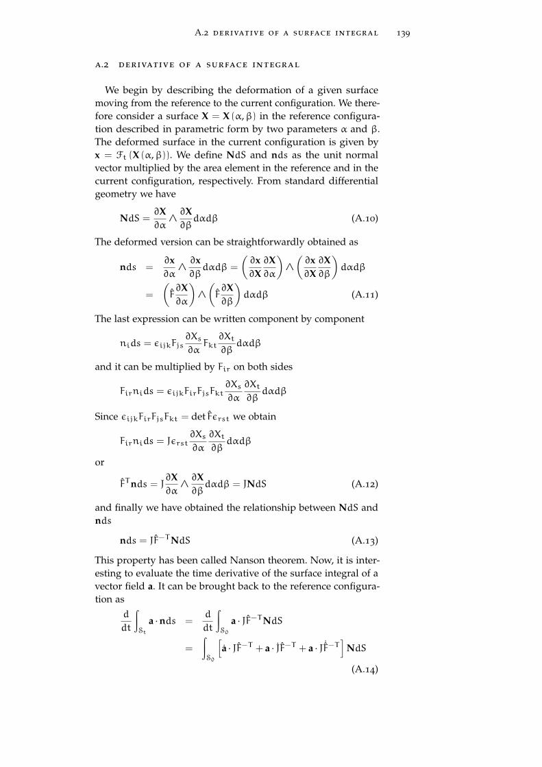
A.2 derivative of a surface integral 139
a.2 derivative of a surface integral
We begin by describing the deformation of a given surfacemoving from the reference to the current configuration. We there-fore consider a surface X = X (α,β) in the reference configura-tion described in parametric form by two parameters α and β.The deformed surface in the current configuration is given byx = Ft (X (α,β)). We define NdS and nds as the unit normalvector multiplied by the area element in the reference and in thecurrent configuration, respectively. From standard differentialgeometry we have
NdS =∂X∂α
∧∂X∂βdαdβ (A.10)
The deformed version can be straightforwardly obtained as
nds =∂x∂α
∧∂x∂βdαdβ =
(∂x∂X∂X∂α
)∧
(∂x∂X∂X∂β
)dαdβ
=
(F∂X∂α
)∧
(F∂X∂β
)dαdβ (A.11)
The last expression can be written component by component
nids = εijkFjs∂Xs
∂αFkt
∂Xt
∂βdαdβ
and it can be multiplied by Fir on both sides
Firnids = εijkFirFjsFkt∂Xs
∂α
∂Xt
∂βdαdβ
Since εijkFirFjsFkt = det Fεrst we obtain
Firnids = Jεrst∂Xs
∂α
∂Xt
∂βdαdβ
or
FTnds = J∂X∂α
∧∂X∂βdαdβ = JNdS (A.12)
and finally we have obtained the relationship between NdS andnds
nds = JF−TNdS (A.13)
This property has been called Nanson theorem. Now, it is inter-esting to evaluate the time derivative of the surface integral of avector field a. It can be brought back to the reference configura-tion as
d
dt
∫St
a · nds =d
dt
∫S0
a · JF−TNdS
=
∫S0
[a · JF−T + a · JF−T + a · J ˙F−T
]NdS
(A.14)
140 appendix
Now J = Jtr(L)
= J∇x · v and ˙F−T = −F−T ˙FT F−T and therefore
d
dt
∫St
a · nds =
∫S0
[a · JF−T + a · J∇x · vF−T − a · JF−T ˙FT F−T
]NdS
=
∫S0
[a + a∇x · v − La
]· JF−TNdS (A.15)
where the relation ˙F = LF has been used. Finally, coming back tothe current configuration we obtain
d
dt
∫St
a · nds =
∫St
[a + a∇x · v − La
]· nds (A.16)
Since the material derivative is given by a = ∂a∂t + ∂a
∂x · v, we obtain
d
dt
∫St
a · nds =
∫St
[∂a∂t
+∂a∂x
· v + a∇x · v − La]
· nds (A.17)
It is simple to verify that∇x ∧ (a ∧ v)+ v∇x · a = ∂a∂x · v + a∇x · v −
La and therefore we can write
d
dt
∫St
a · nds =
∫St
[∂a∂t
+∇x ∧ (a ∧ v) + v∇x · a]
· nds (A.18)
The Nanson relation nds = JF−TNdS can be also applied in orderto obtain the so-called Piola identity. To this aim we use thestandard divergence theorem∫
∂Pt
Ψnids =
∫Pt
∂Ψ
∂xidx (A.19)
if Ψ = 1 identically, we obtain∫∂Pt
nids = 0 and, therefore∫∂Pt
nds =
∫∂P0
JF−TNdS =
∫P0
∇X ·(JF−1
)dX = 0 (A.20)
which means
∇X ·(JF−1
)= 0 ⇒ ∂
∂Xj
(J∂Xj
∂xi
)= 0 (A.21)
This relation will be useful to obtain the balance equations of thecontinuum mechanics in the Lagrangian description.

A.3 novozhilov formulation of lagrangian equations of motion. 141
a.3 novozhilov formulation of lagrangian equations
of motion.
We consider the standard base of unit vectors E1, E2 and E3in the point X of the reference configuration. Since the motion iscontrolled by the transformation x = Ft (X), the unit vectors eiin the deformed configuration are given by the direction of thedeformed coordinate lines
ei =
∂Ft(X)∂Xi
‖∂Ft(X)∂Xi
‖=
FEi‖FEi‖
(A.22)
We remark that they do not form an orthogonal base. First of all,we simply obtain the norm of FEi
‖FEi‖ =
√(FEi)
·(FEi)
=√FkiFki =
√(FT F
)ii
=√Cii (A.23)
where C is the right Cauchy tensor. We define the unit vectorsn1, n2 and n3 perpendicular to the planes (e2, e3), (e1, e3) and(e1, e2). It means that we can write
nk =1
2ηkij
ei ∧ ej‖ei ∧ ej‖ =
1
2ηkij
(FEi)∧(FEj)
‖ (FEi)∧(FEj) ‖ (A.24)
Now, we start with the calculation of ‖ (FEi)∧(FEj) ‖
‖ (FEi)∧(FEj) ‖ =
√ηkstFsiFtjηkabFaiFbj
=√
(δsaδtb − δsbδta) FsiFtjFaiFbj
=√CiiCjj −C
2ij (A.25)
We can also write
dsk
dSk=√CiiCjj −C
2ij (A.26)
where the indices i and j are complementary to k and dSk anddsk are the surface elements in the reference and current con-figuration having unit normal vector nk. Since
(FEi)∧(FEj)
=
ηqstFsiFtjEq, we therefore obtain
nk =1
2ηkij
ηqstFsiFtjEq√CiiCjj −C
2ij
(A.27)
Since ηqstFsiFtjFqa = Jηaij we can simply write ηqstFsiFtj =
Jηaij(F−1)aq; this result can be used in Eq.(A.27) to yield
nk =1
2ηkij
Jηaij(F−1)aqEq√
CiiCjj −C2ij
(A.28)
When k is fixed the indices i and j can assume two couplesof values [if k =1 we have (i, j)=(2,3) or (3,2), if k =2 we have

142 appendix
(i, j)=(1,3) or (3,2) and if k =3 we have (i, j)=(2,1) or (1,2)] andthe index a must assume the value k. At the end we eventuallyobtain
nk =J(F−1)kqEq√CiiCjj −C
2ij
=dSk
dskJ(F−1)kqEq (A.29)
where the indices i and j are complementary to k (there is notthe sum on k). We may consider the forces acting on the threedeformed coordinate planes (e2, e3), (e1, e3) and (e1, e2) (havingnormal unit vectors n1, n2 and n3, respectively) through theexpressions
Tnk =J(F−1)kqTEq√CiiCjj −C
2ij
=dSk
dskJ(F−1)kqTEq (A.30)
These vectors can be represented on both the base Ei and ei asfollows
Tnk = σEskEs (A.31)
Tnk = σeskes (A.32)
where, since E1, E2 and E3 is an orthonormal base, we have
σEsk = Tnk · Es =dSk
dskJ(F−1)kqTEq · Es =
dSk
dskJ(F−1)kqTsq
(A.33)
Moreover, we have the following relation between σEsk and σesk
σEsk = Tnk · Es = σejkej · Es = σejkFEj · Es√Cjj
=1√CjjFsjσ
ejk (A.34)
The representations σEsk and σesk have been introduced by Novozhilovin his pioneering book on nonlinear elasticity. The Lagrangianequation of motion can be written as (see Eq.(4.68))
∂
∂Xk
[J(F−1)kqTsq
]+ Jbs = ρJvs (A.35)
and then it can be expressed in terms of σEsk∂
∂Xk
[dsk
dSkσEsk
]+ Jbs = ρJvs (A.36)
or in terms of σesk
∂
∂Xk
[dsk
dSk
1√CjjFsjσ
ejk
]+ Jbs = ρJvs (A.37)
Finally, since it is evident that√Cjj = dlj/dLj, we can state the
Lagrangian equations of motion in the Novozhilov form
∂
∂Xk
dskdSkdljdLj
Fsjσejk
+ Jbs = ρJvs (A.38)

A.4 crystal symmetry condition 143
a.4 crystal symmetry condition
The stiffness tensor C has a symmetry with respect to a givenorthonormal transformation A if it does not change when sub-jected to that transformation. The matrices A are so defined as theset of orthonormal transformations to which the elastic propertiesare invariant. In Cartesian coordinates the matrix A is given by
A =
A11 A12 A13
A21 A22 A23
A31 A32 A33
. (A.39)
that satisfy the orthogonality condition ATA = I, equivalent toAT = A−1.
Therefore the symmetry condition applied to the stress tensorcan be written as
T ′ = A T AT (A.40)
The stress tensor T can be written in Voigt notation as T =
(T11 T22T33 T23 T13 T12)T so that the Eq. (A.40) becomes
T ′ = A T (A.41)
For conciseness, we fix the stress tensor elements as unity. Webegin by writting the diagonal elements, namely Tij = δiqδqj,with i, j,q ∈ 1, 2, 3, and. hence, we write the Eq. (A.40) as
T ′kl = Aki Tij ATjl = Aki δiqδqj Alj = Akq Alq (A.42)
The out-of-diagonal elements are Tij = δinδmj + δimδnj, so that
T ′kl = Aki Tij ATjl = Aki δinδmj Alj +Aki δimδnj Alj
= Akn Alm +Akm Aln (A.43)
Therefore we have obtained that A in the Eq. (A.41) is
A211 A212 A213 2A12A13 2A11A13 2A11A12
A221 A222 A223 2A22A23 2A21A23 2A21A22
A231 A232 A233 2A32A33 2A31A33 2A31A32
A21A31 A22A32 A23A33 A22A33 +A23A32 A21A33 +A23A31 A21A32 +A22A31
A11A31 A12A32 A13A33 A12A33 +A13A32 A11A33 +A13A31 A11A32 +A12A31
A11A21 A12A22 A13A23 A12A23 +A13A22 A11A23 +A13A21 A11A22 +A12A21
(A.44)
which is the disired transformation matrix given in the Eq. (A.41).Thus, given a transformation matrix A as in Eq. (A.39), whoseentries are Aij, the corresponding A can be written using the Eq.(A.44).

144 appendix
Similarly we can derive the transformation matrix for the straintensor. The invariance of the constitutive equation T = Cε undersuch a transformation requires that
A T = C (A ε) =⇒ T = (A−1 CA) ε (A.45)
Hence, using the definition of an orthonormal transformation
C = A−1 CA = AT CA (A.46)
For a transversely isotropic material, the matrix A has thesimple form
A =
cos θ sin θ 0
− sin θ cos θ 0
0 0 1
. (A.47)
where the x3-axis is the axis of symmetry. The stiffness tensorremains invariant under rotation by any angle θ about the x3-axis.Using the specific values of θ in matrix A, the stiffness tensor fortransversely isotropic materials can be written as
C =
C11 C12 C13 0 0 0
C12 C11 C13 0 0 0
C13 C13 C33 0 0 0
0 0 0 C44 0 0
0 0 0 0 C44 0
0 0 0 0 0 (C11 −C12)/2
(A.48)

A.5 virial stress and periodic boundary conditions 145
ff
extint
image of atom (N)
image of atom (1)
L= Na
x=ax=0 x=Na
Figure A.1: One-dimensional chain of atoms subjected to nearestneighbors internal interaction, fint, and to external forcesfext.The Periodic Boundary Conditions are assumed.
a.5 virial stress and periodic boundary conditions
We present a brief discussion on the calculation of the atomicvirial stress in a system under Periodic Boundary Conditions. Theatomic virial stress is discussed in Section 4.9, where the virialis expressed in terms of the interatomic distances, Eq.(4.180),instead of the atomic positions as in Eq.(4.170). For simplicity,We consider the case of a one-dimensional chain of atoms atzero temperature. We assume that the system is subjected tonearest neighbors interactions of magnitude fint. In Fig.A.1 thesimulation cell of the one-dimensional system is shown. Each cellcontains N particles with constant reciprocal distance, namely a,so that the period of the cell is L = Na, which is kept fixed by the The volume is fixed
by external forcesexternal forces fext due to the interaction with the repeated cellsalong the chain. In such a case, the virial stress can be obtainedby means of the Eq.(4.170) in terms of the atomic positions xi:
T =1
L
N∑i
xifinti = fext (A.49)
Note that, at the equilibrium, the total force on each atoms mustbe zero. Therefore, the internal force acting on the atom in xN,i.e. −fint, is equal in absolute value to the external one fext. As aconsequence, the virial stress is null, as expected, only in absenceof external forces.
On the other hand, in Molecular Dynamics simulations (typi- The volume is fixedby the P.B.C.cally) the system is not subjected to surface forces but the volume
is fixed by means of the Periodic Boundary Conditions, i.e. by theinteractions with the periodic images of the atoms (see Fig.A.1).In order to apply such conditions the interatomic distance xijhave to be calculated by
Interatomic distancesunder PeriodicBoundaryConditions
xij
∣∣∣PBC
= xi − xj − L int[(xi − xj)
L−1
2
](A.50)
In particular, this means that x1N∣∣∣PBC
= a, being a the latticeparameter. In order to get the correct result obtained in Eq. (A.49)

146 appendix
by means of the Eqs.(4.180), the boundary conditions must beproperly consided. This can be done by calculating the virialstress in terms of the interatomic distances xij
∣∣∣PBC
T =1
L
∑ij
xij
∣∣∣PBC
fij = fext (A.51)
which was to be demonstrated.

A.6 symmetry of the elastic moduli of graphane conformers 147
a.6 symmetry of the elastic moduli of graphane con-formers
In accordance with the Hermann’s theorem, the hexagonal crys-tals are transversally isotropic in their elastic properties. All thedirections which make up one and the same angle with the prin-cipal symmetry axis are equal in their elastic properties, althoughfor the hexagonal crystals these directions certainly crystallo-graphically different. This is an example when the symmetry ofa crystal properties is higher than the crystal itself. Hermann’s theorem.
If an r-rank tensorhas an N-foldsymmetry axis andr<N, then this tensoralso has a symmetryaxis of infinite order
Applying an axial tension σ along the arbitrary direction n =
cos θex + sin θey. Under this assumption we get T = σn⊗ n interms of components as
Tij = σninj (A.52)
By inverting the constitutive equation, T = C : ε =⇒ ε = S : T , wefind the corresponding strain tensor ε as follows
εij = sijklTkl = σsijklnknl (A.53)
where sijkl is the compliance tensor. In particular, we easily getits longitudinal component εl = n · ε n along the direction n
εl = εijninj = σsijklnknlninj (A.54)
as well as its transverse component εt = t · ε t along the directiont = − sin θex + cos θey (with t · n = 0).
εt = εijtitj = σsijklnknltitj (A.55)
a.6.1 Young Modulus
The n-dependent Young modulus is defined as the ratio be-tween the applied traction and the longitudinal extension En =
σ/εl. Thus, the reciprocal Young modulus E−1 for the directionn is given by
E−1(n) = sijklnknlninj (A.56)
This formula can be simplified by introducing the notation ninj =
(nn)λ, where ij↔ λ = 1, ..., 6. Finally the Eq. (A.56) becomes
E−1(n) = sλµ(nn)λ(nn)µ (A.57)
The general formula for the reciprocal Young modulus E−1(n)
can be written in terms of the Miller indices hi = h,k, l of the

148 appendix
zz
ac
θ~ey sin θ
~ex cos θ
~n = ~excos
θ + ~eysinθ
~t =−~e
x sinθ+~e
x cos θ
Figure A.2: By applying an axial tension σ along the arbitrary direction~n (θ = ~zz ∠ ~n), the Cauchy stress tensor T = ∂U/∂ε isT = σ~n ⊗ ~n By inverting the constitutive equation T =
C : ε =⇒ ε = S : T we find the corresponding strain tensor ε.εl = ~n · ε ~n longitudinal component; εt = ~t · ε ~t transversecomponent (with ~t · ~n = 0). In particular, we easily get itslongitudinal component εl = ~n · ε ~n along the direction ~n
as well as its transverse component εt = ~t · ε ~t along thedirection ~t = − sin θ~ex + cos θ~ey

A.6 symmetry of the elastic moduli of graphane conformers 149
crystallographic direction [hkl] parallel to direction n as the fol-lows
E−1 = sλµQλQµ (A.58)
Qλ = ninj =AαiAβjhαhβ
gγηhγhη(A.59)
where Aβj are the components of the the matrix of the expansionof vectorial basis aα of the crystal lattice with respect to mutuallyorthogonal unit vectors ei of the system of coordinates; the gγηare the components of the metric tensor G (here Greek and Latinindices enumerate columns and rows, respectively). In the generalcase of the triclinic symmetry, we get
Q1 = q21 = g−1(ha sinβ− kb sinα cosγ†)2
Q2 = q22 = g−1
(k
b†
)2Q3 = q23 = g−1(ha cosβ+ kb cosα+ lc)2
Q4 = q2q3 = g−1
(k
b†
)(ha cosβ+ kb cosα+ lc)
Q5 = q3q1 = g−1(ha cosβ+ kb cosα+ lc)(ha sinβ− kb sinα cosγ†)
Q6 = q1q2 = g−1
(k
b†
)(ha sinβ− kb sinα cosγ†)
g = h2a2 + k2b2 + l2c2 +
+2klbc cosα+ 2lhca cosβ+ 2hkab cosγ (A.60)
where a,b, c are the lengths of the base vectors of the lattice andα,β,γ are the angles between them; a†,b†, c† are the lengths ofthe reciprocal vectors and α†,β†,γ† are the angles between them,which are related as
a† =sinαaω
b† =sinβbω
c† =sinγcω
(A.61)
cosα† =cosβ cosγ− cosα
sinβ sinγ
cosβ† =cosγ cosα− cosβ
sinγ sinα
cosγ† =cosα cosβ− cosγ
sinα sinβ(A.62)
where ω =√1− cosα2 − cosβ2 − cosγ2 + 2 cosα cosβ cosγ 2-dimensional
systemsIn the case of 2-dimensional systems as graphene and graphane,many terms of the Eqs.(A.60) becomes zero and we can neglectall the indices 3, 4, 5. Therefore the expansion of the Eq.(A.58) isreduced to Young modulus in
2-dimensionalsystems
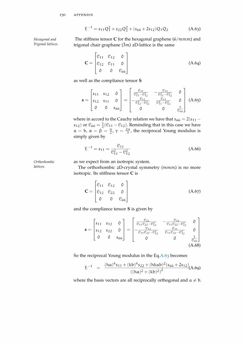
150 appendix
E−1 = s11Q21 + s22Q
22 + (s66 + 2s12)Q1Q2 (A.63)
The stiffness tensor C for the hexagonal graphene (6/mmm) andHexagonal andTrigonal lattices. trigonal chair graphane (3m) 2D-lattice is the same
C =
C11 C12 0
C12 C11 0
0 0 C66
(A.64)
as well as the compliance tensor S
s =
s11 s12 0
s12 s11 0
0 0 s66
=
C11
C211−C212− C12
C211−C2120
− C12C212−C212
C11C211−C212
0
0 0 1C66
(A.65)
where in accord to the Cauchy relation we have that s66 = 2(s11−
s12) or C66 = 12(C11 − C12). Reminding that in this case we have
a = b, α = β = π2 , γ = 2π
3 , the reciprocal Young modulus issimply given by
E−1 = s11 =C11
C211 − C212(A.66)
as we expect from an isotropic system.Orthorhombiclattices. The orthorhombic 2D-crystal symmetry (mmm) is no more
isotropic. Its stiffness tensor C is
C =
C11 C12 0
C12 C22 0
0 0 C66
(A.67)
and the compliance tensor S is given by
s =
s11 s12 0
s12 s22 0
0 0 s66
=
C22
C11C22−C212− C12
C11C22−C2120
− C12C11C22−C212
C11C11C22−C212
0
0 0 1C66
(A.68)
So the reciprocal Young modulus in the Eq.A.63 becomes
E−1 =(ha)4s11 + (kb)4s22 + (hkab)2(s66 + 2s12)
((ha)2 + (kb)2)2
(A.69)
where the basis vectors are all reciprocally orthogonal and a 6= b.

A.6 symmetry of the elastic moduli of graphane conformers 151
a.6.2 Poisson Ratio
In order to generalize the Poisson ratio ν formula for ananisotropic 2D-lattice, we can define it as a function of the defor-mation in two mutually orthogonal directions n and m.
ν(n, m) = −εt/εl =
= −sλµ(mm)λ(nn)µ
sρσ(nn)ρ(nn)σ(A.70)
Poisson ratio can also be define using only one direction, becausethe perpendicularity condiction impose that mimj = (δij−ninj)
ν(q) = −sijklninj (δkl −nknl)
snprtnnnpnrnt(A.71)
that from the Eq.(A.56)
ν(n) =sijklninjnknl
snprtnnnpnrnt−
sijklninjδkl
snprtnnnpnrnt=
= 1− sijkkninjE(n) = (A.72)
= 1− SijninjE(n) (A.73)
where Sij are the components of the compressibility tensor de-fined by the strain under hydrostatic pressure p
εij = −Sijp = −sijkkp (A.74)Poisson Ratio forHexagonal andTrigonal lattices
Both for graphene and chair-graphane, the Poisson ratio isindependent from the direction
ν = −s12
s11=
C12
C11(A.75)
While for the board-graphane with orthorhombic symmetry isquite different due to its anisotropicity. From Eqs.(A.72), (A.60),and (A.69) Poisson Ratio for
boat-graphaneν(n) = 1−
((s11 + s12)q
21 + (s22 + s12)q
22
)ninjE(n)
= 1−
((ha)2s11 + (kb)2s22 + ((ha)2 + (kb)2)s12
((ha)2 + (kb)2)
)·
( ((ha)2 + (kb)2
)2(ha)4s11 + (kb)4s22 + (hkab)2(s66 + 2s12)
)
=(hkab)2(s66 − s11 − s22) − ((ha)4 + (kb)4)s12
(ha)4s11 + (kb)4s22 + (hkab)2(s66 + 2s12)
(A.76)
Both the Young modulus and the Poisson ratio can be writtenin function of the angle θ between the direction n and the basisvector a (see Fig. A.2 ) carry on the Miller indices in terms of thecosine directors of n
E−1(θ) = cos(θ)4s11+ sin(θ)4s22+ cos(θ)2 sin(θ)2(s66+ 2s12)

152 appendix
(A.77)
ν(θ) =tan(θ)2(s66 − s11 − s22) − (1+ tan(θ)4)s12s11 + tan(θ)4s22 + tan(θ)2(s66 + 2s12)
(A.78)

A.7 bending rigidity in nanotubes 153
Ro
l
γo
Figure A.3: A nanotube can be sketched as a simple cylinder. Here theradius Ro and circumference γo are referred to the refer-ence configuration, while the length l is fixed by imposingthe periodic boundary condiction along the cylinder axis(dashed line).
a.7 bending rigidity in nanotubes
We have evaluate the bending rigidity κ of graphene, includingrelaxation effects, in Chapter 8. The same value κ = 1.40 eVhas been obtained using carbon nanotubes instead nanoribbons.The nanotube, of course, do not show any edge effects, but thebending rigidity depends from the curvature, which in nanotubesis a geometric constant. In fact bond stretching is observed downto (15,0) nanotubes [101, 121, 122]. Including relaxation effects infunction of the nanotube radius R it possible to extract the purebending energy term by comparing the ray variation between thereference starting tube, which has all bonds equal to the perfectgraphene, namely 1.41 Å , and the full relaxed one.
In fact the cylindric geometry of a nanotube impose the Gaus-sian curvature null, K = 0. Thus, the elastic energy density U
[eVÅ −2] of a monoatomic layered membrane is defined as
U =1
2
E
1+ νTr(ε2)+1
2
Eν
1− ν2[Tr (ε)]2 +
1
2κ (2H)2 (A.79)
depending on the mean curvature H, and on the strain tensor ε.To evaluate the only bending energy term Ub, we impose
strain ε = 0, so that the strain energy term go to zero, Us =12E1+νTr
(ε2)+ 12Eν1−ν2
[Tr (ε)]2 = 0. The only bending energy den-
154 appendix
sity Ub [eVÅ −2] of a general given surface can be written as
U =1
2κ (2H)2 − κK (A.80)
where the mean curvature is H = k1+k22 [m−1] and the Gaussian
curvature is defined as K = k1k2 [m−2], here k1 = 1R1
andk2 = 1
R2are the principal curvatures, while R1 and R2 are the
local principal radii of curvature. We have chosen a cylindricconfiguration that involving only one curvature k1 = 1
R1(i.e.
k2 = 0), therefore the mean curvature is H = k12 , while the
Gaussian curvature is null, K = 0. Thus in the case of cylindricgeometry, the bending energy density Ub is given by
U =1
2κ k21 (A.81)
To obtain the total bending energy , we have to integratethe bending energy density on the reference surface Σo Ub =∫ ∫Σo
Udσ = 12κl∫γok21dswhere Σ = Lol being the total area
of the reference system, γo = 2πRo is the circumference of thecylinder with radius Ro, and s is the arc length (0 < s < Lo).Note that the reference surface Σo is defined as the surface ofthe corresponding rectangular flat slice which we have rolled tobuild the nanotubes, i.e. the unstrained graphene nanoribbonwherein all the bond length are equal to the equilibrium dinstancedC−C = 1.41Å between a pair of carbon atoms. The solution ofthe integral is as follows
Ub =
∫ ∫Σo
Ubdσ =1
2κl
∫γo
k21ds (A.82)
=1
2κl
∫γo
(R)−2ds (A.83)
=1
2κl2πRo
R2(A.84)
Here the nanotube length l is constant due to the periodic bound-ary condiction imposed along the axis of the cylinder. If thebending does not involve stretching, the radius R after the re-laxation of the nanotube have to be equal the reference cylinderradius Ro. Therefore the bending energy can be simplified as
Ub = limR→Ro
1
2κl2πRo
R2=πκl
Ro(A.85)
Because of the bending energy can be computed by atomisticsimulation as difference between the total energy of the nanotubeEtubeo and the corresponding reference flat system Eflato , namelyUb = Etubeo − Eflato , the bending rigidity κ of a nanotube withradius Ro is given by
κ =Ro
πlUb(A.86)

A.7 bending rigidity in nanotubes 155
in absence of stretching on the surface.Moreover, when a relaxation of the structure is allowed a vari-
ation of radius R is observed down to a certain dimension ofthe nanotube. In these cases besides the bending energy is givenby the solution in Eq. (A.82) with R 6= Ro, it needs to take inaccount the no longer negligible stretching term in the Eq. (A.79).Thus we have to integrate also the stretching energy density Usas follows
Us =
∫ ∫Σo
Usdσ =
∫ ∫Σo
(1
2
E
1+ νTr(ε2)+1
2
Eν
1− ν2[Tr (ε)]2
)dσ
=1
2
E
1+ ν
∫ ∫Σo
(Tr(ε2)+
ν
1− ν[Tr (ε)]2
)dσ
We can considerer only strain ε =(ζ 00 0
)along the circumference,
because the length l is fixed by the periodic boundary conditions.So that
Us =1
2
E
1+ ν
∫ ∫Σo
(ζ2 +
ν
1− νζ2)dσ
=1
2
E
1+ ν
∫ ∫Σo
(ζ2
1− ν
)dσ
but ζ =γ− γo
γo=R− Ro
Ro,
so that
Us =1
2
El
1− ν2
(R− Ro
Ro
)2 ∫γo
ds
=1
2
El
1− ν2
(R− Ro
Ro
)2(2πRo)
(A.87)
Obviously when R → Ro, the stretching energy goes to zero,Us = 0.

156 appendix
1.30
1.32
1.34
1.36
1.38
1.40
1.42
1.44
0 5 10 15 20 25
Ben
ding
rig
idity
,κ c [e
V]
Reference nanotube radius, Ro [Å]
(3,0
) (4
,0) (5
,0)
(6,0
) (7
,0)
(8,0
) (9
,0)
(10,
0)
(11,
0)
(12,
0)
(13,
0)
(14,
0)
(15,
0)
(16,
0)
(17,
0)
(18,
0)
(19,
0)
(20,
0)
(21,
0)
(22,
0)
(23,
0)
(24,
0)
(25,
0)
(26,
0)
(27,
0)
(28,
0)
(29,
0)
(30,
0)
Figure A.4: Bending rigidity κ in function of the radius of a set ofzig-zag nanotubes in the range of (3,0)-(30,0). The symbolsshow the value of the bending rigidity, as defined in theEq. (A.85), obtained by tight-binding simulations. Note thatdown to the (15,0) a deviation from the constant valueis observed. This fact is due to the rising of stretchingbond effects due to the curvature. The asymptotic valueis κ = 1.40 eV, exactly as obtained from the nanoribbonsexperiments discussed in the Chapter 8

A.8 minimal surface of a bended membrane 157
φoθo
x = 0
θ ′o φ ′ox = a
θds
x
z bended ribbon
Figure A.5: A cross-section of a bended ribbon ( blue curve ) withparallel edges at fixed distance a. The ribbon width L andthe edges distance a are taken constant, while the attackangles θo and θ ′o = −θo ( or φ and φ ′) are free up.
a.8 minimal surface of a bended membrane
In the Sec. 8.2 we have discussed the problem of a bendednanoribbon. We show in this Appendix a more detailed discus-sion about the minimization the energy functional in Eq.(8.5) bythe method of Lagrange multipliers λ, i.e. the solution of the Eq. A variational
approach(8.6) ∫a0dx
[z2
(1+ z2)52
+ λ√1+ z2
], (A.88)
enforcing the absence of any in-plane stretching under the followsboundary conditions:
a constrained width, L =∫a0 dx√1+ z2,
a fixed parallel edges, z(0) = z(a) = 0,
a free attack angle, θ = arctg(dzdx), z(0) = z(a) = 0
(A.89)Eulero-PoissonequationThe above integral can be written in the general form
G(z) =
∫a0dxF(z, z, z, x)
which is the solution of the Euler-Poisson differential equation
∂F
∂z−d
dx
∂F
∂z+d2
dx2∂F
∂z= 0 (A.90)

158 appendix
PROOF: We can define the function G(z,h)
G(z,h) = limα→0
G(z+αh) −G(z)
α=d
dαG(z+αh)
∣∣∣α→0
(A.91)
The derivative of the function G(z+ αh) =∫a0 dxF(z+ αh, z+
αh, z+αh, x) is given by
d
dαG(z+αh)
∣∣∣α→0
=
∫a0dx
d
dαF(z+αh, z+αh, z+αh, x)
=
∫a0dx
(∂F
∂zh+
∂F
∂zh+
∂F
∂zh
)= |[by parts]| =
∫a0dx
(∂F
∂z−d
dx
∂F
∂z+d2
dx2∂F
∂z
)h
+
(∂F
∂z−d
dx
∂F
∂z
)h∣∣∣a0
+ h∂F
∂z
∣∣∣a0
= 0
(A.92)
Thus, imposing the follows constrains
a fixed parallel edges, z(0) = z(a) = 0⇒ h(0) = h(a) = 0
a free attack angle, z(0) = z(a) = 0⇒ ∂F(0)∂z =
∂F(a)∂z = 0
or a fixed attack angle, z(0) = z(a) = 0⇒ h(0) = h(a) = 0
(A.93)
we get the Euler-Poisson Eq. (A.90), q.e.d.The corresponding Hamiltonian can be written as follows
H = F − z
(∂F
∂z−d
dx
∂F
∂z
)− z
∂F
∂z(A.94)
Moreover we can proof that dHdx = dF
dx . By deriving the Eq. (A.94)and by using the Eq. (A.90)
dH
dx=
dF
dx− z
(∂F
∂z−d
dx
∂F
∂z
)− z
(d
dx
∂F
∂z−d2
dx
2∂F
∂z
)−
...z∂F
∂z− z
d
dx
∂F
∂z
=dF
dx, q.e.d.
In our case the function F(z, z, z, x) is given by
F =z2
(1+ z2)52
+ λ√1+ z2 (A.95)
Thus the partial derivatives ∂F∂x = ∂F
∂z = have to be null. Weintroduce two parameters, C1, C2 to solve the Hamiltonian, Eq.(A.94), and the Euler-Poisson equation, Eq. (A.90), as follows
F − z(∂F∂z − d
dx∂F∂z
)− z∂F
∂z = −C2
− ddx∂F∂z + d2
dx2∂F∂z = C1
∴ F + zC1 − z∂F∂z = −C2 (A.96)

A.8 minimal surface of a bended membrane 159
Replacing in the Eq. (A.96) the Eq. (A.95) and its derivative ∂F∂z
we obtain
−z2
(1+ z2)52
+ λ√1+ z2 + zC1 = −C2 (A.97)
We have to impose the boundary condiction as in Eqs. (8.7). Firstof all, by the attack angle definition we get
z = tan θ
z = 1cos2 θ
∂θ∂x (A.98)
Introducing the arc length s =∫x0 dx√1+ z2 we get
∂s
∂x=√1+ tan2 θ =
1
cos θ∂θ
∂x=∂θ
∂s
∂s
∂x=
1
cos θdθ
ds(A.99)
Thus, the Eq. (A.97) can be written as
−1
cos θ
(dθ
ds
)2+
1
cos θλ+
sin θcos θ
C1 = −C2 (A.100)
Second, by the conditions for the fixed edges and the free attackangles, we get that dθds = 0 at s = 0 and s = L. Furthermore,the symmetry of the cylinder surface leads to θ(0) = θo andθ(L) = −θo. So that deriving the Eq. (A.100)
dθ
ds
∣∣∣θo
= −√λ+ C1 sin θo + C2 cos θo = 0
∴ λ = −C1 sin θo − C2 cos θo (A.101)dθ
ds
∣∣∣−θo
= −√
−2C1 sin θo = 0
∴ C1 = 0
Therefore the Eq. (A.100) has been simplified as follows
dθ
ds= −
√C(cos θ− cos θo)
S =
∫s0ds =
∫θ(s)
θo
dθ
−√
C(cos θ− cos θo)(A.102)
where C ≡ C2 as well as in the following. Finally, we use thefixed length L =
∫a0 dx√1+ z2 to obtain the parameter C as
follows
L =
∫θo−θo
dθ√C(cos θ− cos θo)
(A.103)
∴ S = L
∫θoθ(s)
dθ√(cosθ−cosθo)∫θo
−θodθ√
(cosθ−cosθo)
(A.104)
160 appendix
In order to turn back in Cartesian coordinates, we observe thatdxds = cos θ, and dz
ds = dzdxdxds = sin θ,
x =
∫θoθ(s)
cos θdθ√C(cos θ− cos θo)
z =
∫θoθ(s)
sin θdθ√C(cos θ− cos θo)
(A.105)
and reminding that the edges of the nanoribbon is at fixed dis-tance, i.e. x(L) = a, we can write
a =
∫θo−θo
cos θdθ√C(cos θ− cos θo)
= L
∫θoθ(s)
cosθdθ√(cosθ−cosθo)∫θo
−θodθ√
(cosθ−cosθo)
(A.106)
which give us θo for any given edges distance a and nanoribbonlength L. Therefore we have obtained the parametric form of theminimized surface
x = L
∫θoθ(s)
cosθdθ√(cosθ−cosθo)∫θo
−θodθ√
(cosθ−cosθo)
z = L
∫θoθ(s)
sinθdθ√(cosθ−cosθo)∫θo
−θodθ√
(cosθ−cosθo)
(A.107)
As shown in Sec. 8.2, we eventually obtain the final geometryin parametric representation [x(s), z(s)]
x
L=
E(q) − E(amK(q)
(1− 2 sL
),q)
K(q)−s
L(A.108)
z
L=
q
K(q)cn
K(q)(1− 2
s
L
)(A.109)
where s is the arc length (0 < s < L), q = sin θ2 is the ellipticmodulus and θ is the attack angle given by
a
L= 2
E(q)
K(q)− 1. (A.110)
The quantities E(q) and K(q) are the complete elliptic integrals,defined as[115, 116]
E(q) = F(π2
,q)
, K(q) = E(π2
,q)
(A.111)
where the functions F(v,q) and E(v,q) are incomplete ellipticintegrals of the first and second kind, respectively [115, 116]
F(v,q) =
v∫0
dα√1− q2 sin2 α
E(v,q) =
v∫0
√1− q2 sin2 αdα. (A.112)

A.8 minimal surface of a bended membrane 161
Moreover, by considering u = F(v,q) we define the inverse re-lation (with fixed modulus q) v = am u, which is called Jacobiamplitude function. Further, cn u = cos v = cos (am u) andsn u = sin v = sin (am u) are the Jacobi elliptic functions.[116] An universal attach
angle.Interesting enough, one can prove for a given (L,a) that lima/L→0 θ= 2.2813rad = 130.709o, an universal value of the attack anglefound whenever a = 0 or L is very large.


B I B L I O G R A P H Y
[1] P. R. Wallace. Phys. Rev., 71,622. (1947). (Cited on page 1.)
[2] Aziz A. Ahmadieh and Hamid A. Rafizadeh. Phys. Rev. B,7,4527. (1973). (Cited on page 1.)
[3] A. Bosak and M. Krisch. Phys. Rev. B, 75,153408. (2007).(Cited on page 1.)
[4] L.-F. Wang and Q.-S. Zhenga. Applied Phys. Lett., 90,153113.(2007). (Cited on page 1.)
[5] A. K. Geim S. V. Morozov D. Jiang Y. Zhang S. V. DubonosI. V. Grigorieva K. S. Novoselov and A. A. Firsov. Science,306. (2004). (Cited on pages 2 and 109.)
[6] A. K. Geim S. V. Morozov D. Jiang M. I. Katsnelson I. V.Grigorieva S. V. Dubonos K. S. Novoselov and A. A. Firsov.Nature, 438,197. (2005). (Cited on page 2.)
[7] V. P. Gusynin and S. G. Sharapov. Phys. Rev. Lett., 95,146801.(2005). (Cited on pages 2 and 109.)
[8] L. D. Landau. Phys. Z. Sowjetunion, 11,26. (1937). (Cited onpage 2.)
[9] R. E. Peierls. Ann. I. H. Poincare 5, 5,177. (1935). (Cited onpage 2.)
[10] N. D. Mermin. Phys. Rev., 176,250. (1968). (Cited on page 2.)
[11] J. H. Los A. Fasolino and M. I. Katsnelson. Nature Materials,6,858. (2007). (Cited on page 3.)
[12] X. Wei W. Kysar C. Lee and J. Hone. Science, 321,385. (2008).(Cited on pages 4, 5, 7, 77, 82, 83, 85, 86, 87, 105, and 110.)
[13] V. M. Pereira and A. H. Castro Neto. Phys. Rev. Lett., 103,046801. (2009). (Cited on pages 4, 7, 110, and 120.)
[14] M. Arroyo and T. Belytschko. Phys. Rev. B, 69,115415. (2004).(Cited on pages 4, 77, and 86.)
[15] Z. C. Ou-Yang and Z. C. Tu. J. Comput. Theor. Nanosci., 5,422. (2008). (Cited on pages 4, 77, and 130.)
[16] H.W. Zhang, J.B. Wang, and X. Guo. Journal of the Mechanicsand Physics of Solids, 53,1929. (2005). (Cited on page 5.)
163

164 bibliography
[17] M. Y. Han, B. Özyilmaz, Y. Zhang, and P. Kim. Phys. Rev.Lett., 98,206805. (2007). (Cited on pages 5 and 110.)
[18] F. Sols, F. Guinea, and A. H. Castro Neto. Phys. Rev. Lett.,99,166803. (2007). (Cited on pages 5, 7, and 110.)
[19] E. R. Mucciolo, A. H. Castro Neto, and C. H. Lewenkopf.Phys. Rev. B, 79,075407. (2009). (Cited on pages 5 and 110.)
[20] K. Nakada, M. Fujita, G. Dresselhaus, and M. S. Dressel-haus. Phys. Rev. B, 54,17954. (1996). (Cited on pages 5
and 110.)
[21] B. Jørgensen L. Nilsson M. Andersen E. Rienks M. BianchiM. Fanetti E. Lægsgaard A. Baraldi S. Lizzit Z. SljivancaninF. Besenbacher B. Hammer T. G. Pedersen P. Hofmann R.Balog and L. Hornekær. Nature, 9. (2010). (Cited on pages 5
and 110.)
[22] A. S. Chaudhari J. O. Sofo and G. D. Barber. Phys. Rev. B,75,153401. (2007). (Cited on pages 6, 89, 90, and 94.)
[23] M. I. Katsnelson D. W. Boukhvalov and A. I. Lichtenstein.Phys. Rev. B, 77,035427. (2008). (Cited on pages 6, 89,and 90.)
[24] R.R. Nair T. M. G. Mohiuddin S. V. Morozov P. Blake M. P.Halsall A. C. Ferrari D. W. Boukhvalov M. I. Katsnelson A.K. Geim D. C. Elias and K.S. Novoselov. Science, art. 610.(2009). (Cited on pages 6 and 90.)
[25] O. Leenaerts, H. Peelaers, A. D. Hernández-Nieves, B. Par-toens, and F. M. Peeters. Phys. Rev. B, 82,195436. (2010).(Cited on pages 6 and 107.)
[26] M. Topsakal, E. Akturk, and S. Ciraci. Phys. Rev. B, 79,115442. (2009). (Cited on pages 6, 90, 92, and 93.)
[27] Y. Ma J. Kasim Y. H. Wu Z. H. Ni H. M. Wang and Z. X.Shen. ACS Nano, 2. (2008). (Cited on pages 7, 110, and 117.)
[28] P. Shemella and S.K. Nayak. Appl. Phys. Lett., 94. (2009).(Cited on pages 7 and 110.)
[29] Y. Zhao H. Jang S. Y. Lee J. M. Kim K.S. Kim J. H. AhnP. Kim J. Y. Choi K. S. Kim and B. H. Hong. Nature, 457.(2009). (Cited on pages 7, 110, and 117.)
[30] T. Yu Y. H. Lu Y. Y. Wang Y. P. Feng Z. H. Ni and Z. X. Shen.ACS Nano, 2. (2008). (Cited on pages 7, 110, and 117.)
[31] A. H. Castro Neto V. M. Pereira and N. M. R. Peres. Phys.Rev. B, 80,045401. (2009). (Cited on pages 7, 110, 114,and 115.)

bibliography 165
[32] T. Wassmann, A. P. Seitsonen, A. M. Saitta, M. Lazzeri, andF. Mauri. Phys. Rev. Lett., 101,096402. (2008). (Cited onpage 7.)
[33] K. A. Ritter and J. W. Lyding. Nature Materials, 8,235. (2009).(Cited on page 7.)
[34] V. B. Shenoy, C. D. Reddy, A. Ramasubramaniam, andY. W. Zhang. Phys. Rev. Lett., 101,245501. (2008). (Cited onpage 7.)
[35] P. Koskinen, S. Malola, and H. Häkkinen. Phys. Rev. Lett.,101,115502. (2008). (Cited on page 7.)
[36] A. K. Geim M. I. Katsnelson K. S. Novoselov T. J. Booth J. C.Meyer and S. Roth. Nature (London), 446,60. (2007). (Citedon pages 7 and 121.)
[37] J. H. Chen W. G. Cullen M. S. Fuhrer M. Ishigami and E. D.Williams. NanoLetters, 7,1643. (2007). (Cited on pages 7
and 121.)
[38] F.Guinea N. M. R. Peres K. S. Novoselov A. H. Castro Netoand A. K. Geim. Rev. Mod. Phys., 81,109. (2009). (Cited onpages 8, 109, and 121.)
[39] A. M. van der Zande S. S. Verbridge I. W. Frank D. M.Tanenbaum J. M. Parpia H. G. Craighead J. S. Bunch andP. L. McEuen. Science, 315,490. (2007). (Cited on pages 8
and 122.)
[40] A. Isacsson J. Atalaya and J. M. Kinaret. NanoLetters, 8,4196.(2008). (Cited on pages 8 and 122.)
[41] K. N. Kudin J.-L. Li R. K. Prud’homme R. Car D. A. SavilleH.C. Schniepp and I. A. Aksay. ACS Nano, 2,2577. (2008).(Cited on pages 8 and 122.)
[42] A. L. Higginbotham A. Sinitskii J. R. Lomeda A. DimievB. K. Price D. V. Kosynkin and J. M. Tour. Nature (London),458,872. (2009). (Cited on pages 8 and 122.)
[43] L. Chico H. Santos and L. Brey. Phys. Rev. Lett., 103,086801.(2009). (Cited on pages 8 and 122.)
[44] P. O. Löwdin, J. Mol. Spectr. 3, 46 (1959). (Cited on page 15.)
[45] L. Colombo, Tight-binding molecular dynamics: A primer, LaRivista del Nuovo Cimento Vol. 28, N. 10 (2005). (Cited onpage 16.)
[46] J. C. Slater and G. F. Koster. Phys. Rev., 94,1498. (1954).(Cited on pages 17 and 18.)

166 bibliography
[47] W. A. Harrison. Electronic Structure and the Properties ofSolids. Dover Pubblications, New York. (1989). (Cited onpage 19.)
[48] R. P. Feynman, Phys. Rev. 56, 340 (1939). (Cited on page 21.)
[49] P. Pulay, Mol. Phys. 17, 197 (1969). (Cited on page 21.)
[50] C. Z. Wang C. T. Chan C. H. Xu and K. M. Ho. Journal ofPhysics: Condensed Matter, 4,6047. (1992). (Cited on pages 21,22, 23, 84, 110, 126, and 127.)
[51] L. Goodwin, A. J. Skinner, and D. G. Pettifor, Europhys.Lett. 9, 701 (1989). (Cited on page 21.)
[52] R. Dreizler and E. Gross. Density Functional Theory. NewYork. (1995). (Cited on page 25.)
[53] R.G. Yang and W. Parr. Density-Functional Theory of Atomsand Molecules. New York. (1989). (Cited on page 25.)
[54] P. Hohenberg and W. Kohn. Phys. Rev., 136,B864. (1964).(Cited on page 25.)
[55] W. Kohn and L. J. Sham. Phys. Rev., 140,A1133. (1965).(Cited on pages 25, 26, and 28.)
[56] E.P. Wigner. Trns. Faraday soc., 34,678. (1938). (Cited onpage 29.)
[57] D. Ceperley. Phys. Rev. B, 18,3126. (1978). (Cited onpage 29.)
[58] D. M. Ceperley and B. J. Alder. Phys. Rev. Lett., 45,566.(1980). (Cited on page 29.)
[59] J. P. Perdew and A. Zunger. Phys. Rev. B, 23,5048. (1981).(Cited on page 29.)
[60] J. P. Perdew and Y. Wang. Phys. Rev. B, 45,13244. (1992).(Cited on pages 30 and 31.)
[61] Y. Wang and J. P. Perdew. Phys. Rev. B, 44,13298. (1991).(Cited on page 30.)
[62] J. P. Perdew, J. A. Chevary, S. H. Vosko, K. A. Jackson, M. R.Pederson, D. J. Singh, and C. Fiolhais. Phys. Rev. B, 46,6671.(1992). (Cited on pages 30 and 31.)
[63] A. D. Becke. Phys. Rev. A, 38,3098. (1988). (Cited onpages 30 and 31.)
[64] J. P. Perdew, K. Burke, and M. Ernzerhof. Phys. Rev. Lett.,77,3865. (1996). (Cited on page 31.)

bibliography 167
[65] C. Lee, W. Yang, and R. G. Parr. Phys. Rev. B, 37,785. (1988).(Cited on page 31.)
[66] M. C. Payne, M. P. Teter, D. C. Allan, T. A. Arias, and J. D.Joannopoulos. Rev. Mod. Phys., 64,1045. (1992). (Cited onpage 33.)
[67] R. M. Pick, M. H. Cohen, and R. M. Martin. Phys. Rev. B, 1,910. (1970). (Cited on page 33.)
[68] X. Gonze. Phys. Rev. A, 52,1096. (1995). (Cited on page 34.)
[69] S. Baroni, S. de Gironcoli, A. Dal Corso, and P. Giannozzi.Rev. Mod. Phys., 73,515. (2001). (Cited on pages 34 and 93.)
[70] X. Gonze and J.-P. Vigneron. Phys. Rev. B, 39,13120. (1989).(Cited on page 34.)
[71] A. K. Subramaniyan and C.T. Sun. International Journal ofSolids and Structures, 45,4340. (2008). (Cited on pages 70
and 71.)
[72] A. G. McLellan. Am. J. Phys., 42,239. (1974). (Cited onpage 70.)
[73] R. J. Swenson. Am. J. Phys., 51,940. (1983). (Cited onpage 70.)
[74] R. Clausius. Phil. Mag., 40,122. (1870). (Cited on page 70.)
[75] J.C. Maxwell. Transactions of the Royal Society of EdinburgXXVI, art. 1. (1870). (Cited on page 70.)
[76] M. Zhou. Proc. R. Soc. Lond. A, 459,2347. (2003). (Cited onpages 70, 85, and 86.)
[77] G.L. Gray F. Costanzo and P.C. Andia. Modelling and Sim-ulation in Materials Science and Engineering, 14,741. (2006).(Cited on page 71.)
[78] G.L. Gray F. Costanzo and P.C. Andia. International Journalof Solids and Structures, 42,6409. (2005). (Cited on page 71.)
[79] J.H. Weiner and J. Gao . Macromolecules, 20,2520. (1987).(Cited on page 71.)
[80] D. Frenkel and B. Smit, Understanding Molecular SImulation(Academic Press, San Diego, 1996). (Cited on page 74.)
[81] K. Kern M. Burghard and C. Gómez-Navarro. Nano Letters,8,2045. (2008). (Cited on page 77.)
[82] J. Zhou and R. Huang. Journal of the Mechanics and Physicsof Solids, 56,1609. (2008). (Cited on pages 77 and 86.)

168 bibliography
[83] G. E. Scuseria K. N. Kudin and B. I. Yakobson. Phys. Rev. B,64,235406. (2001). (Cited on pages 77, 85, 86, 93, and 130.)
[84] L. Colombo. Riv. Nuovo Cimento, 28,1. (2005). (Cited onpages 77 and 126.)
[85] L. D. Landau and E. M. Lifschitz. Theory of Elasticity. But-terworth Heinemann, Oxford. (1986). (Cited on pages 79,96, 122, and 123.)
[86] M. Łopuszynski and J. A. Majewski. Phys. Rev. B, 76,045202.(2007). (Cited on page 83.)
[87] O. H. Nielsen. Phys. Rev. B, 34,5808. (1986). (Cited onpage 83.)
[88] K. H. Michel and B. Verberck. Phys. Stat. Sol. (B), 245,2177.(2008). (Cited on pages 85 and 86.)
[89] F. Liu, P. Ming, and J. Li. Phys. Rev. B, 76,064120. (2007).(Cited on pages 85, 86, and 93.)
[90] J. Li G. Gui and J. Zhong. Phys. Rev. B, 78,075435. (2008).(Cited on pages 85, 86, 93, and 114.)
[91] D. Sánchez-Portal, E. Artacho, J. M. Soler, A. Rubio, andP. Ordejón. Phys. Rev. B, 59,12678. (1999). (Cited on pages 85
and 86.)
[92] H. Gao and M. Buehler. Natur, 439,307. (2006). (Cited onpage 85.)
[93] K. Y. Volokh. J. Mech. Phys. Solids, 55,2237. (2007). (Citedon page 85.)
[94] R. Al-Jishi and G. Dresselhaus. Phys. Rev. B, 26,4514. (1982).(Cited on page 86.)
[95] B. Peng, M. Locascio, P. Zapol, S. Li, S. L. Mielke, G. C.Schatz, and H. D. Espinosa. Nature Nanotechnology, 3,626.(2008). (Cited on page 86.)
[96] S. Lebègue, M. Klintenberg, O. Eriksson, and M. I. Katsnel-son. Phys. Rev. B, 79,245117. (2009). (Cited on page 90.)
[97] M. A. Nkansah I. J. Hutchinson K. E. Evans and S. C. Rogers.Nature, 353. (1991). (Cited on page 92.)
[98] quantum-espresso is a community project for high-quality quantum-simulation software, based ondensity-functional theory, and coordinated by P. Gi-annozzi. See http://www.quantum-espresso.org andhttp://www.pwscf.org. (Cited on page 92.)

bibliography 169
[99] D. Vanderbilt. Phys. Rev. B, 41,7892. (1990). (Cited onpage 92.)
[100] V. I. Artyukhov and L. A. Chernozatonskii. J. Phys. Chem.A, 114. (2010). (Cited on pages 94 and 96.)
[101] G. Dresselhaus R. Saito and M. S. Dresselhaus. PhysicalProperties of Carbon Nanotubes. Imperial College Press, Lon-don. (1998). (Cited on pages 94 and 153.)
[102] H. B. Huntington. The elastic constants of crystals. AcademicPress, New York. (1958). (Cited on pages 96 and 104.)
[103] K. E. Evans and A. Alderson. Adv. Mat., 12,617. (2000).(Cited on page 101.)
[104] G. Montambaux, F. Piéchon, J.-N. Fuchs, and M. O. Goer-big. Phys. Rev. B, 80,153412. (2009). (Cited on pages 109
and 115.)
[105] Z. Jiang Y. Zhang S. V. Morozov H. L. Stormer U. Zeitler J.C. Maan G. S. Boebinger P. Kim K. S. Novoselov and A. K.Geim. Science, 315,1379. (2007). (Cited on page 109.)
[106] P. Dietl, F. Piéchon, and G. Montambaux. Phys. Rev. Lett.,100,236405. (2008). (Cited on page 115.)
[107] Y. Hasegawa, R. Konno, H. Nakano, and M. Kohmoto. Phys.Rev. B, 74,033413. (2006). (Cited on page 115.)
[108] E. Cerda and L. Mahadevan. Phys. Rev. Lett., 90,074302.(2003). (Cited on page 120.)
[109] Y. W. Wong and S. Pellegrino. J. Mech. Mater. Struct., 1,25.(2006). (Cited on page 120.)
[110] F. Miao Z. Chen H. Zhang W. Jang C. Dames W. Baoand C.N. Lau. Nature Nanotech., 4,562. (2009). (Citedon page 120.)
[111] A. K. Geim and K. S. Novoselov. Nature Materials, 6,183.(2007). (Cited on page 121.)
[112] A. E. Green and W. Zerna. Theoretical Elasticity. Oxford.(1954). (Cited on page 122.)
[113] M. P. do Carmo. Differential Geometry of Curves and Surfaces.New Jork. (1976). (Cited on page 123.)
[114] Q. Lu, M. Arroyo, and R. Huang. Journal of Physics D:Applied Physics, 42,102002. (2009). (Cited on pages 123
and 130.)

170 bibliography
[115] I. S. Gradshteyn and I. M. Ryzhik. Table of integrals, seriesand products. San Diego. (1965). (Cited on pages 126
and 160.)
[116] M. Abramowitz and I. A. Stegun. Handbook of MathematicalFunctions. New York. (1970). (Cited on pages 126, 160,and 161.)
[117] A. J. Skinner L. Goodwin and D. G. Pettifor. Europhys. Lett.,9,701. (1989). (Cited on page 126.)
[118] G. Galli C. Bostedt T. W. van Buuren J.-Y. Raty and L. J.Terminello. Phys. Rev. Lett., 90,037401. (2003). (Cited onpage 127.)
[119] L. Colombo P. Piseri L. Ravagnan Y. Yamaguchi and P. Mi-lani. Phys. Rev. B, 76,134119. (2007). (Cited on page 127.)
[120] M.P. Bogana and L.Colombo. Appl. Phys. A, 86,275. (2007).(Cited on page 127.)
[121] L. Shen and J. Li. Phys. Rev. B, 71,165427. (2005). (Cited onpage 153.)
[122] T. Chang and H. Gao. Journal of the Mechanics and Physicsof Solids, 51,1059. (2003). (Cited on page 153.)

I N D E X
Beltrami Saint-Venant equa-tion, 56
Bloch sum, 14
Born-Oppenheimer, 14, 33
Cauchy stress tensor, 43, 66
Cayley-Hamilton theorem, 52
compliance tensor, 58
deformation gradient, 36
Density functional theory, 25
Dirichlet elastic problem, 59
Euler-Poisson, 126, 157
Eulerian coordinate, 36
Fermi-Thomas-Dirac exchangeenergy, 29
frozen core approximation, 32
Generalized Gradient Approx-imation, 28
generalized Hooke’s law, 57
Harrison rule, 19
Hartree-Fock, 28
Hellmann-Feynman theorem,21, 33
Hermann’s theorem, 147
Hohenberg and Kohn lemma,25
hopping integrals, 17
Kirchhoff theory, 123
Kohn-Sham equations, 26
Löwdin theorem, 15
Lagrangian coordinate, 36
Local Density Approximation, 28
Navier equation, 59
Neumann elastic problem, 59
Novozhilov equations, 141
Piola transformation, 48
Piola-Kirchhoff stress tensor,45
pseudopotential, 31
Pulay force, 21
Rayleigh-Ritz variational prin-ciple, 26
Reynolds theorem, 46
Schrödinger equation, 14, 25
Sietz radius, 29
stiffness tensor, 57
theorem, (2n+ 1), 34
Tight Binding, 13
two center approximation, 17
Voigt notation, 60
171


emiliano cadelano
G R A P H E N E U N D E R S T R A I N