Francesco Schillaci Modellizzazione e Diagnostica di Fasci di Ioni ...
150
UNIVERSITÀ DEGLI STUDI DI CATANIA FACOLTÀ DI SCIENZE MATEMATICHE, FISICHE E NATURALI CORSO DI LAUREA MAGISTRALE IN FISICA Francesco Schillaci Modellizzazione e Diagnostica di Fasci di Ioni Accelerati Otticamente Tesi di Laurea Relatori: Chiar.mo Prof. G. Russo Chiar.mo Prof. M. Sumini Chiar.mo Prof. G. Turchetti Correlatore: Dott. G. A. P. Cirrone Anno Accademico 2011/2012
Transcript of Francesco Schillaci Modellizzazione e Diagnostica di Fasci di Ioni ...
UNIVERSITÀ DEGLI STUDI DI CATANIAFACOLTÀ DI SCIENZE MATEMATICHE, FISICHE E NATURALI
CORSO DI LAUREA MAGISTRALE IN FISICA
Francesco Schillaci
Modellizzazione e Diagnostica di Fasci di Ioni Accelerati Otticamente
Tesi di Laurea
Relatori:
Chiar.mo Prof. G. Russo
Chiar.mo Prof. M. Sumini
Chiar.mo Prof. G. Turchetti
Correlatore:
Dott. G. A. P. Cirrone
Anno Accademico 2011/2012

Index
0 Introduzione......................................................................................................................................I0 Introduction...................................................................................................................................IV1 The physics of plasma based laser accelerators............................................................................1
1.1 Basics of plasma physics...........................................................................................................11.1.1 Debye length......................................................................................................................21.1.2 Fluid plasma description....................................................................................................41.1.3 Plasma oscillations and electron plasma waves.................................................................61.1.4 Electromagnetic waves propagation in a cold plasma ....................................................10
1.2 Lasers.......................................................................................................................................131.2.1 Laser interaction with matter...........................................................................................161.2.2 Ponderomotive force........................................................................................................181.2.3 Interaction with solids......................................................................................................21
1.3 Laser induced ion acceleration ...............................................................................................221.3.1 Target Normal Sheath Acceleration (TNSA)...................................................................231.3.2 Radiation pressure Acceleration (RPA)............................................................................25
1.4 Ion-matter interaction..............................................................................................................271.4.1 Application of laser accelerated protons in hadrotherapy................................................28
2 The Thomson parabola-MCP assembly .....................................................................................292.1 Motion of charged particles in electric and magnetic fields....................................................29
2.1.1 Motion of a charged particle in electrostatic field...........................................................302.1.2 Motion of a charged particle in magnetostatic field.........................................................32
2.2 The Thomson parabola spectrometer.......................................................................................34 2.2.1 Resolution of Thomson Parabola spectrometer.................................................37
2.3 Design of TP developed at LNS..............................................................................................422.4 Microchannel Plates detector...................................................................................................46
3 Particles Transport in Thomson Parabola (PTiTP) spectrometer simulation code...............493.1 PTiTP description....................................................................................................................49
3.1.1 Code structure..................................................................................................................503.2 Symplectic Störmer-Verlet integration....................................................................................593.3 Randomization.........................................................................................................................63
4 Experimental activity ...................................................................................................................694.1 Pragua Asterix Laser System (PALS) laboratory.....................................................................694.2 Experimental setup..................................................................................................................714.3 Thomson Parabola resolution..................................................................................................73
4.3.1 Modulation Transfer Function (MTF) evaluation............................................................734.3.2 Accomplishment of the TP...............................................................................................76
4.4 Data analysis............................................................................................................................834.4.1 Golden target....................................................................................................................834.4.2 Double layer target...........................................................................................................944.4.3 Errors assessment...........................................................................................................100
4.5 PTiTP & PIC simulations......................................................................................................1024.5.1 Simulations with LILIA protons....................................................................................1034.5.2 Simulations with ELIMED protons...............................................................................107
5 Conclusions...................................................................................................................................111Appendix: PTiTP source code.......................................................................................................114
A.1 PTiTP Main...........................................................................................................................114A.2 Event_Stop Functions...........................................................................................................127
A.2.1 Event_Stop_Sorgente....................................................................................................127

A.2.2 Event_Stop_Coll...........................................................................................................127A.2.3 Event_Stop_1................................................................................................................127A.2.4 Event_Stop_2................................................................................................................128A.2.5 Event_Stop_3................................................................................................................128A.2.6 Event_Stop_4................................................................................................................128A.2.7 Event_Stop_5................................................................................................................128
A.3 Archive Function...................................................................................................................129A.4 God_Speed Function.............................................................................................................130A.5 Spettro Function....................................................................................................................130
Bibliography....................................................................................................................................132
0 Introduzione
0 IntroduzionePrima regola di Finagle:“Per studiare una materia al meglio comprendila a fondo prima di cominciare.”
Oggi l'adroterapia può essere considerata una delle più importanti ed efficienti strategie per il trattamento di tumori. A differenza delle convenzionali tecniche di radioterapia che utilizzano raggi γ o X, in adroterapia si utilizzano ioni di carbonio o idrogeno. Il vantaggio che si ha nell'utilizzo di ioni positivi sta nel fatto che la perdita di energia nell'interazione con la materia, ossia il loro stopping power, aumenta con il diminuire della loro energia cinetica; il che vuol dire che un protone perde la maggior parte della sua energia alla fine del suo percorso in un dato materiale. Questo comportamento è descritto dalle cosiddette curve di Bragg e consente di risparmiare i tessuti sani vicini al tumore in modo molto più efficiente rispetto alle altre tecniche di radioterapia.
Le macchine acceleratrici usate in questo contesto sono principalmente ciclotroni e sincrotroni, macchine molto grandi e complesse, quindi estremamente costose in termini economici e di risorse umane. Questa è una delle ragioni per cui solo 50 centri di adroterapia sono attualmente attivi nel mondo. Recentemente, però, una nuova tecnica basata sugli ioni accelerati dall'interazione laser-target è stata esplorata e mostra risultati promettenti sia da un punto di vista teorico che sperimentale. Inoltre un acceleratore laser potrebbe risultare, in futuro, più compatto ed economico rispetto a quelli convenzionali, permettendo la realizzazione di più centri e quindi una maggiore diffusione della adroterapia.
L' I.N.F.N. (Istituto Nazionale di Fisica Nucleare) è coinvolto in diversi progetti riguardanti la fisica medica e la fisica dei plasmi. Si ricordi che una delle prime facility europee di adroterapia è stata realizzata presso i Laboratori Nazionali del Sud (L.N.S.) di Catania. Nella facility CATANA (Centro di AdroTerapia e Applicazioni Nucleari Avanzate), inaugurata nel 2002, sono stati trattati con successo alcune centinaia di pazienti affetti da tumori oculari utilizzando, per i trattamenti, i fasci di protoni da 62 MeV prodotti dal ciclotrone superconduttore installato pressi i laboratori di Catania.
Per quanto riguarda la fisica dei plasmi, presso i Laboratori Nazionali di Frascati (L.N.F.) è stata realizzata la facility FLAME (Frascati Laser for Acceleration and Multidisciplinary Experiments) che dispone di un laser ad alta potenza (300 TW) per l'accelerazione di particelle cariche. All'interno di FLAME è stato attivato il progetto LILIA (Laser Induced Light Ions Acceleration) il cui scopo principale è studiare i fasci di ioni prodotti dall'interazione laser-target e verificarne l'applicabilità per scopi terapeutici.
Grazie all'esperienza acquisita con la facility CATANA, un gruppo di ricercatori degli L.N.S. è stato coinvolto nel progetto LILIA con il compito di progettare, realizzare e mettere a punto uno spettrometro alla Thomson capace di rilevare protoni accelerati da laser con energie fino a 20 MeV. Le più importanti e innovative caratteristiche della Parabola di Thomson sviluppata presso i L.N.S. sono la alta risoluzione energetica, la ampia accettanza di 10-4msr, un settore di deflessione che presenta campi elettrici e magnetici parzialmente sovrapposti e l'uso di bobine resistive per generare il campo magnetico, cosa che ne aumenta e migliora la dinamica. Infatti gli spettrometri alla
I
0 Introduzione
Thomson sono, generalmente, strumenti di piccole dimensioni, con accettanza ridotta e un campo magnetico prodotto da magneti permanenti. Inoltre il campo elettrico è di solito posizionato dopo quello magnetico. Il vantaggio di utilizzare magneti permanenti sta nel basso costo e nell'alta uniformità del campo prodotto, ma per raggiungere alte intensità è necessario un gap molto piccolo che riduce l'accettanza dello strumento.
In questa tesi vengono prima descritte le basi della fisica dei plasmi necessarie a comprendere i fenomeni coinvolti nell'accelerazione laser. In seguito viene descritto lo spettrometro alla Thomson sia da un punto di vista teorico che tecnico. Inoltre sono descritti i risultati della prima campagna di misura utilizzando fasci di ioni generati per mezzo dell'interazione laser-target. L'esperimento è stato eseguito presso il laboratorio PALS (Prague Asterix Laser System) di Praga utilizzando il laser Asterix IV da 2 TW di potenza e bersagli di diverso materiale e spessore. Inoltre è stato condotto un test anche con bersagli composti da due strati, uno di allumino e l'altro di mylar. Durante l'esperimento, oltre a testare lo spettrometro sono anche state determinate le migliori condizioni operative del rilevatore MCP (MicroChannel Plate) utilizzato. I risultati ottenuti hanno permesso di valutare funzionamento e di capire quali sono i miglioramenti da realizzare per sfruttare al meglio lo spettrometro.
In preparazione al turno sperimentale è stata sviluppata, in ambiente MATLAB, una procedura di analisi dei dati che consiste in un programma di analisi degli spettrogrammi acquisiti, descritto in un altro lavoro di tesi, e di un programma di simulazione che permette il confronto dei dati sperimentali con quelli teorici. Il software di simulazione è parte del presente lavoro di tesi ed è ampiamente descritto nel capito terzo. Il programma, battezzato PTiTP (Particle Transport in Thomson Parabola), permette la creazione di un fascio di ioni da una sorgente puntiforme, le particelle sono poi collimate e trasportate nello spettrometro fino a che non raggiungono la posizione a cui si trova il rivelatore, quindi viene stampato su schermo un plot con un set di parabole che corrispondono a quelle che ci si aspetta di rilevare durante un esperimento. Le caratteristiche più originali del programma sono la simulazione del sistema di collimazione e la soluzione delle equazioni del moto di particelle cariche in campi elettrici e magnetici in forma differenziale. Infatti in letteratura sono solitamente riportati programmi di simulazione che si basano su una trattazione geometrica dello strumento. Inoltre il risolutore delle equazioni differenziali utilizzato è basato sul metodo di Störmer-Verlet ed assicura la conservazione dell'energia in un campo magnetico, cosa che non è possibile con un algoritmo di tipo Runge-Kutta. I risultati sperimentali hanno mostrato ottimo accordo con le simulazioni, il che può essere interpretato come una conferma del fatto che il programma PTiTP è affidabile e può essere utilizzato per la preparazione dei successivi esperimenti con lo spettrometro.
Alcuni dei risultati discussi in questa tesi sono stati già presentati in occasione della venticinquesima conferenza SPPT (Symposium on Plasma Physics and Technology) tenuta a Praga, il 19 di Giugno, come parte del talk “ELIMED: Medical application at ELI-Beamlines. Status of the collaboration and first results”, i cui autori sono coinvolti nel progetto ELIMED [84]. Inoltre i contributi della conferenza verranno pubblicati sulla rivista Acta Technica.
Si sottolinea infine che lo spettrometro presentato in questa tesi è in realtà il primo prototipo di una più performante Parabola di Thomson che sarà in grado di rivelare protoni con energie fino a 100 MeV che sono l'obiettivo principale del progetto Europeo denominato ELI-Beamlines, uno dei quattro pilastri del più ampio progetto ELI (Extreme Light Infrastructure) con sede in quattro diverse nazioni. I Laboratori Nazionali del Sud
II
0 Introduzione
sono coinvolti nel pilastro che avrà sede a Praga, all'interno dell'infrastruttura denominata ELIMED (Medical Application at ELI-Beamlines), sia per quanto riguarda la diagnostica e la selezione dei fasci prodotti che per lo studio dosimetrico e radio-biologico.
Lo scopo principale di ELIMED è dimostrare l'applicabilità di fasci di ioni accelerati da laser per scopi terapeutici ed è suddiviso in tre fasi. Alla fine del progetto, programmata per il 2020, ci si aspetta di produrre fasci di protoni con energie fino a 60-100 MeV all'interno di una sala dedicata all'interno della struttura di ELI. Uno studio preliminare delle migliorie che dovranno essere apportate allo spettrometro per soddisfare i requisiti di ELIMED è in fase di esecuzione utilizzando il software PTiTP e alcuni risultati sono riportati nel capitolo relativo alle conclusioni del presente lavoro.
Un altro talk, preparato dalla collaborazione ELIMED, dal il titolo “ELIMED a New Concept of Hadrontherapy with Laser-Driven Beams” [85] e che conterrà parte di questo lavoro di tesi è in attesa di approvazione per essere presentato alla conferenza NSS-MIC (Nuclear Science Symposium and Medical Imaging Conference). La conferenza si terrà ad Anaheim, California dal 29 Ottobre al 3 Novembre.
III
0 Introduction
0 IntroductionFinagle's first rule:“To study a subject best, understand it thorougly before you start.”
Hadrontherapy can be considered today one of the most important and efficient strategies in cancer treatment. Conventional radiotherapy treatments use γ and X rays while in hadrotherapy carbon and hydrogen ions are used. The ions average rate of energy loss, i. e. stopping power, increases with the decreasing of kinetic energy, it means that a proton will lose the more energy at the end of its path in the matter. The so called Bragg curves describe this characteristic behavior of ions which allows to spear the healthy tissues near the tumor in a most efficient way with respect to other radio-therapeutic techniques.
The accelerating machines used in this field are mainly cyclotrons and synchrotrons which are huge and complex, hence expensive machines. This is one of the reasons why only 50 centers are available around the world. In recent years a novel technique based on laser-target interaction has been explored because of its promising results showed both in experiments and simulations. Moreover laser based accelerators would be smaller and cheaper than conventional ones and more centers could be realized world wide.
I.N.F.N. (Istituto Nazionale di Fisica Nucleare) is involved in different project concerning both medical and plasma physics. It worth to remember one of the first European hadrontherapy facilities realized at L.N.S. (National Southern Laboratory) of Catania, the CATANA (Centro di AdroTerapia e Applicazioni Nucleari Avanzate) facility. Since its inauguration, in 2002, several patients suffering ocular tumors have been successfully treated with the 62 MeV proton beam of the superconducting cyclotron.
On plasma physics the facility FLAME (Frascati Laser for Acceleration and Multidisciplinary Experiments) have been realized in Frascati National Laboratory (LNF). FLAME has a high power laser (300 TW) for laser-plasma acceleration. Within FLAME the project LILIA (Laser Induced Light Ions Acceleration) has been activated with the purpose to study ion beams from laser-target interaction and to verify their application for medical treatments.
Because of the experience gained in the CATANA facility, a research group at L.N.S. has been involved in LILIA in order to design and to accomplish a Thomson spectrometer able to detect protons with energy up to 20 MeV from laser-plasma acceleration. The most innovative feature of the Thomson Parabola (TP) developed at L.N.S. are the high energy resolution, the wide acceptance of 10-4msr, the partially overlapped electric and magnetic fields and the use of resistive coils, which increase the dynamics of the device. In fact TPs are usually small devices, with small acceptance; the magnetic field is produced by permanent magnets and usually the electric field take its place after the magnetic one. The advantage of permanent magnets are their low cost and the high uniformity of the field produced but the small gap required to achieve high uniformity and intensity reduces the acceptance of the device.
In this thesis work are firstly described the basic features of plasma physics in order to understand the phenomena involved in laser acceleration. Then the Thomson Parabola spectrometer will be presented and described both in theoretical and technical terms.
IV
0 Introduction
Moreover the first measurement campaign and its results on laser-target generated beams will be presented. The measurement session has been performed at PALS (Prague Asterix Laser System) laboratory in Prague with the 2 TW laser irradiating on thick polyhetilen targets and thin gold targets. A test on thin double layer targets (mylar and aluminum) have been also performed. This measurement session allows us not only to test the device but also to state which are the best conditions in which the MCP detector have to be set and which are the improvements required in order to exploit the device at its best.
In order to prepare the experiment a MatLab based analysis procedure have been developed; it consists on an analysis tool for the acquired images, described in another thesis work, and on a simulation tool which allows comparison with theoretical results. The simulation tool is part of this thesis work and will be also described in details. The simulation program I have written down and called PTiTP (Particle Transport in Thomson Parabola) allows the creation of the beam from a point-like source. The particles are then collimated and transported till the distance at which the detector takes its place and, finally, the parabolas one is supposed to see during experiments are plotted. The most original features of the code are the simulation of the collimating system and the solution of the differential equations of motion. In fact the simulation tools described in literature are usually based on a geometrical treatments. Moreover the ODE solver used is a symplectic one, based on the Störmer-Verlet method, which ensure energy conservation in a magnetic field, that is not possible with a standard Runge-Kutta scheme. The experimental results have been in very good agreement with simulations which can be seen as a confirmation of the fact that the code works fine and it can be used for next experiments.
Some results discussed in this thesis have been also presented at the 25 th SPPT (Symposium on Plasma Physics and Technology) in Praga, on the 19 th of June, as part of the talk “ELIMED: Medical application at ELI-Beamlines. Status of the collaboration and first results”, all the authors are involved in ELIMED project[84]. The conference contributions will be published on Acta Technica.
The spectrometer presented in this work is actually the first prototype of a more performing Thomson Parabola able to detect protons with energy up to 100 MeV which are the main goal of the pan-European project ELI-Beamlines, one of the four pillars of the main European project ELI (Extreme Light Infrastructure) which will be based in four different countries. The LNS are involved in the pillar based in Prague, within the infrastructure called ELIMED (Medical Applications at ELI-Beamlines) for the beam handling and analysis and for the dosimetric part of the project.
ELIMED main goal is to demonstrate the clinical applicability of laser-driven ions for cancer treatment. It is planned to be scheduled in three phases and at the end of the project, scheduled for the 2020, proton beams with maximum energy up to 60 -100 MeV are expected to be delivered inside a dedicated room at ELI infrastructure. A preliminary study of the improvement to be made on the spectrometer is work in progress with the help of the simulation tool PTiTP. Some results are reported in the last chapter of this work.
Another talk, written by ELIMED collaboration, that will contain part of this thesis is awaiting approval to be presented at the NSS-MIC (Nuclear Science Symposium and Medical Imaging Conference) with the title "New Concept of ELIMED Hadrontherapy Beams with Laser-Driven" [85].
The conference will be held in Anaheim, California from the 29th of October to the 3rd of Novemberand.
V
1 The physics of plasma based laser accelerators
1 The physics of plasma based laser accelerators
Murphy's Law of Plasma Physics:“If a plasma can go unstable, then it will do so in the most damaging manner possible [5].”
This chapter is supposed to underline the basics features of plasmas and laser plasma interactions. More detailed descriptions could be find in [1, 2, 4, 5, 6]. There will be also a brief description of different ion acceleration regimes for which more references will provided in the following.
1.1 Basics of plasma physics
A plasma is basically a fully ionized gas. For any temperature, an ordinary gas has a certain amount of ionized atoms even if the number of neutral particles exceeds the number of ions. In a plasma is the number of ionized particles that exceeds the number on neutral ones.
The most easy way to form a plasma is to warm up a gas to such a temperature that the mean energy of its particles is at least equal, or higher, to the ionization energy of its atoms. As a plasma can be obtained by heating a gas, sometimes it is referred as the fourth state of matter.
For a plasma with only one species of neutral particles, monovalent ions of the same kind and electrons, the ionization state at thermodynamic equilibrium is described by the so called Saha equation [1,2]:
ni ne
n0
=2 (2πme T )3 /2
h3 exp(−E i
T )≡ f (T ) (1.1.1)
where ne, ni and n0 are the electron, ion and neutral atoms densities, Ei is the atoms ionization energy, me is the electron mass, h is the Plank's constant and T is the temperature in energetic units (eV), namely T=kBTk, being Tk the temperature in Kelvin.
The thermodynamic equilibrium is not a common condition for a plasma. A more realistic situation is the so called local thermodynamic equilibrium (LTE) which is characterized by the fact that the dynamic properties of plasma particles, such as electron and ion velocities, population among the excited atomic state and ionization state densities, follow Boltzmann distribution:
n jm∝exp(−ε jm
T ) (1.1.2)
but the temperature of the distributions is different for electrons and ions.
1
1 The physics of plasma based laser accelerators
The Saha equation is satisfied for plasma in LTE and a more general version of (1.1.1) for a plasma with different species of atoms and ions is derived in [2].
In contrast to complete thermodynamic equilibrium, in LTE the radiation may escape from the plasma, therefore it is not necessarily in equilibrium with the plasma particles. In this case all laws of thermodynamic equilibrium are valid except Plank's law.
LTE is mainly valid for high-density plasmas, where the frequent collisions between electrons and ions, or between electrons themselves, produce equilibrium. This is possible if the electron and ion densities are high enough for collisional processes to be more important than the dissipative processes.
From a dynamical point of view a plasma is a statistically relevant number of charged particles interacting with each other and generating electromagnetic fields. In principle, the dynamics of a plasma is fully determined considering that the force acting on each relativistic particle is the Lorentz force and the electromagnetic fields evolution is governed by Maxwell equations. In cgs we have:
{x i=v i
pi=qi(E (x i)+v i∧B( x i)
c ) (1.1.3)
{∇⋅B=0∇⋅E=4π ρ
∇∧B−1c∂E∂ t=
4πc
J
∇∧E=−1c∂B∂ t
(1.1.4)
where xi and pi=miγivi are the vector position and momentum of the i-th particle and ρ and J are the source term calculated starting from particles' phase space distribution without doing any spatial average operation in order to include binary collision in the model.
From equations (1.1.3) and (1.1.4) it is easy to understand that if we consider a plasma with N charges, coupled one to another via their self-consistent electromagnetic fields, we would have to solve a system of 6N coupled equations.
This approach is very impractical both numerically and analytically, but the model can be simplified focusing our attention to collisionless plasmas. The validity of the collisioneless model is evaluated considering the Debye length and its relation with other parameters.
1.1.1 Debye length
In order to understand the meaning of the Debye length we consider a hydrogen-like fully ionized plasma with electron and ion densities ne and ni respectively. If the plasma is in LTE condition, then the electron and ion densities are ne= ni= n0 everywhere; it means that the plasma is in an unperturbed state.
Let's suppose to perturb the system with a point-like charge Q>0 at rest in the origin of the coordinates frame surrounded by plasma particles. In vacuum the electrostatic field of
2
1 The physics of plasma based laser accelerators
Q would be ϕ (r )=Q / r but inside the plasma the electric charge density ρe to be used in Poisson equation have to take in account even the polarization charge density due to the difference between the electron and ion density near the charge Q which can be written as e(ni − ne). Then Poisson equation for our problem reads:
∇2ϕ=−4π ρ e=4π e(ni−ne )−4π Qδ (r ) (1.1.5)
In LTE conditions, electron and ion densities follow the Boltzmann distribution:
n j=n0 exp(−q jϕ
T j) (1.1.6)
where j=e, i for electron and ion respectively and n0 is the average electron and ion density in the unperturbed region where the plasma is neutral, i.e. far from the charge Q. Inserting equations (1.1.6) in (1.1.5) we get the self-consistent equation for the potential:
∇2ϕ=4π e n0[exp(− q iϕ
T i)−exp(− qe ϕ
T e)]−4π Qδ (r ) (1.1.7)
This equation can be solved for great distances from the charge Q, where the potential energy is much less than thermal energy: eϕ≪T i ,e
For such distances we can expand the RHS of (1.1.7) with the condition r ≠ 0 to get:
∇2ϕ=4π e2 n0( 1
T e
+1T i)ϕ (1.1.8)
Using the point symmetry of the problem, and defining
λ De ,i=√ T e , i
4π n0 e2 and 1
λ D2=
1
λ De
2+
1
λ Di
2 (1.1.9)
the above equation becomes:
1r2
ddr (r 2 d ϕ
dr )=ϕ
λ D2 (1.1.10)
which solution, with the conditions
{ϕ→0 if r→∞
ϕ→Qr
if r≪λ D (1.1.11)
is:
ϕ=Qr
exp(− rλ D) (1.1.12)
3
1 The physics of plasma based laser accelerators
The solutions (1.1.12) with the second condition (1.1.11) means that close to the charge Q its potential is the usual Coulomb potential because there is no screening effect. On the other hand, if r>λD the potential is much weaker than the usual Coulomb potential because of the screening effect of the plasma, implying that the effective range of Coulomb interaction is shortened to a distance of the order of λD. In other words, on the sphere of radius λD there is a polarization charge that screens the electrostatic field. Such a sphere is called Debye sphere and the characteristic screening distance is the Debye length, i.e. the space scale at which the plasma shields the electrostatic potential generated by a single point-like charge.
Note that the second equation (1.1.9) shows that for a plasma with a non zero temperature Ti , the ions contribute to the Debye shielding, too.
Assuming now that in a plasma with dimension L> λD, an external potential is introduced. In this case the created electric fields are shielded for a distance smaller than L. However, within dimensions of the order of λD the plasma is not neutral and the electric forces do not vanish there, although the plasma is neutral on the large scale. This situation describes the so called quasineutrality of the plasma.
Being mi≫me it is reasonable to consider the ions as immobile in most of cases, specially for short time scales; it means Ti=0 and we can rewrite the Debye length as:
λ D=√ T4π n0 e2
(1.1.13)
where T is now the electron temperature in energetic units (eV).With the above assumption it is easy to understand that the Debey shielding is effective only if the number of electron in the cloud surrounding charge Q is large enough. If there are only few electron in the Debey sphere the shielding is not relevant.
Therefore, defining the number of particles (e_) in the Debye sphere as:
N D=43π ne λ D
3 (1.1.14)
the effective Debye shielding requires:N D≫1 (1.1.15)
ND is called plasma parameter, and condition (1.1.15) is strictly related with the collisionless limit, as it will be shown later.
1.1.2 Fluid plasma description
The collisionless model can be further simplified to a fluid model if the phase space distribution can be considered as single valued for each point in space; i.e. for each point in space the velocity is defined univocally. The fluid model can be used to describe different collective behavior but it can not include wavebreaking phenomena in which different particles have different velocities in the same point.
A kinetic model that describes the state of the particles of a plasma can be developed by means of a distribution function fj(x, p, t) which represent the particles density of species j in the phase (x, p=mγv). In this way the number of particles in an elementary volume dxdp is:
4
1 The physics of plasma based laser accelerators
(1.1.16)
Averaging the distribution function over momenta we can obtain macroscopical quantities for each species j of particles:
n j(x )=∫ f j( x , p , t )d x d p particle density
n ju j( x)=∫ v f j( x , p , t)d x d p mean velocity
[P kl( x )] j=m j∫ vk v l f j(x , p , t)d x d p mean pressure
ρ j (x )=q j∫ f j( x , p , t)d x d p charge density
J j( x )=q i∫ v f j( x , p ,t )d x d p current density
(1.1.17)
If we suppose that the number of particles and the volume in the phase space does not change, as stated by Liouville theorem, it is:
df j
dt=0 (1.1.18)
and considering that x and p are both function of time, equation (1.1.18) reads:
∂ f j
∂ t+v ∇ x f j+ p∇ p f j=0 (1.1.19)
that is Vlasov equation which does not take in account collisions between particles. On a time scale of the same order of collision frequency, we should include a collisional term and use Boltzmann equation.
Coupling Vlasov equation with equations of motion (1.1.3) we have:
∂ f j
∂ t+v ∇ x f j+qi(E (x i)+
v i∧B( x i)
c )∇ p f j=0 (1.1.20)
where the electromagnetic fields are given by Maxwell equations (1.1.4) that close the system and make it self-consistent.
If we consider the momenta of Vlasov equation, we can describe the plasma with n-fluid models in which each species j of particles is treated as a separate fluid interacting with the others by means of electromagnetic fields. This is the standard technique used to solve Vlasov equation, but the high cost to pay is that we get a hierarchy of equations coupled by terms that represent the next moment, as it is possible to see writing the first two momenta:
5
1 The physics of plasma based laser accelerators
∫ d p[ ∂ f j
∂ t+v ∇ x f j+qi(E (x i)+
v i∧B( x i)
c )∇ p f j]=0
∫ d p p[ ∂ f j
∂ t+v∇ x f j+q i(E( x i)+
v i∧B( x i)
c )∇ p f j]=0
(1.1.21)
Integrating the first equation (1.1.21) one gets the zero order moment equation, namely the continuity equation, as expected having assumed a constant number of particles:
∂n j
∂ t+∇ x J j=0 (1.1.22)
Integrating the second equation (1.1.21) one gets the first order moment equation, namely the Euler equation expressing momentum conservation:
∂ J j
∂ t+
1m∇ x [P kl ] j−
q j n j
m (E+u i∧B
c )=0 (1.1.23)
In this equation appears the tensor pressure P that represents the next moment, anyway it is reasonable to truncate the set of equation if we are able to link the pressure with other thermodynamic variables of the plasma. Usually if the system is in LTE conditions we can close the system as follow:
for a cold plasma in which the electromagnetic forces prevail we can set the pressure Pj=0;
if the heat flux is so fast that the fluid can be considered isothermal and we can set Pj= njTj ;
if the heat flux in negligible and we can use the adiabatic equation for pressure: P j /n j
γ=constant where the adiabatic exponent γ is defined as the ratio between the
specific heats at constant pressure and volume and it is related with the number of freedom degree of the system.
With the above assumptions the energy equation, the third order moment, is no longer required and the hierarchy of equations is truncated.
1.1.3 Plasma oscillations and electron plasma waves
Using fluid equations we can study a common form of collective motions in a plasma: the charge and electrostatic field oscillation associated with the motion of the electrons.
We start considering a cold plasma, which temperature is zero and therefore the thermal velocities of electrons and ions vanish. In a hydrodynamic approach this means that no pressure forces exist in the plasma. Also, we assume that ions are a stationary background of charge which neutralizes the unperturbed plasma at each point.
If a perturbation, such as an electromagnetic wave traveling in the plasma, is applied only to electrons an electromagnetic field is created. How do the electrons move in this case?
To answer this question the following Maxwell equation is of interest:
∇⋅E=4π ρ e (1.1.24)
6
1 The physics of plasma based laser accelerators
where ρe is the electric charge density related to the current density by the continuity equation:
∇⋅J e+∂ ρ e
∂ t=0 (1.1.25)
Using Ohm law J e=−ne e ve=σ E in (1.25), deriving with respect of the time and using (1.1.24), we obtain an equation for ρe:
∂2ρ e
∂ t 2 +(4π e2 ne
me)ρ e=0 (1.1.26)
This equation describes an harmonic oscillation of the density. The quantity in brackets has the dimensions of the square of an angular frequency [rad2/sec2] and it is called plasma frequency:
ω pe=( 4π e2 ne
me)
1/2
≃5.64×10⁴√ne
(1.1.27)
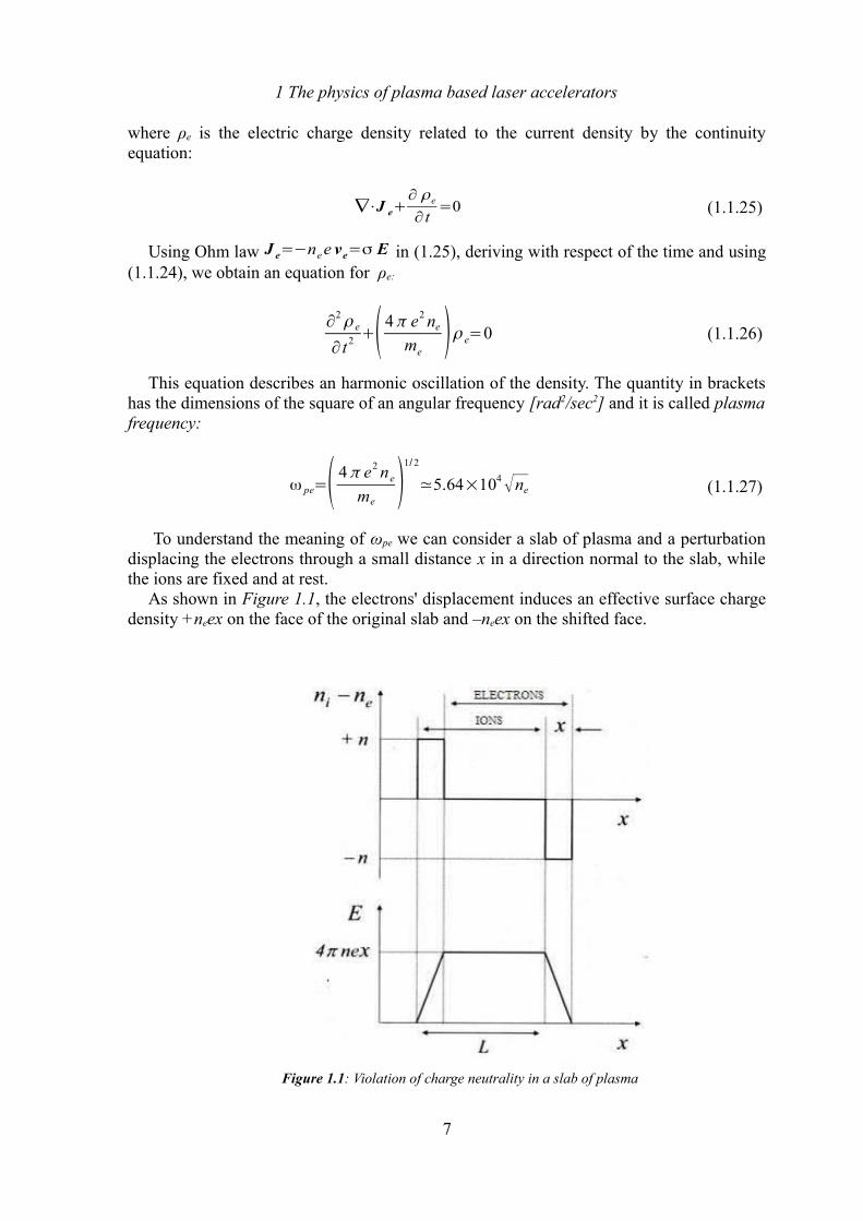
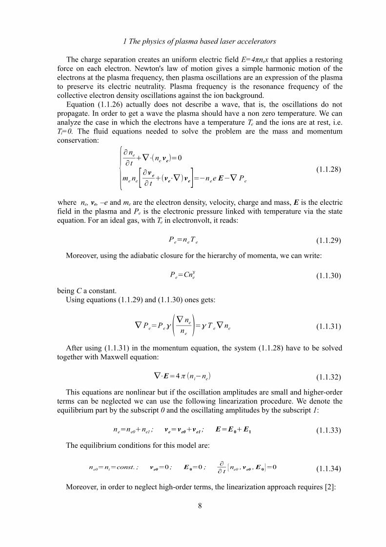
To understand the meaning of ωpe we can consider a slab of plasma and a perturbation displacing the electrons through a small distance x in a direction normal to the slab, while the ions are fixed and at rest.
As shown in Figure 1.1, the electrons' displacement induces an effective surface charge density +neex on the face of the original slab and –neex on the shifted face.
7
Figure 1.1: Violation of charge neutrality in a slab of plasma
1 The physics of plasma based laser accelerators
The charge separation creates an uniform electric field E=4πnex that applies a restoring force on each electron. Newton's law of motion gives a simple harmonic motion of the electrons at the plasma frequency, then plasma oscillations are an expression of the plasma to preserve its electric neutrality. Plasma frequency is the resonance frequency of the collective electron density oscillations against the ion background.
Equation (1.1.26) actually does not describe a wave, that is, the oscillations do not propagate. In order to get a wave the plasma should have a non zero temperature. We can analyze the case in which the electrons have a temperature Te and the ions are at rest, i.e. Ti=0. The fluid equations needed to solve the problem are the mass and momentum conservation:
{∂ ne
∂ t+∇⋅(ne ve)=0
me ne[∂v e
∂ t+(ve⋅∇)ve]=−ne e E−∇ P e
(1.1.28)
where ne, ve, –e and me are the electron density, velocity, charge and mass, E is the electric field in the plasma and Pe is the electronic pressure linked with temperature via the state equation. For an ideal gas, with Te in electronvolt, it reads:
Pe=ne T e (1.1.29)
Moreover, using the adiabatic closure for the hierarchy of momenta, we can write:
Pe=Cneγ
(1.1.30)
being C a constant.Using equations (1.1.29) and (1.1.30) ones gets:
∇ Pe=P eγ (∇ ne
ne)=γ T e∇ ne (1.1.31)
After using (1.1.31) in the momentum equation, the system (1.1.28) have to be solved together with Maxwell equation:
∇⋅E=4π (n i−ne) (1.1.32)
This equations are nonlinear but if the oscillation amplitudes are small and higher-order terms can be neglected we can use the following linearization procedure. We denote the equilibrium part by the subscript 0 and the oscillating amplitudes by the subscript 1:
ne=ne0+ne1 ; ve=ve0+ve1 ; E=E 0+E1 (1.1.33)
The equilibrium conditions for this model are:
ne0=ni=const. ; ve0=0 ; E 0=0 ;∂
∂ t{ne0 , ve0 , E 0}=0 (1.1.34)
Moreover, in order to neglect high-order terms, the linearization approach requires [2]:
8
1 The physics of plasma based laser accelerators
(ne1
ne0)
2
≪ne1
ne0
; (ve1⋅∇)ve1≪∂ ve1
∂ t; ... (1.1.35)
In this way the proper linearized system to be solved is:
{∂ ne1
∂ t+ne1∇⋅(ve1)=0
me
∂ ve
∂ t=−e E−γ T e∇ ne1
∇⋅E1=−4π e ne1
(1.1.36)
For further simplicity we consider a one-dimension model so that all variables are function of time t and space x; for one freedom degree the adiabatic exponent is γ=3.
In this model we look for monochromatic wave solution with frequency ω and wave number k=2π/λ, so that:
{ne1=nexp [ i(kx−ω t )]v e1=v exp [i(kx−ω t )]E1=E exp [i (kx−ω t)]
(1.1.37)
Using (1.1.36) in (1.1.37) a set of linear algebric equations is obtained whose solution is the following dispersion relation, also known as plasmon, describing electrostatic longitudinal waves:
ω 2=ω pe
2+3k 2 v th
2 (1.1.38)
where the thermal velocity in our 1D model is:
v th=√T e
me
(1.1.39)
The concept of plasma frequency can be used also to have a better understanding of the collisionless limit and how it is related with the plasma parameter.
In a fully-ionized plasma binary interactions between particles are mostly due to the Coulomb force whose range is the same order of the Debye length.
We consider a population of charged particle with density n mass m0, charge e and mean velocity v0 approaching a target particle at rest, with same charge and mass M≫m0 .
It can be demonstrated that the high angle scattering rate is:
ν c=4π e4 n
m2v03 (1.1.40)
Using equation (1.1.13), (1.1.27) and (1.1.39) we can say that a thermal electron travels a Debye length in a plasma oscillation period:
9
1 The physics of plasma based laser accelerators
ω pe=v th
λ D
=2πτ pe
(1.1.41)
It is easy to show, making use of the definition of ND (1.1.14), that the ratio between νc
and ωpe is:ω pe
ν c
=τ c
τ pe
∝N D (1.1.42)
Now it is clear that ND, the number of particles in the Debye sphere, connect the collective motion with the collision time scale. Nevertheless, Debye shielding is effective if equation (1.1.15) N D≫1 is true, that means that the collisionless limit, in which the collision time scale is slow with respect to collective phenomena, can be expressed by the condition:
ω pe
ν c
=τ c
τ pe
∝N D≫1 (1.1.43)
1.1.4 Electromagnetic waves propagation in a cold plasma
The interaction between an electromagnetic wave and a plasma can be easily described starting from Maxwell equations in MKS units:
{∇⋅B=0∇⋅D=ρ
∇∧H=J+∂D∂ t
∇∧E=−∂B∂ t
(1.1.44)
The wave, traveling in the plasma, interacts with all species of particles, but the interaction with neutral atoms is much weaker with respect to the interaction with charged particles. Moreover, ions mass is much bigger than electrons mass, this means that the interaction with ions can also be neglected in first approximation.
The interaction between the wave and the electrons is described by the density current vector J whose expression can be derived solving the motion equation of the electron that reads:
m∂ v∂ t=e E (1.1.45)
where we have neglected collision and used the assumption that v depends only on the time. Moreover we have take in account that magnetic force is much weaker than the electric one. A more detailed description that take in account collisional effect is in [4].
If we consider a monochromatic electric field E=E0 e−iω t , we can look for a solution
for the velocity with the same time dependance v=v0 e−iω t . Hence the solution of (1.1.45) is:
10
1 The physics of plasma based laser accelerators
v=e E
−iω me (1.1.46)
The density current J is proportional to v then, after rationalization of (1.1.46), we have:
J=ne v=iωn e2 Eω 2 me
(1.1.47)
where n and m are the electron density and mass rispectively.Using the vacuum permittivity ε0 we can introduce in the above expression the plasma
frequency, that in MKS units reads ω pe2=( e2 n
meε 0 ) and writing:
J=iωε 0ω pe
2 E
ω 2 (1.1.48)
We can insert this expression of J in the curl equation for H to have:
∇∧H=iωε 0ω pe
2 E
ω2 −iω ε 0 E=iω ε 0(1−ω pe
2
ω2 )E=iω ε E=iω D (1.1.49)
We have found that a plasma is a dispersive medium because its permittivity depends on the frequency of the radiation propagating through it: ε=ε (ω ) , being:
ε (ω )=ε 0(1−ω pe2
ω2 ) (1.1.50)
In the previous section we have shown longitudinal waves in plasma. Now we can study the propagation of transversal waves starting form the usual realtions [3,4,7]:
k 2=ω 2 με+iω μσ => k=β+iα (1.1.51)
where:
β=ω √μ ε2 [1+√1+σ 2
ω 2ε 2 ]; α=ω √ με2 [√1+σ 2
ω 2ε 2−1] (1.1.52)
In the collisionless limit σ=0 , as shown in [4], then we have, setting μ=μ0 :
β=ωc √1−
ω pe2
ω; α=0 ; n refr=√1−
ω pe2
ω (1.1.53)
It is easy to understand that if ω<ω pe the propagating coefficient β is an imaginary one. Then if we consider an electromagnetic plane wave propagating along z the direction whose equation is:
11
1 The physics of plasma based laser accelerators
E=E 0 exp [ i(kz−ω t)]=E 0exp (iβ z−α z−iω t) (1.1.54)
it is clear that the spatial term becomes a damping term. In this case there is no propagation, only a vanishing wave exponentially damped with a characteristic length:
l sd=c
√ω pe2 −ω
(1.1.55)
called skin depth and representing the length scale at which plasma damps electromagnetic waves with frequency below the plasma frequency, which is the cut-off.
For a fixed frequency of the electromagnetic wave, the density at which ω=ω pe is called critical density and can be defined, using equation (1.1.27), as:
nc(ω )=( me
4π e2)ω 2 (1.1.56)
If the plasma density is bigger than critical density, namely ne>nc , the plasma is opaque and the wave is damped, otherwise the plasma is transparent and the wave can propagate without damping, in the collisionless limit. In the first case the plasma is called overdense, or overcritic, in the second case is called underdense.
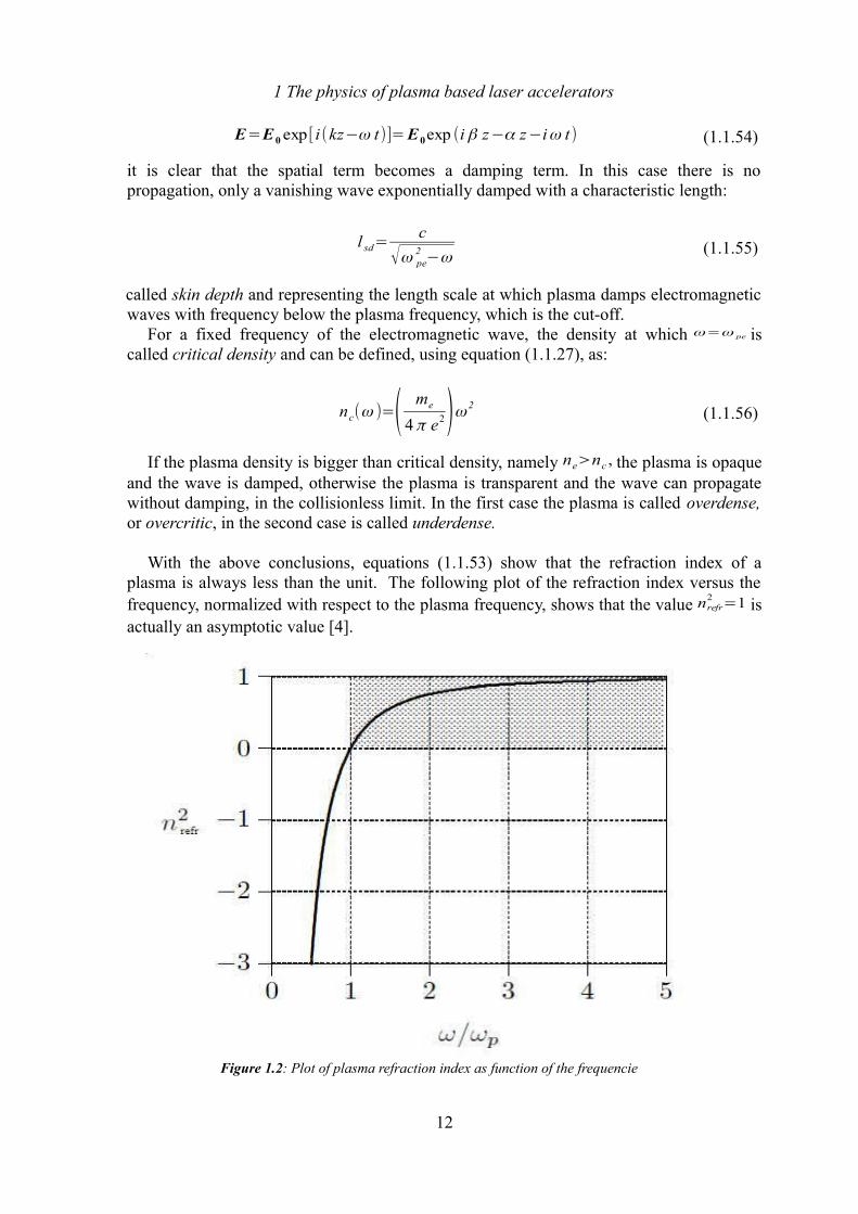
With the above conclusions, equations (1.1.53) show that the refraction index of a plasma is always less than the unit. The following plot of the refraction index versus the frequency, normalized with respect to the plasma frequency, shows that the value nrefr
2=1 is
actually an asymptotic value [4].
12
Figure 1.2: Plot of plasma refraction index as function of the frequencie
1 The physics of plasma based laser accelerators
This means that the phase velocity of an electromagnetic wave in a plasma is always bigger than the light velocity:
vϕ=ωk=
cnrefr
=c
√1−ωpe
2
ω
(1.1.57)
Hence, we can look at the phase velocity as the rate at which the phase of the wave propagates in space, but it is not the propagation velocity of the wave in plasma. The actual propagation velocity is the group velocity, that corresponds with the velocity at which energy, or information, is conveyed along a wave and, for a plasma is:
v g=∂ω∂ k=c√1−
ω pe2
ω (1.1.58)
If we suppose that the plasma is in an external magnetic field B0=B0 z along the z axis, the motion equation of the electron in this case reads:
me∂ v∂ t=e E+e v∧B0 (1.1.59)
that, using the cyclotron frequency ω c=e B0
me
, can be written as:
∂v∂ t=
e Eme
+ω cv∧ z (1.1.60)
Solving this equation, one can find that plasma permittivity becomes a 3x3 hermitian tensor. It means that a magnetized plasma is an anisotropic medium. As a result of this anisotropy, studying the wave propagation one can see that the electromagnetic wave traveling in a magnetized plasma is decomposed in two waves with different propagating constant: one is called ordinary wave (O-mode) because, for a wave propagating perpendicularly to B0, it is identical to those obtained in the unmagnetized plasma; the other one is called extraordinary wave (X-mode).
Moreover, for a linearly polarized wave propagating along B0 direction, it can be shown that the polarization plane suffers a rotation of an angle:
θ=VB0 l (1.1.61)
where l is the path length of the wave in the plasma and V is the Verdet constant. This effect is typical of optically active media and is called Faraday effect. Further details on magnetized plasmas can be found in [1, 2, 3].
1.2 Lasers
A laser (acronym of Light Amplification by Stimulated Emission of Radiation) is a
13
1 The physics of plasma based laser accelerators
device that generates or amplifies electromagnetic radiation, ranging from the long infrared region up through the visible region and extending to the ultraviolet and recently even to the x-ray region.
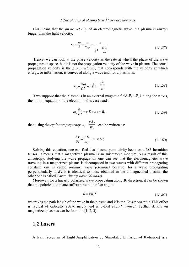
Lasers are based on stimulated emission, discovered by Einstein in 1917 who postulated that an atom in an excited level could decay to lower energetic level either spontaneously either by stimulated emission.
Let E1 and E2 represent the two level of a system and we consider an electromagnetic radiation whose frequency satisfies:
hν=E2−E1 (1.2.1)
If the system is in its ground state it will absorb radiation and will get excited, but if the system is already excited it can decay with emission of a photon in a random direction (spontaneous decay) or with emission of a photon in the same direction of the electromagnetic incident photon, as shown in Fig.1.3:
It can be demonstrated that the radiation emitted by stimulated emission is in phase, i.e. coherent, with the incident one.
Since the transition rate depends on the atoms number in the ground state, to be the system able to amplify the incident radiation, therefore it is able to emit radiation coherent with and exceeding the incident one, it is necessary that the number of atoms in the upper level, E2, is greater than the number in the ground level, E1. This condition, called population inversion, can not be achieved if the above two level system follows a Maxwell-Boltzmann distribution. On the other hand, population inversion is possible for system with three or more level [2, 9, 10].
Laser light is monochromatic since the amplification is done for frequency satisfying equation (1.2.1). Moreover, the optically active medium is used together with two mirrors, forming a resonant cavity and causing the natural line-width to be narrowed by many order of magnitude.
The spatial coherence that characterizes a laser is defined as the phase change of the electromagnetic field of two separated points. If the phase difference of two points that are separated by a distance L is constant in time, then this two points are coherent. The
14
Figure 1.3: Representation of spontaneous and stimulated emission
1 The physics of plasma based laser accelerators
maximum value of L is called coherent length.The temporal coherence is defined as the phase change of the electromagnetic field in
time in a fixed point. If the phase in this point is equal at time t and t+τ, for all times t, the point is coherent during the time τ. The maximum value of τ is called temporal coherence of the laser.
The maximum power available from lasers reaches today intensities over 1021W/cm2 in a femtosecond pulse. The field reaches 1012V/m that is greater than the electric field binding the electrons to nucleus. When such a pulse interacts with matter, it instantly ionizes the target creating a plasma.
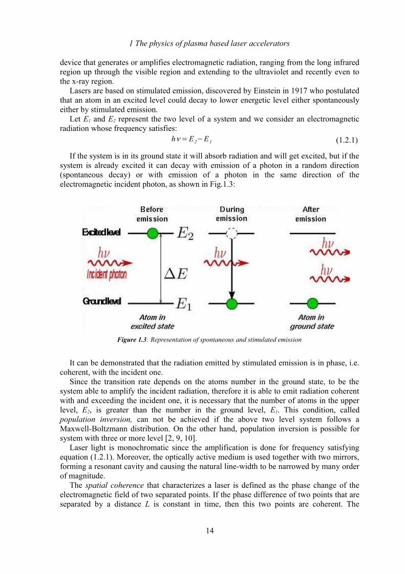
The key in reaching such high power is the chirped pulse amplification (CPA) technique, developed for radar devices more than 40 years ago. In the CPA scheme a pulse made by a low power laser (the oscillator in Fig 1.4) which is able to create a really short packet, ~50fs, is first starched in time (chirped in frequency) by a factor ~104, then amplified and finally recompressed.
Stretching and compression are obtained using a pair of gratings, or prisms, that can be arranged to separate the output pulse spectrum from the oscillator in such a way that different wavelengths follow different path through the optical system. This enable pulse compression using the reverse procedure.
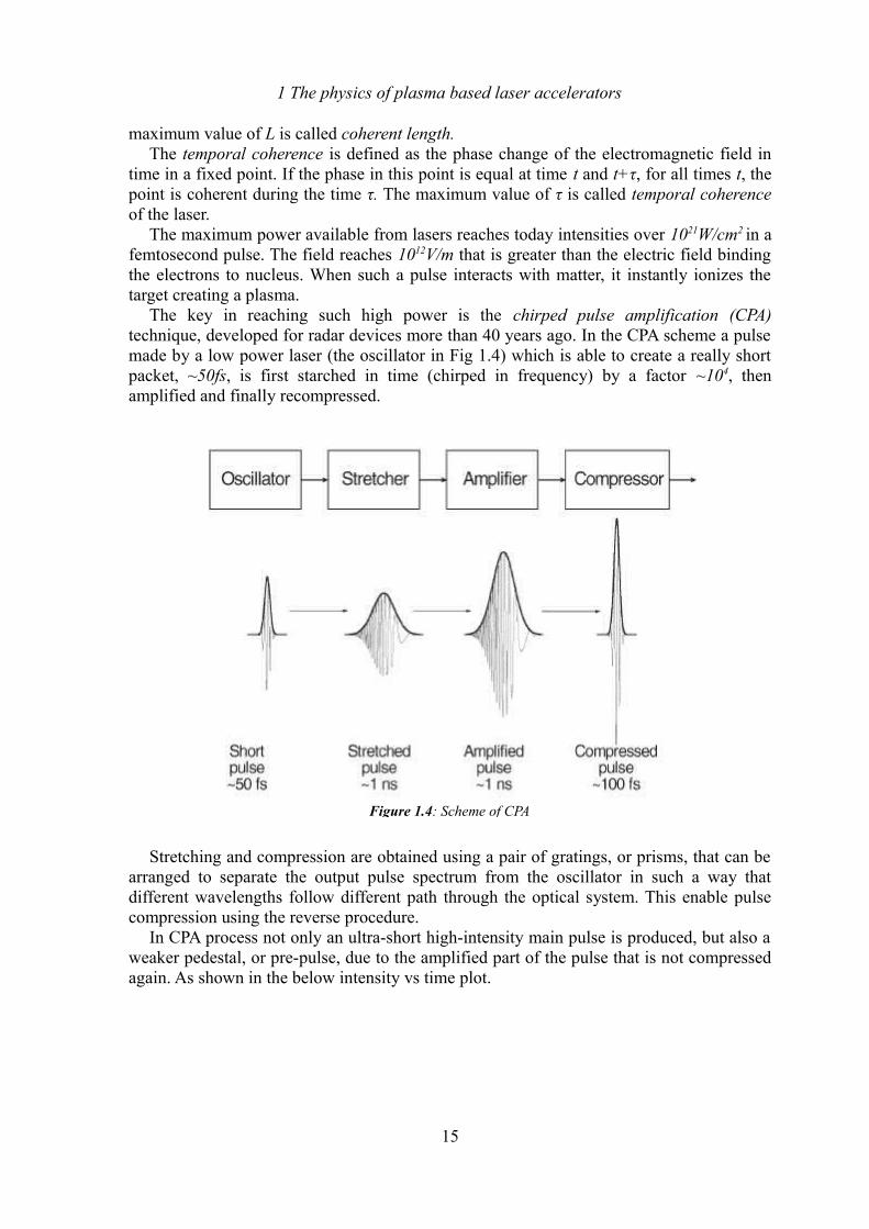
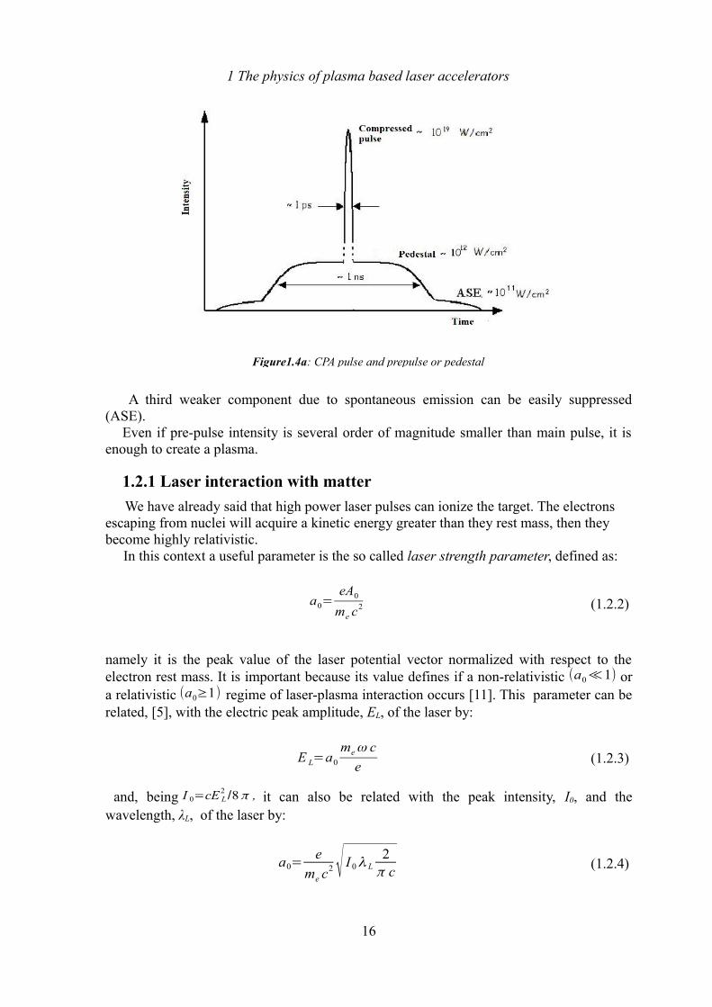
In CPA process not only an ultra-short high-intensity main pulse is produced, but also a weaker pedestal, or pre-pulse, due to the amplified part of the pulse that is not compressed again. As shown in the below intensity vs time plot.
15
Figure 1.4: Scheme of CPA
1 The physics of plasma based laser accelerators
A third weaker component due to spontaneous emission can be easily suppressed
(ASE).Even if pre-pulse intensity is several order of magnitude smaller than main pulse, it is
enough to create a plasma.
1.2.1 Laser interaction with matter
We have already said that high power laser pulses can ionize the target. The electrons escaping from nuclei will acquire a kinetic energy greater than they rest mass, then they become highly relativistic.
In this context a useful parameter is the so called laser strength parameter, defined as:
a0=eA0
me c2 (1.2.2)
namely it is the peak value of the laser potential vector normalized with respect to the electron rest mass. It is important because its value defines if a non-relativistic (a0≪1) or a relativistic (a0≥1) regime of laser-plasma interaction occurs [11]. This parameter can be related, [5], with the electric peak amplitude, EL, of the laser by:
E L=a0
meω c
e (1.2.3)
and, being I 0=cE L2/8π , it can also be related with the peak intensity, I0, and the
wavelength, λL, of the laser by:
a0=e
me c2 √ I 0λ L2π c
(1.2.4)
16
Figure1.4a: CPA pulse and prepulse or pedestal
1 The physics of plasma based laser accelerators
The a0 can be seen as the maximum momentum of an electron quivering in the laser field, normalized with respect to its rest mass, and the previous relation shows that relativistic regime is reached for laser intensity I 0>1018W /cm2 .
The laser intensity needed to ionize an hydrogen atom can be estimate using Bohr model. At the Bohr radius the electric field strength is, in cgs units, Ea=e /aB . The intensity at which the laser field matches the binding strength of the electron to the atom, the so called atomic intensity, is [5]:
I a=cEa
2
8π≃3.51×10¹⁶ W /cm2 (1.2.5)
A laser intensity I L>I a will guarantee at least partial ionization for any target material, though this can occur well below this threshold. In fact an electron can be ejected from an atom if it receives enough energy by absorbing a single photon with right frequency, as in the photoelectric effect, or absorbing several photons of lower frequency. Latter process is called multiphoton ionization (MPI) and depends strongly on the light intensity, or, that is the same, on the photon density. According perturbation theory, the n-photon ionization rate is given by:
Γ n=σ n I Ln
(1.2.6)
where σn decreases with n, but the dependence on InL ensures that ionization events occur
provided that the intensity is high enough (>1010W/cm2).The above relation is true until the atomic binding potential remains undisturbed, as
consequence of perturbation theory. If the laser electric field becomes strong enough it can distort the electric field felt by the electron. In this case the Coulomb barrier will be change in a finite height barrier and the electron can escape from the atom via tunneling ionization. Moreover, if the electric field intensity is very high it can suppress the Coulomb barrier, in this case we can talk of barrier suppression ionization (BSI), as a variant of tunneling ionization regime.
Keldysh parameter can be used to understand which regime (Tunneling or MPI) will prevail using a certain laser intensity:
γ=√ E ion
Φ pond
(1.2.7)
where Eion is the ionization energy and Φpond is the ponderomotive potential of the laser field:
Φ pond=e2 EL
2
4 meω L2 (1.2.8)
expressing the effective quiver energy acquired by an oscillating electron in the laser field.As a rule, tunneling regime prevails for strong fields and long wavelengths, hence when
γ<1; multiphoton ionization prevails when γ>1, in this case laser electric field is not enough intense to perturb the potential barrier.
At the beginning of the interaction, when the pre-pulse impinges on the target,
17
1 The physics of plasma based laser accelerators
multiphoton ionization dominates, because of its low intensity. When the main pulse arrives tunneling effect dominates.
1.2.2 Ponderomotive force
We have shown that a plane electromagnetic wave propagates in a plasma with a phase velocity expressed by equation (1.1.57). For short laser pulses this result does not hold anymore because their focal spot has dimensions of the order of micron. Hence, short pulses create strong radial and longitudinal field gradients associated with the so-called ponderomotive force that can eject electrons from the regions where the field is higher and is responsible for longitudinal waves in plasma.
In the non-relativistic limit we can easily evaluate the effect of an electric field gradient assuming that the gradient is fairly weak and the displacement of a particle over a field oscillation period is small compared to the typical distance of the gradient.
The motion equation of a charged particle in an oscillating electric field along x axis is:
m x=qE0cos(ω t ) (1.2.9)
Integrating the motion equation twice with respect to the time and with the initial condition x0=0 we have:
x= x0−qE0
mω 2 cos(ω t ) (1.2.10)
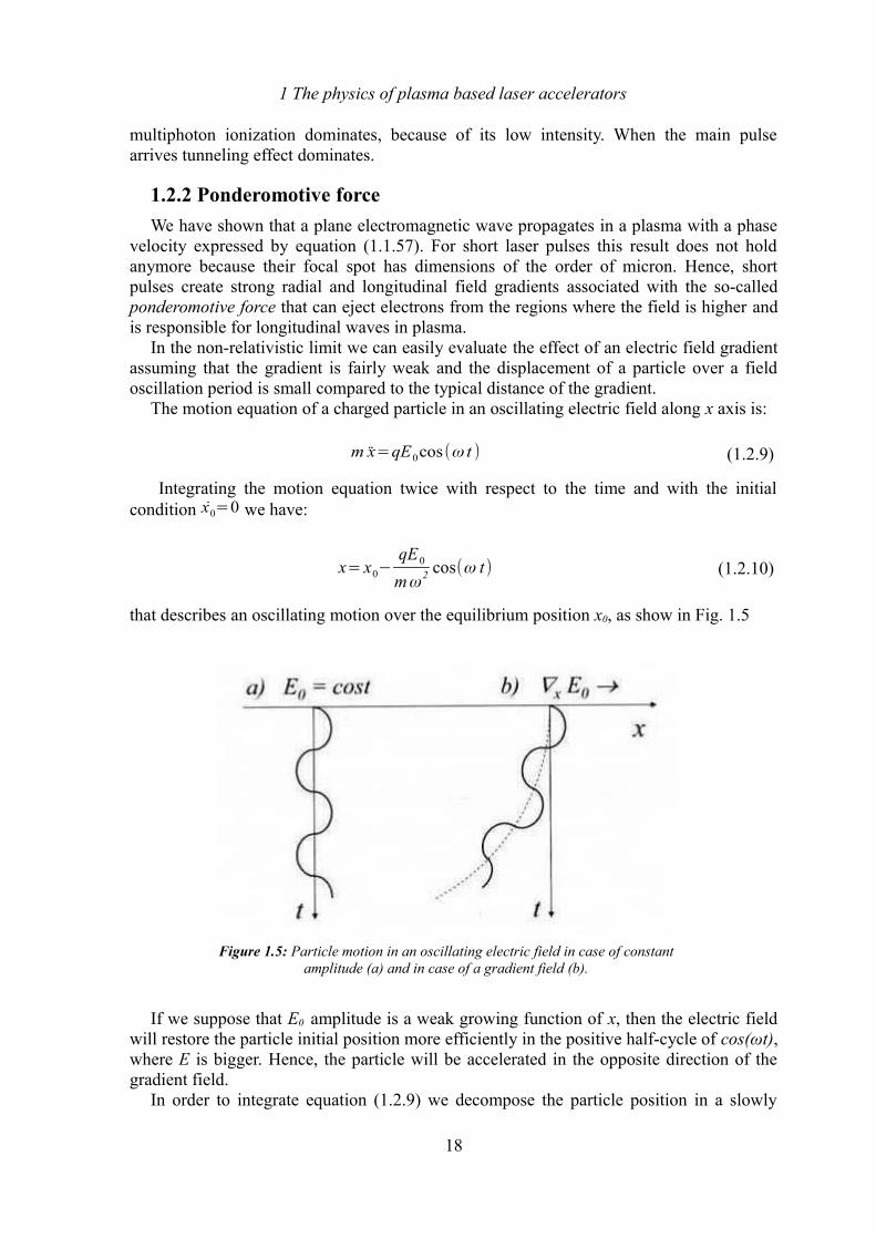
that describes an oscillating motion over the equilibrium position x0, as show in Fig. 1.5
If we suppose that E0 amplitude is a weak growing function of x, then the electric field will restore the particle initial position more efficiently in the positive half-cycle of cos(ωt), where E is bigger. Hence, the particle will be accelerated in the opposite direction of the gradient field.
In order to integrate equation (1.2.9) we decompose the particle position in a slowly
18
Figure 1.5: Particle motion in an oscillating electric field in case of constant amplitude (a) and in case of a gradient field (b).
1 The physics of plasma based laser accelerators
varying part x , and in quickly varying part x. Then x= x+ x where:
x (t )=⟨ x ⟩T=1T∫
t−T2
t−T2 x ( t ' )dt '=
2ωπ∫
t−T2
t−T2 x (t ' )dt ' (1.2.11)
is the average value of x over a period of the electric field.Taylor expansion of the electric field around x is:
E≃(E0( x )+∇ x E0( x) x )cos(ω t ) (1.2.12)
and equation (1.2.9) can be written as:
m ¨x+m ¨x=q(E0( x )+∇ x E0( x) x)cos(ω t) (1.2.13)
With the above assumptions we have ¨x≪ ¨x and because of weak spatial dependance of the field amplitude we can set E0( x )≫∇ x E0( x ) x. Then for the quickly varying part of the motion we have an oscillation with frequency ω:
x≃−qE0
mω 2 cos(ω t ) (1.2.14)
For the slowly varying part, which represent the motion of oscillating center, we have, after averaging equation (1.2.13) over a field period:
¨x=−q2
2 m2ω 2 E0( x )∇ x E0( x ) (1.2.15)
From the above equation we can see that the oscillating center is accelerated in the opposite direction of the gradient field. Pondermotive force is responsible for this acceleration and can be expressed as:
F P=−q2
4mω 2 ∇ E02
(1.2.16)
that is the gradient of the ponderomotive potential (1.2.8). It is important to note that ponderomotive force depends on the square of the charge,
then its direction is the same for positive or negative particles; on the other hand its modulus in bigger for electron than for proton because of the dependence on 1/m.
This force will tend to push electrons away from regions of locally higher intensity and therefore a single electron will drift away from the center of a focused laser beam picking up a quiver velocity:
vos=eEmω (1.2.17)
The fully relativistic version of equation (1.2.16) reads:
19
1 The physics of plasma based laser accelerators
F P=−mc2∇ ⟨γ ⟩ (1.2.18)
where ⟨γ ⟩=√1+⟨ p ⟩
mc2+⟨a0
2⟩
2, as shown in [5].
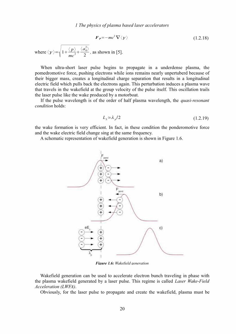
When ultra-short laser pulse begins to propagate in a underdense plasma, the pomedromotive force, pushing electrons while ions remains nearly unpertuberd because of their bigger mass, creates a longitudinal charge separation that results in a longitudinal electric field which pulls back the electrons again. This perturbation induces a plasma wave that travels in the wakefield at the group velocity of the pulse itself. This oscillation trails the laser pulse like the wake produced by a motorboat.
If the pulse wavelength is of the order of half plasma wavelength, the quasi-resonant condition holds:
LL≃λ p/2 (1.2.19)
the wake formation is very efficient. In fact, in these condition the ponderomotive force and the wake electric field change sing at the same frequency.
A schematic representation of wakefield generation is shown in Figure 1.6.
Wakefield generation can be used to accelerate electron bunch traveling in phase with
the plasma wakefield generated by a laser pulse. This regime is called Laser Wake-Field Acceleration (LWFA).
Obviously, for the laser pulse to propagate and create the wakefield, plasma must be
20
Figure 1.6: Wakefield generation
1 The physics of plasma based laser accelerators
underdense. Moreover if the parameter a0≪1 the wakefield is linear, if it is a0≃1 it becomes non linear and the electron quiver motion becomes relativistic, if a0≫1 different regimes can be achieved.
1.2.3 Interaction with solids
When an electromagnetic wave with optical or near infrared frequency ω is focused on a gas, the plasma produced has an electron density ne less than critical densitync=meω
2/4π e2 . Hence the plasma is called underdense and the wave can propagates
through it.Interaction with a solid target is radically different, in fact the electromagnetic wave
promptly ionizes the target forming an overdense plasma with ne>nc . The laser pulse can only penetrate in the skin layer l sd=c/ω p=(λ /2π )√nc/ne and the interaction is then a surface interaction.
In the interaction part of laser light is reflected but a significant fraction of laser energy may be absorbed by the target.
For short laser pulses with relativistic intensity, plasma temperature rises very fast and the collision in the plasma can be considered ineffective during the interaction. In this situation different collisionless absorption mechanism can arise, such as resonance absorption, J∧B heating, vacuum heating [5, 2]. In any case the absorbed energy will result in the heating of part of the electron population at temperature much higher than the initial bulk temperature.
Laser energy absorption by electrons is a crucial phenomenon in ion acceleration and will be dissed further.
Self-induced Transparency:
We have seen, in Sec. 1.2.1, how the electron motion in an electromagnetic wave becomes relativistic if the field intensity is high enough. At extreme intensities, this motion can modify the refractive index of an overdense plasma to permit propagation [5]. This phenomenon is known as self-induced transparency (SIT). If we consider a high intensity wave (a0⩾1) the electron quivering motion is highly relativistic and its relativistic factor take the form γ 0=√1+a0
2/2≃a0 /√2.
The effective plasma frequency appearing in the dispersion relation should be corrected as:
ω ' p=ω p
γ 0
∝(ne
a0)
1 /2
(1.2.20)
being ne the electron density. The plasma frequency gets smaller and the critical density moves to larger values. That means that the plasma at the former critical density becomes transparent and the laser pulse can propagate through it.
Hence, there will be a critical intensity above which the plasma loses its natural opacity, i. e. ω ' p⩽ω , and the condition for the laser strength parameter is:
a0SIT≥√2
ne
nc (1.2.21)
21
1 The physics of plasma based laser accelerators
In terms of electron density, we can state that the plasma is transparent for an intense laser if nc<ne<γ nc .
The propagation of laser pulses through slightly ovecritical plasmas is gaining interest after some ion acceleration regimes have been proposed but is not straightforward to produce a target with ne≃nc , therefore such condition has not been accurately investigate.
1.3 Laser induced ion acceleration
When a laser pulse irradiates a solid target an overdense plasma slab is formed and several absorption mechanism can be involved. The absorbed laser energy accelerates and heats electrons in plasma. Moreover, if normal incidence is considered, the ponderomotive force pushes inward the electrons from the rear surface of the target creating a charge separation which produces an electrostatic field experienced by ions.
The first experiments, exploiting interaction of short (τ < 1ps) and intense (Ilλ2 > 1018W/cm2) laser pulses with thin solid foil, showed the production of protons beams in the range of several tens of MeV coming from the rear surface of the target.
The bunches produced exhibit a remarkable collimation and a high energy cut-off; the maximum energy record of 58MeV has not been beaten yet. On the other hand there have been significant improvement in the control of the beam quality and energy spectra that made possible to propose the laser-accelerated ions for therapy, even if many study are still required on the transport of the optically accelerated beams and post accelerations in order to delivery ions with right characteristics to the patients.
In most experiments the dominant regime is the so called Target Normal Sheath Acceleration (TNSA) in which the accelerated protons come from the rear surface of the target and the accelerating field is due to the expansion of heated electrons around the target. Different regimes have been theoretically proposed and tested, in which the radiation pressure of the laser dominates on the heating process and the accelerated bunch is composed by ions coming from the irradiated surface of the target. These regimes are called Radiation Pressure Acceleration (RPA) and the accelerating mechanism depends on the target thickness.
The laser intensities available reaches 1021W/cm2 and the corresponding radiation pressure is about 300Gbar.
The physics of these regimes is not simple because of the non-linear phenomena involved in the extreme conditions of high power laser interactions with overcritical plasmas. Difficulties remain even considering simplified models, i.e. preformed plasma, no ionization, no collision and so on.
Before analyzing the acceleration regimes it worth to note that in the previous discussions we have regarded the ions as being fixed and providing a neutralizing background to the electron density fluctuations generated by the laser. At high intensities this situation alters quite dramatically due to the large electric field, of the order of GV/m, induced when many electrons are rapidly displaced from their initial positions. As a result, a substantial fraction of ions may be accelerated to energies in the multi-MeV range.
It is important to note that ions quiver motion in a laser field is negligible compared to that of electrons, because of ions bigger mass. For an ion of mass Mi and charge Ze its quiver velocity can be written as [5]:
22
1 The physics of plasma based laser accelerators
v i
c=
Zme
M i
a0 (1.3.1)
Thus, to accelerate ions to relativistic velocities directly by the laser field, one would need intensities of Iλ2>1024W/cm2, or a0≈2000, which are well beyond the intensities available with current laser systems. In a plasma, however, the electrons mediate between the laser field and the ions via charge separation. In other words the laser displaces and heats electrons and the consequent electrostatic fields pulls on the ions. Because of their higher inertia, the ion response is delayed by a factor [M i /Zme]
1/2which can be related
with the ratio between electron and ion plasma frequencies ω p/ω pi . Derivation of ion plasma frequency can be found in [1, 2, 4].
1.3.1 Target Normal Sheath Acceleration (TNSA)
In the interaction of an intense electromagnetic wave with a solid, the front surface of the target becomes ionized well ahead the pulse peak. The successive laser-plasma interaction heats the electrons via different absorption mechanism to high temperature (T ≈ MeV) and their free path becomes bigger than the plasma skin depth and than the target thickness. These hot electrons have a diffusive motion both in the laser direction and in the opposite one. Thus they can propagate in the target reaching its rear surface where they expand into vacuum for several Debye lengths forming a cloud of relativistic electrons. The charge imbalance due to the cloud gives rise to an extremely intense longitudinal electric fields, which is responsible for the efficient ion acceleration. The most effective acceleration mechanism takes place at the rear surface of the target where the high intensity electrostatic field can ionize the atoms present on the unperturbed surface and then accelerates the ions produced. This mechanism is know as Target Normal Sheath Acceleration (TNSA).
The accelerated multi-MeV protons from the rear surface of the irradiated solid foil is achieved no matter its composition, because they came from the hydrogen rich contaminants, such as hydrocarbons or water vapor, present on the target surface.
The energy spectrum of the protons is typically exponential with a high cut-off in the range of tens MeV.
Several theoretical models have been proposed in order to describe the TNSA regime, but the most efficient in predicting the energy cut-off and that gives also a good interpretation of the acceleration mechanism is the one proposed by Passoni [22], despite the strong assumptions. This model will be briefly described in the following.
The electron involved in TNSA regime can be two different populations. The first is the hot (or fast) electron component, directly created by the laser pulse in the plasma plume at the front surface of the target. Its density is of the critical density order (nh ≈ 1020-1021cm-3) and its temperature is of the ponderomotive potenzial order (Th ≈MeV). The free motion of this hot electron beam through the target require the presence of a return current that locally compensates the flow of the hot electrons. In metallic target this current is provided by the second component of conduction (or cold) electrons that are put in motion by the electric field of fast electrons. The second electron component density is of the solid density order, that is, much bigger than fast component, so the required velocity for current neutralization is small and their temperature is much lower than hot electrons.
23
1 The physics of plasma based laser accelerators
The ion population can be also divided in two species: one being the heavy ions of the target, possibly constituted of several ion species, with a low charge over mass ratio ZH/M and density nH, the other one is light ion component usually present as contaminant on target surface, with charge ZL and density nL.
The acceleration is most effective on light ions while the heavy component provides a positive charge that offers more inertia and make the charge separation responsible for the huge accelerating field.
Now we assume one-dimensional geometry and we describe the electron population as a two-temperature distribution ne = nh +nc ≈ nc, where the subscript c stays for the conduction and h stays for the hot electrons; moreover the target is a plane sharp-edged plasma slab. Then Poisson equation for the self-consistent electrostatic potential ϕ (r ,t ) is:
d 2ϕ
dt 2 =4 π e (N e−Z H nH−Z L nL) (1.3.2)
For short pulses, laser-target interaction occurs on a time scale shorter than typical ion motion scale, then heavy ions can be assumed immobile, while light ions are mobile but, because of the low density, their effect on the electrostatic potential evolution can be neglected. For simplicity, the cold electron population is assumed to have constant density n0c, while the hot population is assumed to be in thermal equilibrium with the electrostratic potential, then described by a Boltzmann distribution.
The most energetic electrons can leave the system escaping from the self-consistent potential, because of this the self-consistent solution for the potential diverges at large distance from the target. Then one describes the hot electrons assuming a single temperature Maxwell-Jüttner relativistic distribution function and considers only electrons with negative energy, i. e. bound to the system.
With these assumptions the solution for the electrostatic potential at the target vacuum interface results to be a function of the temperature T and of the maximum energy of a bound electron, εemax,:
ϕ (0 )=ϕ (T ,ε emax) (1.3.3)
In order to evaluate the maximum ion energy and the energy spectrum, the hot electron temperature, which determines the maximum binding energy, must be know. It is assumed to be described by:
T h=mc2(√1+a0
2
2−1) (1.3.4)
which relates the electron temperature with the laser irradiance Iλ2 via the parameter a0.The maximum proton energy, or the cut-off energy of the spectrum is then given by:
Ecutoff=Z Lϕ (0)=Z L f (E L , I L) (1.3.5)
Despite of the strong assumption the model successfully describes the scaling law of the proton acceleration in TNSA regime and is compatible with experimental results showing a linear dependence of Ecut-off with I1/2
.
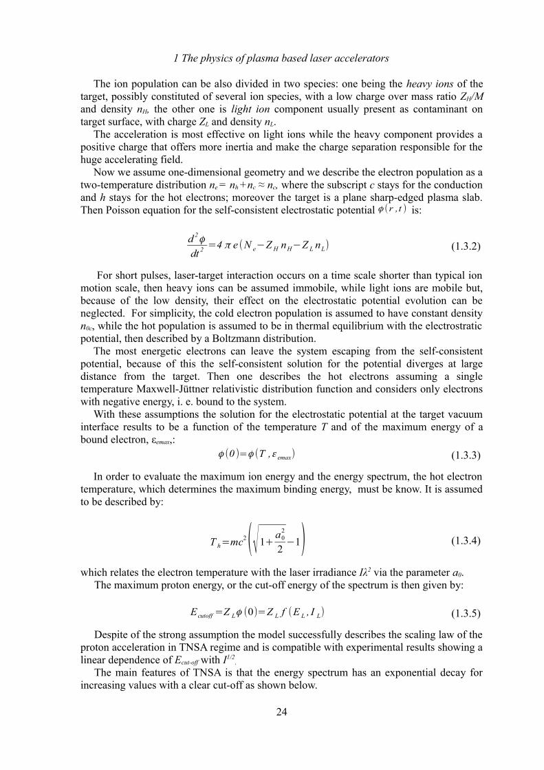
The main features of TNSA is that the energy spectrum has an exponential decay for increasing values with a clear cut-off as shown below.
24
1 The physics of plasma based laser accelerators
The efficiency of TNSA acceleration can be enhanced increasing the efficiency of the energy transfer from laser to target. For this reason different design of targets can be considered where a foam layer is deposited on the target leading to a considerably energy absorption.
Moreover the angular spread is significant and the beam is not suitable for free propagation.
1.3.2 Radiation pressure Acceleration (RPA)
A possible route to accelerate ions up to relativistic energies has been investigated with numerical simulations and theoretical models and it is the acceleration regimes which start dominate over TNSA at higher intensity. Simulations show that if a thin target is irradiated with a laser intensity I≥1023W /cm2 its ions reach energies in the GeV/nucleon range and the scaling of the ion energy vs. laser pulse is linear.
Laser with such intensities are not currently available but RPA can dominate over TNSA at lower intensities if circularly polarized light is used instead of linearly polarized. In fact in this conditions electrons heating becomes negligible, ruling out TNSA which is driven from the space charge produced by energetic electrons escaping in vacuum, and the ponderomotive force acts directly accelerating electrons and ions.
Two different models exist for this regime, depending on the thickness of the target: the Hole Boring (HB) for thicker target and the Light Sail (LS) for thinner ones.
25
Figure 1.8: Energy spectrum of protons accelerated in TNSA regime [23]
1 The physics of plasma based laser accelerators
Hole Boring:
In this regime the ion acceleration is due to the electrostatic field Ex arise from the electron displacement generated by the ponderomotive force, being x the propagation direction of the laser. A phenomenological model [20] considers a quasi-equilibrium between the ponderomotive force and the electrostatic force.
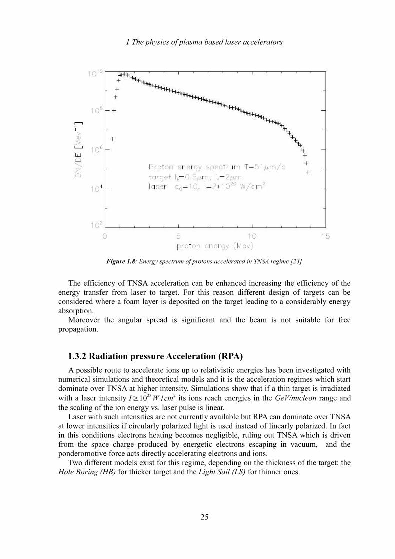
A target of thickness h ≈ λL is considered. At the initial stage the laser radiation pressure pushes the electrons creating a space-charge field Ex that balances the ponderomotive force, while the ions do not move significantly. So electron density is depleted on a layer of thickness xd and ion density n0 remains constant, as shown in figure 1.9.
The resulting electric field has a maximum E0=4π e n0 xd which accelerates the ions in the depleted region. The ions move forward and pile up until their density becomes singular and the fast particles overcome the slowest ones leaving the accelerating region. In this last stage a wavebreaking occurres and the ions can not gain energy anymore.
What we can observe from simulation is that the fast ions form a narrow bunch of velocity vm and penetrate into the overdense plasma; the others form another peak moving with velocity vb = vm/2, where vb is the speed at with a hole is bored in the plasma.
The estimate of ion energy is:
E I=2Zme c2 nc
ne
a02
(1.3.6)
which exhibits a linear dependency on the laser intensity, though the parameter a0, whereas is inversely proportional to electron density.
The ion acceleration in this regime is rather low, but a target design with a low density might help, even if there are several difficulties in using target with intermediate densities.
Light Sail:
For a thin target of thickness h < λL , after the first acceleration the ions do not pile up to a singular density because they constitute the whole target. The laser is then able to further push the electrons repeating the acceleration stage. The laser interacts basically with electrons, but because the target is thin the ion motion is strictly bound with the electrons' and the target can be considered as a rigid object. Then the equation of motion of the target
26
Figure 1.9: Profile of ion density ni (blue), electron density ne (green) and electrostatic field Ex (red) at three different stage of ion acceleration [19]
1 The physics of plasma based laser accelerators
retrieves the model of a “flying mirror” pushed by the radiation pressure of the laser. As shown in [25] the thinner is the target the higher is the efficiency of the accelerating
process. However the main limit is imposed by the transparency limit, in fact the target remains opaque and is accelerated as a mirror provided that:
a≤π ne h
nc λ L (1.3.7)
Considering the technical difficulties in preparing target near the transparency limit and the presence of instabilities shown in 2D and 3D simulations, this regime is not likely to be interesting for applications. Nevertheless the high laser intensity required for RPA regime is not currently available, the requirement of circularly polarization and high contrast, i. e. the ration between the peak of the main laser pulse and pre-pulse intensity, required to achieve this regime at lower laser intensity set others technical difficulties.
1.4 Ion-matter interaction
When a particle beam get through a medium a total or partial energy exchange occurs between the incident radiation and the target component. As a consequence the particles in the beams will loose their energy and will be deflected from the incident direction.
Ions are charged particles and undergo coulombian interactions. The nature of interactions are similar for any kind of ions and can be scaled from the corresponding proton interaction.
Protons traveling through matter can either interact with both nuclei and electrons that are close to their path. As the proton mass is much greater than atomic electrons, the deflection angle after an electronic interaction is extremely small and, to a good approximation, the protons travel on a straight path. The proton energy fraction transferred to the electron could either excites the atoms or ionizes it. Also the interactions with atomic electrons are so frequent that protons appear to lose energy continuously along their path.
Interactions with nuclei can be described as elastic collisions and are responsible for greater deflection angles. Anyway nuclear interactions are very rare and the dominant energy loss mechanism are the electronic collision.
The behavior of a proton in a medium can be described by the stopping power which represents the average rate of energy loss along its path in the matter. It can be expressed by the Bethe-Block formula:
−dEdx=2π N A me re
2c2 ρZA
z
β 2 [ ln(2γ 2 me v 2W max
I 2 )−2 β 2−δ−2C ( I ,β γ )
z ] (1.4.1)
where re and me are the classical electron radius and the electron mass, A and Z are the atomic mass and number of the medium, I is the mean excitation potential of the target and ρ its density, β and γ are the particle velocity and its relativistic factor, Wmax is the maximum energy transfer in a single electronic collision.
The last two terms in Bethe-Block formula are correction terms; the first one, δ, is the
27
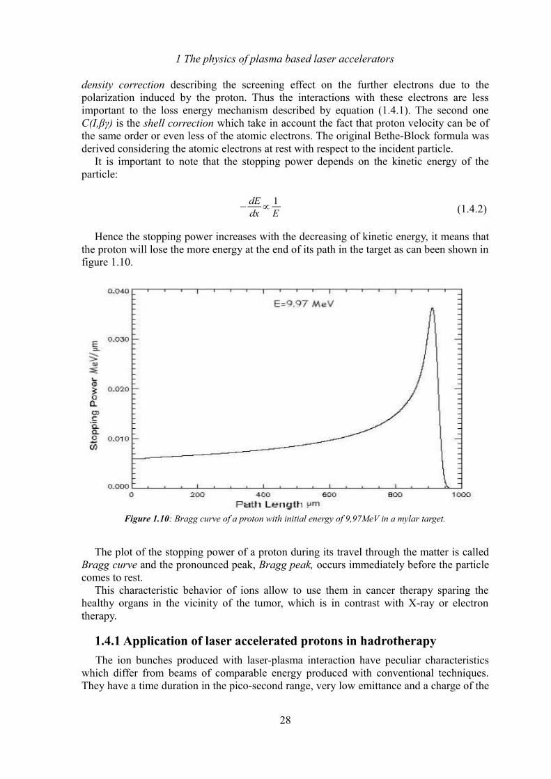
1 The physics of plasma based laser accelerators
density correction describing the screening effect on the further electrons due to the polarization induced by the proton. Thus the interactions with these electrons are less important to the loss energy mechanism described by equation (1.4.1). The second one C(I,βγ) is the shell correction which take in account the fact that proton velocity can be of the same order or even less of the atomic electrons. The original Bethe-Block formula was derived considering the atomic electrons at rest with respect to the incident particle.
It is important to note that the stopping power depends on the kinetic energy of the particle:
−dEdx∝
1E (1.4.2)
Hence the stopping power increases with the decreasing of kinetic energy, it means that the proton will lose the more energy at the end of its path in the target as can been shown in figure 1.10.
The plot of the stopping power of a proton during its travel through the matter is called Bragg curve and the pronounced peak, Bragg peak, occurs immediately before the particle comes to rest.
This characteristic behavior of ions allow to use them in cancer therapy sparing the healthy organs in the vicinity of the tumor, which is in contrast with X-ray or electron therapy.
1.4.1 Application of laser accelerated protons in hadrotherapy
The ion bunches produced with laser-plasma interaction have peculiar characteristics which differ from beams of comparable energy produced with conventional techniques. They have a time duration in the pico-second range, very low emittance and a charge of the
28
Figure 1.10: Bragg curve of a proton with initial energy of 9,97MeV in a mylar target.
1 The physics of plasma based laser accelerators
order of μC. Also laser-plasma accelerators offer a reduction of size and cost of proton accelerators that would allow the creation of regional centers for proton therapy.
Anyway some issues are to be solved before it will be possible to delivery a laser-accelerated proton beam to patients.
Proton therapy requires energies from 60MeV up to 200-300MeV for deep tumors. These values are not available at the moment, as the highest published energy obtained for proton is 58MeV with the very large high-power, high-energy laser system at Lawrence Livermore National Laboratory. Modeling studies and scaling extrapolations indicate that an increasing of laser energy by about a factor of 10, with also improvement of pulse compression techniques, could produce protons in the 200MeV range [34]. Another strategy would be to use the laser system as injector into a drift tube linac to increase the energy [27] or to inject a 30MeV laser-accelerated proton bunch into a high field linac in order to raise the energy.
The latter strategy, which is just an hybrid acceleration scheme does not requires new laser system but only the improvement of targets and the design of a transport line able to shape the beams and make it suitable for injection. Simulations and experiments are being developed in this direction in order to explore the feasibility of transporting an optically accelerated proton bunch reaching the beam quality required for irradiation and injection in a post-acceleration device [31, 33].
After post-acceleration the high energies required for deep tumors could be reached, but the real problem with TNSA, or improved TNSA, is that the protons having the desired energy are a small fraction of the total and carry out a small fraction of the total energy. In fact, as seen in Sec. 1.3.1, laser-accelerated protons are far from monochromatic. Progress is being made to improve this issue with shaped targets to maximize the proton flux in a narrow cone [29] or using CO2 laser on a gas jet [25].
In order to have a complete diagnostic of the laser-accelerated beams it is necessary to understand how the conventional dosimeters will respond to the pulsed nature of the beam. A ionization chamber, for instance, is expected to be effected on a sever under-response due to the very large ion recombination effect, which limits its use in a laser-ion source. Radiochromic films seem to be ideal detector because their high spatial resolution would allow to get a spatial resolved energy distribution of the protons in the beam.
Information on energy, momentum and charge to mass ratio of particle beams can be provided by a Thomson Parabola spectrometer, widely used to study ion sources such as ion accelerators, laser produced plasma, etc. In such a device charged particle are deflected by parallel electric and magnetic fields. The electric deflection depends on the energy of particles while the magnetic ones depends on their momentum; moreover particle with different charge to mass ratio are deflected on different trajectories. The Thomson spectrometer requires a high-sensitivity detector to record the ion beam intensities hence it is often coupled to a CR-39. Fast response detector are micro-channel plate (MPC) detectors coupled to a phosphor screen that avoid etching procedures required by CR-39 and allow an online diagnostic of the beams.
A Thomson parabola-MCP assembly has been used in this work as ion beam diagnostic device and will be discussed in the next chapter.
29
2 The Thomson parabola-MCP assembly
2 The Thomson parabola-MCP assembly C. Verdone, from the movie “Un sacco bello”:"Alfio che c'è? hai bisogno di qualcosa? Allora risposi: Mamma non vedi che sto parlando con me stesso?Cioè, come vedete anche in questo racconto, o paraBBola, a seconda di quella che la vogliamo considerare, ci sono anche molti elementi analoghe... analoghe..." .
In this chapter the general features of a typical Thomson spectrometer are described. In particular the device developed in the framework of the INFN “LILIA” (Laser Induced Light Ion Acceleration) project will be described. The aim of LILIA project is to study the mechanism of charged particles acceleration with high power laser.
In literature different Thomson spectrometer designs have been proposed in order to improve resolution or other specific characteristic. The spectrometer developed at LNS has two pinholes upstream as collimator, the deflection is provided by a magnetic field, produced by two resistive coils, and an electric field, produced by two electrodes placed in the magnetic gap. The detector is a micro-channel plate coupled to a phosphor screen which allows an online monitoring of beam particles. On the other hand the use of MCP detector does not allow to get information on the particle spectrum because of the non-linear response of the detector. A possible solution could be the use of a scintillating screens which has a linear response [63] or to calibrate the MCP using a CR39.
2.1 Motion of charged particles in electric and magnetic fields
The working principle of a Thomson-type spectrometer is based on the motion of a charged particle in an electric and magnetic fields. In the following it is proposed a brief and general relativistic treatment of the problem and than it is scaled to the non relativistic case of interest for the energy involved in the practical use of the spectrometer.
As starting point we recall the Lagrangian for the electromagnetic field [3,7], that is:
L=−mc2√1−u2
c2−qφ+qu⋅A (2.1.1)
The first term on the right hand side is the Lagrangian of the free particle, where m is its proper mass and u its velocity, and the other two term represent the Lagrangian of interaction with the potentials φ and A.
The particle energy in an electromagnetic field is given by its Hamiltonian
H=u∂ L∂u−L (2.1.2)
where the derivative of L with respect of the velocity is the particle canonical momentum:
29
2 The Thomson parabola-MCP assembly
P=∂ L∂u= p+q A (2.1.3)
with p=mu
√(1−u2/c2)
its relativistic momentum.
Thus the Hamiltonian can be written as:
H=mc2
√1−u2/c2+qu⋅A+mc2√1−
u2
c2+qφ−qu⋅A=
mc2
√(1−u2/c2)+qφ=ε+qφ (2.1.4)
where:
ε=mc2
√(1−u2/c2) (2.1.5)
is the energy of the free particle which can be also expressed, using the relativistic energy momentum relation, as ε 2
=( pc )2+(mc2)
2 .
It worth noting that the potential vector does not appear in the expression of H because the magnetic field does no work and does not give any contribution to the energy.
2.1.1 Motion of a charged particle in electrostatic field
Let's consider a charged particle, q>0 in an uniform electrostatic field, namely a particle moving in a parallel plate capacitor large enough to neglect edge effects.
We suppose that the particle enters the capacitor at the time t=0 with initial velocity u0
along the positive direction of abscissas and the entry point matches with the axes origin. The motion equation of the particle in the electrostatic filed E=(0, E, 0) of the capacitor
is:
d pdt=q E (2.1.6)
Projecting the motion equation along the three spatial directions we get three scalar equations that can be solved using the initial conditions to get a system of equations which ensures that the motion is on the x-y plane (planar motion) and the momentum along the x direction is constant. From a classical point of view at a constant momentum corresponds a constant velocity while in the relativistic case it does not hold true [3].
The x component of the particle velocity is:
u x( t)=c2
εp x( t )=
pox c2
√ε 02+(qEct )2
(2.1.7)
Integration of (2.1.7) gives the kinematic equation of the particle whose solution, after using the initial condition x (0)=0, is:
x (t )=poxc
qEsettsenh(qEct
ε 0 ) (2.1.8)
30
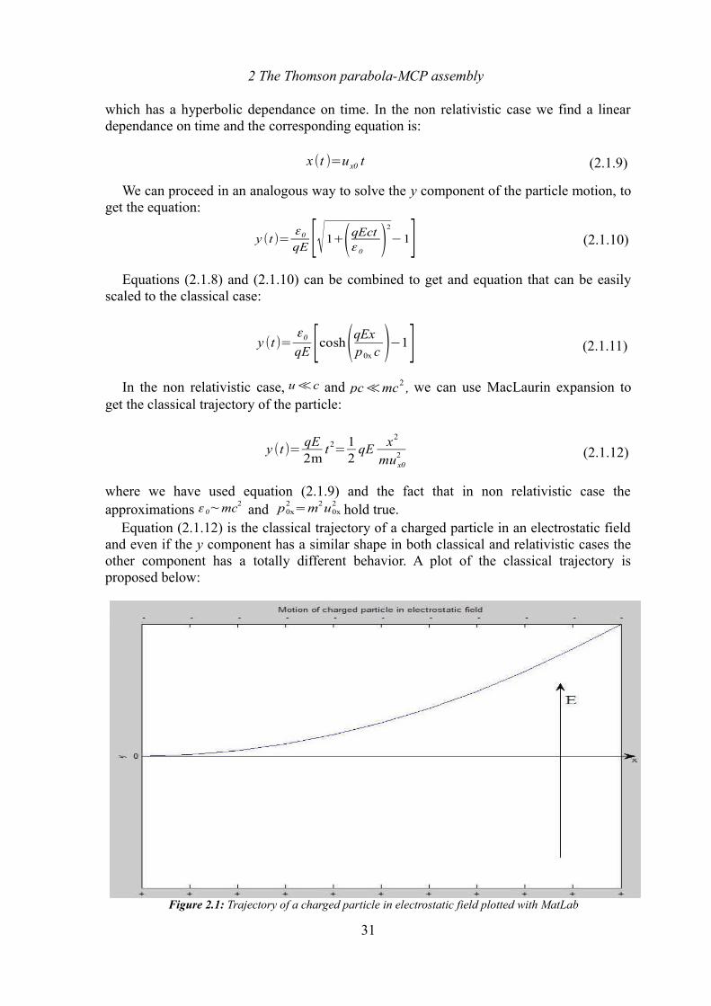
2 The Thomson parabola-MCP assembly
which has a hyperbolic dependance on time. In the non relativistic case we find a linear dependance on time and the corresponding equation is:
x (t )=ux0 t (2.1.9)
We can proceed in an analogous way to solve the y component of the particle motion, to get the equation:
y (t)=ε0
qE [√1+(qEctε 0 )
2
−1] (2.1.10)
Equations (2.1.8) and (2.1.10) can be combined to get and equation that can be easily scaled to the classical case:
y (t)=ε0
qE [cosh(qExp0x c )−1] (2.1.11)
In the non relativistic case, u≪c and pc≪mc2 , we can use MacLaurin expansion to get the classical trajectory of the particle:
y (t)=qE2m
t 2=
12
qEx2
mu x02 (2.1.12)
where we have used equation (2.1.9) and the fact that in non relativistic case the approximations ε 0∼mc2
and p0x2=m2u0x
2hold true.
Equation (2.1.12) is the classical trajectory of a charged particle in an electrostatic field and even if the y component has a similar shape in both classical and relativistic cases the other component has a totally different behavior. A plot of the classical trajectory is proposed below:
31
Figure 2.1: Trajectory of a charged particle in electrostatic field plotted with MatLab
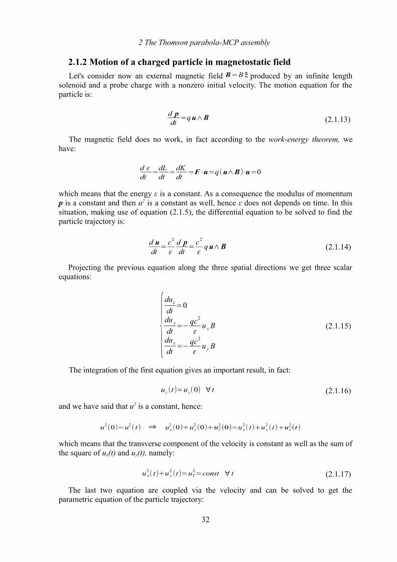
2 The Thomson parabola-MCP assembly
2.1.2 Motion of a charged particle in magnetostatic field
Let's consider now an external magnetic field B=B z produced by an infinite length solenoid and a probe charge with a nonzero initial velocity. The motion equation for the particle is:
d pdt=q u∧B (2.1.13)
The magnetic field does no work, in fact according to the work-energy theorem, we have:
d εdt=
dLdt=
dKdt=F⋅u=q(u∧B)⋅u=0
which means that the energy ε is a constant. As a consequence the modulus of momentum p is a constant and then u2 is a constant as well, hence ε does not depends on time. In this situation, making use of equation (2.1.5), the differential equation to be solved to find the particle trajectory is:
d udt=
c2
εd pdt=
c2
εq u∧B (2.1.14)
Projecting the previous equation along the three spatial directions we get three scalar equations:
{duz
dt=0
du y
dt=−
qc2
εu x B
dux
dt=−
qc2
εu y B
(2.1.15)
The integration of the first equation gives an important result, in fact:
uz (t)=uz(0) ∀t (2.1.16)
and we have said that u2 is a constant, hence:
u2(0)=u2
( t) ⇒ ux2(0)+uy
2(0)+uz
2(0)=u x
2( t)+u y
2(t)+uz
2(t)
which means that the transverse component of the velocity is constant as well as the sum of the square of ux(t) and uy(t), namely:
u x2( t)+u y
2(t)=uT
2=const ∀ t (2.1.17)
The last two equation are coupled via the velocity and can be solved to get the parametric equation of the particle trajectory:
32
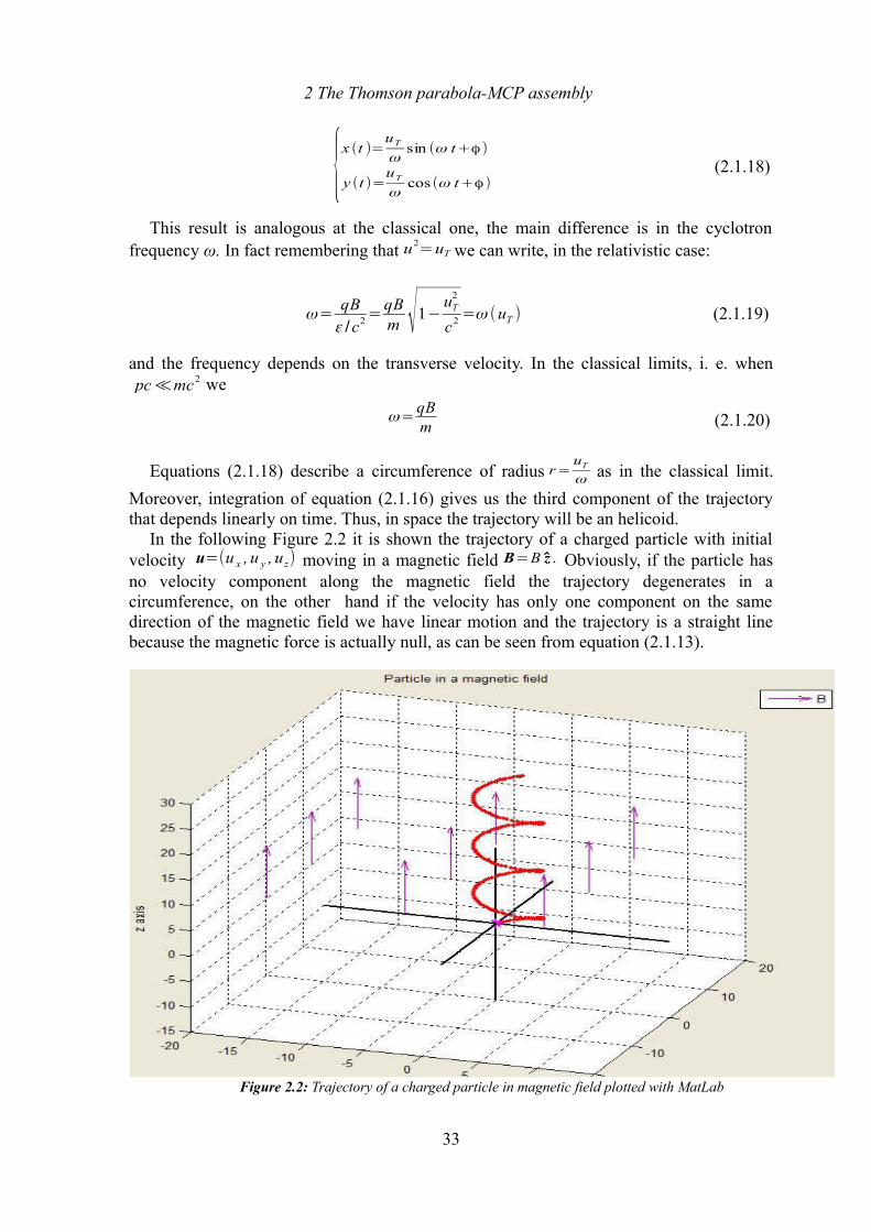
2 The Thomson parabola-MCP assembly
{x (t )=uT
ωsin (ω t+ϕ)
y (t )=uT
ωcos (ω t+ϕ)
(2.1.18)
This result is analogous at the classical one, the main difference is in the cyclotron frequency ω. In fact remembering that u2
=uT we can write, in the relativistic case:
ω=qBε /c2=
qBm √1−
uT2
c2=ω (uT ) (2.1.19)
and the frequency depends on the transverse velocity. In the classical limits, i. e. whenpc≪mc2 we
ω=qBm (2.1.20)
Equations (2.1.18) describe a circumference of radius r=uT
ω as in the classical limit.
Moreover, integration of equation (2.1.16) gives us the third component of the trajectory that depends linearly on time. Thus, in space the trajectory will be an helicoid.
In the following Figure 2.2 it is shown the trajectory of a charged particle with initial velocity u=(u x , u y , uz) moving in a magnetic field B=B z . Obviously, if the particle has no velocity component along the magnetic field the trajectory degenerates in a circumference, on the other hand if the velocity has only one component on the same direction of the magnetic field we have linear motion and the trajectory is a straight line because the magnetic force is actually null, as can be seen from equation (2.1.13).
33
Figure 2.2: Trajectory of a charged particle in magnetic field plotted with MatLab
2 The Thomson parabola-MCP assembly
2.2 The Thomson parabola spectrometer
The Thomson Parabola (TP) spectrometer, invented in 1912 by J. J. Thomson, the discoverer of the electron, is successfully used as charged particles analyzer for studying ion beams ejected from laser-generated plasmas. The deflection sector of the Thomsom spectrometer consists of parallel electric and magnetic fields and both perpendicular to the direction of the incident beam. The main feature of this kind of spectrometer is to provide information on energy, momentum, charge-to-mass ratio, ect., of the deflected ions simultaneously.
Assuming that both field are uniform over a length L and zero outside, using the theory exposed above and a small angle approximation by setting tg θ ≈ θ , it can be shown, from equation (2.1.12) that the trajectories of non-relativistic ions moving perpendicularly to the electric field is parabolic and the deflection angle at the exit of the electrodes is:
θ e=ZeEL
Aμ v2=
ZeEL2 E kin
(2.2.1)
where θe is the electric deflection angle in radians, Z is the charge state of the ion, e is the electronic charge, EL is the product of the electric field and its length, A is the ion mass number, μ is the unit nucleon mass based on C12, v and Ekin are the velocity and kinetic energy of the ion.
Similarly, from equations (2.1.18), the trajectories of ions moving perpendicularly to the magnetic field is circular and the deflection angle at the exit of the magnets is:
θ m=ZeBLAμ v
=ZeBL
√2Aμ Ekin
(2.2.2)
where θm is the magnetic deflection angle in radians and BL is the product of the electric field and its length [47].
Since the fields are parallel the corresponding deflections are orthogonal each other. The electric and magnetic deflection are proportional to the corresponding deflection angles by:
θ i= xi /D
where i=e,m stays for electric or magnetic angle and D is the drift length between the electromagnetic device and the detector plane. Thus assuming that the magnetic field deflects on x axis and the electric field deflects on y axis, from the above equations one gets:
y=qELD2E kin
x=qBLD
√2mv (2.2.3)
where q=Ze is the ion charge and m=Aμ is its mass in kilograms [49]. Solving the second equation for v and replacing it in the first one we get the parabolic
equation:
34
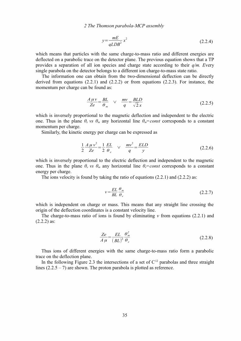
2 The Thomson parabola-MCP assembly
y=mE
qLDB2x2
(2.2.4)
which means that particles with the same charge-to-mass ratio and different energies are deflected on a parabolic trace on the detector plane. The previous equation shows that a TP provides a separation of all ion species and charge state according to their q/m. Every single parabola on the detector belongs to a different ion charge-to-mass state ratio.
The information one can obtain from the two-dimensional deflection can be directly derived from equations (2.2.1) and (2.2.2) or from equations (2.2.3). For instance, the momentum per charge can be found as:
Aμ vZe
=BLθ m
∨mvq=
BLD√2 x (2.2.5)
which is inversely proportional to the magnetic deflection and independent to the electric one. Thus in the plane θe vs θm any horizontal line θm=const corresponds to a constant momentum per charge.
Similarly, the kinetic energy per charge can be expressed as
12
Aμ v2
Ze=
12
ELθ e
∨mv2
q=
ELDy (2.2.6)
which is inversely proportional to the electric deflection and independent to the magnetic one. Thus in the plane θe vs θm any horizontal line θe=const corresponds to a constant energy per charge.
The ions velocity is found by taking the ratio of equations (2.2.1) and (2.2.2) as:
v=ELBL
θ m
θ e (2.2.7)
which is independent on charge or mass. This means that any straight line crossing the origin of the deflection coordinates is a constant velocity line.
The charge-to-mass ratio of ions is found by eliminating v from equations (2.2.1) and (2.2.2) as:
ZeAμ=
EL(BL)2
θ m2
θ e (2.2.8)
Thus ions of different energies with the same charge-to-mass ratio form a parabolic trace on the deflection plane.
In the following Figure 2.3 the intersections of a set of C12 parabolas and three straight lines (2.2.5 – 7) are shown. The proton parabola is plotted as reference.
35

2 The Thomson parabola-MCP assembly
The Thomson spectrometer provides the charge-to-mass ratio of a given parabola using a reference parabola of known q/m ratio. In fact the intersections of parabolas of equation (2.2.8) with lines θe=const are proportional to θm, thus having a reference parabola the charge-to-mass ratio of unknown parabolas can be found by means of:
Z /A(Z /A)ref
=θ m
(θ m)ref (2.2.9)
Thomson spectrometer does not indicate the charge or mass of the parabola separately but the number of intersections of the constant velocity line from the origin to the parabola of interest can give information on the charge state. Thus knowing the charge-to-mass ratio and the charge state it is possible to get the ion mass and to identify the ion species.
An interesting feature of the spectrogram is that all of the parabolas begin with a line of constant θe, namely the peak energy per charge of each parabolas is constant.
36
Figure 2.3: Thomson parabolas of C12 ions and their intersections with constant velocity, energy and momentum lines[47].
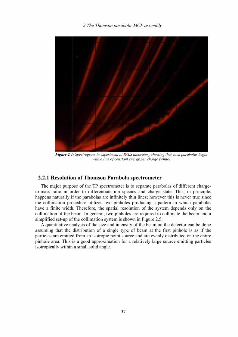
2 The Thomson parabola-MCP assembly
2.2.1 Resolution of Thomson Parabola spectrometer
The major purpose of the TP spectrometer is to separate parabolas of different charge-to-mass ratio in order to differentiate ion species and charge state. This, in principle, happens naturally if the parabolas are infinitely thin lines; however this is never true since the collimation procedure utilizes two pinholes producing a pattern in which parabolas have a finite width. Therefore, the spatial resolution of the system depends only on the collimation of the beam. In general, two pinholes are required to collimate the beam and a simplified set-up of the collimation system is shown in Figure 2.5.
A quantitative analysis of the size and intensity of the beam on the detector can be done assuming that the distribution of a single type of beam at the first pinhole is as if the particles are emitted from an isotropic point source and are evenly distributed on the entire pinhole area. This is a good approximation for a relatively large source emitting particles isotropically within a small solid angle.
37
Figure 2.4: Spectrogram in experiment at PALS laboratory showing that each parabolas begin with a line of constant energy per charge (white)
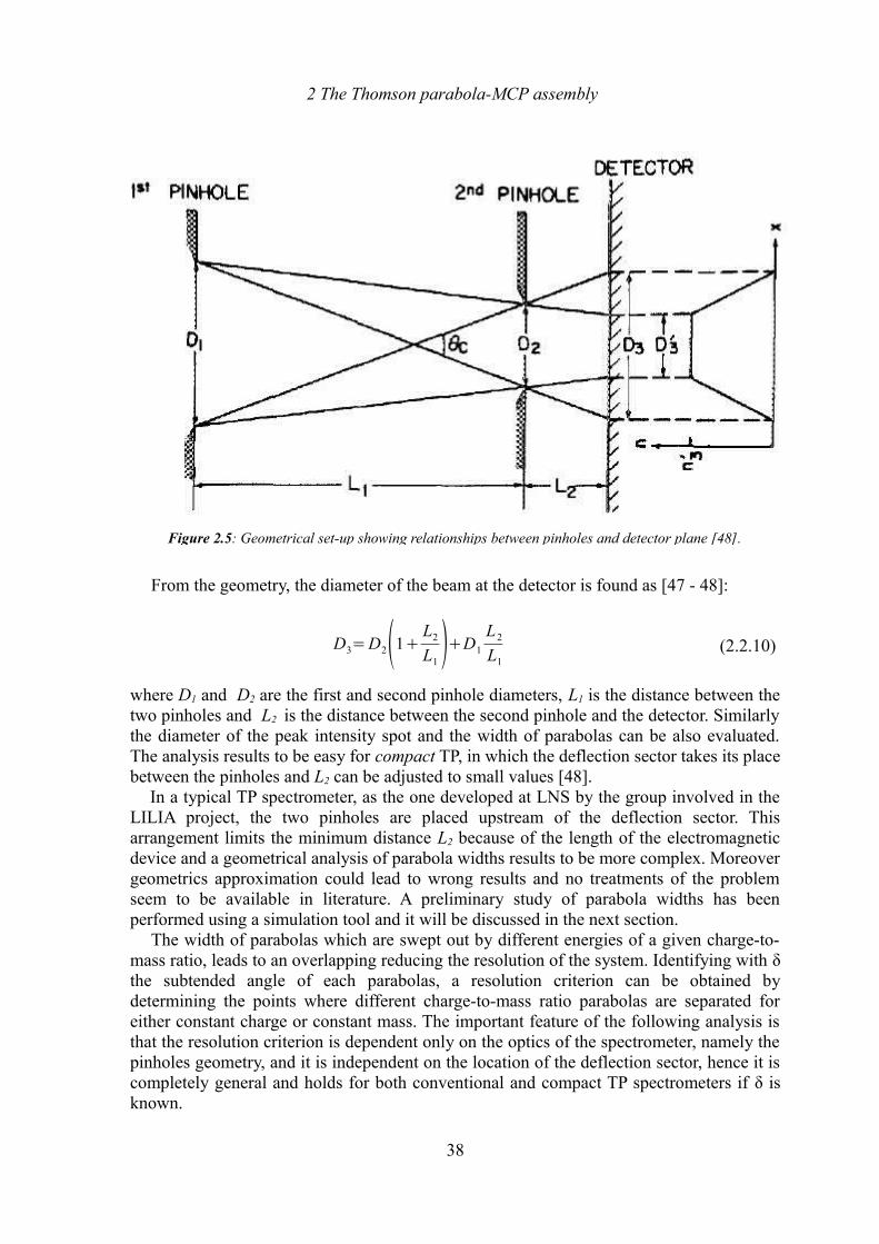
2 The Thomson parabola-MCP assembly
From the geometry, the diameter of the beam at the detector is found as [47 - 48]:
D3=D2(1+ L2
L1)+D1
L2
L1 (2.2.10)
where D1 and D2 are the first and second pinhole diameters, L1 is the distance between the two pinholes and L2 is the distance between the second pinhole and the detector. Similarly the diameter of the peak intensity spot and the width of parabolas can be also evaluated. The analysis results to be easy for compact TP, in which the deflection sector takes its place between the pinholes and L2 can be adjusted to small values [48].
In a typical TP spectrometer, as the one developed at LNS by the group involved in the LILIA project, the two pinholes are placed upstream of the deflection sector. This arrangement limits the minimum distance L2 because of the length of the electromagnetic device and a geometrical analysis of parabola widths results to be more complex. Moreover geometrics approximation could lead to wrong results and no treatments of the problem seem to be available in literature. A preliminary study of parabola widths has been performed using a simulation tool and it will be discussed in the next section.
The width of parabolas which are swept out by different energies of a given charge-to-mass ratio, leads to an overlapping reducing the resolution of the system. Identifying with δ the subtended angle of each parabolas, a resolution criterion can be obtained by determining the points where different charge-to-mass ratio parabolas are separated for either constant charge or constant mass. The important feature of the following analysis is that the resolution criterion is dependent only on the optics of the spectrometer, namely the pinholes geometry, and it is independent on the location of the deflection sector, hence it is completely general and holds for both conventional and compact TP spectrometers if δ is known.
38
Figure 2.5: Geometrical set-up showing relationships between pinholes and detector plane [48].
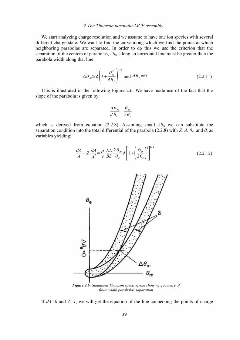
2 The Thomson parabola-MCP assembly
We start analyzing charge resolution and we assume to have one ion species with several different charge state. We want to find the curve along which we find the points at which neighboring parabolas are separated. In order to do this we use the criterion that the separation of the centers of parabolas, Δθm, along an horizontal line must be greater than the parabola width along that line:
Δθ m≥δ(1+ θ m2
4θ e)
1/2
and Δθ e=0 (2.2.11)
This is illustrated in the following Figure 2.6. We have made use of the fact that the slope of the parabola is given by:
dθ m
d θ e
=θ m
2θ e
which is derived from equation (2.2.8). Assuming small Δθm we can substitute the separation condition into the total differential of the parabola (2.2.8) with Z, A, θm and θe as variables yielding:
dZA−Z
dA
A2=μe
ELBL
2θ m
θ e
δ [1+( θm
2θe)
2
]1/2
(2.2.12)
If dA=0 and Z=1, we will get the equation of the line connecting the points of charge
39
Figure 2.6: Simulated Thomson spectrogram showing geometry of finite width parabolas saparation
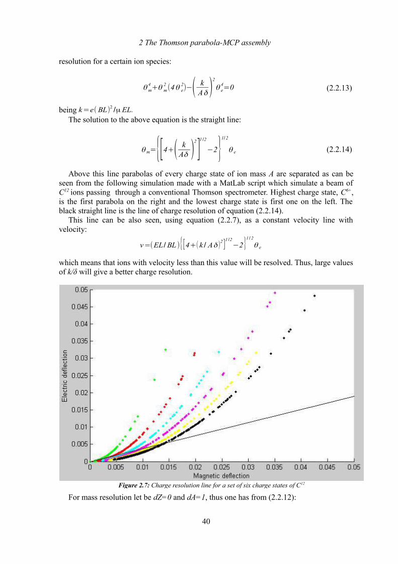
2 The Thomson parabola-MCP assembly
resolution for a certain ion species:
θ m4+θ m
2(4θ e
2)−( k
Aδ )2
θ e4=0 (2.2.13)
being k=e(BL)2 /μEL.
The solution to the above equation is the straight line:
θ m={[4+( kAδ )
2
]1 /2
−2}1/2
θ e (2.2.14)
Above this line parabolas of every charge state of ion mass A are separated as can be seen from the following simulation made with a MatLab script which simulate a beam of C12 ions passing through a conventional Thomson spectrometer. Highest charge state, C6+, is the first parabola on the right and the lowest charge state is first one on the left. The black straight line is the line of charge resolution of equation (2.2.14).
This line can be also seen, using equation (2.2.7), as a constant velocity line with velocity:
v=(EL/BL ){[4+( k / Aδ )2 ]1 /2−2}1 /2
θ e
which means that ions with velocity less than this value will be resolved. Thus, large values of k/δ will give a better charge resolution.
For mass resolution let be dZ=0 and dA=1, thus one has from (2.2.12):
40
Figure 2.7: Charge resolution line for a set of six charge states of C12
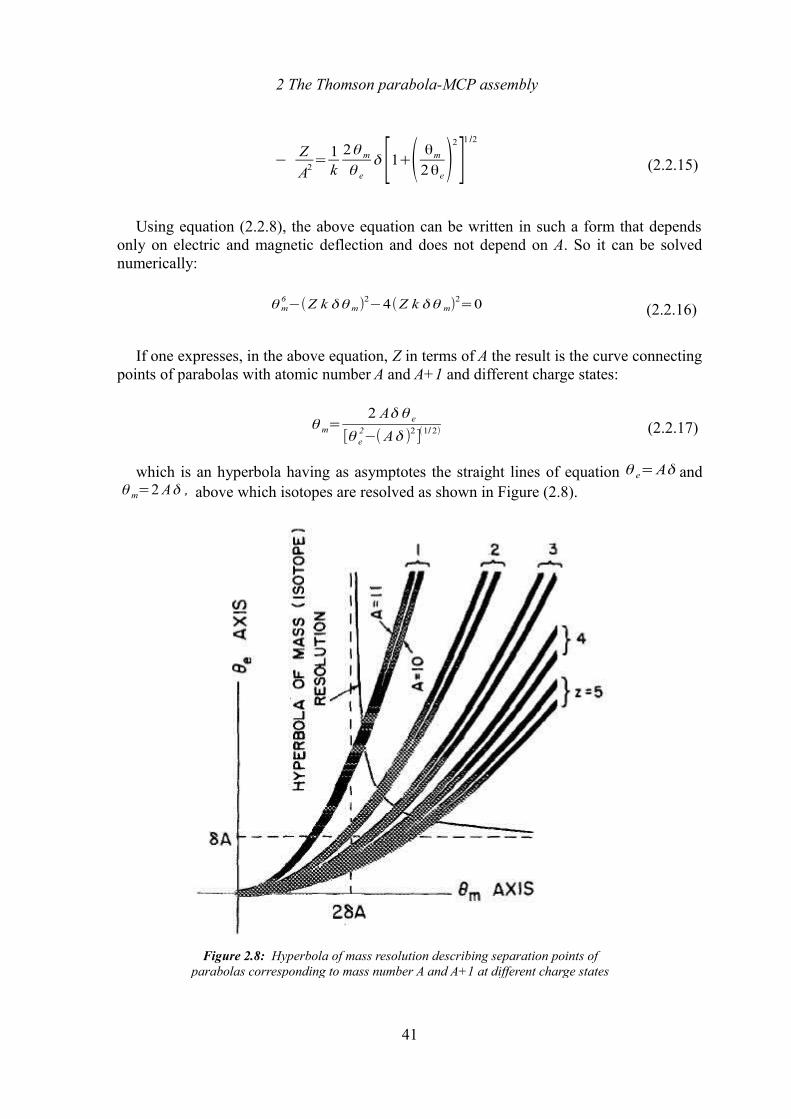
2 The Thomson parabola-MCP assembly
−Z
A2=
1k
2θ m
θ e
δ [1+( θm
2θe)
2
]1 /2
(2.2.15)
Using equation (2.2.8), the above equation can be written in such a form that depends only on electric and magnetic deflection and does not depend on A. So it can be solved numerically:
θ m
6−(Z k δθ m)
2−4(Z k δθ m)
2=0 (2.2.16)
If one expresses, in the above equation, Z in terms of A the result is the curve connecting
points of parabolas with atomic number A and A+1 and different charge states:
θ m=2 Aδ θ e
[θ e2−(Aδ )2](1/2) (2.2.17)
which is an hyperbola having as asymptotes the straight lines of equation θ e=Aδ andθ m=2 Aδ , above which isotopes are resolved as shown in Figure (2.8).
41
Figure 2.8: Hyperbola of mass resolution describing separation points of parabolas corresponding to mass number A and A+1 at different charge states
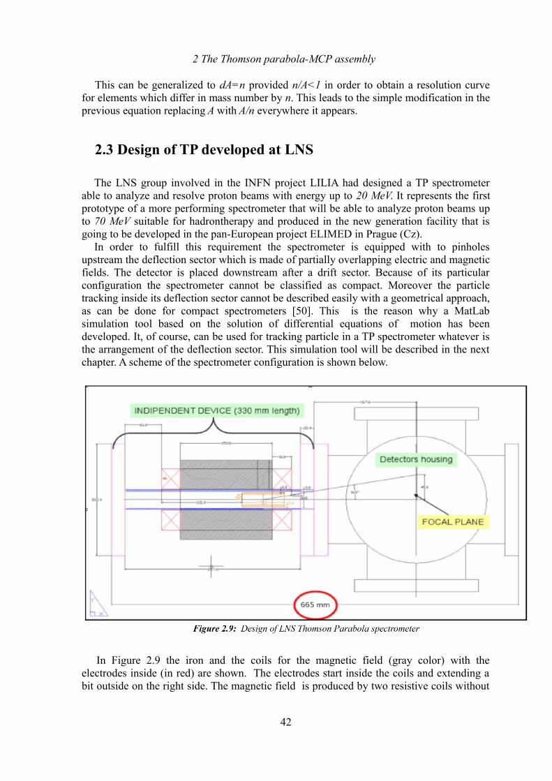
2 The Thomson parabola-MCP assembly
This can be generalized to dA=n provided n/A<1 in order to obtain a resolution curve for elements which differ in mass number by n. This leads to the simple modification in the previous equation replacing A with A/n everywhere it appears.
2.3 Design of TP developed at LNS
The LNS group involved in the INFN project LILIA had designed a TP spectrometer able to analyze and resolve proton beams with energy up to 20 MeV. It represents the first prototype of a more performing spectrometer that will be able to analyze proton beams up to 70 MeV suitable for hadrontherapy and produced in the new generation facility that is going to be developed in the pan-European project ELIMED in Prague (Cz).
In order to fulfill this requirement the spectrometer is equipped with to pinholes upstream the deflection sector which is made of partially overlapping electric and magnetic fields. The detector is placed downstream after a drift sector. Because of its particular configuration the spectrometer cannot be classified as compact. Moreover the particle tracking inside its deflection sector cannot be described easily with a geometrical approach, as can be done for compact spectrometers [50]. This is the reason why a MatLab simulation tool based on the solution of differential equations of motion has been developed. It, of course, can be used for tracking particle in a TP spectrometer whatever is the arrangement of the deflection sector. This simulation tool will be described in the next chapter. A scheme of the spectrometer configuration is shown below.
In Figure 2.9 the iron and the coils for the magnetic field (gray color) with the electrodes inside (in red) are shown. The electrodes start inside the coils and extending a bit outside on the right side. The magnetic field is produced by two resistive coils without
42
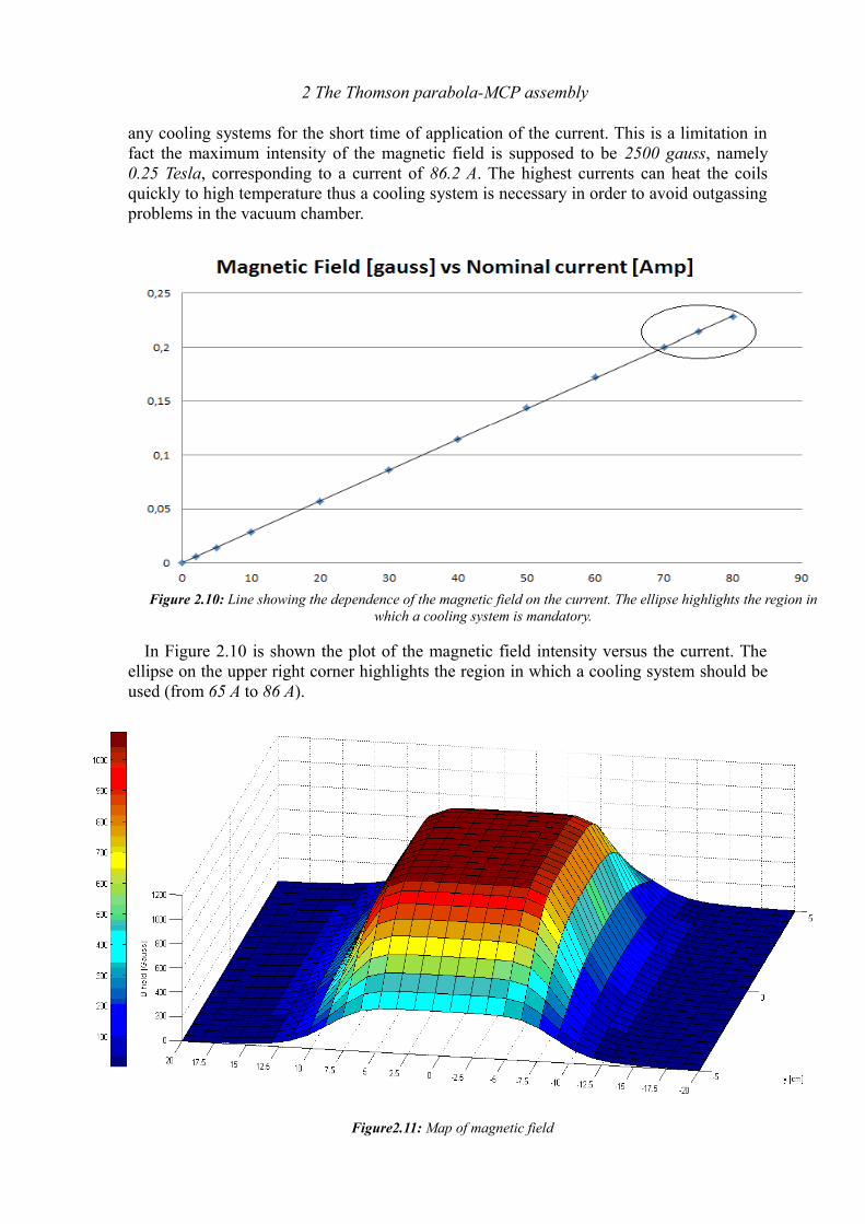
2 The Thomson parabola-MCP assembly
any cooling systems for the short time of application of the current. This is a limitation in fact the maximum intensity of the magnetic field is supposed to be 2500 gauss, namely 0.25 Tesla, corresponding to a current of 86.2 A. The highest currents can heat the coils quickly to high temperature thus a cooling system is necessary in order to avoid outgassing problems in the vacuum chamber.
In Figure 2.10 is shown the plot of the magnetic field intensity versus the current. The ellipse on the upper right corner highlights the region in which a cooling system should be used (from 65 A to 86 A).
43
Figure 2.10: Line showing the dependence of the magnetic field on the current. The ellipse highlights the region in which a cooling system is mandatory.
Figure2.11: Map of magnetic field
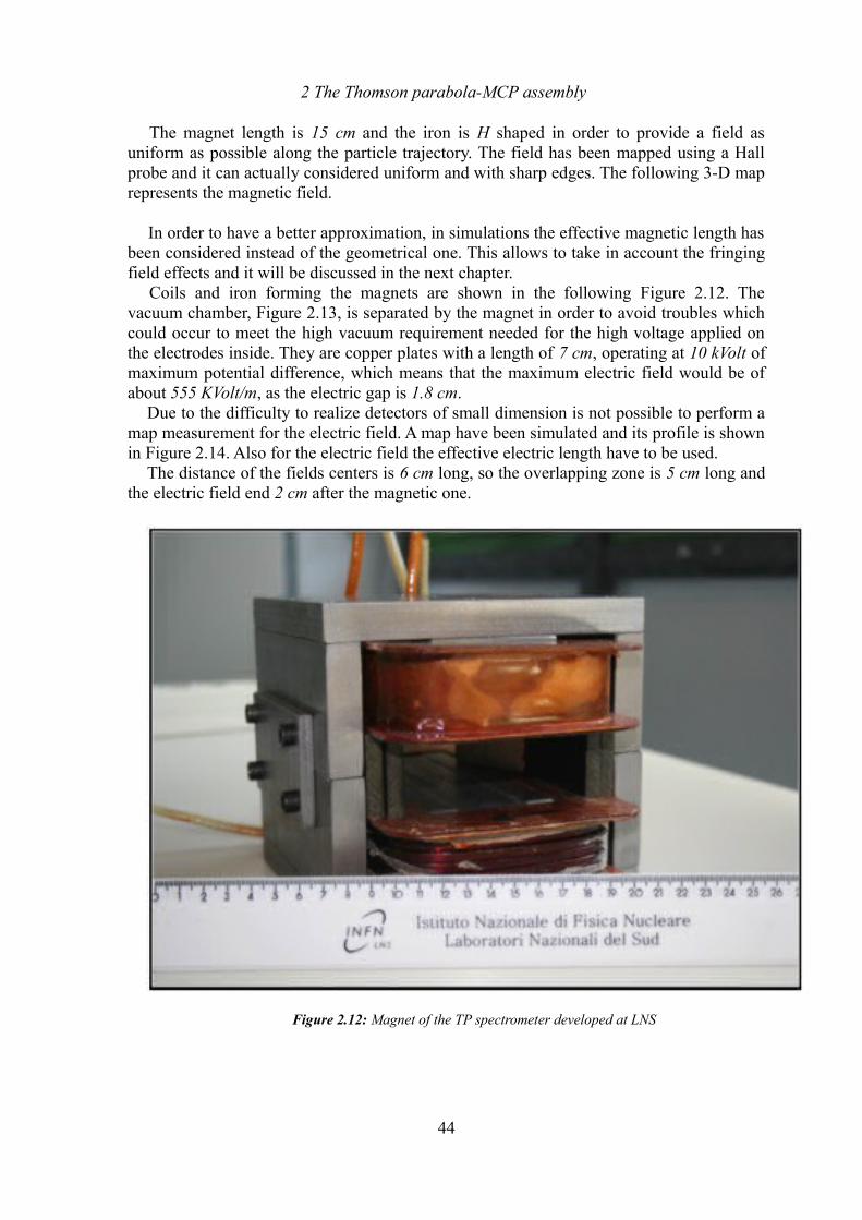
2 The Thomson parabola-MCP assembly
The magnet length is 15 cm and the iron is H shaped in order to provide a field as uniform as possible along the particle trajectory. The field has been mapped using a Hall probe and it can actually considered uniform and with sharp edges. The following 3-D map represents the magnetic field.
In order to have a better approximation, in simulations the effective magnetic length has been considered instead of the geometrical one. This allows to take in account the fringing field effects and it will be discussed in the next chapter.
Coils and iron forming the magnets are shown in the following Figure 2.12. The vacuum chamber, Figure 2.13, is separated by the magnet in order to avoid troubles which could occur to meet the high vacuum requirement needed for the high voltage applied on the electrodes inside. They are copper plates with a length of 7 cm, operating at 10 kVolt of maximum potential difference, which means that the maximum electric field would be of about 555 KVolt/m, as the electric gap is 1.8 cm.
Due to the difficulty to realize detectors of small dimension is not possible to perform a map measurement for the electric field. A map have been simulated and its profile is shown in Figure 2.14. Also for the electric field the effective electric length have to be used.
The distance of the fields centers is 6 cm long, so the overlapping zone is 5 cm long and the electric field end 2 cm after the magnetic one.
44
Figure 2.12: Magnet of the TP spectrometer developed at LNS
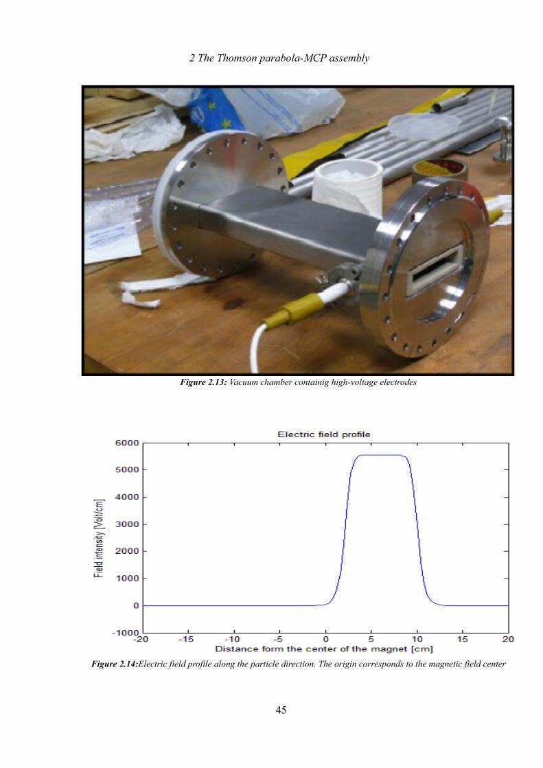
2 The Thomson parabola-MCP assembly
45
Figure 2.13: Vacuum chamber containig high-voltage electrodes
Figure 2.14:Electric field profile along the particle direction. The origin corresponds to the magnetic field center
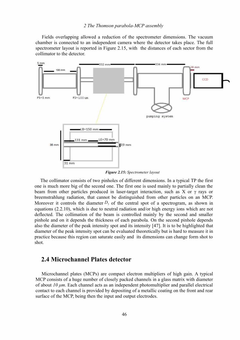
2 The Thomson parabola-MCP assembly
Fields overlapping allowed a reduction of the spectrometer dimensions. The vacuum chamber is connected to an independent camera where the detector takes place. The full spectrometer layout is reported in Figure 2.15, with the distances of each sector from the collimator to the detector.
The collimator consists of two pinholes of different dimensions. In a typical TP the first one is much more big of the second one. The first one is used mainly to partially clean the beam from other particles produced in laser-target interaction, such as X or γ rays or breemstrahlung radiation, that cannot be distinguished from other particles on an MCP. Moreover it controls the diameter D3 of the central spot of a spectrogram, as shown in equations (2.2.10), which is due to neutral radiation and/or high energy ions which are not deflected. The collimation of the beam is controlled mainly by the second and smaller pinhole and on it depends the thickness of each parabola. On the second pinhole depends also the diameter of the peak intensity spot and its intensity [47]. It is to be highlighted that diameter of the peak intensity spot can be evaluated theoretically but is hard to measure it in practice because this region can saturate easily and its dimensions can change form shot to shot.
2.4 Microchannel Plates detector
Microchannel plates (MCPs) are compact electron multipliers of high gain. A typical MCP consists of a huge number of closely packed channels in a glass matrix with diameter of about 10 μm. Each channel acts as an independent photomultiplier and parallel electrical contact to each channel is provided by depositing of a metallic coating on the front and rear surface of the MCP, being then the input and output electrodes.
46
Figure 2.15: Spectrometer layout
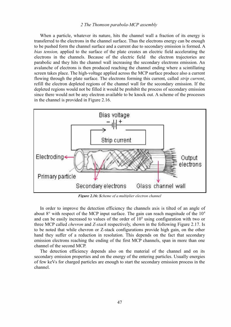
2 The Thomson parabola-MCP assembly
When a particle, whatever its nature, hits the channel wall a fraction of its energy is transferred to the electrons in the channel surface. Thus the electrons energy can be enough to be pushed form the channel surface and a current due to secondary emission is formed. A bias tension, applied to the surface of the plate creates an electric field accelerating the electrons in the channels. Because of the electric field the electron trajectories are parabolic and they hits the channel wall increasing the secondary electrons emission. An avalanche of electrons is then produced reaching the channel ending where a scintillating screen takes place. The high-voltage applied across the MCP surface produce also a current flowing through the plate surface. The electrons forming this current, called strip current, refill the electron depleted regions of the channel wall for the secondary emission. If the depleted regions would not be filled it would be prohibit the process of secondary emission since there would not be any electron available to be knock out. A scheme of the processes in the channel is provided in Figure 2.16.
In order to improve the detection efficiency the channels axis is tilted of an angle of about 8° with respect of the MCP input surface. The gain can reach magnitude of the 104
and can be easily increased to values of the order of 108 using configuration with two or three MCP called chevron and Z-stack respectively, shown in the following Figure 2.17. Is to be noted that while chevron or Z-stack configurations provide high gain, on the other hand they suffer of a reduction in resolution. This depends on the fact that secondary emission electrons reaching the ending of the first MCP channels, span in more than one channel of the second MCP.
The detection efficiency depends also on the material of the channel and on its secondary emission properties and on the energy of the entering particles. Usually energies of few keVs for charged particles are enough to start the secondary emission process in the channel.
47
Figure 2.16: Scheme of a multiplier electron channel
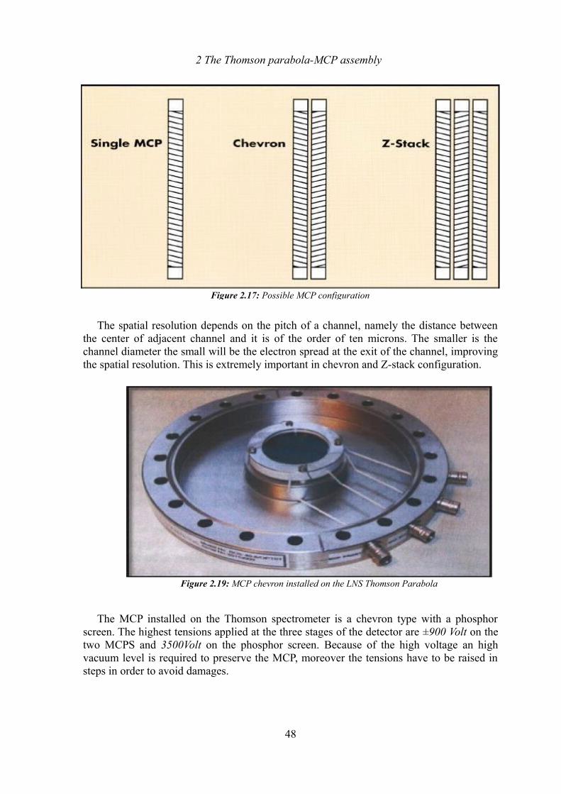
2 The Thomson parabola-MCP assembly
The spatial resolution depends on the pitch of a channel, namely the distance between the center of adjacent channel and it is of the order of ten microns. The smaller is the channel diameter the small will be the electron spread at the exit of the channel, improving the spatial resolution. This is extremely important in chevron and Z-stack configuration.
The MCP installed on the Thomson spectrometer is a chevron type with a phosphor screen. The highest tensions applied at the three stages of the detector are ±900 Volt on the two MCPS and 3500Volt on the phosphor screen. Because of the high voltage an high vacuum level is required to preserve the MCP, moreover the tensions have to be raised in steps in order to avoid damages.
48
Figure 2.17: Possible MCP configuration
Figure 2.19: MCP chevron installed on the LNS Thomson Parabola
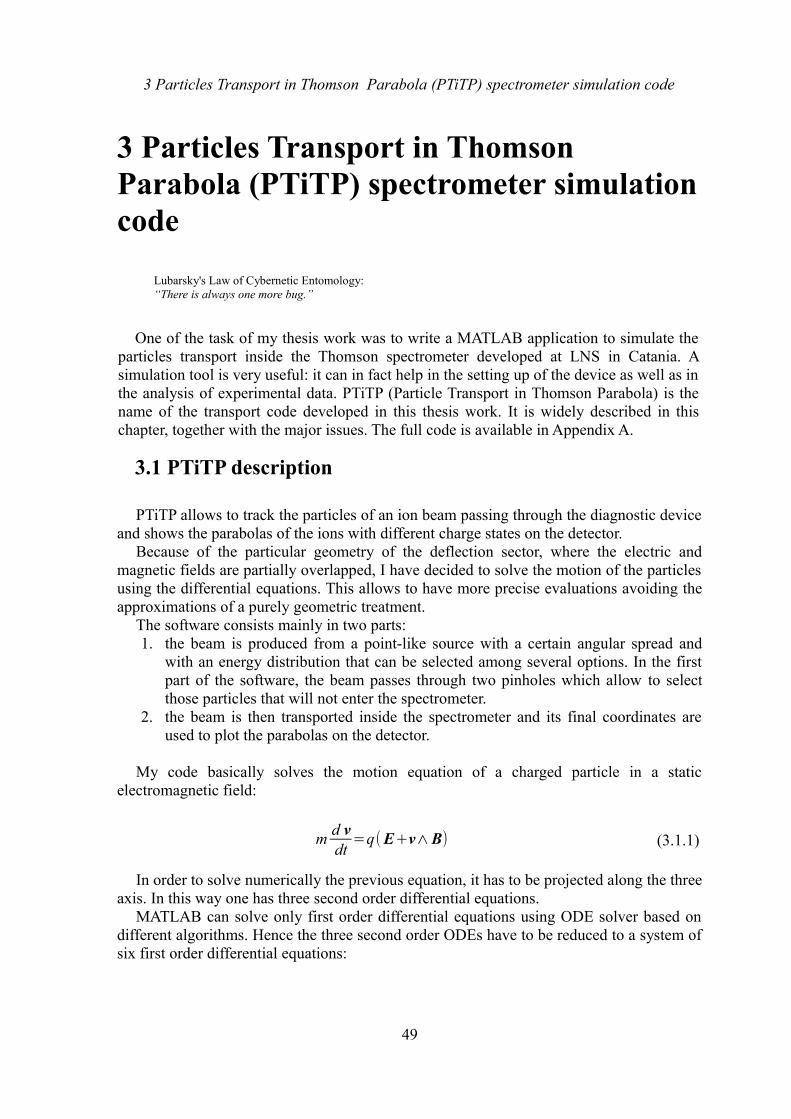
3 Particles Transport in Thomson Parabola (PTiTP) spectrometer simulation code
3 Particles Transport in Thomson Parabola (PTiTP) spectrometer simulation code
Lubarsky's Law of Cybernetic Entomology:“There is always one more bug.”
One of the task of my thesis work was to write a MATLAB application to simulate the particles transport inside the Thomson spectrometer developed at LNS in Catania. A simulation tool is very useful: it can in fact help in the setting up of the device as well as in the analysis of experimental data. PTiTP (Particle Transport in Thomson Parabola) is the name of the transport code developed in this thesis work. It is widely described in this chapter, together with the major issues. The full code is available in Appendix A.
3.1 PTiTP description
PTiTP allows to track the particles of an ion beam passing through the diagnostic device and shows the parabolas of the ions with different charge states on the detector.
Because of the particular geometry of the deflection sector, where the electric and magnetic fields are partially overlapped, I have decided to solve the motion of the particles using the differential equations. This allows to have more precise evaluations avoiding the approximations of a purely geometric treatment.
The software consists mainly in two parts:1. the beam is produced from a point-like source with a certain angular spread and
with an energy distribution that can be selected among several options. In the first part of the software, the beam passes through two pinholes which allow to select those particles that will not enter the spectrometer.
2. the beam is then transported inside the spectrometer and its final coordinates are used to plot the parabolas on the detector.
My code basically solves the motion equation of a charged particle in a static electromagnetic field:
md vdt=q(E+v∧B) (3.1.1)
In order to solve numerically the previous equation, it has to be projected along the three axis. In this way one has three second order differential equations.
MATLAB can solve only first order differential equations using ODE solver based on different algorithms. Hence the three second order ODEs have to be reduced to a system of six first order differential equations:
49
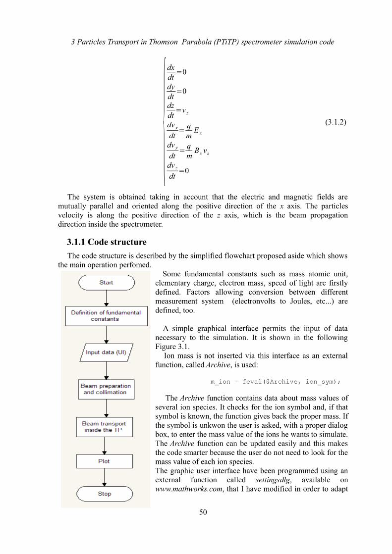
3 Particles Transport in Thomson Parabola (PTiTP) spectrometer simulation code
{dxdt=0
dydt=0
dzdt=v z
dv x
dt=
qm
E x
dv y
dt=
qm
Bx vz
dv z
dt=0
(3.1.2)
The system is obtained taking in account that the electric and magnetic fields are mutually parallel and oriented along the positive direction of the x axis. The particles velocity is along the positive direction of the z axis, which is the beam propagation direction inside the spectrometer.
3.1.1 Code structure
The code structure is described by the simplified flowchart proposed aside which shows the main operation perfomed.
Some fundamental constants such as mass atomic unit, elementary charge, electron mass, speed of light are firstly defined. Factors allowing conversion between different measurement system (electronvolts to Joules, etc...) are defined, too.
A simple graphical interface permits the input of data necessary to the simulation. It is shown in the following Figure 3.1. Ion mass is not inserted via this interface as an external function, called Archive, is used:
m_ion = feval(@Archive, ion_sym);
The Archive function contains data about mass values of several ion species. It checks for the ion symbol and, if that symbol is known, the function gives back the proper mass. If the symbol is unkwon the user is asked, with a proper dialog box, to enter the mass value of the ions he wants to simulate. The Archive function can be updated easily and this makes the code smarter because the user do not need to look for the mass value of each ion species.The graphic user interface have been programmed using an external function called settingsdlg, available on www.mathworks.com, that I have modified in order to adapt
50
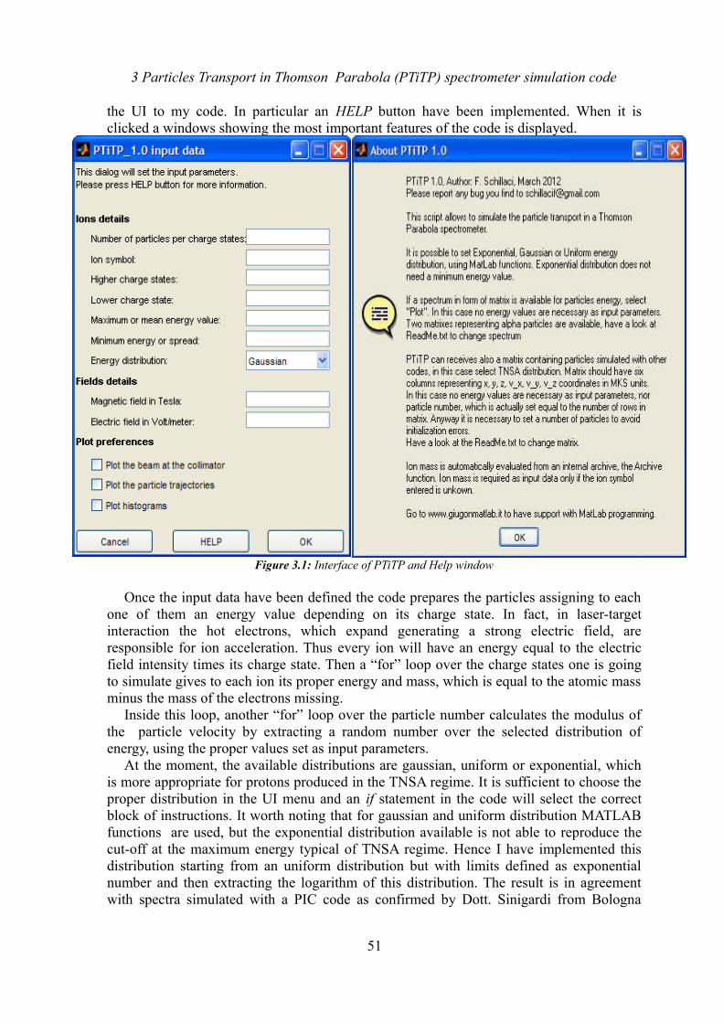
3 Particles Transport in Thomson Parabola (PTiTP) spectrometer simulation code
the UI to my code. In particular an HELP button have been implemented. When it is clicked a windows showing the most important features of the code is displayed.
Once the input data have been defined the code prepares the particles assigning to each one of them an energy value depending on its charge state. In fact, in laser-target interaction the hot electrons, which expand generating a strong electric field, are responsible for ion acceleration. Thus every ion will have an energy equal to the electric field intensity times its charge state. Then a “for” loop over the charge states one is going to simulate gives to each ion its proper energy and mass, which is equal to the atomic mass minus the mass of the electrons missing.
Inside this loop, another “for” loop over the particle number calculates the modulus of the particle velocity by extracting a random number over the selected distribution of energy, using the proper values set as input parameters.
At the moment, the available distributions are gaussian, uniform or exponential, which is more appropriate for protons produced in the TNSA regime. It is sufficient to choose the proper distribution in the UI menu and an if statement in the code will select the correct block of instructions. It worth noting that for gaussian and uniform distribution MATLAB functions are used, but the exponential distribution available is not able to reproduce the cut-off at the maximum energy typical of TNSA regime. Hence I have implemented this distribution starting from an uniform distribution but with limits defined as exponential number and then extracting the logarithm of this distribution. The result is in agreement with spectra simulated with a PIC code as confirmed by Dott. Sinigardi from Bologna
51
Figure 3.1: Interface of PTiTP and Help window
3 Particles Transport in Thomson Parabola (PTiTP) spectrometer simulation code
group who double-checked the protons I have simulated. On the other side the angular distribution is not in perfect agreement with the realistic one, but in first approximation it results to be acceptable.
The energy spectrum can be also passed as an external set of data, namely a nx2 matrix, in which the first column contains the energy values and the second column contains the probability to have a particle with a certain energy. In this case the user have to call the function Spettro which reads the matrix and performs a random extraction on the energy values according to the probability associated to each row of the first column. The Spettro function is called with the following instruction:
K_ion=feval(@Spettro, n);
where n is the number of particles in the simulation and it is used as input parameter for the external function to extract the right number of energy values.
Moreover a distribution of protons produced in a laser-plasma interaction from a PIC simulation can be used as input data. In this case the distribution is a nx6 matrix, where n is the protons number and the columns are their phase space coordinates. Thus the rows of this matrix are used as initial values for the solution of the motion equation.
In order to obtain the components of the ion's velocity along the three spatial directions, an external function is used which has, as input data, the number of particles, the angular spread and the modulus of ion velocity. The function, which will be discussed in the following, extracts a random direction cosine for each particle and gives, as output a nx3 matrix in which each column represents the velocity component along one axes and each row refers to each particle. The syntax for calling the function is:
v0=feval(@God_Speed,n,ang_spread,v_ion);
where God_Speed is the function name, and n, ang_spread and v_ion are the input data.Using these components and assuming that the beam is produced from a point-like
source, a matrix of initial conditions is created in order to solve the differential equation in the drift sector before the pinholes.
The God_Speed function is not necessary if a proton distribution from a PIC code is used as input data. As it has already said, this distribution can be used as an actual matrix of initial conditions.
To solve the particle motion, I have chosen to use the differential equations even in the drift sectors in order to have consistent data. This make it easier to update the particles trajectory and velocity avoiding conversion data procedures. The differential equation that has to be solved in the first drift sector between the source and the first pinhole is:
md vdt=0 (3.1.3)
The equation is solved until the z coordinate of a particle reaches a value that is equal to the distance between the source and the collimator. This can be done using in the ode solver options an external function, called Event_Stop_Sorgente, written ad hoc. It receives, as input, the time t, the solution vector of the equation ys containing data about the particle's position and velocity and the distance at which the first pinhole is, called Pinhole1. When the particle reaches the distance at which the ODE solver has to be stopped
52
3 Particles Transport in Thomson Parabola (PTiTP) spectrometer simulation code
the Event_Stop function calculates a zero passing condition and stops the ode solver. Thus when the condition:
z−Pinhole1=0 (3.1.4)
is true the code passes to the next instructions.The same result can be obtained using a “while” loop with a condition on the final
coordinates of the particle. In this case a very small time step have to be chosen. The differential equation is then solved over the time step selected a great number of times, till the final particle coordinates satisfy the loop condition. On the other hand the solution implemented allows to solve the differential equations only once, until the zero passing condition is true. In this way the code results to be faster.
An “if” statement is then used to decide whether the particle passes through or not the pinholes and the code counts those that do. Particles passing through the pinhole are saved in a structure with different fields containing all the information needed in the following part of the code:
Particella(k).ionizzazione=s; % field containing ionization degree Particella(k).stato_di_carica=s*q; % field containing charge state in C Particella(k).massa=m_ions; % field containing ion mass Particella(k).q_over_m= s*q/m_ions; % field containing q/m value Particella(k).energia_iniziale=Ein_s; % field containing initial energy Particella(k).traiettoria=ys(:,1:3); % field containing trajectory matrix Particella(k).velocita=ys(:,4:6); % field containing velocity matrix
With this structure one can avoid the “for” loop over the charge states, making the code a little bit faster. The passage through the second pinhole, 0.1m far from the first one, is simulated with a “for” loop over the number of particles passing the first pinhole in which the code solves the differential equation (3.1.3). Another “if” loop is used to select those particles that pass the pinhole. These particles are saved in a new structure, called Part_trasp(i), similar to the previous one. This structure is used in the second part of the code in which is simulated the transport inside the spectrometer. A simplified flowchart of the beam preparation and collimation is shown in the next page.
In order to simulate the transport inside the spectrometer I have figure out the diagnostic device divided in five parts:
1. drift zone between the collimator and the beginning of the magnetic field2. zone with magnetic field only3. zone of electric and magnetic field superposition4. zone with electric field only5. drift zone between the electric field and the detector In each zone, the code solves the system of ODEs (3.1.2) with different value for the
fields, depending on the above list.The distances in meters are listed in the following together with the parameter used as
input for the Event_Stop functions used to stop the ODE solver.
53
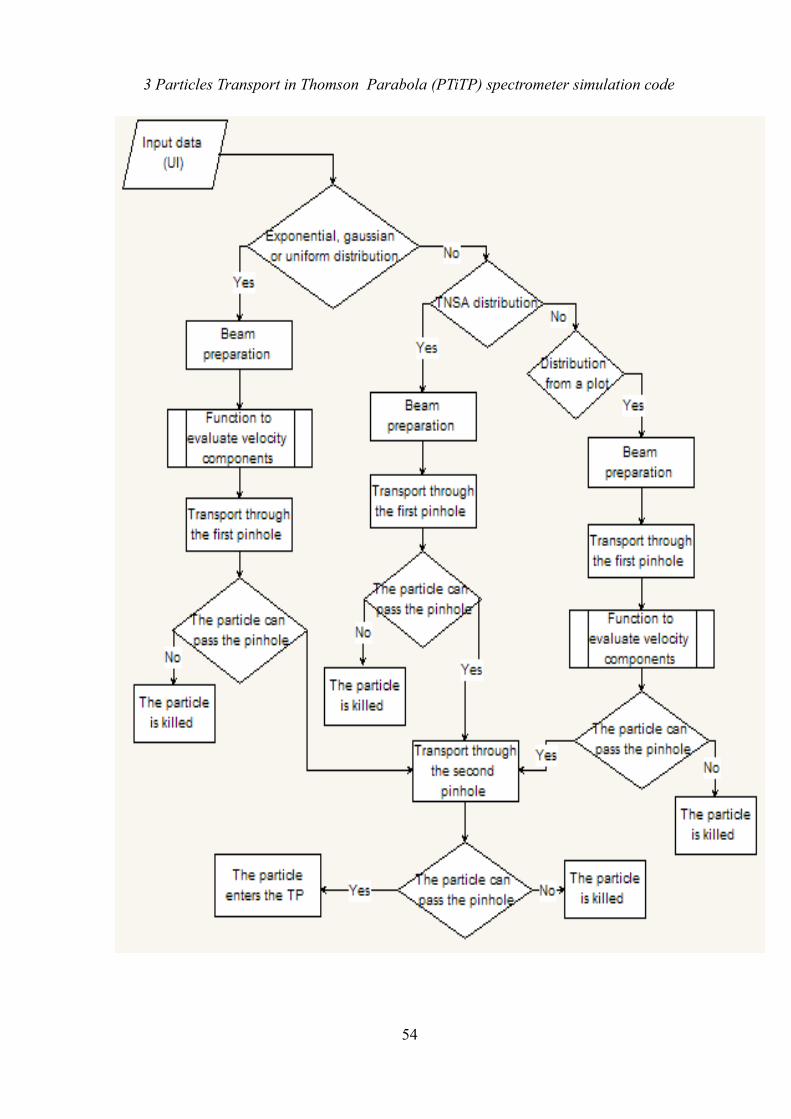
3 Particles Transport in Thomson Parabola (PTiTP) spectrometer simulation code
54
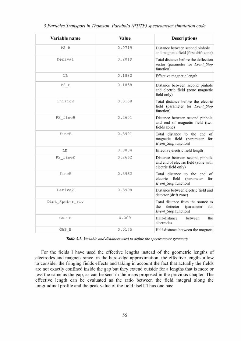
3 Particles Transport in Thomson Parabola (PTiTP) spectrometer simulation code
Variable name Value Descriptions
P2_B 0.0719 Distance between second pinhole and magnetic field (first drift zone)
Deriva1 0.2019 Total distance before the deflection sector (parameter for Event_Stop function)
LB 0.1882 Effective magnetic length
P2_E 0.1858 Distance between second pinhole and electric field (zone magnetic field only)
inizioE 0.3158 Total distance before the electric field (parameter for Event_Stop function)
P2_fineB 0.2601 Distance between second pinhole and end of magnetic field (two fields zone)
fineB 0.3901 Total distance to the end of magnetic field (parameter for Event_Stop function)
LE 0.0804 Effective electric field length
P2_fineE 0.2662 Distance between second pinhole and end of electric field (zone with electric field only)
fineE 0.3962 Total distance to the end of electric field (parameter for Event_Stop function)
Deriva2 0.3998 Distance between electric field and detector (drift zone)
Dist_Spettr_riv Total distance from the source to the detector (parameter for Event_Stop function)
GAP_E 0.009 Half-distance between the electrodes
GAP_B 0.0175 Half-distance between the magnets
Table 3.1: Variable and distances used to define the spectrometer geometry
For the fields I have used the effective lengths instead of the geometric lengths of electrodes and magnets since, in the hard-edge approximation, the effective lengths allow to consider the fringing fields effects and taking in account the fact that actually the fields are not exactly confined inside the gap but they extend outside for a lengths that is more or less the same as the gap, as can be seen in the maps proposed in the previous chapter. The effective length can be evaluated as the ratio between the field integral along the longitudinal profile and the peak value of the field itself. Thus one has:
55
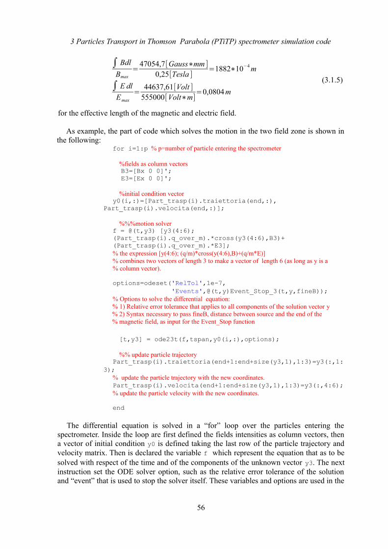
3 Particles Transport in Thomson Parabola (PTiTP) spectrometer simulation code
∫ Bdl
Bmax
=47054,7[Gauss∗mm ]
0,25[Tesla ]=1882∗10−4 m
∫ E dl
Emax
=44637,61[Volt ]
555000[Volt∗m]=0,0804 m
(3.1.5)
for the effective length of the magnetic and electric field.
As example, the part of code which solves the motion in the two field zone is shown in the following:
for i=1:p % p=number of particle entering the spectrometer %fields as column vectors
B3=[Bx 0 0]';E3=[Ex 0 0]';
%initial condition vector y0(i,:)=[Part_trasp(i).traiettoria(end,:),
Part_trasp(i).velocita(end,:)]; %%%motion solverf = @(t,y3) [y3(4:6);(Part_trasp(i).q_over_m).*cross(y3(4:6),B3)+ (Part_trasp(i).q_over_m).*E3]; % the expression [y(4:6); (q/m)*cross(y(4:6),B)+(q/m*E)]% combines two vectors of length 3 to make a vector of length 6 (as long as y is a % column vector).
options=odeset('RelTol',1e-7, 'Events',@(t,y)Event_Stop_3(t,y,fineB)); % Options to solve the differential equation:
% 1) Relative error tolerance that applies to all components of the solution vector y% 2) Syntax necessary to pass fineB, distance between source and the end of the % magnetic field, as input for the Event_Stop function
[t,y3] = ode23t(f,tspan,y0(i,:),options); %% update particle trajectoryPart_trasp(i).traiettoria(end+1:end+size(y3,1),1:3)=y3(:,1:
3); % update the particle trajectory with the new coordinates. Part_trasp(i).velocita(end+1:end+size(y3,1),1:3)=y3(:,4:6); % update the particle velocity with the new coordinates.
end
The differential equation is solved in a “for” loop over the particles entering the spectrometer. Inside the loop are first defined the fields intensities as column vectors, then a vector of initial condition y0 is defined taking the last row of the particle trajectory and velocity matrix. Then is declared the variable f which represent the equation that as to be solved with respect of the time and of the components of the unknown vector y3. The next instruction set the ODE solver option, such as the relative error tolerance of the solution and “event” that is used to stop the solver itself. These variables and options are used in the
56
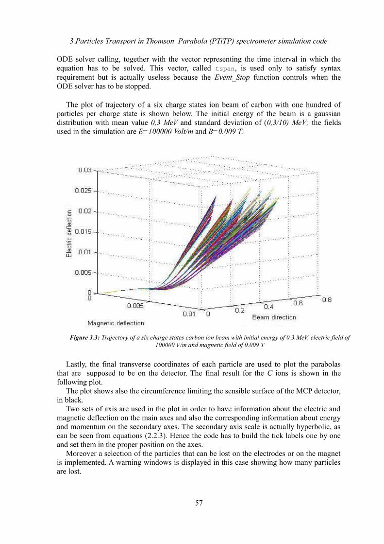
3 Particles Transport in Thomson Parabola (PTiTP) spectrometer simulation code
ODE solver calling, together with the vector representing the time interval in which the equation has to be solved. This vector, called tspan, is used only to satisfy syntax requirement but is actually useless because the Event_Stop function controls when the ODE solver has to be stopped.
The plot of trajectory of a six charge states ion beam of carbon with one hundred of particles per charge state is shown below. The initial energy of the beam is a gaussian distribution with mean value 0,3 MeV and standard deviation of (0,3/10) MeV; the fields used in the simulation are E=100000 Volt/m and B=0.009 T.
Lastly, the final transverse coordinates of each particle are used to plot the parabolas that are supposed to be on the detector. The final result for the C ions is shown in the following plot.
The plot shows also the circumference limiting the sensible surface of the MCP detector, in black.
Two sets of axis are used in the plot in order to have information about the electric and magnetic deflection on the main axes and also the corresponding information about energy and momentum on the secondary axes. The secondary axis scale is actually hyperbolic, as can be seen from equations (2.2.3). Hence the code has to build the tick labels one by one and set them in the proper position on the axes.
Moreover a selection of the particles that can be lost on the electrodes or on the magnet is implemented. A warning windows is displayed in this case showing how many particles are lost.
57
Figure 3.3: Trajectory of a six charge states carbon ion beam with initial energy of 0.3 MeV, electric field of 100000 V/m and magnetic field of 0.009 T
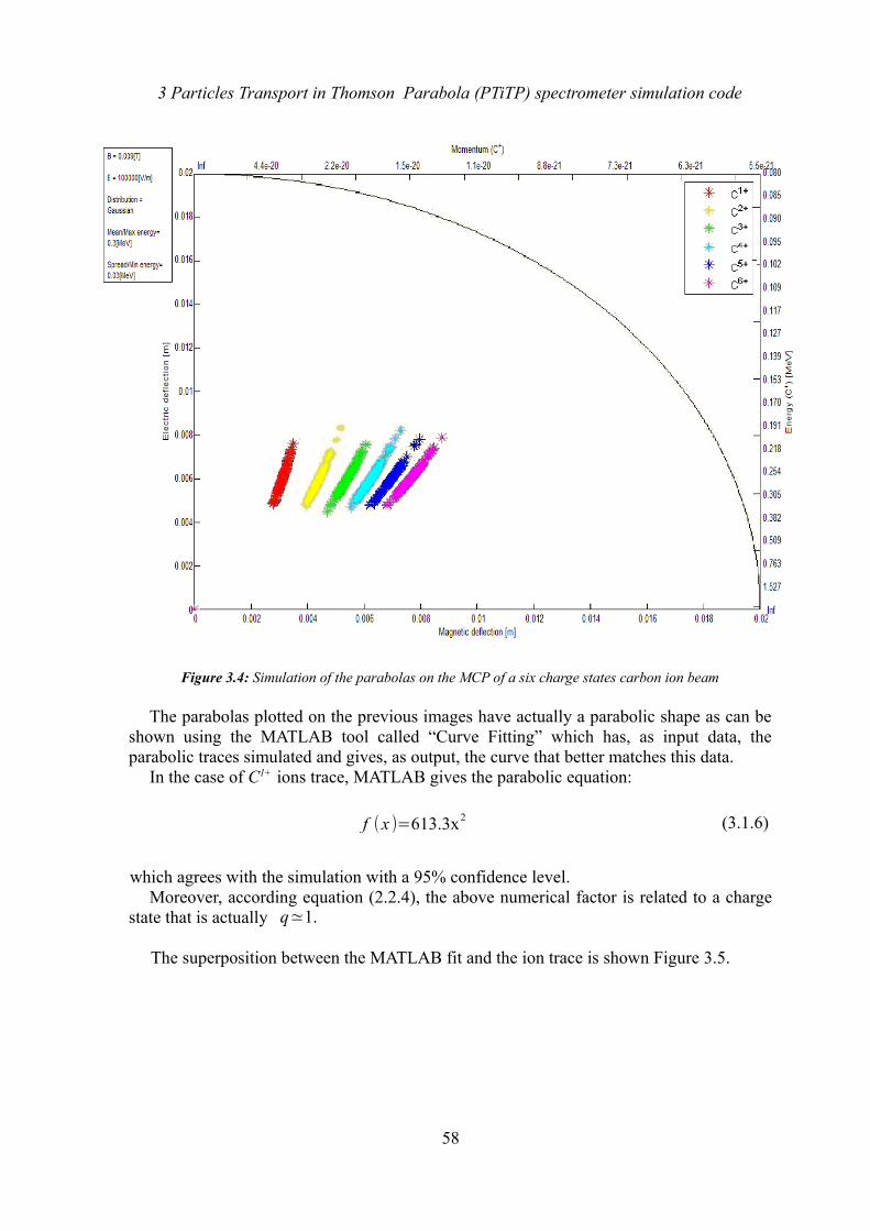
3 Particles Transport in Thomson Parabola (PTiTP) spectrometer simulation code
The parabolas plotted on the previous images have actually a parabolic shape as can be shown using the MATLAB tool called “Curve Fitting” which has, as input data, the parabolic traces simulated and gives, as output, the curve that better matches this data.
In the case of C1+ ions trace, MATLAB gives the parabolic equation:
f (x )=613.3x2 (3.1.6)
which agrees with the simulation with a 95% confidence level.Moreover, according equation (2.2.4), the above numerical factor is related to a charge
state that is actually q≃1.
The superposition between the MATLAB fit and the ion trace is shown Figure 3.5.
58
Figure 3.4: Simulation of the parabolas on the MCP of a six charge states carbon ion beam
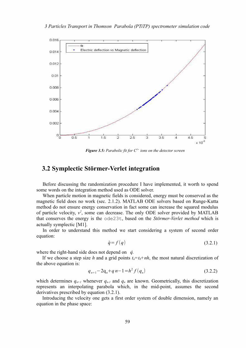
3 Particles Transport in Thomson Parabola (PTiTP) spectrometer simulation code
3.2 Symplectic Störmer-Verlet integration
Before discussing the randomization procedure I have implemented, it worth to spend some words on the integration method used as ODE solver.
When particle motion in magnetic fields is considered, energy must be conserved as the magnetic field does no work (sec. 2.1.2). MATLAB ODE solvers based on Runge-Kutta method do not ensure energy conservation in fact some can increase the squared modulus of particle velocity, v2, some can decrease. The only ODE solver provided by MATLAB that conserves the energy is the ode23t, based on the Störmer-Verlet method which is actually symplectic [M1].
In order to understand this method we start considering a system of second order equation:
q= f (q) (3.2.1)
where the right-hand side does not depend on q.If we choose a step size h and a grid points tn=t0+nh, the most natural discretization of
the above equation is:
qn+1−2qn+q n−1=h2 f (qn) (3.2.2)
which determines qn+1 whenever qn-1 and qn are known. Geometrically, this discretization represents an interpolating parabola which, in the mid-point, assumes the second derivatives prescribed by equation (3.2.1).
Introducing the velocity one gets a first order system of double dimension, namely an equation in the phase space:
59
Figure 3.5: Parabolic fit for C1+ ions on the detector screen
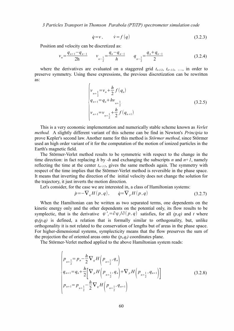
3 Particles Transport in Thomson Parabola (PTiTP) spectrometer simulation code
q=v , v= f (q) (3.2.3)
Position and velocity can be discretized as:
vn=qn+1−qn−1
2hv
n−12
=qn−qn−1
hq
n− 12
=qn+qn−1
2 (3.2.4)
where the derivatives are evaluated on a staggered grid tn-1/2, tn+1/2, …, in order to preserve symmetry. Using these expressions, the previous discretization can be rewritten as:
{v
n+ 12
=vn+h2
f (qn)
qn+1=qn+hvn+ 1
2
v n+1=vn+1
2
+h2
f (qn+1)
(3.2.5)
This is a very economic implementation and numerically stable scheme known as Verlet method. A slightly different variant of this scheme can be find in Newton's Principia to prove Kepler's second law. Another name for this method is Störmer method, since Störmer used an high order variant of it for the computation of the motion of ionized particles in the Earth's magnetic field.
The Störmer-Verlet method results to be symmetric with respect to the change in the time direction: in fact replacing h by -h and exchanging the subscripts n and n+1, namely reflecting the time at the center tn+1/2, gives the same methods again. The symmetry with respect of the time implies that the Störmer-Verlet method is reversible in the phase space. It means that inverting the direction of the initial velocity does not change the solution for the trajectory, it just inverts the motion direction.
Let's consider, for the case we are interested in, a class of Hamiltonian systems:p=−∇ q H ( p ,q) , q=∇ p H ( p ,q) (3.2.7)
When the Hamiltonian can be written as two separated terms, one dependents on the kinetic energy only and the other dependents on the potential only, its flow results to be symplectic, that is the derivative φ ' t=∂φ t /∂( p , q) satisfies, for all (p,q) and t where φt(p,q) is defined, a relation that is formally similar to orthogonality, but, unlike orthogonality it is not related to the conservation of lengths but of areas in the phase space. For higher-dimensional systems, symplecticity means that the flow preserves the sum of the projection the of oriented areas onto the (pi,qi) coordinates plane.
The Störmer-Verlet method applied to the above Hamiltonian system reads:
{p
n+ 12
= pn−h2∇ q H ( p
n+12
, qn)qn+1=qn+
h2 [∇ p H ( p
n+12
, qn)+∇ p H ( pn+
12
, qn+1)]pn+1= p
n+12
−h2∇ q H ( p
n+ 12
, qn+1)
(3.2.8)
60
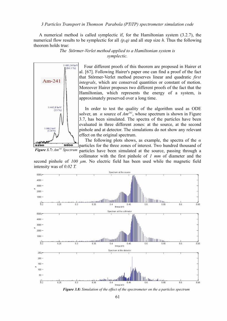
3 Particles Transport in Thomson Parabola (PTiTP) spectrometer simulation code
A numerical method is called symplectic if, for the Hamiltonian system (3.2.7), the numerical flow results to be symplectic for all (p,q) and all step size h. Thus the following theorem holds true:
The Störmer-Verlet method applied to a Hamiltonian system is symplectic.
Four different proofs of this theorem are proposed in Hairer et al. [67]. Following Hairer's paper one can find a proof of the fact that Störmer-Verlet method preserves linear and quadratic first integrals, which are conserved quantities or constant of motion. Moreover Hairer proposes two different proofs of the fact that the Hamiltonian, which represents the energy of a system, is approximately preserved over a long time.
In order to test the quality of the algorithm used as ODE solver, an α source of Am241, whose spectrum is shown in Figure 3.7, has been simulated. The spectra of the particles have been evaluated in three different zones: at the source, at the second pinhole and at detector. The simulations do not show any relevant effect on the original spectrum.
The following plots shows, as example, the spectra of the α particles for the three zones of interest. Two hundred thousand of particles have been simulated at the source, passing through a collimator with the first pinhole of 1 mm of diameter and the
second pinhole of 100 μm. No electric field has been used while the magnetic field intensity was of 0.02 T.
61
Figure 3.7: Am241 Spectrum
Figure 3.8: Simulation of the effect of the spectrometer on the a particles spectrum
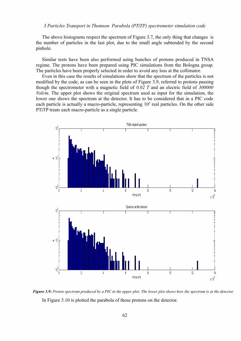
3 Particles Transport in Thomson Parabola (PTiTP) spectrometer simulation code
The above histograms respect the spectrum of Figure 3.7, the only thing that changes is the number of particles in the last plot, due to the small angle subtended by the second pinhole.
Similar tests have been also performed using bunches of protons produced in TNSA regime. The protons have been prepared using PIC simulations from the Bologna group. The particles have been properly selected in order to avoid any loss at the collimator.
Even in this case the results of simulations show that the spectrum of the particles is not modified by the code, as can be seen in the plots of Figure 3.9, referred to protons passing though the spectrometer with a magnetic field of 0.02 T and an electric field of 300000 Volt/m. The upper plot shows the original spectrum used as input for the simulation, the lower one shows the spectrum at the detector. It has to be considered that in a PIC code each particle is actually a macro-particle, representing 105 real particles. On the other side PTiTP treats each macro-particle as a single particle.
In Figure 3.10 is plotted the parabola of those protons on the detector.
62
Figure 3.9: Proton spectrum produced by a PIC in the upper plot. The lower plot shows how the spectrum is at the detector
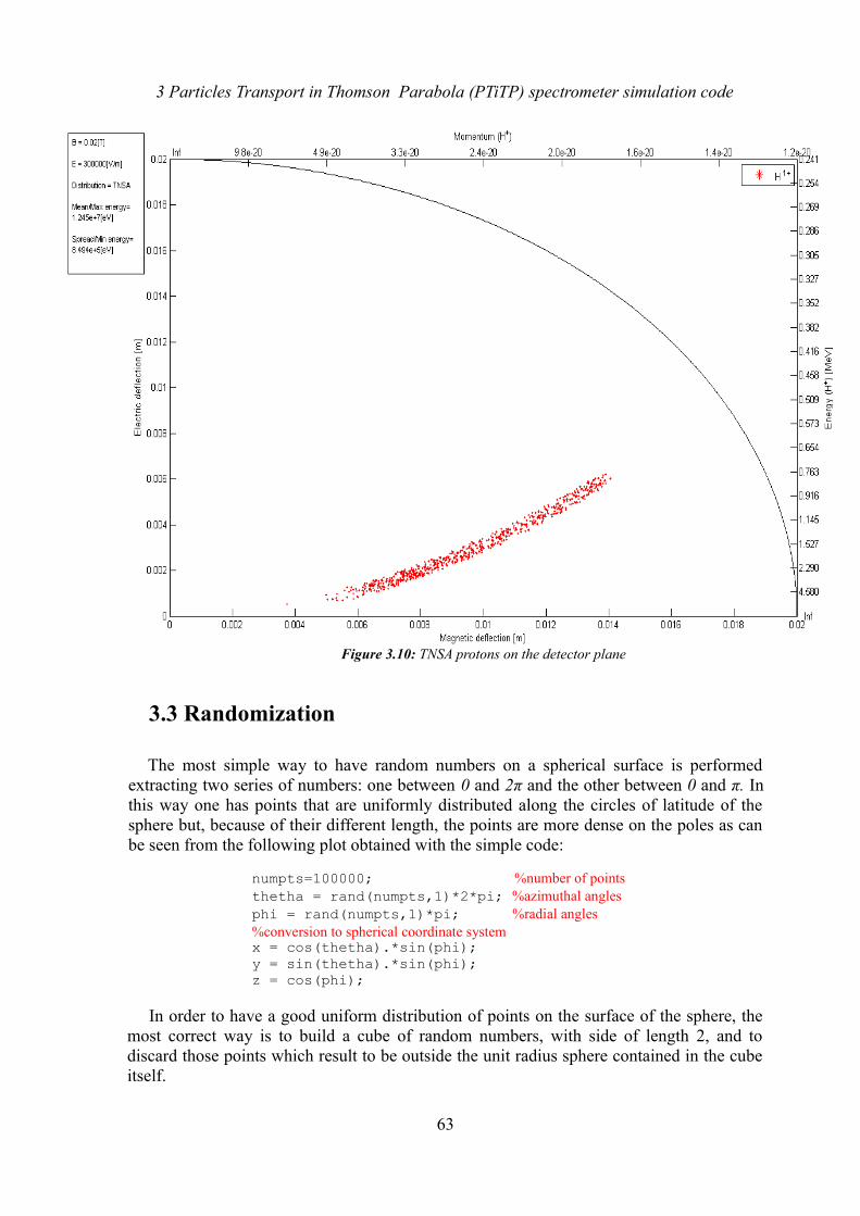
3 Particles Transport in Thomson Parabola (PTiTP) spectrometer simulation code
3.3 Randomization
The most simple way to have random numbers on a spherical surface is performed extracting two series of numbers: one between 0 and 2π and the other between 0 and π. In this way one has points that are uniformly distributed along the circles of latitude of the sphere but, because of their different length, the points are more dense on the poles as can be seen from the following plot obtained with the simple code:
numpts=100000; %number of pointsthetha = rand(numpts,1)*2*pi; %azimuthal anglesphi = rand(numpts,1)*pi; %radial angles%conversion to spherical coordinate systemx = cos(thetha).*sin(phi); y = sin(thetha).*sin(phi);z = cos(phi);
In order to have a good uniform distribution of points on the surface of the sphere, the most correct way is to build a cube of random numbers, with side of length 2, and to discard those points which result to be outside the unit radius sphere contained in the cube itself.
63
Figure 3.10: TNSA protons on the detector plane
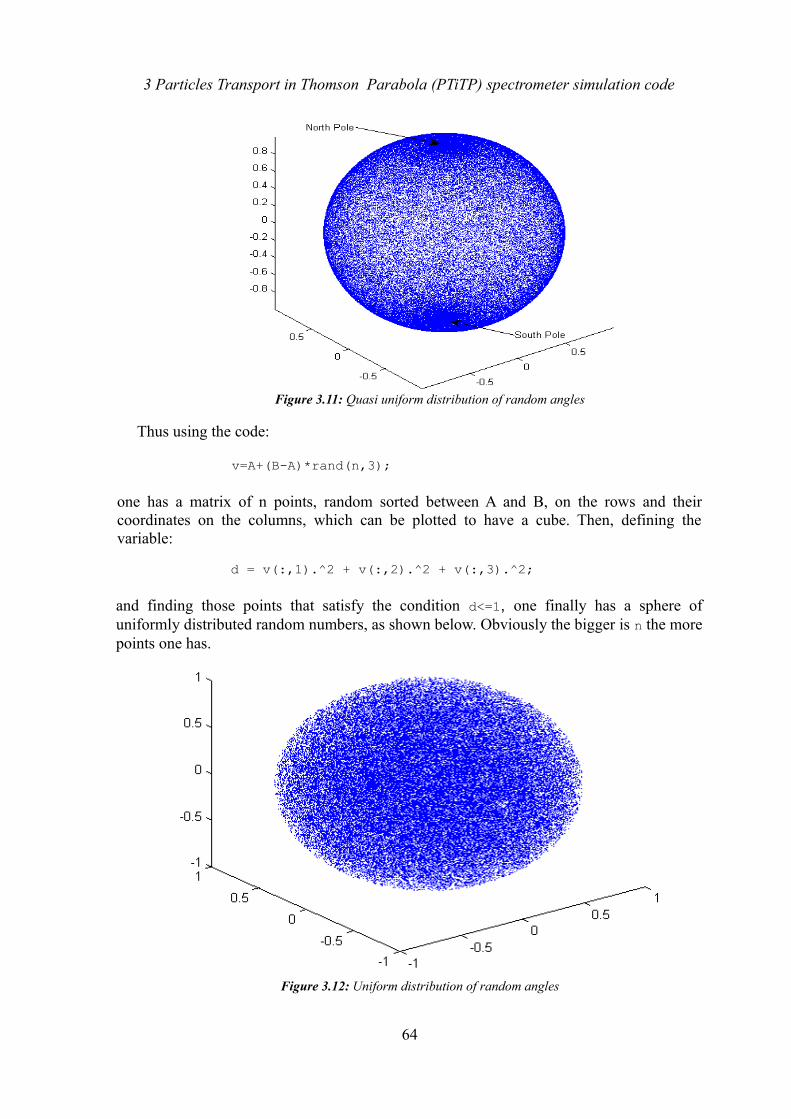
3 Particles Transport in Thomson Parabola (PTiTP) spectrometer simulation code
Thus using the code:
v=A+(B-A)*rand(n,3);
one has a matrix of n points, random sorted between A and B, on the rows and their coordinates on the columns, which can be plotted to have a cube. Then, defining the variable:
d = v(:,1).^2 + v(:,2).^2 + v(:,3).^2;
and finding those points that satisfy the condition d<=1, one finally has a sphere of uniformly distributed random numbers, as shown below. Obviously the bigger is n the more points one has.
64
Figure 3.11: Quasi uniform distribution of random angles
Figure 3.12: Uniform distribution of random angles
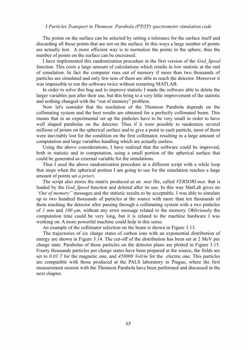
3 Particles Transport in Thomson Parabola (PTiTP) spectrometer simulation code
The points on the surface can be selected by setting a tolerance for the surface itself and discarding all those points that are not on the surface. In this ways a large number of points are actually lost. A more efficient way is to normalize the points in the sphere, thus the number of points on the surface can be encreased.
I have implemented this randomization procedure in the first version of the God_Speed function. This costs a large amount of calculations which results in low statistic at the end of simulation. In fact the computer runs out of memory if more than two thousands of particles are simulated and only few tens of them are able to reach the detector. Moreover it was impossible to run the software twice without restarting MATLAB.
In order to solve this bug and to improve statistic I made the software able to delete the larger variables just after their use, but this bring to a very little improvement of the statistic and nothing changed with the “out of memory” problem.
Now let's consider that the resolution of the Thomson Parabola depends on the collimating system and the best results are obtained for a perfectly collimated beam. This means that in an experimental set up the pinholes have to be very small in order to have well shaped parabolas on the detector. Thus if it were possible to randomize several millions of points on the spherical surface and to give a point to each particle, most of them were inevitably lost for the condition on the first collimator, resulting in a large amount of computation and large variables handling which are actually useless.
Using the above considerations, I have realized that the software could be improved, both in statistic and in computation, using a small portion of the spherical surface that could be generated as external variable for the simulations.
Thus I used the above randomization procedure in a different script with a while loop that stops when the spherical portion I am going to use for the simulation reaches a large amount of points set a priori.
The script also stores the matrix produced as an .mat file, called VERSORI.mat, that is loaded by the God_Speed function and deleted after its use. In this way MatLab gives no “Out of memory” messages and the statistic results to be acceptable. I was able to simulate up to two hundred thousands of particles at the source with more than ten thousands of them reaching the detector after passing through a collimating system with a two pinholes of 1 mm and 100 μm, without any error message related to the memory. Obliviously the computation time could be very long, but it is related to the machine hardware I was working on. A more powerful machine could help in this sense.
An example of the collimator selection on the beam is shown in Figure 3.13.The trajectories of six charge states of carbon ions with an exponential distribution of
energy are shown in Figure 3.14. The cut-off of the distribution has been set at 2 MeV per charge state. Parabolas of those particles on the detector plane are plotted in Figure 3.15. Fourty thousands particles per charge states have been prepared at the source, the fields are set to 0.03 T for the magnetic one, and 450000 Volt/m for the electric one. This particles are compatible with those produced at the PALS laboratory in Prague, where the first measurement session with the Thomson Parabola have been performed and discussed in the next chapter.
65
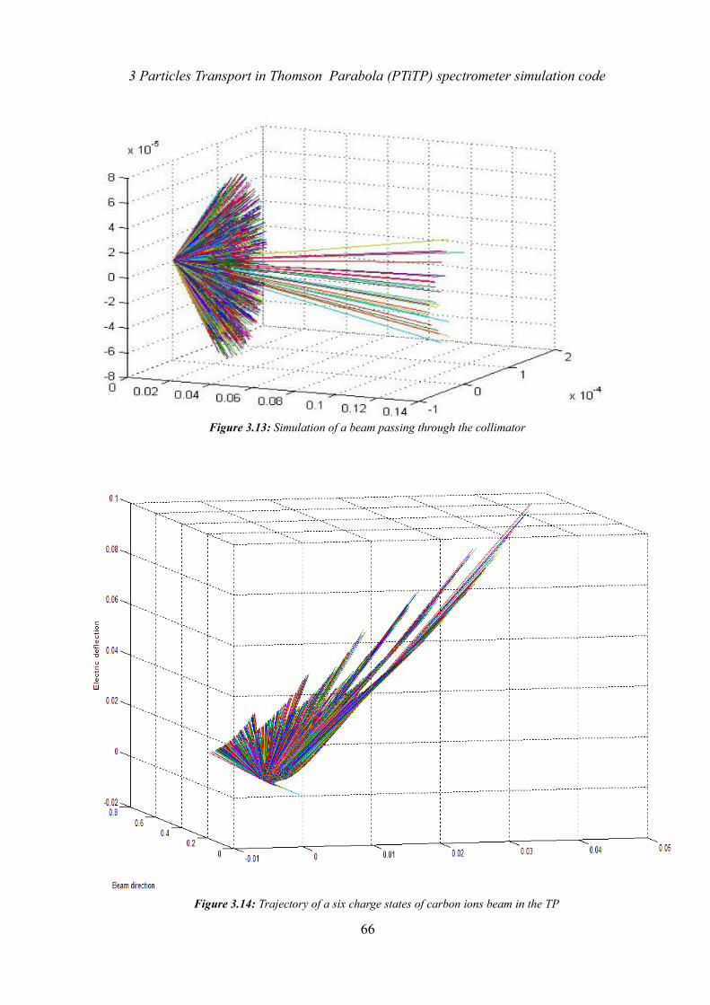
3 Particles Transport in Thomson Parabola (PTiTP) spectrometer simulation code
66
Figure 3.14: Trajectory of a six charge states of carbon ions beam in the TP
Figure 3.13: Simulation of a beam passing through the collimator
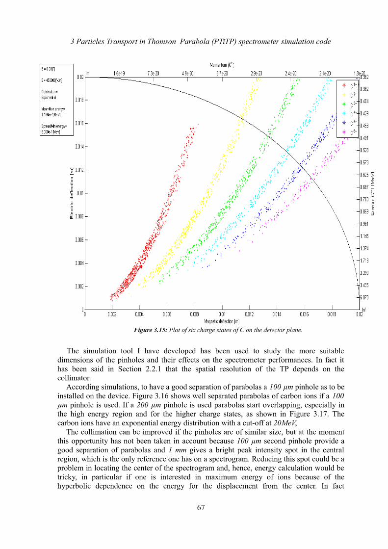
3 Particles Transport in Thomson Parabola (PTiTP) spectrometer simulation code
The simulation tool I have developed has been used to study the more suitable dimensions of the pinholes and their effects on the spectrometer performances. In fact it has been said in Section 2.2.1 that the spatial resolution of the TP depends on the collimator.
According simulations, to have a good separation of parabolas a 100 µm pinhole as to be installed on the device. Figure 3.16 shows well separated parabolas of carbon ions if a 100 µm pinhole is used. If a 200 µm pinhole is used parabolas start overlapping, especially in the high energy region and for the higher charge states, as shown in Figure 3.17. The carbon ions have an exponential energy distribution with a cut-off at 20MeV,
The collimation can be improved if the pinholes are of similar size, but at the moment this opportunity has not been taken in account because 100 µm second pinhole provide a good separation of parabolas and 1 mm gives a bright peak intensity spot in the central region, which is the only reference one has on a spectrogram. Reducing this spot could be a problem in locating the center of the spectrogram and, hence, energy calculation would be tricky, in particular if one is interested in maximum energy of ions because of the hyperbolic dependence on the energy for the displacement from the center. In fact
67
Figure 3.15: Plot of six charge states of C on the detector plane.
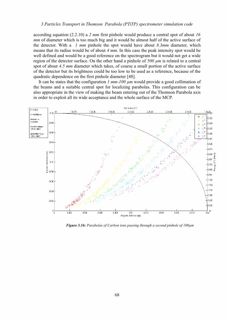
3 Particles Transport in Thomson Parabola (PTiTP) spectrometer simulation code
according equation (2.2.10) a 2 mm first pinhole would produce a central spot of about 16 mm of diameter which is too much big and it would be almost half of the active surface of the detector. With a 1 mm pinhole the spot would have about 8.3mm diameter, which means that its radius would be of about 4 mm. In this case the peak intensity spot would be well defined and would be a good reference on the spectrogram but it would not get a wide region of the detector surface. On the other hand a pinhole of 500 µm is related to a central spot of about 4.5 mm diameter which takes, of course a small portion of the active surface of the detector but its brightness could be too low to be used as a reference, because of the quadratic dependence on the first pinhole diameter [48].
It can be states that the configuration 1 mm-100 µm would provide a good collimation of the beams and a suitable central spot for localizing parabolas. This configuration can be also appropriate in the view of making the beam entering out of the Thomson Parabola axis in order to exploit all its wide acceptance and the whole surface of the MCP.
68
Figure 3.16: Parabolas of Carbon ions passing through a second pinhole of 100µm
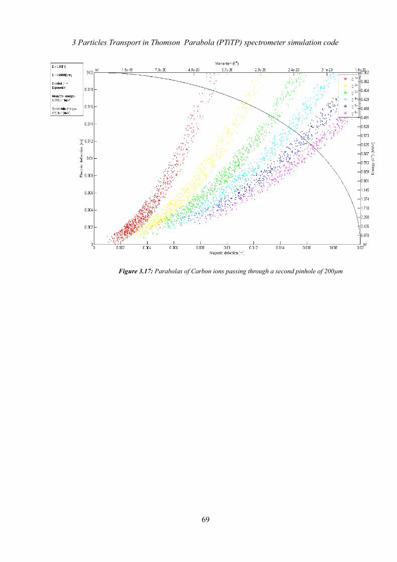
3 Particles Transport in Thomson Parabola (PTiTP) spectrometer simulation code
C
69
Figure 3.17: Parabolas of Carbon ions passing through a second pinhole of 200µm
4 Experimental activity
4 Experimental activity 25th Murphy’s law on technology: “If an experiment works, something has gone wrong.”
In this chapter the experimental session performed at PALS (Prague Asterix Laser System) from the 17th of April to the 9th of May is described . During the experiment the Thomson Parabola has been tested with laser accelerated ion beams produced by the Asterix IV laser. The results obtained will be analyzed.
In order to prepare this the first experimental run, some preliminary tests have been performed on the TP at LNS using monochromatic source, such as Am241 and the laser system available in Catania. This activity has been useful to improve and to fix some major issues on the spectrometer and also to get the feeling with the instrument. Some of this tests will be mentioned in the following.
Moreover simulations with realistic beams in TNSA regime have been also performed. The particles have been produced using a PIC code from both Bologna and Prague groups. Some results will be also proposed in the following.
4.1 Pragua Asterix Laser System (PALS) laboratory
The long pulse, terawatt iodine laser system ASTERIX IV is installed in the Research Centre PALS in Prague. The laser is a single beam iodine laser system which supplies up to 1 kJ of energy at the fundamental wavelength 1.315 μm, in pulses of ~400 ps duration. The primary pulse is generated in an oscillator with a contrast ratio, namely the ratio between the peak of the main laser pulse and the pre-pulse intensities, of ~109. The pulse is seeded into a chain of one preamplifier and five power amplifiers separated by spatial filters removing the high spatial components from the angular beam spectrum. They ensure also an optimum coupling between adjacent amplifiers through increasingly large diameter section. The beam at the output of the last amplifier is 29 cm of diameter. A characteristic feature of the system is the high spatial uniformity of the beam, typically within ±6% of the mean value. The laser can fire a full-energy shot every 20 minutes [68]. A simplified scheme of the laser system is shown on the left side of Figure 4.1; on the right side a view of the chain of amplifiers is provided.
The laboratory is provided with two interaction chambers. The main spherical chamber is 1 m in diameter and has a pneumatic gate for accessing easily to the target optical bench. A picture of the main interaction chamber and the Thomson Parabola is provided in Figure 4.2. The pipe linking the chamber and the spectrometer has an ICR set upstream the collimator.
The laser intensity of 2 TW allows to reach extremely high energy for protons. Measurements of time of flight (TOF) show that the mean proton energy should be approximately 550 keV, and the maximum proton energy detected is more than 2.5 MeV [69]. From the experimental results the accelerating potential inside the plasma has to reach a value of about 550 kV.
69
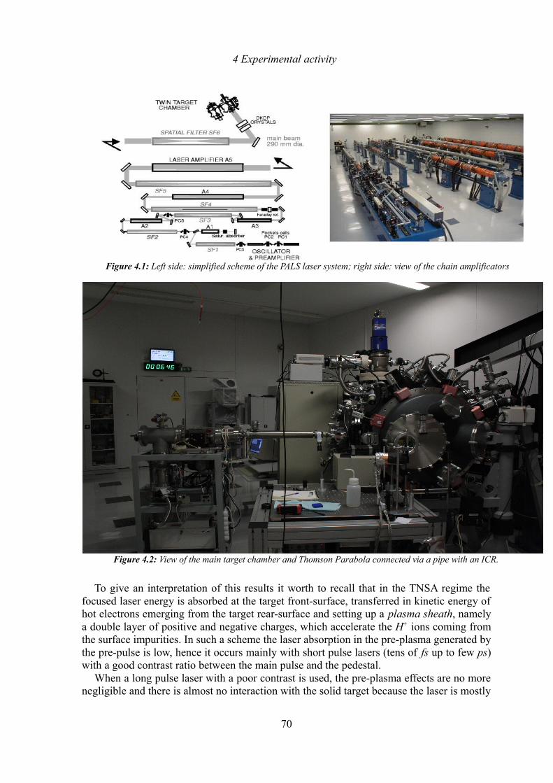
4 Experimental activity
To give an interpretation of this results it worth to recall that in the TNSA regime the focused laser energy is absorbed at the target front-surface, transferred in kinetic energy of hot electrons emerging from the target rear-surface and setting up a plasma sheath, namely a double layer of positive and negative charges, which accelerate the H+ ions coming from the surface impurities. In such a scheme the laser absorption in the pre-plasma generated by the pre-pulse is low, hence it occurs mainly with short pulse lasers (tens of fs up to few ps) with a good contrast ratio between the main pulse and the pedestal.
When a long pulse laser with a poor contrast is used, the pre-plasma effects are no more negligible and there is almost no interaction with the solid target because the laser is mostly
70
Figure 4.1: Left side: simplified scheme of the PALS laser system; right side: view of the chain amplificators
Figure 4.2: View of the main target chamber and Thomson Parabola connected via a pipe with an ICR.
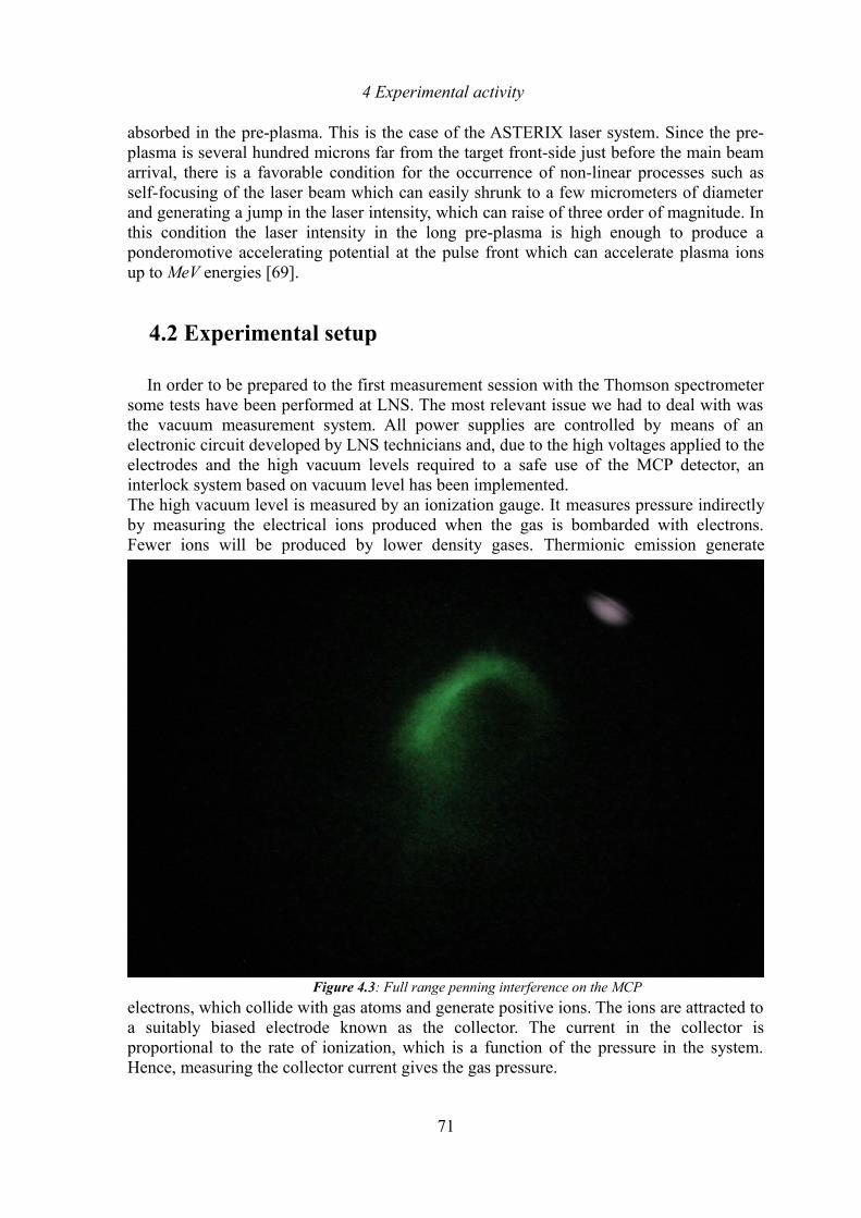
4 Experimental activity
absorbed in the pre-plasma. This is the case of the ASTERIX laser system. Since the pre-plasma is several hundred microns far from the target front-side just before the main beam arrival, there is a favorable condition for the occurrence of non-linear processes such as self-focusing of the laser beam which can easily shrunk to a few micrometers of diameter and generating a jump in the laser intensity, which can raise of three order of magnitude. In this condition the laser intensity in the long pre-plasma is high enough to produce a ponderomotive accelerating potential at the pulse front which can accelerate plasma ions up to MeV energies [69].
4.2 Experimental setup
In order to be prepared to the first measurement session with the Thomson spectrometer some tests have been performed at LNS. The most relevant issue we had to deal with was the vacuum measurement system. All power supplies are controlled by means of an electronic circuit developed by LNS technicians and, due to the high voltages applied to the electrodes and the high vacuum levels required to a safe use of the MCP detector, an interlock system based on vacuum level has been implemented. The high vacuum level is measured by an ionization gauge. It measures pressure indirectly by measuring the electrical ions produced when the gas is bombarded with electrons. Fewer ions will be produced by lower density gases. Thermionic emission generate
electrons, which collide with gas atoms and generate positive ions. The ions are attracted to a suitably biased electrode known as the collector. The current in the collector is proportional to the rate of ionization, which is a function of the pressure in the system. Hence, measuring the collector current gives the gas pressure.
71
Figure 4.3: Full range penning interference on the MCP
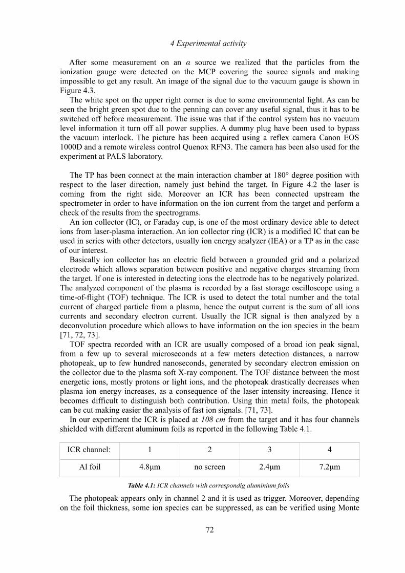
4 Experimental activity
After some measurement on an α source we realized that the particles from the ionization gauge were detected on the MCP covering the source signals and making impossible to get any result. An image of the signal due to the vacuum gauge is shown in Figure 4.3.
The white spot on the upper right corner is due to some environmental light. As can be seen the bright green spot due to the penning can cover any useful signal, thus it has to be switched off before measurement. The issue was that if the control system has no vacuum level information it turn off all power supplies. A dummy plug have been used to bypass the vacuum interlock. The picture has been acquired using a reflex camera Canon EOS 1000D and a remote wireless control Quenox RFN3. The camera has been also used for the experiment at PALS laboratory.
The TP has been connect at the main interaction chamber at 180° degree position with respect to the laser direction, namely just behind the target. In Figure 4.2 the laser is coming from the right side. Moreover an ICR has been connected upstream the spectrometer in order to have information on the ion current from the target and perform a check of the results from the spectrograms.
An ion collector (IC), or Faraday cup, is one of the most ordinary device able to detect ions from laser-plasma interaction. An ion collector ring (ICR) is a modified IC that can be used in series with other detectors, usually ion energy analyzer (IEA) or a TP as in the case of our interest.
Basically ion collector has an electric field between a grounded grid and a polarized electrode which allows separation between positive and negative charges streaming from the target. If one is interested in detecting ions the electrode has to be negatively polarized. The analyzed component of the plasma is recorded by a fast storage oscilloscope using a time-of-flight (TOF) technique. The ICR is used to detect the total number and the total current of charged particle from a plasma, hence the output current is the sum of all ions currents and secondary electron current. Usually the ICR signal is then analyzed by a deconvolution procedure which allows to have information on the ion species in the beam [71, 72, 73].
TOF spectra recorded with an ICR are usually composed of a broad ion peak signal, from a few up to several microseconds at a few meters detection distances, a narrow photopeak, up to few hundred nanoseconds, generated by secondary electron emission on the collector due to the plasma soft X-ray component. The TOF distance between the most energetic ions, mostly protons or light ions, and the photopeak drastically decreases when plasma ion energy increases, as a consequence of the laser intensity increasing. Hence it becomes difficult to distinguish both contribution. Using thin metal foils, the photopeak can be cut making easier the analysis of fast ion signals. [71, 73].
In our experiment the ICR is placed at 108 cm from the target and it has four channels shielded with different aluminum foils as reported in the following Table 4.1.
ICR channel: 1 2 3 4
Al foil 4.8μm no screen 2.4μm 7.2μm
Table 4.1: ICR channels with correspondig aluminium foils
The photopeak appears only in channel 2 and it is used as trigger. Moreover, depending on the foil thickness, some ion species can be suppressed, as can be verified using Monte
72
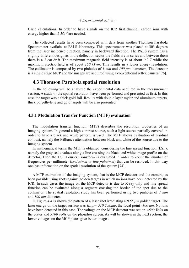
4 Experimental activity
Carlo calculations. In order to have signals on the ICR first channel, carbon ions with energy higher than 5 MeV are needed.
The collected results have been compared with data from another Thomson Parabola Spectrometer availabe at PALS laboratory. This spectrometer was placed at 30° degrees from the laser incidence direction, namely in backward direction. The PALS system has a slightly different design as in the deflection sector the fields are in series and between them there is a 1 cm drift. The maximum magnetic field intensity is of about 0.2 T while the maximum electric field is of about 150 kV/m. This results in a lower energy resolution. The collimator is composed by two pinholes of 1 mm and 100 μm diameters. The detector is a single stage MCP and the images are acquired using a conventional reflex camera [76].
4.3 Thomson Parabola spatial resolutionIn the following will be analyzed the experimental data acquired in the measurement
session. A study of the spatial resolution have been performed and presented as first. In this case the target was a thick gold foil. Results with double layer mylar and aluminum targets, thick polyethylene and gold targets will be also presented.
4.3.1 Modulation Transfer Function (MTF) evaluation
The modulation transfer function (MTF) describes the resolution properties of an imaging system. In general a high contrast source, such a light source partially covered in order to have a black and white pattern, is used. The MTF allows evaluation of residual contrast, namely the brilliance attenuation between black and white of the source due to the imaging system.
In mathematical terms the MTF is obtained considering the line spread function (LSF), namely the gray scale values along a line crossing the black and white image profile on the detector. Then the LSF Fourier Transform is evaluated in order to count the number of frequencies per millimeter (cycles/mm or line pairs/mm) that can be resolved. In this way one has information on the spatial resolution of the system [74].
A MTF estimation of the imaging system, that is the MCP detector and the camera, as been possible using shots against golden targets in which no ions have been detected by the ICR. In such cases the image on the MCP detector is due to X-ray only and line spread function can be evaluated along a segment crossing the border of the spot due to the collimator. The spatial resolution study has been performed using two pinholes of 1 mm and 100 μm diameter.
In Figure 4.4 is shown the pattern of a laser shot irradiating a 0.65 μm golden target. The laser energy on the target surface was Etarget= 510.2 Joule, the focal point -100 μm. No ions have been detected in this case. The voltage on the MCP detector was set on ±600 Volts on the plates and 3700 Volts on the phosphor screen. As will be shown in the next section, the lower voltages on the MCP plates give better images.
73
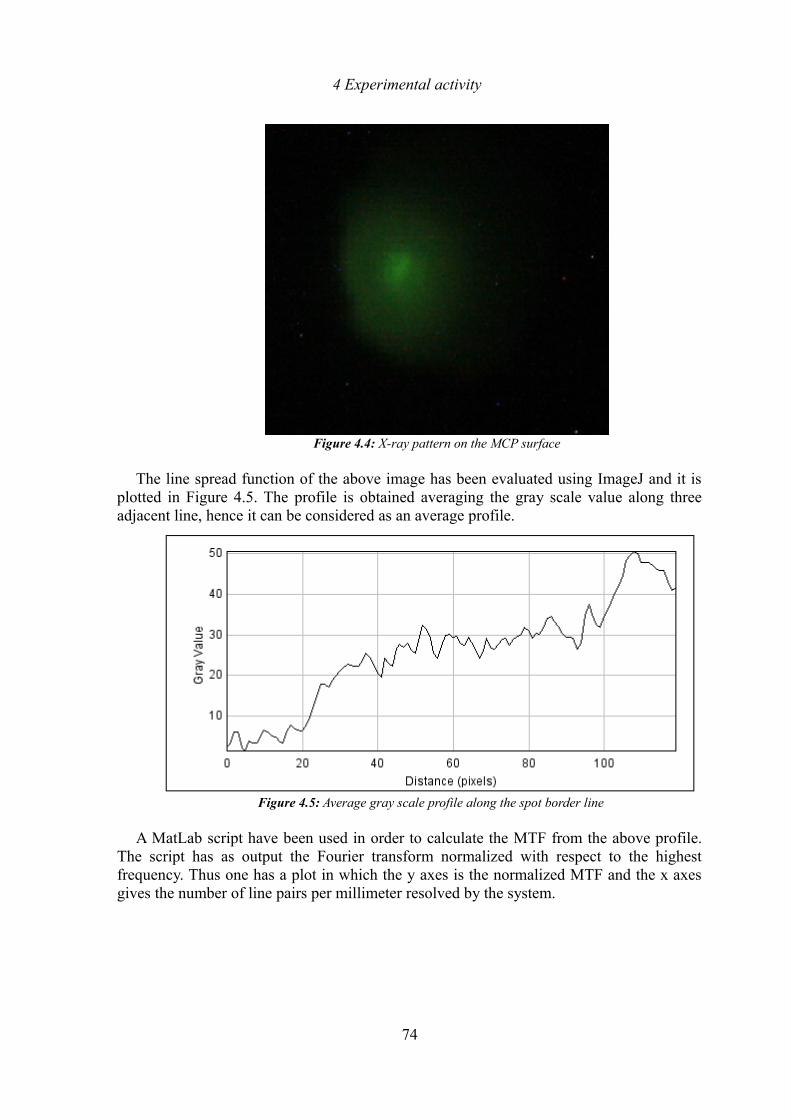
4 Experimental activity
The line spread function of the above image has been evaluated using ImageJ and it is plotted in Figure 4.5. The profile is obtained averaging the gray scale value along three adjacent line, hence it can be considered as an average profile.
A MatLab script have been used in order to calculate the MTF from the above profile.
The script has as output the Fourier transform normalized with respect to the highest frequency. Thus one has a plot in which the y axes is the normalized MTF and the x axes gives the number of line pairs per millimeter resolved by the system.
74
Figure 4.4: X-ray pattern on the MCP surface
Figure 4.5: Average gray scale profile along the spot border line
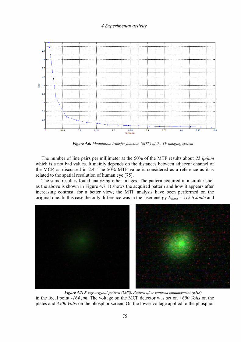
4 Experimental activity
The number of line pairs per millimeter at the 50% of the MTF results about 25 lp/mm which is a not bad values. It mainly depends on the distances between adjacent channel of the MCP, as discussed in 2.4. The 50% MTF value is considered as a reference as it is related to the spatial resolution of human eye [75].
The same result is found analyzing other images. The pattern acquired in a similar shot as the above is shown in Figure 4.7. It shows the acquired pattern and how it appears after increasing contrast, for a better view; the MTF analysis have been performed on the original one. In this case the only difference was in the laser energy Etarget = 512.6 Joule and
in the focal point -164 μm. The voltage on the MCP detector was set on ±600 Volts on the plates and 3500 Volts on the phosphor screen. On the lower voltage applied to the phosphor
75
Figure 4.7: X-ray original pattern (LHS). Pattern after contrast enhancement (RHS)
Figure 4.6: Modulation transfer function (MTF) of the TP imaging system
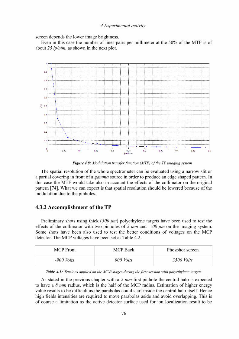
4 Experimental activity
screen depends the lower image brightness.Even in this case the number of lines pairs per millimeter at the 50% of the MTF is of
about 25 lp/mm, as shown in the next plot.
The spatial resolution of the whole spectrometer can be evaluated using a narrow slit or a partial covering in front of a gamma source in order to produce an edge shaped pattern. In this case the MTF would take also in account the effects of the collimator on the original pattern [74]. What we can expect is that spatial resolution should be lowered because of the modulation due to the pinholes.
4.3.2 Accomplishment of the TP
Preliminary shots using thick (300 μm) polyethylene targets have been used to test the effects of the collimator with two pinholes of 2 mm and 100 μm on the imaging system. Some shots have been also used to test the better conditions of voltages on the MCP detector. The MCP voltages have been set as Table 4.2.
MCP Front MCP Back Phosphor screen
-900 Volts 900 Volts 3500 Volts
Table 4.1: Tensions applied on the MCP stages during the first session with polyethylene targets
As stated in the previous chapter with a 2 mm first pinhole the central halo is expected to have a 8 mm radius, which is the half of the MCP radius. Estimation of higher energy value results to be difficult as the parabolas could start inside the central halo itself. Hence high fields intensities are required to move parabolas aside and avoid overlapping. This is of course a limitation as the active detector surface used for ion localization result to be
76
Figure 4.8: Modulation transfer function (MTF) of the TP imaging system
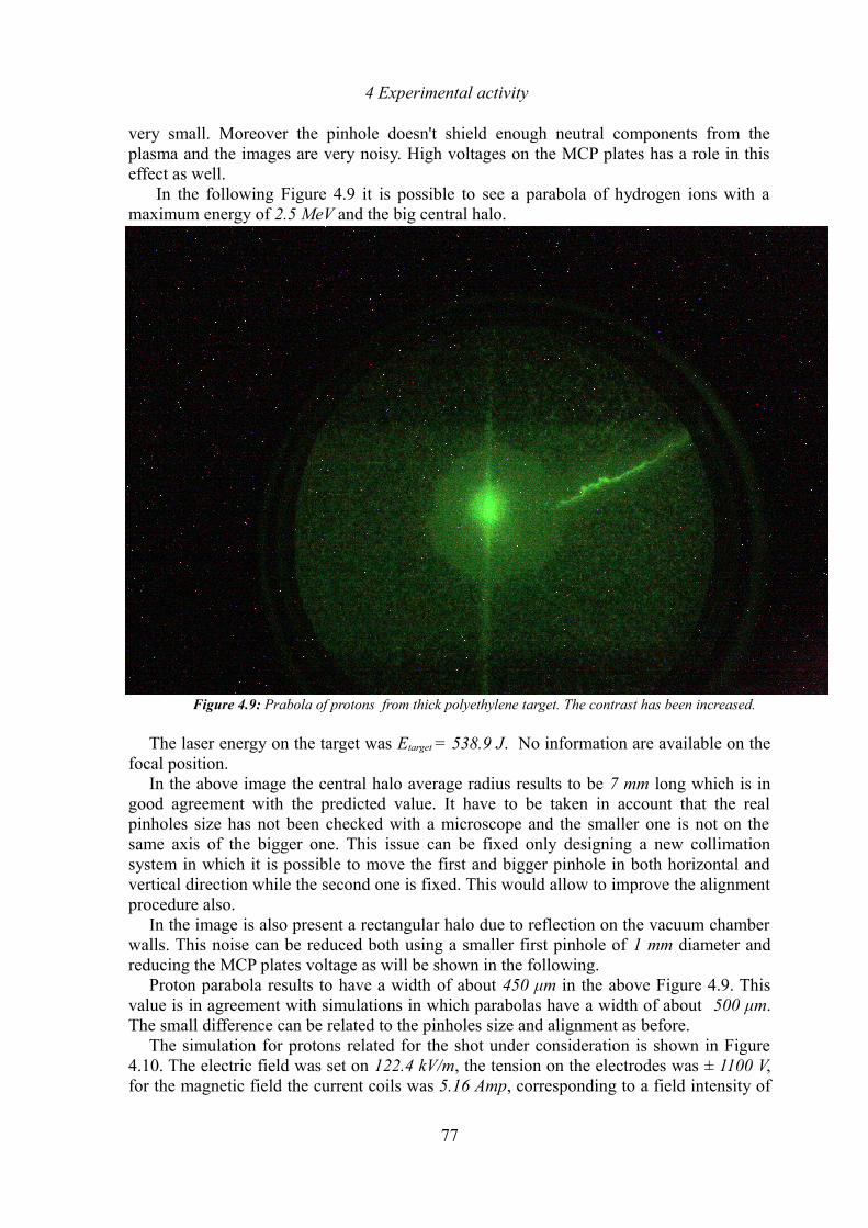
4 Experimental activity
very small. Moreover the pinhole doesn't shield enough neutral components from the plasma and the images are very noisy. High voltages on the MCP plates has a role in this effect as well.
In the following Figure 4.9 it is possible to see a parabola of hydrogen ions with a maximum energy of 2.5 MeV and the big central halo.
The laser energy on the target was Etarget = 538.9 J. No information are available on the focal position.
In the above image the central halo average radius results to be 7 mm long which is in good agreement with the predicted value. It have to be taken in account that the real pinholes size has not been checked with a microscope and the smaller one is not on the same axis of the bigger one. This issue can be fixed only designing a new collimation system in which it is possible to move the first and bigger pinhole in both horizontal and vertical direction while the second one is fixed. This would allow to improve the alignment procedure also.
In the image is also present a rectangular halo due to reflection on the vacuum chamber walls. This noise can be reduced both using a smaller first pinhole of 1 mm diameter and reducing the MCP plates voltage as will be shown in the following.
Proton parabola results to have a width of about 450 μm in the above Figure 4.9. This value is in agreement with simulations in which parabolas have a width of about 500 μm. The small difference can be related to the pinholes size and alignment as before.
The simulation for protons related for the shot under consideration is shown in Figure 4.10. The electric field was set on 122.4 kV/m, the tension on the electrodes was ± 1100 V, for the magnetic field the current coils was 5.16 Amp, corresponding to a field intensity of
77
Figure 4.9: Prabola of protons from thick polyethylene target. The contrast has been increased.
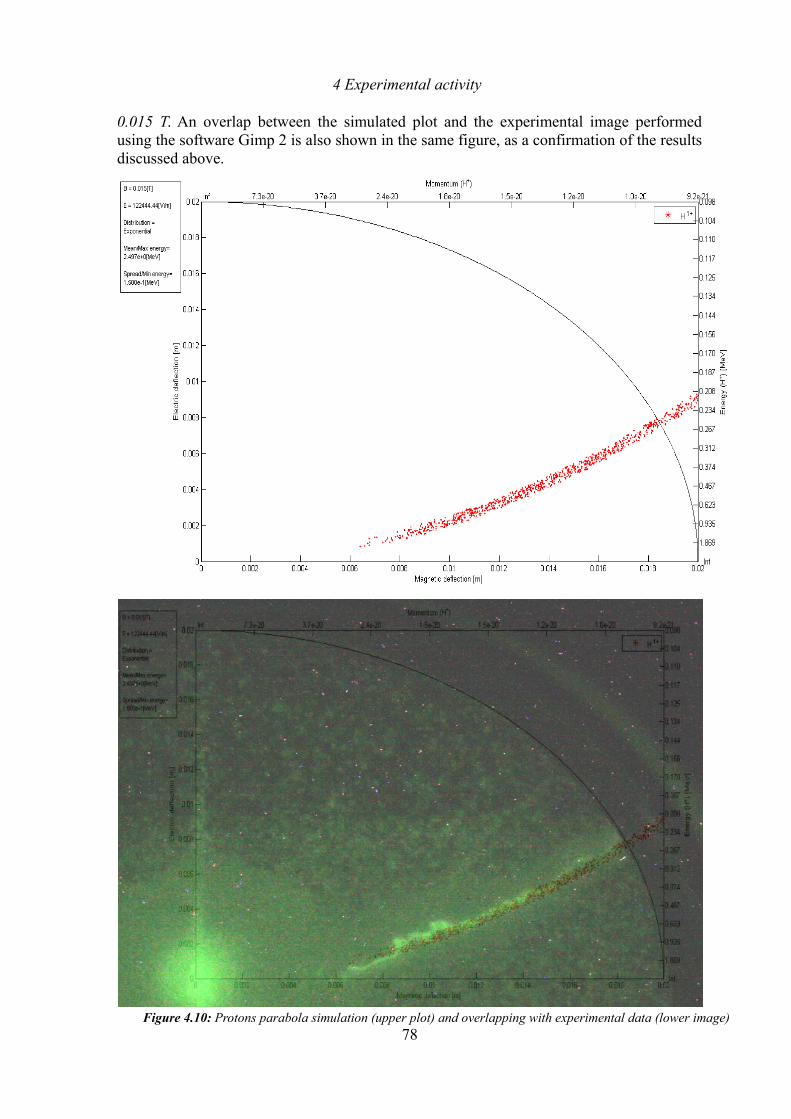
4 Experimental activity
0.015 T. An overlap between the simulated plot and the experimental image performed using the software Gimp 2 is also shown in the same figure, as a confirmation of the results discussed above.
78Figure 4.10: Protons parabola simulation (upper plot) and overlapping with experimental data (lower image)
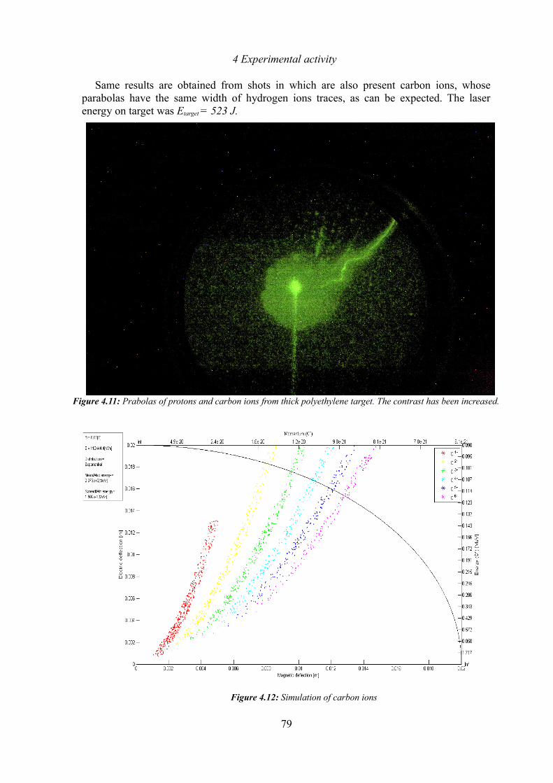
4 Experimental activity
Same results are obtained from shots in which are also present carbon ions, whose parabolas have the same width of hydrogen ions traces, as can be expected. The laser energy on target was Etarget = 523 J.
79
Figure 4.12: Simulation of carbon ions
Figure 4.11: Prabolas of protons and carbon ions from thick polyethylene target. The contrast has been increased.
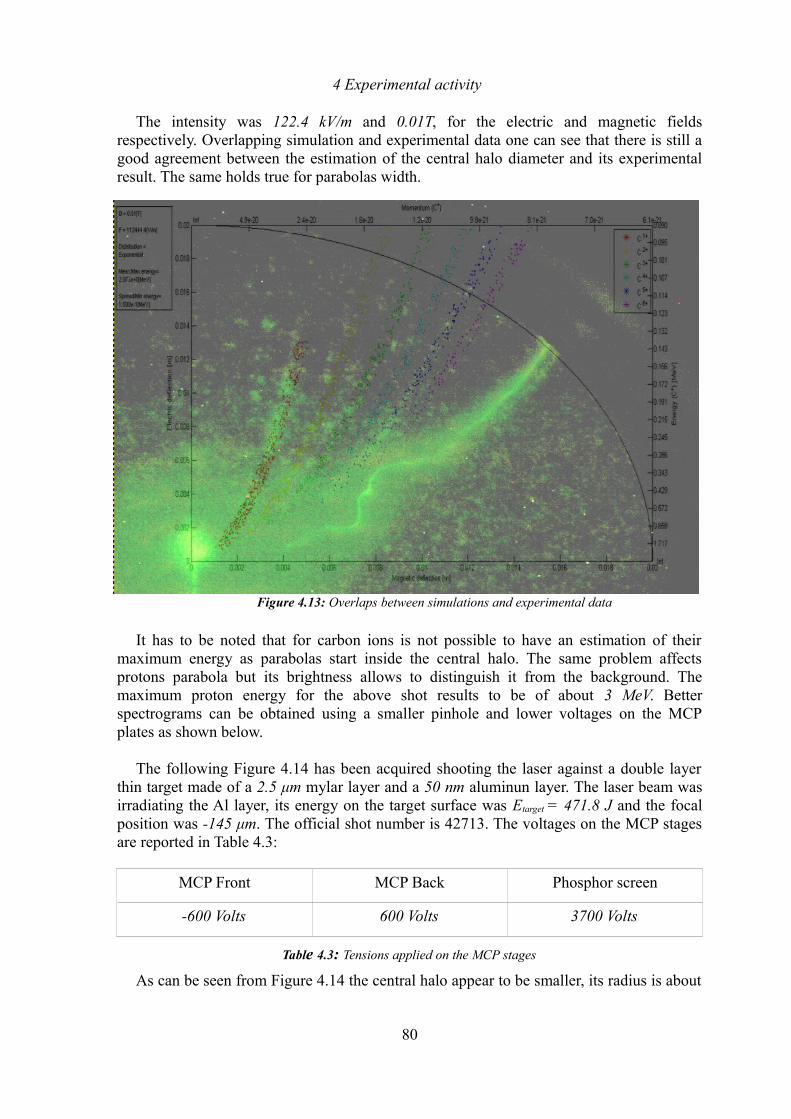
4 Experimental activity
The intensity was 122.4 kV/m and 0.01T, for the electric and magnetic fields respectively. Overlapping simulation and experimental data one can see that there is still a good agreement between the estimation of the central halo diameter and its experimental result. The same holds true for parabolas width.
It has to be noted that for carbon ions is not possible to have an estimation of their maximum energy as parabolas start inside the central halo. The same problem affects protons parabola but its brightness allows to distinguish it from the background. The maximum proton energy for the above shot results to be of about 3 MeV. Better spectrograms can be obtained using a smaller pinhole and lower voltages on the MCP plates as shown below.
The following Figure 4.14 has been acquired shooting the laser against a double layer thin target made of a 2.5 μm mylar layer and a 50 nm aluminun layer. The laser beam was irradiating the Al layer, its energy on the target surface was Etarget = 471.8 J and the focal position was -145 μm. The official shot number is 42713. The voltages on the MCP stages are reported in Table 4.3:
MCP Front MCP Back Phosphor screen
-600 Volts 600 Volts 3700 Volts
Table 4.3: Tensions applied on the MCP stages
As can be seen from Figure 4.14 the central halo appear to be smaller, its radius is about
80
Figure 4.13: Overlaps between simulations and experimental data
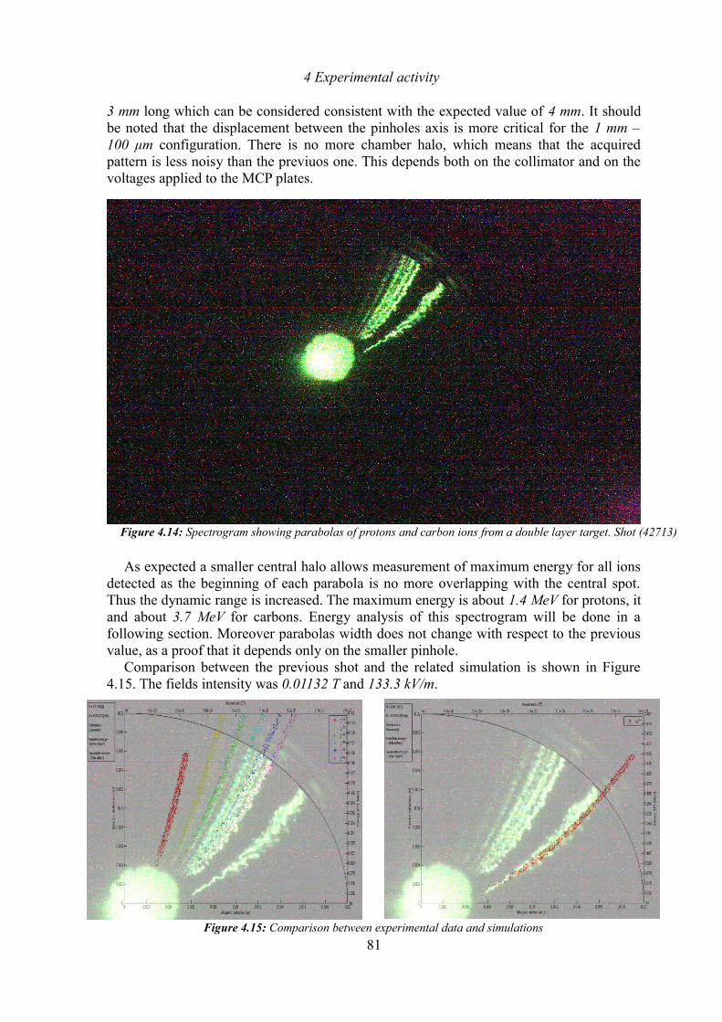
4 Experimental activity
3 mm long which can be considered consistent with the expected value of 4 mm. It should be noted that the displacement between the pinholes axis is more critical for the 1 mm – 100 μm configuration. There is no more chamber halo, which means that the acquired pattern is less noisy than the previuos one. This depends both on the collimator and on the voltages applied to the MCP plates.
As expected a smaller central halo allows measurement of maximum energy for all ions detected as the beginning of each parabola is no more overlapping with the central spot. Thus the dynamic range is increased. The maximum energy is about 1.4 MeV for protons, it and about 3.7 MeV for carbons. Energy analysis of this spectrogram will be done in a following section. Moreover parabolas width does not change with respect to the previous value, as a proof that it depends only on the smaller pinhole.
Comparison between the previous shot and the related simulation is shown in Figure 4.15. The fields intensity was 0.01132 T and 133.3 kV/m.
81
Figure 4.14: Spectrogram showing parabolas of protons and carbon ions from a double layer target. Shot (42713)
Figure 4.15: Comparison between experimental data and simulations
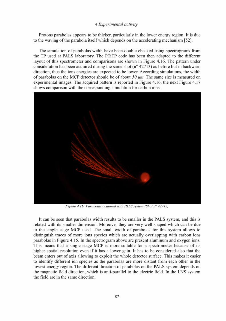
4 Experimental activity
Protons parabolas appears to be thicker, particularly in the lower energy region. It is due to the waving of the parabola itself which depends on the accelerating mechanism [52].
The simulation of parabolas width have been double-checked using spectrograms from the TP used at PALS laboratory. The PTiTP code has been then adapted to the different layout of this spectrometer and comparisons are shown in Figure 4.16. The pattern under consideration has been acquired during the same shot (n° 42713) as before but in backward direction, thus the ions energies are expected to be lower. According simulations, the width of parabolas on the MCP detector should be of about 50 μm. The same size is measured on experimental images. The acquired pattern is reported in Figure 4.16, the next Figure 4.17 shows comparison with the corresponding simulation for carbon ions.
It can be seen that parabolas width results to be smaller in the PALS system, and this is related with its smaller dimension. Moreover they are very well shaped which can be due to the single stage MCP used. The small width of parabolas for this system allows to distinguish traces of more ions species which are actually overlapping with carbon ions parabolas in Figure 4.15. In the spectrogram above are present aluminum and oxygen ions. This means that a single stage MCP is more suitable for a spectrometer because of its higher spatial resolution even if it has a lower gain. It has to be considered also that the beam enters out of axis allowing to exploit the whole detector surface. This makes it easier to identify different ion species as the parabolas are more distant from each other in the lowest energy region. The different direction of parabolas on the PALS system depends on the magnetic field direction, which is anti-parallel to the electric field. In the LNS system the field are in the same direction.
82
Figure 4.16: Parabolas acquired with PALS system (Shot n° 42713)
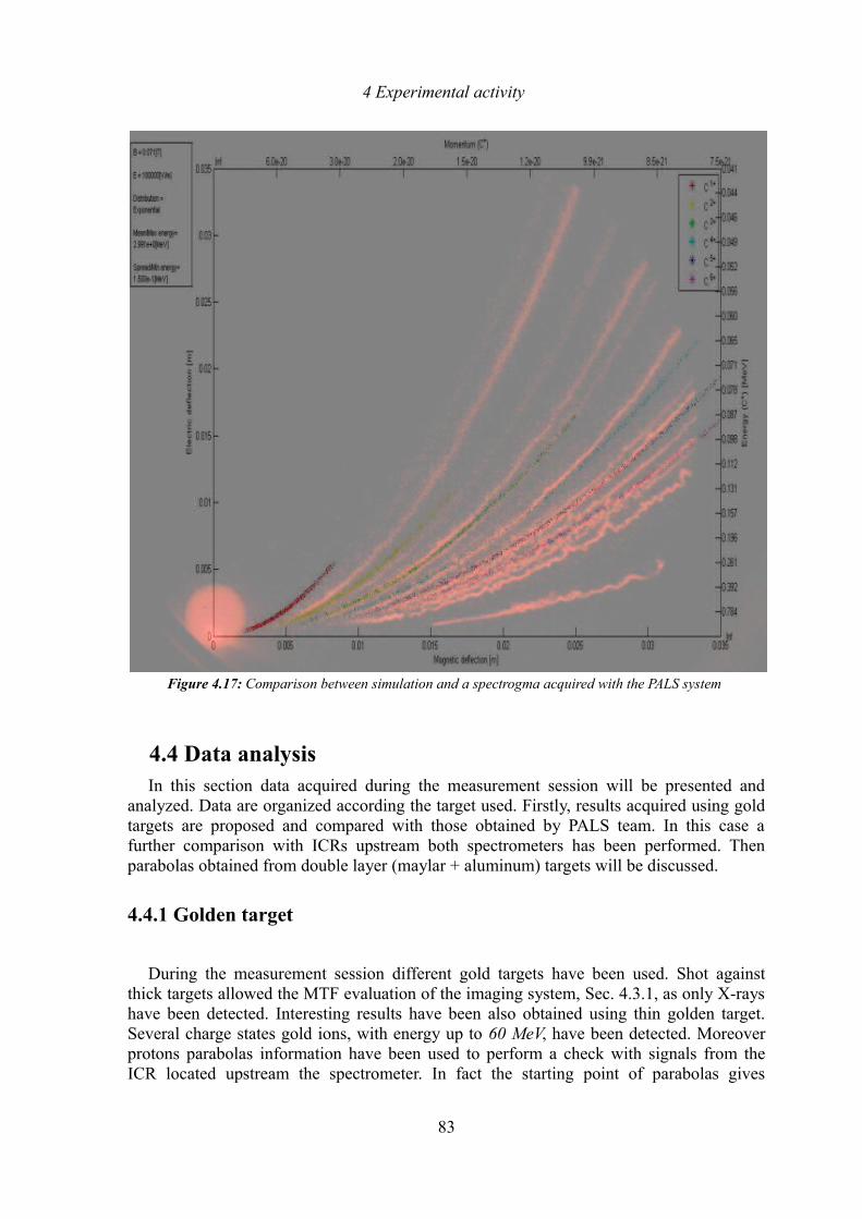
4 Experimental activity
4.4 Data analysisIn this section data acquired during the measurement session will be presented and
analyzed. Data are organized according the target used. Firstly, results acquired using gold targets are proposed and compared with those obtained by PALS team. In this case a further comparison with ICRs upstream both spectrometers has been performed. Then parabolas obtained from double layer (maylar + aluminum) targets will be discussed.
4.4.1 Golden target
During the measurement session different gold targets have been used. Shot against thick targets allowed the MTF evaluation of the imaging system, Sec. 4.3.1, as only X-rays have been detected. Interesting results have been also obtained using thin golden target. Several charge states gold ions, with energy up to 60 MeV, have been detected. Moreover protons parabolas information have been used to perform a check with signals from the ICR located upstream the spectrometer. In fact the starting point of parabolas gives
83
Figure 4.17: Comparison between simulation and a spectrogma acquired with the PALS system
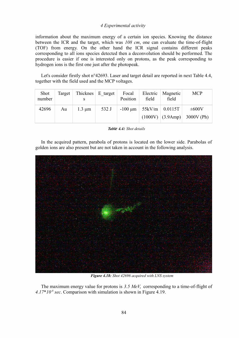
4 Experimental activity
information about the maximum energy of a certain ion species. Knowing the distance between the ICR and the target, which was 108 cm, one can evaluate the time-of-flight (TOF) from energy. On the other hand the ICR signal contains different peaks corresponding to all ions species detected then a deconvolution should be performed. The procedure is easier if one is interested only on protons, as the peak corresponding to hydrogen ions is the first one just after the photopeak.
Let's consider firstly shot n°42693. Laser and target detail are reported in next Table 4.4, together with the field used and the MCP voltages.
Shot number
Target Thickness
E_target Focal Position
Electric field
Magnetic field
MCP
42696 Au 1.3 μm 532 J -100 μm 55kV/m
(1000V)
0.0115T
(3.9Amp)
±600V
3000V (Ph)
Table 4.4: Shot details
In the acquired pattern, parabola of protons is located on the lower side. Parabolas of golden ions are also present but are not taken in account in the following analysis.
The maximum energy value for protons is 3.5 MeV, corresponding to a time-of-flight of 4.17*10-8 sec. Comparison with simulation is shown in Figure 4.19.
84
Figure 4.18: Shot 42696 acquired with LNS system
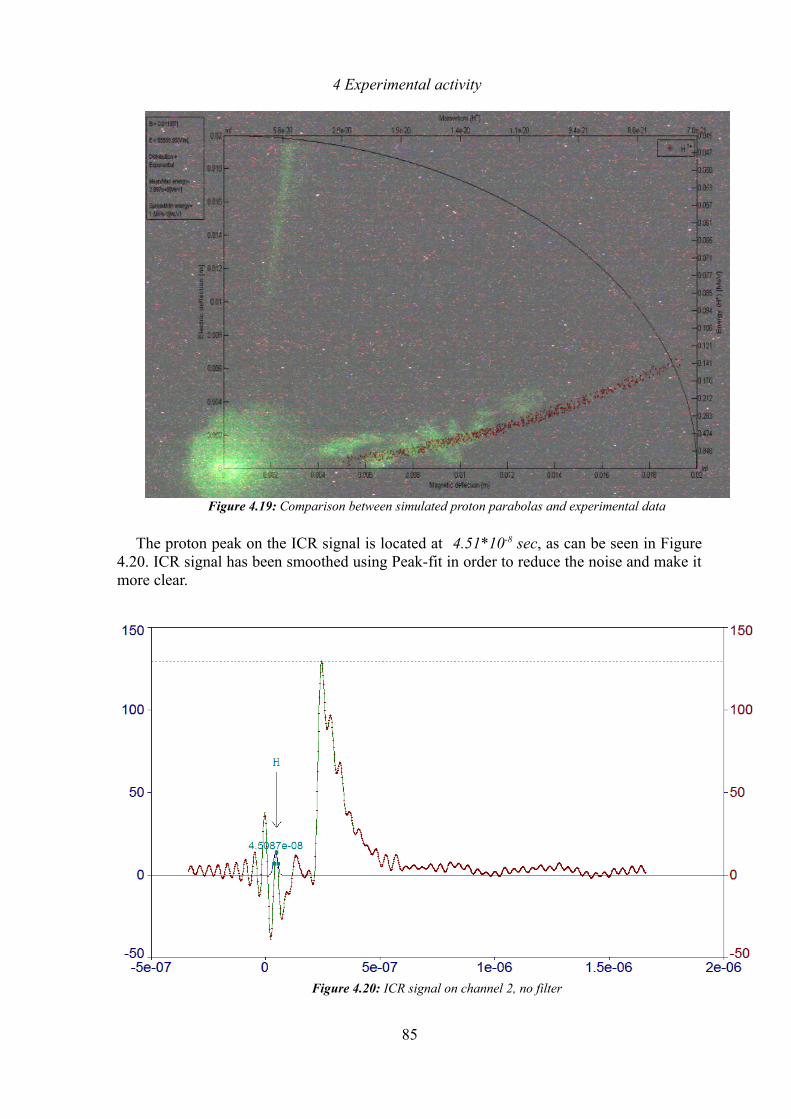
4 Experimental activity
The proton peak on the ICR signal is located at 4.51*10-8 sec, as can be seen in Figure 4.20. ICR signal has been smoothed using Peak-fit in order to reduce the noise and make it more clear.
85
Figure 4.19: Comparison between simulated proton parabolas and experimental data
Figure 4.20: ICR signal on channel 2, no filter
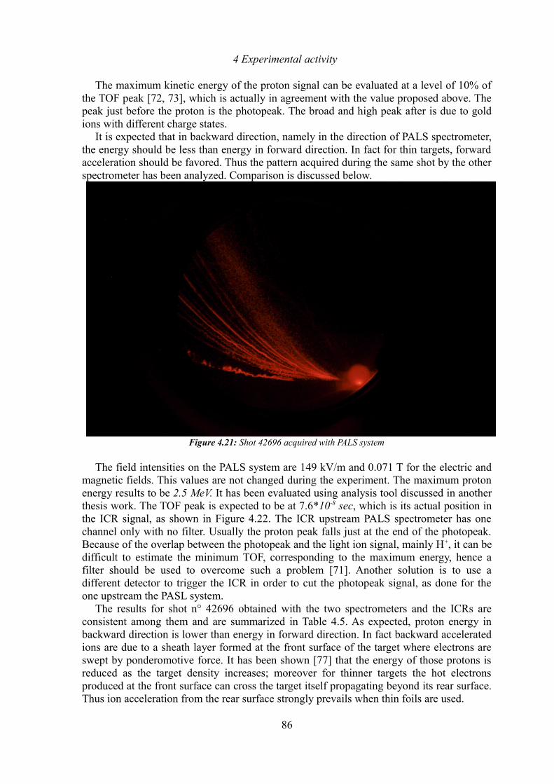
4 Experimental activity
The maximum kinetic energy of the proton signal can be evaluated at a level of 10% of the TOF peak [72, 73], which is actually in agreement with the value proposed above. The peak just before the proton is the photopeak. The broad and high peak after is due to gold ions with different charge states.
It is expected that in backward direction, namely in the direction of PALS spectrometer, the energy should be less than energy in forward direction. In fact for thin targets, forward acceleration should be favored. Thus the pattern acquired during the same shot by the other spectrometer has been analyzed. Comparison is discussed below.
The field intensities on the PALS system are 149 kV/m and 0.071 T for the electric and magnetic fields. This values are not changed during the experiment. The maximum proton energy results to be 2.5 MeV. It has been evaluated using analysis tool discussed in another thesis work. The TOF peak is expected to be at 7.6*10-8 sec, which is its actual position in the ICR signal, as shown in Figure 4.22. The ICR upstream PALS spectrometer has one channel only with no filter. Usually the proton peak falls just at the end of the photopeak. Because of the overlap between the photopeak and the light ion signal, mainly H+, it can be difficult to estimate the minimum TOF, corresponding to the maximum energy, hence a filter should be used to overcome such a problem [71]. Another solution is to use a different detector to trigger the ICR in order to cut the photopeak signal, as done for the one upstream the PASL system.
The results for shot n° 42696 obtained with the two spectrometers and the ICRs are consistent among them and are summarized in Table 4.5. As expected, proton energy in backward direction is lower than energy in forward direction. In fact backward accelerated ions are due to a sheath layer formed at the front surface of the target where electrons are swept by ponderomotive force. It has been shown [77] that the energy of those protons is reduced as the target density increases; moreover for thinner targets the hot electrons produced at the front surface can cross the target itself propagating beyond its rear surface. Thus ion acceleration from the rear surface strongly prevails when thin foils are used.
86
Figure 4.21: Shot 42696 acquired with PALS system
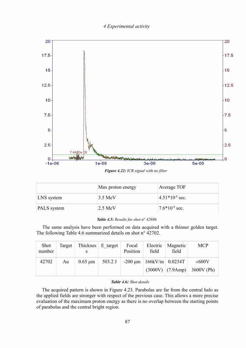
4 Experimental activity
Max proton energy Average TOF
LNS system 3.5 MeV 4.51*10-8 sec.
PALS system 2.5 MeV 7.6*10-8 sec.
Table 4.5: Results for shot n° 42696
The same analysis have been performed on data acquired with a thinner golden target. The following Table 4.6 summarized details on shot n° 42702.
Shot number
Target Thickness
E_target Focal Position
Electric field
Magnetic field
MCP
42702 Au 0.65 μm 503.2 J -200 μm 166kV/m
(3000V)
0.0234T
(7.9Amp)
±600V
3600V (Ph)
Table 4.6: Shot details
The acquired pattern is shown in Figure 4.23. Parabolas are far from the central halo as the applied fields are stronger with respect of the previous case. This allows a more precise evaluation of the maximum proton energy as there is no overlap between the starting points of parabolas and the central bright region.
87
Figure 4.22: ICR signal with no filter
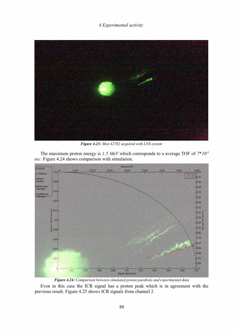
4 Experimental activity
The maximum proton energy is 1.5 MeV which corresponds to a average TOF of 7*10-8
sec. Figure 4.24 shows comparison with simulation.
Even in this case the ICR signal has a proton peak which is in agreement with the previous result. Figure 4.25 shows ICR signals from channel 2
88
Figure 4.23: Shot 42702 acquired with LNS system
Figure 4.24: Comparison between simulated proton parabola and experimental data
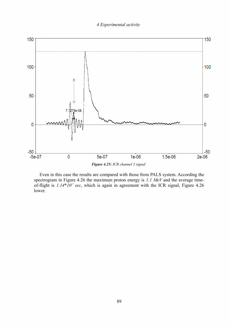
4 Experimental activity
Even in this case the results are compared with those from PALS system. According the spectrogram in Figure 4.26 the maximum proton energy is 1.1 MeV and the average time-of-flight is 1.14*10-7 sec, which is again in agreement with the ICR signal, Figure 4.26 lower.
89
Figure 4.25: ICR channel 2 signal
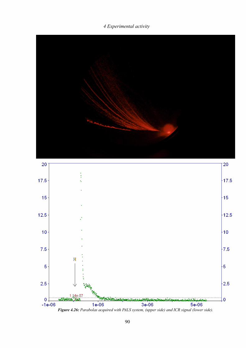
4 Experimental activity
90
Figure 4.26: Parabolas acquired with PALS system, (upper side) and ICR signal (lower side).
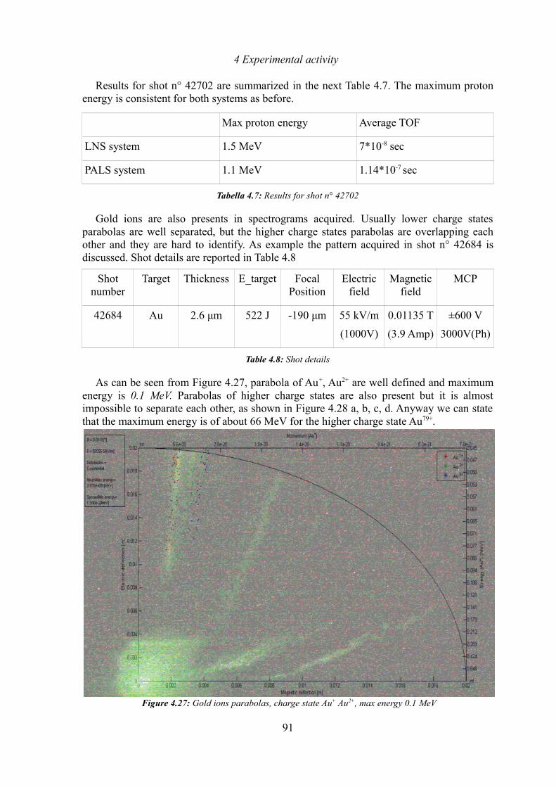
4 Experimental activity
Results for shot n° 42702 are summarized in the next Table 4.7. The maximum proton energy is consistent for both systems as before.
Max proton energy Average TOF
LNS system 1.5 MeV 7*10-8 sec
PALS system 1.1 MeV 1.14*10-7 sec
Tabella 4.7: Results for shot n° 42702
Gold ions are also presents in spectrograms acquired. Usually lower charge states parabolas are well separated, but the higher charge states parabolas are overlapping each other and they are hard to identify. As example the pattern acquired in shot n° 42684 is discussed. Shot details are reported in Table 4.8
Shot number
Target Thickness E_target Focal Position
Electric field
Magnetic field
MCP
42684 Au 2.6 μm 522 J -190 μm 55 kV/m
(1000V)
0.01135 T
(3.9 Amp)
±600 V
3000V(Ph)
Table 4.8: Shot details
As can be seen from Figure 4.27, parabola of Au+, Au2+ are well defined and maximum energy is 0.1 MeV. Parabolas of higher charge states are also present but it is almost impossible to separate each other, as shown in Figure 4.28 a, b, c, d. Anyway we can state that the maximum energy is of about 66 MeV for the higher charge state Au79+.
91
Figure 4.27: Gold ions parabolas, charge state Au+ Au2+, max energy 0.1 MeV
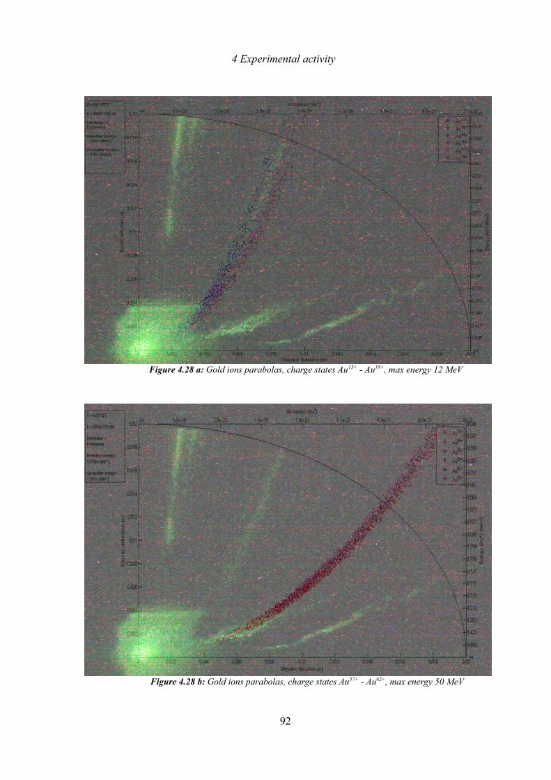
4 Experimental activity
92
Figure 4.28 a: Gold ions parabolas, charge states Au13+ - Au18+, max energy 12 MeV
Figure 4.28 b: Gold ions parabolas, charge states Au57+ - Au62+, max energy 50 MeV
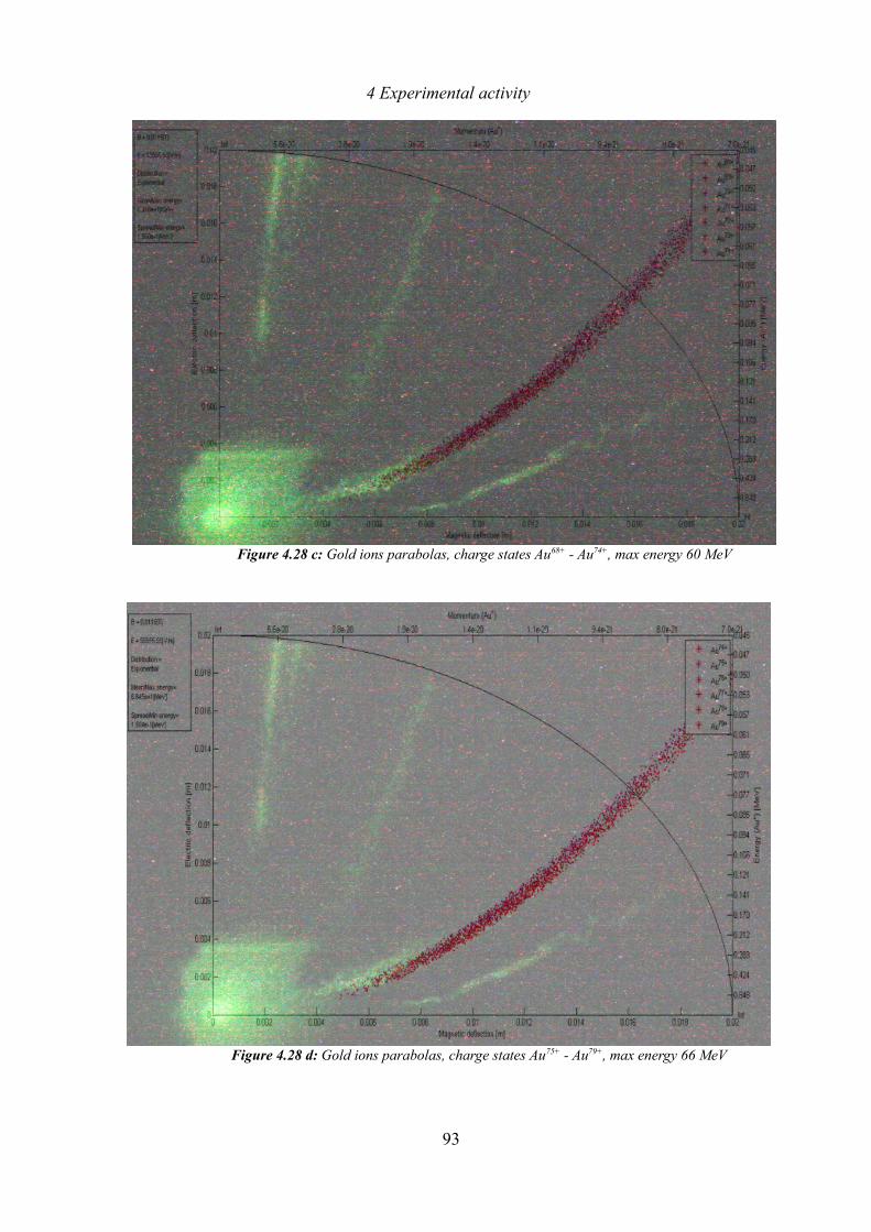
4 Experimental activity
93
Figure 4.28 c: Gold ions parabolas, charge states Au68+ - Au74+, max energy 60 MeV
Figure 4.28 d: Gold ions parabolas, charge states Au75+ - Au79+, max energy 66 MeV
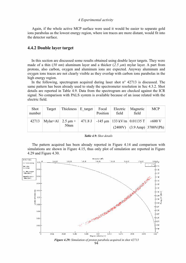
4 Experimental activity
Again, if the whole active MCP surface were used it would be easier to separate gold ions parabolas as the lowest energy region, where ion traces are more distant, would fit into the detector surface.
4.4.2 Double layer target
In this section are discussed some results obtained using double layer targets. They were made of a thin (50 nm) aluminum layer and a thicker (2.5 μm) mylar layer. A part from protons, also carbon, oxygen and aluminum ions are expected. Anyway aluminum and oxygen ions traces are not clearly visible as they overlap with carbon ions parabolas in the high energy region.
In the following, spectrogram acquired during laser shot n° 42713 is discussed. The same pattern has been already used to study the spectrometer resolution in Sec 4.3.2. Shot details are reported in Table 4.9. Data from the spectrogram are checked against the ICR signal. No comparison with PALS system is available because of an issue related with the electric field.
Shot number
Target Thickness E_target Focal Position
Electric field
Magnetic field
MCP
42713 Mylar+Al 2.5 μm + 50nm
471.8 J -145 μm 133 kV/m
(2400V)
0.01135 T
(3.9 Amp)
±600 V
3700V(Ph)
Table 4.9: Shot details
The pattern acquired has been already reported in Figure 4.14 and comparison with simulations are shown in Figure 4.15, thus only plot of simulation are reported in Figure 4.29 and Figure 4.30.
94Figure 4.29: Simulation of proton parabola acquired in shot 42713
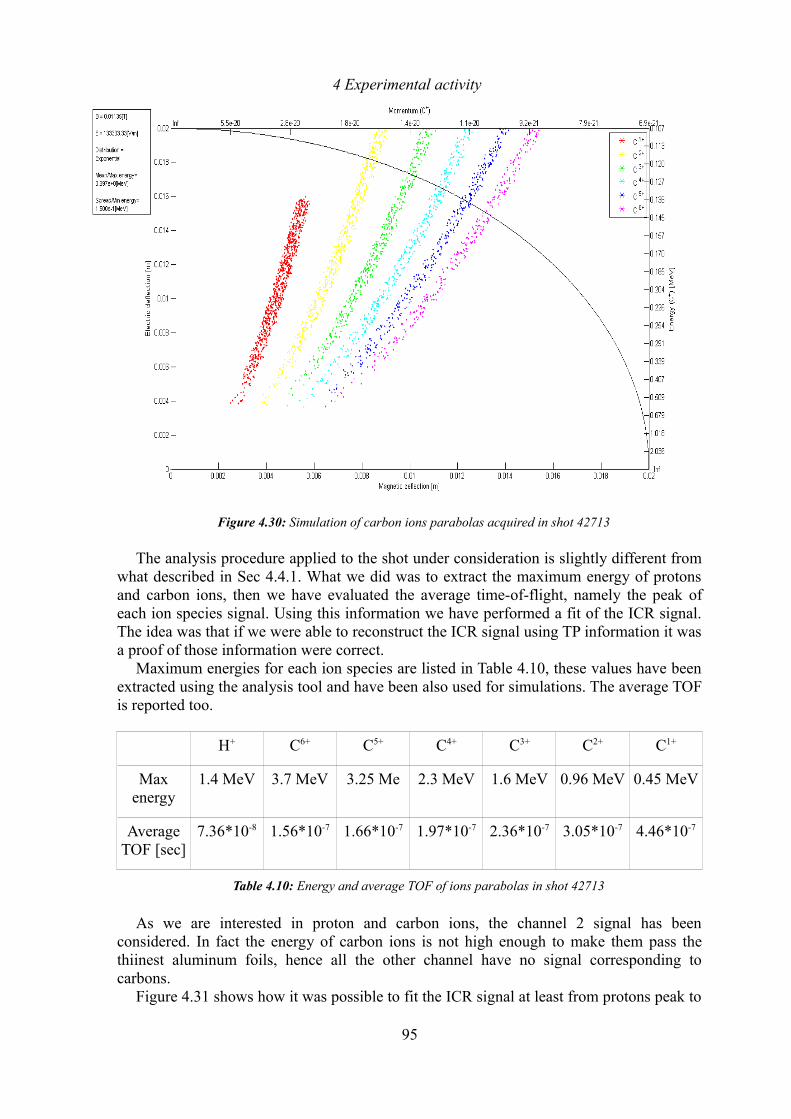
4 Experimental activity
The analysis procedure applied to the shot under consideration is slightly different from what described in Sec 4.4.1. What we did was to extract the maximum energy of protons and carbon ions, then we have evaluated the average time-of-flight, namely the peak of each ion species signal. Using this information we have performed a fit of the ICR signal. The idea was that if we were able to reconstruct the ICR signal using TP information it was a proof of those information were correct.
Maximum energies for each ion species are listed in Table 4.10, these values have been extracted using the analysis tool and have been also used for simulations. The average TOF is reported too.
H+ C6+ C5+ C4+ C3+ C2+ C1+
Max energy
1.4 MeV 3.7 MeV 3.25 Me 2.3 MeV 1.6 MeV 0.96 MeV 0.45 MeV
Average TOF [sec]
7.36*10-8 1.56*10-7 1.66*10-7 1.97*10-7 2.36*10-7 3.05*10-7 4.46*10-7
Table 4.10: Energy and average TOF of ions parabolas in shot 42713
As we are interested in proton and carbon ions, the channel 2 signal has been considered. In fact the energy of carbon ions is not high enough to make them pass the thiinest aluminum foils, hence all the other channel have no signal corresponding to carbons.
Figure 4.31 shows how it was possible to fit the ICR signal at least from protons peak to
95
Figure 4.30: Simulation of carbon ions parabolas acquired in shot 42713
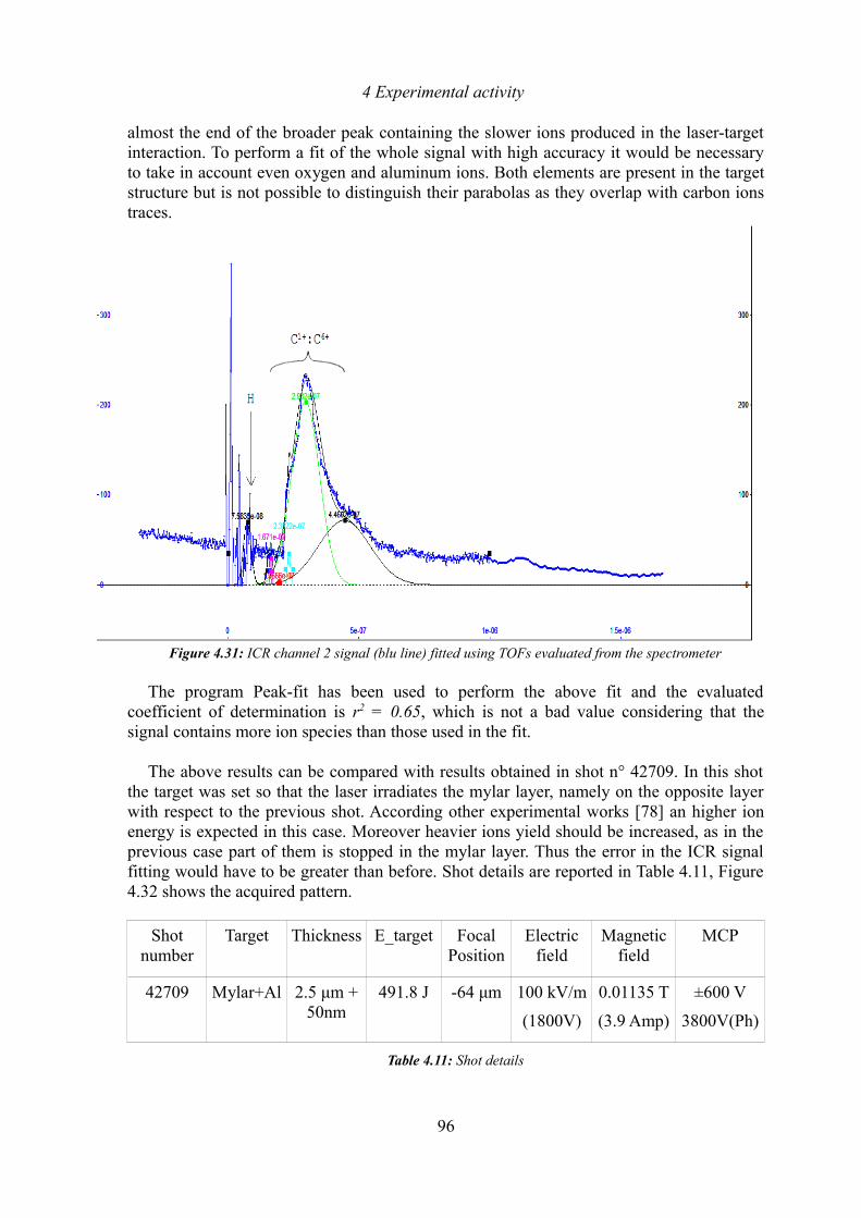
4 Experimental activity
almost the end of the broader peak containing the slower ions produced in the laser-target interaction. To perform a fit of the whole signal with high accuracy it would be necessary to take in account even oxygen and aluminum ions. Both elements are present in the target structure but is not possible to distinguish their parabolas as they overlap with carbon ions traces.
The program Peak-fit has been used to perform the above fit and the evaluated coefficient of determination is r2 = 0.65, which is not a bad value considering that the signal contains more ion species than those used in the fit.
The above results can be compared with results obtained in shot n° 42709. In this shot the target was set so that the laser irradiates the mylar layer, namely on the opposite layer with respect to the previous shot. According other experimental works [78] an higher ion energy is expected in this case. Moreover heavier ions yield should be increased, as in the previous case part of them is stopped in the mylar layer. Thus the error in the ICR signal fitting would have to be greater than before. Shot details are reported in Table 4.11, Figure 4.32 shows the acquired pattern.
Shot number
Target Thickness E_target Focal Position
Electric field
Magnetic field
MCP
42709 Mylar+Al 2.5 μm + 50nm
491.8 J -64 μm 100 kV/m
(1800V)
0.01135 T
(3.9 Amp)
±600 V
3800V(Ph)
Table 4.11: Shot details
96
Figure 4.31: ICR channel 2 signal (blu line) fitted using TOFs evaluated from the spectrometer
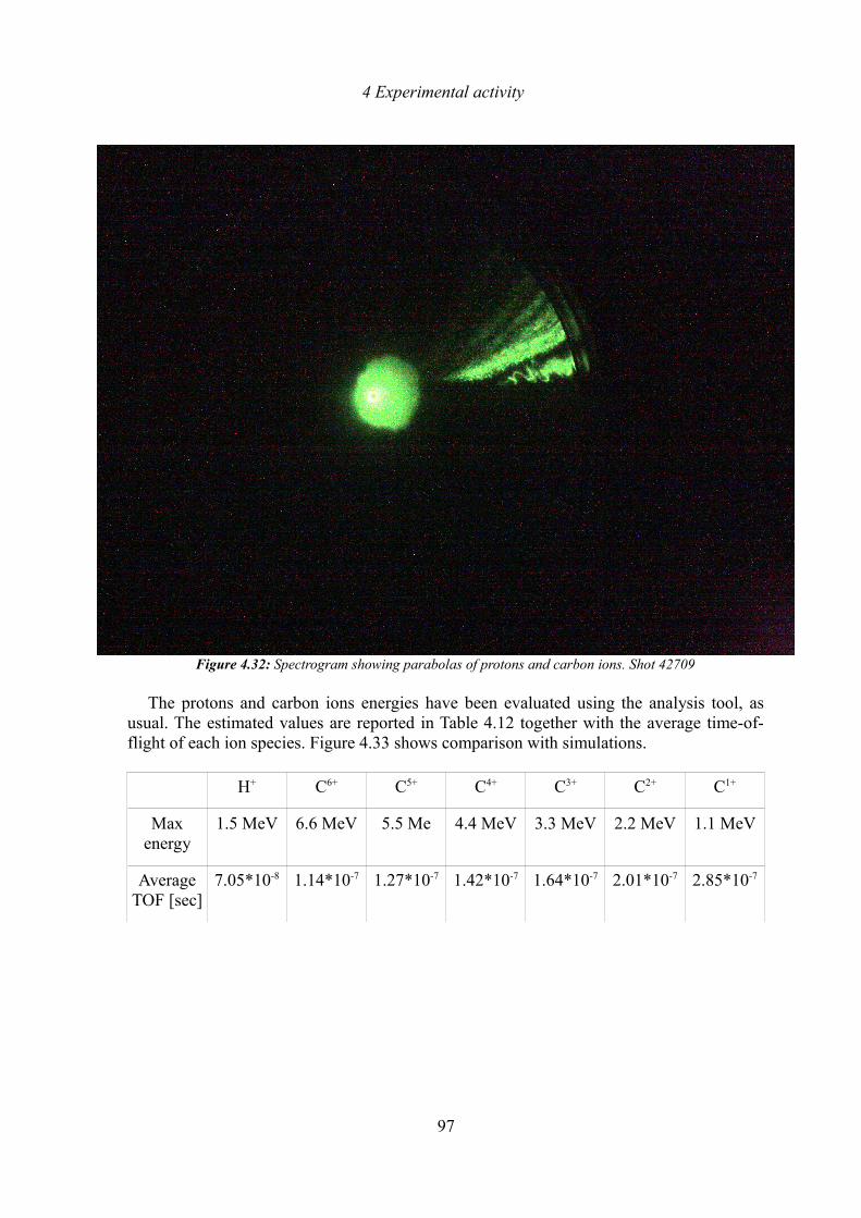
4 Experimental activity
The protons and carbon ions energies have been evaluated using the analysis tool, as usual. The estimated values are reported in Table 4.12 together with the average time-of-flight of each ion species. Figure 4.33 shows comparison with simulations.
H+ C6+ C5+ C4+ C3+ C2+ C1+
Max energy
1.5 MeV 6.6 MeV 5.5 Me 4.4 MeV 3.3 MeV 2.2 MeV 1.1 MeV
Average TOF [sec]
7.05*10-8 1.14*10-7 1.27*10-7 1.42*10-7 1.64*10-7 2.01*10-7 2.85*10-7
97
Figure 4.32: Spectrogram showing parabolas of protons and carbon ions. Shot 42709
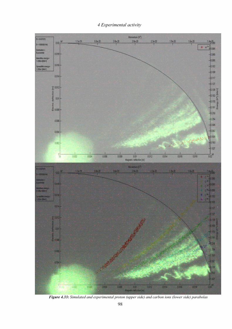
4 Experimental activity
98
Figure 4.33: Simulated and experimental proton (upper side) and carbon ions (lower side) parabolas
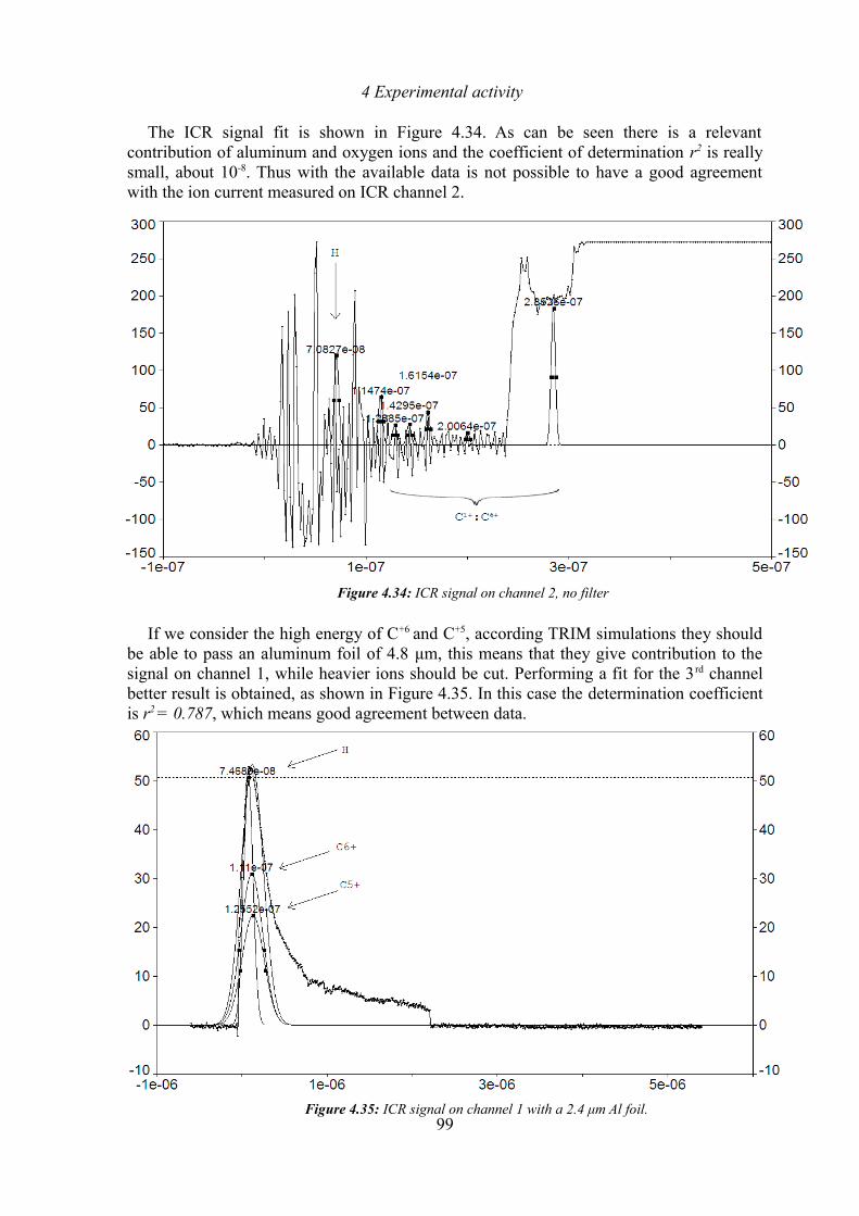
4 Experimental activity
The ICR signal fit is shown in Figure 4.34. As can be seen there is a relevant contribution of aluminum and oxygen ions and the coefficient of determination r2 is really small, about 10-8. Thus with the available data is not possible to have a good agreement with the ion current measured on ICR channel 2.
If we consider the high energy of C+6 and C+5, according TRIM simulations they should be able to pass an aluminum foil of 4.8 μm, this means that they give contribution to the signal on channel 1, while heavier ions should be cut. Performing a fit for the 3 rd channel better result is obtained, as shown in Figure 4.35. In this case the determination coefficient is r2 = 0.787, which means good agreement between data.
99
Figure 4.34: ICR signal on channel 2, no filter
Figure 4.35: ICR signal on channel 1 with a 2.4 μm Al foil.
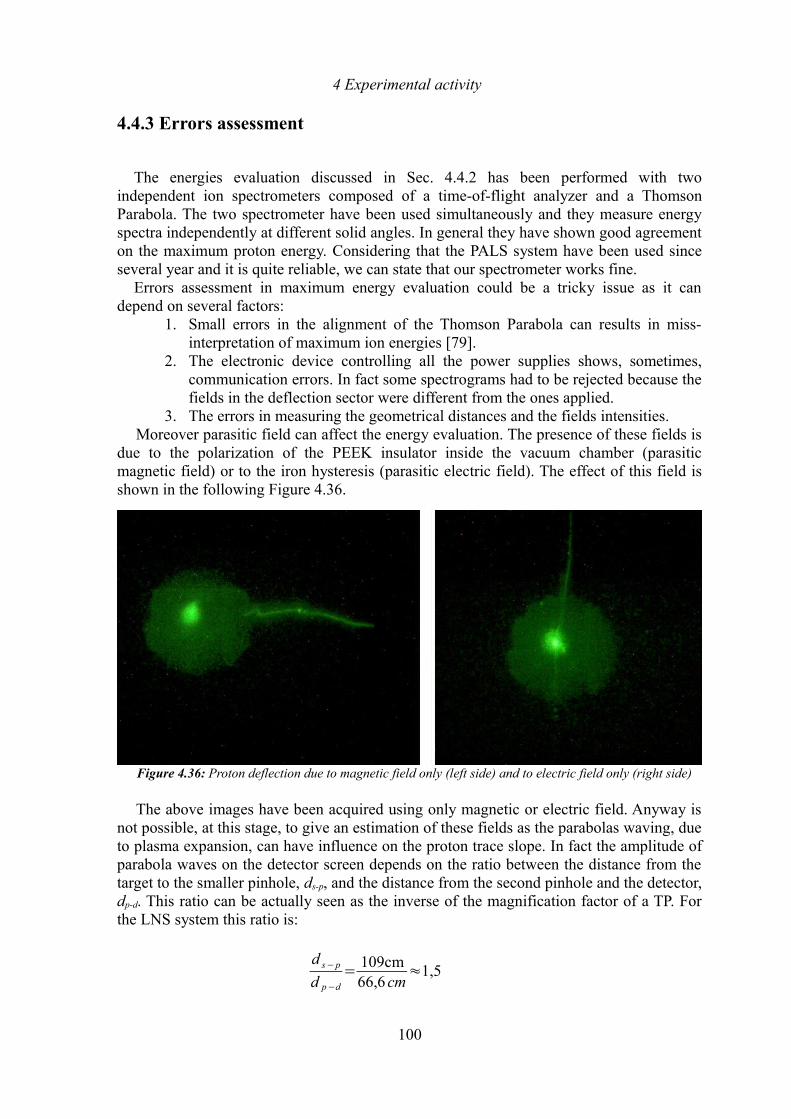
4 Experimental activity
4.4.3 Errors assessment
The energies evaluation discussed in Sec. 4.4.2 has been performed with two independent ion spectrometers composed of a time-of-flight analyzer and a Thomson Parabola. The two spectrometer have been used simultaneously and they measure energy spectra independently at different solid angles. In general they have shown good agreement on the maximum proton energy. Considering that the PALS system have been used since several year and it is quite reliable, we can state that our spectrometer works fine.
Errors assessment in maximum energy evaluation could be a tricky issue as it can depend on several factors:
1. Small errors in the alignment of the Thomson Parabola can results in miss-interpretation of maximum ion energies [79].
2. The electronic device controlling all the power supplies shows, sometimes, communication errors. In fact some spectrograms had to be rejected because the fields in the deflection sector were different from the ones applied.
3. The errors in measuring the geometrical distances and the fields intensities. Moreover parasitic field can affect the energy evaluation. The presence of these fields is
due to the polarization of the PEEK insulator inside the vacuum chamber (parasitic magnetic field) or to the iron hysteresis (parasitic electric field). The effect of this field is shown in the following Figure 4.36.
The above images have been acquired using only magnetic or electric field. Anyway is not possible, at this stage, to give an estimation of these fields as the parabolas waving, due to plasma expansion, can have influence on the proton trace slope. In fact the amplitude of parabola waves on the detector screen depends on the ratio between the distance from the target to the smaller pinhole, ds-p, and the distance from the second pinhole and the detector, dp-d. This ratio can be actually seen as the inverse of the magnification factor of a TP. For the LNS system this ratio is:
d s−p
d p−d
=109cm66,6 cm
≈1,5
100
Figure 4.36: Proton deflection due to magnetic field only (left side) and to electric field only (right side)
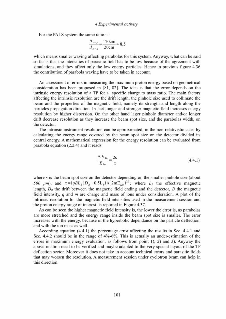
4 Experimental activity
For the PALS system the same ratio is:d s− p
d p−d
=170cm20cm
≈8,5
which means smaller waving affecting parabolas for this system. Anyway, what can be said so far is that the intensities of parasitic field has to be low because of the agreement with simulations, and they affect only the low energy particles. Hence in previous figure 4.36 the contribution of parabola waving have to be taken in account.
An assessment of errors in measuring the maximum proton energy based on geometrical consideration has been proposed in [81, 82]. The idea is that the error depends on the intrinsic energy resolution of a TP for a specific charge to mass ratio. The main factors affecting the intrinsic resolution are the drift length, the pinhole size used to collimate the beam and the properties of the magnetic field, namely its strength and length along the particles propagation direction. In fact longer and stronger magnetic field increases energy resolution by higher dispersion. On the other hand lager pinhole diameter and/or longer drift decrease resolution as they increase the beam spot size, and the parabolas width, on the detector.
The intrinsic instrument resolution can be approximated, in the non-relativistic case, by calculating the energy range covered by the beam spot size on the detector divided its central energy. A mathematical expression for the energy resolution can be evaluated from parabola equation (2.2.4) and it reads:
ΔE kin
E kin
=2sx
(4.4.1)
where s is the beam spot size on the detector depending on the smaller pinhole size (about 500 μm), and x=(qBLB(DB+0.5LB))/(2mEKin)
0.5 ; where LB the effective magnetic length, DB the drift between the magnetic field ending and the detector, B the magnetic field intensity, q and m are charge and mass of ions under consideration. A plot of the intrinsic resolution for the magnetic field intensities used in the measurement session and the proton energy range of interest, is reported in Figure 4.37.
As can be seen the higher magnetic field intensity is, the lower the error is, as parabolas are more stretched and the energy range inside the beam spot size is smaller. The error increases with the energy, because of the hyperbolic dependance on the particle deflection, and with the ion mass as well.
According equation (4.4.1) the percentage error affecting the results in Sec. 4.4.1 and Sec. 4.4.2 should be in the range of 4%-6%. This is actually an under-estimation of the errors in maximum energy evaluation, as follows from point 1), 2) and 3). Anyway the above relation need to be verified and maybe adapted to the very special layout of the TP deflection sector. Moreover it does not take in account technical errors and parasitic fields that may worsen the resolution. A measurement session under cyclotron beam can help in this direction.
101
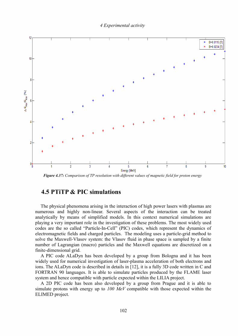
4 Experimental activity
4.5 PTiTP & PIC simulations
The physical phenomena arising in the interaction of high power lasers with plasmas are numerous and highly non-linear. Several aspects of the interaction can be treated analytically by means of simplified models. In this context numerical simulations are playing a very important role in the investigation of these problems. The most widely used codes are the so called “Particle-In-Cell” (PIC) codes, which represent the dynamics of electromagnetic fields and charged particles. The modeling uses a particle-grid method to solve the Maxwell-Vlasov system: the Vlasov fluid in phase space is sampled by a finite number of Lagrangian (macro) particles and the Maxwell equations are discretized on a finite-dimensional grid.
A PIC code ALaDyn has been developed by a group from Bologna and it has been widely used for numerical investigation of laser-plasma acceleration of both electrons and ions. The ALaDyn code is described in details in [12], it is a fully 3D code written in C and FORTRAN 90 languages. It is able to simulate particles produced by the FLAME laser system and hence compatible with particle expected within the LILIA project.
A 2D PIC code has been also developed by a group from Prague and it is able to simulate protons with energy up to 100 MeV compatible with those expected within the ELIMED project.
102
Figure 4.37: Comparison of TP resolution with different values of magnetic field for proton energy
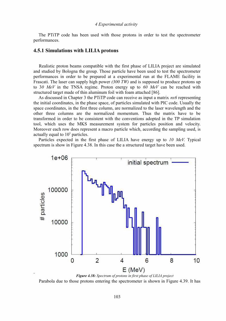
4 Experimental activity
The PTiTP code has been used with those protons in order to test the spectrometer performances.
4.5.1 Simulations with LILIA protons
Realistic proton beams compatible with the first phase of LILIA project are simulated and studied by Bologna the group. Those particle have been used to test the spectrometer performances in order to be prepared at a experimental run at the FLAME facility in Frascati. The laser can supply high power (300 TW) and is supposed to produce protons up to 30 MeV in the TNSA regime. Proton energy up to 60 MeV can be reached with structured target made of thin aluminum foil with foam attached [86].
As discussed in Chapter 3 the PTiTP code can receive as input a matrix nx6 representing the initial coordinates, in the phase space, of particles simulated with PIC code. Usually the space coordinates, in the first three column, are normalized to the laser wavelength and the other three columns are the normalized momentum. Thus the matrix have to be transformed in order to be consistent with the conventions adopted in the TP simulation tool, which uses the MKS measurement system for particles position and velocity. Moreover each row does represent a macro particle which, according the sampling used, is actually equal to 105 particles.
Particles expected in the first phase of LILIA have energy up to 10 MeV. Typical spectrum is show in Figure 4.38. In this case the a structured target have been used.
Parabola due to those protons entering the spectrometer is shown in Figure 4.39. It has
103
Figure 4.38: Spectrum of protons in first phase of LILIA project
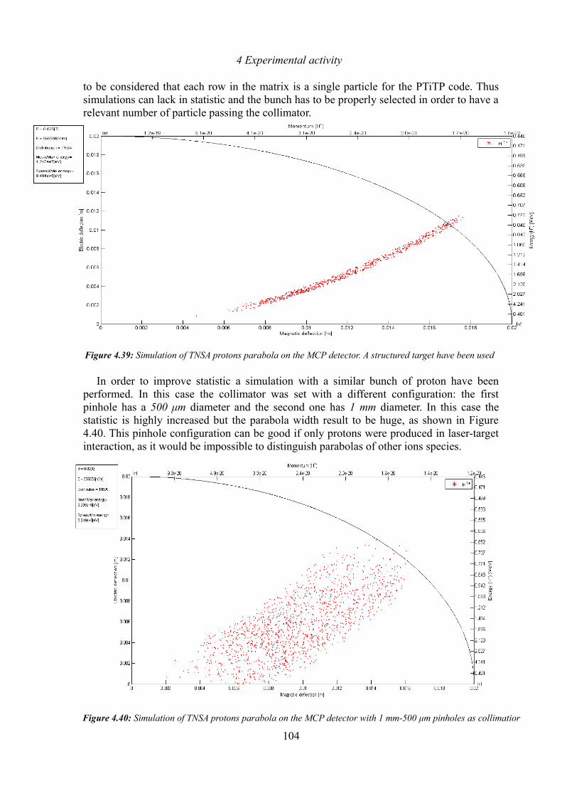
4 Experimental activity
to be considered that each row in the matrix is a single particle for the PTiTP code. Thus simulations can lack in statistic and the bunch has to be properly selected in order to have a relevant number of particle passing the collimator.
In order to improve statistic a simulation with a similar bunch of proton have been performed. In this case the collimator was set with a different configuration: the first pinhole has a 500 μm diameter and the second one has 1 mm diameter. In this case the statistic is highly increased but the parabola width result to be huge, as shown in Figure 4.40. This pinhole configuration can be good if only protons were produced in laser-target interaction, as it would be impossible to distinguish parabolas of other ions species.
104
Figure 4.39: Simulation of TNSA protons parabola on the MCP detector. A structured target have been used
Figure 4.40: Simulation of TNSA protons parabola on the MCP detector with 1 mm-500 μm pinholes as collimatior
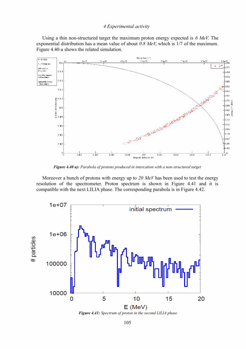
4 Experimental activity
Using a thin non-structured target the maximum proton energy expected is 6 MeV. The exponential distribution has a mean value of about 0.8 MeV, which is 1/7 of the maximum. Figure 4.40-a shows the related simulation.
Moreover a bunch of protons with energy up to 20 MeV has been used to test the energy
resolution of the spectrometer. Proton spectrum is shown in Figure 4.41 and it is compatible with the next LILIA phase. The corresponding parabola is in Figure 4.42.
105
Figure 4.41: Spectrum of proton in the second LILIA phase
Figure 4.40 a): Parabola of protons produced in intercation with a non-structured target
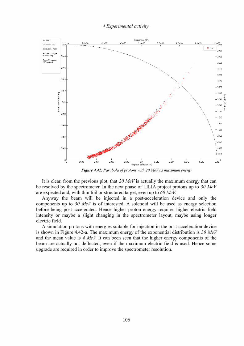
4 Experimental activity
It is clear, from the previous plot, that 20 MeV is actually the maximum energy that can be resolved by the spectrometer. In the next phase of LILIA project protons up to 30 MeV are expected and, with thin foil or structured target, even up to 60 MeV.
Anyway the beam will be injected in a post-acceleration device and only the components up to 30 MeV is of interested. A solenoid will be used as energy selection before being post-accelerated. Hence higher proton energy requires higher electric field intensity or maybe a slight changing in the spectrometer layout, maybe using longer electric field.
A simulation protons with energies suitable for injection in the post-acceleration device is shown in Figure 4.42-a. The maximum energy of the exponential distribution is 30 MeV and the mean value is 4 MeV. It can been seen that the higher energy components of the beam are actually not deflected, even if the maximum electric field is used. Hence some upgrade are required in order to improve the spectrometer resolution.
106
Figure 4.42: Parabola of protons with 20 MeV as maximum energy
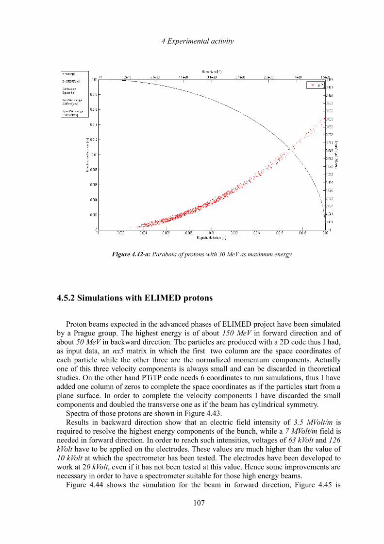
4 Experimental activity
4.5.2 Simulations with ELIMED protons
Proton beams expected in the advanced phases of ELIMED project have been simulated by a Prague group. The highest energy is of about 150 MeV in forward direction and of about 50 MeV in backward direction. The particles are produced with a 2D code thus I had, as input data, an nx5 matrix in which the first two column are the space coordinates of each particle while the other three are the normalized momentum components. Actually one of this three velocity components is always small and can be discarded in theoretical studies. On the other hand PTiTP code needs 6 coordinates to run simulations, thus I have added one column of zeros to complete the space coordinates as if the particles start from a plane surface. In order to complete the velocity components I have discarded the small components and doubled the transverse one as if the beam has cylindrical symmetry.
Spectra of those protons are shown in Figure 4.43.Results in backward direction show that an electric field intensity of 3.5 MVolt/m is
required to resolve the highest energy components of the bunch, while a 7 MVolt/m field is needed in forward direction. In order to reach such intensities, voltages of 63 kVolt and 126 kVolt have to be applied on the electrodes. These values are much higher than the value of 10 kVolt at which the spectrometer has been tested. The electrodes have been developed to work at 20 kVolt, even if it has not been tested at this value. Hence some improvements are necessary in order to have a spectrometer suitable for those high energy beams.
Figure 4.44 shows the simulation for the beam in forward direction, Figure 4.45 is
107
Figure 4.42-a: Parabola of protons with 30 MeV as maximum energy
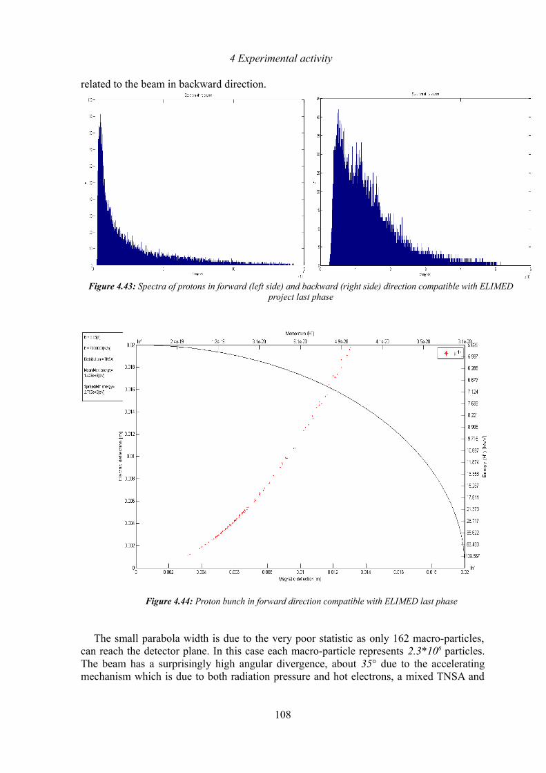
4 Experimental activity
related to the beam in backward direction.
The small parabola width is due to the very poor statistic as only 162 macro-particles, can reach the detector plane. In this case each macro-particle represents 2.3*106 particles. The beam has a surprisingly high angular divergence, about 35° due to the accelerating mechanism which is due to both radiation pressure and hot electrons, a mixed TNSA and
108
Figure 4.44: Proton bunch in forward direction compatible with ELIMED last phase
Figure 4.43: Spectra of protons in forward (left side) and backward (right side) direction compatible with ELIMED project last phase
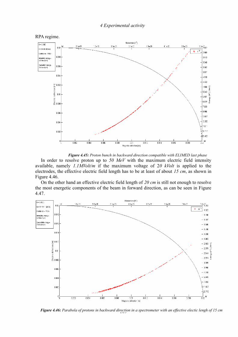
4 Experimental activity
RPA regime.
In order to resolve proton up to 50 MeV with the maximum electric field intensity available, namely 1.1MVolt/m if the maximum voltage of 20 kVolt is applied to the electrodes, the effective electric field length has to be at least of about 15 cm, as shown in Figure 4.46.
On the other hand an effective electric field length of 20 cm is still not enough to resolve the most energetic components of the beam in forward direction, as can be seen in Figure 4.47.
109Figure 4.46: Parabola of protons in backward direction in a spectrometer with an effective electic lengh of 15 cm
Figure 4.45: Proton bunch in backward direction compatible with ELIMED last phase
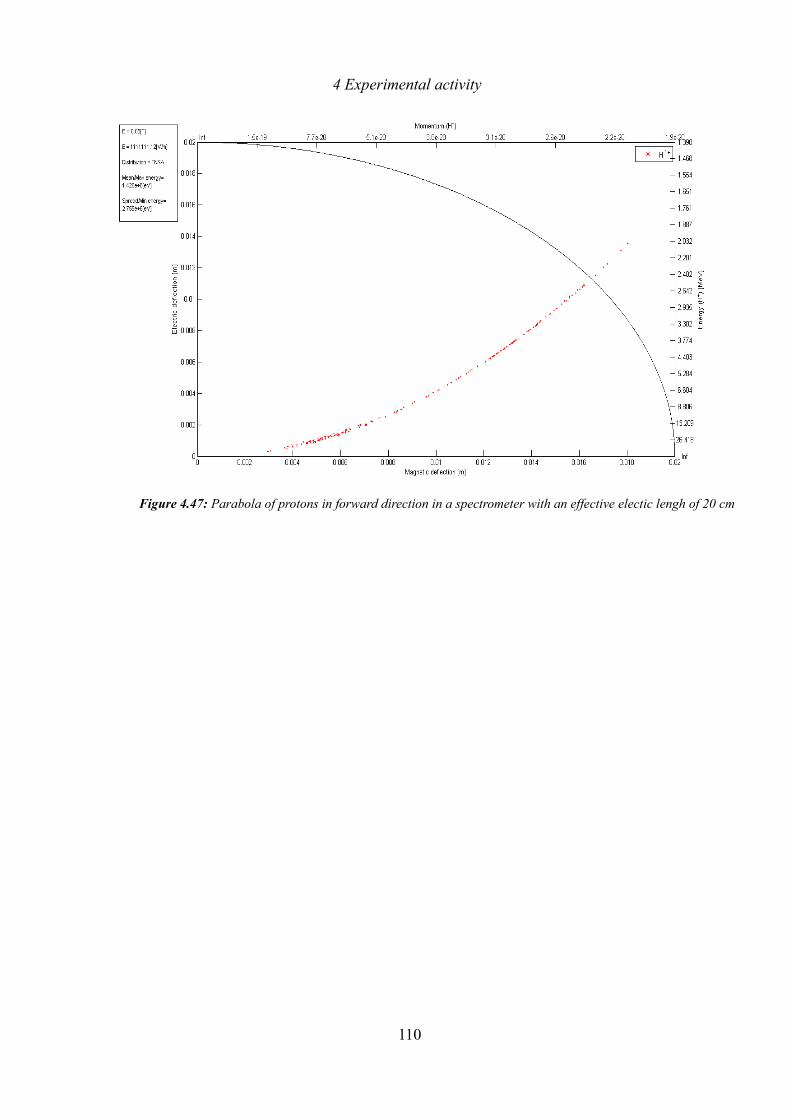
4 Experimental activity
110
Figure 4.47: Parabola of protons in forward direction in a spectrometer with an effective electic lengh of 20 cm
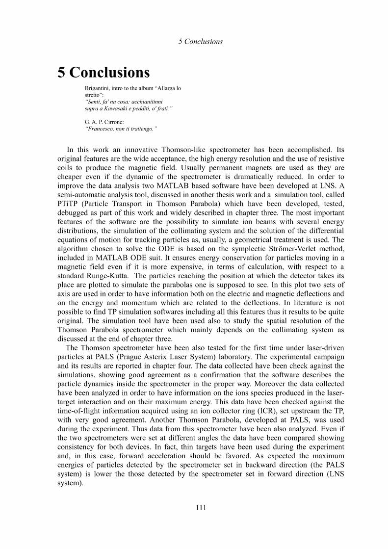
5 Conclusions
5 ConclusionsBrigantini, intro to the album “Allarga lo stretto”:“Senti, fa' na cosa: acchianitinni supra a Kawasaki e pedditi, o' frati.”
G. A. P. Cirrone:“Francesco, non ti trattengo.”
In this work an innovative Thomson-like spectrometer has been accomplished. Its original features are the wide acceptance, the high energy resolution and the use of resistive coils to produce the magnetic field. Usually permanent magnets are used as they are cheaper even if the dynamic of the spectrometer is dramatically reduced. In order to improve the data analysis two MATLAB based software have been developed at LNS. A semi-automatic analysis tool, discussed in another thesis work and a simulation tool, called PTiTP (Particle Transport in Thomson Parabola) which have been developed, tested, debugged as part of this work and widely described in chapter three. The most important features of the software are the possibility to simulate ion beams with several energy distributions, the simulation of the collimating system and the solution of the differential equations of motion for tracking particles as, usually, a geometrical treatment is used. The algorithm chosen to solve the ODE is based on the symplectic Strömer-Verlet method, included in MATLAB ODE suit. It ensures energy conservation for particles moving in a magnetic field even if it is more expensive, in terms of calculation, with respect to a standard Runge-Kutta. The particles reaching the position at which the detector takes its place are plotted to simulate the parabolas one is supposed to see. In this plot two sets of axis are used in order to have information both on the electric and magnetic deflections and on the energy and momentum which are related to the deflections. In literature is not possible to find TP simulation softwares including all this features thus it results to be quite original. The simulation tool have been used also to study the spatial resolution of the Thomson Parabola spectrometer which mainly depends on the collimating system as discussed at the end of chapter three.
The Thomson spectrometer have been also tested for the first time under laser-driven particles at PALS (Prague Asterix Laser System) laboratory. The experimental campaign and its results are reported in chapter four. The data collected have been check against the simulations, showing good agreement as a confirmation that the software describes the particle dynamics inside the spectrometer in the proper way. Moreover the data collected have been analyzed in order to have information on the ions species produced in the laser-target interaction and on their maximum energy. This data have been checked against the time-of-flight information acquired using an ion collector ring (ICR), set upstream the TP, with very good agreement. Another Thomson Parabola, developed at PALS, was used during the experiment. Thus data from this spectrometer have been also analyzed. Even if the two spectrometers were set at different angles the data have been compared showing consistency for both devices. In fact, thin targets have been used during the experiment and, in this case, forward acceleration should be favored. As expected the maximum energies of particles detected by the spectrometer set in backward direction (the PALS system) is lower the those detected by the spectrometer set in forward direction (LNS system).
111
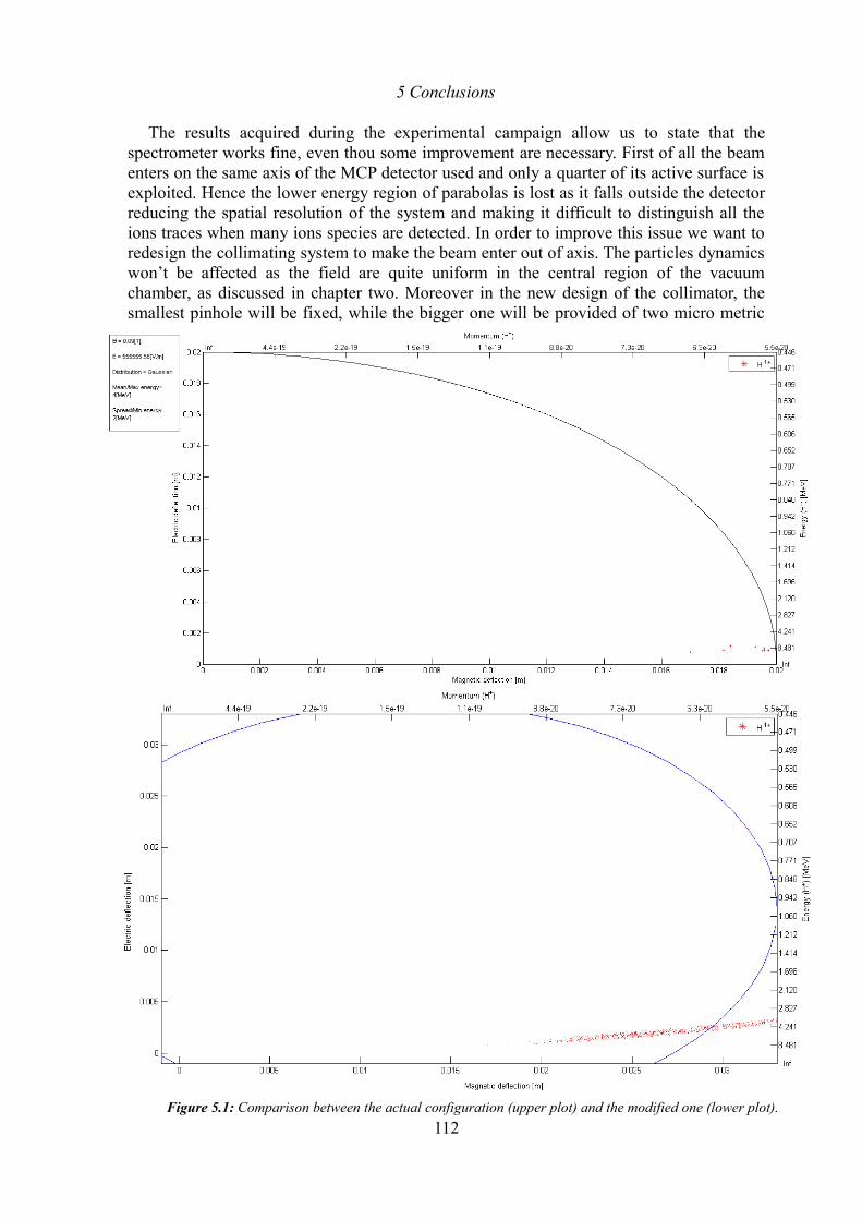
5 Conclusions
The results acquired during the experimental campaign allow us to state that the spectrometer works fine, even thou some improvement are necessary. First of all the beam enters on the same axis of the MCP detector used and only a quarter of its active surface is exploited. Hence the lower energy region of parabolas is lost as it falls outside the detector reducing the spatial resolution of the system and making it difficult to distinguish all the ions traces when many ions species are detected. In order to improve this issue we want to redesign the collimating system to make the beam enter out of axis. The particles dynamics won’t be affected as the field are quite uniform in the central region of the vacuum chamber, as discussed in chapter two. Moreover in the new design of the collimator, the smallest pinhole will be fixed, while the bigger one will be provided of two micro metric
112Figure 5.1: Comparison between the actual configuration (upper plot) and the modified one (lower plot).
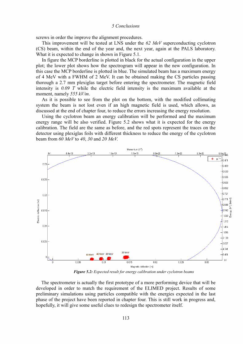
5 Conclusions
screws in order the improve the alignment procedures.This improvement will be tested at LNS under the 62 MeV superconducting cyclotron
(CS) beam, within the end of the year and, the next year, again at the PALS laboratory. What it is expected to change in shown in Figure 5.1.
In figure the MCP borderline is plotted in black for the actual configuration in the upper plot; the lower plot shows how the spectrogram will appear in the new configuration. In this case the MCP borderline is plotted in blue. The simulated beam has a maximum energy of 4 MeV with a FWHM of 2 MeV. It can be obtained making the CS particles passing thorough a 2.7 mm plexiglas target before entering the spectrometer. The magnetic field intensity is 0.09 T while the electric field intensity is the maximum available at the moment, namely 555 kV/m.
As it is possible to see from the plot on the bottom, with the modified collimating system the beam is not lost even if an high magnetic field is used, which allows, as discussed at the end of chapter four, to reduce the errors increasing the energy resolution.
Using the cyclotron beam an energy calibration will be performed and the maximum energy range will be also verified. Figure 5.2 shows what it is expected for the energy calibration. The field are the same as before, and the red spots represent the traces on the detector using plexiglas foils with different thickness to reduce the energy of the cyclotron beam from 60 MeV to 40, 30 and 20 MeV.
Figure 5.2: Expected result for energy calibration under cyclotron beams
The spectrometer is actually the first prototype of a more performing device that will be developed in order to match the requirement of the ELIMED project. Results of some preliminary simulations using particles compatible with the energies expected in the last phase of the project have been reported in chapter four. This is still work in progress and, hopefully, it will give some useful clues to redesign the spectrometer itself.
113
Appendix: PTiTP source code
Appendix: PTiTP source code
In this section is reported the source code of TPiPT.
A.1 PTiTP Main
clear allclose all %%%%Fundamental constantsuma=1.66e-27; %[Kg], mass atomic unitq=1.602e-19; %[C], elementary charge m_e=5.485799e-4*uma; %[kg], electron mass eV=1.6021765e-19; %[J], conversion factor eV-->Jc= 2.99792458e8; %[m/s], light speeduma1=931.494028; %[MeV/c^2], conversion factor uma-->MeV/c^2 (mass)KB=8.617e-5; %[eV*K^-1], Boltzmann constanKBT=1076*KB; ang_spread=0.999997; %angular spread tspan=[0,100];
%%%%% INPUT DATA INPUT = settingsdlg2(... 'title', 'PTiTP_1.0 input data',... 'Description', strvcat('This dialog will set the input parameters. ',... 'Please press HELP button for more information.'),... 'separator', 'Ions details', ... {'Number of particles per charge states', 'n'}, '',... {'Ion symbol', 'ion_sym'}, '',... {'Higher charge states', 'stati'}, '',... {'Lower charge state', 'low'},'',... {'Maximum or mean energy value', 'Ein'},'',... {'Minimum energy or spread', 'E_spread'},'',... {'Energy distribution','distribution'},{'Gaussian','Exponential', 'Uniform',... 'Plot', 'TNSA'},... 'separator', 'Fields details', ... {'Magnetic field in Tesla', 'Bx'},'',... {'Electric field in Volt/meter', 'Ex'}, '',... 'separator', 'Plot preferences', ... {'Plot the beam at the collimator'; 'Check_Coll'},false,... {'Plot the particle trajectories'; 'Check_Traiett'},false,... {'Plot histograms'; 'Check_Hist'}, false ); n= INPUT.n; %number of particles per charge state ion_sym = INPUT.ion_sym; %input ('Ion symbol: ', 's');
114
Appendix: PTiTP source code
%%%% Ion Massm_ion = feval(@Archive, ion_sym); % Call Archive functionm_ion = m_ion*uma; stati = INPUT.stati; %Higher charge statelow = INPUT.low; %Lower charge state Ein = INPUT.Ein; %Initial beam energyE_spread= INPUT.E_spread; distribution = INPUT.distribution; Bx = INPUT.Bx; %Magnetic field in Tesla Ex = INPUT.Ex; %Electric field in Volt/meter %%Flags for secondary plotPlot_Coll=INPUT.Check_Coll; Plot_Traiett=INPUT.Check_Traiett; Plot_hist=INPUT.Check_Hist; %%%%%%%%%%%%%%%%%%%%%%%%%%%%%%%%%%%%%%%%%%%%%%%%%%%%%%%%%%%%%%%%%%%%%%%%%%%%%%%%%%%%%%%%%%%%%%%%%%%%%%%%%%%%%%%%%%%%%%%%%%%%%%%%%%%%%%%%%%%%%%%%%%%%%%%%%%%%%%%%%%%%%Beam collimation%%%%%%%%%%%%%%%%%%First pinhole%%%%%%%%%%%%Pinhole1=0.03; %Distance between source and first pinholeDiametroPinhole1=0.0005; %First pinhole diamiterr_pin1=DiametroPinhole1/2; %First pinhole radius %Initializing energy matrixEtot_ion=zeros(n,1);betasquare_ion=zeros(n,1);v_ion=zeros(n,1); %%%%% COLLIMATION FOR MATLAB INTERNAL FUNCTIONif (strcmp(distribution, 'Gaussian') || strcmp(distribution,'Exponential') || strcmp(distribution,'Uniform')) %Have a for loop over a bunch of particles. For each particle, set its %velocity (speed and angle) vector using the rand() function. Then use an %"if" statement to decide whether the particle passed through or not and %count those that do. k=1; %Additional index to select particles in the inner if loop O=[0 0 0]'; %Differential equation to be solved in the ode solver. Drift sector before collimator
for s=low:stati Ein_s=Ein; %Ein_s=s*Ein; %E_spread=s*E_spread m_ions=m_ion-(s*m_e); %K_ion(1:n,1)=Ein_s; if strcmp(distribution, 'Gaussian') K_ion=normrnd(Ein_s,E_spread,n,1);
115
Appendix: PTiTP source code
% normrnd(mu,sigma,m,n) generates random numbers from % the normal distribution with mean parameter mu and % standard deviation parameter sigma, where scalars m % and n are the row and column dimensions of R. elseif strcmp(distribution,'Exponential') %% TNSA-like exponential distribution with a sharp cut-off at max mu=Ein_s/7; % The average energy value of a TNSA distribution is 1/7 % of the maximum energy E_spread=0.15; %Lower energies are discarded a=exp(-E_spread/mu)/mu; %minimum of exp distribution b=exp(-Ein_s/mu)/mu; %maximum of exp distribution f = a + (b-a).*rand(n,1); %reverse the cdf (cumulative distribution %function) (exponential) to create a %uniform randmon number distribution K_ion=-mu*log(mu*f); %Reverted exponential distributio (matlab uses %exp(-K_ion/mu)/mu) elseif strcmp(distribution,'Uniform') K_ion= E_spread+(Ein_s-E_spread)*rand(1,n,1); %Uniform distribution %between [A,Eins] K_ion=K_ion'; end Etot_ion=K_ion+((m_ions*uma1)/uma); betasquare_ion=1-(((m_ions*uma1)./(uma.*Etot_ion)).^2); v_ion=sqrt(betasquare_ion.*c^2); v0=feval(@God_Speed,n,ang_spread,v_ion); %initial velocity matrix r0=zeros(n,3); %initial position matrix y_sorgente=[r0,v0]; %vinitial condition matrix for i=1:n %%%Motion solver f = @(t,ys) [ys(4:6); O]; % the expression [y(4:6); O] % combines two vectors of length 3 to make a vector of % length 6(as long as y is a column vector). options=odeset('RelTol',1e-7, 'Events',@(t,ys)Event_Stop_Sorgente(t,ys,Pinhole1)); % ode set options %set relative error tollerance--- %Syntax to call Event_Stop_Sorgente with Pinhole1 as input [t,ys] = ode23(f,tspan,y_sorgente(i,:),options); %Particle passing the first pinhole if (ys(end,1)^2+ys(end,2)^2<r_pin1^2) %Particle passing through are stored in a structure Particella(k).simbolo= ion_sym; Particella(k).ionizzazione=s; Particella(k).stato_di_carica=s*q; Particella(k).massa=m_ions;
116
Appendix: PTiTP source code
Particella(k).q_over_m= s*q/m_ions; Particella(k).energia_iniziale=K_ion(i); Particella(k).traiettoria=ys(:,1:3); Particella(k).velocita=ys(:,4:6); k=k+1; end end end%%%%%%%COLLIMATION IF THE SPECTRUM IS TAKEN FROM A PLOTelseif strcmp(distribution, 'Plot') k=1; %%Additional index to select particles in the inner if loop O=[0 0 0]'; for s=low:stati m_ions=m_ion-(s*m_e); K_ion=feval(@Spettro, n); %Calls the function "Spettro" to evaluate %energy from a distribution Etot_ion=K_ion+((m_ions*uma1)/uma); betasquare_ion=1-(((m_ions*uma1)./(uma.*Etot_ion)).^2); v_ion=sqrt(betasquare_ion.*c^2); v0=feval(@God_Speed,n,ang_spread,v_ion); r0=zeros(n,3); %initial position y_sorgente=[r0,v0]; %initial condition matrix for i=1:n %%%Motion solver f = @(t,ys) [ys(4:6); O]; % the expression [y(4:6); O] % combines two vectors of length 3 to make a vector of % length 6(as long as y is a column vector). options=odeset('RelTol',1e-7, 'Events',@(t,ys)Event_Stop_Sorgente(t,ys,Pinhole1)); %ode set options %set relative error tollerance--- %Syntax to call Event_Stop_Sorgente with Pinhole1 as input [t,ys] = ode23(f,tspan,y_sorgente(i,:),options); if (ys(end,1)^2+ys(end,2)^2<r_pin1^2)
Particella(k).simbolo= ion_sym; Particella(k).ionizzazione=s; Particella(k).stato_di_carica=s*q; Particella(k).massa=m_ions; Particella(k).q_over_m= s*q/m_ions; Particella(k).energia_iniziale=K_ion(i); Particella(k).traiettoria=ys(:,1:3); Particella(k).velocita=ys(:,4:6); k=k+1; end end end %%%%%%%COLLIMATION FOR TNSA PROTON
117
Appendix: PTiTP source code
elseif strcmp(distribution, 'TNSA') k=1; O=[0 0 0]'; for s=low:stati m_ions=m_ion-(s*m_e); y_sorgente=load('MatriceProtoni'); %initial condition matrix y_sorgente=y_sorgente.MatriceProtoni; n=length(y_sorgente); V2=y_sorgente(:,4).^2+y_sorgente(:,5).^2+y_sorgente(:,6).^2; K_ion=0.5*m_ions.*V2/eV; for i=1:n %%%Motion solver f = @(t,ys) [ys(4:6); O]; % the expression [y(4:6); O] % combines two vectors of length 3 to make a vector of % length 6(as long as y is a column vector). options=odeset('RelTol',1e-7, 'Events',@(t,ys)Event_Stop_Sorgente(t,ys,Pinhole1));
[t,ys] = ode23(f,tspan,y_sorgente(i,:),options); if (ys(end,1)^2+ys(end,2)^2<r_pin1^2)
Particella(k).simbolo= ion_sym; Particella(k).ionizzazione=s; Particella(k).stato_di_carica=s*q; Particella(k).massa=m_ions; Particella(k).q_over_m= s*q/m_ion; Particella(k).energia_iniziale=K_ion(i); Particella(k).traiettoria=ys(:,1:3); Particella(k).velocita=ys(:,4:6); k=k+1; end end endend %%%%%%%%%%%%%%%Second pinhole%%%%%%%%%%Pinhole2=0.1; %distance between pinholes Distanzap1p2=Pinhole1+Pinhole2;DiametroPinhole2=0.0001;r_pin2=DiametroPinhole2/2; m=k-1; %number of particles passing the first pinhole y_pin2=zeros(m,6); %%%Initial condition matrix for the second pinhole %%%collimation
118
Appendix: PTiTP source code
j=1; % Additional index to save the transported particles
for i=1:m y_pin2(i,:)=[Particella(i).traiettoria(end,:),Particella(i).velocita(end,:)]; %vector of initial condition
%%%Motion solver f = @(t,yp) [yp(4:6); O]; % the expression [y(4:6); O] % combines two vectors of length 3 to make a vector of % length 6(as long as y is a column vector). options2=odeset('RelTol',1e-7, 'Events',@(t,yp)Event_Stop_Coll(t,yp,Distanzap1p2)); [t,yp] = ode23(f,tspan,y_pin2(i,:),options2); %Structure containing particles between the two pinholes Part_collimata(i).simbolo=Particella(i).simbolo; Part_collimata(i).ionizzazione = Particella(i).ionizzazione; Part_collimata(i).stato_di_carica = Particella(i).stato_di_carica; Part_collimata(i).massa = Particella(i).massa; Part_collimata(i).q_over_m= Particella(i).q_over_m; Part_collimata(i).energia_iniziale=Particella(i).energia_iniziale; Part_collimata(i).traiettoria=yp(:,1:3); Part_collimata(i).velocita=yp(:,4:6); %Flag to differentiat particle which pass the second pinhole from particles that don't pass if (yp(end,1)^2+yp(end,2)^2<r_pin2^2) %%Second pinhole passing condition %Flag to differentiat particle which pass the second pinhole from particles that %don't pass Part_collimata(i).viva=1; %Structure of particles to be trasported Part_trasp(j)=Part_collimata(i); j=j+1; else Part_collimata(i).viva=0; end end
%%%%%%%%%Plot collimation%number of particles entering the spectrometerp=j-1; if Plot_Coll == 1 %% figure('color', 'white') hold all for j=1:m plot3(Particella(j).traiettoria(:,3),Particella(j).traiettoria(:,2), Particella(j).traiettoria(:,1)) if (Part_collimata(j).viva==1) plot3(Part_collimata(j).traiettoria(:,3),Part_collimata(j).traiettoria(:,2), Part_collimata(j).traiettoria(:,1)) end
119
Appendix: PTiTP source code
end grid onend %clear Particella%%%%%%%%%%%%%%%%%%%%%%%%%%%%%%%%%%%%%%%%%%%%%%%%%%%%%%%%%%%%%%%%%%%%%%%%%%%%%%%%%%%%%%%%%%%%%%%%%%%%%%%%%%%%%%%%%%%%%%%%%%%%%%%%%%%%%%%%%%%%%%%%%%%%%%%%%%%%%%%%%%%%%%%%%%%%%%%%%%%%%%%%%%%%%%%%%%%%%%%%%%%%%%%%%%%%%%%%%%%%%%%%%%%%%%%%%%%%%%%%%%%%%%Transport inside TP%%%%%%Distances in meters P2_B = 0.0719; % distance between second pinhole and magnetic field (drift)Deriva1=Distanzap1p2+P2_B; % total distance before the deflection sector → % Event_Stop LB=0.1882; %effectiv magnetic length P2_E = 0.1858; % distance between second pinhole and electric field (magnetic % field only)inizioE=Distanzap1p2+P2_E; % total distance before the electric field → % Event_Stop P2_fineB=0.2601; % distance between second pinhole and end of magnetic field % (two fields zone)fineB= Distanzap1p2+P2_fineB; % total distance to the end of magnetic field → % Event_Stop
LE=0.0804; %Effective electric length GAP_E=0.0075; %half-distance between electrodesGAP_B=0.0175; %half-distance between magnets P2_fineE=0.2662; % distance between second pinhole and end of electric field %(electric field only)fineE=Distanzap1p2+P2_fineE; % total distance to the end of electric field → % Event_Stop Deriva2=0.3998; %distance between electric field and detectorDist_Spettr_riv=Distanzap1p2+P2_fineE+Deriva2; %Total distance to the detector → %Event_Stop %%%Zone 1%Trajectory in the first drifty0=zeros(p,6); %Initializing condition matrix (to speed up) %Fields B=[0 0 0]'; E=[0 0 0]'; for i=1:p
y0(i,:) = [Part_trasp(i).traiettoria(end,:),Part_trasp(i).velocita(end,:)]; %Initializing condition matrix %%%Motion solver f = @(t,y1) [y1(4:6); (Part_trasp(i).q_over_m).*cross(y1(4:6),B)+(Part_trasp(i).q_over_m).*E];
120
Appendix: PTiTP source code
% the expression [y(4:6); (q/m)*cross(y(4:6),B)] % combines two vectors of length 3 to make a vector of % length 6(as long as y is a column vector). options=odeset('RelTol',1e-7,'Events',@(t,y)Event_Stop_1(t,y,Deriva1)); % Ode set option [t,y1] = ode23t(f,tspan,y0(i,:),options); Part_trasp(i).traiettoria(end+1:end+size(y1,1),1:3)=y1(:,1:3); %Updating particle's trajectory Part_trasp(i).velocita(end+1:end+size(y1,1),1:3)=y1(:,4:6); %Updating particle's velocity end
%% %Zone 2%Trajectory in the magnetic field %Fields B=[Bx 0 0]'; E=[0 0 0]'; for i=1:p
y0(i,:) = [Part_trasp(i).traiettoria(end,:),Part_trasp(i).velocita(end,:)]; q_over_m= Part_trasp(i).q_over_m; %%%Motion solver f = @(t,y2) [y2(4:6); (q_over_m).*cross(y2(4:6),B)+(q_over_m).*E]; % the expression [y(4:6); (q/m)*cross(y(4:6),B)] % combines two vectors of length 3 to make a vector of % length 6(as long as y is a column vector). options=odeset('RelTol',1e-7,'Events',@(t,y)Event_Stop_2(t,y,inizioE)); [t,y2] = ode23t(f,tspan,y0(i,:),options); Part_trasp(i).traiettoria(end+1:end+size(y2,1),1:3)=y2(:,1:3);
Part_trasp(i).velocita(end+1:end+size(y2,1),1:3)=y2(:,4:6);
%%%Check if particles are lost on the camera wall if (Part_trasp(i).traiettoria(end,1)>=GAP_B) Part_trasp(i).viva=0; end end
%%%Zone 3%Trajectory where the fields are overlapped
%Fields B=[Bx 0 0]'; E=[Ex 0 0]'; for i=1:p
121
Appendix: PTiTP source code
y0(i,:) = [Part_trasp(i).traiettoria(end,:),Part_trasp(i).velocita(end,:)]; %%%Motion solver f = @(t,y3) [y3(4:6); (Part_trasp(i).q_over_m).*cross(y3(4:6),B)+(Part_trasp(i).q_over_m).*E]; % the expression [y(4:6); (q/m)*cross(y(4:6),B)] % combines two vectors of length 3 to make a vector of % length 6(as long as y is a column vector). options=odeset('RelTol',1e-7,'Events',@(t,y)Event_Stop_3(t,y,fineB));
[t,y3] = ode23t(f,tspan,y0(i,:),options); Part_trasp(i).traiettoria(end+1:end+size(y3,1),1:3)=y3(:,1:3);
Part_trasp(i).velocita(end+1:end+size(y3,1),1:3)=y3(:,4:6); %
%%%Check if particles are lost on the electrodes if (Part_trasp(i).traiettoria(end,1)>=GAP_E) Part_trasp(i).viva=0; endend
%%%Zone 4%Trajectory in the electric field sector %Fields B=[0 0 0]'; E=[Ex 0 0]'; for i=1:p
y0(i,:) = [Part_trasp(i).traiettoria(end,:),Part_trasp(i).velocita(end,:)]; %Motion solver f = @(t,y4) [y4(4:6); (Part_trasp(i).q_over_m).*cross(y4(4:6),B)+(Part_trasp(i).q_over_m).*E]; % the expression [y(4:6); (q/m)*cross(y(4:6),B)] % combines two vectors of length 3 to make a vector of % length 6(as long as y is a column vector).
options=odeset('RelTol',1e-7,'Events',@(t,y)Event_Stop_4(t,y,fineE));
[t,y4] = ode23t(f,tspan,y0(i,:),options); Part_trasp(i).traiettoria(end+1:end+size(y4,1),1:3)=y4(:,1:3);
Part_trasp(i).velocita(end+1:end+size(y4,1),1:3)=y4(:,4:6); %%%Check if particles are lost on the electrodes if (Part_trasp(i).traiettoria(end,1)>=GAP_E) Part_trasp(i).viva=0; end end %%%Zone 5%Trajectory in the drift secotor before the detector
122
Appendix: PTiTP source code
%Fields B=[0 0 0]'; E=[0 0 0]'; for i=1:p y0(i,:) = [Part_trasp(i).traiettoria(end,:),Part_trasp(i).velocita(end,:)]; %Motion sover f = @(t,y5) [y5(4:6); (Part_trasp(i).q_over_m).*cross(y5(4:6),B)+(Part_trasp(i).q_over_m).*E]; % the expression [y(4:6); (q/m)*cross(y(4:6),B)] % combines two vectors of length 3 to make a vector of % length 6(as long as y is a column vector). options=odeset('RelTol',1e-7, 'Events',@(t,y)Event_Stop_5(t,y,Dist_Spettr_riv)); [t,y5] = ode23t(f,tspan,y0(i,:),options); Part_trasp(i).traiettoria(end+1:end+size(y5,1),1:3)=y5(:,1:3);
Part_trasp(i).velocita(end+1:end+size(y5,1),1:3)=y5(:,4:6);
end %%%%PLOT if Plot_Traiett==1 figure('color', 'white') hold all for i=1:p plot3(Part_trasp(i).traiettoria(:,3),Part_trasp(i).traiettoria(:,2), Part_trasp(i).traiettoria(:,1)) end grid on xlabel ('Beam direction'); zlabel ('Electric deflection'); ylabel ('Magnetic deflection');end %%%On the MCP%% %MCP contourRmcp=0.02; %MCP radiusXmcporigine=linspace(0,Rmcp,1000); %1000 elements vector [0-Rmpc]
Ymcporigine=sqrt(Rmcp^2-Xmcporigine.^2); %Equation of MCP contour figure('color', 'white', 'units','normalized','position',[0 0 1 1]) %%%%Fixed size of legend marker cmap = hsv(stati); %# Creates a j-by-3 set of colors from the HSV colormap
123
Appendix: PTiTP source code
legendtext =''; partlost=0; for j=low:s for i=1:p if (Part_trasp(i).ionizzazione == j && Part_trasp(i).viva==1) B_defl(i,j) = Part_trasp(i).traiettoria(end,2); E_defl(i,j) = Part_trasp(i).traiettoria(end,1); hplot(j) = plot(B_defl(:,j), E_defl(:,j),'*','Color',cmap(j,:),'Markersize', 2); %'Color',cmap(j,:) %# Plot each column with a different color hold on elseif (Part_trasp(i).ionizzazione == j && Part_trasp(i).viva==0) partlost=partlost+1; end end if j<10 legendtext = [legendtext; ion_sym, ' ^{', num2str(j),'+}']; hold on else legendtext = [legendtext; ion_sym, '^{', num2str(j),'+}']; hold on end end hold onplot(Ymcporigine,Xmcporigine,'k-','MarkerEdgeColor','k','MarkerSize',1); %Plot MCP contour %Main axis label - It is necessary to give the label instructions after plot in %order to avoid overlap xlabel(gca, 'Magnetic deflection [m]'); % label lower x axis ylabel(gca,'Electric deflection [m]'); %label left y axis %particles outside MCP radius won't appear in figure xlim([0, Rmcp]) ylim([0, Rmcp]) %%%% legend l=legend(legendtext, 'Location', 'NorthEast'); a=get(l, 'children'); j=s; for i = 1:3:length(a) set(a(i),'Color', cmap(j,:)); j=j-1; end set(a(1:3:end),'MarkerSize', 10); %%%% Secondary axes %set secondary x limit as the momentum of a H+ at distance equal to the MCP radius % Harres [49]: y=(q*B*LB*L)/sqrt(2mEkin) ==> mv=q*B*LB*L/y
124
Appendix: PTiTP source code
L=Deriva2+0.0053;%Deriva2+0.02; %L=Distance between the end of CB and MCP %%%% Create secondary x axis scale x_tick = linspace(0,Rmcp,9); mv_label = (q*Bx*LB*L)./x_tick; mv_label=num2str(mv_label','%3.1e'); %formatting x label array for i=1:size(mv_label,1) mv_newlabel{i}=strrep(mv_label(i,:),'-0','-'); end %set secondary y limit as the energy of a H+ at distance equal to the MCP radius % Harres[49] x=(q*E*Le*L)/(2Ekin) ==> Ekin=q*E*Le*L/2x y_tick = linspace(0,Rmcp,20); Ekin_label = ((q*Ex*LE*Deriva2)*10^-6./(2.*y_tick))./eV; Ekin_label=num2str(Ekin_label','%5.3f'); %formatting y label array %(6.3g is a length 6 field with 3 decimal digit) %Layout instruction set(gca,'Box','off'); % Turn off the box surrounding the whole axes axesUnits=get(gca,'Units'); axesPosition = get(gca,'Position'); %# Get the current axes position hNewAxes = axes('Position', axesPosition,... %# Place a new axes on top... 'Units', 'normalized',... 'ActivePositionProperty', 'Position',... 'Color','none',... %# ... with no background color 'YAxisLocation', 'right',... 'XAxisLocation','top',... %# ... located on the top 'Ylim', [min(y_tick), max(y_tick)],... %# ... define y axis limits 'YTick',y_tick,... %# ... set y tick position 'YTickLabel',Ekin_label,... %# ... set y tick label 'Xlim', [min(x_tick), max(x_tick)],... %# ... define x axis limits 'XTick',x_tick,... %# ... set y tick position 'XTickLabel',mv_newlabel,... %# ... set y tick label 'Box','off'); %# ... and no surrounding box xlabel(hNewAxes,['Momentum (', ion_sym ,'^+)']); %# Add a label to the top axis ylabel(hNewAxes,['Energy (',ion_sym,'^+) [MeV]']); %# Add a label to the right axis
%% %%% TEXT BOX %%Add annotation box %write text
txtstr1 = strcat(['B = ', num2str(Bx),'[T]']); txtstr2 = strcat(['E = ', num2str(Ex),'[V/m]']); txtstr3 = strcat(['Distribution = ', distribution]); if strcmpi(distribution, 'Gaussian') MinEtxtbox = num2str(E_spread); MaxEtxtbox = num2str(Ein); else MinEtxtbox = num2str(min(K_ion),'%4.3e'); MinEtxtbox = strrep(MinEtxtbox,'+00','+'); MinEtxtbox = strrep(MinEtxtbox,'-00','-'); MaxEtxtbox = num2str(max(K_ion),'%4.3e'); MaxEtxtbox = strrep(MaxEtxtbox,'+00','+'); end
125
Appendix: PTiTP source code
%%TNSA distribution needs [eV] units, others distribution not if strcmpi(distribution, 'TNSA') txtstr4 = char('Mean/Max energy= ', strcat([num2str(MaxEtxtbox),'[eV]'])); txtstr5 = char('Spread/Min energy= ', strcat([num2str(MinEtxtbox),'[eV]'])); else txtstr4 = char('Mean/Max energy= ', strcat([num2str(MaxEtxtbox),'[MeV]'])); txtstr5 = char('Spread/Min energy= ', strcat([num2str(MinEtxtbox),'[MeV]'])); end txtstr = strvcat( txtstr1, ' ', txtstr2, ' ', txtstr3, ' ', txtstr4, ' ', txtstr5); %%Set up textbox textbox=annotation('textbox',[0.004 0.72 0.094 0.25], 'String', txtstr, 'FontSize', 8); %% %%%Warining message for lost particles if (partlost>0) warndlg([num2str(partlost),' particles are lost on the electrodes and/or on the magnets']) end %% %%%%% Histogram for spectrum % Plot_hist=INPUT.Check_Hist; if Plot_hist== 1 figure() for i=1:m Ecoll(i)=Part_collimata(i).energia_iniziale; end for i=1:p EMCP(i)=Part_trasp(i).energia_iniziale; end xx=linspace(min(K_ion),max(K_ion),n/5); xx2=linspace(min(Ecoll),max(Ecoll),m/5); xx3=linspace(min(EMCP),max(EMCP),p); subplot(3,1,1); hist(K_ion,xx) title('Spectrum at the source') xlabel('Energy [eV]','FontSize',6) ylabel('#','FontSize',6) subplot(3,1,2); hist(Ecoll,xx2) title('Spectrum at the collimator') xlabel('Energy [eV]','FontSize',6) ylabel('#','FontSize',6) subplot(3,1,3); hist(EMCP,xx3) title('Spectrum at the detector') xlabel('Energy [eV]','FontSize',6) ylabel('#','FontSize',6) end
126
Appendix: PTiTP source code
A.2 Event_Stop Functions
The Event_Stop functions code are reported:
A.2.1 Event_Stop_Sorgentefunction [value,isterminal,direction]=Event_Stop_Sorgente(t,ys, Pinhole1)%%%%%%%%%%%%%%%%%%%%%%%%%%%%%%%%%%%%%%%%%%%%%%%%%%%%%%%%%%%%%%%%%%%%%%%%%%%% % % Function stopping ode solver.% % In the 'events' case, the ODE file returns to the solver the values% % that it needs to perform event location. When the Events property is set% % to on, the ODE solvers examine any elements of the event vector for % % transitions to, from, or through zero. If the corresponding element of % % the logical isterminal vector is set to 1, integration will halt when a% % zero-crossing is detected. The elements of the direction vector are -1,% % 1, or 0, specifying that the corresponding event must be decreasing, % % increasing, or that any crossing is to be detected.%%%%%%%%%%%%%%%%%%%%%%%%%%%%%%%%%%%%%%%%%%%%%%%%%%%%%%%%%%%%%%%%%%%%%%%%%%%% % When "value" is equal to zero, an event is triggered.% % set isterminal to 1 to stop the solver at the first event, or 0 to% % get all the events.% % direction=0 if all zeros are to be computed (the default), +1 if% % only zeros where the event function is increasing, and -1 if only% % zeros where the event function is decreasing.% value = ......; % when value = 0, an event is triggered% isterminal = 1; % terminate after the first event% direction = 0; % get all the zeros z=ys(3); %z is initialized with the particle positioncond_z=z-Pinhole1; % evaluate the zero passing condition value=cond_z; % event isterminal=1; % Stop the integration when the particle reach the first pinholedirection=0; % Stop the integration when the zero crossing occurs from every % direction.
A.2.2 Event_Stop_Collfunction [value,isterminal,direction]=Event_Stop_Coll(t,yp, Distanzap1p2)%%%%%%%%%%%%%%%%%%%%%%%%%%%%%%%%%%%%%%%%%%%%%%%%%%%%%%%%%%%%%%%%%%%%%%%%%%% z=yp(3); cond_z=z-Distanzap1p2; value=cond_z; isterminal=1; % Stop the integration when the particle reach the second pinholedirection=0; % Stop the integration when the zero crossing occurs from every % direction.
A.2.3 Event_Stop_1function [value,isterminal,direction]=Event_Stop_1(t,y1, Deriva1)%%%%%%%%%%%%%%%%%%%%%%%%%%%%%%%%%%%%%%%%%%%%%%%%%%%%%%%%%%%%%%%%%%%%%%%%%%% z=y1(3); cond_z=z-Deriva1;
value=cond_z;
127
Appendix: PTiTP source code
isterminal=1; direction=0;
A.2.4 Event_Stop_2function [value,isterminal,direction]=Event_Stop_2(t,y2,inizioE) z=y2(3); cond_z=z-inizioE; value=cond_z; isterminal=1; direction=0;
A.2.5 Event_Stop_3function [value,isterminal,direction]=Event_Stop_3(t,y3,fineB) z=y3(3); cond_z=z-fineB;
value=cond_z; isterminal=1; direction=0;
A.2.6 Event_Stop_4function [value,isterminal,direction]=Event_Stop_4(t,y4,fineE)
z=y4(3); cond_z=z-fineE; value=cond_z; isterminal=1;
direction=0;
A.2.7 Event_Stop_5function [value,isterminal,direction]=Event_Stop_5(t,y5,Dist_Spettr_riv) z=y5(3); cond_z=z-Dist_Spettr_riv;
value=cond_z;
isterminal=1;
direction=0;
128
Appendix: PTiTP source code
A.3 Archive Function
function [m_ion]=Archive(ion_sym)%%%%%%%%%%%%%%%%%%%%%%%%%%%%%%%%%%%%%%%%%%%%%%%%%%%%%%%%%%%%%%%%%%%%%%%%%%%%%%%% EXPLANATION:%%% The function gives the proper mass if the ion simbol is known, otherwise%%% asks for mass value%%%%%%%%%%%%%%%%%%%%%%%%%%%%%%%%%%%%%%%%%%%%%%%%%%%%%%%%%%%%%%%%%%%%%%%%%%% sym=ion_sym;%%if strcmpi(sym, 'Al') %sym=='Al'; %The strcmpi compares strings without sensitivity to letter case m_Al = 29.9815; %*uma[kg], massa atomica di Al m_ion=m_Al; elseif strcmpi(sym, 'Au')%sym=='Au' m_Au=196.96655; %*uma[kg], massa atomica di Au m_ion=m_Au; elseif strcmpi(sym, 'C')%sym=='C'; m_C = 12.0107; %*uma[kg], massa atomica di C m_ion=m_C; elseif strcmpi(sym, 'D')%sym=='D'; DEUTERIO m_D = 2.01363; %*uma[kg], massa atomica di D m_ion=m_D; elseif strcmpi(sym, 'Fe')%sym=='Fe'; Ferro m_Fe = 55.84; %*uma[kg], massa atomica di Fe m_ion=m_Fe; elseif strcmpi(sym, 'H')%sym=='H' m_H = 1.00794; %*uma[kg], massa atomica di H m_ion=m_H; elseif strcmpi(sym, 'He')%sym=='He' m_He = 4.002602; %*uma[kg], massa atomica di He m_ion=m_He; elseif strcmpi(sym, 'O')%sym=='O' m_O = 15.9994; %*uma[kg], massa atomica di O m_ion=m_O; elseif strcmpi(sym, 'Si')%sym=='Si' m_Si = 28.0855; %*uma[kg], massa atomica di Si m_ion=m_Si; elseif strcmpi(sym, 'Ta')%sym=='Ta'; TANTALIO m_Ta = 180.9479; %*uma[kg], massa atomica di C m_ion=m_Ta; else title = 'WARNING!'; text = strcat(['Ion symbol ', sym, ' is unknow. Please enter ion mass']); dialogbox = inputdlg(text, title); %m_ion = input('Atomic mass in amu: '); m_ion = str2num(dialogbox{1});end
129
Appendix: PTiTP source code
A.4 God_Speed Function
function [v0] = God_Speed(n, ang_spread, v_ion) %%%%%%%%%%%%%%%%%%%%%%%%%%%%%%%%%%%%%%%%%%%%%%%%%%%%%%%%%%%%%%%%%%%%%%%%%%%%%%%%%%%%%%%%%%%%%%%%%%%%%%%%%%%%%%%%%%%%%%%%%%%%%%%%%%%%%%%%%%%%%%%%%%%%%%%%%% The function calls a matrix of random points on a sphere with unit%%%% radius in order to evaluate the velocity component of each particle%%%%%%%%%%%%%%%%%%%%%%%%%%%%%%%%%%%%%%%%%%%%%%%%%%%%%%%%%%%%%%%%%%%%%%%%%%%%%%%%%%%%%%%%%%%%%%%%%%%%%%%%%%%%%%%%%%%%%%%%%%%%%%%%%%%%%%%%%%%%%%%%%%%%%% versore=load('VERSORI'); %Matrix of random pointsversore=versore.VERSORI; vers=find(versore(:,3)>=ang_spread); % Select point on a spherical capvers_select=versore(vers,:); % direction cosine clear versore r = randperm(size(vers_select,1)); %creates a vector of random number between 1 %and size(vers_select) num = floor(n/length(vers_select)); %B = floor(A) rounds the elements of A to the nearest integers less than or %equal to A.
for i = 1 : num r1=randperm(size(vers_select,1)); r=[r r1]; end vers=vers_select(r(1:n),:); v_ion=repmat(v_ion,1,3);v0=vers.*v_ion; %Matrix of initial conditions %%%OUTPUT
A.5 Spettro Function
function [ K_ion ] = Spettro( n )%%%%%%%%%%%%%%%%%%%%%%%%%%%%%%%%%%%%%%%%%%%%%%%%%%%%%%%%%%%%%%%%%%%%%%%%%%%%%%%% EXPLANATION:%%% The function uses some kind of roulette-wheel selection process.%%% It loads a matrix with energy values on a column and the probability on %%% the other to have a particle of a certain energy on the other column, %%% basically a spectrum.%%%%%%%%%%%%%%%%%%%%%%%%%%%%%%%%%%%%%%%%%%%%%%%%%%%%%%%%%%%%%%%%%%%%%%%%%%%%%
Spectrum=load('AlfaAM241'); %load matrix with energy and probability Spectrum=Spectrum.AlfaAM241;
Energy=Spectrum(:,1); % energy columnpby=Spectrum(:,2); % probability column
130
Appendix: PTiTP source code
pby=pby'; %should be a row N=n; %How many numbers to generate K_ion=Energy( sum ( bsxfun(@ge, rand(N,1), cumsum(pby./sum(pby))), 2) + 1);
end
131
Bibliography
BibliographyChuck Prophet, “You did”, track in “Age of Miracles”:Who put the “bomp” in the “Bomp Shooby Dooby Bomp”?Who put the “ram” in the “Rama Lama Ding Dong”?
You did (I got a letter this morning)[...]
Who dug the crude and made it flow?Who proved that anything was possible?
You did Who built an house and brought it down?Who raised a roof and never made a sound?
You did , you did[…]
I don't believe it.I got a... I got letter... I got a letter this morning
[…]Who put the “flip” in the “Flippity Flop”?Who put the “hip” in the “Hippity Pop”?Who put the “boom” in the “Boom Boom Shaka Laka”?
You did (I got a letter this morning)Who put the “bomp” in the “Bomp Shooby Dooby Bomp”?Who put the “ram” in the “Rama Lama Ding Dong”?Who put the “wang” in the “Wang Dang Noo, Baby”?
You did (I got a letter this morning)Wake me up if should drift away out, don't want to miss a thing.
(I got a letter this morning)Take my hand and lead me all around, I don't care where we're going.
(I got a... I got a letter this morning)
[1] G. Pucella, S. E. Segre, Fisica dei Plasmi, Zanichelli editore S.p.A, Bologna, 2010.
[2] S. Eliezer, The Interaction of High-Power Laser with Plasmas, IOP Publishing Ltd, 2002.
[3] J.D. Jackson, Classical Electrodynamics, John Wiley & Sons, Inc., 1975.
[4] S. Barbarino, Appunti di Campi Elettromagnetici, online book.
[5] P. Gibbon, Short Pulse Laser Interaction with Matter, Imperial CollegePress, 2005.
[6] W. L. Kruer, The Physics of Laser Plasma Interactions, Addison-Wesley, New York, 1988.
[7] G. Russo, Classical Electrodynamics, lectures notes.
[8] G. Russo, The Physics of Nuclear Reactor, lectures notes.
[9] S. Barbarino, Appunti di Microonde, online book.
132
Bibliography
[10] L. Pappalardo, Interferometria e Olografia Applicate ai Beni Culturali, online book.
[11] E. Esarey, C. B. Schroeder, W. P. Leemans, Physics of laser-driven plasma -based accelerators, Review of Modern Physics, 81(3):1229 (2009). [12] A. Sgattoni, Theoretical and numerical study of laser-plasma ion acceleration, PhD thesis in Physics A.A. 2011.
[13] S. Sinigardi, Dynamical aspects of optical acceleration and transport of proton, Master Degree thesis in Physics A.A. 2009-2010.
[14] F. Rossi, Development of algorithms for an electromagnetic particle in cell code and implementation on a hybrid architecture (CPU+GPU), Master Degree thesis in Physics A.A. 2010-2011.
[15] F. Vittori, Accelerazione Laser-plasma: primi risultati sperimentali dal progetto PlasmonX, Master Degree thesis in Physics A.A. 2007-2008.
[16] V. S. Popov, Tunnel and multiphoton ionization of atoms and ions in a strong laser field, Physics-Uspekhi 47 (9) 855-885 (2004).
[17] D. Giulietti, L.A. Gizzi, X-ray emission from laser-produced plasmas, Rivista del Nuovo Cimento Vol. 21, N.10 (1998).
[18] L. Spitzer, R. Härm, Transport phenomena in a completely ionized gas, Physical Review Vol 89, N.5 (1953).
[19] A. Macchi, C. Benedetti, Ion acceleration by radiation pressure in thin and thick targets.
[20] A. Macchi, F. Cattani, T.V. Liseykina, F. Cornolti, Laser acceleration of ion bunches at the front surface of overdense plasmas, arXiv:physics/0411023v2 (2005).
[21] G. Hairapetian, R. L. Stenzel, Expansion of a two-electron-population plasma into vacuum, Physical Review Letters Vol. 61, N. 14.
[22] M. Passoni, L. Bertagna, A. Zani, Target normal sheath acceleration: theory, comparison with experiments and future perspective, New J. Phys. 12 045012 (2010).
[23] G. Turchetti, A. Sgattoni, C. Benedetti, P. Londrillo, L. Di Lucchio, Comparison of scaling laws with PIC simulation for proton acceleration with long wavelength pulses, Nuclear Instruments and Methods in Physics Research A 620 (2010) 51–55. [24] P. Bolton, P. Londrillo, A. Sgattoni, M. Sumini, G. Turchetti., Numerical investigation of optical acceleration of protons and perspective for hadrotherapy, (2011 Preprint). [25] P. Londrillo, A. Sgattoni, S. Sinigardi, M. Sumini, G. Turchetti, Protons acceleration from CO2 laser pulses for biomedical applications, (2011 Preprint).
133
Bibliography
[26] G. Turchetti, Mathematical models in beam dynamics, personal note.
[27] P. Antici, M. Migliorati, A. Mostacci, L. Picardi, L. Palumbo, C. Ronsivalle, A compact post-acceleration scheme for laser-generated protons, Physics of Plasmas 18,000000 (2011).
[28] T. Toncian, M. Amin, M. Borghesi, C. A. Cecchetti, R. J. Clarke, J. Fuchs, R. Jung, T. Kudyakov, M. Notley, A. C. Pipahl, P. A. Wilson and O. Willi, Propertiesof a plasma-based laser-triggered micro-lens, AIP Advances 1, 022141 (2011). [29] T. Toncian, M. Borghesi, J. Fuchs, E. d’Humières, P. Antici, P. Audebert, E. Brambrink, C. A. Cecchetti, A. Pipahl, L. Romagnani, O. Willi, Ultrafast laser-driven microlens to focus and energy-select mega-electron volt protons, Science Vol 312, pag 410, 21/04/2006.
[30] V. G. Vaccaro, M. R. Masullo, C. De Martinis, L. Gini, D. Giove, A. Rainò, V. Variale, L. Calabretta, A. Rovelli, S. Barone, S. Lanzone, A side coupled proton LINAC module 30-35 MeV: first acceleration tests.
[31] M. Nishiuchi, H. Sakaki, T. Hori, P. R. Bolton, K. Ogura, A. Sagisaka, A. Yogo, M. Mori, S. Orimo, A. S. Pirozhkov, I. Daito, H. Kiriyama, H. Okada, S. Kanazawa, S. Kondo, T. Shimomura, M. Tanoue, Y. Nakai, H. Sasao, D. Wakai, H. Daido, K. Kondo, H. Souda, H. Tongu, A. Noda, Y. Iseki, T. Nagafuchi, K. Maeda, K. Hanawa, T. Yoshiyuki, T. Shirai, Measured and simulated transport of 1.9 MeV laser-accelerated proton bunches through an integrated test beam line at 1 Hz, PhysRevSTAB.13, 071304 (2010).
[32] U. Linz, J. Alonso, What will it take for laser driven proton accelerators to be applied to tumor therapy?, PhysRevSTAB.10.094801 (2007).
[33] M. Schollmeier, S. Becker, M. Geißel, K. A. Flippo, A. Blazĕvić, S. A. Gaillard, D. C. Gautier, F. Grüner, K. Harres, M. Kimmel, F. Nürnberg, P. Rambo, U. Schramm, J. Schreiber, J. Schütrumpf, J. Schwarz, N. A. Tahir, B. Atherton, D. Habs, B. M. Hegelich, and M. Roth, Controlled Transport and Focusing of Laser-Accelerated Protons with Miniature Magnetic Devices, PRL 101, 055004 (2008).
[34] I. Hofmann, J. Meyer-ter-Vehn, X. Yan, A. Orzhekhovskaya, S. Yaramyshev, Collection and focusing of laser accelerated ion beams for therapy applications, Physical Review Special Topics - Accelerators and Beams 14, 031304 (2011).
[35] I. Hofmann, A. Orzhekhovskaya, S. Yaramyshev, I. Alber, K. Harres and M. Roth, Laser accelerated ions and their potential for therapy accelerators, GSI Internal Report.
[36] H. Sakaki, T. Hori, M. Nishiuchi, P. Bolton, H. Daido, S. Kawanishi, K. Sutherland, H. Souda, A. Noda, Y. Iseki, T. Yoshiyuki, Designing integrated laser-driven ion accelerator system for hadron therapy at PMRC (Photo Medical Research Center), Proceedings of PAC09, Vancouver, BC, Canada TU6PFP009.
[37] D. Haberberger, S. Tochitsky, C. Gong, C. Joshi, Production of 25 MeV protons in
134
Bibliography
CO2 laser-plasma interactions in a gas jet, Proceedings of 2011 Particle Accelerator Conference, New York, NY, USA (TUOBN6).
[38] P. Londrillo, A. Sgattoni, M. Sumini, G. Turchetti, Optical acceleration and per-spectives for cancer therapy with proton beams, Proceedings of OSCM -Oncogenesi tra scienza e clinica medica workshop - Frascati 10-11 giugno 2010 - ENEA report.
[39] F. Nürnberg, M. Schollmeier, E. Brambrink, A. Blažević, D. C. Carroll, K. Flippo, D.
C. Gautier, M. Geißel, K. Harres, B. M. Hegelich, O. Lundh, K. Markey, P. McKenna4, D. Neely, J. Schreiber, and M. Roth, Radiochromic film imaging spectroscopy of laser-accelerated proton beams, Rev. Sci. Instrum. 80, 033301 (2009).
[40] E. Breschi, Analisi dello spettro energetico di protoni generati da interazione ultra-intensa laser-plasma, Master Degree thesis in Physics A.A. 2001-2002
[41] A. Niroomand-Rad, C. R. Blackwell, B. M. Coursey, K. P. Gall, J. M. Galvin, W. L. McLaughlin, A. S. Meigooni, R. Nath, J. E. Rodgers, C. G. Soares, Radiochromic film dosimetry: Recommendation of AAPM Radiation Therapy Committee Task Group 55, Med. Phys, 25(11):2093-2115, 1998.
[42] L. Zhao, I. Das, Gafchromic EBT film dosimetry in proton beams, Phys. Med Biol. 55 (2010) N291-N301
[43] D. Kirby, Radiation dosimetry of conventional and laser-driven particle beams, PhD thesis in Physics A.A. 2011.
[44] ISP, Gafchromic® EBT2: self-developing film for radiotherapy dosimetry, data-sheet (2009). [45] G. A. P. Cirrone, G. Cuttone, M. Maggiore, L. Torrisi, F. Tudisco, Diagnostic for the radiotherapy use of laser accelerated proton beams, Radiation Effects and Defects in Solids, Vol 00, No. 00, January 2008,1-7.
[46] M. Maggiore, S. Cavallaro, G. A. P. Cirrone, G. Cuttone, L. Giuffrida, F. Romano, L. Torrisi, Design and realisation of a Thosom Spectrometer for Laser Plasma Facilities, Nejaka Hlavicka 123(2020), 123-456.
[47] M. J. Rhee, Compact Thomson spectrometer, Rev. Sci. instrum. 55 (8), August 1984.
[48] R. F. Schneider, C. M. Luo, M. J. Rhee, Resolution of the Thomson spectrometer, J. Appl. Phys. 57 (1), 1 January 1985.
[49] K. Harres, M. Schollmeier, E. Brambrik, P. Audebert, A. Blažević, K. Flippo, D. C. Gautier, M. Geißel, B. M. Hegelich, F. Nürnberg, J. Schreiber, H. Wahl, M. Roth, Development and calibration of a Thomson parabola with microchannel plate for the detection of a laser-accelerated MeV ions, Rev. Sci. Instrum. 79, 093306 (2008).
[50] L. Andò, Parabola di Thomson, personal note.
135
Bibliography
[51] J. R. Smith, C. M. Armstrong, W. O. Dogget, Thomson spectrometer analysis of collectively accelerated ions, J. Appl. Phys. 56 (5), 1 September 1984.
[52] S. Ter-Avetisyan, L. Romagnani, M. Borghesi, M. Schnürer, P. V. Nickels, Ion diagnostic for laser plasma experiments, Nucl. Instr. and Meth. A (2010), doi: 10.1016/j.nim.2010.02.094
[53] R. Prasad, D. Doria, S. Ter-Avetisyan, P. S. Foster, K. E. Quinn, L. Romagnani, C. M. Brenner, J. S. Green, P. Gallegos, M. J. V. Streeter, D. C. Carroll, O. Tresca, N. Dover, C. A. J. Palmer, J. Schreiber. D. Neely, Z. Najmudin, P. McKenna, M. Zepf, M. Borghesi, Calibration of Thomson parabola-MCP assembly for multi-Mev ion spectroscopy, Nucl. Instr. and Meth. A (2010), doi: 10.1016/j.nim.2010.02.078
[54] K. Czaus, E. Skladnik-Sadowska, K. Malinowsky, M. J. Sadowsky, Miniature Thomson-type spectrometer for mass- and energy-analysis of pulsed plasma-ion streams, Czechoslovak Journal of Physics, Vol. 56 (2006), Suppl. B.
[55] W. Mróz, P. Norek, A. Prokopiuk, P. Parys, M. Pfeifer, L. Laska, M. P. Stöckli, D. Fry, K. Kasuya, Method of processing ion energy distributions using Thomson parabola ion spectograph with a microchannelplate image converter camera, Rev. Sci. Instrum., Vol. 71, No. 3, March 2000.
[56] I. W. Choi, C. M. Kim, J. H. Sung, T. J. Yu, S. K. Lee, I. J. Kim, Y.-Y. Jim, T. M. Jeong, N. Hafz, K. H. Pae, Y.-C. Noh, D.-K. Ko, A. Yogo, A. S. Pirozhkov, K. Ogura, S. Orimo, A. Sagisaka, M. Nishiuchi, I. Daito, Y. Oishi, Y. Iwashita, S. Nakamura, K. Nemoto, A. Noda, H. Daido, J. Lee, Ion spectrometer composed of time-flight and Thomson parabola spectrometers for simultaneous characterization of laser-driven ions, Rev. Sci. Instrum., Vol. 80, 053302 (2009).
[57] S. Bandyopadhyay, D. Neely, G. Gregori, D. C. Carroll, P. McKenna, M. Borghesi, F. Lindau, O. Lundh, C.-G Wahlström, A. Higginbotham, Analysis on a Wedge-shaped Thomson spectrometer for ion studies, Central Laser Facility Annual Report 2005/2006.
[58] D. C. Carroll, K. Jones, L. Robson, P. McKenna, S. Bandyopadhyay, P. Brummitt, D. Neely, F. Lindau, O. Lundh, C.-G Wahlström, The desing, development and use of a novel Thomson spectrometer for high resolution ion detection, Central Laser Facility Annual Report 2005/2006.
[59] D. C. Carroll, P. McKenna, P. Brummitt, D. Neely, F. Lindau, O. Lundh, C.-G Wahlström, A modified Thomson parabola spectrometer for high resolution multi-MeV ion measurements – application to laser-driven ion acceleration, Preprint submitted to Nucl. Instr. and Meth. A, November 5, 2009.
[60] J. L. Wiza, Microchannel plate detectors, Nucl. Instr. and Meth. Vol 162, 1979, 587-601.
[61] A. I. Mrigakshi, Study and test of micro-channel plate used in the Dual Ion Spectrometer of the MMS mission by NASA, Master's Thesis (2008).
136
Bibliography
[62] Beam Imaging Solution, User's Manual of MCP BOS-40-8 (Chevron), B. I. S. September 2011.
[63] A. Pappalardo, L. Cosentino, P. Finocchiaro, An imaging technique for detection and absolute calibration of scintillation light, Rev. Sci. Instrum., Vol. 81, 033308 (2010).
[64] B. M. Heghelich, Acceleration of heavy ions to MeV/nucleon energies by ultrahigh-intensity laser, Ph. D. Thesis (2002).
[65] L. Giuffrida, Ion production form laser ion source (LIS), post-acceleration methods and their application, Ph. D. Thesis (2010).
[66] A. Scuderi, Accelerazione ionica da plasmi generati da laser pulsati, Master's Thesis (2012).
[67] E. Hairer, C. Lubich, G. Wanner, Geometric numerical integration illustrated by the Störmer-Verlet method, Acta Numerica (2003) pp. 399-450, DOI: 10.1017/ S0962492902000144.
[68] K. Jungwirth, A. Cejnarova, L. Juha, B. Kralikova, J. Kràsa, E. Krousky, P. Krupickova, L. Laska, K. Masek, T. Mocek, M. Pfeifer, A. Präg, O. Renner, K. Rohlena, B. Rus, J. Skala, P. Straka, and J. Ullschmied, The Prague ASTERIX Laser System, Physics of Plasmas, Volume 8, number 5, May 2001.
[69] D. Margarone, J. Kràsa, J. Prokupek, A. Velyhan, L. Torrisi, A. Picciotto, L. Giuffrida, S. Gammino, P. Cirrone, M. Cutroneo, F. Romano, E. Serra, A. Mangione, M. Rosinski, P. Parys, L. Ryc, J. Limpouch, L. Laska, K. Jungwirth, J. Ullschmied, T. Mocek, G. Korn, and B. Rus, New methods for high current fast ion beam production by laser-driven accelerationa, Review of Scientific Instruments 83, 02B307 (2012).
[70] S. I. Illari, Diagnostica di fasci generati da interazione laser-target per applicazioni mediche, Master Degree Thesis A.A. 2010-2011.
[71] D. Margarone, J. Kràsa, L. Giuffrida, A. Picciotto, L. Torrisi, T. Nowak, P. Musumeci, A. Velyhan, J. Prokupek, L. Làska, T. Mocek, J. Ullschmied, B. Rus, Full characterization of laser-accelerated ion beams using Farady cup, silicon carbide and single-crystal diamond detectors, Jurnal of Applied Physics 109, 103302 (2011).
[72] D. Margarone, J. Kràsa, A. Picciotto, J. Prokupek, Real-time diagnostic of fast light ion beams accelerated by a sub-nanosecond laser, Nukleonika 2011; 56(2):136-141.
[73] D. Margarone, J. Kràsa, L. Laska, A. Velyhan, T. Mocek, J. Prokupek, E. Krousky, M. Pfeifer, S. Gammino, L. Torrisi, J. Ullschmied, B. Rus, Measurement of the highest acceleration gradient for ions produced with a long laser pulse, Review of Scientific Instruments 81, 02A506 (2010).
[74] E. Samei, M. J. Flynn, A method for measuring the presampled MTF of a digital radiographic system using the edge test device, Met. Physi. 25 (1), June 1998.
137
Bibliography
[75] ICRU Report 41, Modulation Transfer Function of Screen-Film Systems, issue 15 August 1986.
[76] L. Torrisi, L. Giuffrida, M. Cutroneo, P. Cirrone, A. Picciotto, J. Kràsa, D. Margarone, A. Velyhan, L. Laska, J. Ullschmied, J. Wolowski, J. Badziak, M. Rosinski, Proton emission from thin hydrogenated targets irradiated by laser pulses at 1016 W/cm2, Review of Scientific Instruments 83, 02B315 (2012).
[77] J. Psikal, V. T. Tikhonchuk, J. Limpuoch, A. A. Andreev, A. V. Brantov, Ion acceleration by femtosecond laser pulses in small multispecies targets, Physics of Plasmas 15, 053102 (2008).
[78]L. Torrisi, F. Caridi, M. Cutroneo, A. Baglione, Ion production and detection from laser-thin-target interaction, IEEE Transactions on plasma science, Vol. 40 No 6, June 2012.
[79] M. Tampo, S. Awano, P. R. Bolton, K. Kondo, K. Mima, Y. Mori, H. Nakamura, M. Nakatsutsumi, R. B. Stephens, K. A. Tanaka, T. Tanimoto, T. Yabuuchi, R. Kodama, Correlation between laser accelerated MeV proton and electron beams using simple fluid model for target normal sheath acceleration, Physics of Plasma 17, 073110 (2010).
[80] S. Pfotenhauer, Generation of quasi-monoenergetic proton beams from high intensity laser plasmas, Ph.D Thesis, Jena University.
[81] D. Jung, Ion acceleration from relativistic laser nano-target interaction, Dissertation an der Fakultat fur Physik der Ludwig Maximilians Universitat, 6 January 2012.
[82] D. Jung, R. Horlein, D. Keifer, S. Letzring, D. C. Gautier, U. Schramm, C. Hubsch, R. Ohm, B. J. Albright, J. C. Fernandez, D. Habs, B. M. Hegelich, Development of a high resolution and high dispersion Thomson parabola, Review of Scientific Instruments, 82(1):013306, 2011.
[83] J. Psikal, O. Klimo, J. Limpouch, First estimates of numbers, divergence, and max. energies of ions accelerated by 1 PW ELI laser beam, ELI Beams Scientific Group Meeting, Prague 24/05/2012.
[84] G. A. P. Cirrone, G. Korn, M. Maggiore, D. Margarone, L. Calabretta, S. Cavallaro, L. Celona, G. Cuttone, M. Favetta, S. Gammino, M. Renis, F. Romano, B. Tomasello, L. Torrisi, F. Schillaci, A. Tramontana, ELIMED: Medical application at ELI-Beamlines. Status of the collaboration and first results”, Acta Technica, to be published.
[85] P. G. A. Cirrone, G. Cuttone, G. Korn, M. Maggiore, D. Margarone, L. Calabretta, S. Cavallaro, L. Celona, M. Favetta, S. Gammino, T. Levato, G. Malfa, L. Manti, J. Prokupek, M. Renis, F. Romano, F. Schillaci, B. Tomasello, L. Torrisi, A. Tramontana, ELIMED a New Concept of Hadrontherapy with Laser-Driven Beams”, to be approved for the NSS-MIC conference.
[86] G. Turchetti, P. Londrillo, F. Rossi, S. Sinigardi, M. Sumini, A. Fazzi, D. Giove, C. de
138
Bibliography
Martinis, Transport of laser generated protons and post-acceleration by compact linac, talk presented at Advanced Accelerator Concept Workshop, Austin June 10-15.
MatLab references:
[M1] Shampine, L. F. and M. W. Reichelt, "The MATLAB ODE Suite," SIAM Journal on Scientific Computing, Vol. 18, 1997, pp 1-22.
[M2 ] www.mathworks.com
[M3] www.giugonmatlab.it[M4] G.Aletti, G.Naldi, L.Pareschi, Laboratorio MatLab, online book.
[M4] M. Rorro, M. Sagona, Laboratorio di Visualizzazione Grafica in Matlab, online book.[M5] G. Ciaburro, Manuale MatLab, online book.
[M6] R. Bucher, Introduzione a MatLab, online book.
[M7] The MathWorks, Getting started with MatLab, Copyright 1984-2002 by The MathWorks, Inc.
[M8] I. Graham, MatLab manual and introductory tutorials, online book.
139