DISA

WOR

KING

PAPE

R

DISA

Dipartimento di Informaticae Studi Aziendali

2010

/1

Th e impact of vertical integration and outsourcing on fi rm effi ciency:

evidence from the Italianmachine tool industry

Fabio Pieri, Enrico Zaninotto

DISA

Dipartimento di Informaticae Studi Aziendali

A bank covenants pricing modelFlavio Bazzana

DISA

WOR

KING

PAPE

R20

10/1

Th e impact of vertical integration and outsourcing on fi rm effi ciency:

evidence from the Italianmachine tool industry

Fabio Pieri, Enrico Zaninotto

DISA Working PapersThe series of DISA Working Papers is published by the Department of Computer and Management Sciences (Dipartimento di

Informatica e Studi Aziendali DISA) of the University of Trento, Italy.

EditorRicardo Alberto MARQUES PEREIRA ricalb.marper@unitn.it

Managing editorRoberto GABRIELE roberto.gabriele@unitn.it

Associate editorsFlavio BAZZANA fl avio.bazzana@unitn.it Finance

Michele BERTONI michele.bertoni@unitn.it Financial and management accounting

Pier Franco CAMUSSONE pierfranco.camussone@unitn.it Management information systems

Luigi COLAZZO luigi.colazzo@unitn.it Computer Science

Michele FEDRIZZI michele.fedrizzi@unitn.it Mathematics

Andrea FRANCESCONI andrea.francesconi@unitn.it Public Management

Loris GAIO loris.gaio@unitn.it Business Economics

Umberto MARTINI umberto.martini@unitn.it Tourism management and marketing

Pier Luigi NOVI INVERARDI pierluigi.noviinverardi@unitn.it Statistics

Marco ZAMARIAN marco.zamarian@unitn.it Organization theory

Technical offi cerPaolo FURLANI paolo.furlani@unitn.it

Guidelines for authorsPapers may be written in English or Italian but authors should provide title, abstract, and keywords in both languages. Manuscripts

should be submitted (in pdf format) by the corresponding author to the appropriate Associate Editor, who will ask a member of

DISA for a short written review within two weeks. The revised version of the manuscript, together with the author's response to

the reviewer, should again be sent to the Associate Editor for his consideration. Finally the Associate Editor sends all the material

(original and fi nal version, review and response, plus his own recommendation) to the Editor, who authorizes the publication and

assigns it a serial number.

The Managing Editor and the Technical Offi cer ensure that all published papers are uploaded in the international RepEc public-

action database. On the other hand, it is up to the corresponding author to make direct contact with the Departmental Secretary

regarding the offprint order and the research fund which it should refer to.

Ricardo Alberto MARQUES PEREIRADipartimento di Informatica e Studi Aziendali

Università degli Studi di Trento

Via Inama 5, TN 38122 Trento ITALIA

Tel +39-0461-282147 Fax +39-0461-282124

E-mail: ricalb.marper@unitn.it

The impact of Vertical Integration and Outsourcing onFirm Efficiency: Evidence from the Italian Machine

Tool Industry ∗

Fabio Pieri† Enrico Zaninotto‡

February 2010

Abstract

In this paper we made use of an econometric approach to efficiency analysis inorder to capture the role of vertical integration and outsourcing on firm’s efficiency.Vertical integration is considered an indicator of structure, while outsourcing rep-resents the process of its change. We consider inefficiency measures as indicatorsof organizational heterogeneity, related to the firm’s choices regarding the phasesof the production process that are under its control. We find support for the hy-pothesis of a relationship between vertical integration and efficiency. The resultson outsourcing activity, and in particular the interaction between outsourcing andvertical structure, indicate that heterogeneous patterns, far from tending to can-cel out each other as a consequence of common external changes, are reinforcing.Moreover, the sensitivity of inefficiency variance to the cycle, indicate that differentfirms may have different dynamic properties.

Keywords: Vertical Integration, outsourcing, technical efficiency, double heteroskedas-tic model

JEL Classification: D24, L23, L25, L64

∗We would like to thank Davide Castellani, Paolo Polinori, Antonio Alvarez Pinilla and the R.O.C.K.group at the University of Trento for comments on previous versions of this work. Useful comments andsuggestions from participants at the XI EWEPA conference at the University of Pisa (2009) and theIndustrial Organization Workshop at the University of Lecce (2009) are gratefully acknowledged. Theusual disclaimer applies.†Corresponding author PhD Candidate at Doctoral School in Economics and Management - CIFREM,

University of Trento and Research Assistant, University of Perugia; e-mail : fabio.pieri.1@email.unitn.it‡Dipartimento di Informatica e Studi Aziendali, University of Trento; e-mail : en-

rico.zaninotto@unitn.it

1

1 Introduction

The investigation in this paper focuses on how the choices made by firms in Italian Ma-chine Tools (MT) industry, in terms of vertical integration and outsourcing, affect theirtechnical efficiency. We make use of stochastic frontier techniques in order to obtain areliable measure of each producer’s distance from the best-practice frontier, exploitingoriginal panel data including over 2,500 observations and information on firm size, degreeof vertical integration, outsourcing, ownership type and location.

The MT industry is very representative of Italian competitiveness in the broader me-chanical engineering sector: in 2007, Italy was in the third place for export value andfourth for value of production, making it one of the world leaders for production of MT)1.The figures in Table 1 provide an overview of the value of production trends since 1998,and Table 2 provides country rankings for exports value: after Japan, Germany and (morerecently) China, Italy is among the leaders.

Table 1: Value of Production by country - Trend

1998 1999 2000 2001 2002 2003 2004 2005 2006 2007Japan 8018 7074 9564 8470 5712 6189 7504 9382 9634 9406Germany 6822 7167 7559 8640 7427 6818 7206 7876 8075 9282China 1690 1747 2445 2928 2487 2635 3280 4100 5653 7360Italy 3258 3519 4163 4240 4007 3678 3735 3912 4554 5330South Korea 436 808 1851 1521 1653 1792 1985 2320 3300 3319Taiwan 1419 1432 2056 1825 1879 1874 2321 2737 3058 3193U.S. 4216 3980 4534 3670 2570 2129 2554 2788 2937 2610Switzerland 1753 1905 1965 2319 1930 1664 1878 2120 2363 2543Spain 844 910 929 990 915 820 822 904 979 1048France 703 363 517 500 405 418 574 692 762 845

Source: Ucimu,Industry Report, 2007; Millions of euro

The reasons for Italy’s success are not straightforward; it is debatable whether such anhighly competitive industry can adapt to the re-organization of the international divisionof labour. The Italian MT industry is characterized by the coexistence of highly com-petitive firms, which are able to compete in foreign markets, customize products and useadvanced technologies, and a large tier of smaller firms, ranging from highly specializedsubcomponent makers, to firms that provide buffer capacity and help the larger firms tolevel out their plant utilization (see Rolfo, 1998; Rolfo and Calabrese, 2006). According

1For a detailed report on the evolution of the industry in terms of value of production, exports andimports see Ucimu (2007a) and Ucimu (2007b).

2

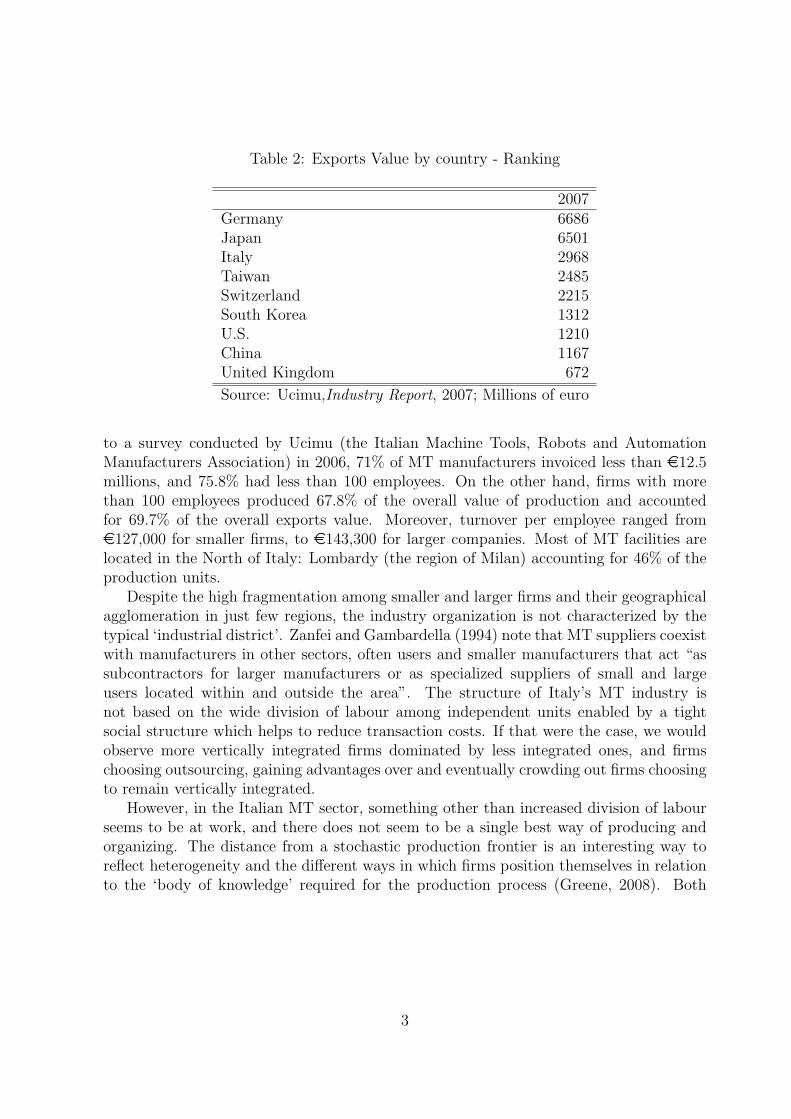
Table 2: Exports Value by country - Ranking

2007Germany 6686Japan 6501Italy 2968Taiwan 2485Switzerland 2215South Korea 1312U.S. 1210China 1167United Kingdom 672

Source: Ucimu,Industry Report, 2007; Millions of euro

to a survey conducted by Ucimu (the Italian Machine Tools, Robots and AutomationManufacturers Association) in 2006, 71% of MT manufacturers invoiced less than e12.5millions, and 75.8% had less than 100 employees. On the other hand, firms with morethan 100 employees produced 67.8% of the overall value of production and accountedfor 69.7% of the overall exports value. Moreover, turnover per employee ranged frome127,000 for smaller firms, to e143,300 for larger companies. Most of MT facilities arelocated in the North of Italy: Lombardy (the region of Milan) accounting for 46% of theproduction units.

Despite the high fragmentation among smaller and larger firms and their geographicalagglomeration in just few regions, the industry organization is not characterized by thetypical ‘industrial district’. Zanfei and Gambardella (1994) note that MT suppliers coexistwith manufacturers in other sectors, often users and smaller manufacturers that act “assubcontractors for larger manufacturers or as specialized suppliers of small and largeusers located within and outside the area”. The structure of Italy’s MT industry isnot based on the wide division of labour among independent units enabled by a tightsocial structure which helps to reduce transaction costs. If that were the case, we wouldobserve more vertically integrated firms dominated by less integrated ones, and firmschoosing outsourcing, gaining advantages over and eventually crowding out firms choosingto remain vertically integrated.

However, in the Italian MT sector, something other than increased division of labourseems to be at work, and there does not seem to be a single best way of producing andorganizing. The distance from a stochastic production frontier is an interesting way toreflect heterogeneity and the different ways in which firms position themselves in relationto the ‘body of knowledge’ required for the production process (Greene, 2008). Both

3

vertical integration and outsourcing represent different ways of organizing how inputs aretransformed into outputs. From a study of the relationship between vertical integration,outsourcing and efficiency, we gain some insight into how heterogeneous firms coexist inthe market. Our study of efficiency and its relationship to vertical integration, show: first,that vertically integrated firms draw on the frontier technology; second, that less efficientfirms are not crowded out; third, that outsourcing has a different impact on efficiency,depending on the level of vertical integration. We interpret these results as that lessintegrated and less efficient firms trade off the need for flexibility, which is typical ofall sectors characterized by high levels of customization and volatility. Heterogeneousfirms can complement or compete with each other, depending on the context, which mayhighlight the value of complementarity, or make some technological characteristics moreimportant, such as occurs in downward phases of the economic cycle.

The paper is structured as follows. Section 2 provides the basic framework for theanalysis, and presents the hypotheses to be tested. Section 3 describes the stochasticfrontier model. Section 4 describes the data. Section 5 discusses the results of the analysis.Section 6 offers some conclusions and suggestions for further research.

2 Basic framework and hypotheses

2.1 Vertical integration and outsourcing in the Italian MT in-dustry

The vertical structure of the Italian MT industry took different configurations since the1950s (see Rolfo, 1998, 2000). At that time, alongside firms that were specialized inmarket-oriented MT manufacture, the most important mechanical engineering firms pro-duced their own MT in-house (from foundry to finished products) thus the prevailingmodel was that of vertically integrated firms. The 1960s saw, a significant increase ininternal demand stimulated the growth of an independent MT industry and the 1970swere characterized by the small firm model, and a consequent vertical dis-integration offirms: electronic and computer components tended to be outsourced. Altough there havebeen with slight deviation over time, this low level of vertical integration has tended todominate for the majority of Italian MT firms2. Presently, MT builders basically ‘leaveto the outside’ the manufacture of standardized components (mainly electronics) and,sometimes, also machine design and software planning. The vertical position of the firmalong the production chain, therefore, is a key dimension in this industry, which hasconsequences both for firms’ productive efficiency, and also control of the knowledge and

2Italian manufacturing firms have traditionally showed lower levels of vertical integration than theircounterparts in other European countries e.g. Germany and the UK (see Arrighetti, 1999).

4

innovation processes (Poledrini, 2008).

2.2 Technical efficiency as measure of organizational hetero-geneity

An output-oriented measure of technical efficiency evaluates the ability of the firm to avoidwaste by producing as much output as input usage allows3. Thus, technical efficiency isan indicator of firm performance, and empirical studies show that, at different levels ofdisaggregation, some firms are efficient while others operate behind the frontier. Basedon reliable firm level measures of efficiency, empirical analysis helps us to identify factorsthat influence the variations in efficiency among similar economic units4.

Despite the large body of empirical evidence, there is no single theoretical model iden-tifying the determinants of technical efficiency (Lovell, 1993; Fried, Lovell, and Schmidt,2008). Observation of firms behind the estimated production frontier contrasts with theexpected behaviour of a maximizing agent5(see Pozzana and Zaninotto, 1989). The em-pirical observation of inefficiency is generally attributed to two aspects. The first isnon–observed inputs or outputs. The case of non–observed factors is justified by thenon–observable quality of inputs or outputs, different access to externalities, or other notaccounted for inputs. The existence of Marshallian externalities might explain the higherefficiency of small firms located in industrial districts with respect to outside districtfirms6. The second group of determinants is represented by a combination of pure ineffi-ciency and market power. Some form of X-Inefficiency a la Leibenstein (1966), or non–costminimizing behaviour due, for instance, to managerial goals (Shleifer and Vishny, 1986)(i.e. conflicts between ownership and management), could combine with market imper-fection to explain the persistence of non–efficient units.

3Koopmans (1951) first defined the concept technical efficiency; Debreu (1951) and Shepard (1953)defined an output (input) oriented measure of efficiency, as the maximum equiproportional increment(decrement) of all outputs (inputs), taking the value of inputs (outputs) as constant. Farrell (1957) wasthe first to measure productive efficiency empirically: he first defined cost efficiency, and then decomposeit into its technical and allocative components, providing an empirical application to US agriculture usinglinear programming techniques.

4Kumbhakar and Lovell (2000, p.261) writes that “The analysis of productive efficiency [. . . ] shouldhave, two components. The first is the estimation of a stochastic production (or cost or profit or other)frontier [. . . ]. [t]he second component is to associate variation in producer performance with variation inthe exogenous variables characterizing the environment in which production occurs”.

5Greene (1993, p.70) writes that: “Strictly speaking, an orthodox reading of microeconomics rulesout Farrell’s interpretation. A competitive market in equilibrium would not tolerate inefficiency the sortconsidered here.”

6E.g., estimating stochastic production frontiers for firms belonging to 13 Italian manufacturingindustries, Fabiani, Pellegrini, Romagnano, and Signorini (1998) find that firms located in industrialdistricts are more efficient than non district firms.

5

However, neither non–observability, nor pure inefficiency explain why the different de-grees of inefficiency among firms in similar environments, and operating in markets wherecompetitive pressures are high (in 2006, 56% of Italian MT production was exported).Our hypothesis is that different degrees of efficiency, i.e. different distances from the pro-duction frontier, may be an empirical reflection of organizational heterogeneity7. Differentcombinations in the production possibility set can persist due to their different proper-ties. Efficiency is just one dimension of the firm’s productive performance, which has tobe traded off against other characteristics, such as flexibility, i.e. the ability to producesmall batches without incurring high costs, or to modify production plans. While produc-tion theory generally assumes homogeneous firms, each of which selects the organizationthat best trades off its particular economic features, we observe a mix of heterogeneousfirms which may be either complementary or competing. Different firms can survive andadapt reciprocally to each other according to how competitive environment is evolving.In the present study we use distance from the production frontier, usually interpreted asa measure of inefficiency, to identify a particular form of heterogeneity that can be relatedto different motivations for firm behaviour8.

Thus, we hypothesize that competitiveness is based on the survival of heterogeneousorganizations acting on the same set of technical possibilities: firms using frontier input-output combinations do not compete directly with firms behind the frontier, but takeadvantage of proximity. We define this as a sort of complementarity among productivecombinations: less efficient technologies can be used to complement the production mix,respond in a timely way to market requests and buffer productions cycles. This comple-mentarity is specially important in sectors as MT, where customization is very importantand demand is very volatile.

2.3 Vertical integration, outsourcing and efficiency

Vertical integration is a measure of the degree to which a firm ‘controls’ the upstream anddownstream phases of the production process, and outsourcing is the change in the level ofvertical integration. According to transaction costs economics (Williamson, 1971, 1975),keeping the institutional environment fixed, and controlling for the economic contextin which firms operate, different levels of vertical integration should be related to thespecificity of upward inputs. Firms can choose to manage technologies internally relying

7Obviously, all observation specific characteristics which cannot be taken into account (because oflack of information) will affect the estimated inefficiency —which is a part of the overall residual—, i.e.the estimated distances to the frontier. Management skills and some forms of externalities (other thanthose enjoyed by industrial district firms) can be natural candidates. See 4.2 for further discussion of thisissue.

8See Greene (2008, par. 2.6) for a detailed discussion of the different forms of heterogeneity that canbe identified using a stochastic frontier model.

6

on specific upward investments, or can acquire inputs through the market, risking ofeither wasting resources in transaction or using less specific inputs. In the transactioncosts economics and property rights tradition, the area under the control of the firm,and the borders between the market and the hierarchy of firms are dictated by a trade offbetween the advantages of using specific inputs, and the costs of managing bilateral powerwith incomplete contracts (Hart and Moore, 1990). In our approach, different choicescan complement each other: for instance, inferior (from the point of view of efficiency)organizations can conduct fundamental activities in the context of a competitive sector.Thus we can formulate the following hypothesis :

H1: Vertically integrated firms define the efficiency frontier, because they are able tomanage specific inputs. The observed distance from the production function (measure ofinefficiency) is not fully explained by the economies of agglomeration (hidden inputs), orby ownership structure: persistent inefficiency measures are related to vertical integration.

An indirect test of the organizational heterogeneity hypothesis comes from the studyof the dynamics of vertical integration, i.e. the choice to outsource. Outsourcing isjustified either by production cost savings, based on the economies of scale enjoyed bythe external supplier predicted by the industrial organization literature, or by lower inputspecificity (as transaction cost economics claim), or on both. Globalization and newtechnologies impact on both these aspects and, in general, we can expect a positiverelationship between outsourcing and productivity 9. The organizational heterogeneityhypothesis, however is coherent with the possibility of a non–linear relationship betweenoutsourcing and efficiency. This means that, as a result of external changes, organizationalchoices might diverge rather than converge. Our second hypothesis is as follows:

H2: Organizational heterogeneity means that the impact of outsourcing on firmsefficiency may not to be uniform.

3 The stochastic frontier model

3.1 A double heteroskedastic model

In order to investigate the relationship between firm efficiency and the firm’s choicesregarding vertical organization, we exploit the following stochastic production frontier

9Some measurement and econometric issues concerning the relationship between outsourcing andproductivity are reviewed by Hashmati (2003); a survey of the empirical studies on the relationshipbetween productivity, outsourcing and offshoring can be found in Olsen (2006)

7

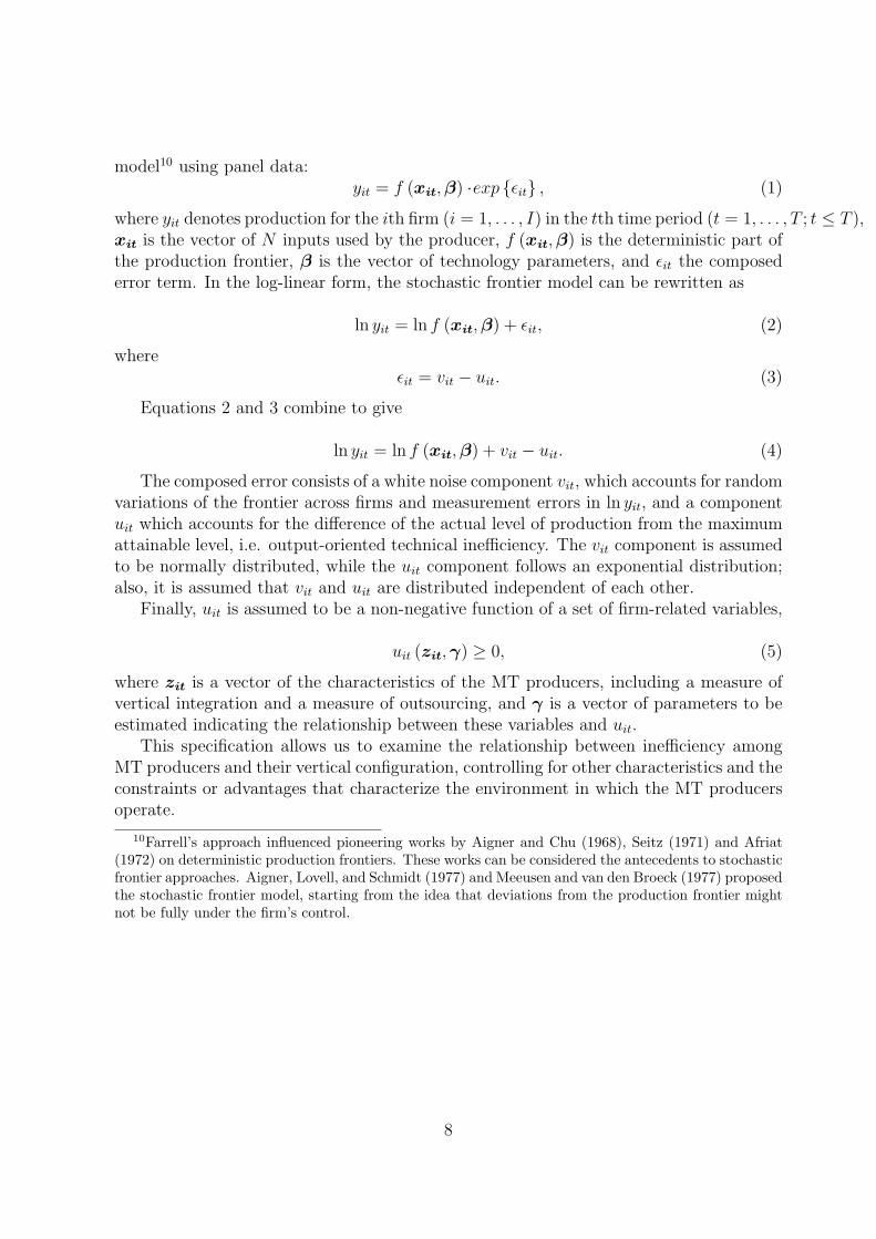
model10 using panel data:yit = f (xit,β) ·exp {εit} , (1)

where yit denotes production for the ith firm (i = 1, . . . , I) in the tth time period (t = 1, . . . , T ; t ≤ T ),xit is the vector of N inputs used by the producer, f (xit,β) is the deterministic part ofthe production frontier, β is the vector of technology parameters, and εit the composederror term. In the log-linear form, the stochastic frontier model can be rewritten as

ln yit = ln f (xit,β) + εit, (2)

whereεit = vit − uit. (3)

Equations 2 and 3 combine to give

ln yit = ln f (xit,β) + vit − uit. (4)

The composed error consists of a white noise component vit, which accounts for randomvariations of the frontier across firms and measurement errors in ln yit, and a componentuit which accounts for the difference of the actual level of production from the maximumattainable level, i.e. output-oriented technical inefficiency. The vit component is assumedto be normally distributed, while the uit component follows an exponential distribution;also, it is assumed that vit and uit are distributed independent of each other.

Finally, uit is assumed to be a non-negative function of a set of firm-related variables,

uit (zit,γ) ≥ 0, (5)

where zit is a vector of the characteristics of the MT producers, including a measure ofvertical integration and a measure of outsourcing, and γ is a vector of parameters to beestimated indicating the relationship between these variables and uit.

This specification allows us to examine the relationship between inefficiency amongMT producers and their vertical configuration, controlling for other characteristics and theconstraints or advantages that characterize the environment in which the MT producersoperate.

10Farrell’s approach influenced pioneering works by Aigner and Chu (1968), Seitz (1971) and Afriat(1972) on deterministic production frontiers. These works can be considered the antecedents to stochasticfrontier approaches. Aigner, Lovell, and Schmidt (1977) and Meeusen and van den Broeck (1977) proposedthe stochastic frontier model, starting from the idea that deviations from the production frontier mightnot be fully under the firm’s control.

8

Different models have been proposed to take account of the effects of ‘third variables’zit

11. From a methodological point of view, a preference for a one-step estimation strategyin which frontier parameters, inefficiency scores and the effects of ‘third variables’ oninefficiency are jointly estimated is justified by Wang and Schmidt (2002): this is theapproach adopted in the present work. One method is to directly specify the distributionparameters of uit as functions of the firm-related variables, and then to estimate allthe parameters in the model (technology parameters of the frontier function plus allparameters of the inefficiency equation) via maximum likelihood (ML) estimation. Severalmodels have been proposed in which either the mean (Huang and Liu, 1994; Batteseand Coelli, 1995), or the variance (Caudill, Ford, and Gropper, 1995) of the inefficiencydistribution is modelled. Wang (2003) proposes a model in which both the mean andthe variance of the inefficiency distribution are allowed to be functions of a set a set offirm-related variables.

In this paper, we adopt a specification in which the variance of uit depends on a setof firm specific variables and the variance of vit (noise) is a function of a firm-relatedvariable, i.e. firm size.

We can write these assumptions as

vit ∼ N(0, σ2vit), (6)

anduit ∼ Exp(ηit), (7)

where ηit is the scale parameter of the exponential distribution. The error componentsdiffer among production units in terms of variance parameters, thus the model is het-eroskedastic for both error terms.

We chose to implement a double heteroskedastic frontier model for two reasons. First,as Italian MT producers are highly heterogeneous with respect to the dimensions of in-terest, namely the vertical integration structure and the outsourcing process, inefficiency(uit) is allowed to change according to variations in these characteristics through thevariance parameter of the exponential distribution. Figure 1 and Table 3 show that theMT producers in the sample are heterogeneous in terms of vertical (dis)integration andoutsourcing12. Even though MT producers, on average tend to demonstrate high degrees

11This type of heterogeneity is referred to as ‘observable’ heterogeneity because it is reflected inobservable firm-related variables. ‘Unobserved’ heterogeneity, on the other hand, refers to time-invariantunobserved firm characteristics (Greene, 2008).

12The measure of vertical disintegration is equal to the sum of the costs for acquired intermediates andservice over total costs of production: a value of 1, means that the firm depends on external suppliers foralmost all of its production inputs; 0 or near 0 means that the firm bases its production on its own capitaland labour, i.e. its is vertically integrated. The measure of outsourcing is computed as the differencebetween the degrees of vertical disintegration in 2007 and the same measure in 2005: thus, it can be

9

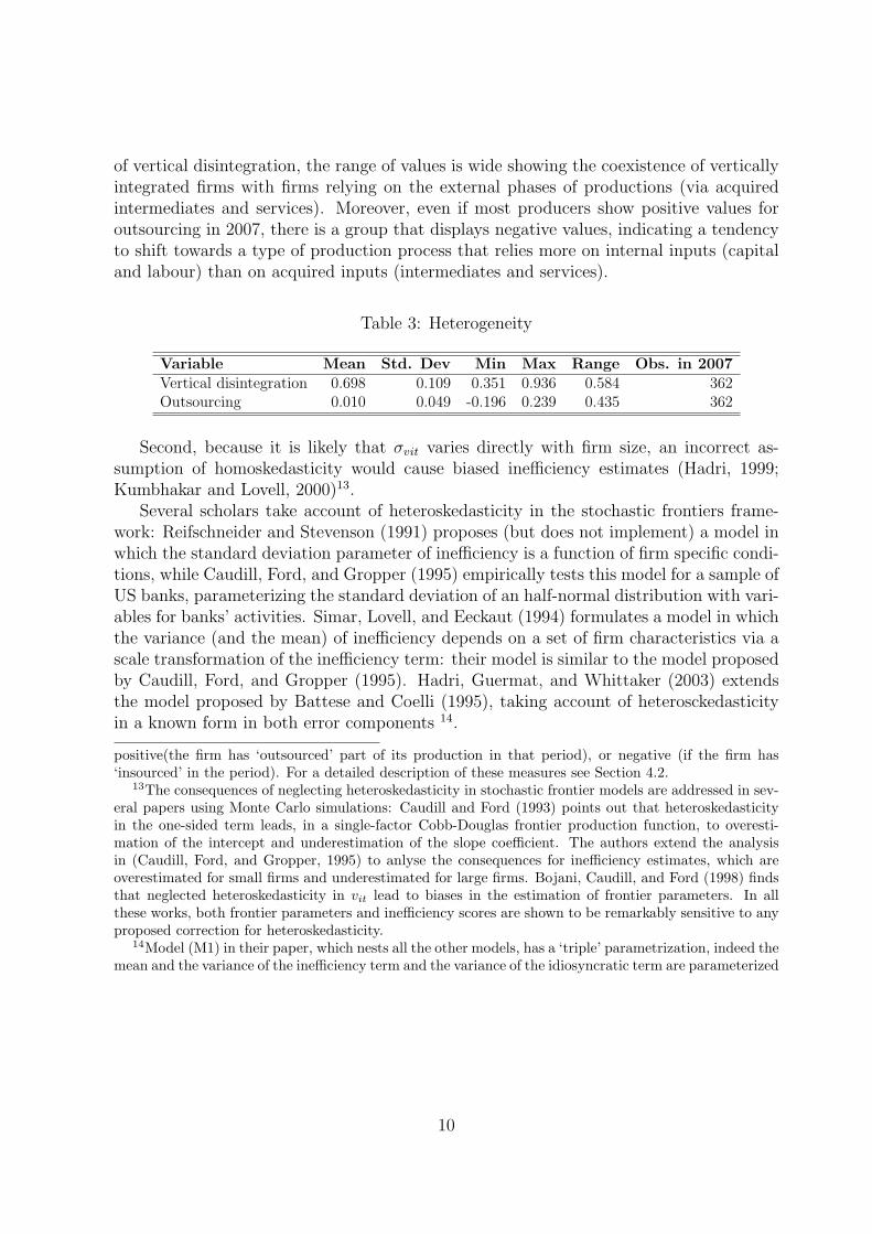
of vertical disintegration, the range of values is wide showing the coexistence of verticallyintegrated firms with firms relying on the external phases of productions (via acquiredintermediates and services). Moreover, even if most producers show positive values foroutsourcing in 2007, there is a group that displays negative values, indicating a tendencyto shift towards a type of production process that relies more on internal inputs (capitaland labour) than on acquired inputs (intermediates and services).

Table 3: Heterogeneity

Variable Mean Std. Dev Min Max Range Obs. in 2007Vertical disintegration 0.698 0.109 0.351 0.936 0.584 362Outsourcing 0.010 0.049 -0.196 0.239 0.435 362

Second, because it is likely that σvit varies directly with firm size, an incorrect as-sumption of homoskedasticity would cause biased inefficiency estimates (Hadri, 1999;Kumbhakar and Lovell, 2000)13.

Several scholars take account of heteroskedasticity in the stochastic frontiers frame-work: Reifschneider and Stevenson (1991) proposes (but does not implement) a model inwhich the standard deviation parameter of inefficiency is a function of firm specific condi-tions, while Caudill, Ford, and Gropper (1995) empirically tests this model for a sample ofUS banks, parameterizing the standard deviation of an half-normal distribution with vari-ables for banks’ activities. Simar, Lovell, and Eeckaut (1994) formulates a model in whichthe variance (and the mean) of inefficiency depends on a set of firm characteristics via ascale transformation of the inefficiency term: their model is similar to the model proposedby Caudill, Ford, and Gropper (1995). Hadri, Guermat, and Whittaker (2003) extendsthe model proposed by Battese and Coelli (1995), taking account of heterosckedasticityin a known form in both error components 14.

positive(the firm has ‘outsourced’ part of its production in that period), or negative (if the firm has‘insourced’ in the period). For a detailed description of these measures see Section 4.2.

13The consequences of neglecting heteroskedasticity in stochastic frontier models are addressed in sev-eral papers using Monte Carlo simulations: Caudill and Ford (1993) points out that heteroskedasticityin the one-sided term leads, in a single-factor Cobb-Douglas frontier production function, to overesti-mation of the intercept and underestimation of the slope coefficient. The authors extend the analysisin (Caudill, Ford, and Gropper, 1995) to anlyse the consequences for inefficiency estimates, which areoverestimated for small firms and underestimated for large firms. Bojani, Caudill, and Ford (1998) findsthat neglected heteroskedasticity in vit lead to biases in the estimation of frontier parameters. In allthese works, both frontier parameters and inefficiency scores are shown to be remarkably sensitive to anyproposed correction for heteroskedasticity.

14Model (M1) in their paper, which nests all the other models, has a ‘triple’ parametrization, indeed themean and the variance of the inefficiency term and the variance of the idiosyncratic term are parameterized

10

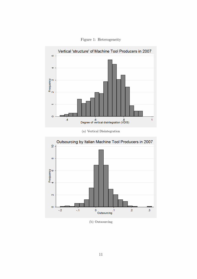
Figure 1: Heterogeneity

(a) Vertical Disintegration

(b) Outsourcing

11

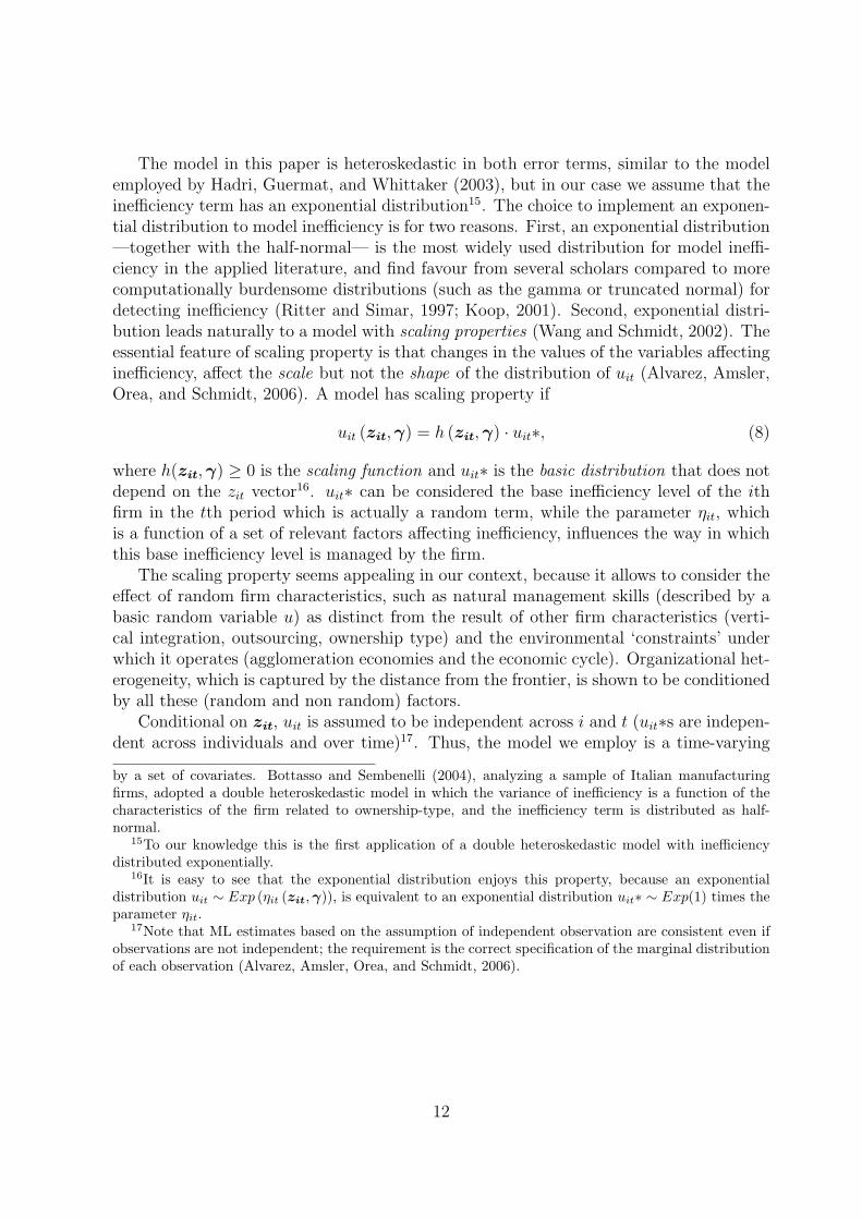
The model in this paper is heteroskedastic in both error terms, similar to the modelemployed by Hadri, Guermat, and Whittaker (2003), but in our case we assume that theinefficiency term has an exponential distribution15. The choice to implement an exponen-tial distribution to model inefficiency is for two reasons. First, an exponential distribution—together with the half-normal— is the most widely used distribution for model ineffi-ciency in the applied literature, and find favour from several scholars compared to morecomputationally burdensome distributions (such as the gamma or truncated normal) fordetecting inefficiency (Ritter and Simar, 1997; Koop, 2001). Second, exponential distri-bution leads naturally to a model with scaling properties (Wang and Schmidt, 2002). Theessential feature of scaling property is that changes in the values of the variables affectinginefficiency, affect the scale but not the shape of the distribution of uit (Alvarez, Amsler,Orea, and Schmidt, 2006). A model has scaling property if

uit (zit,γ) = h (zit,γ) · uit∗, (8)

where h(zit,γ) ≥ 0 is the scaling function and uit∗ is the basic distribution that does notdepend on the zit vector16. uit∗ can be considered the base inefficiency level of the ithfirm in the tth period which is actually a random term, while the parameter ηit, whichis a function of a set of relevant factors affecting inefficiency, influences the way in whichthis base inefficiency level is managed by the firm.

The scaling property seems appealing in our context, because it allows to consider theeffect of random firm characteristics, such as natural management skills (described by abasic random variable u) as distinct from the result of other firm characteristics (verti-cal integration, outsourcing, ownership type) and the environmental ‘constraints’ underwhich it operates (agglomeration economies and the economic cycle). Organizational het-erogeneity, which is captured by the distance from the frontier, is shown to be conditionedby all these (random and non random) factors.

Conditional on zit, uit is assumed to be independent across i and t (uit∗s are indepen-dent across individuals and over time)17. Thus, the model we employ is a time-varying

by a set of covariates. Bottasso and Sembenelli (2004), analyzing a sample of Italian manufacturingfirms, adopted a double heteroskedastic model in which the variance of inefficiency is a function of thecharacteristics of the firm related to ownership-type, and the inefficiency term is distributed as half-normal.

15To our knowledge this is the first application of a double heteroskedastic model with inefficiencydistributed exponentially.

16It is easy to see that the exponential distribution enjoys this property, because an exponentialdistribution uit ∼ Exp (ηit (zit,γ)), is equivalent to an exponential distribution uit∗ ∼ Exp(1) times theparameter ηit.

17Note that ML estimates based on the assumption of independent observation are consistent even ifobservations are not independent; the requirement is the correct specification of the marginal distributionof each observation (Alvarez, Amsler, Orea, and Schmidt, 2006).

12

inefficiency model in which inefficiency does not vary over time in a systematic way (seeGreene, 2008, p.156)18.

The probability density function of uit is:

f (uit) =1

ηit

· exp{−uit

ηit

}, (9)

with E (uit) = Sd (uit) = ηit and V ar (uit) = η2it.

With the above distributional assumptions on uit and vit, it is possible to write thedensity function of the composed error term f(εit) as a generalization of the Normal-Exponential model presented by Meeusen and van den Broeck (1977) and Aigner, Lovell,and Schmidt (1977):

f (εit) =1

ηit

· Φ(− εitσvit

− σvit

ηit

)· exp

(εitηit

+σ2

vit

2η2it

), (10)

where Φ is the standard normal cumulative distribution function, ηit is the standarddeviation of the inefficiency component, σvit the standard deviation of the idiosyncraticpart and εit = yit − xit

′β.We assume that

η2it = g(z2γ) (11)

andσ2

vit = f(z1δ), (12)

where z2 includes the measures of firm vertical disintegration and outsourcing as wellas several controls and z1 is a measure of firm size, while δ and γ are vectors of theparameters to be estimated.

Thus, the log-likelihood function, lnL (y|β, δ, γ), can be written as:

I∑i=1

t≤T∑t=1

(− log

(√g(z2, γ)

))+

I∑i=1

t≤T∑t=1

log

[Φ

(−εit√f(z1, δ)

−√f(z1, δ)√g(z2, γ)

)]+

+I∑

i=1

t≤T∑t=1

εit√g(z2, γ)

+I∑

i=1

t≤T∑t=1

(f(z1, δ)2g(z2, γ)

), (13)

whereσ2

it = σ2vit + η2

it = f(z1, δ) + g(z2,γ), (14)

18This characteristic is shared by other models, e.g. Battese and Coelli (1995), and models developedfor the purpose of separating unobserved heterogeneity from inefficiency, e.g. the ‘true’ fixed effects modelsproposed by William Greene (Greene, 2005). (Cornwell, Schmidt, and Sickels, 1990; Kumbhakar, 1990;Battese and Coelli, 1992), on the other hand, propose models in which inefficiency has a parameterizedtime structure.

13

λi =ηit

σvit

=

√g(z2,γ)

f(z1, δ). (15)

Equation 13 can be maximized to obtain estimates of β, γ and δ; the estimates of γ andδ in turn can be used to obtain estimates of ηit and σvit.

3.2 Model specification

In order to estimate the parameters of the model via ML, we have to assume specific func-tional forms for the functions in Equations 4, 11 and 12. We adopt a translog specificationfor the production function frontier:

ln yit = α0 +∑

n

βn lnxnit +1

2

∑n

∑p

βnp lnxnit lnxpit + τt + αj + vit − uit, (16)

where n, p=(K, Capital; L, Labour; M Intermediate inputs and services). In order tocontrol for unobserved heterogeneity among firms producing different typologies of ma-chines, we include (j − 1) dummies αj in the frontier, where j = (1, . . . , 9) refers to thefirm’s main production (the principal type of machine). We control also for factors af-fecting all firms in the same way in a given year including (t− 1) year dummies τt. Theinclusion of ‘effects’ in the stochastic frontier allows us to differentiate between unobservedheterogeneity and time-variant inefficiency and, thus, correctly estimate the parametersof the production frontier19. In order to maximize (13) with respect to β, γ and δ, it isnecessary to assume some specific functional forms for (11) and (12).

Following Hadri (1999), we employ an exponential functional form to model variancesof the error components:

η2it = exp (z2γ) = exp(γ0 + γ1V DIS + γ2OUT + γ3SIZE+

γ4DOWNER + γ5DDIST + γ6DDOWN), (17)

where z2 denotes the measure of firm vertical disintegration, outsourcing, and includescontrols for firm size, ownership type, agglomeration economies and the economic cycle(the formal definition of these variables are given in Section 4.2) and

σ2vit = exp (z1δ) = exp(δ0 + δ1SIZE), (18)

where z1 is a measure of firm size. ML estimation is implemented in order to obtainjointly consistent and efficient estimates of the parameters in equations 16, 17 and 18, i.e.α, τ , β, δ and γ.

19Given that inefficiency estimates are conditional on overall residuals, if the frontier parametersestimates are inappropriate or inconsistent, then estimation of the inefficiency component, uit is likely tobe problematic.

14

4 The Data

4.1 Data sources

The database was compiled from several data sources. The list of MT producers is fromUcimu and includes information on firm’s main production20.

Information on output and inputs is from Bureau Van Dijk’s AIDA database, whichcontains balance sheet information for firms with turnovers over e500,000 (we were notable to recover balance sheet information for firms below that threshold). Information onthe ownership status is from the Bureau Van Dijk’s Ownership Database, and informationon district location was obtained by comparing the locations of local firm units — con-tained in AIDA— with the list of Italian Labor Local Systems (LLS) regularly updated bythe Italian National Institute of Statistics, ISTAT 21. Deflators for output, intermediateinputs and capital stock respectively, were computed from the Value of Production andInvestments series published by Istat annually at the sectoral level (2-digit level), 22.

4.2 Description of the variables

Variables for the production frontier

The output (Y ) is measured by the amount of revenues from sales and services at theend of the year, net of inventory changes and changes to contract work in progress. Thismeasure is deflated in order to account for price variations during a years. The deflatorwas built at the 2-digit level (Ateco 2007 classification) and is equal to the ratio of thevalue of production at current prices, in a given year, over the corresponding value in thechained level series23. The measure is expressed in e’000.

The labour input (L) is measured as the total number of employees at the end ofthe year. Capital stock (K) in a given year is proxied by the nominal value of tangiblefixed assets, which is deflated using the ratio of gross fixed investments at current pricesover corresponding values in the chained level series (base year 2000). Given the unavail-ability of series at the 2-digit level, we use a common deflator for all firms (investmentsfor aggregate C-D-E Ateco 2007 Industry sectors). The measure is expressed in e’000.Intermediate inputs (M) are measured as the sum of (i) costs of raw, materials consumedand goods for resale (net of changes in inventories) plus (ii) costs of services. The measureis deflated by the same deflator applied to output. It is expressed in e’000.

20Note that the list does not include only Ucimu associates, it includes all firms covered by surveysand research questionnaires administered by the Association. There are almost 550 firms on this list.

21http://www.istat.it.22http://www.istat.it/conti/nazionali/.23The base year for the chained series is 2000.

15

All inputs and the output are included in logs for the production frontier.

Variables affecting inefficiency

The degree of vertical disintegration (V DIS) is measured as the ratio of intermediateinputs (M) over total costs of production for the year. For the ith firm in the tth timeperiod, this can be written as:

V DISit =CRM,it + CS,it

CRM,it + CS,it + CL,it + CK,it + CO,it

(19)

where CRM,it is the cost of raw, materials consumption and goods for resale (net of changesin inventories), CS,it is the cost of services, CL,it is total personnel costs, CK,it is totaldepreciation, amortization and write downs (thus it can be interpreted as the figurativecost of capital) and CO,it is a residual class, which is a negligible portion of the total costsof production and can be considered equal to zero for the purpose of the present analysis.This ratio is an indicator of the relative ‘weight’ of the factors of production external tothe firm (i.e. acquired from other firms), over all factors of production including labourand capital.

This measure is related to that proposed in the international trade literature by Feen-stra and Hanson (1996, p.241): the authors suggest share of imported intermediate inputsto total purchases of non-energy materials as a measure of outsourcing, reflecting the ideathat the more a firm (industry) purchases (imports) inputs from other firms (industries)with respect to its total costs (purchases), the more its vertical structure shrinks. Thismeasure is also related to the ratio of value added to sales, proposed by Adelman (1955)as a measure of vertical integration.

Adelman’s index has been criticized mostly for the problems involved in applying itin cross-industry studies24 and its asymmetry25. In the case analyzed in this paper, ourmeasure should not be so problematic. First, the Italian MT industry is a quite narrowlydefined industry so there should be no cross-industry problems. The major drawback isthat we do not have information on prices, thus we cannot control explicitly for the likelydifferent unitary costs which may be faced by different firms in the sample. This couldresult in incorrect assignation of the different degrees of vertical disintegration to firmswhich simply have to deal with different unitary costs. However, it is important to note

24The literature on the determinants and consequences of vertical integration make some proposalsto overcome these drawbacks, such as the use of other measures. See, e.g. the input/output matricesproposed by Maddigan (1981) to build a ‘vertical industry connection index’ for all industries in which thefirm operates, which was adapted in Acemoglu, Johnson, and Mitton (2009) to evaluate the determinantsof vertical integration within a cross-country perspective.

25Holding the ratio(VA/Sales) constant, firms near the end of the production chain (and final con-sumers) appear less integrated (Davies and Morris, 1995).

16

that capital and labour are part of the denominator and, for labour, given the well knownsalary ‘rigidities’ in the Italian labour market, it is not restrictive to assume wit = wjt forall firms i 6= j. For capital, it is reasonable to assume that the differences affecting varia-tions in CK,it among firms, depend on the amount of machines and equipment acquired26.Finally, differences in the costs of intermediates materials CRM,it and services CS,it amongfirms in the same year affect both the numerator and the denominator in the ratio, thusany price distortions should be smoothed.

For these reasons, the measure we use appears to be the best available solution to cap-ture the firms’ vertical structure, given the available data and in this context is preferredto Adelman’s index27.

Outsourcing (OUT ) is measured as the difference between the level of vertical disin-tegration, in year t and the level of vertical disintegration in year t− 2:

OUTi,t = V DISi,t − V DISi,t−2. (20)

If we consider outsourcing as a process that takes place over time, then a measurethat captures variations in the vertical structure of the firm (industry) over time shouldbe used. This is why we use a measure in differences for outsourcing. In order to capturesome sizeable changes in the vertical structure of the firms under analysis, we computetwo years differences for V DIS.

In some estimations, quartiles (DQUARTq) of the distribution of V DIS in year t− 1are employed as proxies for the firm’s vertical structure, instead of V DIS. One reasonfor this is to cope with a ‘reverse causality’ effect which could be at work in the model ofinefficiency (Equation 17), i.e. a firm could observe its inefficiency level in any year, whichcould have the effect of modifying the relative use of ‘external’ factors of production, thuschanging the V DIS level. This would create problems in the interpretation of our results.However, it is less likely that a firm not near the quantile threshold, would be able tomodify its vertical structure so dramatically as to change its quartile position within thesame year or in the next year. The transitional probability matrix in Table 4 confirmsthis, showing low probability for MT producers belonging to a given quartile of the V DISdistribution moving to another quartile in the next year. This is especially true for thefirst (the most vertical integrated firms) and the fourth (the most vertical disintegratedfirms) quartile.

Moreover, this allows us to capture possible non–homogeneous effects of outsourcing,once we control for different classes of vertical structures. In fact, due to the heterogeneity

26In fact, year quota of depreciations and amortizations are computed following fiscal deductibilitypurposes, using the coefficients established by the Ministry of Economy and Finance at sectoral level —and thus are common to all firms belonging to the same sector— in the Ministerial Decree 31.12.1988.

27Moreover, given that the framework of our analysis is a stochastic production frontier model, vari-ables in the z could be functions of the inputs (x) but should not be functions of output (Alvarez, Amsler,Orea, and Schmidt, 2006), and Adelman’s measure is clearly a function of y.

17

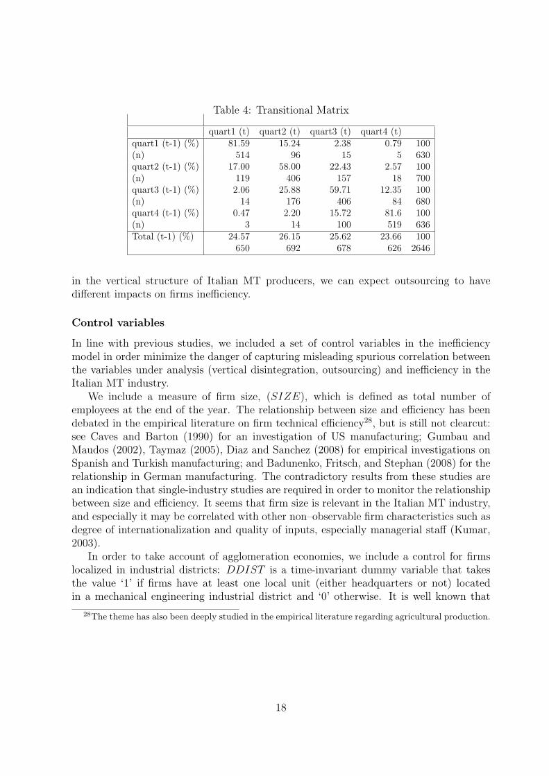
Table 4: Transitional Matrix

quart1 (t) quart2 (t) quart3 (t) quart4 (t)quart1 (t-1) (%) 81.59 15.24 2.38 0.79 100(n) 514 96 15 5 630quart2 (t-1) (%) 17.00 58.00 22.43 2.57 100(n) 119 406 157 18 700quart3 (t-1) (%) 2.06 25.88 59.71 12.35 100(n) 14 176 406 84 680quart4 (t-1) (%) 0.47 2.20 15.72 81.6 100(n) 3 14 100 519 636Total (t-1) (%) 24.57 26.15 25.62 23.66 100

650 692 678 626 2646

in the vertical structure of Italian MT producers, we can expect outsourcing to havedifferent impacts on firms inefficiency.

Control variables

In line with previous studies, we included a set of control variables in the inefficiencymodel in order minimize the danger of capturing misleading spurious correlation betweenthe variables under analysis (vertical disintegration, outsourcing) and inefficiency in theItalian MT industry.

We include a measure of firm size, (SIZE), which is defined as total number ofemployees at the end of the year. The relationship between size and efficiency has beendebated in the empirical literature on firm technical efficiency28, but is still not clearcut:see Caves and Barton (1990) for an investigation of US manufacturing; Gumbau andMaudos (2002), Taymaz (2005), Diaz and Sanchez (2008) for empirical investigations onSpanish and Turkish manufacturing; and Badunenko, Fritsch, and Stephan (2008) for therelationship in German manufacturing. The contradictory results from these studies arean indication that single-industry studies are required in order to monitor the relationshipbetween size and efficiency. It seems that firm size is relevant in the Italian MT industry,and especially it may be correlated with other non–observable firm characteristics such asdegree of internationalization and quality of inputs, especially managerial staff (Kumar,2003).

In order to take account of agglomeration economies, we include a control for firmslocalized in industrial districts: DDIST is a time-invariant dummy variable that takesthe value ‘1’ if firms have at least one local unit (either headquarters or not) locatedin a mechanical engineering industrial district and ‘0’ otherwise. It is well known that

28The theme has also been deeply studied in the empirical literature regarding agricultural production.

18

industrial districts are key socio-economic structures in the Italian industrial system (Be-cattini, 1990). Fabiani, Pellegrini, Romagnano, and Signorini (1998) found positive effectson efficiency for district location, for a sample of Italian manufacturing firms in the period1982 to 1995, and Becchetti, Panizza, and Oropallo (2008) shows that industrial districtfirms demonstrate higher value added per employee and higher export intensity.

In Italian MT industry, different decades are characterized by different ownershipforms. The 1980s were characterized by a structural strengthening of the industry viaexternal growth aimed at gaining control of the filiere (Rolfo, 1993). This tendency sloweddown in the first half of the 1990s, but was reinvigorated at the end of that decade, as MTbuilders tried to maintain control of the production process. During the second half ofthe 1990s, the mechanical engineering sector experienced a wave of mergers (Rolfo, 1998),designed to cope better with risk and to exploit market and production complementarities.This means that ownership structure is very relevant for an analysis of firm efficiency.First, because it can be a substitute for vertical integration, and second, in line withBottasso and Sembenelli (2004) controlling for the ownership structure is crucial, becausefirm efficiency is heavily driven by managerial effort, and seriously affected by conflictsbetween ownership (shareholders) and control (management) (Shleifer and Vishny, 1986).To control for type of ownership we included a dummy variable DOWNER)that takes thevalue ‘1’ if firms belong to an industrial group (either national or international), i.e.firmscontrolled by or controlling other firms with a share of ≥50%29.

Finally we include a dummy, DDOWN , for the years showing a downward trend inthe value of production , i.e. 2001, 2002 and 2003. Given the cyclical nature of the MTindustry, failing to control for the cycle could bias our estimates of the effect of outsourcingand vertical structure on inefficiency. Moreover, it allows us to investigate further effectof the economic cycle on firm efficiency, for different classes of vertical disintegration.Here, we have in mind that a kind of ‘trade-off’ between efficiency and flexibility couldbe operating in the industry in the period under analysis.

4.3 Descriptive statistics

Based on the reference list provided by Ucimu, we collected balance sheet data for 524firms and 5,240 observations from Bureau Van Dijk’s AIDA database. We discarded someobservations after a preliminary analysis which revealed missing values and outliers. First,we excluded observations with missing values for outputs, inputs and the variables in our

29This may be a restrictive threshold. Control over other firms may be possible even at much lowershares; also, in the Italian MT industry there are informal groups which are linked not just by ownershipof relevant shares quotas, but by familial links. However, this conservative measure of ownership controlensures a clear distinction between firms belonging to established groups and other firms (independent,or part of an informal group.

19

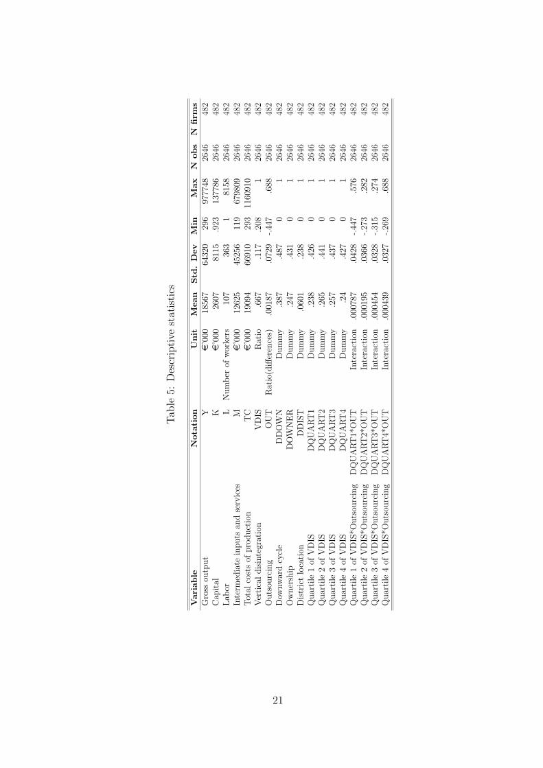
inefficiency model. The number of not usable observations is 2,002 (mostly due to theunavailability of information employee numbers). We conducted an ordinary least squares(OLS) estimation of the translog production function, and found that the residuals-versus-fitted plot revealed five more observations which had not been included in the frontieranalysis, due to their exceptional distance from the cloud of observations, i.e. observationswith standardized residuals > |5|). These preliminaries reduced number of firms in thesample 508 and 3,229 observations. We found that information on main productionwas missing for eight of these firms, which reduced the sample to 500 firms and 3,185observations. Finally, when we applied a measure in differences (with a 2-year lag) asa proxy for outsourcing, this means that observations in 1998 and 1999 could not beincluded in the estimation of the frontier (this applies also to d 1998 and d 1999 yeardummies). Our final sample is an unbalanced panel of 482 firms for the period 2000to 2007, and 2,646 usable observations. Table 5 presents descriptive statistics for theunbalanced panel; Table 6 presents a breakdown of the observations with respect to themain production of the firm.

As already highlighted in Section 3.1, the degree of heterogeneity in the variablesis high: this supports the choice of an heteroskedastic frontier model (Hadri, Guermat,and Whittaker, 2003; Laureti, 2008). Some of the descriptive evidence is in line withprevious research. First, Italian MT firms in our sample show high levels of verticaldisintegrations (.66) on average, and this is in line with previous results, e.g. Arrighetti(1999), which provides an analysis of vertical integration among Italian manufacturingfirms using the Adelman index, and shows an average degree of vertical integration of .35for mechanical engineering firms. Given that our measure of vertical disintegration can beconsidered the multiplicative inverse of Adelman, our descriptive statistics are in line withArrighetti’s results. In other studies on the MT industry, Rolfo (1998) underlines thatfrom 1995 onwards, Italian MT builders tried to strengthen their control over suppliers viaexternal growth and the establishment of small industrial groups. In our sample almost25% of firms belong to an industrial group (either a subsidiary or the holding company).Our descriptive statistics show that not all firms in the sample are actually engaged in‘outsourcing’, i.e. moving toward a greater use of acquired materials, intermediate goodsand services for their own production. Finally, in our sample only a small proportionof firms are localized in a mechanics industrial district, that is in line with the studiesreferred to above. The two largest product specializations are metal cutting machines (e.g.machining centres, lathes) and metal forming machines (presses, sheet metal deformationmachines).

20

Tab

le5:

Des

crip

tive

stat

isti

cs

Vari

able

Nota

tion

Unit

Mean

Std

.D

ev

Min

Max

Nobs

Nfirm

sG

ross

outp

ut

Ye

’000

1856

764

320

296

9777

4826

4648

2C

apit

alK

e’0

0026

0781

15.9

2313

7786

2646

482

Lab

orL

Nu

mb

erof

wor

kers

107

363

181

5826

4648

2In

term

edia

tein

pu

tsan

dse

rvic

esM

e’0

0012

625

4525

611

967

9809

2646

482

Tot

alco

sts

ofp

rod

uct

ion

TC

e’0

0019

094

6691

029

311

6091

026

4648

2V

erti

cal

dis

inte

grat

ion

VD

ISR

atio

.667

.117

.208

126

4648

2O

uts

ourc

ing

OU

TR

atio

(diff

eren

ces)

.001

87.0

729

-.44

7.6

8826

4648

2D

ownw

ard

cycl

eD

DO

WN

Du

mm

y.3

87.4

870

126

4648

2O

wn

ersh

ipD

OW

NE

RD

um

my

.247

.431

01

2646

482

Dis

tric

tlo

cati

onD

DIS

TD

um

my

.060

1.2

380

126

4648

2Q

uar

tile

1of

VD

ISD

QU

AR

T1

Du

mm

y.2

38.4

260

126

4648

2Q

uar

tile

2of

VD

ISD

QU

AR

T2

Du

mm

y.2

65.4

410

126

4648

2Q

uar

tile

3of

VD

ISD

QU

AR

T3

Du

mm

y.2

57.4

370

126

4648

2Q

uar

tile

4of

VD

ISD

QU

AR

T4

Du

mm

y.2

4.4

270

126

4648

2Q

uar

tile

1of

VD

IS*O

uts

ourc

ing

DQ

UA

RT

1*O

UT

Inte

ract

ion

.000

787

.042

8-.

447

.576

2646

482

Qu

arti

le2

ofV

DIS

*Ou

tsou

rcin

gD

QU

AR

T2*

OU

TIn

tera

ctio

n.0

0019

5.0

366

-.27

3.2

8226

4648

2Q

uar

tile

3of

VD

IS*O

uts

ourc

ing

DQ

UA

RT

3*O

UT

Inte

ract

ion

.000

454

.032

8-.

315

.274

2646

482

Qu

arti

le4

ofV

DIS

*Ou

tsou

rcin

gD

QU

AR

T4*

OU

TIn

tera

ctio

n.0

0043

9.0

327

-.26

9.6

8826

4648

2

21

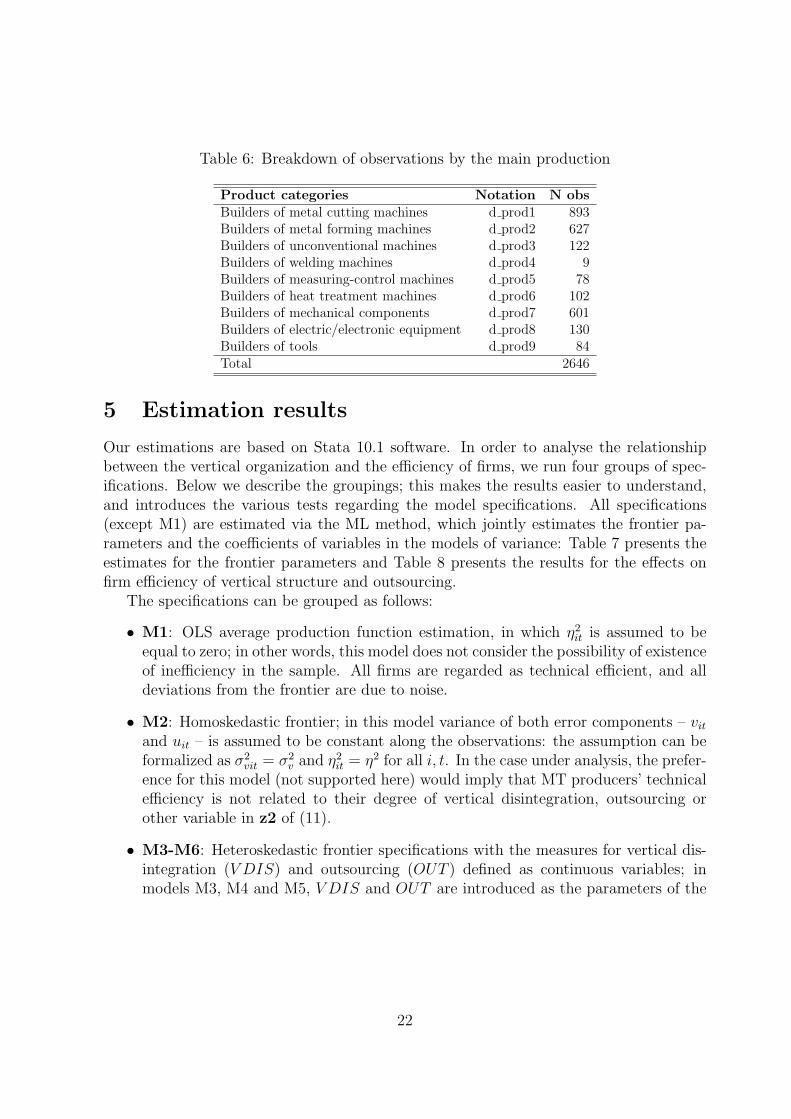
Table 6: Breakdown of observations by the main production

Product categories Notation N obsBuilders of metal cutting machines d prod1 893Builders of metal forming machines d prod2 627Builders of unconventional machines d prod3 122Builders of welding machines d prod4 9Builders of measuring-control machines d prod5 78Builders of heat treatment machines d prod6 102Builders of mechanical components d prod7 601Builders of electric/electronic equipment d prod8 130Builders of tools d prod9 84Total 2646

5 Estimation results

Our estimations are based on Stata 10.1 software. In order to analyse the relationshipbetween the vertical organization and the efficiency of firms, we run four groups of spec-ifications. Below we describe the groupings; this makes the results easier to understand,and introduces the various tests regarding the model specifications. All specifications(except M1) are estimated via the ML method, which jointly estimates the frontier pa-rameters and the coefficients of variables in the models of variance: Table 7 presents theestimates for the frontier parameters and Table 8 presents the results for the effects onfirm efficiency of vertical structure and outsourcing.

The specifications can be grouped as follows:

• M1: OLS average production function estimation, in which η2it is assumed to be

equal to zero; in other words, this model does not consider the possibility of existenceof inefficiency in the sample. All firms are regarded as technical efficient, and alldeviations from the frontier are due to noise.

• M2: Homoskedastic frontier; in this model variance of both error components – vit

and uit – is assumed to be constant along the observations: the assumption can beformalized as σ2

vit = σ2v and η2

it = η2 for all i, t. In the case under analysis, the prefer-ence for this model (not supported here) would imply that MT producers’ technicalefficiency is not related to their degree of vertical disintegration, outsourcing orother variable in z2 of (11).

• M3-M6: Heteroskedastic frontier specifications with the measures for vertical dis-integration (V DIS) and outsourcing (OUT ) defined as continuous variables; inmodels M3, M4 and M5, V DIS and OUT are introduced as the parameters of the

22

Tab

le7:

Fro

nti

erpar

amet

ers

esti

mat

ion

Model

M1

M2

M3

M4

M5

M6

M7

M8

Var

iable

Coeffi

cien

tC

oeffi

cien

tC

oeffi

cien

tC

oeffi

cien

tC

oeffi

cien

tC

oeffi

cien

tC

oeffi

cien

tC

oeffi

cien

tln

K0.

017

0.03

1*0.

031*

0.03

3**

0.03

2**

0.04

4***

0.04

3***

0.04

5***

(0.0

16)

(0.0

16)

(0.0

16)

(0.0

16)

(0.0

16)

(0.0

16)

(0.0

16)

(0.0

16)

lnL

0.83

6***

0.85

4***

0.85

3***

0.85

8***

0.84

7***

0.82

4***

0.81

8***

0.80

7***

(0.0

31)

(0.0

31)

(0.0

32)

(0.0

30)

(0.0

31)

(0.0

31)

(0.0

33)

(0.0

32)

lnM

0.09

5***

0.06

5*0.

065*

0.06

0*0.

071*

*0.

086*

*0.

094*

**0.

101*

**(0

.035

)(0

.035

)(0

.036

)(0

.035

)(0

.035

)(0

.035

)(0

.036

)(0

.036

)(.

5)(l

nK

)20.

008*

**0.

010*

**0.

010*

**0.

011*

**0.

011*

**0.

011*

**0.

011*

**0.

011*

**(0

.002

)(0

.002

)(0

.002

)(0

.002

)(0

.002

)(0

.002

)(0

.002

)(0

.002

)(.

5)(l

nL

)20.

115*

**0.

120*

**0.

120*

**0.

121*

**0.

119*

**0.

119*

**0.

119*

**0.

116*

**(0

.007

)(0

.007

)(0

.007

)(0

.006

)(0

.007

)(0

.007

)(0

.007

)(0

.007

)(.

5)(l

nM

)20.

142*

**0.

148*

**0.

148*

**0.

149*

**0.

148*

**0.

146*

**0.

144*

**0.

143*

**(0

.007

)(0

.007

)(0

.007

)(0

.007

)(0

.007

)(0

.007

)(0

.007

)(0

.007

)(l

nK

)·(ln

L)

0.00

50.

005

0.00

50.

005

0.00

50.

005

0.00

40.

004

(0.0

03)

(0.0

03)

(0.0

03)

(0.0

03)

(0.0

03)

(0.0

03)

(0.0

03)

(0.0

03)

(lnK

)·(ln

M)

-0.0

08**

*-0

.011

***

-0.0

11**

*-0

.011

***

-0.0

11**

*-0

.013

***

-0.0

13**

*-0

.013

***

(0.0

03)

(0.0

03)

(0.0

03)

(0.0

03)

(0.0

03)

(0.0

03)

(0.0

03)

(0.0

03)

(lnL

)·(ln

M)

-0.1

28**

*-0

.131

***

-0.1

31**

*-0

.132

***

-0.1

31**

*-0

.128

***

-0.1

26**

*-0

.125

***

(0.0

06)

(0.0

06)

(0.0

06)

(0.0

06)

(0.0

06)

(0.0

06)

(0.0

06)

(0.0

06)

Con

stan

t3.

113*

**3.

224*

**3.

222*

**3.

230*

**3.

200*

**3.

158*

**3.

143*

**3.

116*

**(0

.110

)(0

.108

)(0

.110

)(0

.107

)(0

.110

)(0

.108

)(0

.111

)(0

.110

)Y

ear

dum

mie

sY

esY

esY

esY

esY

esY

esY

esY

esM

ainP

rod

dum

mie

sY

esY

esY

esY

esY

esY

esY

esY

esL

og-l

ikel

ihood

2054

.333

2090

.120

2090

.124

2096

.801

2097

.592

2124

.225

2124

.562

2136

.057

Obse

rvat

ions

2646

2646

2646

2646

2646

2646

2646

2646

St.

err.

ofco

effici

ents

inpar

enth

eses

Sig

nifi

cance

leve

ls:

*10

%,

**5%

,***

1%Y

ear

and

Mai

nP

rod

par

amet

ers

omit

ted.

Com

ple

teta

ble

avai

lable

up

onre

ques

t

23

Table 8: Inefficiency model

Model M2 M3 M4 M5 M6 M7 M8ln(η2) functionVDIS 0.083 1.68 2.136**

(0.858) (0.934) (0.974)OUT -4.151*** -4.681*** -6.205*** -4.650***

(1.234) (1.349) (1.507) (1.311)SIZE 8.6×10−5 8.4×10−5 2.6×10−5

(2.4×10−4) (2.6×10−4) (2.5×10−4)DOWNER -0.700*** -0.736*** -0.937***

(0.241) (0.243) (0.330)DDIST -1.316** -1.388** -1.365*

(0.667) (0.704) (0.766)DDOWN -1.619*** -1.386*** -1.440***

(0.513) (0.418) (0.461)DQUART2 0.557** 0.574

(0.275) (0.392)DQUART3 0.579** 0.857**

(0.294) (0.408)DQUART4 0.498 0.857*

(0.345) (0.469)DQUART1·OUT 3.225

(3.235)DQUART2·OUT -12.554***

2.711DQUART3·OUT -4.760*

(2.850)DQUART4·OUT 0.229

(2.556)Constant -6.082*** -6.136*** -6.187*** -6.966*** -7.059*** -6.075*** -6.459***

(0.140) (0.578) (0.160) (0.656) (0.683) (0.291) (0.433)ln(sigv2) functionSIZE -2.7×10−4** -3.1×10−4* -2.7×10−4**

(1.2×10−4) (1.7×−4) (1.2×10−4)Constant -4.632*** -4.632*** -4.625*** -4.622*** -4.595*** -4.596*** -4.574***

(0.038) (0.038) (0.038) (0.039) (0.041) (0.042) (0.041)Observations 2646 2646 2646 2646 2646 2646 2646Year dummies Yes Yes Yes Yes Yes Yes YesMainProd dummies Yes Yes Yes Yes Yes Yes YesLog-likelihood 2090.120 2090.124 2096.801 2097.592 2124.225 2124.562 2136.057St. err. of coefficients in parenthesesSignificance levels: * 10%, ** 5%,*** 1%

variance of inefficiency either separately (in M3 and M4) or jointly (model M5).Model M6, which nests the other three models plus the homoskedastic frontier, in-troduces controls to account for spurious correlations among the variables underanalysis and firm inefficiency.

• M7-M8: Heteroskedastic frontier specifications with dummies for groups of firmswith different degrees of vertical disintegration and their interaction effects withOUT . Model M8, which nests M7, allows us to identify if there exist non-lineareffects of outsourcing on firm efficiency.

Generalized likelihood ratio tests of the form LR = −2 [lnL(H0)− lnL(H1)] ∼ χ2J

30 can

30J is the number of restrictions: see (Coelli, Rao, O’Donnell, and Battese, 2005, pp.258-259) for a

24

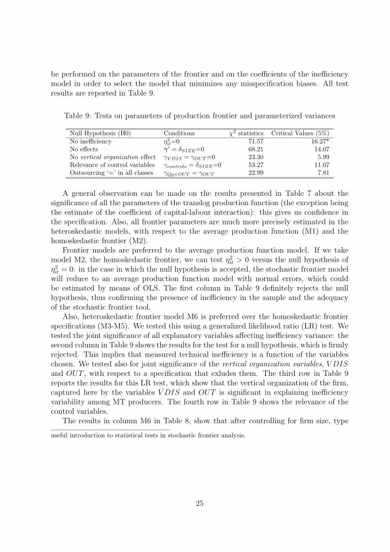
be performed on the parameters of the frontier and on the coefficients of the inefficiencymodel in order to select the model that minimizes any misspecification biases. All testresults are reported in Table 9.

Table 9: Tests on parameters of production frontier and parameterized variances

Null Hypothesis (H0) Conditions χ2 statistics Critical Values (5%)No inefficiency η2

it=0 71.57 16.27*No effects γ′ = δSIZE=0 68.21 14.07No vertical organization effect γV DIS = γOUT =0 23.30 5.99Relevance of control variables γcontrols = δSIZE=0 53.27 11.07Outsourcing ‘=’ in all classes γQq×OUT = γOUT 22.99 7.81

A general observation can be made on the results presented in Table 7 about thesignificance of all the parameters of the translog production function (the exception beingthe estimate of the coefficient of capital-labour interaction): this gives us confidence inthe specification. Also, all frontier parameters are much more precisely estimated in theheteroskedastic models, with respect to the average production function (M1) and thehomoskedastic frontier (M2).

Frontier models are preferred to the average production function model. If we takemodel M2, the homoskedastic frontier, we can test η2

it > 0 versus the null hypothesis ofη2

it = 0: in the case in which the null hypothesis is accepted, the stochastic frontier modelwill reduce to an average production function model with normal errors, which couldbe estimated by means of OLS. The first column in Table 9 definitely rejects the nullhypothesis, thus confirming the presence of inefficiency in the sample and the adequacyof the stochastic frontier tool.

Also, heteroskedastic frontier model M6 is preferred over the homoskedastic frontierspecifications (M3-M5). We tested this using a generalized likelihood ratio (LR) test. Wetested the joint significance of all explanatory variables affecting inefficiency variance: thesecond column in Table 9 shows the results for the test for a null hypothesis, which is firmlyrejected. This implies that measured technical inefficiency is a function of the variableschosen. We tested also for joint significance of the vertical organization variables, V DISand OUT , with respect to a specification that exludes them. The third row in Table 9reports the results for this LR test, which show that the vertical organization of the firm,captured here by the variables V DIS and OUT is significant in explaining inefficiencyvariability among MT producers. The fourth row in Table 9 shows the relevance of thecontrol variables.

The results in column M6 in Table 8, show that after controlling for firm size, type

useful introduction to statistical tests in stochastic frontier analysis.

25

of ownership, agglomeration economies and economic cycle, the higher degree of verticaldisintegration is significantly related to an higher variance (and higher mean) in theinefficiency distribution, ceteris paribus lower inefficiency for vertical integrated firms.They show also that coefficient of outsourcing is negatively related to the variance (andthe mean) of the inefficiency distribution, ceteris paribus firms that have engaged inoutsourcing in the previous two years are more efficient.

We now comment on the results for firms’ vertical integration. The negative coefficientof V DIS suggests that more integrated organizations are advantaged: firms that carry outmore phases of the production process internally, and produce certain components directly(especially mechanical ones) probably enjoy advantages over less integrated producersin terms of transaction costs affecting delivery time, active interaction between variousphases of production, and capacity to guarantee quality and reliability of finished products(Rolfo, 1993). This is confirmed by the significant negative value of the coefficient of theownership dummy (DOWNER), in all of the specifications M6–M8. A group structure cansubstitute for vertical integration in some respects: both internal and external (throughthe group) vertical integration have positive effects on efficiency. The positive effectof group structure cancels out any potential negative outcomes of ownership–managerconflicts, such as the ones arising from Bottasso and Sembenelli (2004).

The value of other parameters is worthy of comment. It should be noted that size isnot significant in any of the models it enters. This contrasts the commonly held view thata larger size can be used as a proxy for a non–observable better organization, and wouldfacilitate activity in larger markets and higher quality input. A second robust result inall the heteroskedastic frontier models, is the significant negative effect of the dummy fordownward cycle. As expected, this confirms that, when demand is low, the variance ofinefficiency decreases. Taken together with the result for the effect of vertical integration,this means that down phases result in partial loss of the efficiency advantages from verticalintegration and could suggest a sort of dynamic advantage among less integrated firms.31

For the effect of outsourcing, the estimated coefficient indicates that ‘on average’outsourcing is beneficial for efficiency, and that the economic performance of firms improveif they shift their production organization from making to buying. These results could bebased on two underlying phenomena. The first is the possibility that vertically integratedfirms are more efficient, but that there is a general tendency towards outsourcing someproduction phases or some services; the second is that outsourcing has a positive effect onlyfor firms with a particular organization, captured by the degree of vertical integration.If the first phenomenon is at work, we should observe a tendency toward convergence

31It is also interesting to note that the coefficient for vertical integration becomes significant only afterhaving controlled for the outsourcing and other firms characteristics: without controlling for firm size,type of ownership, agglomeration economies and the cycle, the relationship between vertical structureand efficiency is confounded.

26

of all MT producers towards a given degree of vertical disintegration. However, deeperanalysis of the variables OUT and V DIS, provides a different interpretation. In Figure2, the scatter plot (a) shows the persistence in the outsourcing decision of firms: moreintegrated firms (lower V DIS values) show negative values of OUT , i.e. they continueto rely more on external inputs, while the opposite is true for more disintegrated firms,which present positive values of OUT . The kernel density of V DIS in Figure 2(b) seemsto be clustered around two peaks, one around the value of .75 (much clearer) and onenear a value of .55.

The preliminary evidence on the existence of two groups of MT producers is in linewith previous works on the Italian MT industry, e.g. Wengel and Shapira (2004) whopoints to a dualistic structure of the industry. However, while previous work has stressedthe general characteristic of ‘size’ as point of differentiation between the two groups wethink that vertical structure better represent the different choices for the organization ofproduction.

In order to explore further the possibility of the existence of two (or more) kinds of‘choices’ of vertical organization by firms in the Italian MT industry, we need differentspecifications. First, in specification M7 and M8 we substitute the continuous V DISvariable with three dummies that distinguish among four broad classes of vertical dis-integration degrees (in t − 1), as explained in 4.2. This allows us to check whether thenegative relationship between vertical disintegration and efficiency is constant across dif-ferent groups. Also, in specification M8 we include the interaction effects of OUT with theclasses of vertical disintegration: this specification allows us to observe possible non-lineareffects of the outsourcing strategy across different vertical structures. Specification M8 isexploited to enable deeper analysis of M6, possibly accounting for non-linear effects. Thenature of the variables involved in the last two specifications, should improve the reliabil-ity of our results: specification M8 identifies the relationship between vertical structure(V DIS) and changes to it (OUT ), and is also less sensitive (altough we cannot totallyexclude this effect) to the ‘reverse causality’ of efficiency on the vertical organization ofthe firm.

In line with the results of specification M6, the second, third and fourth quartiles ofthe V DIS distribution (i.e. less integrated firms), present higher variance (and mean) ofinefficiency with respect to the first quartile (more vertically integrated firms), meaning,ceteris paribus, lower inefficiency for vertically integrated firms. This applies to M7 andM8, altough the different coefficients are poorly estimated in both these models. The mostinterestingly result is from specification M8, which shows that outsourcing is beneficialfor efficiency only in the second and the third quartiles of vertical disintegration. Ouranalysis shows that outsourcing improves efficiency for vertical organizations that are notfar from the median, but does not affect the efficiency of the most and the least integratedones. More integrated firms (those in the first quartile - omitted dummy) should should

27

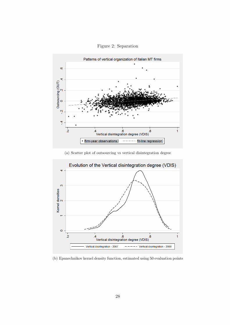
Figure 2: Separation

(a) Scatter plot of outsourcing vs vertical disintegration degree

(b) Epanechnikov kernel density function, estimated using 50 evaluation points

28

show well defined types of productions (i.e. types of machines) and higher involvementon specific investments or high-value added services. Such firms rely heavily on internalorganization of production, which minimizes transaction costs and enhances control overthe process. Firms in the second and the third quartiles of the distribution benefit fromoutsourcing, probably trading off cost–saving strategies with a certain degree control overthe production process. Finally, the more vertically disintegrated firms obtain no benefit(in terms of efficiency) from outsourcing.

6 Concluding remarks and suggested further research

In the analysis in this paper we applied an econometric approach to efficiency analysisin order to capture the roles of vertical integration and outsourcing on firms’ efficiency.Vertical integration is considered an indicator of structure, while outsourcing representsthe process of its change. In our approach, inefficiency measures are considered indicatorsof organizational heterogeneity, which is related to the choices made by the firm regard-ing the phases of the production process that remain under its direct control. In stronglycompetitive markets and in similar environmental conditions, heterogeneous productionchoices need to be justified on different grounds. Our hypothesis is that there is a com-plementarity between efficiency and flexibility. Instead of being a trade off within theindividual firm, complementarity is achieved through the co-existence of heterogeneousfirms, some (the most integrated ones) located at the frontier of the production function,others behind it.

The relationship between vertical integration and efficiency is supported by directevidence of the specific parameter and the value of the parameter for belonging to agroup. The results on outsourcing and, in particular, the interaction between outsourcingand vertical structure, indicate that heterogeneous patterns, far from tending to negateone another as a consequence of common external changes, are reinforcing. Also, thesensitivity of inefficiency variance to the cycle, indicates that different firms can havedifferent dynamic properties.

We propose a rather new measure of outsourcing, which draws on those proposed byFeenstra and Hanson (1996) and Adelman (1955), but which tries to be coherent with thedynamic nature of the outsourcing phenomenon.

In the literature efficiency measure are used mainly to detect the position of individualfirms with respect to a benchmark (the locus of the best producers). Our approachattempts to discuss efficiency as a tool for understanding the structure and functioningof a whole industry. Thus our results constitute only a step along a pathway that needto be continued. Among the lines for future research, we highlight some major issues:

• We need new evidence on our hypotheses based on direct observation of a lim-

29

ited number of cases: the kind of heterogeneity we detected through our statisticalanalysis should be grounded in a careful description of production choices, and therelationships among firms that made different choices about their vertical structure.

• A direct study should be made of the residual and the persistence of inefficiency.This will require new data to extend the time series and resolve the unbalancednature of our panel.

• Finally, there should be some econometric refinements. One such is related to the‘simultaneity’ problem, which, in our case, could affect both inputs and the variablesin the inefficiency model. Interestingly, in a work by Guan, Kumbhakar, Myers, andLansink (2009), the authors apply a two step procedure (Generalized Method ofMoments in the first step and implementation of the residual obtained in the secondstep ML frontier estimation) in order to cope with this problem. This might be aninteresting way to improve the robustness of our results. However, it should be notedthat in order to obtain unbiased ML estimates it would be sufficient to employ aspecification that encompasses empirically relevant data properties: including inputs(as we do for labour, and also intermediates to some extent) as explanatory variablesin the inefficiency equation would be logical, and this specification should limit anypossible biases in the estimates of the coefficients (Koop, 2001, p.81).

References

Acemoglu, D., S. Johnson, and T. Mitton (2009): “Determinants of Vertical In-tegration: Financial Development and Contracting Costs,” Journal of Finance, 64,1251–1290.

Adelman, M. A. (1955): “Concept and Statistical Measurement of Vertical Integra-tion,” in Business Concentration and Price Policy, ed. by U.-N. Bureau, pp. 279–328.Princeton University Press.

Afriat, S. N. (1972): “Efficiency Estimation of Production Functions,” InternationalEconomic Review, 13, 568–98.

Aigner, D., K. Lovell, and P. Schmidt (1977): “Formulation and Estimation ofStochastic Frontier Production Function Models,” Journal of Econometrics, 6, 21–37.

Aigner, D. J., and S. F. Chu (1968): “On Estimating the Industry Production Func-tion,” American Economic Review, 58, 826–39.

30

Alvarez, A., C. Amsler, L. Orea, and P. Schmidt (2006): “Interpreting and test-ing the scaling property in models where inefficiency depends on firm characteristics,”Journal of Productivity Analysis, 25, 201–212.

Arrighetti, A. (1999): “Integrazione verticale in Italia e in Europa: tendenze ed ipotesiinterpretative,” in La ’questione dimensionale’ nell’industria italiana, ed. by F. Trau.Il Mulino.

Badunenko, O., M. Fritsch, and A. Stephan (2008): “What drives the productiveefficiency of a firm?,” DIW Berlin, Discussion Papers 2008.

Battese, G. E., and T. Coelli (1992): “Frontier production functions, technicalefficiency and panel data: with applications to paddy farmers in India,” Journal ofProductivity Analysis, 3, 153–169.

(1995): “A model for technical inefficiency effects in a stochastic frontier pro-duction function for panel data,” Empirical Economics, 20, 325–332.

Becattini, G. (1990): “The marshallian industrial district as socio-economic notion,”in Industrial Districts and Inter-firm Cooperation in Italy, ed. by F. Pyke, G. Becattini,and W. Sengenberger. International Institute of Labour Studies.

Becchetti, L., A. D. Panizza, and F. Oropallo (2008): “Il ruolo dei distrettiindustriali nella performance in termini di export e di valore aggiunto: evidenze em-piriche dall’universo delle imprese italiane,” in Competitivita ed efficienza dell’economiaitaliana: fattori sistemici e valutazioni quantitative, ed. by G. Cella, and A. Zago, pp.291–335. Il Mulino.

Bojani, A. N., S. B. Caudill, and J. M. Ford (1998): “Small-sample properties ofML, COLS, and DEA estimators of frontier models in the presence of heteroscedastic-ity,” European Journal of Operational Research, 108(1), 140–148.

Bottasso, A., and A. Sembenelli (2004): “Does Ownership affect firms’ efficiency?,”Empirical Economics, 29, 769–786.

Caudill, S., and J. Ford (1993): “Biases in Frontier Estimation Due to Heteroskedas-ticity,” Economics Letters, 41, 17–20.

Caudill, S., J. Ford, and D. Gropper (1995): “Frontier Estimation and Firm Spe-cific Inefficiency Measures in the Presence of Heteroscedasticity,” Journal of Businessand Economic Statistics, 13, 105–111.

31

Caves, R. E., and D. Barton (1990): Efficiency in U.S. Manufacturing Industries.The MIT Press.

Coelli, T. J., D. S. P. Rao, C. J. O’Donnell, and G. E. Battese (2005): Anintroduction to efficiency and productivity analysis. Springer, New York, NY, 2. ed. edn.

Cornwell, C., P. Schmidt, and R. C. Sickels (1990): “Production Frontier withcross-sectional and time-series variation in efficiency levels,” Journal of Econometrics,pp. 185–200.

Davies, S. W., and C. Morris (1995): “A new index of vertical integration,” Interna-tional Journal of Industrial Organization, 13, 151–177.

Debreu, G. (1951): “The Coefficient of Resource Utilization,” Econometrica, 19, 273–292.

Diaz, M. A., and R. Sanchez (2008): “Firm size and productivity in Spain: a stochas-tic frontier analysis,” Small Business Economics, 30, 315–323.

Fabiani, S., G. Pellegrini, G. Romagnano, and L. F. Signorini (1998): “Effi-ciency and localisation: the case of industrial districts,” in The competitive advantageof industrial districts: theoretical and empirical analysis, ed. by M. Bagella, and L. Bec-chetti.

Farrell, M. J. (1957): “The Measurement of Productive Efficiency,” Journal of theRoyal Statistical Society, Series A, 253–81.

Feenstra, R. C., and G. H. Hanson (1996): “Globalization, Outsourcing, and WageInequality,” American Economic Review, 86(2), 240–45.

Fried, H. O., C. A. K. Lovell, and S. S. Schmidt (2008): “Productivity andEfficiency,” in The measurement of productive efficiency and productivity growth, ed.by H. O. Fried, C. A. K. Lovell, and S. S. Schmidt, pp. 1–105. Oxford University Press.

Greene, W. H. (1993): “The Econometric Approach to Efficiency Analysis,” in Themeasurement of productive efficiency and productivity growth, ed. by H. O. Fried,C. A. K. Lovell, and S. Schmidt, chap. 2, pp. 68–120. Oxford University Press.

(2005): “Reconsidering heterogeneity in panel data estimators of the stochasticfrontier model,” Journal of Econometrics, 126, 269–303.

(2008): “The Econometric Approach to Efficiency Analysis,” in The measure-ment of productive efficiency and productivity growth, ed. by H. O. Fried, C. A. K.Lovell, and S. S. Schmidt, chap. 2, pp. 92–250. Oxford University Press.

32

Guan, Z., S. C. Kumbhakar, R. J. Myers, and A. O. Lansink (2009): “MeasuringExcess capital capacity in Agricultural Production,” American Journal of AgriculturalEconomics, 91, 765–776.

Gumbau, M., and J. Maudos (2002): “The Determinants of Efficiency: The Case ofthe Spanish Industry,” Applied Economics, 34, 1941–1948.

Hadri, K. (1999): “Estimation of a Doubly Heteroscedastic Stochastic Frontier CostFunction,” Journal of Business and Economic Statistics, 17, 359–363.

Hadri, K., C. Guermat, and J. Whittaker (2003): “Estimation of technical in-efficiency effects using panel data and doubly heteroscedastic stochastic productionfrontiers,” Empirical Economics, 28, 203–222.

Hart, O. D., and J. Moore (1990): “Property Rights and the Nature of the Firm,”Journal of Political Economy, 98, 1119–1158.

Hashmati, A. (2003): “Productivity Growth, Efficiency and Outsourcing in Manufac-turing and Service Industries,” Journal of Economic Surveys, 17, 79–112.

Huang, C. J., and J. T. Liu (1994): “Estimation of a non-neutral stochastic frontierproduction function,” Journal of Productivity Analysis, 5, 171–180.

Koop, G. (2001): “Cross-Sectoral Patterns of Efficiency and Technical Change in Man-ufacturing,” International Economic Review, 42, 73–103.

Koopmans, T. C. (1951): “An Analysis of Production as an Efficient Combination ofActivities,” in Activity Analysis of Production and Allocation, ed. by T. Koopmans.New York: Wiley.

Kumar, J. (2003): “Ownership Structure and Corporate Firm Performance,” Discussionpaper, EconWPA.

Kumbhakar, S. (1990): “Production frontiers, panel data, and time varying technicalefficiency,” Journal of Econometrics, 46, 201–211.

Kumbhakar, S., and C. A. K. Lovell (2000): Stochastic Frontier Analysis. Cam-bridge: Cambridge University Press.

Laureti, T. (2008): “Modelling Exogenous Variables in Human Capital Formationthrough a Heteroscedastic Stochastic Frontier,” International Advances in EconomicResearch, 14, 76–89.

33

Leibenstein, H. (1966): “Allocative Efficiency vs. X-Efficiency,” American EconomicReview, 56, 392–415.

Lovell, C. A. K. (1993): “Production Frontiers and Productive Efficiency,” in TheMeasurement of Productive Efficiency: Tecniques and Applications, ed. by F. H. O.,C. A. K. Lovell, and S. S. Schmidt. Oxford University Press.

Maddigan, R. J. (1981): “The Measurement of Vertical Integration,” The Review ofEconomics and Statistics, 63, 328–335.

Meeusen, W., and J. van den Broeck (1977): “Efficiency Estimation for Cobb-Douglas Production Functions with Composed Error,” International Economic Review,18, 435–444.

Olsen, K. B. (2006): “Productivity Impact of Offshoring and Outsourcing: a Review,”Discussion Paper 2006/1, OECD Directorate for Science, Technology and Industry.

Poledrini, S. (2008): “From modular innovation to Systems Integration: the main expe-riences from some Italian machine tool builders,” in 8th global Conference on Business& Economics.

Pozzana, and E. Zaninotto (1989): Efficienza produttiva e concorrenza : il caso delladistribuzione commerciale. F. Angeli.

Reifschneider, D., and R. Stevenson (1991): “Systematic departures from thefrontier: A framework for the analysis of firm inefficiency,” International EconomicReview, 32, 715–723.

Ritter, C., and L. Simar (1997): “Pitfalls of Normal-Gamma Stochastic FrontierModels,” Journal of Productivity Analysis, 8, 167–182.

Rolfo, S. (1993): “The Italian Machine Tool Industry,” Ceris-CNR working paper, 4.

(1998): “L’Industria italiana della meccanica strumentale di fronte alla global-izzazione: opportunita e limiti,” L’Industria, 4, 881–894.

(2000): “The Italian Machine Tool Industry Towards Production DevelopmentNetworks,” in New product development and production networks, ed. by H. Juergens,chap. 8. Springer.

Rolfo, S., and G. Calabrese (2006): “Struttura industriale e profili di competitivitanella meccanica strumentale,” L’Industria, 4, 603–622.

34

Seitz, W. D. (1971): “Productive Efficiency in the Steam-Electric Generating Industry,”Journal of Political Economy, 79, 878–886.

Shepard, R. W. (1953): Cost and Production Functions. Princeton: Princeton Univer-sity Press.

Shleifer, A., and R. Vishny (1986): “Large Shareholders and Corporate Control,”Journal of Political Economy, 94, 461–488.

Simar, L., C. A. K. Lovell, and P. V. Eeckaut (1994): “Stochastic FrontiersIncorporating Exogenous Influences on Efficiency,” Discussion Paper n. 9403, Institutde Statistique, Universite Catholique de Louvain.

Taymaz, E. (2005): “Are Small Firms Really Less Productive?,” Small Business Eco-nomics, 25, 429–445.

Ucimu (2007a): “Industry Report,” Ucimu-Centro Studi.

(2007b): “L’industria italiana di settore: evoluzione dal dopoguerra a oggi,”Ucimu.

Wang, H.-J. (2003): “A Stochastic Frontier Analysis of Financing Constraints on In-vestment: The Case of Financial Liberalization in Taiwan,” Journal of Business andEconomic Statistics, 21, 406–419.

Wang, H.-J., and P. Schmidt (2002): “One-Step and Two-Step Estimation of theEffects of Exogenous Variables on Technical Efficiency Levels,” Journal of ProductivityAnalysis, 18, 129–144.

Wengel, J., and P. Shapira (2004): “Machine tools: the remaking of a traditionalsectoral innovation system,” in Sectoral systems of Innovation, ed. by F. Malerba.Cambridge: Cambridge University Press.

Williamson, O. E. (1971): “The Vertical Integration of Production: Market FailureConsiderations,” American Economic Review, 61(2), 112–23.

Williamson, O. E. (1975): Market and Hierarchies: Analysis and Antitrust Implica-tions. New York: Free Press.

Zanfei, A., and A. Gambardella (1994): “The Italian Machine-Tool Industry,” inThe Decline of the U.S. Machine Tool Industry and Prospects for Its Recovery. Vol. 2,Appendices, ed. by D. Finegold. Santa Monica, CA: RAND.

35

DISA

WOR

KING

PAPE

R

DISA

Dipartimento di Informaticae Studi Aziendali

2010

/1

Th e impact of vertical integration and outsourcing on fi rm effi ciency:

evidence from the Italianmachine tool industry

Fabio Pieri, Enrico Zaninotto