1

CHAPTER 6 : Some Alternative Investment Rules 1. INTERNAL RATE OF RETURN [IRR] IIRRRR iiss tthhee dd iiss ccoouunntt rraattee wwhhiicchh mmaakkeess NNPPVV==00

0)1()1()1( 2

210 =

+++

++

++=

TT

IRR

C

IRR

C

IRR

CCNPV L

2. NPV PROFILE NNPPVV PPrrooffiillee CC00 == -- 44 CC11 == ++22 CC22 == ++44 TTrriiaall aanndd EErrrroorr EEssttiimmaattiioonn..

IIff ddiissccoouunntt rraattee == 00%%,, tthheenn NNPPVV ==?? IIff ddiissccoouunntt rraattee == 2255%% tthheenn NNPPVV == ?? IIff ddiissccoouunntt rraattee == 3300%%,, tthheenn NNPPVV == ?? IIff ddiissccoouunntt rraattee == 2288%%,, tthheenn NNPPVV == ??

3. IRR RULE AAcccceepp tt tthhee pprroo jjeecctt

IIff IIRRRR >> OOppppoorrttuunniittyy CCoosstt ooff CCaappiittaall.. LLooookkiinngg aatt tthhee NNPPVV pprrooffiillee ffoorr aa ccoonnvveennttiioonnaall pprroojjeecctt,, wwee wwiillll bbee aacccceeppttiinngg pprroojjeeccttss wwiitthh ppoossiittiivvee NNPPVV.. 4. MULTIPLE IRRs •• EExxaammppllee YYeeaarr 00 11 22 CCFF --$$44 $$2255 --$$2255 •• TTwwoo cchhaannggeess iinn ssiiggnn ooff ccaasshh fflloowwss..

-- GGeenneerraatteess ttwwoo IIRRRRss :: 2255%% aanndd 440000%% -- IIff rr << 2255%%,, NNPPVV << 00 -- IIff 2255%% << rr << 440000%%,, NNPPVV >> 00 -- IIff rr >> 440000,, NNPPVV << 00..

•• HHooww ddooeess NNPPVV pprrooffiillee llooookk lliikkee ??

2

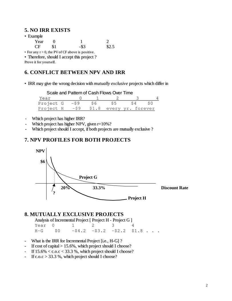
5. NO IRR EXISTS •• EExxaammppllee YYeeaarr 00 11 22 CCFF $$11 --$$33 $$22..55 •• FFoorr aannyy rr >> 00,, tthhee PPVV ooff CCFF aabboovvee iiss ppooss iitt iivvee..

•• TThheerreeffoorree,, sshhoouulldd II aacccceepptt tthhiiss pprroojjeecctt ?? PPrroovvee iitt ffoorr yyoouurrss eellff.. 6. CONFLICT BETWEEN NPV AND IRR •• IIRRRR mmaayy ggiivvee tthhee wwrroonngg ddeecciissiioonn wwiitthh mmuuttuuaallllyy eexxcclluussiivvee pprroojjeeccttss wwhhiicchh ddiiffffeerr iinn

SSccaallee aanndd PPaatttteerrnn ooff CCaasshh FFlloowwss OOvveerr TTiimmee YYeeaarr 00 11 22 33 44 PPrroojjeecctt GG --$$99 $$66 $$55 $$44 $$00 Project H -$9 $1.8 every yr. forever

-- WWhhiicchh pprroojjeecctt hhaass hhiigghheerr IIRRRR?? -- WWhhiicchh pprroojjeecctt hhaass hhiigghheerr NNPPVV,, ggiivveenn rr==1100%%?? -- WWhhiicchh pprroojjeecctt sshhoouulldd II aacccceepptt,, iiff bbootthh pprroojjeeccttss aarree mmuuttuuaallllyy eexxcclluussiivvee ?? 7. NPV PROFILES FOR BOTH PROJECTS

NPV $6 Project G 20% 33.3% Discount Rate ? Project H 8. MUTUALLY EXCLUSIVE PROJECTS

AAnnaallyyssiiss ooff IInnccrreemmeennttaall PPrroojjeecctt [[ PPrroojjeecctt HH -- PPrroojjeecctt GG ]] YYeeaarr 00 11 22 33 44 HH--GG $$00 --$$44..22 --$$33..22 --$$22..22 $$11..88 .. .. .. -- WWhhaatt iiss tthhee IIRRRR ffoorr IInnccrreemmeennttaall PPrroojjeecctt [[ii..ee..,, HH--GG]] ?? -- IIff ccoosstt ooff ccaappiittaall >> 1155..66%%,, wwhhiicchh pprroojjeecctt sshhoouulldd II cchhoooossee?? -- IIff 1155..66%% << cc..oo..cc << 3333..33 %%,, wwhhiicchh pprroojjeecctt sshhoouulldd II cchhoooossee?? -- IIff cc..oo..cc >> 3333..33 %%,, wwhhiicchh pprroojjeecctt sshhoouulldd II cchhoooossee??

3

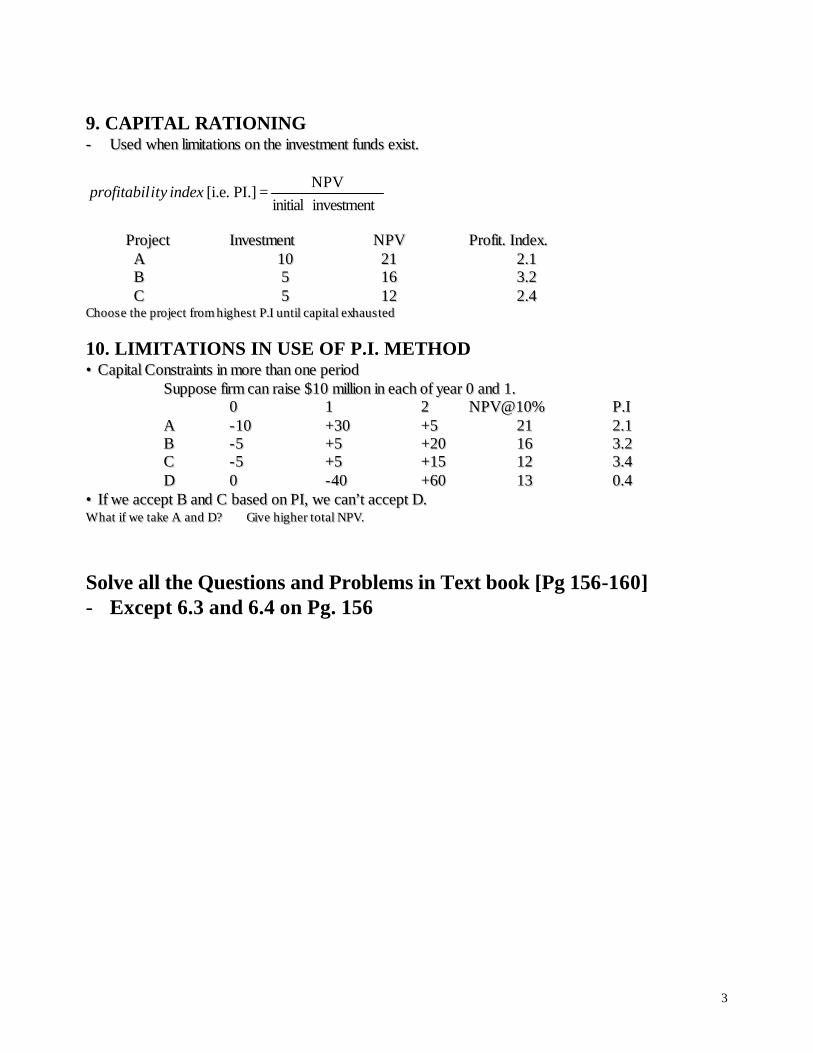
9. CAPITAL RATIONING -- UUsseedd wwhheenn lliimmiittaattiioonnss oonn tthhee iinnvveessttmmeenntt ffuunnddss eexxiisstt..

investment initialNPV

= PI.] [i.e. indexityprofitabil

PPrroojjeecctt IInnvveessttmmeenntt NNPPVV PPrrooffiitt.. IInnddeexx..

AA 1100 2211 22..11 BB 55 1166 33..22 CC 55 1122 22..44 CChhooooss ee tthhee pprroo jjeecctt ffrroomm hh iigghheess tt PP..II uunn tt iill ccaapp iittaall eexxhhaauuss tteedd 10. LIMITATIONS IN USE OF P.I. METHOD •• CCaappiittaall CCoonnssttrraaiinnttss iinn mmoorree tthhaann oonnee ppeerriioodd

SSuuppppoossee ffiirrmm ccaann rraaiissee $$1100 mmiilllliioonn iinn eeaacchh ooff yyeeaarr 00 aanndd 11.. 00 11 22 NNPPVV@@1100%% PP..II AA --1100 ++3300 ++55 2211 22..11 BB --55 ++55 ++2200 1166 33..22 CC --55 ++55 ++1155 1122 33..44 DD 00 --4400 ++6600 1133 00..44

•• IIff wwee aacccceepptt BB aanndd CC bbaasseedd oonn PPII,, wwee ccaann’’tt aacccceepptt DD.. WW hhaatt iiff wwee ttaakkee AA aanndd DD?? GGiivvee hh iigghheerr ttoo ttaall NNPPVV..

Solve all the Questions and Problems in Text book [Pg 156-160] - Except 6.3 and 6.4 on Pg. 156

4

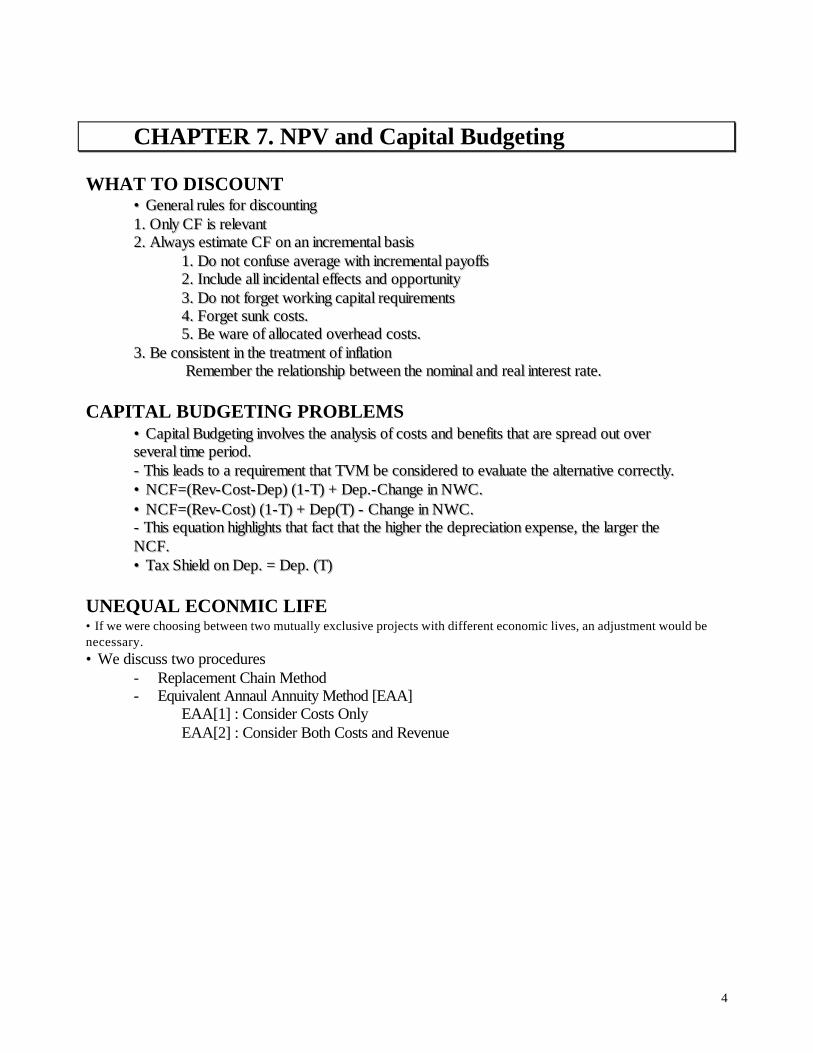
CHAPTER 7. NPV and Capital Budgeting WHAT TO DISCOUNT

•• GGeenneerraall rruulleess ffoorr ddiissccoouunnttiinngg 11.. OOnnllyy CCFF iiss rreelleevvaanntt 22.. AAllwwaayyss eessttiimmaattee CCFF oonn aann iinnccrreemmeennttaall bbaassiiss

11.. DDoo nnoott ccoonnffuussee aavveerraaggee wwiitthh iinnccrreemmeennttaall ppaayyooffffss 22.. IInncclluuddee aallll iinncciiddeennttaall eeffffeeccttss aanndd ooppppoorrttuunniittyy 33.. DDoo nnoott ffoorrggeett wwoorrkkiinngg ccaappiittaall rreeqquuiirreemmeennttss 44.. FFoorrggeett ssuunnkk ccoossttss.. 55.. BBee wwaarree ooff aallllooccaatteedd oovveerrhheeaadd ccoossttss..

33.. BBee ccoonnssiisstteenntt iinn tthhee ttrreeaattmmeenntt ooff iinnffllaattiioonn RReemmeemmbbeerr tthhee rreellaattiioonnsshhiipp bbeettwweeeenn tthhee nnoommiinnaall aanndd rreeaall iinntteerreesstt rraattee..

CAPITAL BUDGETING PROBLEMS

•• CCaappiittaall BBuuddggeettiinngg iinnvvoollvveess tthhee aannaallyyssiiss ooff ccoossttss aanndd bbeenneeffiittss tthhaatt aarree sspprreeaadd oouutt oovveerr sseevveerraall ttiimmee ppeerriioodd.. -- TThhiiss lleeaaddss ttoo aa rreeqquuiirreemmeenntt tthhaatt TTVVMM bbee ccoonnssiiddeerreedd ttoo eevvaalluuaattee tthhee aalltteerrnnaattiivvee ccoorrrreeccttllyy.. •• NNCCFF==((RReevv--CCoosstt--DDeepp)) ((11--TT)) ++ DDeepp..--CChhaannggee iinn NNWWCC.. •• NNCCFF==((RReevv--CCoosstt)) ((11--TT)) ++ DDeepp((TT)) -- CChhaannggee iinn NNWWCC.. -- TThhiiss eeqquuaattiioonn hhiigghhlliigghhttss tthhaatt ffaacctt tthhaatt tthhee hhiigghheerr tthhee ddeepprreecciiaattiioonn eexxppeennssee,, tthhee llaarrggeerr tthhee NNCCFF.. •• TTaaxx SShhiieelldd oonn DDeepp.. == DDeepp.. ((TT))

UNEQUAL ECONMIC LIFE • If we were choosing between two mutually exclusive projects with different economic lives, an adjustment would be necessary. • We discuss two procedures

- Replacement Chain Method - Equivalent Annaul Annuity Method [EAA]

EAA[1] : Consider Costs Only EAA[2] : Consider Both Costs and Revenue

5

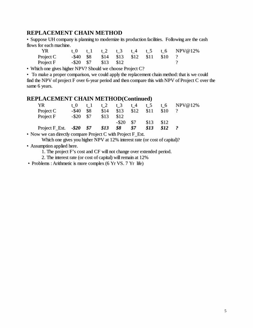
REPLACEMENT CHAIN METHOD •• SSuuppppoossee UUHH ccoommppaannyy iiss ppllaannnniinngg ttoo mmooddeerrnniizzee iittss pprroodduuccttiioonn ffaacciilliittiieess.. FFoolllloowwiinngg aarree tthhee ccaasshh fflloowwss ffoorr eeaacchh mmaacchhiinnee.. YYRR tt__00 tt__11 tt__22 tt__33 tt__44 tt__55 tt__66 NNPPVV@@1122%% PPrroojjeecctt CC --$$4400 $$88 $$1144 $$1133 $$1122 $$1111 $$1100 ?? PPrroojjeecctt FF --$$2200 $$77 $$1133 $$1122 ?? •• WWhhiicchh oonnee ggiivveess hhiigghheerr NNPPVV?? SShhoouulldd wwee cchhoooossee PPrroojjeecctt CC?? •• TToo mmaakkee aa pprrooppeerr ccoommppaarriissoonn,, wwee ccoouulldd aappppllyy tthhee rreeppllaacceemmeenntt cchhaaiinn mmeetthhoodd:: tthhaatt iiss wwee ccoouulldd ffiinndd tthhee NNPPVV ooff pprroojjeecctt FF oovveerr 66--yyeeaarr ppeerriioodd aanndd tthheenn ccoommppaarree tthhiiss wwiitthh NNPPVV ooff PPrroojjeecctt CC oovveerr tthhee ssaammee 66 yyeeaarrss.. REPLACEMENT CHAIN METHOD(Continued) YYRR tt__00 tt__11 tt__22 tt__33 tt__44 tt__55 tt__66 NNPPVV@@1122%% PPrroojjeecctt CC --$$4400 $$88 $$1144 $$1133 $$1122 $$1111 $$1100 ?? PPrroojjeecctt FF --$$2200 $$77 $$1133 $$1122 --$$2200 $$77 $$1133 $$1122

PPrroojjeecctt FF__EExxtt.. --$$2200 $$77 $$1133 $$88 $$77 $$1133 $$1122 ?? •• NNooww wwee ccaann ddiirreeccttllyy ccoommppaarree PPrroojjeecctt CC wwiitthh PPrroojjeecctt FF__EExxtt.. WWhhiicchh oonnee ggiivveess yyoouu hhiigghheerr NNPPVV aatt 1122%% iinntteerreesstt rraattee ((oorr ccoosstt ooff ccaappiittaall))?? •• AAssssuummppttiioonn aapppplliieedd hheerree..

11.. TThhee pprroojjeecctt FF’’ss ccoosstt aanndd CCFF wwiillll nnoott cchhaannggee oovveerr eexxtteennddeedd ppeerriioodd.. 22.. TThhee iinntteerreesstt rraattee ((oorr ccoosstt ooff ccaappiittaall)) wwiillll rreemmaaiinn aatt 1122%%

•• PPrroobblleemmss :: AArriitthhmmeettiicc iiss mmoorree ccoommpplleexx ((66 YYrr VVSS.. 77 YYrr lliiffee))

6

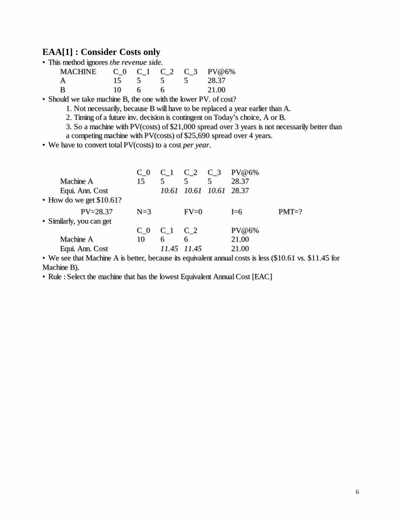
EAA[1] : Consider Costs only •• TThhiiss mmeetthhoodd iiggnnoorreess tthhee rreevveennuuee ssiiddee.. MMAACCHHIINNEE CC__00 CC__11 CC__22 CC__33 PPVV@@66%% AA 1155 55 55 55 2288..3377 BB 1100 66 66 2211..0000 •• SShhoouulldd wwee ttaakkee mmaacchhiinnee BB,, tthhee oonnee wwiitthh tthhee lloowweerr PPVV.. ooff ccoosstt??

11.. NNoott nneecceessssaarriillyy,, bbeeccaauussee BB wwiillll hhaavvee ttoo bbee rreeppllaacceedd aa yyeeaarr eeaarrlliieerr tthhaann AA.. 22.. TTiimmiinngg ooff aa ffuuttuurree iinnvv.. ddeecciissiioonn iiss ccoonnttiinnggeenntt oonn TTooddaayy’’ss cchhooiiccee,, AA oorr BB.. 33.. SSoo aa mmaacchhiinnee wwiitthh PPVV((ccoossttss)) ooff $$2211,,000000 sspprreeaadd oovveerr 33 yyeeaarrss iiss nnoott nneecceessssaarriillyy bbeetttteerr tthhaann aa ccoommppeettiinngg mmaacchhiinnee wwiitthh PPVV((ccoossttss)) ooff $$2255,,669900 sspprreeaadd oovveerr 44 yyeeaarrss..

•• WWee hhaavvee ttoo ccoonnvveerrtt ttoottaall PPVV((ccoossttss)) ttoo aa ccoosstt ppeerr yyeeaarr.. CC__00 CC__11 CC__22 CC__33 PPVV@@66%% MMaacchhiinnee AA 1155 55 55 55 2288..3377 EEqquuii.. AAnnnn.. CCoosstt 1100..6611 1100..6611 1100..6611 2288..3377 •• HHooww ddoo wwee ggeett $$1100..6611??

PPVV==2288..3377 NN==33 FFVV==00 II==66 PPMMTT==?? •• SSiimmiillaarrllyy,, yyoouu ccaann ggeett CC__00 CC__11 CC__22 PPVV@@66%% MMaacchhiinnee AA 1100 66 66 2211..0000 EEqquuii.. AAnnnn.. CCoosstt 1111..4455 1111..4455 2211..0000 •• WWee sseeee tthhaatt MMaacchhiinnee AA iiss bbeetttteerr,, bbeeccaauussee iittss eeqquuiivvaalleenntt aannnnuuaall ccoossttss iiss lleessss (($$1100..6611 vvss.. $$1111..4455 ffoorr MMaacchhiinnee BB)).. •• RRuullee :: SSeelleecctt tthhee mmaacchhiinnee tthhaatt hhaass tthhee lloowweesstt EEqquuiivvaalleenntt AAnnnnuuaall CCoosstt [[EEAACC]]

7

EAA[2] : Consider Costs and Revenue •• CCoonnssiiddeerr tthhee PPrroojjeecctt CC aanndd FF YYRR tt__00 tt__11 tt__22 tt__33 tt__44 tt__55 tt__66 NNPPVV@@1122%% PPrroojjeecctt CC --$$4400 $$88 $$1144 $$1133 $$1122 $$1111 $$1100 $$66..449911 PPrroojjeecctt FF --$$2200 $$77 $$1133 $$1122 $$55..115555 •• SShhoouulldd wwee cchhoooossee PPrroojjeecctt CC,, wwhhiicchh ggiivveess tthhee hhiigghheerr NNPPVV?? •• IIff nnoott,, hhooww ccaann wwee eevvaalluuaattee tthheessee ttwwoo pprroojjeeccttss??

11.. UUnnlliikkee tthhee EEAACC ccaassee,, hheerree wwee ccoonnssiiddeerr ccoosstt aanndd rreevveennuuee.. 22.. WWhheenn ccoommppaarriinngg pprroojjeeccttss ooff uunneeqquuaall lliivveess,, tthhee oonnee wwiitthh tthhee hhiigghheerr eeqquuiivvaalleenntt aannnnuuaall aannnnuuiittyy sshhoouulldd bbee cchhoosseenn..

•• PPrroocceedduurreess 11.. FFiinndd eeaacchh pprroojjeecctt’’ss NNPPVV oovveerr iittss iinnii tt iiaall lliiffee.. 22.. TThheerree iiss ssoommee ccoonnssttaanntt aannnnuuiittyy ccaasshh ffllooww [[II..ee..,, EEAAAA]] -- TToo ffiinndd EEAAAA ffoorr pprroojjeecctt FF,, eenntteerr NN==33,, II==1122,, PPVV==--55115555,, aanndd FFVV==00 aanndd ssoollvvee ffoorr PPMMTT.. -- SSiimmiillaarrllyy yyoouu ccaann ffiinndd EEAAAA ffoorr pprroojjeecctt CC.. 33.. TThhee pprroojjeecctt wwiitthh tthhee hhiigghheerr EEAAAA wwiillll aallwwaayyss hhaavvee tthhee hhiigghheerr NNPPVV wwhheenn eexxtteennddeedd oouutt ttoo aannyy ccoommmmoonn lliiffee.. TThheerreeffoorree cchhoooossee tthhee pprroojjeecctt wwiitthh hhiigghheerr EEAAAA.. [[EEAAAA ffoorr CC==$$11..557799,, EEAAAA ffoorr FF==$$22..114466]]

•• EEAAAA mmeetthhoodd iiss eeaassiieerr ttoo aappppllyy,, bbuutt cchhaaiinn mmeetthhoodd iiss eeaassiieerr ttoo uunnddeerrssttaanndd..

8

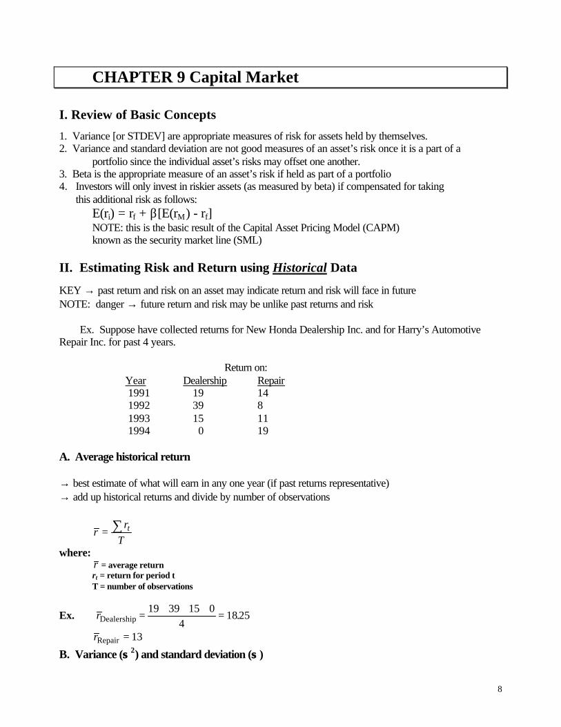
CHAPTER 9 Capital Market I. Review of Basic Concepts

1. Variance [or STDEV] are appropriate measures of risk for assets held by themselves. 2. Variance and standard deviation are not good measures of an asset’s risk once it is a part of a

portfolio since the individual asset’s risks may offset one another. 3. Beta is the appropriate measure of an asset’s risk if held as part of a portfolio 4. Investors will only invest in riskier assets (as measured by beta) if compensated for taking

this additional risk as follows: E(ri) = rf + β[E(rM) - rf] NOTE: this is the basic result of the Capital Asset Pricing Model (CAPM) known as the security market line (SML)

II. Estimating Risk and Return using Historical Data

KEY → past return and risk on an asset may indicate return and risk will face in future NOTE: danger → future return and risk may be unlike past returns and risk

Ex. Suppose have collected returns for New Honda Dealership Inc. and for Harry’s Automotive Repair Inc. for past 4 years. Return on: Year Dealership Repair 1991 19 14 1992 39 8 1993 15 11 1994 0 19 A. Average historical return → best estimate of what will earn in any one year (if past returns representative) → add up historical returns and divide by number of observations

rr

Tt= ∑

where: r = average return rt = return for period t T = number of observations

Ex. rDealership = + + + =19 39 15 04

1825.

rRepair = 13

B. Variance (σσ 2) and standard deviation (σσ )

9

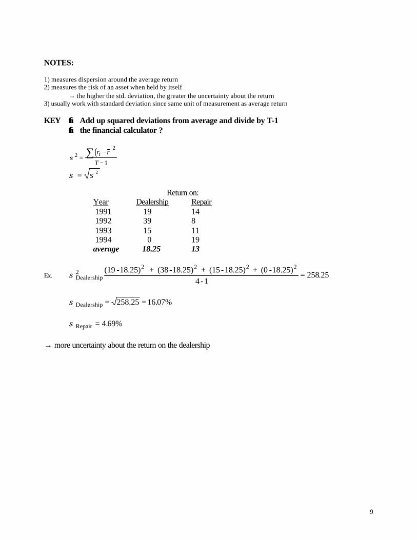
NOTES: 1) measures dispersion around the average return 2) measures the risk of an asset when held by itself

→ the higher the std. deviation, the greater the uncertainty about the return 3) usually work with standard deviation since same unit of measurement as average return

KEY →→ Add up squared deviations from average and divide by T-1 →→ the financial calculator ?

( )σ2

2

1=

−

−∑ r r

Tt

σ σ= 2 Return on: Year Dealership Repair 1991 19 14 1992 39 8 1993 15 11 1994 0 19 average 18.25 13

Ex. σDealership

2 2 2 2(19 -18.25) + (38-18.25) + (15-18.25) + (0 -18.25)4 -1

2 258 25= .

σDealership 258.25= = 16 07%. σRepair = 4 69%.

→ more uncertainty about the return on the dealership

10

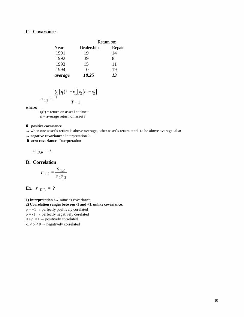
C. Covariance Return on: Year Dealership Repair 1991 19 14 1992 39 8 1993 15 11 1994 0 19 average 18.25 13

( )[ ] ( )[ ]σ1 2

1 1 2 2

1, =− −

−

∑ r t r r t r

Tt

where: ri(t) = return on asset i at time t ri = average return on asset i

→→ positive covariance → when one asset’s return is above average, other asset’s return tends to be above average also → negative covariance : Interpretation ? →→ zero covariance : Interpretation

σD R, = ?

D. Correlation

ρσ

σ σ 1 2

1 2

1 2,

,=

Ex. ρ D,R = ?

1) Interpretation :→ same as covariance 2) Correlation ranges between -1 and +1, unlike covariance. ρ = +1 → perfectly positively corelated ρ = -1 → perfectly negatively corelated 0 < ρ < 1 → positively correlated -1 < ρ < 0 → negatively correlated

11

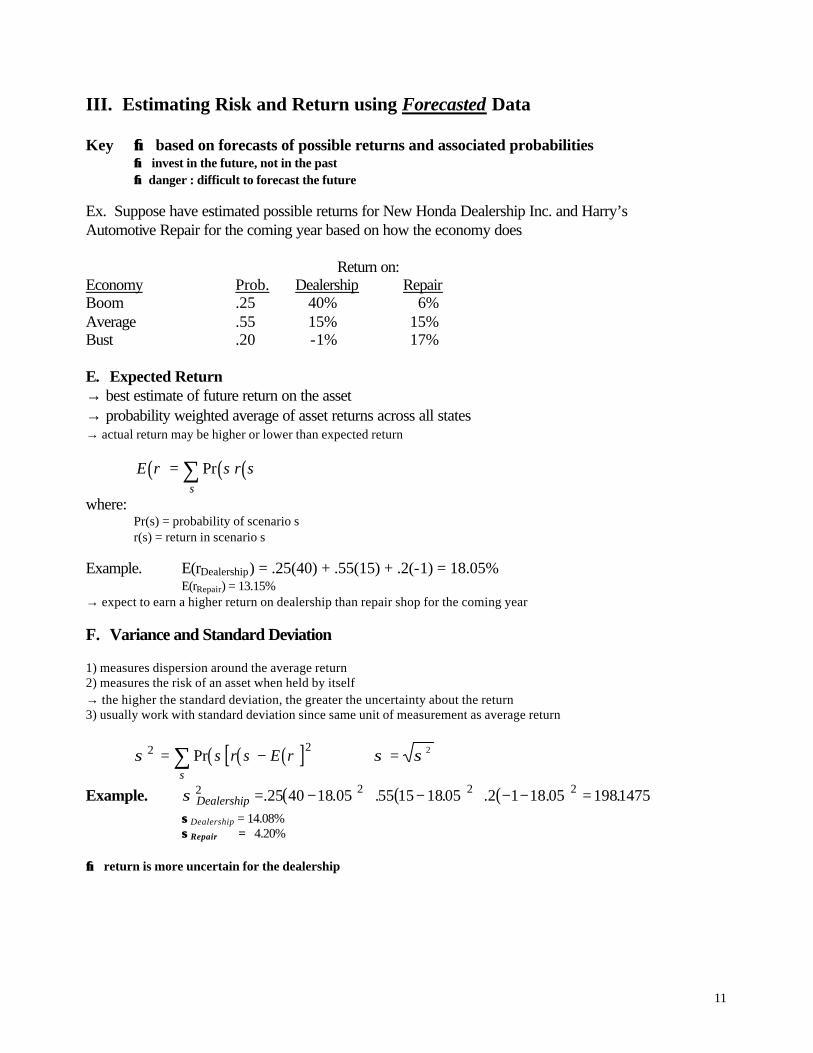
III. Estimating Risk and Return using Forecasted Data Key →→ based on forecasts of possible returns and associated probabilities

→→ invest in the future, not in the past →→ danger : difficult to forecast the future

Ex. Suppose have estimated possible returns for New Honda Dealership Inc. and Harry’s Automotive Repair for the coming year based on how the economy does Return on: Economy Prob. Dealership Repair Boom .25 40% 6% Average .55 15% 15% Bust .20 -1% 17% E. Expected Return → best estimate of future return on the asset → probability weighted average of asset returns across all states → actual return may be higher or lower than expected return

( ) ( ) ( )E r s r ss

= ∑ Pr

where: Pr(s) = probability of scenario s r(s) = return in scenario s

Example. E(rDealership) = .25(40) + .55(15) + .2(-1) = 18.05%

E(rRepair) = 13.15% → expect to earn a higher return on dealership than repair shop for the coming year

F. Variance and Standard Deviation 1) measures dispersion around the average return 2) measures the risk of an asset when held by itself → the higher the standard deviation, the greater the uncertainty about the return 3) usually work with standard deviation since same unit of measurement as average return

( ) ( ) ( )[ ]σ2 2= −∑ Pr s r s E rs

σ σ= 2

Example. ( ) ( ) ( )σDealership2 2 2 225 40 18 05 55 15 1805 2 1 18 05 1981475= − + − + − − =. . . . . . .

σσDealership = 14.08% σσRepair = 4.20%

→→ return is more uncertain for the dealership

12

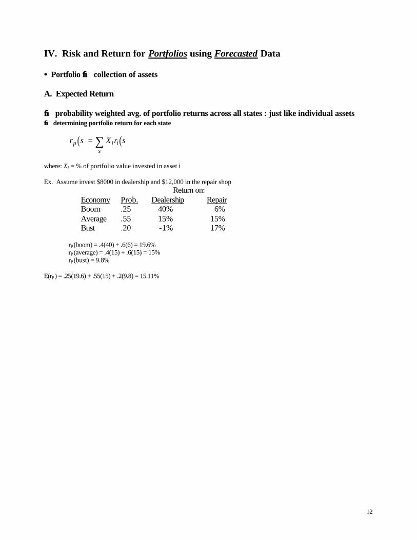
IV. Risk and Return for Portfolios using Forecasted Data

•• Portfolio →→ collection of assets

A. Expected Return →→ probability weighted avg. of portfolio returns across all states : just like individual assets →→ determining portfolio return for each state

( ) ( )r s X r sp is

i= ∑

where: Xi = % of portfolio value invested in asset i Ex. Assume invest $8000 in dealership and $12,000 in the repair shop Return on: Economy Prob. Dealership Repair Boom .25 40% 6% Average .55 15% 15% Bust .20 -1% 17%

rP(boom) = .4(40) + .6(6) = 19.6% rP(average) = .4(15) + .6(15) = 15% rP(bust) = 9.8%

E(rP) = .25(19.6) + .55(15) + .2(9.8) = 15.11%

13

B. Variance and Standard Deviation Return on: Economy Prob. Dealership Repair Boom .25 40% 6% Average .55 15% 15% Bust .20 -1% 17% 1. weighted average of squared deviations from E(r)→→ same as individual assets

( ) ( ) ( )σP = − + − + − =. . . . . . . . .25 19 6 1511 55 15 1511 2 9 8 1511 3 27%2 2 2

NOTE: when combined dealership and repair shop, std. deviation of portfolio (3.27) less than either the dealership (14.08) or the repair shop (4.19) 2. what happened to the risk? → diversification : risk reduction from offsetting variability → key to diversification : more closely related returns, less diversification possible NOTE: The relationship between asset returns and diversification benefits will be more obvious with a following portfolio example.

C. Covariance

( ) ( ) ( )[ ] ( ) ( )[ ]σ1 2 1 1 2 2, Pr= − −∑ s r s E r r s E rs

where: Pr(s) = probability of scenario s ri(s) = return on asset i in scenario s E(ri) = expected return on asset i

Ex. σσ D,R = ?

14

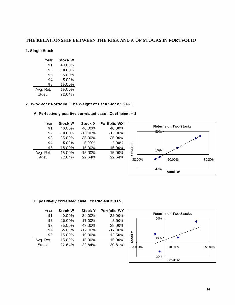
THE RELATIONSHIP BETWEEN THE RISK AND #. OF STOCKS IN PORTFOLIO

1. Single Stock

Year Stock W91 40.00%92 -10.00%93 35.00%94 -5.00%95 15.00%

Avg. Ret. 15.00%Stdev. 22.64%

2. Two-Stock Portfolio [ The Weight of Each Stock : 50% ]

A. Perfectively positive correlated case : Coefficient = 1

Year Stock W Stock X Portfolio WX91 40.00% 40.00% 40.00%92 -10.00% -10.00% -10.00%93 35.00% 35.00% 35.00%94 -5.00% -5.00% -5.00%95 15.00% 15.00% 15.00%

Avg. Ret. 15.00% 15.00% 15.00%Stdev. 22.64% 22.64% 22.64%

B. positively correlated case : coefficient = 0.69

Year Stock W Stock Y Portfolio WY91 40.00% 24.00% 32.00%92 -10.00% 17.00% 3.50%93 35.00% 43.00% 39.00%94 -5.00% -19.00% -12.00%95 15.00% 10.00% 12.50%

Avg. Ret. 15.00% 15.00% 15.00%Stdev. 22.64% 22.64% 20.81%

Returns on Two Stocks

-30%

10%

50%

-30.00% 10.00% 50.00%

Stock W

Sto

ck X

Returns on Two Stocks

-30%

10%

50%

-30.00% 10.00% 50.00%

Stock W

Sto

ck Y

15

THE RELATIONSHIP BETWEEN THE RISK AND #. OF STOCKS IN PORTFOLIO(Continued)

C. Negatively correlated case : coefficient = -0.72

Year Stock W Stock Z Portfolio WZ91 40.00% 11.41% 25.71%92 -10.00% 32.49% 11.25%93 35.00% -4.00% 15.50%94 -5.00% 43.60% 19.30%95 15.00% -8.50% 3.25%

Avg. Ret. 15.00% 15.00% 15.00%Stdev. 22.64% 22.64% 8.45%

D. Perfectively negative correlated case : Coefficient = -1

Year Stock W Stock P Portfolio WP91 40.00% -10.00% 15.00%92 -10.00% 40.00% 15.00%93 35.00% -5.00% 15.00%94 -5.00% 35.00% 15.00%95 15.00% 15.00% 15.00%

Avg. Ret. 15.00% 15.00% 15.00%Stdev. 22.64% 22.64% 0.00%

Returns on Two Stocks

-30%

10%

50%

-30.00% 10.00% 50.00%

Stock WS

tock

Y

Returns on Two Stocks

-30%

10%

50%

-30.00% 10.00% 50.00%

Stock W

Sto

ck Y

16

V. Relationship Between Risk and Return

A. Systematic vs. Unsystematic Risk

systematic risk - risk that affects all assets in the market portfolio unsystematic risk - risk that only affects a single asset or a small group of assets

B. Impact of Diversification 1. unsystematic risk

→ as combine assets, unsystematic risk begins to cancel out → after combine 20 or 30 randomly chosen assets, almost all unsystematic risk gone reason: very unlikely that all 20 have positive surprises at same time → once part of market portfolio, all is gone

2. systematic risk

→ not affected by diversification → affects all assets → should only be compensated for systematic risk since only it remains once part of market portfolio

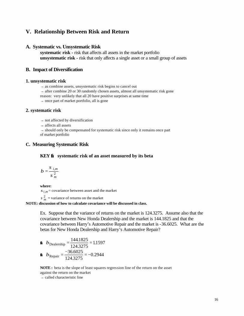
C. Measuring Systematic Risk

KEY →→ systematic risk of an asset measured by its beta

βσ

σ= i m

m

,2

where: σi m, = covariance between asset and the market

σm2 = variance of returns on the market

NOTE: discussion of how to calculate covariance will be discussed in class.

Ex. Suppose that the variance of returns on the market is 124.3275. Assume also that the covariance between New Honda Dealership and the market is 144.1825 and that the covariance between Harry’s Automotive Repair and the market is -36.6025. What are the betas for New Honda Dealership and Harry’s Automotive Repair?

→→ βDealership = =1441825124 3275

11597..

.

→→ βRepair = − = −36 6025124 3275

0 2944..

.

NOTE : beta is the slope of least squares regression line of the return on the asset against the return on the market → called characteristic line

17

ri

rM

....

.

....

Graph #6

→ dots represent period returns → slope of line is the beta for asset i

→→ slope = 1.5 (β = 1.5) →→ stock tends to be 1.5 times as volatile as the market →→ slope = .8 (β= 0.8) →→ stock tends to be 80% as volatile as the market → deviations from line = unique risk

NOTE: an easier approach →→ look up β in value line or S&P

18

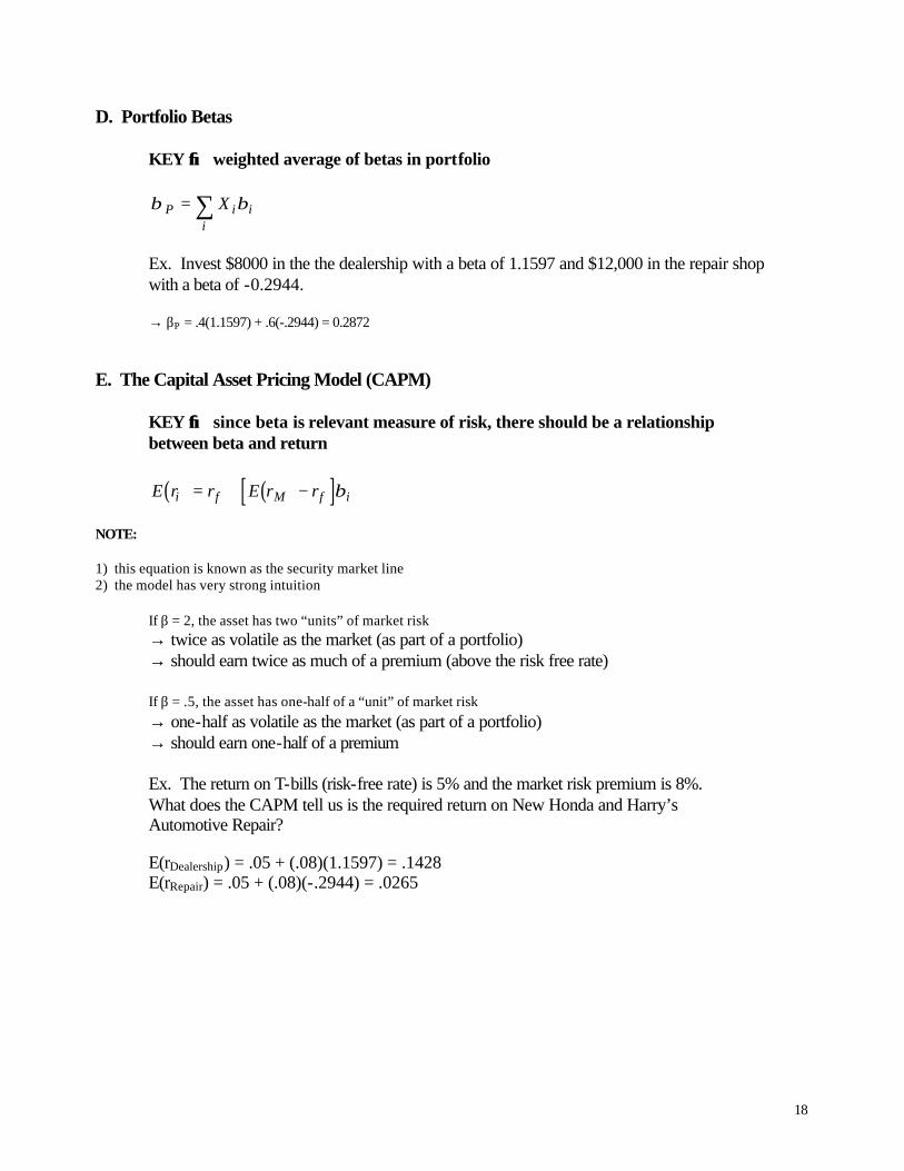
D. Portfolio Betas

KEY →→ weighted average of betas in portfolio

β βP i ii

X= ∑

Ex. Invest $8000 in the the dealership with a beta of 1.1597 and $12,000 in the repair shop with a beta of -0.2944.

→ βP = .4(1.1597) + .6(-.2944) = 0.2872

E. The Capital Asset Pricing Model (CAPM)

KEY →→ since beta is relevant measure of risk, there should be a relationship between beta and return

( ) ( )[ ]E r r E r ri f M f i= + − β

NOTE: 1) this equation is known as the security market line 2) the model has very strong intuition

If β = 2, the asset has two “units” of market risk → twice as volatile as the market (as part of a portfolio) → should earn twice as much of a premium (above the risk free rate)

If β = .5, the asset has one-half of a “unit” of market risk

→ one-half as volatile as the market (as part of a portfolio) → should earn one-half of a premium

Ex. The return on T-bills (risk-free rate) is 5% and the market risk premium is 8%. What does the CAPM tell us is the required return on New Honda and Harry’s Automotive Repair?

E(rDealership) = .05 + (.08)(1.1597) = .1428 E(rRepair) = .05 + (.08)(-.2944) = .0265

19

EXERCISE PROBLEMS FOR CHAPTER 9. 1. Find the expected return on Bio-Pharma stock when there are two possible states of economy. The

probability that the high state will occur is 32% and that the low state will occur is 68%. The return on Bio-Pharma stock is 16.83% in the high state and 7.91% in the low state. [[10.76%]]

2. With two possible states of the economy, find the variance of returns on Texas Eastern stock. The

probability that State 1 will occur is 28% and that State 2 will occur is 72%. The return in State 1 is 16.49% and in State 2 is 7.04%. [[18.0034]]

3. Your budget manager demands new calculations of covariance of returns based on the best case and

worst case possibilities. You estimate that your firm will receive returns given in the following table in the two states. You also estimate returns to the Dow Jones 30 in these two states. Find the covariance of returns. [[0.2855]] State of Nature Probability Texas Eastern Return Index Return The best state 52% 16.79% 16.02% The worst state 48% 5.35% 6.02%

4. You are considering investing in a portfolio of two stocks, with 57% of your money in the first stock and

43% in the second stock. You calculate that the expected returns for the two stocks are 9.60% and 16.25%, respectively. Find the portfolio expected return.[[12.46%]]

5. Find the variance of the portfolio when the variance of expected returns is 0.10262 for Asset 1 and

0.11397 for Asset 2. The covariance of returns is 0.01925. Funds are invested with 53% of the money in Asset 1 and 47% in Asset 2.[[0.0636]]

6. The stock analyst for US East has determined that if the best state occurs in the economy, US East stock

will yield a return of 16.17%. If the worst state occurs, the return will be 6.96%. If the normal state occurs, the return will be 12.56%. With probabilities of 17% on the best state, 31% on the worst state, and 52% on the normal state, what is the expected return on the stock? [[11.44%]]

7. Before approving acquisition of new machinery, the treasurer of Sip-n-Smoke wants to know the

standard deviation of returns on it. You tell him that the firm should receive a return of 15.15% with a probability of 49%, and a return of 5.21% with a probability of 51%. What is the standard deviation of returns on the machinery?[[4.97%]]

8. The project manager at O'Reilly Corp figures the states of nature and returns for O'Reilly Corp from a

new project and also the returns for the value weighted stock index. These appear in the following table . What is the covariance of returns of the project with the value weighted stock index? [[0.1348]] State of Nature Probability O'Reilly Corp Return Index Return The boom state 73% 15.47% 14.64% The recession 27% 6.15% 7.30%

9. You have invested 29% of your money in Stock X, 50% in Stock Y, and the rest in Stock Z. The portfolio expected return is 7.48%, and the expected returns of X and Y are 7.83% and 6.83%. What is the expected return of Stock Z? [[8.54%]]

10. You are considering a portfolio of two stocks, with 90% of your money in the first stock, and 10% in the

second stock. The variance of returns of Stock 1 is 0.10065 and the variance of returns of Stock 2 is 0.13753. The correlation coefficient of returns is 0.598. Find the variance of the portfolio. [[0.0956]]

20

CHAPTER 10. RISK AND RETURN [CAPM]

I. Examples from Chapter 9.

Ex. Historical Returns for Dealership Inc. and for Repair Inc. for past 4 years.

- How to compute by using financial calculator ? Return on: Year Dealership Repair 1992 19 14 1993 39 8 1994 15 11 1995 0 19 r 18.25 13.00 σ 16.07 4.69 Ex. Estimated possible future returns for Dealership Inc. and Repair Inc for the coming year

based on how the economy does Return on: Economy Prob. Dealership Repair Boom .25 40% 6% Average .55 15% 15% Bust .2 -1% 17% E(r) 18.05 13.15 σ 14.08 4.20 II. Risk and Return for Portfolios using Forecasted Data

→ weighted average of variances and covariances

σ σ σ σp X X X X212

12

1 2 1 2 22

222= + +,

where:

σp2 = variance of returns on portfolio

Xi = % of portfolio invested in asset i [=weight or proportion]

σi2 = variance of returns on asset i

=2,1σ covariance between asset 1 and asset 2

21

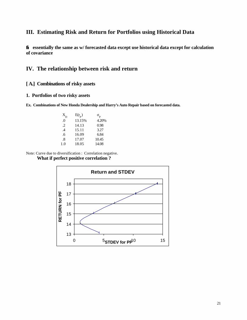
III. Estimating Risk and Return for Portfolios using Historical Data

→→ essentially the same as w/ forecasted data except use historical data except for calculation of covariance

IV. The relationship between risk and return

[ A.] Combinations of risky assets 1. Portfolios of two risky assets Ex. Combinations of New Honda Dealership and Harry’s Auto Repair based on forecasted data.

XD

E(rP) σ

P

.0 13.15% 4.20% .2 14.13 0.98 .4 15.11 3.27 .6 16.09 6.84 .8 17.07 10.45 1.0 18.05 14.08

Note: Curve due to diversification : Correlation negative. What if perfect positive correlation ?

Return and STDEV

13

14

15

16

17

18

0 5 10 15STDEV for PF

RE

TUR

N fo

r P

F

22

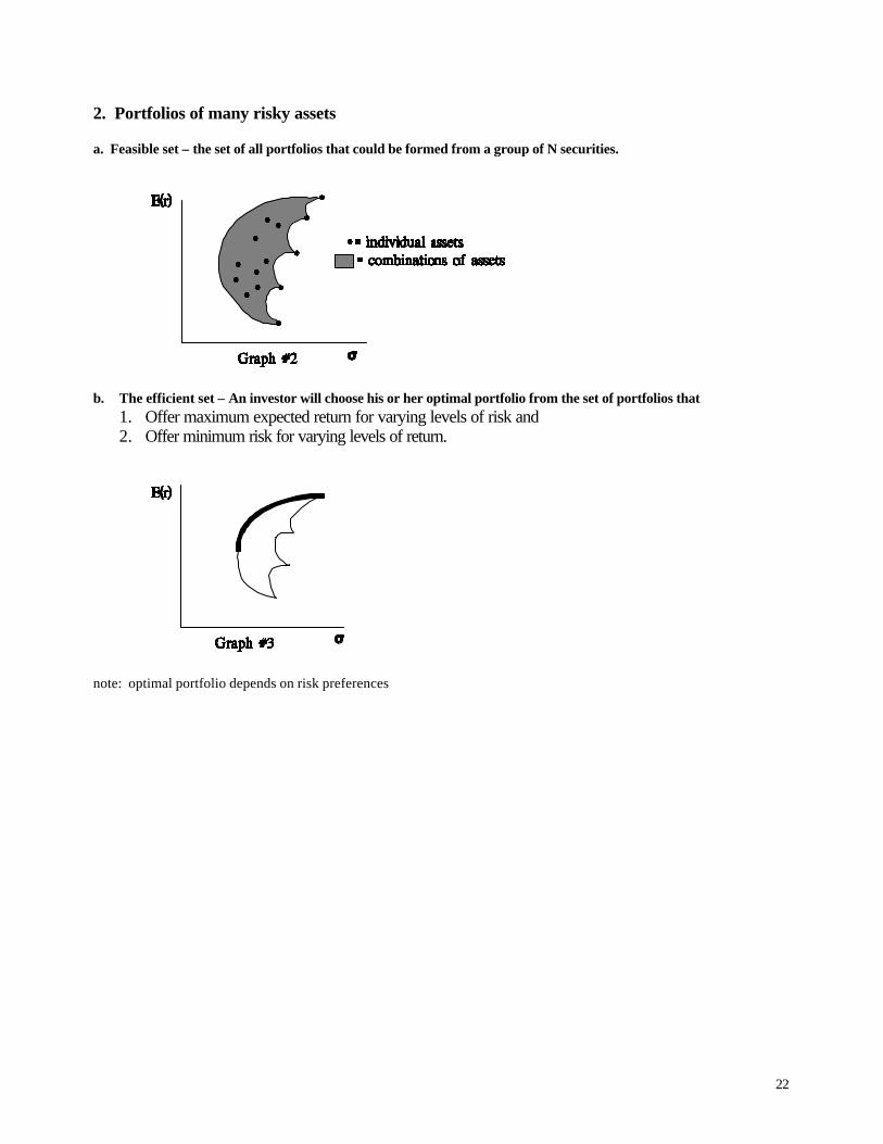
2. Portfolios of many risky assets a. Feasible set – the set of all portfolios that could be formed from a group of N securities.

b. The efficient set – An investor will choose his or her optimal portfolio from the set of portfolios that

1. Offer maximum expected return for varying levels of risk and 2. Offer minimum risk for varying levels of return.

note: optimal portfolio depends on risk preferences

23

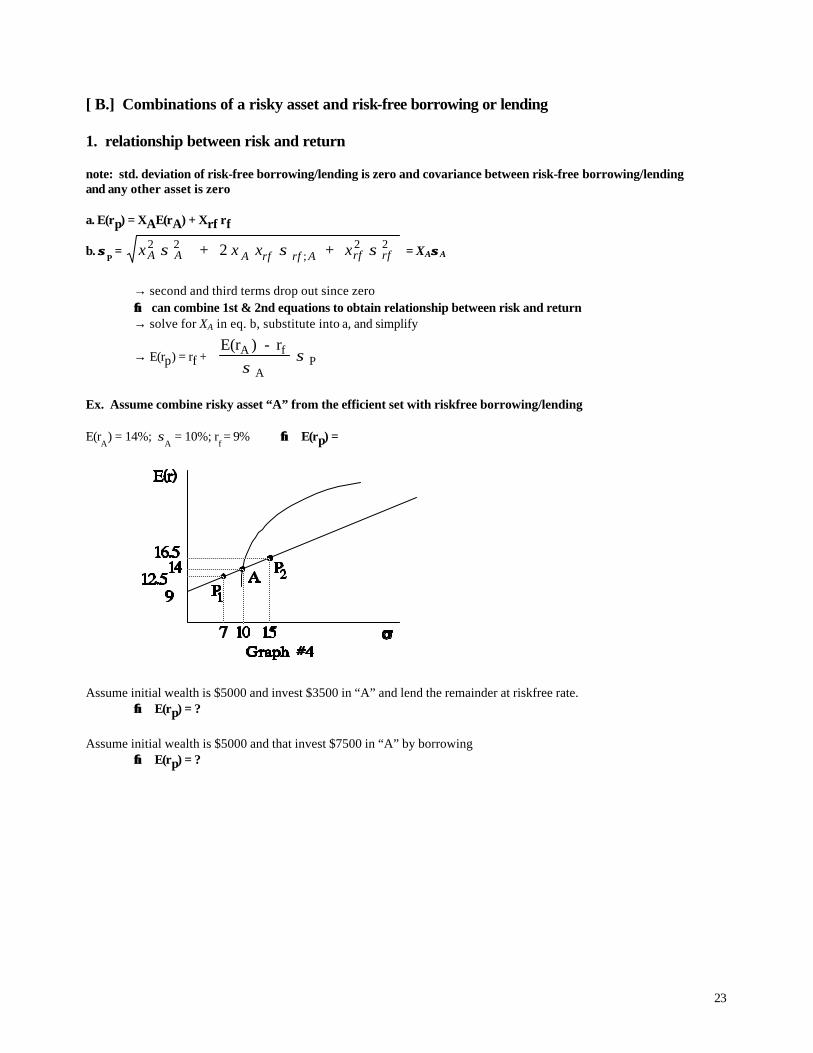
[ B.] Combinations of a risky asset and risk-free borrowing or lending 1. relationship between risk and return note: std. deviation of risk-free borrowing/lending is zero and covariance between risk-free borrowing/lending and any other asset is zero a. E(rp) = XAE(rA) + Xrf rf

b. σσP = x x x xA A A rf rf A rf rf

2 2 2 2 + 2 + σ σ σ; = XAσσA

→ second and third terms drop out since zero →→ can combine 1st & 2nd equations to obtain relationship between risk and return → solve for XA in eq. b, substitute into a, and simplify

→ E(rp) = rf + E(r ) - rA f

APσ

σ

Ex. Assume combine risky asset “A” from the efficient set with riskfree borrowing/lending E(r

A) = 14%; σ

A = 10%; r

f = 9% →→ E(rp) =

Assume initial wealth is $5000 and invest $3500 in “A” and lend the remainder at riskfree rate.

→→ E(rp) = ?

Assume initial wealth is $5000 and that invest $7500 in “A” by borrowing

→→ E(rp) = ?

24

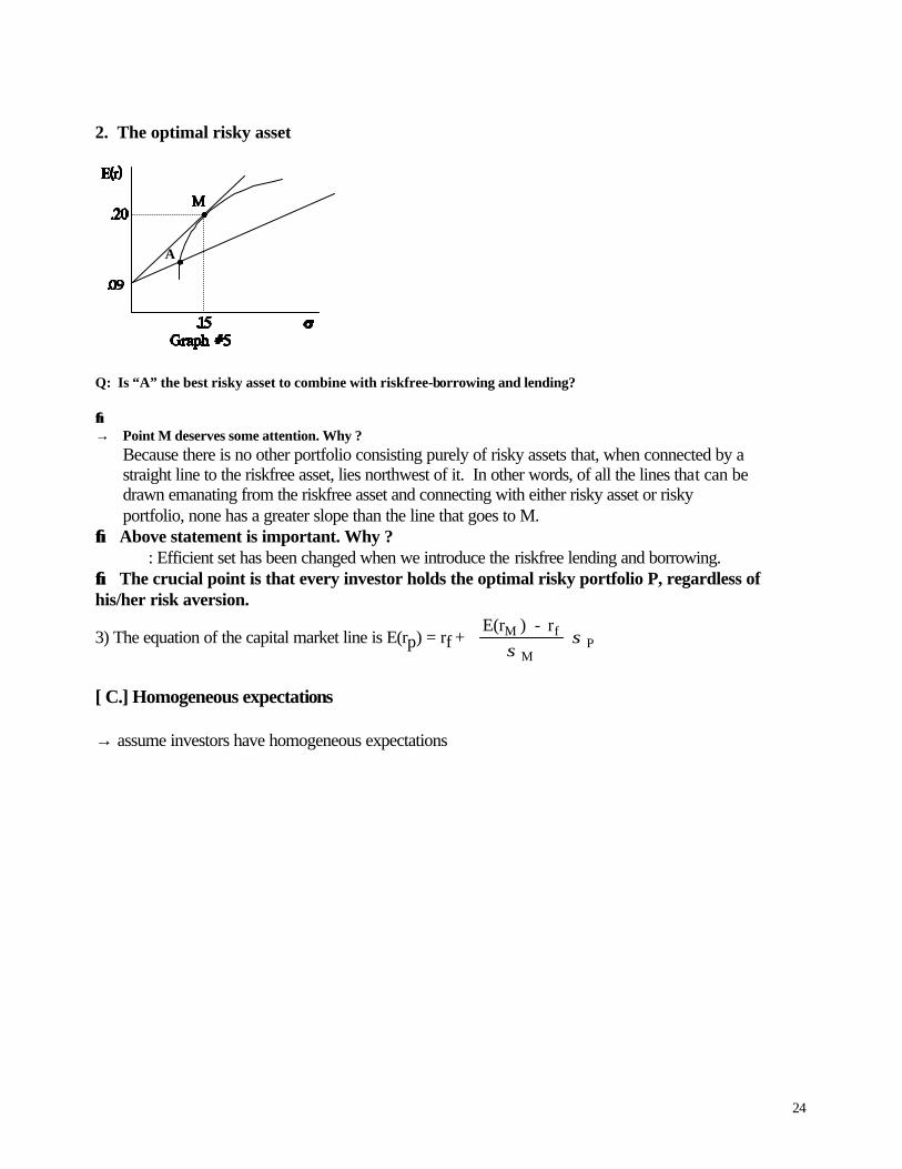
2. The optimal risky asset

A

Q: Is “A” the best risky asset to combine with riskfree-borrowing and lending? →→ → Point M deserves some attention. Why ?

Because there is no other portfolio consisting purely of risky assets that, when connected by a straight line to the riskfree asset, lies northwest of it. In other words, of all the lines that can be drawn emanating from the riskfree asset and connecting with either risky asset or risky portfolio, none has a greater slope than the line that goes to M.

→→ Above statement is important. Why ? : Efficient set has been changed when we introduce the riskfree lending and borrowing. →→ The crucial point is that every investor holds the optimal risky portfolio P, regardless of his/her risk aversion.

3) The equation of the capital market line is E(rp) = rf + E(r ) - rM f

MPσ

σ

[ C.] Homogeneous expectations → assume investors have homogeneous expectations

25

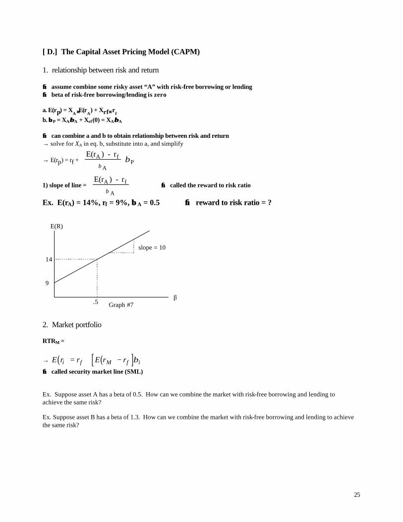
[ D.] The Capital Asset Pricing Model (CAPM) 1. relationship between risk and return →→ assume combine some risky asset “A” with risk-free borrowing or lending →→ beta of risk-free borrowing/lending is zero a. E(rp) = X

A ⋅⋅ E(rA

) + Xrf⋅⋅ rf b. ββ P = XAββA + Xrf(0) = XAββA →→ can combine a and b to obtain relationship between risk and return → solve for XA in eq. b, substitute into a, and simplify

→ E(rp) = rf + E(r ) - rA f

AP

ββ

1) slope of line = E(r ) - rA f

Aβ

→→ called the reward to risk ratio

Ex. E(rA) = 14%, rf = 9%, ββ A = 0.5 →→ reward to risk ratio = ?

β

E(R)

.5

9

14

Graph #7

slope = 10

2. Market portfolio RTRM =

→ ( ) ( )[ ]E r r E r ri f M f i= + − β

→→ called security market line (SML) Ex. Suppose asset A has a beta of 0.5. How can we combine the market with risk-free borrowing and lending to achieve the same risk? Ex. Suppose asset B has a beta of 1.3. How can we combine the market with risk-free borrowing and lending to achieve the same risk?

26

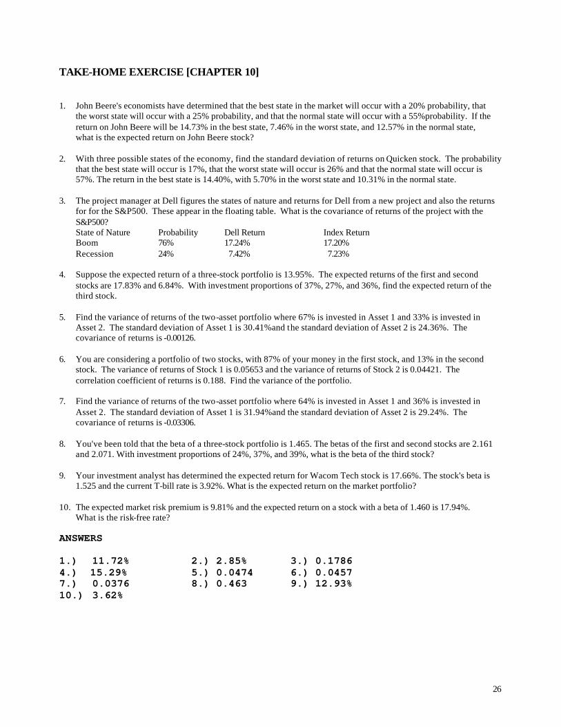
TAKE-HOME EXERCISE [CHAPTER 10] 1. John Beere's economists have determined that the best state in the market will occur with a 20% probability, that

the worst state will occur with a 25% probability, and that the normal state will occur with a 55%probability. If the return on John Beere will be 14.73% in the best state, 7.46% in the worst state, and 12.57% in the normal state, what is the expected return on John Beere stock?

2. With three possible states of the economy, find the standard deviation of returns on Quicken stock. The probability

that the best state will occur is 17%, that the worst state will occur is 26% and that the normal state will occur is 57%. The return in the best state is 14.40%, with 5.70% in the worst state and 10.31% in the normal state.

3. The project manager at Dell figures the states of nature and returns for Dell from a new project and also the returns

for for the S&P500. These appear in the floating table. What is the covariance of returns of the project with the S&P500? State of Nature Probability Dell Return Index Return Boom 76% 17.24% 17.20% Recession 24% 7.42% 7.23%

4. Suppose the expected return of a three-stock portfolio is 13.95%. The expected returns of the first and second

stocks are 17.83% and 6.84%. With investment proportions of 37%, 27%, and 36%, find the expected return of the third stock.

5. Find the variance of returns of the two-asset portfolio where 67% is invested in Asset 1 and 33% is invested in

Asset 2. The standard deviation of Asset 1 is 30.41%and the standard deviation of Asset 2 is 24.36%. The covariance of returns is -0.00126.

6. You are considering a portfolio of two stocks, with 87% of your money in the first stock, and 13% in the second

stock. The variance of returns of Stock 1 is 0.05653 and the variance of returns of Stock 2 is 0.04421. The correlation coefficient of returns is 0.188. Find the variance of the portfolio.

7. Find the variance of returns of the two-asset portfolio where 64% is invested in Asset 1 and 36% is invested in

Asset 2. The standard deviation of Asset 1 is 31.94%and the standard deviation of Asset 2 is 29.24%. The covariance of returns is -0.03306.

8. You've been told that the beta of a three-stock portfolio is 1.465. The betas of the first and second stocks are 2.161

and 2.071. With investment proportions of 24%, 37%, and 39%, what is the beta of the third stock? 9. Your investment analyst has determined the expected return for Wacom Tech stock is 17.66%. The stock's beta is

1.525 and the current T-bill rate is 3.92%. What is the expected return on the market portfolio? 10. The expected market risk premium is 9.81% and the expected return on a stock with a beta of 1.460 is 17.94%.

What is the risk-free rate? ANSWERS 1.) 11.72% 2.) 2.85% 3.) 0.1786 4.) 15.29% 5.) 0.0474 6.) 0.0457 7.) 0.0376 8.) 0.463 9.) 12.93% 10.) 3.62%

27

CHAPTER 13. Financing and Efficient Capital Markets So far, you've learned how to spend money--how to choose among different potential investment projects. Now let's figure out how to raise it--how firms interface with the capital markets to raise the money to undertake investment projects. I. What Is an "Efficient" Market? We assume that capital markets are efficient. By "efficient" we mean a bunch of things that • All relevant and ascertainable information is reflected in the market price already because it is widely and cheaply available to investors. • Stock prices are a random walk (with drift) • Weak Form Efficiency → Past pattern of prices doesn't allow you to make abnormal return. : Serial correlations [corr(RETt, RETt-1)] → Indications of market inefficiencies. • Semi-strong Form Efficiency → Published information doesn't allow you to make abnormal return. • Strong Form Efficiency → Any information in the world doesn't allow you to make abnormal return. Stock prices appeared to be a random walk (with drift). Price changes are independent of the most recent price changes. What this means for "technical analysis". Competition among investment analysts should lead prices to reflect "true values"--true value does not mean future value, but an expected value that incorporates all the information available to investors at that time. If prices always reflect all information, they will only change when new "information" arrives. But by definition we don't know whether new information will be good or bad. • By denying that future market movements can be predicted from past movements, we are denying the profitability of technical analysis. •• See the Summary on textbook pg. 339.

28

II. We Always Come Back to NPV The decision to sell a share of stock, and the decision to purchase an electromechanical capital good are basically similar. Both involve the "valuation" of a risky asset, and the comparison of the value of a risky future stream with a present sum. The fact that one asset is "real" and the other "financial" shouldn't bother you. • The present value of borrowing.

Suppose the government agrees to lend your firm $100,000 for 10 years at an interest rate of 3%:

NPVr t

t

= + +−

+=∑100 000

3 00011

10

,( , )( )

If the appropriate discount rate is 10%, what is NPV? When the appropriate discount rate is 10%, an offer to loan you money for 10 years at 3% is truly an amazing deal...

In financial markets, you are facing a nearly perfect, competitive market If selling a security has a positive NPV to you, it probably has a negative NPV to the purchaser. You probably will not find many such purchasers. If capital markets are efficient, then purchase or sale of any security at the prevailing market price is never a positive (or negative) NPV transaction... III. No Theory Is Perfect: Anomalies: • Small firm effect → small firm estimated betas are not high enough to account for their high returns • January effect → small firms earn high returns in January (people wait until after the end of the tax year to dump losing positions in big stocks?) • P/E Effect. • B/M Effect. [Book to Market Value]