Automatic real-time bass transcription system based on ... · POLITECNICO DI MILANO Facolt a di...
85
POLITECNICO DI MILANO Facolt` a di Ingegneria dell’Informazione Corso di Laurea in Ingegneria e Design del Suono Automatic real-time bass transcription system based on Combined Difference Function Supervisor: Prof. Augusto Sarti Co-Supervisor: Dr. Massimiliano Zanoni Master graduation thesis by: Davide Montorio, ID 724839 Academic Year 2009-2010
Transcript of Automatic real-time bass transcription system based on ... · POLITECNICO DI MILANO Facolt a di...
POLITECNICO DI MILANOFacolta di Ingegneria dell’Informazione
Corso di Laurea in Ingegneria e Design del Suono
Automatic real-time bass transcription
system based on Combined Difference
Function
Supervisor: Prof. Augusto Sarti
Co-Supervisor: Dr. Massimiliano Zanoni
Master graduation thesis by:
Davide Montorio, ID 724839
Academic Year 2009-2010

POLITECNICO DI MILANOFacolta di Ingegneria dell’Informazione
Corso di Laurea in Ingegneria e Design del Suono
Automatic real-time bass transcription
system based on Combined Difference
Function
Relatore: Prof. Augusto Sarti
Correlatore: Dr. Massimiliano Zanoni
Tesi di Laurea Magistrale di:
Davide Montorio, ID 724839
Anno Accademico 2009-2010
“There is no end to learning”
Robert Alexander Schumann

Abstract
Due to the recent worldwide diffusion of internet and audio digital formats,
in past few years the amount of multimedia contents highly increased. Our
approach to produce, listen to and search for music is consequently changing
and a great number of applications to help us in these tasks are proposed.
For this reason, researchers’ studies in music and technology field becomes
more and more important. One of the most relevant field is Music Informa-
tion Retrieval: the interdisciplinary science of retrieving information from
music. One of the most interesting field within MIR is Automatic Music
Transcription. That is the process of taking a digital sound waveform and
extracting the symbolic information related to the high-level musical struc-
tures that might be seen on a score.
This thesis proposes an application for real-time bass transcription from an
audio signal. Possible users of the application are both amateur and stu-
dents with few musical notions and expert musicians. For that reason the
application is intended to have an extremely simple to use interface and
functionalities. The core of the application is the pitch detection algorithm.
We used an algorithm based on the composition of two techniques (YIN and
SMSDF) that proposes a new method to estimate the pitch, called Com-
bined Difference Function. The application gives the possibility to plug a
bass directly in the computer and perform transcription in real-time. A
real-time approach has been chosen to provide the user an instant feedback
on the bass line played.
I

Sommario
Grazie alla recente diffusione mondiale di internet e dei formati audio digi-
tali, negli ultimi anni la quantita di contenuti multimediali e notevolmente
aumentata. Di conseguenza, l’approccio alla produzione, all’ascolto e alla
ricerca di musica sta cambiando e sempre nuove applicazioni ci aiutano in
questo genere di attivita. Per queste ragioni, la ricerca nel campo della mu-
sica e della tecnologia ha acquisito sempre piu importanza. Un settore di
ricerca tra i piu rilevanti e quello del Music Information Retrieval (MIR).
MIR e quella scienza interdisciplinare che si occupa di recuperare infor-
mazioni dai brani musicali. Uno degli ambiti piu interessanti all’interno
di MIR e quello che si occupa di Trascrizione Musicale Automatica. Con
trascrizione musicale intendiamo il processo di estrazione, da un segnale au-
dio digitale, di informazioni simboliche relative alle strutture musicali che
possiamo vedere in un comune spartito.
Questa tesi propone un’applicazione per la trascrizione del basso in tempo
reale partendo da un segnale audio. Possibili fruitori dell’applicazione sono
sia studenti e dilettanti, con poche conoscenze musicali, sia musicisti esperti
e competenti. Per questa ragione l’applicazione e stata realizzata in modo
da essere estremamente semplice da utilizzare sia nell’interfaccia che nelle
funzionalita.
Il nucleo dell’applicazione e l’algoritmo di stima dell’altezza della nota (pitch).
Per questo compito e stato usato un algoritmo, basato sulla composizione
di due diverse tecniche (YIN e SMSDF), che propone un nuovo metodo
per stimare l’altezza della nota, chiamato Combined Difference Function.
L’applicazione da la possibilita di collegare il basso direttamente nel com-
puter ed effettuare la trascrizione in tempo reale: un approccio di questo
tipo e stato scelto per poter dare all’utente un feedback immediato sulla
propria esecuzione.
II


Contents
Abstract I
Sommario II
Abbreviations X
1 Introduction 1
1.1 Background . . . . . . . . . . . . . . . . . . . . . . . . . . . . 2
1.1.1 Automatic transcription . . . . . . . . . . . . . . . . . 2
1.1.2 Electric Bass . . . . . . . . . . . . . . . . . . . . . . . 4
1.1.3 Fundamental frequency and Pitch . . . . . . . . . . . 4
1.2 Brief work description . . . . . . . . . . . . . . . . . . . . . . 5
1.2.1 Frequency Tracking . . . . . . . . . . . . . . . . . . . 5
1.2.2 Onset Detection . . . . . . . . . . . . . . . . . . . . . 6
1.2.3 User Interface . . . . . . . . . . . . . . . . . . . . . . . 6
1.3 Overview of the thesis . . . . . . . . . . . . . . . . . . . . . . 6
2 State of the art 7
2.1 Algorithms . . . . . . . . . . . . . . . . . . . . . . . . . . . . 7
2.1.1 Fundamental Frequency . . . . . . . . . . . . . . . . . 7
2.1.2 Time-Domain Methods . . . . . . . . . . . . . . . . . 8
2.1.3 Frequency-Domain Methods . . . . . . . . . . . . . . . 10
2.2 Software Applications . . . . . . . . . . . . . . . . . . . . . . 12
2.2.1 MP3 to MIDI converter, by IntelliScore . . . . . . . 13
2.2.2 Melodyne, by Celemony . . . . . . . . . . . . . . . . 14
2.2.3 Audioscore Ultimate 6, by Neutraron . . . . . . . . . 14
2.2.4 Capo, by Supermegaultragroovy . . . . . . . . . . . 15
2.2.5 Digital Music Mentor, by Sienzo . . . . . . . . . . . 16
2.2.6 Guitarmaster, by RoboSens . . . . . . . . . . . . . . 16
IV
3 Theoretical Background 17
3.1 Introduction . . . . . . . . . . . . . . . . . . . . . . . . . . . . 17
3.1.1 Requirements . . . . . . . . . . . . . . . . . . . . . . . 17
3.1.2 Bass Constraints . . . . . . . . . . . . . . . . . . . . . 18
3.1.3 Frequency Estimation Methods . . . . . . . . . . . . . 19
3.2 Algorithm . . . . . . . . . . . . . . . . . . . . . . . . . . . . . 19
3.2.1 Difference Function . . . . . . . . . . . . . . . . . . . . 20
3.2.2 The YIN algorithm . . . . . . . . . . . . . . . . . . . . 21
3.2.3 The Combined Difference Function algorithm . . . . . 21
3.2.4 Cumulative Mean Normalized DF . . . . . . . . . . . 26
3.2.5 Errors . . . . . . . . . . . . . . . . . . . . . . . . . . . 28
3.3 MIDI . . . . . . . . . . . . . . . . . . . . . . . . . . . . . . . . 28
4 System Design 30
4.1 Tools and Frameworks . . . . . . . . . . . . . . . . . . . . . . 30
4.1.1 Matlab . . . . . . . . . . . . . . . . . . . . . . . . . . 30
4.1.2 PlayRec . . . . . . . . . . . . . . . . . . . . . . . . . 31
4.1.3 MIDI Toolbox . . . . . . . . . . . . . . . . . . . . . . 31
4.2 Implementation . . . . . . . . . . . . . . . . . . . . . . . . . . 32
4.2.1 Audio file acquisition . . . . . . . . . . . . . . . . . . . 32
4.2.2 Real-time acquisition . . . . . . . . . . . . . . . . . . . 33
4.2.3 Frame creation . . . . . . . . . . . . . . . . . . . . . . 34
4.2.4 Analysis . . . . . . . . . . . . . . . . . . . . . . . . . . 35
4.2.5 MIDI Elaboration . . . . . . . . . . . . . . . . . . . . 43
4.2.6 Score Creation . . . . . . . . . . . . . . . . . . . . . . 44
4.3 Conclusions . . . . . . . . . . . . . . . . . . . . . . . . . . . . 44
5 Software development 46
5.1 Requirements . . . . . . . . . . . . . . . . . . . . . . . . . . . 46
5.2 Environment and libraries . . . . . . . . . . . . . . . . . . . . 47
5.2.1 Java . . . . . . . . . . . . . . . . . . . . . . . . . . . . 47
5.2.2 JTransform . . . . . . . . . . . . . . . . . . . . . . . . 48
5.2.3 Java Sound . . . . . . . . . . . . . . . . . . . . . . . . 48
5.2.4 JMusic . . . . . . . . . . . . . . . . . . . . . . . . . . 50
5.2.5 JFreeChart . . . . . . . . . . . . . . . . . . . . . . . . 50
5.3 Implementation . . . . . . . . . . . . . . . . . . . . . . . . . . 51
5.3.1 GUI . . . . . . . . . . . . . . . . . . . . . . . . . . . . 52
5.3.2 Thread . . . . . . . . . . . . . . . . . . . . . . . . . . 53
5.3.3 Analysis . . . . . . . . . . . . . . . . . . . . . . . . . . 54
5.3.4 Audio Operations . . . . . . . . . . . . . . . . . . . . 55
V
5.3.5 Visualization . . . . . . . . . . . . . . . . . . . . . . . 57
6 Experimental Results and Evaluations 60
6.1 Dataset . . . . . . . . . . . . . . . . . . . . . . . . . . . . . . 60
6.1.1 Synthesized Dataset . . . . . . . . . . . . . . . . . . . 60
6.1.2 Users Dataset . . . . . . . . . . . . . . . . . . . . . . . 61
6.2 Results . . . . . . . . . . . . . . . . . . . . . . . . . . . . . . . 61
6.2.1 Objective . . . . . . . . . . . . . . . . . . . . . . . . . 62
6.2.2 Subjective . . . . . . . . . . . . . . . . . . . . . . . . . 63
6.3 Algorithm’s evaluation and comments . . . . . . . . . . . . . 65
7 Conclusions and future developments 68
7.1 Conclusions . . . . . . . . . . . . . . . . . . . . . . . . . . . . 68
7.2 Future developments . . . . . . . . . . . . . . . . . . . . . . . 69
Bibliography 70
List of Figures
1.1 Acoustic signal to score notation . . . . . . . . . . . . . . . . 3
1.2 Fender Jazz Bass . . . . . . . . . . . . . . . . . . . . . . . . . 4
1.3 Structure of the transcription system . . . . . . . . . . . . . . 5
2.1 Influence of higher harmonics on zero crossing rate . . . . . . 8
2.2 Stages in the cepstrum analysis algorithm . . . . . . . . . . . 12
2.3 MP3 to MIDI converter interface, by IntelliScore . . . . . . . 13
2.4 Melodyne, by Celemony . . . . . . . . . . . . . . . . . . . . . 14
2.5 Audioscore Ultimate 6, Neuratron.com . . . . . . . . . . . . . 15
2.6 Capo, by Supermegaultragroovy . . . . . . . . . . . . . . . . 16
3.1 Sinusoidal wave with upper harmonics . . . . . . . . . . . . . 18
3.2 A sinusoidal wave . . . . . . . . . . . . . . . . . . . . . . . . . 19
3.3 A periodic function with period T . . . . . . . . . . . . . . . 20
3.4 The difference between left-to-right SMDSF and right-to-left
SMDSF . . . . . . . . . . . . . . . . . . . . . . . . . . . . . . 24
3.5 The difference between the bidirectional SMDSF and the cir-
cular SMDSF . . . . . . . . . . . . . . . . . . . . . . . . . . . 26
3.6 The difference between the DF and the CMNDF . . . . . . . 27
4.1 System overview for an audio file . . . . . . . . . . . . . . . . 32
4.2 System overview with bass plugged-in . . . . . . . . . . . . . 33
4.3 Blocks organization . . . . . . . . . . . . . . . . . . . . . . . . 34
4.4 Analysis overview . . . . . . . . . . . . . . . . . . . . . . . . . 35
4.5 Blocks’ structure of the pitch detection phase . . . . . . . . . 35
4.6 Pitch Detection structure . . . . . . . . . . . . . . . . . . . . 37
4.7 Combined DF of a frame . . . . . . . . . . . . . . . . . . . . . 38
4.8 CMNDF of a frame . . . . . . . . . . . . . . . . . . . . . . . . 39
4.9 Onset Detection Function . . . . . . . . . . . . . . . . . . . . 41
4.10 The new Onset Detection Function . . . . . . . . . . . . . . . 43
4.11 Piano roll visualization . . . . . . . . . . . . . . . . . . . . . . 45
VII
5.1 A typical audio architecture . . . . . . . . . . . . . . . . . . . 49
5.2 A line configuration for audio output . . . . . . . . . . . . . . 50
5.3 Logic scheme of the Java application . . . . . . . . . . . . . . 51
5.4 Application user interface . . . . . . . . . . . . . . . . . . . . 53
5.5 Use of thread in the application . . . . . . . . . . . . . . . . . 54
5.6 Audio blocks segmentation . . . . . . . . . . . . . . . . . . . 55
5.7 Score of a transcribed music excerpt . . . . . . . . . . . . . . 57
5.8 Application’s menu for further score modification . . . . . . . 58
5.9 Real-time score representation . . . . . . . . . . . . . . . . . . 59
List of Tables
3.1 Doubling/halving error rates for the LR, the RL and the Bidi-
rectional difference function . . . . . . . . . . . . . . . . . . . 25
3.2 Doubling/halving error rates using the bidirectional function,
the circular function and the combined solution . . . . . . . . 27
6.1 Results of the algorithm performance with the synthesized
dataset . . . . . . . . . . . . . . . . . . . . . . . . . . . . . . . 63
6.2 Results of user1 performance . . . . . . . . . . . . . . . . . . 63
6.3 Results of user2 performance . . . . . . . . . . . . . . . . . . 64
6.4 Results of user3 performance . . . . . . . . . . . . . . . . . . 64
6.5 Doubling and halving errors for the synthesized dataset . . . 66
6.6 Doubling and halving errors for the user dataset . . . . . . . 66
IX
Abbreviations
ACF Autocorrelation function
CAMDF Circular Average Magnitude Difference Function
CMNDF Cumulative Mean Normalized Difference Function
DF Difference Function
DFT Discrete Fourier transform
EM Expectation-maximization
F0(f0) Fundamental frequency
FFT Fast Fourier transform
IDFT Inverse discrete Fourier transform
MIDI Musical Instrument Digital Interface
PCM Pulse Code Modulation
SMSDF Sum Magnitude Difference Square Function
Chapter 1
Introduction
“An orchestra without a double bass is inconceivable. It is the
essential orchestral instrument.
You can almost say that an orchestra set about to exist only when
there’s a double bass.
There are orchestras with no first violin, no horns, no drums and
trumpets, nothing at all.
But not without a double bass.
What I want to establish is that double bass is by far the most
important instrument of the orchestra.
Even if it does not seem.”
Double Bass - Patrick Suskind
Thanks to the wide diffusion of internet and digital technologies in past few
years, our way to approach music is extremely changed. Digital audio play-
ers, mp3 files and music software are new tools to interact with music. The
way we listen or how we record music is completely different from ten years
ago. The availability of musical contents in digital form is exponentially
increased and thus the need to organize and provide access. The pressure
of consumers has drawn the attention of researchers and industry to this
tasks. The large amount of audio material raised new issue on handling and
organizing it. A new field in audio research was born: Music Information Re-
trieval. MIR is the interdisciplinary science of retrieving information from
music and includes music classification, feature extraction, database cre-
ation, indexing, signal processing, music analysis and music representation.
An important area of research within MIR is automatic music transcription.
Music transcription is intended as the act of writing down the notes played
1.1. Background
in a music excerpt, in a coded notation which includes notes, pitch, length
and expression. With Automatic Music Transcription we intend the process
of transcribing music performed automatically by a computer. In last few
years the problem has been easily solved using MIDI protocols and MIDI
instrument interfaces (MIDI keyboard, MIDI Drum, MIDI Guitar, etc. . . ).
MIDI is a protocol thought to send music messages between MIDI interfaces
and no audio signal is transmitted. Messages as note pitch or note starting
or ending instant are transmitted: it’s easy to store this messages and cre-
ate, automatically, a transcription of a MIDI performance. Although, MIDI
protocols has some limitation in expressivity to describe a performance. For
that reason researchers started to focus on more expressive automatic music
transcription. The new line to cross is music transcription using content-
based methods based on the direct analysis of the audio signal. Automatic
music transcription research is divided in two main areas:
• Monophonic transcription: analysis of music instruments that produce
only one note at a time, composing a melody;
• Polyphonic transcription: concerns music instruments that can pro-
duce more notes at a time, generating chords and or instruments in a
polyphonic context (mixed excerpt).
The focus of this thesis is on monophonic instruments and the goal is to real-
ize a real time application for automatic bass transcription. The application
is realized for being simple and usable for everyone, from the professional
musician to the entry-level music student.
1.1 Background
1.1.1 Automatic transcription
Since ages, one of musicians’ hardest work has been music transcription.
This is a hard work required of a good ”musical ear”, that is the capability of
discerning a sequence of music notes. Usually, this ability comes with years
of study, practice and exercises. But, nowadays, the help of technology and
the rising of the research in the audio-music field let the musicians be helped
by software applications and algorithms capable of automatic transcription.
This applications open wides scenarios for the professional musician as well
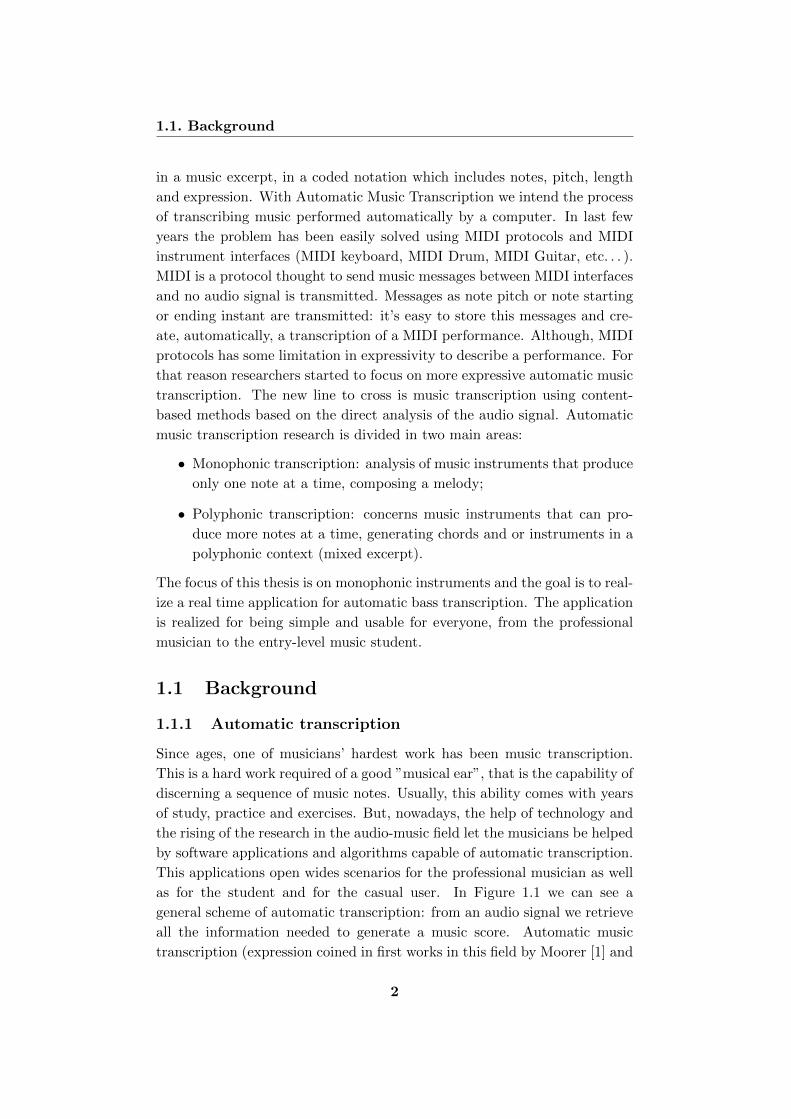
as for the student and for the casual user. In Figure 1.1 we can see a
general scheme of automatic transcription: from an audio signal we retrieve
all the information needed to generate a music score. Automatic music
transcription (expression coined in first works in this field by Moorer [1] and
2
1.1. Background
Figure 1.1: Acoustic signal to score notation
by Piszczalski and Galler [2]) is the process through music transcription is
performed by an algorithm. Generally, someone with no musical education,
can’t figure out a song’s score and, to tell the truth, this process comes to be
hard for who has this education too. The richer is the polyphonic complexity
of a musical composition, the more experience is needed in the musical style
and the instruments in question, and in music theory. The positive aspect
of Automatic Music Transcription could be:
• to helps researchers and musicians to learn all the musical aspect, like
the harmony, structure, chord progression or single notes, of a song;
• it can give a less space consuming representation of music: a score or
an xml file occupy less than a mp3 file;
• to allows the organization and cataloging of a songs database;
• jam musician can have all performance transcribed on a score;
• to help composer in composition.
Today music transcription algorithms already reached good results in mono-
phonic context, but most of them have high computational complexity. The
3
1.1. Background
available applications, also, do not perform automatic music transcription in
a real-time fashion. We choose, then, to use simpler and low computational
complexity methods in order to implement automatic music transcription
in real-time. The purpose of this work is to create a real-time application
using state-of-art methods for pitch tracking for bass-guitar instrument.
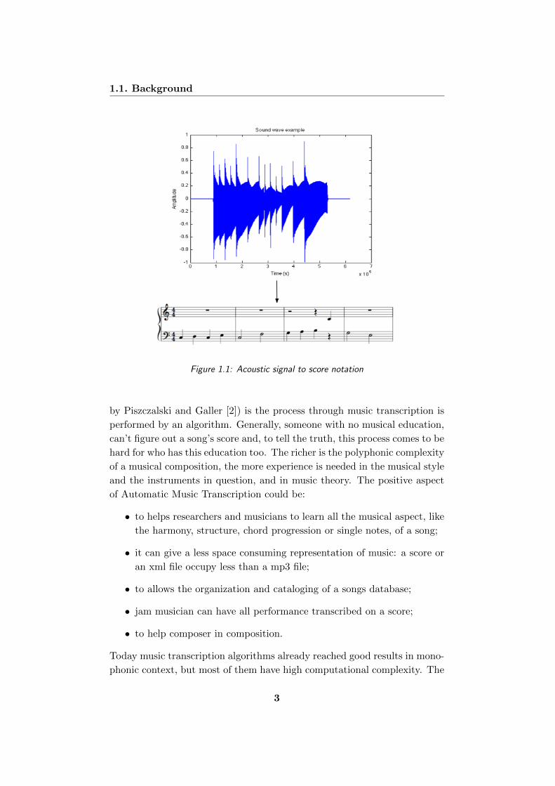
1.1.2 Electric Bass
The thesis work is based on the electric bass. The bass (or bass guitar)
is a stringed instrument played primarily with the fingers or thumb. It is
similar in appearance and construction to an electric guitar, but with a
longer neck and scale length, and four, five, or six strings. The four string
bass, by far the most common, is usually tuned the same as the double bass,
which correspond to pitches one octave lower than the four lower strings of
a guitar (E, A, D, and G). The bass guitar is a transposing instrument, as it
is notated in bass clef an octave higher than it sounds. Since the 1950s, the
electric bass guitar has largely replaced the double bass in popular music as
the bass instrument in the rhythm section. In Figure 1.2 a typical Fender
Jazz bass is shown.
Figure 1.2: Fender Jazz Bass
1.1.3 Fundamental frequency and Pitch
The core of monophonic transcription systems is the fundamental frequency
tracking. The fundamental frequency, often referred to simply as the fun-
damental and abbreviated f0 or F0, is defined as the lowest frequency of
a periodic waveform, while pitch represents the perceived fundamental fre-
quency of a sound [5]. Pitch it is one of the major auditory attributes of
musical tones along with duration, loudness, timbre, and sound source loca-
tion. Pitches are compared as ”higher” and ”lower” in the sense that allows
the construction of melodies. Pitch may be quantified as a frequency in
4
1.2. Brief work description
cycles per second (Hertz - Hz), however pitch is not a purely objective phys-
ical property, but a subjective psycho-acoustical attribute of sound. Pitch
is related to frequency, but they are not equivalent: frequency is the sci-
entific measure of pitch. While frequency is objective, pitch is completely
subjective.
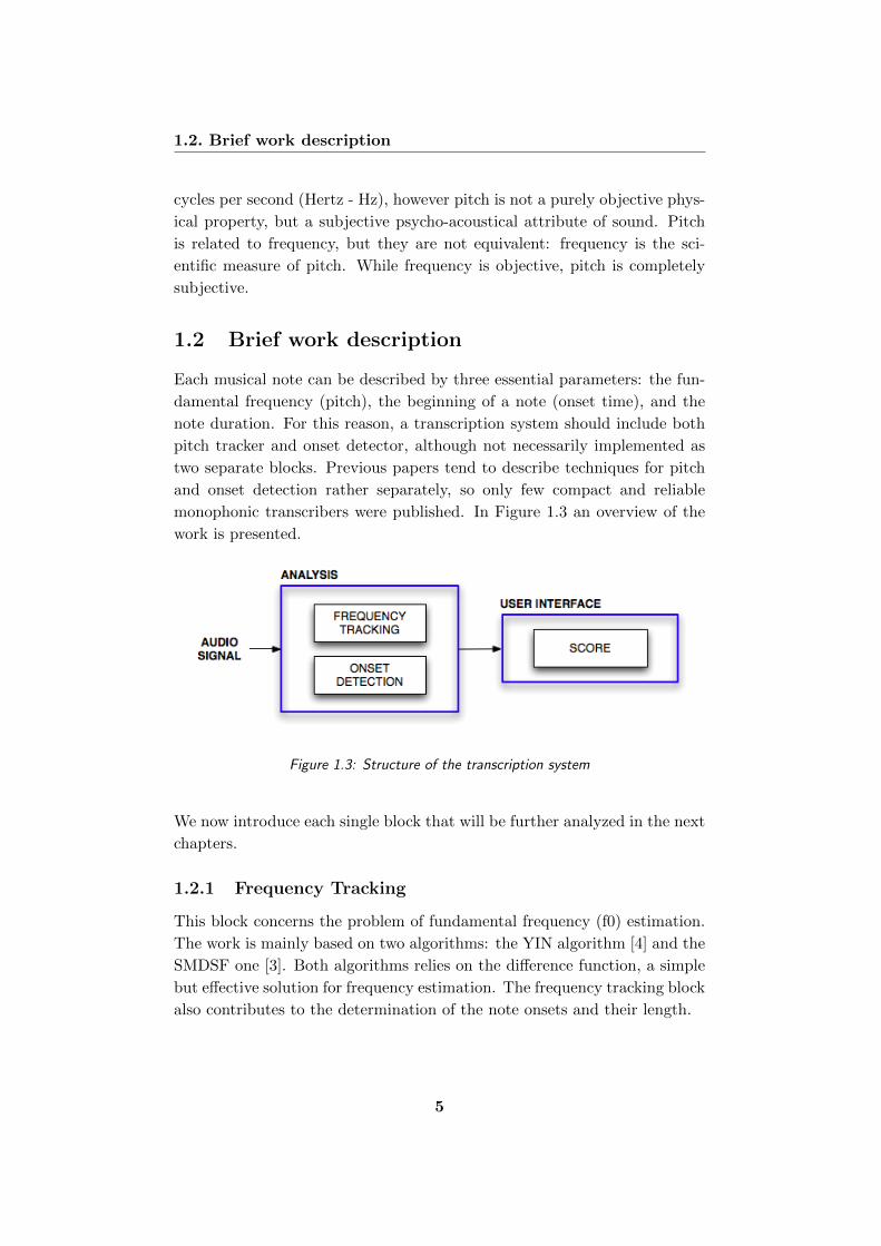
1.2 Brief work description
Each musical note can be described by three essential parameters: the fun-
damental frequency (pitch), the beginning of a note (onset time), and the
note duration. For this reason, a transcription system should include both
pitch tracker and onset detector, although not necessarily implemented as
two separate blocks. Previous papers tend to describe techniques for pitch
and onset detection rather separately, so only few compact and reliable
monophonic transcribers were published. In Figure 1.3 an overview of the
work is presented.
Figure 1.3: Structure of the transcription system
We now introduce each single block that will be further analyzed in the next
chapters.
1.2.1 Frequency Tracking
This block concerns the problem of fundamental frequency (f0) estimation.
The work is mainly based on two algorithms: the YIN algorithm [4] and the
SMDSF one [3]. Both algorithms relies on the difference function, a simple
but effective solution for frequency estimation. The frequency tracking block
also contributes to the determination of the note onsets and their length.
5
1.3. Overview of the thesis
1.2.2 Onset Detection
Onset detection refers to the detection of the beginning instants of discrete
events in the acoustic signals. A percept of an onset is caused by a noticeable
change in the intensity, pitch or timbre of the sound. The onset of the note
is a single instant chosen to mark the temporally extended transient. In
most cases, it will coincide with the start of the transient, or the earliest
time at which the transient can be reliably detected.
1.2.3 User Interface
A graphical part for the real-time score visualization is needed. The user
interface provides a feedback to the user and let him use the application in
a simple way.
1.3 Overview of the thesis
The thesis is organized as follows:
• In chapter 2 we’ll take a view of the state of the art of the monophonic
automatic music transcription field in research and then we’ll have a
look of some commercial applications.
• In chapter 3, the algorithm is presented by means of the mathematical
background and a complete explanation of its work.
• In chapter 4 the system design details are presented.
• Chapter 5 discuss about the developing of the software application.
• In Chapter 6 we show the results of the application.
• Finally, chapter 7 presents conclusions and guidelines for future im-
provements and evolutions.
6

Chapter 2
State of the art
In past few years, audio research and industries made several progress to-
wards achieving the state-of-the-art in automatic music transcription. Many
algorithms and applications have been developed. In this section we will
discuss about related works from both research and commercial application.
The core of monophonic music transcription is the pitch estimation: the
first part of this chapter concerns about the most used algorithms for this
purpose. Afterward, the most recent applications for automatic monophonic
music transcription are considered.
2.1 Algorithms
In this section we describe some fundamental frequency estimation algo-
rithms for monophonic audio, organized by type of input and processing
paradigm. In the case of polyphonic audio, with more instruments mixed
on a single track, the aim of the algorithms is to extract the single instrument
parts (source separation) and transcribe them. In this work we concentrate
on the transcription of a bass-line in a monophonic context, so we will not
consider algorithm for source separation.
Time domain methods are presented first, as they are usually computation-
ally simple. Frequency domain methods, presented next, are usually more
complex. First, a brief excursus on fundamental frequency is proposed.
2.1.1 Fundamental Frequency
As we mentioned in the previous chapter the core of the work is represented
by the fundamental frequency estimation. We refer to the fundamental
frequency, or f0, as the lowest frequency of a periodic waveform. On the
7
2.1. Algorithms
other hand pitch represents the perceived fundamental frequency of a sound.
The fundamental frequency is a measurable quantity while pitch is a purely
subjective property of the sound. What we need for our work is to estimate
the fundamental frequency.
2.1.2 Time-Domain Methods
Time-Event Rate Detection
There is a family of related time-domain F0 estimation methods which looks
for the number of repetition of the waveform period. The theory behind
these methods relies on the fact that if a waveform is periodic, then some
time-repeating events can be retrieved and counted. The number of repe-
titions that occurs in a second is inversely related to the frequency. Each
of these methods is useful for particular kinds of waveforms. In the case of
non-periodic waveform this methods are not valid.
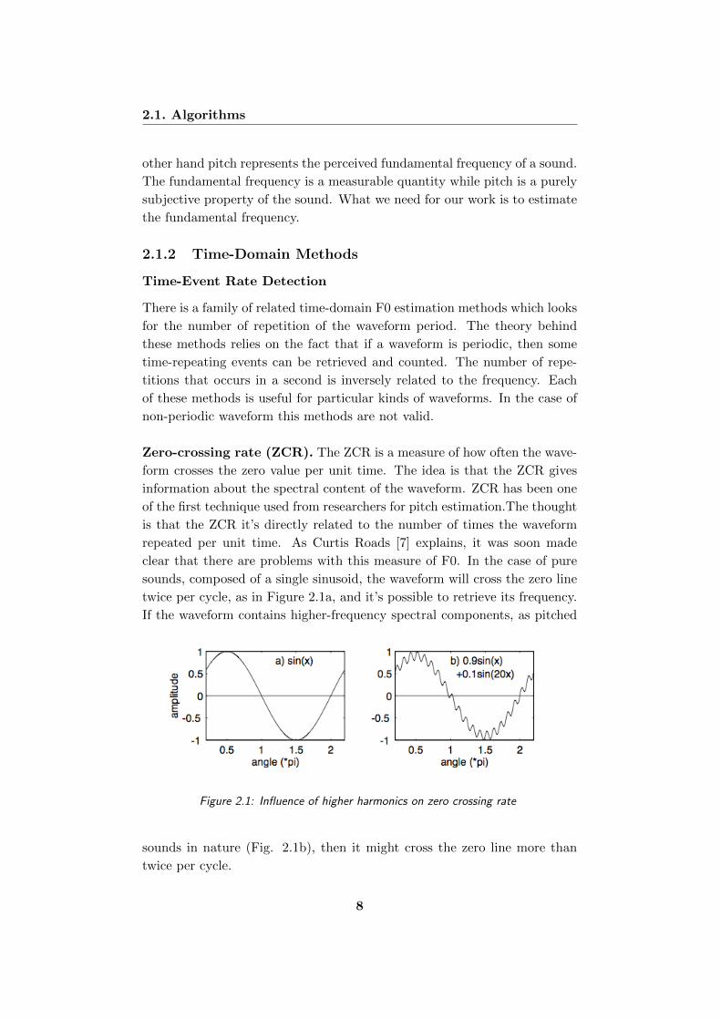
Zero-crossing rate (ZCR). The ZCR is a measure of how often the wave-
form crosses the zero value per unit time. The idea is that the ZCR gives
information about the spectral content of the waveform. ZCR has been one
of the first technique used from researchers for pitch estimation.The thought
is that the ZCR it’s directly related to the number of times the waveform
repeated per unit time. As Curtis Roads [7] explains, it was soon made
clear that there are problems with this measure of F0. In the case of pure
sounds, composed of a single sinusoid, the waveform will cross the zero line
twice per cycle, as in Figure 2.1a, and it’s possible to retrieve its frequency.
If the waveform contains higher-frequency spectral components, as pitched
Figure 2.1: Influence of higher harmonics on zero crossing rate
sounds in nature (Fig. 2.1b), then it might cross the zero line more than
twice per cycle.
8
2.1. Algorithms
Peak rate. This method counts the number of positive peaks per second
in the waveform. In pure sounds, the waveform have a maximum value and
a minimum value each cycle, and one needs only to count these maximum
values (or minimum values) to determine the frequency of the waveform. In
real sounds, a local peak detector must be used to find where the waveform
is locally largest, and the number of these local maxima in one second is the
frequency of the waveform, unless each period of the waveform contains more
than one local maximum. The distance between this local maxima gives the
wavelength which is inversely proportional to the frequency. As explained
by David Gerhar in his pitch extraction history report [15], peak counters
have been the choice of hardware frequency-detectors for many years, be-
cause the easiness of the circuit which coupled with a simple low-pass filter,
provides a fairly robust module.
The main problems using ZCR and peak rate methods for pitch estima-
tion stand by the fact that real waveforms are never composed of a single
sinusoid but, instead, have a complex spectra formed by more partials and,
often, by noise. By this fact, waveforms rarely have just one event per cy-
cle: they may cross zero many times or have many peaks in a cycle. In the
case of bass transcription these methods are never used because of the bass
waveform that consists of a high frequency attack and a harmonically rich
spectrum due to the partials superposition.
Nevertheless, there are some positive aspects of these time-event rate detec-
tion algorithms. These methods are simple to understand and implement,
and they take very little computing power to execute. In case of non-ideal
situations or for better performances is better to use more effective algo-
rithms.
Autocorrelation
Autocorrelation method is firstly introduced in speech processing in 1968 by
M. Sondhi [8], and then considered as a model in most of the pitch detection
works. The autocorrelation method doesn’t suffer of problems on the wave-
form complexity and it is considered one of the most performing algorithm.
The correlation between two waveforms is a measure of their similarity. The
waveforms are compared at different time intervals, and their likeness is cal-
culated at each interval. The result of a correlation is a measure of similarity
as a function of time lag between the beginnings of the two waveforms. The
autocorrelation function is the case of the correlation of a waveform with it-
9
2.1. Algorithms
self. One would expect exact similarity at a time lag of zero, with increasing
dissimilarity as the time lag increases. The mathematical definition of the
autocorrelation function is shown for a discrete signal x[n] in equation 2.1:
Rx(ν) =∑
x[n]x[n+ ν] (2.1)
De Cheveigne and Kawahara [9] noted that as the time lag increases to half
of the period of the waveform, the correlation decreases to a minimum. This
is because the waveform is out of phase with its time-delayed copy. As the
time lag increases again to the length of one period, the autocorrelation again
increases back to a maximum, because the waveform and its time-delayed
copy are in phase. The first peak in the autocorrelation indicates the period
of the waveform. The autocorrelation method has been widely used in pitch
detection and also in bass transcription by Ryynanen and Klapuri on their
works on bass line transcription [10] [11].
2.1.3 Frequency-Domain Methods
There are a lot of information in the frequency domain that can be related
to the fundamental frequency of the signal. Pitched signals tend to be
composed of a series of harmonically related partials, which can be identified
and used to extract the F0. Many attempts have been made to extract and
follow the f0 of a signal in this manner.
Filter-Based Methods
Filters are used for f0 estimation by using different filters with different cen-
ter frequencies, and comparing their output. When a spectral peak lines up
with the passband of a filter, the result is a higher value in the output of
the filter than when the passband does not line up.
Comb Filter. The optimum comb f0 estimator by J. A. Moorer [12] is
a robust but computationally intensive algorithm. A comb filter has many
equally spaced pass-bands. In the case of the optimum comb filter algo-
rithm, the location of the passbands depends on the location of the first
passband. For example, if the centre frequency of the first passband is 10
Hz, then there will be narrow pass-bands every 10 Hz after that, up to the
Shannon frequency. In his algorithm, the input waveform is comb filtered
based on many different frequencies. If a set of regularly spaced harmonics
are present in the signal, then the output of the comb filter will be greatest
when the passbands of the comb line up with the harmonics. If the signal
10
2.1. Algorithms
has only one partial, the fundamental, then the method will fail because
there will be many comb filters that will have the same output amplitude,
wherever a passband of the comb filter lines up with that fundamental. No
papers on comb-filter algorithms used for bass transcription have been found.
IIR Filter. A more recent filter-based f0 estimator is suggested by J. E.
Lane in [13]. This method consists of a narrow user-tunable band-pass fil-
ter, which is swept across the frequency spectrum. When the filter is in line
with a strong frequency partial, a maximum output will be present in the
output of the filter, and the f0 can then be read off the centre frequency of
the filter. The author suggests that an experienced user of this tunable filter
will be able to recognize the difference between an evenly spaced spectrum,
characteristic of a richly harmonic single note, and a spectrum containing
more than one distinct pitch.
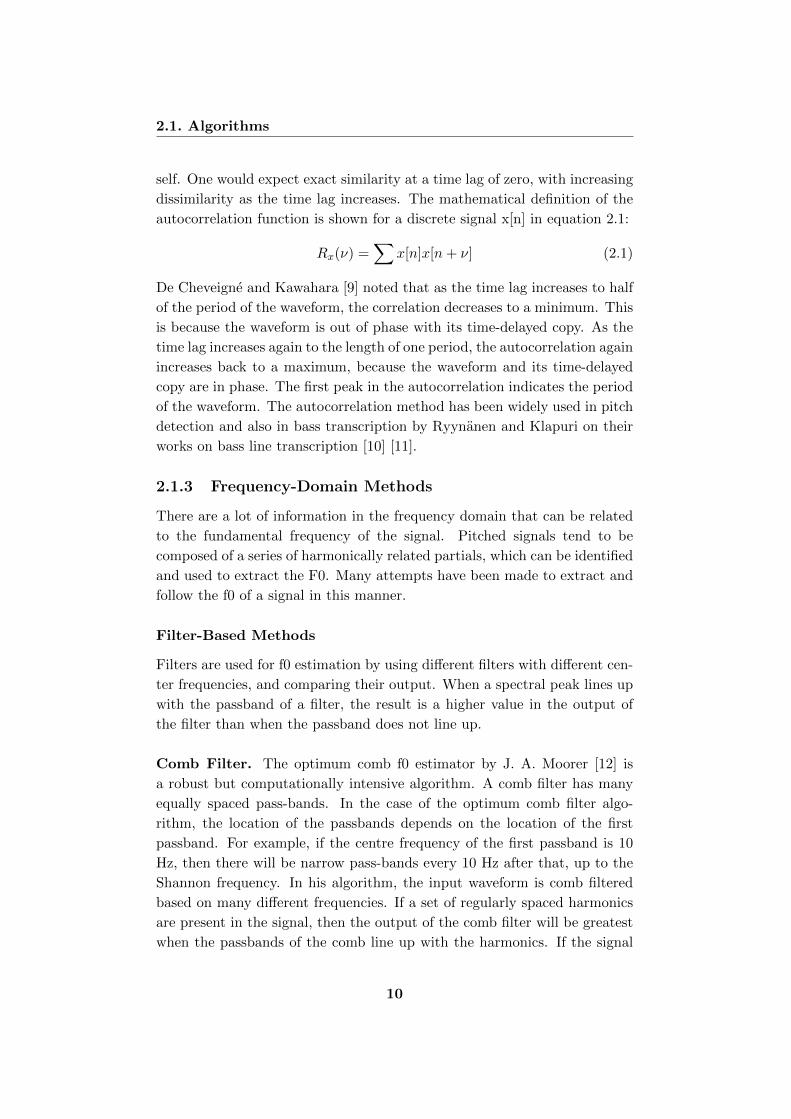
Cepstrum. Cepstrum analysis is a form of spectral analysis where the
output is the Fourier transform of the log of the magnitude spectrum of
the input waveform. This procedure was early developed by J. L. Flanagan
[14] in the attempt to make a non-linear system more linear. Naturally oc-
curring partials in a frequency spectrum are often slightly inharmonic, and
the cepstrum attempts to mediate this effect by using the log spectrum.
The name cepstrum comes from reversing the first four letters in the word
”spectrum”, indicating a modified spectrum. The independent variable re-
lated to the cepstrum transform has been called ”quefrency”, and since this
variable is very closely related to time, as explained by C. Roads in [7], it is
acceptable to refer to this variable as time. The theory behind this method
relies on the fact that the Fourier transform of a pitched signal usually has
a number of regularly spaced peaks, representing the harmonic spectrum of
the signal. When the log magnitude of a spectrum is taken, these peaks are
reduced, their amplitude brought into a usable scale, and the result is a pe-
riodic waveform in the frequency domain, the period of which (the distance
between the peaks) is related to the fundamental frequency of the original
signal. The Fourier transform of this waveform has a peak at the period
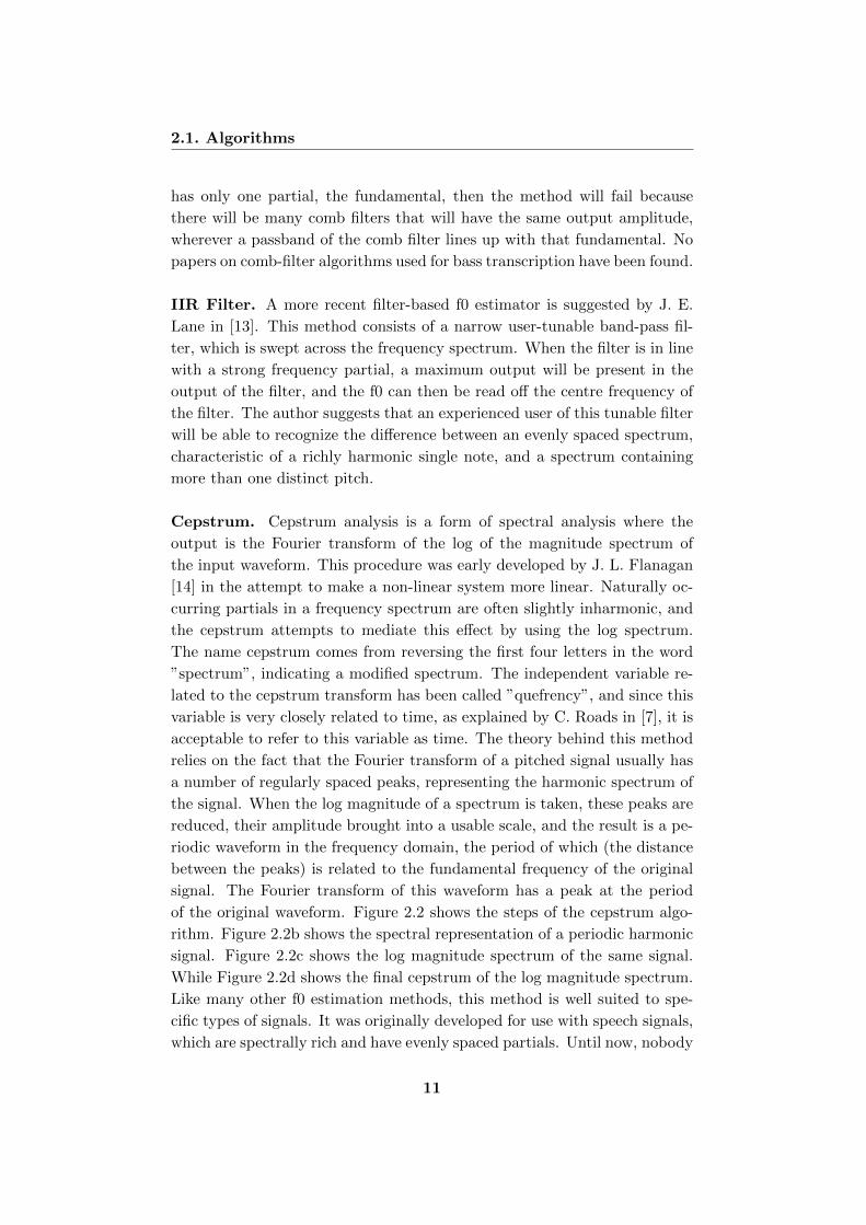
of the original waveform. Figure 2.2 shows the steps of the cepstrum algo-
rithm. Figure 2.2b shows the spectral representation of a periodic harmonic
signal. Figure 2.2c shows the log magnitude spectrum of the same signal.
While Figure 2.2d shows the final cepstrum of the log magnitude spectrum.
Like many other f0 estimation methods, this method is well suited to spe-
cific types of signals. It was originally developed for use with speech signals,
which are spectrally rich and have evenly spaced partials. Until now, nobody
11
2.2. Software Applications
Figure 2.2: Stages in the cepstrum analysis algorithm
tried to perform bass transcription with the Cepstrum analysis.
2.2 Software Applications
The aim of this thesis is to realize a real-time bass transcription application.
As requirement the application user interface is built to be as simple as pos-
sible: it should be usable by music students as well as professional musicians.
In this section a review of similar applications is presented. Nevertheless,
these applications are commercial, built for people with a big experience in
music, and significantly different from our work: transcription applications
12
2.2. Software Applications
are not in real-time, while real-time applications do not perform transcrip-
tion. In particular none of the applications is specifically for bass.
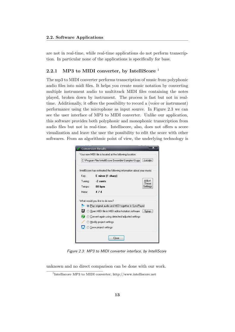
2.2.1 MP3 to MIDI converter, by IntelliScore 1
The mp3 to MIDI converter performs transcription of music from polyphonic
audio files into midi files. It helps you create music notation by converting
multiple instrument audio to multitrack MIDI files containing the notes
played, broken down by instrument. The process is fast but not in real-
time. Additionally, it offers the possibility to record a (voice or instrument)
performance using the microphone as input source. In Figure 2.3 we can
see the user interface of MP3 to MIDI converter. Unlike our application,
this software provides both polyphonic and monophonic transcription from
audio files but not in real-time. Intelliscore, also, does not offers a score
visualization and leave the user the possibility to edit the score with other
softwares. From an algorithmic point of view, the underlying technology is
Figure 2.3: MP3 to MIDI converter interface, by IntelliScore
unknown and no direct comparison can be done with our work.
1Intelliscore MP3 to MIDI converter, http://www.intelliscore.net
13
2.2. Software Applications
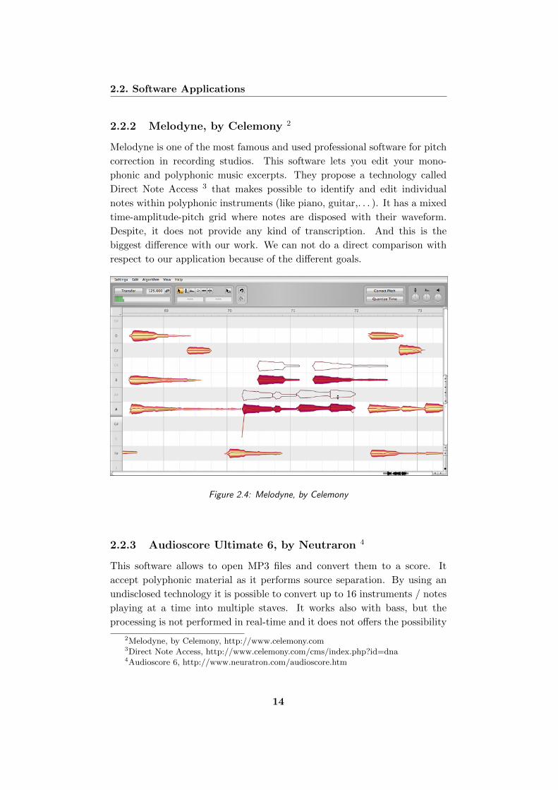
2.2.2 Melodyne, by Celemony 2
Melodyne is one of the most famous and used professional software for pitch
correction in recording studios. This software lets you edit your mono-
phonic and polyphonic music excerpts. They propose a technology called
Direct Note Access 3 that makes possible to identify and edit individual
notes within polyphonic instruments (like piano, guitar,. . . ). It has a mixed
time-amplitude-pitch grid where notes are disposed with their waveform.
Despite, it does not provide any kind of transcription. And this is the
biggest difference with our work. We can not do a direct comparison with
respect to our application because of the different goals.
Figure 2.4: Melodyne, by Celemony
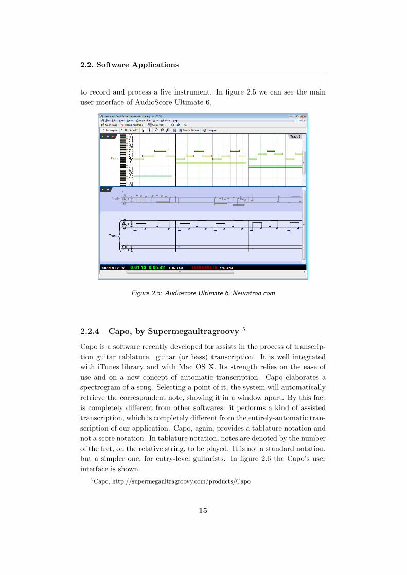
2.2.3 Audioscore Ultimate 6, by Neutraron 4
This software allows to open MP3 files and convert them to a score. It
accept polyphonic material as it performs source separation. By using an
undisclosed technology it is possible to convert up to 16 instruments / notes
playing at a time into multiple staves. It works also with bass, but the
processing is not performed in real-time and it does not offers the possibility
2Melodyne, by Celemony, http://www.celemony.com3Direct Note Access, http://www.celemony.com/cms/index.php?id=dna4Audioscore 6, http://www.neuratron.com/audioscore.htm
14
2.2. Software Applications
to record and process a live instrument. In figure 2.5 we can see the main
user interface of AudioScore Ultimate 6.
Figure 2.5: Audioscore Ultimate 6, Neuratron.com
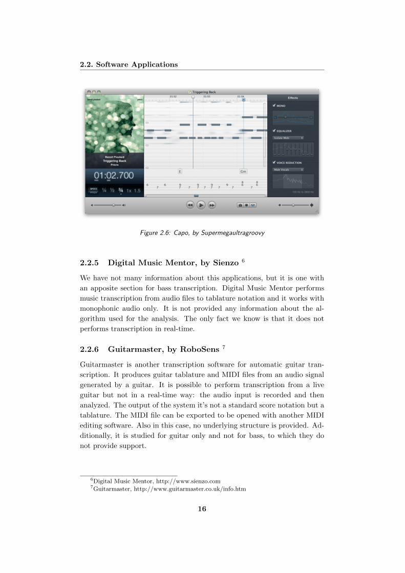
2.2.4 Capo, by Supermegaultragroovy 5
Capo is a software recently developed for assists in the process of transcrip-
tion guitar tablature. guitar (or bass) transcription. It is well integrated
with iTunes library and with Mac OS X. Its strength relies on the ease of
use and on a new concept of automatic transcription. Capo elaborates a
spectrogram of a song. Selecting a point of it, the system will automatically
retrieve the correspondent note, showing it in a window apart. By this fact
is completely different from other softwares: it performs a kind of assisted
transcription, which is completely different from the entirely-automatic tran-
scription of our application. Capo, again, provides a tablature notation and
not a score notation. In tablature notation, notes are denoted by the number
of the fret, on the relative string, to be played. It is not a standard notation,
but a simpler one, for entry-level guitarists. In figure 2.6 the Capo’s user
interface is shown.
5Capo, http://supermegaultragroovy.com/products/Capo
15
2.2. Software Applications
Figure 2.6: Capo, by Supermegaultragroovy
2.2.5 Digital Music Mentor, by Sienzo 6
We have not many information about this applications, but it is one with
an apposite section for bass transcription. Digital Music Mentor performs
music transcription from audio files to tablature notation and it works with
monophonic audio only. It is not provided any information about the al-
gorithm used for the analysis. The only fact we know is that it does not
performs transcription in real-time.
2.2.6 Guitarmaster, by RoboSens 7
Guitarmaster is another transcription software for automatic guitar tran-
scription. It produces guitar tablature and MIDI files from an audio signal
generated by a guitar. It is possible to perform transcription from a live
guitar but not in a real-time way: the audio input is recorded and then
analyzed. The output of the system it’s not a standard score notation but a
tablature. The MIDI file can be exported to be opened with another MIDI
editing software. Also in this case, no underlying structure is provided. Ad-
ditionally, it is studied for guitar only and not for bass, to which they do
not provide support.
6Digital Music Mentor, http://www.sienzo.com7Guitarmaster, http://www.guitarmaster.co.uk/info.htm
16

Chapter 3
Theoretical Background
As seen in the previous chapters the main issue of monophonic music tran-
scription is the fundamental frequency estimation (F0). Section 3.1 explains
the reason of our choice, followed by the description of the algorithm’s the-
ory. In the last section we will briefly introduce the MIDI protocol used by
our application.
3.1 Introduction
In real world, an audio waveform is composed not of a single sinusoid but by
a sum of more overlapping sinusoids. It can be described as a combination
of many simple periodic waves (i.e., sinusoids), called partials, each with its
own frequency. An harmonic (harmonic partial) is a partials with the fre-
quency multiple of the fundamental frequency. As a pitched instrument, the
bass is characterized by the prevalence of harmonic contents. The funda-
mental frequency (F0) of the waveform can be seen as the harmonic partial
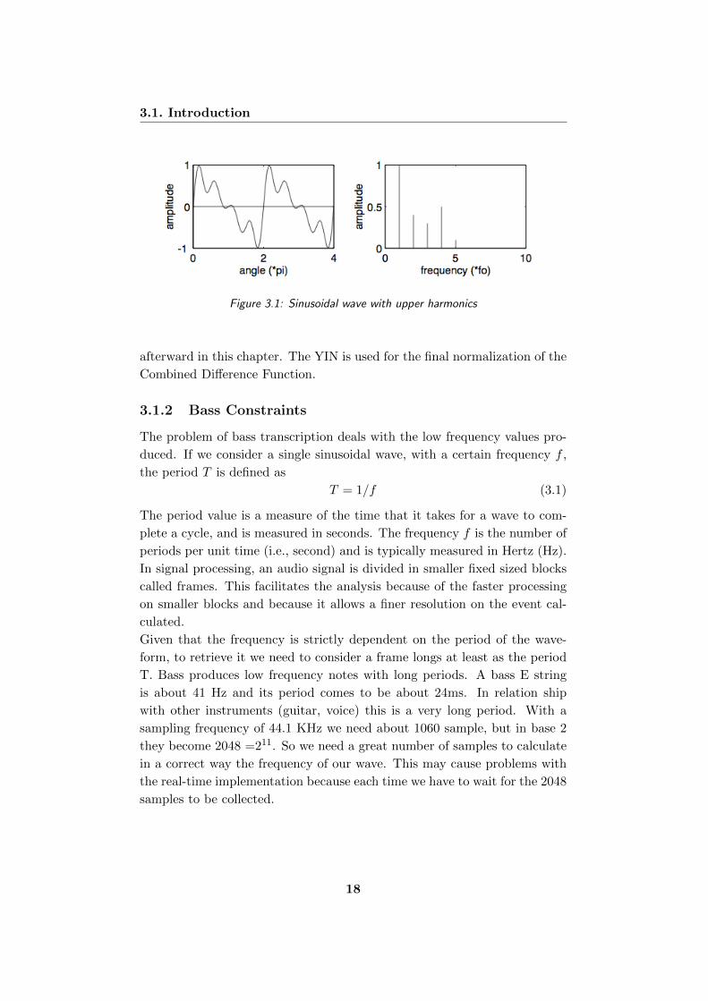
with the lowest frequency. Figure 3.1 shows a periodic wave with different
partials (harmonics).
3.1.1 Requirements
From the beginning the system was designed to have an instant response to
user. Real-time issues came up. There is a trade-off between the accuracy
of the algorithm and the latency. A more accurate and effective method
needs a more computationally complex algorithm with consequently latency
problems. We decided to use a mix of two algorithms, based on simple math-
ematical structures that gives us the possibility of real-time processing: YIN
algorithm [4] and SMDSF [3] algorithm. The SMDSF is an improving of the
YIN, and it is based on the Combined Difference Function, that is explained
3.1. Introduction
Figure 3.1: Sinusoidal wave with upper harmonics
afterward in this chapter. The YIN is used for the final normalization of the
Combined Difference Function.
3.1.2 Bass Constraints
The problem of bass transcription deals with the low frequency values pro-
duced. If we consider a single sinusoidal wave, with a certain frequency f ,
the period T is defined as
T = 1/f (3.1)
The period value is a measure of the time that it takes for a wave to com-
plete a cycle, and is measured in seconds. The frequency f is the number of
periods per unit time (i.e., second) and is typically measured in Hertz (Hz).
In signal processing, an audio signal is divided in smaller fixed sized blocks
called frames. This facilitates the analysis because of the faster processing
on smaller blocks and because it allows a finer resolution on the event cal-
culated.
Given that the frequency is strictly dependent on the period of the wave-
form, to retrieve it we need to consider a frame longs at least as the period
T. Bass produces low frequency notes with long periods. A bass E string
is about 41 Hz and its period comes to be about 24ms. In relation ship
with other instruments (guitar, voice) this is a very long period. With a
sampling frequency of 44.1 KHz we need about 1060 sample, but in base 2
they become 2048 =211. So we need a great number of samples to calculate
in a correct way the frequency of our wave. This may cause problems with
the real-time implementation because each time we have to wait for the 2048
samples to be collected.
18
3.2. Algorithm
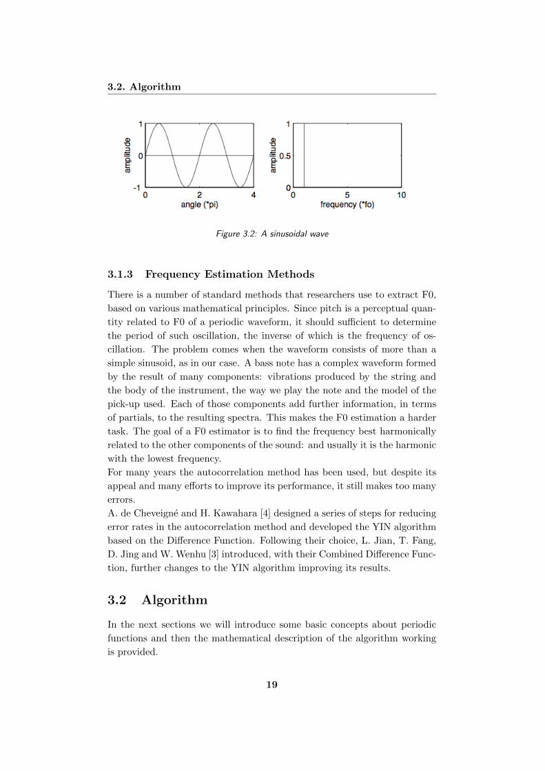
Figure 3.2: A sinusoidal wave
3.1.3 Frequency Estimation Methods
There is a number of standard methods that researchers use to extract F0,
based on various mathematical principles. Since pitch is a perceptual quan-
tity related to F0 of a periodic waveform, it should sufficient to determine
the period of such oscillation, the inverse of which is the frequency of os-
cillation. The problem comes when the waveform consists of more than a
simple sinusoid, as in our case. A bass note has a complex waveform formed
by the result of many components: vibrations produced by the string and
the body of the instrument, the way we play the note and the model of the
pick-up used. Each of those components add further information, in terms
of partials, to the resulting spectra. This makes the F0 estimation a harder
task. The goal of a F0 estimator is to find the frequency best harmonically
related to the other components of the sound: and usually it is the harmonic
with the lowest frequency.
For many years the autocorrelation method has been used, but despite its
appeal and many efforts to improve its performance, it still makes too many
errors.
A. de Cheveigne and H. Kawahara [4] designed a series of steps for reducing
error rates in the autocorrelation method and developed the YIN algorithm
based on the Difference Function. Following their choice, L. Jian, T. Fang,
D. Jing and W. Wenhu [3] introduced, with their Combined Difference Func-
tion, further changes to the YIN algorithm improving its results.
3.2 Algorithm
In the next sections we will introduce some basic concepts about periodic
functions and then the mathematical description of the algorithm working
is provided.
19
3.2. Algorithm
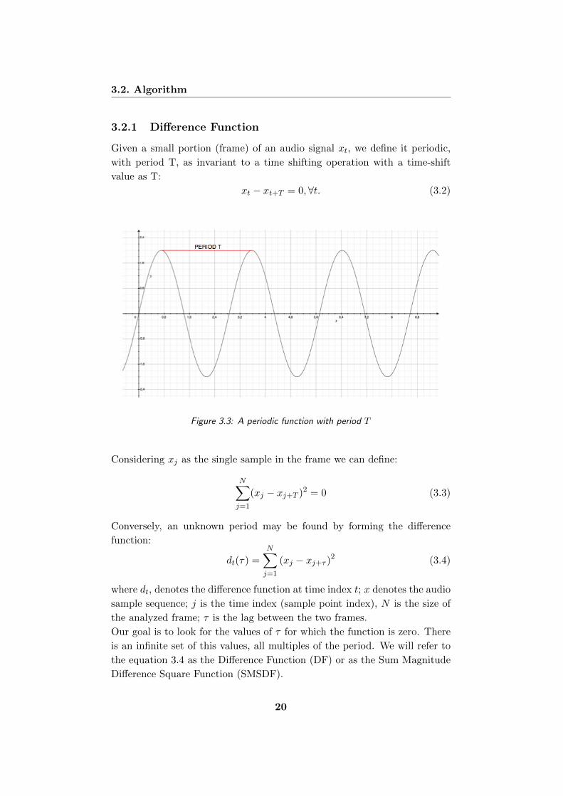
3.2.1 Difference Function
Given a small portion (frame) of an audio signal xt, we define it periodic,
with period T, as invariant to a time shifting operation with a time-shift
value as T:
xt − xt+T = 0,∀t. (3.2)
Figure 3.3: A periodic function with period T
Considering xj as the single sample in the frame we can define:
N∑j=1
(xj − xj+T )2 = 0 (3.3)
Conversely, an unknown period may be found by forming the difference
function:
dt(τ) =N∑j=1
(xj − xj+τ )2 (3.4)
where dt, denotes the difference function at time index t; x denotes the audio
sample sequence; j is the time index (sample point index), N is the size of
the analyzed frame; τ is the lag between the two frames.
Our goal is to look for the values of τ for which the function is zero. There
is an infinite set of this values, all multiples of the period. We will refer to
the equation 3.4 as the Difference Function (DF) or as the Sum Magnitude
Difference Square Function (SMSDF).
20
3.2. Algorithm
3.2.2 The YIN algorithm
The YIN F0 estimator [4], developed by Alain de Cheveigne and Hideki
Kawahara, takes the name from the oriental yin-yang philosophical princi-
pal of balance, representing the authors’ attempt to balance autocorrelation
and cancellation in the algorithm. One of the main problems of the auto-
correlation method is that it can frequently occurs that the intensity of the
first harmonic partial is lower then other harmonic partials. In those cases
the resulting pitch it’s wrongly estimated. YIN attempts to solve this prob-
lem in several ways. It is based on the difference function, which, attempts
to minimize the difference between the waveform and its delayed duplicate,
instead of maximizing the product as autocorrelation does. The difference
function is presented in equation 3.4 and it’s re-proposed in equation 3.5:
dt(τ) =N∑j=1
(xj − xj+τ )2 (3.5)
The calculation of this equation is computationally expensive and two differ-
ent mathematical solutions have been proposed by YIN [4]: the first based
on a recursive technique, the second on the FFT algorithm.
In order to reduce the occurrence of subharmonic errors, YIN employes a
cumulative mean function (equation 3.6) which de-emphasizes higher period
dips in the difference function:
cmdft(τ) =
1, if τ = 0
dt(τ)
1τ
τ∑j=1
dt(j), otherwise (3.6)
Other improvements for the YIN f0 estimation system include a parabolic
interpolation of the local minima, which has the effect of reducing the er-
rors when the period estimation is not a factor of the window length used.
(For a more complete discussion of this method, including computational
implementation and results, see the cited paper)
3.2.3 The Combined Difference Function algorithm
Liu, Zheng, Deng and Wu proposed a new approach in order to calculate
efficiently the Difference Function (equation 3.4) as an improvement of YIN
method, using the FFT algorithm [3]. They calculated the Difference Func-
tion as the combination of two others kind of functions: the bidirectional
and the circular difference functions. This two new functions are summed
with a bias factor.
21
3.2. Algorithm
Bidirectional SMDSF
This function is calculated between two adjacent frames for two times: the
first time from left to right and second one from right to left. The Bidirec-
tional function is formed as the mean of the two new functions.
Left-To-Right
We expanded the difference equation dt(τ), which is like the power of a
binomial (x+ y)2, in the sum of its component :
dt(τ) =t+N−1∑j=t
x2(j) +t+N−1∑j=t
x2(j + τ)− 2 ·t+N−1∑j=t
x(j)x(j + τ) (3.7)
In order to simplify the equation, one frame of the audio signal at time index
t can be also defined as:
xt(j) =
{x(t+ j), j = 0, 1, . . . , N − 1
0, otherwise(3.8)
According to the last equation, we can transform the expanded difference
function (equation 3.7) in a new simpler function:
dt(τ) = at(0) + rt(τ)− 2(at(τ) + ct(τ)) (3.9)
We now explain how to calculate the single components:
• at(τ): the equation 3.10 shows the autocorrelation function of the
frame at the time index t (xt).
at(τ) =N−1∑j=0
xt(j)xt(j + τ) (3.10)
The equation 3.10 can be calculated efficiently and in a fast way by
means of the FFT algorithm.
Xt(f) = FFT (xt) (3.11)
S(f) = Xt(f)Xt(f)∗ (3.12)
at(τ) = IFFT (S(f)) (3.13)
where xt represents the frame at time index t; FFT is the Fast Fourier
Transform; Xf is the FFT of the frame; Sf is the product in frequency
domain; IFFT is the Inverse FFT and at(τ) is the autocorrelation
function.
22
3.2. Algorithm
• rt(τ): the equation 3.14 represents is the frame’s power at current lag
τ , which is a recursive formula over τ in linear time.
rt(τ) =
{at(0), τ = 0
rt(τ − 1)− (x(t+ τ − 1))2 + (x(t+N + τ − 1))2, oth.
(3.14)
• ct(τ): in equation 3.12 we see the cross-correlation between the two
adjacent frames.
ct(τ) =N−1∑j=0
xt(j +N − τ)xt+N (j) (3.15)
The equation 3.15 can be calculated efficiently by means of the follow-
ing equations:
Xt(f) = FFT (xt) (3.16)
Xt+N (f) = FFT (xt+N ) (3.17)
S(f) = Xt(f)Xt+N (f)∗ (3.18)
ct(τ) = IFFT (S(f)) (3.19)
We finally have re-written equation (3.4) in a more efficient way in order
to take advantage of the FFT algorithm and its low complexity. We ob-
tain a final computational complexity of O(Nlog2N), much smaller than the
starting O(N2). We refer to this this function as the left-to-right SMDSF.
Right-To-Left
In a similar way we can define a right-to-left SMDSF as:
d′t(τ) =t+N−1∑j=t
(x(j +N)− x(j +N − τ)2 (3.20)
As we did before, we can expand the last equation in the following:
d′t(τ) = at+N (0) + r′t(τ)− 2(at+N (τ) + ct(τ)) (3.21)
The single components are:
• at+N (τ): it’s calculated as in equation 3.10.
• ct(τ): can be calculated with equation 3.15.
23
3.2. Algorithm
• rt(τ): is similar to equation 3.14 but is defined as:
r′t(τ) =
{at+N (0), τ = 0
r′t(τ − 1)− (x(t+ 2N − τ))2 + (x(t+N + τ))2, oth.
(3.22)
Also in this case we take advantage of the low time complexity of the FFT
algorithm. This two equation (3.9 and 3.14) are the different functions at
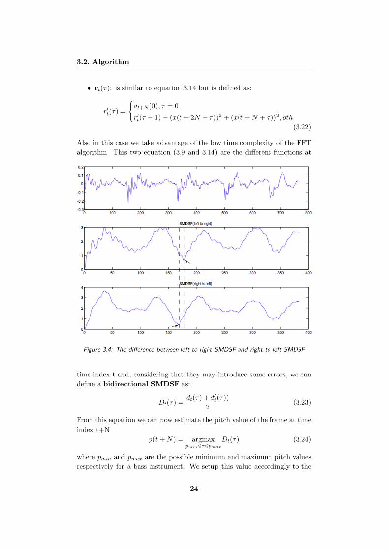
Figure 3.4: The difference between left-to-right SMDSF and right-to-left SMDSF
time index t and, considering that they may introduce some errors, we can
define a bidirectional SMDSF as:
Dt(τ) =dt(τ) + d′t(τ))
2(3.23)
From this equation we can now estimate the pitch value of the frame at time
index t+N
p(t+N) = argmaxpmin6τ6pmax
Dt(τ) (3.24)
where pmin and pmax are the possible minimum and maximum pitch values
respectively for a bass instrument. We setup this value accordingly to the
24
3.2. Algorithm
lowest note for a common 4 string bass which is 41 Hz and the maximum
one which is about 600Hz. As we can see in Table 3.1, pitch estimation
using bidirectional SMDSF can lead to an average pitch value during two
adjacent frames. In this way we can lower the doubling/halving error rate:
the doubling error is when we retrieve a note one octave higher then its
actual octave, the halving error occurs when the note retrieved is one octave
lower its actual octave.
Method Doubling (%) Halving (%)
Left-to-right 5.8 1.5
Right-to-left 6.9 5.5
Bidirectional 4.9 1.7
Table 3.1: Doubling/halving error rates for the LR, the RL and the Bidirectional differ-
ence function
Circular SMDSF
We introduce now another method with higher halving errors, because we
think that by combining it with the previous method, we can obtain a more
balanced error level, with lower doubling and halving errors. A new type of
SMDSF for this purpose is defined as:
D′t(τ) =t+2N−1∑j=t
(x(j)− x(t+ (j + τ − t)%(2N)))2 (3.25)
where ”%” represents the modulo operation.
This function is called circular SMDSF due to the modulo operation on the
sample point index. The analyzing frame size used in the circular SMDSF is
2N , so we need two times the frame size used in the bidirectional SMDSF.
This equation can be re-written with the help of the equation (3.10):
D′t(τ) = 2a′t(0) + 2(a′t(τ)− a′t(2N − τ)) (3.26)
with the remind that the frame size is now 2N and not N . The compu-
tational complexity for the calculation of the circular SMDSF is still O(N
log2(N)). The pitch value estimation is similar to that using the bidirectional
SMDSF and the same equation (3.17) can be applied to estimate the pitch
at time index t+N.
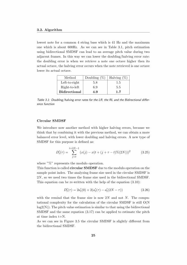
As we can see in Figure 3.5 the circular SMDSF is slightly different from
the bidirectional SMDSF.
25
3.2. Algorithm
Figure 3.5: The difference between the bidirectional SMDSF and the circular SMDSF
Combined SMDSF
The bidirectional and the circular SMDSFs have their own characteristics,
which are different in the doubling error rate and the halving error rate.
This two functions can complement each other in some sense when they are
combined together. A combined SMDSF is defined as a linear interpolation
between the bidirectional SMDSF and the circular SMDSF:
D′′t (τ) = αDt(τ) + (1− α)D′t(τ) (3.27)
Table 3.1 shows the error rates (with α = 0.3) for the two method and
for the final one, confirming our hypothesis: the bidirectional SMDSF has
higher doubling error rate and the circular SSDMF has higher halving er-
ror rate, while the combined SMDSF has the lowest error and balanced
doubling/halving error rates.
3.2.4 Cumulative Mean Normalized DF
This difference function is zero at the zero lag and often non-zero at the
period lag because of imperfect periodicity. Unless a lower limit is set on the
search range, the algorithm must choose the zero-lag instead of the period
26

3.2. Algorithm
Method Doubling(%) Halving (%)
Bidirectional 4.9 1.7
Circular 1.9 2.6
Combined 2.0 2.1
Table 3.2: Doubling/halving error rates using the bidirectional function, the circular
function and the combined solution
one and the method should fail. The YIN algorithm introduce a solution
to this problem with a normalization function. The solution is to replace
the (combined) difference function with the Cumulative Mean Normalized
Difference Function (CMNDF):
D′′t (τ) =
1, ifτ = 0
D′′t (τ)
(1/τ)τ∑j=1
D′′t (j)
, otherwise (3.28)
Figure 3.6: The difference between the DF and the CMNDF
The new function is obtained by dividing each value by its average over
shorter-lag values. It differs from the combined difference function in that it
starts at 1 rather than 0, tends to remain large at low lags, and drops below 1
27
3.3. MIDI
only where the difference function falls below average. This solution reduces
”too high” errors and prevents high frequency contents and normalizes the
function for the next steps.
3.2.5 Errors
Sampling, windowing and strong harmonic content are known to be the key
factors that limit the accuracy of pitch estimation. Two typical kinds of
errors in pitch estimation are period-doubling and period-halving. Many
pitch estimation algorithms have methods to prevent these two types of
errors from taking place. These methods generally consist of two stages:
a pre-processing stage, using, for example, low-pass filtering and a post-
processing stage. However, only one certain type of time-domain functions
(ACF, AMDF, et c.) is used in these algorithms during pitch candidate
generation, which inevitably limits the accuracy of pitch estimation. Differ-
ent time-domain functions used in pitch estimation lead to different error
distributions: some functions have a higher doubling error rate while others
have a higher halving error rate. In our case a combined function is used,
which has the common merit of several existing difference functions and it
is shown to have the lowest error rate for pitch estimation.
3.3 MIDI
MIDI (Musical Instrument Digital Interface) is a standard protocol defined
in 1982 that enables electronic musical instruments (synthesizers, drum ma-
chines), computers and other electronic equipment (MIDI controllers, sound
cards, . . . ) to communicate and synchronize with each other. MIDI does
not transmit audio signals but it sends event messages about pitch, inten-
sity and control signals for parameters such as volume, vibrato and panning,
cues, and clock signals to set the tempo. The standard MIDI 1.0 specifica-
tion permits to interpret any given MIDI message in the same way, and so
all MIDI instrument can communicate and understand each other.
MIDI allows to store music as instructions rather than recorded audio wave-
forms and the resulting size of the files is quite small by comparison.
When a musical performance is played on a MIDI instrument, it transmits
MIDI channel messages from its MIDI Out connector. A typical MIDI chan-
nel message sequence corresponding to a key being struck and released on a
keyboard includes the pitch (expressed in value between 0 and 127), the ve-
locity (which is the volume of the note, again between 0 and 127), a Note-On
and Note-Off message. Other messages can be sent as well, like a program
28

3.3. MIDI
change, aftertouch, pitch-bend messages.
In our work, the operating system itself associate sounds of the default
wavetable to the MIDI musical messages. The wavetable sounds are, usually,
those provided by the General MIDI (GM). GM includes a set of 120 stan-
dard sounds, plus drum kit definitions. All MIDI instruments and sound-
cards use the GM sound-set to ensure compatibility.
29
Chapter 4
System Design
This chapter illustrates the design phase of our system. The goal of this
part is to properly chose and validate algorithms. In addition, the algorithm
parameters needs to be set up to verify that the results agree with our initial
expectations. As a result of this phase a prototype has been built and used
as a test for the next implementation step. Thanks to the easy of use, the
great amount of available functions and the aptitude to work with digital
signals we chose to use the Matlab framework to create the prototype.
After a first introduction on the environment and the tools used, we present
the algorithm implementation details
4.1 Tools and Frameworks
In this section we illustrate the framework used and the tools that helped
us to realize the prototype.
4.1.1 Matlab 1
The prototype has been created within the Matlab framework because of the
easiness of its use with mathematical functions and digital signal process-
ing. Matlab is a high-level language which provides the user many functions
ready to use. It is an environment that provides good support for math-
ematical operations, for example, about array operations as well as with
signal processing. It permits us to perform fast calculation and can gives
a real-time feedback of our results. Matlab let us to write algorithms in
a easy way, with few source code lines, and in a performing way. It helps
a lot with an easy debug interface, and the possibility to visualize quickly
1Matlab, http://www.mathworks.com/products/matlab
4.1. Tools and Frameworks
the data. By these fact we chose Matlab to design and test the prototype.
Moreover, Matlab has the possibility to add some external plug-in to extend
the environment. We used the PlayRec utility for the audio management,
and the MIDI Toolbox for notes creation and visualization.
4.1.2 PlayRec 2
Since one of the main requirements of our system a real-time feedback to
the user and since Matlab doesn’t integrate any native toolbox for real-time
audio recording and playback, we used Playrec, that is an external plug-
in. Playrec is a Matlab utility that provides simple and versatile access
to the sound-card using PortAudio, a free, open-source audio I/O library.
It is multi-platforms and provides access to the sound-card via different
host API. It offers a non-blocking access to the sound-card: all samples
are buffered so Matlab can continue with other processing while output
and recording occur. New output samples are automatically appended to
the remaining samples: this makes it possible for the audio data to be
generated as required. The only limit for PlayRec is the processing power
of the computer: lower computational power means higher latency, sample
skipping, glitches and delays.
Before any kind of audio is played or recorded, PlayRec must be initialized:
the audio device and the frequency sampling must be defined. PlayRec
divides the signal in frames called ”pages” with a sample-rate depending
length: the set up of the pages is peculiar to avoid clicks, glitches, delay or
pause whilst playing or recording. Pages are then sequentially collected in
a buffer, from which it’s possible to extract data needed for our operations.
4.1.3 MIDI Toolbox 3
Since one purpose of the system is to show the notation of the transcribed
song, we used an external plug-in to translate the result of the analysis step
to a human-readable form, as standard notation. The MIDI Toolbox is a
compilation of functions for analyzing and creating MIDI files in Matlab
environment. It also offers the possibility to show a notation of the MIDI
file created. The toolbox supports the creation of MIDI messages with note
pitch, timing and velocity information that MIDI provides.
2PlayRec, http://www.playrec.co.uk3MIDI Toolbox, https://www.jyu.fi/hum/laitokset/musiikki/en/research/coe/materials/miditoolbox
31
4.2. Implementation
4.2 Implementation
The prototype performs a real-time transcription both from a loaded audio
file and from a live input bass. By this fact, two different systems have
been created, although the main analysis part is the same for both. In the
following sections the systems differences are explained, while the similar
blocks are described afterwards.
4.2.1 Audio file acquisition
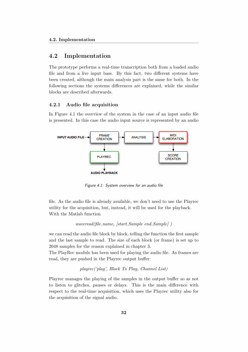
In Figure 4.1 the overview of the system in the case of an input audio file
is presented. In this case the audio input source is represented by an audio
Figure 4.1: System overview for an audio file
file. As the audio file is already available, we don’t need to use the Playrec
utility for the acquisition, but, instead, it will be used for the playback.
With the Matlab function
waveread(file name, [start Sample end Sample] )
we can read the audio file block by block, telling the function the first sample
and the last sample to read. The size of each block (or frame) is set up to
2048 samples for the reason explained in chapter 3.
The PlayRec module has been used for playing the audio file. As frames are
read, they are pushed in the Playrec output buffer:
playrec(’play’, Block To Play, Channel List)
Playrec manages the playing of the samples in the output buffer so as not
to listen to glitches, pauses or delays. This is the main difference with
respect to the real-time acquisition, which uses the Playrec utility also for
the acquisition of the signal audio.
32
4.2. Implementation
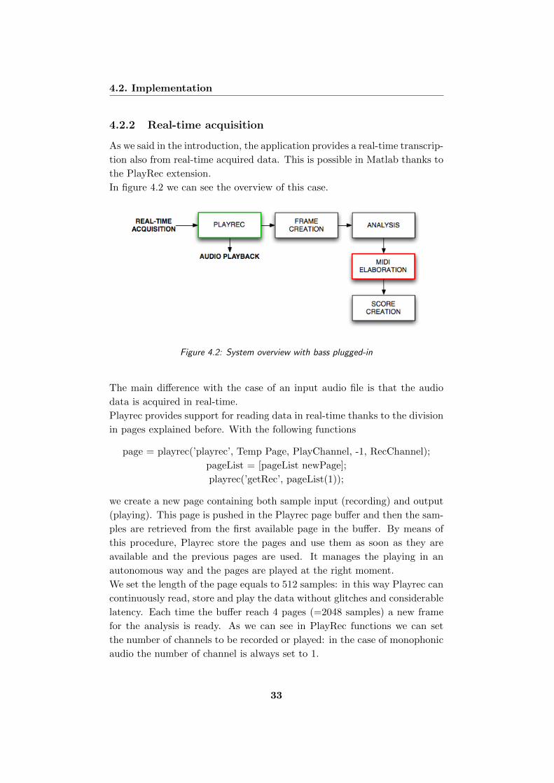
4.2.2 Real-time acquisition
As we said in the introduction, the application provides a real-time transcrip-
tion also from real-time acquired data. This is possible in Matlab thanks to
the PlayRec extension.
In figure 4.2 we can see the overview of this case.
Figure 4.2: System overview with bass plugged-in
The main difference with the case of an input audio file is that the audio
data is acquired in real-time.
Playrec provides support for reading data in real-time thanks to the division
in pages explained before. With the following functions
page = playrec(’playrec’, Temp Page, PlayChannel, -1, RecChannel);
pageList = [pageList newPage];
playrec(’getRec’, pageList(1));
we create a new page containing both sample input (recording) and output
(playing). This page is pushed in the Playrec page buffer and then the sam-
ples are retrieved from the first available page in the buffer. By means of
this procedure, Playrec store the pages and use them as soon as they are
available and the previous pages are used. It manages the playing in an
autonomous way and the pages are played at the right moment.
We set the length of the page equals to 512 samples: in this way Playrec can
continuously read, store and play the data without glitches and considerable
latency. Each time the buffer reach 4 pages (=2048 samples) a new frame
for the analysis is ready. As we can see in PlayRec functions we can set
the number of channels to be recorded or played: in the case of monophonic
audio the number of channel is always set to 1.
33
4.2. Implementation
In the next sections we will explain the remaining blocks which are the
same for both cases.
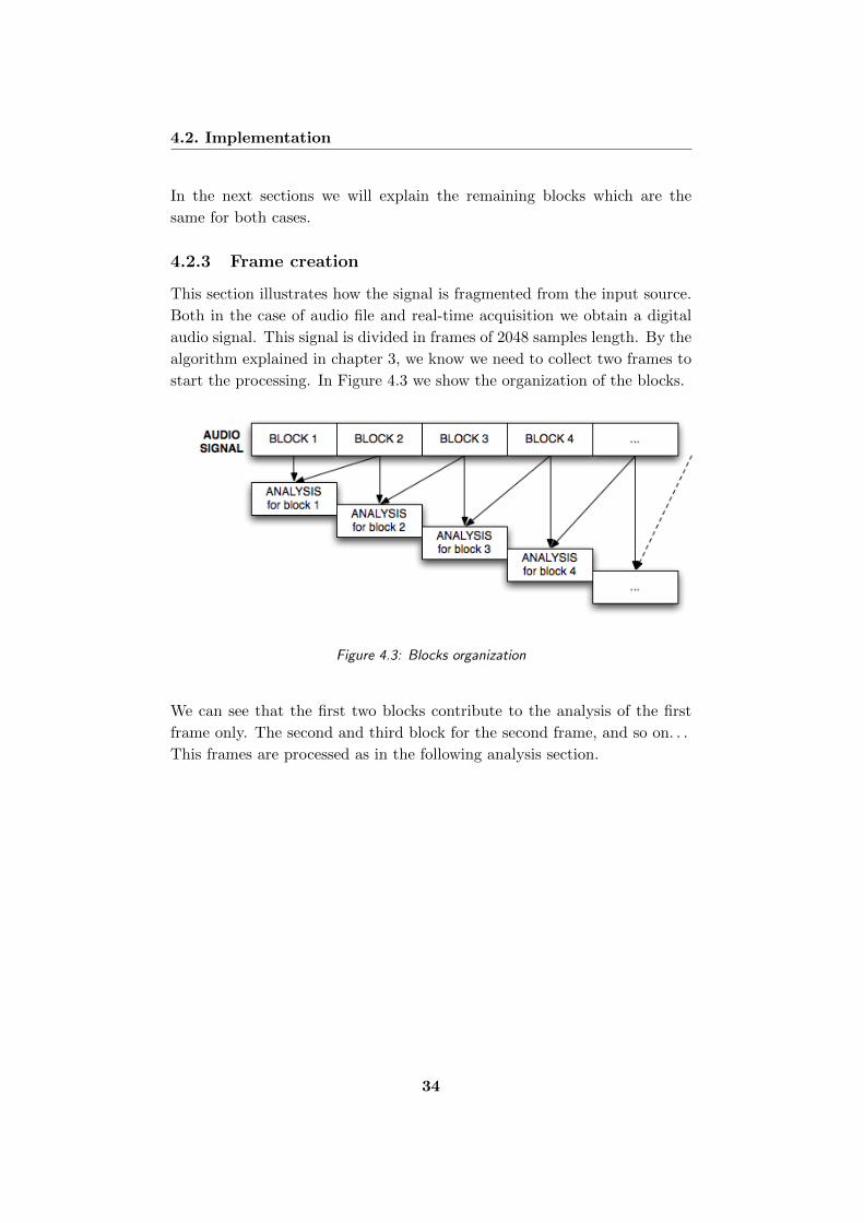
4.2.3 Frame creation
This section illustrates how the signal is fragmented from the input source.
Both in the case of audio file and real-time acquisition we obtain a digital
audio signal. This signal is divided in frames of 2048 samples length. By the
algorithm explained in chapter 3, we know we need to collect two frames to
start the processing. In Figure 4.3 we show the organization of the blocks.
Figure 4.3: Blocks organization
We can see that the first two blocks contribute to the analysis of the first
frame only. The second and third block for the second frame, and so on. . .
This frames are processed as in the following analysis section.
34

4.2. Implementation
4.2.4 Analysis
Once the audio signal has been acquired and segmented into frames, we can
start the main processing of the prototype. If we zoom in on the analysis
block in Figure 4.1(or 4.2) we obtain the scheme in Figure 4.4. This section
illustrates an overview of the analysis.
Figure 4.4: Analysis overview
The pitch detection stage need two adjacent frames to correctly retrieve the
pitch. In Figure 4.5 we can see how frames are managed as input of pitch
detection. Two adjacent frames are collected and their FFT is calculated;
the frames and their spectra are the input parameters for the pitch estima-
tion algorithm.
Figure 4.5: Blocks’ structure of the pitch detection phase
35

4.2. Implementation
The analysis section is composed by three main steps:
• FFT: it performs the Fourier transform of the input frame.
• Pitch Detection: from the input frame and the FFT frame, it returns
the fundamental frequency value.
• Onset Detection: it returns the temporal instant of the beginning of
the note.
Both pitch detection and onset detection blocks provide informations for
creating the notes and the score.
In the following sections we describe each block.
FFT
An extensive use of the Fast Fourier Transform (FFT) is done. FFT is an
efficient algorithm to compute the Discrete Fourier Transform (DFT) and
its inverse. A DFT permits to investigate the frequency characteristics of a
signal. It is useful to analyze the frequencies contained in a sampled signal.
The DFT is a computationally very onerous operation. An FFT is a way
to compute the same result more quickly: computing a DFT of N points
using the definition, takes O(N2) arithmetical operations, while an FFT can
compute the same result in only O(N log N) operations. The difference in
speed is substantial, this is the reason because it’s widely used in digital
signal processing.
Matlab provides a fast implementation of the FFT: their algorithm is based
on FFTW, ”The Fastest Fourier Transform in the West” 4.
The Matlab command
blockFFT = fft(block, size(block))
has been used to calculate the transform of the frame. The size indicate
the transform length: the number of samples on which the FFT should be
calculated.
For each frame of the audio signal the FFT is computed on 2048 samples
(the frame length): the frequency bin is wide
Fs
N=
44100
2048= 21Hz (4.1)
4FFTW, http://www.fftw.org
36
4.2. Implementation
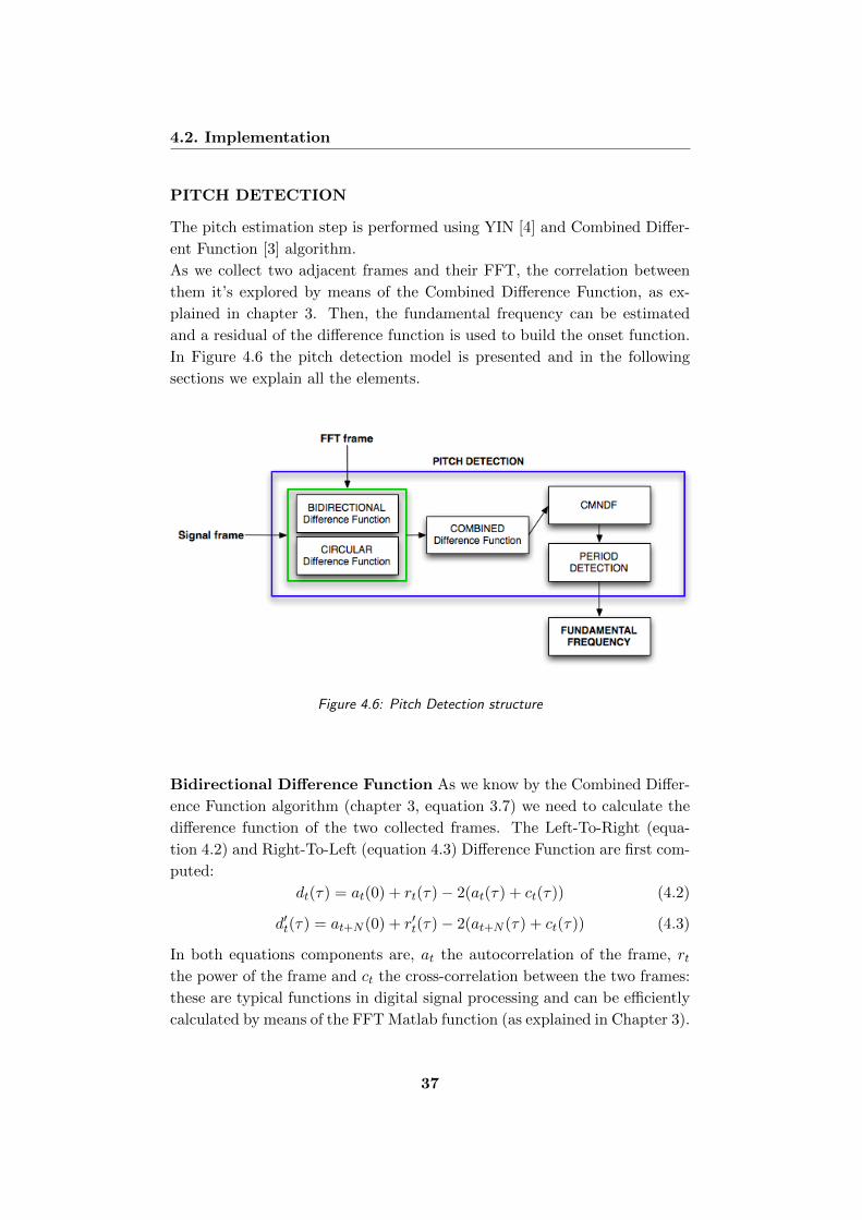
PITCH DETECTION
The pitch estimation step is performed using YIN [4] and Combined Differ-
ent Function [3] algorithm.
As we collect two adjacent frames and their FFT, the correlation between
them it’s explored by means of the Combined Difference Function, as ex-
plained in chapter 3. Then, the fundamental frequency can be estimated
and a residual of the difference function is used to build the onset function.
In Figure 4.6 the pitch detection model is presented and in the following
sections we explain all the elements.
Figure 4.6: Pitch Detection structure
Bidirectional Difference Function As we know by the Combined Differ-
ence Function algorithm (chapter 3, equation 3.7) we need to calculate the
difference function of the two collected frames. The Left-To-Right (equa-
tion 4.2) and Right-To-Left (equation 4.3) Difference Function are first com-
puted:
dt(τ) = at(0) + rt(τ)− 2(at(τ) + ct(τ)) (4.2)
d′t(τ) = at+N (0) + r′t(τ)− 2(at+N (τ) + ct(τ)) (4.3)
In both equations components are, at the autocorrelation of the frame, rtthe power of the frame and ct the cross-correlation between the two frames:
these are typical functions in digital signal processing and can be efficiently
calculated by means of the FFT Matlab function (as explained in Chapter 3).
37
4.2. Implementation
The Bidirectional Function is formed as the mean of two different functions:
Dt(τ) =dt(τ) + d′t(τ))
2(4.4)
Circular Difference Function Also in this case we take advantage of
the low time complexity of the FFT function to calculate the Circular Dif-
ference Function. The two adjacent frames are joint forming a new frame of
length 2*2048 = 4096 samples. The different function is calculated on this
new longer frame:
D′t(τ) = 2a′t(0) + 2(a′t(τ)− a′t(2N − τ)) (4.5)
where N = 2048 and a′t is the autocorrelation.
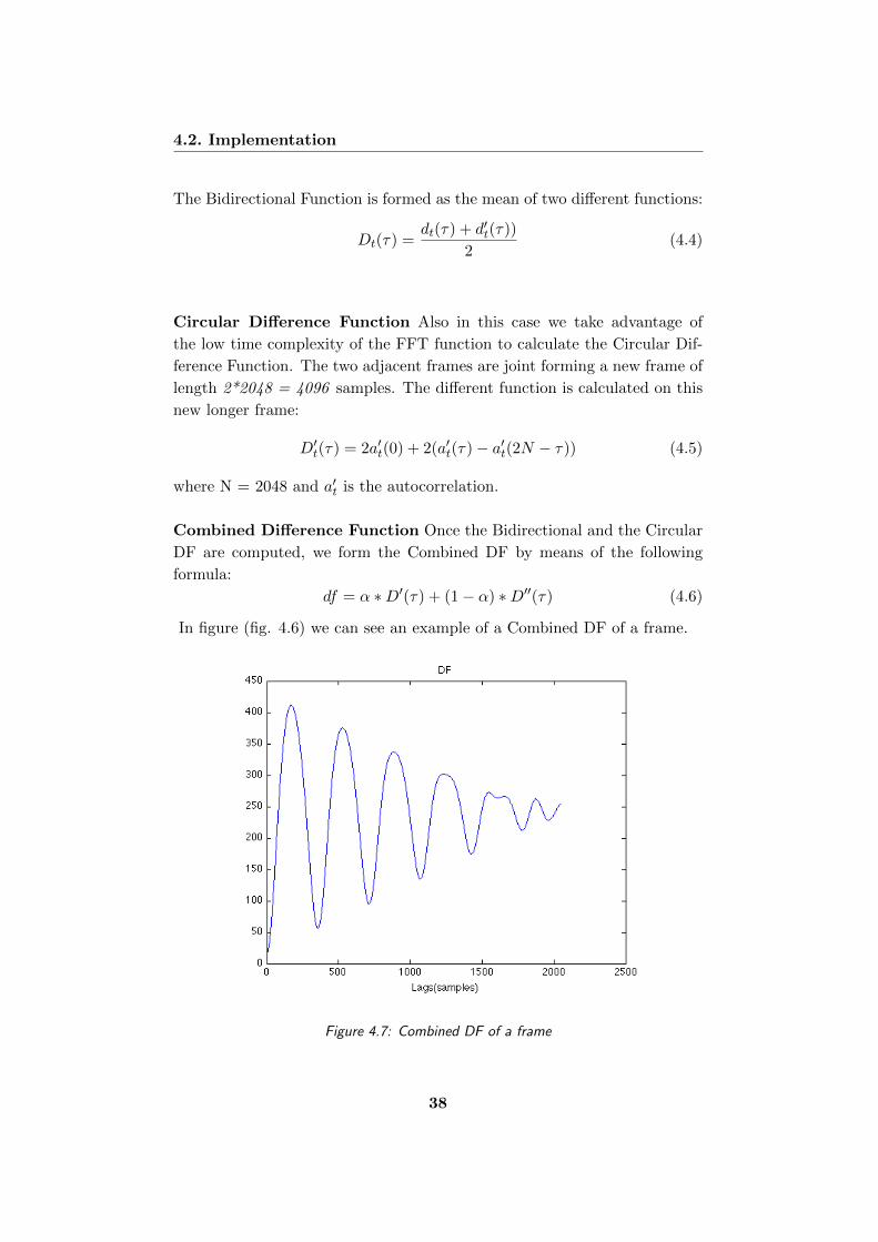
Combined Difference Function Once the Bidirectional and the Circular
DF are computed, we form the Combined DF by means of the following
formula:
df = α ∗D′(τ) + (1− α) ∗D′′(τ) (4.6)
In figure (fig. 4.6) we can see an example of a Combined DF of a frame.
Figure 4.7: Combined DF of a frame
38
4.2. Implementation
The tuning of the α parameter is critical for the correct algorithm working.
The value α = 0.35 is found experimentally, testing the prototype with sev-
eral audio files.
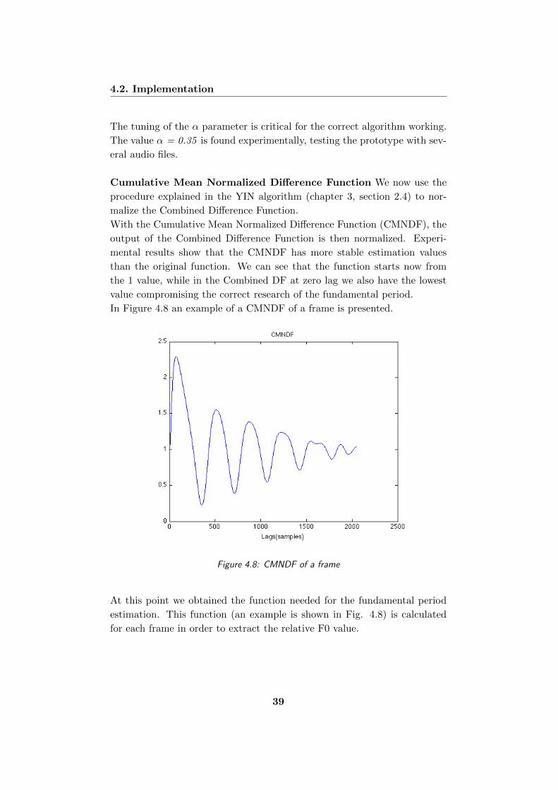
Cumulative Mean Normalized Difference Function We now use the
procedure explained in the YIN algorithm (chapter 3, section 2.4) to nor-
malize the Combined Difference Function.
With the Cumulative Mean Normalized Difference Function (CMNDF), the
output of the Combined Difference Function is then normalized. Experi-
mental results show that the CMNDF has more stable estimation values
than the original function. We can see that the function starts now from
the 1 value, while in the Combined DF at zero lag we also have the lowest
value compromising the correct research of the fundamental period.
In Figure 4.8 an example of a CMNDF of a frame is presented.
Figure 4.8: CMNDF of a frame
At this point we obtained the function needed for the fundamental period
estimation. This function (an example is shown in Fig. 4.8) is calculated
for each frame in order to extract the relative F0 value.
39
4.2. Implementation
Fundamental Period Detection
From the CMNDF function (see Section 4.2.4) we can retrieve the funda-
mental period of the current frame. We search for the first minimum below
a threshold k. The location of this minimum (lag τ) gives us the fundamen-
tal period of the frame. If none minimum below the threshold is found, we
chose the location of the global minimum. From the location (τ) we can
easily determine the frequency:
T =τ
Fs(4.7)
F0 =1
T(4.8)
where T is the period, τ is the lag and F0 is the fundamental frequency of
the frame.
The value of the threshold k has been found experimentally.
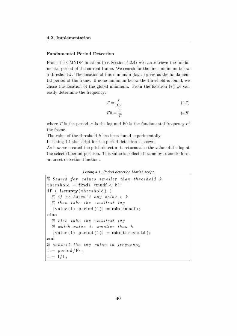
In listing 4.1 the script for the period detection is shown.
As how we created the pitch detector, it returns also the value of the lag at
the selected period position. This value is collected frame by frame to form
an onset detection function.
Listing 4.1: Period detection Matlab script
% Search f o r v a l u e s s m a l l e r than t h r e s h o l d k
th r e sho ld = find ( cmndf < k ) ;
i f ( isempty ( th r e sho ld ) )
% i f we haven ’ t any v a l u e < k
% than ta ke the s m a l l e s t l a g
[ va lue (1 ) per iod ( 1 ) ] = min( cmndf ) ;
else
% e l s e ta ke the s m a l l e s t l a g
% which v a l u e i s s m a l l e r than k
[ va lue (1 ) per iod ( 1 ) ] = min( th r e sho ld ) ;
end
% conver t the l a g v a l u e in f requency
f = per iod /Fs ;
f = 1/ f ;
40
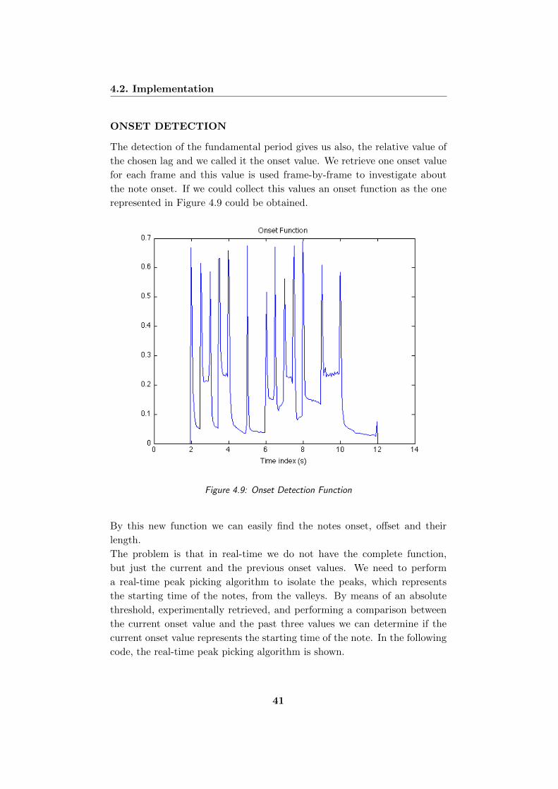
4.2. Implementation
ONSET DETECTION
The detection of the fundamental period gives us also, the relative value of
the chosen lag and we called it the onset value. We retrieve one onset value
for each frame and this value is used frame-by-frame to investigate about
the note onset. If we could collect this values an onset function as the one
represented in Figure 4.9 could be obtained.
Figure 4.9: Onset Detection Function
By this new function we can easily find the notes onset, offset and their
length.
The problem is that in real-time we do not have the complete function,
but just the current and the previous onset values. We need to perform
a real-time peak picking algorithm to isolate the peaks, which represents
the starting time of the notes, from the valleys. By means of an absolute
threshold, experimentally retrieved, and performing a comparison between
the current onset value and the past three values we can determine if the
current onset value represents the starting time of the note. In the following
code, the real-time peak picking algorithm is shown.
41
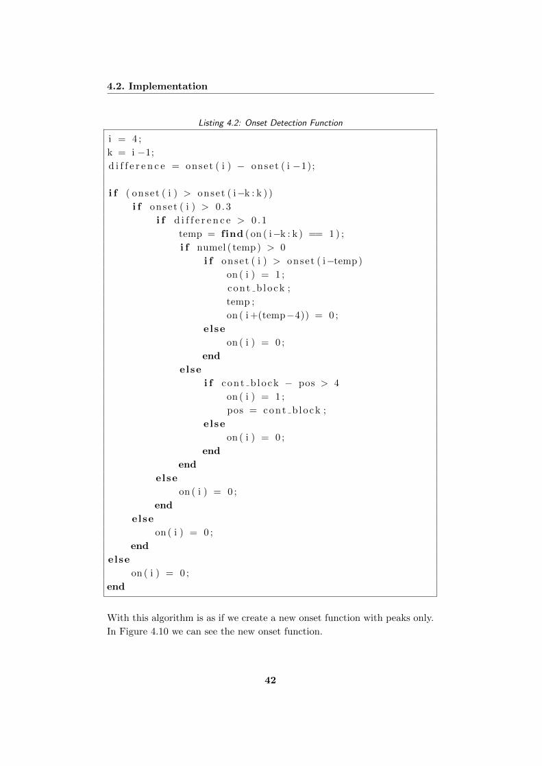
4.2. Implementation
Listing 4.2: Onset Detection Function
i = 4 ;
k = i −1;
d i f f e r e n c e = onset ( i ) − onset ( i −1);
i f ( onset ( i ) > onset ( i−k : k ) )
i f onset ( i ) > 0 .3
i f d i f f e r e n c e > 0 .1
temp = find ( on ( i−k : k ) == 1 ) ;
i f numel ( temp ) > 0
i f onset ( i ) > onset ( i−temp )
on ( i ) = 1 ;
cont b lock ;
temp ;
on ( i +(temp−4)) = 0 ;
else
on ( i ) = 0 ;
end
else
i f cont b lock − pos > 4
on ( i ) = 1 ;
pos = cont b lock ;
else
on ( i ) = 0 ;
end
end
else
on ( i ) = 0 ;
end
else
on ( i ) = 0 ;
end
else
on ( i ) = 0 ;
end
With this algorithm is as if we create a new onset function with peaks only.
In Figure 4.10 we can see the new onset function.
42
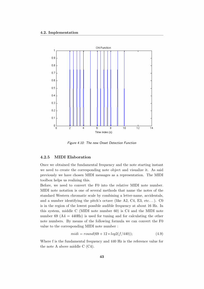
4.2. Implementation
Figure 4.10: The new Onset Detection Function
4.2.5 MIDI Elaboration
Once we obtained the fundamental frequency and the note starting instant
we need to create the corresponding note object and visualize it. As said
previously we have chosen MIDI messages as a representation. The MIDI
toolbox helps us realizing this.
Before, we need to convert the F0 into the relative MIDI note number.
MIDI note notation is one of several methods that name the notes of the
standard Western chromatic scale by combining a letter-name, accidentals,
and a number identifying the pitch’s octave (like A2, C4, E3, etc. . . ). C0
is in the region of the lowest possible audible frequency at about 16 Hz. In
this system, middle C (MIDI note number 60) is C4 and the MIDI note
number 69 (A4 = 440Hz) is used for tuning and for calculating the other
note numbers. By means of the following formula we can convert the F0
value to the corresponding MIDI note number :
midi = round(69 + 12 ∗ log2(f/440)); (4.9)
Where f is the fundamental frequency and 440 Hz is the reference value for
the note A above middle C (C4).
43
4.3. Conclusions
With the MIDI note number and length we can create an array for each
note:
row = [onset(beats); duration(beats); midi channel; pitch, velocity=120;
onset(s); duration(s)];
midi matrix(contatore note, :) = row;
In the row array we have the onset and the duration both in beats and in
seconds, the midi channel to use, the velocity and pitch which is the trans-
formed frequency we retrieved. Pushing each row in a matrix (midi matrix)
we obtain a score matrix to be used with the MIDI Toolbox in order to
create the score and the MIDI file.
4.2.6 Score Creation
With the help of the MIDI toolbox we created a midi matrix in which
every row is a MIDI note with its pitch and duration. The MIDI Toolbox
provides a set of functions for visualizing a notation of a MIDI file: it offers
a pianoroll notation. Pianoroll is a simple representation of piano notes with
a time axis.
The notation is performed in real-time: as the algorithm find a note, it
appears immediately in the notation. With a call to the function
pianoroll(midi matrix);
the pianoroll visualization is created as in Figure 4.11. The horizontal line
represents the reference C3 note.
4.3 Conclusions
The system has been tested both with audio files and realt-time bass. En-
couraging results were obtained from these test. The main problem has been
with the real-time performances: long latency has been experienced. This
may me caused by the Matlab inability to work with real-time processing
or by the total low computational power as the sum of the system, Matlab,
Playrec and script realized.
In the next implementation step this problem will be solved.
44

4.3. Conclusions
Figure 4.11: Piano roll visualization
45
Chapter 5
Software development
In the previous chapter we illustrated the design of the application’s pro-
totype. The algorithm has been tested and the parameters have been set
up. In this chapter we focused on the development details of the software
application realized.
5.1 Requirements
Let’s imagine a new user approaching at this application for the very first
time. He would like to understand its usage almost immediately. He may
wants to try it first with a recorded bass line. So he runs the application
and loads an audio file: if everything works, he could decide to to plug the
bass directly in the computer. Probably he would like to listen at what he’s
playing, and it would also be nice to record his performance and make it
available for playing/editing. And the score and the midi file accessible as
soon as possible.
If we think at this typical scenario we can get some important information
about the requirements to meet:
• Application usability: we need to realize a simple and friendly interface
for a variety of users, from the professional musician to the entry-level
music student to the amateur. The graphical interface should then be
accurate, simple to understand and clean.
• Input: the application need to transcribe a music excerpt both from
audio files and from real-time performances.
• Fast computation: the computation part should be pretty fast and
accurate in order to have a real-time feedback. We need a fast and
reliable environment to work on.
5.2. Environment and libraries
• Audio playback: the user wants to hear back at what is listening. This
part should be seriously taken in account. Not everybody has a bass
amplifier or a professional sound card for recording and this could be
a point worthy of remark.
• Metronome: playing with a metronome is very important for a musi-
cian. We should give the user the possibility to use it.
• Score: the score is the most important feedback for the user. It would
be nice for him to modify some notes or adding others and listen back
to the changes.
• Midi/MusicXML: we can give the user the possibility to export the
midi and music xml file for future editing.
5.2 Environment and libraries
To meet the requirements and offer to each potential user the possibility
to use the application, we chose a platform-independent programming lan-
guage: Java. With Java, we can also solve the latency problems in the
real-time processing occurred in the prototype implementation. In this sec-
tion we present the environment and the libraries used.
5.2.1 Java 1
Java is a programming language introduced in 1991 and now it runs on more
than 850 million personal computers worldwide, and on billions of devices
worldwide, including mobile and TV devices. This is one reason to develop
the application with Java: we are sure it will works on many computers with
a little effort. In fact, Java applications are compiled to bytecode that can
run on any Java Virtual Machine (JVM) regardless of computer architecture.
Further more, there are a lot of libraries that can be added to extend the
environment. Among all libraries we used JTransform, Java Sound, JMusic
and JFreeChart. The first let us calculate efficiently the FFT transform.
Java Sound us manage the audio playback and recording at a low-level
programming. JMusic help us to create the score view of the transcribed
work. The last library is useful for plotting graphs.
1Java, http://www.java.com
47

5.2. Environment and libraries
5.2.2 JTransform 2
JTransforms is an open source FFT library written in Java. It permits the
calculation of the Discrete Fourier Transform (DFT) by means of the Fast
Fourier Transform (FFT). The code is derived from General Purpose FFT
Package 3 written by Takuya Ooura and from Java FFTPack 4 written by
Baoshe Zhang.
5.2.3 Java Sound 5
The Java Sound API [17] specification provides low-level support for audio
operations such as audio playback and capture (recording), mixing, MIDI
sequencing, and MIDI synthesis in an extensible, flexible framework. It
provides explicit control over the capabilities normally required for sound
input and output. It represents the lowest level of sound support on the
Java platform. For example, the Java Sound API supplies mechanisms for
installing, accessing, and manipulating system resources such as audio mix-
ers, MIDI synthesizers, other audio or MIDI devices, file readers and writers,
and sound format converters. The Java Sound API does not include sophis-
ticated sound editors or graphical tools, but it provides capabilities upon
which such programs can be built.
Java Sound is composed by two main package: Sampled and MIDI. We used
the Sampled package which provides interfaces and classes for capture, pro-
cessing, and playback of sampled audio data. The MIDI package provides
interfaces and classes for I/O, sequencing, and synthesis of MIDI data, and
it was used for the metronome.
Java Sound Sampled
The package javax.sound.sampled is good for our purpose: it handles digital
audio data, which the Java Sound API refers to as sampled audio. The
Java Sound API does not assume a specific audio hardware configuration;
it is designed to allow different sorts of audio components to be installed on
a system and accessed by the specific API. The Java Sound API supports
common functionality such as input and output from a sound card (for
example, for recording and playback of sound files) as well as mixing of
multiple streams of audio.
2JTransform, http://sites.google.com/site/piotrwendykier/software/jtransforms3General Purpose FFT Package, http://www.kurims.kyoto-
u.ac.jp/%7Eooura/fft.html4Java FFTPack, http://jfftpack.sourceforge.net/5Java Sound, http://www.oracle.com/technetwork/java/index-139508.html
48

5.2. Environment and libraries
A typical audio architecture is shown in Figure 5.1:
Figure 5.1: A typical audio architecture
A device such as a sound card has various input and output ports, and
mixing is provided in the software. The mixer might receive data that has
been read from a file, streamed from a network, generated on the fly by
an application program, or produced by a MIDI synthesizer. The mixer
combines all its audio inputs into a single stream, which can be sent to an
output device for rendering. To play or capture sound in our application we
need three different components:
• Formatted audio data: it refers to the audio format used. An audio
format tells how to interpret a series of bytes of ”raw” sampled audio
data and tells you the sample rate and the number of bits per sample.
In our case the PCM standard audio format has been used. The audio
format we used accounts for: 16 bit per sample, sampling rate of 44100
Hz and 1 channel for monophonic audio.
• Mixer: the purpose of a mixer is to handle one or more streams of audio
input and one or more streams of audio output. It mixes together
multiple incoming streams into one outgoing stream.
• Line: a line is an element of the digital audio ”pipeline”, that is, a
path for moving audio into or out of the mixer. As metaphor, lines
are analogous to the microphones and speakers connected to a mixing
console.
49
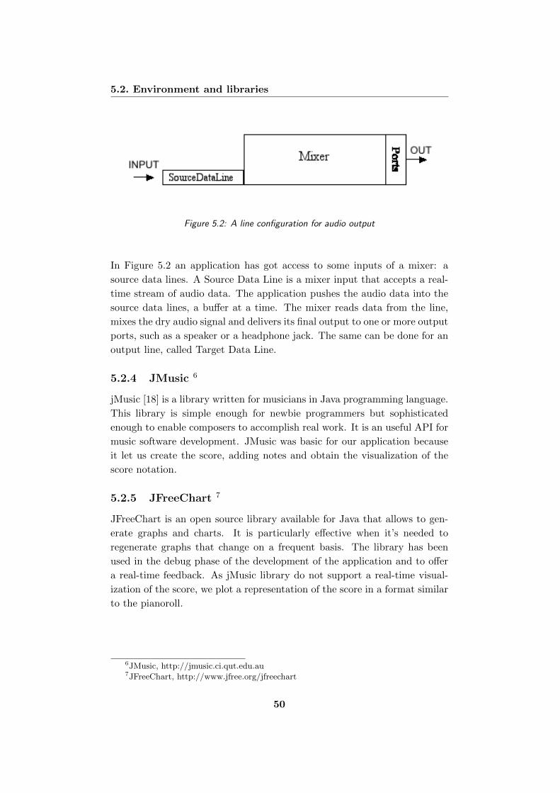
5.2. Environment and libraries
Figure 5.2: A line configuration for audio output
In Figure 5.2 an application has got access to some inputs of a mixer: a
source data lines. A Source Data Line is a mixer input that accepts a real-
time stream of audio data. The application pushes the audio data into the
source data lines, a buffer at a time. The mixer reads data from the line,
mixes the dry audio signal and delivers its final output to one or more output
ports, such as a speaker or a headphone jack. The same can be done for an
output line, called Target Data Line.
5.2.4 JMusic 6
jMusic [18] is a library written for musicians in Java programming language.
This library is simple enough for newbie programmers but sophisticated
enough to enable composers to accomplish real work. It is an useful API for
music software development. JMusic was basic for our application because
it let us create the score, adding notes and obtain the visualization of the
score notation.
5.2.5 JFreeChart 7
JFreeChart is an open source library available for Java that allows to gen-
erate graphs and charts. It is particularly effective when it’s needed to
regenerate graphs that change on a frequent basis. The library has been
used in the debug phase of the development of the application and to offer
a real-time feedback. As jMusic library do not support a real-time visual-
ization of the score, we plot a representation of the score in a format similar
to the pianoroll.
6JMusic, http://jmusic.ci.qut.edu.au7JFreeChart, http://www.jfree.org/jfreechart
50
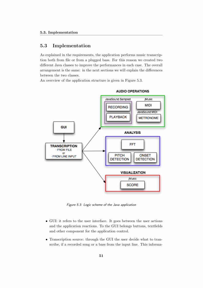
5.3. Implementation
5.3 Implementation
As explained in the requirements, the application performs music transcrip-
tion both from file or from a plugged bass. For this reason we created two
different Java classes to improve the performances in each case. The overall
arrangement is the same: in the next sections we will explain the differences
between the two classes.
An overview of the application structure is given in Figure 5.3.
Figure 5.3: Logic scheme of the Java application
• GUI: it refers to the user interface. It goes between the user actions
and the application reactions. To the GUI belongs buttons, textfields
and other component for the application control.
• Transcription source: through the GUI the user decide what to tran-
scribe, if a recorded song or a bass from the input line. This informa-
51
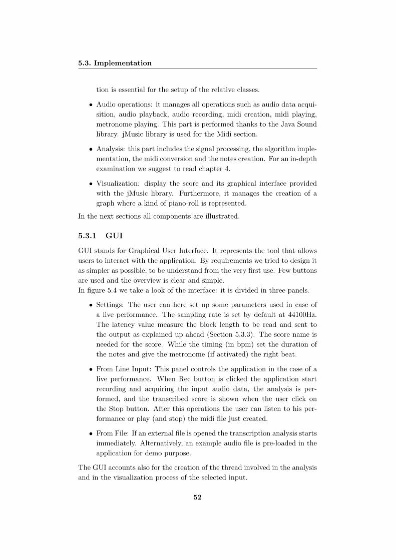
5.3. Implementation
tion is essential for the setup of the relative classes.
• Audio operations: it manages all operations such as audio data acqui-
sition, audio playback, audio recording, midi creation, midi playing,
metronome playing. This part is performed thanks to the Java Sound
library. jMusic library is used for the Midi section.
• Analysis: this part includes the signal processing, the algorithm imple-
mentation, the midi conversion and the notes creation. For an in-depth
examination we suggest to read chapter 4.
• Visualization: display the score and its graphical interface provided
with the jMusic library. Furthermore, it manages the creation of a
graph where a kind of piano-roll is represented.
In the next sections all components are illustrated.
5.3.1 GUI
GUI stands for Graphical User Interface. It represents the tool that allows
users to interact with the application. By requirements we tried to design it
as simpler as possible, to be understand from the very first use. Few buttons
are used and the overview is clear and simple.
In figure 5.4 we take a look of the interface: it is divided in three panels.
• Settings: The user can here set up some parameters used in case of
a live performance. The sampling rate is set by default at 44100Hz.
The latency value measure the block length to be read and sent to
the output as explained up ahead (Section 5.3.3). The score name is
needed for the score. While the timing (in bpm) set the duration of
the notes and give the metronome (if activated) the right beat.
• From Line Input: This panel controls the application in the case of a
live performance. When Rec button is clicked the application start
recording and acquiring the input audio data, the analysis is per-
formed, and the transcribed score is shown when the user click on
the Stop button. After this operations the user can listen to his per-
formance or play (and stop) the midi file just created.
• From File: If an external file is opened the transcription analysis starts
immediately. Alternatively, an example audio file is pre-loaded in the
application for demo purpose.
The GUI accounts also for the creation of the thread involved in the analysis
and in the visualization process of the selected input.
52
5.3. Implementation
Figure 5.4: Application user interface
5.3.2 Thread
Since we wants to maximize the real-time experience, as shown in Fig. 5.3,
the macro-blocks (Audio operations, Analysis, Visualization) are managed
using different synchronized thread running in parallel.
A thread is a division of the process in two or more parts executed concur-
rently. The Java Virtual Machine allows an application to have multiple
threads of execution running concurrently. Multithreaded applications de-
liver their potent power by running many threads concurrently within a
single program. From a logical point of view, multithreading means multi-
ple lines of a single program can be executed at the same time. By starting
a thread an efficient path of execution is created while still sharing the orig-
inal data area from the parent.
In the application we have three main part that runs concurrently: the GUI,
53
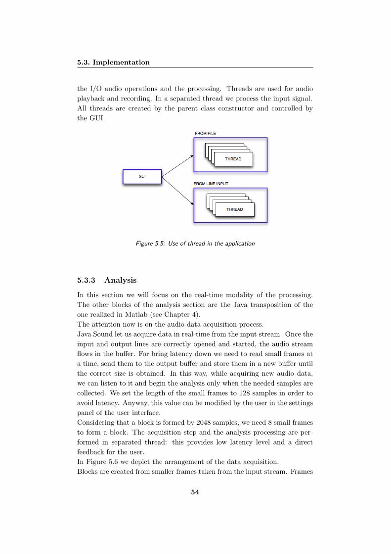
5.3. Implementation
the I/O audio operations and the processing. Threads are used for audio
playback and recording. In a separated thread we process the input signal.
All threads are created by the parent class constructor and controlled by
the GUI.
Figure 5.5: Use of thread in the application
5.3.3 Analysis
In this section we will focus on the real-time modality of the processing.
The other blocks of the analysis section are the Java transposition of the
one realized in Matlab (see Chapter 4).
The attention now is on the audio data acquisition process.
Java Sound let us acquire data in real-time from the input stream. Once the
input and output lines are correctly opened and started, the audio stream
flows in the buffer. For bring latency down we need to read small frames at
a time, send them to the output buffer and store them in a new buffer until
the correct size is obtained. In this way, while acquiring new audio data,
we can listen to it and begin the analysis only when the needed samples are
collected. We set the length of the small frames to 128 samples in order to
avoid latency. Anyway, this value can be modified by the user in the settings
panel of the user interface.
Considering that a block is formed by 2048 samples, we need 8 small frames
to form a block. The acquisition step and the analysis processing are per-
formed in separated thread: this provides low latency level and a direct
feedback for the user.
In Figure 5.6 we depict the arrangement of the data acquisition.
Blocks are created from smaller frames taken from the input stream. Frames
54

5.3. Implementation
Figure 5.6: Audio blocks segmentation
are collected to form one block. As a block is created the process continue to
form the other blocks. The analysis starts only when two consecutive blocks
are collected: from the first two blocks we estimate the pitch of the first
block. From the second and the third we estimate the pitch of the second
block, and so on. . .
Obviously some part of the analysis, like the FFT transform (using JTrans-
form), is reused in the next step. There is a variable recovery that speed
up the algorithm execution time. The remaining process of the algorithm is
much similar to the one in the Matlab development (see chapter 4): the FFT
is performed and then pitch detection and onset detection are calculated in
the same way.
5.3.4 Audio Operations
This section is about the audio data acquisition and operations.
55
5.3. Implementation
Java Sound
We deals with the creation and the control of the mixer and the I/O lines.
Moreover, the input audio data is recorded so that the user can listen to his
performance. Java Sound returns a software mixer to control the input and
output lines. With this functions
INPUT line = (TargetDataLine) mixer.getLine(targetInfo);
OUTPUT line = (SourceDataLine) mixer.getLine(sourceInfo);
we obtain the lines through which we record and play the samples. To read
samples from the input buffer we use the function
numberOfBytesRead = targetDataLine.read(byteData, 0,
byteData.length);
where we can specify the number of bytes to read. Bytes will be further
converted in double Java type for the signal processing. The bytes stored in
byteData are then pushed in a buffer until the right frame length is reached
(2048 sample = 4096 bytes).
For writing the frame to the output line we use
sourceDataLine.write(byteData, 0, numberOfBytesRead);
that let us specify the number of sample to write. Java Sound is then
responsible for the correct playing.
jMusic
This part covers the MIDI functions for creating and playing the MIDI
file. Once the frame has been processed and the necessary information are
retrieved we need to create the single note object, provided by jMusic, to be
added in the score. jMusic let us create a score where notes and rest can be
added by simply specifying duration and the pitch (for the note):
note = new Note(note pitch, note duration); rest = new
Rest(rest duration);
As the analysis retrieve the fundamental frequency and the onset instant,
the note is created and added sequentially to the score. This score will be
used for visualizing the standard notation.
56

5.3. Implementation
Metronome
A metronome is a device that produces regular clicks, settable in beats per
minute. The metronome is a mandatory tool for every musician. It assists
them in keeping a regular tempo while playing or practicing. We decided to
implement the metronome as an extra feature to prompt users for using the
application.
The metronome have been realized using the JavaSound MIDI package. A
Synthesizer from MidiSystem has been created and opened, the MIDIChan-
nel 10 has been retrieved (Channel 10 has all sorts of percussion instruments
that make metronome sounds). With the metronome toggle button in the
setting panel the user decide about the activation of the metronome. If so,
as Rec button is pressed, a metronome thread is created. This thread starts
and loops until the Stop button is pressed. In the loop cycle it occurs a
noteOn MIDI message, a sleep of the thread, and a noteOff MIDI message:
one beat of the metronome is played.
The metronome and the real-time playback threads are synchronized. If
metronome is playing the playback thread is paused for the length of cur-
rent frame plus the latency of the MIDI Synthesizer plus an estimate of the
sound-card latency (about 20ms, this value is not retrievable from Java).
This because when the metronome is playing, it has a higher priority with
respect to the playback.
5.3.5 Visualization
In this section we illustrate the creation of the score notation.
As we explained, the score is created and we need to visualize it. The jMusic
library visualize the score in a standard notation simply using the function:
View.notate(score);
This function produces an interface where score is shown as in Figure 5.7.
Figure 5.7: Score of a transcribed music excerpt
With the standard music notation, jMusic also provides an additional inter-
57
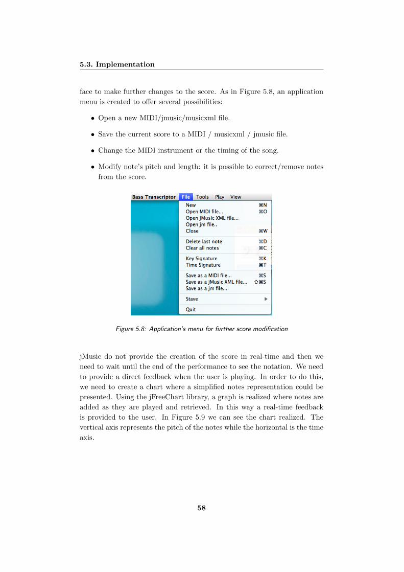
5.3. Implementation
face to make further changes to the score. As in Figure 5.8, an application
menu is created to offer several possibilities:
• Open a new MIDI/jmusic/musicxml file.
• Save the current score to a MIDI / musicxml / jmusic file.
• Change the MIDI instrument or the timing of the song.
• Modify note’s pitch and length: it is possible to correct/remove notes
from the score.
Figure 5.8: Application’s menu for further score modification
jMusic do not provide the creation of the score in real-time and then we
need to wait until the end of the performance to see the notation. We need
to provide a direct feedback when the user is playing. In order to do this,
we need to create a chart where a simplified notes representation could be
presented. Using the jFreeChart library, a graph is realized where notes are
added as they are played and retrieved. In this way a real-time feedback
is provided to the user. In Figure 5.9 we can see the chart realized. The
vertical axis represents the pitch of the notes while the horizontal is the time
axis.
58
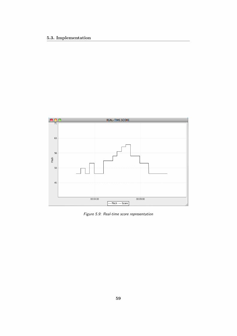
5.3. Implementation
Figure 5.9: Real-time score representation
59

Chapter 6
Experimental Results and
Evaluations
In this chapter we will show the experimental results and we will give an
evaluation on the system.
Given that the application is realized to work both from audio file and for
real-time performances, we need to test the system in both cases. The ap-
plication has been tested with a synthesized dataset and by users. Objective
and subjective results are provided.
In section 6.1 the datasets used for the test are illustrated. Section 6.2 shows
the results performed on the testing dataset and by the single users. Section
6.3 contains considerations on the obtained results.
6.1 Dataset
In order to test the system properly we created a synthesized dataset and
we let three people use the application. Then, we obtained their impresses
about the application.
6.1.1 Synthesized Dataset
For testing purpose we created a dataset of ten bass lines. The audio files
with the bass lines were created with a bass synthesizer using some effects
to reproduce a real bass sound. The ten different pieces were realized with
growing complexity as number of notes, timing, and presence of rests. The
files have been sampled at 44100Hz and coded in PCM format at 16bit. In
the next listing we explain a little each bass line created:
• bass line 01: quarter and half notes, beat of 100bpm, no rests;
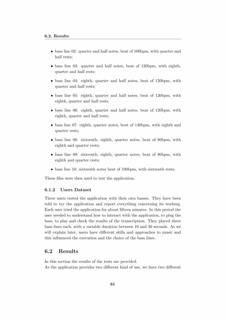
6.2. Results
• bass line 02: quarter and half notes, beat of 100bpm, with quarter and
half rests;
• bass line 03: quarter and half notes, beat of 120bpm, with eighth,
quarter and half rests;
• bass line 04: eighth, quarter and half notes, beat of 120bpm, with
quarter and half rests;
• bass line 05: eighth, quarter and half notes, beat of 120bpm, with
eighth, quarter and half rests;
• bass line 06: eighth, quarter and half notes, beat of 120bpm, with
eighth, quarter and half rests;
• bass line 07: eighth, quarter notes, beat of 140bpm, with eighth and
quarter rests;
• bass line 08: sixteenth, eighth, quarter notes, beat of 80bpm, with
eighth and quarter rests;
• bass line 09: sixteenth, eighth, quarter notes, beat of 80bpm, with
eighth and quarter rests;
• bass line 10: sixteenth notes beat of 100bpm, with sixteenth rests;
These files were then used to test the application.
6.1.2 Users Dataset
Three users tested the application with their own basses. They have been
told to try the application and report everything concerning its working.
Each user tried the application for about fifteen minutes. In this period the
user needed to understand how to interact with the application, to plug the
bass, to play and check the results of the transcription. They played three
bass lines each, with a variable duration between 10 and 30 seconds. As we
will explain later, users have different skills and approaches to music and
this influenced the execution and the choice of the bass lines.
6.2 Results
In this section the results of the tests are provided.
As the application provides two different kind of use, we have two different
61
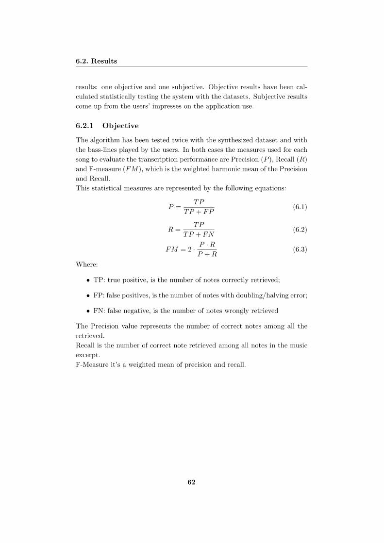
6.2. Results
results: one objective and one subjective. Objective results have been cal-
culated statistically testing the system with the datasets. Subjective results
come up from the users’ impresses on the application use.
6.2.1 Objective
The algorithm has been tested twice with the synthesized dataset and with
the bass-lines played by the users. In both cases the measures used for each
song to evaluate the transcription performance are Precision (P ), Recall (R)
and F-measure (FM), which is the weighted harmonic mean of the Precision
and Recall.
This statistical measures are represented by the following equations:
P =TP
TP + FP(6.1)
R =TP
TP + FN(6.2)
FM = 2 · P ·RP +R
(6.3)
Where:
• TP: true positive, is the number of notes correctly retrieved;
• FP: false positives, is the number of notes with doubling/halving error;
• FN: false negative, is the number of notes wrongly retrieved
The Precision value represents the number of correct notes among all the
retrieved.
Recall is the number of correct note retrieved among all notes in the music
excerpt.
F-Measure it’s a weighted mean of precision and recall.
62
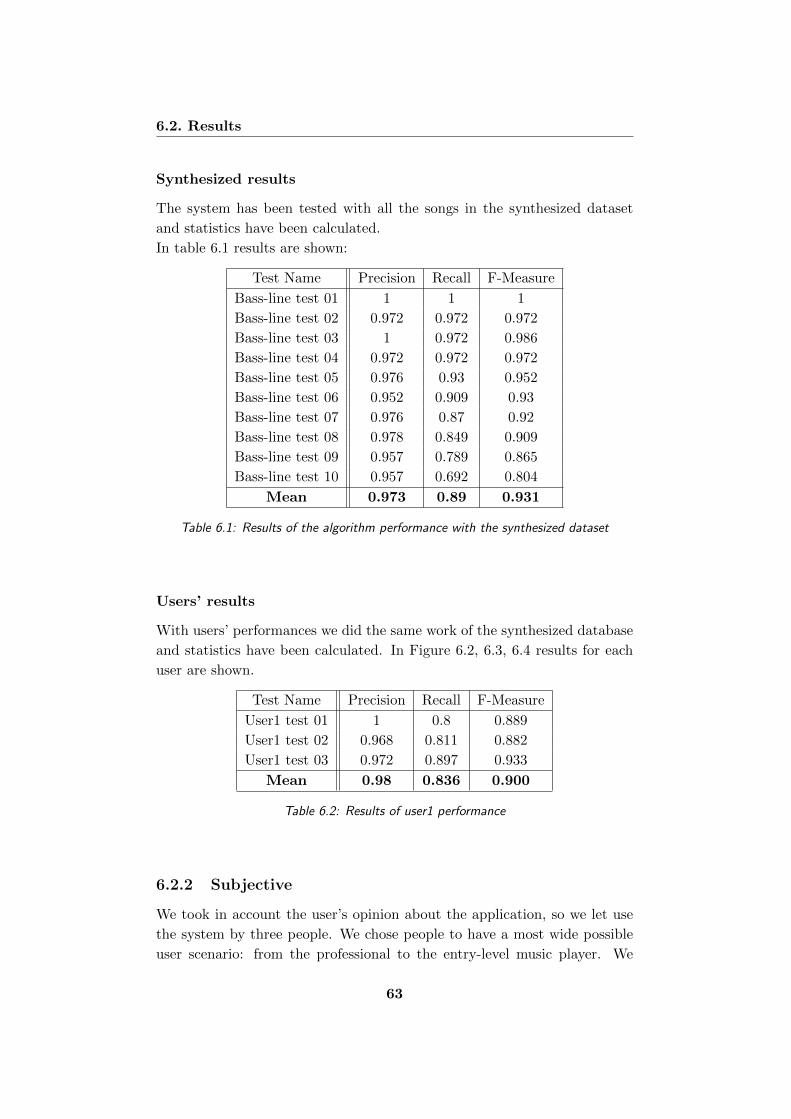
6.2. Results
Synthesized results
The system has been tested with all the songs in the synthesized dataset
and statistics have been calculated.
In table 6.1 results are shown:
Test Name Precision Recall F-Measure
Bass-line test 01 1 1 1
Bass-line test 02 0.972 0.972 0.972
Bass-line test 03 1 0.972 0.986
Bass-line test 04 0.972 0.972 0.972
Bass-line test 05 0.976 0.93 0.952
Bass-line test 06 0.952 0.909 0.93
Bass-line test 07 0.976 0.87 0.92
Bass-line test 08 0.978 0.849 0.909
Bass-line test 09 0.957 0.789 0.865
Bass-line test 10 0.957 0.692 0.804
Mean 0.973 0.89 0.931
Table 6.1: Results of the algorithm performance with the synthesized dataset
Users’ results
With users’ performances we did the same work of the synthesized database
and statistics have been calculated. In Figure 6.2, 6.3, 6.4 results for each
user are shown.
Test Name Precision Recall F-Measure
User1 test 01 1 0.8 0.889
User1 test 02 0.968 0.811 0.882
User1 test 03 0.972 0.897 0.933
Mean 0.98 0.836 0.900
Table 6.2: Results of user1 performance
6.2.2 Subjective
We took in account the user’s opinion about the application, so we let use
the system by three people. We chose people to have a most wide possible
user scenario: from the professional to the entry-level music player. We
63
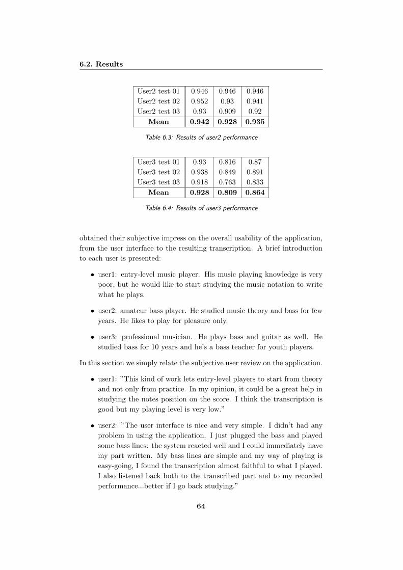
6.2. Results
User2 test 01 0.946 0.946 0.946
User2 test 02 0.952 0.93 0.941
User2 test 03 0.93 0.909 0.92
Mean 0.942 0.928 0.935
Table 6.3: Results of user2 performance
User3 test 01 0.93 0.816 0.87
User3 test 02 0.938 0.849 0.891
User3 test 03 0.918 0.763 0.833
Mean 0.928 0.809 0.864
Table 6.4: Results of user3 performance
obtained their subjective impress on the overall usability of the application,
from the user interface to the resulting transcription. A brief introduction
to each user is presented:
• user1: entry-level music player. His music playing knowledge is very
poor, but he would like to start studying the music notation to write
what he plays.
• user2: amateur bass player. He studied music theory and bass for few
years. He likes to play for pleasure only.
• user3: professional musician. He plays bass and guitar as well. He
studied bass for 10 years and he’s a bass teacher for youth players.
In this section we simply relate the subjective user review on the application.
• user1: ”This kind of work lets entry-level players to start from theory
and not only from practice. In my opinion, it could be a great help in
studying the notes position on the score. I think the transcription is
good but my playing level is very low.”
• user2: ”The user interface is nice and very simple. I didn’t had any
problem in using the application. I just plugged the bass and played
some bass lines: the system reacted well and I could immediately have
my part written. My bass lines are simple and my way of playing is
easy-going, I found the transcription almost faithful to what I played.
I also listened back both to the transcribed part and to my recorded
performance...better if I go back studying.”
64
6.3. Algorithm’s evaluation and comments
• user3: ”I think the application still has some problems but, in my
opinion, it has great capability. I think its best use is for transcribe, in
a while, a melody you have in your head. In few seconds the application
lets you set up the beat and record and write down the part. Yes,
there are some problems with the note’s duration and the halving and
doubling errors, but you can edit the part on the instant. In a future
version it could be great to add support for slap, slides and hammer-on
techniques. But it is great. I think it could achieve very good results
because it’s very useful. Good job!”
6.3 Algorithm’s evaluation and comments
The system has been tested with the dataset created and also with an in-line
bass playing. Encouraging results were obtained in both cases.
In tables 6.1-6.4 we can see the performances of the algorithm proposed. In
general we have good results.
The high precision values mean that the system find the right fundamental
frequency more than 90% of the time in both cases. We can see that this
value goes down when fast notes occours.
In case of the users performances the recall is slightly lower then with the
synthesized dataset: this depends on the way of playing of each user. A more
clear an shaped note is better retrieved, while tentative notes are wrongly
or not retrieved. The synthesized dataset does not contain errors and the
sound is the most clear possible: for these reasons the recall is higher in this
case.
The f-measure confirm this results with a mean of 88% of good algorithm
performances.
Nevertheless, some errors were noticed: these may be caused by the pitch
detector or by the onset detector.
We first see the pitch detector algorithm errors:
• Pitch Halving: it could happen that the algorithm wrong octave. A
note on a octave is identified but one octave lower. This happen spe-
cially when fast notes occur.
• Pitch Doubling: it’s the opposite of the halving problem. A note on a
octave is identified at one octave higher.
65

6.3. Algorithm’s evaluation and comments
In table 6.5 and 6.6 the Doubling/Halving errors are shown for both
cases.
Test Name Doubling & Halving Error
Bass-line test 01 0
Bass-line test 02 0.027
Bass-line test 03 0
Bass-line test 04 0.027
Bass-line test 05 0.022
Bass-line test 06 0.043
Bass-line test 07 0.021
Bass-line test 08 0.018
Bass-line test 09 0.033
Bass-line test 10 0.029
Mean 0.0220
Table 6.5: Doubling and halving errors for the synthesized dataset
Test Name Doubling & Halving Error
User1 test 01 0
User1 test 02 0.026
User1 test 03 0.025
User2 test 01 0.051
User2 test 02 0.044
User2 test 03 0.063
User3 test 01 0.057
User3 test 02 0.053
User3 test 03 0.063
Mean 0.0424
Table 6.6: Doubling and halving errors for the user dataset
Onset detector errors:
• Note length: a wrong duration of the note is set. This kind of errors
are caused by the onset detector. The pick picking algorithm of the
onset detection has been created experimentally and this may be the
cause of errors on notes duration.
Other kind of errors:
66
6.3. Algorithm’s evaluation and comments
• Non-existing notes: it happens few times that the system retrieve non-
existing notes. This can be caused by the initialization of the audio
driver in Matlab (not in Java) that produces some clicks, or by some
noise in the audio file.
• Latency (measure of time delay in a system): in Matlab long latency
has been experienced with plugged-in bass while hearing back what
playing. This has been solved porting the application in Java with
better management of the audio resources.
67
Chapter 7
Conclusions and future
developments
7.1 Conclusions
Due to the wide diffusion of digital audio formats on the web in last few
years, our way to produce, listen to and search for music is progressively
changing. Automatic music transcription is one of the main topic in audio
research. Our work attempts to solve the problem of real-time automatic
music transcription of a bass-guitar instrument in a monophonic context.
Many applications in commerce perform automatic instrument transcrip-
tion, but no one in real time and specific for bass. The goal of our thesis
was to realize a real-time bass transcription system. The core of the appli-
cation is the pitch detection algorithm based on the Combined Difference
Function, proposed as an improvement of the Yin algorithm. In this work all
the details, from the algorithm mathematical background to the application
development, have been presented.
As initial requirements, our goal was to create a simple to understand and
effective application. The system should perform the transcription in real-
time and give an instant feedback to the final user. Additionally, some more
features were added to improve the user experience, like the metronome, the
audio playback and the MIDI files creation.
In Chapter 6 results are presented in an objective and subjective form. The
application achieved interesting results both in performances and usability.
Two types of dataset were created for the tests: one composed of synthe-
sized bass-lines and one of few live performances of three users.
Objective evaluations tell us about the goodness of the performances of the
7.2. Future developments
algorithm, validating what we expected. The doubling and halving errors
rate are similar to the results in the original papers and the precision ob-
tained is very high. We noticed that the recall depends much on the user’s
way of playing. More clear and noiseless are the notes played, more effective
is the transcription. This is validate also from the synthesized dataset that
provides better results, because of the perfect played bass-lines.
Making a comparison between the initial requirements and the user experi-
ence the results are very interesting. Users remain satisfied by the overall
feeling with the application. As no a-priori information was provided, each
user understood by himself how the system worked and tested the system
with its own bass. The impresses obtained are much positive about the in-
terface, its usage and the general feedback of the system. Also transcriptions
were faithful to the users’ performances. Despite this, few problems raised
with particular playing technique such as slap, pop, sliding, vibratos and
hammer-on/pull-off, but the application is not focused on those techniques
which need specific methodologies. The overall results are positive and the
application created works with good performances: in the next section we
describe the possible future developments of the application
7.2 Future developments
The purpose of the thesis was to create an application for a variety of users:
from the entry-level bass player to the professional musician. We can think
to this application as a mix of a music composition and a learning software.
Nevertheless, the application could be improved to add support for missing
techniques as slap, pop, sliding, vibratos, hammer-on and pull-off. The poly-
phonic case (more notes played together) also should be taken in account:
it often happens to use chords, or bi-chords, in a live performance. Further
more, more functionality can be added to the application, as the possibility
of saving the live performance, adding some effects or retrieve the tablature.
As users said, one of the best usage is “for transcribe, in a while, a melody
that we have in our head”. In this sense, the application can be used to
create a database of bass phrases that can be played in different situations.
The database itself can be used for cataloging and for studies on melodies.
As another possibility a learning application could be created: lessons and
exercise with a real-time feedback and valuation on what the student is
playing.
69
Bibliography
[1] Moorer. (1975). ”On the Transcription of Musical Sound by Computer”.
Computer Music Journal, Nov. 1977.
[2] M. Piszczalski and B. Galler (1977). ”Automatic Music Transcription”,
Computer Music Journal, 1(4):24-31.
[3] Liu, Jian / Zheng, Thomas Fang / Deng, Jing / Wu, Wenhu
(2005): ”Real-time pitch tracking based on combined SMDSF”, In
INTERSPEECH-2005, 301-304.
[4] A. de Cheveigne and H. Kawahara. ”YIN, a fundamental frequency es-
timator for speech and music.” In the Journal of the Acoustical Society
of America, 111:1917, 2002.
[5] Joseph Machlis 1984, ”The enjoyment of music: an introduction to
perceptive listening”.
[6] Benjamin Kedem. ”Spectral analysis and discrimination by zero-
crossings.” Proceedings of the IEEE 74(11):1477-1493, November 1986.
[7] Curtis Roads. ”The Computer Music Tutorial.” MIT Press, Cambridge,
1996.
[8] Sondhi, M. , ”New methods of pitch extraction” Audio and Electroa-
coustics, IEEE Transactions on , vol.16, no.2, pp. 262- 266, Jun 1968
[9] De Cheveigne, A., and Kawahara, H. (2001). ”Running autocorrelation
model of F0 estimation.” Journal of the Acoustical Society of America,
109, 2417.
[10] Ryynanen, M. and Klapuri, A., ”Automatic Transcription of Melody,
Bass Line, and Chords in Polyphonic Music” Computer Music Journal,
32(3), Fall 2008.
70

[11] Ryynanen, M., Klapuri, A., ”Automatic bass line transcription from
streaming polyphonic audio” IEEE International Conference on Audio,
Speech and Signal Processing (ICASSP), Hawaii, USA, 2007.
[12] James A. Moorer. ”On the transcription of musical sound by computer”.
Computer Music Journal, pages 32-38, November 1977.
[13] John E. Lane. ”Pitch detection using a tunable IIR filter”. Computer
Music Journal, 14(3):46-57.
[14] James L. Flanagan. ”Speech Analysis, Synthesis and Perception”.
Springer-Verlag, New York, 1965.
[15] David Gerhar, ”Pitch Extraction and Fundamental Frequency: History
and Current Techniques”. Technical Report TR-CS 2003-06 November,
2003.
[16] Eerola, T. & Toiviainen, P. (2004). MIDI Tool-
box: MATLAB Tools for Music Research. University of
Jyvaskyla: Kopijyva, Jyvaskyla, Finland. Available at
http://www.jyu.fi/hum/laitokset/musiikki/en/research/coe/materials/miditoolbox/.
[17] Java Sound API Programmer’s Guide,
http://download.oracle.com/javase/1.5.0/docs/guide/sound/.
[18] Sorensen, A. and A. R. Brown (2000). ”Introducing jMusic”. In Brown,
A.R. and Wilding, R., InterFACES: Proceedings of The Australasian
Computer Music Conference. Brisbane: ACMA, pp. 68-76.
71