Alma Mater Studiorum - Università di Bologna

Istituto Superiore per la Protezione e Ricerca Ambientale

DOTTORATO DI RICERCA

Biodiversità ed Evoluzione

Ciclo XXIII

Settore scientifico disciplinare di afferenza: BIO/11 BIOLOGIA

MOLECOLARE

PPhhyyllooggeennyy aanndd ggeenneett iicc ddiivveerr ssii ttyy ooff II ttaall iiaann ssppeecciieess ooff hhaarr eess ((ggeennuuss LLeeppuuss))

Presentata da: Dott. CHIARA MENGONI

Coordinatore Dottorato: Relatore: Prof. MANTOVANI BARBARA Prof. ETTORE RANDI

Esame finale anno 2011

Alma Mater Studiorum - Università di Bologna

Istituto Superiore per la Protezione e Ricerca Ambientale

DOTTORATO DI RICERCA

Biodiversità ed Evoluzione

Ciclo XXIII

Settore scientifico disciplinare di afferenza: BIO/11 BIOLOGIA

MOLECOLARE

PPhhyyllooggeennyy aanndd ggeenneett iicc ddiivveerr ssii ttyy ooff II ttaall iiaann ssppeecciieess ooff hhaarr eess ((ggeennuuss LLeeppuuss))..

Presentata da: Dott. CHIARA MENGONI

Coordinatore Dottorato: Relatore: Prof. MANTOVANI BARBARA Prof. ETTORE RANDI

Esame finale anno 2011

I

INDEX

CHAPTER FIRST:INTRODUCTION ................................................................ Pag. 1 1.1 - INTRODUCTION TO THE SPECIES ................................................................. “ 1 1.2 - LEPUS CORSICANUS ........................................................................................... “ 3

1.2.1 - Distribution ....................................................................................................... “ 3 1.2.2 - Ecology ............................................................................................................... “ 5 1.2.3 - Threats .............................................................................................................. “ 7 1.2.4 - Legal protection ............................................................................................... “ 8

1.3 - INTRODUCTION TO CONSERVATION GENETICS ........ .............................. “ 9

1.3.1 - Conservation genetics ...................................................................................... “ 9 1.3.2 - DNA structure and function ........................................................................... “ 9 1.3.3 - Mitochondrial DNA ......................................................................................... “ 10 1.3.4 - Nuclear DNA .................................................................................................... “ 10 1.3.5 - Genetic mutations and polymorphism............................................................ “ 11 1.3.6 - Genetic markers ............................................................................................... “ 12

1.4 - STATISTICAL METHODS ................................................................................... “ 13 1.5 - GENETIC STUDIES ON HARES.......................................................................... “ 17 1.6 - AIMS ......................................................................................................................... “ 20 CHAPTER SECOND: MATERIALS AND METHODS .............................. “ 22 2.1 - SAMPLE COLLECTION ....................................................................................... “ 22 2.2 – MOLECULAR ANALYSES................................................................................... “ 23

2.2.1 - DNA extraction.................................................................................................. “ 23 2.2.2 - DNA amplification ........................................................................................... “ 25 2.2.3 - DNA markers used for the analysis ................................................................ “ 26

2.3 - MITOCHONDRIAL DNA (MTDNA) .................................................................. “ 29

2.3.1 - MtDNA amplification ...................................................................................... “ 29 2.3.2 - Sequence analysis ............................................................................................. “ 30

2.4 - MICROSATELLITES ........................................................................................... “ 32

II

2.4.1 - Microsatellites amplification ........................................................................... Pag. 32 2.4.2 - Microsatellites analysis .................................................................................... “ 33

2.5 - SINGLE NUCLEOTIDE POLYMORPHISM (SNP) .......................................... “ 35

2.5.1 - SNPs amplification ........................................................................................... “ 35 2.5.2 - SNaPshot analysis ............................................................................................ “ 36

2.6 - SEX IDENTIFICATION ......................................................................................... “ 38 2.7 - MAJOR HISTOCOMPATIBILITY COMPLEX ............ .................................... “ 38

2.7.1 - MHC loci amplification ................................................................................... “ 38 2.7.2 - SSCP analysis ................................................................................................... “ 39

CHAPTER THIRD: RESULTS ............................................................................. “ 41 3.1 - MITOCHONDRIAL DNA ...................................................................................... “ 41 3.2 - MICROSATELLITES ............................................................................................ “ 47 3.3 - SINGLE NUCLEOTIDE POLYMORPHISM (SNP) ........................................... “ 54 3.4 - SEX-BIASED DISPERSAL..................................................................................... “ 56 3.5 - MHC DQA LOCUS ................................................................................................. “ 58

3.5.1 - Variability analysis .......................................................................................... “ 58 3.5.2 - Testing for selection .......................................................................................... “ 61

CHAPTER FOURTH: DISCUSSION ................................................................. “ 67 CONCLUSIONS .......................................................................................................... “ 71 ACKNOWLEDGEMENTS ...................................................................................... “ 72 REFERENCES............................................................................................................. “ 73

III

1

CHAPTER FIRST: INTRODUCTION

1.1 INTRODUCTION TO THE SPECIES

Hares are placental mammals belonging to the family Leporidae, included in the order Lagomorphs.

Lagomorphs retained many primitive characters and didn’t develop special morphological

adaptations and behavioural differences between the different species, despite their ancient origin

(about 55 million years ago) and wide distribution, which originally included the Palaearctic and

Ethiopian regions and the Americas. Currently they are also present in Australia and New Zealand

as a result of recent introductions.

They’re plantigrade terrestrial animals and they are of medium size and slender shape, with small

head, big eyes and long ears, highly developed hind legs designed for running and jumping; front

limbs are equipped with five toes, and back four.

The diet is essentially vegetarian; common features are the presence of four incisors with no roots in

the upper jaw and the lack of canines.

In this study we consider different species belonging to the family Leporidae:

- Lepus corsicanus (Italian hare). The Italian hare, or Apennine hare, was described in 1898 by

W.E. de Winton as a distinct species from Lepus europaeus, based on some morphological

characters observed on specimens in museum collections. The Italian hare, which was probably

widely distributed in the past in central-southern Italy and in Sicily, and which was introduced in

the 16th century in Corsica (Vigne 1992), was later downgraded to a subspecies of L. europaeus. In

the middle of last century, because of hunting pressure and restocking with the European hare also

in central and southern Italy, the subspecies corsicanus was considered extinct (Toschi 1965). The

description of diagnostic morphological characters (Palacios 1996), and the results of recent genetic

studies (Pierpaoli et al. 1999), have confirmed the status of species and have shown the presence of

residual populations of hares in different areas of central-southern Italy and Sicily.

- Lepus europaeus (European brown hare). The current Eurasian distribution of Lepus europaeus

extends from the northern provinces of Spain, to introduced populations in the United Kingdom and

southern regions of Scandinavia, south to northern portions of the Middle East, and has naturally

expanded east to sections of Siberia (Flux and Angermann 1990). This species has been extensively

introduced as a game species into several countries across the globe. These countries are: Argentina,

2

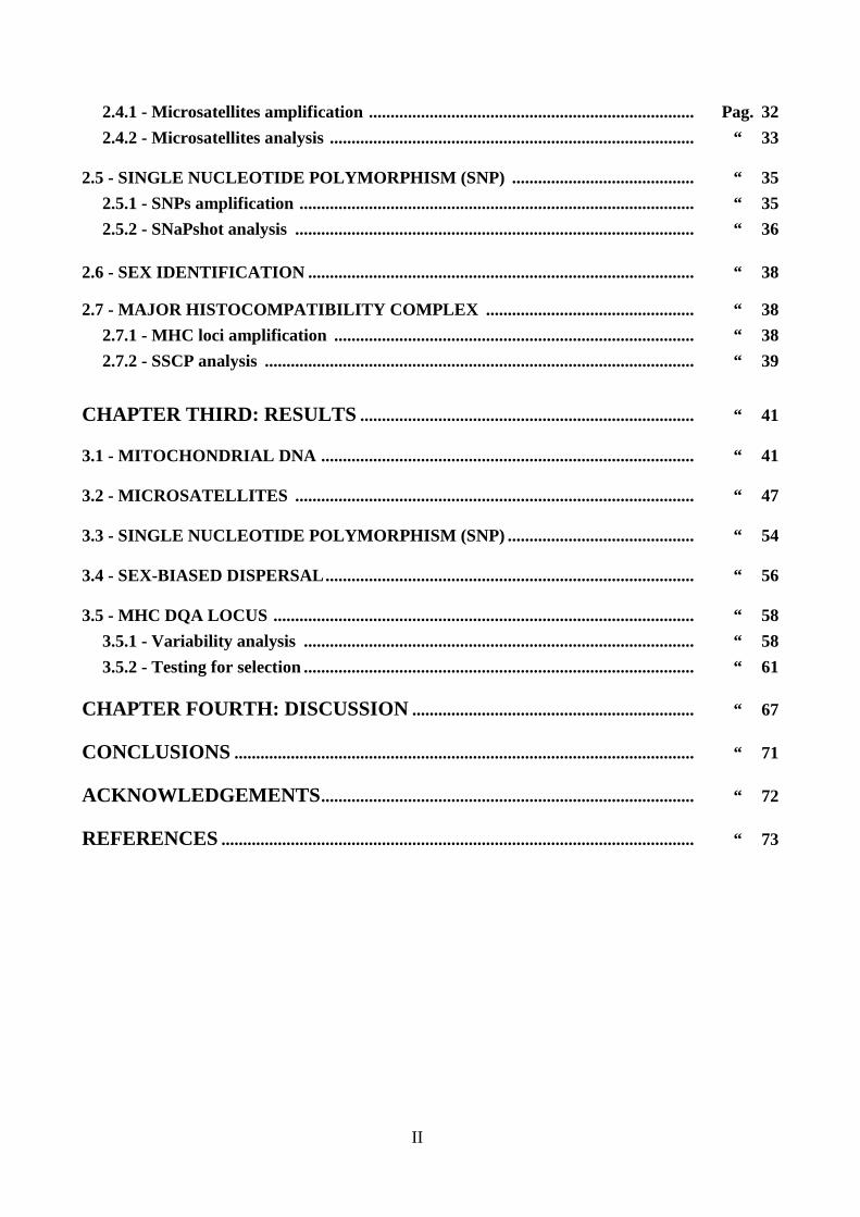
Australia, Barbados, Brazil, Canada, Chile, Falkland Islands, New Zealand (North and South

Island), Rèunion, the United Kingdom, Ireland and the United States (Flux and Angermann 1990).

Fig. 1. Geographical distribution of the European and northern African hares (Alves et al. 2008)

In Italy the species has been subject to massive repopulation in the last century, that have led to the

release of animals imported from abroad, or, in small part, raised in the peninsula. The populations

of the subspecies L. europaeus meridiei, originally distributed throughout north-central Italy, have

been replaced by introduced non-native hares and probably belonging to different subspecies.

- Lepus timidus varronis (Mountain hare). Lepus timidus has a widespread distribution and there are

currently 15 recognized subspecies; we consider the subspecies varronis, distributed in the Alps.

Historical hybridization events and genetic introgression with L. europaeus, recently documented in

Scandinavia, in the Iberian Peninsula and in Russia (Thulin et al. 1997, Melo-Ferreira et al. 2005,

Waltari and Cook 2005, Thulin et al. 2006, Melo-Ferreira et al. 2007), have made more

complicated the identification of the genetic structure of populations.

- Lepus capensis (Cape hare). The geographic range of Lepus capensis (in Arabia) includes isolated

populations scattered across the entire peninsula and extends east into India. It is also found on the

3

islands of Sardinia (ssp. Lepus capensis mediterraneus, but taxonomy is still uncertain

(Suchentrunk et al., 1998) and Cyprus. Geographic range in Africa is extensive and separated into

two distinct regions of non-forested areas (Boitani et al. 1999). The southern distribution includes

the following countries: South Africa, Lesotho, Swaziland, Namibia, Botswana, Zimbabwe,

southern portions of Angola, Mozambique, and Zambia (Boitani et al. 1999). The northern

distribution includes: Tanzania, Kenya, Uganda, Eritrea, Sudan, Egypt, Libya, Chad, Niger,

Tunisia, Algeria, Burkina Faso, Mali, Morocco, Western Sahara, Mauritania, and Senegal.

- Lepus granatensis (Iberian hare). The geographic range of Lepus granatensis includes Portugal

and nearly the entire Spain (Alves et al. 2003). It is absent from northern regions of Spain where L.

castroviejoi and europaeus exist (Alves et al. 2003). In most of the northern provinces (Navarra,

Asturias, Cantabria, Aragon, Catalunya, and Basque Country), L. europaeus and L. granatensis

exist in parapatry, the Iberian hare inhabits the southern region and the Brown hare can be found to

the north (Fernandez et al. 2004). L. granatensis is also located on the island of Mallorca of the

Balearic chain (Schneider 2001). It has been introduced in southern France and Corsica (Perpignan)

(Alves et al. 2003).

- Lepus castroviejoi (Broom hare). The distribution of L. castroviejoi is limited to the Cantabrian

Mountains in the northwest of Spain (Flux and Angermann 1990).

1.2 LEPUS CORSICANUS

1.2.1 Distribution

This research project wants to focus the attention especially on the Italian hare, as an important

endemic threatened species.

In this century, the distribution area of the species has been subjected to a substantial contraction

accompanied by a significant reduction in density of populations. The most important risk factors

have been identified in the fragmentation of the distribution area, isolation and low population

density, deterioration of the habitat, introduction of L. europaeus and over-hunting.

Lepus corsicanus may be considered a typical Italian endemism, because in Corsica the species was

introduced by humans: it is important to adopt as soon as possible measures for the conservation

and management.

4

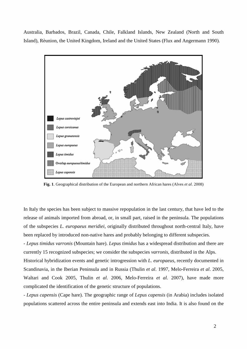
Currently, the distribution area of the Italian hare (Fig. 3) recognizes as the northern limit Monte

Amiata in the province of Grosseto, on the Tyrrhenian coast, and a small area near the National

Park of Abruzzo, in the province of L'Aquila, on the Adriatic coast. South of these areas, the taxon

is still present in all peninsular regions up to the province of Reggio Calabria, but with relict

populations, often isolated in protected or inaccessible

mountainous areas (Angelici, 2001).

On the contrary, in Sicily the species is relatively

widespread and is also observed in hunting areas far from

protected parks (for example, in the province of Enna,

where there aren’t protected areas). Despite the

identification of several tens of hares taken in recent years

in the territory where hunting is practiced, it was not

possible to confirm the presence of the Italian hare on the

Island of Elba, but only the European Hare (introduced for

Fig.2. Lepus corsicanus hunting purposes).

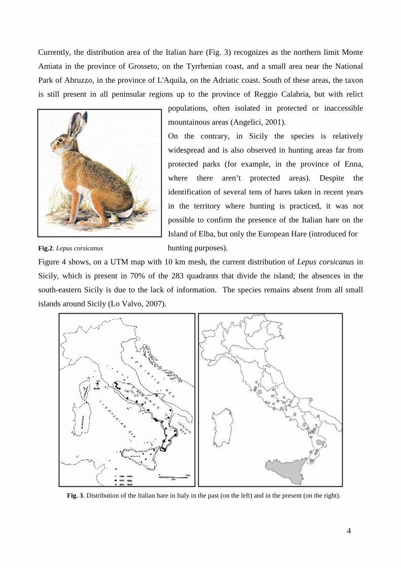
Figure 4 shows, on a UTM map with 10 km mesh, the current distribution of Lepus corsicanus in

Sicily, which is present in 70% of the 283 quadrants that divide the island; the absences in the

south-eastern Sicily is due to the lack of information. The species remains absent from all small

islands around Sicily (Lo Valvo, 2007).

Fig. 3. Distribution of the Italian hare in Italy in the past (on the left) and in the present (on the right).

5

Lepus corsicanus was introduced also in Corsica for hunting purpose, such as other sedentary game

species (Pietri, 2002), but currently there aren’t data about his distribution.

Fig. 4- Distribution of the Italian hare in Sicily.

1.2.2 Ecology

The Italian hare, as all Leporidae, shows a laterally compressed head, very long auricles, narrow

and elongated body usually kept bent, hind legs much longer and stronger than the front legs and

suitable for jumping, short tail. The fur is reddish-gray on the neck, shoulders, hips, grayish-black

on the back, white on the belly; long ears are black-tipped, black is also the top of the queue, and

eyes are big and brown. There isn’t sexual dimorphism.

Although similar in general to the European hare, the Italian hare has a relatively more slender

shape, in fact the head-body length, the back foot and the ears are proportionally longer, the average

weight of adults is about 800 g lower. The morphological characteristics of Lepus corsicanus may

imply a greater potential for thermal regulation and adaptation to the warm climate of the

Mediterranean regions, whereas it is known that the European hare is well adapted to open

environments with a continental climate.

The distinction between the two species in nature is not easy (Fig. 5), especially with the naked eye

and with animals moving. The coat colour of the Italian hare differs from that of the European hare

for tawny shades and for the clear transition between the reddish fur of the hip and the white belly.

6

Fig. 5. Differences in the coat colours between the European hare (on the left) and the Italian hare (on the right).

The ecological distribution of L. corsicanus confirms the adaptation to habitats characterized by a

Mediterranean climate (Tomaselli et al. 1973, Blondel and Aronson, 1999), although it is present

from sea level up to 1900 m above sea level in the Apennines and 2400 m above sea level on Mount

Etna. Favourite habitats seems to be those with alternating clearings, also grown, bushy areas and

broad-leaved woods; can also occupy areas with dense cover of Mediterranean vegetation,

including dune environments.

The species seems to have a sedentary behaviour with relatively small living spaces, attending after

sunset and for the entire night almost the same areas of pasture, in which close it sets up a day den.

In areas of sympatry with the European hare they were observed frequenting the same pastures.

The diet of L. corsicanus, studied in Sicily, varies seasonally as the available vegetation changes.

Monocotyledones, Cyperaceae and Juncaceae, are ingested year round, while Gramineae and

Labiatae are consumed during spring and summer, respectively (De Battisti et al. 2004).

Dicotyledones ingested year round by L. corsicanus are Leguminosae and Compositae (De Battisti

et al. 2004).

The sexual rest period is relatively short (about sixty-seventy days), between October and

December and for the other months the species doesn’t know practically sexual activity stops,

although it is more intense in summer season.

The species is polygamous and doesn’t form stable pairs, for the possession of the females, males

often fight with aggression and violence, hitting with the front legs, and rarely, trying to bite.

7

Mating takes place mostly at dusk or at night and the act of copulation is often preceded by a sort of

courtship; the female prepares a special haven where giving birth to leverets (the number of births

varies from one to five), which born after a gestation of about 41-42 days. A female can reproduce

an average of three or four times a year, but as the breeding season is more or less long in relation to

latitude, in regions with a warmer climate also occur five births.

Hares have therefore a relatively high reproductive potential and this condition is well suited to a

medium-sized herbivore that is subjected to a strong predation by several species of carnivores.

1.2.3 Threats

There are several conservation problems about the Italian hare that make this species threatened

with extinction. Listed below are the main ones:

- Fragmentation and isolation of the distribution areas. The genetic differences observed

between the haplotypes of specimens of L. corsicanus coming from central Italy, from south

Italy and Sicily (Pierpaoli et al. 1999) reflect an evolutionary history with the presence of

ancient subdivisions in the distribution area and consequently long periods of reproductive

isolation. Current distribution data show an important fragmentation that must necessarily

be attributed to anthropogenic causes, with very small populations isolated from each other,

within an environmental matrix became increasingly unfavourable. The erosion and

fragmentation of habitat due to human impacts are the major causes of isolation of the

populations.

- Interspecific competition. The protracted restocking with L. europaeus for hunting purposes

may have led to interspecific competition and the transmission of infectious diseases

(Guberti et al. 2000). Competition may occur mainly through the use of the same food

resources or breeding sites and shelters; this may affect the coexistence of the populations

concerned, in terms of changes in their size, distribution and structure.

- Genetic pollution. In the genus Lepus hybridization between species has already been

documented; in Sweden hybrids were observed between the native form L. timidus and

introduced L. europaeus (Thulin et al., 1997), and in Spain the three Iberian species of hares

(L. granatensis, L. castroviejoi, L. europaeus) harbour high frequencies of mitochondrial

DNA (mtDNA) from Lepus timidus, now extinct in the region (Melo Ferreira et al. 2005).

The absence of observation of intermediate phenotypes and the lack of introgression in

mitochondrial haplotypes of a species in the other leads to the belief that hybridization

8

between the European and the Italian hare is an unlikely event. More concretely, however, is

the risk of genetic pollution from translocated individuals (often from breeding station) in

areas where genetically and morphologically different populations live (Pierpaoli et al.,

1999; Riga et al., 2001).

- Hunting activity. Although the species is not included in the list of hunted species (L. n.

157/92) in the peninsula, the hunting exercise can be a real limiting factor: this is a complex

issue because of the coexistence in the same areas of L. corsicanus and L. europaeus, of the

difficulties in the recognition in nature, of the lack of a specific tradition in hares

management and of the knowledge basis for sustainable management. These difficulties are

reflected in a high impact on the residual populations of Italian hare and a practical

impossibility in the implementation of conservation strategies, different between the two

species.

- Poaching. In central and southern Italy and Sicily poaching on hares is traditional and

widespread, encouraged by the lack of supervisory activities.

- Habitat degradation. Reforestation in general represents a threat to the habitat of the hare.

Moreover, the intensification of cultivation occurred since the war has led to a series of very

heavy impact on the agricultural environment and adjacent natural areas, as well as for

wildlife directly. They are also various consequences about the use of chemicals products

(fertilizers and pesticides): direct consequences for acute and chronic toxicity, and indirect

consequences for trophic sources significant reduction.

1.2.4 Legal protection

In 2008 the species was classified as “vulnerable” according to the criteria of the IUCN Red List. In

2001 the National Action Plan for the Italian has been published, which contains guidelines for

conservation actions for the species.

The DPCM 07.05.2003 (Official Gazette. July 3, 2003, No. 152) introduced this species among

those hunted ("Only population living in Sicily" for the period October 15-November 30), of which

art. 18, paragraph 1, letter e) of National Law 157/1992.

9

1.3 - INTRODUCTION TO CONSERVATION GENETICS

1.3.1 Conservation genetics

Conservation genetics is the application of genetic techniques and analysis methods to preserve

species and dynamics entities capable of coping with environmental change. It deals with the

genetic factors that affect extinction risk and genetic management regimes required to minimise

these risks. It is a discipline that focuses on methods and techniques of population genetics, but also

considers the ecology of the species, ethology, physiology, molecular biology, the evolution and

demography. The role of population genetics is to investigate the origin, the maintenance, the

organization and the causes of genetic variation between natural populations. Natural populations

are treated as evolution units and their gene pools, resulting from the set of all alleles in various

loci, constitute the raw material of evolutionary changes.

There are several genetic issues in conservation genetics (Frankham et al. 2002):

- The deleterious effects of inbreeding on reproduction and survival (inbreeding depression).

- Loss of genetic diversity and ability to evolve in response to environmental change.

- Fragmentation of population and reduction in gene flow.

- Random processes (genetic drift) overriding natural selection as the main evolutionary

process.

- Accumulation and loss (purging) of deleterious mutations.

- Resolving taxonomic uncertainties.

- Defining management units within species.

- Use of molecular genetic analysis in forensics.

- Use of molecular genetic analysis to understand aspects of species biology (mating,

dispersal and migration patterns, reproduction systems) important for conservation.

1.3.2 DNA structure and function

Each individual, with the exception of identical twins, is genetically unique because he possesses a

unique patrimony of genetic information (DNA) organized in the chromosomes that are contained

in cell nucleus (nuclear DNA), and in mitochondria, organelles present in cell cytoplasm

(mitochondrial DNA or mtDNA).

10

Each DNA molecule takes the form of a double helix built by four nucleotides, the chemical

building blocks (Adenine-A, Thymine-T; Guanine-G and Cytosine-C). The structure of the double

helix consists of two ribbon-like entities that are entwined around each other and held together by

crossbars composed of two bases that have strong affinities for each other. The bases within each

chain are bound together by a pentose sugar and phosphate ion, while the opposing strands are held

together by weak hydrogen bonds that are relatively easy to break by heating. The linear order in

which these four nucleotides follow each other in the double helix of the DNA is called a nucleotide

sequence. This very simple structure is extremely stable and allows the DNA to act as a template for

protein synthesis and replication (Watson & Crick, 1953).

1.3.3 Mitochondrial DNA

Unlike most cells, whose functions are defined by the nuclear DNA, mitochondria have their own

DNA and are believed to have evolved separately.

Vertebrate mitochondrial DNA is a circular double helix made up of 15.000-20.000 nucleotides,

depending on the species (Hartl & Clark, 1993). It is replicated,

independently from cell and DNA nuclear replication, each time

the mitochondria divide. During the gametogenesis, the content of

cytoplasm and, therefore, the number of mitochondria contained

in the gametes significantly change. Mitochondria are provide

entirely by cell eggs, therefore during fertilization is the egg cell

of the mother that transmits all the mitochondria to the zygotes.

Hence mtDNA is haploid and does not recombine. The different

types of mtDNA that are originated from mutations and that are

present in populations are called “mitochondrial haplotypes”.

Fig. 6. Mitochondrial DNA structure.

1.3.4 Nuclear DNA

The genome of vertebrates and many other living organisms is largely made up of coding and non

coding DNA sequences.

Coding regions are organized in functional domains and are necessary to regulate the protein

11

synthesis consisting of a first phase of transcription of DNA into messenger RNA (mRNA)

followed by a phase of translation of the messenger RNA into protein.

Non coding, tandem repeated DNA exists in the genome of every species (repetitive DNA).

Tandem repetitive sequences, commonly known as “satellite DNAs” are classified into three major

groups:

- Satellite DNA: highly repetitive sequences with very long repeat lengths (up to 5.000.000

nucleotides), usually associated with centromeres.

- Minisatellite DNA: present in hundreds or thousands of loci in eukaryotic genomes. These

tandem repeats often contain a repeat of more than 10 nucleotides and are present in

multiple pairs that produce clusters of 500-30.000 nucleotides. Profiling of these

minisatellite loci is done using multi-locus probes-MLP or single-locus probes-SLP to

obtain DNA fingerprinting.

- Microsatellite DNA: present in many thousands of loci in eukaryotic genomes. They are

made up of very short repeats, from 2 to 8 nucleotides, repeated only few times that produce

clusters of a few dozen or few hundred nucleotides at every locus. Microsatellites are used

extensively in forensic genetics and are profiled through PCR

Hinf I Hinf I

restriction site minisatellite

repeat 1 R2 R3 R4

restriction site

DNA

Alleles R8R5

Genotype R5/R8

Alleles R4R2

Genotype R4/R2

Hinf I Hinf I

restriction site minisatellite

repeat 1 R2 R3 R4

restriction site

Hinf I Hinf I

restriction site minisatellite

repeat 1 R2 R3 R4

restriction site

DNA

Alleles R8R5

Genotype R5/R8

Alleles R4R2

Genotype R4/R2

Alleles R8R5

Genotype R5/R8

Alleles R4R2

Genotype R4/R2

Fig. 7. Minisatellite’s scheme.

1.3.5 Genetic mutations and polymorphisms

A genetic mutation is any change in the nucleotide sequence of a genome or, more generally, of

genetic material (DNA or RNA); mutations modify the genotype of an individual and can possibly

change their phenotype depending on its characteristics and interactions with the environment.

12

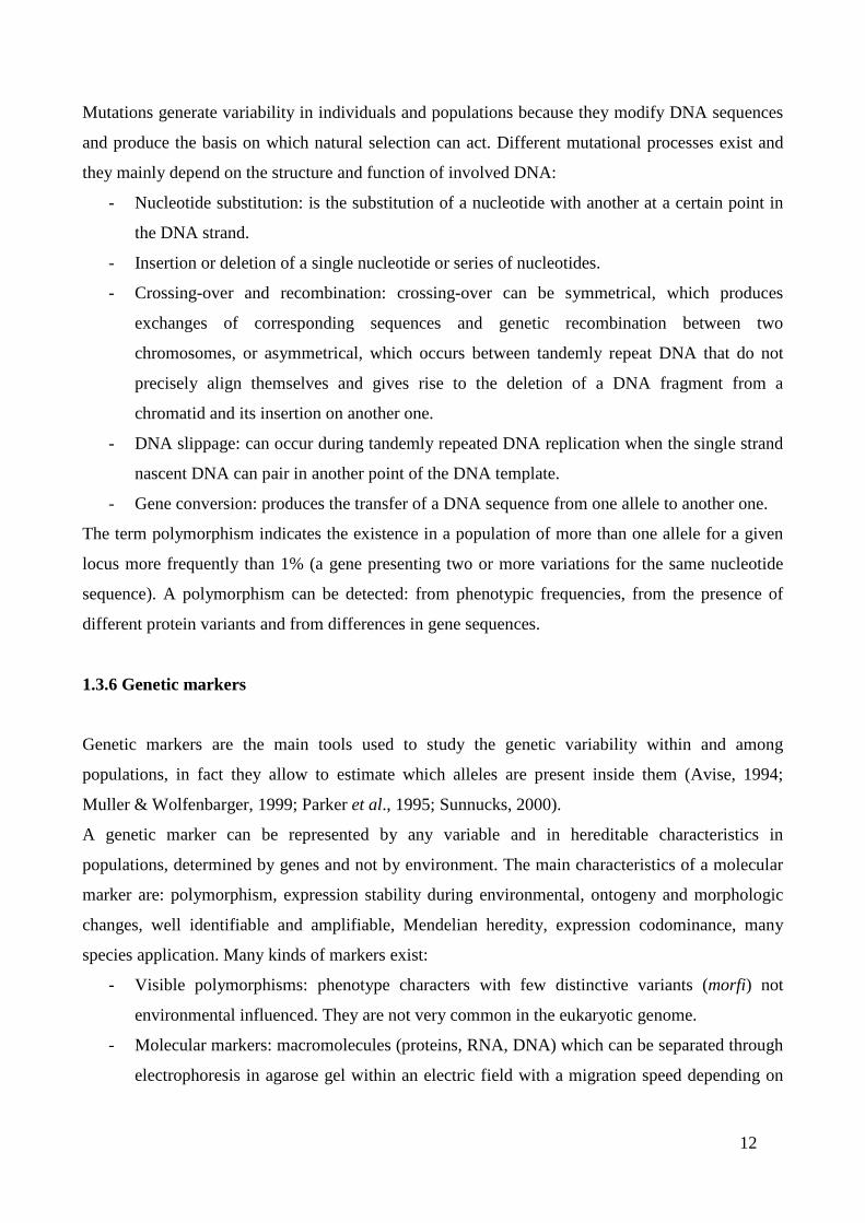
Mutations generate variability in individuals and populations because they modify DNA sequences

and produce the basis on which natural selection can act. Different mutational processes exist and

they mainly depend on the structure and function of involved DNA:

- Nucleotide substitution: is the substitution of a nucleotide with another at a certain point in

the DNA strand.

- Insertion or deletion of a single nucleotide or series of nucleotides.

- Crossing-over and recombination: crossing-over can be symmetrical, which produces

exchanges of corresponding sequences and genetic recombination between two

chromosomes, or asymmetrical, which occurs between tandemly repeat DNA that do not

precisely align themselves and gives rise to the deletion of a DNA fragment from a

chromatid and its insertion on another one.

- DNA slippage: can occur during tandemly repeated DNA replication when the single strand

nascent DNA can pair in another point of the DNA template.

- Gene conversion: produces the transfer of a DNA sequence from one allele to another one.

The term polymorphism indicates the existence in a population of more than one allele for a given

locus more frequently than 1% (a gene presenting two or more variations for the same nucleotide

sequence). A polymorphism can be detected: from phenotypic frequencies, from the presence of

different protein variants and from differences in gene sequences.

1.3.6 Genetic markers

Genetic markers are the main tools used to study the genetic variability within and among

populations, in fact they allow to estimate which alleles are present inside them (Avise, 1994;

Muller & Wolfenbarger, 1999; Parker et al., 1995; Sunnucks, 2000).

A genetic marker can be represented by any variable and in hereditable characteristics in

populations, determined by genes and not by environment. The main characteristics of a molecular

marker are: polymorphism, expression stability during environmental, ontogeny and morphologic

changes, well identifiable and amplifiable, Mendelian heredity, expression codominance, many

species application. Many kinds of markers exist:

- Visible polymorphisms: phenotype characters with few distinctive variants (morfi) not

environmental influenced. They are not very common in the eukaryotic genome.

- Molecular markers: macromolecules (proteins, RNA, DNA) which can be separated through

electrophoresis in agarose gel within an electric field with a migration speed depending on

13

their weigh and electric charge and visible under ultraviolet light. Alloenzymes belong to

these markers (Murphy et al., 1996).

- DNA markers: they allow to isolate genetic variability in DNA fragments with different

dimensions and weighs and to separate them within electrophoresis gel. Many kinds of

markers belong to them:

RFLP: restriction enzymes and restriction fragments length polymorphisms analysis

(Jefferies et al., 1985).

RAPD: random amplified polymorphic DNA (Williams, 1990).

AFLP : amplified fragment length polymorphisms (Vos et al., 1995).

VNTRS: variable number of tandem repeats. They are non-coding regions characterized

by tandemly repeated sequences. Each repeat can be made up from 10 to 64 nucleotides

(minisatellites) or from 2 to 9 nucleotides (microsatellites).

SNPs: Single Nucleotide Polymorphisms. They’re widespread in all genomes (coding

and non-coding regions), and they evolve in a manner well described by simple mutation

models, such as the infinite sites model (Vignal et al., 2002). These polymorphisms are

base substitutions, insertions, or deletions that occur at single positions in the genome

(Budowle, 2004). They are hypothesized to become the marker of choice in

evolutionary, ecological and conservation studies as genomic sequence information

accumulates. As a biallelici marker, SNPs are innately less variable than microsatellites

but they are the most prevalent form of genetic variation and hence there is a substantial

increase in the number of loci available (Brumfield et al. 2003).

1.4 STATISTICAL METHODS

The aim of population genetics is to describe the genetic composition of population and to

understand the causes of the evolutionary change. Genetic variability in population is described

through allele frequencies. Allele frequencies at each locus can vary across the generations due to

mutations, natural selection, migration or genetic drift.

The different combinations of alleles present at each locus determine individual genotypes, whose

frequency in populations can be calculated. In an ideal population, in which population forces are

not active, genotype frequencies remain constant from one generation to the next. Population

genetics is based on an abstract, ideal population model, supported by a series of assumptions.

14

The Hardy-Weinberg law defines the relationship that exists between allele and genotypes

frequencies at each locus in a population. In a locus with two alleles (a1 and a2), with frequencies p

and q, with p+q=1, the genotype frequencies are obtained from the proportion:

a1a1: 2a1a2:a2a2=p2:2pq:q2.

It is possible to estimate the genotype frequencies of a population in Hardy-Weinberg Equilibrium

(HWE) using the observed allele frequencies. If a population is not in HWE an estimate of genotype

frequencies, starting from the allele frequencies, may be wrong. Deviation from HWE may be

caused from non-random mating, gene flow, founder effect, bottleneck and random drift.

Even though many reasonable statistic approaches are available to analyse the genetic structure of

populations and to estimate the absolute and effective population sizes, most of them, used in this

study are based on F and Bayesian Statistics.

In population genetics, F-statistics (also known as fixation indices) describe the level of

heterozygosity in a population; more specifically the degree of a reduction in homozygosity when

compared to Hardy-Weinberg expectation. Such changes can be caused by the Wahlund effect (the

reduction of heterozygosity in a population caused by subpopulation structure), inbreeding, natural

selection or any combination of these.

The concept of F-statistics was developed during the 1920s by the American geneticist Sewall

Wright who was interested in inbreeding in cattle, but its applications deeply increased after the

1960s when the advent of molecular genetics allowed heterozygosity in populations to be reliably

measured.

F-statistics measure the correlation between genes drawn at different levels of a (hierarchically)

subdivided population. This correlation is influenced by several evolutionary forces, such as

mutation and migration, but it was originally designed to measure how far populations had gone in

the process of fixation owing to genetic drift.

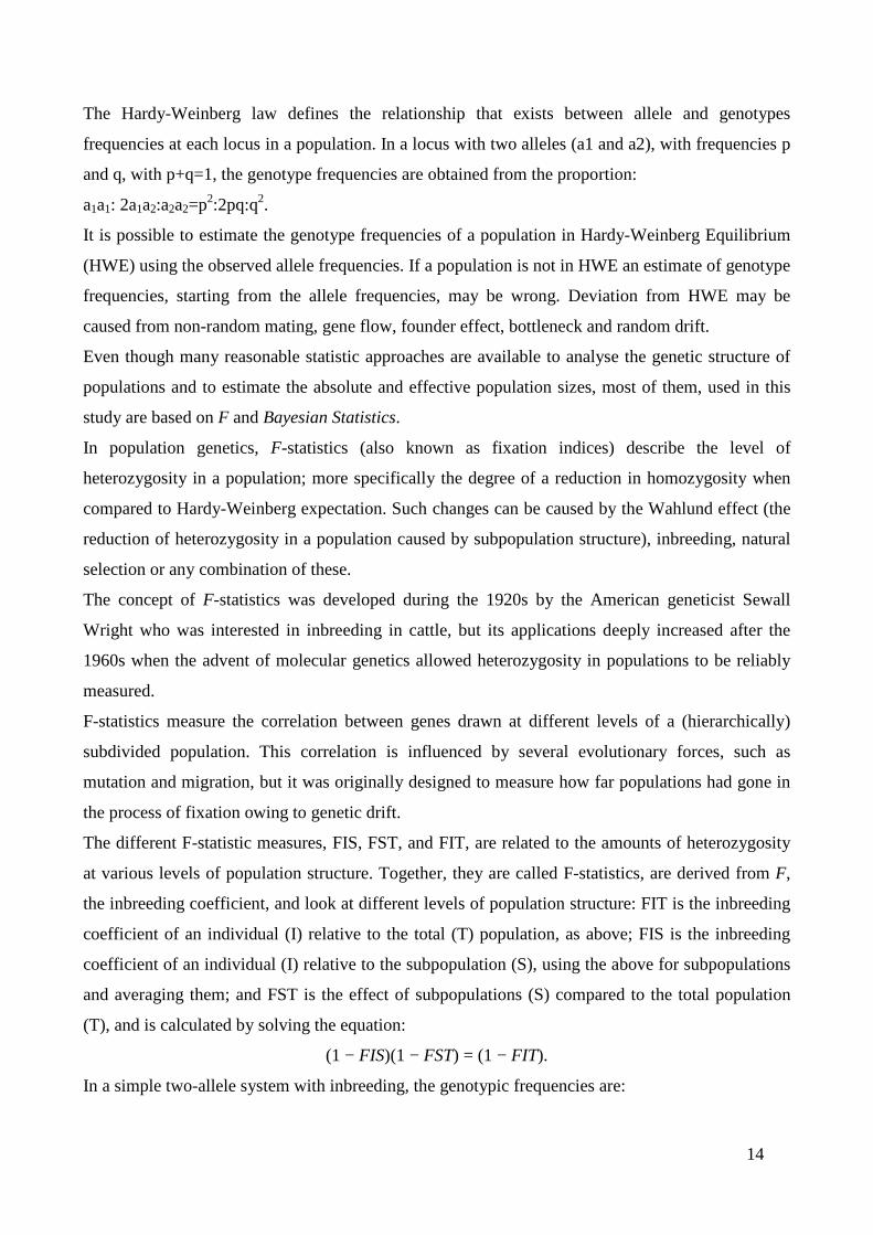
The different F-statistic measures, FIS, FST, and FIT, are related to the amounts of heterozygosity

at various levels of population structure. Together, they are called F-statistics, are derived from F,

the inbreeding coefficient, and look at different levels of population structure: FIT is the inbreeding

coefficient of an individual (I) relative to the total (T) population, as above; FIS is the inbreeding

coefficient of an individual (I) relative to the subpopulation (S), using the above for subpopulations

and averaging them; and FST is the effect of subpopulations (S) compared to the total population

(T), and is calculated by solving the equation:

(1 − FIS)(1 − FST) = (1 − FIT).

In a simple two-allele system with inbreeding, the genotypic frequencies are:

15

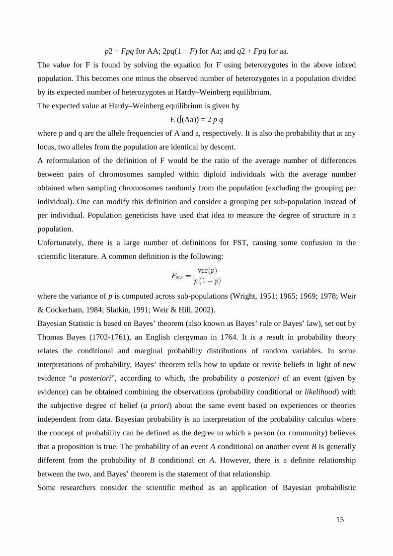
p2 + Fpq for AA; 2pq(1 − F) for Aa; and q2 + Fpq for aa.

The value for F is found by solving the equation for F using heterozygotes in the above inbred

population. This becomes one minus the observed number of heterozygotes in a population divided

by its expected number of heterozygotes at Hardy–Weinberg equilibrium.

The expected value at Hardy–Weinberg equilibrium is given by

E (∫(Aa)) = 2 p q

where p and q are the allele frequencies of A and a, respectively. It is also the probability that at any

locus, two alleles from the population are identical by descent.

A reformulation of the definition of F would be the ratio of the average number of differences

between pairs of chromosomes sampled within diploid individuals with the average number

obtained when sampling chromosomes randomly from the population (excluding the grouping per

individual). One can modify this definition and consider a grouping per sub-population instead of

per individual. Population geneticists have used that idea to measure the degree of structure in a

population.

Unfortunately, there is a large number of definitions for FST, causing some confusion in the

scientific literature. A common definition is the following:

where the variance of p is computed across sub-populations (Wright, 1951; 1965; 1969; 1978; Weir

& Cockerham, 1984; Slatkin, 1991; Weir & Hill, 2002).

Bayesian Statistic is based on Bayes’ theorem (also known as Bayes’ rule or Bayes’ law), set out by

Thomas Bayes (1702-1761), an English clergyman in 1764. It is a result in probability theory

relates the conditional and marginal probability distributions of random variables. In some

interpretations of probability, Bayes’ theorem tells how to update or revise beliefs in light of new

evidence “a posteriori”, according to which, the probability a posteriori of an event (given by

evidence) can be obtained combining the observations (probability conditional or likelihood) with

the subjective degree of belief (a priori) about the same event based on experiences or theories

independent from data. Bayesian probability is an interpretation of the probability calculus where

the concept of probability can be defined as the degree to which a person (or community) believes

that a proposition is true. The probability of an event A conditional on another event B is generally

different from the probability of B conditional on A. However, there is a definite relationship

between the two, and Bayes’ theorem is the statement of that relationship.

Some researchers consider the scientific method as an application of Bayesian probabilistic

16

inference because they claim Bayes’ Theorem is explicitly or implicitly used to update the strength

of prior scientific beliefs in the truth of hypotheses in the light of new information from observation

or experiment. This is said to be done by the use of Bayes’ Theorem to calculate a posterior

probability using that evidence and is justified by the Principle of Conditionalisation that P’(h) =

P(h/e), where P’(h) is the posterior probability of the hypothesis ‘h’ in the light of the evidence ‘e’,

but which principle is denied by some. Adjusting original beliefs could mean (coming closer to)

accepting or rejecting the original hypotheses.

Since the 1950s, Bayesian theory and Bayesian probability have been widely applied and it has

recently been shown that Bayes’ Rule and the Principle of Maximum Entropy (MaxEnt) are

completely compatible and can be seen as special cases of the Method of Maximum (relative)

Entropy (ME). This method reproduces every aspect of orthodox Bayesian inference methods. In

addition this new method opens the door to tackling problems that could not be addressed by either

the MaxEnt or orthodox Bayesian methods individually (Lindley, 1990; West & Harrison, 1989;

O’Hagan, 1994; Sivia, 1996; Pritchard et al., 2000; Tijms, 2004).

The main differences between F (or frequency) and Bayesian Statistics lie in the definition,

interpretations and in the effective calculus of probabilities (Press, 1972), in fact:

- F statistics assigns probabilities to random events according to their frequencies of occurrence or

to subsets of populations as proportions of the whole and allows to compare the test hypothesis to a

model/hypothesis (the “null” hypothesis). The probability p of an event H depends on the number of

times (n) the event occurs on the total number of tests (N). The probability p of H corresponds

therefore to its frequency:

pH = n(H)/N.

- Bayesian statistics assigns probabilities to propositions that are uncertain; conditions on the data

actually observed, and is therefore able to assign posterior probabilities to any number of

hypotheses directly. The requirement to assign probabilities to the parameters of models

representing each hypothesis is the cost of this more direct approach. The probability p is an

estimation of likelihood that that the event H occurs. We can have convictions (subjective) or

information (objective, even though not exactly quantifiable) that an event may more or less occur

frequently. Posterior probability of an event H corresponds on the probability that the event H

occurs given the evidence E:

Pr (H) = Pr (H/E).

17

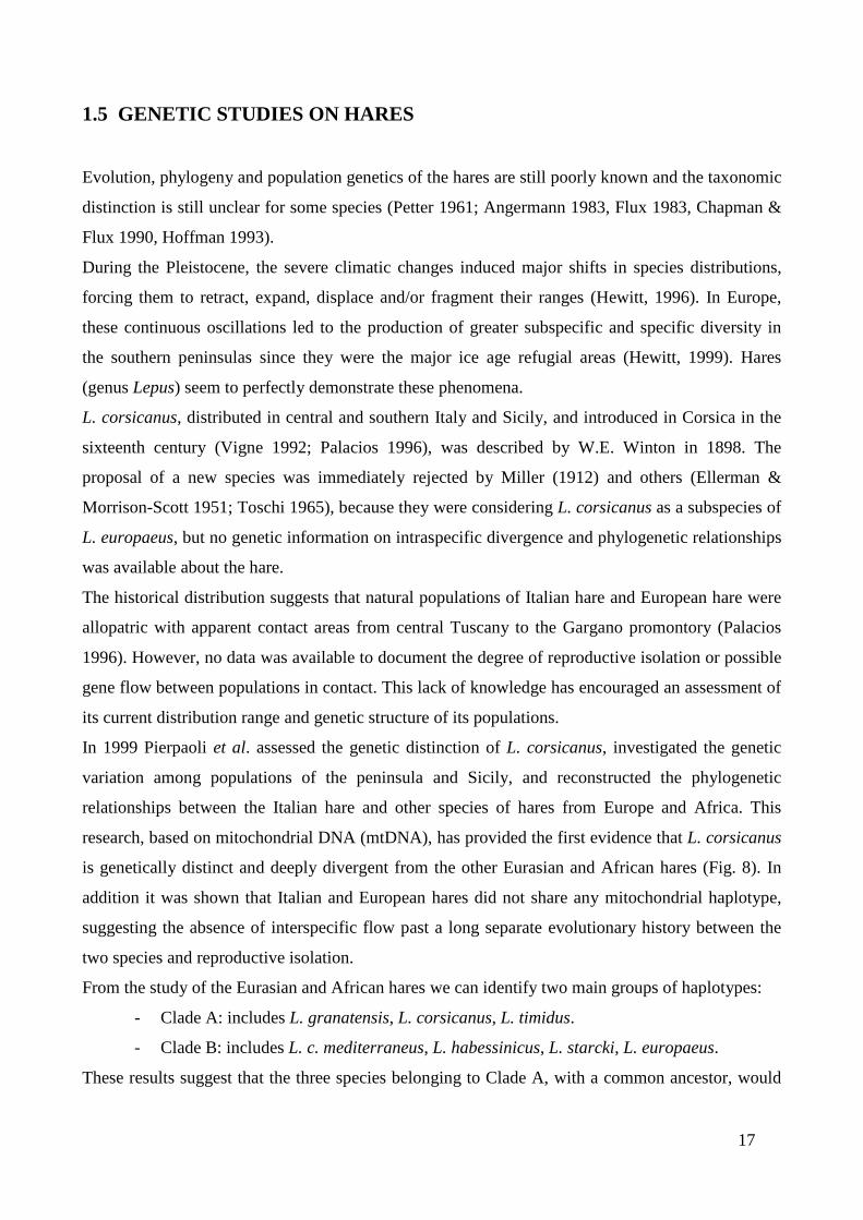
1.5 GENETIC STUDIES ON HARES

Evolution, phylogeny and population genetics of the hares are still poorly known and the taxonomic

distinction is still unclear for some species (Petter 1961; Angermann 1983, Flux 1983, Chapman &

Flux 1990, Hoffman 1993).

During the Pleistocene, the severe climatic changes induced major shifts in species distributions,

forcing them to retract, expand, displace and/or fragment their ranges (Hewitt, 1996). In Europe,

these continuous oscillations led to the production of greater subspecific and specific diversity in

the southern peninsulas since they were the major ice age refugial areas (Hewitt, 1999). Hares

(genus Lepus) seem to perfectly demonstrate these phenomena.

L. corsicanus, distributed in central and southern Italy and Sicily, and introduced in Corsica in the

sixteenth century (Vigne 1992; Palacios 1996), was described by W.E. Winton in 1898. The

proposal of a new species was immediately rejected by Miller (1912) and others (Ellerman &

Morrison-Scott 1951; Toschi 1965), because they were considering L. corsicanus as a subspecies of

L. europaeus, but no genetic information on intraspecific divergence and phylogenetic relationships

was available about the hare.

The historical distribution suggests that natural populations of Italian hare and European hare were

allopatric with apparent contact areas from central Tuscany to the Gargano promontory (Palacios

1996). However, no data was available to document the degree of reproductive isolation or possible

gene flow between populations in contact. This lack of knowledge has encouraged an assessment of

its current distribution range and genetic structure of its populations.

In 1999 Pierpaoli et al. assessed the genetic distinction of L. corsicanus, investigated the genetic

variation among populations of the peninsula and Sicily, and reconstructed the phylogenetic

relationships between the Italian hare and other species of hares from Europe and Africa. This

research, based on mitochondrial DNA (mtDNA), has provided the first evidence that L. corsicanus

is genetically distinct and deeply divergent from the other Eurasian and African hares (Fig. 8). In

addition it was shown that Italian and European hares did not share any mitochondrial haplotype,

suggesting the absence of interspecific flow past a long separate evolutionary history between the

two species and reproductive isolation.

From the study of the Eurasian and African hares we can identify two main groups of haplotypes:

- Clade A: includes L. granatensis, L. corsicanus, L. timidus.

- Clade B: includes L. c. mediterraneus, L. habessinicus, L. starcki, L. europaeus.

These results suggest that the three species belonging to Clade A, with a common ancestor, would

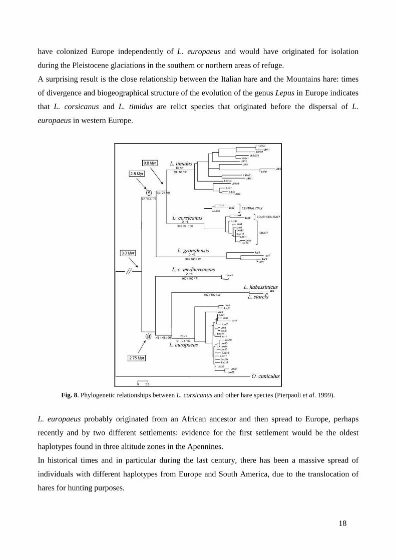
18

have colonized Europe independently of L. europaeus and would have originated for isolation

during the Pleistocene glaciations in the southern or northern areas of refuge.

A surprising result is the close relationship between the Italian hare and the Mountains hare: times

of divergence and biogeographical structure of the evolution of the genus Lepus in Europe indicates

that L. corsicanus and L. timidus are relict species that originated before the dispersal of L.

europaeus in western Europe.

Fig. 8. Phylogenetic relationships between L. corsicanus and other hare species (Pierpaoli et al. 1999).

L. europaeus probably originated from an African ancestor and then spread to Europe, perhaps

recently and by two different settlements: evidence for the first settlement would be the oldest

haplotypes found in three altitude zones in the Apennines.

In historical times and in particular during the last century, there has been a massive spread of

individuals with different haplotypes from Europe and South America, due to the translocation of

hares for hunting purposes.

19

For the L. corsicanus haplotype divergence time is estimated between 45,000 and 121,000 years

ago, suggesting the hypothesis of an ancient isolation in glacial refuge areas in central and southern

Italy; during this period it was possible the colonization of Sicily due to sea level drop (about 110

meters from the current as a consequence of the glacial period).

To confirm these results we can see that hares sampled in central Italy have unique haplotypes, not

found in hares sampled in southern Italy (Campania and Calabria) and Sicily. The separation of

Sicily, from the end of the last ice age, may explain the divergence between Sicilian hares and

peninsula’s hares (Pierpaoli et al., 1999).

L. castroviejoi and L. corsicanus have allopatric and restricted ranges: the first one lives in the

Cantabrian Mountains of the Iberian Peninsula and the second one in the Apennines from central

and southern Italy and in Sicily.

Analysis of partial sequences of mtDNA cytochrome b showed that L. corsicanus and L.

castroviejoi are closely related to L. timidus (2.2–2.7% of divergence) and, further, that the level of

differentiation between them is very low when compared with the levels among typical hare species

(circa 1.4% vs. 9% average between Lepus species; Alves et al., 2003).

Moreover the results based on three independent nuclear loci suggest that L. corsicanus and L.

castroviejoi might be conspecific and distinct from L. timidus. These findings emphasize once again

the fundamental role of the southern European peninsulas as deposits of biodiversity and natural

laboratories for the study of evolution and speciation (Alves et al. 2008). These two southern

european endemisms occupy highly specialized patches of scarce habitat and thus the establishment

of suitable conservation mechanisms is a major concern (e.g., Temple and Terry, 2007).

Fig. 9. Geographical distribution of Lepus

granatensis, L. europaeus, L. castroviejoi

in the Iberian Peninsula. The pie charts

show the frequencies of mtDNA of L.

timidus origin in Iberia (Melo-Ferreira et

al. 2009).

20

In some areas the alternation of species due to climatic fluctuations during glaciations set the

conditions for competition and eventually hybridization. Hares in the Iberian Peninsula appear to

illustrate this phenomenon: populations of the three species of hares present in the Iberian Peninsula

harbour high frequencies of mitochondrial DNA (mtDNA) from Lepus timidus, an arctic/boreal

species now extinct in the region (Fig. 9).

The hypothesis is that this massive introgression of mtDNA occurred during the competitive

replacement of the arctic species by the temperate ones as climate became warmer at the end of the

last glaciation (Melo-Ferreira et al. 2009).

1.6 AIMS

Present-day distribution of the Italian hare is extremely fragmented in central and southern Italy.

Populations survive at low density, mainly in protected areas and National Parks, where the species

has managed to escape overhunting and competition with introduced Brown hares.

Extensive human disturbance (overhunting and restocking) could have threatened, severely

restricted and eventually eradicated the Italian hare from most of its former historical range.

The knowledge of the genetic status of Italian hare populations and in particular the certainty of its

reproductive isolation from the European brown hare are indispensable for the design of adequate

management and conservation plans of this species in the country.

The main purposes of this conservation genetic study are:

- to investigate the extent of genetic variability among Italian hares collected in peninsular

Italy and Sicily;

- to detect any signs of hybridization (and thus of possible gene flow) between the species

L. corsicanus and L. europaeus in sympatric areas of Italy;

- to confirm the phylogenetic relationships between the Italian and the other European

species;

- to evaluate the use of new genetic markers (SNPs) which allow to identify with precision

the species of individual samples (e.g. in cases of genotyping of faecal samples collected

in non-invasive genetic programs), and of geographic populations.

- to investigate Major Histocompatibility Complex (MHC) variability at class II DQA

locus between the brown hare and the Italian hare.

21

For the development of this work various molecular genetic techniques have been used such as

DNA extraction from biological samples (using different extraction methods), DNA amplification

by PCR, genotyping and sequencing by special laboratory equipment.

22

CHAPTER SECOND: MATERIALS AND METHODS

2.1 SAMPLE COLLECTION

We analyzed nearly 700 samples belonging to six different species; sampling details are shown in

Table 1. Most of the samples were collected in Italian regions, but sampling also covered other

european and non-european countries between 1992 and 2009.

The distribution map in Fig. 10 shows sampling areas in the Italian peninsula, in Sicily, in Sardinia

and in Corsica.

SPECIES ORIGIN SAMPLES

L. corsicanus Italy-Corsica 154

L. capensis? Africa 12

L. cap. mediterraneus Sardinia 92

L. castroviejoi Spain 5

L. europeaus Italy-Hungary-Romania-Austria-Bulgaria-Greece-Uruguay 343

L. granatensis Spain 29

L. timidus Italy-Finland-Sweden-Ireland-Scotland 75

Tab. 1. List of species analysed, collecting areas, and number of samples for every species.

Fig. 10. Map of sampling areas in Italy and Corsica: red points represents samples belonging to L. corsicanus, green

points to L. europaeus, yellow points to L. c. mediterraneus and blue points to L. timidus.

23

The sample collection phase is fundamental to ensure a good success of the following genetic

analysis based on PCR techniques because analysis procedures and the quality of the results are

dependent on the quality of samples and possible contaminations. For these reasons it necessary to

collect and preserve biological samples in the best possible way.

We analysed invasive biological samples (tissues or blood) coming, for the most part, from

individuals killed during the hunting seasons. Tissue samples should be kept in sterile plastic tubes

airtight containing 90-100% ethanol (EtOH 100%) according to a report alcohol-sample 1 to 10,

this is because ethanol dehydrates the tissues by blocking the biochemical reactions subsequent to

cell death, which would lead to degradation of DNA. Blood samples are placed in a preservative

solution like Longmire Buffer respecting the proportions of 1 to 1 (for example 1 ml of solution

must be added to 1 ml of blood).

Samples can then be frozen at -20 ° C to -80 ° C in liquid nitrogen or, alternatively may be kept at

room temperature or refrigerated at all temperatures below room temperature (ethanol and buffer

make DNA stable).

2.2 MOLECULAR ANALYSES

2.2.1 DNA extraction

The extraction process is a crucial step because it must isolate DNA molecules which are present in

a sample producing available solutions of DNA without contaminants and must impede further

degradations during laboratory procedures. In this study both manual and automated extraction

methods to isolate available DNA from tissues and blood were used (for details see Box 1).

Negative controls (no biological material added to the extractions) were always used to check

possible contaminations during both extraction processes.

Manual extraction uses a guanidinium thiocyanate and diatomaceus earth (guanidinium-silica)

protocol (Gerloff et al., 1995). The used solutions are characterized by the presence of:

TRIS: it maintains a constant pH value that inhibits the activity of enzymes that degrade DNA;

EDTA : it acts as chelants of bivalent calcium and magnesium ions inhibiting the activity of DNase

that requires the presence of these ions;

GUS (Guanidinium Thiocyanate): it produces the chemical disintegration of protein structures.

24

Guanidinium-silica protocol (summary)

Preparation of the samples:

- a piece of tissue (50 mg) is cut and transferred into an “eppendorf” test tube of 1.5 ml containing 500 µl of GUS Lysis Buffer;

flamed sterilized scalpels and forceps are used.

- a small amount of blood is added to 800 µl of water into an “eppendorf” test tube of 1.5 ml to produce cell lysis and extract

hemoglobin, which would otherwise interfere with the extraction process. We centrifuge for 1 minute, eliminate the supernatant

and add 500 µl of GUS Lysis Buffer.

Digestion of the samples:

- in rotation at 56°C overnight.

Collecting DNA:

- centrifuge at room temperature for 10 minutes and collect the supernatant;

- add 500 µl of GUS Binding Solution and in rotation for 1 hour;

- centrifuge at room temperature for 1 minute and eliminate the supernatant.

DNA is now bound to micro-granules of pelleted silica at the bottom of the test tube. Each pellet is washed twice, each time with 500

µl of GUS Washing Solution and then centrifuged at room temperature for 1 minute. The supernatant is eliminated, each pellet is

washed again twice, each time with 500 µl of EtOH 70% and centrifuged at room temperature for 3 minutes. The pellet is dried in

open “eppendorf” in a thermostatic multiblock at 56 °C for 10 minute. The pellet is re-suspended in 300 µl of TE for 15 minutes at

56°C, transferred in a new “eppendorf” and preserved at -20°C.

QUIAGEN Stool and tissue extraction kit protocol (summary)

Manual phase:

Preparation of the samples:

- Preparation is the same written above in the Guanidinium-silica protocol; in this case we add to the sample 20 µl of Proteinase K

and 180 µl of ATL Lysis Buffer (previously warmed up at 57°C for 5 minutes); flamed sterilized scalpels and forceps are used.

Digestion of the samples:

- in rotation at 56°C for 30 minutes.

Collecting DNA:

- centrifuge at room temperature for 10 minutes and collect the supernatant;

- transfer the supernatant in a new “eppendorf” and centrifuge at room temperature for other 10 minutes;

- transfer the supernatant in a new appropriate QUIAGEN tube.

Automated phase:

- link the multiblock with QUIAGEN tubes to the robot’s platform containing a vacuum pump system to aspirate liquid solutions and

a serious of silica-gel filters to trap the DNAs.

- the mechanical hands add 410 µl of AL/E Lysis Buffer (previously warmed up at 57°C for 5 minutes) to each QUIAGEN tube

containing digested sample solutions and the software activates the pup system to isolate the DNA;

- the mechanical hands add 500 µl of AW1 Washing Solution and the software activates the vacuum for 10 minutes;

- the mechanical hands add 500 µl of AW2 Washing Solution and the software activates the vacuum for 10 minutes;

- the mechanical hands add 300 µl of AE Solution (elution solution) to each sample re-suspending the DNA linked to silica filters at

room temperature for 1 hour.

The solution with the DNA is transferred in a new “eppendorf” and preserved in freezer at - 20°C.

Box.1. DNA extraction protocols.

25

Automated extraction in an automated manner by the MULTIPROBE IIEX robot (Perkin Elmer) and

using the QUIAGEN Stool and tissue extraction kit (QUIAGEN). The robot consists of 2

mechanical hands controlled by an appropriate software which can be set up each time according to

the number of samples and to the extraction kind and conditions. This procedure consists of a first

manual phase and of a second automated one.

2.2.2 DNA amplification

DNA amplification is a necessary procedure to obtain sufficient DNA quantity for molecular

analysis. DNA sequences made up of a few dozen or thousands nucleotides and present in a single

copy in DNA samples can be amplified effectively up to 10 million times in a few hours using

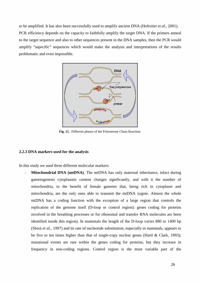
Polymerase chain reaction (PCR) (Mullis et al., 1986).

PCR occurs by reconstructing the chemical conditions necessary to obtain DNA synthesis in vitro.

First, it is necessary to identify the gene or DNA sequence that one wishes to amplify. The sequence

to be amplified is flanked on both side by sequences that must be at least partially known, in fact to

start off PCR it is necessary to chemical synthesise a pair of oligonucleotides (20-30 bp) “primers”

that are at least partially complementary to the flanking sequences and can bind to flanking regions

starting the duplication process of the target sequence. PCR occurs in a test tube that contains: the

DNA sample, the two primers, the DNA polymerase enzyme, a certain quantity of free nucleotides,

all this in a buffer solution that optimises DNA synthesis. Every test tube for PCR is placed in a

thermal cycler that carries out a prefixed thermal cycle made up of the following steps and repeats it

many times:

- denaturation of the DNA sample at temperatures up to 90-95°C;

- annealing of the primers to the flanking sequences: it occurs at temperatures which vary

from 40°C and 55°C, depending on the length of the primers and their base sequence;

- extension of the primers through the enzymatic action of a thermoresitant DNA polymerase

(Taq Polymerase) which catalyses the extension of the primers: it occurs at 72°C end ends in

the complete replication of both strands of the target sequence.

By the end of the first cycle, every form of the target sequence present in the sample is replicated

once, and the thermal cycle of the PCR is repeated a second time and then many other times (20-40)

producing an exponential replication of the target sequence because with every successive cycle the

synthesised DNA is doubled.

The advantage of using PCR is that the DNA does not have to be in large amounts or even purified

26

to be amplified. It has also been successfully used to amplify ancient DNA (Hofreiter et al., 2001).

PCR efficiency depends on the capacity to faithfully amplify the target DNA. If the primers anneal

to the target sequence and also to other sequences present in the DNA samples, then the PCR would

amplify “aspecific” sequences which would make the analysis and interpretations of the results

problematic and even impossible.

Fig. 11. Different phases of the Polymerase Chain Reaction.

2.2.3 DNA markers used for the analysis

In this study we used three different molecular markers:

- Mitochondrial DNA (mtDNA) . The mtDNA has only maternal inheritance, infact during

gametogenesis cytoplasmic content changes significantly, and with it the number of

mitochondria, to the benefit of female gametes that, being rich in cytoplasm and

mitochondria, are the only ones able to transmit the mtDNA zygote. Almost the whole

mtDNA has a coding function with the exception of a large region that controls the

replication of the genome itself (D-loop or control region): genes coding for proteins

involved in the breathing processes or for ribosomal and transfer RNA molecules are been

identified inside this region). In mammals the length of the D-loop varies 880 to 1400 bp

(Sbisà et al., 1997) and its rate of nucleotide substitution, especially in mammals, appears to

be five to ten times higher than that of single-copy nuclear genes (Hartl & Clark, 1993);

mutational events are rare within the genes coding for proteins, but they increase in

frequency in non-coding regions. Control region is the most variable part of the

27

mitochondrial genome and therefore the most interesting from the evolutionary point of

view: this allows to successfully use it as molecular marker in the genetic studies, at both

interspecific and intraspecific level. Most of the studies in which control region sequences

have been used have focused on intraspecific patterns of variability and phylogenetic

relationships of closely related species.

- Nuclear DNA: Microsatellites. They have quickly become of standard usage as genetic

markers in DNA fingerprinting. They are nuclear DNA sequences made up of a simple

motif of 2-8 nucleotides, that is repeated in tandem for a certain number of times with or

without interruptions due to the insertion of other nucleotides or other sequences.

Microsatellites have been identified in the genome of all organisms analysed up to now and

are distributed in a more or less random way in chromosomes (Mellersh & Ostrander, 1997).

They are not frequent in coding sequences of genes (exons), while they may be present in

introns. The composition of microsatellite sequences is variable. In fact the short DNA

segments can be made up of mono, di, tri or tetranucleotides (Mellersh & Ostrander, 1997;

Stallings et al., 1991; Tautz & Renz, 1984). Microsatellites present very high estimated

mutation rates (in vertebrates 10-4-10-5 mutations per locus for every generation) which

determine high levels of polymorphisms, in fact in a single locus more than 10 alleles can be

present which differ for the number of repeats and therefore for their molecular weight.

Moreover they find many applications in population genetics, in fact they represent

particularly useful tools to study population story and structure, their genetic variability and

allow to correctly assign the belonging species and to detect potential hybrids.

- Nuclear DNA: Single Nucleotidic Polymorphisms (SNPs). This marker consists just in a

single base change in a DNA sequence, with a usual alternative of two possible

nucleotides at a given position. For such a base position with sequence alternatives in

genomic DNA to be considered as an SNP, it is considered that the least frequent allele

should have a frequency of 1% or greater. Although in principle, at each position of a

sequence stretch, any of the four possible nucleotide bases can be present, SNPs are

usually biallelic in practice. One of the reasons for this, is the low frequency of single

nucleotide substitutions at the origin of SNPs, estimated to be between 1 x 10-9 and 5 x

10-9 per nucleotide and per year at neutral positions in mammals (Li et al., 1981,

Martinez-Arias et al., 2001). Therefore, the probability of two independent base changes

occurring at a single position is very low. Another reason is due to a bias in mutations,

leading to the prevalence of two SNP types. Mutation mechanisms result either in

28

transitions: purine-purine (A_G) or pyrimidine-pyrimidine (C_T) exchanges, or

transversions: purine-pyrimidine or pyrimidine-purine (A_C, A_T, G_C, G_T) exchanges.

Some authors consider one base pair indels (insertions or deletions) as SNPs, although

they certainly occur by a different mechanism. The very high density of SNPs in genomes

usually allows to analyse several of them at a single locus of a few hundred base pairs, so

that SNPs could represent a more reliable and faster genotyping method.

- Nuclear DNA: Major Histocompatibility Complex (MHC genes). In all vertebrates

studied to date, the MHC is a multigene family encoding receptors that act at the interface

between the immune system and infectious diseases (Koutsogannouli et al. 2009). The

primary role of the MHC is to bind fragments of antigenic proteins within cells and then

transport them to the surface of the cell membrane. There, the complex is recognized by T-

cell receptors (TCRs), which can initiate the cascade of immune responses (Janeway et al.

2005). The peptide-binding region (PBR) is responsible for antigen recognition, binding and

presentation, and a match between the PBR, antigenic peptide and TCR is required to

initiate an immune cascade (Brown et al. 1993; McFarland & Beeson 2002). Although

PBRs show a degree of specificity, a single MHC molecule can bind multiple peptides that

share common amino acids at specific anchor positions (Rammensee et al. 1995). Many of

the MHC genes that have been studied are highly polymorphic across a wide taxonomic

range in vertebrates. Polymorphism occurs mainly within the PBR, and the majority of

studies have revealed that the pattern of nucleotide substitutions in the PBR deviates from

neutral evolution expectation (Klein & Takahata 1990; Hill et al. 1991; Abbott et al. 2006).

It has been suggested that the pattern observed can be maintained by overdominance and ⁄ or

frequency dependence, reinforced by maternal–foetal incompatibility and mating preference

(Penn & Potts 1999; Piertney & Oliver 2006). Nevertheless, generally it is accepted that this

variability in the PBR is the key factor that enables the MHC proteins to bind a variety of

pathogens. In addition, different MHC alleles have been associated with other important

biological characteristics, such as susceptibility to infectious or autoimmune diseases,

individual odours, mating preferences, kin recognition, cooperation and outcome of

pregnancy (Hedrick 1994; Bernatchez & Landry 2003; Sommer 2005). Due to these

functions and characteristics, the MHC has been the focus of studies of population genetics

and evolutionary ecology that are concerned with the mechanisms and significance of

molecular adaptation in vertebrates (Potts & Wakeland 1993; Hedrick 1994; Bernatchez &

Landry 2003). Although different selective models have been proposed with regard to the

29

mechanisms that maintain MHC polymorphism in natural populations, this field still

remains an open question and a central goal in evolutionary biology (Potts & Slev 1995;

Edwards & Hedrick 1998).

2.3 MITOCHONDRIAL DNA (MTDNA)

2.3.1 MtDNA amplification

We sequenced nearly 450 nucleotides of the mtDNA D-loop using the forward primer Lepcyb2L

(5’-GAAACTGGCTCCAATAACCC-3’) and the reverse primer LepD2H (5’-

ATTTAAGAGGAACGTGTGGG-3’), (Pierpaoli et al. 1999).

Amplification was performed in 10 µl of volume, using 2 µl of DNA solution, 1 µl of PCR Buffer

10X (1,5 mM of MgCl2), 1 µl of BSA (Bovine Serum Albumin), 0,4 µl of deossinucleotides

(dATP, dCTP, dTTP, dGTP) 2,5mM, 0,15 µl of each primer 10 µM, 0,25 units of Taq and 5,25 µl

of PCR water, in a 9700 ABI Thermocycler (Applied Biosystems) using the following protocol:

94°C x 2’→( 94°C x 30’’→ 50°C x 30’’→ 72°C x 30’’) for 40 cycles →

72°C x 10’ → 4°C x 10’ → 15°C

Positive amplifications were detected on a 2% agarose gel and binding DNA with an UV

fluorescent reagent (Gel Red); PCR products were purified using 1 µl of a mixture of Exonuclease I

and Shrimp Alkaline Phosphatase that remove respectively unincorporated primers and dNTPs

using the following thermocycling program:

37°C x 30’→ 80°C x 15’ →4°C x 10’ →15°C

Sequencing PCR was carried out in 10 µl of volume, using 1 µl of PCR product, 0,7 µl of Big Dye

terminator Mix, 0,2 µl of the extension primer 10 µM, 8,1 µl of PCR water using the following

thermocycling program:

(96°C x 10’’ → 55°C x 5’’ → 60°C x 4’) for 25 cycles → 4°C x 10’ → 15°C

The main difference from the first PCR is that involves the use of one primer only to start DNA

replication. The Big Dye terminator Mix contains a reaction buffer, Taq polymerase,

deossinucleotides (dATP, dGTP, dCTP, dTTP) and dideossinucleotides (ddATP, ddGTP, ddCTP,

ddTTP); dideossinucleotides (ddNTPs) are modified bases which posses an OH in 3’-position and

avoid the formation of a phosphodiesteric link with another deossinucleotide, so that when a ddNTP

is randomly incorporated in the chain, it stops the extension of the same and thus generate

30

fragments terminating with one of the four ddNTPs.

PCR products are purified by precipitation using 3M Sodium acetate (Na acetate) and Etoh 70-

100%. One µl of each sequencing PCR product was resuspended in a denaturation solution

(Formamide) and analysed by electrophoresis on an AB Prism 3130 Genetic Analyser with a 36 cm

capillary array, POP4 polymer.

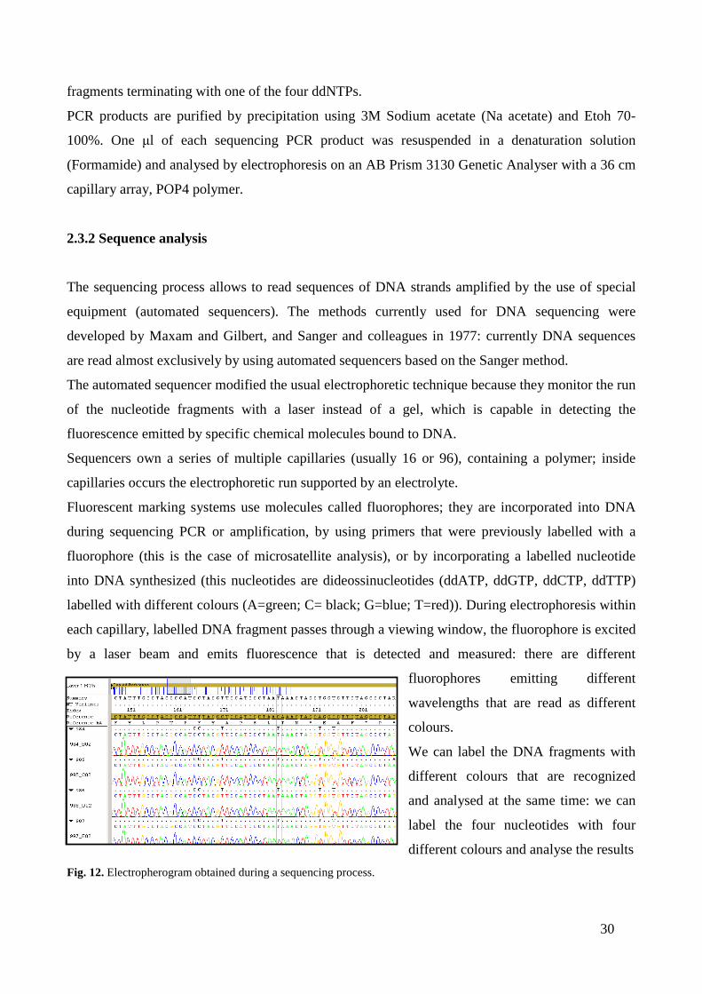
2.3.2 Sequence analysis

The sequencing process allows to read sequences of DNA strands amplified by the use of special

equipment (automated sequencers). The methods currently used for DNA sequencing were

developed by Maxam and Gilbert, and Sanger and colleagues in 1977: currently DNA sequences

are read almost exclusively by using automated sequencers based on the Sanger method.

The automated sequencer modified the usual electrophoretic technique because they monitor the run

of the nucleotide fragments with a laser instead of a gel, which is capable in detecting the

fluorescence emitted by specific chemical molecules bound to DNA.

Sequencers own a series of multiple capillaries (usually 16 or 96), containing a polymer; inside

capillaries occurs the electrophoretic run supported by an electrolyte.

Fluorescent marking systems use molecules called fluorophores; they are incorporated into DNA

during sequencing PCR or amplification, by using primers that were previously labelled with a

fluorophore (this is the case of microsatellite analysis), or by incorporating a labelled nucleotide

into DNA synthesized (this nucleotides are dideossinucleotides (ddATP, ddGTP, ddCTP, ddTTP)

labelled with different colours (A=green; C= black; G=blue; T=red)). During electrophoresis within

each capillary, labelled DNA fragment passes through a viewing window, the fluorophore is excited

by a laser beam and emits fluorescence that is detected and measured: there are different

fluorophores emitting different

wavelengths that are read as different

colours.

We can label the DNA fragments with

different colours that are recognized

and analysed at the same time: we can

label the four nucleotides with four

different colours and analyse the results

Fig. 12. Electropherogram obtained during a sequencing process.

31

of a sequencing reaction in a single capillary. During electrophoresis the computer connected to the

sequencer builds one or more image files, to track the performance of real-time analysis; results of

sequence analysis are saved in shape of electropherograms.

When a fluorophore is excited by the laser produces a light emission recorded as peak: the peak

height indicates the intensity of the emission and the colour indicates the colour of the fluorophore.

Because each colour is uniquely associated with a specific termination reaction (i.e. one of the four

nucleotides), the coloured peaks sequence of the electropherogram corresponds exactly to the DNA

sequence (Fig. 12).

Softwares mainly used to process sequencing data are:

- SeqScape v. 2.5 (Applied Biosystems 2001), an application especially designed for the

processing of genetic which makes it possible to automatically align sequences with a

sequence reference (appropriately chosen from those obtained from the sequencer or

contained in the database) and it also allows to view electropherograms to correct any

ambiguous nucleotides.

- BioEdit (Hall, 1999) allows to align sequences when they present gaps, sequences can also

be edited and may be cut in order to take all the same length.

- Dnasp v. 5 (Giulio Rosaz et al. 2003) is an interactive computer program for the analysis of

DNA polymorphism from nucleotide sequence data.

- Mega 5 (Tamura et al. 2011) allows to calculate a distance matrix between different

sequences on the basis of a comparison in pairs (i.e. counting the number of mutations

existing between them and comparing it, every time, with the number of total nucleotides)

and allows to build phylogenetic trees based on different statistical methods; it is also

particularly useful for identifying various types of mutations found by differentiating

transitions, transversions or indel (deletions and insertions).

- Network 4.5.1.6. (Fluxus Technology, 2004-2010) is used to reconstruct phylogenetic

networks and trees, infer ancestral types and potential types, evolutionary branchings and

variants, and to estimate datings.

32

2.4 MICROSATELLITES

2.4.1 Microsatellites amplification

In this work we analysed 13 microsatellites loci (Tab. 2); 12 of them were amplified using

QIAGEN Multiplex PCR Kit in four multiplex PCR in 7 µl of volume, using 2 µl of DNA solution,

3,5 µl of Qiagen Master Mix, 0,7 µl of Q-solution, 0,14 µl of each primer used in the multiplex

PCR, 0,38 µl of RNase-free water.

Cycling conditions were optimized for each multiplex, starting from the following general PCR

program:

95°C x 15’→ (94°C x 30’’→Ta°C (57/60°C) x 90’’→72°C x 60'') for 40 cycles →

60°C x 30’ → 4°C x 10’ → 15°C

Only locus SOL30, because of his large allele range, was amplified separately with a simplex PCR

in 10 µl of volume, using 2 µl of DNA solution, 1 µl of PCR Buffer 10X (1,5 mM of MgCl2), 1 µl

of BSA (Bovine Serum Albumin), 0,4 µl of deossinucleotides (dATP, dCTP, dTTP, dGTP) 2,5mM,

0,15 µl of each primer 10 µM, 0,25 units of Taq, 5,25 µl of PCR water, with the following general

PCR program:

94°C x 2’→( 94°C x 30’’→ 60°C x 30’’→ 72°C x 30’’) for 40 cycles →

72°C x 10’ → 4°C x 10’ → 15°C

Tab.2. List of microsatellites loci used for the analysis.

Locus Multiplex Size Dye Reference

SAT12 102-134 6-FAM Mougel et al., Animal Genetics, 1997.

LSA1 161-175 HEX Kryger et al., Molecular Ecology, 2002.

SOL33

1

199-226 6-FAM Surridge et al., Animal Genetics, 1997.

OCLS1B 142-180 HEX Hamill et al., Heredity, 2006.

LSA2 234-251 6-FAM Kryger et al., Molecular Ecology, 2002.

D7UTRI

2

110-168 6-FAM Hamill et al., Heredity, 2006.

LSA8 179-193 6-FAM Kryger et al., Molecular Ecology, 2002.

OCELAMB 106-130 HEX Hamill et al., Heredity, 2006.

LSA3

3

197-213 HEX Kryger et al., Molecular Ecology, 2002.

LSA4 100-110 6-FAM Kryger et al., Molecular Ecology, 2002.

LSA5 222-273 HEX Kryger et al., Molecular Ecology, 2002.

LSA6

4

164-173 6-FAM Kryger et al., Molecular Ecology, 2002.

SOL30 simplex 149-236 HEX Hamill et al., Heredity, 2006.

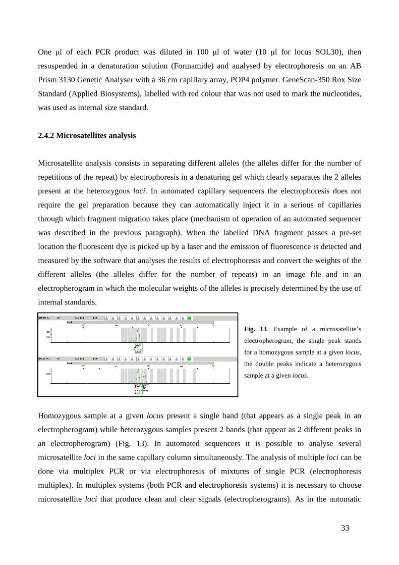
33

One µl of each PCR product was diluted in 100 µl of water (10 µl for locus SOL30), then

resuspended in a denaturation solution (Formamide) and analysed by electrophoresis on an AB

Prism 3130 Genetic Analyser with a 36 cm capillary array, POP4 polymer. GeneScan-350 Rox Size

Standard (Applied Biosystems), labelled with red colour that was not used to mark the nucleotides,

was used as internal size standard.

2.4.2 Microsatellites analysis

Microsatellite analysis consists in separating different alleles (the alleles differ for the number of

repetitions of the repeat) by electrophoresis in a denaturing gel which clearly separates the 2 alleles

present at the heterozygous loci. In automated capillary sequencers the electrophoresis does not

require the gel preparation because they can automatically inject it in a serious of capillaries

through which fragment migration takes place (mechanism of operation of an automated sequencer

was described in the previous paragraph). When the labelled DNA fragment passes a pre-set

location the fluorescent dye is picked up by a laser and the emission of fluorescence is detected and

measured by the software that analyses the results of electrophoresis and convert the weights of the

different alleles (the alleles differ for the number of repeats) in an image file and in an

electropherogram in which the molecular weights of the alleles is precisely determined by the use of

internal standards.

Fig. 13. Example of a microsatellite’s

electropherogram, the single peak stands

for a homozygous sample at a given locus,

the double peaks indicate a heterozygous

sample at a given locus.

Homozygous sample at a given locus present a single band (that appears as a single peak in an

electropherogram) while heterozygous samples present 2 bands (that appear as 2 different peaks in

an electropherogram) (Fig. 13). In automated sequencers it is possible to analyse several

microsatellite loci in the same capillary column simultaneously. The analysis of multiple loci can be

done via multiplex PCR or via electrophoresis of mixtures of single PCR (electrophoresis

multiplex). In multiplex systems (both PCR and electrophoresis systems) it is necessary to choose

microsatellite loci that produce clean and clear signals (electropherograms). As in the automatic

34

analysis of microsatellite one of the two PCR primers is labelled with a fluorescent dye, in

multiplex systems it is necessary to label primers at different loci with different colours. Three

colours (yellow, green and blue) are currently used to label the primers while a fourth colour (red) is

used to label the standard molecular weight.

Microsatellite whose alleles have different molecular weights can be combined in multiplex systems

and PCR products are separated in different areas of the gel or capillary and the identification of

alleles is facilitated by reading the coloured signals that do not overlap.

Softwares mainly used to process microsatellites data are:

- GeneMapper v 3.0 (Applied Biosystems ABI), a software used to manually or automatically

correct the results of the automated analysis. When the electrophoresis ends every allele may

be made up of a single band (that appear as a single peak in an electropherogram) or of a

main band plus a serious of secondary bands that represent aspecific amplification products.

After defining the variation range of molecular weight and of the main peak of the

electropherogram as well as the colour of the locus, the software allows to identify the signal

produced by the main band and assign the respective molecular weight. The program uses

an algorithm to filter that information which ignores the secondary signals and assigns the

correct molecular weight to the principle signal of the allele. The final result can be

visualized as a correct electropherogram, and the data, that contains the values of the

molecular weight assigned to each allele, can be exported to database Microsoft Excel-type

format, or to input formats of various data elaboration software.

- GenAlex v. 6.0 (Peakall & Smouse, 2005; 2006) is a software provided as an Excel add-in,

with a compiled module and an associated menu, particularly useful to study population

genetics and produce output files which can be directly used in other elaboration software. It

can be used to estimate allele frequency by locus and population, observed (HO) and

expected unbiased (HE) heterozygosities, mean number of alleles per locus (NA), number of

private alleles (NP) per population (i.e. the number of alleles unique to a single population

in the data set), to compute the HWE and Chi-square testing procedures, to perform genetic

distance and assignment tests (through Principal Coordinate Analysis PCA) and several

other parameters.

- Structure v. 2.1 (Pritchard et al. 2000); it is an important software that perform population

assignment and hybrids detection using a Bayesian clustering procedure. The program

Structure implements a model-based clustering method which uses multilocus genotype

data, consisting of unlinked markers, to infer population structure and to assign individuals

35

to populations.

- Genetix v. 4.2 (Belkhir et al. 2001) allows to simplify the graphic visualization of Structure

and GenAlex results; it can describe in three dimensions all the variability analysed in

GenAlex by Principal Coordinate Analysis and the different Structure clusterings.

2.5 SINGLE NUCLEOTIDE POLYMORPHISM (SNP)

2.5.1 SNPs amplification

We checked 13 SNPs loci found in four nuclear coding genes, but only 9 of these were variable (see

Tab. 3, Melo-Ferreira et al. 2009) and were used for the analysis of 150 samples belonging to Lepus

corsicanus (88 samples collected in central-southern Italy, 62 from Sicily) and 15 samples

belonging to Lepus europaeus.

GENE SNPs SIZE REFERENCE

SPTBN1-7Bf 40 Melo-Ferreira et al., Molecular Ecology 2009. SPTBN1

(Spectrin Beta non-erythrocytic 1) SPTBN1-7Cr 48 Melo-Ferreira et al., Molecular Ecology 2009.

UCP2-10Cf 44 Melo-Ferreira et al., Molecular Ecology 2009.

UCP2-10Df 60 Melo-Ferreira et al., Molecular Ecology 2009. UCP2

(Uncoupling Protein 2) UCP2-10Br 76 Melo-Ferreira et al., Molecular Ecology 2009.

CA2-2Ar 52 Melo-Ferreira et al., Molecular Ecology 2009. CA2

(Carbonic Anhydrase 2) CA2-2Cr 80 Melo-Ferreira et al., Molecular Ecology 2009.

HPX-4Br 58 Melo-Ferreira et al., Molecular Ecology 2009. HPX

(Hemopexin) HPX-4Af 84 Melo-Ferreira et al., Molecular Ecology 2009.

Tab.3. List of SNPs belonging to four nuclear genes used for the analysis.

Sequence containing SNPs were PCR-amplified separately for every gene in 8 µl of volume, using

2 µl of DNA solution, 0,8 µl of PCR Buffer 10X (1,5 mM of MgCl2), 0,8 µl of BSA (Bovine Serum

Albumin), 0,32 µl of deossinucleotides (dATP, dCTP, dTTP, dGTP) 2,5 mM, 0,12 µl of each

primer 10 µM, 0,25 units of Taq and 3,8 µl of PCR water.

In this case we use a Touchdown PCR method which allows to avoid amplification of nonspecific

sequences; the earliest steps of a touchdown PCR cycle have high annealing temperatures, then the

annealing temperature is decreased in increments for every subsequent set of cycles (in this case

temperature (starting from 60°C or 55°C depending on primer) decreases every cycle of 0,5°C for a

total of 10 cycles).

36

Cycling conditions were optimized for each primer pair (annealing temperature changes from 60°C

to 55°C depending on primer), and this is the general PCR program:

94°C x 2’→( 94°C x 30’’→ Ta°C (Touchdown PCR) x 30’’→ 72°C x 30’’) for 10 cycles →

( 94°C x 30’’→ Ta°C x 30’’→ 72°C x 30’’) for 40 cycles→

72°C x 10’ → 4°C x 10’ → 15°C

PCR products were purified using 1 µl of a mixture of Exonuclease I (EXO) and Shrimp Alkaline

Phosphatase (SAP) that remove respectively unincorporated primers and dNTPs using the following

thermocycling program:

37°C x 30’→ 80°C x 15’ →4°C x 10’ →15°C

The SNaPshot extension reaction (Minisequencing Multiplex PCR) were carried out in 10 µl of

volume, using 1 µl of PCR product for every SNPs locus analysed, 1 µl of SNaPshot Reaction Mix,

0,2 µl of the extension primer 10 µM for every SNPs locus, and a variable quantity of PCR water

using the following thermocycling program:

(96°C x 10’’→ 55°C/50°C x 5’’→60°C x 30’’) for 25 cycles →4°C x 10’ →15°C

SNaPshot Reaction Mix contains a reaction buffer, the enzyme Taq polymerase and the four

dideossinucleotides (ddATP, ddGTP, ddCTP, ddTTP) labelled with different colours: A=green; C=

black; G=blue; T=red. Dideossinucleotides are modified bases which posses an OH in 3’-position

and avoid the formation of a phosphodiesteric link with another deossinucleotide so that the

incorporation of one of them stop the extension generating fragments consisting of the primer and

the SNP at that locus.

PCR products were purified using 1 µl of Shrimp Alkaline Phosphatase (SAP) that removes

unincorporated dNTPs, using the thermocycling program written above for EXO/SAP.

One µl of each purified minisequencing PCR product was resuspended in a denaturation solution

(Formamide) and analysed by electrophoresis on an AB Prism 3130 Genetic Analyser with a 36 cm

capillary array, POP4 polymer. GeneScan-120 Liz Size Standard (Applied Biosystems), labelled

with orange colour that was not used to mark the nucleotides, was used as internal size standard.

2.5.2 SNaPshot analysis

SNaPshotTM (Applied Biosystems) is a solution-based assay that uses the single nucleotide primer

extension assay (Syvanen et al., 1990; Syvanen, 1999; Budowle et al., 2004). The method is based

on the use of three primers for the analysis of each SNP: an external forward, an external reverse

and an internal primer consisting of a few nucleotides until the one which precedes the mutation.

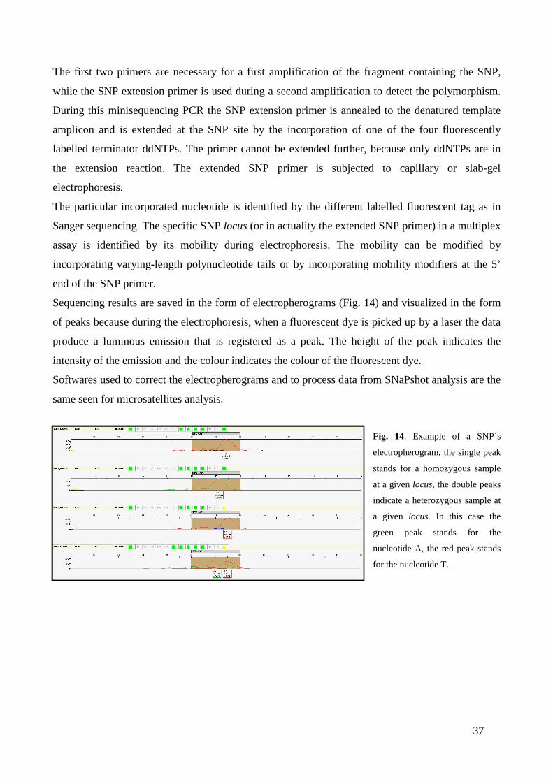
37

The first two primers are necessary for a first amplification of the fragment containing the SNP,

while the SNP extension primer is used during a second amplification to detect the polymorphism.

During this minisequencing PCR the SNP extension primer is annealed to the denatured template

amplicon and is extended at the SNP site by the incorporation of one of the four fluorescently

labelled terminator ddNTPs. The primer cannot be extended further, because only ddNTPs are in

the extension reaction. The extended SNP primer is subjected to capillary or slab-gel

electrophoresis.

The particular incorporated nucleotide is identified by the different labelled fluorescent tag as in

Sanger sequencing. The specific SNP locus (or in actuality the extended SNP primer) in a multiplex

assay is identified by its mobility during electrophoresis. The mobility can be modified by

incorporating varying-length polynucleotide tails or by incorporating mobility modifiers at the 5’

end of the SNP primer.

Sequencing results are saved in the form of electropherograms (Fig. 14) and visualized in the form

of peaks because during the electrophoresis, when a fluorescent dye is picked up by a laser the data

produce a luminous emission that is registered as a peak. The height of the peak indicates the

intensity of the emission and the colour indicates the colour of the fluorescent dye.

Softwares used to correct the electropherograms and to process data from SNaPshot analysis are the

same seen for microsatellites analysis.

Fig. 14. Example of a SNP’s

electropherogram, the single peak

stands for a homozygous sample

at a given locus, the double peaks

indicate a heterozygous sample at

a given locus. In this case the

green peak stands for the

nucleotide A, the red peak stands

for the nucleotide T.

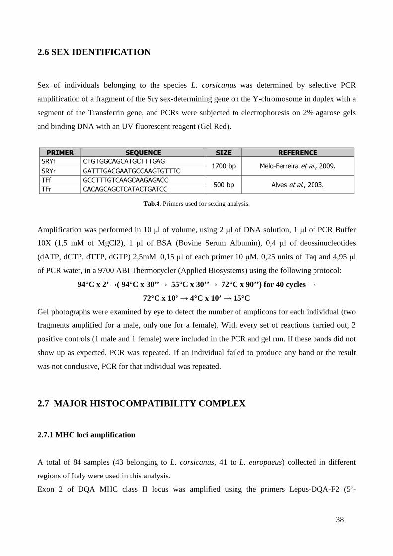
38

2.6 SEX IDENTIFICATION

Sex of individuals belonging to the species L. corsicanus was determined by selective PCR

amplification of a fragment of the Sry sex-determining gene on the Y-chromosome in duplex with a

segment of the Transferrin gene, and PCRs were subjected to electrophoresis on 2% agarose gels

and binding DNA with an UV fluorescent reagent (Gel Red).

Tab.4. Primers used for sexing analysis.

Amplification was performed in 10 µl of volume, using 2 µl of DNA solution, 1 µl of PCR Buffer

10X (1,5 mM of MgCl2), 1 µl of BSA (Bovine Serum Albumin), 0,4 µl of deossinucleotides

(dATP, dCTP, dTTP, dGTP) 2,5mM, 0,15 µl of each primer 10 µM, 0,25 units of Taq and 4,95 µl

of PCR water, in a 9700 ABI Thermocycler (Applied Biosystems) using the following protocol:

94°C x 2’→( 94°C x 30’’→ 55°C x 30’’→ 72°C x 90’’) for 40 cycles →

72°C x 10’ → 4°C x 10’ → 15°C

Gel photographs were examined by eye to detect the number of amplicons for each individual (two

fragments amplified for a male, only one for a female). With every set of reactions carried out, 2

positive controls (1 male and 1 female) were included in the PCR and gel run. If these bands did not

show up as expected, PCR was repeated. If an individual failed to produce any band or the result

was not conclusive, PCR for that individual was repeated.

2.7 MAJOR HISTOCOMPATIBILITY COMPLEX

2.7.1 MHC loci amplification

A total of 84 samples (43 belonging to L. corsicanus, 41 to L. europaeus) collected in different

regions of Italy were used in this analysis.

Exon 2 of DQA MHC class II locus was amplified using the primers Lepus-DQA-F2 (5’-

PRIMER SEQUENCE SIZE REFERENCE

SRYf CTGTGGCAGCATGCTTTGAG

SRYr GATTTGACGAATGCCAAGTGTTTC 1700 bp Melo-Ferreira et al., 2009.

TFf GCCTTTGTCAAGCAAGAGACC

TFr CACAGCAGCTCATACTGATCC 500 bp Alves et al., 2003.

39

CTTTCACTCATCAGCTGACC-3’) and Lepus-DQA-R1 (5’-ACAGCAGCAGTAGAGTTGGA-

3’), (de Bellocq et al. 2009): forward primer was labelled with 6'FAM dye and reverse primer was

labelled with NED dye.

PCR was carried out in 12,5 µl of volume, using 1 µl of DNA solution, 2,5 µl of Phusion HF Buffer

5X, 1,25 µl of deossinucleotides (dATP, dCTP, dTTP, dGTP), 0,2 µl of each primer, 0,1 µl of

Phusion DNA polymerase (Fynnzymes), and 7,25 µl of RNase-free water using the following

protocol:

98°C x 5’→ (98°C x 10’’→58°C x 20’’→72°C x 15'') for 34 cycles →72°C x 5’

One µl of each PCR product was diluted in 10/30 µl of water, then resuspended in a denaturation

solution (Formamide) and analysed by electrophoresis on an AB Prism 3130 Genetic Analyser with

a 36 cm capillary array, POP4 polymer. GeneScan-350 Rox Size Standard (Applied Biosystems),

labelled with red colour that was not used to mark the nucleotides, was used as internal size

standard. The solution was denaturated at 96°C for 3 min and immediately placed on ice.

2.7.2 SSCP analysis

Often population genetic studies need sequencing large number of samples. A widely used

technique to achieve this goal is single-stranded conformation polymorphism (SSCP) analysis,

which can also be used to characterize genotypes also in paternity testing.

The SSCP analysis detects point mutations and other electrophoretic mobility differences that can

result from small changes in nucleotide sequences. A single base change can cause a

conformational change in the DNA molecule. Under non-denaturing conditions and reduced

temperature, single-stranded DNA molecules assume unique conformations that vary, depending on

their nucleotide sequences. These conformational changes result in detectable differences in

mobility.

SSCP analysis, which is widely used for mutation detection because it is simple and fast, includes

the following processes: PCR amplification of the DNA region containing the potential mutation of

interest, using primers that flank the desired region; denaturation of the resulting double-stranded

PCR product with Formamide and heat (to separate the component single DNA strands), followed

by rapid chilling to prevent re-annealing of the complementary strands; separation of the single-

stranded DNA by capillary electrophoresis, using a non-denaturing sieving medium, such as a

flowable polymer; comparison of the mobility of an unknown sample to that of wild-type DNA or

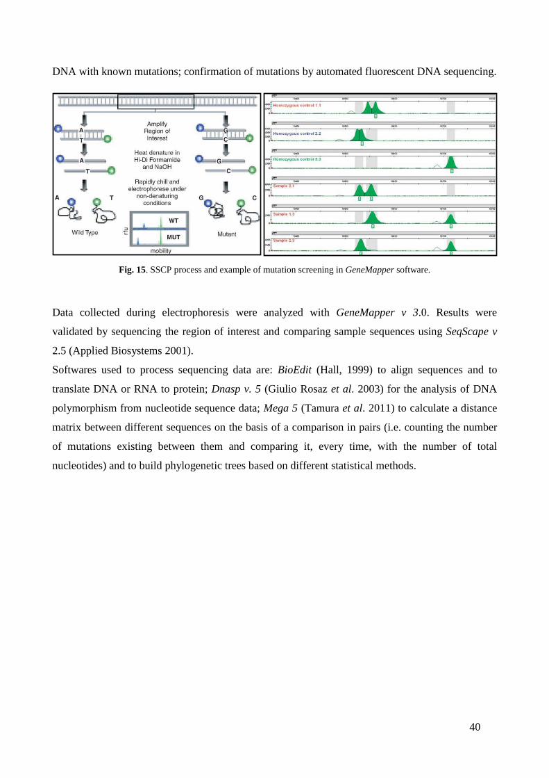
40

DNA with known mutations; confirmation of mutations by automated fluorescent DNA sequencing.

Fig. 15. SSCP process and example of mutation screening in GeneMapper software.

Data collected during electrophoresis were analyzed with GeneMapper v 3.0. Results were

validated by sequencing the region of interest and comparing sample sequences using SeqScape v

2.5 (Applied Biosystems 2001).

Softwares used to process sequencing data are: BioEdit (Hall, 1999) to align sequences and to

translate DNA or RNA to protein; Dnasp v. 5 (Giulio Rosaz et al. 2003) for the analysis of DNA

polymorphism from nucleotide sequence data; Mega 5 (Tamura et al. 2011) to calculate a distance

matrix between different sequences on the basis of a comparison in pairs (i.e. counting the number

of mutations existing between them and comparing it, every time, with the number of total

nucleotides) and to build phylogenetic trees based on different statistical methods.

41

CHAPTER THIRD: RESULTS

3.1 MITOCHONDRIAL DNA

We sequenced 459 nucleotides of the mtDNA D-Loop, which included 204 (44,4%) polymorphic

sites and 146 (31,8%) parsimony-informative sites in nearly 700 samples of six species of hare.

Haplotype diversity (Hd), nucleotide diversity statistics, genetic distances and other parameters

were computed using DNASP 5 (Rozas et al. 2003).

The alignment identified 248 different haplotypes (40 in L. corsicanus, 104 in L. europaeus, 44 in

L. timidus, 21 in L. granatensis, 5 in L. castroviejoi, 27 in L. c. mediterraneus, 7 in hares collected

in different areas of Africa); Italian and brown hares had different haplotypes that diverged by an

average TN93 genetic distance of 0.138 (Table 6).

Mountain hares and Iberian hares showed approximately one different haplotype per individual,

while brown hares and Italian hares showed one haplotype per three individuals (Table 5); also the

number of polymorphic sites was high for L. timidus and L. granatensis when compared to the

number of samples.

Species Samples Haplotypes Polymorphic

sites (s)

Haplotype

diversity (h)

Nucleotide

diversity (ππππ)

Theta

(Watterson)

L. corsicanus 136 40 48/459 0.935 (0.016) 0.016 (0.0008) 0.020 (0.005)

L. europaeus 314 104 113/459 0.942 (0.006) 0.018 (0.001) 0.042 (0.009)

L. timidus 63 44 73/459 0.982 (0.007) 0.038 (0.001) 0.036 (0.010)

L. granatensis 26 21 83/459 0.978 (0.022) 0.070 (0.004) 0.051 (0.016)

L. castroviejoi 5 5 67/459 1.000 (0.126) 0.081 (0.018) 0.075 (0.038)

L. cap. med. 86 27 38/459 0.830 (0.032) 0.012 (0.001) 0.017 (0.005)

L. capensis? 8 7 82/459 0.964 (0.077) 0.084 (0.009) 0.074 (0.032)

Tab. 5:. Values of interpopulation genetic diversity between the six species (standard deviations are in parenthesis).

With the software Mega we calculated a distance matrix: the software compares the various

sequences in pairs, counting the number of mutations existing between them, reporting, from time

to time, the total number of nucleotides and allows us to identify the type of mutations by

differentiating transversions, transitions and indel (deletions and insertions).

The genetic distances thus obtained were then displayed by a phylogenetic tree, constructed with

the Neighbor Joining (NJ) algorithm (Saitou & Nei, 1987) and Tamura and Nei TN93 genetic

42

Tab. 6:. Interspecific genetic distances (Tamura & Nei 1993) computed using control region sequences in six species of

hares.

distance model (Tamura & Nei 1993) widely used for displaying the phylogenetic relationships

among taxa. In addition to hare samples analysed was added a sequence belonging to Oryctolagus

cuniculus (wild rabbit) with the function of outgroup to emphasize the time of divergence between

different species.

The phylogenetic tree shows two main distinct groups of haplotypes:

- Clade A: including Lepus europaeus, Lepus capensis e Lepus capensis mediterraneus;

- Clade B: including Lepus timidus, Lepus granatensis, Lepus castroviejoi e Lepus

corsicanus.

The tree structure (Fig. 16) shows a clear genetic distinction among the mtDNA sequences of L.

corsicanus and the other taxa included in this study. D-Loop haplotypes of Italian hares group in a

strongly supported (bootstrap value 98) monophyletic clade, and DNA distinction is concordant

with both qualitative and quantitative morphological classification (Riga et al. 1998). Italian and

brown hares seem to have a long-lasting history of independent evolution and seem to be

reproductively isolated.

The tree confirms that Eurasian and African hares belong to two different phylogenetic clades;

brown hares originated from an African ancestor and dispersed in Europe, and Italian and Mountain

hares are relictual species that originated before the dispersal of L. europaeus in western Europe,

and which became adapted to the different Mediterranean and Alpine habitats.

A high frequency of Lepus timidus mitochondrial haplotypes was found in Iberian species (L.

castroviejoi and L. granatensis), although the Mountain hare is extinct in these regions; this could

result from the invasive replacement of L. timidus by the temperate species during deglaciation.

The sequence analysis of the control region also confirms the close relationship between L.

corsicanus and L. castroviejoi: two haplotypes belonging to individuals of L. catroviejoi (Fig.17) in

L. europaeus L. castroviejoi L. cap. med L. cap.? L. corsicanus L. granatensis L. timidus

L. europaeus -

L. castroviejoi 0.137 -

L. c. med. 0.106 0.138 -

L. capensis? 0.105 0.145 0.076 -

L. corsicanus 0.138 0.076 0.144 0.142 -

L. granatensis 0.142 0.100 0.136 0.145 0.119 -

L. timidus 0.135 0.078 0.133 0.141 0.088 0.094 -

43

Leu11

Leu143

Leu174

Leu173

Leu34

Leu121

Leu28

Leu177

Leu132

Leu22

Leu21

Leu8

Leu172

Leu179

Leu114

Leu16

Leu7

Leu116

Leu175

Leu29

Leu2

Leu134

Leu136

Leu33

Leu128

Leu17

Leu127

Leu141

Leu135

Leu118

Leu140

Leu137

Leu119

Leu126

Leu124

Leu125

Leu133

Leu27

Leu12

Leu14

Leu77

Leu104

Leu110

Leu229

Leu144

Leu32

Leu19

Leu26

Leu148

Leu150

Leu131

Leu139

Leu122

Leu147

Leu176

Leu146

Leu1

Leu5

Leu130

Leu120

Leu3

Leu153

Leu159

Leu160

Leu162

Leu170

Leu158

Leu155

Leu152

Leu156

Leu161

Leu167

Leu168

Leu169

Leu157

Leu154

Leu171

Leu123

Leu163

Leu164

Leu165

Leu180

Leu6

Leu115

Leu166

Leu23

Leu25

Leu10

Leu138

Leu151

Leu129

Leu117

Leu149

Leu142

Leu20

Leu18

Leu4

Leu13

Leu9

Lcap65

Lcap66

Leu178

Leu24

Leu30

Leu31

Lsa202

Lsa203

Lcap64

Lme40

Lme41

Lcap62

Lme47

Lcap63

Lme43

Lme61

Lme54

Lme56

Lme48

Lme58

Lme37

Lme59

Lme38

Lme53

Lme52

Lme42

Lme60

Lme35

Lme39

Lme55

Lme36

Lme57

Lme44

Lme45

Lme46

Lme51

Lme49

Lme50

Lgr195

Lgr198

Lgr199

Lgr194

Lgr196

Lgr188

Lgr190

Lgr187

Lgr193

Lgr191

Lgr186

Lgr192

Lgr197

Lgr189

Lcas68

Lti225

Lti224

Lti239

Lti232

Lti238

Lti204

Lti223

Lti237

Lti230

Lti205

Lti227

Lti226

Lti231

Lti207

Lti236

Lti233

Lgr185

Lgr184

Lgr183

Lcas70

Lcas69

Lti243

Lti242

Lti235

Lti208

Lti206

Lti240

Lti248

Lti247

Lti241

Lti246

Lti245

Lti222

Lti220

Lti221

Lgr201

Lgr200

Lti228

Lti234

Lti219

Lti244

Lgr182

Lgr181

Lti214

Lti215

Lti213

Lti209

Lti217

Lti211

Lti216

Lti212

Lti218

Lti210

Lgr15

Lcas67

Lco73

Lco112

Lco99

Lco86

Lco85

Lco82

Lco107

Lco87

Lco102

Lco92

Lco109

Lco80

Lco74

Lco95

Lco81

Lco83

Lco100

Leu145

Lco91

Lco106

Lco108

Lco101

Lco79

Lco111

Lco94

Lco76

Lco88

Lco72

Lco78

Lco98

Lco96

Lco89

Lco75

Lco90

Lco93

Lco71

Lco97

Lco84

Lco113

Lco105

Lco103

Oryctolagus cuniculus

98

83

55

42

65

18

44

37

11

33

61

100

55

100

62

86

99

80

93

66

65

100

55

99

70

87

43

97

32

44

57

37

6

17

36

93

41

7

8

12

41

71

66

28

57

88

72

100

2

18

37

40

35

80

23

63

62

30

42

72

89

90

34

86

56

73

91

38

42

56

67

60

77

15

45

14

35

27

22

77

89

98

78

80

90

96

47

61

58

17

0

23

58

79

98

54

69

68

69

95

55

79

97

98

20

90

10

65

22

98

24

70

65

54

64

51

78

86

41

41

89

54

39

45

50

63

72

97

65

44

46

27

47

45

44

22

17

36

22

60

18

27

29

55

4

5

20

52

21

40

11

8

4

5

13

12

4

0.000.050.100.15

Lepus europaeus

Lepus capensis mediterraneus

Lepus capensis ?

Lepus timidus

Lepus granatensis

Lepus castroviejoi

Lepus corsicanus

Fig. 16. Neighbour-joining (NJ)

phylogenetic tree computed by

Mega using TN93 genetic

distances among the 248 aligned

haplotypes of mitochondrial DNA

(mtDNA) control region I (CR-I)

of six species of hares, and using

the correspondent sequence of

rabbit as an outgroup.

Clade A

Clade B

44

Fig. 17. Neighbour-joining (NJ)

phylogenetic tree computed by

Mega using TN93 genetic distances

among the 110 aligned haplotypes

of mitochondrial DNA (mtDNA)

control region I (CR-I) of species

belonging to clade B (L. corsicanus,

L. timidus, L. granatensis, L.

castroviejoi) and using the

correspondent sequence of rabbit as

an outgroup. The red points stand

for L. castroviejoi samples.

Lgr196

Lgr194

Lgr199

Lgr190

Lgr188

Lgr197

Lgr198

Lgr195

Lgr193

Lgr187

Lgr191

Lgr192

Lgr186

Lgr189

Lcas68

Lti204

Lti238

Lti223

Lti239

Lti224

Lti225

Lti237

Lti230

Lti232

Lti205

Lti226

Lti227

Lti207

Lti236

Lti231

Lti233

Lti242

Lti243

Lti240

Lti208

Lti235

Lti206

Lti241

Lti248

Lti247

Lti245

Lti246

Lti244

Lgr181

Lgr182

Lti220

Lti222

Lti221

Lgr200

Lgr201

Lti228

Lti219

Lti234

Lcas69

Lcas70

Lgr183

Lgr184

Lgr185

Lti215

Lti209

Lti213

Lti214

Lti211

Lti217

Lti210

Lti218

Lti212

Lti216

Lcas67

Lgr15

Lco112

Lco73

Lco99

Lco82

Lco85

Lco86

Lco107

Lco87

Lco109

Lco102

Lco92

Lco74

Lco80

Lco79

Lco111

Lco101

Lco108

Lco106

Lco95

Lco81

Lco83

Lco100

Lco91

Lco93

Lco76

Lco94

Lco72

Lco88

Lco98

Lco78

Lco89

Lco75

Lco71

Lco103

Lco105

Lco113

Lco90

Lco84

Lco96

Lco97

Oryctolagus cuniculus

96

83

64

43

42

11

40

5

36

30

17

68

42

100

100

89

71

73

99

49

59

99

99

49

86

74

72

80

85

97

59

61

26

62

100

33

39

89

46

57

13

25

29

33

33

37

45

83

19

77

48

67

61

67

97

65

78

47

69

40

41

33

4

1

7

23

61

81

60

87

87

92

97

98

68

64

85

47

89

61

52

86

33

26

18

72

40

1913

2

6

65

67

58

47

21

20

0.05

Lepus timidus

Lepus granatensis

Lepus granatensis

Lepus corsicanus

45

fact are included in the clade of the Italian hare.

The phylogenetic tree in Figure 19 shows that L. corsicanus’s populations are geographically

differentiated and confirms the existence of a genetic diversity of mitochondrial haplotypes between

the samples collected in central-southern Italy and Sicily; the Sicilian samples in fact are grouped

together and show a slight differentiation compared to samples of the peninsula.

An important result concerns the Leu41 haplotype, found in two samples collected in 1999 in

Calabria identified morphologically and genetically (through microsatellites analysis) as belonging

to L. europaeus; analysing mitochondrial DNA we verified with surprise that this sample owns an

Italic haplotype. This finding can be interpreted as an introgression of L. corsicanus mitochondrial

genome in L. europaeus genome occurred in historical times as a result of an hybridization

(eventually anthropogenic) event.

Networks are better suited than phylogenetic methods to infer haplotype genealogies at the

population level because they explicitly allow for extant ancestral sequences and alternative

connections (Bandelt et al. 1999). We used 41 haplotypes identified in 138 L. corsicanus samples

with the median-joining network procedure (Bandelt et al. 1999), implemented in Network 4.5.1.6.

(http://www.fluxustechnology. com/) to draw the network (Fig. 18).

Haplotype diversity was high (Hd= 0,935) and the haplotype H1 (Lco1), found in 28 samples from

Sicily, has the highest frequency; in the network sicilian haplotypes are identify with pink colour

and the haplotype Leu41 with blue colour. In the network we can identify several haplotypes

groups, and this variability indicates an ancient origin of these populations; it was not possible to

observe any spatial structure considering sampling regions.

Fig. 18: Mitochondrial

DNA haplotypes

network with L.

corsicanus samples:

pink colour stands for

samples collected in

Sicily, yellow colour

for samples from the

peninsula, the blue dot

identify haplotype

Leu41.

46

Lco19

Lco26

Lco5

Lco13

Lco40

Lco32

Lco33

Lco1

Lco25

Lco7

Lco27

Lco2

Lco17

Lco18

Lco6

Lco23

Lco22

Lco38

Lco20

Leu41

Lco29

Lco10

Lco12

Lco24

Lco34

Lco30

Lco36

Lco21

Lco31

Lco37

Lco16

Lco35

Lco11

Lco14

Lco15

Lco28

Lco3

Lco39

Lco8

Lco4

Lco9

L. europaeus

6287

84

95

88

64

5366

44

86

36

71

63

33

39

5169

30

21

27

22

3722

7

14

67

64

50

38

15

20

15

0.01

Fig. 19. Neighbour-joining (NJ)

phylogenetic tree computed by Mega

using TN93 genetic distances among

the 41 aligned haplotypes of

mitochondrial DNA (mtDNA) control

region I (CR-I) of L. corsicanus

obtained from samples collected in

Italy, using the correspondent

sequence of L. europaeus as an

outgroup.

Sicily

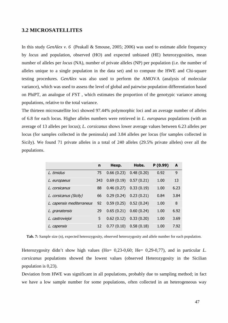
47

3.2 MICROSATELLITES

In this study GenAlex v. 6 (Peakall & Smouse, 2005; 2006) was used to estimate allele frequency

by locus and population, observed (HO) and expected unbiased (HE) heterozygosities, mean

number of alleles per locus (NA), number of private alleles (NP) per population (i.e. the number of

alleles unique to a single population in the data set) and to compute the HWE and Chi-square

testing procedures. GenAlex was also used to perform the AMOVA (analysis of molecular

variance), which was used to assess the level of global and pairwise population differentiation based

on PhiPT, an analogue of FST , which estimates the proportion of the genotypic variance among

populations, relative to the total variance.

The thirteen microsatellite loci showed 97.44% polymorphic loci and an average number of alleles

of 6.8 for each locus. Higher alleles numbers were retrieved in L. europaeus populations (with an

average of 13 alleles per locus); L. corsicanus shows lower average values between 6.23 alleles per

locus (for samples collected in the peninsula) and 3.84 alleles per locus (for samples collected in

Sicily). We found 71 private alleles in a total of 240 alleles (29.5% private alleles) over all the

populations.

n Hexp. Hobs. P (0.99) A

L. timidus 75 0.66 (0.23) 0.48 (0.20) 0.92 9

L. europaeus 343 0.69 (0.19) 0.57 (0.21) 1.00 13

L. corsicanus 88 0.46 (0.27) 0.33 (0.19) 1.00 6.23

L. corsicanus (Sicily) 66 0.29 (0.24) 0.23 (0.21) 0.84 3.84

L. capensis mediterraneus 92 0.59 (0.25) 0.52 (0.24) 1.00 8

L. granatensis 29 0.65 (0.21) 0.60 (0.24) 1.00 6.92

L. castroviejoi 5 0.62 (0.12) 0.33 (0.20) 1.00 3.69

L. capensis 12 0.77 (0.10) 0.58 (0.18) 1.00 7.92

Tab. 7: Sample size (n), expected heterozygosity, observed heterozygosity and allele number for each population.

Heterozygosity didn’t show high values (Ho= 0,23-0,60; He= 0,29-0,77), and in particular L.

corsicanus populations showed the lowest values (observed Heterozygosity in the Sicilian

population is 0,23).

Deviation from HWE was significant in all populations, probably due to sampling method; in fact

we have a low sample number for some populations, often collected in an heterogeneous way

48

considering the different distribution areas.

Differentiation between all populations was assessed also by Analysis of MOlecular VAriance

(AMOVA). A significant average multilocus FST = 0.37 (P = 0,01; computed from AMOVA)

indicated that genetic diversity was significant.

Fig. 20: Number of alleles found in each locus

for all populations.

Fig.21: Number of private alleles for each

population.

GenAlex was also utilized for assignment tests and Principal Coordinates Analysis (PCA): this

software calculate for each sample the expected genotype frequency at each locus and logtransform

to give a log likelihood value which is calculated even for each population, using the allele

frequencies of the respective population. A sample is assigned to the population with the highest log

likelihood. Genetic distance and assignment tests allow, through Principal Coordinate Analysis

(PCA), to detect the different considered populations despite a Cartesian axe system not linked to a

geographic reference system. The software, in fact, synthesizes all variability of the populations,

expressed by many variables, in 2 or 3 variability axes around which the analysis and the further

assignments occur.

To simplify the graphic visualization of GenAlex results the program Genetix v.4.2 (Belkhir et al.,

2001; http://www.University-montp2.fr/-genetix/genetix.htm) was used.

0,692

1,923

0,308

0,769

0,385

0,923

0,000

0,200

0,400

0,600

0,800

1,000

1,200

1,400

1,600

1,800

2,000

L. tim.

L. eur.

L. cor.

L. cor. Sicilia

L. cap. med.

L. gra.

L. cas.

L. cap.

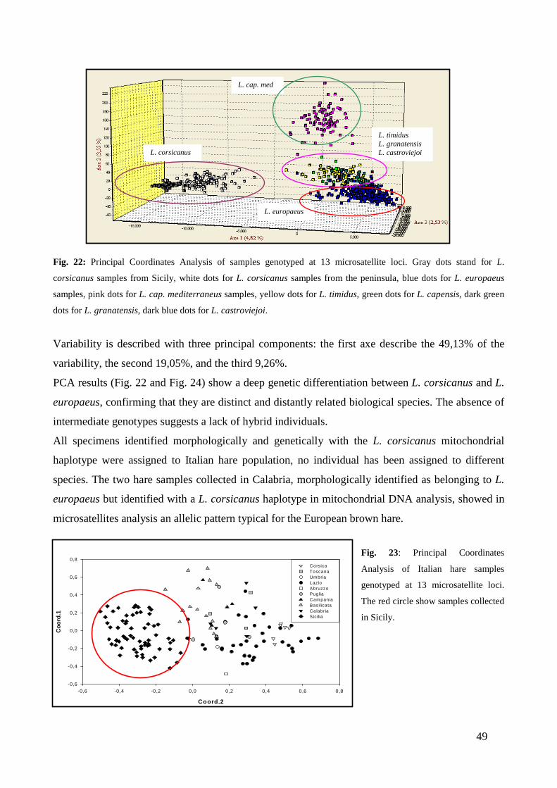
49

Coord.2

-0,6 -0,4 -0,2 0,0 0,2 0,4 0,6 0,8

Co

ord

.1

-0,6

-0,4

-0,2

0,0

0,2

0,4

0,6

0,8CorsicaToscanaUmbriaLaz io AbruzzoPugliaCampania BasilicataCalabria S icilia

Fig. 22: Principal Coordinates Analysis of samples genotyped at 13 microsatellite loci. Gray dots stand for L.

corsicanus samples from Sicily, white dots for L. corsicanus samples from the peninsula, blue dots for L. europaeus

samples, pink dots for L. cap. mediterraneus samples, yellow dots for L. timidus, green dots for L. capensis, dark green

dots for L. granatensis, dark blue dots for L. castroviejoi.

Variability is described with three principal components: the first axe describe the 49,13% of the

variability, the second 19,05%, and the third 9,26%.

PCA results (Fig. 22 and Fig. 24) show a deep genetic differentiation between L. corsicanus and L.

europaeus, confirming that they are distinct and distantly related biological species. The absence of

intermediate genotypes suggests a lack of hybrid individuals.

All specimens identified morphologically and genetically with the L. corsicanus mitochondrial

haplotype were assigned to Italian hare population, no individual has been assigned to different

species. The two hare samples collected in Calabria, morphologically identified as belonging to L.

europaeus but identified with a L. corsicanus haplotype in mitochondrial DNA analysis, showed in

microsatellites analysis an allelic pattern typical for the European brown hare.

Fig. 23: Principal Coordinates

Analysis of Italian hare samples

genotyped at 13 microsatellite loci.

The red circle show samples collected

in Sicily.

L. corsicanus

L. cap. med

L. timidus L. granatensis L. castroviejoi

L. europaeus

50

As we showed in the analysis of the mitochondrial DNA, also in nuclear DNA we found a level of

genetic differentiation between hare populations in Sicily and in the peninsula (Fig.23 shows a PCA

carried out only with Italian hare samples).

Fig. 24: Principal Coordinates

Analysis of all samples collected in

Italy belonging to L. corsicanus, L.

europaeus, L. timidus genotyped at

13 microsatellite loci. White dots

stand for L. corsicanus samples

from Sicily, blue dots for L.

corsicanus samples from the

peninsula, yellow dots for L.

europaeus samples, grey dots for

L. timidus samples.

Fig. 25: Principal Coordinates

Analysis of all samples belonging to

L. corsicanus, L. granatensis, L.

castroviejoi, L. timidus genotyped at

13 microsatellite loci. Blue dots

stand for L. corsicanus samples,

yellow dots for L. timidus samples,

white dots for L. granatensis

samples, red dots for L. castroviejoi

samples.

Fig. 25 shows results obtained from Principal Coordinates Analysis regarding the species L.

corsicanus, L. granatensis, L. castroviejoi and L. timidus. As for mitochondrial DNA analysis, we

can confirm the close genetic relationship between the Italian hare and the Broom hare; in fact the

two individuals from Spain (morphologically identified as belonging to L. castroviejoi) presenting

L. corsicanus haplotype, show an allelic pattern typical of the Italian hare also with microsatellites

analysis.

All genotypes were analyzed also with the software Structure v. 2.1 (Pritchard et al., 2000; Falush

et al., 2003) to establish their belonging population considering their microsatellite allele

frequencies. The program uses multilocus genotype data to infer population structure and to assign

individuals to populations.

51

The model assumes Hardy-Weinberg (HWE) and linkage (LE) equilibrium among the unlinked

loci, and that there are K populations (where K may be unknown), each of which is characterized by

a set of allele frequencies at each locus. Individuals in the sample are assigned (probabilistically) to

populations, or jointly to two or more populations if their genotypes indicate that they are admixed

(or hybrids). Departures from HWE and LE lead the population to be split into subpopulations, to

which individuals are assigned.

The program starts with a series of simulations to randomly assign the individuals, computing each

time the reliability of these clusterings through a likelihood value estimation. Clustering occurs

through Markov Chain and Monte Carlo algorithms that are able to maximize results, collecting

only the permutations with high likelihood values. As the first simulations are usually not reliable

and they are considered as burnings, they are deleted from the results interpretation that are based

only on the following permutations. In this study 130000 simulations were used (30000 as

burnings) to carried out the assignment, with the admixture model and we set K=1-15. Each run

was 5 time independently replicated.

Fig. 26: Likelihood values and Delta K graphs obtained with the software Structure analyzing all samples belonging to

the six species.

The clustering produced by Structure is shown with a graphs (Fig. 27). Using a cartesian reference

system, individuals belonging to the different populations have been reported on the horizontal axis

and the likelihood of belonging to one of the cluster considered in this assignment test for every

single genotype on the vertical axis; assignment groups more distinguishable were marked with

different colours to have a clearer view.

52

Fig. 27: Bayesian clustering of the populations obtained with the software Structure: population N°1 is L. timidus, N°2

L. europeus, N°3 L. corsicanus, N°4 L. corsicanus from Sicily, N°5 L. c. mediterraneus, N°6 L. granatensis, N°7 L.

castroviejoi, N°8 L. capensis.

Genetic variability was described with K between 4 and 5 (Fig. 26), it has not the best likelihood,

but permit to identify different populations.

Considering K=3 L. corsicanus and L. europaeus populations are clearly separated, but the other

species seem not to be differentiated.

Considering K=4 L. corsicanus, L. europaeus, L. c. mediterraneus populations are distinct, while L.

timidus and Iberian species are assigned to the same cluster; as already seen for microsatellites, two

individuals belonging to L. castroviejoi are assigned to the L. corsicanus cluster.

Considering K=5 we get the same clustering, but there is a further division between sicilian

populations and peninsular populations of L. corsicanus.

We repeated the same analysis considering only samples belonging to L. corsicanus, L. timidus, L.

granatensis, L. castroviejoi; 130000 simulations were used (30000 as burnings) to carried out the

assignment, with the admixture model and we set K=1-10. Each run was 5 time independently

replicated.

K=3

K=4

K=5

53

Fig. 28: Likelihood values and Delta K graphs obtained with the software Structure analyzing samples belonging to L.

corsicanus, L. timidus, L. granatensis, L. castroviejoi.

Fig. 29: Bayesian clustering of the populations obtained with the software Structure: population N°1 is L. timidus, N°2

L. corsicanus, N°3 L. granatensis, N°4 L. castroviejoi.

Considering K=3 L. timidus population is assigned to the same cluster with Iberian populations,

considering K=4 we have two distinct clusters.

In both cases L. corsicanus populations show genetic differentiation between Sicily and the

peninsula, and we get the same results obtained with previous analysis also on L. castroviejoi.

K=3

K=4

54

3.3 SINGLE NUCLEOTIDES POLYMORPHISM (SNP)

Genetic distance and Principal Coordinate Analysis (PCA) were calculated using GenAlex and

Genetix (the same softwares used for microsatellites analysis) on 150 samples belonging to L.

corsicanus and 15 samples belonging to L. europaeus collected in Italy analysed with nine single

nucleotides polymorphism loci found in four nuclear coding genes (see Table 3).

All the nine SNP loci were polymorphic and often L. europaeus population showed diagnostic and

private alleles (NP=0,556).

Allele Frequency

0,0000,2000,4000,6000,8001,0001,200

T C T C A G A T A T C A G A C A C A G

UCP2-10BR

UCP2-10CF

UCP2-10DF

HPX-4AF HPX-4BR CA2-2AR

CA2-2CR SPTBN1-7BF

SPTBN1-7CR

Locus

Fre

qu

ency L.corsicanus

L.corsicanus Sicilia

L.europaeus

Fig. 30: Allele frequency for each SNP locus for the two considered species.

Variability is described with three principal components: the first axe describe the 64,49% of the

variability, the second 20,87%, and the third 6,93%.

PCA results (Fig. 31) show a clear and deep distinction between the two species L. corsicanus and

L. europaeus, and the absence of shared genotypes. We repeated the analysis (PCA) also combining

genotypes obtained from microsatellites and SNPs and the result is shown in Figure 32. All

specimens identified morphologically and genetically with the L. corsicanus mitochondrial

haplotype were assigned to Italian hare population, no individual has been assigned to different

species. The two hare samples collected in Calabria, morphologically identified as belonging to L.

europaeus but identified with a L. corsicanus haplotype in mitochondrial DNA analysis, also with

SNPs analysis showed an allelic pattern typical for the European brown hare.

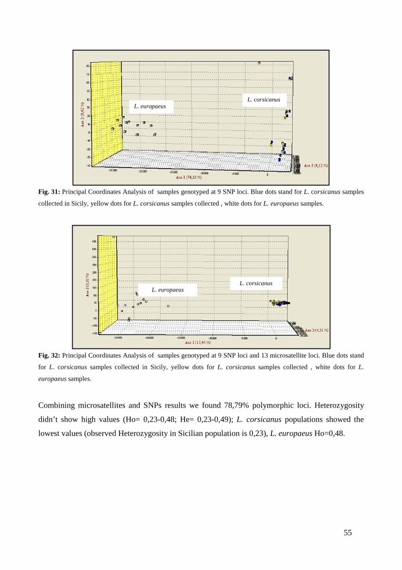
55

Fig. 31: Principal Coordinates Analysis of samples genotyped at 9 SNP loci. Blue dots stand for L. corsicanus samples

collected in Sicily, yellow dots for L. corsicanus samples collected , white dots for L. europaeus samples.

Fig. 32: Principal Coordinates Analysis of samples genotyped at 9 SNP loci and 13 microsatellite loci. Blue dots stand

for L. corsicanus samples collected in Sicily, yellow dots for L. corsicanus samples collected , white dots for L.

europaeus samples.

Combining microsatellites and SNPs results we found 78,79% polymorphic loci. Heterozygosity

didn’t show high values (Ho= 0,23-0,48; He= 0,23-0,49); L. corsicanus populations showed the

lowest values (observed Heterozygosity in Sicilian population is 0,23), L. europaeus Ho=0,48.

L. europaeus L. corsicanus

L. europaeus L. corsicanus

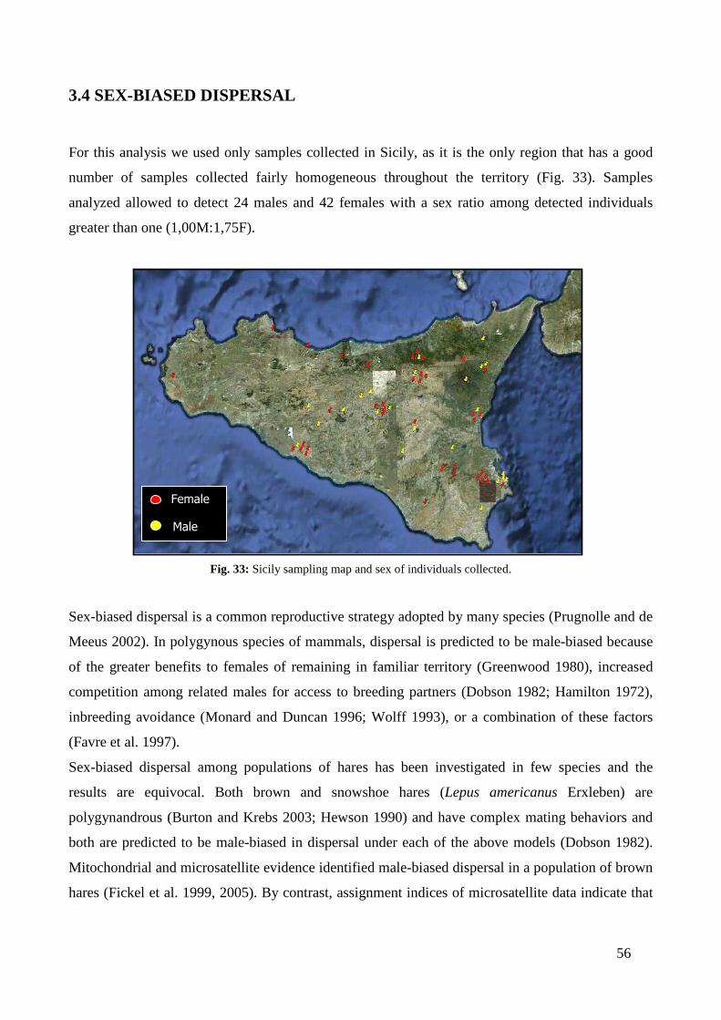
56

3.4 SEX-BIASED DISPERSAL

For this analysis we used only samples collected in Sicily, as it is the only region that has a good

number of samples collected fairly homogeneous throughout the territory (Fig. 33). Samples

analyzed allowed to detect 24 males and 42 females with a sex ratio among detected individuals

greater than one (1,00M:1,75F).

Fig. 33: Sicily sampling map and sex of individuals collected.

Sex-biased dispersal is a common reproductive strategy adopted by many species (Prugnolle and de

Meeus 2002). In polygynous species of mammals, dispersal is predicted to be male-biased because

of the greater benefits to females of remaining in familiar territory (Greenwood 1980), increased

competition among related males for access to breeding partners (Dobson 1982; Hamilton 1972),

inbreeding avoidance (Monard and Duncan 1996; Wolff 1993), or a combination of these factors

(Favre et al. 1997).

Sex-biased dispersal among populations of hares has been investigated in few species and the

results are equivocal. Both brown and snowshoe hares (Lepus americanus Erxleben) are

polygynandrous (Burton and Krebs 2003; Hewson 1990) and have complex mating behaviors and

both are predicted to be male-biased in dispersal under each of the above models (Dobson 1982).

Mitochondrial and microsatellite evidence identified male-biased dispersal in a population of brown

hares (Fickel et al. 1999, 2005). By contrast, assignment indices of microsatellite data indicate that

Female

Male

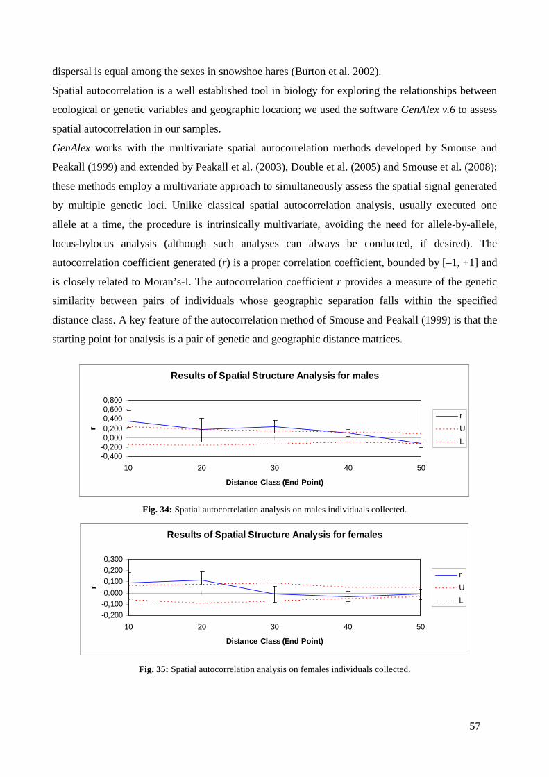
57

dispersal is equal among the sexes in snowshoe hares (Burton et al. 2002).

Spatial autocorrelation is a well established tool in biology for exploring the relationships between

ecological or genetic variables and geographic location; we used the software GenAlex v.6 to assess

spatial autocorrelation in our samples.

GenAlex works with the multivariate spatial autocorrelation methods developed by Smouse and

Peakall (1999) and extended by Peakall et al. (2003), Double et al. (2005) and Smouse et al. (2008);

these methods employ a multivariate approach to simultaneously assess the spatial signal generated

by multiple genetic loci. Unlike classical spatial autocorrelation analysis, usually executed one

allele at a time, the procedure is intrinsically multivariate, avoiding the need for allele-by-allele,

locus-bylocus analysis (although such analyses can always be conducted, if desired). The

autocorrelation coefficient generated (r) is a proper correlation coefficient, bounded by [–1, +1] and

is closely related to Moran’s-I. The autocorrelation coefficient r provides a measure of the genetic

similarity between pairs of individuals whose geographic separation falls within the specified

distance class. A key feature of the autocorrelation method of Smouse and Peakall (1999) is that the

starting point for analysis is a pair of genetic and geographic distance matrices.

Results of Spatial Structure Analysis for males

-0,400-0,2000,0000,2000,4000,6000,800

10 20 30 40 50

Distance Class (End Point)

r

r

U

L

Fig. 34: Spatial autocorrelation analysis on males individuals collected.

Results of Spatial Structure Analysis for females

-0,200-0,1000,000

0,1000,2000,300

10 20 30 40 50

Distance Class (End Point)

r

r

U

L

Fig. 35: Spatial autocorrelation analysis on females individuals collected.

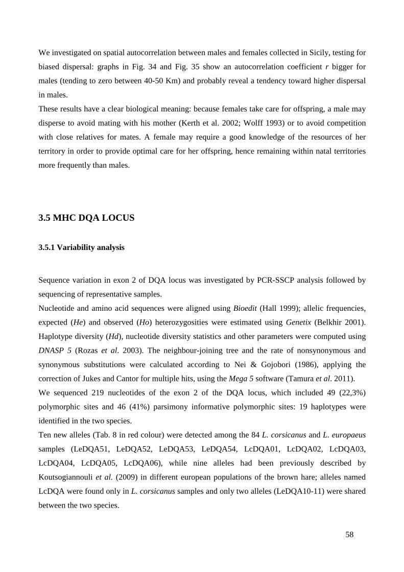
58

We investigated on spatial autocorrelation between males and females collected in Sicily, testing for

biased dispersal: graphs in Fig. 34 and Fig. 35 show an autocorrelation coefficient r bigger for

males (tending to zero between 40-50 Km) and probably reveal a tendency toward higher dispersal

in males.

These results have a clear biological meaning: because females take care for offspring, a male may

disperse to avoid mating with his mother (Kerth et al. 2002; Wolff 1993) or to avoid competition

with close relatives for mates. A female may require a good knowledge of the resources of her

territory in order to provide optimal care for her offspring, hence remaining within natal territories

more frequently than males.

3.5 MHC DQA LOCUS

3.5.1 Variability analysis

Sequence variation in exon 2 of DQA locus was investigated by PCR-SSCP analysis followed by

sequencing of representative samples.

Nucleotide and amino acid sequences were aligned using Bioedit (Hall 1999); allelic frequencies,

expected (He) and observed (Ho) heterozygosities were estimated using Genetix (Belkhir 2001).

Haplotype diversity (Hd), nucleotide diversity statistics and other parameters were computed using

DNASP 5 (Rozas et al. 2003). The neighbour-joining tree and the rate of nonsynonymous and

synonymous substitutions were calculated according to Nei & Gojobori (1986), applying the

correction of Jukes and Cantor for multiple hits, using the Mega 5 software (Tamura et al. 2011).

We sequenced 219 nucleotides of the exon 2 of the DQA locus, which included 49 (22,3%)

polymorphic sites and 46 (41%) parsimony informative polymorphic sites: 19 haplotypes were

identified in the two species.

Ten new alleles (Tab. 8 in red colour) were detected among the 84 L. corsicanus and L. europaeus

samples (LeDQA51, LeDQA52, LeDQA53, LeDQA54, LcDQA01, LcDQA02, LcDQA03,

LcDQA04, LcDQA05, LcDQA06), while nine alleles had been previously described by

Koutsogiannouli et al. (2009) in different european populations of the brown hare; alleles named

LcDQA were found only in L. corsicanus samples and only two alleles (LeDQA10-11) were shared

between the two species.

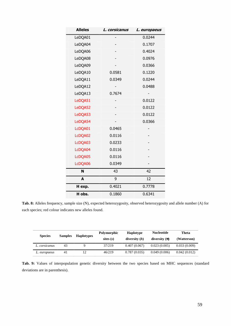
59

Tab. 8: Alleles frequency, sample size (N), expected heterozygosity, observed heterozygosity and allele number (A) for

each species; red colour indicates new alleles found.

Tab. 9: Values of interpopulation genetic diversity between the two species based on MHC sequences (standard

deviations are in parenthesis).

Alleles L. corsicanus L. europaeus

LeDQA01 - 0.0244

LeDQA04 - 0.1707

LeDQA06 - 0.4024

LeDQA08 - 0.0976

LeDQA09 - 0.0366

LeDQA10 0.0581 0.1220

LeDQA11 0.0349 0.0244

LeDQA12 - 0.0488

LeDQA13 0.7674 -

LeDQA51 - 0.0122

LeDQA52 - 0.0122

LeDQA53 - 0.0122

LeDQA54 - 0.0366

LcDQA01 0.0465 -

LcDQA02 0.0116 -

LcDQA03 0.0233 -

LcDQA04 0.0116 -

LcDQA05 0.0116 -

LcDQA06 0.0349 -

N 43 42

A 9 12

H exp. 0.4021 0.7778

H obs. 0.1860 0.6341

Species Samples Haplotypes Polymorphic

sites (s)

Haplotype

diversity (h)

Nucleotide

diversity (ππππ)

Theta

(Watterson)

L. corsicanus 43 9 37/219 0.407 (0.067) 0.023 (0.005) 0.033 (0.009)

L. europaeus 41 12 46/219 0.787 (0.035) 0.049 (0.006) 0.042 (0.012)

60

Fig. 36: Neighbour-joining phylogenetic tree for MHC class II DQA exon 2 sequences using a rabbit (Oryctolagus

cuniculus) sequence as an outgroup; sequences marked with a red circles are alleles found in L. corsicanus samples.

Allele LeQDA13, previously described by de Bellocq et al. (2009) in Belgian populations of the

brown hare, was found with a high frequency in the Italian hare population. The estimation of

heterozygosity values showed that all populations exhibited lower levels of heterozygosity than

expected, especially L. corsicanus.

The relationships among the 19 alleles identified in the present study were assessed by the

construction of a neighbour-joining tree (Fig. 36), using a rabbit sequence as an outgroup (GenBank

AN: M15557.1); alleles named “Lc” were found only in L. corsicanus samples, alleles named “Le”

were found in L. europaeus samples. Alleles LeDQA10, LeDQA11, LeDQA13 were shared

between the two species.

Although some of the branches did not have very strong bootstrap support, many internal allele

lineages were supported strongly. However, the phylogenetic analysis showed clearly that

61

population-specific alleles did not cluster together, and no separation of alleles on the basis of

geographical distances was observed.

3.5.2 Testing for selection

Examined the level of MHC genetic diversity, we tried to search for signal of selection in the

evolution of the DQA gene.

Forty-nine out of 219 (22,37%) nucleotide and 27 out of 73 (36,98%) amino acids positions were

variable (Fig. 37).

Fig. 37: Amino acid sequence alignment of 19 exon 2 DQA alleles of the brown hare and the Italian hare.

Examination of synonymous vs. nonsynonymous substitutions and Selection Test were computed

with both softwares Mega 5 (Tamura et al. 2011) and DNASP 5 (Rozas et al. 2003), and they gave

the same results. We computed the analysis first on alleles sequences found in L. corsicanus, then

on alleles found in L. europaeus (Tab. 10).

The Tajima’s D (Neutrality Test) test is a widely used test of neutrality in population genetics. The

purpose of the test is to distinguish between a DNA sequence evolving randomly ("neutrally") and

one evolving under a non-random process, including directional selection or balancing selection,

demographic expansion or contraction, genetic hitchhiking, or introgression. A randomly evolving

DNA sequence contains mutations with no effect on the fitness and survival of an organism. The

randomly evolving mutations are called "neutral", while mutations under selection are "non-

neutral".

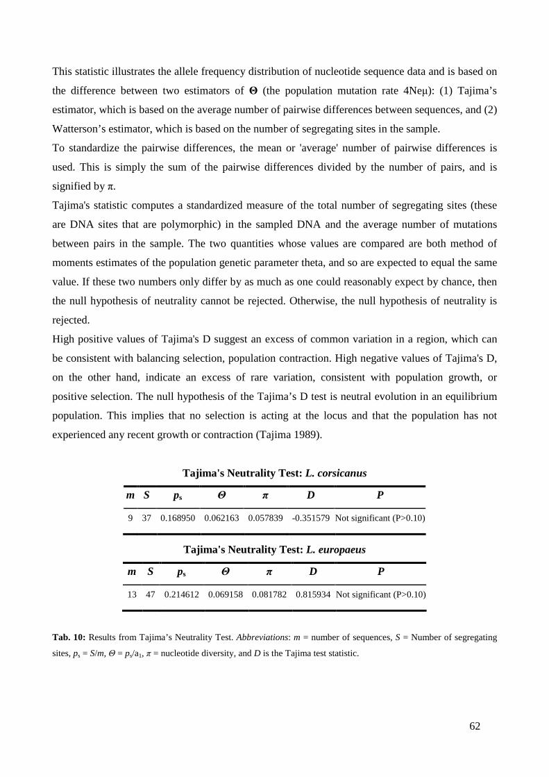
62

This statistic illustrates the allele frequency distribution of nucleotide sequence data and is based on

the difference between two estimators of Θ (the population mutation rate 4Neµ): (1) Tajima’s

estimator, which is based on the average number of pairwise differences between sequences, and (2)

Watterson’s estimator, which is based on the number of segregating sites in the sample.

To standardize the pairwise differences, the mean or 'average' number of pairwise differences is

used. This is simply the sum of the pairwise differences divided by the number of pairs, and is

signified by π.

Tajima's statistic computes a standardized measure of the total number of segregating sites (these

are DNA sites that are polymorphic) in the sampled DNA and the average number of mutations

between pairs in the sample. The two quantities whose values are compared are both method of

moments estimates of the population genetic parameter theta, and so are expected to equal the same

value. If these two numbers only differ by as much as one could reasonably expect by chance, then

the null hypothesis of neutrality cannot be rejected. Otherwise, the null hypothesis of neutrality is

rejected.

High positive values of Tajima's D suggest an excess of common variation in a region, which can

be consistent with balancing selection, population contraction. High negative values of Tajima's D,

on the other hand, indicate an excess of rare variation, consistent with population growth, or

positive selection. The null hypothesis of the Tajima’s D test is neutral evolution in an equilibrium

population. This implies that no selection is acting at the locus and that the population has not

experienced any recent growth or contraction (Tajima 1989).

Tajima's Neutrality Test: L. corsicanus

Tajima's Neutrality Test: L. europaeus

Tab. 10: Results from Tajima’s Neutrality Test. Abbreviations: m = number of sequences, S = Number of segregating

sites, ps = S/m, Θ = ps/a1, π = nucleotide diversity, and D is the Tajima test statistic.

m S ps Θ π D P

9 37 0.168950 0.062163 0.057839 -0.351579 Not significant (P>0.10)

m S ps Θ π D P

13 47 0.214612 0.069158 0.081782 0.815934 Not significant (P>0.10)

63

Codon# Triplet Syn sites (S) Nonsyn sites (N) dS dN dN-dS P-value

1 CAC 0,381104 2,6189 2,624 0 -2,624 1

2 ATT 0,980462 2,01954 0 0,4952 0,49516 0,6732

3 GGC 1 1,99257 2 0,5019 -1,4981 0,9627

4 TCC 1 2 0 1 1 0,4444

5 TAT 0,391507 2 0 0 0 0

6 GGC 1 2 0 0 0 0

7 ATA 0,449654 2,55035 0 0 0 0

8 AAC 0,270933 2,72907 3,691 0 -3,691 1

9 GTC 1 2 0 0 0 0

10 TAC 0,263584 2 0 0 0 0

11 CAG 0,538753 2,19766 1,8561 0 -1,8561 1

12 TCT 0,641134 2,00262 0 0,9987 0,99869 0,5738

13 TAT 0,391507 2 0 0 0 0

14 GGT 1 2 0 0 0 0

15 CCC 1 2 0 0 0 0

16 TCT 1 2 0 0 0 0

17 GGC 0,991982 2,00802 0 0,498 0,498 0,6693

18 CAG 0,522816 2,2136 0 0 0 0

19 TAC 0,263584 2 0 0 0 0

20 ACC 1 2 1 0 -1 1

21 CAT 0,391507 2,60849 0 0 0 0

22 GAA 0,550346 2,31405 0 0 0 0

23 TTT 0,391507 2,60849 0 0 0 0

24 GAT 0,391507 2,60849 0 0 0 0

25 GGA 1 1,8644 0 0 0 0

26 GAT 0,391507 2,60849 0 0 0 0

27 GAA 0,525055 2,33934 1,9046 0 -1,9046 1

28 GAG 0,565374 2,21762 0 1,3528 1,3528 0,506

29 TTC 0,263584 2,73642 0 0 0 0

30 TAT 0,391507 2 0 0 0 0

31 GTG 1 2 2 0 -2 1

32 GAC 0,263584 2,73642 0 0 0 0

33 CTG 1,26358 1,73642 0 0 0 0

34 GAT 0,426466 2,57353 0 0,3886 0,38857 0,8578

35 AAG 0,522816 2,25841 0 0 0 0

36 AAG 0,522816 2,25841 0 0 0 0

37 GAG 0,522816 2,34158 0 0 0 0

38 ACT 1 2 0 0 0 0

39 ATC 0,659495 2,34051 0 0,4273 0,42726 0,7802

40 TGG 0 1,95437 0 0 0 0

41 AGG 0,694177 2,30582 0 0,4337 0,43369 0,7686

42 CTT 1,04331 1,95669 0,9585 0 -0,9585 1

43 CCT 1 2 0 0 0 0

44 GAG 0,601228 2,28545 0 0,4376 0,43755 0,7917

45 TTT 0,391507 2,60849 0 0 0 0

46 AGC 0,689877 2,31012 0 0,8658 0,86576 0,593

47 AGA 0,647574 2,13365 0 0,4687 0,46868 0,7672

48 TTT 0,391507 2,60849 0 0 0 0

49 GCA 0,961034 2,02698 1,0406 0,9867 -0,0539 0,7562

50 AGT 0,391507 2,60849 0 0 0 0

64

51 TTT 0,391507 2,60849 0 0 0 0

52 GAT 0,391507 2,60849 0 0 0 0

53 CCA 1 2 0 0 0 0

54 CAG 0,538753 2,19766 1,8561 0 -1,8561 1

55 GGT 1 2 0 0 0 0

56 GCA 1 1,9215 0 0,5204 0,52043 0,6577

57 CTG 1,26358 1,73642 0 0 0 0

58 GGA 0,873355 1,94289 0 0,5147 0,5147 0,6899

59 AAC 0,416774 2,49859 0 1,2007 1,20068 0,6295

60 ATA 0,449654 2,55035 0 0 0 0

61 GCC 1 2 1 0 -1 1

62 ACA 1 2 0 0 0 0

63 GCA 1 2 0 0 0 0

64 AAA 0,550346 2,23088 0 0 0 0

65 TAC 0,263584 2 0 0 0 0

66 AAC 0,263584 2,73642 0 0 0 0

67 TTG 0,914323 1,71744 0 0 0 0

68 GAC 0,280058 2,71215 0 0,7374 0,73742 0,8216

69 ATC 0,538485 2,46151 0 0,4063 0,40625 0,8205

70 ATG 1,24982 1,75018 0 0,5714 0,57137 0,5834

71 ATT 0,315932 2,68407 0 0,7451 0,74514 0,8005

72 AAA 0,550346 2,23088 0 0 0 0

73 CGC 0,943829 2,05617 0 0,4863 0,48634 0,6854

Tab. 11: Examination of synonymous vs. nonsynonymous substitutions for L. corsicanus alleles obtained with Mega 5

software using the HyPhy software package.

We did not find any evidence of selection, in fact Tajima’s D values are low and close to zero,

indicating the hypothesis that no selection is acting at the locus analysed.

With the software Mega we computed also, for each codon and for each species (Tab. 11-12), the

numbers of sites that are estimated to be synonymous (S) and nonsyonymous (N). These estimates

are produced using the joint Maximum Likelihood reconstructions of ancestral states under a Muse-

Gaut model (Muse et al. 1994) of codon substitution and Tamura-Nei model (Tamura et al. 1993)

of nucleotide substitution. The test statistic dN - dS is used for detecting codons that have

undergone positive selection, where dS is the number of synonymous substitutions per site (s/S) and

dN is the number of nonsynonymous substitutions per site (n/N). A positive value for the test

statistic indicates an overabundance of nonsynonymous substitutions. In this case, the probability of

rejecting the null hypothesis of neutral evolution (P-value) is calculated (Kosakovsky et al. 2005;

Suzuki et al. 1999). Values of P less than 0.05 are considered significant at a 5% level and are

highlighted. Also in this case, codons with significant P values show test statistic values compatible

with the null hypothesis of strict neutrality (dN = dS) for both species.

65

Codon# Triplet Syn sites (S) Nonsyn sites (N) dS dN dN-dS P-value

1 CAC 0,375835 2,62416 2,6607 0 -2,6607 1

2 ATT 0,977995 2,02201 0 0,4946 0,49456 0,674

3 GGC 1 1,99532 4 1,0024 -2,9977 0,982

4 TCC 1 2 0 1 1 0,4444

5 TAT 0,384468 2 0 0 0 0

6 GGC 1 2 0 0 0 0

7 ATA 0,327929 2,67207 0 0 0 0

8 AAC 0,297281 2,70272 3,3638 0 -3,3638 1

9 ATC 0,956139 2,04386 0 0,9785 0,97854 0,4642

10 TAC 0,285813 2 0 0 0 0

11 CAG 0,615863 2,09832 1,6237 0 -1,6237 1

12 TCT 0,699938 2 0 0,5 0,5 0,7408

13 TAT 0,384468 2 0 0 0 0

14 GGT 1 2 0 0 0 0

15 CCC 1 2 0 0 0 0

16 TCT 1 2 0 0 0 0

17 GGC 1 2 0 0 0 0

18 CAA 0,571998 2,14219 1,7483 0 -1,7483 1

19 TAC 0,285813 2 0 0 0 0

20 ACC 1 2 1 0 -1 1

21 CAT 0,384468 2,61553 0 0 0 0

22 GAA 0,672071 2,20906 0 0 0 0

23 TTT 0,384468 2,61553 0 0 0 0

24 GAT 0,384468 2,61553 0 0 0 0

25 GGA 1 1,88113 0 0 0 0

26 GAT 0,384468 2,61553 0 0 0 0

27 GAG 0,57176 2,30937 1,749 0 -1,749 1

28 CAG 0,646495 2,14829 0 1,3965 1,39646 0,4542

29 TTC 0,285813 2,71419 0 0 0 0

30 TAT 0,384468 2 0 0 0 0

31 GTA 1 2 4 0 -4 1

32 GAC 0,285813 2,71419 0 0 0 0

33 CTG 1,28581 1,71419 0 0 0 0

34 GAT 0,393602 2,6064 0 0,3837 0,38367 0,8688

35 AAG 0,57176 2,22257 1,749 0 -1,749 1

36 AAG 0,562401 2,23193 0 0 0 0

37 GAG 0,562401 2,31873 0 0 0 0

38 ACT 1 2 0 0 0 0

39 ATC 0,641014 2,35899 0 0,8478 0,84782 0,6183

40 TGG 0 1,8752 0 0 0 0

41 ATG 0,580984 2,41902 0 1,2402 1,24017 0,5243

42 CTT 1,05671 1,94329 1,8927 0 -1,8927 1

43 CCT 1 2 1 0 -1 1

44 GAG 0,629683 2,28271 0 1,3142 1,31423 0,4815

45 TTT 0,384468 2,61553 0 0 0 0

46 AGC 0,833415 2,16658 0 0,9231 0,92311 0,5216

47 AAA 0,698789 2,09554 0 0,9544 0,95441 0,5624

48 TTT 0,384468 2,61553 0 0 0 0

49 GCA 0,922084 2,05623 1,0845 1,459 0,37448 0,6347

50 AGT 0,384468 2,61553 0 0 0 0

66

51 TTT 0,384468 2,61553 0 0 0 0

52 GAT 0,384468 2,61553 0 0,3823 0,38233 0,8718

53 CCA 1 2 0 0 0 0

54 CAG 0,615863 2,09832 1,6237 0 -1,6237 1

55 GGT 1 2 0 0,5 0,5 0,6667

56 GCA 1 1,94205 0 0,5149 0,51492 0,6601

57 CTG 1,28581 1,71419 0 0 0 0

58 GGA 0,899738 1,93908 0 0,5157 0,51571 0,6831

59 AAC 0,421816 2,51821 2,3707 0,7942 -1,5765 0,9442

60 ATA 0,327929 2,67207 0 0 0 0

61 GCC 1 2 1 0 -1 1

62 ACA 1 2 0 0 0 0

63 GAA 0,971303 2,01829 0 0,4955 0,49547 0,6751

64 AGA 0,682769 2,11156 0 0,4736 0,47358 0,7557

65 TAC 0,285813 2 0 0 0 0

66 AAC 0,297504 2,7025 0 0,7401 0,74006 0,8115

67 TTG 0,946869 1,68906 0 0 0 0

68 GAC 0,291544 2,70669 0 1,1084 1,10836 0,7357

69 ATC 0,487108 2,51289 0 0,7959 0,7959 0,7016

70 ATG 0,985896 2,0141 0 0,4965 0,4965 0,6714

71 ATT 0,38364 2,61636 0 0,3822 0,38221 0,8721

72 AAA 0,672071 2,12226 0 0 0 0

73 CGC 1 2 0 0 0 0

Tab. 12: Examination of synonymous vs. nonsynonymous substitutions for L. europaeus alleles obtained with Mega 5

software using the HyPhy software package.

67

CHAPTER FOURTH: DISCUSSION

The taxonomic status of the Italian hare Lepus corsicanus has been uncertain since its first

description by W. E. de Winton in 1898 (de Winton WE. Annual Magazine of Natural History,

London, 1898, 1, 149–158). The distribution range of this species has shrunk severely over the last

few decades owing to overhunting and restocking with nonindigenous Brown hares (L. europaeus)

in central and southern Italy and Sicily. Recently, scanty populations of Italian hares were

rediscovered, and samples for morphological and molecular analyses were collected.

Extensive human disturbance (overhunting and restocking) could have threatened, severely

restricted and eventually eradicated the Italian hare from most of its former historical range.

Historical distributions suggested that natural populations of Italian and Brown hares were

allopatric with putative contact zones running from central Tuscany to the Gargano promontory

(Palacios 1996). However, no data were available to document the effective degree of reproductive

isolation or eventual gene flow among populations in contact. Moreover, hares can hybridize in

nature, and the integrity of local Italian hare gene pools could have been disrupted by gene

introgression owing to released, nonindigenous Brown hares (Rhymer & Simberloff 1996; Thulin et

al. 1997).

Results obtained from mtDNA and nuclear DNA analysis (microsatellites and SNPs) confirm that

L. corsicanus and L. europaeus species are distinct and genetically different from all other species

studied.

The Italian hare and the European brown hare, which live in sympatric areas along the Italian

peninsula often artificially created as a result of repopulation events, do not share any nuclear

genotype, suggesting the absence of hybridization between the two species.

Results obtained from phylogenetic analysis show that L. corsicanus and L. europaeus possess a

long history of independent evolution, and are reproductively isolated in nature. The Italian hare’s

adaptation to the Mediterranean ecosystems may explain the absence of gene flow between the two

species.

Concerning Leu41 haplotype (found in two samples collected in 1999 in Calabria identified

morphologically and genetically, through microsatellites analysis, as belonging to L. europaeus)

which is placed in the phylogenetic tree in the same group of L. corsicanus haplotypes, we can

interpret this phenomenon as an introgression of L. corsicanus mitochondrial genome in L.

europaeus genome occurred in historical times as a result of an hybridization event. Recent

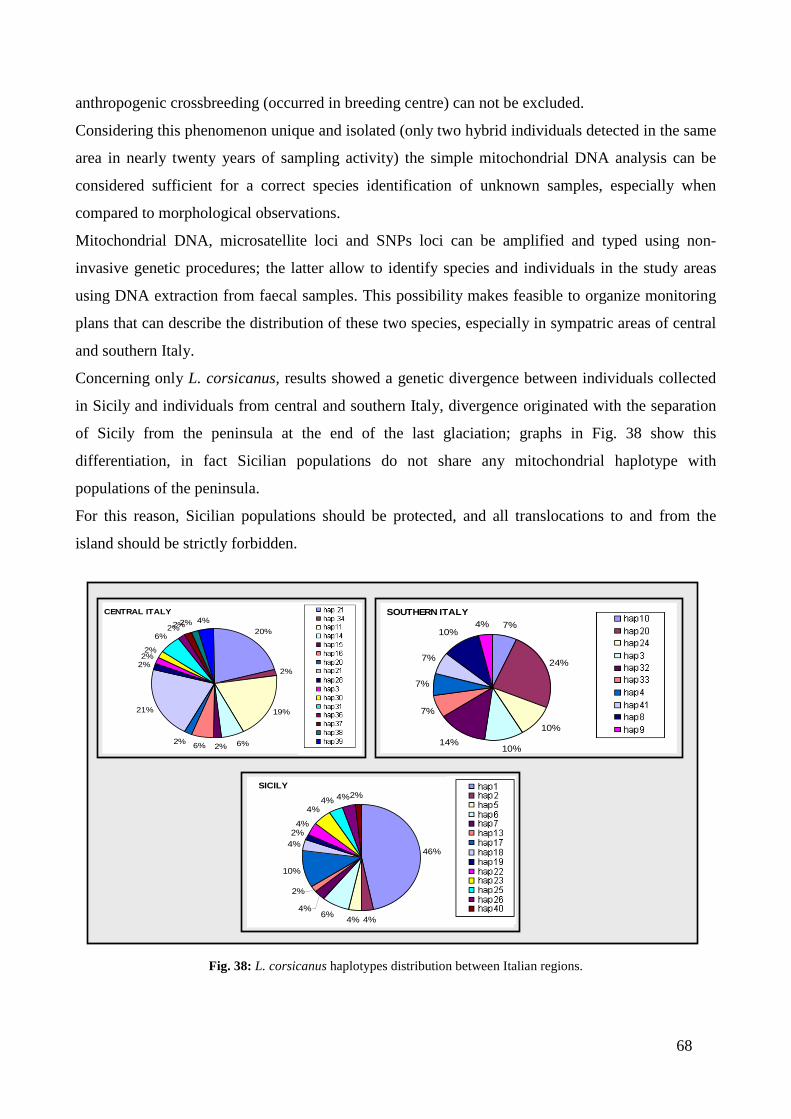
68

anthropogenic crossbreeding (occurred in breeding centre) can not be excluded.

Considering this phenomenon unique and isolated (only two hybrid individuals detected in the same

area in nearly twenty years of sampling activity) the simple mitochondrial DNA analysis can be

considered sufficient for a correct species identification of unknown samples, especially when

compared to morphological observations.

Mitochondrial DNA, microsatellite loci and SNPs loci can be amplified and typed using non-

invasive genetic procedures; the latter allow to identify species and individuals in the study areas

using DNA extraction from faecal samples. This possibility makes feasible to organize monitoring

plans that can describe the distribution of these two species, especially in sympatric areas of central

and southern Italy.

Concerning only L. corsicanus, results showed a genetic divergence between individuals collected

in Sicily and individuals from central and southern Italy, divergence originated with the separation

of Sicily from the peninsula at the end of the last glaciation; graphs in Fig. 38 show this

differentiation, in fact Sicilian populations do not share any mitochondrial haplotype with

populations of the peninsula.

For this reason, Sicilian populations should be protected, and all translocations to and from the

island should be strictly forbidden.

Fig. 38: L. corsicanus haplotypes distribution between Italian regions.

SICILY

46%

4%4%6%

4%

2%

10%

4%2%4%

4%4% 4%2%

APLO1APLO2APLO5APLO6APLO7APLO13APLO17APLO18APLO19APLO22APLO23APLO25APLO26APLO40

CENTRAL ITALY

20%

2%

19%

6%2%6%2%

21%

2%2%2%

6%2%2%2% 4%

APLO 21APLO 34APLO11APLO14APLO15APLO16APLO20APLO21APLO28APLO3APLO30APLO31APLO36APLO37APLO38APLO39

SOUTHERN ITALY7%

24%

10%

10%14%

7%

7%

7%

10%4% APLO10

APLO20APLO24APLO3APLO32APLO33APLO4APLO41APLO8APLO9

69

Low genetic variability was described among all populations of L. corsicanus populations; these

results could be explained assuming poor differentiation among populations and/or a recent

population decline.

Both markers also showed a close genetic relationship between L. corsicanus and L. castroviejoi,

suggesting the hypothesis that the two taxa are very recently derived from common ancestors. It can

be assumed that these two taxa are currently involved in a speciation process consequently to the

fragmentation of their geographic range (Alves et al. 2008); additional analysis would be useful for

a deeper evaluation of their taxonomic status.

In this project we analysed individuals from different areas of Africa, but we have chosen to not

explore phylogenetic analysis because the number of samples was very small and, in spite of several

molecular phylogenetic works on hares of the genus Lepus, no clear picture of phylogenetic

relationships among African taxa within this genus is yet at hand.

Historically, many different species have been identified in Africa, very often based on poor

morphological descriptions in terms of modern standards. Neighbour joining (NJ) and principal

coordinate analyses (PCA) revealed relatively close relationships between Lepus capensis and the

clades of African scrub hares (L. saxatilis) and brown hares (L. europaeus) (Slimen H.B., et al.

2007). However, further analyses are suggested including many more population samples from

Africa, the Middle East, and Europe.

The presence of L. timidus mtDNA in populations of other hares species (as in the case of the

Iberian hares), indicates widespread and ancient hybridization and genetic introgression events. The

most likely hypothesis is that massive mitochondrial DNA introgression occurred as a result of

hybridization events between these species, during the competitive replacement of arctic species

with temperate species at the end of the last ice age (Melo-Ferreira et al. 2009).

Molecular markers associated with host-pathogen interactions are of great interest to understand the

interplay between population dynamics and natural selection. Among these markers, MHC genes

are of particular significance given their function in the adaptive immune system conferring

protection against parasites and infectious diseases (Deter et al. 2008). The high level of

polymorphism of these genes indicates that they are under some form of balancing selection and are

adaptive in natural populations (Campos et al. 2010; Koutsogiannouli et al. 2009; Surridge et al

2008).

Concerning MHC analysis the overall results show a substantial high level of polymorphism and

variability of the DQA locus, especially for L. europaeus. In general, this is in accordance with the

results of our previous analyses on the brown hare, which examined the diversity of mtDNA and

70

microsatellite markers, and confirms the high genetic variability of this species. Italian hares

showed six private alleles, not found in European brown hares, but very low values of

heterozygosity.

The phylogeny of the exon 2 DQA alleles did not show a strong phylogeographic signal because

alleles that belonged to a specific population did not group together and we found shared haplotypes

between L. corsicanus and L. europaeus. This result contradicts the data obtained for mtDNA

markers (Stamatis et al. 2009), which demonstrated a strong phylogeographic signal.

The absence of a phylogeographic signal is a characteristic feature of some MHC loci (Klein et al.

1998) and is thought to result from balancing selection (Hughes et al. 1996). In addition, when we

included in the analysis alleles from other Lepus species i.e. L. timidus, L. granatensis, L. saxatilis,

L. capensis and L. californicus, which mainly inhabit different areas of the world, in addition to

alleles from a different Lagomorpha order (Oryctolagus cuniculus), these alleles were found to be

scattered throughout the tree and mixed with the L. europaeus DQA alleles (Koutsogiannouli et al.

2009). Such a phenomenon has been observed for MHC loci in several organisms, such as fish,

rodents, carnivores, ungulates and primates (Seddon & Ellegren 2002; Otting et al. 2002; Musolf et

al. 2004; Ottova et al. 2005; Surridge et al. 2008), and may be derived from ancestral sequences that

were present in a common ancestor and have persisted in the populations since their divergence.

Pathogen recognition might provide the selection pressure required to maintain particular MHC

sequences, and sharing similar allelic sequences may be evidence of the need for a specific immune

response to a common pathogen. Furthermore, the bootstrap values for the phylogenetic tree were

low, which implies a low phylogenetic signal. This is in accordance with the proposed antiquity of

the MHC loci and the observed high level of nucleotide polymorphism.

Selection tests performed on our Italian hare and brown hare samples gave contrasting results when

compared to those already present in literature (Campos et al. 2010; Koutsogiannouli et al. 2009;

Surridge et al 2008), in which it is confirmed that different MHC loci are under positive selection;

in fact, our tests did not reveal any evidence of selective pressure and all statistics values obtained

are compatible with the null hypothesis of strict neutrality.

For us, this was a first approach to this type of analysis and tests are still ongoing; probably it will

be necessary to conduct further analysis considering a higher number of samples and different

statistical approaches.

71

CONCLUSIONS

Present-day distribution of the Italian hare is extremely fragmented in central and southern Italy.

Populations survive at low density, mainly in protected areas and National Parks, where the species

has managed to escape overhunting and competition with introduced Brown hares.

Although hybridization seems not to be a threat to the survival of Lepus corsicanus in central and

southern Italy, strict prohibition of restocking with Brown hares should be enforced, at least in

selected priority areas (especially in Sicily).

Despite the intensive release of Brown hares during the last 20 years, field surveys (Lo Valvo et al.

1997; Riga et al. 1998) have shown that hares of Sicily belong only to L. corsicanus. It is therefore

possible that the peculiar conditions of Sicily are unsuitable for the Brown hare and that it cannot

survive in the Mediterranean-type climate and habitats of the island. Although Sicilian populations

of L. corsicanus are rather widespread and stable, conservation measures should be enforced in

order to prevent the release of Brown hares in the island and to plan a controlled hunting and wise

use of the Italian hare populations.

The aim of the National Action Plan (published in 2001) for Lepus corsicanus is to collect

knowledges on the status and biology of the species to better promote its conservation. Genetics has

provided and can continue to provide important informations for the conservation of the species.

The genetic analysis of non-invasive samples collected in central and south Italy is an useful tool to

identify the species distribution areas; the identification of these areas, through the combination of

genetic and environmental data, could allow the discrimination on a small scale of preferential or

exclusive habitat for the Italian hare.

Key objectives in these areas to ensure the protection of the species would have to be: the reduction

of hunting pressure, ecological corridors recovery between fragmented and separated distribution

areas, and the quantitative and qualitative improvement of habitats.

The population dynamics study through the typing of non-invasive samples would also provide an

opportunity to assess the status of single local communities and to assess, in concrete terms, which

measures are necessary to prevent the extinction of local populations of the Italian hare.

72

ACKNOWLEDGEMENTS

First of all I want to thank Ettore Randi for giving me the opportunity to carry out this PhD project.

Many thanks to Valter Trocchi, Francesco Riga, Egidio Mallia and all the people involved in

samples collection, and the DPN MATTM for supporting the work of the genetic laboratory and the

implementation of the National Action Plan for the Italian hare.

Many thanks to Franz Suchentrunk and Steve Smith from the Research Institute of Wildlife

Ecology of Vienna, for their endless hospitality and for all the work done.

Sincere thanks to all my colleagues of the genetic laboratory for their fundamental support during

these three years of work.

73

REFERENCES

2008 IUCN Red List of Threatened Species. Available at: http://www.iucnredlist.org.

Abbott K.M., Wickings E.J., Knapp L.A., 2006. High levels of diversity characterize mandrill

(Mandrillus sphinx) Mhc-DRB sequences. Immunogenetics, 58: 628–640.

Alves P.C., Niethammer J., 2003. Die iberischen Hasen. In: Handbuch der Säugetiere Europas

(eds Niethammer J, Krapp F), pp. 137–154. Aula-Verlag, Vienna, Austria.

Alves P.C., Melo-Ferreira J., Branco M. et al., 2008a. Evidence for genetic similarity of two

allopatric European hares (Lepus corsicanus and L. castroviejoi) inferred from nuclear DNA

sequences. Molecular Phylogenetics and Evolution, 46: 1191–1197.

Alves P.C., Melo-Ferreira J., Freitas H., Boursot P., 2008b. The ubiquitous mountain hare

mitochondria: multiple introgressive hybridization in hares, genus Lepus. Philosophical

Transactions of the Royal Society B: Biological Sciences, 363: 2831–2839.

Amori G., Coresetti L., Esposito C., 2002. Mammiferi dei Monti Lepini. Quad. Cons. Natura, 11,

Min. Ambiente – Ist.Naz. Fauna Selvatica.

Andersson A. C., Thulin C. G., Tegelström H., 1999. Applicability of rabbit microsatellite

primers for studies of hybridisation between an introduced and a native hare species. Hereditas 130:

309-315.

Angelici F. M. and Luiselli L., 2001. Distribution and status of the Apennine hare Lepus

corsicanus in continental Italy and Sicily. Oryx 35(3): 245-249.

Angermann R., 1983. The taxonomy of Old World Lepus. Acta Zoologica Fennica, 174: 17–21.

Avise J.C., 1994. Molecular Markers, Natural History and Evolution. Nature, 352: 192.

74

Bandelt H.L., Forster P., Rohl A., 1999. Median-joining networks for inferring intraspecific

phylogenies. Molecular Biology and Evolution 16: 37–48.

de Battisti R., Migliore S., Masutti L. and Trocchi V., 2004. The diet of the Italian hare Lepus

corsicanus on Etna Mountain, Sicily. Research Center in Biodiversity and Genetic Resources,

Vairao, Portugal.

Belkhir K., Borsa P., Chikhi L., Raufaste N., Bonhomme F., 2001. GENETIX 4.02, logiciel sous

Windows TM pour la génétique des populations. Laboratoire Génome, Populations, Interactions,

CNRS UMR 5000, Université de Montpellier II, Montpellier, France; http://www.univ-

montp2.fr/~genetix/genetix.

de Bellocq J.G., Suchentrunk F., Baird S.J.E., Schaschl H., 2009. Evolutionary history of an

MHC gene in two leporid species: characterisation of Mhc-DQA in the European brown hare and

comparison with the European rabbit. Immunogenetics, 61: 131–144.

Bernatchez L., Landry C., 2003. MHC studies in nonmodel vertebrates: what have we learned

about natural selection in 15 years? Journal of Evolutionary Biology, 16: 363–377.

Blondel J., Aronson :, 1999. Biology and Wildlife of the Mediterranean Region. Oxford

University, pp. 328.

Boitani L., Corsi F., De Biase A., D'Inzillo Caranza I., Ravagli M., Reggiani G., Sinibaldi I.

and Trapanese P., 1999. A Databank for the Conservation and Management of the African

Mammals. Istituto di Ecologia Applicata, Rome, Italy.

Brown J.H., Jardetzky T.S., Gorga J.C. et al., 1993. Threedimensional structure of the human

class II histocompatability antigen HLA-DR1. Nature, 364: 33–39.

Brumfield R.T., Beerli P., Nickerson & D.A., Edwards S.V., 2003. The utility of single

nucleotide polymorphisms in inferences of population history. Trends in Ecology and Evolution 18:

249-256.

75

Budowle B., 2004. SNP typing strategies. Forensic Science International 146: 139-142.

Burton C., Krebs C.J., Taylor E., 2002. Population genetic structure of the cyclic snowshoe hare

(Lepus americanus) in southwestern Yukon, Canada. Molecular Ecology 11: 1689–1701.

Burton C., Krebs C.J., 2003. Influence of relatedness on snowshoe hare spacing behavior. Journal

of Mammalogy 84: 1100–1111.

Campos J.L., de Bellocq J.G., Schaschl H., Suchentrunk F., 2010. MHC class II DQA gene

variation across cohorts of brown hares (Lepus europaeus) from eastern Austria: Testing for

different selection hypotheses. Mammalian Biology, In Press.

Chapman J.A., Flux J.E.C., 1990. Rabbits, Hares and Pikas. Status Survey and Conservation

Action Plan. IUCN/SSC Lagomorph Specialist Group, Glaud.

Deter J., Bryja J., Chaval Y., Galan M., Henttonen H., Laakkonen J., Voutilainen L.,

Vapalahti O., Vaheri A., Salvador A.R., 2008. Association between the DQA MHC class II gene

and Puumala virus infection in Myodes glareolus, the bank vole. Infect. Genet. Evol. 8: 450–458.

Dobson F., 1982. Competition for mates and predominant juvenile dispersal in mammals.

American Naturalist 30:1183–1192.

Edwards S.V., Hedrick P.W., 1998. Evolution and ecology of MHC molecules: from genomics to

sexual selection. Trends in Ecology and Evolution, 13: 305–311.

Ellerman J.R., Morrison-Scott T.C.S., 1951. Checklist of Palaearctic and Indian mammals

(1758–1946). British Museum (Natural History), London, pp. 810.

Falush D., Stephens M., Pritchard J.K., 2003. Inference of population Structure using multilocus

genotype data: Linked loci and correlated allele frequencies. Genetics 164: 1567-1587.

Favre L., Balloux F., Goudet J., Perrin N., 1997. Femalebiased dispersal in the monogamous

mammal Crocidura russula: evidence from field data and microsatellite patterns. Proceedings of the

76

Royal Society of London, B. Biological Sciences 264: 127–132.

Fernandez A., Soriguer R., Carro F. and Castien E., 2004. Population trends of two hare species

(Lepus granatensis and Lepus europaeus) present in Navarra province (northern Iberian Peninsula)

over the last two decades. Research Center in Biodiversity and Genetic Resources, Vairao.

Fickel J., Lieckfeldt D., Pitra C., 1999. Analysis of genetic diversity and structure in neighboring

populations of the European brown hare (Lepus europaeus, Pallas 1778). Zeitschrift fur

Jagdwissenschaft 45: 230–237.

Fickel J., et al. 2005. Genetic structure of populations of European brown hare: implications for

management. Journal of Wildlife Management 69: 760–770.

Flux J.E.C., 1983. Introduction to taxonomic problems in hares. Acta Zoologica Fennica, 174: 7–

10.

Flux J.E.C., Angermann R., 1990. The hares and jackrabbits. In: Rabbits, Hares and Pikas. Status

Survey and Conservation Action Plan (eds A Cj, JEC Flux). International Union for the

Conservation of Nature and Natural Resources, Gland, Switzerland.

Frankham R., Ballou J.D. & Briscoe D.A. (eds.), 2002. Introduction to conservation genetics.

Cambridge University Press, Cambridge, UK.

Gerloff U., Schlotterer C., Rassmann K., Rambold I., Hohmann G., Fruth B., Tautz D., 1995.

Amplification of hypervariable simple sequence repeats (microsatellites) from excremental DNA of

wild living Bonobos (Pan paniscus). Molecular Ecology, 4: 515-518.

Greenwood P., 1980. Mating systems, philopatry and dispersal in birds and mammals. Animal

Behaviour 28: 1140–1162.

Guberti V., de Marco M.A., Riga F., Cavazza A., Trocchi V., Capucci L., 2000. Virolog and

species conservation: the case of EBHSV and the Italian hare (Lepus corsicanus De Winton, 1898).

Proceedings of V Int. Congress of European Society for Veterinary Virology, Brescia 27-30.8.2000:

77

198-199.

Hall T.A., 1999. BioEdit: a user-friendly biological sequence alignment editor and analysis

program for Windows 95/98/NT. Nucleic Acids Symposium Series, 41: 95-98.

Hamill R.M., Doyle D., Duke E.K., 2006. Spatial patterns of genetic diversity across European

subspecies of the mountain hare, Lepus timidus L. Heredity 97: 355–365.

Hamill R.M., Doyle D., Duke E.K., 2007. Microsatellite analysis of mountain hares (Lepus

timidus hibernicus): low genetic differentitation and possible sex-bias in dispersal. Journal of

Mammalogy 88(3): 784-792.

Hamilton W., 1972. Altruism and related phenomena, mainly in social insects. Annual Review of

Ecology and Systematics 13: 1–21.

Hartl D.L. & Clark A.G., 1993. Principles of Population Genetics (Genetica di popolazione). Eds.

Zanichelli, Bologna.

Hedrick P.W., 1994. Evolutionary genetics at the major histocompatibility complex. American

Naturalist, 143: 945–964.

Hewitt G.M., 1996. Some genetic consequences of ice ages, and their role in divergence and

speciation. Biological Journal of Linnean Society, 58: 247-279.

Hewitt G.M., 1999. Post-glacial recolonization of European biota. Biological Journal of Linnean

Society, 68:1-2.

Hewson R., 1990. Interactions between mountain hares (Lepus timidus L.) and other mammals.

Journal of Zoology (London) 221: 302–305.

Hill A.V.S., Allsopp E.M., Dwiatkowski D. et al., 1991. Common West African HLA antigens are

associated with protection from severe malaria. Nature, 352: 595–600.

78

Hoffmann R.S., 1993. Order Lagomorpha. In: Mammal Species of the World: a Taxonomic and

Geographic Reference, 2nd edn. (eds Wilson DE, Reeder DM), pp. 807–827. Smithsonian

Institution Press, Washington.

Hofreiter M., Sere D., Pioneer H.A.N.& Ouch M Pääbo, S., 2001. Ancient DNA. Nature 2:353-

359.

Hughes A., Yeager M., Carrington M., 1996. Peptide binding function and the paradox of HLA

disease associations. Immunology and Cell Biology, 74: 444–448.

Janeway C.A., Travers P., Walport M., Shlomchik M.J., 2005. Immunobiology, 6th edn.

Garland Science, London, pp 183–201.

Jefferis A. J., Wilson V. & Thein S.L., 1985. Hypervariable ‘‘minisatellite’’ regions in human

DNA. Nature, 314: 67-73.

Klein J., Takahata N., 1990. The major histocompatibility complex and the quest for origins.

Immunological Reviews, 113: 5–25.

Klein J., Sato A., Nagl S., O’hUigin C., 1998. Molecular transspecies polymorphism. Annual

Review of Ecology and Systematics, 29: 1–21.

Kosakovsky Pond S.L., Frost S.D.W., 2005. Not So Different After All: A Comparison of

Methods for Detecting Amino Acid Sites Under Selection . Molecular Biology and Evolution 22:

1208-1222.

Koutsogiannouli E.A., Moutou K.A., Sarafidou T., Stamatis C., Spyrou V., Mamuris Z., 2009.

Major histocompatibility complex variation a tclass II DQA locus in the brown hare (Lepus

europaeus). Mol.Ecol. 18: 4631–4649.

Kryger U., Robinson T.J., Bloomer P., 2002. Isolation and characterization of six polymorphic

microsatellite loci in South African hares (Lepus saxatilis F. Cuvier, 1823 and Lepus capensis

Linnaeus, 1758). Molecular Ecology Notes 2: 422-424.

79

Kumar S., Tamura K., Jakobsen I.B., Nei M., 2001. MEGA2: Molecular Evolutionary Genetics

Analysis Software. Arizona. State University, Tempe, AZ.

Li W.H., Gojobori T., Nei M., 1981. Pseudogenes as a paradigm of neutral evolution, Nature 292:

237-239.

Lindley D. V., 1990. The 1988. Wald memorial lecture: The present position in Bayesian Statistics.

Statist. Sci. 5: 44-89.

Lo Valvo M., Barera A., Seminara S., 1997. Biometria e status della lepre appenninica (Lepus

corsicanus, de Winton 1898) in Sicilia. Naturalista Siciliano, IV , 67–74.

Lo Valvo M., 2007. Status di Lepus corsicanus in Sicilia. A cura di De Filippo G., De Riso L.,Riga

F., Trocchi V. e Troisi S.R. Conservazione di Lepus corsicanus De Winton, 1898 e stato delle

conoscenze. IGF Publ., Napoli, Italia.

Martinez-Arias R., Calafell F., Mateu E., Comas D., Andres A., Bertranpetit J., 2001.

Sequence variability of a human pseudogene, Genome Res; 11: 1071-1085.

McFarland B.J., Beeson C., 2002. Binding interactions between peptides and proteins of the class

II major histocompatibility complex. Medicinal Research Reviews, 22: 168–203.

Mellersh C.S.& Ostrander E.A.,1997. The Canine Genome. Adv Veter Med 40:191-215.

Melo-Ferreira J., Boursot P., Suchentrunk F., Ferrand N., Alves P.C., 2005. Invasion from the

cold past: extensive introgression of mountain hare (Lepus timidus) mitochondrial DNA into three

other hare species in northern Iberia. Molecular Ecology, 14: 2459–2464.

Melo-Ferreira J., Boursot P., Randi E. et al., 2007. The rise and fall of the mountain hare (Lepus

timidus) during Pleistocene glaciations: expansion and retreat with hybridization in the Iberian

Peninsula. Molecular Ecology, 16: 605–618.

Melo-Ferreira J., Alves P.C., Freitas H., Ferrand N., Boursot P., 2009. The genomic legacy

80

from the extinct Lepus timidus to the three hare species of Iberia: contrast between mtDNA, sex

chromosomes and autosomes. Molecular Ecology 18: 2643–2658.

Monard A., Duncan P., 1996. Consequences of natal dispersal in female horses. Animal

Behaviour 52: 565–579.

Mougel F., Mounolou J.C., Monnerot M., 1997. Nine polymorphic microsatellite loci in the

rabbit, Oryctolagus cuniculus. Animal Genetics, 28: 58-71.

Muller U. G. & LaReesa Wolfenbarger L., 1999. AFLP genotyping and fingerprinting. Trends

Ecol. Evol. 10: 389-394.

Mullis K., Erlich H. , Faloona F., Horn G., Saiki R. & Scharf S., 1986. Specific enzymatic

amplification of DNA in vitro: the polymerase chain reaction. Cold Spring Harbor Symp. Quant.

Biol., 51: 263-273.

Murphy M., Hinman A. & Levine A.J., 1996. Wild-type p53 negatively regulates the expression

of a microtubule-associated protein. Genes & Dev., 10: 2971-2980.

Muse S.V., Gaut B.S., 1994. A likelihood approach for comparing synonymous and

nonsynonymous nucleotide substitution rates, with application to the chloroplast genome.

Molecular Biology and Evolution 11: 715-724.

Musolf K., Meyer-Lucht Y., Sommer S., 2004. Evolution of MHC-DRB class II polymorphism in

the genus Apodemus and a comparison of DRB sequences within the family Muridae (Mammalia:

Rodentia). Immunogenetics, 56: 420–426.

Nei M. and Kumar S., 2000. Molecular Evolution and Phylogenetics. Oxford University Press,

New York.

O’Hagan A., 1994. Bayesian Inference. London: Edward Arnold. Press, S. J. (1972). Applied

Multivariate Analysis: using Bayesian and Frequentist Methods of Inference. Melbourne, FL:

Krieger.

81

Otting N., de Groot N.G., Doxiadis G.G.M., Bontrop R.E., 2002. Extensive Mhc-DQB variation

in humans and non-human primate species. Immunogenetics, 54: 230–239.

Ottova E., Simkova A., Martin J.F. et al., 2005. Evolution and trans-species polymorphism of

MHC class IIb genes in cyprinid fish. Fish & Shellfish Immunology, 18: 199–222.

Palacios F., 1996. Systematics of the indigenous hares of Italy traditionally identified as Lepus

europaeus Pallas, 1778 (Mammalia: Leporidae). Bonner Zoologische Beitragen, 56: 59–91.

Parker Q.A., Phillipps S. & Morgan D.H. , 1995. IAU Colloq. 148, ASP Conf. Ser. 84, eds.

Chapman, J. M. et al. (San Francisco: ASP), p. 96.

Peakall R. , Smouse P. E. , 2005. GenAlEx 6: Genetic Analysis in Excel., Population Genetic

Software for Teaching and Research. Australian National University, Canberra, Australia.

http://www.anu.edu.au/BoZo/GenAlEx

Peakall R. and Smouse P.E., 2006. GENALEX 6: genetic analysis in Excel. Population genetic

software for teaching and research Molecular Ecology Notes 6: 288–295.

Penn D.J., Potts W.K., 1999. The evolution of mating preferences and major histocompatibility

complex genes. The American Naturalist, 153: 145–164.

Petter F., 1961. Elements d’une révision des lièvres européens et asiatiques du sous-genre Lepus.

Zeitschrift für Säugetierkunde, 26 : 30–40.

Pierpaoli M., Riga F., Trocchi V., Randi E., 1999. Species distinction and evolutionary

relationships of the Italian hare (Lepus corsicanus) as described by mitochondrial DNA sequencing.

Molecular Ecology, 8: 1805–1817.

Piertney S.B., Oliver M.K., 2006. The evolutionary ecology of the major histocompatability

complex. Heredity, 96: 7–21.

Pietri C., 2002. Premières données physiques et biologiques sur les Lièvres (Lepus sp.) actuels de

82

Corse. Rapp. Techn. 29 (Doc. int.) FDCHC, Bastia.

Potts W.K., Slev P.R., 1995. Pathogen-based models favoring MHC genetic diversity.

Immunological Reviews, 143: 181–197.

Potts W.K., Wakeland E.K., 1993. Evolution of MHC genetic diversity: a tale of incest, pestilence

and sexual preference. Trends in Genetics, 9: 408–412.

Pritchard J.K., Stephens M. & Donnelly P.J., 2000. Inference of population structure using

multilocus genotype data. Genetics 155: 945-959.

Prugnolle F., de Meeus T., 2002. Inferring sex-biased dispersal from population genetic tools: a

review. Heredity 88: 161–165.

Rammensee H.G., Friede T., Stevanovic S., 1995. MHC ligands and peptide motifs: first listing.

Immunogenetics, 41: 178–228.

Rhymer J.M. & Simberloff D., 1996. Extinction by hybridisation and introgression. Annual

Review of Ecology and Systematics 27: 29-44.

Riga F., Trocchi V., Randi E., Toso S., 1998. What, if anything, is the Italian hare? In: Euro-

American Mammal Congress, Abstracts (ed. Reig S), p. 97. Universidad de Santiago de

Compostela, Spain, July 19–24, 1998.

Riga F., Trocchi V., Randi E., Toso S., 2001. Morphometric differentiation between the Italian

hare (Lepus corsicanus De Winton, 1898) and the European Brown hare (Lepus europaeus Pallas,

1778). J. Zool. 253: 241–252.

Rozas J., Sanchez-DeI., Barrio J.C., Messeguer X., Rozas R., 2003. DnaSP, DNA polymorphism

analyses by the coalescent and other methods. Bioinformatics, 19: 2496–2497.

Saitou N., Nei M., 1987. The neighbor-joining method: a new method for reconstructing

phylogenetic trees. Molecular Biology and Evolution 4: 406–425.

83

Sanger F., Coulson A.R., 1975. A rapid method for determining sequences in DNA by primed

synthesis with DNA polymerase. J. Mol. Biol., 94: 441-448

Sbisà E., Tanzariello F., Reyes A., Pesole G., Saccone C., 1997. Mammalian mitochondrial D-

loop region structural analysis: identification of new conserved sequences and their functional and

evolutionary implications. Gene, 205: 125-140.

Schneider E., 2001. Rabbits and Hare Species. In: D. Macdonald (ed.), The New Encyclopedia of

Mammals, pp. 702-704. Andromeda Oxford Limited, Oxfordshire.

Seddon J.M., Ellegren H., 2002. MHC class II genes in European wolves: a comparison with

dogs. Immunogenetics, 54: 490–500.

Sivia D., 1996. Data Analysis: A Bayesian Tutorial. Oxford: Clarendon Press (1996), pp. 7-8.

Slatkin M., 1991. Inbreeding coefficients and coalescence times. Genetical Research, Cambridge,

58: 167-175.

Slimen H.B., Suchentrunk F., Shahin A.B., Ammar Elgaaied A.B., 2007. Phylogenetic analysis

of mtCR-1 sequences of Tunisian and Egyptian hares (Lepus sp. or spp., Lagomorpha) with

different coat colours. Mammalian Biology, 72(4): 224-239.

Sommer S., 2005. The importance of immune gene variability (MHC) in evolutionary ecology and

conservation. Frontiers in Zoology, 2: 16.

Spagnesi M., Trocchi V., 1992. La lepre: biologia, allevamento, patologia, gestione. Edizioni

Agricole.

Spagnesi M., De Marinis A., 2002. Mammiferi d’Italia: Lagomorfi. Quad. Cons. Natura, 14, Min.

Ambiente – Ist.Naz. Fauna Selvatica.

Stallings R.L., Ford A.F., Nelson D., Torney D.C., Hildebrand C.E.& Moyzis, R., 1991.

Evolution and Distribution of (GT)n Repetitive Sequences in Mammalian Genomes. Genomics 10:

84

807-815.

Stamatis C., Suchentrunk F., Moutou K.A., et al., 2009. Phylogeography of the brown hare

(Lepus europaeus) in Europe: a legacy of south-eastern Mediterranean refugia? Journal of

Biogeography, 36: 515–528.

Suchentrunk F., Nadlinger K., Alkon P.U., Haiden A., 1998. Allozyme and mtDNA RFLP data

pertinent to the evolution of the brown and Cape hares (Lepus europaeus and L. capensis). In: Euro-

American Mammal Congress, Abstracts (ed. Reig S), p. 98. Universidad de Santiago de

Compostela, Spain, July 19–24, 1998.

Sunnucks P. , 2000. Efficient genetic markers for population biology. Trends Ecol Evol, 15: 199-

203.

Surridge A. K., Bell D. J., Rico C., Hewitt G. M., 1997. Polymorphic microsatellite loci in the

European rabbit (Oryctolagus cuniculus) are also amplified in other lagomorph species. Animal

Genetics, 28: 302-305.

Surridge A.K., van der Loo W., Abrentes J. et al., 2008. Diversity and evolutionary history of

the MHC DQA gene in leporids. Immunogenetics, 60: 515–525.

Suzuki Y., Gojobori T., 1999. A method for detecting positive selection at single amino acid sites.

Molecular Biology and Evolution 16: 1315-28.

Syvanen A.C., 1999. From gels to chips: mini-sequencing primer extension for analysis of point

mutation and single nucleotide polymorphisms, Hum. Mut. 13: 1-10.

Syvanen A.C., Aalto-Setala K., Harju L., Kontula K. &. Soderlund H.A., 1990. Primerguided

nucleotide incorporation assay in genotyping of apolipoprotein E, Genomics 8: 684-692.

Tajima F., 1989. Statistical methods to test for nucleotide mutation hypothesis by DNA

polymorphism. Genetics 123: 585-595.

85

Tamura K., Nei M., 1993. Estimation of the number of nucleotide substitutions in the control

region of mitochondrial DNA in humans and chimpanzees. Molecular Biology and Evolution, 10:

512–526.

Tamura K., Dudley J., Nei M., and Kumar S., 2007. MEGA4: Molecular Evolutionary Genetics

Analysis (MEGA) software version 4.0. Molecular Biology and Evolution 24: 1596-1599.

Tamura K., Peterson D., Peterson N., Stecher G., Nei M., and Kumar S., 2011. MEGA5:

Molecular Evolutionary Genetics Analysis using Maximum Likelihood, Evolutionary Distance, and

Maximum Parsimony Methods. Molecular Biology and Evolution (submitted).

Tautz D.& Renz M., 1984. Simple Sequences are Ubiquitous Repetitive Components of

Eukaryotic Genomes. Nucleic Acids Res 12: 4127-4137.

Temple H.J., Terry A. (Compilers), 2007. The Status and Distribution of European Mammals.

World Conservation Union (IUCN). Office for Official Publications of the European Communities,

Luxembourg.

Thulin C. G., Fang M., Averianov A. O., 2006. Introgression from Lepus europaeus to L. timidus

in Russia revealed by mitochondrial single nucleotide polymorphisms and nuclear microsatellites.

Hereditas, 143: 68-76.

Thulin C.G., Jaarola M., Tegelström H., 1997. The occurrence of mountain hare mitochondrial

DNA in wild brown hares. Molecular Ecology, 6: 463–467.

Tijms H., 2004. Understanding probability. Cambridge University Press.

Tomaselli R., Balduzzi A., Filipello S., 1973. Carta bioclimatica d’Italia. Collana Verde, 33,

Ministero dell’Agricoltura e delle Foreste.

Toschi A., 1965. Fauna d’Italia, VII. Mammalia (Lagomorpha-Rodentia-Carnivora-Artiodactyla-

Cetacea). Calderini, Bologna, pp. 467.

86

Trocchi V. e F. Riga (a cura di), 2001 - Piano d’azione nazionale per la Lepre italica (Lepus

corsicanus). Quad. Cons. Natura, 9, Min. Ambiente - Ist. Naz. Fauna Selvatica.

Vignal A., Milan D., SanCristobal M., & Eggen A., 2002. A review on SNP and other types of

molecular markers and their use in animal genetics. Genet. Sel. Evol, 34: 275-305.

Vigne J.D., 1992. Zooarchaeology and the biogeographical history of the mammals of Corsica and

Sardinia since the last ice age. Mammal Review, 2: 87–89.

Vos P., Hogers R., Bleeker M., Reijans M., Van de Lee T., Hornes M., Frijters A., Pot J.,

Peleman J., Kuiper M., & Zabeau M., 1995. AFLP: a new technique for DNA fingerprinting.

Nucl. Acids Res. 23: 4407-4414.

Waltari E., Cook J.A., 2005. Hares on ice: phylogeography and historical demographics of Lepus

arcticus, L. othus and L. timidus (Mammalia: Lagomorpha). Molecular Ecology. 14: 3005–3016.

Watson J. D. & Crick F. H. C., 1953. Molecular structure of nucleic acids. A structure for

deoxyribose nucleic acid. Nature, 171: 737-738.

Weir B.S. & Cockerham C.C., 1984. Estimating F-statistics for the analysis of population

structure. Evolution 38: 1358-1370.

Weir B.S. & Hill W.G., 2002. Estimating f-statistics. Annual Review of Genetics 36:721-750.

West M. & Harrison P. J., 1989. Bayesian Forecasting and Dynamic Models. Berlin: Springer.

Williams J. G. K., Kubelik A. R., Livak K. L. & Tin gey S.V., 1990. DNA polymorphism

amplified by arbitrary primers are useful as genetic markers. Nucleic Acids Res., 18: 6531- 6535.

de Winton W.E., 1898. On the hares of Western Europe and North Africa. Annual Magazine of

Natural History, London, 1: 149–158.

Wolff J., 1993. What is the role of adults in mammalian juvenile dispersal? Oikos 68: 173–176.

87

Wright S., 1951. The genetical structure of populations. Annals of Eugenics 15: 323-354.

Wright S., 1965. The interpretation of population structure by F-statistics with special regard to

systems of mating. Evolution. 19: 395-420.

Wright S., 1969. Evolution and the Genetics of Populations, volume 2. The Theory of Gene

Frequencies. University of Chicago Press, Chicago, IL, 1969.

Wright S., 1978. Evolution and the Genetics of Populations. Vol. 4. Variability Within and Among

Natural Populations. Univ. of Chicago Press, Chicago.