arX

iv:a

stro

-ph/

9707

252v

1 2

2 Ju

l 199

7

A Determination of the Spectral Index of Galactic SynchrotronEmission in the 1-10 GHz range

P.Platania1, M.Bensadoun2, M.Bersanelli1, G.De Amici3, A.Kogut4, S.Levin5,

D.Maino6, G.F.Smoot2

1 Istituto di Fisica Cosmica, Consiglio Nazionale delle Ricerche, via Bassini 15, 20133 Milano,Italy2 Space Science Laboratory and Lawrence Berkeley Laboratory, M/S 50-205, University ofCalifornia, Berkeley CA 94720, USA3 TRW, Space and Technology Division, R1 - 2136, 1 Space Park, Redondo Beach CA 90278,USA4 Hughes STX, Code 685, NASA/GSFC, Greenbelt MD 20771, USA5 Jet Propulsion Laboratory, Pasadena CA 91109, USA6 SISSA, International School for Advanced Studies, Strada Costiera 11, 34014, Trieste, Italy

DRAFT

( 22–JULY–1997 )

1

ABSTRACT — We present an analysis of simultaneous multifrequency measurementsof the Galactic emission in the 1-10 GHz range with 18◦ angular resolution taken from a highaltitude site. Our data yield a determination of the synchrotron spectral index between 1.4GHz and 7.5 GHz of αsyn = 2.81 ± 0.16. Combining our data with the maps from Haslamet al. (1982) and Reich & Reich (1986) we find αsyn = 2.76 ± 0.11 in the 0.4 - 7.5 GHzrange. These results are in agreement with the few previously published measurements. Thevariation of αsyn with frequency based on our results and compared with other data foundin the literature suggests a steepening of the synchrotron spectrum towards high frequenciesas expected from theory, because of the steepening of the parent cosmic ray electron energyspectrum. Comparison between the Haslam data and the 19 GHz map (Cottingham 1987)also indicates a significant spectral index variation on large angular scale. Addition qualitydata are necessary to provide a serious study of these effects.

1 Introduction

The detailed study of continuous radio emission allows a direct evaluation of some importantparameters that describe the dynamics and structure of the Galaxy: the mean intensity ofthe magnetic field, the spectral index of the energy spectrum of cosmic ray electrons and thetemperature and density of interstellar clouds. Additional strong motivation for systematicstudies of the diffuse Galactic emission arises in conjunction with measurements of the CMB(Cosmic Microwave Background): Galactic emission is one of the main sources of unwantedsignal in CMB observations, and it is unavoidable even in satellite measurements. It is thenvery important to understand in detail the spectral and spatial variations of the variouscomponents of Galactic emission in order to separate them from those due to the CMB. Forthis purpose an experiment dedicated to measuring the low-frequency Galactic emission withmultifrequency measurements has been carried out in 1988 from White Mountain, California,as part of a USA-Italy collaboration for measuring the spectrum of the CMB in the Rayleigh-Jeans region (Smoot et al. 1985). In this paper we present these previously unpublished data;because of the lack of Galactic emission surveys in this frequency range, new results in thisfield are very important.

1.1 The Galactic emission

At frequencies lower than ∼ 30 GHz Galactic emission is mainly due to synchrotron emis-sion from cosmic ray electrons interacting with the Galactic magnetic fields and to thermalbremsstrahlung (free-free) emission. In the frequency range of our experiment (1-10 GHz) thedominant contribution comes from synchrotron radiation (Fig. 1), with free-free radiationcontributing ∼ 30 − 50% on the Galactic plane. Our first goal is to determine a mean syn-chrotron spectral index and its possible variation with frequency. The synchrotron emissionarises from relativistic cosmic ray electrons moving in the Galactic magnetic fields; for anelectron population with energy distribution N(E) described by a power law

N(E)dE ∼ E−δdE (1)

the ensemble synchrotron radiation spectrum in terms of brightness temperature is also apower law

T (ν) ∼ ν−α (2)

2

where ν is the radiation frequency and α = (δ + 3)/2. In the energy range 2 <∼

E <∼

15GeV (corresponding to frequencies between 408 MHz and 10 GHz) the spectral index ofthe energy distribution of the cosmic rays electrons is δ ∼ 3 and then α ∼ 3. For higherelectron energies, the energy spectrum steepens and so does the radiation spectrum (Banday& Wolfendale 1991).The brightness temperature distribution depends on the electron density along the line ofsight N(E, l) and on the power P emitted by an electron of energy E into a magnetic field B

T (ν) ∼

∫ ∫P (ν,B,E)N(E, l)dEdl (3)

Because of the dependence of B and N(E) with the position in the Galaxy, one expects Tand α to be also functions of the position in the sky.

2 The Experiment

Our analysis is based upon a set of data collected during three nights (6, 8, 10 September1988), from the White Mountain Barcroft Station, California (altitude 3800 m, latitude+37◦.5; hereafter WM; for a review of the entire experiment campaign see Smoot et al. 1985)with radiometers operating at 1.375, 1.55, 3.8 and 7.5 GHz (Table 1). The instruments aretotal power radiometers, whose output signal, S, is proportional to the power, P , entering theantenna aperture. The two lower frequencies were covered by a single radiometer (Bensadounet al. 1993) which could switch the center frequency of its YIG filter. Details on the 3.8 and7.5 GHz radiometer can be found in De Amici et al. 1990 and Kogut et al. 1990. Hereafter thesignals are expressed in units of antenna temperature TA = P/kB, where P is the receivedpower, k is the Boltzmann’s constant and B is the bandwidth of the radiometer.

During the Galactic scans, each radiometer was tipped 15◦ to the East and 15◦ to theWest of the zenith, measuring the signal from the sky for 32 seconds in each position. Wetook the difference of the signal in these two positions; in this way we were able to cancel, atfirst order, all the isotropic contributions (the CMB and the extragalactic sources) and thosewhich give symmetric contributions with respect to the zenith angle (the atmospheric andground emissions). (We consider the CMB as isotropic, since the CMB dipole contribution inthe observed region is negligible, less than 2 mK). The differenced signal can thus be written:

TA,+15◦ − TA,−15◦ ≃ ∆TA,Gal + δT (4)

where δT includes the second-order contributions from the other terms and ∆TA,Gal is thesum of differential (± 15◦) synchrotron (∆TA,syn) and free-free (∆TA,ff ) emissions relativeto the observed sky regions:

∆TA,gal = ∆TA,syn + ∆TA,ff (5)

For each night we observed for several hours (see Table 1), thus covering significant sectionsof the sky, with some overlap and redundancy for checking systematic effects.Calibration measurements were done every hour during the experiment using the signal froman ambient temperature load (typically TA,amb ∼ 300 K) and the zenith sky (TA,zenith ∼ 4K). The calibration constant G is

G =TA,amb − TA,zenith

Samb − Szenith(6)

where TA,amb and Samb are the temperature and the signal when the radiometer is looking atthe ambient load and TA,zenith and Szenith the temperature and the signal when it looks tothe zenith sky. We calibrated the differential signals between the 15◦ E and 15◦ W positionsusing the value of G resulting from the interpolation between two calibration measurements.

3

3 Data Analysis

The integration time is 2 seconds for all the radiometers; we rejected those points showingoccasional spikes and also those immediately after the change in the position of the radiome-ters. The data were then binned in 4◦ RA intervals and the differences in Eq. (4) werecalculated with their statistical errors.

In order to increase information about the synchrotron spectral index, we compared ourdata with two sky surveys: the map at 408 MHz of Haslam et al. (1982) and the map at 1420MHz of Reich & Reich (1986).

Sections 3.1 describes data analysis, while Section 3.2 describes the procedure we used tomake the maps comparable with our data.

3.1 Differential profiles and corrections

The WM experiment was designed to have similar antenna beams for all the radiometers (seeTable 1). For a comparison of data taken at different frequencies, we corrected the profilesin order to “normalize” the different antennas responses to our average antenna beam (HalfPower Beam Width = 18◦). We generated a “synthetic” sky by scaling to our frequenciesand convolving with the radiometers beam the full-sky 408 MHz Haslam et al. map and acatalogue of 7400 HII sources at 2.7 GHz (Witebsky 1978) . We then calculated for every RAbin a in the profiles the coefficient η to convert the measured signal into a signal correspondingto an antenna with 18◦ HPBW:

η(a) =T18◦(a)

THPBW(a)(7)

For the points of the differential profile, this translates into the conversion coefficient:

ηdiff =∆T18◦

∆THPBW

(8)

where∆T18◦ = T18◦(a) − T18◦(b) = THPBW(a)η(a) − THPBW(b)η(b) (9)

where a and b are generic sky bins whose separation (in RA) is 38◦ (in fact, observationsof points at 15◦ from the zenith, carried out at a terrestrial latitude of 38◦ , correspond topoints at 19◦ from the zenith and declination of 36◦ on the celestial sphere). Because all theinstruments have similar antenna beams, the coefficient ηdiff typically varies in the range0.8-1, thus giving rise to small corrections to the data.After this correction, the resulting Galactic profiles are directly comparable and are shownin Figs. 2a-2d. Note the decreasing signal-to-noise ratio with increasing frequency due to thespectral behaviour of the synchrotron spectral index (Eq. (2)).

Because the main goal of this work is to evaluate a mean synchrotron spectral index in theobserved sky region, for all the profiles the bremsstrahlung contribution has been evaluatedusing the catalogue of HII sources, convolved with the 18◦ “standard” antenna beam andscaled at the observation frequencies with a spectral index αff = 2.1 (Scheffler & Elsasser,1987). This component has been subtracted leaving the synchrotron component as a result(see Section 4.1 for systematic errors arising from the subtraction).

3.2 The Maps

The 408 MHz Haslam map is a full-sky survey composed from several data sets at the samefrequency obtained using different telescopes with similar beam size; the final angular resolu-tion is 0.85◦. The 1420 MHz Reich & Reich map covers declinations δ > −19◦ and the angular

4

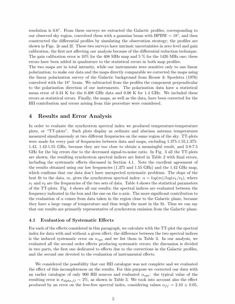
resolution is 0.6◦. From these surveys we extracted the Galactic profiles, corresponding toour observed sky region, convolved them with a gaussian beam with HPBW = 18◦, and thenconstructed the differential profiles by simulating the observation strategy; the profiles areshown in Figs. 2e and 2f. These two surveys have intrinsic uncertainties in zero level and gaincalibration, the first not affecting our analysis because of the differential reduction technique.The gain calibration error is 10% for the 408 MHz map and 5 % for the 1420 MHz one; theseerrors have been added in quadrature to the statistical errors in both map profiles.The two maps are in total intensity, while our instruments were sensitive only to one linearpolarization; to make our data and the maps directly comparable we corrected the maps usingthe linear polarization survey of the Galactic background from Brouw & Spoelstra (1976)convolved with the 18◦ beam. We subtracted from the profiles the component perpendicularto the polarization direction of our instruments. The polarization data have a statisticalmean error of 0.34 K for the 0.408 GHz data and 0.06 K for 1.4 GHz. We included theseerrors as statistical errors. Finally, the maps, as well as the data, have been corrected for theHII contribution and errors arising from this procedure were considered.

4 Results and Error Analysis

In order to evaluate the synchrotron spectral index we produced temperature-temperatureplots, or “TT-plots”. Such plots display as ordinate and abscissa antenna temperaturesmeasured simultaneously at two different frequencies on the same region of the sky. TT-plotswere made for every pair of frequencies between data and maps, excluding 1.375-1.55,1.375-1.42, 1.42-1.55 GHz, because they are too close to obtain a meaningful result, and 3.8-7.5GHz for the big errors due to the decreased signal-to-noise ratio. In Fig. 3 all the TT-plotsare shown; the resulting synchrotron spectral indices are listed in Table 2 with final errors,including the systematic effects discussed in Section 4.1. Note the excellent agreement ofthe results obtained using our low frequencies (1.375 and 1.55 GHz) and the 1.42 GHz map,which confirms that our data don’t have unexpected systematic problems. The slope of thebest fit to the data, m, gives the synchrotron spectral index: α = log(m)/log(ν1/ν2), whereν1 and ν2 are the frequencies of the two sets of data. Table 4 shows the statistical parametersof the TT-plots. Fig. 4 shows all our results; the spectral indices are evaluated between thefrequency indicated in the box and the one on the x-axis. The more significant contribution tothe evaluation of α comes from data taken in the region close to the Galactic plane, becausethey have a large range of temperature and thus weigh the most in the fit. Thus we can saythat our results are primarily representative of synchrotron emission from the Galactic plane.

4.1 Evaluation of Systematic Effects

For each of the effects considered in this paragraph, we calculate with the TT-plot the spectralindex for data with and without a given effect; the difference between the two spectral indicesis the induced systematic error on αsyn and we list them in Table 3. In our analysis, weevaluated all the second order effects producing systematic errors; the discussion is dividedin two parts, the first one dedicated to effects due to the corrections in the Galactic profiles,and the second one devoted to the evaluation of instrumental effects.

We considered the possibility that our HII catalogue was not complete and we evaluatedthe effect of this incompleteness on the results. For this purpose we corrected our data withan earlier catalogue of only 900 HII sources and evaluated αsyn: the typical value of theresulting error is σalpha,ff ∼ 2%, as shown in Table 3. We took into account also the effectproduced by an error on the free-free spectral index, considering values αff = 2.10 ± 0.05,

5

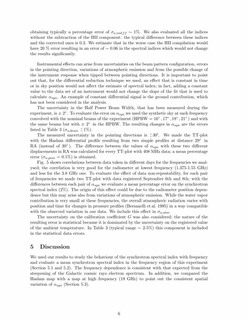
obtaining typically a percentage error of σα,ind,ff ∼ 1%. We also evaluated all the indiceswithout the subtraction of the HII component: the typical difference between these indicesand the corrected ones is 0.3. We estimate that in the worse case the HII compilation wouldhave 20 % error resulting in an error of ∼ 0.06 in the spectral indices which would not changethe results significantly.

Instrumental effects can arise from uncertainties on the beam pattern configuration, errorsin the pointing direction, variations of atmospheric emission and from the possible change ofthe instrument response when tipped between pointing directions. It is important to pointout that, for the differential reduction technique we used, an effect that is constant in timeor in sky position would not affect the estimate of spectral index; in fact, adding a constantvalue to the data set of an instrument would not change the slope of the fit that is used tocalculate αsyn. An example of constant differential signal is the ground contribution, whichhas not been considered in the analysis.

The uncertainty in the Half Power Beam Width, that has been measured during theexperiment, is ± 2◦. To evaluate the error on αsyn we used the synthetic sky at each frequencyconvolved with the nominal beams of the experiment (HPBW = 16◦ , 17◦ , 18◦ , 21◦ ) and withthe same beams but with ± 2◦ in the HPBW. The resulting changes in αsyn are the errorslisted in Table 3 (σα,beam

<∼

1%).The measured uncertainty in the pointing directions is <

∼30′. We made the TT-plot

with the Haslam differential profile resulting from two simple profiles at distance 29◦ inRA (instead of 30◦ ). The difference between the values of αsyn with these two differentdisplacements in RA was calculated for every TT-plot with 408 MHz data; a mean percentageerror (σα,poin = 0.1%) is obtained.

Fig. 5 shows correlations between data taken in different days for the frequencies we anal-ysed; the correlation is very good for the radiometer at lowest frequency (1.375-1.55 GHz)and less for the 3.8 GHz one. To evaluate the effect of data non-repeatability, for each pairof frequencies we made two TT-plot with data registered September 6th and 8th; with thedifferences between each pair of αsyn we evaluate a mean percentage error on the synchrotronspectral index (2%). The origin of this effect could be due to the radiometer position depen-dence but this may arise also from variations of atmospheric emission. While the water vaporcontribution is very small at these frequencies, the overall atmospheric radiation varies withposition and time for changes in pressure profiles (Bersanelli et al. 1995) in a way compatiblewith the observed variation in our data. We include this effect in σα,atm.

The uncertainty on the calibration coefficient G was also considered; the nature of theresulting error is statistical because it is dominated by the uncertainty on the registered valueof the ambient temperature. In Table 3 (typical range ∼ 2-5%) this component is includedin the statistical data errors.

5 Discussion

We used our results to study the behaviour of the synchrotron spectral index with frequencyand evaluate a mean synchrotron spectral index in the frequency region of this experiment(Section 5.1 and 5.2). The frequency dependence is consistent with that expected from thesteepening of the Galactic cosmic rays electron spectrum. In addition, we compared theHaslam map with a map at high frequency (19 GHz) to point out the consistent spatialvariation of αsyn (Section 5.3).

6

5.1 Frequency Variation

As discussed in Section 1, synchrotron radiation arises from cosmic ray electrons; the inter-stellar energy spectrum does not have a constant slope, but steepens at an energy of ∼ 10-20GeV. In fact cosmic ray electrons lose energy with different mechanisms: at energies <

∼10-20

GeV they escape from the Galaxy, for E >∼

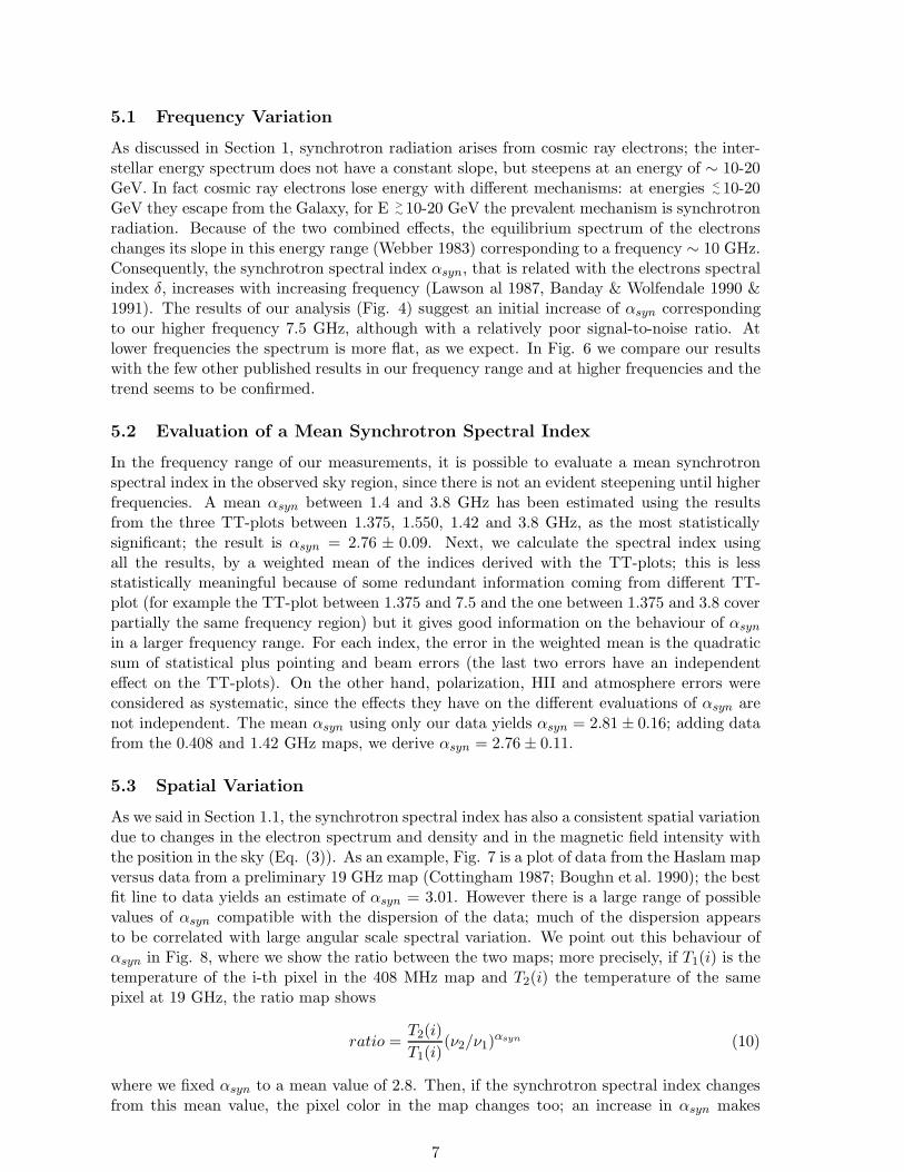
10-20 GeV the prevalent mechanism is synchrotronradiation. Because of the two combined effects, the equilibrium spectrum of the electronschanges its slope in this energy range (Webber 1983) corresponding to a frequency ∼ 10 GHz.Consequently, the synchrotron spectral index αsyn, that is related with the electrons spectralindex δ, increases with increasing frequency (Lawson al 1987, Banday & Wolfendale 1990 &1991). The results of our analysis (Fig. 4) suggest an initial increase of αsyn correspondingto our higher frequency 7.5 GHz, although with a relatively poor signal-to-noise ratio. Atlower frequencies the spectrum is more flat, as we expect. In Fig. 6 we compare our resultswith the few other published results in our frequency range and at higher frequencies and thetrend seems to be confirmed.

5.2 Evaluation of a Mean Synchrotron Spectral Index

In the frequency range of our measurements, it is possible to evaluate a mean synchrotronspectral index in the observed sky region, since there is not an evident steepening until higherfrequencies. A mean αsyn between 1.4 and 3.8 GHz has been estimated using the resultsfrom the three TT-plots between 1.375, 1.550, 1.42 and 3.8 GHz, as the most statisticallysignificant; the result is αsyn = 2.76 ± 0.09. Next, we calculate the spectral index usingall the results, by a weighted mean of the indices derived with the TT-plots; this is lessstatistically meaningful because of some redundant information coming from different TT-plot (for example the TT-plot between 1.375 and 7.5 and the one between 1.375 and 3.8 coverpartially the same frequency region) but it gives good information on the behaviour of αsyn

in a larger frequency range. For each index, the error in the weighted mean is the quadraticsum of statistical plus pointing and beam errors (the last two errors have an independenteffect on the TT-plots). On the other hand, polarization, HII and atmosphere errors wereconsidered as systematic, since the effects they have on the different evaluations of αsyn arenot independent. The mean αsyn using only our data yields αsyn = 2.81 ± 0.16; adding datafrom the 0.408 and 1.42 GHz maps, we derive αsyn = 2.76 ± 0.11.

5.3 Spatial Variation

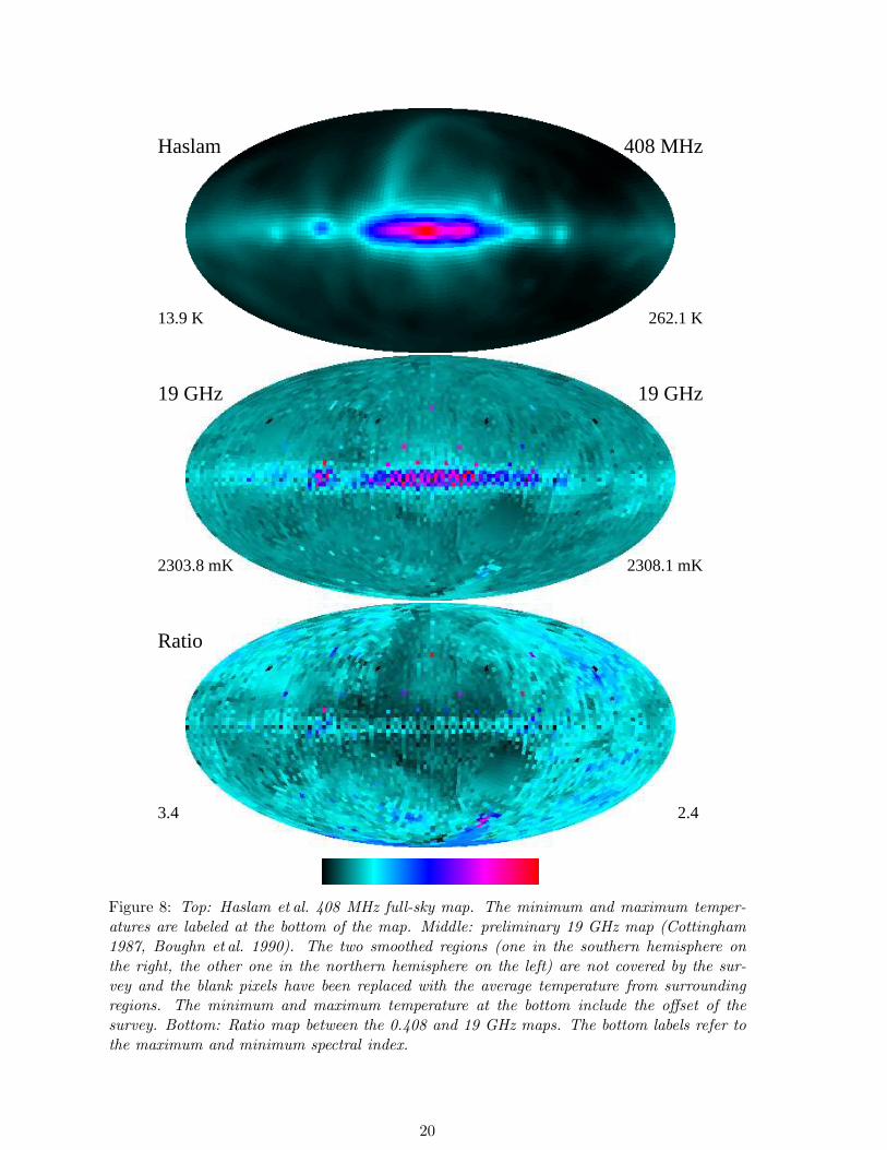
As we said in Section 1.1, the synchrotron spectral index has also a consistent spatial variationdue to changes in the electron spectrum and density and in the magnetic field intensity withthe position in the sky (Eq. (3)). As an example, Fig. 7 is a plot of data from the Haslam mapversus data from a preliminary 19 GHz map (Cottingham 1987; Boughn et al. 1990); the bestfit line to data yields an estimate of αsyn = 3.01. However there is a large range of possiblevalues of αsyn compatible with the dispersion of the data; much of the dispersion appearsto be correlated with large angular scale spectral variation. We point out this behaviour ofαsyn in Fig. 8, where we show the ratio between the two maps; more precisely, if T1(i) is thetemperature of the i-th pixel in the 408 MHz map and T2(i) the temperature of the samepixel at 19 GHz, the ratio map shows

ratio =T2(i)

T1(i)(ν2/ν1)

αsyn (10)

where we fixed αsyn to a mean value of 2.8. Then, if the synchrotron spectral index changesfrom this mean value, the pixel color in the map changes too; an increase in αsyn makes

7

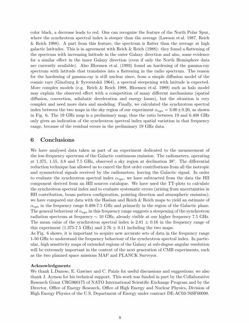
color black, a decrease leads to red. One can recognize the feature of the North Polar Spur,where the synchrotron spectral index is steeper than the average (Lawson et al. 1987, Reich& Reich 1988). A part from this feature, the spectrum is flatter than the average at highgalactic latitudes. This is in agreement with Reich & Reich (1988): they found a flattening ofthe spectrum with increasing latitude in the outer Galaxy direction and also, some evidencefor a similar effect in the inner Galaxy direction (even if only the North Hemisphere dataare currently available). Also Bloemen et al. (1993) found an hardening of the gamma-rayspectrum with latitude that translates into a flattening in the radio spectrum. The reasonfor the hardening of gamma-ray is still unclear since, from a simple diffusion model of thecosmic rays (Ginzburg & Syrovatskii 1964), a spectral steepening with latitude is expected.More complex models (e.g. Reich & Reich 1988, Bloemen et al. 1989) such as halo modelmay explain the observed effect with a competition of many different mechanisms (spatialdiffusion, convection, adiabatic deceleration and energy losses), but the situation is verycomplex and need more data and modeling. Finally, we calculated the synchrotron spectralindex between the two maps in the sky region of our experiment αsyn = 3.00±0.20, as shownin Fig. 6. The 19 GHz map is a preliminary map, thus the ratio between 19 and 0.408 GHzonly gives an indication of the synchrotron spectral index spatial variation in that frequencyrange, because of the residual errors in the preliminary 19 GHz data.

6 Conclusions

We have analysed data taken as part of an experiment dedicated to the measurement ofthe low-frequency spectrum of the Galactic continuous emission. The radiometers, operatingat 1.375, 1.55, 3.8 and 7.5 GHz, observed a sky region at declination 38◦. The differentialreduction technique has allowed us to cancel the first order contributions from all the isotropicand symmetrical signals received by the radiometers, leaving the Galactic signal. In orderto evaluate the synchrotron spectral index αsyn, we have subtracted from the data the HIIcomponent derived from an HII sources catalogue. We have used the TT-plots to calculatethe synchrotron spectral index and to evaluate systematic errors (arising from uncertainties inHII contribution, beam pattern configuration, pointing direction and atmospheric emission);we have compared our data with the Haslam and Reich & Reich maps to yield an estimate ofαsyn in the frequency range 0.408-7.5 GHz and primarily in the region of the Galactic plane.The general behaviour of αsyn in this frequency range suggests a steepening of the synchrotronradiation spectrum at frequency ∼ 10 GHz, already visible at our higher frequency 7.5 GHz.The mean value of the synchrotron spectral index is 2.81 ± 0.16 in the frequency range ofthis experiment (1.375-7.5 GHz) and 2.76 ± 0.11 including the two maps.As Fig. 6 shows, it is important to acquire new accurate sets of data in the frequency range1-50 GHz to understand the frequency behaviour of the synchrotron spectral index. In partic-ular, high sensitivity maps of extended regions of the Galaxy at sub-degree angular resolutionwill be extremely important in the context of the next generation of CMB experiments, suchas the two planned space missions MAP and PLANCK Surveyor.

Acknowledgments

We thank L.Danese, E. Gawiser and C. Paizis for useful discussions and suggestions; we alsothank J. Aymon for his technical support. This work was funded in part by the CollaborativeResearch Grant CRG960175 of NATO International Scientific Exchange Program and by theDirector, Office of Energy Research, Office of High Energy and Nuclear Physics, Division ofHigh Energy Physics of the U.S. Department of Energy under contract DE-AC03-76SF00098.

8

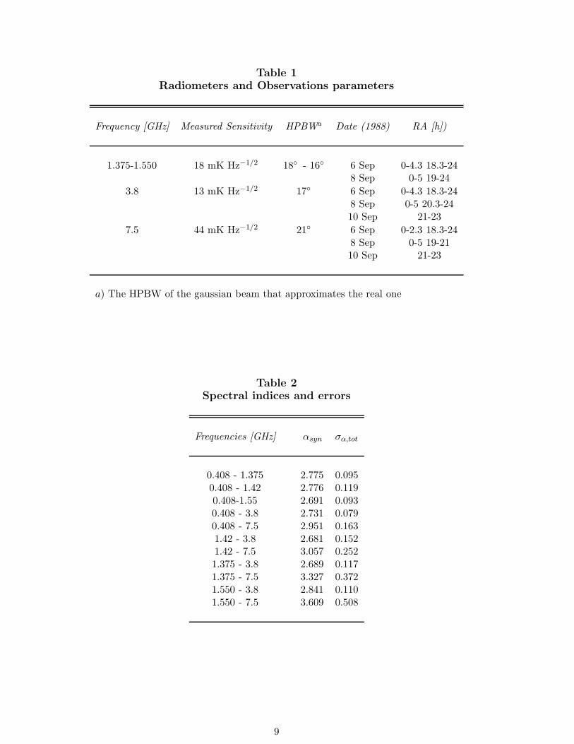
Table 1Radiometers and Observations parameters

Frequency [GHz] Measured Sensitivity HPBWa Date (1988) RA [h])

1.375-1.550 18 mK Hz−1/2 18◦ - 16◦ 6 Sep 0-4.3 18.3-248 Sep 0-5 19-24

3.8 13 mK Hz−1/2 17◦ 6 Sep 0-4.3 18.3-248 Sep 0-5 20.3-2410 Sep 21-23

7.5 44 mK Hz−1/2 21◦ 6 Sep 0-2.3 18.3-248 Sep 0-5 19-2110 Sep 21-23

a) The HPBW of the gaussian beam that approximates the real one

Table 2Spectral indices and errors

Frequencies [GHz] αsyn σα,tot

0.408 - 1.375 2.775 0.0950.408 - 1.42 2.776 0.1190.408-1.55 2.691 0.0930.408 - 3.8 2.731 0.0790.408 - 7.5 2.951 0.1631.42 - 3.8 2.681 0.1521.42 - 7.5 3.057 0.2521.375 - 3.8 2.689 0.1171.375 - 7.5 3.327 0.3721.550 - 3.8 2.841 0.1101.550 - 7.5 3.609 0.508

9

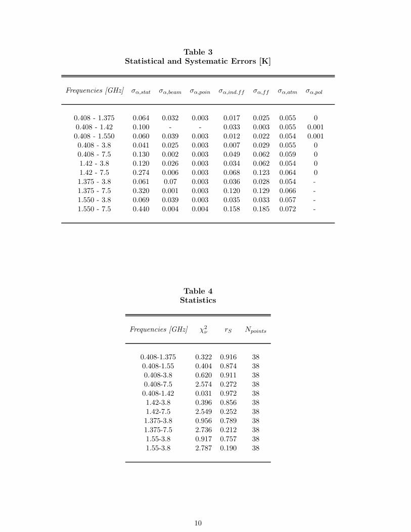
Table 3Statistical and Systematic Errors [K]

Frequencies [GHz] σα,stat σα,beam σα,poin σα,ind.ff σα,ff σα,atm σα,pol

0.408 - 1.375 0.064 0.032 0.003 0.017 0.025 0.055 00.408 - 1.42 0.100 - - 0.033 0.003 0.055 0.0010.408 - 1.550 0.060 0.039 0.003 0.012 0.022 0.054 0.0010.408 - 3.8 0.041 0.025 0.003 0.007 0.029 0.055 00.408 - 7.5 0.130 0.002 0.003 0.049 0.062 0.059 01.42 - 3.8 0.120 0.026 0.003 0.034 0.062 0.054 01.42 - 7.5 0.274 0.006 0.003 0.068 0.123 0.064 01.375 - 3.8 0.061 0.07 0.003 0.036 0.028 0.054 -1.375 - 7.5 0.320 0.001 0.003 0.120 0.129 0.066 -1.550 - 3.8 0.069 0.039 0.003 0.035 0.033 0.057 -1.550 - 7.5 0.440 0.004 0.004 0.158 0.185 0.072 -

Table 4Statistics

Frequencies [GHz] χ2ν rS Npoints

0.408-1.375 0.322 0.916 380.408-1.55 0.404 0.874 380.408-3.8 0.620 0.911 380.408-7.5 2.574 0.272 380.408-1.42 0.031 0.972 381.42-3.8 0.396 0.856 381.42-7.5 2.549 0.252 381.375-3.8 0.956 0.789 381.375-7.5 2.736 0.212 381.55-3.8 0.917 0.757 381.55-3.8 2.787 0.190 38

10

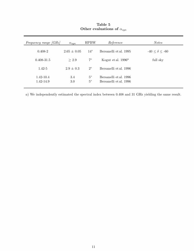
Table 5Other evaluations of αsyn

Frequency range [GHz] αsyn HPBW Reference Notes

0.408-2 2.65 ± 0.05 14◦ Bersanelli et al. 1995 -40 ≤ δ ≤ -60

0.408-31.5 ≥ 2.9 7◦ Kogut et al. 1996a full sky

1.42-5 2.9 ± 0.3 2◦ Bersanelli et al. 1996

1.42-10.4 3.4 5◦ Bersanelli et al. 19961.42-14.9 3.0 5◦ Bersanelli et al. 1996

a) We independently estimated the spectral index between 0.408 and 31 GHz yielding the same result.

11

References

??anday, A. J. & Wolfendale, A. W. 1990, MNRAS, 245, 182.??anday, A. J. & Wolfendale, A. W. 1991, MNRAS, 248, 705.??ensadoun, M. et al. 1993, ApJ, 409, 1.??ersanelli, M. et al. 1995, Astro. Lett. and Communications, 32, 7.??ersanelli, M. et al. 1995, ApJ, 448, 8.??ersanelli, M., Bouchet, F.R., Efstathiou, G., Griffin, M., Lamarre, J.M., Mandolesi, N.,

Nordgaard-Nielsen, H.U., Pace, O., Polny, J., Puget, J.L., Tauber, J., Vittorio, N., Volonte’,S. 1996, COBRAS-SAMBA: report on the phase A study, ESA.

??loemen, H. et al. 1993, Astron. Astrophys., 267, 372.??oughn, S. P.et al. 1990, Rev. Sci. Instr., 61, 158.??rouw, W. N. & Spoelstra, T. A. Th. 1976, Astron. Astrophys. Suppl. Ser., 26, 129.??ottingham, D. A. 1987, PhD thesis, Princeton Univ.??e Amici, G. et al. 1990, APJ, 359, 219.??inzburg, V. L. & Syrovatskii, S. I. 1964, The origin of the Cosmic Rays, Oxford, Perg-

amon Press.??aslam, C. G. T. et al. 1982, Astron. Astrophys. Suppl. Ser., 47, 1.??ogut, A. et al. 1990, ApJ, 355, 102.??ogut, A. et al. 1996, ApJ, 460, 1.??awson, K. D. et al. 1987, MNRAS, 225, 307.??eich, P. & Reich, W. 1986, Astron. Astrophys. Suppl. Ser., 63, 205.??eich, P. & Reich, W. 1988, Astron. Astrophys. Suppl. Ser., 74, 7.??cheffler, H. & Elsasser, H. 1987, Physics of the Galaxy and Interstellar Matter, Springer-

Verlag, Heidelberg.??moot, G. F. et al. 1985, ApJ Lett., 291, L23.??ebber, W. R. 1983, in Composition and origin of cosmic rays; Proceedings of the Ad-

vanced Study Institute, Erice, Italy, June 20-30, 1982, Dordrecth, D. Reidel Publishing Co.,83.

??itebsky, C. 1978, not published.

12

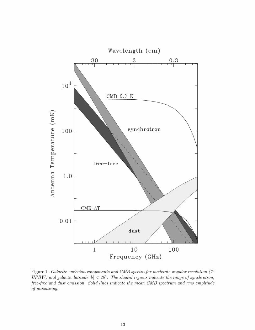
Figure 1: Galactic emission components and CMB spectra for moderate angular resolution (7◦

HPBW) and galactic latitude |b| < 20◦. The shaded regions indicate the range of synchrotron,free-free and dust emission. Solid lines indicate the mean CMB spectrum and rms amplitudeof anisotropy.

13

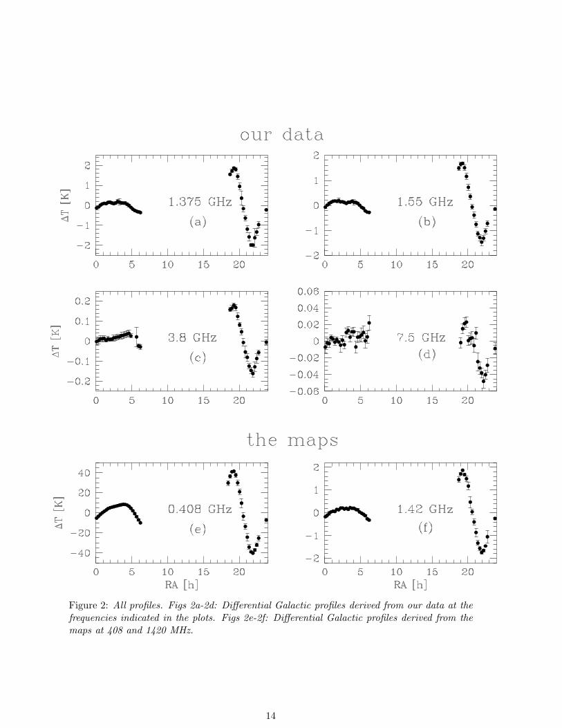
Figure 2: All profiles. Figs 2a-2d: Differential Galactic profiles derived from our data at thefrequencies indicated in the plots. Figs 2e-2f: Differential Galactic profiles derived from themaps at 408 and 1420 MHz.

14

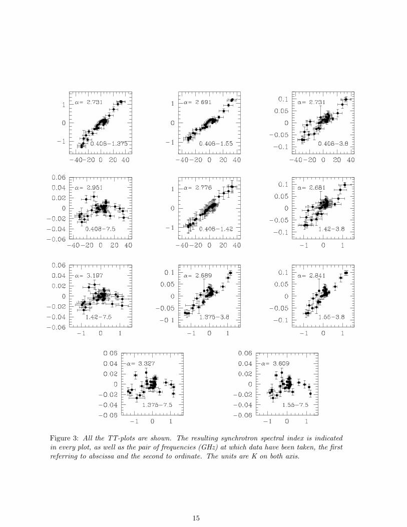
Figure 3: All the TT-plots are shown. The resulting synchrotron spectral index is indicatedin every plot, as well as the pair of frequencies (GHz) at which data have been taken, the firstreferring to abscissa and the second to ordinate. The units are K on both axis.

15

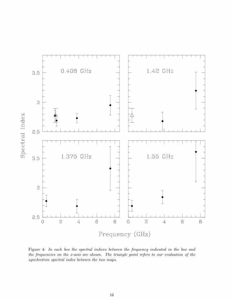
Figure 4: In each box the spectral indices between the frequency indicated in the box andthe frequencies on the x-axis are shown. The triangle point refers to our evaluation of thesynchrotron spectral index between the two maps.

16

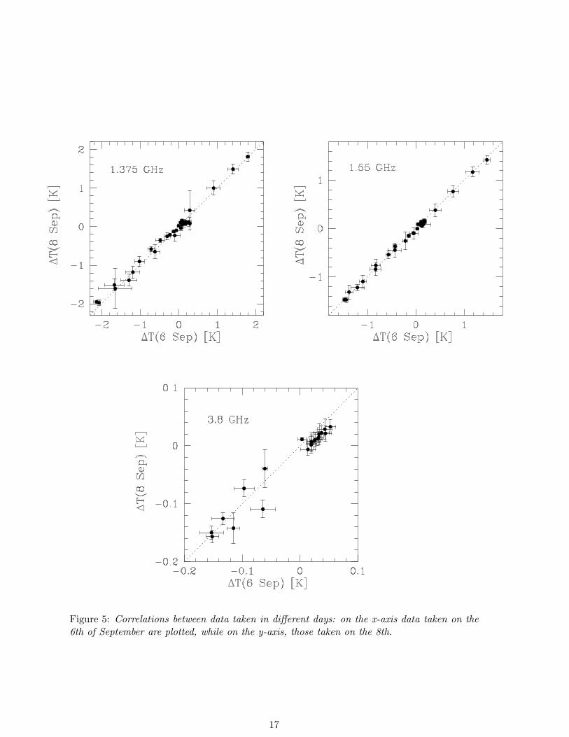
Figure 5: Correlations between data taken in different days: on the x-axis data taken on the6th of September are plotted, while on the y-axis, those taken on the 8th.

17

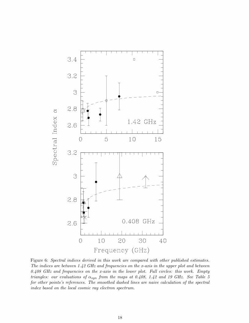
Figure 6: Spectral indices derived in this work are compared with other published estimates.The indices are between 1.42 GHz and frequencies on the x-axis in the upper plot and between0.408 GHz and frequencies on the x-axis in the lower plot. Full circles: this work. Emptytriangles: our evaluations of αsyn from the maps at 0.408, 1.42 and 19 GHz. See Table 5for other points’s references. The smoothed dashed lines are naive calculation of the spectralindex based on the local cosmic ray electron spectrum.

18

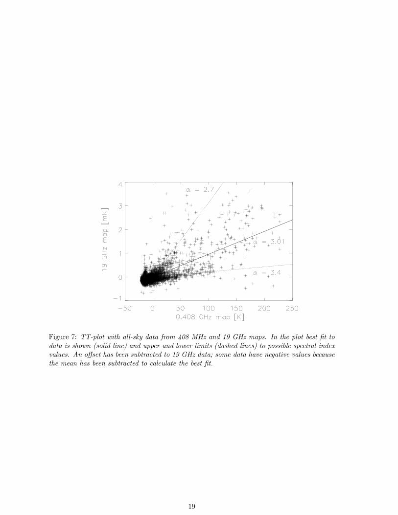
Figure 7: TT-plot with all-sky data from 408 MHz and 19 GHz maps. In the plot best fit todata is shown (solid line) and upper and lower limits (dashed lines) to possible spectral indexvalues. An offset has been subtracted to 19 GHz data; some data have negative values becausethe mean has been subtracted to calculate the best fit.

19

Haslam 408 MHz

13.9 K 262.1 K

19 GHz 19 GHz

2303.8 mK 2308.1 mK

Ratio

3.4 2.4

Figure 8: Top: Haslam et al. 408 MHz full-sky map. The minimum and maximum temper-atures are labeled at the bottom of the map. Middle: preliminary 19 GHz map (Cottingham1987, Boughn et al. 1990). The two smoothed regions (one in the southern hemisphere onthe right, the other one in the northern hemisphere on the left) are not covered by the sur-vey and the blank pixels have been replaced with the average temperature from surroundingregions. The minimum and maximum temperature at the bottom include the offset of thesurvey. Bottom: Ratio map between the 0.408 and 19 GHz maps. The bottom labels refer tothe maximum and minimum spectral index.

20