Dipartimento di Economia e Finanza Percorso Banche ed Intermediari Finanziari

Option pricing A comparison between Black-Scholes model and a Deep Learning approach

NICOLA BORRI PIERPAOLO BENIGNO

RELATORE CO-RELATORE

GIAMPAOLO TUMMINELLO

CANDIDATO

ANNO ACCADEMICO 2018/2019

2

Un sentito ringraziamento al Professor Borri,

per avermi permesso di realizzare un elaborato

i cui temi sento profondamente vicini.

Ai miei genitori, che mi hanno incondizionatamente

sostenuto ed aiutato in ogni mia scelta,

rendendomi la persona che sono oggi.

A Lisa, per la sua immensa pazienza e

per la forza e l’amore che mi ha trasmesso

lungo tutto il mio percorso universitario.

A John von Neumann, fonte di ispirazione e motivazione.

3

Contents

Introduction ...................................................................................................................................................... 4

Literature review ............................................................................................................................................. 6

Artificial neural network literature.................................................................................................... 6

Option pricing literature ..................................................................................................................... 7

Theoretical Part ............................................................................................................................................... 9

Option fundamentals ........................................................................................................................... 9

Volatility .............................................................................................................................................. 12

Black- Scholes-Merton model ........................................................................................................... 14

Hypothesis ................................................................................................................................. 17

Deep Learning models ....................................................................................................................... 18

Feedforward Neural Networks ................................................................................................ 20

Backprogragation algorithm ................................................................................................... 22

Gradient-based Optimization .................................................................................................. 25

Activation functions ................................................................................................................. 27

Empirical Part ................................................................................................................................................ 28

Data and environments ...................................................................................................................... 28

On volatility ............................................................................................................................... 32

Performance metrics .......................................................................................................................... 33

Implementing Black-Scholes model ................................................................................................. 35

Neural network architecture ............................................................................................................. 37

Results ................................................................................................................................................. 40

Critical issues ...................................................................................................................................... 43

Conclusions ..................................................................................................................................................... 44

References ....................................................................................................................................................... 45

Summary ........................................................................................................................................................ 48

Chapter 1

Introduction

A system can be considered a group of variable interconnected interacting each other in a defined

environment1. Building a model means attempting to describe a system using abstract concepts and logical

language. One example of this concept is the financial market, an economic system in which financial

securities and derivatives are traded. There are many mathematical models trying to describe and abstracting

how the financial market and all its components work. The history of modern mathematical finance can be

brought back to the work of Louis Bachelier (1900), Théorie de la speculation2, in which is introduced the

stochastic process called Brownian motion and its use for stock options pricing. Later, in 1973, starting from

the assumption that stock prices follow a geometric Brownian motion, Fischer Black and Myron Scholes

published their famous and influential paper The Pricing of Options and Corporate Liabilities3, where a closed

formula for European option pricing is given, solving a parabolic partial differential equation, with initial

conditions based on continuous “Delta-hedging”. After, many authors tried to improve the Black-Scholes

model, by relaxing the assumption on volatility (Scott, 1987 ) (Heston, 1993) , or using other methods such as

Monte Carlo simulation (Boyle, 1977). Nevertheless, between all mathematical (parametric) models for option

pricing, the Black-Scholes model is still the most used in practice, due to its ease of implementation and

simplicity of interpretation. With the informatic revolution in the new millennium and the rise of technological

giants, the advent of Big Data changed the way data was analysed and how models were built. After a period,

called the “AI winter”, with fresh projects such as IBM Watson (High, 2012) , AlphaGo (Silver et al., 2016),

and OpenAI Five (Berner et al., 2019), a new series of models, mostly derived from statistics and linear

algebra, started to be used in practice in many fields. For instance, in the financial area, they’re currently used

for cluster analysis (Şchiopu, 2010), portfolio management (Liu et al., 2011), credit risk evaluation (Angelini

et al., 2008), and asset pricing. As concerns pricing, a vast amount of literature has compared mathematical

models with machine learning and deep learning methods for derivates pricing. Hutchinson et al. (1994)4

proposed a non-parametric approach, using artificial neural networks for pricing and hedging derivatives,

trying to replicate the Black-Scholes formula, but without the same restrictions in hypothesis. Other studies

used deep learning specifically to relax the hypothesis of Black-Scholes model about volatility and showed

that a semi-parametric model can outperform Black-Scholes model when an option is strongly in the money

or strongly out of the money (Baruníkova & Baruník, 2011).

Although, none of the literature cited used the same variables when comparing mathematical models against

artificial neural networks or machine learning models. This thesis aims to compare a simple feed forward

1 https://www.merriam-webster.com/dictionary/system 2 Bachelier, L. (1900a), Théorie de la spéculation, Annales Scientifiques de l'École Normale Supérieure, 3. 3 Black, F.; Scholes, M. (1973), The Pricing of Options and Corporate Liabilities, Journal of Political Economy, 81. 4 Hutchinson, J. M., A. W. Lo, & T. Poggio (1994), A nonparametric approach to pricing and hedging derivative securities via

learning networks, The Journal of Finance 49 (3)

5

neural network with the Black-Scholes model, using for both models the same variables:

𝑺 : the underlying price;

𝑲 : the strike price of the option;

𝑻 : the time to maturity;

𝝈 : the volatility of the option;

R : the risk free interest rate5.

The next chapter will review some of the most important literature, useful for the contextualization of the

thesis. The third chapter is a review of the main topics and hypothesis concerning neural networks and

mathematical models for option pricing. In the second part, the study is explained, giving attention on the

structure of the dataset used, the implementation of the two models, the results and the critical issues found.

5 Dividends expected or already payed are not considered both for simplicity of treatment and lack of specific data.

6

Chapter 2

Literature review

Artificial neural network literature

Warren McCulloch and Walter Pitts (1943)6 showed that simple neural network has the ability to

approximate any arithmetic function. This concept is the base on which the later literature on artificial neural

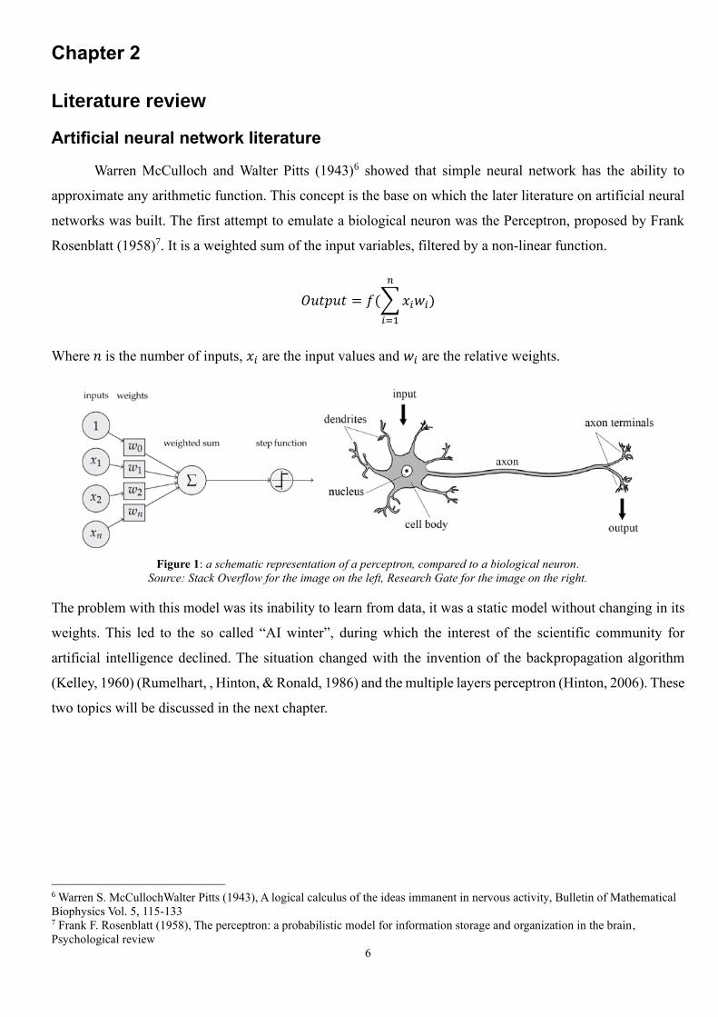
networks was built. The first attempt to emulate a biological neuron was the Perceptron, proposed by Frank

Rosenblatt (1958)7. It is a weighted sum of the input variables, filtered by a non-linear function.

𝑂𝑢𝑡𝑝𝑢𝑡 = 𝑓(∑ 𝑥𝑖𝑤𝑖

𝑛

𝑖=1

)

Where 𝑛 is the number of inputs, 𝑥𝑖 are the input values and 𝑤𝑖 are the relative weights.

Figure 1: a schematic representation of a perceptron, compared to a biological neuron.

Source: Stack Overflow for the image on the left, Research Gate for the image on the right.

The problem with this model was its inability to learn from data, it was a static model without changing in its

weights. This led to the so called “AI winter”, during which the interest of the scientific community for

artificial intelligence declined. The situation changed with the invention of the backpropagation algorithm

(Kelley, 1960) (Rumelhart, , Hinton, & Ronald, 1986) and the multiple layers perceptron (Hinton, 2006). These

two topics will be discussed in the next chapter.

6 Warren S. McCullochWalter Pitts (1943), A logical calculus of the ideas immanent in nervous activity, Bulletin of Mathematical

Biophysics Vol. 5, 115-133 7 Frank F. Rosenblatt (1958), The perceptron: a probabilistic model for information storage and organization in the brain,

Psychological review

7

Option pricing literature

As discussed before, the most influential paper can be considered The Pricing of Options and

Corporate Liabilities by Fisher Black and Myron Scholes (1973), later expanded by Robert Merton in his

Theory of Rational Option Pricing8. Their work legitimized and contributed to the spread of the Chicago Board

Options Exchange, established in 1973, which uses standardized contracts guaranteed by a clearing house. All

the variables in the Black-Scholes model are unequivocally observable, except the volatility, which is non-

constant and must be deduced with various methods (that will be discussed later). Heston (1993)9 tried to avoid

this problem by modelling the volatility with a stochastic process based on a Brownian motion. Other methods

use Fast Fourier transform (Carr & Madan, 1999) or Jump diffusion processes (Kou, 2002).

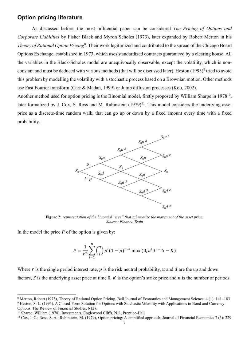
Another method used for option pricing is the Binomial model, firstly proposed by William Sharpe in 197810,

later formalized by J. Cox, S. Ross and M. Rubinstein (1979)11. This model considers the underlying asset

price as a discrete-time random walk, that can go up or down by a fixed amount every time with a fixed

probability.

Figure 2: representation of the binomial “tree” that schematize the movement of the asset price.

Source: Finance Train

In the model the price 𝑃 of the option is given by:

𝑃 =1

𝑟𝑛∑ (

𝑛

𝑖) 𝑝𝑖(1 − 𝑝)𝑛−𝑖

𝑛

𝑖=1

max (0, 𝑢𝑖𝑑𝑛−𝑖𝑆 − 𝐾)

Where 𝑟 is the single period interest rate, 𝑝 is the risk neutral probability, 𝑢 and 𝑑 are the up and down

factors, 𝑆 is the underlying asset price at time 0, 𝐾 is the option’s strike price and 𝑛 is the number of periods

8 Merton, Robert (1973), Theory of Rational Option Pricing, Bell Journal of Economics and Management Science. 4 (1): 141–183 9 Heston, S. L. (1993). A Closed-Form Solution for Options with Stochastic Volatility with Applications to Bond and Currency

Options. The Review of Financial Studies, 6 (2). 10 Sharpe, William (1978), Investments, Englewood Cliffs, N.J., Prentice-Hall 11 Cox, J. C.; Ross, S. A.; Rubinstein, M. (1979), Option pricing: A simplified approach, Journal of Financial Economics 7 (3): 229

8

considered. It can be demonstrated that, under similar assumptions, the binomial distribution of the binomial

model converges to the lognormal distribution assumed by Black-Scholes model, thus, in this perspective,

the binomial model can be considered a discrete time approximation of the continuous process in the Black-

Scholes model (Leisen & Reimer, 2006) (Chance, 2008). Technical features of European options and Black-

Scholes model are discussed in the next chapter.

9

Chapter 3

Theoretical Part

Option fundamentals

A European option is a contract which gives the owner (the holder or the buyer) the right, but not the duty,

to buy (or sell) an underlying asset at a specified price (strike price) and at specified date (expiration date,

exercise date or maturity). The other part involved in the contract (the seller) has the obligation to sell (or buy)

the underlying asset if the buyer exercises her right. Buyers are referred to as having long positions, sellers as

having short positions. In the case the holder has the right to buy the underlying instrument, the option is

referred to as Call option, in the opposite case it’s called Put option. The two counterparties must specify in

the contract:

• the type of option: Call or Put;

• the quantity of the underlying asset;

• the strike price (𝐾);

• the expiration date (𝑇).

The price of the underlying asset (𝑆0) is not considered at the time of the stipulation of the contract (except for

pricing purposes), because the underlying price matters only at the settlement date (or expiration date), when

the option can be exercised.

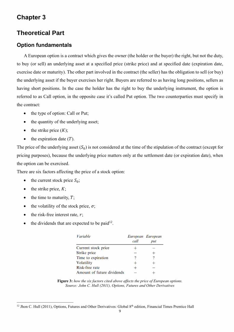
There are six factors affecting the price of a stock option:

• the current stock price 𝑆0;

• the strike price, 𝐾;

• the time to maturity, 𝑇;

• the volatility of the stock price, 𝜎;

• the risk-free interest rate, 𝑟;

• the dividends that are expected to be paid12.

Figure 3: how the six factors cited above affects the price of European options.

Source: John C. Hull (2011), Options, Futures and Other Derivatives

12 Jhon C. Hull (2011), Options, Futures and Other Derivatives: Global 8th edition, Financial Times Prentice Hall

10

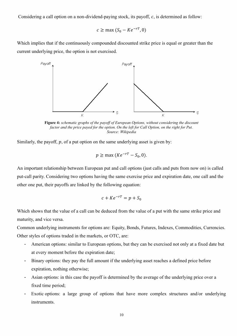
Considering a call option on a non-dividend-paying stock, its payoff, 𝑐, is determined as follow:

𝑐 ≥ max (𝑆0 − 𝐾𝑒−𝑟𝑇, 0)

Which implies that if the continuously compounded discounted strike price is equal or greater than the

current underlying price, the option is not exercised.

Figure 4: schematic graphs of the payoff of European Options, without considering the discount

factor and the price payed for the option. On the left for Call Option, on the right for Put.

Source: Wikipedia

Similarly, the payoff, 𝑝, of a put option on the same underlying asset is given by:

𝑝 ≥ max (𝐾𝑒−𝑟𝑇 − 𝑆0, 0).

An important relationship between European put and call options (just calls and puts from now on) is called

put-call parity. Considering two options having the same exercise price and expiration date, one call and the

other one put, their payoffs are linked by the following equation:

𝑐 + 𝐾𝑒−𝑟𝑇 = 𝑝 + 𝑆0

Which shows that the value of a call can be deduced from the value of a put with the same strike price and

maturity, and vice versa.

Common underlying instruments for options are: Equity, Bonds, Futures, Indexes, Commodities, Currencies.

Other styles of options traded in the markets, or OTC, are:

- American options: similar to European options, but they can be exercised not only at a fixed date but

at every moment before the expiration date;

- Binary options: they pay the full amount if the underlying asset reaches a defined price before

expiration, nothing otherwise;

- Asian options: in this case the payoff is determined by the average of the underlying price over a

fixed time period;

- Exotic options: a large group of options that have more complex structures and/or underlying

instruments.

11

Most of the literature that will be cited in this thesis regards the pricing of European options, because other

styles of option do not fall within the scope of this discussion. From now on, with the term option will be

indicated a European option.

12

Volatility

Volatility is defined in this context as the variation of the price of a financial instrument over time. It

is generally measured by standard deviation of log-returns. It can be estimated using various methods. The

first method, the historical volatility, consists in calculating the standard deviation of the stock log-return over

some period:

𝜎𝐻 = √1

𝑇 − 1∑ 𝑠𝑡 − �̅�

𝑇

𝑡=1

Where 𝜎𝐻 is the historical volatility estimator, T is the total period considered, 𝑠𝑡 is the stock log-return in the

period t, �̅� is the average of all the stock log-returns considered. The returns are calculated as follow:

𝑠𝑡 = ln (𝑆𝑡

𝑆𝑡−1)

Where 𝑆𝑡 is the stock price at the time 𝑡. Some problems about this method are highlighted by Figlewski

(1994), such as the serial correlation in returns and the variation of volatility over time. Other methods involve

GARCH models (Bollerslev, 1986), the simplest of which is GARCH(1,1), in which the unconditional

volatility is given by the following relationship:

𝜎𝑡2 = 𝜔 + 𝛼𝜎𝑡−1

2 + 𝛽𝜀𝑡−12

Where 𝜔, 𝛼, 𝛽 are the estimation parameters and 𝜀𝑡−12 are squared residuals. Some studies have shown that

using neural networks can improve the forecasting performance of GARCH models for volatility

(Kristjanpolle, Fadic, & Minutolo, 2014).

Another method for volatility estimation involves the so-called Implied volatility (IV). It derives directly from

the Black-Scholes model as the inverse function of the pricing model:

𝑃 = 𝑓(𝜎, ∙) , 𝜎𝐼𝑉 = 𝑔(𝑃, ∙)

Where P is the price of the option, 𝑓(∙) is the pricing model, 𝑔(∙) is its inverse function of 𝑓 and 𝜎𝐼𝑉 is the

estimator of the implied volatility. The inversion is possible because 𝑓(∙) is monotonically increasing in 𝜎, so

the inverse function theorem can be applied. However, this method doesn’t have a closed form solution and

an approximation method must be used, such as Newton’s method.

Deep learning models have been developed to approximate the implied volatility and make predictions about

future volatility, such as in Malliaris and Salchenberger 199613.

13 Malliaris, Mary and Salchenberger, Linda (2004), Using neural networks to forecast the S&P 100 implied volatility, Elsevier

Vol. 10 (2): 183-195

13

In his The misbehaviour of markets, Benoit Mandelbrot (2004)14 states that saying that “volatility is easier to

predict than prices” is an heresy. The statement highlights how is important to consider carefully how the

volatility is calculated when pricing an instrument.

14 Mandelbrot, Benoit (2004), The Misbehavior of Markets: A Fractal View of Financial Turbulence, Basic Books

14

Black- Scholes-Merton model

The model presented is the most influential model in the field of derivatives pricing, which led Robert

Merton and Myron Scholes to be awarded the Nobel Prize for economics in 1997. The following derivation

of the Black-Scholes differential equation follows the work of Robert Merton (Merton, 1973), which doesn’t

rely on the assumptions of the capital asset pricing model (Sharpe, 1964). The hypothesis of the model are

discussed in details in the next paragraph.

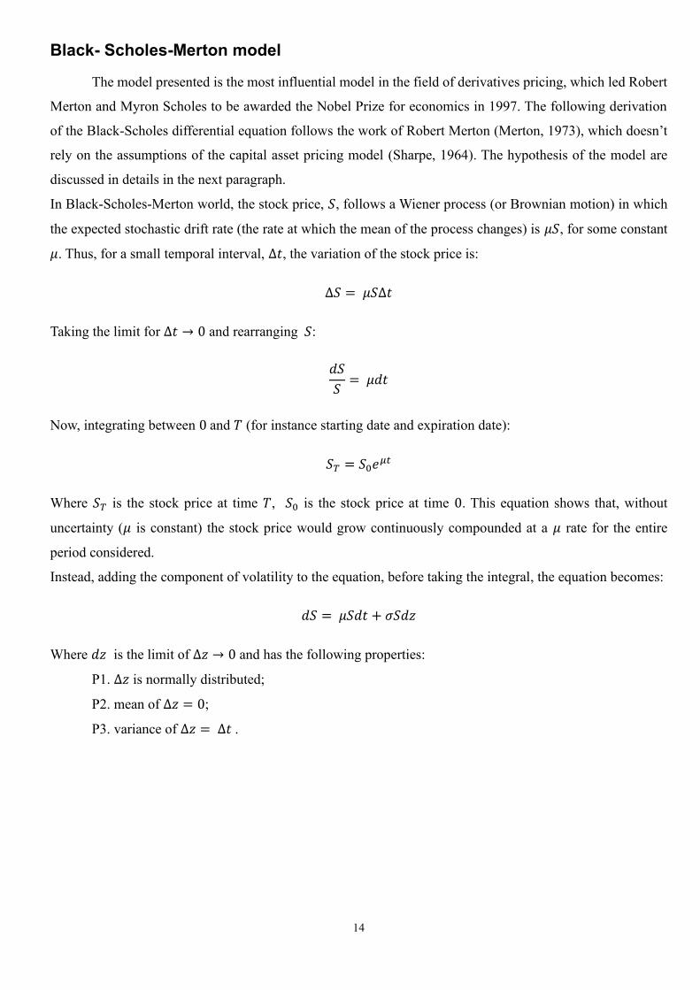
In Black-Scholes-Merton world, the stock price, 𝑆, follows a Wiener process (or Brownian motion) in which

the expected stochastic drift rate (the rate at which the mean of the process changes) is 𝜇𝑆, for some constant

𝜇. Thus, for a small temporal interval, ∆𝑡, the variation of the stock price is:

∆𝑆 = 𝜇𝑆∆𝑡

Taking the limit for ∆𝑡 → 0 and rearranging 𝑆:

𝑑𝑆

𝑆= 𝜇𝑑𝑡

Now, integrating between 0 and 𝑇 (for instance starting date and expiration date):

𝑆𝑇 = 𝑆0𝑒𝜇𝑡

Where 𝑆𝑇 is the stock price at time 𝑇, 𝑆0 is the stock price at time 0. This equation shows that, without

uncertainty (𝜇 is constant) the stock price would grow continuously compounded at a 𝜇 rate for the entire

period considered.

Instead, adding the component of volatility to the equation, before taking the integral, the equation becomes:

𝑑𝑆 = 𝜇𝑆𝑑𝑡 + 𝜎𝑆𝑑𝑧

Where 𝑑𝑧 is the limit of ∆𝑧 → 0 and has the following properties:

P1. ∆𝑧 is normally distributed;

P2. mean of ∆𝑧 = 0;

P3. variance of ∆𝑧 = ∆𝑡 .

15

Figure 5: representation of some of the possible trajectories of a geometric Brownian motion.

Source: simulation in Python 3.7

Now, supposing 𝐶 the price of a call on the stock considered before. 𝐶 has to be some function of 𝑆. By

applying the Itō’s Lemma for stochastic calculus (Itō, 1951), it can be demonstrated that the following

relationship subsist:

𝑑𝐶 = (𝜕𝐶

𝜕𝑆𝜇𝑆 +

𝜕𝐶

𝜕𝑡+

1

2

𝜕2𝐶

𝜕𝑆2𝜎2𝑆2) 𝑑𝑡 +

𝜕𝐶

𝜕𝑆𝜎𝑆𝑑𝑧

Consider a portfolio built with the option and the underlying asset, such that there is a short position in one

option and a long position in +𝜕𝐶

𝜕𝑆 stocks. The value of such portfolio is:

𝒫 = −𝐶 +𝜕𝐶

𝜕𝑆𝑆

The variation of 𝒫 at an infinitesimal time is:

𝑑𝒫 = −𝑑𝐶 +𝜕𝐶

𝜕𝑆𝑑𝑆

And substituting the equation for 𝑑𝐶 and 𝑑𝑆 written before:

𝑑𝒫 = (−𝜕𝐶

𝜕𝑡−

1

2

𝜕2𝐶

𝜕𝑆2𝜎2𝑆2) 𝑑𝑡

Because this equation doesn’t have 𝑑𝑧, for the same argument stated for 𝑑𝑆 without considering 𝑑𝑧 , the

portfolio is riskless during 𝑑𝑡 and, given 𝑟 as the constant risk-free rate:

𝑑𝒫 = 𝑟𝒫𝑑𝑡

16

Now, substituting in the precedent equation, simplifying for 𝑑𝑡, the Black-Scholes-Merton parabolic

differential equation is obtained:

𝑟𝐶 =𝜕𝐶

𝜕𝑡+

𝜕𝐶

𝜕𝑆𝑟𝑆 +

1

2

𝜕2𝐶

𝜕𝑆2𝜎2𝑆2

To solve the equation the boundary conditions must be specified. In this case is considered:

𝐶 = max (𝑆 − 𝐾, 0), when 𝑡 = 𝑇

for a call option and:

𝐶 = max (𝐾 − 𝑆, 0), when 𝑡 = 𝑇

for a put option.

Under these boundary conditions, it is possible to derive a closed form solution both for call, 𝑐, and put, 𝑝,

options:

𝑐 = 𝑆0𝑁(𝑑1) − 𝐾 𝐾𝑒−𝑟𝜏𝑁(𝑑2)

𝑝 = 𝐾𝑒−𝑟𝜏𝑁(−𝑑2) − 𝑆0𝑁(−𝑑1)

Where 𝜏 = 𝑇 − 𝑡, 𝑁(∙) is the cumulative probability distribution function of the standardized normal

distribution, 𝑑1 and 𝑑2 are defined as:

𝑑1 =𝑙𝑛 (𝑆0 𝐾)⁄ + (𝑟 + 𝜎2 2⁄ )𝜏

𝜎√𝜏

𝑑1 = 𝑑1 − 𝜎√𝜏 =𝑙𝑛 (𝑆0 𝐾)⁄ + (𝑟 − 𝜎2 2⁄ )𝜏

𝜎√𝜏

It’s important to notice how risk-preferences of individuals are not involved in the above formulas, hence they

can’t affect the solution. This lead to a Black-Scholes-Merton world where all investors can be considered

Risk-Neutral, though this is just an expedient to obtain the solution of the differential equation. In fact, the

formulas above can be applied (and are applied) in many real-world scenarios.

From the model presented the implied volatility can be calculated, inverting the function 𝑐(𝜎, ∙) or 𝑝(𝜎, ∙)

for 𝜎𝐼𝑉 and using numerical methods in order to solve the new equation found. The implied volatility,

automatically calculated in this manner for every option in the dataset, will be used in the development and

implementation of both the Black-Scholes model and the neural network architecture in the empirical part of

the thesis.

17

Hypothesis

The assumptions implied when deriving the Black–Scholes–Merton differential equation are:

i. the stock price follows a Brownian motion with constant 𝜇 and 𝜎;

ii. short selling is allowed;

iii. all instruments are perfectly divisible and infinitely available;

iv. there are no market frictions, such as transactions costs or taxes;

v. no dividends are paid during the life of the derivative;

vi. there are no arbitrage opportunities, neither type I nor type II;

vii. securities trading is in continuous time;

viii. the risk-free rate is constant and the same for all expiration dates.

The first assumption, described in a rigorous way in the above paragraph, can be relaxed assuming that also

volatility follows a Brownian motion, like in Hull, White (1987)15 and Heston (1993). The second hypothesis

allows to consider both positive and negative numbers and, combined with the third assumption, permits to

use all Real numbers, ℝ, in the development of the model, simplifying the approach. Fourth and fifth

assumptions have been relaxed in the literature, leading to more complex models involving, in the case of

growing dividends, the rate of growth, 𝑞, which is incorporated in the formula. The presence of transaction

costs has been addressed by Leland (1985)16, who started with discrete time and considered a proportional

costs model, adjusting the volatility of the Black-Scholes formula as follow:

�̂�2 = 𝜎2 (1 +√2 𝜋⁄ 𝑘

𝜎√∆𝑡 )

Where 𝑘 is the cost proportion of 𝑆.

As regards arbitrage opportunities, the work of Kreps (1981) highlights that “the non-existence of ‘arbitrage

opportunities’ is necessary and sufficient for the existence of an economic equilibrium”17 which makes this

assumption difficult to avoid in developing any economic model. The seventh hypothesis allows to work in

continuous time, in the domain of ℝ+, even thought, as presented before, many models start with the

assumption of discrete time for simplicity of comprehension. The last hypothesis regards the risk-free rate,

which is defined as the rate of return of a riskless investment. This assumption can be relaxed using various

risk-free rates, depending on the type of option and the type of underlying asset, and then applying Black-

Scholes model using those different rates.

15 Hull, Jhon, White, Alan (1987), The Pricing of Options on Assets with Stochastic Volatilities, The Journal of Finance Vol. 42 (2) 16 Leland, H. E. (1985), Option Pricing and Replication with Transactions Costs, The Journal of Finance Vol. 40 (5): 1283-1301 17 Kreps, D. M. (1981), Arbitrage and equilibrium in economies with infinitely many commodities, Journal of Mathematical

Economic Vol. 8 (1):15-35

18

Deep Learning models

Artificial intelligence (or Computational intelligence) is the study of intelligent agents, namely agents

that acts in an environment in an intelligent way, mimicking the human intelligence (Poole, Mackworth, &

Goebel, 1998). A subfield of artificial intelligence is machine learning, a set of algorithms and statistical

models that perform tasks without explicit instructions, learning by discovering patterns in data by themselves.

A particular set of machine learning models is called deep learning, which is based on neural networks

structures. The applications of deep learning vary from computer vision (Voulodimos et al., 2018) to speech

recognition (Amodei et al., 2016), from natural language processing (Collobert & Weston, 2008) to financial

predictions and classifications (Heaton, Polson, & Witte, 2018). All deep learning (and machine learning)

models are often referred to as representation learning or feature learning, to state that this type of models

allows the machine to automatically discover the representation needed to execute the task. Deep learning

models can be supervised or unsupervised. In the first case data are labelled, or the objective function is

specified, and the model tries to learn from other features in order to get the required result (the label or the

approximation of the function). In the second case no objective is given to the model and it has to figure out

patterns between data by itself or modelling the probability distribution of the inputs.

Well-known deep learning models are:

• Perceptron: as discussed before, it takes several inputs and directly gives the output.

• Feedforward neural network: a set of perceptrons, fully interconnected with each other and distributed

in layers, generally one input layer, several hidden layers and one final output layer. It is trained via

the backpropagation algorithm and gradient-based optimization.

• Recurrent neural network: similar to feedforward networks, but with so called recurrent cells (artificial

neurons) in it, which take their own value as an input for themselves.

• Long/Short term memory: these are recurrent neural networks with some cells that account for time

gaps (or time lags) between input data. These models are able to “remember” and “forgot” data while

training.

• Autoencoder: network with hidden layers smaller than input and output layers, where the inputs are

“summarized” and then recreated in the output as similar as possible. These models are an example of

unsupervised learning and are used to generalise data or to compress large files.

• Markov chain: this is a relatively old concept (Markov, 1906) that could be express in terms of a neural

network with probabilities that determine the activation of the next neuron (or node). These models

don’t have a structure of layers and are often used for classifications based on probabilities.

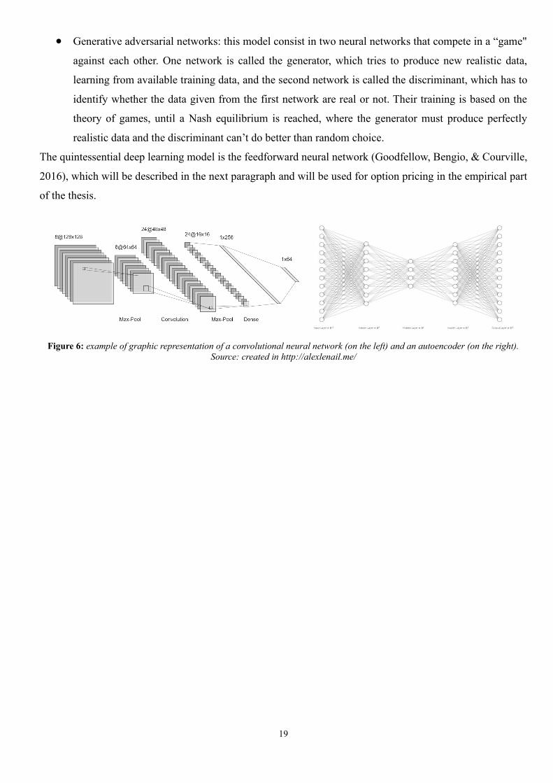
• Convolutional neural network: model typically used for image recognition, in which the layers are 2-

dimentional or 3-dimentional. The hidden layers are intended to identify patterns gradually more

complex (for instance colour gradient, lines, faces), until the whole picture content is correctly

detected.

19

• Generative adversarial networks: this model consist in two neural networks that compete in a “game"

against each other. One network is called the generator, which tries to produce new realistic data,

learning from available training data, and the second network is called the discriminant, which has to

identify whether the data given from the first network are real or not. Their training is based on the

theory of games, until a Nash equilibrium is reached, where the generator must produce perfectly

realistic data and the discriminant can’t do better than random choice.

The quintessential deep learning model is the feedforward neural network (Goodfellow, Bengio, & Courville,

2016), which will be described in the next paragraph and will be used for option pricing in the empirical part

of the thesis.

Figure 6: example of graphic representation of a convolutional neural network (on the left) and an autoencoder (on the right).

Source: created in http://alexlenail.me/

20

Feedforward Neural Networks

Deep feedforward networks (or multilayer perceptron) are models whose objective is to approximate

some function 𝑓(∙) by utilizing a map 𝑦 = 𝑓(∙, 𝜃) and learning the value of the parameters 𝜃 that lead to the

best approximation. The name “network” is attributed because the function 𝑓(∙) is approximated using a

composition of many functions (the number depends on the size of the network). The adjective “feedforward”

is added to highlight that there are no connections in reverse order between the neurons and the information

flows always from one layer to the next and not vice versa. The adjective “deep” refers to the depth of the

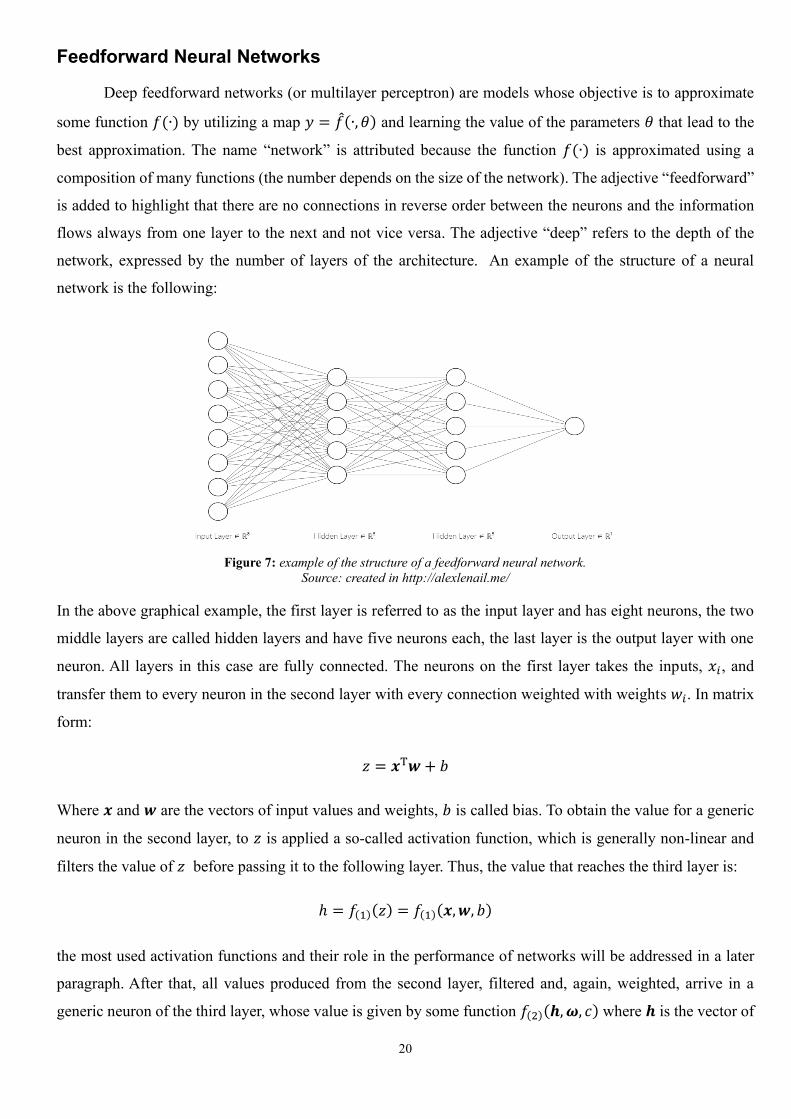
network, expressed by the number of layers of the architecture. An example of the structure of a neural

network is the following:

Figure 7: example of the structure of a feedforward neural network.

Source: created in http://alexlenail.me/

In the above graphical example, the first layer is referred to as the input layer and has eight neurons, the two

middle layers are called hidden layers and have five neurons each, the last layer is the output layer with one

neuron. All layers in this case are fully connected. The neurons on the first layer takes the inputs, 𝑥𝑖, and

transfer them to every neuron in the second layer with every connection weighted with weights 𝑤𝑖. In matrix

form:

𝑧 = 𝒙T𝒘 + 𝑏

Where 𝒙 and 𝒘 are the vectors of input values and weights, 𝑏 is called bias. To obtain the value for a generic

neuron in the second layer, to 𝑧 is applied a so-called activation function, which is generally non-linear and

filters the value of 𝑧 before passing it to the following layer. Thus, the value that reaches the third layer is:

ℎ = 𝑓(1)(𝑧) = 𝑓(1)(𝒙, 𝒘, 𝑏)

the most used activation functions and their role in the performance of networks will be addressed in a later

paragraph. After that, all values produced from the second layer, filtered and, again, weighted, arrive in a

generic neuron of the third layer, whose value is given by some function 𝑓(2)(𝒉, 𝝎, 𝑐) where 𝒉 is the vector of

21

values of the preceding layers, 𝝎 is the new set of weights, 𝑐 is the new bias. The value of the output layer is

the composition of the functions described before:

𝑔(𝒙, 𝑾, 𝒄, 𝒃) = 𝑓(2)(𝑓(1)(𝒙, 𝒘, 𝑏), 𝝎, 𝒄)

where 𝑾 is the matrix obtained using as columns the vectors of 𝒘 and 𝝎.

Finally, the output layer gives the “guess” of the model, 𝑦, which is generally not accurate at first, because the

weights are chosen randomly, and they are not optimized for the specific objective. The way to allow the model

to learn and optimize itself is via backpropagation (Rumelhart, , Hinton, & Ronald, 1986) and stochastic

gradient descent (Robbins & Monro, 1951).

22

Backprogragation algorithm

Often backpropagation is referred to be the entire process that leads a neural network to learn from

data, but backpropagation refers only to the method of computing the gradient, which is used by algorithms,

like gradient descent, to perform learning. In order for a neural network to learn, it is necessary to specify a

loss (or objective) function 𝐿(𝒙, 𝒚) , which depends on the set of input data 𝒙 and output data 𝒚. Generally,

for a classification problem the loss function used is the Cross Entropy, 𝐻(∙), which compares the estimated

probability distribution, 𝑞, with the actual probability distribution, 𝑝, of the data:

𝐻(𝑝, 𝑞) = − ∑ 𝑝(𝑥) log 𝑞(𝑥)𝑥∈ℤ for discrete time distributions

𝐻(𝑝, 𝑞) = − ∫ 𝑝(𝑥) log 𝑞(𝑥)ℝ

𝑑𝑟(𝑥) for continuous time distributions

where 𝑟(𝑥) is a Lebesgue measure on a Borel σ-algebra.

For a prediction or estimation problem, the mean squared error, 𝑀𝑆𝐸, is the most used metric:

𝑀𝑆𝐸 =1

𝑛∑(𝑌𝑖 − �̂�𝑖)

2𝑛

𝑖=1

Where 𝑌𝑖 are actual values and �̂�𝑖 are the values predicted by the model, 𝑛 is the number of observation in the

test set chosen, which has to be different from the training set, to avoid data memorization problems.

Sometimes also mean absolute error is used for this purpose.

𝑀𝐴𝐸 =∑ |𝑌𝑖 − �̂�𝑖|

𝑛𝑖=1

𝑛

To explain backpropagation, the function which gives the output for a general feedforward neural network is

defined as follow:

𝑔(𝒙) ≔ 𝑓(𝑛)(𝑾𝑛𝑓(𝑛−1)(𝑾𝑛−1 ⋯ 𝑓(1)(𝑾1𝒙) ⋯ )

A generic loss function is applied for a generic set of inputs and outputs 𝐿(𝑔(𝒙), 𝒚). Backpropagation permits

to compute the gradient of the loss function as expressed above. This means computing all partial derivatives

of the loss function with respect to weights and biases: 𝜕𝐿 𝜕𝑤𝑗𝑙⁄ and 𝜕𝐿 𝜕𝑏𝑗

𝑙⁄ . Where the apex 𝑙 indicates the

layer and the subscript 𝑗 indicates the 𝑗th neuron in the layer. In order to achieve that, an intermediate quantity,

𝜀𝑗𝑙, is introduced and it’s called the error of the 𝑗th neuron in the layer 𝑙 18. It subsist: 𝜀𝑗

𝑙 = 𝜕𝐿 𝜕𝑧𝑗𝑙⁄ by definition,

where 𝑧𝑗𝑙 is the weighted input to the activation function for neuron 𝑗 in layer 𝑙. Now ℎ𝑗

𝑙 = 𝑓(𝑙)(𝑧𝑗𝑙) is defined,

and, merging the notions above:

18 The absence of the subscript 𝑗 indicates that the value refers to an entire layer.

23

𝜀𝑗𝑙 =

𝜕𝐿

𝜕ℎ𝑗𝑙 𝑓(𝑙)′(𝑧𝑗

𝑙)

Which, for an entire layer, becomes:

𝜀𝑙 = 𝛻ℎ𝐿 ∙ 𝑓(𝑙)′(𝑧𝑙)

Where ∇ℎ𝐿 is a vector whose components are the partial derivatives 𝜕𝐿 𝜕ℎ𝑗𝑙⁄ . ∇ℎ𝐿 can be interpreted as the

rate of change of 𝐿(∙) with respect to the output ℎ of the activation function. This equation is furnished without

proof, but the concept from which it comes is that 𝜕𝐿 𝜕𝑧𝑗𝑙⁄ can be expressed in terms of ℎ𝑗

𝑙 as follow:

𝜕𝐿

𝜕𝑧𝑗𝑙 =

𝜕𝐿

𝜕ℎ𝑗𝑙

𝜕ℎ𝑗𝑙

𝜕𝑧𝑗𝑙

This permits to rewrite ∇ℎ𝐿 in terms of 𝜀𝑙.

Another step in understanding backpropagation is linking the error in one layer to the next layer and the

relationship that subsists is derived from 𝜀𝑗𝑙 = 𝜕𝐿 𝜕𝑧𝑗

𝑙⁄ and 𝜀𝑗𝑙+1 = 𝜕𝐿 𝜕𝑧𝑗

𝑙+1⁄ . Using the chain rule:

𝜀𝑗𝑙 =

𝜕𝐿

𝜕𝑧𝑗𝑙 = ∑

𝜕𝐿

𝜕𝑧𝑘𝑙+1

𝑘

𝜕𝑧𝑘𝑙+1

𝜕𝑧𝑗𝑙 = ∑

𝜕𝑧𝑘𝑙+1

𝜕𝑧𝑗𝑙 𝜀𝑘

𝑙+1

𝑘

Recalling 𝑧 = 𝒙T𝒘 + 𝑏, now expressed in terms of summation, for the layer 𝑙 + 1 and the 𝑗th neuron:

𝑧𝑗𝑙+1 = ∑ 𝑤𝑘𝑗

𝑙+1ℎ𝑗𝑙

𝑘+ 𝑏𝑘

𝑙+1 = ∑ 𝑤𝑘𝑗𝑙+1𝑓(𝑙)(𝑧𝑗

𝑙)𝑘

+ 𝑏𝑘𝑙+1

Differentiating:

𝜕𝑧𝑘𝑙+1

𝜕𝑧𝑗𝑙 = 𝑤𝑘𝑗

𝑙+1𝑓(𝑙)′(𝑧𝑗𝑙)

And, substituting for 𝜕𝑧𝑘𝑙+1 𝜕𝑧𝑗

𝑙⁄ in the precedent equation of 𝜀𝑗𝑙 , the formula that links one layer to the next is

given:

𝜀𝑗𝑙 = ∑ 𝑤𝑘𝑗

𝑙+1𝑓(𝑙)′(𝑧𝑗𝑙) 𝜀𝑘

𝑙+1

𝑘

or, in matrix form:

𝜀𝑗𝑙 = [(𝒘𝒍+𝟏)

𝑇𝜹𝒍+𝟏] ∙ 𝑓(𝑙)′(𝑧𝑗

𝑙)

24

As regards weights and biases, the following relationships are given without proof (they follow from the

application of the chain rule):

𝜀𝑗𝑙 =

𝜕𝐿

𝜕𝑏𝑗𝑙

𝜀𝑗𝑙 ∙ ℎ𝑘

𝑙−1 =𝜕𝐿

𝜕𝑤𝑘𝑗𝑙

Resuming how the backpropagation algorithm works, we can identify four main steps:

1. Set the output of the first activation function ℎ1;

2. For each layer 𝑙 = 2,3, … , ℒ, compute 𝑧𝑙 ,ℎ𝑙 and 𝜀𝑙;

3. For each layer 𝑙 = ℒ − 1, ℒ − 2, … ,2, compute 𝜀𝑙 relating it to its next layer;

4. The gradient of 𝐿(∙) is given by the following equations for weights and biases:

𝜀𝑗𝑙 =

𝜕𝐿

𝜕𝑏𝑗𝑙

𝜀𝑗𝑙 ∙ ℎ𝑘

𝑙−1 =𝜕𝐿

𝜕𝑤𝑘𝑗𝑙

The third step indicates why the algorithm described is called backpropagation.

After the gradient is computed using backpropagation algorithm, to optimize the model (and to train it) a

gradient-based optimization algorithm has to be applied. The most used optimization methods are described

in detail in the next paragraph.

25

Gradient-based Optimization

The stochastic gradient descent algorithm is an iterative method to optimize the loss function (or

objective function) expressed above. Consider 𝑛 observations in the dataset and an objective function 𝐿(𝜸) to

be minimized with a set of parameters 𝜸 that minimize the function and that have to be estimated. The basic

algorithm works as follow:

1. An initial vector 𝜸 is chosen and a learning rate 𝜂 is defined;

2. for 𝑖 = 1,2, … , 𝑛 do: 𝜸 ≔ 𝜸 − 𝜂∇𝐿𝑖(𝜸)19;

3. repeat until a minimum is reached.

The algorithm is performed by randomly shuffle examples in the training set and can be executed analysing

more than one example at the same time. The number of examples executed at the same time is called mini-

batch size.

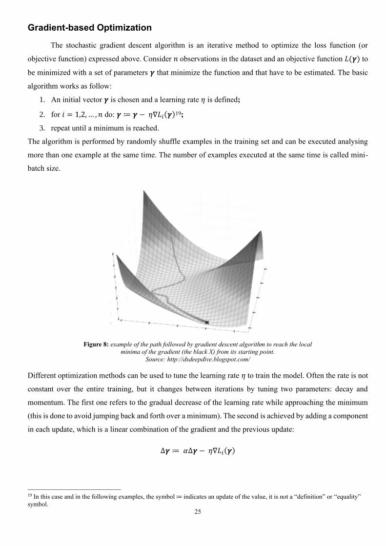
Figure 8: example of the path followed by gradient descent algorithm to reach the local

minima of the gradient (the black X) from its starting point.

Source: http://dsdeepdive.blogspot.com/

Different optimization methods can be used to tune the learning rate 𝜂 to train the model. Often the rate is not

constant over the entire training, but it changes between iterations by tuning two parameters: decay and

momentum. The first one refers to the gradual decrease of the learning rate while approaching the minimum

(this is done to avoid jumping back and forth over a minimum). The second is achieved by adding a component

in each update, which is a linear combination of the gradient and the previous update:

∆𝜸 ≔ 𝛼∆𝜸 − 𝜂∇𝐿𝑖(𝜸)

19 In this case and in the following examples, the symbol ≔ indicates an update of the value, it is not a “definition” or “equality”

symbol.

26

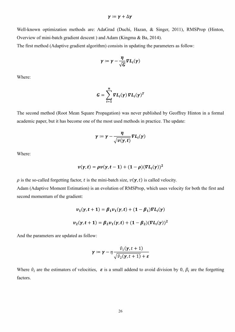
𝜸 ≔ 𝜸 + ∆𝜸

Well-known optimization methods are: AdaGrad (Duchi, Hazan, & Singer, 2011), RMSProp (Hinton,

Overview of mini-batch gradient descent ) and Adam (Kingma & Ba, 2014).

The first method (Adaptive gradient algorithm) consists in updating the parameters as follow:

𝜸 ≔ 𝜸 −𝜼

√𝑮𝜵𝑳𝒊(𝜸)

Where:

𝑮 = ∑ 𝜵𝑳𝒊(𝜸)

𝒏

𝒊=𝟏

𝜵𝑳𝒊(𝜸)𝑻

The second method (Root Mean Square Propagation) was never published by Geoffrey Hinton in a formal

academic paper, but it has become one of the most used methods in practice. The update:

𝜸 ≔ 𝜸 −𝜼

√𝒗(𝜸, 𝒕)𝜵𝑳𝒊(𝜸)

Where:

𝒗(𝜸, 𝒕) = 𝝆𝒗(𝜸, 𝒕 − 𝟏) + (𝟏 − 𝝆)(𝜵𝑳𝒊(𝜸))𝟐

𝜌 is the so-called forgetting factor, 𝑡 is the mini-batch size, 𝑣(𝜸, 𝑡) is called velocity.

Adam (Adaptive Moment Estimation) is an evolution of RMSProp, which uses velocity for both the first and

second momentum of the gradient:

𝒗𝟏(𝜸, 𝒕 + 𝟏) = 𝜷𝟏𝒗𝟏(𝜸, 𝒕) + (𝟏 − 𝜷𝟏)𝜵𝑳𝒊(𝜸)

𝒗𝟐(𝜸, 𝒕 + 𝟏) = 𝜷𝟐𝒗𝟏(𝜸, 𝒕) + (𝟏 − 𝜷𝟐)(𝜵𝑳𝒊(𝜸))𝟐

And the parameters are updated as follow:

𝜸 ≔ 𝜸 − 𝜂𝑣1(𝜸, 𝑡 + 1)

√𝑣2(𝜸, 𝑡 + 1) + 𝜺

Where 𝑣𝑖 are the estimators of velocities, 𝜺 is a small addend to avoid division by 0, 𝛽𝑖 are the forgetting

factors.

27

Activation functions

The activation function of a neuron can be considered as a filter that is applied to the input of the node,

which is given from a linear operation (matrix or vector multiplications), to modify it and transfer to the

subsequent layer. Based on the type of function, activation assumes different interpretations. Below there is a

list and a brief explanation of some well-known activation functions.

The ReLU function (Rectified Linear Unit) is given by:

𝑓(𝑥) = {0 𝑓𝑜𝑟 𝑥 ≤ 0𝑥 𝑓𝑜𝑟 𝑥 > 0

It avoids negative values as output of the neuron and is useful in the problems that involves only positive

values.

The Sigmoid (or Logistic) function is given by:

𝑓(𝑥) =1

1 + 𝑒−𝑥

It varies between 0 and 1 and can be interpreted as transforming real numbers into probabilities. It is often

used in classification problems where a probability for the output is needed.

The TanH (Hyperbolic Tangent) function is given by:

𝑓(𝑥) =𝑒𝑥 − 𝑒−𝑥

𝑒𝑥 + 𝑒−𝑥

It varies between −1 and 1 and it is often used in classification problems involving two classes.

The ELU function (Exponential Linear Unit) is given by:

𝑓(𝛼, 𝑥) = {𝛼(𝑒𝑥 − 1) 𝑓𝑜𝑟 𝑥 < 0𝑥 𝑓𝑜𝑟 𝑥 ≥ 0

It differs from other activation functions for the parameter 𝛼 > 0 , which needs to be tuned. It works similarly

to ReLU function, but it’s smoother and assigns values different from 0 to every real number (except 0).

Figure 9: schematic graphs of most used activation functions. From left to right: ReLU, Sigmoid, TanH, ELU.

Source: Wikipedia

28

Chapter 4

Empirical Part

Data and environments

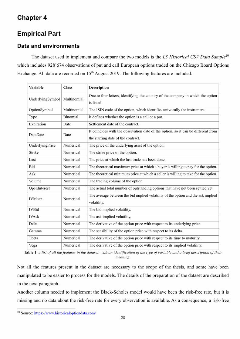
The dataset used to implement and compare the two models is the L3 Historical CSV Data Sample20

which includes 928’674 observations of put and call European options traded on the Chicago Board Options

Exchange. All data are recorded on 15th August 2019. The following features are included:

Variable Class Description

UnderlyingSymbol Multinomial One to four letters, identifying the country of the company in which the option

is listed.

OptionSymbol Multinomial The ISIN code of the option, which identifies univocally the instrument.

Type Binomial It defines whether the option is a call or a put.

Expiration Date Settlement date of the contract.

DataDate Date It coincides with the observation date of the option, so it can be different from

the starting date of the contract.

UnderlyingPrice Numerical The price of the underlying asset of the option.

Strike Numerical The strike price of the option.

Last Numerical The price at which the last trade has been done.

Bid Numerical The theoretical maximum price at which a buyer is willing to pay for the option.

Ask Numerical The theoretical minimum price at which a seller is willing to take for the option.

Volume Numerical The trading volume of the option.

OpenInterest Numerical The actual total number of outstanding options that have not been settled yet.

IVMean Numerical The average between the bid implied volatility of the option and the ask implied

volatility.

IVBid Numerical The bid implied volatility.

IVAsk Numerical The ask implied volatility.

Delta Numerical The derivative of the option price with respect to its underlying price.

Gamma Numerical The sensibility of the option price with respect to its delta.

Theta Numerical The derivative of the option price with respect to its time to maturity.

Vega Numerical The derivative of the option price with respect to its implied volatility.

Table 1: a list of all the features in the dataset, with an identification of the type of variable and a brief description of their

meaning.

Not all the features present in the dataset are necessary to the scope of the thesis, and some have been

manipulated to be easier to process for the models. The details of the preparation of the dataset are described

in the next paragraph.

Another column needed to implement the Black-Scholes model would have been the risk-free rate, but it is

missing and no data about the risk-free rate for every observation is available. As a consequence, a risk-free

20 Source: https://www.historicaloptiondata.com/

29

rate is chosen arbitrarily, and it will be the same for all the observations. This represents a strong assumption

and its implications will be discussed later. The risk-free rate chosen is the US Tree Months Treasury Bill rate

at the 15th August 2019 date. The choice has been made because the average time to maturity of all the options

in the dataset is 0.4028, which is close to 3 months, and the date is the date at which all options have been

observed. The value of the rate discussed is 0.0187 or 1.87%.

The models will be implemented using Python 3.7 programming language. The choice has been made due to

the simplicity of the language and all the pre-built libraries for machine learning, which make the workflow

faster and the debugging process easier. In particular, the libraries used throughout the empirical part of the

thesis are:

• Pandas (McKinney, 2010), used to read, write and manipulate the dataset;

• NumPy (Oliphant, 2006), which uses arrays as the main data structure to perform computations;

• SciPy (Virtanen et al., 2019), a large library, which includes a variety of branches of science, used in

this case for statistical tools;

• Time, present in the Python Standard Library21, used to calculate the time of computation and training

for the two models;

• Matplotlib (Hunter, 2007), used to make the graphs and plots to have a visual interpretation of the

models;

• TensorFlow (Abadi et al., 2015), an interface from Google made to implement machine learning

models, particularly deep learning ones. The name derives from the fact that data are imported in

TensorFlow using tensors, which speeds up the process of training the model.

21 Ufficial documentation: https://docs.python.org/3/library/

30

Cleaning and preparing the data

The dataset doesn’t have missing or wrong recorded cells, thus the process of cleaning and preparing

the data is made only by working on columns. In particular, some columns have been eliminated because they

don’t enter as inputs for the models, such as Volume, OpenInterest, IVBid, IVAsk, UndelyingSymbol, Last,

Delta, Gamma, Theta, Vega.

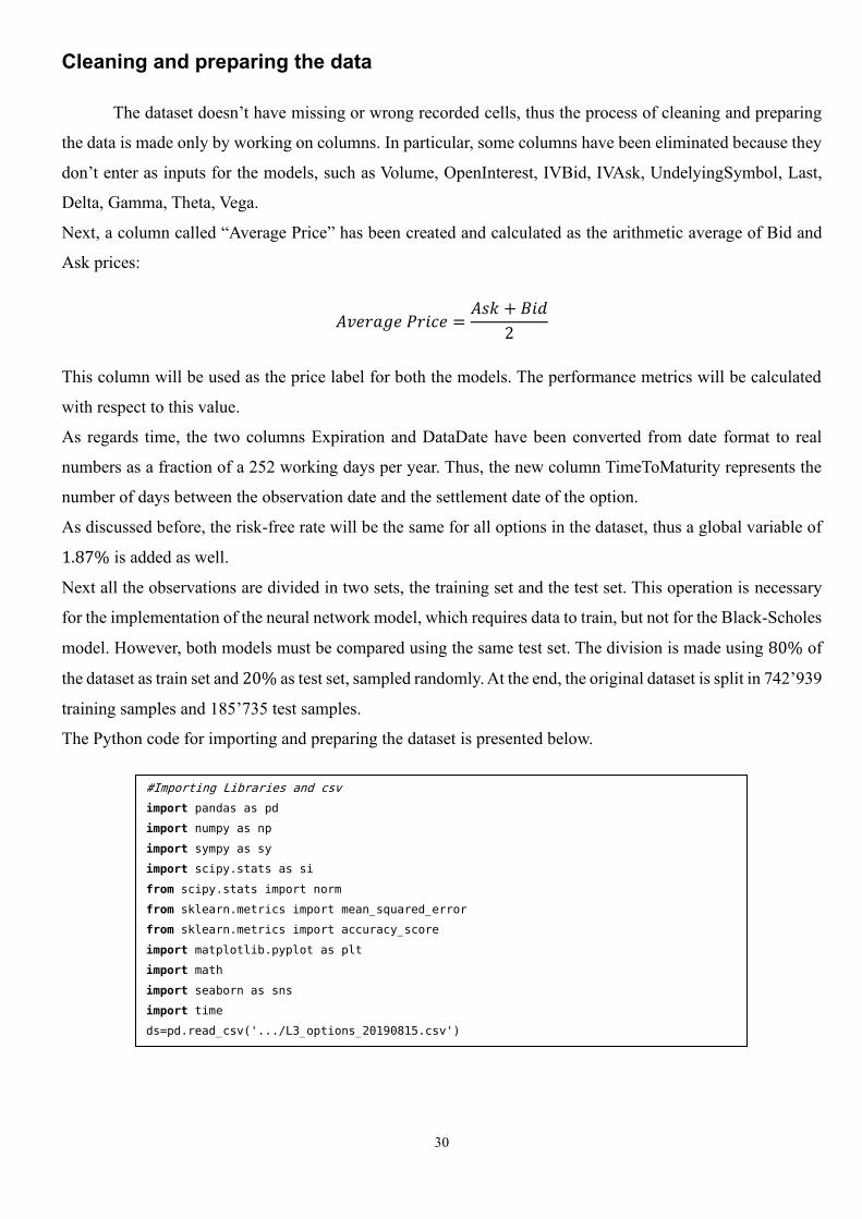
Next, a column called “Average Price” has been created and calculated as the arithmetic average of Bid and

Ask prices:

𝐴𝑣𝑒𝑟𝑎𝑔𝑒 𝑃𝑟𝑖𝑐𝑒 =𝐴𝑠𝑘 + 𝐵𝑖𝑑

2

This column will be used as the price label for both the models. The performance metrics will be calculated

with respect to this value.

As regards time, the two columns Expiration and DataDate have been converted from date format to real

numbers as a fraction of a 252 working days per year. Thus, the new column TimeToMaturity represents the

number of days between the observation date and the settlement date of the option.

As discussed before, the risk-free rate will be the same for all options in the dataset, thus a global variable of

1.87% is added as well.

Next all the observations are divided in two sets, the training set and the test set. This operation is necessary

for the implementation of the neural network model, which requires data to train, but not for the Black-Scholes

model. However, both models must be compared using the same test set. The division is made using 80% of

the dataset as train set and 20% as test set, sampled randomly. At the end, the original dataset is split in 742’939

training samples and 185’735 test samples.

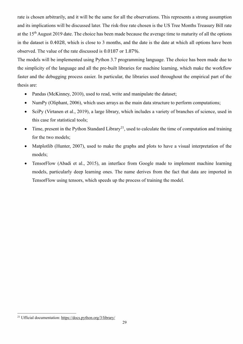
The Python code for importing and preparing the dataset is presented below.

#Importing Libraries and csv

import pandas as pd

import numpy as np

import sympy as sy

import scipy.stats as si

from scipy.stats import norm

from sklearn.metrics import mean_squared_error

from sklearn.metrics import accuracy_score

import matplotlib.pyplot as plt

import math

import seaborn as sns

import time

ds=pd.read_csv('.../L3_options_20190815.csv')

31

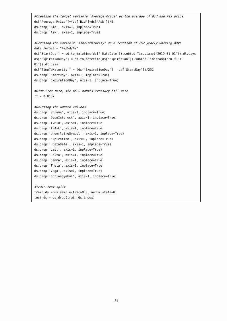
#Creating the target variable 'Average Price' as the average of Bid and Ask price

ds['Average Price']=(ds['Bid']+ds['Ask'])/2

ds.drop('Bid', axis=1, inplace=True)

ds.drop('Ask', axis=1, inplace=True)

#Creating the variable 'TimeToMaturity' as a fraction of 252 yearly working days

date_format = "%m/%d/%Y"

ds['StartDay'] = pd.to_datetime(ds[' DataDate']).sub(pd.Timestamp('2019-01-01')).dt.days

ds['ExpirationDay'] = pd.to_datetime(ds['Expiration']).sub(pd.Timestamp('2019-01-

01')).dt.days

ds['TimeToMaturity'] = (ds['ExpirationDay'] - ds['StartDay'])/252

ds.drop('StartDay', axis=1, inplace=True)

ds.drop('ExpirationDay', axis=1, inplace=True)

#Risk-Free rate, the US 3 months treasury bill rate

rf = 0.0187

#Deleting the unused columns

ds.drop('Volume', axis=1, inplace=True)

ds.drop('OpenInterest', axis=1, inplace=True)

ds.drop('IVBid', axis=1, inplace=True)

ds.drop('IVAsk', axis=1, inplace=True)

ds.drop('UnderlyingSymbol', axis=1, inplace=True)

ds.drop('Expiration', axis=1, inplace=True)

ds.drop(' DataDate', axis=1, inplace=True)

ds.drop('Last', axis=1, inplace=True)

ds.drop('Delta', axis=1, inplace=True)

ds.drop('Gamma', axis=1, inplace=True)

ds.drop('Theta', axis=1, inplace=True)

ds.drop('Vega', axis=1, inplace=True)

ds.drop('OptionSymbol', axis=1, inplace=True)

#train-test split

train_ds = ds.sample(frac=0.8,random_state=0)

test_ds = ds.drop(train_ds.index)

32

On volatility

As discussed before, implied volatility is provided by the dataset and it is calculated both for bid

(IVBid) and ask (IVAsk) prices and, then, their average (IVMean). The IVMean will be used in next paragraphs

as a feature for both models and this point, as will be discussed later, is a strong assumption, because it implies

that the volatility considered by both models is constant and it is calculated by approximation, without a closed

form solution. Furthermore, the volatility calculated as the average of the IVBid and IVAsk doesn’t necessarily

matches with the “real” implied volatility of the column “Average price” calculated before. Therefore, part of

the error in both models could be attributed to forcing the use of volatility without an appropriate calculation,

which could have been achieved using one of the methods discussed before, in the volatility paragraph.

33

Performance metrics

Two types of measures will be used to evaluate the performance of the models, one involving the

distance between the predicted price and the actual price, the other one involving the temporal aspect of the

computation. Initially the first measure considered was the Root Mean Squared Error (RMSE) or root mean

squared deviation, calculated as the square root of the sum of all squared errors, divided by the number of

observations:

𝑅𝑀𝑆𝐸 = √∑ (�̂�𝑖 − 𝑦𝑖)2𝑛

𝑖=1

𝑛

Where 𝑛 is the number of observations in the dataset, �̂�𝑖 is the model estimation for the price of the ith

observation, 𝑦𝑖 is the actual price of the option. This measure would have been chosen for many reasons, firstly

because is a synthetic and easy to interpret measure of performance for the models. It is also easy to calculate

and implement and it can be used as a loss function for the deep learning model.

However, in literature some have argued that Mean Absolute Error (MAE) is a better performance metric for

machine learning problems like the one addressed in this thesis (Willmott & Matsuura, 2005). The RMSE is

more appropriate than the MAE to represent model performance when the error distribution is expected to be

Gaussian (Chai & Draxler, 2014), but in this case this assumption does not hold. In fact, the distribution of

errors in both models is expected to be leptokurtic.

Figure 10: histogram of the distribution of errors applying the Black and Scholes model to the test set.

So, the deep learning model will be trained to minimize MAE as loss function, and the same measure will be

used as performance metric for both models.

𝑀𝐴𝐸 =∑ |�̂�𝑖 − 𝑦𝑖|𝑛

𝑖=1

𝑛

The second performance metric will be the time necessary for the hardware to compute and apply the model

to all test’s observations. This measure is introduced to compare the models both in spatial and temporal aspect.

34

The mere “time to compute” (measured in fraction of seconds) is chosen instead of computational complexity

(measured using the Big O notation) because it is a measure easy to understand and has a practical implication,

while computational complexity requires more sophisticated techniques to be calculated and has less

immediate explicative power.

35

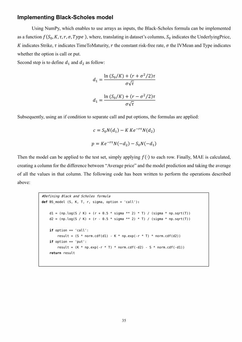
Implementing Black-Scholes model

Using NumPy, which enables to use arrays as inputs, the Black-Scholes formula can be implemented

as a function 𝑓(𝑆0, 𝐾, 𝜏, 𝑟, 𝜎, 𝑇𝑦𝑝𝑒 ), where, translating in dataset’s columns, 𝑆0 indicates the UnderlyingPrice,

𝐾 indicates Strike, 𝜏 indicates TimeToMaturity, 𝑟 the constant risk-free rate, 𝜎 the IVMean and Type indicates

whether the option is call or put.

Second step is to define 𝑑1 and 𝑑2 as follow:

𝑑1 =ln (𝑆0 𝐾)⁄ + (𝑟 + 𝜎2 2⁄ )𝜏

𝜎√𝜏

𝑑1 =ln (𝑆0 𝐾)⁄ + (𝑟 − 𝜎2 2⁄ )𝜏

𝜎√𝜏

Subsequently, using an if condition to separate call and put options, the formulas are applied:

𝑐 = 𝑆0𝑁(𝑑1) − 𝐾 𝐾𝑒−𝑟𝜏𝑁(𝑑2)

𝑝 = 𝐾𝑒−𝑟𝜏𝑁(−𝑑2) − 𝑆0𝑁(−𝑑1)

Then the model can be applied to the test set, simply applying 𝑓(∙) to each row. Finally, MAE is calculated,

creating a column for the difference between “Average price” and the model prediction and taking the average

of all the values in that column. The following code has been written to perform the operations described

above:

#Defining Black and Scholes formula

def BS_model (S, K, T, r, sigma, option = 'call'):

d1 = (np.log(S / K) + (r + 0.5 * sigma ** 2) * T) / (sigma * np.sqrt(T))

d2 = (np.log(S / K) + (r - 0.5 * sigma ** 2) * T) / (sigma * np.sqrt(T))

if option == 'call':

result = (S * norm.cdf(d1) - K * np.exp(-r * T) * norm.cdf(d2))

if option == 'put':

result = (K * np.exp(-r * T) * norm.cdf(-d2) - S * norm.cdf(-d1))

return result

36

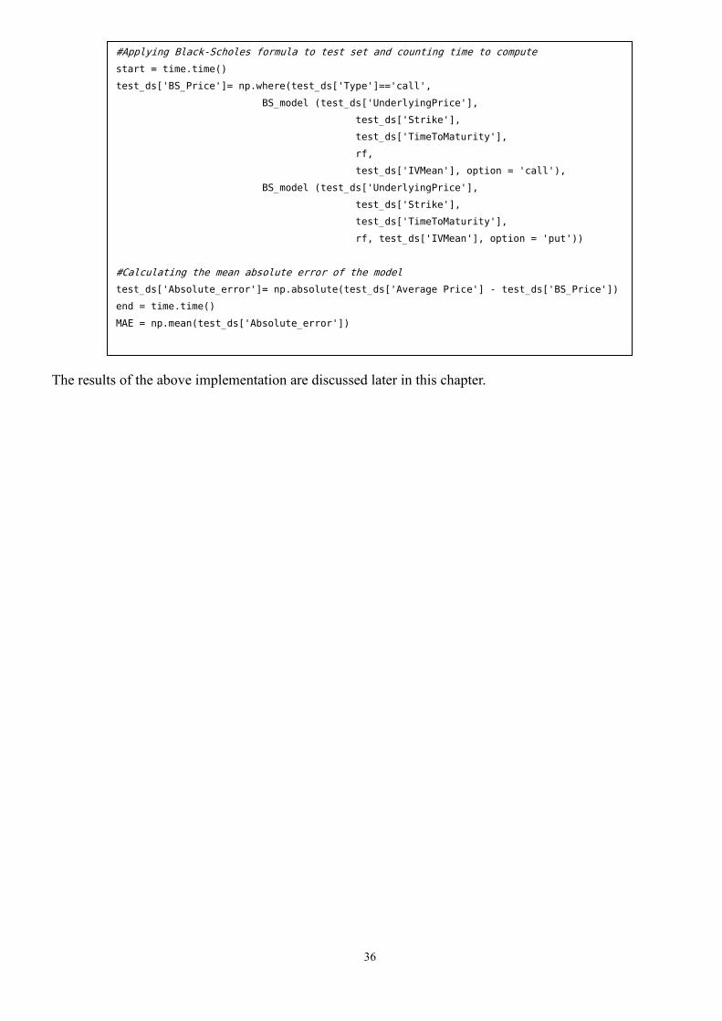
The results of the above implementation are discussed later in this chapter.

#Applying Black-Scholes formula to test set and counting time to compute

start = time.time()

test_ds['BS_Price']= np.where(test_ds['Type']=='call',

BS_model (test_ds['UnderlyingPrice'],

test_ds['Strike'],

test_ds['TimeToMaturity'],

rf,

test_ds['IVMean'], option = 'call'),

BS_model (test_ds['UnderlyingPrice'],

test_ds['Strike'],

test_ds['TimeToMaturity'],

rf, test_ds['IVMean'], option = 'put'))

#Calculating the mean absolute error of the model

test_ds['Absolute_error']= np.absolute(test_ds['Average Price'] - test_ds['BS_Price'])

end = time.time()

MAE = np.mean(test_ds['Absolute_error'])

37

Neural network architecture

Before applying the chosen feedforward neural network to evaluate the price of options, some

preparing operations have to be performed. First, because the neural network takes as inputs only numerical

features, the column “Type” has been transformed using 1 for calls and 0 for puts22. Next, normalization of

the data is performed, using the mean and standard deviation for each column:

𝑧 =𝑥 − 𝑚𝑒𝑎𝑛(𝑥)

𝑠𝑡. 𝑑𝑣. (𝑥)

Where 𝑥 represents a vector of original data, 𝑧 the vector of standardized data, while 𝑚𝑒𝑎𝑛(∙) and 𝑠𝑡. 𝑑𝑣. (∙)

are the functions for mean and standard deviation respectively. After this process is applied the variable

representing the risk-free rate disappears, leaving all zeros, therefore it’s eliminated and the model will be

trained using only UnderlyingPrice, Strike, IVMean, TimeToMaturity, Type_code (the code referring to the

Type).

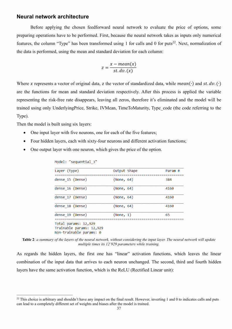
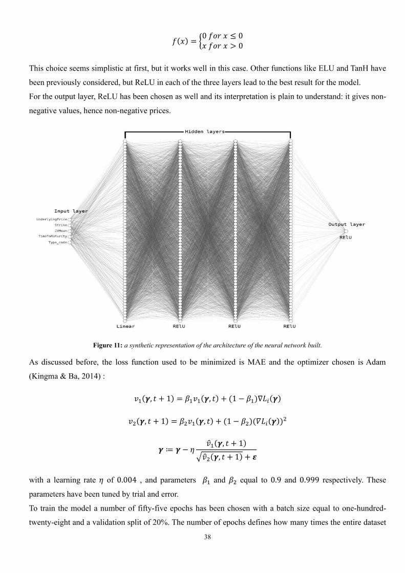
Then the model is built using six layers:

• One input layer with five neurons, one for each of the five features;

• Four hidden layers, each with sixty-four neurons and different activation functions;

• One output layer with one neuron, which gives the price of the option.

Table 2: a summary of the layers of the neural network, without considering the input layer. The neural network will update

multiple times its 12’929 parameters while training.

As regards the hidden layers, the first one has “linear” activation functions, which leaves the linear

combination of the input data that arrives to each neuron unchanged. The second, third and fourth hidden

layers have the same activation function, which is the ReLU (Rectified Linear unit):

22 This choice is arbitrary and shouldn’t have any impact on the final result. However, inverting 1 and 0 to indicates calls and puts

can lead to a completely different set of weights and biases after the model is trained.

38

𝑓(𝑥) = {0 𝑓𝑜𝑟 𝑥 ≤ 0𝑥 𝑓𝑜𝑟 𝑥 > 0

This choice seems simplistic at first, but it works well in this case. Other functions like ELU and TanH have

been previously considered, but ReLU in each of the three layers lead to the best result for the model.

For the output layer, ReLU has been chosen as well and its interpretation is plain to understand: it gives non-

negative values, hence non-negative prices.

Figure 11: a synthetic representation of the architecture of the neural network built.

As discussed before, the loss function used to be minimized is MAE and the optimizer chosen is Adam

(Kingma & Ba, 2014) :

𝑣1(𝜸, 𝑡 + 1) = 𝛽1𝑣1(𝜸, 𝑡) + (1 − 𝛽1)∇𝐿𝑖(𝜸)

𝑣2(𝜸, 𝑡 + 1) = 𝛽2𝑣1(𝜸, 𝑡) + (1 − 𝛽2)(𝛻𝐿𝑖(𝜸))2

𝜸 ≔ 𝜸 − 𝜂𝑣1(𝜸, 𝑡 + 1)

√𝑣2(𝜸, 𝑡 + 1) + 𝜺

with a learning rate 𝜂 of 0.004 , and parameters 𝛽1 and 𝛽2 equal to 0.9 and 0.999 respectively. These

parameters have been tuned by trial and error.

To train the model a number of fifty-five epochs has been chosen with a batch size equal to one-hundred-

twenty-eight and a validation split of 20%. The number of epochs defines how many times the entire dataset

39

will be analysed by the neural network, while the batch size indicates the number of observations considered

before updating the weights of the model (Goodfellow, Bengio, & Courville, 2016). The validation split

indicates the number of observations used to test the model during training, it is expressed as a percentage of

the training set. The difference between validation set and test set is that the test set is not considered by the

model while training, so it gives more information about the generalization power of the model.

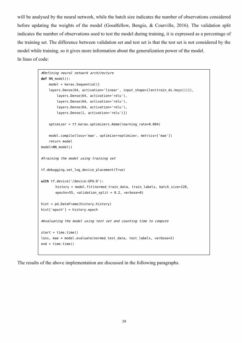
In lines of code:

The results of the above implementation are discussed in the following paragraphs.

#Defining neural network architecture

def NN_model():

model = keras.Sequential([

layers.Dense(64, activation='linear', input_shape=[len(train_ds.keys())]),

layers.Dense(64, activation='relu'),

layers.Dense(64, activation='relu'),

layers.Dense(64, activation='relu'),

layers.Dense(1, activation='relu')])

optimizer = tf.keras.optimizers.Adam(learning_rate=0.004)

model.compile(loss='mae', optimizer=optimizer, metrics=['mae'])

return model

model=NN_model()

#training the model using training set

tf.debugging.set_log_device_placement(True)

with tf.device('/device:GPU:0'):

history = model.fit(normed_train_data, train_labels, batch_size=128,

epochs=55, validation_split = 0.2, verbose=0)

hist = pd.DataFrame(history.history)

hist['epoch'] = history.epoch

#evaluating the model using test set and counting time to compute

start = time.time()

loss, mae = model.evaluate(normed_test_data, test_labels, verbose=2)

end = time.time()

40

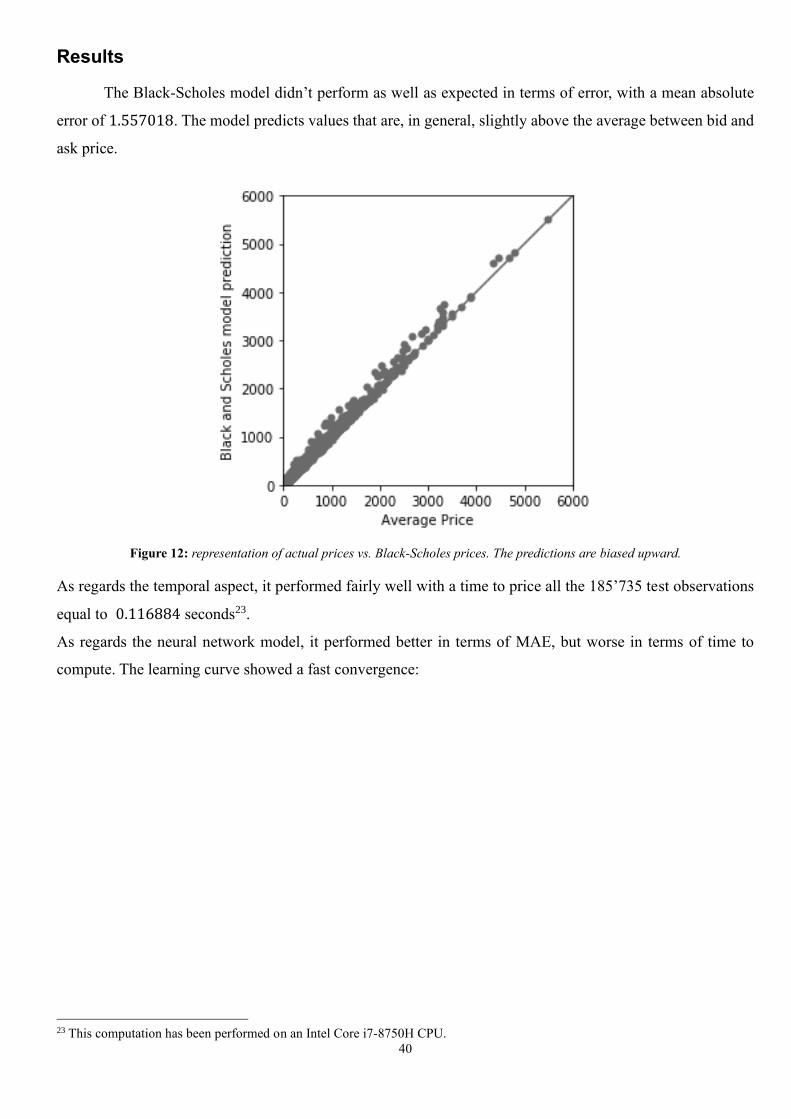
Results

The Black-Scholes model didn’t perform as well as expected in terms of error, with a mean absolute

error of 1.557018. The model predicts values that are, in general, slightly above the average between bid and

ask price.

Figure 12: representation of actual prices vs. Black-Scholes prices. The predictions are biased upward.

As regards the temporal aspect, it performed fairly well with a time to price all the 185’735 test observations

equal to 0.116884 seconds23.

As regards the neural network model, it performed better in terms of MAE, but worse in terms of time to

compute. The learning curve showed a fast convergence:

23 This computation has been performed on an Intel Core i7-8750H CPU.

41

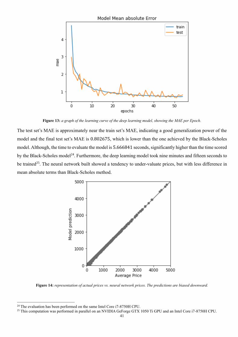
Figure 13: a graph of the learning curve of the deep learning model, showing the MAE per Epoch.

The test set’s MAE is approximately near the train set’s MAE, indicating a good generalization power of the

model and the final test set’s MAE is 0.802675, which is lower than the one achieved by the Black-Scholes

model. Although, the time to evaluate the model is 5.666841 seconds, significantly higher than the time scored

by the Black-Scholes model24. Furthermore, the deep learning model took nine minutes and fifteen seconds to

be trained25. The neural network built showed a tendency to under-valuate prices, but with less difference in

mean absolute terms than Black-Scholes method.

Figure 14: representation of actual prices vs. neural network prices. The predictions are biased downward.

24 The evaluation has been performed on the same Intel Core i7-8750H CPU. 25 This computation was performed in parallel on an NVIDIA GeForge GTX 1050 Ti GPU and an Intel Core i7-8750H CPU.

42

In general, given the same features for both models, the neural network model performed better than Black-

Scholes at the expenses of time to compute, which is approximately fifty-six times higher for the neural

network. However, the result achieved by the deep learning model has no underlying assumptions and could

work with different data without the necessity to explicitly make hypothesis about volatility, arbitrage

opportunities and stock prices movements.

The result is anyway quite surprising, because the deep learning model was not only able to approximate the

Black-Scholes function, but also outperform it, using the same exact variables.

In practical field the use of a more complex deep learning model, with a larger dataset for training and

evaluation and a more powerful hardware component, could lead to an even better performance, both in terms

of errors and time (both to compute and train). On the other hand, the Black-Scholes model has fixed formulas

and, even improving the hardware component, it cannot show better results in terms of MAE.

It can be argued that the result of the neural network has been achieved at the expenses of the explicatory

power of the model. That’s because, without any assumption and without the knowledge of what happened

inside the hidden layers while training, a decision in a bargaining environment, based on the result of the

model, couldn’t be fully explained.

In fact, the Black-Scholes formula is fully understood and universally shared in the finance field, while deep

learning models offer only results and not full explanation of why those results were achieved.

43

Critical issues

As regards the dataset used, it has been collected using only twenty-two working days, which could be

a short temporal interval to fully evaluate the performance of the models. Other market tendencies may have

been raised in the period considered, which could have deviated the prices from their theoretical value and

could have been captured in the dataset available, leading to a biased performance of the models.

As regards volatility, the comparison between the models have been done assuming that the IVMean described

in previous chapter was representative of the average between bid and ask prices. This assumption not always

holds and could have caused biases for both the models.

Another aspect is the risk-free rate considered. As stated before, the risk-free rate should have been different

for each option, based on the market, the timing and the geographical position of the option. The simplification

adopted could have caused deviations in the Black-Scholes model and the neural network architecture built

should have been different to account for different risk-free rates (for instance one neuron should have been

added in the input layer). This aspect can be considered for further improvements of this work.

Other criticisms regard the models compared. The neural network outperformed Black-Scholes model, but is

not sure if, considering more complex models such as Heston model (Heston, 1993) or Hull-White model

(Hull & White, 1990), this tendency would be confirmed or not. On the other side, using more complex deep

learning models may also lead to better results.

Therefore, this work represents a tiny step in comparing mathematical models and deep learning approaches

in option pricing, using the same features for both.

44

Chapter 5

Conclusions

Option pricing has been a prolific topic in literature. A variety of different models have been built to

achieve the goal of a reasonable option pricing, involving mathematics, statistics and probability. The most

influential model is the Black-Scholes model (Black & Scholes, 1973), which legitimized the activities of

the Chicago Board Options Exchange and other options markets around the world (MacKenzie, 2006).

In the last decade, the rise of Big Data and machine learning led to the spread of new models, based on linear

algebra and vector calculus, which have found a wide range of applications.

In this thesis, a deep learning model was built for option pricing and compared to the Black-Scholes model,

using the same features: Underlying price, Strike price, Time to maturity, Risk-Free rate, Implied Volatility.

The feedforward neural network built outperformed the Black-Scholes model in terms of mean absolute error,

but it took more time for computation.

The aim of this thesis was to make a step in the favour of use of deep learning models in the field of pricing

in finance and the results achieved go in the desired direction.

Nevertheless, some critical issues are present, such as the temporal range of options considered in the dataset,

the price label considered, the use of implied volatility, the simplification made about risk-free rate, and,

finally, the poor hardware environment in which both model have been implemented.

Further improvements can solve these issues by using different labels for prices, more accurately chosen,

different methods for approximating the volatility and more specific data, which includes different risk-free

rates for different options.

Next step could be to compare deep learning models with more advanced mathematical models and see if the

same result holds.

Practical implications of this result can influence trading and portfolio management. The deep learning model

presented, in fact, can be used to price options and can be re-trained with new options traded every day, making

it more precise over time. Also, this process can be automated and, perhaps, co-adjuvanted with a specific

trading algorithm to improve performance and returns. The usefulness of the model presented is that it only

requires the same features of the Black-Scholes model, which are information easy to acquire in practice.

Finally, is helpful to consider that in some cases, where a complete and understandable explanation is needed,

using Black-Scholes or other mathematical methods for option pricing is advisable, because the “black-box”

of deep learning models could negatively impact in those situations, or in cases where the model fails without

explanation.

45

References

Abadi et al. (2015). TensorFlow: Large-scale machine learning on heterogeneous system. tensorflow.org.

Amodei et al. (2016). Deep Speech 2 : End-to-End Speech Recognition in English and Mandarin. Proceedings

of Machine Learning Research Vol. 48, 173-182.

Angelini et al. (2008). A neural network approach for credit risk evaluation. Elsevier, Vol 48 (4), 735-755.

Bachelier, L. (1900a). Théorie de la spéculation . Annales Scientifiques de l'École Normale Supérieure.

Baruníkova, M., & Baruník, J. (2011). Neural networks as a semiparametric option pricing tool. Bulletin of

the Czech Econometric Society.

Berner et al. (2019). Dota 2 with Large Scale Deep Reinforcement Learning. https://openai.com/.

Black, F., & Scholes, M. (1973). The Pricing of Options and Corporate Liabilities. Journal of Political

Economy 81 (3).

Bollerslev, T. (1986). Generalized autoregressive conditional heteroskedasticity. Journal of econometrics 31

(3), 307–327.

Boyle, P. P. (1977). Options: A Monte Carlo Approach. Journal of Financial Economics, 4 (3).

Carr, P., & Madan, D. (1999). Option valuation using the fast fourier transform. Journal of computational

finance 2 (4), 61-73.

Chai, T., & Draxler, R. (2014). Root mean square error (RMSE) or mean absolute error (MAE)? - Arguments

against avoiding RMSE in the literature. Geoscientific model development.

Chance, D. (2008). A Synthesis of Binomial Option Pricing Models for Lognormally Distributed Assets .

Journal of Applied Finance, Vol. 18.

Collobert, R., & Weston, J. (2008). A unified architecture for natural language processing: deep neural

networks with multitask learning. Proceeding, 160-167.

Duchi, J., Hazan, E., & Singer, Y. (2011). Adaptive Subgradient Methods for Online Learning and Stochastic

Optimization. Journal of Machine Learning Research 12.

Figlewski, S. (1994). Forecasting Volatility Using Historical Data. NYU Working Paper No. FIN-94-032.

Goodfellow, I., Bengio, Y., & Courville, A. (2016). Deep Learning. MIT Press,

http://www.deeplearningbook.org.

Heaton, J., Polson, N., & Witte, J. (2018). Deep Learning in Finance. Cornell University, arXiv:1602.06561.

Heston, S. L. (1993). A Closed-Form Solution for Options with Stochastic Volatility with Applications to Bond

and Currency Options. The Review of Financial Studies, 6 (2).

High, R. (2012). The era of cognitive systems: An inside look at IBM Watson and how it works. IBM

Corporation, Redbooks.

Hinton, G. (2006). A Fast Learning Algorithm for Deep Belief Nets. Neural Computation Vol. 18 (7).

Hinton, G. (s.d.). Overview of mini-batch gradient descent . Neural Network for Machine Learning course -

Coursera.

46

Hull, J., & White, A. (1990). Pricing interest-rate derivative securities. The Review of Financial Studies, Vol 3

(4) , 573–592.

Hunter, J. (2007). Matplotlib: A 2D Graphics Environment. Computing in Science & Engineering, vol. 9, (3),

90-95.

Itō, K. (1951). On Stochastic Differential Equations. Memoirs of the American Mathematical Society 4, 1-51.

Kelley, H. J. (1960). Gradient theory of optimal flight paths. ARS Journal. 30 (10), 947–954.

Kingma, D., & Ba, J. (2014). Adam: A Method for Stochastic Optimization. International conference on

Learning Representations.

Kou, S. G. (2002). A jump-diffusion model for option pricing. Management science 48 (8), 1086-1101.

Kristjanpolle, W., Fadic, A., & Minutolo, M. (2014). Volatility forecast using hybrid Neural Network models.

Elsevier Vol. 41, 2437-2442.

Leisen, D., & Reimer, M. (2006). Binomial models for option valuation - examining and improving

convergence. Applied Mathematical Finance Vol. 3 (4).

Liu et al. (2011). A one-layer recurrent neural network for constrained pseudoconvex optimization and its

application for dynamic portfolio optimization. Elsevier, Vol 26, 99-109.

MacKenzie, D. (2006). An Engine, Not a Camera: How Financial Models Shape Markets. Cambridge, MIT

Press.

Markov, A. A. (1906). Extension of the law of large numbers to dependent quantities. Izvestiia Fiz.-Matem.

Obsch. Kazan Univ Vol. 2 (15), 135-156.

McKinney, W. (2010). Data Structures for Statistical Computing in Python. Proceedings of the 9th Python in

Science Conference, 51-56.

Merton, R. (1973). Theory of Rational Option Pricing,. Bell Journal of Economics and Management Science

4 (1), 141-183.

Oliphant, T. (2006). A guide to NumPy. USA: Trelgol.

Poole, D., Mackworth, A., & Goebel, R. (1998). Computational Intelligence: A Logical Approach. Oxford

University Press.

Robbins, H., & Monro, S. (1951). A Stochastic Approximation Method. The Annals of Mathematical Statistics

Vol. 22 (3).

Rumelhart, , D., Hinton, G., & Ronald, J. (1986). Learning representations by back-propagating errors. Nature

323 , 533-536.

Şchiopu, D. (2010). Applying TwoStep cluster analysis for identifying bank customers' profile. UniversităŃii

Petrol – Gaze din Ploieşti, Vol. LXII.

Scott, L. O. (1987 ). Option pricing when the variance changes randomly. Journal of Financial and

Quantitative analysis, 22 (4).

Sharpe, W. (1964). Capital Asset Prices: a Theory of Market Equilibrium Under Conditions of Risk,. Journal

of Finance 19 (3), 425-442.

47

Silver et al. (2016). Mastering the game of Go with deep neural networks and tree search. Nature 529, 484–

489.

Virtanen et al. (2019). SciPy 1.0–Fundamental Algorithms for Scientific Computing in Python. arXiv e-prints.

Voulodimos et al. (2018). Deep Learning for Computer Vision: A Brief Review. Computational Intelligence

and Neuroscience.

Willmott, C., & Matsuura, K. (2005). Advantages of the mean absolute error (MAE) over the root mean square

error (RMSE) in assessing average model performance. Center for Climatic Research, Department of

Geography, University of Delaware.

48

Summary

Introduction

This thesis aims to compare the Black-Scholes model with a deep learning approach in the field of

option pricing, using the same variables as inputs for both models: 𝑆, the underlying price; 𝐾, the strike price;

𝑇, the time to maturity; 𝜎, the volatility; r, the risk free interest rate.

The first part of the thesis is dedicated to a review of the literature and to the explanation of the main concepts

involving options, mathematical models for pricing and deep learning. In the second part the study is

explained, giving attention on the structure of the dataset used, the implementation of the two models, the

results and the critical issues found.

Basic concepts of options

A European option is a contract which gives the owner the right, but not the duty, to buy an underlying

asset at a specified price and at specified date. The other part involved in the contract has the obligation to sell

the underlying asset if the buyer exercises his right. Buyers are referred to as having long positions, sellers as

having short positions. In the case the holder has the right to buy the underlying instrument, the option is

referred to as Call option, in the opposite case it’s called Put option. Considering a call option on a non-

dividend-paying stock, its payoff, 𝑐, is determined as follow:

𝑐 ≥ max (𝑆0 − 𝐾𝑒−𝑟𝑇, 0)

Similarly, the payoff, 𝑝, of a put option on the same underlying asset is given by:

𝑝 ≥ max (𝐾𝑒−𝑟𝑇 − 𝑆0, 0)

An important relationship between European puts and calls is called put-call parity. Considering a call and a

put having the same exercise price and expiration, their payoffs are linked by the following equation:

𝑐 + 𝐾𝑒−𝑟𝑇 = 𝑝 + 𝑆0

Mathematical option pricing models

The history of mathematical option pricing models can be brought back to the work of Louis Bachelier

(1900), Théorie de la speculation26, in which is introduced the stochastic process called Brownian motion and

its use for stock options pricing. Later, in 1973, starting from the assumption that stock prices follow a

26 Bachelier, L. (1900a), Théorie de la spéculation, Annales Scientifiques de l'École Normale Supérieure, 3.

49

geometric Brownian motion, Fischer Black and Myron Scholes published their famous and influential paper

The Pricing of Options and Corporate Liabilities27, where a closed formula for European option pricing is

given, solving a parabolic partial differential equation, with initial conditions based on continuous “Delta-

hedging”. In particular, in Black-Scholes model, the stock price, 𝑆, follows a Brownian motion in which the

expected stochastic drift rate is 𝜇𝑆, for some constant 𝜇. For a small temporal interval, ∆𝑡 → 0 , the variation

of the stock price is:

𝑑𝑆 = 𝜇𝑆𝑑𝑡

Adding the component of volatility to the equation, it becomes:

𝑑𝑆 = 𝜇𝑆𝑑𝑡 + 𝜎𝑆𝑑𝑧

Where 𝑑𝑧 has the following properties:

P1. 𝑑𝑧 is normally distributed;

P2. mean of 𝑑𝑧 = 0;

P3. variance of 𝑑𝑧 = 𝑑𝑡 .

Starting from this formulation, using Itō’s Lemma for stochastic calculus (Itō, 1951), the Black-Scholes-

Merton parabolic differential equation is obtained (presented without proof):

𝑟𝐶 =𝜕𝐶

𝜕𝑡+

𝜕𝐶

𝜕𝑆𝑟𝑆 +

1

2

𝜕2𝐶

𝜕𝑆2𝜎2𝑆2

To solve the equation the boundary conditions are:

𝐶 = max (𝑆 − 𝐾, 0), when 𝑡 = 𝑇

for a call and:

𝐶 = max (𝐾 − 𝑆, 0), when 𝑡 = 𝑇

for a put.

Under these conditions, it is possible to derive a closed form solution both for call, 𝑐, and put, 𝑝, options:

𝑐 = 𝑆0𝑁(𝑑1) − 𝐾 𝐾𝑒−𝑟𝜏𝑁(𝑑2)

𝑝 = 𝐾𝑒−𝑟𝜏𝑁(−𝑑2) − 𝑆0𝑁(−𝑑1)

Where 𝜏 = 𝑇 − 𝑡, 𝑁(∙) is the cumulative probability distribution function of the standardized normal

27 Black, F.; Scholes, M. (1973), The Pricing of Options and Corporate Liabilities, Journal of Political Economy, 81.

50

distribution, 𝑑1 and 𝑑2 are defined as:

𝑑1 =𝑙𝑛 (𝑆0 𝐾)⁄ + (𝑟 + 𝜎2 2⁄ )𝜏

𝜎√𝜏

𝑑1 = 𝑑1 − 𝜎√𝜏 =𝑙𝑛 (𝑆0 𝐾)⁄ + (𝑟 − 𝜎2 2⁄ )𝜏

𝜎√𝜏

It’s important to notice how risk-preferences of individuals are not involved in the above formulas, hence they

can’t affect the solution.

As regards the assumptions of the model, they are listed below:

i. the stock price follows a Brownian motion with constant 𝜇 and 𝜎;

ii. short selling is allowed;

iii. all instruments are perfectly divisible and infinitely available;

iv. there are no market frictions, such as transactions costs or taxes;

v. no dividends are paid during the life of the derivative;

vi. there are no arbitrage opportunities, neither type I nor type II;

vii. securities trading is in continuous time;

viii. the risk-free rate is constant and the same for all expiration dates.

In the first hypothesis, 𝜎 indicates the volatility, which is defined in this context as the variation of the price

of a financial instrument over time and it is generally measured by standard deviation of log-returns. The

assumption about volatility can be relaxed assuming that also volatility follows a Brownian motion, like in

Hull, White (1987)28 and Heston (1993)29.

Deep learning models

As regards deep learning, the quintessential model is the feedforward neural network (Goodfellow,

Bengio, & Courville, 2016). This is a model whose objective is to approximate some function 𝑓(∙) by utilizing

a map 𝑦 = 𝑓(∙, 𝜃) and learning the value of the parameters 𝜃 that lead to the best approximation. This purpose

is achieved using a structure called artificial neural network:

28 Hull, John, White, Alan (1987), The Pricing of Options on Assets with Stochastic Volatilities, The Journal of Finance Vol. 42 (2) 29 Heston, S. L. (1993). A Closed-Form Solution for Options with Stochastic Volatility with Applications to Bond and Currency

Options. The Review of Financial Studies, 6 (2).

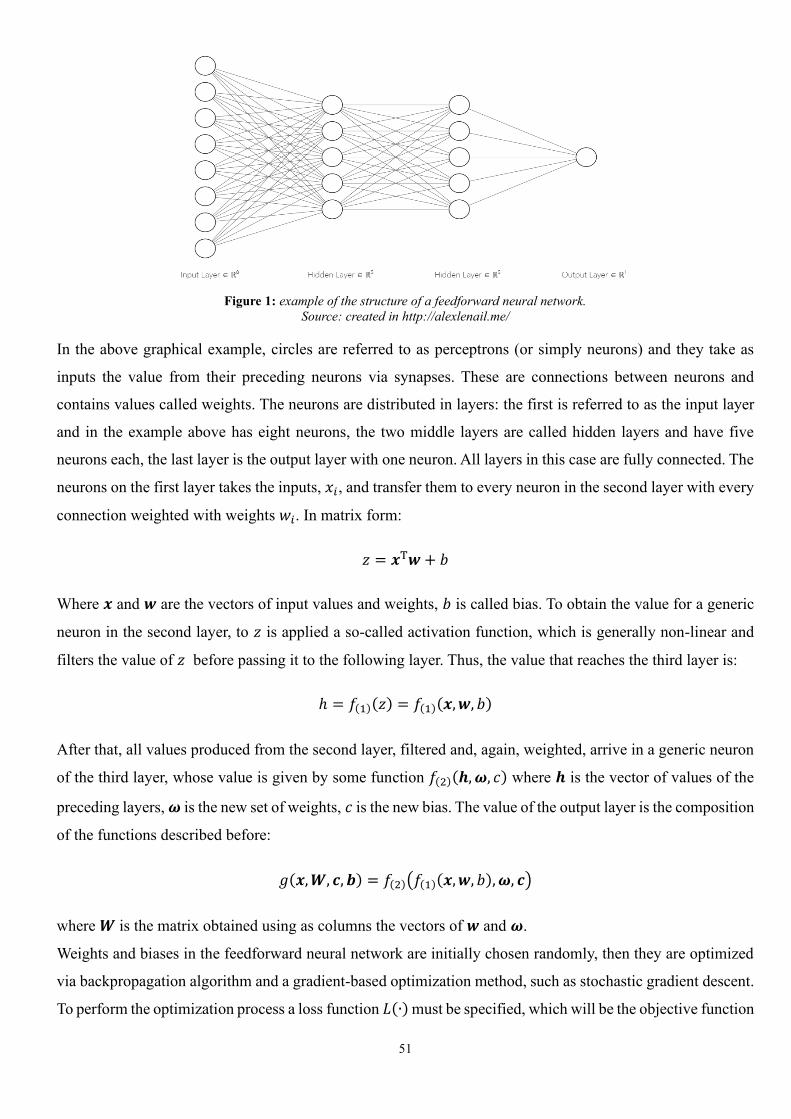
51

Figure 1: example of the structure of a feedforward neural network.

Source: created in http://alexlenail.me/

In the above graphical example, circles are referred to as perceptrons (or simply neurons) and they take as

inputs the value from their preceding neurons via synapses. These are connections between neurons and

contains values called weights. The neurons are distributed in layers: the first is referred to as the input layer

and in the example above has eight neurons, the two middle layers are called hidden layers and have five

neurons each, the last layer is the output layer with one neuron. All layers in this case are fully connected. The

neurons on the first layer takes the inputs, 𝑥𝑖, and transfer them to every neuron in the second layer with every

connection weighted with weights 𝑤𝑖. In matrix form:

𝑧 = 𝒙T𝒘 + 𝑏

Where 𝒙 and 𝒘 are the vectors of input values and weights, 𝑏 is called bias. To obtain the value for a generic

neuron in the second layer, to 𝑧 is applied a so-called activation function, which is generally non-linear and

filters the value of 𝑧 before passing it to the following layer. Thus, the value that reaches the third layer is:

ℎ = 𝑓(1)(𝑧) = 𝑓(1)(𝒙, 𝒘, 𝑏)

After that, all values produced from the second layer, filtered and, again, weighted, arrive in a generic neuron

of the third layer, whose value is given by some function 𝑓(2)(𝒉, 𝝎, 𝑐) where 𝒉 is the vector of values of the

preceding layers, 𝝎 is the new set of weights, 𝑐 is the new bias. The value of the output layer is the composition

of the functions described before:

𝑔(𝒙, 𝑾, 𝒄, 𝒃) = 𝑓(2)(𝑓(1)(𝒙, 𝒘, 𝑏), 𝝎, 𝒄)

where 𝑾 is the matrix obtained using as columns the vectors of 𝒘 and 𝝎.

Weights and biases in the feedforward neural network are initially chosen randomly, then they are optimized

via backpropagation algorithm and a gradient-based optimization method, such as stochastic gradient descent.

To perform the optimization process a loss function 𝐿(∙) must be specified, which will be the objective function

52

to be minimized.

The backpropagation algorithm works with the following four main steps:

1. Set the output of the first activation function ℎ1;

2. For each layer 𝑙 = 2,3, … , ℒ, compute 𝑧𝑙 ,ℎ𝑙 and 𝜀𝑙;

3. For each layer 𝑙 = ℒ − 1, ℒ − 2, … ,2, compute 𝜀𝑙 relating it to its next layer;

4. The gradient of 𝐿(∙) is given by the following equations for weights and biases:

𝜀𝑗𝑙 =

𝜕𝐿

𝜕𝑏𝑗𝑙

𝜀𝑗𝑙 ∙ ℎ𝑘

𝑙−1 =𝜕𝐿

𝜕𝑤𝑘𝑗𝑙

Where 𝜀𝑙 is called the error of the 𝑗th neuron in the layer 𝑙 and 𝜀𝑗𝑙 = 𝜕𝐿 𝜕𝑧𝑗

𝑙⁄ by definition.

The third step indicates why the algorithm described is called backpropagation.

Now, considering 𝑛 observations in a dataset and an objective function 𝐿(𝜸) to be minimized, with a set of

parameters 𝜸 that minimize the function and which have to be estimated, the basic algorithm of gradient

descent works as follow:

1. An initial vector 𝜸 is chosen and a learning rate 𝜂 is defined;

2. for 𝑖 = 1,2, … , 𝑛 do: 𝜸 ≔ 𝜸 − 𝜂∇𝐿𝑖(𝜸)30;

3. repeat until a minimum is reached.

A method called RMSProp (Root Mean Square Propagation), never published by Geoffrey Hinton in a formal

academic paper, has become one of the most used methods in practice. In this case, the update (step 2 above)

is made as follows:

𝜸 ≔ 𝜸 −𝜼

√𝒗(𝜸, 𝒕)𝜵𝑳𝒊(𝜸)

Where:

𝒗(𝜸, 𝒕) = 𝝆𝒗(𝜸, 𝒕 − 𝟏) + (𝟏 − 𝝆)(𝜵𝑳𝒊(𝜸))𝟐

𝜌 is the so-called forgetting factor, 𝑡 is the mini-batch size, 𝑣(𝜸, 𝑡) is called velocity.

In the neural network built in this thesis, Adam (Adaptive Moment Estimation) optimizer is used, which is an

evolution of RMSProp, which uses velocity for both the first and second momentum of the gradient:

𝒗𝟏(𝜸, 𝒕 + 𝟏) = 𝜷𝟏𝒗𝟏(𝜸, 𝒕) + (𝟏 − 𝜷𝟏)𝜵𝑳𝒊(𝜸)

30 In this case and in the following examples, the symbol ≔ indicates an update of the value, it is not a “definition” or “equality”

symbol.

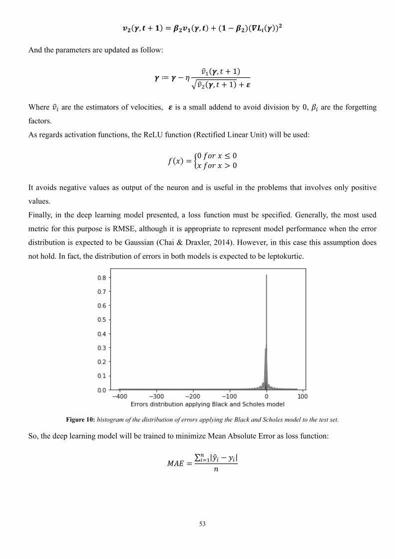
53

𝒗𝟐(𝜸, 𝒕 + 𝟏) = 𝜷𝟐𝒗𝟏(𝜸, 𝒕) + (𝟏 − 𝜷𝟐)(𝜵𝑳𝒊(𝜸))𝟐

And the parameters are updated as follow:

𝜸 ≔ 𝜸 − 𝜂𝑣1(𝜸, 𝑡 + 1)

√𝑣2(𝜸, 𝑡 + 1) + 𝜺

Where 𝑣𝑖 are the estimators of velocities, 𝜺 is a small addend to avoid division by 0, 𝛽𝑖 are the forgetting

factors.

As regards activation functions, the ReLU function (Rectified Linear Unit) will be used:

𝑓(𝑥) = {0 𝑓𝑜𝑟 𝑥 ≤ 0𝑥 𝑓𝑜𝑟 𝑥 > 0

It avoids negative values as output of the neuron and is useful in the problems that involves only positive

values.

Finally, in the deep learning model presented, a loss function must be specified. Generally, the most used

metric for this purpose is RMSE, although it is appropriate to represent model performance when the error

distribution is expected to be Gaussian (Chai & Draxler, 2014). However, in this case this assumption does

not hold. In fact, the distribution of errors in both models is expected to be leptokurtic.

Figure 10: histogram of the distribution of errors applying the Black and Scholes model to the test set.

So, the deep learning model will be trained to minimize Mean Absolute Error as loss function:

𝑀𝐴𝐸 =∑ |�̂�𝑖 − 𝑦𝑖|𝑛

𝑖=1

𝑛

54

Data preparation and implementation of the models

For the same reason stated before, MAE will be used as performance metric for both models. The

second performance measure with which Black-Scholes model and the deep learning approach will be

compared is the time necessary for the hardware to compute and apply the model to all test’s observations.

This measure is introduced to compare the models both in spatial and temporal aspect.

The dataset used to implement and compare the two models is the L3 Historical CSV Data Sample31 which

includes 928’674 observations of put and call European options traded on the Chicago Board Options

Exchange. All data are recorded on 15th August 2019. The following features are included:

Variable Class Description

UnderlyingSymbol Multinomial One to four letters, identifying the country of the company in which the option

is listed.

OptionSymbol Multinomial The ISIN code of the option, which identifies univocally the instrument.

Type Binomial It defines whether the option is a call or a put.

Expiration Date Settlement date of the contract.

DataDate Date It coincides with the observation date of the option, so it can be different from

the starting date of the contract.

UnderlyingPrice Numerical The price of the underlying asset of the option.

Strike Numerical The strike price of the option.

Last Numerical The price at which the last trade has been done.

Bid Numerical The theoretical maximum price at which a buyer is willing to pay for the option.

Ask Numerical The theoretical minimum price at which a seller is willing to take for the option.

Volume Numerical The trading volume of the option.

OpenInterest Numerical The actual total number of outstanding options that have not been settled yet.

IVMean Numerical The average between the bid implied volatility of the option and the ask implied

volatility.

IVBid Numerical The bid implied volatility.

IVAsk Numerical The ask implied volatility.

Delta Numerical The derivative of the option price with respect to its underlying price.

Gamma Numerical The sensibility of the option price with respect to its delta.

Theta Numerical The derivative of the option price with respect to its time to maturity.

Vega Numerical The derivative of the option price with respect to its implied volatility.

Table 1: a list of all the features in the dataset, with an identification of the type of variable and a brief description of their

meaning.

As regards the risk-free rate, the US Tree Months Treasury Bill rate at the 15th August 2019 date has been

chosen. The choice has been made because the average time to maturity of all the options in the dataset is

0.4028, which is close to 3 months, and the date is the date at which all options have been observed. The value

of the rate discussed is 0.0187.

31 Source: https://www.historicaloptiondata.com/

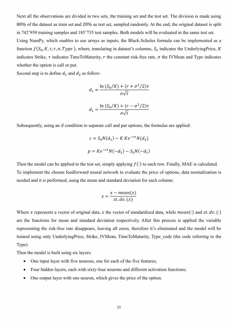
55

Next all the observations are divided in two sets, the training set and the test set. The division is made using

80% of the dataset as train set and 20% as test set, sampled randomly. At the end, the original dataset is split

in 742’939 training samples and 185’735 test samples. Both models will be evaluated in the same test set.

Using NumPy, which enables to use arrays as inputs, the Black-Scholes formula can be implemented as a

function 𝑓(𝑆0, 𝐾, 𝜏, 𝑟, 𝜎, 𝑇𝑦𝑝𝑒 ), where, translating in dataset’s columns, 𝑆0 indicates the UnderlyingPrice, 𝐾

indicates Strike, 𝜏 indicates TimeToMaturity, 𝑟 the constant risk-free rate, 𝜎 the IVMean and Type indicates

whether the option is call or put.

Second step is to define 𝑑1 and 𝑑2 as follow:

𝑑1 =ln (𝑆0 𝐾)⁄ + (𝑟 + 𝜎2 2⁄ )𝜏

𝜎√𝜏

𝑑1 =ln (𝑆0 𝐾)⁄ + (𝑟 − 𝜎2 2⁄ )𝜏

𝜎√𝜏

Subsequently, using an if condition to separate call and put options, the formulas are applied:

𝑐 = 𝑆0𝑁(𝑑1) − 𝐾 𝐾𝑒−𝑟𝜏𝑁(𝑑2)

𝑝 = 𝐾𝑒−𝑟𝜏𝑁(−𝑑2) − 𝑆0𝑁(−𝑑1)

Then the model can be applied to the test set, simply applying 𝑓(∙) to each row. Finally, MAE is calculated.

To implement the chosen feedforward neural network to evaluate the price of options, data normalization is

needed and it is performed, using the mean and standard deviation for each column:

𝑧 =𝑥 − 𝑚𝑒𝑎𝑛(𝑥)

𝑠𝑡. 𝑑𝑣. (𝑥)

Where 𝑥 represents a vector of original data, 𝑧 the vector of standardized data, while 𝑚𝑒𝑎𝑛(∙) and 𝑠𝑡. 𝑑𝑣. (∙)

are the functions for mean and standard deviation respectively. After this process is applied the variable

representing the risk-free rate disappears, leaving all zeros, therefore it’s eliminated and the model will be

trained using only UnderlyingPrice, Strike, IVMean, TimeToMaturity, Type_code (the code referring to the

Type).

Then the model is built using six layers:

• One input layer with five neurons, one for each of the five features;

• Four hidden layers, each with sixty-four neurons and different activation functions;

• One output layer with one neuron, which gives the price of the option.

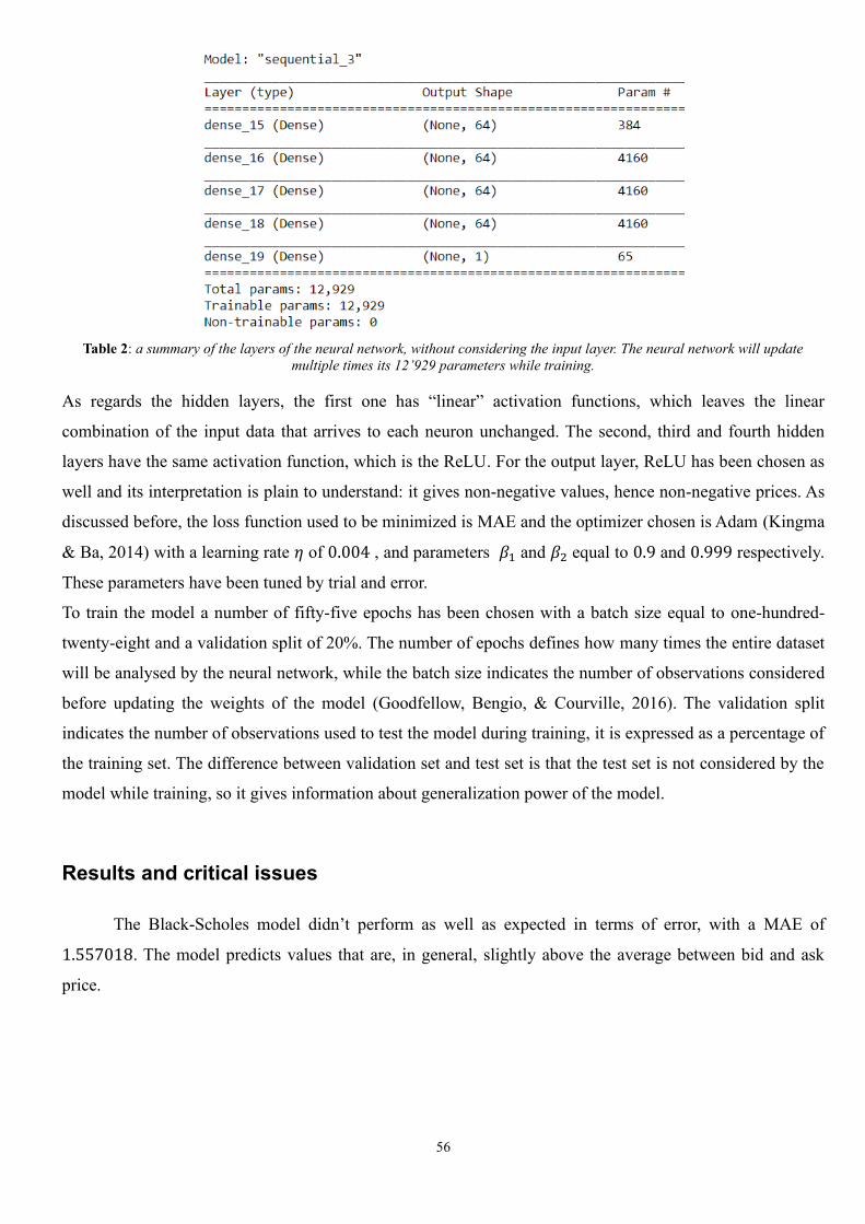
56

Table 2: a summary of the layers of the neural network, without considering the input layer. The neural network will update

multiple times its 12’929 parameters while training.

As regards the hidden layers, the first one has “linear” activation functions, which leaves the linear

combination of the input data that arrives to each neuron unchanged. The second, third and fourth hidden

layers have the same activation function, which is the ReLU. For the output layer, ReLU has been chosen as

well and its interpretation is plain to understand: it gives non-negative values, hence non-negative prices. As

discussed before, the loss function used to be minimized is MAE and the optimizer chosen is Adam (Kingma

& Ba, 2014) with a learning rate 𝜂 of 0.004 , and parameters 𝛽1 and 𝛽2 equal to 0.9 and 0.999 respectively.

These parameters have been tuned by trial and error.

To train the model a number of fifty-five epochs has been chosen with a batch size equal to one-hundred-

twenty-eight and a validation split of 20%. The number of epochs defines how many times the entire dataset

will be analysed by the neural network, while the batch size indicates the number of observations considered

before updating the weights of the model (Goodfellow, Bengio, & Courville, 2016). The validation split

indicates the number of observations used to test the model during training, it is expressed as a percentage of

the training set. The difference between validation set and test set is that the test set is not considered by the

model while training, so it gives information about generalization power of the model.

Results and critical issues

The Black-Scholes model didn’t perform as well as expected in terms of error, with a MAE of

1.557018. The model predicts values that are, in general, slightly above the average between bid and ask

price.

57

Figure 12: representation of actual prices vs. Black-Scholes prices. The predictions are biased upward.

As regards the temporal aspect, it performed fairly well with a time to price all the 185’735 test observations

equal to 0.116884 seconds32.

As regards the neural network model, it performed better in terms of MAE, but worse in terms of time to

compute. The learning curve showed a fast convergence:

Figure 13: a graph of the learning curve of the deep learning model, showing the MAE per Epoch.

The test set’s MAE is approximately near the train set’s MAE, indicating a good generalization power of the

model and the final test set’s MAE is 0.802675, which is lower than the one achieved by the Black-Scholes

32 This computation has been performed on an Intel Core i7-8750H CPU.

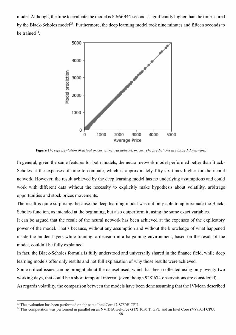
58

model. Although, the time to evaluate the model is 5.666841 seconds, significantly higher than the time scored

by the Black-Scholes model33. Furthermore, the deep learning model took nine minutes and fifteen seconds to

be trained34.

Figure 14: representation of actual prices vs. neural network prices. The predictions are biased downward.

In general, given the same features for both models, the neural network model performed better than Black-

Scholes at the expenses of time to compute, which is approximately fifty-six times higher for the neural

network. However, the result achieved by the deep learning model has no underlying assumptions and could

work with different data without the necessity to explicitly make hypothesis about volatility, arbitrage

opportunities and stock prices movements.

The result is quite surprising, because the deep learning model was not only able to approximate the Black-

Scholes function, as intended at the beginning, but also outperform it, using the same exact variables.

It can be argued that the result of the neural network has been achieved at the expenses of the explicatory

power of the model. That’s because, without any assumption and without the knowledge of what happened

inside the hidden layers while training, a decision in a bargaining environment, based on the result of the

model, couldn’t be fully explained.

In fact, the Black-Scholes formula is fully understood and universally shared in the finance field, while deep

learning models offer only results and not full explanation of why those results were achieved.

Some critical issues can be brought about the dataset used, which has been collected using only twenty-two

working days, that could be a short temporal interval (even though 928’674 observations are considered).

As regards volatility, the comparison between the models have been done assuming that the IVMean described

33 The evaluation has been performed on the same Intel Core i7-8750H CPU. 34 This computation was performed in parallel on an NVIDIA GeForce GTX 1050 Ti GPU and an Intel Core i7-8750H CPU.

59

in previous chapter was representative of the average between bid and ask prices. This assumption not always

holds and could have caused biases for both the models.

Another aspect is the risk-free rate considered, the same for all options in the dataset. The risk-free rate should

have been different for each option, based on the market, the timing and the geographical position of the

option. The simplification adopted could have caused deviations in the Black-Scholes model and the neural

network architecture built should have been different to account for different risk-free rates (for instance one

neuron should have been added in the input layer). This aspect can be considered for further improvements of

this work.

This work represents a tiny step in comparing mathematical models and deep learning approaches in option

pricing, using the same features for both.

Conclusions

Option pricing has been a prolific topic in literature. The most influential model is the Black-Scholes

model (Black & Scholes, 1973), but, in the last decade, the rise of Big Data and machine learning led to the

spread of new models, which have found a wide range of applications. In this thesis, a deep learning model

was built for option pricing and compared to the Black-Scholes model, using the same features for both.

The feedforward neural network built outperformed the Black-Scholes model in terms of mean absolute error,

but it took more time for computation. The aim of this thesis was to make a step in the favour of use of deep

learning models in the field of pricing in finance and the results achieved go in the desired direction.

Nevertheless, some critical issues are present, such as the temporal range of options considered in the dataset,

the price label considered, the use of implied volatility, the simplification made about risk-free rate, and,

finally, the poor hardware environment in which both model have been implemented. Further improvements

can solve these issues by using different labels for prices, more accurately chosen, different methods for

approximating the volatility and more specific data, which includes different risk-free rates for different

options.

Practical implications of this result can influence trading and portfolio management. The deep learning model

presented, in fact, can be used to price options and can be re-trained with new options traded every day, making

it more precise over time. The usefulness of the model presented is that it only requires the same features of

the Black-Scholes model, which are information easy to acquire in practice.