14/02/05C. Barbieri Elementi_AA_2004-05 Quinta settimana 1 Elementi di Astronomia e Astrofisica per...

14/02/05 C. Barbieri Elementi_AA_2004-05 Quinta settimana

1

Elementi di Astronomia e Astrofisica per il Corso di Ingegneria Aerospaziale

V settimanaParallasse Diurna e AnnuaLa missione NEARParallassi dinamiche e secolariMoti propri e velocità radiali La missione Hipparcos e la missione GAIAApice del moto solare e il Local Standard of Rest Esercizi

Avvertenza: in inglese!


2

The ParallaxThe phenomenon of the parallax is due to the finite distance of the object from the observer. Two observers located in two different positions, or the same observer moving from one place to another because of the diurnal rotation or annual revolution, will see the object in two different locations on the celestial sphere. Of all the phenomena described so far, that alter the apparent direction of the source, the parallax is the first to give information on the distance, and therefore on the nature, of the heavenly body, and not only on the motions of the observer or on fundamental properties of light. Furthermore, the knowledge in meters of the distance between the observers provides a link between the terrestrial and the cosmic distance scales. The determination of the parallaxes is therefore one of the most fundamental (but also most difficult) astronomical measurements.


3

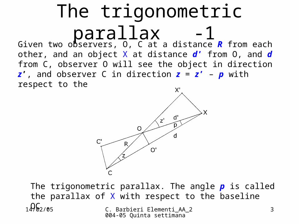
The trigonometric parallax -1 Given two observers, O, C at a distance R from each other, and an object X at distance d’ from O, and d from C, observer O will see the object in direction z’, and observer C in direction z = z’ – p with respect to the baseline OC :

The trigonometric parallax. The angle p is called the parallax of X with respect to the baseline OC .


4

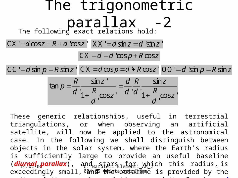
The trigonometric parallax -2The following exact relations hold:

CX' cos 'cos 'd z R d z XX' sin 'sin 'd z d z CX 'cos cosd d p R z

CC' sin sin 'd p R z C'X cos ' cos 'd p d R z OO' 'sin sind p R z

sin ' sintan

' ' '1 cos ' 1 cos '' '

R z d R zp

R Rd d dz zd d

These generic relationships, useful in terrestrial triangulations, or when observing an artificial satellite, will now be applied to the astronomical case. In the following we shall distinguish between objects in the solar system, where the Earth’s radius is sufficiently large to provide an useful baseline (diurnal parallax), and stars for which this radius is exceedingly small, and the baseline is provided by the radius of the annual revolution around the Sun (annual parallax).


5

The diurnal parallax - 1 When determining the celestial coordinates of an object of the solar system (say a planet, but the same will hold for a comet or an asteroid), it will be necessary to take into account the location of the observer on the terrestrial surface, namely his topography, in order to translate these coordinates to an ideal geocentric observer. This process will therefore transform topocentric into geocentric coordinates.

Be C the center of the Earth, O the generic observer on the surface, at a distance R = a from C ( 1), X the planet distant d from C and d’ from O (see Figure), the angle p = CXO is the instantaneous parallax of X.

The instantaneous diurnal parallax p. The ellipticity of the Earth is greatly exaggerated. The plane COC’ doesn’t necessarily coincide with the meridian of C.


6

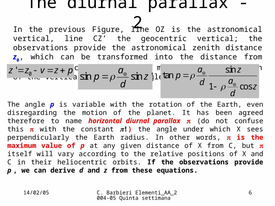
The diurnal parallax - 2In the previous Figure, line OZ is the astronomical vertical, line CZ’ the geocentric vertical; the observations provide the astronomical zenith distance z0,

which can be transformed into the distance from the geocentric vertical z’ by means of the deviation of the vertical v = ’- . The angle p is then given by:

0'z z v z p sin sin '

ap z

d

sintan

1 cos

a zp

ad zd

The angle p is variable with the rotation of the Earth, even disregarding the motion of the planet. It has been agreed therefore to name horizontal diurnal parallax (do not confuse this with the constant !) the angle under which X sees perpendicularly the Earth radius. In other words, is the maximum value of p at any given distance of X from C, but itself will vary according to the relative positions of X and C in their heliocentric orbits. If the observations provide p , we can derive d and z from these equations.


7

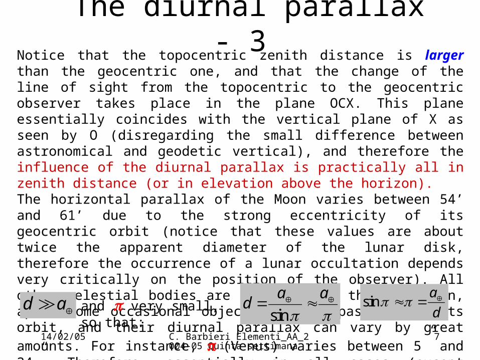
The diurnal parallax - 3Notice that the topocentric zenith distance is larger than the geocentric one, and that the change of the line of sight from the topocentric to the geocentric observer takes place in the plane OCX. This plane essentially coincides with the vertical plane of X as seen by O (disregarding the small difference between astronomical and geodetic vertical), and therefore the influence of the diurnal parallax is practically all in zenith distance (or in elevation above the horizon). The horizontal parallax of the Moon varies between 54’ and 61’ due to the strong eccentricity of its geocentric orbit (notice that these values are about twice the apparent diameter of the lunar disk, therefore the occurrence of a lunar occultation depends very critically on the position of the observer). All other celestial bodies are much farther than the Moon, apart some occasional object than can pass inside

its orbit, and their diurnal parallax can vary by great amounts. For instance, (Venus) varies between 5” and 34”. Therefore, essentially in all cases (except artificial satellites) we are justified to assume:

d a and very small, so that:sin

a ad

sin

a

d


8

The diurnal parallax -4

For the Sun, averaging over the slight ellipticity of the orbit, the distance d is the astronomical unit a = 1 AU 1.49x108 km, the horizontal parallax is essentially constant, so that:

ad a

" 8".8

For any other body of the solar system, expressing its distance d in AU and the parallax in seconds of arc we have:

1"= "

(AU)d

" sin ' 8.8" sin '(AU)

p z zd d

When observing it in the meridian, we also have:


9

Effect of the diurnal parallax on the equatorial coordinates

" sin" " cos '

(AU) cos

"" (sin 'cos cos 'sin cos )

(AU)

HAHA

d

HAd

After several passages, taking advantage of the great distance of the bodies with respect to the Earth's radius, we obtain the following relationships:

which express (in seconds of arc) the change in HA and Dec due to the finite distance. No sensible error is made if the observed quantities HA’, ’ are substituted to the geocentric values in the right side of these equations. Notice however that the symmetry between geocentric and topocentric coordinates in is illusory: indeed, the knowledge of the geocentric coordinates depends on the previous knowledge of the geocentric distance. For a new comet or asteroid, d is unknown, so that only the trigonometric expressions (named also parallactic factors) can be computed.


10

Diurnal parallax and apparent diameterThe diurnal parallax has also an interesting consequence on the apparent diameters. Let s be the diameter in km of a planet (treated here for simplicity as a disk), S its apparent geocentric angular radius when at geocentric distance d, and S’, d’ the corresponding topocentric values; the following relations will hold:sin

sS

d

sin 'sin ' sin

' ' sin

s s d zS S

d d d z

The angles are usually small quantities, so that: sin '

'sin

zS S

z

From the Earth’s surface, the effect for the Sun never exceeds 0.1”, but it is noticeable for the Moon, whose geocentric apparent radius is given by S = 0.272, with a maximum variation of approximately 40”. Therefore this change in lunar diameter with the location of the observer must be taken into account when calculating precise circumstances of eclipses and occultations. Another effect could be considered for the Moon, namely the slight retardation of the rising and anticipation of the setting instants (at most 1.5 minutes), an effect contrary to the much larger one due to the atmospheric refraction.


11

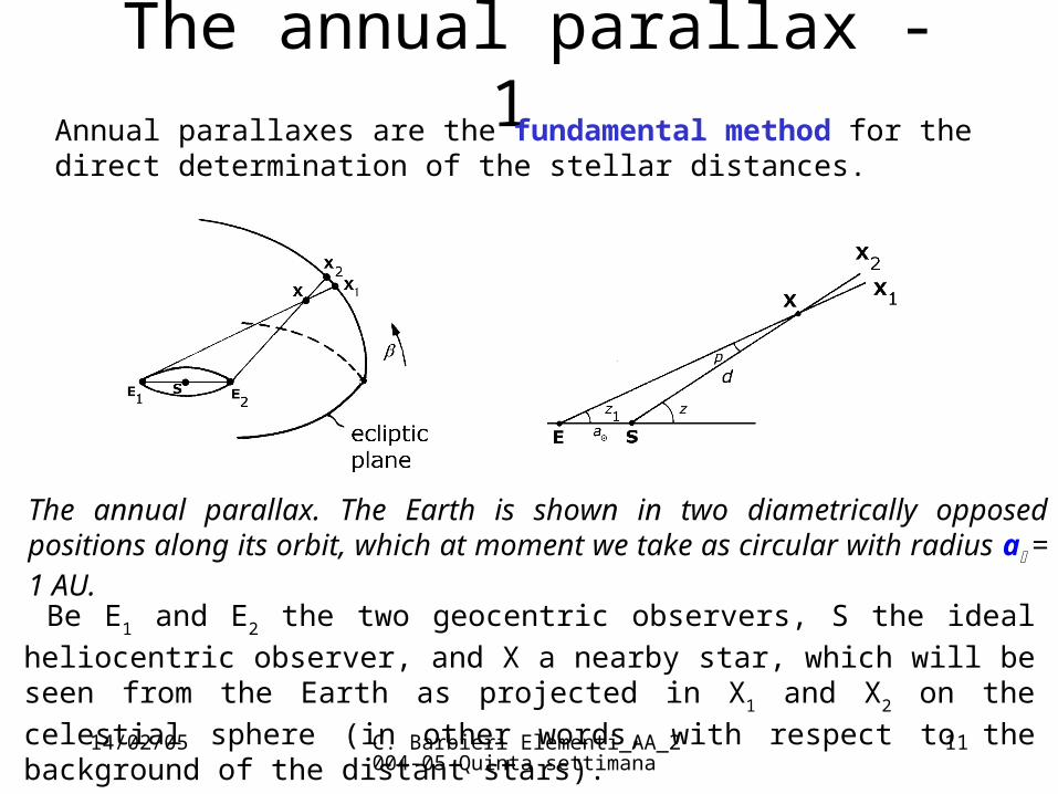
The annual parallax - 1 Annual parallaxes are the fundamental method for the direct determination of the stellar distances.

The annual parallax. The Earth is shown in two diametrically opposed positions along its orbit, which at moment we take as circular with radius a = 1 AU.

Be E1 and E2 the two geocentric observers, S the ideal heliocentric observer, and X a

nearby star, which will be seen from the Earth as projected in X1 and X2 on the

celestial sphere (in other words, with respect to the background of the distant stars).


12

The annual parallax - 2Let ES be the direction Earth-Sun, z the angle of the line of sight with that

direction from S and z’ from E, d the heliocentric distance of X. We have:

sin ' sin( ') sina z d z z d p sina

d sin( ' )

sin 'sin

z zz

The angle , under which the Astronomical Unit is seen perpendicularly from the star, namely the maximum value of p, is called the annual parallax of X. Until now, star Proxima Centauri (in the triple system of Cen) has the largest

observed value, = 0.76”; no sensible error is therefore made in using arcs instead of their sine or tangent, and therefore:

' sin ' sinz z z z z Therefore, the geocentric observer sees the star closer to the Sun by the slight amount (z’-z); on the celestial sphere this apparent movement occurs along the great circle passing through X and S.


13

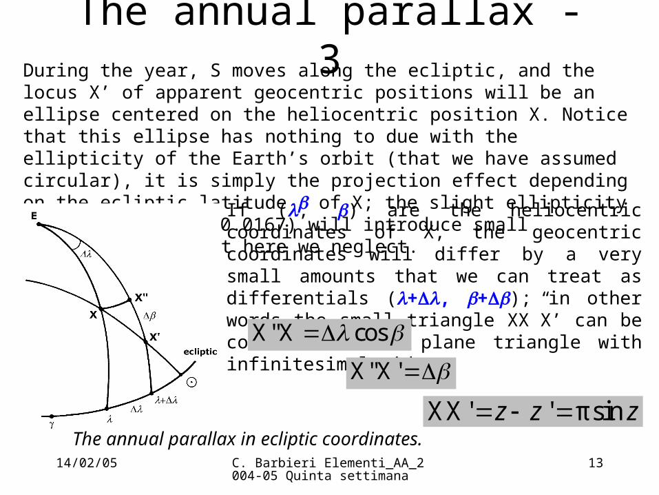
The annual parallax - 3During the year, S moves along the ecliptic, and the locus X’ of apparent geocentric positions will be an ellipse centered on the heliocentric position X. Notice that this ellipse has nothing to due with the ellipticity of the Earth’s orbit (that we have assumed circular), it is simply the projection effect depending on the ecliptic latitude of X; the slight ellipticity of the orbit (e = 0.0167) will introduce small modifications, that here we neglect.

If (, ) are the heliocentric coordinates of X, the geocentric coordinates will differ by a very small amounts that we can treat as differentials (+, +); in other words the small triangle XX”X’ can be considered as a plane triangle with infinitesimal sides:

X"X cos

X"X'

XX' ' π sinz z z The annual parallax in ecliptic coordinates.


14

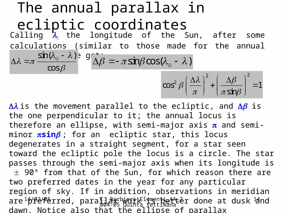
The annual parallax in ecliptic coordinatesCalling the longitude of the Sun, after some calculations (similar to those made for the annual aberration), we get:

sin( )

cos

sin cos( )

222cos 1

sin

is the movement parallel to the ecliptic, and is the one perpendicular to it; the annual locus is therefore an ellipse, with semi-major axis and semi-minor sin ; for an ecliptic star, this locus degenerates in a straight segment, for a star seen toward the ecliptic pole the locus is a circle. The star passes through the semi-major axis when its longitude is 90° from that of the Sun, for which reason there are two preferred dates in the year for any particular region of sky. If in addition, observations in meridian are preferred, parallax work is better done at dusk and dawn. Notice also that the ellipse of parallax anticipates by 3 months that of annual aberration, and of course its dimensions are proportional to the distance, and not fixed as the one of aberration.


15

The annual parallax in equatorial coordinatesIn equatorial coordinates, this ellipse will be rotated by a certain angle, and it is not difficult to prove the following relations:

cos (cos cos sin sin cos )

( cos sin )

(sin cos sin cos sin cos cos sin sin sin )

( cos cos sin sin sin )

Y X

Z X Y

where (X, Y, Z) are the geocentric equatorial coordinates of the Sun. These corrections , must be added with their signs to the heliocentric coordinates, subtracted from the geocentric ones.


16

The parsecUsing the Astronomical Unit as baseline, it is possible to institute the fundamental unit of astronomical distances, namely the parsec:

one parsec (pc) is the distance from where the AU subtends perpendicularly an angle of 1”. Therefore:

1 pc = 206264.8 AU = 3.09 x1013 km where the last conversion factor is derived from the solar parallax. Any revision of this latter value will not change the distance as expressed in parsecs. On the practical side, this remark is not so important today, because the precision with which the solar parallax is known is much higher than the precision of stellar distances; it is useful to remember it, however, considering how the cosmic distances ladder has been connected to the laboratory units.

A secondary unit of distance is the light-year (l-y), corresponding to the distance traveled in vacuum by the light in one year; it is easily found that 1 pc 3.26 l-y.


17

A list of approximations The above treatment of stellar parallaxes is approximate for several reasons:- the orbit of the Earth is slightly elliptical.- the heliocentric observer should be substituted by the barycentric observer. The distance between the two never exceeds 0.01 AU (2 solar radii), with a complex behavior in time according to the longitude of Jupiter, Saturn and the other planets (see previous lectures for a graph of the position of the Solar System barycenter)- the relativistic deflection of light affects the apparent directions at the level of 0.001”- the geocentric observer should be replaced by the Earth-Moon barycentric observer; the effect is smaller than the diurnal aberration on that particular star, because the barycenter is inside the body of the Earth. The differences between our approximate treatment and a more rigorous one are of the order of (a/d)2 from the trigonometric point of view. Furthermore, a correct treatment in the frame of General Relativity would introduce terms depending from the radial velocity Vr and the proper motion of the star, because

parallaxes cannot be totally separated from aberration and velocities.


18

Secular parallaxesThe Solar System moves with respect to the ensemble of the nearby stars with a velocity of approximately 20 km/s in direction of the constellation Lyra (a point named apex of solar motion). An hypothetic observer, at rest in the frame of this group of nearby stars, would observe the Sun in rectilinear motion toward this apex, and the planets describing open orbits around it; the distance covered by the traveling Sun is approximately 4 AU per year. This baseline is four times that of the annual parallaxes, and we call secular parallax H of the star X the angle under which this baseline is seen perpendicular. Let’s call s (km/s) the velocity of the Sun, n the number of seconds in one year, d (km) the heliocentric distance of X; after simple conversion of the relevant units we find:

44.74

sH

However, this is a secular, not a periodic, motion, and it is observed entangled with the proper motion of that particular star. It is however an useful distance indicator for a group of stars having the same distance, as we shall discuss also in the next lectures.


19

Dynamic Parallaxes - 1a) A body of the solar systemconsider Kepler’s third law for a given planet, in its approximate expression:

being P the sidereal period, a the semimajor axis of its orbit and M the mass of the Sun. Comparing this with the Earth's values:

2 3(4 / )P M a €

2 2 3 3/ /P P a a

we can derive only the relative dimensions of each orbit. At least one absolute determination in km is needed to fix the scale of the Solar System. To reach this goal, it is advantageous to observe from several locations an asteroid (having a star-like image) whose orbit takes it as close as possible to the Earth. Several asteroids were tried, the one giving the best results being 433 Eros.


20

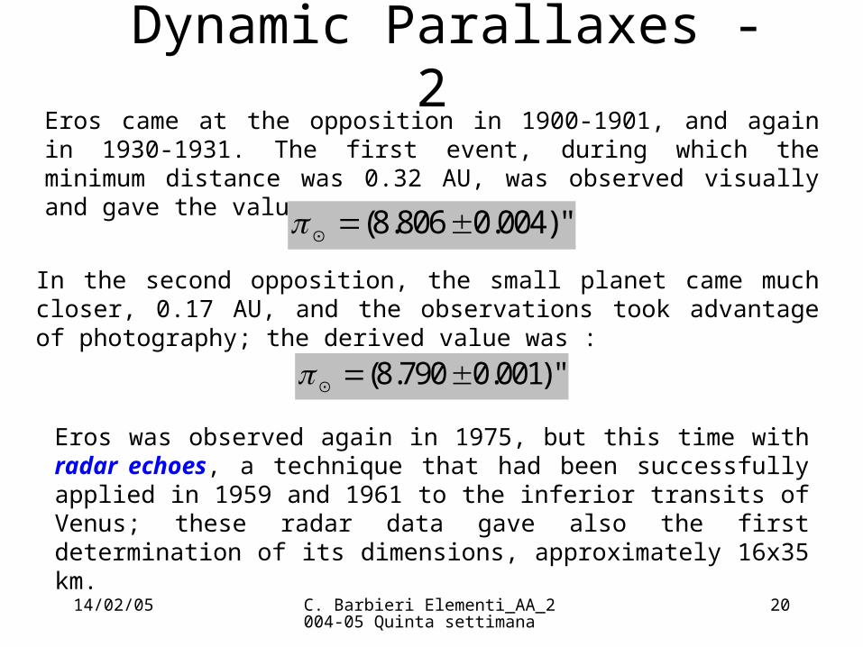
Dynamic Parallaxes - 2Eros came at the opposition in 1900-1901, and again in 1930-1931. The first event, during which the minimum distance was 0.32 AU, was observed visually and gave the value :

Eros was observed again in 1975, but this time with radar echoes, a technique that had been successfully applied in 1959 and 1961 to the inferior transits of Venus; these radar data gave also the first determination of its dimensions, approximately 16x35 km.

(8.806 0.004)"

In the second opposition, the small planet came much closer, 0.17 AU, and the observations took advantage of photography; the derived value was :

(8.790 0.001)"


21

The asteroid EROSEros orbits the Sun with a perihelion of 1.13 Astronomical Units (169,045,593 kilometers) and an aphelion of 1.78 AU (266,284,209 kilometers), and it rotates once every 5 hours and 16 minutes. The dimensions are of 33 kilometers long, 13 kilometers wide and 13 km thick . Eros is an S-type asteroid, the most common type found in the inner asteroid belt. Asteroids are classified by their albedos and colors as determined by spectrographic observation. The spectra of S-types imply a composition of iron- and magnesium-bearing silicates (pyroxene and olivine) mixed with metallic nickel and iron. Comparison with meteorites: Ordinary chondrites, the most common meteorites, seem primitive and relatively unchanged since the solar system formed 4.6 billion years ago. Stony-iron meteorites, on the other hand, appear to be remnants of larger bodies that were once melted so that the heavier metals and lighter rocks separated into different layers. Eros is spectrally similar to both ordinary chondrite and stony iron meteorites, but its composition more closely matches the ordinary chondrites.


22

The NEAR mission

Before reaching EROS, the NEAR S/C had a close flyby with the large asteroid Mathilde


23

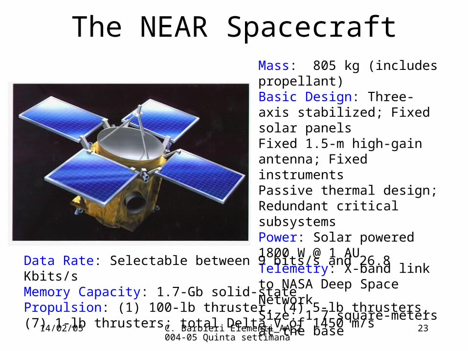
The NEAR SpacecraftMass: 805 kg (includes propellant)Basic Design: Three-axis stabilized; Fixed solar panelsFixed 1.5-m high-gain antenna; Fixed instrumentsPassive thermal design;Redundant critical subsystemsPower: Solar powered 1800 W @ 1 AUTelemetry: X-band link to NASA Deep Space NetworkSize: 1.7 square-meters at the base

Data Rate: Selectable between 9 bits/s and 26.8 Kbits/sMemory Capacity: 1.7-Gb solid-state Propulsion: (1) 100-lb thruster, (4) 5-lb thrusters, (7) 1-lb thrusters; total Delta V of 1450 m/s


24

Images of EROS from NEAR - 1

Eros was reached in 2000- 2001 by the spacecraft NEAR, who crashed on its surface at the end of a very successful mission.


25

Images of EROS from NEAR - 2

It is difficult to understand how these large boulders can stick to the surface, having EROS such low gravity.


26

Radar Images of Toutatis

The NASA-JPL 70-m Goldstone radar is most effective to study asteroids.

High-Resolution Model of Asteroid 4179 Toutatis. Hudson, R. S., S. J. Ostro, and D. J. Scheeres. Icarus 161, 346-355 (2003).

A model of the shape of Toutatis based on high-resolution radar images obtained in 1992 and 1996 consists of 39,996 triangular facets of roughly equal area, defined by the locations of 20,000 vertices. These define the average spatial resolution of the model as approximately 34 m.


27

Dynamic Parallaxes - 3b) A binary starLet A, B be the two components of a binary star, having respectively MA and

MB masses, and orbital period P. Kepler’s third law states that: 3

2

A B

4

( )

aP

G M M

In astronomical units (M in solar masses, P in years):

3

3 2

1A B

aM M M

P

(pay attention to = 3.1415... in the first formula, and = parallax in the second).

In the second equation, a and are both in arcsec. Masses in general are

unknown, but putting M = 2 an acceptable value for is obtained, because of the small weight of M on the error. The method can be refined by using an appropriate mass-luminosity function, calibrated on well known systems, but

usually the uncertainties on a and P dominate the error on .


28

The orbits of a binary starThe case of Sirius, the brightest star in the sky.Sirius A has a very faint companion, Sirius B, which has however practically the same mass of Sirius A, and also the same high surface temperature (approximately 10000 K). Historically, Sirius B was the first case of a white dwarf.From the apparent orbit (upper figure) one can deduce the relative orbit of the secondary referred to the primary, but this is a very favourable case.


29

The proper motions - 1Let us consider the proper motion of the nearer stars.

Be S the heliocentric observer, and X a generic star at a distance d with heliocentric velocity V, at a certain date (see Figure). Due to the enormous distances, apart very few exceptions such as Barnard’s star, for many decades or centuries the velocities can be considered as rectilinear and uniform. Expressing their modules in km/s, and indicating with n the number of seconds in one year, after one year the star will be seen in X’, having traveled a course of Vn km along a rectilinear path forming an unknown angle with axis SX. On the plane tangent to the celestial sphere, the star will appear to have moved by the small angle:

sinV

μd

n rad


30

The proper motions - 2The component of V perpendicular to the line of sight,Vt , is said transverse, or tangential, velocity. The corresponding apparent angular velocity is said proper motion of the star X, and is commonly measured in arcsec/year, or

arcsec/century. By using the parallax in arcsec instead of the distance d in km, and taking into account the appropriate conversion factors (namely: 1 km/s = 0.21095 AU/y, 1 AU/y = 4.74045 km/s), we derive:

tV Vsin 4.740

km/s tV4.740

arcsec/year

Barnard’s star has the highest known proper motion, = 10”/y. 61 Cyg (the first annual parallax, amounting to = 0.30”, was determined in 1838 by F. Bessel for this star, which had been suggested by G. Piazzi as likely to be near to the Sun because of its very large proper motion) has = 5”/year. Very few

stars have larger than 2”/year; obviously, the nearer stars have in general larger proper motions, but the viceversa is not true, many nearby stars have small motions because of the orientation of their velocity vectors.


31

The proper motions - 3For the nearer stars, the annual ellipse of parallax is trailed by the proper motion, as evidenced in the Figure.

The proper motion trails the annual

parallax ellipse of a nearby star having

= 0”.08 and = 0”.03 /year

(from satellite Hipparcos data: the segments give the instantaneous positions and associated errors, the continuous line is the best fitting path).


32

Proper motions as vectors - 1It is convenient to consider the proper motion as a vector (, q) on the plane tangent to the celestial sphere, with modulus expressed in angular units (arcsec/year) along the great circle XX”, and direction expressed by a position angle q measured from the North through the East (0° q <360°). Alternatively, the two equatorial components (, ) can be given; attention must be paid to the

units of , because the angular distance between two successive positions of the

star must be measured along the great circle passing through XX”, but quite often is derived by the difference between two successive Right Ascensions.

sα

1( / y) ("/ y)sin sec

15q

δ ("/ y) ("/ y)cos q

s("/ ) 15 ( /y)cosy

α

δ

("/ )tan

("/ )

yq

y


33

Proper motions as vectors - 2In the same manner, the tangential velocity components are derived as:

tα

("/y)V 4.740

δ

tδ

("/y)V 4.740

km/s

2 2 2 2

4.74t t

tant

qt

namely, the position angle of the proper motions is the same as that of the tangential velocity, and is independent of the parallax of the star. Again with reference to the Figure, from the spherical triangle XNCPX’ we notice that:

cos sin cos "sin "q q namely that the quantity is conserved during the movement of the star, implying that: d

(cos sin ) 0d

qt

tan tanq q


34

Effect of the proper motions on the equatorial coordinates

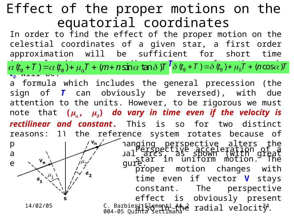
In order to find the effect of the proper motion on the celestial coordinates of a given star, a first order approximation will be sufficient for short time intervals; its mean coordinates T years after the epoch t0 will be:

0 0 α( ) ( ) ( sin tan )t T t T m n T 0 0 δ( ) ( ) ( cos )t T t T n T

a formula which includes the general precession (the sign of T can obviously be reversed), with due attention to the units. However, to be rigorous we must note that (, ) do vary in time even if the velocity is rectilinear and constant. This

is so for two distinct reasons: 1) the reference system rotates because of precession; 2) the changing perspective alters the apparent length of equal arcs, as shown (with great exaggeration) in the Figure.

Perspective acceleration of a star in uniform motion. The proper motion changes with time even if vector V stays constant. The perspective effect is obviously present also in the radial velocity.


35

Derivatives of the proper motion Consider the successive terms in (t), (t):

20 0 α

1( ) ( ) ( sin tan )

2t T t T m n T T

20 0 δ

1( ) ( ) ( cos )

2t T t T n T T

The time derivatives of (, ) are composed of two terms:

a) a term due to precession, independent from radial velocity and distance, and clearly the dominating one; b) a term due to the variation of the projection of the velocity on the line of sight, and that can be written down explicitly only if parallax and radial velocity are both known. The components due to precession clearly modify only the direction of , but not its modulus.


36

Radial Velocities -1From a formal point of view, if r is the heliocentric (or better barycentric) position vector of a star at a given initial epoch t0, and

0 0 01/ sin 1/r

its distance in terms of the trigonometric parallax , the velocity vector could be easily derived:

0 0 0

0 0 0 0

0 0

cos cos

( ) sin cos

sin

r

t r

r

r0 0 0 0 0 0 0 0

0 0 0 0 0 0 0 0 0

0 0 0

sin cos cos sin cos cos

( ) cos cos sin sin sin cos

0 cos sin

r

t r

r

r

where 0, 0 are the proper motions in Right Ascension and Declination, and

dr/dt is the radial velocity. The position of the star at a following date t1, but

referred to the same epoch t0, would then be derived from:

1 0 1 0( ) ( ) ( )t t t t r r r


37

Radial velocities -2However, the knowledge of the needed quantities is usually incomplete, so that in the following the radial velocities and the proper motions will be considered separately. It also clear that the treatment of the system of proper motions and velocities is fundamentally linked to that of precession, a great complication indeed for transferring catalogues based on stellar observations from one epoch to another, if the highest precision is to be maintained. The radial velocity is measured through the Doppler effect, namely through the variation in wavelength of the radiation, caused by the relative motion Vr along

the line of sight; the velocities of the planets or of the stars of the Milky Way are usually so small in comparison with the velocity of the light c that no sensible error is made in using the pre-relativistic formula:

O Sr

S

V c c cz

O r

S

V1 1 z

c

where O is the wavelength measured by the observer, and S is that measured in

the rest-frame of the source. The use of letter z is fairly widespread.

/z


38

Radial Velocities -3Notice that the radial velocity can be positive (z > 0, namely the wavelength is red-shifted), or negative (z < 0, namely the wavelength is blue-shifted). When the velocities exceed say 0.01c, then Special Relativity must be taken into account. It is more advantageous then to work in terms of frequency than of wavelength . In vacuum: /c 2d d /c

the classical formula would be:

S O1 /z

In the Relativistic formula:2

12

V 11 (1 )O S c c

V n

where n is the normal to the wavefront. It is seen therefore that Special Relativity foresees a transverse Doppler effect (when n is perpendicular to V), which is not present in the pre-relativistic formula. In other words, the whole velocity vector, and not only its radial component, enter in the observed frequency displacement.


39

Radial velocities - 4

21 V / 1 V

11 V / 2

c Vz

c c c

O S

1 V /

1 V /

c

c

If the velocity is all radial:

After simple passages, we derive:

21

cos11

O

21

cos111

Oz

=V/c, and angle = - is the angle between the line of sight and the velocity vector of S.


40

Radial velocities in the Solar System

In the Solar System, velocities of few tens of km/s prevail, with the notable exception of comets and asteroids skimming the surface of the Sun, whose heliocentric velocity can exceed 700 km/s.Therefore, the classical formula is adequate for most applications.

However, another factor must be carefully taken into account, that of the extreme precision (say 1 mm/s) with which the velocity of a spacecraft, possibly orbiting a planet, can be measured. The consequence is that for accurate navigation inside the Solar System, General Relativity must be taken into account in expressing the metric of space-time.


41

Radial velocities of the stars

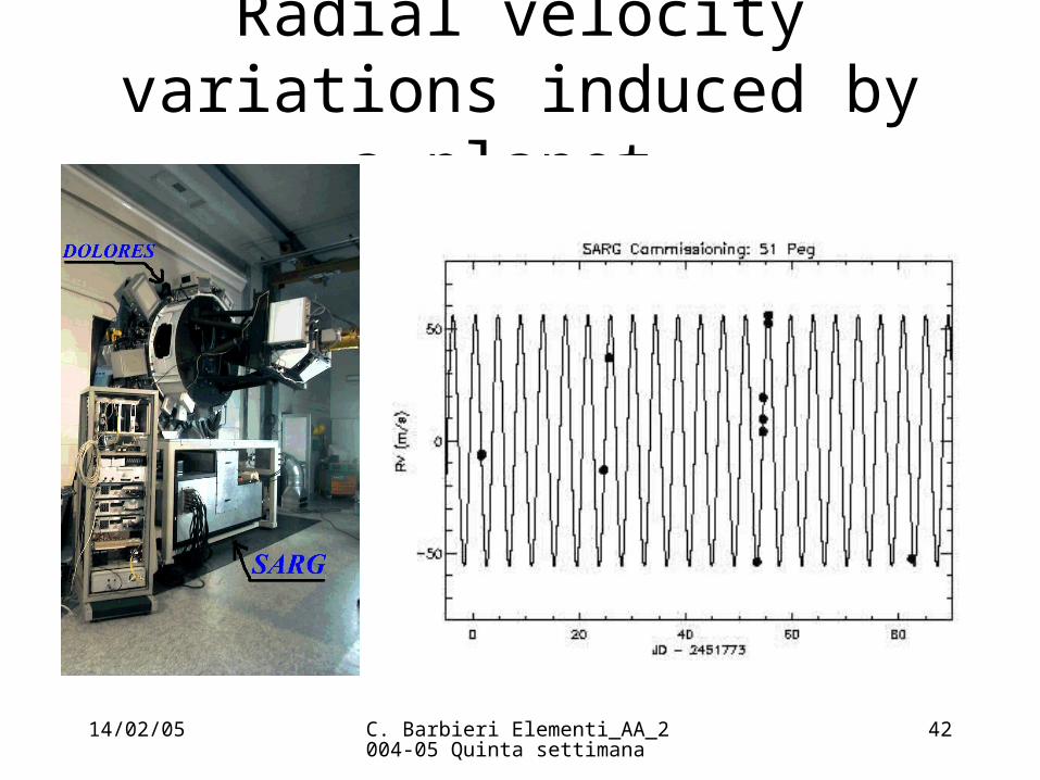
The radial velocities of the normal stars of the Galaxy rarely reach 500 km/s; among the nearest stars, velocities higher than 50 km/s are seldom encountered, with notable exceptions such as Barnard’s star, which moves at Vr = –108 km/s with respect to the Sun. For the great majority of stars, a precision of at best 100 m/s is reached; only in favorable cases and with refined techniques, e.g. in searches for extra-solar planets by means of radial velocity variations, 3 m/s are achieved, the limiting factors being on one side the technical limitations and on the other the turbulent structure of the stellar spectral lines themselves. Therefore the classical formula is usually adequate.

There are cases however where Special Relativity must be applied, e.g. for the variable star SS433, or for the expanding gaseous envelopes of explosive variables (novae, supernovae), where velocities of tens of thousands km/s are encountered.


42

Radial velocity variations induced by a planet


43

Radial velocities of galaxiesFor galaxies, beyond a certain distance roughly coinciding with that of the cluster of galaxies in Virgo, whose velocity is of about +1000 km/s, only positive velocities are encountered (for closer galaxies, negative velocities can be found, e.g. for M31 in Andromeda). The spectral lines of the distant galaxies and of other objects of cosmological significance, e.g. the Quasi Stellar Objects (named also Quasars, or QSOs), are always red-shifted, with an amount zc increasing with the

distance, as was discovered by E. Hubble around 1930. This observational effect is at the basis of all Cosmology, and is referred to as expansion of the Universe. Values of zc up to 6 have already been measured (so that for instance the spectral

line of Hydrogen Lyman-, with = 1216 Å as measured in the laboratory, is observed at = 8512 Å). Of course to derive the radial velocity, the relativistic formula must be employed; however, in Cosmology the simple connection between z and velocity breaks down, because the expansion of the Universe is an expansion of the metric itself, and it does not reflect the motion of the source in a fixed coordinate frame. Nor it is possible to reason in terms of three spatial coordinates and one time coordinate. For these reasons, the radial velocities are better called indicative velocities.


44

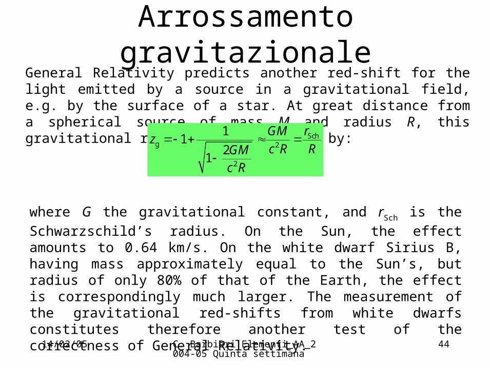
Arrossamento gravitazionaleGeneral Relativity predicts another red-shift for the light emitted by a source in a gravitational field, e.g. by the surface of a star. At great distance from a spherical source of mass M and radius R, this gravitational red-shift is expressed by:

Schg 2

2

11

21

rGMz

c R RGMc R

where G the gravitational constant, and rSch is the Schwarzschild’s radius. On

the Sun, the effect amounts to 0.64 km/s. On the white dwarf Sirius B, having mass approximately equal to the Sun’s, but radius of only 80% of that of the Earth, the effect is correspondingly much larger. The measurement of the gravitational red-shifts from white dwarfs constitutes therefore another test of the correctness of General Relativity.


45

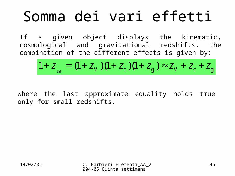
Somma dei vari effettiIf a given object displays the kinematic, cosmological and gravitational redshifts, the combination of the different effects is given by:

tot V c g V c g1 (1 )(1 )(1 )z z z z z z z

where the last approximate equality holds true only for small redshifts.


46

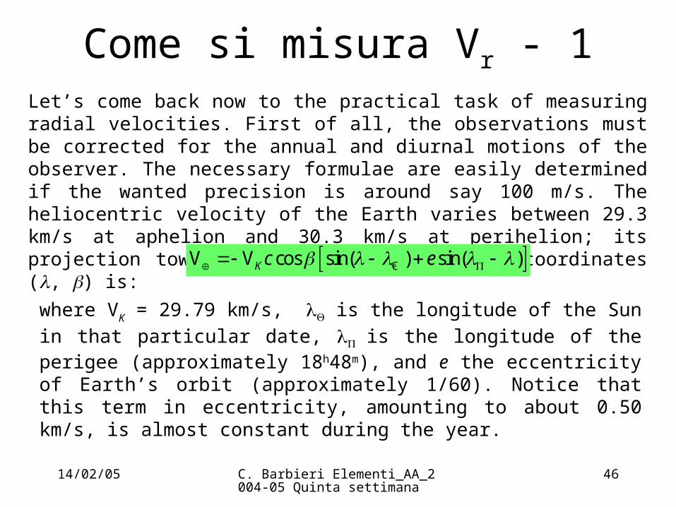
Come si misura Vr - 1Let’s come back now to the practical task of measuring radial velocities. First of all, the observations must be corrected for the annual and diurnal motions of the observer. The necessary formulae are easily determined if the wanted precision is around say 100 m/s. The heliocentric velocity of the Earth varies between 29.3 km/s at aphelion and 30.3 km/s at perihelion; its projection toward a direction of ecliptic coordinates (, ) is:

V V cos sin( ) sin( )K c e €

where VK = 29.79 km/s, is the longitude of the Sun in that particular date,

is the longitude of the perigee (approximately 18h48m), and e the eccentricity of Earth’s orbit (approximately 1/60). Notice that this term in eccentricity, amounting to about 0.50 km/s, is almost constant during the year.


47

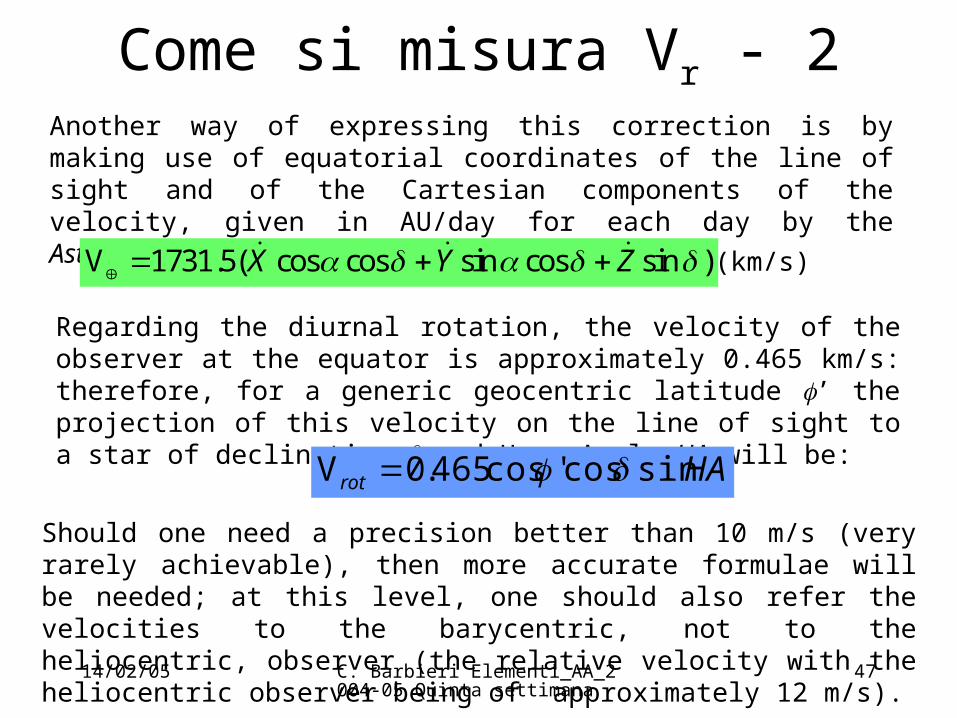
Come si misura Vr - 2Another way of expressing this correction is by making use of equatorial coordinates of the line of sight and of the Cartesian components of the velocity, given in AU/day for each day by the Astronomical Almanac:

V 1731.5( cos cos sin cos sin )X Y Z (km/s)

Regarding the diurnal rotation, the velocity of the observer at the equator is approximately 0.465 km/s: therefore, for a generic geocentric latitude ’ the projection of this velocity on the line of sight to a star of declination and Hour Angle HA will be:

HArot sincos'cos465.0V

Should one need a precision better than 10 m/s (very rarely achievable), then more accurate formulae will be needed; at this level, one should also refer the velocities to the barycentric, not to the heliocentric, observer (the relative velocity with the heliocentric observer being of approximately 12 m/s).


48

Moti propri più velocità radialiIf also the radial velocity of star X can be measured from the Doppler effect:

rV V cos 4.740 cotc

km/s

(the non-relativistic formula being certainly valid), then the full velocity vector of the star can be reconstructed.

But for the majority of cases, tangential angular velocities in arcsec per year, and radial velocities in km/s, but not the parallaxes, are available .


49

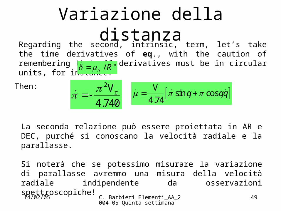
Variazione della distanzaRegarding the second, intrinsic, term, let’s take the time derivatives of eq., with the caution of remembering that all derivatives must be in circular units, for instance:

Then:

/ "R

2rV

4.740- V

sin cos4.74

q qq

La seconda relazione può essere proiettata in AR e DEC, purché si conoscano la velocità radiale e la parallasse.

Si noterà che se potessimo misurare la variazione di parallasse avremmo una misura della velocità radiale indipendente da osservazioni spettroscopiche!


50

Relazione tra moti propri e costanti di precessione

The previous discussion shows that the uncertainties in the precessional constants will enter into the uncertainty of the proper motion. Such uncertainty is not so important for the single star, but instead for the system of proper motions. For instance, the FK5 could affected by a spurious rotation at the level of about 0”.15/century. This seemingly small systematic error enters into the knowledge of the overall field of motions and forces of the Milky Way. Looking at the problem from the other side, a reasonable model of the distribution of proper motions can lead to the determination of the precessional constants. Any effort must therefore be made to obtain a system of proper motions as precise as possible, and free from systematic effect. The satellite Hipparcos could not produce a major improvement, because its operational life was too short. An alternative way is to derive proper motions in respect to a non-rotating background of fixed objects, such as the distant quasars; the reference system ICRF is by definition devoid of rotation, so that many efforts are presently made to refer the proper motions to it.


51

The Hipparcos mission

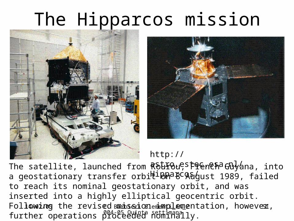
http://astro.estec.esa.nl/Hipparcos/

The satellite, launched from Kourou, French Guyana, into a geostationary transfer orbit on 8 August 1989, failed to reach its nominal geostationary orbit, and was inserted into a highly elliptical geocentric orbit. Following the revised mission implementation, however, further operations proceeded nominally.


52

The Hipparcos design - 1

The payload was centred around an all-reflective Schmidt telescope. A novel feature of the telescope was the `beam combining' mirror, which brought the light from the two fields of view, separated by about 58 degrees and each of dimension 0.9 x 0.9 degrees, to a common focal surface, and thus achieved both large- and small-field measurements simultaneously. The satellite swept out great circles over the celestial sphere, and the star images from two fields of view were modulated by a highly regular grid of 2688 transparent parallel slits located at the focal surface. The satellite was designed to spin slowly, completing a full revolution in two hours. At the same time, it was controlled so that there was a continuous slow change of direction of the axis of rotation. In this way the telescope was able to scan the complete celestial sphere several times during its planned mission. As the telescope scanned the sky, the starlight was modulated by the slit system, and the modulated light was sampled by an image-dissector-tube detector, at a frequency of 1200 Hz. At any one time, some four or five of the selected (or programme) stars were present in the combined fields of view.


53

The Hipparcos design - 2The telescope was continually determining the relative (along-scan) positions of the programme stars which appeared first in the preceding field of view and then in the following field of view due to the rotation of the satellite. In this way several comparisons with different stars were made. As the scans also overlapped `sideways' when the satellite axis of rotation changed on each sweep of the sky, the stars appeared again, but this time compared with other stars. In this way, a dense net of measurements of the relative angular separations of the stars was progressively built up.In addition to the main instrument (designed to measure about 105 stars down to about 12 mag, the Hipparcos catalogue), the payload included two star mappers (one redundant), whose function was to provide data allowing precise real-time satellite attitude determination (a task performed on board the satellite), and the a posteriori reconstruction of the attitude (a task carried out on the ground). The star mapper data are also used by the Tycho experiment to perform astrometric and two-colour photometric measurements of about 106 stars down to about 10-11 mag.


54

The 3-D structure of the Hyades

The image above shows the projected positions of the 218 Hyades members in Galactic coordinates. The Sun is at (X,Y,Z)=(0,0,0), The negative X-axis is towards the Galactic anti-centre, and the positive Y-axis is in the direction of Galactic rotation. The red circle show the tidal radius (about 10 pc) of the cluster. Note that about 85 stars are located beyond the tidal radius, of which about 45 are located between one and two tidal radii.


55

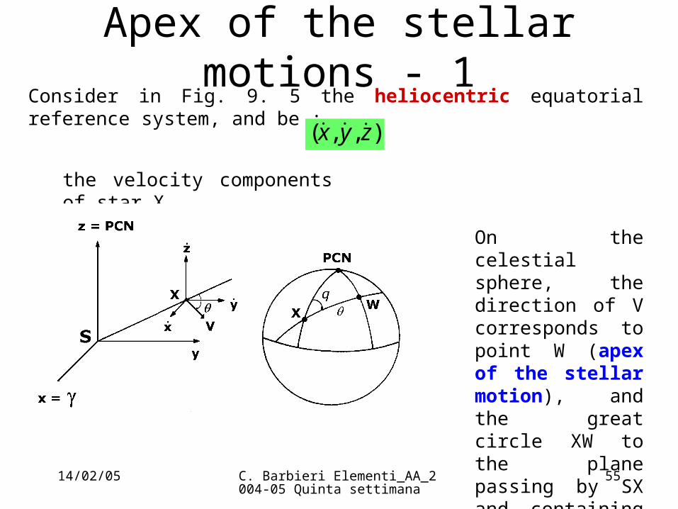
Apex of the stellar motions - 1Consider in Fig. 9. 5 the heliocentric equatorial reference system, and be :

the velocity components of star X.

),,( zyx

On the celestial sphere, the direction of V corresponds to point W (apex of the stellar motion), and the great circle XW to the plane passing by SX and containing the vector V.


56

Apex of the stellar motions - 2These Cartesian components can be expressed in terms of (Vt, Vt, Vr) by a

suitable rotation of coordinates. The Table gives the rotation matrix that transforms (Vt, Vt, Vr) into and viceversa.),,( zyx

Vt Vt Vr x sin sincos coscos y cos sinsin cossin

z 0 cos sin

for instance:

coscosVsincosV-sinV rtδtα -x

cossinVtα yx


57

Apex of the stellar motions - 3Recalling the expression f the tangential velocity Vt, we derive the Cartesian

equatorial components by the observable quantities:

α δ r

α δ r

δ r

4.740( sin cos sin ) V cos cos

4.740( cos sin sin ) V sin cos

4.740cos V sin

x -

y

z

From the knowledge of the entire velocity vector V, the direction of the motion of the star in the heliocentric reference system S(x, y, z) can be determined.


58

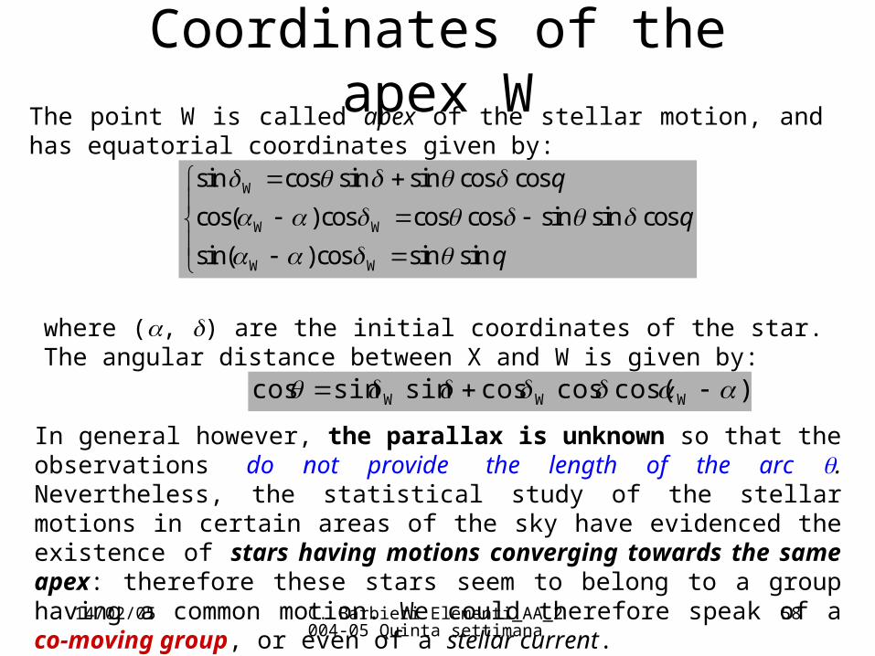
Coordinates of the apex WThe point W is called apex of the stellar motion, and has equatorial coordinates given by:

W

W W

W W

sin cos sin sin cos cos

cos( )cos cos cos sin sin cos

sin( )cos sin sin

q

q

q

where (, ) are the initial coordinates of the star. The angular distance between X and W is given by:

)cos(coscossinsincos WWW

In general however, the parallax is unknown so that the observations do not provide the length of the arc . Nevertheless, the statistical study of the stellar motions in certain areas of the sky have evidenced the existence of stars having motions converging towards the same apex: therefore these stars seem to belong to a group having a common motion. We could therefore speak of a co-moving group, or even of a stellar current.


59

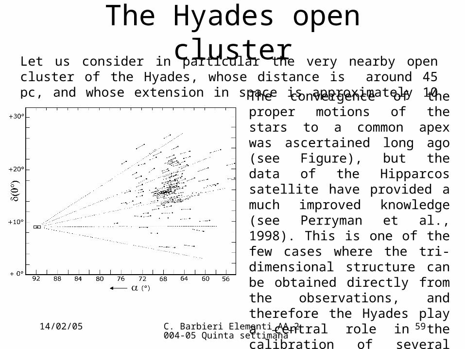
The Hyades open clusterLet us consider in particular the very nearby open cluster of the Hyades, whose distance is around 45 pc, and whose extension in space is approximately 10 pc.

The convergence of the proper motions of the stars to a common apex was ascertained long ago (see Figure), but the data of the Hipparcos satellite have provided a much improved knowledge (see Perryman et al., 1998). This is one of the few cases where the tri-dimensional structure can be obtained directly from the observations, and therefore the Hyades play a central role in the calibration of several relationships, e.g. the Hertzsprung - Russel (H-R) diagram.


60

The peculiar proper motion of the Sun Siccome abbiamo riferito le velocità radiali e i moti propri all’osservatore solare, dobbiamo attenderci che se questi ha un moto peculiare rispetto all’insieme delle stelle vicine, tale moto si trovi riflesso in qualche misura nelle osservazioni. Esaminiamo dapprima i moti propri.Already W. Herschel in 1783 had laid down the foundations of the method, utilizing only the position angles of 12 stars. Indeed, q is independent from the parallax, and it coincides with the position angle of the tangential velocity. The method of Herschel can be easily visualized: draw on the celestial sphere the great circles defined by the proper motions, and consider the semi-circle oriented as the motion itself. All these semi-circles will intersect, within the errors, in a point (more realistically, in a small area) which is the antapex of the solar motion; the modulus of the velocity of the Sun will remain undetermined by this method.


61

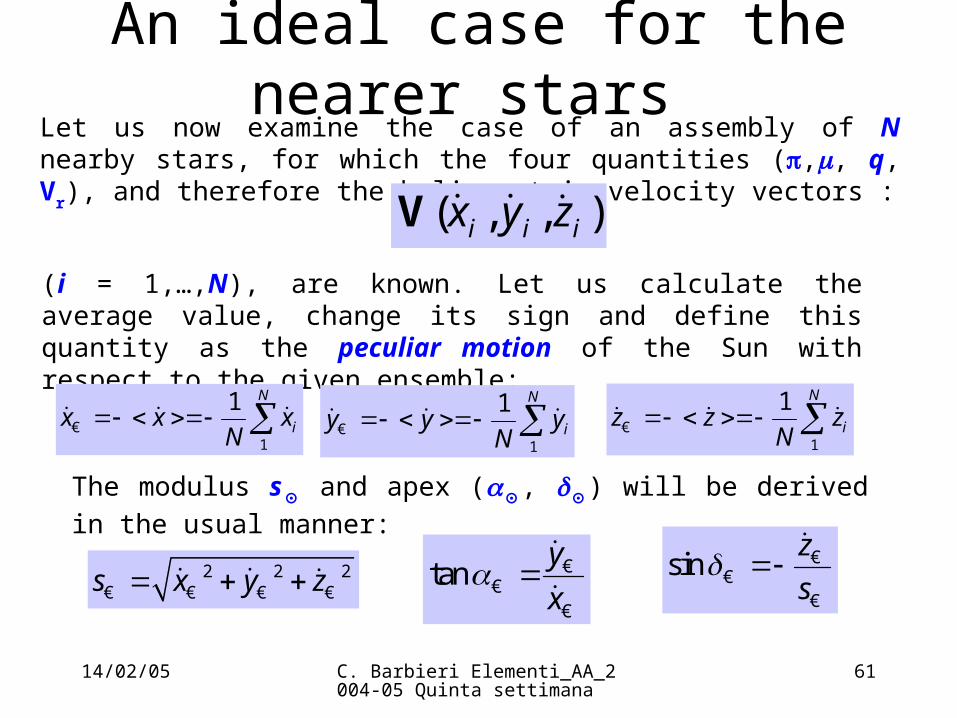
An ideal case for the nearer stars Let us now examine the case of an assembly of N nearby stars, for which the four quantities (,, q, Vr), and therefore the heliocentric velocity vectors :

(i = 1,…,N), are known. Let us calculate the average value, change its sign and define this quantity as the peculiar motion of the Sun with respect to the given ensemble:

),,( iii zyx V

1

1 N

ix x xN

€1

1 N

iy y yN

€1

1 N

iz z zN

€

The modulus s⊙ and apex (⊙, ⊙) will be derived in the usual manner:

2 2 2s x y z € € € € tany

x €

€€

sinz

s €

€€


62

The Local Standard of Rest (LSR)The early observations provided a velocity of approximately 20 km/s, in direction W⊙(⊙, ⊙) (18h, +30), not far from Vega.

We stress that this value depends on the particular set of stars used to define it. Ideally, if we could take into account all nearby stars, we would obtain a Local Standard of Rest (LSR), a velocity reference system of great interest for the study of the velocity field of objects in the Milky Way. It is therefore useful to transform the coordinate system from the equatorial to the galactic one (see Chapter 3): let’s denote with (ui, vi, wi) the three velocity components derived

by appropriate rotation of ( , , )i i ix y z

with axis u directed toward the Galactic Center, axis v at 90 in the galactic plane (toward the constellation of Cygnus), and axis w toward the galactic pole. Notice that this LSR has a purely kinematics significance, the masses of the stars not having been taken into account, and does not posses a precise origin in space. We can assume that the Sun (or better, the barycenter of the Solar System) is passing by the LSR origin at the present time.


63

The future of astrometry - GAIAhttp://www.rssd.esa.int/index.php?project=GAIA&page=More_about_Gaia

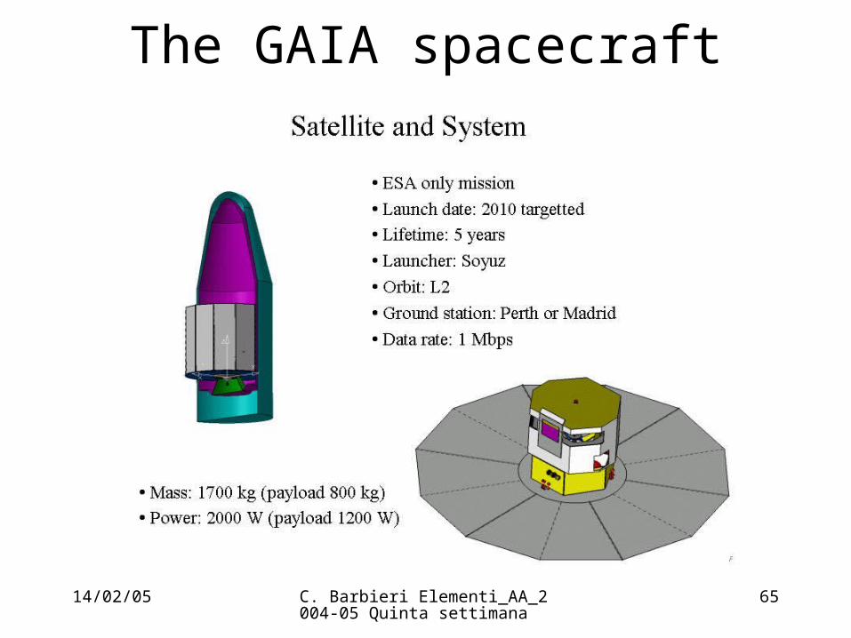
Gaia will survey more than one billion stars, including many of the closest stars to the Sun. Its goal is to make the largest, most precise map of where we live in space by surveying an unprecedented one per cent of our Galaxy's population of 100 billion stars.The expected precision is around 10-15 arcsec at the 15th mag.Gaia is a single spacecraft, consisting of three telescopes that will constantly sweep the sky, recording every visible celestial object that crosses its lines of sight. During its anticipated lifetime of five years, Gaia will observe each of its one billion sources about 100 times. Each time, it will detect changes in the object's brightness and position.


64

GAIA - 2

Gaia will be placed in an orbit around the Sun, at a distance of 1.5 million kilometres further out than Earth. This special location, known as L2, will keep pace with the orbit of the Earth. Gaia will map the stars from here.


65

The GAIA spacecraft


66

The GAIA payload and telescope


67

Esercizi1 - Discutere l’equazione

dove è la direzione tra la visuale e il vettore velocità per diversi valori di tra 0° (velocità in allontanamento) e 180° (velocità in avvicinamento).

21

cos111

Oz

2 - Reconstruct the velocity vector of the bright star Capella, which has = 0”.075, = 0”.439/year, Vr = + 30.2 km/s. The vector V is directed to =

42.5 deg, with modulus of 41.0 km/s.

3 – Trovare sul sito del satellite astrometrico Hipparcos le 20 stelle di maggior parallasse e le 10 stelle di maggior moto proprio. I due insiemi coincidono?

14/02/05C. Barbieri Elementi_AA_2004-05 Quinta settimana 1 Elementi di Astronomia e Astrofisica per...

Documents

Transcript of 14/02/05C. Barbieri Elementi_AA_2004-05 Quinta settimana 1 Elementi di Astronomia e Astrofisica per...