12th International Workshop on Wave Hindcasting and Forecasting, Kohala Coast, Hawai’i, HI, 2011.

CALIBRATION OF THE “IOWAGA” GLOBAL WAVE HINDCAST (1991–2011)USING ECMWF AND CFSR WINDS

Fabrice Ardhuin1, Jenny Hanafin,Yves Quilfen, Bertrand Chapron, Pierre Queffeulou, Mathias ObrebskiIFREMER, Laboratoire d’Oceanographie Spatiale, Plouzane, FRANCE

Joseph SienkiewiczNOAA/NCEP, Ocean Prediction Center, Camp Springs, MD

Doug VandemarkUniversity of New Hampsire, Durham, NH

1 Introduction

Numerical wave models have traditionnally been cal-ibrated mostly in terms of wave heights, and toa lesser extent peak periods and directions. How-ever, new applications require the validation of air-sea fluxes [e.g. Il-Ju Moon et al., 2004], higher or-der spectral moments such as the surface Stokesdrift and mean square slopes [e.g. Tran et al., 2010],and spectral shape parameters that control the sec-ond order spectrum which is responsible for drivinglong waves and generating seismic noise [e.g. Renierset al., 2010, Ardhuin et al., 2011a]. Physical parame-terizations have been proposed recently that capturesome of the variability of the high frequency spectrallevels, and these also lead to more accurate resultsfor the dominant waves [Ardhuin et al., 2010]. Basedon this experience, we expect that improvements forspecific applications will generally lead to benefitsfor all users of numerical wave models. Also, thevalidation of many different parameters estimatedfrom wave spectra may also provide some constraintson the otherwise ‘free parameters’ that are still toomany in wave generation and dissipation parameter-izations. With these ideas in mind, we are pursuingthe development of new parameterizations as partof the National Ocean Partnership Program oper-ational wave model improvement project [Tolmanet al., 2011]. In particular, wave breaking statisticsare used to improve on the parameterization of wavedissipation [Leckler et al., 2011].

Leaving out wave breaking properties, we focus on

other parameters and present here some preliminaryresult from the project ”Integrated Ocean Wavesfor Geophysical and other Applications” (http://wwz.ifremer.fr/iowaga). The numerical modelused for this is a global implementation of WAVE-WATCH III(R) version 4.04, using the parameteriza-tion ‘TEST441b’ described in detail in Ardhuin et al.[2010]. This parameterization has now been used forthe last three years as part of the Previmer forecast-ing system (http://www.previmer.org/), using op-erational wind analyses and forecasts from ECMWF,with multi-grid systems and stand-alone unstruc-tured grids [e.g. Ardhuin et al., 2009]. Results fromthe regular grids appear under the ‘SHOM’ tag inthe JCOMM model inter-comparisons [e.g. Bidlot,2009]. Monthly validation reports have shown excel-lent performance against buoy data, typically pro-ducing the smallest errors for forecast ranges of 48hours and beyond. This has lead Meteo-France toadapt the same physical parameterization in theirnew operational wave forecasting system in 2010,and test are under way at NOAA/NCEP for a pos-sible use in operations. One of the issues faced byNCEP is the longer CPU time for the new pa-rameterizations, which make the full model about40% more expensive than using the parameteriza-tion by Tolman and Chalikov [1996]. This cost is dueto non-isotropic dependence of dissipation rates forone component on the energy of other componentsand their associated breaking probabilities, which re-quires the calculation of convolution integrals overpart of the two-dimensional spectrum.

1 E-mail:ardhuin-at-ifremer.fr

1

0 1 2 3 4 5 6 7 8 9 1011121314151617−20−15−10−505101520

Hs(m)

Normalized

bias

(%) GLOBAL05−ECMWF−2008

GLOBAL05−CFSR−2008

0 1 2 3 4 5 6 7 8 9 1011121314151617691215182124273033363942

Hs(m)

NormalizedRMSE(%)

GLOBAL05−ECMWF−2008GLOBAL05−CFSR−2008

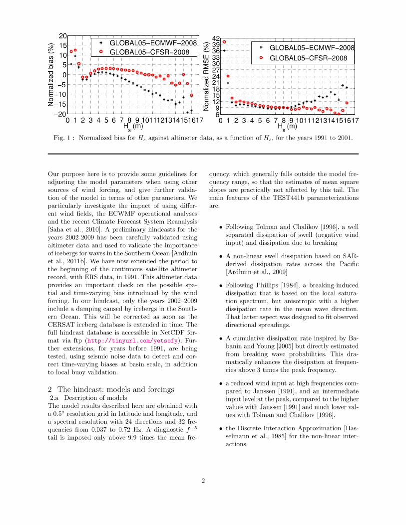
Fig. 1 : Normalized bias for Hs against altimeter data, as a function of Hs, for the years 1991 to 2001.

Our purpose here is to provide some guidelines foradjusting the model parameters when using othersources of wind forcing, and give further valida-tion of the model in terms of other parameters. Weparticularly investigate the impact of using differ-ent wind fields, the ECWMF operational analysesand the recent Climate Forecast System Reanalysis[Saha et al., 2010]. A preliminary hindcasts for theyears 2002-2009 has been carefully validated usingaltimeter data and used to validate the importanceof icebergs for waves in the Southern Ocean [Ardhuinet al., 2011b]. We have now extended the period tothe beginning of the continuous satellite altimeterrecord, with ERS data, in 1991. This altimeter dataprovides an important check on the possible spa-tial and time-varying bias introduced by the windforcing. In our hindcast, only the years 2002–2009include a damping caused by icebergs in the South-ern Ocean. This will be corrected as soon as theCERSAT iceberg database is extended in time. Thefull hindcast database is accessible in NetCDF for-mat via ftp (http://tinyurl.com/yetsofy). Fur-ther extensions, for years before 1991, are beingtested, using seismic noise data to detect and cor-rect time-varying biases at basin scale, in additionto local buoy validation.

2 The hindcast: models and forcings2.a Description of models

The model results described here are obtained witha 0.5◦ resolution grid in latitude and longitude, anda spectral resolution with 24 directions and 32 fre-quencies from 0.037 to 0.72 Hz. A diagnostic f−5

tail is imposed only above 9.9 times the mean fre-

quency, which generally falls outside the model fre-quency range, so that the estimates of mean squareslopes are practically not affected by this tail. Themain features of the TEST441b parameterizationsare:

• Following Tolman and Chalikov [1996], a wellseparated dissipation of swell (negative windinput) and dissipation due to breaking

• A non-linear swell dissipation based on SAR-derived dissipation rates across the Pacific[Ardhuin et al., 2009]

• Following Phillips [1984], a breaking-induceddissipation that is based on the local satura-tion spectrum, but anisotropic with a higherdissipation rate in the mean wave direction.That latter aspect was designed to fit observeddirectional spreadings.

• A cumulative dissipation rate inspired by Ba-banin and Young [2005] but directly estimatedfrom breaking wave probabilities. This dra-matically enhances the dissipation at frequen-cies above 3 times the peak frequency.

• a reduced wind input at high frequencies com-pared to Janssen [1991], and an intermediateinput level at the peak, compared to the highervalues with Janssen [1991] and much lower val-ues with Tolman and Chalikov [1996].

• the Discrete Interaction Approximation [Has-selmann et al., 1985] for the non-linear inter-actions.

2

0 2 4 6 8 10 12 14 16 18 20 22−20

−10

0

10

20

30

Hs

(m)

Nor

mal

ized

bias

(%)

1991

1992

19931994

1995

1996

1997

19981999

2000

2001

Fig. 2 : Normalized bias and normalized RMSE for Hs in 2008 against altimeter data, as a function of Hs.

The modelled grids include

• A global multi-grid system with a baseline0.5◦ resolution in latitude and longitude, withzooms on the North-West European shelf at0.1◦, West Indies (Puerto Rico to Venezuela),Tuamotus, New Caledonia, U.S. East Coastand Gulf of Mexico at 0.2◦, French Atlanticcoast at 1/30◦. At the time of writing, the fulltime period has only been run on a single grid0.5◦, and only the period 2002-2011 has beenrun with the multi-grid system.

• A Mediterranean multigrid system, with abaseline 0.1◦ resolution split in a Mediter-ranean and a Black Sea grids, and a 1/30◦

French Mediterranean domain, including Cor-sica.

• An unstructured grid (resolution 100 m to5 km) over the Iroise sea, including currentsand water levels, for the years 2002-2011.

Other unstructured grids used for the routine Pre-vimer forecasts will probably also be used for hind-casts.

The built-in shortcomings of this parameterizationis that the dissipation rate near the peak is local infrequency. Given the higher saturation level at thepeak, this leads to a strong peak in the dissipationrate that is not consistent with breaking statistics[Leckler et al., 2011]. Also, the relative weak input

level tends to produce mean directions in slantingfetch conditions that are too oblique relative to theshoreline.

We note that the model was ran with 10-m winds,without any air-sea stability correction. Absolutelyno wave measurement, direct or indirect, was assim-ilated in the model. In contrast, many observationsfrom satellite altimeter and SAR to buoys and seis-mic noise spectra were used to calibrate the modelparameters over the year 2008 [Ardhuin et al., 2010,2011a].

2.b Differences with ECMWF or CFSR windsAs a result of our forcing choices, the hindcasts con-tains some discontinuities due to the effects of ice-bergs. That latter effect was minimized by adjust-ing the wind-wave growth parameter βmax = 1.52used for ECMWF winds, to βmax = 1.33 for CFSRor NCEP analyses. To avoid confusion the param-eterization with βmax = 1.33 is called TEST441f.This adjustment compensates the high relative biasof CFSR winds for average values. This adjustmentwas calibrated for the year 2008 and was found togive good results for the years 1994 to 2009.

However, due to a different shape in the histogramof high winds, this calibration cannot correct bi-ases equally for the full range of wave heights. In-terestingly, the strength of high winds in CFSR,compared to ECMWF analysis, reduces the nega-tive bias for very high (Hs > 9 m) and phenomenalseas (Hs > 14 m), and allows a remarkable reduc-

3

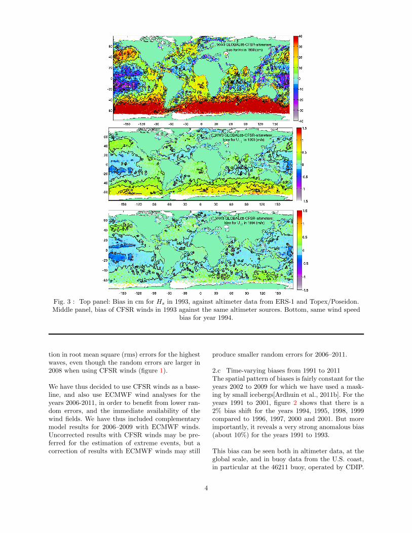
Fig. 3 : Top panel: Bias in cm for Hs in 1993, against altimeter data from ERS-1 and Topex/Poseidon.Middle panel, bias of CFSR winds in 1993 against the same altimeter sources. Bottom, same wind speed

bias for year 1994.

tion in root mean square (rms) errors for the highestwaves, even though the random errors are larger in2008 when using CFSR winds (figure 1).

We have thus decided to use CFSR winds as a base-line, and also use ECMWF wind analyses for theyears 2006-2011, in order to benefit from lower ran-dom errors, and the immediate availability of thewind fields. We have thus included complementarymodel results for 2006–2009 with ECMWF winds.Uncorrected results with CFSR winds may be pre-ferred for the estimation of extreme events, but acorrection of results with ECMWF winds may still

produce smaller random errors for 2006–2011.

2.c Time-varying biases from 1991 to 2011The spatial pattern of biases is fairly constant for theyears 2002 to 2009 for which we have used a mask-ing by small icebergs[Ardhuin et al., 2011b]. For theyears 1991 to 2001, figure 2 shows that there is a2% bias shift for the years 1994, 1995, 1998, 1999compared to 1996, 1997, 2000 and 2001. But moreimportantly, it reveals a very strong anomalous bias(about 10%) for the years 1991 to 1993.

This bias can be seen both in altimeter data, at theglobal scale, and in buoy data from the U.S. coast,in particular at the 46211 buoy, operated by CDIP.

4

Fig. 4 : (a) Bias and normalized (b) RMS error for the modeled significant wave heights for the year 2009,against data from Jason-1, Jason-2 and Envisat altimeters. Both model and altimeter data are averaged

along the satellite tracks over 1 degree in latitude. There are 2.4 million averaged values.

At that buoy the model bias exceeds 17% for Hs forthese years, compared about 3% for the years 2004–2008 (not shown).

The examination of CFSR winds and waves com-pared to altimeter data shows that the errors arestrongest over the Southern ocean (top panel in fig-ure 3) and disappear in 1994. This pattern is clearlyassociated with a change in wind speed biases for theyears 1991–1993, up to 1 m/s right around Antarc-tica (middle panel in figure 3), and a weaker bias inthe North Pacific, compared to more realistic valuesin 1994 (bottom panel in figure 3) and the followingyears (not shown).

Looking at the details of the data used in the CFSRanalysis, we can see that 1994 corresponds to thestart of SSM-I wind speed assimilation [figure S14

in Saha et al., 2010]. It thus appears that SSM-Idata has a beneficial impact, reducing the high biasof high winds in the sub-polar regions. So far we haveleft the 1991-1993 results uncorrected. It is possiblethat a correction of the CFSR wind speed histogrammay be enough to correct the biases on wave param-eters.

For the years before 1991, in the absence of globalvalidation data from satellite altimeters, it is difficultto guarantee the stability of biases for the modeledwave parameters.

Ongoing work on the use of seismic noise data [e.g.Ardhuin et al., 2011a] should provide a reliable biasestimator at global scales, which is readily availableback to the early 1980s, when numerical seismic datais available. Going further back in time will require

5

a careful and well planned effort for digitizing oldseismograph data [e.g. Grevemeyer et al., 2000], withsome data sources going back to the late 19th cen-tury [Algue, 1900].

3 Validation3.a Significant wave heights

For the full altimeter era, patterns in model error aresimilar to what is shown on figure 4. Using CFSRwinds for the years 1994–2009, the positive bias forHs in the Southern Ocean is increased by 5 to 10 cm.This local pattern is consistent with relatively stronghigh winds in CFSR. Overall, random errors aresmallest in the recent years and with ECMWF windfields. This is the reason why we chose to show re-sults for 2009 on figure 4, for which the errors areleast. With CFSR winds, there is also a slow decreaseof random errors with time from 1994 to 2001. Atthis stage we have not sought to discriminate thesource of that trend, between more accurate windfields and more accurate altimeter measurements.

Besides obvious low biases in the Northern Mediter-ranean, Black Seas and Indonesian archipelago,which may be largely attributed to wind errors anda coarse model resolution, we note persistent lowbiases to the South-East of Greenland, east of Ar-gentina, east of India to the south-east of Australiaand New-Zealand, and in the South-West Pacific.

There are probably several factors that contribute tothis low bias, one of them being the relatively slowgrowth of the of young waves, in the model, in par-ticular for short fetches [Ardhuin et al., 2010]. Someearly validation tests of the spatial distribution ofswell fields also showed that the model had a ten-dency to produce swells in a range of directions thatis more narrow than what is observed from space[Delpey et al., 2010].

Because the dominant weather systems have windsto the East, a too narrow swell distribution will failto send energy towards the east coasts. This maybe related to diffraction or some unresolved scat-tering effects, as suggested by the apparent turningof swells behind large island groups such as FrenchPolynesia (Fabrice Collard, personal communication2008).

Another outstanding problem is the change from alow Hs bias for Hs > 2 m to a high bias for Hs < 2 m(figure 1). These biases yield a histogram of Hs thatis very peaked at 2 m, and unrealistic. This problemmay be due to the transition in from a laminar to

a turbulent boundary layer. In our swell dissipationparameterization, this transition includes a discon-tinuity in the air-sea friction factor.

3.b Mean square slopes (mss)Either from model or satellite altimeter, the esti-mates of the mss are indirect but they provide aninteresting check on the variability spectral tails,which is very much controlled by the cumulative dis-sipation term [e.g. Leckler et al., 2011].

Here we estimate a mss from Ku band cross sectionas

mssKu =0.48

exp [(σ0 + 1.4) × (0.1 log(10))](1)

where σ0 is the normalized radar cross section as pro-vided in the Globwave homogenized dataset [Quef-feulou and Croize-Fillon, 2010], 1.4 is a bias correc-tion in dB, and 0.48 is an effective Fresnel coefficient[Chapron et al., 2000].

For the model, a corresponding mss is extrapolatedfrom the mss (mss3m) integrated over the limitedfrequency range of the model which as a maximumfrequency of 0.72 Hz that corresponds to a wave-length of 3 m. For this we use an expression adaptedfrom Vandemark et al. [2004],

mssKu,model = mss3m+0.0035+0.0093 log(U10) (2)

with

mss3m =

∫ 2π

0

∫ 0.72 Hz

0

k2E(f, θ)dfdθ (3)

Figure 5 shows that the variability of the mss asa function of wind speed and wave height usingsatellite data, and also taking one example offshoreof California, with NDBC buoy 46013. In orderto test the impact of the buoy sensor quality, wealso used winds from buoy 46013 with wave datafrom a nearby Datawell Waverider buoy (WMO code46214, operated by the Coastal Data InformationProgram). When offshore waves are removed, we geta similar pattern of mss variation with wind speedand Hs. When the Jason-1 wind is used, one re-covers the geophysical model function (GMF) usedto estimate the wind speed from σ0 and Hs. Un-fortunately the GMF chosen for Jason does not in-clude the full variability os σ0 with sea state for lowwind speeds [e.g. Gourrion et al., 2002]. Compari-son with Quikscat winds (Fabrice Collard, personalcommunication 2011) shows that the true distribu-tion of mssKu with wind and wave height is closer towhat is shown in the central panel of figure 5, when

6

0 5 10 15 20 25U10(m/s)

0 2 4 6 8 10Hs (m)

0 5 10 15 20 25U10(m/s)

0.2

0.4

0.6

0.8

1.0

1.2

1.4

pseu

do−m

.s.s

.( %

, 0.0

37 -

0.40

5 H

z)

Buoy data Wave model

Fig. 5 : Comparison of mss distributions (on the vertical) as a function of wind speed (U10) and significantwave height (Hs) for the year 2008. Top line, for the global ocean, on the left is the distribution using onlyJason data, but this means that the wind speed is not an independent estimate as it is derived from σ0 andHs using a geophysical model function. In the central plot, U10 is given by ECMWF analyses and on theright, mss and Hs are given by the wave model. Bottom line, for the buoy 46013, off Central California

using (a) the buoy data and (b) the wave model, using a high frequency cut-off at 0.4 Hz.

the Jason-derived wind is replaced by ECMWF windanalyses.

Comparing the top and bottom panels shows thata little more than 10% of the Ku-band mss is ac-counted for by waves of frequencies less than 0.4 Hz,i.e. wavelengths more than 10 m, and the mss vari-ability from satellite data is comparable to the mssestimated from the buoy spectrum up to 0.4 Hz,showing that fairly long waves (L > 10 m) accountfor a large part of the variability of the mssku thatis not due to winds.

The top-right and bottom-right panels show that themodel is able to predict most of the variability thatis observed. For wind speeds above 10 m/s the mss isoverestimated by the wave model using the transfor-mation given by eq. (2). The analysis of buoy datasuggests that this overestimation is a real model ef-

fect, and not an artifact of the interpretation of thealtimeter σ0. The modeled mss3m at low winds hasa relatively low bias by 0.05 percentage points at thelocation of buoy 46013.

A similar low bias off the California coast is alsofound when comparing the model to altimeter data(figure 6). It is difficult to validate the global dis-tribution of mean square slopes with buoys, giventheir very sparse distribution, and this is where thealtimeter data is very useful. Once the regional bi-ases are removed, the relative error in the estimate ofmssKu varies around 13% (figure 6), which is almostas low as the error on Hs, around 10%.

4 Hindcasts of extra-tropical storm Quirin:what trust in wave models up to Hs = 20 m?Given the very different behavior of wave height bi-

7

Fig. 6 : Top: Bias of the model estimations of mss given by eq. (2), after a reduction by 10%, againstaltimeter data using eq. (1). Bottom: Scatter index for the model estimation of mss (this is the normalized

RMS error after bias correction).

ases for very high and phenomenal seas when shift-ing from CFSR to ECMWF winds (figure 1), we havemade a preliminary investigation of the source of thisbias: is the wind too low, or, as suggested by Cavaleri[2009], is there any systematic problem in the wavemodel that would make it ‘miss the peaks’? For thiswe jumped on the occasion given by a recent event,with the largest sea state ever recorded by a satellitealtimeter.

Although wave models have seldom been validatedfor extreme wave heights, some numerical hindcastsstudies have shown a good consistency of very highwave heights, up to Hs = 20 m with satellite mea-surements, provided that the winds used to drivethe wave model are made consistent with observa-

tions [Cardone et al., 2009]. The 2011 storm Quiringenerated wave with a record-breaking maximumvalue of Hs = 20.12 m reported by Jason 2 onFebruary 14 at 11:03:09 UTC, at location 29.57W49.17 N (cycle number 96, pass number 139, 1 Hzdata). This number is the uncorrected value in theNASA/CNES product. This exceeds the maximumin the 2007 event discussed in Cardone et al. [2009],which has been reprocessed by NASA and CNES to‘only’ Hs = 19.13 m. The wind and waves of Quirinare investigated in detail in Hanafin et al. [2011],which is summarized below.

This particular storm moved rapidly across thenorth Atlantic, with a minimum sea level pressuredeepening from 984 hPA on 13 February at 0000

8

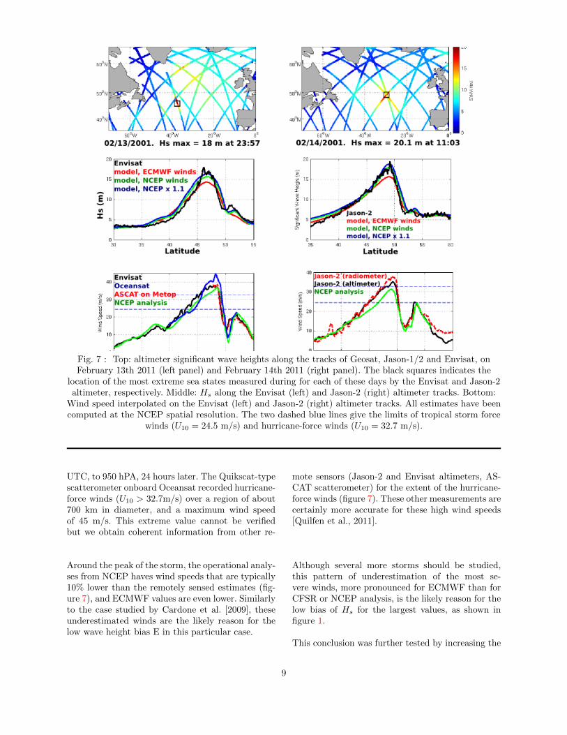
Fig. 7 : Top: altimeter significant wave heights along the tracks of Geosat, Jason-1/2 and Envisat, onFebruary 13th 2011 (left panel) and February 14th 2011 (right panel). The black squares indicates the

location of the most extreme sea states measured during for each of these days by the Envisat and Jason-2altimeter, respectively. Middle: Hs along the Envisat (left) and Jason-2 (right) altimeter tracks. Bottom:

Wind speed interpolated on the Envisat (left) and Jason-2 (right) altimeter tracks. All estimates have beencomputed at the NCEP spatial resolution. The two dashed blue lines give the limits of tropical storm force

winds (U10 = 24.5 m/s) and hurricane-force winds (U10 = 32.7 m/s).

UTC, to 950 hPA, 24 hours later. The Quikscat-typescatterometer onboard Oceansat recorded hurricane-force winds (U10 > 32.7m/s) over a region of about700 km in diameter, and a maximum wind speedof 45 m/s. This extreme value cannot be verifiedbut we obtain coherent information from other re-

mote sensors (Jason-2 and Envisat altimeters, AS-CAT scatterometer) for the extent of the hurricane-force winds (figure 7). These other measurements arecertainly more accurate for these high wind speeds[Quilfen et al., 2011].

Around the peak of the storm, the operational analy-ses from NCEP haves wind speeds that are typically10% lower than the remotely sensed estimates (fig-ure 7), and ECMWF values are even lower. Similarlyto the case studied by Cardone et al. [2009], theseunderestimated winds are the likely reason for thelow wave height bias E in this particular case.

Although several more storms should be studied,this pattern of underestimation of the most se-vere winds, more pronounced for ECMWF than forCFSR or NCEP analysis, is the likely reason for thelow bias of Hs for the largest values, as shown infigure 1.

This conclusion was further tested by increasing the

9

Fig. 8 : Peak periods as calculated by the model with enhanced NCEP wind analyses (background colors),and measured by Envisat’s ASAR in wave mode (circles), wave buoys (squares) and seismic stations

(diamonds: SFJD - Greenland, CMLA - Azores, ESK - Scotland, SSB - France, PABO - Spain, and KONO- Norway). The model output is shown for 12:00 UTC on February 15th, as the longest swells were

encroaching on the west coast of Scotland. Buoy and seismic data correspond to the time of maximum Tp,with the time indicated on the plot, and the SAR data was acquired on February 14th and reprocessed

from level 1 data since this very long swell is removed by the operational level 2 processing.

NCEP wind speeds by 10% over the full modeldomain, and re-running the model for the monthof February 2011. The results with these enhancedwinds are now in very good agreement with the mea-sured heights, and are rather slightly higher in termsof wave height. Also, the very large peak periods ob-served at European buoys and recorded by seismicstations, from 21 to 25 s, are also well reproduced bythe model (figure 8 and table 1). All these measure-ments have been inspected for quality. Among these

the Datawell Waverider with WMO code 62069,owned by Ifremer, operated by CETMEF, and situ-ated at 4.97 W and 48.29 N recorded a peak periodof 23.5 s and 4.4 m.

These very long periods made this sea state trulyspecial. One of our colleagues, Abel Balanche, es-caped with a few bruises after underestimating thepower of the swell while surfing near Brest.

Surfer Benjamin Sanchis was more lucky and tookthe 2011 worldwide biggest wave prize for hisrun down one of these waves on February 16 on

the Belhara reef, off the south-west French coast(http://www.billabongxxl.com/biggest_wave_nom/index_5.html). There were also some occa-

10

sional damage associated with a 1 m seiche set upby strong infragravity waves in the usually quietharbor or Royan, France.

5 ConclusionsA 20 year hindcast of global wave parameters hasbeen produced using new parameterizations for wavedissipation [Ardhuin et al., 2010], and forcing from acombination of ECMWF analysis and CFSR reanal-yses, sea ice from CFSR and ECMWF and icebergsfrom CERSAT. The continuous validation with al-timeter and buoy data reveals several importantfacts,

• CSFR and NCEP analyses have systematicallyhigher values than ECMWF analyses of thewind speed, and this is even more true for thehighest speed range.

• a simple calibration of the wind wave growthparameter, βmax = 1.33 for CFSR or NCEPwinds compared to βmax = 1.52 for ECMWFwinds corrected the average to high waveheights.

• Modeled wave heights are still too low for thehighest values (Hs > 12 m), likely due to anunderestimation of the winds in these condi-tions.

• the mean square slope of the sea surface is rela-tively well estimated with the model, and maybe a useful parameter for remote sensing ap-plications.

• CFSR winds are anomalously high in theSouthern Ocean for the years 1991–1993, com-pared to following years, resulting in anoma-lous high biases for these year, including offthe U.S. West coast. This bias is corrected forthe following years, probably due to the startof SSM-I data assimilation in CFSR.

• a hindcast of 2011 storm Quirin, which holdsthe record for the highest ever measured seastate by a satellite altimeter, was well repro-duced after correcting for the wind bias. Theexceptional swell periods reaching the Atlanticcoasts of Europe were also well reproduced.

6 AcknowledgementsWe thank all the providers of wind and wave mea-surements at NDBC, CDIP, SHOM, CNES, NASA,ESA, and ISA that have been critical for assessingthe quality of wind and wave models. We thank J.-F. Piolle and M. Accensi for their homogenization ofthe buoy data formats and work on NetCDF post-processing, and the entire WAVEWATCH III(R) de-velopment team, in particular H. L. Tolman, J. H.G. M. Alves, and A. Chawla. This work is supportedby a FP7-ERC young investigator grant number240009 for the IOWAGA project, the U.S. NationalOcean Partnership Program, under grant U.S. Of-fice of Naval Research grant N00014-10-1-0383. Ad-ditional support from ESA and CNES for the Glob-wave project is gratefully acknowledged.

References

J. Algue. Relation entre quelques mouvements microseismiques et l’existence, la position et la distance descyclones a Manille (Philippines). In Congres international de Meteorlogie, Paris, pages 131–136, 1900.

F. Ardhuin, L. Marie, N. Rascle, P. Forget, and A. Roland. Observation and estimation of Lagrangian,Stokes and Eulerian currents induced by wind and waves at the sea surface. J. Phys. Oceanogr., 39(11):2820–2838, 2009. URL http://journals.ametsoc.org/doi/pdf/10.1175/2009JPO4169.1.

F. Ardhuin, E. Rogers, A. Babanin, J.-F. Filipot, R. Magne, A. Roland, A. van der Westhuysen, P. Queffeulou,J.-M. Lefevre, L. Aouf, and F. Collard. Semi-empirical dissipation source functions for wind-wave models:part I, definition, calibration and validation. J. Phys. Oceanogr., 40(9):1917–1941, 2010.

F. Ardhuin, E. Stutzmann, M. Schimmel, and A. Mangeney. Ocean wave sources of seismic noise. J. Geophys.Res., 116:C09004, 2011a. doi: 10.1029/2011JC006952. URL http://wwz.ifremer.fr/iowaga/content/

download/48407/690392/file/Ardhuin_etal_JGR2011.pdf.

F. Ardhuin, J. Tournadre, P. Queffelou, and F. Girard-Ardhuin. Observation and parameterization of smallicebergs: drifting breakwaters in the southern ocean. Ocean Modelling, 39:405–410, 2011b. doi: 10.1016/j.ocemod.2011.03.004.

11

A. V. Babanin and I. R. Young. Two-phase behaviour of the spectral dissipation of wind waves. In Proceedingsof the 5th International Symposium Ocean Wave Measurement and Analysis, Madrid, june 2005. ASCE,2005. paper number 51.

J.-R. Bidlot. Intercomparison of operational wave forecasting systems against buoys: data from ECMWF,MetOffice, FNMOC, NCEP, DWD, BoM, SHOM and JMA, September 2008 to November 2009.Technical report, Joint WMO-IOC Technical Commission for Oceanography and Marine Meteorology,2009. URL http://www.jcomm-services.org/modules/documents/documents/model_comparison_

second_list_200809_200811.pdf. available from http://tinyurl.com/3vpr7jd.

V. J. Cardone, A. T. Cox, M. A. Morrone, and V. R. Swail. Satellite altimeter detection of global veryextreme sea states. In Proceedings, 11th Int. Workshop of Wave Hindcasting and Forecasting, Halifax,Canada, 2009.

L. Cavaleri. Wave modeling: Missing the peaks. J. Phys. Oceanogr., 39:2557–2778, 2009. URL http:

//journals.ametsoc.org/doi/pdf/10.1175/2009JPO4067.1.

B. Chapron, V. Kerbaol, D. Vandemark, and T. Elfouhaily. Importance of peakedness in sea surface slopemeasurements. J. Geophys. Res., 105(C7):17195–17202, 2000.

M. Delpey, F. Ardhuin, F. Collard, and B. Chapron. Space-time structure of long swell systems. J. Geophys.Res., 115:C12037, 2010. doi: 10.1029/2009JC005885.

J. Gourrion, D. Vandemark, S. Bailey, and B. Chapron. Investigation of C-band altimeter cross sectiondependence on wind speed and sea state. Can. J. Remote Sensing, 28(3):484–489, 2002.

I. Grevemeyer, R. Herber, and H.-H. Essen. Microseismological evidence for a changing wave climate in thenortheast Atlantic Ocean. Nature, 408:349–1129, 2000.

J. Hanafin, Y. Quilfen, D. Vandemark, B. Chapron, H. Feng, and J. SienkiewiCZ. Phenomenal sea statesand swell radiation: a comprehensive analysis of the 12-16 February 2011 North Atlantic storms. Bull.Amer. Meterol. Soc., 2011. submitted.

S. Hasselmann, K. Hasselmann, J. Allender, and T. Barnett. Computation and parameterizations of thenonlinear energy transfer in a gravity-wave spectrum. Part II: Parameterizations of the nonlinear energytransfer for application in wave models. J. Phys. Oceanogr., 15:1378–1391, 1985. URL http://journals.

ametsoc.org/doi/pdf/10.1175/1520-0485%281985%29015%3C1378%3ACAPOTN%3E2.0.CO%3B2.

T. H. Il-Ju Moon, I. Ginis, S. E. Belcher, and H. L. Tolman. Effect of surface waves on air-sea momentumexchange. Part I: Effect of mature and growing seas. J. Atmos. Sci., 61(19):2321–2333, 2004.

P. A. E. M. Janssen. Quasi-linear theory of wind wave generation applied to wave forecasting. J. Phys.Oceanogr., 21:1631–1642, 1991. URL http://journals.ametsoc.org/doi/pdf/10.1175/1520-0485%

281991%29021%3C1631%3AQLTOWW%3E2.0.CO%3B2. See comments by D. Chalikov, J. Phys. Oceanogr. 1993,vol. 23 pp. 1597–1600.

F. Leckler, F. Ardhuin, N. Reul, B. Chapron, and J.-F. Filipot. estimation of breaking crest density andwhitecap coverage from a numerical wave model. In Proceedings, 12th Int. Workshop of Wave Hindcastingand Forecasting, Hawaii, 2011.

O. M. Phillips. On the response of short ocean wave components at a fixed wavenumber to ocean currentvariations. J. Phys. Oceanogr., 14:1425–1433, 1984. URL http://journals.ametsoc.org/doi/pdf/10.

1175/1520-0485%281984%29014%3C1425%3AOTROSO%3E2.0.CO%3B2.

P. Queffeulou and D. Croize-Fillon. Global altimeter SWH data set, version 7, may 2010. Technicalreport, Ifremer, 2010. URL ftp://ftp.ifremer.fr/ifremer/cersat/products/swath/altimeters/

waves/documentation/altimeter_wave_merge__7.0.pdf. URL:http://tinyurl.com/2cj5sez.

Y. Quilfen, D. Vandemark, B. Chapron, H. Feng, and J. SienkiewiCZ. Estimating gale to hurricane forcewinds using the satellite altimeter. J. Atmos. Ocean Technol., 28:453–458, 2011.

12

A. Reniers, M. Groenewegen, K. Ewans, S. Masterton, G. Stelling, and J. Meek. Estimation of infragravitywaves at intermediate water depth. Coastal Eng., 57:52–61, 2010.

S. Saha, S. Moorthi, H.-L. Pan, X. Wu, J. Wang, S. Nadiga, P. Tripp, R. Kistler, J. Woollen, D. Behringer,H. Liu, D. Stokes, R. Grumbine, G. Gayno, J. Wang, Y.-T. Hou, H. ya Chuang, H.-M. H. a. J. S. Juang,M. Iredell, R. Treadon, D. Kleist, P. V. Delst, D. Keyser, J. Derber, M. Ek, J. Meng, H. Wei, R. Yang,S. Lord, H. van den Dool, A. Kumar, W. Wang, C. Long, M. Chelliah, Y. Xue, B. Huang, J.-K. Schemm,W. Ebisuzaki, R. Lin, P. Xie, M. Chen, S. Zhou, W. Higgins, C.-Z. Zou, Q. Liu, Y. Chen, Y. Han,L. Cucurull, R. W. Reynolds, G. Rutledge, and M. Goldberg. The NCEP Climate Forecast SystemReanalysis. Bull. Amer. Meterol. Soc., 91:1015–1057, 2010.

H. L. Tolman and D. Chalikov. Source terms in a third-generation wind wave model. J. Phys. Oceanogr., 26:2497–2518, 1996. URL http://journals.ametsoc.org/doi/pdf/10.1175/1520-0485%281996%29026%

3C2497%3ASTIATG%3E2.0.CO%3B2.

H. L. Tolman, M. L. Banner, and J. M. Kaihatu. The NOPP operational wave improvement project. InProceedings, 12th Int. WOrkshop of Wave Hindcasting and Forecasting, Hawaii, 2011.

N. Tran, D. Vandemark, S. Labroue, H. Feng, B. Chapron, H. L. Tolman, J. Lambin, and N. Picot. Thesea state bias in altimeter sea level estimates determined by combining wave model and satellite data. J.Geophys. Res., 115:C03020, 2010. doi: 10.1029/2009JC005534.

D. Vandemark, B. Chapron, J. Sun, G. H. Crescenti, and H. C. Graber. Ocean wave slope observations usingradar backscatter and laser altimeters. J. Phys. Oceanogr., 34:2825–2842, 2004.

13