UNIVERSIT A DI PISA

Scuola di Ingegneria

Corso di Laurea Magistrale in

INGEGNERIA CHIMICA

Dipartimento di Ingegneria Chimica e Industriale (DICI)

Tesi di Laurea Magistrale

“Modelling the behaviour of pressurized vessels exposed to fire

with defective thermal protection systems”

Relatore Candidato

Dott. Ing. Gabriele Landucci Federica Ovidi

Controrelatore

Prof. Leonardo Bertini

Anno accademico 2014/2015

UNIVERSIT A DI PISA

Scuola di Ingegneria

Corso di Laurea Magistrale in

INGEGNERIA CHIMICA

Dipartimento di Ingegneria Chimica e Industriale (DICI)

Tesi di Laurea Magistrale

“Modelling the behaviour of pressurized vessels exposed to fire

with defective thermal protection systems”

Autore:

Federica Ovidi Firma: ____________________

Relatore:

Dott. Ing. Gabriele Landucci Firma: ____________________

Controrelatore:

Prof. Leonardo Bertini Firma: ____________________

Anno accademico 2014/2015

To my Mum and Dad,

and Chicco

Abstract

Industrialized society is linked to the transport of hazardous materials by road and rail,

among other. During transportation, accidents may occur and propagate among the

tankers leading to severe fires, explosion or toxic dispersions. This may increase the

level of individual and social risk associated to those activities, since the transport

network often crosses densely populated area. The escalation of a primary event, in this

case the fire, is typically denoted as domino effect, and the triggered secondary events

typically are amplified.

In the framework of liquefied petroleum gas (LPG) transportation, severe fire and

explosion hazards are associated to the possible catastrophic rupture of tankers, which

may be induced by domino effect of accidental fires. Heat resistant coatings may

protected tankers against the fire, reducing the heat load that reaches the tank shell wall

and the lading. Indeed, the rupture is the result of the double effect of thermal weakening

of the tank material and the increasing pressure due to LPG evaporation. However, this

protection systems are not ideal and undergo defects due to both material degradation

and accidental damage. Therefore, protection may be ineffective. The present work is

aimed at characterizing the performance of defective coatings.

The first part of the work is devoted to the characterization of past accidents occurred

in the framework of road and rail transportation of hazardous materials. The ARIA and

MHIDAS databases are adopted as data sources, identifying 245 road and 220 rail

accidents involving hazardous materials. The analysis highlighted the importance of

protecting tank from heat load to avoid the rupture and related severe scenario. For these

reasons, in North America the installation of a heat resistant coating is used to protect

dangerous good tankers from accidental fire exposure. In Europe, ADR and RID

regulations govern transnational transport of hazardous materials by road and by rail,

respectively, and still not include any section about thermal protection systems of

tankers.

Possible concerns related to the installation of these systems is due presence of defects

that may be formed accidentally in the fireproofing layer. It is therefore important to

establish what level of defect is acceptable in order to avoid the failure of tankers, in the

prospective of a wider implementation of tankers fire protections in the European

framework. Since large scale bonfire tests are expensive and difficult to be carried out

in order to verify the thermal protections adopted, modelling the behaviour of

pressurized insulated tankers when exposed to the fire is a possible solution to test the

adequateness of defective protections.

In order to describe the thermal behaviour of real scale LPG tanks exposed to fire, a

lumped model (namely, ‘RADMOD’) and a Finite Elements Model (FEM) are

developed. The models are validated against available experimental data and allow

predicting the thermal behaviour of tankers with defective coating when exposed to fire,

with the aim to assess the thermal protection performance. The phenomena taking place

through the vessel in presence of defects are investigated and characterized, in order to

reproduce the experimental data on thermal behaviour of defective thermal protection

systems exposed to fire.

The FEM model allows to determine the wall temperature profile and the stress

distribution over the vessel, determining, in the end, a critical defect size that lead to the

tank failure, with respect different fire conditions. A sensitivity analysis is performed

on the FEM model in order to identify the parameters that mostly affect the heat

exchanges of the system. This analysis highlights the main relevance of the flame

temperature against other parameters, such as convective heat transfer coefficients and

emissivity of flame and steel.

The complex analysis performed by FEM model, requires high computational times,

which may be prohibitive when a wide number of runs is required. The RADMOD code

is a simplified lumped model, which allows to assess the behaviour, among other, of the

pressure and the fluid temperature with lower, and thus acceptable, computational time.

Another plus of the RADMOD model is that it can be run for a wide range of materials,

substances, geometries and fire scenario, estimating a conservative but credible time to

failure of the tank. The novel mathematical code for defective thermal protection system

is added to the previous version of the RADMOD model, which was implemented for

unprotected or completely coated tanks, thus all the phenomena related to the defect

enclosure are characterised. In addition, other phenomena, already present in the

RADMOD model, are revised to enhance the potentiality of the code. The comparison

of results with available experimental data on small-scale shows that the model

proposed in this thesis work can reasonably predict the thermal response. The

application of the modelling tool to different geometries is performed considering real-

scale defects. Thus, several case-studies were defined in order to reproduce medium-

and large-scale tanks varying a few parameters, such as defect size and liquid filling

level, for testing the reproducibility of the new model. The results from the case studies

highlight the potentiality and the flexibility of the RADMOD code in modelling the

thermal response.

The ultimate goal would be to apply the data collected from RADMOD code about

temperature and pressure of lading, as boundary condition in the FEM model for an

improved modelling of thermal behaviour of real-scale LPG tanks in fire scenarios even

if there is a defective thermal protection system.

Sommario

La società industrializzata è inevitabilmente legata al trasporto di sostanze pericolose

che, tra le altre modalità, viaggiano giornalmente su strada e su rotaia. Durante questi

trasporti, esiste la possibilità che si verifichino incedenti con sviluppo d’incendio, in

questi casi le fiamme possono estendersi alle cisterne e provocare altri incendi, severe

esplosioni o dispersioni tossiche. L’esistenza di queste casualità nel trasporto di

materiali pericolosi porta ad un aumento del livello di rischio associato a tali attività,

sul piano del rischio individuale e sociale, visto che la rete dei trasporti attraversa spesso

aree densamente popolate. L’escalation di un evento primario, in questo caso l’incendio,

è generalmente indicata come effetto domino, e gli eventi secondari che vengono

innescati sono tipicamente amplificati.

Nell’ambito del trasporto di gas di petrolio liquefatti (GPL), gravi incendi e severe

esplosioni possono verificarsi a seguito della rottura catastrofica della cisterna, causata,

ad esempio, dall’effetto domino di incendi accidentali. Un modo per proteggere la

cisterna da tali eventualità potrebbe essere installare un rivestimento termico sul

serbatoio. Questo ridurrebbe il calore ricevuto sia dalle pareti della cisterna che dal

fluido al suo interno, ottenendo un duplice effetto protettivo. Infatti, le cause che portano

alla rottura della cisterna sono due: l’alta temperatura raggiunta delle pareti, che

indebolisce termicamente i materiali di costruzione, e l’aumento della pressione interna

dovuto all’evaporazione del GPL. Tuttavia, questi sistemi di protezione termica non

sono ideali e sono soggetti alla formazione di difetti, che possono essere dovuti sia alla

degradazione del materiale stesso che a danneggiamenti accidentali del coibente.

Pertanto, l’azione di protezione può risultare inefficace. Lo scopo del presente lavoro è

quello di caratterizzare le prestazioni dei rivestimenti termici affetti dalla presenza di

questi difetti.

La prima parte del lavoro è dedicata allo studio di incidenti avvenuti in passato

nell’ambito del trasporto stradale e ferroviario di sostanze pericolose. I dati sono raccolti

da due diversi database: ARIA e MHIDAS; identificando 245 incidenti stradali e 220

incidenti ferroviari in cui sono stati coinvolti materiali pericolosi. L’analisi evidenzia

l’incidentalità delle rotture dovute ad incendi esterni e la gravità degli scenari associati

alla rottura dei serbatoi pressurizzati. Per queste ragioni, in Nord America le cisterne

adibite al trasporto di sostanze pericolose vengono equipaggiate con rivestimenti termici

in grado di proteggerle dall’esposizione al fuoco. Al contrario, le regolamentazioni

europee sul trasporto stradale e ferroviario, rispettivamente gli accordi ADR e RID, non

prevedono ancora nessuna sezione sui sistemi di protezione termica delle cisterne.

Una problematica relativa all’installazione di tali sistemi è legata proprio alla possibile

formazione di difetti nello strato termico protettivo. Quindi, stabilire quale livello di

difetto può considerarsi accettabile per evitare la rottura del serbatoio, risulta importante

sia dal punto di vista della sicurezza ed anche nella prospettiva di una più ampia

implementazione di questi sistemi nel panorama europeo. Per testare l’adeguatezza delle

protezioni termiche in presenza di difetti si può ricorrere ad esperimenti su grande-scala

di serbatoi incendiati. Poiché tali esperimenti sono molto costosi e difficili da realizzare,

una delle possibili alternative è modellarne il comportamento tramite software specifici.

In questo studio sono implementati due diversi modelli, al fine di descrivere la risposta

termica dei serbatoi GPL incendiati su grande-scala: un modello a parametri concentrati

(chiamato ‘RADMOD’) ed un modello ad elementi finiti (FEM). Entrambi sono validati

a fronte di dati sperimentali e consentono di predire il comportamento delle cisterne

coibentate esposte al fuoco, con l’obbiettivo di valutare la prestazione della protezione

termica difettata. Per permettere la modellazione di tale problema tutti i fenomeni ad

esso legati sono prima analizzati e caratterizzati.

Il modello FEM esegue un’analisi avanzata tramite la quale è possibile calcolare, in

funzione di diverse condizioni di incendio, i profili termici delle pareti e la distribuzione

delle tensioni sul serbatoio, determinando, infine, una dimensione critica del difetto

capace di portare alla rottura della cisterna. In questo studio il modello FEM viene

utilizzato al fine di identificare i parametri che maggiormente influiscono sugli scambi

di calore del sistema, tramite l’esecuzione di un’analisi di sensitività. I risultati

dell’analisi evidenziano la rilevanza della temperatura di fiamma come parametro nella

risposta termica, a fronte di altre variabili come i coefficienti di scambio convettivo o

l’emissività della fiamma e dell’acciaio.

Le simulazioni eseguite con il modello FEM sono complesse e richiedono tempi di

calcolo elevati che possono risultare proibitivi, ad esempio quando sono richieste

simulazioni multiple. Per questo motivo viene implementato un secondo modello: il

modello RADMOD. RADMOD, infatti, è un modello semplificato che permette di

determinare l’andamento della temperatura del fluido e della pressione nel serbatoio,

con tempi di calcolo minori e, quindi, accettabili. Un altro vantaggio di RADMOD è

quello di riuscire a simulare diversi tipi di materiali, sostanze, geometrie e scenari

d’incendio, stimando un tempo di cedimento della cisterna conservativo ma comunque

credibile. In questo studio, il codice per la simulazione di sistemi coibenti difettati viene

implementato ed aggiunto alla precedente versione del modello RADMOD, sviluppata

solo per la simulazione di serbatoi non protetti o completamente coibentati. Quindi, tutti

i fenomeni legati alla presenza del difetto vengono prima caratterizzati e poi modellati

all’interno del codice; ed alcuni fenomeni già presenti nel modello vengono rivisitati

per aumentarne le potenzialità. Il confronto dei risultati ottenuti dal codice con i dati

sperimentali su piccola-scala, evidenzia la potenzialità del modello RADMOD nel

prevedere la risposta termica di tali sistemi. Successivamente il codice è applicato a

diversi difetti, considerando geometrie reali. Vengono, quindi, definiti diversi casi-

studio relativi a serbatoi di media e grande scala variando alcuni parametri, come la

dimensione dei difetti ed il livello di riempimento del serbatoio, per testare la

riproducibilità del nuovo modello. I risultati dei casi-studio evidenziano la potenzialità

e la flessibilità del modello RADMOD.

L’obiettivo finale dell’implementazione dei due modelli è quello di ottenere i dati su

temperatura del fluido e pressione nel serbatoio tramite il modello RADMOD, ed usarli

come condizioni a contorno nel modello FEM, per migliorare la modellazione della

risposta termica di cisterne GPL coibentate in scenari d’incendio, anche in presenza di

difetti nel sistema di protezione.

1

Summary

List of Figures ................................................................................... 4

List of Tables ..................................................................................... 7

1 Introduction .................................................................................... 9

2 Safety issues in the transportation of hazardous materials .......... 12

2.1 Transportation of hazardous materials in European framework ............. 12

2.1.1 Transport volume of hazardous materials ................................................... 12

2.1.2 The ADR / RID agreements ........................................................................ 13

2.1.3 Classification of dangerous goods .............................................................. 13

2.2 Past accidents data analysis ..................................................................... 15

2.2.1 Past accident report – Viareggio 2009 ........................................................ 15

2.2.2 Methodology and selection criteria ............................................................. 15

2.2.3 Results of the historical analysis ................................................................. 17

2.3 Safety issues related to the transportation of pressurized flammable gases

....................................................................................................................... 21

2.3.1 BLEVE definition ....................................................................................... 21

2.3.2 Fireball definitions ...................................................................................... 22

2.3.3 Analysis of cascading scenarios in the transportation of LPG .................... 23

2.4 Safety devices adopted for the protection of the tank ............................. 24

2.4.1 Passive fire protection systems ................................................................... 24

2.4.2 Pressure relief valves .................................................................................. 25

2.4.3 Safety requirements for the effective fire protection of LPG tankers ......... 26

2.5 Discussion and conclusions ..................................................................... 27

3 Characterisation of defective coatings for fire protection ........... 28

3.1 Insulation discontinuities ......................................................................... 28

3.2 Insulation defects ..................................................................................... 29

3.2.1 Real-scale defects geometries identified by thermographic inspection of

tank-car ................................................................................................................ 30

3.3 Thermal protection deficiency fire tests on a quarter section tank-car –

FEM validation data ...................................................................................... 31

3.3.1 Tests conditions .......................................................................................... 31

3.3.2 Tests results ................................................................................................. 33

3.4 Fired tests on propane pressure vessels with defective coating –

RADMOD validation data ............................................................................. 34

3.4.1 Tests conditions .......................................................................................... 34

2

3.4.2 Tests results ................................................................................................. 38

4 Methodological approach ............................................................. 41

5 Analysis of the behaviour of pressurized vessels exposed to fire:

theoretical considerations ................................................................ 43

5.1 Material balances ..................................................................................... 43

5.2 Heat transfer mechanisms and balances .................................................. 44

5.2.1 Fire .............................................................................................................. 44

5.2.2 Tank insulation and shell ............................................................................ 45

5.2.3 Liquid phase ................................................................................................ 45

5.2.4 Vapour phase .............................................................................................. 47

5.3 Stratification phenomenon....................................................................... 47

5.5 PRV opening effects ................................................................................ 49

5.4 Vessel failure mechanisms ...................................................................... 49

6 Modelling the thermal response of insulated vessels exposed to

fire in presence of defective coatings: FEM simulations ................ 51

6.1 Theoretical background on defective coating assessment ...................... 51

6.1.1 Heat transfer mechanism inside the defect enclosure ................................. 51

6.2 Modelling approach and energy balace ................................................... 52

6.3 Numerical implementation on a distribuited parameters code ................ 55

6.3.1 Types of models .......................................................................................... 55

6.3.2 Mesh ............................................................................................................ 55

6.3.3 Mesh independence ..................................................................................... 56

7 Evaluation of pressure build-up in tankers exposed to fire through

lumped codes ................................................................................... 58

7.1 Overview of the lumped modelling approaches ...................................... 58

7.2 RADMOD code ....................................................................................... 59

7.2.1 Model set-up ............................................................................................... 59

7.2.2 RADMOD nodes ........................................................................................ 60

7.2.3 RADMOD variables and equations ............................................................ 61

7.2.4 Failure criteria ............................................................................................. 65

7.2.5 Simplified stratification sub-models ........................................................... 67

7.3 Upgrade of the lumped model: simulation of defective coatings ............ 69

7.3.1 Thermal sub-model for defects on thermal insulation system .................... 69

7.3.2 Validation thermal sub-model for defects on thermal insulation system .... 78

7.3.3 Software implementation ............................................................................ 82

3

8 Definition of sensitivity analysis and case studies ....................... 84

8.1 Sensitivity analysis .................................................................................. 84

8.2 Case studies ............................................................................................. 86

9 Results and discussion ................................................................. 89

9.1 FEM validation results ............................................................................ 89

9.2 Sensitivity analysis results ....................................................................... 89

9.2.1 Dynamic analysis of temperature in the center of defect ............................ 89

9.2.2 Temperature profile along the defect .......................................................... 92

9.2.3 Discussion on the sensitivity analysis results .............................................. 94

9.4 RADMOD validation .............................................................................. 95

9.4.1 Validation results – Pressure prediction ...................................................... 95

9.4.2 Validation results – Lading temperature prediction .................................... 97

9.4.2 Validation results – Wall temperature prediction ....................................... 98

9.4.3 Discussion on the RADMOD model for defective coatings validation

results ................................................................................................................... 99

9.5 Results of the case studies ..................................................................... 100

9.5.1 Pressure ..................................................................................................... 101

9.5.2 Lading temperature ................................................................................... 103

9.5.3 Discussion ................................................................................................. 106

10 Conclusions and future works .................................................. 108

References ..................................................................................... 110

Appendix A ................................................................................... 113

Summary of equations system in the RADMOD code ............................... 120

RADMOD code – Equations set ........................................................................ 120

Novel RADMOD sub-model for defective coatings – Equations set ................ 122

RADMOD validation sub-model for defective coatings – Equations set .......... 124

Ringraziamenti .............................................................................. 126

4

List of Figures

Figure 2.1: Classes of substances involved in hazmat road transportation accidents

Figure 2.2: Primary causes of accidents occurred in hazmat road transportation

Figure 2.3: Primary causes of accidents occurred in LPG road transportation

Figure 2.4: Consequences of accidents occurred in LPG road transportation

Figure 2.5: Classes of substances involved in hazmat rail transportation accidents

Figure 2.6: Primary causes of accidents occurred in hazmat rail transportation

Figure 2.7: Primary causes of accidents occurred in LPG rail transportation

Figure 2.8: Consequences of accidents occurred in LPG rail transportation

Figure 3.1 – Two different tank-cars, each with underlined insulation deficiencies [Birk

& Cunningham, 2000]

Figure 3.2 – Front view of test apparatus, showing the outer steel jacket (no insulation)

[VanderSteen & Birk, 2003]

Figure 3.3 – Front (sx) and side (dx) views of fire engulfment [VanderSteen & Birk,

2003 ]

Figure 3.4 – Temperature profile across defect at various times during one of the tests

(test 4) [VanderSteen & Birk, 2003]

Figure 3.5 – Burner array configuration over the tank [Birk et al. 2006]

Figure 3.6 – Standard ASME 18901 test tank and nominal flame width and location

relative to tank insulation defects and steel jacket [Birk et al. 2006]

Figure 3.7 – Lading thermocouple location [Birk et al. 2006]

Figure 3.8 – Wall thermocouple layout for one of the tests (test 04-03) [Birk et al. 2006]

Figure 3.9 – Burner array and evaporator set-up [Birk et al. 2006]

Figure 3.10 – Test 04-03 tank after rupture. The steel jacket split open at the top tack

weld. [Birk et al. 2006]

Figure 3.11– Tank failure, test 04-03 [Birk et al. 2006]

Figure 3.12 – Tank rupture test 04-04 [Birk et al. 2006]

Figure 4.1 – Flow chart describing the methodology used in the present work

Figure 5.1 - Behaviour of the liquid heat transfer coefficient with the driving force, the

difference of temperature between the wall and the saturation temperature of the liquid

at a given pressure [Kern, 1965]

Figure 5.2 – Schematisation of the thermohydraulic behaviour of liquid-phase lading in

the vessel exposed to fire [D'Aluisa et al. 2014]

Figure 6.1 – Sketch of the zones identified for the domain in the FEM model and

assignment of boundary condition [Scarponi et al. 2016]

5

Figure 6.2 – sketch of geometries (a) fully protected (b) sealed (c) defect 15.2

Figure 6.3 – Mesh implemented in the FEM model [Scarponi et al. 2016]

Figure 6.4 – Mesh independence results

Figure 7.1 – Sketch of horizontal cylindrical tank of the RADMOD code [Landucci et

al. 2013]

Figure 7.2 Nodes illustration of horizontal cylindrical tank of the RADMOD code

Figure 7.3 – Failure criteria according to BS7910:2013 [BS7910, 2013]

Figure 7.4 – Lading nodes according to the Strat 3 model [Bazzocchi, 2014]

Figure 7.5 – Sketch of the vessel and the related node division in the novel RADMOD

model for defective coatings

Figure 7.6 – Node division in the novel RADMOD model for defective coatings

Figure 7.7 – Required input defect data in the novel RADMOD model for defective

coatings

Figure 7.8 – Definition of defect angles in the novel RADMOD model

Figure 7.9 – Schematization of the nodes and the exchanges between them of the novel

RADMOD sub-model for defective coatings

Figure 7.10 – Tank central section schematised of the nodes for the validation sub-

model of the RADMOD for defective coatings

Figure 7.11 – Schematization of the nodes and the exchanges between them of the

RADMOD validation sub-model for defective coatings

Figure 8.1 – Schematisation of geometry ID “Defect 15.2” implemented in the FEM

model, lengths in mm

Figure 9.1 – Sensitivity analysis results, dynamic defect center temperature, influence

of: a) black body temperature (TBB in °C); b) flame emissivity (εf); c) exposed steel

emissivity (𝜀𝑠); d) convective coefficient between the flame and the external jacket (ℎ𝑓𝑙 𝑖𝑛 𝑊/𝑚2𝐾); e) convective coefficient between the internal steel and ambient air (ℎ𝑓 𝑖𝑛

𝑊/𝑚2𝐾)

Figure 9.2 – Sensitivity analysis results, temperature along defect at 20 min, influence

of: a) black body temperature (TBB in °C); b) flame emissivity (εf); c) exposed steel

emissivity (𝜀𝑠); d) convective coefficient between the flame and the external jacket (ℎ𝑓𝑙 𝑖𝑛 𝑊/𝑚2𝐾); e) convective coefficient between the internal steel and ambient air (ℎ𝑓 𝑖𝑛

𝑊/𝑚2𝐾)

Figure 9.3 – RADMOD validation results, pressure comparison of experimental test a)

04-03; b) 04-04; c) 04-05

Figure 9.4 – RADMOD validation results, lading temperature comparison, experimental

test a) 04-03; b) 04-04. A sketch of vessel section and thermocouples bundle are

reported in the upper left

Figure 9.5 – Sketch of vessel and wall thermocouples position, experimental test a) 04-

03; b) 04-04; c) 04-05

6

Figure 9.6 – RADMOD validation results, wall temperature comparison, experimental

test 04-03; b) 04-04; c) 04-05

Figure 9.7 – a) Medium-; b)Large-; scale case study, pressure comparison between

unprotected, fully protected and 30% defective insulation area

Figure 9.8 – a) Medium-; b)Large-; scale case study, pressure comparison between

different ratio of defective area (fully protected, 15%, 30% and 40% of defective area)

Figure 9.9 – a) Medium-; b)Large-; scale case study, pressure comparison between

different initial filling level (45%, 70% and 95% filling; 15% defective area)

Figure 9.10 – a) Medium-; b)Large-; scale case study, vapour temperature comparison

between unprotected, fully protected and 15% defective insulation area

Figure 9.11 – a) Medium-; b)Large-; scale case study, vapour temperature comparison

between different ratio of defective area (fully protected, 15%, 30% and 40% of

defective area)

Figure 9.12 – a) Medium-; b)Large-; scale case study, vapour temperature comparison

between different initial filling level (45%, 70% and 95% filling; 15% defective area)

Figure 9.13 – Different tank scale results comparison, liquid and vapour temperatures

are reported jointly the pressure inside the tank

7

List of Tables

Table 2.1 – Rail transport of dangerous goods in Italy during 2011-2012 [MIT,

2012/2013]

Table 2.2 – ADR classification of dangerous good [ADR, 2015]

Table 3.1 - Summary of Insulation Discontinuity U values, from [Johnson, 1995]

Table 3.2 - Geometries of real-defects individuated by Birk and Cunningham in 1999

[Scarponi et al. 2016]

Table 3.3 – Properties of insulation used in the trial [VanderSteen & Birk, 2003]

Table 3.4 - Summary of the validation data adopted for the FEM validation presented

in this thesis work. The cell marked with an “X” represent an available data set

[Scarponi et al. 2016]

Table 3.5 – Tank properties and geometry used in the trial [Birk et al. 2006]

Table 3.6 – Properties of insulation used in the trial [Birk et al. 2006]

Table 3.7 – Summary of data adopted for the RADMOD validation presented in this

thesis work.

Table 6.1 – Summary of the models implemented with the FEM model

Table 6.2 – Summary of independence tests conducted on the FEM model mesh

Table 7.3 – Coefficient values for the evaluation of ℎ1 in the novel implementation of

Strat 3 model [Rum, 2015]

Table 7.4 – Summary of the MatLab code available associated with the appropriates

input Excel file

Table 8.1 – Summary of the parameters varied for each geometry in the sensitivity

analysis performed on the FEM model

Table 8.2 – Material properties implemented in the FEM simulations, related to carbon

steel with density equal to 7850 𝑘𝑔/𝑚3 [Scarponi et al. 2016]

Table 8.3 – Material properties implemented in the FEM simulations, related to thermal

protection coating with density 72 𝑘𝑔/𝑚3 and specific heat 1130 𝑗/𝑘𝑔 𝐾 [Scarponi et

al. 2016]

Table 8.4 – Geometrical details related to tanks for case studies implemented with the

RADMOD model [Landucci et al. 2013 ; Nigro, 2015]

Table 8.5 – Summary of the case studies implemented with the RADMOD model

Table 9.1 – Relative errors obtained from the sensitivity analysis, results obtained for

the temperature at the center of defect

Table 9.2 – Relative errors obtained from the sensitivity analysis, results obtained for

the temperature along the defect at 20 minutes for central point and external points

Table 9.3 – Information on the input data used in the RADMOD validation

Table 9.4 – Summary of the time to failure results of the medium-scale case-studies

8

Table 9.5 – Summary of the time to failure results of the large-scale case-studies

Table A.1 – Summary of the RADMOD code equations set for the Sub-Cooled liquid

condition, 𝑃>P𝑠𝑎(𝑇𝐿)

Table A.2 – Summary of the RADMOD code equations set for the boiling liquid

condition, 𝑃≤𝑃𝑠𝑎(𝑇𝐿).

Table A.3 – Summary of equations set of the novel RADMOD code for defective

coatings, for the boiling liquid condition, 𝑃>𝑃𝑠𝑎(𝑇𝐿).

Table A.4 – Summary of equations set of the novel RADMOD code for defective

coatings, for the boiling liquid condition, 𝑃≤𝑃𝑠𝑎(𝑇𝐿).

Table A.5 – Summary of equations set of the novel RADMOD validation sub-model for

defective coatings, for the boiling liquid condition, 𝑃>𝑃𝑠𝑎(𝑇𝐿).

Table A.6 – Summary of equations set of the novel RADMOD validation sub-model for

defective coatings, for the boiling liquid condition, 𝑃≤𝑃𝑠𝑎(𝑇𝐿).

9

1 Introduction

All over the world, and particularly in industrialized countries, the transport of

hazardous materials has till years continuously increasing trend. [Paltrinieri et al. 2009]

The transportation of chemicals is necessary for the manufacturing and distribution of

products within and across regional and international borders. Although, transportation

of hazardous materials is affected by severe accidents. Public concern is focused mainly

on road and rail transport, since the road and rail networks used in transportation of

hazardous materials necessarily come closer, and sometimes also cross, densely

populated areas. Transport of dangerous goods need to be regulated in order to prevent,

as far as possible, accidents to persons or property and damage to the environment, the

means of transport employed or to other goods. [UNECE, Model Regulations Volume

I , 2013]

In Europe, the legislation for hazardous materials transportation is designed and

managed by ONU through the UNECE. The legislation is divided into several

documents tailored to the specific needs of the various means of transport, covering

transport of dangerous goods by road, rail and inland waterways. In particular, the road

and rail transportation are regulate, respectively, by the ADR and RID agreement. The

ADR agreement, for instance, concerns determination and classification of dangerous

substances, characteristics of packaging and containers, construction, equipment and

operation of the vehicle carrying the goods in question. [ADR, 2015]

Focusing attention on the transportation of liquefied flammable products (such as

liquefied petroleum gas – LPG, propylene, butadiene, etc.) an accidental spill may lead

to severe fire and explosion scenarios having the potential to cause injuries and fatalities

also among the off-road population. Among them, one of the more severe is the BLEVE,

which consists in the explosive release of expanding vapour and boiling liquid when a

container holding a pressure-liquefied gas fails catastrophically. [Birk & Cunningham,

1994] The pressurized liquefied gas vaporizes instantly and expands, originating a blast

that is often followed by a fireball due to the ignition of the flammable substance. [Reid,

1979]

The BLEVE may be caused by an external fire that impinges the tank. The fire exposure

causes a temperature increase of the tank wall and, thus, of the fluid inside the tank. The

mechanical resistance of the shell material is compromised by high wall temperature

and by pressure-induce stress, due to the evaporation of the liquid. Even with a properly

working and sized pressure relieving device, able to keep the internal pressure within

the vessel design limits, the tank can rupture due to wall material degradation at high

temperature. Thus, the combination of both these factors may lead to the catastrophic

rupture of the tank, and consequent BLEVE and fireball. Hence, the chance of BLEVE

can be reduced by the installation of systems able to prevent or, at least, to delay for a

time lapse sufficient for emergency response, the thermal collapse of the tank.

In North America, specific transport regulations have been adopted, requiring road and

rail tankers carrying flammable liquefied gases to be equipped with pressure relief

valves and, mainly, rail tank-cars have to be thermally insulated. For instance in Canada

the thermal protection system is designed so that the tank-car will not rupture for 100

minutes in an engulfing pool fire or 30 minutes in a torching fire [CFR Code of Federal

Regulation, 2015; CGSB, 2002] However, such protective measures are not compulsory

in Europe. In fact ADR and RID regulations do not require any passive fire protection

10

on LPG tankers. Possible concerns related to the implementation of protections on

tankers is related to the possible formation of defects, that may deplete the thermal

protection performance.

There are intrinsic defects related to the installation of a coating, i.e. in correspondence

of joints or external hooks the coating can not cover the entire surface of the tank.

Moreover, as thermal protection system on tank undergoes wear or insufficient

maintenance, it is possible that the insulation degrades. Vibrations and shocks may

cause the slippage or the crushing of insulation blanket, reducing the thermal protection

to the tank.

It is therefore crucial to assess whether or not a given degree of defect is acceptable.

Addressing this issue requires a deep understanding of the phenomena which take place

when a tank-car covered by defective thermal protection is exposed to fire. For instance,

the slippage of the blanket results in the formation of an air gap between the external

steel jacket, that covers the coating, and the tank-car shell. In case of exposure to fire,

complex mechanisms occur for heat transfer from the flame through the several layer

of the tank, i.e. steel jacket, undamaged coating or air gap, shell wall and, finally, to the

lading which is in vapour or liquid phase. [Scarponi et al. 2016]

The thermal response of such system needs to be investigated deeper. The best way to

achieve this aim would be reproducing real-scale bonfire tests concerning pressurized

insulated tankers and testing the behaviour of several insulation deficiencies. Trials of

this kind are not nimbly feasible, since they are almost prohibitive under the economical

point of view and also for safety and environmental concerns. The implementation of

simulation tools overcomes the impossibility of testing the effect of defects on real-

tanks, the closer the model reproduces the reality, the lower the need to perform bonfire

tests. Modelling the thermal behaviour through a computer model also allows the

simulation of a wide range of geometries, materials, fire conditions and other

parameters.

In the present work, two different models are presented in order to determine the thermal

behaviour of real-scale LPG tanks with defective insulation system, involved in

accidental fire impingement: a FEM model and a lumped parameters model.

The FEM method divides the vessel in elements and nodes and allows to obtain the

approximated value of exact solution of temperature and equivalent stress, in each

nodes. The model is based on two distinct simulations, thermal and mechanical, which

are concatenate in order to obtain accurate modelling of pressurized vessels exposed to

fire. In detail, the model determines the wall temperature profile by a thermal analysis,

the results of which are extracted and used in a mechanical analysis, determining the

stress distribution over the vessels. The results obtained in each nodes allows the use of

correct failure criteria to evaluate the time to failure of the tank. The computational time

of this analysis is very high and being not acceptable in case multiple runs are required.

A sensitivity analysis is performed on a thermal FEM model reproducing the

experiments carried out by Birk and VanderSteen [VanderSteen & Birk, 2003] on a

portion of tanker shell, with several insulation deficiencies. The sensitivity analysis aims

to identify the most critical parameters affecting the heat exchange in tankers exposed

to fires, therefore varying a few of several parameters, as the flame temperature and the

steel emissivity, the temperature behaviour of the defect is analysed.

In order to reducing the computational time of the FEM model, a lumped parameters

model (namely ‘RADMOD’) is developed. The lumped parameters analysis

11

substantially reduces computational costs dividing the system in different zones (macro-

nodes), depending on the fire conditions, in which are defined and obtained by the

model, averaged value of parameters.

The RADMOD model is developed, based on a previous model developed by

[Landucci et al. 2013]. With respect to the previous version of the model, the novel

developed tool defective insulation systems. The model was further enhanced for

different types of heat exposure conditions, the heat and material balances were revised

for fully engulfing fire and for half engulfing fire. Complex phenomena are also

enhanced, as the liquid thermal stratification. The novel sub-model is developed for

small-scale tanks, in order to validate it against experimental test data on a 1.9 m3 tanks

conducted by Birk et al. in 2006. [Birk et al. 2006]

The model was then extended to medium- and large-scale vessels in order to run

different real-scale geometries of defects. The latter were identified by Birk and

Cunningham through a thermographic method for the inspection of tank-car thermal

insulation in 1994. [Birk & Cunningham, 1994] Several case studies were defined and

analysed varying some parameters, as the liquid filling level and the vessel geometry,

in order to test the potentialities of the present approach.

12

2 Safety issues in the transportation of hazardous materials

2.1 Transportation of hazardous materials in European framework

In everyday language the term hazardous materials also referred to as

dangerous/hazardous substances or goods solids, liquids, or gases that can harm people,

other living organisms, property, or the environment. They not only include materials

that are toxic, radioactive, flammable, explosive, corrosive, oxidizers, asphyxiates,

biohazards, pathogen or allergen substances and organisms, but also materials with

physical conditions or other characteristics that render them hazardous in specific

circumstances, such as compressed gases and liquids, or hot/cold materials. [TSO, 2012]

2.1.1 Transport volume of hazardous materials

All over the world, and particularly in industrialized countries, the transport of

hazardous materials (hazmat) rise continuously in years. [Directive 94/55/CE] Every

day large amounts of these materials are involved in road, rail and inland waterway

transport. It was estimated that more than 4 billion of hazmat tons were transported

annually at worldwide level in the first half of the past decade [Zografos &

Androutsopoulos, 2004]: in USA, there are at least 300 million hazmat shipments each

year, and totally approximately 3.2 billion tons. In Germany, each year around 300

million tons of dangerous goods are conveyed, around 140 million tons of which by

road. In Italy, 74 millions of hazmat tons were transported on trucks in 2001, [BAM,

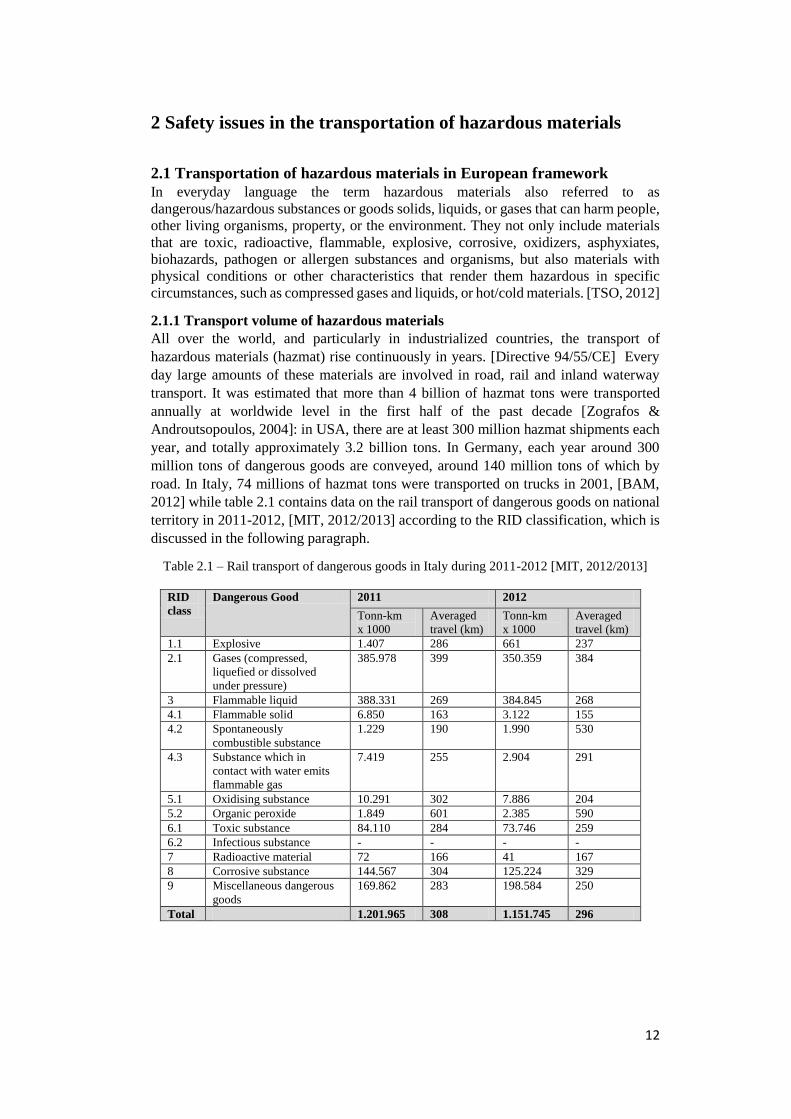
2012] while table 2.1 contains data on the rail transport of dangerous goods on national

territory in 2011-2012, [MIT, 2012/2013] according to the RID classification, which is

discussed in the following paragraph.

Table 2.1 – Rail transport of dangerous goods in Italy during 2011-2012 [MIT, 2012/2013]

RID

class

Dangerous Good 2011 2012

Tonn-km

x 1000

Averaged

travel (km)

Tonn-km

x 1000

Averaged

travel (km)

1.1 Explosive 1.407 286 661 237

2.1 Gases (compressed,

liquefied or dissolved

under pressure)

385.978 399 350.359 384

3 Flammable liquid 388.331 269 384.845 268

4.1 Flammable solid 6.850 163 3.122 155

4.2 Spontaneously

combustible substance

1.229 190 1.990 530

4.3 Substance which in

contact with water emits

flammable gas

7.419 255 2.904 291

5.1 Oxidising substance 10.291 302 7.886 204

5.2 Organic peroxide 1.849 601 2.385 590

6.1 Toxic substance 84.110 284 73.746 259

6.2 Infectious substance - - - -

7 Radioactive material 72 166 41 167

8 Corrosive substance 144.567 304 125.224 329

9 Miscellaneous dangerous

goods

169.862 283 198.584 250

Total 1.201.965 308 1.151.745 296

13

2.1.2 The ADR / RID agreements

Since hazmat daily cross international borders an harmonized regulation system was

needed. The different regulations from country to country make international trade in

chemicals and dangerous products seriously impeded, if not impossible and unsafe.

[UNECE, 2016] In the European Community, the hazmat transportation is regulated by

ONU through the United Nations Economic Commission for Europe (UNECE). The

agreement is divided into several documents tailored to the specific needs of the various

means of transport, starting from a common basis:

RID (Règlement concernant le trasport International ferroviaire des

merchandises Dangereuses), for the railway sector

ADR (Accord Européen Relatif au Transport International des Marchandises

Dangereuses par Route), for the road sector

IMDG (International Maritime Dangerous Goods), for shipbuilding, maritime

sector

ADN (Accord Européen Relatif au Transport International des Marchandises

Dangereuses par Voies de Navigation Intérieures), for inland waterways

The ADR agreement was signed in Geneva on September 1957 and entered into force

in January 1968. [ADR, 2015] In 1962 Italy adhered to the ADR agreement [L.

1839/1962] and it was originally applied to international transport only. Than the ADR,

RID and ADN agreements were extended to internal transport under the intention of

European Union to harmonize across the Community the conditions under which

dangerous goods are transported [Directive 94/55/CE] and Italy transposes that directive

in January 1996 [D.M. 4 settembre 1996] The agreement itself is brief and simple, most

of the provisions are indicated in the annexes: A - General provisions and provisions

concerning dangerous articles and substances, and annexes B - Provisions concerning

transport equipment and transport operations. [ADR, 2015]

The ADR agreement regulates:

the classification of dangerous substances in regard to the road sector

standards and tests that determine the classification of individual substances as

dangerous

the conditions of packaging of goods, characteristics of packaging and

containers

construction methods for vehicles and tanks

the requirements for the means of transport, including travel documents

Moreover, the agreement refers to employees who are involved in hazmat transport at

various levels: from the drivers of vehicles to people loading and unloading to

operations managers. Persons of those categories must have been trained and often have

achieved patent permits. [ADR, 2015] The prevision laid down the ADR do not apply

to the transport of dangerous goods by private vehicles or under the responsibility of the

armed force. [D.M. 4 settembre 1996]

2.1.3 Classification of dangerous goods

The ADR agreement classifies the substances in nine hazard classes that define the type

of risk that hazardous material may pose. Some substances have main risks and

secondary risks, and thus meet the definition of more than one hazard class. To further

group substances with similar risks, some hazard classes contain divisions. [ADR, 2015]

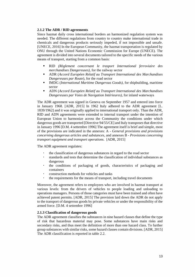
The ADR classification is reported in table 2.2.

14

Table 2.2 – ADR classification of dangerous good [ADR, 2015]

Class Dangerous Goods

1 Explosive substances and articles

2 Gases

2 Flammable liquids

4.1 Flammable solids, self-reactive substances and solid desensitized explosives

4.2 Substances liable to spontaneous combustion

4.3 Substances which, in contact with water, emit flammable gases

5.1 Oxidising substances

5.2 Organic peroxides

6.1 Toxic substance

6.2 Infectious substances

7 Radioactive material

8 Corrosive substances

9 Miscellaneous dangerous substances and articles

ADR also defines three packing groups, which indicate the degree of risk a hazardous

material may pose in transport in relation to other materials. Packing group is not

applicable to all hazard classes divisions, it refers to classes 1, 2, 5.2, 6.2, 7 and to self-

reactive substances of class 4.1. This classes are assigned to packing groups in

accordance with the degree of danger they present [ADR, 2015] as follow:

Packing group I – Substances presenting high danger

Packing group II – Substances presenting medium danger

Packing group III – Substances presenting low danger

Then, once the dangerous goods class has been defined, the European legislation give

some provisions of how to avoid or reduce the accident of the tanks subjected to an

external heat load, such as an accidental fire. For flammable substances the most

hazardous condition of transportation is the state of pressurized liquefied gas, in case of

sub cooled liquids or high pressure gases the consequences are not as much severe

[Landucci et al. 2013]. Therefore in the former scenario (and also for toxic gases) the

European Agreements RID and ADR, commit all filling and discharge openings of tanks

be equipped with an internal instant closing stop-valve which closes automatically in

the event of unintended movement of the vessel or in the event of fire (for tank-

containers, this requirements only applies if they have a capacity of more than 1 m3) for

risk reduction. In addition it also contains requirements for pressure relief devices to

ensure the integrity of the tank even if the tank is fully engulfed in fire. For example,

for tanks of non-refrigerated liquefied gases, the internal pressure does not exceed 20%

of the working pressure. [ADR, 2015]

The present work focuses on liquefied petroleum gas (LPG) which transportation is

extremely frequent in Europe. LPG is a mixture of saturated hydrocarbons, primarily

propane and butane, in their liquid state, that is, under pressure at ambient temperature.

It is a useful fuel for mobile and remote applications, because it requires only moderate

pressure (< 2 MPa) to remain liquid form at ambient temperature and it readily

vaporized when the pressure is released. This is the main advantage of LPG as fuel,

because it is liquid for transportation and storage, but gaseous for use. The composition

of LPG consequently depends on the season and the location where it is marketed. In

fact, propane evaporates at -42 °C, at atmospheric pressure, instead at 0.6 °C, which is

15

the boiling point of butane at the same pressure condition. Thus, different grades of LPG

can be produced. In regions where the winter temperatures drop below 0°C, the main

constituent of LPG is propane, because butanes are liquids at such conditions. In hot

climates, LPG can be a butane-propane mixture. [Maitlis & De Klerk, 2013]

In the ADR classification LPG belongs to class 2, division 2.1. As mentioned before,

the hazard related to LPG is also due to its liquefied gas condition. A flammable gas

liquefied through pressurization is a gas that has internal energy sufficient to suddenly

evaporates and turns out in a flammable mixture with air.

2.2 Past accidents data analysis

In order to identify the major safety issues associated to the transportation of hazardous

materials, past accidents data analysis was carried out. In fact, this type of analysis

grants valuable information on causes, dynamics and consequences, which can provide

the necessary experience to be used for safety improvement and to the characterization

of accidental scenarios.

2.2.1 Past accident report – Viareggio 2009

One of the most severe accident connected with the rail transportation of hazmat

occurred in Viareggio (Italy) in 2009. On Monday June 29th 2009, a freight train was

composed of 14 tank wagons, each having a nominal capacity of about 46.7 t (100,000

L) was passing through Viareggio. At 23:45 the first tank wagon derailed and

overturned after passing through Viareggio railway station at a speed of 90 km/h, below

the imposed limit of 100km/h. The following 4 tank cars also derailed and overturned.

The train engine did not derail and stopped few meters ahead of the first car. After

derailment, an intense loss of containment took place from the first tank wagon. The

entire inventory of a commercial LPG mixture was released from the breach. No loss of

containment occurred from the other 13 tank vessels. Firemen emptied all the derailed

cars on July 2nd. According to the report of the engine drivers, no immediate ignition

followed the release. Before the ignition of the gas cloud, the drivers had time to shut-

down the engine, to remove the documents from the engine and to run about 200m away

from the railway. Several witnesses remember a cloud of cold and white mist

propagating around the area where the derailment took place. The cloud ignited few

minutes after the start of the release. It is still uncertain which was the ignition point. A

flash fire resulting in severe damage took place. Several houses were involved in the

fire and 31 fatalities were caused by intense heat radiation exposure or collapse of

building. [Landucci et al. 2011]

2.2.2 Methodology and selection criteria

The data were collected from two different databases, the ARIA (Analysis, Research

and Information on Accidents) database and the MHIDAS (Major Hazard Incident Data

Service) database; the first one was used as primary source while the second one was

used as supplement since it is no longer updated. The MHIDAS database was hosted by

United Kingdom Health and Safety Executive. The ARIA database operated by the

French Ministry of Ecology, Sustainable Development and Energy lists the accidental

events, which have, or could have damaged health or public safety, agriculture, nature

or the environment. [ARIA, 2016] It collects events that are mainly caused by hazardous

industrial or agricultural facilities and also by transportation of hazardous materials.

The research was carried out on all countries but France, this is due to the 40000

accidents collected in France against the 6000 collected in other countries, but France.

The French data also concern small accidents which are not important for this research

16

that aiming at the classification of substances and primary causes involved in hazmat

transportation. The selection of contextual accidents would be laborious and it would

not have lead to significant changes in the final results, assuming that there is no reason

why France should be out of European average accidents in hazmat transportation. For

this reason it was assessed the exclusion of the France from the location of accidents.

The following scenarios were considered during the research:

Accidents occurred during transport of dangerous goods by road, inside a

company or on the road

Accidents occurred during transport of dangerous goods by rail, in or outside

of an classified installation

This analysis has taken into account all accidents of this type occurred from 1980 to

September 2015.

Three categories of substances were individuated and classified by the physical state in

which they were transported, through the following methodology:

Liquid

Liquefied gas

Other

The flammable and toxic substances transported in liquid phase, at ambient temperature,

are classified as liquid if their boiling point is under 30°C, otherwise they are classified

as liquefied gas, if their boiling point is over 30°C. Solid, gaseous and cryogenic

substances, both flammable and toxic, are classified as other. In addition to the above

classification, substances were divided by hazardous properties (flammable or toxic)

specifying what type of substance were involved in the accident (ammonia, LPG, etc.).

Primary causes are the events that turn out in the involvement of hazmat transportation

tank in the road or rail accident, which is followed by the failure of the tanker an

subsequent leakage of substance. The analysis of primary cause was conducted by

classifying them in the following categories:

Human error

Failure of truck/locomotive

Failure of tanker

Failure of rail/rail control system, for rail transportation

External event

Human error includes all the events which were not intended by the actor, which are a

deviation from intention, expectation or desirability. Collision, truck overturns, lost of

control of the vehicle, derailment, failure to close the valves, unsafe welding, failure of

operating hook, etc. are some example of what the human error category contains.

The failure of truck or locomotive includes the failure of every elements belonging to

the truck or convoy except the tankers; such as the breakdown of a wheel, lost of the

tanker, fire on truck not related to an external event, failure of the axle, etc.

The failure of the tanker could occur in several modes including the failure of a valve

or pressure relief valve, the premature opening of rupture disk, the crash of a part of the

tanker which was deformed. The leakage from the tank was also included in this

category, as well as the fire on the tanker, which was considered as the consequence of

a leakage.

17

In the rail transportation it was necessary to add another category: the failure of the rail

or of the rail control system, which includes the causes related to the rail damage, such

as fracture, corrosion, defective rail, misalignment; and to the failure of “rail” control

system, such as the failure of automatic stop device, of a switch and, more generally, of

traffic control system.

The external event is the last category, it includes: external impact, sabotage,

earthquakes, hurricane and external fire. The latter is the cause on which this work will

focus. The external fire could occur, amongst other events, from another tank or from

another unit, by the ignition of a flammable substance leakage during the tank

loading/unloading operations or from a short circuit of electrical cable. All the unknown

causes were included in the external event category.

Focusing on the LPG transportation, the primary causes were investigated as the causes

that led to the tank failure; if a human error caused the accident it may lead to a cold

BLEVE (Boiling Liquid Expanding Vapour Explosion), with the instantaneous loss of

containment, or it may generate a fire which engulfs the tank and may turns out in the

failure of the tank. In the first scenario the primary cause was considered as the human

error, while the external fire was considered as the cause of the second scenario. The

same classification of primary causes of accidents reported above were used for LPG

tanks causes of failure.

Also the consequences were collected for the LPG accidents and they were classified as

follows:

Release only leakage without ignition

Instantaneous release cold BLEVE

Release, ignition and fire no BLEVE occurred

Release, ignition and fire with consequent fired BLEVE

2.2.3 Results of the historical analysis

As mentioned before, the data were collected principally from ARIA database, which

lists 339 occurrences referred to road transportation and 320 occurrences referred to rail

transportation, in relation to the selection criteria aforesaid between 1980 and 2015.

After selection of contextual accidents and implementation with MHIDAS database,

245 occurrences referred to road transportation and 220 occurrences referred to rail

transportation have been examined. The results of the analysis is reported and than

discussed in this section.

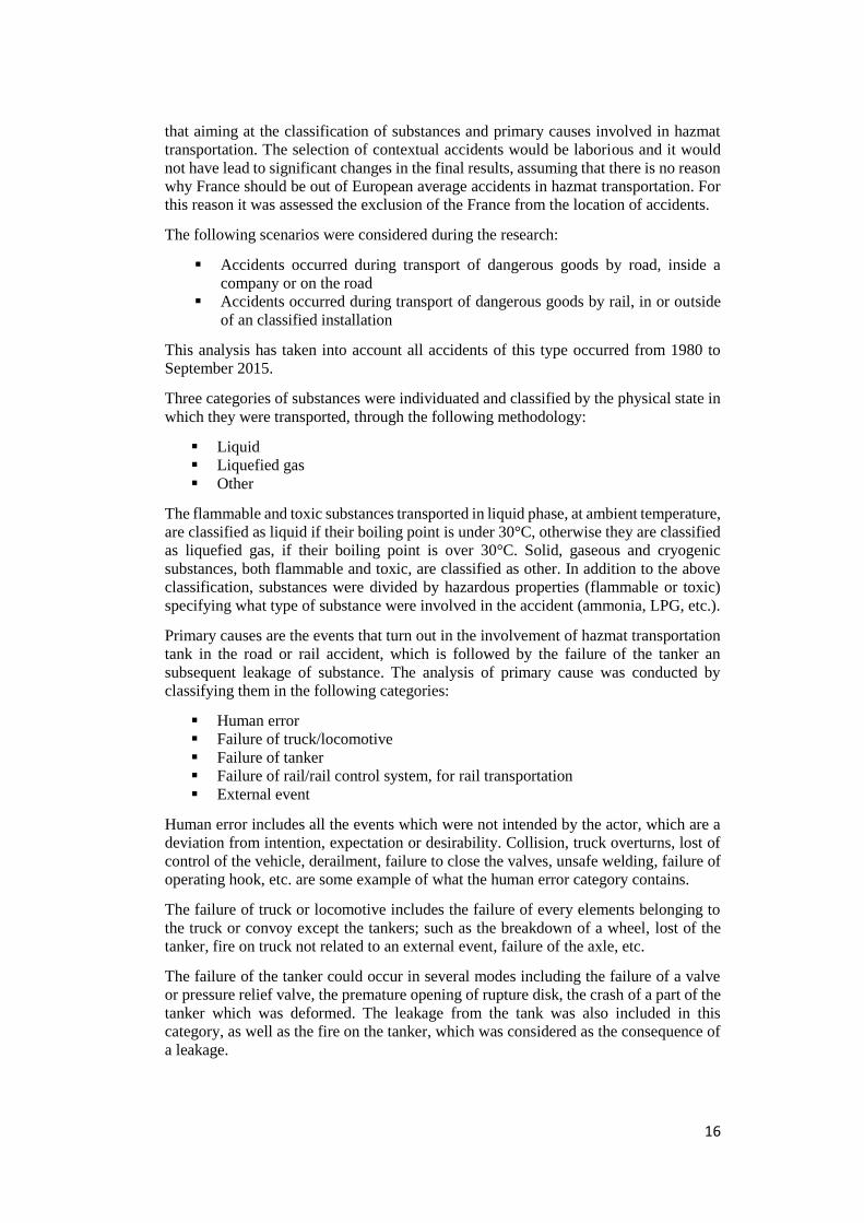
Road transportation results

Figure 2.1 reports the category of substances involved in severe accidents in road

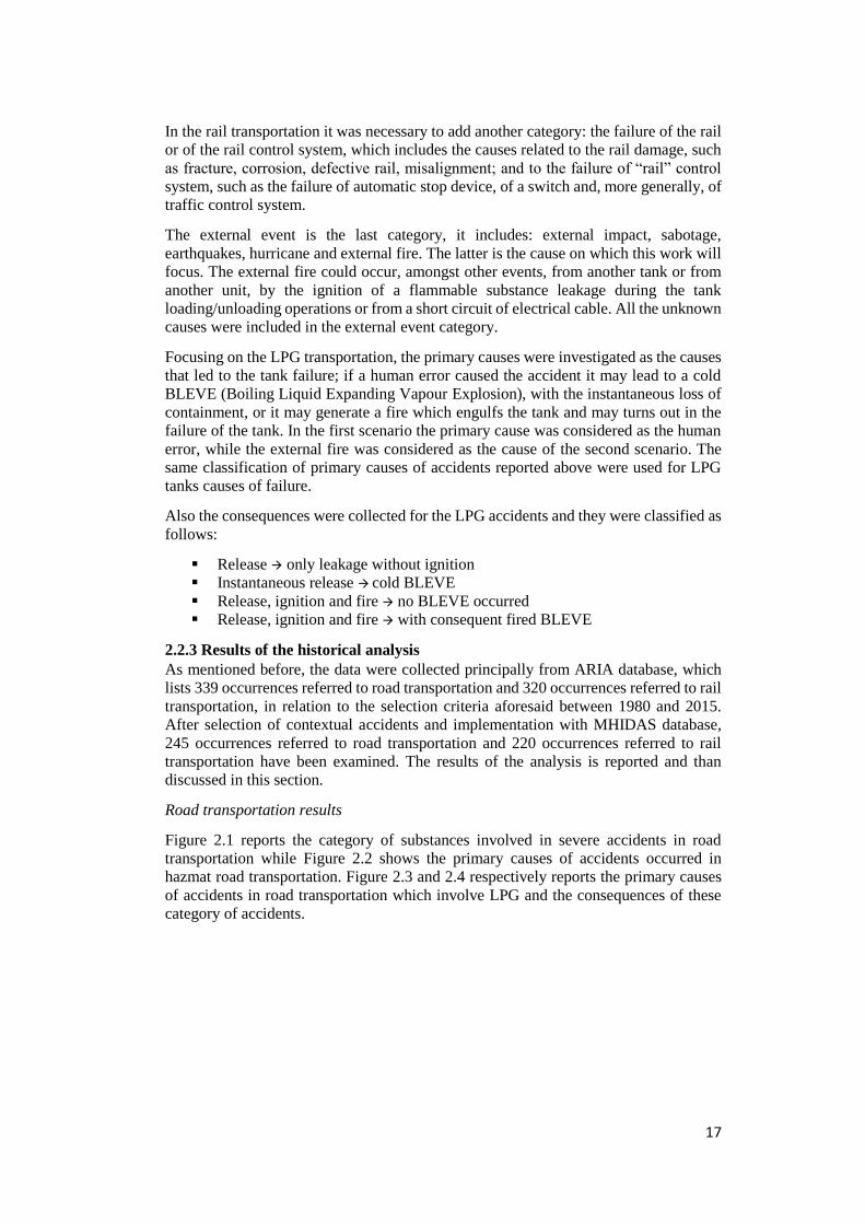
transportation while Figure 2.2 shows the primary causes of accidents occurred in

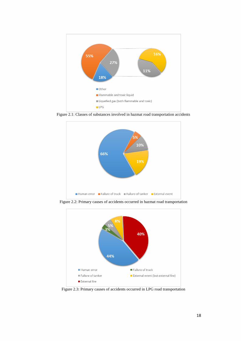
hazmat road transportation. Figure 2.3 and 2.4 respectively reports the primary causes

of accidents in road transportation which involve LPG and the consequences of these

category of accidents.

18

Figure 2.1: Classes of substances involved in hazmat road transportation accidents

Figure 2.2: Primary causes of accidents occurred in hazmat road transportation

Figure 2.3: Primary causes of accidents occurred in LPG road transportation

19

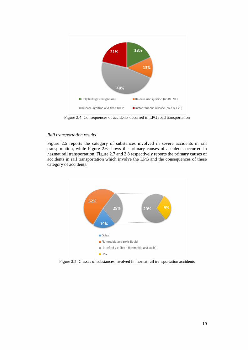
Figure 2.4: Consequences of accidents occurred in LPG road transportation

Rail transportation results

Figure 2.5 reports the category of substances involved in severe accidents in rail

transportation, while Figure 2.6 shows the primary causes of accidents occurred in

hazmat rail transportation. Figure 2.7 and 2.8 respectively reports the primary causes of

accidents in rail transportation which involve the LPG and the consequences of these

category of accidents.

Figure 2.5: Classes of substances involved in hazmat rail transportation accidents

20

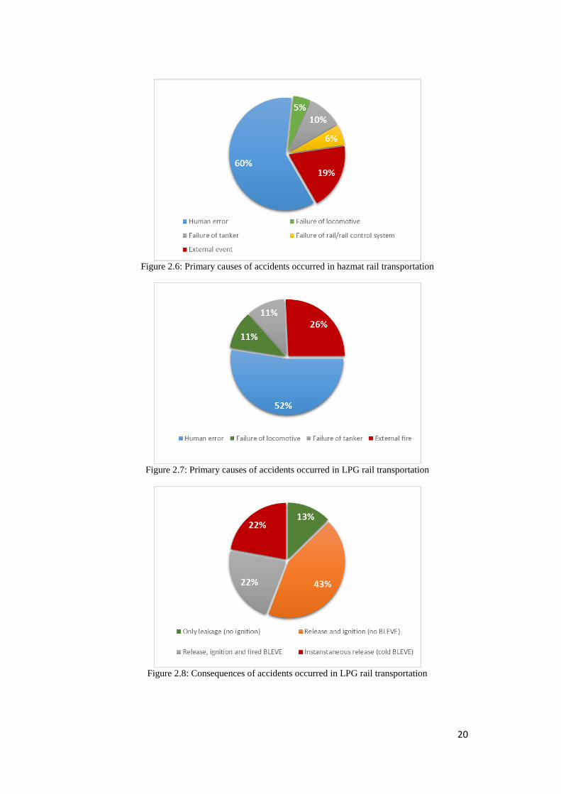
Figure 2.6: Primary causes of accidents occurred in hazmat rail transportation

Figure 2.7: Primary causes of accidents occurred in LPG rail transportation

Figure 2.8: Consequences of accidents occurred in LPG rail transportation

21

2.3 Safety issues related to the transportation of pressurized flammable

gases

Past accidents data analysis identified the relevant accidents occurred in years during

the road and rail transportation of dangerous goods, around the world. The classes of

substances involved and the main causes of accidents are classified, with particular

focus on accidents occurred during LPG transportation, the consequences of which are

also identified and classified. It is timely, therefore, to detailed analyse the safety issues

related to LPG transport. They are discussed in this section to complete the picture and

come to some conclusions.

Dangerous goods are carried through a transportation network, which civilians daily use

and which crosses vulnerable and densely populated areas. During the transportation of

LPG or, generally, pressurized flammable gas, if an accidental leak occurs it may lead

to catastrophic event which can harm people and neighbouring buildings, as occurred

in the Viareggio accidents. (see paragraph 2.2.1)

2.3.1 BLEVE definition

As evidenced by past accident data analysis, one of the most critical scenarios that may

follow an accidental leakage of LPG is the boiling liquid expanding vapour explosion

(BLEVE). This event typically follows the catastrophic rupture of a tank containing the

pressurized liquefied gas, which instantly vaporizes and expands. The liberated energy

in such cases is very high, causing high blast pressures and generation of fragments with

high initial velocities, and resulting in propulsion of fragments over long distances.

[TNO Yellow Book, 2005] The blast is often followed by a fireball due to LPG ignition.

[Reid, 1979] In the end of the 1970s, the BLEVE was a mysterious phenomenon, several

theories have been put forward to explain this very energetic event but none have been

proved. [Birk & Cunningham, 1994] Among the large number of definitions that can be

found in literature, [Hemmatian et al. 2015] Walls defined BLEVEs for first time in

1957 [Walls, 1979] as a failure of a major container into two or more pieces occurring

at a moment when the container liquid is at a temperature above its boiling point at

normal atmospheric pressure. Then Reid in 1976 [Reid, 1979], defined BLEVEs as the

sudden loss of containment of a liquid that is at a superheated temperature for

atmospheric conditions. More recently, on the basis of some observations which

highlight that there is no practical reason why fragments or superheat limits need to be

mentioned in the definition, some authors proposed less restrictive definitions. In

particular, Birk and Cunningham in 1994 have defined BLEVEs as the explosive release

of expanding vapour and boiling liquid when a container, holding a pressure-liquefied

gas, fails catastrophically. Catastrophic failure was defined as the sudden opening of a

tank/container to release its contents nearly instantaneously. [Birk & Cunningham,

1994; Eckhoff, 2014]

In the present work the latter definition of BLEVEs will be used. The TNO definition is

also reported: BLEVE is an explosion resulting from the sudden failure of a vessel

containing a liquid at a temperature significantly above its boiling point at normal

atmospheric pressure, e.g. pressure liquefied gases. The fluid in the vessel is usually a

combination of liquid and vapour. Before rupture, the liquid contained is more or less

in equilibrium with the saturated vapour. If the vessel ruptures, vapour is vented and the

pressure in the liquid drops sharply. Upon loss of equilibrium, liquid flashes at the

liquid-vapour interface, the liquid-container-wall interface, and, depending on

temperature, throughout the liquid. [TNO Yellow Book, 2010]

22

Usually two types of BLEVE are defined: “fired” BLEVE and “unfired” or “cold”

BLEVE. [Paltrinieri et al. 2009] The first one is thermally induced by an external fire,

thus it usually follows the tank collapse due to fire engulfment. If the ignition of the

vapour is immediate, and very often it is because the external fire, a fireball occurs. The

“cold” BLEVE is not thermally induced, it may be caused by a violent impact on the

tank during a traffic accident or by the tank sudden failure due to material defect or to

overfilling. [Prugh, 1991] In a cold BLEVE there is no certain ignition so the fireball

may not be present, surely it is easy that in a road/rail environment there is enough

energy and sources to ignite the flammable cloud. If the ignition is delayed the cloud

will cause a flash fire rather than a fireball. [TNO Yellow Book, 2005]

The primary causes of a “cold” BLEVE are wholly incidental, as this type of BLEVE,

of course happens only if the severity of the accident is enough for the tank strength,

but it cannot be delayed or avoided at the time of accident. The focus in this work is on

“fired” BLEVE, which can be avoided, or at least delayed, through the installation of

an adequate fireproofing system in combination with appropriate designed pressure

relief valves (see the detailed analysis in Section 2.3). Moreover in a statistic on several

transport accidents reported by Paltrinieri et al. more than 85% of BLEVEs recorded

are thermally induced. [Paltrinieri et al. 2009]

2.3.2 Fireball definitions

As seen above, when a BLEVE occurs a given amount of flammable vapour is suddenly

released into the atmosphere. A fraction of liquid droplets can deposit on the ground

(rain-out fraction) and form a flammable pool, while another part is entrained by the

vapour causing an aerosol cloud. If the cloud is immediately ignited it turns out in a

phenomenon called fireball. A fireball is defined as a fire, burning sufficiently rapidly

for the burning mass to rise into the air as a cloud or ball. [TNO Yellow Book, 2005]

The ignition must be immediate for the fireball to occur, if the mass of flammable

vapour mixes sufficiently with air, the delayed ignition will give rise to a flash fire rather

than a fireball. Since the mixing with air is limited, the flame is only on the external

surface of the volume of the released gas, thus it can be considered a diffusion flame.

While the external surface burns, the internal fuel droplets act as fuel reservoir. In fact

they progressively vaporize, mix with air and burn. The resulting fireball is a transient

phenomenon the duration of which lasts up to a minute. The fireball passes through

three phases [Lees, 1996] :

growth growth to half diameter upon final diameter

steady burning roughly spherical

burnout size held steady

The growth phase may be divide into two intervals, each lasting about 1 second. In the

first interval the flame is bright and the flame temperature is about 1300°C, the smaller

droplets of fuel vaporize and the fireball grows to about half its final diameter. In the

second interval of the growth phase, the fireball grows to its final volume, the surface

starts to be dark and sooty and the flame temperature decreases by approximately

200°C. In the second phase, which lasts some 10 seconds, the fireball, which is now

roughly spherical, is no longer growing. At the start of this phase, it begins to lift off. It

rises and changes to the familiar mushroom shape. The estimated effective flame

temperature is 1100-1200°C as in the second interval of the growth phase. In the third

phase, which lasts some 5 seconds, the fireball remains of the same size, but the flame

becomes less sooty and more translucent. [TNO Yellow Book, 2005] Once there is no

more fuel the fire extinguish itself. The radius of the fireball can be calculated from the

23

quantity of combusting material. It was found that peak emissions came from areas at

the top of the expanding fireball whereas the emission was lower from lower portions

of the fireball because of increased soot shielding and poorer mixing with ambient air.

[TNO Yellow Book, 2005]

2.3.3 Analysis of cascading scenarios in the transportation of LPG

As mentioned before, the most dangerous scenario that may follows an accidental

leakage of LPG is the BLEVE with consequent fireball.

The typical mechanism which leads to the fired BLEVE can be considered as a domino

effect or “cascading event” [TNO Yellow Book, 2005], consisting in the following

steps:

occurrence of primary event a road or rail accident occurs with development

of fire

propagation of the event the fire extends to LPG tankers

starting of BLEVE mechanism temperature of the tank walls increases, thus

pressure increases by LPG evaporation

tank catastrophic rupture due to increased pressure and thermal weakening of

materials BLEVE with blast wave and possible debris thrown away

rapid ignition of flammable aerosol fireball with high radiation heat flux

When a road or rail accident happens, it is likely that a fire develops from the ignition

of the fuel that leaks from the vehicle. The ignition sources in these situations can be

many, e.g. the metal sheets of the vehicle involved in the crush easily generate sparks.

Moreover there are several flammable materials in vehicles that may go to feed the

flames. If one or more, as is easily in rail transportation, LPG tanks are involved in the

accident, directly or indirectly, the flames may extend up to them.

From this moment on, the situation becomes much more critical. The heat is transferred

from the fire to the tank outer surface by convection and thermal radiation. If the fire is

large or if the tank is sufficiently distant from the flame radiation will dominate,

otherwise also convection must be taken into account. [Landucci et al. 2013] The heat

is transferred by conduction through all layers of tank: through external jacket and

insulation blanket (if present) and through the tank shell.

The heat is now received by the internal load by convection and radiation. The liquid-

side tank wall usually has high heat transfer coefficients, particularly if the liquid is

boiling, resulting in a cooling effect. On the contrary, the vapour-side tank wall has a

less efficient heat exchange due to low heat transfer coefficients, with consequent wall

temperature increase. The latter weakens the tank materials which are, moreover,

subjected to the differential dilation in correspondence of liquid-vapour interface. At

this stage, LPG starts boiling and inner pressure of tank increases; one must recall that

the LPG is a liquefied pressure gas, thus in saturated condition in vapour-liquid

equilibrium. Although the tank is constructed to withstand the internal pressure that is

generated, the combination with the weakening of materials can lead to the catastrophic

failure with instantaneous release of the contents. The time between the start of the fire

and the tank rupture is defined as time to failure (ttf). [Landucci, 2008] The energy

released in the physical explosion following the rupture of the vessel, is the work of

expansion of the LPG from the burst pressure to atmospheric. The burst pressure depend

from the situation in which the tank fails, in case of external fire the pressure at failure

is estimated as the 21% more of the opening pressure of safety valves. [TNO Yellow

Book, 2005] Part of the released energy is spent for the projection of fragments and the

rest for the formation of pressure wave. Primary fragments have high kinetic energy and

24

are projected at distance, they impact what is surrounding causing damages and

secondary fragment. The explosion overpressure affects buildings, vehicles and humans

nearby. The damage to humans are due to the action of shock wave on the sensitive

organs, i.e. lungs and tympanic membrane, and to the impact of debris fragments and

collapsed buildings. The ignition of the cloud generates a heat flux, which affects a large

area around the accident. For instance, an LPG fireball generated from 10 tonn of

substance, after 5 second from the ignition has a radiative heat flux with a lethality zone

of about 80 meters diameter and it causes irreversible injuries up to 100 meters, at

ground level. [TNO Yellow Book, 2005]

It is clear that if a road or rail accident may be confined in its close proximity, an

accident that involves one or more LPG tanks may afflict people and buildings relatively

distant. Taking into account the mechanism described above, it is evident that the

catastrophic rupture of the tank can be avoided by controlling the load temperature, thus

the wall temperature. When it is possible and only after the safety enhancement for

workers, the temperature increase is controlled by fire fighters spaying water on the wall

of the tank until the external fire is extinguished.

2.4 Safety devices adopted for the protection of the tank

BLEVEs caused by fire can be avoided or at least delayed providing tank with adequate

thermal protections. [Paltrinieri et al., 2009] Thermal protections consist of an insulating

coating layer and a pressure relief valve (PRV). The insulating coating is aimed at

reduce the heat flux reaches by tank shell walls, so as avoid the thermal weakening of

material. PRVs are aimed at preventing the pressure build up during fire exposure by

venting the overpressure. The benefits of safety device coupled with thermal insulation

on LPG tank will be developed in this section.

2.4.1 Passive fire protection systems

A generic passive protection is defined by CCPS as a barrier which does not require any

external activation to perform the safety function. [CCPS, 2010]

Passive fire protection (PFP) systems consist in coating, cladding or free-standing

system which, in the event of fire, will provide thermal protection to restrict the rate at

which heat is transmitted to the object or area being protected. [EN ISO 13702, 1999]

Firewall are thermal shields placed between the targets and the potential fire sources,

which are able to absorb the thermal radiation ensuring the survivability of the target.

Clearly enough they are only applied in fixed installations. [Landucci, 2008]

PFP through PFP coatings can be suitable for transport vessels, since they are directly

applied on the tank shell.

The PFP systems are differentiated according to the materials they are made of, whether

organic or inorganic. Inorganic-based materials are typically vermiculite sprays or

cement boards that are inert to flame impingement and keep the initial structure with

good thermal resistance. They are not able to adapt their configuration to the fire

aggression so they may become brittle after fire exposure. Due to high thickness applied

and consequent weight, they are mostly only suitable for fixed installations. [Landucci

et al. 2009] The cementitious products protect the tank by evaporation of the moisture

trapped within the material, keeping the underlying steel temperature around 100°C.

[Zuccaro, 2012] The heat input is also reduce by the concrete high mass and low thermal

conductivity. The weight of concrete can be lightened by aggregation with lightweight

25

products, as vermiculite. In this case due to the lower mass and in order to obtain the

appropriate water content, structural steel shell are typically covered with a very thick

coating layer. [Landucci et al. 2009] Another type of inorganic materials used as

fireproofing are the thermal insulation systems, such as mineral wool and cellular glass.

Both are lightweight, dimensionally stable, essentially impermeable to moisture, and

they are non-combustible. [Zuccaro, 2012] The density of these materials is one order

of magnitude lower than other products and these property makes it a convenient

solution even if it needs higher thickness to perform adequate protection. Thus, different

layers of material are applied on equipment to protect and than stainless steel jacketing

is employed to obtain fire resistance. [Landucci et al. 2009] The latter type of

fireproofing materials are particularly suitable for the application on tanks for the

transport of hazardous goods.

Organic-based materials present better mechanical properties and they may be more

adequate to obtain light structures, like portable tanks of dangerous goods. [Landucci et

al. 2009] Intumescent coatings are the organic-based material normally used in

hydrocarbon-processing complexes, generally they are epoxy based, spray or hand

applied. When exposed to sufficient heat, intumescent coating expands to form a thick,

insulating carbonaceous char. The reduction of the heat load to the steel substrate relies

on the thermal insulating capability of the char and the ability of the char to remain

adherent and physically intact. [Zuccaro, 2012] The application of several layers of

material is necessary to assure a sufficient duration of the fire protection, since the

material tends to be slowly burned by the flames. [Landucci et al. 2009] One main

problem with intumescent coatings is related to corrosion of steel substrate that has been

sometimes reported beneath apparently intact coating. Moreover, intumescent products

and in general organic-based materials may degrade with prolonged outdoor weathering

and exposure to slightly elevated temperatures. [Zuccaro, 2012] This does not render

organic-based materials optimal for protection of tanks for the transport of goods.

2.4.2 Pressure relief valves

As mentioned before, pressure relief valves are also common tool in the passive fire

protection, they don’t reduce the heat flux entering the system, but reduce the pressure

ejecting mass from the process. [Crowl & Tipler, 2013] The pressure relieving devices

are designed to open during emergency or abnormal conditions to prevent rise of

internal fluid pressure in excess of a specified design value. [CCPS, 1998]

A pressure relief valve has the task to vent off excess pressure enough quickly and re-

close for preventing the further flow of fluid after normal conditions have been restored.

The required relieving area of the safety valve depends on scenario and this aspect is

the basis for the selection of the type and size of device. The standard regulations API

520 [API 520, 2014] is a design manual widely used for sizing of relief valves on both

liquid and gas filled vessels and the standard API 527 [API 527, 2014] gives permissible

leakage rate of valves and testing procedure.

During the relief the fluid may be in liquid, liquid-vapour mixture, gas or supercritical

phase. Thus, the safety system must be able to handle various process condition.

Pressure relief valves have spring-loaded disks that close a main orifice against a

pressure source. As pressure rises, the disk begins to rise off the orifice and a small

amount of fluid passes through the valve. Continued rise in pressure above the opening

pressure causes the disk to open the orifice in a proportional fashion. The safety valve

26

is similar to the relief valve except it is designed to open fully, or pop, with only a small

amount of pressure over the rated limit. Conventional safety valves are sensitive to

downstream pressure and may have unsatisfactory operating characteristics in variable

back pressure applications. The balanced safety relief valve is available and minimizes

the effect of downstream pressure on performance. [ASM, 2015]

2.4.3 Safety requirements for the effective fire protection of LPG tankers

Focusing on LPG transportation, if a severe accident occurs the emergency teams should

have the time for the intervention, since, in the fired-domino described in previously

section, the tank failure due to the propagation of fire is delayed respect to primary

event, i.e. the external fire. The problem is the tank resistance, which in the case of

absent protection may withstand fire conditions for a limited period (5-30 minutes). This

lapse of time is usually not sufficient to avoid the safe suppression of the fire due to fire

brigade intervention. A realistic evaluation of the time required for effective mitigation

by the fire brigades, based on actual data available from past accidents in the

Netherlands, evidenced that a time lapse of 75 minutes is required to allow an effective

protection or prevention of BLEVE by active measures upon the arrival of the fire

brigades. [Molag & Kruithof, 2005] Therefore the comparison between the ttf of tank

and the time for arrival of rescuers shows that the intervention time is not sufficient for

avoid the rupture unless the tank resistance has been enhanced. Thermal insulation

around the tank can reduce the excessive heating of the steel wall and PRV can reduce

the internal pressure. These coupled actions extend the time to BLEVE and can avoid

the failure of the tank. [Landucci et al, 2009]

In North America specific transport regulation [CFR, 2015; CGSB, 1997] have been

adopted, requiring road and rail tankers carrying flammable liquefied gases to be

equipped with pressure relief valves. In addition, rail tankers have to be also thermally

insulated. The Canadian General Standards Board requires that the thermal insulation

system must be able to avoid the rupture of the tank for 100 minutes in an engulfing

pool fire, or 30 minutes in an engulfing torching fire. One common system includes a

13 mm blanket of high-temperature ceramic fibre thermal insulation covered with 3

mm steel jacket. [Birk & Cunningham, 1994] This insulation system is the one used in

the model development later in this work.

Even if the double action of thermal insulation and PRV seems to be the answer of

safety issues related to transportation of LPG, it may be insufficient to avoid the vessel

catastrophic rupture. Indeed, the fireproofing system is not ideal and it may degrade

during its lifetime. The PFP effectiveness can be influenced by damages or defects

which lead to a double negative effects: the thermal weakening of the constriction

material, due to the temperature increase, and strong local thermal dilatation. In fact, the

shell wall in contact with the liquid undergoes a cooler effect while the shell wall in

contact with vapour does not. If a defect in the thermal insulation system is present, the

difference of the vapour and liquid temperatures is very strong, the vapour-side wall

thermal dilation will be much higher than the liquid-side wall one, these phenomenon

at the interface leads to the increase of the mechanical stress distribution in the defective

part.

Characterization of thermal insulation defects is the central purpose of this work and it

will be deeply analysed in Section 3.

27

2.5 Discussion and conclusions

In the present Chapter Past accident data analysis, which results are reported in Section

2.2.3, showed that the percentage of classes of substances involved in severe accidents

are in line with the percentage of hazardous materials transported by road and rail. It

was estimated that over 50% of hazardous materials transported (both by rail and road)

are liquids, while gases (compressed, liquefied) occupy around 10%. [Paltrinieri et al.,

2009] In fact, flammable and toxic liquid is the class of substances more involved in

severe accidents both in road and rail transportation. This is due to the global quantities

of hazardous materials transported, as said, but also due to the lower thickness of the

shell of the tank used for transportation at ambient pressure, as in the case of liquids,

than the tanks used for liquefied gases, which have to resist a higher pressure. If an

accident occurs, the tank with the thicker shell is more likely to resists.

The results of accidents involving LPG highlight that the problem related to the

transportation of such hazardous substance is relevant to public safety. The external fire

is the cause of the 40% for road and 26% for rail transportation accidents, approximately

half party of which led to fired BLEVE in the road transportation, while in the rail

transportation BLEVE occurs in 22% of accidents. The percentage of accidents in which

LPG does not ignite after leakage is 18% in road transportation and 13% in rail

transportation, this means that in the remaining 82% and 87%, respectively road and

rail, of accidents there is development of a fire. These results highlight that the safety

issues related to the hazmat transportation is relevant for public safety in order to avoid

severe consequences from transportation accidents and prevent Viareggio-like

accidents. In the Viareggio accident only a series of random events avoid the BLEVE

occurrence and the propagation of fire to other LPG tankers. The LPG leak found many

obstacles through the expansion area, such as wall of the station, car and tree. This type

of confinement could have caused an overpressure in case of ignition. When such

overpressure occurs, the event is a vapour cloud explosion (VCE) rather than a flash

fire. [TNO Yellow Book, 2005]

Finally, even if other worst-case scenarios have been avoided, the flash fire resulted in

31 fatalities and in extended damages to residential buildings around the railway line.

The need of specific regulations which concern the possible implementation of safety

devices is now evident. As mentioned before, the European framework, the installation

of thermal insulation system on transportation tankers is still not approved because of

defects and degradation in which these systems undergo. Since the coating systems are

not ideal, they have to be well characterised in terms of protection performance, in

particular if defects are present. Assessing the acceptability levels for the coating

defects, in order to avoid vessels failure when exposed to fire, is of utmost importance

for the wider implementation of coatings as relevant safety measure.

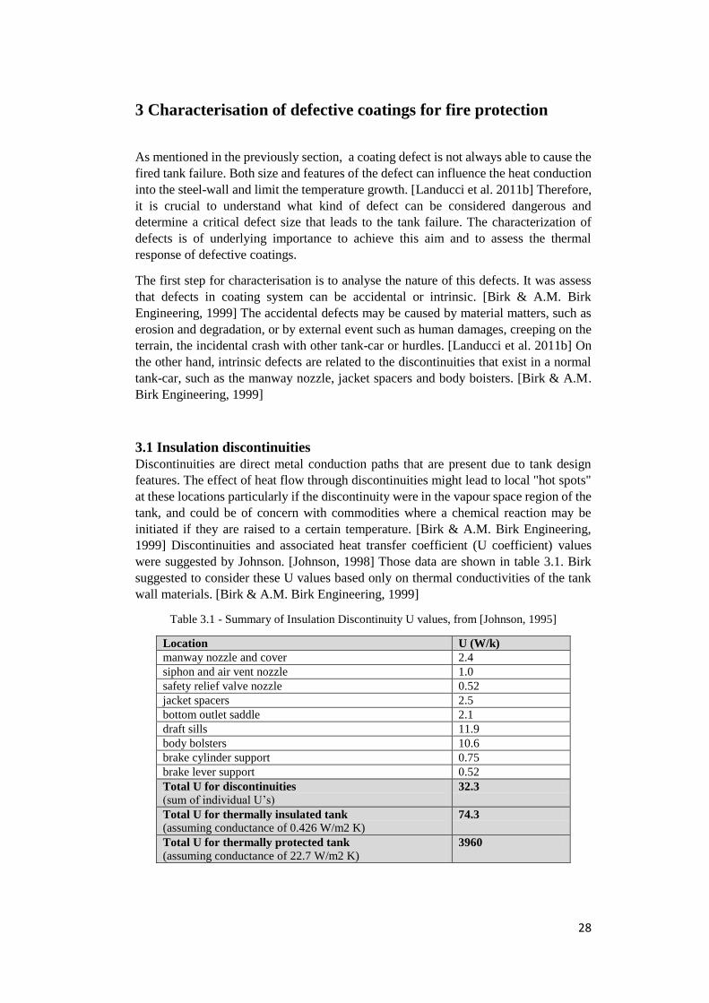
28

3 Characterisation of defective coatings for fire protection

As mentioned in the previously section, a coating defect is not always able to cause the

fired tank failure. Both size and features of the defect can influence the heat conduction

into the steel-wall and limit the temperature growth. [Landucci et al. 2011b] Therefore,

it is crucial to understand what kind of defect can be considered dangerous and

determine a critical defect size that leads to the tank failure. The characterization of

defects is of underlying importance to achieve this aim and to assess the thermal

response of defective coatings.

The first step for characterisation is to analyse the nature of this defects. It was assess

that defects in coating system can be accidental or intrinsic. [Birk & A.M. Birk

Engineering, 1999] The accidental defects may be caused by material matters, such as

erosion and degradation, or by external event such as human damages, creeping on the

terrain, the incidental crash with other tank-car or hurdles. [Landucci et al. 2011b] On

the other hand, intrinsic defects are related to the discontinuities that exist in a normal

tank-car, such as the manway nozzle, jacket spacers and body boisters. [Birk & A.M.

Birk Engineering, 1999]

3.1 Insulation discontinuities

Discontinuities are direct metal conduction paths that are present due to tank design

features. The effect of heat flow through discontinuities might lead to local "hot spots"

at these locations particularly if the discontinuity were in the vapour space region of the

tank, and could be of concern with commodities where a chemical reaction may be

initiated if they are raised to a certain temperature. [Birk & A.M. Birk Engineering,

1999] Discontinuities and associated heat transfer coefficient (U coefficient) values

were suggested by Johnson. [Johnson, 1998] Those data are shown in table 3.1. Birk

suggested to consider these U values based only on thermal conductivities of the tank

wall materials. [Birk & A.M. Birk Engineering, 1999]

Table 3.1 - Summary of Insulation Discontinuity U values, from [Johnson, 1995]

Location U (W/k)

manway nozzle and cover 2.4

siphon and air vent nozzle 1.0

safety relief valve nozzle 0.52

jacket spacers 2.5

bottom outlet saddle 2.1

draft sills 11.9

body bolsters 10.6

brake cylinder support 0.75

brake lever support 0.52

Total U for discontinuities

(sum of individual U’s) 32.3

Total U for thermally insulated tank

(assuming conductance of 0.426 W/m2 K) 74.3

Total U for thermally protected tank

(assuming conductance of 22.7 W/m2 K) 3960

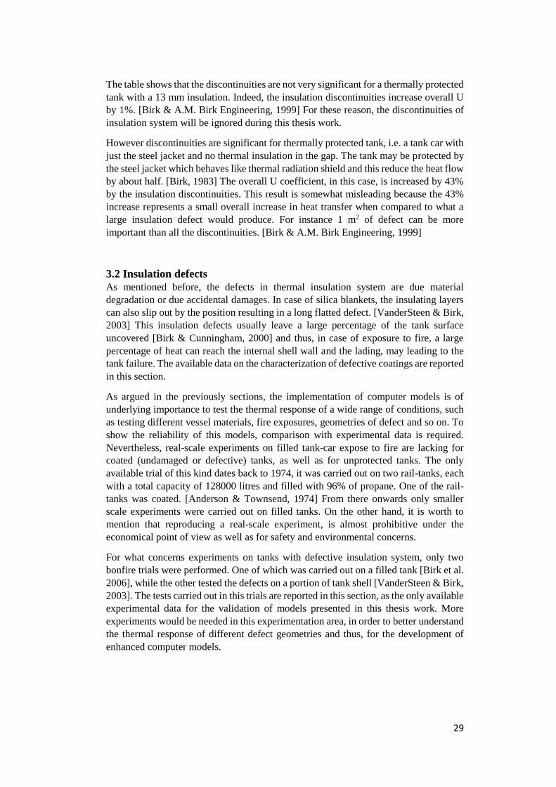
29

The table shows that the discontinuities are not very significant for a thermally protected

tank with a 13 mm insulation. Indeed, the insulation discontinuities increase overall U

by 1%. [Birk & A.M. Birk Engineering, 1999] For these reason, the discontinuities of

insulation system will be ignored during this thesis work.

However discontinuities are significant for thermally protected tank, i.e. a tank car with

just the steel jacket and no thermal insulation in the gap. The tank may be protected by

the steel jacket which behaves like thermal radiation shield and this reduce the heat flow

by about half. [Birk, 1983] The overall U coefficient, in this case, is increased by 43%

by the insulation discontinuities. This result is somewhat misleading because the 43%

increase represents a small overall increase in heat transfer when compared to what a

large insulation defect would produce. For instance 1 m2 of defect can be more

important than all the discontinuities. [Birk & A.M. Birk Engineering, 1999]

3.2 Insulation defects

As mentioned before, the defects in thermal insulation system are due material

degradation or due accidental damages. In case of silica blankets, the insulating layers

can also slip out by the position resulting in a long flatted defect. [VanderSteen & Birk,

2003] This insulation defects usually leave a large percentage of the tank surface

uncovered [Birk & Cunningham, 2000] and thus, in case of exposure to fire, a large

percentage of heat can reach the internal shell wall and the lading, may leading to the

tank failure. The available data on the characterization of defective coatings are reported

in this section.

As argued in the previously sections, the implementation of computer models is of

underlying importance to test the thermal response of a wide range of conditions, such

as testing different vessel materials, fire exposures, geometries of defect and so on. To

show the reliability of this models, comparison with experimental data is required.

Nevertheless, real-scale experiments on filled tank-car expose to fire are lacking for

coated (undamaged or defective) tanks, as well as for unprotected tanks. The only

available trial of this kind dates back to 1974, it was carried out on two rail-tanks, each

with a total capacity of 128000 litres and filled with 96% of propane. One of the rail-

tanks was coated. [Anderson & Townsend, 1974] From there onwards only smaller

scale experiments were carried out on filled tanks. On the other hand, it is worth to

mention that reproducing a real-scale experiment, is almost prohibitive under the

economical point of view as well as for safety and environmental concerns.

For what concerns experiments on tanks with defective insulation system, only two

bonfire trials were performed. One of which was carried out on a filled tank [Birk et al.

2006], while the other tested the defects on a portion of tank shell [VanderSteen & Birk,

2003]. The tests carried out in this trials are reported in this section, as the only available

experimental data for the validation of models presented in this thesis work. More

experiments would be needed in this experimentation area, in order to better understand

the thermal response of different defect geometries and thus, for the development of

enhanced computer models.

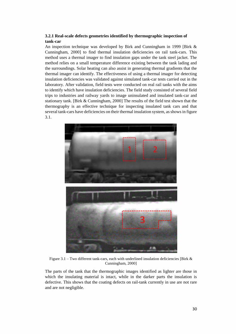
30

3.2.1 Real-scale defects geometries identified by thermographic inspection of

tank-car

An inspection technique was developed by Birk and Cunningham in 1999 [Birk &

Cunningham, 2000] to find thermal insulation deficiencies on rail tank-cars. This

method uses a thermal imager to find insulation gaps under the tank steel jacket. The

method relies on a small temperature difference existing between the tank lading and

the surroundings. Solar heating can also assist in generating thermal gradients that the

thermal imager can identify. The effectiveness of using a thermal imager for detecting

insulation deficiencies was validated against simulated tank-car tests carried out in the

laboratory. After validation, field tests were conducted on real rail tanks with the aims

to identify which have insulation deficiencies. The field study consisted of several field

trips to industries and railway yards to image uninsulated and insulated tank-car and

stationary tank. [Birk & Cunningham, 2000] The results of the field test shown that the

thermography is an effective technique for inspecting insulated tank cars and that

several tank-cars have deficiencies on their thermal insulation system, as shows in figure

3.1.

Figure 3.1 – Two different tank-cars, each with underlined insulation deficiencies [Birk &

Cunningham, 2000]

The parts of the tank that the thermographic images identified as lighter are those in

which the insulating material is intact, while in the darker parts the insulation is

defective. This shows that the coating defects on rail-tank currently in use are not rare

and are not negligible.

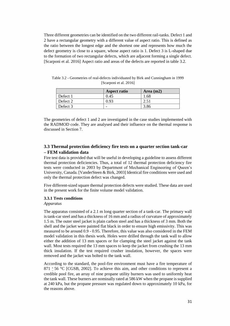
31

Three different geometries can be identified on the two different rail-tanks. Defect 1 and

2 have a rectangular geometry with a different value of aspect ratio. This is defined as

the ratio between the longest edge and the shortest one and represents how much the

defect geometry is close to a square, whose aspect ratio is 1. Defect 3 is L-shaped due

to the formation of two rectangular defects, which are adjacent forming a single defect.

[Scarponi et al. 2016] Aspect ratio and areas of the defects are reported in table 3.2.

Table 3.2 - Geometries of real-defects individuated by Birk and Cunningham in 1999

[Scarponi et al. 2016]

Aspect ratio Area (m2)

Defect 1 0.45 1.68

Defect 2 0.93 2.51

Defect 3 - 3.86

The geometries of defect 1 and 2 are investigated in the case studies implemented with

the RADMOD code. They are analysed and their influence on the thermal response is

discussed in Section 7.

3.3 Thermal protection deficiency fire tests on a quarter section tank-car

– FEM validation data

Fire test data is provided that will be useful in developing a guideline to assess different

thermal protection deficiencies. Thus, a total of 12 thermal protection deficiency fire

tests were conducted in 2003 by Department of Mechanical Engineering of Queen’s

University, Canada. [VanderSteen & Birk, 2003] Identical fire conditions were used and

only the thermal protection defect was changed.

Five different-sized square thermal protection defects were studied. These data are used

in the present work for the finite volume model validation.

3.3.1 Tests conditions

Apparatus

The apparatus consisted of a 2.1 m long quarter section of a tank-car. The primary wall

is tank-car steel and has a thickness of 16 mm and a radius of curvature of approximately

1.5 m. The outer steel jacket is plain carbon steel and has a thickness of 3 mm. Both the

shell and the jacket were painted flat black in order to ensure high emissivity. This was

measured to be around 0.9 - 0.95. Therefore, this value was also considered in the FEM

model validation in this thesis work. Holes were drilled through the tank wall to allow

either the addition of 13 mm spaces or for clamping the steel jacket against the tank

wall. Most tests required the 13 mm spaces to keep the jacket from crushing the 13 mm

thick insulation. If the test required crusher insulation, however, the spaces were

removed and the jacket was bolted to the tank wall.

According to the standard, the pool-fire environment must have a fire temperature of

871 +−

56 °C [CGSB, 2002]. To achieve this aim, and other conditions to represent a

credible pool fire, an array of nine propane utility burners was used to uniformly heat

the tank wall. These burners are nominally rated at 586 kW when the propane is supplied

at 240 kPa, but the propane pressure was regulated down to approximately 10 kPa, for

the reasons above.

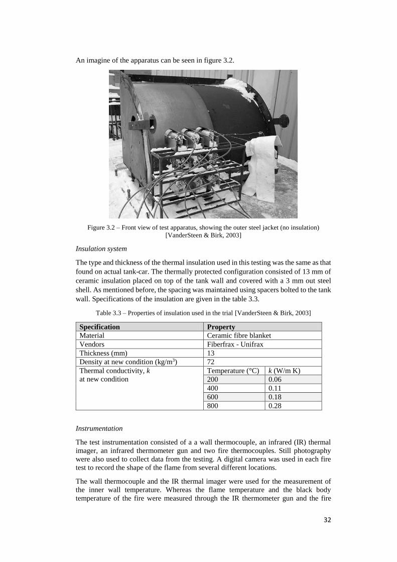
32

An imagine of the apparatus can be seen in figure 3.2.

Figure 3.2 – Front view of test apparatus, showing the outer steel jacket (no insulation)

[VanderSteen & Birk, 2003]

Insulation system

The type and thickness of the thermal insulation used in this testing was the same as that

found on actual tank-car. The thermally protected configuration consisted of 13 mm of

ceramic insulation placed on top of the tank wall and covered with a 3 mm out steel

shell. As mentioned before, the spacing was maintained using spacers bolted to the tank

wall. Specifications of the insulation are given in the table 3.3.

Table 3.3 – Properties of insulation used in the trial [VanderSteen & Birk, 2003]

Specification Property

Material Ceramic fibre blanket

Vendors Fiberfrax - Unifrax

Thickness (mm) 13

Density at new condition (kg/m3) 72

Thermal conductivity, k

at new condition

Temperature (°C) k (W/m K)

200 0.06

400 0.11

600 0.18

800 0.28

Instrumentation

The test instrumentation consisted of a a wall thermocouple, an infrared (IR) thermal

imager, an infrared thermometer gun and two fire thermocouples. Still photography

were also used to collect data from the testing. A digital camera was used in each fire

test to record the shape of the flame from several different locations.

The wall thermocouple and the IR thermal imager were used for the measurement of

the inner wall temperature. Whereas the flame temperature and the black body

temperature of the fire were measured through the IR thermometer gun and the fire

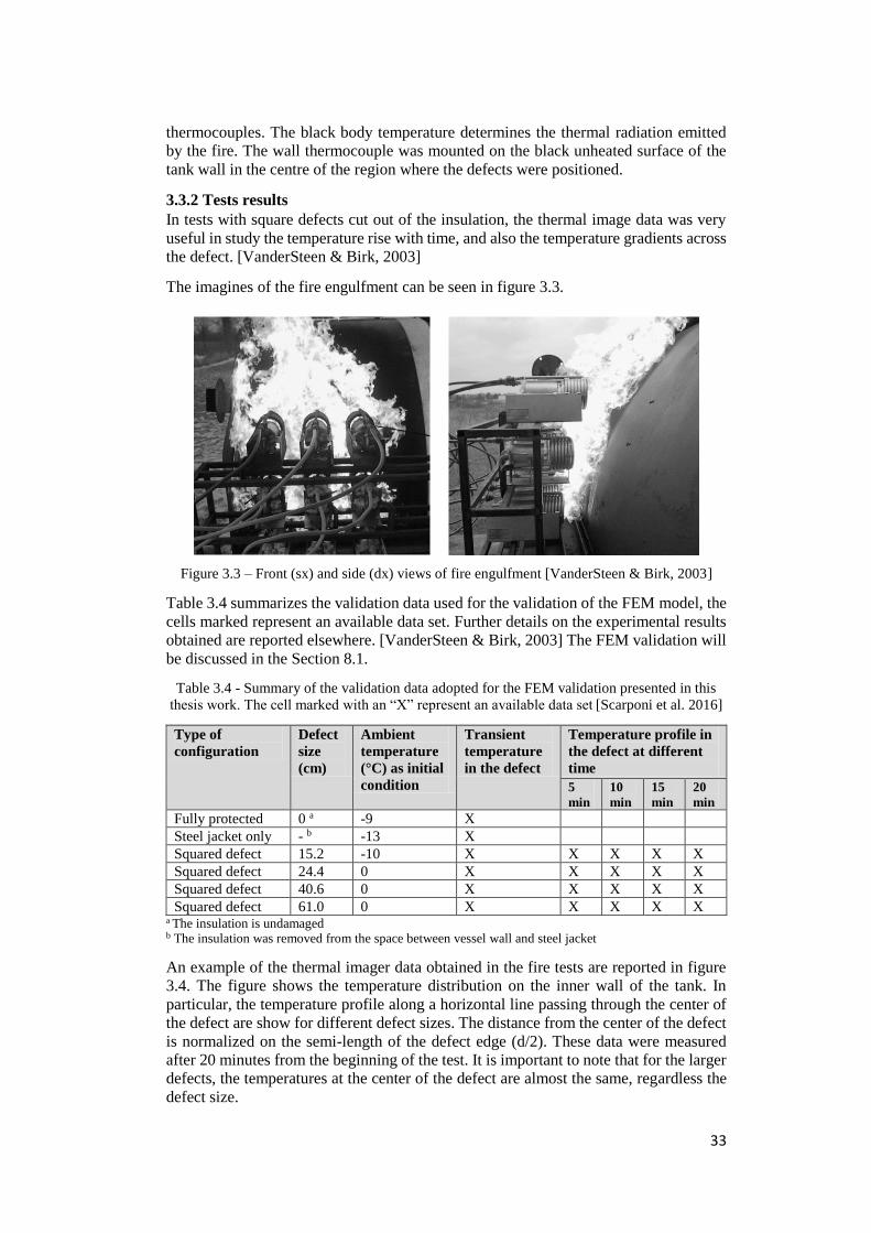
33

thermocouples. The black body temperature determines the thermal radiation emitted

by the fire. The wall thermocouple was mounted on the black unheated surface of the

tank wall in the centre of the region where the defects were positioned.

3.3.2 Tests results

In tests with square defects cut out of the insulation, the thermal image data was very

useful in study the temperature rise with time, and also the temperature gradients across

the defect. [VanderSteen & Birk, 2003]

The imagines of the fire engulfment can be seen in figure 3.3.

Figure 3.3 – Front (sx) and side (dx) views of fire engulfment [VanderSteen & Birk, 2003]

Table 3.4 summarizes the validation data used for the validation of the FEM model, the

cells marked represent an available data set. Further details on the experimental results

obtained are reported elsewhere. [VanderSteen & Birk, 2003] The FEM validation will

be discussed in the Section 8.1.

Table 3.4 - Summary of the validation data adopted for the FEM validation presented in this

thesis work. The cell marked with an “X” represent an available data set [Scarponi et al. 2016]

Type of

configuration

Defect

size

(cm)

Ambient

temperature

(°C) as initial

condition

Transient

temperature

in the defect

Temperature profile in

the defect at different

time

5

min

10

min

15

min

20

min

Fully protected 0 a -9 X

Steel jacket only - b -13 X

Squared defect 15.2 -10 X X X X X

Squared defect 24.4 0 X X X X X

Squared defect 40.6 0 X X X X X

Squared defect 61.0 0 X X X X X a The insulation is undamaged b The insulation was removed from the space between vessel wall and steel jacket

An example of the thermal imager data obtained in the fire tests are reported in figure

3.4. The figure shows the temperature distribution on the inner wall of the tank. In

particular, the temperature profile along a horizontal line passing through the center of

the defect are show for different defect sizes. The distance from the center of the defect

is normalized on the semi-length of the defect edge (d/2). These data were measured

after 20 minutes from the beginning of the test. It is important to note that for the larger

defects, the temperatures at the center of the defect are almost the same, regardless the

defect size.

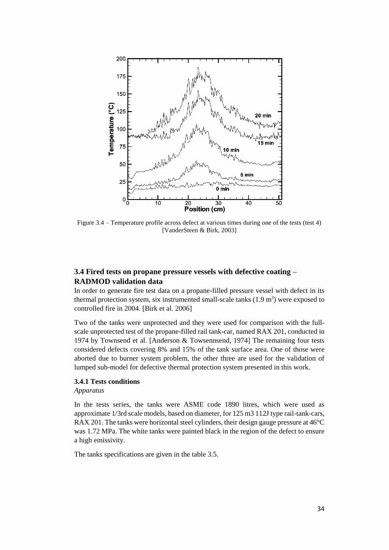
34

Figure 3.4 – Temperature profile across defect at various times during one of the tests (test 4)

[VanderSteen & Birk, 2003]

3.4 Fired tests on propane pressure vessels with defective coating –

RADMOD validation data

In order to generate fire test data on a propane-filled pressure vessel with defect in its

thermal protection system, six instrumented small-scale tanks (1.9 m3) were exposed to

controlled fire in 2004. [Birk et al. 2006]

Two of the tanks were unprotected and they were used for comparison with the full-

scale unprotected test of the propane-filled rail tank-car, named RAX 201, conducted in

1974 by Townsend et al. [Anderson & Towsennsend, 1974] The remaining four tests

considered defects covering 8% and 15% of the tank surface area. One of those were

aborted due to burner system problem, the other three are used for the validation of

lumped sub-model for defective thermal protection system presented in this work.

3.4.1 Tests conditions

Apparatus

In the tests series, the tanks were ASME code 1890 litres, which were used as

approximate 1/3rd scale models, based on diameter, for 125 m3 112J type rail-tank-cars,

RAX 201. The tanks were horizontal steel cylinders, their design gauge pressure at 46°C

was 1.72 MPa. The white tanks were painted black in the region of the defect to ensure

a high emissivity.

The tanks specifications are given in the table 3.5.

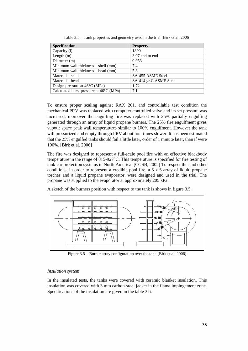
35

Table 3.5 – Tank properties and geometry used in the trial [Birk et al. 2006]

Specification Property

Capacity (l) 1890

Length (m) 3.07 end to end

Diameter (m) 0.953

Minimum wall thickness – shell (mm) 7.4

Minimum wall thickness – head (mm) 5.3

Material – shell SA-455 ASME Steel

Material – head SA-414 gr.C ASME Steel

Design pressure at 46°C (MPa) 1.72

Calculated burst pressure at 46°C (MPa) 7.1

To ensure proper scaling against RAX 201, and controllable test condition the

mechanical PRV was replaced with computer controlled valve and its set pressure was

increased, moreover the engulfing fire was replaced with 25% partially engulfing

generated through an array of liquid propane burners. The 25% fire engulfment gives

vapour space peak wall temperatures similar to 100% engulfment. However the tank

will pressurized and empty through PRV about four times slower. It has been estimated

that the 25% engulfed tanks should fail a little later, order of 1 minute later, than if were

100%. [Birk et al. 2006]

The fire was designed to represent a full-scale pool fire with an effective blackbody

temperature in the range of 815-927°C. This temperature is specified for fire testing of

tank-car protection systems in North America. [CGSB, 2002] To respect this and other

conditions, in order to represent a credible pool fire, a 5 x 5 array of liquid propane

torches and a liquid propane evaporator, were designed and used in the trial. The

propane was supplied to the evaporator at approximately 205 kPa.

A sketch of the burners position with respect to the tank is shows in figure 3.5.

Figure 3.5 – Burner array configuration over the tank [Birk et al. 2006]

Insulation system

In the insulated tests, the tanks were covered with ceramic blanket insulation. This

insulation was covered with 3 mm carbon-steel jacket in the flame impingement zone.

Specifications of the insulation are given in the table 3.6.

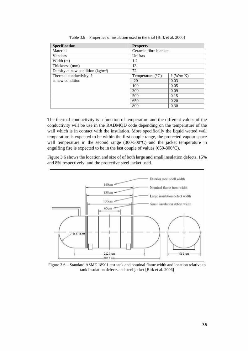
36

Table 3.6 – Properties of insulation used in the trial [Birk et al. 2006]

Specification Property

Material Ceramic fibre blanket

Vendors Unifrax

Width (m) 1.2

Thickness (mm) 13

Density at new condition (kg/m3) 72

Thermal conductivity, k

at new condition

Temperature (°C) k (W/m K)

-20 0.03

100 0.05

300 0.09

500 0.15

650 0.20

800 0.30

The thermal conductivity is a function of temperature and the different values of the

conductivity will be use in the RADMOD code depending on the temperature of the

wall which is in contact with the insulation. More specifically the liquid wetted wall

temperature is expected to be within the first couple range, the protected vapour space

wall temperature in the second range (300-500°C) and the jacket temperature in

engulfing fire is expected to be in the last couple of values (650-800°C).

Figure 3.6 shows the location and size of of both large and small insulation defects, 15%

and 8% respectively, and the protective steel jacket used.

Figure 3.6 – Standard ASME 18901 test tank and nominal flame width and location relative to

tank insulation defects and steel jacket [Birk et al. 2006]

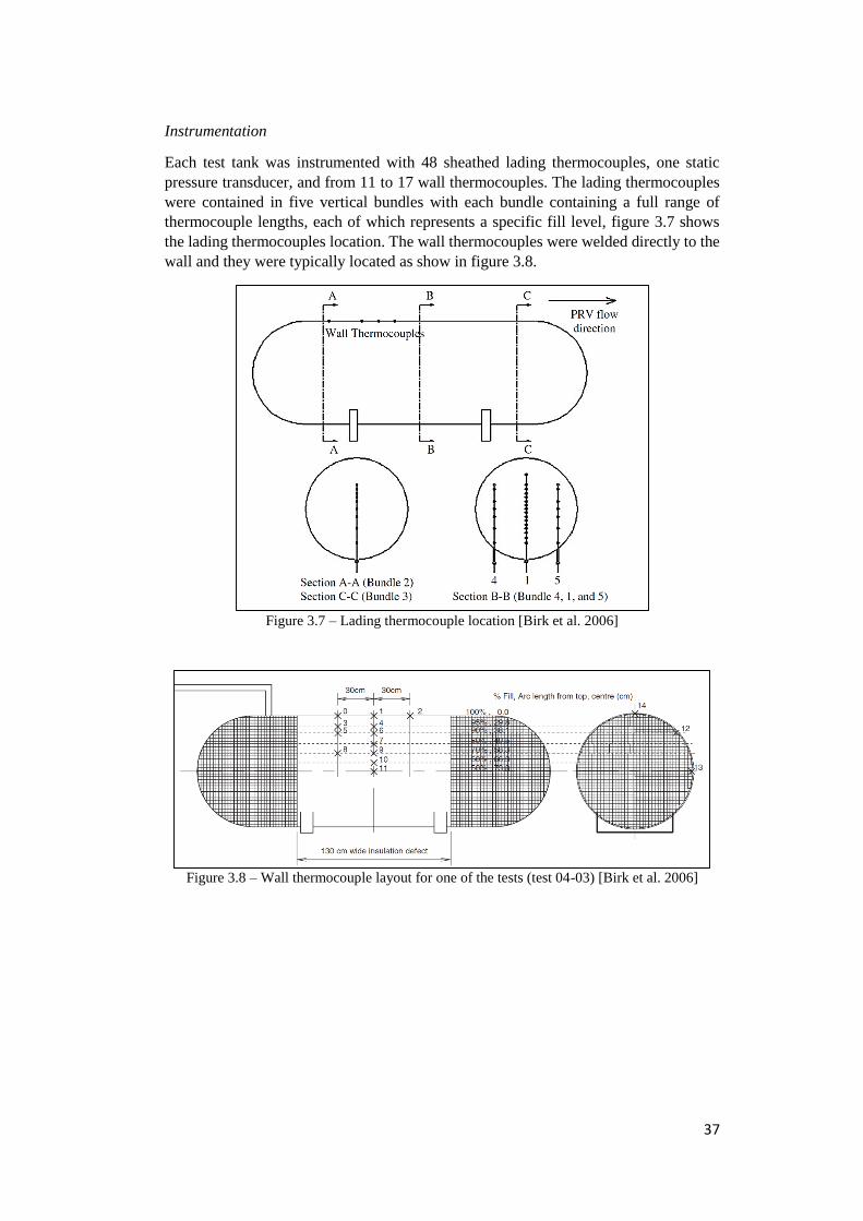
37

Instrumentation

Each test tank was instrumented with 48 sheathed lading thermocouples, one static

pressure transducer, and from 11 to 17 wall thermocouples. The lading thermocouples

were contained in five vertical bundles with each bundle containing a full range of

thermocouple lengths, each of which represents a specific fill level, figure 3.7 shows

the lading thermocouples location. The wall thermocouples were welded directly to the

wall and they were typically located as show in figure 3.8.

Figure 3.7 – Lading thermocouple location [Birk et al. 2006]

Figure 3.8 – Wall thermocouple layout for one of the tests (test 04-03) [Birk et al. 2006]

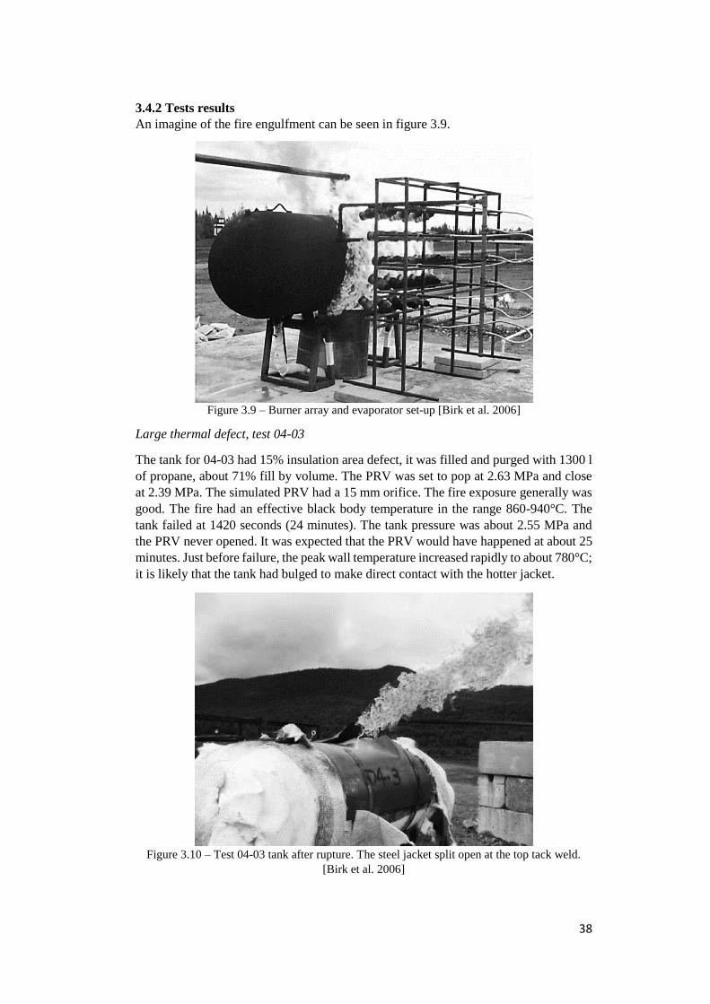
38

3.4.2 Tests results

An imagine of the fire engulfment can be seen in figure 3.9.

Figure 3.9 – Burner array and evaporator set-up [Birk et al. 2006]

Large thermal defect, test 04-03

The tank for 04-03 had 15% insulation area defect, it was filled and purged with 1300 l

of propane, about 71% fill by volume. The PRV was set to pop at 2.63 MPa and close

at 2.39 MPa. The simulated PRV had a 15 mm orifice. The fire exposure generally was

good. The fire had an effective black body temperature in the range 860-940°C. The

tank failed at 1420 seconds (24 minutes). The tank pressure was about 2.55 MPa and

the PRV never opened. It was expected that the PRV would have happened at about 25

minutes. Just before failure, the peak wall temperature increased rapidly to about 780°C;

it is likely that the tank had bulged to make direct contact with the hotter jacket.

Figure 3.10 – Test 04-03 tank after rupture. The steel jacket split open at the top tack weld.

[Birk et al. 2006]

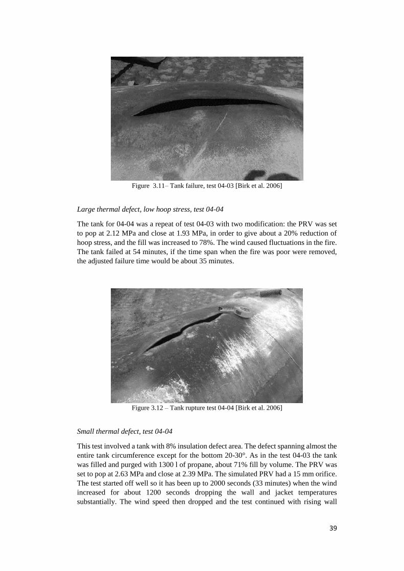
39

Figure 3.11– Tank failure, test 04-03 [Birk et al. 2006]

Large thermal defect, low hoop stress, test 04-04

The tank for 04-04 was a repeat of test 04-03 with two modification: the PRV was set

to pop at 2.12 MPa and close at 1.93 MPa, in order to give about a 20% reduction of

hoop stress, and the fill was increased to 78%. The wind caused fluctuations in the fire.

The tank failed at 54 minutes, if the time span when the fire was poor were removed,

the adjusted failure time would be about 35 minutes.

Figure 3.12 – Tank rupture test 04-04 [Birk et al. 2006]

Small thermal defect, test 04-04

This test involved a tank with 8% insulation defect area. The defect spanning almost the

entire tank circumference except for the bottom 20-30°. As in the test 04-03 the tank

was filled and purged with 1300 l of propane, about 71% fill by volume. The PRV was

set to pop at 2.63 MPa and close at 2.39 MPa. The simulated PRV had a 15 mm orifice.

The test started off well so it has been up to 2000 seconds (33 minutes) when the wind

increased for about 1200 seconds dropping the wall and jacket temperatures

substantially. The wind speed then dropped and the test continued with rising wall

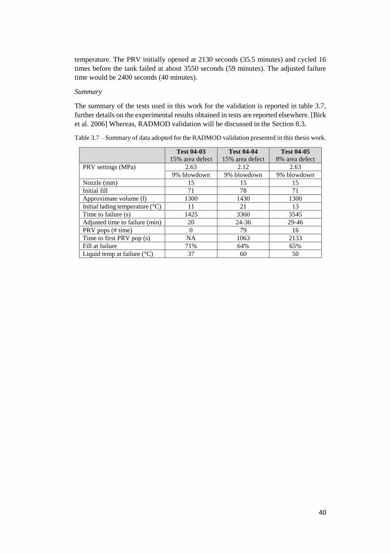
40

temperature. The PRV initially opened at 2130 seconds (35.5 minutes) and cycled 16

times before the tank failed at about 3550 seconds (59 minutes). The adjusted failure

time would be 2400 seconds (40 minutes).

Summary

The summary of the tests used in this work for the validation is reported in table 3.7,

further details on the experimental results obtained in tests are reported elsewhere. [Birk

et al. 2006] Whereas, RADMOD validation will be discussed in the Section 8.3.

Table 3.7 – Summary of data adopted for the RADMOD validation presented in this thesis work.

Test 04-03

15% area defect Test 04-04

15% area defect Test 04-05

8% area defect

PRV settings (MPa) 2.63 2.12 2.63

9% blowdown 9% blowdown 9% blowdown

Nozzle (mm) 15 15 15

Initial fill 71 78 71

Approximate volume (l) 1300 1430 1300

Initial lading temperature (°C) 11 21 13

Time to failure (s) 1425 3360 3545

Adjusted time to failure (min) 20 24-36 29-46

PRV pops (# time) 0 79 16

Time to first PRV pop (s) NA 1063 2133

Fill at failure 71% 64% 65%

Liquid temp at failure (°C) 37 60 50

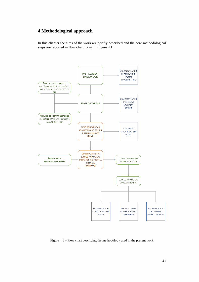
41

4 Methodological approach

In this chapter the aims of the work are briefly described and the core methodological

steps are reported in flow chart form, in Figure 4.1.

Figure 4.1 – Flow chart describing the methodology used in the present work

42

The analysis of past accidents data allowed for the characterisation of the main causes

and main consequences related to the transportation of hazardous materials, focusing on

the scenarios involving LPG. This analysis aimed to assess the need of a passive fire

protection system for LPG tanks, in order to avoid their catastrophic failure due to

external heat load. The presence of deficiencies in such insulation system was

characterised first through the analysis of bonfire experiments [VanderSteen & Birk,

2003; Birk et al. 2006] and then, through the analysis of literature studies [Scarponi et

al. 2016], both, experiments and literature, focused on coated tanks exposed to fire with

defective insulation systems.

This basis permits to characterise the problem and achieve the two aims of this thesis

work:

1. The development of an advanced finete elementes method (FEM) model able

to predict the thermal response of insulated tanks exposed to fire in presence of

defects in their insulation systems. The FEM model is validated [Scarponi et al.

2016] against available experimental data [VanderSteen & Birk, 2003] and then

a sensitivity analysis is performed. This part of the work is aimed at evaluating

the dependence of the temperature reached by the wall of the tank in

correspondence of defect on main parameters, such as temperature and

emissivity of the flame, steel emissivity and convective heat coefficients.

2. The more innovative progress of this thesis work is the development of a

lumped parameters model for evaluation of thermal behaviour of tanks exposed

to fire with defective coating system. The goal is to implement a simplified

model with low time of simulation and adaptable to different materials, tank

and defect geometries, and configurations, which allows to obtain informations

on the fluid lading behaviour, among other parameters, during the fire exposure.

The model is validated against available experimental data [Birk et al., 2006]

showing also a conservative but credible prediction of the time to failure of the

tank. The model is then applied to different reale-scale tanks and reale-scale

defect geoetries, varying some of the several parameters, such as the initial

filling, in order to assess the thermal response of the system. This model

requires less dettailed informations to run and obtains less dettailed results

giving in any case a credible response of the performance of defective insulation

systems installed on tanks in case of flame impingement.

43

5 Analysis of the behaviour of pressurized vessels exposed to

fire: theoretical considerations

In case fire scenario affects one or more transport tankers, thermal radiation and

convection associated to the flame may trigger a domino-effect chain with associated

escalation of events, as it was shown in paragraph 2.3.3. In the framework of the LPG

transport, accidental fire may develop and affects the pressurized vessel, the heat from

the flame is transferred to the tank by radiation and convection. This causes the tank

shell to heat up, conduction takes place through the tank walls up to the lading which

reaches the heat by means of convection mainly, and radiation. [Moodie, 1988] Where

the tank inner surface is in contact with the lading in vapour phase, the heat exchange

coefficients are relatively low and the wall temperature in these regions increases

rapidly. [Birk, 1988] The increase of the wall temperature causes a degradation of the

shell material properties and thus a decrease in the material strength. Otherwise, the heat

transfer coefficients in the regions where the wall is wetted by the liquid are relatively

high and the wall is cooled by the liquid as a result. The liquid phase is not usually

homogeneous and while heated, the near-wall liquid becomes hotter and less dense so

it rises reaching the interface with the vapour. This leads to a stratification phenomenon

[Aydemir et al. 1988] which determines the increasing liquid temperature and thus the

internal pressure to rise until it reaches a level where the pressure relief valve will open

venting mass and resulting in the mixing of lading. The thermal rupture of the tank

depends on the tank internal pressure, the tank wall temperature distribution, and the

tank material strength at the elevated temperature which exist during the fire. [Birk,

1988] In this chapter all the phenomena and the related issues tanking place in such

scenario are discussed.

5.1 Material balances

The material balances are strictly dependent by the presence of the PRV. The flux

through the valve depend on the discharge pressure for which two fluxes can be

registered:

Sonic flux

Supersonic flux

The discharge pressure determines the critical conditions for which the supersonic flux

occurs. This critical conditions are due to the compressibility of the vapour, in fact the

flow through the PRV nozzle will increase to a maximum value as the downstream

pressure is reduced, and any further decrease in the downstream pressure will not affect

the flow. [Perry & Green, 2007] The determination of the appropriate methodology for

the evaluation of mass flow through the PRV depends on the approximation considered

for the situation:

Ideal gas [API 520, 2014]

Non-ideal gas [Leung & Epstein, 1988] or [CCPS, 1998]

Two-phase relief [Leung & Nazario, 1992] or [Leung & Epstein, 1990]

44

The methods reported above are some of the guidelines available for determine the mass

vented by the PRV (Φ). From this evaluation is possible to define the mass balances

that relates the mass liquid variation to the vapour mass variation (eq. 5.1):

𝑑𝑚𝑣

𝑑𝑡=

𝑑𝑚𝑙

𝑑𝑡− Φ (5.1)

Where 𝑚𝑣 and 𝑚𝑙 are respectively the vapour and the liquid mass. The rate of liquid

evaporated is related to the liquid conditions (𝑇𝑙 and P), if the temperature of the liquid

is lower that the boiling temperature of the liquid at the pressure inside the vessel then

the heat absorbed by the liquid causes an increase in the liquid temperate (eq. 5.2), on

the contrary the heat absorbed by the liquid causes an evaporation of the liquid itself, if

the temperature of the liquid is higher than the boiling temperature (eq. 5.3).

Not boiling liquid: 𝑑𝑚𝑙

𝑑𝑡= 0 (5.2)

Boiling liquid: −∆𝐻𝑣𝑎𝑝𝑑𝑚𝑙

𝑑𝑡= ��𝑙

𝑖𝑛 (5.3)

Where ∆𝐻𝑣𝑎𝑝 is the latent heat of vaporisation of the liquid and ��𝑙𝑖𝑛 is the heat load to

the liquid and it will be discussed in the Paragraph 5.2.3.

5.2 Heat transfer mechanisms and balances

5.2.1 Fire

Fire heat transfer to a tank is very case-specific. The fire heat input will depend on many

variables, such as the fuel type, the wind conditions, the size of the fire, etc. It is only

possible to discuss trends and likely case situations. [Birk, 1995] The fire that a general

equipment can be subjected to is generally categorized as either a pool fire or a jet fire.

A jet fire is a pressurized release of flammable gas and/or liquid with a high momentum,

forming a cone shaped flame envelope in the direction of the release. Jet fires radiate

high heat fluxes of about 230 kW/m2 when JP-type fuels are involved, and the

momentum can push firewall protection away and burn through steel like a blow torch.

Heat fluxes of hydrocarbon pool fires are significantly lower than for jet fire, due to the

limited convective term associated to the flame velocity. May be expected to reach

effective flame temperature of between 700-800 °C [Keltner et al. 1990] which gives a

heat fluxes in the range of 70-100 kW/m2. [Birk, 1995] In this thesis work the focus is

on LPG transportation issues, thus the fire impingement considered here is the pool fire.

The flammable pool may develop from leakage of the fuel of vehicles involved in an

accident or from the leakage of flammable liquid content, if hazmat tankers are involved

in the accident.

The thermal load from the flame to the tank is a combination of convection from the hot

combustion products passing over the tank surface and radiation emitted by the flame

to the tank surface. This event is complex and depends on several issues. [Landucci et

al. 2009] In fact, the relative proportions of radiative and convective load from a flame

varies depending on the fuel type and location of the tank within the flame, while the

total heat loads depends on the fuel type, the size and shape and the location of the tank

within the fire. Moreover the heat loads are not constant over the surface of the tank

surface. [Roberts et al., 2004] In most cases, it can be assumed that the flame and the

tank wall are diffuse grey bodies and that the ambient temperature of the surroundings

45

is low compared to the flame temperature. With this assumptions the heat flux absorbed

by the tank wall can be expressed as:

��𝑓𝑙𝑎𝑚𝑒→𝑤𝑎𝑙𝑙 = ��𝑟𝑎𝑑 (𝜎𝜀𝑠(𝜀𝑓𝑇𝑓4 − 𝑇𝑤

4)) + ��𝑐𝑜𝑛𝑣 (ℎ(𝑇𝑓 − 𝑇𝑤)) (5.4)

Where 𝜀𝑠 and 𝜀𝑓 are the flame and the steel surface emissivity, respectively, σ is the

Stefan-Boltzmann constant, Tf and Tw are the flame and the wall temperature

respectively, and h is the convective heat transfer coefficient of the flame. The worse

case if the fire is sooty, in this case the vessel will become a black body (𝜀𝑠 = 1)

receiving all the heat radiation. [Birk, 1995]

5.2.2 Tank insulation and shell

The heat transfers through the tank wall and associated coverings is determined by the

temperature gradient in the radial direction. [Aydemir et al. 1988] The heat load is

transported by mean conduction through the tank layers. In case of protected tank, the

wall have an outer passive fire protection coating and the surrounding steel jacket. The

conduction through a solid material, written in cartesian coordinate system, is:

��𝑖𝑛 − ��𝑜𝑢𝑡 =𝛿

𝛿𝑥(𝑘𝑥

𝛿𝑇

𝛿𝑥) +

𝛿

𝛿𝑦(𝑘𝑦

𝛿𝑇

𝛿𝑦) +

𝛿

𝛿𝑧(𝑘𝑧

𝛿𝑇

𝛿𝑧) (5.5)

Where T is the temperature, t the time, c the heat capacity, ρ the density and k the thermal

conductivity.

The terms of heat entering and leaving the wall depend on the layer considered. The

insulating material reaches the heat from the fire and transfer through conduction to the

vessel inner walls. The latter then exchanges with the lading through both convection

and radiation. The wall in contact with the vapour phase has low convective heat

exchange coefficient and thus the heat is not easily dispersed to the vapour and the

temperature increases. As the wall reaches higher temperature, thermal radiation from

the tank to the lading becomes increasingly important. A small part of radiation is

absorbed by the vapour, because of the transparent nature of vapour, and the major

proportion of radiative heat transfer is to the liquid surface facing to vapour-space wall.

[Moodie, 1988]

5.2.3 Liquid phase

In the liquid zone the temperature is lower one, since the heat transfer coefficients are

higher and the heat is dispersed from the wall to the liquid. The heat transfer mechanism

at the initial phase is pure natural convection. In fact the liquid is heated from the bottom

and by side, temperature difference between the liquid in contact with the walls and the

liquid bulk, generate density gradients that drive the natural flow and it can give

stratification, leaving a cold bulk in the middle and a hot layer around and at the top.

[Birk, 1995] The effects of this phenomenon are discussed in section 5.3. If the heat flux

is high enough the wall temperatures rises up and saturated or sub cooled nucleate

boiling will start. Bubbles of gas start to form in contact with the wall and grow up, until

they become big enough to go up to the liquid surface. If the heat flux is even bigger,

there is a point where a film of gas is created by the wall and the heat transfer coefficient

drops down intensely, and that is the critical flux. The qualitative behaviour of the liquid

heat transfer coefficient, as called h, is illustrated in figure 5.1. The last transition

indicates in the graph is from nucleate boiling and film boiling, this occurs when the

temperature gradient increases and radiation takes place in the gaseous film on the wall.

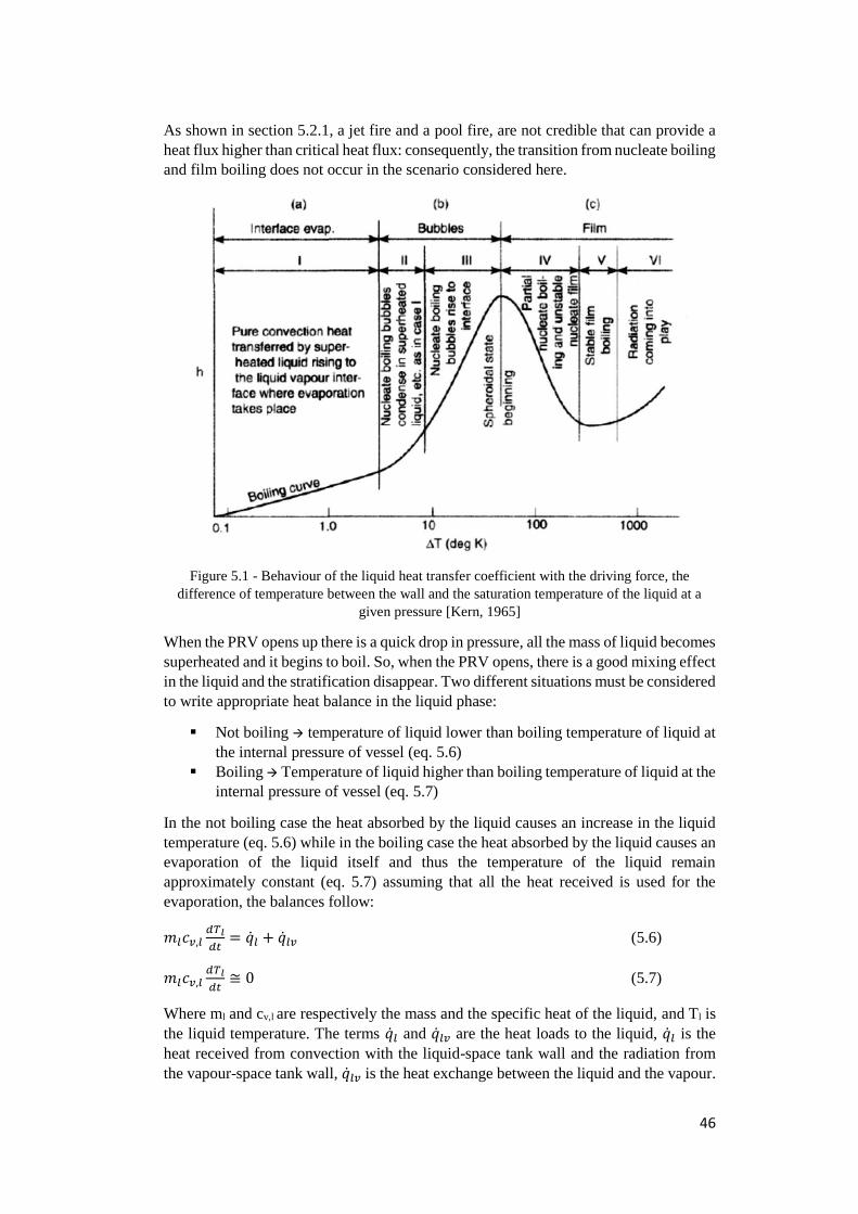
46

As shown in section 5.2.1, a jet fire and a pool fire, are not credible that can provide a

heat flux higher than critical heat flux: consequently, the transition from nucleate boiling

and film boiling does not occur in the scenario considered here.

Figure 5.1 - Behaviour of the liquid heat transfer coefficient with the driving force, the

difference of temperature between the wall and the saturation temperature of the liquid at a

given pressure [Kern, 1965]

When the PRV opens up there is a quick drop in pressure, all the mass of liquid becomes

superheated and it begins to boil. So, when the PRV opens, there is a good mixing effect

in the liquid and the stratification disappear. Two different situations must be considered

to write appropriate heat balance in the liquid phase:

Not boiling temperature of liquid lower than boiling temperature of liquid at

the internal pressure of vessel (eq. 5.6)

Boiling Temperature of liquid higher than boiling temperature of liquid at the

internal pressure of vessel (eq. 5.7)

In the not boiling case the heat absorbed by the liquid causes an increase in the liquid

temperature (eq. 5.6) while in the boiling case the heat absorbed by the liquid causes an

evaporation of the liquid itself and thus the temperature of the liquid remain

approximately constant (eq. 5.7) assuming that all the heat received is used for the

evaporation, the balances follow:

𝑚𝑙𝑐𝑣,𝑙𝑑𝑇𝑙

𝑑𝑡= ��𝑙 + ��𝑙𝑣 (5.6)

𝑚𝑙𝑐𝑣,𝑙𝑑𝑇𝑙

𝑑𝑡≅ 0 (5.7)

Where ml and cv,l are respectively the mass and the specific heat of the liquid, and Tl is

the liquid temperature. The terms ��𝑙 and ��𝑙𝑣 are the heat loads to the liquid, ��𝑙 is the

heat received from convection with the liquid-space tank wall and the radiation from

the vapour-space tank wall, ��𝑙𝑣 is the heat exchange between the liquid and the vapour.

47

The latter is due the temperature difference between the two phases which determines a

heat transfer process in the phase interface. The two equations are approximate, in fact

another transfer mechanism is present in the liquid phase when stratification occurs, that

is the transferring of heat to the sub-cooled bulk fluid (see section 5.3). [Aydemir et al.

1988]

5.2.4 Vapour phase

The convective heat transfer coefficient for the vapour space is low and the wall

temperature increases as the vapour temperature. The gas in the vapour space is

superheated and severely stratified. [Aydemir et al. 1988] The entering heat load is by

convection from the vapour-space tank wall and a small account of radiation,

considering the vapour not transparent, in addition there is the heat provided from the

liquid mass evaporated. The situations in which the heat balances change are in function

of:

PRV opening (eq. 5.8)

PRV stay closed (eq. 5.9)

if the PRV is open, a term is added to the stay closed balance (eq. 5.8) this term is related

to the PRV which vents out mass dissipating heat from the vapour, as shown in eq. 5.9.

𝑚𝑣𝑐𝑣,𝑣𝑑𝑇𝑣

𝑑𝑡= ��𝑣 + ��𝑙𝑣 +

𝑑𝑚𝑙

𝑑𝑡𝐻𝑙 (5.8)

𝑚𝑣𝑐𝑣,𝑣𝑑𝑇𝑣

𝑑𝑡= ��𝑣 + ��𝑙𝑣 +

𝑑𝑚𝑙

𝑑𝑡𝐻𝑙 − Φ𝐻Φ (5.9)

Where mv and cv,v are respectively the mass and the specific heat of the vapour and Tv

is the vapour temperature. ��𝑣 is the heat received by convection and radiation from the

tank wall and ��𝑙𝑣 represent sthe heat exchange with the liquid phase. 𝐻𝑙 and 𝐻Φ are the

entalpies associated respectively to the mass of liquid evaporated (𝑑𝑚𝑙

𝑑𝑡) and to the mass

vented by the PRV (Φ) (see Section 5.1).

5.3 Stratification phenomenon

When a tank is heated from a fire the liquid is not usually heated uniformly, from

experimental evidence the liquid at the bottom of the tank is cooler than the liquid on

the top. [Birk, Cunningham, 1996] Thermal stratification occurs frequently in vessels

of liquefied gases, such as LPG, due to external heating. This stratification effect has a

relevant effect on safety aspect like BLEVE prediction and energy. [Birk &

Cunningham, 1996]

As said in paragraph 5.2.3, due to the heating of inner tank walls in the liquid-space, the

fluid particles near the wall are heat and thus became less dense. They begin rising along

the walls of the vessel. Upon reaching the liquid surface, these particles spread towards

the centre and fall back into the cooler regions of the fluid, they then re-enter the

boundary layer to repeat the above process. This recirculating natural convective flow

establishes a vertical temperature gradient inside the tank, and thus the liquid became

thermally stratified. [Aydemir et al., 1988] Due to this phenomenon, the liquid on the

free surface has a higher temperature than the bulk liquid: the pressure in the vessel is

controlled by this warmest liquid layer. It is possible to divide the lading liquid domain

in three different zones [Aydemir et al. 1988] :

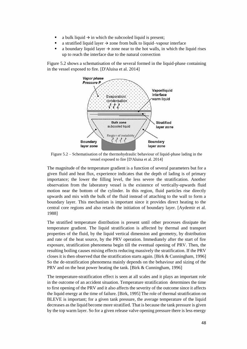
48

a bulk liquid in which the subcooled liquid is present;

a stratified liquid layer zone from bulk to liquid–vapour interface

a boundary liquid layer zone near to the hot walls, in which the liquid rises

up to reach the interface due to the natural convection

Figure 5.2 shows a schematisation of the several formed in the liquid-phase containing

in the vessel exposed to fire. [D'Aluisa et al. 2014]

Figure 5.2 – Schematisation of the thermohydraulic behaviour of liquid-phase lading in the

vessel exposed to fire [D'Aluisa et al. 2014]

The magnitude of the temperature gradient is a function of several parameters but for a

given fluid and heat flux, experience indicates that the depth of lading is of primary

importance; the lower the filling level, the less severe the stratification. Another

observation from the laboratory vessel is the existence of vertically-upwards fluid

motion near the bottom of the cylinder. In this region, fluid particles rise directly

upwards and mix with the bulk of the fluid instead of attaching to the wall to form a

boundary layer. This mechanism is important since it provides direct heating to the

central core regions and also retards the initiation of boundary layer. [Aydemir et al.

1988]

The stratified temperature distribution is present until other processes dissipate the

temperature gradient. The liquid stratification is affected by thermal and transport

properties of the fluid, by the liquid vertical dimension and geometry, by distribution

and rate of the heat source, by the PRV operation. Immediately after the start of fire

exposure, stratification phenomena begin till the eventual opening of PRV. Then, the

resulting boiling causes mixing effects reducing massively the stratification. If the PRV

closes it is then observed that the stratification starts again. [Birk & Cunningham, 1996]

So the de-stratification phenomena mainly depends on the behaviour and sizing of the

PRV and on the heat power heating the tank. [Birk & Cunningham, 1996]

The temperature-stratification effect is seen at all scales and it plays an important role

in the outcome of an accident situation. Temperature stratification determines the time

to first opening of the PRV and it also affects the severity of the outcome since it affects

the liquid energy at the time of failure. [Birk, 1995] The role of thermal stratification on

BLEVE is important; for a given tank pressure, the average temperature of the liquid

decreases as the liquid become more stratified. That is because the tank pressure is given

by the top warm layer. So for a given release valve opening pressure there is less energy

49

in the liquid the more it is stratified. The response upon sudden depressurization does

not only depend on the average liquid temperature. If the liquid is stratified, then the hot

layers will be more super-heated than the cool layers, so the pressure recovery given by

the boiling of the liquid will start earlier from the warm layer. Eventually, this can

suppress the boiling from the cold layers, since also the hydrostatic pressure is

contributing to this. If the temperature of the liquid is uniform the pressure recovery

after the opening of the PRV is going to be stronger and therefore more likely to fail the

tank. [Birk & Cunningham, 1996]

On the other hand, the more the liquid is stratified the faster the pressure rises, so the

time to PRV opening will be shorter if the liquid is stratified respect to a situation in

which the liquid is homogenous. [Birk & Cunningham, 1996] The effect of the PRV

opening are discussed in the following section 5.5.

5.5 PRV opening effects

When the PRV opens and vents vapour, the depressurization leads a boiling process,

that consumes energy in the warmest liquid layers and the resulting bubble rise causes

mixing in the warmest layer, so the combination of these effect reduces the stratification.

So, as time progresses, continuous mixing of the fluid results in more uniform

temperatures throughout the liquid. [Aydemir et al. 1988]

The time to destratify depends on the tank scale and the PRV action which itself is

controlled by the degree of fire exposure. If a tank is engulfed in fire the resulting large

PRV flow will tend to destratify the liquid quickly, whereas if the tank is exposed to a

small fire the liquid may not destratify at all. [Birk & Cunningham, 1996] While

destratification takes place, little mass is being lost from the tank through the PRV, since

most of the heat input is going into the bulk of the liquid (sub-cooled boiling where

vapour-bubbles collapse into cooler core liquid) and not into vapour generation for

venting. when the liquid temperature becomes uniform, the mass flow through the PRV

increases because all of the fire heat is now going into vapour production at the PRV

set pressure. This is when the liquid level starts to drop more rapidly. [Birk, 1995] While

the liquid level decreases the tank surface area in contact with the vapour phase

increases, and thus reducing the area with the liquid cooler effect.

5.4 Vessel failure mechanisms

A tank may suffer a failure during a fire for a number of reasons, for the horizontal

cylindrical vessel these include:

uncontrolled pressure built-up due to heating or reaction

wall-thinning due to hoop stress and high-temperature material degradation

severe bending stressess due to thermal stresses induced by differential

temperature on tank top and bottom

mechanical damage due to impacts, corrosion or poor manufacture

Of the above types of failure, mechanical damage is difficult if not impossible to identify

in an accident situation, as the severe bending stresses. The latter may not alone be

capable of causing a failure but may cause premature failure when coupled to

mechanical damage of some kind. Uncontrolled pressure build-up is strictly related to

50

the design and sizing of pressure relief system. While, wall thinning due to hoop stress

and high-temperature material degradation is a likely scenario in the event that a tank

in good condition is exposed to severe fire impingement. [Birk, 1995] In this scenario,

with continuing fire attack the vapour metal walls weaken and commence plastic

deformation at the hottest locations eventually leading to the formation of a creep. If the

PRV opens the liquid level decreases and the tank surface in which the creep may form

increases. Over some period of time, the creep results in the formation of a fissure or

hole in the tank wall. This fissure may grow leading to the catastrophic failure or it may

stop leading to a depressurisation due to the content discharge. This two scenarios

depend on the condition of the wall and the thermodynamic condition of the tank

contents. [Venart, 2000]

51

6 Modelling the thermal response of insulated vessels exposed to

fire in presence of defective coatings: FEM simulations

6.1 Theoretical background on defective coating assessment

Scant data are available for the characterisation and the modelling of defective coating

used for the thermal insulation of vessels. The possible presence of defects in the

thermal coating and the critical size of a defect in compromising the performance of the

thermal protection system were never systematically explored before the past decade.

[Scarponi et al. 2016] In fact, as discussed in paragraph 3.2.1, the first step through the

characterisation of defective coatings has been through the thermographic inspection

method proposed by Birk and Cunningham in 2000. [Birk & Cunningham, 2000]

Subsequently, two bonfire trials were performed aimed at the definition of criteria to

tests the performance of defective insulation system, one of which aimed to test the

effect on a portion of tank shell of different coating deficiencies [VanderSteen & Birk,

2003] and the other one tests the effect of small and large insulation defects on LPG

filled tanks. [Birk et al. 2006]

Nevertheless, there weren’t any studies on insulated tank exposed to fire with defective

coating, the thermal behaviour of such system was investigated only in the past year by

G. Emrys Scarponi et al. [Scarponi et al. 2016] which developed a thermal model

supported by finite elements analysis and perform a study on the heat transfer

mechanism inside the enclosure, which is discussed below. The finite elements method,

discussed in this section, is aimed to reproduce the thermal response of defective

coatings in order to define a specific set of key performance indicators (KPIs) aimed at

provide a tool to facilitate the task of assessing the acceptability of a given degree of

defectiveness.

6.1.1 Heat transfer mechanism inside the defect enclosure

Coating defect forms an enclosure between steel jacket and tank shell-wall, within there

is a layer of air which can transfer the heat through convection, conduction and

radiation. The hypothesis is that radiation is the dominant heat transfer mechanism. In

fact, the radiative heat flux is proportional to the temperature raised to the fourth power

and in the enclosure there is a high temperature gradient between the steel jacket

temperature, which rises quickly up near to flame temperature, and the shell-wall

temperature, which remains much lower especially if in contact with liquid-phase.

[Landucci et al. 2011] On the other hand, the conductive and convective transports are

expected to be low.

The three mechanisms were modelled and tested in order to assess which of those is

dominant and which is negligible. The tests were conducted through a mono-

dimensional finite volume model developed by Scarponi et al. [Scarponi et al. 2016]

Therefore, three models were applied: the first model considers only the radiation

mechanism, in the second also convection was considered and the third model considers

a static layer of air in which the heat is transferred by conduction, in addition to the

radiation between the two walls. In the computation of the radiation flux, it is assumed

that each point forming the enclosure radiates and receives radiation towards and from

all other points according to a view factor, which depends on the reciprocal position of

the points. In the case of convection model, a convective heat transfer coefficient in the

enclosure and the heat flows entering and leaving the latter, all solved in function of a

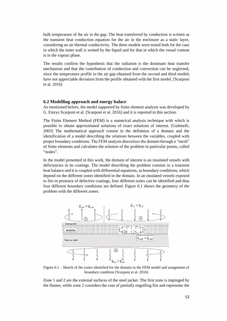
52

bulk temperature of the air in the gap. The heat transferred by conduction is written as

the transient heat conduction equation for the air in the enclosure as a static layer,

considering an air thermal conductivity. The three models were tested both for the case

in which the inner wall is wetted by the liquid and for that in which the vessel content

is in the vapour phase.

The results confirm the hypothesis that the radiation is the dominant heat transfer

mechanism and that the contribution of conduction and convection can be neglected,

since the temperature profile in the air gap obtained from the second and third models

have not appreciable deviation from the profile obtained with the first model. [Scarponi

et al. 2016]

6.2 Modelling approach and energy balace

As mentioned before, the model supported by finite element analysis was developed by

G. Emrys Scarponi et al. [Scarponi et al. 2016] and it is reported in this section.

The Finite Element Method (FEM) is a numerical analysis technique with which is

possible to obtain approximated solutions of exact solutions of interest. [Gubinelli,

2003] The mathematical approach consist in the definition of a domain and the

identification of a model describing the relations between the variables, coupled with

proper boundary conditions. The FEM analysis discretizes the domain through a “mesh”

of finite elements and calculates the solution of the problem in particular points, called

“nodes”.

In the model presented in this work, the domain of interest is an insulated vessels with

deficiencies in its coatings. The model describing the problem consists in a transient

heat balance and it is coupled with differential equations, as boundary conditions, which

depend on the different zones identified in the domain. In an insulated vessels exposed

to fire in presence of defective coatings, four different zones can be identified and thus

four different boundary conditions are defined. Figure 6.1 shows the geometry of the

problem with the different zones.

Figure 6.1 – Sketch of the zones identified for the domain in the FEM model and assignment of

boundary condition [Scarponi et al. 2016]

Zone 1 and 2 are the external surfaces of the steel jacket. The first zone is impinged by

the flames, while zone 2 considers the case of partially engulfing fire and represents the

53

not impinged area. In zone 1 the flame exchanges with the steel jacket through both

radiative and convective mechanism, expressed respectively by eq. 6.2 and 6.3. The sum

of these boundary conditions represents the total heat power entering the system. The

mechanisms governing the first region are the same for zone 2 but the heat leaves the

system. So, for zone 2 the radiative and convective flows are from the steel jacket to the

ambient air, with the corresponding temperatures and properties, as shown in eq. 6.4.

Zone 3 is the defect enclosure, the insulation is missing forming an air gap. The heat

transport mechanisms in this region is discussed in paragraph 3.2.2, where is stated that

radiation is the main heat transport mechanism inside this enclosure. Therefore, the

boundary condition zone 3 is a radiative flux in which each point radiates and receives

radiations towards and from all the other points forming the enclosure according to a

view factor, which depends on the reciprocal position of the points. A deeper discussion

of radiative heat exchange in enclosures can be find elsewhere [Modest, 2003].

The last zone, zone 4, is the internal surface of the tank shell, where heat reaches the

lading, both in vapour or in liquid phase, depending on the liquid level. In this thesis

work, the model is used in its validation form. Thus, the entire internal surface was

supposed to be in contact with air according to the experimental setup [VanderSteen &

Birk, 2003] reported in section 3.3. So, the convective flux leaving the system written

for zone 2 is used also here, as eq. 6.5 shows, but changing the correlation for the

convective heat exchange coefficient.

The governing equation, i.e. the transient heat balance, for a solid material can be written

as:

𝜌𝑐𝛿𝑇

𝛿𝑡=

𝛿

𝛿𝑥(𝑘𝑥

𝛿𝑇

𝛿𝑥) +

𝛿

𝛿𝑦(𝑘𝑦

𝛿𝑇

𝛿𝑦) +

𝛿

𝛿𝑧(𝑘𝑧

𝛿𝑇

𝛿𝑧) (6.1)

Where T is the temperature, t the time, c the heat capacity, ρ the density and k the thermal

conductivity.

While the boundary conditions coupled with eq. 6.1 are:

Zone 1 – radiative and convective flows entering the system:

��𝑟,𝑓 = 𝜎𝜀𝑠(𝑇𝐵𝐵4 − 𝑇𝑤

4) (6.2)

��𝑐,𝑓 = ℎ𝑓(𝑇𝑓 − 𝑇𝑤) (6.3)

Zone 2 – radiative and convective flows leaving the system:

��𝑟+𝑐,𝑜𝑢𝑡 = 𝜎𝜀𝑠(𝑇𝑤4 − 𝑇𝑎𝑖𝑟

4 ) + ℎ𝑎𝑖𝑟(𝑇𝑤 − 𝑇𝑎𝑖𝑟) (6.4)

Zone 4 – validation model, convective heat flux leaving the internal wall:

��𝑟+𝑐,𝑣𝑎𝑙𝑖𝑑_𝑎𝑖𝑟 = 𝜎𝜀𝑠(𝑇𝑤4 − 𝑇𝑎𝑖𝑟

4 ) + ℎ𝑣𝑎𝑙𝑖𝑑_𝑎𝑖𝑟(𝑇𝑤 − 𝑇𝐿) (6.5)

Where σ is the Stefan-Boltzmann constant, Tw and εs are the temperature and the

emissivity of the steel wall respectively, TBB is the black body temperature of the fire,

Tf is the flame temperature, Tair is the ambient temperature. The black body temperature

depends on the flame temperature and the emissivity assigned to the flame.

εs is the emissivity of the steel wall, it depends from the temperature reached by the

wall. Both the steel jacket and the tank wall are made of carbon steel, thus the average

54

value of the emissivity is set to 0.7 according with the temperature range of interest (0

– 700 °C) [Eurocode 1, 2005].

The convective heat exchange coefficients hf and hair are, respectively, between the

flame and the tank wall (zone 1) and between the tank wall and the ambient air (zone

3). While hvalid_air is between the internal tank wall and the air (zone 4). For each

convective coefficient is needed a correlation for evaluate its value.

The convective coefficient hf is a function of the fluid dynamic regime of the flame

impinging the tank wall, which depends in turn on the burning rate of the fire. For low

momentum flames, as in the case of the simulated pool fire in the experiments, the

coefficient can be estimated as follows [Knudsen et al. 1999]:

𝑁𝑢 =ℎ𝑓𝐿

𝑘𝑓= 0.26 𝑅𝑒0.6 𝑃𝑟0.3 (6.6)

Where Nu, Re and Pr are the Nusselt, Reynolds and Prandtl numbers respectively, L is

the characteristic dimension of the system and kf is the thermal conductivity of the

flame. Reynolds number introduces the regimes of flow, laminar or turbulent, with

respect flame velocity, while Prandtl merges the fluid properties, function of

temperature. [Mauri, 2012]

For the determination of the natural convective heat transfer coefficient hair for

cylindrical geometry, several correlation can be found in literature [Boetcher, 2014].

Most of them require the preliminary calculation of the Nusselt number (Nu) by

empirical correlations:

𝑁𝑢 =ℎ𝑎𝑖𝑟𝐿

𝑘𝑎𝑖𝑟= 𝛼 𝑅𝑎𝛽 (6.7)

Where kair is the thermal conductivity of the air, L is the characteristic dimension of the

system and Ra is the Rayleigh number. Ra number is associated to the natural

convection and, in the conditions considered here, its expected value varies between

1010 and 1011 . [ Scarponi et al. 2016] According to King [King, 1932] for the expected

Ra value range, the coefficients α and β are assumed equal to 0.13 and 0.33 respectively.

The convective heat exchange coefficient hvalid_air was calculated using eq. 6.8, valid in

case of natural convection under an inclined plate [Churchill & Chu, 1975].

𝑁𝑢 = (0.825 +0.387 𝑅𝑎1 6⁄

(1+(0.492

𝑃𝑟)

9 16⁄)

8 27⁄ )

2

(6.8)

In addition to the assignment of the boundary conditions, material properties have to be

defined for the steel and the insulation. Both the tank shell and the jacket are made of

carbon steel, for which detailed thermal properties can be easily find in literature

[Eurocode 1, 2005]. The thermal protection used in the test and its properties are

reported in paragraph 3.3.1.

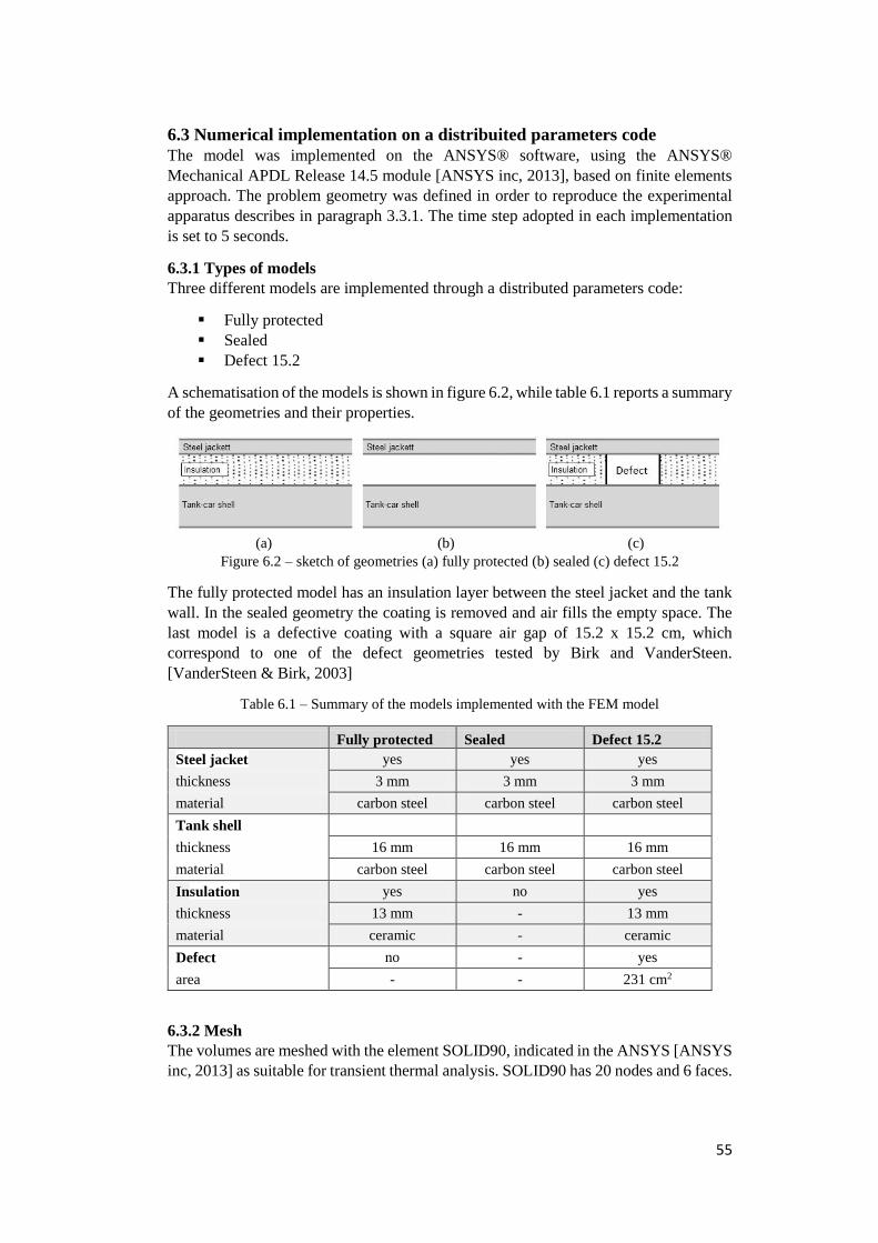
55

6.3 Numerical implementation on a distribuited parameters code

The model was implemented on the ANSYS® software, using the ANSYS®

Mechanical APDL Release 14.5 module [ANSYS inc, 2013], based on finite elements

approach. The problem geometry was defined in order to reproduce the experimental

apparatus describes in paragraph 3.3.1. The time step adopted in each implementation

is set to 5 seconds.

6.3.1 Types of models

Three different models are implemented through a distributed parameters code:

Fully protected

Sealed

Defect 15.2

A schematisation of the models is shown in figure 6.2, while table 6.1 reports a summary

of the geometries and their properties.

(a) (b) (c)

Figure 6.2 – sketch of geometries (a) fully protected (b) sealed (c) defect 15.2

The fully protected model has an insulation layer between the steel jacket and the tank

wall. In the sealed geometry the coating is removed and air fills the empty space. The

last model is a defective coating with a square air gap of 15.2 x 15.2 cm, which

correspond to one of the defect geometries tested by Birk and VanderSteen.

[VanderSteen & Birk, 2003]

Table 6.1 – Summary of the models implemented with the FEM model

Fully protected Sealed Defect 15.2

Steel jacket yes yes yes

thickness 3 mm 3 mm 3 mm

material carbon steel carbon steel carbon steel

Tank shell

thickness 16 mm 16 mm 16 mm

material carbon steel carbon steel carbon steel

Insulation yes no yes

thickness 13 mm - 13 mm

material ceramic - ceramic

Defect no - yes

area - - 231 cm2

6.3.2 Mesh

The volumes are meshed with the element SOLID90, indicated in the ANSYS [ANSYS

inc, 2013] as suitable for transient thermal analysis. SOLID90 has 20 nodes and 6 faces.

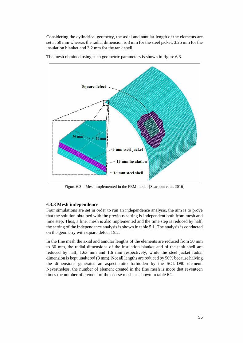
56

Considering the cylindrical geometry, the axial and annular length of the elements are

set at 50 mm whereas the radial dimension is 3 mm for the steel jacket, 3.25 mm for the

insulation blanket and 3.2 mm for the tank shell.

The mesh obtained using such geometric parameters is shown in figure 6.3.

Figure 6.3 – Mesh implemented in the FEM model [Scarponi et al. 2016]

6.3.3 Mesh independence

Four simulations are set in order to run an independence analysis, the aim is to prove

that the solution obtained with the previous setting is independent both from mesh and

time step. Thus, a finer mesh is also implemented and the time step is reduced by half,

the setting of the independence analysis is shown in table 5.1. The analysis is conducted

on the geometry with square defect 15.2.

In the fine mesh the axial and annular lengths of the elements are reduced from 50 mm

to 30 mm, the radial dimensions of the insulation blanket and of the tank shell are

reduced by half, 1.63 mm and 1.6 mm respectively, while the steel jacket radial

dimension is kept unaltered (3 mm). Not all lengths are reduced by 50% because halving

the dimensions generates an aspect ratio forbidden by the SOLID90 element.

Nevertheless, the number of element created in the fine mesh is more that seventeen

times the number of element of the coarse mesh, as shown in table 6.2.

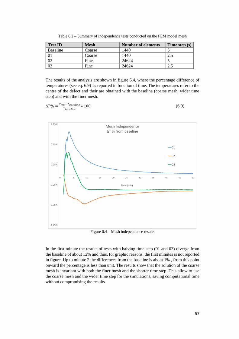
57

Table 6.2 – Summary of independence tests conducted on the FEM model mesh

Test ID Mesh Number of elements Time step (s)

Baseline Coarse 1440 5

01 Coarse 1440 2.5

02 Fine 24624 5

03 Fine 24624 2.5

The results of the analysis are shown in figure 6.4, where the percentage difference of

temperatures (see eq. 6.9) is reported in function of time. The temperatures refer to the

centre of the defect and their are obtained with the baseline (coarse mesh, wider time

step) and with the finer mesh.

∆𝑇% =𝑇𝑡𝑒𝑠𝑡−𝑇𝑏𝑎𝑠𝑒𝑙𝑖𝑛𝑒

𝑇𝑏𝑎𝑠𝑒𝑙𝑖𝑛𝑒∗ 100 (6.9)

Figure 6.4 – Mesh independence results

In the first minute the results of tests with halving time step (01 and 03) diverge from

the baseline of about 12% and thus, for graphic reasons, the first minutes is not reported

in figure. Up to minute 2 the differences from the baseline is about 1% , from this point

onward the percentage is less than unit. The results show that the solution of the coarse

mesh is invariant with both the finer mesh and the shorter time step. This allow to use

the coarse mesh and the wider time step for the simulations, saving computational time

without compromising the results.

58

7 Evaluation of pressure build-up in tankers exposed to fire

through lumped codes

7.1 Overview of the lumped modelling approaches

The modelling of the the pressure build-up of an equipment exposed to fire is a very

complex problem. Different and particular problems must be solved, more specifically,

the radiant flux over the target and the wall temperature behaviour must be modelled,

then the possible failure conditions have to be analysed in order to assess the proper

failure criteria to be adopted in the evaluation of the time to failure. The use of a

distributed parameter approach (see chapter 6) would require many hours for

preparation and for run time, which may be unacceptable even in the case of the analysis

of a single scenario, limiting the analysis to a reduce number of accidents. Moreover,

the uncertainty that affects the definition of the primary accidental scenarios will in any

case affect the precision of the modelling results. [Landucci et al. 2009] Thus a lumped

model approach was developed to evaluate the performance of tankers exposed to fire.

This method requires less detailed information and it also obtains less accurate results

which provides anyway a conservative but credible behaviour of the system. [Landucci

et al. 2009] The easiness of use and the time-saving, few minutes for running, are key

advantages of the lumped approach.

The lumped model is based on the division of the domain in different zone, called

“nodes”. In each node conditions and properties of the material can be considered

uniform, averaged over the node, and the variable of interest (pressure, temperature, ..)

are function of time alone. Then is set the heat balance in each node, with attention at

the boundary conditions between different region, and the global conservation laws,

concerning both mass and heat, obtaining a set of equations time-dependent able to

assess the thermal behaviour of the different nodes as the pressure behaviour of the

system. [Landucci et al. 2009; Landucci et al. 2013]

Several lumped models were developed from 1970 to nowadays for assessment of the

thermal response of the vessels and its contents in case of fire exposure. These models

generally concern horizontal cylindrical LPG vessels to engulfing fire and they allow

the analysis of phenomena as the fire protection system influence or the PRV. [Landucci

et al. 2009] The models and their developed setting are shown in tables 7.1.

Table 7.1 – Available lumped parameter models, for the predicting the consequences of fire

attack [Landucci et al. 2016]

(FE = fully engulfed; PE = partially engulfed; JF = jet fire engulfment)

Reference date Model Name Fire

exposure

Thermal

insulation

[Graves, 28] 1973 FE Yes

[Johnson, 25 26] 1980-1998 FE Yes

[Aydemir et al. 1988] 1987 PLGS-I FE No

[Beynon et al. 1988] 1987 HEAT-UP FE Yes

[Ramskill, 1988] 1984-1987 ENGULF I & II FE, PE No

[Forrest, 1985] 1986 SAFIRE FE No

[Birk, 1988]33 1988-2006 TANKCAR FE, PE No

[Shebeko et al. 2000] 2000 FE Yes

[Salzano et al. 2003] 2003 FE, JF No

[Gong et al. 2004] 2004 FE No

59

[Lautkaski, 40] 2009 ENGULF II FE, PE No

[Landucci et al. 2009] 23 2009 RADMOD FE, PE, JF Yes

[Heymes et al., 42] 2013 DS No

[Birk et al. 24] 2013 FE, PE No

Between the models reported above, before 2006 only few models manage different

vessel geometries and different vessel categories (e.g. ENGULF and SAFIRE) and only

few models are able to predict correctly the influence of the PRV action (e.g. HEAT-

UP and Salzano et al. codes). Hence the need to develop a lumped model able to predict

the time to failure of insulated and unprotected vessels of any type, atmospheric and

pressurized, undergoing different modes of fire exposure, taking into account the

influence of the PRV action. [Landucci et al. 2009] This model, namely RADMOD, and

its enhancement for defective coatings, are the main items of this work. In the next

section the novel RADMOD model implementations are described, section 7.2 focusing

on the enhancements of the previously code and the novel implementation for defective

coating is discussed in section 7.3.

7.2 RADMOD code

The RADMOD code was developed first by the PhD project of Gubinelli and then by

[Landucci et al. 2013]. The novel versions of the RADMOD model for horizontal

cylinders was developed by Bazzocchi [Bazzocchi, 2014] and subsequently enhanced

by Nigro [Nigro, 2015] who also extended the model for vertical configurations.

The last version of RADMOD model [Nigro, 2015] for horizontal cylinders is the basis

of the code novel implementation for defective coatings presented in this thesis work.

The updating are discussed in this section (7.2.2) and the fundamental equations

implemented in the model are reported in appendix A. For what concerns the failure

criteria adopted in the code, they are reported in Section 7.2.4.

Moreover, three sub-models are available for the evaluation of thermal stratification

phenomena, two of which are implemented in the novel RADMOD model and discussed

in paragraph 7.2.5. Whereas, the more improvement of the RADMOD code for

defective coatings is discussed in section 7.3.

For further details on the RADMOD model and sub-models implementation refer to

[Nigro, 2015] and previously works [Bazzocchi, 2014; Landucci et al. 2013].

7.2.1 Model set-up

The thermal model was setup in MatLab, with a link to the Excel to allow the insertion

of initial condition and have a simplified view of the results of the simulation which are

collected in another Excel spreadsheet. In order to solve a system of First-Order

differential equations an explicit solution procedure was chosen, i.e. Matlab ODE45

solver. Explicit procedure in time is more simple to program, but requires small enough

time steps to prevent numerical instability. So its simplicity and a medium order of

accuracy has led us to choose this calculation procedure. [Nigro, 2015]

Another assumption made is that the fluid inside the tank is a pure substance (propane).

If a mixture (propane-butane for LPG case) is considered the simulation will be more

complex because the different concentrations in vapour and liquid have be calculated.

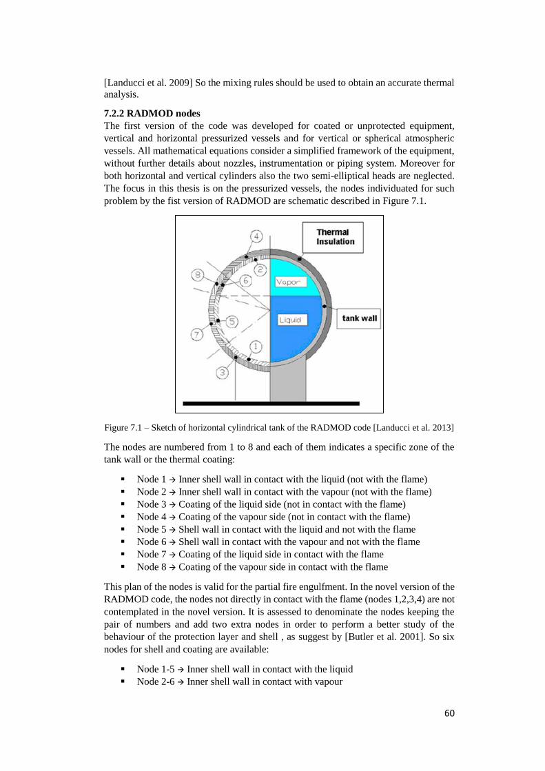
60

[Landucci et al. 2009] So the mixing rules should be used to obtain an accurate thermal

analysis.

7.2.2 RADMOD nodes

The first version of the code was developed for coated or unprotected equipment,

vertical and horizontal pressurized vessels and for vertical or spherical atmospheric

vessels. All mathematical equations consider a simplified framework of the equipment,

without further details about nozzles, instrumentation or piping system. Moreover for

both horizontal and vertical cylinders also the two semi-elliptical heads are neglected.

The focus in this thesis is on the pressurized vessels, the nodes individuated for such

problem by the fist version of RADMOD are schematic described in Figure 7.1.

Figure 7.1 – Sketch of horizontal cylindrical tank of the RADMOD code [Landucci et al. 2013]

The nodes are numbered from 1 to 8 and each of them indicates a specific zone of the

tank wall or the thermal coating:

Node 1 Inner shell wall in contact with the liquid (not with the flame)

Node 2 Inner shell wall in contact with the vapour (not with the flame)

Node 3 Coating of the liquid side (not in contact with the flame)

Node 4 Coating of the vapour side (not in contact with the flame)

Node 5 Shell wall in contact with the liquid and not with the flame

Node 6 Shell wall in contact with the vapour and not with the flame

Node 7 Coating of the liquid side in contact with the flame

Node 8 Coating of the vapour side in contact with the flame

This plan of the nodes is valid for the partial fire engulfment. In the novel version of the

RADMOD code, the nodes not directly in contact with the flame (nodes 1,2,3,4) are not

contemplated in the novel version. It is assessed to denominate the nodes keeping the

pair of numbers and add two extra nodes in order to perform a better study of the

behaviour of the protection layer and shell , as suggest by [Butler et al. 2001]. So six

nodes for shell and coating are available:

Node 1-5 Inner shell wall in contact with the liquid

Node 2-6 Inner shell wall in contact with vapour

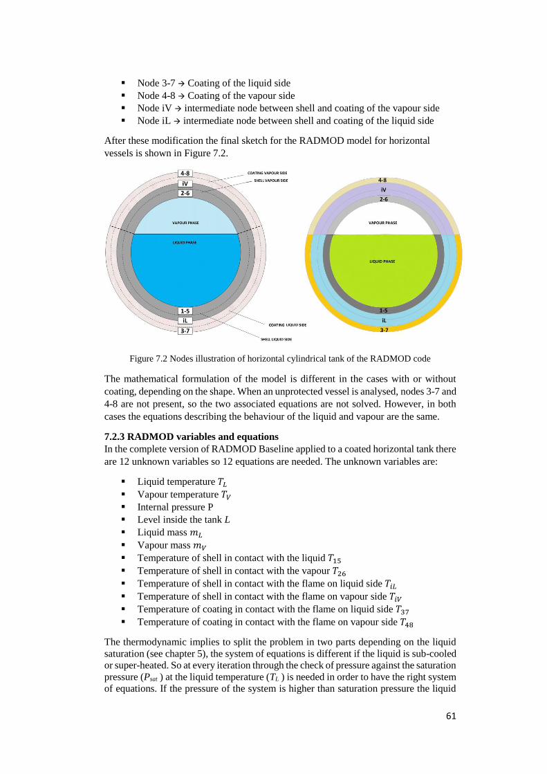
61

Node 3-7 Coating of the liquid side

Node 4-8 Coating of the vapour side

Node iV intermediate node between shell and coating of the vapour side

Node iL intermediate node between shell and coating of the liquid side

After these modification the final sketch for the RADMOD model for horizontal

vessels is shown in Figure 7.2.

Figure 7.2 Nodes illustration of horizontal cylindrical tank of the RADMOD code

The mathematical formulation of the model is different in the cases with or without

coating, depending on the shape. When an unprotected vessel is analysed, nodes 3-7 and

4-8 are not present, so the two associated equations are not solved. However, in both

cases the equations describing the behaviour of the liquid and vapour are the same.

7.2.3 RADMOD variables and equations In the complete version of RADMOD Baseline applied to a coated horizontal tank there

are 12 unknown variables so 12 equations are needed. The unknown variables are:

Liquid temperature 𝑇𝐿

Vapour temperature 𝑇𝑉

Internal pressure P

Level inside the tank L

Liquid mass 𝑚𝐿

Vapour mass 𝑚𝑉

Temperature of shell in contact with the liquid 𝑇15

Temperature of shell in contact with the vapour 𝑇26

Temperature of shell in contact with the flame on liquid side 𝑇𝑖𝐿

Temperature of shell in contact with the flame on vapour side 𝑇𝑖𝑉

Temperature of coating in contact with the flame on liquid side 𝑇37

Temperature of coating in contact with the flame on vapour side 𝑇48

The thermodynamic implies to split the problem in two parts depending on the liquid

saturation (see chapter 5), the system of equations is different if the liquid is sub-cooled

or super-heated. So at every iteration through the check of pressure against the saturation

pressure (Psat ) at the liquid temperature (TL ) is needed in order to have the right system

of equations. If the pressure of the system is higher than saturation pressure the liquid

62

is sub-cooled otherwise it is superheated. The saturation pressure is evaluated through

Antoine equation. The only energy balances to split in this two cases are the ones written

for the lading (liquid and vapour phase) since the heat transfers through the tank layer

(shell, coating and jacket) are not related to the liquid saturation.

The improvements of the heat balances are reported below, whereas the failure criteria

adopted in the code are reported in paragraph 7.2.4.

Vapour transparency

The first improvement of the RADMOD code regards the radiation received by the

vapour phase. The vapour is not considered transparent to the radiation from the vapour-

space wall, thus the radiation received by the liquid is reduced by a quantity which is

added to heat loads to the vapour, with respect to heat transfer coefficients between the

vapour and the wall. Thus, the liquid and the vapour temperature balances are modified

as shown in equation (7.1) and (7.2) for the liquid node and (7.6) and (7.7) for the vapour

node.

Liquid temperature (𝑇L) Not boiling liquid:

𝑚𝐿𝑐𝑣𝐿𝑑𝑇𝐿

𝑑𝑡= 𝑞𝐿,𝑏𝑜𝑖𝑙 + 𝑞𝐿,𝑟𝑎𝑑 + 𝑞𝐿𝑉 (7.1)

Liquid temperature (𝑇𝐿) Boiling liquid:

𝑑𝑇𝐿

𝑑𝑡= 0 (7.2)

Where 𝑚𝐿is the liquid mass, 𝑐𝑣𝐿 is the heat capacity of liquid at constant volume. Since

the liquid can be assumed uncompressible, the specific heat at constant volume is

considered equal to the specific heat at constant pressure (𝑐𝑝𝐿). 𝑞𝐿𝑉 is the convective

and radiative heat power between the vapour-phase and the liquid-phase. The terms

𝑞𝐿,𝑏𝑜𝑖𝑙 and 𝑞𝐿,𝑟𝑎𝑑 are the convective and radiative heat powers received by the liquid

from the walls, the convection is from the liquid-space walls and the radiation from the

vapour-space ones. The radiative contribution is define as:

𝑞𝐿,𝑟𝑎𝑑 = 𝐴26𝑖𝑛𝑡𝜎𝜀𝐹𝑣,𝐿(𝑇264 − 𝑇𝐿

4) − 𝑞𝑉,𝑟𝑎𝑑 (7.3)

Where 𝜀 is the steel emissivity, σ is the Stefan-Boltzmann constant (5.6703x10-8) , 𝐹𝑣,𝐿is

the view factor between the tank wall and the liquid surface, 𝐴26𝑖𝑛𝑡 and 𝑇26 are the

internal surface of node26, facing on the lading and its temperature. 𝑞𝑉,𝑟𝑎𝑑 is the

radiation received by the vapour, thus, the novel term, defined as:

𝑞𝑉,𝑟𝑎𝑑 = 𝐴26𝑖𝑛𝑡ℎ𝑉,𝑟(𝑇26 − 𝑇𝑉) (7.4)

Where the radiative heat-transfer coefficient from the wall to the vapour-phase (ℎ𝑉,𝑟) is

calculate by the empirical correlation [Perry & Green, 1997]:

ℎ𝑉,𝑟 = 5.6783[(

𝑇26100

)4

−(𝑇𝑉100

)4

]0.173

(𝑇26−𝑇𝑉) (7.5)

The term of absorbed radiation by the vapour-phase in then added to the vapour node

energy balance, as follows:

Vapour temperature (𝑇𝑉) Not boiling liquid:

𝑚𝑉𝑐𝑣𝑉𝑑𝑇𝑉

𝑑𝑡= 𝑞𝑉 + 𝑞𝑉,𝑟𝑎𝑑 − 𝑞𝐿𝑉 − 𝑧𝑧𝜙

𝑅𝑇𝑉

𝑀𝑊 (7.6)

63

Vapour temperature (𝑇𝑉) Boiling liquid:

𝑚𝑉𝑐𝑣𝑉𝑑𝑇𝑉

𝑑𝑡= 𝑞𝑉 + 𝑞𝑉,𝑟𝑎𝑑 − 𝑞𝐿𝑉 − 𝑧𝑧𝜙

𝑅𝑇𝑉

𝑀𝑊+

𝑑𝑚𝐿

𝑑𝑡(𝑐𝑣𝑉(𝑇𝑉 − 𝑇𝐿) − 𝑧𝑧

𝑅𝑇𝐿

𝑀𝑊) (7.7)

Where 𝑚𝑉 is the vapour mass, 𝑐𝑣𝑉 is the heat capacity of vapour at constant volume, zz

is the compressibility factor, Ф is the mass flux discharged from PRV, R is the ideal gas

constant and MW is the molecular weight. If the pressure relief valve is not installed or

it is closed Ф is equal to zero simplifying the equation. The heat power 𝑞𝑉 is the

convective contribution pf the vapour-space walls.

Heat load from the flame

The heat flux from the flame to the shell was set as a constant input data in the previously

version of the RADMOD code, in the novel implementation the input data are different

and require to set the flame temperature and the flame emissivity, allowing the

evaluation of a dynamic heat flux with respect to the wall effective temperature. The

total flux from the flame to the external nodes can be expressed as the sum of a

convective and a radiative contribution (𝐼𝑒𝑥𝑡 = 𝐼𝑐𝑜𝑛𝑣 + 𝐼𝑟𝑎𝑑). The radiative term is

written in function of the generic temperature of the wall, in order to adapt the equation

by replacing the generic wall temperature with the specific temperature, as shown

below:

𝐼𝑒𝑥𝑡 = (𝜎𝜀𝑠(𝜀𝑓𝑇𝑓4 + (1 − 𝜀𝑓)𝑇𝑎𝑚𝑏

4 ) − (𝜎𝜀𝑠𝑇𝑤4)) 𝐹𝑣,𝑎 + (1 − 𝐹𝑣,𝑎)𝜎𝜀𝑠𝑇𝑎𝑚𝑏

4 (7.8)

Where 𝑇𝑤 is the generic wall temperature, 𝑇𝑓 is the flame temperature, 𝜀𝑓 and 𝜀𝑠 are the

emissivity of the flame and of the steel wall, respectively, σ is the Stefan-Boltzmann

constant (5.6703x10-8). 𝐹𝑣,𝑎 is a shape factor, it takes into account the case of distant

source, in which the near-flame shell exchanges both with the ambient air and with the

distant flame. Equation (7.8) is suggested by Heymes et al. through the study of an LPG

tank exposed to fire. [Heymes et al. 2013] In the novel version of RADMOD 𝐹𝑣,𝑎 is

implemented to allow further development, thus its value is currently set equal to the

unit.

Partial engulfment

In case the flame impingement affects only a portion of tank, the equations set remains

unchanged as well as the nodes division, the only difference concerns the exchange

areas between the flame and the external nodes. Thus, the temperatures obtained by the

code are average over the nodes. The idea comes from the first RADMOD version

[Landucci et al. 2013] where, in case of distant source, the nodes kept their configuration

and only the external areas of exchange were modified. This improvement affects the

balances of external nodes, node37 and node48 in case of coated tank or nodeiL and nodeiV

if the vessel is unprotected, since the other two external nodes are not present, see Figure

7.2.

Unprotected tank external nodeiL and nodeiV (𝑇𝑖𝑉 and 𝑇𝑖𝐿)

𝑑𝑠𝑐𝑝𝑠𝐿𝑠𝑠

2𝐴𝑖𝐿 𝑑𝑇𝑖𝐿

𝑑𝑡= 𝐴𝑖𝐿,𝐹𝐼𝑒𝑥𝑡,𝐿 − 𝐴𝑖𝐿,𝐴𝐼𝑎𝑚𝑏,𝐿−𝐴𝑖𝐿𝑖𝑛𝑡

𝑘𝑠𝐿

𝑠𝑠(𝑇𝑖𝐿 − 𝑇15) (7.9)

𝑑𝑠𝑐𝑝𝑠𝑉𝑠𝑠

2𝐴𝑖𝑉 𝑑𝑇𝑖𝑉

𝑑𝑡= 𝐴𝑖𝑉,𝐹𝐼𝑒𝑥𝑡,𝑉−𝐴𝑖𝑉,𝐴𝐼𝑎𝑚𝑏,𝑉 − 𝐴𝑖𝑉𝑖𝑛𝑡

𝑘𝑠𝑉

𝑠𝑠(𝑇𝑖𝑉 − 𝑇26) (7.10)

Coated tank external node37 and node48 (𝑇37 and 𝑇48)

64

𝑑𝑖𝑐𝑝𝑖𝑠𝑖

2𝐴37 𝑑𝑇37

𝑑𝑡= 𝐴37,𝐹𝐼𝑒𝑥𝑡,𝐿−𝐴37,𝐴𝐼𝑎𝑚𝑏,𝐿 − 𝐴37𝑖𝑛𝑡

𝑘𝑖𝐿

𝑠𝑖(𝑇37 − 𝑇𝑖𝐿) (7.11)

𝑑𝑖𝑐𝑝𝑖𝑠𝑖

2𝐴48 𝑑𝑇48

𝑑𝑡= 𝐴48,𝐹𝐼𝑒𝑥𝑡,𝑉 − 𝐴48,𝐴𝐼𝑎𝑚𝑏,𝑉 − 𝐴48𝑖𝑛𝑡

𝑘𝑖𝑉

𝑠𝑖(𝑇48 − 𝑇𝑖𝑉) (7.12)

Where d, cp, k and s are respectively the density, the heat capacity, the thermal

conductivity and the thickness of the steel, with subscript, or relative to the insulation,

depending by the subscript s or i.

The areas ( 𝐴𝑛𝑜𝑑𝑒 ) represent the average nodal areas, the heat leaving the systems to the

inner nodes is expressed in each equation as: 𝐴𝑛𝑜𝑑𝑒,𝑖𝑛𝑡𝑘

𝑠(𝑇𝑛𝑜𝑑𝑒 − 𝑇𝑖𝑛𝑡𝑒𝑟𝑛𝑎𝑙 𝑛𝑜𝑑𝑒), and

represents the power heat transferred by conduction from the node of interest to the

internal layer of the tank with which the node is in contact.

In case of partial engulfment 𝐼𝑒𝑥𝑡𝐿/𝑉 and 𝐼𝑎𝑚𝑏𝐿/𝑉 are respectively, the heat flux that the

shell receives from the flames and the heat flux transferred by the shell wall to the

ambient air, on the liquid or vapour shell space depending by the subscript L or V.

The areas with the subscript F or A represent the surfaces engulfed by the flame (F) and

the not engulfed surfaces in contact with ambient air (A). They are defined in equations

set (7.13) and (7.14) respectively.

Fully engulfed tank

𝐴𝑒𝑥𝑡_𝑛𝑜𝑑𝑒,𝐹 = 𝐴𝑒𝑥𝑡_𝑛𝑜𝑑𝑒 (7.13a)

𝐴𝑒𝑥𝑡_𝑛𝑜𝑑𝑒,𝐴 = 0 (7.13b)

Half engulfed tank

𝐴𝑒𝑥𝑡_𝑛𝑜𝑑𝑒,𝐹 =𝐴𝑒𝑥𝑡_𝑛𝑜𝑑𝑒

2 (7.14a)

𝐴𝑒𝑥𝑡_𝑛𝑜𝑑𝑒,𝐴 =𝐴𝑒𝑥𝑡_𝑛𝑜𝑑𝑒

2 (7.14b)

The total external area of the node is 𝐴𝑒𝑥𝑡_𝑛𝑜𝑑𝑒, and it is calculated only on geometrical

considerations on the tank geometry and on the liquid level. Whereas, the other terms

depend on the engulfment degree, when the tank is partially engulfed the external

surface of the nodes are halved and each half is redefined as the subscripted areas (F)

and (A), respectively (eq. set 7.14). If the tank is fully engulfed in the flame, the areas

which exchange with ambient (A) are set to zero, whereas the areas which exchange

with the flame (F) are set equal to the totality of the external nodal surface (eq. set 7.13).

So, in this case, the outgoing terms from the walls to the air being zero.

Thermal conductivity of insulation

The last novel implementation regards the input data required for the coating layer. This

include the setting of the thermal conductivity, which could be insert as a constant or, if

more information are available, as temperature dependent values. The second case is

the new implementation, there are three values to insert depending on the temperature

range and defining three thermal conductivities: kiL, kiV and kiJ. The subscripts refer to

different zone with which the insulation is in contact: the liquid wetted wall (L), the

vapour space wall covered by the coating (V) and the external steel jacket (J). Each

thermal conductivity differs from the others by the temperature range which is expected

65

to be reached in the zone in contact with the insulation. Thus, for coated tank, kiJ is

associated to the external nodes (node37 and node48), kiL and kiV are indeed associated to

the intermediate nodes (nodeiL and nodeiV) respectively.

7.2.4 Failure criteria

Two different failure criteria are used in the RADMOD code for the evaluation of the

time to failure (ttf) of the tank. Both predict a conservative ttf, the first is the more

simplified and conservative using the Von Mises criterion for the evaluation of ttf,

whereas the second criterion is based on the standard BS7910:2013 “Guide to methods

for assessing the acceptability of flaws in metallic structures”. [BS7910, 2013]

Von Mises criterion

The axial (𝜎𝑎𝑥), the circumferential (𝜎𝑐𝑖𝑟𝑐) and the equivalent (𝜎𝑒𝑞) stresses, according

to Von Mises, are calculated as follows:

𝜎𝑎𝑥 =𝑃𝑅𝑒

2𝑠𝑠 (7.15a)

𝜎𝑎𝑥 =𝑃𝑅𝑒

𝑠𝑠 (7.15b)

𝜎𝑒𝑞 = √𝜎𝑎𝑥2 + 𝜎𝑐𝑖𝑟𝑐

2 − 𝜎𝑎𝑥𝜎𝑐𝑖𝑟𝑐 (7.16)

The equivalent stress is compared with the admissible stress of the material (𝜎𝑎𝑑𝑚) that

is a function of temperature. For the evaluation of the admissible stress, the yield

strength of the material (𝜎𝑌) is divided for a safety factor (S.F.), considered equal to 1.1

in this work, which considers all the welds and the other unknown details that makes

the vessel weaker:

𝜎𝑎𝑑𝑚 =𝜎𝑌(𝑇𝑠ℎ𝑒𝑙𝑙)

𝑆.𝐹. (7.17)

The temperature at which is evaluated the yield strength is the maximum temperature

among those of the shell nodes. This approach is the most easy and conservative for the

evaluation of the ttf because the yield strength is calculated at the 0.2% of deformation,

so it considers only the elastic field. The time to failure of the vessel is predicted through

equation (7.18) as the first time when the following inequality is no more verified:

𝜎𝑒𝑞 > 𝜎𝑎𝑑𝑚 (7.18)

As already said, the results obtained from this criterion are very conservative, anyway

in an actual accident there can be unpredictable severe damage on the shell itself and

this results gives an idea of the worst real-case.

Standard BS7910:2013

The criterion used in the code is the basic application, low level called option 1, of the

standard “Guide to methods for assessing the acceptability of flaws in metallic

structures”. [BS7910, 2013] It evaluates the ductile rupture considers the flaws in the

material, in particular the weld as the critical zones. The crack propagation mode

considered in this work is Mode I where the crack is opened by a tensile stress normal

to the plane of the crack. Knowing detailed information on metallic surface much more

detailed results could be obtained compared with the simplified approach explained

above.

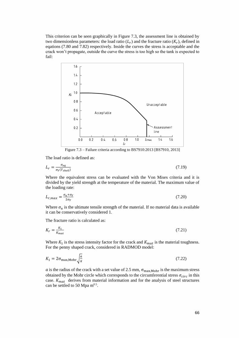
66

This criterion can be seen graphically in Figure 7.3, the assessment line is obtained by

two dimensionless parameters: the load ratio (𝐿𝑟) and the fracture ratio (𝐾𝑟), defined in

eqations (7.80 and 7.82) respectively. Inside the curves the stress is acceptable and the

crack won’t propagate, outside the curve the stress is too high so the tank is expected to

fail:

Figure 7.3 – Failure criteria according to BS7910:2013 [BS7910, 2013]

The load ratio is defined as:

𝐿𝑟 =𝜎𝑒𝑞

𝜎𝑌(𝑇𝑠ℎ𝑒𝑙𝑙) (7.19)

Where the equivalent stress can be evaluated with the Von Mises criteria and it is

divided by the yield strength at the temperature of the material. The maximum value of

the loading rate:

𝐿𝑟,𝑚𝑎𝑥 =𝜎𝑢+𝜎𝑌

2𝜎𝑌 (7.20)

Where 𝜎𝑢 is the ultimate tensile strength of the material. If no material data is available

it can be conservatively considered 1.

The fracture ratio is calculated as:

𝐾𝑟 =𝐾1

𝐾𝑚𝑎𝑡 (7.21)

Where 𝐾1 is the stress intensity factor for the crack and 𝐾𝑚𝑎𝑡 is the material toughness.

For the penny shaped crack, considered in RADMOD model:

𝐾1 = 2σmax,Mohr√𝑎

𝜋 (7.22)

𝑎 is the radius of the crack with a set value of 2.5 mm, σmax,Mohr is the maximum stress

obtained by the Mohr circle which corresponds to the circumferential stress 𝜎𝑐𝑖𝑟𝑐 in this

case. 𝐾𝑚𝑎𝑡 derives from material information and for the analysis of steel structures

can be settled to 50 Mpa m0.5.

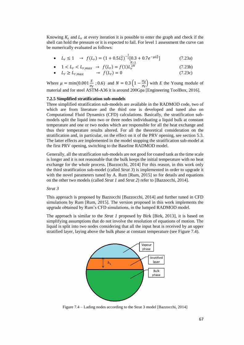
67

Knowing 𝐾r and 𝐿𝑟 at every iteration it is possible to enter the graph and check if the

shell can hold the pressure or it is expected to fail. For level 1 assessment the curve can

be numerically evaluated as follows:

𝐿𝑟 ≤ 1 → 𝑓(𝐿𝑟) = (1 + 0.5𝐿𝑟2)−

1

2[0.3 + 0.7𝑒−𝜇𝐿𝑟6

] (7.23a)

1 < 𝐿𝑟 < 𝐿𝑟,𝑚𝑎𝑥 → 𝑓(𝐿𝑟) = 𝑓(1)𝐿𝑟

𝑁−1

2𝑁 (7.23b)

𝐿𝑟 ≥ 𝐿𝑟,𝑚𝑎𝑥 → 𝑓(𝐿𝑟) = 0 (7.23c)

Where 𝜇 = min (0.001𝐸

𝜎𝑌 ; 0.6) and 𝑁 = 0.3 (1 −

𝜎𝑈

𝜎𝑌) with E the Young module of

material and for steel ASTM-A36 it is around 200Gpa [Engineering ToolBox, 2016].

7.2.5 Simplified stratification sub-models

Three simplified stratification sub-models are available in the RADMOD code, two of

which are from literature and the third one is developed and tuned also on

Computational Fluid Dynamics (CFD) calculations. Basically, the stratification sub-

models split the liquid into two or three nodes individuating a liquid bulk at constant

temperature and one or two nodes which are responsible for all the heat exchange and

thus their temperature results altered. For all the theoretical consideration on the

stratification and, in particular, on the effect on it of the PRV opening, see section 5.3.

The latter effects are implemented in the model stopping the stratification sub-model at

the first PRV opening, switching to the Baseline RADMOD model.

Generally, all the stratification sub-models are not good for coated tank as the time scale

is longer and it is not reasonable that the bulk keeps the initial temperature with no heat

exchange for the whole process. [Bazzocchi, 2014] For this reason, in this work only

the third stratification sub-model (called Strat 3) is implemented in order to upgrade it

with the novel parameters tuned by A. Rum [Rum, 2015] so for details and equations

on the other two models (called Strat 1 and Strat 2) refer to [Bazzocchi, 2014].

Strat 3

This approach is proposed by Bazzocchi [Bazzocchi, 2014] and further tuned in CFD

simulations by Rum [Rum, 2015]. The version proposed in this work implements the

upgrade obtained by Rum’s CFD simulations, in the lumped RADMOD model.

The approach is similar to the Strat 1 proposed by Birk [Birk, 2013], it is based on

simplifying assumptions that do not involve the resolution of equations of motion. The

liquid is split into two nodes considering that all the input heat is received by an upper

stratified layer, laying above the bulk phase at constant temperature (see Figure 7.4).

Figure 7.4 – Lading nodes according to the Strat 3 model [Bazzocchi, 2014]

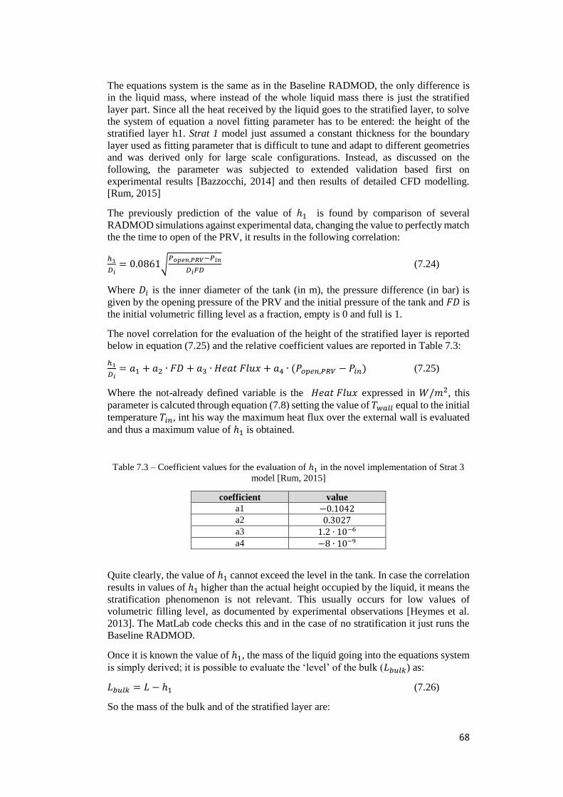
68

The equations system is the same as in the Baseline RADMOD, the only difference is

in the liquid mass, where instead of the whole liquid mass there is just the stratified

layer part. Since all the heat received by the liquid goes to the stratified layer, to solve

the system of equation a novel fitting parameter has to be entered: the height of the

stratified layer h1. Strat 1 model just assumed a constant thickness for the boundary

layer used as fitting parameter that is difficult to tune and adapt to different geometries

and was derived only for large scale configurations. Instead, as discussed on the

following, the parameter was subjected to extended validation based first on

experimental results [Bazzocchi, 2014] and then results of detailed CFD modelling.

[Rum, 2015]

The previously prediction of the value of ℎ1 is found by comparison of several

RADMOD simulations against experimental data, changing the value to perfectly match

the the time to open of the PRV, it results in the following correlation:

ℎ1

𝐷𝑖= 0.0861√

𝑃𝑜𝑝𝑒𝑛,𝑃𝑅𝑉−𝑃𝑖𝑛

𝐷𝑖𝐹𝐷 (7.24)

Where 𝐷𝑖 is the inner diameter of the tank (in m), the pressure difference (in bar) is

given by the opening pressure of the PRV and the initial pressure of the tank and 𝐹𝐷 is

the initial volumetric filling level as a fraction, empty is 0 and full is 1.

The novel correlation for the evaluation of the height of the stratified layer is reported

below in equation (7.25) and the relative coefficient values are reported in Table 7.3:

ℎ1

𝐷𝑖= 𝑎1 + 𝑎2 ∙ 𝐹𝐷 + 𝑎3 ∙ 𝐻𝑒𝑎𝑡 𝐹𝑙𝑢𝑥 + 𝑎4 ∙ (𝑃𝑜𝑝𝑒𝑛,𝑃𝑅𝑉 − 𝑃𝑖𝑛) (7.25)

Where the not-already defined variable is the 𝐻𝑒𝑎𝑡 𝐹𝑙𝑢𝑥 expressed in 𝑊/𝑚2, this

parameter is calcuted through equation (7.8) setting the value of 𝑇𝑤𝑎𝑙𝑙 equal to the initial

temperature 𝑇𝑖𝑛, int his way the maximum heat flux over the external wall is evaluated

and thus a maximum value of ℎ1 is obtained.

Table 7.3 – Coefficient values for the evaluation of ℎ1 in the novel implementation of Strat 3

model [Rum, 2015]

coefficient value a1 −0.1042 a2 0.3027 a3 1.2 ∙ 10−6 a4 −8 ∙ 10−9

Quite clearly, the value of ℎ1 cannot exceed the level in the tank. In case the correlation

results in values of ℎ1 higher than the actual height occupied by the liquid, it means the

stratification phenomenon is not relevant. This usually occurs for low values of

volumetric filling level, as documented by experimental observations [Heymes et al.

2013]. The MatLab code checks this and in the case of no stratification it just runs the

Baseline RADMOD.

Once it is known the value of ℎ1, the mass of the liquid going into the equations system

is simply derived; it is possible to evaluate the ‘level’ of the bulk (𝐿𝑏𝑢𝑙𝑘) as:

𝐿𝑏𝑢𝑙𝑘 = 𝐿 − ℎ1 (7.26)

So the mass of the bulk and of the stratified layer are:

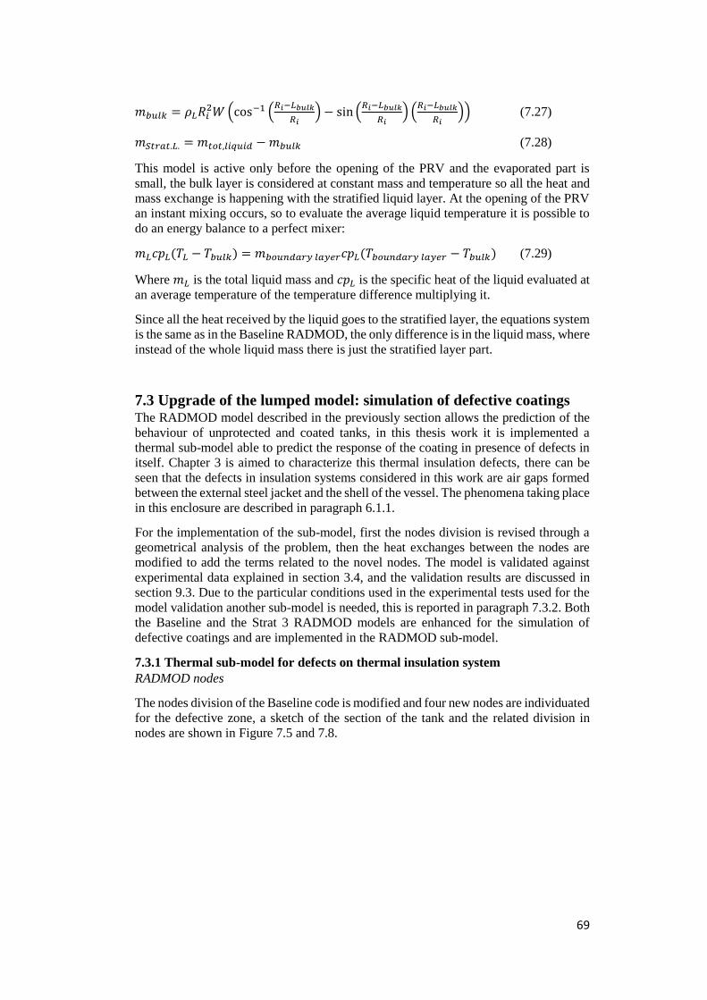
69

𝑚𝑏𝑢𝑙𝑘 = 𝜌𝐿𝑅𝑖2𝑊 (cos−1 (

𝑅𝑖−𝐿𝑏𝑢𝑙𝑘

𝑅𝑖) − sin (

𝑅𝑖−𝐿𝑏𝑢𝑙𝑘

𝑅𝑖) (

𝑅𝑖−𝐿𝑏𝑢𝑙𝑘

𝑅𝑖)) (7.27)

𝑚𝑆𝑡𝑟𝑎𝑡.𝐿. = 𝑚𝑡𝑜𝑡,𝑙𝑖𝑞𝑢𝑖𝑑 − 𝑚𝑏𝑢𝑙𝑘 (7.28)

This model is active only before the opening of the PRV and the evaporated part is

small, the bulk layer is considered at constant mass and temperature so all the heat and

mass exchange is happening with the stratified liquid layer. At the opening of the PRV

an instant mixing occurs, so to evaluate the average liquid temperature it is possible to

do an energy balance to a perfect mixer:

𝑚𝐿𝑐𝑝𝐿(𝑇𝐿 − 𝑇𝑏𝑢𝑙𝑘) = 𝑚𝑏𝑜𝑢𝑛𝑑𝑎𝑟𝑦 𝑙𝑎𝑦𝑒𝑟𝑐𝑝𝐿(𝑇𝑏𝑜𝑢𝑛𝑑𝑎𝑟𝑦 𝑙𝑎𝑦𝑒𝑟 − 𝑇𝑏𝑢𝑙𝑘) (7.29)

Where 𝑚𝐿 is the total liquid mass and 𝑐𝑝𝐿 is the specific heat of the liquid evaluated at

an average temperature of the temperature difference multiplying it.

Since all the heat received by the liquid goes to the stratified layer, the equations system

is the same as in the Baseline RADMOD, the only difference is in the liquid mass, where

instead of the whole liquid mass there is just the stratified layer part.

7.3 Upgrade of the lumped model: simulation of defective coatings The RADMOD model described in the previously section allows the prediction of the

behaviour of unprotected and coated tanks, in this thesis work it is implemented a

thermal sub-model able to predict the response of the coating in presence of defects in

itself. Chapter 3 is aimed to characterize this thermal insulation defects, there can be

seen that the defects in insulation systems considered in this work are air gaps formed

between the external steel jacket and the shell of the vessel. The phenomena taking place

in this enclosure are described in paragraph 6.1.1.

For the implementation of the sub-model, first the nodes division is revised through a

geometrical analysis of the problem, then the heat exchanges between the nodes are

modified to add the terms related to the novel nodes. The model is validated against

experimental data explained in section 3.4, and the validation results are discussed in

section 9.3. Due to the particular conditions used in the experimental tests used for the

model validation another sub-model is needed, this is reported in paragraph 7.3.2. Both

the Baseline and the Strat 3 RADMOD models are enhanced for the simulation of

defective coatings and are implemented in the RADMOD sub-model.

7.3.1 Thermal sub-model for defects on thermal insulation system RADMOD nodes

The nodes division of the Baseline code is modified and four new nodes are individuated

for the defective zone, a sketch of the section of the tank and the related division in

nodes are shown in Figure 7.5 and 7.8.

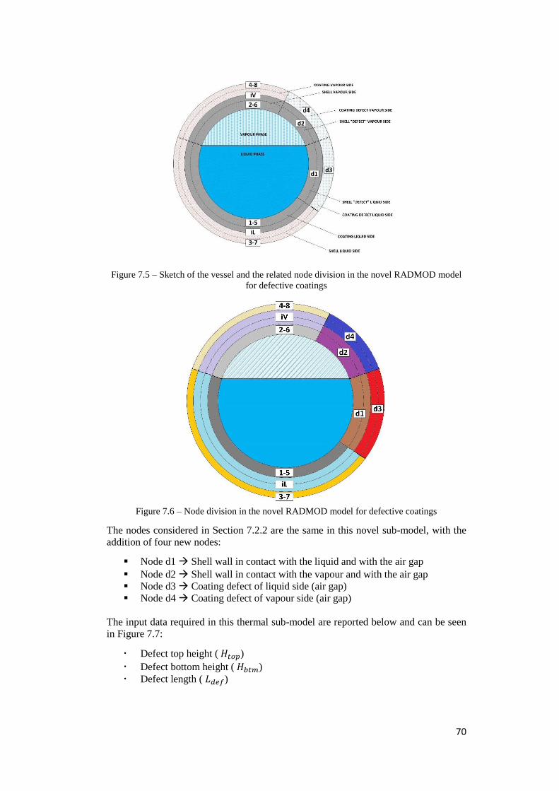
70

Figure 7.5 – Sketch of the vessel and the related node division in the novel RADMOD model

for defective coatings

Figure 7.6 – Node division in the novel RADMOD model for defective coatings

The nodes considered in Section 7.2.2 are the same in this novel sub-model, with the

addition of four new nodes:

Node d1 Shell wall in contact with the liquid and with the air gap

Node d2 Shell wall in contact with the vapour and with the air gap

Node d3 Coating defect of liquid side (air gap)

Node d4 Coating defect of vapour side (air gap)

The input data required in this thermal sub-model are reported below and can be seen

in Figure 7.7:

Defect top height ( 𝐻𝑡𝑜𝑝)

Defect bottom height ( 𝐻𝑏𝑡𝑚)

Defect length ( 𝐿𝑑𝑒𝑓)

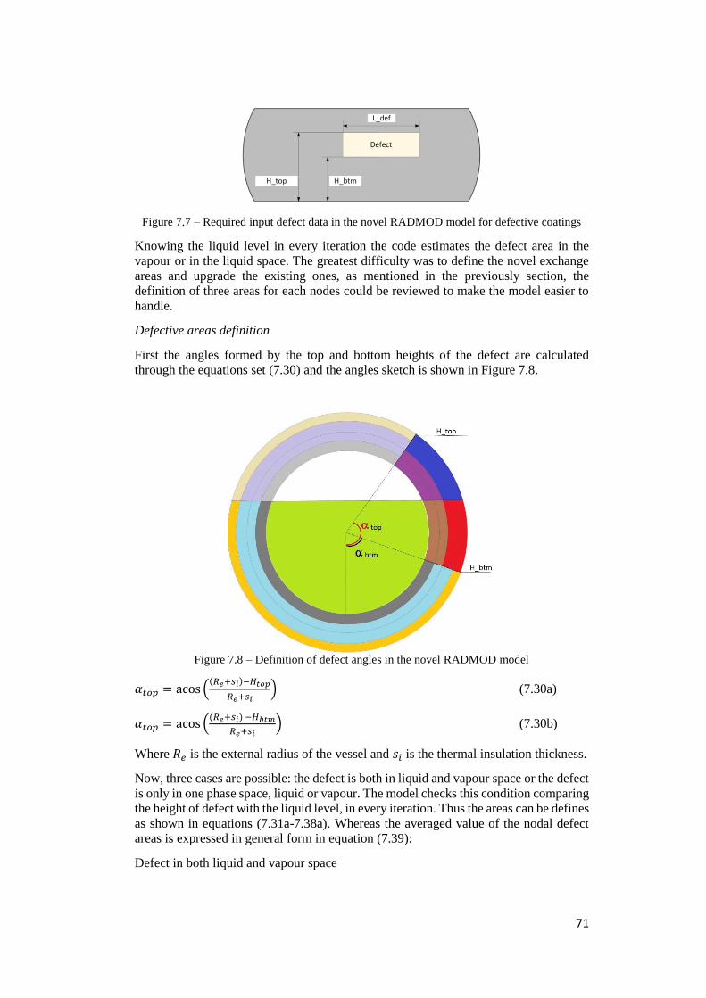
71

Figure 7.7 – Required input defect data in the novel RADMOD model for defective coatings

Knowing the liquid level in every iteration the code estimates the defect area in the

vapour or in the liquid space. The greatest difficulty was to define the novel exchange

areas and upgrade the existing ones, as mentioned in the previously section, the

definition of three areas for each nodes could be reviewed to make the model easier to

handle.

Defective areas definition

First the angles formed by the top and bottom heights of the defect are calculated

through the equations set (7.30) and the angles sketch is shown in Figure 7.8.

Figure 7.8 – Definition of defect angles in the novel RADMOD model

𝛼𝑡𝑜𝑝 = acos ((𝑅𝑒+𝑠𝑖)−𝐻𝑡𝑜𝑝

𝑅𝑒+𝑠𝑖) (7.30a)

𝛼𝑡𝑜𝑝 = acos ((𝑅𝑒+𝑠𝑖) −𝐻𝑏𝑡𝑚

𝑅𝑒+𝑠𝑖) (7.30b)

Where 𝑅𝑒 is the external radius of the vessel and 𝑠𝑖 is the thermal insulation thickness.

Now, three cases are possible: the defect is both in liquid and vapour space or the defect

is only in one phase space, liquid or vapour. The model checks this condition comparing

the height of defect with the liquid level, in every iteration. Thus the areas can be defines

as shown in equations (7.31a-7.38a). Whereas the averaged value of the nodal defect

areas is expressed in general form in equation (7.39):

Defect in both liquid and vapour space

72

𝐴𝑑1,𝑖𝑛𝑡 = 𝐿𝑑𝑒𝑓𝑅𝑖 (acos (𝑅𝑖−𝐿

𝑅𝑖) − 𝛼𝑏𝑡𝑚) (7.31a)

𝐴𝑑1,𝑒𝑥𝑡 = 𝐿𝑑𝑒𝑓𝑅𝑒 (acos (𝑅𝑒−𝐿

𝑅𝑒) − 𝛼𝑏𝑡𝑚) (7.32a)

𝐴𝑑2,𝑖𝑛𝑡 = 𝐿𝑑𝑒𝑓𝑅𝑖 (𝛼𝑡𝑜𝑝 − acos (𝑅𝑖−𝐿

𝑅𝑖)) (7.33a)

𝐴𝑑2,𝑒𝑥𝑡 = 𝐿𝑑𝑒𝑓𝑅𝑒 (𝛼𝑡𝑜𝑝 − acos (𝑅𝑒−𝐿

𝑅𝑒)) (7.34a)

𝐴𝑑3,𝑖𝑛𝑡 = 𝐴𝑑1,𝑒𝑥𝑡 (7.35a)

𝐴𝑑3,𝑒𝑥𝑡 = 𝐿𝑑𝑒𝑓(𝑅𝑒 + 𝑠𝑖) (acos ((𝑅𝑒+𝑠𝑖)−𝐿

𝑅𝑒+𝑠𝑖) − 𝛼𝑏𝑡𝑚) (7.36a)

𝐴𝑑4,𝑖𝑛𝑡 = 𝐴𝑑2,𝑒𝑥𝑡 (7.37a)

𝐴𝑑4,𝑒𝑥𝑡 = 𝐿𝑑𝑒𝑓(𝑅𝑒 + 𝑠𝑖) (𝛼𝑡𝑜𝑝 − acos ((𝑅𝑒+𝑠𝑖)−𝐿

𝑅𝑒+𝑠𝑖)) (7.38a)

𝐴𝑑 =

𝐴𝑑,𝑖𝑛𝑡+𝐴𝑑,𝑒𝑥𝑡

2 (7.39)

Where 𝑅𝑖 is the internal radius of the vessel and 𝐿 is the liquid level, thus acos (𝑅−𝐿

𝑅)

represents the angle formed by the liquid level defined in the same way as 𝛼𝑡𝑜𝑝 and

𝛼𝑏𝑡𝑚 are defined in equations set (7.30).

The case in which the defect is only on the liquid side can happen only if the initial

value of 𝐻𝑡𝑜𝑝 results lower that the liquid level. Whereas the other case, defect in vapour

side only, corresponds to 𝐻𝑏𝑡𝑚 greater than 𝐿 and it can also take place during the

simulation due to level falls below the defect lower height 𝐻𝑏𝑡𝑚. In these cases one side

(liquid or vapour) has no “defective” nodes, so, to keep the model simple, rather than

define another set of equations for each case, the areas corresponding to the nodes no

more present are set to zero. Thus the areas definitions reported in sets (7.31a – 7.38a)

are modified in the equations (7-31b – 7.38b) and (7-37c – 7.38c) for defect only in

liquid and vapour side, respectively, as follows:

Defect in liquid side only

𝐴𝑑1,𝑖𝑛𝑡 = 𝐿𝑑𝑒𝑓𝑅𝑖 (𝛼𝑡𝑜𝑝 − 𝛼𝑏𝑡𝑚) (7.31b)

𝐴𝑑1,𝑒𝑥𝑡 = 𝐿𝑑𝑒𝑓𝑅𝑒 (𝛼𝑡𝑜𝑝 − 𝛼𝑏𝑡𝑚) (7.32b)

𝐴𝑑2,𝑖𝑛𝑡 = 0 (7.33b)

𝐴𝑑2,𝑒𝑥𝑡 = 0 (7.34b)

𝐴𝑑3,𝑖𝑛𝑡 = 𝐴𝑑1,𝑒𝑥𝑡 (7.35b)

𝐴𝑑3,𝑒𝑥𝑡 = 𝐿𝑑𝑒𝑓(𝑅𝑒 + 𝑠𝑖)(𝛼𝑡𝑜𝑝 − 𝛼𝑏𝑡𝑚) (7.36b)

𝐴𝑑4,𝑖𝑛𝑡 = 0 (7.37b)

𝐴𝑑4,𝑒𝑥𝑡 = 0 (7.38b)

Defect in vapour side only

𝐴𝑑1,𝑖𝑛𝑡 = 0 (7.31c)

73

𝐴𝑑1,𝑒𝑥𝑡 = 0 (7.32c)

𝐴𝑑2,𝑖𝑛𝑡 = 𝐿𝑑𝑒𝑓𝑅𝑖 (𝛼𝑡𝑜𝑝 − 𝛼𝑏𝑡𝑚) (7.33c)

𝐴𝑑2,𝑒𝑥𝑡 = 𝐿𝑑𝑒𝑓𝑅𝑒 (𝛼𝑡𝑜𝑝 − 𝛼𝑏𝑡𝑚) (7.34c)

𝐴𝑑3,𝑖𝑛𝑡 = 0 (7.35c)

𝐴𝑑3,𝑒𝑥𝑡 = 0 (7.36b)

𝐴𝑑4,𝑖𝑛𝑡 = 𝐴𝑑2,𝑒𝑥𝑡 (7.37c)

𝐴𝑑4,𝑒𝑥𝑡 = 𝐿𝑑𝑒𝑓(𝑅𝑒 + 𝑠𝑖)(𝛼𝑡𝑜𝑝 − 𝛼𝑏𝑡𝑚) (7.38c)

In both cases the average area of the not-present nodes cannot be calculated as the mean

of internal and external areas, because the heat exchange equations between the nodes

are not changed and thus an averaged value of the nodal area equal to zero generates an

indeterminate form in the resolution of the equation. For these reason, in case of defect

only in one of the fluid-phase side, the averaged defect nodal areas are set to unit for the

not-present nodes, the equations results do not change because all the other related areas

are set to zero but it avoids the inseminate form. Thus, equation (7.39a) is valid for the

existing nodes, while for the other nodes it is defined as in equation (7.39b):

If 𝐴𝑑,𝑖𝑛𝑡/𝑒𝑥𝑡 ≠ 0

𝐴𝑑 =

𝐴𝑑,𝑖𝑛𝑡+𝐴𝑑,𝑒𝑥𝑡

2 (7.39a)

If 𝐴𝑑,𝑖𝑛𝑡/𝑒𝑥𝑡 = 0

𝐴𝑑 = 1 (7.39b)

Now that the defect nodal areas are defined they are subtracted from the surfaces defined

in the Baseline RADMOD model, following the schematization reported in Figure 7.6.

With the configuration reported above, the defect can cover a maximum of half total

insulation surface and in case of half engulfed tank the defect is assumed to be on the

engulfed side. The validation model (see paragraph 7.3.2) has a different configuration

that may be used for implementation of a defect on both tank sides.

RADMOD equations in presence of defective coatings

Since all the nodal are are modified with respect the defect position, which changes in

function of the liquid level during the simulation, and since no conduction through the

shell is considered in the RADMOD model, the heat exchange equations defined for the

Baseline RADMOD are valid and untouched with the exception of the liquid and vapour

ones. This equations are the same as in the Baseline but with the addition of the

exchanging terms with the defective nodes. At the variables defined for the Baseline

RADMOD model are added four new variables and related equations for the defective

nodes:

Temperature of shell in contact with the liquid and defect 𝑇𝑑1

Temperature of shell in contact with the vapour and defect 𝑇𝑑2

Temperature of defect in contact with the flame on liquid side 𝑇𝑑3

Temperature of defect in contact with the flame on vapour side 𝑇𝑑4

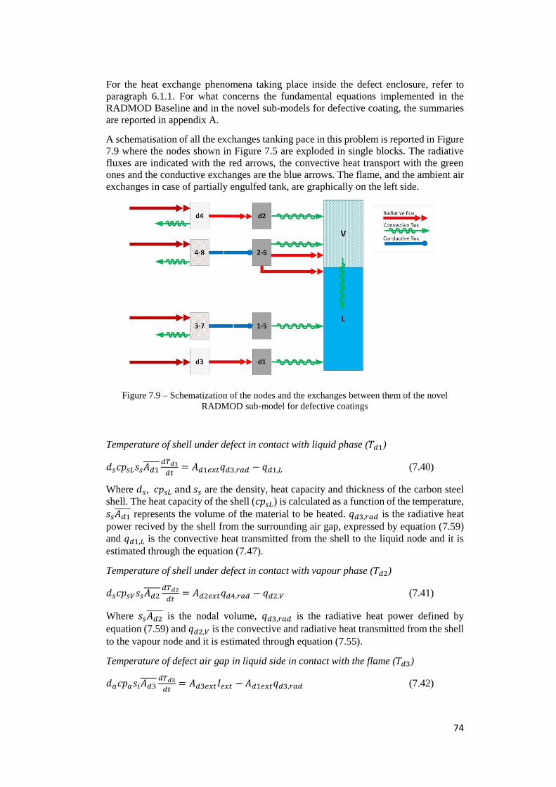
74

For the heat exchange phenomena taking place inside the defect enclosure, refer to

paragraph 6.1.1. For what concerns the fundamental equations implemented in the

RADMOD Baseline and in the novel sub-models for defective coating, the summaries

are reported in appendix A.

A schematisation of all the exchanges tanking pace in this problem is reported in Figure

7.9 where the nodes shown in Figure 7.5 are exploded in single blocks. The radiative

fluxes are indicated with the red arrows, the convective heat transport with the green

ones and the conductive exchanges are the blue arrows. The flame, and the ambient air

exchanges in case of partially engulfed tank, are graphically on the left side.

Figure 7.9 – Schematization of the nodes and the exchanges between them of the novel

RADMOD sub-model for defective coatings

Temperature of shell under defect in contact with liquid phase (𝑇𝑑1)

𝑑𝑠𝑐𝑝𝑠𝐿𝑠𝑠𝐴𝑑1 𝑑𝑇𝑑1

𝑑𝑡= 𝐴𝑑1𝑒𝑥𝑡𝑞𝑑3,𝑟𝑎𝑑 − 𝑞𝑑1,𝐿 (7.40)

Where 𝑑𝑠, 𝑐𝑝𝑠𝐿 and 𝑠𝑠 are the density, heat capacity and thickness of the carbon steel

shell. The heat capacity of the shell (𝑐𝑝𝑠𝐿) is calculated as a function of the temperature,

𝑠𝑠𝐴𝑑1 represents the volume of the material to be heated. 𝑞𝑑3,𝑟𝑎𝑑 is the radiative heat

power recived by the shell from the surrounding air gap, expressed by equation (7.59)

and 𝑞𝑑1,𝐿 is the convective heat transmitted from the shell to the liquid node and it is

estimated through the equation (7.47).

Temperature of shell under defect in contact with vapour phase (𝑇𝑑2)

𝑑𝑠𝑐𝑝𝑠𝑉𝑠𝑠𝐴𝑑2 𝑑𝑇𝑑2

𝑑𝑡= 𝐴𝑑2𝑒𝑥𝑡𝑞𝑑4,𝑟𝑎𝑑 − 𝑞𝑑2,𝑉 (7.41)

Where 𝑠𝑠𝐴𝑑2 is the nodal volume, 𝑞𝑑3,𝑟𝑎𝑑 is the radiative heat power defined by

equation (7.59) and 𝑞𝑑2,𝑉 is the convective and radiative heat transmitted from the shell

to the vapour node and it is estimated through equation (7.55).

Temperature of defect air gap in liquid side in contact with the flame (𝑇𝑑3)

𝑑𝑎𝑐𝑝𝑎𝑠𝑖𝐴𝑑3 𝑑𝑇𝑑3

𝑑𝑡= 𝐴𝑑3𝑒𝑥𝑡𝐼𝑒𝑥𝑡 − 𝐴𝑑1𝑒𝑥𝑡𝑞𝑑3,𝑟𝑎𝑑 (7.42)

75

Where 𝑑𝑎 and 𝑐𝑝𝑎 are respectively the density and the heat capacity of the air inside the

enclosure defined in equation (7.60) and (7.61) respectively. 𝐼𝑒𝑥𝑡 is the radiative and

convective heat load from the flame to the external nodal surface, it is calculated with

the equation (7.8) defined for the Baseline RADMOD with adequate value of variables.

𝑠𝑖𝐴𝑑3 represent the nodal volume.

Temperature of defect air gap in liquid side in contact with the flame (𝑇𝑑4)

𝑑𝑎𝑐𝑝𝑎𝑠𝑖𝐴𝑑4 𝑑𝑇𝑑3

𝑑𝑡= 𝐴𝑑4𝑒𝑥𝑡𝐼𝑒𝑥𝑡 − 𝐴𝑑2𝑒𝑥𝑡𝑞𝑑4,𝑟𝑎𝑑 (7.43)

In the same way in which the balance of external node in liquid side is defined, also the

equation for the vapour side external node is defined as shown in equation (7.43).

Liquid temperature upgrades

Equation (7.1) for the evaluation of the liquid temperature in case of not boiling liquid

is valid because the fluid still receives the same heat powers from the pre-existent nodes.

Since the radiative flux from the noded2 is currently neglected, only one term is added

to this equation: the convective contribute from the inner wall of noded1. Equation (7.2)

relative at the liquid temperature in case of boiling liquid is clearly untouched, since the

variation of the liquid temperature in this case is zero. The novel equation for the not

boiling liquid is:

𝑚𝐿𝑐𝑣𝐿𝑑𝑇𝐿

𝑑𝑡= [𝑞𝐿,𝑏𝑜𝑖𝑙 + 𝑞𝐿,𝑟𝑎𝑑 + 𝑞𝐿𝑉] + 𝑞𝑑1,𝐿 (7.44)

The unchanged terms are in square bracket, and the only term in more than (7.1) is 𝑞𝑑1,𝐿

which is defined in equation (7.47) with the appropriate parameters reported before.

Vapour temperature upgrades

The equations (7.6) and (7.7) for the vapour temperature evaluation, respectively for not

boiling and boiling liquid, both have in this sub-model one more term, which

corresponds to the convective exchange with noded2 inner surface defined as 𝑞𝑑2,𝑉 and

calculated from equation (7.55) with the appropriate parameters. The equations

implemented in the RADMOD model for defective coating are:

Not boiling liquid:

𝑚𝑉𝑐𝑣𝑉𝑑𝑇𝑉

𝑑𝑡= [𝑞𝑉 + 𝑞𝑉,𝑟𝑎𝑑 − 𝑞𝐿𝑉 − 𝑧𝑧𝜙

𝑅𝑇𝑉

𝑀𝑊] + 𝑞𝑑2,𝑉 (7.45)

Boiling liquid:

𝑚𝑉𝑐𝑣𝑉𝑑𝑇𝑉

𝑑𝑡= [𝑞𝐿 + 𝑞𝑉,𝑟𝑎𝑑 − 𝑞𝐿𝑉 − 𝑧𝑧𝜙

𝑅𝑇𝑉

𝑀𝑊+

𝑑𝑚𝐿

𝑑𝑡(𝑐𝑣𝑉(𝑇𝑉 − 𝑇𝐿) − 𝑧𝑧

𝑅𝑇𝐿

𝑀𝑊)] + 𝑞𝑑2,𝑉

(7.46)

Heat power to the liquid from “defective” liquid-space wall (noded1)

The heat power received through convection by the liquid from noded1 walls, is

expressed as:

𝑞𝑑1,𝐿 = 𝐴𝑑1𝑖𝑛𝑡ℎ𝐿(𝑇𝑑1 − 𝑇𝐿) (7.47)

Where ℎ𝐿 is the convective heat transfer coefficient and it depends on the pool boiling

regime (see chapter 5). Two cases are possible:

Interface evaporation 𝑇𝑑1 < 𝑇𝑏𝑜𝑖𝑙 + 2℃ Natural convection

76

Nucleate boiling 𝑇𝑑1 ≥ 𝑇𝑏𝑜𝑖𝑙 + 2℃

For natural convection, the coefficient is obtained defining first the dimensionless

numbers Prandtl, Grashof and Rayleigh, for liquid properties (subscript L) and for the

hot horizontal flat surfaces facing upward, as reported in [Perry & Green, 1997], as:

𝑃𝑟𝐿 =𝜇𝐿𝑐𝑝𝐿

𝑘𝐿 (7.48a)

𝐺𝑟𝐿 =𝑥𝑖

3𝜌𝐿2𝑔(𝑇𝑑1−𝑇𝐿)𝛽𝐿

𝜇𝐿2 (7.48b)

𝑅𝑎𝐿 = 𝐺𝑟𝐿𝑃𝑟𝐿 (7.48c)

Where g is the gravitational acceleration and 𝛽𝐿 the compressibility of liquid and 𝑥𝑖 is

the characteristic length and it is calculated as ratio of four times the surface and the

wetted perimeter involved in the phenomenon:

𝑥𝑖 =4𝐴𝑑1𝑖𝑛𝑡

2(𝑊+𝐴𝑑1𝑖𝑛𝑡

𝑊⁄ ) (7.49)

Where W is the tank length.

Then the coefficient ℎ𝐿 is calculated through the Nusselt number, as follows:

𝑁𝑢𝐿 = 𝑓(𝑅𝑎𝐿) =ℎ𝐿𝑥𝑖

𝑘𝐿 (7.50)

Where the function which links NuL to RaL, depends on the value of the latter

dimensionless number (RaL).

In the case of nucleate boiling, there are several possible formulations for this

phenomenon which have been included in the Matlab code following the design

correlations of evaporators. Here it is reported one of the equation suggested in [Perry

& Green, 1997]:

ℎ𝐿 = 3.75 ∗ 10−5𝑃𝑐0.69𝑞"0.7 [1.8 (

𝑃

𝑃𝑐)

0.17+ 4 (

𝑃

𝑃𝑐)

1.2+ 18 (

𝑃

𝑃𝑐)

10] (7.51)

Where 𝑃𝑐 is the critical pressure and 𝑞" = ℎ𝐿(𝑇15 − 𝑇𝐿).

The critical flux (see chapter 5) is reached when the inequality (7.54) by [Perry & Green,

1997] is not more verified:

𝑞𝑚𝑎𝑥" = 0.18𝜌𝑉Λ (

(𝜌𝐿−𝜌𝑉)𝜎𝑔

𝜌𝑉2 )

14⁄

> ℎ𝐿(𝑇𝑑1 − 𝑇𝐿) (7.52)

Where 𝜌𝐿 and 𝜌𝑉 are the density of the liquid and the vapour of the fluid calculated at

𝑇𝐿.

Heat power to the vapour from “defective” vapour-space wall (noded2)

The total heat entering the vapour node is the sum of a convective contribution 𝑞𝑉,𝑐𝑜𝑛𝑣

and a radiative contribution 𝑞𝑉,𝑟𝑎𝑑:

𝑞𝑑2,𝑉 = 𝑞𝑉,𝑐𝑜𝑛𝑣 + 𝑞𝑉,𝑟𝑎𝑑 = 𝐴𝑑2𝑖𝑛𝑡ℎ𝑉,𝑐(𝑇𝑑2 − 𝑇𝑉) + 𝐴𝑑2𝑖𝑛𝑡ℎ𝑉,𝑟(𝑇𝑑2 − 𝑇𝑉) (7.53)

77

The radiative heat transfer coefficient ℎ𝑉,𝑟 is currently set equal to zero, for further

evaluation. Whereas, the convective coefficient is calculate with the equations (7.56) or

with equation (7.58) depending on the PRV function.

If the PRV is closed, defining the dimensionless key parameters of equations set (7.48)

but with the subscript V and changing the characteristic length as shown in equation

(7.57), the convective coefficient is [Perry & Green, 1997]:

𝑁𝑢 =ℎ𝑉,𝑐 𝑥𝑖

𝑘𝑉= 0.27𝑅𝑎

14⁄ (7.54)

𝑥𝑖 =4𝐴𝑑2𝑖𝑛𝑡

2(𝑊+𝐴𝑑2𝑖𝑛𝑡

𝑊⁄ ) (7.55)

If the PRV is opened, forced convection is also considered (ℎ𝑉,𝑓𝑜𝑟𝑐𝑒𝑑) and added to the

natural convection coefficient.

𝑁𝑢 =ℎ𝑉,𝑓𝑜𝑟𝑐𝑒𝑑 𝑥𝑖

𝑘𝑉= 0.0243𝑅𝑒0.8𝑃𝑟0.4 (7.56)

Where:

𝑃𝑟 =𝜇𝑉𝑐𝑝𝑉

𝑘𝑉 ; 𝑅𝑒 =

4𝜙

𝑝𝜇𝑉 (7.57)

Where 𝜙 is the mass flow throughout the PRV and characteristic length (𝑥𝑖) is given

by the ratio of the section of vapour phase and the wetted perimeter according to:

𝑥𝑖 =4𝐴𝑣𝑎𝑝

𝑝𝑤𝑒𝑡𝑡𝑒𝑑=

𝑅𝑖2(𝑐𝑜𝑠−1(

𝐿−𝑅𝑖𝑅𝑖

)−𝑠𝑖𝑛(𝐿−𝑅𝑖

𝑅𝑖)(

𝐿−𝑅𝑖𝑅𝑖

))

2𝜋𝑐𝑜𝑠−1(𝐿−𝑅𝑖

𝑅𝑖)

(7.58)

Heat exchange inside the defect

The mechanisms of heat transport in the enclosure are discussed in paragraph 6.1.1,

where is assessed that the radiation is the main mechanism in the air gap. Thus the two

terms of radiative transport 𝑞𝑑3,𝑟𝑎𝑑 and 𝑞𝑑4,𝑟𝑎𝑑 can be the defined as:

𝑞𝑑,𝑟𝑎𝑑 = 𝜎𝜀𝑠(𝑇𝑑,𝑒𝑥𝑡4 − 𝑇𝑑,𝑖𝑛𝑡

4 ) (7.59)

Where 𝑇𝑑,𝑒𝑥𝑡 is the temperature of the external node which irradiates the internal node

at temperature 𝑇𝑑,𝑖𝑛𝑡.

Air properties inside the enclosure

The density of the air is calculated through the ideal gas law:

𝑑𝑎 =𝑃 𝑀𝑤𝑎

𝑅 𝑇 (7.60)

𝑀𝑤𝑎 is the molecular weight of air, 𝑃 and 𝑇 are the pressure inside the enclosure, the

pressure is set equal to the atmospheric value and the temperature is the mean between

the temperature of the defect nodes (noded3 and noded4).

The heat capacity of the air inside the enclosure is estimated as a function of the

temperature, defined as the mean of the defect nodes temperatures. The correlation is

from [Knudsen et al. 1999b]. The equation for the air heat capacity is:

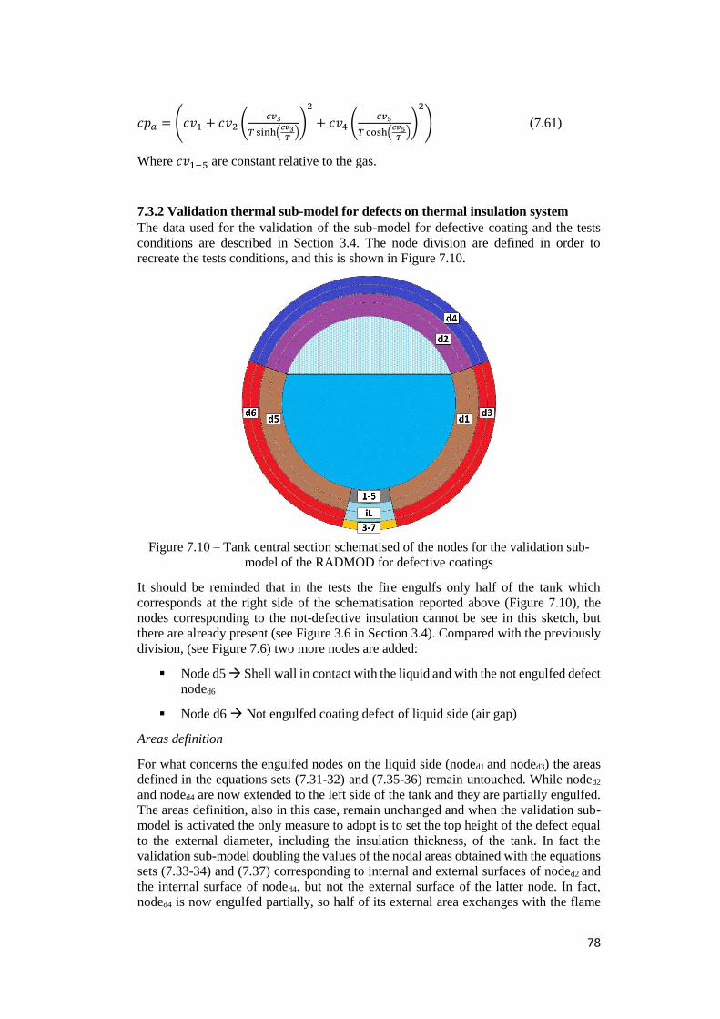
78

𝑐𝑝𝑎 = (𝑐𝑣1 + 𝑐𝑣2 (𝑐𝑣3

𝑇 sinh(𝑐𝑣3

𝑇))

2

+ 𝑐𝑣4 (𝑐𝑣5

𝑇 cosh(𝑐𝑣5

𝑇))

2

) (7.61)

Where 𝑐𝑣1−5 are constant relative to the gas.

7.3.2 Validation thermal sub-model for defects on thermal insulation system

The data used for the validation of the sub-model for defective coating and the tests

conditions are described in Section 3.4. The node division are defined in order to

recreate the tests conditions, and this is shown in Figure 7.10.

Figure 7.10 – Tank central section schematised of the nodes for the validation sub-

model of the RADMOD for defective coatings

It should be reminded that in the tests the fire engulfs only half of the tank which

corresponds at the right side of the schematisation reported above (Figure 7.10), the

nodes corresponding to the not-defective insulation cannot be see in this sketch, but

there are already present (see Figure 3.6 in Section 3.4). Compared with the previously

division, (see Figure 7.6) two more nodes are added:

Node d5 Shell wall in contact with the liquid and with the not engulfed defect

noded6

Node d6 Not engulfed coating defect of liquid side (air gap)

Areas definition

For what concerns the engulfed nodes on the liquid side (noded1 and noded3) the areas

defined in the equations sets (7.31-32) and (7.35-36) remain untouched. While noded2

and noded4 are now extended to the left side of the tank and they are partially engulfed.

The areas definition, also in this case, remain unchanged and when the validation sub-

model is activated the only measure to adopt is to set the top height of the defect equal

to the external diameter, including the insulation thickness, of the tank. In fact the

validation sub-model doubling the values of the nodal areas obtained with the equations

sets (7.33-34) and (7.37) corresponding to internal and external surfaces of noded2 and

the internal surface of noded4, but not the external surface of the latter node. In fact,

noded4 is now engulfed partially, so half of its external area exchanges with the flame

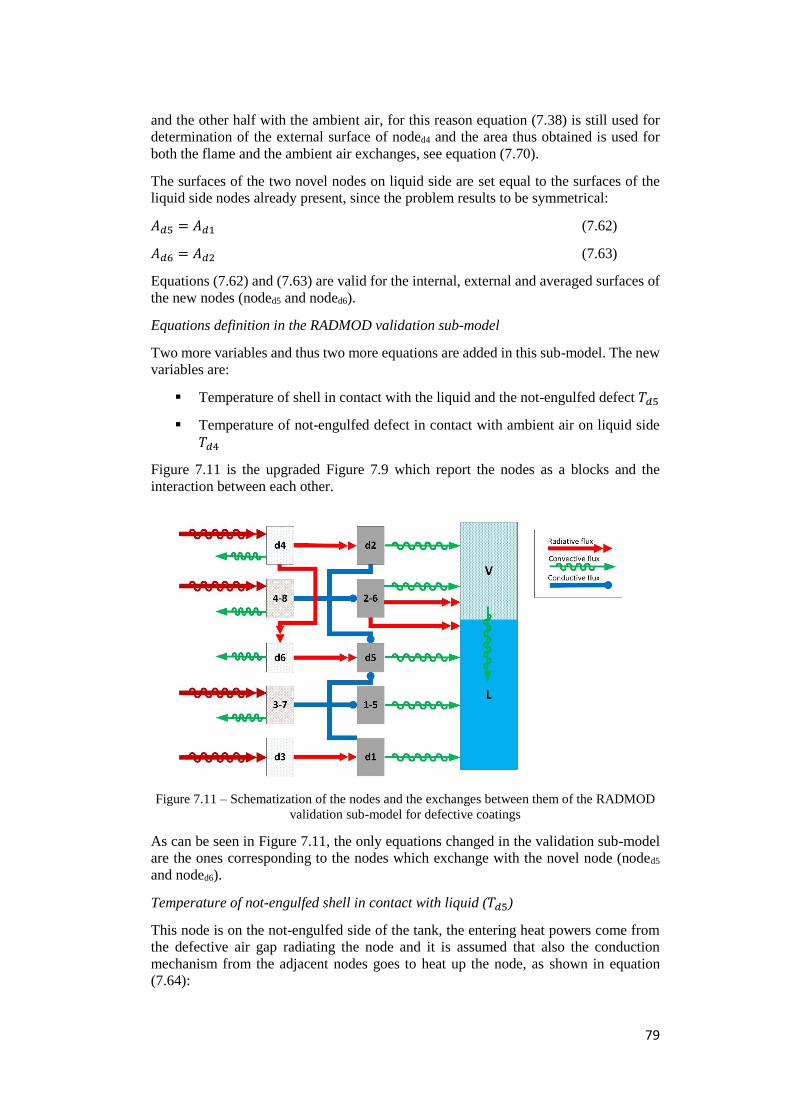
79

and the other half with the ambient air, for this reason equation (7.38) is still used for

determination of the external surface of noded4 and the area thus obtained is used for

both the flame and the ambient air exchanges, see equation (7.70).

The surfaces of the two novel nodes on liquid side are set equal to the surfaces of the

liquid side nodes already present, since the problem results to be symmetrical:

𝐴𝑑5 = 𝐴𝑑1 (7.62)

𝐴𝑑6 = 𝐴𝑑2 (7.63)

Equations (7.62) and (7.63) are valid for the internal, external and averaged surfaces of

the new nodes (noded5 and noded6).

Equations definition in the RADMOD validation sub-model

Two more variables and thus two more equations are added in this sub-model. The new

variables are:

Temperature of shell in contact with the liquid and the not-engulfed defect 𝑇𝑑5

Temperature of not-engulfed defect in contact with ambient air on liquid side

𝑇𝑑4

Figure 7.11 is the upgraded Figure 7.9 which report the nodes as a blocks and the

interaction between each other.

Figure 7.11 – Schematization of the nodes and the exchanges between them of the RADMOD

validation sub-model for defective coatings

As can be seen in Figure 7.11, the only equations changed in the validation sub-model

are the ones corresponding to the nodes which exchange with the novel node (noded5

and noded6).

Temperature of not-engulfed shell in contact with liquid (𝑇𝑑5)

This node is on the not-engulfed side of the tank, the entering heat powers come from

the defective air gap radiating the node and it is assumed that also the conduction

mechanism from the adjacent nodes goes to heat up the node, as shown in equation

(7.64):

80

𝑑𝑠𝑐𝑝𝑠𝐿𝑠𝑠𝐴𝑑5 𝑑𝑇𝑑5

𝑑𝑡= 𝐴𝑑5𝑒𝑥𝑡𝑞𝑑6,𝑟𝑎𝑑 + 𝐴𝑑2𝑑5𝑞𝑑2,𝑐𝑜𝑛𝑑 − 𝐴𝑑5𝑖𝑛𝑡𝑞𝑑5,𝐿 + 𝐴𝑑1𝑑5𝑞𝑑1,𝑐𝑜𝑛𝑑

(7.64)

The heat capacity of the steel shell (𝑐𝑝𝑠𝐿) is calculated as a function of the temperature

of the node. 𝑠𝑠𝐴𝑑5 is the nodal volume and 𝐴𝑑5

, 𝐴𝑑5𝑒𝑥𝑡 and 𝐴𝑑5𝑖𝑛𝑡 are obtained through

the equation (7.62), 𝑞𝑑6,𝑟𝑎𝑑 is the heat flux entering the node by radiation from the

surrounding noded6, it is evaluated as shown in equation (7.71). 𝑞𝑑5,𝐿 is the convective

heat from the shell to the liquid, as for the evaluation of 𝑞𝑑1,𝐿 , it is estimated through

the equation (7.47) with appropriate value of area (𝐴𝑑5𝑖𝑛𝑡) and temperature difference

(𝑇𝑑5 − 𝑇𝐿). Two conduction terms are present in equation (7.64) one from the vapour

side node (𝑞𝑑2,𝑐𝑜𝑛𝑑) and the other one from the liquid engulfed side (𝑞𝑑1,𝑐𝑜𝑛𝑑), they are

introducted to increase the heat load reached by this node and are respectively defined

in equations (7.72) and (7.73). The exchanging area associated with the conduction

terms are:

𝐴𝑑2𝑑5 = 𝐴𝑑1𝑑5 = 𝐿𝑑𝑒𝑓𝑠𝑠 (7.65)

There are the orthogonal surfaces to the cylinder axis, in the interface of noded2 - noded5

and noded1 - noded5 , respectively.

Temperature of not-engulfed defect of liquid in contact with the ambient air (𝑇𝑑6)

This node receives heat from the above noded4 and removes the heat away from noded5

through radiation and from external ambient air:

𝑑𝑎𝑐𝑝𝑎𝑠𝑖𝐴𝑑6 𝑑𝑇𝑑6

𝑑𝑡= 𝐴𝑑4𝑑6𝑞𝑑4,𝑟𝑎𝑑 − 𝐴𝑑5𝑒𝑥𝑡𝑞𝑑6,𝑟𝑎𝑑 − 𝐴𝑑6𝑒𝑥𝑡𝐼𝑎𝑚𝑏 (7.66)

The air properties 𝑑𝑎 and 𝑐𝑝𝑎 are respectively calculated by equations (7.60) and (7.61),

the volume of the air in the node is expressed by 𝑠𝑖𝐴𝑑6 and 𝑞𝑑4,𝑟𝑎𝑑 is the radiative

power from noded6 ,defined in equation (7.78), its exchange surface is defined as:

𝐴𝑑4𝑑6 = 𝐿𝑑𝑒𝑓𝑠𝑖 (7.67)

The latter equation is the same as those defined for the conductive exchange in equation

(7.65), thus it is the interface between the two nodes (noded4 and noded6). Further

investigation on this area definition should be considered. The other areas 𝐴𝑑6𝑒𝑥𝑡 and

𝐴𝑑6 follow the equation (7.63).

𝐼𝑎𝑚𝑏 is the exchange by radiative and convective mechanisms from the node external

surface to the ambient air.

Equations upgrade

The equations used for the implementation of the thermal sub-model for defective

coating are the same in the validation model with the addition of the terms of exchange

with noded5 and noded6, the modified equations are reported below with the unchanged

terms in square bracket:

Temperature of noded1 (𝑇𝑑1)

𝑑𝑠𝑐𝑝𝑠𝐿𝑠𝑠𝐴𝑑1 𝑑𝑇𝑑1

𝑑𝑡= [𝐴𝑑1𝑒𝑥𝑡𝑞𝑑3,𝑟𝑎𝑑 − 𝑞𝑑1,𝐿]−𝐴𝑑1𝑑5𝑞𝑑1,𝑐𝑜𝑛𝑑 (7.68)

Temperature of noded2 (𝑇𝑑2)

𝑑𝑠𝑐𝑝𝑠𝑉𝑠𝑠𝐴𝑑2 𝑑𝑇𝑑2

𝑑𝑡= [𝐴𝑑2𝑒𝑥𝑡𝑞𝑑4,𝑟𝑎𝑑 − 𝑞𝑑2,𝑉] − 𝐴𝑑2𝑑5𝑞𝑑2,𝑐𝑜𝑛𝑑 (7.69)

81

Temperature of noded4 (𝑇𝑑4)

𝑑𝑎𝑐𝑝𝑎𝑠𝑖𝐴𝑑4 𝑑𝑇𝑑4

𝑑𝑡= [𝐴𝑑4𝑒𝑥𝑡𝐼𝑒𝑥𝑡 − 𝐴𝑑2𝑒𝑥𝑡𝑞𝑑4,𝑟𝑎𝑑] − 𝐴𝑑4𝑒𝑥𝑡𝐼𝑎𝑚𝑏 − 𝐴𝑑4𝑑6𝑞𝑑4,𝑟𝑎𝑑

(7.70)

Temperature of liquid (𝑇𝐿)

𝑚𝐿𝑐𝑣𝐿𝑑𝑇𝐿

𝑑𝑡= [𝑞𝐿 + 𝑞𝐿𝑉 + 𝑞𝑑1,𝐿] + 𝐴𝑑5𝑖𝑛𝑡𝑞𝑑5,𝐿 (7.71)

Heat load from the flame

The radiative part of heat that from the flame reaches the external steel jacket, expressed

through equation (7.8) in the validation model is modified in order to set the black body

temperature as input instead of the flame temperature. The two temperatures are linked

together through the flame emissivity as: 𝜀𝑓 ∙ 𝑇𝑓4 = 𝑇𝐵𝐵

4 [Modest, 2003], thus, replacing

the term (𝜀𝑓 ∙ 𝑇𝑓4) in equation (7.8), the latter becomes:

𝐼𝑒𝑥𝑡 = 𝜎𝜀𝑠(𝑇 𝐵𝐵4 + (1 − 𝜀𝑓)𝑇𝑎𝑚𝑏

4 ) − (𝜎𝜀𝑠𝑇𝑤4) (7.72)

Heat loads to the shell node of not-engulfed liquid side (noded5)

The radiant flux at input of the node is written as:

𝑞𝑑6,𝑟𝑎𝑑 = 𝜎𝜀𝑠(𝑇𝑑64 − 𝑇𝑑5

4 ) (7.73)

Equation (7.73) corresponds to the equation (7.59), with the adequate parameters, used

for the evaluation of the heat transported by radiation inside the enclosure.

The other two thermal inputs at the shell node are both conductive from the engulfed

shell nodes:

𝑞𝑑1,𝑐𝑜𝑛𝑑 =𝑘𝑠𝐿

𝑑𝑐𝑜𝑛𝑑𝐿(𝑇𝑑1 − 𝑇𝑑5) (7.74)

𝑞𝑑2,𝑐𝑜𝑛𝑑 =𝑘𝑠𝑉

𝑑𝑐𝑜𝑛𝑑𝑉(𝑇𝑑2 − 𝑇𝑑5) (7.75)

The thermal conductivities 𝑘𝑠𝐿 and 𝑘𝑠𝑉 are estimating as functions of the temperature

of each node. The term 𝑑𝑐𝑜𝑛𝑑 is the distance between the node through which the

conductive exchange takes place. It is assumed equal to the circumferential arc from the

higher point of the heating node, to the start of the node to be heat, that are:

𝑑𝑐𝑜𝑛𝑑𝐿 =𝑅𝑖

2acos (

𝑅𝑖−𝐿

𝑅𝑖) (7.76)

𝑑𝑐𝑜𝑛𝑑𝑉 = (𝑅𝑖 +𝑠𝑠

2) 𝛼𝑡𝑜𝑝 (7.77)

The subscript (L) is associated to the conduction from the engulfed liquid side node

(noded1) and the subscript (V) indicates the conduction from the engulfed, even if

partially, vapour side node (noded2). Two of the test used for the validation have the

defect covering all the circumference of the vessel, while one test has the configuration

shown in Figure 7.10, where the “defective” shell node on the liquid side are not in

direct contact, thus the term 𝑞𝑑1,𝑐𝑜𝑛𝑑 should not be present or at least should be referred

to the node in real contact with the defect (node15), but in the code this term is left

unchanged since the difference between the temperature of the real-contact node

(node15) and the implemented node (noded1) is not so relevant (about 10°C).

82

Heat loads to the not-engulfed defect node of liquid side (noded6)

The only term entering the node is from the surrounding air gap (noded4) which radiates

noded4, the equation for the evaluation of this radiative flux is defined in the same way

as for the radiative exchange inside the enclosure, equation (7.59), by including the

appropriate temperature, as shown in equation (7.78):

𝑞𝑑4,𝑟𝑎𝑑 = 𝜎𝜀𝑠(𝑇𝑑44 − 𝑇𝑑6

4 ) (7.78)

Validation set-up

The RADMOD validation sub-model described in this paragraph (7.3.2) is used

considering also the stratification sub-model (strat3). During the validation a tuning

factor is introduced for the height of the stratified layer, its value is set equal to 2. The

doubled height of the stratified layer resulted to be around 60% of the total liquid filling

level, such value of stratified depth, imposed in the stratification sub-model, represents

a halfway between the Baseline and the stratified RADMOD models, respectively

advised for unprotected and coated tanks, just as the problem implemented was.

Moreover, the heat exchanges between the not engulfed defect (noded4) and ambient air

was overestimated by 3 times.

7.3.3 Software implementation

There are five main MatLab codes developed, four of which are pre-existing codes and

they consider the baseline and the three stratification sub-models version of RADMOD.

They are called RADMOD_Baseline.m , RADMOD_Strat1.m, RADMOD_Strat2.m and

RADMOD_Strat3.m. The fifth main code is called RADMOD_defect and considers both

the Baseline and the Strat3 version. Other than these core files there are several

functions for external evaluation, like for the thermodynamic properties of lading and

wall material and for the heat-transfer coefficients. Each function can be called up

within the main code to calculate the variation of these parameters with the time.

Three Excel files are included, two for the initial data set-up: InitialData.xlsx for the

pre-existing main codes and InitialData_def.xlsx for the novel implementation of the

code for defective coatings (RADMOD_defect.m); and a third Excel file for reporting

results (Results.xlsx). The two files for the input set-up are identical except for the

section dedicated to the defect, which it was not present in the previously version of the

code, and for the position of the cell. The first recommendation is to use the appropriate

input file with the appropriate .m file or MatLab cannot read correctly the cell, so with

respect to the model version that has to be run choose the appropriate input Excel file

following the Table 7.4.

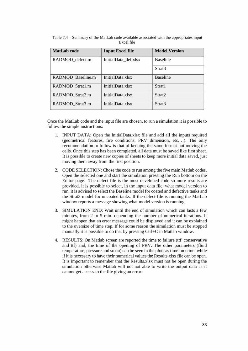
83

Table 7.4 – Summary of the MatLab code available associated with the appropriates input

Excel file

MatLab code Input Excel file Model Version

RADMOD_defect.m InitialData_def.xlsx Baseline

Strat3

RADMOD_Baseline.m InitialData.xlsx Baseline

RADMOD_Strat1.m InitialData.xlsx Strat1

RADMOD_Strat2.m InitialData.xlsx Strat2

RADMOD_Strat3.m InitialData.xlsx Strat3

Once the MatLab code and the input file are chosen, to run a simulation it is possible to

follow the simple instructions:

1. INPUT DATA: Open the InitialData.xlsx file and add all the inputs required

(geometrical features, fire conditions, PRV dimension, etc.…). The only

recommendation to follow is that of keeping the same format not moving the

cells. Once this step has been completed, all data must be saved like first sheet.

It is possible to create new copies of sheets to keep more initial data saved, just

moving them away from the first position.

2. CODE SELECTION: Chose the code to run among the five main Matlab codes.

Open the selected one and start the simulation pressing the Run bottom on the

Editor page. The defect file is the most developed code so more results are

provided, it is possible to select, in the input data file, what model version to

run, it is advised to select the Baseline model for coated and defective tanks and

the Strat3 model for uncoated tanks. If the defect file is running the MatLab

window reports a message showing what model version is running.

3. SIMULATION END: Wait until the end of simulation which can lasts a few

minutes, from 2 to 5 min. depending the number of numerical iterations. It

might happen that an error message could be displayed and it can be explained

to the oversize of time step. If for some reason the simulation must be stopped

manually it is possible to do that by pressing Ctrl+C in Matlab window.

4. RESULTS: On Matlab screen are reported the time to failure (ttf_conservative

and ttf) and, the time of the opening of PRV. The other parameters (fluid

temperature, pressure and so on) can be seen in the plots as time function, while

if it is necessary to have their numerical values the Results.xlsx file can be open.

It is important to remember that the Results.xlsx must not be open during the

simulation otherwise Matlab will not not able to write the output data as it

cannot get access to the file giving an error.

84

8 Definition of sensitivity analysis and case studies

Two modelling approaches are adopted in this thesis work: an advanced finite elements

method (FEM) model and a simplified lumped parameters model, both are aimed to

assess the performance of insulated tanks exposed to fire in presence of defects in their

thermal insulation system. A sensitivity analysis is performed on the FEM model, the

parameters to vary and their values are discussed in this chapter in the following section

8.1. Whereas the lumped model is applied to real-scale case studies, section 8.2 is

dedicated to the definition of variables and geometries individuated for the simulations.

The results of the sensitivity analysis and case studies are reported and discussed in

chapter 9.

8.1 Sensitivity analysis

In order to provide a sensitivity analysis for the FEM model, a series of variables are

selected, in order to assess the effect of their variation. The implementation of a model,

in general, requires several guesses and approximations of the realty. In the specific case

of a model for tanks engulfed in fires, the assumptions made, especially in the

approximation of flame conditions, may lead to relevant modification in the final results

[Birk, 1995].

This part of the thesis work is aimed to understand how each assumption adopted in the

model influences the simulation results, in order to assess which parameters should be

modelled more accurately and which not significantly influence the response. This is

aimed at determining the uncertainties affecting the model and the reliability of

computer simulations.

he mesh and time step implemented in the analysis are described in chapter 6, where it

is also assessed the mesh independency (see section 6.3.3). The geometries and the

boundary conditions implemented are the same used for the validation of the FEM

model. As in the validation, the geometry is a quarter portion of a tank equipped with a

coating blanket of ceramic fibre to which a square portion (15.2x15.2 mm2) of insulation

is removed. Both the external steel jacket and the shell wall are made of carbon steel.

The internal shell wall surface is supposed to be in contact with ambient air while the

flame engulfs the complete external surface of the jacket.

Three model geometries are simulated, each varying five variables related both to the

flame and to the steel, as follows:

Geometries

Fully protected

Sealed

Defect 15.2

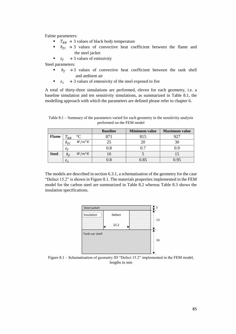
85

Falme parameters:

𝑇𝐵𝐵 3 values of black body temperature

ℎ𝑓𝑙 3 values of convective heat coefficient between the flame and

the steel jacket

𝜀𝑓 3 values of emissivity

Steel parameters:

ℎ𝑓 3 values of convective heat coefficient between the tank shell

and ambient air

𝜀𝑠 3 values of emessivity of the steel exposed to fire

A total of thirty-three simulations are performed, eleven for each geometry, i.e. a

baseline simulation and ten sensitivity simulations, as summarized in Table 8.1, the

modelling approach with which the parameters are defined please refer to chapter 6.

Table 8.1 – Summary of the parameters varied for each geometry in the sensitivity analysis

performed on the FEM model

Baseline Minimum value Maximum value

Flame 𝑇𝐵𝐵 °C 871 815 927

ℎ𝑓𝑙 𝑊/𝑚2𝐾 25 20 30

𝜀𝑓 0.8 0.7 0.9

Steel ℎ𝑓 𝑊/𝑚2𝐾 10 5 15

𝜀𝑠 0.8 0.85 0.95

The models are described in section 6.3.1, a schematisation of the geometry for the case

“Defect 15.2” is shown in Figure 8.1. The materials properties implemented in the FEM

model for the carbon steel are summarized in Table 8.2 whereas Table 8.3 shows the

insulation specifications.

Figure 8.1 – Schematisation of geometry ID “Defect 15.2” implemented in the FEM model,

lengths in mm

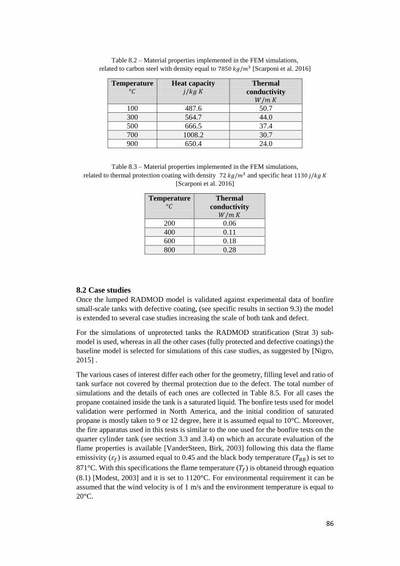
86

Table 8.2 – Material properties implemented in the FEM simulations,

related to carbon steel with density equal to 7850 𝑘𝑔/𝑚3 [Scarponi et al. 2016]

Temperature °𝐶

Heat capacity 𝑗/𝑘𝑔 𝐾

Thermal

conductivity 𝑊/𝑚 𝐾

100 487.6 50.7

300 564.7 44.0

500 666.5 37.4

700 1008.2 30.7

900 650.4 24.0

Table 8.3 – Material properties implemented in the FEM simulations,

related to thermal protection coating with density 72 𝑘𝑔/𝑚3 and specific heat 1130 𝑗/𝑘𝑔 𝐾

[Scarponi et al. 2016]

Temperature °𝐶

Thermal

conductivity 𝑊/𝑚 𝐾

200 0.06

400 0.11

600 0.18

800 0.28

8.2 Case studies

Once the lumped RADMOD model is validated against experimental data of bonfire

small-scale tanks with defective coating, (see specific results in section 9.3) the model

is extended to several case studies increasing the scale of both tank and defect.

For the simulations of unprotected tanks the RADMOD stratification (Strat 3) sub-

model is used, whereas in all the other cases (fully protected and defective coatings) the

baseline model is selected for simulations of this case studies, as suggested by [Nigro,

2015] .

The various cases of interest differ each other for the geometry, filling level and ratio of

tank surface not covered by thermal protection due to the defect. The total number of

simulations and the details of each ones are collected in Table 8.5. For all cases the

propane contained inside the tank is a saturated liquid. The bonfire tests used for model

validation were performed in North America, and the initial condition of saturated

propane is mostly taken to 9 or 12 degree, here it is assumed equal to 10°C. Moreover,

the fire apparatus used in this tests is similar to the one used for the bonfire tests on the

quarter cylinder tank (see section 3.3 and 3.4) on which an accurate evaluation of the

flame properties is available [VanderSteen, Birk, 2003] following this data the flame

emissivity (𝜀𝑓) is assumed equal to 0.45 and the black body temperature (𝑇𝐵𝐵) is set to

871°C. With this specifications the flame temperature (𝑇𝑓) is obtaneid through equation

(8.1) [Modest, 2003] and it is set to 1120°C. For environmental requirement it can be

assumed that the wind velocity is of 1 m/s and the environment temperature is equal to

20°C.

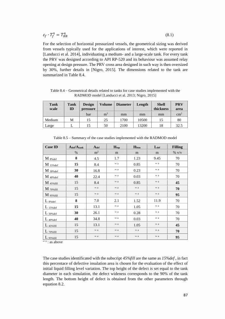
87

𝜀𝑓 ∙ 𝑇𝑓4 = 𝑇𝐵𝐵

4 (8.1)

For the selection of horizontal pressurized vessels, the geometrical sizing was derived

from vessels typically used for the applications of interest, which were reported in

[Landucci et al. 2014], individuating a medium- and a large-scale tank. For every tank

the PRV was designed according to API RP-520 and its behaviour was assumed relay

opening at design pressure. The PRV cross area designed in such way is then oversized

by 30%, further details in [Nigro, 2015]. The dimensions related to the tank are

summarized in Table 8.4.

Table 8.4 – Geometrical details related to tanks for case studies implemented with the

RADMOD model [Landucci et al. 2013; Nigro, 2015]

Tank

scale

Tank

ID

Design

pressure

Volume Diameter Length Shell

thickness

PRV

area

bar m3 mm mm mm cm2

Medium M 15 25 1700 10500 15 80

Large L 15 50 2100 13200 18 32.5

Table 8.5 – Summary of the case studies implemented with the RADMOD model

Case ID Adef/Atank Adef Htop Hbtm Ldef Filling

% m2 m m m % v/v

M 8%def 8 4.5 1.7 1.23 9.45 70

M 15%def 15 8.4 “ a 0.85 “ a 70

M 30%def 30 16.8 “ a 0.23 “ a 70

M 40%def 40 22.4 “ a 0.03 “ a 70

M 45%fill 15 8.4 “ a 0.85 “ a 45

M 70%fill 15 “ a “ a “ a “ a 70

M 95%fill 15 “ a “ a “ a “ a 95

L 8%def 8 7.0 2.1 1.52 11.9 70

L 15%def 15 13.1 “ a 1.05 “ a 70

L 30%def 30 26.1 “ a 0.28 “ a 70

L 40%def 40 34.8 “ a 0.03 “ a 70

L 45%fill 15 13.1 “ a 1.05 “ a 45

L 70%fill 15 “ a “ a “ a “ a 70

L 95%fill 15 “ a “ a “ a “ a 95

“ a : as above

The case studies identificated with the subscript 45%fill are the same as 15%def , in fact

this percentace of defective insulation area is chosen for the evaluation of the effect of

initial liquid filling level variation. The top height of the defect is set equal to the tank

diameter in each simulation, the defect wideness corresponds to the 90% of the tank

length. The bottom height of defect is obtained from the other parameters through

equation 8.2.

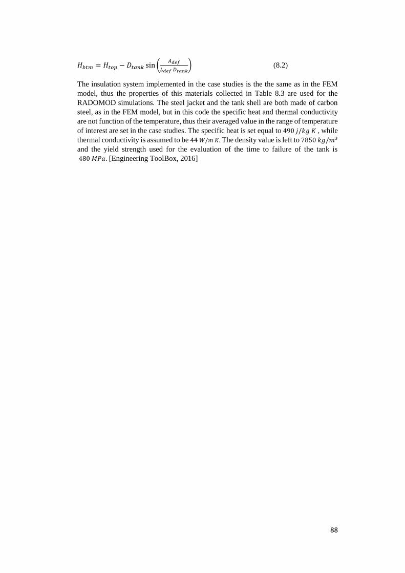
88

𝐻𝑏𝑡𝑚 = 𝐻𝑡𝑜𝑝 − 𝐷𝑡𝑎𝑛𝑘 sin (𝐴𝑑𝑒𝑓

𝐿𝑑𝑒𝑓 𝐷𝑡𝑎𝑛𝑘) (8.2)

The insulation system implemented in the case studies is the the same as in the FEM

model, thus the properties of this materials collected in Table 8.3 are used for the

RADOMOD simulations. The steel jacket and the tank shell are both made of carbon

steel, as in the FEM model, but in this code the specific heat and thermal conductivity

are not function of the temperature, thus their averaged value in the range of temperature

of interest are set in the case studies. The specific heat is set equal to 490 𝑗/𝑘𝑔 𝐾 , while

thermal conductivity is assumed to be 44 𝑊/𝑚 𝐾. The density value is left to 7850 𝑘𝑔/𝑚3

and the yield strength used for the evaluation of the time to failure of the tank is

480 𝑀𝑃𝑎. [Engineering ToolBox, 2016]

89

9 Results and discussion

9.1 FEM validation results

The validation of the FEM model was carried out against the experimental data

described in section 3.3. Several squared defects on a quarter portion of tank were

bonfire tested and thus the geometries implemented for the validation aimed to

reproduce them. The geometries implemented were specified according to Section 6.3

and the boundary conditions were modelled as reported in section 6.2. For further details

on the FEM model validation refer to [Scarponi et al. 2016].

9.2 Sensitivity analysis results

In this section are reported the results of the sensitivity analysis performed on the FEM

model. The aim of this analysis is understanding which of the several parameters

implemented in the model, have significant influence on the results obtained. The

geometries, the parameters and the boundary conditions of the simulations performed

during the sensitivity analysis are reported in section 8.1. The results are collected in

Figures 9.3 and Figures 9.4, where the curves are obtained setting-up a baseline

simulation, taking its parameters value as a reference to the comparison with the results

of the sensitivity simulations, in which only one parameter value differs from the

baseline.

The sensitivity analysis was performed on three different geometries: with coating,

completely without coating and with coating in presence of defect; in this section are

shown only the results of the latter geometry since it involved more phenomena and

thus it can be considers the completest-case examined.

9.2.1 Dynamic analysis of temperature in the center of defect

Figures 9.3 (a, b, c, d, e) show the dynamic temperature behaviour of the central point

of the defect in function of the time. In particular each figure shows the results obtained

changing one parameter: (a) black body temperature of the flame, (b) emissivity of the

flame, (c) emissivity of the steel exposed to fire, convective heat coefficient between

the flame and external steel jacket (d) or between the internal shell and ambient air (e).

The baseline simulation is indicated as “Base_” followed by the reference-value of the

parameters on which the sensitivity analysis is performed, the results of the other

simulations are identified specifying the variable name and its associated value

implemented in the model. The results are summarized in Table 9.1 reporting the

relative error of each simulation with respect the baseline temperature.

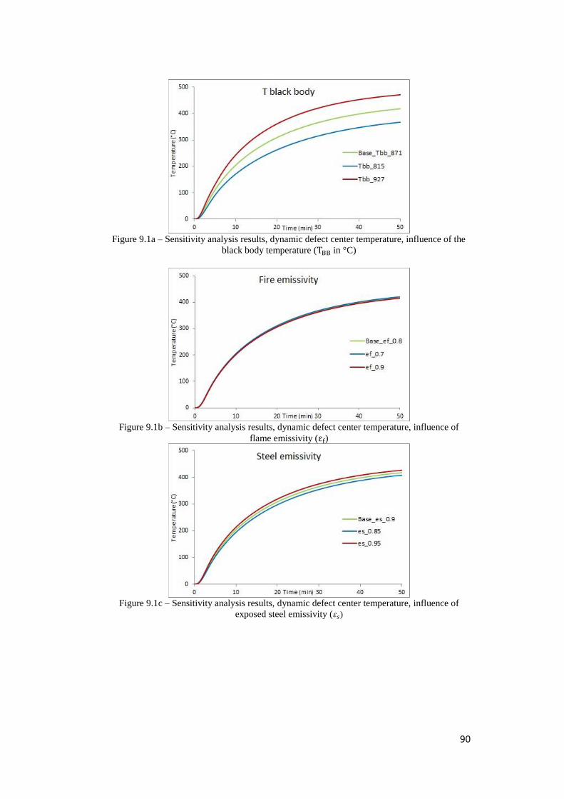
90

Figure 9.1a – Sensitivity analysis results, dynamic defect center temperature, influence of the

black body temperature (TBB in °C)

Figure 9.1b – Sensitivity analysis results, dynamic defect center temperature, influence of

flame emissivity (εf)

Figure 9.1c – Sensitivity analysis results, dynamic defect center temperature, influence of

exposed steel emissivity (𝜀𝑠)

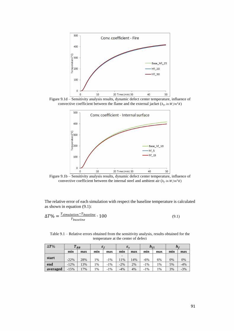
91

Figure 9.1d – Sensitivity analysis results, dynamic defect center temperature, influence of

convective coefficient between the flame and the external jacket (ℎ𝑓𝑙 𝑖𝑛 𝑊/𝑚2𝐾)

Figure 9.1b – Sensitivity analysis results, dynamic defect center temperature, influence of

convective coefficient between the internal steel and ambient air (ℎ𝑓 𝑖𝑛 𝑊/𝑚2𝐾)

The relative error of each simulation with respect the baseline temperature is calculated

as shown in equation (9.1):

∆𝑇% =𝑇𝑠𝑖𝑚𝑢𝑙𝑎𝑡𝑖𝑜𝑛−𝑇𝑏𝑎𝑠𝑒𝑙𝑖𝑛𝑒

𝑇𝑏𝑎𝑠𝑒𝑙𝑖𝑛𝑒∙ 100 (9.1)

Table 9.1 – Relative errors obtained from the sensitivity analysis, results obtained for the

temperature at the center of defect

∆𝑻% 𝑻𝑩𝑩 𝜺𝒇 𝜺𝒔 𝒉𝒇𝒍 𝒉𝒇 min max min max min max min max min max

start -22% 28% 1% -1%

-

11% 14% -6% 6% 0% 0%

end -12% 13% 1% -1% -2% 2% -1% 1% 5% -4%

averaged -15% 17% 1% -1% -4% 4% -1% 1% 3% -3%

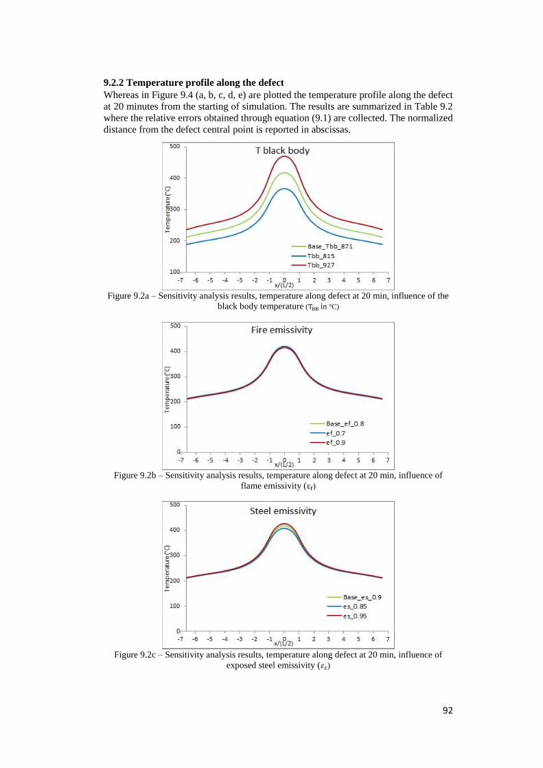
92

9.2.2 Temperature profile along the defect

Whereas in Figure 9.4 (a, b, c, d, e) are plotted the temperature profile along the defect

at 20 minutes from the starting of simulation. The results are summarized in Table 9.2

where the relative errors obtained through equation (9.1) are collected. The normalized

distance from the defect central point is reported in abscissas.

Figure 9.2a – Sensitivity analysis results, temperature along defect at 20 min, influence of the

black body temperature (TBB in °C)

Figure 9.2b – Sensitivity analysis results, temperature along defect at 20 min, influence of

flame emissivity (εf)

Figure 9.2c – Sensitivity analysis results, temperature along defect at 20 min, influence of

exposed steel emissivity (𝜀𝑠)

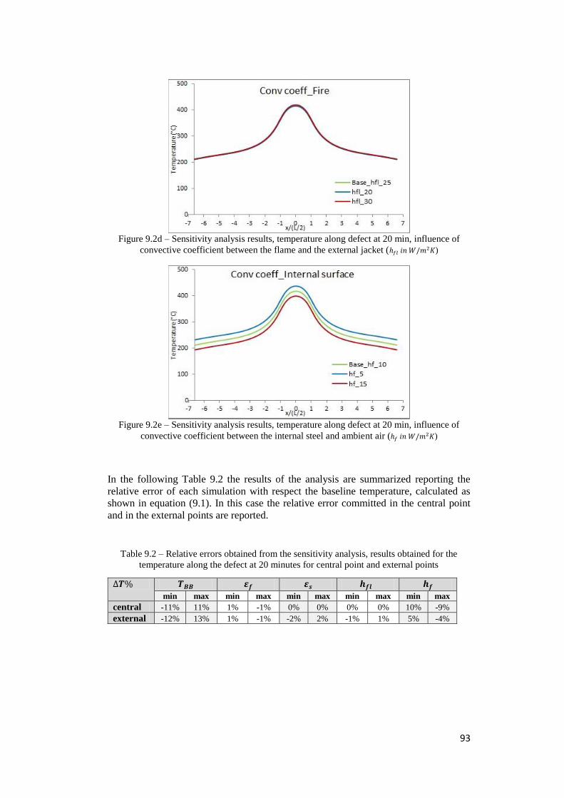
93

Figure 9.2d – Sensitivity analysis results, temperature along defect at 20 min, influence of

convective coefficient between the flame and the external jacket (ℎ𝑓𝑙 𝑖𝑛 𝑊/𝑚2𝐾)

Figure 9.2e – Sensitivity analysis results, temperature along defect at 20 min, influence of

convective coefficient between the internal steel and ambient air (ℎ𝑓 𝑖𝑛 𝑊/𝑚2𝐾)

In the following Table 9.2 the results of the analysis are summarized reporting the

relative error of each simulation with respect the baseline temperature, calculated as

shown in equation (9.1). In this case the relative error committed in the central point

and in the external points are reported.

Table 9.2 – Relative errors obtained from the sensitivity analysis, results obtained for the

temperature along the defect at 20 minutes for central point and external points

∆𝑻% 𝑻𝑩𝑩 𝜺𝒇 𝜺𝒔 𝒉𝒇𝒍 𝒉𝒇 min max min max min max min max min max

central -11% 11% 1% -1% 0% 0% 0% 0% 10% -9%

external -12% 13% 1% -1% -2% 2% -1% 1% 5% -4%

94

9.2.3 Discussion on the sensitivity analysis results

The sensibility analysis highlights that the results are main influenced by the flame black

body temperature amongst other parameters. This results was expected since the

radiative heat power received by the system from the flame is a function of the

temperature raised to the fourth power, thus a variation in the flame temperature should

significantly affect the thermal behaviour of the system. The results of the

implementation supports the previously assumption, different black body temperatures

show variation from the baseline of about 30% in the dynamic analysis and a little bit

more than the 10% in the defect temperature profile at 20 minutes. Clearly, a black

body temperature increase leads to an increase of the temperature reached in the defect,

and vice versa.

The other parameter which was expected to influence the thermal behaviour of the

system was the flame emissivity, it determines, in this case, the temperature of

convective exchange of the flame. In fact in this model the black body temperature and

the flame emissivity are set as input data and the flame temperature (𝑇𝑓) is obtained

from this two parameters, as equation (9.2) shows.

𝜀𝑓 ∙ 𝑇𝑓4 = 𝑇𝐵𝐵

4 (9.2)

Nevertheless, the results of this analysis point out that changing the emissivity of the

flame a maximum of 1% error can be reached. This is probably due to the few

contribution of the convective heat transfer mechanism compared to the radiative one,

this can be see also in the results obtained changing the emissivity of the steel exposed

to fire and the convective heat exchange from the flame and the jacket. Changing the

steel emissivity the results get far from the baseline ones of a 5% and in fact, the it

regulates the radiative exchange between the flame and the external jacket. Whereas

different value of the convective heat exchange of the flame do not affect the

temperature reached in the defect.

The last variable analysed is the convective heat transport coefficient of the inner tank

wall in contact with ambient air. Its influence can be seen in the temperature profile

along the defect at 20 minutes (Figure 9.3e), if the coefficient increases the dissipative

power from the wall increases and thus the temperature in the defect results to be lower,

and vice versa.

The sensitivity analysis highlights the importance of modelling the parameters linked to

the radiative exchange between the flame and the jacket. In particular the main variable

able to affect significantly the results is the black body temperature of the flame.

95

9.4 RADMOD validation

The lumped parameters model (RADMOD) was enhanced for the simulation of coated

tanks exposed to fire in presence of defect in their insulation system. In order to assess

the credibility of the results obtained with the novel RADMOD model, a validation

against experimental data was needed. The validation of the model was carried out by

comparison the results obtained with the RADMOD model and the results of the bonfire

tests described in section 3.4.

The boundary conditions were set-up according to section 7.4. The geometries and the

insulation properties were implemented in order to recreate the same conditions of the

bonfire tests, thus all details are specified in section 3.4, with the exception of the tank

length, which value was set to 2.12 m neglecting the heads of the tank. The steel

properties are reported in section 8.2 as they were also used for the case-studies

simulations.

The experimental available data concern: the temperature of the lading (vapour and

liquid phase), the temperature of the wall exposed to fire and the pressure reached inside

the tank. Three bonfire tests were carried out and thus three set of data were available

for the validation of the model, some specifications on the set-up related to the three

cases are summarized in table 9.3.

Table 9.3 – Information on the input data used in the RADMOD validation

Bonfire test ID 04-03 04-04 04-05

Adef/Atank (%) 15% 15% 8%

Filling degree (%) 71% 78% 71%

Time step (s) 1 1 1

Initial lading pressure (bar) 6.6 8.9 6.6

PRV opening P (bar) 26.26 21.2 26.26

PRV closing P (bar) 23.85 19.3 23.85

The PRV behaviour was assumed to be relay and the discharge area was set to 1.8 cm2

. The ambient temperature was estimated to be 18°C with a wind velocity of 1 m/s. The

time checked for each simulation was choose equal to the time at which the tanks failed

during the bonfire tests. The black body temperature of the flame was set equal to 871°C

with an emissivity of 0.45.

9.4.1 Validation results – Pressure prediction

Figure 9.4 shows the pressure results obtained with the RADMOD model compared

with the results of the experimental tests, in particular: (a) test 04-03, (b) test 04-04 and

(c) test 04-05. It is reported also the time to failure predicted by the model with the two

different criteria explained in paragraph 7.2.4 and the experimental ones estimated by

Birk [Birk et al. 2006], more details in section 3.4.

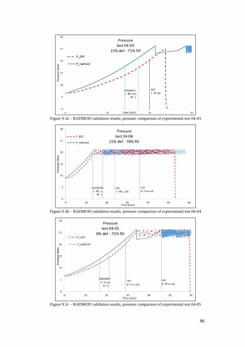
96

Figure 9.3a – RADMOD validation results, pressure comparison of experimental test 04-03

Figure 9.3b – RADMOD validation results, pressure comparison of experimental test 04-04

Figure 9.3c – RADMOD validation results, pressure comparison of experimental test 04-05

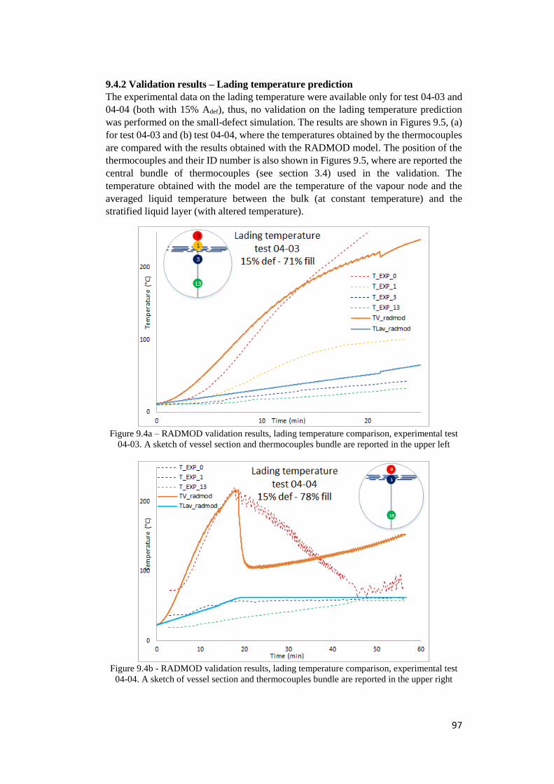
97

9.4.2 Validation results – Lading temperature prediction

The experimental data on the lading temperature were available only for test 04-03 and

04-04 (both with 15% Adef), thus, no validation on the lading temperature prediction

was performed on the small-defect simulation. The results are shown in Figures 9.5, (a)

for test 04-03 and (b) test 04-04, where the temperatures obtained by the thermocouples

are compared with the results obtained with the RADMOD model. The position of the

thermocouples and their ID number is also shown in Figures 9.5, where are reported the

central bundle of thermocouples (see section 3.4) used in the validation. The

temperature obtained with the model are the temperature of the vapour node and the

averaged liquid temperature between the bulk (at constant temperature) and the

stratified liquid layer (with altered temperature).

Figure 9.4a – RADMOD validation results, lading temperature comparison, experimental test

04-03. A sketch of vessel section and thermocouples bundle are reported in the upper left

Figure 9.4b - RADMOD validation results, lading temperature comparison, experimental test

04-04. A sketch of vessel section and thermocouples bundle are reported in the upper right

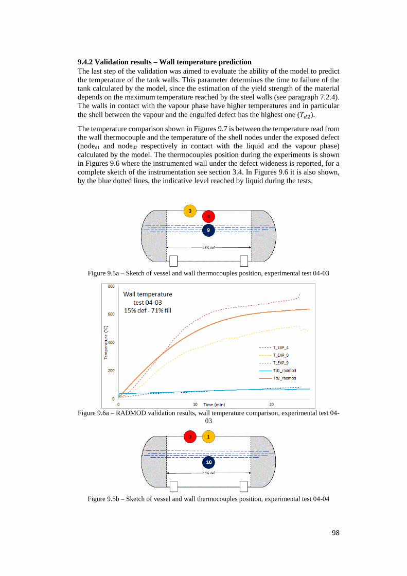
98

9.4.2 Validation results – Wall temperature prediction

The last step of the validation was aimed to evaluate the ability of the model to predict

the temperature of the tank walls. This parameter determines the time to failure of the

tank calculated by the model, since the estimation of the yield strength of the material

depends on the maximum temperature reached by the steel walls (see paragraph 7.2.4).

The walls in contact with the vapour phase have higher temperatures and in particular

the shell between the vapour and the engulfed defect has the highest one (𝑇𝑑2).

The temperature comparison shown in Figures 9.7 is between the temperature read from

the wall thermocouple and the temperature of the shell nodes under the exposed defect

(noded1 and noded2 respectively in contact with the liquid and the vapour phase)

calculated by the model. The thermocouples position during the experiments is shown

in Figures 9.6 where the instrumented wall under the defect wideness is reported, for a

complete sketch of the instrumentation see section 3.4. In Figures 9.6 it is also shown,

by the blue dotted lines, the indicative level reached by liquid during the tests.

Figure 9.5a – Sketch of vessel and wall thermocouples position, experimental test 04-03

Figure 9.6a – RADMOD validation results, wall temperature comparison, experimental test 04-

03

Figure 9.5b – Sketch of vessel and wall thermocouples position, experimental test 04-04

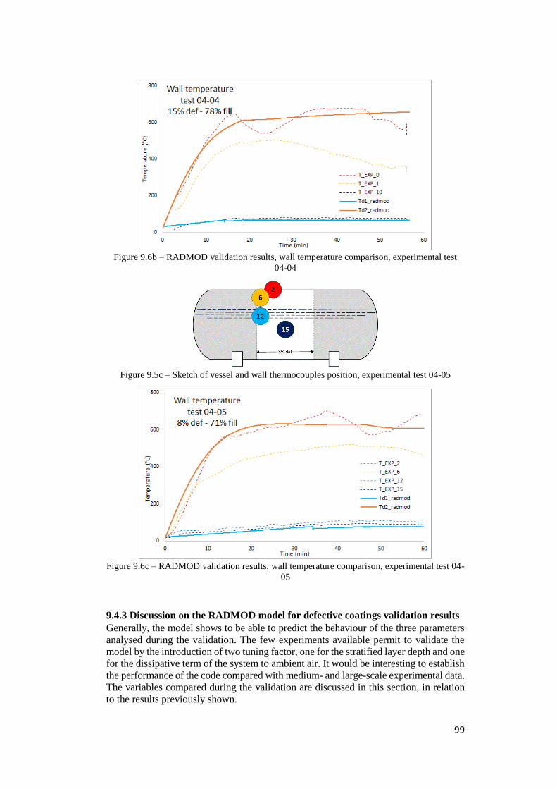
99

Figure 9.6b – RADMOD validation results, wall temperature comparison, experimental test

04-04

Figure 9.5c – Sketch of vessel and wall thermocouples position, experimental test 04-05

Figure 9.6c – RADMOD validation results, wall temperature comparison, experimental test 04-

05

9.4.3 Discussion on the RADMOD model for defective coatings validation results

Generally, the model shows to be able to predict the behaviour of the three parameters

analysed during the validation. The few experiments available permit to validate the

model by the introduction of two tuning factor, one for the stratified layer depth and one

for the dissipative term of the system to ambient air. It would be interesting to establish

the performance of the code compared with medium- and large-scale experimental data.

The variables compared during the validation are discussed in this section, in relation

to the results previously shown.

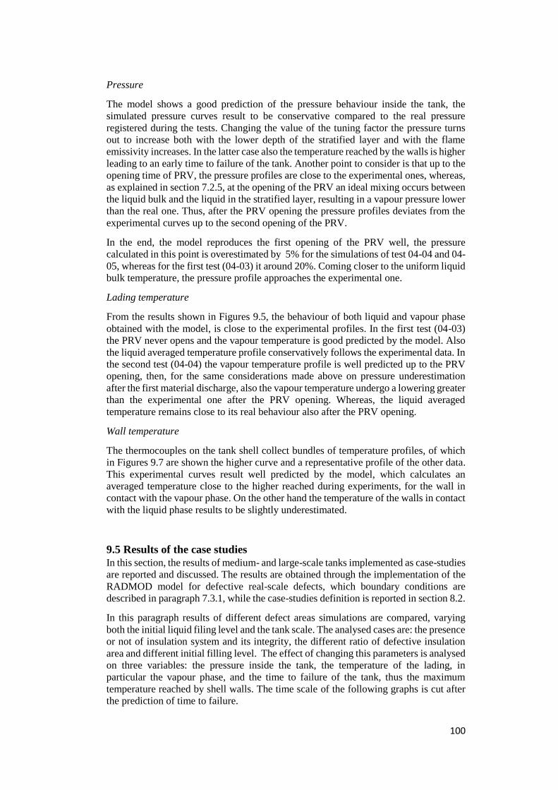
100

Pressure

The model shows a good prediction of the pressure behaviour inside the tank, the

simulated pressure curves result to be conservative compared to the real pressure

registered during the tests. Changing the value of the tuning factor the pressure turns

out to increase both with the lower depth of the stratified layer and with the flame

emissivity increases. In the latter case also the temperature reached by the walls is higher

leading to an early time to failure of the tank. Another point to consider is that up to the

opening time of PRV, the pressure profiles are close to the experimental ones, whereas,

as explained in section 7.2.5, at the opening of the PRV an ideal mixing occurs between

the liquid bulk and the liquid in the stratified layer, resulting in a vapour pressure lower

than the real one. Thus, after the PRV opening the pressure profiles deviates from the

experimental curves up to the second opening of the PRV.

In the end, the model reproduces the first opening of the PRV well, the pressure

calculated in this point is overestimated by 5% for the simulations of test 04-04 and 04-

05, whereas for the first test (04-03) it around 20%. Coming closer to the uniform liquid

bulk temperature, the pressure profile approaches the experimental one.

Lading temperature

From the results shown in Figures 9.5, the behaviour of both liquid and vapour phase

obtained with the model, is close to the experimental profiles. In the first test (04-03)

the PRV never opens and the vapour temperature is good predicted by the model. Also

the liquid averaged temperature profile conservatively follows the experimental data. In

the second test (04-04) the vapour temperature profile is well predicted up to the PRV

opening, then, for the same considerations made above on pressure underestimation

after the first material discharge, also the vapour temperature undergo a lowering greater

than the experimental one after the PRV opening. Whereas, the liquid averaged

temperature remains close to its real behaviour also after the PRV opening.

Wall temperature

The thermocouples on the tank shell collect bundles of temperature profiles, of which

in Figures 9.7 are shown the higher curve and a representative profile of the other data.

This experimental curves result well predicted by the model, which calculates an

averaged temperature close to the higher reached during experiments, for the wall in

contact with the vapour phase. On the other hand the temperature of the walls in contact

with the liquid phase results to be slightly underestimated.

9.5 Results of the case studies

In this section, the results of medium- and large-scale tanks implemented as case-studies

are reported and discussed. The results are obtained through the implementation of the

RADMOD model for defective real-scale defects, which boundary conditions are

described in paragraph 7.3.1, while the case-studies definition is reported in section 8.2.

In this paragraph results of different defect areas simulations are compared, varying

both the initial liquid filing level and the tank scale. The analysed cases are: the presence

or not of insulation system and its integrity, the different ratio of defective insulation

area and different initial filling level. The effect of changing this parameters is analysed

on three variables: the pressure inside the tank, the temperature of the lading, in

particular the vapour phase, and the time to failure of the tank, thus the maximum

temperature reached by shell walls. The time scale of the following graphs is cut after

the prediction of time to failure.

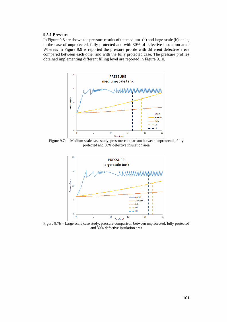
101

9.5.1 Pressure

In Figure 9.8 are shown the pressure results of the medium- (a) and large-scale (b) tanks,

in the case of unprotected, fully protected and with 30% of defective insulation area.

Whereas in Figure 9.9 is reported the pressure profile with different defective areas

compared between each other and with the fully protected case. The pressure profiles

obtained implementing different filling level are reported in Figure 9.10.

Figure 9.7a – Medium scale case study, pressure comparison between unprotected, fully

protected and 30% defective insulation area

Figure 9.7b – Large scale case study, pressure comparison between unprotected, fully protected

and 30% defective insulation area

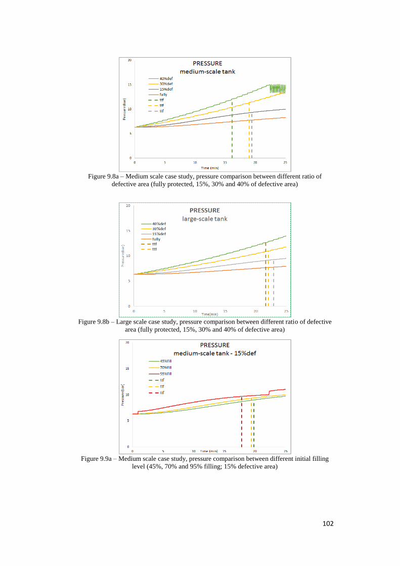
102

Figure 9.8a – Medium scale case study, pressure comparison between different ratio of

defective area (fully protected, 15%, 30% and 40% of defective area)

Figure 9.8b – Large scale case study, pressure comparison between different ratio of defective

area (fully protected, 15%, 30% and 40% of defective area)

Figure 9.9a – Medium scale case study, pressure comparison between different initial filling

level (45%, 70% and 95% filling; 15% defective area)

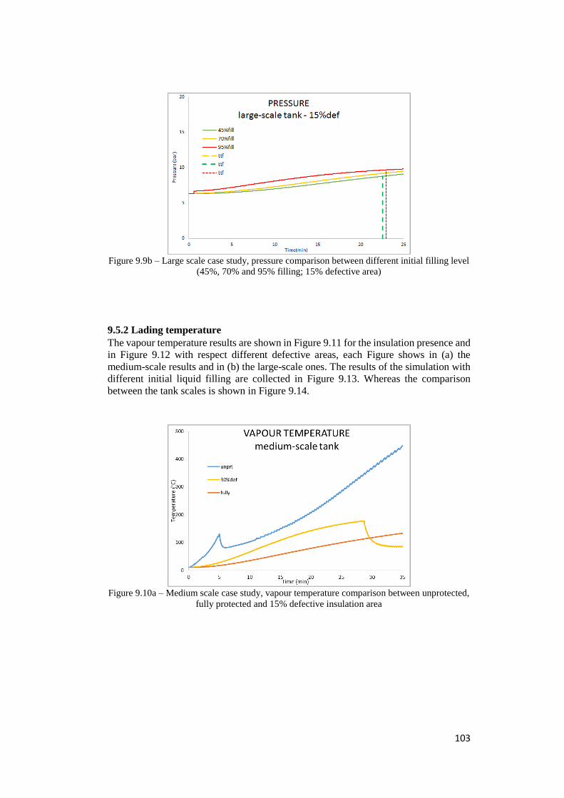
103

Figure 9.9b – Large scale case study, pressure comparison between different initial filling level

(45%, 70% and 95% filling; 15% defective area)

9.5.2 Lading temperature

The vapour temperature results are shown in Figure 9.11 for the insulation presence and

in Figure 9.12 with respect different defective areas, each Figure shows in (a) the

medium-scale results and in (b) the large-scale ones. The results of the simulation with

different initial liquid filling are collected in Figure 9.13. Whereas the comparison

between the tank scales is shown in Figure 9.14.

Figure 9.10a – Medium scale case study, vapour temperature comparison between unprotected,

fully protected and 15% defective insulation area

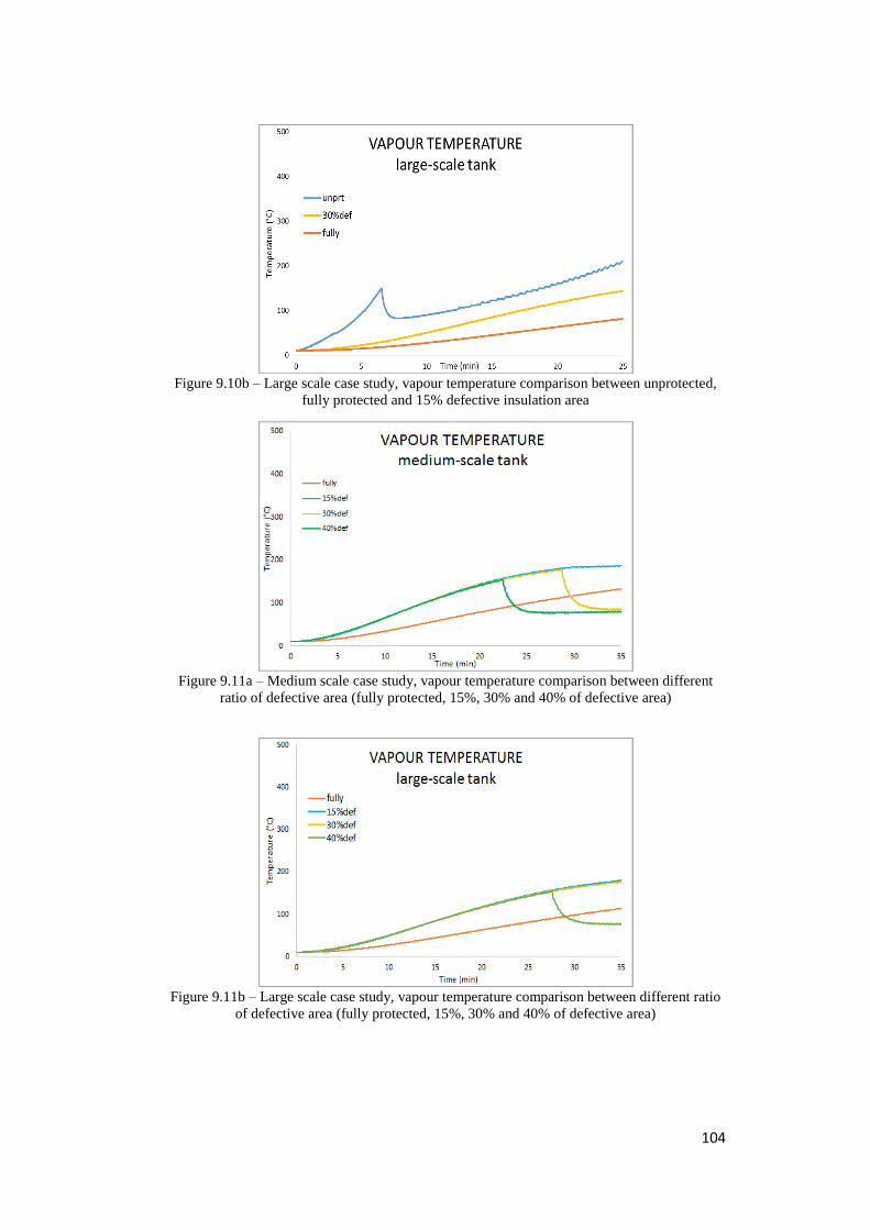
104

Figure 9.10b – Large scale case study, vapour temperature comparison between unprotected,

fully protected and 15% defective insulation area

Figure 9.11a – Medium scale case study, vapour temperature comparison between different

ratio of defective area (fully protected, 15%, 30% and 40% of defective area)

Figure 9.11b – Large scale case study, vapour temperature comparison between different ratio

of defective area (fully protected, 15%, 30% and 40% of defective area)

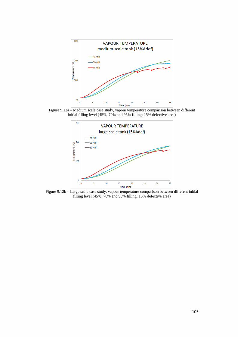
105

Figure 9.12a – Medium scale case study, vapour temperature comparison between different

initial filling level (45%, 70% and 95% filling; 15% defective area)

Figure 9.12b – Large scale case study, vapour temperature comparison between different initial

filling level (45%, 70% and 95% filling; 15% defective area)

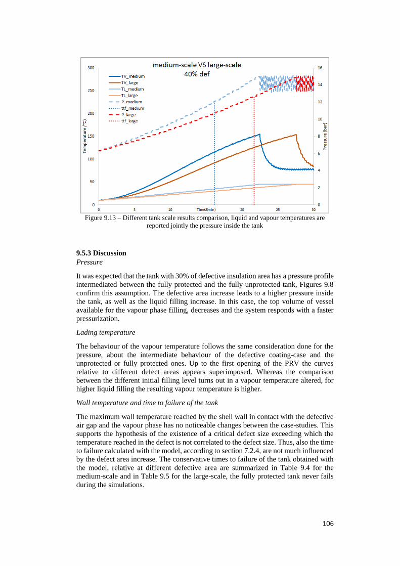
106

Figure 9.13 – Different tank scale results comparison, liquid and vapour temperatures are

reported jointly the pressure inside the tank

9.5.3 Discussion

Pressure

It was expected that the tank with 30% of defective insulation area has a pressure profile

intermediated between the fully protected and the fully unprotected tank, Figures 9.8

confirm this assumption. The defective area increase leads to a higher pressure inside

the tank, as well as the liquid filling increase. In this case, the top volume of vessel

available for the vapour phase filling, decreases and the system responds with a faster

pressurization.

Lading temperature

The behaviour of the vapour temperature follows the same consideration done for the

pressure, about the intermediate behaviour of the defective coating-case and the

unprotected or fully protected ones. Up to the first opening of the PRV the curves

relative to different defect areas appears superimposed. Whereas the comparison

between the different initial filling level turns out in a vapour temperature altered, for

higher liquid filling the resulting vapour temperature is higher.

Wall temperature and time to failure of the tank

The maximum wall temperature reached by the shell wall in contact with the defective

air gap and the vapour phase has no noticeable changes between the case-studies. This

supports the hypothesis of the existence of a critical defect size exceeding which the

temperature reached in the defect is not correlated to the defect size. Thus, also the time

to failure calculated with the model, according to section 7.2.4, are not much influenced

by the defect area increase. The conservative times to failure of the tank obtained with

the model, relative at different defective area are summarized in Table 9.4 for the

medium-scale and in Table 9.5 for the large-scale, the fully protected tank never fails

during the simulations.

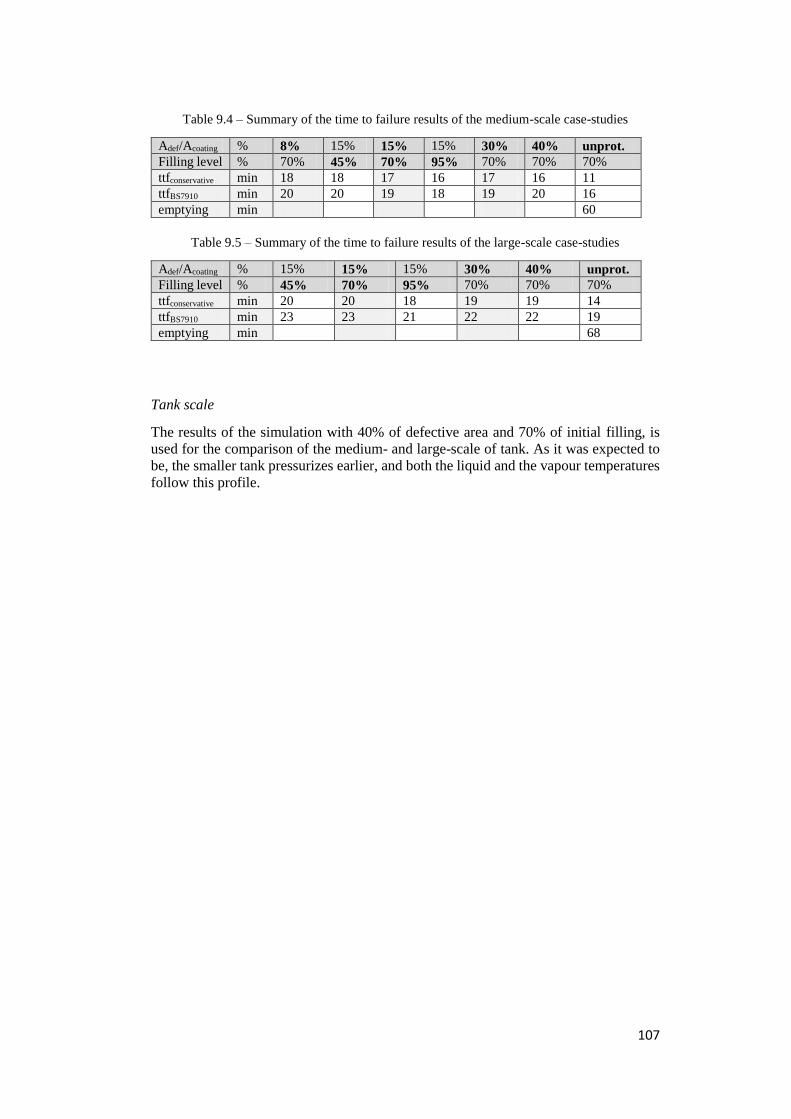
107

Table 9.4 – Summary of the time to failure results of the medium-scale case-studies

Adef/Acoating % 8% 15% 15% 15% 30% 40% unprot.

Filling level % 70% 45% 70% 95% 70% 70% 70%

ttfconservative min 18 18 17 16 17 16 11

ttfBS7910 min 20 20 19 18 19 20 16

emptying min 60

Table 9.5 – Summary of the time to failure results of the large-scale case-studies

Adef/Acoating % 15% 15% 15% 30% 40% unprot.

Filling level % 45% 70% 95% 70% 70% 70%

ttfconservative min 20 20 18 19 19 14

ttfBS7910 min 23 23 21 22 22 19

emptying min 68

Tank scale

The results of the simulation with 40% of defective area and 70% of initial filling, is

used for the comparison of the medium- and large-scale of tank. As it was expected to

be, the smaller tank pressurizes earlier, and both the liquid and the vapour temperatures

follow this profile.

108

10 Conclusions and future works

Starting from the data analysis of past accidents occurred in road and rail hazmat

transportation, the main causes and consequences of accidents involving LPG were

identified. Accidental fire exposures emerged among causes of LPG tankers failure, in

this scenario the BLEVEs are the worst case occurrence. Thus, the analysis raised the

question of the need of passive fire protection systems able to avoid, or at least delay,

the BLEVEs, since ADR and RID regulations do not require any PFP on LPG tankers.

The matter with the implementation of such protections on tankers is that thermal

coatings undergo defects, as discovered by thermographic inspection of tank-cars [Birk

& Cunningham, 2000], thus the action of thermal protection may be compromised. To

assess the performance of defective insulation systems, overcoming real-scale bonfire

tests, the implementation of simulation tools was considered. Thus, the issues

concerning insulated tanks exposed to fire with defective insulation system were

characterized first through the analysis of available bonfire experiments [Birk et al.

2006; VanderSteen & Birk, 2003] and then through the analysis of literature studies

[Scarponi et al. 2016].

With this basis, an advanced FEM model was presented. The model was implemented

and validated by [Scarponi et al. 2016] and then it was applied to a sensitivity analysis,

to assess the influence of several parameters on the behaviour of a quarter cylinder tank

exposed to fire, with different deficiencies configuration. The FEM model requires and

provides detailed information on the problem, allowing the use of a correct failure

criteria to evaluate the time to failure of the tank. This analysis has very high

computational time, a way to reduce it is to skip the computing of pressure and lading

temperature providing these data as external boundary conditions.

Thus, a simplified lumped parameters model was implemented to assess the

performance of defective coatings, in order to save computation time and requiring less

detailed information in input. The RADMOD model was improved for the simulation

of defective coatings with respect to a previously work [Landucci et al. 2013] which

was developed only for unprotected and completely insulated tanks. The model

validation was performed against available experimental data [Birk et al. 2006] on

small-scale tanks. Then the model was extended to the simulation of medium- and large-

scale tanks through the definition of several case-studies.

The results obtained with the RADMOD code have showed that the model generally

realizes a conservative analysis of the thermal behaviour of LPG tanks, providing

credible temperatures and pressure profiles and also computing a conservative time to

failure, which anyway gives an idea of tank behaviour. However, some keys

improvements could be considered in the development of the work as discussed in the

following:

Add extra nodes

Partial engulfment enhancement

Heat transfer coefficients detailed correlations

Vapour transparency detailed analysis

Itemized studies on PRV opening effect

De-stratification sub-model

109

Widening type of substances implemented

Software lightening and speeding up

Introducing extra nodes, generally, could be a good improvement of the code. Firstly,

the steel jacket could also be considered adding the associated nodes, whereas more

nodes in the shell could bring more detailed maximum temperature of the shell. Farther,

the current version of the model considers the partial engulfment of the tank only

dividing the external surfaces, thus the computed temperature is averaged on the node.

Add extra nodes, with respect the engulfment, could allow the simulation of different

flame impingements and it would be interesting especially for the analysis in the first

time step when the fire is not usually fully propagated.

For what concerns the heat transfer modelling and balances, the evaluation of heat-

transfer coefficients affects the temperature profiles, thus, many simplified correlations

were adopted and more detailed correlation could be considered. Moreover, for the heat

transfer by radiation between the shell walls and vapour-phase, an improvement was

already done not considering the vapour as completely transparent, but a detailed

analysis could be done considering three quantities; gas emissivity, gas absorptivity and

gas transmissivity among which the first one is a function of the gas temperature, while

the others are functions of both gas and surface radiation temperatures. Moreover, a

conductive contribution through the liquid side shell and the vapour side shell could be

considered.

A limit of the model is in the vapour temperature after the opening of the PRV, now

there is already a heat transfer coefficient boost considering a forced convective

contribution after PRV opening, anyway some extra studies could be done on that.

Actually, the vapour is also considered as a pure gas, it is reasonable to believe that

some liquid droplets could be present in the gas bulk as the consequence of boiling

process and it has a 2-phases venting through PRV. Another improvement related to the

PRV could be the implementation of a de-stratification sub-model, since at the PRV

opening the model considers the immediate mixing of the stratified layer and this,

clearly, needs further improvement to model the real behaviour of the liquid-phase

inside the tank.

The model could be also extended to other substances like pure compound or mixture.

In latter case also the mixing rule could be considered, which requires quite more efforts.

Also the software code could be improved, first rewriting it from brand new to make

the simulation faster and to add less approximation in the mathematical calculation, and

then checking the analytical stability of the model.

The defect sub-model could be modified allowing setting the percentage of defective

area in each side, vapour or liquid. This action requires a geometrical analysis of the

problem which is complicated if different fire impingement want to be simulated.

In conclusion, when experimental data will be available for medium- and large-scale

tanks some validation studies have to be carried to verify the ability of the defective

RADMOD sub-model.

110

References

Rum, Modeling the behaviour of pressurized vessels exposed to fires through Computational Fluid

Dynamics, Master's Degree Thesis in Chemical Engineering at University of Pisa, Pisa, 2015

A.M. Birk, Analysis of a Propane Sphere Bleve, CEt - AIDIC 31, 2013

A.M. Birk, Modelling the response of tankers exposed to external fire impingement, J. Hazard.

Mater. 20 (1988) 197-225

A.M. Birk, Scae effects with fire exposure of pressure-liquefied gas tanks, J. Loss Prev. Process Ind.

Vol. 8 No. 5. pp. 275-290, 1995

ADR, European Agreement, Concerning the International Carriage of Dangerous Good by Road,

Volume I and II, United Nations, 2014

ANSYS inc, ANSYS Mechanical APDL Theory Reference (R. 14.5), ANSYS Inc, Canonsburg, PA,

2013

API Standard 520, Sizing, Selection, and Installation of Pressure-relieving Devices - Part 1 Sizing

and selection, 2014

API Standard 520, Sizing, Selection, and Installation of Pressure-relieving Devices - Part 1 Sizing

and selection, 2014

API Standard 527, Seat Tightness of Pressure Relief Valves, 2014

ARIA database, Web Site, Home Page, Accessed in January 2016, Available to:

www.aria.developpement-durable.gouv.fr

ASME, Boiler and Pressure Vessel Code, Section VIII, Division 1, Rules for Construction of

Pressure Vessels, 2015

Hemmatian, E. Planas, J. Casal, On BLEVE definition, the significance of superheat limit

temperature (Tsl) and LNG BLEVE's, J. Loss Prev. Process Ind., 40 (2016) 81, 2015

BAM - Federal Institute for Materials Research and Testing, BLEVE (Boiling Liquid Expanding

Vapour Explosion) in dangerous goods tanks - investigation into the performance of tank

constructions and equipment, particularly thermal and fire protection insulation in the event of fire,

2012

Birk A.M., Cunningham M.H., Thermographic inspection of rail-car thermal insulation, S0094-

9930(00)01104-5

Birk A.M., Cunningham M.H., Thermographic Inspection of Rail-Car Thermal Insulation,J.

Pressure Vessel Technol 122(4), 494-501, 2000

Birk, A.M, Poirier, D., Davison, C., On the thermal rupture of 1.9 m3 propane pressure vessels with

defects in their thermal protection system, Journal of Loss Prevention in the Process Industries 19

(2006) 582-597

Birk, A.M., A.M. Birk Engineering, Tank-car insulation defect assessment criteria: thermal analysis

of defects, Transportation development centre, TP 13518E, October 1999

Birk, A.M., and M.H. Cunningham. Liquid temperature stratification and its effect on BLEVEs and

their hazards. Journal of Hazardous Material, 1996: 219-237.

Birk, A.M., Cunningham, M.H.,The boiling liquid expanding vapor explosion, J. Loss Prev. Process

Ind., 7 (1994), pp. 474–480

Birk, A.M., Development and validation of a mathematical model of a rail tank-car engulfed in fire,

PhD Thesis, Queen's University, Ontario, Canada, 1983

BS7910, Guide to methods for assessing the acceptability of flaws in metallic structures, 2013

Butler, C.J., M.A. Persaud, T.A. Roberts, L.C. Shirvill, and S. Wright. “Heat-up and failure of

Liquefied Petroleum Gas storage vessel exposed to a jet-fire.” In Loss Prevention in the Process

Industries, 1069-1106. Stockholm, 2001.

Canadian General Standards Board Standard CAN/CGSB 43.147-2002

CCPS; Guidelines for pressure relief and effluent handling system, March 1998

Center for Chemical Process Safety (CCPS), Vapour Cloud Explosion, Pressure Vessel Burst,

BLEVE and Flash Fire Hazards, 2nd ed., Hoboken, NJ: John Wiley and Sons, 2010

CFR Code of Federal Regulation, 49 CFR Part 179 "specification for tankwagons" U.S.

Government Publishing Office, Washington, DC, 2015. https://www.law.cornell.edu/cfr/text/49/part-

179/appendix-B

CGSB - Canadian General Standards Board Standard, Ottawa, Ontario, Canada, CAN/CGSB

43.147-97, 1997

COUNCIL DIRECTIVE 94/55/EC of 21 November 1994 on the approximation of the laws of the

Member States with regard to the transport of dangerous goods by road

Crowl, S. A. Tipler, Sizing Pressure-Relief Devices, AIChE, October 2013

D.W. Sallet, Pressure relief valve sizing for vessels containing compressed liquefied gases.

I.Mech.E.Symp. Paper No C274/79, 1979

111

D'Aulisa A., Tugnoli A., Cozzani V., Landucci G. & Birk A. (2014). CFD Modeling of LPG essels

Under Fire Exposure Conditions. AIChe Journal, pp. 4292-4305.

"Decreto Ministeriale 4 settembre 1996 - Attuazione della direttiva 94/55/CE del Consiglio

concernente il

ravvicinamento delle legislazioni degli Stati membri relative al trasporto di merci pericolose su

strada"

Droste, B., Schoen, W., Full scale fire tests with unprotected and thermal insulated LPG storage

tanks, Journal of Hazardous Materials, 20 (1988) 41-53

1993-1-2, Eurocode 1: Action on structures - Part 1-2: General actions - Actions on structures

exposed to fire , 2005

Elastic Properties and Young Modulus for some Materials, The Engineering ToolBox, Accessed in

January 2016, Available to: www.engineeringtoolbox.com

Emrys Scarponi, G., Landucci, G., Tugnoli, A., Cozzani, V., Birk, A.M., International Journal of

Themal Sciences, 2016

Heymes, L. Aprin, A.M. Birk, P. Slangen, J.B. Jarry, H. François, G. Dusserre, An experimental

study of an LPG tank at low filling level heated by a remote wall fire, J. Loss Prev. Process Ind. 26

(2013) 1484-1491

Forrest, H.S., Emergency relief vent sizing for fire exposure when teo-phase flows must be

considered, Proceeding of the 19th Loss Prevention Symposium. American Institute of Chemical

Engineers, Houston

"G. Gubinelli, Models for the Assessment of Domino Accidents in the

Process Industry, Ph.D. thesis in Chemical

Engineering. University of Pisa, Pisa, 2006"

Landucci et al., Reliability Engineering and System Safety 132(2014)125–145, 2014

Landucci, A. Tugnoli, V. Busini, M. Derudi, R. Rota, V. Cozzani, The Viareggio LPG accident:

Lessons learnt, J. Of Loss Prev. In the Process Ind., 24 (2011) 466-476

Landucci, Development and Modelling of Passive Fire Protection Systems, Ph.D. thesis in Chemical

Engineering. University of Pisa, Pisa, 2008

G. Landucci, et al., Modeling heat transfer and pressure build-up in LPG vessels exposed to fire,

International Journal of Thermal Science, 2016

"G. Landucci, G. Gubinelli, G. Antonioni, V. Cozzani, The assessment of the damage probability of

storage tanks in domino events

triggered by fire, Accident Analysis and Prevention 41 (2009) 1206-1215, 2009"

G. Landucci, M. Molag, J. Reinders, V. Cozzani, Experimental and analytical investigation of

thermal coating effectiveness for 3m3 LPG tanks engulfed by fire, J. Hazard. Mater. 161 (2009)

1182-1192, 2009

"G. Zuccaro, A Case of Choice of Passive Fire Protection (PFP) in an

Oil & Gas EPC Project, AIDIC DOI: 10.3303/CET1226053, 2012"

International Standard EN ISO 13702:1999, Petroleum and natural gas industries - Control and

mitigation of fire and explosions on oggshore production installations - Requirements and

Guidelines, 1999

J.E.S. Venart, Boiling liquid expanding vapour explosions (BLEVE): possibe failure mechanisms

and their consequences, papaer 10 in Harzards XV, Volume 1, 2000

J.G. Knudsen, H.C. Hottel, A.F. Sarofim, P.C. Wankat, K.S. Knaebel, Heat and mass transfer,

Section 5, in: M. Hill (Ed.), Perry's Chem. Eng. Handb., 7th ed., McGraw Hill, New York, NY, 1999

J.G. Knudsen, H.C. Hottel, A.F. Sarofim, P.C. Wankat, K.S. Knaebel, PHYSICAL AND CHEMICAL

DATA, Section 2, in: M: Hill (Ed.), Perry's Chem. Eng. Handb., 7th ed., McGraw Hill, New York,

NY, 1999

Johnson M.R., Tank car thermal analysus, Volume 1 and 2, DOT/FRA/ORD-98/09A and

DOT/FRA/ORD-98/09B, November 1998

Johnson M.R., TCFIRE: A model for prediction of fire effects on tank cars, AAR Publucation SD-

053, 1995

K. Moodie, Experiments and modelling: an overview with particular reference to fire engulfment, J.

Hazard. Mater. 20 (1988) 149-175

Keltner, N. R., Nicolette, V. F., Brown, N. N. and Bainbridge, B. L. J. Hazard. Mater. 1990, 25, 33-

47

Kern, Process heat transfer, McGraw-Hill book company, International edition, 1965.

L. Nigro, Analysis And Simulation Of The Thermal Behaviour Of Lpg Tankers Exposed To Fire,

Master's Degree Thesis in "Progettazione Di Apparecchiature E Impianti M", Alma Mater

Studiorum - University of Bologna, Bologna, 2015

Landucci G., Cozzani V., Birk M., Heat Radiation Effects in Domino Effects in the Process

Industries, Cozzani V. and Reniers G. Amsterdam-Elsevier, 2013: 70-115.

Landucci G., Tugnoli A., Cozzani V., Analysis of fired coated vessels in presence of defects in the

thermal protection, 2011

112

Lees, F.P., Loss Prevention in the Process Industries-Hazard Identification, Assessment, and

Control, vols. 1–3, Butterworth-Heinemann, Oxford, 1996

Legge 12 agosto 1962 n.1839

Leung and Epstein, A generalized correlation for two-phase non-flashing homogeneous chocked

flow, Trans. ASME J. Heat Tranfer 112 (May), pp. 528-530, 1990

Leung and Epstein, A generalized critical flow model for non-ideal gases, AIChe J. 34(9), pp. 1568-

1572, 1988

Leung and Nazario, Sizing pressure relief valves in flashing, two-phase service: an alternative

procedure, J. Loss Prev. Process Ind. 5 (5), pp. 263-269, 1992

M. Bazzocchi, Evaluation Of The Pressure Build Up In Pressurized Tankers Exposed To Fire,

Master's Degree Thesis in "Progettazione Di Apparecchiature E Impianti M", Alma Mater

Studiorum - University of Bologna, Bologna, 2014

M. Molag, A. Kruithof, BLEVE prevention of a LPG tank vehicle or a LPG tank wagon, report

R2005/364, Netherlands Organisation for Applied Scientific Research – TNO, Apeldoorn, 2005

M.F. Modest, Radiative Heat Transfer, Academic Press, New York, NY, 2003

Ministero delle Infrastrutture e dei Trasporti, Conto Nazionale delle Infrastrutture e dei Trasporti,

Anni 2012-2013

Moodie, K., Cowley, L.T., Denny, R.B., Small, L.M., Williams, I., Fire engulfment tests on a 5 tonne

LPG tank, Journal of Hazardous Materials, 20 (1988) 55-71

N.U. Aydemir, V.K. Magapu, A.C.M. Souse and J.E.S. Venart, Thermal response analysis of LPG

tanks exposed to fire, J. Hazard. Mater. 20 (1988) 239-262

Paltrinieri, N. et al., Risk reduction in road and rail LPG transportation by passive fire protection,

J. Hazard. Mater. (2009), doi: 10.1016/j.jhazmat.2008.12.122

Perry, R. H., and D. W. Green, Eds., “Process Safety” Chapter 23, in Perry’s Chemical Engineers’

Handbook, 8th ed., McGraw-Hill, New York (1984)

Peter M. Maitlis, A. de Klerk, Greener Fischer-Tropsch Processes for Fuels and Feedstocks,

Februar 2013

R. Mauri, Elementi di Fenomeni di Trasporto (II ed.). PLUS, Pisa University Press, 2012

R.C. Reid. Possible mechanism for pressurized-liquid tank explosions or BLEVE's. Science

1979;203:1263-1265

R.K. Eckhoff, Boiling liquid expanding vapour explosions (BLEVEs): A brief review, J. Loss Prev.

Process Ind. 32 (2014) 30-43, 2014

R.W. Prugh, Quantify BLEVE hazards, Chem. Eng. Prog. 87 (2) (1991) 66–71.

Recommendations on the transport of dangerous goods, Model Regulations, Volume I, UN,

ST/SG/AC.10/1/Rev.18 (Vol.I), 2013

S.K.S. Boetcher, Natural convection from circular cylinders, Springer, Heidelberg, Germany, 2014

S.W. Churchill, H.H.S. Chu, Correlating equations for laminar and turbolent free convection from

vertical plate, Int. J. Heat Mass Transf. 18 (1975) 1323-1329

Smith J.M, Van Ness H.C., Abbot M.M. In “Introduction to chemical engineering thermodynamics”.

7th Revised edition 2004

"T. A. Roberts, I. Buckland, L. C. Shirvill, B. J. Lowesmith And P. Salater, Design And Protection Of

Pressure Systems To Withstand Severe Fires, Trans IChemE, Part B, March 2004

Process Safety and Environmental Protection, 82(B2): 89–96"

TNO Methods for the calculation of Physical Effects -due to releases of hazardous materials (liquids

and gases)-Yellow Book, 3th ed., 2005

Townsend, W., Anderson, C., Zook, J., Cowgill, G., Comparison of thermally coated and uninsulated

rail tank-cars filled with LPG subjected to a fire environment, US Department of Transportation,

Washington DC, 1974

TSO, Fire and Rescue Service, Operational guidance - Incidents involving hazardous materials,

ID2511951 C5 11/12, 2012

UNECE Official Web Site, in Transport – Areas of work – Dangerous Goods, Accessed in January

2016 , Available to: www.unece.org

VanderSteen, J.D.J., Birk, A.M., Fire tests on defective tank-car thermal protection systems, Journal

of Loss Prevention in the Process Industries 16 (2003) 417-425

W.J. King, The basic laws and data of heat transmission, American Society of Mechanical

Engineers, 1932

Walls W.L., The BLEVE - Part 1, Fire Command, vol. 17, 1979

Walls W.L., What is BLEVE?, Fire Journal, vol. 31, 1978

Yu, C.M., N.U. Aydemir, e J.E.S. Venart. «Transient Free Convection and Thermal Stratification in

Uniformly-Heated Partially-Filled Horizontal Cylindical and Spherical Vessels.» Journal of

Thermal Science 1, n. 2, 1992

Zografos, K.G., Androutsopoulos, K.N., 2004. A heuristic algorithm for solving hazardous materials distribution problems. European Journal of Operations Research 152, 507–519, 2004

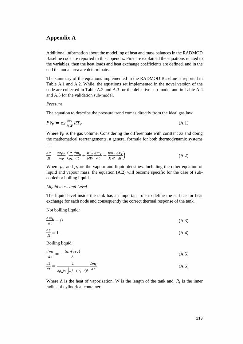
113

Appendix A

Additional information about the modelling of heat and mass balances in the RADMOD

Baseline code are reported in this appendix. First are explained the equations related to

the variables, then the heat loads and heat exchange coefficients are defined. and in the

end the nodal area are determinate.

The summary of the equations implemented in the RADMOD Baseline is reported in

Table A.1 and A.2. While, the equations set implemented in the novel version of the

code are collected in Table A.2 and A.3 for the defective sub-model and in Table A.4

and A.5 for the validation sub-model.

Pressure

The equation to describe the pressure trend comes directly from the ideal gas law:

𝑃𝑉𝑉 = 𝑧𝑧𝑚𝑉

𝑀𝑊𝑅𝑇𝑉 (A.1)

Where 𝑉𝑉 is the gas volume. Considering the differentiate with constant zz and doing

the mathematical rearrangements, a general formula for both thermodynamic systems

is:

𝑑𝑃

𝑑𝑡=

𝑧𝑧𝜌𝑉

𝑚𝑉(

𝑃

𝜌𝐿

𝑑𝑚𝐿

𝑑𝑡+

𝑅𝑇𝑉

𝑀𝑊

𝑑𝑚𝑉

𝑑𝑡+

𝑅𝑚𝑉

𝑀𝑊

𝑑𝑇𝑉

𝑑𝑡) (A.2)

Where 𝜌𝑉 and 𝜌𝐿are the vapour and liquid densities. Including the other equation of

liquid and vapour mass, the equation (A.2) will become specific for the case of sub-

cooled or boiling liquid.

Liquid mass and Level

The liquid level inside the tank has an important role to define the surface for heat

exchange for each node and consequently the correct thermal response of the tank.

Not boiling liquid:

𝑑𝑚𝐿

𝑑𝑡= 0 (A.3)

𝑑𝐿

𝑑𝑡= 0 (A.4)

Boiling liquid:

𝑑𝑚𝐿

𝑑𝑡= −

(𝑞𝐿+𝑞𝐿𝑉)

Λ (A.5)

𝑑𝐿

𝑑𝑡=

1

2𝜌𝐿𝑊√𝑅𝑖2−(𝑅𝑖−𝐿)2

𝑑𝑚𝐿

𝑑𝑡 (A.6)

Where Λ is the heat of vaporization, W is the length of the tank and, 𝑅𝑖 is the inner

radius of cylindrical container.

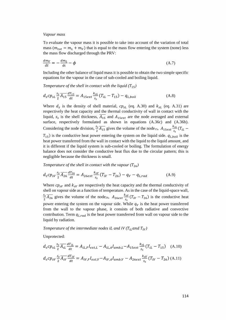
114

Vapour mass

To evaluate the vapour mass it is possible to take into account of the variation of total

mass (𝑚𝑡𝑜𝑡 = 𝑚𝐿 + 𝑚𝑉) that is equal to the mass flow entering the system (none) less

the mass flow discharged through the PRV:

𝑑𝑚𝑉

𝑑𝑡= −

𝑑𝑚𝐿

dt− 𝜙 (A.7)

Including the other balance of liquid mass it is possible to obtain the two simple specific

equations for the vapour in the case of sub-cooled and boiling liquid.

Temperature of the shell in contact with the liquid (𝑇15)

𝑑𝑠𝑐𝑝𝑠𝐿𝑠𝑠

2𝐴15 𝑑𝑇15

𝑑𝑡= 𝐴15𝑒𝑥𝑡

𝑘𝑠𝐿

𝑠𝑠(𝑇𝑖𝐿 − 𝑇15) − 𝑞𝐿,𝑏𝑜𝑖𝑙 (A.8)

Where 𝑑𝑠 is the density of shell material, 𝑐𝑝𝑠𝐿 (eq. A.30) and 𝑘𝑠𝐿 (eq. A.31) are

respectively the heat capacity and the thermal conductivity of wall in contact with the

liquid, 𝑠𝑠 is the shell thickness, 𝐴15 and 𝐴15𝑒𝑥𝑡 are the node averaged and external

surface, respectively formulated as shown in equations (A.36c) and (A.36b).

Considering the node division, 𝑠𝑠

2𝐴15 gives the volume of the node15, 𝐴15𝑒𝑥𝑡

𝑘𝑠𝐿

𝑠𝑠(𝑇𝑖𝐿 −

𝑇15) is the conductive heat power entering the system on the liquid side. 𝑞𝐿,𝑏𝑜𝑖𝑙 is the

heat power transferred from the wall in contact with the liquid to the liquid amount, and

it is different if the liquid system is sub-cooled or boiling. The formulation of energy

balance does not consider the conductive heat flux due to the circular pattern; this is

negligible because the thickness is small.

Temperature of the shell in contact with the vapour (𝑇26)

𝑑𝑠𝑐𝑝𝑠𝑉𝑠𝑠

2𝐴26 𝑑𝑇26

𝑑𝑡= 𝐴26𝑒𝑥𝑡

𝑘𝑠𝑉

𝑠𝑠(𝑇𝑖𝑉 − 𝑇26) − 𝑞𝑉 − 𝑞𝐿,𝑟𝑎𝑑 (A.9)

Where 𝑐𝑝𝑠𝑉 and 𝑘𝑠𝑉 are respectively the heat capacity and the thermal conductivity of

shell on vapour side as a function of temperature. As in the case of the liquid-space wall, 𝑠𝑠

2𝐴26 gives the volume of the node26, 𝐴26𝑒𝑥𝑡

𝑘𝑠𝑉

𝑠𝑠(𝑇𝑖𝑉 − 𝑇26) is the conductive heat

power entering the system on the vapour side. While 𝑞𝑉 is the heat power transferred

from the wall to the vapour phase, it consists of both radiative and convective

contribution. Term 𝑞𝐿,𝑟𝑎𝑑 is the heat power transferred from wall on vapour side to the

liquid by radiation.

Temperature of the intermediate nodes iL and iV (𝑇𝑖𝐿𝑎𝑛𝑑 𝑇𝑖𝑉)

Unprotected:

𝑑𝑠𝑐𝑝𝑠𝐿𝑠𝑠

2𝐴𝑖𝐿 𝑑𝑇𝑖𝐿

𝑑𝑡= 𝐴𝑖𝐿,𝐹𝐼𝑒𝑥𝑡,𝐿 − 𝐴𝑖𝐿,𝐴𝐼𝑎𝑚𝑏,𝐿−𝐴15𝑒𝑥𝑡

𝑘𝑠𝐿

𝑠𝑠(𝑇𝑖𝐿 − 𝑇15) (A.10)

𝑑𝑠𝑐𝑝𝑠𝑉𝑠𝑠

2𝐴𝑖𝑉 𝑑𝑇𝑖𝑉

𝑑𝑡= 𝐴𝑖𝑉,𝐹𝐼𝑒𝑥𝑡,𝑉−𝐴𝑖𝑉,𝐴𝐼𝑎𝑚𝑏,𝑉 − 𝐴26𝑒𝑥𝑡

𝑘𝑠𝑉

𝑠𝑠(𝑇𝑖𝑉 − 𝑇26) (A.11)

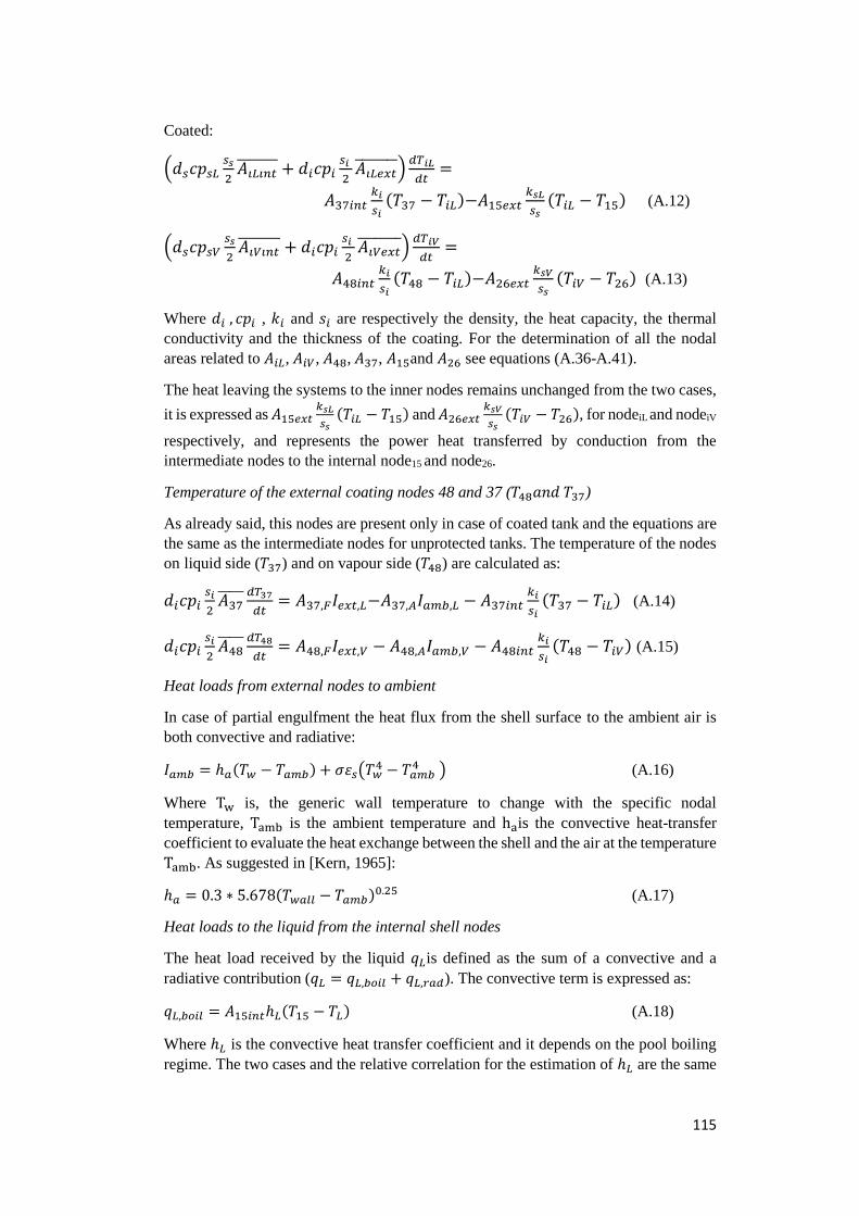
115

Coated:

(𝑑𝑠𝑐𝑝𝑠𝐿𝑠𝑠

2𝐴𝑖𝐿𝑖𝑛𝑡 + 𝑑𝑖𝑐𝑝𝑖

𝑠𝑖

2𝐴𝑖𝐿𝑒𝑥𝑡 )

𝑑𝑇𝑖𝐿

𝑑𝑡=

𝐴37𝑖𝑛𝑡𝑘𝑖

𝑠𝑖(𝑇37 − 𝑇𝑖𝐿)−𝐴15𝑒𝑥𝑡

𝑘𝑠𝐿

𝑠𝑠(𝑇𝑖𝐿 − 𝑇15) (A.12)

(𝑑𝑠𝑐𝑝𝑠𝑉𝑠𝑠

2𝐴𝑖𝑉𝑖𝑛𝑡 + 𝑑𝑖𝑐𝑝𝑖

𝑠𝑖

2𝐴𝑖𝑉𝑒𝑥𝑡 )

𝑑𝑇𝑖𝑉

𝑑𝑡=

𝐴48𝑖𝑛𝑡𝑘𝑖

𝑠𝑖(𝑇48 − 𝑇𝑖𝐿)−𝐴26𝑒𝑥𝑡

𝑘𝑠𝑉

𝑠𝑠(𝑇𝑖𝑉 − 𝑇26) (A.13)

Where 𝑑𝑖 , 𝑐𝑝𝑖 , 𝑘𝑖 and 𝑠𝑖 are respectively the density, the heat capacity, the thermal

conductivity and the thickness of the coating. For the determination of all the nodal

areas related to 𝐴𝑖𝐿, 𝐴𝑖𝑉, 𝐴48, 𝐴37, 𝐴15and 𝐴26 see equations (A.36-A.41).

The heat leaving the systems to the inner nodes remains unchanged from the two cases,

it is expressed as 𝐴15𝑒𝑥𝑡𝑘𝑠𝐿

𝑠𝑠(𝑇𝑖𝐿 − 𝑇15) and 𝐴26𝑒𝑥𝑡

𝑘𝑠𝑉

𝑠𝑠(𝑇𝑖𝑉 − 𝑇26), for nodeiL and nodeiV

respectively, and represents the power heat transferred by conduction from the

intermediate nodes to the internal node15 and node26.

Temperature of the external coating nodes 48 and 37 (𝑇48𝑎𝑛𝑑 𝑇37)

As already said, this nodes are present only in case of coated tank and the equations are

the same as the intermediate nodes for unprotected tanks. The temperature of the nodes

on liquid side (𝑇37) and on vapour side (𝑇48) are calculated as:

𝑑𝑖𝑐𝑝𝑖𝑠𝑖

2𝐴37 𝑑𝑇37

𝑑𝑡= 𝐴37,𝐹𝐼𝑒𝑥𝑡,𝐿−𝐴37,𝐴𝐼𝑎𝑚𝑏,𝐿 − 𝐴37𝑖𝑛𝑡

𝑘𝑖

𝑠𝑖(𝑇37 − 𝑇𝑖𝐿) (A.14)

𝑑𝑖𝑐𝑝𝑖𝑠𝑖

2𝐴48 𝑑𝑇48

𝑑𝑡= 𝐴48,𝐹𝐼𝑒𝑥𝑡,𝑉 − 𝐴48,𝐴𝐼𝑎𝑚𝑏,𝑉 − 𝐴48𝑖𝑛𝑡

𝑘𝑖

𝑠𝑖(𝑇48 − 𝑇𝑖𝑉) (A.15)

Heat loads from external nodes to ambient

In case of partial engulfment the heat flux from the shell surface to the ambient air is

both convective and radiative:

𝐼𝑎𝑚𝑏 = ℎ𝑎(𝑇𝑤 − 𝑇𝑎𝑚𝑏) + 𝜎𝜀𝑠(𝑇𝑤4 − 𝑇𝑎𝑚𝑏

4 ) (A.16)

Where Tw is, the generic wall temperature to change with the specific nodal

temperature, Tamb is the ambient temperature and hais the convective heat-transfer

coefficient to evaluate the heat exchange between the shell and the air at the temperature

Tamb. As suggested in [Kern, 1965]:

ℎ𝑎 = 0.3 ∗ 5.678(𝑇𝑤𝑎𝑙𝑙 − 𝑇𝑎𝑚𝑏)0.25 (A.17)

Heat loads to the liquid from the internal shell nodes

The heat load received by the liquid 𝑞𝐿is defined as the sum of a convective and a

radiative contribution (𝑞𝐿 = 𝑞𝐿,𝑏𝑜𝑖𝑙 + 𝑞𝐿,𝑟𝑎𝑑). The convective term is expressed as:

𝑞𝐿,𝑏𝑜𝑖𝑙 = 𝐴15𝑖𝑛𝑡ℎ𝐿(𝑇15 − 𝑇𝐿) (A.18)

Where ℎ𝐿 is the convective heat transfer coefficient and it depends on the pool boiling

regime. The two cases and the relative correlation for the estimation of ℎ𝐿 are the same

116

used in the novel RADMOD version and described in paragraph 7.3.1 for the two cases

of interface evaporation or nucleate boiling.

Regarding the radiative heat transfer between the vapour-space internal surface and the

liquid, in the novel implementation of the code, see paragraph 7.3.1.

Heat loads to the liquid from the vapour phase

𝑞𝐿𝑉 = 𝐴𝐿𝑉ℎ𝐿𝑉(𝑇𝑉 − 𝑇𝐿) (A.19)

𝐴𝐿𝑉 is surface of the liquid-vapour interface calculated throught equation (A.42). The

heat-transfer coefficient ℎ𝐿𝑉 is consist of two terms, a natural convective coefficient and

other radiative. For convective contribution the correlation of hot horizontal plate facing

downward are adopted as suggested in [Perry & Green, 1997]. Defining the same

dimensionless key parameter of (7.28 , paragraph 7.3.1), but with the subscript V and

the characteristic length defined as in equation (A.21) , the heat coefficient ℎ𝐿𝑉,𝑐𝑜𝑛𝑣 is

derived from:

𝑁𝑢 =ℎ𝐿𝑉𝑥𝑖

𝑘𝑉= 0.27𝑅𝑎

14⁄ (A.20)

𝑥𝑖 =4𝐴𝐿𝑉

2(𝑊+𝐴𝐿𝑉

𝑊⁄ ) (A.21)

Whereas the radiative heat-transfer coefficient from vapour to liquid is calculate by the

empirical correlation [Perry & Green, 1997]:

ℎ𝐿𝑉,𝑟𝑎𝑑 = 5.6783[(

𝑇𝑉100

)4

−(𝑇𝐿

100)

4]0.173

(𝑇𝑉−𝑇𝐿) (A.22)

Heat loads to the vapour from the internal shell nodes

The total heat entering the vapour node is the sum of a convective contribution 𝑞𝑉,𝑐𝑜𝑛𝑣

and a radiative contrivution 𝑞𝑉,𝑟𝑎𝑑:

𝑞𝑉 = 𝑞𝑉,𝑐𝑜𝑛𝑣 + 𝑞𝑉,𝑟𝑎𝑑 = 𝐴26𝑖𝑛𝑡ℎ𝑉,𝑐(𝑇26 − 𝑇𝑉) + 𝐴26𝑖𝑛𝑡ℎ𝑉,𝑟(𝑇26 − 𝑇𝑉) (A.23)

The convective coefficient is calculate with the equations (A.24) or with equation

(A.26) depending on the PRV function.

If PRV is closed:

Defining the dimensionless key parameters of (7.48, paragraph 7.3.1) but with the

subscript V and characteristic length defined as shown in equation (A.25), the

convective coefficient is:

𝑁𝑢 =ℎ𝑉,𝑐 𝑥𝑖

𝑘𝑉= 0.27𝑅𝑎

14⁄ (A.24)

𝑥𝑖 =4𝐴26𝑖𝑛𝑡

2(𝑊+𝐴26𝑖𝑛𝑡

𝑊⁄ ) (A.25)

If PRV is opened:

Forced convection is also considered and added to the natural convection coefficient.

117

𝑁𝑢 =ℎ𝑉,𝑓𝑜𝑟𝑐𝑒𝑑 𝑥𝑖

𝑘𝑉= 0.0243𝑅𝑒0.8𝑃𝑟0.4 (A.26)

Where:

𝑃𝑟 =𝜇𝑉𝑐𝑝𝑉

𝑘𝑉 ; 𝑅𝑒 =

4𝜙

𝑝𝜇𝑉 (A.27)

Where 𝜙 is the mass flow throughout the PRV derived with equation (A.35)

Characteristic length 𝑥𝑖 is given by the ratio of the section of vapour phase and the

wetted perimeter according to:

𝑥𝑖 =4𝐴𝑣𝑎𝑝

𝑝𝑤𝑒𝑡𝑡𝑒𝑑=

𝑅𝑖2(𝑐𝑜𝑠−1(

𝐿−𝑅𝑖𝑅𝑖

)−𝑠𝑖𝑛(𝐿−𝑅𝑖

𝑅𝑖)(

𝐿−𝑅𝑖𝑅𝑖

))

2𝜋𝑐𝑜𝑠−1(𝐿−𝑅𝑖

𝑅𝑖)

(A.28)

The radiative coefficient ℎ𝑉,𝑟𝑎𝑑 is calculated as follow:

ℎ𝑉,𝑟 = 5.6783[(

𝑇26100

)4

−(𝑇𝑉100

)4

]0.173

(𝑇26−𝑇𝑉) (A.29)

Thermal properties of wall material

The thermodynamic properties of the steel wall (stainless and carbon steel) are

dependent of the temperature of the wall. Properties of interest are the heat capacity,

and the conductive heat transfer coefficient.

The specific heat of carbon steel (subscript CS) is a fit of the properties for steel taken

from Eurocode [Eurocode 1, 2005] as seen in equation set (A.30), where 𝑐𝑝 is

calculated in J/kgK and the steel temperature T is in°C.

20 ≤ 𝑇(°𝐶) < 600

𝑐𝑝𝐶𝑆 = 425 + 0.773 ∙ 𝑇 − 0.00168 ∙ 𝑇2 + 2.22 ∙ 10−6 ∙ 𝑇3 (A.30a)

600 ≤ 𝑇(°𝐶) < 735

𝑐𝑝𝐶𝑆 = 666 +13002

738−𝑇 (A.30b)

735 ≤ 𝑇(°𝐶) < 900

𝑐𝑝𝐶𝑆 = 545 +17820

𝑇−731 (A.30c)

900 ≤ 𝑇(°𝐶) < 1200

𝑐𝑝𝐶𝑆 = 650 (A.30d)

The thermal conductivity (𝑘𝐶𝑆) is modelled from equation set (A.31), as found by

Eurocode [Eurocode 1, 2005]. It is estimated as W/mK.

20 ≤ 𝑇(°𝐶) < 800

𝑘𝐶𝑆 = 54 − 0.0333 ∙ 𝑇 (A.31a)

800 ≤ 𝑇(°𝐶) < 1200

118

𝑘𝐶𝑆 = 27.3 (A.31b)

The same approach is considered for the stainless steel (subscript SS). The specific heat

of stainless steel may be determined from the following equation (A.32), whereas the

conductive heat transfer coefficient follows the equation (A.33). Both correlations are

found by Eurocode [Eurocode 1, 2005].

20 ≤ 𝑇(°𝐶) < 1200

𝑐𝑝𝑆𝑆 = 450 + 0.280 ∙ 𝑇 − 2.91 ∙ 10−4 ∙ 𝑇2 + 1.34 ∙ 10−7 ∙ 𝑇3 (A.32)

20 ≤ 𝑇(°𝐶) < 1200

𝑘𝑆𝑆 = 14.6 − 0.0127 ∙ 𝑇 (A.33)

Mass flow through PRV

The general equation for determination of the mass flow discharged through he PRV is

defined as: 𝜙 = 𝜌𝑣𝑢𝐴𝑐𝑟𝑜𝑠𝑠. The density of the vapour 𝜌𝑣 is calculated through the ideal

gas law, and for considering the real gas behaviour the compressibility factor (zz) is

inserted in the equation. The cross-sectional area (𝐴𝑐𝑟𝑜𝑠𝑠) is the area of valve through

which the fluid has the efflux velocity 𝑢. Making use of Mach number definition

(eqation A.34) for a subsritical flow (more detail in Chapter 5), the mass flow is

calculated with hypothesis of a isentropic process and, considering that the internal

dissipative phenomena (wall friction) and the heat exchanges with the external

environment are negligible.

𝑀𝑎 = √ (𝑃

𝑃𝑑𝑖𝑠𝑐)

𝛾−1𝛾

−1

𝛾−1

2

(A.34)

𝜙 = 𝑐𝐷𝐴𝑃𝑅𝑉𝑃

𝑧𝑧√

𝛾𝑀𝑊

𝑅𝑇𝑉

𝑀𝑎

(1+𝛾−1

2𝑀𝑎2)

𝛾+12(𝛾−1)

(A.35)

Nodal areas

The nodal areas are calculated in function of the liquid level, which determines the

surfaces in the liquid space and the ones in the vapour space. The the definition of three

exchanging areas for each node, specifically: internal, external and averaged area, is

complex and the difference between the three surfaces on the same node is not that

significative. The internal and the external areas are are the surfaces through with the

heat powers passing through, whereas the averaged areas are used for the volumes

evaluation. A simplification is advisable in the future works, by the definition of one

area of exchange for each node. Starting the inner nodes, the different nodal areas are

defined as follow, subscripts 𝑖 or 𝑠 means that the variables are referred to the insulation

or to the steel walls, 𝐿 is the liquid level and 𝑊 is the tank length:

Liquid side inner node (node15)

𝐴15𝑖𝑛𝑡 = 2𝑊𝑅𝑖𝑐𝑜𝑠−1 (𝑅𝑖−𝐿

𝑅𝑖) (A.36a)

119

𝐴15𝑒𝑥𝑡 =𝐴15𝑖𝑛𝑡+𝐴𝑖𝐿

2 (A.36b)

𝐴15 =

𝐴15𝑖𝑛𝑡+𝐴15𝑒𝑥𝑡

2 (A.36c)

Vapour side inner node (node26)

𝐴26𝑖𝑛𝑡 = 2𝜋𝑊𝑅𝑖 − 𝐴15𝑖𝑛𝑡 (A.37a)

𝐴26𝑒𝑥𝑡 =𝐴26𝑖𝑛𝑡+𝐴𝑖𝑉

2 (A.37b)

𝐴26 =

𝐴26𝑖𝑛𝑡+𝐴26𝑒𝑥𝑡

2 (A.37c)

Liquid side intermediate node (nodeiL)

𝐴𝑖𝐿𝑖𝑛𝑡 =

𝐴𝑖𝐿 +𝐴15𝑒𝑥𝑡

2 (A.38a)

𝐴𝑖𝐿𝑒𝑥𝑡 =

𝐴𝑖𝐿 +𝐴37𝑖𝑛𝑡

2 (A.38b)

𝐴𝑖𝐿 = 2𝑊𝑅𝑒𝑐𝑜𝑠−1 (

𝑅𝑒−𝐿

𝑅𝑒) (A.38c)

Vapour side intermediate node (nodeiV)

𝐴𝑖𝑉𝑖𝑛𝑡 =

𝐴𝑖𝑉 +𝐴26𝑒𝑥𝑡

2 (A.39a)

𝐴𝑖𝑉𝑒𝑥𝑡 =

𝐴𝑖𝑉 +𝐴48𝑖𝑛𝑡

2 (A.39b)

𝐴𝑖𝑉 = 2𝜋𝑊𝑅𝑒 − 𝐴𝑖𝐿

(A.39c)

Liquid side external node (node37)

𝐴37𝑖𝑛𝑡 =𝐴𝑖𝐿 +𝐴37𝑒𝑥𝑡

2 (A.40a)

𝐴37𝑒𝑥𝑡 = 2𝑊(𝑅𝑒 + 𝑠𝑖)𝑐𝑜𝑠−1 (𝑅𝑒+𝑠𝑖−𝐿

𝑅𝑒+𝑠𝑖) (A.40b)

𝐴37 =

𝐴37𝑖𝑛𝑡+𝐴37𝑒𝑥𝑡

2 (A.40c)

Vapour side external node (node48)

𝐴48𝑖𝑛𝑡 =𝐴𝑖𝑉 +𝐴48𝑒𝑥𝑡

2 (A.41a)

𝐴48𝑒𝑥𝑡 = 2𝑊(𝑅𝑒 + 𝑠𝑖) − 𝐴37𝑒𝑥𝑡 (A.41b)

𝐴48 =

𝐴48𝑖𝑛𝑡+𝐴48𝑒𝑥𝑡

2 (A.41c)

Liquid-vapour interface

𝐴𝐿𝑉 = 𝑊𝐷𝑖𝑠𝑖𝑛 (𝑐𝑜𝑠−1 |𝐿−𝑅𝑖

𝑅𝑖|) (A.42)

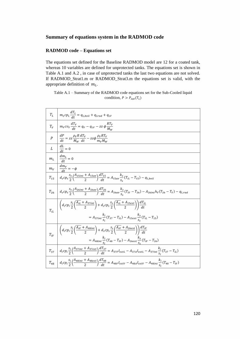
120

Summary of equations system in the RADMOD code

RADMOD code – Equations set

The equations set defined for the Baseline RADMOD model are 12 for a coated tank,

whereas 10 variables are defined for unprotected tanks. The equations set is shown in

Table A.1 and A.2 , in case of unprotected tanks the last two equations are not solved.

If RADMOD_Strat1.m or RADMOD_Strat3.m the equations set is valid, with the

appropriate definition of 𝑚𝐿.

Table A.1 – Summary of the RADMOD code equations set for the Sub-Cooled liquid

condition, 𝑃 > 𝑃𝑠𝑎𝑡(𝑇𝐿)

𝑇𝐿 𝑚𝐿𝑐𝑝𝐿

𝑑𝑇𝐿

𝑑𝑡= 𝑞𝐿,𝑏𝑜𝑖𝑙 + 𝑞𝐿𝑟𝑎𝑑 + 𝑞𝐿𝑉

𝑇𝑉 𝑚𝑉𝑐𝑣𝑉

𝑑𝑇𝑉

𝑑𝑡= 𝑞𝑉 − 𝑞𝐿𝑉 − 𝑧𝑧 𝜙

𝑅𝑇𝑉

𝑀𝑊

𝑃 𝑑𝑃

𝑑𝑡= 𝑧𝑧

𝜌𝑉𝑅

𝑀𝑊

𝑑𝑇𝑉

𝑑𝑡− 𝑧𝑧𝜙

𝜌𝑉𝑅𝑇𝑉

𝑚𝑉𝑀𝑊

𝐿 𝑑𝐿

𝑑𝑡= 0

𝑚𝐿 𝑑𝑚𝐿

𝑑𝑡= 0

𝑚𝑉 𝑑𝑚𝑉

𝑑𝑡= −𝜙

𝑇15 𝑑𝑠𝑐𝑝𝑠

𝑠𝑠

2(

𝐴15𝑖𝑛𝑡 + 𝐴15𝑎𝑣

2)

𝑑𝑇15

𝑑𝑡= 𝐴15𝑎𝑣

𝑘𝑠

𝑠𝑠

(𝑇𝑖𝐿 − 𝑇15) − 𝑞𝐿,𝑏𝑜𝑖𝑙

𝑇26 𝑑𝑠𝑐𝑝𝑠

𝑠𝑠

2(

𝐴26𝑖𝑛𝑡 + 𝐴26𝑎𝑣

2)

𝑑𝑇26

𝑑𝑡= 𝐴26𝑎𝑣

𝑘𝑠

𝑠𝑠

(𝑇𝑖𝑉 − 𝑇26) − 𝐴26𝑖𝑛𝑡ℎ𝑉(𝑇26 − 𝑇𝑉) − 𝑞𝐿,𝑟𝑎𝑑

𝑇𝑖𝐿

(𝑑𝑖𝑐𝑝𝑖

𝑠𝑖

2(

𝐴𝑖𝐿 + 𝐴37𝑖𝑛𝑡

2) + 𝑑𝑠𝑐𝑝𝑠

𝑠𝑠

2(

𝐴𝑖𝐿 + 𝐴15𝑒𝑥𝑡

2))

𝑑𝑇𝑖𝐿

𝑑𝑡

= 𝐴37𝑖𝑛𝑡

𝑘𝑖

𝑠𝑖

(𝑇37 − 𝑇𝑖𝐿) − 𝐴15𝑒𝑥𝑡

𝑘𝑠

𝑠𝑠

(𝑇𝑖𝐿 − 𝑇15)

𝑇𝑖𝑉

(𝑑𝑖𝑐𝑝𝑖

𝑠𝑖

2(

𝐴𝑖𝑉 + 𝐴48𝑖𝑛𝑡

2) + 𝑑𝑠𝑐𝑝𝑠

𝑠𝑠

2(

𝐴𝑖𝑉 + 𝐴26𝑒𝑥𝑡

2))

𝑑𝑇𝑖𝑉

𝑑𝑡

= 𝐴48𝑖𝑛𝑡

𝑘𝑖

𝑠𝑖

(𝑇48 − 𝑇𝑖𝑉) − 𝐴26𝑒𝑥𝑡

𝑘𝑠

𝑠𝑠

(𝑇𝑖𝑉 − 𝑇26)

𝑇37 𝑑𝑖𝑐𝑝𝑖

𝑠𝑖

2(

𝐴37𝑖𝑛𝑡 + 𝐴37𝑒𝑥𝑡

2)

𝑑𝑇37

𝑑𝑡= 𝐴37𝐹𝐼𝑒𝑥𝑡𝐿 − 𝐴37𝐴𝐼𝑒𝑥𝑡𝐿 − 𝐴37𝑖𝑛𝑡

𝑘𝑖

𝑠𝑖

(𝑇37 − 𝑇𝑖𝐿)

𝑇48 𝑑𝑖𝑐𝑝𝑖

𝑠𝑖

2(

𝐴48𝑖𝑛𝑡 + 𝐴48𝑒𝑥𝑡

2)

𝑑𝑇48

𝑑𝑡= 𝐴48𝐹𝐼𝑒𝑥𝑡𝑉 − 𝐴48𝐴𝐼𝑒𝑥𝑡𝑉 − 𝐴48𝑖𝑛𝑡

𝑘𝑖

𝑠𝑖

(𝑇48 − 𝑇𝑖𝑉)

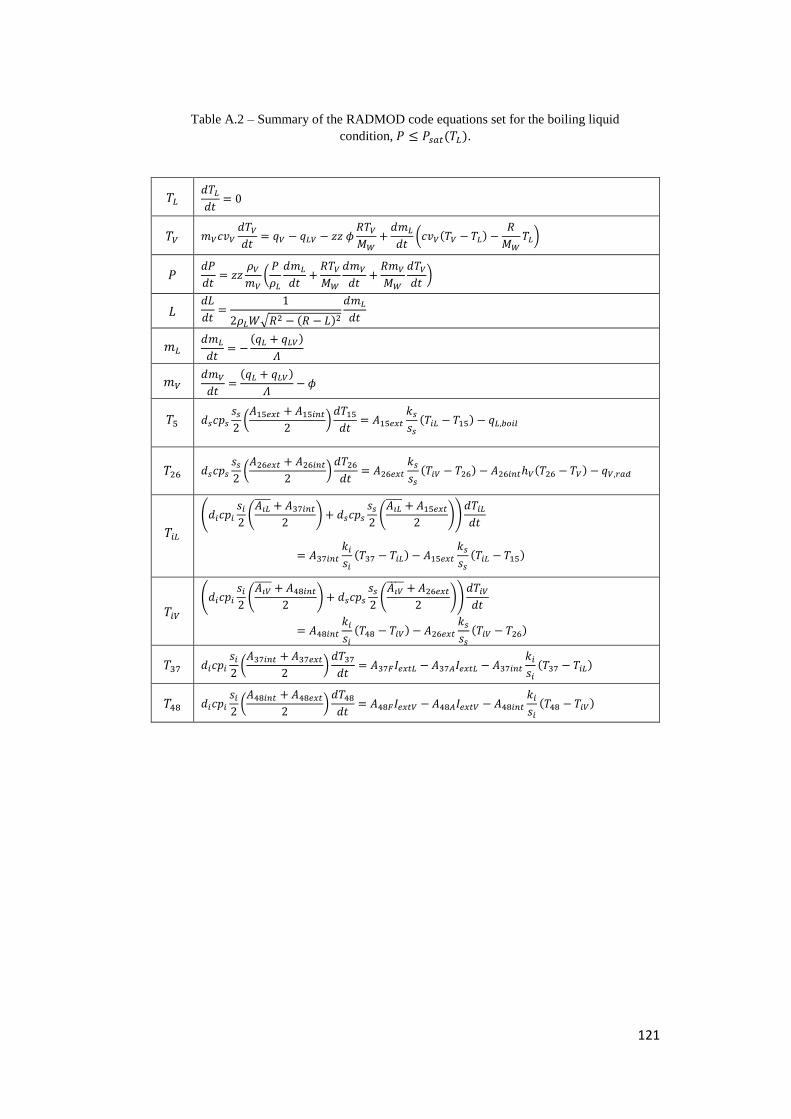
121

Table A.2 – Summary of the RADMOD code equations set for the boiling liquid

condition, 𝑃 ≤ 𝑃𝑠𝑎𝑡(𝑇𝐿).

𝑇𝐿 𝑑𝑇𝐿

𝑑𝑡= 0

𝑇𝑉 𝑚𝑉𝑐𝑣𝑉

𝑑𝑇𝑉

𝑑𝑡= 𝑞𝑉 − 𝑞𝐿𝑉 − 𝑧𝑧 𝜙

𝑅𝑇𝑉

𝑀𝑊+

𝑑𝑚𝐿

𝑑𝑡(𝑐𝑣𝑉(𝑇𝑉 − 𝑇𝐿) −

𝑅

𝑀𝑊𝑇𝐿)

𝑃 𝑑𝑃

𝑑𝑡= 𝑧𝑧

𝜌𝑉

𝑚𝑉(

𝑃

𝜌𝐿

𝑑𝑚𝐿

𝑑𝑡+

𝑅𝑇𝑉

𝑀𝑊

𝑑𝑚𝑉

𝑑𝑡+

𝑅𝑚𝑉

𝑀𝑊

𝑑𝑇𝑉

𝑑𝑡)

𝐿 𝑑𝐿

𝑑𝑡=

1

2𝜌𝐿𝑊√𝑅2 − (𝑅 − 𝐿)2

𝑑𝑚𝐿

𝑑𝑡

𝑚𝐿 𝑑𝑚𝐿

𝑑𝑡= −

(𝑞𝐿 + 𝑞𝐿𝑉)

𝛬

𝑚𝑉 𝑑𝑚𝑉

𝑑𝑡=

(𝑞𝐿 + 𝑞𝐿𝑉)

𝛬− 𝜙

𝑇5 𝑑𝑠𝑐𝑝𝑠

𝑠𝑠

2(

𝐴15𝑒𝑥𝑡 + 𝐴15𝑖𝑛𝑡

2)

𝑑𝑇15

𝑑𝑡= 𝐴15𝑒𝑥𝑡

𝑘𝑠

𝑠𝑠

(𝑇𝑖𝐿 − 𝑇15) − 𝑞𝐿,𝑏𝑜𝑖𝑙

𝑇26 𝑑𝑠𝑐𝑝𝑠

𝑠𝑠

2(

𝐴26𝑒𝑥𝑡 + 𝐴26𝑖𝑛𝑡

2)

𝑑𝑇26

𝑑𝑡= 𝐴26𝑒𝑥𝑡

𝑘𝑠

𝑠𝑠

(𝑇𝑖𝑉 − 𝑇26) − 𝐴26𝑖𝑛𝑡ℎ𝑉(𝑇26 − 𝑇𝑉) − 𝑞𝑉,𝑟𝑎𝑑

𝑇𝑖𝐿

(𝑑𝑖𝑐𝑝𝑖

𝑠𝑖

2(

𝐴𝑖𝐿 + 𝐴37𝑖𝑛𝑡

2) + 𝑑𝑠𝑐𝑝𝑠

𝑠𝑠

2(

𝐴𝑖𝐿 + 𝐴15𝑒𝑥𝑡

2))

𝑑𝑇𝑖𝐿

𝑑𝑡

= 𝐴37𝑖𝑛𝑡

𝑘𝑖

𝑠𝑖

(𝑇37 − 𝑇𝑖𝐿) − 𝐴15𝑒𝑥𝑡

𝑘𝑠

𝑠𝑠

(𝑇𝑖𝐿 − 𝑇15)

𝑇𝑖𝑉

(𝑑𝑖𝑐𝑝𝑖

𝑠𝑖

2(

𝐴𝑖𝑉 + 𝐴48𝑖𝑛𝑡

2) + 𝑑𝑠𝑐𝑝𝑠

𝑠𝑠

2(

𝐴𝑖𝑉 + 𝐴26𝑒𝑥𝑡

2))

𝑑𝑇𝑖𝑉

𝑑𝑡

= 𝐴48𝑖𝑛𝑡

𝑘𝑖

𝑠𝑖

(𝑇48 − 𝑇𝑖𝑉) − 𝐴26𝑒𝑥𝑡

𝑘𝑠

𝑠𝑠

(𝑇𝑖𝑉 − 𝑇26)

𝑇37 𝑑𝑖𝑐𝑝𝑖

𝑠𝑖

2(

𝐴37𝑖𝑛𝑡 + 𝐴37𝑒𝑥𝑡

2)

𝑑𝑇37

𝑑𝑡= 𝐴37𝐹𝐼𝑒𝑥𝑡𝐿 − 𝐴37𝐴𝐼𝑒𝑥𝑡𝐿 − 𝐴37𝑖𝑛𝑡

𝑘𝑖

𝑠𝑖

(𝑇37 − 𝑇𝑖𝐿)

𝑇48 𝑑𝑖𝑐𝑝𝑖

𝑠𝑖

2(

𝐴48𝑖𝑛𝑡 + 𝐴48𝑒𝑥𝑡

2)

𝑑𝑇48

𝑑𝑡= 𝐴48𝐹𝐼𝑒𝑥𝑡𝑉 − 𝐴48𝐴𝐼𝑒𝑥𝑡𝑉 − 𝐴48𝑖𝑛𝑡

𝑘𝑖

𝑠𝑖

(𝑇48 − 𝑇𝑖𝑉)

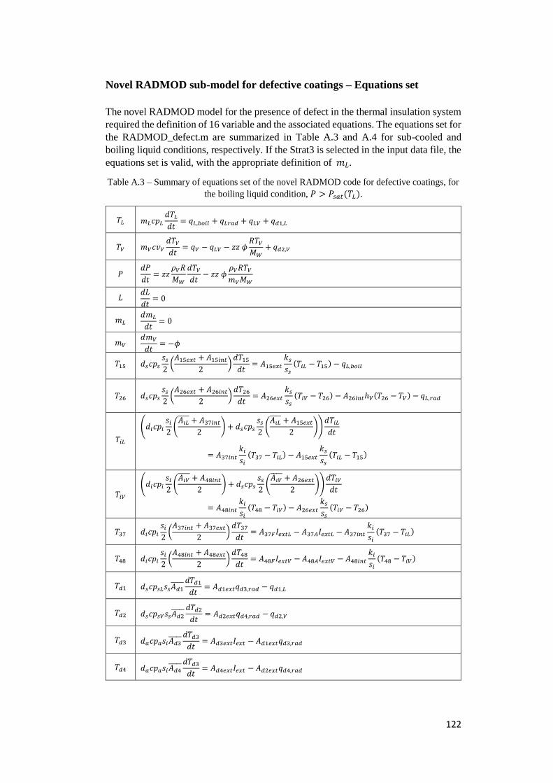
122

Novel RADMOD sub-model for defective coatings – Equations set

The novel RADMOD model for the presence of defect in the thermal insulation system

required the definition of 16 variable and the associated equations. The equations set for

the RADMOD_defect.m are summarized in Table A.3 and A.4 for sub-cooled and

boiling liquid conditions, respectively. If the Strat3 is selected in the input data file, the

equations set is valid, with the appropriate definition of 𝑚𝐿.

Table A.3 – Summary of equations set of the novel RADMOD code for defective coatings, for

the boiling liquid condition, 𝑃 > 𝑃𝑠𝑎𝑡(𝑇𝐿).

𝑇𝐿 𝑚𝐿𝑐𝑝𝐿

𝑑𝑇𝐿

𝑑𝑡= 𝑞𝐿,𝑏𝑜𝑖𝑙 + 𝑞𝐿𝑟𝑎𝑑 + 𝑞𝐿𝑉 + 𝑞𝑑1,𝐿

𝑇𝑉 𝑚𝑉𝑐𝑣𝑉

𝑑𝑇𝑉

𝑑𝑡= 𝑞𝑉 − 𝑞𝐿𝑉 − 𝑧𝑧 𝜙

𝑅𝑇𝑉

𝑀𝑊+ 𝑞𝑑2,𝑉

𝑃 𝑑𝑃

𝑑𝑡= 𝑧𝑧

𝜌𝑉𝑅

𝑀𝑊

𝑑𝑇𝑉

𝑑𝑡− 𝑧𝑧 𝜙

𝜌𝑉𝑅𝑇𝑉

𝑚𝑉𝑀𝑊

𝐿 𝑑𝐿

𝑑𝑡= 0

𝑚𝐿 𝑑𝑚𝐿

𝑑𝑡= 0

𝑚𝑉 𝑑𝑚𝑉

𝑑𝑡= −𝜙

𝑇15 𝑑𝑠𝑐𝑝𝑠

𝑠𝑠

2(

𝐴15𝑒𝑥𝑡 + 𝐴15𝑖𝑛𝑡

2)

𝑑𝑇15

𝑑𝑡= 𝐴15𝑒𝑥𝑡

𝑘𝑠

𝑠𝑠

(𝑇𝑖𝐿 − 𝑇15) − 𝑞𝐿,𝑏𝑜𝑖𝑙

𝑇26 𝑑𝑠𝑐𝑝𝑠

𝑠𝑠

2(

𝐴26𝑒𝑥𝑡 + 𝐴26𝑖𝑛𝑡

2)

𝑑𝑇26

𝑑𝑡= 𝐴26𝑒𝑥𝑡

𝑘𝑠

𝑠𝑠

(𝑇𝑖𝑉 − 𝑇26) − 𝐴26𝑖𝑛𝑡ℎ𝑉(𝑇26 − 𝑇𝑉) − 𝑞𝐿,𝑟𝑎𝑑

𝑇𝑖𝐿

(𝑑𝑖𝑐𝑝𝑖

𝑠𝑖

2(

𝐴𝑖𝐿 + 𝐴37𝑖𝑛𝑡

2) + 𝑑𝑠𝑐𝑝𝑠

𝑠𝑠

2(

𝐴𝑖𝐿 + 𝐴15𝑒𝑥𝑡

2))

𝑑𝑇𝑖𝐿

𝑑𝑡

= 𝐴37𝑖𝑛𝑡

𝑘𝑖

𝑠𝑖

(𝑇37 − 𝑇𝑖𝐿) − 𝐴15𝑒𝑥𝑡

𝑘𝑠

𝑠𝑠

(𝑇𝑖𝐿 − 𝑇15)

𝑇𝑖𝑉

(𝑑𝑖𝑐𝑝𝑖

𝑠𝑖

2(

𝐴𝑖𝑉 + 𝐴48𝑖𝑛𝑡

2) + 𝑑𝑠𝑐𝑝𝑠

𝑠𝑠

2(

𝐴𝑖𝑉 + 𝐴26𝑒𝑥𝑡

2))

𝑑𝑇𝑖𝑉

𝑑𝑡

= 𝐴48𝑖𝑛𝑡

𝑘𝑖

𝑠𝑖

(𝑇48 − 𝑇𝑖𝑉) − 𝐴26𝑒𝑥𝑡

𝑘𝑠

𝑠𝑠

(𝑇𝑖𝑉 − 𝑇26)

𝑇37 𝑑𝑖𝑐𝑝𝑖

𝑠𝑖

2(

𝐴37𝑖𝑛𝑡 + 𝐴37𝑒𝑥𝑡

2)

𝑑𝑇37

𝑑𝑡= 𝐴37𝐹𝐼𝑒𝑥𝑡𝐿 − 𝐴37𝐴𝐼𝑒𝑥𝑡𝐿 − 𝐴37𝑖𝑛𝑡

𝑘𝑖

𝑠𝑖

(𝑇37 − 𝑇𝑖𝐿)

𝑇48 𝑑𝑖𝑐𝑝𝑖

𝑠𝑖

2(

𝐴48𝑖𝑛𝑡 + 𝐴48𝑒𝑥𝑡

2)

𝑑𝑇48

𝑑𝑡= 𝐴48𝐹𝐼𝑒𝑥𝑡𝑉 − 𝐴48𝐴𝐼𝑒𝑥𝑡𝑉 − 𝐴48𝑖𝑛𝑡

𝑘𝑖

𝑠𝑖

(𝑇48 − 𝑇𝑖𝑉)

𝑇𝑑1 𝑑𝑠𝑐𝑝𝑠𝐿𝑠𝑠𝐴𝑑1

𝑑𝑇𝑑1

𝑑𝑡= 𝐴𝑑1𝑒𝑥𝑡𝑞𝑑3,𝑟𝑎𝑑 − 𝑞𝑑1,𝐿

𝑇𝑑2 𝑑𝑠𝑐𝑝𝑠𝑉𝑠𝑠𝐴𝑑2

𝑑𝑇𝑑2

𝑑𝑡= 𝐴𝑑2𝑒𝑥𝑡𝑞𝑑4,𝑟𝑎𝑑 − 𝑞𝑑2,𝑉

𝑇𝑑3 𝑑𝑎𝑐𝑝𝑎𝑠𝑖𝐴𝑑3

𝑑𝑇𝑑3

𝑑𝑡= 𝐴𝑑3𝑒𝑥𝑡𝐼𝑒𝑥𝑡 − 𝐴𝑑1𝑒𝑥𝑡𝑞𝑑3,𝑟𝑎𝑑

𝑇𝑑4 𝑑𝑎𝑐𝑝𝑎𝑠𝑖𝐴𝑑4

𝑑𝑇𝑑3

𝑑𝑡= 𝐴𝑑4𝑒𝑥𝑡𝐼𝑒𝑥𝑡 − 𝐴𝑑2𝑒𝑥𝑡𝑞𝑑4,𝑟𝑎𝑑

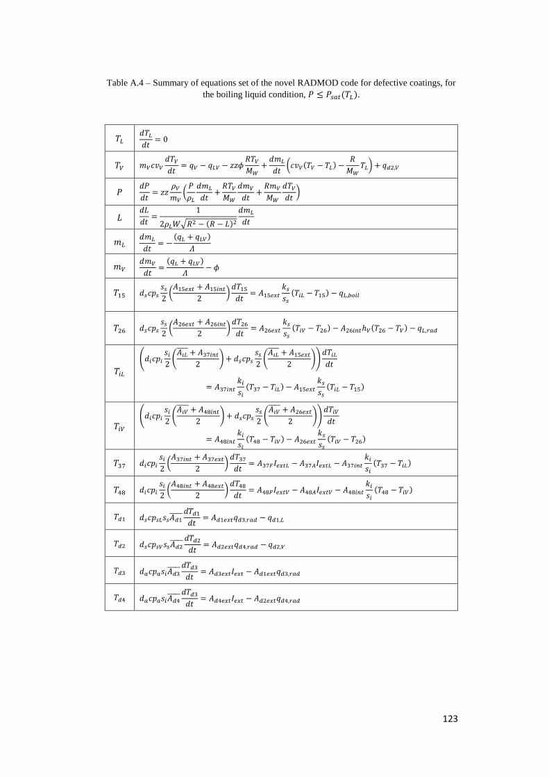
123

Table A.4 – Summary of equations set of the novel RADMOD code for defective coatings, for

the boiling liquid condition, 𝑃 ≤ 𝑃𝑠𝑎𝑡(𝑇𝐿).

𝑇𝐿 𝑑𝑇𝐿

𝑑𝑡= 0

𝑇𝑉 𝑚𝑉𝑐𝑣𝑉

𝑑𝑇𝑉

𝑑𝑡= 𝑞𝑉 − 𝑞𝐿𝑉 − 𝑧𝑧𝜙

𝑅𝑇𝑉

𝑀𝑊+

𝑑𝑚𝐿

𝑑𝑡(𝑐𝑣𝑉(𝑇𝑉 − 𝑇𝐿) −

𝑅

𝑀𝑊𝑇𝐿) + 𝑞𝑑2,𝑉

𝑃 𝑑𝑃

𝑑𝑡= 𝑧𝑧

𝜌𝑉

𝑚𝑉(

𝑃

𝜌𝐿

𝑑𝑚𝐿

𝑑𝑡+

𝑅𝑇𝑉

𝑀𝑊

𝑑𝑚𝑉

𝑑𝑡+

𝑅𝑚𝑉

𝑀𝑊

𝑑𝑇𝑉

𝑑𝑡)

𝐿 𝑑𝐿

𝑑𝑡=

1

2𝜌𝐿𝑊√𝑅2 − (𝑅 − 𝐿)2

𝑑𝑚𝐿

𝑑𝑡

𝑚𝐿 𝑑𝑚𝐿

𝑑𝑡= −

(𝑞𝐿 + 𝑞𝐿𝑉)

𝛬

𝑚𝑉 𝑑𝑚𝑉

𝑑𝑡=

(𝑞𝐿 + 𝑞𝐿𝑉)

𝛬− 𝜙

𝑇15 𝑑𝑠𝑐𝑝𝑠

𝑠𝑠

2(

𝐴15𝑒𝑥𝑡 + 𝐴15𝑖𝑛𝑡

2)

𝑑𝑇15

𝑑𝑡= 𝐴15𝑒𝑥𝑡

𝑘𝑠

𝑠𝑠

(𝑇𝑖𝐿 − 𝑇15) − 𝑞𝐿,𝑏𝑜𝑖𝑙

𝑇26 𝑑𝑠𝑐𝑝𝑠

𝑠𝑠

2(

𝐴26𝑒𝑥𝑡 + 𝐴26𝑖𝑛𝑡

2)

𝑑𝑇26

𝑑𝑡= 𝐴26𝑒𝑥𝑡

𝑘𝑠

𝑠𝑠

(𝑇𝑖𝑉 − 𝑇26) − 𝐴26𝑖𝑛𝑡ℎ𝑉(𝑇26 − 𝑇𝑉) − 𝑞𝐿,𝑟𝑎𝑑

𝑇𝑖𝐿

(𝑑𝑖𝑐𝑝𝑖

𝑠𝑖

2(

𝐴𝑖𝐿 + 𝐴37𝑖𝑛𝑡

2) + 𝑑𝑠𝑐𝑝𝑠

𝑠𝑠

2(

𝐴𝑖𝐿 + 𝐴15𝑒𝑥𝑡

2))

𝑑𝑇𝑖𝐿

𝑑𝑡

= 𝐴37𝑖𝑛𝑡

𝑘𝑖

𝑠𝑖

(𝑇37 − 𝑇𝑖𝐿) − 𝐴15𝑒𝑥𝑡

𝑘𝑠

𝑠𝑠

(𝑇𝑖𝐿 − 𝑇15)

𝑇𝑖𝑉

(𝑑𝑖𝑐𝑝𝑖

𝑠𝑖

2(

𝐴𝑖𝑉 + 𝐴48𝑖𝑛𝑡

2) + 𝑑𝑠𝑐𝑝𝑠

𝑠𝑠

2(

𝐴𝑖𝑉 + 𝐴26𝑒𝑥𝑡

2))

𝑑𝑇𝑖𝑉

𝑑𝑡

= 𝐴48𝑖𝑛𝑡

𝑘𝑖

𝑠𝑖

(𝑇48 − 𝑇𝑖𝑉) − 𝐴26𝑒𝑥𝑡

𝑘𝑠

𝑠𝑠

(𝑇𝑖𝑉 − 𝑇26)

𝑇37 𝑑𝑖𝑐𝑝𝑖

𝑠𝑖

2(

𝐴37𝑖𝑛𝑡 + 𝐴37𝑒𝑥𝑡

2)

𝑑𝑇37

𝑑𝑡= 𝐴37𝐹𝐼𝑒𝑥𝑡𝐿 − 𝐴37𝐴𝐼𝑒𝑥𝑡𝐿 − 𝐴37𝑖𝑛𝑡

𝑘𝑖

𝑠𝑖

(𝑇37 − 𝑇𝑖𝐿)

𝑇48 𝑑𝑖𝑐𝑝𝑖

𝑠𝑖

2(

𝐴48𝑖𝑛𝑡 + 𝐴48𝑒𝑥𝑡

2)

𝑑𝑇48

𝑑𝑡= 𝐴48𝐹𝐼𝑒𝑥𝑡𝑉 − 𝐴48𝐴𝐼𝑒𝑥𝑡𝑉 − 𝐴48𝑖𝑛𝑡

𝑘𝑖

𝑠𝑖

(𝑇48 − 𝑇𝑖𝑉)

𝑇𝑑1 𝑑𝑠𝑐𝑝𝑠𝐿𝑠𝑠𝐴𝑑1

𝑑𝑇𝑑1

𝑑𝑡= 𝐴𝑑1𝑒𝑥𝑡𝑞𝑑3,𝑟𝑎𝑑 − 𝑞𝑑1,𝐿

𝑇𝑑2 𝑑𝑠𝑐𝑝𝑠𝑉𝑠𝑠𝐴𝑑2

𝑑𝑇𝑑2

𝑑𝑡= 𝐴𝑑2𝑒𝑥𝑡𝑞𝑑4,𝑟𝑎𝑑 − 𝑞𝑑2,𝑉

𝑇𝑑3 𝑑𝑎𝑐𝑝𝑎𝑠𝑖𝐴𝑑3

𝑑𝑇𝑑3

𝑑𝑡= 𝐴𝑑3𝑒𝑥𝑡𝐼𝑒𝑥𝑡 − 𝐴𝑑1𝑒𝑥𝑡𝑞𝑑3,𝑟𝑎𝑑

𝑇𝑑4 𝑑𝑎𝑐𝑝𝑎𝑠𝑖𝐴𝑑4

𝑑𝑇𝑑3

𝑑𝑡= 𝐴𝑑4𝑒𝑥𝑡𝐼𝑒𝑥𝑡 − 𝐴𝑑2𝑒𝑥𝑡𝑞𝑑4,𝑟𝑎𝑑

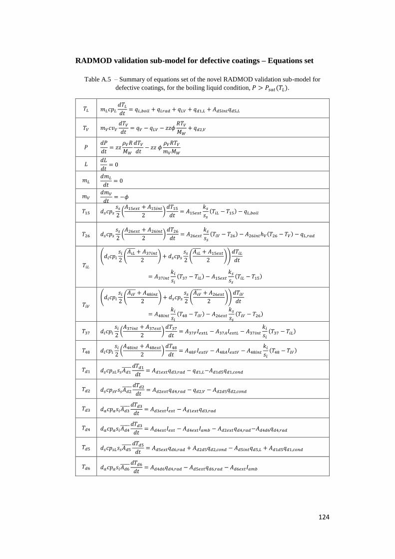
124

RADMOD validation sub-model for defective coatings – Equations set

Table A.5 – Summary of equations set of the novel RADMOD validation sub-model for

defective coatings, for the boiling liquid condition, 𝑃 > 𝑃𝑠𝑎𝑡(𝑇𝐿).

𝑇𝐿 𝑚𝐿𝑐𝑝𝐿

𝑑𝑇𝐿

𝑑𝑡= 𝑞𝐿,𝑏𝑜𝑖𝑙 + 𝑞𝐿𝑟𝑎𝑑 + 𝑞𝐿𝑉 + 𝑞𝑑1,𝐿 + 𝐴𝑑5𝑖𝑛𝑡𝑞𝑑5,𝐿

𝑇𝑉 𝑚𝑉𝑐𝑣𝑉

𝑑𝑇𝑉

𝑑𝑡= 𝑞𝑉 − 𝑞𝐿𝑉 − 𝑧𝑧𝜙

𝑅𝑇𝑉

𝑀𝑊+ 𝑞𝑑2,𝑉

𝑃 𝑑𝑃

𝑑𝑡= 𝑧𝑧

𝜌𝑉𝑅

𝑀𝑊

𝑑𝑇𝑉

𝑑𝑡− 𝑧𝑧 𝜙

𝜌𝑉𝑅𝑇𝑉

𝑚𝑉𝑀𝑊

𝐿 𝑑𝐿

𝑑𝑡= 0

𝑚𝐿 𝑑𝑚𝐿

𝑑𝑡= 0

𝑚𝑉 𝑑𝑚𝑉

𝑑𝑡= −𝜙

𝑇15 𝑑𝑠𝑐𝑝𝑠

𝑠𝑠

2(

𝐴15𝑒𝑥𝑡 + 𝐴15𝑖𝑛𝑡

2)

𝑑𝑇15

𝑑𝑡= 𝐴15𝑒𝑥𝑡

𝑘𝑠

𝑠𝑠

(𝑇𝑖𝐿 − 𝑇15) − 𝑞𝐿,𝑏𝑜𝑖𝑙

𝑇26 𝑑𝑠𝑐𝑝𝑠

𝑠𝑠

2(

𝐴26𝑒𝑥𝑡 + 𝐴26𝑖𝑛𝑡

2)

𝑑𝑇26

𝑑𝑡= 𝐴26𝑒𝑥𝑡

𝑘𝑠

𝑠𝑠

(𝑇𝑖𝑉 − 𝑇26) − 𝐴26𝑖𝑛𝑡ℎ𝑉(𝑇26 − 𝑇𝑉) − 𝑞𝐿,𝑟𝑎𝑑

𝑇𝑖𝐿

(𝑑𝑖𝑐𝑝𝑖

𝑠𝑖

2(

𝐴𝑖𝐿 + 𝐴37𝑖𝑛𝑡

2) + 𝑑𝑠𝑐𝑝𝑠

𝑠𝑠

2(

𝐴𝑖𝐿 + 𝐴15𝑒𝑥𝑡

2))

𝑑𝑇𝑖𝐿

𝑑𝑡

= 𝐴37𝑖𝑛𝑡

𝑘𝑖

𝑠𝑖

(𝑇37 − 𝑇𝑖𝐿) − 𝐴15𝑒𝑥𝑡

𝑘𝑠

𝑠𝑠

(𝑇𝑖𝐿 − 𝑇15)

𝑇𝑖𝑉

(𝑑𝑖𝑐𝑝𝑖

𝑠𝑖

2(

𝐴𝑖𝑉 + 𝐴48𝑖𝑛𝑡

2) + 𝑑𝑠𝑐𝑝𝑠

𝑠𝑠

2(

𝐴𝑖𝑉 + 𝐴26𝑒𝑥𝑡

2))

𝑑𝑇𝑖𝑉

𝑑𝑡

= 𝐴48𝑖𝑛𝑡

𝑘𝑖

𝑠𝑖

(𝑇48 − 𝑇𝑖𝑉) − 𝐴26𝑒𝑥𝑡

𝑘𝑠

𝑠𝑠

(𝑇𝑖𝑉 − 𝑇26)

𝑇37 𝑑𝑖𝑐𝑝𝑖

𝑠𝑖

2(

𝐴37𝑖𝑛𝑡 + 𝐴37𝑒𝑥𝑡

2)

𝑑𝑇37

𝑑𝑡= 𝐴37𝐹𝐼𝑒𝑥𝑡𝐿 − 𝐴37𝐴𝐼𝑒𝑥𝑡𝐿 − 𝐴37𝑖𝑛𝑡

𝑘𝑖

𝑠𝑖

(𝑇37 − 𝑇𝑖𝐿)

𝑇48 𝑑𝑖𝑐𝑝𝑖

𝑠𝑖

2(

𝐴48𝑖𝑛𝑡 + 𝐴48𝑒𝑥𝑡

2)

𝑑𝑇48

𝑑𝑡= 𝐴48𝐹𝐼𝑒𝑥𝑡𝑉 − 𝐴48𝐴𝐼𝑒𝑥𝑡𝑉 − 𝐴48𝑖𝑛𝑡

𝑘𝑖

𝑠𝑖

(𝑇48 − 𝑇𝑖𝑉)

𝑇𝑑1 𝑑𝑠𝑐𝑝𝑠𝐿𝑠𝑠𝐴𝑑1

𝑑𝑇𝑑1

𝑑𝑡= 𝐴𝑑1𝑒𝑥𝑡𝑞𝑑3,𝑟𝑎𝑑 − 𝑞𝑑1,𝐿−𝐴𝑑1𝑑5𝑞𝑑1,𝑐𝑜𝑛𝑑

𝑇𝑑2 𝑑𝑠𝑐𝑝𝑠𝑉𝑠𝑠𝐴𝑑2

𝑑𝑇𝑑2

𝑑𝑡= 𝐴𝑑2𝑒𝑥𝑡𝑞𝑑4,𝑟𝑎𝑑 − 𝑞𝑑2,𝑉 − 𝐴𝑑2𝑑5𝑞𝑑2,𝑐𝑜𝑛𝑑

𝑇𝑑3 𝑑𝑎𝑐𝑝𝑎𝑠𝑖𝐴𝑑3

𝑑𝑇𝑑3

𝑑𝑡= 𝐴𝑑3𝑒𝑥𝑡𝐼𝑒𝑥𝑡 − 𝐴𝑑1𝑒𝑥𝑡𝑞𝑑3,𝑟𝑎𝑑

𝑇𝑑4 𝑑𝑎𝑐𝑝𝑎𝑠𝑖𝐴𝑑4

𝑑𝑇𝑑3

𝑑𝑡= 𝐴𝑑4𝑒𝑥𝑡𝐼𝑒𝑥𝑡 − 𝐴𝑑4𝑒𝑥𝑡𝐼𝑎𝑚𝑏 − 𝐴𝑑2𝑒𝑥𝑡𝑞𝑑4,𝑟𝑎𝑑−𝐴𝑑4𝑑6𝑞𝑑4,𝑟𝑎𝑑

𝑇𝑑5 𝑑𝑠𝑐𝑝𝑠𝐿𝑠𝑠𝐴𝑑5

𝑑𝑇𝑑5

𝑑𝑡= 𝐴𝑑5𝑒𝑥𝑡𝑞𝑑6,𝑟𝑎𝑑 + 𝐴𝑑2𝑑5𝑞𝑑2,𝑐𝑜𝑛𝑑 − 𝐴𝑑5𝑖𝑛𝑡𝑞𝑑5,𝐿 + 𝐴𝑑1𝑑5𝑞𝑑1,𝑐𝑜𝑛𝑑

𝑇𝑑6 𝑑𝑎𝑐𝑝𝑎𝑠𝑖𝐴𝑑6

𝑑𝑇𝑑6

𝑑𝑡= 𝐴𝑑4𝑑6𝑞𝑑4,𝑟𝑎𝑑 − 𝐴𝑑5𝑒𝑥𝑡𝑞𝑑6,𝑟𝑎𝑑 − 𝐴𝑑6𝑒𝑥𝑡𝐼𝑎𝑚𝑏

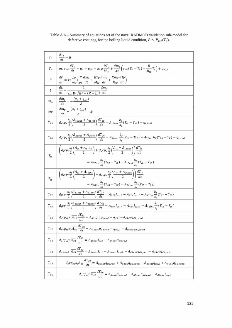
125

Table A.6 – Summary of equations set of the novel RADMOD validation sub-model for

defective coatings, for the boiling liquid condition, 𝑃 ≤ 𝑃𝑠𝑎𝑡(𝑇𝐿).

𝑇𝐿 𝑑𝑇𝐿

𝑑𝑡= 0

𝑇𝑉 𝑚𝑉𝑐𝑣𝑉

𝑑𝑇𝑉

𝑑𝑡= 𝑞𝑉 − 𝑞𝐿𝑉 − 𝑧𝑧𝜙

𝑅𝑇𝑉

𝑀𝑊+

𝑑𝑚𝐿

𝑑𝑡(𝑐𝑣𝑉(𝑇𝑉 − 𝑇𝐿) −

𝑅

𝑀𝑊𝑇𝐿) + 𝑞𝑑2,𝑉

𝑃 𝑑𝑃

𝑑𝑡= 𝑧𝑧

𝜌𝑉

𝑚𝑉(

𝑃

𝜌𝐿

𝑑𝑚𝐿

𝑑𝑡+

𝑅𝑇𝑉

𝑀𝑊

𝑑𝑚𝑉

𝑑𝑡+

𝑅𝑚𝑉

𝑀𝑊

𝑑𝑇𝑉

𝑑𝑡)

𝐿 𝑑𝐿

𝑑𝑡=

1

2𝜌𝐿𝑊√𝑅2 − (𝑅 − 𝐿)2

𝑑𝑚𝐿

𝑑𝑡

𝑚𝐿 𝑑𝑚𝐿

𝑑𝑡= −

(𝑞𝐿 + 𝑞𝐿𝑉)

𝛬

𝑚𝑉 𝑑𝑚𝑉

𝑑𝑡=

(𝑞𝐿 + 𝑞𝐿𝑉)

𝛬− 𝜙

𝑇15 𝑑𝑠𝑐𝑝𝑠

𝑠𝑠

2(

𝐴15𝑒𝑥𝑡 + 𝐴15𝑖𝑛𝑡

2)

𝑑𝑇15

𝑑𝑡= 𝐴15𝑒𝑥𝑡

𝑘𝑠

𝑠𝑠

(𝑇𝑖𝐿 − 𝑇15) − 𝑞𝐿,𝑏𝑜𝑖𝑙

𝑇26 𝑑𝑠𝑐𝑝𝑠

𝑠𝑠

2(

𝐴26𝑒𝑥𝑡 + 𝐴26𝑖𝑛𝑡

2)

𝑑𝑇26

𝑑𝑡= 𝐴26𝑒𝑥𝑡

𝑘𝑠

𝑠𝑠

(𝑇𝑖𝑉 − 𝑇26) − 𝐴26𝑖𝑛𝑡ℎ𝑉(𝑇26 − 𝑇𝑉) − 𝑞𝐿,𝑟𝑎𝑑

𝑇𝑖𝐿

(𝑑𝑖𝑐𝑝𝑖

𝑠𝑖

2(

𝐴𝑖𝐿 + 𝐴37𝑖𝑛𝑡

2) + 𝑑𝑠𝑐𝑝𝑠

𝑠𝑠

2(

𝐴𝑖𝐿 + 𝐴15𝑒𝑥𝑡

2))

𝑑𝑇𝑖𝐿

𝑑𝑡

= 𝐴37𝑖𝑛𝑡

𝑘𝑖

𝑠𝑖

(𝑇37 − 𝑇𝑖𝐿) − 𝐴15𝑒𝑥𝑡

𝑘𝑠

𝑠𝑠

(𝑇𝑖𝐿 − 𝑇15)

𝑇𝑖𝑉

(𝑑𝑖𝑐𝑝𝑖

𝑠𝑖

2(

𝐴𝑖𝑉 + 𝐴48𝑖𝑛𝑡

2) + 𝑑𝑠𝑐𝑝𝑠

𝑠𝑠

2(

𝐴𝑖𝑉 + 𝐴26𝑒𝑥𝑡

2))

𝑑𝑇𝑖𝑉

𝑑𝑡

= 𝐴48𝑖𝑛𝑡

𝑘𝑖

𝑠𝑖

(𝑇48 − 𝑇𝑖𝑉) − 𝐴26𝑒𝑥𝑡

𝑘𝑠

𝑠𝑠

(𝑇𝑖𝑉 − 𝑇26)

𝑇37 𝑑𝑖𝑐𝑝𝑖

𝑠𝑖

2(

𝐴37𝑖𝑛𝑡 + 𝐴37𝑒𝑥𝑡

2)

𝑑𝑇37

𝑑𝑡= 𝐴37𝐹𝐼𝑒𝑥𝑡𝐿 − 𝐴37𝐴𝐼𝑒𝑥𝑡𝐿 − 𝐴37𝑖𝑛𝑡

𝑘𝑖

𝑠𝑖

(𝑇37 − 𝑇𝑖𝐿)

𝑇48 𝑑𝑖𝑐𝑝𝑖

𝑠𝑖

2(

𝐴48𝑖𝑛𝑡 + 𝐴48𝑒𝑥𝑡

2)

𝑑𝑇48

𝑑𝑡= 𝐴48𝐹𝐼𝑒𝑥𝑡𝑉 − 𝐴48𝐴𝐼𝑒𝑥𝑡𝑉 − 𝐴48𝑖𝑛𝑡

𝑘𝑖

𝑠𝑖

(𝑇48 − 𝑇𝑖𝑉)

𝑇𝑑1 𝑑𝑠𝑐𝑝𝑠𝐿𝑠𝑠𝐴𝑑1

𝑑𝑇𝑑1

𝑑𝑡= 𝐴𝑑1𝑒𝑥𝑡𝑞𝑑3,𝑟𝑎𝑑 − 𝑞𝑑1,𝐿−𝐴𝑑1𝑑5𝑞𝑑1,𝑐𝑜𝑛𝑑

𝑇𝑑2 𝑑𝑠𝑐𝑝𝑠𝑉𝑠𝑠𝐴𝑑2

𝑑𝑇𝑑2

𝑑𝑡= 𝐴𝑑2𝑒𝑥𝑡𝑞𝑑4,𝑟𝑎𝑑 − 𝑞𝑑2,𝑉 − 𝐴𝑑2𝑑5𝑞𝑑2,𝑐𝑜𝑛𝑑

𝑇𝑑3 𝑑𝑎𝑐𝑝𝑎𝑠𝑖𝐴𝑑3

𝑑𝑇𝑑3

𝑑𝑡= 𝐴𝑑3𝑒𝑥𝑡𝐼𝑒𝑥𝑡 − 𝐴𝑑1𝑒𝑥𝑡𝑞𝑑3,𝑟𝑎𝑑

𝑇𝑑4 𝑑𝑎𝑐𝑝𝑎𝑠𝑖𝐴𝑑4

𝑑𝑇𝑑3

𝑑𝑡= 𝐴𝑑4𝑒𝑥𝑡𝐼𝑒𝑥𝑡 − 𝐴𝑑4𝑒𝑥𝑡𝐼𝑎𝑚𝑏 − 𝐴𝑑2𝑒𝑥𝑡𝑞𝑑4,𝑟𝑎𝑑 − 𝐴𝑑4𝑑6𝑞𝑑4,𝑟𝑎𝑑

𝑇𝑑5 𝑑𝑠𝑐𝑝𝑠𝐿𝑠𝑠𝐴𝑑5

𝑑𝑇𝑑5

𝑑𝑡= 𝐴𝑑5𝑒𝑥𝑡𝑞𝑑6,𝑟𝑎𝑑 + 𝐴𝑑2𝑑5𝑞𝑑2,𝑐𝑜𝑛𝑑 − 𝐴𝑑5𝑖𝑛𝑡𝑞𝑑5,𝐿 + 𝐴𝑑1𝑑5𝑞𝑑1,𝑐𝑜𝑛𝑑

𝑇𝑑6 𝑑𝑎𝑐𝑝𝑎𝑠𝑖𝐴𝑑6

𝑑𝑇𝑑6

𝑑𝑡= 𝐴𝑑4𝑑6𝑞𝑑4,𝑟𝑎𝑑 − 𝐴𝑑5𝑒𝑥𝑡𝑞𝑑6,𝑟𝑎𝑑 − 𝐴𝑑6𝑒𝑥𝑡𝐼𝑎𝑚𝑏

126

Ringraziamenti

Vorrei ringraziare anzitutto l’Ing. Landucci, relatore di questa tesi, per la guida,

l’attenzione ed il supporto dato a questo lavoro.

Ringrazio il Prof. Bertini, controrelatore, per la disponibilità ed i consigli datami.

Un particolare ringraziamento va a Giordano, per la grande disponibilità al confronto e

l’amicizia dimostratami.

Desidero ringraziare con il cuore in mano i miei genitori, Lorella e Pietro, e mio fratello

Chicco per il loro incrollabile sostegno, che è stato la mia forza durante questi anni.

Grazie per questa opportunità.

Ringrazio Anna, Sara e Angelo, che negli anni sono stati prima compagni di classe, poi

amici e coinquilini, fino a ritrovarci in una famiglia a tutti gli effetti. Ringrazio inoltre

Dario, che da solo è la mia squadra più forte, per esserci ed esserci sempre stato; il caro

Frà che mi ha presa per mano ed accompagnata lungo questo percorso universitario e di

vita; e Carmelo nel quale ho ritrovato un vero amico oltre ad un compagno di studi. Un

grazie particolare ai miei compagni di corso: Bruno, Flavio, Gianluca, Giuseppe, Laura,

Luigi e Luigi, Marina, Saverio e Vincenzo; con i quali ho condiviso davvero molto fuori

e dento le mura di ingegneria. Vi voglio bene.

Vorrei ringraziare Giacomo, il mio fidanzato e colonna portante, per il supporto non

quantificabile, soprattutto in questi ultimi mesi molto duri.

Un ultimo ringraziamento a tutte le persone a me vicine, in particolare a Martina, Silvia,

Federico, Carletta e alla Federazione Cugini LON, tutta; ognuno di voi è stato parte di

questo percorso.