UNIVERSITA' DEGLI STUDI DI PADOVA -...

UNIVERSITA' DEGLI STUDI DI PADOVA

Sede Amministrativa: Università degli Studi di Padova

Dipartimento di Psicologia dello Sviluppo e delle Socializzazioni

SCUOLA DI DOTTORATO DI RICERCA IN: Scienze Psicologiche

INDIRIZZO: Scienze Cognitive

CICLO XXI

BEYOND MIND READING: ADVANCED MACHINE LEARNING

TECHNIQUES FOR FMRI DATA ANALYSIS

Direttore della Scuola: Ch.mo Prof. Luciano Stegagno

Supervisore: Ch.mo Prof. Marco Zorzi

Dottorando: Maria Grazia Di Bono

Table of Contents

Abstract ......................................................................................................................................... 7

Sommario ...................................................................................................................................... 9

Acknowledgments ....................................................................................................................... 11

Chapter 1..................................................................................................................................... 13

Thesis Overview .......................................................................................................................... 13

Chapter 2..................................................................................................................................... 17

Foundations of Functional Magnetic Resonance Imaging......................................................... 17

Introduction............................................................................................................................... 17

MRI Scanners ........................................................................................................................... 19

Static Magnetic Field............................................................................................................. 19

Radiofrequency Coils ............................................................................................................ 20

Gradient Coils ....................................................................................................................... 20

Shimming Coils..................................................................................................................... 21

Basic Principles of MR signal generation .................................................................................. 21

Basic Principles of MR Image formation................................................................................... 26

Functional MRI......................................................................................................................... 30

BOLD Hemodynamic Response characterization .................................................................. 31

Spatial and temporal properties of fMRI................................................................................ 31

Linearity of the BOLD response............................................................................................ 33

Signal and noise in fMRI....................................................................................................... 34

Noise variability corrections of fMRI data................................................................................. 35

Slice time correction.............................................................................................................. 35

Motion correction and functional-structural coregistration..................................................... 36

Spatial normalization............................................................................................................. 37

Spatial and temporal filtering ................................................................................................ 38

Basic principles of fMRI experimental designs.......................................................................... 39

Conclusion ................................................................................................................................ 40

Chapter 3..................................................................................................................................... 43

Beyond mind-reading: different approaches to fMRI data Analysis........................................ 43

Introduction............................................................................................................................... 43

Conventional parametric approaches to fMRI data analysis ....................................................... 44

Non Parametric approaches to fMRI data Analysis: Multi-voxel Pattern Analysis ..................... 49

Multivariate Analysis: a deeper look at statistical and technical aspects..................................... 55

Statistical and practical perspective on multivariate analysis.................................................. 56

Pattern-based Analysis of fMRI data: building the model for classification and regression .... 64

Conclusion and discussion ........................................................................................................ 66

Chapter 4..................................................................................................................................... 69

Nonlinear Support Vector Regression: a Virtual Reality Experiment ..................................... 69

Introduction............................................................................................................................... 69

Support Vector Regression........................................................................................................ 71

Experimental setting.................................................................................................................. 74

4

Participants............................................................................................................................ 75

fMRI Dataset......................................................................................................................... 76

fMRI Decoding Method ........................................................................................................ 76

Results and Discussion.............................................................................................................. 78

Conclusion ................................................................................................................................ 80

Chapter 5..................................................................................................................................... 83

Nonlinear Support Vector Machine in fMRI data Analysis: a Wrapper Approach to Voxel

Selection....................................................................................................................................... 83

Introduction............................................................................................................................... 83

Genetic Algorithms ................................................................................................................... 84

Selection ............................................................................................................................... 86

Crossover .............................................................................................................................. 86

Mutation................................................................................................................................ 87

Materials and Methods .............................................................................................................. 88

Description of the fMRI experiment ...................................................................................... 88

fMRI dataset ......................................................................................................................... 88

Methodology description....................................................................................................... 89

Results and Discussion.............................................................................................................. 92

Conclusion ................................................................................................................................ 96

Chapter 6..................................................................................................................................... 97

Functional ANOVA models of Gaussian kernels: an Embedded Approach to Voxel Selection

in Nonlinear Regression.............................................................................................................. 97

Introduction............................................................................................................................... 97

Embedded methods for variable selection.................................................................................. 99

Functional ANOVA models of Gaussian kernels..................................................................... 102

Tensor product formalism into the framework of functional ANOVA models ..................... 105

The extension of the tensor product to Gaussian RBF kernels.............................................. 106

Selection of functional components via concave-convex optimization ................................. 107

FAM-GK on synthetic fMRI data simulation........................................................................... 108

Synthetic data generation..................................................................................................... 108

Method description.............................................................................................................. 109

Results and discussion............................................................................................................. 112

Conclusions ............................................................................................................................ 116

Chapter 7................................................................................................................................... 119

Neural correlates of numerical and non-numerical ordered sequence representation in the

horizontal segment of intraparietal sulcus: evidence from pattern recognition analysis ....... 119

Introduction............................................................................................................................. 119

The representation of numerical and non-numerical ordered sequences: evidence from

behavioural and neuroimaging studies..................................................................................... 121

Materials and methods ............................................................................................................ 127

Experimental setting............................................................................................................ 127

ROI analysis with pattern recognition: a comparative approach ........................................... 128


Classifier performances ....................................................................................................... 134

Discriminating maps............................................................................................................ 137

Conclusion .............................................................................................................................. 142

Chapter 8................................................................................................................................... 145

5

Pattern recognition for fast event-related fMRI data analysis: A preliminary study ............ 145

Introduction............................................................................................................................. 145

Materials and methods ............................................................................................................ 147

Experimental setting............................................................................................................ 147

ROI analysis with pattern recognition.................................................................................. 148


Conclusion .............................................................................................................................. 155

Chapter 9................................................................................................................................... 157

General conclusions .................................................................................................................. 157

Bibliography.............................................................................................................................. 163

7

Abstract

The advent of functional Magnetic Resonance Imaging (fMRI) has significantly improved the

knowledge about the neural correlates of perceptual and cognitive processes. The aim of this thesis

is to discuss the characteristics of different approaches for fMRI data analysis, from the

conventional mass univariate analysis (General Linear Model GLM), to the multivariate analysis

(i.e., data-driven and pattern based methods), and propose a novel, advanced method (Functional

ANOVA Models of Gaussian Kernels FAM-GK) for the analysis of fMRI data acquired in the

context of fast event-related experiments. FAM-GK is an embedded method for voxel selection and

is able to capture the nonlinear spatio-temporal dynamics of the BOLD signals by performing

nonlinear estimation of the experimental conditions. The impact of crucial aspects concerning the

use of pattern recognition methods on the fMRI data analysis, such as voxel selection, the choice of

classifier and tuning parameters, the cross-validation techniques, are investigated and discussed by

analysing the results obtained in four neuroimaging case studies.

In a first study, we explore the robustness of nonlinear Support Vector regression (SVR), combined

with a filter approach for voxel selection, in the case of an extremely complex regression problem,

in which we had to predict the subjective experience of participants immersed in a virtual reality

environment.

In a second study, we face the problem of voxel selection combined with the choice of the best

classifier, and we propose a methodology based on genetic algorithms and nonlinear support vector

machine (GA-SVM) efficiently combined in a wrapper approach.

In a third study we compare three pattern recognition techniques (i.e., linear SVM, nonlinear SVM,

and FAM-GK) for investigating the neural correlates of the representation of numerical and non-

numerical ordered sequences (i.e., numbers and letters) in the horizontal segment of the Intraparietal

Sulcus (hIPS). The FAM-GK method significantly outperformed the other two classifiers. The

results show a partial overlapping of the two representation systems suggesting the existence of

neural substrates in hIPS codifying the cardinal and the ordinal dimensions of numbers and letters

in a partially independent way.

Finally, in the last preliminary study, we tested the same three pattern recognition methods on fMRI

data acquired in the context of a fast event-related experiment. The FAM-GK method shows a very

high performance, whereas the other classifiers fail to achieve an acceptable classification

performance.

9

Sommario

L’avvento della tecnica di Risonanza Magnetica funzionale (fMRI) ha notevolmente migliorato le

conoscenze sui correlati neurali sottostanti i processi cognitivi. Obiettivo di questa tesi è stato

quello di illustrare e discutere criticamente le caratteristiche dei diversi approcci per l’analisi dei

dati fMRI, dai metodi convenzionali di analisi univariata (General Linear Model GLM) ai metodi

di analisi multivariata (metodi data-driven e di pattern recognition), proponendo una nuova tecnica

avanzata (Functional ANOVA Models of Gaussian Kernels FAM-GK) per l’analisi di dati fMRI

acquisiti con paradigmi sperimentali fast event-related. FAM-GK è un metodo embedded per la

selezione dei voxels, che è in grado di catturare le dinamiche non lineari spazio-temporali del

segnale BOLD, effettuando stime non lineari delle condizioni sperimentali. L’impatto degli aspetti

critici riguardanti l’uso di tecniche di pattern recognition sull’analisi di dati fMRI, tra cui la

selezione dei voxels, la scelta del classificatore e dei suoi parametri di apprendimento, le tecniche di

cross-validation, sono valutati e discussi analizzando i risultati ottenuti in quattro casi di studio.

In un primo studio, abbiamo indagato la robustezza di Support Vector regression (SVR) non lineare,

integrato con un approccio di tipo filter per la selezione dei voxels, in un caso di un problema di

regressione estremamente complesso, in cui dovevamo predire l’esperienza soggettiva di alcuni

partecipanti immersi in un ambiente di realtà virtuale.

In un secondo studio, abbiamo affrontato il problema della selezione dei voxels integrato con la

scelta del miglior classificatore, proponendo un metodo basato sugli algoritmi genetici e SVM non

lineare (GA-SVM) in un approccio di tipo wrapper.

In un terzo studio, abbiamo confrontato tre metodi di pattern recognition (SVM lineare, SVM non

lineare e FAM-GK) per indagare i correlati neurali della rappresentazione di sequenze ordinate

numeriche e non-numeriche (numeri e lettere) a livello del segmento orizzontale del solco

intraparitale (hIPS). Le prestazioni di classificazione di FAM-GK sono risultate essere

significativamente superiori rispetto a quelle degli alti due classificatori. I risultati hanno mostrato

una parziale sovrapposizione dei due sistemi di rappresentazione, suggerendo l’esistenza di substrati

neurali nelle regioni hIPS che codificano le dimensioni cardinale e ordinale dei numeri e delle

lettere in modo parzialmente indipendente.

Infine, nel quarto studio preliminare, abbiamo testato e confrontato gli stessi tre classificatori su dati

fMRI acquisiti durante un esperimento fast event-related. FAM-GK ha mostrato delle prestazioni di

classificazione piuttosto elevate, mentre le prestazioni degli altri due classificatori sono risultate

essere di poco superiori al caso.

11

Acknowledgments

I whish to thank my supervisor, Prof. Marco Zorzi, for giving me this opportunity, for his support

and his precious suggestions during these three years. Many thanks also to Marco Signoretto, for his

precious collaboration and interesting and challenging conversations, Prof. Johan Suykens for his

supervision, during my period of research abroad.

Thanks to all my colleges of the CCNL group, for their kindness and their stimulating and

fascinating discussions, also during the lunch breaks.

Thank you so much, father to be of my little baby Aliki, for your strong support, patience, mildness

and enthusiasm, especially during the last months. Thank you my sweet Aliki, my main inspiration,

my heart.

13

Chapter 1

Thesis Overview

The advent of functional Magnetic Resonance Imaging (fMRI) has considerably improved the

knowledge about the neural substrates underlying perceptual and cognitive processes, generating a

growing scientific literature that is focused on the investigation and identification of cerebral areas

involved in specific experimental tasks. A new line of research, involving a multidisciplinary

scientific community, investigates Machine Learning (ML) techniques for decoding specific

cognitive states by classifying biosignals derived from functional images. Over the last few years,

several studies have tested the potential of ML techniques for fMRI data analysis. These methods,

among which Support Vector Machines (SVMs), have gradually become a gold standard in the

analysis of neuroimaging data, overcoming the stringent assumptions of conventional univariate

approaches (General Linear Model GLM) and other limits imposed by data-driven techniques

like Principal Component Analysis (PCA), Independent Component Analysis (ICA), and clustering

algorithms.

The aim of the present thesis is to discuss the characteristics of the different approaches for fMRI

data analysis, and propose a novel, advanced technique that can solve the open questions of using

ML techniques for the analysis of fMRI data in the context of fast event-related experiments.

Chapter 2 discusses the theoretical foundations of Magnetic Resonance Imaging and its use for the

acquisition of functional data (fMRI). The characteristics of the Blood Oxygenation Level

Dependent (BOLD) signal, its spatial and temporal properties, and the critical issue of the Signal to

Noise Ratio in fMRI data are discussed and the main pre-processing steps for preparing fMRI data

for statistical analysis are outlined.

Chapter 3 describes the principal approaches to fMRI data analysis. In particular, the conventional

parametric approaches based on univariate analysis (General Linear Model GLM), data-driven

methods (PCA, ICA, and clustering algorithms), and pattern recognition methods (e.g. SVM for

classification and regression) are described, highlighting their peculiarities and their key

differences. Statistical and practical aspects related to the use of multivariate methods are then

examined, and the most widely used techniques and their mathematical formulation are explained.

14

Finally, a review of recent fMRI studies employing multivariate methods for decoding perceptual

and cognitive processes is presented.

Chapter 4 presents a first neuroimaging study in which Support Vector Regression (SVR) is used to

investigate the impact of different kernel functions (linear and nonlinear) for analysing fMRI data.

The fMRI data were provided by the University of Pittsburgh in the context of the Pittsburgh Brain

Activity Interpretation Competition (PBAIC 2007). The objective of this study was to explore the

robustness of this method in the case of an extremely complex regression problem, in which we had

to predict the subjective experience of participants immersed in a virtual reality environment. This

first study has highlighted that the selection of a more compact and informative voxel set to use as

input to the classifier (i.e., voxel selection) is one of the key factors to achieve a good accuracy

level and a high generalization performance. This requirement is not only due to computational

constraints, but also to statistical problems like the “curse of dimensionality”. The latter refers to the

fact that the higher the dimensionality of the input space, the more data may be needed to find out

what is important and what is not in the classification. Therefore, the number of samples increases

exponentially with the number of variables in order to maintain a given level of accuracy.

Chapter 5 presents a second study facing the problem of voxel selection combined with the choice

of the best classifier. One of the most widely used ML technique in fMRI data analysis is SVM,

generally used with a linear kernel. In that case it is possible to obtain the discriminating voxel

maps for each experimental condition, just by looking at the weight vector associated by the

classifier to the training data. In contrast, nonlinear kernels usually achieve a much more accurate

classification, but there is no direct way to quantify and qualify the discriminating voxels. Several

heuristics can be used to extract these maps. In this study we employed an approach based on

Genetic Algorithms (GAs) and SVMs with nonlinear kernels, combined in a wrapper approach to

concurrently select the discriminating voxel regions, the shape of the kernel function (nonlinear)

and its parameters, maximising the classification accuracy for each experimental condition. This

approach was tested on fMRI data from an experiment on the modulation of attention in motion

perception (Buchel & Friston, 1997). The results show a consistent improvement of the

classification accuracy in comparison to that of other classifiers (feed-forward neural networks,

Elman recurrent neural networks) and SVM not combined with GAs. This second study has

highlighted, in addition to issue of the voxel selection, that the use of nonlinear classifiers generally

leads to an improvement of classification accuracy because the spatio-temporal dynamics of the

BOLD signals is nonlinear.

In Chapter 6 a novel and advanced technique for analysing fMRI data in the context of fast event-

related experimental designs is proposed. ML methods are appropriate only in block or slow event-

15

related designs. Fast event-related experimental paradigms require new methods that improve the

stringent model approximations imposed by conventional data analysis approaches. The objective

of this study was to develop a new method, Functional ANOVA Models of Gaussian Kernels

(FAM-GK). Considering for each trial a pattern of voxels concatenated to a set of other patterns

within an adjacent temporal window of different lags, FAM-GK is able to capture the nonlinear

spatio-temporal dynamics of the BOLD signals to predict each experimental condition, while

concurrently performing an embedded voxel selection. To evaluate the potential and the

effectiveness of the new method, FAM-GK was tested on a synthetic dataset (fMRI data simulated

in the context of a fast event-related experiment) constructed ad-hoc. The results show an excellent

performance of the method.

Chapter 7 presents a study aimed at testing and comparing the performance of three ML techniques

(linear SVM, nonlinear SVM, and the new method FAM of Gaussian kernels) on fMRI data

obtained from an experiment with a block design. The objective was to perform a fine-grained

analysis of fMRI data from the study of Fias, Lammertyn, Caessens, and Orban (2007), in which a

conventional (GLM) analysis demonstrated that ordinal judgments on numbers and letters activate

the same brain regions. Specifically, the identical activation of the horizontal segment of the

intraparietal sulcus (hIPS) challenges the specificity of this region for number representation. The

data of Fias et al. (2007) were analyzed considering as Regions Of Interest (ROIs) the left and right

hIPS and applying the three ML techniques (linear SVM, non-linear SVM, FAM-GK). From a

methodological perspective, the results show that all the three methods can be used with a different

level of success for fMRI data within a block design. From the cognitive neuroscience perspective,

the results show only a partial overlap of the two representation systems (numbers vs. letters),

highlighting that is possible, within the hIPS region, to identify selective activation patterns for the

representation of numbers and letters.

Chapter 8 presents a preliminary study testing the three ML techniques (linear SVM, non-linear

SVM, FAM-GK) on fMRI data acquired in the context of a fast event-related experimental

paradigm. We selected two ROIs (left and right motor areas) and used the three ML techniques to

predict the left and right motor response. The results demonstrate that the standard classifiers (linear

and nonlinear SVMs) fail to achieve a satisfactory classification performance. In contrast, the new

FAM-GK method is able to model and capture the nonlinear BOLD dynamics in the context of this

fast event-related design, predicting the experimental conditions with an excellent accuracy.

In Chapter 9, the general conclusions of this thesis are discussed.

17

Chapter 2

Foundations of Functional Magnetic Resonance Imaging

Introduction

The most important scientific developments to modern functional Magnetic Resonance Imaging

(fMRI) can be described through five main historical phases. The basic physics from 1920s to

1940s confirmed the idea that atomic nuclei have magnetic properties and that these properties can

be controlled experimentally. The properties of Nuclear Magnetic Resonance (NMR) were first

described in 1946 by two physicists, Felix Bloch at the Stanford University and Edward Purcell at

MIT/Harvard University. For their separate discoveries of magnetic resonance in bulck matter, they

received the Nobel prize in Physics in 1952 and opened the way for several decades of non-

biological studies. Only in 1970s the first MR images were created in the context of concurrent

advances in image acquisition methods. In those years, the American physicist Paul Lauterbur

introduced the use of magnetic field gradients that allowed recovery of spatial information and the

British physicist Peter Mansfield proposed the echo-planar imaging methods which allowed rapid

collection of images, reducing the time for collecting a single image from minutes down to fractions

of a second. By the 1980s MR imaging (MRI) became clinically widespread together with structural

scanning of the brain. Finally, in early 1990s the discovery that changes in blood oxygenation could

be measured by using MRI opened the new scenario of functional studies of the brain.

The idea of functional localization within the brain has only been accepted from the last century and

a half. Let’s come back to the early 19th

century. In those years, Franz Joseph Gall and Johann

Gaspar Spurzheim, were ostracised by the scientific community for their so-called science of

phrenology. They suggested that there were twenty-seven separate organs in the brain, governing

various moral, sexual and intellectual traits. According to their theory, the importance of each trait

to the individual was determined by feeling the bumps on their skull. The science behind this may

have not been working, but it first introduced the idea of functional localisation within the brain,

which was developed from the middle of 1800 onwards by clinicians such as John Hughlings

18

Jackson and Paul Pierre Broca. They highlighted two basic principles: the brain cortex can be

decomposed into several areas performing different functions and that these areas are independent

to each other. During the second half of 1800s most of the information available on the human brain

came from subjects with head lesions, or who suffered from various mental disorders. By

determining the extent of brain damage, and the nature of the loss of function, it was possible to

infer which regions of the brain were responsible for which function. In the early 1900s, this

modular approach was abandoned in favour of an holistic approach, according to which the

functional deficits caused by cerebral lesions depended only by the quantity of destroyed cerebral

tissue instead of the lesion loci. In the second half of the 1900s the modular approach was revived

by the theoretical contributes of Teuber (1955) and Geschwind (1965a) and Geschwind (1965b) and

in the successive years neuropsychology reached a high degree of scientific maturity.

With the development of the imaging techniques of computerised tomography (CT) and MRI it was

possible to be more specific as to the location of damage in brain injured patients. The measurement

of the electrical signals on the scalp, arising from the synchronous firing of the neurons in response

to a stimulus, known as electroencephalography (EEG), opened up new possibilities in studying

brain functions in normal subjects. However it was the advent of the functional imaging modalities

of positron emission tomography (PET), single photon emission computed tomography (SPECT),

functional magnetic resonance imaging (fMRI), and magnetoencephalography (MEG), that led to a

new era in the study of brain function.

The progress of technology from one hand and the advances in the field of brain imaging analysis

methods allow us to read about a growing number of surprising findings within neuroimage

research, but curiously, the logic behind these research find its foundation in the 1800. At the end of

1870s, the Italian physiologist Angelo Mosso (Posner & Raichle, 1994) was studying the blood

pressure variations caused by the heart contractions. He observed that cerebral pulsations were

wider when a patient heard the sound of the bells, associated by the patient itself to the remember of

reciting a prayer. The relation between the mental functions and the regional cerebral blood flow

(rCBF) were confirmed by the fact that when the same patient performed simple mental

multiplications there was an increase of cerebral pulsations (blood flow) in localised areas of the

brain. Maybe, even if without good quality instruments, Mosso anticipated the process that has

conducted to the modern neuroimaging.

In this chapter the theoretical foundations, first of NMR, MR imaging, and then fMRI are

explained. Then the characteristics of the Blood Oxigenation level Dependent (BOLD) signal are

outlined, the spatial and temporal properties of fMRI and the presence of Signal and Noise in fMRI

are explained and the main pre-processing steps for preparing fMRI to the statistical analysis are

19

discussed. This chapter serves only as an outline of the basic principles of NMR, MRI and fMRI.

More details are found in the standard texts on the subject, such as those by Huettel, Song &

McCarthy (2004).

MRI Scanners

The basic components of an MRI scanner include a superconducting magnet for generating the

static magnetic field, radiofrequency coils (transmitter and receiver) to collect MR signal, gradient

coils to provide spatial information in MR signal and shimming coils to ensure the uniformity of the

magnetic field (Figure 2.1). In this section the general description of these components is discussed.

Figure 2.1. An MRI scanner and its basic components.

Static Magnetic Field

The static magnetic field is the basic component of an MRI scanner. Some earlier scanners used

permanent magnet to generate the static magnetic field for imaging. This type of magnet generates

weak magnetic fields. Another way for generating a static magnetic field was discovered by the

physicist Hans Oersted in 1820 and was quantified later by the physicists Biot and Savart, who

discovered that the strength of the magnetic field is proportional to the current strength, so that, by

adjusting the current passing in a set of wires, it is possible to control the magnetic field intensity.

This result led to the development of the electromagnets, the basis for creating a static magnetic

field for all the MRI scanners today.

There are two properties for generating appropriate magnetic field in MRI. The first is uniformity or

homogeneity that is necessary because we want to create images that do not depend on the specific

scanner and on how the body is located in the field. The second property is the field strength. For

20

generating a large magnetic field it is necessary to use a huge amount of current. Modern MRI

scanner use superconducting electromagnets whose wires are refrigerated with cryogens for

reducing their temperature near the absolute zero. Modern scanners can generate homogeneous and

stable field strength in the range 1 to 9 Tesla for human use and up to 20 Tesla for animal studies.

Radiofrequency Coils

A strong and static magnetic field is needed for MRI but is not sufficient for producing any MR

signal. The MR signal is produced by the use of two electromagnetic coils, the transmitter and the

receiver coils, that generate and receive the electromagnetic field at the resonance frequency of the

atomic nuclei (e.g. hydrogen) within the static magnetic field. When the body is positioned in any

magnetic field, the atomic nuclei within the body are aligned with the magnetic field reaching an

equilibrium state. The radiofrequency coils send electromagnetic waves that resonate at a specific

frequency, determined by the strength of the static field, to the body and perturb its equilibrium

state. This process is called excitation. When atomic nuclei are excited they absorb the energy of the

radiofrequency pulse and when it stops, they released the absorbed energy that can be detected by

the radiofrequency coils in a process called reception. This detected electromagnetic pulse defines

the raw MR signal. In the case o fMRI the radiofrequency coils are positioned immediately close to

the head in a surface coil or in a volume coil. In the case of surface coil, the receiver coil is placed

adjacent to the surface of the skull, thus it can increase the signal to noise ratio (SNR) in the brain

regions close to the coil, whereas the recorded signal will decrease in intensity as the distance from

the coil increase. Volume coils are more appropriate for fMRI studies that need to cover multiple

brain regions.

Gradient Coils

Combining the static magnetic field and radiofrequency coils allow the generation of the MR signal.

This signal alone is not sufficient for the reconstruction of the MR image, because it measures the

amount of current passing through a coil and does not provide any spatial information. The point of

the gradient coil is to cause the MR signal to be spatially dependent in a controlled way, thus

different locations in space can contribute differently over time to the MR signal production. To

recover spatial information, gradient coils are used to generate a magnetic field with an increasing

strength along one direction.

21

The gradient coils are evaluated on two properties: linearity and field strength. The simplest

example of linear gradient coil is a pair of loops with opposite current separated by a distance of

1.73 times their radius, known as Maxwell pair that produces a magnetic field gradient along the

line between the two loops. This is the basic concept for generating the z-gradient (parallel to the

main static magnetic field) used today. The transverse gradients (x- and y-gradients) are both

generated in the same manner, but their production is best done using a saddle-coil, such as the

Golay coil. This consists of four saddles running along the bore of the magnet which produces a

linear variation in the main magnetic field along the x or y axis, depending on the axial orientation.

This configuration produces a very linear field at the central plane, but this linearity is lost rapidly

away from it. In order to improve this, a number of pairs can be used which have different axial

separations. The strength of the gradient coil depends on both the current density and the physical

size of the coil.

Shimming Coils

In the scanner, additional coils generate high-order magnetic fields to correct for no-homogeneity of

the static field. These coils are called shimming coils. They can produce typically first, second or

third-order magnetic field that for example depends upon the position along the x direction (first-

order) or on its cube (third-order). Combining these high order magnetic fields in the x, y and z

axis, it is possible to correct for no-homogeneities.

For fMRI studies, each person’s head distorts the magnetic field in a different way. Thus, the

uniformity of the field can be optimised for each person at the beginning of the session and then, the

shimming coils can be left on for the duration of the session.

Basic Principles of MR signal generation

The set of physical principles which forms the basis for MRI were discovered in the first half of the

1900s, by Rabi, Bloch, Purcell and other physicists. These principles let possible the detection of

MR signals exploiting the magnetic properties of atomic nuclei.

All the matter is composed by atoms containing protons, neutrons and electrons. Protons and

neutrons are together in the atom nuclei. In particular the hydrogen nuclei, that is the most abundant

in human body and for this reason the most used nuclei for imaging, are composed of only one

22

proton. Let consider a single proton of hydrogen. Under normal conditions, thermal energy causes

the proton to spin around itself. This motion produces two effects. First, the proton spin generates

an electrical current moving its positive electrical charge in a loop wire. When the proton is placed

within an external magnetic field, this current generates a small magnetic field, called magnetic

moment and detonated by µ. Any moving charge has a magnetic moment that can be expressed as

the ratio between the maximum torque of the charge exerted by the external magnetic field and the

strength of that field:

0

max

B

τµ = (2.1)

Secondly, the proton has also a mass, thus its rotation produces an angular momentum denoted by

J, defining the direction and the quantity of angular motion of the proton. The angular momentum

is defined by the product of the mass, the velocity and the rotation radius of the proton:

mvrJ = (2.2)

There exist a relation between µ and J, they are in the same direction and differ in module only by a

scalar factor γ that is called gyromagnetic ratio:

Jγµ = (2.3)

Let denote the charge of the proton by q, its rotation radius by r and its rotation period by T, we can

express the magnetic moment by multiplying the size of the current and the loop area, thus we can

write the equation (2.3) as:

2r

T

qπµ = (2.4)

Substituting the (2.4) in the equation obtained by substituting the (2.2) in (2.3), we can obtain a

more expressive equation for defining the gyromagnetic ratio:

m

q

2=γ (2.5)

23

Since the mass and the charge of the proton are constant, the scalar factor is the same for every

nucleus and does not depend on the magnetic field, the temperature or other quantities.

When a uniform magnetic field is applied, protons can be assumed two different equilibrium states:

a parallel state of low energy aligned with the magnetic field, and a anti-parallel state of high energy

opposite to the magnetic field.

The MR signal generation can be simply summarised as follows. Excitation process: if energy is

applied to the nuclei at a specific resonance frequency, some low energy spins (parallel state) will

absorb that energy and change to the high energy state (anti-parallel state). Relaxation process:

when the source energy is removed, some spins will come back to their original low energy state,

releasing that absorbed energy. The raw MR signal is the measurement of this emitted energy that

provides data for MR image creation.

The amount of energy needed for the excitation process, that is the energy difference between the

two states, can be computed by integrating the torque τ over the rotation angle θ . From the

equation (2.1) we can derive the torque τ and we can express it by considering only the component

of the magnetic field that is perpendicular to the static field:

θµτ sin0B= (2.6)

Thus the energy difference can be expressed by:

∫ ∫ =−===∆π π

πµθθµθθµθτ

0

0

0

000 2cossin BdBdBdE (2.7)

From the Bohr relation:

hvE =∆ (2.8)

Where h is the Plank’s constant and v is the frequency of the electromagnetic pulse. Furthermore, it

was experimentally measured by physicists that the longitudinal component of the angular

momentum J is equivalent to π4h , thus we can write:

πγγµ

4

hJ == (2.9)

24

Substituting the (2.9) in the combination of the equations (2.7) and (2.8), we obtain:

02

Bvπ

γ= (2.10)

Thus, for a given atomic nucleus and MR scanner, we can calculate the frequency of

electromagnetic radiation that is necessary to change spins to one state to another. This frequency is

called Larmor Frequency, which depends only on the gyromagnetic ratio of the nuclei and the static

magnetic field strength.

Let now consider the external magnetic field on the motion of atomic nuclei (precession). From

equations (2.1) and (2.3) and considering that the torque can be expressed also as the variation of

the angular momentum in time ( dtdJ=τ ), we can derive:

( )0Bdt

d×= µγ

µ (2.11)

We can write the magnetic moment as the sum of its three components ( zyx zyx µµµµ ++= ), thus

we can separate the equation (2.11) into three components:

( )

( )

=

−=

=

0

0

0

dt

d

Bdt

d

Bdt

d

z

x

y

yx

µ

µγµ

µγµ

(2.12)

Given the initial condition at time zero (i.e., zyx µµµ ,, ), the solution of this differential equation

system is given by:

( ) ( ) ( ) zyttxttt zxyyx µωµωµωµωµµ +−++= sincossincos (2.13)

The angular velocity ω is given by 0Bγ and is equal to the frequency of an emitted or absorbed

electromagnetic pulse during spin state change that is the Larmor frequency.

25

MR does not measure single nuclei, but measures the net magnetization of all the spins in a volume

that is a vector with a longitudinal (parallel to the static magnetic field) and a transverse

(perpendicular to the magnetic field) component. Because the huge number of spins in a volume,

the transverse component of the net magnetization is close to zero (the transverse components will

tend to cancel out), whereas the longitudinal component measure the difference in the number of

spins in parallel and antiparallel states. The net magnetization will precess around the main axis of

the field just like a single magnetic moment. Thus the equation of the motion of the net

magnetization M , following an excitation pulse in time, given the initial condition for M (i.e.,

000 ,, zyx MMM ), is given by:

( ) ( ) ( ) zMytMtMxtMtMtM zxyyx 00000 sincossincos +−++= ωωωω (2.14)

The change in magnetization over time, when the excitation pulse is presented to the resonance

frequency is given by:

BMdt

dM×= γ (2.15)

where B is the sum of two magnetic field, the static field B0 and the magnetic field induced by the

excitation pulse B1, and the magnetization vector rotate from the z-direction to the transverse plane

(x-y). When the pulse is presented at different frequency, that is off-resonance, the field

experienced by the spin system is not B1, but a new field B1eff that is influenced by B0 and B1.

The MR signal created during the excitation process does not last for an indefinite period, but it

decay over time (in few seconds). This phenomenon is called relaxation. The two contributions to

this phenomenon are the longitudinal relaxation and the transverse relaxation. When the excitation

pulse is taken away, excited spins in high energy state (antiparallel) come back to their original low

energy state (parallel) and the net magnetization returns to be parallel to the main field. This is the

longitudinal relaxation. The constant associated to the longitudinal relaxation is called T1 and the

process is called T1 recovery. The longitudinal component of the net magnetization is given by

( ) ( )110

Tt

z eMtM−−= (2.17)

The transverse relaxation phenomenon can be described as follows. Initially, after the excitation

pulse, the spins are precessing around the main field at about the same phase. During time the initial

26

coherence among the spins is lost and they become out of phase. This is mainly due to spin-spin

interaction, because when many spins are excited at once there is a loss of coherence due to their

effect to each other. The signal loss in this process is called T2 decay that is characterised by the

constant T2. The amount of transverse magnetization is given by:

( ) 2

0

Tt

xy eMtM−= (2.18)

Another possible cause of loss of spin coherence is the effect due to the external field

inhomogeneity. Variation in the field in different locations cause spins to precess at different

frequencies, causing the loss of coherence. The combined effect of spin-spin interactions and the

field inhomogeneity guides the T2* decay characterised by the time constant T2

* and is faster than

the T2 decay.

The MR phenomenon can be finally describe by a single equation which adds the effect to the

equation (2.15). This MR equation is called the Bloch equation:

( ) ( )yxz MM

TMM

TBM

dt

dM+−−+×=

2

0

1

11γ (2.19)

The Bloch equation describes that the net magnetization of a spin system precesses at the Larmor

frequency around the main field axis and that its longitudinal component is governed by T1,

whereas its transverse component is governed by T2, and provides the theoretical basis for all the

MRI experiment.

Basic Principles of MR Image formation

As illustrated in the previous section, the net magnetization of a spin system can be described by the

Bloch equation and can be decomposed into two spatial components, the longitudinal component

along the z axis and the transverse component along x-y axes.

2T

MBM

dt

dM xy

x −×= γ (2.20a)

27

2T

MBM

dt

dM y

x

y −×−= γ (2.20b)

( )

1

0

T

MM

dt

dM zz −−= (2.20c)

From the last three equations it is clear that after the excitation process, the recovery of the

longitudinal component of the net magnetization is governed by the time constant T1, whereas its

transverse component, expressed by the x and y components, is governed by T2.

The recovery of the longitudinal magnetization is obtained by integrating the (2.20c) and the final

result is given by the equation (2.17). For the solution for the transverse component we have to

consider both two axes and the results for Mx and My, are given by:

( ) ( ) 2cos0

Tt

x etMtM−−= ω (2.21a)

( ) ( ) 2sin0

Tt

y etMtM−= ω (2.21b)

Thus, combining the last two equations in a more general single quantity that represents the

transverse component of the net magnetization, on specific initial condition for Mx=-M0 and My=0,

we can obtain the quantity Mxy represented as a complex number:

( ) ( ) 2sincos0

Tt

yxxy etitMiMMtM−−−=+= ωω (2.22)

For arbitrary initial magnitude of Mx and My, the equation (2.22) can be expressed by:

( ) tiTt

xyyxxy eeMiMMtM ω−−=+= 2

0 (2.23)

where, 0xyM represents the initial magnitude of the transverse magnetization, 2Tt

e− represents the

loss of the transverse magnetization over time due to T2 effect, and tie

ω− is the accumulated phase.

After the excitation, the total magnetic field B experienced by spins at different spatial locations

takes into account both the main static magnetic field B0 and the smaller gradient field G that

modulates the strength of B0 along the three axes:

28

( ) ( ) ( ) ( )ztGytGxtGBtB zyx +++= 0 (2.24)

We can rewrite the transverse component of the net magnetization, taking into account the time

varying gradient field in its three spatial components and known that Bγω = :

( )( ) ( ) ( )( )∫

=++−

−−

t

zyx dtztGytGxtGitBiTt

xyxy eeeMtM 002

0

γγ

(2.25)

In the last equation, the accumulated phase is composed of the phase due to the main magnetic field

and that due to the gradient field.

The total signal measured in MRI considers the net magnetization changes in every excited voxel.

Thus we can express the MR signal at a given time point as a spatial summation of the MR signal

generated for every voxel by the following the MR signal equation:

( ) ( )( ) ( ) ( )( )

∫∫∫∫∫∫∫

==++−

−−

z

dtztGytGxtGitBiTt

xy

yxz

xy

yx

dxdydzeeeMdxdydztzyxMtS

t

zyx

002

0,,,

γγ

(2.26)

The last equation refers to the contribution from each spatial locations depending on the three

spatial components of the gradient field. In order to consider the contribution of two spatial

dimensions (x-y) we have to select a specific slice. The basic concept for slice selection is to apply

an electromagnetic pulse that excites spins in that slice but has no effect on spins out of that slice. If

we want to select a slice with a certain thickness z∆ centred in 0zz = , the equation that describes a

magnetization of a specific voxel (with x-y coordinates) of that slice can be expressed by:

( ) ( )∫

∆+

∆−

=2

2

0

0

0,,,

zz

zz

xy dzzyxMyxM (2.27)

And the MR signal equation in two-dimensional form can be expressed by:

( ) ( )( ) ( )( )

∫∫∫

=+−

y

dtytGxtGi

x

dxdyeyxMtS

t

yx

0,γ

(2.28)

29

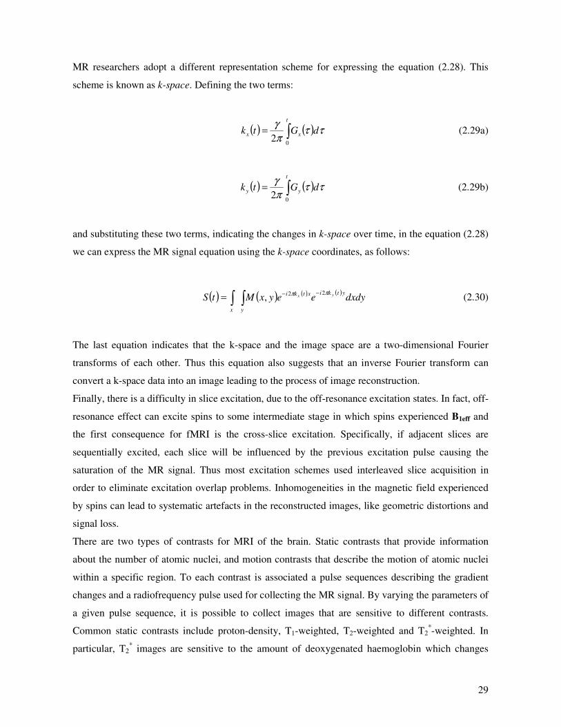
MR researchers adopt a different representation scheme for expressing the equation (2.28). This

scheme is known as k-space. Defining the two terms:

( ) ( )∫=t

xx dGtk0

2ττ

π

γ (2.29a)

( ) ( )∫=t

yy dGtk0

2ττ

π

γ (2.29b)

and substituting these two terms, indicating the changes in k-space over time, in the equation (2.28)

we can express the MR signal equation using the k-space coordinates, as follows:

( ) ( ) ( ) ( )∫∫

−−=y

ytkixtki

x

dxdyeeyxMtS yxππ 22

, (2.30)

The last equation indicates that the k-space and the image space are a two-dimensional Fourier

transforms of each other. Thus this equation also suggests that an inverse Fourier transform can

convert a k-space data into an image leading to the process of image reconstruction.

Finally, there is a difficulty in slice excitation, due to the off-resonance excitation states. In fact, off-

resonance effect can excite spins to some intermediate stage in which spins experienced B1eff and

the first consequence for fMRI is the cross-slice excitation. Specifically, if adjacent slices are

sequentially excited, each slice will be influenced by the previous excitation pulse causing the

saturation of the MR signal. Thus most excitation schemes used interleaved slice acquisition in

order to eliminate excitation overlap problems. Inhomogeneities in the magnetic field experienced

by spins can lead to systematic artefacts in the reconstructed images, like geometric distortions and

signal loss.

There are two types of contrasts for MRI of the brain. Static contrasts that provide information

about the number of atomic nuclei, and motion contrasts that describe the motion of atomic nuclei

within a specific region. To each contrast is associated a pulse sequences describing the gradient

changes and a radiofrequency pulse used for collecting the MR signal. By varying the parameters of

a given pulse sequence, it is possible to collect images that are sensitive to different contrasts.

Common static contrasts include proton-density, T1-weighted, T2-weighted and T2*-weighted. In

particular, T2* images are sensitive to the amount of deoxygenated haemoglobin which changes

30

according to the metabolic demand of active neurons, and provide the foundation for high temporal

resolution studies of functional changes in human brain through fMRI.

Functional MRI

The main goal of functional neuroimaging is to create images that are sensitive to neuronal activity.

Instead, fMRI creates images sensitive to physiological activity that is a correlate of the neuronal

activity. The processing activity of neurons increases the metabolic demand, and to meet this

necessity, energy must be provided. The vascular system provides the cells of two energy sources,

glucose and oxygen that are carrying on by haemoglobin molecules. Different properties of

oxygenated and deoxygenated haemoglobin can be used to construct images based on the Blood-

Oxygenated-Level-Dependent (BOLD) contrast. These properties were discovered by Pauling &

Coryell (1936). They found that hemoglobin molecules have magnetic properties, specifically that

oxygenated hemoglobin is diamagnetic, whereas deoxygenated hemoglobin is paramagnetic (having

a significant magnetic moment). The completely deoxygenated blood has a magnetic susceptibility

about 20% grater than that of the completely oxygenated blood. Thus, in the presence of an external

magnetic field, it will cause spin dephasing that can be measured by a T2* contrast. Specifically,

MR pulse sequences sensitive to T2* will show much more signal when the blood is highly

oxygenated and less signal when it is highly deoxygenated.

In 1990s Ogawa and colleagues verified that the manipulation of the proportion of blood oxygen

would led to the increase of visibility in blood vessels in T2* contrast images. Specifically, they

manipulated the oxygen content in hair breathed by rats. When rats breathed pure oxygen, the

cortical surface had a uniform texture, whereas when they breathed normal air, there was a signal

loss corresponding to blood vessels in that regions in which there was an increase of deoxygenated

hemoglobin. These findings were the base for the BOLD contrast. Indeed they postulated that

functional changing in brain activity would be measured by the BOLD contrast, and hypothesised

two basic nonexclusive mechanisms for explaining the BOLD contrast: changes in oxygen

metabolism and changes in blood flow. From one hand, neuronal activity will cause an increase of

metabolic demands and subsequently of oxygen utilization, that led to an increase of

deoxyhemoglobin within a constant blood flow. From the other hand, an increased blood flow,

without an increased metabolic demand, would decrease the amount of deoxyhemoglobin.

Basically, the BOLD contrast is a consequence of a series of indirect effects. It results from changes

in magnetic properties of water molecules influenced by the deoxyhemoglobin, that is a

31

physiological correlate of the oxygen consumption which is finally a correlate of neuronal activity

induced by cognitive processes.

BOLD Hemodynamic Response characterization

The change in MR signal guided by neuronal activity is known as the Hemodynamic Response

(HDR). Despite the fact that the shape of the HDR changes with the properties of the evoking

stimulus and the underlining neural activity, the increase of neuronal firing would increase the

amplitude of HDR and the duration of neuronal activity would increase its width. Furthermore, the

temporal resolution of the neuronal activity is in the order of tens o milliseconds after the stimulus

onset, whereas the first change in HDR does not occur before about two seconds later. Thus the

BOLD hemodynamic response is a low signal that delays the neuronal event. Some studies (Menon

et al., 1995) have reported an initial negative dip of a duration of 1 or 2 sec, that was attributed to an

initial transient increase of the deoxyhemoglobin. After this short latency the increase of metabolic

demand, related to the increased neuronal activity, results in an increased oxygenated blood and

subsequently in a decrease of deoxygenated hemoglobin within the voxel. Thus, the signal increases

above the baseline at about 2 sec after the onset of the neuronal activity and reaches a maximum

value at about 5 sec for a short duration event. This maximum value is known as the peak of the

HDR and it may reach a plateau if the neuronal activity is maintained across a block time. After

reaching the peak, the BOLD signal decrease to the baseline and remains under the baseline level

for a certain period of time. This effect is known as post-stimulus undershoot. This effect can be

explained by considering the dynamic of the blood flow and the blood volume separately. After the

cessation of the neuronal activity, blood flow decrease more quickly with respect to the blood

volume, thus if the blood volume is above the baseline and the blood flow is at the baseline level,

there is an increase of deoxygenated hemoglobin leading to a general decrease of the fMRI signal

under the baseline. When the blood volume returns to normal values, the BOLD signal will increase

to the baseline.

Spatial and temporal properties of fMRI

Functional MRI has become one of the most prominent neuroimaging techniques in large part

because of its spatial and temporal properties.

32

The spatial resolution of an fMRI experiment determines the ability to separate adjacent brain

regions with different functional properties. A key role in determining spatial resolution is

attributable to the voxel dimensions. Grater is the voxel size, smaller is the spatial resolution. Each

voxel is a three-dimensional rectangular prism and its dimensions are expressed by three

parameters. The first parameter is the field of view that represents the extent of the imaging volume

within a slice and is measured in centimetres. The second parameter is the matrix size, that

quantifies how many voxels are acquired in each dimension. From these two parameters it is

possible to derive the voxel size within a slice that is expressed in millimetres. The third parameter

is the slice thickness that is the direct measure (in mm) of the third dimension of the voxel size.

Increasing the spatial resolution produces advantages for fMRI studies, because reducing the

distance between adjacent voxels improves the ability to distinguish boundaries between neighbour

functional areas. But with an increased spatial resolution there are two challenging problems to deal

with: the SNR will decrease and the acquisition time will increase. The variation in the BOLD

signal measure by the fMRI depends on the total amount of the deoxyhemoglobin, thus if we

consider the size of a voxel reduced by a factor of 2, then the signal that is measured in each voxel

is approximately the half, leading to a smaller . Depending on the region of interest (ROI) in an

fMRI study and on the experimental task, reducing the voxel size cannot be a problem. If a specific

task generates a large BOLD signal in a specific region, the decreasing of the SNR can remain

acceptable. Furthermore, reducing the voxel size of a factor of 2 will augment of the same factor the

matrix size of a gradient pulse sequence, leading to a double or quadruple acquisition time.

Thus the right spatial scale for an fMRI experiment depends upon the question being asked.

The temporal resolution of fMRI refers to the ability to estimate the time of the neuronal activity

from the measured hemodynamic changes. A key parameter for temporal resolution of an fMRI

experiment is the Repetition Time (TR) used. Decreasing the TR to better sample the fMRI

hemodynamic response is useful, because it improves the estimate that we can obtained of the HDR

shape, also improving the inferences that we can make about the underlying neural activity. Even if

adopting longer TR would have little effect on the temporal resolution, for a better estimation of the

HDR shape it could be possible to use a linear interpolation, but when TR is grater that 2 sec, linear

interpolation does not provide a good estimation of the missing values. Another technique for better

approximating the HDR shape with long TR is to use the interleaved stimulus presentation, where

for different trials the experimental stimuli are presented at different time points within a TR. On

the other hand, if the TR is too short, the amplitude of the transverse magnetization following

excitation will be reduced causing that a less MR signal is measured. Furthermore, short TRs reduce

33

also the spatial coverage: if a scanner is able to acquire 16 slices in a second, using a TR of 500 ms,

only 8 slices could be acquired against the 32 slices in 2000 ms RT.

Linearity of the BOLD response

When multiple stimuli are presented in succession, it is possible that the same hemodynamic

response is evoked by every stimulus, independently from the previous presented stimulus. In this

case, if two successive stimuli are sufficiently close together such that their hemodynamic responses

overlap, the total MR signal will be the sum of each individual response. We refer to this case as the

dynamic of a linear system. Otherwise, it is possible that the hemodynamic response evoked by a

stimulus depends on the response evoked by the previous stimuli. In this case, if two stimuli are

presented very close together, the MR signal may be less than the summation of the two individual

responses. The reduction of the amplitude of the hemodynamic response as a function of the

interstimulus interval (ISI) is known as the refractory effect.

The main properties of a linear system are the scaling and the superimposition. The scaling property

is expressed by the fact that the output of a linear system is proportional to the magnitude of its

input. Thus, for fMRI data the scaling property says that changes in the amplitude of the underlying

neuronal activity correspond to proportional changes in the amplitude of the hemodynamic

response. The principle of superimposition refers to the timing of the neuronal activity, and simply

says that the total response of two or more events results in the summation of the individual

responses. Even if the hypothesis of linear system has resulted robust at TR longer than 6 sec, the

fMRI hemodynamic response may be nonlinear at intervals of about 2 sec to 6 sec, since

superimposition was found at duration of 6 sec but not 3 sec and better scaling was observed at

intervals of 5 sec than 2 sec. Research in nonlinearities of hemodynamic response investigated if

there was a refractory period following a stimulus presentation that lead to a smaller hemodynamic

response evoked by a subsequent stimulus in both blocked-designed and event-related studies.

Blocked-designed studies revealed the presence of refractory effects at short stimulus durations, that

is superimposition held for stimuli of 6 sec or more in duration, but its violation become grater as

the stimuli become shorter (Boynton & Finney, 2003; Robson, Dorosz, & Gore, 1998). Similar

results were reported by Vazquez & Noll (1998), where the authors found out significant

nonlinearities for stimulus durations shorter that 4 sec. In event-related studies, the presence of

refractory effects was also demonstrated. Huettel & McCarthy (2000) presented short duration

visual stimuli, single or in pairs separated by 1sec to 6 sec ISI. Examining the primary visual cortex

they found that at short ISI (1 and 2 sec) the hemodynamic response amplitude was reduced and the

34

latency was increased. The presence of a refractory period in both blocked-designed and event-

related studies suggest the nonlinear nature of the hemodynamic response, under certain

experimental conditions, and represents a challenge in the major part of research fMRI studies. In

contrast, many researchers have exploited these effects in order to study adaptation within a brain

region.

Signal and noise in fMRI

Noise in fMRI data has both spatial and temporal features, that have several main causes: thermal

noise within the subject and the scanner electronics; system noise associated with defects of the

scanner hardware; noise resulting from head motion, respiration, heart rate and other physiological

processes; variability in neuronal activity associated with non task related processes and changes in

cognitive strategy.

All MR images, both anatomical and functional, are subject to thermal (or intrinsic) noise that is

changes in signal intensity over time due to thermal motion of electrons within the subject and the

scanner electronics. After the excitation process the brain emits a radiofrequency signal that is

detected by the receiver coil. Then this signal is processed by a series of electronic hardware, and

within each hardware component free electrons collide with atoms increasing the temperature of the

system and producing a distortion of the current signal.

Some frequent causes of system noise are inhomogeneities due to defective shimming, or

nonlinearities of the gradient fields. One specific form of system noise is the scanner drift, which

consists of slow changes of the voxel intensity over time.

More consistent variations in fMRI signal are due to head motion and other physiological noise.

During a scanning session subjects can shift their head or move their arms or legs to be in a more

comfortable position. In the best case small head motion can be corrected during the pre-processing

phase before the analysis, but in the worst case large motion can lead data to be difficultly

interpreted. Other sources of motion noise are related with cardiac and respiratory activity. In

general motion causes problems in variability across the time series of images that is critical for the

SNR. Furthermore, other changes in physiological parameters as blood flow, blood volume, oxygen

metabolism and their interactions lead to variability in the detected BOLD signal. Thus,

physiological noise is the main source of variability in fMRI studies.

Moreover, it could be taken into account that during an fMRI experiment, task-related responses in

which we are interested, are strictly connected, maybe alternated by other responses evoked by

35

external stimuli activating also brain systems associated with memory or mental imagery (i.e., the

subject is thinking about something else in her/his life).

Finally, speed-accuracy trade off represents an important factor for inter-trial variability, but the

relation between reaction time and brain activity depends on the brain activity, that is only some

cognitive processes are delayed within an increasing reaction time. Moreover, different strategies

can be employed in performing the same task, thus the hemodynamic response evoked by the same

event can be influenced by the adopted strategy, leading to a source of inter-trial variability.

Noise variability corrections of fMRI data

After image reconstruction, we can consider fMRI data consisting in a series of brain volumes

acquired over time. Specifically, we have a three-dimensional matrix (an image volume) containing

different BOLD activations, one for each voxel location, that vary over time. BOLD signals are

correlated across successive scans, meaning that they cannot be treated as independent samples. The

main reason for this correlation is the fast acquisition time (TR) for fMRI (2-4 sec) relative to the

duration of the BOLD response (about 20-30 sec).

The main problem addressed by fMRI studies is to correlate signals that change temporally in

different cortical areas to certain events opportunely coded in the experimental paradigm. All

analysis procedures are based on a common set of assumptions, among which that each voxel can

be assumed to preserve the same location in the acquisition of brain volumes over time so that each

voxel time series can be correctly determined. Actually, this assumption is incorrect. fMRI data

experiences both spatial and temporal noise artefacts, such as head motion, cardiac and respiration

motion and other physiological noise, moreover differences in the timing of image acquisition.

To deal with these consistency problems, a set of pre-processing steps is necessary in order to

increase the SNR for each voxel time series and to prepare them for the successive statistical

analysis. In this section, all the necessary pre-processing steps are briefly described.

Slice time correction

Depending on the capabilities of the scanner, a certain number of slices are acquired in

ascending/descending or interleaved modality. Furthermore, depending on TR and the acquisition

modality, different slices within the TR are acquired at a different time. This problem is more

36

evident in the case of interleaved slice acquisition. If we use interleave slice acquisition and acquire

12 slices with a TR = 3 sec, the first slice will be acquired at time 0 sec, the second slice will be

acquire at time 1.5 sec, and last slice at time 2.75 sec. This problem is faced by using temporal

interpolation (e.g., linear, sinc) that uses information from closed time points to estimate the

amplitude of the MR signal at that reference TR. Considering the temporal variation of fMRI data,

interpolation for slice time correction has more sense for shorter TRs (e.g., TR = 1 sec). In contrast,

the need of an accurate interpolation is greater in the case of longer TR (e.g., TR > 3 sec), where

there is a larger interval between successive acquisitions. In the case of interleaved slice acquisition

with long TR, the slice time correction has to be applied before the motion correction, in which case

the timing error will be reduced with an increasing in sensitivity to hand motion. In contrast, in the

case of sequential acquisition or data acquired within a short TR, motion correction has to be

applied as first step, thus the motion effects associated with interpolation across adjacent voxels is

minimised, with a cost of a the small timing correctness certainty.

Motion correction and functional-structural coregistration

During an fMRI experiment it is common a certain degree of head motion, thus some image

volumes are acquired with the brain in a wrong spatial location. The objective of motion correction

is to adjust the voxel time series in order to have the brain in the same position in all the image

volumes. Thus, successive image volumes in a time series are realigned to a reference volume,

generally the first of the sequence, using a rigid-body transformation. The fundamental assumption

of rigid-body transformation is that two objects must have the same size and shape such that one

object can be superimposed on the other just by using a set of three translations (along x, y and z

axes) and three rotations (through x-y, x-z and y-z planes). In order to determine the six parameters

that account for the amount of motion in each transformation, a similarity measure or cost function

is to be minimised. A simple cost function is the sum of squared intensity differences between each

image volume (considering each voxel within the volume) and the reference one. Very often the

motion correction is done after a smoothing filter in order to minimize the noise effect upon the cost

function. Ones the parameters have been estimated the original data are resliced in order to estimate

the values corresponding to correct values without head motion. This second step is known as

spatial interpolation (e.g., linear methods such as bilinear or trilinear interpolation), which assumes

that each interpolated point is the weighted average of all adjacent points. Other algorithms for

spatial interpolation are based on sinc interpolation, very computationally expensive, or spline

37

interpolations, a computationally compromise between linear and sinc methods that produce good

interpolation results for MRI data.

The coregistration process is motivated by the need to understand how brain activity maps into

anatomy. Functional images have low resolution and lack anatomical details, thus we need to map

functional data into high contrast structural images. As in the realignment procedure, a rigid-body

transformation has to be applied for functional-structural coregistration in which a cost function has

to be minimised. Because functional and structural images have a very different contrast, a cost

function based on the sum of squared intensity differences is not appropriate. Instead, mutual

information is generally used.

Spatial normalization

Once functional brain images have been realigned and after the functional structural coregistration,

the fMRI data are sufficiently processed for a single subject functional analysis. But with different

subject’s data it is important to understand how much consistent is the mapping across subjects. For

this reason each subject brain can be transformed in such a way that it has the same shape and size

of each other. This process is known as spatial normalization. Normalization is a sort of

coregistration excepted for the fact that now brains that have to be coregistered are of consistently

different shapes. The process of normalization has to account for these differences and compensate

for them by mathematically stretching, squeezing and warping each brain in a way that at the end of

the process each brain is in the same reference space, or stereotaxic space. The most used

stereotaxic space is the Talairach space, that was based on a simple reference space derived from a

single brain, specifically that of an elderly woman. The origin of this space is settled at the midpoint

of the anterior commisure. This stereotaxic space has been so important for neuroscience, but its

limit consist in the fact that it is made by only one brain that is not representative of the population

at large. A better approach has been used by a more recent probabilistic space, created by the

Montreal Neurological Institute (MNI) and consists of an average of 152 T1-weighted brain images.

The MNI template has been scaled in order to mach the landmarks of the standard Talairach space.

For applying normalization, algorithms determine the size of the brain and its coarse anatomical

features.

Normalization is basically applied to subjects extracted from a standard population of participants,

which are yang or adults and neurologically intact. Many subject groups differ from this standard

population, for example elderly people who can present local atrophies or children which can have

different brain shapes due to local delayed brain maturation. Thus, using normalization on different

38

subjects groups may mask important group differences. Moreover, patient groups may have local

pathologies like tumours and present local deformations in the lesion sites. In this case, some

different normalization approaches have been developed (generally based on nonlinear

transformations) for taking into account non typical subject populations, because the common

approach will fail producing low matching accuracy.

Spatial and temporal filtering

In neuroimaging both spatial and temporal filers are used in order to remove variability in the data

that can be due to different sources of noise, preserving the signal of interest, thus increasing the

SNR. Filters have also another important impact on the statistical analysis of fMRI data, reducing

the problem of multiple comparisons in voxelwise analysis.

Spatial filters, commonly Gaussian filters, are used for reducing high frequency spatial components,

spreading the intensity of each voxel in the image over neighbour voxels. The number of neighbour

voxels is guided by the Width of the Gaussian Filter and is expressed in mm at Half of the

Maximum value (FWHM). The idea of a spatial filter is based on the assumption that neighbour

voxels in brain cortex are functionally correlated, thus this filter can increase the SNR. But, if there

are not spatial correlation (e.g., in functionally different adjacent regions) the SNR will be

decreased and functional differences will be masked. Thus, a critical parameter in applying spatial

filter is its width that determines the level change in SNR and also the degree of functional

differences masking. Another motivation for using spatial filters lies on improving the validity of

statistical techniques in voxelwise analysis. Introducing a certain degree of correlation in voxel time

series there will be fewer local maxima with a significant activity and the number of voxel active

due to chance alone can be reduced. Spatial smoothing also increases the normality of data, which is

a pre-requisite of many statistical tests. However, spatial filters can reduce SNR in specific adjacent

regions of the brain and can introduce one more artefact, another source of variability in fMRI data,

thus even if it produces some advantages for voxelwise analysis, it has little effect or is dangerous

in ROI analysis or in multivariate brain analysis.

The use of temporal filters can improve the quality of fMRI data, by increasing the SNR. Typically

Fourier filters are applied for maintaining information related to changes in data that occur at the

task frequency and minimizing the changes in data that occur at other frequencies. In particular, the

voxel time series can be converted, through the Fourier transform, to the frequency domain. In

general the maximum frequency that can be identified is equal to an half of the TR, and any

frequency in the signal that is higher than this maximum frequency would not be taken into account.

39

Thus using a low-pass filter we can attenuate high frequency, maintaining low frequencies.

Depending on the source of variability that we want to eliminate, it is possible to use a low-pass, a

high-pass filter or both. Typically heart rate has a high frequency (e.g., 1, 1.5 Hz), whereas

breathing effect has low frequencies (e.g., 0.2, 0.3 Hz). But also temporal filters have to be applied

with caution, because it could be possible, especially in fast event related, that the task and the

respiration could be at similar frequencies, thus a low-pass filter could be very difficult to apply and

can reduce the quality of data.

Once fMRI data have been pre-processed, they are ready to be analysed for finding statistical maps

of voxels that are significantly active during the execution of a specific task condition.

Basic principles of fMRI experimental designs

The main questions for realising an fMRI experimental design are the creation of specific research

hypothesis, the crucial choice of experimental conditions to test those hypotheses, and the way to

present the stimuli for manipulating the experimental conditions over time.

Initially the fMRI studies used a sequential way to present stimuli within block conditions. It was

due principally to historical reason related to PET studies, in which participants had to maintain

their cognitive engagement for a period of time up of one minute, during which the changes in

blood flow were measured. During the last decade the fMRI technique reached a greater maturity

and a lot of different presentation schemes were employed (see Huettel, Song, & McCarthy (2004)

and Amaro & Barker (2006) for review). They can be summarised into four main categories of

fMRI experimental designs: blocked; slow event-related; fast event-related; mixed designs.

The basic idea of a block design is that of maintaining a cognitive engagement for a certain period

of time within a specific condition, alternating this presentation with a different condition. Thus,

stimuli of the same condition are presented successively and the BOLD response is composed of the

single HRFs relative to each stimulus in the sequence and is usually of higher magnitude.

The event-related design presents several benefits with respect to the block design, among which

the main advantage is the ability to detect transient variations in the hemodynamic responses

permitting a temporal characterization of the BOLD activity. In fact, brain regions correlated to a

specific task can have different HRF even if they are active for the same task. With the advent of

this experimental design it was possible to relate individual responses to single trials. Each stimulus

HRF is detected and can be analysed separately, allowing for the randomization of order of the

presented conditions, and it was also possible to vary the inter stimulus interval (ISI) in order to

40

avoid participant’s strategies based on the prediction of the event that will happen (i.g. ISI on the

order of 12 sec. slow event-related) and maintaining a certain attention level across the

experiment. On the other hand, the early implementation of this design was time consuming and

those experiments were longer than block designed experiments. Moreover, longer ISI can produce

very long boring experiments for participants, and can lead to possible lacks of attention to the

specific task during the scanning sessions.

In order to overcome these limitations, it was investigated a variant of the event-related design

where the ISI is shorter than the duration of the HRF evoked by the previous stimulus: the fast

event-related design. In these paradigms the ISI is of the same order of that used in conventional

psychological experiments, making easer the interpretation of the neural correlates of many

experiments. Furthermore, the augmented number of stimuli increases the statistical power in the

analysis and the lesser ISI combined with the randomization of the order of presentation of the

stimuli makes the experiment less boring that the previous one. Conversely, it is more difficult to

estimate the HRF for the single trial and it introduces problems related to the linearity vs

nonlinearity of the BOLD interactions in overlapping HRFs. A possible way to overcome the

limitation of the impact of a rapid ISI on the linearity of the BOLD interactions consists in using a

variable ISI from a minimum of 4 sec between two successively stimuli that can reasonably allow

us to assume linearity (Glover, 1999).

A combination of block and event-related designs, jointed into mixed designs, can offer an

interesting mixture of the advantages of both the paradigms. Thus, it is possible to obtain on one

hand the measurements of the same repetitive set of stimuli, like in the block designs, and on the

other hand the transient response detected in event-related designs. In this way it is possible to

extract brain regions that exhibit both an item-related and task-related pattern of information

processing, and are useful for comparison of long term sustained activity and short term transient

activity.

Conclusion

The basic physics for the development of the modern fMRI derive from the remote 1920s to 1940s

in which the idea of the experimentally controlled magnetic properties of atomic nuclei was

confirmed. Then, the properties of NMR were first described in 1946 by Bloch and Purcell, and

only in 1970s the first MR images were created in the context of concurrent advances in image

acquisition methods. By the 1980s MRI for structural scanning of the brain became clinically

41

prevalent. Only in early 1990s the findings about changes in blood oxygenation measurable by MRI

opened the new era of functional studies of the brain.

The idea of functional localization within the brain has been accepted from the early 19th

century

with Gall and its phrenology, but only from the middle of 1800s, it was confirmed by Broca and his

studies on brain lesion patients highlighting two basic principles: the brain cortex can be

decomposed into several areas performing different functions and these areas are independent to

each other. Only from the middle of 1900s neuropsychology reached a high degree of scientific

maturity. With the development of the imaging techniques like CT and MRI it was possible to be

more specific as to the location of damage in brain injured patients. The development of EEG and

mainly of the functional imaging modalities of PET, SPECT, MEG, and fMRI opened a new era in

the study of brain functions.

In this chapter the theoretical foundations, of NMR, MRI, and fMRI have been explained. Then the

characteristics BOLD signal has been outlined, discussing its spatial and temporal properties and

the amount of SNR contained in the signal. The key steps for the pre-processing of fMRI data have

been also critically discussed.

Once fMRI data have been pre-processed, they are ready to be analysed for finding statistical maps

of voxels that are significantly active during the execution of specific task conditions. The methods

to analyse fMRI are widespread. The common and conventional approaches lies on parametric

methods based on the General Linear Model (GLM), but in the last years a lot of non-parametric

approaches, based on the Machine Learning theory have been developed and successfully employed

in a growing number of fMRI studies. The detailed description and the critical comparison of both

parametric and non-parametric approaches to the fMRI data analysis is describe in the Chapter 3.

43

Chapter 3

Beyond mind-reading: different approaches to fMRI data

Analysis

Introduction

The main issue in cognitive neuroscience concerns the questions about what information is

represented in specific brain areas, how it is represented and how this information is processed

during different elaboration stages. Certainly, fMRI, combined with behavioural,

neuropsychological studies and other neuroscience methods (e.g. TMS, PET, EEG), provides a

powerful tool for answering these scientific questions.

Conventional neuroimaging approaches have treated the problem of determining how specific

sensory, perceptual or cognitive states are encoded into brain activity, by finding out which brain

areas are involved in the processing of specific tasks. The main problem addressed by these fMRI

studies is to correlate BOLD signals that change temporally in different cortical areas to certain

events (task conditions) opportunely coded in the experimental paradigm. Basically, conventional

fMRI data analysis is based on the statistical Parametric Approach (e.g. General Linear Model

GLM) which correlates external regressors (task conditions) with the activity in specific brain

regions, generating a sort of brain statistical maps of localised activity (Worsley & Friston, 1995).

In these approaches, regressors are computed assuming a predefined shape of the Hemodinamic

Response Function (HRF) that is convolved with each task condition and used for detecting some

correlation. However, the HRF can differ from the a priori assumed shape, varying within different

brain regions, from task to task and on the base of the strategies adopted by each participant. Thus,

also if the GLM takes into account a certain degree of HRF variability, in a way that the model can

explain more variability in the data, it is not essentially the best model able to capture and detect

those correlations, and can lead to a much more complexity in the interpretation of the final results.

Moreover, traditional statistical methods are voxel-wise, that is they measure the activity from

44

many thousands of voxels in the brain images analysing each voxel time series separately, treating

each voxel as an independent measure, and comparing two or more task conditions at each voxel

location.

Recent methods, belonging to the class of Multivariate Analysis (Non Parametric Approaches),

have the potential to improve our understanding of the complex pattern of brain activity measured

by fMRI. These approaches are based on boosting the weak information available at each voxel

location by a simultaneous analysis of hundreds or thousands of voxels to predict specific cognitive

states. These methods do not consider any parametric model of the HRF, obtaining a correlation of

responses even in the cases in which it differs from a specific assumed shape, and exploiting all the

spatio-temporal information contained in fMRI data.

In his chapter, the conventional parametric and non parametric approaches to fMRI data analysis

are described, their peculiarities are highlighted and their key differences are critically discussed. A

review of the more recent literature on fMRI studies is examined, with a special look to the growing

literature on the multivariate methods that are becoming the standard de facto for a comprehensive

analysis of fMRI data. Finally, statistical and practical aspects on the proper use of multivariate

methods are discussed and the mathematical formulation of the general learning problem is shown.

Conventional parametric approaches to fMRI data analysis

Most of fMRI analysis is based on hypothesis testing: the first hypothesis with some prediction

about the data and a second null hypothesis based on random chance. For testing a single hypothesis

in fMRI studies there is a certain number of statistical tests, which are all variants of the General

Linear Model (GLM). The simple basic idea beyond the GLM consists in modelling the observed

fMRI data in a linear way. Thus fMRI data are treated as a linear summation of single dissociable

factors.

Suppose we have an fMRI time series of N observations Nk YYYYY ,....,,....,,, 321 acquired at a

specific voxel at timekt , where Nk ,...,1= , is the scan number. The idea is to model each time point

in each voxel time series as a linear combination of explanatory factors, plus an error term:

( ) ( ) ( ) kkLLkkk txtxtxY εβββ ++++= ...2211 (3.1)

45

where L is the number of the model factors (regressors) ideated by the experimenter. This equation

can be extended to include a large number of dependent variable, such as all the time points within

an fMRI experiment:

( ) ( ) ( )( ) ( ) ( )( ) ( ) ( )

( ) ( ) ( ) NNLLNNN

LL

LL

LL

txtxtxY

txtxtxY

txtxtxY

txtxtxY

εβββ

εβββ

εβββ

εβββ

++++=

++++=

++++=

++++=

...

.

.

...

...

...

2211

333223113

222222112

111221111

(3.2)

which can be expressed in a matrix form:

( ) ( ) ( )( ) ( ) ( )( ) ( ) ( )

( ) ( ) ( )

+

=

NLNLNN

L

L

L

N txtxtx

txtxtx

txtxtx

txtxtx

Y

Y

Y

Y

ε

ε

ε

ε

β

β

β

β

.

.

.

.

,...,,

.

.

,...,,

,...,,

,...,,

.

.

3

2

1

3

2

1

21

33231

22221

11211

3

2

1

(3.3)

Or in a matrix notation:

εβ += XY (3.4)

Where Y is the is the colon vector of the voxel observations, β is the parameter vector to be

estimated, ε is the error vector, whose elements ( )2,0 σε Ν≈iid

k , with Nk ,...,1= , are considered as

independent and identically normally distributed with zero mean and variance 2σ , and the LN ×

matrix X is the design matrix defined by the experimenter.

Basically, the multiple equation system implied in the formulation of the GLM cannot be solved

because the number of parameters L is less than the number of observations N , thus the method

employed for solving the system is the method of ordinary least squares. The set of estimated

parameters [ ]TLβββββ

~,...,

~,

~,

~~321= led to fitted values [ ] εβ +==

~~,...,

~,

~,

~~321 XYYYYY

T

N ,

where [ ] βεεεεε~~

,...,,, 321 XYYYT

N −=−== . The least square estimates are the parameter

estimates that minimised the residual sum of squares:

46

( ) ( ) ( )( )∑=

−−−−=N

i

LiLiii txtxtxYS1

2

2211

~...

~~βββ (3.5)

that is minimised when ( )( ) ( ) ( ) ( )( ) 0~

...~~

2~

1

2

2211 =−−−−−=∂∂ ∑=

N

i

LiLiiiill txtxtxYtxS ββββ , that

corresponds to the lth

row of the normal equation:

( )β~XXYXTT = (3.6)

If XX T is invertible, that is if and only if the design matrix X is of full rank (all columns in X are

linearly independent) it is possible to derive the parameter estimates:

( ) YXXXTT 1~ −

=β (3.7)

Generally, in the design matrix are included all experimental factors that are of interest for the

study, but it is possible to add some other factors associated with known sources of variability (e.g.

scanner drift or subject respiration). These included factors can reduce the error term, but on the

contrary reduces the number of degrees of freedom, thus these factors have to be used carefully.

The GLM is the most widely used method for analysing fMRI data, but its validity is supported by a

series of assumptions. First of all, a basic assumption lays on the fact that the design matrix factors

have to accurately represent the BOLD changes related to the neural activity of interest (i.e. the

cognitive process under examination will occur several second after the stimulus onset with a

delayed peak of the HRF). Thus it is important to insert qualifier factors in the design matrix,

estimating the peak delay of any process under examination. In fact, the basic assumption of the

design matrix is that the BOLD response can be estimated convolving a predefined shape of the

HRF with the time of stimulus presentation, thus a delay in the BOLD peak associable with the

cognitive process under study has to be taken into account for obtaining a valid result. Indeed, the

major part of fMRI studies models the BOLD activity by using a predefined shape of the HRF,

ignoring that it can vary from task to task. However, more complex design matrix can be created in

order to model some differences in the hemodynamic onset or in the shape of the HRF, which can

include some additional factor such as time and dispersion derivatives. Moreover, the variability of

the HRF can be considered also employing a combination of multiple basis functions, thus voxels

47

whose activity do not follow a canonical HRF can be otherwise detected. However, the final results

will be much more complex to interpret and understand. Another limit of the GLM relays on the

fact that the BOLD response does not obey to linearity assumptions: the hemodynamic response

evoked by a stimulus depends on the response evoked by the previous stimuli, and if two stimuli are

presented very close together or for short duration, the BOLD signal may be less than the

summation of the two individual responses (see more details about the refractory effect in Chapter

2). To deal with this problem, a possibility in the GLM is to incorporate the refractory effect into

the design matrix, and a possible way to do this is to add interaction terms into the design matrix.

Another method proposed by Friston, Josephs, Rees, & Turner (1998) uses Volterra Kernels which

allow modelling the influence of a stimulus on the successive ones. In summary, without an

accurate construction of the design matrix, considering all the correction terms, the GLM can fail to

capture the BOLD dynamics.

Furthermore, the design matrix is the same for all the voxels within the brain. Conversely, the HRF

can differ, especially in its latency, across different brain regions. Again, the use of a set of multiple

basis functions can help in detecting some correlation, but this lead to a more difficult interpretation

of the obtained results. Another way to overcome this region variability in the HRF latency could be

to combine the GLM analysis over the whole brain with a ROI analysis, by limiting the analysis to

anatomical or better functional ROIs. This procedure presents several advantages over voxelwise

methods. Each ROI combines data from many voxels leading to a possible increase in SNR in the

case in which the ROI is functionally homogeneous. Furthermore, the number of ROIs is lesser then

the number of voxels, thus the number of independent statistical tests is reduced, reducing the need

of multiple comparisons and the related confounds.

Another critical point concerns the assumption that the components of the error term in the

formulation of the GLM (equation 3.3) are considered as independent and identically normally

distributed with zero mean and variance 2σ , assuming that the amount of noise in a single voxel

does not depend on the task condition. This assumption may be not always valid; in fact the noise

level during the BOLD activity may be higher then in the rest condition (Huettel & McCarthy,

2001). Moreover, each voxel time series is considered as an independent measure of brain activity

and is treated independently in the GLM analysis, ignoring spatial correlation within adjacent

voxels that is especially and commonly induced by using spatial smoothing in the pre-processing

steps.

Basically, the GLM is a flexible model in which it is possible to incorporate several factors to take

into account, apart from the experimental conditions, noise variability and other appropriate model

factors. If an inappropriate model is specified, including incorrect model factors or not considering

48

crucial factors, the analysis can infer incorrect or null results. Likewise, it is based on several

assumptions that cannot be considered valid, and even if researchers tried to solve these problems

caused by the model error, in that cases the interpretation of the final results is often difficult.

An additional central problem of this fMRI data analysis is that of multiple comparisons. Briefly,

the huge number of statistical tests increases the number of false positives (Type I errors), that is

there is a high probability to detect some active voxels that are active only by chance. The standard

way to overcome the problem of multiple comparisons is to reduce the α value, thus the voxels are

less probable to pass the significance threshold by chance. A stringent and conservative method to

do this is applying the Bonferroni correction, according to which the α value is reduced

proportionally to the number n of independent statistical tests ( nαα =~ ). Even if this method

allows reducing the occurrence of Type I errors (false positives), it increases the probability of

incurring in Type II errors (false negatives) increasing the likelihood to fail in detecting voxels that

are really active, and the increasing of the false negatives is absolutely not acceptable in an fMRI

study. Another less conservative method for dealing with the problem of multiple comparisons is

the False Discovering Rate (FDR) method (Genovese, Lazar, & Nichols, 2002) that is a different

way to correct the α value in order to control the false discovery rate trying to balance between

Type I and Type II errors. To find out a better correction factor, (Worsley & Friston, 1995) applied

the theory of Gaussian Random Field to fMRI data. Random field theory estimates the number of

independent statistical tests as a function of the smoothing factor used in the experimental data that

depends on the properties of the Gaussian filter used in the pre-processing phase. Thus the number

of independent statistical tests, for α value correction, can be obtained by dividing the number of all

the voxels by the cube of the smoothness width expressed in terms of voxel number. Another way

to treat this problem consists in considering the size of the active voxel clusters, rather then their

number. This cluster-size thresholding method (Xiong, Gao, Lancaster, & Fox, 1995; Forman et al.,

1995) is based on the concept of a high probability that only a single isolated voxel can result active

by chance. In this way, it is possible to use a moderately liberal α value (e.g. 01.0<p ) for single

voxel comparison and increase the conservatism of the test by considering only active voxel clusters

that are larger than some threshold (typically 3-6 voxels).

Finally, till now we have considered only the single subject analysis. Typically, an fMRI study

collects data from multiple subjects (e.g. 10 or more), thus the analysis has to combine data across

subjects. A first common approach, known as fixed-effect analysis, is based on combining all data

points of all subjects into a single analysis, assuming that the experimental manipulation has the

same effect on the BOLD signal in every subject. It is often a wrong assumption. In fact the

characteristics of the BOLD signal (e.g., latency, amplitude, width), suppose in the same region and

49

for the same task, can vary also across subjects. Thus a second approach, known as random-effect

analysis, has been introduced to allow making inferences about the population from which the

subjects were extracted and not about the specific subjects in a particular study. In this approach

statistical maps are created for every subject and then the distribution of the single subject’s

statistics is tested again for significance.

In conclusion, the GLM has been the most widely used approach to fMRI data analysis, and has

produced an enormous amount of published studies from the 1990s to the last year. It is a flexible

method and researchers have tried to overcome every single problem related to basic assumptions or

to the model error, by integrating different methods that, conversely, do not lead to an easy

interpretation of the obtained results. The crucial point of GLM is that it is based on a series of

assumptions that cannot be considered valid, and as mentioned by O’Tool et al. (2007, p. 1738)

“The disadvantages of this approach are well known, but are rarely taken seriously enough to limit

the use of these techniques”.

Non Parametric approaches to fMRI data Analysis: Multi-voxel

Pattern Analysis

The major part of the neuroimaging research has been based on approaches, like the GLM, using a

forward inference mechanism, as called by Henson (2006). In a forward inference process, two or

more experimental conditions that are based on different perceptual or cognitive processes are

compared, and the brain regions that show BOLD activity differences for those conditions are

supposed to be involved in the compared mental processes. Because of the correlation nature of this

analysis, it is not possible to infer the causality of these relations between brain activations and

mental states. Neuroimage alone is not the unique tool for assessing if certain brain region

activations are necessary or sufficient conditions for predicting a specific mental state, but it needs

to be integrated by lesion or TMS studies. Nevertheless, lesion studies likewise TMS studies have

the limit to follow a modular approach, but the way the brain could discover for performing

cognitive processes may be multiple. Many cognitive processes could be clearly separated not by

the activity of a specific brain region but by patterns of activity across different regions.

Recently, it has become more common to infer the presence of perceptual or cognitive processes by

just looking at neuroimaging data, in a way called reverse inference (Poldrack, 2006; Poldrack,

2008; Poldrack, 2007). In terms of the deductive logic, the reverse inference mechanism is based on

the erroneous belief of affirming the consequent (fMRI data and BOLD signal variation along the

50

experiment) for estimating the antecedent (experimental condition). Despite this logic fallacy,

cognitive neuroscience relays upon the logic of explaining behavioural events rather than on

deducing behaviour laws, thus the impact of the reverse inference in cognitive neuroscience is more

robust than that of the forward inference. The reverse inference is an informal way for describing

the process of predicting mental states from brain imaging data.

The question about how much accurately could be possible to predict cognitive states by fMRI data

has been managed by the class of non parametric approaches known as multi-voxel pattern analysis.

Conventional approaches estimate the fit of a specified model to sample data, whereas the multi-

voxel pattern analysis methods construct the model on the base of a portion of the available data

and measure the prediction accuracy on data not used for estimating the model. The advent of

multivariate pattern analysis in the field of neuroscience has improved the quality of the inferences

that can be done on fMRI data, identifying pattern of BOLD activity that are explicitly diagnostic

for specific experimental tasks or stimuli.

Certainly, multivariate pattern analysis presents several advantages with respect to the traditional

statistical methods; it is able to produce models which overcome the precise hypotheses assumed by

the conventional approaches, leading to a smaller model error. In particular, multi-voxel pattern

analysis methods boost the weak information available at a single voxel location by combining the

BOLD activation levels across several spatial locations. As well, if a specific region (or voxel) is

not able to capture the dynamic underlying a particular cognitive process, it could be possible that a

pattern of brain activity (compact or distributed spatial network of activity) is predictive for that

target process. Generally, cognitive processes involve the activation of networks of brain regions,

thus when two cognitive processes differ not only on the activation level but also on the functional

connectivity, multivariate methods can capture these dynamics and the obtained voxel activation

maps could be more informative than that obtained with the conventional mass univariate

approaches (Sato et al., 2008).

Crucially, conventional approaches determine if there is a significant difference averaging brain

activity related to specific experimental conditions through time, acquiring a large number of

samples to maximise the statistical sensitivity. Averaging the activity trough time leads to the loss

of single trail information. Conversely, with multi-voxel pattern analysis it is possible to decode

cognitive states at a level of the single trial. This essential property has opened the way for the idea

of mind reading in related fields of Brain Computer Interface (BCI) of Bio-feedback. In common

approaches to BCI, mental states are decoded from EEG or fMRI signals. The decoded cognitive

states are successively encoded into computer programs to control artificial devices that can change

the environment according to the subject thinking. Several works have faced the problem of

51

developing BCI for healthy people (Lee, Ryu, Jolesz, Cho, & Yoo, 2008); Noirhomme, Kitney, &

Macq, 2008; Yang, Li, Yao, & Wu, 2008), and especially for patients (Birbaumer, Murguialday, &

Cohen, 2008); Daly & Wolpaw, 2008; Kubler & Birbaumer, 2008; Nijboer et al., 2008; Piccione et

al., 2008; F. Piccione et al., 2006).

Additionally, multi-voxel pattern analysis methods do not assume any specific shape of the HRF,

conversely they are able to discover patterns of activity that are predictive for the experimental

conditions, just by looking at the measured brain activity.

Basically, the central idea of these methods is to exploit the complex nature of fMRI data available,

constructing a model of the problem under examination without assuming any a priori specific

hypothesis that can lead to increasing the model error: if data are informative they just contain all

that we need for finding out their implicit embedded relations. In this context, the complexity of the

model plays also a crucial role in extracting those relations. If the nature of those hidden relations is

linear, a linear model able to explicit them could be a quite good solution, otherwise more complex

models, both nonlinear models or linear models processing a much more significant set of features

extracted by the same data, could be able to capture their more complex dynamics. Additionally, the

nature of the questions that it can be possible to investigate is richer and much more comprehensive

with respect to the elementary questions the conventional analysis approaches deal with, and can

lead researchers toward the key questions in cognitive neuroscience in a more productive way.

One of the main question in cognitive neuroscience deals with the problem of understanding the

level of modularity or distribution of the information representation in the brain. Particular type of

visually presented information is represented in human brain in specific regions in a segregated

way. For example, the Fusiform Face Area (FFA) responds more strongly to faces that to any other

object categories (Grill-Spector, Knouf, & Kanwisher, 2004; Kanwisher, McDermott, & Chun,

1997; Kanwisher, Stanley, & Harris, 1999; Kanwisher & Yovel, 2006). Likewise, the

Parahippocampal Place Area (PPA) responds most to visual images containing view of houses and

buildings. Thus, many anatomically distinct regions in the brain could be considered as specialised

modules able to process specific tasks or stimuli, but the number of these regions is certainly

limited. Generally, there is a distributed neuronal activity in the cortex, often with a certain degree

of overlapping for representing information predictive for different task conditions. A single area

could be activated in many different task conditions at different modulation levels, and in these

cases it could be difficult or impossible to use activity of a specific area for finding particular

precepts or thoughts by using conventional fMRI data analysis. Clearly, conventional approaches

underestimate the amount of information contained in fMRI data. Otherwise, multivariate analysis

52

helps in discriminating among different modulation activity of the same area for different tasks, and

allows a fine-grained analysis of fMRI data with respect to conventional voxel based approaches.

Many neuroimaging studies have, till now, provided evidences of the existence of a strong link

between the mind and the brain activity, leading to the possibility of decoding what people is

thinking just by looking its brain activity (Haynes & Rees, 2006; Norman, Polyn, Detre, & Haxby,

2006).

The use of multi-voxel pattern analysis begun with a landmark fMRI study of the object-vision

pathway (Haxby et al., 2001), in which the authors demonstrated that spatial multi-voxel patterns of

BOLD activity evoked by a visual stimulus are informative for the subjective perceptual or

cognitive state. The authors highlighted that analysing the spatial pattern of responses in

ventrotemporal (VT) cortex of subjects presented with visual stimuli of different object categories

(e.g. faces, chairs, shoes, bottles), it was possible to individuate distinct spatial patterns useful for

decoding the cognitive state of subjects (perception of each different object category). Importantly,

they found out that the information of perceiving object categories was not represented only in

maximally responding regions, but also in spatially distributed patterns of non maximally responses

in VT cortex. This information is substantially ignored by conventional approaches that basically

detect voxel by voxel statistical significant activation differences. Similar results were obtained by

other studies following Haxby et al. (2001), in which different visual object categories were found

to be associated with different voxel activity patterns in VT cortex (Carlson, Schrater, & He, 2003;

Hanson, Matsuka, & Haxby, 2004; O'Toole, Jiang, Abdi, & Haxby, 2005; Spiridon & Kanwisher,

2002), confirming the same findings of the first landmark study. Moreover, multi-voxel pattern

analysis has been used for decoding the orientation of striped pattern that were being view by

participants (Haynes & Rees, 2005a; Kamitani & Tong, 2005). In particular, (Kamitani & Tong,

2005) studied the representation of line orientation in visual cortex. Previous electrophysiological

and optical imaging studies have shown the existence of orientation selectivity in primary visual

cortex at a level of cortical columns changing at the resolution of 1 mm (Bartfeld & Grinvald,

1992), thus the authors investigated, at a resolution of 3 mm cubic voxels, if multi-voxel pattern

analysis was able to discriminate between different orientations. Their results confirmed the

previous studies (Bartfeld & Grinvald, 1992; Vanduffel, Tootell, Schoups, & Orban, 2002) and

demonstrated that these methods can be used also for characterising neural representation

underlying the voxel level. Decisively, Haynes & Rees (2005b) confirmed that the representation of

line orientation can be decoded from primary visual cortex, and furthermore they demonstrated that

multi-voxel pattern analysis is able to discover discriminative activity patterns also at an

unconscious level of subjects. Surely, the improvement in the spatial resolution of fMRI can

53

increase the possibility to investigate the ways to discriminate cognitive processes at a finer grained

level, in order to understand what information and how it is represented into brain cortex.

Multivariate methods were also employed for decoding the motion direction of a view field of dots

(Kamitani & Tong, 2006), or for decoding if a subject was looking at a picture vs. a sentence, if the

subject was reading an ambiguous vs. non ambiguous sentence, and the semantic category of a

specific word (T. M. Mitchell et al., 2004; T. M. Mitchell et al., 2003).

All these studies were based on interpreting properties related to the perception of visual stimuli,

whereas other studies aimed at decoding more complex cognitive states that were not possible to be

inferred just by examining the stimuli. In these studies can be included the growing literature on lie

detection that started with preliminary studies in the first half of the 2000s (Davatzikos et al., 2005;

Kozel et al., 2004; Langleben et al., 2005; T. M. Lee et al., 2002) for continuing till the most recent

researches (Bhatt et al., 2008; Hakun et al., 2008; Haynes, 2008; Spence & Kaylor-Hughes, 2008).

Other studies demonstrated that it is possible to decode which of two competitor stimuli are

perceived by subjects at a certain time in a binocular rivalry paradigm (Haynes & Rees, 2005b),

which of the two overlapping striped patterns (Kamitani & Tong, 2005) or moving dot patterns

(Kamitani & Tong, 2006) are focused by subjects trial per trial, tracing a time course of the

behavioural prediction. Moreover, in a memory retrieval task, some researchers were able to

discriminate which of three categories of pictures (faces, locations and objects) subjects were

thinking about (Polyn, Natu, Cohen, & Norman, 2005). In particular, the authors used a classifier to

track the re-emergence of the activity patterns discriminating the three categories, during the recall

period. The recurrence of each specific activity pattern correlated with verbal recalls made from that

category and preceded the recall event by several seconds, demonstrating that category-specific

activity is cueing the memory system to retrieve studied items.

Another recent work has shown that such approaches can also be used to detect high-level cognitive

processes such as intention (Haynes et al., 2007). The authors, studied subjects that freely had to

decide which of two tasks (adding or subtracting two numbers) to perform with a variable delay

before the task execution. During the delay period, they were able to decode which of two tasks the

subjects were intending to perform from activity in medial and lateral regions of prefrontal cortex,

highlighting distributed patterns of activity in the prefrontal cortex. Conversely, during task

execution, the area involved in the discrimination of the two tasks was a more posterior region of

prefrontal cortex, suggesting a difference in representation between task preparation and task

execution.

Concluding, multi-voxel pattern analysis has changed the way to think about the research questions

in fMRI data analysis, and due to its more powerful and deeper way to look at the data, can lead

54

neuroscientists to improve the quality of their questions that can become more in line with the main

questions of cognitive neuroscience: investigate the modularity or spatial distribution of the

information representation in the brain, without the basic purpose to deduce behavioural lows but

just aiming at explaining those behaviours. These new methods surely present several advantages

on the conventional analysis, exploiting the spatial distributed nature of fMRI data in a multivariate

way, providing quite good predictions of subject behaviour at a level of the single trial, and without

assuming any specific a priori hypothesis on the way to model the unknown variables of the

problem. Assuming that it is unfeasible to model the reality without carrying on a certain degree of

model error, it is not acceptable to talk about a perfect model and a bad model, but surely we can

think about a better and better approximation process for increasing the representation level of the

real problem we want to deal with. Thus, the aim that methodological research for fMRI data

analysis must have in mind is that of constructing models as simple as possible, eventually

increasing their complexity when needed, trying to reduce the model error.

Multivariate analysis represents the first general step for improving the accuracy in the way we can

model the problem of fMRI data analysis. Within the field of multivariate analysis, several

algorithms can take into account different faces of the problem to model, reaching different results

on the base of their intrinsic potentials and the nature of the fMRI data to which are applied. A

crucial point in using multivariate analysis is the way fMRI data are collected, in particular the

specific experimental paradigm adopted (see Chapter 2 for more details on fMRI experimental

paradigms), that obviously is strictly related to the specific research questions. All the multivariate

analysis methods, at least those involving supervised learning, can be appropriate only for block or

slow event-related designs. The case of fast event-related design should be treated differently,

because of the more complex nature of the acquired fMRI data, and other constraints should be

taken into account in order to model the problem without an unacceptable additive model error and

to be able to reach some significant result (see next sections for a deeper discussion about the model

choice).

Anyway, multi-voxel pattern analysis has been widely used in the last seven years from the first

publication of Haxby et al. (2001) on object category discrimination. Several domains have been

successfully investigated and a lot of other domains need to be studied in a new and richer research

perspective by using multivariate methods.

55

Multivariate Analysis: a deeper look at statistical and technical

aspects

The main objective of multivariate pattern based classification applied to neuroimaging data is to

link, in a reliable way, brain activity patterns to the experimental conditions experienced by

participants during the scanning sessions.

Multivariate analysis methods can be divided into two classes on the base of the critical point of

considering or not an explicit association between brain activity patterns and experimental

conditions: multivariate exploratory analysis and multi-voxel pattern analysis (see O'Toole et al.

(2007) for review). Multivariate analysis techniques such as Principal Component Analysis (PCA)

or Independent Component Analysis (ICA) are well known in psychological sciences and can be

considered belonging to the class of exploratory data analysis. Conversely, multivariate pattern

based analysis that has been well described from the theoretical viewpoint in the previous section,

includes all the algorithms able to learn specific labelled associations between brain activity

patterns and the experimental conditions or presented stimuli. Moreover, these two different classes

of approaches can be considered, from the wider perspective of Machine Learning (ML), as

belonging to two distinct types of classification algorithms: unsupervised learning and supervised

learning (learning with a teacher). In unsupervised learning the goal is to teach an agent to learn

without any given association between data and target events. Basically there are two approaches of

performing unsupervised learning. The first approach is based on using a sort of reward and

punishment mechanism, in a way that the agent can learn a reward function without assuming any

knowledge on pre-classified examples. A second approach, more common in the time series

analysis applications, and thus in neuroimage domain, is known as clustering. In this type of

learning the goal is not to maximise a utility function, but just finding similarities in the training

data. Clustering algorithms, equally to PCA and ICA statistical methods are also known as data-

driven approaches. They work well if the available data are sufficient to extract their implicit

relations by means of their statistical structural properties, but they suffer of the problem of

overfitting (an excessive specialization on the training data associated with poor generalization

ability). Conversely, supervised learning is based on learning the statistical relations between the

training data and their explicitly associated target labels. Generally, the problem of overfitting could

be present also in this type of learning, thus the challenge is to find algorithms that are powerful

enough for learning complex functions and robust enough for having good generalization

properties.

56

These methods provide a powerful tool that allows researchers to have a deeper look at some

properties of brain activation, learning the statistical relations between patterns of brain activity and

experimental conditions, and determining the probability estimation that a specific perceptual or

cognitive state is being actually experienced by participants.

As discussed in the previous section, these methods have changed the way of asking research

questions in neuroimaging studies, moving the axis of the fMRI questions from a simple localising

perspective to a more comprehensive way of understanding what information and how it is

represented in the brain. Basically, it is possible to individuate three different way to formulate

research questions in neuroimaging studies that correspond to the three main different ways to

analyse functional data. In particular, conventional voxelwise statistical methods ask the question if

the activation of the single voxel varies significantly as a function of the experimental conditions.

Exploratory methods ask the question of what brain activity patterns explain variation across a set

of brain maps. Finally, pattern based classification methods ask the question of how, and at what

extent, patterns of brain activation can consistently predict the processes underlying a specific task

condition or the stimuli that the participant is processing.

In the following subsections, after a brief characterization and critical comparison between

exploratory data analysis and pattern based classifiers, the focus of the discussion will address the

statistical learning formulation and the practical aspects related to a proper use of multi-voxel

pattern analysis.

Statistical and practical perspective on multivariate analysis

Pattern based classification methods present the most important advantages in the analysis of fMRI

data, combining the characterization of different patterns of brain activity with a quantifiable

association between these activity patterns and the experimental conditions.

The two most common approaches to functional neuroimaging analysis are based on either the

principle of pattern activity localization or linking the data to the experimental conditions, but not

both. In particular, conventional voxelwise analysis, as previously discussed, provides a

quantification of the fMRI data in terms of the experimental variables, but operates on each single

voxel independently, without considering patterns of activity. Conversely, exploratory analysis (e.g.

PCA, ICA, and clustering algorithms) overcome some limitations of the voxelwise approaches, but

are limited in their ability to quantify patterns of activity in terms of the correspondent experimental

conditions. Exploratory data analysis can quantify the variance in brain activation patterns without

57

explicating the sources (specific experimental condition, or otherwise) of these variations.

Specifically, exploratory data analysis methods are appropriate for functional neuroimaging data

that vary across both spatial and temporal dimensions. In fact, the fMRI data properties impose that

there can be a significant pattern structure both in time among voxels and in space among time

points. The exploratory data analysis can allow understanding the spatio-temporal properties of

functional data. It is generally applied the whole fMRI data, in the form of a data matrix ),( mtX ,

where t is the number of time points and m is the number of voxels. The result is usually in the form

of n (n < m) brain activity patterns (e.g. principal or independent components) that explain different

amount of variance in the neuroimaging data. These components can be then ordered according to

the proportion of variance explained. Likewise, clustering algorithms create mathematical

estimation of similarity, using different metrics, between the time courses of different voxels in a

way that voxels can be grouped into different clusters. The main problem related to these methods

is that the emergent components have to be interpreted “by eye” in a post hoc way. The

interpretation of results is completely left to the experimenter, thus it is a difficult and potentially

error prone process. Generally, the interpretation can be easier only for some components that are in

line with the hypothesised regions of brain activity or hypothesised temporal structure in the

original data, but all the components that are difficult to understand are discarded or ignored. These

methods based on exploratory analysis are often referred to as data-driven or model-free methods.

In fact, they do not depend on the estimation of the HRF, but all data-driven approaches rely on a

series of different underlying assumptions that are less stringent with respect to those of the GLM,

but are still present. First of all, it is necessary to fix how many components or clusters have to be

considered for a given data set. More components are included, more of the variance in the original

data set can be explained, but more difficult could be the interpretation of the results. Furthermore,

it is assumed that all the considered voxels have the same statistical properties, which is quite

incorrect. Voxels belonging to different regions (e.g. gray matter, white matter or voxels on the

edges of the brain) can have markedly differences in their statistical properties, thus a segmentation

process is frequently used and required before the application of data-driven methods.

Concluding, exploratory analysis, even if overcoming some stringent assumptions of the voxelwise

analysis, relies on other underlying assumptions and presents several disadvantages: it is needed to

consider only voxels belonging to regions with the same statistical properties; it is necessary to

specify the exact number of components; the interpretation of the derived components is left

completely to the experimenter; there is no systematic way to determine if and how the explained

variance is related to the manipulation of the experimental variables, substantially there is no formal

way to fix the relations between the discovered patterns and the experimental conditions. Trying to

58

overcome some of these disadvantageous limitations, several studies have considered the idea to

combine the use of data-driven approaches with the use of a classifier, in order to provide a link

with the experimental conditions. Carlson et al. (2003) used a two step procedure in modelling data

from an experiment in which participants viewed three categories of objects (faces, houses, and

chairs). In the first step they performed a PCA on the set of acquired images; then they used Linear

Discriminant Analysis (LDA) classifier for learning to predict the experimental conditions from the

projections of the original data into the PCA space. Importantly in this study, the inputs to the

classifier are not the original voxels, but the components explaining variance related to the

manipulation of the experimental conditions and signal artefacts, thus the weights associated to the

information useful for predicting the experimental conditions are related to the whole, potentially

overlapping, activation patters rather then to the single voxel. De Martino et al. (2007) used a

similar two step procedure in which they first applied the ICA on the original fMRI voxel time

series, obtaining a series of independent components (ICs) that they associated to a corresponding

set of IC-fingerprints composed of a set of parameters reflecting global properties of the ICs. In the

second step the IC-fingerprints were separated by a machine learning algorithm into six general

classes after preliminary training performed on a small subset of expert-labelled components. In this

way the authors bridged the gap between spatially distributed patterns of activity and the

experimental conditions, but the question of how to label each independent component is

completely left to the experimenter, thus it is a potentially error prone process that do not provide a

formal way to link brain activity and the experimental variables.

In the light of these considerations, also among multivariate analysis techniques, pattern based

classification methods play a key role in the analysis of fMRI data. These methods are able to

provide a direct quantifiable link between patterns of brain activity and the experimental conditions,

offering insights about the functional structure of neuronal substrates underlying perceptual or

cognitive processes.

There are several critical points to have in mind when using a classifier, which correspond to a

series of determinant choices in defining the learning model. These crucial choices could have a

different impact on the classification results that have to be taken into account: the impact of the

pre-processing steps facing the statistical problems related to both the amount of SNR in the fMRI

original data and the so called problem of the curse of dimensionality; the impact of different ways

of evaluating the accuracy and the generalization ability of pattern based classifiers; the impact of

the choice of the best classifier, not only in terms of its learning parameters, but also in terms of the

learning algorithm and the learning function.

59

The first point that can have an impact on the classification performance is without doubt the pre-

processing phase, about which more details have been discussed in chapter 2. The way in which we

apply spatial and/or temporal filters to the original data can alter the classification accuracy

performed within the same model.

Secondly, the number of voxel activations measured during an fMRI experiment is of the order of

several hundred thousand voxels, whereas each voxel time series has a length of several hundreds

time points. Using all the voxels as input to he classifier lead to the problem of curse of

dimensionality, that refers to the fact that the higher the dimensionality of the input space, the more

data may be needed to find out what is important and what is not in the classification: the number of

samples per variable increase exponentially with the number of variables in order to maintain a

given level of accuracy. Using a huge number of input variables with respect to the number of data

samples produces the phenomenon of ovefitting, leading to poor generalization ability. Another

reason beyond the need of dimensionality reduction is more related to theoretical questions about

the objective of the fMRI study. Using the whole set of voxels could be problematic in case in

which is required a fine grained discrimination between perceptual or cognitive states. The number

of voxels containing discriminating information could be smaller than the entire set, thus the

solution of the classifier could be sub-optimal. Furthermore, the performance of ML algorithms is

known to be degraded by the use of irrelevant input features (voxels), thus a variable selection

problem has to be faced by researchers that want to deal with fMRI data analysis (see Guyon &

Elisseeff (2003) for review). Generally, the objective of variable selection is three-fold: improving

the prediction performance of the classifier, providing faster and more cost-effective classifier, and

providing a better understanding of the underlying process that generated the data.

Commonly the input used by a classifier never include the total set of voxels, and several voxel

selection methods are employed for reducing the dimensionality of the input space. One possible

way to overcome the problem is to perform a ROI analysis, selecting specific regions in the brain

and restricting the analysis to those voxels. This solution has potential advantages in those studies

in which it is possible to start from specific theoretical hypotheses, but presents the big

disadvantage of limiting the analysis to a small set of spatial hypotheses when no a priory

hypothesis on the nature of spatial activity patters can be formulated.

Alternatively, several variable (voxel) selection strategies based on both univariate and multivariate

measures have been applied. Univariate variable selection techniques, classified as filter approaches

because they are used in a pre-processing step independently of the classifier and the target

condition, are based on different univariate measures, like single variable correlation, mutual

information, or F-statistics. All these voxel selection strategies are based on univariate measures,

60

thus they do not take into account the information coded in a spatial distributed way within the

brain, leading to a sub-optimal result. An interesting alternative to univariate measures for voxel

selection has been proposed by Kriegeskorte, Goebel, & Bandettini (2006). The authors proposed a

voxel selection method based on a “searchlight” sphere of a certain radius that was moving within

the voxel location space, and processed the voxels within the moving sphere in a multivariate way.

This locally distributed analysis could also lead to sub-optimal solutions, in fact without prior

hypothesis about the radius of the sphere it is possible to loose discriminating activation patterns

that are encoded in distant brain regions. Basically, multivariate variable (voxel) selection strategies

can be classified into two main categories: wrapper, and embedded methods, that use the classifier

for finding the most discriminating voxel subsets. Specifically, wrapper methods use the classifier

as a black box to score subsets of variable according to their predictive power, whereas embedded

methods perform variable selection in the process of training and are usually specific to given

classifiers.

In its general formulation a wrapper approach uses the classifier performance for assessing the

helpfulness of subsets of variables. In practice it is needed to define how to search the space of all

possible variable subsets and how to assess the prediction performance of the classifier that guides

the search. Certainly, an exhaustive search should be theoretically appropriate when the number of

variable is not too large, but this problem is known to be NP-hard in the computational complexity

theory, and effectively is computationally intractable. In particular, following an exhaustive

approach in the context of fMRI pattern recognition, dealing with a huge amount of input variables

(voxels), leads to a computationally intractable problem. A wide range of research strategies can

reduce the computational complexity without reducing the classifier performance. Particularly

interesting are greedy search strategies, like forward selection and backward elimination that seem

to be computationally advantageous and robust against the problem of overfitting. In forward

selection, variables are progressively incorporated into larger and larger subsets, whereas in

backward elimination one starts with the set of all variables and gradually eliminates the least

promising ones. An approach based on Recursive Feature Elimination (RFE) combined with ls-

SVM (Suykens, Vandewalle, & De Moor, 2001) has been proposed by De Martino et al. (2008).

The authors employed a RFE approach that use SVM to recursively eliminate irrelevant voxels on

the base of their discrimination ability, and they found an increasing of the classifier performance

by pruning those irrelevant voxels with respect to using the same classifier with the entire dataset,

or the mass-univariate statistical analysis (GLM). By using the classifier as a black box, wrapper

approaches are extremely widespread and conceptually simple, but in contrast they are very

computationally expensive. In fact, in order to avoid overfitting, variable selection must be

61

performed on the training dataset alone, leaving test data untouched in this procedure, and the

classifier has to be retrained on each variable subset selected. Conversely, embedded methods that

incorporate variable selection as part of the training process may be more efficient in several ways:

they make better use of the available data because they do not need splitting the training data into a

training and validation set. Moreover, they reach a solution faster by avoiding retraining the

classifier on a specific target condition for every variable subset investigated (see Chapter 6 for

deeper details on embedded methods for variable selection).

Commonly, researchers use also a different way to perform variable selection based on PCA

compression technique. Actually, this process reduces the dimensionality of the input space only as

an indirect consequence, but effectively it can be referred to as a feature extraction process that

transforms the original input data in a new space defined by the principal components extracted on

the base of the statistical properties of the original data. Thus these components can be order by the

explained variance of the original data and can be used as input to the classifier. Crucially, the

weight vectors produced by the classifier can be associated with each component, hence to a set of

hundreds or thousand of voxels. At the same way, using pre-processing steps like ICA or clustering

algorithms produce a dimensionality data reduction but do not offer a way to individuate each

single voxel contribution to the classification. Concluding, there are several ways to reduce input

dimensionality, but from the theoretical viewpoint the more advantageous way is to use embedded

methods, overcoming the limits imposed by filter and wrapper approaches, respectively based on a

univariate filtering and requiring much more computationally resources, and, in contrast to the

common pre-processing steps (PCA, ICA, and clustering algorithms), providing a direct way to link

experimental conditions to each single selected voxel.

Another critical point to consider in using pattern recognition classifiers is the impact of the way to

evaluate the generalization ability of the classifier. The most common way to evaluate the accuracy

and the reliability of results obtained by pattern based classifiers is to use cross-validation

techniques.

Generally, any cross-validation technique involves the process to split the data into training and test

sets. Then, after the training phase, a model is constructed taking into account only the training data

set, and the quality of the learned mapping between the brain activation maps and the experimental

conditions is evaluated on the test data, left out from the training process. Basically, cross-

validation represents a formal way to assess the validity of pattern based classifiers, and provide a

way to evaluate the robustness and the reliability of the classifier results.

Several versions of cross-validation techniques have been investigated. The basic process is the

simple n-fold cross-validation in which the original dataset is split into n subsets, then the classifier

62

is trained on a portion of data (n-1 adjacent subsets) and its performance evaluated on the test data

(the nth subset) in an iteration process that continues till covering the entire dataset in the test phase.

Other versions include leave-one-out cross validation technique or the similar jackknifing or more

complex bootstrapping techniques (Efron & Tibshirani, 1993) or reproducibility resampling

techniques (Strother et al., 2002). Independently to the cross-validation strategy employed, the

application of these techniques requires to be careful when dealing with fMRI data, due to the

intrinsic temporal correlation within scan image volumes. This question is reflected in a different

way to apply cross-validation to fMRI data acquired in the context of block or slow event-related

designs with respect to fast event-related paradigms.

The same issue can be seen on the perspective of deciding how to use or to choose a classifier for

building the model that better approximates the dynamics behind the data acquired in a specific

fMRI experiment. The question of how to use a classifier regards directly the problem of

constructing an informative set of input data patterns. Otherwise, the question of how to choose a

classifier is more related to algorithmic aspects about the selection of the best learning parameters

or theoretical and practical aspects related to the choice of the learning algorithm itself and the

characteristics of the learning function (linear vs nonlinear).

Regarding the first question, in a block design experiment, each acquired brain volume within a

block, excluding the first few volumes, can be considered as an independent acquisition without a

large model error, or better a single volume from each block can be considered as an independent

measure. Likewise, in slow event-related design experiments, if successive events are sufficiently

far-between (e.g. about 12 sec.), the evoked BOLD signals, specifically each activation peak can be

considered as well separated to each other and used as independent measures by the classifier. In

these cases any cross-validation technique can be applied without any problem. Otherwise, in fast

event-related experiments, the question is much more complex due to the presence of the refractory

effect (see Chapter 2 for more details) that results in nonlinearity effects on the acquired signals,

and the activation peaks that are not easy distinguishable by eye. Thus, it is not possible to consider

each acquired volume as an independent measure for the classification. A possible way to face this

problem could be to consider the temporal nonlinear correlations within successive volumes as

explicitly coded in the input to the classifier that now can operate on both the nonlinear spatial and

temporal dimensions of fMRI data. A recent study dealing with these two dimensions of the BOLD

signal was conducted, in the context of a blocked experimental design, by Mourao-Miranda,

Friston, & Brammer (2007). The authors modelled the dynamics of fMRI time series, by defining

spatio-temporal fMRI input patterns, and applying a SVM classifier to these temporally extended

patterns. Their results showed that the accuracy of the spatio-temporal SVM was better than the

63

accuracy of the spatial SVM trained with single fMRI volumes and similar to the accuracy of the

spatial SVM trained with averages of fMRI volumes. Furthermore, they found out dynamic

discrimination maps changing during the temporal window considered for creating the spatio-

temporal input patterns. Their results suggest that the advantages of performing a spatio-temporal

analysis are evident in the case of a block design experiment, and that they will increase with event-

related designs, where dynamic changes may be more evident.

Regarding the question of the choice of the best classifier, in terms of its learning parameters, the

learning algorithm itself and the linear or nonlinear learning function, there are several

methodological lines that can be followed. Specifically, the leaning parameters can be estimated by

using a cross-validation technique in order to increase the generalization ability of the classifier.

Moreover, even if the standard pattern based classifier is becoming SVM, due to its higher

generalization ability, the choice of the learning algorithm or the type of classifier can be done by

generally using a comparative approach for testing the performance of the different models on the

specific fMRI data. The question about choosing linear or nonlinear classifier is trickier than the

previous one. Linear classifiers work in the fMRI data space, trying to find the best hyper-plane that

separates the scans for each experimental condition. Otherwise, nonlinear classifiers can curve and

transform the hyper-plane to looking for a better separation of the scans. In particular, in the case of

SVM used with nonlinear kernels the working space is not the original finite-dimensional fMRI

data space, but the original data are transformed, through a nonlinear mapping function, into a

higher dimensional (infinite-dimensional) space, the so called feature space, in which samples can

be easily linearly separated. As also recommended in O'Toole et al. (2007), a possible approach for

choosing linear vs nonlinear classifiers is to start with the linear classifier, and if it does not reach a

theoretically acceptable accuracy try to use a nonlinear one. In the case in which the accuracy of a

linear classifier is not above chance, it could be also possible to use a nonlinear classifier and

compare their performance, but is not so clear in literature if in that cases the most important

properties of the neural dynamics underlying the BOLD signals can be lost by not using nonlinear

classifiers. In fact, Cox & Savoy (2003) compared three classifiers (LDA, linear SVM , and cubic-

polynomial SVM) for predicting object categories from their fMRI data. They did not find any

accuracy difference in applying linear vs nonlinear SVM, that could be explained by the fact that

cubic-polynomial kernel failed to capture the true nature of the decision boundaries in a problem

where data were well linearly separated. In those cases, it could be appropriate to explore different

nonlinear kernel functions and comparing also the achieved results. Concluding the discussion

about these last aspects, it is important to take into account that the highest level of classification

accuracy is not the only parameter to consider, but crucially arriving to interpret in a transparent

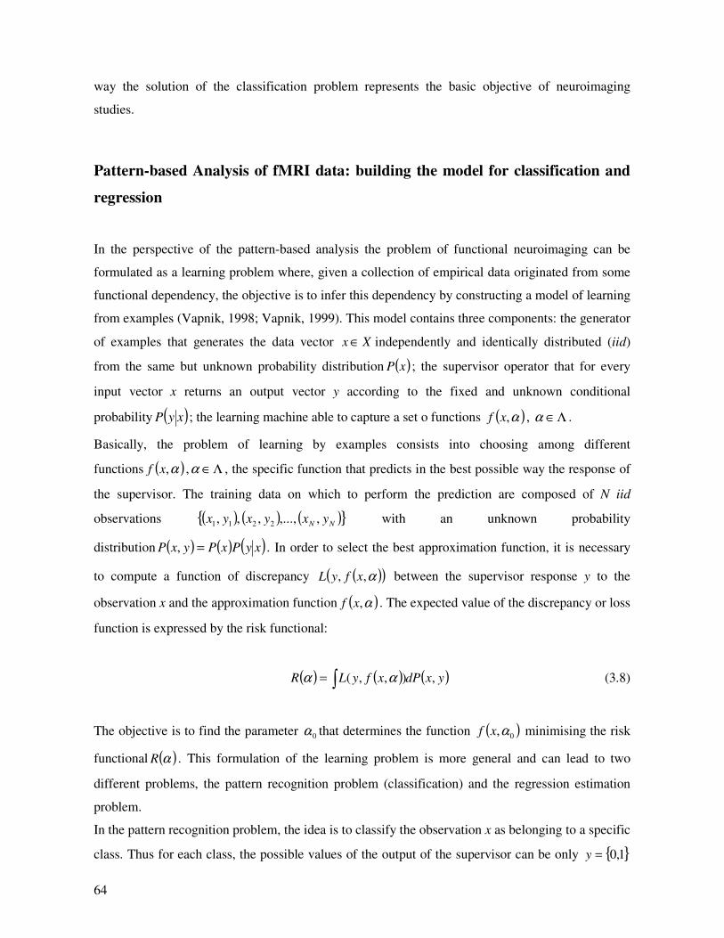
64

way the solution of the classification problem represents the basic objective of neuroimaging

studies.

Pattern-based Analysis of fMRI data: building the model for classification and

regression

In the perspective of the pattern-based analysis the problem of functional neuroimaging can be

formulated as a learning problem where, given a collection of empirical data originated from some

functional dependency, the objective is to infer this dependency by constructing a model of learning

from examples (Vapnik, 1998; Vapnik, 1999). This model contains three components: the generator

of examples that generates the data vector Xx ∈ independently and identically distributed (iid)

from the same but unknown probability distribution ( )xP ; the supervisor operator that for every

input vector x returns an output vector y according to the fixed and unknown conditional

probability ( )xyP ; the learning machine able to capture a set o functions ( )α,xf , Λ∈α .

Basically, the problem of learning by examples consists into choosing among different

functions ( )α,xf , Λ∈α , the specific function that predicts in the best possible way the response of

the supervisor. The training data on which to perform the prediction are composed of N iid

observations ( ) ( ) ( ) NN yxyxyx ,,...,,,, 2211 with an unknown probability

distribution ( ) ( ) ( )xyPxPyxP =, . In order to select the best approximation function, it is necessary

to compute a function of discrepancy ( )( )α,, xfyL between the supervisor response y to the

observation x and the approximation function ( )α,xf . The expected value of the discrepancy or loss

function is expressed by the risk functional:

( ) ( ) ( )yxdPxfyLR ,),,(∫= αα (3.8)

The objective is to find the parameter 0α that determines the function ( )0,αxf minimising the risk

functional ( )αR . This formulation of the learning problem is more general and can lead to two

different problems, the pattern recognition problem (classification) and the regression estimation

problem.

In the pattern recognition problem, the idea is to classify the observation x as belonging to a specific

class. Thus for each class, the possible values of the output of the supervisor can be only 1,0=y

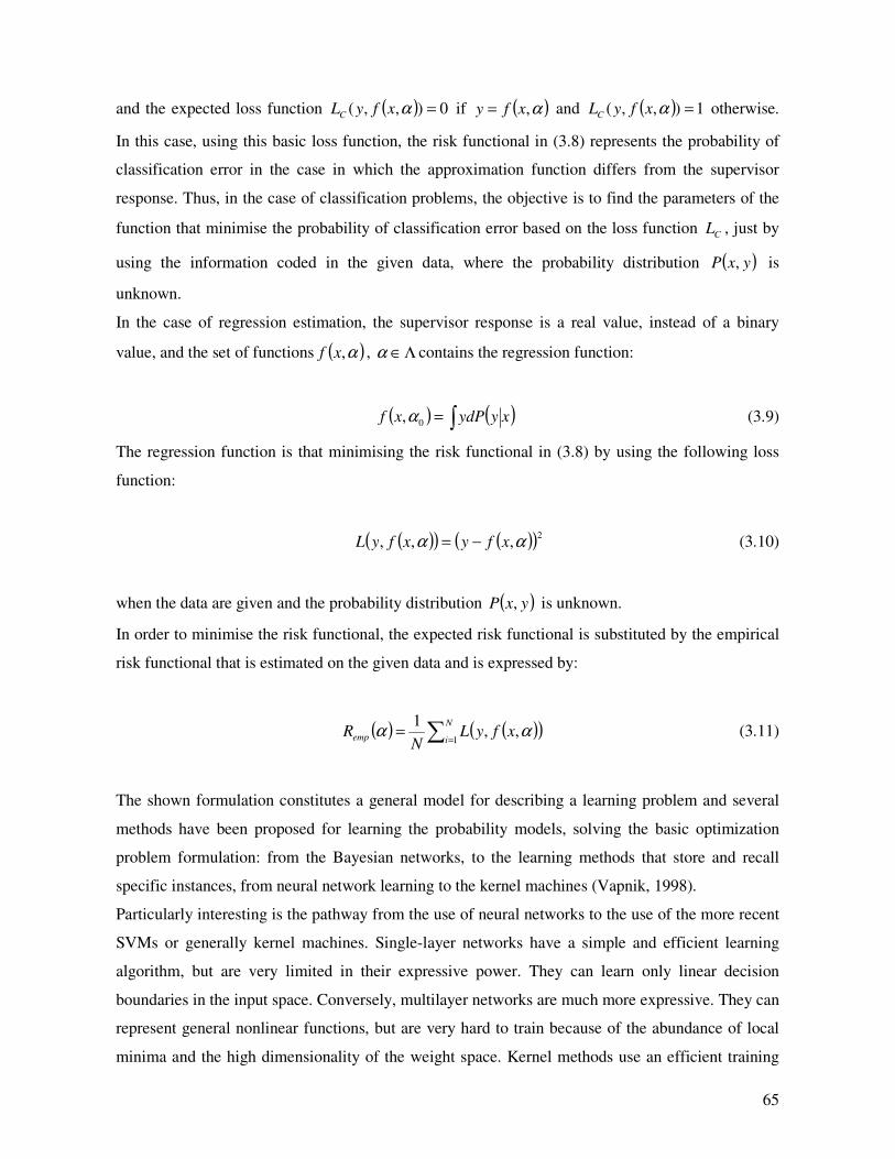
65

and the expected loss function ( ) 0),,( =αxfyLC if ( )α,xfy = and ( ) 1),,( =αxfyLC otherwise.

In this case, using this basic loss function, the risk functional in (3.8) represents the probability of

classification error in the case in which the approximation function differs from the supervisor

response. Thus, in the case of classification problems, the objective is to find the parameters of the

function that minimise the probability of classification error based on the loss function CL , just by

using the information coded in the given data, where the probability distribution ( )yxP , is

unknown.

In the case of regression estimation, the supervisor response is a real value, instead of a binary

value, and the set of functions ( )α,xf , Λ∈α contains the regression function:

( ) ( )∫= xyydPxf 0,α (3.9)

The regression function is that minimising the risk functional in (3.8) by using the following loss

function:

( )( ) ( )( )2,,, αα xfyxfyL −= (3.10)

when the data are given and the probability distribution ( )yxP , is unknown.

In order to minimise the risk functional, the expected risk functional is substituted by the empirical

risk functional that is estimated on the given data and is expressed by:

( ) ( )( )∑ ==

N

iemp xfyLN

R1

,,1

αα (3.11)

The shown formulation constitutes a general model for describing a learning problem and several

methods have been proposed for learning the probability models, solving the basic optimization

problem formulation: from the Bayesian networks, to the learning methods that store and recall

specific instances, from neural network learning to the kernel machines (Vapnik, 1998).

Particularly interesting is the pathway from the use of neural networks to the use of the more recent

SVMs or generally kernel machines. Single-layer networks have a simple and efficient learning

algorithm, but are very limited in their expressive power. They can learn only linear decision

boundaries in the input space. Conversely, multilayer networks are much more expressive. They can

represent general nonlinear functions, but are very hard to train because of the abundance of local

minima and the high dimensionality of the weight space. Kernel methods use an efficient training

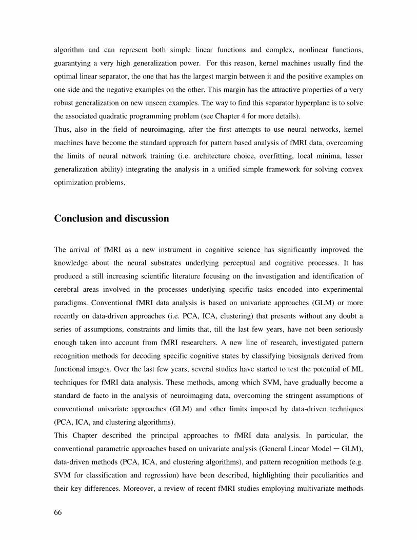
66

algorithm and can represent both simple linear functions and complex, nonlinear functions,

guarantying a very high generalization power. For this reason, kernel machines usually find the

optimal linear separator, the one that has the largest margin between it and the positive examples on

one side and the negative examples on the other. This margin has the attractive properties of a very

robust generalization on new unseen examples. The way to find this separator hyperplane is to solve

the associated quadratic programming problem (see Chapter 4 for more details).

Thus, also in the field of neuroimaging, after the first attempts to use neural networks, kernel

machines have become the standard approach for pattern based analysis of fMRI data, overcoming

the limits of neural network training (i.e. architecture choice, overfitting, local minima, lesser

generalization ability) integrating the analysis in a unified simple framework for solving convex

optimization problems.

Conclusion and discussion

The arrival of fMRI as a new instrument in cognitive science has significantly improved the

knowledge about the neural substrates underlying perceptual and cognitive processes. It has

produced a still increasing scientific literature focusing on the investigation and identification of

cerebral areas involved in the processes underlying specific tasks encoded into experimental

paradigms. Conventional fMRI data analysis is based on univariate approaches (GLM) or more

recently on data-driven approaches (i.e. PCA, ICA, clustering) that presents without any doubt a

series of assumptions, constraints and limits that, till the last few years, have not been seriously

enough taken into account from fMRI researchers. A new line of research, investigated pattern

recognition methods for decoding specific cognitive states by classifying biosignals derived from

functional images. Over the last few years, several studies have started to test the potential of ML

techniques for fMRI data analysis. These methods, among which SVM, have gradually become a

standard de facto in the analysis of neuroimaging data, overcoming the stringent assumptions of

conventional univariate approaches (GLM) and other limits imposed by data-driven techniques

(PCA, ICA, and clustering algorithms).

This Chapter described the principal approaches to fMRI data analysis. In particular, the

conventional parametric approaches based on univariate analysis (General Linear Model GLM),

data-driven methods (PCA, ICA, and clustering algorithms), and pattern recognition methods (e.g.

SVM for classification and regression) have been described, highlighting their peculiarities and

their key differences. Moreover, a review of recent fMRI studies employing multivariate methods

67

for decoding perceptual and cognitive processes has been presented. Finally, statistical and practical

aspects related to the use of multivariate methods have been examined, and the general

mathematical formulation of a learning problem has been presented.

In conclusion, time is ripe for considering pattern recognition techniques as state-of-the-art for

functional neuroimaging analysis. From the cognitive neuroscience perspective, these techniques

have changed the way to formulate research questions, from localization of brain activation to a

more sophisticated study of modular vs. distributed representation of information in the brain. From

a methodological perspective, the crucial issues for the use of these techniques regard voxel

selection, choice of the classifier, and the cross-validation methods for properly testing the

generalization abilities of the classifiers. However, new ML methods are required for modelling in a

more accurate way the nonlinear spatio-temporal dynamics of fMRI signals in the context of fast

event-related designs.

69

Chapter 4

Nonlinear Support Vector Regression: a Virtual Reality

Experiment

Introduction

When facing the problem of fMRI data analysis by using pattern recognition methods, several

crucial points have to be taken into account. Firstly, the choice of the classifier strictly depends on

the experimental paradigm to deal with. In particular, the context of the experiment determines the

choice of the learning problem that could be a classification problem when each experimental

condition to manipulate is codified as a specific event (1 if the event is present, 0 otherwise), or a

regression problem when the experimental conditions could be coded using real values. Likewise,

the experimental design (blocked, slow or fast event-related, or mixed) employed in the research

determines the possibility or the way to use certain learning machines instead of others. Finally, the

pre-processing phase, including the basic pre-processing steps (i.e. realignment, coregistration,

normalization, spatial and temporal smoothing) and the way to perform voxel selection, determines

the quality of the reachable prediction accuracy.

Certainly, in spite of all the expedients that can be used by researchers for extracting the

information contained in the available data in the best way, it could be possible that the trained

model is affected by a model error that can be decreased by different choices of the algorithm

parameters, as a linear vs nonlinear approximation function, learning parameters or the architecture

of the model itself, in the case of neural networks or combined systems (i.e. hierarchical or modular

systems).

Many pattern recognition methods have been employed as multivariate techniques for fMRI data

analysis. Machine learning techniques based on artificial neural networks (Chuang, Chiu, Lin, &

Chen, 1999; Voultsidou, Dodel, & Herrmann, 2005) or different clustering algorithms (Meyer &

Chinrungrueng, 2003; H. Chen, Yuan, Yao, Chen, & Chen, 2006; S. Chen, Bouman, & Lowe,

70

2004; Heller, Stanley, Yekutieli, Rubin, & Benjamini, 2006; Liao, 2005) have been employed for

time series data analysis in different domain applications, among which fMRI data analysis. Other

methodologies, such as independent component analysis (ICA), have also been used for processing

fMRI data (Hu et al., 2005; Meyer-Baese, Wismueller, & Lange, 2004).

Presently, one of the most widely used Machine Learning techniques for fMRI data analysis are

Support Vector Machines (SVM), which are kernel-based methods designed to find functions of the

input data that enable both classification and regression (Vapnik, 1998). In particular, SVMs

classify data with different class labels by determining a set of support vectors, which are members

of the training set, outlining a hyperplane in the feature space. SVM provides a mechanism to fit the

hyperplane surface to the training data using a specific kernel function. SMV classifiers are well

known for their very good generalization ability and have been used in recent studies of fMRI data

analysis (see Chapter 3 for an extensive review). However, most of the previous studies have

focused on classification problems. In the case of regression problems, the target conditions assume

real values instead of binary values, and the goal is to find a functional shape for the function that

can correctly predict new cases that the SVM has not been presented with before. This latter method

is usually referred to as Support Vector Regression (SVR; see Smola & Schölkopf (2004), for a

review). Thus, our primary goal was to explore the feasibility of SVR in the case of an extremely

complex regression problem.

Particularly interesting for pattern based analysis of fMRI data is the impact of different voxel

selection techniques on the level of accuracy reachable by the learning machine. As discussed in

Chapter 3, the problem of voxel selection is not only faced for computational problems, but also

because in machine learning using a huge number of input variables with respect to the number of

data samples produces the phenomenon of ovefitting, leading to poor generalization ability. This

requirement is implicitly related to statistical problems like the “curse of dimensionality” that refers

to the fact that the higher the dimensionality of the input space, the more data may be needed to find

out what is important and what is not in the classification. Moreover, the useful information for the

prediction of the experimental conditions is contained in a small subset of voxels, thus using

irrelevant voxels could produce a decreasing of the prediction performance and certainly a sub-

optimal solution. Consequently, and more related to theoretical questions, using the whole set of

voxels could be a problematic choice if it is required a fine grained discrimination between

perceptual or cognitive states. Thus, a secondary objective of this study was to use different voxel

selection techniques for comparing the impact of different choices on the accuracy achievable by

the learning machine.

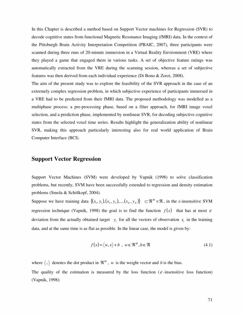
71

In this Chapter is described a method based on Support Vector machines for Regression (SVR) to

decode cognitive states from functional Magnetic Resonance Imaging (fMRI) data. In the context of

the Pittsburgh Brain Activity Interpretation Competition (PBAIC, 2007), three participants were

scanned during three runs of 20-minute immersion in a Virtual Reality Environment (VRE) where

they played a game that engaged them in various tasks. A set of objective feature ratings was

automatically extracted from the VRE during the scanning session, whereas a set of subjective

features was then derived from each individual experience (Di Bono & Zorzi, 2008).

The aim of the present study was to explore the feasibility of the SVR approach in the case of an

extremely complex regression problem, in which subjective experience of participants immersed in

a VRE had to be predicted from their fMRI data. The proposed methodology was modelled as a

multiphase process: a pre-processing phase, based on a filter approach, for fMRI image voxel

selection, and a prediction phase, implemented by nonlinear SVR, for decoding subjective cognitive

states from the selected voxel time series. Results highlight the generalization ability of nonlinear

SVR, making this approach particularly interesting also for real world application of Brain

Computer Interface (BCI).

Support Vector Regression

Support Vector Machines (SVM) were developed by Vapnik (1998) to solve classification

problems, but recently, SVM have been successfully extended to regression and density estimation

problems (Smola & Schölkopf, 2004).

Suppose we have training data ( ) ( ) ( ) NN yxyxyx ,,...,,,, 2211 ℜ×ℜ⊂ M , in the ε-insensitive SVM

regression technique (Vapnik, 1998) the goal is to find the function ( )xf that has at most ε

deviation from the actually obtained target iy for all the vectors of observation

ix in the training

data, and at the same time is as flat as possible. In the linear case, the model is given by:

( ) bxwxf += , , ℜ∈ℜ∈ bw M , (4.1)

where ⋅⋅, denotes the dot product in Mℜ , w is the weight vector and b is the bias.

The quality of the estimation is measured by the loss function (ε -insensitive loss function)

(Vapnik, 1998):

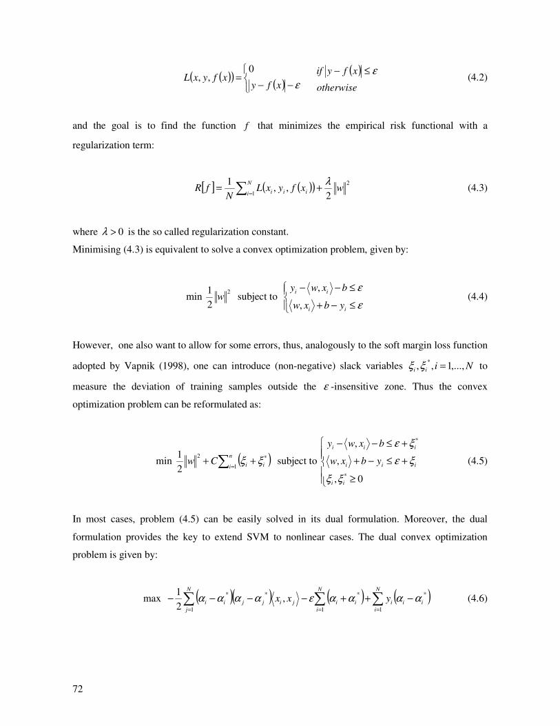
72

( )( )( )

−−=

εxfyxfyxL

0,,

( )otherwise

xfyif ε≤− (4.2)

and the goal is to find the function f that minimizes the empirical risk functional with a

regularization term:

[ ] ( )( ) 2

1 2,,

1wxfyxL

NfR

N

i iii

λ+= ∑ =

(4.3)

where 0>λ is the so called regularization constant.

Minimising (4.3) is equivalent to solve a convex optimization problem, given by:

min 2

2

1w subject to

≤−+

≤−−

ε

ε

ii

ii

ybxw

bxwy

,

, (4.4)

However, one also want to allow for some errors, thus, analogously to the soft margin loss function

adopted by Vapnik (1998), one can introduce (non-negative) slack variables Niii ,...,1,,*

=ξξ to

measure the deviation of training samples outside the ε -insensitive zone. Thus the convex

optimization problem can be reformulated as:

min ( )∑ =++

n

i iiCw1

*2

2

1ξξ subject to

≥

+≤−+

+≤−−

0,

,

,

*

*

ii

iii

iii

ybxw

bxwy

ξξ

ξε

ξε

(4.5)

In most cases, problem (4.5) can be easily solved in its dual formulation. Moreover, the dual

formulation provides the key to extend SVM to nonlinear cases. The dual convex optimization

problem is given by:

max ( )( ) ( ) ( )∑∑∑===

−++−−−−N

i

iii

N

i

ii

N

j

jijjii yxx1

*

1

*

1

**,

2

1ααααεαααα (4.6)

73

subject to ( )

[ ]

∈

=−∑=

Cii

N

i

ii

,0,

0

*

1

*

αα

αα

where *

, ii αα are the so called Lagrange multipliers.

From the optimality constraints that are behind the dual problem definition, it is possible to derive

w as a linear combination of the training patterns:

( ) i

N

i

ii xw ∑=

−=1

*αα (4.7)

thus, the function ( )xf can be expressed as:

( )∑=

−=N

i

iii xxxf1

*,)( αα

(4.8)

In nonlinear SVM regression, the input vector x is first mapped onto a high dimensional feature

space using some fixed nonlinear mapping, and then a linear model is constructed in this feature

space as:

( ) ( ) bxwxf +Φ= , , ℜ∈ℜ∈ bw M , (4.9)

where )(xΦ denotes a set of nonlinear transformation.

As noted in (4.6), the SVM algorithm only depends on dot products between patterns ix, hence it is

sufficient to know the kernel function ( ) ( ) ( )'' ,, xxxxK ΦΦ=

rather then Φ explicitly, which

allows us to write w and ( )xf in the nonlinear case as:

( ) ( )i

N

i

ii xw Φ−=∑=1

*αα (4.10)

( ) ( ) ( ) bxxKxf i

n

i ii

SV +−=∑ =,

1

*αα (4.11)

74

As can be noted in (4.10), the difference to the linear case is that w can no longer given explicitly,

whereas the flattest function ( )xf , that has to be found in the feature space (not in the input space),

can be expressed through the trick of the kernel function.

Several functions, such as polynomial functions, radial basis functions (RBF), splines, hyperbolic

tangent functions, can be used as kernel in SVM regression (Burges, 1998; Smola & Schölkopf,

2004). These functions have to satisfy the conditions of the Mercer’s theorem (Mercer, 1909), that

is the conditions under which it could be possible to write ( )', xxk as a dot product in some feature

space. In particular, translation invariant kernels ( ) ( )'', xxkxxk −= , that are proofed to be

admissible kernels, are widespread, among which one of the most widely used is the RBF kernel

that can be write as:

( ) 2

2

2

'

', σ

xx

exxk

−−

= (4.12)

It is well known that SVM generalization performance (estimation accuracy) depends on a good

setting of meta-parameters C, ε and the kernel parameters (Burges, 1998; Smola & Schölkopf,

2004). The parameter C determines the trade off between the model complexity and the degree to

which deviations larger than ε are tolerated in optimization formulation. Parameter ε controls the

width of the ε -insensitive zone, used to fit the training data. The value of ε can affect the number

of support vectors used to construct the regression function. The biggerε , the fewer support vectors

are selected. Hence, both C and ε -values affect model complexity, but in a different way.

Experimental setting

The VRE experiment was organized in the context of the Pittsburgh Brain Activity Interpretation

Competition (PBAIC, 2007). The purpose of this competition was to infer subjective experience of

the participants experiencing an immersion in a virtual reality environment, from a contextually

gathered set of fMRI data. The VRE experiment, the gathered fMRI data and the proposed fMRI

decoding method are described in the next sections.

75

Participants

Fifteen subjects participated in this study. In particular, after a selection procedure made by the

PBAIC staff (see PBAIC, 2007 for details), the only data available for the competition were relative

to three subjects (age range: 20-26).

Procedure

Participants were instructed to play a game in a virtual world during three runs of fMRI data

acquisition. In the game they were paid by an anthropology department grant to gather information

about urban people. In particular, they were visiting several times the virtual reality environment,

outside and inside some specified places, and were instructed to collect as much as possible samples

of toy weapons and fruits, in a predefined order; moreover, they had to take pictures of people with

piercings and avoid an aggressive dog. Participants were also informed and asked to keep in mind

that any money obtained in the game corresponded to an earning in real life.

The study was completed over a period of four days. During the first day, participants watched a

13-minute video for a first phase of familiarization with the VRE and completed a battery of

questionnaires, implicit association tests for assessing the ingroup/outgroup and canines perception,

the level of anxiety and sickness, the sense of direction, the computer familiarity scale (see PBAIC,

2007 for details). During the second day, participants played the virtual reality game outside the

scanner and every 2 minutes they were asked to rate their level of sickness. At the end of the session

they completed three questionnaires for assessing the level of simulator sickness and the level of

presence and comfort during the navigation. In the third day, subjects were asked to perform search

tasks during three 20 minute runs of the game inside the scanner. As in the previous day,

participants were asked to rate every 2 minutes their level of sickness.

During the navigation of the virtual world, a set of target feature ratings was gathered for a total of

13 required and 10 optional features. In particular, some features were obtained through software

loggings of subject actions in the virtual world, soundtrack analysis and eye-tracking based analysis

of video from each run, and were referred to as objective features (e.g., Hits: whenever subjects

correctly picked up fruit or weapon or took pictures of persons with piercings; Instructions:

whenever task instructions were presented; Search people; Search weapons; Search fruit; Faces:

whenever subjects looked at faces of pierced or unpierced people). The other features were referred

to as subjective features, such as the level of arousal or valence (how positive or negative is the

76

environment), and they were assigned by each participant on the last day of the study while

watching a playback of the own actions in the virtual world. Figure 4.1 shows a screenshot of the

virtual world and the behavioural time vector ratings of multiple categories representing what

participants perceived/experienced during the navigation of the virtual world.

Figure 4.1. Screenshot of the virtual world (a); illustration of behavioural time vector ratings of multiple

categories (b).

For the first two runs, videos of the subject’s path through the virtual reality environment along

with 20 minutes of continuous fMRI data and target feature ratings were provided, whereas for the

third run the ratings were not provided. The purpose of the competition was to predict feature rating

vectors for the third segment.

fMRI Dataset

3T EPI fMRI data from three subjects in three runs were downloadable from the Pittsburgh Brain

Activity Interpretation Competition web site (PBAIC 2007). Twenty minutes of continuous

functional data, consisting of 704 of 64x64x34 image volumes, were available for each participant

in each run. The acquired images were motion corrected, slice time corrected, detrended and

spatially normalized. The fMRI data of the first two runs were used for the learning phase, whereas

the last run was used as test set for the prediction of the related ratings.

fMRI Decoding Method

The proposed fMRI decoding method is modelled as a multiphase process (preprocessing phase,

prediction phase) as shown in Figure 4.2. In the pre-processing phase we first extracted only those

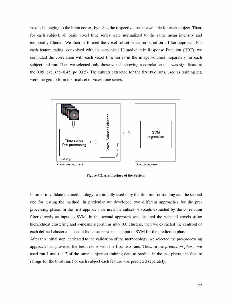
77

voxels belonging to the brain cortex, by using the respective masks available for each subject. Then,

for each subject, all brain voxel time series were normalized to the same mean intensity and

temporally filtered. We then performed the voxel subset selection based on a filter approach. For

each feature rating, convolved with the canonical Hemodynamic Response Function (HRF), we

computed the correlation with each voxel time series in the image volumes, separately for each

subject and run. Then we selected only those voxels showing a correlation that was significant at

the 0.05 level (r > 0.45, p< 0.05). The subsets extracted for the first two runs, used as training set,

were merged to form the final set of voxel time series.

Figure 4.2. Architecture of the System.

In order to validate the methodology, we initially used only the first run for training and the second

one for testing the method. In particular we developed two different approaches for the pre-

processing phase. In the first approach we used the subset of voxels extracted by the correlation

filter directly as input to SVM. In the second approach we clustered the selected voxels using

hierarchical clustering and k-means algorithms into 100 clusters, then we extracted the centroid of

each defined cluster and used it like a super-voxel as input to SVM for the prediction phase.

After this initial step, dedicated to the validation of the methodology, we selected the pre-processing

approach that provided the best results with the first two runs. Thus, in the prediction phase, we

used run 1 and run 2 of the same subject as training data to predict, in the test phase, the feature

ratings for the third run. For each subject each feature was predicted separately.

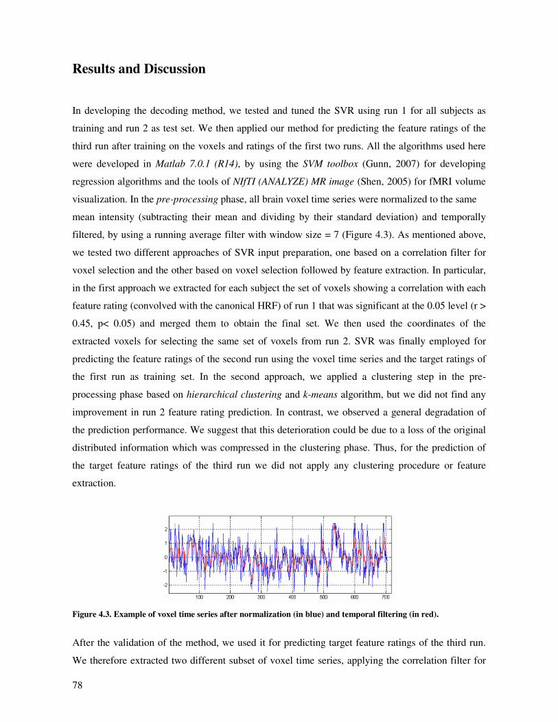
78

Results and Discussion

In developing the decoding method, we tested and tuned the SVR using run 1 for all subjects as

training and run 2 as test set. We then applied our method for predicting the feature ratings of the

third run after training on the voxels and ratings of the first two runs. All the algorithms used here

were developed in Matlab 7.0.1 (R14), by using the SVM toolbox (Gunn, 2007) for developing

regression algorithms and the tools of NIfTI (ANALYZE) MR image (Shen, 2005) for fMRI volume

visualization. In the pre-processing phase, all brain voxel time series were normalized to the same

mean intensity (subtracting their mean and dividing by their standard deviation) and temporally

filtered, by using a running average filter with window size = 7 (Figure 4.3). As mentioned above,

we tested two different approaches of SVR input preparation, one based on a correlation filter for

voxel selection and the other based on voxel selection followed by feature extraction. In particular,

in the first approach we extracted for each subject the set of voxels showing a correlation with each

feature rating (convolved with the canonical HRF) of run 1 that was significant at the 0.05 level (r >

0.45, p< 0.05) and merged them to obtain the final set. We then used the coordinates of the

extracted voxels for selecting the same set of voxels from run 2. SVR was finally employed for

predicting the feature ratings of the second run using the voxel time series and the target ratings of

the first run as training set. In the second approach, we applied a clustering step in the pre-

processing phase based on hierarchical clustering and k-means algorithm, but we did not find any

improvement in run 2 feature rating prediction. In contrast, we observed a general degradation of

the prediction performance. We suggest that this deterioration could be due to a loss of the original

distributed information which was compressed in the clustering phase. Thus, for the prediction of

the target feature ratings of the third run we did not apply any clustering procedure or feature

extraction.

Figure 4.3. Example of voxel time series after normalization (in blue) and temporal filtering (in red).

After the validation of the method, we used it for predicting target feature ratings of the third run.

We therefore extracted two different subset of voxel time series, applying the correlation filter for

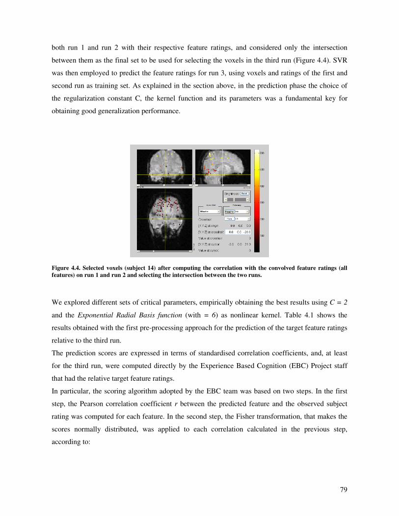
79

both run 1 and run 2 with their respective feature ratings, and considered only the intersection

between them as the final set to be used for selecting the voxels in the third run (Figure 4.4). SVR

was then employed to predict the feature ratings for run 3, using voxels and ratings of the first and

second run as training set. As explained in the section above, in the prediction phase the choice of

the regularization constant C, the kernel function and its parameters was a fundamental key for

obtaining good generalization performance.

Figure 4.4. Selected voxels (subject 14) after computing the correlation with the convolved feature ratings (all

features) on run 1 and run 2 and selecting the intersection between the two runs.

We explored different sets of critical parameters, empirically obtaining the best results using C = 2

and the Exponential Radial Basis function (with = 6) as nonlinear kernel. Table 4.1 shows the

results obtained with the first pre-processing approach for the prediction of the target feature ratings

relative to the third run.

The prediction scores are expressed in terms of standardised correlation coefficients, and, at least

for the third run, were computed directly by the Experience Based Cognition (EBC) Project staff

that had the relative target feature ratings.

In particular, the scoring algorithm adopted by the EBC team was based on two steps. In the first

step, the Pearson correlation coefficient r between the predicted feature and the observed subject

rating was computed for each feature. In the second step, the Fisher transformation, that makes the

scores normally distributed, was applied to each correlation calculated in the previous step,

according to:

80

−

+=

r

rz

1

1log

2

1' (4.13)

The obtained predictions, at least for a subset of features, reached a good correlation with the target

ones. A consistency across subjects can be noted with respect to the features that are more reliably

predicted.

Subject

1

Subject

13

Subject

14

Body 0.2421 0.4178 0.3438

Velocity 0.4554 0.5197 0.7126

Hits 0.3035 0.4339 0.3959

Instruction 0.5453 0.7957 0.7842

Faces 0.2611 0.3595 0.5871

Table 4.1. The best feature rating predictions, expressed in terms of correlations, achieved on run 3 for all

subjects. The best three correlations for each subject are shown in bold font.

In conclusion, the aim of this study was to explore the feasibility of SVR in the case of an extremely

complex regression problem, in which subjective experience of participants immersed in a VRE had

to be predicted from their fMRI data. We used a decoding method modelled as a multiphase

process: a pre-processing phase, based on a filter approach, for fMRI image voxel selection, and a

prediction phase, implemented by nonlinear SVR, for decoding subjective cognitive states from the

selected voxel time series. Results are quite good, at least for a subset of feature ratings. The

emphasis of SVM/SVR on generalization ability makes this approach particularly interesting for

real world applications of BCI (Weiskopf et al., 2004; Sitaram et al., 2007; F. Piccione et al., 2008;

F. Piccione et al., 2006), in particular when the amount of training data is limited and the input

space has a high dimension (as in the case of fMRI data).

Conclusion

The analysis of fMRI data based on pattern recognition methods requires critical choices related to

the learning machine on the base of the nature of the learning problem, the experimental paradigm,

the pre-processing steps and the way to perform voxel selection. Many pattern recognition methods

have been employed for fMRI data analysis, but all the previous studies focused on classification

problems, in which the experimental conditions were codified as binary values.

81

In this study we explored the robustness of SVR with nonlinear kernel in the case of a particularly

intricate regression problem, in which we predicted the subjective experience of participants

engaged in several tasks to perform in a VRE.

We developed a methodology modelled as a multiphase process: a pre-processing phase, based on a

filter approach, for fMRI image voxel selection, and a prediction phase, implemented by nonlinear

SVR, for decoding subjective cognitive states from the selected voxel time series. The obtained

results have shown a certain degree of consistency across participants, highlighting the

generalization ability of nonlinear SVR, and leading this approach to be a promising and

particularly interesting instrument also for real world application of Brain Computer Interface

(BCI). Planned extensions to this work included the evaluation of different feature extraction

techniques to combine with SVM/SVR or the use of embedded methods, in the context of nonlinear

kernels, for voxel selection and ranking, in order to extract a more compact and informative set of

voxels and to further increase the prediction accuracy for both classification and regression

problems.

83

Chapter 5

Nonlinear Support Vector Machine in fMRI data Analysis: a

Wrapper Approach to Voxel Selection

Introduction

The advent of the multivariate analysis of fMRI data, led SVM to become one of the most widely

used pattern recognition method in the most recent year literature. These learning machines are

notably known for their higher generalization abilities and, at least in neuroimaging literature, they

are generally used with a linear kernel. In those cases it is possible to obtain the discriminating brain

regions for each experimental condition, just by examining the weight vector associated by the

classifier to the training data. Using SVM with nonlinear kernels generally allows the classifier to

reach a much more accurate performance, but in that case there is not a direct way to characterise

the most discriminating voxel regions. Basically, more often when linear kernels do not allow the

classifier to achieve good generalization accuracy, using nonlinear functions can help in

discriminating the different cognitive processes underlying the experimental conditions. Usually, in

those cases several heuristics are used for extracting these maps (see Chapter 3 for more details).

The problem of variable (voxel) selection has been faced by researchers following two different

methodological perspectives: a univariate approach (filter methods) and a multivariate approach.

Multivariate methods to perform voxel selection are generally classified into wrapper, and

embedded methods. These methods use the classifier for finding the most discriminating voxel

subsets. In particular, wrapper methods use the classifier as a black box to rank subsets of voxels

according to their prediction ability, whereas embedded methods perform voxel selection implicitly

in the training process and are usually specific to the given classifier.

The aim of this research was to define a novel and effective methodology for decoding brain

activity from fMRI data and contextually providing a way to obtain cortical activity maps for each

experimental condition, by using a wrapper approach to voxel selection in a nonlinear classification

84

framework. In wrapper approaches the classifier performance is evaluated on a validation set for

assessing the importance of the selected voxels in the prediction task. Basically, from the practical

point of view it has to define in which way to search the space of all possible voxel subsets and how

to measure the prediction performance of the classifier that guides the search.

In this study we used a methodology based on Genetic Algorithms (GAs) and Support Vector

Machines (SVMs), efficiently combined to decode cognitive states from fMRI data. The proposed

methodology was modelled as a multiphase process: a pre-processing phase in which we extracted a

set of Region of Interest (ROIs) and a classification phase based on a GA-SVM wrapper approach,

in which both the most promising subset of voxels and classifier parameters were selected for

increasing the classification accuracy. Thus, the solution of this multi-objective optimization

problem gives us, for each experimental condition, a measure of the prediction accuracy and

concurrently the most predictive subset of voxels.

In this Chapter, after a brief overview of the basic principles of the genetic algorithms, the

description of the fMRI data used for test purpose, the comparative approach for choosing the best

classifier, and the proposed methodology are illustrated.

Genetic Algorithms

Genetic algorithms (GAs) are a class of computational models inspired by evolution. They are

probabilistic optimization methods that are based on principles of evolution. The theory and

applicability of these algorithms was strongly influenced by J. H. Holland, which can be considered

the pioneer of GAs (Holland, 1975). These algorithms encode a potential solution to a specific

problem into a chromosome-like data structure and apply recombination operators to this data

structure in order to preserve crucial information.

Basically, the implementation of GAs starts with a population of individuals (chromosomes),

generally randomly generated. Then a series of recombination operators are applied in order to

augment the reproduction probability of the better solutions (chromosomes) with respect to poor

solutions. Generally speaking, a genetic algorithm is any population based model that use selection

and recombination methods for generating new potential solutions in a search space. There are two

main components, depending on the problem, that have to be considered when dealing with

optimization problems with GAs: the problem encoding and the evaluation function.

Let consider an optimization problem, commonly we want to optimize a set of variables in order to

maximize a target earnings or minimize a certain error measure. Substantially the problem is to find

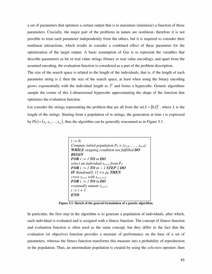
85

a set of parameters that optimize a certain output that is to maximize (minimize) a function of those

parameters. Crucially, the major part of the problems in nature are nonlinear, therefore it is not

possible to treat each parameter independently from the others, but it is required to consider their

nonlinear interactions, which results in consider a combined effect of these parameter for the

optimization of the target output. A basic assumption of Gas is to represent the variables that

describe parameters as bit or real value strings (binary or real value encoding), and apart from the

assumed encoding, the evaluation function is considered as a part of the problem description.

The size of the search space is related to the length of the individuals, that is, if the length of each

parameter string is L then the size of the search space, at least when using the binary encoding

grows exponentially with the individual length as 2L and forms a hypercube. Genetic algorithms

sample the corner of this L-dimensional hypercube approximating the shape of the function that

optimizes the evaluation function.

Let consider the strings representing the problem that are all from the set LS 1,0= , where L is the

length of the strings. Starting from a population of m strings, the generation at time t is expressed

by ( ) ( )mssstP ,,, 21 K= , thus the algorithm can be generally reassumed as in Figure 5.1.

Figure 5.1. Sketch of the general formulation of a genetic algorithm.

In particular, the first step in the algorithm is to generate a population of individuals, after which,

each individual is evaluated and is assigned with a fitness function. The concept of fitness function

and evaluation function is often used as the same concept, but they differ in the fact that the

evaluation (or objective) function provides a measure of performance on the base of a set of

parameters, whereas the fitness function transforms this measure into a probability of reproduction

in the population. Thus, an intermediate population is created by using the selection operator, then

t := 0;

Compute initial population P0 = (s1,0, . . . , sm,0);

WHILE stopping condition not fulfilled DO

BEGIN FOR i := 1 TO m DO

select an individual si,t+1 from Pt;

FOR i := 1 TO m − 1 STEP 2 DO

IF Random[0, 1] <= pC THEN

cross si,t+1 with si+1,t+1;

FOR i := 1 TO m DO

eventually mutate si,t+1;

t := t + 1

END

86

the recombination operators like crossover and mutation are applied to the intermediate population

in order to create the next population. As shown in the sketch of the algorithm, after the operations

of crossover and mutation, each selected string is replaced in the new generation by one of its

children, whereas unselected individuals are eliminated.

Let examine each single operator used by the algorithm in the following subsections.

Selection

The operator of selection guides the algorithm in the choice of the individuals that show a high

fitness function. Often this operator is implemented with a random component, for example

considering the probability to choose an individual as proportional to its fitness as:

( ) ( )

( )∑=

=m

k

tk

tj

tj

sf

sfselectedsP

1

,

,

, (5.1)

where f is the evaluation function. The (5.1) can be used if we assume that the fitness function has

positive values for all the individuals in the population, otherwise it could be necessary to apply a

transformation +ℜ→ℜ:ϕ to the fitness function value before to apply the selection operator. This

selection method is called proportional selection and can be realised by using a Roulette Wheel

function, in which ach individual is represented by a space proportional to its fitness function. By

spinning the roulette wheel, individuals are chosen by using a stochastic sampling with

replacement.

Crossover

After the creation of the intermediate population, the crossover is applied to randomly paired

individuals with a probability Cp . The selected parents are recombined for generating new

individuals for the next population. The mechanism of crossover is a useful tool for introducing new

genetic material and maintaining genetic diversity. In essence, crossover is the exchanging of genes

between chromosomes of two parents. In the simpler case (one point crossover), it consists in

cutting two strings at a randomly chosen point and exchanging the two tails for creating the

87

offspring. There are other methods for realizing the crossover operator: the N-point crossover, in

which N breaking points are randomly chosen and each second part is exchanged; the uniform

crossover, in which for each position it is randomly chosen if it has to be exchanged; the shuffle

crossover, in which a random permutation is applied to the parents and then the N-point crossover

is used on the transformed parents, and at last the inverse permutation is applied to the generated

offspring.

Mutation

After the recombination of the individuals by the crossover operator, the mutation operator can be

applied. Basically, mutation is a random deformation of the genetic information that is the random

generation of a new bit that will replace the older one. Each gene of each individual has the same

probability Mp to be mutated that is a very low probability, in order to avoid that the algorithm

behaves chaotically as a random search. Similarly to crossover, the choice of an appropriate

mutation method depends on the coding of the problem itself. In the binary coding, some well

known methods are:

Inversion of a single bit: with probability Mp one randomly chosen bit is inverted.

Bitwise inversion: the entire string is inverted bit by bit with probability Mp .

Random selection: the entire string is replaced by a randomly chosen one with probability

Mp .

There are many optimization methods that have been developed in mathematics and operational

research based on gradient information, such as Newton or gradient descent methods. In this

context, GAs are well known as global search methods without considering any gradient

information. Thus any non-differentiable function or functions with multiple local optima can be

optimized by using GAs. Moreover, comparing genetic algorithms with conventional continuous

optimization techniques, several additional differences can be outlined: GAs manipulate an encoded

form of the problem parameters instead of the parameters themselves; the conventional search

methods start from a single point, whereas GAs operate on a population of possible solutions

increasing the probability to reach a global optimum; GAs use probabilistic transition operators in

approximating the problem solution, whereas conventional continuous optimization methods use

deterministic operators without any random component.

88

Materials and Methods

In this section we describe a GA-SVM wrapper approach to classify cognitive states from fMRI

data. In order to asses our methodology we test it on an fMRI data gathered during an experiment

about the modulation of attention in visual motion (Buchel & Friston, 1997). We first performed a

pre-processing phase in which a set of regions of interest (ROIs) were extracted, by using prior

domain knowledge for the selection of specific cortical areas. Thus, after a comparative approach

for the choice of the best classifier, we used the GA-SVM approach for the classification phase.

Description of the fMRI experiment

The experimental data were scanned by Buchel & Friston (1997). In their experiment, three right-

handed subjects were scanned during four runs of ten blocks, each with duration of five min and 22

s. Each experimental condition lasted 32.2 s and provided 90 sliced image volumes per run. Four

conditions were used: fixation, attention to visual motion, no attention to visual motion, stationary.

During the fixation condition, the screen was dark and only a fixation cross was visible. In the

stationary condition, 250 white dots appeared on the black screen in a static way and subjects were

asked to just look on the screen, whereas in visual motion conditions, dots moved, at a constant

speed, from the fixation cross in random directions toward the border of the screen. During the

attention condition, subjects were asked to pay attention to changes in speed. Finally, in the last

condition, subjects were asked to just look the motion.

fMRI dataset

2T EPI fMRI data from one subject in a session of four runs were available from the Statistical

Parametric Mapping (SPM) web site (http://www.fil.ion.ucl.ac.uk/spm/data/attention/). Five

minutes and twenty two seconds of continuous functional data, consisting of 90 of 64x64x32 image

volumes, were available for the participant in each run. The objective of this study was purely

methodological: we wanted to compare different classifiers, and to test the wrapper approach for

voxel and learning parameter selection on the same data without any research purpose in the field of

cognitive science.

89

Methodology description

The proposed methodology is modelled as a multiphase process (pre-processing phase and

classification phase). We first extract a set of voxels belonging to specific ROIs (pre-processing

phase); afterwards we used GA-SVM approach for classifying cognitive states (classification

phase) and providing a subset of the most predictive voxels for each condition. In the classification

phase the current subset of selected voxels evolves during several generations with the objective to

minimise the number of voxels and maximise the classification accuracy.

Data Pre-processing

Common problems in fMRI data analysis are related to the high data dimensionality, their

heterogeneity and the presence of a certain amount of signal to noise ratio. Typically in an fMRI

scanning session, each acquired volume is composed of a set of sliced images and each volume is to

be considered as a function of time. Another problem related with fMRI data is that cortical

anatomical differences across subjects generate a difference in the intensity and variability of the

BOLD signal: basically, people may think in different ways. To deal with these problems, a lot of

techniques have been developed. Voxel selection is employed in order to reduce the amount of data.

Data heterogeneity is faced by using signal normalization, data transformation (e. g. registration to

standard 3D space, Talairach or MNI) and temporal filters are used for reducing the signal to noise

ratio. In conventional approaches, the problem of classification across multiple subjects has been

faced by using spatial smoothing for reducing subjective differences. The main problem caused by

the smoothing procedure is the reduction of the potential information that data can provide. For this

reason, different approaches have been explored, for extracting some invariant features (e. g. ROI

active averaging) in order to represent fMRI active patterns across subjects. Alternatively, strategies

based on leave one-subject-out classifiers have been explored, decoding the subjective variability

directly from multiple subject data.

We performed a first voxel selection, focusing our attention on specific cortical areas and reducing

the computational effort in the classification phase. The acquired images were previously smoothed,

spatially normalised, realigned and slice-time corrected. In order to extract significant cortical areas,

we applied the General Linear Model (GLM) analysis, performed with SPM5

(http://www.fil.ion.ucl.ac.uk/spm), and then we extracted distinct ROIs for the classification phase.

Specific effects were tested with appropriate linear contrasts of the parameter estimation for each

condition, resulting in a series of t-statistic for each voxel. Then, we localised and selected specific

90

regions of interest according to the hypotheses used by the authors. The purpose of the classification

phase was to discriminate among the ROI voxels, which are the most predictive for each task

condition.

Toward the best classifier: a comparative approach

In pattern recognition, the choice of a classifier for a specific problem plays a key role for

increasing the classification accuracy.

In this paper we compared different classifiers in order to select the one which provided the better

classification accuracy, using all the voxels. We evaluated the prediction accuracy of three different

classifiers for fMRI data classification: a feed-forward neural network, a partial recurrent neural

network (Elman network) and SVMs whit different kernel functions. Then we used GAs combined

with the best classifier for selecting both voxel subsets and classifier parameters, in with the

purpose to maximise the classification accuracy.

Both feed-forward and recurrent neural networks are the most generally used networks for

classification and prediction problems. In particular, recurrent neural networks, due to their

dynamical properties, are widely used for processing temporal information coded in input data

sequences, for both classification and prediction tasks. One of the critical points for neural networks

is the definition of the network architecture (i.e., number of hidden layers, number of neurons per

layer) that can offer the best classification results. Moreover, the network training has to be

controlled in order to avoid overfitting. Support vector machines (SVMs) are kernel-based methods

designed to find functions of the input data that enable classification or regression. In particular,

SVM classifies data with different class labels by determining a set of support vectors, which are

members of the training set, outlining a hyperplane in the feature space. It provides a mechanism to

fit the hyperplane surface to the training data using a specific kernel function. SMV classifiers are

well known for their very good generalization ability. However, the choice of the kernel function

and its parameters is a crucial point for obtaining a good generalization performance.

For all the tested classifiers the input pattern matrix was composed of a set of voxel time series,

whereas the output was the class vector representing the corresponding experimental condition. In

the case of neural networks, their topology was empirically determined, by training different

network architectures and evaluating their generalization accuracy. In the case of SVM, four

different kernel functions (i.e., linear, polynomial, Gaussian RBF and Exponential RBF) were tested

in order to estimate the generalization performance. SVM outperformed the other neural networks

in the classification, thus we used it in a GA-SVM approach for the final classification.

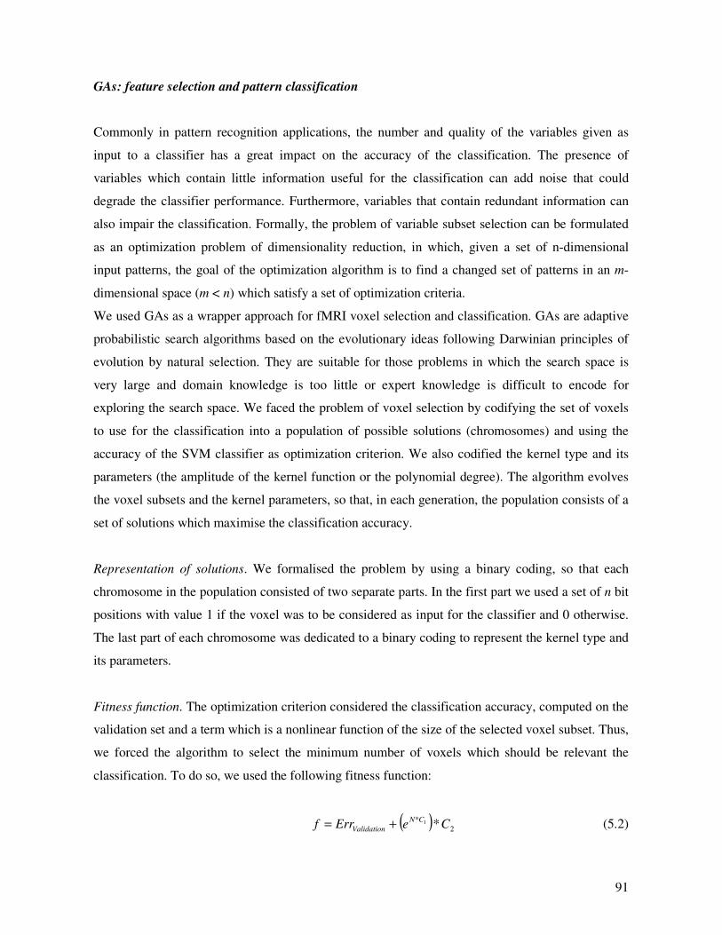
91

GAs: feature selection and pattern classification

Commonly in pattern recognition applications, the number and quality of the variables given as

input to a classifier has a great impact on the accuracy of the classification. The presence of

variables which contain little information useful for the classification can add noise that could

degrade the classifier performance. Furthermore, variables that contain redundant information can

also impair the classification. Formally, the problem of variable subset selection can be formulated

as an optimization problem of dimensionality reduction, in which, given a set of n-dimensional

input patterns, the goal of the optimization algorithm is to find a changed set of patterns in an m-

dimensional space (m < n) which satisfy a set of optimization criteria.

We used GAs as a wrapper approach for fMRI voxel selection and classification. GAs are adaptive

probabilistic search algorithms based on the evolutionary ideas following Darwinian principles of

evolution by natural selection. They are suitable for those problems in which the search space is

very large and domain knowledge is too little or expert knowledge is difficult to encode for

exploring the search space. We faced the problem of voxel selection by codifying the set of voxels

to use for the classification into a population of possible solutions (chromosomes) and using the

accuracy of the SVM classifier as optimization criterion. We also codified the kernel type and its

parameters (the amplitude of the kernel function or the polynomial degree). The algorithm evolves

the voxel subsets and the kernel parameters, so that, in each generation, the population consists of a

set of solutions which maximise the classification accuracy.

Representation of solutions. We formalised the problem by using a binary coding, so that each

chromosome in the population consisted of two separate parts. In the first part we used a set of n bit

positions with value 1 if the voxel was to be considered as input for the classifier and 0 otherwise.

The last part of each chromosome was dedicated to a binary coding to represent the kernel type and

its parameters.

Fitness function. The optimization criterion considered the classification accuracy, computed on the

validation set and a term which is a nonlinear function of the size of the selected voxel subset. Thus,

we forced the algorithm to select the minimum number of voxels which should be relevant the

classification. To do so, we used the following fitness function:

( )2

**1 CeErrf

CN

Validation += (5.2)

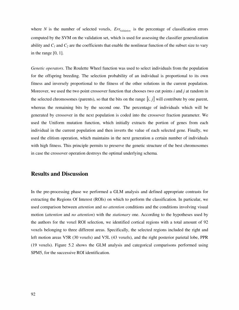
92

where N is the number of selected voxels, ValidationErr is the percentage of classification errors

computed by the SVM on the validation set, which is used for assessing the classifier generalization

ability and C1 and C2 are the coefficients that enable the nonlinear function of the subset size to vary

in the range [0, 1].

Genetic operators. The Roulette Wheel function was used to select individuals from the population

for the offspring breeding. The selection probability of an individual is proportional to its own

fitness and inversely proportional to the fitness of the other solutions in the current population.

Moreover, we used the two point crossover function that chooses two cut points i and j at random in

the selected chromosomes (parents), so that the bits on the range [ ]ji, will contribute by one parent,

whereas the remaining bits by the second one. The percentage of individuals which will be

generated by crossover in the next population is coded into the crossover fraction parameter. We

used the Uniform mutation function, which initially extracts the portion of genes from each

individual in the current population and then inverts the value of each selected gene. Finally, we

used the elitism operation, which maintains in the next generation a certain number of individuals

with high fitness. This principle permits to preserve the genetic structure of the best chromosomes

in case the crossover operation destroys the optimal underlying schema.

Results and Discussion

In the pre-processing phase we performed a GLM analysis and defined appropriate contrasts for

extracting the Regions Of Interest (ROIs) on which to perform the classification. In particular, we

used comparison between attention and no attention conditions and the conditions involving visual

motion (attention and no attention) with the stationary one. According to the hypotheses used by

the authors for the voxel ROI selection, we identified cortical regions with a total amount of 92

voxels belonging to three different areas. Specifically, the selected regions included the right and

left motion areas V5R (30 voxels) and V5L (43 voxels), and the right posterior parietal lobe, PPR

(19 voxels). Figure 5.2 shows the GLM analysis and categorical comparisons performed using

SPM5, for the successive ROI identification.

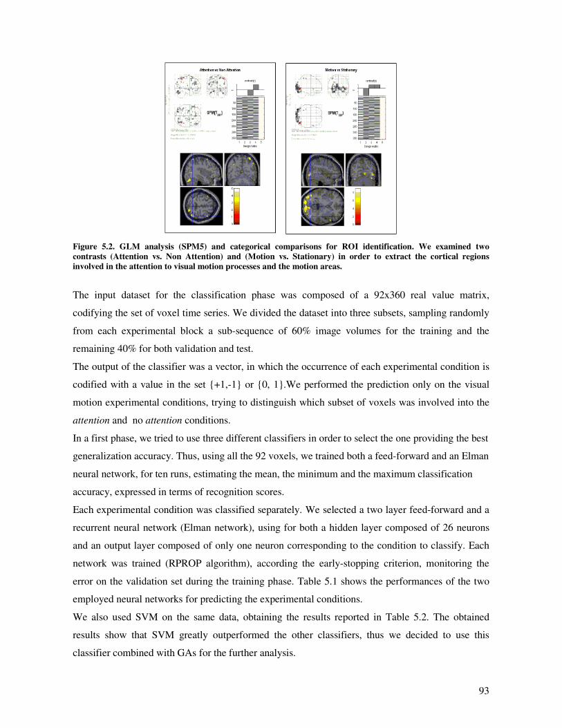
93

Figure 5.2. GLM analysis (SPM5) and categorical comparisons for ROI identification. We examined two

contrasts (Attention vs. Non Attention) and (Motion vs. Stationary) in order to extract the cortical regions

involved in the attention to visual motion processes and the motion areas.

The input dataset for the classification phase was composed of a 92x360 real value matrix,

codifying the set of voxel time series. We divided the dataset into three subsets, sampling randomly

from each experimental block a sub-sequence of 60% image volumes for the training and the

remaining 40% for both validation and test.

The output of the classifier was a vector, in which the occurrence of each experimental condition is

codified with a value in the set +1,-1 or 0, 1.We performed the prediction only on the visual

motion experimental conditions, trying to distinguish which subset of voxels was involved into the

attention and no attention conditions.

In a first phase, we tried to use three different classifiers in order to select the one providing the best

generalization accuracy. Thus, using all the 92 voxels, we trained both a feed-forward and an Elman

neural network, for ten runs, estimating the mean, the minimum and the maximum classification

accuracy, expressed in terms of recognition scores.

Each experimental condition was classified separately. We selected a two layer feed-forward and a

recurrent neural network (Elman network), using for both a hidden layer composed of 26 neurons

and an output layer composed of only one neuron corresponding to the condition to classify. Each

network was trained (RPROP algorithm), according the early-stopping criterion, monitoring the

error on the validation set during the training phase. Table 5.1 shows the performances of the two

employed neural networks for predicting the experimental conditions.

We also used SVM on the same data, obtaining the results reported in Table 5.2. The obtained

results show that SVM greatly outperformed the other classifiers, thus we decided to use this

classifier combined with GAs for the further analysis.

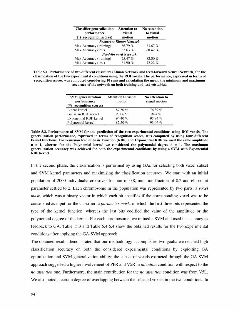
94

Classifier generalization

performance

(% recognition scores)

Attention to

visual

motion

No Attention

to visual

motion

Recurrent Elman Network

Max Accuracy (training) 86.79 % 83.67 %

Max Accuracy (test) 63.63 % 68.42 %

Feed-forward Network

Max Accuracy (training) 75.47 % 82.00 %

Max Accuracy (test) 61.90 % 72.22 %

Table 5.1. Performance of two different classifiers (Elman Network and feed-forward Neural Network) for the

classification of the two experimental conditions using the ROI voxels. The performance, expressed in terms of

recognition scores, was computed considering 10 runs and calculating the mean, the minimum and maximum

accuracy of the network on both training and test setstables.

SVM generalization

performance

(% recognition scores)

Attention to visual

motion

No attention to

visual motion

Linear kernel 87.50 % 76.39 %

Gaussian RBF kernel 93.06 % 94.4 %

Exponential RBF kernel 94.40 % 95.84 %

Polynomial kernel 87.50 % 93.06 %

Table 5.2. Performance of SVM for the prediction of the two experimental conditions using ROI voxels. The

generalization performance, expressed in terms of recognition scores, was computed by using four different

kernel functions. For Gaussian Radial basis Function (RBF) and Exponential RBF we used the same amplitude

σσσσ = 1, whereas for the Polynomial kernel we considered the polynomial degree d = 1. The maximum

generalization accuracy was achieved for both the experimental conditions by using a SVM with Exponential

RBF kernel.

In the second phase, the classification is performed by using GAs for selecting both voxel subset

and SVM kernel parameters and maximising the classification accuracy. We start with an initial

population of 2000 individuals: crossover fraction of 0.8, mutation fraction of 0.2 and elit-count

parameter settled to 2. Each chromosome in the population was represented by two parts: a voxel

mask, which was a binary vector in which each bit specifies if the corresponding voxel was to be

considered as input for the classifier; a parameter mask, in which the first three bits represented the

type of the kernel function, whereas the last bits codified the value of the amplitude or the

polynomial degree of the kernel. For each chromosome, we trained a SVM and used its accuracy as

feedback to GA. Table 5.3 and Table 5.4 5.4 show the obtained results for the two experimental

conditions after applying the GA-SVM approach.

The obtained results demonstrated that our methodology accomplishes two goals: we reached high

classification accuracy on both the considered experimental conditions by exploiting GA

optimization and SVM generalization ability; the subset of voxels extracted through the GA-SVM

approach suggested a higher involvement of PPR and V5R in attention condition with respect to the

no attention one. Furthermore, the main contribution for the no attention condition was from V5L.

We also noted a certain degree of overlapping between the selected voxels in the two conditions. In

95

particular the algorithm selected the same number of voxels from PPR in both the experimental

conditions, but only three voxels were selected for the prediction of both conditions.

Attention to visual motion

SVM

parameters

SVM

performance

PPR voxels V5R voxels V5L voxels

Exponential RBF

kernel (σ = 2)

97.22 %

7/19

17/30

14/43

Table 5.3. . GA-SVM approach for the classification of attention condition. The selected voxles and the kernel

parameters show an increase of 2.82 % on the classification accuracy with respect to the application of SVM on

all the ROI voxels.

No attention to visual motion

SVM

parameters

SVM

performance

PPR voxels V5R voxels V5L voxels

Gaussian RBF

kernel (σ = 3)

97.22 %

7/19

12/30

21/43

Table 5.4. GA-SVM approach for the classification of the no attention condition. The selected voxles and the

kernel parameters show an increase of 1.38 % on the classification accuracy with respect to the application of

SVM on the ROI voxels.

The nature of the information used by a classifier to distinguish different classes corresponding to

different experimental conditions is not completely clear. Anyway, this trouble should be

considered for all types of analysis (Parametric and Non Parametric approaches), due to their

intrinsic nature which is based on correlation. Further contribution analysis for ranking the selected

voxels could suggest a better interpretation of these results.

Our study suggests a promising method to automatically detect and identify the most predictive

voxels for the classification of specific cognitive states. Theoretically, it could be used to investigate

any cognitive domain where distributed representations might be present. In addition, GAs are

independent of the learning algorithm used by the classifier. Multiple algorithms can be flexibly

incorporated into our method. In this study we used a SVM classifier, which in our tests

outperformed the feed-forward neural network and the Elman network.

Further investigation is necessary to assess the reliability of the proposed GA-SVM wrapper

approach by using different fMRI datasets. Planned extensions to this work include the evaluation

of different feature extraction techniques and the use of voxel ranking to explore the role of the

selected voxels to further increase the classification accuracy.

96

Conclusion

Facing the problem of fMRI data analysis by pattern recognition methods, SVMs are becoming the

standard de facto. They are well known for their high generalization abilities and are generally used

with a linear kernel reaching quite good prediction accuracy. The question of voxel selection is

solved together with the problem of learning the linear relations between the information about

BOLD variations encoded into the voxel time series and experimental events that evoked them. In

fact, using linear SVM it is possible to obtain, for each experimental condition, the most

discriminating voxel subsets, just by analysing the weight vector produced by the classifier after

training. Using SVM with nonlinear kernels generally improves the classification accuracy, but in

that case the weight vector is not related to the input variables (voxels) but to a new representation

of the input space (the feature space) through an unknown nonlinear function (see Chapter 4 for

more details about SVM algorithm), thus is not possible to use this information for our purpose.

Generally, in those cases several heuristics are used for extracting the discriminating maps (see

Chapter 3, for more details). Thus, in this study we proposed a methodology based on GA-SVM

wrapper approach that allow us to estimate, for each experimental condition, the prediction

accuracy of a nonlinear SVM, comparing it to the accuracies achieved in the case of different

classifiers, but also to select the most promising discriminating voxel subsets. This study has

highlighted not only the need for voxel selection, but also another important aspect for a proper use

of pattern recognition methods for predicting cognitive states: the use of nonlinear classifiers

generally lead to an improvement of the classification accuracy due to the spatio-temporal dynamics

of the BOLD signals that is nonlinear. The obtained results shown a consistent improvement of the


Elman recurrent neural networks) and SVM not combined with GAs, confirming the key role of

crucial variables in pattern recognition methods for fMRI data analysis as voxel selection, learning

algorithm, nonlinear classification and the choice of learning parameters. However, due to the high

computational cost, the proposed methodology can be applied only for fine-grained analysis of

fMRI data, when the analysis regards few ROIs containing a relatively small number of voxel time-

series. Moreover, GAs are probabilistic approaches that suffer of the problem of local minima, thus

embedded methods based on optimization frameworks able to solve a convex optimization problem

(with a global minimum) and to perform voxel subset selection implicitly in the training process,

could be more promising and overcome also these limitations.

97

Chapter 6

Functional ANOVA models of Gaussian kernels: an Embedded

Approach to Voxel Selection in Nonlinear Regression

Introduction

The use of pattern recognition methods in fMRI data analysis requires facing the problem of

variable (voxel) selection, in order to select the voxel subsets relevant for the target (experimental)

condition and useful for increasing the classifier generalization ability. This is a crucial problem to

deal with in order to face the statistical problem of overfitting and the course of dimensionality.

Overfitting means that the model is very accurate on training data, but it has poor accuracy on

previously unseen test data. It occurs when the model is too complex compared with the true

underlying source of the data. The curse of dimensionality occurs in learning from few observations

in a high-dimensional space, and describes the problem caused by the exponential increase in

volume associated with adding extra dimensions to a vector space. Substantially, more observations

are needed to obtain the same density of data when the dimensionality increases.

Many approaches have been proposed over the years for dealing with the problem of voxel

selection in fMRI data analysis. One way to categorize the approaches is to divide them into three

main categories: filter, wrapper, and embedded approaches (Blum & Langley, 1997; Guyon &

Elisseeff, 2003).

The filter approach is composed of two distinct steps. In the first step irrelevant variables are

discarded and, then, a model is fitted with the selected variables. Possible criteria for guiding the

selection are, for example, correlation, mutual information, or F-statistics. The main disadvantage

of the filter approach is that it is a univariate approach, hence it does not take into account the

interactions among different variables, and searches for variables that are rather relevant than

useful. Thus, it totally ignores the effects of the selected variable subset on the performance of the

final predictive model. Filters are more like pre-processors, which can be used with any model to

98

reduce the number of variables. Filter methods are typically computationally efficient, at least

compared with wrappers.

The wrapper approach considers the model as a black box and uses only its interface with the data.

Different variable subsets are explored using the generalization accuracy of the model, estimated on

a validation set, as the measure of utility for a particular variable subset (Kohavi & John, 1997).

Wrappers can be used with any model and the approach usually leads to higher generalization

accuracy than using filters, but a great disadvantage is the high computational load that leads to

these approaches to be infeasible for some problems where the amount of data is to large.

The embedded approach incorporates variable selection as a part of model fitting and the selection

technique is specific to the model. The external search algorithms that are used in the filter and

wrapper approaches cannot cover all possible variable combinations, excluding problems in which

the input data are described by using only a few variables. Thus, their solutions are likely to be

suboptimal. Conversely, global optimality is often easier to guarantee in the embedded approach.

Moreover, embedded methods are typically computationally more efficient than wrappers. They are

a relatively new approach to feature selection and overcome limits of the first two approaches.

Unlike filter methods, which do not incorporate learning, and wrapper approaches, which can be

used with arbitrary classifiers, in embedded methods the features selection part can not be separated

from the learning part and this approach is specific to a classifier.

Besides, when using pattern recognition, another question to deal with is the choice of linear vs

nonlinear classification approach. Linear classifiers work in the fMRI data space, trying to find the

best hyper-plane that separates the scans for each experimental condition. Otherwise, nonlinear

classifiers can transform the hyper-plane to explore a better separation of the scans. The idea behind

the question is that a nonlinear classifier generally increases the prediction performance. In this last

case, exploring the voxel subsets that mostly predict each experimental condition allows us to

contextually pursue two correlated objectives: increasing the prediction performance and selecting

the more promising voxels involved in the prediction process.

Furthermore, pattern recognition methods are appropriate only in block or slow event-related

designs. Fast event-related experimental paradigms require new methods that improve the stringent

model approximations imposed by conventional data analysis approaches.

In this Chapter a novel and advanced technique for analysing fMRI data also in the context of fast

event-related experimental designs is proposed. The objective of this study was to develop a new

method, Functional ANOVA Models of Gaussian Kernels (FAM-GK), that considering for each

trial a pattern of voxels concatenated to a set of other patterns within an adjacent temporal window

of different lags, is able to capture the nonlinear spatio-temporal dynamics of the BOLD signals to

99

predict each experimental condition, while concurrently performing an embedded voxel selection.

To evaluate the potential and the effectiveness of the new method, FAM-GK was tested on a

synthetic dataset constructed ad-hoc, specifically on fMRI data simulated in the context of a fast

event-related experiment.

Embedded methods for variable selection

Embedded methods differ from other feature selection methods in the way feature selection and

learning interact. Filter methods do not include learning. Wrapper methods use a learning machine

to measure the quality of subsets of variables without including knowledge about the specific

structure of the classification or regression function, and can therefore be combined with any

learning machine.

We start this section by defining a general framework which covers many embedded methods.

Then, we will briefly discuss some of the proposed embedded methods on the base of their way to

solve the variable selection problem, focusing our attention on a particular type of embedded

methods, the direct objective optimization.

Feature selection can be described as the process of finding the feature subset of a certain size that

leads to the largest generalization, or equivalently to the minimal risk of the classification. A subset

of variables can be modelled by a vector n1,0∈σ of indicator variables such that the i

th

component of the vectorσ , with ni ,,1 K= , is equal to 1 indicating that the ith

variable is present

and is absent if it is equal to zero. Let ( ) ( )xfxfn ,,,: αα →ℜ→ℜ×Λ a parameterised family of

classification or regression functions, the objective of a minimization problem is to find an indicator

variable n1,0* ∈σ and a parameter Λ∈*α that minimise the expected risk:

( ) ( )( ) ( )yxdPxfLR ,,, ∫ ∗= σασα (6.1)

where ∗ denotes the pointwise product and L is the loss function. Generally we can also have a

constraint on the indicator variable that measures its sparsity in the form ( ) 0σσ ≤s , where the

function s could be a specific norm, for example a zero-norm ( )σ0l that counts the number of non

zero entries in σ , bounded by a certain number 0σ . The embedded approach for approximating the

minimiser of the (6.1) can be formulated in the following way:

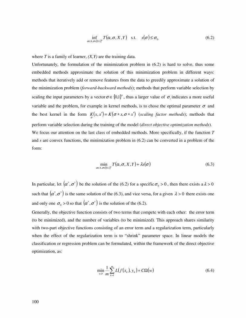
100

( )YXT

n,,,inf

1,0,σα

σα ∈Λ∈ s.t. ( ) 0σσ ≤s (6.2)

where T is a family of learner, (X,Y) are the training data.

Unfortunately, the formulation of the minimization problem in (6.2) is hard to solve, thus some

embedded methods approximate the solution of this minimization problem in different ways:

methods that iteratively add or remove features from the data to greedily approximate a solution of

the minimization problem (forward-backward methods); methods that perform variable selection by

scaling the input parameters by a vector n1,0∈σ , thus a larger value of iσ indicates a more useful

variable and the problem, for example in kernel methods, is to chose the optimal parameter σ and

the best kernel in the form ( ) ( )xxKxxK ′∗∗=′ σσσ

,, (scaling factor methods); methods that

perform variable selection during the training of the model (direct objective optimization methods).

We focus our attention on the last class of embedded methods. More specifically, if the function T

and s are convex functions, the minimization problem in (6.2) can be converted in a problem of the

form:

( ) ( )σλσα

σαsYXT

n+

∈Λ∈,,,min

1,0, (6.3)

In particular, let ( )**,σα be the solution of the (6.2) for a specific 00 >σ , then there exists a 0>λ

such that ( )**,σα is the same solution of the (6.3), and vice versa, for a given 0>λ there exists one

and only one 00 >σ so that ( )**,σα is the solution of the (6.2).

Generally, the objective function consists of two terms that compete with each other: the error term

(to be minimized), and the number of variables (to be minimized). This approach shares similarity

with two-part objective functions consisting of an error term and a regularization term, particularly

when the effect of the regularization term is to “shrink” parameter space. In linear models the

classification or regression problem can be formulated, within the framework of the direct objective

optimization, as:

( )( ) ( )wCyxfLm

m

k

kkbw

Ω+∑=1

,,

1min (6.4)

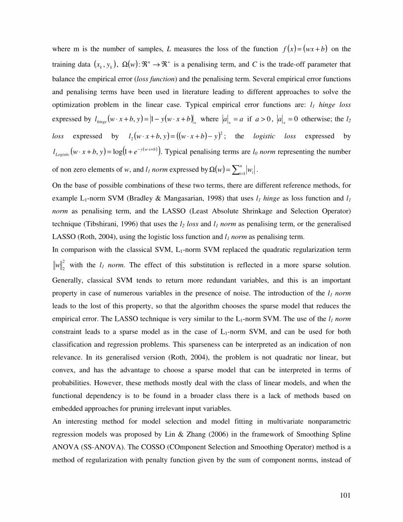
101

where m is the number of samples, L measures the loss of the function ( ) ( )bwxxf += on the

training data ( )kk yx , , ( ) +ℜ→ℜΩ nw : is a penalising term, and C is the trade-off parameter that

balance the empirical error (loss function) and the penalising term. Several empirical error functions

and penalising terms have been used in literature leading to different approaches to solve the

optimization problem in the linear case. Typical empirical error functions are: l1 hinge loss

expressed by ( ) ( )+

+⋅−=+⋅ bxwyybxwlhinge 1, where aa =+

if 0>a , 0=+

a otherwise; the l2

loss expressed by ( ) ( )( )2

2 , ybxwybxwl −+⋅=+⋅ ; the logistic loss expressed by

( ) ( )( )bxwy

Logistic eybxwl+⋅−+=+⋅ 1log, . Typical penalising terms are l0 norm representing the number

of non zero elements of w, and l1 norm expressed by ( ) ∑ ==Ω

n

i iww1

.

On the base of possible combinations of these two terms, there are different reference methods, for

example L1-norm SVM (Bradley & Mangasarian, 1998) that uses l1 hinge as loss function and l1

norm as penalising term, and the LASSO (Least Absolute Shrinkage and Selection Operator)

technique (Tibshirani, 1996) that uses the l2 loss and l1 norm as penalising term, or the generalised

LASSO (Roth, 2004), using the logistic loss function and l1 norm as penalising term.

In comparison with the classical SVM, L1-norm SVM replaced the quadratic regularization term

2

2w with the l1 norm. The effect of this substitution is reflected in a more sparse solution.

Generally, classical SVM tends to return more redundant variables, and this is an important

property in case of numerous variables in the presence of noise. The introduction of the l1 norm

leads to the lost of this property, so that the algorithm chooses the sparse model that reduces the

empirical error. The LASSO technique is very similar to the L1-norm SVM. The use of the l1 norm

constraint leads to a sparse model as in the case of L1-norm SVM, and can be used for both

classification and regression problems. This sparseness can be interpreted as an indication of non

relevance. In its generalised version (Roth, 2004), the problem is not quadratic nor linear, but

convex, and has the advantage to choose a sparse model that can be interpreted in terms of

probabilities. However, these methods mostly deal with the class of linear models, and when the

functional dependency is to be found in a broader class there is a lack of methods based on

embedded approaches for pruning irrelevant input variables.

An interesting method for model selection and model fitting in multivariate nonparametric

regression models was proposed by Lin & Zhang (2006) in the framework of Smoothing Spline

ANOVA (SS-ANOVA). The COSSO (COmponent Selection and Smoothing Operator) method is a

method of regularization with penalty function given by the sum of component norms, instead of

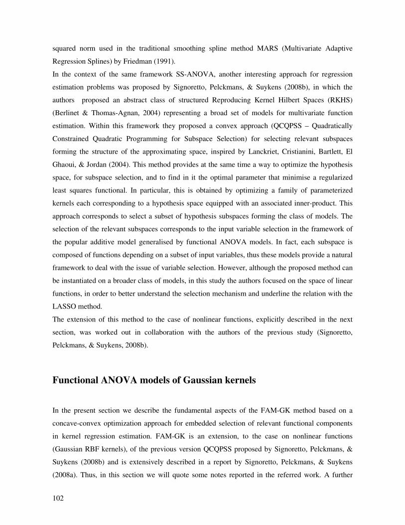
102

squared norm used in the traditional smoothing spline method MARS (Multivariate Adaptive

Regression Splines) by Friedman (1991).

In the context of the same framework SS-ANOVA, another interesting approach for regression

estimation problems was proposed by Signoretto, Pelckmans, & Suykens (2008b), in which the

authors proposed an abstract class of structured Reproducing Kernel Hilbert Spaces (RKHS)

(Berlinet & Thomas-Agnan, 2004) representing a broad set of models for multivariate function

estimation. Within this framework they proposed a convex approach (QCQPSS – Quadratically

Constrained Quadratic Programming for Subspace Selection) for selecting relevant subspaces

forming the structure of the approximating space, inspired by Lanckriet, Cristianini, Bartlett, El

Ghaoui, & Jordan (2004). This method provides at the same time a way to optimize the hypothesis

space, for subspace selection, and to find in it the optimal parameter that minimise a regularized

least squares functional. In particular, this is obtained by optimizing a family of parameterized

kernels each corresponding to a hypothesis space equipped with an associated inner-product. This

approach corresponds to select a subset of hypothesis subspaces forming the class of models. The

selection of the relevant subspaces corresponds to the input variable selection in the framework of

the popular additive model generalised by functional ANOVA models. In fact, each subspace is

composed of functions depending on a subset of input variables, thus these models provide a natural

framework to deal with the issue of variable selection. However, although the proposed method can

be instantiated on a broader class of models, in this study the authors focused on the space of linear

functions, in order to better understand the selection mechanism and underline the relation with the

LASSO method.

The extension of this method to the case of nonlinear functions, explicitly described in the next

section, was worked out in collaboration with the authors of the previous study (Signoretto,

Pelckmans, & Suykens, 2008b).

Functional ANOVA models of Gaussian kernels

In the present section we describe the fundamental aspects of the FAM-GK method based on a

concave-convex optimization approach for embedded selection of relevant functional components

in kernel regression estimation. FAM-GK is an extension, to the case on nonlinear functions

(Gaussian RBF kernels), of the previous version QCQPSS proposed by Signoretto, Pelckmans, &

Suykens (2008b) and is extensively described in a report by Signoretto, Pelckmans, & Suykens

(2008a). Thus, in this section we will quote some notes reported in the referred work. A further

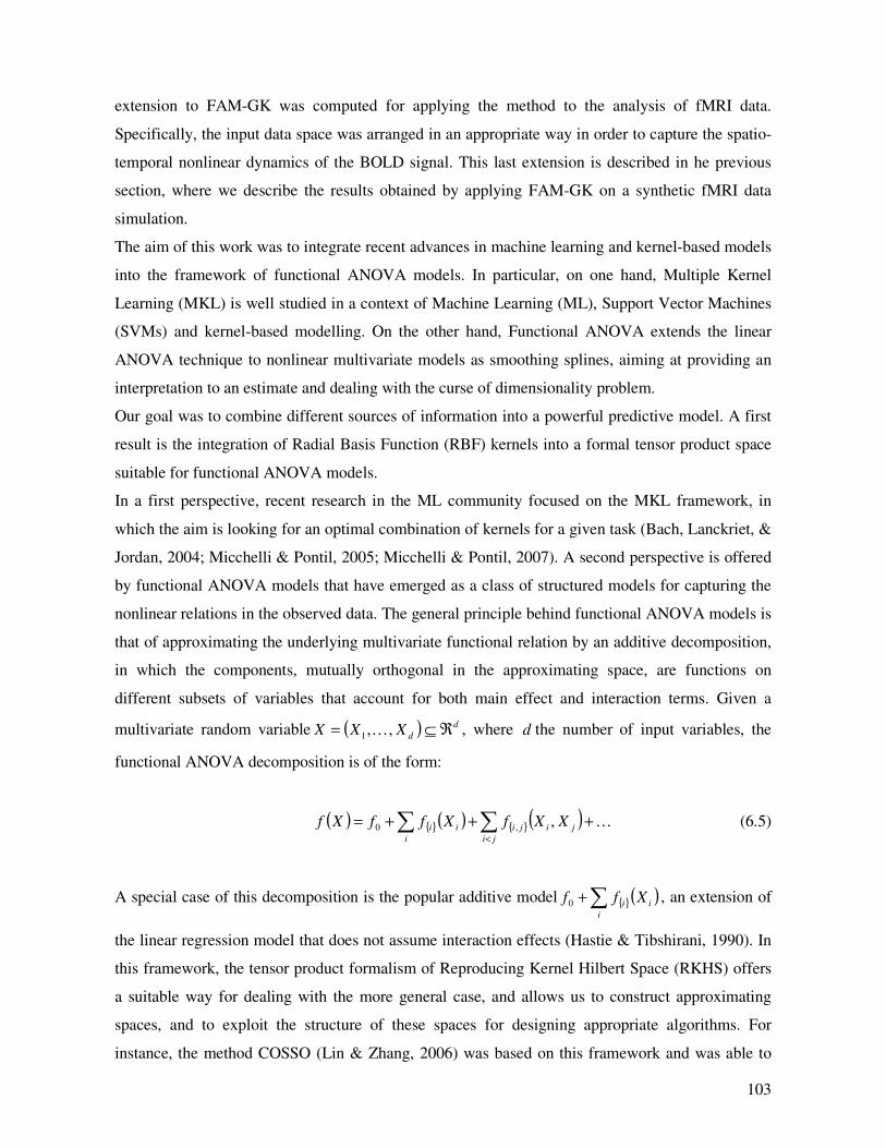
103

extension to FAM-GK was computed for applying the method to the analysis of fMRI data.

Specifically, the input data space was arranged in an appropriate way in order to capture the spatio-

temporal nonlinear dynamics of the BOLD signal. This last extension is described in he previous

section, where we describe the results obtained by applying FAM-GK on a synthetic fMRI data

simulation.

The aim of this work was to integrate recent advances in machine learning and kernel-based models

into the framework of functional ANOVA models. In particular, on one hand, Multiple Kernel

Learning (MKL) is well studied in a context of Machine Learning (ML), Support Vector Machines

(SVMs) and kernel-based modelling. On the other hand, Functional ANOVA extends the linear

ANOVA technique to nonlinear multivariate models as smoothing splines, aiming at providing an

interpretation to an estimate and dealing with the curse of dimensionality problem.

Our goal was to combine different sources of information into a powerful predictive model. A first

result is the integration of Radial Basis Function (RBF) kernels into a formal tensor product space

suitable for functional ANOVA models.

In a first perspective, recent research in the ML community focused on the MKL framework, in

which the aim is looking for an optimal combination of kernels for a given task (Bach, Lanckriet, &

Jordan, 2004; Micchelli & Pontil, 2005; Micchelli & Pontil, 2007). A second perspective is offered

by functional ANOVA models that have emerged as a class of structured models for capturing the

nonlinear relations in the observed data. The general principle behind functional ANOVA models is

that of approximating the underlying multivariate functional relation by an additive decomposition,

in which the components, mutually orthogonal in the approximating space, are functions on

different subsets of variables that account for both main effect and interaction terms. Given a

multivariate random variable ( ) d

dXXX ℜ⊆= ,,1 K , where d the number of input variables, the

functional ANOVA decomposition is of the form:

( ) ( ) ( ) K+++= ∑∑< ji

jiji

i

ii XXfXffXf ,,0 (6.5)

A special case of this decomposition is the popular additive model ( )∑+i

ii Xff0 , an extension of

the linear regression model that does not assume interaction effects (Hastie & Tibshirani, 1990). In

this framework, the tensor product formalism of Reproducing Kernel Hilbert Space (RKHS) offers

a suitable way for dealing with the more general case, and allows us to construct approximating

spaces, and to exploit the structure of these spaces for designing appropriate algorithms. For

instance, the method COSSO (Lin & Zhang, 2006) was based on this framework and was able to

104

concurrently perform model fitting and model selection, leading to a sparse solution f with a

controlled number of non-zero components.

These two perspectives are related, because in both cases the selection corresponds to learn a sparse

combination of kernel matrices constructed on the observed data sample.

In the following we quote some results described in (Signoretto, Pelckmans, & Suykens, 2008a),

specifically the classical tensor product formalism of functional ANOVA models and the tensor

product space constructed on the popular RBF Gaussian kernel that effectively constitutes an

alternative choice for the construction of functional ANOVA models. We then illustrate the

proposed method for the selection of Functional Components performed via convex-concave

optimization.

In the context of regression estimation it is assumed that for each Χ∈x drown from a probability

distribution ( )xp there is a corresponding Υ∈y attributed by a supervisor according to an

unknown probability distribution ( )xyp , and the learning algorithm is required to estimate the

regression function ( ) ( )dxxyypxh ∫= based on a training set ( ) ( ) nn yxyx ,,,, 11 K of n

independently and identically distributed (i.i.d.) observations drown according to a probability

distribution ( ) ( ) ( )xpxypyxp =, .

The problem of learning can be described as the choice in a predefined set of functions, of the one

minimising the expected risk ( )( ) ( )∫ yxdpyxfL ,, where L is the loss function proper for the

specific task. Generally, for regression problems a commonly used loss function is the least square

error ( )( ) ( )( )2, xfyyxfL −= . From another perspective, one can formulate the problem of learning

as recovering the true values of a function f at given locations ( ) ( ) ( ) niYXYxxf iiiii ,,1,,,: K=∈

from the collection of noisy observations at the same locations

( ) ( ) ( ) niYXYxxfY iiiiiii ,,1,,,: K=∈+= ε where nii ,,1, K=ε is the set of i.i.d. zero-mean

random variables. In both perspectives, the most common approach is to minimise the

regularization functional, in the RKHS, given by

( )( ) ( )∑=

+n

i

iifJxfyL

n 1

,1

µ (6.6)

where ℜ→HJ : is the penalty functional, where H is a functional space. We consider a structured

approximating functional space ( ) ( )χχ ii FH ⊕= where dχχχχ K××= 21is the product domain in

105

which each set in the Cartesian product is a subset ofℜ , and ( ) χiF is a family of subspaces

mutually orthogonal with a defined inner product ⋅⋅, . The functions in the subspaces can be

functions of specific subset of input variables. Hence, this structured functional space allows us to

overcome the problem of the curse of dimensionality and to select those variables that are more

relevant for the specific task

In the next section we will describe the tensor product formalism in functional ANOVA models.

Tensor product formalism into the framework of functional ANOVA models

The tensor product represents a classical scheme for the construction of functions on a product

domain dχχχχ K××= 21. For simplicity we consider a simple case of two variables and a product

domain of the form 21χχχ ×= . Then all the concepts can be generalised to the case of d variables.

Let consider the Hilbert spaces of functions ( )( )⋅⋅,,11 χW , ( )( )⋅⋅,,22 χW and two bases jfB 11 = and

jfB 22 = for each space of functions, the 2-fold tensor product space ( )( )⋅⋅⊗ ,,21 χWW can be

defined by the vector space generated by the functions ( ) ( )21: xgxfxgf a⊗ for any

1Bf ∈ and 2Bg ∈ with a valid inner product defined for ( ) 1121, BBff ×∈ and ( ) 2221, BBgg ×∈

by2211212211 ,,, ggffgfgf =⊗⊗ . Furthermore, if ( )11

χW and ( )22 χW are RKHSs with

kernels 1k and 2k , then also the tensor product space is a RKHS with kernel given by

( ) ( ) ( )22211121 ,,,: yxkyxkyxkk a⊗ (6.7)

A fundamental property of the tensor product approach is that, let 1 be the set of constant

functions and suppose that ( )1

11 1 WW ⊕= and ( )1

22 1 WW ⊕= , then the tensor product can be

written as ( ) ( ) ( ) ( )( ) ( ) ( )( )1

2

1

1

1

2

1

121 1111 WWWWWW ⊗⊕⊗⊕⊗⊕⊗=⊗ . Certainly, the definition

of the 2-fold tensor product and its property in the case of two input variables generalise to the case

of d-fold tensor product, in which we consider d input variables. Thus, assuming that each factor

space assumes the decomposition as in the 2-fold case, the tensor product space has a

decomposition into d2 subspaces. Thus any ( )iidiWf χ

,,1K=⊗∈ can be univocally written as sum of

functions in the subspaces, and if the factor spaces diWi ,,1, K= are RKHSs, then we can generalise

the (6.7) to the case of d functional terms.

106

The extension of the tensor product to Gaussian RBF kernels

In this section we describe the salient aspects related to the extension of the classical tensor product

formalism, in the context of functional ANOVA framework, to the case of Gaussian RBF kernels.

Radial Basis Function has been recognised as a powerful tool in approximation problems and has

become the de-facto standard choice for kernel-based algorithms in machine learning. For a product

domain dχχχχ K××= 21 dℜ⊂ with a Euclidean norm

2⋅ , RBF can be defined as

( ) ( )2

, yxyxk −=ψ for a function ℜ→ℜ+:ψ . The most popular function in Machine Learning is

the Gaussian kernel ℜ→× χχ:k , so that ( ) ( )2

2

2exp, yxyxk −−= σ for a width parameter 0>σ .

Although Gaussian RBF kernels are one of the most often used kernels in modern machine learning

methods such as SVMs, little is known about the structure of their RKHSs. Steinwart, Hush, &

Scovel (2006) studied these aspects, described the RKHSs corresponding to Gaussian RBF kernels

and provided an orthonormal basis for these spaces. According to their study, for any djj K,1, =

the RKHS ( )( )jjjW ⋅⋅,,χ associated with the univariate RBF Gaussian kernel

( ) ( )( )22exp, jjjj yxyxk −−= σ has an orthonormal basis ( ) ( )

=− 22

!

2 2

jxn

j

n

jn exn

xeσσ

with jjx χ∈

and 0Nn ∈ . Thus we have that ( ) ( )

∈== ∑∈

02,:0

NlaeaffWNi

iijj χ and for any pair

( ) ( ) ( )0202, NlNlba ×∈ and their corresponding functions ( ) ( ) ( )jjjj WWgf χχ ×∈, , we have that the

inner product is given by 2

,,l

bagf = . Moreover, from a corollary in Steinwart et al. (2006) any

non identically zero constant function is not in ( )jj XW , thus we have to insert the set of constant

functions 1 for describing a tensor product decomposition as

( ) ( ) ( )

( )χχ uniiPu

iini

WW,,1:,,1

1KK =∈=

⊕=⊕⊗ , where ( )AP is the set of all the subset of A , and ( )χuW is a

RKHS with kernel ( ) ( )

−−= ∑

∈uj

jju yxyxk22

exp, σ , thus the (6.7) can be generalised to the case

of d functional components and to the case on Gaussian RBF kernels.

107

Selection of functional components via concave-convex optimization

In this section we describe the problem of performing component selection and model fitting in the

framework of functional ANOVA models by using FAM-GK via concave-convex optimization,

with the objective of approximating the regression function by an ANOVA model based on the

training set ( ) niYX ii ,,1,, K= .

The concave-convex optimization problem, taking into account the (6.6), can be formulated as:

( ) [ ] ( )

==≥

+−=

′ ∑ =ℜ∈ℜ∈

01,1,0

2

1,maxmin

*

* 1

αγγ

αλγαααγλαγ

TT

n

d

i

i

i

TT

p

IKyJnd (6.8)

The idea behind it is that of optimizing simultaneously both γ and α . Correspondingly we get at

the same time the selection of subspaces and the optimal coefficients α that minimise the error

term of (6.6) in the actual structure of the hypothesis space.

Relying on the same argument used in Lanckriet et al. (2004) it is not difficult to demonstrate that

the (6.8) is a concave-convex optimization problem, thus every pair ( )αγ ˆ,ˆ that for every feasible

point satisfies the property ( ) ( ) ( )αγαγαγ λλλˆ,ˆ,ˆ,ˆ JJJ ′≤′≤′ is a solution of the (6.8). Hence, the

function [ ] [ ] ( )bkf

d

j

j

xi

n

i

ip i

ˆˆˆˆ*

11

, +

= ∑∑

==

γαλ , where b follows from optimality conditions, is the

minimiser of the regularised risk functional ( )( ) [ ] ( ) 21

11

2

*

ˆF

i

i

d

i

n

i

ii fPyxf

−

==

∑∑ +− γλ in the model

space ( )i

iFH ⊕=ˆ , where ( )iP is the projector operator that maps f into ( )iF .

The solution of the formalised concave-convex optimization problem of FAM-GK can be computed

with general interior point solvers by resorting to a convex formulation in the class of second order

cone programming (SOCP) problems. A more direct approach we have been using corresponds to

directly exploit the convex-concave structure via a simple barrier method and an appropriate

modification of an infeasible-start Newton method inspired by Boyd & Vandenberghe (2004). More

detailed about the algorithm can be found in Signoretto, Pelckmans, & Suykens (2008a).

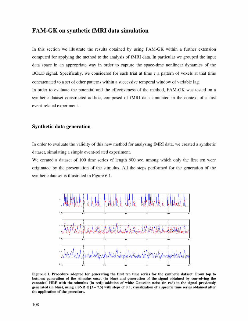
108

FAM-GK on synthetic fMRI data simulation

In this section we illustrate the results obtained by using FAM-GK within a further extension

computed for applying the method to the analysis of fMRI data. In particular we grouped the input

data space in an appropriate way in order to capture the space-time nonlinear dynamics of the

BOLD signal. Specifically, we considered for each trial at time 1t a pattern of voxels at that time

concatenated to a set of other patterns within a successive temporal window of variable lag.

In order to evaluate the potential and the effectiveness of the method, FAM-GK was tested on a

synthetic dataset constructed ad-hoc, composed of fMRI data simulated in the context of a fast

event-related experiment.

Synthetic data generation

In order to evaluate the validity of this new method for analysing fMRI data, we created a synthetic

dataset, simulating a simple event-related experiment.

We created a dataset of 100 time series of length 600 sec, among which only the first ten were

originated by the presentation of the stimulus. All the steps performed for the generation of the

synthetic dataset is illustrated in Figure 6.1.

Figure 6.1. Procedure adopted for generating the first ten time series for the synthetic dataset. From top to

bottom: generation of the stimulus onset (in blue) and generation of the signal obtained by convolving the

canonical HRF with the stimulus (in red); addition of white Gaussian noise (in red) to the signal previously

generated (in blue), using a SNR ∈[3 – 7.5] with steps of 0.5; visualization of a specific time series obtained after

the application of the procedure.

109

Firstly, we generated an input signal ( )tu as random impulses lasting 1 sec that represented the

presentation of a specific experimental condition within an event-related fMRI experiment.

Specifically, we constructed the input signal in a way that for a period of 600 sec when the

experimental condition was on ( ) 1=tu , whereas when it was off ( ) 0=tu . Then, we generated the

first ten time series by convolving the impulse signal ( )tu with the canonical Hemodynamic

Response Function (HRF) with TR= 2 sec, using the default parameters as in SPM (Statistical

Parametric Mapping, http://www.fil.ion.ucl.ac.uk/spm) and by adding Gaussian noise with different

signal to noise ratio (SNR) in the range [3 - 7.5] with an increasing step of 0.5.

We generated the remaining ninety time series as random white Gaussian noise, and we added a

correlation 2.0=c among all the time series in the whole dataset.

Method description

The aim of fMRI data analysis is to detect the activated regions of the brain analysing the dynamic

of the BOLD signal. Most of the fMRI data analysis methods rely on the assumption that the HRF

caused by the stimuli add in a roughly linear way (scaling and superimposition). However the

assumption of linearity is valid only for stimulus duration or inter stimulus interval (ISI) larger that

4-6 sec. Within the advances in fMRI design, rapid event-related experiments became popular. In

this type of design, the nonlinearities in HRF are often observed. Furthermore, the BOLD signals

are also observed to exhibit regional differences, thus the HRF can vary, for the same subject, from

voxel to voxel, from session to session and depending on the task to perform. There is also a great

inter-subject variability that has to be taken into account.

The non-linear dynamic of the BOLD signal can be described by a state-space model that can be

concisely described by the following equations:

+=

=+

ttt

ttt

exhy

uxfx

)(

),(1 (6.9)

where m

tx ℜ∈ represents the state vector (the underlying cognitive state), ℜ∈tu is the input to the

system (stimulus), m

te ℜ∈ represents the drift and the measurement noise, and m

ty ℜ∈ is the

output of the system (the measured fMRI signal). The functions mmf ℜ→ℜ×ℜ: and

mmh ℜ→ℜ: are nonlinear functions that correlate respectively, in a nonlinear way, each state of

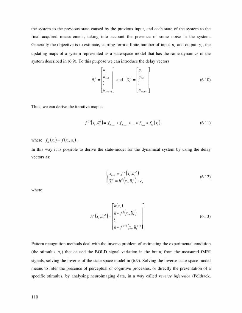
110

the system to the previous state caused by the previous input, and each state of the system to the

final acquired measurement, taking into account the presence of some noise in the system.

Generally the objective is to estimate, starting form a finite number of input tu and output ty , the

updating maps of a system represented as a state-space model that has the same dynamics of the

system described in (6.9). To this purpose we can introduce the delay vectors

=

−+

+

1

1~

dt

t

t

d

t

u

u

u

uM

and

=

−+

+

1

1~

dt

t

t

d

t

y

y

y

yM

(6.10)

Thus, we can derive the iterative map as

( )( ) ( )tuuuu

i

tt

ixffffuxf

ttititooKoo

121

~,+−+−+

= (6.11)

where ( ) ( )tttu uxfxft

,= .

In this way it is possible to derive the state-model for the dynamical system by using the delay

vectors as:

( )( )

+=

=+

t

d

tt

dd

t

d

tt

d

dt

euxhy

uxfx

~,~

~, (6.12)

where

( )

( )

( )

( )

=

−− 11

11

~,

~,~,

d

tt

d

tt

t

d

tt

d

uxfh

uxfh

xh

uxh

o

M

o (6.13)

Pattern recognition methods deal with the inverse problem of estimating the experimental condition

(the stimulus tu ) that caused the BOLD signal variation in the brain, from the measured fMRI

signals, solving the inverse of the state space model in (6.9). Solving the inverse state-space model

means to infer the presence of perceptual or cognitive processes, or directly the presentation of a

specific stimulus, by analysing neuroimaging data, in a way called reverse inference (Poldrack,

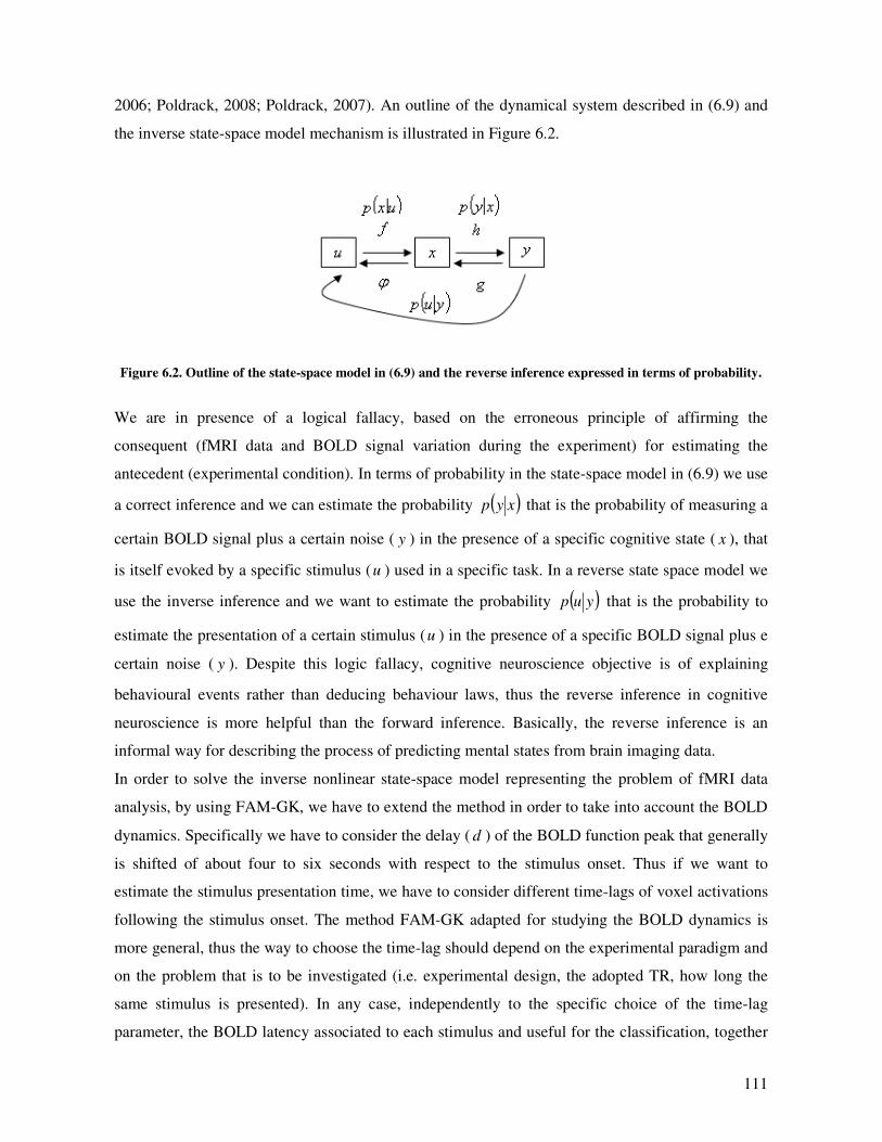
111

2006; Poldrack, 2008; Poldrack, 2007). An outline of the dynamical system described in (6.9) and

the inverse state-space model mechanism is illustrated in Figure 6.2.

Figure 6.2. Outline of the state-space model in (6.9) and the reverse inference expressed in terms of probability.

We are in presence of a logical fallacy, based on the erroneous principle of affirming the

consequent (fMRI data and BOLD signal variation during the experiment) for estimating the

antecedent (experimental condition). In terms of probability in the state-space model in (6.9) we use

a correct inference and we can estimate the probability ( )xyp that is the probability of measuring a

certain BOLD signal plus a certain noise ( y ) in the presence of a specific cognitive state ( x ), that

is itself evoked by a specific stimulus (u ) used in a specific task. In a reverse state space model we

use the inverse inference and we want to estimate the probability ( )yup that is the probability to

estimate the presentation of a certain stimulus (u ) in the presence of a specific BOLD signal plus e

certain noise ( y ). Despite this logic fallacy, cognitive neuroscience objective is of explaining

behavioural events rather than deducing behaviour laws, thus the reverse inference in cognitive

neuroscience is more helpful than the forward inference. Basically, the reverse inference is an

informal way for describing the process of predicting mental states from brain imaging data.

In order to solve the inverse nonlinear state-space model representing the problem of fMRI data

analysis, by using FAM-GK, we have to extend the method in order to take into account the BOLD

dynamics. Specifically we have to consider the delay ( d ) of the BOLD function peak that generally

is shifted of about four to six seconds with respect to the stimulus onset. Thus if we want to

estimate the stimulus presentation time, we have to consider different time-lags of voxel activations

following the stimulus onset. The method FAM-GK adapted for studying the BOLD dynamics is

more general, thus the way to choose the time-lag should depend on the experimental paradigm and

on the problem that is to be investigated (i.e. experimental design, the adopted TR, how long the

same stimulus is presented). In any case, independently to the specific choice of the time-lag

parameter, the BOLD latency associated to each stimulus and useful for the classification, together

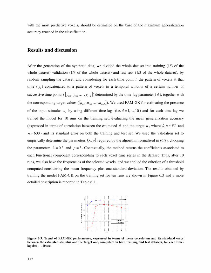
112

with the most predictive voxels, should be estimated on the base of the maximum generalization

accuracy reached in the classification.

Results and discussion

After the generation of the synthetic data, we divided the whole dataset into training (1/3 of the

whole dataset) validation (1/3 of the whole dataset) and test sets (1/3 of the whole dataset), by

random sampling the dataset, and considering for each time point t the pattern of voxels at that

time ( ty ) concatenated to a pattern of voxels in a temporal window of a certain number of

successive time points ( [ ]dttt yyy +++ ,,, 21 K ) determined by the time-lag parameter ( d ), together with

the corresponding target values ( [ ]dttt uuu +++ ,,, 21 K ). We used FAM-GK for estimating the presence

of the input stimulus tu by using different time-lags (i.e. 10,,1 K=d ) and for each time-lag we

trained the model for 10 runs on the training set, evaluating the mean generalization accuracy

(expressed in terms of correlation between the estimated u and the target u , where nuu ℜ∈,ˆ and

600=n ) and its standard error on both the training and test set. We used the validation set to

empirically determine the parameters ( )p,λ required by the algorithm formalised in (6.8), choosing

the parameters 3.0=λ and 3=p . Contextually, the method returns the coefficients associated to

each functional component corresponding to each voxel time series in the dataset. Thus, after 10

runs, we also have the frequencies of the selected voxels, and we applied the criterion of a threshold

computed considering the mean frequency plus one standard deviation. The results obtained by

training the model FAM-GK on the training set for ten runs are shown in Figure 6.3 and a more

detailed description is reported in Table 6.1.

Figure 6.3. Trend of FAM-GK performance, expressed in terms of mean correlation and its standard error

between the estimated stimulus and the target one, computed on both training and test datasets, for each time-

lag d=1,…,10 sec.

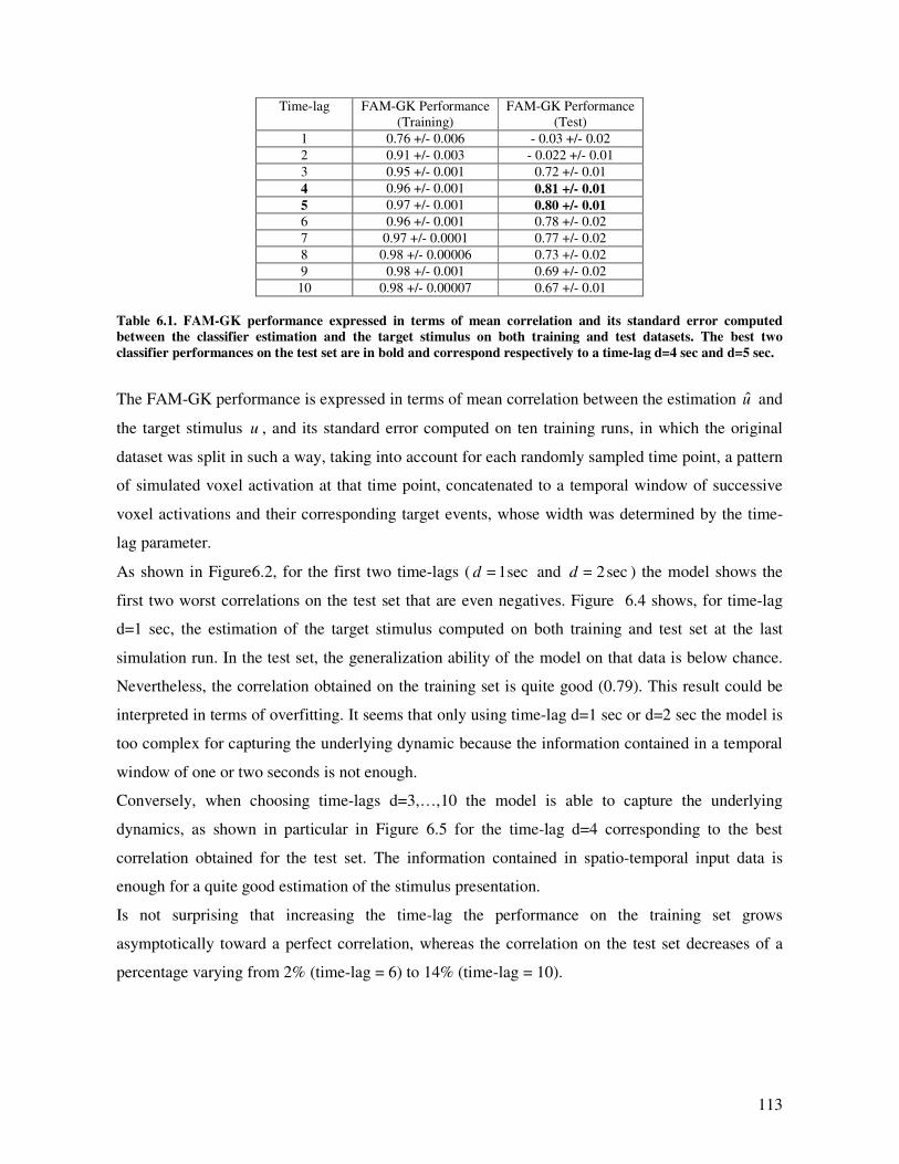
113

Time-lag FAM-GK Performance

(Training)

FAM-GK Performance

(Test)

1 0.76 +/- 0.006 - 0.03 +/- 0.02

2 0.91 +/- 0.003 - 0.022 +/- 0.01

3 0.95 +/- 0.001 0.72 +/- 0.01

4 0.96 +/- 0.001 0.81 +/- 0.01

5 0.97 +/- 0.001 0.80 +/- 0.01

6 0.96 +/- 0.001 0.78 +/- 0.02

7 0.97 +/- 0.0001 0.77 +/- 0.02

8 0.98 +/- 0.00006 0.73 +/- 0.02

9 0.98 +/- 0.001 0.69 +/- 0.02

10 0.98 +/- 0.00007 0.67 +/- 0.01

Table 6.1. FAM-GK performance expressed in terms of mean correlation and its standard error computed

between the classifier estimation and the target stimulus on both training and test datasets. The best two

classifier performances on the test set are in bold and correspond respectively to a time-lag d=4 sec and d=5 sec.

The FAM-GK performance is expressed in terms of mean correlation between the estimation u and

the target stimulus u , and its standard error computed on ten training runs, in which the original

dataset was split in such a way, taking into account for each randomly sampled time point, a pattern

of simulated voxel activation at that time point, concatenated to a temporal window of successive

voxel activations and their corresponding target events, whose width was determined by the time-

lag parameter.

As shown in Figure6.2, for the first two time-lags ( sec1=d and sec2=d ) the model shows the

first two worst correlations on the test set that are even negatives. Figure 6.4 shows, for time-lag

d=1 sec, the estimation of the target stimulus computed on both training and test set at the last

simulation run. In the test set, the generalization ability of the model on that data is below chance.

Nevertheless, the correlation obtained on the training set is quite good (0.79). This result could be

interpreted in terms of overfitting. It seems that only using time-lag d=1 sec or d=2 sec the model is

too complex for capturing the underlying dynamic because the information contained in a temporal

window of one or two seconds is not enough.

Conversely, when choosing time-lags d=3,…,10 the model is able to capture the underlying

dynamics, as shown in particular in Figure 6.5 for the time-lag d=4 corresponding to the best

correlation obtained for the test set. The information contained in spatio-temporal input data is

enough for a quite good estimation of the stimulus presentation.

Is not surprising that increasing the time-lag the performance on the training set grows

asymptotically toward a perfect correlation, whereas the correlation on the test set decreases of a

percentage varying from 2% (time-lag = 6) to 14% (time-lag = 10).

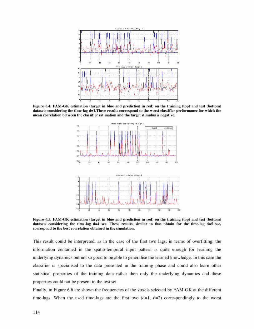
114

Figure 6.4. FAM-GK estimation (target in blue and prediction in red) on the training (top) and test (bottom)

datasets considering the time-lag d=1.These results correspond to the worst classifier performance for which the

mean correlation between the classifier estimation and the target stimulus is negative.

Figure 6.5. FAM-GK estimation (target in blue and prediction in red) on the training (top) and test (bottom)

datasets considering the time-lag d=4 sec. These results, similar to that obtain for the time-lag d=5 sec,

correspond to the best correlation obtained in the simulation.

This result could be interpreted, as in the case of the first two lags, in terms of overfitting: the

information contained in the spatio-temporal input pattern is quite enough for learning the

underlying dynamics but not so good to be able to generalise the learned knowledge. In this case the

classifier is specialised to the data presented in the training phase and could also learn other

statistical properties of the training data rather then only the underlying dynamics and these

properties could not be present in the test set.

Finally, in Figure 6.6 are shown the frequencies of the voxels selected by FAM-GK at the different

time-lags. When the used time-lags are the first two (d=1, d=2) correspondingly to the worst

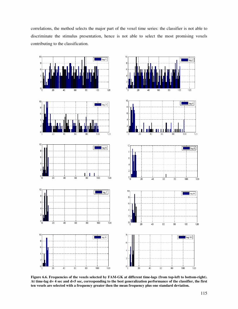
115

correlations, the method selects the major part of the voxel time series: the classifier is not able to

discriminate the stimulus presentation, hence is not able to select the most promising voxels

contributing to the classification.

Figure 6.6. Frequencies of the voxels selected by FAM-GK at different time-lags (from top-left to bottom-right).

At time-lag d= 4 sec and d=5 sec, corresponding to the best generalization performance of the classifier, the first

ten voxels are selected with a frequency greater then the mean frequency plus one standard deviation.

116

At time-lag d=4 sec and d=5 sec, corresponding to the best generalization performance of the

classifier, the first ten voxels are selected with a frequency greater then the mean frequency plus a

standard deviation, confirming the effectiveness of FAM-GK. For the remaining time-lags

(d=6,…,10), the number of selected voxels, a subgroup of the first ten time series, decreases leading

to a more sparse solution.

Conclusions

The analysis of fMRI data includes several crucial points to take into account and sub problems to

face when using pattern recognition methods. In particular, in this chapter we faced the problem of

variable (voxel) selection combined with the problem of the choice of nonlinear classifiers with

respect to the linear one.

The problem of voxel selection has been faced by the ML community partially in order to limit the

problem of overfitting and mainly for deal with the problem of the curse of dimensionality.

Researchers managed the variable selection problem in several ways that can be classified into three

main categories: filter, wrapper and embedded approaches. In particular, embedded methods differ

from the first two, mainly in its property to perform variable selection implicitly during learning and

offer many advantages with respect to the previous methods: unlike the filter methods that are

univariate embedded methods incorporate variable selection into the multivariate model fitting;

unlike the wrapper approaches that use the classifier as a black box and require a high

computational effort, embedded methods are specific to the learning machine and are more

computational efficient.

The other crucial aspect in dealing with pattern recognition techniques is the choice of the classifier,

specifically of the linearity or nonlinearity of the learning function. Typically, nonlinear classifiers

reach better performance than the linear one, at least in problems complex enough to be explained

by more complex models. Furthermore, pattern recognition methods are able to work quite well for

fMRI data analysis, but can be used in the standard way only with fMRI data acquired in block or

slow event-related designs. The challenge today is to find methods working with fast event-related

designs as well. To this purpose, new methods and more complex models are required that can

capture the nonlinear dynamics occurring when using this type of experimental design.

Several embedded methods have been developed in the last twelve years, facing the problem of

variable selection in different ways. We focused our attention on direct objective optimization

methods that formalise the optimization problem of regression estimation, taking into account both

117

the error term, relative to the regression, and the penalty (sparsity) term, relative to the variable

selection. The major part of these methods has been developed in the class of linear regression or

classification problems, whereas when functional dependencies are to be established in a broader

class there is a lack of methods based on embedded approaches for pruning irrelevant input

variables.

The objective of this study was to develop an embedded method able to deal with variable selection

and the class of nonlinear models. Firstly, we worked out a novel and effective method (FAM-GK)

extending an embedded method developed in the framework of functional ANOVA models,

developed for linear regression problems, in order to boost the potential of the algorithm in

discovering nonlinear relations. Furthermore, we adapted this extended method to the analysis of

fMRI data by following the inverse logic of the nonlinear state-space model describing the BOLD

dynamics. Specifically we considered spatio-temporal input patterns composed of a temporal

window of different lags of voxel activations, thus the method is also able to discover the optimal

time-lag that allow us to insert the more useful information for the classification. We tested FAM-

GK on a synthetic dataset constructed ad-hoc in order confirm the efficacy of the method and better

understand the way it works. In particular we simulate a simple fast event-related fMRI dataset,

arranging the generated voxel time series in a way to group the voxels with an underlying relation

with the presented stimulus. We used different time-lags for preparing spatio-temporal input data, in

order to understand the property, implicit in the method, to discover the optimal lag lading to the

more informative patterns for the estimation problem. The obtained results confirmed the validity

and the efficacy of the FAM-GK that is a very promising tool for a new methodological perspective

in fMRI data analysis.

119

Chapter 7

Neural correlates of numerical and non-numerical ordered

sequence representation in the horizontal segment of

intraparietal sulcus: evidence from pattern recognition

analysis

Introduction

In the last decade, the spatial nature of the representation of numerical and non-numerical ordered

sequences has been investigated through behavioural experiments, based on quite different

paradigms and neuropsychological studies on neglect patients. The results of these studies have

shown that, while the spatial nature of numerical quantity representation has been largely

demonstrated, results from neuropsychological findings (Zorzi, Priftis, Meneghello, Marenzi, &

Umilta, 2006), in contrast with other studies, have verified that the spatial representation is a

specific property of numbers and not a more general characteristic of other non-numerical ordered

sequences, like letters of the alphabet. Thus the scientific question about the spatial nature of

numbers and letters is still controversial.

Several studies, investigating the neural correlates of number representation, have revealed a

specific quantity system, identified in the anterior part of the horizontal segment of Intraparietal

Sulcus (hIPS), which has been considered the neural correlate of the Mental Number Line (MNL).

This system seems to be supported by two other neural circuits: the left angular gyrus, supporting

the manipulation of numbers in verbal code, and a bilateral posterior superior parietal circuit

supporting the orientation of attention on the MNL (S. Dehaene, Piazza, Pinel, & Cohen, 2003).

Some neuroimaging studies established a stronger activation of the hIPS during processing numbers

with respect to non-numerical sequences like letters of the alphabet, suggesting that the hIPS is

involved in processing quantitative information, rather than a more general ordinal information.

120

Conversely, (Fias, Lammertyn, Caessens, & Orban, 2007) shown that both letters and numbers

seem to activate similar neural networks and that the anterior part of the hIPS is specifically

activated by the comparison task with numbers and letters. Thus, these results cannot be considered

conclusive. Due to the limited spatial resolution of fMRI and the limitations imposed by the

conventional fMRI data analysis (GLM), the results by (Fias et al., 2007) do not necessarily mean

that the same neuron populations within hIPS are involved for processing both numbers and letters,

and new investigations are required for exploring these controversial results. The growing literature

in patter recognition methods and the related methodological questions led to an improvement of

these techniques for fMRI data analysis, which are promising tools for investigating, at a deeper

level, a possible segregation in the representation of similar information within the brain.

Considering that in literature, no study using pattern recognition methods has been performed in the

field of numerical cognition, the question about the neural correlates of the representation of

numerical and non-numerical ordered sequences represent a challenging problem to face.

In this Chapter we compare the performance of three pattern recognition methods (linear SVM,

nonlinear SVM, and the new method FAM-GK) in a neuroimaging study based on a block

experimental design in which to objective of the work was to explore the role of the hIPS in the

representation of numerical and non-numerical ordered sequences (letters). In particular, Fias et al.

(2007) shown that, by using a conventional approach (GLM) for the analysis of the fMRI data,

approximately the same cerebral regions were active for both number and letter comparison tasks.

They concluded that the hIPS seems to be also involved in the representation of ordinal knowledge,

due to its activation for the representation of both numbers and letters. The objective of this study

was to perform a fine-grained analysis of fMRI data from the study of (Fias et al., 2007),

considering as Regions Of Interest (ROIs) the left and right hIPS and applying the three pattern

recognition techniques. On one hand, we had the purpose to compare the results obtained by using

conventional approaches (i.e., GLM) and pattern recognition techniques, exploiting the more

robustness of these methods with respect to the conventional one, for exploring the controversial

question about the hIPS involvement in the representation of abstract ordinal knowledge. On the

other hand, our aim was to compare the results obtained by using FAM-GK, with the results

obtained in the case of linear and nonlinear SVM applied in the standard way. As fully described in

Chapter 6, FAM-GK is a new technique for nonlinear regression estimation, equipped with an

embedded process for voxel selection, in which we consider spatio-temporal patterns instead of

only spatial patters as input to the classifier. Thus the comparison is made for better understanding

the potential and the effectiveness of these three pattern recognition methods together with the

121

effect produced by the spatio-temporal information, coded into the input data, on the classification

performance.

The representation of numerical and non-numerical ordered

sequences: evidence from behavioural and neuroimaging studies

In the last decade evidence of a strong link between the spatial and numerical quantity

representation has been provided as summarised in a very recent review by Umilta, Priftis, & Zorzi

(2008). In the light of these findings, it seems that the spatial representation is a specific property of

numbers rather than a more general property of both numerical and non-numerical ordered

sequences. Furthermore, several neuroimaging studies have highlighted the neural correlates of

numerical quantities representation. However, the question about how specific are the discovered

neuronal cortical networks, subserving cognitive processes for the elaboration of numbers or other

non-numerical ordered sequences like letters of the alphabet, remain questionable.

The notion that number magnitudes are encoded along a continuous left-to-right oriented “mental

number line” has reached a position of full consensus in numerical cognition research (e.g.,

Dehaene (2003), for review) overcoming the sense of the popular metaphor. Several studies

investigated the mental representation of numbers and demonstrated an association between number

processing and spatial cognition (S. Dehaene, Bossini, & Giraux, 1993; S. Dehaene, Dupoux, &

Mehler, 1990), by investigating the phenomenon known as Spatial Numerical Association of

Response Code (SNARC). This phenomenon was firstly investigated in a numerical comparison

task with two digit Arabic numbers (S. Dehaene et al., 1993) and then commonly with a parity

(odd/even) judgment task. When performing parity judgments to centrally presented single

numbers, participants respond faster in the left space to relatively small numbers and in the right

space to relatively large numbers. Indeed, has been demonstrated that the SNARC effect is

independent on the effector used for the response selection, such as hands, fingers of the same hand

(Priftis, Zorzi, Meneghello, Marenzi, & Umilta, 2006), feet (Schwarz & Muller, 2006), and

saccades (Fischer, Warlop, Hill, & Fias, 2004; Schwarz & Keus, 2004). The classical explanation of

the SNARC effect relies on the central idea of the existence of an analogue, left-to-right oriented

MNL, with relatively small numbers on the left and relatively large numbers on the right (Dehaene

et al., 1993). The foundation of the existence of a direct association between numbers spatially

positioned on the MNL and the spatially coded response has recently been contrasted by two main

studies. Gevers, Verguts, Reynvoet, Caessens, & Fias (2006) proposed a computational model for

122

explaining the SNARC effect. The model consists in three layers: the first layer is for number

representation, the last one codifies the response alternatives, whereas the second layer codifies the

conceptual categorization of numbers as belonging to the class of small/large, odd/even numbers or

any category required by the task. These categorical associations are then associated with the

response alternatives. Furthermore, another study by Proctor & Cho (2006) has provided an

explanation contrasting with the idea that the existence of the MNL is necessary for explaining the

SNARC effect. The authors have shown that the perceptual or conceptual similarity is not a

necessary condition for obtaining a stimulus-response compatibility effect, whereas the structural

similarity represents a sufficient condition. Specifically, the correspondence between the positive or

negative polarities, with which the stimulus and the response are coded, represents a sufficient

condition for producing the stimulus-response compatibility. Thus, according to the last two studies,

the SNARC effect emerges in all tasks requiring a response polarity. Finally, in a recent study by

Santens & Gevers (2008), the authors found a SNARC effect in a number comparison task in which

the response alternatives, codified along the dimension near/far, were produced by using only a

specific hand. This study, according to the first two (Gevers et al., 2006; Proctor & Cho, 2006)

suggests that the SNARC effect cannot be longer considered as a solid evidence of the spatial

representation of numbers.

In a recent study, Stoianov, Kramer, Umilta, & Zorzi (2008) explored the spatial representation of

numbers, studying visuospatial priming effect in accessing the MNL in number comparison and

parity judgement tasks. In order to control the SNARC effect, in both the tasks the authors used a

verbal response. They observed that the visuospatial prime has an effect on the elaboration of

numerical stimuli only when the prime follows the number (backward priming) rather than when it

preceded the numerical stimulus (forward priming), confirming the hypothesis according to which

if the visual and numerical spatial representation are concurrently activated then it should be

revealed by an interaction between visual and numerical space before the response selection.

Other evidences on the spatial nature of number representation comes from the study of Zorzi,

Priftis, & Umilta (2002), in which patients with left hemispatial neglect performing a mental

number bisection task, shown a systematic bias, erring to the right of the true midpoint, as they were

neglecting the left side of the mental number line (small numbers). These results have been

replicated by Rossetti et al. (2004), where the authors also shown that the disruption of the mental

number line, in left neglect patients, was improved by a rightward deviating prism. More recently, a

research by Loftus, Nicholls, Mattingley, & Bradshaw (2008), shown that, in a task in which

healthy participants viewed number triplets and determined if the numerical distance was greater on

the right or on the left of the inner number, the leftward bias was corrected by a short period of

123

visuomotor adaptation to the left-shifting prisms, whereas remained unaffected by the adaptation to

the right-shifting prisms. Importantly, the spatial processing of numbers seems to be fast and

automatic (S. Dehaene et al., 1993; Mapelli, Rusconi, & Umilta, 2003). Further evidence of the

relation between spatial attention and number processing comes from Fischer, Castel, Dodd, & Pratt

(2003), in which the authors have shown that number perception induces a shift of attention to the

side of visual space corresponding to the numerical magnitude. Thus, numbers seems to hold a

special status, their spatial nature seems to influence subject performance also in different tasks.

Interestingly, neurologically intact participants systematically misbisect horizontal visual lines

placing a mark to the left of the true midpoint. This phenomenon, referred to as pseudoneglect (see

Jewell & McCourt (2000), for review), has been recently extended to the mental representation of

numbers (Gobel, Calabria, Farne, & Rossetti, 2006; Longo & Lourenco, 2007) using the number

bisection task of Zorzi et al. (2002). These findings suggest that hemispheric asymmetries in spatial

attention operate similarly in physical and numerical space.

Other evidence of the spatial representation of numbers comes from a study by Loetscher &

Brugger (2007). In this research, the authors re-analysed a series of studies in which a Mental Dice

Task was employed. In this task, participants were required to randomly generate numbers (in the

range [1-6]) by imagining 66 consecutive rolls of a die. Their results showed that participants

significantly preferred to generate small numbers. This systematic Small Number Bias (SNB) has

been interpreted by the authors in terms of pseudoneglect in number space. An alternative

explanation of this effect could be provided by the fact that smaller numbers are more available, due

to their higher frequency in everyday life. In contrast, Loetscher, Schwarz, Schubiger, & Brugger

(2008) observed that the SNB is modulated by the head rotation: participants showed a bias toward

the production of large numbers when they rotated their head to the right, otherwise, when they

rotate their head to the left there was a bias toward the production of smaller numbers.

Other evidence of the spatial nature of numbers comes from a study by Casarotti, Michielin, Zorzi,

& Umilta (2007), in which the authors observed a processing facilitation toward one side of the

space, produced by number cues but not by letter cues. However, it has been suggested that this

format of representation is not specific to numbers because other non-numerical sequences (e.g.,

letters of the alphabet, months of the year) would be spatially coded in the same way (Gevers,

Reynvoet, & Fias, 2003). In contrast, neuropsychological studies suggest that the spatial layout of

the MNL is a specific property of numerical representations rather than a general characteristic of

ordered sequences (Zorzi et al., 2006). In this last study, left neglect patients and a group of healthy

control subjects performed visual line bisection and a mental bisection task on numerical and non-

numerical sequences (e.g. numbers, letters and months). The authors found a similar pattern for

124

visual lines and numbers consisting into a rightward bias for longer lines or number intervals and a

leftward bias (i.e. the crossover effect) for the shortest ones. For letters, results have shown a

rightward bias that was not modulated by the bisection interval length, suggesting a possible

categorical representation for letters. No significant effect was found for months. Thus, the authors

suggested that the spatial representation seems to be a specific property of numbers rather than a

property of more general ordered sequences. In contrast, a more recent study by (Zamarian, Egger,

& Delazer, 2007), in which a group of neglect patients and a group of healthy control subjects

performed a mental bisection task on numerical and non-numerical ordered sequences (e.g.

numbers, letters, days and months), shown a spatial bias for numbers, letters and days, but not for

months.

In conclusion, excluding the controversial question about the possible explanations about the

SNARC effect, the study on neglect patients, on pseudoneglect, the studies based on random

number generation, and the priming paradigms (Stoianov et al., 2008) remain as the well-founded

scientific sources demonstrating the spatial nature of numerical quantity representation. Conversely,

from neuropsychological findings (Zorzi et al., 2006) these effects do not seem to be extendible to

items of non-numerical ordered sequences, like letters of the alphabet, thus the scientific question

seems to remain open and controversial.

Furthermore, several fMRI studies have investigated the neural correlates of the numerical quantity

representation. In human, different parietal regions seem to be involved in cognitive processes

subserving different numerical tasks. In particular, the anterior part of the hIPS seems to code

numerical quantities (S. Dehaene et al., 2003). It is activated during several numerical tasks (i.e.,

mental arithmetic, number comparison), independently from number notation and with an

increasing activation corresponding to an increasing quantity of number processing. The authors

hypothesized that this quantity system could be considered the neural correlate of the MNL. This

system seem to be supported by two other neural systems: the left angular gyrus area supporting the

manipulation of numbers in verbal code, and a bilateral posterior superior parietal circuit,

supporting the orientation of attention on the MNL. Moreover, Pinel, Dehaene, Riviere, & LeBihan

(2001) found out that, during a comparison task, the activation of hIPS was modulated by the

numerical distance between the compared numbers. The same modulation was found by Piazza,

Izard, Pinel, Le Bihan, & Dehaene (2004) during passive viewing. The authors found that when

participants were viewing a set of items varying in the quantity dimension, this change was

selectivity detected by the activation of the bilateral intraparietal sulci. Specifically, the most

anterior part of the selected voxels in the bilateral intraparietal suclus, especially in the right part,

coincided with the hIPS site found by Dehaene et al. (2003) for many arithmetic tasks, and the

125

shape of this response suggested that, in humans, numerical quantities are encoded on a

compressive scale. This distance effect was also found in a single cell recording study by Nieder &

Miller (2004), during which monkeys were tested in a delayed match-to-numerosity task, while

analysing activity in the posterior parietal cortex (PPC) and anterior inferior temporal cortex (aITC).

The activity of this population of neurons was compared with that of the prefrontal cortex (PFC). In

the PPC the authors identified the major part of numerosity selective neurons in the fundus of the

intraparietal cortex (IPS), whereas only few selective neurons were found in the remaining part of

the PPC and the aITC. The authors postulated the existence of a parieto-frontal network, since they

found that the numerosity-selective neurons of the IPS responded to numerosities earlier than that of

the PFC. Moreover, they found that PPC neurons showed a progressive decline of activity with

increasing numerical distance from numerosities. Furthermore, another study on humans by Piazza,

Pinel, Le Bihan, & Dehaene (2007), using the fMRI Adaptation (fMRIA) paradigm, showed a

notation-independent representation of numbers in hIPS, suggesting an abstract coding of numerical

quantities. Independently from the used notation, the authors also found a distance-related

activation bilaterally in hIPS. They found an increasing of activation corresponding to deviant

quantities, with respect to the habituation one, modulated from the distance of the deviant numbers.

Larger was the deviant number, larger was the increasing of activation. Numerical knowledge, in

the way it is commonly used by humans, can be classified into three main categories referring to

different dimensions of the number concept (Nieder, 2005): the cardinal dimension, that concerns

the question of evaluating how many elements belong to a discrete set, or how much is a continuous

measure; the ordinal dimension, that is related to ranking elements in a sequence; the nominal

dimension concerning the nominal number assignments and are related to human verbal aspects.

Beyond the linguistic aspects, number concept requires not only a representation of quantities, but

also an ordinal representation that governs the relationships among quantities. Thus, the crucial

question concerns if the role of the hIPS in the processing of numbers could be related to both the

cardinal and ordinal dimensions of number representation rather then just the cardinal one. Previous

studies established a stronger activation of the hIPS during processing numbers, containing both

cardinal and ordinal dimensions in their representation, with respect to the only ordinal dimension

of non-numerical sequences like letters of the alphabet (Eger, Sterzer, Russ, Giraud, &

Kleinschmidt, 2003) or body part positions (Le Clec'H et al., 2000). These studies have suggested

the involvement of hIPS in processing specifically quantitative information (Piazza & Dehaene,

2004), rather than a more general ordinal information. However, in the study by Eger et al. (2003)

letters were investigated in a simple identification task in which they were processed without

considering the ordinal dimension, thus, results obtained with non-numerical sequences like letters

126

cannot be considered definitive. Fias et al. (2007) investigated the same issue from a different

perspective, considering the ordinal dimension explicitly encoded in the experimental task. In

particular, they asked participants to perform a comparison task by using numbers and letters, and

colour saturation as control task. Their results shown that both letter and number comparison tasks

seem to activate similar neural networks composed of occipital cortex, temporal cortex, intraparietal

sulci and frontal areas. In particular, a large part of this network subserves more general processing,

whereas the anterior part of the hIPS, the same brain areas supporting the number sense (Dehaene et

al., 2003), is specifically activated by the comparison task with numbers and letters. Thus, their

results, proving that the hIPS is involved in the processes underlying the representation of

numerical and non-numerical (letters) ordered sequences, disagree with the hypothesis that hIPS is

selectively involved in the processing of numbers, suggesting a common neural mechanism

subserving the representation of both cardinal and ordinal dimensions.

As stated in a very recent review on the cardinal and ordinal number representation by Jacob &

Nieder (2008), the results by Fias et al. (2007) do not imply that the same neuron populations within

hIPS are involved for processing both numbers and letters, and new investigations are required in

that sense. Specifically, given the limited spatial and temporal resolution of fMRI, together with the

limitations imposed by the conventional fMRI data analysis (GLM), their results do not perforce

indicate that single neurons encode both cardinal and ordinal representation dimensions.

Single-cell recording studies in monkeys have investigated the cardinal and ordinal dimensions

separately, whereas other findings on the representation of discrete and continuous quantities or

simultaneously and sequentially presented quantities, have shown that these different aspects of

quantity representation led to different neuron populations in IPS. On the base of these findings,

Jacob & Nieder (2008) postulated that distinct neuron populations will also be involved in the

processing of cardinal and ordinal item dimensions.

From the neuroimaging perspective, the improvement of the quality of the fMRI data in terms of

spatial resolution, and the more robust and powerful analysis methods offered by the prolific ground

of pattern recognition, offer a new way and new instruments for investigating the crucial question

whether quantity and rank might share the concept of number but not the neural substrates.

The aim of our study was to explore the neural correlates of the representation of numbers and

letters, in their proper cardinal and ordinal dimensions, in hIPS, by using fMRI data from the

experiment by Fias et al. (2007) and applying and comparing three pattern recognition techniques

(linear-SVM, nonlinear-SVM, and FAM-GK), exploiting the superiority of these methods on the

conventional one.

127

Materials and methods

In this section we briefly describe the fMRI data acquired by Fias et al. (2007) in the context of an

fMRI blocked designed experiment. Then, a detailed description of the methodology used for

analysing these fMRI data is given. In particular, we illustrate the methodological aspects related to

the three previous described pattern recognition techniques: linear-SVM, nonlinear-SVM (see

Chapter 4 for a mathematical formulation, and Chapter 3 for statistical and practical aspects), and

FAM-GK (see Chapter 6, for a detailed description of the method).


The aim of the experiment by Fias et al. (2007) was to investigate the controversial question about

the involvement of hIPS in selectively processing numerical information in its cardinal dimension

or its generalization to non-numerical order dimension. Thus, they used functional magnetic

resonance imaging during comparison task, in the context of a block experimental paradigm, for

revealing if hIPS is responsive to both the two dimension. In the following we summarise the

stimuli and the procedure used by the authors, giving also a brief description of the fMRI data

acquisition. All details of the experiment are found in the original paper (Fias et al., 2007).

Stimuli

The authors used three types of stimuli: numbers and letters, presented in white, and coloured

squares. In each trial, they presented two stimuli of the same type on both side of a fixation cross

presented at the centre of the screen. Participants had to perform two different tasks: a comparison

task and a dimming detection task. Thus, the resulting experimental conditions were: number

comparison, letter comparison, or saturation comparison and dimming detection of numbers, letters,

or squares. For both tasks, the first item of the presented pair was randomly chosen from a set of 24

letters (B–Y), or 89 numbers (10–98), or any combination of hue and saturation values in the hue–

saturation–brightness (HSB) colour space. The second item of the pair was chosen in a way that it

differed by a certain distance from the first one. This distance was determined, for each subject,

examining the accuracy performance of each subject during a training session executed before the

scanning sessions. In both tasks, the brightness of one randomly selected item of the pair was

reduced for a period of 75 msec. In an initial practice session the authors determined the amplitude

128

of the luminance reduction, on the base of the accuracy reached by each participant in the dimming

detection task.

Procedure

The experiment was structured into five sessions (runs). All the runs were composed of 12 blocks (2

blocks per condition) of 16 trials. In each block, before the presentation of the trials, there was a

period of fixation (5.6 sec), followed by a period of 2.8 sec during which the instructions of that

block were visualised. In the number comparison task, participants were asked to select which one

of the presented numbers was the larger. In the same task with letters, participants had to select

which letter come later in the alphabet, whereas when stimuli were the coloured squares they have

to select the most saturated one. In the dimming detection task, participants had to select the

dimmed stimulus. In all the tasks the selection was performed by pressing a key on the same side of

the chosen stimulus.

fMRI data acquisition

For each participant, a T1 anatomical image (176 slices; slice thickness, 0.90 mm; in-plane

resolution, 0.9 x 0.9 mm; repetition time (TR), 1550 msec; echo time (TE), 2.89 msec) was acquired

for coregistration with the functional images, by using a Siemens 3T Trio scanner. Functional

volumes were acquired using a multiple slice T2*-weighted echo planar imaging (EPI), with

TR=2800 msec, TE=33 msec, flip angle = 90°; in-plane resolution = 3x3 mm; matrix dimension

=64x64, filed of view = 192x192 mm; slice thickness =2 mm. For each run, forty slices per volume

and a total of 132 volumes were acquired, resulting in 660 functional volumes.

ROI analysis with pattern recognition: a comparative approach

When facing the problem of fMRI data analysis using pattern recognition techniques, there are

several crucial points to take into account. First, the experimental paradigm determines the choice

of the learning problem to deal with, that could be a classification or regression problem. Then, the

adopted experimental design (blocked, slow or fast event-related) play a key role in determining the

choice of the classifier or the better way to use the classifier (or a set of classifiers) within the

problem under investigation. Certainly, a central role in the degree of success reachable in the

129

classification is played by a series of pre-processing steps applied to fMRI data (i.e., realignment,

coregistration, normalization, spatial and temporal smoothing). Among these pre-processing steps,

the role of the spatial smoothing is very critical. Spatial smoothing introduces a certain degree of

correlation in voxel time series and also increases the normality of data, which is a pre-requisite of

many statistical tests. However, spatial filters can also reduce the Signal to Noise Ratio (SNR) in

adjacent functional regions of the brain and can introduce one more artefact, further source of

variability in fMRI data. Thus even if it produces some advantages for voxelwise analysis, it has

little effect or is even dangerous in ROI analysis or in multivariate brain analysis. Furthermore, as

discussed in the previous chapters, the way to perform voxel selection (univariate or multivariate

filters), determines the quality of the reachable prediction accuracy. Finally, the choice of linear or

nonlinear classifier has to be faced, especially in that cases in which a linear classification does not

produce satisfactory results. Commonly, as also recommended in (O'Toole et al., 2007), a possible

approach for choosing linear vs nonlinear classifiers is to start with the linear classifier, and if it

does not reach an acceptable accuracy try to use a nonlinear one. In the case in which the accuracy

of a linear classifier is not above chance, it could be also possible to use a nonlinear classifier and

compare their performance together with the corresponding obtained activation maps.

In this section I describe a methodology based on a comparative approach, in which I used three

pattern recognition techniques (linear-SVM, nonlinear-SVM and FAM-GK) for estimating the

experimental conditions (number comparison and letter comparison) from fMRI data by Fias et al.

(2007), restricting the analysis to voxel time series within bilateral hIPS. The objective of this study

was to investigate if the involvement of hIPS in processing the cardinal and the ordinal dimension

of numerical knowledge can be extended to non-numerical ordered sequences like letters, and in

which way the neural substrates subserving those processes are related.

The methodology is composed of a series of successive phases: extraction of the ROIs from the

functional images; basic pre-processing phase; classifier estimations and comparison of the

performance and the corresponding activation maps. These phases are described in the following.

ROI extraction phase

The functional images used for ROI extraction were pre-processed by Fias et al. (2007), and were

obtained without spatial smoothing that, from the pattern recognition perspective, is a dangerous

operation, blurring the neighbour voxel activations and causing the loss of information useful for

possibly separating adjacent functional brain areas. For ROI extraction I used the results obtained

by the original paper relative to the statistical parametric maps of the conjunction analysis of

130

numbers and letters. In particular I focused my attention on the bilateral hIPS regions, extracting a

sphere with centre in [-39, -39, 36] and radius r = 8 mm and a sphere with centre in [45, -36, 48]

and radius r = 8 mm, respectively for the left and right hIPS. After the ROI extraction, I obtained a

set of 162 voxel time series of 660 volumes each.

Basic pre-processing phase

After the extraction of the ROIs, the voxel time series were pre-processed through a series of basic

commonly used steps: standardization, detrending and temporal filter. In particular, each of the five

runs was processed separately. At first, the time series were standardised, forcing them to have zero

mean and standard deviation one, by subtracting their mean and dividing by their standard

deviation. Then, linear trends in each time series were removed by applying a simple linear detrend

filter. Finally, a temporal filter (moving average filter, window size = 5) was applied. This

averaging action removes the high frequency components present in the signal. Moving average

filters are normally used as low pass filters. The obtained set of 162 voxel time series of length 660

were finally ready for the classification phase.

Classification phase

A critical point to take into account in using pattern recognition classifiers is the impact of the way

to evaluate the generalization ability of the classifier. The most common way to evaluate the

accuracy and the reliability of results obtained by pattern based methods is to use cross-validation

techniques. In this way, it is possible to evaluate the robustness of the classifier and concurrently to

select some learning parameters for tuning the classifier on a better model for data description.

Commonly, using the classifier in the context of the cross-validation, requires splitting data into

training, validation and test sets. The validation set is usually used for tuning the learning

parameters by evaluating the performance of the classifier on the base of the chosen parameter

values.

In the following I describe, for each used classifier, the procedure for preparing data for training and

assessing the impact of different learning parameters on its generalization ability, and the procedure

used for assessing the robustness of the results. All the analyses were performed for each subject

separately. The performances obtained for all the subjects were submitted to a statistical analysis

and the corresponding discriminating maps were statistically and qualitatively compared.

131

Linear-SVM and nonlinear-SVM

Once defined the fMRI dataset, after the ROI extraction and the basic pre-processing phases, it is

necessary to label this data, by selecting the target condition to predict and labelling it in order to

define the dataset for the learning problem.

When using linear SVM for classification, the critical parameter to tune is the regularization

constant C that governs the error penalty term in the soft margin formulation of SVM by Vapnik

(1998). Another crucial point is the evaluation of the consistency of the generalization ability of the

classifier that is often measured by using a cross-validation technique. In the nonlinear case, the

only difference is that it is needed to choose among different kernel functions (i.e, polynomial,

radial basis function – RBF) and their corresponding parameters (i.e, the polynomial degree or the

width of the RBF). Once made these choices, the methodological procedure for training and testing

the classifier is the same in both cases.

The target conditions (number comparison and letter comparison) were codified in such a way to

have, for each experimental condition to predict, a vector N

iT 1,1 −+∈ , where N is the number of

volumes, in which all the volumes within the block corresponding to the target condition was

labelled with +1, whereas all the other volumes with -1.

In order to choose the regularization constant leading to a better classification accuracy, the

parameter C was varied in the range [1-10] with step of 1, and for each choice of the parameter, the

SVM classifier was trained for 10 runs. In order to assess the robustness and the stability of the

classification, a receiver operating characteristic (ROC) analysis (Fawcett, 2006) was performed

and the Area Under Curve (AUC) measure was used, taking into account the imbalance of the

distribution of the target conditions (labelled with +1), with respect to the non target one (labelled

with -1). For each of the 10 runs, the fMRI data were randomly sampled and then split into training

(50%) and test (50%) sets, and the number of True Positives (TP) and False Positive (FP) were

computed based on the predictions of the classifier on the test set. Thus, after ten runs, the ROC

analysis produced an AUC measure. At the end of this process, a series of AUC measures were

available, one for each chosen value of the parameter C. The best model was then selected in

correspondence to the maximum AUC value. Once chosen the model, a series of performance

measures were computed for quantifying the relations between the TP and FP in terms of

recognition scores. In particular three classical performance indexes were used as statistical

measures of binary classification tests. Specifically I used the accuracy, the sensitivity (recall rate)

and the specificity, defined as follows:

132

100*FNFPTNTP

TNTPAccuracy

+++

+= (7.1)

100*FNTP

TPySensitivit

+= (7.2)

100*FPTN

TNySpecificit

+= (7.3)

The Accuracy is the proportion of true results (both true positives and true negatives) in the

population, the Sensitivity measures the proportion of actual positives which are correctly identified

and the Specificity measures the proportion of negatives which are correctly identified.

FAM-GK

When using FAM-GK method, the fMRI dataset and the target conditions, selected and codified as

in the case of linear and nonlinear SVM, were normalised in the range [ ]10 − . The whole fMRI

dataset was split into training (33% of the whole dataset) validation (33%) and test (33%) sets, by

random sampling the dataset, and considering for each time point t the pattern of voxels at that

time (ty ) concatenated to a pattern of voxels in a temporal window of a certain number of

successive time points ( [ ]dttt yyy +++ ,,, 21 K ) determined by the time-lag parameter ( d ), together with

the corresponding target values ( [ ]dttt uuu +++ ,,, 21 K ). The lag parameter d was estimated by

considering the probable peak delay of the HRF (about 6 sec) and the TR used in the experiment

(TR =2.8 sec). Considering that each volume was acquired every TR=2.8 sec, and that the response

of each participant could be delayed for about 1 sec from the presentation of the stimulus pair on the

screen, the volume corresponding to the probable BOLD peak can be estimated as

( )( ) ( )( ) ( )secsecsec1 TRpeakd HRF += , thus the lag value was fixed at 3=d . The validation set was used

to empirically determine the parameters ( )p,λ required by the algorithm (see Chapter 6), leading to

the choice of the parameters 3.0=λ and 3=p . For estimating the reliability of the results

produced by the algorithm, for each experimental condition to predict, each model was trained on a

different part of the original dataset for 10 runs, during which the correlation between the model

prediction and the target condition was computed. For each of the 10 runs, the algorithm provided a

correlation measure between the target condition and the estimated one, and contextually a set of

133

selected voxels according to the optimal γ parameters computed in the concave-convex

optimization. Thus, after 10 runs, the method allows us to have also the frequencies of the selected

voxels. Applying the criterion of a threshold computed considering the mean frequency plus one

standard deviation, it is possible to have the final set of the most predictive voxels for each

experimental target condition. For a direct comparison among the three pattern recognition methods

(linear-SVM, nonlinear-SVM and FAM-GK) the classification performance of the FAM-GK,

naturally expressed as a correlation measure, was also converted in the classical performance

measures given by the index triple (Accuracy, Sensitivity and Specificity), as shown in (7.1), (7.2)

and (7.3), choosing as threshold α the mean value between the maximum and minimum value of

the target condition. In this way it was possible to compare the performance indexes of the used

classifiers for evaluating the impact of each method on the faced learning problem.


In this section the results obtained by using the three pattern recognition methods are illustrated and

discussed in terms of both classification performances reached in the prediction task and the

corresponding obtained discriminating maps. Specifically, the classification performance of each of

the three applied methods is described by analysing the two crucial statistical indexes: the

classification accuracy on one hand and the sensitivity measure on the other hand. These indexes

are then statistically compared in order to asses, among the classifiers, which one provide the best

model approximation. From the symmetric perspective, the discriminating maps, obtained by using

the different classifiers for the prediction of each experimental condition, are then compared in

order to better understand the intrinsic relations existing between the three classifier behaviours,

characterised by their specific properties, and the way they act on the same fMRI data in selecting

the most promising voxels for the prediction of each single condition.

As previously described, the used methodology is composed of a series of successive phases: ROI

extraction phase; basic pre-processing phase; classification phase. We acquired the functional

images pre-processed by Fias et al. (2007), without spatial smoothing, for the considerations

discussed in the previous section. Figure 7.1 shows the results obtained in the ROI extraction phase,

that provided us a set of 162 voxel time series of 660 volumes each.

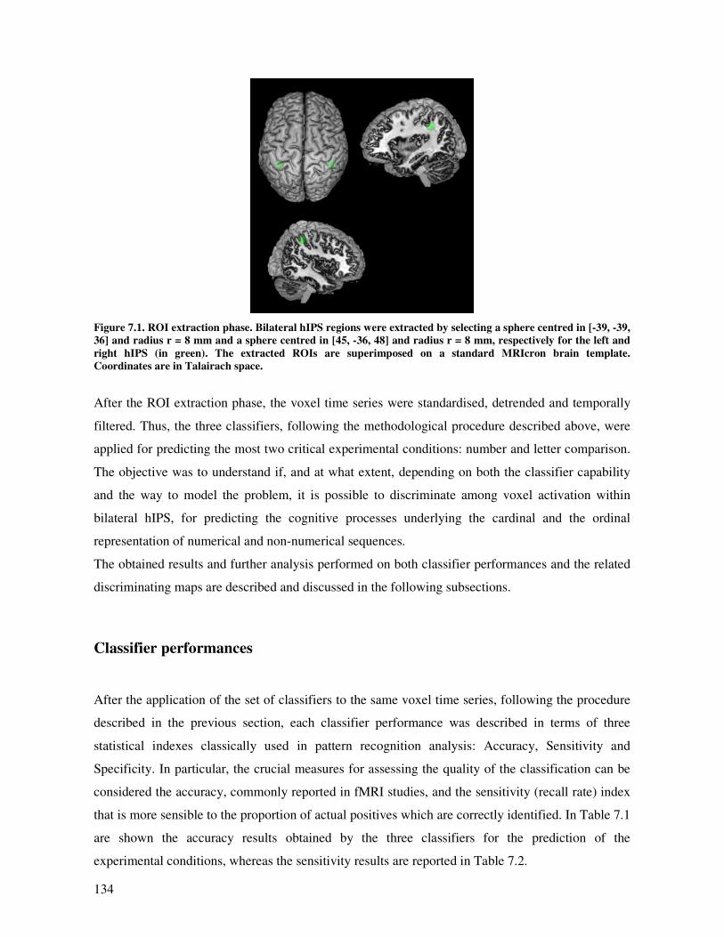
134

Figure 7.1. ROI extraction phase. Bilateral hIPS regions were extracted by selecting a sphere centred in [-39, -39,

36] and radius r = 8 mm and a sphere centred in [45, -36, 48] and radius r = 8 mm, respectively for the left and

right hIPS (in green). The extracted ROIs are superimposed on a standard MRIcron brain template.

Coordinates are in Talairach space.

After the ROI extraction phase, the voxel time series were standardised, detrended and temporally

filtered. Thus, the three classifiers, following the methodological procedure described above, were

applied for predicting the most two critical experimental conditions: number and letter comparison.

The objective was to understand if, and at what extent, depending on both the classifier capability

and the way to model the problem, it is possible to discriminate among voxel activation within

bilateral hIPS, for predicting the cognitive processes underlying the cardinal and the ordinal

representation of numerical and non-numerical sequences.

The obtained results and further analysis performed on both classifier performances and the related

discriminating maps are described and discussed in the following subsections.

Classifier performances

After the application of the set of classifiers to the same voxel time series, following the procedure

described in the previous section, each classifier performance was described in terms of three

statistical indexes classically used in pattern recognition analysis: Accuracy, Sensitivity and

Specificity. In particular, the crucial measures for assessing the quality of the classification can be

considered the accuracy, commonly reported in fMRI studies, and the sensitivity (recall rate) index

that is more sensible to the proportion of actual positives which are correctly identified. In Table 7.1

are shown the accuracy results obtained by the three classifiers for the prediction of the

experimental conditions, whereas the sensitivity results are reported in Table 7.2.

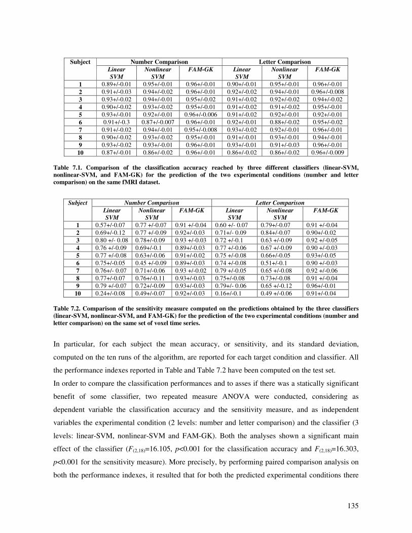
135

Number Comparison Letter Comparison Subject

Linear

SVM

Nonlinear

SVM

FAM-GK Linear

SVM

Nonlinear

SVM

FAM-GK

1 0.89+/-0.01 0.95+/-0.01 0.96+/-0.01 0.90+/-0.01 0.95+/-0.01 0.96+/-0.01

2 0.91+/-0.03 0.94+/-0.02 0.96+/-0.01 0.92+/-0.02 0.94+/-0.01 0.96+/-0.008

3 0.93+/-0.02 0.94+/-0.01 0.95+/-0.02 0.91+/-0.02 0.92+/-0.02 0.94+/-0.02

4 0.90+/-0.02 0.93+/-0.02 0.95+/-0.01 0.91+/-0.02 0.91+/-0.02 0.95+/-0.01

5 0.93+/-0.01 0.92+/-0.01 0.96+/-0.006 0.91+/-0.02 0.92+/-0.01 0.92+/-0.01

6 0.91+/-0.3 0.87+/-0.007 0.96+/-0.01 0.92+/-0.01 0.88+/-0.02 0.95+/-0.02

7 0.91+/-0.02 0.94+/-0.01 0.95+/-0.008 0.93+/-0.02 0.92+/-0.01 0.96+/-0.01

8 0.90+/-0.02 0.93+/-0.02 0.95+/-0.01 0.91+/-0.01 0.93+/-0.01 0.94+/-0.01

9 0.93+/-0.02 0.93+/-0.01 0.96+/-0.01 0.93+/-0.01 0.91+/-0.03 0.96+/-0.01

10 0.87+/-0.01 0.86+/-0.02 0.96+/-0.01 0.86+/-0.02 0.86+/-0.02 0.96+/-0.009

Table 7.1. Comparison of the classification accuracy reached by three different classifiers (linear-SVM,

nonlinear-SVM, and FAM-GK) for the prediction of the two experimental conditions (number and letter

comparison) on the same fMRI dataset.

Number Comparison Letter Comparison Subject

Linear

SVM

Nonlinear

SVM

FAM-GK Linear

SVM

Nonlinear

SVM

FAM-GK

1 0.57+/-0.07 0.77 +/-0.07 0.91 +/-0.04 0.60 +/- 0.07 0.79+/-0.07 0.91 +/-0.04

2 0.69+/-0.12 0.77 +/-0.09 0.92+/-0.03 0.71+/- 0.09 0.84+/-0.07 0.90+/-0.02

3 0.80 +/- 0.08 0.78+/-0.09 0.93 +/-0.03 0.72 +/-0.1 0.63 +/-0.09 0.92 +/-0.05

4 0.76 +/-0.09 0.69+/-0.1 0.89+/-0.03 0.77 +/-0.06 0.67 +/-0.09 0.90 +/-0.03

5 0.77 +/-0.08 0.63+/-0.06 0.91+/-0.02 0.75 +/-0.08 0.66+/-0.05 0.93+/-0.05

6 0.75+/-0.05 0.45 +/-0.09 0.89+/-0.03 0.74 +/-0.08 0.51+/-0.1 0.90 +/-0.03

7 0.76+/- 0.07 0.71+/-0.06 0.93 +/-0.02 0.79 +/-0.05 0.65 +/-0.08 0.92 +/-0.06

8 0.77+/-0.07 0.76+/-0.11 0.93+/-0.03 0.75+/-0.08 0.73+/-0.08 0.91 +/-0.04

9 0.79 +/-0.07 0.72+/-0.09 0.93+/-0.03 0.79+/- 0.06 0.65 +/-0.12 0.96+/-0.01

10 0.24+/-0.08 0.49+/-0.07 0.92+/-0.03 0.16+/-0.1 0.49 +/-0.06 0.91+/-0.04

Table 7.2. Comparison of the sensitivity measure computed on the predictions obtained by the three classifiers

(linear-SVM, nonlinear-SVM, and FAM-GK) for the prediction of the two experimental conditions (number and

letter comparison) on the same set of voxel time series.

In particular, for each subject the mean accuracy, or sensitivity, and its standard deviation,

computed on the ten runs of the algorithm, are reported for each target condition and classifier. All

the performance indexes reported in Table and Table 7.2 have been computed on the test set.

In order to compare the classification performances and to asses if there was a statically significant

benefit of some classifier, two repeated measure ANOVA were conducted, considering as

dependent variable the classification accuracy and the sensitivity measure, and as independent

variables the experimental condition (2 levels: number and letter comparison) and the classifier (3

levels: linear-SVM, nonlinear-SVM and FAM-GK). Both the analyses shown a significant main

effect of the classifier (F(2,18)=16.105, p<0.001 for the classification accuracy and F(2,18)=16.303,

p<0.001 for the sensitivity measure). More precisely, by performing paired comparison analysis on

both the performance indexes, it resulted that for both the predicted experimental conditions there

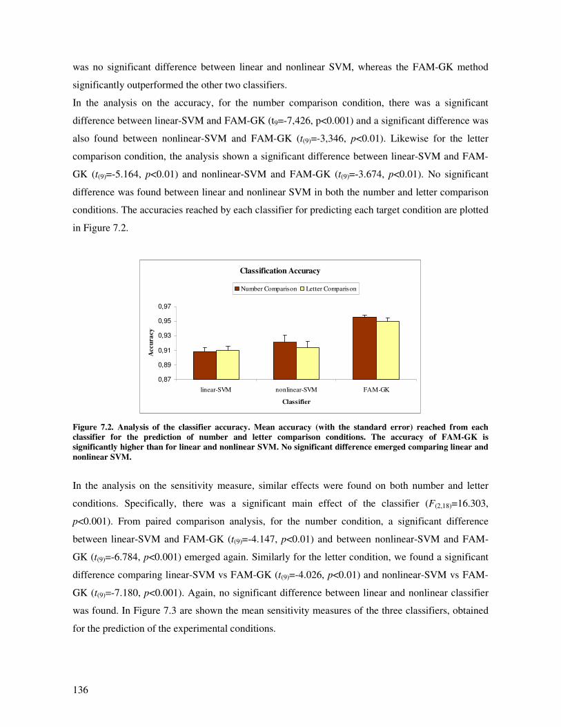
136

was no significant difference between linear and nonlinear SVM, whereas the FAM-GK method

significantly outperformed the other two classifiers.

In the analysis on the accuracy, for the number comparison condition, there was a significant

difference between linear-SVM and FAM-GK (t9=-7,426, p<0.001) and a significant difference was

also found between nonlinear-SVM and FAM-GK (t(9)=-3,346, p<0.01). Likewise for the letter

comparison condition, the analysis shown a significant difference between linear-SVM and FAM-

GK (t(9)=-5.164, p<0.01) and nonlinear-SVM and FAM-GK (t(9)=-3.674, p<0.01). No significant

difference was found between linear and nonlinear SVM in both the number and letter comparison

conditions. The accuracies reached by each classifier for predicting each target condition are plotted

in Figure 7.2.

Classification Accuracy

0,87

0,89

0,91

0,93

0,95

0,97

linear-SVM nonlinear-SVM FAM-GK

Classifier

Accu

ra

cy

Number Comparison Letter Comparison

Figure 7.2. Analysis of the classifier accuracy. Mean accuracy (with the standard error) reached from each

classifier for the prediction of number and letter comparison conditions. The accuracy of FAM-GK is

significantly higher than for linear and nonlinear SVM. No significant difference emerged comparing linear and

nonlinear SVM.

In the analysis on the sensitivity measure, similar effects were found on both number and letter

conditions. Specifically, there was a significant main effect of the classifier (F(2,18)=16.303,

p<0.001). From paired comparison analysis, for the number condition, a significant difference

between linear-SVM and FAM-GK (t(9)=-4.147, p<0.01) and between nonlinear-SVM and FAM-

GK (t(9)=-6.784, p<0.001) emerged again. Similarly for the letter condition, we found a significant

difference comparing linear-SVM vs FAM-GK (t(9)=-4.026, p<0.01) and nonlinear-SVM vs FAM-

GK (t(9)=-7.180, p<0.001). Again, no significant difference between linear and nonlinear classifier

was found. In Figure 7.3 are shown the mean sensitivity measures of the three classifiers, obtained

for the prediction of the experimental conditions.

137

Classifier Sensitivity

0

0,2

0,4

0,6

0,8

linear-SVM nonlinear-SVM FAM-GK

Classifier

Sen

siti

vit

y


Figure 7.3. Analysis of the classifier sensitivity. Mean sensitivity (with the standard error) obtained for the

prediction of number and letter comparison conditions, for each classifier. For FAM-GK the sensitivity is

significantly higher than for linear and nonlinear SVM. No significant difference emerged comparing linear and

nonlinear SVM.

In conclusion, also in the case of a block designed fMRI experiment, the FAM-GK method, used on

spatio-temporal input patterns outperformed the linear SVM and the nonlinear SVM, which were

used only on spatial input patterns. The level of accuracy reached with the linear classifier was very

high (over 90%), but the sensitivity measure, more sensible to the percentage of real positives

correctly identified, although remaining at an acceptable level (about 70%), shows a great

discrepancy with the corresponding accuracy level. This is not the case of FAM-GK, which

provided very similar accuracy and sensitivity measures (about 90 %) for the prediction of both the

two conditions. Thus, from the classifier ability perspective, the FAM-GK method offered the best

performance, confirming the key role, in fMRI data analysis, of using spatio-temporal information

as input to the classifier combined with a nonlinear classification function.

Discriminating maps

The fMRI data of each subject were analysed separately. Thus, after the application of the pattern

recognition analysis, to each subject was associated a discriminating map, extracted by the

algorithm, for each predicted experimental condition. In the case of linear SVM, it was possible to

obtain the discriminating brain regions, just by analysing the weight vector associated by the

classifier to the training data. Using SVM with nonlinear kernel generally allows the classifier to

reach a much more accurate performance, but this was not the case of the obtained results in this

study. Perhaps in our case, the nonlinear SVM was not able to exploit the input data information in

a richer way probably because the nonlinear model was to complex for the way we present the input

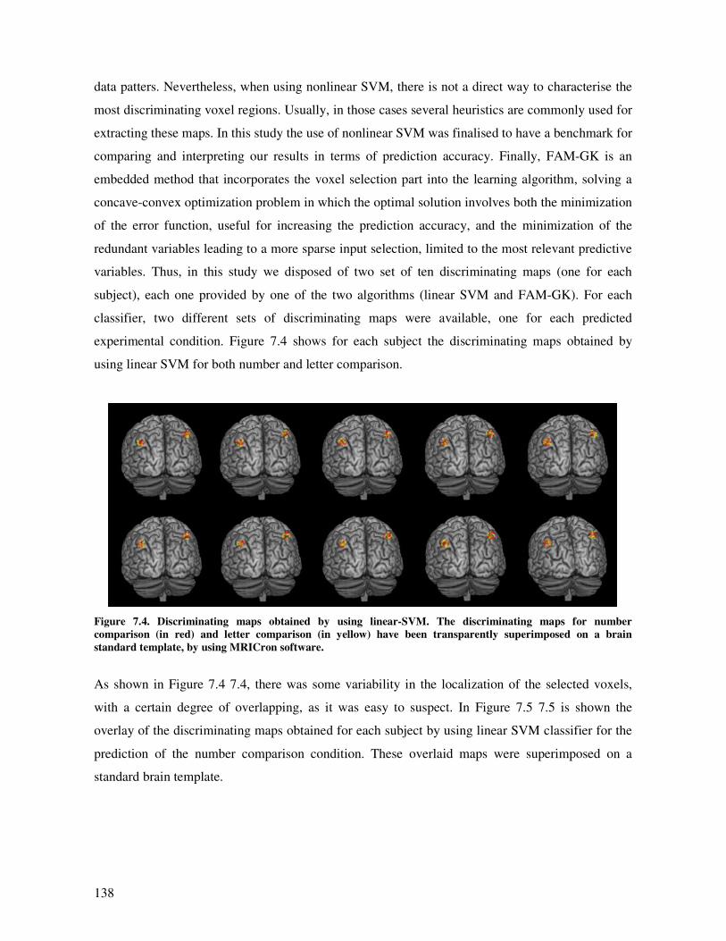
138

data patters. Nevertheless, when using nonlinear SVM, there is not a direct way to characterise the

most discriminating voxel regions. Usually, in those cases several heuristics are commonly used for

extracting these maps. In this study the use of nonlinear SVM was finalised to have a benchmark for

comparing and interpreting our results in terms of prediction accuracy. Finally, FAM-GK is an

embedded method that incorporates the voxel selection part into the learning algorithm, solving a

concave-convex optimization problem in which the optimal solution involves both the minimization

of the error function, useful for increasing the prediction accuracy, and the minimization of the

redundant variables leading to a more sparse input selection, limited to the most relevant predictive

variables. Thus, in this study we disposed of two set of ten discriminating maps (one for each

subject), each one provided by one of the two algorithms (linear SVM and FAM-GK). For each

classifier, two different sets of discriminating maps were available, one for each predicted

experimental condition. Figure 7.4 shows for each subject the discriminating maps obtained by

using linear SVM for both number and letter comparison.

Figure 7.4. Discriminating maps obtained by using linear-SVM. The discriminating maps for number

comparison (in red) and letter comparison (in yellow) have been transparently superimposed on a brain

standard template, by using MRICron software.

As shown in Figure 7.4 7.4, there was some variability in the localization of the selected voxels,

with a certain degree of overlapping, as it was easy to suspect. In Figure 7.5 7.5 is shown the

overlay of the discriminating maps obtained for each subject by using linear SVM classifier for the

prediction of the number comparison condition. These overlaid maps were superimposed on a

standard brain template.

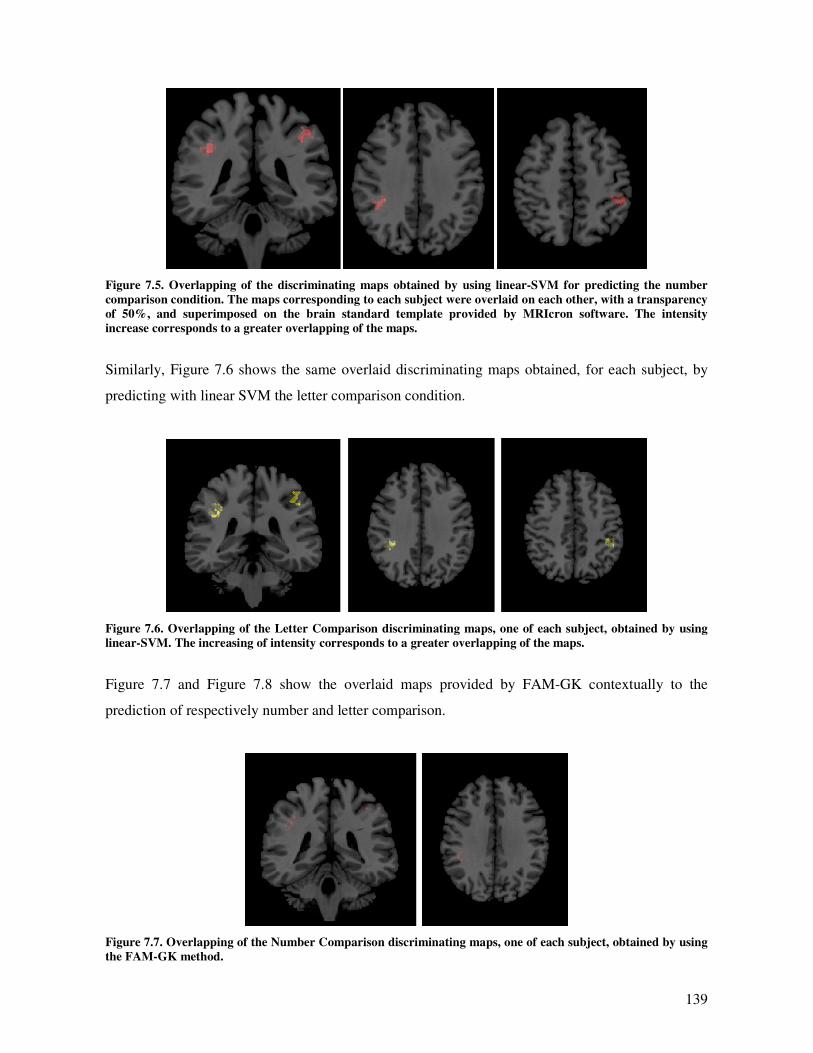
139

Figure 7.5. Overlapping of the discriminating maps obtained by using linear-SVM for predicting the number

comparison condition. The maps corresponding to each subject were overlaid on each other, with a transparency

of 50%, and superimposed on the brain standard template provided by MRIcron software. The intensity

increase corresponds to a greater overlapping of the maps.

Similarly, Figure 7.6 shows the same overlaid discriminating maps obtained, for each subject, by

predicting with linear SVM the letter comparison condition.

Figure 7.6. Overlapping of the Letter Comparison discriminating maps, one of each subject, obtained by using

linear-SVM. The increasing of intensity corresponds to a greater overlapping of the maps.

Figure 7.7 and Figure 7.8 show the overlaid maps provided by FAM-GK contextually to the

prediction of respectively number and letter comparison.

Figure 7.7. Overlapping of the Number Comparison discriminating maps, one of each subject, obtained by using

the FAM-GK method.

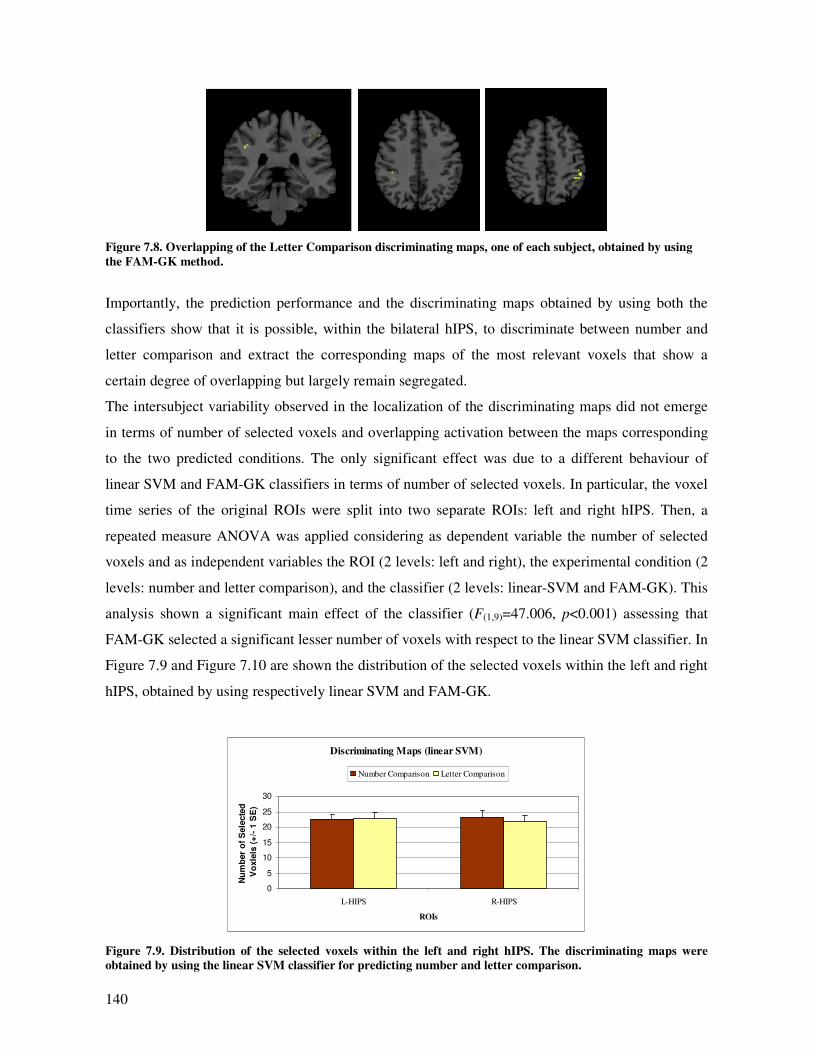
140

Figure 7.8. Overlapping of the Letter Comparison discriminating maps, one of each subject, obtained by using

the FAM-GK method.

Importantly, the prediction performance and the discriminating maps obtained by using both the

classifiers show that it is possible, within the bilateral hIPS, to discriminate between number and

letter comparison and extract the corresponding maps of the most relevant voxels that show a

certain degree of overlapping but largely remain segregated.

The intersubject variability observed in the localization of the discriminating maps did not emerge

in terms of number of selected voxels and overlapping activation between the maps corresponding

to the two predicted conditions. The only significant effect was due to a different behaviour of

linear SVM and FAM-GK classifiers in terms of number of selected voxels. In particular, the voxel

time series of the original ROIs were split into two separate ROIs: left and right hIPS. Then, a

repeated measure ANOVA was applied considering as dependent variable the number of selected

voxels and as independent variables the ROI (2 levels: left and right), the experimental condition (2

levels: number and letter comparison), and the classifier (2 levels: linear-SVM and FAM-GK). This

analysis shown a significant main effect of the classifier (F(1,9)=47.006, p<0.001) assessing that

FAM-GK selected a significant lesser number of voxels with respect to the linear SVM classifier. In

Figure 7.9 and Figure 7.10 are shown the distribution of the selected voxels within the left and right

hIPS, obtained by using respectively linear SVM and FAM-GK.

Discriminating Maps (linear SVM)

0

5

10

15

20

25

30

L-HIPS R-HIPS

ROIs

Nu

mb

er

of

Sele

cte

d

Vo

xle

ls (

+/-

1 S

E)


Figure 7.9. Distribution of the selected voxels within the left and right hIPS. The discriminating maps were

obtained by using the linear SVM classifier for predicting number and letter comparison.

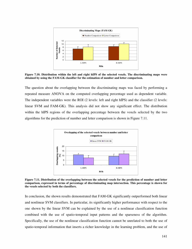
141

Discriminating Maps (FAM-GK)

0

2

4

6

8

10

12

L-HIPS R-HIPS

ROIs

Nu

mb

er

of

Se

lec

ted

Vo

xe

ls


Figure 7.10. Distribution within the left and right hIPS of the selected voxels. The discriminating maps were

obtained by using the FAM-GK classifier for the estimation of number and letter comparison.

The question about the overlapping between the discriminating maps was faced by performing a

repeated measure ANOVA on the computed overlapping percentage used as dependent variable.

The independent variables were the ROI (2 levels: left and right hIPS) and the classifier (2 levels:

linear SVM and FAM-GK). This analysis did not show any significant effect. The distribution

within the hIPS regions of the overlapping percentage between the voxels selected by the two

algorithms for the prediction of number and letter comparison is shown in Figure 7.11.

Overlapping of the selected voxels between number and letter

comparison

0

5

10

15

20

L-HIPS R-HIPS

ROIs

Overl

ap

pin

g v

oxels

(%)

linear SVM FAM-GK

Figure 7.11. Distribution of the overlapping between the selected voxels for the prediction of number and letter

comparison, expressed in terms of percentage of discriminating map intersection. This percentage is shown for

the voxels selected by both the classifiers.

In conclusion, the shown results demonstrated that FAM-GK significantly outperformed both linear

and nonlinear SVM classifiers. In particular, its significantly higher performance with respect to the

one shown by the linear SVM can be explained by the use of a nonlinear classification function

combined with the use of spatio-temporal input patterns and the sparseness of the algorithm.

Specifically, the use of the nonlinear classification function cannot be unrelated to both the use of

spatio-temporal information that inserts a richer knowledge in the learning problem, and the use of

142

sparseness for voxel selection that is implicitly coded in the algorithm and lead to reducing the

amount of redundant voxels selected by the linear SVM. This issue is confirmed by the fact that the

performance of FAM-GK is also significantly higher than that of the nonlinear SVM classifier used

in the classical way, considering only spatial input patterns. Nevertheless, both the classifiers

provided discriminating maps that did not significantly differ in terms of overlapping percentage

between the two experimental conditions. These percentages seem to be comparable and remain

quite small (about 10 %).

The comparison between pattern recognition techniques, which results have been illustrated and

discussed in this section, and the conventional approaches to fMRI data analysis (GLM), which

results have been reported by Fias et al. (2007) has shown the limits of the conventional methods in

discriminating, at a much more refined level, the voxel activations predictive for some experimental

condition. The information contained in fMRI data is commonly blurred by the model constraints

imposed by the GLM, including the application of the spatial smoothing in the pre-processing

phase, the univariate nature of the conventional analysis, and the model assumptions on the shape of

the HRF. The results obtained by Fias et al. (2007) can be interpreted, in the light of the results

discussed in this section, as a possible confound of the conventional approach to fMRI data

analysis.

Conclusion

The spatial nature of the representation of numerical and non-numerical ordered sequences has been

investigated by several behavioural experiments, and neuropsychological studies on neglect

patients. Several findings, in particular those demonstrated by neuropsychological studies, are very

strong and in disagreement with other studies suggesting that the spatial representation is a general

characteristic of the ordered sequences, instead of a specific property of the numerical quantities.

Furthermore, the findings in neuroimaging literature, investigating the neural correlates of

numerical quantity representation, have shown agreement among several studies and have

highlighted essentially three parietal circuits for number processing (Dehaene et al., 2003), in

particular the involvement of the bilateral hIPS as a specific quantity system. In contrast, the fMRI

literature investigating the implication of hIPS in processing numerical and non-numerical ordered

sequences seems to be controversial and not conclusive at all. Thus, the objective of this study was

to exploit the advantages of the pattern recognition methods for fMRI data analysis, for

investigating this issue. To this purpose, we reanalysed the fMRI data by Fias et al. (2007),

143

comparing three pattern recognition techniques, the linear and nonlinear SVM and the novel

proposed method FAM-GK (see Chapter 6 for a deep description of the method). From a

methodological perspective, the obtained results have shown that for fMRI data acquired within a

block design, all the three compared classifiers can be used with a different level of success. In

particular FAM-GK significantly outperformed the other two classifiers showing discriminating

maps containing only the most predictive voxels. From the neuroscience perspective, the obtained

results have shown a partial overlapping of the two representation systems (numbers vs. letters),

highlighting that is possible, at bilateral hIPS level, to locate different activation patterns for the

representation of numbers and letters, which show a certain degree of overlapping. These results

suggest that within hIPS regions there are neural substrates codifying the cardinal dimension

(numbers) and the ordinal dimension (numbers and letters) in a partially independent way. The

representation of numerical and non-numerical sequences, at least for letters of the alphabet, seems

to be based on a partially common metric, but the processes underlying these representations could

remain independent.

145

Chapter 8

Pattern recognition for fast event-related fMRI data analysis:

A preliminary study

Introduction

The use of pattern recognition techniques for the analysis of fMRI data has reached full consensus

in the cognitive neuroscience community, and is becoming the commonly accepted way to

investigate the modular and/or the distributed representation of information in the brain.

Generally, the crucial aspects that have to be considered when using pattern recognition methods

can be summarised as follows: the fMRI experiment determines the nature of the learning problem

(classification / regression); the pre-processing phase and the way to perform voxel selection play

an important role in reaching high classification accuracy; the experimental design (i.e., block, slow

or fast event-related) indicates the way to model the problem and the possibility to use a pattern

recognition method instead of another. Once the problem has been modelled, possibly with the

minimal theoretical error model, the choice of the algorithm parameters (e.g.., linear vs nonlinear

approximation function and tuning learning parameters) may also improve the generalization

performance of the learning machine, leading to more robust and reliable results.

Among pattern recognition techniques, SVM has become the standard de facto for analysing

functional neuroimaging data. Nevertheless, this method has been largely employed for analysing

data in the context of a block or slow event related design paradigms. In these cases, SVM can

predict the experimental conditions at the single trial level, by deriving a response pattern estimate

for each TR (i.e., acquired image volume). In a block design experiment, each acquired brain

volume within a block, excluding the first few volumes, can be considered as an independent

measure maintaining a good approximation model, or better a single volume from each block can be

considered as an independent measure. Likewise, in slow event-related design experiments, if

successive events are sufficiently far-between (i.e., about 12 sec.), the evoked BOLD signals,

146

specifically each activation peak can be considered as well separated to each other and used as

independent measures by the classifier. In these cases any cross-validation technique can be applied

without any problem. Otherwise, in fast event-related experiments, the question is much more

complex due to the presence of the refractory effect (see Chapter 2, for more details) resulting in

nonlinearities on the acquired signals, and the activation peaks are not easy distinguishable. Thus, it

is not possible to consider each acquired volume as an independent measure for the classification. In

these cases, as suggested by (De Martino et al., 2008), a way for applying pattern recognition

methods could be to choose a series of temporal-windows from the fMRI dataset, in an appropriate

way, and using these sub-run measurements as in the slow event related design, for deriving the

response pattern estimates.

Furthermore, a recent study dealing with these spatial and temporal dimensions of the BOLD signal

was conducted, in the context of a block experimental design, by (Mourao-Miranda, Friston, &

Brammer, 2007). The authors defined spatio-temporal fMRI input patterns, and applied a linear

SVM classifier to these temporally extended patterns. Their results showed that the accuracy of the

spatio-temporal SVM was better than the accuracy of the spatial SVM trained with single fMRI

volumes and similar to the accuracy of the spatial SVM trained with averages of fMRI volumes.

Their results suggest that the advantages of performing a spatio-temporal analysis are evident in the

case of a block design experiment, and that they will increase with event-related designs, where

dynamic changes may be more evident.

At the state of the art, new pattern based methods are required for modelling in a more accurate way

the nonlinear spatio-temporal dynamics of fMRI signals in the context of fast event-related designs.

The FAM-GK method, fully described in Chapter 6, seems to bridge the gap between both spatial

and spatio-temporal input data dimensions, and linear and nonlinear classification, becoming a

suitable tool for analysing rapid event-related functional images.

In this Chapter, preliminary results obtained by testing three pattern recognition techniques (linear

SVM, non-linear SVM, and FAM-GK) on fMRI data acquired in the context of a rapid event-

related experimental design are presented. The main objective of the primal study, which is still a

work in progress, was to investigate the neural correlates of an automatic spatial coding of the

perceived gaze direction, as demonstrated by (Zorzi, Mapelli, Rusconi, & Umilta, 2003). Beyond

this main goal, the aim of the preliminary study presented in this Chapter was just to compare and

analyse methodological aspects related to three pattern recognition methods applied to rapid event-

related fMRI data. To this purpose, we selected two ROIs (left and right motor areas) and tried to

use SVM (linear/nonlinear) in a way to limit the temporal correlation within the voxel patterns, and

147

FAM-GK, with an appropriate estimated temporal delay window, with the objective to predict the

left and right motor response.

Materials and methods

In this section we briefly describe the fMRI data acquired in the context of a fast event-related

fMRI experiment. A description of the methodological aspects for analysing these fMRI data by

using three pattern recognition methods is given. More details about the linear and nonlinear SVM

can be found in Chapter 4 and Chapter 3. Similarly, deeper details about FAM-GK can be found in

Chapter 6, where the method is fully described.


The original aim of the experiment that is described in the next sub-sections was to investigate the

neural correlates of an automatic spatial coding of the perceived eye gaze direction, as confirmed by

(Zorzi et al., 2003). Beyond this main goal, the aim of this preliminary study was just to analyse

theoretical aspects related to three pattern recognition methods applied to rapid event-related fMRI

data and comparing their potential on the same data. In the following we summarise the stimuli and

the procedure used for this experiment, describing also the acquired fMRI data.

Stimuli and procedure

In the experiment, participants viewed biological (i.e., eyes having two different colours) and non-

biological (i.e., flags having the same two different colours) cues at the centre of the screen.

Specifically the biological cues were realised by using schematic eyes composed of elliptic circles

with the area corresponding to the iris coloured in green or blue. The non-biological cues, used as

control stimuli, were obtained by substituting the ellipses forming the eyes with rectangles. The

direction of both biological and non-biological cues was determined by the movement of the

ellipses/rectangles that were centrally presented or to the left or to the right side of the space,

whereas the coloured areas were constantly at the same position for both type of stimuli. The

movement direction of both cues was irrelevant for the task. In particular, participants were asked to

press a left (right) key on the keyboard if the cue colour was green (blue).

148

The experiment was composed of four runs. During the first two runs participants viewed the non-

biological cues, whereas the schematic eyes were presented in the last two runs. During each run, a

set of 180 trials was presented according to the following procedure: at the beginning of each trial, a

fixation of 400 ms was required, followed by 400 ms of the cue presentation after which there was a

fixed time of 3200 ms consisting of the response time and the Inter Trial Interval (ITI). Thus, each

trial had a fixed duration of 4000 ms. At the end of each run a simple fixation trial, lasting for 4000

ms was inserted.

fMRI data acquisition

For each participant, functional volume images were acquired by using a Siemens 3T Trio scanner

using a multiple slice T2*-weighted echo planar imaging (EPI), with TR=1000 ms, TE=30 ms; in-

plane resolution = 3.1x3.1 mm; matrix dimension =64x64, filed of view = 200x200 mm; slice

thickness =5 mm. For each of the four runs, sixteen slices per volume and a total of 728 volumes

were acquired, resulting in 2012 functional volumes.

ROI analysis with pattern recognition

In order to apply pattern recognition methods for ROI analysis of the fMRI data, some crucial

processing phases are required. The first phase is the classical functional image pre-processing (i.e.,

realignment, coregistration, normalization, spatial and temporal smoothing) performed in order to

extract the voxel time series in a proper way.

A discussed point in literature is spatial smoothing. It produces some advantages for voxel-wise

analysis performed with conventional approaches, by introducing a certain correlation in voxel time

series and increasing the normality of data. However, it is dangerous in multivariate brain analysis,

due to the loss of potential discriminating information contained in adjacent functional brain areas.

Thus, no spatial filter was applied to our functional images. This first phase, together with the ROI

extraction, a further signal pre-processing phase and the classification phase are fully described in

the following sub-sections.

149

Pre-processing phase

The first step in analysing fMRI is the classical image pre-processing. The functional images were

pre-processed by using SPM5 (http://www.fil.ion.ucl.ac.uk/spm/software/spm5/). Specifically, they

were realigned, coregistered and normalised. Aiming at removing movement artefacts in fMRI time

series, a 6 parameter (rigid body) spatial transformation was used for realigning functional images.

In particular, the first scan of each of the four sessions was realigned to the first scan of the first

session. Then, all scans within each session were realigned to first one. All images were then

coregistered with the participant’s corresponding anatomical (T1-weighted) images by using the

normalised mutual information method. The resulting images were normalized with a 12-parameter

affine transformation into SPM5’s Montreal Neurological Institute (MNI) EPI 3x3x3 mm template

using the corresponding anatomical image as a reference. We did not perform any spatial smoothing

on the pre-processed images, avoiding blurring functional activations of neighbour voxels of

adjacent different functional areas.

ROI extraction phase

The pre-processed functional images (without spatial smoothing) were used for the ROI extraction

phase. For selecting the left and right primary motor areas we used the results obtained by

(Binkofski et al., 2002) relative to a study investigating the modulation of attention on neural

activity in human Primary Motor Cortex (PMC) areas. According to the results obtained by the

authors, we selected two focuses of the PMC, one of which was demonstrated to be modulated by

attention, and we selected them bilaterally. In particular we extracted a sphere with centre in [-36, -

20, 48] and radius r = 8 mm, modulated by attention, and a sphere with centre in [-48, -8, 56] and

radius r = 8 mm. We also selected the corresponding areas of the right hemisphere with the same

procedure applied respectively on the centres [36, -20, 48] and [48, -8, 56].

After the ROI extraction, we obtained a set of 324 voxel time series of 2880 volumes each (i.e., 4

runs of 720 volumes each), discarding the first and the last four volumes, for each run.

Basic pre-processing phase

The ROI extracted voxel time series were z-standardized, forcing them to have zero mean and

standard deviation one. Then, linear trends in each time series were removed by applying a simple

linear detrend filter. At last, for removing the high frequency components present in the signal the

150

time series were temporally filtered by using a moving average filter with window size equal to 5

time points. Each of the four runs was processed separately and then concatenated to the successive

one. Thus, we obtained a set of 324 voxel time series of 2880 functional volumes, which were

finally ready for the classification phase.

Classification phase

For each used classifier, the procedure used for the preparation of the training and test datasets, and

the cross-validation procedure used for tuning the learning parameters and assessing the

generalization ability, are described in the following subsections. All the analyses were performed

for each subject separately.

Linear-SVM and nonlinear-SVM

The target conditions (left-response and right-response) were codified in order to have, for each

experimental condition, a vector N

iT 1,1 −+∈ , where N is the number of volumes, in which all the

volumes corresponding to the target condition was labelled with +1, whereas all the other volumes

with -1. In order to apply the classifiers in a correct way, it is necessary that the input data are

sampled in such a way that they can be considered independent to each other. Thus, the fMRI data

were sampled selecting those volumes corresponding to each trial, so that they can be considered as

much as possible as independent measures. In particular, in order to capture the BOLD dynamics,

for each trial it we considered the second volume acquired during the successive trial 1+it (i.e., the

sixth volume after the beginning of the trial it ). As just described in the previous Chapter, the

critical tuning parameter for SVM classification (linear/nonlinear) is the regularization constant C.

Thus we used cross-validation for determining the best C parameter leading to the best

generalization ability of the classifier and at the same time we estimated, over several runs of the

algorithm, the robustness of the classifier performance. In particular, the regularization constant was

varied in the range [ ]101− with an increasing step of 1 and for each chosen parameter the classifier

was trained for 10 runs, after which its performance on the test data was evaluated. Specifically, for

each of the 10 runs, the original fMRI data were randomly split into training (50%) and test (50%)

sets, and the number of TP and FP was computed on the basis of the prediction obtained on the test

set. We used the receiver operating characteristic (ROC) analysis (Fawcett, 2006) and specifically

the Area Under Curve (AUC) for assessing the classification performance for each choice of the

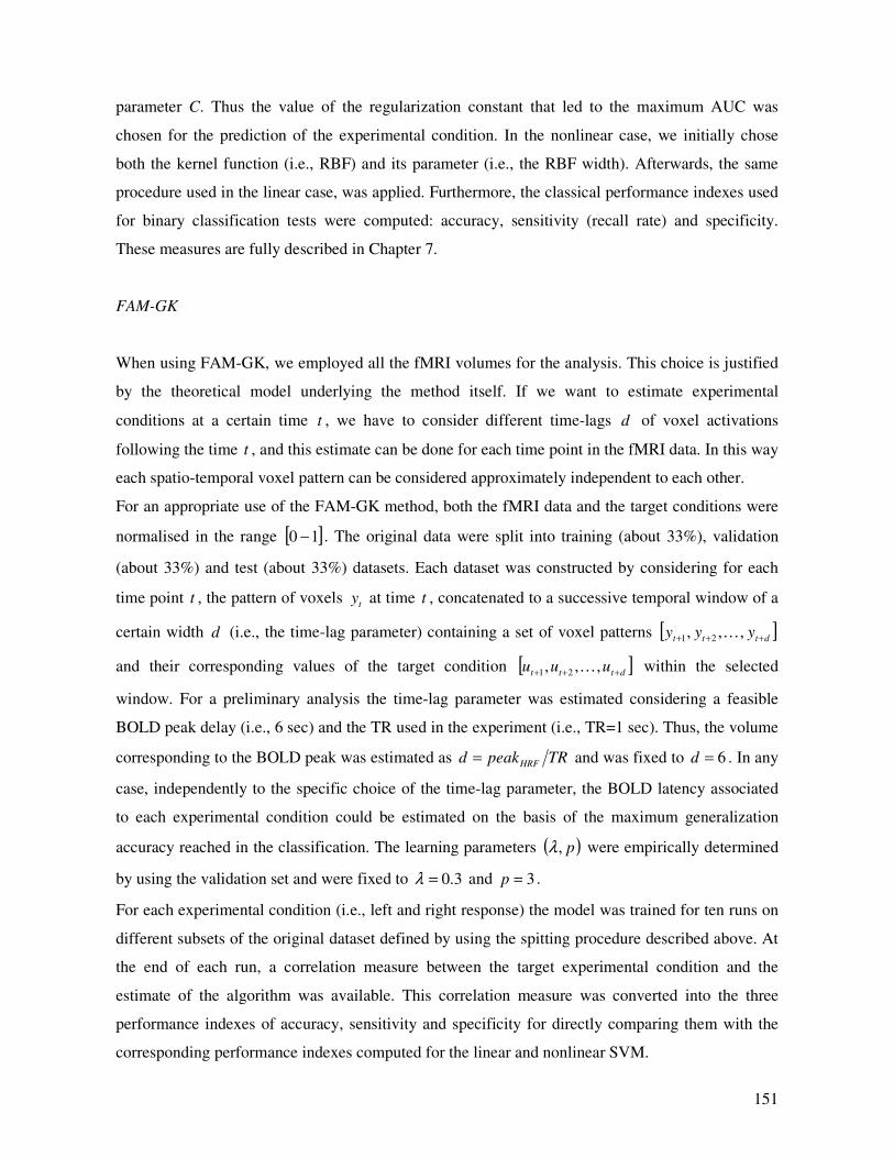
151

parameter C. Thus the value of the regularization constant that led to the maximum AUC was

chosen for the prediction of the experimental condition. In the nonlinear case, we initially chose

both the kernel function (i.e., RBF) and its parameter (i.e., the RBF width). Afterwards, the same

procedure used in the linear case, was applied. Furthermore, the classical performance indexes used

for binary classification tests were computed: accuracy, sensitivity (recall rate) and specificity.

These measures are fully described in Chapter 7.

FAM-GK

When using FAM-GK, we employed all the fMRI volumes for the analysis. This choice is justified

by the theoretical model underlying the method itself. If we want to estimate experimental

conditions at a certain time t , we have to consider different time-lags d of voxel activations

following the time t , and this estimate can be done for each time point in the fMRI data. In this way

each spatio-temporal voxel pattern can be considered approximately independent to each other.

For an appropriate use of the FAM-GK method, both the fMRI data and the target conditions were

normalised in the range [ ]10 − . The original data were split into training (about 33%), validation

(about 33%) and test (about 33%) datasets. Each dataset was constructed by considering for each

time point t , the pattern of voxels ty at time t , concatenated to a successive temporal window of a

certain width d (i.e., the time-lag parameter) containing a set of voxel patterns [ ]dttt yyy +++ ,,, 21 K

and their corresponding values of the target condition [ ]dttt uuu +++ ,,, 21 K within the selected

window. For a preliminary analysis the time-lag parameter was estimated considering a feasible

BOLD peak delay (i.e., 6 sec) and the TR used in the experiment (i.e., TR=1 sec). Thus, the volume

corresponding to the BOLD peak was estimated as TRpeakd HRF= and was fixed to 6=d . In any

case, independently to the specific choice of the time-lag parameter, the BOLD latency associated

to each experimental condition could be estimated on the basis of the maximum generalization

accuracy reached in the classification. The learning parameters ( )p,λ were empirically determined

by using the validation set and were fixed to 3.0=λ and 3=p .

For each experimental condition (i.e., left and right response) the model was trained for ten runs on

different subsets of the original dataset defined by using the spitting procedure described above. At

the end of each run, a correlation measure between the target experimental condition and the

estimate of the algorithm was available. This correlation measure was converted into the three

performance indexes of accuracy, sensitivity and specificity for directly comparing them with the

corresponding performance indexes computed for the linear and nonlinear SVM.

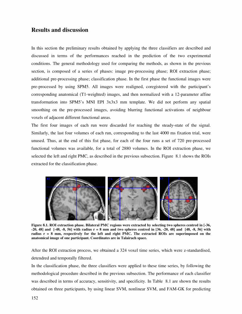
152


In this section the preliminary results obtained by applying the three classifiers are described and

discussed in terms of the performances reached in the prediction of the two experimental

conditions. The general methodology used for comparing the methods, as shown in the previous

section, is composed of a series of phases: image pre-processing phase; ROI extraction phase;

additional pre-processing phase; classification phase. In the first phase the functional images were

pre-processed by using SPM5. All images were realigned, coregistered with the participant’s

corresponding anatomical (T1-weighted) images, and then normalized with a 12-parameter affine

transformation into SPM5’s MNI EPI 3x3x3 mm template. We did not perform any spatial

smoothing on the pre-processed images, avoiding blurring functional activations of neighbour

voxels of adjacent different functional areas.

The first four images of each run were discarded for reaching the steady-state of the signal.

Similarly, the last four volumes of each run, corresponding to the last 4000 ms fixation trial, were

unused. Thus, at the end of this fist phase, for each of the four runs a set of 720 pre-processed

functional volumes was available, for a total of 2880 volumes. In the ROI extraction phase, we

selected the left and right PMC, as described in the previous subsection. Figure 8.1 shows the ROIs

extracted for the classification phase.

Figure 8.1. ROI extraction phase. Bilateral PMC regions were extracted by selecting two spheres centred in [-36,

-20, 48] and [-48, -8, 56] with radius r = 8 mm and two spheres centred in [36, -20, 48] and [48, -8, 56] with

radius r = 8 mm, respectively for the left and right PMC. The extracted ROIs are superimposed on the

anatomical image of one participant. Coordinates are in Talairach space.

After the ROI extraction process, we obtained a 324 voxel time series, which were z-standardised,

detendred and temporally filtered.

In the classification phase, the three classifiers were applied to these time series, by following the

methodological procedure described in the previous subsection. The performance of each classifier

was described in terms of accuracy, sensitivity, and specificity. In Table 8.1 are shown the results

obtained on three participants, by using linear SVM, nonlinear SVM, and FAM-GK for predicting

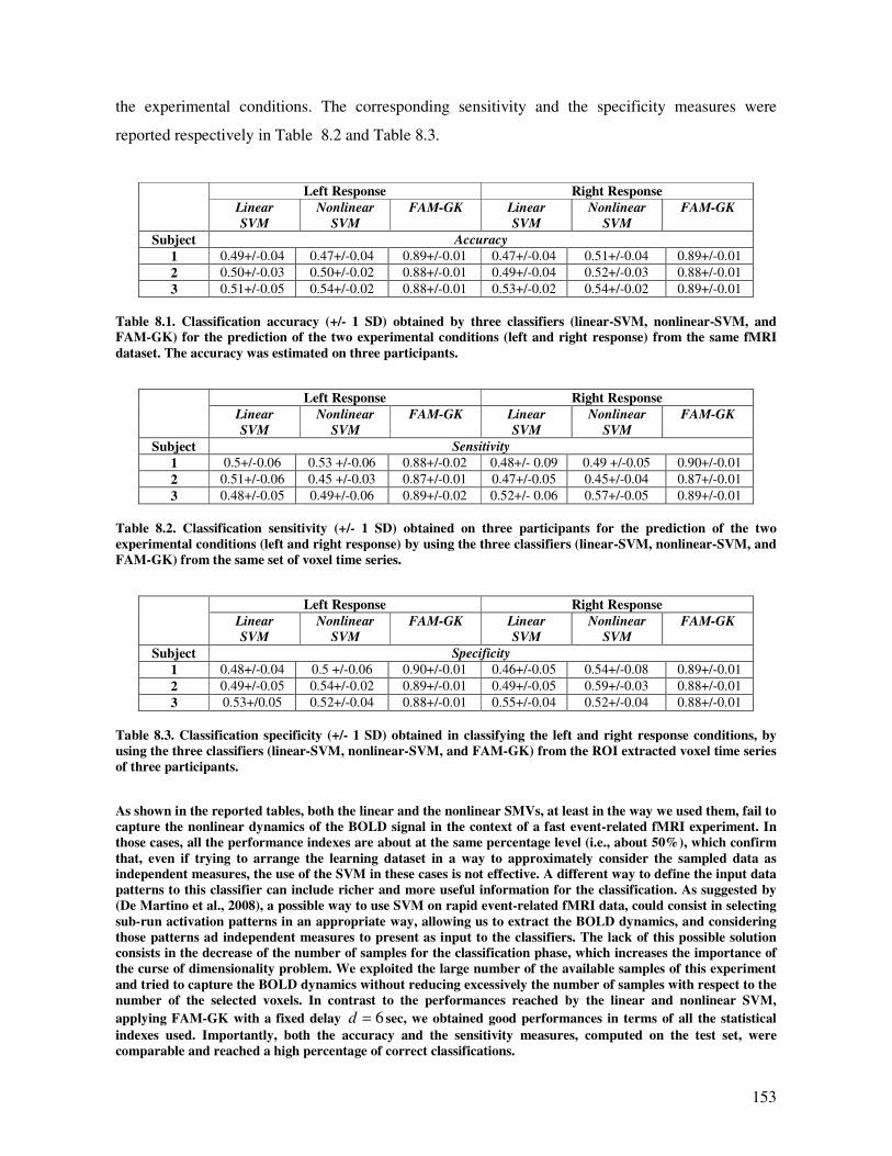
153

the experimental conditions. The corresponding sensitivity and the specificity measures were

reported respectively in Table 8.2 and Table 8.3.

Left Response Right Response

Linear

SVM

Nonlinear

SVM

FAM-GK Linear

SVM

Nonlinear

SVM

FAM-GK

Subject Accuracy

1 0.49+/-0.04 0.47+/-0.04 0.89+/-0.01 0.47+/-0.04 0.51+/-0.04 0.89+/-0.01

2 0.50+/-0.03 0.50+/-0.02 0.88+/-0.01 0.49+/-0.04 0.52+/-0.03 0.88+/-0.01

3 0.51+/-0.05 0.54+/-0.02 0.88+/-0.01 0.53+/-0.02 0.54+/-0.02 0.89+/-0.01

Table 8.1. Classification accuracy (+/- 1 SD) obtained by three classifiers (linear-SVM, nonlinear-SVM, and

FAM-GK) for the prediction of the two experimental conditions (left and right response) from the same fMRI

dataset. The accuracy was estimated on three participants.


Linear

SVM

Nonlinear

SVM

FAM-GK Linear

SVM

Nonlinear

SVM

FAM-GK

Subject Sensitivity

1 0.5+/-0.06 0.53 +/-0.06 0.88+/-0.02 0.48+/- 0.09 0.49 +/-0.05 0.90+/-0.01

2 0.51+/-0.06 0.45 +/-0.03 0.87+/-0.01 0.47+/-0.05 0.45+/-0.04 0.87+/-0.01

3 0.48+/-0.05 0.49+/-0.06 0.89+/-0.02 0.52+/- 0.06 0.57+/-0.05 0.89+/-0.01

Table 8.2. Classification sensitivity (+/- 1 SD) obtained on three participants for the prediction of the two

experimental conditions (left and right response) by using the three classifiers (linear-SVM, nonlinear-SVM, and

FAM-GK) from the same set of voxel time series.


Linear

SVM

Nonlinear

SVM

FAM-GK Linear

SVM

Nonlinear

SVM

FAM-GK

Subject Specificity

1 0.48+/-0.04 0.5 +/-0.06 0.90+/-0.01 0.46+/-0.05 0.54+/-0.08 0.89+/-0.01

2 0.49+/-0.05 0.54+/-0.02 0.89+/-0.01 0.49+/-0.05 0.59+/-0.03 0.88+/-0.01

3 0.53+/0.05 0.52+/-0.04 0.88+/-0.01 0.55+/-0.04 0.52+/-0.04 0.88+/-0.01

Table 8.3. Classification specificity (+/- 1 SD) obtained in classifying the left and right response conditions, by

using the three classifiers (linear-SVM, nonlinear-SVM, and FAM-GK) from the ROI extracted voxel time series

of three participants.

As shown in the reported tables, both the linear and the nonlinear SMVs, at least in the way we used them, fail to

capture the nonlinear dynamics of the BOLD signal in the context of a fast event-related fMRI experiment. In

those cases, all the performance indexes are about at the same percentage level (i.e., about 50%), which confirm

that, even if trying to arrange the learning dataset in a way to approximately consider the sampled data as

independent measures, the use of the SVM in these cases is not effective. A different way to define the input data

patterns to this classifier can include richer and more useful information for the classification. As suggested by

(De Martino et al., 2008), a possible way to use SVM on rapid event-related fMRI data, could consist in selecting

sub-run activation patterns in an appropriate way, allowing us to extract the BOLD dynamics, and considering

those patterns ad independent measures to present as input to the classifiers. The lack of this possible solution

consists in the decrease of the number of samples for the classification phase, which increases the importance of

the curse of dimensionality problem. We exploited the large number of the available samples of this experiment

and tried to capture the BOLD dynamics without reducing excessively the number of samples with respect to the

number of the selected voxels. In contrast to the performances reached by the linear and nonlinear SVM,

applying FAM-GK with a fixed delay 6=d sec, we obtained good performances in terms of all the statistical

indexes used. Importantly, both the accuracy and the sensitivity measures, computed on the test set, were

comparable and reached a high percentage of correct classifications.

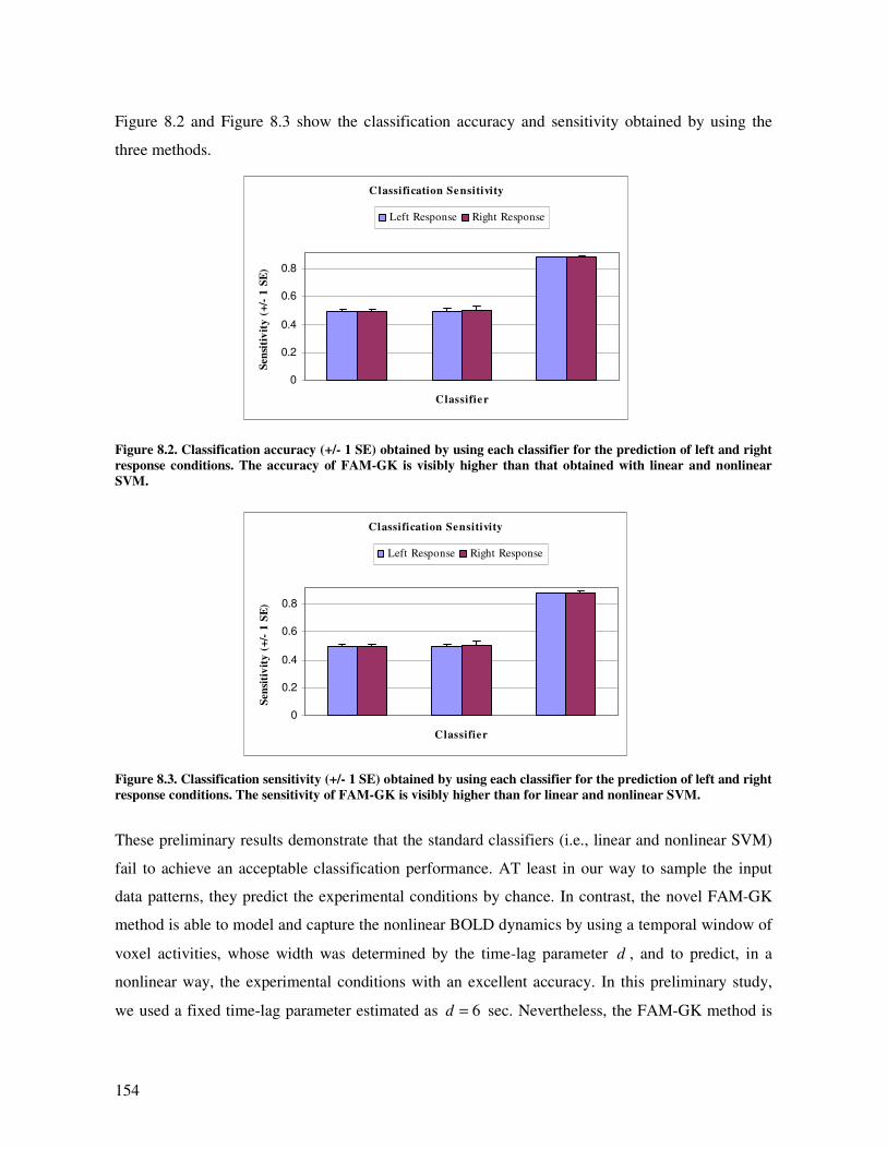
154

Figure 8.2 and Figure 8.3 show the classification accuracy and sensitivity obtained by using the

three methods.

Figure 8.2. Classification accuracy (+/- 1 SE) obtained by using each classifier for the prediction of left and right

response conditions. The accuracy of FAM-GK is visibly higher than that obtained with linear and nonlinear

SVM.

Figure 8.3. Classification sensitivity (+/- 1 SE) obtained by using each classifier for the prediction of left and right

response conditions. The sensitivity of FAM-GK is visibly higher than for linear and nonlinear SVM.

These preliminary results demonstrate that the standard classifiers (i.e., linear and nonlinear SVM)

fail to achieve an acceptable classification performance. AT least in our way to sample the input

data patterns, they predict the experimental conditions by chance. In contrast, the novel FAM-GK

method is able to model and capture the nonlinear BOLD dynamics by using a temporal window of

voxel activities, whose width was determined by the time-lag parameter d , and to predict, in a

nonlinear way, the experimental conditions with an excellent accuracy. In this preliminary study,

we used a fixed time-lag parameter estimated as 6=d sec. Nevertheless, the FAM-GK method is

Classification Sensitivity

0

0.2

0.4

0.6

0.8

Classifier

Sen

siti

vit

y (

+/-

1 S

E)


Classification Sensitivity

0

0.2

0.4

0.6

0.8

Classifier

Sen

siti

vit

y (

+/-

1 S

E)


155

more general and the time-lag d can be estimated by performing several simulations with different

delays and choosing the one leading to the best generalization performance on the test data.

Conclusion

In the last five years, pattern recognition methods, especially SVM, have become the standard way

for analysing fMRI data, overcoming the limitations imposed by the conventional univariate

approaches. However, these methods have been extensively used for fMRI data acquired in the

context of block or slow event-related experimental designs. In these cases, pattern recognition

analysis can estimate the experimental conditions at a single trial level. In fast event-related

experiments the nonlinearities on the acquired signals lead to BOLD activation peaks that are not

easy distinguishable. New methods were required for facing the fMRI data analysis of rapid event-

related designs.

In this Chapter we presented a preliminary study in which we tested three pattern recognition

methods on data acquired in a fast event-related experiment. Specifically, we were interested in

comparing FAM-GK method with the standard SVM (linear/nonlinear) used in a way that allow us

to consider each volume employed in the training and test datasets as much as possible as

independent measures. The preliminary results obtained in this first study, in which we performed a

ROI analysis on the bilateral PMC for predicting the left and right response conditions, confirmed

that SVM, used with both linear and nonlinear kernel did not reach an acceptable classification

performance, failing in capturing the nonlinear BOLD dynamics. Conversely, FAM-GK reached

very good accuracy levels in estimating the response pattern for each experimental condition.

In conclusion, we can affirm that from the theoretical and methodological perspective the FAM-GK

method is certainly a suitable tool for analysing fMRI data. It is usable in both block and fast event-

related designs. In particular, the high performance obtained for analysing the rapid event related

data presented in the discussed study allow us to conclude that FAM-GK is a useful and promising

tool for analysing fMRI data acquired in the context of fast event-related designs. Further

investigations are required for a more comprehensive understanding of its potential and

effectiveness.

157

Chapter 9

General conclusions

The advent of fMRI in cognitive science has significantly improved the knowledge about the neural

substrates underlying perceptual and cognitive processes. A still increasing scientific literature have

been produced by researchers, focusing on the investigation and identification of cerebral areas

involved in the cognitive processes, opportunely encoded in the experimental paradigms.

Conventional fMRI data analysis is based on univariate approaches (GLM) or more recently on

data-driven approaches (i.e., PCA, ICA, clustering algorithms) that characterised by a series of

assumptions and constraints, which validity has not been seriously enough taken into account from

fMRI researchers in the last years.

The conventional approaches for fMRI data analysis perform a multiple linear regression

correlating external predictors (task conditions) with the activity in specific brain regions,

generating statistical maps of localised activity (Worsley & Friston, 1995). In these approaches,

regressors are computed assuming a predefined shape of the HRF that is convolved with each task

condition and used for detecting some correlation. Nevertheless, the HRF can differ from the a

priori assumed shape, varying within different brain regions, from task to task, and on the base of

the strategies adopted by each participant. In order to model some differences in the hemodynamic

onset or in the shape of the HRF, which can include some additional factor such as time and

dispersion derivatives, the variability of the HRF has been considered as composed of a

combination of multiple basis functions, thus voxels whose activity do not follow a canonical HRF

could be otherwise detected, paying the cost of a more complex interpretation and understanding of

the obtained results. Moreover, the BOLD response does not obey to linearity assumptions: due to a

temporal correlation between the hemodynamic response evoked by a stimulus and that evoked by

the previous stimulus, if two stimuli are presented very close together or for short duration, the

BOLD signal may be lesser than the linear summation of the two individual responses. In order to

face this problem Volterra Kernels have been employed, which allow modelling the influence of a

stimulus on the successive ones. However, the GLM consider each voxel time series as an

independent measure of brain activity, ignoring spatial correlation within adjacent voxels that is

158

especially induced by using spatial smoothing in the pre-processing steps. Finally, the GLM

supposes that the components of the error term, in the multiple linear regression formulation, are

considered as independent and identically normally distributed, with the assumption that the amount

of noise in a single voxel does not depend on the task condition that may be not always valid.

Concluding, the GLM is based on a series of hypotheses that cannot be considered valid at all, and

as mentioned by O’Tool et al. (2007, page 1738) “The disadvantages of this approach are well

known, but are rarely taken seriously enough to limit the use of these techniques”.

In order to overcome some limitations of the GLM, multivariate analysis has been used in several

fMRI studies. In particular, these methods have been categorised into two classes depending on

considering or not an explicit association between brain activity patterns and experimental

conditions: multivariate exploratory analysis (i.e., data-driven methods) and multi-voxel pattern

analysis (see O'Toole et al. (2007) for a review). Specifically data-driven methods, like PCA, ICA

and clustering algorithms overcome some limitations of the voxelwise approaches, but are limited

in their ability to quantify patterns of activity in terms of the correspondent experimental conditions.

Commonly the interpretation of results is completely left to the experimenter, thus it is a difficult

and potentially error prone process. When using data-driven methods it is necessary to fix how

many components or clusters have to be considered for a given data set. More components are

included, more of the variance in the original data set can be explained, but more difficult could be

the interpretation of the results. Concluding, exploratory analysis, even if overcoming some severe

assumptions of the voxelwise analysis, relies on other fundamental assumptions and presents

several disadvantages: it is needed to consider only voxels belonging to regions with the same

statistical properties; it is necessary to specify the exact number of components or clusters; the

interpretation of the derived components is left completely to the experimenter; there is no

systematic way to determine if and how the explained variance is related to the manipulation of the

experimental variables.

Multi-voxel pattern analysis relays on the so-called reverse inference mechanism (Poldrack, 2006;

Poldrack, 2008; Poldrack, 2007) that inverts the forward inference of the GLM by inferring the

presence of perceptual or cognitive processes by just looking at neuroimaging data. Over the last

few years, several studies have started to test the effectiveness of these pattern based approaches for

fMRI data analysis. These methods, among which SVM, characterised by its higher generalization

ability and simplicity with respect to other ML techniques (i.e., artificial neural networks), has

gradually become the reference standard for the analysis of neuroimaging data, having the ability to

overcome the assumptions and the limitations of conventional univariate approaches (i.e., GLM)

and other data-driven techniques (i.e., PCA, ICA, and clustering algorithms).

159

These three methodological research lines have led to three different ways to ask research questions

for investigating the neural correlates of cognitive processes: conventional voxelwise statistical

methods ask the question if the activation of the single voxel varies significantly as a function of the

experimental conditions; exploratory methods ask the question of what brain activity patterns

explain variation across a set of brain maps; pattern based classification methods ask the question of

how, and at what extent, patterns of brain activation can consistently predict the cognitive processes

underlying the experimental conditions.

From a methodological perspective, the crucial issues for the use of these techniques regard voxel

selection, the choice of the classifier and its parameters, and the cross-validation methods for

properly testing the generalization abilities of the classifiers.

The problem of voxel selection has to be faced in order to limit the problem of overfitting and to

reduce the impact of the curse of dimensionality. Generally ML researchers deal with the variable

selection problem by using three different approaches: filter, wrapper and embedded approaches. In

particular, embedded methods differ from the first two, mainly in its property to perform variable

selection implicitly during learning and offer many advantages with respect to the previous

methods: unlike the filter methods, which are univariate methods independent of the used learning

machine, embedded methods incorporate variable selection into the multivariate model fitting;

unlike the wrapper approaches that use the classifier as a black box and require a high

computational effort, embedded methods are specific to the learning machine and are more

computational efficient. Another crucial aspect in dealing with pattern recognition techniques

concerns the choice of the classifier (i.e., linear vs nonlinear). Typically, nonlinear classifiers reach

better performance than the linear one, at least in problems complex enough to be explained by

more complex models. SVM can be classified as embedded methods for variable selection. In

particular, using linear SVM it is possible to obtain, for each experimental condition, the most

discriminating voxel subsets, just by analysing the weight vector produced by the classifier after

training. Conversely, on one hand using SVM with nonlinear kernels improves the classification

accuracy, but on the other hand the weight vector is not related to the input variables (voxels) but to

a new representation of the input space (the feature space) through an unknown nonlinear function.

In those cases, it is not possible to use the weight information, and several heuristics are used for

extracting the discriminating maps. This theoretical reason justifies the wide use of SVM with

linear kernels in the major part of the neuroimaging studies produced in the last few years.

Furthermore, these pattern based methods have been employed only for analysing fMRI data

acquired in the context of block or slow event-related designs, and new methods are required for

160

modelling in a more accurate way the nonlinear spatio-temporal dynamics of fMRI signals in the

context of fast event-related designs.

The aim of this thesis was to discuss the characteristics of the different approaches for fMRI data

analysis, and propose a novel, advanced technique that can solve the open questions of using pattern

recognition techniques for the analysis of fMRI data also in the context of fast event-related

experiments.

In a first study we explored the robustness of SVR used with nonlinear kernel, combined with a

filter approach for dimensionality reduction, in the case of an extremely complex regression

problem. The fMRI data were available through the Pittsburgh Brain Activity Interpretation

Competition (PBAIC, 2007), where we predicted the subjective experience of participants engaged

in several tasks performed in a virtual reality environment. The obtained results were quite good

and showed a certain degree of consistency across participants, highlighting the generalization

ability of nonlinear SVR, and leading this approach to be a promising and particularly interesting

tool also for real world BCI application. However, the obtained results highlighted that further

investigation on different voxel selection methods can increase the classification performances.

In a second study we proposed a methodology based on GA-SVM wrapper approach that allow us

to select, for each experimental condition, the most promising discriminating voxel subsets leading

to the best classification accuracy. The obtained results shown a consistent improvement of the


Elman recurrent neural networks) and SVM not combined with GAs, confirming the key role of

several aspects in the application of pattern recognition methods for fMRI data analysis, like voxel

selection, learning algorithm, nonlinear classification and the choice of learning parameters.

However, GAs are probabilistic approaches that suffer of the problem of local minima, thus

embedded methods based on optimization frameworks able to solve a concave-convex optimization

problem (i.e., finfing a global minimum) and to perform voxel selection implicitly in the training

process, could be more promising and can overcome also these limitations.

Several embedded methods have been developed in the last twelve years, facing the problem of

variable selection in different ways. We focused our attention on direct objective optimization

methods that formalise the optimization problem of regression estimation, taking into account both

the error term, relative to the regression, and the penalty (i.e., sparsity) term, relative to the variable

selection. Thus, the aim of a third study was to develop an embedded method able to deal with

variable selection and the class of nonlinear models. Firstly, we worked out a novel and effective

method (FAM-GK) extending an embedded method developed in the framework of functional

ANOVA models, developed for linear regression problems, in order to boost the effectiveness of

161

the algorithm in discovering nonlinear relations. Furthermore, we adapted this extended method to

the analysis of fMRI data, by considering spatio-temporal input patterns composed of a temporal

window of different width of voxel activations. The method is also able to discover the optimal

time-lag that allows us to insert the more useful information for the classification. We tested FAM-

GK on a synthetic dataset constructed by simulating a simple fast event-related fMRI dataset and by

using different time-lags for the preparation of the spatio-temporal input data, in order to understand

the property, implicit in the method, to discover the optimal lag lading to the more informative

patterns for the estimation problem. The obtained results confirmed the validity and the efficacy of

the FAM-GK method that seems to be a very promising tool for fMRI data analysis.

In a forth study, we reanalysed the fMRI data by Fias et al. (2007), comparing three pattern

recognition techniques, the linear and nonlinear SVM and the novel proposed method FAM-GK,

investigating the neural correlates of the representation of numerical and non-numerical ordered

sequences within the bilateral hIPS. The main findings of neuroimaging studies investigating the

neural correlates of numerical quantity representation, have shown the existence of three parietal

circuits for number processing (Dehaene et al., 2003), in particular the involvement of the bilateral

hIPS as a specific quantity system. The fMRI literature investigating the implication of hIPS in

processing numerical and non-numerical ordered sequences seems to be controversial. On the other

hand, the representation of numerical and non-numerical ordered sequences has been investigated

by several behavioural experiments, and neuropsychological studies on neglect patients. Several

results, in particular the neuropsychological findings, suggest that the spatial representation is a

specific property of the numerical quantities. Thus, the objective of this study was to exploit the

advantages of the pattern recognition methods for fMRI data analysis, for investigating this issue.

The obtained results showed that for fMRI data acquired within a block design, all the three

compared classifiers reached a different level of success. The FAM-GK method significantly

outperformed the other two classifiers producing discriminating maps containing only the most

predictive voxels. These results also showed a partial overlapping of the two representation systems

(i.e., numbers vs. letters), suggesting that within the hIPS regions there are neural substrates

codifying the cardinal dimension (numbers) and the ordinal dimension (numbers and letters) in a

partially independent way.

Finally, in the last preliminary study we tested three pattern recognition methods on data acquired in

the context of a fast event-related experiment. The first results obtained in this study confirmed that

SVM, used with both linear and nonlinear kernel, did not reach an acceptable classification

performance, failing in capturing the nonlinear BOLD dynamics. Conversely, FAM-GK reached

very good accuracy levels in estimating the response pattern for each experimental condition.

162

From the theoretical perspective the FAM-GK method is a suitable tool for analysing fMRI data. It

is usable in both block and fast event-related designs. Further investigations are required for a more

comprehensive understanding of its efficacy in rapid event-related fMRI experiments.

Concluding, from the methodological perspective we can conclude that time is ripe for considering

pattern recognition techniques as the status quo in the field of functional neuroimaging analysis.

The questions about the use of these techniques, like the voxel selection problem, the classifier

choice, and the cross-validation techniques for testing the generalization abilities of the classifiers,

have lead to a growing literature in the field of cognitive neuroscience, whereas new methods are

required for modelling the nonlinear spatio-temporal dynamics of fMRI signals in the context of

fast event-related designs. The proposed advanced method (i.e., FAM-GK) is able to capture these

dynamics in an excellent way, simultaneously providing a way for selecting the most predictive

voxels for each experimental condition. These analysis techniques have changed the way to

formulate research questions, from the simple cerebral activation localization, to a more

sophisticated way for studying modular or distributed representation of the information within the

brain, opening a new era in functional neuroscience.

163

Bibliography

Amaro, E.,Jr, & Barker, G. J. (2006). Study design in fMRI: Basic principles. Brain and Cognition,

60(3), 220-232. doi:10.1016/j.bandc.2005.11.009

Bach, F. R., Lanckriet, G. R. G., & Jordan, M. I. (2004). Multiple kernel learning, conic duality, and

the SMO algorithm. ACM International Conference Proceeding Series.

Bartfeld, E., & Grinvald, A. (1992). Relationships between orientation-preference pinwheels,

cytochrome oxidase blobs, and ocular-dominance columns in primate striate cortex.

Proceedings of the National Academy of Sciences of the United States of America, 89(24),

11905-11909.

Berlinet, A., & Thomas-Agnan, C. (2004). Reproducing kernel hilbert spaces in probability and

statistics. Kluwer Academic Publishers.

Bhatt, S., Mbwana, J., Adeyemo, A., Sawyer, A., Hailu, A., & Vanmeter, J. (2008). Lying about

facial recognition: An fMRI study. Brain and Cognition, doi:10.1016/j.bandc.2008.08.033

Binkofski, F., Fink, G. R., Geyer, S., Buccino, G., Gruber, O., Shah, N. J., et al. (2002). Neural

activity in human primary motor cortex areas 4a and 4p is modulated differentially by attention

to action. Journal of Neurophysiology, 88(1), 514-519.

Birbaumer, N., Murguialday, A. R., & Cohen, L. (2008). Brain-computer interface in paralysis.

Current Opinion in Neurology, 21(6), 634-638. doi:10.1097/WCO.0b013e328315ee2d

Boyd, S. P., & Vandenberghe, L. (2004). Convex optimization. Cambridge University Press.

164

Boynton, G. M., & Finney, E. M. (2003). Orientation-specific adaptation in human visual cortex.

The Journal of Neuroscience : The Official Journal of the Society for Neuroscience, 23(25),

8781-8787.

Bradley, P. S., & Mangasarian, O. L. (1998). Feature selection via concave minimization and

support vector machine. Paper presented at the 15th International Conference on Machine

Learning, San Francisco. 82-90.

Carlson, T. A., Schrater, P., & He, S. (2003). Patterns of activity in the categorical representations

of objects. Journal of Cognitive Neuroscience, 15(5), 704-717.

doi:10.1162/089892903322307429

Casarotti, M., Michielin, M., Zorzi, M., & Umilta, C. (2007). Temporal order judgment reveals how

number magnitude affects visuospatial attention. Cognition, 102(1), 101-117.

doi:10.1016/j.cognition.2006.09.001

Cox, D. D., & Savoy, R. L. (2003). Functional magnetic resonance imaging (fMRI) "brain reading":

Detecting and classifying distributed patterns of fMRI activity in human visual cortex.

NeuroImage, 19(2 Pt 1), 261-270.

Daly, J. J., & Wolpaw, J. R. (2008). Brain-computer interfaces in neurological rehabilitation. Lancet

Neurology, 7(11), 1032-1043. doi:10.1016/S1474-4422(08)70223-0

Davatzikos, C., Ruparel, K., Fan, Y., Shen, D. G., Acharyya, M., Loughead, J. W., et al. (2005).

Classifying spatial patterns of brain activity with machine learning methods: Application to lie

detection. NeuroImage, 28(3), 663-668. doi:10.1016/j.neuroimage.2005.08.009

165

De Martino, F., Gentile, F., Esposito, F., Balsi, M., Di Salle, F., Goebel, R., et al. (2007).

Classification of fMRI independent components using IC-fingerprints and support vector

machine classifiers. NeuroImage, 34(1), 177-194. doi:10.1016/j.neuroimage.2006.08.041

De Martino, F., Valente, G., Staeren, N., Ashburner, J., Goebel, R., & Formisano, E. (2008).

Combining multivariate voxel selection and support vector machines for mapping and

classification of fMRI spatial patterns. NeuroImage, 43(1), 44-58.

doi:10.1016/j.neuroimage.2008.06.037

Dehaene, S., Bossini, S., & Giraux, P. (1993). The mental representation of parity and number

magnitude. Journal of Experimental Psychology: General, 122, 371–396.

Dehaene, S., Piazza, M., Pinel, P., & Cohen, L. (2003). Three parietal circuits for number

processing. Cognitive Neuropsychology, 20, 487–506.

Dehaene, S. (2003). The neural basis of the weber-fechner law: A logarithmic mental number line.

Trends in Cognitive Sciences, 7(4), 145-147.

Dehaene, S., Dupoux, E., & Mehler, J. (1990). Is numerical comparison digital? analogical and

symbolic effects in two-digit number comparison. Journal of Experimental Psychology.Human

Perception and Performance, 16(3), 626-641.

Di Bono, M. G., & Zorzi, M. (2008). Decoding cognitive states from fMRI data using support

vector regression. PsychNology Journal, 6(2), 189-201.

Efron, B., & Tibshirani, R. (1993). An introduction to the bootstrap CHAPMAN & HALL/CRC,

Boca Raton.

Eger, E., Sterzer, P., Russ, M. O., Giraud, A. L., & Kleinschmidt, A. (2003). A supramodal number

representation in human intraparietal cortex. Neuron, 37(4), 719-725.

166

Fawcett, T. (2006). An introduction to ROC analysis. Pattern Recognition Letters, 27, 861-874.

Fias, W., Lammertyn, J., Caessens, B., & Orban, G. A. (2007). Processing of abstract ordinal

knowledge in the horizontal segment of the intraparietal sulcus. The Journal of Neuroscience :

The Official Journal of the Society for Neuroscience, 27(33), 8952-8956.

doi:10.1523/JNEUROSCI.2076-07.2007

Fischer, M. H., Castel, A. D., Dodd, M. D., & Pratt, J. (2003). Perceiving numbers causes spatial

shifts of attention. Nature Neuroscience, 6(6), 555-556. doi:10.1038/nn1066

Fischer, M. H., Warlop, N., Hill, R. L., & Fias, W. (2004). Oculomotor bias induced by number

perception. Experimental Psychology, 51(2), 91-97.

Forman, S. D., Cohen, J. D., Fitzgerald, M., Eddy, W. F., Mintun, M. A., & Noll, D. C. (1995).

Improved assessment of significant activation in functional magnetic resonance imaging

(fMRI): Use of a cluster-size threshold. Magnetic Resonance in Medicine : Official Journal of

the Society of Magnetic Resonance in Medicine / Society of Magnetic Resonance in Medicine,

33(5), 636-647.

Friedman, J. H. (1991). Multivariate adaptive regression splines (with discussion). Annals of

Statistics, 19, 1-141.

Friston, K. J., Josephs, O., Rees, G., & Turner, R. (1998). Nonlinear event-related responses in

fMRI. Magnetic Resonance in Medicine : Official Journal of the Society of Magnetic Resonance

in Medicine / Society of Magnetic Resonance in Medicine, 39(1), 41-52.

Genovese, C. R., Lazar, N. A., & Nichols, T. (2002). Thresholding of statistical maps in functional

neuroimaging using the false discovery rate. NeuroImage, 15(4), 870-878.

doi:10.1006/nimg.2001.1037

167

Geschwind, N. (1965a). Disconnexion syndromes in animals and man. I. Brain : A Journal of

Neurology, 88(2), 237-294.

Geschwind, N. (1965b). Disconnexion syndromes in animals and man. II. Brain : A Journal of

Neurology, 88(3), 585-644.

Gevers, W., Reynvoet, B., & Fias, W. (2003). The mental representation of ordinal sequences is

spatially organized. Cognition, 87(3), B87-95.

Gevers, W., Verguts, T., Reynvoet, B., Caessens, B., & Fias, W. (2006). Numbers and space: A

computational model of the SNARC effect. Journal of Experimental Psychology.Human

Perception and Performance, 32(1), 32-44. doi:10.1037/0096-1523.32.1.32

Glover, G. H. (1999). Deconvolution of impulse response in event-related BOLD fMRI.

NeuroImage, 9(4), 416-429.

Gobel, S. M., Calabria, M., Farne, A., & Rossetti, Y. (2006). Parietal rTMS distorts the mental

number line: Simulating 'spatial' neglect in healthy subjects. Neuropsychologia, 44(6), 860-868.

doi:10.1016/j.neuropsychologia.2005.09.007

Grill-Spector, K., Knouf, N., & Kanwisher, N. (2004). The fusiform face area subserves face

perception, not generic within-category identification. Nature Neuroscience, 7(5), 555-562.

doi:10.1038/nn1224

Guyon, I., & Elisseeff, A. (2003). An introduction to variable and feature selection. Journal of

Machine Learning Research, 3(7), 1157-1182.

Hakun, J. G., Ruparel, K., Seelig, D., Busch, E., Loughead, J. W., Gur, R. C., et al. (2008). Towards

clinical trials of lie detection with fMRI. Social Neuroscience, , 1-10.

doi:10.1080/17470910802188370

168

Hanson, S. J., Matsuka, T., & Haxby, J. V. (2004). Combinatorial codes in ventral temporal lobe for

object recognition: Haxby (2001) revisited: Is there a "face" area? NeuroImage, 23(1), 156-166.

doi:10.1016/j.neuroimage.2004.05.020

Hastie, ,Trevor J., & Tibshirani, ,Robert. (1990). Generalized additive models. London etc.:

Chapman and Hall.

Haxby, J. V., Gobbini, M. I., Furey, M. L., Ishai, A., Schouten, J. L., & Pietrini, P. (2001).

Distributed and overlapping representations of faces and objects in ventral temporal cortex.

Science (New York, N.Y.), 293(5539), 2425-2430. doi:10.1126/science.1063736

Haynes, J. D. (2008). Detecting deception from neuroimaging signals--a data-driven perspective.

Trends in Cognitive Sciences, 12(4), 126-7; author reply 127-8. doi:10.1016/j.tics.2008.01.003

Haynes, J. D., & Rees, G. (2005a). Predicting the orientation of invisible stimuli from activity in

human primary visual cortex. Nature Neuroscience, 8(5), 686-691. doi:10.1038/nn1445

Haynes, J. D., & Rees, G. (2005b). Predicting the stream of consciousness from activity in human

visual cortex. Current Biology : CB, 15(14), 1301-1307. doi:10.1016/j.cub.2005.06.026

Haynes, J. D., & Rees, G. (2006). Decoding mental states from brain activity in humans. Nature

Reviews.Neuroscience, 7(7), 523-534. doi:10.1038/nrn1931

Haynes, J. D., Sakai, K., Rees, G., Gilbert, S., Frith, C., & Passingham, R. E. (2007). Reading

hidden intentions in the human brain. Current Biology : CB, 17(4), 323-328.

doi:10.1016/j.cub.2006.11.072

Henson, R. (2006). Forward inference using functional neuroimaging: Dissociations versus

associations. Trends in Cognitive Sciences, 10(2), 64-69. doi:10.1016/j.tics.2005.12.005

169

Huettel, ,Scott A., Song, ,Allen W., & McCarthy, ,Gregory. (2004). Functional magnetic resonance

imaging. Sunderland: Sinauer Associates.

Huettel, S. A., & McCarthy, G. (2000). Evidence for a refractory period in the hemodynamic

response to visual stimuli as measured by MRI. NeuroImage, 11(5 Pt 1), 547-553.

doi:10.1006/nimg.2000.0553

Huettel, S. A., & McCarthy, G. (2001). The effects of single-trial averaging upon the spatial extent

of fMRI activation. Neuroreport, 12(11), 2411-2416.

Jacob, S. N., & Nieder, A. (2008). The ABC of cardinal and ordinal number representations. Trends

in Cognitive Sciences, 12(2), 41-43. doi:10.1016/j.tics.2007.11.006

Jewell, G., & McCourt, M. E. (2000). Pseudoneglect: A review and meta-analysis of performance

factors in line bisection tasks. Neuropsychologia, 38(1), 93-110.

Kamitani, Y., & Tong, F. (2005). Decoding the visual and subjective contents of the human brain.

Nature Neuroscience, 8(5), 679-685. doi:10.1038/nn1444

Kamitani, Y., & Tong, F. (2006). Decoding seen and attended motion directions from activity in the

human visual cortex. Current Biology : CB, 16(11), 1096-1102. doi:10.1016/j.cub.2006.04.003

Kanwisher, N., McDermott, J., & Chun, M. M. (1997). The fusiform face area: A module in human

extrastriate cortex specialized for face perception. The Journal of Neuroscience : The Official

Journal of the Society for Neuroscience, 17(11), 4302-4311.

Kanwisher, N., Stanley, D., & Harris, A. (1999). The fusiform face area is selective for faces not

animals. Neuroreport, 10(1), 183-187.

170

Kanwisher, N., & Yovel, G. (2006). The fusiform face area: A cortical region specialized for the

perception of faces. Philosophical Transactions of the Royal Society of London.Series B,

Biological Sciences, 361(1476), 2109-2128. doi:10.1098/rstb.2006.1934

Kohavi, R., & John, G. H. (1997). Wrappers for feature subset selection. Artificial Intelligence,

97(1-2), 273-324.

Kozel, F. A., Revell, L. J., Lorberbaum, J. P., Shastri, A., Elhai, J. D., Horner, M. D., et al. (2004).

A pilot study of functional magnetic resonance imaging brain correlates of deception in healthy

young men. The Journal of Neuropsychiatry and Clinical Neurosciences, 16(3), 295-305.

doi:10.1176/appi.neuropsych.16.3.295

Kriegeskorte, N., Goebel, R., & Bandettini, P. (2006). Information-based functional brain mapping.

Proceedings of the National Academy of Sciences of the United States of America, 103(10),

3863-3868. doi:10.1073/pnas.0600244103

Kubler, A., & Birbaumer, N. (2008). Brain-computer interfaces and communication in paralysis:

Extinction of goal directed thinking in completely paralysed patients? Clinical Neurophysiology

: Official Journal of the International Federation of Clinical Neurophysiology, 119(11), 2658-

2666. doi:10.1016/j.clinph.2008.06.019

Lanckriet, G., Cristianini, N., Bartlett, P., El Ghaoui, L., & Jordan, M. (2004). Learning the kernel

matrix with semidefinite programming. The Journal of Machine Learning Research, 5, 27-72.

Langleben, D. D., Loughead, J. W., Bilker, W. B., Ruparel, K., Childress, A. R., Busch, S. I., et al.

(2005). Telling truth from lie in individual subjects with fast event-related fMRI. Human Brain

Mapping, 26(4), 262-272. doi:10.1002/hbm.20191

171

Le Clec'H, G., Dehaene, S., Cohen, L., Mehler, J., Dupoux, E., Poline, J. B., et al. (2000). Distinct

cortical areas for names of numbers and body parts independent of language and input modality.

NeuroImage, 12(4), 381-391. doi:10.1006/nimg.2000.0627

Lee, J. H., Ryu, J., Jolesz, F. A., Cho, Z. H., & Yoo, S. S. (2008). Brain-machine interface via real-

time fMRI: Preliminary study on thought-controlled robotic arm. Neuroscience Letters,

doi:10.1016/j.neulet.2008.11.024

Lee, T. M., Liu, H. L., Tan, L. H., Chan, C. C., Mahankali, S., Feng, C. M., et al. (2002). Lie

detection by functional magnetic resonance imaging. Human Brain Mapping, 15(3), 157-164.

Lin, Y., & Zhang, H. H. (2006). Component selection and smoothing in multivariate nonparametric

regression. The Annals of Statistics, 34(5), 2272-2297.

Loetscher, T., & Brugger, P. (2007). Exploring number space by random digit generation.

Experimental Brain Research.Experimentelle Hirnforschung.Experimentation Cerebrale,

180(4), 655-665. doi:10.1007/s00221-007-0889-0

Loetscher, T., Schwarz, U., Schubiger, M., & Brugger, P. (2008). Head turns bias the brain's

internal random generator. Current Biology : CB, 18(2), R60-2. doi:10.1016/j.cub.2007.11.015

Loftus, A. M., Nicholls, M. E., Mattingley, J. B., & Bradshaw, J. L. (2008). Left to right:

Representational biases for numbers and the effect of visuomotor adaptation. Cognition, 107(3),

1048-1058. doi:10.1016/j.cognition.2007.09.007

Longo, M. R., & Lourenco, S. F. (2007). Spatial attention and the mental number line: Evidence for

characteristic biases and compression. Neuropsychologia, 45(7), 1400-1407.

doi:10.1016/j.neuropsychologia.2006.11.002

172

Mapelli, D., Rusconi, E., & Umilta, C. (2003). The SNARC effect: An instance of the simon effect?

Cognition, 88(3), B1-10.

Menon, R. S., Ogawa, S., Hu, X., Strupp, J. P., Anderson, P., & Ugurbil, K. (1995). BOLD based

functional MRI at 4 tesla includes a capillary bed contribution: Echo-planar imaging correlates

with previous optical imaging using intrinsic signals. Magnetic Resonance in Medicine : Official

Journal of the Society of Magnetic Resonance in Medicine / Society of Magnetic Resonance in

Medicine, 33(3), 453-459.

Micchelli, C. A., & Pontil, M. (2005). Learning the kernel function via regularization. The Journal

of Machine Learning Research, 6, 1099–1125.

Micchelli, C. A., & Pontil, M. (2007). Feature space perspectives for learning the kernel. Machine

Learning, 66(2), 297–319.

Mitchell, T. M., Hutchinson, R., Niculescu, R. S., Pereira, F., Wang, X., Just, M., et al. (2004).

Learning to decode cognitive states from brain images. Machine Learnig, 57, 145-175.

Mitchell, T. M., Hutchinson, R., Just, M. A., Niculescu, R. S., Pereira, F., & Wang, X. (2003).

Classifying instantaneous cognitive states from FMRI data. AMIA ...Annual Symposium

Proceedings / AMIA Symposium.AMIA Symposium, , 465-469.

Mourao-Miranda, J., Friston, K. J., & Brammer, M. (2007). Dynamic discrimination analysis: A

spatial-temporal SVM. NeuroImage, 36(1), 88-99. doi:10.1016/j.neuroimage.2007.02.020

Nieder, A. (2005). Counting on neurons: The neurobiology of numerical competence. Nature

Reviews.Neuroscience, 6(3), 177-190. doi:10.1038/nrn1626

173

Nieder, A., & Miller, E. K. (2004). A parieto-frontal network for visual numerical information in

the monkey. Proceedings of the National Academy of Sciences of the United States of America,

101(19), 7457-7462. doi:10.1073/pnas.0402239101

Nijboer, F., Sellers, E. W., Mellinger, J., Jordan, M. A., Matuz, T., Furdea, A., et al. (2008). A

P300-based brain-computer interface for people with amyotrophic lateral sclerosis. Clinical

Neurophysiology : Official Journal of the International Federation of Clinical Neurophysiology,

119(8), 1909-1916. doi:10.1016/j.clinph.2008.03.034

Noirhomme, Q., Kitney, R. I., & Macq, B. (2008). Single-trial EEG source reconstruction for brain-

computer interface. IEEE Transactions on Bio-Medical Engineering, 55(5), 1592-1601.

doi:10.1109/TBME.2007.913986

Norman, K. A., Polyn, S. M., Detre, G. J., & Haxby, J. V. (2006). Beyond mind-reading: Multi-

voxel pattern analysis of fMRI data. Trends in Cognitive Sciences, 10(9), 424-430.

doi:10.1016/j.tics.2006.07.005

O'Toole, A. J., Jiang, F., Abdi, H., & Haxby, J. V. (2005). Partially distributed representations of

objects and faces in ventral temporal cortex. Journal of Cognitive Neuroscience, 17(4), 580-590.

doi:10.1162/0898929053467550

O'Toole, A. J., Jiang, F., Abdi, H., Penard, N., Dunlop, J. P., & Parent, M. A. (2007). Theoretical,

statistical, and practical perspectives on pattern-based classification approaches to the analysis

of functional neuroimaging data. Journal of Cognitive Neuroscience, 19(11), 1735-1752.

doi:10.1162/jocn.2007.19.11.1735

Pauling, L., & Coryell, C. D. (1936). The magnetic properties and structure of hemoglobin,

oxyhemoglobin and carbonmonoxyhemoglobin. Proceedings of the National Academy of

Sciences of the United States of America, 22(4), 210-216.

174

Piazza, M., & Dehaene, S. (2004). From number neurons to mental arithmetic: The cognitive

neuroscience of number sense. The cognitive neurosciences (3rd ed., pp. 865–875). Cambridge,

MA:MIT: Gazzaniga, M.S.

Piazza, M., Izard, V., Pinel, P., Le Bihan, D., & Dehaene, S. (2004). Tuning curves for approximate

numerosity in the human intraparietal sulcus. Neuron, 44(3), 547-555.

doi:10.1016/j.neuron.2004.10.014

Piazza, M., Pinel, P., Le Bihan, D., & Dehaene, S. (2007). A magnitude code common to

numerosities and number symbols in human intraparietal cortex. Neuron, 53(2), 293-305.

doi:10.1016/j.neuron.2006.11.022

Piccione, F., Priftis, K., Tonin, P., Vidale, D., Furlan, R., Cabinato, M., et al. (2008). Task and

stimulation paradigm effects in a P300 brain computer interface exploitable in a virtual

environment: A pilot study.6(1), 99-108.

Piccione, F., Giorgi, F., Tonin, P., Priftis, K., Giove, S., Silvoni, S., et al. (2006). P300-based brain

computer interface: Reliability and performance in healthy and paralysed participants. Clinical

Neurophysiology : Official Journal of the International Federation of Clinical Neurophysiology,

117(3), 531-537. doi:10.1016/j.clinph.2005.07.024

Pinel, P., Dehaene, S., Riviere, D., & LeBihan, D. (2001). Modulation of parietal activation by

semantic distance in a number comparison task. NeuroImage, 14(5), 1013-1026.

doi:10.1006/nimg.2001.0913

Poldrack, R. A. (2006). Can cognitive processes be inferred from neuroimaging data? Trends in

Cognitive Sciences, 10(2), 59-63. doi:10.1016/j.tics.2005.12.004

175

Poldrack, R. A. (2007). Region of interest analysis for fMRI. Social Cognitive and Affective

Neuroscience, 2(1), 67-70. doi:10.1093/scan/nsm006

Poldrack, R. A. (2008). The role of fMRI in cognitive neuroscience: Where do we stand? Current

Opinion in Neurobiology, 18(2), 223-227. doi:10.1016/j.conb.2008.07.006

Polyn, S. M., Natu, V. S., Cohen, J. D., & Norman, K. A. (2005). Category-specific cortical activity

precedes retrieval during memory search. Science (New York, N.Y.), 310(5756), 1963-1966.

doi:10.1126/science.1117645

Posner, ,Michael I., & Raichle, ,Marcus E. (1994). Images of mind. New York: Scientific american

library.

Priftis, K., Zorzi, M., Meneghello, F., Marenzi, R., & Umilta, C. (2006). Explicit versus implicit

processing of representational space in neglect: Dissociations in accessing the mental number

line. Journal of Cognitive Neuroscience, 18(4), 680-688. doi:10.1162/jocn.2006.18.4.680

Proctor, R. W., & Cho, Y. S. (2006). Polarity correspondence: A general principle for performance

of speeded binary classification tasks. Psychological Bulletin, 132(3), 416-442.

doi:10.1037/0033-2909.132.3.416

Robson, M. D., Dorosz, J. L., & Gore, J. C. (1998). Measurements of the temporal fMRI response

of the human auditory cortex to trains of tones. NeuroImage, 7(3), 185-198.

doi:10.1006/nimg.1998.0322

Rossetti, Y., Jacquin-Courtois, S., Rode, G., Ota, H., Michel, C., & Boisson, D. (2004). Does action

make the link between number and space representation? visuo-manual adaptation improves

number bisection in unilateral neglect. Psychological Science : A Journal of the American

Psychological Society / APS, 15(6), 426-430. doi:10.1111/j.0956-7976.2004.00696.x

176

Roth, V. (2004). The generalized LASSO. IEEE Transactions on Neural Networks / a Publication

of the IEEE Neural Networks Council, 15(1), 16-28. doi:10.1109/TNN.2003.809398

Santens, S., & Gevers, W. (2008). The SNARC effect does not imply a mental number line.

Cognition, 108(1), 263-270. doi:10.1016/j.cognition.2008.01.002

Sato, J. R., Mourao-Miranda, J., Morais Martin Mda, G., Amaro, E.,Jr, Morettin, P. A., &

Brammer, M. J. (2008). The impact of functional connectivity changes on support vector

machines mapping of fMRI data. Journal of Neuroscience Methods, 172(1), 94-104.

doi:10.1016/j.jneumeth.2008.04.008

Schwarz, W., & Keus, I. M. (2004). Moving the eyes along the mental number line: Comparing

SNARC effects with saccadic and manual responses. Perception & Psychophysics, 66(4), 651-

664.

Schwarz, W., & Muller, D. (2006). Spatial associations in number-related tasks: A comparison of

manual and pedal responses. Experimental Psychology, 53(1), 4-15.

Signoretto, M., Pelckmans, K., & Suykens, J. A. K. (2008a). Functional ANOVA models: Convex-

concave approach and concurvity analysis (Internal Report No. 08-203). ESAT-SISTA,

K.U.Leuven (Leuven, Belgium): Retrieved from

ftp://ftp.esat.kuleuven.ac.be/pub/SISTA//signoretto/Signoretto08203.pdf

Signoretto, M., Pelckmans, K., & Suykens, J. A. K. (2008b). Quadratically constrained quadratic

programming for subspace selection in kernel regression estimation. Paper presented at the 18th

International Conference on Artificial Neural Networks (ICANN), Prague, Czech Republic.

177

Spence, S. A., Kaylor-Hughes, C., Farrow, T. F., & Wilkinson, I. D. (2008). Speaking of secrets

and lies: The contribution of ventrolateral prefrontal cortex to vocal deception. NeuroImage,

40(3), 1411-1418. doi:10.1016/j.neuroimage.2008.01.035

Spiridon, M., & Kanwisher, N. (2002). How distributed is visual category information in human

occipito-temporal cortex? an fMRI study. Neuron, 35(6), 1157-1165.

Steinwart, I., Hush, D., & Scovel, C. (2006). An explicit description of the reproducing kernel

hilbert spaces of gaussian rbf kernels. IEEE Trans. Inform. Theory, 52, 4635–4643.

Stoianov, I., Kramer, P., Umilta, C., & Zorzi, M. (2008). Visuospatial priming of the mental

number line. Cognition, 106(2), 770-779. doi:10.1016/j.cognition.2007.04.013

Strother, S. C., Anderson, J., Hansen, L. K., Kjems, U., Kustra, R., Sidtis, J., et al. (2002). The

quantitative evaluation of functional neuroimaging experiments: The NPAIRS data analysis

framework. NeuroImage, 15(4), 747-771. doi:10.1006/nimg.2001.1034

Suykens, J. A., Vandewalle, J., & De Moor, B. (2001). Optimal control by least squares support

vector machines. Neural Networks : The Official Journal of the International Neural Network

Society, 14(1), 23-35.

TEUBER, H. L. (1955). Physiological psychology. Annual Review of Psychology, 6, 267-296.

doi:10.1146/annurev.ps.06.020155.001411

Tibshirani, R. (1996). Regression shrinkage and selection via the lasso. Journal of the Royal

Statistical Society. Series B(Methodological), 58(1), 267–288.

Umilta, C., Priftis, K., & Zorzi, M. (2008). The spatial representation of numbers: Evidence from

neglect and pseudoneglect. Experimental Brain Research.Experimentelle

Hirnforschung.Experimentation Cerebrale, doi:10.1007/s00221-008-1623-2

178

Vanduffel, W., Tootell, R. B., Schoups, A. A., & Orban, G. A. (2002). The organization of

orientation selectivity throughout macaque visual cortex. Cerebral Cortex (New York, N.Y.:

1991), 12(6), 647-662.

Vapnik, ,Vladimir N. (1998). Statistical learning theory. New York etc.: Wiley.

Vapnik, V. N. (1999). An overview of statistical learning theory. IEEE Transactions on Neural

Networks / a Publication of the IEEE Neural Networks Council, 10(5), 988-999.

doi:10.1109/72.788640

Vazquez, A. L., & Noll, D. C. (1998). Nonlinear aspects of the BOLD response in functional MRI.

NeuroImage, 7(2), 108-118. doi:10.1006/nimg.1997.0316

Worsley, K. J., & Friston, K. J. (1995). Analysis of fMRI time-series revisited--again. NeuroImage,

2(3), 173-181. doi:10.1006/nimg.1995.1023

Xiong, J., Gao, J., Lancaster, J. L., & Fox, P. T. (1995). Clustered pixels analysis of functional MRI

activation studies of the human brain. Human Brain Mapping, 3, 287-301.

Yang, L., Li, J., Yao, Y., & Wu, X. (2008). A P300 detection algorithm based on F-score feature

selection and support vector machines. Sheng Wu Yi Xue Gong Cheng Xue Za Zhi = Journal of

Biomedical Engineering = Shengwu Yixue Gongchengxue Zazhi, 25(1), 23-6, 52.

Zamarian, L., Egger, C., & Delazer, M. (2007). The mental representation of ordered sequences in

visual neglect. Cortex; a Journal Devoted to the Study of the Nervous System and Behavior,

43(4), 542-550.

Zorzi, M., Mapelli, D., Rusconi, E., & Umilta, C. (2003). Automatic spatial coding of perceived

gaze direction is revealed by the simon effect. Psychonomic Bulletin & Review, 10(2), 423-429.

179

Zorzi, M., Priftis, K., Meneghello, F., Marenzi, R., & Umilta, C. (2006). The spatial representation

of numerical and non-numerical sequences: Evidence from neglect. Neuropsychologia, 44(7),

1061-1067. doi:10.1016/j.neuropsychologia.2005.10.025

Zorzi, M., Priftis, K., & Umilta, C. (2002). Brain damage: Neglect disrupts the mental number line.

Nature, 417(6885), 138-139. doi:10.1038/417138a

UNIVERSITA' DEGLI STUDI DI PADOVA -...

Documents

Transcript of UNIVERSITA' DEGLI STUDI DI PADOVA -...