
UNIVERSITÀ DEGLI STUDI DI PADOVA - core.ac.uk · DIPARTIMENTO DI TECNICA E GESTIONE DEI ......
166
UNIVERSITÀ DEGLI STUDI DI PADOVA DIPARTIMENTO DI TECNICA E GESTIONE DEI SISTEMI INDUSTRIALI CORSO DI LAUREA MAGISTRALE IN INGEGNERIA MECCATRONICA Model-based development of a self-balancing, two-wheel transporter Relatore: Roberto Oboe Laureando: Dino Spiller 1084324-IMC ANNO ACCADEMICO: 2017-2018
Transcript of UNIVERSITÀ DEGLI STUDI DI PADOVA - core.ac.uk · DIPARTIMENTO DI TECNICA E GESTIONE DEI ......
UNIVERSITÀ DEGLI STUDI DI PADOVA
DIPARTIMENTO DI TECNICA E GESTIONE DEI SISTEMI INDUSTRIALICORSO DI LAUREA MAGISTRALE IN INGEGNERIA MECCATRONICA
Model-based development of a self-balancing,two-wheel transporter
Relatore: Roberto Oboe
Laureando: Dino Spiller1084324-IMC
ANNO ACCADEMICO: 2017-2018
[ December 2, 2017 at 17:06 – classicthesis ]

[ December 2, 2017 at 17:06 – classicthesis ]
S U M M A RY
The current work aim to propose an evolute theoretical model for the two-wheelself-balancing transporter, together with a practical implementation of the device,that serves as proof for the model itself.
Inside this document the mathematical modeling, the control strategies (LQR forthe equilibrium and PI for steering) and the management the system non-idealitiesthat affects the real-device.
An automated powerful tool was realized and described, to make it possiblethe easy compare of simulation and real-device performances/behavior. It can beconsidered a useful tool for the proof of future studies and system improvements.
The results of this work are a good correspondence between the theoreticalmodel simulation and the real device behavior, in addition to the good stabilityperformances of both the simulated and real device.
iii
[ December 2, 2017 at 17:06 – classicthesis ]

[ December 2, 2017 at 17:06 – classicthesis ]
Perché la vita é un brivido che vola via,é tutto un equilibrio sopra la follia.
(Vasco Rossi)
T H A N K S
To Prof. Roberto Oboe: thanks for all your kindness and support, especially for en-couraging me in the moment when I believed I couldn’t ever make the devicework. You made the things "lighter", with your sympathy and that finally helpedme. Sometimes I think I’d love to be like you.
To Simone: you were not simply a colleague. You always had the patience oflistening me when I told you my difficulties about this project and even gave meuseful keys to see difficult situations from the right perspective.
To Maria, my mother: you always believed in me and see something that some-times even I couldn’t. I’m your seventh son, but you always made me feel like Iwas the only.
To Antonio, my father: thanks for your example. What I learned from you is thelove for the honesty and that for the study: an activity you never stopped in everymoment of your life.
To Nicola and Andrea: you are the "sun" of my life. You’re one of the main moti-vation of this work: it’s a toy for you! I will never forget the times passed with yousleeping on my knees, when I studied and the times you told me "don’t give up,papa!". I wish you’ll be blessed by equally lovelies children.
And over all, to Michela: It’s you I miss, every day, when I can’t wait to be backat home. This work is only the "iceberg top" of what you helped me to do theseyears of university: your patience, your encouragements and your love made itpossible the completion of this hard work. I’ll always remember the moments wehad a break together, making our "terrazza-parties": pleased by the aroma of yourpresence, of your beauty and your love, that is even better than that of the coffeewe had together.
Without you none of the words in this story might have been written... eventhose in this book.
v
[ December 2, 2017 at 17:06 – classicthesis ]

[ December 2, 2017 at 17:06 – classicthesis ]

C O N T E N T S
1 introduction 1
1.0.1 Existing literature 2
1.0.2 Motivation and attempts 2
1.0.3 Thesis outline 3
2 definition of system specifications 5
2.1 Introduction 5
2.2 Problem definition 5
2.3 Dimensions 5
2.4 Motor torque 6
2.4.1 Speed at full weight, inclined ground 6
2.4.2 Maximum deceleration 7
2.4.3 Motor choice 7
2.5 Battery 10
2.6 Motor Driver 11
2.7 IMU 12
2.8 Joystick 13
2.9 Remote communication 14
2.10 Overall architecture and Shematic 15
2.10.1 Master board 17
2.10.2 Slave Board 17
3 system modelling 19
3.1 Introduction 19
3.2 Kinematic model 19
3.2.1 Assumptions 21
3.3 Dynamic model 22
3.4 Lagrangian 23
3.5 System linearization 24
3.6 System decoupling 26
3.7 Stability analisys 28
3.8 Conclusions 30
4 a more realistic model 31
4.1 introduction 31
4.2 Linearization of the new system 33
4.2.1 decoupling 34
4.3 Transfer function and stability analisys 35
5 control 37
5.1 Introduction 37
5.2 Control of Equilibrium subsystem 37
5.2.1 The optimum (LQR) controller 37
5.2.2 Application of LQR to the equilibrium subsystem 41
5.2.3 Stability analysis 42
5.2.4 LQR tuning 45
5.3 Control of Steering subsystem 46
5.3.1 LQR steering controller 47
5.3.2 PI steering controller 48
5.4 Conclusions 51
vii
[ December 2, 2017 at 17:06 – classicthesis ]
viii contents
6 system non-idealities 53
6.1 Introduction 53
6.2 Motor torque 53
6.3 Current Loop 58
6.4 Angle and angle-rate reading 62
6.4.1 IMU modelling and calibration 63
6.4.2 angle measurement 67
6.4.3 Sensor fusion 69
6.4.4 Kalman filtering 70
6.4.5 Kalman tuning 71
6.4.6 The Bartlett’s test 72
6.4.7 Application of Kalman Filter to the system 73
6.5 Position and Velocity reading 75
6.6 Conclusions 84
7 algorithms implementation 85
7.1 Introduction 85
7.2 Overall architecture and behavior 85
7.3 The Matlab environment 87
7.3.1 Vehicle parameters 88
7.3.2 overall model 88
7.3.3 Equilibrium model and controller 90
7.3.4 Steering model and controller 91
7.3.5 Digital filters 93
7.3.6 Simulink simulation 94
7.3.7 bluetooth param writer 95
7.3.8 Data collection and post-processing 96
7.4 The embedded environment 98
7.5 The control firmware 98
7.5.1 The control algorithm 99
7.5.2 data filtering/processing 102
7.5.3 state recontstruction 105
7.5.4 control signals generation 106
7.5.5 errors management and safety strategies 109
7.6 Conclusions 111
8 model validation 113
8.1 Introduction 113
8.2 Velocity and acceleration reconstruction 113
8.2.1 position and acceleration 114
8.3 IMU model validation and tuning 116
8.3.1 datasheet verification 116
8.4 Tuning sensor fusion algorithm 120
8.4.1 Verification of linear acceleration subtraction 120
8.4.2 Finding the best coefficients for complementary filter 121
8.5 Validation of the first model 123
8.5.1 Steady state 123
8.5.2 Reference-following sequence 125
8.6 Steering model and controller tuning 128
8.7 Equilibrium model and controller tuning 129
8.8 Tuning and validation of the evolved (rider’s) model 131
8.8.1 Controller tuning, for the rider 133
[ December 2, 2017 at 17:06 – classicthesis ]
contents ix
8.8.2 Tuning the parameters of "Q" matrix 134
8.9 Conclusions 136
Conclusions 139
Appendix 141
a appendix-a : lagrangian derivation step-by-step 143
a.1 Lagrangian: derivation for the first model 143
bibliography 147
[ December 2, 2017 at 17:06 – classicthesis ]
L I S T O F F I G U R E S
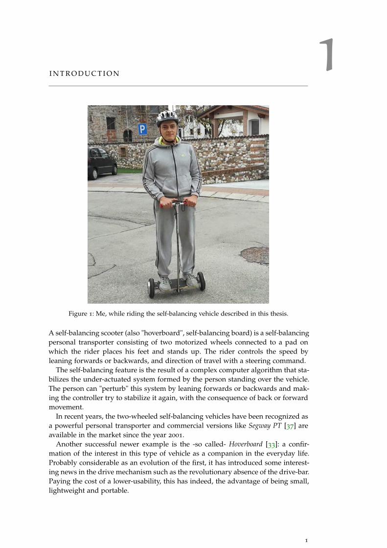
Figure 1 Me, while riding the self-balancing vehicle described in thisthesis. 1
Figure 2 Base dimensions (observed from upside) 6
Figure 3 The requirement of a certain minimum speed at full weight,along an inclined plane. Figure from [38]. 6
Figure 4 HUB motor, used in many self-balancing toys. Figure from[10]. 8
Figure 5 RC model motor, image from [1] 9
Figure 6 Battery used for the high-current RC motor. Figure from[6]. 10
Figure 7 Open-hardware motor controller, a project of Benjamin Ved-der [35] image also from [35] 12
Figure 8 Open-hardware IMU i2C evaluation module of Invensense’sMPU6050. Figure from [28]. 13
Figure 9 Joystick used during experiments. Image from [2] 14
Figure 10 Serial-to-bluetooth (HC-06) module used for remote loggingof data coming from the self-balancing transporter, to thehost PC. Figure from [5] 15
Figure 11 Hardware architecture schematic of the self-balancing trans-porter. Note the absence of a "central board" and the choiceof a master-slave architecture 16
Figure 12 Graphical representation of the entities of the system. 19
Figure 13 Detailed description of torques and references on right wheel.In the left, the wheel, while in the right the TWSBT base:note that the torque generated by the motor applies equaland opposite in the two bodies. The symmetric holds for theleft wheel. 23
Figure 14 Poles and zero-es of equilibrium subsystem (open-loop un-stable poles). 28
Figure 15 Free evolution of the model ?? with θP(0) = 5° and τθ = 0
. 29
Figure 16 Root locus and Bode plot with stability margins of the δτδ
transter function (33). 30
Figure 17 A more-complex model comes with the introduction of afurther freedom-degree: the separation of the angle betweenthe rider and the base. 31
Figure 18 Zero-order-hold process, used (as default method) by MAT-LAB, for the continous-to-discrete conversion of a system.Figure from MATLAB’s website. 41
Figure 19 Control scheme for the equilibrium of the self-balancingtransporter: a discrete-time LQR acts on the "equilibriumtorque". The unit delay represents the processing limit ofthe micro-controntroller, which must collect data (via serial-link), calculate the necessary torque (current), and send backthe current reference to the motors. 42
x
[ December 2, 2017 at 17:06 – classicthesis ]
List of Figures xi
Figure 20 Poles of the system: in the upper figure, the uncontrolledsystem, in the lower the controlled one. The choice of thecoefficients of Q and R yielded to both real and complex-conjugated, under-damped poles. 44
Figure 21 Poles of the system: differently from the situation of figure20, the controlled-poles are now all negative-real. 45
Figure 22 Steering control block: two different algorithms are availablefor simulation. 47
Figure 23 Poles of the steering system: too-negative poles might de-termine unstable controller. 48
Figure 24 PI controller blocks. 49
Figure 25 Frequency representation of the steering subsystem. In theupper graph the uncontrolled system, in the middle theloop-gain of the PI-controlled system, and in the lower thefrequency response of the overall controlled system. 50
Figure 26 Torque ripple in a BLDC motor, due to a variation of ke ≈ ktalong the electrical angle. Figure from [29]. 54
Figure 27 Block-diagram of a field-oriented control for a 3-phase BLDCmotor. Figure from [17]. 55
Figure 28 Electrical schematic (simplified) of a BLDC motor. Figurefrom [29]. 56
Figure 29 Graphical interface of the board controller: motor identifica-tion panel. 57
Figure 30 Noise torque applied to the motors: it represents mainly theterrain irregularities and other uncontrolled external torquedisturbances. 58
Figure 31 Current limit in the current controller. In the figure it is alsonoticeable the simplified linear relation (kt) between currentand torque. 60
Figure 32 Variable voltage across inductor and corresponding current. 60
Figure 33 Block-model of a current proportional controller, acting onstator’s inductor. 61
Figure 34 The control scheme represented in figure 33, is equivalent toa high-frequency pole at pulsation of Kp/Ls rad/s. 61
Figure 35 Final model for the current controller: the linear effect of alow-pass filter, plus the nonlinear effect of current satura-tion. 61
Figure 36 Current transient, with blocked rotor, measured at one ofthe motor-phases. Its effect is similar to that of a first-orderLPF, thus it is possible to estimate its time-constant and putit into the model of figure 34. 62
Figure 37 IMU magnetometer reference axes. Figure from [28] 63
Figure 38 IMU accelerometer and gyroscope rotation directions. Fig-ure from [28] 63
Figure 39 Block-model of the accelerometer unit. 65
Figure 40 Accelerometer reading affected not only by the gravitationalacceleration, but also by the movement-correlated linear ac-celeration 66
Figure 41 Block-model of the gyroscope unit. 67
[ December 2, 2017 at 17:06 – classicthesis ]
xii List of Figures
Figure 42 Linear approximation of angle: valid in the interval of ±20°.Figure from [25] 68
Figure 43 Model of angle reading from accelerometer: note the possi-bility to test the benefit of subtracting the acceleration cal-culated, from the x output of the accelerometer. 68
Figure 44 Comparison of angle reading with accelerometer and com-plementary filter. In this setup α = 0.98 and β = 0.02 70
Figure 45 Complementary filter model: the simplest approach for IMUsensor fusion. 70
Figure 46 The Bartlett whiteness test: If a signal is white the result-ing plotting is similar to the green line (almost coincidentwith te dashed diagonal), the red line indicates a "high-frequency-dominated" signal. The blue a "low-frequency-dominated". 72
Figure 47 Possible solutions for the sensor-fusion algorithm to use,during simulations. 75
Figure 48 Model for the motor position reading: a quantized angle, incombination with a discrete-time reading. 77
Figure 49 Position reading (higher) graph: after the introduction of asecond-order, 5 Hz LPF, the "steps" (in the blue track) havebeen smoothed (red track), at the cost of a measure delay.This had a great benefit in velocity and acceleration read-ing. 78
Figure 50 Position reading complete chain: hall quantization in theleft, in the center the reduction and the coordinate trans-form. In the right, the selectable second-order LPF. 78
Figure 51 Wheel velocity retrieving: a high-pass filter is equivalent toa time derivative, plus a high-frequency pole, that makes ita proper system. 79
Figure 52 First-order, discrete high-pass filter, with a pole at 40rad/s. 80
Figure 53 Average-derivative for velocity calculation. 80
Figure 54 Simulink model of a 10-tap, average derivative block, suit-able for velocity estimation. 81
Figure 55 PLL scheme, used for the derivation of velocity, from posi-tion. For simplicity the controller is not a PI, but a simpleproportional one. 81
Figure 56 Bode plot of the transfer function (104). This emulates thePLL circuit with a Butterworth-tuned complex-conjugatedpoles. 82
Figure 57 Different velocity-calculation blocks: the model’s outputs wereselect-able, in order to make different simulations and choosethe best solution. 84
Figure 58 Logic architecture of the system 85
Figure 59 Simulink: blocks for exporting state variables to the MAT-LAB environment. 95
Figure 60 After having run the model parameters calculation, thesedata are sent from the PC, to the embedded board 95
Figure 61 Master board reading its internal motor position (in REDthe data flow). 100
[ December 2, 2017 at 17:06 – classicthesis ]

List of Figures xiii
Figure 62 Master board reading the IMU registers (in RED the dataflow). 101
Figure 63 Master board reading the remote motor position (in REDthe data flow). 101
Figure 64 Retrieving the state variables from the quantized measures.These blocks represents the work inside the microcontrollerroutines. 105
Figure 65 Position, velocity and acceleration reading: comparison ofdifferent algorithms. 113
Figure 66 Position, velocity and acceleration reading: a zoom for in-vestigation about algorithm’s behavior during fast and slowtransients. 114
Figure 67 Position, velocity and acceleration reading during a simu-lated control sequence (not in free evolution). 115
Figure 68 Yaw angle and angle-rate reading, during a simulated con-trol sequence (not in free evolution) using the velocity-readingfilter "HPF+pole" set with ωHPF = 2π ∗ 5Hz. 115
Figure 69 Section of the datasheet of MPU9250, regarding the accelerom-eter. 117
Figure 70 Noise at the "X" output of the accelerometer. On the left,the simulated block, modeled with a Power Spectral Densityequal ot the value found in the datasheet. On the right thereal-one. The outputs are very close each other and the noisevariance is also similar. 117
Figure 71 Section of the datasheet of MPU9250, regarding the gyro-scope. 118
Figure 72 Noise at the output of the gyroscope. On the left, the sim-ulated block, with the value found in the datasheet. On theright the real-one. The outputs are very close each other andthe variance is also similar: the real-device variance is evensmaller than that of the datasheet. 119
Figure 73 Noise at the output of the gyroscope, when filtered at 5Hz.On the left, the simulated block, on the right the real-onethat has the embedded digital filter. The frequency behavioris very similar in the two situations. 119
Figure 74 Investigation in linear acceleration subtraction: signals with-out linear acceleration subtraction. 120
Figure 75 Investigation in linear acceleration subtraction: signals withlinear acceleration subtraction. 121
Figure 76 Simulation with different values of complementary filter co-efficients (left α = 0.95, right α = 0.999). 122
Figure 77 Wood cylinder anchored to the self-balancing transporter.The simple and regular geometry and the knowledge ofweight and dimensions, makes it easy to model it into thesimulator. 123
[ December 2, 2017 at 17:06 – classicthesis ]
Figure 78 Steady state simulation: here the "real-device" shows a dif-ferent behavior in both horizontal position and velocity, andin pitch angle: it is visible an oscillation around a value, thatdenotes the seamlessly presence of an unconsidered limit-cycle. Note that even if the reference is 0, the equilibriumpoint is not in θP = 0 and Xb = 0, probably because of animperfection in the angle reading, from the IMU. 124
Figure 79 In the yaw angle the real-device behavior is very similar tothe simulation, except by the presence of an offset in the yawangle: it is due to the fact that here the controller is a PI andit doesn’t care about yaw, but only about yaw-rate. 125
Figure 80 Reference-following simulation: during velocity ramps thereis a good matching between the simulated and the real-device behavior, while when the reference turns to 0, it isvisible the limit-cycle previously mentioned. Note that likethe "steady" test, when the reference is 0, the equilibriumpoint is not in θP = 0 and Xb = 0. This means that duringthe following rotation, caused by the following of yaw-anglereference, a deviation in the position and velocity happens.126
Figure 81 In the yaw angle the real-device behavior is different be-cause the model has a low-value in the friction coefficient ofthe wheels. 127
Figure 82 Reference-following of yaw-angle: by setting the wheel’s fric-tion coefficient to ψ = 0.1, it is visible a better matching be-tween the simulation and the real-device experiment. 128
Figure 83 Reference-following of yaw-angle: the LQR controller tracksnot only the yaw-rate, but also the yaw-angle: this is con-sidered a great improvement in the overall performances.129
Figure 84 Horizontal displacement and angle tracking with definitiveweights of Q = diag([10, 3, 1, 0.1]) and R = 0.1. 130
Figure 85 Last tests with a human rider, driving the TWSBT. 131
Figure 86 Controller for the model of chapter 4, with rider’s pitch an-gle different from that of the base. 132
Figure 87 First simulation of rider with controller tuned with param-eters of table 10: the controller is unstable. 133
Figure 88 Comparison of the results of simulation and real-device,while it controls the rider. 136
L I S T O F TA B L E S
Table 1 Motor Requirements (with a margin of approx. 2) 8
Table 2 Pros& cons of hub motor 9
Table 3 Pros& cons of RC motor 10
Table 4 Conventions 20
xiv
[ December 2, 2017 at 17:06 – classicthesis ]

List of Tables xv
Table 5 Values set to the Q and R matrices of the equilibrium con-troller. Two sets are provided, in order to accomplish thetask of "real-life" or "simulation". 46
Table 6 Values set to the Q and R matrices of the steering con-troller. 48
Table 7 Values chosen for the PI steering controller, in the case of arigid-cylindric-body 1m height and 30kg weight. 51
Table 8 Parameters of the Hub Motor described in chapter 2. 59
Table 9 Parameters of the wood cylinder of figure. 123
Table 10 Parameters of the rider governing the TWSBT. 132
[ December 2, 2017 at 17:06 – classicthesis ]

[ December 2, 2017 at 17:06 – classicthesis ]
1I N T R O D U C T I O N
Figure 1: Me, while riding the self-balancing vehicle described in this thesis.
A self-balancing scooter (also "hoverboard", self-balancing board) is a self-balancingpersonal transporter consisting of two motorized wheels connected to a pad onwhich the rider places his feet and stands up. The rider controls the speed byleaning forwards or backwards, and direction of travel with a steering command.
The self-balancing feature is the result of a complex computer algorithm that sta-bilizes the under-actuated system formed by the person standing over the vehicle.The person can "perturb" this system by leaning forwards or backwards and mak-ing the controller try to stabilize it again, with the consequence of back or forwardmovement.
In recent years, the two-wheeled self-balancing vehicles have been recognized asa powerful personal transporter and commercial versions like Segway PT [37] areavailable in the market since the year 2001.
Another successful newer example is the -so called- Hoverboard [33]: a confir-mation of the interest in this type of vehicle as a companion in the everyday life.Probably considerable as an evolution of the first, it has introduced some interest-ing news in the drive mechanism such as the revolutionary absence of the drive-bar.Paying the cost of a lower-usability, this has indeed, the advantage of being small,lightweight and portable.
1
[ December 2, 2017 at 17:06 – classicthesis ]
2 introduction
Both those vehicles, together with many other similar alternatives are deriva-tions of the self-balancing robot: a non-linear multi- variable and naturally unstablesystem.
Controlling such a system is a challenge, therefore it attracts attention of manymodern control researchers, included the author.
Control stability, robustness and safety have been studied over the years both bymanufacturers of such vehicles and by the research community.
1.0.1 Existing literature
Many studies concerning the control of the two-wheel self-balancing transporter(TWSBT) have focused on different aspects of the problem.
Some studies have focuses on the problem of modellization: starting from bal-ancing a single-wheel transporter (only 2-DOF) [8], to a more-complex problem,which is the decoupling of the two-wheel robot into two subsystems that are thebalancing and the Yaw angle subsystems [39] and [15] .
Other studies like [16],[12] and [3] have focused on the comparison betweenbalancing control techniques, attempting to find the stability, points-of-force andlimits of different techniques, like PID, LQR, LQG.
Some other studies like [7] and [34] have focused on the solution of self-balancingproblem with alternative methods like fuzzy logic and neural networks.
Further interesting materials have been found, concerning some less-conventionalthemes about this problem: the model of the interaction between human and theself-balancing vehicle [20] and [19], the problem of the security in case of necessityof sudden braking [23] and finally some studies on the sensor-fusion scheme, forthe accelerometer-gyroscope pitch angle detector [25].
1.0.2 Motivation and attempts
The first motivation of this thesis’ argument is the love for my son Nicola: it is away to build "a self-balancing toy" for him. At the same time, the TWSBT problemis probably the most powerful and economic way to test the knowledge of thetheoretical concepts learned in the Mechatronic Engineering master degree course.The realization of such "toy" was the way to face in a rigorous way arguments likepower electronics, mechanics, system and motion control, both in theory and inpractice, with the real-world problems.
The success of this study, and the quality of the work performed might becomein a short time a starting point for a high-quality open-source project, where ad-vanced control techniques and high quality hardware might be used or simplystudied by the community.
The intent of this thesis is the building of a reliable model, with a high-performancecontroller, differently from the popular PID, used in many hobby projects.
The analysis of the literature just exposed, served as inspiration for the success-ful implementation of control strategies, using methods and models proposed bysuch studies.
The device model, control scheme and the algorithms were simulated usingMatlab and Simulink, but during the thesis a real prototype of the vehicle wasrealized, using state-of-the-art electronics boards taken from an open-source elec-
[ December 2, 2017 at 17:06 – classicthesis ]
introduction 3
tronic project [35], equipped with a real-time embedded operating system, a coupleof motors and wheels and other home-made hardware.
This prototype served as a test-bed for the proof of the model the control algo-rithm performances.
1.0.3 Thesis outline
In chapter 2, a complete description of the system requirements and the conse-quent component chosen.In chapter 3, the description of the derivation of the dynamic model for the self-balancing, two-wheel vehicle. Also in this chapter, the block-model derived fromequations, useful for the successive simulation of the vehicle.In chapter 4, the description of an evoluted model, where differently from thefirst, the rider has a freedom degree against the angle of the base. Even here ablock model was built: the model’s parameters regarding the rider and its behav-ior, were derived from physiological studies.In chapter 5 and the control schemes adopted, together with the motivations thatdrove the choices, the stability check and the simulation of the control scheme ap-plied to the model.In chapter 6 a discussion about the non-idealities of the system, whose presencehas a direct consequence on the controlled system. They are important since theymade the difference between a pure-theoretic model and a real-one, and also theirstudy made it possible to design a more-realistic model and do better-tune of thecontroller.In chapter 7 the practical implementation of the algorithms: the software structure,the algorithm code, and the telemetry system.In chapter 8 the validation of the model which is essentially the comparison be-tween simulation blocks’ behavior and real-world prototype.In the last chapter, the conclusions and future work.
[ December 2, 2017 at 17:06 – classicthesis ]

[ December 2, 2017 at 17:06 – classicthesis ]
2D E F I N I T I O N O F S Y S T E M S P E C I F I C AT I O N S
2.1 introduction
The current thesis aims to design a self-balancing human transporter and to teston it some strategies about control (discussed in the successive chapters).The goal of this project is to implement it by using a simple and robust architec-ture, using as less components as possible, possibly cheap.In such a way, the whole work can be converted in an open-source project, usefulfor hobbyists, students and everyone that needs an open-source platform for test-ing self-balancing control strategies.In this chapter it will be discussed the specifications of the project and then thecalculus that drove the choices about components.
2.2 problem definition
The human transporter being designed needs to verify the following expected fea-tures:
• The vehicle must carry persons, so the dimensions of the vehicle must takeit into account
• Maximum weight to transport: MMAX = 90kg
• Maximum Velocity in horizontal ground: VMAX = 15km/h
• Speed at full-weigth, 10% ground inclination: Vincl,MIN = 10km/h
• Minimum deceleration capability: Adec,MIN = 0.5m/s2
• Battery autonomy (under normal-use): Wbatt,MIN = 1hour
All the previous specification are the drivers for the components choice.
2.3 dimensions
As for that in the specifications, the transporter has to carry persons. The choice isthat of making the vehicle usable, but as compact as possible.Using a simple table, a meter, and by making simple usability tests , it was cho-sen to have a base width of about 0.4m. This will translate in a wheel-to wheeldistance of about D = 0.45m. In order to use cheap, non-custom materials, thebase structure was done using a skateboard table, and reducing its width to 0.4m.This because souch tables are cheap, but made-up with high-performance andlightweight materials, capable of carrying up to 100kg even under vibrations andjumps.The other motivation about the use of skateboard table is that their geometry isfamiliar to the people, so it is a kind of warranty in the usability of the vehicle.The use of skateboard table as base, fixes the base length to that of the standard
5
[ December 2, 2017 at 17:06 – classicthesis ]
6 definition of system specifications
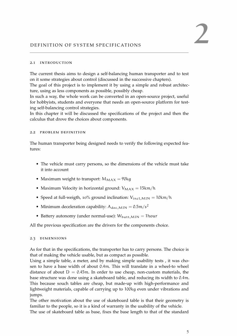
tables: L = 0.2m. This implicitly defines approximately the dimension of the wheel(its diameter must be approximately equal to the base length). The wheel andmotor choice will be discussed later, but the important thing is that the wheel di-ameter is chosen to be approximately equal to L = 0.2m, thus the wheel radiusis half of this: rw = 0.1m. The height of the base is that of the skateboard table(H = 0.01m), the space for the battery is under the skateboard table, so the choiceof that was made taking this into account.
Figure 2: Base dimensions (observed from upside)
2.4 motor torque
For the definition of motor torque needs, two requirements holds. In the followingsections the discussion about these:
2.4.1 Speed at full weight, inclined ground
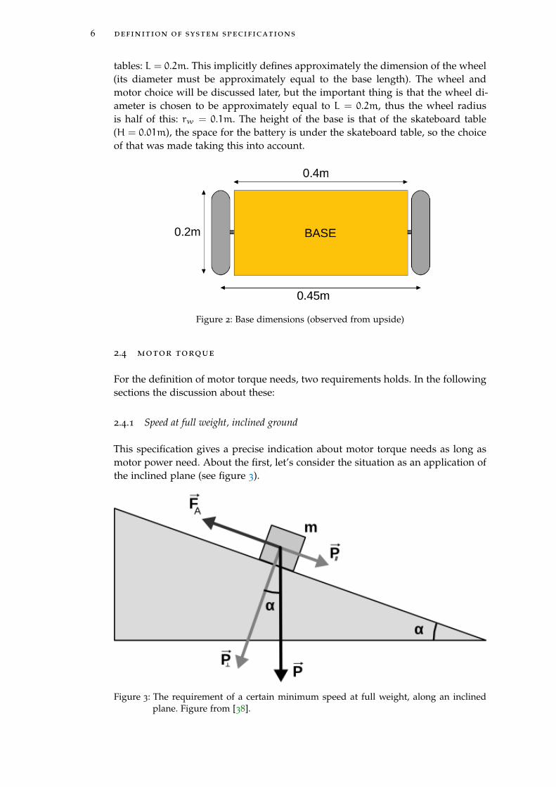
This specification gives a precise indication about motor torque needs as long asmotor power need. About the first, let’s consider the situation as an application ofthe inclined plane (see figure 3).
Figure 3: The requirement of a certain minimum speed at full weight, along an inclinedplane. Figure from [38].
[ December 2, 2017 at 17:06 – classicthesis ]
2.4 motor torque 7
The force P is given by:
P = m ∗ g
Thus, considering the critical condition, let’s apply the maximum weightMMAX =
90kg:
PMAX = MMAX ∗ g = 883N
Since the maximum inclination specified is 10%, which corresponds to an angle ofα = 5.71°, the resulting weight-force, acting parallel to the plane is:
P‖MAX = PMAX ∗ sin(α) = 883N ∗ 0.997 = 87.86N
Having the wheel a radius of 0.1m, as stated in the previous section, and havingtwo motors, the torque need is:
τMAX = P‖MAX ∗ rw/2 = 87.86N ∗ 0.1m/2 = 8.79Nm/2 = 4.39 [Nm] (1)
At the same time, it is possible to derive the power need for the motor: supposingslip absence, the Vincl,MIN specification translates into:
Vincl,MIN = 10km/h = 10/3.6m/s = 2.78 [m/s]
thus:
ωw,inclinMAX = VinclinMAXrw
= 27.8 [rad/s]
defining a power-need of:
Pmotmin = τMAX ∗ωwinclinMAX = 122 [W]
(2)
2.4.2 Maximum deceleration
The other requirement that defines the motor torque need is the maximum decel-eration capability. By ignoring the equilibrium problem, let’s apply the D’alembertprinciple to the transporter:
Fdec,MAX = MMAX ∗Adec,MINthus:
τdec,MAX = Fdec,MAX ∗ rw/2 = 90kg ∗ 0.5m/s2 ∗ 0.1m/2 = 2.75 [Nm]
(3)
In this last equation it is possible to observe that the requrement is less-strict thanthat of the inclined plane, thus, using the torque calculated for the inclined plane,it is possible to obtain stronger decelerations:
Adec,MAX = τMAX∗2MMAX∗rw = 4.39∗2
90∗0.1 = 0.976 [m/s2] (4)
2.4.3 Motor choice
The previous requirements are theoretical, thus a consistent margin of about 2 istaken:
The other important requirement of the motor (as it will be clear in the succes-sive chapters), is the presence of a position-feedback. In the case of a DC motor, it
[ December 2, 2017 at 17:06 – classicthesis ]

8 definition of system specifications
Motor Torque needed 8 [Nm]
Motor Power needed 250 [W]
Table 1: Motor Requirements (with a margin of approx. 2)
is often used an encoder, but since the application does not need a high-precisionpositioning, it is possible to use simple BLDC motors, with HALL sensors incor-porated. The hall-sensors are very important since the motors, during the stand-still self-balancing condition, will work almost in steady position (not generatingenough BEMF) and sensor-less driving is not possible with simple drivers. Giventhe previous, two BLDC alternatives are considered:
1. Hub motor (direct-drive motor, incorporated into the wheel)
2. Small RC motor with gear-reduction
2.4.3.1 Hub motor
The hub-motor is that used in many modern self-balancing toys. Its characteristicsare:
• maximum voltage = 36V
• maximum current = 10A
• maximum power = 360W
• Ke=Kt= 0.694Nm/A
• maximum velocity = 30km/h
• motor configuration = 27N, 30P
This motor has three built-in hall sensors, thus allowing to have a position-readingdefinition of 3 hall-sensors * 30 poles = 90 steps of position reading for every wheelrotation.
Figure 4: HUB motor, used in many self-balancing toys. Figure from [10].
The "pros" and "cons" of that solution are:
[ December 2, 2017 at 17:06 – classicthesis ]
2.4 motor torque 9
pros cons
robust construction , with wheel incorporated high weigth (2.5kg)
silent and very-regular torque expensive(approx. 70 e)
low current need high voltage need
Table 2: Pros& cons of hub motor
2.4.3.2 RC motor
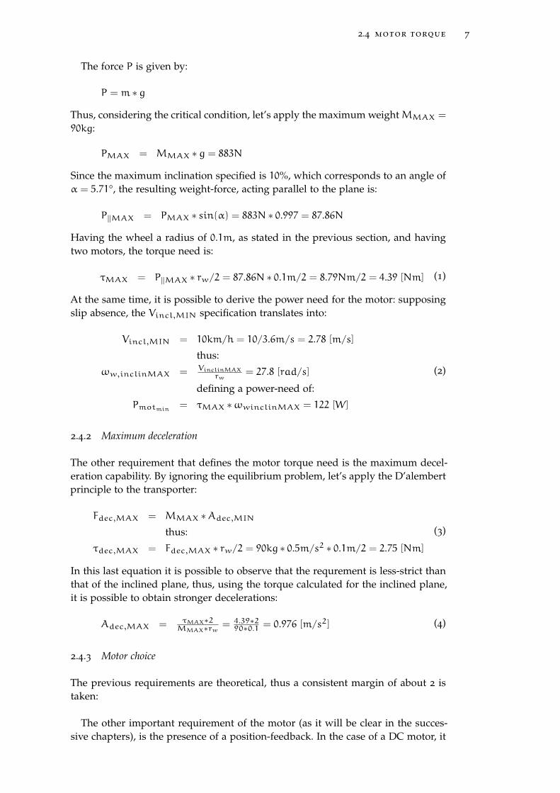
The RC motor is a kind of motor used in RC models. It has been considered be-cause of its high torque and high power density, in a very lightweight device. Thedrawback of this solution is the need to design a wheel and a reduction system (ofabout 1:6), but here are reported the characteristics:
• maximum voltage = 29.6V
• maximum current = 80A
• maximum power = 2200W
• Ke=Kt= 0.035Nm/A (considering a KV = 270RPM/V)
• motor configuration= 12N, 14P
This motor has three built-in hall sensors, thus allowing to have a position-readingdefinition of 3 hall-sensors * 14 poles = 42 steps of position reading for everymotor rotation. Supposing a gear-reduction of about 1 : 6, the total steps of positionreading for every wheel rotation is: 42 ∗ 6 = 252 steps.
Figure 5: RC model motor, image from [1]
The "pros" and "cons" of this solution are:For the purpose of the project it was chosen to use the hub motor, because it is
very simple to mount it into the structure and since there wasn’t the possibility to
[ December 2, 2017 at 17:06 – classicthesis ]
10 definition of system specifications
pros cons
very lightweight (320g) need for external gearbox and wheel
cheap (approx. 30 e) very high current needed
Table 3: Pros& cons of RC motor
prototype complex gearboxes/wheel, the RC motor was not used.Nevertheless, since the RC motor represents a very-lightweight solution and alsocheap, even if not used in our prototype, it was considered into the simulationsand for the possibility of using it in cheap open-source projects.
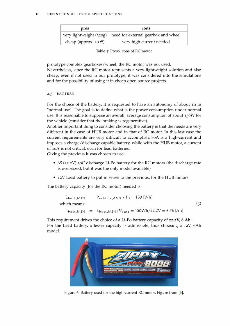
2.5 battery
For the choice of the battery, it is requested to have an autonomy of about 1h in"normal use". The goal is to define what is the power consumption under normaluse. It is reasonable to suppose an overall, average consumption of about 150W forthe vehicle (consider that the braking is regenerative).Another important thing to consider choosing the battery is that the needs are verydifferent in the case of HUB motor and in that of RC motor. In this last case thecurrent requirements are very difficult to accomplish: 80A is a high-current andimposes a charge/discharge capable battery, while with the HUB motor, a currentof 10A is not critical, even for lead batteries.Giving the previous it was chosen to use:
• 6S (22.2V) 30C discharge Li-Po battery for the RC motors (the discharge rateis over-sized, but it was the only model available)
• 12V Lead battery to put in series to the previous, for the HUB motors
The battery capacity (for the RC motor) needed is:
Ebatt,MIN = Pvehicle,AVG ∗ 1h = 150 [Wh]
which means:
Ibatt,MIN = Ebatt,MIN/Vbatt = 150Wh/22.2V = 6.76 [Ah]
(5)
This requirement drives the choice of a Li-Po battery capacity of 22.2V, 8 Ah.For the Lead battery, a lesser capacity is admissible, thus choosing a 12V, 6Ahmodel.
Figure 6: Battery used for the high-current RC motor. Figure from [6].
[ December 2, 2017 at 17:06 – classicthesis ]
2.6 motor driver 11
The last requirement is the vertical dimension: the wheel radius is rw = 10cm
is the maximum height admissible. The batteries chosen satisfied this dimensionconstraint.
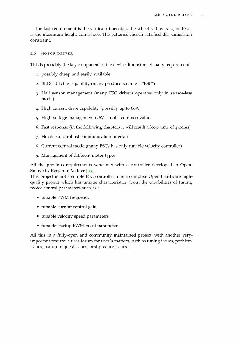
2.6 motor driver
This is probably the key component of the device. It must meet many requirements:
1. possibly cheap and easily available
2. BLDC driving capability (many producers name it "ESC")
3. Hall sensor management (many ESC drivers operates only in sensor-lessmode)
4. High current drive capability (possibly up to 80A)
5. High voltage management (36V is not a common value)
6. Fast response (in the following chapters it will result a loop time of 4-10ms)
7. Flexible and robust communication interface
8. Current control mode (many ESCs has only tunable velocity controller)
9. Management of different motor types
All the previous requirements were met with a controller developed in Open-Source by Benjamin Vedder [35].This project is not a simple ESC controller: it is a complete Open Hardware high-quality project which has unique characteristics about the capabilities of tuningmotor control parameters such as :
• tunable PWM frequency
• tunable current control gain
• tunable velocity speed parameters
• tunable startup PWM-boost parameters
All this in a fully-open and community maintained project, with another very-important feature: a user-forum for user’s matters, such as tuning issues, problemissues, feature-request issues, best practice issues.
[ December 2, 2017 at 17:06 – classicthesis ]
12 definition of system specifications
Figure 7: Open-hardware motor controller, a project of Benjamin Vedder [35] image alsofrom [35]
In addition to the previous requirement meets, this device has several furtherpoint-of-force:
1. very powerful micro-controller (STM32F405), with embedded floating-pointhardware accelerator
2. USB interface for motor diagnosis and configuration of motor characteristics
3. UART interface for external communication
4. High-speed CAN interface, useful for inter-board communication
5. I2C interface for external sensors interface
6. Management of HALL sensors and also ENCODER, with embedded calibra-tion and position incremental output
7. Open-source software (easily customizable for integrating self-balancing con-trol routines)
8. Uses an embedded real-time OS (Chibi-OS), very useful and easy to integratesuspensive routines and sync mechanisms
This solution was chosen because it has all the features needed for the controlpurpose, in a compact solution and with the unique possibility to customize thefirmware, allowing the integration of control loop without external boards. Thepresence of an embedded real-time Operating System, made it easier to managewait conditions, threads, mutexes and inter-task synchronization via events.
2.7 imu
In this project there is the need to measure base inclination and rotation veloc-ity. The most popular solution to this task is the use of a sensor-fusion scheme,based on accelerometer and gyroscope (as it will be explained in the followingchapters). A component integrating these sensor is called Inertial Movement Units(IMU). IMUs are very popular (almost always MEMS-based) devices, available inthe market with different features, sizes and interfacing system (analog, i2C, SPI...).
[ December 2, 2017 at 17:06 – classicthesis ]
2.8 joystick 13
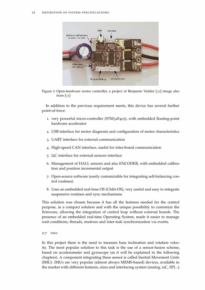
Giving that the micro-controller has an available I2C interface, it was chosen to usean IMU device with that interface, avoiding the problem of different ADC channelsand bias management.In the panorama of possible solutions, the choice was to use a single-componentone, integrating both accelerometer and gyroscope and with an evaluation boardcompact and suitable for easy connection with out controller board. Another im-portant thing is the choice of an IMU with ready-to-use libraries. This is veryhelpful for time-saving and error-avoidance.
Having the previous, the choice was the Invensense’s MPU6050-based open-hardware module:
Figure 8: Open-hardware IMU i2C evaluation module of Invensense’s MPU6050. Figurefrom [28].
Its features are:
• I2C interface
• 400kHz Fast Mode I2C for communicating with all registers
• Digital-output X-, Y-, and Z-Axis angular rate sensors (gyroscopes) with auser-programmable full-scale range of ±250,±500,±1000, and ±2000°/sec
• Digital-output 3-Axis accelerometer with a programmable full scale range of±2g,±4g,±8gand± 16g
• 3-axis silicon monolithic Hall-effect magnetic sensor with magnetic concen-trator
In addition to the features needed, the chosen component owns a 3D magnetic sen-sor (often called "compass"), but it was never used in the application. Nevertheless,this feature might be an interesting and powerful one, in a future scenario, givingto the controller the possibility to manage a further sensor, useful for features likeslip-detection or others.
2.8 joystick
The Joystick was hardly-used during the experiments: is was very helpful for driv-ing the transporter back-and-forth, making rotations or simply standing, while
[ December 2, 2017 at 17:06 – classicthesis ]
14 definition of system specifications
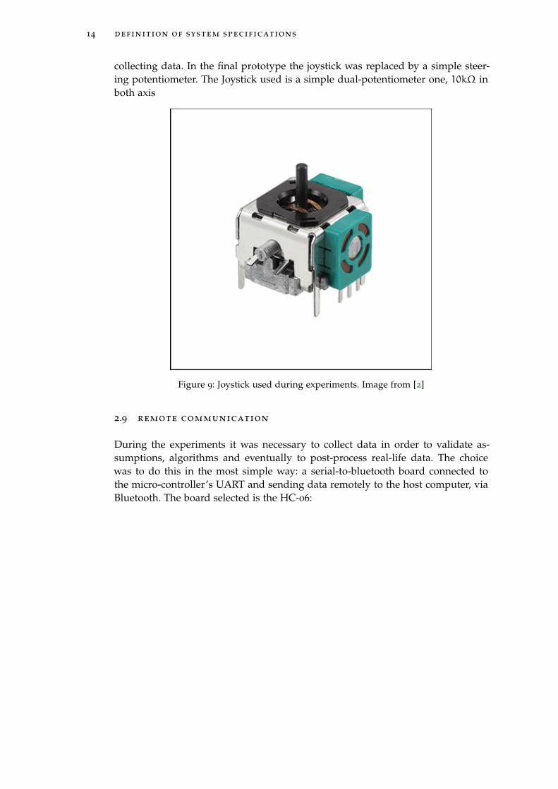
collecting data. In the final prototype the joystick was replaced by a simple steer-ing potentiometer. The Joystick used is a simple dual-potentiometer one, 10kΩ inboth axis
Figure 9: Joystick used during experiments. Image from [2]
2.9 remote communication
During the experiments it was necessary to collect data in order to validate as-sumptions, algorithms and eventually to post-process real-life data. The choicewas to do this in the most simple way: a serial-to-bluetooth board connected tothe micro-controller’s UART and sending data remotely to the host computer, viaBluetooth. The board selected is the HC-06:
[ December 2, 2017 at 17:06 – classicthesis ]

2.10 overall architecture and shematic 15
Figure 10: Serial-to-bluetooth (HC-06) module used for remote logging of data comingfrom the self-balancing transporter, to the host PC. Figure from [5]
It was chosen because of its very-interesting features:
• very cheap (sold as a component of Arduino project it is available even atonly 3$
• very compact: only 2.7 cm x 1.3 cm
• fully compliant with Serial Port Profile (SPP), thus very easy to integrate withevery operating system
• baudrate up to 115200bps (and over)
• UART level and Vdd=3.3V: the same as that of the controller board
The need to use a wireless module for remote communication/logging is obvious:having a moving device, it is strongly forbidden to use a wired communicationscheme. The use of Bluetooth has the advantage to be embedded in almost everylaptop (while other wireless standards such as zig-bee or others needs a counter-part USB key and drivers.
2.10 overall architecture and shematic
After having described the requirements, here it is described the overall connectionscheme with the corresponding descriptions. The scheme of connections is visiblein the figure:
[ December 2, 2017 at 17:06 – classicthesis ]
16 definition of system specifications
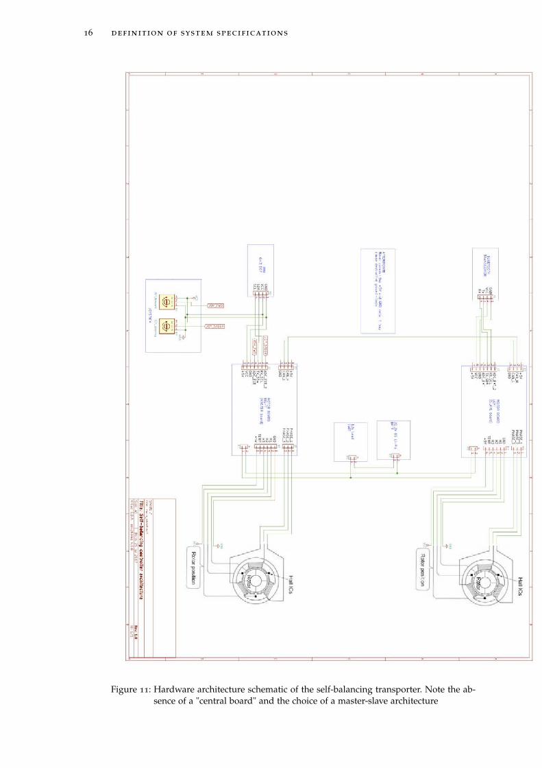
Figure 11: Hardware architecture schematic of the self-balancing transporter. Note the ab-sence of a "central board" and the choice of a master-slave architecture
[ December 2, 2017 at 17:06 – classicthesis ]
2.10 overall architecture and shematic 17
The open-hardware and open-source feature of the controller board, makes itpossible to integrate the self-balancing control algorithm directly inside the motor-control board, without the need for an external "super-part" board. In order toimplement correctly the control, it is compulsory to communicate with the otherboard for:
• retrieve information about motor’s rotor position
• set the desired current
Those needs drived the choice of a "Master-Slave" architecture, described below.
2.10.1 Master board
Master board is "the heart" of the self-balancing controller: in order to work, thisboard must collect all the available sensor’s data and translate them into state vari-able’s values.Giving that this board drives (in real-time) one HALL-sensor-ed motor, it implic-itly has the real-time info about its motor’s rotor position.The rotor’s position of the opposite motor is available thanks to the inter-boardcommunication via CAN bus: it is very fast (500kbaud/s) and robust against EMIinterferences and data corruption. It makes it possible to design a fast control-loop,thanks to the fast variable update (approx. every 300 microseconds).The board collects also the base inclination thanks to the i2C IMU attached to it.Even this interface is very fast (400kHz SCL), making it possible to have a very-fastangle readout (approx. every 100 microseconds).The Joystick attached to this board is used as reference for steering and forward ac-celeration references. It doesn’t need a very-fast update (like the balancing control-loop): it is read at a speed of about 10Hz, which is sufficient for reference speed.Once the algorithm produces its output, the current to the Master board is imposedsimply by an internal function, while that for the other board is set via a CAN-buscommunication message.
2.10.2 Slave Board
The slave board duties are the feedback of its rotor position and the reception/ac-tuation of the current reference. This board has another "unusual" duty: since theinterfaces of the master-board were all occupied by the sensors, this board wasused to communicate to host PC: the master board sends and receives UART com-mands to/from the PC via a "TUNNELLING" inside the CAN bus (a functionutility already present in the original open-source project).This last function obviously can’t be too fast, since the communication has many"hops" to travel in: this is not a tragic drawback since that interface is used simplyfor sending state variable and command signal entities to the PC. This data sendcan be performed at a lower-rate than the loop speed, thus the choice was taken assuitable.
[ December 2, 2017 at 17:06 – classicthesis ]

[ December 2, 2017 at 17:06 – classicthesis ]
3S Y S T E M M O D E L L I N G
3.1 introduction
The problem of controlling the Two-Wheel Self Balancing Transporter (TWSBT)starts with the modeling of the system. In this chapter it will be introduced thekinematic model, the dynamic model (using Lagrange approach) and the decou-pling of the system in balancing and steering subsystems. At the end of the chapterit will be presented some considerations about the results and the block-modelsderived from the equations.
3.2 kinematic model
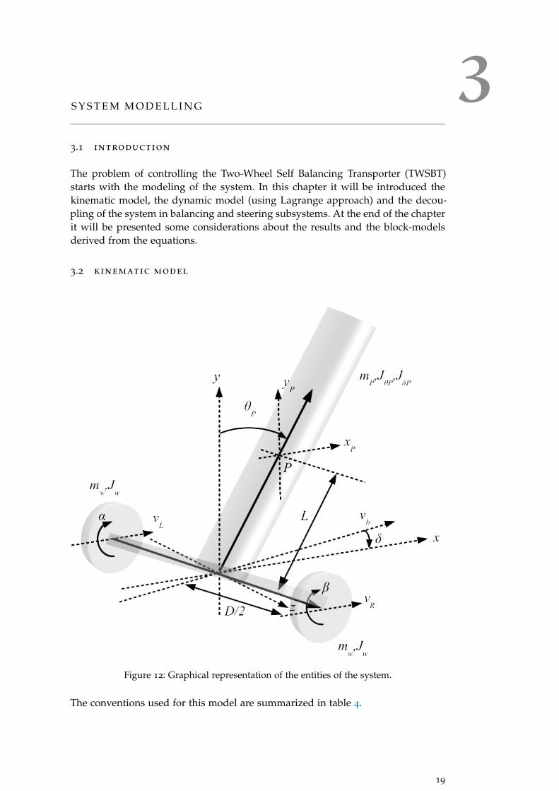
Figure 12: Graphical representation of the entities of the system.
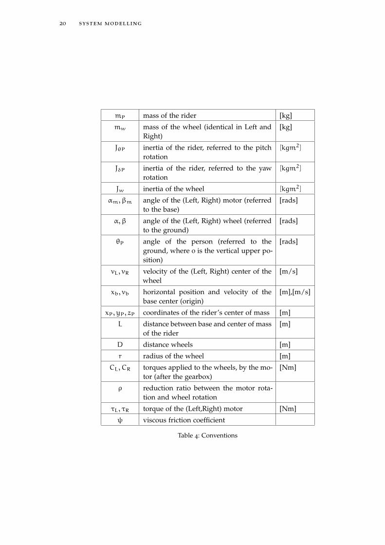
The conventions used for this model are summarized in table 4.
19
[ December 2, 2017 at 17:06 – classicthesis ]
20 system modelling
mP mass of the rider [kg]
mw mass of the wheel (identical in Left andRight)
[kg]
JθP inertia of the rider, referred to the pitchrotation
[kgm2]
JδP inertia of the rider, referred to the yawrotation
[kgm2]
Jw inertia of the wheel [kgm2]
αm, βm angle of the (Left, Right) motor (referredto the base)
[rads]
α,β angle of the (Left, Right) wheel (referredto the ground)
[rads]
θP angle of the person (referred to theground, where 0 is the vertical upper po-sition)
[rads]
vL, vR velocity of the (Left, Right) center of thewheel
[m/s]
xb, vb horizontal position and velocity of thebase center (origin)
[m],[m/s]
xP, yP, zP coordinates of the rider’s center of mass [m]
L distance between base and center of massof the rider
[m]
D distance wheels [m]
r radius of the wheel [m]
CL, CR torques applied to the wheels, by the mo-tor (after the gearbox)
[Nm]
ρ reduction ratio between the motor rota-tion and wheel rotation
τL, τR torque of the (Left,Right) motor [Nm]
ψ viscous friction coefficient
Table 4: Conventions
[ December 2, 2017 at 17:06 – classicthesis ]
3.2 kinematic model 21
3.2.1 Assumptions
The following assumptions are used for the problem:
1. The friction is considered linear and proportional to the motor’s rotationspeed, even if different from reality
2. The rider is modeled as a rigid body (cylinder) of "2L" height
3. The efficiency of the gearbox is equal to 1
4. The reduction has no elasticity
5. The friction produced by the air, with the system’s components, is neglected
6. The vertical coordinate of the base is taken as system’s vertical origin
The relation between motor’s position (referred to the rider’s angle) and thewheel’s angle (referred to the ground) is:
α = θP + ραm
β = θP + ρβm
α = θP + ραm
β = θP + ρβm
(6)
The congruence equations for the wheels and base are:
vL = rα
vR = rβ
vb = vL+vR2 = r α+β2
δ = vL−vRD = r α−βD
(7)
while, concerning the rider’s center of mass:
xP = xb + LsinθPcosδ
yP = LcosθP
zP = zb + LsinθPsinδ
xP = xb + LθPcosθPcosδ− LδsinθPsinδ
yP = LθPsinθP
zP = zb + LθPcosθPsinδ+ LδsinθPcosδ
v2P = x2P + y2P + z
2P =
= v2b + L2θ2P + 2LθP[xbcosθPcosδ+ zbcosθPsinδ]+
+2Lδ[−xbsinθPsinδ+ zbsinθPcosδ]
(8)
where:
xb = vbcosδ
zb = vbsinδ(9)
thus:
v2P = v2b + L2θ2P + 2LθP[vbcosθPcos
2δ+ vbcosθPsin2δ] =
= v2b + L2θ2P + 2LθPvbcosθP
(10)
[ December 2, 2017 at 17:06 – classicthesis ]
22 system modelling
3.3 dynamic model
The resulting torque, after the gearbox of each motor, suffers of the viscous frictionand it is modeled as:
CL = 1ρ(τL −ψαm) = 1
ρτL −ψρ2(α− θP)
CR = 1ρ(τR −ψβm) = 1
ρτR −ψρ2(β− θP)
(11)
kinetic energy of the wheels:
the following equations accounts for both translational and rotational compo-nents of the wheel motion. The kinetic energy associated with rotation of the wheelaround its vertical axis is neglected.
TL = 12mwv
2L +
12Jwα
2 = 12(mwr
2 + Jw)α2
TR = 12mwv
2R +
12Jwβ
2 = 12(mwr
2 + Jw)β2
Tw = TL + TR = 12(mwr
2 + Jw)(α+ β)2
(12)
kinetic energy of the rider:
the kinetic energy of the rider is built-up with three components:The translational kinetic energy is the following:
TtP = 12mPv
2P = 1
2mP(v2b + L
2θ2P + 2LθPvbcosθP)
= 12mP
[(r α+β2
)2+ L2θ2P + 2LθPr
α+β2 cosθP
](13)
The rotational kinetic energy due to the rotation of the rider around the wheel’scentre (θP) is made-up by the following:
TθP = 12JθPθ
2P
(14)
The rotational kinetic energy due to the rotation around the vertical axis (y) ismade-up by the following:
TyP = 12
(JδP +mPL
2sinθ2P)δ2 = 1
2
(JδP +mPL
2sinθ2P) (r α−βD
)2(15)
The total kinetic energy of the rider is given by:
TP = TtP + TθP + TyP =
12mP
[(r α+β2
)2+ L2θ2P + 2LθPr
α+β2 cosθP
]+
12JθPθ
2P+
12
(JδP +mPL
2sin2θP) (r α−βD
)2(16)
kinetic energy of the motors:
The kinetic energy of the motors is:
Tm = TmL + TmR = 12Jm(α2m + β2m) =
= 12Jmρ2
(α2 + β2 + 2θ2P − 2αθP − 2βθP)(17)
[ December 2, 2017 at 17:06 – classicthesis ]
3.4 lagrangian 23
Total kinetic energy:The overall kinetic energy of the system is:
T = TP + Tw + Tm =
12mP
[(r α+β2
)2+ L2θ2P + 2LθPr
α+β2 cosθP
]+
12JθPθ
2P+
12
(JδP +mPL
2sin2θP) (r α−βD
)2+
12(mwr
2 + Jw)(α+ β)2+12Jmρ2
(α2 + β2 + 2θ2P − 2αθP − 2βθP)
(18)
potential energy (of the rider):
This contribute of potential energy is given by simply the vertical position of therider’s center of mass:
U = mPgLcosθP (19)
3.4 lagrangian
Given the previous, it is possible to write the expression of the Lagrangian for thesystem
L = T −U (20)
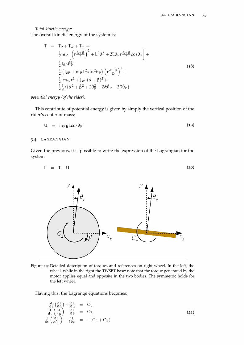
Figure 13: Detailed description of torques and references on right wheel. In the left, thewheel, while in the right the TWSBT base: note that the torque generated by themotor applies equal and opposite in the two bodies. The symmetric holds forthe left wheel.
Having this, the Lagrange equations becomes:
ddt
(∂L∂α
)− ∂L∂α = CL
ddt
(∂L∂β
)− ∂L∂β = CR
ddt
(∂L∂θP
)− ∂L∂θP
= −(CL +CR)
(21)
[ December 2, 2017 at 17:06 – classicthesis ]
24 system modelling
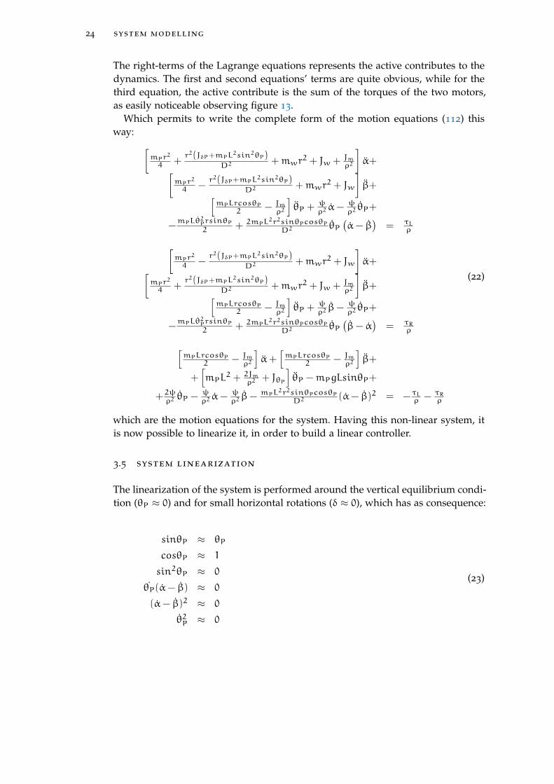
The right-terms of the Lagrange equations represents the active contributes to thedynamics. The first and second equations’ terms are quite obvious, while for thethird equation, the active contribute is the sum of the torques of the two motors,as easily noticeable observing figure 13.
Which permits to write the complete form of the motion equations (112) thisway: [
mPr2
4 +r2(JδP+mPL
2sin2θP)D2
+mwr2 + Jw + Jm
ρ2
]α+[
mPr2
4 −r2(JδP+mPL
2sin2θP)D2
+mwr2 + Jw
]β+[
mPLrcosθP2 − Jm
ρ2
]θP +
ψρ2α− ψ
ρ2θP+
−mPLθ
2PrsinθP2 + 2mPL
2r2sinθPcosθPD2
θP(α− β
)= τL
ρ[mPr
2
4 −r2(JδP+mPL
2sin2θP)D2
+mwr2 + Jw
]α+[
mPr2
4 +r2(JδP+mPL
2sin2θP)D2
+mwr2 + Jw + Jm
ρ2
]β+[
mPLrcosθP2 − Jm
ρ2
]θP +
ψρ2β− ψ
ρ2θP+
−mPLθ
2PrsinθP2 + 2mPL
2r2sinθPcosθPD2
θP(β− α
)= τR
ρ[mPLrcosθP
2 − Jmρ2
]α+
[mPLrcosθP
2 − Jmρ2
]β+
+[mPL
2 + 2Jmρ2
+ JθP
]θP −mPgLsinθP+
+2ψρ2θP −
ψρ2α− ψ
ρ2β− mPL
2r2sinθPcosθPD2
(α− β)2 = −τLρ − τRρ
(22)
which are the motion equations for the system. Having this non-linear system, itis now possible to linearize it, in order to build a linear controller.
3.5 system linearization
The linearization of the system is performed around the vertical equilibrium condi-tion (θP ≈ 0) and for small horizontal rotations (δ ≈ 0), which has as consequence:
sinθP ≈ θP
cosθP ≈ 1
sin2θP ≈ 0
θP(α− β) ≈ 0
(α− β)2 ≈ 0
θ2P ≈ 0
(23)
[ December 2, 2017 at 17:06 – classicthesis ]
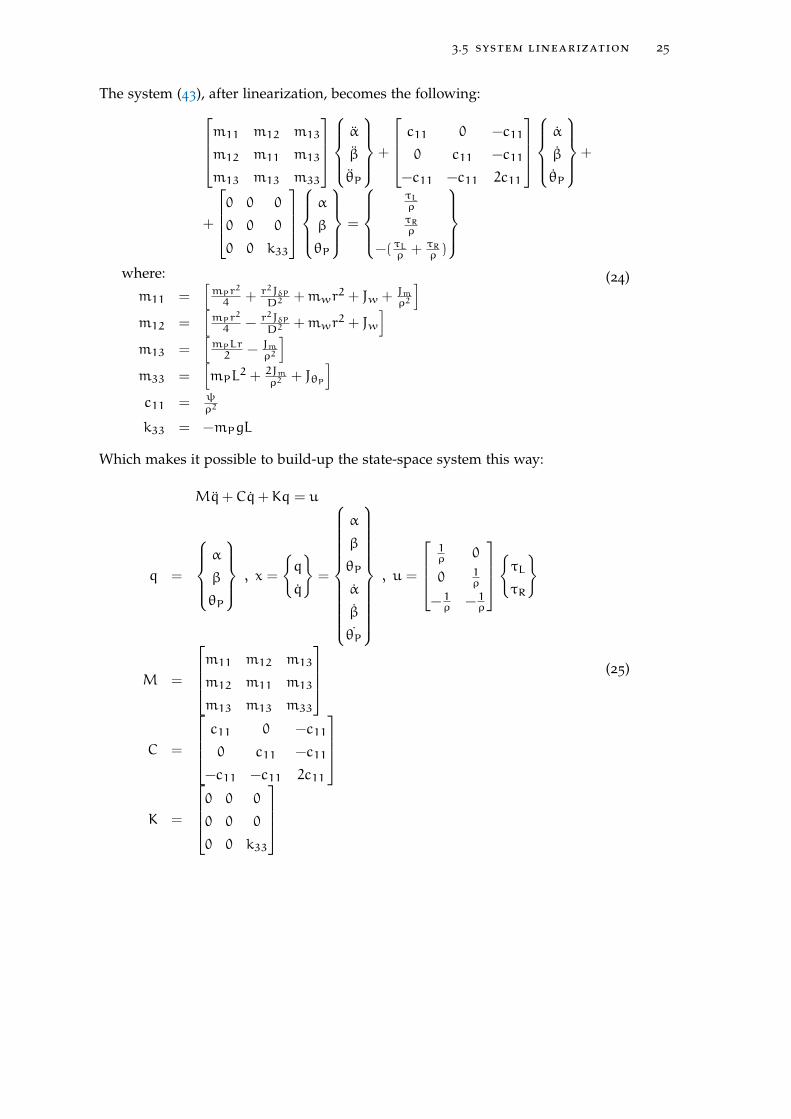
3.5 system linearization 25
The system (43), after linearization, becomes the following:m11 m12 m13
m12 m11 m13
m13 m13 m33
α
β
θP
+
c11 0 −c11
0 c11 −c11
−c11 −c11 2c11
α
β
θP
+
+
0 0 0
0 0 0
0 0 k33
α
β
θP
=
τLρ
τRρ
−(τLρ + τRρ )
where:
m11 =[mPr
2
4 + r2JδPD2
+mwr2 + Jw + Jm
ρ2
]m12 =
[mPr
2
4 − r2JδPD2
+mwr2 + Jw
]m13 =
[mPLr2 − Jm
ρ2
]m33 =
[mPL
2 + 2Jmρ2
+ JθP
]c11 = ψ
ρ2
k33 = −mPgL
(24)
Which makes it possible to build-up the state-space system this way:
Mq+Cq+Kq = u
q =
α
β
θP
, x =
q
q
=
α
β
θP
α
β
θP
, u =
1ρ 0
0 1ρ
−1ρ −1ρ
τL
τR
M =
m11 m12 m13
m12 m11 m13
m13 m13 m33
C =
c11 0 −c11
0 c11 −c11
−c11 −c11 2c11
K =
0 0 0
0 0 0
0 0 k33
(25)
[ December 2, 2017 at 17:06 – classicthesis ]
26 system modelling
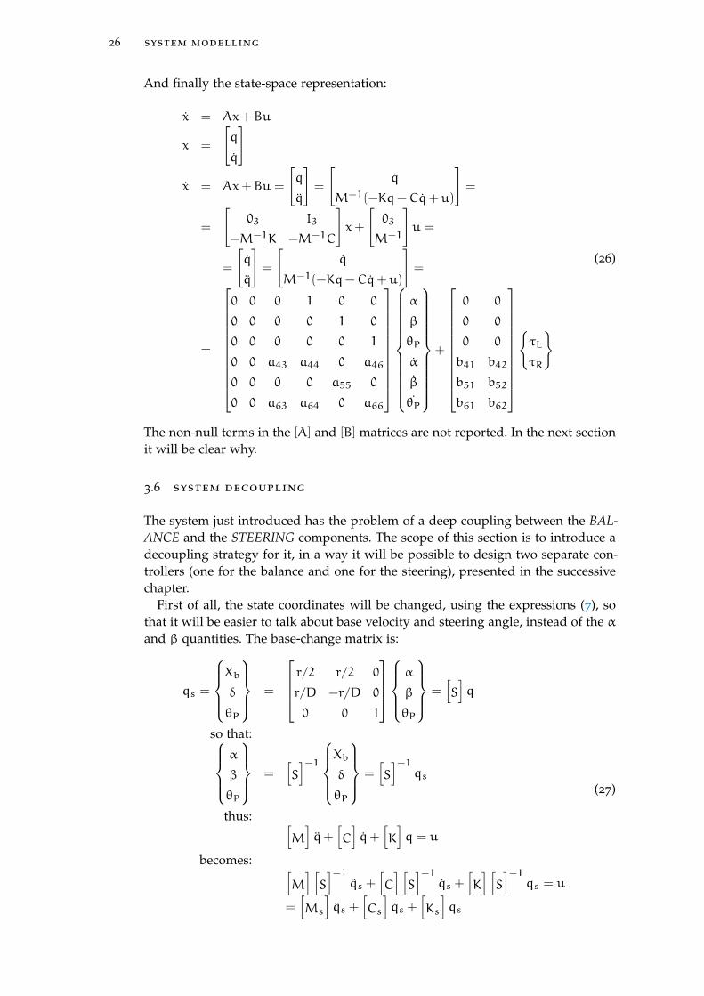
And finally the state-space representation:
x = Ax+Bu
x =
[q
q
]
x = Ax+Bu =
[q
q
]=
[q
M−1(−Kq−Cq+ u)
]=
=
[03 I3
−M−1K −M−1C
]x+
[03
M−1
]u =
=
[q
q
]=
[q
M−1(−Kq−Cq+ u)
]=
=
0 0 0 1 0 0
0 0 0 0 1 0
0 0 0 0 0 1
0 0 a43 a44 0 a46
0 0 0 0 a55 0
0 0 a63 a64 0 a66
α
β
θP
α
β
θP
+
0 0
0 0
0 0
b41 b42
b51 b52
b61 b62
τL
τR
(26)
The non-null terms in the [A] and [B] matrices are not reported. In the next sectionit will be clear why.
3.6 system decoupling
The system just introduced has the problem of a deep coupling between the BAL-ANCE and the STEERING components. The scope of this section is to introduce adecoupling strategy for it, in a way it will be possible to design two separate con-trollers (one for the balance and one for the steering), presented in the successivechapter.
First of all, the state coordinates will be changed, using the expressions (7), sothat it will be easier to talk about base velocity and steering angle, instead of the αand β quantities. The base-change matrix is:
qs =
Xb
δ
θP
=
r/2 r/2 0
r/D −r/D 0
0 0 1
α
β
θP
=[S
]q
so that:α
β
θP
=[S
]−1Xb
δ
θP
=[S
]−1qs
thus: [M
]q+
[C
]q+
[K
]q = u
becomes: [M
] [S
]−1qs +
[C
] [S
]−1qs +
[K
] [S
]−1qs = u
=[Ms
]qs +
[Cs
]qs +
[Ks
]qs
(27)
[ December 2, 2017 at 17:06 – classicthesis ]
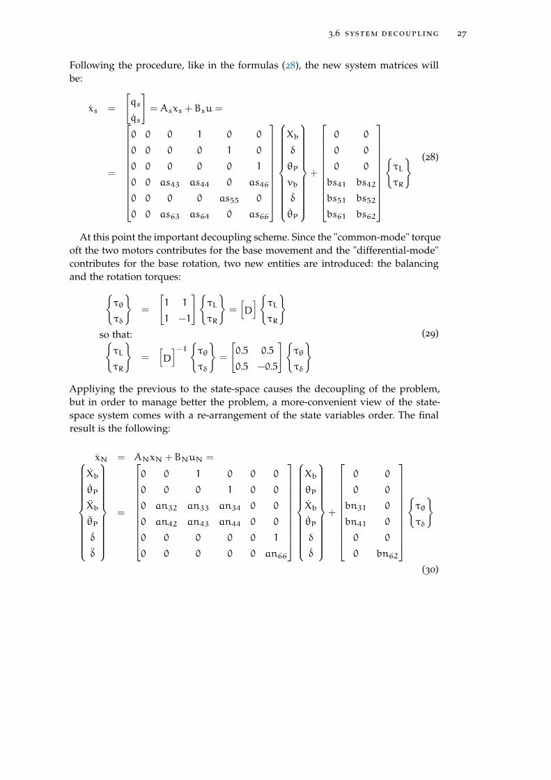
3.6 system decoupling 27
Following the procedure, like in the formulas (28), the new system matrices willbe:
xs =
[qs
qs
]= Asxs +Bsu =
=
0 0 0 1 0 0
0 0 0 0 1 0
0 0 0 0 0 1
0 0 as43 as44 0 as46
0 0 0 0 as55 0
0 0 as63 as64 0 as66
Xb
δ
θP
vb
δ
θP
+
0 0
0 0
0 0
bs41 bs42
bs51 bs52
bs61 bs62
τL
τR
(28)
At this point the important decoupling scheme. Since the "common-mode" torqueoft the two motors contributes for the base movement and the "differential-mode"contributes for the base rotation, two new entities are introduced: the balancingand the rotation torques:
τθ
τδ
=
[1 1
1 −1
]τL
τR
=[D
]τLτR
so that:τL
τR
=
[D
]−1τθτδ
=
[0.5 0.5
0.5 −0.5
]τθ
τδ
(29)
Appliying the previous to the state-space causes the decoupling of the problem,but in order to manage better the problem, a more-convenient view of the state-space system comes with a re-arrangement of the state variables order. The finalresult is the following:
xN = ANxN +BNuN =
Xb
θP
Xb
θP
δ
δ
=
0 0 1 0 0 0
0 0 0 1 0 0
0 an32 an33 an34 0 0
0 an42 an43 an44 0 0
0 0 0 0 0 1
0 0 0 0 0 an66
Xb
θP
Xb
θP
δ
δ
+
0 0
0 0
bn31 0
bn41 0
0 0
0 bn62
τθ
τδ
(30)
[ December 2, 2017 at 17:06 – classicthesis ]
28 system modelling
In this final system it is clearly visible that the problem can be divided in thefollowing two separate systems:
Equilibrium subsystem:
xθ = Aθxθ +Bθτθ =Xb
θP
Xb
θP
=
0 0 1 0
0 0 0 1
0 an32 an33 an34
0 an42 an43 an44
Xb
θP
Xb
θP
+
0
0
bn31
bn41
τθand Steering subsystem:
xδ = Aδxδ +Bδτδ =δ
δ
=
[0 1
0 an66
]δ
δ
+
[0
bn62
]τδ
(31)
3.7 stability analisys
The linearized, decoupled system has two subsystems that are interesting to ana-lyze. In the following rows, some considerations about the linearized models (31),considering these parameters : a rider of 80kg and 1.80m height.
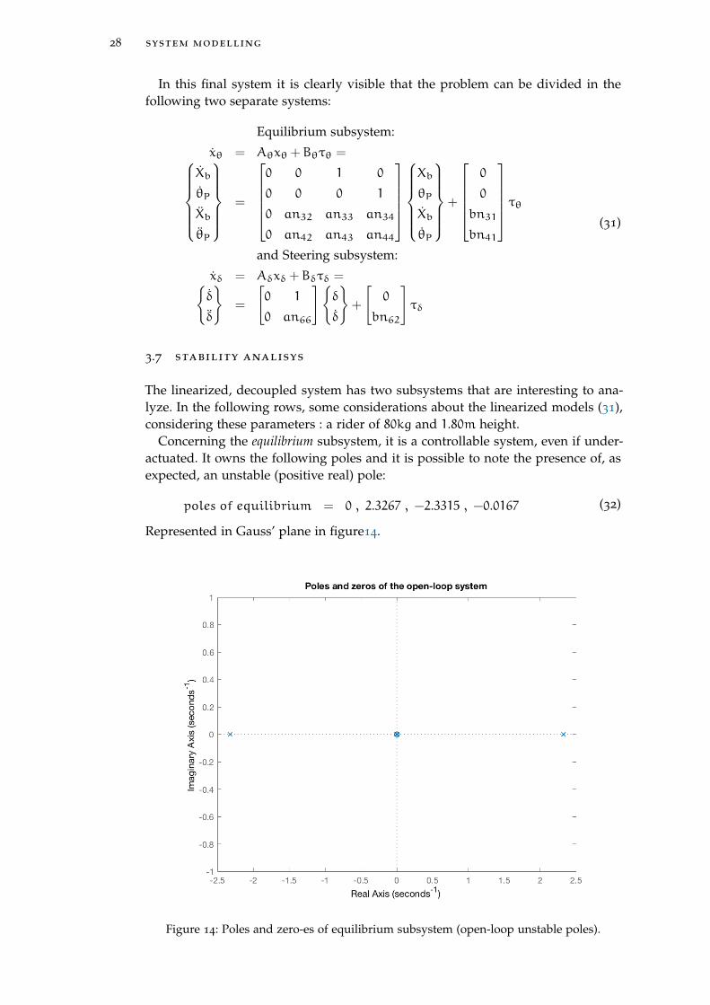
Concerning the equilibrium subsystem, it is a controllable system, even if under-actuated. It owns the following poles and it is possible to note the presence of, asexpected, an unstable (positive real) pole:
poles of equilibrium = 0 , 2.3267 , −2.3315 , −0.0167 (32)
Represented in Gauss’ plane in figure14.
Figure 14: Poles and zero-es of equilibrium subsystem (open-loop unstable poles).
[ December 2, 2017 at 17:06 – classicthesis ]
3.7 stability analisys 29
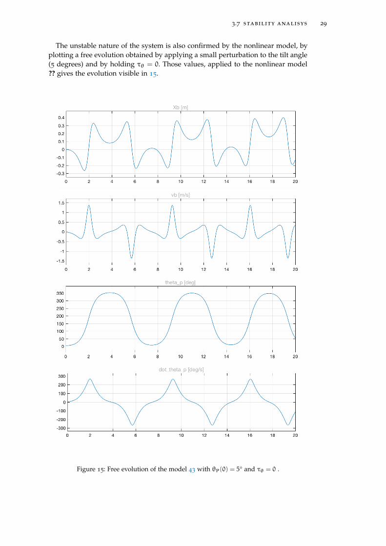
The unstable nature of the system is also confirmed by the nonlinear model, byplotting a free evolution obtained by applying a small perturbation to the tilt angle(5 degrees) and by holding τθ = 0. Those values, applied to the nonlinear model?? gives the evolution visible in 15.
Figure 15: Free evolution of the model 43 with θP(0) = 5° and τθ = 0 .
[ December 2, 2017 at 17:06 – classicthesis ]
30 system modelling
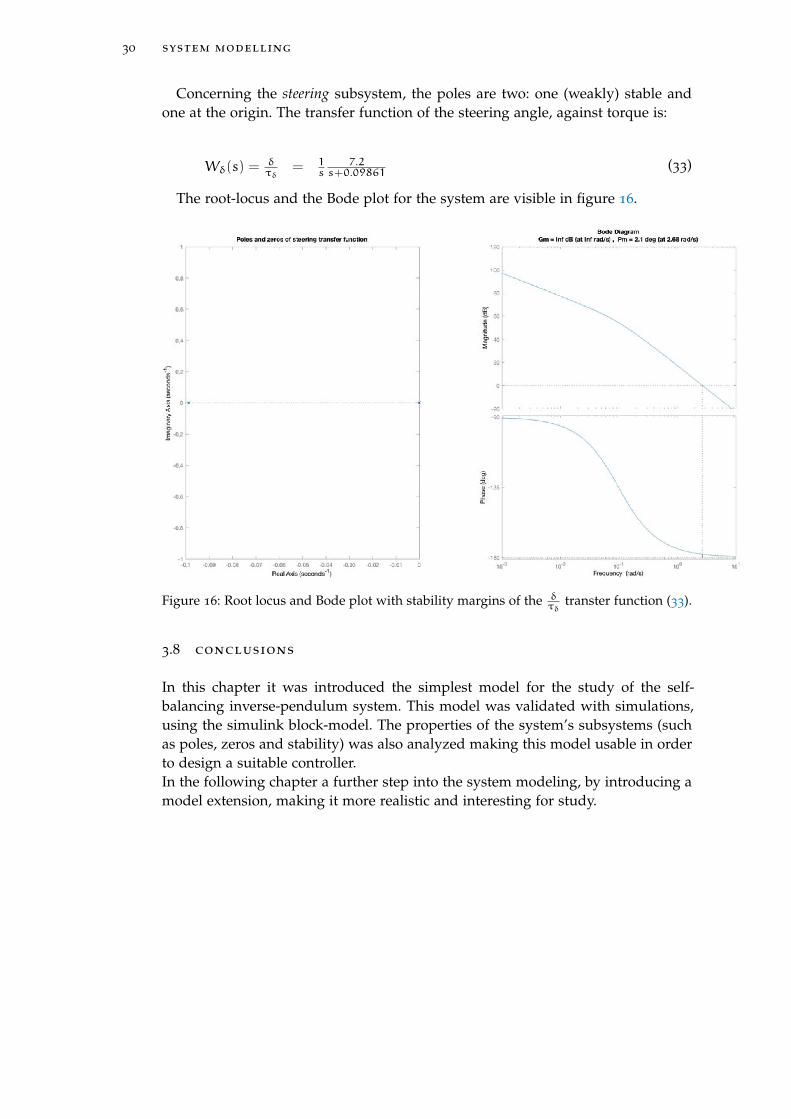
Concerning the steering subsystem, the poles are two: one (weakly) stable andone at the origin. The transfer function of the steering angle, against torque is:
Wδ(s) =δτδ
= 1s
7.2s+0.09861 (33)
The root-locus and the Bode plot for the system are visible in figure 16.
Figure 16: Root locus and Bode plot with stability margins of the δτδ
transter function (33).
3.8 conclusions
In this chapter it was introduced the simplest model for the study of the self-balancing inverse-pendulum system. This model was validated with simulations,using the simulink block-model. The properties of the system’s subsystems (suchas poles, zeros and stability) was also analyzed making this model usable in orderto design a suitable controller.In the following chapter a further step into the system modeling, by introducing amodel extension, making it more realistic and interesting for study.
[ December 2, 2017 at 17:06 – classicthesis ]
4A M O R E R E A L I S T I C M O D E L
4.1 introduction
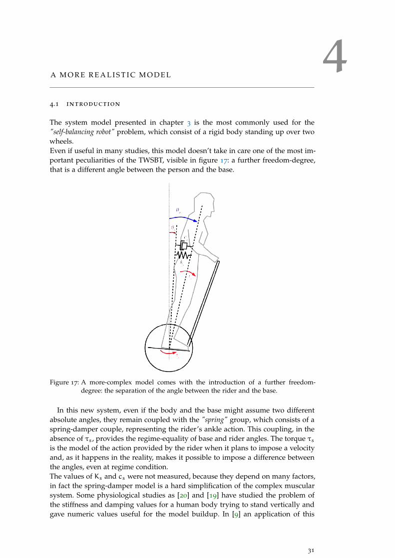
The system model presented in chapter 3 is the most commonly used for the"self-balancing robot" problem, which consist of a rigid body standing up over twowheels.Even if useful in many studies, this model doesn’t take in care one of the most im-portant peculiarities of the TWSBT, visible in figure 17: a further freedom-degree,that is a different angle between the person and the base.
Figure 17: A more-complex model comes with the introduction of a further freedom-degree: the separation of the angle between the rider and the base.
In this new system, even if the body and the base might assume two differentabsolute angles, they remain coupled with the "spring" group, which consists of aspring-damper couple, representing the rider’s ankle action. This coupling, in theabsence of τs, provides the regime-equality of base and rider angles. The torque τsis the model of the action provided by the rider when it plans to impose a velocityand, as it happens in the reality, makes it possible to impose a difference betweenthe angles, even at regime condition.The values of Ks and cs were not measured, because they depend on many factors,in fact the spring-damper model is a hard simplification of the complex muscularsystem. Some physiological studies as [20] and [19] have studied the problem ofthe stiffness and damping values for a human body trying to stand vertically andgave numeric values useful for the model buildup. In [9] an application of this
31
[ December 2, 2017 at 17:06 – classicthesis ]
32 a more realistic model
model to the self-balancing vehicle was used. This was taken as a starting point forthis chapter.Thanks to this, it is possible to rewrite in a convenient way the extended model ofthe system that will be called MODEL2, that differs from the first, mainly by thepresence of the additional freedom degree.
The presence of this further freedom degree will change the lagrangian expres-sion, introducing a further term of potential energy:
Us = 12ks(θb − θP)
2
so:
U = mPgLcosθP +12ks(θb − θP)
2
(34)
and a dissipation term, given by the damper, whose contribute is subtracted fromthe active force τs, resulting in:
Cs = τs − cs(θP − θb) = τs + cs(θb − θP) (35)
The torques supplied by the motors now are referred to the base angle (not therider’s one):
CL = 1ρ(τL −ψαm) = 1
ρτL −ψρ2(α− θb)
CR = 1ρ(τR −ψβm) = 1
ρτR −ψρ2(β− θb)
(36)
Also the kinetic energy of the motors varies in:
Tm = TmL + TmR = 12Jm(α2m + β2m) =
= 12Jmρ2
(α2 + β2 + 2θ2b − 2αθb − 2βθb)(37)
And it is introduced the kinetic energy of the base (translational and rotational):
Tb = 12Jbθ
2b +
12mbv
2b =
= 12Jbθ
2b +
12mb
(r α+β2
)2= 12Jbθ
2b +
14mbrα
2 + 14mbrβ
2 + 12mbrαβ
(38)
The new coordinates vector and the Lagrangian becomes:
q =
α
β
θb
θP
L = T −U = 1
2mP
[r2 α
2
4 + r2 β2
4 + r2 αβ2 + L2θ2P + LθPr(α+ β)cosθP
]+
12JθPθ
2P +
12
(JδP +mPL
2sin2θP) [r2 α
2
D2+ r2 β
2
D2− 2r2 αβ
D2
]+
12(mwr
2 + Jw)(α2 + β2 + 2αβ)+
12Jmρ2
(α2 + β2 + 2θ2b − 2αθb − 2βθb)+
12Jbθ
2b +
14mbrα
2 + 14mbrβ
2 + 12mbrαβ
−mPgLcosθP −12ks(θb − θP)
2
(39)
thus:ddt
(∂L∂α
)− ∂L∂α = CL
ddt
(∂L∂β
)− ∂L∂β = CR
ddt
(∂L∂θb
)− ∂L∂θb
= −(CL +CR) −Cs
ddt
(∂L∂θP
)− ∂L∂θP
= Cs
(40)
[ December 2, 2017 at 17:06 – classicthesis ]
4.2 linearization of the new system 33
The final result of these last expressions are the equations of motion in the newcoordinates:[mPr
2
4 +r2(JδP+mPL
2sin2θP)D2
+mwr2 + Jw + Jm
ρ2+ 12mbr
]α+[
mPr2
4 −r2(JδP+mPL
2sin2θP)D2
+mwr2 + Jw + 1
2mbr
]β+
−Jmρ2θb +
mPLrcosθP2 θP+
+ ψρ2α− ψ
ρ2θb+
−mPLθ
2PrsinθP2 + 2mPL
2r2sinθPcosθPD2
θP(α− β
)= τL
ρ[mPr
2
4 −r2(JδP+mPL
2sin2θP)D2
+mwr2 + Jw + 1
2mbr
]α+[
mPr2
4 +r2(JδP+mPL
2sin2θP)D2
+mwr2 + Jw + Jm
ρ2+ 12mbr
]β+
−Jmρ2θb +
mPLrcosθP2 θP+
+ ψρ2β− ψ
ρ2θb+
−mPLθ
2PrsinθP2 + 2mPL
2r2sinθPcosθPD2
θP(β− α
)= τR
ρ[−Jmρ2
]α+
[−Jmρ2
]β+
+[2Jmρ2
+ Jb
]θb +
[2ψρ2
+ cs
]θb+
−csθP −ψρ2α− ψ
ρ2β+ ksθb − ksθP = −τLρ − τR
ρ − τs
[mPLrcosθP
2
]α+
[mPLrcosθP
2
]β+
+[mPL
2 + JθP]θP −mPgLsinθP − ksθb + ksθP+
+csθP − csθb −mPL
2r2sinθPcosθPD2
(α− β)2 = τs
(41)
4.2 linearization of the new system
As before, the system linearization is performed around the vertical equilibriumcondition (θP ≈ 0 ≈ θb) and for small horizontal rotations (δ ≈ 0), which has asconsequence:
sinθP ≈ θP
sinθb ≈ θb
cosθP ≈ 1
sin2θP ≈ 0
θP(α− β) ≈ 0
(α− β)2 ≈ 0
θ2P ≈ 0
(42)
[ December 2, 2017 at 17:06 – classicthesis ]
34 a more realistic model
The system (43), after linearization, becomes the following:m11 m12 m13 m14
m12 m11 m13 m14
m13 m13 m33 0
m14 m14 0 m44
α
β
θb
θP
+
c11 0 −c11 0
0 c11 −c11 0
−c11 −c11 c33 c34
0 0 c34 −c34
α
β
θb
θP
+
+
0 0 0 0
0 0 0 0
0 0 k33 −k33
0 0 −k33 k44
α
β
θb
θP
=
τLρ
τRρ
−(τLρ + τRρ ) + τs
−τs
=
1ρ 0 0
0 1ρ 0
−1ρ −1ρ −1
0 0 1
τL
τR
τs
where:
m11 =[mPr
2
4 + r2JδPD2
+mwr2 + Jw + 1
2mbr+Jmρ2
]m12 =
[mPr
2
4 − r2JδPD2
+mwr2 + Jw + 1
2mbr]
m13 =−Jmρ2
m14 =mPLr2
m33 =2Jmρ2
+ Jb
m44 =[mPL
2 + JθP]
c11 =ψρ2
c33 =[2ψρ2
+ cs
]c34 = −cs
k33 = ks
k44 = −mPgL+ ks
(43)
4.2.1 decoupling
The presence of θs doesn’t change the decoupling scheme adopted, whose modifi-cation is very limited:
qs =
Xb
δ
θb
θP
=
r/2 r/2 0 0
r/D −r/D 0 0
0 0 1 0
0 0 0 1
α
β
θb
θP
=[S
]q
so that:α
β
θb
θP
=[S
]−1Xb
δ
θb
θP
=[S
]−1qs
and the decoupling matrix is:τθ
τs
τδ
=
1 1 0
0 0 1
1 −1 0
τL
τR
τs
=[D
]τL
τR
τs
(44)
[ December 2, 2017 at 17:06 – classicthesis ]
4.3 transfer function and stability analisys 35
Following the same steps done for the derivation of the (31), the state-spaceexpression of the system with this further freedom degree is:
xθ = Aθxθ +Bθτθ =
Xb
Xb
θb
θb
θP
θP
=
0 1 0 0 0 0
0 an22 an23 an24 an25 an26
0 0 0 1 0 0
0 an42 an43 an44 an45 an46
0 0 0 0 0 1
0 an62 an63 an64 an65 an66
Xb
Xb
θb
θb
θP
θP
+
0 0
bn21 bn22
0 0
bn41 bn42
0 0
bn61 bn62
τθ
τs
and:
xδ = Aδxδ +Bδτδ =δ
δ
=
[0 1
0 an88
]δ
δ
+
[0
bn83
]τδ
(45)
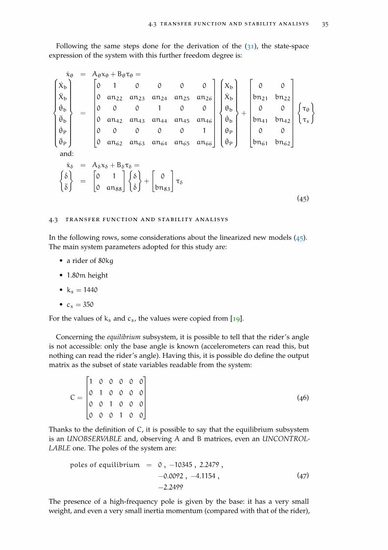
4.3 transfer function and stability analisys
In the following rows, some considerations about the linearized new models (45).The main system parameters adopted for this study are:
• a rider of 80kg
• 1.80m height
• ks = 1440
• cs = 350
For the values of ks and cs, the values were copied from [19].
Concerning the equilibrium subsystem, it is possible to tell that the rider’s angleis not accessible: only the base angle is known (accelerometers can read this, butnothing can read the rider’s angle). Having this, it is possible do define the outputmatrix as the subset of state variables readable from the system:
C =
1 0 0 0 0 0
0 1 0 0 0 0
0 0 1 0 0 0
0 0 0 1 0 0
(46)
Thanks to the definition of C, it is possible to say that the equilibrium subsystemis an UNOBSERVABLE and, observing A and B matrices, even an UNCONTROL-LABLE one. The poles of the system are:
poles of equilibrium = 0 , −10345 , 2.2479 ,
−0.0092 , −4.1154 ,
−2.2499
(47)
The presence of a high-frequency pole is given by the base: it has a very smallweight, and even a very small inertia momentum (compared with that of the rider),
[ December 2, 2017 at 17:06 – classicthesis ]

36 a more realistic model
thus resulting in a contribute of a very-high frequency.As for the first model, the main scope of the control will be to maintain upside therider.
[ December 2, 2017 at 17:06 – classicthesis ]
5C O N T R O L
5.1 introduction
In the previous chapters there were built two linearized models of the vehicle: one(simplified) where the rider was -linked with the vehicle base, and one where ithad a further freedom degree. Even the first, simplified model have demonstratedto be a multi-input, multi-output (MIMO) system.
Further transforms permitted to separate the inverse-pendulum system into twodistinct subsystems algebraically independent, thus that might be separately con-trolled. The steering subsystem is a single-input, single-output (SISO) system, thathas a simple dynamic description, while the equilibrium subsystem is a single-input,multi-output (SIMO) system.
This chapter describes the control strategies adopted for the two subsystems,together with considerations about the stability of that controllers.
5.2 control of equilibrium subsystem
The equilibrium subsystem is a single-input, multi-output (SIMO) system, thus it isnecessary to adopt a suitable controller.
In the panorama of possible controllers, some possibilities are:
• Pole-placement technique
• Self-learning controllers
• Linear Quadratic (optimum) controllers
Since the poles and their meaning is such a system is not obvious, the Pole-placement was discarded. Also the choice of self-learning controllers was dis-carded, since the aim was to build a precise-behavior system, where it was alwayspossible to know and discuss the control behavior. Also there was not enough timeto properly train an algorithm.
The final choice was the adoption of an optimum controller (LQR) because it wasvery easy to relate the controller weights, with the system’s coordinates. The draw-back of this approach is that it is not that simple to relate the controller’s gains,with the coordinate’s dynamics.
Regarding this missing relation, some studies like [13] and [22] have proposedthe use of a genetic algorithm in order to properly tune the LQR coefficients, forobtaining the desired system dynamics. In this section it will be described theLQR controller designed for the self-balancing vehicle and some discussion aboutthe coefficient choice and the consequent stability.
5.2.1 The optimum (LQR) controller
The classic approach in controlling a system is to find a feedback controller inorder to make it place the poles/zeroes of the system in a way to obtain stabilityand some other performances such as bandwidth. Many times it is of interest to
37
[ December 2, 2017 at 17:06 – classicthesis ]
38 control
have a controller that can guarantee adequate rejection to disturbances. The limitof this approach is that it is difficult to evaluate the effect of bandwidth, poleposition, disturbance rejection, in other aspects such as single state deviation orenergy consumption. This is the main scope of the optimum controller: designerhas a tool to privilege the economicity or the deviation from one or a set of statevariables, giving the possibility to have a very powerful and flexible control thatsatisfies different characteristics.
All the previous is possible with a "cost functional", which is a quadratic formthat describes the "cost" (always non-negative) when privileging one aspect insteadof another. For a discrete-time proper system defined as:x(k+ 1) = Fx(k) +G(k)
x(0) = x0
(48)
The cost functional is:
J(u, x0) =
T−1∑k=0
[x(k)TQx(k) + u(k)TRu(k)]dk+ x(T)TSx(T)
Where it is possible to observe three terms in a quadratic form, associated with amatrix.
• The first term is that with Q, which is positive semi-definite. It describes thecost related to the deviation of the state during the sequence 0− T . HavingQ diagonal, for every single element in the diagonal, corresponds the costof the deviation of that singular state variable. Note: the higher the values, themore precise the controller.
• The second term is that with R, which is also positive semi-definite. It de-scribes the cost related to the input sequence (the power consumption forobtaining a result). Note: the higher the values, the more economic the controller.
• The third term is that with S, which is also positive definite. It describes thecost related to the error in the final state. Note: the higher the values, the moreprecise the controller.
5.2.1.1 Infinite-horizon control
The previous functional is valid in the case that T is a finite number (control overa finite-time horizon).In the case T → ∞ there is the advantage that the input can be built with a linearand constant feedback from the state, but some problem arises:
1. In order to have J non-infinite, it is important to verify the existence of aninput sequence with which J assumes a finite value.
2. Having a control in the form of a feedback, it must be internally stable.
3. The feedback matrix might be found by solving the Algebraic Riccati Equa-tion (ARE), which admits several solutions. Only one of such solution is theoptimum: the problem is to determine the solution that matches the require-ments.
[ December 2, 2017 at 17:06 – classicthesis ]
5.2 control of equilibrium subsystem 39
In the same discrete-system in 48, at infinite-time horizon, the cost functional be-comes:
J(u, x0) =
∞∑k=0
(x(k)TQx(k) + u(k)TRu(k)) (49)
Where Q is symmetric and positive-semidefinite and R is symmetric and positive-definite.- lemma 1 If the system 48 is stabilizable, there exist input-sequences for whom theindex 49 is finite.- lemma 2 If the system 48 is stabilizable, the succession of matrices M(0),M(−1)...defined as:
M(0) = 0
M(k) = Q+ FTM(k+ 1)F+
−FTM(k+ 1)G[R+GTM(k+ 1)G]−1GTM(k+ 1)F
converges (for k → ∞) to a symmetric, positive semi-definite matrix that satisfiesthe ARE:
M = Q+ FTMF+−FTMG[R+GTMG]−1GTMF (50)
- lemma 3 Assume M is a solution symmetric, positive semi-definite solution ofARE. For every input succession u(0), u(1), ...u(T − 1) and every initial state x0, itresults that:
T−1∑k=0
(x(k)TQx(k) + u(k)TRu(k)) = (51)
xT0Mx0 − xT (T)Mx(T)+ (52)
+
T−1∑k=0
[(R+GTMG)u(k) +GTMFx(k)]T∗ (53)
[R+GTMG][(R+GTMG)u(k) +GTMFx(k)] (54)
Observing also the theorem:Theorem 1:Having the system 48 and M, the solution found with lemma 2, then
1. the control law
u∞(k) = K∞(k)x(k)K∞ = −(R+GTM∞G)−1GTM∞F
minimizes the index J
2. For every other solution symmetric, positive-semi-definite M of ARE, thematrix M−M∞ is positive-semidefinite
The theorem gives a way to calculate an optimum controller with linear-feedbackfunction that creates an input sequence, directly from the system state. The draw-back is that the solution found might be not-stabilizing. It depends on some prop-erties of the matrices F and G .
[ December 2, 2017 at 17:06 – classicthesis ]
40 control
Another aspect is that if M∞ is positive-semi-definite (not definite), the optimuminput for some state configuration might be the NULL sequence, since there existsnon-null initial states for which it exists a minimum value of the cost J. This corre-sponds to have no action on the system, by the controller.Theorem 2:If M∞ is the solution of ARE that minimizes the 49 for the system 48. Having a Cmatrix such that:
Q = CTC
Then M∞ is positive-definite only if the couple (F, C) is observable.
5.2.1.2 Optimum control and stabilization
The stabilization of the system is the most important requirement for our control,since it must act in an unstable system and make it stable. Here are some importantaspects of the internal stability requirements for the control:Theorem 3:Given the system 48, with (F,G) stabilizable, and M∞ the optimum solution ofARE. This solution is also stabilyzing if the couple (F, C) is observable.Theorem 4:Given the system 48, with (F,G) stabilizable and Q = CTC. It is true that:
• ARE has at most one symmetric positive-semi-definite solution associatedwith a stabilizing control.
• This solution exists only if the couple (F, C) is observable.
• If a stabilizing solution MS exists, for every symmetric positive-semi-definitesolution M the matrix MS − M is symmetric positive-semi-definite.
• If a stabilizing solution MS exists, it is possible to derive it starting with as alimit for k→∞ of the ARE solution assuming M(0) an arbitrary symmetricpositive-definite matrix.
Corollary:If the solution MS of ARE is stabilizing, it is the only symmetric positive-semi-definite solution of the equation.
At this point a scenario is possible: MS and M∞ both exists and different. It isobvious that the stabilyzing solution is the obligatory choice. In this case the con-trol will be:
us(k) = ksx(k) (55)
This solution, in the space of the stabilyzing laws, is that associated with the mini-mum cost index.
[ December 2, 2017 at 17:06 – classicthesis ]
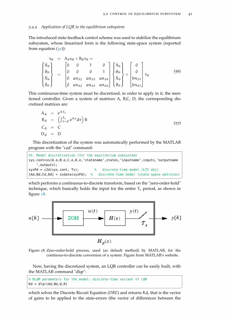
5.2 control of equilibrium subsystem 41
5.2.2 Application of LQR to the equilibrium subsystem
The introduced state-feedback control scheme was used to stabilize the equilibriumsubsystem, whose linearized form is the following state-space system (reportedfrom equation (31)):
xθ = Aθxθ +Bθτθ =Xb
θP
Xb
θP
=
0 0 1 0
0 0 0 1
0 an32 an33 an34
0 an42 an43 an44
Xb
θP
Xb
θP
+
0
0
bn31
bn41
τθ (56)
This continuous-time system must be discretized, in order to apply in it, the men-tioned controller. Given a system of matrices A, B,C, D, the corresponding dis-cretized matrices are:
Ad = eATs
Bd =(∫Tsτ=0 e
Aτdτ)B
Cd = C
Dd = D
(57)
This discretization of the system was automatically performed by the MATLABprogram with the "c2d" command:
%% Model discretization (for the equilibrium subsystem)
sys_cont=ss(A_e,B_e,C_e,D_e,’statename’,states,’inputname’,inputs,’outputname
’,outputs);
sysPd = c2d(sys_cont, Ts); % discrete-time model (LTI obj)
[Ad,Bd,Cd,Dd] = ssdata(sysPd); % discrete-time model (state-space matrices) which performs a continuous-to-discrete transform, based on the "zero-order-hold"technique, which basically holds the input for the entire Ts period, as shown infigure 18.
Figure 18: Zero-order-hold process, used (as default method) by MATLAB, for thecontinous-to-discrete conversion of a system. Figure from MATLAB’s website.
Now, having the discretized system, an LQR controller can be easily built, withthe MATLAB command "dlqr":
% DLQR parameters for the model: discrete-time variant of LQR
Kd = dlqr(Ad,Bd,Q,R) which solves the Discrete Riccati Equation (DRE) and returns Kd, that is the vectorof gains to be applied to the state-errors (the vector of differences between the
[ December 2, 2017 at 17:06 – classicthesis ]
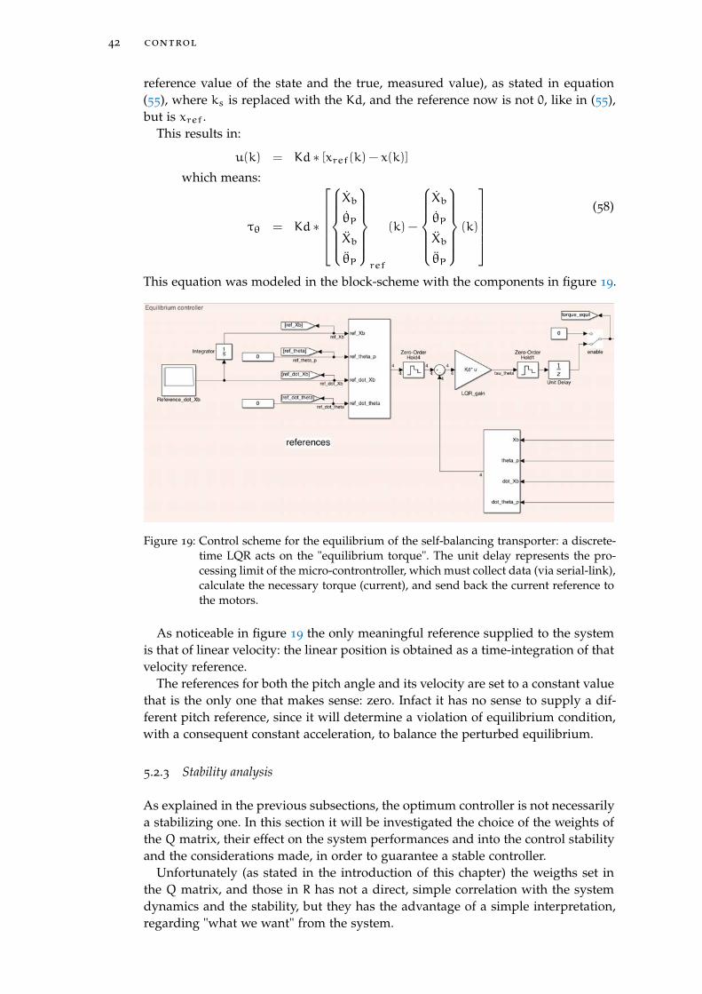
42 control
reference value of the state and the true, measured value), as stated in equation(55), where ks is replaced with the Kd, and the reference now is not 0, like in (55),but is xref.
This results in:
u(k) = Kd ∗ [xref(k) − x(k)]which means:
τθ = Kd ∗
Xb
θP
Xb
θP
ref
(k) −
Xb
θP
Xb
θP
(k)
(58)
This equation was modeled in the block-scheme with the components in figure 19.
Figure 19: Control scheme for the equilibrium of the self-balancing transporter: a discrete-time LQR acts on the "equilibrium torque". The unit delay represents the pro-cessing limit of the micro-controntroller, which must collect data (via serial-link),calculate the necessary torque (current), and send back the current reference tothe motors.
As noticeable in figure 19 the only meaningful reference supplied to the systemis that of linear velocity: the linear position is obtained as a time-integration of thatvelocity reference.
The references for both the pitch angle and its velocity are set to a constant valuethat is the only one that makes sense: zero. Infact it has no sense to supply a dif-ferent pitch reference, since it will determine a violation of equilibrium condition,with a consequent constant acceleration, to balance the perturbed equilibrium.
5.2.3 Stability analysis
As explained in the previous subsections, the optimum controller is not necessarilya stabilizing one. In this section it will be investigated the choice of the weights ofthe Q matrix, their effect on the system performances and into the control stabilityand the considerations made, in order to guarantee a stable controller.
Unfortunately (as stated in the introduction of this chapter) the weigths set inthe Q matrix, and those in R has not a direct, simple correlation with the systemdynamics and the stability, but they has the advantage of a simple interpretation,regarding "what we want" from the system.
[ December 2, 2017 at 17:06 – classicthesis ]
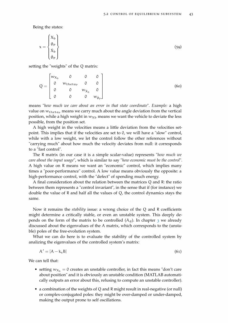
5.2 control of equilibrium subsystem 43
Being the states:
x =
Xb
θP
Xb
θP
(59)
setting the "weights" of the Q matrix:
Q =
wXb 0 0 0
0 wthetaP 0 0
0 0 wXb 0
0 0 0 wθP
(60)
means "how much we care about an error in that state coordinate". Example: a highvalue onwthetaP means we carry much about the angle deviation from the verticalposition, while a high weight in wXb means we want the vehicle to deviate the lesspossible, from the position set.
A high weight in the velocities means a little deviation from the velocities set-point. This implies that if the velocities are set to 0, we will have a "slow" control,while with a low weight, we let the control follow the other references without"carrying much" about how much the velocity deviates from null: it correspondsto a "fast control".
The R matrix (in our case it is a simple scalar-value) represents "how much wecare about the input usage", which is similar to say "how economic must be the control".A high value on R means we want an "economic" control, which implies manytimes a "poor-performance" control. A low value means obviously the opposite: ahigh-performance control, with the "defect" of spending much energy.
A final consideration about the relation between the matrices Q and R: the ratiobetween them represents a "control invariant", in the sense that if (for instance) wedouble the value of R and half all the values of Q, the control dynamics stays thesame.
Now it remains the stability issue: a wrong choice of the Q and R coefficientsmight determine a critically stable, or even an unstable system. This deeply de-pends on the form of the matrix to be controlled (Ad). In chapter 3 we alreadydiscussed about the eigenvalues of the A matrix, which corresponds to the (unsta-ble) poles of the free-evolution system.
What we can do here is to evaluate the stability of the controlled system byanalizing the eigenvalues of the controlled system’s matrix:
A ′ = [A− ksB] (61)
We can tell that:
• setting wXb = 0 creates an unstable controller, in fact this means "don’t careabout position" and it is obviously an unstable condition (MATLAB automati-cally outputs an error about this, refusing to compute an unstable controller).
• a combination of the weights ofQ and Rmight result in real-negative (or null)or complex-conjugated poles: they might be over-damped or under-damped,making the output prone to self oscillations.
[ December 2, 2017 at 17:06 – classicthesis ]
44 control
The last statement is visible in figures 20 and 21. In the first figure, the choice of Qand R yelded to both real and complex-conjugated, under-damped poles, while inthe second figure, the poles are all negative.
Figure 20: Poles of the system: in the upper figure, the uncontrolled system, in the lowerthe controlled one. The choice of the coefficients of Q and R yielded to both realand complex-conjugated, under-damped poles.
[ December 2, 2017 at 17:06 – classicthesis ]
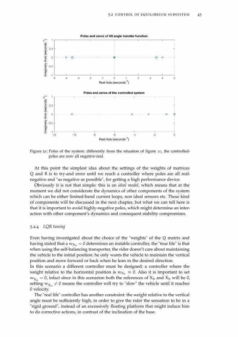
5.2 control of equilibrium subsystem 45
Figure 21: Poles of the system: differently from the situation of figure 20, the controlled-poles are now all negative-real.
At this point the simplest idea about the settings of the weights of matricesQ and R is to try-and error until we reach a controller where poles are all real-negative and "as negative as possible", for getting a high performance device.
Obviously it is not that simple: this is an ideal model, which means that at themoment we did not considerate the dynamics of other components of the systemwhich can be either limited-band current loops, non ideal sensors etc. These kindof components will be discussed in the next chapter, but what we can tell here isthat it is important to avoid highly-negative poles, which might determine an inter-action with other component’s dynamics and consequent stability compromises.
5.2.4 LQR tuning
Even having investigated about the choice of the "weights" of the Q matrix andhaving stated that awXb = 0 determines an instable controller, the "true life" is thatwhen using the self-balancing transporter, the rider doesn’t care about maintainingthe vehicle to the initial position: he only wants the vehicle to maintain the verticalposition and move forward or back when he lean in the desired direction.In this scenario a different controller must be designed: a controller where theweight relative to the horizontal position is wXb ≈ 0. Also it is important to setwXb = 0, infact since in this scenarion both the references of Xb and Xb will be 0,setting wXb 6= 0 means the controller will try to "slow" the vehicle until it reaches0 velocity.
The "real life" controller has another constraint: the weight relative to the verticalangle must be sufficiently high, in order to give the rider the sensation to be in a"rigid ground", instead of an excessively floating platform that might induce himto do corrective actions, in contrast of the inclination of the base.
[ December 2, 2017 at 17:06 – classicthesis ]
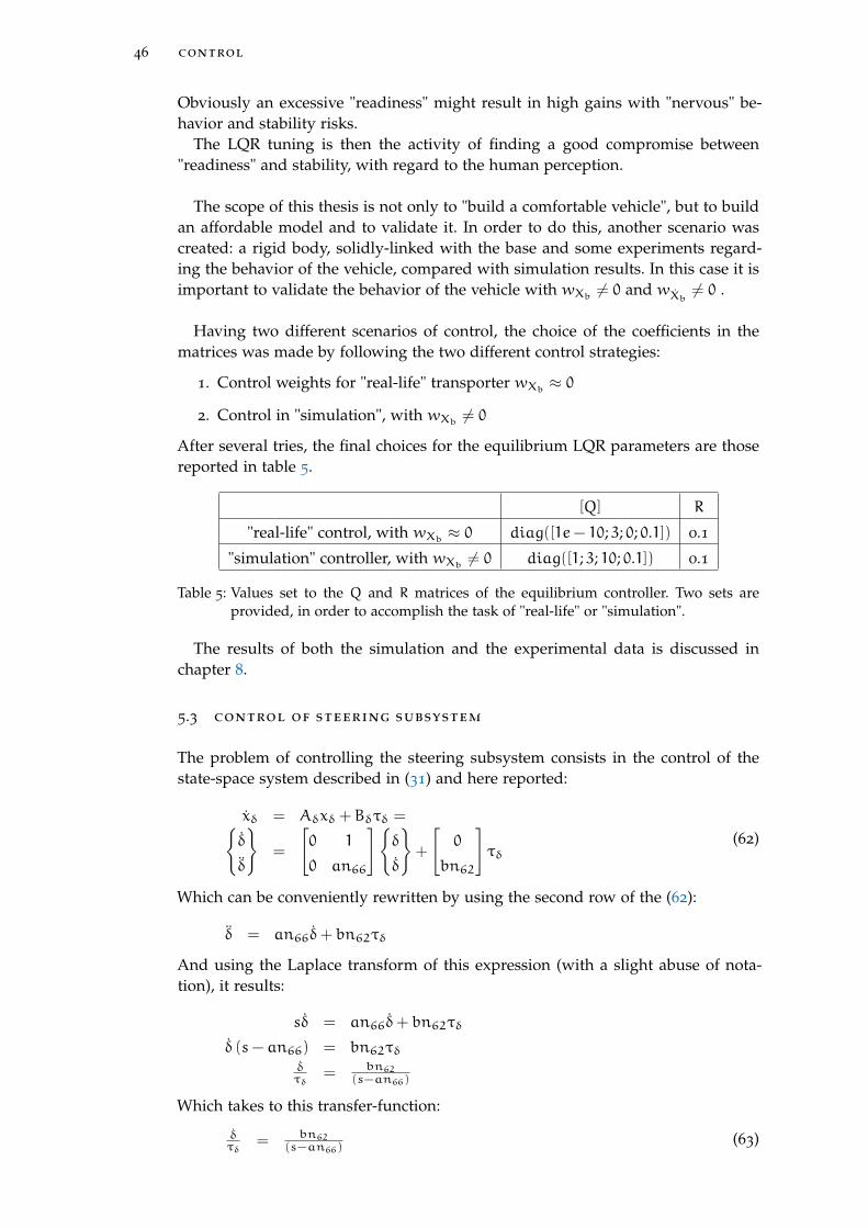
46 control
Obviously an excessive "readiness" might result in high gains with "nervous" be-havior and stability risks.
The LQR tuning is then the activity of finding a good compromise between"readiness" and stability, with regard to the human perception.
The scope of this thesis is not only to "build a comfortable vehicle", but to buildan affordable model and to validate it. In order to do this, another scenario wascreated: a rigid body, solidly-linked with the base and some experiments regard-ing the behavior of the vehicle, compared with simulation results. In this case it isimportant to validate the behavior of the vehicle with wXb 6= 0 and wXb 6= 0 .
Having two different scenarios of control, the choice of the coefficients in thematrices was made by following the two different control strategies:
1. Control weights for "real-life" transporter wXb ≈ 0
2. Control in "simulation", with wXb 6= 0
After several tries, the final choices for the equilibrium LQR parameters are thosereported in table 5.
[Q] R
"real-life" control, with wXb ≈ 0 diag([1e− 10; 3; 0; 0.1]) 0.1
"simulation" controller, with wXb 6= 0 diag([1; 3; 10; 0.1]) 0.1
Table 5: Values set to the Q and R matrices of the equilibrium controller. Two sets areprovided, in order to accomplish the task of "real-life" or "simulation".
The results of both the simulation and the experimental data is discussed inchapter 8.
5.3 control of steering subsystem
The problem of controlling the steering subsystem consists in the control of thestate-space system described in (31) and here reported:
xδ = Aδxδ +Bδτδ =δ
δ
=
[0 1
0 an66
]δ
δ
+
[0
bn62
]τδ
(62)
Which can be conveniently rewritten by using the second row of the (62):
δ = an66δ+ bn62τδ
And using the Laplace transform of this expression (with a slight abuse of nota-tion), it results:
sδ = an66δ+ bn62τδ
δ (s− an66) = bn62τδδτδ
= bn62(s−an66)
Which takes to this transfer-function:
δτδ
= bn62(s−an66)
(63)
[ December 2, 2017 at 17:06 – classicthesis ]
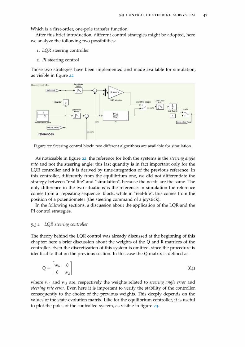
5.3 control of steering subsystem 47
Which is a first-order, one-pole transfer function.After this brief introduction, different control strategies might be adopted, here
we analyze the following two possibilities:
1. LQR steering controller
2. PI steering control
Those two strategies have been implemented and made available for simulation,as visible in figure 22.
Figure 22: Steering control block: two different algorithms are available for simulation.
As noticeable in figure 22, the reference for both the systems is the steering anglerate and not the steering angle: this last quantity is in fact important only for theLQR controller and it is derived by time-integration of the previous reference. Inthis controller, differently from the equilibrium one, we did not differentiate thestrategy between "real life" and "simulation", because the needs are the same. Theonly difference in the two situations is the reference: in simulation the referencecomes from a "repeating sequence" block, while in "real-life", this comes from theposition of a potentiometer (the steering command of a joystick).
In the following sections, a discussion about the application of the LQR and thePI control strategies.
5.3.1 LQR steering controller
The theory behind the LQR control was already discussed at the beginning of thischapter: here a brief discussion about the weights of the Q and R matrices of thecontroller. Even the discretization of this system is omitted, since the procedure isidentical to that on the previous section. In this case the Q matrix is defined as:
Q =
[wδ 0
0 wδ
](64)
where wδ and wδ are, respectively the weights related to steering angle error andsteering rate error. Even here it is important to verify the stability of the controller,consequently to the choice of the previous weights. This deeply depends on thevalues of the state-evolution matrix. Like for the equilibrium controller, it is usefulto plot the poles of the controlled system, as visible in figure 23.
[ December 2, 2017 at 17:06 – classicthesis ]
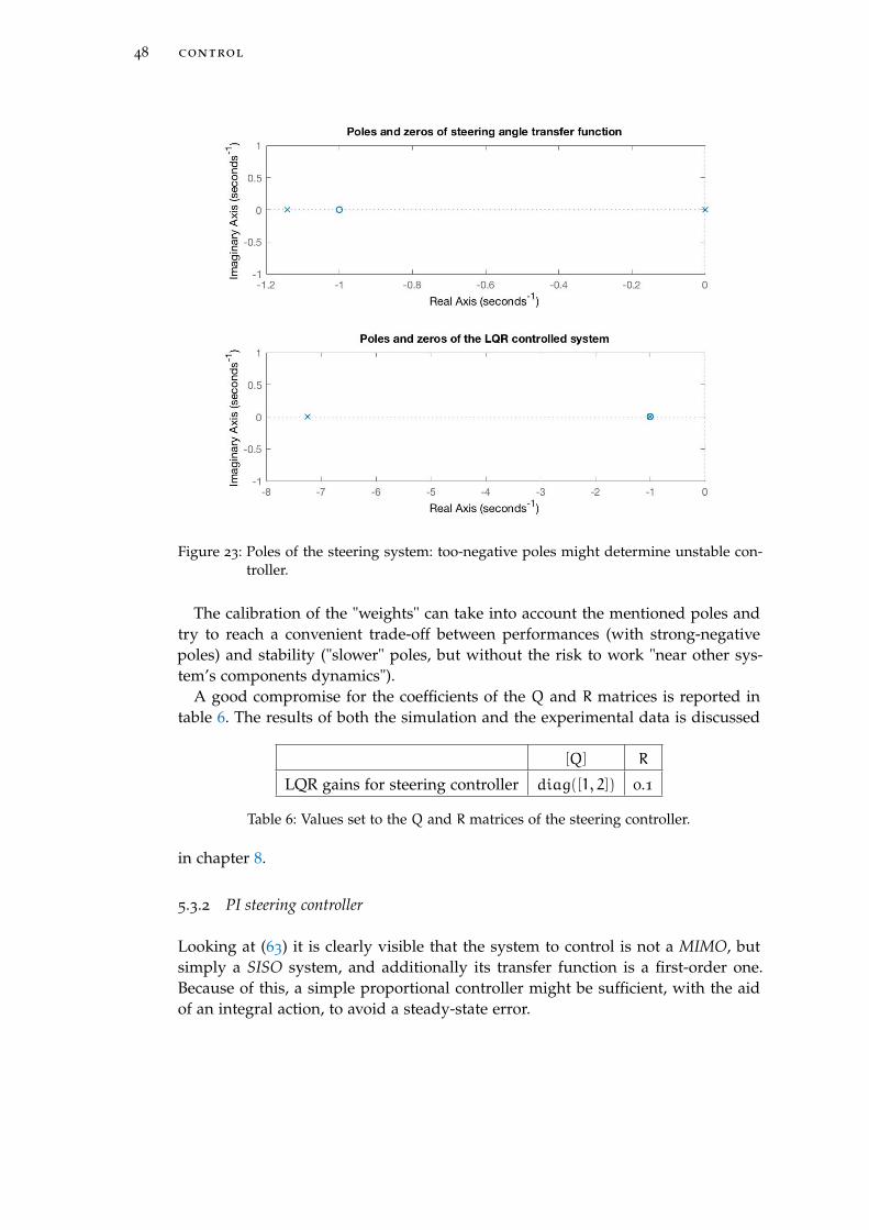
48 control
Figure 23: Poles of the steering system: too-negative poles might determine unstable con-troller.
The calibration of the "weights" can take into account the mentioned poles andtry to reach a convenient trade-off between performances (with strong-negativepoles) and stability ("slower" poles, but without the risk to work "near other sys-tem’s components dynamics").
A good compromise for the coefficients of the Q and R matrices is reported intable 6. The results of both the simulation and the experimental data is discussed
[Q] R
LQR gains for steering controller diag([1, 2]) 0.1
Table 6: Values set to the Q and R matrices of the steering controller.
in chapter 8.
5.3.2 PI steering controller
Looking at (63) it is clearly visible that the system to control is not a MIMO, butsimply a SISO system, and additionally its transfer function is a first-order one.Because of this, a simple proportional controller might be sufficient, with the aidof an integral action, to avoid a steady-state error.
[ December 2, 2017 at 17:06 – classicthesis ]
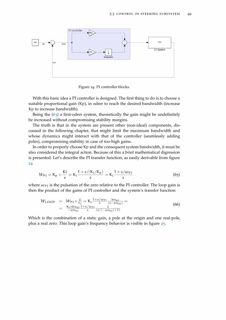
5.3 control of steering subsystem 49
Figure 24: PI controller blocks.
With this basic idea a PI controller is designed. The first thing to do is to choose asuitable proportional gain (Kp), in odrer to reach the desired bandwidth (increaseKp to increase bandwidth).
Being the (63) a first-odrer system, theoretically the gain might be undefinitelybe increased without compromising stability margins.
The truth is that in the system are present other (non-ideal) components, dis-cussed in the following chapter, that might limit the maximum bandwidth andwhose dynamics might interact with that of the controller (seamlessly addingpoles), compromising stability in case of too-high gains.
In order to properly choose Kp and the consequent system bandwidth, it must bealso considered the integral action. Because of this a brief mathematical digressionis presented. Let’s describe the PI transfer function, as easily derivable from figure24
WPI = Kp +Ki
s= Ki
1+ s/(Ki/Kp)
s= Ki
1+ s/ωPIs
(65)
where ωPI is the pulsation of the zero relative to the PI controller. The loop gain isthen the product of the gains of PI controller and the system’s transfer function:
WLOOP = WPI ∗ δτδ = Ki1+s/ωPI
sbn62
(s−an66)=
= Ki∗bn62−an66
1+s/ωPIs
1(s/(−an66)+1)
(66)
Which is the combination of a static gain, a pole at the origin and one real-pole,plus a real zero. This loop gain’s frequency behavior is visible in figure 25.
[ December 2, 2017 at 17:06 – classicthesis ]
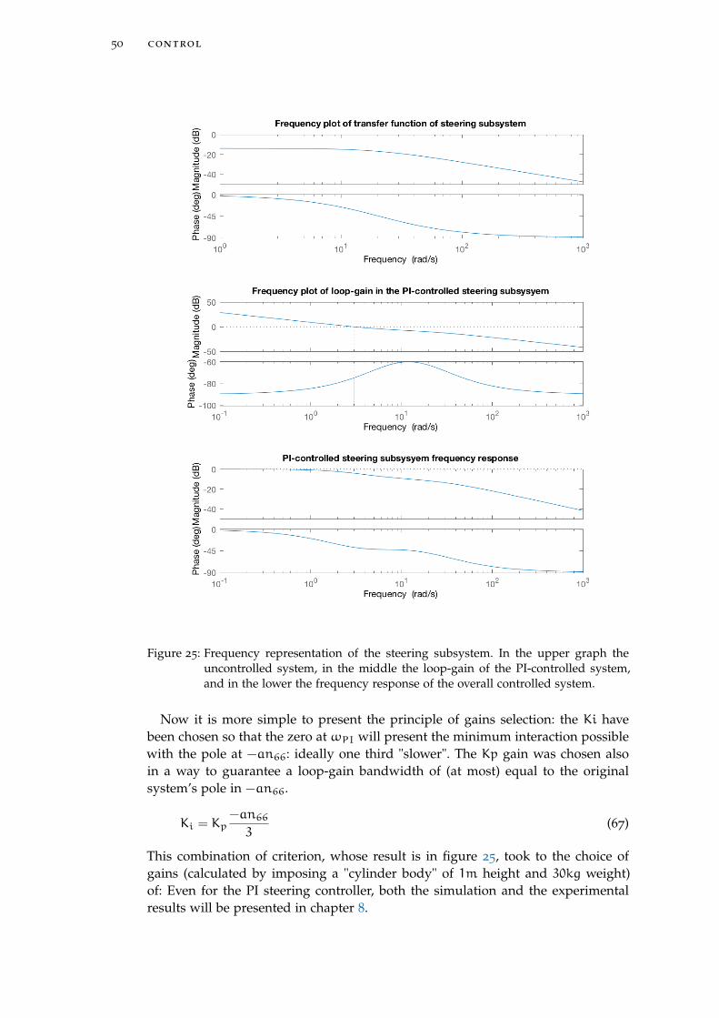
50 control
Figure 25: Frequency representation of the steering subsystem. In the upper graph theuncontrolled system, in the middle the loop-gain of the PI-controlled system,and in the lower the frequency response of the overall controlled system.
Now it is more simple to present the principle of gains selection: the Ki havebeen chosen so that the zero at ωPI will present the minimum interaction possiblewith the pole at −an66: ideally one third "slower". The Kp gain was chosen alsoin a way to guarantee a loop-gain bandwidth of (at most) equal to the originalsystem’s pole in −an66.
Ki = Kp−an663
(67)
This combination of criterion, whose result is in figure 25, took to the choice ofgains (calculated by imposing a "cylinder body" of 1m height and 30kg weight)of: Even for the PI steering controller, both the simulation and the experimentalresults will be presented in chapter 8.
[ December 2, 2017 at 17:06 – classicthesis ]

5.4 conclusions 51
Kp Ki
PI coefficients for the steering controller 2 13.8241
Table 7: Values chosen for the PI steering controller, in the case of a rigid-cylindric-body1m height and 30kg weight.
5.4 conclusions
In this chapter it was described the control algorithms chosen for the two subsys-tems that forms the TWSBT. It was described the motivation of the controller typeand the tuning strategies. Also it was reported a discussion about the stability.
All the controllers described here are designed on the base of an "ideal" system:it is a simplistic approach and lacks of many real-life limits that might modify a lotthe controller performances and its stability, but a first model-based control designis a good base for further tuning, based on real-life non-idealities.
In the following chapter, a detailed description of those real-life non-idealities,and how they were modeled, and used to properly tune the described controllers.
[ December 2, 2017 at 17:06 – classicthesis ]

[ December 2, 2017 at 17:06 – classicthesis ]
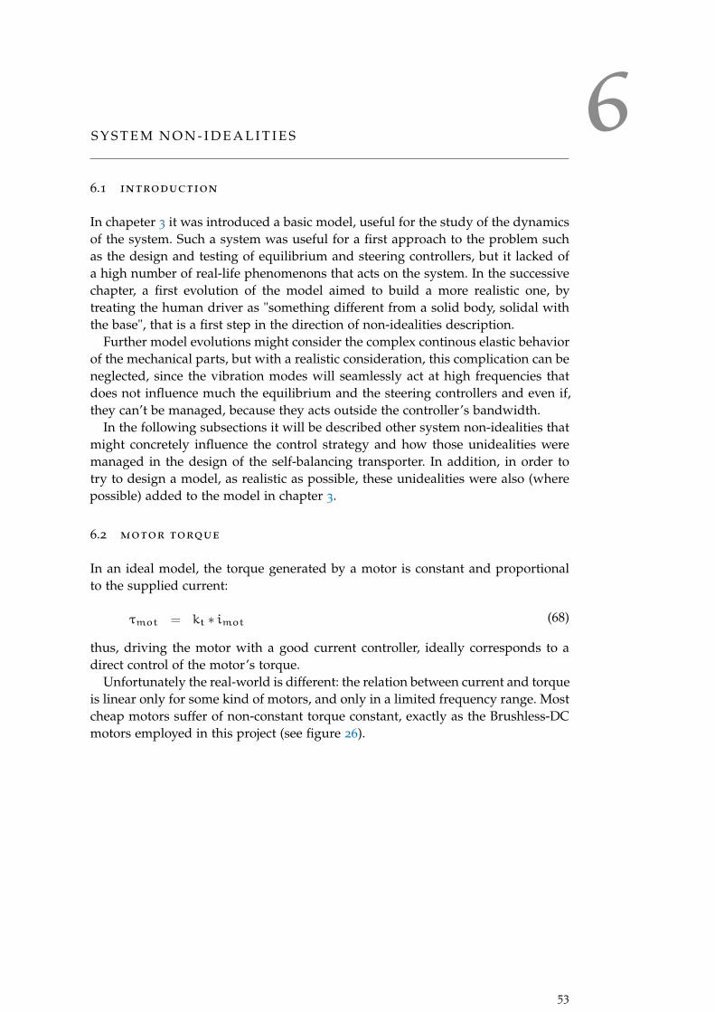
6S Y S T E M N O N - I D E A L I T I E S
6.1 introduction
In chapeter 3 it was introduced a basic model, useful for the study of the dynamicsof the system. Such a system was useful for a first approach to the problem suchas the design and testing of equilibrium and steering controllers, but it lacked ofa high number of real-life phenomenons that acts on the system. In the successivechapter, a first evolution of the model aimed to build a more realistic one, bytreating the human driver as "something different from a solid body, solidal withthe base", that is a first step in the direction of non-idealities description.
Further model evolutions might consider the complex continous elastic behaviorof the mechanical parts, but with a realistic consideration, this complication can beneglected, since the vibration modes will seamlessly act at high frequencies thatdoes not influence much the equilibrium and the steering controllers and even if,they can’t be managed, because they acts outside the controller’s bandwidth.
In the following subsections it will be described other system non-idealities thatmight concretely influence the control strategy and how those unidealities weremanaged in the design of the self-balancing transporter. In addition, in order totry to design a model, as realistic as possible, these unidealities were also (wherepossible) added to the model in chapter 3.
6.2 motor torque
In an ideal model, the torque generated by a motor is constant and proportionalto the supplied current:
τmot = kt ∗ imot (68)
thus, driving the motor with a good current controller, ideally corresponds to adirect control of the motor’s torque.
Unfortunately the real-world is different: the relation between current and torqueis linear only for some kind of motors, and only in a limited frequency range. Mostcheap motors suffer of non-constant torque constant, exactly as the Brushless-DCmotors employed in this project (see figure 26).
53
[ December 2, 2017 at 17:06 – classicthesis ]
54 system non-idealities
Figure 26: Torque ripple in a BLDC motor, due to a variation of ke ≈ kt along the electricalangle. Figure from [29].
In the Brushless-DC (BLDC) motors, the value of kt is not constant along therotation of the motor, and results in a torque ripple during the motor rotation thatrepeats at six-times the rate of rotation.
kt(θr) = ke(θr) =dλe(θr)
dθr(69)
This phenomena is acceptable for many applications, where the motor worksat high-rotation-speeds, because the load inertia and the friction has a low-passeffect on the torque transmission, resulting in a "sufficiently smooth" motion, atthe endpoint of the transmission chain. As opposite, this torque-ripple can resultunacceptable for many industrial processes, having a need of high-precision andregularity.
The design of a self-balancing vehicle is partially a low-cost transportation ap-plication, where the torque ripple is not a big matter, but at the same time, thetorque ripple could strongly influence the on-board accelerometer reading, thusseriously disturb, or even compromise the reading of the pitch angle, especially atlow-speed.
Another fact is that the torque-ripple might probably excite some vibrationmodes of the structure, thus it might affect not only the controller, but can evencompromise the long-term mechanical structure of the product, with possible fail-ures.
6.2.0.1 Torque vs driving technique
In our application (for a matter of cost and dimension) it was not feasible to thinkabout the use of sinusoidal morots, so eliminating the pure-DC motor, the BLDCchoice was almost obvious. In the BLDC world, the motor construction and quality,strongly influences the magnitude and form of the ripple torque, thus a first choiceof low-torque-ripple motor was made.
Even with this, the problem of the ripple torque will always be, as long as aBLDC motor will be employed. Nevertheless, if the choice of a BLDC motor isalmost compulsory, the choice of the driving technique might play a decisive im-provement in the torque ripple. Several studies such as [18] and [17] have testedthe possibility to apply some advanced control techniques like Field-Orient Con-trol (FOC) in order to reduce the torque ripple in the motor.
[ December 2, 2017 at 17:06 – classicthesis ]

6.2 motor torque 55
The scheme of the 3-phase BLDC FOC control is shown in figure 27
Figure 27: Block-diagram of a field-oriented control for a 3-phase BLDC motor. Figure from[17].
This control technique, widely used in the motor control world is mainly basedon the knowledge of the 3-phase motor’s model (reported on figure) and it’s pa-rameters.
[ December 2, 2017 at 17:06 – classicthesis ]

56 system non-idealities
Figure 28: Electrical schematic (simplified) of a BLDC motor. Figure from [29].
Infact, by precisely orienting the magnetic field generated by the stator currents(named ia , ib and ic), against the flux linkage, generated by the permanent mag-net, it is possible to directly control the torque generated by the motor.
The application of the field-oriented control to the permanent-magnet motors,was originally on the sinusoidal PMSM, while an application to the BLDC wasillustrated in [18].
The complete FOC theory will not be reported, but what is important is that fora proper control, the motor must be IDENTIFIED: the parameters shown on figure28 must be measured or calculated.
In the board used in the project, a simple graphical interface (figure 29) made itpossible to do the automatic identification process by measuring/calculating:
• winding resistance
• winding inductance
• flux linkage
• hall position
• current controller gain
This simple, but convenient GUI made it possible to "tune" the controller by simplyconnecting with an USB cord, the PC to the controller board.
[ December 2, 2017 at 17:06 – classicthesis ]
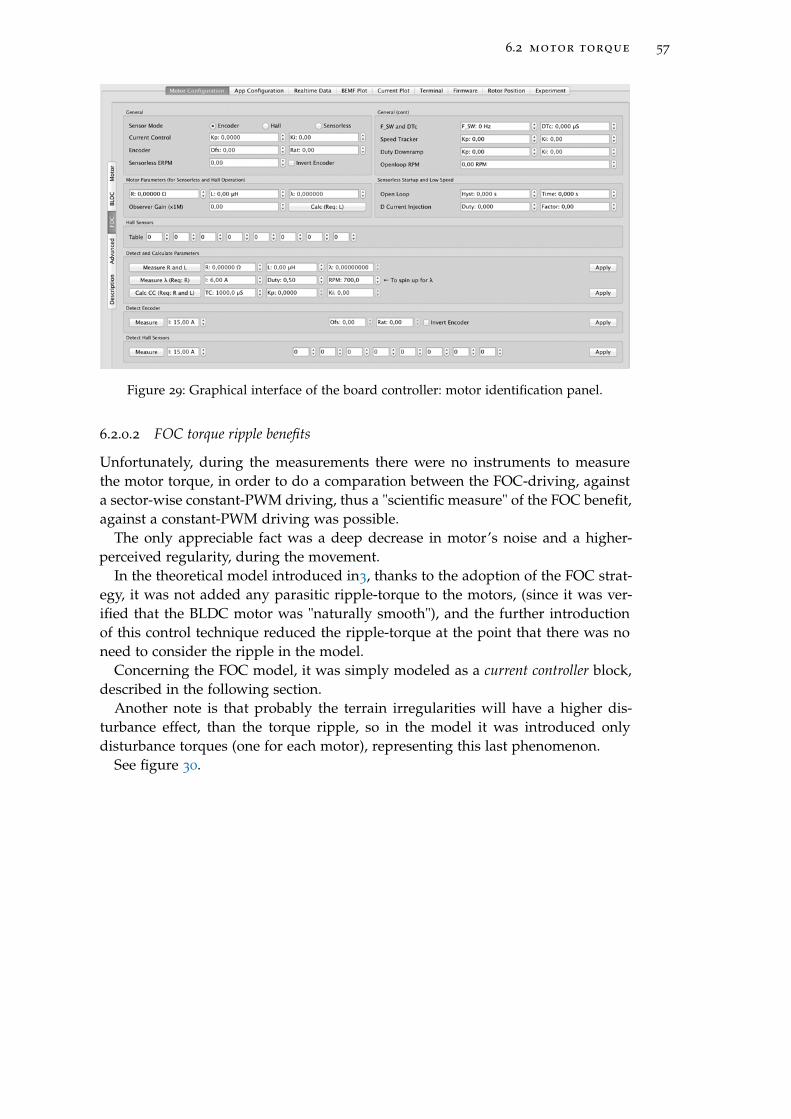
6.2 motor torque 57
Figure 29: Graphical interface of the board controller: motor identification panel.
6.2.0.2 FOC torque ripple benefits
Unfortunately, during the measurements there were no instruments to measurethe motor torque, in order to do a comparation between the FOC-driving, againsta sector-wise constant-PWM driving, thus a "scientific measure" of the FOC benefit,against a constant-PWM driving was possible.
The only appreciable fact was a deep decrease in motor’s noise and a higher-perceived regularity, during the movement.
In the theoretical model introduced in3, thanks to the adoption of the FOC strat-egy, it was not added any parasitic ripple-torque to the motors, (since it was ver-ified that the BLDC motor was "naturally smooth"), and the further introductionof this control technique reduced the ripple-torque at the point that there was noneed to consider the ripple in the model.
Concerning the FOC model, it was simply modeled as a current controller block,described in the following section.
Another note is that probably the terrain irregularities will have a higher dis-turbance effect, than the torque ripple, so in the model it was introduced onlydisturbance torques (one for each motor), representing this last phenomenon.
See figure 30.
[ December 2, 2017 at 17:06 – classicthesis ]
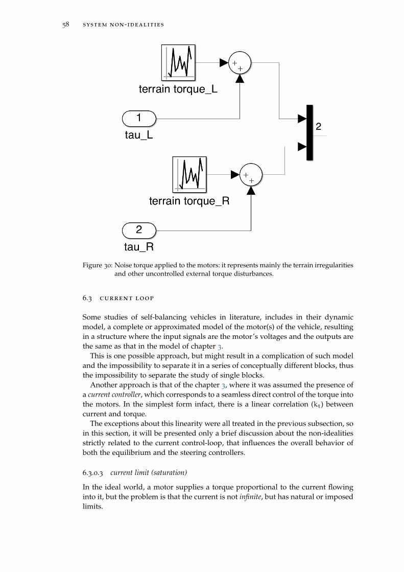
58 system non-idealities
Figure 30: Noise torque applied to the motors: it represents mainly the terrain irregularitiesand other uncontrolled external torque disturbances.
6.3 current loop
Some studies of self-balancing vehicles in literature, includes in their dynamicmodel, a complete or approximated model of the motor(s) of the vehicle, resultingin a structure where the input signals are the motor’s voltages and the outputs arethe same as that in the model of chapter 3.
This is one possible approach, but might result in a complication of such modeland the impossibility to separate it in a series of conceptually different blocks, thusthe impossibility to separate the study of single blocks.
Another approach is that of the chapter 3, where it was assumed the presence ofa current controller, which corresponds to a seamless direct control of the torque intothe motors. In the simplest form infact, there is a linear correlation (kt) betweencurrent and torque.
The exceptions about this linearity were all treated in the previous subsection, soin this section, it will be presented only a brief discussion about the non-idealitiesstrictly related to the current control-loop, that influences the overall behavior ofboth the equilibrium and the steering controllers.
6.3.0.3 current limit (saturation)
In the ideal world, a motor supplies a torque proportional to the current flowinginto it, but the problem is that the current is not infinite, but has natural or imposedlimits.
[ December 2, 2017 at 17:06 – classicthesis ]
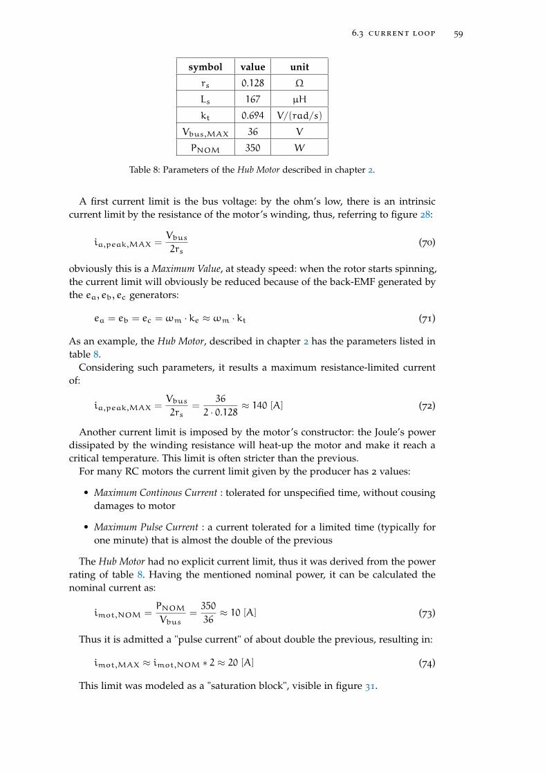
6.3 current loop 59
symbol value unit
rs 0.128 Ω
Ls 167 µH
kt 0.694 V/(rad/s)
Vbus,MAX 36 V
PNOM 350 W
Table 8: Parameters of the Hub Motor described in chapter 2.
A first current limit is the bus voltage: by the ohm’s low, there is an intrinsiccurrent limit by the resistance of the motor’s winding, thus, referring to figure 28:
ia,peak,MAX =Vbus2rs
(70)
obviously this is a Maximum Value, at steady speed: when the rotor starts spinning,the current limit will obviously be reduced because of the back-EMF generated bythe ea, eb, ec generators:
ea = eb = ec = ωm · ke ≈ ωm · kt (71)
As an example, the Hub Motor, described in chapter 2 has the parameters listed intable 8.
Considering such parameters, it results a maximum resistance-limited currentof:
ia,peak,MAX =Vbus2rs
=36
2 · 0.128≈ 140 [A] (72)
Another current limit is imposed by the motor’s constructor: the Joule’s powerdissipated by the winding resistance will heat-up the motor and make it reach acritical temperature. This limit is often stricter than the previous.
For many RC motors the current limit given by the producer has 2 values:
• Maximum Continous Current : tolerated for unspecified time, without cousingdamages to motor
• Maximum Pulse Current : a current tolerated for a limited time (typically forone minute) that is almost the double of the previous
The Hub Motor had no explicit current limit, thus it was derived from the powerrating of table 8. Having the mentioned nominal power, it can be calculated thenominal current as:
imot,NOM =PNOMVbus
=350
36≈ 10 [A] (73)
Thus it is admitted a "pulse current" of about double the previous, resulting in:
imot,MAX ≈ imot,NOM ∗ 2 ≈ 20 [A] (74)
This limit was modeled as a "saturation block", visible in figure 31.
[ December 2, 2017 at 17:06 – classicthesis ]
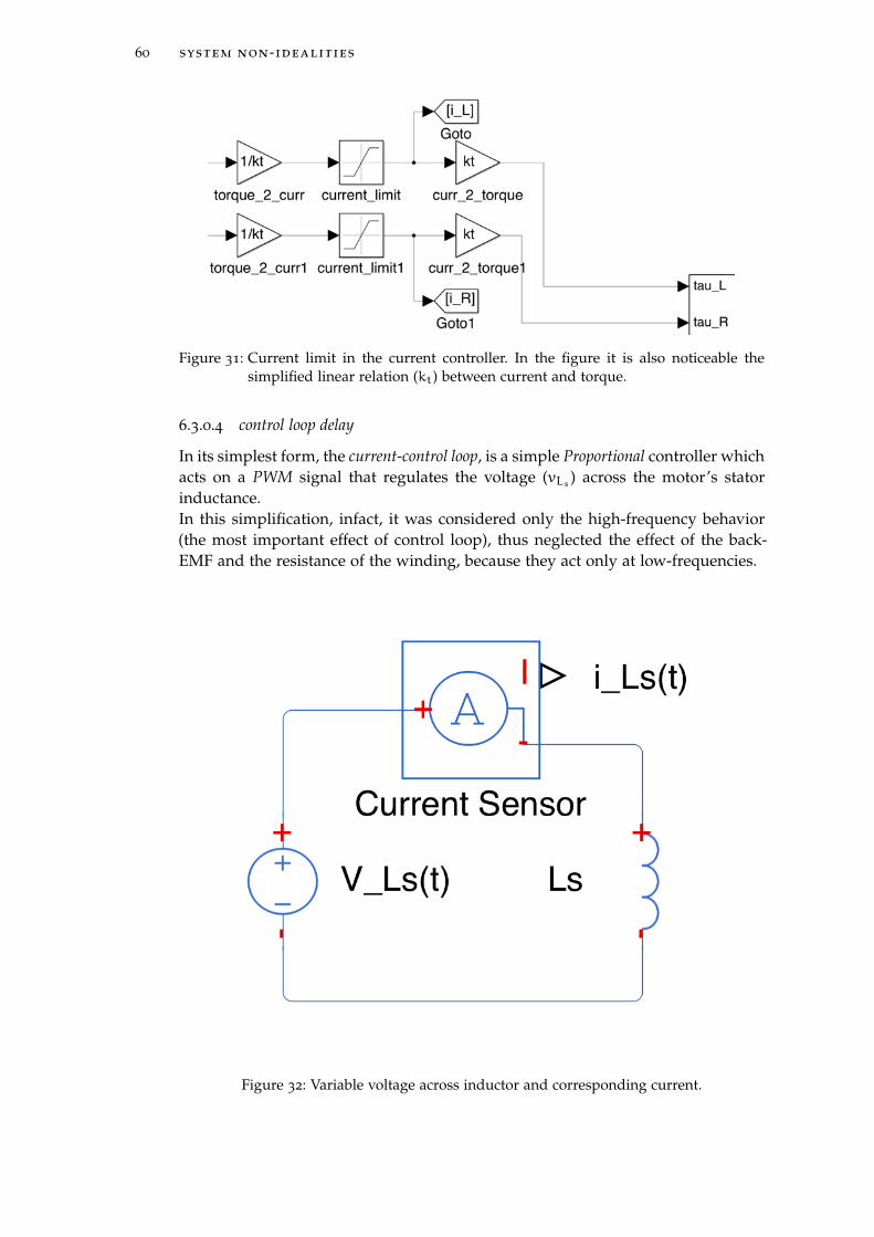
60 system non-idealities
Figure 31: Current limit in the current controller. In the figure it is also noticeable thesimplified linear relation (kt) between current and torque.
6.3.0.4 control loop delay
In its simplest form, the current-control loop, is a simple Proportional controller whichacts on a PWM signal that regulates the voltage (vLs) across the motor’s statorinductance.In this simplification, infact, it was considered only the high-frequency behavior(the most important effect of control loop), thus neglected the effect of the back-EMF and the resistance of the winding, because they act only at low-frequencies.
Figure 32: Variable voltage across inductor and corresponding current.
[ December 2, 2017 at 17:06 – classicthesis ]
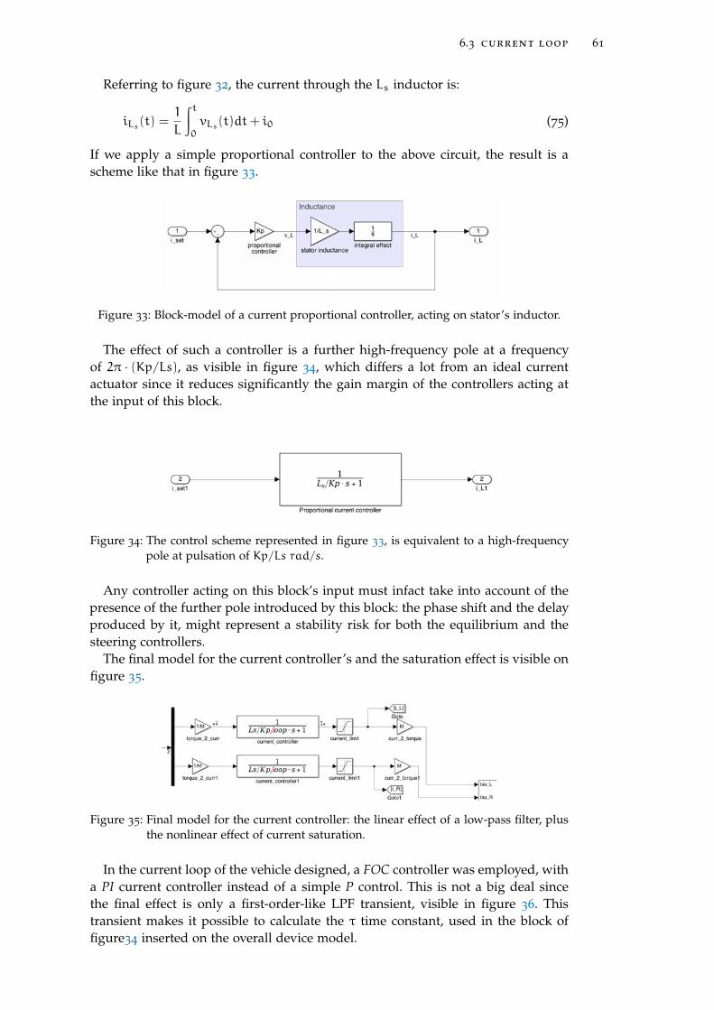
6.3 current loop 61
Referring to figure 32, the current through the Ls inductor is:
iLs(t) =1
L
∫t0
vLs(t)dt+ i0 (75)
If we apply a simple proportional controller to the above circuit, the result is ascheme like that in figure 33.
Figure 33: Block-model of a current proportional controller, acting on stator’s inductor.
The effect of such a controller is a further high-frequency pole at a frequencyof 2π · (Kp/Ls), as visible in figure 34, which differs a lot from an ideal currentactuator since it reduces significantly the gain margin of the controllers acting atthe input of this block.
Figure 34: The control scheme represented in figure 33, is equivalent to a high-frequencypole at pulsation of Kp/Ls rad/s.
Any controller acting on this block’s input must infact take into account of thepresence of the further pole introduced by this block: the phase shift and the delayproduced by it, might represent a stability risk for both the equilibrium and thesteering controllers.
The final model for the current controller’s and the saturation effect is visible onfigure 35.
Figure 35: Final model for the current controller: the linear effect of a low-pass filter, plusthe nonlinear effect of current saturation.
In the current loop of the vehicle designed, a FOC controller was employed, witha PI current controller instead of a simple P control. This is not a big deal sincethe final effect is only a first-order-like LPF transient, visible in figure 36. Thistransient makes it possible to calculate the τ time constant, used in the block offigure34 inserted on the overall device model.
[ December 2, 2017 at 17:06 – classicthesis ]
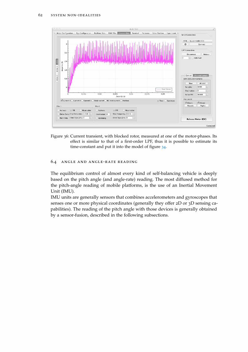
62 system non-idealities
Figure 36: Current transient, with blocked rotor, measured at one of the motor-phases. Itseffect is similar to that of a first-order LPF, thus it is possible to estimate itstime-constant and put it into the model of figure 34.
6.4 angle and angle-rate reading
The equilibrium control of almost every kind of self-balancing vehicle is deeplybased on the pitch angle (and angle-rate) reading. The most diffused method forthe pitch-angle reading of mobile platforms, is the use of an Inertial MovementUnit (IMU).IMU units are generally sensors that combines accelerometers and gyroscopes thatsenses one or more physical coordinates (generally they offer 2D or 3D sensing ca-pabilities). The reading of the pitch angle with those devices is generally obtainedby a sensor-fusion, described in the following subsections.
[ December 2, 2017 at 17:06 – classicthesis ]
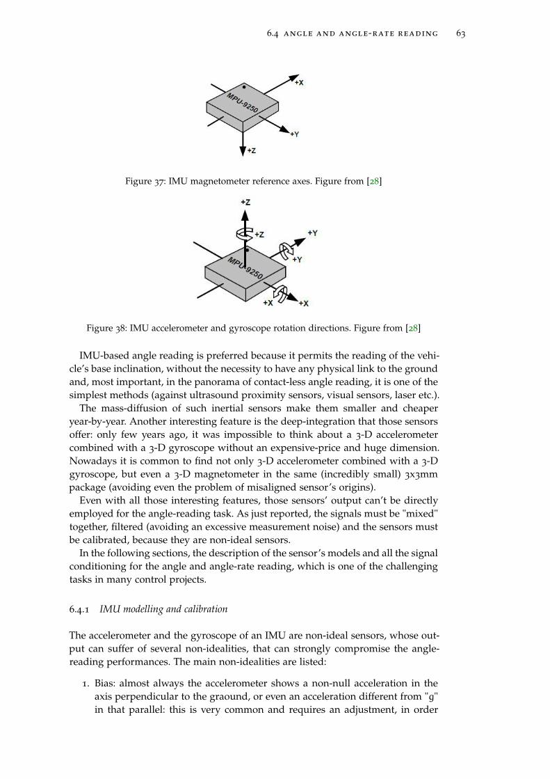
6.4 angle and angle-rate reading 63
Figure 37: IMU magnetometer reference axes. Figure from [28]
Figure 38: IMU accelerometer and gyroscope rotation directions. Figure from [28]
IMU-based angle reading is preferred because it permits the reading of the vehi-cle’s base inclination, without the necessity to have any physical link to the groundand, most important, in the panorama of contact-less angle reading, it is one of thesimplest methods (against ultrasound proximity sensors, visual sensors, laser etc.).
The mass-diffusion of such inertial sensors make them smaller and cheaperyear-by-year. Another interesting feature is the deep-integration that those sensorsoffer: only few years ago, it was impossible to think about a 3-D accelerometercombined with a 3-D gyroscope without an expensive-price and huge dimension.Nowadays it is common to find not only 3-D accelerometer combined with a 3-Dgyroscope, but even a 3-D magnetometer in the same (incredibly small) 3x3mmpackage (avoiding even the problem of misaligned sensor’s origins).
Even with all those interesting features, those sensors’ output can’t be directlyemployed for the angle-reading task. As just reported, the signals must be "mixed"together, filtered (avoiding an excessive measurement noise) and the sensors mustbe calibrated, because they are non-ideal sensors.
In the following sections, the description of the sensor’s models and all the signalconditioning for the angle and angle-rate reading, which is one of the challengingtasks in many control projects.
6.4.1 IMU modelling and calibration
The accelerometer and the gyroscope of an IMU are non-ideal sensors, whose out-put can suffer of several non-idealities, that can strongly compromise the angle-reading performances. The main non-idealities are listed:
1. Bias: almost always the accelerometer shows a non-null acceleration in theaxis perpendicular to the graound, or even an acceleration different from "g"in that parallel: this is very common and requires an adjustment, in order
[ December 2, 2017 at 17:06 – classicthesis ]
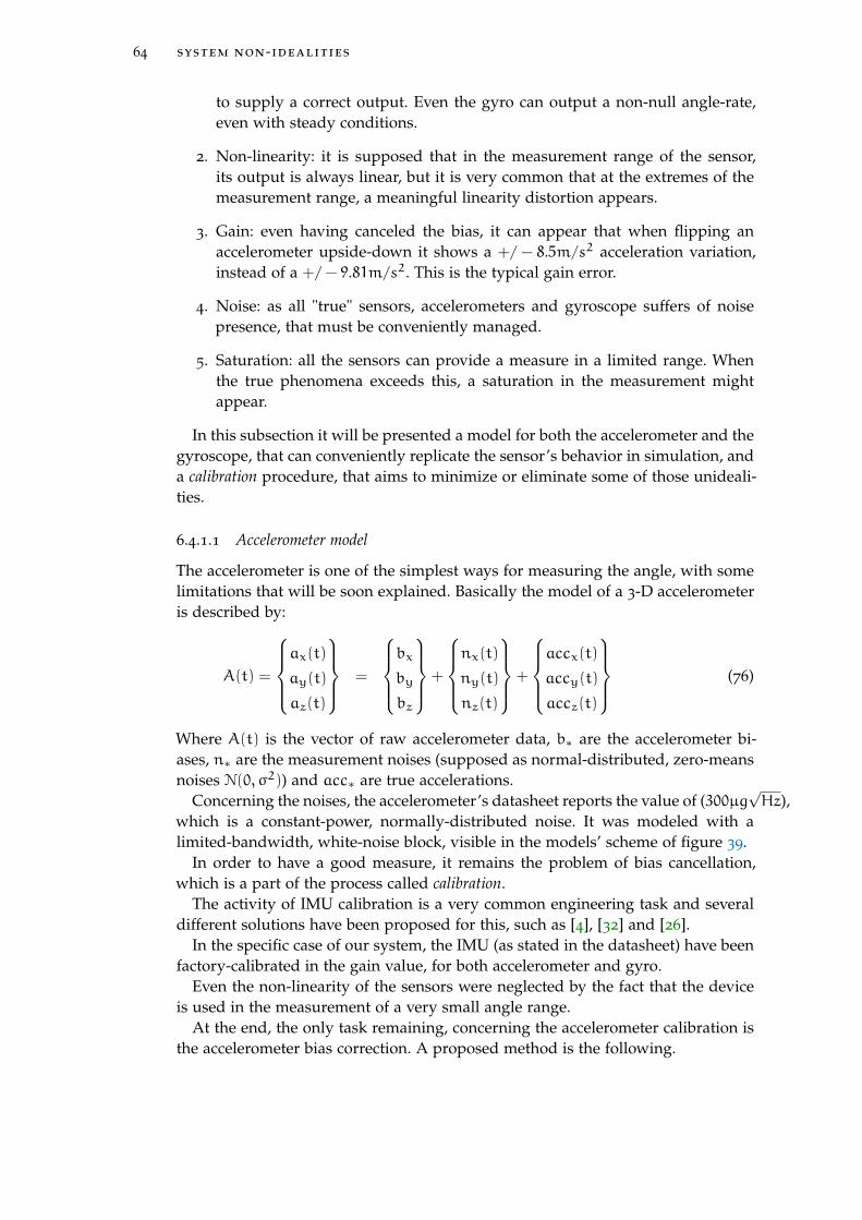
64 system non-idealities
to supply a correct output. Even the gyro can output a non-null angle-rate,even with steady conditions.
2. Non-linearity: it is supposed that in the measurement range of the sensor,its output is always linear, but it is very common that at the extremes of themeasurement range, a meaningful linearity distortion appears.
3. Gain: even having canceled the bias, it can appear that when flipping anaccelerometer upside-down it shows a +/− 8.5m/s2 acceleration variation,instead of a +/− 9.81m/s2. This is the typical gain error.
4. Noise: as all "true" sensors, accelerometers and gyroscope suffers of noisepresence, that must be conveniently managed.
5. Saturation: all the sensors can provide a measure in a limited range. Whenthe true phenomena exceeds this, a saturation in the measurement mightappear.
In this subsection it will be presented a model for both the accelerometer and thegyroscope, that can conveniently replicate the sensor’s behavior in simulation, anda calibration procedure, that aims to minimize or eliminate some of those unideali-ties.
6.4.1.1 Accelerometer model
The accelerometer is one of the simplest ways for measuring the angle, with somelimitations that will be soon explained. Basically the model of a 3-D accelerometeris described by:
A(t) =
ax(t)
ay(t)
az(t)
=
bx
by
bz
+
nx(t)
ny(t)
nz(t)
+
accx(t)
accy(t)
accz(t)
(76)
Where A(t) is the vector of raw accelerometer data, b∗ are the accelerometer bi-ases, n∗ are the measurement noises (supposed as normal-distributed, zero-meansnoises N(0, σ2)) and acc∗ are true accelerations.
Concerning the noises, the accelerometer’s datasheet reports the value of (300µg√Hz),
which is a constant-power, normally-distributed noise. It was modeled with alimited-bandwidth, white-noise block, visible in the models’ scheme of figure 39.
In order to have a good measure, it remains the problem of bias cancellation,which is a part of the process called calibration.
The activity of IMU calibration is a very common engineering task and severaldifferent solutions have been proposed for this, such as [4], [32] and [26].
In the specific case of our system, the IMU (as stated in the datasheet) have beenfactory-calibrated in the gain value, for both accelerometer and gyro.
Even the non-linearity of the sensors were neglected by the fact that the deviceis used in the measurement of a very small angle range.
At the end, the only task remaining, concerning the accelerometer calibration isthe accelerometer bias correction. A proposed method is the following.
[ December 2, 2017 at 17:06 – classicthesis ]
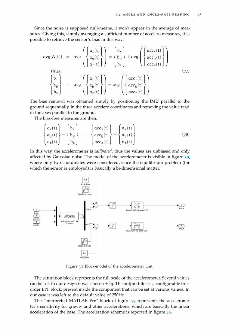
6.4 angle and angle-rate reading 65
Since the noise is supposed null-means, it won’t appear in the average of mea-sures. Giving this, simply averaging a sufficient number of accelero measures, it ispossible to retrieve the sensor’s bias in this way:
avg(A(t)) = avg
ax(t)
ay(t)
az(t)
=
bx
by
bz
+ avg
accx(t)
accy(t)
accz(t)
thus :bx
by
bz
= avg
ax(t)
ay(t)
az(t)
− avg
accx(t)
accy(t)
accz(t)
(77)
The bias removal was obtained simply by positioning the IMU parallel to theground sequentially, in the three accelero coordinates and removing the value readin the axes parallel to the ground.
The bias-free measures are then:ax(t)
ay(t)
az(t)
−
bx
by
bz
=
accx(t)
accy(t)
accz(t)
+
nx(t)
ny(t)
nz(t)
(78)
In this way, the accelerometer is calibrated, thus the values are unbiased and onlyaffected by Gaussian noise. The model of the accelerometer is visible in figure 39,where only two coordinates were considered, since the equilibrium problem (forwhich the sensor is employed) is basically a bi-dimensional matter.
Figure 39: Block-model of the accelerometer unit.
The saturation block represents the full-scale of the accelerometer. Several valuescan be set. In our design it was chosen ±2g. The output filter is a configurable first-order LPF block, present inside the component that can be set at various values. Inour case it was left to the default value of 250Hz.
The "Interpreted MATLAB Fcn" block of figure 39 represents the accelerome-ter’s sensitivity for gravity and other accelerations, which are basically the linearacceleration of the base. The acceleration scheme is reported in figure 40.
[ December 2, 2017 at 17:06 – classicthesis ]
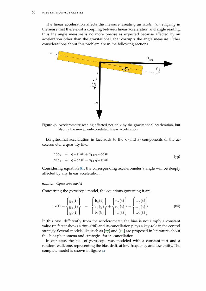
66 system non-idealities
The linear acceleration affects the measure, creating an acceleration coupling inthe sense that there exist a coupling between linear acceleration and angle reading,thus the angle measure is no more precise as expected because affected by anacceleration other than the gravitational, that corrupts the angle measure. Otherconsiderations about this problem are in the following sections.
Figure 40: Accelerometer reading affected not only by the gravitational acceleration, butalso by the movement-correlated linear acceleration
Longitudinal acceleration in fact adds to the x (and z) components of the ac-celerometer a quantity like:
accx = g ∗ sinθ+ aLIN ∗ cosθaccz = g ∗ cosθ− aLIN ∗ sinθ
(79)
Considering equation 81, the corresponding accelerometer’s angle will be deeplyaffected by any linear acceleration.
6.4.1.2 Gyroscope model
Concerning the gyroscope model, the equations governing it are:
G(t) =
gx(t)
gy(t)
gz(t)
=
bx(t)
by(y)
bz(b)
+
nx(t)
ny(t)
nz(t)
+
ωx(t)
ωy(t)
ωz(t)
(80)
In this case, differently from the accelerometer, the bias is not simply a constantvalue (in fact it shows a time-drift) and its cancellation plays a key-role in the controlstrategy. Several models like such as [27] and [24] are proposed in literature, aboutthis bias phenomena and strategies for its cancellation.
In our case, the bias of gyroscope was modeled with a constant-part and arandom-walk one, representing the bias-drift, at low-frequency and low entity. Thecomplete model is shown in figure 41.
[ December 2, 2017 at 17:06 – classicthesis ]
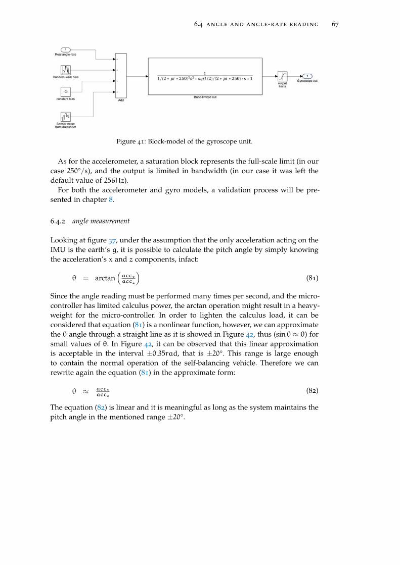
6.4 angle and angle-rate reading 67
Figure 41: Block-model of the gyroscope unit.
As for the accelerometer, a saturation block represents the full-scale limit (in ourcase 250°/s), and the output is limited in bandwidth (in our case it was left thedefault value of 256Hz).
For both the accelerometer and gyro models, a validation process will be pre-sented in chapter 8.
6.4.2 angle measurement
Looking at figure 37, under the assumption that the only acceleration acting on theIMU is the earth’s g, it is possible to calculate the pitch angle by simply knowingthe acceleration’s x and z components, infact:
θ = arctan(accxaccz
)(81)
Since the angle reading must be performed many times per second, and the micro-controller has limited calculus power, the arctan operation might result in a heavy-weight for the micro-controller. In order to lighten the calculus load, it can beconsidered that equation (81) is a nonlinear function, however, we can approximatethe θ angle through a straight line as it is showed in Figure 42, thus (sin θ ≈ θ) forsmall values of θ. In Figure 42, it can be observed that this linear approximationis acceptable in the interval ±0.35rad, that is ±20°. This range is large enoughto contain the normal operation of the self-balancing vehicle. Therefore we canrewrite again the equation (81) in the approximate form:
θ ≈ accxaccz
(82)
The equation (82) is linear and it is meaningful as long as the system maintains thepitch angle in the mentioned range ±20°.
[ December 2, 2017 at 17:06 – classicthesis ]
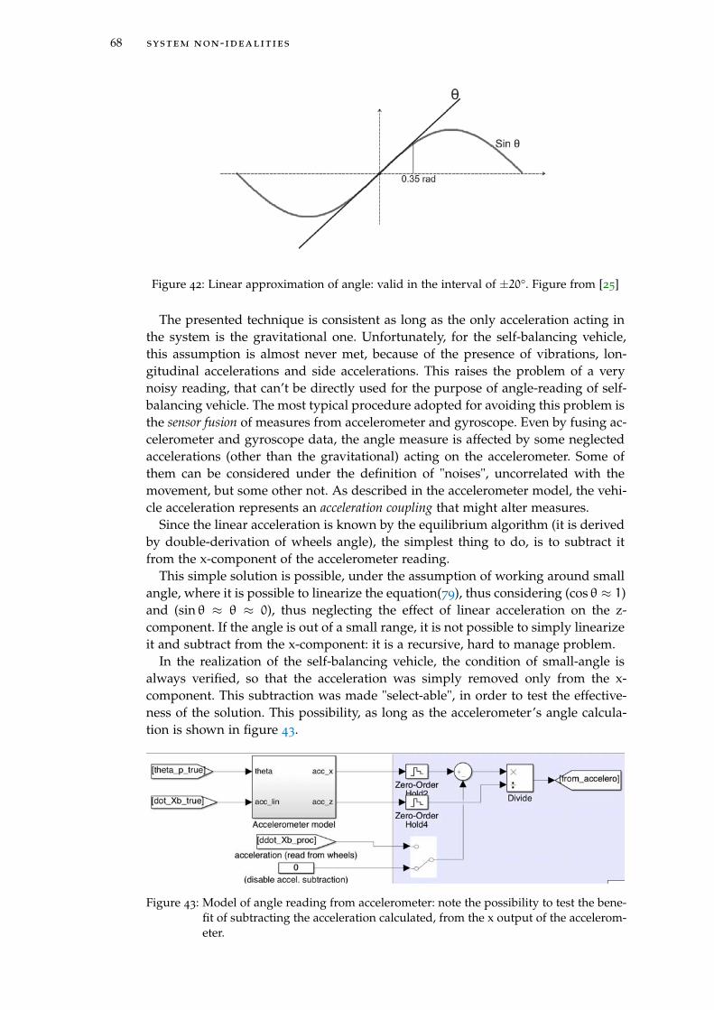
68 system non-idealities
Figure 42: Linear approximation of angle: valid in the interval of ±20°. Figure from [25]
The presented technique is consistent as long as the only acceleration acting inthe system is the gravitational one. Unfortunately, for the self-balancing vehicle,this assumption is almost never met, because of the presence of vibrations, lon-gitudinal accelerations and side accelerations. This raises the problem of a verynoisy reading, that can’t be directly used for the purpose of angle-reading of self-balancing vehicle. The most typical procedure adopted for avoiding this problem isthe sensor fusion of measures from accelerometer and gyroscope. Even by fusing ac-celerometer and gyroscope data, the angle measure is affected by some neglectedaccelerations (other than the gravitational) acting on the accelerometer. Some ofthem can be considered under the definition of "noises", uncorrelated with themovement, but some other not. As described in the accelerometer model, the vehi-cle acceleration represents an acceleration coupling that might alter measures.
Since the linear acceleration is known by the equilibrium algorithm (it is derivedby double-derivation of wheels angle), the simplest thing to do, is to subtract itfrom the x-component of the accelerometer reading.
This simple solution is possible, under the assumption of working around smallangle, where it is possible to linearize the equation(79), thus considering (cos θ ≈ 1)and (sinθ ≈ θ ≈ 0), thus neglecting the effect of linear acceleration on the z-component. If the angle is out of a small range, it is not possible to simply linearizeit and subtract from the x-component: it is a recursive, hard to manage problem.
In the realization of the self-balancing vehicle, the condition of small-angle isalways verified, so that the acceleration was simply removed only from the x-component. This subtraction was made "select-able", in order to test the effective-ness of the solution. This possibility, as long as the accelerometer’s angle calcula-tion is shown in figure 43.
Figure 43: Model of angle reading from accelerometer: note the possibility to test the bene-fit of subtracting the acceleration calculated, from the x output of the accelerom-eter.
[ December 2, 2017 at 17:06 – classicthesis ]
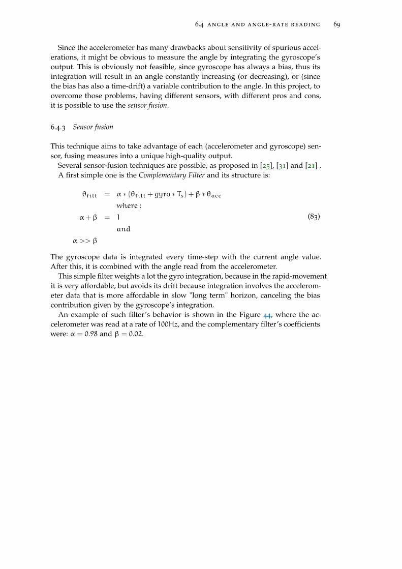
6.4 angle and angle-rate reading 69
Since the accelerometer has many drawbacks about sensitivity of spurious accel-erations, it might be obvious to measure the angle by integrating the gyroscope’soutput. This is obviously not feasible, since gyroscope has always a bias, thus itsintegration will result in an angle constantly increasing (or decreasing), or (sincethe bias has also a time-drift) a variable contribution to the angle. In this project, toovercome those problems, having different sensors, with different pros and cons,it is possible to use the sensor fusion.
6.4.3 Sensor fusion
This technique aims to take advantage of each (accelerometer and gyroscope) sen-sor, fusing measures into a unique high-quality output.
Several sensor-fusion techniques are possible, as proposed in [25], [31] and [21] .A first simple one is the Complementary Filter and its structure is:
θfilt = α ∗ (θfilt + gyro ∗ Ts) +β ∗ θaccwhere :
α+β = 1
and
α >> β
(83)
The gyroscope data is integrated every time-step with the current angle value.After this, it is combined with the angle read from the accelerometer.
This simple filter weights a lot the gyro integration, because in the rapid-movementit is very affordable, but avoids its drift because integration involves the accelerom-eter data that is more affordable in slow "long term" horizon, canceling the biascontribution given by the gyroscope’s integration.
An example of such filter’s behavior is shown in the Figure 44, where the ac-celerometer was read at a rate of 100Hz, and the complementary filter’s coefficientswere: α = 0.98 and β = 0.02.
[ December 2, 2017 at 17:06 – classicthesis ]

70 system non-idealities
Figure 44: Comparison of angle reading with accelerometer and complementary filter. Inthis setup α = 0.98 and β = 0.02
The result is good, but in some cases it might result "too noisy", or "too slow", ifnot properly calibrated. The complementary filter must then be tuned properly, inorder to give the expected output. A model for this filter is presented in figure 45.
Figure 45: Complementary filter model: the simplest approach for IMU sensor fusion.
A validation of this model will be presented in chapter 8.
6.4.4 Kalman filtering
Even if the complementary-filter works fine in many applications, it has to be prop-erly tuned in order to obtain a trade-off between responsiveness and noise removal.Many times, in order to reduce the noise in the measures it is necessary to deeplylow-pass accelerometer’s data, resulting in the introduction of heavy time-delaysin measures, that sometimes might result unacceptable and might compromise de-
[ December 2, 2017 at 17:06 – classicthesis ]

6.4 angle and angle-rate reading 71
vice’s performances.
An alternative to the simple complementary filter is the powerful and more-sophisticatedKalman filter.
The Kalman filter is a powerful algorithm used to identify (find a description thatis the variance of) a disturbing signal acting on a system. It is a recursive algorithmbased on the innovation signal of the process (which is the difference between thetrue and the estimated system output) to estimate the current state of a system.It is often used when the state of a system is not available, but necessary for thecontrol purpose.The correctness of the estimation must be verified: the residual noise of the inno-vation signal must be "white". For this scope it will be used a Bartlett test to verifythis condition (explained in the following sections).In our specific case, the process is the sensor’s fusion model and the state is the"ideal" measure, without the additive noises.The starting point is a discrete system in which acts noises, like the following:
x(k) = Fx(k− 1) +Gu(k− 1) +m(k)
y(k) = Hx(k) +w(k)(84)
The noises m(k) acting on x(k) can eventually be correlated. The important as-sumption that must be met, is that the noises m(k) and w(k) are uncorrelated (ifthey are correlated, they must be previously uncorrelated).The correlation of the m(k) signals is expressed by their co-variance (discrete) ma-trix obtained with:
Qd = E[mm ′]
and the variance of the output error (for a scalar output) is:
R = E[ww ′] = E[w2]
The Kalman filter then executes a recursive prediction of the successive state, basedon a Minimum variance prediction in the form:
x(k) = Fx(k− 1) +Gu(k− 1) +K[y(k− 1) −Hx(k− 1)]
where:
K = PHT (HPHT + R)−1
and P is the solution of Algebric Riccati Equation (ARE):
P = FPFT +Q1d − FPHT (R+HPHT )−1HPFT
Where the term e(k− 1) = [y(k− 1) −Hx(k− 1)] is the Innovation signal that willbe investigated if "white".The term Q1d is the "true process co-variance", which describes the uncertainty ofthe noise acting on the process. It might be different form Qd, because this one isthe "nominal" value.
6.4.5 Kalman tuning
The process for discovering the correct Q1d, called the Kalman tuning, consists in:
[ December 2, 2017 at 17:06 – classicthesis ]
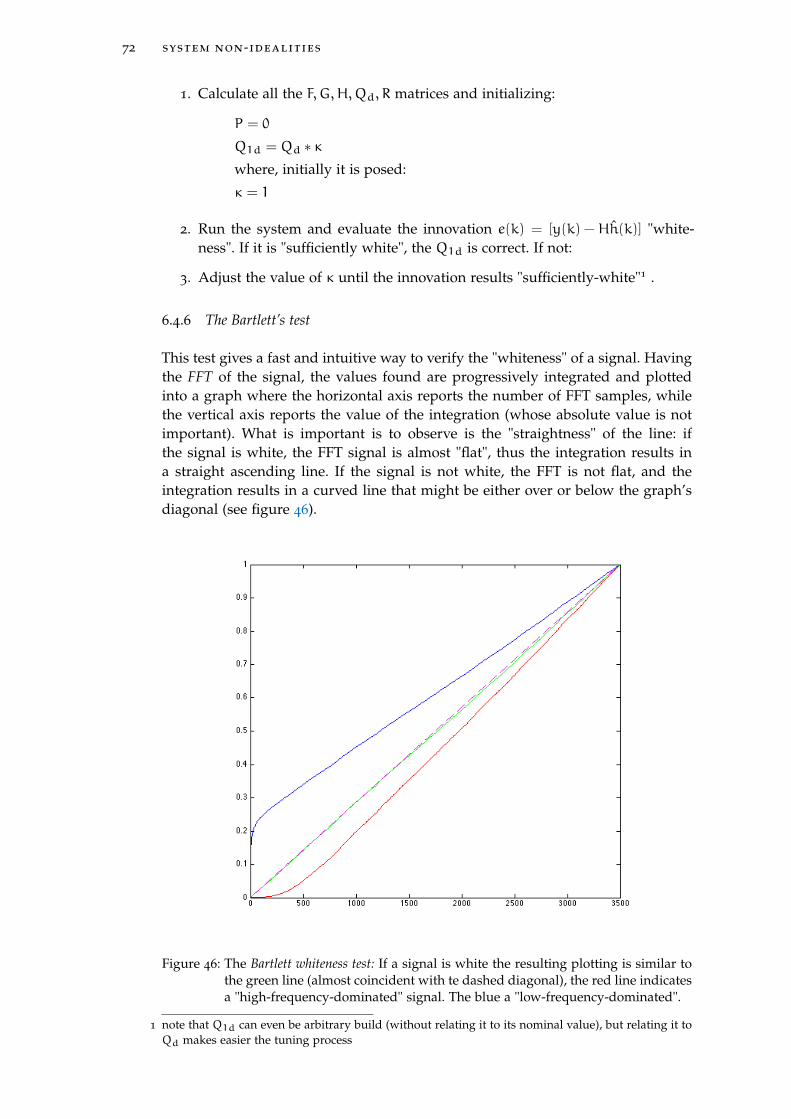
72 system non-idealities
1. Calculate all the F,G,H,Qd, R matrices and initializing:
P = 0
Q1d = Qd ∗ κwhere, initially it is posed:
κ = 1
2. Run the system and evaluate the innovation e(k) = [y(k) −Hh(k)] "white-ness". If it is "sufficiently white", the Q1d is correct. If not:
3. Adjust the value of κ until the innovation results "sufficiently-white"1 .
6.4.6 The Bartlett’s test
This test gives a fast and intuitive way to verify the "whiteness" of a signal. Havingthe FFT of the signal, the values found are progressively integrated and plottedinto a graph where the horizontal axis reports the number of FFT samples, whilethe vertical axis reports the value of the integration (whose absolute value is notimportant). What is important is to observe is the "straightness" of the line: ifthe signal is white, the FFT signal is almost "flat", thus the integration results ina straight ascending line. If the signal is not white, the FFT is not flat, and theintegration results in a curved line that might be either over or below the graph’sdiagonal (see figure 46).
Figure 46: The Bartlett whiteness test: If a signal is white the resulting plotting is similar tothe green line (almost coincident with te dashed diagonal), the red line indicatesa "high-frequency-dominated" signal. The blue a "low-frequency-dominated".
1 note that Q1d can even be arbitrary build (without relating it to its nominal value), but relating it toQd makes easier the tuning process
[ December 2, 2017 at 17:06 – classicthesis ]
6.4 angle and angle-rate reading 73
6.4.7 Application of Kalman Filter to the system
In order to use the Kalman filter in the IMU reading process, a proper model ofgyroscope, accelerometer and their combination must be done.
6.4.7.1 Gyroscope model
Following the model proposed by [25], which corresponds to the single-dimension,discrete form of (80), the gyroscope output (considering only the "pitch" angle rateoutput coordinate) can be modeled as:
sg(t) = ω(t) + bg(t) +ng(t) = θ(t) + bg(t) +ng(t) (85)
where:
• sg is the gyroscope output
• ω is the angular velocity
• bg is the gyro measure bias, supposed slightly variable
• ng is the Gaussian noise added to the gyroscope measure, whose variance isunknown
The angle reading, starting from the gyro output, can be achieved by integrationof the angle-rate:
θ(t) = θ(t0) +∫tt0θ(t)dt (86)
Now, substituting (85) in (86) it results:
θ(t) = θ(t0) +1s(sg(t) − bg(t) −ng(t)) (87)
The bias is supposed to be affected by a process (white) noise nb, thus its evolutionmodel is:
bg(t) = bg(t) +nb(t) (88)
6.4.7.2 Accelerometer model
Even for the accelerometer, a discrete-time model is build:
sa(t) = θ(t) +na(t) (89)
where:
• sa is the accelerometer output, already conditioned by subtracting bias andcoupled acceleration, as described in section 6.4.1.1
• θ is the pitch angle
• na is the Gaussian noise added to the accelerometer measure, whose varianceis unknown
In this case, the angle reading model for the accelerometer will be:
θ(t) = sa(t) −na(t) (90)
Note that the signal θ(k) is not simply the accelerometer’s output, but the resultof the angle calculus explained in the previous section.
[ December 2, 2017 at 17:06 – classicthesis ]
74 system non-idealities
6.4.7.3 Sensors combination
The previous models of the sensors can be conveniently used to build a state-spacesystem, affected by noise. Using the (87), we define the state of the system as thevector:
x(t) =
[θ(t)
bg(t)
]and u(t) = sg(t) (91)
The output definition is derived directly by the (90), thus the complete system, inthe form (84) is obtained by substitution of all the previous, yielding to:
x(t) =
[θ(t)
bg(t)
]=
[0 1
0 0
]θ(t)
bg(t)
+
[1
0
][sg(t) +ng(k− 1)] +
[0
1
]nb
y(t) =[1 0
]x(t) +na(t)
(92)
Where, as obvious:
x(t) =
θ(t)
bg(t)
u(t) = sg(t) A =
[0 1
0 0
]B1 =
[1
0
]B2 =
[0
1
]
C =[1 0
]m1(t) = ng(t) m2(t) = nb(t) w(t) = na(t)
(93)
Since the controller is discrete-time, the just-presented model must be discretizedand it is necessary to find a model for the co-variance of the noise processes (to beapplied to the kalman filter). Here the results:
F = eATs =
[1 Ts
0 1
]
G =∫Ts0 e
AτBdτ =
[Ts
0
]Q = σ2ngw
10→Ts + σ
2nbw20→Ts
where:
w10→Ts =∫Ts0 e
AτB1BT1 (e
Aτ)Tdτ =
[Ts 0
0 0
]
w20→Ts =∫Ts0 e
AτB2BT2 (e
Aτ)Tdτ =
[T3s /3 T2s /2
T2s /2 Ts
]R = σ2na
(94)
Note that the variance related to the accelerometer angle (σ2na) is not simply thesensor’s noise variance, but since the angle coming from the accelerometer is aratio between the two signals (see (82)), the corresponding variance is the productof the variances of the accx signal noise and the inverse variance of the accz signalnoise (which is obtained by first-order Taylor approximation of the process).
The model of Kalman filter is already part of the Simulink environment. In figure47, it is presented the blocks that makes possible to choose which sensor-fusionstrategy to adopt.
[ December 2, 2017 at 17:06 – classicthesis ]
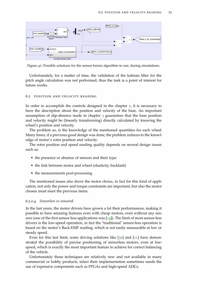
6.5 position and velocity reading 75
Figure 47: Possible solutions for the sensor-fusion algorithm to use, during simulations.
Unfortunately, for a matter of time, the validation of the kalman filter for thepitch angle calculation was not performed, thus the task is a point of interest forfuture works.
6.5 position and velocity reading
In order to accomplish the controls designed in the chapter 5, it is necessary tohave the description about the position and velocity of the base. An importantassumption of slip-absence made in chapter 3 guarantees that the base positionand velocity might be (linearly transforming) directly calculated by knowing thewheel’s position and velocity.
The problem so, is the knowledge of the mentioned quantities for each wheel.Many times, if a previous good design was done, the problem reduces to the knowl-edge of motor’s rotor position and velocity.
The rotor position and speed reading quality depends on several design issuessuch as:
• the presence or absence of sensors and their type
• the link between motor and wheel (elasticity, backlash)
• the measurements post-processing
The mentioned issues also drove the motor choice, in fact for this kind of appli-cation, not only the power and torque constraints are important, but also the motorchosen must meet the previous items.
6.5.0.4 Sensorless vs sensored
In the last years, the motor drivers have grown a lot their performances, making itpossible to have amazing features even with cheap motors, even without any sen-sors (one of the first sensor-less applications was [14]). The limit of most sensor-lessdrivers is the low-speed operation, in fact the "traditional" sensor-less operation isbased on the motor’s Back-EMF reading, which is not easily measurable at low orsteady speed.
Even for this last limit, some driving solutions like [30] and [11] have demon-strated the possibility of precise positioning of sensorless motors, even at low-speed, which is exactly the most important feature to achieve for correct balancingof the vehicle.
Unfortunately those techniques are relatively new and not available in manycommercial or hobby products, infact their implementation sometimes needs theuse of expensive components such as FPGAs and high-speed ADCs.
[ December 2, 2017 at 17:06 – classicthesis ]
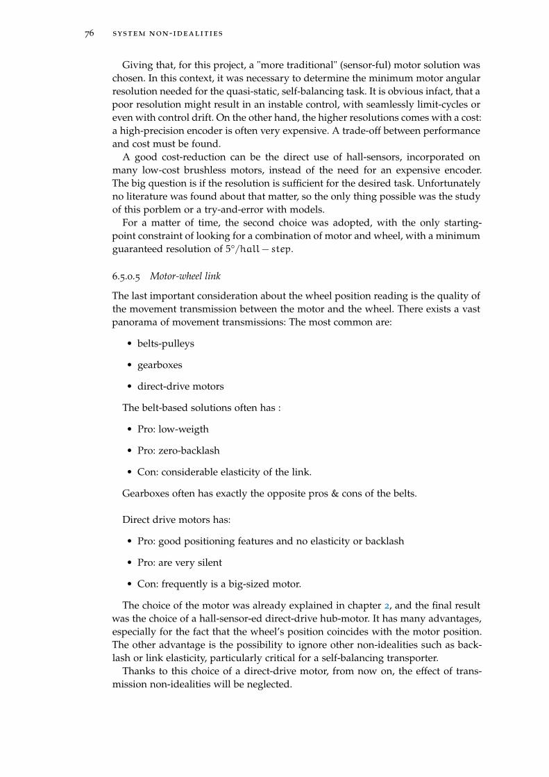
76 system non-idealities
Giving that, for this project, a "more traditional" (sensor-ful) motor solution waschosen. In this context, it was necessary to determine the minimum motor angularresolution needed for the quasi-static, self-balancing task. It is obvious infact, that apoor resolution might result in an instable control, with seamlessly limit-cycles oreven with control drift. On the other hand, the higher resolutions comes with a cost:a high-precision encoder is often very expensive. A trade-off between performanceand cost must be found.
A good cost-reduction can be the direct use of hall-sensors, incorporated onmany low-cost brushless motors, instead of the need for an expensive encoder.The big question is if the resolution is sufficient for the desired task. Unfortunatelyno literature was found about that matter, so the only thing possible was the studyof this porblem or a try-and-error with models.
For a matter of time, the second choice was adopted, with the only starting-point constraint of looking for a combination of motor and wheel, with a minimumguaranteed resolution of 5°/hall− step.
6.5.0.5 Motor-wheel link
The last important consideration about the wheel position reading is the quality ofthe movement transmission between the motor and the wheel. There exists a vastpanorama of movement transmissions: The most common are:
• belts-pulleys
• gearboxes
• direct-drive motors
The belt-based solutions often has :
• Pro: low-weigth
• Pro: zero-backlash
• Con: considerable elasticity of the link.
Gearboxes often has exactly the opposite pros & cons of the belts.
Direct drive motors has:
• Pro: good positioning features and no elasticity or backlash
• Pro: are very silent
• Con: frequently is a big-sized motor.
The choice of the motor was already explained in chapter 2, and the final resultwas the choice of a hall-sensor-ed direct-drive hub-motor. It has many advantages,especially for the fact that the wheel’s position coincides with the motor position.The other advantage is the possibility to ignore other non-idealities such as back-lash or link elasticity, particularly critical for a self-balancing transporter.
Thanks to this choice of a direct-drive motor, from now on, the effect of trans-mission non-idealities will be neglected.
[ December 2, 2017 at 17:06 – classicthesis ]
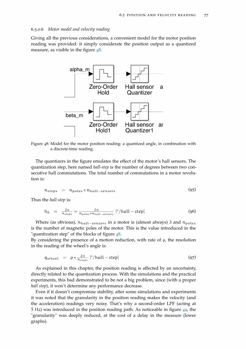
6.5 position and velocity reading 77
6.5.0.6 Motor model and velocity reading
Giving all the previous considerations, a convenient model for the motor positionreading was provided: it simply considerate the position output as a quantizedmeasure, as visible in the figure 48.
Figure 48: Model for the motor position reading: a quantized angle, in combination witha discrete-time reading.
The quantizers in the figure emulates the effect of the motor’s hall sensors. Thequantization step, here named hall-step is the number of degrees between two con-secutive hall commutations. The total number of commutations in a motor revolu-tion is:
nsteps = npoles ∗nhall−sensors (95)
Thus the hall-step is:
hS = 2πnsteps
= 2πnpoles∗nhall−sensors [°/hall− step] (96)
Where (as obvious), nhall−sensors in a motor is (almost always) 3 and npolesis the number of magnetic poles of the motor. This is the value introduced in the"quantization step" of the blocks of figure 48.By considering the presence of a motion reduction, with rate of ρ, the resolutionin the reading of the wheel’s angle is:
qwheel = ρ ∗ 2πnsteps
[°/hall− step] (97)
As explained in this chapter, the position reading is affected by an uncertainty,directly related to the quantization process. With the simulations and the practicalexperiments, this had demonstrated to be not a big problem, since (with a properhall step), it won’t determine any performance decrease.
Even if it doesn’t compromise stability, after some simulations and experimentsit was noted that the granularity in the position reading makes the velocity (andthe acceleration) readings very noisy. That’s why a second-order LPF (acting at5 Hz) was introduced in the position reading path. As noticeable in figure 49, the"granularity" was deeply reduced, at the cost of a delay in the measure (lowergraphs).
[ December 2, 2017 at 17:06 – classicthesis ]
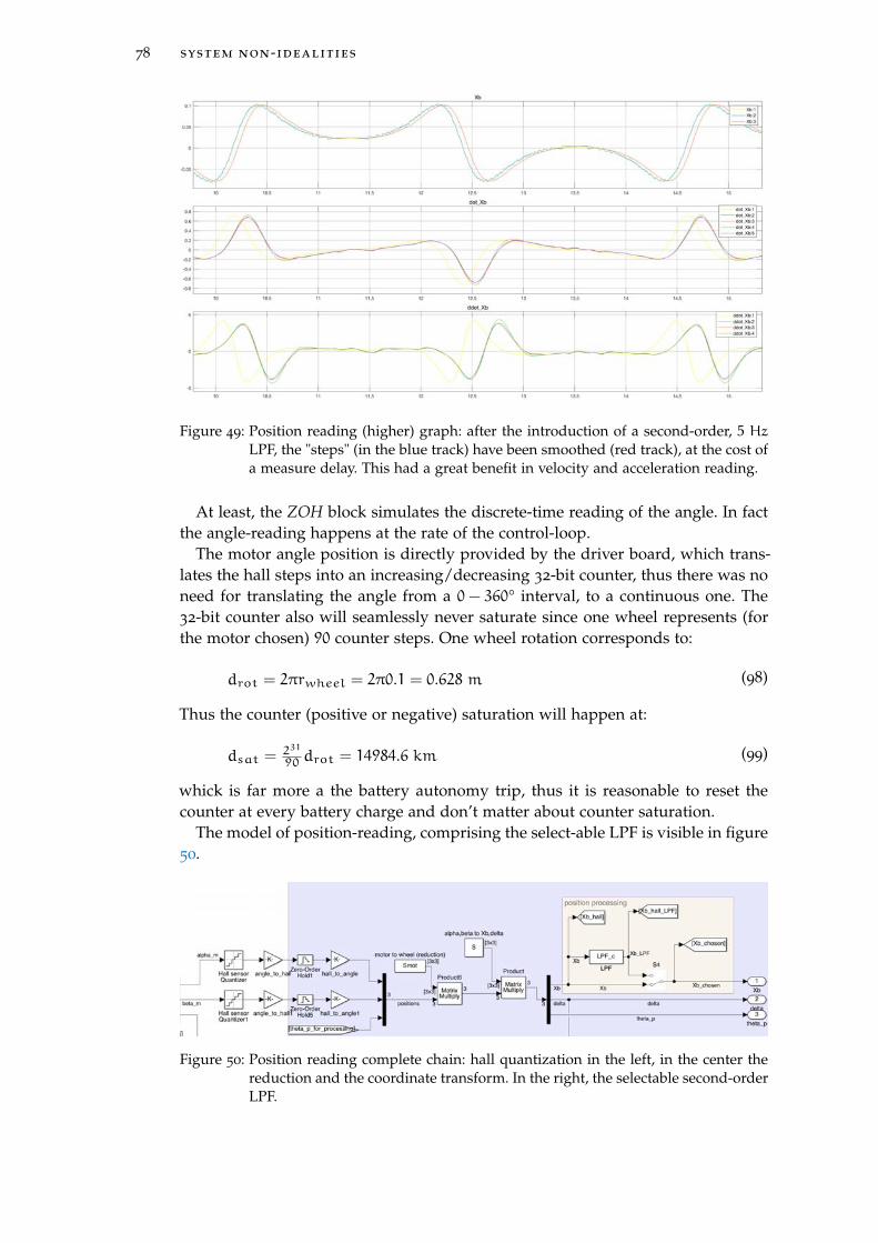
78 system non-idealities
Figure 49: Position reading (higher) graph: after the introduction of a second-order, 5 HzLPF, the "steps" (in the blue track) have been smoothed (red track), at the cost ofa measure delay. This had a great benefit in velocity and acceleration reading.
At least, the ZOH block simulates the discrete-time reading of the angle. In factthe angle-reading happens at the rate of the control-loop.
The motor angle position is directly provided by the driver board, which trans-lates the hall steps into an increasing/decreasing 32-bit counter, thus there was noneed for translating the angle from a 0− 360° interval, to a continuous one. The32-bit counter also will seamlessly never saturate since one wheel represents (forthe motor chosen) 90 counter steps. One wheel rotation corresponds to:
drot = 2πrwheel = 2π0.1 = 0.628 m (98)
Thus the counter (positive or negative) saturation will happen at:
dsat =231
90 drot = 14984.6 km (99)
whick is far more a the battery autonomy trip, thus it is reasonable to reset thecounter at every battery charge and don’t matter about counter saturation.
The model of position-reading, comprising the select-able LPF is visible in figure50.
Figure 50: Position reading complete chain: hall quantization in the left, in the center thereduction and the coordinate transform. In the right, the selectable second-orderLPF.
[ December 2, 2017 at 17:06 – classicthesis ]
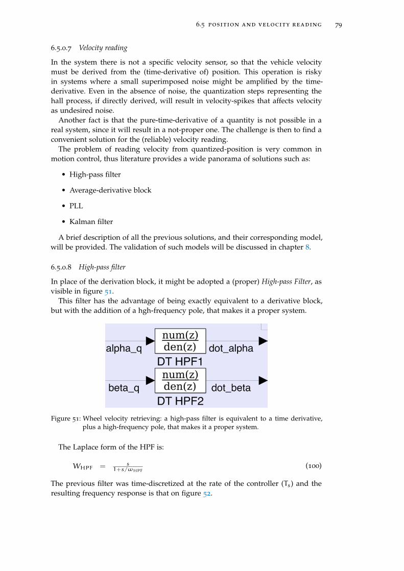
6.5 position and velocity reading 79
6.5.0.7 Velocity reading
In the system there is not a specific velocity sensor, so that the vehicle velocitymust be derived from the (time-derivative of) position. This operation is riskyin systems where a small superimposed noise might be amplified by the time-derivative. Even in the absence of noise, the quantization steps representing thehall process, if directly derived, will result in velocity-spikes that affects velocityas undesired noise.
Another fact is that the pure-time-derivative of a quantity is not possible in areal system, since it will result in a not-proper one. The challenge is then to find aconvenient solution for the (reliable) velocity reading.
The problem of reading velocity from quantized-position is very common inmotion control, thus literature provides a wide panorama of solutions such as:
• High-pass filter
• Average-derivative block
• PLL
• Kalman filter
A brief description of all the previous solutions, and their corresponding model,will be provided. The validation of such models will be discussed in chapter 8.
6.5.0.8 High-pass filter
In place of the derivation block, it might be adopted a (proper) High-pass Filter, asvisible in figure 51.
This filter has the advantage of being exactly equivalent to a derivative block,but with the addition of a hgh-frequency pole, that makes it a proper system.
Figure 51: Wheel velocity retrieving: a high-pass filter is equivalent to a time derivative,plus a high-frequency pole, that makes it a proper system.
The Laplace form of the HPF is:
WHPF = s1+s/ωHPF
(100)
The previous filter was time-discretized at the rate of the controller (Ts) and theresulting frequency response is that on figure 52.
[ December 2, 2017 at 17:06 – classicthesis ]
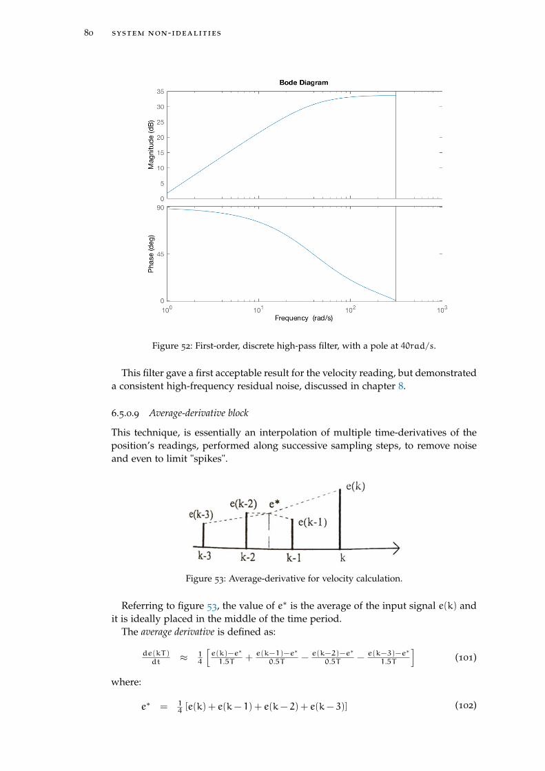
80 system non-idealities
Figure 52: First-order, discrete high-pass filter, with a pole at 40rad/s.
This filter gave a first acceptable result for the velocity reading, but demonstrateda consistent high-frequency residual noise, discussed in chapter 8.
6.5.0.9 Average-derivative block
This technique, is essentially an interpolation of multiple time-derivatives of theposition’s readings, performed along successive sampling steps, to remove noiseand even to limit "spikes".
Figure 53: Average-derivative for velocity calculation.
Referring to figure 53, the value of e∗ is the average of the input signal e(k) andit is ideally placed in the middle of the time period.
The average derivative is defined as:
de(kT)dt ≈ 1
4
[e(k)−e∗
1.5T +e(k−1)−e∗
0.5T −e(k−2)−e∗
0.5T −e(k−3)−e∗
1.5T
](101)
where:
e∗ = 14[e(k) + e(k− 1) + e(k− 2) + e(k− 3)] (102)
[ December 2, 2017 at 17:06 – classicthesis ]
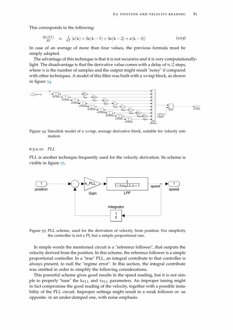
6.5 position and velocity reading 81
This corresponds to the following:
de(kT)dt ≈ 1
6T[e(k) + 3e(k− 1) + 3e(k− 2) + e(k− 3)] (103)
In case of an average of more than four values, the previous formula must besimply adapted.
The advantage of this technique is that it is not recursive and it is very computationally-light. The disadvantage is that the derivative value comes with a delay of n/2 steps,where n is the number of samples and the output might result "noisy" if comparedwith other techniques. A model of this filter was built with a 10-tap block, as shownin figure 54.
Figure 54: Simulink model of a 10-tap, average derivative block, suitable for velocity esti-mation.
6.5.0.10 PLL
PLL is another technique frequently used for the velocity derivation. Its scheme isvisible in figure 55.
Figure 55: PLL scheme, used for the derivation of velocity, from position. For simplicitythe controller is not a PI, but a simple proportional one.
In simple words the mentioned circuit is a "reference follower", that outputs thevelocity derived from the position. In this scheme, the reference follower is a simpleproportional controller. In a "true" PLL, an integral contribute to that controller isalways present, to null the "regime error". In this section, the integral contributewas omitted in order to simplify the following considerations.
This powerful scheme gives good results in the speed reading, but it is not sim-ple to properly "tune" the kPLL and τPLL parameters. An improper tuning mightin fact compromise the good reading of the velocity, together with a possible insta-bility of the PLL circuit. Improper settings might result in a weak follower or -asopposite- in an under-damped one, with noise emphasis.
[ December 2, 2017 at 17:06 – classicthesis ]
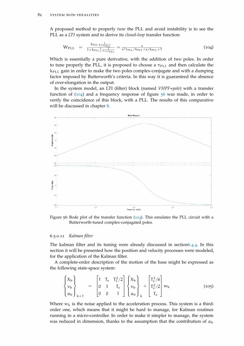
82 system non-idealities
A proposed method to properly tune the PLL and avoid instability is to see thePLL as a LTI system and to derive its closed-loop transfer function:
WPLL =kPLL
11+sτPLL
1+kPLL1s
11+sτPLL
= ss2τPLL/kPLL+s/kPLL+1
(104)
Which is essentially a pure derivative, with the addition of two poles. In orderto tune properly the PLL, it is proposed to choose a τPLL and then calculate thekPLL gain in order to make the two poles complex-conjugate and with a dumpingfactor imposed by Butterworth’s criteria. In this way it is guaranteed the absenceof over-elongation in the output.
In the system model, an LTI (filter) block (named VHPF+pole) with a transferfunction of (104) and a frequency response of figure 56 was made, in order toverify the coincidence of this block, with a PLL. The results of this comparativewill be discussed in chapter 8.
Figure 56: Bode plot of the transfer function (104). This emulates the PLL circuit with aButterworth-tuned complex-conjugated poles.
6.5.0.11 Kalman filter
The kalman filter and its tuning were already discussed in section6.4.4. In thissection it will be presented how the position and velocity processes were modeled,for the application of the Kalman filter.
A complete-order description of the motion of the base might be expressed asthe following state-space system:
Xb
vb
ab
k+1
=
1 Ts T2s /2
0 1 Ts
0 0 1
Xb
vb
ab
k
+
T3s /6
T2s /2
Ts
wk (105)
Where wk is the noise applied to the acceleration process. This system is a third-order one, which means that it might be hard to manage, for Kalman routinesrunning in a micro-controller. In order to make it simpler to manage, the systemwas reduced in dimension, thanks to the assumption that the contribution of ab
[ December 2, 2017 at 17:06 – classicthesis ]
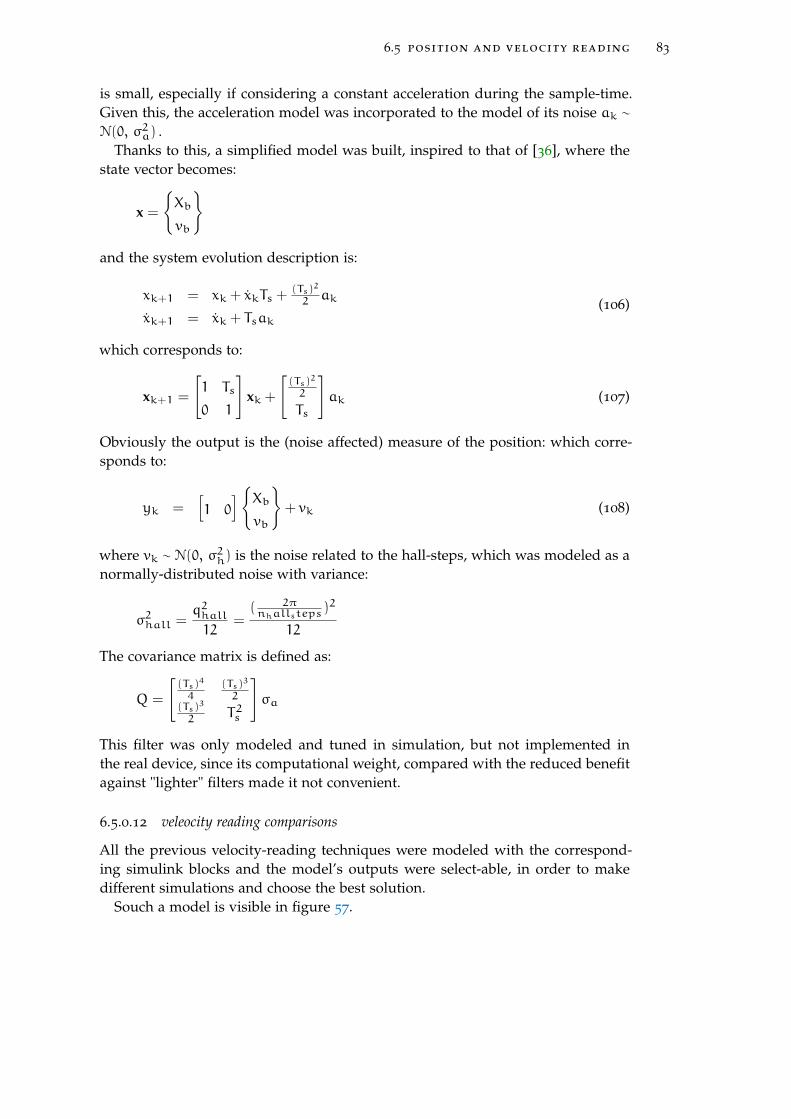
6.5 position and velocity reading 83
is small, especially if considering a constant acceleration during the sample-time.Given this, the acceleration model was incorporated to the model of its noise ak ∼
N(0, σ2a) .Thanks to this, a simplified model was built, inspired to that of [36], where the
state vector becomes:
x =
Xb
vb
and the system evolution description is:
xk+1 = xk + xkTs +(Ts)
2
2 ak
xk+1 = xk + Tsak(106)
which corresponds to:
xk+1 =
[1 Ts
0 1
]xk +
[(Ts)
2
2
Ts
]ak (107)
Obviously the output is the (noise affected) measure of the position: which corre-sponds to:
yk =[1 0
]Xbvb
+ vk (108)
where vk ∼ N(0, σ2h) is the noise related to the hall-steps, which was modeled as anormally-distributed noise with variance:
σ2hall =q2hall12
=( 2πnhallsteps
)2
12
The covariance matrix is defined as:
Q =
[(Ts)
4
4(Ts)
3
2(Ts)
3
2 T2s
]σa
This filter was only modeled and tuned in simulation, but not implemented inthe real device, since its computational weight, compared with the reduced benefitagainst "lighter" filters made it not convenient.
6.5.0.12 veleocity reading comparisons
All the previous velocity-reading techniques were modeled with the correspond-ing simulink blocks and the model’s outputs were select-able, in order to makedifferent simulations and choose the best solution.
Souch a model is visible in figure 57.
[ December 2, 2017 at 17:06 – classicthesis ]
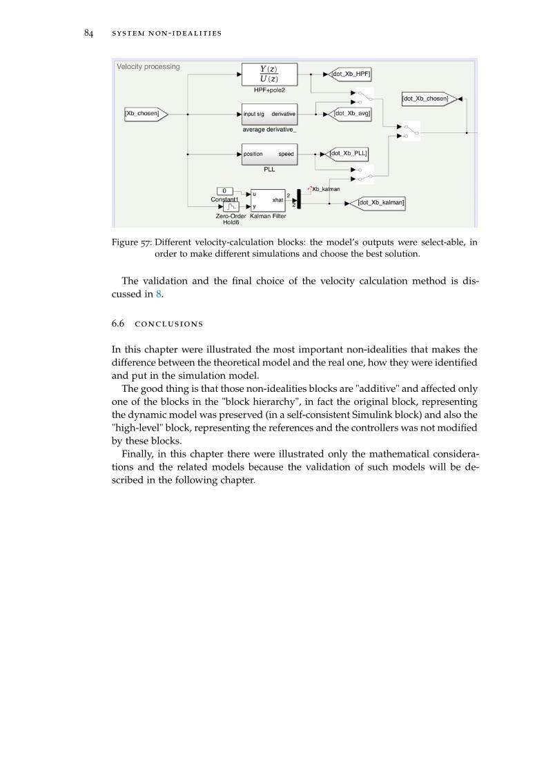
84 system non-idealities
Figure 57: Different velocity-calculation blocks: the model’s outputs were select-able, inorder to make different simulations and choose the best solution.
The validation and the final choice of the velocity calculation method is dis-cussed in 8.
6.6 conclusions
In this chapter were illustrated the most important non-idealities that makes thedifference between the theoretical model and the real one, how they were identifiedand put in the simulation model.
The good thing is that those non-idealities blocks are "additive" and affected onlyone of the blocks in the "block hierarchy", in fact the original block, representingthe dynamic model was preserved (in a self-consistent Simulink block) and also the"high-level" block, representing the references and the controllers was not modifiedby these blocks.
Finally, in this chapter there were illustrated only the mathematical considera-tions and the related models because the validation of such models will be de-scribed in the following chapter.
[ December 2, 2017 at 17:06 – classicthesis ]
7A L G O R I T H M S I M P L E M E N TAT I O N
7.1 introduction
Until now it was presented the system’s components, the mathematical modeland the system non-idealities models. In this chapter it will be presented how themodels were traduced into code and how it "fits" into the system architecture andthe practical issues that have been solved.
In particular, since the algorithm runs into an embedded microcontroller, a deepfocus on the mechanisms lying into it and the motivation that drove some imple-mentation choices.
7.2 overall architecture and behavior
As introduced in chapter 2, the hardware architecture of the device consists of twoidentical motor-driver boards, where the one attached to the IMU acts as MASTERand the other as SLAVE, the -just mentioned- IMU board and a bluetooth mod-ule board. Differently from figure 11, which is a mere "schematic" representation,figure 58 will be used to represent the data flows, during the algorithm running.
Figure 58: Logic architecture of the system
The two Motor boards are the components addicted to the generation of high-power signals that moves the motors, even making use of the motor’s sensors.Even though, this is not the only work performed by those boards, since theyare equipped with a powerful micro-controller with a real-time operating system(RTOS) that permits to perform several tasks in addition to the motor control. Theoriginal firmware that performs all this motor control and other tasks is well doc-umented in [35].
The powerful platform and the operating system are a good starting point: thiscombination is the reason behind the idea of adding a further TASK into the RTOS
85
[ December 2, 2017 at 17:06 – classicthesis ]
86 algorithms implementation
which performs the control of both equilibrium and steering, without the need ofan external board for this task.
The implementation and integration of the algorithm inside the micro-controllerwas successful, thanks also to the reliability of the high-speed CAN-bus communi-cation channel that transfers data at a rate of ≈ 500 kbaud/s. Another advantageis the fact that part of the data for the algorithm is resident in the MASTER boardand don’t need to be remotely read.
The biggest problem in this implementation, is that the boards are identical, butmust behave differently. Also there was the need to add some communication com-mands for data-exchange between the two boards (other commands in addition tothose in the original firmware), and those commands must be symmetric betweento the two boards.
The need was then to have:
• two hardware-identical boards
• a different behavior between the two boards
• a set of communication commands, shared between the boards
The solution adopted was to have a unique firmware in both the boards: in thisway the communication protocol is automatically shared. The problem of the dif-ferent behavior was solved by a non-volatile software parameter : the CAN address.In this way the MASTER board is that with CAN address=0 and the slave has CANaddress=1. This convention served also as definition of LEFT=CAN address=1 andRIGHT=CAN address=0. At start-up, the micro-controller checks its address andconsequently knows if it has to behave as MASTER or SLAVE inside the system.
Thanks to this solution also the firmware maintenance was very easy, with aunique firmware version and without the need to worry about cross-versions com-patibility.
The IMU board is an i2c-SLAVE device, whose MASTER is the MASTER mo-tor control board. The communication between the two is the fastest possible inthe i2c standard 400kHz bit-clock. The micro-controller reads the IMU standardregisters and doesn’t use the special function (such as sensor-fusion or quaternionbuil-up) provided by the manufacturer. In this way a possible replacement of theIMU model is possible, without the loss of specific algorithms.
The bluetooth board needed a minimum configuration since it is factory-set witha fixed UART-baudrate of 9600bps. Following the procedure described in [28], thebaud-rate was changed with the fastest universally-supported bitrate (115200bps),that made it possible to exchange data with PC with low latencies and high data-throughput (particulary useful for data exchange between the self-balancing vehi-cle and the PC, during work). Note that the bluetooth module is simply an "in-terface bridge" between the serial ports of the PC and that of the micro-controller:there is infact no protocol overhead for the communication: both the PC and mi-crocontrollers works like they were wire-connected by serial port.
[ December 2, 2017 at 17:06 – classicthesis ]
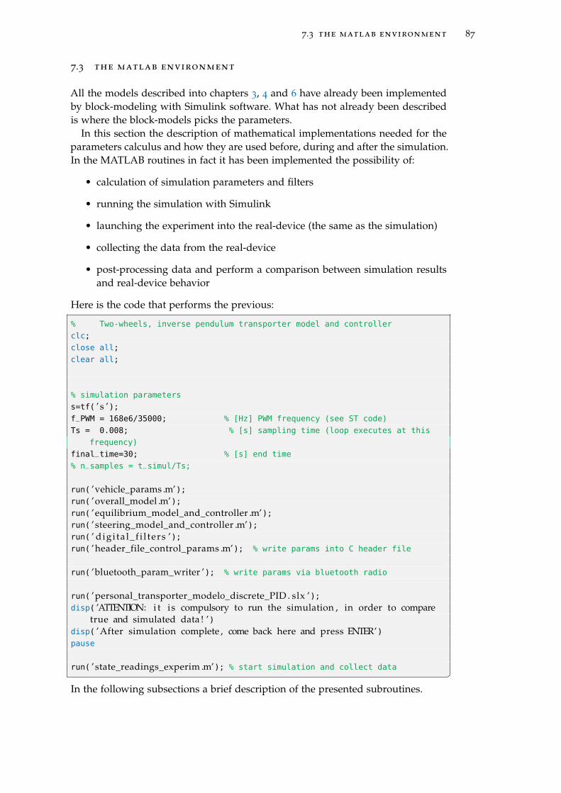
7.3 the matlab environment 87
7.3 the matlab environment
All the models described into chapters 3, 4 and 6 have already been implementedby block-modeling with Simulink software. What has not already been describedis where the block-models picks the parameters.
In this section the description of mathematical implementations needed for theparameters calculus and how they are used before, during and after the simulation.In the MATLAB routines in fact it has been implemented the possibility of:
• calculation of simulation parameters and filters
• running the simulation with Simulink
• launching the experiment into the real-device (the same as the simulation)
• collecting the data from the real-device
• post-processing data and perform a comparison between simulation resultsand real-device behavior
Here is the code that performs the previous:
% Two-wheels, inverse pendulum transporter model and controller
clc;
close all;
clear all;
% simulation parameters
s=tf( ’ s ’);f_PWM = 168e6/35000; % [Hz] PWM frequency (see ST code)
Ts = 0.008; % [s] sampling time (loop executes at this
frequency)
final_time=30; % [s] end time
% n_samples = t_simul/Ts;
run( ’vehicle_params .m’);run( ’overall_model .m’);run( ’equilibrium_model_and_controller .m’);run( ’ steering_model_and_controller .m’);run( ’ digi ta l_f i l ters ’);run( ’header_file_control_params .m’); % write params into C header file
run( ’bluetooth_param_writer ’); % write params via bluetooth radio
run( ’personal_transporter_model0_discrete_PID . slx ’);disp( ’ATTENTION: i t is compulsory to run the simulation , in order to compare
true and simulated data ! ’)disp( ’After simulation complete , come back here and press ENTER’)pause
run( ’ state_readings_experim .m’); % start simulation and collect data In the following subsections a brief description of the presented subroutines.
[ December 2, 2017 at 17:06 – classicthesis ]
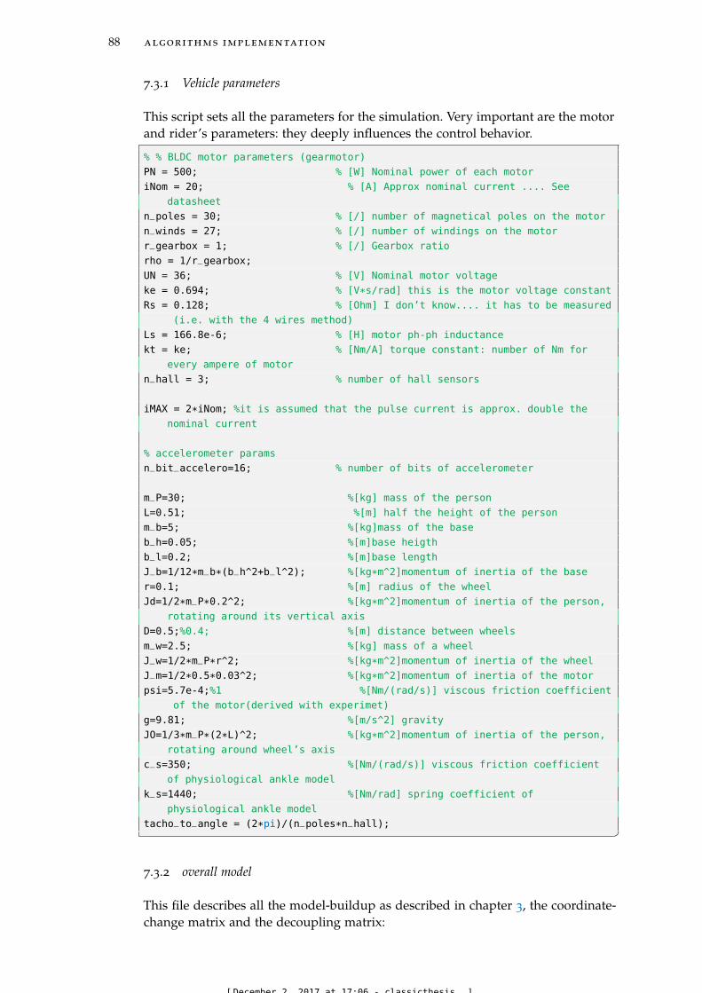
88 algorithms implementation
7.3.1 Vehicle parameters
This script sets all the parameters for the simulation. Very important are the motorand rider’s parameters: they deeply influences the control behavior.
% % BLDC motor parameters (gearmotor)
PN = 500; % [W] Nominal power of each motor
iNom = 20; % [A] Approx nominal current .... See
datasheet
n_poles = 30; % [/] number of magnetical poles on the motor
n_winds = 27; % [/] number of windings on the motor
r_gearbox = 1; % [/] Gearbox ratio
rho = 1/r_gearbox;
UN = 36; % [V] Nominal motor voltage
ke = 0.694; % [V*s/rad] this is the motor voltage constant
Rs = 0.128; % [Ohm] I don’t know.... it has to be measured
(i.e. with the 4 wires method)
Ls = 166.8e-6; % [H] motor ph-ph inductance
kt = ke; % [Nm/A] torque constant: number of Nm for
every ampere of motor
n_hall = 3; % number of hall sensors
iMAX = 2*iNom; %it is assumed that the pulse current is approx. double the
nominal current
% accelerometer params
n_bit_accelero=16; % number of bits of accelerometer
m_P=30; %[kg] mass of the person
L=0.51; %[m] half the height of the person
m_b=5; %[kg]mass of the base
b_h=0.05; %[m]base heigth
b_l=0.2; %[m]base length
J_b=1/12*m_b*(b_h^2+b_l^2); %[kg*m^2]momentum of inertia of the base
r=0.1; %[m] radius of the wheel
Jd=1/2*m_P*0.2^2; %[kg*m^2]momentum of inertia of the person,
rotating around its vertical axis
D=0.5;%0.4; %[m] distance between wheels
m_w=2.5; %[kg] mass of a wheel
J_w=1/2*m_P*r^2; %[kg*m^2]momentum of inertia of the wheel
J_m=1/2*0.5*0.03^2; %[kg*m^2]momentum of inertia of the motor
psi=5.7e-4;%1 %[Nm/(rad/s)] viscous friction coefficient
of the motor(derived with experimet)
g=9.81; %[m/s^2] gravity
JO=1/3*m_P*(2*L)^2; %[kg*m^2]momentum of inertia of the person,
rotating around wheel’s axis
c_s=350; %[Nm/(rad/s)] viscous friction coefficient
of physiological ankle model
k_s=1440; %[Nm/rad] spring coefficient of
physiological ankle model
tacho_to_angle = (2*pi)/(n_poles*n_hall); 7.3.2 overall model
This file describes all the model-buildup as described in chapter 3, the coordinate-change matrix and the decoupling matrix:
[December 2, 2017 at 17:06 - classicthesis ]
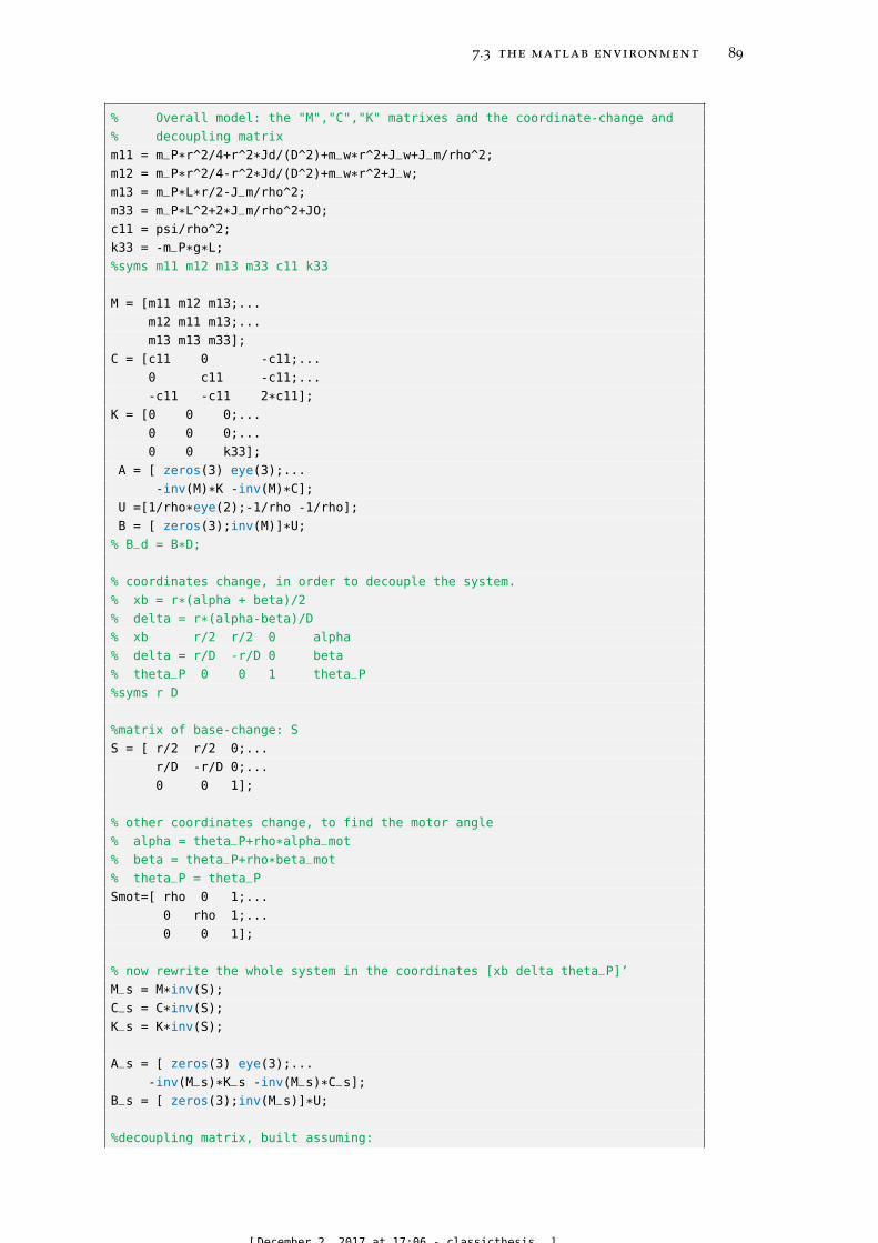
7.3 the matlab environment 89
% Overall model: the "M","C","K" matrixes and the coordinate-change and
% decoupling matrix
m11 = m_P*r^2/4+r^2*Jd/(D^2)+m_w*r^2+J_w+J_m/rho^2;
m12 = m_P*r^2/4-r^2*Jd/(D^2)+m_w*r^2+J_w;
m13 = m_P*L*r/2-J_m/rho^2;
m33 = m_P*L^2+2*J_m/rho^2+JO;
c11 = psi/rho^2;
k33 = -m_P*g*L;
%syms m11 m12 m13 m33 c11 k33
M = [m11 m12 m13;...
m12 m11 m13;...
m13 m13 m33];
C = [c11 0 -c11;...
0 c11 -c11;...
-c11 -c11 2*c11];
K = [0 0 0;...
0 0 0;...
0 0 k33];
A = [ zeros(3) eye(3);...
-inv(M)*K -inv(M)*C];
U =[1/rho*eye(2);-1/rho -1/rho];
B = [ zeros(3);inv(M)]*U;
% B_d = B*D;
% coordinates change, in order to decouple the system.
% xb = r*(alpha + beta)/2
% delta = r*(alpha-beta)/D
% xb r/2 r/2 0 alpha
% delta = r/D -r/D 0 beta
% theta_P 0 0 1 theta_P
%syms r D
%matrix of base-change: S
S = [ r/2 r/2 0;...
r/D -r/D 0;...
0 0 1];
% other coordinates change, to find the motor angle
% alpha = theta_P+rho*alpha_mot
% beta = theta_P+rho*beta_mot
% theta_P = theta_P
Smot=[ rho 0 1;...
0 rho 1;...
0 0 1];
% now rewrite the whole system in the coordinates [xb delta theta_P]’
M_s = M*inv(S);
C_s = C*inv(S);
K_s = K*inv(S);
A_s = [ zeros(3) eye(3);...
-inv(M_s)*K_s -inv(M_s)*C_s];
B_s = [ zeros(3);inv(M_s)]*U;
%decoupling matrix, built assuming:
[December 2, 2017 at 17:06 - classicthesis ]
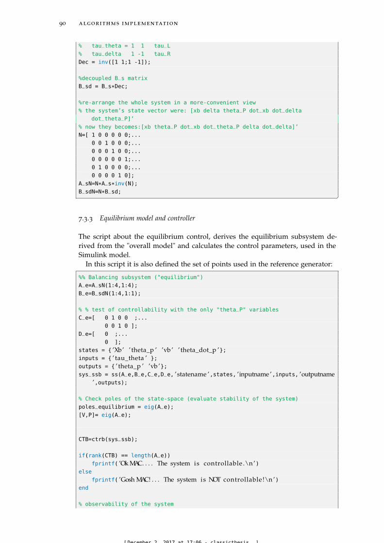
90 algorithms implementation
% tau_theta = 1 1 tau_L
% tau_delta 1 -1 tau_R
Dec = inv([1 1;1 -1]);
%decoupled B_s matrix
B_sd = B_s*Dec;
%re-arrange the whole system in a more-convenient view
% the system’s state vector were: [xb delta theta_P dot_xb dot_delta
dot_theta_P]’
% now they becomes:[xb theta_P dot_xb dot_theta_P delta dot_delta]’
N=[ 1 0 0 0 0 0;...
0 0 1 0 0 0;...
0 0 0 1 0 0;...
0 0 0 0 0 1;...
0 1 0 0 0 0;...
0 0 0 0 1 0];
A_sN=N*A_s*inv(N);
B_sdN=N*B_sd; 7.3.3 Equilibrium model and controller
The script about the equilibrium control, derives the equilibrium subsystem de-rived from the "overall model" and calculates the control parameters, used in theSimulink model.
In this script it is also defined the set of points used in the reference generator:
%% Balancing subsystem ("equilibrium")
A_e=A_sN(1:4,1:4);
B_e=B_sdN(1:4,1:1);
% % test of controllability with the only "theta_P" variables
C_e=[ 0 1 0 0 ;...
0 0 1 0 ];
D_e=[ 0 ;...
0 ];
states = ’Xb’ ’ theta_p ’ ’vb ’ ’ theta_dot_p ’;inputs = ’ tau_theta ’ ;
outputs = ’ theta_p ’ ’vb ’;sys_ssb = ss(A_e,B_e,C_e,D_e, ’statename ’,states, ’inputname ’,inputs, ’outputname
’,outputs);
% Check poles of the state-space (evaluate stability of the system)
poles_equilibrium = eig(A_e);
[V,P]= eig(A_e);
CTB=ctrb(sys_ssb);
if(rank(CTB) == length(A_e))
fprintf( ’Ok MAC. . . . The system is controllable .\n’)else
fprintf( ’Gosh MAC! . . . The system is NOT controllable !\n’)end
% observability of the system
[December 2, 2017 at 17:06 - classicthesis ]
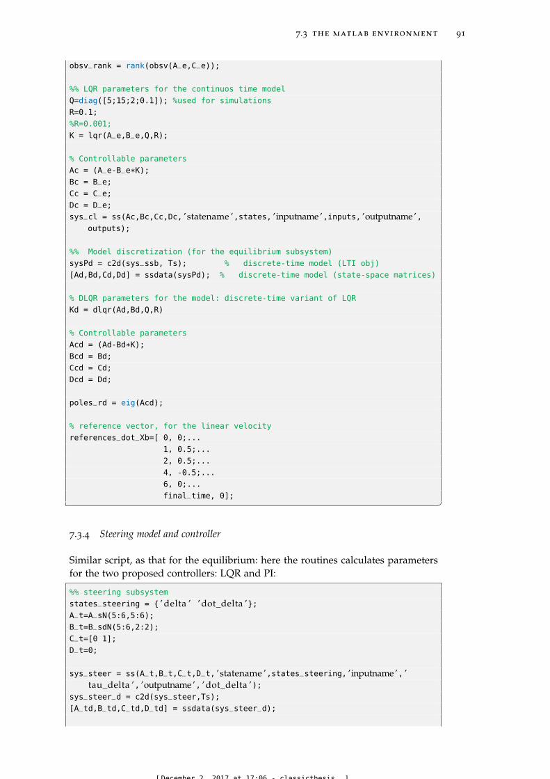
7.3 the matlab environment 91
obsv_rank = rank(obsv(A_e,C_e));
%% LQR parameters for the continuos time model
Q=diag([5;15;2;0.1]); %used for simulations
R=0.1;
%R=0.001;
K = lqr(A_e,B_e,Q,R);
% Controllable parameters
Ac = (A_e-B_e*K);
Bc = B_e;
Cc = C_e;
Dc = D_e;
sys_cl = ss(Ac,Bc,Cc,Dc, ’statename ’,states, ’inputname ’,inputs, ’outputname’,outputs);
%% Model discretization (for the equilibrium subsystem)
sysPd = c2d(sys_ssb, Ts); % discrete-time model (LTI obj)
[Ad,Bd,Cd,Dd] = ssdata(sysPd); % discrete-time model (state-space matrices)
% DLQR parameters for the model: discrete-time variant of LQR
Kd = dlqr(Ad,Bd,Q,R)
% Controllable parameters
Acd = (Ad-Bd*K);
Bcd = Bd;
Ccd = Cd;
Dcd = Dd;
poles_rd = eig(Acd);
% reference vector, for the linear velocity
references_dot_Xb=[ 0, 0;...
1, 0.5;...
2, 0.5;...
4, -0.5;...
6, 0;...
final_time, 0]; 7.3.4 Steering model and controller
Similar script, as that for the equilibrium: here the routines calculates parametersfor the two proposed controllers: LQR and PI:
%% steering subsystem
states_steering = ’ delta ’ ’dot_delta ’;A_t=A_sN(5:6,5:6);
B_t=B_sdN(5:6,2:2);
C_t=[0 1];
D_t=0;
sys_steer = ss(A_t,B_t,C_t,D_t, ’statename ’,states_steering, ’inputname ’, ’tau_delta ’, ’outputname’, ’dot_delta ’);
sys_steer_d = c2d(sys_steer,Ts);
[A_td,B_td,C_td,D_td] = ssdata(sys_steer_d);
[December 2, 2017 at 17:06 - classicthesis ]
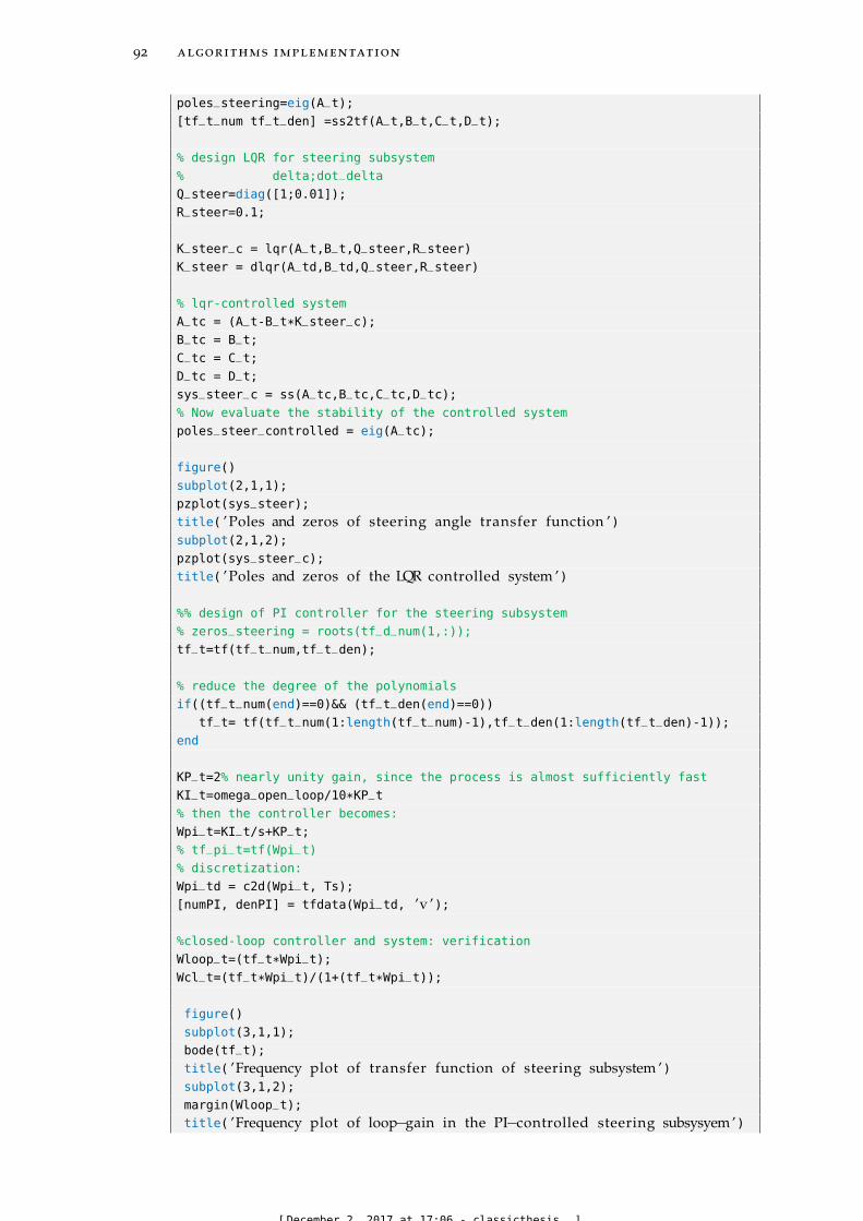
92 algorithms implementation
poles_steering=eig(A_t);
[tf_t_num tf_t_den] =ss2tf(A_t,B_t,C_t,D_t);
% design LQR for steering subsystem
% delta;dot_delta
Q_steer=diag([1;0.01]);
R_steer=0.1;
K_steer_c = lqr(A_t,B_t,Q_steer,R_steer)
K_steer = dlqr(A_td,B_td,Q_steer,R_steer)
% lqr-controlled system
A_tc = (A_t-B_t*K_steer_c);
B_tc = B_t;
C_tc = C_t;
D_tc = D_t;
sys_steer_c = ss(A_tc,B_tc,C_tc,D_tc);
% Now evaluate the stability of the controlled system
poles_steer_controlled = eig(A_tc);
figure()
subplot(2,1,1);
pzplot(sys_steer);
title( ’Poles and zeros of steering angle transfer function ’)subplot(2,1,2);
pzplot(sys_steer_c);
title( ’Poles and zeros of the LQR controlled system ’)
%% design of PI controller for the steering subsystem
% zeros_steering = roots(tf_d_num(1,:));
tf_t=tf(tf_t_num,tf_t_den);
% reduce the degree of the polynomials
if((tf_t_num(end)==0)&& (tf_t_den(end)==0))
tf_t= tf(tf_t_num(1:length(tf_t_num)-1),tf_t_den(1:length(tf_t_den)-1));
end
KP_t=2% nearly unity gain, since the process is almost sufficiently fast
KI_t=omega_open_loop/10*KP_t
% then the controller becomes:
Wpi_t=KI_t/s+KP_t;
% tf_pi_t=tf(Wpi_t)
% discretization:
Wpi_td = c2d(Wpi_t, Ts);
[numPI, denPI] = tfdata(Wpi_td, ’v ’);
%closed-loop controller and system: verification
Wloop_t=(tf_t*Wpi_t);
Wcl_t=(tf_t*Wpi_t)/(1+(tf_t*Wpi_t));
figure()
subplot(3,1,1);
bode(tf_t);
title( ’Frequency plot of transfer function of steering subsystem ’)subplot(3,1,2);
margin(Wloop_t);
title( ’Frequency plot of loop−gain in the PI−controlled steering subsysyem’)
[December 2, 2017 at 17:06 - classicthesis ]
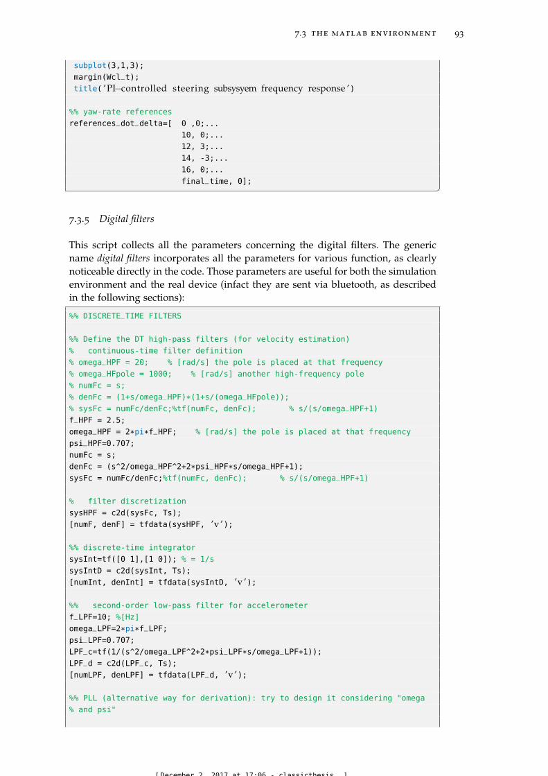
7.3 the matlab environment 93
subplot(3,1,3);
margin(Wcl_t);
title( ’PI−controlled steering subsysyem frequency response ’)
%% yaw-rate references
references_dot_delta=[ 0 ,0;...
10, 0;...
12, 3;...
14, -3;...
16, 0;...
final_time, 0]; 7.3.5 Digital filters
This script collects all the parameters concerning the digital filters. The genericname digital filters incorporates all the parameters for various function, as clearlynoticeable directly in the code. Those parameters are useful for both the simulationenvironment and the real device (infact they are sent via bluetooth, as describedin the following sections):
%% DISCRETE_TIME FILTERS
%% Define the DT high-pass filters (for velocity estimation)
% continuous-time filter definition
% omega_HPF = 20; % [rad/s] the pole is placed at that frequency
% omega_HFpole = 1000; % [rad/s] another high-frequency pole
% numFc = s;
% denFc = (1+s/omega_HPF)*(1+s/(omega_HFpole));
% sysFc = numFc/denFc;%tf(numFc, denFc); % s/(s/omega_HPF+1)
f_HPF = 2.5;
omega_HPF = 2*pi*f_HPF; % [rad/s] the pole is placed at that frequency
psi_HPF=0.707;
numFc = s;
denFc = (s^2/omega_HPF^2+2*psi_HPF*s/omega_HPF+1);
sysFc = numFc/denFc;%tf(numFc, denFc); % s/(s/omega_HPF+1)
% filter discretization
sysHPF = c2d(sysFc, Ts);
[numF, denF] = tfdata(sysHPF, ’v ’);
%% discrete-time integrator
sysInt=tf([0 1],[1 0]); % = 1/s
sysIntD = c2d(sysInt, Ts);
[numInt, denInt] = tfdata(sysIntD, ’v ’);
%% second-order low-pass filter for accelerometer
f_LPF=10; %[Hz]
omega_LPF=2*pi*f_LPF;
psi_LPF=0.707;
LPF_c=tf(1/(s^2/omega_LPF^2+2*psi_LPF*s/omega_LPF+1));
LPF_d = c2d(LPF_c, Ts);
[numLPF, denLPF] = tfdata(LPF_d, ’v ’);
%% PLL (alternative way for derivation): try to design it considering "omega
% and psi"
[December 2, 2017 at 17:06 - classicthesis ]
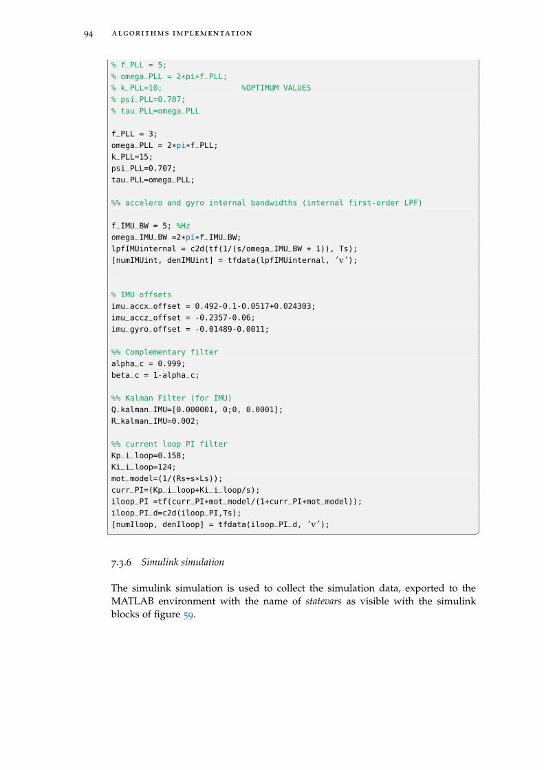
94 algorithms implementation
% f_PLL = 5;
% omega_PLL = 2*pi*f_PLL;
% k_PLL=10; %OPTIMUM VALUES
% psi_PLL=0.707;
% tau_PLL=omega_PLL
f_PLL = 3;
omega_PLL = 2*pi*f_PLL;
k_PLL=15;
psi_PLL=0.707;
tau_PLL=omega_PLL;
%% accelero and gyro internal bandwidths (internal first-order LPF)
f_IMU_BW = 5; %Hz
omega_IMU_BW =2*pi*f_IMU_BW;
lpfIMUinternal = c2d(tf(1/(s/omega_IMU_BW + 1)), Ts);
[numIMUint, denIMUint] = tfdata(lpfIMUinternal, ’v ’);
% IMU offsets
imu_accx_offset = 0.492-0.1-0.0517+0.024303;
imu_accz_offset = -0.2357-0.06;
imu_gyro_offset = -0.01489-0.0011;
%% Complementary filter
alpha_c = 0.999;
beta_c = 1-alpha_c;
%% Kalman Filter (for IMU)
Q_kalman_IMU=[0.000001, 0;0, 0.0001];
R_kalman_IMU=0.002;
%% current loop PI filter
Kp_i_loop=0.158;
Ki_i_loop=124;
mot_model=(1/(Rs+s*Ls));
curr_PI=(Kp_i_loop+Ki_i_loop/s);
iloop_PI =tf(curr_PI*mot_model/(1+curr_PI*mot_model));
iloop_PI_d=c2d(iloop_PI,Ts);
[numIloop, denIloop] = tfdata(iloop_PI_d, ’v ’); 7.3.6 Simulink simulation
The simulink simulation is used to collect the simulation data, exported to theMATLAB environment with the name of statevars as visible with the simulinkblocks of figure 59.
[ December 2, 2017 at 17:06 – classicthesis ]
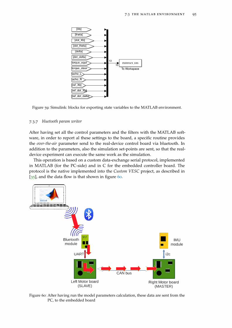
7.3 the matlab environment 95
Figure 59: Simulink: blocks for exporting state variables to the MATLAB environment.
7.3.7 bluetooth param writer
After having set all the control parameters and the filters with the MATLAB soft-ware, in order to report al these settings to the board, a specific routine providesthe over-the-air parameter send to the real-device control board via bluetooth. Inaddition to the parameters, also the simulation set-points are sent, so that the real-device experiment can execute the same work as the simulation.
This operation is based on a custom data-exchange serial protocol, implementedin MATLAB (for the PC-side) and in C for the embedded controller board. Theprotocol is the native implemented into the Custom VESC project, as described in[35], and the data flow is that shown in figure 60.
Figure 60: After having run the model parameters calculation, these data are sent from thePC, to the embedded board
[ December 2, 2017 at 17:06 – classicthesis ]
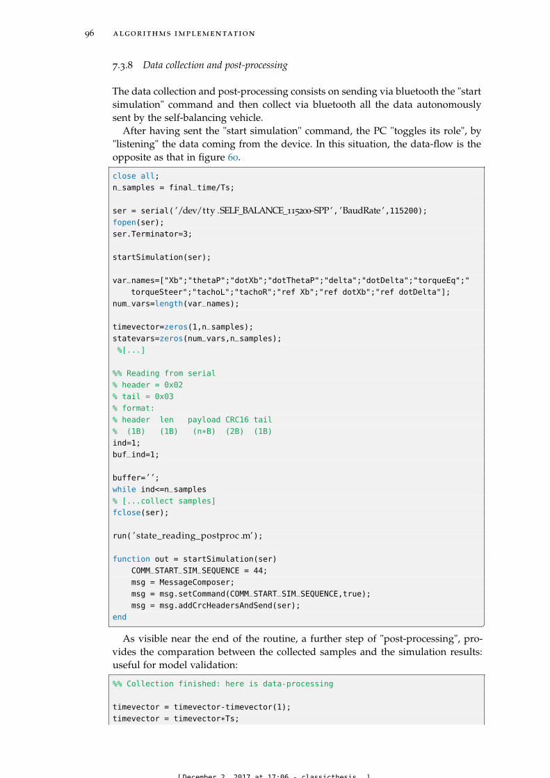
96 algorithms implementation
7.3.8 Data collection and post-processing
The data collection and post-processing consists on sending via bluetooth the "startsimulation" command and then collect via bluetooth all the data autonomouslysent by the self-balancing vehicle.
After having sent the "start simulation" command, the PC "toggles its role", by"listening" the data coming from the device. In this situation, the data-flow is theopposite as that in figure 60.
close all;
n_samples = final_time/Ts;
ser = serial( ’/dev/tty .SELF_BALANCE_115200−SPP’, ’BaudRate ’,115200);fopen(ser);
ser.Terminator=3;
startSimulation(ser);
var_names=["Xb";"thetaP";"dotXb";"dotThetaP";"delta";"dotDelta";"torqueEq";"
torqueSteer";"tachoL";"tachoR";"ref Xb";"ref dotXb";"ref dotDelta"];
num_vars=length(var_names);
timevector=zeros(1,n_samples);
statevars=zeros(num_vars,n_samples);
%[...]
%% Reading from serial
% header = 0x02
% tail = 0x03
% format:
% header len payload CRC16 tail
% (1B) (1B) (n*B) (2B) (1B)
ind=1;
buf_ind=1;
buffer= ’ ’;while ind<=n_samples
% [...collect samples]
fclose(ser);
run( ’ state_reading_postproc .m’);
function out = startSimulation(ser)
COMM_START_SIM_SEQUENCE = 44;
msg = MessageComposer;
msg = msg.setCommand(COMM_START_SIM_SEQUENCE,true);
msg = msg.addCrcHeadersAndSend(ser);
end As visible near the end of the routine, a further step of "post-processing", pro-
vides the comparation between the collected samples and the simulation results:useful for model validation:
%% Collection finished: here is data-processing
timevector = timevector-timevector(1);
timevector = timevector*Ts;
[December 2, 2017 at 17:06 - classicthesis ]
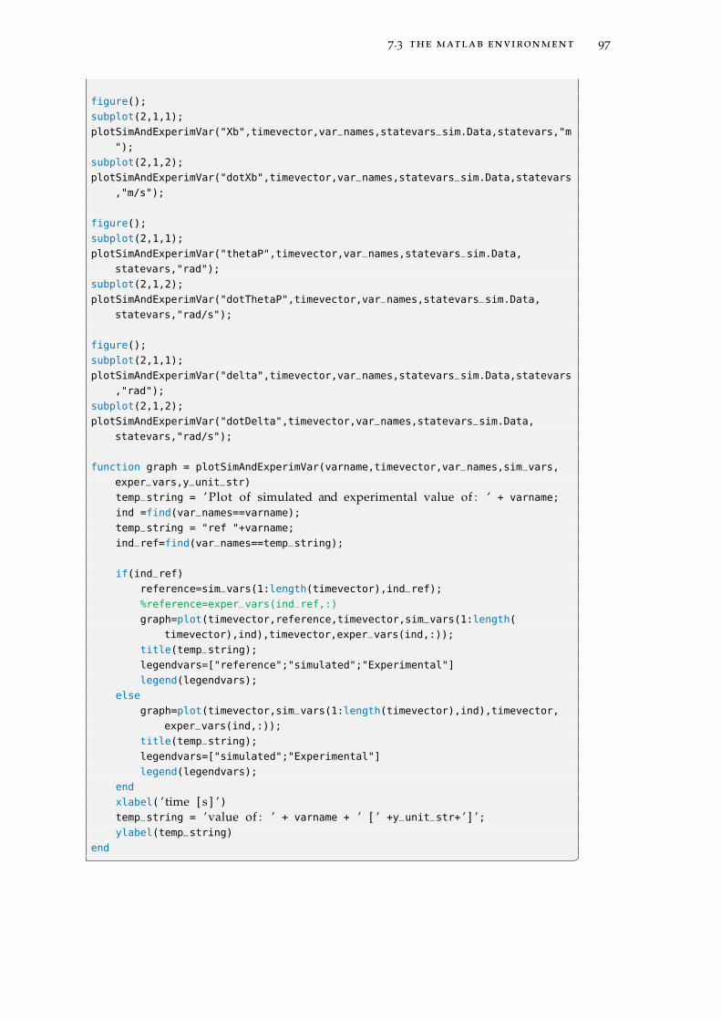
7.3 the matlab environment 97
figure();
subplot(2,1,1);
plotSimAndExperimVar("Xb",timevector,var_names,statevars_sim.Data,statevars,"m
");
subplot(2,1,2);
plotSimAndExperimVar("dotXb",timevector,var_names,statevars_sim.Data,statevars
,"m/s");
figure();
subplot(2,1,1);
plotSimAndExperimVar("thetaP",timevector,var_names,statevars_sim.Data,
statevars,"rad");
subplot(2,1,2);
plotSimAndExperimVar("dotThetaP",timevector,var_names,statevars_sim.Data,
statevars,"rad/s");
figure();
subplot(2,1,1);
plotSimAndExperimVar("delta",timevector,var_names,statevars_sim.Data,statevars
,"rad");
subplot(2,1,2);
plotSimAndExperimVar("dotDelta",timevector,var_names,statevars_sim.Data,
statevars,"rad/s");
function graph = plotSimAndExperimVar(varname,timevector,var_names,sim_vars,
exper_vars,y_unit_str)
temp_string = ’ Plot of simulated and experimental value of : ’ + varname;
ind =find(var_names==varname);
temp_string = "ref "+varname;
ind_ref=find(var_names==temp_string);
if(ind_ref)
reference=sim_vars(1:length(timevector),ind_ref);
%reference=exper_vars(ind_ref,:)
graph=plot(timevector,reference,timevector,sim_vars(1:length(
timevector),ind),timevector,exper_vars(ind,:));
title(temp_string);
legendvars=["reference";"simulated";"Experimental"]
legend(legendvars);
else
graph=plot(timevector,sim_vars(1:length(timevector),ind),timevector,
exper_vars(ind,:));
title(temp_string);
legendvars=["simulated";"Experimental"]
legend(legendvars);
end
xlabel( ’time [ s ] ’)temp_string = ’value of : ’ + varname + ’ [ ’ +y_unit_str+ ’ ] ’;ylabel(temp_string)
end
[ December 2, 2017 at 17:06 – classicthesis ]
98 algorithms implementation
7.4 the embedded environment
This section describes the environment in which the control algorithm works. Thefocus is the firmware architecture and how the control algorithm uses it.
The microcontroller is the STM32F405RGT6, which is a Cortex-M4 microcon-troller working at 168MHz, with hardware floating-point unit: this feature wasvery helpful for the algorithms performances.The compilation toolchain chosen for the project was gcc-arm-none-eabi 4.8 2014q2and the operating system is a custom porting of ChibiOs ver. 3.2 provided by [35].
The whole setup of the toolchain and the debugging tools (STM32F3discoveryevaluation board with embedded ST-link) is also well-described in [35].Here it will be shortly described the operating-system components involved forthe (equilibrium and steering) control.
As visible in figure [], the control software makes use of the following peripher-als, with the corresponding drivers named Hardware Abstraction Layers (HAL):
• Timer/counter 5, with PWM HAL: used for the time base that triggers thecontrol algorithm
• I2c2, with i2c HAL: used for the communication between microcontroller andIMU
• UART, with serial HAL: used for the communication with PC: the communi-cation channel is bluetooth, but it is "transparent" for the serial communica-tion to the PC
• CAN bus with CAN HAL: used for inter-board communication. In the fol-lowing sections, a detailed description of the data exchanged for the twoboards.
• Threads and signals: those are not peripherals, but it is important to note thatthe control algorithm works inside one of the running threads: this is a keyfeature offered by the operating system, that deeply simplifies the firmwaredevelopment. Also the signals were very helpful for synchronization withexternal events. These operating system features were very helpful and sim-plified a lot both the firmware structure and the "code readability".
• time measurement: also this is not a peripheral, but a primitive offered bythe operating system. The time measurement was used for the calculus ofalgorithm performance.
The embedded environment is a short description of the hardware and firmwareenvironment where the algorithm works. In the following section a deeper descrip-tion of the control algorithm.
7.5 the control firmware
In this section a detailed description of the control algorithm: how it works andhow the external components are involved. Also some short code-blocks describingthe algorithm.
Even in this section, a short discussion of the board’s data flow, during othersystem tasks.
[ December 2, 2017 at 17:06 – classicthesis ]
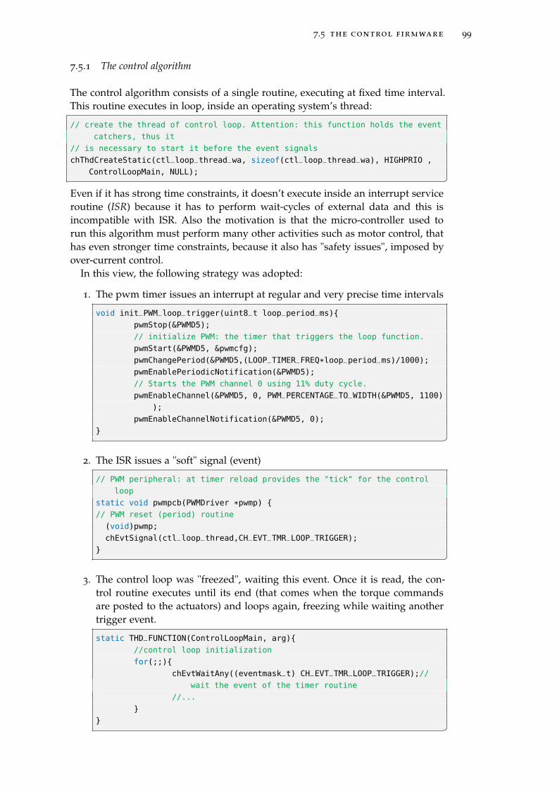
7.5 the control firmware 99
7.5.1 The control algorithm
The control algorithm consists of a single routine, executing at fixed time interval.This routine executes in loop, inside an operating system’s thread:
// create the thread of control loop. Attention: this function holds the event
catchers, thus it
// is necessary to start it before the event signals
chThdCreateStatic(ctl_loop_thread_wa, sizeof(ctl_loop_thread_wa), HIGHPRIO ,
ControlLoopMain, NULL); Even if it has strong time constraints, it doesn’t execute inside an interrupt serviceroutine (ISR) because it has to perform wait-cycles of external data and this isincompatible with ISR. Also the motivation is that the micro-controller used torun this algorithm must perform many other activities such as motor control, thathas even stronger time constraints, because it also has "safety issues", imposed byover-current control.
In this view, the following strategy was adopted:
1. The pwm timer issues an interrupt at regular and very precise time intervals
void init_PWM_loop_trigger(uint8_t loop_period_ms)
pwmStop(&PWMD5);
// initialize PWM: the timer that triggers the loop function.
pwmStart(&PWMD5, &pwmcfg);
pwmChangePeriod(&PWMD5,(LOOP_TIMER_FREQ*loop_period_ms)/1000);
pwmEnablePeriodicNotification(&PWMD5);
// Starts the PWM channel 0 using 11% duty cycle.
pwmEnableChannel(&PWMD5, 0, PWM_PERCENTAGE_TO_WIDTH(&PWMD5, 1100)
);
pwmEnableChannelNotification(&PWMD5, 0);
2. The ISR issues a "soft" signal (event)
// PWM peripheral: at timer reload provides the "tick" for the control
loop
static void pwmpcb(PWMDriver *pwmp)
// PWM reset (period) routine
(void)pwmp;
chEvtSignal(ctl_loop_thread,CH_EVT_TMR_LOOP_TRIGGER);
3. The control loop was "freezed", waiting this event. Once it is read, the con-
trol routine executes until its end (that comes when the torque commandsare posted to the actuators) and loops again, freezing while waiting anothertrigger event.
static THD_FUNCTION(ControlLoopMain, arg)
//control loop initialization
for(;;)
chEvtWaitAny((eventmask_t) CH_EVT_TMR_LOOP_TRIGGER);//
wait the event of the timer routine
//...
[ December 2, 2017 at 17:06 – classicthesis ]
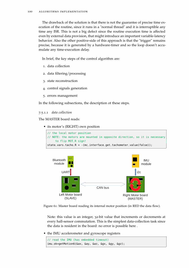
100 algorithms implementation
The drawback of the solution is that there is not the guarantee of precise time ex-ecution of the routine, since it runs in a "normal thread" and it is interruptible anytime any ISR. This is not a big defect since the routine execution time is affectedeven by external data provision, that might introduce an important variable-latencybehavior. Also the other positive-side of this approach is that the "trigger" remainsprecise, because it is generated by a hardware-timer and so the loop doesn’t accu-mulate any time-execution delay.
In brief, the key steps of the control algorithm are:
1. data collection
2. data filtering/processing
3. state reconstruction
4. control signals generation
5. errors management
In the following subsections, the description ot these steps.
7.5.1.1 data collection
The MASTER board reads:
• its motor’s (RIGHT) own position
// the local motor position
// NOTE: the motors are mounted in opposite direction, so it is necessary
to flip MOT_R sign!
state_vars.tacho_R = -(mc_interface_get_tachometer_value(false));
Figure 61: Master board reading its internal motor position (in RED the data flow).
Note: this value is an integer, 32-bit value that increments or decrements atevery hall-sensor commutation. This is the simplest data-collection task sincethe data is resident in the board: no error is possible here .
• the IMU accelerometer and gyroscope registers
// read the IMU (has embedded timeout)
imu_ok=getMotion6(&ax, &ay, &az, &gx, &gy, &gz);
[ December 2, 2017 at 17:06 – classicthesis ]
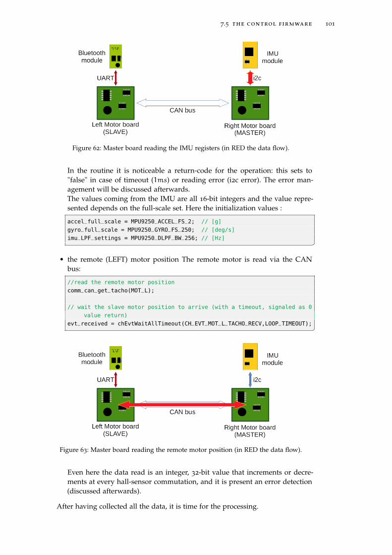
7.5 the control firmware 101
Figure 62: Master board reading the IMU registers (in RED the data flow).
In the routine it is noticeable a return-code for the operation: this sets to"false" in case of timeout (1ms) or reading error (i2c error). The error man-agement will be discussed afterwards.The values coming from the IMU are all 16-bit integers and the value repre-sented depends on the full-scale set. Here the initialization values :
accel_full_scale = MPU9250_ACCEL_FS_2; // [g]
gyro_full_scale = MPU9250_GYRO_FS_250; // [deg/s]
imu_LPF_settings = MPU9250_DLPF_BW_256; // [Hz] • the remote (LEFT) motor position The remote motor is read via the CAN
bus:
//read the remote motor position
comm_can_get_tacho(MOT_L);
// wait the slave motor position to arrive (with a timeout, signaled as 0
value return)
evt_received = chEvtWaitAllTimeout(CH_EVT_MOT_L_TACHO_RECV,LOOP_TIMEOUT);
Figure 63: Master board reading the remote motor position (in RED the data flow).
Even here the data read is an integer, 32-bit value that increments or decre-ments at every hall-sensor commutation, and it is present an error detection(discussed afterwards).
After having collected all the data, it is time for the processing.
[ December 2, 2017 at 17:06 – classicthesis ]
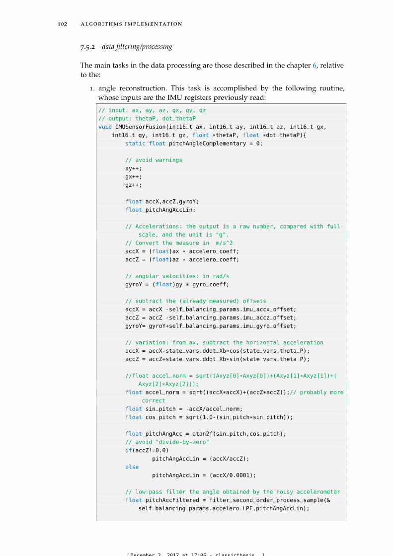
102 algorithms implementation
7.5.2 data filtering/processing
The main tasks in the data processing are those described in the chapter 6, relativeto the:
1. angle reconstruction. This task is accomplished by the following routine,whose inputs are the IMU registers previously read:
// input: ax, ay, az, gx, gy, gz
// output: thetaP, dot_thetaP
void IMUSensorFusion(int16_t ax, int16_t ay, int16_t az, int16_t gx,
int16_t gy, int16_t gz, float *thetaP, float *dot_thetaP)
static float pitchAngleComplementary = 0;
// avoid warnings
ay++;
gx++;
gz++;
float accX,accZ,gyroY;
float pitchAngAccLin;
// Accelerations: the output is a raw number, compared with full-
scale, and the unit is "g".
// Convert the measure in m/s^2
accX = (float)ax * accelero_coeff;
accZ = (float)az * accelero_coeff;
// angular velocities: in rad/s
gyroY = (float)gy * gyro_coeff;
// subtract the (already measured) offsets
accX = accX -self_balancing_params.imu_accx_offset;
accZ = accZ -self_balancing_params.imu_accz_offset;
gyroY= gyroY+self_balancing_params.imu_gyro_offset;
// variation: from ax, subtract the horizontal acceleration
accX = accX-state_vars.ddot_Xb*cos(state_vars.theta_P);
accZ = accZ+state_vars.ddot_Xb*sin(state_vars.theta_P);
//float accel_norm = sqrt((Axyz[0]*Axyz[0])+(Axyz[1]*Axyz[1])+(
Axyz[2]*Axyz[2]));
float accel_norm = sqrt((accX*accX)+(accZ*accZ));// probably more
correct
float sin_pitch = -accX/accel_norm;
float cos_pitch = sqrt(1.0-(sin_pitch*sin_pitch));
float pitchAngAcc = atan2f(sin_pitch,cos_pitch);
// avoid "divide-by-zero"
if(accZ!=0.0)
pitchAngAccLin = (accX/accZ);
else
pitchAngAccLin = (accX/0.0001);
// low-pass filter the angle obtained by the noisy accelerometer
float pitchAccFiltered = filter_second_order_process_sample(&
self_balancing_params.accelero_LPF,pitchAngAccLin);
[December 2, 2017 at 17:06 - classicthesis ]
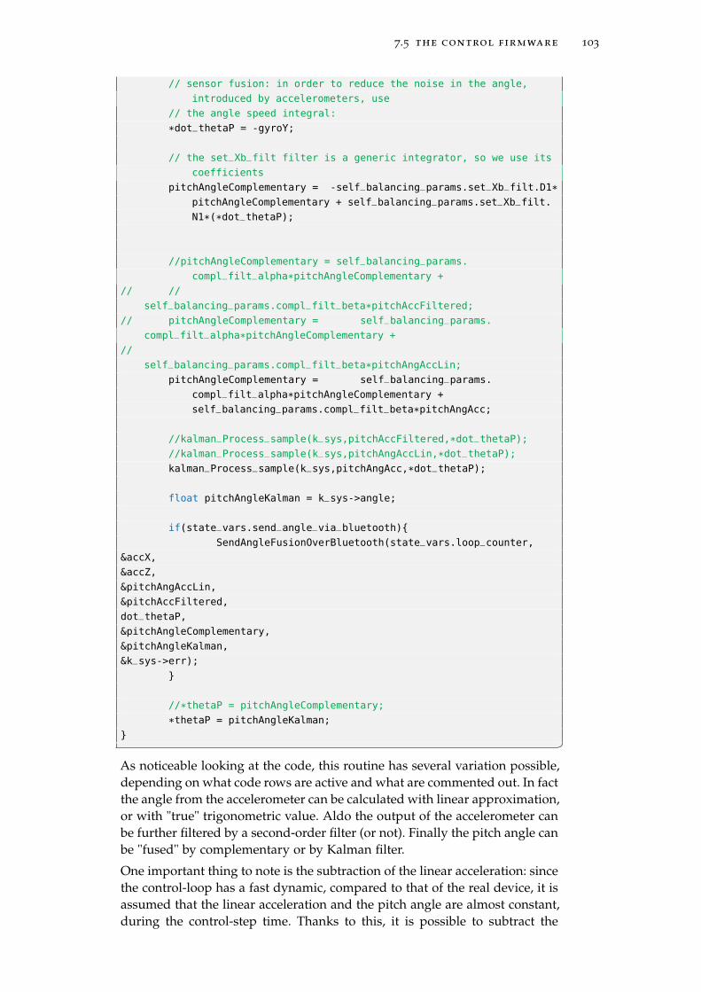
7.5 the control firmware 103
// sensor fusion: in order to reduce the noise in the angle,
introduced by accelerometers, use
// the angle speed integral:
*dot_thetaP = -gyroY;
// the set_Xb_filt filter is a generic integrator, so we use its
coefficients
pitchAngleComplementary = -self_balancing_params.set_Xb_filt.D1*pitchAngleComplementary + self_balancing_params.set_Xb_filt.
N1*(*dot_thetaP);
//pitchAngleComplementary = self_balancing_params.
compl_filt_alpha*pitchAngleComplementary +
// //
self_balancing_params.compl_filt_beta*pitchAccFiltered;
// pitchAngleComplementary = self_balancing_params.
compl_filt_alpha*pitchAngleComplementary +
//
self_balancing_params.compl_filt_beta*pitchAngAccLin;
pitchAngleComplementary = self_balancing_params.
compl_filt_alpha*pitchAngleComplementary +
self_balancing_params.compl_filt_beta*pitchAngAcc;
//kalman_Process_sample(k_sys,pitchAccFiltered,*dot_thetaP);
//kalman_Process_sample(k_sys,pitchAngAccLin,*dot_thetaP);
kalman_Process_sample(k_sys,pitchAngAcc,*dot_thetaP);
float pitchAngleKalman = k_sys->angle;
if(state_vars.send_angle_via_bluetooth)
SendAngleFusionOverBluetooth(state_vars.loop_counter,
&accX,
&accZ,
&pitchAngAccLin,
&pitchAccFiltered,
dot_thetaP,
&pitchAngleComplementary,
&pitchAngleKalman,
&k_sys->err);
//*thetaP = pitchAngleComplementary;
*thetaP = pitchAngleKalman;
As noticeable looking at the code, this routine has several variation possible,depending on what code rows are active and what are commented out. In factthe angle from the accelerometer can be calculated with linear approximation,or with "true" trigonometric value. Aldo the output of the accelerometer canbe further filtered by a second-order filter (or not). Finally the pitch angle canbe "fused" by complementary or by Kalman filter.
One important thing to note is the subtraction of the linear acceleration: sincethe control-loop has a fast dynamic, compared to that of the real device, it isassumed that the linear acceleration and the pitch angle are almost constant,during the control-step time. Thanks to this, it is possible to subtract the
[ December 2, 2017 at 17:06 – classicthesis ]
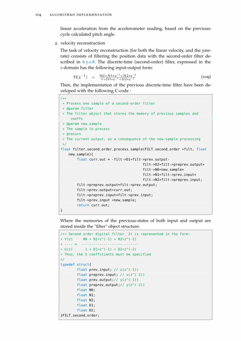
104 algorithms implementation
linear acceleration from the accelerometer reading, based on the previous-cycle calculated pitch angle.
2. velocity reconstruction
The task of velocity reconstruction (for both the linear velocity, and the yaw-rate) consists of filtering the position data with the second-order filter de-scribed in 6.5.0.8. The discrete-time (second-order) filter, expressed in thez-domain has the following input-output form:
H(z−1) = N0+N1∗z−1+N2∗z−21+D1∗z−1+D2∗z−2
(109)
Then, the implementation of the previous discrete-time filter have been de-veloped with the following C-code :
/**
* Process one sample of a second-order filter
* @param filter
* The filter object that stores the memory of previous samples and
coeffs
* @param new_sample
* The sample to process
* @return
* The current output, as a consequence of the new-sample processing
*/
float filter_second_order_process_sample(FILT_second_order *filt, float
new_sample)
float curr_out = -filt->D1*filt->prev_output-
filt->D2*filt->preprev_output+
filt->N0*new_sample+
filt->N1*filt->prev_input+
filt->N2*filt->preprev_input;
filt->preprev_output=filt->prev_output;
filt->prev_output=curr_out;
filt->preprev_input=filt->prev_input;
filt->prev_input =new_sample;
return curr_out;
Where the memories of the previous-states of both input and output arestored inside the "filter" object structure:
/** Second order digital filter. It is represented in the form:
* Y(z) N0 + N1*z^(-1) + N2*z^(-2)
* ---- = ----------------------------
* U(z) 1 + D1*z^(-1) + D2*z^(-2)
* Thus, the 5 coefficients must be specified
*/
typedef struct
float prev_input; // u(z^(-1))
float preprev_input; // u(z^(-2))
float prev_output;// y(z^(-1))
float preprev_output;// y(z^(-2))
float N0;
float N1;
float N2;
float D1;
float D2;
FILT_second_order;
[ December 2, 2017 at 17:06 – classicthesis ]

7.5 the control firmware 105
The velocity is then the desired output value coming with the output of thefilter second order process sample function.
The velocity reconstruction is part of the following "state reconstruction"stage, described in the following subsection.
7.5.3 state recontstruction
The state reconstruction is (in this specific-case) the process of appliying all thenecessary linear transforms that permits to obtain the state-variables, starting fromde device’s measures, as described by the blocks of figure 64:
Figure 64: Retrieving the state variables from the quantized measures. These blocks repre-sents the work inside the microcontroller routines.
The corresponding code is:
void UpdateStateVars(int32_t alpha_tacho, int32_t beta_tacho, float theta_P)
state_vars.Xb = TachoToAngle()*theta_P + (alpha_tacho*self_balancing_params.r_wheel*self_balancing_params.rho*TachoToAngle())/2 + (beta_tacho*self_balancing_params.r_wheel*self_balancing_params.rho*TachoToAngle())/2;
state_vars.delta = TachoToAngle()*theta_P + (alpha_tacho*self_balancing_params.r_wheel*self_balancing_params.rho*TachoToAngle())/self_balancing_params.d_interwheel - (beta_tacho*R_WHEEL*RHO*TachoToAngle())/self_balancing_params.d_interwheel;
state_vars.theta_P=theta_P;
// calculate velocities by HPF of positions
state_vars.dot_Xb=filter_second_order_process_sample(&
self_balancing_params.dot_Xb_filt,state_vars.Xb);
state_vars.dot_delta=filter_second_order_process_sample(&
self_balancing_params.dot_delta_filt,state_vars.delta);
// calculate acceleration
state_vars.ddot_Xb=filter_second_order_process_sample(&
self_balancing_params.ddot_Xb_filt,state_vars.dot_Xb);
[ December 2, 2017 at 17:06 – classicthesis ]
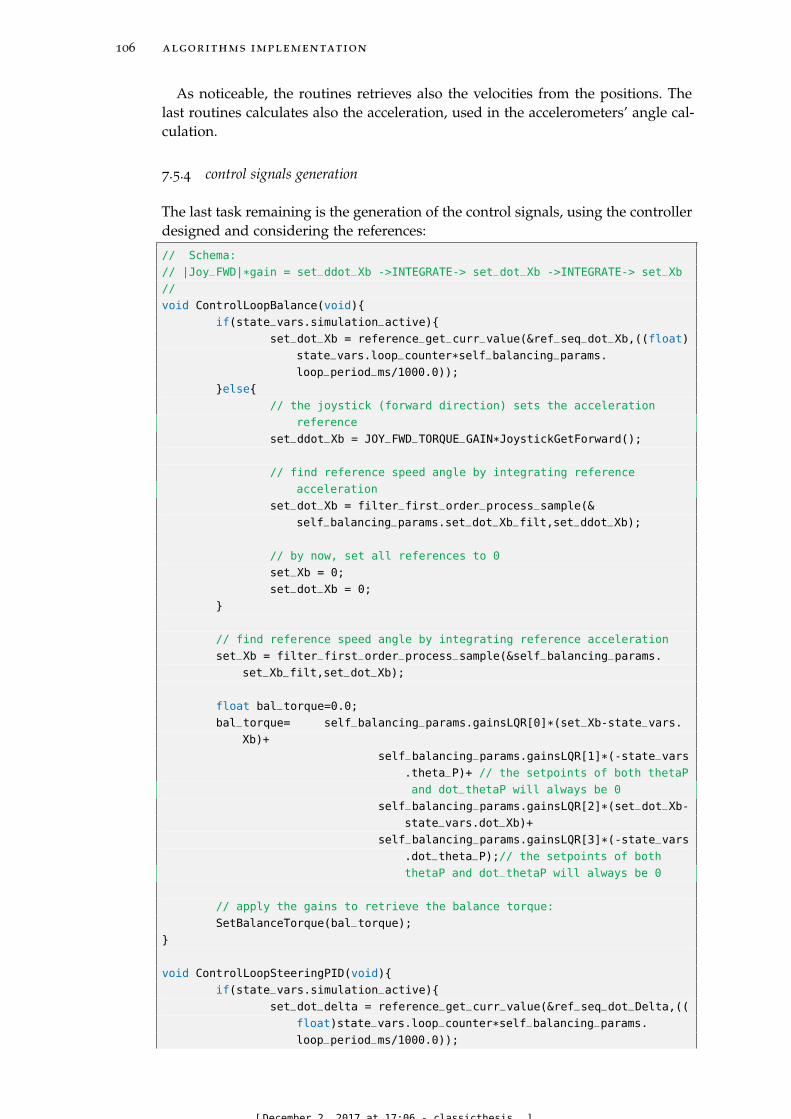
106 algorithms implementation
As noticeable, the routines retrieves also the velocities from the positions. Thelast routines calculates also the acceleration, used in the accelerometers’ angle cal-culation.
7.5.4 control signals generation
The last task remaining is the generation of the control signals, using the controllerdesigned and considering the references:
// Schema:
// |Joy_FWD|*gain = set_ddot_Xb ->INTEGRATE-> set_dot_Xb ->INTEGRATE-> set_Xb
//
void ControlLoopBalance(void)
if(state_vars.simulation_active)
set_dot_Xb = reference_get_curr_value(&ref_seq_dot_Xb,((float)
state_vars.loop_counter*self_balancing_params.
loop_period_ms/1000.0));
else
// the joystick (forward direction) sets the acceleration
reference
set_ddot_Xb = JOY_FWD_TORQUE_GAIN*JoystickGetForward();
// find reference speed angle by integrating reference
acceleration
set_dot_Xb = filter_first_order_process_sample(&
self_balancing_params.set_dot_Xb_filt,set_ddot_Xb);
// by now, set all references to 0
set_Xb = 0;
set_dot_Xb = 0;
// find reference speed angle by integrating reference acceleration
set_Xb = filter_first_order_process_sample(&self_balancing_params.
set_Xb_filt,set_dot_Xb);
float bal_torque=0.0;
bal_torque= self_balancing_params.gainsLQR[0]*(set_Xb-state_vars.
Xb)+
self_balancing_params.gainsLQR[1]*(-state_vars
.theta_P)+ // the setpoints of both thetaP
and dot_thetaP will always be 0
self_balancing_params.gainsLQR[2]*(set_dot_Xb-
state_vars.dot_Xb)+
self_balancing_params.gainsLQR[3]*(-state_vars
.dot_theta_P);// the setpoints of both
thetaP and dot_thetaP will always be 0
// apply the gains to retrieve the balance torque:
SetBalanceTorque(bal_torque);
void ControlLoopSteeringPID(void)
if(state_vars.simulation_active)
set_dot_delta = reference_get_curr_value(&ref_seq_dot_Delta,((
float)state_vars.loop_counter*self_balancing_params.
loop_period_ms/1000.0));
[December 2, 2017 at 17:06 - classicthesis ]
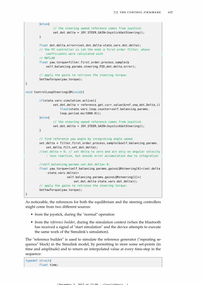
7.5 the control firmware 107
else
// the steering speed reference comes from joystick
set_dot_delta = JOY_STEER_GAIN*JoystickGetSteering();
float dot_delta_error=(set_dot_delta-state_vars.dot_delta);
// the PI controller is (at the end) a first-order filter, whose
coefficients were calculated with
// MATLAB
float yaw_torque=filter_first_order_process_sample(&
self_balancing_params.steering_PID,dot_delta_error);
// apply the gains to retrieve the steering torque:
SetYawTorque(yaw_torque);
void ControlLoopSteeringLQR(void)
if(state_vars.simulation_active)
set_dot_delta = reference_get_curr_value(&ref_seq_dot_Delta,((
float)state_vars.loop_counter*self_balancing_params.
loop_period_ms/1000.0));
else
// the steering speed reference comes from joystick
set_dot_delta = JOY_STEER_GAIN*JoystickGetSteering();
// find reference yaw angle by integrating angle speed
set_delta = filter_first_order_process_sample(&self_balancing_params.
set_delta_filt,set_dot_delta);
//set_delta = 0; // set delta to zero and act only on angular velocity
: less reactive, but avoids error accumulation due to integration
//self_balancing_params.set_dot_delta= 0;
float yaw_torque=(self_balancing_params.gainsLQRsteering[0]*(set_delta
-state_vars.delta)+
self_balancing_params.gainsLQRsteering[1]*(
set_dot_delta-state_vars.dot_delta));
// apply the gains to retrieve the steering torque:
SetYawTorque(yaw_torque);
As noticeable, the references for both the equilibrium and the steering controllersmight come from two different sources:
• from the joystick, during the "normal" operation
• from the reference builder, during the simulation context (when the bluetoothhas received a signal of "start simulation" and the device attempts to executethe same work of the Simulink’s simulation).
The "reference builder" is used to simulate the reference generator ("repeating se-quence" block) in the Simulink model, by permitting to store some set-points (intime and amplitude) and to return an interpolated value at every time-step in thesequence:
typedef struct
float time;
[December 2, 2017 at 17:06 - classicthesis ]
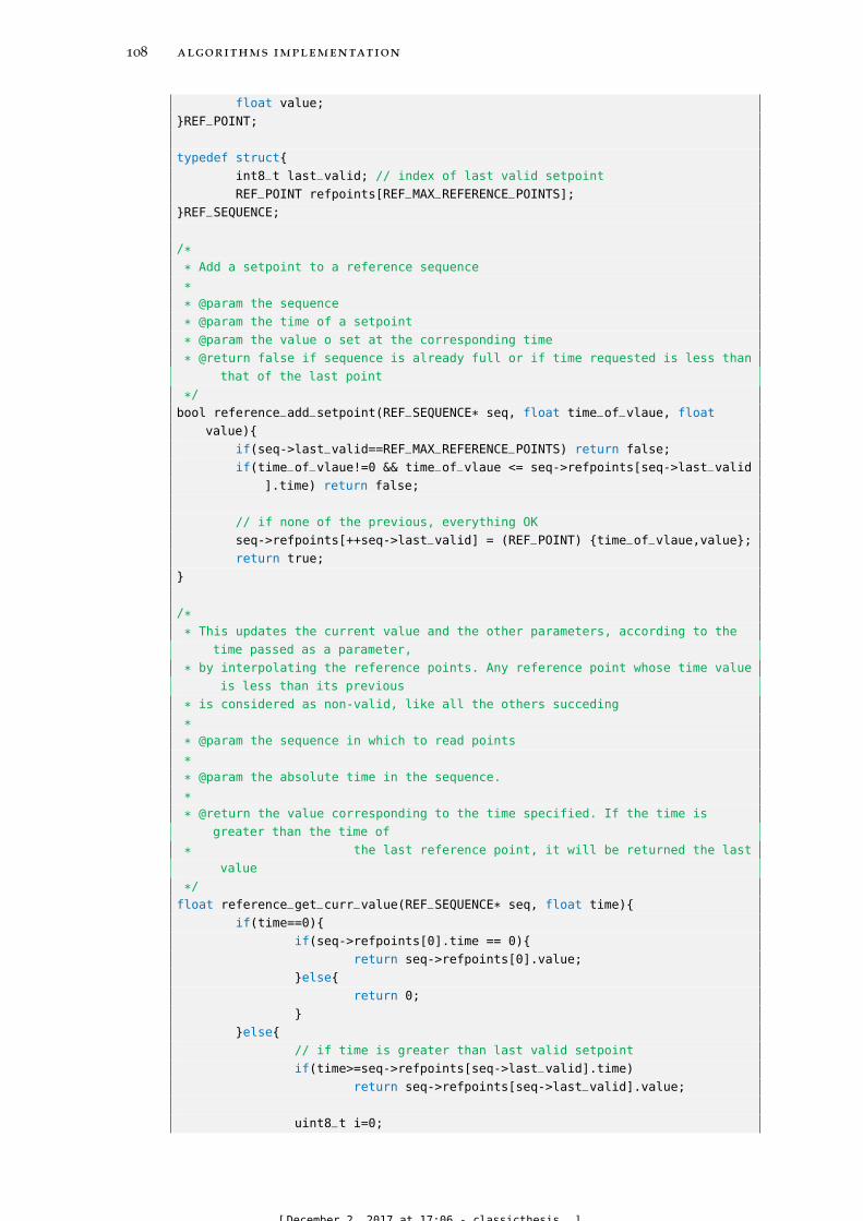
108 algorithms implementation
float value;
REF_POINT;
typedef struct
int8_t last_valid; // index of last valid setpoint
REF_POINT refpoints[REF_MAX_REFERENCE_POINTS];
REF_SEQUENCE;
/*
* Add a setpoint to a reference sequence
*
* @param the sequence
* @param the time of a setpoint
* @param the value o set at the corresponding time
* @return false if sequence is already full or if time requested is less than
that of the last point
*/
bool reference_add_setpoint(REF_SEQUENCE* seq, float time_of_vlaue, float
value)
if(seq->last_valid==REF_MAX_REFERENCE_POINTS) return false;
if(time_of_vlaue!=0 && time_of_vlaue <= seq->refpoints[seq->last_valid
].time) return false;
// if none of the previous, everything OK
seq->refpoints[++seq->last_valid] = (REF_POINT) time_of_vlaue,value;
return true;
/*
* This updates the current value and the other parameters, according to the
time passed as a parameter,
* by interpolating the reference points. Any reference point whose time value
is less than its previous
* is considered as non-valid, like all the others succeding
*
* @param the sequence in which to read points
*
* @param the absolute time in the sequence.
*
* @return the value corresponding to the time specified. If the time is
greater than the time of
* the last reference point, it will be returned the last
value
*/
float reference_get_curr_value(REF_SEQUENCE* seq, float time)
if(time==0)
if(seq->refpoints[0].time == 0)
return seq->refpoints[0].value;
else
return 0;
else
// if time is greater than last valid setpoint
if(time>=seq->refpoints[seq->last_valid].time)
return seq->refpoints[seq->last_valid].value;
uint8_t i=0;
[December 2, 2017 at 17:06 - classicthesis ]
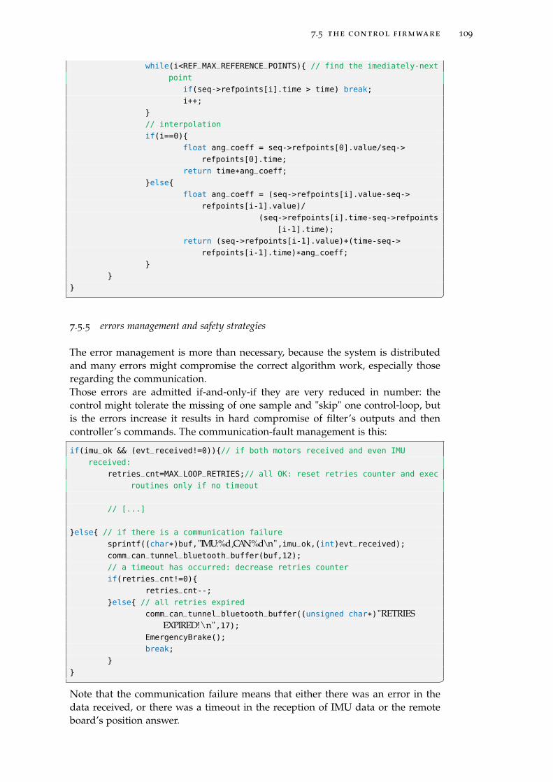
7.5 the control firmware 109
while(i<REF_MAX_REFERENCE_POINTS) // find the imediately-next
point
if(seq->refpoints[i].time > time) break;
i++;
// interpolation
if(i==0)
float ang_coeff = seq->refpoints[0].value/seq->
refpoints[0].time;
return time*ang_coeff;
else
float ang_coeff = (seq->refpoints[i].value-seq->
refpoints[i-1].value)/
(seq->refpoints[i].time-seq->refpoints
[i-1].time);
return (seq->refpoints[i-1].value)+(time-seq->
refpoints[i-1].time)*ang_coeff;
7.5.5 errors management and safety strategies
The error management is more than necessary, because the system is distributedand many errors might compromise the correct algorithm work, especially thoseregarding the communication.Those errors are admitted if-and-only-if they are very reduced in number: thecontrol might tolerate the missing of one sample and "skip" one control-loop, butis the errors increase it results in hard compromise of filter’s outputs and thencontroller’s commands. The communication-fault management is this:
if(imu_ok && (evt_received!=0))// if both motors received and even IMU
received:
retries_cnt=MAX_LOOP_RETRIES;// all OK: reset retries counter and exec
routines only if no timeout
// [...]
else // if there is a communication failure
sprintf((char*)buf,"IMU:%d,CAN:%d\n",imu_ok,(int)evt_received);comm_can_tunnel_bluetooth_buffer(buf,12);
// a timeout has occurred: decrease retries counter
if(retries_cnt!=0)
retries_cnt--;
else // all retries expired
comm_can_tunnel_bluetooth_buffer((unsigned char*)"RETRIESEXPIRED!\n",17);
EmergencyBrake();
break;
Note that the communication failure means that either there was an error in thedata received, or there was a timeout in the reception of IMU data or the remoteboard’s position answer.
[ December 2, 2017 at 17:06 – classicthesis ]

110 algorithms implementation
In case of fault, even only one, a notification is sent via bluetooth and if the retriesexpires the controller can’t perform any other correct work, thus calls the Emergen-cyBrake procedure, that simply sets 0 current to the motors (let them free-rotate).Those errors were frequent in the initial part of the project, but once the com-munications were all correctly tuned, no failure notifications have been registeredduring all the experiments.
Two conditions are checked for the purpose of safety:
1. The controller must work only if tilt angle doesn’t exceeds the limit (set to±20°), where the linearization assumptions doesn’t hold anymore and thecontrol action might result "risky":
// attention: apply the controls only if the tilt angle is within the
limits!!!
if((state_vars.theta_P<CTL_MAX_TILT_ANGLE_RADS)&&(state_vars.theta_P>(-
CTL_MAX_TILT_ANGLE_RADS)))
ControlLoopSteeringPID();
//ControlLoopSteeringLQR();
ControlLoopBalance();
eq_cnt=0;
else
if((eq_cnt)<10)
EmergencyBrake();
eq_cnt++;
if not possible, stop any action to the motors and let them free-rotate.
2. At every control loop it is monitored the state of the Safety button: a normallyclosed contact that serves for the Emergency Stop of the vehicle:
// IMPORTANT safety guard: monitoring red button pressure
if(palReadPad(EMERGENCY_BUTT_PORT,EMERGENCY_BUTT_BIT)) // if red button
is pressed
if(emgcy_cnt<10)
EmergencyBrake();
// reset the tachometers of both left and right wheels
mc_interface_get_tachometer_value(true); // local motor’s
tacho
comm_can_reset_tacho(MOT_L); //
remote motor’s tacho
ResetStateVars();
emgcy_cnt++;
else
emgcy_cnt=0;
UpdateTorquesToVehicle();
the emergency button was very useful during the experiments, even for stop-ping/restarting the device and to test its free-evolution behavior.
[ December 2, 2017 at 17:06 – classicthesis ]
7.6 conclusions 111
7.6 conclusions
In this chapter it was presented "all the software" in the project (all the source-codewill become shortly open-source and published), both for the model buildup andfor the real-time embedded controller.
This chapter have focused only on the key-routines, explaining some algorithmsand underlying considerations. As stated before, the embedded code of the con-troller and the filters coexists in the micro-controller that drives the right motor.The correct work and the absence of communication errors and latency failureswas considered a big success of integration of an evolved-controller code into asuccessful open-hardware project’s device.
The possibility to perform many automated tasks (such as parameter update,start/stop simulations and collecting data) remotely via bluetooth is consideredby the author a great result, useful for future investigations and/or improvementsworks.
Those are the motivations that drove the idea of sharing the work with an open-source project, fort the benefit of both hobbyists/passionate and for scientific anal-ysis and community-provided project improvement contributions.
[ December 2, 2017 at 17:06 – classicthesis ]

[ December 2, 2017 at 17:06 – classicthesis ]
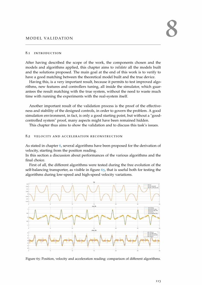
8M O D E L VA L I D AT I O N
8.1 introduction
After having described the scope of the work, the components chosen and themodels and algorithms applied, this chapter aims to validate all the models builtand the solutions proposed. The main goal at the end of this work is to verify tohave a good matching between the theoretical model built and the true device.
Having this, is a very important result, because it permits to test improved algo-rithms, new features and controllers tuning, all inside the simulator, which guar-antees the result matching with the true system, without the need to waste muchtime with running the experiments with the real-system itself.
Another important result of the validation process is the proof of the effective-ness and stability of the designed controls, in order to govern the problem. A goodsimulation environment, in fact, is only a good starting point, but without a "good-controlled system" proof, many aspects might have been remained hidden.
This chapter thus aims to show the validation and to discuss this task’s issues.
8.2 velocity and acceleration reconstruction
As stated in chapter 6, several algorithms have been proposed for the derivation ofvelocity, starting from the position reading.In this section a discussion about performances of the various algorithms and thefinal choice.
First of all, the different algorithms were tested during the free evolution of theself-balancing transporter, as visible in figure 65, that is useful both for testing thealgorithms during low-speed and high-speed velocity variations.
Figure 65: Position, velocity and acceleration reading: comparison of different algorithms.
113
[ December 2, 2017 at 17:06 – classicthesis ]
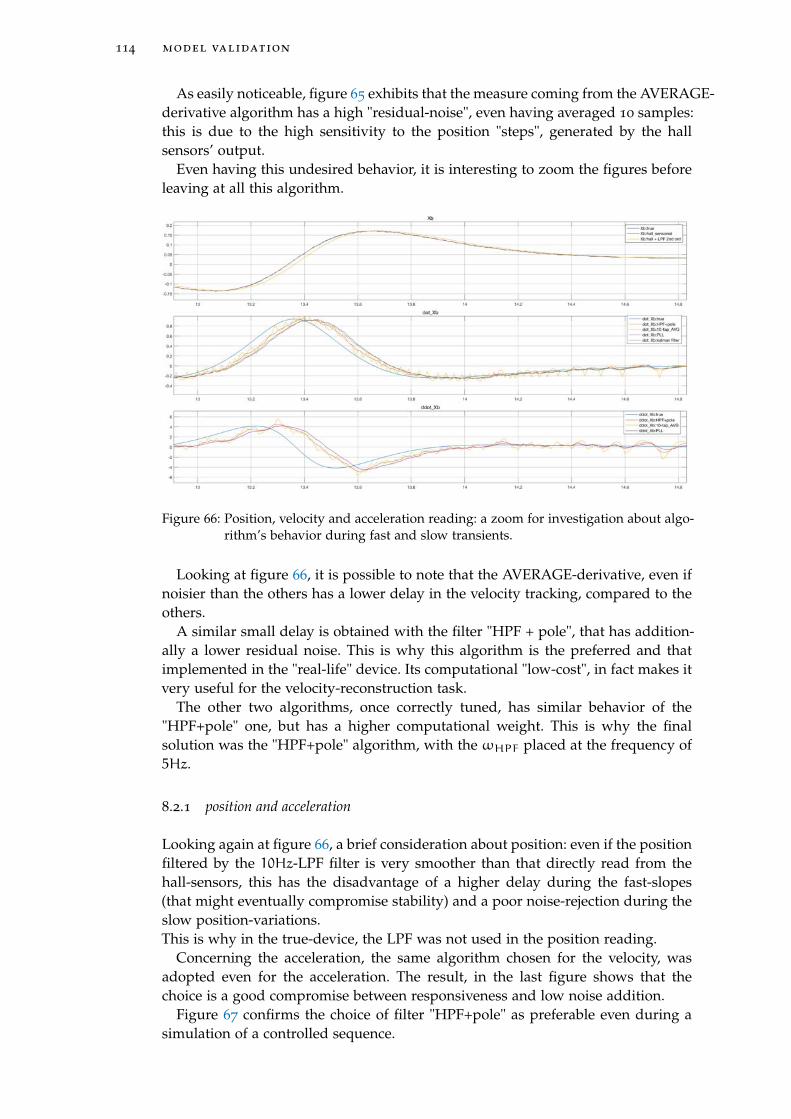
114 model validation
As easily noticeable, figure 65 exhibits that the measure coming from the AVERAGE-derivative algorithm has a high "residual-noise", even having averaged 10 samples:this is due to the high sensitivity to the position "steps", generated by the hallsensors’ output.
Even having this undesired behavior, it is interesting to zoom the figures beforeleaving at all this algorithm.
Figure 66: Position, velocity and acceleration reading: a zoom for investigation about algo-rithm’s behavior during fast and slow transients.
Looking at figure 66, it is possible to note that the AVERAGE-derivative, even ifnoisier than the others has a lower delay in the velocity tracking, compared to theothers.
A similar small delay is obtained with the filter "HPF + pole", that has addition-ally a lower residual noise. This is why this algorithm is the preferred and thatimplemented in the "real-life" device. Its computational "low-cost", in fact makes itvery useful for the velocity-reconstruction task.
The other two algorithms, once correctly tuned, has similar behavior of the"HPF+pole" one, but has a higher computational weight. This is why the finalsolution was the "HPF+pole" algorithm, with the ωHPF placed at the frequency of5Hz.
8.2.1 position and acceleration
Looking again at figure 66, a brief consideration about position: even if the positionfiltered by the 10Hz-LPF filter is very smoother than that directly read from thehall-sensors, this has the disadvantage of a higher delay during the fast-slopes(that might eventually compromise stability) and a poor noise-rejection during theslow position-variations.This is why in the true-device, the LPF was not used in the position reading.
Concerning the acceleration, the same algorithm chosen for the velocity, wasadopted even for the acceleration. The result, in the last figure shows that thechoice is a good compromise between responsiveness and low noise addition.
Figure 67 confirms the choice of filter "HPF+pole" as preferable even during asimulation of a controlled sequence.
[ December 2, 2017 at 17:06 – classicthesis ]
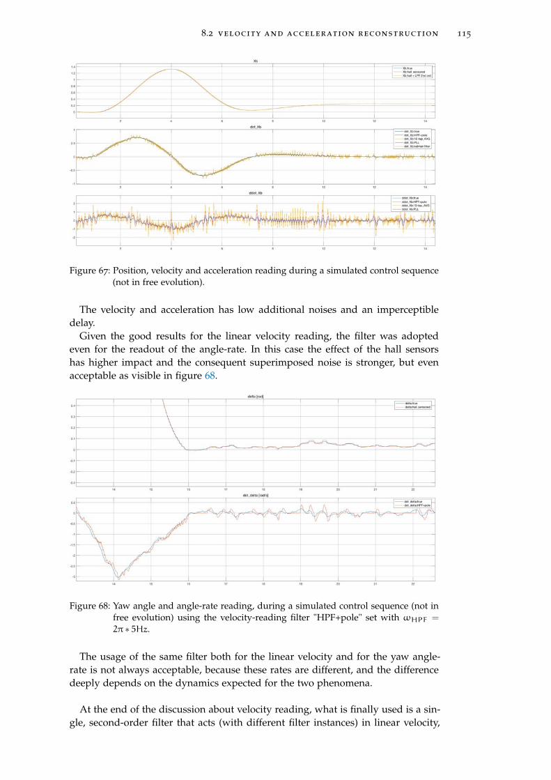
8.2 velocity and acceleration reconstruction 115
Figure 67: Position, velocity and acceleration reading during a simulated control sequence(not in free evolution).
The velocity and acceleration has low additional noises and an imperceptibledelay.
Given the good results for the linear velocity reading, the filter was adoptedeven for the readout of the angle-rate. In this case the effect of the hall sensorshas higher impact and the consequent superimposed noise is stronger, but evenacceptable as visible in figure 68.
Figure 68: Yaw angle and angle-rate reading, during a simulated control sequence (not infree evolution) using the velocity-reading filter "HPF+pole" set with ωHPF =
2π ∗ 5Hz.
The usage of the same filter both for the linear velocity and for the yaw angle-rate is not always acceptable, because these rates are different, and the differencedeeply depends on the dynamics expected for the two phenomena.
At the end of the discussion about velocity reading, what is finally used is a sin-gle, second-order filter that acts (with different filter instances) in linear velocity,
[ December 2, 2017 at 17:06 – classicthesis ]

116 model validation
acceleration and yaw rate. This means that the self-balancing device will imple-ment three second-order-filters with identical parameters.The definition of filters’ parameters was automated by the MATLAB scripts in-side the file "digital filters". Once defined there, the scripts provides the automaticparameters upgrade to the real-device, via bluetooth.
8.3 imu model validation and tuning
The IMU is one of the key components of the system. Its description and the cor-responding model have been already described in chapter 6. Also in that chaptera discussion about the angle measurement by sensor-fusion.
In this section it will be described the validation procedures that aim to verify:
• the matching between datasheet’s data and true measures
• the model scheme validation by measures
• the calibration of the IMU
• the tuning of the sensor-fusion algorithms
In this section it is described the analisys, valid for the specific component In-vensense MPU9250 [28].
8.3.1 datasheet verification
One of the most important things reported in the datasheet is the noise entity andtype. Noise affects both accelerometer and gyroscope measures: in order to buildan affordable model, it must report the same type of noises of the real one.
For both sensors, the noise type is a white noise, with constant power along thefrequency span. In the following subsections the verification of the datasheets dataand the models’ parameters data population.
8.3.1.1 Accelerometer noise and bias
The datasheet of the accelerometer reports the following data:
[ December 2, 2017 at 17:06 – classicthesis ]
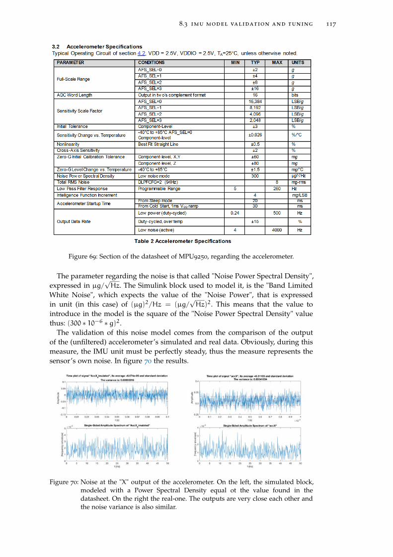
8.3 imu model validation and tuning 117
Figure 69: Section of the datasheet of MPU9250, regarding the accelerometer.
The parameter regarding the noise is that called "Noise Power Spectral Density",expressed in µg/
√Hz. The Simulink block used to model it, is the "Band Limited
White Noise", which expects the value of the "Noise Power", that is expressedin unit (in this case) of (µg)2/Hz = (µg/
√Hz)2. This means that the value to
introduce in the model is the square of the "Noise Power Spectral Density" valuethus: (300 ∗ 10−6 ∗ g)2.
The validation of this noise model comes from the comparison of the outputof the (unfiltered) accelerometer’s simulated and real data. Obviously, during thismeasure, the IMU unit must be perfectly steady, thus the measure represents thesensor’s own noise. In figure 70 the results.
Figure 70: Noise at the "X" output of the accelerometer. On the left, the simulated block,modeled with a Power Spectral Density equal ot the value found in thedatasheet. On the right the real-one. The outputs are very close each other andthe noise variance is also similar.
[ December 2, 2017 at 17:06 – classicthesis ]
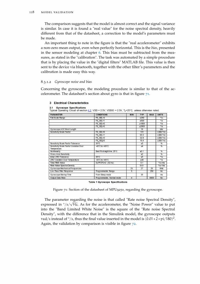
118 model validation
The comparison suggests that the model is almost correct and the signal varianceis similar. In case it is found a "real value" for the noise spectral density, heavilydifferent from that of the datasheet, a correction to the model’s parameters mustbe made.
An important thing to note in the figure is that the "real accelerometer" exhibitsa non-zero mean output, even when perfectly horizontal. This is the bias, presentedin the sensor modeling at chapter 6. This bias must be subtracted from the mea-sures, as stated in the "calibration". The task was automated by a simple procedurethat is by placing the value in the "digital filters" MATLAB file. This value is thensent to the device via bluetooth, together with the other filter’s parameters and thecalibration is made easy this way.
8.3.1.2 Gyroscope noise and bias
Concerning the gyroscope, the modeling procedure is similar to that of the ac-celerometer. The datasheet’s section about gyro is that in figure 71.
Figure 71: Section of the datasheet of MPU9250, regarding the gyroscope.
The parameter regarding the noise is that called "Rate noise Spectral Density",expressed in °/s/
√Hz. As for the accelerometer, the "Noise Power" value to put
into the "Band Limited White Noise" is the square of the "Rate noise SpectralDensity", with the difference that in the Simulink model, the gyroscope outputsrad/s instead of °/s, thus the final value inserted in the model is (0.01∗2∗pi/180)2.Again, the validation by comparison is visible in figure 72.
[ December 2, 2017 at 17:06 – classicthesis ]

8.3 imu model validation and tuning 119
Figure 72: Noise at the output of the gyroscope. On the left, the simulated block, with thevalue found in the datasheet. On the right the real-one. The outputs are veryclose each other and the variance is also similar: the real-device variance is evensmaller than that of the datasheet.
Even for the gyroscope, a good correspondence between the model and the true-life measures has been verified.
Concerning the bias, even for the gyroscope, the value of the average of the signalcan be put into the "digital filters" file, so that the "parameters update" procedureprovides the automatic bias removal (part of the IMU calibration task).
A note about this: in the case of the gyroscope, the bias has a higher impact onthe measures, since the gyroscope’s output is integrated during time, for retrievingthe pitch angle (even if "fused" for with the accelerometer).
8.3.1.3 IMU low-pass filter verification
A further model verification was performed to proof the effect of the digital fil-ter modeled inside the accelerometer and gyroscope. In figure 73 a comparisonbetween the simulation-block and the true device behavior.
Figure 73: Noise at the output of the gyroscope, when filtered at 5Hz. On the left, thesimulated block, on the right the real-one that has the embedded digital filter.The frequency behavior is very similar in the two situations.
The correct correspondence is useful because the simulation results is tight simi-lar to the reality, making it possible to have affordable simulation and test benefitsor drawbacks of filtering, directly by simulation, without the need to have a realdevice.
[ December 2, 2017 at 17:06 – classicthesis ]
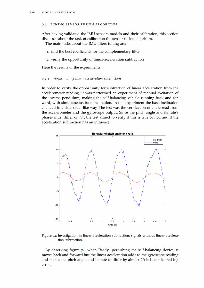
120 model validation
8.4 tuning sensor fusion algorithm
After having validated the IMU sensors models and their calibration, this sectiondiscusses about the task of calibration the sensor fusion algorithm.
The main tasks about the IMU filters tuning are:
1. find the best coefficients for the complementary filter
2. verify the opportunity of linear-acceleration subtraction
Here the results of the experiments.
8.4.1 Verification of linear acceleration subtraction
In order to verify the opportunity for subtraction of linear acceleration from theaccelerometer reading, it was performed an experiment of manual excitation ofthe inverse pendulum, making the self-balancing vehicle running back and for-ward, with simultaneous base inclination. In this experiment the base inclinationchanged in a sinusoidal-like way. The test was the verification of angle read fromthe accelerometer and the gyroscope output. Since the pitch angle and its rate’sphases must differ of 90°, the test aimed to verify if this is true or not, and if theacceleration subtraction has an influence.
Figure 74: Investigation in linear acceleration subtraction: signals without linear accelera-tion subtraction.
By observing figure 74, when "fastly" perturbing the self-balancing device, itmoves back and forward but the linear acceleration adds to the gyroscope readingand makes the pitch angle and its rate to differ by almost 0°: it is considered bigerror.
[ December 2, 2017 at 17:06 – classicthesis ]
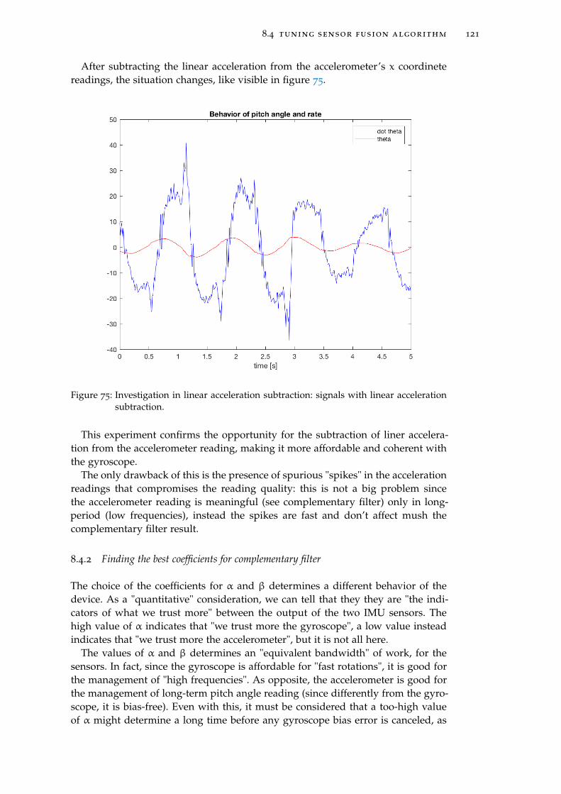
8.4 tuning sensor fusion algorithm 121
After subtracting the linear acceleration from the accelerometer’s x coordinetereadings, the situation changes, like visible in figure 75.
Figure 75: Investigation in linear acceleration subtraction: signals with linear accelerationsubtraction.
This experiment confirms the opportunity for the subtraction of liner accelera-tion from the accelerometer reading, making it more affordable and coherent withthe gyroscope.
The only drawback of this is the presence of spurious "spikes" in the accelerationreadings that compromises the reading quality: this is not a big problem sincethe accelerometer reading is meaningful (see complementary filter) only in long-period (low frequencies), instead the spikes are fast and don’t affect mush thecomplementary filter result.
8.4.2 Finding the best coefficients for complementary filter
The choice of the coefficients for α and β determines a different behavior of thedevice. As a "quantitative" consideration, we can tell that they they are "the indi-cators of what we trust more" between the output of the two IMU sensors. Thehigh value of α indicates that "we trust more the gyroscope", a low value insteadindicates that "we trust more the accelerometer", but it is not all here.
The values of α and β determines an "equivalent bandwidth" of work, for thesensors. In fact, since the gyroscope is affordable for "fast rotations", it is good forthe management of "high frequencies". As opposite, the accelerometer is good forthe management of long-term pitch angle reading (since differently from the gyro-scope, it is bias-free). Even with this, it must be considered that a too-high valueof α might determine a long time before any gyroscope bias error is canceled, as
[ December 2, 2017 at 17:06 – classicthesis ]

122 model validation
opposite a low-value might result in a loosely-stable equilibrium controller, sincethe accelerometer is very noisy.
The tuning activity is a trade-off between system stability and measure preci-sion. In this case there were performed several experiments, simply by testing thereaction (angle and horizontal position deviation) of the TWSBT to external distur-bances (kicks) with different values of α and "quantitatively" verify the effect onthe equilibrium performances:
• α = 0.95
• α = 0.99
• α = 0.999
Also the simulations have demonstrated the different behavior of the systemwith different settings of α. Their results are reported in figure 76.
Figure 76: Simulation with different values of complementary filter coefficients (left α =
0.95, right α = 0.999).
As noticeable in figure 76, higher values of α guarantees less noise in the statevariables and less elongations in the transients. Another key-consideration is thepresence of strong oscillations in the device with α = 0.95, confirming a looselystability. This is also confirmed by the real-device, where a value of α < 0.95determines an unstable device.
At the end of the tests, it was chosen to adopt α = 0.999, since the device has anintrinsic "slow dynamic", and the accelerometer output must be considered onlyfor very-slow frequencies. The value chosen also guaranteed less deviation of thevehicle in case of external perturbations. It has also demonstrated to be a goodchoice to be employed for the transport of the rider, since it gives the (subjective)sensation of a "stable base", much more than with lower α values.
[ December 2, 2017 at 17:06 – classicthesis ]
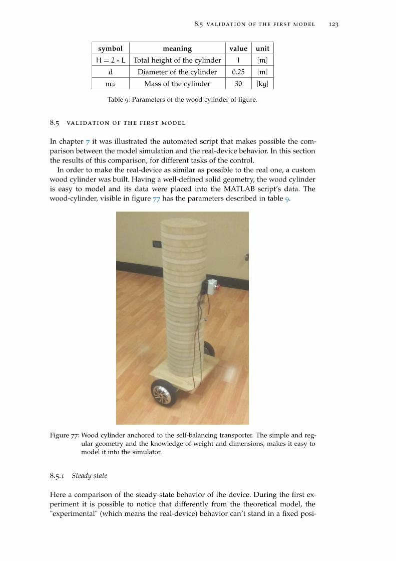
8.5 validation of the first model 123
symbol meaning value unit
H = 2 ∗ L Total height of the cylinder 1 [m]
d Diameter of the cylinder 0.25 [m]
mP Mass of the cylinder 30 [kg]
Table 9: Parameters of the wood cylinder of figure.
8.5 validation of the first model
In chapter 7 it was illustrated the automated script that makes possible the com-parison between the model simulation and the real-device behavior. In this sectionthe results of this comparison, for different tasks of the control.
In order to make the real-device as similar as possible to the real one, a customwood cylinder was built. Having a well-defined solid geometry, the wood cylinderis easy to model and its data were placed into the MATLAB script’s data. Thewood-cylinder, visible in figure 77 has the parameters described in table 9.
Figure 77: Wood cylinder anchored to the self-balancing transporter. The simple and reg-ular geometry and the knowledge of weight and dimensions, makes it easy tomodel it into the simulator.
8.5.1 Steady state
Here a comparison of the steady-state behavior of the device. During the first ex-periment it is possible to notice that differently from the theoretical model, the"experimental" (which means the real-device) behavior can’t stand in a fixed posi-
[ December 2, 2017 at 17:06 – classicthesis ]
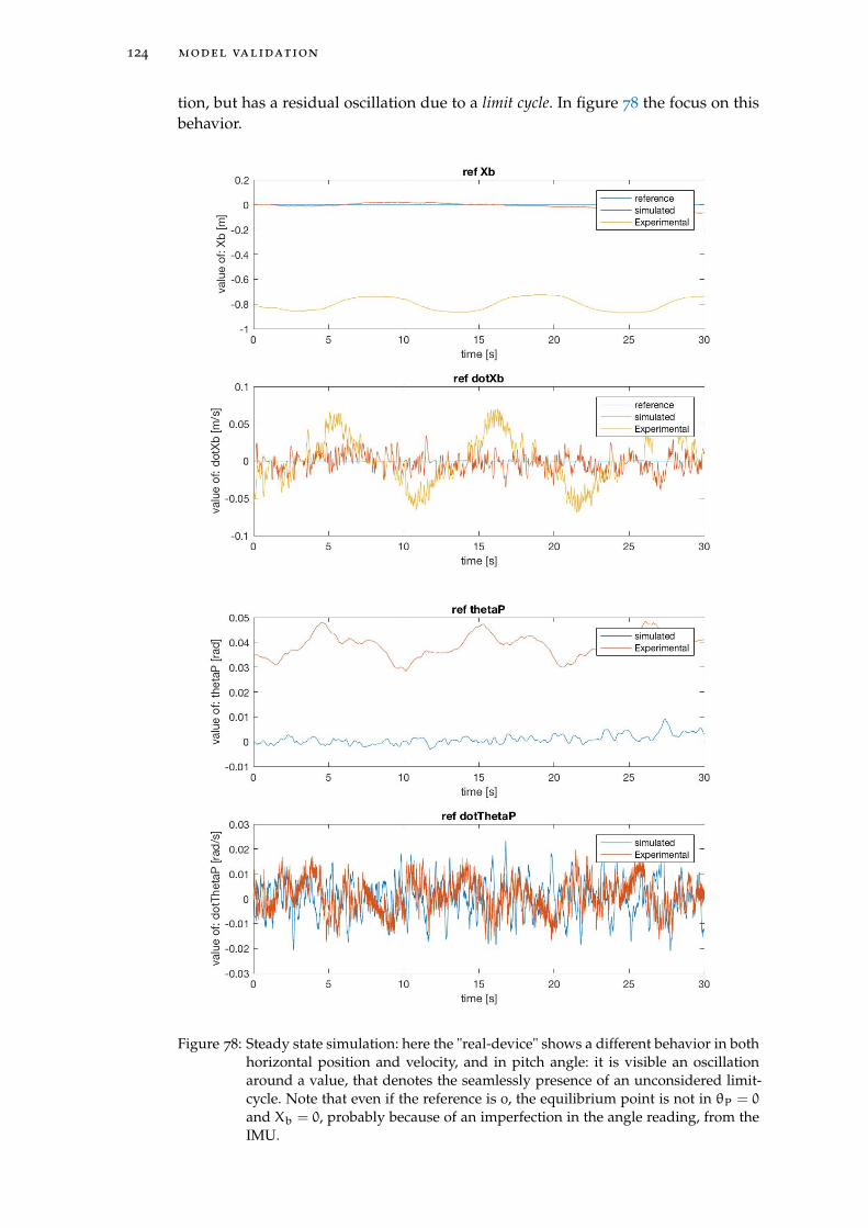
124 model validation
tion, but has a residual oscillation due to a limit cycle. In figure 78 the focus on thisbehavior.
Figure 78: Steady state simulation: here the "real-device" shows a different behavior in bothhorizontal position and velocity, and in pitch angle: it is visible an oscillationaround a value, that denotes the seamlessly presence of an unconsidered limit-cycle. Note that even if the reference is 0, the equilibrium point is not in θP = 0
and Xb = 0, probably because of an imperfection in the angle reading, from theIMU.
[ December 2, 2017 at 17:06 – classicthesis ]
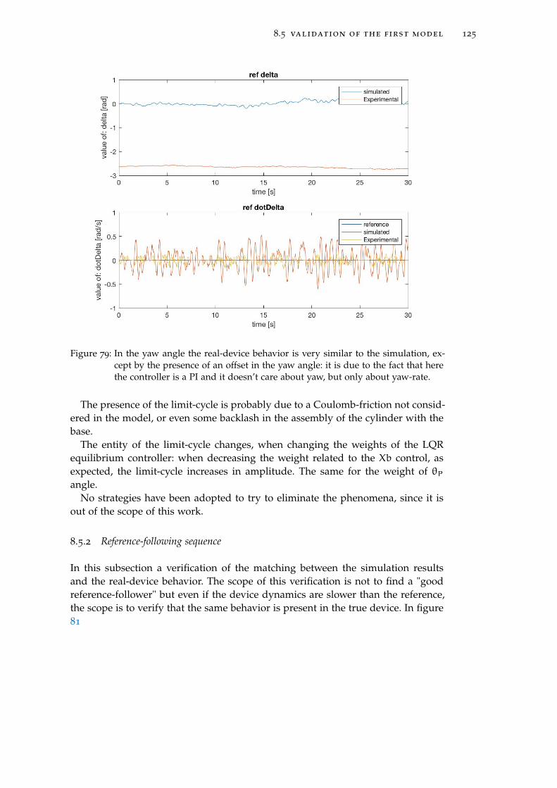
8.5 validation of the first model 125
Figure 79: In the yaw angle the real-device behavior is very similar to the simulation, ex-cept by the presence of an offset in the yaw angle: it is due to the fact that herethe controller is a PI and it doesn’t care about yaw, but only about yaw-rate.
The presence of the limit-cycle is probably due to a Coulomb-friction not consid-ered in the model, or even some backlash in the assembly of the cylinder with thebase.
The entity of the limit-cycle changes, when changing the weights of the LQRequilibrium controller: when decreasing the weight related to the Xb control, asexpected, the limit-cycle increases in amplitude. The same for the weight of θPangle.
No strategies have been adopted to try to eliminate the phenomena, since it isout of the scope of this work.
8.5.2 Reference-following sequence
In this subsection a verification of the matching between the simulation resultsand the real-device behavior. The scope of this verification is not to find a "goodreference-follower" but even if the device dynamics are slower than the reference,the scope is to verify that the same behavior is present in the true device. In figure81
[ December 2, 2017 at 17:06 – classicthesis ]
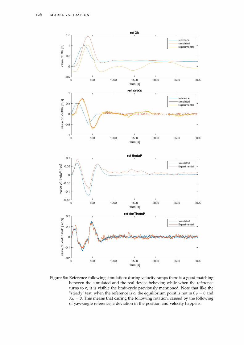
126 model validation
Figure 80: Reference-following simulation: during velocity ramps there is a good matchingbetween the simulated and the real-device behavior, while when the referenceturns to 0, it is visible the limit-cycle previously mentioned. Note that like the"steady" test, when the reference is 0, the equilibrium point is not in θP = 0 andXb = 0. This means that during the following rotation, caused by the followingof yaw-angle reference, a deviation in the position and velocity happens.
[ December 2, 2017 at 17:06 – classicthesis ]
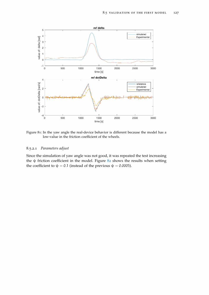
8.5 validation of the first model 127
Figure 81: In the yaw angle the real-device behavior is different because the model has alow-value in the friction coefficient of the wheels.
8.5.2.1 Parameters adjust
Since the simulation of yaw angle was not good, it was repeated the test increasingthe ψ friction coefficient in the model. Figure 82 shows the results when settingthe coefficient to ψ = 0.1 (instead of the previous ψ = 0.0005).
[ December 2, 2017 at 17:06 – classicthesis ]
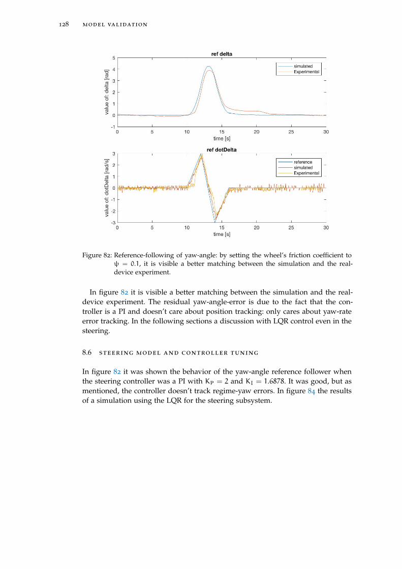
128 model validation
Figure 82: Reference-following of yaw-angle: by setting the wheel’s friction coefficient toψ = 0.1, it is visible a better matching between the simulation and the real-device experiment.
In figure 82 it is visible a better matching between the simulation and the real-device experiment. The residual yaw-angle-error is due to the fact that the con-troller is a PI and doesn’t care about position tracking: only cares about yaw-rateerror tracking. In the following sections a discussion with LQR control even in thesteering.
8.6 steering model and controller tuning
In figure 82 it was shown the behavior of the yaw-angle reference follower whenthe steering controller was a PI with KP = 2 and KI = 1.6878. It was good, but asmentioned, the controller doesn’t track regime-yaw errors. In figure 84 the resultsof a simulation using the LQR for the steering subsystem.
[ December 2, 2017 at 17:06 – classicthesis ]
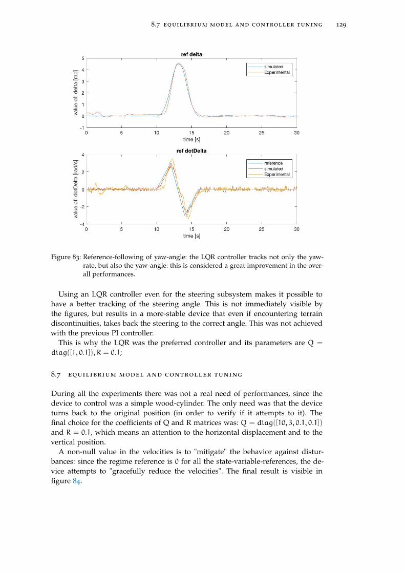
8.7 equilibrium model and controller tuning 129
Figure 83: Reference-following of yaw-angle: the LQR controller tracks not only the yaw-rate, but also the yaw-angle: this is considered a great improvement in the over-all performances.
Using an LQR controller even for the steering subsystem makes it possible tohave a better tracking of the steering angle. This is not immediately visible bythe figures, but results in a more-stable device that even if encountering terraindiscontinuities, takes back the steering to the correct angle. This was not achievedwith the previous PI controller.
This is why the LQR was the preferred controller and its parameters are Q =
diag([1, 0.1]), R = 0.1;
8.7 equilibrium model and controller tuning
During all the experiments there was not a real need of performances, since thedevice to control was a simple wood-cylinder. The only need was that the deviceturns back to the original position (in order to verify if it attempts to it). Thefinal choice for the coefficients of Q and R matrices was: Q = diag([10, 3, 0.1, 0.1])and R = 0.1, which means an attention to the horizontal displacement and to thevertical position.
A non-null value in the velocities is to "mitigate" the behavior against distur-bances: since the regime reference is 0 for all the state-variable-references, the de-vice attempts to "gracefully reduce the velocities". The final result is visible infigure 84.
[ December 2, 2017 at 17:06 – classicthesis ]
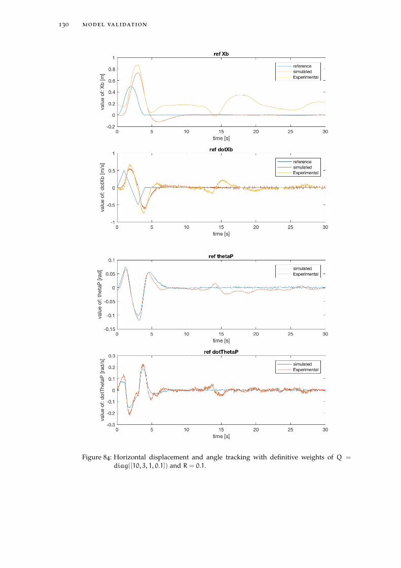
130 model validation
Figure 84: Horizontal displacement and angle tracking with definitive weights of Q =
diag([10, 3, 1, 0.1]) and R = 0.1.
[ December 2, 2017 at 17:06 – classicthesis ]
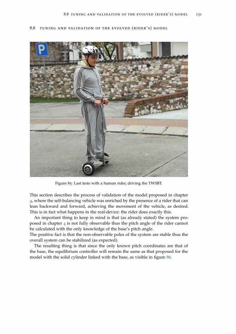
8.8 tuning and validation of the evolved (rider’s) model 131
8.8 tuning and validation of the evolved (rider’s) model
Figure 85: Last tests with a human rider, driving the TWSBT.
This section describes the process of validation of the model proposed in chapter4, where the self-balancing vehicle was enriched by the presence of a rider that canlean backward and forward, achieving the movement of the vehicle, as desired.This is in fact what happens in the real-device: the rider does exactly this.
An important thing to keep in mind is that (as already stated) the system pro-posed in chapter 4 is not fully observable thus the pitch angle of the rider cannotbe calculated with the only knowledge of the base’s pitch angle.The positive fact is that the non-observable poles of the system are stable thus theoverall system can be stabilized (as expected).
The resulting thing is that since the only known pitch coordinates are that ofthe base, the equilibrium controller will remain the same as that proposed for themodel with the solid cylinder linked with the base, as visible in figure 86.
[ December 2, 2017 at 17:06 – classicthesis ]
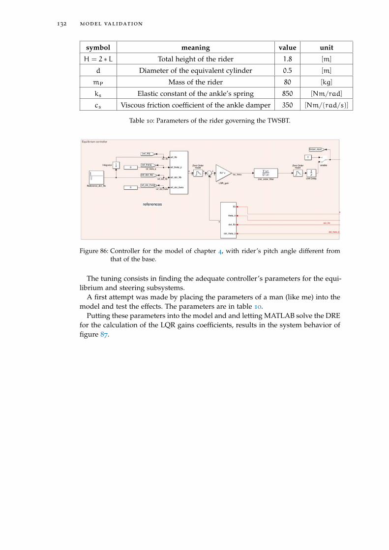
132 model validation
symbol meaning value unit
H = 2 ∗ L Total height of the rider 1.8 [m]
d Diameter of the equivalent cylinder 0.5 [m]
mP Mass of the rider 80 [kg]
ks Elastic constant of the ankle’s spring 850 [Nm/rad]
cs Viscous friction coefficient of the ankle damper 350 [Nm/(rad/s)]
Table 10: Parameters of the rider governing the TWSBT.
Figure 86: Controller for the model of chapter 4, with rider’s pitch angle different fromthat of the base.
The tuning consists in finding the adequate controller’s parameters for the equi-librium and steering subsystems.
A first attempt was made by placing the parameters of a man (like me) into themodel and test the effects. The parameters are in table 10.
Putting these parameters into the model and and letting MATLAB solve the DREfor the calculation of the LQR gains coefficients, results in the system behavior offigure 87.
[ December 2, 2017 at 17:06 – classicthesis ]

8.8 tuning and validation of the evolved (rider’s) model 133
Figure 87: First simulation of rider with controller tuned with parameters of table 10: thecontroller is unstable.
As noticeable in figure 87 the controller attempts to take the rider vertical, butsuddenly a strong vibration in the pitch angle makes it impossible and the con-troller diverges.
This behavior was verified also in the real-device: a strong base vibration madeit impossible to ride it. It is a negative thing since the controller can’t achieve stableequilibrium, but is also positive since the simulated behavior is similar to the realone.
In the following subsection the actions performed to achieve the self-balancingfeature.
8.8.1 Controller tuning, for the rider
The actions taken to try to stabilize are a first strategy to make the vehicle suitablefor a rider’s transport. The result obtained is not fully satisfactory, but for a matterof time it was not possible to perform further actions in that sense.
In brief, the actions that solved the problem of equilibrium for a rider, were two:
[ December 2, 2017 at 17:06 – classicthesis ]
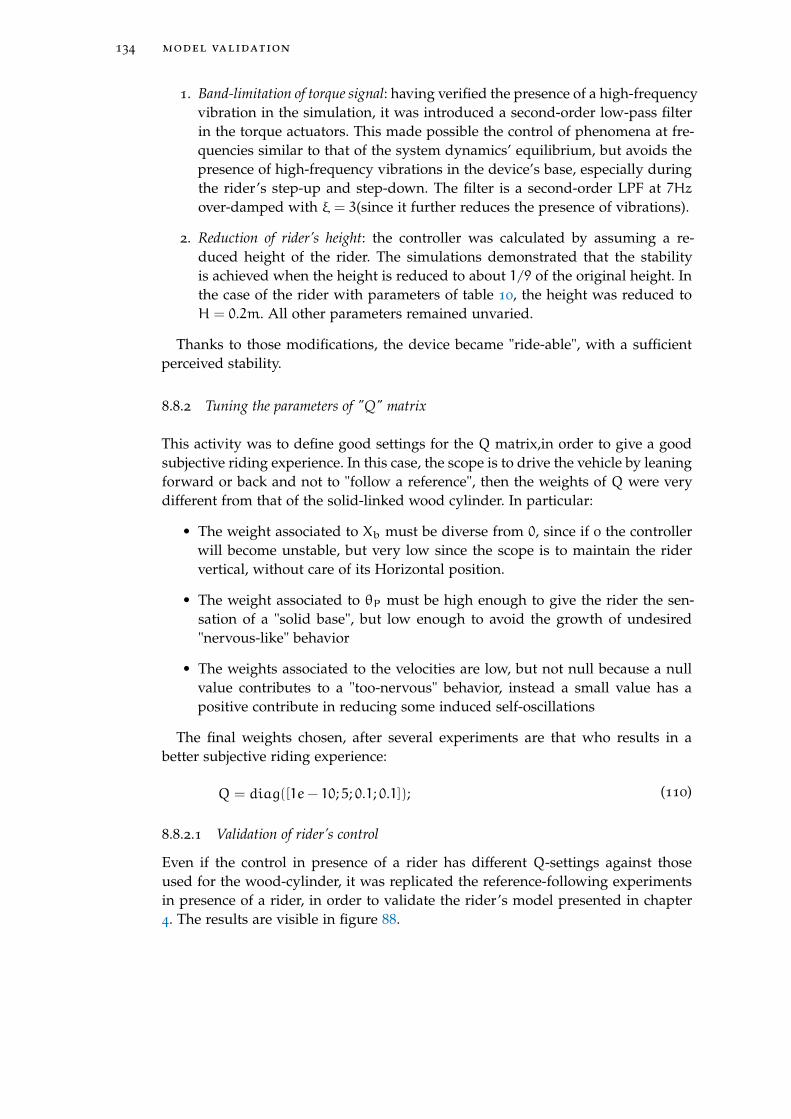
134 model validation
1. Band-limitation of torque signal: having verified the presence of a high-frequencyvibration in the simulation, it was introduced a second-order low-pass filterin the torque actuators. This made possible the control of phenomena at fre-quencies similar to that of the system dynamics’ equilibrium, but avoids thepresence of high-frequency vibrations in the device’s base, especially duringthe rider’s step-up and step-down. The filter is a second-order LPF at 7Hzover-damped with ξ = 3(since it further reduces the presence of vibrations).
2. Reduction of rider’s height: the controller was calculated by assuming a re-duced height of the rider. The simulations demonstrated that the stabilityis achieved when the height is reduced to about 1/9 of the original height. Inthe case of the rider with parameters of table 10, the height was reduced toH = 0.2m. All other parameters remained unvaried.
Thanks to those modifications, the device became "ride-able", with a sufficientperceived stability.
8.8.2 Tuning the parameters of "Q" matrix
This activity was to define good settings for the Q matrix,in order to give a goodsubjective riding experience. In this case, the scope is to drive the vehicle by leaningforward or back and not to "follow a reference", then the weights of Q were verydifferent from that of the solid-linked wood cylinder. In particular:
• The weight associated to Xb must be diverse from 0, since if 0 the controllerwill become unstable, but very low since the scope is to maintain the ridervertical, without care of its Horizontal position.
• The weight associated to θP must be high enough to give the rider the sen-sation of a "solid base", but low enough to avoid the growth of undesired"nervous-like" behavior
• The weights associated to the velocities are low, but not null because a nullvalue contributes to a "too-nervous" behavior, instead a small value has apositive contribute in reducing some induced self-oscillations
The final weights chosen, after several experiments are that who results in abetter subjective riding experience:
Q = diag([1e− 10; 5; 0.1; 0.1]); (110)
8.8.2.1 Validation of rider’s control
Even if the control in presence of a rider has different Q-settings against thoseused for the wood-cylinder, it was replicated the reference-following experimentsin presence of a rider, in order to validate the rider’s model presented in chapter4. The results are visible in figure 88.
[ December 2, 2017 at 17:06 – classicthesis ]

8.8 tuning and validation of the evolved (rider’s) model 135
[ December 2, 2017 at 17:06 – classicthesis ]
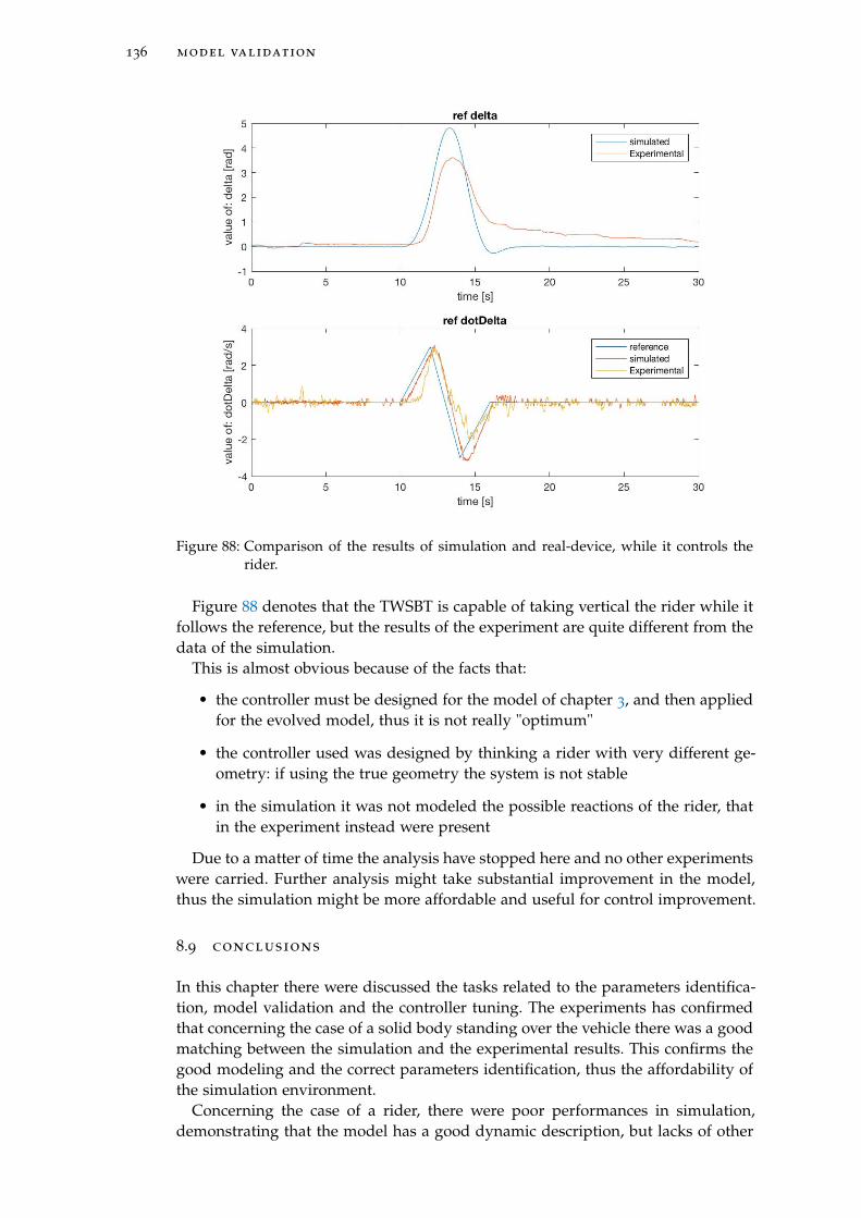
136 model validation
Figure 88: Comparison of the results of simulation and real-device, while it controls therider.
Figure 88 denotes that the TWSBT is capable of taking vertical the rider while itfollows the reference, but the results of the experiment are quite different from thedata of the simulation.
This is almost obvious because of the facts that:
• the controller must be designed for the model of chapter 3, and then appliedfor the evolved model, thus it is not really "optimum"
• the controller used was designed by thinking a rider with very different ge-ometry: if using the true geometry the system is not stable
• in the simulation it was not modeled the possible reactions of the rider, thatin the experiment instead were present
Due to a matter of time the analysis have stopped here and no other experimentswere carried. Further analysis might take substantial improvement in the model,thus the simulation might be more affordable and useful for control improvement.
8.9 conclusions
In this chapter there were discussed the tasks related to the parameters identifica-tion, model validation and the controller tuning. The experiments has confirmedthat concerning the case of a solid body standing over the vehicle there was a goodmatching between the simulation and the experimental results. This confirms thegood modeling and the correct parameters identification, thus the affordability ofthe simulation environment.
Concerning the case of a rider, there were poor performances in simulation,demonstrating that the model has a good dynamic description, but lacks of other
[ December 2, 2017 at 17:06 – classicthesis ]

8.9 conclusions 137
phenomena not already investigated (such as human reaction models) that mightbe studied in successive investigations.
The positive thing about the rider configuration is that a first set of configura-tions made it possible to have a good riding experience, that is (after all) one of themost important goals for that kind of vehicle.
[ December 2, 2017 at 17:06 – classicthesis ]

[ December 2, 2017 at 17:06 – classicthesis ]
C O N C L U S I O N S
The scope of this work was to design a controller capable to drive a vehicle basedon the (inherently unstable) inverse pendulum system.
This result was achieved by following a rigorous engineering process that con-sisted on:
• collection of the product requirements
• build-up of the system model, by solving the dynamic equations
• build-up of the simulation environment with introduction of system non-idealities, for better simulation results
• parameters identification of the real device
• control design with stability verification and simulation
• practical implementation into a distributed embedded system
• verification of simulation environment by comparison with real-device exper-iments
The result at the end of the work is a stable device, capable of carrying bothsolid-attached loads and persons, with a good riding experience.
Also important is a high-quality simulation environment, that has good simulation-experiment matching when carrying solid bodies linked with the TWSBT, usefulfor further investigation, control tuning or control model evolution.
The limits of the system are the starting-points for possible future works, suchas:
• elimination of limit-cycle found in the device
• further improvements in tuning of Kalman filter applied to the IMU
• further tuning of rider’s model and controller, with better matching betweensimulation and real-device experiments
• design of an adaptive or self-tuning controller, for better rider-experience,according to the rider’s weight and geometry
The work has confirmed to be very interesting and challenging. It demonstratedto be "complete" both for the theoretical content and the practical issues thatneeded to be solved. At the end of the work, an excellent simulator and data-collection system was built: this work will be soon published as an open-sourceproject, for the benefit of other researchers.
139
[ December 2, 2017 at 17:06 – classicthesis ]

[ December 2, 2017 at 17:06 – classicthesis ]

A P P E N D I X
141
[ December 2, 2017 at 17:06 – classicthesis ]

[ December 2, 2017 at 17:06 – classicthesis ]
AA P P E N D I X - A : L A G R A N G I A N D E R I VAT I O N S T E P - B Y- S T E P
Even having the possibility to derive the expression of motion equations with au-tomated tools, such as Wolfram Mathematica, in this appendix, the mathematicalsteps of the derivation of the motion equations. The final equations were verifiedalso with the mentioned software.
a.1 lagrangian : derivation for the first model
Here the extended expression of the Lagrangian for the system
L = T −U =
= 12mP
[r2 α
2
4 + r2 β2
4 + r2 αβ2 + L2θ2P + LθPr(α+ β)cosθP
]+
12JθPθ
2P +
12
(JδP +mPL
2sin2θP) [r2 α
2
D2+ r2 β
2
D2− 2r2 αβ
D2
]+
12(mwr
2 + Jw)(α2 + β2 + 2αβ)+
12Jmρ2
(α2 + β2 + 2θ2P − 2αθP − 2βθP)+
−mPgLcosθP
(111)
Having this, the Lagrange equations becomes:
ddt
(∂L∂α
)− ∂L∂α = CL
ddt
(∂L∂β
)− ∂L∂β = CR
ddt
(∂L∂θP
)− ∂L∂θP
= −(CL +CR)
(112)
The right-terms of the Lagrange equations represents the active contributes to thedynamics. The first and second equations’ terms are quite obvious, while for thethird equation, the active contribute is the sum of the torques of the two motors,as easily noticeable observing figure 13.
143
[ December 2, 2017 at 17:06 – classicthesis ]
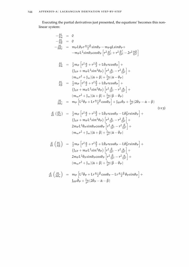
144 appendix-a : lagrangian derivation step-by-step
Executing the partial derivatives just presented, the equations’ becomes this non-linear system:
−∂L∂α = 0
−∂L∂β = 0
− ∂L∂θP
= mPLθPrα+β2 sinθP −mPgLsinθP+
−mPL2sinθPcosθP
[r2 α
2
D2+ r2 β
2
D2− 2r2 αβ
D2
]∂L∂α = 1
2mP
[r2 α2 + r2 β2 + LθPrcosθP
]+(
JδP +mPL2sin2θP
) [r2 αD2
− r2 βD2
]+
(mwr2 + Jw)[α+ β] + Jm
ρ2(α− θP)
∂L∂β
= 12mP
[r2 α2 + r2 β2 + LθPrcosθP
]+(
JδP +mPL2sin2θP
) [r2 βD2
− r2 αD2
]+
(mwr2 + Jw)[α+ β] + Jm
ρ2(β− θP)
∂L∂θP
= mP
[L2θP + Lr
α+β2 cosθP
]+ JθPθP +
Jmρ2
(2θP − α− β)
ddt
(∂L∂α
)= 1
2mP
[r2 α2 + r2 β2 + LθPrcosθP − Lθ
2PrsinθP
]+(
JδP +mPL2sin2θP
) [r2 αD2
− r2 βD2
]+
2mPL2θPsinθPcosθP
[r2 αD2
− r2 βD2
]+
(mwr2 + Jw)[α+ β] + Jm
ρ2(α− θP)
ddt
(∂L∂β
)= 1
2mP
[r2 α2 + r2 β2 + LθPrcosθP − Lθ
2PrsinθP
]+(
JδP +mPL2sin2θP
) [r2 βD2
− r2 αD2
]+
2mPL2θPsinθPcosθP
[r2 βD2
− r2 αD2
]+
(mwr2 + Jw)[α+ β] + Jm
ρ2(β− θP)
ddt
(∂L∂θP
)= mP
[L2θP + Lr
α+β2 cosθP − Lr
α+β2 θPsinθP
]+
JθPθP +Jmρ2
(2θP − α− β)
(113)
[ December 2, 2017 at 17:06 – classicthesis ]
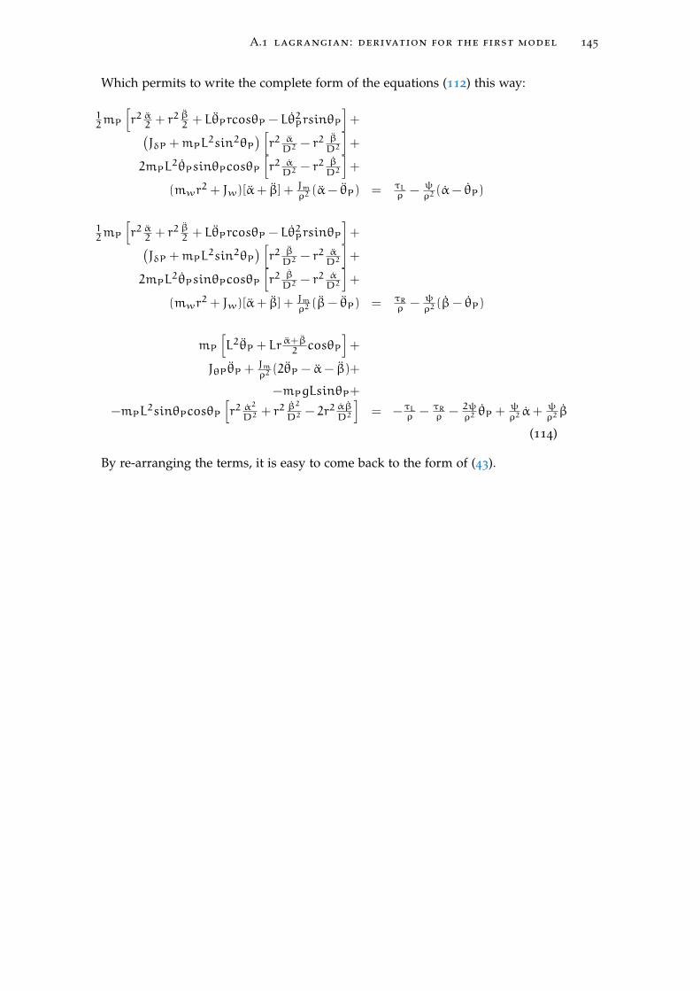
A.1 lagrangian : derivation for the first model 145
Which permits to write the complete form of the equations (112) this way:
12mP
[r2 α2 + r2 β2 + LθPrcosθP − Lθ
2PrsinθP
]+(
JδP +mPL2sin2θP
) [r2 αD2
− r2 βD2
]+
2mPL2θPsinθPcosθP
[r2 αD2
− r2 βD2
]+
(mwr2 + Jw)[α+ β] + Jm
ρ2(α− θP) = τL
ρ − ψρ2(α− θP)
12mP
[r2 α2 + r2 β2 + LθPrcosθP − Lθ
2PrsinθP
]+(
JδP +mPL2sin2θP
) [r2 βD2
− r2 αD2
]+
2mPL2θPsinθPcosθP
[r2 βD2
− r2 αD2
]+
(mwr2 + Jw)[α+ β] + Jm
ρ2(β− θP) = τR
ρ − ψρ2(β− θP)
mP
[L2θP + Lr
α+β2 cosθP
]+
JθPθP +Jmρ2
(2θP − α− β)+
−mPgLsinθP+
−mPL2sinθPcosθP
[r2 α
2
D2+ r2 β
2
D2− 2r2 αβ
D2
]= −τLρ − τR
ρ − 2ψρ2θP +
ψρ2α+ ψ
ρ2β
(114)
By re-arranging the terms, it is easy to come back to the form of (43).
[ December 2, 2017 at 17:06 – classicthesis ]

[ December 2, 2017 at 17:06 – classicthesis ]
B I B L I O G R A P H Y
[1] alienpowersystems. alien-5065-sensored-outrunner-brushless-motor, 2017.URL http://tinyurl.com/zdl27ww.
[2] Alps. Alps joystick, 2017. URL http://www.alps.com/prod/info/E/HTML/
MultiControl/Potentiometer/RKJXK/RKJXK1210002.html.
[3] W. An and Y. Li. Simulation and control of a two-wheeled self-balancingrobot. In 2013 IEEE International Conference on Robotics and Biomimetics (RO-BIO), pages 456–461, Dec 2013. doi: 10.1109/ROBIO.2013.6739501.
[4] R. Antonello, I. Nogarole, and R. Oboe. Motion reconstruction with a low-costmems imu for the automation of human operated specimen manipulation. In2011 IEEE International Symposium on Industrial Electronics, pages 2189–2194,June 2011. doi: 10.1109/ISIE.2011.5984500.
[5] Arduino. Hc-06 uart-bluetooth module, 2017. URL http://tinyurl.com/
yd3w3ayh.
[6] Zippy batteries. Zippy 6s 8000mah, 2017. URL http://tinyurl.com/
ybs4uddc.
[7] J. R. Cao, C. P. Huang, and J. C. Hung. Stabilizing controller design usingfuzzy t-s model on two wheeled self-balancing vehicle. In 2016 InternationalConference on Advanced Materials for Science and Engineering (ICAMSE), pages520–523, Nov 2016. doi: 10.1109/ICAMSE.2016.7840187.
[8] C. H. Chiu and Y. F. Peng. Electric unicycle control. In 2017 InternationalConference on Applied System Innovation (ICASI), pages 1546–1549, May 2017.doi: 10.1109/ICASI.2017.7988222.
[9] M. Ciezkowski and E. Pawluszewicz. Determination of interactions betweentwo-wheeled self-balancing vehicle and its rider. In 2015 20th InternationalConference on Methods and Models in Automation and Robotics (MMAR), pages851–855, Aug 2015. doi: 10.1109/MMAR.2015.7283988.
[10] funefunshop. 8 inch hub motor, 2017. URL https://www.fonefunshop.com/
8-Inch-Electric-Scooter-Balance-Board-Wheel-With-Motor.html.
[11] F. Gabriel, F. De Belie, and X. Neyt. Inductance-based position self-sensing ofa brushless dc-machine using high-frequency signal injection. In IECON 2012- 38th Annual Conference on IEEE Industrial Electronics Society, pages 3682–3687,Oct 2012. doi: 10.1109/IECON.2012.6389306.
[12] Y. Gong, X. Wu, and H. Ma. Research on control strategy of two-wheeledself-balancing robot. In 2015 International Conference on Computer Science andMechanical Automation (CSMA), pages 281–284, Oct 2015. doi: 10.1109/CSMA.2015.63.
[13] Y. Gong, X. Wu, and H. Ma. Research on control strategy of two-wheeledself-balancing robot. In 2015 International Conference on Computer Science and
147
[ December 2, 2017 at 17:06 – classicthesis ]
148 bibliography
Mechanical Automation (CSMA), pages 281–284, Oct 2015. doi: 10.1109/CSMA.2015.63.
[14] K. Iizuka, H. Uzuhashi, M. Kano, T. Endo, and K. Mohri. Microcomputer con-trol for sensorless brushless motor. IEEE Transactions on Industry Applications,IA-21(3):595–601, May 1985. ISSN 0093-9994. doi: 10.1109/TIA.1985.349715.
[15] L. Jiang, H. Qiu, Z. Wu, and J. He. Active disturbance rejection control basedon adaptive differential evolution for two-wheeled self-balancing robot. In2016 Chinese Control and Decision Conference (CCDC), pages 6761–6766, May2016. doi: 10.1109/CCDC.2016.7532214.
[16] W. Junfeng and Z. Wanying. Research on control method of two-wheeledself-balancing robot. In 2011 Fourth International Conference on Intelligent Com-putation Technology and Automation, volume 1, pages 476–479, March 2011. doi:10.1109/ICICTA.2011.132.
[17] B. P. Kumar and Krishnan C. M. C. Comparative study of different controlalgorithms on brushless dc motors. In 2016 Biennial International Conference onPower and Energy Systems: Towards Sustainable Energy (PESTSE), pages 1–5, Jan2016. doi: 10.1109/PESTSE.2016.7516444.
[18] Yong Liu, Z. Q. Zhu, and D. Howe. Direct torque control of brushless dcdrives with reduced torque ripple. IEEE Transactions on Industry Applications,41(2):599–608, March 2005. ISSN 0093-9994. doi: 10.1109/TIA.2005.844853.
[19] Loram I. D. Kelly S. M. and M. Lakie. Human balancing of an inverted pen-dulum: is sway size controlled by ankle impedance. Journal of Physiology, 532
(3):879–891, 2001.
[20] Winter D. A. Patla A. E. Prince F. Ishac M. and Gielo-Perczak K. Stiffnesscontrol of balance in quiet standing. Journal of Neurophysiology, 80(3):1211–1221, 1998.
[21] K. Madhira, A. Gandhi, and A. Gujral. Self balancing robot using comple-mentary filter: Implementation and analysis of complementary filter on sbr.In 2016 International Conference on Electrical, Electronics, and Optimization Tech-niques (ICEEOT), pages 2950–2954, March 2016. doi: 10.1109/ICEEOT.2016.7755240.
[22] H. Mansoor, I. U. H. shaikh, and S. Habib. Genetic algorithm based lqr controlof hovercraft. In 2016 International Conference on Intelligent Systems Engineering(ICISE), pages 335–339, Jan 2016. doi: 10.1109/INTELSE.2016.7475145.
[23] S. Noguchi and S. Jeong. Evaluation of rapid rider weight shifting behaviorfor a stand-riding-type self-balancing personal mobility vehicle: Pilot study.In 2013 13th International Conference on Control, Automation and Systems (ICCAS2013), pages 1474–1479, Oct 2013. doi: 10.1109/ICCAS.2013.6704119.
[24] N. O-larnnithipong and A. Barreto. Gyroscope drift correction algorithm forinertial measurement unit used in hand motion tracking. In 2016 IEEE SEN-SORS, pages 1–3, Oct 2016. doi: 10.1109/ICSENS.2016.7808525.
[25] J. Juan Rincon Pasaye, J. Alberto Bonales Valencia, and F. Jimenez Perez. Tiltmeasurement based on an accelerometer, a gyro and a kalman filter to control
[ December 2, 2017 at 17:06 – classicthesis ]
bibliography 149
a self-balancing vehicle. In 2013 IEEE International Autumn Meeting on PowerElectronics and Computing (ROPEC), pages 1–5, Nov 2013. doi: 10.1109/ROPEC.2013.6702711.
[26] U. Qureshi and F. Golnaraghi. An algorithm for the in-field calibration ofa mems imu. IEEE Sensors Journal, PP(99):1–1, 2017. ISSN 1530-437X. doi:10.1109/JSEN.2017.2751572.
[27] M. I. Rashed, S. Lim, and H. Bang. Numerical modeling, testing and bias driftanalysis of mems based three-axis gyroscope for accurate angular rate estima-tion for attitude determination of nano-satellites. In 2013 13th InternationalConference on Control, Automation and Systems (ICCAS 2013), pages 376–381,Oct 2013. doi: 10.1109/ICCAS.2013.6703928.
[28] seedstudio. Grove - imu 9dof, 2017. URL http://wiki.seeedstudio.com/
wiki/Grove_-_IMU_9DOF.
[29] Fairchild Semiconductor. Bldc-ripple-torque-reduction-via-modified-sinusoidal-pwm, 2008. URLhttps://www.fairchildsemi.com/technical-articles/
BLDC-Ripple-Torque-Reduction-via-Modified-Sinusoidal-PWM.pdf.
[30] M. K. L. Siu and K. T. Woo. A high-frequency signal injection based sensorlessdrive method for brushless dc motor. In 2017 18th International Conference onAdvanced Robotics (ICAR), pages 367–372, July 2017. doi: 10.1109/ICAR.2017.8023634.
[31] F. Sun, Z. Yu, and H. Yang. A design for two-wheeled self-balancing robotbased on kalman filter and lqr. In 2014 International Conference on Mechatron-ics and Control (ICMC), pages 612–616, July 2014. doi: 10.1109/ICMC.2014.7231628.
[32] D. Tedaldi, A. Pretto, and E. Menegatti. A robust and easy to implementmethod for imu calibration without external equipments. In 2014 IEEE Inter-national Conference on Robotics and Automation (ICRA), pages 3042–3049, May2014. doi: 10.1109/ICRA.2014.6907297.
[33] Wikipedia the hoverboard. Self balancing scooter (hoverboard). URL https:
//en.wikipedia.org/wiki/Self-balancing_scooter.
[34] C. C. Tsai, H. C. Huang, and S. C. Lin. Adaptive neural network control of aself-balancing two-wheeled scooter. IEEE Transactions on Industrial Electronics,57(4):1420–1428, April 2010. ISSN 0278-0046. doi: 10.1109/TIE.2009.2039452.
[35] Benjamin Vedder. A custom vesc, 2015. URL http://vedder.se/2015/01/
vesc-open-source-esc/.
[36] Wikipedia. Kalman filter. URL https://en.wikipedia.org/wiki/Kalman_
filter#Example_application.2C_technical.
[37] Wikipedia-segwayPT. Segway personal transporter. URL https://en.
wikipedia.org/wiki/Segway_PT.
[38] Zanichelli. attrito sul piano inclinato, 2017. URL http://tinyurl.com/
y8fjk2on.
[ December 2, 2017 at 17:06 – classicthesis ]

150 bibliography
[39] Z. Zheng and M. Teng. Modeling and decoupling control for two-wheeledself-balancing robot. In 2016 Chinese Control and Decision Conference (CCDC),pages 5263–5267, May 2016. doi: 10.1109/CCDC.2016.7531939.
[ December 2, 2017 at 17:06 – classicthesis ]