UNIVERSITA DEGLI STUDI DI BARI

Aldo Moro

FACOLTA DI SCIENZE MATEMATICHE FISICHE E NATURALIDipartimento Interateneo di Fisica M. Merlin

Tesi di Laurea

SEARCH FOR THE STANDARD MODEL HIGGS BOSON

IN THE DECAY CHANNEL H→ ZZ→ 4l

WITH THE CMS EXPERIMENT AT√

s = 7 TeV

Relatori:Ch.mo Prof. Mauro de PalmaDott. Nicola De Filippis

Laureanda:Giorgia Miniello

Anno Accademico 2011-2012

To my Zoe

“If I have seen a little further

it is by standing

on the shoulders of Giants”

Sir Isaac Newton

Index

Introduction 1

1 The Standard Model Higgs Boson 3

1.1 Electroweak Interactions . . . . . . . . . . . . . . . . . . . . . 3

1.2 Gauge Symmetries . . . . . . . . . . . . . . . . . . . . . . . . 6

1.3 Electroweak Spontaneous Symmetry Breaking: The Higgs Mech-

anism . . . . . . . . . . . . . . . . . . . . . . . . . . . . . . . 9

1.4 Renormalizability of the Standard Model . . . . . . . . . . . . 16

1.4.1 The Higgs Field Choice . . . . . . . . . . . . . . . . . . 16

1.4.2 Standard Model free parameters: Gauge Boson Masses,

Fermions Masses . . . . . . . . . . . . . . . . . . . . . 18

1.4.3 Renormalization . . . . . . . . . . . . . . . . . . . . . . 20

1.4.4 The Final S.M. Lagrangian . . . . . . . . . . . . . . . . 22

2 The Large Hadron Collider and the CMS Detector 25

2.1 The Large Hadron Collider at CERN . . . . . . . . . . . . . . 25

2.1.1 Performance Goals . . . . . . . . . . . . . . . . . . . . 27

2.1.2 LHC Collision Detectors . . . . . . . . . . . . . . . . . 29

2.2 The Compact Muon Solenoid (CMS) Detector . . . . . . . . . 32

2.2.1 Coordinate System . . . . . . . . . . . . . . . . . . . . 32

2.2.2 The CMS detector structure and the Magnet . . . . . . 33

2.2.3 Inner Tracking System . . . . . . . . . . . . . . . . . . 34

2.2.4 Electromagnetic Calorimeter . . . . . . . . . . . . . . . 37

2.2.5 Hadron Calorimeter . . . . . . . . . . . . . . . . . . . . 41

2.2.6 The Muon System . . . . . . . . . . . . . . . . . . . . 42

2.2.7 Trigger . . . . . . . . . . . . . . . . . . . . . . . . . . . 44

i

2.3 Lepton Reconstruction . . . . . . . . . . . . . . . . . . . . . . 48

2.3.1 Electron Reconstruction . . . . . . . . . . . . . . . . . 48

2.3.2 Muon Reconstruction . . . . . . . . . . . . . . . . . . . 53

3 The Higgs Boson Production and Simulation at LHC 57

3.1 Higgs Production Mechanism . . . . . . . . . . . . . . . . . . 58

3.1.1 The higher-order corrections and the K-factor . . . . . 58

3.2 Decays of the SM Higgs boson . . . . . . . . . . . . . . . . . . 61

3.2.1 Decays into electroweak gauge bosons: two body decay 64

3.3 Monte Carlo samples . . . . . . . . . . . . . . . . . . . . . . . 65

3.4 Monte Carlo generator studies . . . . . . . . . . . . . . . . . . 71

4 Data Analysis 75

4.1 Experimental Data samples . . . . . . . . . . . . . . . . . . . 76

4.2 Physics Objects: Electrons and Muons . . . . . . . . . . . . . 78

4.2.1 Lepton Identification . . . . . . . . . . . . . . . . . . . 78

4.2.2 Electrons and Muons Isolation . . . . . . . . . . . . . . 82

4.2.3 Pile-up Corrections . . . . . . . . . . . . . . . . . . . . 84

4.2.4 Primary and Secondary leptons: the significance of the

impact parameter . . . . . . . . . . . . . . . . . . . . . 86

4.3 Selection cuts . . . . . . . . . . . . . . . . . . . . . . . . . . . 86

4.3.1 Selection Efficiency . . . . . . . . . . . . . . . . . . . . 89

4.4 Data to MC comparison . . . . . . . . . . . . . . . . . . . . . 93

4.5 Studies about the best four-lepton algorithm . . . . . . . . . . 106

4.5.1 The Method . . . . . . . . . . . . . . . . . . . . . . . . 112

4.6 Background Evaluation and Control . . . . . . . . . . . . . . . 120

4.7 Systematic uncertainties . . . . . . . . . . . . . . . . . . . . . 121

4.7.1 Theoretical uncertainties . . . . . . . . . . . . . . . . . 121

5 Results 127

5.1 Mass Distributions and Kinematics . . . . . . . . . . . . . . . 127

5.2 Statistical interpretation: The CLs Method . . . . . . . . . . . 129

5.2.1 The Likelihood function and the test statistics . . . . . 133

5.2.2 Determination of the exclusion limits . . . . . . . . . . 136

5.3 Latest Results of the Standard Model Higgs Search in the

H→ ZZ→ 4` channel at√s = 8 TeV with 2012 data. . . . . 139

Conclusions 147

Bibliography 151

Introduction

The aim of particle physics is to study the fundamental constituents and

interactions of matter. In the twentieth century, from this theoretical branch

of physics a new experimental one came up, the high energy physics, which

studies the interactions between elementary particles at very high energy.

These high energy interactions allow the production of new particles, not

existing in nature in ordinary conditions, by means of particle accelerators

(colliders).

The Standard Model (SM) of the electroweak and strong interaction is the

quantum field theory which has the greatest number of experimental veri-

fications, with some exception like the proton lifetime and the existence of

the Higgs boson. In particular, the Higgs boson mass, like those of quarks,

leptons and gauge bosons, is a free parameter of the theory.

The SM predicts the existence of a unique physical Higgs scalar boson as-

sociated to the spontaneous electroweak symmetry breaking, the so called

Higgs mechanism. The motivation for introducing the Higgs scalar boson

is completely theoretical and takes as foundation the fact that it allows to

generate the weak boson masses without spoiling the renormalizability of the

electroweak gauge theory. So far, no evidence of the existence of SM Higgs

has been found, although both theoretical and experimental constraints have

been put on Higgs mass.

Direct searches for SM Higgs boson have been already performed at the e+e−

collider LEP and at the pp collider Tevatron. A lower bound of mH ≥ 114.4

GeV/c2 at 95% CL (Confidence Level) has been found for the Higgs mass

at LEP, while the experiments D0 and CDF at Tevatron excluded the mass

range 158 ≤ mH ≤ 173 GeV/c2 (95% CL).

The search of Higgs boson is one of the main goals of CMS and ATLAS

1

experiments at the Large Hadron Collider (LHC) located at CERN since it

started to provide pp collision on November 2009. These two experiments

have been designed to cover a large spectrum of signatures in LHC eviron-

ment and the Higgs search has been the major guide criterion followed to

define the detectors requirements and performances.

The aim of this thesis work is to develop a physics analysis to search for

the SM Higgs boson in the decay channel H → ZZ(∗) for which each vector

boson Z decays into a di-electron or di-muon object, by using data collected

by the experiment in 2010 and 2011 at center of mass energy of 7 TeV.

In the first chapter a wide view on the theoretical basis of the SM and the

spontaneous symmetry breaking mechanism generating the Higgs boson is

presented. The second chapter shows a description of the LHC and the

whole CMS detector along with an overview of the subdetectors. The third

chapter is focused on the SM Higgs boson production and decay channels in

hadron colliders. It also contains a detailed description of all the samples

of real and simulated data used for this analysis. In the fourth chapter the

analysis selection is detailed along with the description of the physics objects

and the main physics observables used. For a better understanding of the

goodness of event selection criteria, a study of the vector boson recostruction

efficiency is also presented. The results are then shown in the last chapter.

Not any clusterization has been found by the analysis of the 2010 and 2011

data. First collisions at√s = 8 TeV started the 5th of April 2012. During

the last period, extremely important results have been derived at that en-

ergy, showing an excess of about 3σ in the H → ZZ → 4` analysis and a 5σ

excess overall when combining all the Higgs analyses for the different chan-

nels. Some details about those amazing results are given in the last section

of my thesis.

2

Chapter 1

The Standard Model Higgs

Boson

In the early 1970’s, a new quantum field theory was enounced by Wein-

berg and Salam and later completed by ’t Hooft: the Standard Model for

electroweak interactions. This soon turned out to be a very powerful tool,

being the only model able of explaining a wide variety of physics phenomena.

Through many decades and a lot of experiments, the Standard Model has be-

come the one which has the greatest number of experimental confirmations.

It was developed starting from the need of finding a single unified symmetry

group describing both electromagnetic and weak interactions. It’s no useless

to remind that one of the most fascinating ideas in particle physics is that

the interactions are dictated by simmetry principles, the so-called local gauge

symmetries. This insight is deeply connected with the fact that conserved

physical quantities are conserved in local (not global) regions of space.

All the treatise presented in the following sections was sourced from [26] and

[42].

1.1 Electroweak Interactions

The problem of finding a common symmetry group structure rose already

within the weak currents themselves. It’s worth reminding that the forms

for the weak charged currents are

3

Jµ ≡ J+µ = uνγµ

1

2(1− γ5)ue ≡ νγµ

1

2(1− γ5)e = νLγµeL (1.1)

and

J†µ ≡ J−µ = ueγµ1

2(1− γ5)uν = eLγµνL, (1.2)

where ue and (as well as e in a more compact form) and uν (as well as ν) are

the four component spinors relative to electron e and neutrino ν respectvely,

γµ’s are the 4× 4 Dirac matrices and γ5 is a matrix obtained by the product

of the four previous γ-matrices

γ5 = iγ0γ1γ2γ3. (1.3)

The apices + and - indicate the charge raising and charge lowering char-

acter of the currents respectively, while the subscript L stands for “left” and

is used to denote the left-handed spinors, attesting the V-A nature of the

charged currents. The form of the Dirac γ-matrices depends on the repre-

sentation chosen to state them. In the Dirac-Pauli representation they have

the following form:

γ0 =

(I 0

0 −I

), γ =

(0 σ

−σ 0

), γ5 =

(0 I

I 0

). (1.4)

Introducing a two-dimensional form for the previous spinors

χL =

(ν

e−

)L

, (1.5)

along with the step-up and step-down operators τ± = 12(τ1 ± iτ2), where

τ+ =

(0 1

0 0

), τ− =

(0 0

1 0

)(1.6)

and the τ1,2 are the spin Pauli matrices, the two charged currents can be

rewritten as

J+µ (x) = χLγµτ+χL , (1.7)

4

J−µ (x) = χLγµτ−χL. (1.8)

Supposing a SU(2) group structure for the weak current, a neutral one

of the same form can be introduced

J3µ(x) = χLγµ

1

2τ3χL =

1

2νLγµνL −

1

2eLγµeL . (1.9)

Nevertheless, it can be noticed that the last one cannot be identified with

the weak neutral current, whose costumary definition is

JNCµ (q) =

(uqγµ

1

2(cqV − c

qAγ

5)uq

), (1.10)

because in general the neutral current JNCµ , unlike the charged ones that are

pure V-A currents in which cV 6= cA, has a right-handed component. Just

for trying to solve this puzzle and attempting to save the SU(2)L simmetry

supposed for the neutral currents, it can be reminded that the electromag-

netic current has both right- and left-handed components. For example, the

electromagnetic current for an electron can be written as

jemµ (x) = −eγµe = −eRγµeR − eLγµeL. (1.11)

Including the coupling costant e omitted until now, the last equation

becomes

jµ ≡ ejemµ = eψγµQψ, (1.12)

where Q is the charge operator and it can be considered the generator of

the group U(1)em simmetry group of electromagnetic interactions. It can be

noticed that, even if the the two neutral currents JNCµ and jemµ do not respect

the SU(2)L simmetry, these two combinations do have definite transforma-

tion properties under this group and allow us to complete the weak isospin

triplet J iµ, keeping the jYµ (where Y stands for hypercharge) unchanged un-

der SU(2)L transformations. As the operator charge Q generates the sym-

metry group U(1)em, the hypercharge operator Y generates the symmetry

group U(1)Y and so, including the electromagnetic interactions, the symme-

5

try group we are dealing with has become SU(2)L ×U(1)Y . That is why we

can say that, using this approach, we unified the electromagnetic and the

weak interactions.

This theory was proposed for the first time by Glashow in 1961 and later

modified by Weinberg and Salam just to include the vector bosons W± and

Z0. The assumption made at this point is that, as in QED the interactions

are based on photon exchange, the electroweak interactions are based on

the exchange of massive vector bosons and just as electromagnetic current is

coupled to the photon, the electroweak currents are coupled to vector bosons

W± and Z0. The electroweak interaction can be written as

− ig(J i)µW iµ − i

g′

2(jY )µBµ, (1.13)

where W iµ is an isotriplet of vector fields, whose components W 1

µ and W 2µ are

connected by the relation

W±µ =

√1

2

(W 1µ ∓ iW 2

µ

), (1.14)

which describes massive charged bosons W+and W−, Bµ, along with W 3µ ,

is a neutral field, g is the coupling constant by which these vector fields are

coupled to the weak isospin current J iµ and Bµ is a vector field coupled to

the weak hypercharge current jYµ

with the coupling constant g′/2.

1.2 Gauge Symmetries

As we pointed out at the beginning of this chapter, the interactions between

particles are ruled by gauge symmetries. We have already mentioned that

we are interested in local gauge symmetries rather than global ones. As

an example, it can be shown how the imposition of the gauge invariance

of the lagrangian connected to a particular kind of interaction, e.g. the

electromagnetic one, could bring to conditions on the gauge particles. In

this case, an electron can be described by a complex field ψ(x), and the

6

associated lagrangian

L = iψγµ∂µψ −mψψ (1.15)

is found to be invariant under global phase trasformation

ψ(x)→ eiαψ(x). (1.16)

It can be easily found that this is not the most general kind of invariance. To

make it more general, the phase factor α should assume different values in

different space-time points and the previous trasformation should be written

as

ψ(x)→ eiα(x)ψ(x). (1.17)

In this case, it could be easily demonstrated that the previous lagrangian

is no more invariant under (local) phase trasformation. To compensate for

this liability trying to preserve the goal of keeping the gauge invariance of

the lagrangian, this last can be modified using the “covariant derivative”

Dµ ≡ ∂µ − ieAµ instead of the simple derivative form ∂µ, where Aµ is a

vector field added just for the purpose. Therefore, demanding the local

phase invariance for the lagrangian, this last vector field, called gauge field, is

necessarily included. It can be identified with the physical photon field and

the new expression for the Quantum Electro-Dynamics (QED) lagrangian

becomes

L = ψ(iγµ∂µ −m)ψ + eψγµAµψ −1

2FµνF

µν , (1.18)

where last term is the kinetic energy corresponding to the vector field and it

is constructed from gauge invariant field strenght tensor

Fµν = ∂µAν − ∂νAµ (1.19)

for preserving its Uem(1) local gauge invariance. It can be noticed that no

mass term connected to Aµ can be found in the last expression, because it

would be prohibited by the gauge invariance. This bring us to the conclusion

that the photon, as a gauge particle, is massless within this theory.

Following the same criteria, the structure of Quantum Chromo-Dynamics

7

(QCD) can be deduced using local gauge invariance again, extending the

previous procedure and using the SU(3) group of the phase transformations

on quark colored fields instead of the U(1) one. From a physical point of view,

the starting point is a bit different from the previous QED case because this

time SU(3) is not an abelian group, since not all its generators Ta commute

each other. The Ta’s are a set of eight (a = 1, .., 8) linearly indipendent

traceless 3× 3 matrices, which satisfy the commutation relation

[Ta, Tb] = ifabcTc, (1.20)

where fabc are real constants and they are called the structure constants of

the group. If an invariance under local α phase tranformation of the free

lagrangian

Lq = qj (iγµ∂µ −m) qj, (1.21)

(where qj=1,2,3 are three color fields) is required, it can be written in the

following form

q(x)→ Uq(x) ≡ eiαa(x)Taq(x), (1.22)

where U is an arbitrary unit matrix. Imposing the SU(3) gauge invariance

on the Lagrangian and following steps very similar to the previous case, we

come to a new form for the lagrangian for interacting colored quarks q and

vector gluons Gµ

L = q (iγµ∂µ −m) q − g(qγµTaq)Gaµ −

1

4GaµνG

µνa , (1.23)

where Gµa represents the eight gauge fields introduced to preserve the invari-

ance of L, trasforming as

Gaµ → Ga

µ −1

g∂µαa, (1.24)

the last term is the kinetic energy term for each of the Gµa fields, and g is the

coupling costant associated to this interaction. Not even in the QCD case

we can find in the lagrangian a mass term and then we can deduce that, by

imposing the local gauge invariance, the gluons (as the photons previously)

8

are forced to be massless.

It can be worth underlying that the QCD kinetic energy term is not only

purely kinetic as in QED. It includes an induced self-interaction between

gauge bosons, accordingly to the non-Abelian nature of the group and, con-

sequently, of the theory. Therefore in the QCD theory, unlike QED, the

gauge particles (the gluons) interact each other exchanging color charge.

If we want to apply the same procedure for the electroweak interactions, we

have just to keep in mind that the gauge bosons which mediate those interac-

tions are massive and then the procedure to get a lagrangian which includes

a mass term will be different. It can be seen through calculations that pre-

serving the lagrangian gauge invariance is not just an option, because, if

we do not take it into account, unrenormalizable divergences will appear in

the propagators and the theory would become physically meaningless. The

mechanism by which the massive bosons could be included without breaking

the gauge invariance is called Spontaneous Symmetry Breaking.

1.3 Electroweak Spontaneous Symmetry Break-

ing: The Higgs Mechanism

Let us consider the simplest form for a lagrangian

L = T − V =1

2(∂muφ)2 −

(1

2µ2φ2 +

1

4λφ4

)(1.25)

in which φ describes a scalar field. Skipping the trivial case for µ2 > 0 which

describes a scalar field with mass µ, we can focus on µ2 < 0 case. In the

previous lagrangian the relative sign of the φ2 term and the kinetic one is

positive, determining a mass term 12µ2φ2 with the “wrong” sign. This time,

the potential V has two minimum values

φ = ±v with v =√−µ2/λ. (1.26)

9

Applying perturbative expansions around these two classical minima, the

field φ could be written in the form

φ(x) = v + η(x), (1.27)

where η(x) is the quantum fluctuation around the minimum +v. Considering

that translating the field φ to φ = +v does not involve any loss of generality,

we can substitute the last relation in the lagrangian obtaining

L′ = 1

2(∂µη)2 − λv2η2 − λvη3 − 1

4λη4 + const. (1.28)

The mass term λv2η2 associated to the field η has the correct sign. This

mass mη can be calculated comparing the last lagrangian with the one for a

scalar field

L =1

2(∂µφ)(∂µφ)− 1

2m2φ2 (1.29)

obtaining

mη =√

2λv2 (1.30)

Even if the two lagrangians L and L′ are completely equivalent (because the

choice φ(x) = v + η(x) does not change the physics), we have to choose the

second one. The use of L would imply that the perturbation series does not

converge because φ = 0 (the value around which the expansion would be

performed) is an unstable point. The correct way to proceed is expanding

L′ around a stable point (called vacuum point). This last lagrangian is the

one which offers the correct picture of the physics and the scalar particle

associated to η field is massive. We use to say that choosing one of the

possible vacuum point breaks the symmetry and so we refer to this mechanism

as Spontaneous Symmetry Breaking. Iterating an analogous procedure for a

complex scalar field φ = (φ1 + φ2)/√

2 and the relative lagrangian

L =1

2(∂µφ)∗(∂µφ)− µ2φ∗φ− λ(φ∗φ)2 =

=1

2(∂µφ1)2 +

1

2(∂µφ2)2 − 1

2µ2(φ1

2 + φ22)− 1

4λ(φ1

2 + φ22)2,(1.31)

10

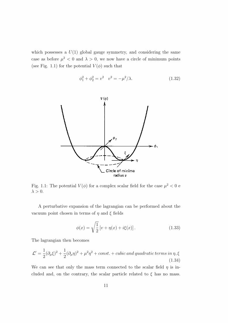
which possesses a U(1) global gauge symmetry, and considering the same

case as before µ2 < 0 and λ > 0, we now have a circle of minimum points

(see Fig. 1.1) for the potential V (φ) such that

φ21 + φ2

2 = v2 v2 = −µ2/λ. (1.32)

Fig. 1.1: The potential V (φ) for a complex scalar field for the case µ2 < 0 eλ > 0.

A perturbative expansion of the lagrangian can be performed about the

vacuum point chosen in terms of η and ξ fields

φ(x) =

√1

2[v + η(x) + iξ(x)] . (1.33)

The lagrangian then becomes

L′ = 1

2(∂µξ)

2 +1

2(∂µη)2 + µ2η2 + const.+ cubic and quadratic terms in η, ξ

(1.34)

We can see that only the mass term connected to the scalar field η is in-

cluded and, on the contrary, the scalar particle related to ξ has no mass.

11

This massless scalar particle is called Goldstone boson. So, we can say that

spontaneously symmetry broken gauge theories are someway biased by the

presence of a massless scalar particle which is producted along with the mas-

sive particle we were looking for in attempting to find the way to generate

the mass for the gauge vector bosons. Obviously, the problem is that this

massless particle is unwanted because not observed.

Now we move to study the spontaneous symmetry breaking of a local gauge

transformation in U(1) group. Following the same procedure performed be-

fore, we have to impose the gauge invariance under the phase transformation

φ→ eiα(x)φ. (1.35)

The gauge invariant lagrangian can then be written as

L = (∂µ + ieAµ)φ∗(∂µ + ieAµ)φ− µ2φ∗φ− λ(φ∗φ)2 − 1

4FµνF

µν . (1.36)

Also in this case, we have to consider µ2 < 0, since we want to generate the

gauge boson masses through spontaneous symmetry breaking. Making the

same vacuum choice as before, we can translate the field φ without changing

the physics. The lagrangian then becomes

L′ =1

2(∂µξ)

2 +1

2(∂µη)2 − v2λη2 +

1

2e2v2AµA

µ

− evAµ∂µξ − 1

4FµνF

µν + interaction terms. (1.37)

It can be noticed that there is a mass term associated to the scalar field η

mη =√

2λv2, another one associated to the vector field Aµ, mA = ev, and

we can still observe the presence of the massless Goldstone boson associated

to ξ.

In attempting to eliminate this disturbing element, we can focus on the off-

diagonal term Aµ∂µξ present in L′ and try to understand if the particle

spectrum assigned it is correct.

Owing to the mass assigned to the vector boson associated to the Aµ field, the

polarization degrees of freedom are now three instead of two and this could

12

not just be due to a simple translation of the field. So it can be deduced

that the fields in the last lagrangian are not associated to distinct physical

particles.

What we will see is that this extra degree of freedom, due to the longitudinal

polarization, simply corresponds to the freedom to make a choice about the

gauge transformation. Indeed, to sidestep the problem we can notice that

we can write the vacuum chosen in a different form using the expansion at

the lowest order in ξ

φ(x) =

√1

2[v + η(x) + iξ(x)] '

√1

2(v + η)eiξ/v. (1.38)

From this last equality it can be deduced that a different set of real fields

h, θ, Aµ can replace the previous three ξ, η, Aµ in the previous lagrangian,

where

φ→√

1

2(v + h(x))eiθ(x)/v, (1.39)

and

Aµ → Aµ +1

ev∂µθ. (1.40)

The field h(x) is real, owing to the particular choice of θ field. Substituting

these transformations in the lagrangian, the new one obtained will be

L” =1

2(∂µh)2 − λv2h2 +

1

2e2v2A2

µ − λvh3 − 1

4λh4

+1

2e2A2

µh2 + ve2A2

µh2 + ve2Aµh−

1

4F µνµν (1.41)

In this last version of the lagrangian the Goldstone boson does not exist

anymore and only a massive vector boson Aµ and a massive scalar boson h

can be observed. The mechanism by which the Goldstone boson is turned

in the longitudinal polarization of the massive gauge particle is the so called

Higgs Mechanism.

Since in the previous section we found that the electroweak symmetry

group is the SUL(2)×UY (1) group, the last step will be extending the study

of the spontaneous simmetry breaking to the SU(2) gauge symmetry. Also

13

in this case, we will see another example of Higgs mechanism.

Considering φ as a SU(2) doublet of complex scalar fields

φ =

√1

2

(φ1 + iφ2

φ3 + iφ4

), (1.42)

the lagrangian can be written as

L = (∂µφ)†(∂µφ)− µ2φ†φ− λ(φ†φ)2 (1.43)

As done previously, we are interested in a lagrangian invariant under local

gauge transformation. This goal can be achieved using the covariant deriva-

tive

Dµ = ∂µ+ igτa2W aµ , (1.44)

where W aµ (x) are three gauge fields (a=1,2,3), the τ ’s are the SU(2) group

generators introduced in the first section, and αa(x)’s are three parameters

related to the phase transormation. Under an infinitesimal gauge transfor-

mation, the W aµ (x) fields transform as

Wµ →Wµ −1

g∂µα−α×Wµ. (1.45)

Considering that, under this sort of transformation, the field φ transforms as

φ(x)→ (1 + iα(x) · τ/2)φ(x), (1.46)

the lagrangian 1.43 becomes

L =

(∂µφ+ ig

1

2τ ·Wµφ

)†(∂µφ+ ig

1

2τ ·W µφ

)− V (φ)− 1

4Wµν ·W µν ,

(1.47)

where

V (φ) = µ2φ†φ+ λ(φ†φ)2 (1.48)

14

and the last term is the kinetic energy of the gauge fields with

W µν = ∂µWν∂νWµ − gWµ ×Wν . (1.49)

If µ2 < 0 and λ > 0, it can be seen that the potential V (φ) has its minimum

at a value of |φ| such that

φ†φ ≡ 1

2(φ2

1 + φ22 + φ2

3 + φ24) = −µ

2

2λ. (1.50)

By choosing a particular minimum value of the potential about which the

field φ(x) can be expanded

φ1 = φ2 = φ4 = 0, φ32 = −µ

2

λ≡ v2, (1.51)

the spontaneous symmetry breaking is now applied to SU(2) group. We can

now follow a procedure analogous to the previous case. The fluctuations

about another particular value of the vacuum

φ0 =

√1

2

(0

v

), (1.52)

whose expansion φ(x) about this value is

φx =

√1

2

(0

v + h(x)

), (1.53)

can be parametrized using four real fields θ1, θ2, θ3, and h, so that the field

φ can be written as follows

φ(x) = eiτ ·θ(x)/v

(0

v+h(x)√2

), (1.54)

Studying this case for small pertubations it can be observed that the four

fields are totally independent and that, choosing this particular value for

vacuum, makes the lagrangian locally SU(2) invariant.

15

Operating a gauge choice, we can impose θ1(x), θ2(x), θ3(x) = 0 (related

to the massless Goldstone boson) and so the only scalar field remained is

the Higgs field h(x). Inserting the value of the vacuum φ0 in the lagrangian

the three gauge boson masses can be determined. It can be said that the

Higgs mechanism, in this case, allows the gauge fields “to eat” the Goldstone

bosons becoming massive.

The Higgs Mechanism allow us to bypass the presence of massless particles

in the lagrangian, enabling us to obtain a massive gauge boson and the Higgs

boson. Nevertheless, it must be noticed that one more problem still remains:

obtaining a theory in which the weak bosons are no more massless particles

preserving the renormalizability of the theory.

1.4 Renormalizability of the Standard Model

In the previous section we pointed out that the S.M. of the electroweak

interactions has been built starting from a gauge theory. It includes four

gauge fields, whose associated particles are the massless photon and the three

massive bosons W± and Z0. The aim of this section is just to highlight that

such a theory is renormalizable and so it does not contain any unmanageable

divergence in it.

1.4.1 The Higgs Field Choice

It has been shown that in order to generate particle masses in a gauge in-

variant way we have to use the Higgs mechanism which enables us also to

remove massless scalar particle physically not existing. This mechanism can

be reformulated so that the bosons W± and Z0 are massive, making sure that

the photon remains massless. For this purpose, it can be observed that the

complete expression of the SM lagrangian is composed of several contributes.

One of them is SU(2)×U(1) gauge invariant lagrangian that can be written

as follows

L2 =

∣∣∣∣(i∂µ − gT ·Wµ − g′Y

2bµ

)φ

∣∣∣∣2 − V (φ), (1.55)

16

where the field φ has four scalar components φi.

Repeating the usual steps, for keeping 1.55 invariant under gauge transfor-

mation, we can say, making the simplest choice, that the fields φi must belong

to an isospin doublet with Y = 1:

φ =

(φ+

φ0

)with φ+ ≡ (φ1 + iφ2)/

√2, φ+ ≡ (φ1 + iφ2)/

√2. (1.56)

This is the model originally established by Weinberg in 1967. In order to

trigger the Higgs mechanism, we can use the expression 1.48 for the potential,

always considering only the case µ2 < 0 and λ > 0. The vacuum value

choosen is

φ0 ≡√

1

2

(0

v

). (1.57)

This choice can be justified by the fact that, if φ0 is left invariant under a

subgroup of gauge transformation, the gauge bosons associated to this group

will be kept massless while generating a mass for the corresponding gauge

boson. In this case φ0, being neutral, is invariant under Uem(1) trasformation,

because, for its generator Q, we can write the equation

Qφ0 = 0, (1.58)

where Q can be evaluated by the Gell-Mann-Nishijima relation

Q = T 3 +Y

2(1.59)

and T = 1/2, T 3 = −1/2.

So the corresponding symmetry remains unbroken, ensuring the photon to

be massless. The other three generators T and Y do not satisfy a rela-

tion like 1.58 and the symmetry breaking allows the mass generation for the

corresponding bosons.

17

1.4.2 Standard Model free parameters: Gauge Boson

Masses, Fermions Masses

The gauge bosons and fermions masses could be obtained just substituting

the φ0 chosen in the corresponding term of the SM full lagrangian and com-

paring the mass term with the one expected for a charged boson and for a

fermion respectively. For the gauge boson masses we have

MW =1

2vg. (1.60)

By considering the off-diagonal term of the lagrangian, we can also write the

expression of the physical fields Zµ and Aµ

Aµ =g′W 3

µ + gBµ√g2 + g′2

withMA = 0 (the photon is massless) (1.61)

Zµ =gW 3

µ − g′Bµ√g2 + g′2

withMZ =1

2v√g2 + g′2 (the Z boson is massive). (1.62)

Using the relation correlating g and g′

g′

g= tanθW , (1.63)

where θW is the Weinberg or weak mixing angle, and substituting it into 1.61

and 1.62, we haveMW

MZ

= cosθW , (1.64)

where the difference between the MW and MZ values is due to the the mixing

between W 3µ and Bµ in the off-diagonal term of the lagrangian.

It can be stressed that the only prediction of the SM is about the ratio

between the vector bosons MW and MZ expressed in 1.64, along with the

parameter ρ

ρ ≡ M2W

M2Zcos

2θW. (1.65)

18

Using analogous procedures, we can obtain the electron mass

me =Gev√

2, (1.66)

where Ge is arbitrary and so the electron mass is not predicted by the SM.

Moreover, examining the gauge invariant term which generats the electron

mass

L3 = −meee−me

veeh, (1.67)

where e belongs to the doublet ( ν, e )L, we can find that there is an inter-

action term which couples the Higgs scalar to the electron.

Since v is fixed (v = 246 GeV), we can notice that this coupling is very

small. Again, iterating the same steps, it can be found that also the quark

masses depend on the arbitrary coupling constants called Gu,d and so, like

me, cannot be predicted.

The diagonal form of the quark Lagrangian can be written as

L4 = −middidi

(1 +

h

v

)−mi

uuiui

(1 +

h

v

), (1.68)

where u and d belong to the quark doublet ( u, d )L, and mu and md are

the masses of up and down quark respectevely.

It can be observed that, also in this case, the Higgs coupling to the quarks is

proportional to their masses. This is another feature that could be considered

a prediction of the SM.

In addition to that, analyzing the potential 1.48, we can get the following

expression for the Higgs mass

m2h = 2v2λ. (1.69)

To find the upper and lower limits on mh, it can be noticed that it depends on

λ and, along with the bosons and the fermions masses, it is a free parameter

of the theory. Due to the need to make a perturbative expansion, λ could

not be very large, and so also the Higgs mass has not to be so high. In

19

particular, the upper limit for mh can be a few hundred GeV (up to mh < 1

TeV) . For the lower theoretical limits, based on correction to loop diagrams,

it has been found that m > 10 GeV [26]. Finally, it can be commented

that light fermions (electrons, u and d quarks in protons and neutrons) are

the most experimentally accessible particles. Since the Higgs boson has the

property of coupling to fermions in proportion to their mass, its discovery

turned out to be very difficult in the past.

1.4.3 Renormalization

The renormalizability of the SM theory can be observed in a more direct way

just studying the cross sections of the interactions we are interested in. For

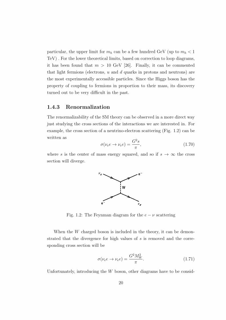
example, the cross section of a neutrino-electron scattering (Fig. 1.2) can be

written as

σ(νee→ νee) =G2s

π, (1.70)

where s is the center of mass energy squared, and so if s → ∞ the cross

section will diverge.

Fig. 1.2: The Feynman diagram for the e− ν scattering

When the W charged boson is included in the theory, it can be demon-

strated that the divergence for high values of s is removed and the corre-

sponding cross section will be

σ(νee→ νee) =G2M2

W

π. (1.71)

Unfortunately, introducing the W boson, other diagrams have to be consid-

20

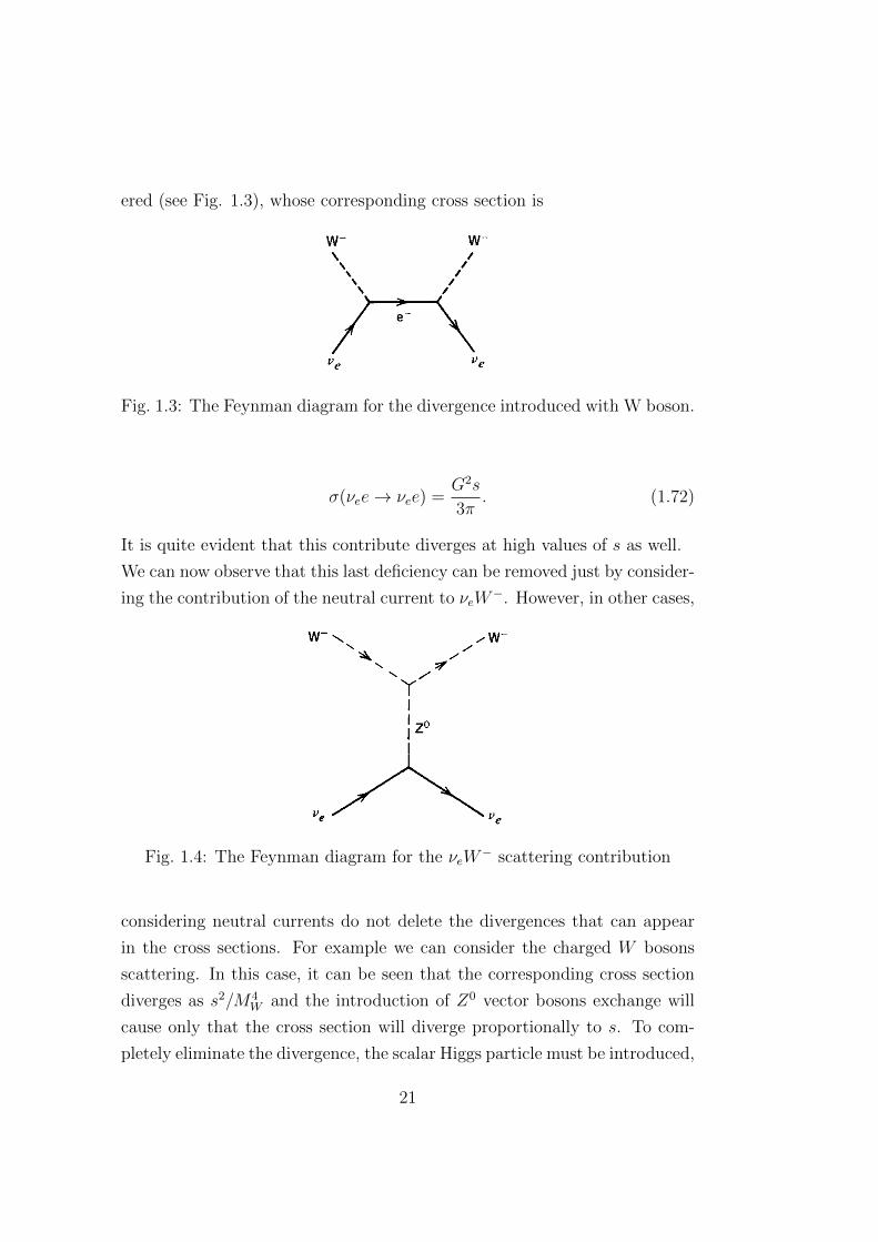
ered (see Fig. 1.3), whose corresponding cross section is

Fig. 1.3: The Feynman diagram for the divergence introduced with W boson.

σ(νee→ νee) =G2s

3π. (1.72)

It is quite evident that this contribute diverges at high values of s as well.

We can now observe that this last deficiency can be removed just by consider-

ing the contribution of the neutral current to νeW−. However, in other cases,

Fig. 1.4: The Feynman diagram for the νeW− scattering contribution

considering neutral currents do not delete the divergences that can appear

in the cross sections. For example we can consider the charged W bosons

scattering. In this case, it can be seen that the corresponding cross section

diverges as s2/M4W and the introduction of Z0 vector bosons exchange will

cause only that the cross section will diverge proportionally to s. To com-

pletely eliminate the divergence, the scalar Higgs particle must be introduced,

21

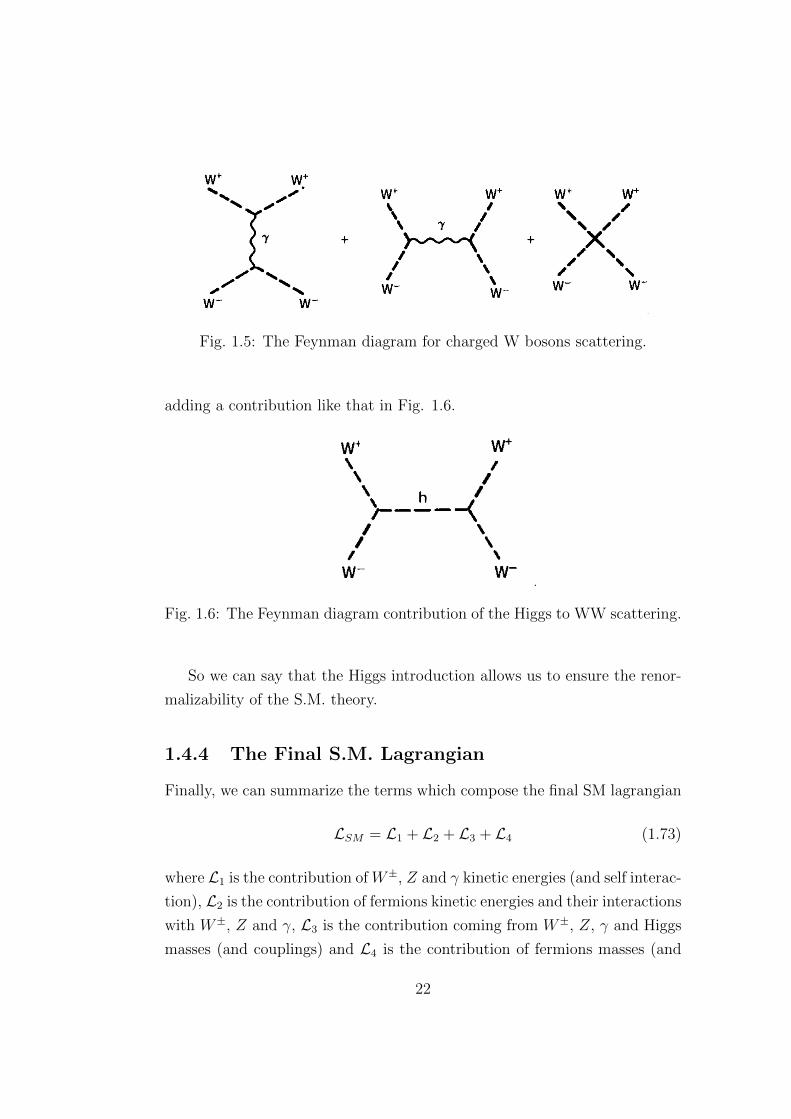
Fig. 1.5: The Feynman diagram for charged W bosons scattering.

adding a contribution like that in Fig. 1.6.

Fig. 1.6: The Feynman diagram contribution of the Higgs to WW scattering.

So we can say that the Higgs introduction allows us to ensure the renor-

malizability of the S.M. theory.

1.4.4 The Final S.M. Lagrangian

Finally, we can summarize the terms which compose the final SM lagrangian

LSM = L1 + L2 + L3 + L4 (1.73)

where L1 is the contribution of W±, Z and γ kinetic energies (and self interac-

tion), L2 is the contribution of fermions kinetic energies and their interactions

with W±, Z and γ, L3 is the contribution coming from W±, Z, γ and Higgs

masses (and couplings) and L4 is the contribution of fermions masses (and

22

Higgs coupling).

23

24

Chapter 2

The Large Hadron Collider

and the CMS Detector

In the previous chapter, it has been pointed out that the Higgs particle is not

easy to detect just because of its peculiar feature of coupling with fermions

proportionally to their masses. In order to produce heavier fermions, which

couple stronger with the Higgs, or igniting its production, a large amount

of energy is required. For this purpose several particles accelerators and

colliders have been projected. LHC (Large Hadron Collider) is one of these

giant machines which hold the responsability of discovering new particles.

The Higgs boson is one of them.

2.1 The Large Hadron Collider at CERN

The CERN (European Organization for Nuclear Research) was established in

1954 as the world’s largest particle physics laboratory. The acronym CERN

originally stood, in french, for Conseil Europen pour la Recherche Nuclaire

(European Council for Nuclear Research), which was a provisional council for

setting up the laboratory, established by twelve European countries in 1952.

It is located in the northwest part of Geneva, on the franco-swiss border, and

currently the organization includes twenty European member states. One of

the CERN main function has been to provide the particle accelerators and

other infrastructures needed for high-energy physics research. Since its birth,

25

many experiments have been built at CERN by international collaborations

but, at present, most of the activities at CERN are directed towards operating

the new Large Hadron Collider (LHC), and the experiments for it. The LHC

[16, 17] represents a large-scale worldwide scientific cooperation project. It

is placed in a tunnel located approximately 100 metres underground, in the

region between the Geneva airport and the nearby Jura mountains. This

tunnel was previously occupied by the LEP (The Large Electron-Positron

Collider) experiment, which also made important headway in hunting for the

Higgs boson. It was closed down in November 2000. The LHC inherited from

LEP some advanced devices as the Proton Synchrotron (PS) and the Super

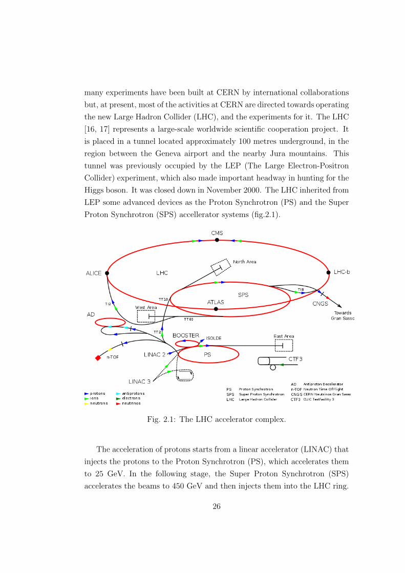
Proton Synchrotron (SPS) accellerator systems (fig.2.1).

Fig. 2.1: The LHC accelerator complex.

The acceleration of protons starts from a linear accelerator (LINAC) that

injects the protons to the Proton Synchrotron (PS), which accelerates them

to 25 GeV. In the following stage, the Super Proton Synchrotron (SPS)

accelerates the beams to 450 GeV and then injects them into the LHC ring.

26

The main experiments ATLAS, CMS, ALICE and LHCb, are located at the

four interaction regions. Two of them, CMS and ATLAS, are particulary

focused on the Higgs boson search within the SM context and on physics

beyond it. LHC has been designed for two kinds of collisions: collisions of

protons, and collisions of heavy ions.

2.1.1 Performance Goals

The LHC was designed to investigate the scalar sector, and the physics be-

yond the Standard Model in case of the failed discovering of the Higgs boson.

The number of events per second of a given physics process is related to the

cross section1 of the corresponding process, via the luminosity L of the ma-

chine, by the following relation

N = Lσ. (2.1)

The relevant events for physics searches, such as Higgs physics and physics

beyond the Standard Model, are predicted to have a quite low production

cross sections in proton-proton collisions. Fig. 2.2 shows that the cross sec-

tion for the production of a Higgs boson is several orders of magnitude smaller

than the total inelastic cross section. Besides, it increases significantly more

than the other ones with the center-of-mass energy of the collisions. That is

the reason why, for reaching the expected high researched event rate, both

the collision luminosity and the center-of-mass energy must be as high as

possible. For the LHC the choice focused on a very high collision luminos-

ity. The nominal center-of-mass energy for LHC collisions is√s = 14 TeV (7

TeV per beam), and the nominal peak luminosity is L = 1034 cm−2s−1 for the

CMS and ATLAS experiments. For these values (see the right axis on Fig.

2.2), a Higgs boson with a mass of 500 GeV/c2 would be produced approx-

imately every 100 s. Since LHC is a proton accelerator with a constrained

circumference, the maximal energy per beam is related to the strength of

1In particle physics, the cross section is used to express the normalized rate or prob-ability of a given particle interaction. It has the dimension of a surface and is usuallyexpressed in barns (b): 1b=10−28m2.

27

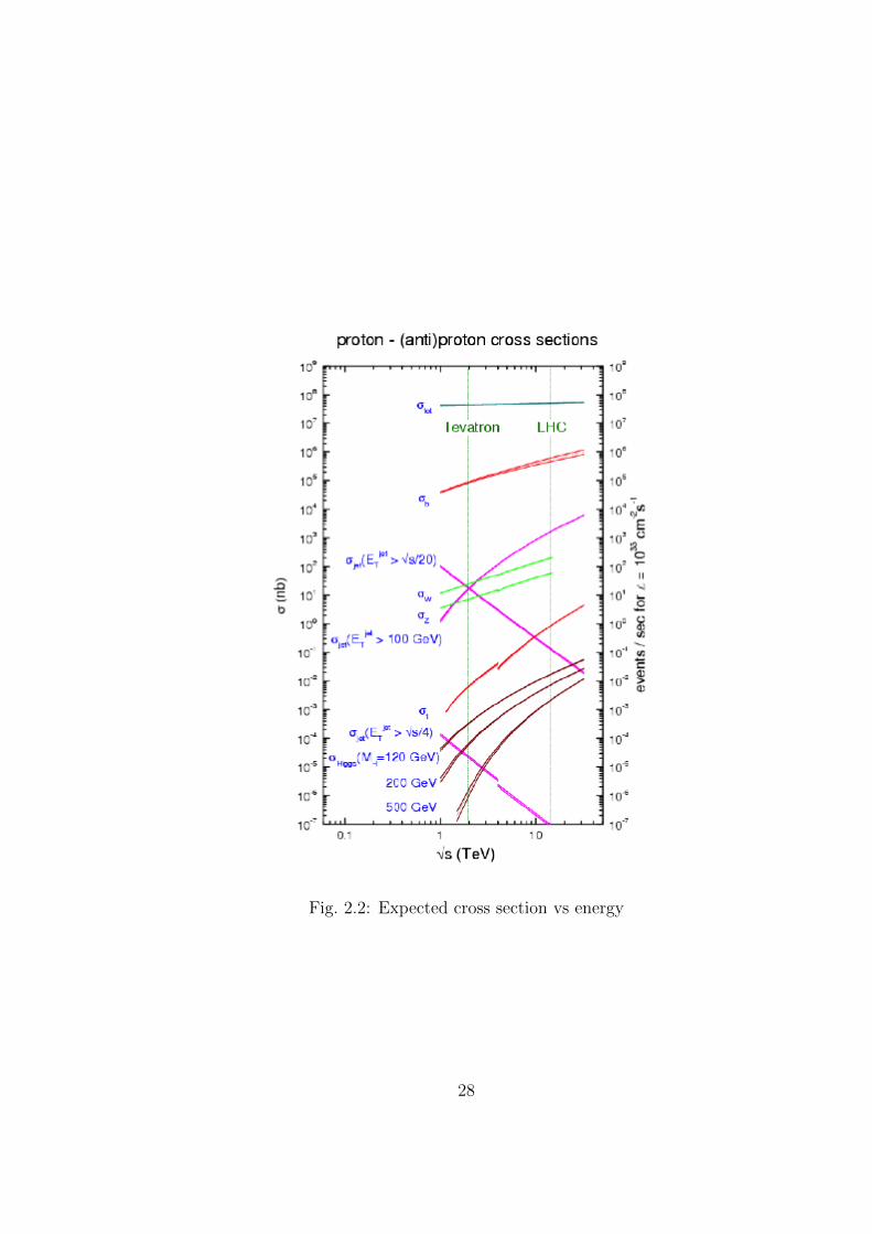
Fig. 2.2: Expected cross section vs energy

28

the dipole field that maintains the beams in orbit. A high technology global

magnet system allows to reach the nominal LHC beam energy of 7 TeV. The

system uses a total of about 9600 magnets.

The 1232 dipole magnets use niobium-titanium (NbTi) cables. By pumping

superfluid helium into the magnets, they are brought to a temperature of 1.9

K. For this purpose, a total of 120 t of superfluid helium is used. At that

temperature, the dipoles are in a superconducting state and a field of 8.33 T

can be provided. Such a magnetic field is necessary to bend the 7 TeV beams

around the 27-km ring of the LHC. Among the other magnets, quadrupoles

play a major role at collision points: they are used to focus the beam, and

maximize the probability of collision.

The very high LHC design luminosity implies many constraints on the pro-

ton beam parameters. The nominal luminosity can be reached with a num-

ber of bunches per beam nb = 2808 and a number of prototons per bunch

Nb = 1.15 · 1011. Such a high beam intensity could not be reached with

antiproton beams, hence a simple particle-antiparticle accelerator collider

configuration cannot be used at LHC.

The LHC has therefore been designed with two separate rings. The common

sections are located at the insertion regions, which are equipped with the

experimental detectors.

The configuration is presented in Fig. 2.3. A summary of the machine pa-

rameters [33] is given in Tab. 2.1. The numbers indicated correspond to the

nominal values.

In addition to the previously mentioned parameters, the luminosity lifetime

is an important parameter at LHC and colliders in general. The luminos-

ity tends to be reduced during a physics run, because of the degradation of

intensities and emittances of the circulating and colliding beams.

2.1.2 LHC Collision Detectors

Reaching the high luminosity values previously discussed imposes tight con-

straints on the design of the detectors. Under nominal conditions, the LHC

29

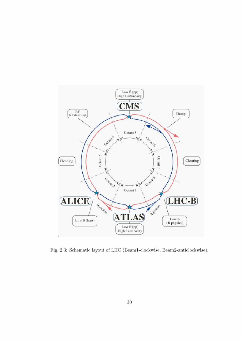
Fig. 2.3: Schematic layout of LHC (Beam1-clockwise, Beam2-anticlockwise).

30

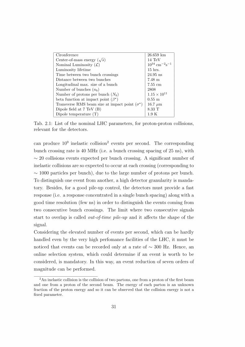
Cironference 26.659 kmCenter-of-mass energy (

√s) 14 TeV

Nominal Luminosity (L) 1034 cm−2s−1

Luminosity lifetime 15 hrs.Time between two bunch crossings 24.95 nsDistance between two bunches 7.48 mLongitudinal max. size of a bunch 7.55 cmNumber of bunches (nb) 2808Number of protons per bunch (Nb) 1.15× 1011

beta function at impact point (β?) 0.55 mTransverse RMS beam size at impact point (σ?) 16.7 µmDipole field at 7 TeV (B) 8.33 TDipole temperature (T) 1.9 K

Tab. 2.1: List of the nominal LHC parameters, for proton-proton collisions,relevant for the detectors.

can produce 109 inelastic collision2 events per second. The corresponding

bunch crossing rate is 40 MHz (i.e. a bunch crossing spacing of 25 ns), with

∼ 20 collisions events expected per bunch crossing. A significant number of

inelastic collisions are so expected to occur at each crossing (corresponding to

∼ 1000 particles per bunch), due to the large number of protons per bunch.

To distinguish one event from another, a high detector granularity is manda-

tory. Besides, for a good pile-up control, the detectors must provide a fast

response (i.e. a response concentrated in a single bunch spacing) along with a

good time resolution (few ns) in order to distinguish the events coming from

two consecutive bunch crossings. The limit where two consecutive signals

start to overlap is called out-of-time pile-up and it affects the shape of the

signal.

Considering the elevated number of events per second, which can be hardly

handled even by the very high perfomance facilities of the LHC, it must be

noticed that events can be recorded only at a rate of ∼ 300 Hz. Hence, an

online selection system, which could determine if an event is worth to be

considered, is mandatory. In this way, an event reduction of seven orders of

magnitude can be performed.

2An inelastic collision is the collision of two partons, one from a proton of the first beamand one from a proton of the second beam. The energy of each parton is an unknownfraction of the proton energy and so it can be observed that the collision energy is not afixed parameter.

31

2.2 The Compact Muon Solenoid (CMS) De-

tector

2.2.1 Coordinate System

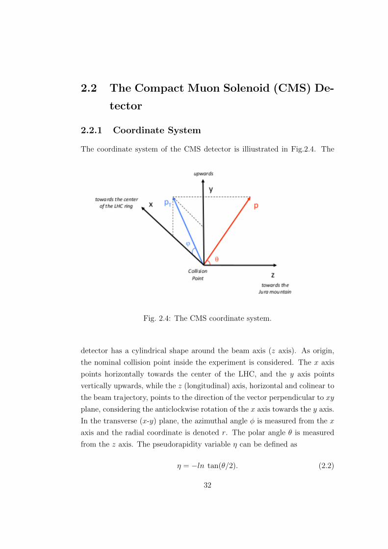
The coordinate system of the CMS detector is illiustrated in Fig.2.4. The

Fig. 2.4: The CMS coordinate system.

detector has a cylindrical shape around the beam axis (z axis). As origin,

the nominal collision point inside the experiment is considered. The x axis

points horizontally towards the center of the LHC, and the y axis points

vertically upwards, while the z (longitudinal) axis, horizontal and colinear to

the beam trajectory, points to the direction of the vector perpendicular to xy

plane, considering the anticlockwise rotation of the x axis towards the y axis.

In the transverse (x-y) plane, the azimuthal angle φ is measured from the x

axis and the radial coordinate is denoted r. The polar angle θ is measured

from the z axis. The pseudorapidity variable η can be defined as

η = −ln tan(θ/2). (2.2)

32

A particle trajectory direction at production point is then described by the

coordinates (η, φ). Two parts of the subdetectors can be considered relying

on the cylindrical shape of the detector:

1. the ‘barrel’, which corresponds to the central cylindrical region

2. the ‘endcaps’, which are two disks at the extremities closing the detector

along the beam axis.

The parton momentum, before the collision, is expected to be longitudinal

(along the beam axis). Being the transverse momentum of each parton neg-

ligible and the total transverse momentum conserved during an interaction,

the transverse momentum of the collision is expected to be negligible too.

2.2.2 The CMS detector structure and the Magnet

The CMS detector is a multi-purpose detector. Its lenght is 21.6 m and it has

a diameter of 14.6 m. It contains two calorimeters: an electromagnetic one

and a hadronic one. In the first, electromagnetic particles are stopped and

measured, while hadronic particles are stopped in the second but measured

in both of them. The trajectories of all the charged particles are measured

by an inner tracking device. Charged particles crossing both the calorimeters

(i.e. muons) are measured instead by an outer tracking device.

The tracking devices are exposed to a magnetic field which curves the trajec-

tories of charged particles. As reminded by its denomination, CMS detector

has been designed [9] paying a particular attention to muons: their energy

is measured through their track curvature information combined in both the

inner and the outer tracking devices. The charge and the transverse momen-

tum (pT ) measurements are performed by using the curvature radius of the

trajectory that is inverse proportional to the pT .

For the Higgs boson search in the decay channel H → ZZ → 4µ, an ex-

tremely precise measurement of the four-lepton mass is mandatory, so a pre-

cise measurement of the muon momentum is necessary, at least for pT values

up to 100 GeV/c and, along with it, a precise measurement of the muon track

curvatures. Hence, a large bending power in the tracker region is mandatory.

33

For this purpose, a 4 T superconducting solenoid is used. The tracker, and

both calorimeters are located inside the solenoid, and exposed to its longitu-

dinal magnetic field. The magnetic flux is returned through a 10000 t iron

yoke comprising 5 wheels and 2 endcaps, composed of three disks each. Four

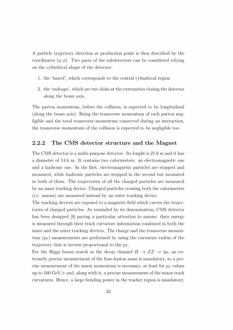
muon stations are included along the detector’s length. The geometry of the

CMS detector [44] is illustrated in Fig. 2.5. The subdetectors and the online

Fig. 2.5: A perspective view of CMS detector.

selection (‘trigger’) system are presented in the next sections.

2.2.3 Inner Tracking System

The CMS tracker is a fundamental tool for the charge and momentum mea-

surements of charged particles. It has a length of 5.8 m and a diameter

34

of 2.5 m around the interaction point. It covers a pseudorapidity range of

|η| < 2.5. Since it is located directly around the collision point, the tracker

material must be very resistant to radiation. The very fine granularity in

the innermost part is an essential feature for the identification of the differ-

ent vertices in a bunch crossing. While the primary vertex corresponds to

the interaction point of the collision, secondary vertices can indicate other

interactions that can occur during the same bunch crossing (pile-up), or the

presence of long-live particles3. A tracker design entirely based on silicon

detector technology has therefore been chosen. However this very powerful

system has some disadvantages:

• it implies a high density of detector electronics, which requires an effi-

cient cooling system;

• the particles coming from collisions may interact with this dense ma-

terial while crossing the tracker detector. It implies a complicated

recostruction procedure (see section 2.3) and a loss in the detector ef-

ficiency.

The high hit occupancy, which imposes constraints to the detector granular-

ity, is the result of the high number of particles crossing the tracker. The

CMS tracker is made of two kinds of silicon sensors:

1. silicon pixels, which constitute the pixel detector in the most inner

part;

2. silicon strips, which constitue the rest of the tracker.

The outer tracker region is made of thicker silicon sensors since the spatial

density of tracks decreases far from the interaction point.

In Fig. 2.6 a schematic cross section of the CMS tracker is presented. Each

line represents a detector module. The double lines indicate back-to-back

modules which deliver stereo hits. The pixel detector contains barrel and

3Leptons coming from late decays indicate a background event in the H → ZZ(∗) → 4`,where ` = e, µ

35

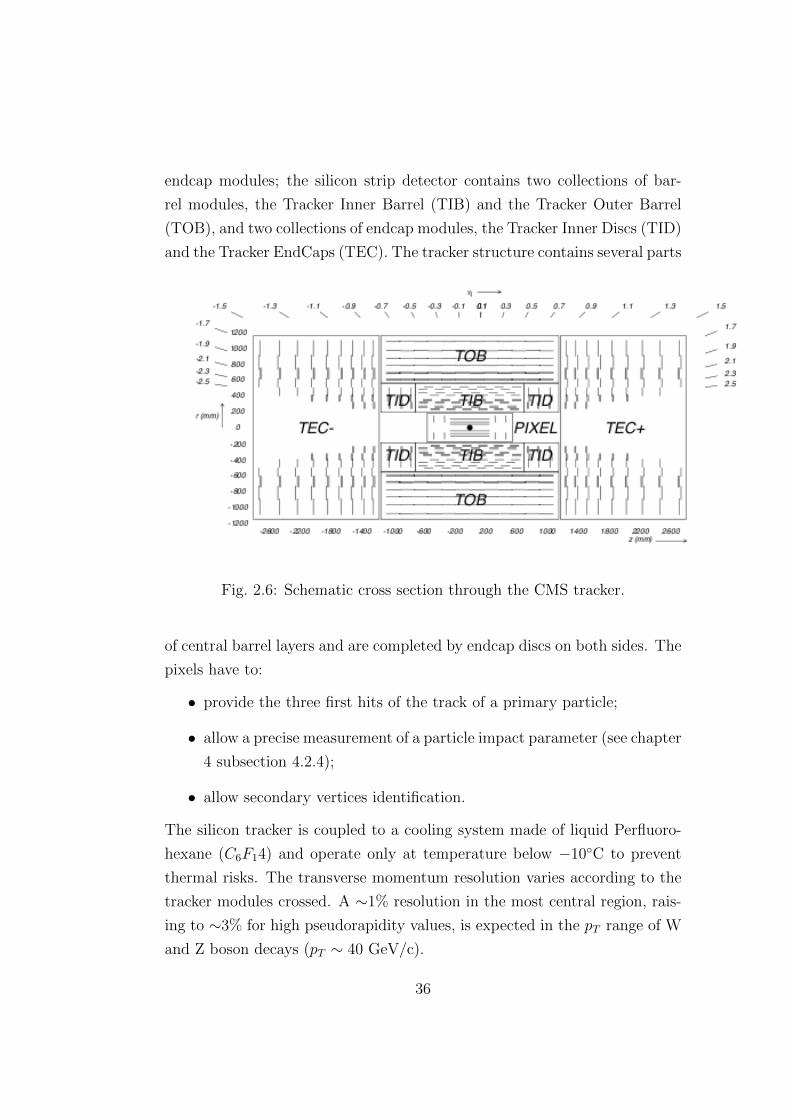
endcap modules; the silicon strip detector contains two collections of bar-

rel modules, the Tracker Inner Barrel (TIB) and the Tracker Outer Barrel

(TOB), and two collections of endcap modules, the Tracker Inner Discs (TID)

and the Tracker EndCaps (TEC). The tracker structure contains several parts

Fig. 2.6: Schematic cross section through the CMS tracker.

of central barrel layers and are completed by endcap discs on both sides. The

pixels have to:

• provide the three first hits of the track of a primary particle;

• allow a precise measurement of a particle impact parameter (see chapter

4 subsection 4.2.4);

• allow secondary vertices identification.

The silicon tracker is coupled to a cooling system made of liquid Perfluoro-

hexane (C6F14) and operate only at temperature below −10◦C to prevent

thermal risks. The transverse momentum resolution varies according to the

tracker modules crossed. A ∼1% resolution in the most central region, rais-

ing to ∼3% for high pseudorapidity values, is expected in the pT range of W

and Z boson decays (pT ∼ 40 GeV/c).

36

2.2.4 Electromagnetic Calorimeter

The Electromagnetic Calorimeter (ECAL) [13] has been calibrated according

to the requirements of the H → γγ search.

It is the only subdetector to provide information about photons. For an ac-

curate di-photon mass reconstruction (∼ 0.1 GeV/c2), a very precise position

and energy measurement is provided by the ECAL.

The ECAL is also of primary importance for the electron reconstruction in

a Higgs boson analysis in a multi-lepton final state. The combination of its

information with the one from the tracker can ensure a very precise mea-

surement of electron position and momentum and a significant background

removal.

A good segmentation is essential to distinguish the energy deposit shape of

an electromagnetic particle from the one belonging to a hadronic particle.

The CMS ECAL is a hermetic and homogeneous calorimeter, that covers

the rapidity range |η| < 3 . It is made of lead tungstate (PbWO4) crystals,

mounted in a barrel (|η| < 1.479) and two endcaps (1.479 < |η| < 3.0).

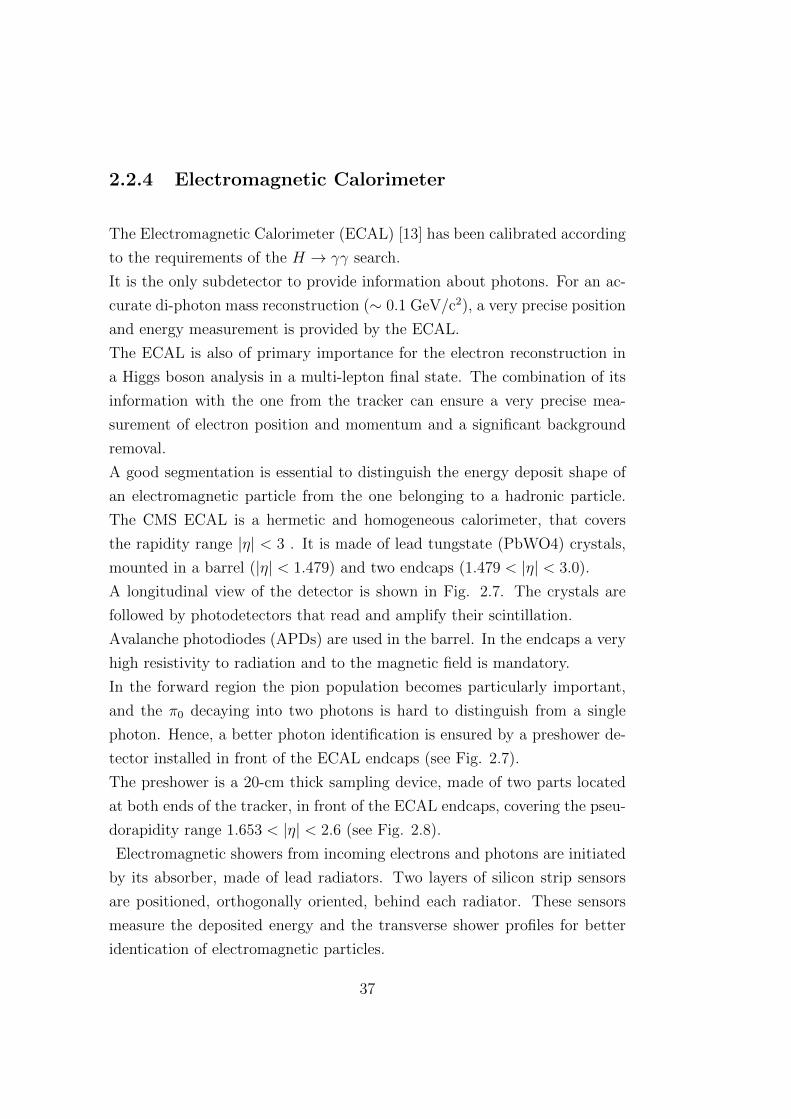
A longitudinal view of the detector is shown in Fig. 2.7. The crystals are

followed by photodetectors that read and amplify their scintillation.

Avalanche photodiodes (APDs) are used in the barrel. In the endcaps a very

high resistivity to radiation and to the magnetic field is mandatory.

In the forward region the pion population becomes particularly important,

and the π0 decaying into two photons is hard to distinguish from a single

photon. Hence, a better photon identification is ensured by a preshower de-

tector installed in front of the ECAL endcaps (see Fig. 2.7).

The preshower is a 20-cm thick sampling device, made of two parts located

at both ends of the tracker, in front of the ECAL endcaps, covering the pseu-

dorapidity range 1.653 < |η| < 2.6 (see Fig. 2.8).

Electromagnetic showers from incoming electrons and photons are initiated

by its absorber, made of lead radiators. Two layers of silicon strip sensors

are positioned, orthogonally oriented, behind each radiator. These sensors

measure the deposited energy and the transverse shower profiles for better

identication of electromagnetic particles.

37

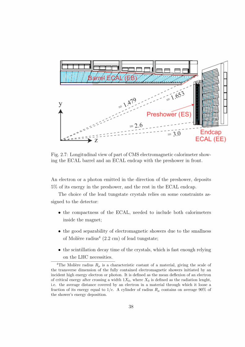
Fig. 2.7: Longitudinal view of part of CMS electromagnetic calorimeter show-ing the ECAL barrel and an ECAL endcap with the preshower in front.

An electron or a photon emitted in the direction of the preshower, deposits

5% of its energy in the preshower, and the rest in the ECAL endcap.

The choice of the lead tungstate crystals relies on some constraints as-

signed to the detector:

• the compactness of the ECAL, needed to include both calorimeters

inside the magnet;

• the good separability of electromagnetic showers due to the smallness

of Moliere radius4 (2.2 cm) of lead tungstate;

• the scintillation decay time of the crystals, which is fast enough relying

on the LHC necessities.4The Moliere radius Rµ is a characteristic costant of a material, giving the scale of

the transverse dimension of the fully contained electromagnetic showers initiated by anincident high energy electron or photon. It is defined as the mean deflexion of an electronof critical energy after crossing a width 1X0, where X0 is defined as the radiation lenght,i.e. the average distance covered by an electron in a material through which it loose afraction of its energy equal to 1/e. A cylinder of radius Rµ contains on average 90% ofthe shower’s energy deposition.

38

Fig. 2.8: Layout of the CMS ECAL showing the arrengement of crystalmodules, supermodules and endcaps, with preshower in front.

The ECAL barrel is made of 36 identical Supermodules, each covering

half the barrel length (−1.479 < η < 0 or 0 < η < 1.479), with a width of

20◦ in φ . Each Supermodule is composed by four Modules in the η direction

(see Fig. 2.8). The presence of acceptance gaps, called cracks, between the

Modules, makes the energy reconstruction more complicated. At η = 0 a

larger crack is present between Supermodules, and an even larger one marks

the barrel-endcap transition.

Each ECAL endcap is made of two semi-circular plates called Dees (Fig.

2.8). Small cracks are also present between the endcap Dees, but they can

be considered negligible.

The energy loss can be measured by comparing the energy measured in the

39

ECAL with the momentum measured in the tracker on electrons with little

bremsstrahlung, considering that the difference is due to energy loss in cracks.

To cancel these losses a recovery method has been conceived, except for the

border corresponding to η = 0 and the barrel-endcap transition, where energy

losses are 5% and 10% respectively.

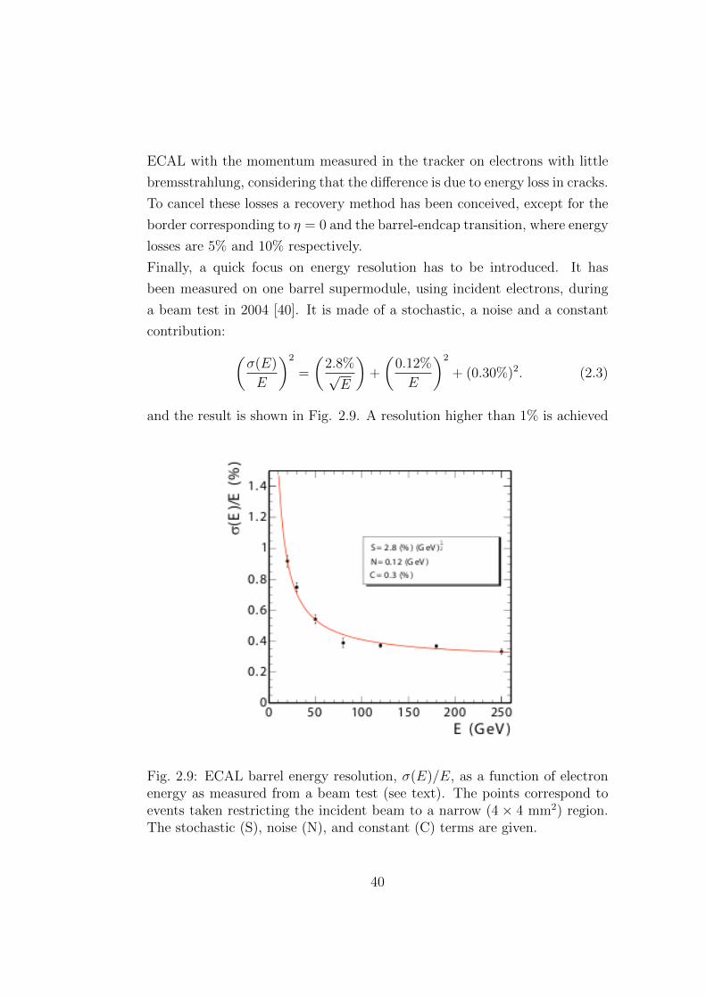
Finally, a quick focus on energy resolution has to be introduced. It has

been measured on one barrel supermodule, using incident electrons, during

a beam test in 2004 [40]. It is made of a stochastic, a noise and a constant

contribution: (σ(E)

E

)2

=

(2.8%√E

)+

(0.12%

E

)2

+ (0.30%)2. (2.3)

and the result is shown in Fig. 2.9. A resolution higher than 1% is achieved

Fig. 2.9: ECAL barrel energy resolution, σ(E)/E, as a function of electronenergy as measured from a beam test (see text). The points correspond toevents taken restricting the incident beam to a narrow (4 × 4 mm2) region.The stochastic (S), noise (N), and constant (C) terms are given.

40

for electrons of energy higher than 15 GeV; for 40 GeV electrons it is of 0.6%.

2.2.5 Hadron Calorimeter

The hadron calorimeter (HCAL) plays a major role in the detection of hadron

jets. It is located behind the Tracker and the Electromagnetic Calorimeter

(from interaction point of view). Its purpose is then to provide a sufficient

containment of the hadron showers. Moreover, a wide extension in pseudora-

pidity is mandatory to have a precise description of the total collision event,

allowing a reliable measurement of the missing transverse energy.

The importance of the HCAL from the point of view of a Higgs boson analy-

sis in a multi-lepton final state, is that it allows to distinguish electrons from

hadron jets, which can be mis-identified as leptons (see chapter 4, section

4.2.1). It is a sampling calorimeter.

Such as the ECAL, it is composed of a barrel part (HB) and an endcap part

(HE).

The HCAL Barrel covers the pseudorapidity range |η| < 1.3. It is limited in

radial dimension, between the outer extent of the ECAL and the inner extent

of the magnet coil (1.77 m < R < 2.95 m). Moreover, the HCAL is extended

outside the solenoid with a tail catcher called the outer calorimeter, HO, just

to ensure adequate sampling depth for |η| < 1.3.

The HCAL Endcaps cover a wide rapidity range: 1.3 < |η| < 3. The forward

hadron calorimeters (HF) are placed at 11.2 m from the interaction point

extend. They extend the pseudorapidity coverage down to |η| < 5.2. The

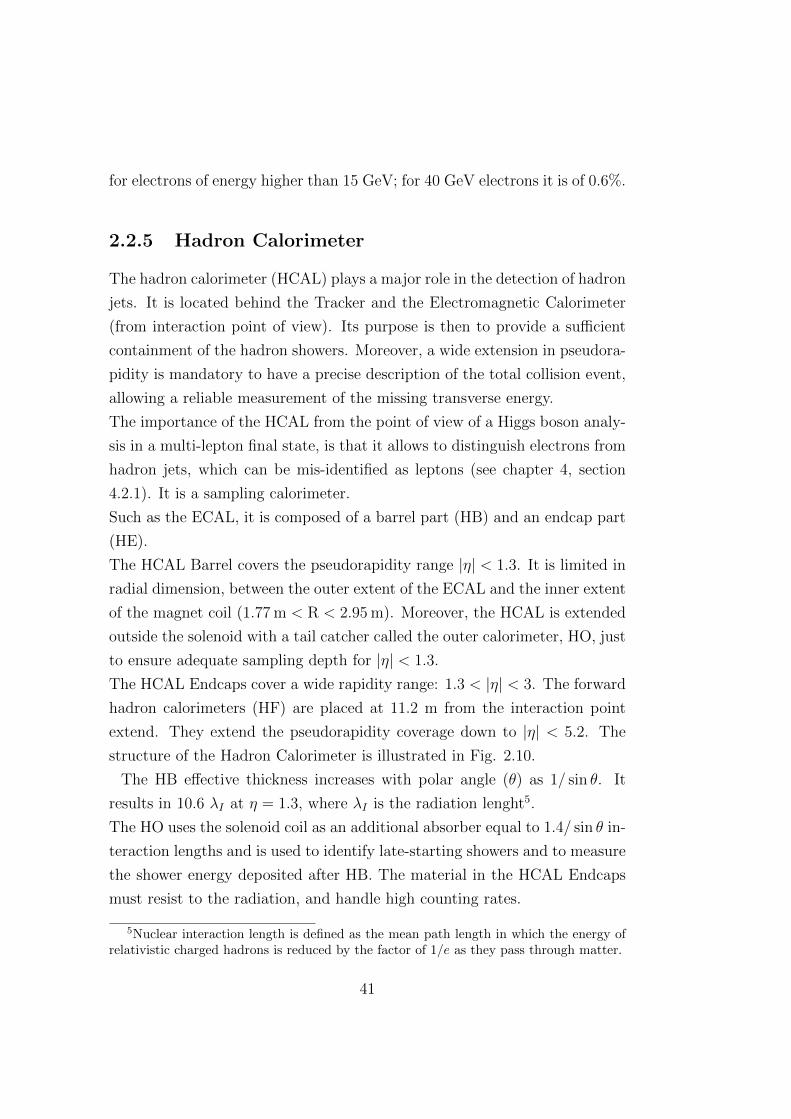
structure of the Hadron Calorimeter is illustrated in Fig. 2.10.

The HB effective thickness increases with polar angle (θ) as 1/ sin θ. It

results in 10.6 λI at η = 1.3, where λI is the radiation lenght5.

The HO uses the solenoid coil as an additional absorber equal to 1.4/ sin θ in-

teraction lengths and is used to identify late-starting showers and to measure

the shower energy deposited after HB. The material in the HCAL Endcaps

must resist to the radiation, and handle high counting rates.

5Nuclear interaction length is defined as the mean path length in which the energy ofrelativistic charged hadrons is reduced by the factor of 1/e as they pass through matter.

41

HF

HE

HB

HO

Fig. 2.10: Longitudinal view of the CMS detector. The locations of thehadron barrel (HB), the endcap (HE), the outer (HO) and the forward (HF)calorimeters.

Because of the magnetic field, the absorber must be made from a non mag-

netic material.

Finally, the HE has to fully contain hadronic showers. The calorimeter bar-

rel energy resolution (EB + HB + HO) has been measured on pions which

energy varies in a range of 3-500 GeV by test beams. It has been found to

be: (σ(E)

E

)=

(84.7%√

E

)⊕ 7.4%. (2.4)

It can be observed that the energy resolution is dominated by the HCAL

contribution.

2.2.6 The Muon System

The topology of the final state of H → ZZ → 4µ analysis give reasons for

the construction of a muon system with a wide angular coverage and no ac-

ceptance gap.

Muons are particularly easy to identify and distinguish from backgrounds

42

with CMS detector, thanks to the absorbing function played by the calorime-

ters.

The muon systems are divided into a cylindrical barrel section and two pla-

nar endcap regions. Less background, a low muon rate and a uniform 4-T

magnetic field, mostly contained in the steel yoke, is measured in the barrel.

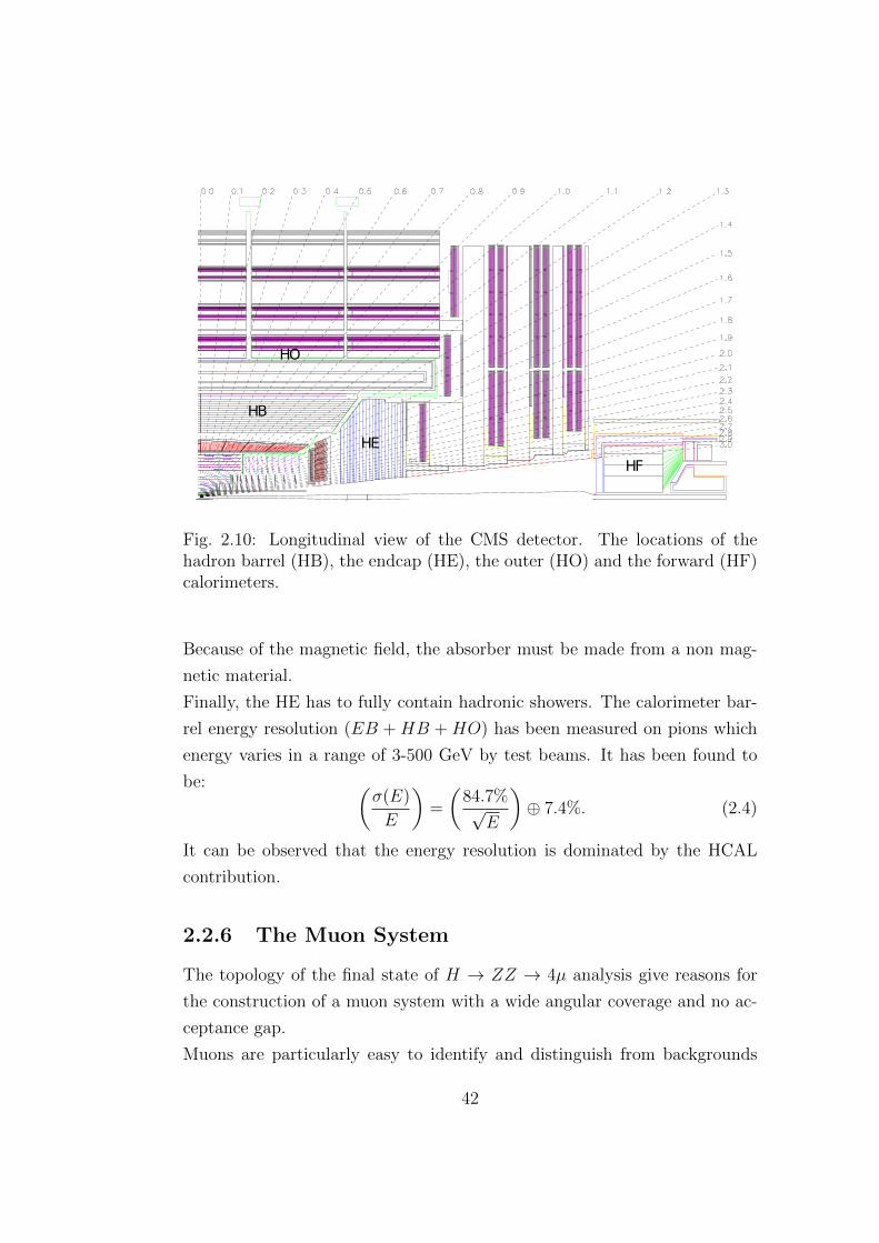
A longitudinal view of the muon detectors can be found in Fig. 2.11.

Fig. 2.11: Longitudinal view of the muon detectors: DT, RPC and CSC.

Muon System Subdetectors

Drift tube (DT) chambers have been used. They cover the pseudorapidity

region |η| < 1.2. Chambers measuring the muon coordinate in the r − φ

bending plane are alternated with chambers providing a measurement in the

z direction. Each of the four stations contains four chambers of each kind.

The most relevant problem of this design is the presence of ‘cracks’, i.e. dead

efficiency spots between the chambers. It has been solved by the presence of

43

an offset of the drift cells between neighbor chambers.

The endcaps cover a region of higher rates. In this region the magnetic field

appears large and non-uniform.

Cathode strip chambers (CSC) are instead used to cover the pseudorapidity

region 0.9 < |η| < 2.4. Each of the four stations contains six layers of

chambers and anode wires.

The chambers are positioned perpendicular to the beam line and provide a

precision measurement in the r − φ bending plane, while the anode wires

provide measurements of the beamcrossing time of muons.

Other tools are included to reject non-muon backgrounds and to match hits

to those in the other stations and in the inner tracker.

A system of resistive plate chambers (RPC) has been added in barrel and

endcap regions, over a large portion of the pseudorapidity range (|η| < 1.6).

They consists of double-gap chambers, operated in avalanche mode to ensure

good operation at high rates.

Six layers are present in the barrel and three in each endcap. They produce

a fast response, with good time resolution but coarser position resolution

than the DTs or CSCs. They provide an independent trigger system with an

optimal time resolution. Moreover, they help to reduce ambiguities in track

reconstruction.

The muon momentum resolution is optimized by a high technology alignment

system, which measures the relative positions of the muon detectors along

with their positions respect with the inner tracker system.

2.2.7 Trigger

The Trigger system can be considered as the first event selection step. The

main feature of this step, which makes it different from the other selection

steps, is that it is not reversible. It indeed performs a fast selection of the

events which seem to be of interest for physics analysis among the huge

amount of those produced by LHC collisions.

This selection can drastically reduce the extremely high event rate (the LHC

nominal bunch crossing rate is ∼ 40 MHz) to a reasonable rate, more suit-

44

able for data recording (∼ 300 Hz). Obviously, all collision data must be

kept untill the trigger decision has been taken, so requiring a fast response.

To fulfill these requirements, a two-level trigger system has been designed.

The Level-1 (L1) Trigger is a hardware system made of largely programmable

electronics. It provides a first rate reduction to 100 kHz, scanning events

fastly in 3.2 µs. This timing constraint are satisfied considering coarse gran-

ularity objects from the calorimeters and from the muon system.

A positive L1 decision is converted in a transfer of the complete event infor-

mation to the next level: the High Level Trigger (HLT). Unlike the previous

one, the HLT is a software system which is based on algorithms of increasing

complexity that use the fine granularity of the event. So, the HLT decision

time is not a fixed value as the L1 trigger one. It may vary according to the

event, with a mean value of 50 ms.

In the case of the Higgs boson analysis in multi-lepton final state here pre-

sented, the trigger relies on events containing electron and muon signals. For

the Level-1 Trigger, an electron signature can be identified with a narrow

and highly energetic deposit in the ECAL, while a muon signature is based

on a track segment or a hit pattern in muon chambers.

The High-Level Trigger considers higher granularity objects, because it re-

constructs the total energy deposits in the calorimeters and muon tracks, and

combines them with the tracker and preshower information.

Level-1 Trigger

The Level-1 Trigger architecture is described in Fig. 2.12.

It is divided into two parallel trigger systems, one corresponding to the

calorimeters and the other to the muon chambers.

Each system is composed of a local, a regional, and a global part, then merged

into a Global Trigger for the final L1 decision.

The candidate categories of the Level-1 Trigger are:

• Muons, built in the Muon Trigger;

• Electrons/Photons (isolated and non-isolated: e− γ);

45

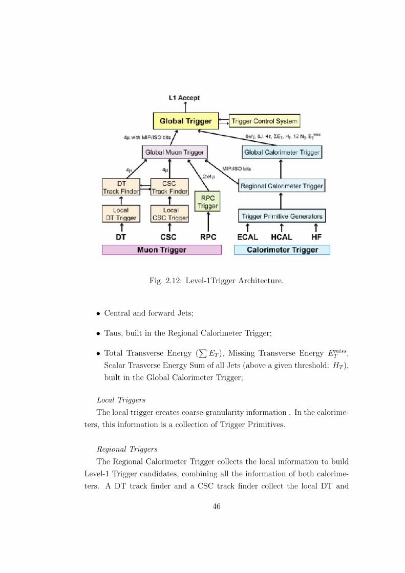
Fig. 2.12: Level-1Trigger Architecture.

• Central and forward Jets;

• Taus, built in the Regional Calorimeter Trigger;

• Total Transverse Energy (∑ET ), Missing Transverse Energy Emiss

T ,

Scalar Trasverse Energy Sum of all Jets (above a given threshold: HT ),

built in the Global Calorimeter Trigger;

Local Triggers

The local trigger creates coarse-granularity information . In the calorime-

ters, this information is a collection of Trigger Primitives.

Regional Triggers

The Regional Calorimeter Trigger collects the local information to build

Level-1 Trigger candidates, combining all the information of both calorime-

ters. A DT track finder and a CSC track finder collect the local DT and

46

CSC information to build Level-1 Trigger Candidates as tracks for the muon

trigger. The RPC trigger is directly regional. The four most relevant Candi-

dates of each category are sent to the Global Calorimeter Trigger or to the

Global Muon Trigger respectively. The regional summed transverse energy

is also sent to the Global Calorimeter Trigger by the Regional one.

Global Calorimeter Trigger and Global Muon Trigger

The Global Calorimeter Trigger has finally the task of sorting the Level-1

Trigger Candidates to send the four most relevant ones of each category to

the Global Trigger. It also calculates the summed ET and the EmissT infor-

mation of the event, as well as the scalar transverse energy sum of all jets

above a given threshold (HT). The Global Trigger riceives this information

as well. The Global Muon Trigger collects and compares the candidates from

the DT, CSC and RPC Triggers and combines them into four Muon Candi-

dates. It also uses some information from the Regional Calorimeter Trigger

for isolation considerations. The Global Trigger finally collects the informa-

tion about the four Muon Candidates.

Global Trigger

The Global Trigger collects the candidates produced by the Global Calorime-

ter Trigger and the Global Muon Trigger, and compares them to the Level-1

Trigger Menu. This menu is a list of Level-1 enabled triggers. If at least one

of the listed triggers is satisfied by a candidate collection, the Level-1 Trigger

response is positive and the fine granularity event information can be sent to

High-Level Trigger. The Level-1 Trigger also follows some rules to prevent

memory overload (e.g. L1 Trigger cannot accept two events separated by

only one single bunch crossing).

The trigger algorithms consist in a threshold applied to the highest ener-

getic candidate of each category. For background reduction, a combination

of triggers is often required.

47

High-Level Trigger

The higher and last level trigger step is the High-Level Trigger which builds

candidates corresponding to all kinds of reconstructed objects considered in

the offline analyses. The algorithms used are very similar to the previous

ones. Its inner sub-structure is made of several increasing complexity levels,

starting from Level 2.

The Level 2 starts generally with the Level-1 Trigger information, and builds

fine granularity objects around the Level-1 candidates, using only the infor-

mation from the calorimeters and the muon system. The tracker information

is also used, only when necessary, at the next 2.5 Level.

2.3 Lepton Reconstruction

2.3.1 Electron Reconstruction

The electron reconstruction [59] combines the information from the elec-

tromagnetic calorimeter (ECAL) and the silicon tracker. It starts by the

recostruction of clusters seeded by hot cells in the ECAL.

Electron seeds are then used to form superclusters (clusters of clusters) to

collect the electron energy radiated by bremsstrahlung in the tracker and

spread in φ by the solenoidal magnetic field and to initiate a track building

and a fitting procedure.

The superclusters are first preselected using a hadronic veto (defined by the

ratio H/E of the hadronic energy estimated by summing HCAL towers en-

ergy within a cone of ∆R = 0.15 behind the supercluster position over the

supercluster energy) and applying a 4 GeV cut on the supercluster transverse

energy.

The superclusters are also used to search for hits in the innermost tracker

layers which are used to accomplish the seeding of the tracks.

The ECAL driven seeding algorithm has been used. It has been optimised

for isolated electrons in the peT range relevant for Z or W decay, down to 5

GeV/c. For lower electron peT values the φ window used for the superclus-

ters becomes too small and the electrons which radiate lead to electron and

48

photon clusters separated by a distance greater than 0.3 rad (the maximum

limit) in the magnetic field.

Moreover, for electrons in jets, the energy collected in the superclusters could

include neutral contribution from jets so biasing the energy measurement

used to seed the tracks.

For these reasons, the driven seeding strategy has been complemented by

a tracker driven seeding algorithm. It can be illustrated with two extreme

cases:

• electrons which do not radiate energy by bremsstrahlung while crossing

the tracker;

• electrons which undergo a significant energy loss by bremsstrahlung.

In the first case, the electron creates a single cluster in the ECAL and its

track may be recostructed well enough by the standard Kalman Filter, which

is able to collect hits up to ECAL.

The track recostructed is then matched with a particle flow6 [25] cluster and

the ratio E/p of the cluster energy over the track momentum can be eval-

uated. If the value of this ratio is close to unity, the seed of the track is

considered as an electron seed.

Instead, in the second case, the Kalman Filter cannot follow the change of

curvature and a small number of hits belongs to the track. In this case,

the electron tracks are selected using the silicon tracker as a preshower and

evaluating the different characteristics of a pion track and an electron track

recostructed by Kalman Filter.

A merging procedure of the seeds of the two algorithms is then carried out so

keeping the track of seed provenance. It can be also noticed that the tracker

driven algorithm for non-isolated electrons brings, if applied, an efficiency

enhancement on isolated electrons too, in particular in the ECAL cracks re-

gions (η ' 0 and |η| ' 1.5) and as expected, at low peT values.

6The aim of the CMS particle flow event-reconstruction algorithm is to identify andreconstruct individually each particle arising from the LHC proton-proton collision, bycombining the information from all subdetectors. The resulting global event descriptionleads to an improved performance for the reconstruction of jets and for the identificationof electrons, muons, and taus.

49

The trajectories in the silicon tracker volume are recostructed using a dedi-

cated modelling of the electron energy loss and fitted with a Gaussian Sum

Filter, which relies on a modelling of electron radiative energy loss. The

seeding algorithm combines the information from pixel and TEC layers so to

get an efficiency gain in the forward region where the coverage by the pixel

layers is limited. To perform the selection, a matching between superclusters

and trajectory seeds built from hit pairs or triplets is required.

The electron momentum is estimated by combining the tracker and ECAL

mesurements. The electron candidates preselection is performed applying

loose cuts on track-cluster matching observables, so preserving a high effi-

ciency value while removing part of QCD background. To resolve ambiguous

cases (due to conversion legs of radiated photons) in which several tracks are

recostructed, a cleaning procedure is carried out.

The mis-identification arising from the early conversions of radiated photons

is coped with electron charge determination which is performed compar-

ing different charge measurement observables. Electrons are classified using

observables sensitive to the bremsstrahlung emission and showering in the

tracker material.

For the analysis presented here, the electron candidates have been required

to have transverse momentum peT larger than 7 GeV/c and a reconstructed

|ηe| <2.5.

The reconstruction efficiency for isolated electron is expected to be above

≈ 90% over the full ECAL acceptance, apart from some narrow ”crack” re-

gions.

The one for basic electron objects integrated over the acceptance rises to

reach ≈ 90% at pT = 10 GeV/c, and then more slowly to reach a plateau of

≈ 95% for peT = 30 GeV/c. The application of identification requirements on

top of the recostructed electron objects collection allows the enhancement of

the purity of the sample of electron candidates.

The electron objects are separated into classes according to the amount of

energy lost by bremsstrahlung processes. A series of different cuts are then

applied to each category.

The variables used, which are sensitive to bremsstrahlung processes, are the

50

fraction of radiated energy as measured from the innermost and outermost

state of the electron track and the ratio E/p between the supercluster energy

and the measured track momentum at the vertex. This procedure allows

to handle the non gaussian fluctuations induced on the ECAL and on the

tracker mesurements by the presence of material in the tracker.

Three different categories are defined with quite different measurement char-

acteristics and purity:

• “brem”;

• “lowbrem”;

• “badtrack”.

In addition, two others categories are defined to separate electron objects in

transition regions:

• ”pure tracker-driven objects”;

• ”crack objects”.

Subcategories are also defined for “brem”,“ lowbrem”, “badtrack” and “pure

tracker-driven” objects according to pseudorapidity regions (barrel and end-

cap), leading to a total number of nine categories. The cuts on each category

are applied just to optimize the signal to background ratio (s/b).

As previously mentioned, the shape of most of the discriminating variables

strongly depends on the transverse energy (ET ) of the electron, and so the

selection cuts are made ET -dependent.

The cuts are defined for the following variables:

• |∆ηin| = |ηsc − ηextrap.in |, where ηsc is the energy weighted position in η

of the supercluster and ηextrap.in is the η coordinate of the position of

closest approach to the supercluster position, extrapolating from the

innermost track position and direction;

• |∆φin| = |φsc−φextrap.in |, where ∆φin is a quantity similar to the previous

one but in azimuthal coordinates;

51

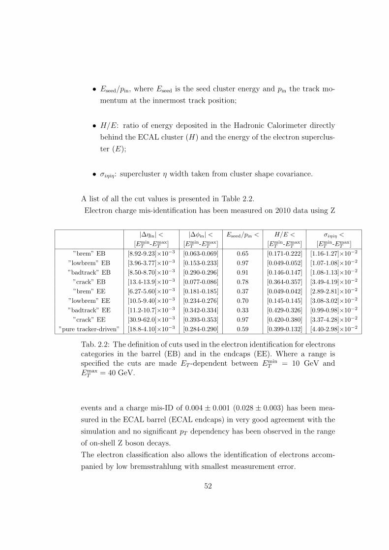
• Eseed/pin, where Eseed is the seed cluster energy and pin the track mo-

mentum at the innermost track position;

• H/E: ratio of energy deposited in the Hadronic Calorimeter directly

behind the ECAL cluster (H) and the energy of the electron superclus-

ter (E);

• σiηiη: supercluster η width taken from cluster shape covariance.

A list of all the cut values is presented in Table 2.2.

Electron charge mis-identification has been measured on 2010 data using Z

|∆ηin| < |∆φin| < Eseed/pin < H/E < σiηiη <

[EminT -Emax

T ] [EminT -Emax

T ] [EminT -Emax

T ] [EminT -Emax

T ]

”brem” EB [8.92-9.23]×10−3 [0.063-0.069] 0.65 [0.171-0.222] [1.16-1.27]×10−2

”lowbrem” EB [3.96-3.77]×10−3 [0.153-0.233] 0.97 [0.049-0.052] [1.07-1.08]×10−2

”badtrack” EB [8.50-8.70]×10−3 [0.290-0.296] 0.91 [0.146-0.147] [1.08-1.13]×10−2

”crack” EB [13.4-13.9]×10−3 [0.077-0.086] 0.78 [0.364-0.357] [3.49-4.19]×10−2

”brem” EE [6.27-5.60]×10−3 [0.181-0.185] 0.37 [0.049-0.042] [2.89-2.81]×10−2

”lowbrem” EE [10.5-9.40]×10−3 [0.234-0.276] 0.70 [0.145-0.145] [3.08-3.02]×10−2

”badtrack” EE [11.2-10.7]×10−3 [0.342-0.334] 0.33 [0.429-0.326] [0.99-0.98]×10−2

”crack” EE [30.9-62.0]×10−3 [0.393-0.353] 0.97 [0.420-0.380] [3.37-4.28]×10−2

”pure tracker-driven” [18.8-4.10]×10−3 [0.284-0.290] 0.59 [0.399-0.132] [4.40-2.98]×10−2

Tab. 2.2: The definition of cuts used in the electron identification for electronscategories in the barrel (EB) and in the endcaps (EE). Where a range isspecified the cuts are made ET -dependent between Emin

T = 10 GeV andEmaxT = 40 GeV.

events and a charge mis-ID of 0.004 ± 0.001 (0.028 ± 0.003) has been mea-

sured in the ECAL barrel (ECAL endcaps) in very good agreement with the

simulation and no significant pT dependency has been observed in the range

of on-shell Z boson decays.

The electron classification also allows the identification of electrons accom-

panied by low bremsstrahlung with smallest measurement error.

52

2.3.2 Muon Reconstruction

Muon detection and reconstruction [27] requires an excellent detection of

muons over the full acceptance of the CMS detector.

The muon recostruction is performed combining the information of the track-

ing and the calorimeter devices.

Three are the high level physics objects (particles travelling through the de-

tector) involved, depending on the muon track reconstruction step:

• stand-alone muons ;

• global muons ;

• tracker muons.

The reconstruction starts in the muon spectrometer with the reconstruction

of the hits positions in DT, CSC and RPC chambers.

A hit corresponds to a signal from a particle recorded by detector com-

ponents. So the signal is recostructed as individual points in space called

recHits. The hits in DT and CSC are then associated together to form ”seg-

ments” (track stubs).

The seeding procedure is then accomplished collecting and matching the seg-

ments. The seeds are so used to perform the actual track fit using also the

RPC hits. The reconstructed track that results in the muon spectrometer

is called stand-alone muon. The stand-alone muon tracks are then matched

with those from the silicon tracker, generating global-muon tracks.

The third high level object, the tracker muon, is recostructed with an al-

gorithm which starts from the silicon tracker tracks and then requests the

matching with segments in the muon chambers. In the studies performed for

the analysis at√s = 8 TeV it has been noticed that the use of the tracker

muons improves the expected limited and so they have been included. From

all these three kinds of objects a unique collection of muons is obtained.

The muon system in CMS has three distinct functions:

• muon identification

• momentum measurement

53

• triggering over the whole kinematic range

The hits are analyzed using a recognition algorithm to associate measure-

ments with trajectories. The procedure used to extract tracks from hits

consists of the following steps:

• trajectory seeding: the determination of the track recostruction initial

point is accomplished using an estimated trajectory state or collection

of hits compatible with the assumed physics process;

• trajectory building: it starts from the position specified by the trajec-

tory seed, proceeding in the direction specified by the seed and search-

ing for compatible hits on the subsequent detector layers. The track

finding and fitting procedure is performed using a Kalman Filter. This

last method uses an iterative approach to update the trajectory esti-

mate, using track parameters and covariance and propagating them to

the next detector layer;

• trajectory cleaning: the trajectory building procedure produces a large

amount of possible trajectories, sharing a lot of hits. This step is then

finalized to remove the ambiguities, keeping a maximum number of

tracks candidates;

• trajectory smoothing: in this step a backward fitting is performed. The

Kalman filter is also used in this case because of its feature of being

linear in the measurements and its backward complement capability to

use the whole information package;

Once the hits are fitted and the fake trajectories are removed, the remaining

tracks are extrapolated to the point of closest approach to the beam line,

where the information from the track is measured in the transverse plane.

In order to improve the pT resolution, a beam spot constraint has been ap-

plied. It can be observed that the muon tracks are not re-fitted to the

common vertex.

The reconstructed muons are required to have transverse momentum pµT

54

larger than 5 GeV/c and |ηµ| < 2.4: the first requirement ensures an ef-

ficiency for the reconstruction of muons above the 80%, while the second

relies on the geometric acceptance of the tracker detector in where the muon

reconstruction is fully efficient.

For ensuring an accurate measurement of the track momentum, more than

ten silicon tracker hits (Nhits > 10) have to be included in the track fit.

55

56

Chapter 3

The Higgs Boson Production

and Simulation at LHC

In this work a search for a Higgs boson in the dacay channel H → ZZ(∗) → 4`

using pp collisions from LHC at√s = 7 TeV is presented. From now on Z

can stand for the real particle Z, for the virtual one Z∗, and, eventually, also

for γ∗.

For the event generation, ` stands for any charged lepton, e, µ or τ but the

analysis here discussed will focus on reconstructed final states with only elec-

trons or muons. In this section a theoretical overview of the production and

decay channels of the SM Higgs boson [22] along with a quick view on the

signal and background MC samples used will be discussed.

The total cross section at hadron colliders is extremely large (about 100 mb

at the LHC), resulting in an interaction rate of ≈ 109 Hz at the design lu-

minosity [22]. In this difficult environment, the detection of processes with

signal to total hadronic cross section ratios (of about 10−10), as is the case

for the SM Higgs production in most channels, is challenging.

The huge QCD-jet backgrounds prevents from the detection of the produced

Higgs boson, or any particle in general, in fully hadronic modes.

For the purpose of this analysis, it can be worth to remind that in the

SM Higgs decay mode H → ZZ/WW, at least one of the W/Z bosons has

to observed in its leptonic decays which have small branching ratios (e.g.

BR(Z→ l+l−) ≈ 6%) but a clear signature of leptons in the final state.

57

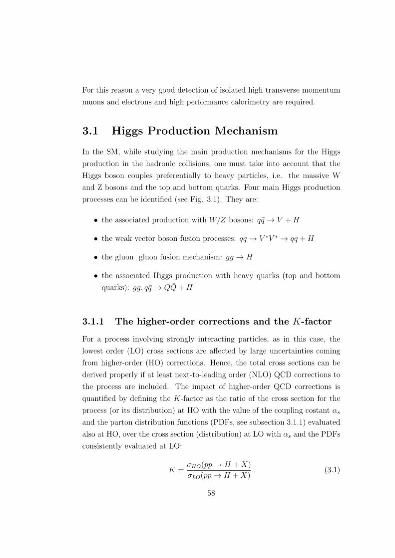
For this reason a very good detection of isolated high transverse momentum

muons and electrons and high performance calorimetry are required.

3.1 Higgs Production Mechanism

In the SM, while studying the main production mechanisms for the Higgs

production in the hadronic collisions, one must take into account that the

Higgs boson couples preferentially to heavy particles, i.e. the massive W

and Z bosons and the top and bottom quarks. Four main Higgs production

processes can be identified (see Fig. 3.1). They are:

• the associated production with W/Z bosons: qq → V +H

• the weak vector boson fusion processes: qq → V ∗V ∗ → qq +H

• the gluon gluon fusion mechanism: gg → H

• the associated Higgs production with heavy quarks (top and bottom

quarks): gg, qq → QQ+H

3.1.1 The higher-order corrections and the K-factor

For a process involving strongly interacting particles, as in this case, the

lowest order (LO) cross sections are affected by large uncertainties coming

from higher-order (HO) corrections. Hence, the total cross sections can be

derived properly if at least next-to-leading order (NLO) QCD corrections to

the process are included. The impact of higher-order QCD corrections is

quantified by defining the K-factor as the ratio of the cross section for the

process (or its distribution) at HO with the value of the coupling costant αs

and the parton distribution functions (PDFs, see subsection 3.1.1) evaluated

also at HO, over the cross section (distribution) at LO with αs and the PDFs

consistently evaluated at LO:

K =σHO(pp→ H +X)

σLO(pp→ H +X). (3.1)

58

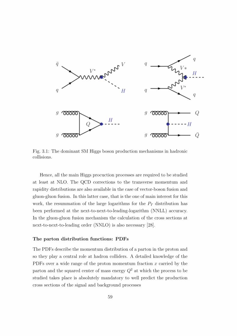
Fig. 3.1: The dominant SM Higgs boson production mechanisms in hadroniccollisions.

Hence, all the main Higgs procuction processes are required to be studied

at least at NLO. The QCD corrections to the transverse momentum and

rapidity distributions are also available in the case of vector-boson fusion and

gluon-gluon fusion. In this latter case, that is the one of main interest for this

work, the resummation of the large logarithms for the PT distribution has

been performed at the next-to-next-to-leading-logarithm (NNLL) accuracy.

In the gluon-gluon fusion mechanism the calculation of the cross sections at

next-to-next-to-leading order (NNLO) is also necessary [28].

The parton distribution functions: PDFs

The PDFs describe the momentum distribution of a parton in the proton and

so they play a central role at hadron colliders. A detailed knowledge of the

PDFs over a wide range of the proton momentum fraction x carried by the

parton and the squared center of mass energy Q2 at which the process to be

studied takes place is absolutely mandatory to well predict the production

cross sections of the signal and background processes

59

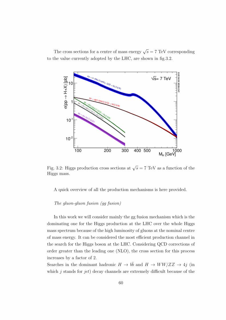
The cross sections for a centre of mass energy√s = 7 TeV corresponding

to the value currently adopted by the LHC, are shown in fig.3.2.

Fig. 3.2: Higgs production cross sections at√s = 7 TeV as a function of the

Higgs mass.

A quick overview of all the production mechanisms is here provided.

The gluon-gluon fusion (gg fusion)

In this work we will consider mainly the gg fusion mechanism which is the

dominating one for the Higgs production at the LHC over the whole Higgs

mass spectrum because of the high luminosity of gluons at the nominal centre

of mass energy. It can be considered the most efficient production channel in

the search for the Higgs boson at the LHC. Considering QCD corrections of

order greater than the leading one (NLO), the cross section for this process

increases by a factor of 2.

Searches in the dominant hadronic H → bb and H → WW/ZZ → 4j (in

which j stands for jet) decay channels are extremely difficult because of the

60

large QCD jet backgrounds. That is the reason why one has to rely on rare

Higgs decays which provide clean signatures involving photons and/or lep-

tons for which the backgrounds are smaller but far from being negligible.

Vector-boson fusion

The Vector-boson fusion is the second main contribution to the Higgs

production cross section. It is about one order of magnitude lower than the

gg fusion for a wide range of Higgs mass values and the two processes become

comparable only for very high Higgs masses (O(1TeV)). The main feature of

this production mechanism is that it has a very clear experimental signature.

The presence of two jets with high invariant mass can be considered a very

powerful tool for tagging the signal events and discriminate the backgrounds.

The W and Z associated production (Higgsstrahlung process)

In the W/Z associated production process the Higgs boson is produced

in association with a W or Z boson that are used for tagging the event. The

cross section corresponding to this process is several orders of magnitude

lower than the ones associated to the mechanisms previously described.

3.2 Decays of the SM Higgs boson

In the SM the profile of the Higgs particle is uniquely determined, once the

Higgs mass is fixed. As already pointed out (see chapter 1), the Higgs cou-

plings to gauge bosons and fermions are directly proportional to the masses

of the particles and so the Higgs boson tends to decay into the heaviest

ones allowed by the phase space. Since the masses of the gauge bosons and

fermions are known:

MZ = 91.187, GeV/c2

61

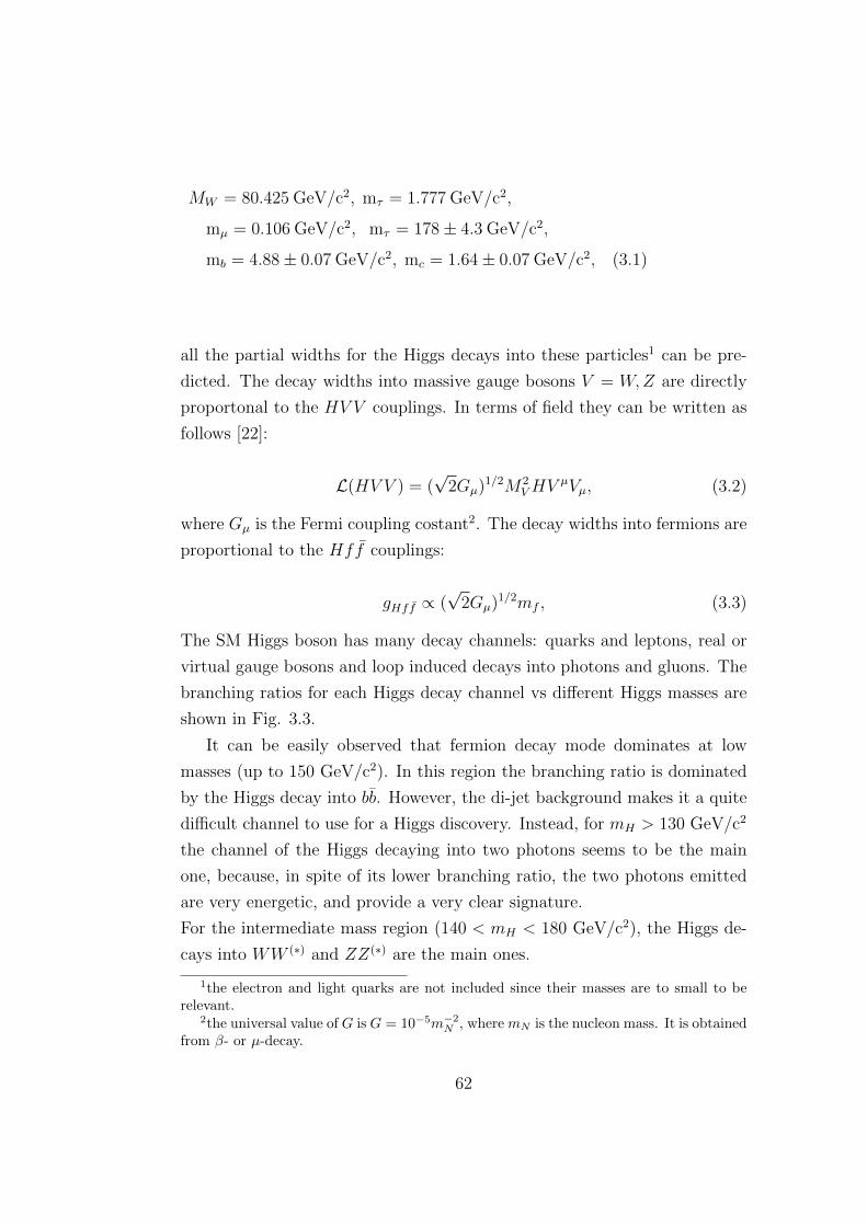
MW = 80.425 GeV/c2, mτ = 1.777 GeV/c2,

mµ = 0.106 GeV/c2, mτ = 178± 4.3 GeV/c2,

mb = 4.88± 0.07 GeV/c2, mc = 1.64± 0.07 GeV/c2, (3.1)

all the partial widths for the Higgs decays into these particles1 can be pre-

dicted. The decay widths into massive gauge bosons V = W,Z are directly

proportonal to the HV V couplings. In terms of field they can be written as

follows [22]:

L(HV V ) = (√

2Gµ)1/2M2VHV

µVµ, (3.2)

where Gµ is the Fermi coupling costant2. The decay widths into fermions are

proportional to the Hff couplings:

gHff ∝ (√

2Gµ)1/2mf , (3.3)

The SM Higgs boson has many decay channels: quarks and leptons, real or

virtual gauge bosons and loop induced decays into photons and gluons. The

branching ratios for each Higgs decay channel vs different Higgs masses are

shown in Fig. 3.3.

It can be easily observed that fermion decay mode dominates at low

masses (up to 150 GeV/c2). In this region the branching ratio is dominated

by the Higgs decay into bb. However, the di-jet background makes it a quite

difficult channel to use for a Higgs discovery. Instead, for mH > 130 GeV/c2

the channel of the Higgs decaying into two photons seems to be the main

one, because, in spite of its lower branching ratio, the two photons emitted

are very energetic, and provide a very clear signature.

For the intermediate mass region (140 < mH < 180 GeV/c2), the Higgs de-

cays into WW (∗) and ZZ(∗) are the main ones.

1the electron and light quarks are not included since their masses are to small to berelevant.

2the universal value of G is G = 10−5m−2N , where mN is the nucleon mass. It is obtained

from β- or µ-decay.

62

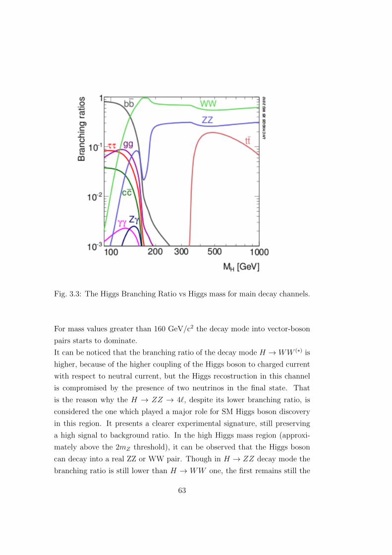
Fig. 3.3: The Higgs Branching Ratio vs Higgs mass for main decay channels.

For mass values greater than 160 GeV/c2 the decay mode into vector-boson

pairs starts to dominate.

It can be noticed that the branching ratio of the decay mode H → WW (∗) is

higher, because of the higher coupling of the Higgs boson to charged current

with respect to neutral current, but the Higgs recostruction in this channel

is compromised by the presence of two neutrinos in the final state. That

is the reason why the H → ZZ → 4`, despite its lower branching ratio, is

considered the one which played a major role for SM Higgs boson discovery

in this region. It presents a clearer experimental signature, still preserving

a high signal to background ratio. In the high Higgs mass region (approxi-

mately above the 2mZ threshold), it can be observed that the Higgs boson

can decay into a real ZZ or WW pair. Though in H → ZZ decay mode the

branching ratio is still lower than H → WW one, the first remains still the

63

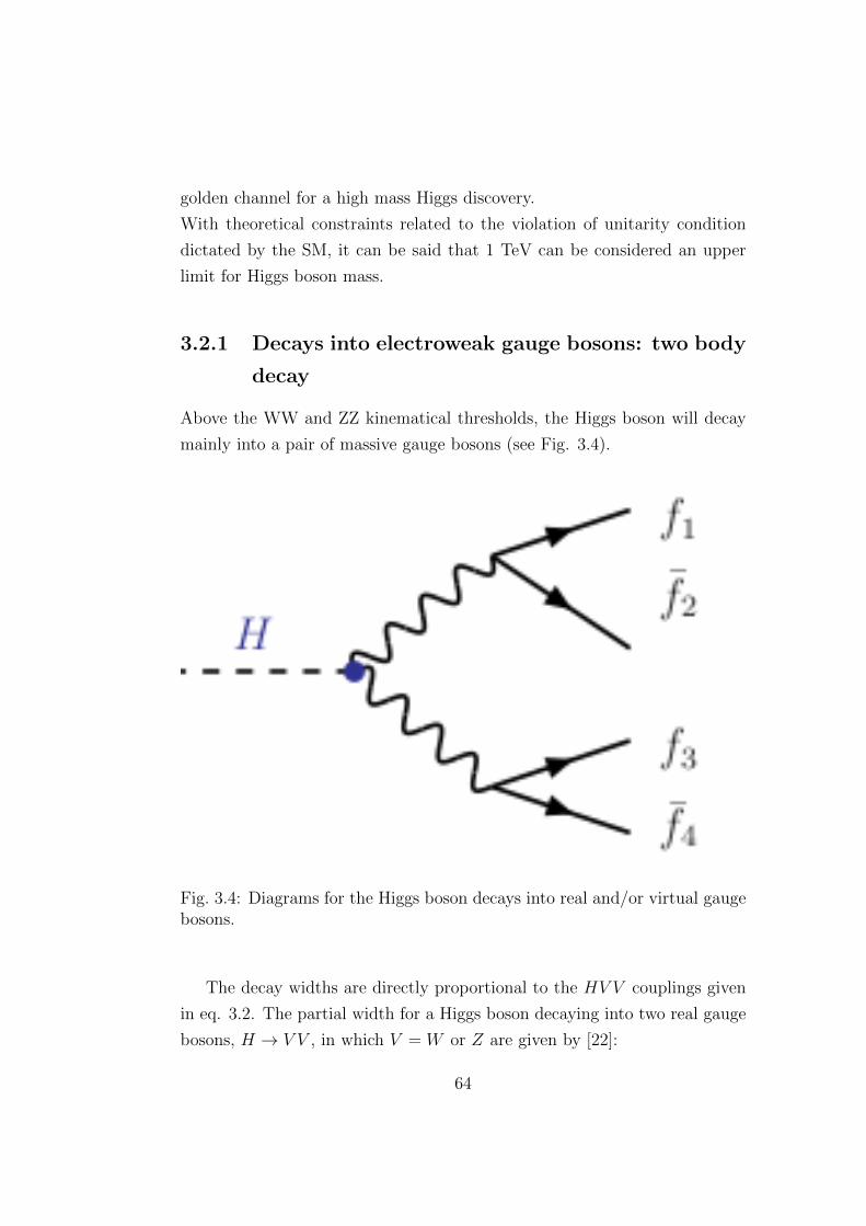
golden channel for a high mass Higgs discovery.

With theoretical constraints related to the violation of unitarity condition

dictated by the SM, it can be said that 1 TeV can be considered an upper

limit for Higgs boson mass.

3.2.1 Decays into electroweak gauge bosons: two body

decay

Above the WW and ZZ kinematical thresholds, the Higgs boson will decay

mainly into a pair of massive gauge bosons (see Fig. 3.4).

Fig. 3.4: Diagrams for the Higgs boson decays into real and/or virtual gaugebosons.

The decay widths are directly proportional to the HV V couplings given

in eq. 3.2. The partial width for a Higgs boson decaying into two real gauge

bosons, H → V V , in which V = W or Z are given by [22]:

64

Γ(H → V V ) =GµM

3H

16√

2πδV√

1− 4x(1− 4x+ 12x2) (3.4)

where x = M2V /M

2H , δW = 2 and δW = 1. It can be noticed that for large

Higgs boson mass values, the decay width into WW bosons is two times

larger than the decay width into ZZ and the respective branching ratios for

the decays would be 2/3 and 1/3 if other decay channels are kinematically

forbidden. One can also observe that a heavy Higgs boson would be “obese”

since its total decay width would become comparable to its mass

Γ(H → WW + ZZ) ∼ 0.5 TeV[MH/1 TeV]3 (3.5)

and behaves as a resonance.

3.3 Monte Carlo samples

Both Higgs boson signal samples and a large number of electroweak and

QCD-induced SM background processes have been simulated using Monte

Carlo (MC) techniques.

The signal and background samples have been used for the definition and

the optimization of the event selection strategy prior to the analysis of the

experimental data, for comparisons with the real measurements, for the eval-

uation of acceptance corrections and for studies about systematics.

The backgrounds for this analysis include indistinguishable 4` contributions

from di-boson production, via the production mechanisms qq → ZZ(∗) and

gg → ZZ(∗), as well as instrumental backgrounds. For instrumental back-

ground we mean the background that has to be considered because of the

limitations in the performance of the detectors. These can cause hadronic

jets or secondary leptons from heavy meson decays to be misidentified as

primary leptons.

The analysis discussed in this work will focus on reconstructed final states

with only electrons or muons in the final state.

The main possible sources of instrumental background are:

65

• Z + light jets production with Z→ `+`− decays;

• Zbb (and Zcc) associated production with Z→ `+`− decays;

• the production of top quark pairs in the decay mode tt → WbWb →`+`−ννbb.

Other contributions to multiple jet production from QCD hard interac-

tions need also to be considered in early stages of the analysis, as well as

other di-boson (WW, WZ, Zγ) and single top backgrounds.

Signal and background processes cross sections are all re-weighted, at least, to

NLO. For the Higgs production mechanism via gluon fusion, NNLO+NNLL

calculations of the cross sections are included.

Several Monte Carlo event generators has been used:

• The multi-purpose generator PYTHIA [57], for example, has been used

for reproducing several processes such as QCD multijet production and

hard process at leading order (LO). For hard processes generated at

higher orders, it is used only for the showering, the hadronization, the

decays, and the simulation of the underlying event 3. In general, PYTHIA

can be used to generate high-energy ‘events’, i.e. sets of outgoing par-

ticles produced in the interactions between incoming particles. An

accurate representation of event properties in a wide range of reactions

can so be provided.

• The MadGraph (MadEvent) Monte Carlo event generators [23] has been

used to generate multi-parton amplitudes and some background events.

• The POWHEG NLO generator [53] has been used for the Higgs boson

signal and for the ZZ and tt background.

• The dedicated tool GG2ZZ [55] has been used to generate the gg → ZZ

contribution to the ZZ cross section.

3The “underlying event (UE) is defined as those aspects of a hadronic interactionattributed not to the hard scattering process, but rather to the accompanying interactionsof the rest of the proton.

66

The tool “PYTHIA tune Z2” [54], which relies on pT -ordered showers, has been

used for the underlying event. The tools CTEQ6M [34] and CT10 [30] have

been used for the parton density function of the colliding protons.

They are summerized along with the datasets in table 3.1.

In the following paragraphs some details about MC signal and background

samples is provided.

Signal: H→ ZZ(∗) → 4`

The Higgs boson samples used are generated with POWHEG, which includes

NLO gluon fusion (gg → H) and weak-boson fusion qq → qqH. Additional

samples with WH, ZH and ttH associated production are also used and pro-

duced with PYTHIA event generator.

The Higgs boson is forced to decay into two Z-bosons, which are allowed to

be off-mass shell, and both Z-bosons are forced to decay into two leptons

via Z→ 2`. A re-weighting procedure has been applied to generated events

according the total cross section σ(pp→ H) which includes the gluon fusion

contribution up to NNLO and NNLL [34, 8, 20, 21, 39, 46, 7, 58, 52, 48] and

the weak-boson fusion contribution at NNLO [34, 36, 37, 56, 32, 41]. The

total cross section is scaled by the BR(H → 4`) [34, 2, 1, 4, 49]. Figure 3.5

shows the number of MC expected events with an integrated luminosity of

L = 5 fb−1 as a function of the Higgs mass.

The current analysis has been performed using only samples for gluon fusion

production mechanism and rescaled to the total cross section including all

other production processes (weak-boson fusion, WH, ZH and ttH associated

production).

The POWHEG MC program used to simulate the gg → H process results in

a Higgs Boson pT spectrum which differs significantly from the theoretical

calculation that is available at NNLL+NLO. A theoretical estimate of this

pT spectrum is computed using the HqT [29] program, which implements such

NNLL+NLO calculation.

A re-weighting procedure has also been applied to the simulated events, but

the total effect has been found very small. In this analysis, indeed, no direct

67

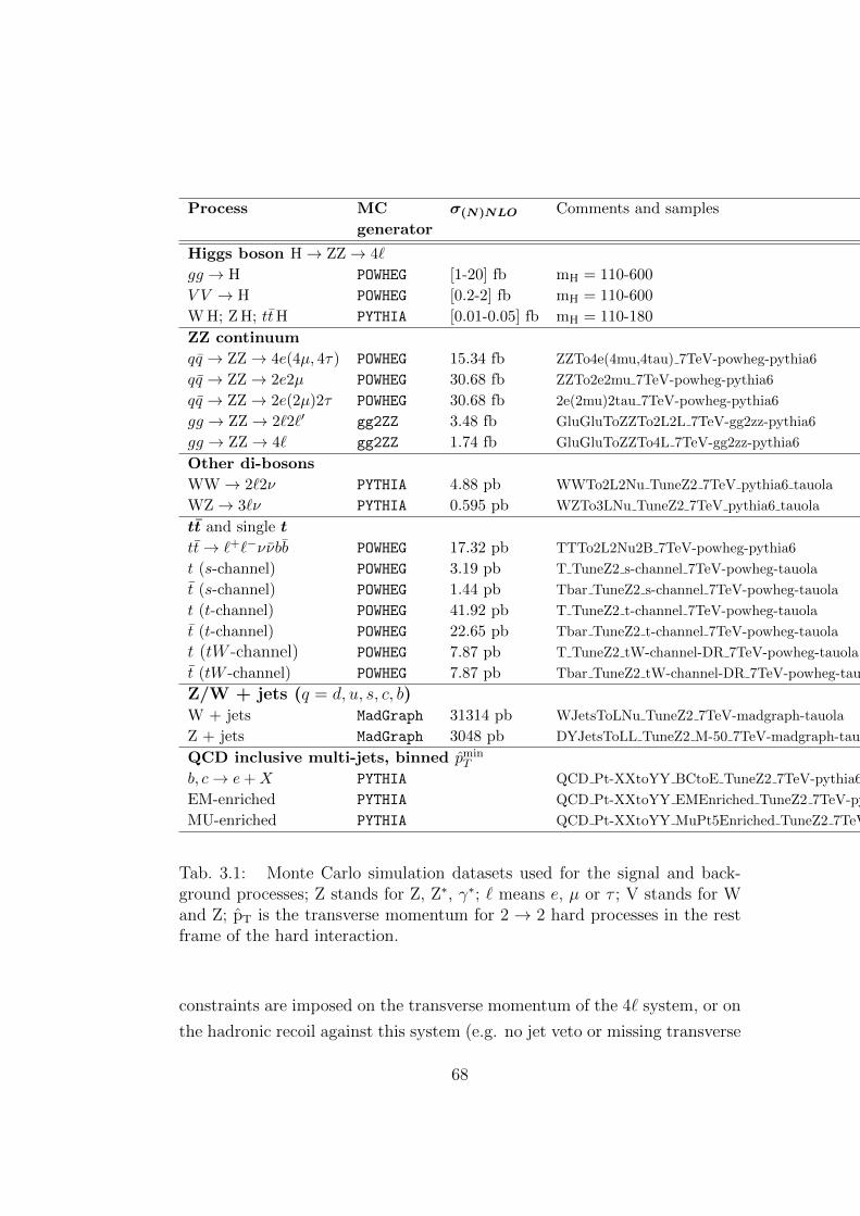
Process MC σ(N)NLO Comments and samples

generator

Higgs boson H→ ZZ→ 4`

gg → H POWHEG [1-20] fb mH = 110-600

V V → H POWHEG [0.2-2] fb mH = 110-600

W H; Z H; ttH PYTHIA [0.01-0.05] fb mH = 110-180

ZZ continuum

qq → ZZ→ 4e(4µ, 4τ) POWHEG 15.34 fb ZZTo4e(4mu,4tau) 7TeV-powheg-pythia6

qq → ZZ→ 2e2µ POWHEG 30.68 fb ZZTo2e2mu 7TeV-powheg-pythia6

qq → ZZ→ 2e(2µ)2τ POWHEG 30.68 fb 2e(2mu)2tau 7TeV-powheg-pythia6

gg → ZZ→ 2`2`′ gg2ZZ 3.48 fb GluGluToZZTo2L2L 7TeV-gg2zz-pythia6

gg → ZZ→ 4` gg2ZZ 1.74 fb GluGluToZZTo4L 7TeV-gg2zz-pythia6

Other di-bosons

WW→ 2`2ν PYTHIA 4.88 pb WWTo2L2Nu TuneZ2 7TeV pythia6 tauola

WZ→ 3`ν PYTHIA 0.595 pb WZTo3LNu TuneZ2 7TeV pythia6 tauola

tt and single t

tt→ `+`−ννbb POWHEG 17.32 pb TTTo2L2Nu2B 7TeV-powheg-pythia6

t (s-channel) POWHEG 3.19 pb T TuneZ2 s-channel 7TeV-powheg-tauola

t (s-channel) POWHEG 1.44 pb Tbar TuneZ2 s-channel 7TeV-powheg-tauola

t (t-channel) POWHEG 41.92 pb T TuneZ2 t-channel 7TeV-powheg-tauola

t (t-channel) POWHEG 22.65 pb Tbar TuneZ2 t-channel 7TeV-powheg-tauola

t (tW -channel) POWHEG 7.87 pb T TuneZ2 tW-channel-DR 7TeV-powheg-tauola

t (tW -channel) POWHEG 7.87 pb Tbar TuneZ2 tW-channel-DR 7TeV-powheg-tauola

Z/W + jets (q = d, u, s, c, b)W + jets MadGraph 31314 pb WJetsToLNu TuneZ2 7TeV-madgraph-tauola

Z + jets MadGraph 3048 pb DYJetsToLL TuneZ2 M-50 7TeV-madgraph-tauola

QCD inclusive multi-jets, binned pminT

b, c→ e+X PYTHIA QCD Pt-XXtoYY BCtoE TuneZ2 7TeV-pythia6

EM-enriched PYTHIA QCD Pt-XXtoYY EMEnriched TuneZ2 7TeV-pythia6

MU-enriched PYTHIA QCD Pt-XXtoYY MuPt5Enriched TuneZ2 7TeV-pythia6

Tab. 3.1: Monte Carlo simulation datasets used for the signal and back-ground processes; Z stands for Z, Z∗, γ∗; ` means e, µ or τ ; V stands for Wand Z; pT is the transverse momentum for 2 → 2 hard processes in the restframe of the hard interaction.

constraints are imposed on the transverse momentum of the 4` system, or on

the hadronic recoil against this system (e.g. no jet veto or missing transverse

68

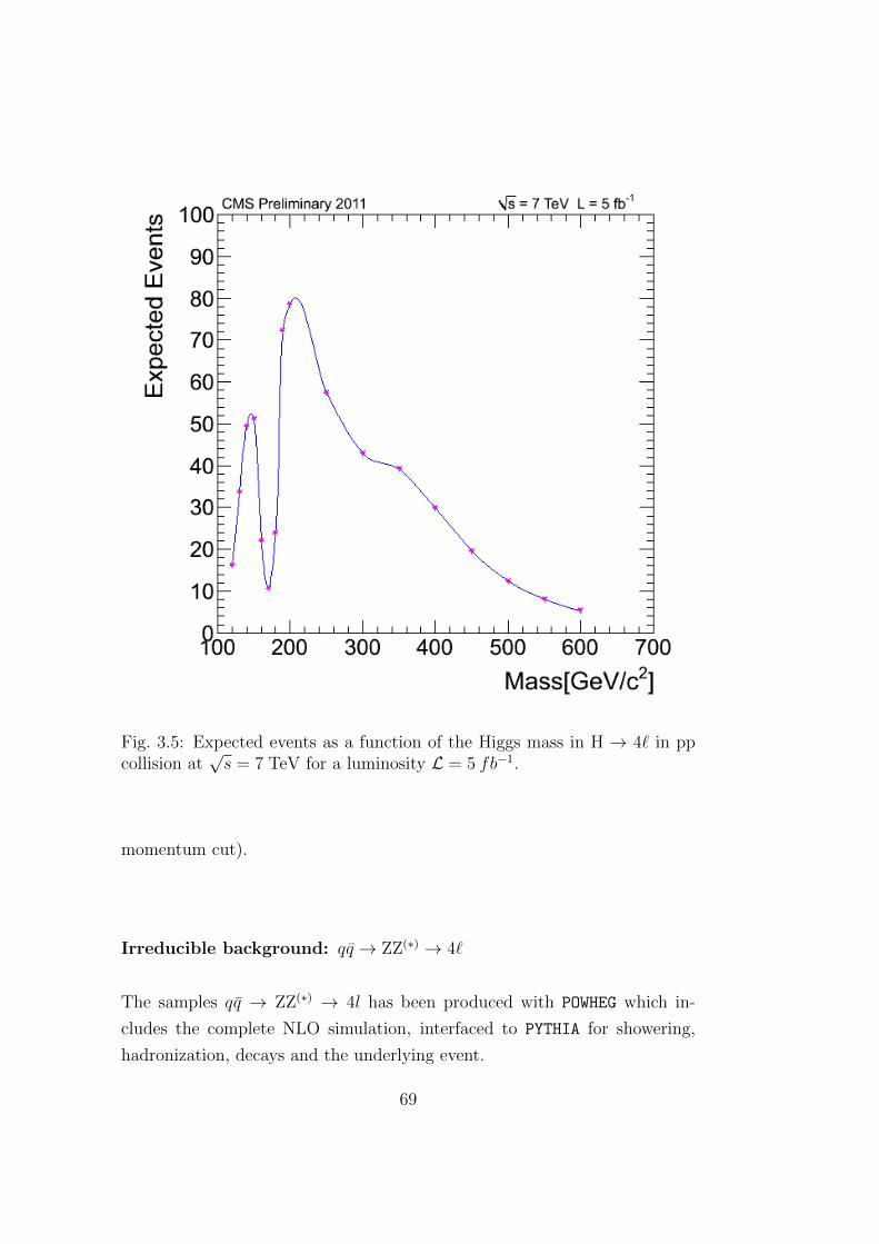
Fig. 3.5: Expected events as a function of the Higgs mass in H → 4` in ppcollision at

√s = 7 TeV for a luminosity L = 5 fb−1.

momentum cut).

Irreducible background: qq → ZZ(∗) → 4`

The samples qq → ZZ(∗) → 4l has been produced with POWHEG which in-

cludes the complete NLO simulation, interfaced to PYTHIA for showering,

hadronization, decays and the underlying event.

69

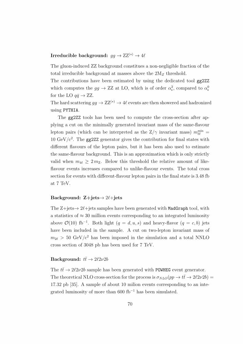
Irreducible background: gg → ZZ(∗) → 4`

The gluon-induced ZZ background constitues a non-negligible fraction of the

total irreducible background at masses above the 2MZ threshold.

The contributions have been estimated by using the dedicated tool gg2ZZ

which computes the gg → ZZ at LO, which is of order α2s , compared to α0

s

for the LO qq → ZZ.

The hard scattering gg → ZZ(∗) → 4` events are then showered and hadronized

using PYTHIA.

The gg2ZZ tools has been used to compute the cross-section after ap-

plying a cut on the minimally generated invariant mass of the same-flavour

lepton pairs (which can be interpreted as the Z/γ invariant mass) mmin`` =

10 GeV/c2. The gg2ZZ generator gives the contribution for final states with

different flavours of the lepton pairs, but it has been also used to estimate

the same-flavour background. This is an approximation which is only strictly

valid when m4` ≥ 2mZ. Below this threshold the relative amount of like-

flavour events increases compared to unlike-flavour events. The total cross

section for events with different-flavour lepton pairs in the final state is 3.48 fb

at 7 TeV.

Background: Z+jets→ 2`+jets

The Z+jets→ 2`+jets samples have been generated with MadGraph tool, with

a statistics of ≈ 30 million events corresponding to an integrated luminosity

above O(10) fb−1. Both light (q = d, u, s) and heavy-flavor (q = c, b) jets

have been included in the sample. A cut on two-lepton invariant mass of

m2` > 50 GeV/c2 has been imposed in the simulation and a total NNLO

cross section of 3048 pb has been used for 7 TeV.

Background: tt→ 2`2ν2b

The tt→ 2`2ν2b sample has been generated with POWHEG event generator.

The theoretical NLO cross-section for the process is σNLO(pp→ tt→ 2`2ν2b) =

17.32 pb [35]. A sample of about 10 milion events corresponding to an inte-

grated luminosity of more than 600 fb−1 has been simulated.

70

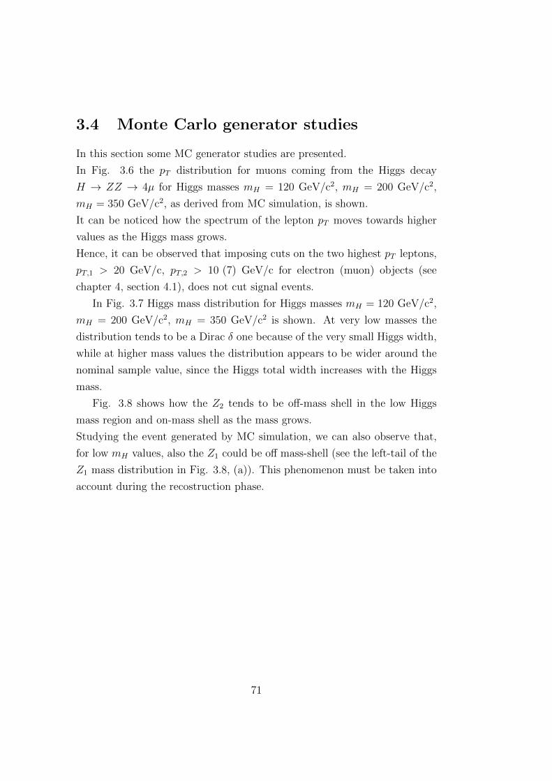
3.4 Monte Carlo generator studies

In this section some MC generator studies are presented.

In Fig. 3.6 the pT distribution for muons coming from the Higgs decay

H → ZZ → 4µ for Higgs masses mH = 120 GeV/c2, mH = 200 GeV/c2,

mH = 350 GeV/c2, as derived from MC simulation, is shown.

It can be noticed how the spectrum of the lepton pT moves towards higher

values as the Higgs mass grows.

Hence, it can be observed that imposing cuts on the two highest pT leptons,

pT,1 > 20 GeV/c, pT,2 > 10 (7) GeV/c for electron (muon) objects (see

chapter 4, section 4.1), does not cut signal events.

In Fig. 3.7 Higgs mass distribution for Higgs masses mH = 120 GeV/c2,

mH = 200 GeV/c2, mH = 350 GeV/c2 is shown. At very low masses the

distribution tends to be a Dirac δ one because of the very small Higgs width,

while at higher mass values the distribution appears to be wider around the

nominal sample value, since the Higgs total width increases with the Higgs

mass.

Fig. 3.8 shows how the Z2 tends to be off-mass shell in the low Higgs

mass region and on-mass shell as the mass grows.

Studying the event generated by MC simulation, we can also observe that,

for low mH values, also the Z1 could be off mass-shell (see the left-tail of the

Z1 mass distribution in Fig. 3.8, (a)). This phenomenon must be taken into

account during the recostruction phase.

71

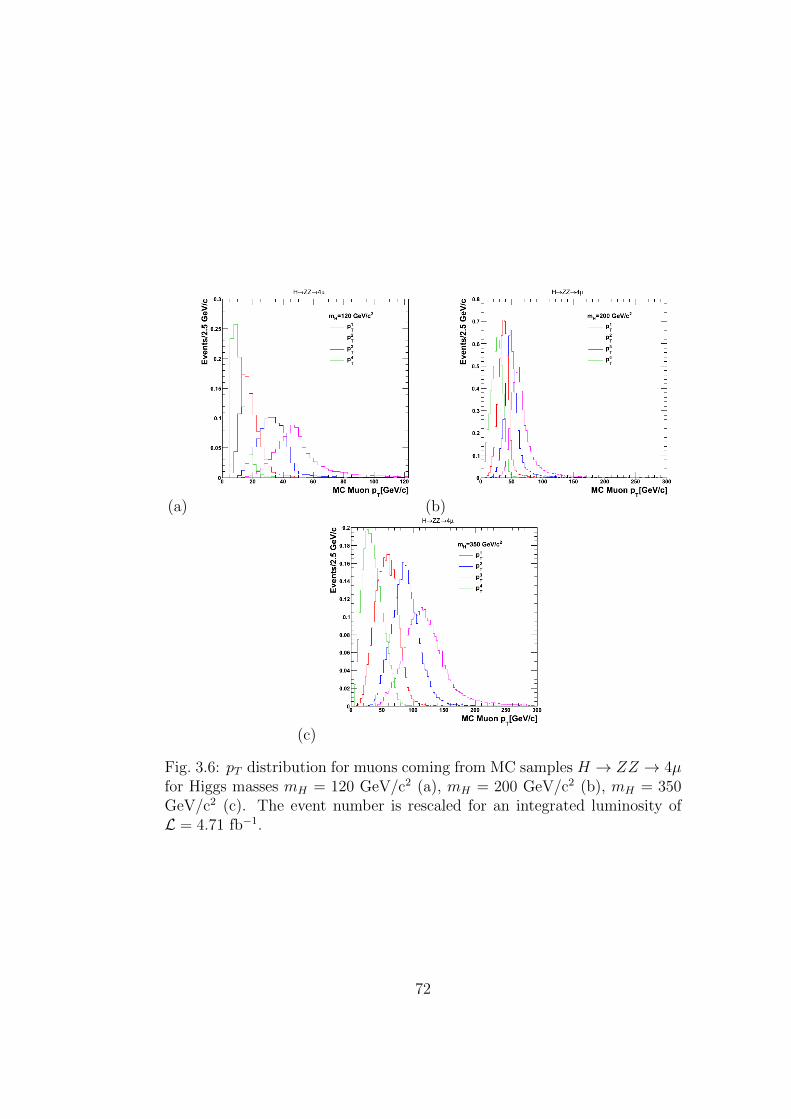
(a) (b)

(c)

Fig. 3.6: pT distribution for muons coming from MC samples H → ZZ → 4µfor Higgs masses mH = 120 GeV/c2 (a), mH = 200 GeV/c2 (b), mH = 350GeV/c2 (c). The event number is rescaled for an integrated luminosity ofL = 4.71 fb−1.

72

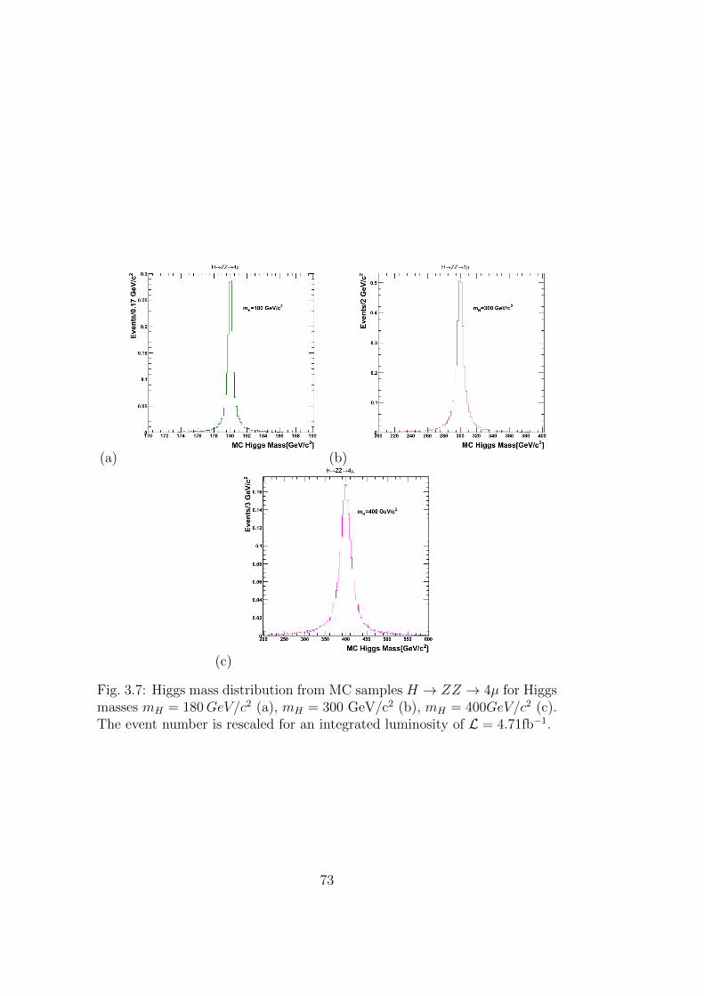
(a) (b)

(c)

Fig. 3.7: Higgs mass distribution from MC samples H → ZZ → 4µ for Higgsmasses mH = 180GeV/c2 (a), mH = 300 GeV/c2 (b), mH = 400GeV/c2 (c).The event number is rescaled for an integrated luminosity of L = 4.71fb−1.

73

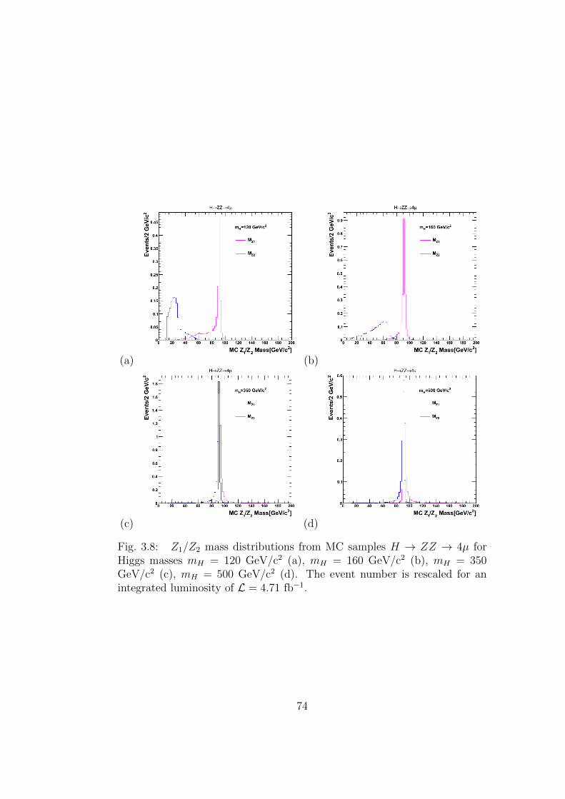
(a) (b)

(c) (d)

Fig. 3.8: Z1/Z2 mass distributions from MC samples H → ZZ → 4µ forHiggs masses mH = 120 GeV/c2 (a), mH = 160 GeV/c2 (b), mH = 350GeV/c2 (c), mH = 500 GeV/c2 (d). The event number is rescaled for anintegrated luminosity of L = 4.71 fb−1.

74

Chapter 4

Data Analysis

In this chapter the analysis selection developed to perform an experimental

search for the Higgs boson in the decay channel H → ZZ(∗) → 4`, with each

Z boson decaying into a muon or electron pair, is presented. It is carried out

using proton-proton (pp) collisions from LHC at√s = 7 TeV. The data col-

lected correspond to an integrated luminosity L = 4.71± 0.21 fb−1 recorded

by CMS detector during 2010 and 2011.

The Higgs boson mass window covered by this analysis is 110 < mH < 600

GeV/c2. Dealing with Higgs bosons with masses mH < 2mZ , at least one

lepton pair can be coupled to an off-mass shell Z∗ boson. The softest lepton

in that pair typically has p`T < 10 GeV/c for masses mH < 140 GeV/c2.

Because of the presence of four leptons in the final state, a high-performance

lepton recostruction, identification and isolation, along with excellent lepton

energy-momentum mesurements, is mandatory. A substantial reduction of

QCD-induced sources of mis-identified (“fake”) leptons has been realized by

identifying isolated leptons coming from the event primary vertex.

High precision energy-momentum measurements allow to obtain a good res-

olution on the reconstructed mass m4`, which is the most important observ-

able for the Higgs boson search. It can be noticed that preserving the highest

possible reconstruction efficiency and ensuring, at the same time, sufficient

discrimination against hadronic jets is particulary challenging for the recon-

struction of leptons with low p`T .

A special method called “tag-and-probe” [12] allows us to measure that ef-

ficiency from data and MC and keep full control of the behaviour at very

75

low p`T values. In this range the combined information from the tracker and

the electromagnetic calorimeter (for electrons) and from the tracker and the

muon spectrometer (for muons) plays the most important role for lepton

reconstruction, identification and isolation.

4.1 Experimental Data samples

The data sample used for this analysis has been recorded by the CMS exper-

iment during 2010 and 2011.

The CMS standard selection of runs and luminosity sections has been ap-

plied, since it assures high quality data.

The validation of the data used for the analysis of the 4e, 4µ and 2e2µ chan-

nels has been guaranteed by detector operation conditions. Only certified

data have been used.

The monitoring and certification of the quality of the CMS data consists

of a multi-step procedure, which goes from online data taking to the offline

reprocessing of data recorded earlier.

The quality assessment is based both on visual inspection of data distribu-

tions by monitoring shift persons and on algorithmic tests of the distributions

against references.

The Run Registry (RR) is the central workflow management and tracking

tool used for collected data certification. It keeps track of the certification

results and make them available to the whole CMS collaboration. It is reg-

ularly used for the creation of official good-run list files which are used as

input to downstream selection of the data for re-processings and for physics

analyses.

Events have been required to pass double lepton (ee, eµ, µµ) High Level Trig-

gers (HLT) with a transverse momentum (pT ) threshold on each lepton and

additional selection criteria that changed during the data taking according

to the instantaneous luminosity and the available data taking bandwidth.

Given the high probability of jets to fake electrons, double electron events

have been selected with more complicated criteria based not only on the elec-

trons transverse momentum but also on their isolation and identification.

76

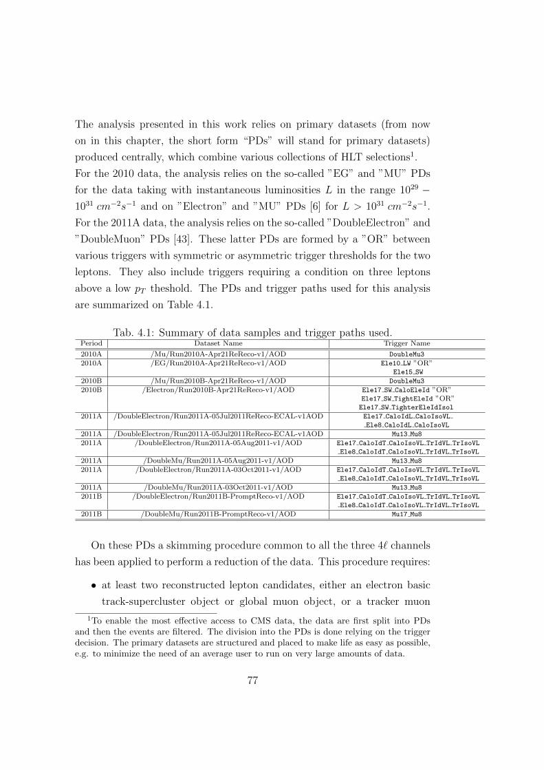
The analysis presented in this work relies on primary datasets (from now

on in this chapter, the short form “PDs” will stand for primary datasets)

produced centrally, which combine various collections of HLT selections1.

For the 2010 data, the analysis relies on the so-called ”EG” and ”MU” PDs

for the data taking with instantaneous luminosities L in the range 1029 −1031 cm−2s−1 and on ”Electron” and ”MU” PDs [6] for L > 1031 cm−2s−1.

For the 2011A data, the analysis relies on the so-called ”DoubleElectron” and

”DoubleMuon” PDs [43]. These latter PDs are formed by a ”OR” between

various triggers with symmetric or asymmetric trigger thresholds for the two

leptons. They also include triggers requiring a condition on three leptons

above a low pT theshold. The PDs and trigger paths used for this analysis

are summarized on Table 4.1.

Tab. 4.1: Summary of data samples and trigger paths used.Period Dataset Name Trigger Name

2010A /Mu/Run2010A-Apr21ReReco-v1/AOD DoubleMu3

2010A /EG/Run2010A-Apr21ReReco-v1/AOD Ele10 LW ”OR”Ele15 SW

2010B /Mu/Run2010B-Apr21ReReco-v1/AOD DoubleMu3

2010B /Electron/Run2010B-Apr21ReReco-v1/AOD Ele17 SW CaloEleId ”OR”Ele17 SW TightEleId ”OR”Ele17 SW TighterEleIdIsol

2011A /DoubleElectron/Run2011A-05Jul2011ReReco-ECAL-v1AOD Ele17 CaloIdL CaloIsoVL

Ele8 CaloIdL CaloIsoVL

2011A /DoubleElectron/Run2011A-05Jul2011ReReco-ECAL-v1AOD Mu13 Mu8

2011A /DoubleElectron/Run2011A-05Aug2011-v1/AOD Ele17 CaloIdT CaloIsoVL TrIdVL TrIsoVL

Ele8 CaloIdT CaloIsoVL TrIdVL TrIsoVL

2011A /DoubleMu/Run2011A-05Aug2011-v1/AOD Mu13 Mu8

2011A /DoubleElectron/Run2011A-03Oct2011-v1/AOD Ele17 CaloIdT CaloIsoVL TrIdVL TrIsoVL

Ele8 CaloIdT CaloIsoVL TrIdVL TrIsoVL

2011A /DoubleMu/Run2011A-03Oct2011-v1/AOD Mu13 Mu8

2011B /DoubleElectron/Run2011B-PromptReco-v1/AOD Ele17 CaloIdT CaloIsoVL TrIdVL TrIsoVL

Ele8 CaloIdT CaloIsoVL TrIdVL TrIsoVL

2011B /DoubleMu/Run2011B-PromptReco-v1/AOD Mu17 Mu8

On these PDs a skimming procedure common to all the three 4` channels

has been applied to perform a reduction of the data. This procedure requires:

• at least two reconstructed lepton candidates, either an electron basic

track-supercluster object or global muon object, or a tracker muon

1To enable the most effective access to CMS data, the data are first split into PDsand then the events are filtered. The division into the PDs is done relying on the triggerdecision. The primary datasets are structured and placed to make life as easy as possible,e.g. to minimize the need of an average user to run on very large amounts of data.

77

object;

• pT,1 > 20 GeV/c, pT,2 > 10 (7) GeV/c for electron (muon) objects;

• an invariant mass M1,2 > 40 GeV/c2

In the next section an overview of the physics objects involved in the

analysis will be shown, paying attention to the recostruction, identification

and isolation for each of them.

4.2 Physics Objects: Electrons and Muons

4.2.1 Lepton Identification

Electrons

A high electron identification efficiency [51] is required in physics analysis

with multi-electron final states just to improve signal selection, in particular

at low ET , where the background and, consequently, the fake rate (rate of

jets reconstructed as electrons, “fake” electrons) increases.

The electron identification largely depends on some CMS detector features,

such as high magnetic field, a thick tracker and lower ECAL response to

pions with respect to electrons.

The electron categories, already presented in the subsection 2.3.1, have been

originally proposed for electron selection and used for the best momentum

determination in the electron recostruction. For instance, electrons coming

from W and Z can be distinguished from other particles due to their feature

of being primarily measured in the ECAL and tracker. The electron track

would match pretty well in position and momentum with the cluster of en-

ergy found in the ECAL.

The electron identification makes use of a set of variables to distinguish be-

tween real electrons and electrons from background. Some of them have

been already mentioned in the reconstruction section (the hadronic to elec-

tromagnetic ratio H/E, the energy-momentum matching variables between

the energy of the supercluster or of the supercluster seed and the electron

78

track momentum at the vertex or at the calorimeter, the geometrical match-

ing between the electron track parameters at the vertex extrapolated to the

supercluster and the supercluster position, see chapter 2 subsection 2.3.1).

In addition to them, the calorimeter shower shape variables can be included.

To cope with the high photon conversion rate due to the material budget in

front of the ECAL, cuts on the impact parameter d0 (the distance between

the track at the point of closest approach and the reconstructed primary ver-

tex) and on missing hits (number of crossed layers without compatible hits

in the back-propagation of the track to the beam line) are applied. Finally,

the performance of electron identification depends on the degree of isolation

imposed on the electron candidates.

Not isolated electrons, i.e. electrons in jets, are reconstructed and identi-

fied using a dedicated particle-flow clustering algorithm which, exploiting

the good ECAL granularity, can saparate overlapping showers. The low pT

electrons are better reconstructed and identified using the same technique

developed for non-isolated electrons.

Muons

Many phenomena can lead to an incorrect muon identification [38]. They

can be classified under several categories.

Fake muon signatures are typically produced by light hadron such as pions

and kaons which are abundantly present in any high energy collision final

state. We call fake muon any reconstructed muon, passing whatever cuts

applied, that is recostructed in single pion or kaon events. Thus, a muon

from a K → µ decay in flight is a fake muon. Fake muon signals in the muon

chambers can also be originated from the leakage of secondary particles pro-

duced in hadronic interactions in the calorimeter. This case is denoted as

punch-through.

The need of establishing the muon identification (muon-ID) can be well

enough illustrated in plots in Fig. 4.1. Here the probability that a gen-

erated kaon/pion of |η| < 2.4 results in a reconstructed muon versus global

and tracker muon pT is presented.

79

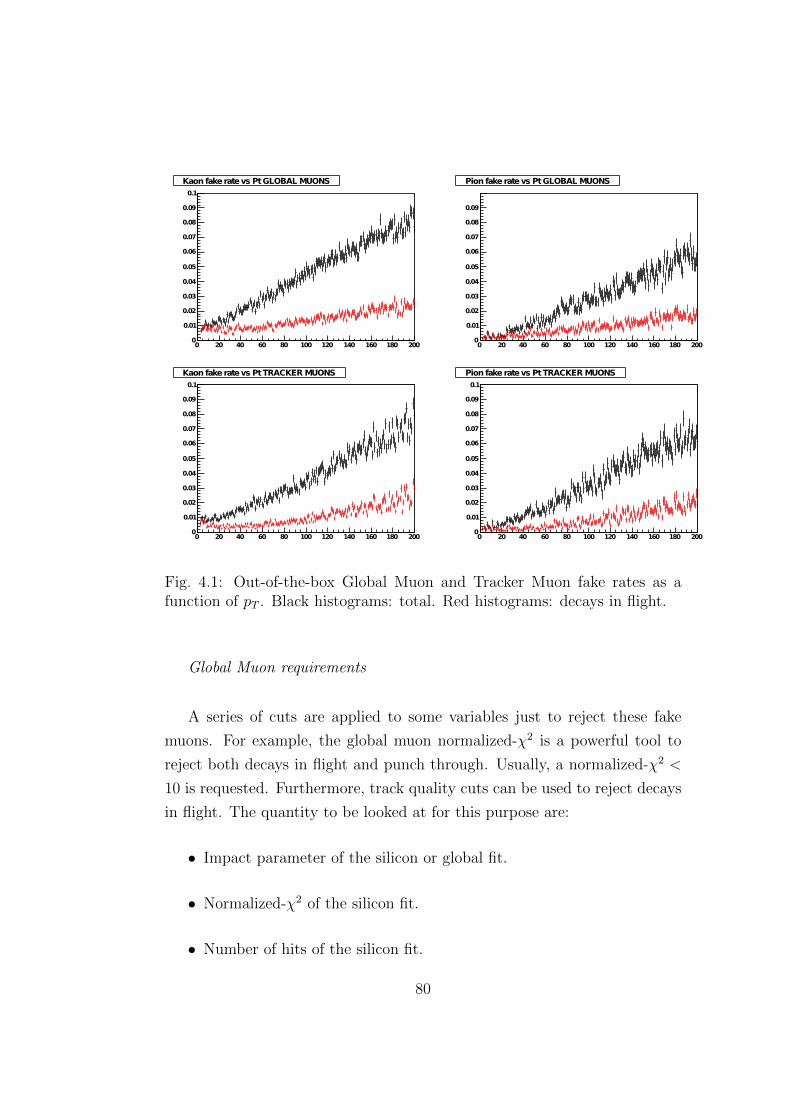
0 20 40 60 80 100 120 140 160 180 2000

0.01

0.02

0.03

0.04

0.05

0.06

0.07

0.08

0.09

0.1

Kaon fakeratevs PtGLOBALMUONS

0 20 40 60 80 100 120 140 160 180 2000

0.01

0.02

0.03

0.04

0.05

0.06

0.07

0.08

0.09

Pion fakeratevs PtGLOBALMUONS

0 20 40 60 80 100 120 140 160 180 2000

0.01

0.02

0.03

0.04

0.05

0.06

0.07

0.08

0.09

0.1

Kaon fakeratevs PtTRACKERMUONS

0 20 40 60 80 100 120 140 160 180 2000

0.01

0.02

0.03

0.04

0.05

0.06

0.07

0.08

0.09

0.1

Pion fakeratevs PtTRACKERMUONS

Fig. 4.1: Out-of-the-box Global Muon and Tracker Muon fake rates as afunction of pT . Black histograms: total. Red histograms: decays in flight.

Global Muon requirements

A series of cuts are applied to some variables just to reject these fake

muons. For example, the global muon normalized-χ2 is a powerful tool to

reject both decays in flight and punch through. Usually, a normalized-χ2 <

10 is requested. Furthermore, track quality cuts can be used to reject decays

in flight. The quantity to be looked at for this purpose are:

• Impact parameter of the silicon or global fit.

• Normalized-χ2 of the silicon fit.

• Number of hits of the silicon fit.

80

It can be worth to remind that a set of five helix parameters can describe a

track in the solenoidal magnetic field:

• the transverse momentum pT

• the azimuthal angle φ

• the pseudorapidity η

• the transverse impact parameter d0, which is the distance of the tra-

jectory from the origin (conventionally the origin is the primary inter-

action vertex) calculated in the point of closest approach (poca)

• the logitudinal impact parameter r0

A loose d0 cut is very efficient for prompt muons, i.e. muons coming from

primary vertex, because it allows to reject a significant fraction of decays in

flight. High-pT muons penetrate deeply into the muon detector and very few

of the global fits for real muons end in the first layer of the barrel detec-

tor. On the contrary, this just often happens for kaons and pions, even after

all the requirements. Rejecting these muons almost a 20% reduction of the

fake rate can be obtained with little cost in efficiency. The muon segment

compatibility is also checked for ensuring muon-ID: in cases in which an ex-

trapolated track passes through a muon station but no associated segment is

found, the muon object stores the distance between the extrapolated track

position and the closest chamber edge. The value of this distance divided by

the multiple scattering uncertainty is used as a measure of the probability

for a trajectory of a given track to deflect from inside to outside of a chamber

boundary or viceversa.

Tracker Muon requirements

Two approaches have been developed to Tracker Muon identification:

• a cut-based approach

81

• an approach based on the costruction of a continous variable, “com-

patibility”

In both cases, the algorithm performs a procedure called “arbitration”.

It has been already pointed out that the tracker muons are built by associat-

ing segments in the muon chambers with the silicon track. A given segment

can be associated to more than one silicon track, so that it can be said that

Tracker Muon can share segments. The arbitration procedure allow to assign

each segment to a unique Tracker Muon.

The arbitration algorithm is relied on the calculation of the quantity ∆R2 =

∆X2 + ∆Y 2, where ∆X and ∆Y are the distance between the extrapolated

silicon track and the segment in local X and Y coordinates. The smallest

∆R value corresponds to the segment uniquely associated to the Tracker

Muon. On the other hand, the aim of the muon compatibility algorithm is to

build a continous variable which can quantify the compatibility of a Tracker

Muon object with the muon hypothesis. Two such variables are constructed,

one based on calorimeter information and the other based on muon chamber

information. The two variables are then combined into a single one. The

cut-based requirements are found to be quite different from the compatibil-

ity ones because they do not require that energy in the towers crossed by

muons be compatible with minimum ionizing.

In the context of this analysis tracker muons have been only used for studies

about the background estimate.

4.2.2 Electrons and Muons Isolation

To establish an isolation criterium for leptons, a lepton track relative isolation

variable has been introduced. This is defined as the sum of the pT of the

tracker tracks within a cone of radius ∆R =√

∆η2 + ∆φ2 < 0.3 around the

lepton candidate direction. The standard veto regions have been used just

to remove the lepton footprint (called “Jurassic” veto in case of electrons).

Finally, other leptons that fall in one lepton isolation cone are also vetoed.

For the ECAL or HCAL, the isolation variable is defined as the sum that is

computed using the transverse energy ET from energy deposits in cells with

82

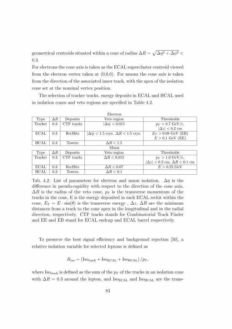
geometrical centroids situated within a cone of radius ∆R =√

∆η2 + ∆φ2 <

0.3.

For electrons the cone axis is taken as the ECAL supercluster centroid viewed

from the electron vertex taken at (0,0,0). For muons the cone axis is taken

from the direction of the associated inner track, with the apex of the isolation

cone set at the nominal vertex position.

The selection of tracker tracks, energy deposits in ECAL and HCAL used

in isolation cones and veto regions are specified in Table 4.2.

ElectronType ∆R Deposits Veto region Thresholds

Tracker 0.3 CTF tracks |∆η| < 0.015 pT > 0.7 GeV/c,|∆z| < 0.2 cm

ECAL 0.3 RecHits |∆η| < 1.5 crys. ∆R < 1.5 crys. ET > 0.08 GeV (EB)E > 0.1 GeV (EE)

HCAL 0.3 Towers ∆R < 1.5Muon

Type ∆R Deposits Veto region ThresholdsTracker 0.3 CTF tracks ∆R < 0.015 pT > 1.0 GeV/c,

|∆z| < 0.2 cm, ∆R < 0.1 cmECAL 0.3 RecHits ∆R < 0.07 E > 0.25 GeVHCAL 0.3 Towers ∆R < 0.1

Tab. 4.2: List of parameters for electron and muon isolation. ∆η is thedifference in pseudo-rapidity with respect to the direction of the cone axis,∆R is the radius of the veto cone, pT is the transverse momentum of thetracks in the cone, E is the energy deposited in each ECAL rechit within thecone, ET = E · sin(θ) is the transverse energy , ∆z, ∆R are the minimumdistances from a track to the cone apex in the longitudinal and in the radialdirection, respectively. CTF tracks stands for Combinatorial Track Finderand EE and EB stand for ECAL endcap and ECAL barrel respectively.

To preserve the best signal efficiency and background rejection [50], a

relative isolation variable for selected leptons is defined as

Riso = (Isotrack + IsoECAL + IsoHCAL) /pT ,

where Isotrack is defined as the sum of the pT of the tracks in an isolation cone

with ∆R = 0.3 around the lepton, and IsoECAL and IsoHCAL are the trans-

83

verse energies measured by the electromagnetic and the hadronic calorimeters

respectively in the same cone. The denominator represents the value of the

lepton pT .

Combining the measurements around two lepton legs ensures the best per-

formance for 4` physics. Hence, a cut on the sum of Riso for pairs of two

leptons i, j has been used, Riso,i +Riso,j < 0.35. Since the combined relative

isolation makes use of the information from the ECAL calorimeter within the

isolation cone of radius ∆R < 0.3, the efficiency loss caused by the presence

of a bremsstrahlung, or an initial state (ISR) or final state (FSR) photon

from the hard collision process must be taken into account.

The working point found for this analysis is sufficiently loose to minimize

the efficiency loss. The combined relative isolation used in the analysis cor-

responds on average to a cut per lepton of Riso ∼ 0.25.

The overall efficiency loss from FSR photons caused by an isolation veto is

estimated to be at most at the % level for the sum of the 4e, 4µ and 2e2µ

channels.

The ambiguities between reconstructed electrons and muons that arise from

the emission from an electron of a FSR photon above the superclustering

threshold of 1 GeV are resolved by discarding electron candidates whose

tracks are found fully shared with a muon candidate (a cone of ∆R = 0.05

around the muon candidate is used).

4.2.3 Pile-up Corrections

Isolation variables are among the mostly pile-up sensitive variables in this

analysis.

The pile-up is responsible for the increasing of mean energy deposited in

the detector, leading to the rise of the mean isolation values. So, it can be

observed that the efficiency of a cut on isolation variables strongly depends

on pile-up conditions. The effect is observed to have a very deep impact in

both the calorimeters (ECAL, HCAL) and to be very feeble in the tracking

system, mostly due to the requirement that the tracks contributing to the

isolation cone originate from a common vertex (∆z cut). Thus the isolation

84

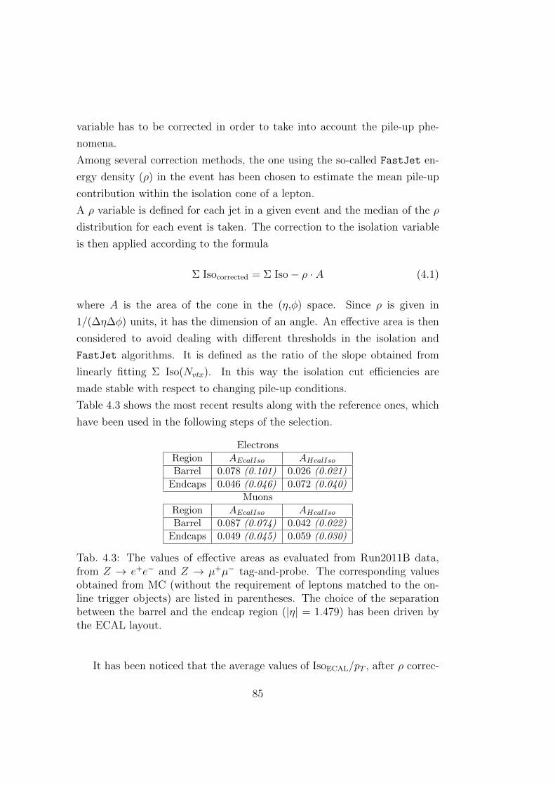
variable has to be corrected in order to take into account the pile-up phe-

nomena.

Among several correction methods, the one using the so-called FastJet en-

ergy density (ρ) in the event has been chosen to estimate the mean pile-up

contribution within the isolation cone of a lepton.

A ρ variable is defined for each jet in a given event and the median of the ρ

distribution for each event is taken. The correction to the isolation variable

is then applied according to the formula

Σ Isocorrected = Σ Iso− ρ · A (4.1)

where A is the area of the cone in the (η,φ) space. Since ρ is given in

1/(∆η∆φ) units, it has the dimension of an angle. An effective area is then

considered to avoid dealing with different thresholds in the isolation and

FastJet algorithms. It is defined as the ratio of the slope obtained from

linearly fitting Σ Iso(Nvtx). In this way the isolation cut efficiencies are

made stable with respect to changing pile-up conditions.

Table 4.3 shows the most recent results along with the reference ones, which

have been used in the following steps of the selection.

Electrons

Region AEcalIso AHcalIsoBarrel 0.078 (0.101) 0.026 (0.021)

Endcaps 0.046 (0.046) 0.072 (0.040)

Muons

Region AEcalIso AHcalIsoBarrel 0.087 (0.074) 0.042 (0.022)

Endcaps 0.049 (0.045) 0.059 (0.030)

Tab. 4.3: The values of effective areas as evaluated from Run2011B data,from Z → e+e− and Z → µ+µ− tag-and-probe. The corresponding valuesobtained from MC (without the requirement of leptons matched to the on-line trigger objects) are listed in parentheses. The choice of the separationbetween the barrel and the endcap region (|η| = 1.479) has been driven bythe ECAL layout.

It has been noticed that the average values of IsoECAL/pT , after ρ correc-

85

tion, are higher in the barrel than in the endcaps. It leads to a lower isolation

efficiency in the barrel than in the endcaps for a given threshold. This effect

is related to the way vetoes are applied when isolating the electrons in ECAL.

4.2.4 Primary and Secondary leptons: the significance

of the impact parameter

For leptons originating from a “common primary vertex” we mean that each

individual lepton has an associated track with a small impact parameter with

respect to the event primary vertex.

For the purpose of the event selection (see section 4.3), the significance of

the impact parameter to the event vertex, |SIP3D = IPσIP| is used where IP is

the lepton impact parameter in three dimensions at the point of closest ap-

proach with respect to the primary interaction vertex, and σIP the associated

uncertainty.

The condition for a lepton to be called a ”primary lepton” is to satisfy

|SIP3D| < 4.

In the background enhanced regions, hereafter referred as control regions, for

the Zbb and tt reducible backgrounds, the |SIP3D| cuts are reverted.

On the other hand, a “secondary lepton” is a lepton which satisfy the con-

dition |SIP3D| > 4. For the background control this is further restricted to

secondary leptons with 5 < |SIP3D| < 100.

4.3 Selection cuts

The selection steps of this analysis act on loosely track isolated lepton can-

didates: the electron reconstructed objects have been requested to be within

the geometrical acceptance of |ηe| < 2.5, with peT > 7 GeV/c and Isotrack/pT <

0.7, while the muons have to satisfy the conditions |ηµ| < 2.4, pµT > 5 GeV/c

and Isotrack/pT < 0.7.

The event selection has been performed after the skimming procedure of

relevant primary datasets and Monte Carlo samples as was described in sec-

tion 4.1.

86

The events have also been requested to have fired the relevant electron and

muon triggers, consistently in data and MC (see section 4.1).

The sequence of selection requirements consists of the following steps:

• 1. First Z reconstruction: a pair of lepton candidates of opposite charge

and same flavour (e+e−, µ+µ−) satisfying m1,2 > 50 GeV/c2, pT,1 > 20

GeV/c and pT,2 > 10 GeV/c; the sum of the combined relative isolation

for the two leptons has to satisfy Riso,j +Riso,i < 0.35; the significance

of the impact parameter with respect to the primary vertex, SIP3D, has

been required to satisfy |SIP3D = IPσIP| < 4 for each lepton; the lepton

pair with reconstructed mass closest to the nominal Z boson mass has

been retained and denoted Z1.

• 2. Three or more leptons: at least another lepton candidate of any

flavour or charge.

• 3. Four or more leptons and a matching pair: a fourth lepton candidate

having the same flavour (SF) of the third lepton candidate from the

previous step, and with opposite charge (OC).

• 4. Choice of the “best 4`” and Z1, Z2 assignments: a second lepton

pair is kept, denoted Z2, among all the remaining `+`− combinations

with mZ2 > 12 GeV/c2 and such that the reconstructed four-lepton

invariant mass satisfies m4` > mmin4` . For the 4e and 4µ final states,

at least three of the four combinations of opposite sign pairs have to

satisfy m`` > 12 GeVc2. If more than one Z2 combination satisfies all

the criteria, the one built from leptons of highest pT has been chosen.

The set of cuts applied up to this step are referred hereafter as preselection

cuts. Further cuts are used after the preselection to further suppress the

remaining contribution of Zbb and tt background events:

• 5. Relative isolation for selected leptons: for any combination of two

leptons i and j, irrespective of flavour or charge, the sum of the com-

bined relative isolation Riso,j +Riso,i < 0.35.

87

• 6. Impact parameter for selected leptons: the significance of the impact

parameter to the event vertex, SIP3D, is required to satisfy |SIP3D =IPσIP| < 4 for each lepton, where IP is the lepton impact parameter in

three dimensions at the point of closest approach with respect to the

primary interaction vertex, and σIP the associated uncertainty.

• 7. Z and Z(∗) kinematics: with mminZ1 < mZ1 < 120 GeV/c2 and mmin

Z2 <

mZ2 < 120 GeV/c2, where mminZ1 and mmin

Z2 are defined below.

The first step ensures that the leptons in the selected events are on the

high efficiency plateau for the trigger. The second step enables the control of

the three-lepton event rates which include WZ di-boson production events.

The first four steps have been designed to reduce the contribution of the

instrumental backgrounds from QCD multi-jets and Z+jets, preserving, at

the same time, the maximal signal efficiency and the phase space for the

evaluation of background systematics. The combinatorial ambiguities which

arise assigning the leptons to candidate Z bosons can be drastically limited

by reducing the number of jets which can be mis-identified as leptons. The

four first steps are completed by the choice of the best combination of four

leptons with m4` > mmin4` . The mmin

4` for this analysis has been set at 100

GeV/c2.

As already mentioned, the subsequent steps further suppress the reducible

backgrounds from Zbb/cc, tt and the remaining WZ+jet(s), and define the

phase space for the Higgs boson signal.

Three sets of kinematic cuts corresponding to three different analysis ty-

pologies are introduced to maximize the sensitivity in different ranges of

Higgs boson mass hypothesis. A baseline analysis is defined by requiring

mminZ2 ≡ 12 GeV/c2 and mmin

Z1 ≡ 50 GeV/c2. This provides a best sensitiv-

ity at low mass values, i.e. mH < 130 GeV/c2. An intermediate-mass

analysis is defined by requiring mminZ2 ≡ 20 GeV/c2 and mmin

Z1 ≡ 60 GeV/c2.

Finally, a high-mass analysis is defined by requiring mminZ2 ≡ 60 GeV/c2 and

mminZ1 ≡ 60 GeV/c2.

The enlarged phase space of the baseline selection for the Higgs boson signal

is needed at very low masses given the very small cross section × branching

88

ratio, at the price of a larger background. The increased acceptance for the

signal becomes small (< 10% compared to the baseline selection) for mass

above ≈ 130 GeV/c2. For Higgs boson masses above ≈ 2 × mZ, a further

restriction of the phase space of the pair of Z boson can be made without

significant loss of acceptance for the signal and with the benefit of a slight

reduction of the ZZ background.

4.3.1 Selection Efficiency

In Fig. 4.2 the signal efficiency versus Higgs mass for 4e, 4µ and 2e2µ

channels at main selection steps for baseline selection is presented. In all cases

the efficiencies are calculated using the events which pass the acceptance cuts

which are pT > 7 GeV/c and |ηe| < 2.5 for electrons and pT > 5 GeV/c and

|ηµ| < 2.4 for muons.

It can be noticed that the efficiency at the last step, i.e. after applying

the kinematics cuts, is evaluated to be raising from about 33% / 69% / 45%

at mH = 120 GeV/c2 to about 63% / 83% / 73% at mH = 400 GeV/c2 for

the 4e / 4µ / 2e2µ channels; this is strictly related to the kinematic of the

Higgs production that enhances the increase of lepton pT when the mass is

large.

It can be also observed that in the low mass region, very low efficiency values

are reached expecially in 4e- (∼ 30% at the kinematics step for mH = 120

GeV/c2) and 2e2µ-channel (∼ 40% at the kinematics step for mH = 120

GeV/c2); the loss is related to the efficiencies of leptons reconstruction and

identification that tends to go down at low pT so degradating the efficiency

to select good four-lepton candidates.

Table 4.4 summarizes the events yields as a function of the selection steps

for the main backgrounds, one Higgs mass hypothesis (mH = 200 GeV/c2)

and data for 4e, 4µ and 2e2µ channels

The events yields as a function of the selection steps are shown in Figs. 4.3,

4.4 and 4.5 for the baseline, intermediate and high-mass selection in the 4e,

4µ and 2e2µ channels. In the plots a fairly good agreement between data and

MC background expectation can be observed generally. It can be noticed how

89

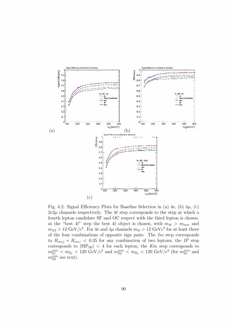
(a) (b)

(c)

Fig. 4.2: Signal Efficiency Plots for Baseline Selection in (a) 4e, (b) 4µ, (c)2e2µ channels respectively. The 4` step corresponds to the step at which afourth lepton candidate SF and OC respect with the third lepton is chosen.at the “best 4`” step the best 4` object is chosen, with m4` > mmin andmZ2 > 12 GeV/c2. For 4e and 4µ channels m`` > 12 GeVc2 for at least threeof the four combinations of opposite sign pairs. The Iso step correspondsto Riso,j + Riso,i < 0.35 for any combination of two leptons; the IP stepcorresponds to |SIP3D| < 4 for each lepton; the Kin step corresponds tommin

Z1 < mZ1 < 120 GeV/c2 and mminZ2 < mZ2 < 120 GeV/c2 (for mmin

Z1 andmmin

Z2 see text).

90

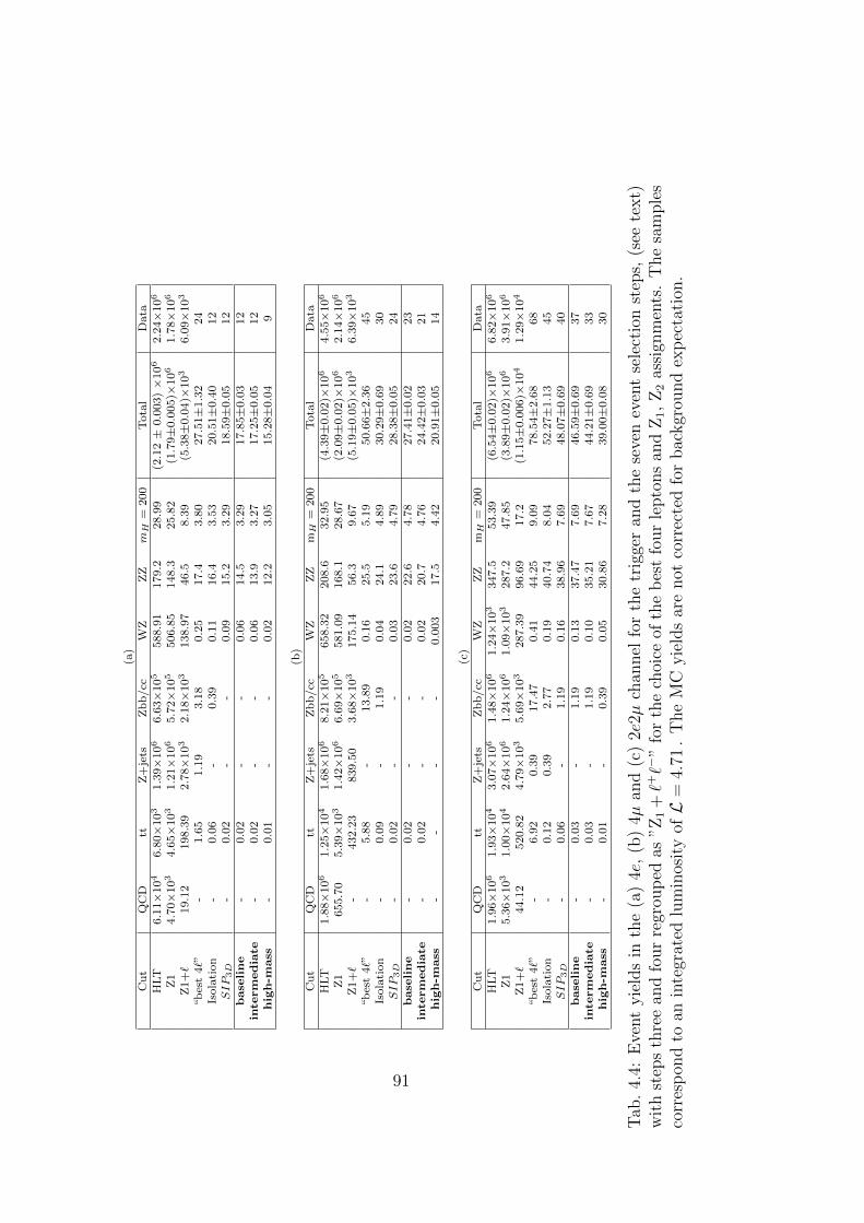
(a)

Cu

tQ

CD

ttZ

+je

tsZ

bb

/cc

WZ

ZZ

mH

=200

Tota

lD

ata

HLT

6.1

1×

104

6.8

0×

103

1.3

9×

106

6.6

3×

105

588.9

1179.2

28.9

9(2

.12±

0.0

03)×

106

2.2

4×

106

Z1

4.7

0×

103

4.6

5×

103

1.2

1×

106

5.7

2×

105

506.8

5148.3

25.8

2(1

.79±

0.0

05)×

106

1.7

8×

106

Z1+`

19.1

2198.3

92.7

8×

103

2.1

8×

103

138.9

746.5

8.3

9(5

.38±

0.0

4)×

103

6.0

9×

103

“b

est

4`”

-1.6

51.1

93.1

80.2

517.4

3.8

027.5

1±

1.3

224

Isola

tion

-0.0

6-

0.3

90.1

116.4

3.5

320.5

1±

0.4

012

SIP3D

-0.0

2-

-0.0

915.2

3.2

918.5

9±

0.0

512

base

line

-0.0

2-

-0.0

614.5

3.2

917.8

5±

0.0

312

inte

rm

ediate

-0.0

2-

-0.0

613.9

3.2

717.2

5±

0.0

512

high-m

ass

-0.0

1-

-0.0

212.2

3.0

515.2

8±

0.0

49

(b)

Cu

tQ

CD

ttZ

+je

tsZ

bb

/cc

WZ

ZZ

mH

=200

Tota

lD

ata

HLT

1.8

8×

106

1.2

5×

104

1.6

8×

106

8.2

1×

105

658.3

2208.6

32.9

5(4

.39±

0.0

2)×

106

4.5

5×

106

Z1

655.7

05.3

9×

103

1.4

2×

106

6.6

9×

105

581.0

9168.1

28.6

7(2

.09±

0.0

2)×

106

2.1

4×

106

Z1+`

-432.2

3839.5

03.6

8×

103

175.1

456.3

9.6

7(5

.19±

0.0

5)×

103

6.3

9×

103

“b

est

4`”

-5.8

8-

13.8

90.1

625.5

5.1

950.6

6±

2.3

645

Isola

tion

-0.0

9-

1.1

90.0

424.1

4.8

930.2

9±

0.6

930

SIP3D

-0.0

2-

-0.0

323.6

4.7

928.3

8±

0.0

524

base

line

-0.0

2-

-0.0

222.6

4.7

827.4

1±

0.0

223

inte

rm

ediate

-0.0

2-

-0.0

220.7

4.7

624.4

2±

0.0

321

high-m

ass

--

--

0.0

03

17.5

4.4

220.9

1±

0.0

514

(c)

Cu

tQ

CD

ttZ

+je

tsZ

bb

/cc

WZ

ZZ

mH

=200

Tota

lD

ata

HLT

1.9

6×

106

1.9

3×

104

3.0

7×

106

1.4

8×

106

1.2

4×

103

347.5

53.3

9(6

.54±

0.0

2)×

106

6.8

2×

106

Z1

5.3

6×

103

1.0

0×

104

2.6

4×

106

1.2

4×

106

1.0

9×

103

287.2

47.8

5(3

.89±

0.0

2)×

106

3.9

1×

106

Z1+`

44.1

2520.8

24.7

9×

103

5.6

9×

103

287.3

996.6

917.2

(1.1

5±

0.0

06)×

104

1.2

9×

104

“b

est

4`”

-6.9

20.3

917.4

70.4

144.2

59.0

978.5

4±

2.6

868

Isola

tion

-0.1

20.3

92.7

70.1

940.7

48.0

452.2

7±

1.1

345

SIP3D

-0.0

6-

1.1

90.1

638.9

67.6

948.0

7±

0.6

940

base

line

-0.0

3-

1.1

90.1

337.4

77.6

946.5

9±

0.6

937

inte

rm

ediate

-0.0

3-

1.1

90.1

035.2

17.6

744.2

1±

0.6

933

high-m

ass

-0.0

1-

0.3

90.0

530.8

67.2

839.0

0±

0.0

830

Tab

.4.

4:E

vent

yie

lds

inth

e(a

)4e

,(b

)4µ

and

(c)

2e2µ

chan

nel

for

the

trig

ger

and

the

seve

nev

ent

sele

ctio

nst

eps,

(see

text)

wit

hst

eps

thre

ean

dfo

ur

regr

oup

edas

”Z1

+`+`−

”fo

rth

ech

oice

ofth

eb

est

four

lepto

ns

and

Z1,

Z2

assi

gnm

ents

.T

he

sam

ple

sco

rres

pon

dto

anin

tegr

ated

lum

inos

ity

ofL

=4.

71.

The

MC

yie

lds

are

not

corr

ecte

dfo

rbac

kgr

ound

exp

ecta

tion

.

91

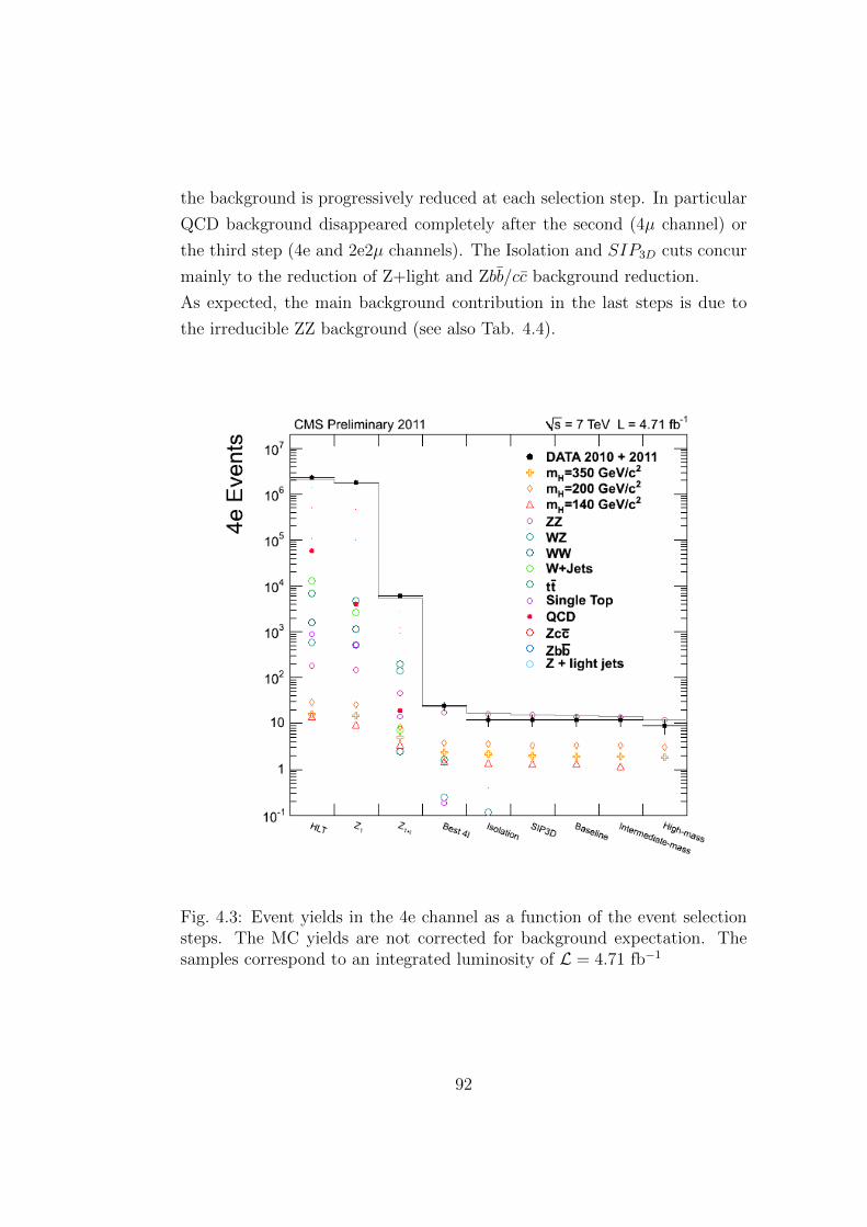
the background is progressively reduced at each selection step. In particular

QCD background disappeared completely after the second (4µ channel) or

the third step (4e and 2e2µ channels). The Isolation and SIP3D cuts concur

mainly to the reduction of Z+light and Zbb/cc background reduction.

As expected, the main background contribution in the last steps is due to

the irreducible ZZ background (see also Tab. 4.4).

Fig. 4.3: Event yields in the 4e channel as a function of the event selectionsteps. The MC yields are not corrected for background expectation. Thesamples correspond to an integrated luminosity of L = 4.71 fb−1

92

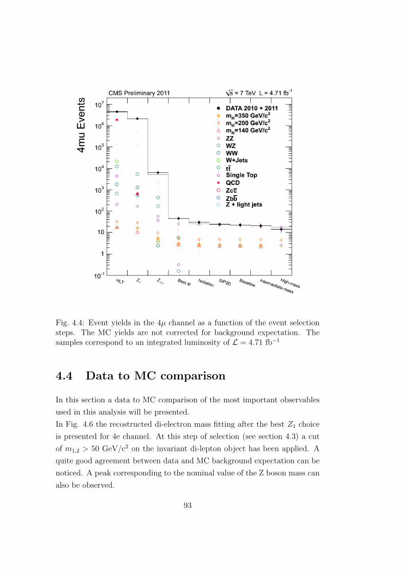
Fig. 4.4: Event yields in the 4µ channel as a function of the event selectionsteps. The MC yields are not corrected for background expectation. Thesamples correspond to an integrated luminosity of L = 4.71 fb−1

4.4 Data to MC comparison

In this section a data to MC comparison of the most important observables

used in this analysis will be presented.

In Fig. 4.6 the recostructed di-electron mass fitting after the best Z1 choice

is presented for 4e channel. At this step of selection (see section 4.3) a cut

of m1,2 > 50 GeV/c2 on the invariant di-lepton object has been applied. A

quite good agreement between data and MC background expectation can be

noticed. A peak corresponding to the nominal value of the Z boson mass can

also be observed.

93

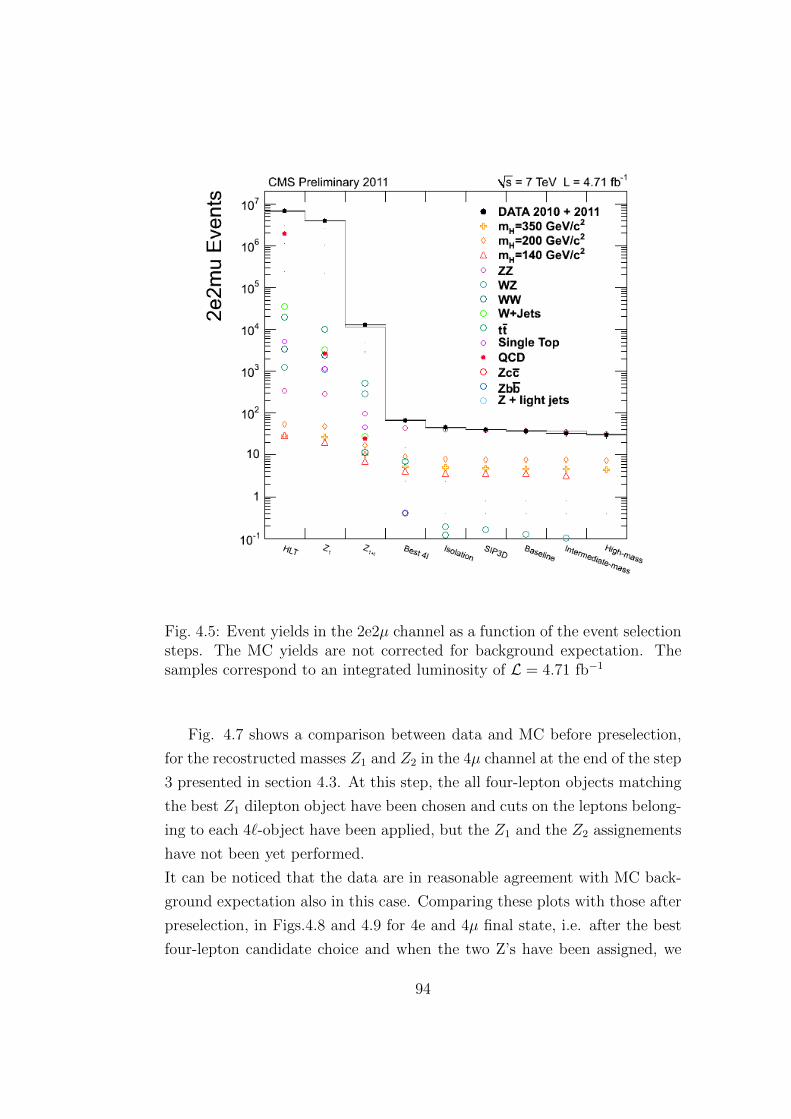
Fig. 4.5: Event yields in the 2e2µ channel as a function of the event selectionsteps. The MC yields are not corrected for background expectation. Thesamples correspond to an integrated luminosity of L = 4.71 fb−1

Fig. 4.7 shows a comparison between data and MC before preselection,

for the recostructed masses Z1 and Z2 in the 4µ channel at the end of the step

3 presented in section 4.3. At this step, the all four-lepton objects matching

the best Z1 dilepton object have been chosen and cuts on the leptons belong-

ing to each 4`-object have been applied, but the Z1 and the Z2 assignements

have not been yet performed.

It can be noticed that the data are in reasonable agreement with MC back-

ground expectation also in this case. Comparing these plots with those after

preselection, in Figs.4.8 and 4.9 for 4e and 4µ final state, i.e. after the best

four-lepton candidate choice and when the two Z’s have been assigned, we

94

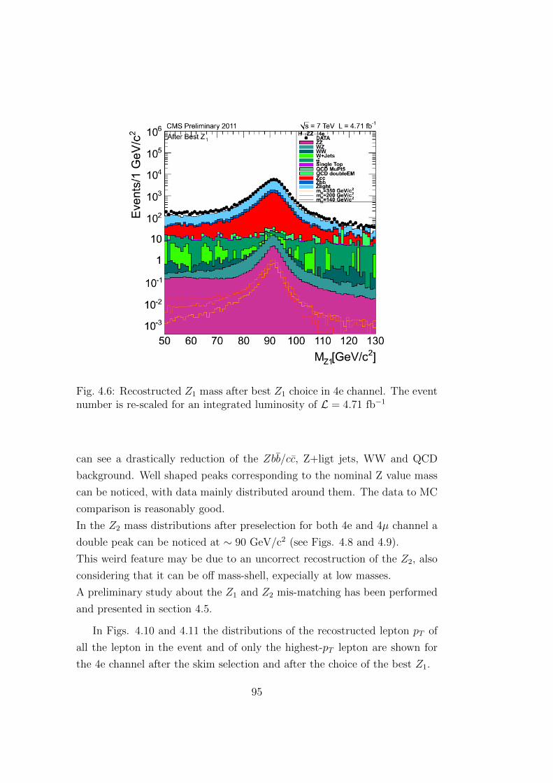
Fig. 4.6: Recostructed Z1 mass after best Z1 choice in 4e channel. The eventnumber is re-scaled for an integrated luminosity of L = 4.71 fb−1

can see a drastically reduction of the Zbb/cc, Z+ligt jets, WW and QCD

background. Well shaped peaks corresponding to the nominal Z value mass

can be noticed, with data mainly distributed around them. The data to MC

comparison is reasonably good.

In the Z2 mass distributions after preselection for both 4e and 4µ channel a

double peak can be noticed at ∼ 90 GeV/c2 (see Figs. 4.8 and 4.9).

This weird feature may be due to an uncorrect recostruction of the Z2, also

considering that it can be off mass-shell, expecially at low masses.

A preliminary study about the Z1 and Z2 mis-matching has been performed

and presented in section 4.5.

In Figs. 4.10 and 4.11 the distributions of the recostructed lepton pT of

all the lepton in the event and of only the highest-pT lepton are shown for

the 4e channel after the skim selection and after the choice of the best Z1.

95

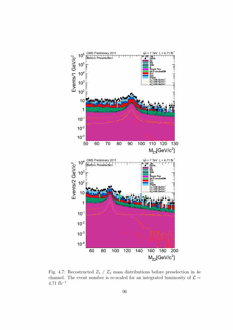
Fig. 4.7: Recostructed Z1 / Z2 mass distributions before preselection in 4echannel. The event number is re-scaled for an integrated luminosity of L =4.71 fb−1

96

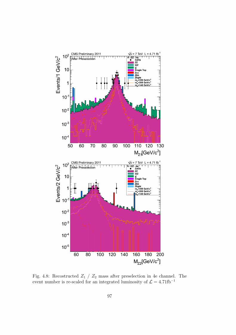
Fig. 4.8: Recostructed Z1 / Z2 mass after preselection in 4e channel. Theevent number is re-scaled for an integrated luminosity of L = 4.71fb−1

97

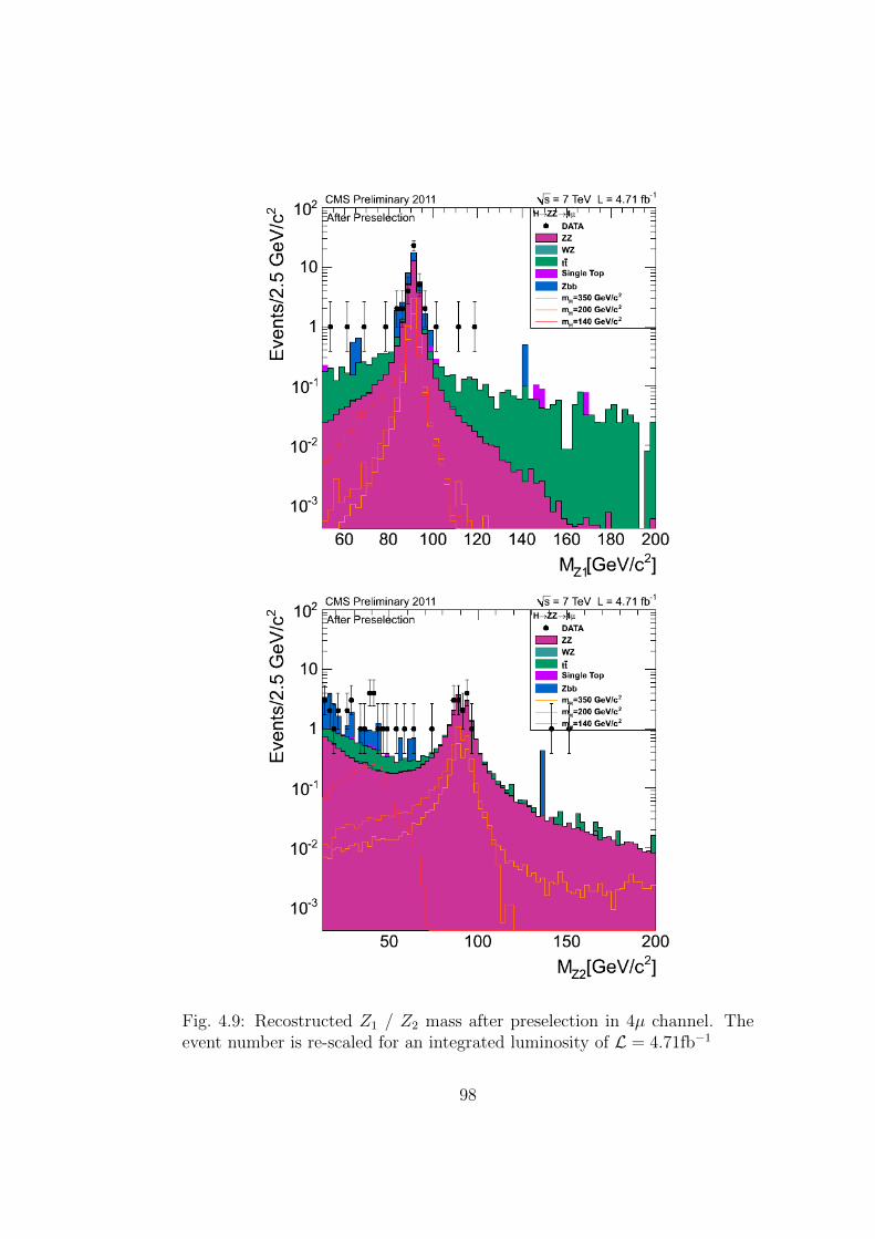
Fig. 4.9: Recostructed Z1 / Z2 mass after preselection in 4µ channel. Theevent number is re-scaled for an integrated luminosity of L = 4.71fb−1

98

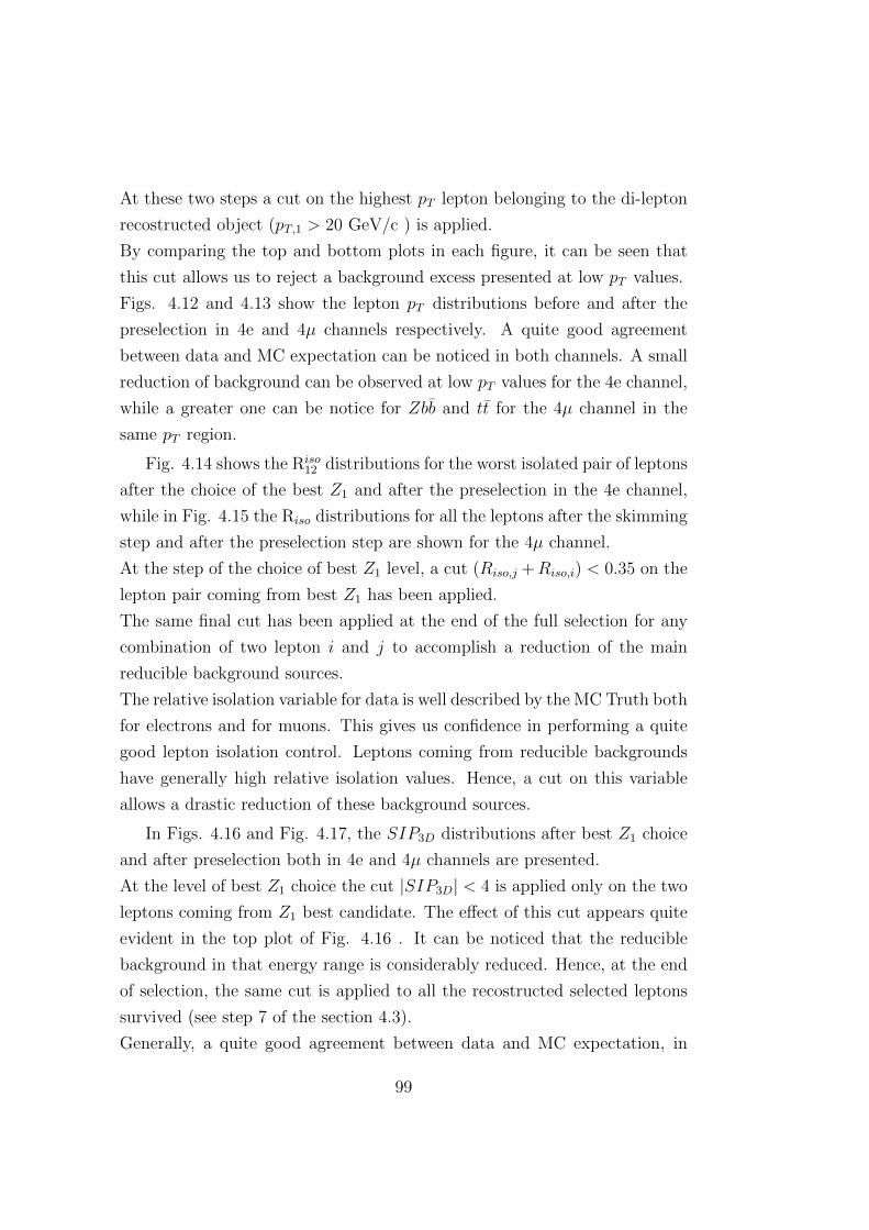
At these two steps a cut on the highest pT lepton belonging to the di-lepton

recostructed object (pT,1 > 20 GeV/c ) is applied.

By comparing the top and bottom plots in each figure, it can be seen that

this cut allows us to reject a background excess presented at low pT values.

Figs. 4.12 and 4.13 show the lepton pT distributions before and after the

preselection in 4e and 4µ channels respectively. A quite good agreement

between data and MC expectation can be noticed in both channels. A small

reduction of background can be observed at low pT values for the 4e channel,

while a greater one can be notice for Zbb and tt for the 4µ channel in the

same pT region.

Fig. 4.14 shows the Riso12 distributions for the worst isolated pair of leptons

after the choice of the best Z1 and after the preselection in the 4e channel,

while in Fig. 4.15 the Riso distributions for all the leptons after the skimming

step and after the preselection step are shown for the 4µ channel.

At the step of the choice of best Z1 level, a cut (Riso,j +Riso,i) < 0.35 on the

lepton pair coming from best Z1 has been applied.

The same final cut has been applied at the end of the full selection for any

combination of two lepton i and j to accomplish a reduction of the main

reducible background sources.

The relative isolation variable for data is well described by the MC Truth both

for electrons and for muons. This gives us confidence in performing a quite

good lepton isolation control. Leptons coming from reducible backgrounds

have generally high relative isolation values. Hence, a cut on this variable

allows a drastic reduction of these background sources.

In Figs. 4.16 and Fig. 4.17, the SIP3D distributions after best Z1 choice

and after preselection both in 4e and 4µ channels are presented.

At the level of best Z1 choice the cut |SIP3D| < 4 is applied only on the two

leptons coming from Z1 best candidate. The effect of this cut appears quite

evident in the top plot of Fig. 4.16 . It can be noticed that the reducible

background in that energy range is considerably reduced. Hence, at the end

of selection, the same cut is applied to all the recostructed selected leptons

survived (see step 7 of the section 4.3).

Generally, a quite good agreement between data and MC expectation, in

99

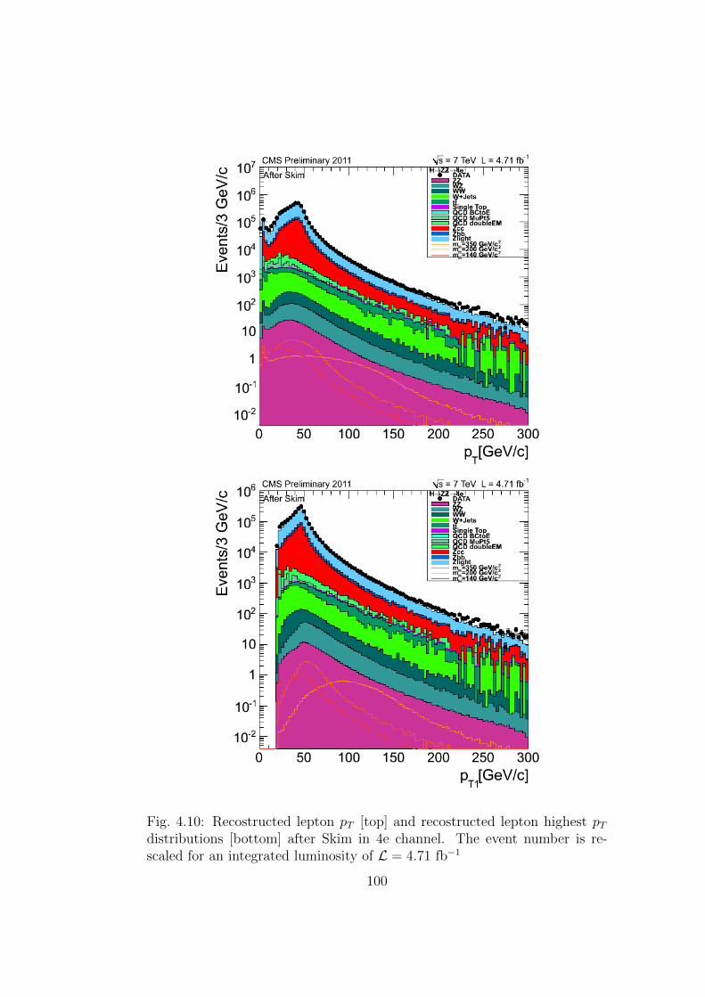
Fig. 4.10: Recostructed lepton pT [top] and recostructed lepton highest pTdistributions [bottom] after Skim in 4e channel. The event number is re-scaled for an integrated luminosity of L = 4.71 fb−1

100

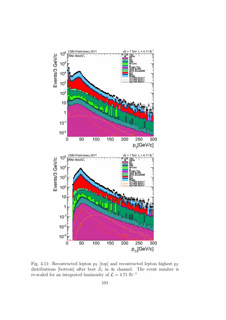
Fig. 4.11: Recostructed lepton pT [top] and recostructed lepton highest pTdistributions [bottom] after best Z1 in 4e channel. The event number isre-scaled for an integrated luminosity of L = 4.71 fb−1

101

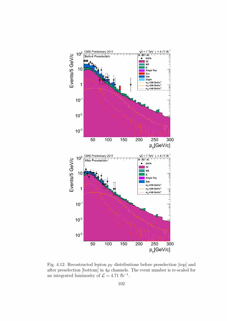
Fig. 4.12: Recostructed lepton pT distributions before preselection [top] andafter preselection [bottom] in 4µ channels. The event number is re-scaled foran integrated luminosity of L = 4.71 fb−1.

102

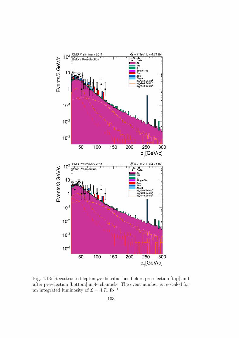
Fig. 4.13: Recostructed lepton pT distributions before preselection [top] andafter preselection [bottom] in 4e channels. The event number is re-scaled foran integrated luminosity of L = 4.71 fb−1.

103

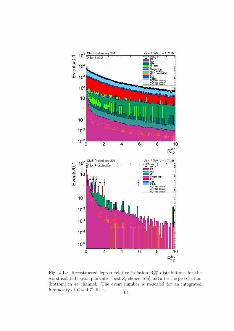
Fig. 4.14: Recostructed lepton relative isolation Riso12 distributions for the

worst isolated lepton pairs after best Z1 choice [top] and after the preselection[bottom] in 4e channel. The event number is re-scaled for an integratedluminosity of L = 4.71 fb−1.

104

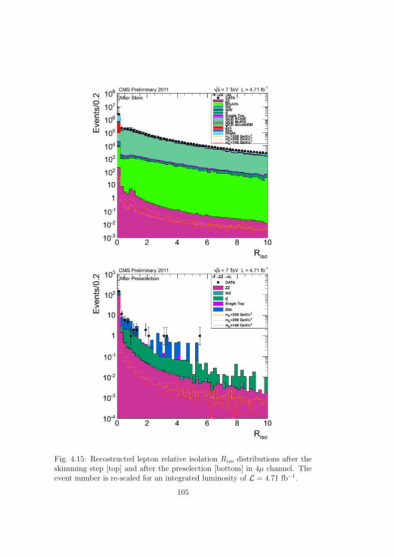
Fig. 4.15: Recostructed lepton relative isolation Riso distributions after theskimming step [top] and after the preselection [bottom] in 4µ channel. Theevent number is re-scaled for an integrated luminosity of L = 4.71 fb−1.

105

particular at low SIP3D values, can be observed. A good control of the

significance of the impact parameter can be performed using data both for

electrons and for muons.

As can be observed from the after preselection plots, applying the SIP cut

allows a good rejection of Z+jets and tt reducible background.

In Figs. 4.18 and 4.19 the invariant mass distibutions after preselection

for all the channels and that for the sum of the 4e, 4µ and 2e2µ channels is

presented.

It’s worth to remind that at this level a cut m4` > 100 GeV/c2 is applied

on the recostructed four-lepton objects survived. It can be noticed that,

expecially for 4µ and 2e2µ channels, a relevant contribution of Zbb/cc and

tt reducible background is still presented.

Comparing these plots with those after full selection (see chapter 5 section

5.1), i.e. after applying relative isolation and impact parameter cuts on the

selected leptons and kinematics cuts previously described (see section 4.3),

it can be observed that the reducible background is strongly reduced (� 1%

over the total yield in the baseline selection as can be derived from Tab 4.4).

4.5 Studies about the best four-lepton algo-

rithm

During my thesis work, an original preliminary study about the efficiency of

reconstruction algorithm for the Z1 and Z2 di-lepton pairs has been studied

by matching the reconstructed masses with the generated ones.

It has already been explained in the event selection subsection that the 4` best

candidate algorithm builds the Z1 looking for opposite sign (OS) and same

flavour (SF) di-leptons candidates with di-lepton mass mll > 50 GeV/c2,

lepton transverse momenta pT1 > 20 GeV/c and pT2 > 10 GeV/c, sum of

the lepton relative isolation Riso,j +Riso,i < 0.35 and 3D significance impact

parameter |SIP3D| < 4.

After applying these cuts, the algorithm selects the di-lepton object with

invariant mass closest to the nominal one (mZ = 91, 1876 GeV/c2).

106

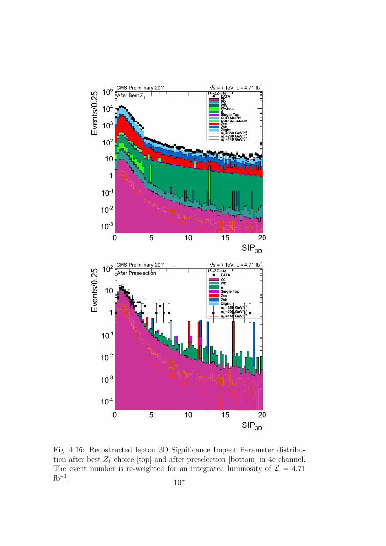
Fig. 4.16: Recostructed lepton 3D Significance Impact Parameter distribu-tion after best Z1 choice [top] and after preselection [bottom] in 4e channel.The event number is re-weighted for an integrated luminosity of L = 4.71fb−1.

107

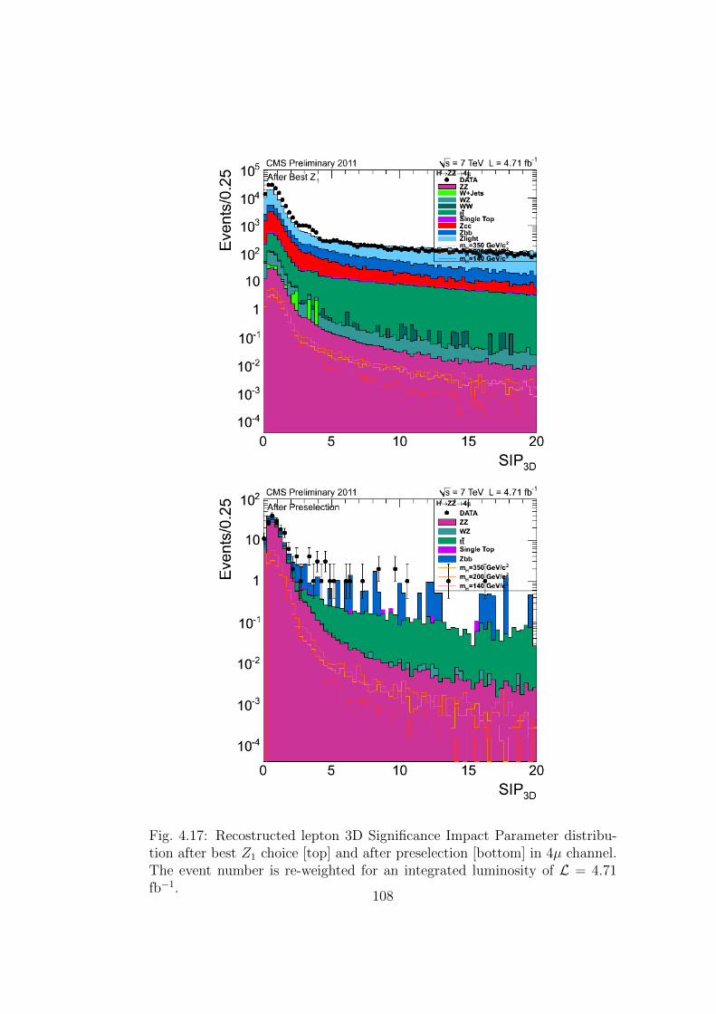
Fig. 4.17: Recostructed lepton 3D Significance Impact Parameter distribu-tion after best Z1 choice [top] and after preselection [bottom] in 4µ channel.The event number is re-weighted for an integrated luminosity of L = 4.71fb−1.

108

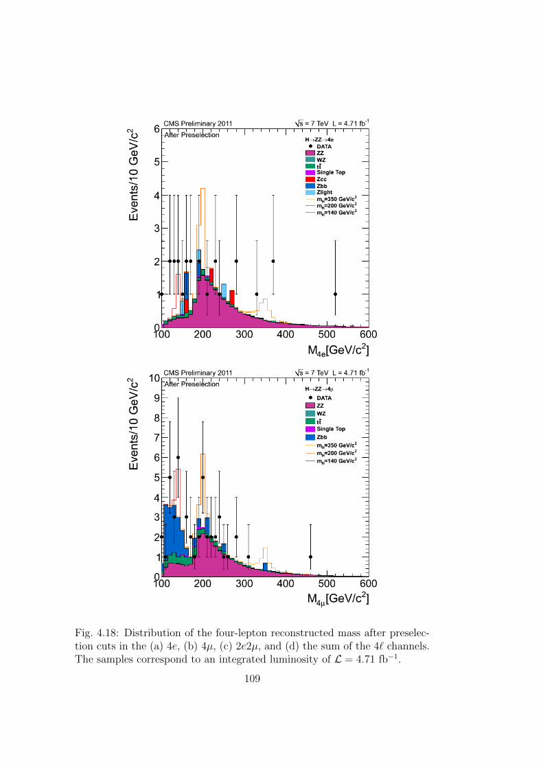
Fig. 4.18: Distribution of the four-lepton reconstructed mass after preselec-tion cuts in the (a) 4e, (b) 4µ, (c) 2e2µ, and (d) the sum of the 4` channels.The samples correspond to an integrated luminosity of L = 4.71 fb−1.

109

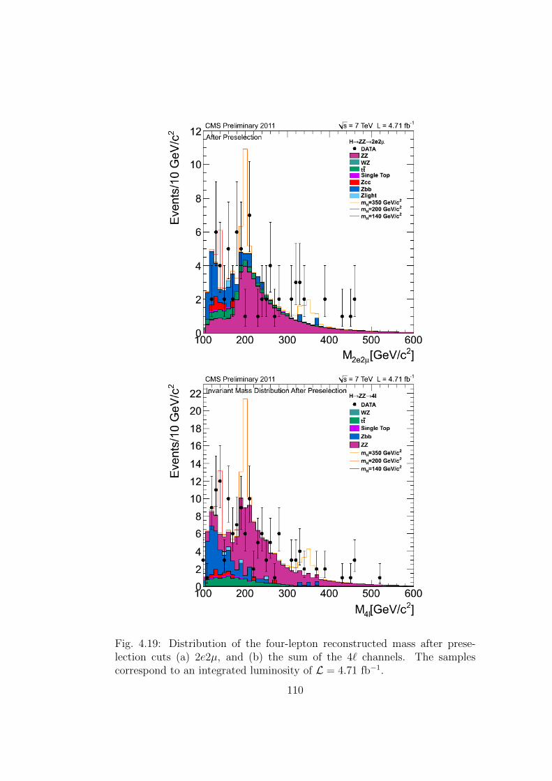
Fig. 4.19: Distribution of the four-lepton reconstructed mass after prese-lection cuts (a) 2e2µ, and (b) the sum of the 4` channels. The samplescorrespond to an integrated luminosity of L = 4.71 fb−1.

110

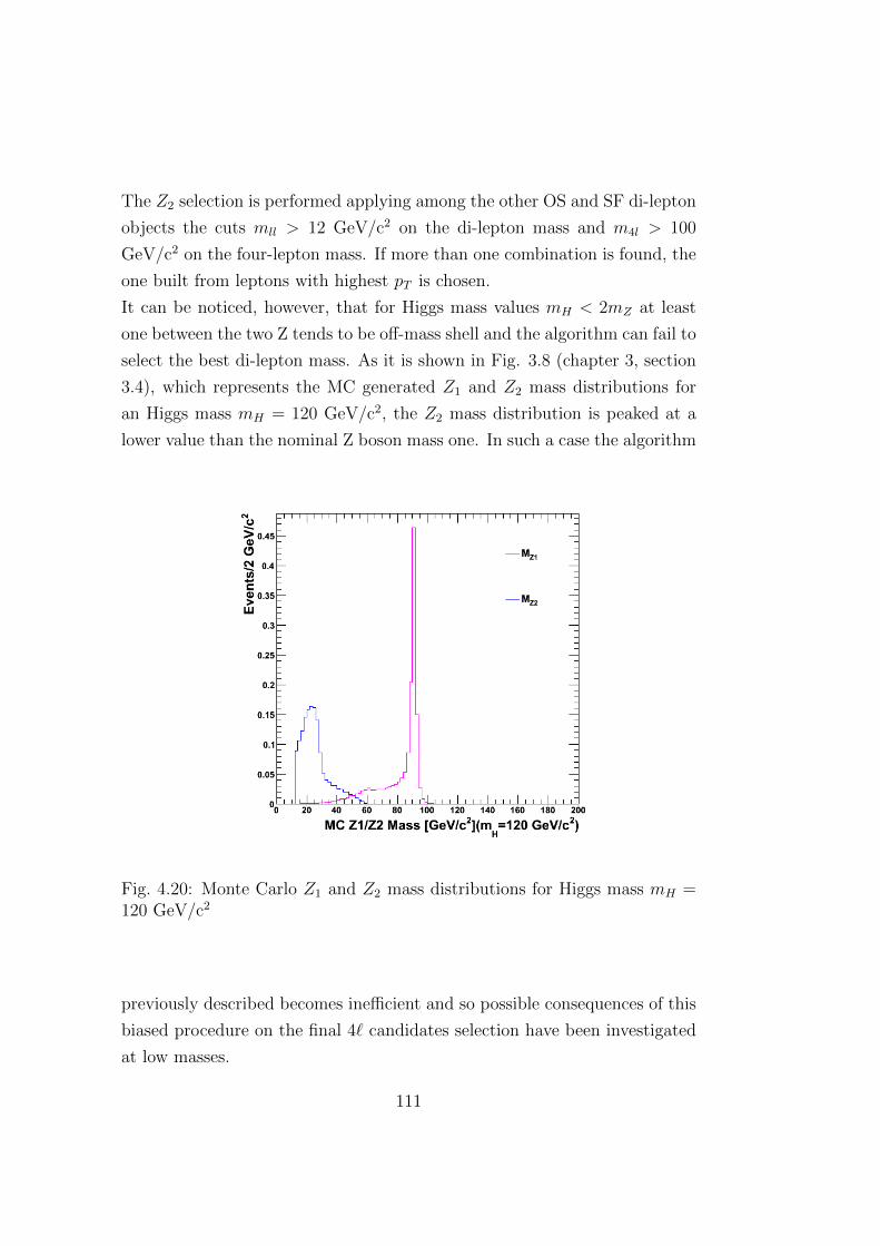
The Z2 selection is performed applying among the other OS and SF di-lepton

objects the cuts mll > 12 GeV/c2 on the di-lepton mass and m4l > 100

GeV/c2 on the four-lepton mass. If more than one combination is found, the

one built from leptons with highest pT is chosen.

It can be noticed, however, that for Higgs mass values mH < 2mZ at least

one between the two Z tends to be off-mass shell and the algorithm can fail to

select the best di-lepton mass. As it is shown in Fig. 3.8 (chapter 3, section

3.4), which represents the MC generated Z1 and Z2 mass distributions for

an Higgs mass mH = 120 GeV/c2, the Z2 mass distribution is peaked at a

lower value than the nominal Z boson mass one. In such a case the algorithm

Fig. 4.20: Monte Carlo Z1 and Z2 mass distributions for Higgs mass mH =120 GeV/c2

previously described becomes inefficient and so possible consequences of this

biased procedure on the final 4` candidates selection have been investigated

at low masses.

111

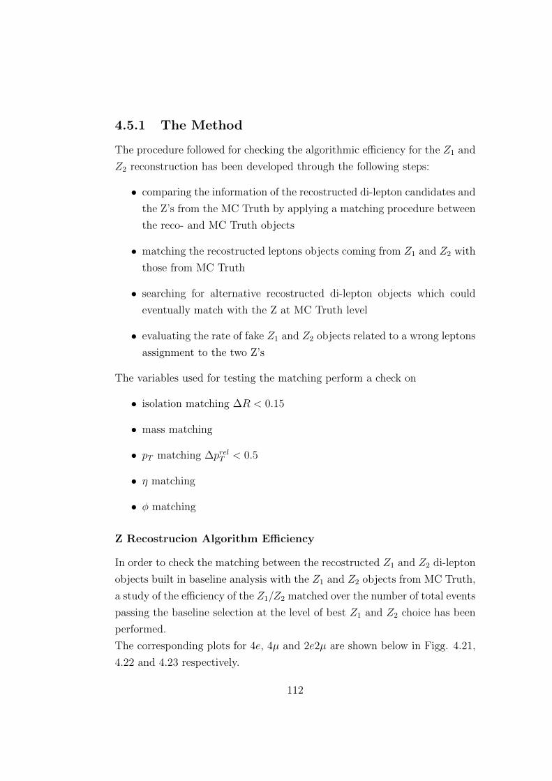
4.5.1 The Method

The procedure followed for checking the algorithmic efficiency for the Z1 and

Z2 reconstruction has been developed through the following steps:

• comparing the information of the recostructed di-lepton candidates and

the Z’s from the MC Truth by applying a matching procedure between

the reco- and MC Truth objects

• matching the recostructed leptons objects coming from Z1 and Z2 with

those from MC Truth

• searching for alternative recostructed di-lepton objects which could

eventually match with the Z at MC Truth level

• evaluating the rate of fake Z1 and Z2 objects related to a wrong leptons

assignment to the two Z’s

The variables used for testing the matching perform a check on

• isolation matching ∆R < 0.15

• mass matching

• pT matching ∆prelT < 0.5

• η matching

• φ matching

Z Recostrucion Algorithm Efficiency

In order to check the matching between the recostructed Z1 and Z2 di-lepton

objects built in baseline analysis with the Z1 and Z2 objects from MC Truth,

a study of the efficiency of the Z1/Z2 matched over the number of total events

passing the baseline selection at the level of best Z1 and Z2 choice has been

performed.

The corresponding plots for 4e, 4µ and 2e2µ are shown below in Figg. 4.21,

4.22 and 4.23 respectively.

112

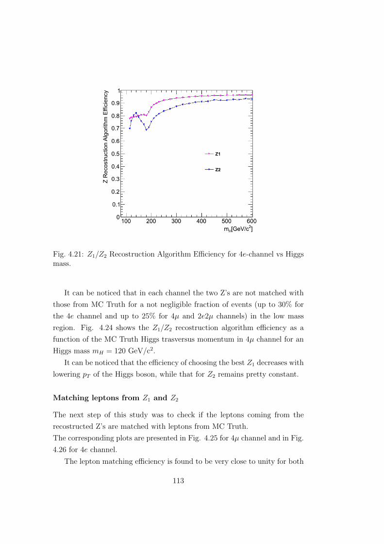
Fig. 4.21: Z1/Z2 Recostruction Algorithm Efficiency for 4e-channel vs Higgsmass.

It can be noticed that in each channel the two Z’s are not matched with

those from MC Truth for a not negligible fraction of events (up to 30% for

the 4e channel and up to 25% for 4µ and 2e2µ channels) in the low mass

region. Fig. 4.24 shows the Z1/Z2 recostruction algorithm efficiency as a

function of the MC Truth Higgs trasversus momentum in 4µ channel for an

Higgs mass mH = 120 GeV/c2.

It can be noticed that the efficiency of choosing the best Z1 decreases with

lowering pT of the Higgs boson, while that for Z2 remains pretty constant.

Matching leptons from Z1 and Z2

The next step of this study was to check if the leptons coming from the

recostructed Z’s are matched with leptons from MC Truth.

The corresponding plots are presented in Fig. 4.25 for 4µ channel and in Fig.

4.26 for 4e channel.

The lepton matching efficiency is found to be very close to unity for both

113

Fig. 4.22: Z1/Z2 Recostruction Algorithm Efficiency for 4µ-channel vs Higgsmass.

Z1 and Z2 in the 4µ channel, while it reaches lower values for 4e channel at

high masses, keeping anyway always above 80%.

The quite good agreement in lepton matching even when the corresponding

Z1 and Z2 are not matched could reveal a possible wrong pairing of the

leptons coming from the two Z’s.

Impact of Z1 and Z2 mis-match on final selection

After the preliminary studies presented above on the Z1 and Z2 mismatch at

Z1/ Z2 choice level, further investigations about the impact on final selection

have been performed. These have been carried out by

• checking the events in which both Z1 and Z2 are matched with those

from MC Truth after passing the full selection

• checking the events in which neither Z1 nor Z2 are matched with those

coming from MC Truth after passing the full selection

114

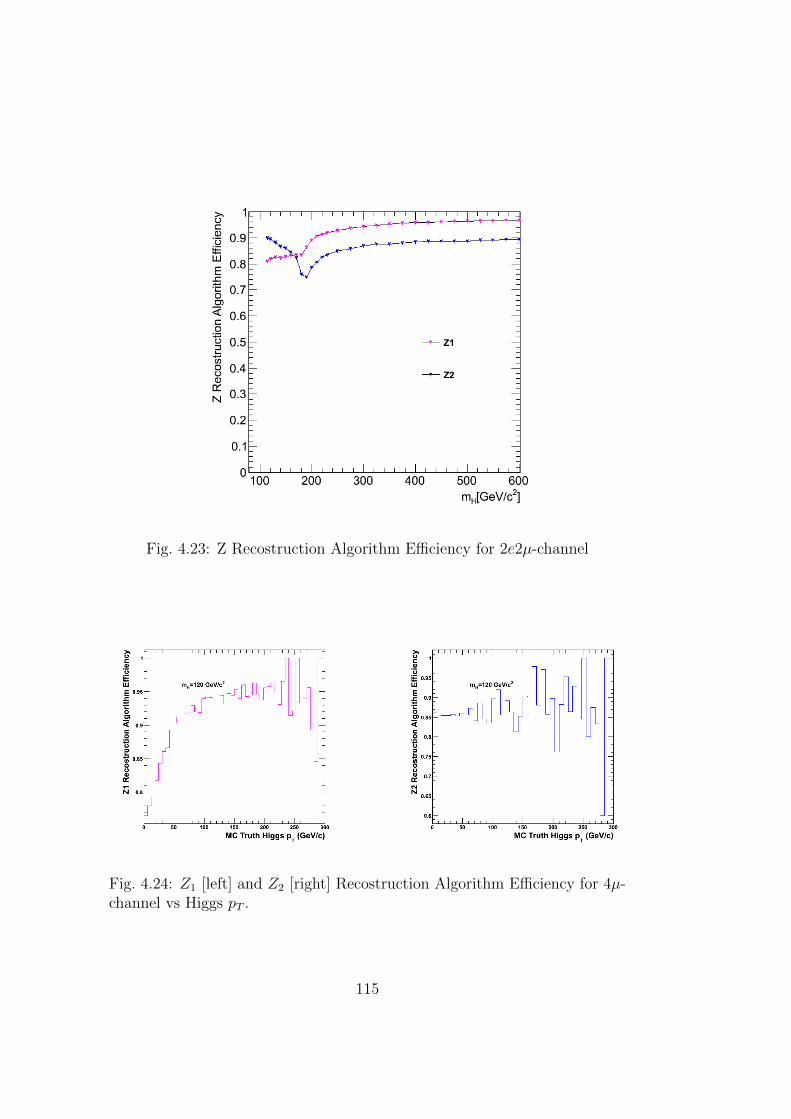
Fig. 4.23: Z Recostruction Algorithm Efficiency for 2e2µ-channel

Fig. 4.24: Z1 [left] and Z2 [right] Recostruction Algorithm Efficiency for 4µ-channel vs Higgs pT .

115

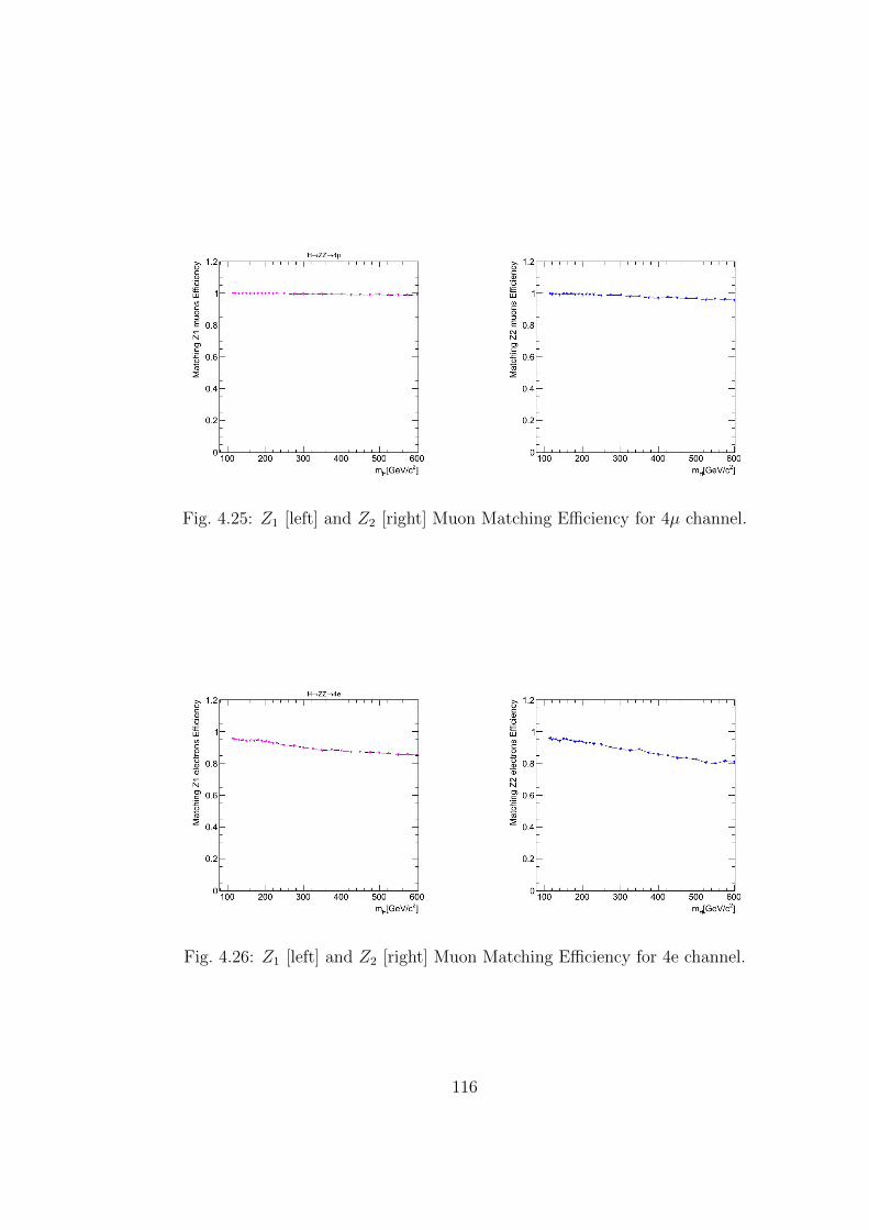
Fig. 4.25: Z1 [left] and Z2 [right] Muon Matching Efficiency for 4µ channel.

Fig. 4.26: Z1 [left] and Z2 [right] Muon Matching Efficiency for 4e channel.

116

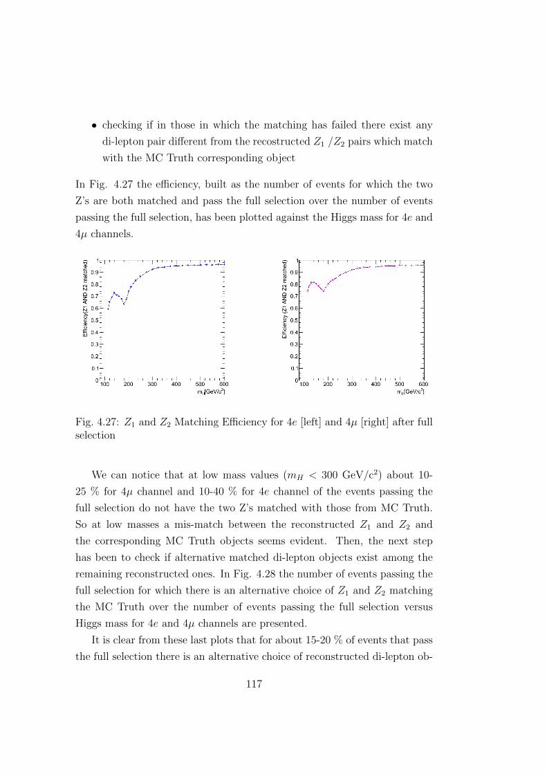
• checking if in those in which the matching has failed there exist any

di-lepton pair different from the recostructed Z1 /Z2 pairs which match

with the MC Truth corresponding object

In Fig. 4.27 the efficiency, built as the number of events for which the two

Z’s are both matched and pass the full selection over the number of events

passing the full selection, has been plotted against the Higgs mass for 4e and

4µ channels.

Fig. 4.27: Z1 and Z2 Matching Efficiency for 4e [left] and 4µ [right] after fullselection

We can notice that at low mass values (mH < 300 GeV/c2) about 10-

25 % for 4µ channel and 10-40 % for 4e channel of the events passing the

full selection do not have the two Z’s matched with those from MC Truth.

So at low masses a mis-match between the reconstructed Z1 and Z2 and

the corresponding MC Truth objects seems evident. Then, the next step

has been to check if alternative matched di-lepton objects exist among the

remaining reconstructed ones. In Fig. 4.28 the number of events passing the

full selection for which there is an alternative choice of Z1 and Z2 matching

the MC Truth over the number of events passing the full selection versus

Higgs mass for 4e and 4µ channels are presented.

It is clear from these last plots that for about 15-20 % of events that pass

the full selection there is an alternative choice of reconstructed di-lepton ob-

117

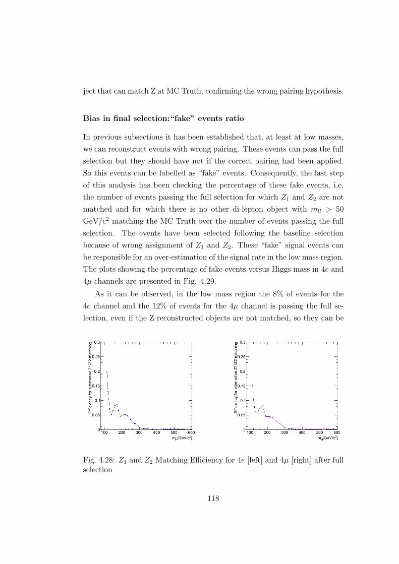
ject that can match Z at MC Truth, confirming the wrong pairing hypothesis.

Bias in final selection:“fake” events ratio

In previous subsections it has been established that, at least at low masses,

we can reconstruct events with wrong pairing. These events can pass the full

selection but they should have not if the correct pairing had been applied.

So this events can be labelled as “fake” events. Consequently, the last step

of this analysis has been checking the percentage of these fake events, i.e.

the number of events passing the full selection for which Z1 and Z2 are not

matched and for which there is no other di-lepton object with mll > 50

GeV/c2 matching the MC Truth over the number of events passing the full

selection. The events have been selected following the baseline selection

because of wrong assignment of Z1 and Z2. These “fake” signal events can

be responsible for an over-estimation of the signal rate in the low mass region.

The plots showing the percentage of fake events versus Higgs mass in 4e and

4µ channels are presented in Fig. 4.29.

As it can be observed, in the low mass region the 8% of events for the

4e channel and the 12% of events for the 4µ channel is passing the full se-

lection, even if the Z reconstructed objects are not matched, so they can be

Fig. 4.28: Z1 and Z2 Matching Efficiency for 4e [left] and 4µ [right] after fullselection

118

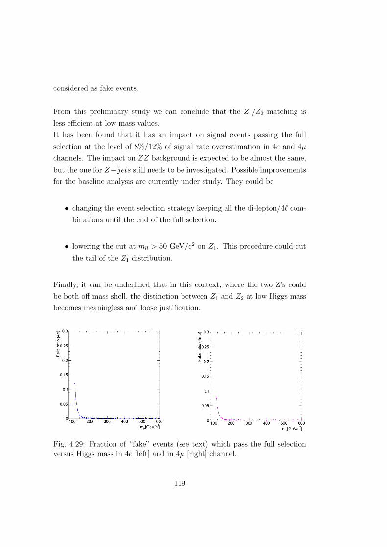
considered as fake events.

From this preliminary study we can conclude that the Z1/Z2 matching is

less efficient at low mass values.

It has been found that it has an impact on signal events passing the full

selection at the level of 8%/12% of signal rate overestimation in 4e and 4µ

channels. The impact on ZZ background is expected to be almost the same,

but the one for Z+jets still needs to be investigated. Possible improvements

for the baseline analysis are currently under study. They could be

• changing the event selection strategy keeping all the di-lepton/4` com-

binations until the end of the full selection.

• lowering the cut at mll > 50 GeV/c2 on Z1. This procedure could cut

the tail of the Z1 distribution.

Finally, it can be underlined that in this context, where the two Z’s could

be both off-mass shell, the distinction between Z1 and Z2 at low Higgs mass

becomes meaningless and loose justification.

Fig. 4.29: Fraction of “fake” events (see text) which pass the full selectionversus Higgs mass in 4e [left] and in 4µ [right] channel.

119

4.6 Background Evaluation and Control

No specific studies on background estimation from data have been performed

for this thesis. Nevertheless, a quick overview of the background evaluation

and control has been included.

The total number of signal-like background events surviving the baseline se-

lection is quite small for the integrated luminosity reached in this analysis

(see section 5.1).

A precise evaluation of the background, using only the side-bands method

[45], is then not possible because of the small number of observed events

in the relevant narrow signal-like region. Then, for background control and

systematics evaluation, other data driven methods have been used.

According to the event yields evaluated from MC simulations and shown in

Table 4.4, the background is overwhelmingly composed of the ZZ(∗) contin-

uum with just a small contamination from the reducible and instrumental

backgrounds.

The tt and WZ backgrounds appear negligible, i.e. they both represent� 1%

of the total background rate expected for the baseline selection. Only a few

events survive for Z+γ but these are actually Z+γ+jets events. The Z de-

cays in a pair of muons while at least one jet fragment is mis-identified as an

electron, and one electron at most comes from the photon conversion. This

background is then treated in common with the Z+jets background.

Unfortunately, the MC event yield in Table 4.4 does not allow to get conclu-

sive results on the the situation for Z+jets, and Zbb backgrounds because of

the low statistics. Hence, these backgrounds must be evaluated from data. It

could be observed in this way, that only a small contamination from Z+jets,

and Zbb remains for the baseline selection, concentrated mostly at low m4`.

The typical procedure for the background evaluation from data consists of

choosing a background control region outside the signal phase space, which

becomes populated with background events, by relaxing some cuts of the

event selection. Then it has to be verified that the event rates change ac-

cording to the Monte Carlo expectation.

The control region has to be chosen carefully for any given background since

120

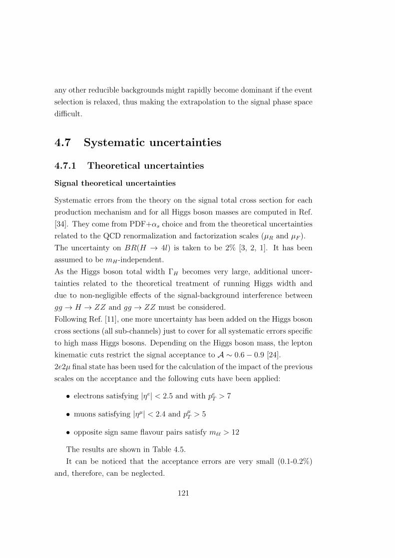
any other reducible backgrounds might rapidly become dominant if the event

selection is relaxed, thus making the extrapolation to the signal phase space

difficult.

4.7 Systematic uncertainties

4.7.1 Theoretical uncertainties

Signal theoretical uncertainties

Systematic errors from the theory on the signal total cross section for each

production mechanism and for all Higgs boson masses are computed in Ref.

[34]. They come from PDF+αs choice and from the theoretical uncertainties

related to the QCD renormalization and factorization scales (µR and µF ).

The uncertainty on BR(H → 4l) is taken to be 2% [3, 2, 1]. It has been

assumed to be mH-independent.

As the Higgs boson total width ΓH becomes very large, additional uncer-

tainties related to the theoretical treatment of running Higgs width and

due to non-negligible effects of the signal-background interference between

gg → H → ZZ and gg → ZZ must be considered.

Following Ref. [11], one more uncertainty has been added on the Higgs boson

cross sections (all sub-channels) just to cover for all systematic errors specific

to high mass Higgs bosons. Depending on the Higgs boson mass, the lepton

kinematic cuts restrict the signal acceptance to A ∼ 0.6− 0.9 [24].

2e2µ final state has been used for the calculation of the impact of the previous

scales on the acceptance and the following cuts have been applied:

• electrons satisfying |ηe| < 2.5 and with peT > 7

• muons satisfying |ηµ| < 2.4 and pµT > 5

• opposite sign same flavour pairs satisfy m`` > 12

The results are shown in Table 4.5.

It can be noticed that the acceptance errors are very small (0.1-0.2%)

and, therefore, can be neglected.

121

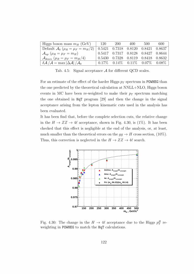
Higgs boson mass mH (GeV) 120 200 400 500 600Default A0 (µR = µF = mH/2) 0.5421 0.7318 0.8120 0.8421 0.8637Aup (µR = µF = mH) 0.5417 0.7317 0.8128 0.8427 0.8644Adown (µR = µF = mH/4) 0.5430 0.7328 0.8119 0.8418 0.8632δA /A = max |∆A| /A0 0.17% 0.14% 0.11% 0.07% 0.08%

Tab. 4.5: Signal acceptance A for different QCD scales.

For an estimate of the effect of the harder Higgs pT spectrum in POWHEG than

the one predicted by the theoretical calculation at NNLL+NLO, Higgs boson

events in MC have been re-weighted to make their pT spectrum matching

the one obtained in HqT program [29] and then the change in the signal

acceptance arising from the lepton kinematic cuts used in the analysis has

been evaluated.

It has been find that, before the complete selection cuts, the relative change

in the H → ZZ → 4` acceptance, shown in Fig. 4.30, is (1%). It has been

checked that this effect is negligible at the end of the analysis, or, at least,

much smaller than the theoretical errors on the gg → H cross section, (10%).

Thus, this correction is neglected in the H → ZZ → 4` search.

/ ndf 2χ 5.134e-06 / 4const 32.32± 56.22 scale 32.79± 55.14 p2 0.4± 0

2 , GeV/cHm150 200 250 300 350 400 450 500

unw

eigh

t/A

wei

ght

A

0.97

0.975

0.98

0.985

0.99

0.995

1

/ ndf 2χ 5.134e-06 / 4const 32.32± 56.22 scale 32.79± 55.14 p2 0.4± 0

unweight/Aweight2e2mu: A

unweight/Aweight4mu: A

unweight/Aweight4e: A

-55.14)H

-56.22)/(mH

Fit: (m

Fig. 4.30: The change in the H → 4` acceptance due to the Higgs pHT re-weighting in POWHEG to match the HqT calculations.

122

ZZ background theoretical uncertainties

PDF+αs and QCD scale uncertainties for qq → ZZ→ 4` at NLO and gg →ZZ→ 4` have been evaluated using MCFM [19].

The 2e2µ final state has been used and the following cuts applied:

• electrons satisfying |ηe| < 2.5 and with peT > 7GeV/c

• muons satisfying |ηµ| < 2.4 and pµT > 5

• opposite sign same flavour pairs satisfy m`` > 12 GeV/c2.

The cuts on the jet energy ET and the minimal jet-lepton ∆R-distance have

been relaxed also in this case.

To estimate QCD scale systematic errors, variations in the differential cross

section dσ/dm4` with changing the renormalization and factorization scales

by a factor of two up and down from their default setting µR = µF = mZ

have been calculated.

Instrumental uncertainties

The uncertainty on the luminosity measurement has been estimated as 4.5% [10].

The pile-up effect has also been evaluated re-weighting the Monte Carlo sim-

ulation to match the number of reconstructed vertices found in data. The

difference between re-weighting and not weighting at all has been taken as

an upper limit of this effect.

The estimate uncertainty on the efficiency is very small and it has been ne-

glected.

The trigger efficiency for signal-like events is very close to 100% within the

acceptance defined by the baseline cuts. Therefore the overall data/MC

discrepancy in trigger efficiency for the signal and for the irreducible back-

grounds turns to be negligible and a systematic uncertainty of 1.5% has

been assigned. The observed data/Monte Carlo discrepancy in the lepton

reconstruction and identification efficiencies measured with the data-driven

technique has been used to correct the Monte Carlo on an event-by-event

basis.

123

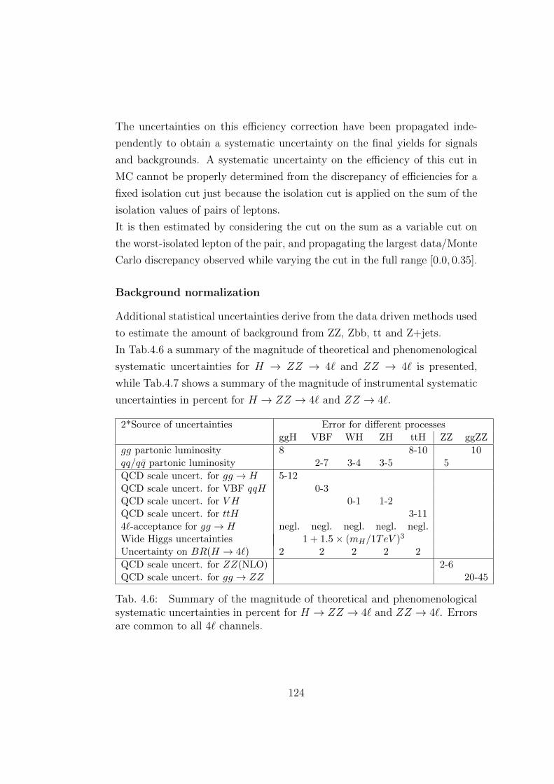
The uncertainties on this efficiency correction have been propagated inde-

pendently to obtain a systematic uncertainty on the final yields for signals

and backgrounds. A systematic uncertainty on the efficiency of this cut in

MC cannot be properly determined from the discrepancy of efficiencies for a

fixed isolation cut just because the isolation cut is applied on the sum of the

isolation values of pairs of leptons.

It is then estimated by considering the cut on the sum as a variable cut on

the worst-isolated lepton of the pair, and propagating the largest data/Monte

Carlo discrepancy observed while varying the cut in the full range [0.0, 0.35].

Background normalization

Additional statistical uncertainties derive from the data driven methods used

to estimate the amount of background from ZZ, Zbb, tt and Z+jets.

In Tab.4.6 a summary of the magnitude of theoretical and phenomenological

systematic uncertainties for H → ZZ → 4` and ZZ → 4` is presented,

while Tab.4.7 shows a summary of the magnitude of instrumental systematic

uncertainties in percent for H → ZZ → 4` and ZZ → 4`.

2*Source of uncertainties Error for different processesggH VBF WH ZH ttH ZZ ggZZ

gg partonic luminosity 8 8-10 10qq/qq partonic luminosity 2-7 3-4 3-5 5

QCD scale uncert. for gg → H 5-12QCD scale uncert. for VBF qqH 0-3QCD scale uncert. for V H 0-1 1-2QCD scale uncert. for ttH 3-114`-acceptance for gg → H negl. negl. negl. negl. negl.Wide Higgs uncertainties 1 + 1.5× (mH/1TeV )3

Uncertainty on BR(H → 4`) 2 2 2 2 2

QCD scale uncert. for ZZ(NLO) 2-6QCD scale uncert. for gg → ZZ 20-45

Tab. 4.6: Summary of the magnitude of theoretical and phenomenologicalsystematic uncertainties in percent for H → ZZ → 4` and ZZ → 4`. Errorsare common to all 4` channels.

124

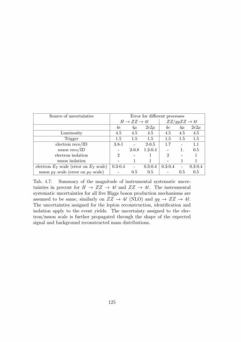
Source of uncertainties Error for different processesH → ZZ → 4` ZZ/ggZZ → 4`

4e 4µ 2e2µ 4e 4µ 2e2µ

Luminosity 4.5 4.5 4.5 4.5 4.5 4.5

Trigger 1.5 1.5 1.5 1.5 1.5 1.5

electron reco/ID 3.8-1 - 2-0.5 1.7 - 1.1muon reco/ID - 2-0.8 1.2-0.4 - 1. 0.5

electron isolation 2 - 1 2 - 1muon isolation - 1 1 - 1 1

electron ET scale (error on ET scale) 0.3-0.4 - 0.3-0.4 0.3-0.4 - 0.3-0.4muon pT scale (error on pT scale) - 0.5 0.5 - 0.5 0.5

Tab. 4.7: Summary of the magnitude of instrumental systematic uncer-tainties in percent for H → ZZ → 4` and ZZ → 4`. The instrumentalsystematic uncertainties for all five Higgs boson production mechanisms areassumed to be same, similarly on ZZ → 4` (NLO) and gg → ZZ → 4`.The uncertainties assigned for the lepton reconstruction, identification andisolation apply to the event yields. The uncertainty assigned to the elec-tron/muon scale is further propagated through the shape of the expectedsignal and background reconstructed mass distributions.

125

126

Chapter 5

Results

5.1 Mass Distributions and Kinematics

The reconstructed four-lepton invariant mass distributions after full selec-

tion (baseline) obtained in the 4e, 4µ, and 2e2µ channels is shown in Figs.

5.1 and 5.2 for the data, and compared to expectations from the SM main

backgrounds. A plot for the sum of the three 4` channel is also shown in

Fig. 5.3. The combination of the three channels does not reveal a particular

clusterization of data around any given mass.

The number of events observed, as well as the background rates in the sig-

nal region within a mass range from m1 = 100 GeV/c2 to m2 = 600 GeV/c2,

are reported for each final state in Table 5.1 for the baseline selection. It can

be seen that, at this last selection step, only a very small fraction (< 1%) of

the reducible Zbb/Zcc, tt, WZ and Single Top backgrounds survived to the

full selection. The main contribution comes obviously from the irreducible

ZZ continuum. The total backgroud after all the selection steps (see chapter

4, section 4.3) is considerably reduced with respect to that presented in Figs.

4.18 and 4.19 in chapter 4, section 4.4, after the preselection step.

A zoom on the low mass range (mH < 160 GeV/c2) is shown in Fig. 5.4 for

the combination of the three channels. It can be observed that the reducible

and instrumental backgrounds have found to be very small or negligible.

127

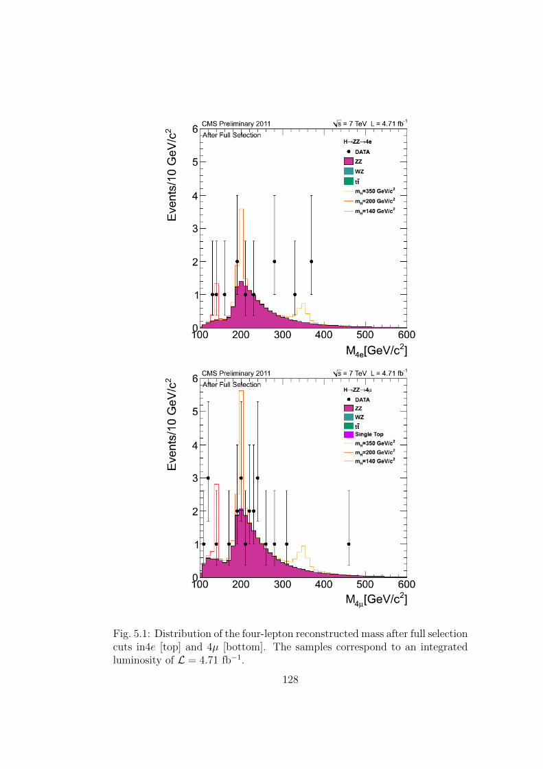
Fig. 5.1: Distribution of the four-lepton reconstructed mass after full selectioncuts in4e [top] and 4µ [bottom]. The samples correspond to an integratedluminosity of L = 4.71 fb−1.

128

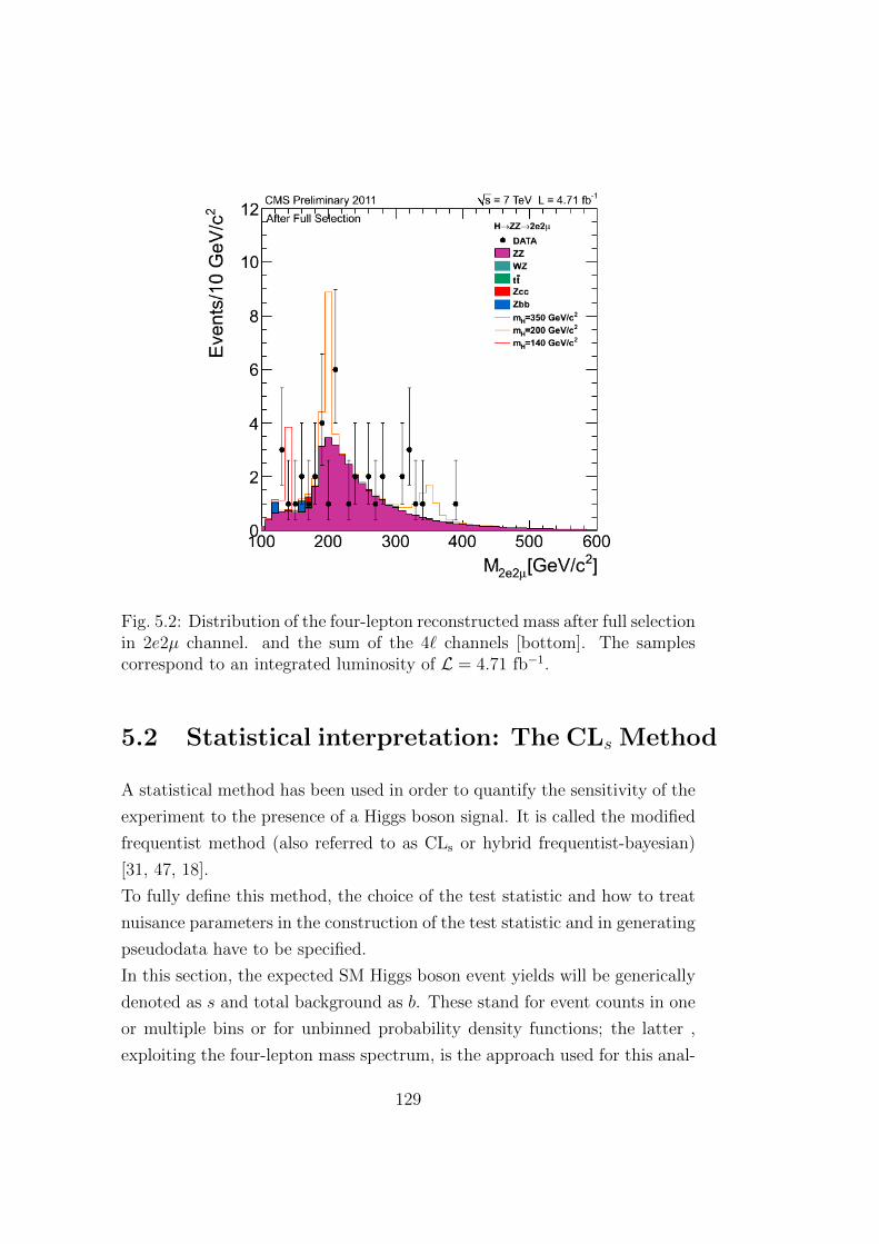
Fig. 5.2: Distribution of the four-lepton reconstructed mass after full selectionin 2e2µ channel. and the sum of the 4` channels [bottom]. The samplescorrespond to an integrated luminosity of L = 4.71 fb−1.

5.2 Statistical interpretation: The CLs Method

A statistical method has been used in order to quantify the sensitivity of the

experiment to the presence of a Higgs boson signal. It is called the modified

frequentist method (also referred to as CLs or hybrid frequentist-bayesian)

[31, 47, 18].

To fully define this method, the choice of the test statistic and how to treat

nuisance parameters in the construction of the test statistic and in generating

pseudodata have to be specified.

In this section, the expected SM Higgs boson event yields will be generically

denoted as s and total background as b. These stand for event counts in one

or multiple bins or for unbinned probability density functions; the latter ,

exploiting the four-lepton mass spectrum, is the approach used for this anal-

129

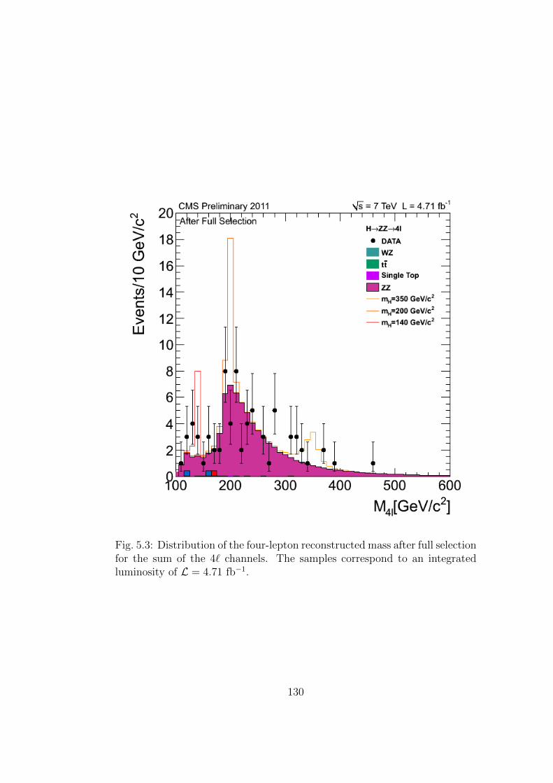
Fig. 5.3: Distribution of the four-lepton reconstructed mass after full selectionfor the sum of the 4` channels. The samples correspond to an integratedluminosity of L = 4.71 fb−1.

130

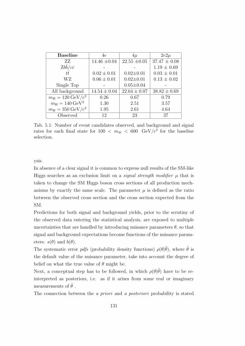
Baseline 4e 4µ 2e2µZZ 14.46 ±0.04 22.55 ±0.05 37.47 ± 0.08

Zbb/cc - - 1.19 ± 0.69tt 0.02± 0.01 0.02±0.01 0.03 ± 0.01

WZ 0.06± 0.01 0.02±0.01 0.13 ± 0.02Single Top - 0.05±0.04 -

All background 14.54± 0.04 22.64± 0.07 38.82± 0.69mH = 120 GeV/c2 0.26 0.67 0.79mH = 140 GeV2 1.30 2.51 3.57mH = 350 GeV/c2 1.95 2.61 4.64

Observed 12 23 37

Tab. 5.1: Number of event candidates observed, and background and signalrates for each final state for 100 < m4` < 600 GeV/c2 for the baselineselection.

ysis.

In absence of a clear signal it is common to express null results of the SM-like

Higgs searches as an exclusion limit on a signal strength modifier µ that is

taken to change the SM Higgs boson cross sections of all production mech-

anisms by exactly the same scale. The parameter µ is defined as the ratio

between the observed cross section and the cross section expected from the

SM.

Predictions for both signal and background yields, prior to the scrutiny of

the observed data entering the statistical analysis, are exposed to multiple

uncertainties that are handled by introducing nuisance parameters θ, so that

signal and background expectations become functions of the nuisance param-

eters: s(θ) and b(θ).

The systematic error pdfs (probability density functions) ρ(θ|θ), where θ is

the default value of the nuisance parameter, take into account the degree of

belief on what the true value of θ might be.

Next, a conceptual step has to be followed, in which ρ(θ|θ) have to be re-

interpreted as posteriors, i.e. as if it arises from some real or imaginary

measurements of θ .

The connection between the a priori and a posteriori probability is stated

131

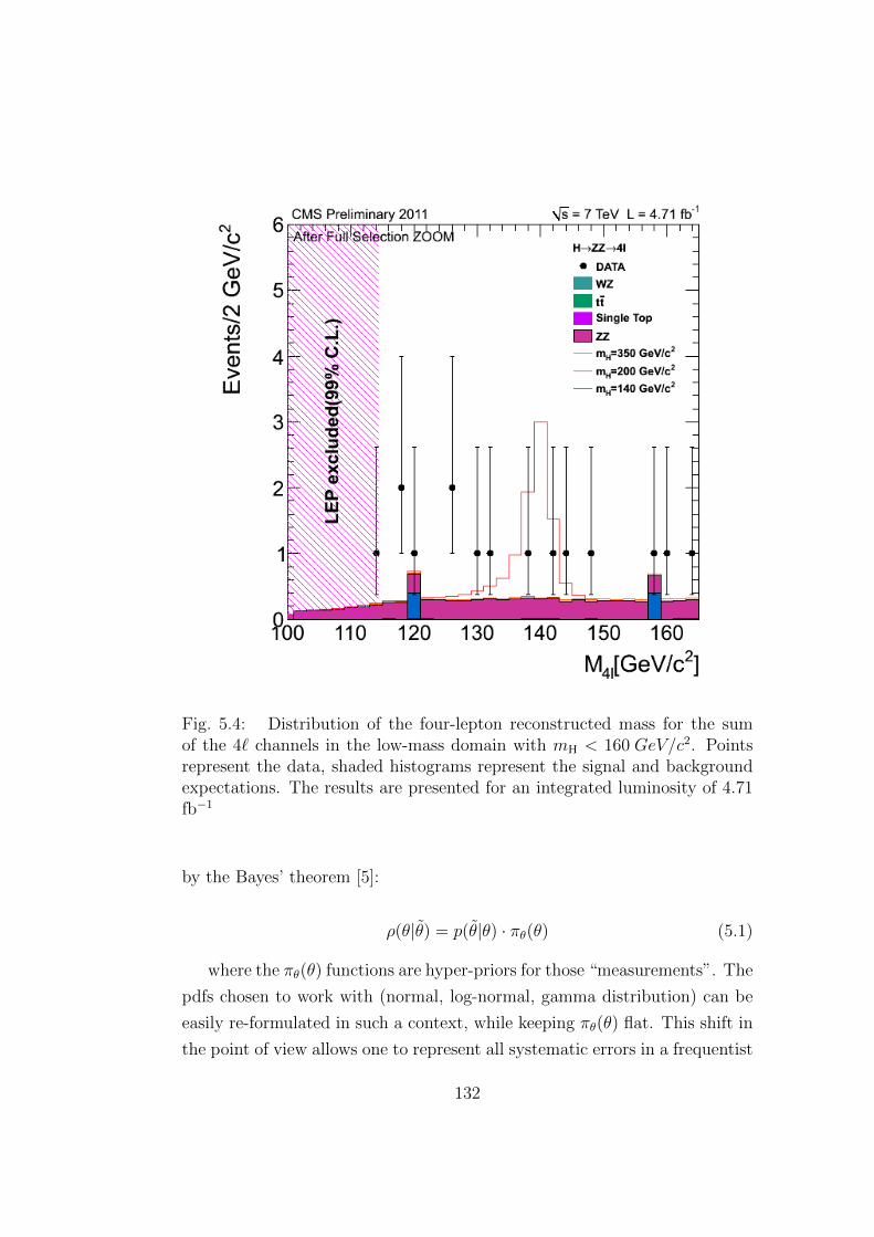
Fig. 5.4: Distribution of the four-lepton reconstructed mass for the sumof the 4` channels in the low-mass domain with mH < 160 GeV/c2. Pointsrepresent the data, shaded histograms represent the signal and backgroundexpectations. The results are presented for an integrated luminosity of 4.71fb−1

by the Bayes’ theorem [5]:

ρ(θ|θ) = p(θ|θ) · πθ(θ) (5.1)

where the πθ(θ) functions are hyper-priors for those “measurements”. The

pdfs chosen to work with (normal, log-normal, gamma distribution) can be

easily re-formulated in such a context, while keeping πθ(θ) flat. This shift in

the point of view allows one to represent all systematic errors in a frequentist

132

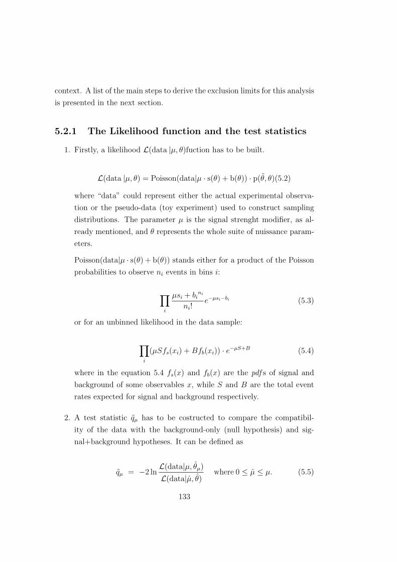
context. A list of the main steps to derive the exclusion limits for this analysis

is presented in the next section.

5.2.1 The Likelihood function and the test statistics

1. Firstly, a likelihood L(data |µ, θ)fuction has to be built.

L(data |µ, θ) = Poisson(data|µ · s(θ) + b(θ)) · p(θ, θ)(5.2)

where “data” could represent either the actual experimental observa-

tion or the pseudo-data (toy experiment) used to construct sampling

distributions. The parameter µ is the signal strenght modifier, as al-

ready mentioned, and θ represents the whole suite of nuissance param-

eters.

Poisson(data|µ · s(θ) + b(θ)) stands either for a product of the Poisson

probabilities to observe ni events in bins i:

∏i

µsi + bini

ni!e−µsi−bi (5.3)

or for an unbinned likelihood in the data sample:

∏i

(µSfs(xi) +Bfb(xi)) · e−µS+B (5.4)

where in the equation 5.4 fs(x) and fb(x) are the pdf s of signal and

background of some observables x, while S and B are the total event

rates expected for signal and background respectively.

2. A test statistic qµ has to be costructed to compare the compatibil-

ity of the data with the background-only (null hypothesis) and sig-

nal+background hypotheses. It can be defined as

qµ = −2 lnL(data|µ, θµ)

L(data|µ, θ)where 0 ≤ µ ≤ µ. (5.5)

133

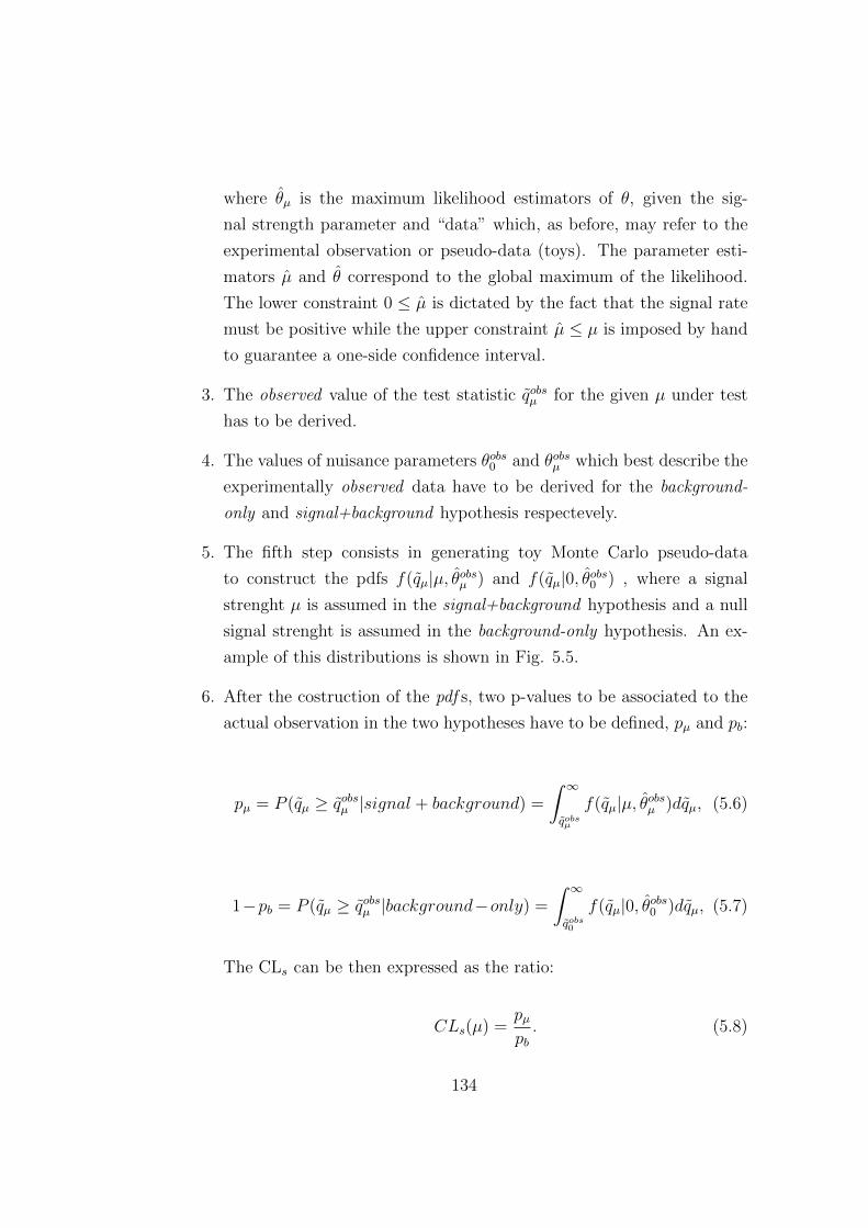
where θµ is the maximum likelihood estimators of θ, given the sig-

nal strength parameter and “data” which, as before, may refer to the

experimental observation or pseudo-data (toys). The parameter esti-

mators µ and θ correspond to the global maximum of the likelihood.

The lower constraint 0 ≤ µ is dictated by the fact that the signal rate

must be positive while the upper constraint µ ≤ µ is imposed by hand

to guarantee a one-side confidence interval.

3. The observed value of the test statistic qobsµ for the given µ under test

has to be derived.

4. The values of nuisance parameters θobs0 and θobsµ which best describe the

experimentally observed data have to be derived for the background-

only and signal+background hypothesis respectevely.

5. The fifth step consists in generating toy Monte Carlo pseudo-data

to construct the pdfs f(qµ|µ, θobsµ ) and f(qµ|0, θobs0 ) , where a signal

strenght µ is assumed in the signal+background hypothesis and a null

signal strenght is assumed in the background-only hypothesis. An ex-

ample of this distributions is shown in Fig. 5.5.

6. After the costruction of the pdf s, two p-values to be associated to the

actual observation in the two hypotheses have to be defined, pµ and pb:

pµ = P (qµ ≥ qobsµ |signal + background) =

∫ ∞qobsµ

f(qµ|µ, θobsµ )dqµ, (5.6)

1−pb = P (qµ ≥ qobsµ |background−only) =

∫ ∞qobs0

f(qµ|0, θobs0 )dqµ, (5.7)

The CLs can be then expressed as the ratio:

CLs(µ) =pµpb. (5.8)

134

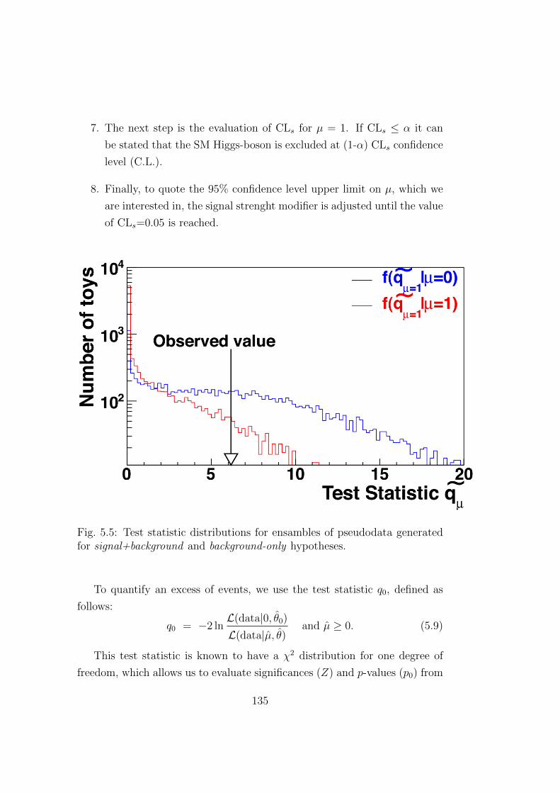
7. The next step is the evaluation of CLs for µ = 1. If CLs ≤ α it can

be stated that the SM Higgs-boson is excluded at (1-α) CLs confidence

level (C.L.).

8. Finally, to quote the 95% confidence level upper limit on µ, which we

are interested in, the signal strenght modifier is adjusted until the value

of CLs=0.05 is reached.

Fig. 5.5: Test statistic distributions for ensambles of pseudodata generatedfor signal+background and background-only hypotheses.

To quantify an excess of events, we use the test statistic q0, defined as

follows:

q0 = −2 lnL(data|0, θ0)

L(data|µ, θ)and µ ≥ 0. (5.9)

This test statistic is known to have a χ2 distribution for one degree of

freedom, which allows us to evaluate significances (Z) and p-values (p0) from

135

the following asymptotic formula, derived from the asymptotic properties of

the test statistic based on the profile likelihood ratio [18]:

Z =√qobs

0 , (5.10)

p0 = P (q0 ≥ qobs0 ) =

∫ ∞Z

e−x2/2

√2π

dx =1

2

[1− erf

(Z/√

2)], (5.11)

where qobs0 is the observed test statistic calculated for µ = 0 and with only

one constraint 0 ≤ µ, which ensures that data deficits are not counted on an

equal footing with data excesses. The “erf” stands for the error function.

The approximation has been tested for the range of expected background

and signal yields. The data can be, as usual, the actual experimental obser-

vation or pseudo-data. As previously pointed out, both the numerator and

the denominator are maximized and θ0, µ, θ are the values corresponding to

this maximum.

The p-value variable is used to quantify the consistency of the observed ex-

cess with the background only hypothesis. Whilst the p-value characterizes

the probability of observing a given excess of events, it does not give any

information about the compatibilty of the excess with the expected signal.

A measure of this compatibility is given by a best fit of µ variable. Two

kinds of p-value can be defined: a local p-value, defined for a particular mass

value or a very restricted range of mass, and a global p-value, which takes

into account the look-elsewhere effect for the entire search mass range (see

Ref. [5]). It can be defined as the probability for a background fluctuation

to match or exceed the observed excess anywhere in a specified mass range

[15].

5.2.2 Determination of the exclusion limits

To define the expected median upper limit and ±1σ and ±2σ bands for the

background-only hypothesis a set of background-only pseudo-data must be

generated. Then, CLs and µ95%CL can be calculated as they were real data.

The µ95%CL is the value of the signal strenght modifier at which the 95%

confidence level upper limit is reached.

136

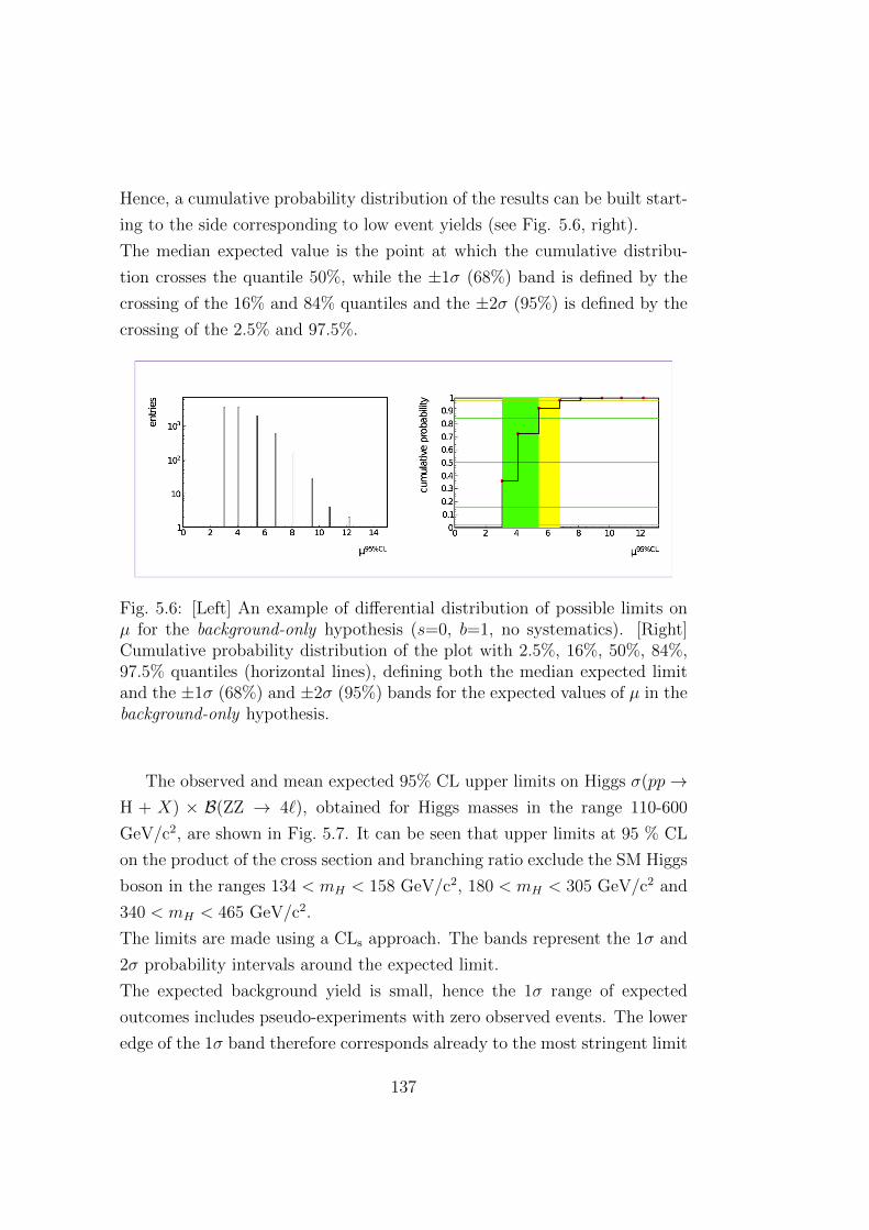
Hence, a cumulative probability distribution of the results can be built start-

ing to the side corresponding to low event yields (see Fig. 5.6, right).

The median expected value is the point at which the cumulative distribu-

tion crosses the quantile 50%, while the ±1σ (68%) band is defined by the

crossing of the 16% and 84% quantiles and the ±2σ (95%) is defined by the

crossing of the 2.5% and 97.5%.

Fig. 5.6: [Left] An example of differential distribution of possible limits onµ for the background-only hypothesis (s=0, b=1, no systematics). [Right]Cumulative probability distribution of the plot with 2.5%, 16%, 50%, 84%,97.5% quantiles (horizontal lines), defining both the median expected limitand the ±1σ (68%) and ±2σ (95%) bands for the expected values of µ in thebackground-only hypothesis.

The observed and mean expected 95% CL upper limits on Higgs σ(pp→H + X) × B(ZZ → 4`), obtained for Higgs masses in the range 110-600

GeV/c2, are shown in Fig. 5.7. It can be seen that upper limits at 95 % CL

on the product of the cross section and branching ratio exclude the SM Higgs

boson in the ranges 134 < mH < 158 GeV/c2, 180 < mH < 305 GeV/c2 and

340 < mH < 465 GeV/c2.

The limits are made using a CLs approach. The bands represent the 1σ and

2σ probability intervals around the expected limit.

The expected background yield is small, hence the 1σ range of expected

outcomes includes pseudo-experiments with zero observed events. The lower

edge of the 1σ band therefore corresponds already to the most stringent limit

137

on the signal cross section, as fluctuations below that value are not possible.

As already pointed out, the systematic uncertainties have been taken into

account in the form of nuisance parameters with a log-normal probability

density function. The exclusion limits extend at high mass beyond the sen-

sitivity of previous collider experiments.

It can be observed that the differences between the observed and the expected

limits are fairly consistent with statistical fluctuation, as the observed limits

fall generally within the green and yellow bands. We can also see that the

expected limits reflect the dependence of the branching ratio B(H→ZZ) on

mH .

The significance of the local excesses relative to the standard model ex-

pectation as a function of mH is shown in Fig. 5.8, obtained both without

or with individual candidate mass measurement uncertainties1 for the com-

bination of the three channels.

Event-by-event mass errors are evaluated starting from the errors on the in-

dividual lepton momenta.

For muons, the full error matrix, as obtained from the muon track fit, as

been used.

For electrons, the estimated error on the momentum magnitude, as obtained

from the combination of the ECAL and tracker measurement is used, ne-

glecting the uncertainty on the track direction from the Gaussian Sum Filter

fit. The lepton momentum measurement errors are then propagated to the

4l mass error and to the Z1 and Z2 mass errors using an analytical error

propagation including all correlations.

Excesses are observed for masses near 120 GeV/c2 and 320 GeV/c2. The

small 2σ excess near 320 GeV/c2 includes three events with p4`T >50 GeV/c.

The most significant excess is present near 120 GeV/c2 and corresponds to

about 2.5σ [2.7σ] significance, not including [or including] candidate mass

1The precision on the estimation of the mH and mZ∗ masses can vary significantly onevent-by-event depending on the p`T and η`. In the case of electrons, energy measurementuncertainties can furthermore vary significantly depending on the “category” of the re-constructed electron object, i.e. depending if the electron initiates a shower early in thetracker volume (“showering” electrons) or reaches the ECAL surface largely unperturbed(”golden” electrons). Overall, uncertainties on the measured ∆mH and ∆mZ∗ can varyby a factor up to three or so for the same initial mass mH.

138

uncertainties.

The significance is less than 1.0σ [about 1.6σ] when the look-elsewhere [5] ef-

fect is taken into account for the full mass range (100 < m4` < 600 GeV/c2).

Hence, we can remark that the data do not reveal a significant clustering of

events at any mass value.

5.3 Latest Results of the Standard Model Higgs

Search in the H → ZZ → 4` channel at√s = 8 TeV with 2012 data.

Even if the 2012 data samples have not been used to develop the selection

cuts for this thesis work, the importance of the 2012 results deserves to be

here presented.

The latest analysis has been designed for a Higgs boson in the mass range

100 < mH < 800 GeV/c2.

It used the data collected by CMS in 2011, combining them with the new

data collected in 2012 at√s = 8 TeV which corresponds to an additional

integrated luminosity of 5 fb−1 [14].

The reconstructed four-lepton invariant mass distribution for the 4` is shown

in Fig. 5.9. It combines the 4e, 4µ and 2e2µ channel information. We fo-

cused only on low mass values which represent the region of main interest.

A good agreement between data and MC background expectation can be

observed. The main background contribution after applying all the selection

cuts, is due to the irreducible background ZZ, with a smaller contribution of

Z+X, calculated by data driven techniques, at low masses.

The measured distributions are compared with the SM background expecta-

tion and exclusion limits at 95% CL on the µ ratio of the production cross

section for the Higgs boson to the SM expectation have been derived.

The upper limits obtained for the 4` and 2`2τ channel combination are shown

in Fig. 5.10. It can be observed that upper limits at 95% CL exclude the

presence of SM Higgs boson in the range 130-520 GeV/c2.

An excess of events has been observed in the low mass range in the 4` chan-

139

nel.

In Fig. 5.11, the local p-values in the full mass range and in the low mass

range region are shown as a function of mH . It can be observed that a lo-

cal minimum is reached approximately for the Higgs boson mass hypothesis

mH = 126 GeV/c2, corresponding to a local significance of 3.2σ.

140

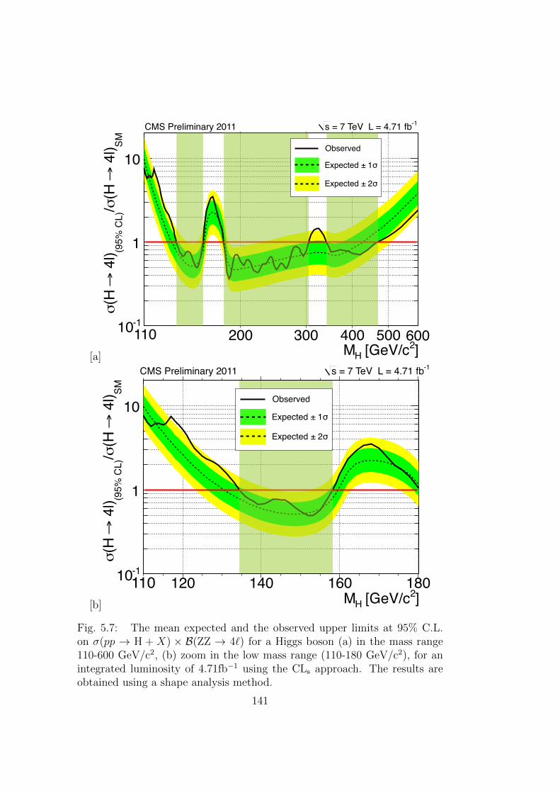
[a] ]2 [GeV/cHM200 300 400 500

SM 4

l)(H

/

(95%

CL)

4l)

(H

-110

1

10

4l, Asym CLs ZZ Observed Limit, H 4l, Asym CLs ZZ Expected Limit, H

68% expectation95% expectation

SM / CMS Preliminary 2011 -1 = 7 TeV, L = 4.7 fbs

110 600

Expected ± 1σ

Expected ± 2σ

Observed

CutHLT Z1 Z1 + l

Presel.Iso IP Kin (basel.)

Kin (int.)Kin (high)

Even

ts/1

Eve

nts

-110

1

10

210

310

410

510

610

710 DATAQCDtt

Z+light jetsc/cbZb

W+jetsSingle topWWWZZZ 2=350 GeV/cHm

2=200 GeV/cHm2=140 GeV/cHm

CMS Preliminary 2011 -1 = 7 TeV L = 4.71 fbs

[b] ]2 [GeV/cHM120 140 160 180

SM 4

l)(H

/

(95%

CL)

4l)

(H

-110

1

10

4l, Asym CLs ZZ Observed Limit, H 4l, Asym CLs ZZ Expected Limit, H

68% expectation95% expectation

SM / CMS Preliminary 2011 -1 = 7 TeV, L = 4.7 fbs

110

Expected ± 1σ

Expected ± 2σ

Observed

CutHLT Z1 Z1 + l

Presel.Iso IP Kin (basel.)

Kin (int.)Kin (high)

Even

ts/1

Eve

nts

-110

1

10

210

310

410

510

610

710 DATAQCDtt

Z+light jetsc/cbZb

W+jetsSingle topWWWZZZ 2=350 GeV/cHm

2=200 GeV/cHm2=140 GeV/cHm

CMS Preliminary 2011 -1 = 7 TeV L = 4.71 fbs

Fig. 5.7: The mean expected and the observed upper limits at 95% C.L.on σ(pp → H + X) × B(ZZ → 4`) for a Higgs boson (a) in the mass range110-600 GeV/c2, (b) zoom in the low mass range (110-180 GeV/c2), for anintegrated luminosity of 4.71fb−1 using the CLs approach. The results areobtained using a shape analysis method.

141

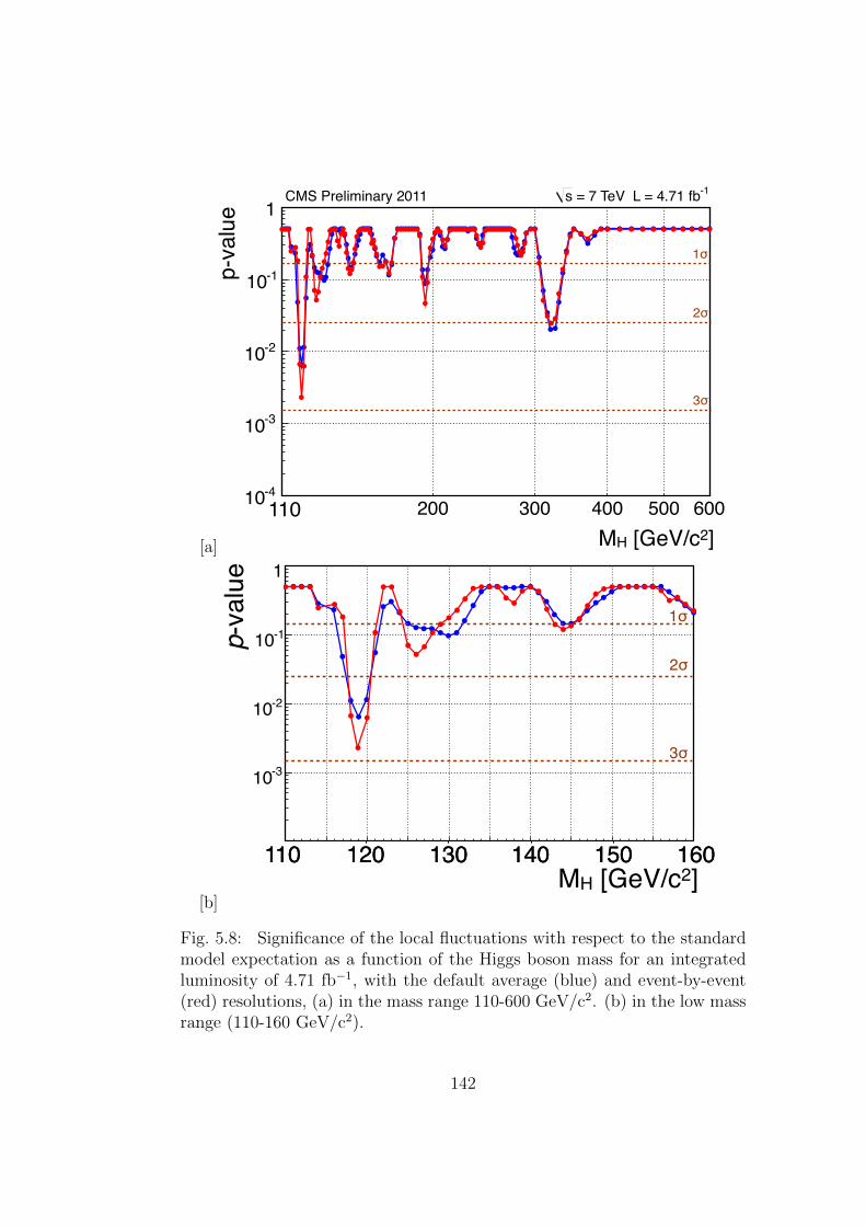
[a] ]2 [GeV/cH

Higgs mass, m200 300 400 500 600

p-v

alue

-410

-310

-210

-110

1-1= ~4.7 fbint=7 TeV LsCMS Private

4l ( without event-by-event mass resolution ) ZZ H

4l ( with event-by-event mass resolution ) ZZ H

MH [GeV/c2]110

CutHLT Z1 Z1 + l

Presel.Iso IP Kin (basel.)

Kin (int.)Kin (high)

Even

ts/1

Eve

nts

-110

1

10

210

310

410

510

610

710 DATAQCDtt

Z+light jetsc/cbZb

W+jetsSingle topWWWZZZ 2=350 GeV/cHm

2=200 GeV/cHm2=140 GeV/cHm

CMS Preliminary 2011 -1 = 7 TeV L = 4.71 fbs

1σ

2σ

3σ

[b]

14

p-value

FOR PRL inside the enlarged

Inclusive analysisZOOM

]2 [GeV/cH

Higgs mass, m110 115 120 125 130 135 140 145 150 155 160

p-v

alue

-410

-310

-210

-110

1-1= ~4.7 fbint=7 TeV LsCMS Private

4l ( without event-by-event mass resolution ) ZZ H

4l ( with event-by-event mass resolution ) ZZ H

]2 [GeV/cH

Higgs mass, m110 115 120 125 130 135 140 145 150 155 160

p-v

alue

-410

-310

-210

-110

1-1= ~4.7 fbint=7 TeV LsCMS Private

4l ( without event-by-event mass resolution ) ZZ H

4l ( with event-by-event mass resolution ) ZZ H

1σ

2σ

3σ

p-va

lue

16

p-value

Without vs. With event-by-event mass errors

Inclusive analysisZOOM

]2 [GeV/cH

Higgs mass, m110 115 120 125 130 135 140 145 150 155 160

p-v

alue

-410

-310

-210

-110

1-1= ~4.7 fbint=7 TeV LsCMS Private

4l ( without event-by-event mass resolution ) ZZ H

4l ( with event-by-event mass resolution ) ZZ H

100 110 120 130 140 150 160100 110 120 130 140 150 160100 110 120 130 140 150 160100 110 120 130 140 150 160100 110 120 130 140 150 160100 110 120 130 140 150 160

]2 [GeV/cH

Higgs mass, m110 115 120 125 130 135 140 145 150 155 160

p-v

alue

-410

-310

-210

-110

1-1= ~4.7 fbint=7 TeV LsCMS Private

4l ( without event-by-event mass resolution ) ZZ H

4l ( with event-by-event mass resolution ) ZZ H

MH [GeV/c2]

Fig. 5.8: Significance of the local fluctuations with respect to the standardmodel expectation as a function of the Higgs boson mass for an integratedluminosity of 4.71 fb−1, with the default average (blue) and event-by-event(red) resolutions, (a) in the mass range 110-600 GeV/c2. (b) in the low massrange (110-160 GeV/c2).

142

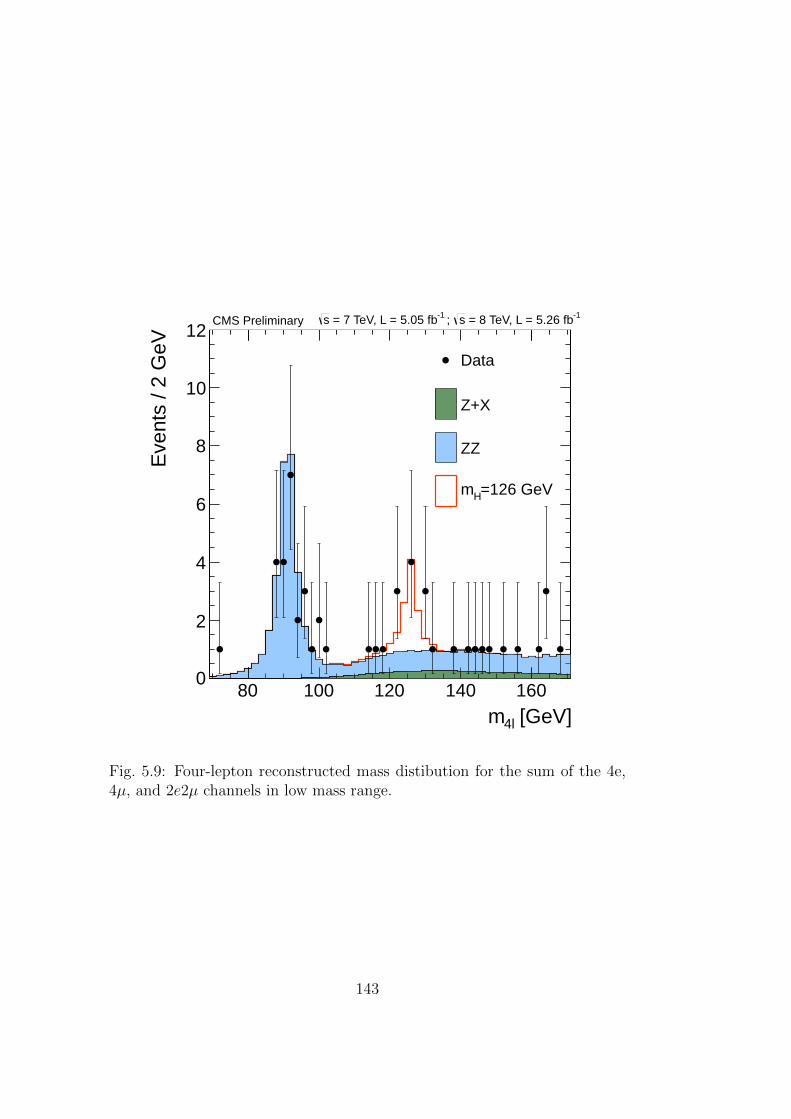
[GeV]4lm80 100 120 140 160

Eve

nts

/ 2 G

eV

0

2

4

6

8

10

12

Data

Z+X

ZZ

=126 GeVHm

CMS Preliminary -1 = 8 TeV, L = 5.26 fbs ; -1 = 7 TeV, L = 5.05 fbs

Fig. 5.9: Four-lepton reconstructed mass distibution for the sum of the 4e,4µ, and 2e2µ channels in low mass range.

143

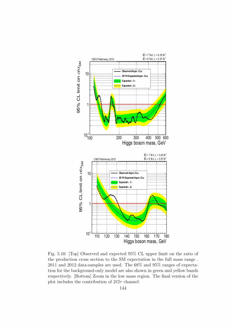
Fig. 5.10: [Top] Observed and expected 95% CL upper limit on the ratio ofthe production cross section to the SM expectation in the full mass range .2011 and 2012 data-samples are used. The 68% and 95% ranges of expecta-tion for the background-only model are also shown in green and yellow bandsrespectively. [Bottom] Zoom in the low mass region. The final version of theplot includes the contribution of 2`2τ channel.

144

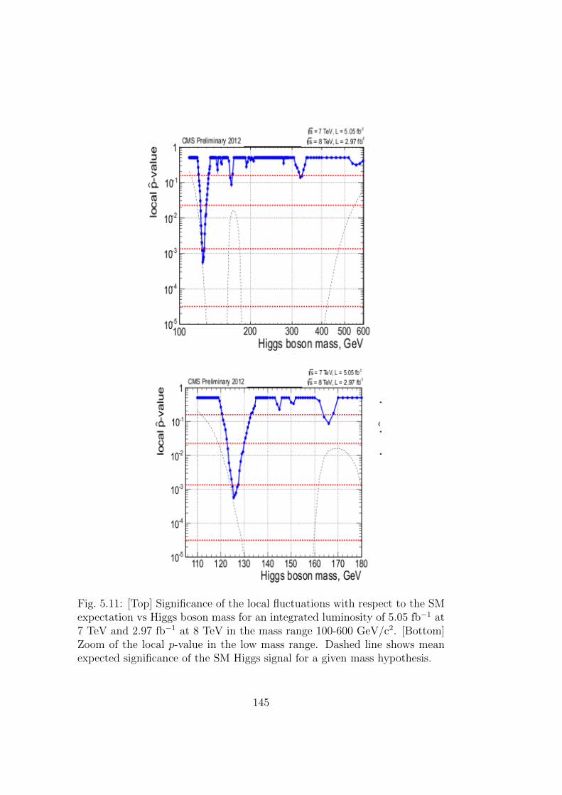
Fig. 5.11: [Top] Significance of the local fluctuations with respect to the SMexpectation vs Higgs boson mass for an integrated luminosity of 5.05 fb−1 at7 TeV and 2.97 fb−1 at 8 TeV in the mass range 100-600 GeV/c2. [Bottom]Zoom of the local p-value in the low mass range. Dashed line shows meanexpected significance of the SM Higgs signal for a given mass hypothesis.

145

146

Conclusions

The results of a search for the Standard Model Higgs boson produced in

pp collisions at√s= 7+ 8 TeV and decaying in ZZ(∗), based on data col-

lected during 2010-2011, have been presented in the leptonic Z decay channel

ZZ(∗) → 4`, with ` = e, µ.

The procedure to get them has followed the simple sequential sets of lepton

reconstruction, identification and isolation cuts and a set of kinematic cuts,

already described in chapter 4, to define a common baseline for the search

at any Higgs boson mass mH in the range 100 < mH < 600 GeV/c2 at√s =

7 TeV and 100 < mH < 800 GeV/c2 at√s = 7 and 8 TeV, respectively.

The instrumental background from Z+jets and the reducible backgrounds

from Zbb and tt, with mis-identified primary leptons, have been shown to be

negligible over most of the mass range, with a small contamination remaining

at low masses.

For the analysis which used only 2010-2011 data samples at√s = 7 TeV,

72 events, 12 in 4e channel, 23 in 4µ channel e 37 in 2e2µ channel, have

been totally observed for an integrated luminosity of 4.71± 0.21 fb−1, while

67.1± 5.5 events are expected from SM background processes.

The distribution of events is compatible with the expectation from the SM

continuum production of Z boson pairs from qq annihilation and gg fusion.

The most significant excess is near 120 GeV/c2, corresponding to about 2.5σ

significance. Taking into account the look-elsewhere effect the significance is

lowered down to about 1.0σ.

The significance values are further lowered when candidate mass uncertain-

ties are not included.

No clustering of events is observed in the measured m4` mass spectrum. Thir-

teen of the candidates are observed within 100 < m4` < 160 GeV/c2 while

147

9.8± 0.8 background events are expected.

Upper limits obtained at 95% CL on the cross section×branching ratio for

a Higgs boson with standard model-like decays exclude cross sections pre-

dicted by the standard model in the mass ranges 134 < mH < 158 GeV/c2,

180 < mH < 305 GeV/c2 and 340 < mH < 465 GeV/c2.

A major fraction of the mass range 100 to 600 GeV/c2 is so excluded at 95%

CL.

At low mass, only the region 114.4 < mH < 134 GeV/c2 remains consistent

with the expectation of the Standard Model.

An original preliminary study about the best 4` algorithm has also been

presented. It revealed a general inefficiency of the reconstructed Z1 and Z2

matching with MC Truth objects (up to 30% for the 4e channel and up to

25% for 4µ and 2e2µ channels) in the low mass region.

A quite good matching (∼ 100% for muons and > 80% for electrons) of the

recostructed lepton objects coming from Z1 and Z2 has also been found.

At low mass values (mH < 300 GeV/c2) about 10- 25 % for 4µ channel and

10-40 % for 4e channel of the events passing the full selection do not have

the two Z’s matched with those from MC Truth.

In this region the 8% of events for the 4e channel and the 12% of events

for the 4µ channel is passing the full selection, even if the Z reconstructed

objects are not matched (fake events).

It can be concluded that a wrong lepton pairing has been performed in the

low energy range.

For the analysis performed at√s = 8 TeV and combined with that at 7

TeV, the invariant mass distribution m4` is found quite consistent with the

SM background expectation over almost all the mass range. In this case,

upper limits calculated at 95% CL enlarge the exclusion mass window to

130-520 GeV/c2.

An excess of event can be observed in the mass range 120 < m4` < 130

GeV/c2. This excess makes the observed limits weaker than expected in the

null hypothesis (only-background hypothesis).

A clusterization of events can be seen at m4` ' 126 GeV/c2, giving rise to

a local excess with the respect to the background expectation. The corre-

148

sponding significance calculated for the SM Higgs boson hypothesis is 3.2σ.

More statistics is required to confirm definitely this amazing result.

149

150

Bibliography

[1] S.Dittmaier et al. A. Bredenstein, A. Denner. “Radiative corrections

to the semileptonic and hadronic Higgs-boson decays H→WW/ZZ→4

fermions”. JHEP, 0702(080), 2007.

[2] A. Bredenstein, A. Denner, S.Dittmaier et al. “Precise predic-

tions for the Higgs-boson decay H→WW/ZZ→4leptons”. Phys. Rev.,

D74(013004), 2006.

[3] I. Pulljak et al. A. Denner, S. Heinemeyer. “Standard Model Higgs-

Boson Branching Ratios with Uncertainties”. Eur. Phys. J., C71(1753),

2011.

[4] A. Djouadi, J. Kalinowski, M. Muhlleitner et al. “An update of the

program HDECAY“. In The Les Houches 2009 workshop on TeV col-

liders:The tools and Monte Carlo working group summary report, 2010.

[5] LHC Higgs Combination Group ATLAS Collaboration, CMS Collab-

oration. “Procedure for the LHC Higgs boson search combination in

Summer 2011”. Technical report, CERN, 2011.

[6] S. Bolognesi. “Talk at the CMS Trigger Plenary Session”.

[7] C. Anastasiou, K. Melnikov. “Higgs boson production at hadron collid-

ers in NNLO QCD“. Nucl. Phys., B646, 2002.

[8] C. Anastasiou, R. Boughezal, F. Petriello. “Mixed QCD-electroweak

corrections to Higgs boson production in gluon fusion“. JHEP, 04(003),

2009.

[9] CMS Collaboration. “The Compact Muon Solenoid technical proposal“.

151

[10] CMS Collaboration. “Absolute Calibration of the Luminosity Measure-

ment at CMS“. CMS-DP-2011-002, 2011.

[11] CMS Collaboration. “ATLAS+CMS Combination of Summer 11 Re-

sults”. CMS Physics Analysis Summary, CMS-PAS-HIG-11-023, 2011.

[12] CMS Collaboration. “Combination of CMS searches for a Standard

Model Higgs boson“. CMS PAS HIG-11-032, December 2011.

[13] CMS Collaboration. “ECAL 2010 performance results“. Technical re-

port, CMS Detector Perfomace SummaryDP-2011/008, 2011.

[14] CMS Collaboration. “Search for the standard model Higgs boson in the

H → ZZ → 4` channel in pp collisions at√s = 7 and 8 TeV“. CMS

PAS HIG-12-016, June 2012.

[15] The CMS Collaboration. “Combination of searches for a standard model

Higgs boson“. Draft Paper HIG-11-032, CERN, 2012.

[16] The LHC Study Group Collaboration. “LHC-the Large Hadron Collider

accelerator project”. Technical report, CERN-AC-93-03, 2003.

[17] The LHC Study Group Collaboration. “LHC-the Large Hadron Collider

conceptual design”. Technical report, CERN-AC-95-05, 2005.

[18] G. Cowan. “Statistical Data Analysis“. Oxford Science Publications,

1998.

[19] K. Ellis C.W J. Campbell. “MCFM-Monte Carlo for FeMtobarn pro-

cess”, 2011.

[20] D. de Florian, M. Grazzini. “Higgs production through gluon fusion:

updated cross section at the Tevatron and the LHC“. Nucl. Phys.,

B359, 1991.

[21] S. Dawson. “Radiative corrections to Higgs boson production“. Nucl.

Phys., B359, 1991.

152

[22] A. Djouadi. “The Anatomy of Electro-Weak Symmetry Breaking”. Tech-

nical report, Laboratoire de Physique Theorique d’Orsay, Universite

Paris Sud; Laboratoire de Physique Mathematique et Theorique, Uni-

versite de Montpellier II, 2005.

[23] J. Alwall et al. “MadGraph/MadEvent v4:The New Web Generation“.

JHEP, 09(028), 2007.

[24] P. Avery et al. “A complete model of the four lepton invariant mass

distribution for H→ZZ→4l and ZZ→ 4l events”. CMS Analysis Note,

2011/202, 2011.

[25] F. Beaudette on behalf of the CMS Collaboration. “Performance of the

particle flow algorithm in CMS“. CMS CR-2010/276, November 2010.

[26] A. D. Martin F. Halzen. “Quarks Leptons: An Introductory Course in

Modern Particle Physics”. Wiley, 1984.

[27] G. Abbiendi, N. Adam et al. “Muon Recostruction in the CMS Detec-

tor“. CMS AN 2008/097, July 2009.

[28] G. Parisi G. Altarelli, 1977.

[29] G.Bozzi, S. Catani, D de Florian et al. “Transverse-momentum resum-

mation and the spectrum of the Higgs boson at the LHC”. Nucl. Phys.,

B737:73–120, 2006.

[30] Hung-Liang Lai et al. “New parton distributions for collider physics“.

Phys. Rev., D82, 2010.

[31] T. Junk. “Confidence level computation for combining searches with

small statistics“. Nucl.Instrum.Meth., A(434):435–443, 1999.

[32] K. Arnold et al. “A parton level MC for processes with electroweak

bosons. Comput. Phys. Commun., 180:1661–1670, 2009.

[33] L. Evans, P. Bryant [LHC Collaboration]. “LHC - Machine“. JINST, 3,

2008.

153

[34] C. Mariotti et al. LHC Higgs Cross Section Working Group,

S. Dittmaier. “Handbook of LHC Higgs Cross Sections:1. Inclusive Ob-

servables”. Technical report, CERN, Geneva., 2011.

[35] M. Cacciari, S. Frixione, M. Mangano et al. “Updated predictions for

the total production crosssections of top and of heavier quark pairs at

the Tevatron and at the LHC”.

[36] S. Dittmaier M. Ciccolini, A. Denner. “Strong and electroweak correc-

tions to the production of Higgs + 2-jets via weak interactions at the

LHC“. Phys. Rev. Lett., 99(161803), 2007.

[37] S. Dittmaier M. Ciccolini, A. Denner. “Electroweak and QCD correc-

tions to Higgs production via vector-boson fusion at the LHC“. Phys.

Rev., D77(013002), 2008.

[38] M. Mulders, I. Bloch et al. “Muon Identification in CMS“. CMS AN-

2008/098, November 2008.

[39] M. Spira, A. Djouadi, D. Graundenz et al. “Higgs boson production at

the LHC“. Nucl. Phys., B453, 1995.

[40] P. Adzic et al. [CMS Collaboration]. “Energy resolution of the barrel of

the CMS Electromagnetic Calorimeter”. JINST, 2, 2007.

[41] P. Bolzoni, F. Maltoni,M. Moch,Sven-Olaf, Zaro. “Higgs pproduction via

vector-boson fusion at NNLO in QCD”. Phys. Rev. Lett., 105(011801),

2010.

[42] D. H. Perkins. “Introduction To High Energy Physics”. Cambridge

University Press, 2000.

[43] M. Pierini. “Talk at the Joint PVT/PO Meeting“.

[44] R. Adolphi et al. [CMS Collaboration]. “The CMS experimentat the

CERN LHC“. JINST, 3, 2008.

154

[45] J. Tucker R. D. Cousin, J. T. Linneman. “Evaluation of three methods

for calculating statistical significance when incorporating a systematic

uncertainty into a test of the background-only hypothesis for a Poisson

process“. Nucl.Instrum.Meth., A595, 2008.

[46] W. B. Kilgore R. V. Harlander. “Next-to-next-to leading order Higgs

production at hadron colliders“. Phys. Rev. Lett., 88(2001801), 2002.

[47] A. L. Read. “Modified Frequentist analysis of search results (the CLs

method)”. Yellow Report 81, CERN-2000-005, 2000.

[48] S. Actis, G.Passarino, C. Sturm et al. “NLO Electroweak Corrections to

Higgs Boson Production at Hadron Colliders“. Phys. Lett., B670, 2008.

[49] S. Actis, G.Passarino, C. Sturm et al. “NNLO Computational Tech-

niques: the Cases H → γγ and H → gg“. Nucl. Phys., B811:182–273,

2009.

[50] S. Baffioni et al. “Search strategy for the Higgs boson in the ZZ∗ decay

channel with the CMS experiment“. CMS AN 2008/050, 2008.

[51] S. Baffioni, F. Beaudette, D. Benedetti et al. “Electron Identification in

CMS“. CMS AN-2009/178, December 2009.

[52] S. Catani,D. de Florian, M. Grazzini et al. “Soft-gluon resummation for

Higgs boson production at hadron colliders“. JHEP, 07(028), 2003.

[53] S. Frixione, P. Nason, and C. Oleari. “Matching NLO QCD computa-

tions with Parton Shower simulations: the POWHEG method”. JHEP,

11(070), 2007.

[54] P. Skands. “The Perugia Tunes“, 2009.

[55] T. Binoth, N. Kauer, and P. Mertsch. “Gluon-induced QCD corrections

to pp→ ` ¯ ′ ¯′”, 2008.

[56] D. Zeppenfeld T. Figy, C. Oleari. “Next-to-leading order jet distribu-

tion for Higgs boson production via weak-boson fusion“. Phys. Rev.,

D68(073005), 2003.

155

[57] T. Sjostrand, S. Mrenna, P.Skands. “Pythia 6.4 Physics and Manual“.

Technical report, FERMILAB, 2006.

[58] W. L. van Neerven V. Ravindran, J. Smith. “NNLO corrections to

the total cross section for Higgs boson production in hadron hadron

collisions“. Nucl. Phys., B665, 2003.

[59] W. Adam, S. Baffioni, F. Beaudette et al. “Electron Reconstruction in

CMS“. CMS AN-2009/164, November 2009.

156