UNIVERSITÀ DEGLI STUDI DELLA TUSCIA DI VITERBO...

UNIVERSITÀ DEGLI STUDI DELLA TUSCIA DI VITERBO

DIPARTIMENTO PER L’INNOVAZIONE NEI SISTEMI BIOLOGICI AGROALIMENTARI E FORESTALI

CORSO DI DOTTORATO DI RICERCA

BIOTECNOLOGIA DEGLI ALIMENTI - XXIV CICLO

TITOLO TESI DI DOTTORATO DI RICERCA

Applicazione di uno spettrofotometro NIR – AOTF per la determinazione della migliore epoca di raccolta dell’uva da vino Sangiovese

AGR/15

Coordinatore: Prof. Marco Esti

Firma ……………………..

Tutor: Prof. Fabio Mencarelli

Firma………………………

Dottorando: Federico Emanuele Barnaba

Firma …………………………

Questo lavoro lo dedico a Martina, la mia fidanzata, che mi ha spinto ad intraprendere questo percorso e a continuarlo anche nei momenti più difficili, a mia madre e mio padre che pazientemente mi hanno sostenuto in questi interminabili anni di studio, a mio fratello, e in ultimo ai miei cari nonni che ricordo con immenso piacere.

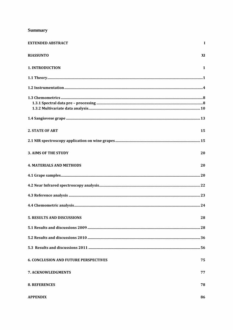
Summary

EXTENDED ABSTRACT I

RIASSUNTO XI

1. INTRODUCTION 1

1.1 Theory .............................................................................................................................................................................. 1

1.2 Instrumentation ........................................................................................................................................................... 4

1.3 Chemometrics ............................................................................................................................................................... 8 1.3.1 Spectral data pre – processing ....................................................................................................................... 8 1.3.2 Multivariate data analysis............................................................................................................................. 10

1.4 Sangiovese grape ...................................................................................................................................................... 13

2. STATE OF ART 15

2.1 NIR spectroscopy application on wine grapes ............................................................................................... 15

3. AIMS OF THE STUDY 20

4. MATERIALS AND METHODS 20

4.1 Grape samples............................................................................................................................................................ 20

4.2 Near Infrared spectroscopy analysis ................................................................................................................. 22

4.3 Reference analysis ................................................................................................................................................... 23

4.4 Chemometric analysis ............................................................................................................................................. 24

5. RESULTS AND DISCUSSIONS 28

5.1 Results and discussions 2009 .............................................................................................................................. 28

5.2 Results and discussions 2010 .............................................................................................................................. 36

5.3 Results and discussions 2011 ............................................................................................................................. 56

6. CONCLUSION AND FUTURE PERSPECTIVES 75

7. ACKNOWLEDGMENTS 77

8. REFERENCES 78

APPENDIX 86

I

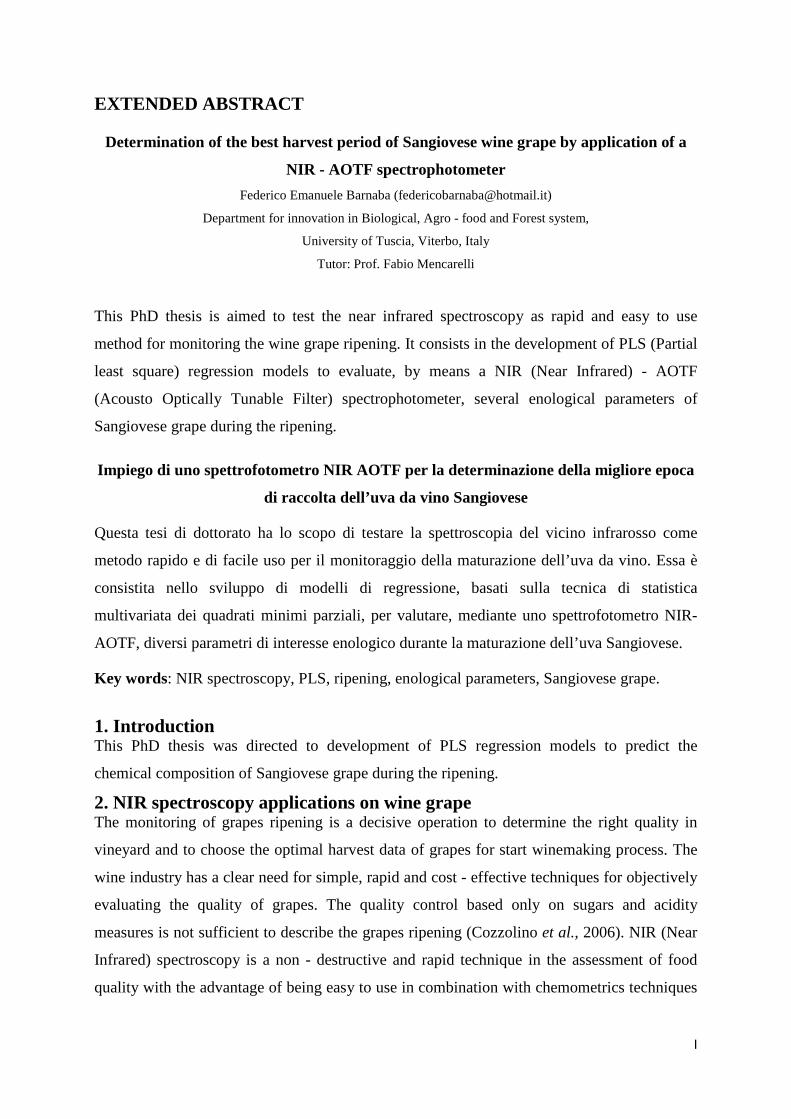
EXTENDED ABSTRACT

Determination of the best harvest period of Sangiovese wine grape by application of a

NIR - AOTF spectrophotometer Federico Emanuele Barnaba ([email protected])

Department for innovation in Biological, Agro - food and Forest system,

University of Tuscia, Viterbo, Italy

Tutor: Prof. Fabio Mencarelli

This PhD thesis is aimed to test the near infrared spectroscopy as rapid and easy to use

method for monitoring the wine grape ripening. It consists in the development of PLS (Partial

least square) regression models to evaluate, by means a NIR (Near Infrared) - AOTF

(Acousto Optically Tunable Filter) spectrophotometer, several enological parameters of

Sangiovese grape during the ripening.

Impiego di uno spettrofotometro NIR AOTF per la determinazione della migliore epoca

di raccolta dell’uva da vino Sangiovese

Questa tesi di dottorato ha lo scopo di testare la spettroscopia del vicino infrarosso come

metodo rapido e di facile uso per il monitoraggio della maturazione dell’uva da vino. Essa è

consistita nello sviluppo di modelli di regressione, basati sulla tecnica di statistica

multivariata dei quadrati minimi parziali, per valutare, mediante uno spettrofotometro NIR-

AOTF, diversi parametri di interesse enologico durante la maturazione dell’uva Sangiovese.

Key words: NIR spectroscopy, PLS, ripening, enological parameters, Sangiovese grape.

1. Introduction This PhD thesis was directed to development of PLS regression models to predict the

chemical composition of Sangiovese grape during the ripening.

2. NIR spectroscopy applications on wine grape The monitoring of grapes ripening is a decisive operation to determine the right quality in

vineyard and to choose the optimal harvest data of grapes for start winemaking process. The

wine industry has a clear need for simple, rapid and cost - effective techniques for objectively

evaluating the quality of grapes. The quality control based only on sugars and acidity

measures is not sufficient to describe the grapes ripening (Cozzolino et al., 2006). NIR (Near

Infrared) spectroscopy is a non - destructive and rapid technique in the assessment of food

quality with the advantage of being easy to use in combination with chemometrics techniques

II

for quality and quantitative analysis (Cen and He, 2007). The near - infrared region (750 -

2500 nm) contains information concerning relative proportions of CH, NH, OH bonds of the

organic molecules. The potential of NIR spectroscopy was tested as an alternative analytical

method for measuring enological parameters on intact or processed grapes (Cozzolino et al.,

2006). Recent studies have shown the applicability of NIR to predict dry matter and

condensed tannin on homogenized grape berry samples in addition to other important

parameters such as total anthocyanins, total soluble solids and pH (Cozzolino et al., 2008).

NIR spectroscopy was tested for determining the concentration of the total polyphenols and

the families of the main polyphenols in grapes and in grape skins throughout the ripening

(Ferrer – Gallego et al., 2011). Studies on Cabernet Franc have also shown that exist

relationships between some wavelengths of VIS / NIR and sensory attributes that describe

ripeness evolution, such as firmness, elasticity and resistance to handling (Le Moigne et al.,

2008). A study by Kaye and Wample (2005) on Cabernet Sauvignon area production showed

that the NIR – AOTF instrument (Barbieri Gonzaga and Pasquini, 2005) may find significant

practical application through non-destructive measurement of total polyphenols,

anthocyanins, tartaric and malic acid in qualitative discrimination within the vineyard. The

use of NIR – AOTF was also aimed at studying the grapes dehydration for dessert wines

production (Bellincontro et al., 2009; Bellincontro et al., 2011).

3. Materials and Methods The trial was conducted during the seasons 2009, 2010 and 2011 on Vitis vinifera L. cv.

Sangiovese. In the season 2009 grape samples were collected by two vineyards sites in

Nipozzano locality (Firenze, Italy). Vineyard 1 was implanted in 2001 year with SS-F9-A5-48

Sangiovese clone grafted on 1103 Paulsen rootstock while the Vineyard 2 was implanted in

2000 year with VCR 23 Sangiovese clone grafted on 420 A rootstock. In the season 2010

grape samples were collected from a vineyard sites in La Capitana locality (Grosseto, Italy).

The vineyard was implanted in 2004 season with Fedit 20 CH and Fedit 21 CH Sangiovese

clones grafted on 1103 and 1175 Paulsen rootstocks. In 2009 season 76 grape samples were

collected from the first decade of September to the harvest data while in 2010 season 20 grape

samples were picked from the third decade of august to the first decade of october. Each

sample was constituted by 100 berries. Each sample had origin from a selected area of

vineyard according to the vigour of the plants. In each area was choose a representative row

from which to withdraw the berries. Berries were collected in random way from the clusters

and were sampling from both sides of the selected rows. Spectral detection was carry out with

a Luminar 5030 Miniature Hand-held NIR Analyzer (Brimrose Corp., Baltimore, MD, USA),

III

based on the AOTF-NIR principle. Two different measurements in diffuse reflectance mode

were performed on each berry from the two opposite sides. Detection was conducted in the

1100 – 2300 nm range, with 2 nm wavelength increments and 100 spectra per average, which

represented a single measurement. Grape samples afterwards the spectral acquisition were

crushed and the juices were centrifuged. Supernatants were analyzed by Wine Scan FT 120

(Foss Corp., Hilleroed, DK) to determine the following enological parameters: total soluble

solids (Brix and Babo), total sugars, glucose, fructose, density, tartaric acid, pH, titratable

acidity, malic acid, gluconic acid, assumable Nitrogen, anthocyanins and total phenols. Raw

spectra were pre - treated for absorbance (1/R) transformation using SNAP! 2.03 software

(Brimrose Corp., Baltimore, MD, USA). Before the calibrations and the building up of the

prediction models, the spectral variations of the data sets were analyzed by Principal

Component Analysis (PCA). The absorbance data were subject to a mean normalization (MN)

and after were treated with the following statistical filter: Standard Normal Variate (SNV)

correction, Multiplicative Scattering Correction (MSC), first order of Savitzky - Golay filter

(SG 1st der) or second order of Savitzky - Golay (SG 2nd der) filter with 11 points of

smoothing. Partial Least Squares (PLS) regression models were developed on the data

collected in the season 2009 and 2010. Data collected in 2010 season were used to improve

the calibration carried out in 2009 season. PLS was built on the full spectrum (1100-2300 nm)

and was applied an internal full cross validation (leave one out). The performance of the

models was evaluated by standard error of calibration (SEC), standard error of cross

validation (SECV), root mean square error of calibration (RMSEC), root mean square error of

cross validation (RMSECV), Bias, coefficient of determination for calibration (R2c) and

coefficient of determination for cross validation (R2cv). Finally was calculated the principal

component suggest number or latent variable (Lv) that minimize the error in prediction and

the residual predictive deviation (RPD) to evaluate model capacity in predicting investigated

chemical data. In the season 2011 25 samples of Sangiovese grape were provide from a

vineyard sites in Montecchio (Terni, Italy). Samples were used as external set for the

validation of the better PLS regression models obtained in the 2009 - 2010 seasons. The

models performance in prediction was evaluated by coefficient of determination for prediction

(R2), root mean standard error of prediction (RMSEP), standard error of prediction (SEP),

Bias and RPD index. Statistical pre-treatments, PCA and PLS models were performed by

Unscrambler v9.7 software (CAMO ASA, Oslo, Norway).

IV

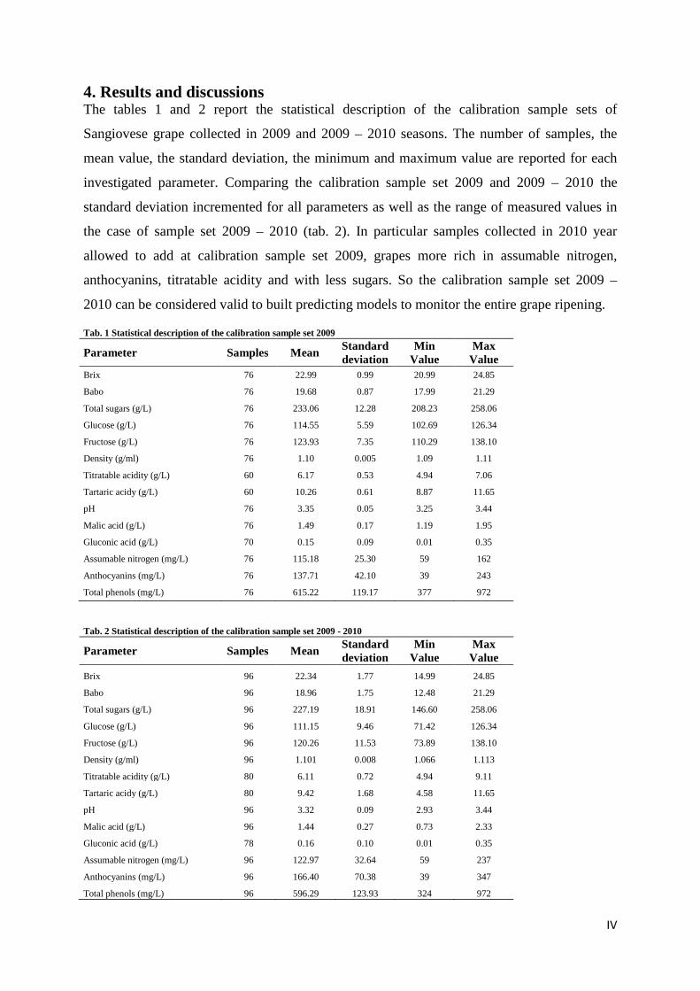
4. Results and discussions The tables 1 and 2 report the statistical description of the calibration sample sets of

Sangiovese grape collected in 2009 and 2009 – 2010 seasons. The number of samples, the

mean value, the standard deviation, the minimum and maximum value are reported for each

investigated parameter. Comparing the calibration sample set 2009 and 2009 – 2010 the

standard deviation incremented for all parameters as well as the range of measured values in

the case of sample set 2009 – 2010 (tab. 2). In particular samples collected in 2010 year

allowed to add at calibration sample set 2009, grapes more rich in assumable nitrogen,

anthocyanins, titratable acidity and with less sugars. So the calibration sample set 2009 –

2010 can be considered valid to built predicting models to monitor the entire grape ripening.

Tab. 1 Statistical description of the calibration sample set 2009

Parameter Samples Mean Standard deviation

Min Value

Max Value

Brix 76 22.99 0.99 20.99 24.85

Babo 76 19.68 0.87 17.99 21.29

Total sugars (g/L) 76 233.06 12.28 208.23 258.06

Glucose (g/L) 76 114.55 5.59 102.69 126.34

Fructose (g/L) 76 123.93 7.35 110.29 138.10

Density (g/ml) 76 1.10 0.005 1.09 1.11

Titratable acidity (g/L) 60 6.17 0.53 4.94 7.06

Tartaric acidy (g/L) 60 10.26 0.61 8.87 11.65

pH 76 3.35 0.05 3.25 3.44

Malic acid (g/L) 76 1.49 0.17 1.19 1.95

Gluconic acid (g/L) 70 0.15 0.09 0.01 0.35

Assumable nitrogen (mg/L) 76 115.18 25.30 59 162

Anthocyanins (mg/L) 76 137.71 42.10 39 243

Total phenols (mg/L) 76 615.22 119.17 377 972

Tab. 2 Statistical description of the calibration sample set 2009 - 2010


Min Value

Max Value

Brix 96 22.34 1.77 14.99 24.85

Babo 96 18.96 1.75 12.48 21.29

Total sugars (g/L) 96 227.19 18.91 146.60 258.06

Glucose (g/L) 96 111.15 9.46 71.42 126.34

Fructose (g/L) 96 120.26 11.53 73.89 138.10

Density (g/ml) 96 1.101 0.008 1.066 1.113



pH 96 3.32 0.09 2.93 3.44

Malic acid (g/L) 96 1.44 0.27 0.73 2.33

Gluconic acid (g/L) 78 0.16 0.10 0.01 0.35


Anthocyanins (mg/L) 96 166.40 70.38 39 347

Total phenols (mg/L) 96 596.29 123.93 324 972

V

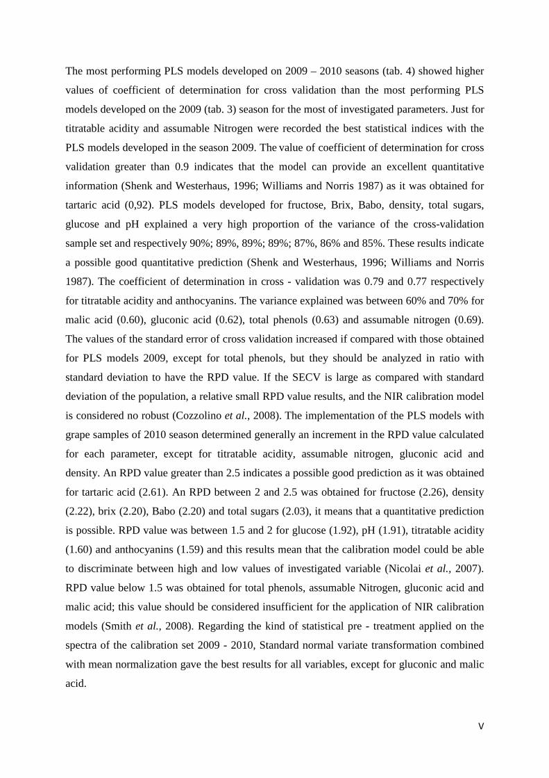
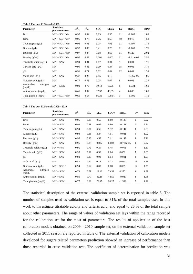
The most performing PLS models developed on 2009 – 2010 seasons (tab. 4) showed higher

values of coefficient of determination for cross validation than the most performing PLS

models developed on the 2009 (tab. 3) season for the most of investigated parameters. Just for

titratable acidity and assumable Nitrogen were recorded the best statistical indices with the

PLS models developed in the season 2009. The value of coefficient of determination for cross

validation greater than 0.9 indicates that the model can provide an excellent quantitative

information (Shenk and Westerhaus, 1996; Williams and Norris 1987) as it was obtained for

tartaric acid (0,92). PLS models developed for fructose, Brix, Babo, density, total sugars,

glucose and pH explained a very high proportion of the variance of the cross-validation

sample set and respectively 90%; 89%, 89%; 89%; 87%, 86% and 85%. These results indicate

a possible good quantitative prediction (Shenk and Westerhaus, 1996; Williams and Norris

1987). The coefficient of determination in cross - validation was 0.79 and 0.77 respectively

for titratable acidity and anthocyanins. The variance explained was between 60% and 70% for

malic acid (0.60), gluconic acid (0.62), total phenols (0.63) and assumable nitrogen (0.69).

The values of the standard error of cross validation increased if compared with those obtained

for PLS models 2009, except for total phenols, but they should be analyzed in ratio with

standard deviation to have the RPD value. If the SECV is large as compared with standard

deviation of the population, a relative small RPD value results, and the NIR calibration model

is considered no robust (Cozzolino et al., 2008). The implementation of the PLS models with

grape samples of 2010 season determined generally an increment in the RPD value calculated

for each parameter, except for titratable acidity, assumable nitrogen, gluconic acid and

density. An RPD value greater than 2.5 indicates a possible good prediction as it was obtained

for tartaric acid (2.61). An RPD between 2 and 2.5 was obtained for fructose (2.26), density

(2.22), brix (2.20), Babo (2.20) and total sugars (2.03), it means that a quantitative prediction

is possible. RPD value was between 1.5 and 2 for glucose (1.92), pH (1.91), titratable acidity

(1.60) and anthocyanins (1.59) and this results mean that the calibration model could be able

to discriminate between high and low values of investigated variable (Nicolai et al., 2007).

RPD value below 1.5 was obtained for total phenols, assumable Nitrogen, gluconic acid and

malic acid; this value should be considered insufficient for the application of NIR calibration

models (Smith et al., 2008). Regarding the kind of statistical pre - treatment applied on the

spectra of the calibration set 2009 - 2010, Standard normal variate transformation combined

with mean normalization gave the best results for all variables, except for gluconic and malic

acid.

VI

Tab. 3 The best PLS results 2009

Parameter Statistical pre - treatment R2

c R2cv SEC SECV Lv Biascv RPD

Brix MN + SG 1° der 0,97 0,84 0,25 0,55 11 -0.008 1,83

Babo MN + SG 1° der 0,95 0,78 0,26 0,56 10 0.010 1,58

Total sugars (g/L) MN + SG 1° der 0,96 0,83 3,25 7,05 11 -0.099 1,75

Glucose (g/L) MN + SG 1° der 0,97 0,83 1,41 3,20 11 -0.060 1,76

Fructose (g/L) MN + SG 1° der 0,97 0,87 1,68 3,65 11 0.125 2,02

Density (g/ml) MN + SG 1° der 0,97 0,85 0,001 0,002 11 -8.11 e-05 2,50

Titratable acidity (g/L) MN + SNV 0,94 0,81 0,17 0,31 9 0.004 1,71

Tartaric acid (g/L) MN 0,99 0,83 0,09 0,34 15 0.005 1,79

pH MN 0,91 0,71 0,02 0,04 12 0.001 1,39

Malic acid (g/L) MN + SNV 0,37 0,23 0,15 0,16 3 -4.36 e-05 1,06

Gluconic acid (g/L) MN 0,77 0,58 0,05 0,07 8 0.001 1,29 Assumable nitrogen (mg/L) MN + MSC 0,91 0,79 10,13 16,06 8 -0.334 1,60

Anthocyanins (mg/L) MN 0,46 0,32 37,32 40,35 4 0.080 1,05

Total phenols (mg/L) MN + SG 1° der 0,69 0,54 86,21 100,91 3 -0.105 1,19

Tab. 4 The best PLS results 2009 - 2010


c R2cv SEC SECV Biascv Lv RPD

Brix MN + SNV 0.95 0.89 0.55 0.80 -0.129 9 2.22

Babo MN + SNV 0.94 0.89 0.62 0.80 -0.121 7 2.20

Total sugars (g/L) MN + SNV 0.94 0.87 6.56 9.32 -0.147 9 2.03

Glucose (g/L) MN + SNV 0.94 0.86 3.27 4.91 -0.031 9 1.92

Fructose (g/L) MN + SNV 0.95 0.90 3.58 5.11 -0.142 9 2.26

Density (g/ml) MN + SNV 0.95 0.89 0.002 0.003 -8.714e 05 9 2.22

Titratable acidity (g/L) MN + SNV 0.91 0.79 0.29 0.45 -0.003 9 1.60

Tartaric acid (g/L) MN + SNV 0.95 0.92 0.53 0.64 0.001 5 2.63

pH MN + SNV 0.92 0.85 0.03 0.04 -0.001 9 1.91

Malic acid (g/L) MN 0.87 0.60 0.13 0.22 0.014 13 1.19

Gluconic acid (g/L) MN + SG 1° 0.94 0.62 0.03 0.08 0.005 14 1.21 Assumable nitrogen (mg/L) MN + SNV 0.73 0.69 22.40 23.52 0.272 3 1.39

Anthocyanins (mg/L) MN + SNV 0.80 0.77 42.18 44.56 -0.029 3 1.58

Total phenols (mg/L) MN + SNV 0.77 0.62 78.47 98.27 -1.589 7 1.26

The statistical description of the external validation sample set is reported in table 5. The

number of samples used as validation set is equal to 31% of the total samples used in this

work to investigate titratable acidity and tartaric acid, and equal to 26 % of the total sample

about other parameters. The range of values of validation set lays within the range recorded

for the calibration set for the most of parameters. The results of application of the best

calibration models obtained on 2009 – 2010 sample set, on the external validation sample set

collected in 2011 season are reported in table 6. The external validation of calibration models

developed for sugars related parameters prediction showed an increase of performance than

those recorded in cross validation test. The coefficient of determination for prediction was

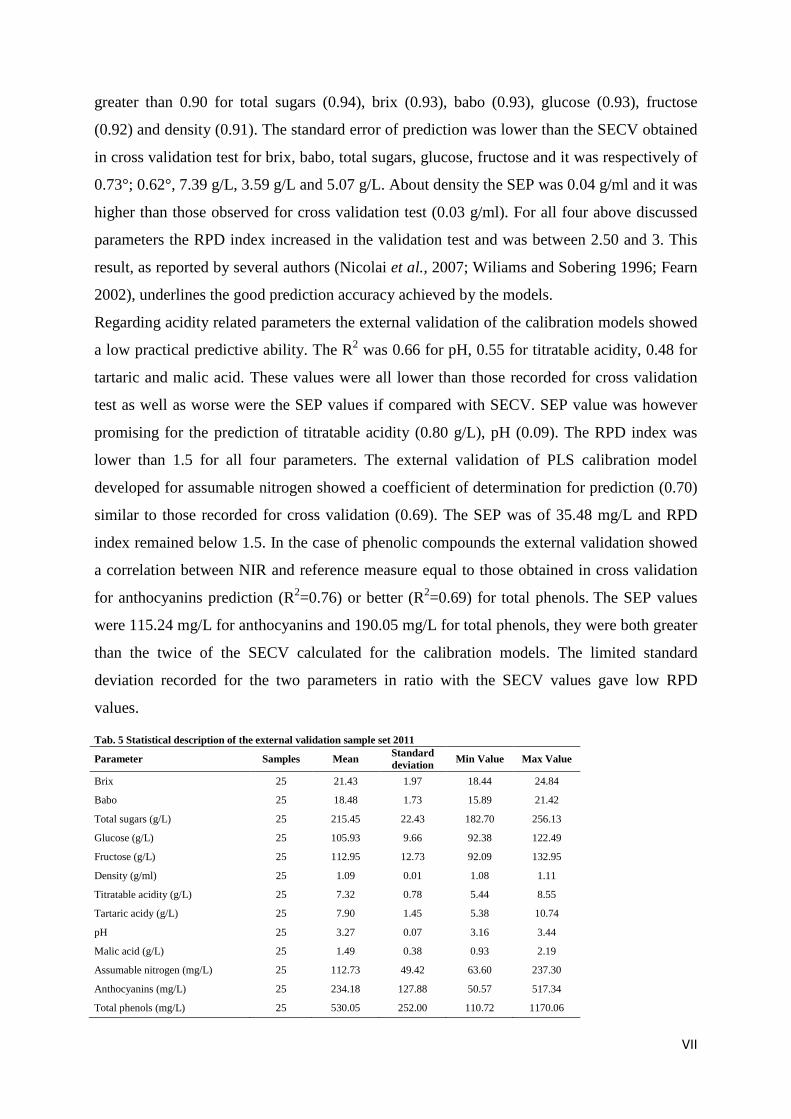
VII

greater than 0.90 for total sugars (0.94), brix (0.93), babo (0.93), glucose (0.93), fructose

(0.92) and density (0.91). The standard error of prediction was lower than the SECV obtained

in cross validation test for brix, babo, total sugars, glucose, fructose and it was respectively of

0.73°; 0.62°, 7.39 g/L, 3.59 g/L and 5.07 g/L. About density the SEP was 0.04 g/ml and it was

higher than those observed for cross validation test (0.03 g/ml). For all four above discussed

parameters the RPD index increased in the validation test and was between 2.50 and 3. This

result, as reported by several authors (Nicolai et al., 2007; Wiliams and Sobering 1996; Fearn

2002), underlines the good prediction accuracy achieved by the models.

Regarding acidity related parameters the external validation of the calibration models showed

a low practical predictive ability. The R2 was 0.66 for pH, 0.55 for titratable acidity, 0.48 for

tartaric and malic acid. These values were all lower than those recorded for cross validation

test as well as worse were the SEP values if compared with SECV. SEP value was however

promising for the prediction of titratable acidity (0.80 g/L), pH (0.09). The RPD index was

lower than 1.5 for all four parameters. The external validation of PLS calibration model

developed for assumable nitrogen showed a coefficient of determination for prediction (0.70)

similar to those recorded for cross validation (0.69). The SEP was of 35.48 mg/L and RPD

index remained below 1.5. In the case of phenolic compounds the external validation showed

a correlation between NIR and reference measure equal to those obtained in cross validation

for anthocyanins prediction (R2=0.76) or better (R2=0.69) for total phenols. The SEP values

were 115.24 mg/L for anthocyanins and 190.05 mg/L for total phenols, they were both greater

than the twice of the SECV calculated for the calibration models. The limited standard

deviation recorded for the two parameters in ratio with the SECV values gave low RPD

values.

Tab. 5 Statistical description of the external validation sample set 2011

Parameter Samples Mean Standard deviation Min Value Max Value

Brix 25 21.43 1.97 18.44 24.84

Babo 25 18.48 1.73 15.89 21.42

Total sugars (g/L) 25 215.45 22.43 182.70 256.13

Glucose (g/L) 25 105.93 9.66 92.38 122.49

Fructose (g/L) 25 112.95 12.73 92.09 132.95

Density (g/ml) 25 1.09 0.01 1.08 1.11



pH 25 3.27 0.07 3.16 3.44

Malic acid (g/L) 25 1.49 0.38 0.93 2.19

Assumable nitrogen (mg/L) 25 112.73 49.42 63.60 237.30

Anthocyanins (mg/L) 25 234.18 127.88 50.57 517.34

Total phenols (mg/L) 25 530.05 252.00 110.72 1170.06

VIII

Tab. 6 Validation statistics for the best PLS models 2009-2010

Parameter R2 RMSEP SEP BIAS RPD

Brix 0.93 0.94 0.73 0.61 2.70

Babo 0.93 0.86 0.62 0.61 2.79

Total sugars (g/L) 0.94 9.44 7.39 6.05 3.03

Glucose (g/L) 0.93 4.73 3.59 3.17 2.69

Fructose (g/L) 0.92 6.20 5.07 3.72 2.51

Density (g/ml) 0.91 0.006 0.004 0.005 2.50

Titratable acidity (g/L) 0.55 1.23 0.80 -0.95 0.97

Tartaric acid (g/L) 0.48 2.31 1.28 1.94 1.13

pH 0.66 0.09 0.09 0.02 0.78

Malic acid (g/L) 0.48 0.35 0.33 -0.14 1.15

Assumable nitrogen (mg/L) 0.70 40.70 35.48 -21.17 1.39

Anthocyanins (mg/L) 0.76 136.17 115.24 -76.11 1.11

Total phenols (mg/L) 0.69 187.96 190.05 25.59 1.32

5. Conclusions and future perspectives The present work shows how the NIR AOTF spectroscopy can be used in viticulture to

investigate several markers of ripening and in particular on Sangiovese wine grape variety.

The building of PLS regression models on different seasons, vineyards, clones and rootstocks

is the right way to operate as suggested by several authors (Cozzolino et al., 2011; Nicolaï et

al., 2007). The results reported for sugars related parameters underlines the high ability of

NIR AOTF to investigate brix, babo, total sugars, glucose, fructose and density. The low SEP

and Bias values recorded suggest the practical application of the presented calibration models.

About acidity related parameters promising results were found in calibration step at least for

tartaric acid, pH and titratable acidity. These results stressed the potential predictive ability of

NIR AOTF for these variables. The low SEP values recorded in the prediction of pH and

titratable acidity suggest that the calibration models obtained can be used for the measure of

these variables. The complexity of the phenolic compounds and the results obtained here

invite for improving the performance of the models to employ a more accurate method of

analysis. Finally this work suggests to use the Luminar 5030 Miniature Hand-held NIR

Analyzer spectrophotometer in vineyard in order to make quality maps for the management of

agronomic operations. The application of NIR system on grapes harvest machine would allow

the quality mapping of harvest and to differentiate the product for the different enological

uses.

IX

6. References Barbieri Gonzaga F, Pasquini C (2005) Near-Infrared emission spectrometry based on an

acousto-optical tunable filter. Anal. Chem., 77(4): 1046-1054.

Bellincontro A, Cozzolino D, Mencarelli F (2011) Application of NIR-AOTF spectroscopy to

monitor aleatico grape dehydration for passito wine production. Am. J. Enol. Vitic. 62 (2):

256-260

Bellincontro A, Nicoletti I, Valentini M, Tomas A, De Santis D, Mencarelli F (2009)

Integration of nondestructive techniques with destructive analyses to study postharvest water

stress of winegrapes. Am J Enol Vitic 60(1): 57-65.

Cen H, He Y (2007) Theory and application of near infrared reflectance spectroscopy in

determination of food quality. Trends Food Sci Technol 18: 72-83.

Cozzolino D, Cynkar W U, Dambergs R G, Mercurio M D, Smith P A (2008) Measurement

of condensed tannins and dry matter in red grape homogenates using near infrared

spectroscopy and partial least square. J Agric Food Chem 56: 7631-7636.

Cozzolino D, Cynkar W. U, Shah N, Smith P (2011) Multivariate data analysis applied to

spectroscopy: potential application to juice and fruit quality. Food Research International, 44:

1888-1896.

Cozzolino D, Dambergs R G, Janik L, Cynkar W U, Gishen M (2006) Analysis of grapes and

wine by near infrared spectroscopy. J. Near Infrared Spectroscopy 14: 279-289.

Fearn T, Assessing calibrations: SEP, RPD, RER and R2. NIR News 13:12-14.

Ferrer-Gallego R, Hernández – Hierro JM, Rivas – Gonzalo JC, Escribano – Bailón MT

(2011) Determination of phenolic compounds of grape skins during ripening by NIR

spectroscopy. Lwt – Food Science and Technology 44: 847-853.

Kaye O, Wample R L (2005) Using near infrared spectroscopy as an analytical tool in

vineyards and wineries. Am J Enol Vitic 56: 296A.

Le Moigne M, Maury C, Bertrand D, Jourjon F (2008) Sensory and instrumental

characterisation of Cabernet Franc grapes according to ripening stages and growing location.

Food Quality and Preference 19: 220-231.

X

Nicolaï B, Beullens K, Bobelyn E, Peirs A, Saeys W, Theron K I, Lammertyn J (2007) Non

destructive measurements of fruit and vegetable quality by means of NIR spectroscopy: A

review. Postharvest Biology and Technology 46: 99-118.

Shenk J S, Westerhaus M O (1996) Calibration the ISI way. In: A. M. C. Davies & P. C.

Williams ed., Near infrared spectroscopy: The future waves, NIR Publications (Chichester):

pp. 198–202.

Smyth HE, Cozzolino D, Cynkar WU, Dambergs RG, Sefton M, Gishen M (2008) Near

infrared spectroscopy as a rapid tool to measure volatile aroma compounds in Riesling wine:

possibilities and limits. Anal. Bio anal. Chem., 390: 1911–1916.

Wiliams PC, Norris K (1987) In: Near – Infrared technology in the agricultural and food

industries, Wiliams PC, Norris K eds, St Paul ACCC, pp. 143 – 167.

Williams PC, Sobering DC (1996) How do we do it: A brief summary of the methods we use

in developing near infrared calibrations. In Near infrared spectroscopy: The future waves, A.

M. C. Davies & P. Williams eds, NIR Publications (Chichester): pp. 185–188.

XI

RIASSUNTO

Uno spettrofotometro NIR AOTF è stato utilizzato nelle stagioni 2009, 2010 e 2011 per

monitorare la maturazione dell’uva da vino Sangiovese. Le acquisizioni spettrali sono state

condotte nella regione del campo elettromagnetico compresa tra 1100 nm e 2300 nm. Due

differenti misure sono state effettuate su ogni acino intero campionato acquisendo gli spettri

in riflettenza diffusa. Modelli di predizione basati sulla tecnica di statistica multivariata dei

quadrati minimi parziali sono stati elaborati per numerosi parametri di interesse viticolo ed

enologico come i solidi solubili totali, gli zuccheri totali, il glucosio, il fruttosio, la densità,

l’acidità titolabile, il pH, l’acido tartarico, l’acido malico, l’acido gluconico, l’azoto

assimilabile, i polifenoli totali e gli antociani. I modelli ottenuti sono stati validati su un set di

campioni indipendente. Un’elevata correlazione è stata registrata tra gli spettri NIR e i valori

misurati per i solidi solubili totali, gli zuccheri totali, il glucosio, il fruttosio e la densità.

Promettenti sono stati i risultati ottenuti in fase di calibrazione dei modelli per la stima

dell’acido tartarico, dell’acidità titolabile e del pH. Bassi errori in predizione sono stati

riscontrati per il pH e l’acidità titolabile. I risultati riguardanti la predizione degli antociani e

dei polifenoli suggeriscono di migliorare l’accuratezza del metodo di riferimento usato per

incrementare la performance predittiva dei modelli PLS. Questa applicazione del NIR AOTF

ha dimostrato la praticabilità di uso di questa tecnologia per determinare il momento più

idoneo per la raccolta dell’uva.

1

1. INTRODUCTION

Near infrared (NIR) radiation is the portion of the electromagnetic spectrum that goes from

780 to 2500 nm (12.820 cm-1 to 4.000 cm-1). It is located among visible and the mid infrared

region. NIR radiation was discovered by Friedrich Wilhelm Hershel in 1800. Spectroscopy is

the science that studies the interaction between the electromagnetic radiation and the matter.

The NIR spectroscopy has developed in the recent past in the food industry especially for

determining chemical and physical properties of foods and food products. In agriculture the

first application of this technique was done on grain by Norris in 1964. Today the great

importance of NIR spectroscopy in this field and in postharvest technology is well described

from the high number of publications, as well as from the fact that many manufacturers of on

– line grading lines have implemented NIR system to measure various quality attributes

(Nicolaï et al., 2007). The growing interest for this technique depend from the many

advantages resulting. NIR analysis is non destructive and it is very speed: commercial and

industrial operations get their results in seconds, rather than hours. The NIR analysis is yet

multiparametric, accurate, reproducible, cheap, environmentally clean, simple and totally safe

for workers. Another big benefit is represented by the little or no sample preparation required

(Williams 2007). The low absorptivity of NIR radiation means that light energy passes easily

through samples without rapid attenuation as in the case of medium infrared (MIR) analysis.

NIR spectroscopy allows also to analyze opaque samples because it has a low reflectivity in

contrast with the ultraviolet or visible light wavelengths (Jaren et al., 2001). NIR region

contains information related the first, second and third overtones of OH, NH, CH and SH

stretching vibrations as well as stretching – bending combinations involving these groups and

can describe chemical and physical properties of matter.

1.1 Theory The effects of radiation on the matter depend from its frequency, when a NIR radiation hit a

sample can cause transitional vibration of molecules. Two kind of vibration are possible:

stretching or bending vibration. Stretching vibration consists in a rhythmic movement along

the axis of bond; bending vibration consist in a variation of bond angle (Riva et al., 2001).

Phenomena involved in these interaction can be explained with the theories of quantum

physic. A molecule absorbs NIR radiation alone when the electrical oscillating field of the

electromagnetic wave is able to produce a change of molecule dipole moment or in the local

2

group of vibrating atoms (Pasquini 2003). The absorption of NIR radiation from a diatomic

molecule can be explained using the Hooke law:

𝜈 =1

2𝜋𝑐� 𝑘𝜇

where v is the frequency of the vibrational mode; k is the force constant and 𝜇 is the reduced

mass.

𝜇 =𝑚1 + 𝑚2𝑚1 𝑥 𝑚2

In this kind of molecules each atom moves toward or away from the other in a simple

harmonic motion. Hooke law means that the frequency of vibrational mode depends on two

parameters: the reduced mass 𝜇 and the force constant k. Light masses oscillate at higher

frequency than heavy masses, but in the case of functional group as OH, NH and SH the 𝜇

values are quite similar (Riva et al., 2001). The force constant k depend on the strength of the

chemical bond, which is mainly controlled by the electronic environment surrounding atoms

in molecules. Electrostatic interactions or formation of hydrogen bonds alter the force

constant and therefore shift the frequency (Sandorfy et al., 2007). In according with harmonic

oscillator model, the energy of the different equally spaced levels can be calculated by:

𝐸𝑣𝑖𝑏 =(𝜐 + 12

)ℎ

2𝜋 �𝑘𝜇

where 𝑣 is the vibrational quantum number and h is the Planck constant (6.62 x 10-34 J s). This

equation means that the vibrational energies Evib have discrete values. In according with

quantum mechanics only those transitions between consecutive energy levels (Δv = ± 1) that

cause a change in dipole moment are possible:

△ 𝐸𝑣𝑖𝑏 = ℎ𝑣

where v is the fundamental vibrational frequency of the bond that yields an absorption band in

the middle IR region. In reality the harmonic oscillator model cannot explain the behavior of

molecules since it doesn’t consider the Coulombic repulsion between atoms and dissociation

of bonds (Blanco e Villaroya 2002). In fact the behavior of molecules is affected by

anharmonicity, that influences the properties of near infrared bands as the intensity, the

frequency and the breadth (Sandorfy et al., 2007). Energy levels are not equally spaced and

3

their difference decrease with increasing of vibrational quantum number υ how reported by

this equation by Blanco and Villaroya 2002:

△ 𝐸𝑣𝑖𝑏 = ℎ𝑣[1 − (2𝜐 +△ 𝜐 + 1)𝑦]

where y is the anharmonicity factor. The potential energy of a diatomic molecule considering

an anharmonic model is well described by the Morse function:

𝑉 = 𝐷𝑒 �1 − 𝑒−𝑎(𝑟−𝑟𝑒)�2

where V is the potential energy, 𝐷𝑒 is the spectral dissociation energy, 𝑟𝑒 is the equilibrium

distance between the atoms and r is the distance between the atoms at any instant. Applying

quantum mechanics to the Morse equation the energy level (E) results by the following

equation:

𝐸 = ℎ𝑣 �𝜐 +12� − 𝑥𝑚 ℎ𝑣 �𝜐 +

12�2

where xm is the anharmonicity constant of the vibration. The value of xm is between 0.005 and

0.05 (Pasquini 2003). In addition to the mechanical anharmonicity due at loss of equidistance

between energetic level can also be present an electrical anharmonicity. The latter affects the

dipole moment of the molecules and can give intensity to overtones even if the potential is

perfectly harmonic. In the general case both mechanical and electrical anharmonicities

contribute to the intensities of the overtones (Sandorfy et al., 2007). The anharmonicity model

predicts the occurrence of transition with Δυ = 2 or higher and the existence of combination

bands between vibration (Pasquini 2003). The transition between non - contiguous vibrational

energy states give rise to absorption bands known as overtones, approximately multiples of

the fundamental vibrational frequency. These bands appear between 780 nm and 2000 nm and

they are much weaker than the fundamental frequency. For example the first overtone is 10 -

100 times weaker than the fundamental frequency. In polyatomic molecules, vibrational

modes can interact in such a way as to cause simultaneous energy changes and give rise

absorption bands called combination bands, the frequencies of which are the sums of

multiples of each interacting frequency. NIR combination bands appear inside 1900 – 2500

nm range. Anharmonicity and the dipole change affect in particular bonds involving the

hydrogen atom and some heavier atoms such us carbon, nitrogen and sulphur. In fact the NIR

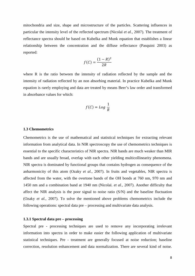
region is dominated by the overtones and combination tones of OH, CH, NH and SH bonds

(Fig. 1). In contrast the bands for bonds such us C=O, C-C, C-Cl are much weaker or absent

in NIR region (Blanco and Villaroya 2002; Pasquini 2003).

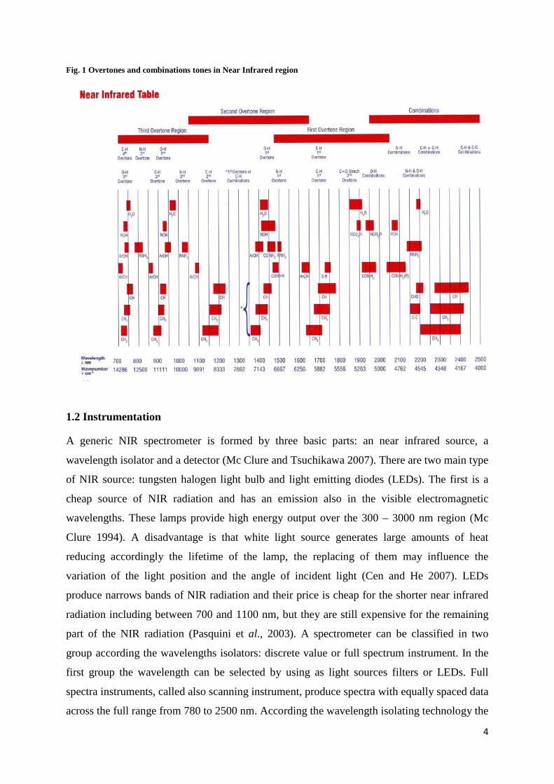
4

Fig. 1 Overtones and combinations tones in Near Infrared region

1.2 Instrumentation

A generic NIR spectrometer is formed by three basic parts: an near infrared source, a

wavelength isolator and a detector (Mc Clure and Tsuchikawa 2007). There are two main type

of NIR source: tungsten halogen light bulb and light emitting diodes (LEDs). The first is a

cheap source of NIR radiation and has an emission also in the visible electromagnetic

wavelengths. These lamps provide high energy output over the 300 – 3000 nm region (Mc

Clure 1994). A disadvantage is that white light source generates large amounts of heat

reducing accordingly the lifetime of the lamp, the replacing of them may influence the

variation of the light position and the angle of incident light (Cen and He 2007). LEDs

produce narrows bands of NIR radiation and their price is cheap for the shorter near infrared

radiation including between 700 and 1100 nm, but they are still expensive for the remaining

part of the NIR radiation (Pasquini et al., 2003). A spectrometer can be classified in two

group according the wavelengths isolators: discrete value or full spectrum instrument. In the

first group the wavelength can be selected by using as light sources filters or LEDs. Full

spectra instruments, called also scanning instrument, produce spectra with equally spaced data

across the full range from 780 to 2500 nm. According the wavelength isolating technology the

5

following instrument categories are available: diodes, filters, prism, grating, FT-NIR and

Hadamard based instruments (Mc Clure and Tsuchikawa 2007). Diodes based instrument

include Emitting Diode Arrays, Photodiode Detector Arrays and Laser diodes. These

instruments can produce NIR radiation with band width of about 30 – 50 nm, centered in any

wavelengths of the spectral region (Pasquini 2003). Diode Emitting Array spectrometers are

very compact and the available of several light emitting diodes allows the construction of

multichannel. Photodiode detector array offers a no moving parts technology that is attractive

for certain applications. Laser diodes are much expansive but have the following advantages:

the bandwidths of laser are very narrow and the output intensity can be very high. Filters have

definite benefits over other wavelength isolation methods. Narrow band NIR interference

filters can be produce for any wavelength in the NIR region. The characteristics of filters can

be reproduced so that is easy duplicate the spectrometer characteristics. Further the bandpass

of a filter may be increase or decrease varying the energy falling on the sample. Among filters

we found a wide list: fixed filter, wedge interference filters, tilting filters, acousto - optical

tunable filter (AOTF), Liquid crystal tunable filter (LCTF) (Mc Clure and Tsuchikawa 2007).

The first commercial NIR analyzers were based on fixed filter and were used at grain

elevators. The bandpass of these filters may be as narrow as 1 nm. Fixed filter include filters

that are useful for calibrations in food applications, such as moisture, protein and fat. Wedge

interference filters are constructed similarly to fixed filters with the exception that the

dielectric between the plates is wedge shaped. The dielectric has different thickness such that

produce longer and shorter wavelengths. Tilting filter spectrometers have encountered many

disadvantages by which today no one produce a commercial version of this technology. In the

last two decades devices based on AOTF has gained a strong momentum. These type of

spectrometers have no moving parts, this characteristic allows an high reproducible

wavelength scans and makes AOTF suitable for equipment working in aggressive conditions,

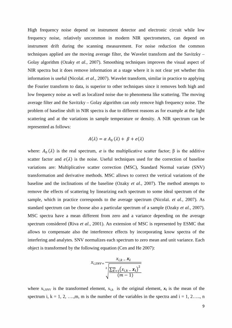
as in plants production (Blanco and Villaroya 2002). AOTF (Fig. 2) is a birefringent crystal of

Tellurium dioxide to which is attached to one side a piezoelectric material that under

excitation from an external radio frequency (rf) signal produces a mechanical wave which

propagates trough the crystal. The acoustic wave produces a periodic variation of the

refractive index of the crystal in a frequency determined by the rf signal, in the range of 50 to

120 MHz. The interaction of the electromagnetic wave and the acoustic wave causes the

crystal to refract selectively a narrow wavelength band. The relationship between the

diffracted radiation wavelength (λ) and the frequency of the acoustic wave (fa) is given by the

following equation:

6

𝜆 =𝛥𝑛 𝛼 𝑣𝑎𝑓𝑎

where Δn is the refractive indexes of the TeO2 crystal, va is the velocity of the acoustic wave

and α is a parameter dependent on the AOTF design. The diffracted light intensity is directed

into two first order beams, which are orthogonally polarized. A beam stop is used to block the

undiffracted , broadband light. The angle between the polarized beams is a function of device

design, but is typically a few degrees. The main benefits of AOTF based instrument are: high

repeatability, the error is less than ± 0.05 nm; wavelength purity, out of band transmissions as

low as 10-5; speed of scanning, high resolution, with typical values in the range 5 to 15 nm for

the wavelength in the NIR region 1000 – 2500 nm (Pasquini 2003; www.brimrose.com).

Fig. 2 Acousto optically tunable filter

Liquid crystal tunable filter (LCTF) spectrometers may be designed to operate in visible, NIR

and MIR range but this kind of device has had a considerable success in the visible region.

Switching time results longer than those of grating and AOTF based instrument. The spectral

resolution is on the order of 10 – 20 nm, but any crystals can reduce the bandpass to 5 – 10

nm. Blocking filters are needed to block out of the range transmission of the filter. Prisms

based spectrometers were used by NIR pioneers and are full spectrum instruments. There are

three type of prisms: dispersing, reflecting and polarizing (Mc Clure and Tsuchikawa 2007).

The instruments based on grating monochromators have the benefit that are cheap if

compared with other scanning instrument. The main disadvantages are the slow scan speed,

the lack of wavelength precision and the presence of moving part. The latter feature limit the

use of this type of instrument in field and in more aggressive environments. Fourier

http://www.brimrose.com/

7

Transform (FT) NIR spectrophotometer employ an entirely different method for producing

spectra compared to dispersive instrumentation. Energy patterns set up by an interaction with

a sample and a reference and moving mirrors produce sample and reference interferograms.

The conventional frequency – domain IR spectrum is obtained by mathematically performing

the FT on the interferograms. Spectrophotometer based on Fourier Transform (FT) combining

the following advantages; wavelengths precision, high signal to noise ratio and scan speed.

The accuracy is better than 0.05 nm and the resolution can achieve values below 1 nm in the

NIR region. Comparing FT with AOTF instruments we can say that the AOTF presents the

most rapid random accesses to various wavelength while the FT shows generally the best

resolution and signal to noise ratio (Pasquini 2003). The third important part of

spectrophotometer is the detector, the part that receives the radiation originated from the

sample and transform it in a electrical signal (McClure 1994; McClure and Tsuchikawa 2007;

Pasquini 2003; Blanco and Villaroya 2002). Detector can be single or multichannel. The first

group includes: silicon, lead sulfide (PbS) and indium gallium arsenide (InGAS) detectors.

Silicon based detectors have a restricted spectral response in the NIR region, in fact they are

sensible to wavelengths between 360 nm and 1000 nm. PbS detectors are used for the range

900 – 2600 nm, while InGAS for 1110 – 2500 nm region. Multichannel detectors allows to

increase the speed at which spectra information can be acquired. Diode arrays and charged

coupled devices are diffuse multichannel detectors. The spectra acquisition can be carry out

with least four different method of measurement. The choice of measurement method depend

on the samples and on the chemical properties that want be analyzed. NIR spectra can be

acquired in transmittance, reflectance, interactance or transflectance mode. Transmittance

mode is usually used for liquid sample or in the case of agriculture products for thick peel

fruit. The detector is positioned opposite to the light source. In the instruments based on

interactance acquisition mode the light source and the detector are positioned parallel to each

other in such a way that specular reflection is not detected. Interactance mode is suitable for

determining the internal quality of several thin peel fruits. The transflectance mode is used for

emulsion and turbid liquid. Comparing the transflectance to transmittance acquisition mode

the optical path is doubling and the radiation beam passes twice through the sample. The

reflection is due to three different phenomena: specular reflection, diffuse reflection and

scattering. NIR spectrometers acquire spectra in diffuse reflection mode. To avoid the

specular reflection the light source and the detector are mounted under a specific angle.

Scattering is due to changes in refractive index of matter. In the case of fruit and vegetables

scattering results mainly from cell wall interfaces, but also from starch granules, chloroplasts,

8

mitochondria and size, shape and microstructure of the particles. Scattering influences in

particular the intensity level of the reflected spectrum (Nicolaï et al., 2007). The treatment of

reflectance spectra should be based on Kubelka and Munk equation that establishes a linear

relationship between the concentration and the diffuse reflectance (Pasquini 2003) as

reported:

𝑓(𝐶) =(1 − 𝑅)2

2𝑅

where R is the ratio between the intensity of radiation reflected by the sample and the

intensity of radiation reflected by an non absorbing material. In practice Kubelka and Munk

equation is rarely employing and data are treated by means Beer’s law order and transformed

in absorbance values for which:

𝑓(𝐶) = 𝐿𝑜𝑔 1𝑅

1.3 Chemometrics

Chemometrics is the use of mathematical and statistical techniques for extracting relevant

information from analytical data. In NIR spectroscopy the use of chemometrics techniques is

essential to the specific characteristics of NIR spectra. NIR bands are much weaker than MIR

bands and are usually broad, overlap with each other yielding multicollinearity phenomena.

NIR spectra is dominated by functional groups that contains hydrogen as consequence of the

anharmonicity of this atom (Ozaky et al., 2007). In fruits and vegetables, NIR spectra is

affected from the water, with the overtone bands of the OH bonds at 760 nm, 970 nm and

1450 nm and a combination band at 1940 nm (Nicolaï. et al., 2007). Another difficulty that

affect the NIR analysis is the poor signal to noise ratio (S/N) and the baseline fluctuation

(Ozaky et al., 2007). To solve the mentioned above problems chemometrics include the

following operations: spectral data pre – processing and multivariate data analysis.

1.3.1 Spectral data pre – processing

Spectral pre - processing techniques are used to remove any incorporating irrelevant

information into spectra in order to make easier the following application of multivariate

statistical techniques. Pre - treatment are generally focused at noise reduction; baseline

correction, resolution enhancement and data normalization. There are several kind of noise.

9

High frequency noise depend on instrument detector and electronic circuit while low

frequency noise, relatively uncommon in modern NIR spectrometers, can depend on

instrument drift during the scanning measurement. For noise reduction the common

techniques applied are the moving average filter, the Wavelet transform and the Savitzky –

Golay algorithm (Ozaky et al., 2007). Smoothing techniques improves the visual aspect of

NIR spectra but it does remove information at a stage where it is not clear yet whether this

information is useful (Nicolaï. et al., 2007). Wavelet transform, similar in practice to applying

the Fourier transform to data, is superior to other techniques since it removes both high and

low frequency noise as well as localized noise due to phenomena like scattering. The moving

average filter and the Savitzky – Golay algorithm can only remove high frequency noise. The

problem of baseline shift in NIR spectra is due to different reasons as for example at the light

scattering and at the variations in sample temperature or density. A NIR spectrum can be

represented as follows:

𝐴(𝜆) = 𝛼 𝐴0 (𝜆) + 𝛽 + 𝑒(𝜆)

where: 𝐴0 (𝜆) is the real spectrum, α is the multiplicative scatter factor; β is the additive

scatter factor and 𝑒(𝜆) is the noise. Useful techniques used for the correction of baseline

variations are: Multiplicative scatter correction (MSC), Standard Normal variate (SNV)

transformation and derivative methods. MSC allows to correct the vertical variations of the

baseline and the inclinations of the baseline (Ozaky et al., 2007). The method attempts to

remove the effects of scattering by linearizing each spectrum to some ideal spectrum of the

sample, which in practice corresponds to the average spectrum (Nicolaï. et al., 2007). As

standard spectrum can be choose also a particular spectrum of a sample (Ozaky et al., 2007).

MSC spectra have a mean different from zero and a variance depending on the average

spectrum considered (Riva et al., 2001). An extension of MSC is represented by ESMC that

allows to compensate also the interference effects by incorporating know spectra of the

interfering and analytes. SNV normalizes each spectrum to zero mean and unit variance. Each

object is transformed by the following equation (Cen and He 2007):

𝑥𝑖,𝑆𝑁𝑉=𝑥𝑖,𝑘 − 𝒙𝒊

�∑ �𝑥𝑖,𝑘 − 𝒙𝒊�2

𝑚𝐾=1

(𝑚− 1)2

where xi,SNV is the transformed element, xi,k is the original element, xi is the mean of the

spectrum i, k = 1, 2, ….,m, m is the number of the variables in the spectra and i = 1, 2….., n

10

and n is the number of validation set. Derivative methods are common used to remove

baseline correction as well as resolution enhancement. A popular derivative used is Savitzky –

Golay algorithm. The parameters of the algorithm (interval width and polynomial order)

should be selected carefully in order to avoid amplification of spectral noise. The derivatives

improve the visual aspect of the spectrum, in particular with a second derivative the

superimposed peaks are divided in clear and distinct peaks. Centering and normalization are

often the first stage in pre - processing NIR spectra and are resolution enhancement methods.

Mean centering consist on subtract the average from each variable, in this way all means are

zero and variances are spread around zero. Normalization allows to equalize the magnitude of

each sample. By applying a mean normalization each point of spectrum is divided for its

mean, so all spectra at the end have the same area (Ozaky et al., 2007; Nicolaï. et al., 2007).

Other useful operation is the difference between spectra that allows to analyze perturbation –

dependent NIR spectra such as temperature – dependent, pH – dependent or concentration –

dependent spectra (Ozaky et al., 2007).

1.3.2 Multivariate data analysis

The aim of multivariate analysis methods is to build models capable of accurately predicting

the characteristic and properties of unknown sample. Multivariate analysis methods can be

classified as qualitative or quantitative. The first, known also as pattern recognition methods,

establish mathematical criteria to define the similarity between samples or a sample and a

class. Qualitative methods define the boundaries between the different classes, or they model

the space occupied by a class and determine whether a sample belongs to it on a basis of

distance measurements or the residual variance (Blanco and Villarroya 2002). A diffuse

qualitative methods used in NIR spectroscopy is the principal component analysis (PCA).

PCA is used as a tool for screening, extracting and compressing multivariate data. PCA

transforms a set of possibly correlated response variables into a new set of non correlated

variables, called principal component or also latent variables. Results of PCA can be

visualized by means the loadings matrix and the scores matrix that describe respectively the

importance of each original variable for the principal component selected and the sample

position in the new N-dimensional space created (Riva et al., 2001). Others pattern

recognition methods are: linear discriminant analysis (LDA); K- nearest neighbors (KNN),

cluster analysis (CA), discriminant partial least analysis (DPLS), soft independent modeling

of class analogy (SIMCA) and support vector machine (SVM) (Cen and He 2007).

Multivariate regression techniques aim to establish a relationship between the observed

11

response value y and the n x N spectral matrix X (Nicolaï et al., 2007). Among linear

regression techniques partial least square (PLS) is the most used. It was introduced by Wold

almost 30 years ago to overcome problems connected to other linear regression methods such

as multiple linear regression (MLR) or principal component regression (PCR). MLR models,

the simplest quantitative multivariate analysis, usually uses fewer than five spectral

wavelengths. MLR assumes concentration to be a function of absorbance, which entails the

knowledge of the concentration of not only the target analysis, but also all other components

contributing to the overall signal (Blanco and Villarroya 2002). MLR models typically do not

perform well because of the often high co – linearity of the spectrum and easily lead to

overfitting and loss of robustness of the calibration models (Saranwong et al., 2001). PCR

has the advantages respect MLR that the noise is filtered and the variables obtained are

uncorrelated, but uses the first principal components for development the regression model

that are not necessary the most informative for the response variables. PLS regression is of

particular interest because can analyze data with strongly collinear, noisy, and numerous x

variable, and simultaneously model several response variables y. In addition PLS regression

has the property that the precision of the model parameters improves with the increasing

number of relevant variables and observations (Wold et al., 2001).

PLS regression model is calculated by the following equation:

𝑦 = 𝑋𝑏 + 𝐸

where y is a column matrix containing the dependent variable, x is a matrix containing the

predictor variables. The parameters b is determined by the least squares regression with the

construction of a generalized inverse x+:

𝑏 = 𝑥+𝑦

Once calculated b is possible determine the property y from the spectroscopic profiles

(Christy and Kvalheim 2007). In PLS regression an orthogonal basis of latent variables is

constructed one by one in such a way that they are oriented along directions of maximal

covariance between the spectral matrix x and the response vector y. In this way the latent

variables are order according their relevance for predicting the y variable. PLS performs very

well when there is a large amount of correlation, even co - linearity, which is the case of

biological materials. In general PLS required a number of latent variables smaller than that in

PCR calibration model (Wold et al., 2001). The number of latent variables is an indication of

the fitting effect. If too many latent variables are used, touch to much redundancy in the x

variables is modeled and the model result overfitted and it is very dependent on the dataset. If

a small number of latent variables is used then the model will not be large to capture the

12

variability in the data and it will result underfitted. In addition PLS regression can be easily

extended to simultaneously predict several quality attribute, in this case is called PLS2

(Cozzolino et al., 2011). Locally weighted regression (LWR) is a variant of PLS. A limit of

PLS is represented by non linearity between the spectral data and the quantitative information

of interest. Non linearity in the spectra is due at factors as experimental conditions, instrument

variation, and analyte characteristics (Chauchard et al., 2004). This problem was found in

grape using a universal calibration developed on many season, growing regions and grape

varieties. The regression curve showed a characteristic “banana” shape (Dambergs et al.,

2006). LWR can be useful to overcome any problems connected to the non linearity and

consequently improve the prediction accuracy for new season samples and reduce regression

curvature (Janik et al., 2007). LWR develops a PLS calibration from samples that best match

the sample to be predicted (Cozzolino et al., 2011). Another problem of PLS regression is due

at the possible great difference existing between spectra of the new season samples and those

of global calibration data base. In this case PLS regression will give an high bias and a

regression slopes considerably less than one. In practice to solve this problem is necessary to

include some of the new season samples in the calibration and recalibrating each year. An

approach to overcome non linearity might be the use of non linear regression techniques as

Artificial neural networks (ANM). ANM simulates the biological neuron by multiplication of

the input signal (x) with the synaptic weight (w) to derive the output signal (y). ANN consist

of three layers called neurons: the input, hidden and output layer. The limit of this approach is

in the difficult of result visualization and interpretation (Janik et al., 2007). Another non

linear regression techniques is represented by Kernel based techniques that in contrast with

ANN allow an easy interpretation of the calibration model (Nicolaï et al., 2007). Least

squares support vectors machines (LS - SVM) is essentially a kernel – based multiple

regression procedure which incorporates a second tuning parameter, so called regularization

parameter, which improves the robustness of the calibration model (Cozzolino et al., 2011).

13

1.4 Sangiovese grape

Sangiovese is in the preeminent position in Italy, where it constitutes the base of numerous

International – know denomination of origin wines (DOC and DOCG). Sangiovese is present

as an authorized vine species in 16 Italian provinces, and as a recommended vine species in

56 Italian provinces and in 2 French departments. The vine is indicated as the main in 88

DOC and DOCG and as complementary in 25 DOC and DOCG. Sangiovese occupies 9.7% of

total vines areas in Italy with 69.746 hectares. The vine is most cultivated in Tuscany with

32.554 hectares. Important region are also Puglia (12.951 hectares) and Emilia Romagna

(8.090 hectares). Sangiovese production is relevant as percentage on total vines area in

Umbria and Marche region where the vine occupies respectively 17% and 23% of total vines

area (Istat 2000). Sangiovese is also cultivated on relevant surfaces in California (2.214

hectares) and in France (1.564 hectares) (Staraz et al., 2006). In the 1999 – 2000 campaign

the production of graft – cuttings of Sangiovese in Italy was of 17.162.346, of which

7.127.802 were certified (Boselli et al., 2000). Nowadays 92 clones are recognized to national

register of vine varieties (www.acovit.it). Sangiovese vine is characterized by great genetic and

morphological intracultivar heterogeneity. The first report date back to Soderini (1590), that

mentioned the vine as “Sangiogheto”. Sangiovese is considered indigenous to Tuscany and

Mainardi (2000) highlighted the bond of this vine with the ancient Etruscans. For well over a

hundred years Italian growers have recognized two main types of Sangiovese, “grosso” and

“piccolo”, based on perceived differences in cluster size and shape, berry size and weight and

other characteristics (Nelson – Kluk and Manning 2006). Calo et al., 1995 have described six

different biotypes based on fruit, cluster, leaf, ripening and must characteristics. They

individuated two biotypes from central Tuscany, one from the Tuscan coast near Pisa (Peccioli

di Pisa), one from the Emilia – Romagna near Predappio (Romagnolo), one cultivated along the

Adriatic sea coast (Marchigiano) and one from Corsica (Nielluccio). The use of DNA profiling

based on microsatellite markers has revolutionized grape diversity in less than a decade. Calò et

al., 2000 studied 30 accessions by means isozymatic, molecular, ampelometric and

ampelographic analysis classifying them in three principal groups. They found that Morellino of

Pitigliano is not be classified as Sangiovese, instead, the Prugnolo gentile is effectively a

Sangiovese biotype. A recent work investigated the kin group and the origin of Sangiovese and

showed as the kin group was composed of a majority of ancient cultivars that are diffused in far

southern Italy (Staraz et al., 2007). Vouillamoz et al., 2007 investigated the parentage of

Sangiovese and proposed a new cultivar Calabrese di Montenuovo as relative to Sangiovese.

14

The main ampelographic characteristics of Sangiovese vine are reported by Calò et al., 2001.

The vine has a shoot top expanded or semi expanded, arachnoid, shiny green. Adult leaf has

medium size, it is pentagonal with five, sometimes three lobes. Bunch of magnitude from

medium-small to large, conical-pyramidal with one or two wings, more or less dense. Berry of

medium size, sub-rounded sometimes almost elliptical, regular in shape, bloom skin, purplish-

black in color, not very thick. The budding and the flowering are medium early while the

veraison and the ripening are medium. Sangiovese has strong vigor, high potential and basal

fertility and good production. The vine prefers hill areas and soils with medium or low fertility,

clay – calcareous soils also rich in gravels. The suitable pruned is mixed but the vine fits well

also at cordon pruned system. The vine is sensible to Oidium tuckeri, Stereum hirsutum and

mites. It is medium sensible to Plasmopora viticola.

15

2. STATE OF ART 2.1 NIR spectroscopy application on wine grapes The monitoring of grapes ripening is a decisive operation to determine the right quality in

vineyard and to choose the optimal harvest date of grapes for start winemaking process. The

harvest date depend mostly from the enological target and from the genetic maturity. Many

parameters related to the physiological process in berries should be monitored during the

ripening such as: pulp consistency, accumulation of sugars, acidity reduction, phenols and

flavor synthesis, nitrogen, enzymes and vitamins variation. In addition sensorial analysis help

to describe the grape quality. Genetic maturity depend strictly on the cultivar and the

viticulturist must write down the flowering date (Fregoni 1998). The quality control based

only on sugars and acidity measures is not sufficient to describe the grapes ripening

(Cozzolino et. al., 2006). Nowadays wineries attribute a great importance to the phenol

maturity for red wine production. Phenol maturity corresponds to simultaneous achievement

of an important potential of pigments in grape and a their good ability to diffusion in the wine.

(Ribéreau-Gayon et al., 2004). Phenol maturity involves a strong breakdown of astringency of

tannins and a reduction of seed tannins extractability (Di Stefano et al., 2000). Conventional

laboratory techniques for the determination of the different quality characteristic of grape are

tedious and time consuming, that represent a serious limit to the widespread of quality

descriptor (Gishen et al., 2005). The modern wine industry has a clear need for simple, rapid

and cheap techniques to assessment the berry maturity for choose the optimal harvest date,

attribute the right payment of grapes and individuate vineyard blocks that have different

qualitative characteristics. The use of NIR spectroscopy in the wine industry is still in its

infancy, but from the literature is clear as it can found application at several steps during wine

production, from the harvest to tasting. Moreover NIR spectroscopy applications are possible

also in field for monitoring agronomic characteristics useful for vineyard management.

Studies reported the use of this technique to evaluate the infection of Erysiphe necator in

Chardonnay grapes: a similar application could be profitable for the mechanical harvesting.

NIR spectroscopy was used yet to predict the level of nutrients in grapevine petioles as

nitrogen, potassium and phosphorus (Cozzolino et al., 2006). A portable NIR AOTF

instrument was applied in field for measuring leaf water potential of Syrah, Merlot and

Cabernet Sauvignon varieties using the wavelength range 1100 – 2300 nm (Santos and Kaye

2009). Measures of leaf water potential of grapevines were conducted also on Syrah, Merlot

and Chardonnay leaves by De Bei et al., 2011 using the VIS NIR electromagnetic range 300 –

16

1100 nm. The potential of NIR spectroscopy was tested as an alternative analytical method

for measuring enological parameters on intact or processed grapes. Many works reported the

scanning of homogenates of grape, but NIR measures are possible also on whole grape or on

single berries. A easy sample presentation means that NIR spectroscopy may have potential

for use at the weighbridge or for in field – analysis. The scanning of whole intact grape is

feasible but with the cost of lower accuracy. In the case of NIR acquisition on single berries is

necessary to consider the high coefficient of variation, about 40%, between spectra acquired

in different part of the berry. This variation within the same berry might be due to variations

in chemical composition, dust and to different of sun exposure. Differences between spectra

of homogenates grapes, whole intact grapes and intact berries were observed around the OH

absorption bands (980 nm, 1400 nm and 1900 nm) (Cozzolino et al., 2006). Cozzolino et. al.,

2004 investigated the effects of homogenization method and freezing on the analysis of grape

quality parameters. Neither the homogenizer type, nor the sample state had a significance

effects on total anthocyanins and total soluble solids determination. The type of homogenizer

and the state of sample influenced the pH analysis while total phenols extraction was

influenced only by the type of homogenizer. A period of frozen storage longer than three

months affected all four quality parameters. The feasibility to use NIR spectroscopy to

investigate quality parameters in wine grape during ripening, at harvest or in post harvest is

widely documented in literature. Applications to predict sugars (Jarén et al., 2001; Cozzolino

et al., 2006, Larraín et al., 2008; Novales et al., 2009; González - Caballero et al., 2011), pH

(Cozzolino et al., 2004a; Larraín et al., 2008; González - Caballero et al., 2011), other related

acidity parameters such as titratable acidity, malic acid and tartaric acid (Chauchard et al.,

2004; González - Caballero et al., 2011) and phenolic compounds (Dambergs et al., 2003;

Cozzolino et al., 2004a; Janik et al., 2007; Cozzolino et al., 2008; Larraín et al., 2008; Kemps

et al.,2010; Ferrer Gallego et al., 2011) are below reported. Jarén et al., 2001 acquired

reflectance spectra, by means a Varian CARY 500 spectrophotometer, between 800 and 2500

nm from whole berries of Garnacha and Viura varieties and developed Multilinear regression

models for Brix prediction. In a review Cozzolino et al., 2006 reported some results of NIR

application on wine grape obtained by several authors using different wavelength range and

different varieties. Arana et al. 2005 acquired reflectance spectra from Viura and Chardonnay

grapes in the electromagnetic range 500 nm – 800 nm to analyze total solids soluble content.

As reported by Cozzolino et al., 2006 predicting models for solid soluble content are often

based on different range of wavelengths according the instrument used, but it seems that the

most important contribution for the calibration in NIR region is due to the absorption related

17

to OH and CH bonds, around 980 nm, 1400 nm, 1900 nm and 2170 nm. VIS - NIR radiation

(400 nm – 2500 nm) was tested by Dambergs et al., 2003 to investigate total anthocyanins,

pH and total solids soluble in Cabernet Sauvignon, Shiraz, Merlot and Grenache varieties.

The same quality parameters were measured by means a portable spectrophotometer Ocean

Optics, using the spectral range between 640 nm and 1300 nm, in grape samples of Cabernet

Sauvignon, Carmenere, Merlot, Pinot Noir and Chardonnay collected in the Maipo Valley

(Chile) (Larraín et al., 2008). Cozzolino et al., 2004a used a diode array spectrophotometer

Zeiss corona 45 VIS NIR to develop a partial least squares calibrations to predict colour and

pH on whole and homogenized grape. They obtained the best calibration models on

homogenized grape. Shortwave (800 nm – 1050 nm) near infrared spectroscopy was tested for

determination of reducing sugar content during grape ripening and winemaking process

(Novales et al., 2009). A Foss NIRS system 5000, who employed the NIR region between

1100 nm and 2000 nm, was used to predict the different families of phenols: anthocyanins,

phenolic acids and flavanols both on intact grapes and grape skins of Graciano variety

(Gallego et al., 2011). A study on phenolic compounds was conducted also by Kemps et al.,

2010. VIS/NIR analysis combined with Partial Least square has shown the possibility to

predict extractable anthocyanins concentration at pH equal to 1.0 and 3.2 in Syrah variety, but

not in Cabernet Sauvignon, Merlot and Carmenere varieties. In the same work, in which was

used a Zeiss corona 45 VIS NIR (320 nm – 1660 nm) on intact grapes, the authors

investigated also the polyphenols and the sugars concentration. A VIS NIR portable

spectrophotometer who used the wavelength range between 450 nm and 980 nm was tested on

fresh whole berries and homogenized grapes of Nebbiolo variety to evaluate both technology

(soluble solids content, titratable acidity, pH ) and phenolic maturity (Guidetti et al., 2010). In

this study was also applied a PLS discriminant analysis (PLS DA) for a qualitative

classification of grapes as ripe or not ripe according the titratable acidity and the brix values.

González - Caballero et al., 2011 tested a Zeiss CORONA portable diode array spectrometer

on whole bunches and musts, who used the VIS/NIR range between 380 nm and 1700 nm.

They investigated during the grape ripening the following quality parameters: solid soluble

solid, reducing sugar content, pH value, titratable acidity, tartaric acid, malic acid and

potassium content. In this work they tested two different regression approaches: MPLS and

Local algorithms. In a precedent trial they used the same spectrophotometer also on grape

berries (González - Caballero et al., 2010). Chauchard et al., 2004 tested the performance of

Least squared Support Vector Machine regression comparing it to PLS and MLR regression

for the prediction of total acidity calculated as sum of malic and tartaric acid concentration.

18

They worked on intact berries of Carignan, Mourverdre and Ugniblanc varieties using a Zeiss

MMS1 polychromatic diode array spectrometer and employing the spectral range between

680 and 1100 nm. Artificial neural networks regression was compared to PLS regression for

anthocyanins concentration prediction in red grape homogenates using a FOSS NIRSystem

6500 VIS NIR spectrometer (Janik et al., 2007). This work showed as ANM regression

reduce the need to refresh existing calibrations for the prediction of new season samples

anthocyanins concentration. A study on application of VIS NIR spectroscopy to predict

condensed tannins and dry matter was done by Cozzolino et al., 2008. They used a FOSS

NIRSystem 6500 in reflectance mode and scanned red grape homogenate of five different

varieties: Cabernet Sauvignon, Shiraz, Merlot, Grenache and Pinot Noir; in the range 1100

nm – 2500 nm. They observed that for dry matter the highest regression coefficients were

observed at wavelength associated with the water content in grape berries. For tannins instead

the highest regression coefficient were observed around 1512 nm, 1628 nm, 1726 nm, 1924

nm, and between 2100 and 2300 nm. NIR spectroscopy was tested also for determination of

ammonia, amino nitrogen and yeast assimilable nitrogen (Dambergs et al., 2005). The authors

reported that MIR spectroscopy outperform NIR analysis in investigate these parameters. NIR

spectroscopy was applied yet to predict glycosylated compounds concentration in white grape

juice (Cynkar et al., 2007). Juice samples of Chardonnay, Riesling and Sauvignon Blanc were

scanned in transmittance mode by means a FOSS NIRSystem 6500 instrument. The authors

suggested that the calibration models obtained could be used for qualitative purposes, as for

example asses the glycosylated compounds concentration as low, medium or high. A NIR -

AOTF was aimed at studying the grapes dehydration for dessert wines production. The

instrument was able to discriminate between the grapes according to the conditions and the

stage of dehydration, showing different absorbance level at a specific wavelengths

(Bellincontro et al., 2009). In addition, during the dehydration process NIR - AOTF allowed a

fast and economical monitoring of two important commercial parameters such as reducing

sugars and weight loss in Aleatico grapes (Bellincontro et al., 2011). A study by Kaye and

Wample (2005) on Cabernet Sauvignon area production showed that the same mentioned

above instrument may find significant practical application through non-destructive

measurement of total polyphenols, anthocyanins, tartaric and malic acid in qualitative

discrimination within the vineyard. Some works documented how the NIR AOTF

spectrometer is suitable for application in agriculture to determine the quality of products.

Cayuela and Weiland 2010 used this device to investigate the quality of intact orange while

He et al., 2006 used NIR AOTF for determining tobacco leaf constituents. An innovative

19

approach for the study of grape ripening was proposed by Le Moigne et al., 2008. They

investigate Cabernet Franc grape ripening according sensory analysis, compression measures

and visible - near spectroscopy. The research showed a relationships between some

wavelengths of VIS / NIR and sensory attributes that describe ripeness evolution, such as

firmness, elasticity and resistance to handling. In this study VIS/NIR spectroscopy is

proposed as tool to discriminate and to predict the ripening stages and the parcel type.

20

3. AIMS OF THE STUDY

The present work is aimed to evaluate the potential of NIR spectroscopy as technique to

investigate the ripening of Sangiovese red grape variety. In particular it wants to test a NIR

AOTF spectrometer as tool for a fast and reliable quality control in vineyard to choose the

optimal harvest date and to discriminate areas within the vineyard with different quality

characteristics. This work develops PLS regression models for the measure of many markers

of ripening process normally controlled by the viticulturist for the harvest management such

as total soluble solids, total reducing sugars, glucose, fructose, density, titratable acidity,

tartaric acid, malic acid, gluconic acid, assumable nitrogen, pH, total phenols and

anthocyanins.

4. MATERIALS AND METHODS

4.1 Grape samples The trial was conducted during the seasons 2009, 2010 and 2011 on Vitis vinifera L. cv.

Sangiovese. In the season 2009 grape samples were collected from two neighboring vineyards

site in Nipozzano locality (Firenze, Italy) and located at a medium altitude of 400 m. The

vineyards are part of Marchesi dè Frescobaldi company. Vineyard 1 called “Balza del

Cimitero” was implanted in 2001 year with SS-F9-A5-48 Sangiovese clone grafted on 1103

Paulsen rootstock for a total area of 5.5 hectares. SS-F9-A 5-48 is a clone selected in Lamole

Greve in Chianti locality (FI, Italy). It has a medium vigor, good and stable productivity, high

fertility, medium cylindrical – pyramidal and semi dense with one wing cluster and medium

berries, good tolerance to Botrytis cinerea. It is suitable to produce wine rich in color, stable

and with a long aging (Tamai 2009).. Vineyard 2 called “Cafaggio” was implanted in 2000

year with VCR 23 Sangiovese clone grafted on 420 A rootstock for a total area of 5.4

hectares. VCR 23 is a clone selected in Vecchiazzano (Forlì, Italy) and it is a “Romagnolo”

biotype. It has a good vigor, productivity less than the medium, small berry and cylindrical,

semi dense and small - medium cluster. Phenolic and aromatic profile is excellent to produce

wine with a medium - long aging (Tamai 2009). Both vineyards had a Guyot pruned system,

2.5 m X 1 m spaced with a north – south rows orientation. Both vineyards were aimed to

produce grape of high quality for manual harvesting. In 2009 season 76 grape samples were

collected from the first decade of September to the harvest data (first October decade): 40

samples were picked from vineyard 1 and 36 from vineyard 2. Each sample was constituted

21

by 100 berries. Each sample had origin from a selected area of vineyard according to the

vigour of the plants so as to increase the variability of chemical composition of grape samples

collected. In each area was chosen a representative row from which to withdraw the berries.

Balza del Cimitero vineyard was divided in six areas while Cafaggio vineyard in 4 areas.

Berries were collected in random way from the clusters and were sampling from both sides of

the rows. In the season 2010 grape samples were collected from a vineyard sites in La

Capitana locality (Grosseto, Italy) and located at a medium altitude of 250 m. The vineyard is

part of Marchesi dè Frescobaldi company. The vineyard was implanted in 2004 season with

Fedit 20 CH and Fedit 21 CH Sangiovese clones grafted on 1103 and 1175 Paulsen rootstocks

for a total area of 1 hectare. Fedit clones (Venturi et al., 2000) were selected in Gaiole in

Chianti area from Federazione Italiana dei Consorzi Agrari. Fedit 20 CH has a good vigor and

production, the ripening is delayed of about 1 week and it ensures a high sugar concentration.

The cluster is pyramidal, medium, quite loose and the berry is medium - small. This clone is

used to produce a aging wine. Fedit 21 CH is vigorous and productive. It advances of about

one week the harvest. The cluster is serried, winged and tapered with small – medium berries.

As Fedit 20 CH this clone produce grape for aging wine. Vineyard had a cordon pruned

system, 2 X 0.9 m spaced with a north-south rows orientation. In the season 2010, 20 grape

samples were collected from the third decade of august to the first decade of october from five

different areas of vineyard in the same way above cited. In 2011 season 25 samples of

Sangiovese grape were provided by Falesco company located in Montecchio (Terni, Italy) to

be used as validation sample set.

Fig. 3 Sampling areas in Balza del Cimitero vineyard

Fig. 4 Bunch of SS-F9-A5-48 Sangiovese clone

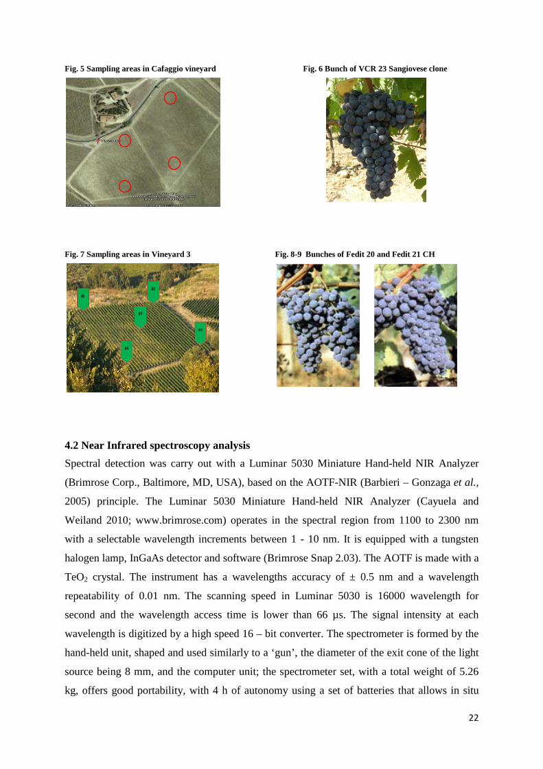
22

Fig. 5 Sampling areas in Cafaggio vineyard

Fig. 6 Bunch of VCR 23 Sangiovese clone

Fig. 7 Sampling areas in Vineyard 3

Fig. 8-9 Bunches of Fedit 20 and Fedit 21 CH

4.2 Near Infrared spectroscopy analysis Spectral detection was carry out with a Luminar 5030 Miniature Hand-held NIR Analyzer

(Brimrose Corp., Baltimore, MD, USA), based on the AOTF-NIR (Barbieri – Gonzaga et al.,

2005) principle. The Luminar 5030 Miniature Hand-held NIR Analyzer (Cayuela and

Weiland 2010; www.brimrose.com) operates in the spectral region from 1100 to 2300 nm

with a selectable wavelength increments between 1 - 10 nm. It is equipped with a tungsten

halogen lamp, InGaAs detector and software (Brimrose Snap 2.03). The AOTF is made with a

TeO2 crystal. The instrument has a wavelengths accuracy of ± 0.5 nm and a wavelength

repeatability of 0.01 nm. The scanning speed in Luminar 5030 is 16000 wavelength for

second and the wavelength access time is lower than 66 µs. The signal intensity at each

wavelength is digitized by a high speed 16 – bit converter. The spectrometer is formed by the

hand-held unit, shaped and used similarly to a ‘gun’, the diameter of the exit cone of the light

source being 8 mm, and the computer unit; the spectrometer set, with a total weight of 5.26

kg, offers good portability, with 4 h of autonomy using a set of batteries that allows in situ

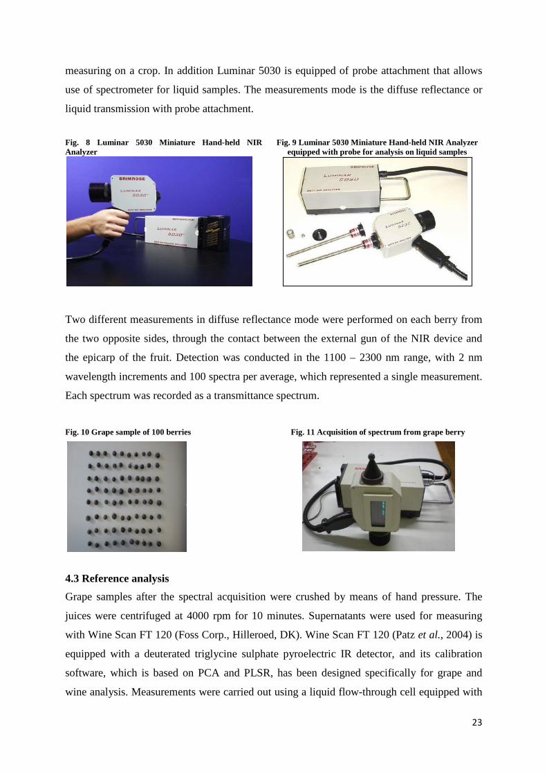
23

measuring on a crop. In addition Luminar 5030 is equipped of probe attachment that allows

use of spectrometer for liquid samples. The measurements mode is the diffuse reflectance or

liquid transmission with probe attachment.

Two different measurements in diffuse reflectance mode were performed on each berry from

the two opposite sides, through the contact between the external gun of the NIR device and

the epicarp of the fruit. Detection was conducted in the 1100 – 2300 nm range, with 2 nm

wavelength increments and 100 spectra per average, which represented a single measurement.

Each spectrum was recorded as a transmittance spectrum.

Fig. 10 Grape sample of 100 berries

Fig. 11 Acquisition of spectrum from grape berry

4.3 Reference analysis Grape samples after the spectral acquisition were crushed by means of hand pressure. The

juices were centrifuged at 4000 rpm for 10 minutes. Supernatants were used for measuring

with Wine Scan FT 120 (Foss Corp., Hilleroed, DK). Wine Scan FT 120 (Patz et al., 2004) is

equipped with a deuterated triglycine sulphate pyroelectric IR detector, and its calibration

software, which is based on PCA and PLSR, has been designed specifically for grape and

wine analysis. Measurements were carried out using a liquid flow-through cell equipped with

Fig. 8 Luminar 5030 Miniature Hand-held NIR Analyzer

Fig. 9 Luminar 5030 Miniature Hand-held NIR Analyzer equipped with probe for analysis on liquid samples

24

two CaF2 windows. Each window has a 10 mm diameter circle with 2 mm thickness,

providing an optical aperture of 88.54 mm2 and a cell volume of 3.276 µL. A polyethylene

terephtalate spacer provides a 37 µm optical path-length. To minimize the problem of internal

reflections (interference fringe) the CaF2 windows are mounted slightly non-parallel. The

interferogram of the sample in the cell is recorded using an optical resolution of 14 cm−1 ×

2000 cm−1, and averaging on the basis of 10 scans. The instrument is equipped with a HeNe

laser (632 nm) and a silicium detector to track the position of the moving mirror in the

interferometer. In the season 2009 and 2010 total soluble solids (Brix and Babo), total sugars,

glucose, fructose, density, tartaric acid, pH, titratable acidity, malic acid, gluconic acid,

assumable nitrogen, anthocyanins and total phenols were measured in grape juices

supernatants in duplicate read by means Wine Scan FT 120. The same parameters with the

exception of gluconic acid were measure with the same instrument also in the 2011 season.

Wine Scan FT 120 has recently received much attention for its performance in terms of

accuracy, precision and speed analysis (Bauer et al., 2008). FT - MIR spectroscopy was tested

with success to investigate interesting parameters in the grape juice such as relative density,

total phenols, reducing sugars, fructose, glucose, titratable acidity, pH value, tartaric and

malic acids (Patz et al., 1999; Patz et al., 2004). Fragoso et al., 2011 showed as FT – MIR

spectroscopy was a valid technique for monitoring the phenolic ripening. In a work

concerning Botrytis cinerea infection on Sangiovese and Trebbiano grape varieties, FT - MIR

infrared technology was used to measure gluconic acid and glycerol (Versari et al., 2008).

Fig 12 Wine Scan FT 120

4.4 Chemometric analysis Transmittance spectra were pre – treated for absorbance (1/R) transformation using SNAP!

2.03 software (Brimrose Corp., Baltimore, MD, USA). For each sample the two hundred

spectra were averaged to 1 spectrum. Before the calibration and the building up of the

prediction models, the spectral variations of the data sets were analyzed by Principal

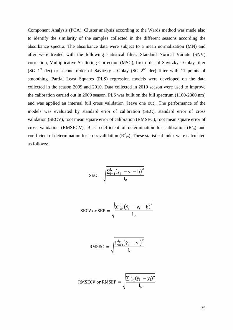
25

Component Analysis (PCA). Cluster analysis according to the Wards method was made also

to identify the similarity of the samples collected in the different seasons according the

absorbance spectra. The absorbance data were subject to a mean normalization (MN) and

after were treated with the following statistical filter: Standard Normal Variate (SNV)

correction, Multiplicative Scattering Correction (MSC), first order of Savitzky - Golay filter

(SG 1st der) or second order of Savitzky - Golay (SG 2nd der) filter with 11 points of

smoothing. Partial Least Squares (PLS) regression models were developed on the data

collected in the season 2009 and 2010. Data collected in 2010 season were used to improve

the calibration carried out in 2009 season. PLS was built on the full spectrum (1100-2300 nm)

and was applied an internal full cross validation (leave one out). The performance of the

models was evaluated by standard error of calibration (SEC), standard error of cross

validation (SECV), root mean square error of calibration (RMSEC), root mean square error of

cross validation (RMSECV), Bias, coefficient of determination for calibration (R2c) and

coefficient of determination for cross validation (R2cv). These statistical index were calculated

as follows:

SEC = �∑ �ŷi − yi − b�2Ic

i=1Ic

SECV or SEP = �∑ �ŷi − yi − b�2Ip

i=1Ip

RMSEC = �∑ �ŷi − yi�2Ic

i=1Ic

RMSECV or RMSEP = �∑ (ŷi − yi)2Ipi=1

Ip

26

Bias =∑ (yi− ŷi)Ipi

Ip

𝑅2 = 1 −�∑ (ŷi − yi)2𝑛𝑖=1

∑ (𝑦i − ȳi)2𝑛𝑖=1

where where ŷi is the predicted value of the ith observation, yi is the measured value of ith

observation, Ic is the number of observation in the calibration set, Ip is the number of

observation in the prediction set, ȳ is the mean of the reference measurement results for all

samples in the calibration or prediction set, and n is the number of observation in the

calibration or prediction set.

The principal components suggest number or latent variable (Lv) was calculated in

corresponding to the minimum RMSECV value.

RMSEP or RMSECV value gives the average uncertainty that can be expected for prediction

of a future samples. The results of future predictions with a 95% confidence interval can be

expressed as the predicted value yi ± 1.96 X RMSEP (Nicolai et al., 2007). Bias value

represents the average difference between predicted and measured values. R2 indicates the

percentage of the variance in the Y variable that is accounted by the X variable. A value for

R2 between 0.50 and 0.65 indicates that more than 50% of the variance in Y is accounted for

variable X, so that discrimination between high and low values can be made. A value for R2

between 0.66 and 0.81 indicates approximate quantitative predictions, whereas, a value for R2

between 0.82 and 0.90 reveals good prediction. Calibration models having a value for R2

above 0.91 are considered to be excellent (Pillonel et al., 2007; Williams and Norris 1987).

To evaluate the model capacity in predicting investigated chemical data the residual

predictive deviation (RPD) was calculated as ratio between standard deviation and standard

error of cross validation. Five levels of prediction accuracy can be individuated according

RPD value. An RPD value below 1.5 means that the calibration is not usable. An RPD

between 1.5 and 2 can be interpreted as the possibility to distinguish between high and low

values of investigated variable. When the RPD value lies between 2 and 2.5 an approximate

quantitative prediction of the dependent variable is feasible. Finally, for RPD values between

2.5 and 3 and above 3, the prediction accuracy is classified respectively as good and excellent

(Nicolai et al., 2007). The better PLS regression models obtained in the seasons 2009 and

27

2010 were tested by an external validation on a independent sample set collected in the season

2011. The models performance in prediction was evaluated by coefficient of determination for

prediction (R2), root mean standard error of prediction (RMSEP), standard error of prediction

(SEP), Bias and RPD index. Statistical pre - treatments, PCA and PLS models were

performed by Unscrambler v9.7 software (CAMO ASA, Oslo, Norway). Cluster analysis was

calculated using R statistics software (ver. 2.13.0, R Development Core Team).

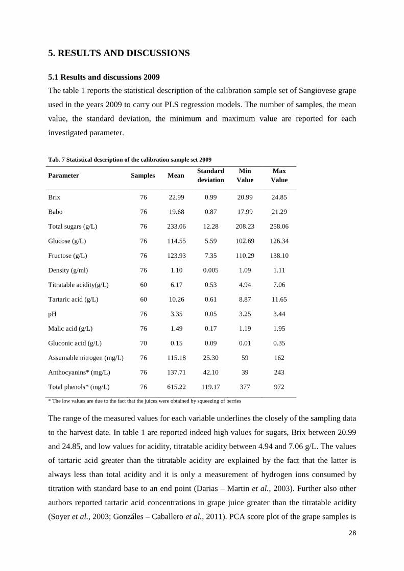
28

5. RESULTS AND DISCUSSIONS

5.1 Results and discussions 2009 The table 1 reports the statistical description of the calibration sample set of Sangiovese grape

used in the years 2009 to carry out PLS regression models. The number of samples, the mean

value, the standard deviation, the minimum and maximum value are reported for each

investigated parameter.

Tab. 7 Statistical description of the calibration sample set 2009


Min Value

Max Value

Brix 76 22.99 0.99 20.99 24.85

Babo 76 19.68 0.87 17.99 21.29

Total sugars (g/L) 76 233.06 12.28 208.23 258.06

Glucose (g/L) 76 114.55 5.59 102.69 126.34

Fructose (g/L) 76 123.93 7.35 110.29 138.10

Density (g/ml) 76 1.10 0.005 1.09 1.11

Titratable acidity(g/L) 60 6.17 0.53 4.94 7.06

Tartaric acid (g/L) 60 10.26 0.61 8.87 11.65

pH 76 3.35 0.05 3.25 3.44

Malic acid (g/L) 76 1.49 0.17 1.19 1.95

Gluconic acid (g/L) 70 0.15 0.09 0.01 0.35


Anthocyanins* (mg/L) 76 137.71 42.10 39 243

Total phenols* (mg/L) 76 615.22 119.17 377 972

* The low values are due to the fact that the juices were obtained by squeezing of berries The range of the measured values for each variable underlines the closely of the sampling data

to the harvest date. In table 1 are reported indeed high values for sugars, Brix between 20.99

and 24.85, and low values for acidity, titratable acidity between 4.94 and 7.06 g/L. The values

of tartaric acid greater than the titratable acidity are explained by the fact that the latter is

always less than total acidity and it is only a measurement of hydrogen ions consumed by

titration with standard base to an end point (Darias – Martin et al., 2003). Further also other

authors reported tartaric acid concentrations in grape juice greater than the titratable acidity

(Soyer et al., 2003; Gonzáles – Caballero et al., 2011). PCA score plot of the grape samples is

29

reported in Fig. 13. The first principal component (PC) explains 98% of the variation in the

spectra of sample set, while the second PC explains 1% alone.

Fig. 13 PCA analysis of samples collected in the season 2009. A: SS-F9-A5-48 Sangiovese clone, B: VCR 23 Sangiovese clone

The following figures (14-18) represent the averaged spectra collected from the grape samples

and treated with different statistical filters. The figures revealed how the spectral trend is

dominated by water contribution which is expressed in the peaks referred to the OH stretch

first overtone at 1450 nm, and the OH asymmetric stretch and bending combination at 1940

nm (Osborne et al., 1993; Bellincontro et al., 2011).

Fig. 14 Absorbance spectra treated with Mean Normalization

Fig. 15 Mean Normalized spectra treated whit SNV

30

Fig. 16 Mean Normalized spectra treated whit MSC

Fig. 17 Mean Normalized spectra treated whit 1st Derivative SG

Fig. 18 Mean Normalized spectra treated whit 2st Derivative SG

The results of PLS regression models elaborated in 2009 season are reported in table 2. In

bold style is highlighted, over the variable, the statistical pre – treatment that allowed to

obtain the best performance of predicting model in the terms of the statistical indices reported.

Tab. 8 PLS calibration results 2009

Brix R2c R2

cv RMSEC RMSECV SEC SECV Slope Cal

Slope Val

Lv RPD

MN 0,94 0,83 0,33 0,55 0,33 0,56 0,89 0,78 10 1,80

MN+SNV 0,93 0,81 0,35 0,58 0,35 0,59 0,86 0,76 9 1,71

MN+MSC 0,93 0,82 0,35 0,58 0,35 0,58 0,87 0,77 9 1,71

MN+SG 1°der 0,97 0,84 0,25 0,54 0,25 0,55 0,94 0,78 11 1,83

MN+SG 2°dere 0,87 0,63 0,49 0,79 0,50 0,80 0,75 0,53 6 1,25

Babo R2C R2

CV RMSEC RMSECV SEC SECV Slope Cal

Slope Val Lv RPD

MN 0,93 0,78 0,33 0,65 0,33 0,56 0,86 0,72 10 1,55

MN+SNV 0,91 0,77 0,34 0,56 0,34 0,57 0,83 0,70 9 1,55

MN+MSC 0,92 0,78 0,34 0,56 0,34 0,56 0,84 0,71 9 1,55

MN+SG 1°der 0,95 0,78 0,26 0,56 0,26 0,56 0,91 0,72 11 1,55

31

MN+SG 2°der 0,84 0,56 0,47 0,76 0,47 0,76 0,71 0,48 6 1,14

Total sugars (g/L)

R2C R2


Slope Val

Lv RPD

MN 0,85 0,79 6,51 7,52 6,55 7,57 0,71 0,66 6 1,63

MN+SNV 0,86 0,79 6,05 7,38 6,09 7,43 0,75 0,69 6 1,66

MN+MSC 0,87 0,80 6,09 7,38 6,13 7,43 0,75 0,70 6 1,66

MN+SG 1°der 0,96 0,83 3,22 7,01 3,25 7,05 0,93 0,79 11 1,75

MN+SG 2°der 0,85 0,63 6,34 9,69 6,38 9,75 0,73 0,52 6 1,27

Glucose (g/L) R2C R2


Slope Val Lv RPD

MN 0,94 0,82 1,87 3,19 1,88 3,21 0,88 0,77 10 1,75

MN+SNV 0,85 0,76 2,87 3,61 2,89 3,63 0,73 0,65 6 1,55

MN+MSC 0,93 0,80 2,05 3,42 2,06 3,44 0,86 0,75 9 1,63

MN+SG 1°der 0,97 0,83 1,40 3,18 1,41 3,20 0,93 0,77 11 1,76

MN+SG 2°der 0,86 0,63 2,83 4,50 2,85 4,53 0,74 0,52 6 1,24

Fructose (g/L) R2C R2


Slope Val

Lv RPD

MN 0,95 0,87 2,19 3,71 2,20 3,74 0,91 0,83 10 1,98

MN+SNV 0,95 0,85 2,32 3,84 2,33 3,87 0,89 0,81 9 1,91

MN+MSC 0,95 0,86 2,29 3,77 2,30 3,79 0,90 0,82 9 1,95

MN+SG 1°der 0,97 0,87 1,67 3,63 1,68 3,65 0,95 0,82 11 2,02

MN+SG 2°der 0,87 0,67 3,55 5,57 3,57 5,61 0,76 0,57 6 1,32

Density (g/ml) R2C R2


Slope Val Lv RPD

MN 0,95 0,84 0,001 0,002 0,001 0,002 0,89 0,80 10 2,50

MN+SNV 0,93 0,82 0,001 0,002 0,001 0,002 0,87 0,78 9 2,50

MN+MSC 0,94 0,82 0,001 0,002 0,001 0,002 0,88 0,79 9 2,50

MN+SG 1°der 0,97 0,85 0,001 0,002 0,001 0,002 0,94 0,80 11 2,50

MN+SG 2°der 0,87 0,65 0,002 0,003 0,002 0,003 0,76 0,56 6 1,67

Titratable acidity (g/L)

R2C R2


Slope Val

Lv RPD

MN 0,86 0,77 0,26 0,33 0,27 0,33 0,74 0,66 6 1,61

MN+SNV 0,94 0,81 0,17 0,31 0,17 0,31 0,89 0,76 9 1,71

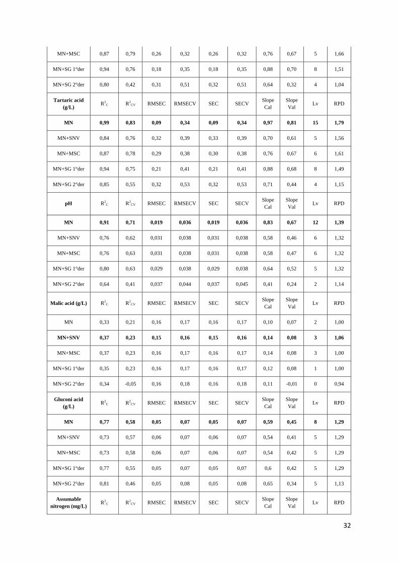
32

MN+MSC 0,87 0,79 0,26 0,32 0,26 0,32 0,76 0,67 5 1,66

MN+SG 1°der 0,94 0,76 0,18 0,35 0,18 0,35 0,88 0,70 8 1,51

MN+SG 2°der 0,80 0,42 0,31 0,51 0,32 0,51 0,64 0,32 4 1,04

Tartaric acid (g/L)

R2C R2


Slope Val Lv RPD

MN 0,99 0,83 0,09 0,34 0,09 0,34 0,97 0,81 15 1,79

MN+SNV 0,84 0,76 0,32 0,39 0,33 0,39 0,70 0,61 5 1,56

MN+MSC 0,87 0,78 0,29 0,38 0,30 0,38 0,76 0,67 6 1,61

MN+SG 1°der 0,94 0,75 0,21 0,41 0,21 0,41 0,88 0,68 8 1,49

MN+SG 2°der 0,85 0,55 0,32 0,53 0,32 0,53 0,71 0,44 4 1,15

pH R2C R2


Slope Val Lv RPD

MN 0,91 0,71 0,019 0,036 0,019 0,036 0,83 0,67 12 1,39

MN+SNV 0,76 0,62 0,031 0,038 0,031 0,038 0,58 0,46 6 1,32

MN+MSC 0,76 0,63 0,031 0,038 0,031 0,038 0,58 0,47 6 1,32

MN+SG 1°der 0,80 0,63 0,029 0,038 0,029 0,038 0,64 0,52 5 1,32

MN+SG 2°der 0,64 0,41 0,037 0,044 0,037 0,045 0,41 0,24 2 1,14

Malic acid (g/L) R2C R2


Slope Val Lv RPD

MN 0,33 0,21 0,16 0,17 0,16 0,17 0,10 0,07 2 1,00

MN+SNV 0,37 0,23 0,15 0,16 0,15 0,16 0,14 0,08 3 1,06

MN+MSC 0,37 0,23 0,16 0,17 0,16 0,17 0,14 0,08 3 1,00

MN+SG 1°der 0,35 0,23 0,16 0,17 0,16 0,17 0,12 0,08 1 1,00

MN+SG 2°der 0,34 -0,05 0,16 0,18 0,16 0,18 0,11 -0,01 0 0,94

Gluconi acid (g/L)

R2C R2


Slope Val Lv RPD

MN 0,77 0,58 0,05 0,07 0,05 0,07 0,59 0,45 8 1,29

MN+SNV 0,73 0,57 0,06 0,07 0,06 0,07 0,54 0,41 5 1,29

MN+MSC 0,73 0,58 0,06 0,07 0,06 0,07 0,54 0,42 5 1,29

MN+SG 1°der 0,77 0,55 0,05 0,07 0,05 0,07 0,6 0,42 5 1,29

MN+SG 2°der 0,81 0,46 0,05 0,08 0,05 0,08 0,65 0,34 5 1,13

Assumable nitrogen (mg/L)

R2C R2


Slope Val Lv RPD

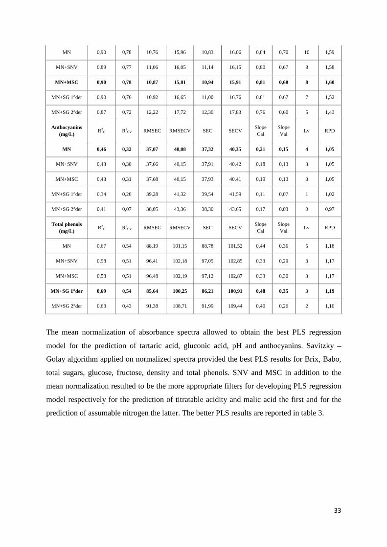
33

MN 0,90 0,78 10,76 15,96 10,83 16,06 0,84 0,70 10 1,59

MN+SNV 0,89 0,77 11,06 16,05 11,14 16,15 0,80 0,67 8 1,58

MN+MSC 0,90 0,78 10,87 15,81 10,94 15,91 0,81 0,68 8 1,60

MN+SG 1°der 0,90 0,76 10,92 16,65 11,00 16,76 0,81 0,67 7 1,52

MN+SG 2°der 0,87 0,72 12,22 17,72 12,30 17,83 0,76 0,60 5 1,43

Anthocyanins (mg/L)

R2C R2


Slope Val Lv RPD

MN 0,46 0,32 37,07 40,08 37,32 40,35 0,21 0,15 4 1,05

MN+SNV 0,43 0,30 37,66 40,15 37,91 40,42 0,18 0,13 3 1,05

MN+MSC 0,43 0,31 37,68 40,15 37,93 40,41 0,19 0,13 3 1,05

MN+SG 1°der 0,34 0,20 39,28 41,32 39,54 41,59 0,11 0,07 1 1,02

MN+SG 2°der 0,41 0,07 38,05 43,36 38,30 43,65 0,17 0,03 0 0,97

Total phenols (mg/L)

R2C R2


Slope Val Lv RPD

MN 0,67 0,54 88,19 101,15 88,78 101,52 0,44 0,36 5 1,18

MN+SNV 0,58 0,51 96,41 102,18 97,05 102,85 0,33 0,29 3 1,17

MN+MSC 0,58 0,51 96,48 102,19 97,12 102,87 0,33 0,30 3 1,17

MN+SG 1°der 0,69 0,54 85,64 100,25 86,21 100,91 0,48 0,35 3 1,19

MN+SG 2°der 0,63 0,43 91,38 108,71 91,99 109,44 0,40 0,26 2 1,10

The mean normalization of absorbance spectra allowed to obtain the best PLS regression

model for the prediction of tartaric acid, gluconic acid, pH and anthocyanins. Savitzky –

Golay algorithm applied on normalized spectra provided the best PLS results for Brix, Babo,

total sugars, glucose, fructose, density and total phenols. SNV and MSC in addition to the

mean normalization resulted to be the more appropriate filters for developing PLS regression

model respectively for the prediction of titratable acidity and malic acid the first and for the

prediction of assumable nitrogen the latter. The better PLS results are reported in table 3.

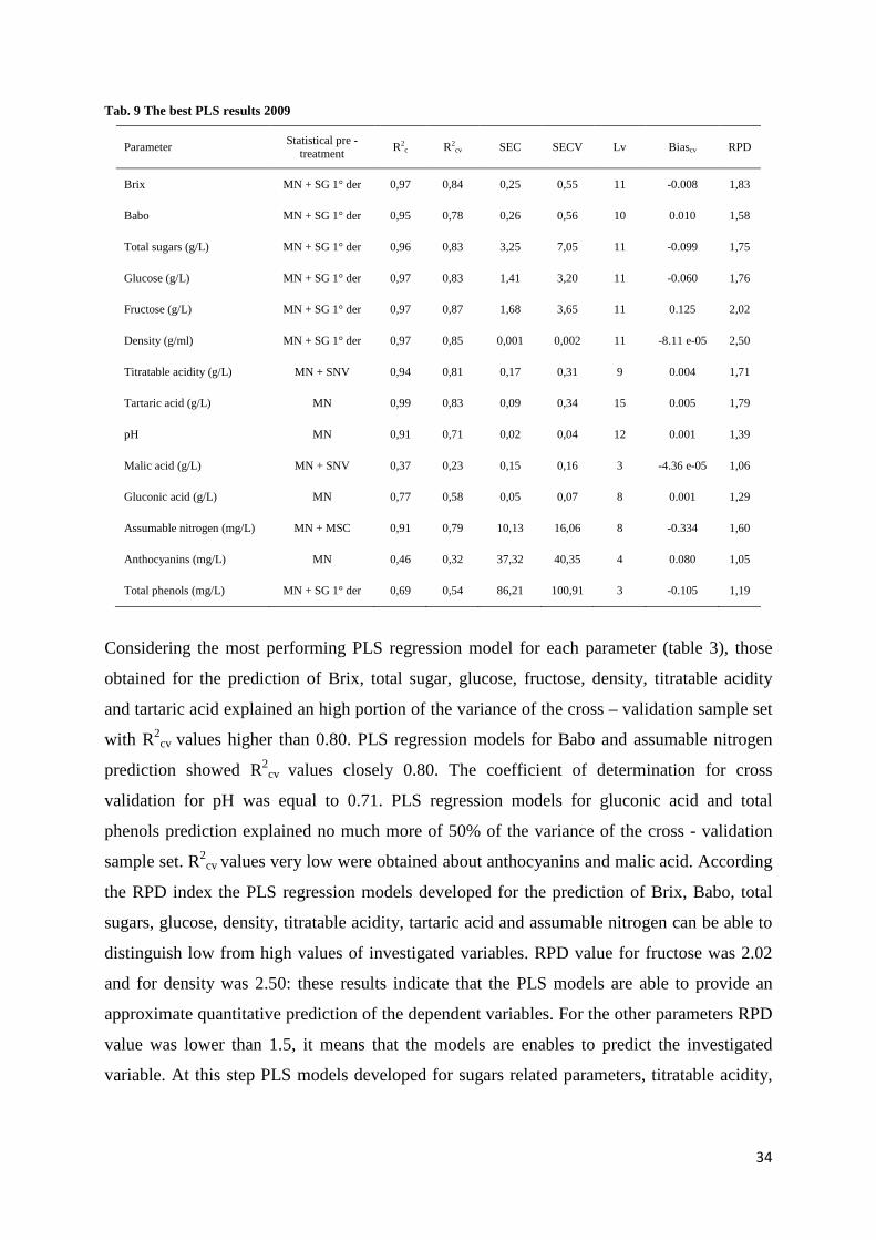
34

Tab. 9 The best PLS results 2009


c R2cv SEC SECV Lv Biascv RPD

Brix MN + SG 1° der 0,97 0,84 0,25 0,55 11 -0.008 1,83

Babo MN + SG 1° der 0,95 0,78 0,26 0,56 10 0.010 1,58

Total sugars (g/L) MN + SG 1° der 0,96 0,83 3,25 7,05 11 -0.099 1,75

Glucose (g/L) MN + SG 1° der 0,97 0,83 1,41 3,20 11 -0.060 1,76

Fructose (g/L) MN + SG 1° der 0,97 0,87 1,68 3,65 11 0.125 2,02

Density (g/ml) MN + SG 1° der 0,97 0,85 0,001 0,002 11 -8.11 e-05 2,50

Titratable acidity (g/L) MN + SNV 0,94 0,81 0,17 0,31 9 0.004 1,71

Tartaric acid (g/L) MN 0,99 0,83 0,09 0,34 15 0.005 1,79

pH MN 0,91 0,71 0,02 0,04 12 0.001 1,39

Malic acid (g/L) MN + SNV 0,37 0,23 0,15 0,16 3 -4.36 e-05 1,06

Gluconic acid (g/L) MN 0,77 0,58 0,05 0,07 8 0.001 1,29

Assumable nitrogen (mg/L) MN + MSC 0,91 0,79 10,13 16,06 8 -0.334 1,60

Anthocyanins (mg/L) MN 0,46 0,32 37,32 40,35 4 0.080 1,05

Total phenols (mg/L) MN + SG 1° der 0,69 0,54 86,21 100,91 3 -0.105 1,19

Considering the most performing PLS regression model for each parameter (table 3), those

obtained for the prediction of Brix, total sugar, glucose, fructose, density, titratable acidity

and tartaric acid explained an high portion of the variance of the cross – validation sample set

with R2cv values higher than 0.80. PLS regression models for Babo and assumable nitrogen

prediction showed R2cv values closely 0.80. The coefficient of determination for cross

validation for pH was equal to 0.71. PLS regression models for gluconic acid and total

phenols prediction explained no much more of 50% of the variance of the cross - validation

sample set. R2cv values very low were obtained about anthocyanins and malic acid. According

the RPD index the PLS regression models developed for the prediction of Brix, Babo, total

sugars, glucose, density, titratable acidity, tartaric acid and assumable nitrogen can be able to

distinguish low from high values of investigated variables. RPD value for fructose was 2.02

and for density was 2.50: these results indicate that the PLS models are able to provide an

approximate quantitative prediction of the dependent variables. For the other parameters RPD

value was lower than 1.5, it means that the models are enables to predict the investigated

variable. At this step PLS models developed for sugars related parameters, titratable acidity,

35

tartaric acid, pH and assumable nitrogen showed promising values of standard error of cross

validation.

36

5.2 Results and discussions 2010 Table 4 shows the statistical description of the calibration sample set resulting from grape

samples collected in 2009 and 2010 seasons. The values range is very wide for the most of

variables investigated. It means that the calibration set is valid to provide predicting models to

monitor the entire grape ripening. In particular samples collected in 2010 year allowed to add

at calibration sample set 2009, grapes with less sugars as can be observed comparing tab. 4

and tab. 1. In the season 2010 were collected also some samples with more titratable acidity,

assumable nitrogen and anthocyanins. Comparing calibration sample set 2009 and 2009 –

2010 the standard deviation increase for all parameters measured. Values concerning the total

phenols and the anthocyanins concentrations can appear underestimated. Buccelli 2000,

reported for Fedit 20 CH Sangiovese clone grafted on 1103 Paulsen rootstock values of

extractable anthocyanins and extractable total phenols respectively of 486 mg/Kg and 1305

mg/kg while for SS-F9-A5-48 Sangiovese clone grafted on 1103 Paulsen rootstock values of

441 mg/kg and 1650 mg/kg. The lower values measured depend on the fact that the reference

method analyzed the concentration of investigated parameters exclusively inside the extracted

juice, who was obtained without a maceration phase. A strong grinding of berries perhaps

could be useful to obtain measured values closer with the values reported in literature for

Sangiovese grape.

PCA score plot (Fig. 19) shows a marked difference between spectra acquired in 2009 season

(A, B) and spectra acquired in 2010 season (C). The first principal component (PC) explained

92% of the variation in the spectra of sample set, while the second PC explained 7%.

37

Tab. 10 Statistical description of the calibration sample set 2009 - 2010


Min Value

Max Value

Brix 96 22.34 1.77 14.99 24.85

Babo 96 18.96 1.75 12.48 21.29

Total sugars (g/L) 96 227.19 18.91 146.60 258.06

Glucose (g/L) 96 111.15 9.46 71.42 126.34

Fructose (g/L) 96 120.26 11.53 73.89 138.10

Density (g/ml) 96 1.101 0.008 1.066 1.113


Tartaric acid (g/L) 80 9.42 1.68 4.58 11.65

pH 96 3.32 0.09 2.93 3.44

Malic acid (g/L) 96 1.44 0.27 0.73 2.33

Gluconic acid (g/L) 78 0.16 0.10 0.01 0.35


Anthocyanins* (mg/L) 96 166.40 70.38 39 347

Total phenols* (mg/L) 96 596.29 123.93 324 972

*The low values are due to the fact that the juices were obtained by squeezing of berries

Fig. 19 PCA analysis of samples collected in the season 2009. A: SS-F9-A5-48 Sangiovese clone, B: VCR 23 Sangiovese clone, C: Fedit 20-21 CH.

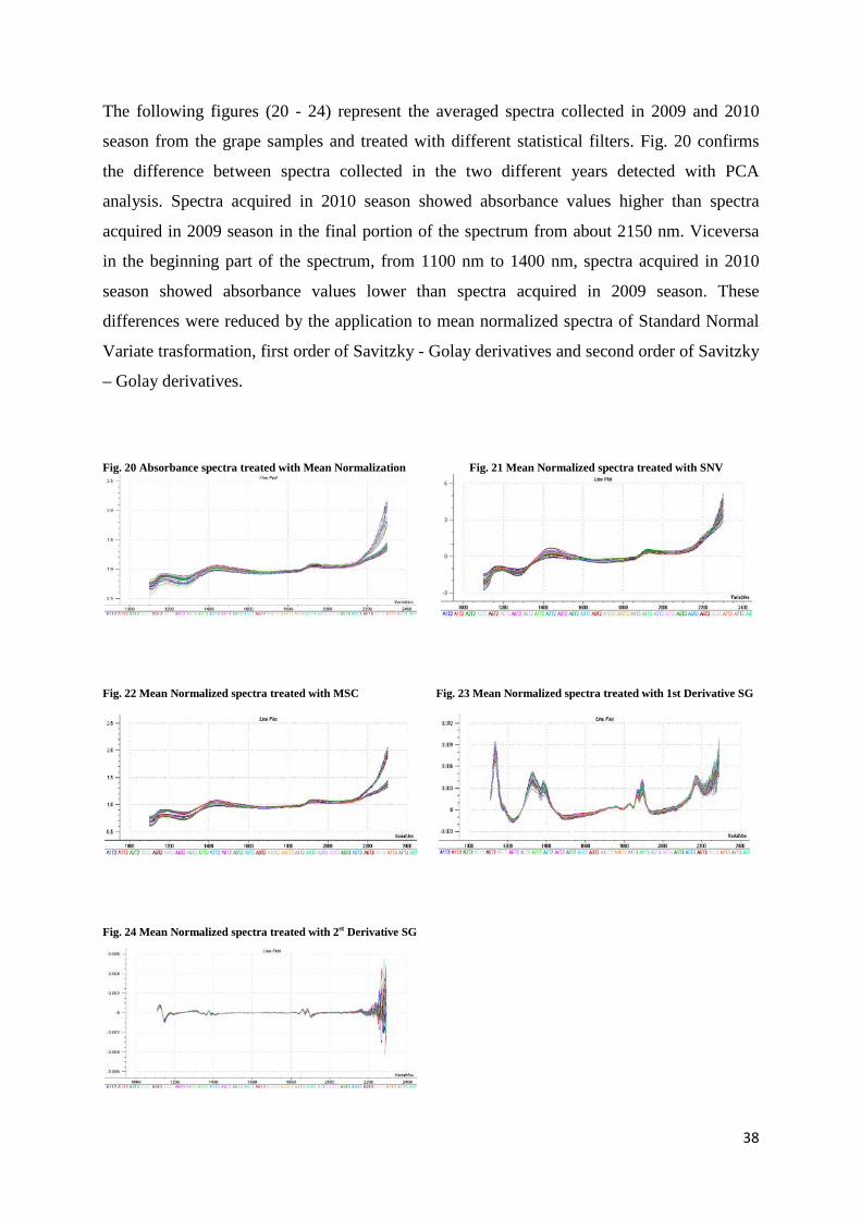
38

The following figures (20 - 24) represent the averaged spectra collected in 2009 and 2010

season from the grape samples and treated with different statistical filters. Fig. 20 confirms

the difference between spectra collected in the two different years detected with PCA

analysis. Spectra acquired in 2010 season showed absorbance values higher than spectra

acquired in 2009 season in the final portion of the spectrum from about 2150 nm. Viceversa

in the beginning part of the spectrum, from 1100 nm to 1400 nm, spectra acquired in 2010

season showed absorbance values lower than spectra acquired in 2009 season. These

differences were reduced by the application to mean normalized spectra of Standard Normal

Variate trasformation, first order of Savitzky - Golay derivatives and second order of Savitzky

– Golay derivatives.

Fig. 20 Absorbance spectra treated with Mean Normalization

Fig. 21 Mean Normalized spectra treated with SNV

Fig. 22 Mean Normalized spectra treated with MSC

Fig. 23 Mean Normalized spectra treated with 1st Derivative SG

Fig. 24 Mean Normalized spectra treated with 2st Derivative SG

39

The results of PLS regression models are reported in table 5. In bold style is highlighted, over

the variable, the statistical pre – treatment that allowed to obtain the best performance of

predicting model in the terms of the statistical indices reported.

Tab. 11 PLS calibration results 2009 - 2010

Brix R2c R2

cv RMSEC RMSECV SEC SECV Slope Cal

Slope Val Lv RPD

MN 0.91 0.80 0.72 0.92 0.72 0.92 0.83 0.79 6 1.93

MN+SNV 0.95 0.89 0.55 0.80 0.55 0.80 0.90 0.84 9 2.22

MN+MSC 0.93 0.86 0.65 0.90 0.65 0.91 0.86 0.80 7 1.95

MN+SG 1°der 0.93 0.86 0.65 0.90 0.65 0.90 0.86 0.80 5 1.97

MN+SG 2°dere 0.85 0.76 0.92 1.15 0.93 1.16 0.72 0.64 6 1.53

Babo R2C R2


Slope Val Lv RPD

MN 0.92 0.88 0.66 0.82 0.66 0.83 0.86 0.84 6 2.11

MN+SNV 0.94 0.89 0.62 0.80 0.62 0.80 0.87 0.84 7 2.20

MN+MSC 0.93 0.88 0.61 0.82 0.61 0.82 0.88 0.82 8 2.13

MN+SG 1°der 0.94 0.89 0.60 0.81 0.60 0.82 0.88 0.84 7 2.13

MN+SG 2°der 0.88 0.81 0.82 1.02 0.82 1.03 0.78 0.70 5 1.70

Total sugars (g/L)

R2C R2


Slope Val Lv RPD

MN 0.89 0.82 8.57 11.01 8.61 11.06 0.79 0.74 6 1.71

MN+SNV 0.94 0.87 6.52 9.28 6.56 9.32 0.88 0.81 9 2.03

MN+MSC 0.91 0.83 7.76 10.69 7.80 10.75 0.83 0.76 8 1.76

MN+SG 1°der 0.91 0.82 7.91 10.88 7.95 10.93 0.82 0.74 7 1.73

MN+SG 2°der 0.81 0.69 11.09 13.79 11.15 13.86 0.65 0.56 5 1.36

Glucose (g/L) R2C R2


Slope Val Lv RPD

MN 0.89 0.82 4.27 5.48 4.29 5.51 0.79 0.75 6 1.72

MN+SNV 0.94 0.86 3.25 4.89 3.26 4.91 0.88 0.79 7 1.92

MN+MSC 0.91 0.81 3.93 5.54 3.95 5.57 0.84 0.74 8 1.70

MN+SG 1°der 0.91 0.82 3.89 5.45 3.90 5.48 0.83 0.75 7 1.73

MN+SG 2°der 0.84 0.73 5.17 6.44 5.19 6.47 0.70 0.59 5 1.46

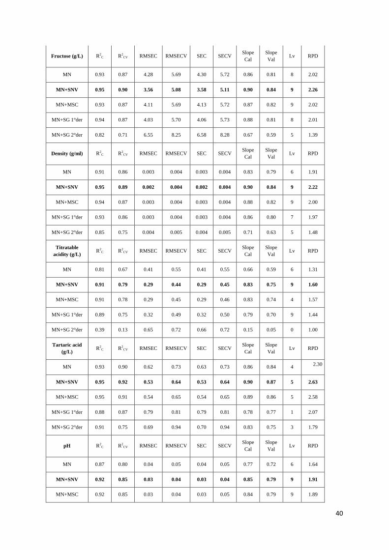
40

Fructose (g/L) R2C R2


Slope Val

Lv RPD

MN 0.93 0.87 4.28 5.69 4.30 5.72 0.86 0.81 8 2.02

MN+SNV 0.95 0.90 3.56 5.08 3.58 5.11 0.90 0.84 9 2.26

MN+MSC 0.93 0.87 4.11 5.69 4.13 5.72 0.87 0.82 9 2.02

MN+SG 1°der 0.94 0.87 4.03 5.70 4.06 5.73 0.88 0.81 8 2.01

MN+SG 2°der 0.82 0.71 6.55 8.25 6.58 8.28 0.67 0.59 5 1.39

Density (g/ml) R2C R2


Slope Val Lv RPD

MN 0.91 0.86 0.003 0.004 0.003 0.004 0.83 0.79 6 1.91

MN+SNV 0.95 0.89 0.002 0.004 0.002 0.004 0.90 0.84 9 2.22

MN+MSC 0.94 0.87 0.003 0.004 0.003 0.004 0.88 0.82 9 2.00

MN+SG 1°der 0.93 0.86 0.003 0.004 0.003 0.004 0.86 0.80 7 1.97

MN+SG 2°der 0.85 0.75 0.004 0.005 0.004 0.005 0.71 0.63 5 1.48

Titratable acidity (g/L)

R2C R2


Slope Val Lv RPD

MN 0.81 0.67 0.41 0.55 0.41 0.55 0.66 0.59 6 1.31

MN+SNV 0.91 0.79 0.29 0.44 0.29 0.45 0.83 0.75 9 1.60

MN+MSC 0.91 0.78 0.29 0.45 0.29 0.46 0.83 0.74 4 1.57

MN+SG 1°der 0.89 0.75 0.32 0.49 0.32 0.50 0.79 0.70 9 1.44

MN+SG 2°der 0.39 0.13 0.65 0.72 0.66 0.72 0.15 0.05 0 1.00

Tartaric acid (g/L)

R2C R2


Slope Val Lv RPD

MN 0.93 0.90 0.62 0.73 0.63 0.73 0.86 0.84 4 2.30

MN+SNV 0.95 0.92 0.53 0.64 0.53 0.64 0.90 0.87 5 2.63

MN+MSC 0.95 0.91 0.54 0.65 0.54 0.65 0.89 0.86 5 2.58

MN+SG 1°der 0.88 0.87 0.79 0.81 0.79 0.81 0.78 0.77 1 2.07

MN+SG 2°der 0.91 0.75 0.69 0.94 0.70 0.94 0.83 0.75 3 1.79

pH R2C R2


Slope Val Lv RPD

MN 0.87 0.80 0.04 0.05 0.04 0.05 0.77 0.72 6 1.64

MN+SNV 0.92 0.85 0.03 0.04 0.03 0.04 0.85 0.79 9 1.91

MN+MSC 0.92 0.85 0.03 0.04 0.03 0.05 0.84 0.79 9 1.89

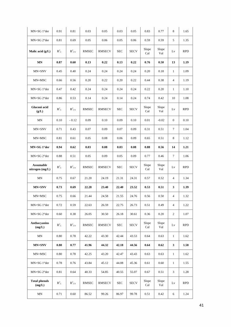
41

MN+SG 1°der 0.91 0.81 0.03 0.05 0.03 0.05 0.83 0.77 8 1.65

MN+SG 2°der 0.81 0.69 0.05 0.06 0.05 0.06 0.59 0.59 5 1.35

Malic acid (g/L) R2C R2


Slope Val Lv RPD

MN 0.87 0.60 0.13 0.22 0.13 0.22 0.76 0.50 13 1.19

MN+SNV 0.45 0.40 0.24 0.24 0.24 0.24 0.20 0.18 1 1.09

MN+MSC 0.66 0.56 0.20 0.22 0.20 0.22 0.44 0.38 4 1.19

MN+SG 1°der 0.47 0.42 0.24 0.24 0.24 0.24 0.22 0.20 1 1.10

MN+SG 2°der 0.86 0.53 0.14 0.24 0.14 0.24 0.74 0.42 10 1.08

Gluconi acid (g/L)

R2C R2


Slope Val Lv RPD

MN 0.10 - 0.12 0.09 0.10 0.09 0.10 0.01 -0.02 0 0.10

MN+SNV 0.71 0.43 0.07 0.09 0.07 0.09 0.31 0.51 7 1.04

MN+MSC 0.81 0.61 0.05 0.08 0.06 0.09 0.65 0.51 8 1.12

MN+SG 1°der 0.94 0.62 0.03 0.08 0.03 0.08 0.88 0.56 14 1.21

MN+SG 2°der 0.88 0.51 0.05 0.09 0.05 0.09 0.77 0.46 7 1.06

Assumable nitrogen (mg/L)

R2C R2


Slope Val Lv RPD

MN 0.75 0.67 21.20 24.19 21.31 24.31 0.57 0.52 4 1.34

MN+SNV 0.73 0.69 22.28 23.40 22.40 23.52 0.53 0.51 3 1.39

MN+MSC 0.75 0.66 21.44 24.58 21.55 24.76 0.56 0.50 4 1.32

MN+SG 1°der 0.72 0.59 22.63 26.59 22.75 26.73 0.51 0.49 4 1.22

MN+SG 2°der 0.60 0.38 26.05 30.50 26.18 30.61 0.36 0.20 2 1.07

Anthocyanins (mg/L)

R2C R2


Slope Val

Lv RPD

MN 0.80 0.78 42.22 43.30 42.44 43.53 0.64 0.63 1 1.62

MN+SNV 0.80 0.77 41.96 44.32 42.18 44.56 0.64 0.62 3 1.58

MN+MSC 0.80 0.78 42.25 43.20 42.47 43.43 0.63 0.63 1 1.62

MN+SG 1°der 0.78 0.76 43.84 45.12 44.08 45.36 0.61 0.60 1 1.55

MN+SG 2°der 0.81 0.64 40.33 54.85 40.55 55.07 0.67 0.51 3 1.28

Total phenols (mg/L)

R2C R2


Slope Val Lv RPD

MN 0.71 0.60 86.52 99.26 86.97 99.78 0.51 0.42 6 1.24

42

MN+SNV 0.77 0.62 78.06 97.77 78.47 98.27 0.60 0.48 7 1.26

MN+MSC 0.63 0.55 95.13 103.21 95.63 103.74 0.40 0.35 4 1.19

MN+SG 1°der 0.70 0.60 87.53 99.01 87.99 99.51 0.49 0.44 5 1.25

MN+SG 2°der 0.40 0.22 112.94 121.74 113.53 122.37 0.16 0.08 1 1.01

Standard Normal Variate transformation combined with the mean normalization gave the best

PLS regression models for all variable except that for gluconic and malic acid. For these

parameters the 1st derivative Savitzky-Golay and the mean normalization were respectively

more appropriate. In table 5 are summarized the PLS results for the most performing models

obtained for the season 2009 -2010.

Tab. 12 The best PLS results 2009 - 2010


c R2cv SEC SECV Biascv Lv RPD

Brix MN + SNV 0.95 0.89 0.55 0.80 -0.129 9 2.22

Babo MN + SNV 0.94 0.89 0.62 0.80 -0.121 7 2.20

Total sugars (g/L) MN + SNV 0.94 0.87 6.56 9.32 -0.147 9 2.03

Glucose (g/L) MN + SNV 0.94 0.86 3.27 4.91 -0.031 9 1.92

Fructose (g/L) MN + SNV 0.95 0.90 3.58 5.11 -0.142 9 2.26

Density (g/ml) MN + SNV 0.95 0.89 0.002 0.003 -8.714e 05 9 2.22

Titratable acidity (g/L) MN + SNV 0.91 0.79 0.29 0.45 -0.003 9 1.60

Tartaric acid (g/L) MN + SNV 0.95 0.92 0.53 0.64 0.001 5 2.63

pH MN + SNV 0.92 0.85 0.03 0.04 -0.001 9 1.91

Malic acid (g/L) MN 0.87 0.60 0.13 0.22 0.014 13 1.19

Gluconic acid (g/L) MN + SG 1° 0.94 0.62 0.03 0.08 0.005 14 1.21

Assumable nitrogen (mg/L) MN + SNV 0.73 0.69 22.40 23.52 0.272 3 1.39

Anthocyanins (mg/L) MN + SNV 0.80 0.77 42.18 44.56 -0.029 3 1.58

Total phenols (mg/L) MN + SNV 0.77 0.62 78.47 98.27 -1.589 7 1.26

The most performing PLS models developed on 2009 – 2010 season (tab. 6) showed higher

values of coefficient of determination for cross validation than the most performing PLS

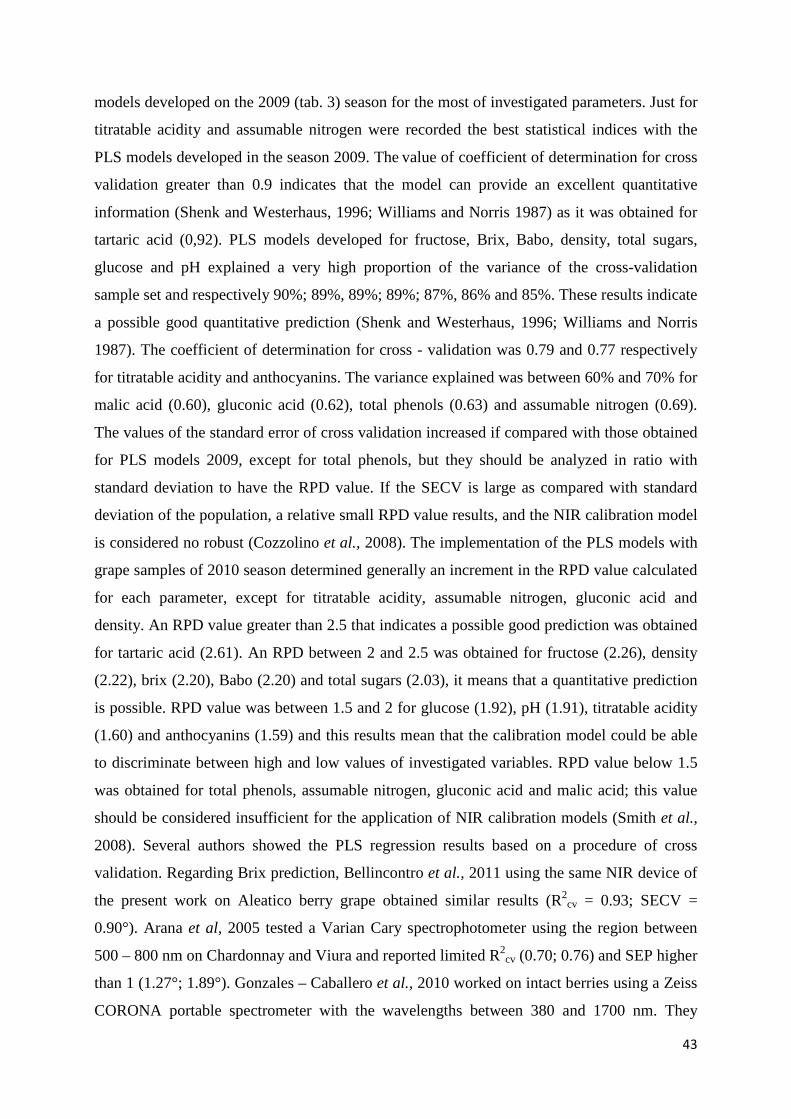
43

models developed on the 2009 (tab. 3) season for the most of investigated parameters. Just for

titratable acidity and assumable nitrogen were recorded the best statistical indices with the

PLS models developed in the season 2009. The value of coefficient of determination for cross

validation greater than 0.9 indicates that the model can provide an excellent quantitative

information (Shenk and Westerhaus, 1996; Williams and Norris 1987) as it was obtained for

tartaric acid (0,92). PLS models developed for fructose, Brix, Babo, density, total sugars,

glucose and pH explained a very high proportion of the variance of the cross-validation

sample set and respectively 90%; 89%, 89%; 89%; 87%, 86% and 85%. These results indicate

a possible good quantitative prediction (Shenk and Westerhaus, 1996; Williams and Norris

1987). The coefficient of determination for cross - validation was 0.79 and 0.77 respectively

for titratable acidity and anthocyanins. The variance explained was between 60% and 70% for

malic acid (0.60), gluconic acid (0.62), total phenols (0.63) and assumable nitrogen (0.69).

The values of the standard error of cross validation increased if compared with those obtained

for PLS models 2009, except for total phenols, but they should be analyzed in ratio with

standard deviation to have the RPD value. If the SECV is large as compared with standard

deviation of the population, a relative small RPD value results, and the NIR calibration model

is considered no robust (Cozzolino et al., 2008). The implementation of the PLS models with

grape samples of 2010 season determined generally an increment in the RPD value calculated

for each parameter, except for titratable acidity, assumable nitrogen, gluconic acid and

density. An RPD value greater than 2.5 that indicates a possible good prediction was obtained

for tartaric acid (2.61). An RPD between 2 and 2.5 was obtained for fructose (2.26), density

(2.22), brix (2.20), Babo (2.20) and total sugars (2.03), it means that a quantitative prediction

is possible. RPD value was between 1.5 and 2 for glucose (1.92), pH (1.91), titratable acidity

(1.60) and anthocyanins (1.59) and this results mean that the calibration model could be able

to discriminate between high and low values of investigated variables. RPD value below 1.5

was obtained for total phenols, assumable nitrogen, gluconic acid and malic acid; this value

should be considered insufficient for the application of NIR calibration models (Smith et al.,

2008). Several authors showed the PLS regression results based on a procedure of cross

validation. Regarding Brix prediction, Bellincontro et al., 2011 using the same NIR device of

the present work on Aleatico berry grape obtained similar results (R2cv = 0.93; SECV =

0.90°). Arana et al, 2005 tested a Varian Cary spectrophotometer using the region between

500 – 800 nm on Chardonnay and Viura and reported limited R2cv (0.70; 0.76) and SEP higher

than 1 (1.27°; 1.89°). Gonzales – Caballero et al., 2010 worked on intact berries using a Zeiss

CORONA portable spectrometer with the wavelengths between 380 and 1700 nm. They

44

found higher coefficient of determination for cross validation for Brix (0.91) and reducing

sugar (0.93) but at the same time obtained higher SECV, 1.43° and 13.10 mg/L for the two

parameters. A greater predictive capacity for the reducing sugar determination was reported

by Fernandez – Novales et al., 2009 (R2cv 0.98; SECV 13.62 g/L), but they scanning the grape

juice in transmittance mode and used the range between 800 nm and 1050 nm.

The result obtained for the prediction of pH was better than those reported by Gonzales –

Caballero et al., 2010 (R2cv = 0.64; SECV = 0.20) and by Cozzolino et al., 2004a (R2

cv = 0.60;

SECV = 0.08). Cozzolino et al., 2004a used a Zeiss CORONA to acquire spectra in the NIR

region between 700 nm and 1100 nm from whole berries. Not many published studies have

reported for the prediction of titratable acidity and organic acids in grape. Gonzales –

Caballero et al., 2010 obtained worse PLS regression models for titratable acidity (R2cv =

0.33; SECV = 1.29), tartaric acid (R2cv = 0.34; SECV = 1.34) and malic acid (R2

cv = 0.49;

SECV = 0.68) than those presented here. Chauchard et al., 2004 showed a PLS regression

model for titratable acidity prediction with a R2cv of 0.76 and a SECV of 1.32 g/L. They used

a Zeiss MMS1 spectrometer and investigated the spectral range from 680 nm to 1100 nm.

About assumable nitrogen prediction the result obtained was comparable with those reported

by Dambergs et al., 2005 (Rcv= 0.77; SECV= 34.2 mg/L).

The PLS regression model for anthocyanins prediction showed a nearly as good explanation

of the variance (R2cv = 0.79) and a promising SECV, equal to 44.56 mg/L. About total phenols

the PLS model explained only the 62% of the variance and gave a SECV of 98.27 mg/L.

Cozzolino et al., 2004a obtained a lower coefficient of determination for cross validation

(R2cv = 0.50) and a SECV of 0.14 mg/g for determining anthocyanins in whole berries. Instead

Ferrer – Gallego et al., 2011 using a Foss system 5000 in the NIR range between 1100 and

2200 nm showed a modified PLS regression models with high predictive ability for

anthocyanins (R2cv = 0.95; SECV = 1.10 mg/g) and for total polyphenols (R2

cv = 0.98; SECV

= 1.33 mg/g) in intact grapes.

Coefficients of regression for the optimal number of terms must be analyzed and interpreted

in order to make sense of the calibration obtained (Cozzolino et al., 2011). Following the

coefficient of regression is reported for each PLS calibration model of table 6.

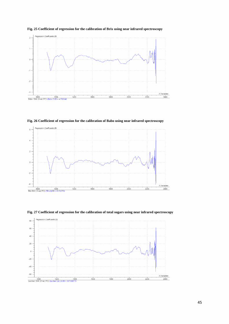
45

Fig. 25 Coefficient of regression for the calibration of Brix using near infrared spectroscopy

Fig. 26 Coefficient of regression for the calibration of Babo using near infrared spectroscopy

Fig. 27 Coefficient of regression for the calibration of total sugars using near infrared spectroscopy

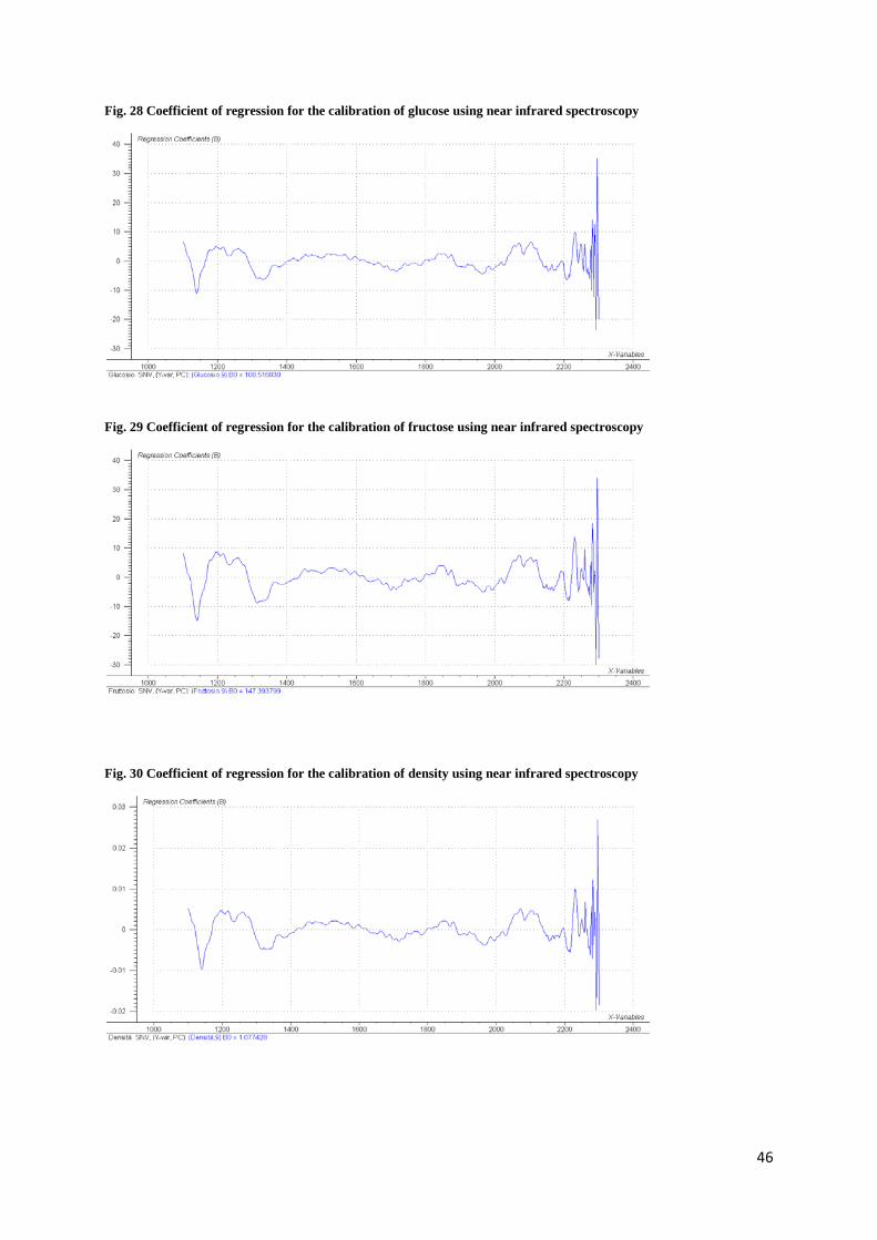
46

Fig. 28 Coefficient of regression for the calibration of glucose using near infrared spectroscopy

Fig. 29 Coefficient of regression for the calibration of fructose using near infrared spectroscopy

Fig. 30 Coefficient of regression for the calibration of density using near infrared spectroscopy

47

Fig. 31 Coefficient of regression for the calibration of titratable acidity using near infrared spectroscopy

Fig. 32 Coefficient of regression for the calibration of tartaric acid using near infrared spectroscopy

Fig. 33 Coefficient of regression for the calibration of pH using near infrared spectroscopy

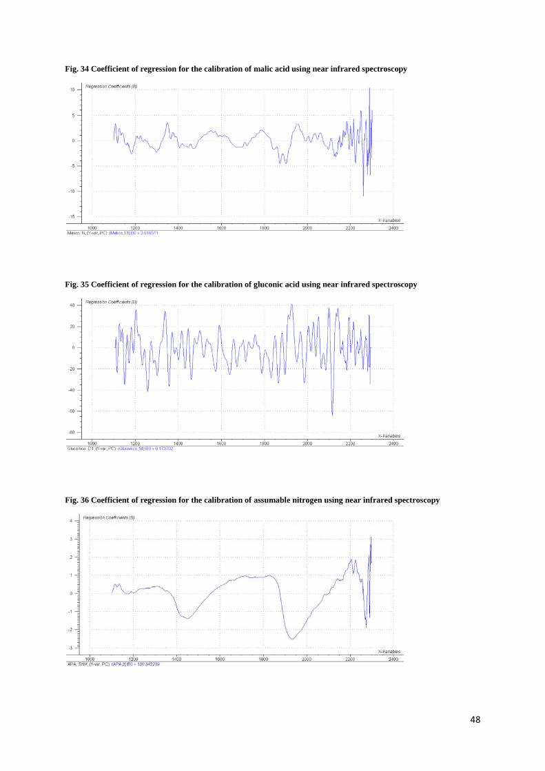
48

Fig. 34 Coefficient of regression for the calibration of malic acid using near infrared spectroscopy

Fig. 35 Coefficient of regression for the calibration of gluconic acid using near infrared spectroscopy

Fig. 36 Coefficient of regression for the calibration of assumable nitrogen using near infrared spectroscopy

49

Fig. 37 Coefficient of regression for the calibration of anthocyanins using near infrared spectroscopy

Fig. 38 Coefficient of regression for the calibration of total phenols using near infrared spectroscopy

About sugars related parameters (Brix, Babo, total sugar, glucose, fructose and density) the

trend of the coefficient of regression was very similar. It showed a pronounced negative peak

around 1140 nm. This region is associated with C-H stretch second overtone. High values of

the coefficient of regression were observed also between 1180 – 1270 nm associated with C-

H stretch second overtone; around1320 nm associated with C-H combination first overtone;

around 2100 nm associated with N-H combinations and around 2230 nm associated with N-H,

O-H and C-H combinations. A negative peak around 1190 nm was observed by Kemps et al.,

2010 developing PLS regression models in the VIS NIR region between 320 nm and 1660 nm

for sugars concentration in Syrah and Merlot varieties using a Zeiss Corona 45

spectrophotometer. They found a positive peak around 1400 nm for Syrah while a negative

peak for the same region for Merlot. Comparing the two works we must take into account that

Kemps et al., 2010 pre - processed spectra by taking first order derivative. The authors

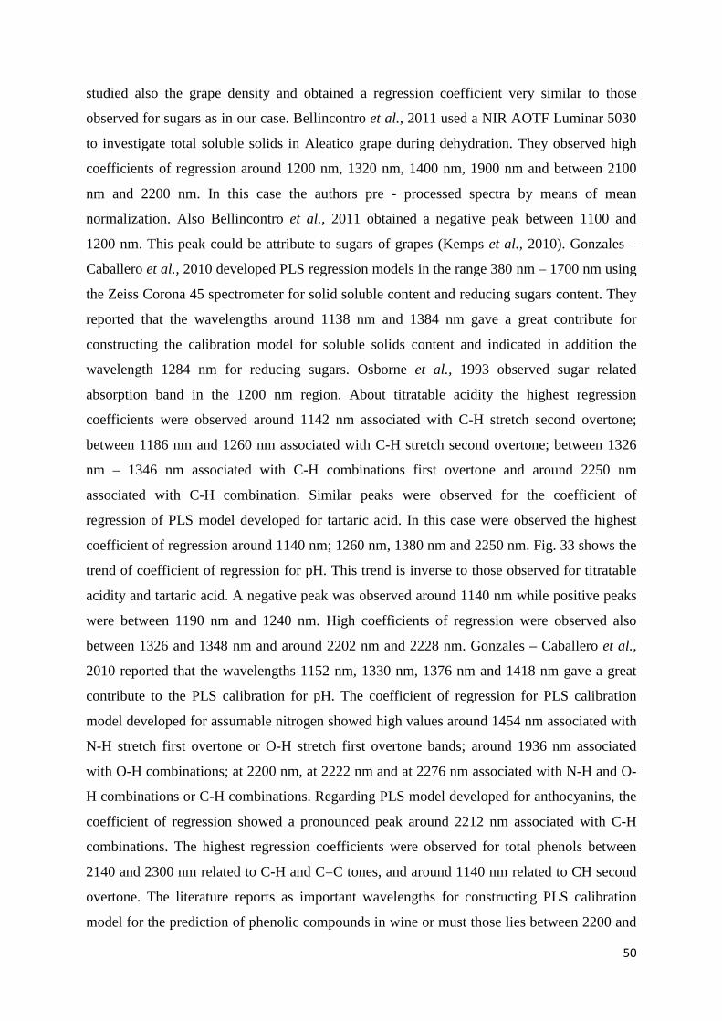
50

studied also the grape density and obtained a regression coefficient very similar to those

observed for sugars as in our case. Bellincontro et al., 2011 used a NIR AOTF Luminar 5030

to investigate total soluble solids in Aleatico grape during dehydration. They observed high

coefficients of regression around 1200 nm, 1320 nm, 1400 nm, 1900 nm and between 2100

nm and 2200 nm. In this case the authors pre - processed spectra by means of mean

normalization. Also Bellincontro et al., 2011 obtained a negative peak between 1100 and

1200 nm. This peak could be attribute to sugars of grapes (Kemps et al., 2010). Gonzales –

Caballero et al., 2010 developed PLS regression models in the range 380 nm – 1700 nm using

the Zeiss Corona 45 spectrometer for solid soluble content and reducing sugars content. They

reported that the wavelengths around 1138 nm and 1384 nm gave a great contribute for

constructing the calibration model for soluble solids content and indicated in addition the

wavelength 1284 nm for reducing sugars. Osborne et al., 1993 observed sugar related

absorption band in the 1200 nm region. About titratable acidity the highest regression

coefficients were observed around 1142 nm associated with C-H stretch second overtone;

between 1186 nm and 1260 nm associated with C-H stretch second overtone; between 1326

nm – 1346 nm associated with C-H combinations first overtone and around 2250 nm

associated with C-H combination. Similar peaks were observed for the coefficient of

regression of PLS model developed for tartaric acid. In this case were observed the highest

coefficient of regression around 1140 nm; 1260 nm, 1380 nm and 2250 nm. Fig. 33 shows the

trend of coefficient of regression for pH. This trend is inverse to those observed for titratable

acidity and tartaric acid. A negative peak was observed around 1140 nm while positive peaks

were between 1190 nm and 1240 nm. High coefficients of regression were observed also

between 1326 and 1348 nm and around 2202 nm and 2228 nm. Gonzales – Caballero et al.,

2010 reported that the wavelengths 1152 nm, 1330 nm, 1376 nm and 1418 nm gave a great

contribute to the PLS calibration for pH. The coefficient of regression for PLS calibration

model developed for assumable nitrogen showed high values around 1454 nm associated with

N-H stretch first overtone or O-H stretch first overtone bands; around 1936 nm associated

with O-H combinations; at 2200 nm, at 2222 nm and at 2276 nm associated with N-H and O-

H combinations or C-H combinations. Regarding PLS model developed for anthocyanins, the

coefficient of regression showed a pronounced peak around 2212 nm associated with C-H

combinations. The highest regression coefficients were observed for total phenols between

2140 and 2300 nm related to C-H and C=C tones, and around 1140 nm related to CH second

overtone. The literature reports as important wavelengths for constructing PLS calibration

model for the prediction of phenolic compounds in wine or must those lies between 2200 and

51

2300 nm (Cozzolino et al., 2004b). Cozzolino et al., 2008 found high regression coefficients

between 2100 and 2300 nm for the prediction of condensed tannins in red grape homogenates.

Gallego et al., 2011 suggested that the spectral regions close 1140 and 1320 nm gave an

important contribution to development PLS regression model to predict phenolic compounds

on intact grapes and grape skins.

Finally the scatter plots are also important in order to show the relationship and distribution of

the data set (Cozzolino et al., 2011).

In the following figures (39-52) are reported the scatter plots of the most performing PLS

models developed on 2009 – 2010 season.

Fig 39 Scatter plot between reference values and predicted NIR values for Brix

Fig. 40 Scatter plot between reference values and predicted NIR values for Babo

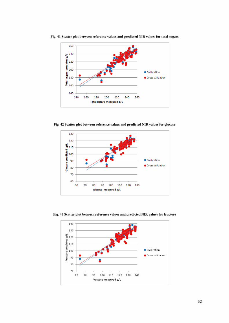
52

Fig. 41 Scatter plot between reference values and predicted NIR values for total sugars

Fig. 42 Scatter plot between reference values and predicted NIR values for glucose

Fig. 43 Scatter plot between reference values and predicted NIR values for fructose

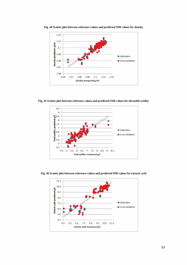
53

Fig. 44 Scatter plot between reference values and predicted NIR values for density

Fig. 45 Scatter plot between reference values and predicted NIR values for titratable acidity

Fig. 46 Scatter plot between reference values and predicted NIR values for tartaric acid

54

Fig. 47 Scatter plot between reference values and predicted NIR values for pH

Fig. 48 Scatter plot between reference values and predicted NIR values for malic acid

Fig. 49 Scatter plot between reference values and predicted NIR values for gluconic acid

55

Fig. 50 Scatter plot between reference values and predicted NIR values for assumable nitrogen

Fig. 51 Scatter plot between reference values and predicted NIR values for anthocyanins

Fig. 52 Scatter plot between reference values and predicted NIR values for total phenols

56

5.3 Results and discussions 2011

The statistical description of the external validation sample set is reported in table 7. The

number of samples used as validation set is equal to 31% of the total samples adopted in this

work to investigate titratable acidity and tartaric acid, and equal to 26 % of the total samples

about other parameters. The range of values of validation set lay within the range recorded for

the calibration set except for anthocyanins and total phenols. In the latter cases were included

grape samples with more anthocyanins content and a more wide total phenols content.

Tab. 13 Statistical description of the external validation sample set 2011

Parameters Samples Mean Standard deviation

Min Value

Max Value

Brix 25 21.43 1.97 18.44 24.84

Babo 25 18.48 1.73 15.89 21.42

Total sugars (g/L) 25 215.45 22.43 182.70 256.13

Glucose (g/L) 25 105.93 9.66 92.38 122.49

Fructose (g/L) 25 112.95 12.73 92.09 132.95

Density (g/ml) 25 1.09 0.01 1.08 1.11



pH 25 3.27 0.07 3.16 3.44

Malic acid (g/L) 25 1.49 0.38 0.93 2.19

Assumable nitrogen (mg/L) 25 112.73 49.42 63.60 237.30

Anthocyanins* (mg/L) 25 234.18 127.88 50.57 517.34

Total phenols* (mg/L) 25 530.05 252.00 110.72 1170.06

*The low values are due to the fact that the juices were obtained by squeezing of berries

The PCA analysis of the absorbance spectra collected in 2009, 2010 and 2011 season shows

as the spectra of validation sample set (D) resulted closer to spectra of SS-F9-A5-48 (A) and

VCR 23 (B) Sangiovese clones than to spectra of Fedit 20 and 21 CH clones (C). The first PC

explained 91% of the variance of the calibration and validation sample sets, and the second

PC explained 8%. The ralationships between the different samples are more clear with the

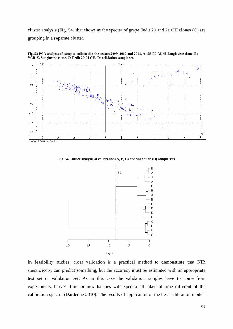
57

cluster analysis (Fig. 54) that shows as the spectra of grape Fedit 20 and 21 CH clones (C) are

grouping in a separate cluster.

Fig. 53 PCA analysis of samples collected in the season 2009, 2010 and 2011. A: SS-F9-A5-48 Sangiovese clone, B: VCR 23 Sangiovese clone, C: Fedit 20-21 CH, D: validation sample set.

Fig. 54 Cluster analysis of calibration (A, B, C) and validation (D) sample sets

In feasibility studies, cross validation is a practical method to demonstrate that NIR

spectroscopy can predict something, but the accuracy must be estimated with an appropriate

test set or validation set. As in this case the validation samples have to come from

experiments, harvest time or new batches with spectra all taken at time different of the

calibration spectra (Dardenne 2010). The results of application of the best calibration models

58

obtained on 2009 – 2010 sample set, on the external validation sample set collected in 2011

season are reported in table 8. Also for assumable nitrogen and titratable acidity parameters

were tested the PLS models 2009- 2010 since based on a wide number of samples.

Tab.14 Validation statistics for the best PLS models 2009-2010

Parameter R2 RMSEP SEP BIAS RPD

Brix 0.93 0.94 0.73 0.61 2.70

Babo 0.93 0.86 0.62 0.61 2.79

Total sugars (g/L) 0.94 9.44 7.39 6.05 3.03

Glucose (g/L) 0.93 4.73 3.59 3.17 2.69

Fructose (g/L) 0.92 6.20 5.07 3.72 2.51

Density (g/ml) 0.91 0.006 0.004 0.005 2.50

Titratable acidity (g/L) 0.55 1.23 0.80 -0.95 0.97

Tartaric acid (g/L) 0.48 2.31 1.28 1.94 1.13

pH 0.66 0.09 0.09 0.02 0.78

Malic acid (g/L) 0.48 0.35 0.33 -0.14 1.15

Assumable nitrogen (mg/L) 0.70 40.70 35.48 -21.17 1.39

Anthocyanins (mg/L) 0.76 136.17 115.24 -76.11 1.11

Total phenols (mg/L) 0.69 187.96 190.05 25.59 1.32

The external validation of calibration models developed for sugars related parameters

prediction showed an increase of performance than those recorded in cross validation test.

The coefficient of determination for prediction was greater than 0.90 for total sugars (0.94),

brix (0.93), babo (0.93), glucose (0.93), fructose (0.92) and density (0.91). The standard error

of prediction was lower than the SECV obtained in cross validation test for brix, babo, total

sugars, glucose, fructose and it was respectively of 0.73°; 0.62°, 7.39 g/L, 3.59 g/L and 5.07

g/L. About density the SEP was 0.04 g/ml and it was higher than those observed in cross

validation test (0.03 g/ml). For all four above discussed parameters the RPD index increased

in the validation test and was between 2.50 and 3. This result, as reported by several authors

(Nicolai et al., 2007; Williams and Sobering 1996; Fearn 2002), underlines the good

prediction accuracy achieved by the models. The performance obtained in prediction can be

59

further appreciated comparing these results with those reported in literature. Bellincontro et

al., 2011 using the same NIR AOTF on Aleatico berries obtained very similar results for the

prediction of Brix (R2 = 0.92; SEP = 0.73). Other authors reported the application of NIR

spectroscopy on single berry, but with other instruments and wavelengths and obtained

generally SEP or RMSEP values greater than those presented in this work. Jarén at al., 2001

working on Garnacha and Viura varieties developed Multilinear regression models for Brix

prediction and obtained a coefficient of determination respectively of 0.89 and 0.92, and a

SEP for Garnacha of 1.05° and for Viura of 1.04°. Larraín et al., 2008 using the range

between 640 nm and 1300 nm developed PLS regression models for predicting Brix and other

parameters in Cabernet sauvignon, Carmenere, Merlot, Pinot Noir and Chardonnay grapes.

About Brix prediction they obtained a R2 between 0.87 and 0.93 and RMSEP between 1.01°

and 1.26°. Guidetti et al., 2010 used a VIS NIR portable spectrophotometer (400 nm – 1000

nm) on Nebbiolo berries and reported for Brix a correlation coefficient and a RMSEP

respectively of 0.82 and 1.48°. Some works tested the NIR spectroscopy to investigate Brix

and others quality grape parameters in whole bunches (Gonzales – Caballero et al., 2011;

Kemps et al., 2010). Gonzales – Caballero et al., 2011 using the wavelength between 380 and

1700 nm obtained as better result for the Brix prediction a R2 and a SEP of 0.88 and 1.33°

respectively. Kemps et al., 2010 with the same spectrometer obtained for different cultivars a

R2 and a SEP values between 0.81-0.98 and between 0.56° - 1.15° respectively.

About the prediction of reducing sugars the results presented here were better than those

reported by Gonzales – Caballero et al., 2011 that used a MPLS regression (R2=0.86; SEP

=16.67 g/L). Novales et al., 2009 working on musts with the NIR region 850 - 1050 nm,

obtained an higher coefficient of determination for prediction (0.98) than those reported here

but also an higher SEP (12.20 g/L).

Regarding acidity related parameters the external validation of the calibration models showed

a lower predictive ability than those expected according the cross validation test. The R2 was

0.66 for pH, 0.55 for titratable acidity, 0.48 for tartaric and malic acid. The SEP values were

all greater than the SECV values. SEP value was however promising for the prediction of

titratable acidity (0.80 g/L), pH (0.09). Higher was the SEP recorded for tartaric acid (1.28

g/L) and associated also an high Bias value (1.94 g/L). Low was the error of prediction for

malic acid (0.33 g/L). The RPD index was lower than 1.5 for all four parameters.

Several authors reported the application of NIR spectroscopy to investigate pH (Cozzolino et

al., 2004a; Larraín et al., 2008; Guidetti et al., 2010; González - Caballero et al., 2011) and

others acidity related parameters in grape such as titratable acidity, tartaric and malic acid

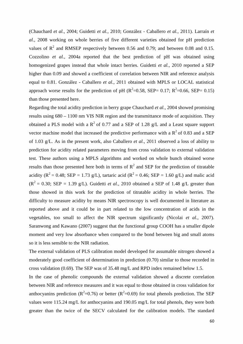
60

(Chauchard et al., 2004; Guidetti et al., 2010; González - Caballero et al., 2011). Larraín et

al., 2008 working on whole berries of five different varieties obtained for pH prediction

values of R2 and RMSEP respectively between 0.56 and 0.79; and between 0.08 and 0.15.

Cozzolino et al., 2004a reported that the best prediction of pH was obtained using

homogenized grapes instead that whole intact berries. Guidetti et al., 2010 reported a SEP

higher than 0.09 and showed a coefficient of correlation between NIR and reference analysis

equal to 0.81. González - Caballero et al., 2011 obtained with MPLS or LOCAL statistical

approach worse results for the prediction of pH (R2=0.58, SEP= 0.17; R2=0.66, SEP= 0.15)

than those presented here.

Regarding the total acidity prediction in berry grape Chauchard et al., 2004 showed promising

results using 680 – 1100 nm VIS NIR region and the transmittance mode of acquisition. They

obtained a PLS model with a R2 of 0.77 and a SEP of 1.28 g/L and a Least square support

vector machine model that increased the predictive performance with a R2 of 0.83 and a SEP

of 1.03 g/L. As in the present work, also Caballero et al., 2011 observed a loss of ability to

prediction for acidity related parameters moving from cross validation to external validation

test. These authors using a MPLS algorithms and worked on whole bunch obtained worse

results than those presented here both in terms of R2 and SEP for the prediction of titratable

acidity (R2 = 0.48; SEP = 1.73 g/L), tartaric acid (R2 = 0.46; SEP = 1.60 g/L) and malic acid

(R2 = 0.30; SEP = 1.39 g/L). Guidetti et al., 2010 obtained a SEP of 1.48 g/L greater than

those showed in this work for the prediction of titratable acidity in whole berries. The

difficulty to measure acidity by means NIR spectroscopy is well documented in literature as

reported above and it could be in part related to the low concentration of acids in the

vegetables, too small to affect the NIR spectrum significantly (Nicolai et al., 2007).

Saranwong and Kawano (2007) suggest that the functional group COOH has a smaller dipole

moment and very low absorbance when compared to the bond between big and small atoms

so it is less sensible to the NIR radiation.

The external validation of PLS calibration model developed for assumable nitrogen showed a

moderately good coefficient of determination in prediction (0.70) similar to those recorded in

cross validation (0.69). The SEP was of 35.48 mg/L and RPD index remained below 1.5.

In the case of phenolic compounds the external validation showed a discrete correlation

between NIR and reference measures and it was equal to those obtained in cross validation for

anthocyanins prediction (R2=0.76) or better (R2=0.69) for total phenols prediction. The SEP

values were 115.24 mg/L for anthocyanins and 190.05 mg/L for total phenols, they were both

greater than the twice of the SECV calculated for the calibration models. The standard

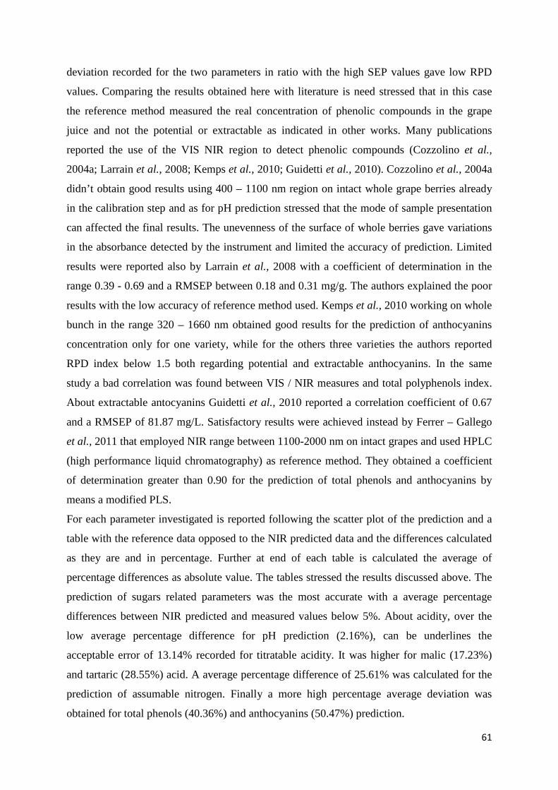
61

deviation recorded for the two parameters in ratio with the high SEP values gave low RPD

values. Comparing the results obtained here with literature is need stressed that in this case

the reference method measured the real concentration of phenolic compounds in the grape

juice and not the potential or extractable as indicated in other works. Many publications

reported the use of the VIS NIR region to detect phenolic compounds (Cozzolino et al.,

2004a; Larrain et al., 2008; Kemps et al., 2010; Guidetti et al., 2010). Cozzolino et al., 2004a

didn’t obtain good results using 400 – 1100 nm region on intact whole grape berries already

in the calibration step and as for pH prediction stressed that the mode of sample presentation

can affected the final results. The unevenness of the surface of whole berries gave variations

in the absorbance detected by the instrument and limited the accuracy of prediction. Limited

results were reported also by Larrain et al., 2008 with a coefficient of determination in the

range 0.39 - 0.69 and a RMSEP between 0.18 and 0.31 mg/g. The authors explained the poor

results with the low accuracy of reference method used. Kemps et al., 2010 working on whole

bunch in the range 320 – 1660 nm obtained good results for the prediction of anthocyanins

concentration only for one variety, while for the others three varieties the authors reported

RPD index below 1.5 both regarding potential and extractable anthocyanins. In the same

study a bad correlation was found between VIS / NIR measures and total polyphenols index.

About extractable antocyanins Guidetti et al., 2010 reported a correlation coefficient of 0.67

and a RMSEP of 81.87 mg/L. Satisfactory results were achieved instead by Ferrer – Gallego

et al., 2011 that employed NIR range between 1100-2000 nm on intact grapes and used HPLC

(high performance liquid chromatography) as reference method. They obtained a coefficient

of determination greater than 0.90 for the prediction of total phenols and anthocyanins by

means a modified PLS.

For each parameter investigated is reported following the scatter plot of the prediction and a

table with the reference data opposed to the NIR predicted data and the differences calculated

as they are and in percentage. Further at end of each table is calculated the average of

percentage differences as absolute value. The tables stressed the results discussed above. The

prediction of sugars related parameters was the most accurate with a average percentage

differences between NIR predicted and measured values below 5%. About acidity, over the

low average percentage difference for pH prediction (2.16%), can be underlines the

acceptable error of 13.14% recorded for titratable acidity. It was higher for malic (17.23%)

and tartaric (28.55%) acid. A average percentage difference of 25.61% was calculated for the

prediction of assumable nitrogen. Finally a more high percentage average deviation was

obtained for total phenols (40.36%) and anthocyanins (50.47%) prediction.

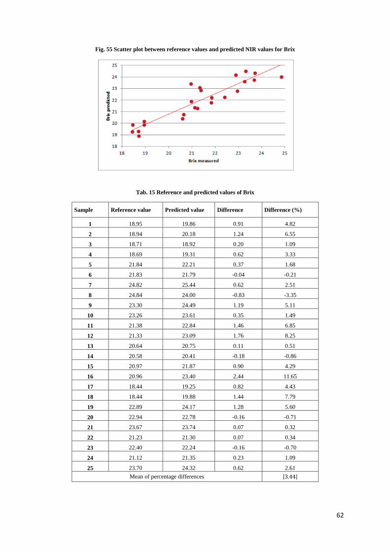
62

Fig. 55 Scatter plot between reference values and predicted NIR values for Brix

Tab. 15 Reference and predicted values of Brix

Sample Reference value Predicted value Difference Difference (%)

1 18.95 19.86 0.91 4.82

2 18.94 20.18 1.24 6.55

3 18.71 18.92 0.20 1.09

4 18.69 19.31 0.62 3.33

5 21.84 22.21 0.37 1.68

6 21.83 21.79 -0.04 -0.21

7 24.82 25.44 0.62 2.51

8 24.84 24.00 -0.83 -3.35

9 23.30 24.49 1.19 5.11

10 23.26 23.61 0.35 1.49

11 21.38 22.84 1.46 6.85

12 21.33 23.09 1.76 8.25

13 20.64 20.75 0.11 0.51

14 20.58 20.41 -0.18 -0.86

15 20.97 21.87 0.90 4.29

16 20.96 23.40 2.44 11.65

17 18.44 19.25 0.82 4.43

18 18.44 19.88 1.44 7.79

19 22.89 24.17 1.28 5.60

20 22.94 22.78 -0.16 -0.71

21 23.67 23.74 0.07 0.32

22 21.23 21.30 0.07 0.34

23 22.40 22.24 -0.16 -0.70

24 21.12 21.35 0.23 1.09

25 23.70 24.32 0.62 2.61 Mean of percentage differences |3.44|

63

Fig. 56 Scatter plot between reference values and predicted NIR values for Babo

Tab. 16 Reference and predicted values of Babo


1 16.30 16.89 0.59 3.64

2 16.28 17.24 0.96 5.87

3 16.09 16.34 0.25 1.54

4 16.06 16.73 0.67 4.16

5 18.86 19.03 0.17 0.90

6 18.83 18.86 0.02 0.13

7 21.40 22.53 1.13 5.28

8 21.42 21.26 -0.16 -0.75

9 20.15 21.27 1.12 5.55

10 20.11 20.81 0.70 3.48

11 18.50 19.91 1.41 7.62

12 18.44 20.29 1.85 10.00

13 17.79 18.56 0.77 4.34

14 17.71 17.78 0.07 0.40

15 18.13 19.16 1.03 5.66

16 18.10 19.99 1.89 10.44

17 15.90 16.67 0.77 4.85

18 15.89 17.29 1.40 8.81

19 19.87 20.52 0.65 3.27

20 20.11 19.82 -0.29 -1.47

21 20.42 20.41 -0.01 -0.03

22 18.14 18.10 -0.04 -0.23

23 19.25 19.17 -0.08 -0.41

24 18.05 18.36 0.31 1.73


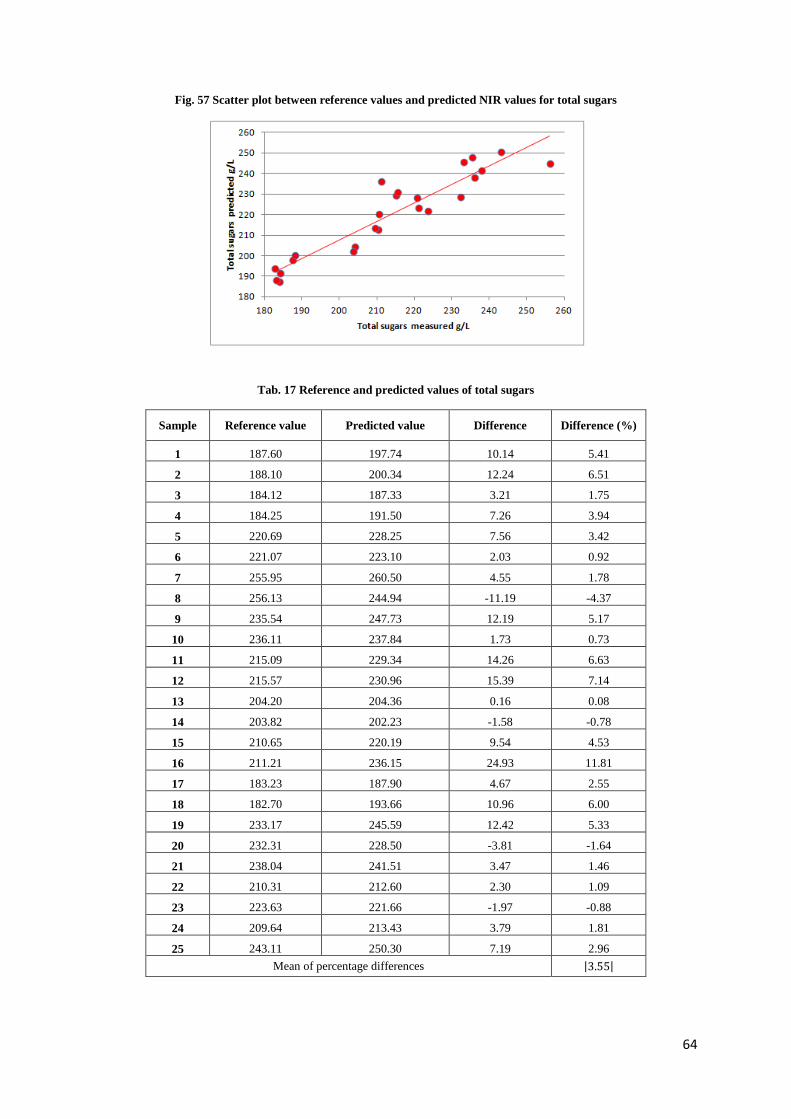
64

Fig. 57 Scatter plot between reference values and predicted NIR values for total sugars

Tab. 17 Reference and predicted values of total sugars


1 187.60 197.74 10.14 5.41

2 188.10 200.34 12.24 6.51

3 184.12 187.33 3.21 1.75

4 184.25 191.50 7.26 3.94

5 220.69 228.25 7.56 3.42

6 221.07 223.10 2.03 0.92

7 255.95 260.50 4.55 1.78

8 256.13 244.94 -11.19 -4.37

9 235.54 247.73 12.19 5.17

10 236.11 237.84 1.73 0.73

11 215.09 229.34 14.26 6.63

12 215.57 230.96 15.39 7.14

13 204.20 204.36 0.16 0.08

14 203.82 202.23 -1.58 -0.78

15 210.65 220.19 9.54 4.53

16 211.21 236.15 24.93 11.81

17 183.23 187.90 4.67 2.55

18 182.70 193.66 10.96 6.00

19 233.17 245.59 12.42 5.33

20 232.31 228.50 -3.81 -1.64

21 238.04 241.51 3.47 1.46

22 210.31 212.60 2.30 1.09

23 223.63 221.66 -1.97 -0.88

24 209.64 213.43 3.79 1.81


65

Fig. 58 Scatter plot between reference values and predicted NIR values for glucose

Tab. 18 Reference and predicted values of glucose


1 94.69 97.43 2.74 2.89

2 94.09 98.72 4.63 4.92

3 93.99 92.15 -1.84 -1.95

4 93.97 95.52 1.55 1.65

5 107.57 110.78 3.21 2.98

6 103.88 108.53 4.65 4.48

7 122.49 127.08 4.59 3.75

8 121.90 118.60 -3.30 -2.71

9 112.66 121.94 9.28 8.24

10 115.23 117.16 1.93 1.68

11 106.45 112.86 6.41 6.02

12 106.52 113.76 7.24 6.80

13 96.28 101.43 5.15 5.35

14 99.69 100.86 1.17 1.17

15 103.25 108.36 5.11 4.95

16 104.49 115.10 10.61 10.15

17 92.38 95.95 3.57 3.86

18 93.08 98.06 4.98 5.35

19 113.51 119.01 5.50 4.85

20 117.63 112.88 -4.75 -4.04

21 118.85 119.44 0.59 0.49

22 104.45 104.82 0.38 0.36

23 110.68 110.10 -0.58 -0.52

24 102.97 105.75 2.79 2.71


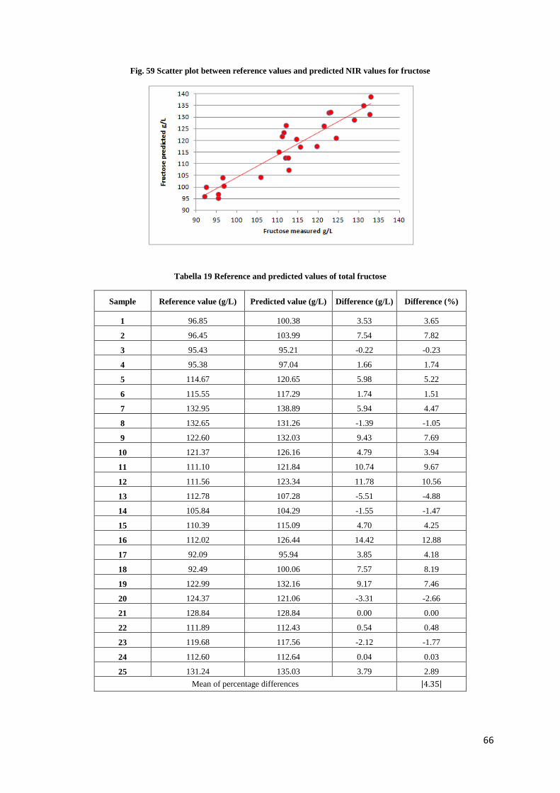
66

Fig. 59 Scatter plot between reference values and predicted NIR values for fructose

Tabella 19 Reference and predicted values of total fructose

Sample Reference value (g/L) Predicted value (g/L) Difference (g/L) Difference (%)

1 96.85 100.38 3.53 3.65

2 96.45 103.99 7.54 7.82

3 95.43 95.21 -0.22 -0.23

4 95.38 97.04 1.66 1.74

5 114.67 120.65 5.98 5.22

6 115.55 117.29 1.74 1.51

7 132.95 138.89 5.94 4.47

8 132.65 131.26 -1.39 -1.05

9 122.60 132.03 9.43 7.69

10 121.37 126.16 4.79 3.94

11 111.10 121.84 10.74 9.67

12 111.56 123.34 11.78 10.56

13 112.78 107.28 -5.51 -4.88

14 105.84 104.29 -1.55 -1.47

15 110.39 115.09 4.70 4.25

16 112.02 126.44 14.42 12.88

17 92.09 95.94 3.85 4.18

18 92.49 100.06 7.57 8.19

19 122.99 132.16 9.17 7.46

20 124.37 121.06 -3.31 -2.66

21 128.84 128.84 0.00 0.00

22 111.89 112.43 0.54 0.48

23 119.68 117.56 -2.12 -1.77

24 112.60 112.64 0.04 0.03


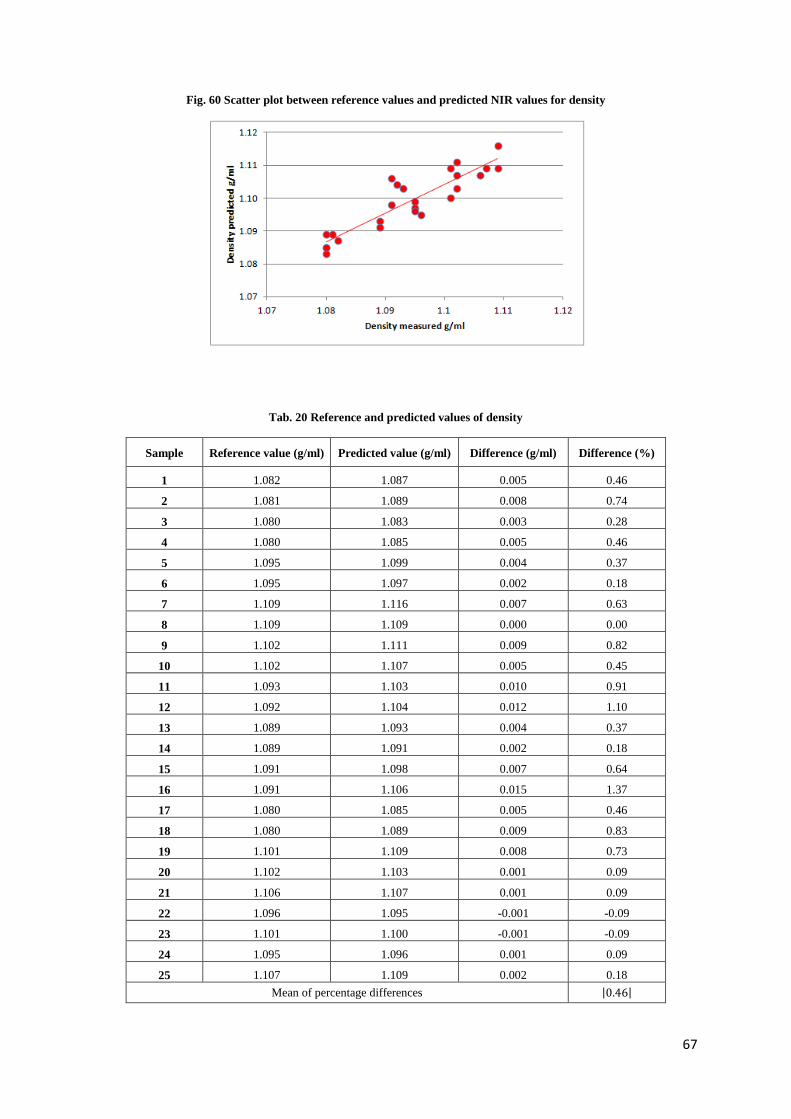
67

Fig. 60 Scatter plot between reference values and predicted NIR values for density

Tab. 20 Reference and predicted values of density

Sample Reference value (g/ml) Predicted value (g/ml) Difference (g/ml) Difference (%)

1 1.082 1.087 0.005 0.46

2 1.081 1.089 0.008 0.74

3 1.080 1.083 0.003 0.28

4 1.080 1.085 0.005 0.46

5 1.095 1.099 0.004 0.37

6 1.095 1.097 0.002 0.18

7 1.109 1.116 0.007 0.63

8 1.109 1.109 0.000 0.00

9 1.102 1.111 0.009 0.82

10 1.102 1.107 0.005 0.45

11 1.093 1.103 0.010 0.91

12 1.092 1.104 0.012 1.10

13 1.089 1.093 0.004 0.37

14 1.089 1.091 0.002 0.18

15 1.091 1.098 0.007 0.64

16 1.091 1.106 0.015 1.37

17 1.080 1.085 0.005 0.46

18 1.080 1.089 0.009 0.83

19 1.101 1.109 0.008 0.73

20 1.102 1.103 0.001 0.09

21 1.106 1.107 0.001 0.09

22 1.096 1.095 -0.001 -0.09

23 1.101 1.100 -0.001 -0.09

24 1.095 1.096 0.001 0.09


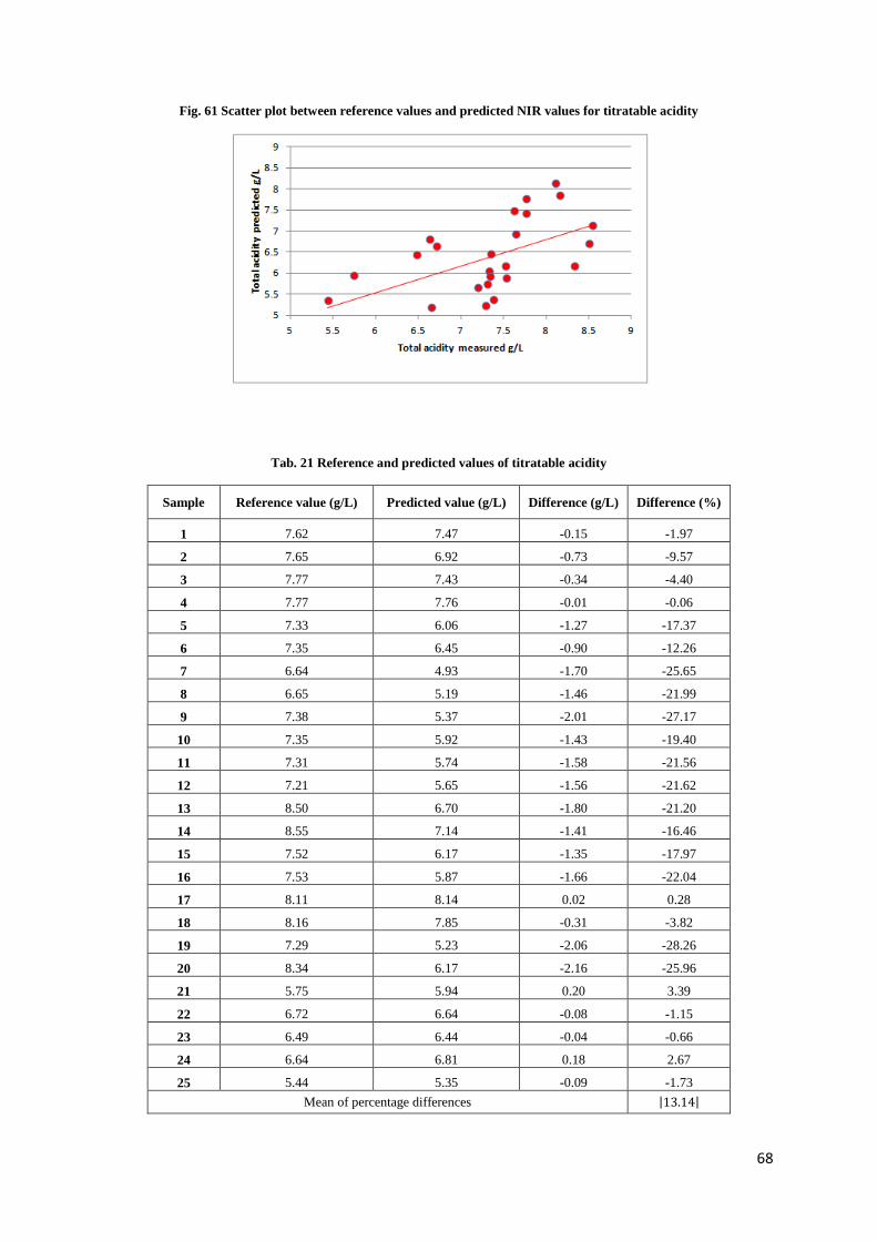
68

Fig. 61 Scatter plot between reference values and predicted NIR values for titratable acidity

Tab. 21 Reference and predicted values of titratable acidity


1 7.62 7.47 -0.15 -1.97

2 7.65 6.92 -0.73 -9.57

3 7.77 7.43 -0.34 -4.40

4 7.77 7.76 -0.01 -0.06

5 7.33 6.06 -1.27 -17.37

6 7.35 6.45 -0.90 -12.26

7 6.64 4.93 -1.70 -25.65

8 6.65 5.19 -1.46 -21.99

9 7.38 5.37 -2.01 -27.17

10 7.35 5.92 -1.43 -19.40

11 7.31 5.74 -1.58 -21.56

12 7.21 5.65 -1.56 -21.62

13 8.50 6.70 -1.80 -21.20

14 8.55 7.14 -1.41 -16.46

15 7.52 6.17 -1.35 -17.97

16 7.53 5.87 -1.66 -22.04

17 8.11 8.14 0.02 0.28

18 8.16 7.85 -0.31 -3.82

19 7.29 5.23 -2.06 -28.26

20 8.34 6.17 -2.16 -25.96

21 5.75 5.94 0.20 3.39

22 6.72 6.64 -0.08 -1.15

23 6.49 6.44 -0.04 -0.66

24 6.64 6.81 0.18 2.67

25 5.44 5.35 -0.09 -1.73 Mean of percentage differences |13.14|

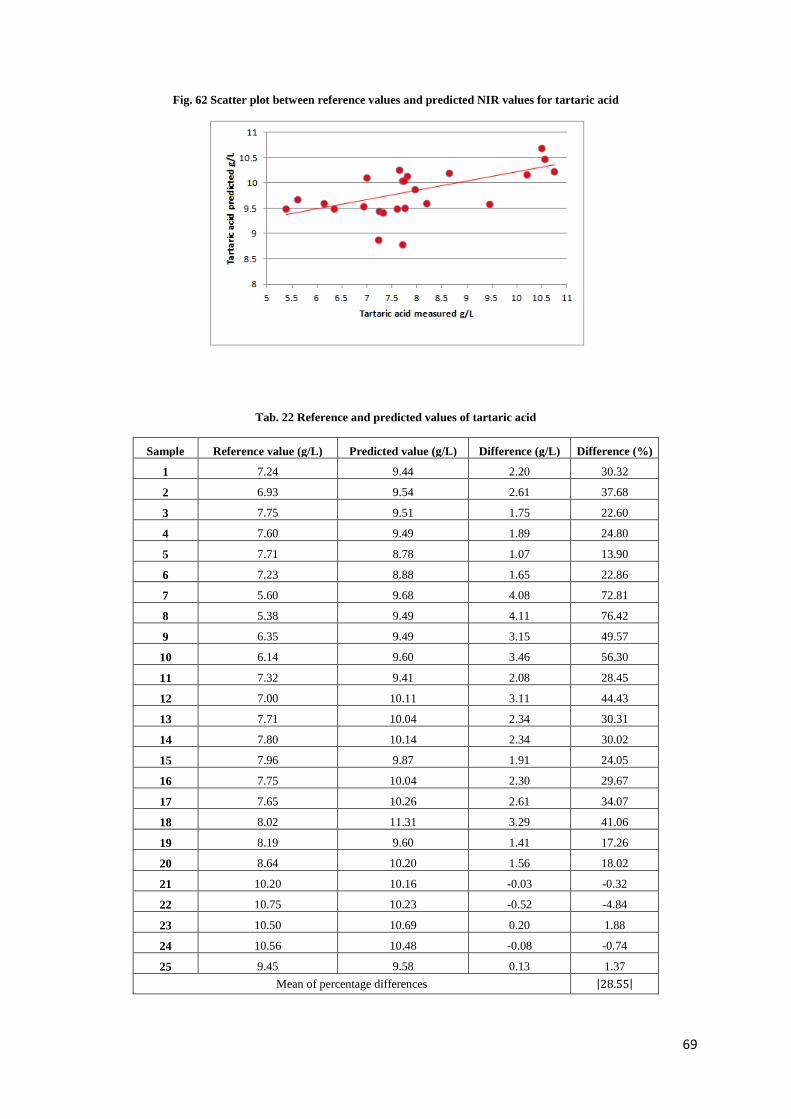
69

Fig. 62 Scatter plot between reference values and predicted NIR values for tartaric acid

Tab. 22 Reference and predicted values of tartaric acid


1 7.24 9.44 2.20 30.32

2 6.93 9.54 2.61 37.68

3 7.75 9.51 1.75 22.60

4 7.60 9.49 1.89 24.80

5 7.71 8.78 1.07 13.90

6 7.23 8.88 1.65 22.86

7 5.60 9.68 4.08 72.81

8 5.38 9.49 4.11 76.42

9 6.35 9.49 3.15 49.57

10 6.14 9.60 3.46 56.30

11 7.32 9.41 2.08 28.45

12 7.00 10.11 3.11 44.43

13 7.71 10.04 2.34 30.31

14 7.80 10.14 2.34 30.02

15 7.96 9.87 1.91 24.05

16 7.75 10.04 2.30 29.67

17 7.65 10.26 2.61 34.07

18 8.02 11.31 3.29 41.06

19 8.19 9.60 1.41 17.26

20 8.64 10.20 1.56 18.02

21 10.20 10.16 -0.03 -0.32

22 10.75 10.23 -0.52 -4.84

23 10.50 10.69 0.20 1.88

24 10.56 10.48 -0.08 -0.74


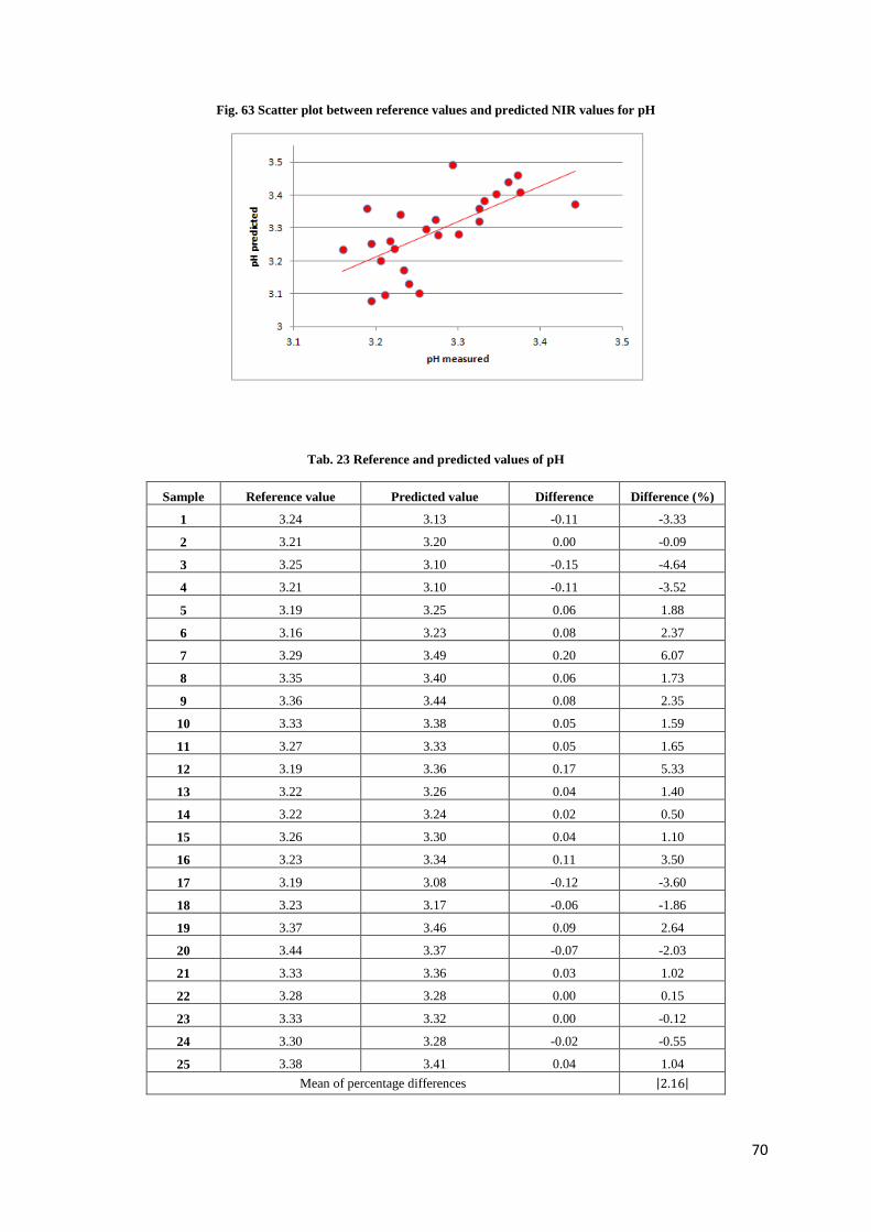
70

Fig. 63 Scatter plot between reference values and predicted NIR values for pH

Tab. 23 Reference and predicted values of pH


1 3.24 3.13 -0.11 -3.33

2 3.21 3.20 0.00 -0.09

3 3.25 3.10 -0.15 -4.64

4 3.21 3.10 -0.11 -3.52

5 3.19 3.25 0.06 1.88

6 3.16 3.23 0.08 2.37

7 3.29 3.49 0.20 6.07

8 3.35 3.40 0.06 1.73

9 3.36 3.44 0.08 2.35

10 3.33 3.38 0.05 1.59

11 3.27 3.33 0.05 1.65

12 3.19 3.36 0.17 5.33

13 3.22 3.26 0.04 1.40

14 3.22 3.24 0.02 0.50

15 3.26 3.30 0.04 1.10

16 3.23 3.34 0.11 3.50

17 3.19 3.08 -0.12 -3.60

18 3.23 3.17 -0.06 -1.86

19 3.37 3.46 0.09 2.64

20 3.44 3.37 -0.07 -2.03

21 3.33 3.36 0.03 1.02

22 3.28 3.28 0.00 0.15

23 3.33 3.32 0.00 -0.12

24 3.30 3.28 -0.02 -0.55


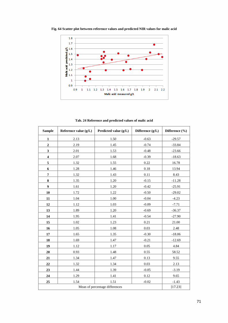
71

Fig. 64 Scatter plot between reference values and predicted NIR values for malic acid

Tab. 24 Reference and predicted values of malic acid


1 2.13 1.50 -0.63 -29.57

2 2.19 1.45 -0.74 -33.84

3 2.01 1.53 -0.48 -23.66

4 2.07 1.68 -0.39 -18.63

5 1.32 1.55 0.22 16.78

6 1.28 1.46 0.18 13.94

7 1.32 1.43 0.11 8.43

8 1.35 1.20 -0.15 -11.28

9 1.61 1.20 -0.42 -25.91

10 1.72 1.22 -0.50 -29.02

11 1.04 1.00 -0.04 -4.23

12 1.12 1.03 -0.09 -7.71

13 1.89 1.20 -0.69 -36.37

14 1.95 1.41 -0.54 -27.90

15 1.02 1.23 0.21 21.00

16 1.05 1.08 0.03 2.48

17 1.65 1.35 -0.30 -18.06

18 1.69 1.47 -0.21 -12.69

19 1.12 1.17 0.05 4.84

20 0.93 1.48 0.55 58.52

21 1.34 1.47 0.13 9.55

22 1.32 1.34 0.03 2.13

23 1.44 1.39 -0.05 -3.19

24 1.29 1.41 0.12 9.65


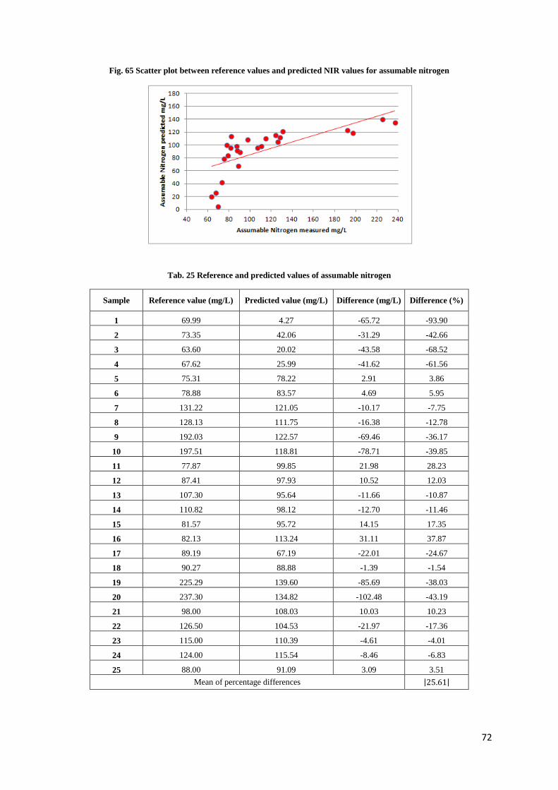
72

Fig. 65 Scatter plot between reference values and predicted NIR values for assumable nitrogen

Tab. 25 Reference and predicted values of assumable nitrogen

Sample Reference value (mg/L) Predicted value (mg/L) Difference (mg/L) Difference (%)

1 69.99 4.27 -65.72 -93.90

2 73.35 42.06 -31.29 -42.66

3 63.60 20.02 -43.58 -68.52

4 67.62 25.99 -41.62 -61.56

5 75.31 78.22 2.91 3.86

6 78.88 83.57 4.69 5.95

7 131.22 121.05 -10.17 -7.75

8 128.13 111.75 -16.38 -12.78

9 192.03 122.57 -69.46 -36.17

10 197.51 118.81 -78.71 -39.85

11 77.87 99.85 21.98 28.23

12 87.41 97.93 10.52 12.03

13 107.30 95.64 -11.66 -10.87

14 110.82 98.12 -12.70 -11.46

15 81.57 95.72 14.15 17.35

16 82.13 113.24 31.11 37.87

17 89.19 67.19 -22.01 -24.67

18 90.27 88.88 -1.39 -1.54

19 225.29 139.60 -85.69 -38.03

20 237.30 134.82 -102.48 -43.19

21 98.00 108.03 10.03 10.23

22 126.50 104.53 -21.97 -17.36

23 115.00 110.39 -4.61 -4.01

24 124.00 115.54 -8.46 -6.83


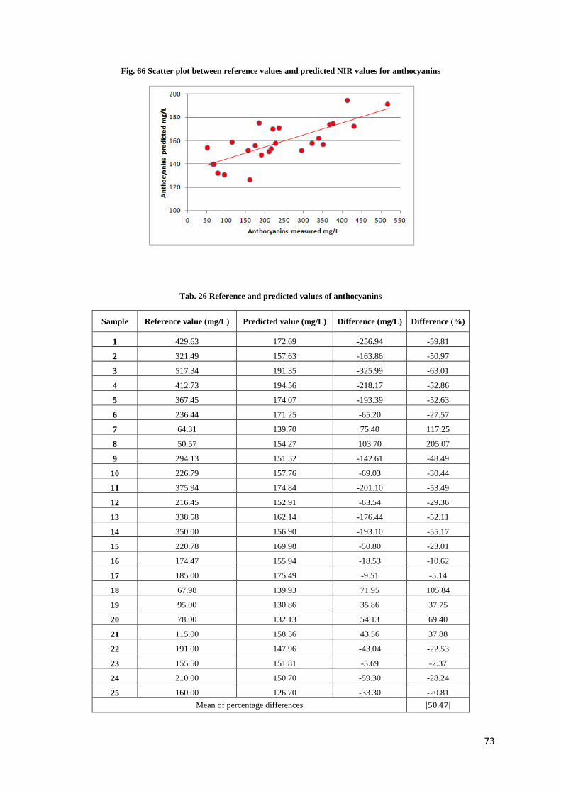
73

Fig. 66 Scatter plot between reference values and predicted NIR values for anthocyanins

Tab. 26 Reference and predicted values of anthocyanins


1 429.63 172.69 -256.94 -59.81

2 321.49 157.63 -163.86 -50.97

3 517.34 191.35 -325.99 -63.01

4 412.73 194.56 -218.17 -52.86

5 367.45 174.07 -193.39 -52.63

6 236.44 171.25 -65.20 -27.57

7 64.31 139.70 75.40 117.25

8 50.57 154.27 103.70 205.07

9 294.13 151.52 -142.61 -48.49

10 226.79 157.76 -69.03 -30.44

11 375.94 174.84 -201.10 -53.49

12 216.45 152.91 -63.54 -29.36

13 338.58 162.14 -176.44 -52.11

14 350.00 156.90 -193.10 -55.17

15 220.78 169.98 -50.80 -23.01

16 174.47 155.94 -18.53 -10.62

17 185.00 175.49 -9.51 -5.14

18 67.98 139.93 71.95 105.84

19 95.00 130.86 35.86 37.75

20 78.00 132.13 54.13 69.40

21 115.00 158.56 43.56 37.88

22 191.00 147.96 -43.04 -22.53

23 155.50 151.81 -3.69 -2.37

24 210.00 150.70 -59.30 -28.24


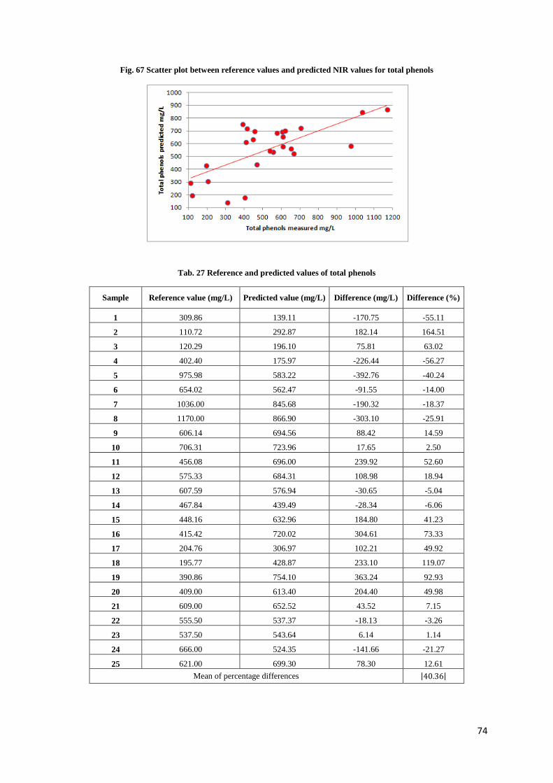
74

Fig. 67 Scatter plot between reference values and predicted NIR values for total phenols

Tab. 27 Reference and predicted values of total phenols


1 309.86 139.11 -170.75 -55.11

2 110.72 292.87 182.14 164.51

3 120.29 196.10 75.81 63.02

4 402.40 175.97 -226.44 -56.27

5 975.98 583.22 -392.76 -40.24

6 654.02 562.47 -91.55 -14.00

7 1036.00 845.68 -190.32 -18.37

8 1170.00 866.90 -303.10 -25.91

9 606.14 694.56 88.42 14.59

10 706.31 723.96 17.65 2.50

11 456.08 696.00 239.92 52.60

12 575.33 684.31 108.98 18.94

13 607.59 576.94 -30.65 -5.04

14 467.84 439.49 -28.34 -6.06

15 448.16 632.96 184.80 41.23

16 415.42 720.02 304.61 73.33

17 204.76 306.97 102.21 49.92

18 195.77 428.87 233.10 119.07

19 390.86 754.10 363.24 92.93

20 409.00 613.40 204.40 49.98

21 609.00 652.52 43.52 7.15

22 555.50 537.37 -18.13 -3.26

23 537.50 543.64 6.14 1.14

24 666.00 524.35 -141.66 -21.27


75

6. CONCLUSION AND FUTURE PERSPECTIVES

The present work shows how the NIR AOTF spectroscopy can be used in viticulture to

investigate simultaneously several markers of ripening and in particular on Sangiovese grape

variety. The building of PLS regression models was based on the knowledge that a good

calibration models to be used in practice should be done on a large datasets, encompassing

different orchards, regions, soil types, climate conditions and seasons (Cozzolino et al., 2011;

Nicolaï et al., 2007). As consequence in this PhD thesis the models were developed on two

different seasons and with grapes origin from different vineyards, clones and rootstocks. The

use of an external validation sample set has been allow to have a first objective evaluation of

the robustness of the calibration models developed.

The results reported for sugars related parameters underlines the high ability of NIR AOTF to

investigate brix, babo, total sugars, glucose, fructose and density. The low SEP and Bias

values recorded suggest the practical application of the presented calibration models.

About acidity related parameters (pH, titratable acidity, tartaric acid, malic acid) promising

results were found in calibration step at least for tartaric acid, pH and titratable acidity. These

results stressed the potential predictive ability of NIR AOTF for these variables. A lower

correlation was found in the validation step, but the low SEP values recorded in the prediction

of pH and titratable acidity suggest that the calibration models obtained can be used for the

measure of these variables. The reasons of the difficulty encountered by NIR spectroscopy in

investigate acidity has been discussed in the previous chapter. Surely the non – linear

phenomena can affect the performance of the calibration models as suggest by Chauchard et

al., 2004.

The PLS model for the prediction of assumable nitrogen showed a discrete predictive ability

and an acceptable error standard of prediction.

The results reported for the total phenols and the anthocyanins showed moderately good

coefficient of determination for prediction but high SEP and high percentage deviations

between NIR and reference measures. In this case the ability of prediction could be affected

by the accuracy of the reference method which as stressed by Cozzolino et al., 2011 is an

important factor in influencing the final performance. The adoption of more accurate

analytical techniques, such as HPLC, could increase the predictive performance of the models

as reported by other authors (Ferrer - Gallego et al., 2011). In alternative could be useful a

homogenization of grapes before the analysis with Wine Scan FT 120 to extract from the

grape skin a major quantity of phenols and anthocyanins. Also in this case regression

76

techniques to overcome the non linearity phenomena are suggested for improving the

performance in prediction (Janik et al., 2007). In any case considering the note difficulty in

determination of the phenols and anthocyanins in wine grape with others methods in terms of

time required, repeatability and reliability, the results presented here can be considered

promising and certainly improving.

The present work shows yet as the use of a fast and multiparametric instrument as Wine Scan

FT 120 can find a valid use for a fast calibration of NIR spectrometer with high reliability at

least for reducing and refractometric sugars, density, pH, titratable acidity, malic acid, tartaric

acid and assumable nitrogen. This aspect is very important considering the time required by

the analytical analysis for each parameter considered.

In conclusion the present NIR AOTF application on wine grapes, during ripening,

demonstrates the feasibility of this technology in monitoring many relevant parameters to

choose the optimal harvest date. The PLS models obtained here are surely improvable with

the addition of new grape samples of Sangiovese to increase the variability of the parameters

investigated and consequently the robustness and the accuracy of the prediction. The Luminar

5030 Miniature Hand-held NIR Analyzer spectrophotometer is therefore a valid instrument

for in field quality grape control. The advantage to gave multiparametric measures in few

second allows easily to have a full description of the ripening in the different parts of vineyard

without loss of grape. This fact makes the instrument particularly attractive for the

viticulturist considering the long time required by the sampling operations, not always

representative the whole vineyard, and by the subsequent analysis. As reported by Cozzolino

et al., 2006 the employ of NIR models can reduce by 80% the time spent for the analytical

procedure in grapes. In front of this big advantage a relatively lower accuracy of method for

any parameters can be tolerate.

By the previous considerations the Luminar 5030 Miniature Hand-held NIR Analyzer

spectrophotometer can be properly employed in vineyard in order to make quality maps for

the management of agronomic operations. Further the instrument could play an important part

in the precision farming. The European precision farmers tends to develop more sensorial

systems rather than remote systems in order to have a direct control of the quality with the

operative machine (Vieri et al., 2010). The application of NIR system on grapes harvest

machine would allow the quality mapping of harvest and to differentiate the product for the

different enological uses.

77

7. ACKNOWLEDGMENTS

I would like to thank Dr. Andrea Bellincontro for the advices and useful comments that he

given me during these three years of doctorate.

I would like to thank Marchesi dè Frescobaldi and Falesco wine companies for the valuable

assistance given to this work .

78

8. REFERENCES

Arana I, Jaren C, Arazuri SA (2005) Maturity, variety, and origin determination in white

grapes (Vitis vinifera L.) using near infrared reflectance technology. Journal Near Infrared

Spectroscopy 13 (6): 349–357.

Barbieri Gonzaga F, Pasquini C (2005) Near-Infrared emission spectrometry based on an

acousto-optical tunable filter. Anal. Chem., 77(4): 1046-1054.

Bauer R, Nieuwoudt H, Bauer FF, Kossmann J, Esbensen KH (2008) FT IR spectroscopy for

grape and wine analysis. Anal. Chem., 80 (5): 1371-1379.

Bellincontro A, Nicoletti I, Valentini M, Tomas A, De Santis D, Mencarelli F (2009)

Integration of non destructive techniques with destructive analyses to study postharvest water

stress of wine grapes. Am. J. Enol. Vitic. 60 (1): 57-65.

Bellincontro A, Cozzolino D, Mencarelli F (2011) Application of NIR-AOTF spectroscopy to

monitor aleatico grape dehydration for passito wine production. Am. J. Enol. Vitic. 62 (2):

256-260.

Blanco M, Villarroya I (2002) NIR spectroscopy: a rapid – response analytical tool. Trends in

analytical chemistry 21 (4): 240 – 250.

Boselli M (2000) Il “Sangiovese”: importanza e diffusione Atti del Simposio Internazionale Il

Sangiovese. Firenze , Palazzo Congressi, 15 – 17 febbraio 2000: pp. 25 – 29.

Buccelli P (2000) Composti fenolici in cloni di Sangiovese su portainnesti diversi. In Atti del

Simposio Internazionale Il Sangiovese. Firenze, Palazzo dei congressi, 15-17 febbraio 2000:

pp. 413-418.

Calò A, Costacurta A, Paludetti G, Crespan M, Giusi M, Egger E, Grasselli A, Storchi P,

Borsa D, Di Stefano R (1995) Characterization of biotypes of Sangiovese as basis for clonal

selection. International Symposium of Clonal Selection, ASEV, Portland, pp. 99 – 104.

Calò A, Costacurta A, Egger E, Storchi P, Crespan M, Milani N, Sensi E, Carraro R (2000)

Caratterizzazione molecolare, ampelografica e ampelometrica di 30 accessioni di Vitis

vinifera L. riferibili al Sangiovese. Atti del Simposio Internazionale Il Sangiovese. Firenze,

Palazzo Congressi, 15 – 17 febbraio 2000: pp. 113-120.

Calò A, Scienza A, Costacurta A (2001) Vitigni d’Italia. Edagricole – Edizione agricole della

Calderini, Bologna, Italy.

79

Cayuela JA, Weiland C (2010) Intact orange quality prediction with two portable NIR

spectrometers. Postharvest Biology and. Technology, 58: 113 - 120.

Cen H, He Y (2007) Theory and application of near infrared reflectance spectroscopy in

determination of food quality. Trends Food Sci. Technol. 18: 72 - 83.

Chauchard F, Cogdill R, Roussel S, Roger J M, Bellon – Maurel V (2004) Application of LS-

SVM to non – linear phenomena in NIR spectroscopy: development of a robust and portable

sensor for acidity prediction in grapes. Chemometrics and Intelligent Laboratory systems 71:

141-150.

Christy AA, Kvalheim OM (2007) Latent variable analysis of multivariate data in infrared

spectrometry. In Near – Infrared spectroscopy in food and science technology, Ozaki Y,

McClure W F, Christy A. A. eds, Wiley J. & Sons, Inc., Hoboken, pp. 145 - 161.

Cozzolino D, Esler MB, Dambergs RG, Cynkar WU, Boehm DR, Francis IL (2004a)

Prediction of colour and pH in grapes using a diode array spectrophotometer (400 - 1110 nm).

J. Near Infrared Spectroscopy 12: 105-111.

Cozzolino D, Kwiatkowski MJ, Parker M, Cynkar WU, Dambergs RG, Gishen M, Herderich

MJ (2004b). Prediction of phenolic compounds in red wine fermentations by visible and near

infrared spectroscopy. Analytica Chimica Acta 513: 73-80.

Cozzolino D, Dambergs RG, Janik L, Cynkar WU, Gishen M (2006) Analysis of grapes and

wine by near infrared spectroscopy. J. Near Infrared Spectroscopy 14: 279-289.

Cozzolino D, Cynkar WU, Dambergs RG, Mercurio MD, Smith PA (2008) Measurement of

condensed tannins and dry matter in red grape homogenates using near infrared spectroscopy

and partial least square. J. Agric. Food Chem. 56: 7631-7636.

Cozzolino D, Cynkar W. U, Shah N, Smith P (2011) Multivariate data analysis applied to

spectroscopy: potential application to juice and fruit quality. Food Research International, 44:

1888-1896.

Cynkar WU, Cozzolino D, Dambergs RG, Janik L, Gishen M (2004). The effects of

homogenisation method and freezing on the determination of quality parameters in red grape

berries of Vitis vinifera. Australian Journal of Grape and Wine Research 10: 236 – 242

Cynkar WU, Cozzolino D, Dambergs RG, Janik L, Gishen M (2007) Effect of variety,

vintage, and winery on the prediction by visible and near infrared spectroscopy of the

80

concentration of glycosylated compounds (G-G) in white grape juice. Australian Journal of

Grape and Wine Research 13: 101 – 105.

Dambergs RG, Cozzolino D, Cynkar MB, Esler MB, Janik LJ, Francis IL, Gishen M (2003)

In proceedings of 11th International NIR Conference. ED. by A.M.C. Davies and A. Garrido

Varo. NIR Publications, Chichester, UK, p.183.

Dambergs R.G., Kambouris B., Cynkar W.U., Janik L.J., Cozzolino D., Henschke P.A.,

Gishen M. (2005). A comparison of near infrared and mid infrared spectroscopy for the

analysis of yeast assimilable nitrogen in grape juice. In proceedings 12th Australian Wine

Industry Technical Conference, Melbourne, Australia (Australian Wine Technical Conference

Inc: Adelaide, SA) pp. 334-335

Dambergs RG, Cozzolino D, Cynkar WU, Gishen M (2006) The determination of red grape

quality parameters using the LOCAL algorithm. J. Near Infrared Spectrosc. 14: pp. 71 – 80.

Dardenne P (2010). Some considerations about NIR spectroscopy: closing speech at NIR-

2009. NIR News 21:12-14.

Darias-Martin J, Socas-Hernandez A, Diaz-Romero C, Diaz-Diaz E (2003) Comparative stuy

of methods for determination of titratable acidityin wine. Journal of Food Composition and

Analysis 16: 555-562.

De Bei R, Cozzolino D, Sullivan W, Cynkar W, Fuentes S, Dambergs R, Pech J, Tyerman S

(2011) Non-destructive measurement of grapevine water potential using near infrared

spectroscopy. Australian Journal of Grape and Wine Research 17: 62-71.

Di Stefano R, Borsa D, Bosso A, Garcia ME (2000). Significati e metodi di determinazione

dello stato di maturità dei polifenoli dell’uva . L’enologo 12: 73- 76.

Di Vecchi Staraz M, Brandinelli R, Boselli M, This P, Boursiquot JM, Laucou V, Lacombe T,

Varès D (2007) Genetic structuring and parentage analysis for evolutionary studies in

grapevine: kin group and origin of the cultivar Sangiovese revealed. J. Amer. Soc. Hort. Sci.,

132(4): 514-524.

Fearn T, Assessing calibrations: SEP, RPD, RER and R2. NIR News 13:12-14.

Fernández - Novales J, López MI, Sánchez MT, Morales J, González - Caballero V (2009)

Shortwave - near infrared spectroscopy for determination of reducing sugar content during

grape ripening, winemaking, and aging of white and red wines. Food Research International

42: 285-291.

81

Ferrer-Gallego R, Hernández – Hierro JM, Rivas – Gonzalo JC, Escribano – Bailón MT

(2011) Determination of phenolic compounds of grape skins during ripening by NIR

spectroscopy. Lwt – Food Science and Technology 44: 847-853.

Fragoso S, Aceña L, Guasch J, Busto O, Mestres M (2011) Application of FT – MIR

spectroscopy for fast control of red grape phenolic ripening. J. Agric. Food Chem., 59: 2175-

2183.

Fregoni M (1998) La vendemmia in Viticoltura di qualità, Ed. L’informatore agrario s.r.l.

Verona, pp. 637 – 687.

Gishen M, Dambergs RG, Cozzolino D (2005) Grape and wine analysis – enhancing the

power of spectroscopy with chemometrics. A review of some applications in the Australian

wine industry. Australian Journal of Grape and Wine Research II: 296-305.

Gonzáles – Caballero V, Sánchez MT, López MI, Pérez – Marín D (2010) First steps towards

the development of a non – destructive technique for the quality control of wine grapes during

on – vine ripening and on arrival at the winery. Journal of Food Engineering 101: 158-165.

Gonzáles – Caballero V, Pérez – Marín D, López MI, Sánchez MT (2011) Optimization of

NIR spectral data management for quality control of grape bunches during on – vine ripening.

Sensors 11: 6109-6124.

Guidetti R, Beghi R, Bodria L (2010) Evaluation of grape quality parametersby a simple Vis

/NIR system. American Society of Agricultural and Biological Engineers 53 (2): 477 – 484.

He Z, Lian W, Wu M, Chen Y, Tang L, Luo J (2006) Determination of tobacco constituents

whit acousto – optic tunable filter – near infrared spectroscopy. J. Near Infrared Spectrosc.

14: 45-50.

Istituto Nazionale di Statistica 2000. Quinto Censimento Nazionale dell’agricoltura. Istituto

Nazionale di Statistica, Roma.

Janik LJ, Cozzolino D, Dambergs R, Cynkar W, Gishen M (2007) The prediction of total

anthocyanin concentration in red grape homogenates using visible – near – infrared

spectroscopy and artificial neural networks. Analytica Chimica Acta 594: 107 – 118.

Jarén C, Ortuño JC, Arazuri JI, Salvadores MC (2001) Sugar determination in grapes using

nir technology. International Journal of Infrared and Millimeter Waves 22: 1521-1529.

82

Kaye O, Wample RL (2005) Using near infrared spectroscopy as an analytical tool in

vineyards and wineries. American Journal of Enology and Viticulture 56 (5): 296.

Kemps B, Leon LM, Best S, De Baerdemaeker J, De Ketelaere B (2010) Assessment of the

quality parameters in grapes using VIS / NIR spectroscopy. Biosystems Engineering 105:

507-513.

Larraín M, Guesalaga AR, Agosín E (2008) A multipurpose portable instrument for

determining ripeness in wine grapes using NIR spectroscopy. IEEE Transactions on

instrumentation and measurement 57(2): 294 - 302.

Le Moigne M, Maury C, Bertrand D, Jourjon F (2008) Sensory and instrumental

characterisation of Cabernet Franc grapes according to ripening stages and growing location.

Food Quality and Preference 19: 220-231.

Mainardi G (2000) Storia di un grande protagonista dell’enologia italiana: il “Sangiovese”.

Atti del Simposio Internazionale Il Sangiovese. Firenze, Palazzo Congressi, 15 – 17 febbraio

2000: pp. 17 – 23.

McClure (1994) Near-infrared spectroscopy: the giant is running strong. Analytical Chemistry

66 (1): 43-53.

Mc Clure WF, and Tsuchikawa S (2007) Instruments. In Near – Infrared spectroscopy in food

and science technology, Ozaki Y, McClure W F, Christy A. A. eds, Wiley J. & Sons, Inc.,

Hoboken, pp. 75 – 107.

Nelson – Kluk S, Manning J (2006) Sangiovese at FPS. FPS Grape Program Newsletter, november: 16 - 23.

Nicolaï B, Beullens K, Bobelyn E, Peirs A, Saeys W, Theron K I, Lammertyn J (2007) Non

destructive measurements of fruit and vegetable quality by means of NIR spectroscopy: A

review. Postharvest Biology and. Technology, 46: 99-118.

Osborne BG, Fearn T, Hindle PH (1993) Practical NIR spectroscopy with applications in

food and beverage analysis, Longman Scientific and Technical eds, Essex, England, UK: p.

227

Ozaki Y, Morita S, DU Y (2007) Spectral analysis. In Near – Infrared spectroscopy in food

and science technology, Ozaki Y, McClure W F, Christy A. A. eds, Wiley J. & Sons, Inc.,

Hoboken, pp. 47 – 72.

83

Pasquini C. (2003) Near infrared spectroscopy: fundamentals, practical aspects and analytical

applications. J. Braz. Chem. Soc. 14 (2): 198 – 219

Patz CC, David A, Thente H, Kurbel P, Dietrich H (1999) Wine analysis with FTIR

spectrometry. Vitis. Enol. Sci. 54: 80-87

Patz CC, Blieke A, Ristow R, Dietrich H (2004) Application of FT – MIR spectrometry in

wine analysis. Analytica Chimica Acta 513: 81-89.

Pillonel L, Dufour E, Schaller E, Bosset JO, De Baerdemaeker J, Karoui R (2007) Prediction

of colour of European Emmental cheeses by using near infrared spectroscopy: a feasibility

study. European Food Research and Technology 226: 63-69.

Ribéreau-Gayon P, Glories Y, Maujean A, Dubourdieu D (2004) I composti fenolici in

Trattato di Enologia Ed. Edagricole S.r.l. Bologna. Vol. 2: pp. 141-204.

Riva M, De Dionigi S, Sinelli N (2001) Introduzione alla spettroscopia FT-NIR. DISTAM

sezione Tecnologie Alimentari.

Sandorfy C, Buchet R, Lachenal G (2007) Principles of molecular vibrations for Near –

Infrared spectroscopy. In Near – Infrared spectroscopy in food and science technology, Ozaki

Y, McClure W F, Christy A A, eds, Wiley J. & Sons, Inc., Hoboken, pp. 11-41.

Santos AO, Kaye O (2009) Grapevine leaf water potential based upon near infrared

spectroscopy. Sci. Agric. 66 (3): 287-292.

Saranwong S, Sornsrivichai J, Kawano S (2001) Improvement of PLS calibration for Brix

value and dry matter of mango using information from MLR calibration. Journal of Near

Infrared Spectroscopy 9: 287 – 295.

Saranwong S, Kawano S 2007. Fruits and vegetables. In Near-infrared spectroscopy in food

science and technology, Ozaki Y, McClure WF,. Christy AA, eds, Wiley J. & Sons, Inc.,

Hoboken: pp. 219-245.

Shenk JS, Westerhaus MO (1996) Calibration the ISI way. In: Near infrared spectroscopy:

The future waves, A. M. C. Davies & P. C. Williams eds, NIR Publications (Chichester): pp.

198–202.

Smyth HE, Cozzolino D, Cynkar WU, Dambergs RG, Sefton M, Gishen M (2008) Near

infrared spectroscopy as a rapid tool to measure volatile aroma compounds in Riesling wine:

possibilities and limits. Anal. Bio anal. Chem., 390: 1911–1916.

84

Soderini G (1590). Coltivazione Toscana delle viti e d’alcuni alberi. Edizioni Giunti, Firenze,

Italy.

Soyer Y, Koca N, Karadeniz F (2003) Organic acid profile of Turkish white grapes and grape

juices. Journal of Food Composition and Analysis 16: 629 – 636.

Tamai G. (2009) Catalogo dei Cloni Varietà di uva da vino. Edizioni Edagricole, Bologna,

Italy.

Venturi A, Fontana M, Tocchetti G (2000) I cloni di “Sangiovese” del nucleo di

premoltiplicazione viticole “C. Naildi”. Atti del Simposio Internazionale Il Sangiovese.

Firenze, Palazzo Congressi, 15 – 17 febbraio 2000: pp. 295 - 298.

Versari A, Parpinello GP, Mattioli AU, Galassi S (2008) Determination of grape quality at

harvest using Fourier – Transform Mid – Infrared spectroscopy and multivariate analysis. Am.

J. Enol. Vitic., 59(3): 317-322.

Vieri M, Spezia G, Pagni PP (2010) Ingegneria delle produzioni viticole: stato dell’arte e

future applicazioni. Italus Hortus 17(1): 33-57.

Vouillamoz JF, Monaco A, Costantini L, Stefanini M, Scienza A, Grando MS (2007) The

parentage of “Sangiovese”: the most important italian wine grape. Vitis 46 (1): 19-22.

Wiliams PC, Norris K (1987) In: Near – Infrared technology in the agricultural and food

industries, Wiliams PC, Norris K eds, St Paul ACCC, pp. 143 – 167.

Williams PC, Sobering DC (1996) How do we do it: A brief summary of the methods we use

in developing near infrared calibrations. In Near infrared spectroscopy: The future waves, A.

M. C. Davies & P. Williams eds, NIR Publications (Chichester): 185–188.

Wiliams WF (2007) Grain and seeds. In Near – Infrared spectroscopy in food and science

technology, Ozaki Y, McClure W F, Christy A. A. eds, Wiley J. & Sons, Inc., Hoboken, pp.

165-217.

Wold S, Sjöström M, Eriksson L (2001) PLS – regression: a basic tool of chemometrics.

Chemometrics and Intellingent Laboratory Systems 58: 109 – 130.

WEBSITES CONSULTED

www.acovit.it

www.brimrose.com

http://www.acovit.it/

http://www.brimrose.com/

85

www.istat.it

http://www.istat.it/

86

APPENDIX

1) Federico E. Barnaba, Andrea Bellincontro, Fabio Mencarelli. (2012) Impiego in vigneto di

uno spettrofotometro NIR-AOTF per la determinazione della migliore epoca di raccolta. Atti

del III Convegno Nazionale di Viticoltura pubblicati sulla collana ACTA Italus Hortus n.3.

Abstract

A NIR (Near infrared) – AOTF (Acousto Optically Tunable Filter) spectrophotometer has

been tested to monitor the ripening evolution of winegrape variety Sangiovese. Predicting

models for the estimation of several enological parameters have been carried out by applying

PLS (partial least squares) chemometric approach. Spectral detections were obtained working

on whole grape berries as well as musts. NIR - AOTF was able to predict, with a high or

acceptable correlation versus the measured data, the following parameters: total soluble solids

(as °Brix or °Babo), total sugars, glucose, fructose, tartaric acid, titratable acidity, assumable

nitrogen and total phenols.

Keywords: NIR spectroscopy, Sangiovese wine grape, ripening, PLS, predicting models.

87

2) Massimo Muganu, Andrea Bellincontro, Federico E. Barnaba, Marco Paolocci, Cristina

Bignami, Gabriella Gambellini and Fabio Mencarelli. (2011). Influence of Bunch Position on

Berry Epicuticular Wax During Ripening and on Weight Loss in Dehydration Process. Am. J.

Enol. Vitic. 62 (1): 91-98 ISSN: 0002-9254

Abstract

Passito wine, made with dehydrated grapes, is widespread in Italy. The quality of the grapes

to be withered is strongly influenced by qualitative factors and the anatomy and morphology

of the berry, which in turn, are affected by vineyard management and microclimate. In

Trebbiano toscano and Rossetto vines grown in the Latium region, the epicuticular wax of

berries from bunches developed in intracanopy and extracanopy positions was analyzed from

pre - veraison to pre - harvest during the 2007 and 2008 growing seasons. At harvest, the

characteristics of cuticle and epidermis of each sample were examined using light and

electron microscopy. The berries were then dehydrated at 20°C to 45% moisture to evaluate

differences in water loss rate and the mechanical characteristics of the skin. The amount of

epicuticular wax decreased during berry development. SEM observations of the berry skin at

harvest showed differences in the structure of the epicuticular wax layers, with a wider berry

surface covered with plate-like wax in extracanopy berries. The number of cell layers and the

thickness of the berry skin were significantly different between cultivars and canopy

positions, but these factors did not affect cuticle thickness. Shaded berries of both varieties

dehydrated more slowly, particularly in vigorous Trebbiano toscano vines, in which

intracanopy berries reached 40% weight loss later than the extracanopy berries. During

dehydration, the berry skin color (hue angle) decreased and berries of both varieties increased

skin resistance to puncturing; this was not affected by the position of the berry in the canopy.

Key words: local grapevines, berry ripening, canopy, microclimate, passito wine

88

3) Federico E. Barnaba, Andrea Bellincontro, Fabio Mencarelli. Spettroscopia NIR-AOTF:

tecnica innovativa per determinare la sostanza secca e quindi l'epoca della raccolta dello

zucchino. Industrie Alimentari (IN PRESS).

Abstract

A NIR (Near - Infrared) – AOTF (Acousto Optically Tunable Filter) spectrophotometer has

been tested to analyze the main parameters that describe the quality of Cucurbita Pepo L.

fruit. Regression models were developed by means Partial Least Square (PLS) chemometric

approach to predict dry matter percentage, Hue angle and firmness. Significant values of

determination coefficient were obtained during calibration for all three parameters

investigated (R2 > 0.90). Predictive ability was good and was tested on a cross validation for

dry matter percentage predicting model with a determination coefficient and a standard error

respectively of 0.81 and 0.46%.

Key words: NIR spectroscopy, Cucurbita pepo L., PLS, dry matter, firmness, Hue angle.

89

4) Muganu M., Bellincontro A., Barnaba F.E., Paolocci M., Mencarelli F. Microclimate

Influence on the Morphology of Grape Berry at Maturity and on the Quality of the Berries

During the Postharvest Dehydration Process. Acta Hort. (IN PRESS)

Abstract

Light intensity and temperature, which distribution in the vineyard is influenced by the

characteristics of the canopy and vineyard architecture, strongly affect grape berry growth and

quality. During the years 2007 and 2008 sun-exposed and shaded bunches of the cultivars

Trebbiano toscano and Rossetto (Trebbiano giallo) grown in Latium region (Centre of Italy)

were selected after berry set with the aim to evaluate the influence of the bunch position in the

canopy on morphological characteristics of the grape berry at maturity and on the quality of

the berries during post harvest dehydration process. The environmental parameters in the

vineyard were detected and PAR (Photosynthetic Active Radiation) and temperature of the

berry skin were measured during ripening. The results showed differences on morphological

characteristics and on qualitative parameters of shaded and sun-exposed samples.

Keywords: Vitis vinifera, environment, canopy, local varieties, passito wine.

90

5) Barnaba Emanuele Federico, Bellincontro Andrea, Mencarelli Fabio (2012). Monitoring of

kiwifruit (Actinidia deliciousa) total soluble solids and dry matter content during field

ripening by means a NIR – AOTF spectrophotometer. (SUBMITTED to 7th International

Postharvest Symposium 2012)

Abstract

Total soluble solids and dry matter are two important commercial parameters to evaluate the

right harvest date for kiwifruit. Dry matter is formed for 75% by carbohydrate, it is sugar and

starch at harvest and it is mostly sugar at eating ripe. Non - destructive techniques are

required from kiwi fruit industry to choose the harvest data, to predict the fruit storability and

to screening for different sweetness classes. A NIR (Near infrared) – AOTF (Acousto

Optically Tunable Filter) spectrophotometer has been tested on kiwifruit (Actinidia deliciousa

cv. Hayward) to investigate total soluble solids and dry matter evolution during 4 different

sampling data until the harvest data. Kiwi fruit were collected from three different orchards

site in Latin (Lazio region, Italy). Detection was conducted in the 1100-2300 nm range, with 2

nm wavelength increments and 100 spectra per average, which represented a single

measurement. Four NIR spectra were acquired as diffuse reflectance for each kiwifruit from

the equatorial region and at the same time the fruits were processed for dry matter and total

soluble solids determination. Raw spectra were transformed in absorbance spectra (1/R) and

different statistical pre - treatments were carry out to reduce the baseline shift and the noise.

Partial least square (PLS) was built on the full spectrum (1100-2300 nm) and was applied an

internal full cross validation (leave one out). The best statistical pre – treatment was selected

for each variables. Determination coefficient for cross validation (R2cv) and the standard error

for cross validation (SECV) were respectively 0.86 and 1.45° for Brix and 0.70 and 0.90% for

dry matter. PLS regression models obtained can be applied on a wide range for measured

variables: between 5.9° and 16.7° for Brix and in the range 9.3 – 16.7% for dry matter

content.

91

6) Federico E. Barnaba, Andrea Bellincontro and Fabio Mencarelli. Portable NIR-AOTF

spectrophotometer: a useful tool for the quality grape control in vineyard (ACCEPTED I

International Workshop on Vineyard Mechanization and Grape and Wine Quality 2012)

Abstract

The monitoring of grape ripening is a decisive operation to determine the right quality in

vineyard and to choose the optimal harvest date for start winemaking process. The control of

grape quality is often done on small samples that are not representative of the whole vineyard.

In addition the conventional analytical methods for determining the quality are time

consuming and expensive. Modern viticulture needs of fast methods to establish directly in

situ the ripening evolution and to provide a qualitative characterization of the vineyard. A

Luminar 5030 Miniature Hand-held NIR Analyzer spectrophotometer based on AOTF

(acousto optically tunable filter) has been tested during 2009, 2010 and 2011 seasons on

different vineyards to monitor the ripening of Sangiovese wine grape variety. Detection was

conducted in the 1100 - 2300 nm range, with 2 nm wavelength increments and 100 spectra

per average, which represented a single measurement. Two different measurements were

performed on each berry, using the diffuse reflectance method of detection. Predicting models

for the estimation of several enological parameters as reducing sugar, titratable acidity, pH,

tartaric acid, malic acid, assumable nitrogen, total phenols and anthocyanins have been carried

out by applying PLS (partial least squares) chemometric approach. A validation procedure of

the models was performed in situ using independent sample sets. An high correlation between

NIR spectra and measured values was recorded for Brix, Babo and total sugars. The

coefficient of determination in prediction (R2) and the standard error of prediction (SEP) were

respectively 0.95 and 0.64° for Brix; 0.96 and 0.53° for Babo; 0.93 and 4 g/L for total sugar.

High value of the coefficient of determination in cross validation was obtained for the

prediction of glucose, fructose, tartaric acid and pH value.

92

7) Massimo Muganu, Federico E. Barnaba, Marco Paolocci, Andrea Bellincontro, Dario

Gnisci, Ionel Grosu and Fabio Mencarelli. Effect of different soil management practices on

grapevine growth and on berry quality assessed by NIR spectroscopy (ACCEPTED I

International Workshop on Vineyard Mechanization and Grape and Wine Quality 2012)

Abstract

Soil cultivation practices and climate significantly affect vine growth and grape

characteristics. Considering agronomical and seasonal variability viticulturist have clear need

for simple, rapid and cost-effective techniques to assess grape composition and harvesting

data. The experiments were carried out during 2010 and 2011 in a 6-year-old vineyard located

in Viterbo (Centre of Italy) (42°25′22″N; 12°04′40″E), with the aim to evaluate the influence

of soil management on vine growth and grape quality. Since vineyard establishment two

different soil cultivation practices were carried out in a randomized block design with three

replications each of five vines: complete soil tillage and permanent resident vegetation. The

grape varieties selected for the experiments were Canaiolo nero and Trebbiano giallo. Vines

were grafted on 420A, spur-pruned and spaced 3 m x 0.90 m, with a north-south orientation

of the rows. With the exception of soil management, all other cultivation practices were the

same in all treatments. Data on vine growth, fertility and phenology were collected during the

two growing seasons and a NIR (Near infrared) – AOTF (Acousto Optically Tunable Filter)

spectrophotometer was tested during ripening to monitor total soluble solids (TSS) (Brix), pH,

titratable acidity, anthocyanins and total phenols of Canaiolo n. and Trebbiano g. berries.

Partial least square (PLS) models were developed on the full spectrum (1100-2300 nm) and

an internal full cross validation (leave one out) was applied. Reference destructive analyses on

the same qualitative grape parameters of the berries were carried out at the same time and the

values were compared with NIR values. Differences referable to soil management were

detected on vine growth, budbreak time and on grape quality, particularly for TSS and

anthocyanins content. High correlation was found between NIR values and destructive

analysis values of titratable acidity and pH. PLS model for anthocyanins prediction in

Canaiolo n. samples has shown an excellent performance with a R2cv (coefficient of

determination for cross validation) of 0.90 and a SECV (standard error of cross validation) of

45.15 mg/Kg. The results show the influence of soil management practices on vine and grape

characteristics and the great potential of NIR spectroscopy as fast technique for grape quality

assessment.

93

Key words: Vitis vinifera, cover crops, ripening, grape quality, Latium region.

UNIVERSITÀ DEGLI STUDI DELLA TUSCIA DI VITERBO...

Documents

Transcript of UNIVERSITÀ DEGLI STUDI DELLA TUSCIA DI VITERBO...