Traffico veicolare e PM10 in area veneziana

dal dettaglio emissivo al contributo alla

concentrazione in atmosfera

S. Pillon1, F. Dalan1, F. Liguori1, and G. Maffeis2

1 ARPAV - Environmental Protection Agency of the Veneto Region, Via Lissa, 30171 Mestre (VE), Italy

fliguori(at)arpa.veneto.it

2 TerrAria s.r.l., Via Zarotto 6, 20124 Milano, Italy

g.maffeis(at)terraria.com

Expert Panel EMISSIONI DA TRASPORTO STRADALE Venezia, 16 Ottobre 2008

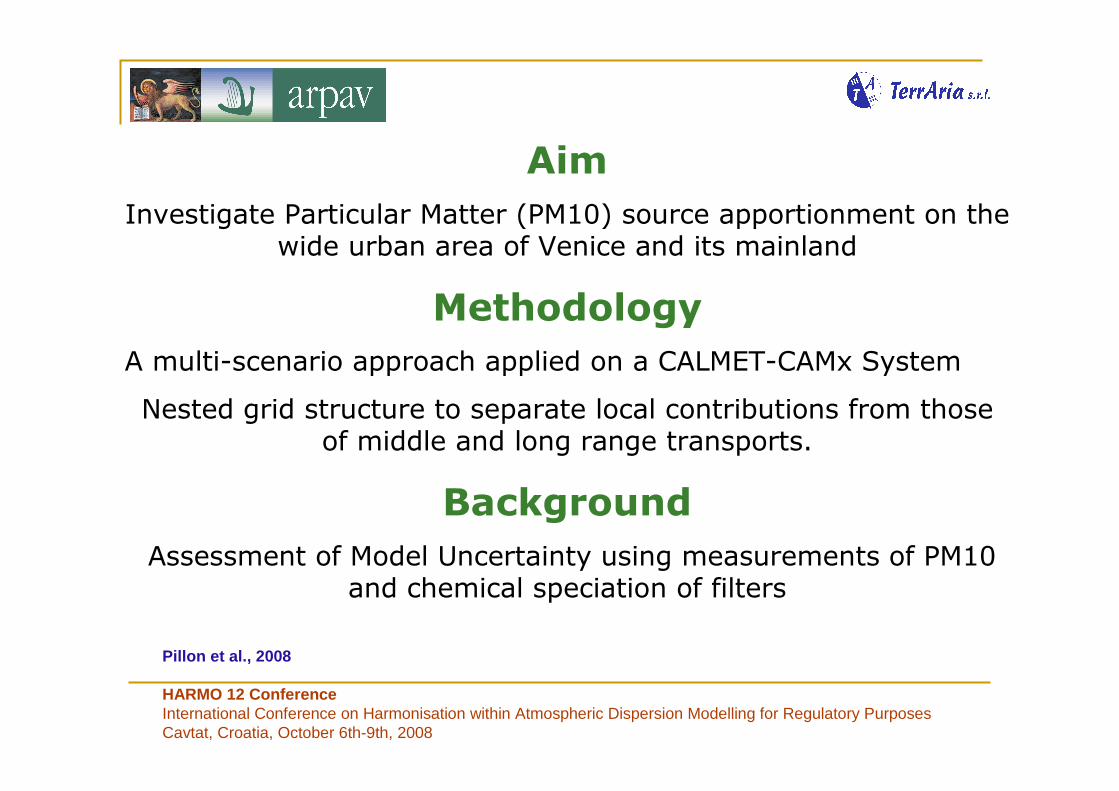
Aim

Investigate Particular Matter (PM10) source apportionment on thewide urban area of Venice and its mainland

Methodology

A multi-scenario approach applied on a CALMET-CAMx System

Nested grid structure to separate local contributions from thoseof middle and long range transports.

Background

Assessment of Model Uncertainty using measurements of PM10 and chemical speciation of filters

Pillon et al., 2008

HARMO 12 ConferenceInternational Conference on Harmonisation within Atmospheric Dispersion Modelling for Regulatory Purposes Cavtat, Croatia, October 6th-9th, 2008

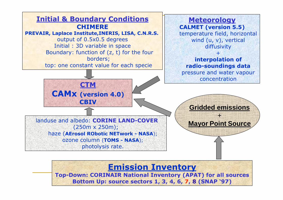
MeteorologyCALMET (version 5.5)temperature field, horizontal

wind (u, v), vertical diffusivity

+interpolation of

radio-soundings datapressure and water vapour

concentration

Emission InventoryTop-Down: CORINAIR National Inventory (APAT) for all sources

Bottom Up: source sectors 1, 3, 4, 6, 7, 8 (SNAP ‘97)

CTM

CAMx (version 4.0)

CBIVGridded emissions

+Mayor Point Source

Initial & Boundary ConditionsCHIMERE

PREVAIR, Laplace Institute,INERIS, LISA, C.N.R.S.

output of 0.5x0.5 degrees Initial : 3D variable in space

Boundary: function of (z, t) for the four borders;

top: one constant value for each specie

landuse and albedo: CORINE LAND-COVER(250m x 250m);

haze (AErosol RObotic NETwork - NASA);

ozone column (TOMS - NASA);

photolysis rate.

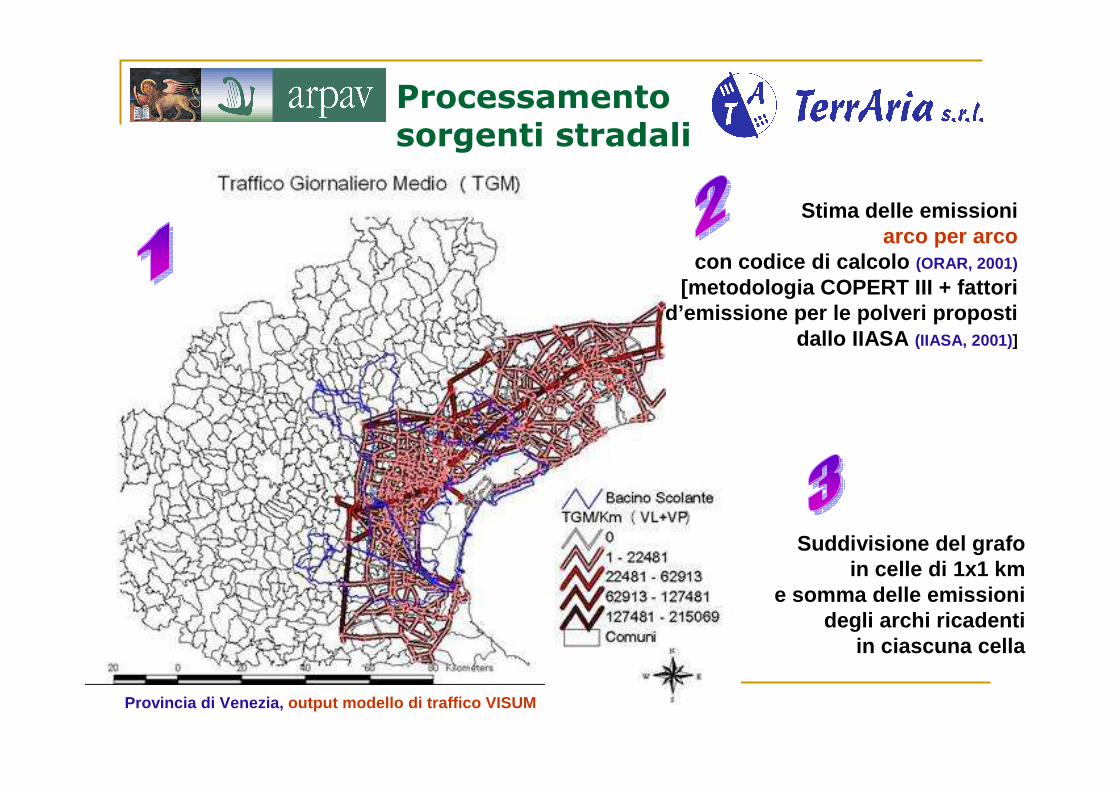
Stima delle emissioniarco per arco

con codice di calcolo (ORAR, 2001)

[metodologia COPERT III + fattori d’emissione per le polveri proposti

dallo IIASA (IIASA, 2001)]

Provincia di Venezia, output modello di traffico VISUM

Suddivisione del grafoin celle di 1x1 km

e somma delle emissionidegli archi ricadenti

in ciascuna cella

Processamentosorgenti stradali

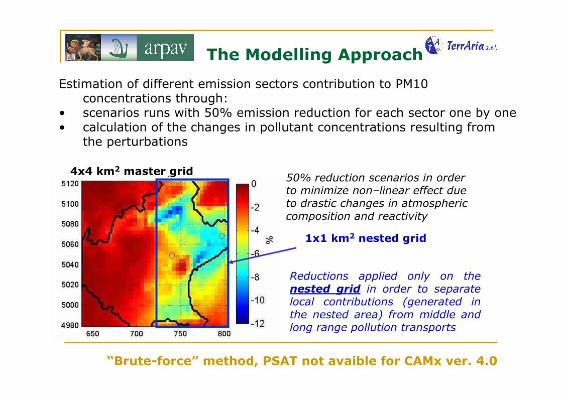
50% reduction scenarios in order to minimize non–linear effect due to drastic changes in atmospheric composition and reactivity

Reductions applied only on the nested grid in order to separate local contributions (generated in the nested area) from middle and long range pollution transports

The Modelling Approach

Estimation of different emission sectors contribution to PM10 concentrations through:

• scenarios runs with 50% emission reduction for each sector one by one • calculation of the changes in pollutant concentrations resulting from

the perturbations

“Brute-force” method, PSAT not avaible for CAMx ver. 4.0

4x4 km2 master grid

1x1 km2 nested grid

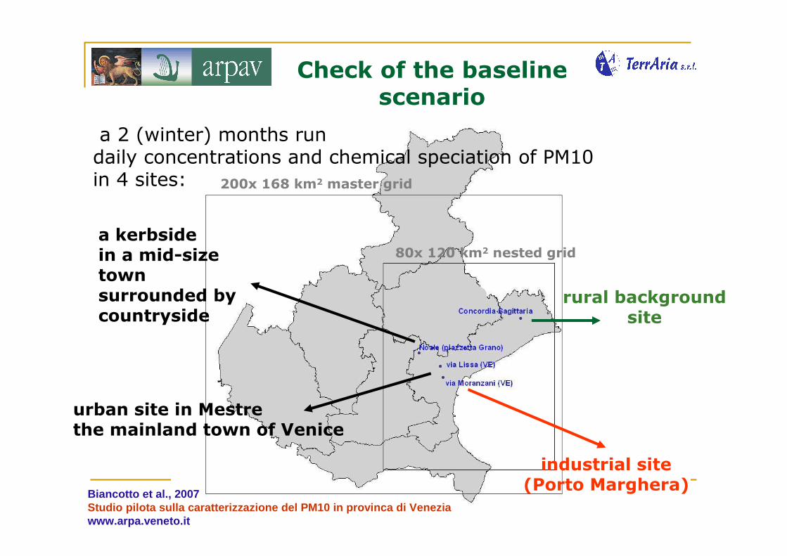
Check of the baselinescenario

a 2 (winter) months rundaily concentrations and chemical speciation of PM10in 4 sites:

rural backgroundsite

industrial site(Porto Marghera)

urban site in Mestrethe mainland town of Venice

a kerbsidein a mid-size town surrounded by countryside

200x 168 km2 master grid

80x 120 km2 nested grid

Biancotto et al., 2007Studio pilota sulla caratterizzazione del PM10 in prov inca di Veneziawww.arpa.veneto.it

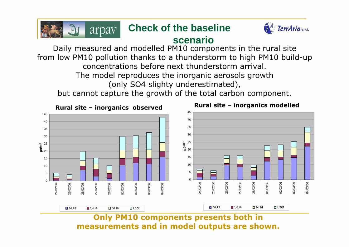
Check of the baselinescenario

Concordia Sagittaria - misure

0

5

10

15

20

25

30

35

40

45

24/0

2/06

25/0

2/06

26/0

2/06

27/0

2/06

28/0

2/06

01/0

3/06

02/0

3/06

03/0

3/06

04/0

3/06

µµ µµg/

m3

NO3 SO4 NH4 Ctot

Concordia Sagittaria - modello

0

5

10

15

20

25

30

35

40

45

24/0

2/06

25/0

2/06

26/0

2/06

27/0

2/06

28/0

2/06

01/0

3/06

02/0

3/06

03/0

3/06

04/0

3/06

µµ µµg/

m3

NO3 SO4 NH4 Ctot

Daily measured and modelled PM10 components in the rural site from low PM10 pollution thanks to a thunderstorm to high PM10 build-up

concentrations before next thunderstorm arrival.The model reproduces the inorganic aerosols growth

(only SO4 slighty underestimated),but cannot capture the growth of the total carbon component.

Only PM10 components presents both in measurements and in model outputs are shown.

Rural site – inorganics observed Rural site – inorganics modelled

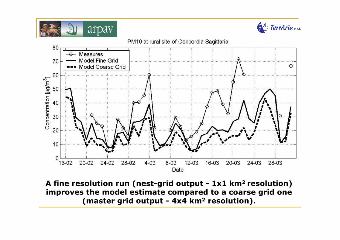
A fine resolution run (nest-grid output - 1x1 km2 resolution) improves the model estimate compared to a coarse grid one

(master grid output - 4x4 km2 resolution).

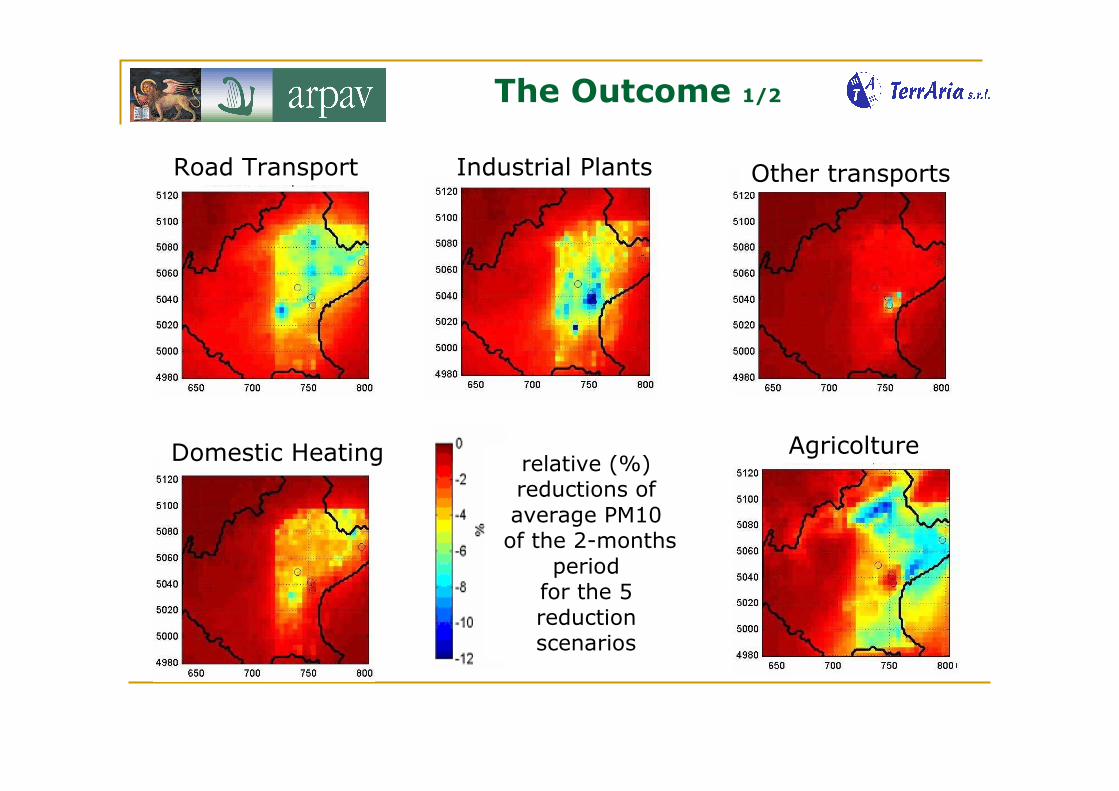
The Outcome 1/2

Industrial PlantsRoad Transport Other transports

Domestic Heating Agricolturerelative (%) reductions of average PM10of the 2-months

periodfor the 5 reduction scenarios

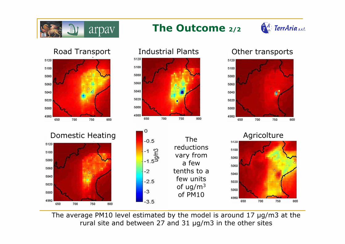
The Outcome 2/2

Industrial PlantsRoad Transport Other transports

Domestic Heating Agricolture

The average PM10 level estimated by the model is around 17 µg/m3 at the rural site and between 27 and 31 µg/m3 in the other sites

The reductions vary from a few

tenths to a few units of ug/m3

of PM10

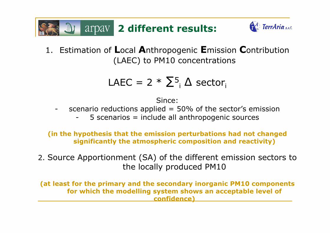
2 different results:

1. Estimation of Local Anthropogenic Emission Contribution (LAEC) to PM10 concentrations

LAEC = 2 * ∑5i ∆ sectori

Since:- scenario reductions applied = 50% of the sector’s emission

- 5 scenarios = include all anthropogenic sources

(in the hypothesis that the emission perturbations had not changed significantly the atmospheric composition and reactivity)

2. Source Apportionment (SA) of the different emission sectors to the locally produced PM10

(at least for the primary and the secondary inorganic PM10 components for which the modelling system shows an acceptable level of

confidence)

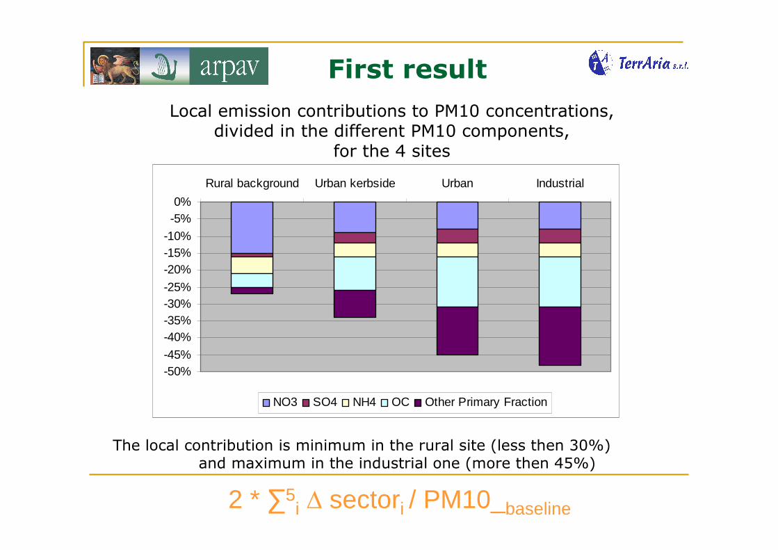
Local emission contributions to PM10 concentrations,divided in the different PM10 components,

for the 4 sites

First result

-50%-45%

-40%-35%-30%-25%

-20%-15%-10%

-5%0%

Rural background Urban kerbside Urban Industrial

NO3 SO4 NH4 OC Other Primary Fraction

The local contribution is minimum in the rural site (less then 30%)and maximum in the industrial one (more then 45%)

2 * ∑5i ∆ sectori / PM10_baseline

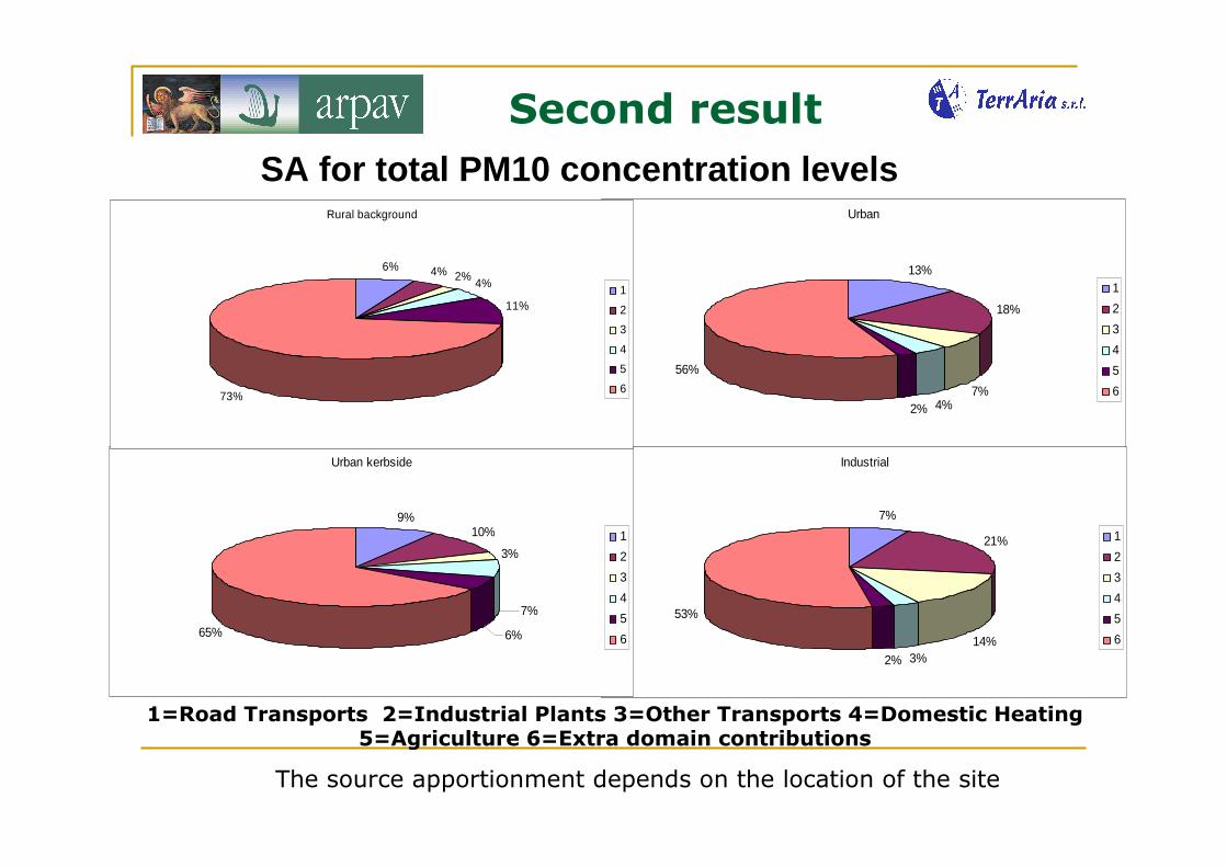
Second result

The source apportionment depends on the location of the site

Urban

13%

18%

7%4%2%

56%

1

2

3

4

5

6

Industrial

7%

21%

14%3%2%

53%

1

2

3

4

5

6

Urban kerbside

9%10%

3%

7%

6%65%

1

2

3

4

5

6

Rural background

6% 4% 2%4%

11%

73%

1

2

3

4

5

6

SA for total PM10 concentration levels

1=Road Transports 2=Industrial Plants 3=Other Transports 4=Domestic Heating5=Agriculture 6=Extra domain contributions

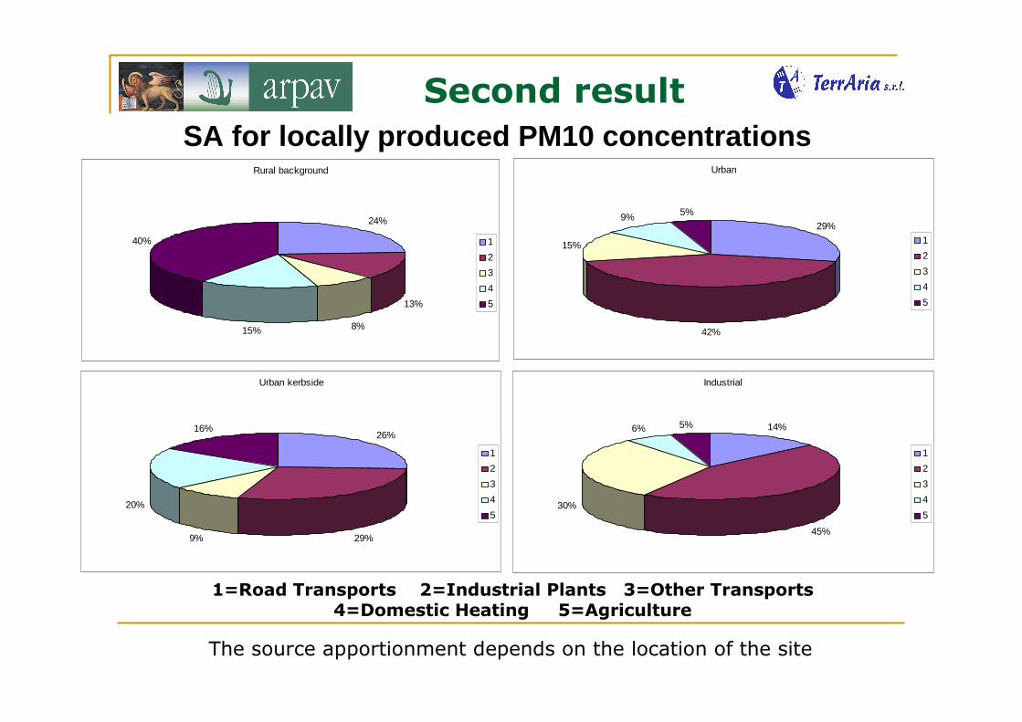
Second result

The source apportionment depends on the location of the site

Urban kerbside

26%

29%9%

20%

16%

1

2

3

4

5

Urban

29%

42%

15%

9% 5%

1

2

3

4

5

Industrial

14%

45%

30%

6% 5%

1

2

3

4

5

Rural background

24%

13%

8%15%

40% 1

2

3

4

5

SA for locally produced PM10 concentrations

1=Road Transports 2=Industrial Plants 3=Other Transports4=Domestic Heating 5=Agriculture

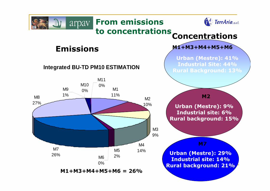
Integrated BU-TD PM10 ESTIMATION

M111%

M210%

M39%

M414%M7

26%

M827%

M52%M6

0%

M110%M10

0%M91%

Urban (Mestre): 29%Industrial site: 14%

Rural background: 21%

Urban (Mestre): 9%Industrial site: 6%

Rural background: 15%

Urban (Mestre): 41%Industrial Site: 44%

Rural Background: 13%

Emissions

Concentrations

From emissionsto concentrations

M1+M3+M4+M5+M6

M2

M7

M1+M3+M4+M5+M6 = 26%

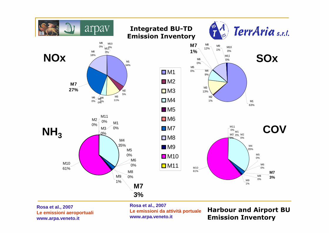
Harbour and Airport BU Emission Inventory

Rosa et al., 2007Le emissioni aeroportualiwww.arpa.veneto.it

Rosa et al., 2007Le emissioni da attività portualewww.arpa.veneto.it

M134%

M25%

M311%

M45%

M818%

M110%

M100%

M90%

M50%

M60%

M727%

M21%

M313%

M49%

M71%

M60%

M50%

M91%

M100%

M110%

M163%

M812%

M30%

M435%

M20%

M73%

M80%

M10%

M110%

M1061%

M91%

M50%

M60%

M30%

M435%

M20%

M73%M8

0%

M10%

M110%

M1061%

M91%

M50%

M60%

SOx

COV

M1

M2

M3

M4

M5

M6

M7

M8

M9

M10

M11

NOx

NH3

Integrated BU-TD Emission Inventory

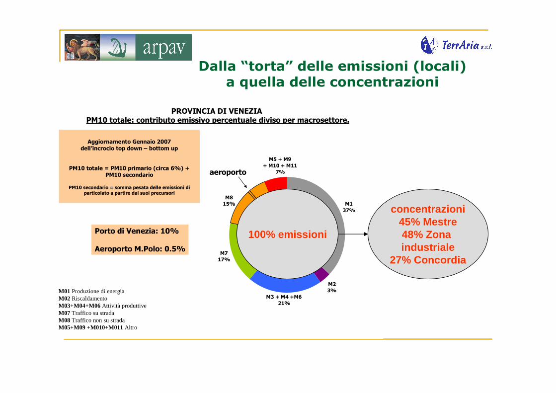
Dalla “torta” delle emissioni (locali)a quella delle concentrazioni

M7

17%

M2

3%

M1

37%

M3 + M4 +M6

21%

M5 + M9

+ M10 + M11

7%

M8

15%

PROVINCIA DI VENEZIAPM10 totale: contributo emissivo percentuale diviso per macrosettore.

Aggiornamento Gennaio 2007dell’incrocio top down – bottom up

PM10 totale = PM10 primario (circa 6%) + PM10 secondario

PM10 secondario = somma pesata delle emissioni diparticolato a partire dai suoi precursori

Porto di Venezia: 10%

Aeroporto M.Polo: 0.5%

porto

aeroporto

M01 Produzione di energiaM02 RiscaldamentoM03+M04+M06 Attività produttiveM07 Traffico su stradaM08 Traffico non su stradaM05+M09 +M010+M011 Altro

100% emissioni

concentrazioni45% Mestre48% Zona industriale

27% Concordia

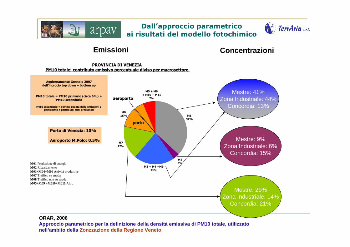
Dall’approccio parametricoai risultati del modello fotochimico

M7

17%

M2

3%

M1

37%

M3 + M4 +M6

21%

M5 + M9

+ M10 + M11

7%

M8

15%

PROVINCIA DI VENEZIAPM10 totale: contributo emissivo percentuale diviso per macrosettore.

Aggiornamento Gennaio 2007dell’incrocio top down – bottom up

PM10 totale = PM10 primario (circa 6%) + PM10 secondario

PM10 secondario = somma pesata delle emissioni diparticolato a partire dai suoi precursori

Porto di Venezia: 10%

Aeroporto M.Polo: 0.5%

porto

aeroporto

M01 Produzione di energiaM02 RiscaldamentoM03+M04+M06 Attività produttiveM07 Traffico su stradaM08 Traffico non su stradaM05+M09 +M010+M011 Altro

Mestre: 29%Zona Industriale: 14%

Concordia: 21%

Mestre: 9%Zona Industriale: 6%

Concordia: 15%

Mestre: 41%Zona Industriale: 44%

Concordia: 13%

Emissioni Concentrazioni

ORAR, 2006Approccio parametrico per la definizione della densità e missiva di PM10 totale, utilizzatonell’ambito della Zonzzazione della Regione Veneto

Conclusions (of general interest)

• daily mean measures of PM10 concentrations are well reproduced by the modelling system for clean days, but model underestimates PM10 levels in the days with stagnant air conditions and the underestimation becomes stronger as the stagnant conditions persist;

• secondary inorganic aerosol production proved to be well described by the model; organic aerosol is underestimated;

• the changes in PM10 concentrations resulting from the emission source perturbations are always less severe then the source perturbation itself. Inorganic secondary components of the aerosol are more resilient then primary ones; however the reduction of the local anthropogenic primary aerosol is not sufficient to turn down significantly PM10 concentration levels.

Conclusions(of local interest)

• the average PM10 level estimated by the model is around 17 µg/m3 at the rural site and between 27 and 31 µg/m3 in the other sites. The average scenarios impact vary between few tenths to few units of micrograms per cubic metre;

• the local emissions contribution to the PM10 varies between 30 and 50% (but the model captures only part of PM in the area under investigation, which, at worst, is about half of the measured value);

• a Source Apportionment analysis has been performed by calculating the differences in concentrations of each scenario and the base case. The traffic emission contributes roughly 26-29% of the locally produced PM10 at kerbside or in a rural background site. Agriculture emission contributes 40% in a rural site and Industrial emissions accounts for 44% of the local portion of PM10 in an industrial site. These estimates do not account for the PM10 concentrations coming from outside the wide Venice area.