
Talk Definitiva
30
The variational formulation Existence and uniqueness The discrete approximations An E -based mixed-FEM and BEM symmetric coupling for a time-dependent eddy current problem Ramiro Acevedo 1 , Salim Meddahi 2 1 Universidad del Cauca, Colombia 2 Universidad de Oviedo, Spain WONAPDE 2010 Universidad de Concepci´ on, January 11 - 15 Acevedo & Meddahi A mixed-FEM and BEM coupling for eddy current problem
-
Upload
ramiro-acevedo -
Category
Documents
-
view
225 -
download
0
Transcript of Talk Definitiva
8/3/2019 Talk Definitiva
http://slidepdf.com/reader/full/talk-definitiva 1/30
The variational formulationExistence and uniqueness
The discrete approximations
An E -based mixed-FEM and BEM symmetric
coupling for a time-dependent eddy current
problem
Ramiro Acevedo1, Salim Meddahi2
1Universidad del Cauca, Colombia2Universidad de Oviedo, Spain
WONAPDE 2010
Universidad de Concepcion, January 11 - 15
Acevedo & Meddahi A mixed-FEM and BEM coupling for eddy current problem
8/3/2019 Talk Definitiva
http://slidepdf.com/reader/full/talk-definitiva 2/30
The variational formulationExistence and uniqueness
The discrete approximations
Outline
1 The variational formulationThe model problemAn E -based formulationThe mixed-FEM and BEM symmetric coupling
2 Existence and uniquenessThe reduced problemA stable decomposition of the kernel of bWell-posedness
3 The discrete approximationsAnalysis of the semi-discrete schemeAnalysis of the fully-discrete scheme
Acevedo & Meddahi A mixed-FEM and BEM coupling for eddy current problem
8/3/2019 Talk Definitiva
http://slidepdf.com/reader/full/talk-definitiva 3/30
The variational formulationExistence and uniqueness
The discrete approximations
The model problemAn E-based formulationThe mixed-FEM and BEM symmetric coupling
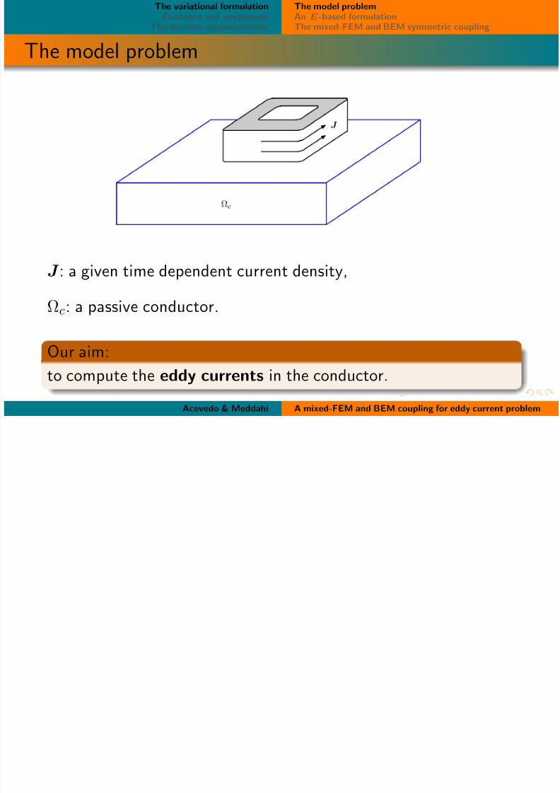
The model problem
J : a given time dependent current density,
Ωc: a passive conductor.
Our aim:
to compute the eddy currents in the conductor.
Acevedo & Meddahi A mixed-FEM and BEM coupling for eddy current problem
8/3/2019 Talk Definitiva
http://slidepdf.com/reader/full/talk-definitiva 4/30
The variational formulationExistence and uniqueness
The discrete approximations
The model problemAn E-based formulationThe mixed-FEM and BEM symmetric coupling
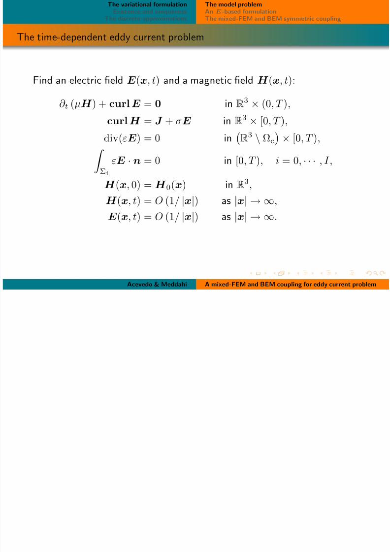
The time-dependent eddy current problem
Find an electric field E (x, t) and a magnetic field H (x, t):
∂ t (µH ) + curlE = 0 in R3 × (0, T ),
curlH = J + σE in R3 × [0, T ),
div(εE ) = 0 inR3 \ Ωc
× [0, T ),
Σi
εE · n = 0 in [0, T ), i = 0, · · · , I,
H (x, 0) = H 0(x) in R3,
H (x, t) = O (1/ |x|) as |x| → ∞,E (x, t) = O (1/ |x|) as |x| → ∞.
Acevedo & Meddahi A mixed-FEM and BEM coupling for eddy current problem
Th i i l f l i Th d l bl
8/3/2019 Talk Definitiva
http://slidepdf.com/reader/full/talk-definitiva 5/30
The variational formulationExistence and uniqueness
The discrete approximations
The model problemAn E-based formulationThe mixed-FEM and BEM symmetric coupling
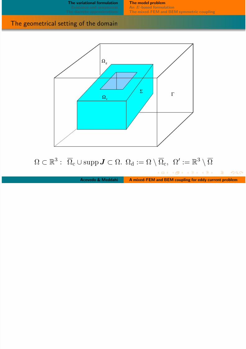
The geometrical setting of the domain
c
Γ Ω
Ω
Σ
d
Ω ⊂ R3 : Ωc ∪ suppJ ⊂ Ω. Ωd := Ω \ Ωc, Ω := R3 \ Ω
Acevedo & Meddahi A mixed-FEM and BEM coupling for eddy current problem
Th i ti l f l ti Th d l bl
8/3/2019 Talk Definitiva
http://slidepdf.com/reader/full/talk-definitiva 6/30
The variational formulationExistence and uniqueness
The discrete approximations
The model problemAn E-based formulationThe mixed-FEM and BEM symmetric coupling
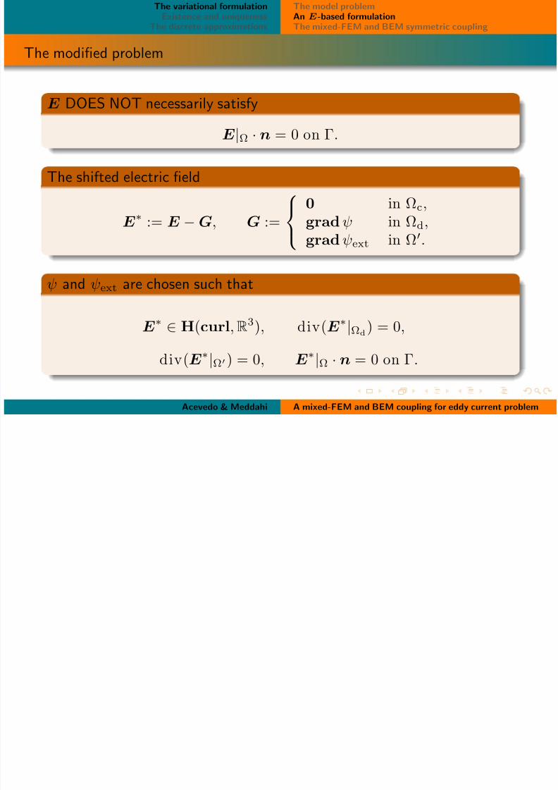
The modified problem
E DOES NOT necessarily satisfy
E |Ω · n = 0 on Γ.
The shifted electric field
E ∗ := E −G, G :=
0 in Ωc,gradψ in Ωd,gradψext in Ω.
ψ and ψext are chosen such that
E ∗ ∈ H(curl,R3), div(E ∗|Ωd) = 0,
div(E ∗|Ω) = 0, E ∗|Ω · n = 0 on Γ.
Acevedo & Meddahi A mixed-FEM and BEM coupling for eddy current problem
The variational formulation The model problem
8/3/2019 Talk Definitiva
http://slidepdf.com/reader/full/talk-definitiva 7/30
The variational formulationExistence and uniqueness
The discrete approximations
The model problemAn E-based formulationThe mixed-FEM and BEM symmetric coupling
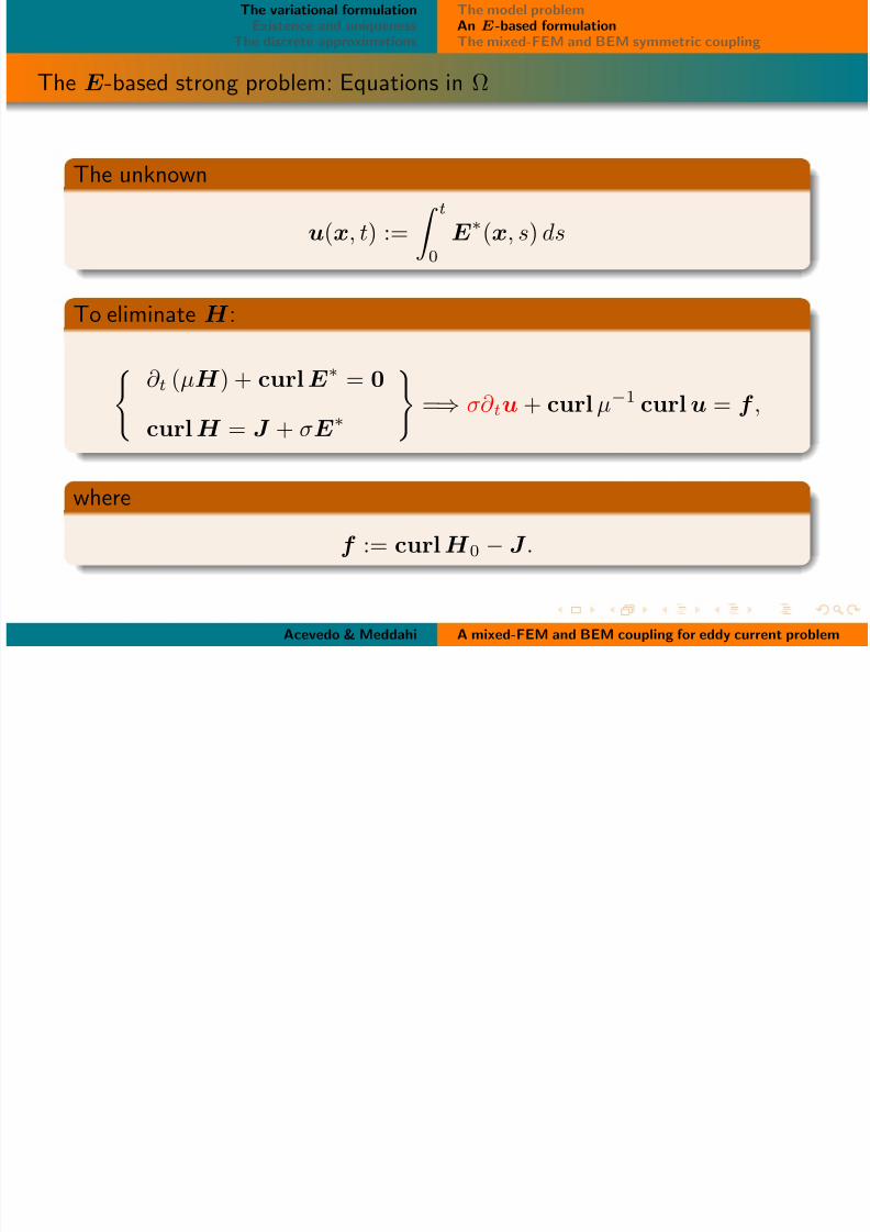
The E -based strong problem: Equations in Ω
The unknown
u(x, t) :=
t0
E ∗(x, s) ds
To eliminate H :
∂ t (µH ) + curlE ∗ = 0
curlH = J + σE ∗
=⇒ σ∂ tu + curlµ−1 curlu = f ,
where
f := curlH 0 − J .
Acevedo & Meddahi A mixed-FEM and BEM coupling for eddy current problem
The variational formulation The model problem
8/3/2019 Talk Definitiva
http://slidepdf.com/reader/full/talk-definitiva 8/30
The variational formulationExistence and uniqueness
The discrete approximations
The model problemAn E-based formulationThe mixed-FEM and BEM symmetric coupling
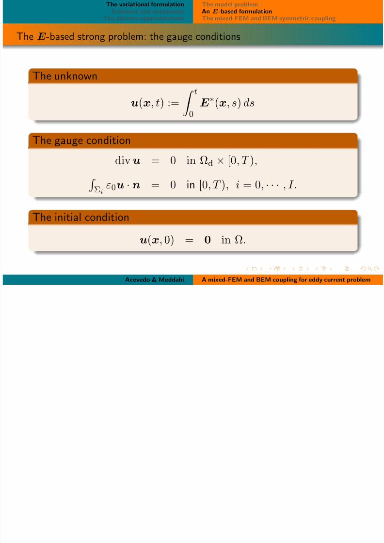
The E -based strong problem: the gauge conditions
The unknown
u(x, t) :=
t0E ∗(x, s) ds
The gauge condition
divu = 0 in Ωd × [0, T ),
Σiε0u · n = 0 in [0, T ), i = 0, · · · , I.
The initial condition
u(x, 0) = 0 in Ω.
Acevedo & Meddahi A mixed-FEM and BEM coupling for eddy current problem
The variational formulation The model problem

8/3/2019 Talk Definitiva
http://slidepdf.com/reader/full/talk-definitiva 9/30
The variational formulationExistence and uniqueness
The discrete approximations
The model problemAn E-based formulationThe mixed-FEM and BEM symmetric coupling
Transmission conditions: some kind of traces
The standard trace
γ : H1(Ω) → H1/2(Γ); γv := v|Γ
The normal trace
γ n : H(div; Ω) → H−1/2(Γ); γ nv := v · n
The tangential trace
γ τ
: H(curl; Ω) → H−1/2 (divΓ
; Γ ) ; γ τ v := v × n
The tangential component trace
πτ : H(curl; Ω) → H−1/2 (curlΓ; Γ ) ; πτ v := n× (v ×n)
Acevedo & Meddahi A mixed-FEM and BEM coupling for eddy current problem
The variational formulation The model problem
8/3/2019 Talk Definitiva
http://slidepdf.com/reader/full/talk-definitiva 10/30
The variational formulationExistence and uniqueness
The discrete approximations
The model problemAn E-based formulationThe mixed-FEM and BEM symmetric coupling
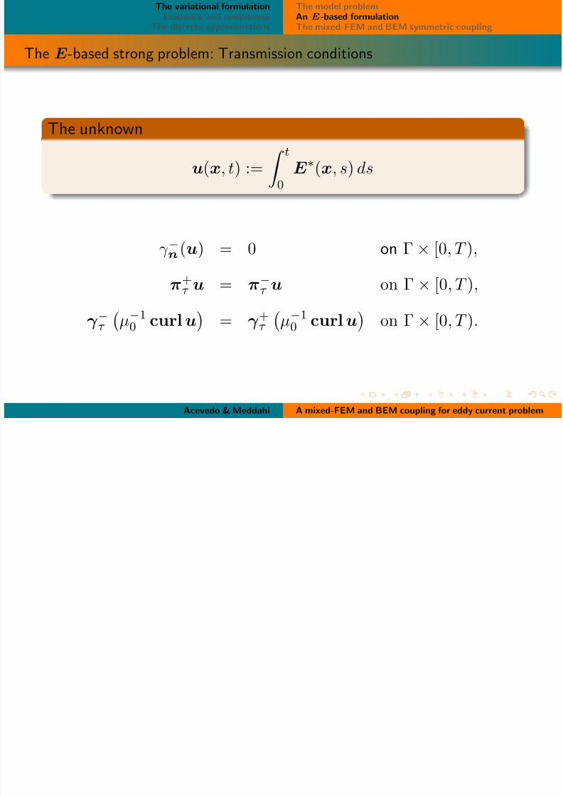
The E -based strong problem: Transmission conditions
The unknown
u(x, t) := t
0E ∗(x, s) ds
γ −n
(u) = 0 on Γ × [0, T ),
π+
τ u = π−
τ u on Γ × [0, T ),
γ −τ
µ−10 curlu
= γ +τ
µ−10 curlu
on Γ × [0, T ).
Acevedo & Meddahi A mixed-FEM and BEM coupling for eddy current problem
The variational formulation The model problem
8/3/2019 Talk Definitiva
http://slidepdf.com/reader/full/talk-definitiva 11/30
The ariational formulationExistence and uniqueness
The discrete approximations
The model problemAn E-based formulationThe mixed-FEM and BEM symmetric coupling
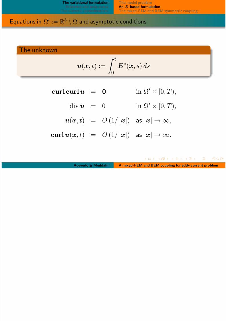
Equations in Ω := R3 \ Ω and asymptotic conditions
The unknown
u(x, t) :=
t0E ∗(x, s) ds
curl curlu = 0 in Ω × [0, T ),
divu = 0 in Ω × [0, T ),
u(x, t) = O (1/ |x|) as |x| → ∞,
curlu(x, t) = O (1/ |x|) as |x| → ∞.
Acevedo & Meddahi A mixed-FEM and BEM coupling for eddy current problem
The variational formulation The model problem
8/3/2019 Talk Definitiva
http://slidepdf.com/reader/full/talk-definitiva 12/30
Existence and uniquenessThe discrete approximations
pAn E-based formulationThe mixed-FEM and BEM symmetric coupling
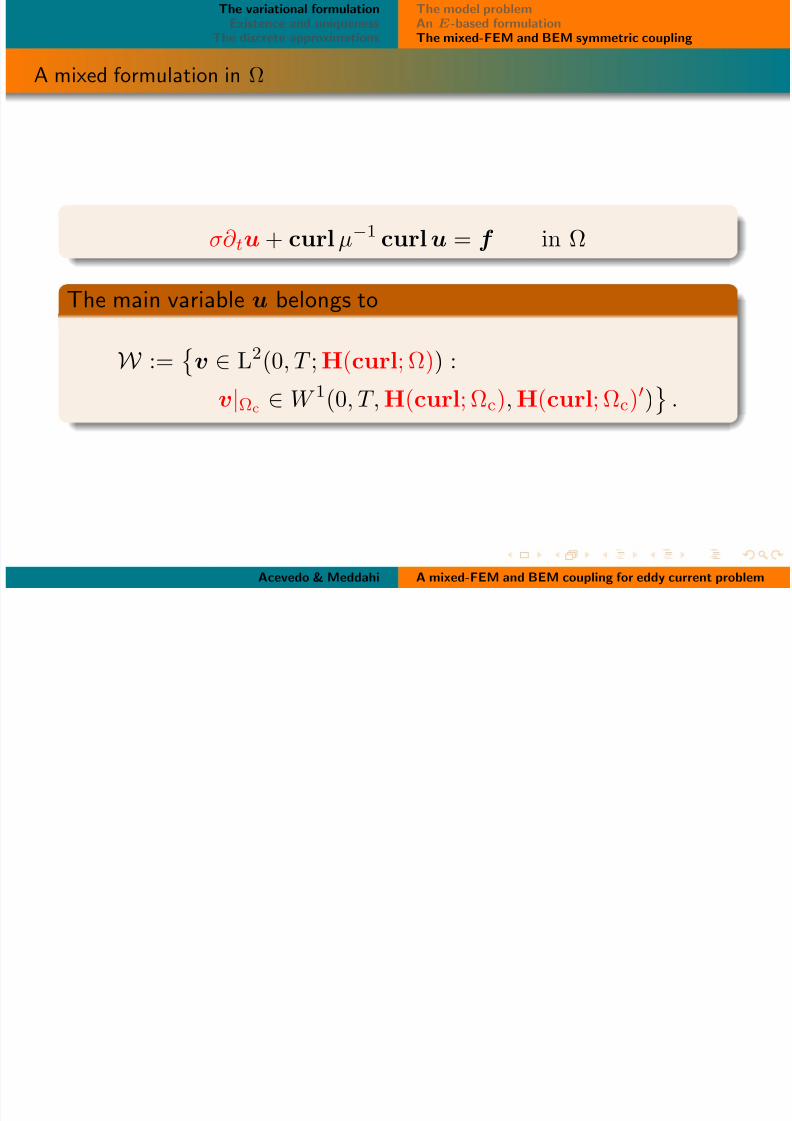
A mixed formulation in Ω
σ∂ tu+ curlµ−1 curlu = f in Ω
The main variable u belongs to
W :=
v ∈ L2(0, T ;H(curl; Ω)) :
v|Ωc∈ W 1(0, T,H(curl; Ωc),H(curl; Ωc)) .
Acevedo & Meddahi A mixed-FEM and BEM coupling for eddy current problem
The variational formulation The model problem
8/3/2019 Talk Definitiva
http://slidepdf.com/reader/full/talk-definitiva 13/30
Existence and uniquenessThe discrete approximations
An E-based formulationThe mixed-FEM and BEM symmetric coupling
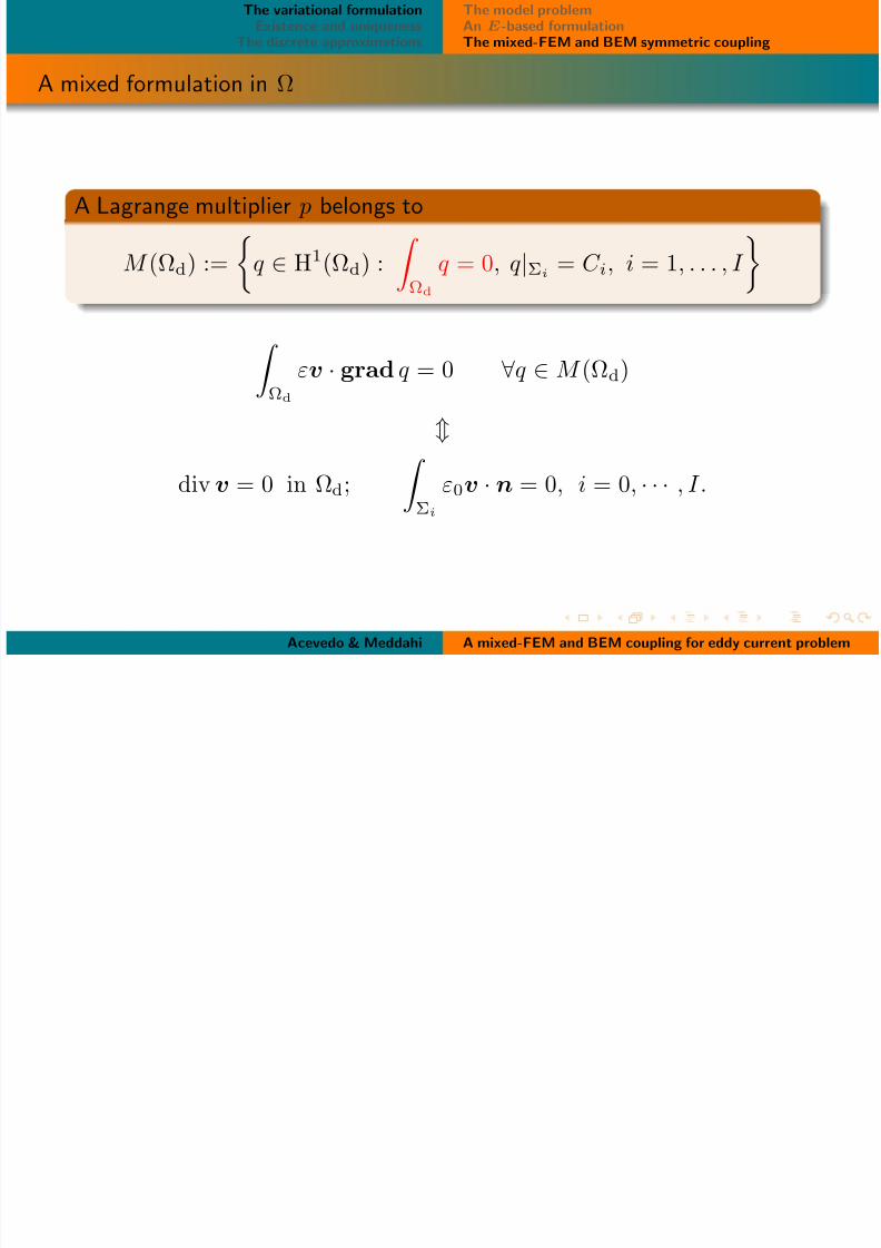
A mixed formulation in Ω
A Lagrange multiplier p belongs to
M (Ωd) :=
q ∈ H1(Ωd) :
Ωd
q = 0, q|Σi= C i, i = 1, . . . , I
Ωd
εv · grad q = 0 ∀q ∈ M (Ωd)
div v = 0 in Ωd; Σi
ε0v · n = 0, i = 0, · · · , I.
Acevedo & Meddahi A mixed-FEM and BEM coupling for eddy current problem
The variational formulation The model problem
8/3/2019 Talk Definitiva
http://slidepdf.com/reader/full/talk-definitiva 14/30
Existence and uniquenessThe discrete approximations
An E-based formulationThe mixed-FEM and BEM symmetric coupling
A mixed formulation in Ω
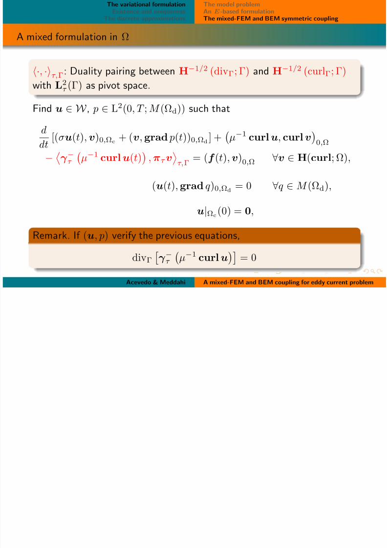
·, ·τ,Γ: Duality pairing between H−1/2 (divΓ; Γ) and H−1/2 (curlΓ; Γ)with L2
τ (Γ) as pivot space.
Find u ∈ W , p ∈ L2(0, T ; M (Ωd)) such that
d
dt [(σu(t),v)0,Ωc + (v,grad p(t))0,Ωd ] +
µ−1 curlu, curlv0,Ω
−γ −τ
µ−1 curlu(t)
,πτ v
τ,Γ
= (f (t),v)0,Ω ∀v ∈ H(curl; Ω),
(u(t),grad q)0,Ωd= 0 ∀q ∈ M (Ωd),
u|Ωc(0) = 0,
Remark. If (u, p) verify the previous equations,
divΓ γ −τ µ−1 curlu = 0
Acevedo & Meddahi A mixed-FEM and BEM coupling for eddy current problem
The variational formulationE i d i
The model problemA E b d f l i
8/3/2019 Talk Definitiva
http://slidepdf.com/reader/full/talk-definitiva 15/30
Existence and uniquenessThe discrete approximations
An E-based formulationThe mixed-FEM and BEM symmetric coupling
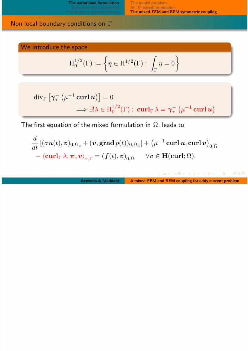
Non local boundary conditions on Γ
We introduce the space
H1/20 (Γ) :=
η ∈ H1/2(Γ) :
Γ
η = 0
divΓγ −τ
µ−1 curlu
= 0
=⇒ ∃!λ ∈ H1/20 (Γ) : curlΓ λ = γ −τ
µ−1 curlu
The first equation of the mixed formulation in Ω, leads to
d
dt[(σu(t),v)0,Ωc
+ (v,grad p(t))0,Ωd] +
µ−1 curlu, curlv
0,Ω
− curlΓ λ,πτ vτ,Γ = (f (t),v)0,Ω ∀v ∈ H(curl; Ω).
Acevedo & Meddahi A mixed-FEM and BEM coupling for eddy current problem
The variational formulationE i t d i
The model problemA E b d f l ti
8/3/2019 Talk Definitiva
http://slidepdf.com/reader/full/talk-definitiva 16/30
Existence and uniquenessThe discrete approximations
An E-based formulationThe mixed-FEM and BEM symmetric coupling
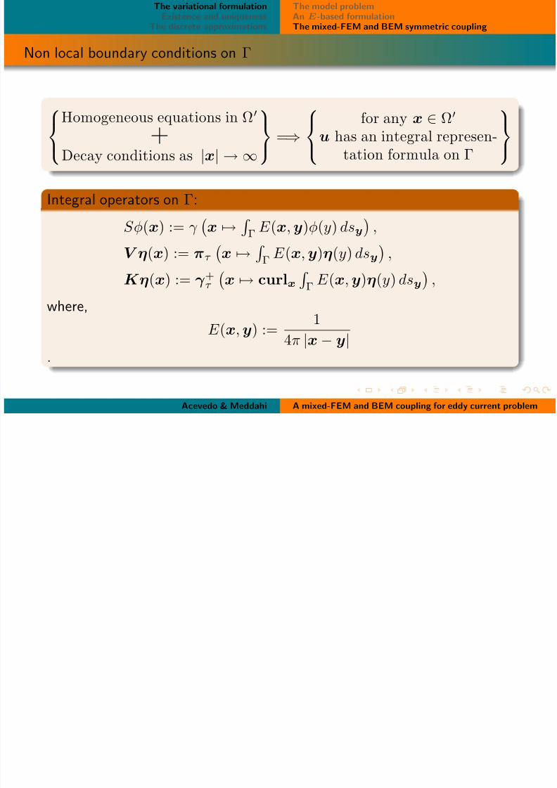
Non local boundary conditions on Γ
Homogeneous equations in Ω
+Decay conditions as |x| → ∞
=⇒
for any x ∈ Ω
u has an integral represen-tation formula on Γ
Integral operators on Γ:
Sφ(x) := γ x →
Γ
E (x,y)φ(y) dsy
,
V η(x) := πτ
x →
Γ
E (x,y)η(y) dsy
,
Kη(x) := γ +τ x → curlx Γ E (x,y)η(y) dsy ,
where,
E (x,y) :=1
4π |x− y|.
Acevedo & Meddahi A mixed-FEM and BEM coupling for eddy current problem
The variational formulationExistence and uniqueness
The model problemAn E based formulation
8/3/2019 Talk Definitiva
http://slidepdf.com/reader/full/talk-definitiva 17/30
Existence and uniquenessThe discrete approximations
An E-based formulationThe mixed-FEM and BEM symmetric coupling
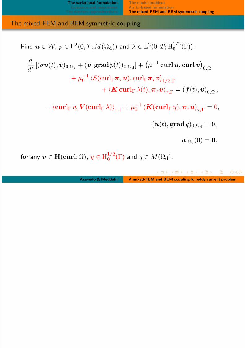
The mixed-FEM and BEM symmetric coupling
Find u ∈ W , p ∈ L2(0, T ; M (Ωd)) and λ ∈ L2(0, T ; H1/20 (Γ)):
d
dt[(σu(t),v)0,Ωc
+ (v,grad p(t))0,Ωd] +
µ−1 curlu, curl v
0,Ω
+ µ−10 S (curlΓπτ u), curlΓπτ v1/2,Γ
+ K curlΓ λ(t),πτ vτ,Γ = (f (t), v)0,Ω ,
− curlΓ η,V (curlΓ λ)τ,Γ + µ−10 K (curlΓ η),πτ uτ,Γ = 0,
(u(t),grad q)0,Ωd= 0,
u|Ωc(0) = 0.
for any v ∈ H(curl; Ω), η ∈ H1/20 (Γ) and q ∈ M (Ωd).
Acevedo & Meddahi A mixed-FEM and BEM coupling for eddy current problem
The variational formulationExistence and uniqueness
The reduced problemThe reduced problem
8/3/2019 Talk Definitiva
http://slidepdf.com/reader/full/talk-definitiva 18/30
Existence and uniquenessThe discrete approximations
The reduced problemWell-posedness
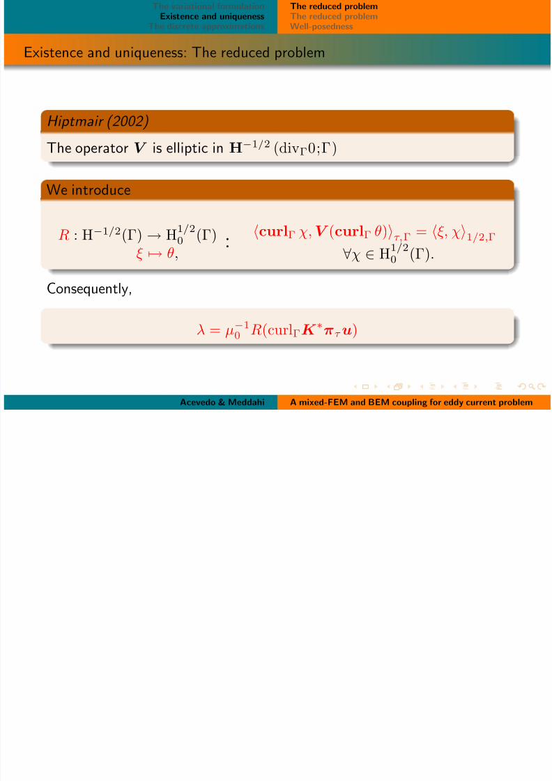
Existence and uniqueness: The reduced problem
Hiptmair (2002)
The operator V is elliptic in H−1/2 (divΓ0;Γ)
We introduce
R : H−1/2(Γ) → H1/20 (Γ)
ξ → θ,:
curlΓ χ,V (curlΓ θ)τ,Γ = ξ, χ1/2,Γ∀χ ∈ H
1/20 (Γ).
Consequently,
λ = µ−10 R(curlΓK
∗πτ u)
Acevedo & Meddahi A mixed-FEM and BEM coupling for eddy current problem
The variational formulationExistence and uniqueness
The reduced problemThe reduced problem
8/3/2019 Talk Definitiva
http://slidepdf.com/reader/full/talk-definitiva 19/30
Existence and uniquenessThe discrete approximations
The reduced problemWell-posedness
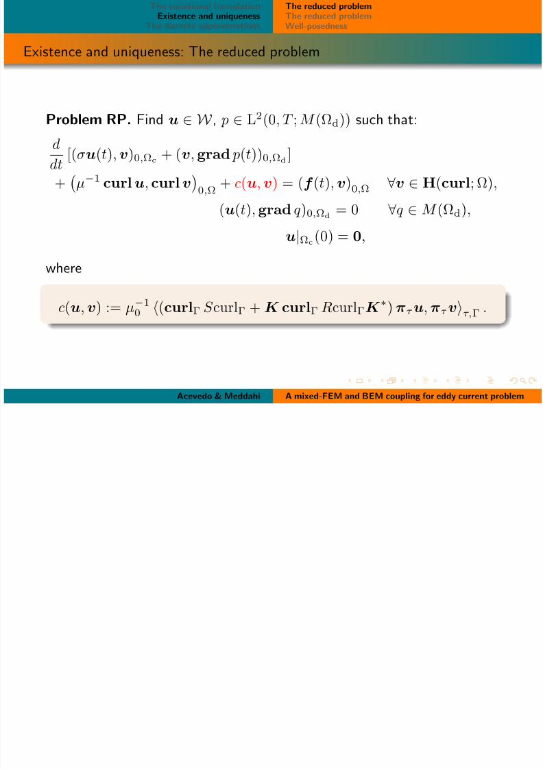
Existence and uniqueness: The reduced problem
Problem RP. Find u ∈ W , p ∈ L2(0, T ; M (Ωd)) such that:
d
dt[(σu(t),v)0,Ωc
+ (v,grad p(t))0,Ωd]
+ µ−1 curlu, curlv0,Ω
+ c(u,v) = (f (t),v)0,Ω
∀v ∈ H(curl; Ω),
(u(t),grad q)0,Ωd= 0 ∀q ∈ M (Ωd),
u|Ωc(0) = 0,
where
c(u,v) := µ−10 (curlΓ S curlΓ + K curlΓ RcurlΓK
∗)πτ u,πτ vτ,Γ .
Acevedo & Meddahi A mixed-FEM and BEM coupling for eddy current problem
The variational formulationExistence and uniqueness
The reduced problemThe reduced problem
8/3/2019 Talk Definitiva
http://slidepdf.com/reader/full/talk-definitiva 20/30
Existence and uniquenessThe discrete approximations
The reduced problemWell-posedness
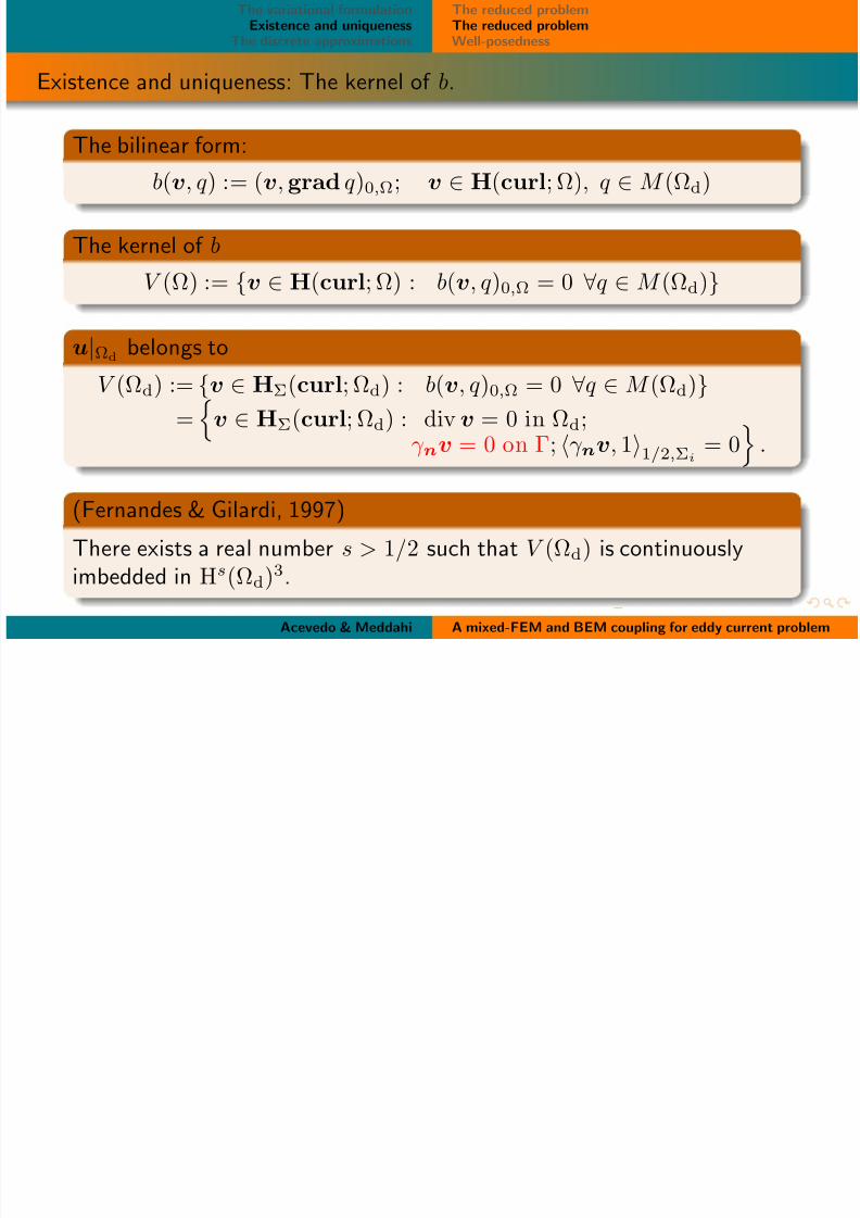
Existence and uniqueness: The kernel of b.
The bilinear form:b(v, q) := (v,grad q)0,Ω; v ∈ H(curl; Ω), q ∈ M (Ωd)
The kernel of b
V (Ω) := v ∈ H(curl; Ω) : b(v, q)0,Ω = 0 ∀q ∈ M (Ωd)
u|Ωdbelongs to
V (Ωd) := v ∈ HΣ(curl; Ωd) : b(v, q)0,Ω = 0 ∀q ∈ M (Ωd)
=v ∈ HΣ(curl; Ωd) : div v = 0 in Ωd;
γ nv = 0 on Γ; γ nv, 11/2,Σi = 0
.
(Fernandes & Gilardi, 1997)
There exists a real number s > 1/2 such that V (Ωd) is continuouslyimbedded in Hs(Ωd)3.
Acevedo & Meddahi A mixed-FEM and BEM coupling for eddy current problem
The variational formulationExistence and uniqueness
The reduced problemThe reduced problem
8/3/2019 Talk Definitiva
http://slidepdf.com/reader/full/talk-definitiva 21/30
qThe discrete approximations
pWell-posedness
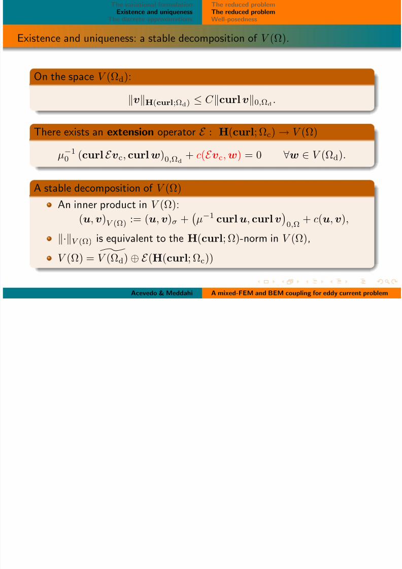
Existence and uniqueness: a stable decomposition of V (Ω).
On the space V (Ωd):
vH(curl;Ωd) ≤ C curlv0,Ωd.
There exists an extension operator E : H(curl; Ωc) → V (Ω)
µ−10 (curl E vc, curlw)0,Ωd
+ c(E vc,w) = 0 ∀w ∈ V (Ωd).
A stable decomposition of V (Ω)
An inner product in V (Ω):
(u,v)V (Ω) := (u, v)σ +
µ−1 curlu, curlv0,Ω
+ c(u,v),
·V (Ω) is equivalent to the H(curl; Ω)-norm in V (Ω),
V (Ω) = V (Ωd) ⊕ E (H(curl; Ωc))
Acevedo & Meddahi A mixed-FEM and BEM coupling for eddy current problem
The variational formulationExistence and uniqueness
The reduced problemThe reduced problem
8/3/2019 Talk Definitiva
http://slidepdf.com/reader/full/talk-definitiva 22/30
qThe discrete approximations
pWell-posedness
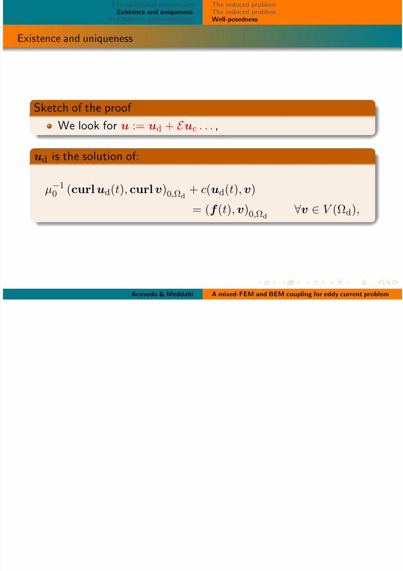
Existence and uniqueness
Sketch of the proof
We look for u := ud + E uc . . . ,
ud is the solution of:
µ−10 (curlud(t), curlv)0,Ωd
+ c(ud(t),v)
= (f (t),v)0,Ωd ∀v ∈ V (Ωd),
Acevedo & Meddahi A mixed-FEM and BEM coupling for eddy current problem
The variational formulationExistence and uniqueness
The reduced problemThe reduced problem
8/3/2019 Talk Definitiva
http://slidepdf.com/reader/full/talk-definitiva 23/30
The discrete approximations Well-posedness
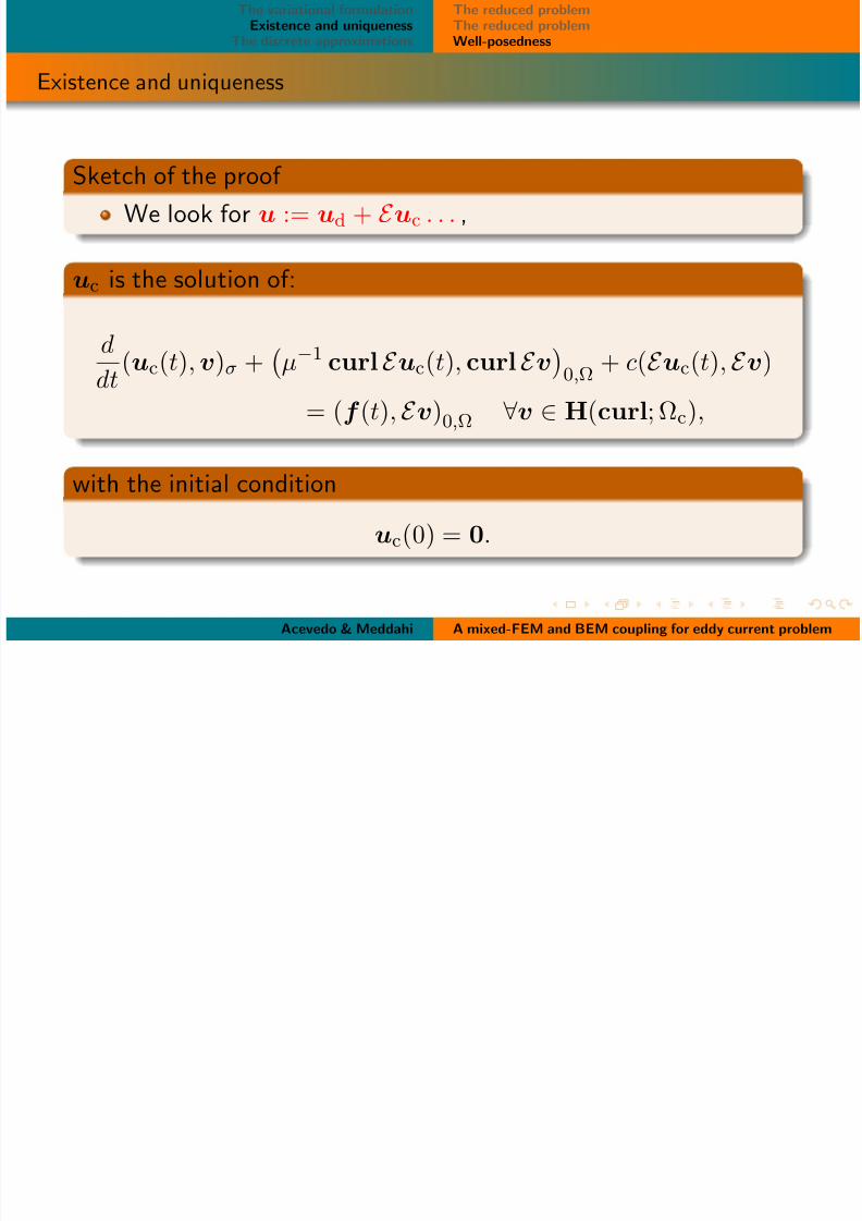
Existence and uniqueness
Sketch of the proof
We look for u := ud + E uc . . . ,
uc is the solution of:
d
dt(uc(t),v)σ +
µ−1 curl E uc(t), curl E v
0,Ω
+ c(E uc(t), E v)
= (f (t), E v)0,Ω ∀v ∈ H(curl; Ωc),
with the initial condition
uc(0) = 0.
Acevedo & Meddahi A mixed-FEM and BEM coupling for eddy current problem
The variational formulationExistence and uniqueness
The reduced problemThe reduced problem
8/3/2019 Talk Definitiva
http://slidepdf.com/reader/full/talk-definitiva 24/30
The discrete approximations Well-posedness
Existence and uniqueness
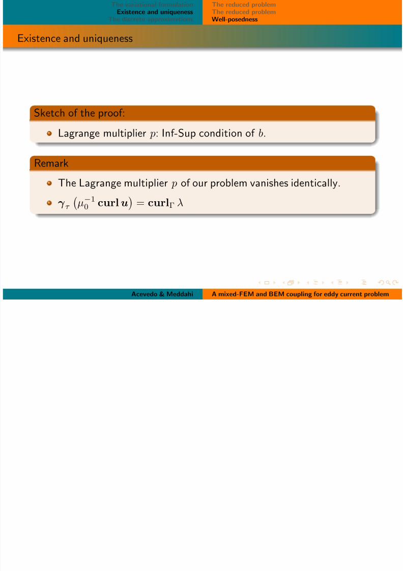
Sketch of the proof:
Lagrange multiplier p: Inf-Sup condition of b.
Remark
The Lagrange multiplier p of our problem vanishes identically.
γ τ µ−10 curlu = curlΓ λ
Acevedo & Meddahi A mixed-FEM and BEM coupling for eddy current problem
The variational formulationExistence and uniqueness
Th di i i
Analysis of the semi-discrete schemeAnalysis of the fully-discrete scheme
8/3/2019 Talk Definitiva
http://slidepdf.com/reader/full/talk-definitiva 25/30
The discrete approximationsAnalysis of the fully discrete scheme
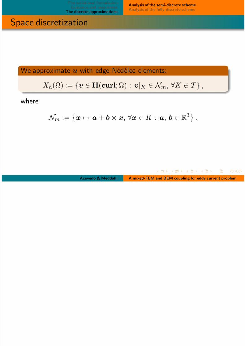
Space discretization
We approximate u with edge Nedelec elements:
X h(Ω) := v ∈ H(curl; Ω) : v|K ∈ N m, ∀K ∈ T ,
where
N m := x → a + b × x, ∀x ∈ K : a, b ∈ R3 .
Acevedo & Meddahi A mixed-FEM and BEM coupling for eddy current problem
The variational formulationExistence and uniqueness
Th di t i ti
Analysis of the semi-discrete schemeAnalysis of the fully-discrete scheme
8/3/2019 Talk Definitiva
http://slidepdf.com/reader/full/talk-definitiva 26/30
The discrete approximationsy y
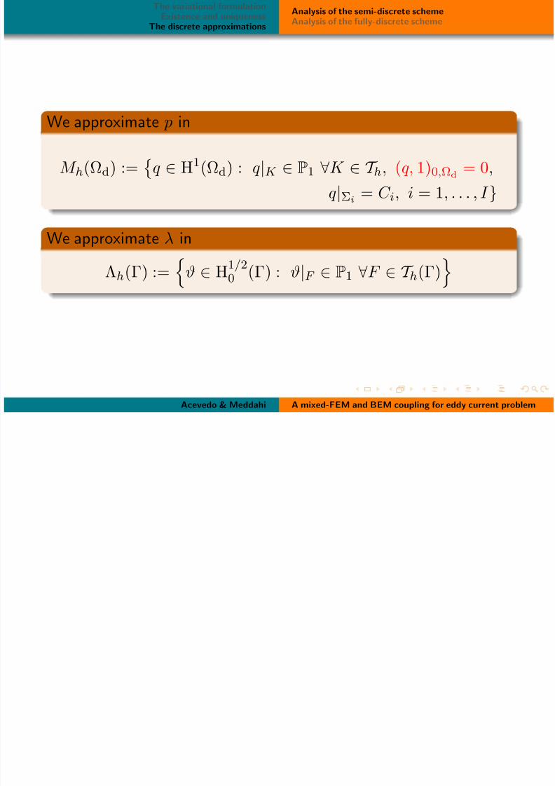
We approximate p in
M h(Ωd) :=
q ∈ H1(Ωd) : q|K ∈ P1 ∀K ∈ T h, (q, 1)0,Ωd
= 0,
q|Σi = C i, i = 1, . . . , I
We approximate λ in
Λh(Γ) := ϑ ∈ H1/20 (Γ) : ϑ|F ∈ P1 ∀F ∈ T h(Γ)
Acevedo & Meddahi A mixed-FEM and BEM coupling for eddy current problem
The variational formulationExistence and uniqueness
The discrete approximations
Analysis of the semi-discrete schemeAnalysis of the fully-discrete scheme
8/3/2019 Talk Definitiva
http://slidepdf.com/reader/full/talk-definitiva 27/30
The discrete approximationsy y
Well-posedness
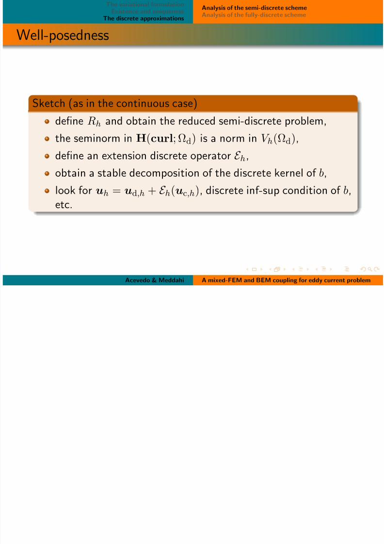
Sketch (as in the continuous case)
define Rh and obtain the reduced semi-discrete problem,
the seminorm in H(curl; Ωd) is a norm in V h(Ωd),define an extension discrete operator E h,
obtain a stable decomposition of the discrete kernel of b,
look for uh = ud,h + E h(uc,h), discrete inf-sup condition of b,
etc.
Acevedo & Meddahi A mixed-FEM and BEM coupling for eddy current problem
The variational formulationExistence and uniqueness
The discrete approximations
Analysis of the semi-discrete schemeAnalysis of the fully-discrete scheme
8/3/2019 Talk Definitiva
http://slidepdf.com/reader/full/talk-definitiva 28/30
The discrete approximations
Semi-discrete error estimates
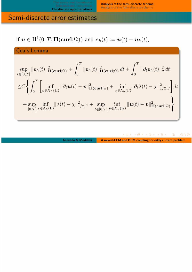
If u ∈ H1(0, T ;H(curl;Ω)) and eh(t) := u(t) − uh(t),
Cea’s Lemma
supt∈[0,T ]
eh(t)2H(curl;Ω) + T 0
eh(t)2H(curl;Ω) dt + T 0
∂ teh(t)2σ dt
≤C
T 0
inf
v∈Xh(Ω)∂ tu(t) − v2
H(curl;Ω) + inf χ∈Λh(Γ)
∂ tλ(t) − χ21/2,Γ
dt
+ sup[0,T ]
inf χ∈Λh(Γ)
λ(t) − χ21/2,Γ + supt∈[0,T ]
inf v∈Xh(Ω)
u(t) − v2H(curl;Ω)
Acevedo & Meddahi A mixed-FEM and BEM coupling for eddy current problem
The variational formulationExistence and uniqueness
The discrete approximations
Analysis of the semi-discrete schemeAnalysis of the fully-discrete scheme
8/3/2019 Talk Definitiva
http://slidepdf.com/reader/full/talk-definitiva 29/30
The discrete approximations
A convergence result
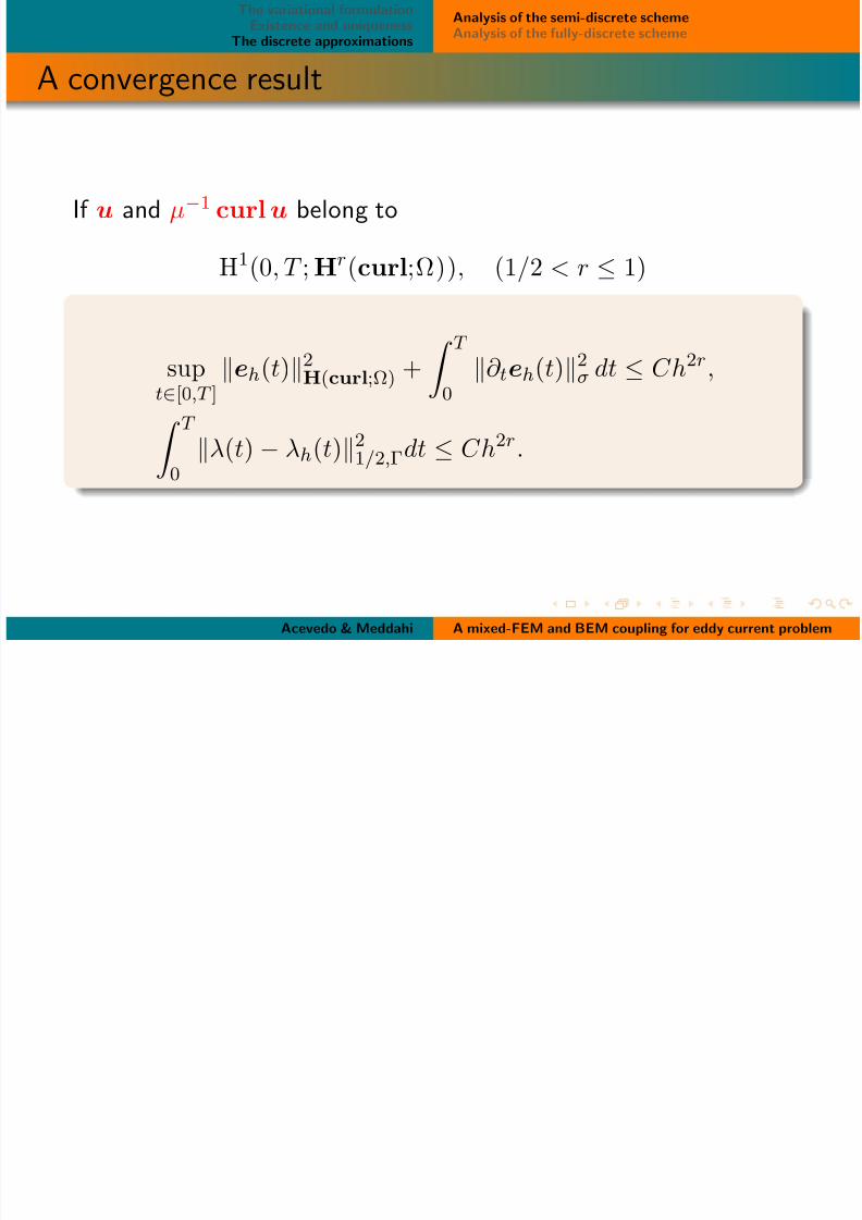
If u and µ−1 curlu belong to
H1(0, T ;Hr(curl;Ω)), (1/2 < r ≤ 1)
supt∈[0,T ]
eh(t)2H(curl;Ω) +
T 0
∂ teh(t)2σ dt ≤ Ch2r,
T 0 λ(t) − λh(t)
2
1/2,Γdt ≤ Ch
2r
.
Acevedo & Meddahi A mixed-FEM and BEM coupling for eddy current problem
The variational formulationExistence and uniqueness
The discrete approximations
Analysis of the semi-discrete schemeAnalysis of the fully-discrete scheme
8/3/2019 Talk Definitiva
http://slidepdf.com/reader/full/talk-definitiva 30/30
The discrete approximations
The fully-discrete scheme
Time discretization: implicit Euler scheme.
Existence and uniqueness: as in the semi-dicrete case.
Convergence analysis: analogous results to the semi-discretecase.
Acevedo & Meddahi A mixed-FEM and BEM coupling for eddy current problem