STRUCTURAL DAMAGE DETECTION AND LOCALIZATION BY …dzonta/download/PhD.pdf · Chiar.mo Prof. Erasmo...
158
UNIVERSITÀ DEGLI STUDI DI BOLOGNA DIPARTIMENTO DI INGEGNERIA DELLE D I S T A R T STRUTTURE, DEI TRASPORTI DELLE ACQUE, DEL RILEVAMENTO, DEL TERRITORIO A Dottorato di ricerca in Meccanica delle Strutture XII CICLO Daniele Zonta STRUCTURAL DAMAGE DETECTION AND LOCALIZATION BY USING VIBRATIONAL MEASUREMENTS Dissertazione presentata per il conseguimento del titolo di Dottore di Ricerca in Meccanica delle Strutture Il Relatore Chiar.mo Prof. Erasmo Viola Il Coordinatore Chiar.mo Prof. Erasmo Viola Bologna, Gennaio 2000
Transcript of STRUCTURAL DAMAGE DETECTION AND LOCALIZATION BY …dzonta/download/PhD.pdf · Chiar.mo Prof. Erasmo...

UNIVERSITÀ DEGLI STUDI DI BOLOGNA DIPARTIMENTO DI INGEGNERIA DELLE
D I S T A R T STRUTTURE, DEI TRASPORTI DELLE ACQUE, DEL RILEVAMENTO, DEL TERRITORIO A
Dottorato di ricerca in Meccanica delle Strutture XII CICLO
Daniele Zonta
STRUCTURAL DAMAGE DETECTION AND LOCALIZATION BY USING VIBRATIONAL
MEASUREMENTS
Dissertazione presentata per il conseguimento del titolo di Dottore di Ricerca in
Meccanica delle Strutture
Il Relatore Chiar.mo Prof. Erasmo Viola
Il Coordinatore Chiar.mo Prof. Erasmo Viola
Bologna, Gennaio 2000


This thesis is dedicated
to Catizza and to Valentina


5
Contents
CONTENTS........................................................................................................5
1 OVERVIEW .................................................................................................9
1.1 INTRODUCTION....................................................................................... 10 1.1.1 Problem statement ........................................................................... 10 1.1.2 Earlier research.............................................................................. 12
1.2 OBJECTIVES ........................................................................................... 13 1.2.1 Aims of the investigation .................................................................. 13 1.2.2 Outlines of the thesis ....................................................................... 13 1.2.3 Innovative aspect of the research ...................................................... 14 1.2.4 Restrictions .................................................................................... 14
2 FUNDAMENTALS OF VIBRATIONAL MECHANICS ................................ 15
2.1 INTRODUCTION....................................................................................... 16 2.2 VIBRATIONAL PROBLEMS......................................................................... 17
2.2.1 Vibration of lumped systems ............................................................. 17 2.2.2 Vibration of continuous systems........................................................ 19
2.3 ANALOGIES BETWEEN DIFFERENT FORMULATIONS........................................ 24 2.3.1 Equations of motion......................................................................... 24 2.3.2 Equations uncoupling ...................................................................... 25
2.4 A GENERALIZED FORMULATION FOR VIBRATIONAL ANALYSIS PROBLEMS ......... 27 2.4.1 Equations of motion......................................................................... 27 2.4.2 Equations uncoupling ...................................................................... 27
2.5 FURTHER DEVELOPMENTS ........................................................................ 29 2.5.1 Analogies between spectral and modal analysis .................................. 29 2.5.2 A time-space domain based formulation ............................................. 30
3 DAMAGE LOCALIZATION PROBLEMS................................................... 31
3.1 INTRODUCTION....................................................................................... 32 3.1.1 A methodological approach to the localization problem ....................... 33 3.1.2 Identification of dynamic measures.................................................... 33 3.1.3 Identification of local damage indicators ........................................... 33 3.1.4 Choice of relation............................................................................ 33
3.2 CHANGES IN MODAL SHAPES AND FREQUENCIES RELATED TO CHANGES IN STIFFNESS ....................................................................................................... 34
3.2.1 Changes in frequency....................................................................... 34 3.2.2 Changes in mode shape.................................................................... 35
Structural damage detection and localization by using vibrational measurements
6
3.3 CHANGES IN DAMPING MECHANISM ........................................................... 37 3.3.1 Changes in modal damping .............................................................. 37 3.3.2 SDOF oscillator with Coulomb friction .............................................. 38 3.3.3 Formulation of the modal friction damping method ............................. 43
4 ANALYSIS OF DISPERSION PHENOMENA.............................................. 45
4.1 INTRODUCTION ...................................................................................... 46 4.1.1 Some experimental evidence ............................................................. 46 4.1.2 Propositions ................................................................................... 47
4.2 A GENERALISED FORM OF THE SDOF OSCILLATOR....................................... 48 4.2.1 Free response of dispersive oscillator................................................ 49 4.2.2 Forced response.............................................................................. 51 4.2.3 Observation.................................................................................... 51
4.3 AN INTERPRETIVE MODEL IN CONTINUUM ................................................... 52 4.4 CONCLUSIONS........................................................................................ 53
5 QUALITY CONTROL IN PRC PANELS..................................................... 55
5.1 INTRODUCTION ...................................................................................... 56 5.2 EXPERIMENTAL INVESTIGATION................................................................ 57
5.2.1 Characteristics of the specimen ........................................................ 57 5.2.2 Boundary conditions........................................................................ 58 5.2.3 Damage applied.............................................................................. 59 5.2.4 Dynamic characterization ................................................................ 63
5.3 MODAL EXTRACTION............................................................................... 67 5.3.1 Natural frequencies and mode shapes ................................................ 67 5.3.2 Modal damping rates....................................................................... 69 5.3.3 Detection of Coulomb friction damping.............................................. 70
5.4 LOCALIZATION OF DAMAGE...................................................................... 71 5.4.1 Changes in frequency method ........................................................... 71 5.4.2 Changes in flexibility method............................................................ 71 5.4.3 MAC and COMAC index methods...................................................... 71 5.4.4 Modal curvature shape method ......................................................... 72 5.4.5 Changes in modal damping method ................................................... 72 5.4.6 Coulomb friction damping method..................................................... 73
5.5 CONCLUSIONS........................................................................................ 75
6 DYNAMIC CHARACTERIZATION OF THE ROMAN AMPHITHEATER (ARENA) IN VERONA ..................................................................................... 77
6.1 INTRODUCTION ...................................................................................... 78 6.2 ND EVALUATION OF STATES OF STRESS AND MECHANICAL PROPERTIES OF WALLS AND VAULTS.................................................................................................... 83 6.3 ANATHYROSIS EFFECT ON THE MASONRY STIFFNESS ..................................... 84 6.4 DYNAMIC INVESTIGATIONS ON THE WING................................................... 85
6.4.1 Stepped-sine tests............................................................................ 86 6.4.2 Shock tests ..................................................................................... 86 6.4.3 Ambient Vibrations Tests ................................................................. 87
6.5 MODAL EXTRACTION............................................................................... 88 6.6 MODELING AND IDENTIFICATION............................................................... 89 6.7 PRELIMINARY DYNAMIC INVESTIGATIONS ON THE VAULTS ............................ 90

Contents
7
6.7.1 Signals Analysis .............................................................................. 91 6.8 CONCLUSIONS ........................................................................................ 92
7 DYNAMIC INVESTIGATIONS ON THE PALAZZO DELLA RAGIONE ROOF IN PADUA ............................................................................................. 93
7.1 INTRODUCTION....................................................................................... 94 7.2 STRUCTURE DESCRIPTION......................................................................... 94 7.3 WIND LOAD ACCORDING TO EC1............................................................... 95 7.4 FULL SCALE AERODYNAMIC MEASUREMENTS............................................... 97 7.5 DYNAMIC TESTS ................................................................................... 103 7.6 CONCLUSIONS ...................................................................................... 105
8 DYNAMIC CHARACTERIZATION OF REINFORCED MASONRY STRUCTURES................................................................................................ 107
8.1 INTRODUCTION..................................................................................... 108 8.2 DESIGN AND CONSTRUCTION OF THE BUILDINGS ........................................ 110
8.2.1 Full scale buildings ....................................................................... 110 8.2.2 Reduced scale model...................................................................... 110
8.3 DYNAMIC CHARACTERIZATION................................................................ 112 8.3.1 Position of transducer and techniques of experimentation .................. 112 8.3.2 Full scale building ........................................................................ 113 8.3.3 Reduced scale building .................................................................. 115 8.3.4 Modeling...................................................................................... 117
8.4 SEISMIC EXPERIMENTATION.................................................................... 118 8.5 QUALITATIVE ANALYSIS OF THE SEISMIC BEHAVIOR ................................... 118
8.5.1 Predicted failure mechanism........................................................... 118 8.5.2 Cracks pattern .............................................................................. 119
8.6 HYPOTHESIS FOR THE STRUCTURAL RESPONSE INTERPRETATION................... 121 8.6.1 Modeling as a single degree of freedom system ................................. 121 8.6.2 Response of a non-linear SDOF system ............................................ 121
8.7 DISCUSSION OF THE RESULTS .................................................................. 125 8.7.1 Yielding displacement and required ductility .................................... 125 8.7.2 5.2 Ultimate limit state of the available ductility............................... 125 8.7.3 Damage evaluation........................................................................ 125 8.7.4 Calculation of the behavior factor ................................................... 126
8.8 CONCLUSIONS ...................................................................................... 127
9 NON DESTRUCTIVE EVALUATION ON THE PRESSS BUILDING MODEL 129
9.1 INTRODUCTION..................................................................................... 130 9.1.1 Seismic design philosophy of building.............................................. 130 9.1.2 Post earthquake damage assessment ................................................ 130 9.1.3 Overview of the experimentation conducted ...................................... 131
9.2 DESCRIPTION OF THE BUILDING ............................................................... 132 9.2.1 Frame connection system ............................................................... 133
9.3 TESTING.............................................................................................. 135 9.3.1 Transducers position ..................................................................... 135 9.3.2 Testing techniques......................................................................... 138

Structural damage detection and localization by using vibrational measurements
8
9.3.3 Test identification ......................................................................... 140 9.3.4 Signal processing.......................................................................... 140
9.4 MODAL EXTRACTION............................................................................. 145 9.4.1 Frequencies .................................................................................. 145 9.4.2 Mode shapes................................................................................. 145
9.5 DAMAGE ASSESSMENT........................................................................... 149 9.5.1 NDE of the whole structures ........................................................... 149 9.5.2 NDE of joints................................................................................ 150
REFERENCES ............................................................................................... 153
NOTATION.................................................................................................... 157
9
1 Overview Abstract The objectives and restrictions of the research are presented, which aims to frame the problem of structural damage detection and localization from a methodological point of view, and to highlight, those aspects of dynamic response, which are actually significant in the damage detection process. The thesis is roughly divided in two parts: chapters 2 to 4 deal with a methodological approach to the problem of vibration and to damage detection; chapters 5 to 9 report some case studies, where those damage detection and localization techniques are applied in engineering practice and research. Sommario Vengono descritti gli obiettivi e i limiti della presente ricerca che mira ad inquadrare il problema del riconoscimento e della localizzazione del danno strutturale da un punto di vista metodologico, e a evidenziare quegli aspetti della risposta dinamica che siano effettivamente significativi nella procedura dell'identificazione del danno. La tesi può considerarsi divisa in due parti: i capitoli dal 2 al 4 riguardano un approccio metodologico ai problemi della meccanica vibrazionale e del riconoscimento del danno; i capitoli dal 5 al 9 riportano alcuni casi studio, dove le tecniche di identificazione e localizzazione del danno formulate sono applicate nella pratica ingegneristica e nella ricerca.

Structural damage detection and localization by using vibrational measurements
10
1.1 Introduction
1.1.1 Problem statement Dynamic tests represent an inexpensive way to achieve abundant information on the mechanical behaviour of a structure. This is why, for many years, experimental modal testing has become a significant topic in the field of structural assessment, not only with regards to structures typical of mechanical engineering, but also in civil engineering.
Perhaps the single most commonly used application is the measurement of vibrational modes in order to compare these with the corresponding data produced by a finite element or other theoretical model (Ewins 1984). This application is often born out of a need or desire to validate the theoretical model for predicting response levels to complex excitations prior to its use. A more recent application of this procedure is in the field of non-destructive evaluation.
Non-destructive damage detection techniques using experimentally measured vibration test data is usually based on the assumption that the damage will change the structural (mass, stiffness or damping) properties which further lead to changes in the dynamic characteristics, such as the natural frequencies, damping ratio and mode shapes (Farrar and Doebling, 1997). Figure 1.1. shows two Frequency Response Functions of a vibrating PRC panel, fixed at the edges, with measurements taken at the middle-span. Details of the experiment could be found in Chapter 5. The light line refers to the undamaged panel and the bold one to the panel after introduction of cracking. Slight differences could be noted in frequencies before and after damaging, but a more accurate modal extraction would highlight changes in mode shape and modal damping. Unfortunately, it is not always possible to carry out a complete set of measurements that allow a satisfactory extraction of mode shapes. And moreover, changes in modal parameter are not always associated with the occurrence of damage.
0.0
0.1
1.0
10.0
100.0
0 20 40 60 80 100 120
[Hz]
[mm
sec
-2 N
-1]
undamaged
damaged
Figure 1.1. Change in dynamic response of a PRC element before and after damaging.

Overview
11
0.0E+00
2.0E-08
4.0E-08
6.0E-08
8.0E-08
1.0E-07
1.2E-07
1.4E-07
1.6E-07
1.8E-07
2.0E-07
0 100 200 300 400 500 600 700 800
[Hz]
[ms-1
N-1
]
0.0E+00
2.0E-08
4.0E-08
6.0E-08
8.0E-08
1.0E-07
1.2E-07
1.4E-07
1.6E-07
1.8E-07
2.0E-07
0 100 200 300 400 500 600 700 800
[Hz]
[ms-1
N-1
]
Figure 1.2. FRF measured at the top of a regular pile (a) and of a pile with imperfections (b).
This is the case for foundation piles integrity assessments, which represent another typical application of dynamic testing in civil engineering practice: Figure 1.2 highlights the differences between FRFs measured at the top of the pile for an almost regular foundation and for an imperfect pile. In this case, absolute changes in frequency can only be associated with the dynamic characteristics of the soil, therefore this is not a significant parameter for damage detection. On the other hand, the spacing between frequencies is even for perfect piles, while an uneven spacing indicates the presence of an anomaly. Figure 1.3 shows another significant example of a change in the dynamic responses of a structure following the introduction of damage; we are dealing with an experimental PRC building (Nakaki et al. 1998, Priestley et al. 1999), designed according to capacity design criteria, subject to an high intensity pseudo dynamic test. Detail of this experiment can be found in Chapter 8. In this case, significant changes in frequency have been measured, while the resulting changes in mode shapes were not so important.
Since the changes in the dynamic characteristics can be measured and studied, it is possible to trace what structural changes have caused the dynamic characteristics to change, thus identifying the damage. The problem of damage detection and localization actually consists of finding out a correlation between these quantities.
1.0E-04
1.0E-03
1.0E-02
1.0E-01
1.0E+00
0 1 2 3 4 5 6 7 8 9 10
[Hz]
[mg
N-1
]
A1A2A3
1.0E-04
1.0E-03
1.0E-02
1.0E-01
1.0E+00
0 1 2 3 4 5 6 7 8 9 10
[Hz]
[mg
N-1
]
A1A2A3
Figure 1.3. FRF achieved through shock tests on the PRESSS building (see Chapter 8), before (a) and after (b) damaging.

Structural damage detection and localization by using vibrational measurements
12
1.1.2 Earlier research An exhaustive state of the art discussion on this subject can be found in Farrar and Doebling (1997) and is briefly summarized below. Early research relating to damage detection focused on using the information of natural frequency changes. Cawley and Adams (1979) are commonly recognised as the authors of the first proposal in this sense: they developed a method for detecting imperfections in a FRP plate, on the basis of changes in frequency. Stubbs and Osegueda (1990) developed a damage detection method using the sensitivity of modal frequencies changes that is based on the work of Cawley and Adams. In this method, an error function for the ith mode and the pth structural member is computed assuming that only one is damaged. The member that minimizes this error is determined to be the damaged member.
West (1984) presents what is possibly the first systematic use of mode shape information for the localization of structural damage without the use of a prior FEM. The author uses the modal assurance criteria (MAC) to determine the level of correlation between modes from the test of an undamaged Space Shuttle Orbiter body flap.
An alternative to the use of mode shapes to obtain spatial information about sources of vibration changes is using mode shape derivatives, such us curvature. It is first noted that for beam, plates and shells there is a direct relationship between curvature and bending strain. Pandey et al. (1991) demonstrates that absolute changes in mode shape curvature can be a good indicator of damage for the FEM beam structures they consider.
Chen and Swamidas (1994), Dong et al. (1994), Kondo and Hamamoto (1994), Nwosu et al. (1995) present other studies that identify the damage and its localization from changes in mode shape curvature or strain based mode shape.
Aktan et al. (1994) proposed the use of flexibility as a condition index to indicate the relative integrity of a bridge. Pandey and Biswas (1994) present a damage detection and localization method on change in the measured flexibility of the structures. Mayes (1995) use measured flexibility to locate damage from the results of a modal test on a bridge.
Overview
13
1.2 Objectives
1.2.1 Aims of the investigation This dissertation resumes the work of the author during the years 1996-1999 in the field of experimental modal testing and theoretical vibrational analysis of civil engineering structures. The objectives of modal testing can be many, including response prediction, model calibration, vibration monitoring and control. In this dissertation, focus is placed on those problems which involve the detection of damage. Particularly, the investigation aims to: • frame the problem of damage detection and localization from a methodological point of view, in order to highlight the potential and restrictions of the methods proposed in litterature; • identify, through the analysis some of the experimental cases, those aspects of dynamic response which are actually significant in the damage detection process, particularly with reference to civil engineering structures.
1.2.2 Outlines of the thesis According to the previously mentioned aims, the thesis can be roughly divided in two parts: chapters 2 to 4 deal with a methodological approach to the problem of vibration in its general form and to damage detection; chapters 5 to 9 report some case studies, where those damage detection and localization techniques, are applied in engineering practice and research. Applications regard quality control of building products on one side, and damage assessment of historically relevant and experimental buildings on the other. In detail: • A general discussion of the analytical vibrational problem is reported in Chapter 2, which includes the proposal for an unified notation for dealing both with lumped and continuous system, based on the introduction of generalized operators and vectors. • Chapter 3 introduces the procedures that have been developed in litterature to estimate location and extent of structural damage, and shows how these methods can be framed inside a 4-step methodological procedure; methods for damage localization are formulated or reviewed, based on modeling of the damage as a local reduction in stiffness, and in the detection of changes in classical modal parameters; two new damage detection/localizing techniques are proposed the first one assuming specific damping changes as a damage index, the other is based on the detection of the appearance of Coulomb friction damping; • Chapter 4 highlights how the presence of damage in many structures of practical interest, is often marked by the appearance of dispersion phenomena, and how these phenomena, are still suitable for linear modeling. • The application of damage detection methods to the quality control in PRC elements is developed in Chapter 5, where techniques described in Chapters 3 are extensively applied. • Two examples of dynamic investigation on historically relevant structures are presented in Chapter 6, in the case of the Roman Amphitheater in Verona, and in Chapter 7, in the case of the XV century Palazzo della Ragione roof in Padova. • The use of dynamic NDT as a tool in experimental seismic research is the topic of the following two chapters: Chapter 8, reports the first experimental phase of an ongoing research regarding the seismic behavior of a full-scale 2-story reinforced

Structural damage detection and localization by using vibrational measurements
14
masonry building and its reduced-scale model; Chapter 9 reports the first results of a modal test performed on an experimental large-scale 5-story precast building, at the UCSD laboratories; • Chapter 10 finally summarizes the most significant outcomes of the study.
1.2.3 Innovative aspect of the research The thesis contains only unpublished material, or partially, material that have been recently presented at conferences by the author in different forms. Information derived from other publications is strictly referenced. Therefore, most of the concepts and experiences presented are new. Some particularly innovative theoretical aspects of the work, which deserve to be mentioned, are listed as follows: • A generalized formulation of the vibrational problem, independent on the position
variable domain is proposed in Chapter 2. • The demonstration of the effectiveness of the flexibility localization method, and a
generalized formulation of the curvature/strain mode shape are reported in 3.2 • A new localization method, based on changes in modal damping, is proposed in 3.3. • The solution to the of the free response problem of a SDOF oscillator with Coulomb
friction is presented in 3.3, where a new damage detection/localization procedure is also proposed, based on the identification of a new parameter, named friction amplitude.
• A new modal parameter is introduced in Chapter 4, named dispersion, in order to model the beating phenomena appearing in the free response of damaged structures.
1.2.4 Restrictions In the current study, the range of investigation has been necessarily restricted to some of the many aspects that the non-destructive evaluation typically involves. In particular: • this thesis is focused on the methodology for damage detection, therefore does not deal extensively with modal testing techniques, even if these aspects were actually developed in the experimental phases; • for the same reason, the numerical algorithms for modal identification, and FEM optimization are not extensively reported herein, even if these tools have been developed and used. • this thesis deals with damage modeling at a local level, but not on a microscopic scale; • the thesis does not deal with problem of fracture mechanics.
15
2 Fundamentals of vibrational mechanics
Abstract In the educational literature, the problem of static equilibrium, in its most general form, is commonly introduced in the case of the 3D continuous system. Instead, in a vibrational mechanics textbook, the problem is commonly formulated for a discrete system, which in most cases is a set of material particles. Nevertheless, strict analogies subsist between the respective equations of motion, as well as in the equations uncoupling procedures (known as modal and spectral analysis). In this chapter, these analogies are clearly highlighted, in order to show how it is possible to carry out a generalized formulation for the vibrational problem, suitable both to discrete and continuos domains. Finally, the development of a more generalized formulation in the time-space domain is proposed, based on the use of a combined modal-spectral operator. Sommario Nella letteratura didattica il problema dell'equilibrio statico, nella sua forma più generale, è generalmente introdotto nel caso del continuo tridimensionale. Al contrario, in un testo di meccanica delle vibrazioni, il problema è comunemente formulato per un sistema discreto, che nella maggior parte dei casi è un insieme di punti materiali. In ogni caso, esistono strette analogie fra le rispettive equazioni del moto, come pure nei metodi (noti come analisi modale e spettrale) di disaccoppiare queste equazioni. In questo capitolo, vengono evidenziate queste analogie, al fine di mostrare come è possibile ottenere una formulazione generalizzata del problema vibrazionale, applicabile sia ai domini discreti che ai continui. Infine, viene proposto lo sviluppo di una formulazione più generale nel dominio dello spazio-tempo, basata sull'uso di un operatore composto modal-spettrale.

Structural damage detection and localization by using vibrational measurements
16
2.1 Introduction Knowledge of the fundamentals of structural mechanics will be assumed in this dissertation: an exhaustive treatment of the fundamental concepts of vibration can be found in many specific textbooks (the author advises Mierovitch1970, Gérardin and Rixen 1994, Inman 1989, Ewins 1984). Thus, there is no reason to include this topic here. Instead, we want to place our attention on some methodological and formal aspects for treating analytical mechanics and modal analysis.
In the educational literature, the problem of static equilibrium, in its most general form, is commonly introduced in the case of the 3-dimensional continuous system. Starting from the 3-dimensional model, more suitable models are subsequently derived, to describe those structural elements, which are commonly used in the engineering practice: beams, plates, and shells. In any case, a continuos model is used, and the equations of motions, which define the equilibrium, are differential equations. For example, in order to calculate the deflection of a beam, it is customary to solve a forth order differential equation. Practically, more complex structures must be analyzed by dividing them up into discrete elements, but this procedure is supposed to be a necessary simplification of the most general case, which is the continuous model.
Instead, in a vibrational mechanics textbook, the problem is commonly formulated for a discrete system, which in most cases is a set of material particles. Therefore, the equations of motion are represented by a system of algebraic equations. The continuum problem is considered only in order to introduce the wave propagation topic, of course, analogies between wave propagation in the continuum and vibrations of discrete systems are underlined, but the two aspects remain basically distinct topics, which require different formulations and notations in the theoretical treatment.
A superficial analysis of these different approaches could lead to the wrong conclusions that a structure is suitable to be modeled as a continuous system in static equilibrium problems, and as a discrete system in dynamic problems. To be correct, a practical reason does not exist for static problems to be formulated as a continuous system, and dynamics problems to be formulated as a discrete system. It appears rather that this depends only on historical and cultural reasons: different from the classical theory of elasticity, modern vibrational mechanics was developed in the sixteenth century, when great attention was given to the numerical solutions of problems, and mainly in the field of mechanical engineering, where lumped systems actually fit the behavior of most real structures.
The fist aspect we intend to highlight in this thesis is that there is no reason to use different approaches when dealing with vibration of continuous or lumped system, whilst it is worthwhile to adopt an unified notation, based on the introduction of generalized operators, as it is described hereafter.
Fundamentals of vibrational mechanics
17
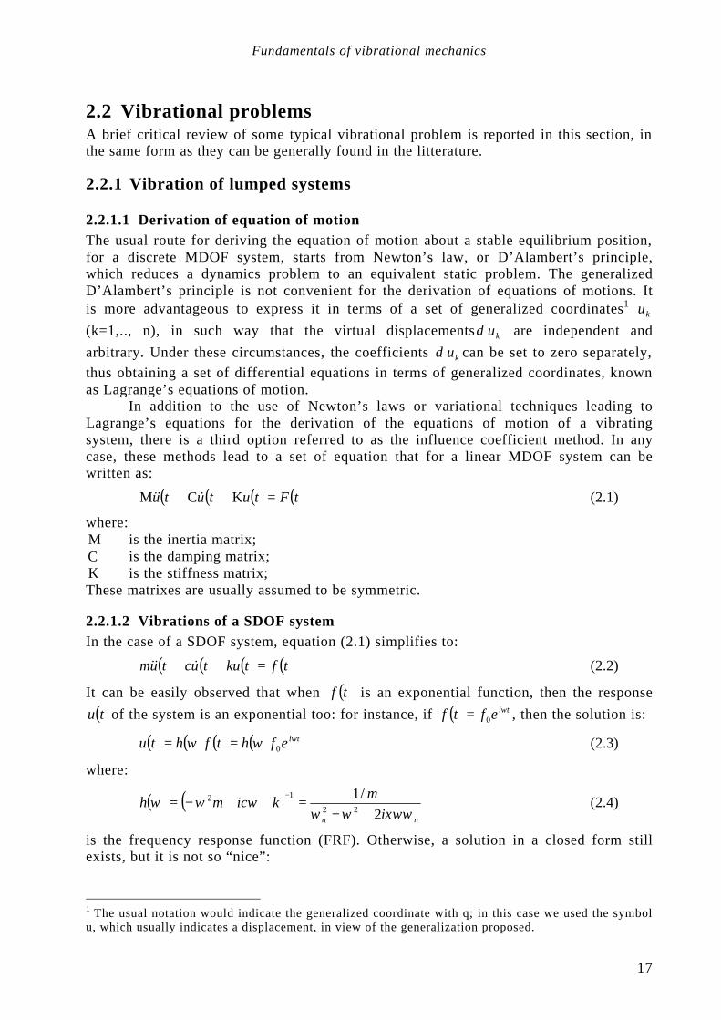
2.2 Vibrational problems A brief critical review of some typical vibrational problem is reported in this section, in the same form as they can be generally found in the litterature.
2.2.1 Vibration of lumped systems
2.2.1.1 Derivation of equation of motion
The usual route for deriving the equation of motion about a stable equilibrium position, for a discrete MDOF system, starts from Newton’s law, or D’Alambert’s principle, which reduces a dynamics problem to an equivalent static problem. The generalized D’Alambert’s principle is not convenient for the derivation of equations of motions. It is more advantageous to express it in terms of a set of generalized coordinates1 ku (k=1,.., n), in such way that the virtual displacements kuδ are independent and arbitrary. Under these circumstances, the coefficients kuδ can be set to zero separately, thus obtaining a set of differential equations in terms of generalized coordinates, known as Lagrange’s equations of motion.
In addition to the use of Newton’s laws or variational techniques leading to Lagrange’s equations for the derivation of the equations of motion of a vibrating system, there is a third option referred to as the influence coefficient method. In any case, these methods lead to a set of equation that for a linear MDOF system can be written as:
( ) ( ) ( ) ( )tFtututu =++ KCM &&& (2.1)
where: M is the inertia matrix; C is the damping matrix; K is the stiffness matrix; These matrixes are usually assumed to be symmetric.
2.2.1.2 Vibrations of a SDOF system
In the case of a SDOF system, equation (2.1) simplifies to:
( ) ( ) ( ) ( )tftkutuctum =++ &&& (2.2)
It can be easily observed that when ( )tf is an exponential function, then the response ( )tu of the system is an exponential too: for instance, if ( ) tieftf ω
0= , then the solution is:
( ) ( ) ( ) ( ) tiefhtfhtu ωωω 0== (2.3)
where:
( ) ( )nn i
mkicmh
ξωωωωωωω
2/1
22
12
+−=++−=
− (2.4)
is the frequency response function (FRF). Otherwise, a solution in a closed form still exists, but it is not so “nice”:
1 The usual notation would indicate the generalized coordinate with q; in this case we used the symbol u, which usually indicates a displacement, in view of the generalization proposed.

Structural damage detection and localization by using vibrational measurements
18
( ) ( ) ( )tfthtu ⊗= (2.5)
where:
( ) iqtteq
th +−= ξω1 (2.6)
represents the response of the system to an impulse (impulse response function IRF), and the operator ⊗ represents the convolution, for which equation (2.4) is also know as convolution integral or Duhamel integral. The convolution of two time functions is defined as:
( ) ( )∫+∞
∞−
−=⊗ τττ dtfhfh (2.7)
The property of an exponential forcing expressed by equation (2.3) suggests interpreting a generic force as a superposition of exponential forces: this is the principle of spectral analysis. Such a change of domain is performed through the Fourier Transform:
( ) ( )∫+∞
∞−
−= dtetfF tiωω (2.8)
and its inverse:
( ) ( ) ωωπ
ω∫+∞
∞−
= deFxf ti
21
(2.9)
Since in the frequency domain an expression exists as follows:
( ) ( ) ( )ωωω FHU = (2.10)
a simple comparison with equation (2.5) demonstrates that IRF in the time domain corresponds to the FRF in the frequency domain, and that a convolution in the time domain correspond to a multiplication in the frequency domain. Actually, to perform a change of domain by exchanging an integral (or differential) operator to an algebraic operator is the essence of spectral analysis.
2.2.1.3 Vibration of MDOF systems
When dealing with a SDOF system, attention was focused on the opportunity of expressing the equation of motion in a domain other than time - the frequency domain - in order to obtain a suitable relation between forcing and response. We use to refer to this process as spectral analysis. In addition to that, MDOF systems deserve further consideration due to the difficulty, which arises from the fact that the equation of motion (2.1) generally represents a set of coupled equations. From a strictly mathematical standpoint, coupled means that not all of the matrixes are diagonal; broadly speaking, it means that the motion of a certain dof inevitably involves the motion of others.
In fact, this condition is not so inevitable as it may appear, but depends only on the choice of the variable system: it can be demonstrated that a change in variable exists:
uu Φ=' (2.11)

Fundamentals of vibrational mechanics
19
such that equation (2.1) remains uncoupled. The matrix Φ , which represent this linear transformation, is called the modal matrix; each column iφ of matrix Φ represents the new ith coordinate expressed in the old domain. Equation (2.11) states the change in variable in the displacement domain. A change in variable in the force space is subjected to the principle that the energy measure must be the same, independently of the coordinate system; we should assume that the following quantity will be conserved:
∫ =><2
1
d,t
t
tuf ∫ +2
1
dt
t
tuf (2.12)
for each 21 , tt . The arbitrariety of the limits of integration implies that also the following quantity must be conserved:
ufuf +>=< , (2.13)
Thus, the coordinate transformation in the force domain is written
'ff +Φ= (2.14)
and a generic linear transformation L modifies
ΨΨ= + LL' It should be remarked that this is a general outcome, which is valid for each change in variable domain, thus not only in the case of the modal matrix. Matrix M , C and K change consequently to:
ΦΦ=′ + MM diag
ΦΦ=′ +CCdiag (2.15)
ΦΦ=′ + KK diag
It is also customary to chose Ψ in such a way as to make M the identity matrix, and in this case we refer to Ψ columns as mass normalized modes. Ψ is generally complex, but simplifies to a real matrix under certain conditions2 that easily suit many practical problems (classically damped systems). Subject to this change in variable, the equation of motion becomes
( ) ( ) ( ) ( )tFtututu diagdiag+Ψ=′+′+ KC' &&& (2.16)
which practically represents a set of uncoupled linear differential equations. Each of these uncoupled equations represent the equation of motion of a SDOF system, which can be solved by using those methods presented in previous paragraph.
2.2.2 Vibration of continuous systems
2.2.2.1 Longitudinal waves in beams
One of the fundamental equations of mechanics is the one-dimensional wave equation given by the following partial-differential equation:
2
22
2
2
x
uv
t
u
∂∂
=∂∂
(2.17)
2 i. e.: (M-1K) (M-1C)=(M-1C) (M-1K)

Structural damage detection and localization by using vibrational measurements
20
where v is the propagation velocity, u is the displacement, t is time and x is space. x
y
z
xNdx
dNN x
x +
zxu dx
duu x
x +
dx
Figure 2.1. Coordinates and displacements for wave motion in an elastic bar.
Some systems, which can be described by this equation, include transverse vibrations of taut strings, rods in longitudinal or torsional vibration, and pressure waves in ideal fluids along an axis of a container. Details of the development of the equations of motion can be found in detail by many authors including Timoshenko and Goodier (1951), Richart, et. al. (1970), and Graff (1975).
A general solution of equation (2.17) is given by:
)()()( 21 vtxuvtxutu ++−= (2.18)
The velocity of propagation of stress waves through infinite elastic media is a function of the material properties of the media, and depends upon the elastic modulus of the material, E, Poisson's ratio ν and the material density ρ. Let us limit our discussion to the case of a finite elastic bar subject to compressive vibration only. The compressive wave velocity, v, (also called plane wave or longitudinal wave velocity) is given by the equation:
ρEA
v = (2.19)
where ρ represents the mass density for unitary length of the axial beam. If the area of the section is constant along the beam, the velocity simplifies to:
ρE
v = (2.20)
Thus the equation of motion could also be written in the following form:
02
2
2
2
=∂∂
−∂∂
x
uE
t
uρ (2.21)
Analogous to the vibrational mode in the case of lumped systems is the concept of stationary wave in the case of continuos systems. We seeks solutions in a form such that the time and position variables are independent:
)()(),( tgxtxu ψ= (2.22)
By substituting into (2.17):
Fundamentals of vibrational mechanics
21
constvgg
=′′
=ψψ2&&
(2.23)
thus with regards to the time-dependent factor we find out: tiAetg ω=)( (2.24)
where as usual ω is defined as the natural pulsation of the system. Analogously, a similar expression should exist for the position-dependent factor:
xiBex αψ =)( (2.25)
where the wavenumber α is introduced. Since both of the following two expressions subsist:
2ω−=ff&&
2αψψ
−=′′
(2.26)
by substituting in (2.23), the following fundamental relation between circular frequency and wavenumber yields:
vωα = (2.27)
which we refer to as the dispersion relation. A similar expression relates the period
ωπ2
=T (2.28)
to the correspondent quantity in the position domain:
kπ
λ2
= (2.29)
which is known as the wavelength. Let us consider the case of a beam fixed at the edges: the boundary condition can be expressed as:
0)()0( == Luu (2.30)
from substitution into (2.24):
kL=nπ (2.31)
The second condition yields:
Lnπ
α = =>nl2
=λ (2.32)
Thus:
Ln
vvkπ
ω == (2.33)
In particular, the fist natural frequency is equal to:
21 lEA
lv
ρπ
πω == (2.34)
Equation (2.33) shows that for a continuous system the number of natural frequencies, and corresponding wavenumbers and eigenvectors ( )xψ , are a numerable infinity. This is different for the discrete system case, where a discrete number of natural frequencies exists.

Structural damage detection and localization by using vibrational measurements
22
2.2.2.2 Vibration in the 3D continuum
This is necessarily a simplified discussion of the vibrational problem in the 3D continuum. Further details can be found in Mierovitch1970 or Gérardin and Rixen 1994.
Reference is made to a linear continuous body, as shown in Figure 2.2. First of all, let us define the fundamental matrix quantities. Vectors u, σ and ε , collect the displacement, stress, and strain components, respectively:
{ }Tuuuu 321= (2.35)
{ }T312312332211 σσσσσσσ = (2.36)
{ }T312312332211 γγγεεεε = (2.37)
with ijij εγ 2= . Let us also define the spatial differentiation operator:
∂∂
∂∂
∂∂
∂∂
∂∂
∂∂
∂∂
∂∂
∂∂
=
123
312
321
000
000
000
xxx
xxx
xxx
DT (2.38)
the associated matrix of the direction cosines of the outward normal:
=
123
312
321
000000
000
nnn
nnn
nnn
N T (2.39)
( )t;xu
( )txf ;
x
1x2x
3x C
Figure 2.2. Model of a 3D continuos system.

Fundamentals of vibrational mechanics
23
and the matrix of the elastic coefficients K ′ pertaining to Hooke's law:
εσ K ′= (2.40)
The equations expressing the local dynamic equilibrium may then be written in matrix form as:
=+=++
00
fN
FDTσσ
σSon
Vin (2.41)
In absence of other external forces, F represents the inertia forces only:
uF &&ρ−= (2.42)
thus (2.41) becomes:
==−+
00
σρσ
TN
uD &&
σSon
Vin (2.43)
Since equation (2.40) can also be written as:
DuKK ′=′= εσ (2.44)
the local dynamic equilibrium expression becomes:
=′=−′+
00
DuKN
uDuKDT
&&ρ
σSon
Vin (2.45)
Since we are seeking harmonic motion solutions, we can write:
=′=+′+
002
DuKN
uDuKDT
ρω
σSon
Vin (2.46)
The corresponding variational form can be expressed as:
( ) ( ) 021
212 =
′− ∫∫ ++
VV
dVDuKDuudVuρωδ (2.47)
The homogeneous system of equations (2.46) and the associated variational form (2.47) defines an eigenvalue problem of the Sturm-Lioville type. Its eigenvalues, of infinite number, are denoted:
K,, 21 ϕϕ (2.48)
K,, 22
21 ωω (2.49)
They verify individually the equations:
=′=+′+
002
iT
iii
DKN
DKD
ψρψωψ
σSon
Vin (2.50)

Structural damage detection and localization by using vibrational measurements
24
2.3 Analogies between different formulations The direct comparison between the different formulations of a vibrational problem previously reported deserves some consideration, with regards to the following aspects:
1. The formulation of the equations of motion 2. The method for uncoupling these equations
2.3.1 Equations of motion Equations of motion are basically a relation between forces on one hand and displacements with correspondent derivatives on the other. Forces and displacements are time-space dependent, i. e. they are defined on a time domain and on a space (or position) domain. Whilst the time domain is practically in all case a continuos domain (even if it is not necessary true, as we are going to remarked in 2.4), the formulations differs in the space domain only.
Inside these equilibrium equations, is possible to distinguish terms common to each formulation: • a term dependent on the displacements (usually referred to as elastic forces); • a term dependent on the velocities (usually referred to as damping forces); • a term dependent on the accelerations (usually referred to as inertia forces); • a term independent on all these (usually referred to as external forces).
It is also possible to distinguish those operators which relate displacements,
velocities and accelerations to elastic, damping and inertia forces, and we will name them stiffness, damping and inertia operators. These actually coincide with stiffness, damping and inertia matrixes in the case of MDOF systems; in the case of SDOF system, we are dealing with coefficients; in the case of continuos systems, we are generally dealing with differential operators.
A correspondence subsists between the order of the differential operators, the diagonalization condition of the matrices and the argument of the coefficients, as summarized in the following table.
SDOF MDOF continuos
coefficient matrix operator real positive diagonal algebric
imaginary or negative not diagonal differential imaginary tri-diagonal skew-
symmetric first order differential
real negative tri-diagonal symmetric second order differential
Table 2.1. Analogies between operators.
A detailed comparison between the equations of motion of the different vibrational problems is reported in Table 2.2.
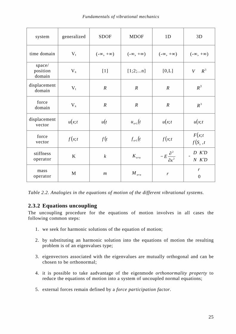
Fundamentals of vibrational mechanics
25
system generalized SDOF MDOF 1D 3D
time domain Vt (-∞, +∞) (-∞, +∞) (-∞, +∞) (-∞, +∞)
space/ position domain
Vx [1] [1;2;...n] [0,L] 3RV ⊂
displacement domain Vt R R R R3
force domain Vx R R R 3R
displacement vector
( )txu ; ( )tu ( )tun 1× ( )txu ; ( )txu ;
force vector ( )txf ; ( )tf ( )tf n 1× ( )txf ;
( )( )
tSf
txF
,;
σ
stiffness operator K k nnK ×
2
2
xE
∂∂
− -
′′
+
+
DKN
DKD
mass operator M m nnM × ρ
0ρ
Table 2.2. Analogies in the equations of motion of the different vibrational systems.
2.3.2 Equations uncoupling The uncoupling procedure for the equations of motion involves in all cases the following common steps:
1. we seek for harmonic solutions of the equation of motion; 2. by substituting an harmonic solution into the equations of motion the resulting
problem is of an eigenvalues type; 3. eigenvectors associated with the eigenvalues are mutually orthogonal and can be
chosen to be orthonormal; 4. it is possible to take aadvantage of the eigenmode orthonormality property to
reduce the equations of motion into a system of uncoupled normal equations; 5. external forces remain defined by a force participation factor.

Structural damage detection and localization by using vibrational measurements
26
A detailed comparison between the expression of orthogonality conditions and force participation factor in different vibrational problems is reported in Table 2.3.
system generalized SDOF MDOF
orthogonality conditions 2,
,
iijij
ijij
K
M
ωδφφ
δφφ
>=<
>=<
1=mm 2ω=mk 2
iijij
ijij
K
M
ωδφφ
δφφ
=
=+
+
force participation
factor >< fi ,φ
mf fi
+φ
system generalized 1D 3D
orthogonality conditions 2,
,
iijij
ijij
K
M
ωδφφ
δφφ
>=<
>=<
2
02
2*
0
*
iij
Li
j
ij
L
ij
dxx
E
dx
ωδφ
φ
δφρφ
=∂∂
−
=
∫
∫
2iij
V
ij
ij
V
ij
dVDKD
dV
ωδφφ
δφρφ
=′−
=
∫
∫
++
+
force participation
factor >< fi ,φ ∫
L
i fdx0
*φ ∫∫ ++ +σ
φφS
i
V
i fdSFdV
Table 2.2. Analogies in the equations of motion of different vibrational systems.
Fundamentals of vibrational mechanics
27
2.4 A generalized formulation for vibrational analysis problems
2.4.1 Equations of motion Reference is made to a general linear mechanical system, about its stable equilibrium position. Forces f and displacements u are the time-space dependent generalized vectors, defined on metric spaces
uVu ∈ fVf ∈ (2.51)
i. e. both provided with an internal operator:
RVuu →>< 2:...,... RV ff →>< 2:...,... (2.52)
In addition, an operator is defined, provided with the analogous properties:
RVV fu →×>< :...,... (2.53)
Time is defined on:
( )+∞∞−≡∈ ,tVt (2.54)
and space on:
xVx ∈ (2.55)
which could be indifferently discrete, continuous or both. The equation of motion can be written:
( ) ( ) ( ) ( )txftxutxutxu ,,K,C,M =++ &&& (2.56)
where: K is the stiffness operator, which relates elastic forces to displacements; C is the damping operator, which relates damping forces to velocities; M is the inertia operator, which relates inertial forces to accelerations. In the undamped case, equation (2.56) simplifies to:
( ) ( ) ( )txftxutxu ,,K,M =+&& (2.57)
2.4.2 Equations uncoupling We seek distributions of displacement such that the following is satisfied:
( ) ( ) tiext;xu ωϕ= (2.58)
and we define these eigenvetors. By substituting (2.3.3), we obtain
( ) ( ) ( ) ( )ωϕϕωϕω ,2 xfxKxCixM =++− (2.59)
The homogeneous problem derived from (2.59) is a classical eigenvalue problem. The solution exists in the complex domain. For our proposes, it is more worthwhile to consider the undamped case:
( ) ( ) ( )ωϕϕω ,2 xfxKxM =+− (2.60)

Structural damage detection and localization by using vibrational measurements
28
In such case, it is possible to demonstrate that a finite number, or a numerable infinity of real solutions:
K,, 22
21 ωω (2.61)
with associated eigenvectors
K,, 21 φφ (2.62)
exist. The eigenvectors satisfy the orthogonality properties, both with respect to the inertia and the stiffness operators:
2,
,
iijij
ijij
K
M
ωδφφ
δφφ
>=<
>=< (2.63)
It is possible to take advantage of the eigenmode orthogonality property to reduce the equations of motion into a system of uncoupled normal equations. Any displacement field of the system may be expressed as:
( ) ( ) ( )xtutxu ii
i φα∑= ,, (2.64)
Substitution of (2.64) in (2.60) yields
( ) ( ) ( ) ( ) ( )txfxtuxtu ii
iii
i ,,K, =+ ∑∑ φαφα&& (2.65)
Premultiplying each member by jφ , the internal product, one finds:
( ) ( ) ( ) ( ) ( ) >>=<<+>< ∑∑ txfxtKuxtuM jii
ijii
ij ,,,,,, φφαφφαφ && (2.66)
Considering the orthogonality property of eigenvectors (2.63), equation (2.66) simplifies to:
( ) ( )tftu jjj ,, 2 αωα =+&& (2.67)
where the force participation factor
( ) ( ) >=< txftf jj ,,, φα (2.68)
is defined. Equation (2.67) represents a set of uncoupled equations of motion, finite or infinite, depending on the considered space domain Vx.
In a compact form, (2.64) one can also write
( ) ( )tutxu ,, αΦ= (2.69)
where
( ) ( ) ( ){ }Ttututu ,...,,,, 21 ααα = (2.70)
is the generalized normal coordinates vector, while Φ is named the modal operator. In an analogous way, a generalized force participation vector is defined, related to the force vector by:
( ) ( )txftf ,, +Φ=α (2.71)
The operator +Φ satisfies the following expression:
>>=<ΦΦ< + ufuf ,, uf ,∀ (2.72)
for which reason it is named the transposed-conjugated modal operator.
Fundamentals of vibrational mechanics
29
2.5 Further developments
2.5.1 Analogies between spectral and modal analysis Time domain presents the following inconvenience: that what happens in a certain instance produces effects on what will happen in the following instances. Apparently, this is only a trivial observation: Basically, the procedure of spectral analysis can be interpreted as a change in variable, from time to frequency. This transformation can be operated both in the displacement space and the force space: in each case, the operators that provide the transformation from time domain to frequency domain, and viceversa, are the Fourier Transform and the Inverse Fourier Transform. This could be shown in the following scheme:
( ) ( )ω,, 1 xutxuF
F
←→
− ( ) ( )ω,, 1 xftxfF
F
←→
− (2.73)
In the same way, modal analysis performs a change in coordinates, from spacial coordinates to modal coordinates (i. e. to the wavenumbers space in the case of continuous systems). But, the operators are different in the case of displacements and forces, as previously shown:
( ) ( )tutxu ,,1
α←→Φ
Φ−
( ) ( ) ( )tftxf ,, 1 α ←→
−+
+
Φ
Φ
(2.74)
Even if the analogy is evident, many differences can be noted: 1. In the case of spectral analysis, the transformation is the same both for forces
and displacements, while in the case of modal analysis, the transformation of the force is the transpose of one related to the displacement.
2. Fourier transforms perform a change from a continuous domain (time) to another continuous domain (frequency), while modal operators usually perform a change from a discrete or continuous domain to a discrete domain.
We want to show that these are only apparent differences, i. e. that spectral analysis and modal analysis are exactly the same operation. The relations are formally the same when we define the correspondence
Φ⇔−1F (2.75)
and we notice that: +− = FF 1 (2.76)
Observation 2 is an immediate consequence of an implicit assumption we use to introduce to treat the vibrational problem: that the time of interest in the vibrational phenomenon is continuous and infinite while the space is restricted to a discrete number of points (discrete systems) or at last to a limited portion of the continuum. These different ways to model time and space are merely a cultural heritage, but ignored in practice. For example in experimental analysis, the time of the phenomenon is limited to the length of the acquisition 1T . Therefore, the frequency domain is actually discrete, with a solution equal to:
1
2Tπ
ω =∆ (2.77)

Structural damage detection and localization by using vibrational measurements
30
Also, digital data acquisition operates with actual discretization in the time domain, which corresponds to a limited frequency domain. In conclusion, even if we are used to considering time and frequency as continuous and infinite domains, in practice, these are discrete and finite. On the other side, no restriction is posed in modeling the space as a continuous and infinite domain.
2.5.2 A time-space domain based formulation According to the previous discussion, a time-space domain based formulation for the vibrational problem is introduced. The same relation as (2.56) can be rewritten in the more compact form:
( ) ( )xfxu =R (2.78)
where: R is the dynamic stiffness operator, x denotes, in this case, the time-space variable. Forces and displacements are in fact defined in a domain which is a sub space of the cronotopos:
tx VVx ×∈ (2.79)
By resolving the eigenvectors problem associated with (2.78), we perform the uncoupling of the equation of motion both in space and time, at the same time. Therefore, the operator Φ results a combined modal/spectral operator.
Damage localization problems
31
3 Damage localization problems Abstract The problem of localization is analyzed from a methodological point of view. Using the general formulation of the problem as a basis, some variations to the classic techniques of localization based on modal parameter changes are proposed. Some experimental outcomes highlight how modal damping is the most sensitive parameter to the formation of a crack. Two new damage detection/localizing techniques are therefore proposed: the first one assumes specific damping changes as a damage index; the second one aims to detect the appearance of Coulomb friction damping in the damaged structures. Sommario Il problema della localizzazione del danno è analizzato dal punto di vista metodologico. Partendo da una formulazione generale del problema, vengono proposte alcune modifiche alle classiche tecniche basate sulle variazioni di parametri modale. Alcuni risultati sperimentali hanno mettono in luce che lo smorzamento modale è il parametro più sensibile alla formazione di una fessura. Pertanto, viene proposta due nuove tecniche di identificazione/localizzazione del danno: la prima utilizza le variazioni di smorzamento specifico come indice di danno; la seconda mira a identificare la comparsa nelle strutture danneggiate di smorzamento per attrito secco alla Coulomb.
Structural damage detection and localization by using vibrational measurements
32
3.1 Introduction The likely presence of damage can be recognised quite simply on the basis of anomalies in the dynamic response. However, giving more precise information about the position and nature of the damage is more complicated. Cawley and Adam (1979), initially proposed investigating the location of damage in a two-dimensional structure on the basis of changes in natural frequency. Their contribution was the first in a series of publications that are now literally uncountable, regarding the frequency approach – a review can be found in Salawu (1997). In reality, the use of frequencies only is very restricted, which makes a practical application difficult. Detailed localization requires the measurement and recognition of numerous modal frequencies, which are technically complicated to obtain in practice. In a symmetrical structure, changes in frequency are identical for damage in a symmetrical position. Generally, frequency is a parameter, which is not particularly sensitive to damage. Above all, it should be noted that, if it is true that the presence of damage causes a variation in frequency, the opposite is not necessarily true. That is, there may be other reasons for frequency changes in a structure (variations in temperature, constraint conditions…). Farrar and Doebling (1998) showed how, in the case of a bridge, the fundamental frequency presented changes on the order of 5% over a 24-hour period. These considerations have progressively moved researchers’ attention towards the study of mode shapes. The first approaches were based on a direct comparison between shapes, in terms of displacement, using MAC index, originally introduced by Allemang and Brown (1982) to correlate shapes, and the COMAC index, introduced by Lieven and Ewins (1998). Pandey et al. (1991) take credit for demonstrating that, in the classic case of the beam, expressing mode shapes in terms of curvature makes it immediately possible to recognize the position of damage, in that a change in curvature is directly linked to a loss of local stiffness. Yao et al. (1992) arrived at a similar observation independently, introducing the concept of strain mode shape for a frame structure. Instead the analysis of modal damping has been ignored in localization problems, even if many authors recognize that this, like other measures, can be used in damage detection. However, numerous studies on the dynamic behaviour of r.c. and p.r.c. structures note the importance. Bachmann (Bachmann and Dieterle 1981, Mahrenholtz and Bachmann 1991), have underlined how cracking radically modifies the dissipative mechanisms in a r.c. structure, also proposing an interpretative model. Hop (1991) studied the dependence of damping on the degree of prestressing. Some direct experience of the authors (Beolchini et al. 1996) also confirms these observations. Studies concerning localization of damage in a r.c. structure are limited to the approaches of frequency and shape. Casas (Casas 1994, Casas and Aparicio 1994), measures significant changes in modal damping in a series of r.c. beams after cracking; however, this information is not used in localizing the damage. Also, Vestroni and Capecchi (1996) prefer the frequency approach in a similar experience. In light of the above-mentioned considerations, the problem of localization is first analyzed from a methodological point of view. Techniques based on the measurement of frequencies and shapes are then reformulated in a more general form, and a new approach exploiting damping changes is proposed. In this contribution, the study of damage localization is limited to the use of the classic modal parameters (frequency, shape and damping) as measures for detecting the presence of damage.

Damage localization problems
33
3.1.1 A methodological approach to the localization problem It is possible to carry out the damage localization procedure according to the following logical sequence: 1. Identification of dynamic measures that express damage at a global level (e.g. change in modal parameters, non-linearity indices...); 2. Modeling damage at a local level and defining the local indicators δ (e.g. local changes in stiffness, structural discontinuity, local changes in viscosity); 3. Choice of a relation that connects global measures z to local damage parameters δ
( )δFz = (3.1)
4. Calculation of local damage parameters by solution of the inverse problem. This logical procedure is always implicit in the methods proposed in the literature. While it is not necessary to review in detail the numerous localization techniques proposed, it is useful to make some observations on how the choice of parameters and measurements is normally made.
3.1.2 Identification of dynamic measures On the basis of the choice of measures to detect damage at a global level, it is possible to distinguish: • Techniques based on the identification of changes in response, generally expressed in the classical modal parameters (frequency, shape, damping), regarding the configuration of a known, and conventionally intact, model. In this case, damage is revealed by a difference in behavior of two structures, which on the basis of the response only could not be declared intact or damaged. • Techniques based on the identification of anomalies, usually a slight non-linearity, in the structural response. In this case, it is the presence of the anomaly that indicates damage. It is worth noting that the second approach is much less frequent in proposals for damage detection, and it would appear that it has never been used in localization problems.
3.1.3 Identification of local damage indicators The choice of damage indicators, like dynamic measures, could be more varied, and make reference to changes in stiffness or viscosity, the presence of local hysteretic and/or non-linear mechanisms. In reality, there do not appear to be any proposals of this type that do not make reference to changes in stiffness.
3.1.4 Choice of relation The relation which links damage indicators to dynamic measurements in structural problems is usually a deterministic mechanical model (for example a FEM), with parameters in the same damage indices (but it could also be a physical model or a black box model, or an empirical relation). A common classification distinguishes model-based and non-model-based methods. The relation is generally non-linear and explicitly non-invertible and the solution of the inverse problem normally implies great computational cost. The existence and unity of the solution cannot generally be guaranteed (in other words the problem is ill-posed).
Structural damage detection and localization by using vibrational measurements
34
When the relation is assumed to be linear, expression (3.1) becomes a simple linear algebraic system:
δDz = (3.2)
where D represents the sensitivity matrix. The solution exists and is unique only if the columns of D are linearly independent, and if the number of the measures equals the number of parameters. If instead, the number of measures is greater then there is a single δ that minimizes the quadratic norm of the residual:
( ) ( )δδδ DzDzDz −−=− + (3.3)
and therefore there is a least squares solution:
( ) zDDD1 +−+=δ (3.4)
The linearity of the relation drastically simplifies the computational time necessary for inversion, which is in fact reduced to the solution of a linear system or to the inversion of a matrix of limited dimensions. The choice of a linear relation can be justified in an appropriate choice of parameters and measures, or as the linearization of a non-linear relation, or it is simply an arbitrary choice.
3.2 Changes in modal shapes and frequencies related to changes in stiffness
A system with frequencies and mode shapes is given.
mn ......xx ωωφφ 110KM ⇒=+&& (3.5)
where, as usual, M represents the mass matrix, K the stiffness matrix and x is the displacement vector. sφ represent the sth mode shape, associated with the sth frequency
sω . Damage is modeled as a change in stiffness K∆ , which is a linear function of a vector of parameters δ that quantify damage at a local level (damage indicators vector):
nn... KKKK 2211 δδδ +++=∆ (3.6)
Changes in sth frequency and mode shape are linked to damage in the following expression:
( )( ) ( ) ( )ssssss φφωωφφ ∆+∆+=∆+∆+ MKK 22 (3.7)
It is evident that the relation is typically non-linear. The idea is to express modal parameters and damage indicators in a form that makes this relation as easy as possible.
3.2.1 Changes in frequency First of all, we propose to verify if, and in what conditions, it is possible to write a linear relation between an expression as a function of the only a change in frequency and an expression as a function of only a change in stiffness. We wonder, therefore, if two functions exist such that:
( ) ( )( )δω K∆∝∆ hg (3.8)
The first consideration, although not always taken into account, is to observe that it is possible to have:
δω ∝∆ 2s (3.9)
when, for example, the sth mode shape does not vary and more generally when:
Damage localization problems
35
ss || φφ KK ∆ (3.10)
In this case, let's say that K∆ is parallel to K for the sth mode. More complex is to define stiffness in series. Consider the problem of eigenvalues:
( ) 0A2 =+− ss ψαω (3.11)
where 1K−=α is called the flexibility matrix and 1MA −= is called the inertance matrix. We are dealing with a problem associated to the direct problem of research of vibration modes, which is derived from integration of the equation of motion written in terms of forces, instead of displacement. It is easy to verify that the eigenvalues of the two problems, direct and associated, coincide while the eigenvector sψ represents the distribution of forces associated with the deformation sφ . Now, if:
ss || αψαψ ∆ (3.12)
K∆ associated to α∆ , is defined as in series for the sth mode. In this case, if the damage is limited, we can write:
δδδ
ω111
2≈
+∝∆
j
(3.13)
Note that this approach generalizes and confirms the same findings of Pandey and Biswas (1994) in the case of a beam with concentrated damage. In fact, in this case, the change in stiffness associated with such damage suites the hypothesis of stiffness in series quite well, as the mode shape varies considerably in terms of displacement or local deformation, but little in terms of forces.
3.2.2 Changes in mode shape We now need to find an expression of the mode shape that makes the relation between variation of shape and stiffness very simple. Ignoring higher order terms, expansion of (3.7) leads to:
( ) sisis φωφωφ ∆−+∆=∆ KMMK 22 (3.14)
Suppose a change of variable exists:
xx ′= S (3.15)
which diagonalizes K:
KKSS ′=+ (3.16)
and at the same time
δ∀′∆=∆+ KKSS (3.17)
If the stiffness matrix can be expressed as a linear combination of the acceptable damage matrices, it is possible to choose the damage indices in such a way that:
n... KKKK 21 +++= (3.18)
where it is natural to choose the transformation for which:
IKSS =+ ( )idiag δ=∆+ KSS (3.19a,b)
In this case (14) becomes a particularly simple explicit expression:
Structural damage detection and localization by using vibrational measurements
36
( )isjsijsiis
i φφωφωφ
δ ′∆−′∆′+′′∆′
= ij2
ij2 mm
1 (3.20)
It can be noted that the change of variable, that diagonalizes K, makes M generally not diagonal. The resulting expression generalizes both the concepts of strain mode shape (Yao et al. 1992) and curvature mode shape (Pandey et al. 1991). In fact S usually represents the linear transformation that links the displacement to the strain. For example, in the case of the vibrating beam, S links displacements to curvatures, and therefore is the inverse of
( )
−−
−
=−
OM
L
210121012
1S 2
1
EJh (3.21)
where (EJ) represents the bending stiffness, and h the distance between two successive measurement points on the axis of the beam.
Damage localization problems
37
3.3 Changes in damping mechanism The presence of damage alters the energy dissipation mechanism in a structure: the direct consequence is that the damaged structure presents higher modal damping rates. This change is particularly significant in the case of RC structures, where damage is usually associated with the formation of a crack. Many experience shows how these variations are in the order of 100% of the values measured in uncracked structures, hence modal damping represents a very sensitive parameter to discriminate damaged from undamaged structures. Since changes in dissipation properties is generally due to a localized modification in the characteristics of the damaged structures, we can expect that this modification affects in different ways each vibration mode. This is at the basis of the localization methods as follows.
3.3.1 Changes in modal damping In the case of a system with viscous damping, the modal damping ratio can be expressed as:
ss
ssss φφ
φφωξ
KC
2 +
+
= (3.22)
but more generally it can be interpreted as a ratio of dissipated energy in a cycle and the maximum potential energy of the system (Dieterle and Bachmann 1981):
ss
D
P
Ds
EE
Eφπφπ
ξK24 +== (3.23)
The same expression can be written, with reference to the vibration mode, for an ith portion of the vibrating system:
sis
i,D)i( E
φπφξ
K2 += (3.24)
and in this case )i(ξ assumes the meaning of specific damping ratio. Given a group of subsystems that satisfies (18), for each vibration mode, it is necessary that:
∑=i i,DD EE (3.25)
for which:
∑ +
+
=i
)i(
ss
siss ξ
φφφφ
ξKK
(3.26)
The presence of a crack in the ith element of the system generally leads to the formation of a local dissipative mechanism which induces an increase in specific damping, and therefore in the local damping ratio. In the simplified hypothesis where damage does not degrade the stiffness of the system, one can write:
∑ +
+
=∆i i
ss
siss δ
φφφφ
ξKK
(3.27)
where: )i(
i ξδ ∆= (3.28)

Structural damage detection and localization by using vibrational measurements
38
represents the damage index.
3.3.2 SDOF oscillator with Coulomb friction In previous paragraph, we have assumed that the energy dissipation model in both a damaged and undamaged structures is linear viscous.
3.3.2.1 Viscous model
The viscous model for a SDOF system is usually represented by means of a viscous dashpot as shown in Figure 3.1(a). The restoring force of such a viscous device is represented in Figure 3.1(b). In the case of sinusoidal oscillation x = a sinω t, the dissipated energy for a cycle is therefore:
∫∫ =⋅⋅=−=∆T
v acdtdtdx
xcdxxFE0
2)( ωπ&& (3.29)
F
c
k
x
F
a-a
cωa
-cωa
Figure 3.1. Viscous damping model (a) and restoring force (b) for a harmonic oscillation.
The oscillation amplitude follows, in the free response, the well-know exponential law, as it is represented in Figure 3.2:
( ) teata ξω−= 0 (3.30)

Damage localization problems
39
Figure 3.2. Free response of a viscous damped oscillator.
3.3.2.2 Coulomb friction damping model
The presence of dry friction in a SDOF system can be represented by a hysteretic dashpot. This reacts with a restoring force, which is constant in amplitude and depends only on the direction of motion:
xx
FF C &
&−= (3.31)
Therefore, the equation of motion of the system is:
0=++ kxxx
Fxm C &
&&& (3.32)
or mass normalized
02lim
2 =++ xxx
xx ωω&
&&& (3.33)
where the limit displacement is defined:
k
Fx C
lim = (3.34)
as xlim represents the limit displacement in static equilibrium. Equation 3.33 is typically non linear. An exact solution could be obtained through numerical integration (Inaudi and Makris 1996, Tomlinson and Hibbert 1979). For our purposes, simple energetic considerations are enough. Figure 3.3(b) shows a typical hysteretic cycle for a friction-damped oscillator.

Structural damage detection and localization by using vibrational measurements
40
Fk
FC
Fk
FC -FC
a-a
FC xlim
x
F
Figure 3.3. Viscous damping model (a) and restoring force (b) for a harmonic oscillation.
in the case of the friction device the dissipated energy gives
aFdx)x(FE Cf 4=−=∆ ∫ & , (3.35)
and this expression is true whatever the time history of the system, as long as a cycle is characterised by no more than two zero-crossing velocities. The energy dissipation is proportional to the vibrational amplitude; therefore, we can expect that the amplitude decay is linear (a complete treatment can be found in Tomlinson and Hibbert 1979), as shown in Figure 3.4. In particular, the decay law is described by the following equation:
( ) txata lim0
2ω
π−= (3.36)
It should be noted that, according to (3.36), the oscillation stops after a finite time, different from the viscous damping model case.
Figure 3.4. Free response of a Coulomb friction damped oscillator.
Damage localization problems
41
3.3.2.3 Combined damping model
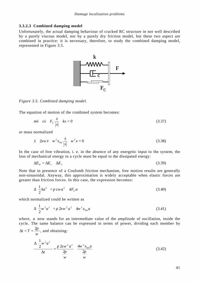
Unfortunately, the actual damping behaviour of cracked RC structure in not well described by a purely viscous model, nor by a purely dry friction model, but these two aspect are combined in practice: it is necessary, therefore, to study the combined damping model, represented in Figure 3.5.
Fc
k
FC
Fc
k
FC
Figure 3.5. Combined damping model.
The equation of motion of the combined system becomes:
0=+++ kxxx
Fxcxm C &
&&&& (3.37)
or mass normalized
02 22 =+++ xxx
xxx lim ωωξω&
&&&& (3.38)
In the case of free vibration, i. e. in the absence of any energetic input to the system, the loss of mechanical energy in a cycle must be equal to the dissipated energy:
fvm EEE ∆+∆=∆ (3.39)
Note that in presence of a Coulomb friction mechanism, free motion results are generally non-sinusoidal. Anyway, this approximation is widely acceptable when elastic forces are greater than friction forces. In this case, the expression becomes:
aFacka C421 22 +=
∆ ωπ (3.40)
which normalized could be written as
axaa lim22222 42
21
ωξωπω +=
∆ (3.41)
where, a now stands for an intermediate value of the amplitude of oscillation, inside the cycle. The same balance can be expressed in terms of power, dividing each member by
ωπ2
==∆ Tt , and obtaining:
ωπ
ω
ωπ
ξωπω
24
222
1222
22
axat
alim+=
∆
∆
(3.42)
Structural damage detection and localization by using vibrational measurements
42
simplifying and taking the limit:
axadt
ad
limωπ
ξω22
1
2
2
+=
(3.43)
and since
adaad =
2
21
(3.44)
the fundamental relation is derived as follows:
limxadtda
ωπ
ξω2
+= (3.45)
Let us define the friction amplitude:
limf xa ⋅⋅
=ξπ
2 (3.46)
so that the previous expression simplifies to:
( )faadtda
+= ξω (3.47)
By separating the variables:
dtaa
da
f
⋅⋅=+
ωξ (3.48)
by integrating both of the terms:
∫ ∫⋅=+
a
a
t
f
dtaa
da
0 0
ωξ (3.49)
taa
aalog
f
f ξω−=+
+
0
(3.50)
t
f
f eaa
aa ⋅⋅−=+
+ ωξ
0
(3.51)
and finally
( ) ft
f ae)aa(ta −⋅+= ⋅⋅− ωξ0 (3.52)
Equation 3.52 shows how the amplitude decay in the combined damping model is still exponential, with the difference for the amplitude does not tend to zero, but to a negative value, equal to the friction amplitude fa (Figure 3.6).
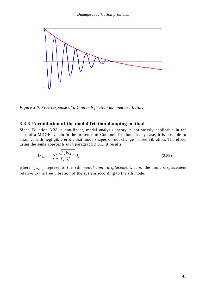
Damage localization problems
43
Figure 3.6. Free response of a Coulomb friction damped oscillator.
3.3.3 Formulation of the modal friction damping method Since Equation 3.38 is non-linear, modal analysis theory is not strictly applicable in the case of a MDOF system in the presence of Coulomb friction. In any case, it is possible to assume, with negligible error, that mode shapes do not change in free vibration. Therefore, using the same approach as in paragraph 3.3.1, it results:
( ) ∑ +
+
=i i
ss
sisslimx δ
φφ
φφ
K
K (3.53)
where ( )slimx represents the sth modal limit displacement, i. e. the limit displacement relative to the free vibration of the system according to the sth mode.

Structural damage detection and localization by using vibrational measurements
44
45
4 Analysis of dispersion phenomena Abstract Recent dynamic tests both on uncracked and on cracked prestressed reinforced concrete elements highlight the presence of a beat in the free response of damaged specimens. It consists of a frequency splitting in the frequency domain. As the modal components associated with each peak are substantially the same, it is not a simple modal coupling. The frequency splitting seems to be connected to the free response only, as it appears in the FRFs obtained from shock tests but not in those obtained by means of stepped sinusoidal tests. Various experiences mirror that the above-mentioned phenomenon is not limited to a particular material or structural system, but it is typical of a cracked structure of reinforced concrete or masonry while it is absent in undamaged structures. The authors demonstrate that the frequency splitting phenomenon can be described through a linear model. In detail, it suffices to admit the presence of an imaginary damping in a SDOF system while it is necessary to admit that the medium or a localized portion of it, is dispersive in a strict sense for a continuous system. This phenomenon is easily recognizable and appears with regularity, thus its knowledge can be of great value if adopted in damage detection problems. Sommario Una recente sperimentazione dinamica su elementi in c. a. p., integri e fessurati, ha messo in evidenza la comparsa di un battimento nella risposta libera dei provini danneggiati, a cui corrisponde uno sdoppiamento del picco di frequenza nel dominio delle frequenze (frequency splitting). Le componenti modali associate a ciascuno dei picchi sono sostanzialmente le stesse, per cui non si tratta di un semplice accoppiamento modale. Lo sdoppiamento del picco sembra essere in relazione solo con la risposta libera, dal momento che compare solo nelle FRF ottenute tramite shock test, ma non in quelle ottenute tramite eccitazione stazionaria. Altre esperienze mostrano come il fenomeno descritto non sia peculiare del materiale o del sistema strutturale, ma è tipico di una struttura fessurata in c. a. o muratura, ed è assente nelle strutture integre. Con questo contributo gli autori intendono mostrare come sia possibile descrivere il fenomeno del frequency splitting con un modello lineare. In particolare, nel caso di un oscillatore semplice, è sufficiente ammettere la presenza di uno smorzamento immaginario; nel caso di un sistema continuo, è necessario ammettere che il mezzo, o una porzione localizzata di esso, sia dispersivo in senso stretto. Questo fenomeno è facilmente riconoscibile, ed appare con regolarità: pertanto potrebbe essere utilizzato proficuamente nei problemi di identificazione del danno.
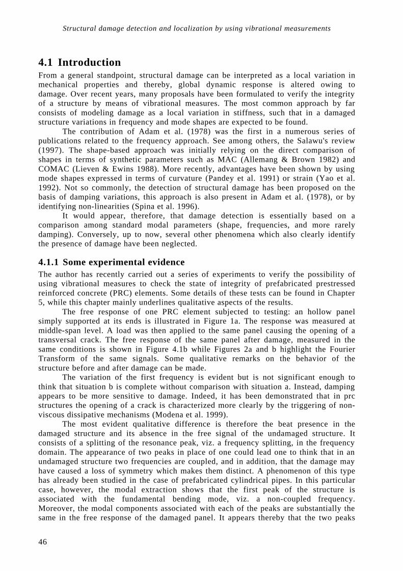
Structural damage detection and localization by using vibrational measurements
46
4.1 Introduction From a general standpoint, structural damage can be interpreted as a local variation in mechanical properties and thereby, global dynamic response is altered owing to damage. Over recent years, many proposals have been formulated to verify the integrity of a structure by means of vibrational measures. The most common approach by far consists of modeling damage as a local variation in stiffness, such that in a damaged structure variations in frequency and mode shapes are expected to be found.
The contribution of Adam et al. (1978) was the first in a numerous series of publications related to the frequency approach. See among others, the Salawu's review (1997). The shape-based approach was initially relying on the direct comparison of shapes in terms of synthetic parameters such as MAC (Allemang & Brown 1982) and COMAC (Lieven & Ewins 1988). More recently, advantages have been shown by using mode shapes expressed in terms of curvature (Pandey et al. 1991) or strain (Yao et al. 1992). Not so commonly, the detection of structural damage has been proposed on the basis of damping variations, this approach is also present in Adam et al. (1978), or by identifying non-linearities (Spina et al. 1996).
It would appear, therefore, that damage detection is essentially based on a comparison among standard modal parameters (shape, frequencies, and more rarely damping). Conversely, up to now, several other phenomena which also clearly identify the presence of damage have been neglected.
4.1.1 Some experimental evidence The author has recently carried out a series of experiments to verify the possibility of using vibrational measures to check the state of integrity of prefabricated prestressed reinforced concrete (PRC) elements. Some details of these tests can be found in Chapter 5, while this chapter mainly underlines qualitative aspects of the results.
The free response of one PRC element subjected to testing: an hollow panel simply supported at its ends is illustrated in Figure 1a. The response was measured at middle-span level. A load was then applied to the same panel causing the opening of a transversal crack. The free response of the same panel after damage, measured in the same conditions is shown in Figure 4.1b while Figures 2a and b highlight the Fourier Transform of the same signals. Some qualitative remarks on the behavior of the structure before and after damage can be made.
The variation of the first frequency is evident but is not significant enough to think that situation b is complete without comparison with situation a. Instead, damping appears to be more sensitive to damage. Indeed, it has been demonstrated that in prc structures the opening of a crack is characterized more clearly by the triggering of non-viscous dissipative mechanisms (Modena et al. 1999).
The most evident qualitative difference is therefore the beat presence in the damaged structure and its absence in the free signal of the undamaged structure. It consists of a splitting of the resonance peak, viz. a frequency splitting, in the frequency domain. The appearance of two peaks in place of one could lead one to think that in an undamaged structure two frequencies are coupled, and in addition, that the damage may have caused a loss of symmetry which makes them distinct. A phenomenon of this type has already been studied in the case of prefabricated cylindrical pipes. In this particular case, however, the modal extraction shows that the first peak of the structure is associated with the fundamental bending mode, viz. a non-coupled frequency. Moreover, the modal components associated with each of the peaks are substantially the same in the free response of the damaged panel. It appears thereby that the two peaks
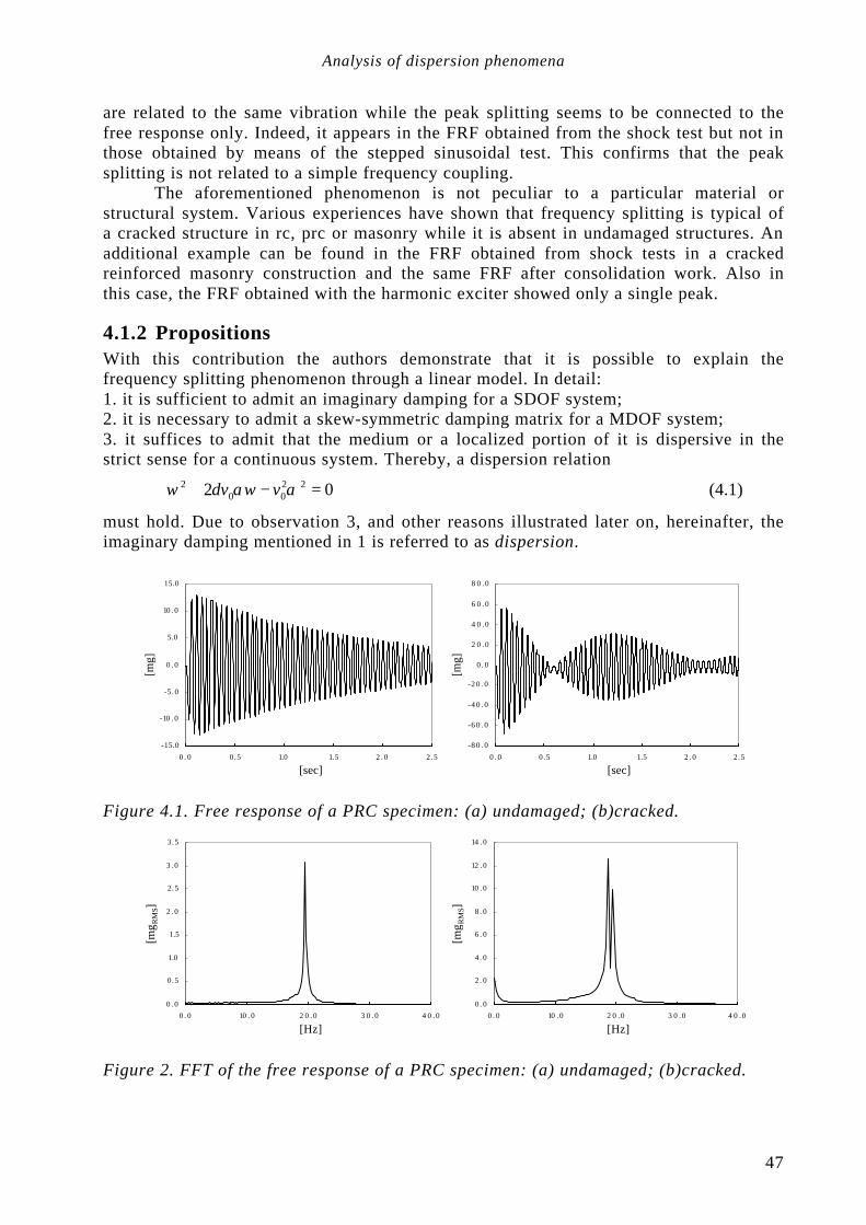
Analysis of dispersion phenomena
47
are related to the same vibration while the peak splitting seems to be connected to the free response only. Indeed, it appears in the FRF obtained from the shock test but not in those obtained by means of the stepped sinusoidal test. This confirms that the peak splitting is not related to a simple frequency coupling.
The aforementioned phenomenon is not peculiar to a particular material or structural system. Various experiences have shown that frequency splitting is typical of a cracked structure in rc, prc or masonry while it is absent in undamaged structures. An additional example can be found in the FRF obtained from shock tests in a cracked reinforced masonry construction and the same FRF after consolidation work. Also in this case, the FRF obtained with the harmonic exciter showed only a single peak.
4.1.2 Propositions With this contribution the authors demonstrate that it is possible to explain the frequency splitting phenomenon through a linear model. In detail: 1. it is sufficient to admit an imaginary damping for a SDOF system; 2. it is necessary to admit a skew-symmetric damping matrix for a MDOF system; 3. it suffices to admit that the medium or a localized portion of it is dispersive in the strict sense for a continuous system. Thereby, a dispersion relation
02 2200
2 =−+ ααωδω vv (4.1)
must hold. Due to observation 3, and other reasons illustrated later on, hereinafter, the imaginary damping mentioned in 1 is referred to as dispersion.
- 8 0 . 0
- 6 0 . 0
- 4 0 . 0
- 2 0 . 0
0 .0
2 0 .0
4 0 .0
6 0 .0
8 0 .0
0 .0 0.5 1.0 1.5 2 .0 2.5
[sec]
[mg]
-15.0
-10 .0
-5.0
0 .0
5.0
10 .0
15.0
0 .0 0.5 1.0 1.5 2 .0 2.5
[sec]
[mg]
Figure 4.1. Free response of a PRC specimen: (a) undamaged; (b)cracked.
0 .0
2 .0
4 .0
6 .0
8 .0
10 .0
12 .0
14 .0
0 .0 10 .0 2 0 .0 3 0 .0 4 0 .0
[Hz]
[mg R
MS]
0 .0
0.5
1.0
1.5
2 .0
2.5
3 .0
3.5
0 .0 10 .0 2 0 .0 3 0 .0 4 0 .0
[Hz]
[mg R
MS]
Figure 2. FFT of the free response of a PRC specimen: (a) undamaged; (b)cracked.

Structural damage detection and localization by using vibrational measurements
48
4.2 A generalised form of the SDOF oscillator In its most general form, the equation of motion of an unforced SDOF oscillator reads:
( ) ( ) 0=++++ xihkxidcxm &&& (4.2)
where m , c and k are known as mass, damping and oscillator stiffness. The coefficient h is adopted to describe structural or hysteretic damping of the system (see for example Ewins 1984). The coefficient d is introduced here and is labeled system dispersion. Equation (4.2) generalizes the most standard form of the oscillator equation, where the terms considering speed and displacement are real. Normalizing each term through the mass and assuming
2nm
kω= , 2
nmh
ηω= , nmc
ξω2= , nmd
δω2= , (4.3)
a normalized equation of motion is obtained:
( ) ( ) 012 2 =++++ xxix nn ηωδξω &&& . (4.4)
Dispersion rate is defined as the adimensional valueδ , in analogy with the definition of damping rate attributed to ξ . The equation of motion admits solutions of the form:
( ) tsts BeAetx 21 += . (4.5)
1s and 2s satisfy the characteristic equation:
( ) ( ) 012 22 =++++ ηωδξω nn sis (4.6)
and since evidently they also satisfy:
( ) 021212 =++− ssssss (4.7)
from a comparison between (6) and (7) it can be deduced that:
n
ssRe ξω−=
+
221 , ( ) nssIm δω221 −=+ (4.8)
Re
Im
s1
s2
q1
q2
s1+s2
∆q
Figure 4.3. Representation of frequency splitting in the complex plane
Analysis of dispersion phenomena
49
On the other hand the following relation holds:
( ) qqqsImsImssIm ∆=−=−=+ 212121 (4.9)
where q∆ represents frequency spitting. From a comparison between (4.8) and (4.9), it can be deduced that:
nq δω2−=∆ (4.10)
that is, the frequency splitting appears if, and only if, the dispersive term is different from zero.
4.2.1 Free response of dispersive oscillator Hereinafter, the free response of an undamped, non-hysteretic oscillator but with dispersive term is analyzed. Under these assumptions, the equation of motion reads:
0=++ kxxidxm &&& (4.11)
which in normalized form becomes:
02 2 =++ xxix nn ωδω &&& (4.12)
The solution of the characteristic equation:
02 2 =++ xxix nn ωδω &&& (4.13)
leads to:
( ) 12
1 1 iqis n +=−−+= δδω (4.14)
( ) 22
2 1 iqis n −=+−−= δδω
Thereby, Eq. (4.11) admits two imaginary oscillating solutions, with pulsations q one greater and the other smaller than the natural frequency according to the plot of Figure 3. The time history has a form of the type
( ) tiqtiq eCeCtx 2121
−+= (4.15)
with C1 and C2 complex coefficients to be defined through the initial conditions. Equation (14) describes the beat phenomenon very clearly and also underlines that the d term is conservative. It would therefore be misleading to talk of imaginary damping. In the same way the hysteretic term, that is the "imaginary stiffness", is dissipative indeed.

Structural damage detection and localization by using vibrational measurements
50
0 .0
0 .2
0 .4
0 .6
0 .8
1.0
1.2
1.4
1.6
0 .0 0 .2 0 .4 0 .6 0 .8 1.0
δ
q/ω
n
q 1
q 2
Figure 4.4. Natural frequency variation of the dispersive oscillator vs the dispersion rate.
0 .1
1.0
10 .0
10 0 .0
10 0 0 .0
0 .0 0 .2 0 .4 0 .6 0 .8 1.0 1.2 1.4 1.6 1.8 2 .0
ω/ω n
α/α
(0)
δ=0.
6
δ=0.
4
δ=0.
2
δ=0.
0
Figure 4.5. FRF of a dispersive oscillator for different values of the dispersion rate.

Analysis of dispersion phenomena
51
4.2.2 Forced response Hereinafter, the forced response of a dispersive oscillator is analyzed. It is therefore necessary to find a particular solution of the equilibrium equation
tieFkxxidxm ω0=++ &&& (4.16)
solutions of the type:
( ) tiextx ω0= (4.17)
are sought, which substituted in (16) give:
( ) 002 Fxkdm =+−− ωω (4.18)
from which the expressions both of the dynamic stiffness
( ) ( )kdmR +−−= ωωω 2 (4.19)
and receptance:
( )22
0
0
21
111
−−
=+−−
==
nn
kkdmx
F
ωω
ωω
δωω
ωα (4.20)
can be found. The receptance function is real and admits a non-finite value corresponding to the resonance. The relevant graph is shown in Figure 5 together with the frequency response of the simple oscillator. The resonance is obtained by assuming that the dynamic stiffness expressed by Equation (20) is null thus obtaining two solutions
( )1221 +±−= δδωω n, (4.21)
However, only one solution, the positive one
( )δδωω −+= 12n (4.22)
is endowed with a physical meaning. Thereby, only a resonance peak in the FRF exists whose value is lower than the one of the simple oscillator.
4.2.3 Observation From Equation (19) it is easy to prove that the presence of the dispersive term is equivalent to admitting that the oscillator embodies a variable stiffness proportional to the frequency:
( ) dkk ωω −=′ (4.23)

Structural damage detection and localization by using vibrational measurements
52
4.3 An interpretive model in continuum A one-dimensional continuous system is considered. Physically, it can represent a bar endowed with a non-dissipative homogeneous elastic material. The equilibrium equation, which describes the propagation of perturbation u along the medium is the classical wave equation:
2
22
2
2
x
uv
t
u
∂∂
=∂∂
(4.24)
where v is the propagation velocity, which in the case of pressure waves reads:
ρE
v = (4.25)
In the literature, acceptance of the dispersive system is used with two different meanings. In a broad sense a dispersive system is any system, which admits solutions of the form
( )txcosAu ωα −= . (4.26)
where ω is the frequency and α the wave number. Equation (24) admits solutions of this type. The expression which links the frequency to the variation of the wave number is called dispersion relation. With regards to Equation (24) a linear relationship holds:
αω
=v (4.27)
In a strict sense, a dispersive system is the one that admits a non-linear dispersion relation or in other words, a system in which the propagation speed varies with the wave frequency. As a result, a system which is described through the classical wave equation is not dispersive in a strict sense.
Hereinafter, a formulation that reproduces the frequency splitting phenomenon in the case of a continuous system is found. In detail, a wave equation which admits two different frequencies for the same wave number is sought. It is evident that the dispersion relation (4.27) associated with the classical wave equation, cannot describe that phenomenon, as a single frequency is associated with one wave number. This means that the system being sought is dispersive in a strict sense. The Equation (4.23) suggests studying a mechanical system where the modulus of elasticity varies linearly with the frequency, according to the expression
( ) γωω += 0EE (4.28)
where γ is a constant. Keeping in mind (24) it is possible to write an analogous equation for the phase speed
γω−= 20
2 vv (4.29)
from which the following dispersion relation is obtained
0202
2
=++ vγωαω
(4.30)
Equation (4.30) formally analogous to the characteristic equation (6) when one assumes that:

Analysis of dispersion phenomena
53
02vγ
δ = (4.31)
Substituting the relationship (4.29) within (4.24) one obtains:
2
22
2
22
2
2
2x
uv
x
uv
t
u
∂∂
−∂∂
=∂∂
δ (4.32)
Since for the sinusoidal wave it also holds
txu
vx
uv
∂∂∂
=∂∂ 2
2
22ω (4.33)
finally, the following wave equation:
txu
vx
uv
t
u∂∂
∂−
∂∂
=∂∂ 2
2
22
2
2
2δ (4.34)
which describes the frequency splitting phenomenon in a continuous system is obtained. The findings obtained above suggest the possibility of modeling localized damage as a part of a continuum, in which the wave propagation follows Equation (4.34). In a similar manner, the common damage simulation ensures the modeling of a part of a continuum with reduced stiffness.
4.4 Conclusions Some experimental evidence has shown that cracking in reinforced concrete or masonry structures is accompanied by a dispersive phenomenon, which has been named frequency splitting. As this phenomenon is easily recognizable and appears with regularity, it could be adopted in damage detection.
It has been demonstrated that the frequency splitting phenomenon cannot be described with classical modal analysis tools. However, it could be still reproduced by a linear model which embodies a skew-symmetric damping operator. For an SDOF system, this corresponds to the presence of an imaginary damping while for continuous systems to the presence of a mixed second order differential operator in the wave equation. In this sense, the proposed model presents formal analogies to the equations of motion in gyroscopic systems (Geradin and Rixen, 1994). Nonetheless, the type of phenomenon is clearly different in damaged structures and not easily detected microscopically.
Finally, it should be emphasized that the presence of damage is evident not only in the variation of classical modal parameters of the structural dynamic response, but also in the appearance of other phenomena like non-linearities, hystereses, non-classical dissipative mechanisms, dispersion, etc., which all deserve further studies.

Structural damage detection and localization by using vibrational measurements
54

55
5 Quality control in PRC panels Abstract The feasibility of using vibrational measurement techniques to detect and localize damage in PRC products is investigated. Particularly, reference is made to the experiment conducted on a hollow core precast PRC panel: the panel has been dynamically characterized before and after a static load test, which caused the opening of a transverse crack at 1/3 of the span. The modal extraction, conducted with different techniques, highlighted minor changes in frequency and mode-shapes, while modal damping rate appears to be the most sensitive parameter to the opening of a crack. The techniques analyzed in chapter 3 are here reformulated and applied to the case study. Only the modal curvature method gives truly satisfying results. Instead, the use of the modal damping method provides results which are comparable with those obtained using techniques based on changes in frequency. This is explained by observing that the cracking causes the appearance of non-viscous dissipative mechanisms, which require the use of the combined damping model. Sommario Viene studiata la possibilità di utilizzare tecniche basate su misure vibrazionali per la verifica della presenza e per la localizzazione di un danno in prodotti in c.a.p. Viene fatto riferimento, in particolare, alla sperimentazione condotta su un pannello alveolare prefabbricato in c.a.p.: il pannello è stato caratterizzato dinamicamente prima e dopo una prova di carico statico, che ha indotto l'apertura di una fessura trasversale in corrispondenza di 1/3 della luce. L'estrazione modale, condotta con differenti tecniche, ha evidenziato variazioni trascurabili in frequenza e nelle forme modali, mentre lo smorzamento modale sembra il parametro più sensibile alla formazione di una fessura. Le tecniche di localizzazione analizzate nel capitolo 3, sono qui riformulate e applicate al caso in studio. Solo il metodo della curvatura modale ha fornito risultati veramente soddisfacenti. Invece, l'uso del metodo dello smorzamento modale, porta a risultati che sono comparabili con quelli ottenuti con tecniche basate sulle variazioni di frequenza. Questo viene spiegato osservando che la fessurazione causa l'innesco di meccanismi dissipativi di tipo non viscoso, che richiedono l'impiego di un modello misto.

Structural damage detection and localization by using vibrational measurements
56
5.1 Introduction A potential field of application of vibrational-based damage detection techniques is represented by the quality control on industrial construction products, most commonly prestressed reinforced concrete (PRC) elements, during the production process and in service. The presence of cracking disqualifies a PRC product, reducing its serviceability performances and durability. For elements in place, the presence of cracks may indicate that the prestressing was not correctly applied, or that the structure experienced loads that were unpredicted in the design process.
As discussed, current damage detection methods are either 1)visual or 2)localized experimental methods, such as acoustic or ultrasonic methods, magnetic field methods, and thermal field methods. Prestressing tends to re-close cracks, when the cause of cracking has been eliminated, therefore this type of damage to a PRC product is usually not visually evident. Damage detection using localized investigation methods is quite expensive if the prior existence and general indications as to the location of cracking are unknown. All of these experimental techniques require that the vicinity of the damage is previously known and that the portion of the structure being inspected is readily accessible. Subject to these limitations, these experimental methods can detect damage on or near the surface of the structure. For these reasons, vibrational techniques are suitable for supplying information about product integrity and the location of possibly damages, with a limited cost.
For many years, at the University of Padova, a theoretical and experimental investigation is ongoing, aiming to define a practical procedure for production quality control in PRC hollow core floor panels (Beolchini et al., 1996, Modena et al., 1998). Types of defects investigated include 1) imperfectly applied prestressing tension and 2) presence of cracks. With regards to the second aspect, lots of experimental work focused on a single panel, where dynamic investigation techniques were extensively applied before and after a controlled damaging of the specimen (Figure 5.1). Damage evaluation was then carried out by using the detection and localization methods described in chapter 3. This chapter reports this experimental work and the significant results of the evaluation.
Figure 5.1. Overview of the tested panel.

Quality control on PRC elements
57
5.2 Experimental investigation
5.2.1 Characteristics of the specimen The experiment consisted of a sequence of dynamic tests conducted on a precast hollow-core panel, before and after the application of a static load, which caused the formation of a crack. The panel is 5.8 m long, 1.2 m wide and 30 cm thick. The geometry of the specimen is shown in Figures 5.2 and 5.3, where the measurement points referring to the dynamic tests are also represented.
Figure 5.2. Cross section of the hollow-core panel.
Figure 5.3. Geometrical dimensions of the specimen and accelerometers position.

Structural damage detection and localization by using vibrational measurements
58
5.2.2 Boundary conditions On the basis of the analysis of data supplied by a previous experiment (Beolchini et al. 1996) all the dynamic tests were conducted using a statically determined three-point supporting system, in order to minimize the uncertainties in the dynamic response related to the influence of the boundary conditions. In practice, the supporting system consisted of two steel trestles, anchored to the laboratory floor by means of steel ties, each surmounted by a bearing device, provided with two and one hollow cylindrical supports respectively, represented in detail in Figure 5.4. The specimen was laid down on these bearings, and secured by means of steel ties. In order to avoid unwanted punching effects, 10-mm thick steel plates were placed between the panel and the cylinders on one side, and the panel and the tendon nuts on the other.
Figure 5.4. Bearing devices.
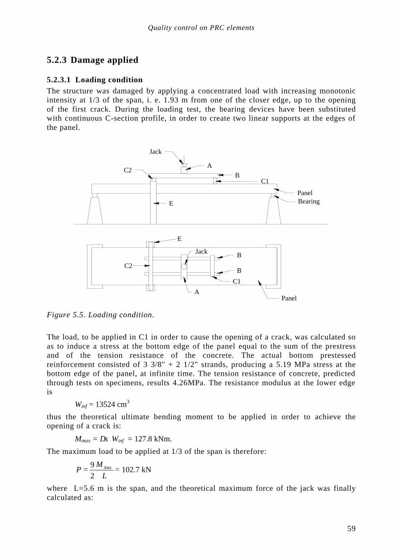
Quality control on PRC elements
59
5.2.3 Damage applied
5.2.3.1 Loading condition
The structure was damaged by applying a concentrated load with increasing monotonic intensity at 1/3 of the span, i. e. 1.93 m from one of the closer edge, up to the opening of the first crack. During the loading test, the bearing devices have been substituted with continuous C-section profile, in order to create two linear supports at the edges of the panel.
Jack
AB
C1
PanelBearing
C2
E
A
B
B
Panel
C1
C2
E
Jack
Figure 5.5. Loading condition.
The load, to be applied in C1 in order to cause the opening of a crack, was calculated so as to induce a stress at the bottom edge of the panel equal to the sum of the prestress and of the tension resistance of the concrete. The actual bottom prestessed reinforcement consisted of 3 3/8" + 2 1/2" strands, producing a 5.19 MPa stress at the bottom edge of the panel, at infinite time. The tension resistance of concrete, predicted through tests on specimens, results 4.26MPa. The resistance modulus at the lower edge is
Winf = 13524 cm3
thus the theoretical ultimate bending moment to be applied in order to achieve the opening of a crack is:
Mmax = ∆σ Winf = 127.8 kNm.
The maximum load to be applied at 1/3 of the span is therefore:
L
MP max
29
= = 102.7 kN
where L=5.6 m is the span, and the theoretical maximum force of the jack was finally calculated as:

Structural damage detection and localization by using vibrational measurements
60
F=205.4 kN
5.2.3.2 Instrumentation
During the load test, deflection values have been measured at the middle-span, the loading axis, and the bearings. In addition, the bottom edge of the panel was instrumented with high precision gauges in correspondence with the loading position, in order to measure the strain of the concrete and to detect the opening of the crack. In detail, the instrumentation setup consisted of: • 8 LVDTs, for the measure of the deflection, 2 of which were mounted at the middlespan, 2 at 1/3 of the span, and 2 at each edge; • 6 strain gauges (DD1) with 150 mm measurement references, placed across the loading axis as shown in Figure 5.6.
Figure 5.6. Instrumentation setup, during loading test.
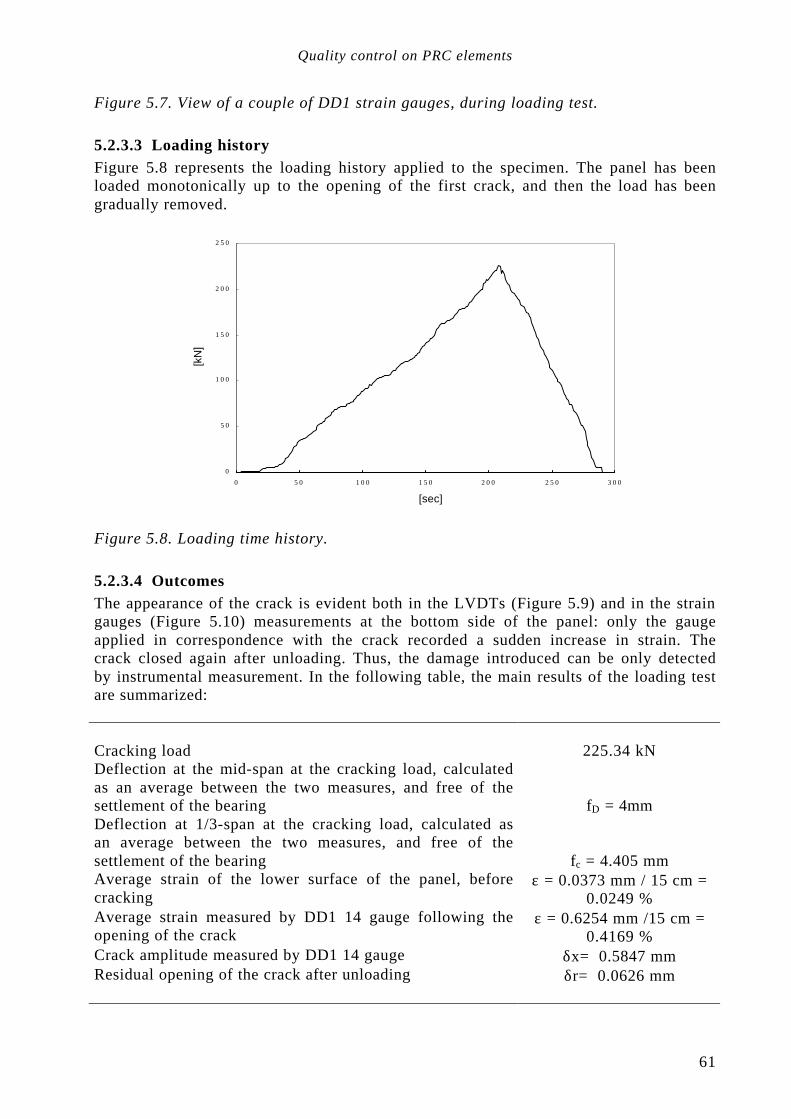
Quality control on PRC elements
61
Figure 5.7. View of a couple of DD1 strain gauges, during loading test.
5.2.3.3 Loading history
Figure 5.8 represents the loading history applied to the specimen. The panel has been loaded monotonically up to the opening of the first crack, and then the load has been gradually removed.
0
5 0
1 0 0
1 5 0
2 0 0
2 5 0
0 5 0 1 0 0 1 5 0 2 0 0 2 5 0 3 0 0
[sec]
[kN
]
Figure 5.8. Loading time history.
5.2.3.4 Outcomes
The appearance of the crack is evident both in the LVDTs (Figure 5.9) and in the strain gauges (Figure 5.10) measurements at the bottom side of the panel: only the gauge applied in correspondence with the crack recorded a sudden increase in strain. The crack closed again after unloading. Thus, the damage introduced can be only detected by instrumental measurement. In the following table, the main results of the loading test are summarized: Cracking load 225.34 kN Deflection at the mid-span at the cracking load, calculated as an average between the two measures, and free of the settlement of the bearing fD = 4mm Deflection at 1/3-span at the cracking load, calculated as an average between the two measures, and free of the settlement of the bearing fc = 4.405 mm Average strain of the lower surface of the panel, before cracking
ε = 0.0373 mm / 15 cm = 0.0249 %
Average strain measured by DD1 14 gauge following the opening of the crack
ε = 0.6254 mm /15 cm = 0.4169 %
Crack amplitude measured by DD1 14 gauge δx= 0.5847 mm Residual opening of the crack after unloading δr= 0.0626 mm

Structural damage detection and localization by using vibrational measurements
62
Table 5.1. Main outcomes of loading test.
0
5 0
1 0 0
1 5 0
2 0 0
2 5 0
0 .0 1 .0 2 .0 3 .0 4 .0 5 .0 6 .0 7 .0 8 .0
[mm]
[kN
]
dx bearing
sx bearing
1 /3 span
1 /2 span
Figure 5.9. Load-deflection history, measured by LVDTs.
0
5 0
1 0 0
1 5 0
2 0 0
2 5 0
0 .0 0 .1 0 .2 0 .3 0 .4 0 .5 0 .6 0 .7
[mm]
[kN
]
D D 1 0
D D 1 1
D D 1 2
D D 1 3
D D 1 4
D D 1 5
Figure 5.10. Load-strain history, measured by DD1s.

Quality control on PRC elements
63
5.2.4 Dynamic characterization The structure was characterized dynamically before and after the introduction of the crack, by using both stepped-sine tests and shock tests.
5.2.4.1 Transducers
The transducers, which were used had the following characteristics:
Voltage sensitivity 9630 mV/g Frequency range (5%) 0.15 - 1000 Hz Frequency range (10%) 0.1 - 1500 Hz Amplitude range ±0.5 g pk Resolution 0.000005 g pk Transverse sensitivity < 5 %
Table 5.2. Accelerometer characteristics.
The position of the accelerometers is represented in Figure 5.3.
5.2.4.2 Stepped-sine tests
For this propose, a single rotating mass shaker was used, with the following features:
Mass 0.057 kg Effective radius 0.15 m Frequency range (horizontal) 1 - 40 Hz Frequency range (vertical) 5 - 40 Hz Max force amplitude 2000 N Frequency resolution 0.05 Hz
Table 5.3. Shaker characteristics.
The shaker has been placed in the center at the panel such as to apply a force in the xz-plane. Harmonic excitation was applied in a frequency range of 12 to 45 Hz. Figures 5.12 and 5.13 show some of the FRFs achieved, before and after damaging.
Rotation axesBearings
Bearing
Mass
Figure 5.11. Shaker position during testing.
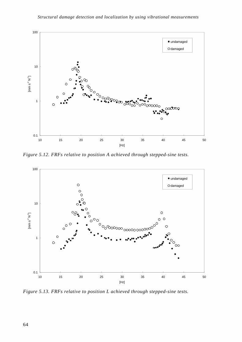
Structural damage detection and localization by using vibrational measurements
64
0.1
1
10
100
10 15 20 25 30 35 40 45 50
[Hz]
[mm
s-2
N-1
]
undamaged
damaged
Figure 5.12. FRFs relative to position A achieved through stepped-sine tests.
0.1
1
10
100
10 15 20 25 30 35 40 45 50
[Hz]
[mm
s-2
N-1
]
undamaged
damaged
Figure 5.13. FRFs relative to position L achieved through stepped-sine tests.
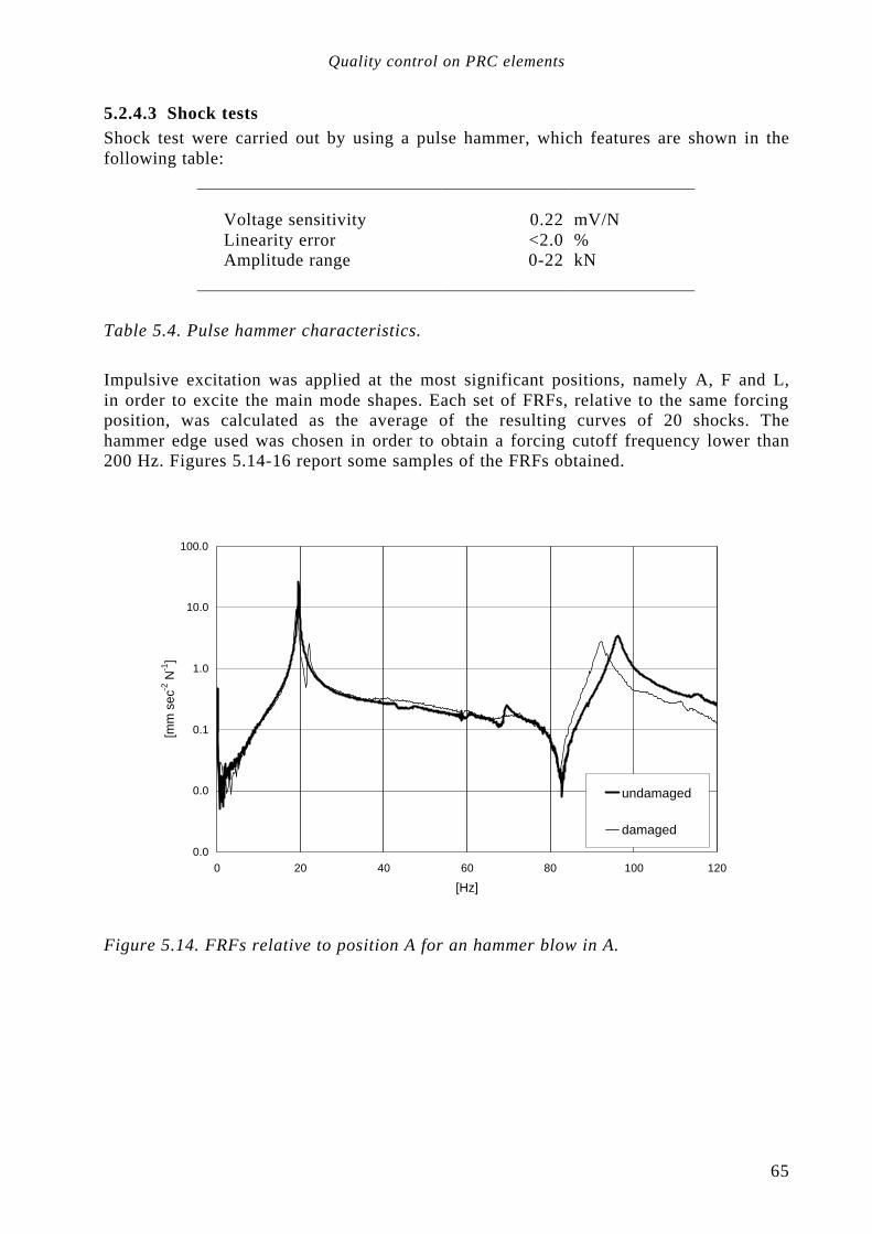
Quality control on PRC elements
65
5.2.4.3 Shock tests
Shock test were carried out by using a pulse hammer, which features are shown in the following table:
Voltage sensitivity 0.22 mV/N Linearity error <2.0 % Amplitude range 0-22 kN
Table 5.4. Pulse hammer characteristics.
Impulsive excitation was applied at the most significant positions, namely A, F and L, in order to excite the main mode shapes. Each set of FRFs, relative to the same forcing position, was calculated as the average of the resulting curves of 20 shocks. The hammer edge used was chosen in order to obtain a forcing cutoff frequency lower than 200 Hz. Figures 5.14-16 report some samples of the FRFs obtained.
0.0
0.0
0.1
1.0
10.0
100.0
0 20 40 60 80 100 120
[Hz]
[mm
sec
-2 N
-1]
undamaged
damaged
Figure 5.14. FRFs relative to position A for an hammer blow in A.

Structural damage detection and localization by using vibrational measurements
66
0.0
0.1
1.0
10.0
100.0
0 20 40 60 80 100 120
[Hz]
[mm
sec
-2 N
-1]
undamaged
damaged
Figure 5.15. FRFs relative to position H for an hammer blow in L.
0.0
0.1
1.0
10.0
100.0
0 20 40 60 80 100 120
[Hz]
[mm
sec
-2 N
-1]
undamaged
damaged
Figure 5.16. FRFs relative to position F for an hammer blow in A.

Quality control on PRC elements
67
5.3 Modal extraction The modal parameters of the structure, before and after the introduction of the damage, were extracted from the acquired signals by using different techniques.
5.3.1 Natural frequencies and mode shapes Natural frequencies and modal shapes were found by MDOF fitting of the experimental FRFs. In Table 5.5, frequencies of corresponding identified modes of both the undamaged and cracked panels are compared; differences are very small.
frequency [Hz] mode undamaged cracked
19.55 19.27 I X-bending mode 20.84 20.52 I torsional mode 42.98 41.93 I Y-bending mode 59.84 59.67 II X-bending mode 68.40 67.02 II torsional mode
Table 5.5. Natural frequencies and modal recognition.
The mode shapes identification was carried out with the support of a FE model: the theoretical shapes calculated are represented in Figure 5.17. The correlation between modes before and after cracking was found out using the MAC index (Modal Assurance Criterion) defined as:
( ) ( )( )rrss
rs
rs ~~
~~
,MACφφφφ
φφφφ ++
+
=
2
(5.1)
in which rrr
~ φφφ ∆+= represents the rth modal shape after damage. MAC values are shown in Table 5.6. The fact that diagonal MAC coefficients are very close to 1, indicates that very slight changes in mode shape occurred following cracking.
Undamaged Cracked
1° flex.
2° flex.
3° flex.
1° torx.
2° torx.
1°flex. 0.969 0.001 0.001 0.529 0.000 2°flex. 0.000 0.998 0.007 0.002 0.835 3°flex. 0.024 0.003 0.978 0.325 0.052 1°torx. 0.392 0.003 0.335 0.993 0.072 2°torx. 0.004 0.921 0.052 0.029 0.947
Table 5.6. MAC index for experimental mode shapes.

Structural damage detection and localization by using vibrational measurements
68
a. First X-bending mode. (19.5 Hz)
b. First torxional mode. (20.8 Hz)
c. First Y-bending mode. (42.9Hz)
d. Second X-bending mode. (59.8 Hz)
e. Second torxional mode. (68.4 Hz)
f. Third X-bending mode. (95.9 Hz)
Figure 5.17. Finite elements model of the panel.
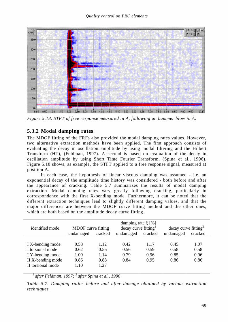
Quality control on PRC elements
69
Figure 5.18. STFT of free response measured in A, following an hammer blow in A.
5.3.2 Modal damping rates The MDOF fitting of the FRFs also provided the modal damping rates values. However, two alternative extraction methods have been applied. The first approach consists of evaluating the decay in oscillation amplitude by using modal filtering and the Hilbert Transform (HT), (Feldman, 1997). A second is based on evaluation of the decay in oscillation amplitude by using Short Time Fourier Transform, (Spina et al., 1996). Figure 5.18 shows, as example, the STFT applied to a free response signal, measured at position A.
In each case, the hypothesis of linear viscous damping was assumed - i.e. an exponential decay of the amplitude time history was considered - both before and after the appearance of cracking. Table 5.7 summarizes the results of modal damping extraction. Modal damping rates vary greatly following cracking, particularly in correspondence with the first X-bending mode. Furthermore, it can be noted that the different extraction techniques lead to slightly different damping values, and that the major differences are between the MDOF curve fitting method and the other ones, which are both based on the amplitude decay curve fitting.
damping rate ξ [%]
identified mode MDOF curve fitting decay curve fitting1 decay curve fitting2
undamaged cracked undamaged cracked undamaged cracked
I X-bending mode 0.58 1.12 0.42 1.17 0.45 1.07 I torsional mode 0.62 0.56 0.56 0.59 0.58 0.58 I Y-bending mode 1.00 1.14 0.79 0.96 0.85 0.96 II X-bending mode 0.86 0.88 0.84 0.95 0.86 0.86 II torsional mode 1.10 1.27
1 after Feldman, 1997; 2 after Spina et al., 1996
Table 5.7. Damping ratios before and after damage obtained by various extraction techniques.

Structural damage detection and localization by using vibrational measurements
70
5.3.3 Detection of Coulomb friction damping Modal limit displacement can be extracted from a free monofrequency signal. The procedure is the same as that described in Spina et al (1996), already applied when extracting modal damping in the previous section. It consists in finding the best fitting of the analytic signal amplitude, this time using Equation (3.52) instead of a simple logarithmic curve, and assuming ( )
sfa and sξ as parameters. These immediately go
back to ( )slimx keeping in mind (3.52). Figure 5.19 shows the results of fitting applied to the free response of the panel according to the first bending frequency, before and after cracking. It can be noted how the hypothesis for the damaged panel of purely viscous damping (exponential fitting) is rather imprecise (Figure 5.20). On the other hand, the decay in signal amplitude is very well described in (3.52). With the purpose of extracting modal limit displacements, it is possible to demonstrate that modal superposition cannot be considered valid, not even approximately. This is a direct consequence of the non-linearity of (3.37). In other words, the sth modal limit displacement must be extracted from the free response of the panel according to the sth vibration mode only. The use of modal filters leads to underestimating the limit displacement relative to higher modes. In practice, however, obtaining free monofrequency vibration of the panel according to superior modes is technically very complex. Current experimentation is developing in this direction.
-50
-25
0
25
50
0.0 0.4 0.8 1.2 1.6 2.0[sec]
[mm
sec
-2]
*
-50
-25
0
25
50
0.0 0.4 0.8 1.2 1.6 2.0[sec]
[mm
sec
-2]
Figure 5.19. Time history free response, measured in A, of the undamaged (a) and cracked (b) panel: filtered real signal.
1
10
100
0.0 0.4 0.8 1.2 1.6 2.0[sec]
[mm
sec
-2]
ξ= 0.0044af= 7.07e-06
1
10
100
0.0 0.4 0.8 1.2 1.6 2.0[sec]
[mm
sec
-2]
ξ = 0.0052af= 9.30e-04
Figure 5.20. Time history free response, measured in A, of the undamaged (a) and cracked (b) panel: amplitude of the analytical signal, exponential fit and non linear fit according to (3.52).

Quality control on PRC elements
71
5.4 Localization of damage The general idea is to divide the panel into a certain number of portions (5 or 9), which are homogeneous in the damage parameter (stiffness or specific damping). The position of the damage is therefore researched by applying the previously formulated techniques. A linear function (sensitivity matrix), is assumed as the relation that links modal parameters to damage indicators.
5.4.1 Changes in frequency method
Damage indices are defined as:
∑=∆i isis s δω (5.2)
where sis is the sensitivity of the sth frequency to damage in i. However, the sensitivity matrix is calculated, and the frequencies were found not to be very sensitive parameters and location did not give good results (Figure 5.21a).
5.4.2 Changes in flexibility method
Correction to the preceding method is represented, on the basis of the considerations previously reported; producing an expression of the type:
∑=∆i
isi
s
sδω11
2 (5.3)
The sensitivity of the modal parameter is low, however it locates damage in two bands of 145 cm width around the actual position of cracking (Figure 5.21b).
5.4.3 MAC and COMAC index methods
As a simple comparison, the use of MAC and COMAC indices are also taken into consideration. These have already been proposed as values for comparison between mode shapes in location problems. Using the MAC index, the indices of damage are calculated by the following semi-empirical relationships. In the case of flexional shapes:
( ) ∑=− i iisss~
,MAC δχφφ 21 (5.4)
where:
211 2
ls,is,is,i
is+− +−
=φφφ
χ (5.5)
is the modal curvature relative to the sth mode and the ith measurement point. In the case of torsional shapes, an analogous expression can be used:
( ) ∑=−i iisss
~,MAC δθφφ 21 (5.6)
where:
ls,iis
is1−−
=ϕϕ
θ (5.7)
is the derivative of the modal rotation ϕ relative to the sth mode and the ith measurement point. The outcome of the location, however, is very uncertain.
Structural damage detection and localization by using vibrational measurements
72
The COMAC (Co-ordinate Modal Assurance Criteria) was introduced by Lieven and Ewins (1988) in order to compare mode shape at a selected measurement point. It is defined for the ith points as:
( ) ( )( ) ( )∑ ∑∑=
s s isis
iss is
~
~iCOMAC 22
2
φφ
φφ (5.8)
and, since it equals 1 in the absence of damage, it would seem natural to introduce a damage index like:
( )iCOMACi −= 1δ (5.9)
However it is easy to demonstrate that there is no direct relation between local stiffness characteristics and the relative COMAC, which is based on the mode shape expressed in terms of absolute displacement. One only has to think of the free extremity of a cantilever beam damaged at the joint. The COMAC values would be very high for non-existent local damage. The use of this index in location problems is therefore unreasonable. Misunderstanding concerning the use of COMAC as an indicator of damage could arise from the fact that in the case of the simply supported beam, displacement and modal curvature present analogous expressions. In conclusion, it turns out that these indices of comparison do not permit damage to be located, even if burdensome elaborations are required in order to extract the modal parameters (Figures 5.21c-d).
5.4.4 Modal curvature shape method
Simplifying the general formula, one finds, apart from the sign, a simple relation of the method of modal curvature:
is
isi χ
χδ
∆= (5.10)
where isχ represents the bending curvature of the sth mode, in the ith portion of the panel. Different from the expression of shape in the MAC and COMAC parameters, the expression of the curvature modal shape does not present indeterminacy of symmetry. The method applied to the difference between the theoretical trend of curvature of the first mode shape before cracking and the experimental trend after cracking, gives a precise location of damage. This is identified around the actual position of cracking with an indeterminacy (depending on the number of measurement positions) of 72 cm (Figure 5.21e).
5.4.5 Changes in modal damping method
In the case in question, expression (3.12) becomes:
∑∑=∆
i is
i isis 2
2
χ
χδξ
∑∑=∆
i is
i isis 2
2
ϑ
ϑδξ (5.11a,b)
for torsional and flexional shapes respectively. Given the anisotropy of the damage, it is reasonable to retain the notion that the change in specific damping appears to be different in the case of bending, compared with torsional modes. Therefore, it can be hypothesized that dissipation due to torsional vibration is proportional to that for bending vibration by means of the index k, also to be identified:

Quality control on PRC elements
73
ii kδδ = (5.12)
A system of non linear equations results, in k and iδ , that can be resolved iteratively. The modal parameter is particularly sensitive to damage and despite the indeterminacy of results due to symmetry, damage is detected in two bands of 145 cm width around the actual cracking (Figure 5.21f).
5.4.6 Coulomb friction damping method
In this case, Equation (3.54) can be rewritten, for torsional and bending modal shapes, with expressions similar to (5.11a,b), already extracted in the case of the modal damping variation method:
( )∑∑
=i is
i isi
sfa2
2
χ
χδ ( )
∑∑
=i is
i isi
sfa2
2
ϑ
ϑδ (5.13a,b)

Structural damage detection and localization by using vibrational measurements
74
0
2
4
6
8
10
1 2 3 4 5
a. Change in frequency method. Crack in 4.
0
0 .5
1
1.5
2
2 .5
3
1 2 3 4 5
b Deformability method. Crack in 4.
0
1
2
3
4
1 2 3 4 5
c. Change in MAC index method. Crack in 4..
0
0 .01
0 .02
0 .03
0 .04
0 .05
1 2 3 4 5
d. Change in COMAC index method. Crack in 4...
- 0 .3
-0 .2
-0 .1
0
0 .1
0 .2
1 2 3 4 5 6 7 8 9
e. Change in modal curvature method. Crack between 6 and 7..
0
5
10
15
2 0
25
3 0
1 2 3 4 5
f. Change in modal damping method. Crack in 4..
Figure 5.21. Damage indexes evaluated through different localization techniques

Quality control on PRC elements
75
5.5 Conclusions Different approaches for first identifying and then localizing damage, have been analyzed and tested. These methods are based on an analysis of the changes in modal parameters, and hypothesize a linear link between the experimental measures and damage index. The experiment was carried out on an element of prestressed concrete where a crack was introduced. The presence of cracking in a p.r.c. structure reduces the quality and the durability. It is therefore useful to be able to identify and, if necessary, localize any cracking. All modal parameters have undergone changes signaling the presence of damage. Instead, among localization techniques, only modal curvature gives truly satisfying results. On the other hand, this technique is complex to apply in that it needs a large number of measurement points and the extraction of at least one modal shape. The modal damping method has given results, which are comparable with other techniques, such as the changes in flexibility method. It should be noted that all these techniques presuppose knowledge of the modal parameters in the undamaged situation that should otherwise be estimated. Regarding frequencies, the uncertainty of the estimation is often greater than the change that the parameter can withstand following damage. For example, in the case in question, changes less that 2% have been measured, while it is unrealistic to be able to measure a frequency with greater precision. Also keeping in mind the changes in frequency due to changes in environmental conditions, it is clear that recognizing damage only on the basis of frequencies measured is a rather uncertain operation. In the case of modal damping, the parameter estimate is affected by the uncertainly of the same entity, and it is linked to the quality of materials, boundary conditions and humidity. But, this uncertainty is negligible if compared with the sensitivity of modal damping to cracking (changes of even 100% have been measured for the first frequency of the panel). Furthermore, the damping ratio is a value largely independent of the geometry and the mass distribution of the system, and can be assumed in advance simply on the basis of typical values. Mahrenholtz and Bachmann (1991) propose values for cracked and uncracked PRC which fit well with the experimental results. Also, the estimate of modal frequencies requires hypotheses on geometry and the distribution of mass. If the structure is not particularly simple, an accurate calculation of the frequencies can require the use of a FEM model, and this represents a further burden.
Treatment of the modal damping method is in terms of viscous equivalent dissipation. In reality, the opening of a crack also modifies dissipative mechanisms qualitatively. This explains the different values obtained with different extraction techniques. Research is currently moving towards a deeper study of dissipative mechanisms that act on cracking and its effects on dynamic response.

Structural damage detection and localization by using vibrational measurements
76
77
6 Dynamic characterization of the Roman Amphitheater (Arena) in Verona
Abstract Experimental NDT and theoretical investigations are being extensively used for the accurate characterization of the mechanical properties and structural behavior of the Roman Amphitheater in Verona. Particularly dynamic identification procedures are employed with the scope of both calibrating numerical models and possibly determining evidence parameters which could be related to structural deterioration phenomena of a very complex masonry structure. The studies are part of a comprehensive restoration and surveillance program aimed to ensure both the conservation and the safe use of the monument. Sommario Al fine di caratterizzare in maniera accurata le proprietà meccaniche e il comportamento strutturale dell'Anfiteatro Romano di Verona, sono state applicate in maniera estensiva prove non distruttive e studi teorici. Sono state in particolare applicate tecniche di identificazione dinamica con il duplice scopo di calibrare modelli numerici e di evidenziare eventuali parametri che possano essere correlati a fenomeni di deterioramento strutturale della complessa struttura muraria. Gli studi sono parte di un programma di recupero e monitoraggio, che mira da una parte alla conservazione, dall'altra a garantire la sicurezza nell'uso del monumento
Structural damage detection and localization by using vibrational measurements
78
6.1 Introduction The Roman Amphitheater located in Verona, built at the beginning of the Christian era, is one of the best preserved and the third biggest amphitheater in Italy (the first being the Coliseum in Rome). The structure (Figure 6.1), currently used for summer musical performances attended by thousands of people, is being subjected to continuos maintenance and more and more strict investigation and surveillance programs as deterioration phenomena are heavily damaging the facing stones and the fear exists that they can undermine the stability of the main structural components.
Particularly, some of the deterioration phenomena (especially those connected to the humidity and water penetration though the numberless cracks and joints) are certainly threatening the efficiency of the past repair interventions starting in the sixteenth century (when the replacement of the stone seats, disappeared during the previous centuries, was completed) and continuing through the present. Investigations and studies are playing a very important role in ensuring the safe use of the monument, as they are used as effective (even if supplementary) measures for avoiding the occurrence of unexpected threats to the safety of people.
They are also furnishing essential information and data for the design of the unavoidable restoration of the monument, which is a very huge construction, based on the typical elliptical plan section, whose main dimensions are approximately 152 and 123 m, and still capable of containing around 30.000 seated people.
From the structural point of view, the very complex structural system of the amphitheater consists of two main components (Figure 6.2 and 6.3). The main body of the monument, i.e. la large elliptical basin (“cavea”) surrounding the “arena”, is essentially a modular structure made of radial walls, subdividing the ellipses into 72 sectors, supporting the vaults that form a continuous surface on which the stone seats are laid. Peripheral elliptical stone frames, made of large dressed stones, surround this system, without interfering with it, completing the construction.
Figure 6.1. View of the Amphiteater in an historical picture.
Dynamic characterization of the Roman Amphitheater (Arena) in Verona
79
Figure 6.2. Plan view of the amphitheater
Major concerns from the structural point of view derive now from the actual conditions of the complex systems of walls and vaults of the “cavea”, almost all repaired and partially reconstructed, and of the freestanding, curved and perforated wall called "the wing", more than 30 m high (the remains of the peripheral circle of dry stone masonry), subjected in the fifties to a strengthening intervention based on the use of the prestressing technique.
In the first case, where masonry made of pozzolanic mortar and rounded rubble stones ("opus caementicium' and "opus incertum") is extensively used, the rain penetration inevitably causes the weakening of mortars and consequently detachments and falling of stones.
In the second case, adequate protection of the steel wires against oxidization is not ensured. From the structural point of view, the “wing” is very simply a slender corbel with no lateral supports or confinement offered by the remaining vault (Fig. 6.4).
Figure 6.3: Section of the amphitheater in correspondence of the wing.

Structural damage detection and localization by using vibrational measurements
80
Figure 6.4 View and typical section of the wing, with details of the prestressed reinforcement The lack of structural redundancy and any kind of protection against the action of adverse environmental agents (e.g. rain, freeze-taw cycles, wind, soil differential settlements), besides of course what could it have suffered due to damages caused in the past and due to the lack of maintenance, makes the risk of inadequate structural safety conditions very high. It was around the thirties that the people responsible for its conservation became aware of the necessity of a strengthening intervention as it was clear that, even due to a pronounced inclination, the wall could not resist the relevant horizontal action which could be expected in that area due to wind and earthquake motions (the region is in fact subjected to a moderate seismic risk).
The debate (long and very interesting) on how to intervene (at least three or four different proposals were discussed) was interrupted by the second World War, when temporary masonry buttresses were erected to protect the wall as much as possible against explosions (Fig. 6.5).
When the problem of removing the buttresses and at the same time strengthening the “wing” was faced after the war, at the beginning of the fifties, the use of the prestressing technique was considered a very smart solution of the always-complex problem of preserving the monument while ensuring acceptable structural safety conditions. The intervention, as described by the designer himself (Morandi 1956), consisted essentially in introducing harmonic steel wires in vertical holes (40 mm in diameter according to Morandi 1956) drilled in the stone (Figure 3, a - 18 wires, 5 mm in diameter, in each of the 6 holes of each pillar).
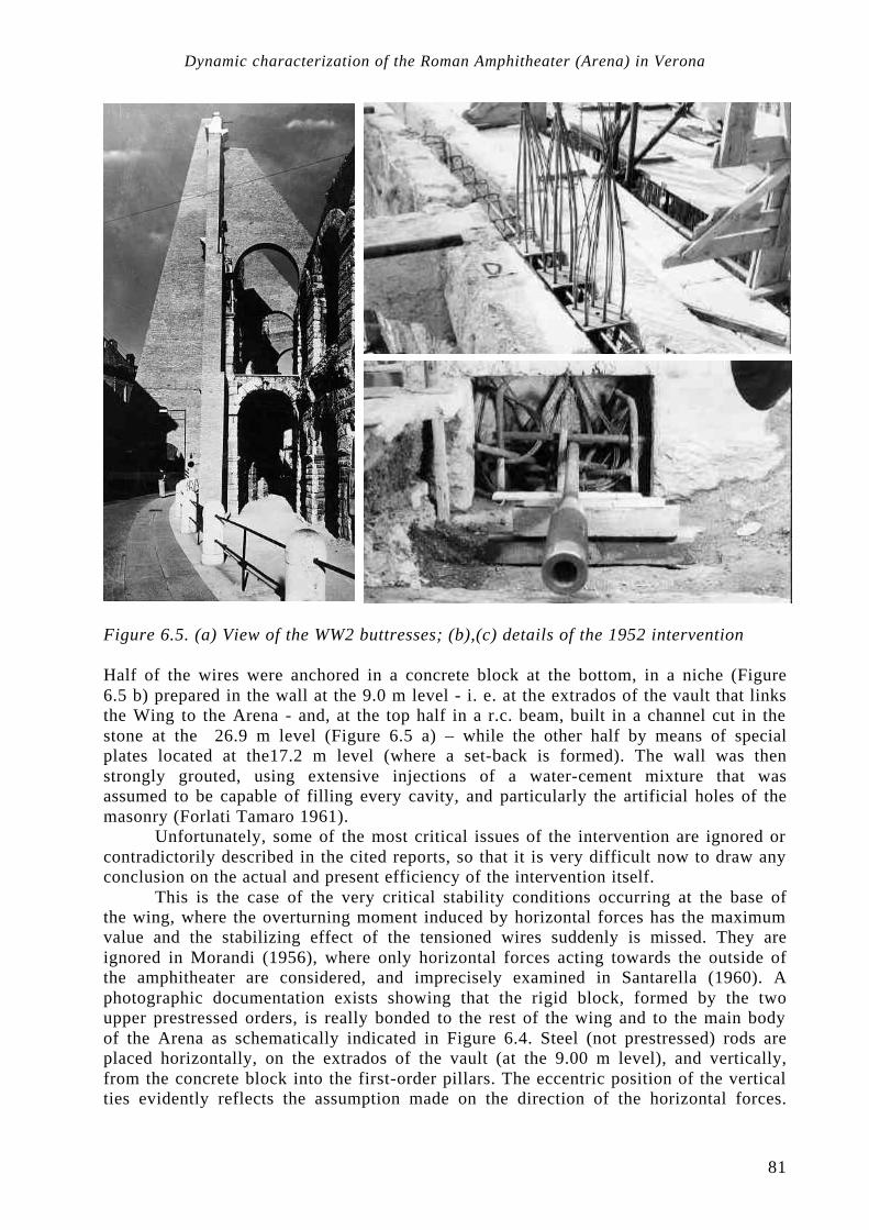
Dynamic characterization of the Roman Amphitheater (Arena) in Verona
81
Figure 6.5. (a) View of the WW2 buttresses; (b),(c) details of the 1952 intervention Half of the wires were anchored in a concrete block at the bottom, in a niche (Figure 6.5 b) prepared in the wall at the 9.0 m level - i. e. at the extrados of the vault that links the Wing to the Arena - and, at the top half in a r.c. beam, built in a channel cut in the stone at the 26.9 m level (Figure 6.5 a) – while the other half by means of special plates located at the17.2 m level (where a set-back is formed). The wall was then strongly grouted, using extensive injections of a water-cement mixture that was assumed to be capable of filling every cavity, and particularly the artificial holes of the masonry (Forlati Tamaro 1961).
Unfortunately, some of the most critical issues of the intervention are ignored or contradictorily described in the cited reports, so that it is very difficult now to draw any conclusion on the actual and present efficiency of the intervention itself.
This is the case of the very critical stability conditions occurring at the base of the wing, where the overturning moment induced by horizontal forces has the maximum value and the stabilizing effect of the tensioned wires suddenly is missed. They are ignored in Morandi (1956), where only horizontal forces acting towards the outside of the amphitheater are considered, and imprecisely examined in Santarella (1960). A photographic documentation exists showing that the rigid block, formed by the two upper prestressed orders, is really bonded to the rest of the wing and to the main body of the Arena as schematically indicated in Figure 6.4. Steel (not prestressed) rods are placed horizontally, on the extrados of the vault (at the 9.00 m level), and vertically, from the concrete block into the first-order pillars. The eccentric position of the vertical ties evidently reflects the assumption made on the direction of the horizontal forces.
Structural damage detection and localization by using vibrational measurements
82
Why such an assumption was made, where exactly the ties are, their number, and dimensions, are unknown.
Even the position of the prestressed wires is a matter of contradictions. According to Morandi (1956), the total prestressing force should be eccentric, in order to counteract horizontal forces acting towards the outside of the Arena, but it is not clear what the eccentricity is. According to Santarella (1960) the masonry should be concentrically prestressed, and this seems to be confirmed, even if not definitively, by some photographic documentation.
Finally, the efficiency of the protection of the steel against oxidization that should be ensured by the water-cement injection is also very doubtful. Particularly the possibility that such a mixture could really penetrate (without using all the additives and injection devices employed in modern prestressed structures) the holes which are 40 mm in diameter and approximately 20 m long, where 18 wires, 5 mm in diameter, are inserted is questionable. The assessment of what actually the safety conditions are of the “wing” under horizontal forces acting towards both the inside and the outside of the amphitheatre, evidently requires that a number of very important questions be answered, particularly regarding: • the actual distribution of stresses induced by the prestressing forces, compared to the design values as they can be drawn from Morandi (1957); • the actual position, dimension and anchorage efficiency of the steel rods; • the possible oxidization attacks to both steel wires and steel rods; • the overall structural behavior of the wing, and particularly the interaction with the main body of the amphitheater.
The chapter presents the more relevant results of investigations so far performed in order to assess the actual structural behavior and conditions of typical vaults and the actual efficiency of the prestressed "wing".
After having described the NDT techniques (core drilling and double fiat jack) used to determine the mechanical material properties of masonry, particular attention is dedicated to the use of dynamic investigations combined with structural identification procedures in order to identify damage and calibrate numerical models of the investigated structures. The experimental part of the dynamic investigations is based mainly on forced vibrations (pulse hammer and shaker). The theoretical analyses are mainly based on physical models.

Dynamic characterization of the Roman Amphitheater (Arena) in Verona
83
6.2 ND evaluation of states of stress and mechanical properties of walls and vaults
Flat jack tests and core drilling were used to assess the actual distribution of stresses, the composition, the strength and deformability properties of masonry walls and vaults. With regards to the “wing,” the following important observations were drawn (Modena et al., 1997) from the investigations. The inspections made by drilling horizontal cores through the dry joints between the stone elements, indicated the importance of the construction technique which has been used (“anathyrosis”). The cavities which are left in the central part of the contact surfaces between the stones (still visible for example as in Figure 6.6 (a) reduce the actual resisting section of the masonry by approximately one half, thus strongly influencing the distribution of stresses and the deformability (especially the flexural stiffness) of the masonry. Moreover, such cavities were found to be empty, and this could not occur if the holes containing the prestressing wire should actually be filled with cement injection material on which the designer (Morandi R., 1956) and the supervisors (Forlati Tamaro B, 1961) relied to ensure the protection of the steel. The cavities are in fact intersected by the vertical holes, and their thickness is of the order of 15 mm, i.e. greater then the dimensions of the spaces that are left free for the injections by the 18 wires (5 mm in diameter) inserted into the 40-45 mm diameter holes.
Other important information came from the very uneven distribution of the measured compressive stresses, with significant variation of the mean values between the pillars and of the local values within each pillar. The uncertain and variable geometry of the actual resisting section, together with the uncertain structural behavior of the perforated wall (especially under forces acting in its own plane, when a frame-like response can be activated) are certainly among the principal causes of this fact.
However, taking into account what was previously stated, no absolute guarantee can be given that the prestressing forces are of the same intensity and in the same position as they are supposed to be according the original design and execution of the intervention.
A limited number of tests on the radial walls and vaults were then enough to produce evidence of the heavy deterioration phenomena which are affecting the masonry. The main cause of the deterioration is the rain penetration, against which no protection at all existed for more than one-thousand years (after the original seats were removed) and too poor a one has been ensured even after the reconstruction was completed in the nineteenth century as the original drainage system was completely lost. The main effects of rain penetration are the well-known chemical reactions through which the mortars miss the binders (hydrated limes) thus becoming substantially weakened.
As a result (Modena et al.., 1997), the masonry exhibits deformability and strength values during double flat jack tests ranging respectively from 200-300 MPa to 2000-3000 MPa and from 0.8-1.0 MPa to 2.0-2.5 MPa, and in some cases cores are drilled where practically no more mortar exists. Not surprisingly then, the compressive stresses locally measured through single flat jack test very rarely comply with the values theoretically calculated on the basis of homogeneous elastic models.
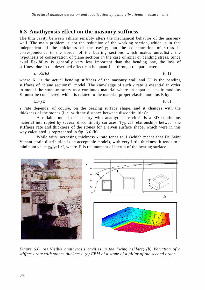
Structural damage detection and localization by using vibrational measurements
84
6.3 Anathyrosis effect on the masonry stiffness The thin cavity between ashlars sensibly alters the mechanical behavior of the masonry wall. The main problem is not the reduction of the working section, which is in fact independent of the thickness of the cavity; but the concentration of stress in correspondence to the border of the bearing sections which makes unrealistic the hypothesis of conservation of plane sections in the case of axial or bending stress. Since axial flexibility is generally very less important than the bending one, the loss of stiffness due to the described effect can be quantified through the parameter
χ=KB/EJ (6.1)
where KB is the actual bending stiffness of the masonry wall and EJ is the bending stiffness of “plane sections” model. The knowledge of such χ rate is essential in order to model the stone-masonry as a continuos material where an apparent elastic modulus Ea must be considered, which is related to the material proper elastic modulus E by:
Ea=χE (6.3)
χ rate depends, of course, on the bearing surface shape, and it changes with the thickness of the stones (i. e. with the distance between discontinuities): A reliable model of masonry with anathyrosis cavities is a 3D continuous material interrupted by several discontinuity surfaces. Typical relationships between the stiffness rate and thickness of the stones for a given surface shape, which were in this way calculated is represented in fig. 6.6 (b). While with increasing thickness χ rate tends to 1 (which means that De Saint Venant strain distribution is an acceptable model), with very little thickness it tends to a minimum value χmin=J’/J, where J’ is the moment of inertia of the bearing surface.
0
0.2
0.4
0.6
0.8
1χ
t/h
t
h
Figure 6.6. (a) Visible anathyrosis cavities in the “wing ashlars; (b) Variation of χ stiffness rate with stones thickness. (c) FEM of a stone of a pillar of the second order.

Dynamic characterization of the Roman Amphitheater (Arena) in Verona
85
With regards to the effect of the bearing surface shapes, typical results of the FEM analyses for a given stone thickness (i.e. that of the stones forming the pillar of the second order of the wing) are shown in Table 6.1.
χ=1 χ=0.75 χ=0.63 χ=0.43 χ=0.38
Table 6.1. Variation of χ rate with the bearing surface shape, for a pillar of the second order.
It is then evident how an incomplete bearing pulls down the apparent stiffness of the continuous elastic model, which may result in even lower than one half of the material modulus, in the case of blade bearing. In the following, these considerations will turn out to be precious in the interpretation of the results of the dynamic investigations and corresponding identification procedures.
6.4 Dynamic investigations on the Wing The overall structural behavior of the Wing, and particularly its interaction with the main body of the amphitheater, is being experimentally analyzed and theoretically modeled by using forced vibration tests and dynamic identification procedures. Modal testing (Ewins D.J., 1984) has already been carried out by using ambient vibrations and forced, both impulsive and stepped-sine excitations (Modena C., Zonta D., 1996).
Response signals were acquired by 4 accelerometers placed in correspondence with the points indicated in Figure 6.7, which have been selected on the basis of preliminary measured signals and FEM analyses. Given the positions of the acceleration transducers, shocks are applied separately in any of such positions while the harmonic exciter has been placed near the accelerometer #3.
3 1
4 2
Figure 6.7: transducers position

Structural damage detection and localization by using vibrational measurements
86
6.4.1 Stepped-sine tests Stepped-sine tests consist of a direct comparison between the amplitude of the response of each DOF to a stationary harmonic excitation generated by a special device. Such scanned single frequency responses are fitted by the theoretical MDOF complex FRF, where number of modes taken in account is suggested by the results of a preliminary FEM. Representative results of modal extraction, performed through simple fitting algorithms, are reported in Figure 6.8.
Because it is based on an actual stationary excitation, stepped-sine technique is the most desirable way to carry out a FRF. Such a technique also allows the scanning of the frequency domain with the best resolution needed by the range of interest. On the other side, it presents significant limitations concerning both the data acquisition and the device installation. In fact: • the range of scanned frequency is limited by the mechanical features of the exciter; • the amplitude response is very sensible to a slight non-linear behavior of the
structure; • the exciter is often a bulky device, not easy to apply to structure (anyway, not
everywhere); • the amplitude of the inducted vibration, especially next to the resonance, may results
unacceptable is the case of particularly sensitive structures, such as many historical buildings.
0.0E+00
2.0E-05
4.0E-05
6.0E-05
8.0E-05
1.0E-04
1.2E-04
0.0 5.0 10.0 15.0Hz
0.0E+00
2.0E-05
4.0E-05
6.0E-05
8.0E-05
1.0E-04
1.2E-04
0.0 5.0 10.0 15.0Hz
0.0E+00
2.0E-05
4.0E-05
6.0E-05
8.0E-05
1.0E-04
1.2E-04
0.0 5.0 10.0 15.0Hz
0.0E+00
2.0E-05
4.0E-05
6.0E-05
8.0E-05
1.0E-04
1.2E-04
0.0 5.0 10.0 15.0Hz
Figure 6.8. FRFs plots obtained from stepped-sine test, and curve fitting
6.4.2 Shock tests Taking into account the above observations, many efforts have been made in order to achieve a good FRF from alternative testing techniques. Particularly pulse hammer measurements can usefully replace a harmonic exciter: it provides as well the frequency domain of the excitation, and tests are simpler (and cheaper) to execute. In the case of
Channel 2 Channel 1
Channel 3 Channel 4
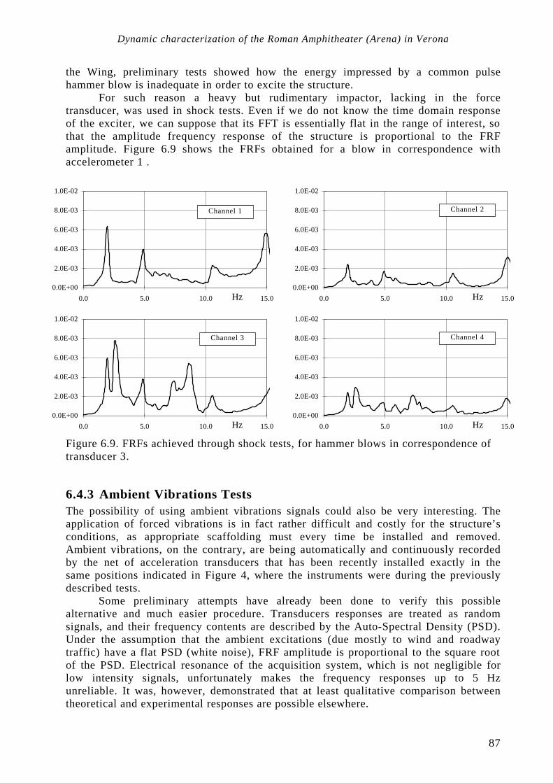
Dynamic characterization of the Roman Amphitheater (Arena) in Verona
87
the Wing, preliminary tests showed how the energy impressed by a common pulse hammer blow is inadequate in order to excite the structure.
For such reason a heavy but rudimentary impactor, lacking in the force transducer, was used in shock tests. Even if we do not know the time domain response of the exciter, we can suppose that its FFT is essentially flat in the range of interest, so that the amplitude frequency response of the structure is proportional to the FRF amplitude. Figure 6.9 shows the FRFs obtained for a blow in correspondence with accelerometer 1 .
0.0E+00
2.0E-03
4.0E-03
6.0E-03
8.0E-03
1.0E-02
0.0 5.0 10.0 15.0Hz
0.0E+00
2.0E-03
4.0E-03
6.0E-03
8.0E-03
1.0E-02
0.0 5.0 10.0 15.0Hz
0.0E+00
2.0E-03
4.0E-03
6.0E-03
8.0E-03
1.0E-02
0.0 5.0 10.0 15.0Hz
0.0E+00
2.0E-03
4.0E-03
6.0E-03
8.0E-03
1.0E-02
0.0 5.0 10.0 15.0Hz
Figure 6.9. FRFs achieved through shock tests, for hammer blows in correspondence of transducer 3.
6.4.3 Ambient Vibrations Tests The possibility of using ambient vibrations signals could also be very interesting. The application of forced vibrations is in fact rather difficult and costly for the structure’s conditions, as appropriate scaffolding must every time be installed and removed. Ambient vibrations, on the contrary, are being automatically and continuously recorded by the net of acceleration transducers that has been recently installed exactly in the same positions indicated in Figure 4, where the instruments were during the previously described tests.
Some preliminary attempts have already been done to verify this possible alternative and much easier procedure. Transducers responses are treated as random signals, and their frequency contents are described by the Auto-Spectral Density (PSD). Under the assumption that the ambient excitations (due mostly to wind and roadway traffic) have a flat PSD (white noise), FRF amplitude is proportional to the square root of the PSD. Electrical resonance of the acquisition system, which is not negligible for low intensity signals, unfortunately makes the frequency responses up to 5 Hz unreliable. It was, however, demonstrated that at least qualitative comparison between theoretical and experimental responses are possible elsewhere.
Channel 2 Channel 1
Channel 4 Channel 3

Structural damage detection and localization by using vibrational measurements
88
6.5 Modal extraction FRF fitting leads to the identification of 8 frequencies in 1-12 Hz range. Resulting frequencies and damping rates, achieved mainly through stepped-sine tests, are reported in the following table, shock tests results confirmed these values and also allowed the detection of the 5th mode, which is essentially characterized by displacements in the surface of the wall.
Mode 1 2 3 4 5 6 7 8 Frequency
(Hz) 1.92 2.61 4.83 5.87 6.10 7.10 8.62 10.65
Damping rate
0.014 0.013 0.018 0.069 0.023 0.011 0.026
Table 6.2. Main results of modal extraction: modal frequencies and dumping rates.
The very light damping rates deserves some considerations. It is a fact that masonry structures usually present high damping; and this is often accompanied with a softening structural behavior appreciable either for rather low displacements. In the case of the Wing masonry structure: • damping rates values stand around 1-2%; the 4th mode (i. e. the 2nd bending mode),
which reach the 6.9% value, represents an exception and it would mean that dissipation occurs especially where such shape presents the maximum bending, i. e. just in correspondence of the anchorage of the second set of wires
• the fact that shock tests, which are very low intensity FVT, and stepped-sine tests lead to identical results, means that frequency response is substantially independent of the amplitude of vibration or, in other words, that the structure does not show non-linear behavior, neither next to resonance.
Such good dynamic behavior may be explained as an effect of the still active prestressing forces.
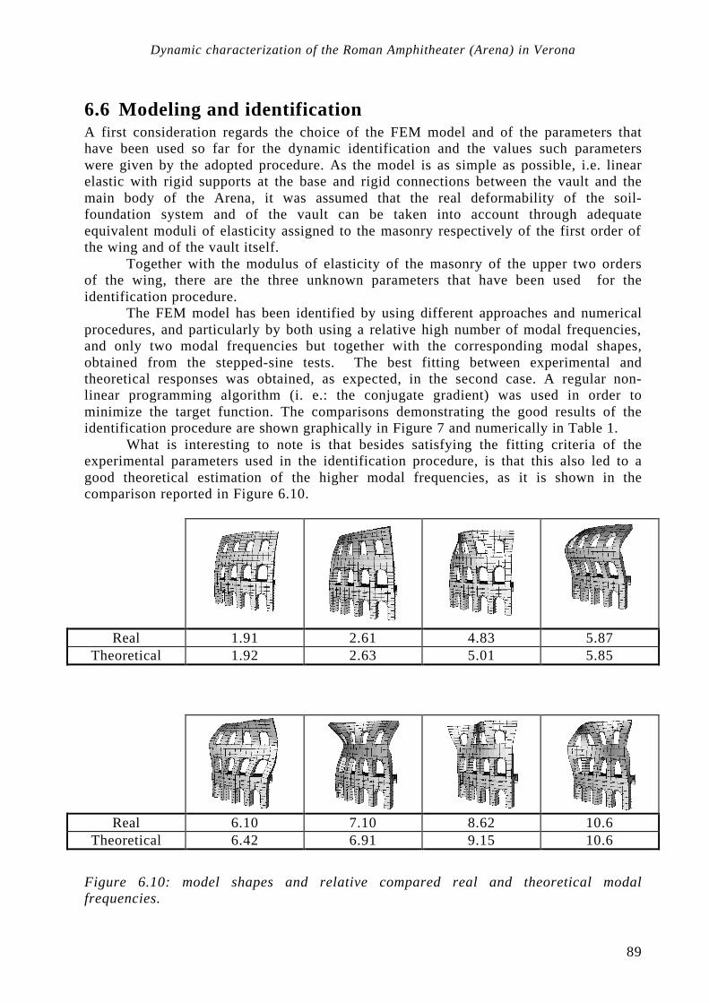
Dynamic characterization of the Roman Amphitheater (Arena) in Verona
89
6.6 Modeling and identification A first consideration regards the choice of the FEM model and of the parameters that have been used so far for the dynamic identification and the values such parameters were given by the adopted procedure. As the model is as simple as possible, i.e. linear elastic with rigid supports at the base and rigid connections between the vault and the main body of the Arena, it was assumed that the real deformability of the soil-foundation system and of the vault can be taken into account through adequate equivalent moduli of elasticity assigned to the masonry respectively of the first order of the wing and of the vault itself.
Together with the modulus of elasticity of the masonry of the upper two orders of the wing, there are the three unknown parameters that have been used for the identification procedure.
The FEM model has been identified by using different approaches and numerical procedures, and particularly by both using a relative high number of modal frequencies, and only two modal frequencies but together with the corresponding modal shapes, obtained from the stepped-sine tests. The best fitting between experimental and theoretical responses was obtained, as expected, in the second case. A regular non-linear programming algorithm (i. e.: the conjugate gradient) was used in order to minimize the target function. The comparisons demonstrating the good results of the identification procedure are shown graphically in Figure 7 and numerically in Table 1.
What is interesting to note is that besides satisfying the fitting criteria of the experimental parameters used in the identification procedure, is that this also led to a good theoretical estimation of the higher modal frequencies, as it is shown in the comparison reported in Figure 6.10.
Real 1.91 2.61 4.83 5.87 Theoretical 1.92 2.63 5.01 5.85
Real 6.10 7.10 8.62 10.6
Theoretical 6.42 6.91 9.15 10.6
Figure 6.10: model shapes and relative compared real and theoretical modal frequencies.
Structural damage detection and localization by using vibrational measurements
90
The values of these apparent parameters given by the analysis are 5700 MPa, 8000 MPa and 11900 MPa respectively for the first order of the wing, the vault and the upper part of the wing, which are evidently very low compared to the value of the modulus of elasticity of the stone (of the order of 60000 MPa). More calibrations will certainly be done in the near future; however, it must be mentioned that approximate evaluations of the modulus of elasticity of the upper part of the wing, obtained by the single flat-jack test measurements, corrected by taking into account the effect of the cavity between the contact faces of the stone elements as indicated in paragraph 6.3 (Figure 6.6), are not in contradiction with the results of the identification process.
It is then expected that also the theoretically calculated higher modal shapes (a representative selection of which are shown in Figure 6.10) are good estimates of the real ones. In this case, more detailed modal testing could in the future allow for modal extraction of the higher modes, and consequently more refined estimates of the relevant parameters on which the structural response of the wing depends. This could very much facilitate the monitoring of possible modifications of the state of conservation of the structure (comprised of the crucial prestressing system) simply by means of periodical repetitions the dynamic analyses.
In this respect, the following important considerations will be taken into account in the future work in order to make as efficient as possible the combined use of different modal testing and dynamic identification procedures as a tool for structural damage detection. This is in fact a very critical point of the surveillance program considering the limitations has been pointed out in chapter 3 of NDT methods from this point of view.
6.7 Preliminary dynamic investigations on the vaults The preliminary dynamic investigations carried out on the vaults were part of a plan of supplementary safety measures that were actually assumed to be capable of ensuring the minimum safety conditions for keeping in use the monument during the summer musical performances, usually attended by thousands of people.
In accordance, a monitoring system was installed keeping in mind that the most potential dangerous situation is connected with the possible triggering of dynamic effects with unpredictable consequences resulting from theoretically possible rhythmical movements of the crowd. The decision was taken as the effects of the deterioration phenomena on the structural safety level of the considered structures were becoming more and more evident. Such as, for example, the detachments of pieces of stone from the peripheral wall and of pieces of mortar and even stones from the vaults and walls.
The dynamic behavior of two different series of the most representative (in terms of geometrical properties and state of deterioration) of the 72 upper and larger vaults has been automatically detected. The system was always under strict control (12) of expert engineers, capable of recognizing anomalous dynamic behavior of the vaults and dangerous trigger level crossings, especially during the musical performances. This could allow for the adoption of timely restrictive measures.
After some preliminary measurements, the decision was taken to keep a very conservative trigger level on the measured accelerations, i.e. 1.0 mg (one thousandth of the acceleration of gravity). Significant signals were generally acquired only in connection with the entry and the going out of the crowd from the amphitheater. During the two months of the opera season, as the dynamic behavior of the structures became clearer and measurements results more comforting, trigger levels have been

Dynamic characterization of the Roman Amphitheater (Arena) in Verona
91
progressively increased to 1.4 mg. However, only very few signals crossed such a quite low acceleration value, and the maximum value was of the order of 2.0 mg.
6.7.1 Signals Analysis As a precise modal extraction results are presently quite difficult, the most interesting information on the structural properties of the masonry vaults were obtained by studying the damping rate of the most evident vibration modes. Joint time-frequency transforms (JTFTs) represent a very useful tool in order to extract damping rate values, as they allow one to decouple single frequency contributions and estimate their amplitude decay in the time domain (Beolchini et al.,1996). Figure 6.11 (a) shows the time history of one of most significant signals acquired and (b) represents its Short Time Fourier Transform, where a Gaussian window was used (this is also known as Gabor Transform). A section of such JTFT is reported in (c) in correspondence to the frequency of 69 Hz: best exponential fitting lead to the damping rate value.
High dumping rates (of the order of 0.6) have been calculated in correspondence to some of the detected resonance frequencies. This fact is quite reassuring, from the point of view of the dynamic response of the structure, as in fact a high damping rate makes the triggering of dangerous resonance phenomena improbable.
On the other hand, however, high damping is undoubtedly a symptom of the presence of damage in the structure, thus confirming the heavy state of the deterioration and the urgent necessity of starting a systematic repair and strengthening of the whole system of walls and related supporting walls.
-3.0-2.0-1.00.01.02.03.0
0.00 0.05 0.10 0.15 0.20 0.25 0.30sec
mg
0
20
40
60
80
100
Hz
0.00.51.01.52.02.53.0
0.0 0.1 0.1 0.2 0.2 0.3 0.3sec
mg
Figure 6.11. Damping rate extraction through STFT: (a) time domain signal, (b) STFT and (c) 70 Hz section of STFT and exponential curve fitting.
Structural damage detection and localization by using vibrational measurements
92
6.8 Conclusions A combination of static non-destructive tests and dynamic investigations is being used for assessing the safety conditions of the Roman amphitheatre in Verona. The second type of tests are particularly discussed in this paper, as they are expected to give substantial contributions in this ambit, as the knowledge of local parameters of the mechanical properties and of the structural behaviors of the construction, which are given by well known NDT methods (particularly core drilling and flat-jacks), are not enough to interpret the very complex situation.
Too numerous are the factors, of quite different nature, and their possible contributions, which could negatively influence the structural safety of the monument. Besides the deterioration processes of the original structural system, it is its interaction with the many restoration and strengthening interventions, together with the actual efficiency of such intervention, and finally with the use of the monument, which makes the problem very difficult. It is sufficient to mention that in addition to the traditional methods of repairing masonry failures by local reconstruction, which have been employed extensively starting in the fifteenth century till our century, the very modern prestressing technique has been used fifty years ago. Moreover, moderate seismic actions and dynamic excitations caused by the thousands of people attending musical performances can be expected.
After having characterized the main mechanical properties of the masonry, several dynamic tests have been performed by using different excitation sources. Signal processing procedures and dynamic identification methodologies, carried out by using adequate theoretical models, are progressively giving useful information, even if not really easy to deal with.
Particularly, besides having allowed the calibration of numerical models, the signal processing in the frequency domain seems capable of interpreting some particularities of the structural behavior, which could be related to possible localization of damage or inadequate structural performance. The use of the calibrated structural models and continuous recording of dynamic signal are then being systematically adopted in the near future.
93
7 Dynamic investigations on the Palazzo della Ragione roof in Padua
Abstract The XIII Century “Palazzo della Ragione” is one of the most important monuments in Padua as it is the civic, political and commercial heart of the old city. From a structural point of view the building is remarkable because of the restoration work (1306 - 1309) that converted the three large rooms on the upper floor into a single hall (known as the Salone) of exceptionally large dimensions: it is the largest covered medieval hall in Italy. The Salone was roofed with an innovative hull-shaped wooden structure. On the occasion of recent restoration work, it appeared justified to analyze the safety conditions to wind load. A research program has therefore been developed to identify the mechanical behavior of the structure, and to study wind effect on the roof surface. Dynamic testing, in-situ monitoring and wind tunnel testing are the tools being used. Full-scale measurement examples are quite scarce in the literature, and have mainly been applied to experimental buildings where general results are investigated. In this sense, the research reported appears quite unique, as it refers to a historic building for which specific answers are required. Sommario Il Palazzo della Ragione (sec. XIII) è uno dei più importanti monumenti di Padova, dal momento che rappresenta il centro civile, politico e commerciale della città storica. Dal punto di vista strutturale, l'eccezionalità dell'edificio trae origine nell'intervento del 1306-1309, quando i tre grandi vani del piano superiore furono uniti in un'unico Salone di dimensioni eccezionali: si tratta della più grande sala medievale coperta in Italia. Il Salone fu coperto con un'innovativa copertura a carena di nave rovescia. In occasione dei recenti lavori di restauro, è parso opportuno procedere ad una verifica di sicurezza dell'edificio in relazione al carico da vento. Pertanto, è stato impostato un programma di ricerca con lo scopo di identificare il comportamento meccanico della struttura e di studiare gli effetti del vento sulla superficie del tetto. A tale scopo si è fatto uso di prove dinamiche, monitoraggio e prove in galleria del vento. Esempi di misure in scala reale sono relativamente scarsi in letteratura, e risultano generalmente utilizzati dove lo scopo dello studio è trarre risultati generali. In questo senso la ricerca presentata può considerarsi innovativa, dal momento che fa riferimento ad un edificio storico, per il quale sono richieste risposte peculiari.
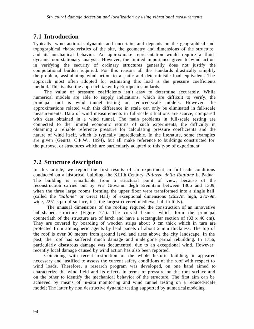
Structural damage detection and localization by using vibrational measurements
94
7.1 Introduction Typically, wind action is dynamic and uncertain, and depends on the geographical and topographical characteristics of the site, the geometry and dimensions of the structure, and its mechanical behavior. An approximate representation would require a fluid-dynamic non-stationary analysis. However, the limited importance given to wind action in verifying the security of ordinary structures generally does not justify the computational burden required. For this reason, all the standards drastically simplify the problem, assimilating wind action to a static and deterministic load equivalent. The approach most often adopted for estimating this load is the pressure coefficients method. This is also the approach taken by European standards.
The value of pressure coefficients isn’t easy to determine accurately. While numerical models are able to supply indications, which are difficult to verify, the principal tool is wind tunnel testing on reduced-scale models. However, the approximations related with this difference in scale can only be eliminated in full-scale measurements. Data of wind measurements in full-scale situations are scarce, compared with data obtained in a wind tunnel. The main problems in full-scale testing are connected to the limited economic returns of such experiments, the difficulty in obtaining a reliable reference pressure for calculating pressure coefficients and the nature of wind itself, which is typically unpredictable. In the literature, some examples are given (Geurts, C.P.W., 1994), but all make reference to buildings constructed for the purpose, or structures which are particularly adapted to this type of experiment.
7.2 Structure description In this article, we report the first results of an experiment in full-scale conditions conducted on a historical building, the XIIIth Century Palazzo della Ragione in Padua. The building is remarkable from a structural point of view, because of the reconstruction carried out by Fra' Giovanni degli Eremitani between 1306 and 1309, when the three large rooms forming the upper floor were transformed into a single hall (called the "Salone" or Great Hall) of exceptional dimensions (26.27m high, 27x79m wide, 2251 sq.m of surface, it is the largest covered medieval hall in Italy).
The unusual dimensions of the roofing required the construction of an innovative hull-shaped structure (Figure 7.1). The curved beams, which form the principal counterlath of the structure are of larch and have a rectangular section of (33 x 40 cm). They are covered by boarding of wooden strips about 3 cm thick which in turn are protected from atmospheric agents by lead panels of about 2 mm thickness. The top of the roof is over 30 meters from ground level and rises above the city landscape. In the past, the roof has suffered much damage and undergone partial rebuilding. In 1756, particularly disastrous damage was documented, due to an exceptional wind. However, recently local damage caused by wind action has also been reported.
Coinciding with recent restoration of the whole historic building, it appeared necessary and justified to assess the current safety conditions of the roof with respect to wind loads. Therefore, a research program was developed, on one hand aimed to characterize the wind field and its effects in terms of pressure on the roof surface and on the other to identify the mechanical behavior of the structure. The first aim can be achieved by means of in-situ monitoring and wind tunnel testing on a reduced-scale model; The latter by non destructive dynamic testing supported by numerical modeling.
Dynamic investigations on the Palazzo della Ragione roof in Padua
95
Figure 7.1. Cross section, aerial view of the wooden roof structure and longitudinal section.
7.3 Wind load according to EC1 According to Eurocode 1 wind pressure on the external surfaces of a structure We, can be calculated by means of the following:
dpeeerefe cc)z(cqW ⋅⋅⋅= (7.1)
where q ref is the base pressure relative to mean wind velocity, c e(ze) is the exposure coefficient (which depends on terrain roughness and exposure height, z), cpe is the external pressure coefficient and cd is the dynamic coefficient. In fact, Eurocode 1 distinguishes three aspects of wind action in three different terms, which must be considered inseparable : - kinetic pressure, that is the product of the first two terms, that takes into
consideration the intrinsic characteristics of wind phenomena, and depends on the profile of wind velocity and terrain roughness of the site where the structure is erected;
- the pressure coefficient cpe which depends on the geometry of the structure; - the dynamic coefficient cd which takes into account the mechanical characteristics
of the structure, the lack of correlation of pressures due to wind and the turbolence intensity.
The standards describe wind field conventionally, assuming a logarithmic type distribution of mean velocity with height z, which can be expressed by the universal law:
0
lnz
z
ê
uv * ⋅= (7.2)
which descends directly from Prandtl’s theory of the turbulent boundary layer.
*u is the shear velocity. ê is the von Karman constant. The value used in this investigatio is 0.4. z0 is the roughness length

Structural damage detection and localization by using vibrational measurements
96
The exposure coefficient appearing in (7.1) is expressed in particular as:
)]z(Ig)[z(c)z(c)z(c vtre ⋅+⋅= 2122 (7.3)
where cr(z) is the roughness coefficient, expressed by:
)zz
ln(Kc rr0
⋅= (7.4)
ct(z) is the topography coefficient, g the peak factor (equal to 3.5) and Iv(z) turbulence intensity, which can be expressed as:
)z(v)z(
)z(I vv
σ= (7.5)
Regarding distribution of pressure coefficients, Eurocode 1 supplies plans as reference for the most common building types. The case reported which most closely resembles the roof shape of the Palazzo della Ragione is the hipped roof, represented in Figure 7.2. Influence areas
Pitch angle F G H I J K L M N
+45 +0.7 +0.7 +0.6 -0.3 -0.6 -0.3 -1.3 -0.8 -0.2
+60 +0.7 +0.7 +0.7 -0.3 -0.6 -0.3 -2.0 -0.4 -0.2
PI
AZ
ZA
DE
LL
A
FR
UT
TA
PI
AZ
ZA
DE
LL
E
ER
BE
F
G
F
LM
K
L M
J
J
HI
e\10
e/10
e\4e\
4
e\1
0
Figure 7.2. Pressure coefficients according to Eurocode 1
Eurocode 1 transforms a typically dynamic load such as wind action into a static load by means of a dynamic coefficient expressed as:
V
xVd I
RQIc
7171 22
0
++⋅+
= (7.6)
where 0Q takes into consideration the lack of correlation of the action on the structure,
and is always less than one; xR the aerodynamic admittance and mechanical admittance, in short the mechanical characteristics of the structure. It should be noted that the dynamic coefficient necessarily includes turbulence intensity, which is an intrinsic characteristic of wind, as a consequence of how wind action has been represented in standards.
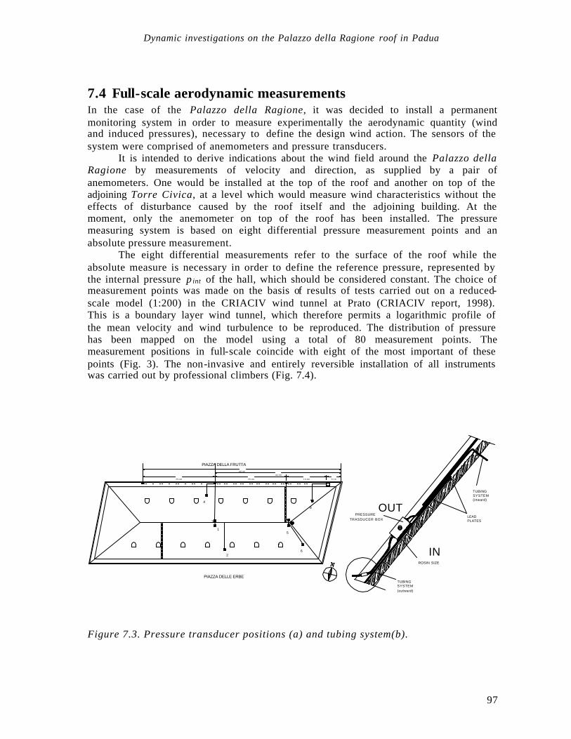
Dynamic investigations on the Palazzo della Ragione roof in Padua
97
7.4 Full-scale aerodynamic measurements In the case of the Palazzo della Ragione, it was decided to install a permanent monitoring system in order to measure experimentally the aerodynamic quantity (wind and induced pressures), necessary to define the design wind action. The sensors of the system were comprised of anemometers and pressure transducers.
It is intended to derive indications about the wind field around the Palazzo della Ragione by measurements of velocity and direction, as supplied by a pair of anemometers. One would be installed at the top of the roof and another on top of the adjoining Torre Civica, at a level which would measure wind characteristics without the effects of disturbance caused by the roof itself and the adjoining building. At the moment, only the anemometer on top of the roof has been installed. The pressure measuring system is based on eight differential pressure measurement points and an absolute pressure measurement.
The eight differential measurements refer to the surface of the roof while the absolute measure is necessary in order to define the reference pressure, represented by the internal pressure p int of the hall, which should be considered constant. The choice of measurement points was made on the basis of results of tests carried out on a reduced-scale model (1:200) in the CRIACIV wind tunnel at Prato (CRIACIV report, 1998). This is a boundary layer wind tunnel, which therefore permits a logarithmic profile of the mean velocity and wind turbulence to be reproduced. The distribution of pressure has been mapped on the model using a total of 80 measurement points. The measurement positions in full-scale coincide with eight of the most important of these points (Fig. 3). The non-invasive and entirely reversible installation of all instruments was carried out by professional climbers (Fig. 7.4).
PIAZZA DELLA FRUTTA
PIAZZA DELLE ERBE
25.00
44.00
25.00
69.00
1
26
5
7
8
3
4
13.84 5.16
IN
OUT
TUBINGSYSTEM
ROSIN SIZE
SYSTEMTUBING
TRASDUCER BOXPRESSURE
PLATESLEAD
(outward)
(inward)
Figure 7.3. Pressure transducer positions (a) and tubing system(b).

Structural damage detection and localization by using vibrational measurements
98
Figure 7.4. Installation of the anemometer and the pressure transducers
Figure 7.5. Anemometer, pressure transducer in plastic box and absolute transducer.
The acquisition system is based on a PC equipped with A/D converter. It continuously acquires signals 5 seconds long from the sensors. It calculates, averages, and determines the variance in real time and immediately files the results. When the average wind speed, as measured by one of the anemometers, exceeds a fixed trigger value (currently 5m/s), the system files the entire signal to be elaborated later. The system is expected to remain in operation for at least 3 years. The diagrams in Fig. 7.6 illustrate the average turbulence intensity as calculated for each signal, for the two directions x, with regard to wind direction, and y , orthogonally.
Turbulence Intensity Ix
0
0.1
0.2
0.3
0.4
0.5
0.6
0.7
0.8
0.9
1
0 30 60 90 120 150
Wind direction (North=0°, East=90°)
Ix
IxMean turbulence
Turbulence Intensity Iy
0
0.1
0.2
0.3
0.4
0.5
0.6
0.7
0.8
0 30 60 90 120 150
Wind Direction (North=0°, East=90°)
Iy
IyMean turbulence
Figure 7.6. Turbulence intensity for x an y directions.

Dynamic investigations on the Palazzo della Ragione roof in Padua
99
Pressure Tap 1
-0.6
0.0
0.6
0 50 100 150
Mean Wind Direction [deg]
Cp
Pressure Tap 2
-0.6
0.0
0.6
0 50 100 150
Mean Wind Direction [deg]
Cp
Pressure Tap 3
-0.6
0.0
0.6
0 50 100 150
Mean Wind Direction [deg]
Cp
Pressure Tap 4
-0.6
0.0
0.6
0 50 100 150
Mean Wind Direction [deg]
Cp
Pressure Tap 6
-0.6
0.0
0.6
0 50 100 150
Mean Wind Direction [deg]
Cp
Pressure Tap 6
-0.6
0.0
0.6
0 50 100 150
Mean Wind Direction [deg]
Cp
Pressure Tap 7
-0.6
0.0
0.6
0 50 100 150
Mean Wind Direction [deg]
Cp
Pressure Tap 8
-0.6
0.0
0.6
0 50 100 150
Mean Wind Direction [deg]
Cp
Figure 7.7. Pressure cp coefficients in full scale (dots) compared with c p given by the wind tunnel (solid line) for wind from the East (North = 0°, East = 90°) For tap 5 experimental measurements are not available.

Structural damage detection and localization by using vibrational measurements
100
(a) Wind tunnel, wind from E (b) Real scale, wind from E
(c) Eurocode 1, wind from E (d) Italian standards, wind from E
(e) Wind tunnel, wind from N-E (f) Real scale, wind from N-E
Figure 7.8. Comparison between pressure coefficients.

Dynamic investigations on the Palazzo della Ragione roof in Padua
101
Installation is now almost complete and the system has been in operation for several months; therefore, some data is already available. The more significant signals acquired refer in particular to the month of March 1999. In this period, numerous trigger signals were recorded for winds from the NE. The direction and intensity of the main winds in this period are in almost entire agreement with data supplied by the Bureau of Meteorology.
The characteristic value of turbulence intensity was calculated in Ix = 0.3. Hypothesising a logarithmic distribution of the average speeds,
−⋅−=
xIexp)dz(z
10 (7.7)
and assuming z=37.5 m as the measurement level and d=10m as the Davenport height, it descends: z0 = 1.0 m
The pressure coefficient is calculated, for each direction, according to Bernoulli’s law and can be written as:
2
0
21
v
ppcp
⋅
−=
ρ (7.8)
In the wind tunnel, it is not a problem to measure the atmospheric reference pressure p0, since it is sufficient to take a measurement with a pressure tap orthogonal to the flow and above the boundary layer. In full-scale, this measurement is a problem.
Accuracy of the measurements of inducted pressures, depends on the accuracy of the pressure transducers and of the admittance of the tubing system. In this case, laboratory test proved that the frequency response function of the overall system was constant in the frequency range of interest. An additional complication is represented by the problem of reference pressure: it is not possible to measure the atmospheric pressure in correspondence of the roof, therefore the average internal pressure of the hall was assumed as reference pressure. The internal pressure was supposed to be constant; this hypothesis is supported by a comparison between the interpolation curve of the wind tunnel results, with those achieved in-situ: the difference between the two curves results practically independent on time t and on wind direction angle )(tα .
Therefore, the pressure coefficient cp-FS , relative to the full-scale measurements, depend on the direction )(tα and on the level h only. Referring to the i-th transducers, located at quote h i , one can write:
( )( )( )( ) ( )( ) ( ) ( )
( )( ) ( )C
p
tp
p
tp
pptp
p
tptp
v
ptptc
ii
i
ii
i
ih
i
i
hc
measured
hc
hmeasured
hchc
hh
hFSp
++∆
=
−+
−=
−=−
int
0intint
2
0
21
α
α
ρ
αα
(7.9)
where: measuredp∆ is the value measured by the i-th transducer;
measuredpint is the internal pressure measured;
ihv is the theoretical mean wind velocity, measured at hi

Structural damage detection and localization by using vibrational measurements
102
Thus, the mean value of the pr essure coefficient cp-FS-M relative to the i-th transducer writes:
( )( )
Cp
pp
pc
ii
i
ihc
measured
hc
hMmeasured
hMFSp ++∆
=−
−−int
αα (7.10)
where: ( )
ihMmeasuredp α−∆ is the average of the measure acquired by the tranducer;
measuredpint is the mean value of the measured internal pressure. Comparing full-scale measurements with the interpolation curve of the mean pressure coefficient cp-WT -M(α) achieved in wind tunnel, the constant C was calculated, by using a least square optimisation:
( ) ( )[ ] ( ) ( )[ ] ==−⇒=− ∑∑∑∑= =
−−−−= =
−−−− 0min1 11
2
1
M
i
N
jhjMFSphjMW Tp
M
i
N
jhjMFSphjMW Tp
i
ii
i
ii
cccc αααα
( )( )
01 1
int =
−−
∆−= ∑∑
= =
−
−−
M
i
N
j hc
measured
hc
hjMmeasured
hjMW Tp
i
ii
i
i
Cp
pp
pc
αα (7.11)
( )( )
i
i
i
i
i
hc
measured
M
i
N
j hc
hjMmeasured
hjMW Tp
pp
NM
p
pc
C int1 1
−⋅
∆−
=
∑∑= =
−
−−
αα
(7.12)
where: M is the number of pressure transducers, equal to 8; Ni is the number of samples acquired by each tranducers.
The diagram of Figure 7.7 shows early results of pressure coefficient measurements. Interpolation of results obtained in the wind tunnel (solid line) is compared with experimental values in the full-scale situation obtained from each signal acquired (dots). In Figure 7.8, values obtained experimentally (full-scale and wind tunnel) are compared with those proposed by Eurocode 1 and the Italian standards for the main wind directions.
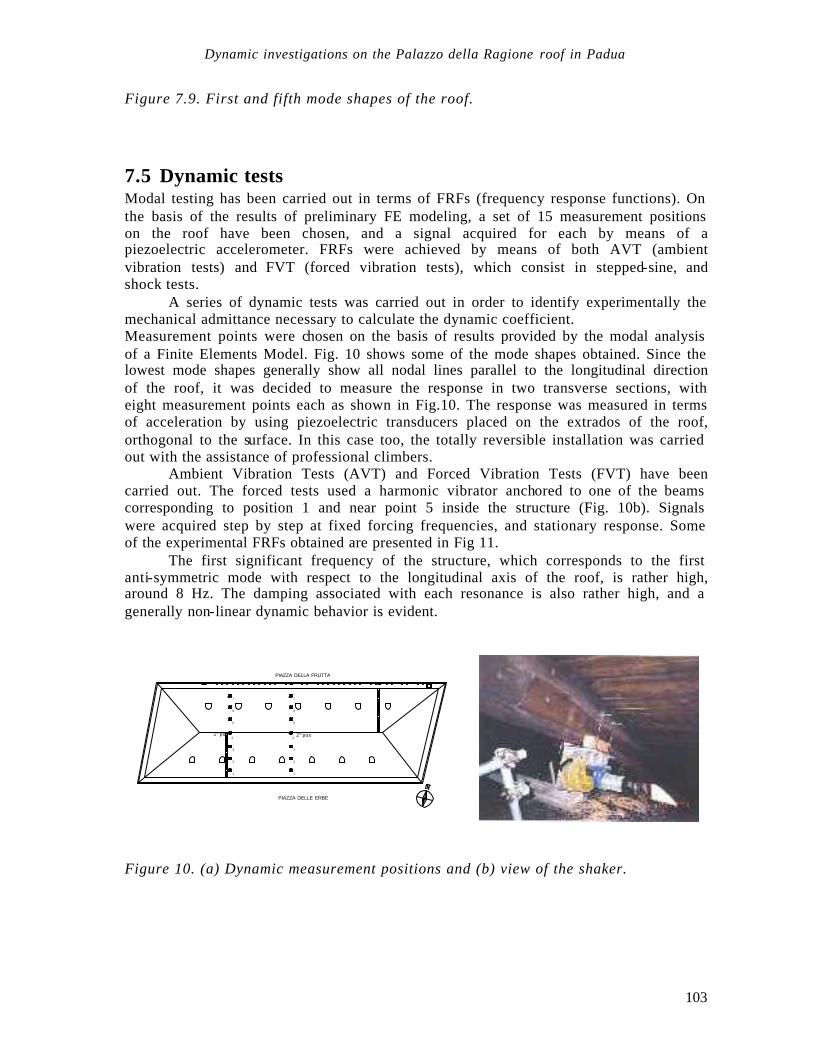
Dynamic investigations on the Palazzo della Ragione roof in Padua
103
Figure 7.9. First and fifth mode shapes of the roof.
7.5 Dynamic tests Modal testing has been carried out in terms of FRFs (frequency response functions). On the basis of the results of preliminary FE modeling, a set of 15 measurement positions on the roof have been chosen, and a signal acquired for each by means of a piezoelectric accelerometer. FRFs were achieved by means of both AVT (ambient vibration tests) and FVT (forced vibration tests), which consist in stepped-sine, and shock tests.
A series of dynamic tests was carried out in order to identify experimentally the mechanical admittance necessary to calculate the dynamic coefficient. Measurement points were chosen on the basis of results provided by the modal analysis of a Finite Elements Model. Fig. 10 shows some of the mode shapes obtained. Since the lowest mode shapes generally show all nodal lines parallel to the longitudinal direction of the roof, it was decided to measure the response in two transverse sections, with eight measurement points each as shown in Fig.10. The response was measured in terms of acceleration by using piezoelectric transducers placed on the extrados of the roof, orthogonal to the surface. In this case too, the totally reversible installation was carried out with the assistance of professional climbers.
Ambient Vibration Tests (AVT) and Forced Vibration Tests (FVT) have been carried out. The forced tests used a harmonic vibrator anchored to one of the beams corresponding to position 1 and near point 5 inside the structure (Fig. 10b). Signals were acquired step by step at fixed forcing frequencies, and stationary response. Some of the experimental FRFs obtained are presented in Fig 11.
The first significant frequency of the structure, which corresponds to the first anti-symmetric mode with respect to the longitudinal axis of the roof, is rather high, around 8 Hz. The damping associated with each resonance is also rather high, and a generally non-linear dynamic behavior is evident.
PIAZZA DELLA FRUTTA
PIAZZA DELLE ERBE
7
6
0
4
3
2
1
5
4
6
7
2
1
3
1° pos 2° pos
Figure 10. (a) Dynamic measurement positions and (b) view of the shaker.

Structural damage detection and localization by using vibrational measurements
104
0.00
0.10
0.20
0.30
0.40
0.0 5.0 10.0 15.0 20.0[Hz]
[ms-2
N-1
]
0.00
0.10
0.20
0.0 5.0 10.0 15.0 20.0[Hz]
[ms-2
N-1
]
(a) position 1 -channel 1 (b) position 1-channel 2
0.00
0.10
0.20
0.0 5.0 10.0 15.0 20.0[Hz]
[ms-2
N-1
]
0.00
0.10
0.20
0.30
0.0 5.0 10.0 15.0 20.0[Hz]
[ms-2
N-1
]
(a) position 1 -channel 3 (a) position 1-channel 4
0.00
0.10
0.0 5.0 10.0 15.0 20.0[Hz]
[ms-2
N-1
]
0.00
0.10
0.0 5.0 10.0 15.0 20.0[Hz]
[ms-2
N-1
]
(a) position 1-channel 5 (a) position 1-channel 6
0.00
0.10
0.20
0.30
0.0 5.0 10.0 15.0 20.0[Hz]
[ms-2
N-1]
0.00
0.10
0.20
0.30
0.0 5.0 10.0 15.0 20.0[Hz]
[ms-2
N-1]
(a) position 1 -channel 7 (a) position 1-channel 8
Figure 11. Experimental FRFs achieved by stepped sinusoidal test.

Dynamic investigations on the Palazzo della Ragione roof in Padua
105
7.6 Conclusions Wind field and exposure coefficient: the characteristics of turbulence measured appear compatible with the terrain roughness defined by the standards.
Induced Pressures and pressure coefficients: comparison with the wind tunnel gives very close results, at least for the directions investigated up to now. This justifies the use of the wind tunnel as an instrument for establishing shape coefficients for structures of a certain importance. Measurements made up to now permit a comparison between the norms and wind direction from the East only. Eurocode 1 gives indications that lead to an overestimation of the pressure coefficients for this direction and the main pitch. The norms in fact only consider the case of a roof comprising four pitchs with constant pitch angle and do not give indications that take into account prevailing winds. Instead, they are limited to giving the coefficients for the two directions orthogonal to the structure. It should be noted how small variations in wind direction lead to large variations in shape coefficients, and therefore the response of the building.
Dynamic coefficient: the fluctuating components of wind have frequencies below 5 Hz., while the dynamic test analysis results suggests that the roof of the Palazzo della Ragione has a basic frequency around 5 Hz. The mechanic response of the building therefore appears of little significance to an evaluation of the effects of wind action. Until a more precise evaluation is available, the dynamic coefficient may be assumed as equal to one.

Structural damage detection and localization by using vibrational measurements
106
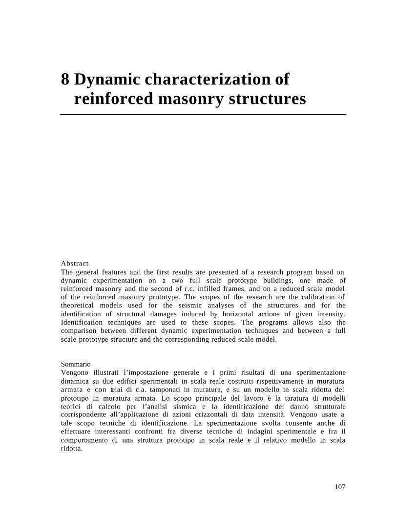
107
8 Dynamic characterization of reinforced masonry structures
Abstract The general features and the first results are presented of a research program based on dynamic experimentation on a two full scale prototype buildings, one made of reinforced masonry and the second of r.c. infilled frames, and on a reduced scale model of the reinforced masonry prototype. The scopes of the research are the calibration of theoretical models used for the seismic analyses of the structures and for the identification of structural damages induced by horizontal actions of given intensity. Identification techniques are used to these scopes. The programs allows also the comparison between different dynamic experimentation techniques and between a full scale prototype structure and the corresponding reduced scale model. Sommario Vengono illustrati l’impostazione generale e i primi risultati di una sperimentazione dinamica su due edifici sperimentali in scala reale costruiti rispettivamente in muratura armata e con telai di c.a. tamponati in muratura, e su un modello in scala ridotta del prototipo in muratura armata. Lo scopo principale del lavoro è la taratura di modelli teorici di calcolo per l’analisi sismica e la identificazione del danno strutturale corrispondente all’applicazione di azioni orizzontali di data intensità. Vengono usate a tale scopo tecniche di identificazione. La sperimentazione svolta consente anche di effettuare interessanti confronti fra diverse tecniche di indagini sperimentale e fra il comportamento di una struttura prototipo in scala reale e il relativo modello in scala ridotta.

Structural damage detection and localization by using vibrational measurements
108
8.1 Introduction Unreinforced brick masonry is usually mechanically characterised by a reasonably good ultimate resistance, but by a brittle type of failure that makes it unsuitable for buildings in a seismic area. Including steel bars in the masonry is the obvious way to increase ductility, while preserving the known properties of the construction system (heat insulation and soundproofing, durability and fire resistance, low construction and maintenance costs). The seismic behaviour of reinforced masonry (r.m.) structures has been systematically studied since the 1980’s. Nevertheless, a check at the design stage of the ductility of an r.m. structure still reveals many uncertainties that are often reflected in conservative code specifications. These uncertainties are not mainly linked to the response of the single structural elements, but more to the global response of the whole building, the design of which is still traditionally driven by architectural rather than structural reasons. This is particularly true in the case of low-medium rise buildings.
In the ambit of a research program jointly founded by the Industry and the European Community (BRITE-EURAM), two identical two-story buildings were built, but one made of reinforced masonry and the other of r.c. infilled frames, in order to compare costs of construction and the level of comfort and the behavior under static and dynamic horizontal actions of the two buildings. Also, a 1:3 scale model of reinforced masonry building was realized in order to study the seismic behavior on the shacking table of the structural system, at the Enea Research Center in Casaccia (Rome).
This research, that involved Italian and Greek industrial partners and 4 European universities (University of Athens, Universities of Padua and Pavia, University of Darmstadt), was promoted to develop a new reinforced masonry building system, based on the use of new types of blocks designed to be produced and used in different European countries and specifically studied in order to have the maximum efficiency as to the capacity of heat insulation and sound proofing, the easiness of use and the structural performance on seismic actions.
Figure 8.1. (a) Overall view of the two experimental buildings, in Trento. (b) Reduced scale model of the reinforced masonry prototype, on test on the vibrating table at the ENEA Research Center.

Dynamic characterization of reinforced masonry structures
109
Before the realization of the buildings and the reduced scale model, we made the complete characterization of the used materials and the experimental individualization of the laws of behavior under horizontal cyclical actions of the most significant reinforced masonry structural components (that is to say panels of different size and shape) made with the type of bloc developed by the Italian industry.
In this chapter, the progress of the dynamic experimentation done on the two building prototypes, and on the reduced scale model is presented, illustrating the first results of the tests and numerical processing.
Figure 8.2. Plan view of the two full scale buildings.

Structural damage detection and localization by using vibrational measurements
110
8.2 Design and construction of the buildings
8.2.1 Full scale buildings During the design of the two buildings, we tried to realize some typical constructions of our country. The constructions (Fig. 8.2) were designed and realized placing them side by side in order to permit the interposition of the required elements to impose the horizontal forces to maximize the mutual contrast offered by the two structures.
Of course, we tried to create the easiest as possible the structural behavior, to facilitate the interpretation of the tests results. This is why the staircase, common to the two buildings, is structurally independent from them, and the experimentation is done in the first phase without internal partitions. The dimension of the structures and the correspondent structural checks were made supposing that the buildings were built in a locality characterized by a high seismicity and using the support of the regulations given by the European standards.
8.2.2 Reduced scale model The model unit was constructed adopting a scale of 1:3 of the lengths, related to the dimensional capacities and load-bearing of the shaking table. Plan dimensions were 3.13 x 2.16 m at ground level, and building height was 2.09 m (Fig. 8.3a). The same building materials as that of the prototype were used, so the scale, relating to the Young’s modulus and density of the materials used, assumed a unitary value. The bricks used for the model were obtained from blocks used in the prototype, cutting them to reach the 1:3 scale. Three types of bricks were made as shown in Fig. 8.3b. As vertical reinforcement smooth steel bars, 8 mm and 6 mm diameter were used at corner locations and intermediate zones, respectively. Horizontal reinforcement consisted of 2mm diameter steel bars. The model was built on a 120 mm thick concrete slab, constructed to allow it to be transported and coupled to the shaking table by means of steel anchors. The concrete masonry floor slabs were reproduced to scale and additional masses were placed at the roof and at the floor slab level, to take into account different specific density and simulate variable live loads equal to 1000 Nm-2 at the first storey and 800 Nm-2 at the second one.
Figure 8.3. Plan of the reduced scale model (a) and masonry bricks adopted (b)
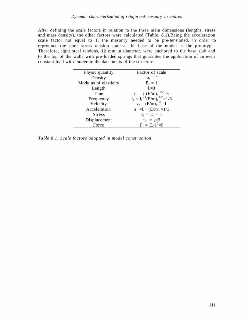
Dynamic characterization of reinforced masonry structures
111
After defining the scale factors in relation to the three main dimensions (lengths, stress and mass density), the other factors were calculated (Table. 8.1).Being the acceleration scale factor not equal to 1, the masonry needed to be pre-tensioned, in order to reproduce the same stress tension state at the base of the model as the prototype. Therefore, eight steel tendons, 12 mm in diameter, were anchored to the base slab and to the top of the walls with pre-loaded springs that guarantee the application of an even constant load with moderate displacements of the structure.
Physic quantity Factor of scale
Density mr = 1 Modulus of elasticity Er = 1
Length lr=3 Time tr = lr (E/m)r
-1/2=3 Frequency f r = lr -1(E/m) r
1/2=1/3 Velocity vr = (E/m) r
1/2=1 Acceleration a r =lr-1 (E/m)r=1/3
Stress sr = Er = 1 Displacement ur = lr=3
Force Fr = Er/lr2=9
Table 8.1. Scale factors adopted in model construction.

Structural damage detection and localization by using vibrational measurements
112
8.3 Dynamic characterization The whole program of dynamic experimentation provides, for each building, a first phase of characterization in elastic field; and a second one of test in non linear field (seismic test on the vibrating table for the model).
The seismic tests were preceded by a series of modal characterization test. Different experimental techniques were compared (stepped sinusoidal test using an harmonic exciter, shock test using a pulse hammer, random vibration and sine-sweeping test using the shaking table) in order to define a procedure for a rapid and effective characterisation to be repeated after each test.
The first phase of experimentation aims to the following targets: (a) to define the correspondence in the mechanic behavior of the structures (b) to calibrate the numerical models (c) to define the seismic loads of the design estimated by the regulation
8.3.1 Position of transducer and techniques of experimentation In both cases, the first of the prototype and the second of the model, the motion of the most significant points of the raising structure was measured through 8 piezoelectric accelerometers, placed as shown in the Fig. 8.4. Then 4 horizontal accelerometers (shown in the picture) and three verticals (Z3, Z6, Z9) were placed on the base to control its movement. Different techniques of experimentation were used for the dynamic characterisation, from AVT to shock tests and stepped sine tests.
Figure 8.4. Transducers position

Dynamic characterization of reinforced masonry structures
113
Figure 8.5. Scheme of the shaker.
8.3.2 Full scale building A dynamic exciter of big dimensions was created to allow the application of harmonic forces, up and more than the elastic region of the structure, in the Laboratory of the Department of Constructions and Transports at the University of Padua.
The dynamic exciter (Fig. 8.5) is composed of two rotating steel discs of 90 cm on which the eccentric masses varying from 5 kg to a maximum of 40 kg; the force generated depends on the eccentric mass and on the frequency of the rotation, up to a maximum estimated during the design equal to 140 KN in a frequency range from 1 to 20 Hz.
The typical frequency response functions, expressed in acceleration, got with the stationary harmonic excitation are reported in Fig. 8.6, and compared with the results of AVT, for the accelerometers X1 and X2, placed in correspondence with the second and the first floor respectively, in the same direction of the force. The use of the technique of the slow linear sweeping gave the same results obtained with the stationary excitation.
5.0 7.0 9.0 11.0 13.0 15.0Hz 5.0 7.0 9.0 11.0 13.0 15.0Hz
Figure 8.6. FRF achieved (b) through stationary harmonic excitation with the dynamic exciter placed in the middle of the second floor and (a) through AVT (fitted)
X1X2
X1X2
Structural damage detection and localization by using vibrational measurements
114
The use of the hammer with specified instruments and other percussion instruments gave medium results because only the high frequencies of the structure had been excited. The main results of the characterization are reported in the Tables 8.2 e 8.3.
AVT stepped sine f ξ f ξ
I mode 6.17 Hz 4.1% - - II mode 8.45 Hz 3.8% 8.01% 7.9%
Table 8.2.
X1 X2 Y1 Y2 Z3 Z9 II mode 1 0.48 0.01 - -0.27 0.42
Table 8.3. Modal components based on the tests with dynamic exciter.
It is important to remark that we cannot neglect the importance of the motion on the base, because the flexibility of the ground produces the inversion of the first two frequencies when compared to the frequencies expected from the numerical model, where we suppose the firm ground condition on the base.
The problem of the motion on the base can be theoretically solved considering the raising structure as a substructure of the system building+ground, which can be completely characterized by the dynamic experimentation and described through the FRFs matrix.
Then, once defined the substructure as the subject-matter of our study, its state will be defined by a vector of variables. Among them, we can differentiate the variables that described only the state of the substructure from the others which describe the state of points of contact from the substructure and the rest of the system. The substructure response to an harmonic forcing of frequency equal to ω, is entirely explained in the following complex relation:
x
y
H H
H H
f
r
−
= − + −
−
xx xy
yx yy
|
|
(8.1)
where the substructures H represent the FRFs (expressed in receptance, mobility or inertance); x and y the vectors of the complex amplitude response (expressed in displacement, velocity or acceleration) in the own points of the structure and in the points of contact respectively; f e r the vectors of the complex components of the force applicated in correspondence with x e y respectively.
Each component hi j(ω) of each submatrix can be achieved through the dynamic testing. Our purpose is to deduce the hi j’ FRFs, components of matrix H’, that relate the amplitude of the motion of each degree of freedom to the amplitude of the forces in the hypothesis in which there was no motion of the points of contact (grounded subsystem). Defining as it is shown y 0= :
[ ]x H H H H f= − −xx xy yy yx
1 (8.2)
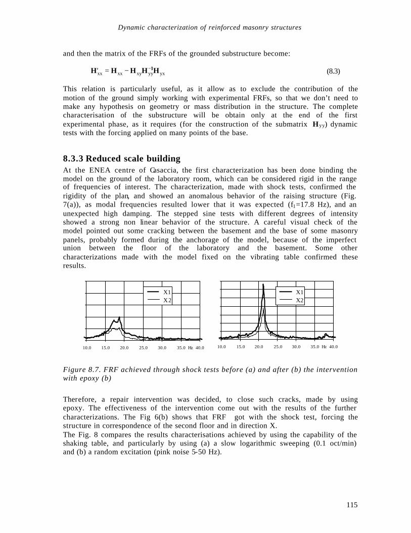
Dynamic characterization of reinforced masonry structures
115
and then the matrix of the FRFs of the grounded substructure become:
′ = − −H H H H Hxx xx xy yy yx1 (8.3)
This relation is particularly useful, as it allow as to exclude the contribution of the motion of the ground simply working with experimental FRFs, so that we don’t need to make any hypothesis on geometry or mass distribution in the structure. The complete characterisation of the substructure will be obtain only at the end of the first experimental phase, as it requires (for the construction of the submatrix Hyy) dynamic tests with the forcing applied on many points of the base.
8.3.3 Reduced scale building At the ENEA centre of Casaccia, the first characterization has been done binding the model on the ground of the laboratory room, which can be considered rigid in the range of frequencies of interest. The characterization, made with shock tests, confirmed the rigidity of the plan, and showed an anomalous behavior of the raising structure (Fig. 7(a)), as modal frequencies resulted lower that it was expected (f1=17.8 Hz), and an unexpected high damping. The stepped sine tests with different degrees of intensity showed a strong non linear behavior of the structure. A careful visual check of the model pointed out some cracking between the basement and the base of some masonry panels, probably formed during the anchorage of the model, because of the imperfect union between the floor of the laboratory and the basement. Some other characterizations made with the model fixed on the vibrating table confirmed these results.
10.0 15.0 20.0 25.0 30.0 35.0 40.0Hz 10.0 15.0 20.0 25.0 30.0 35.0 40.0Hz
Figure 8.7. FRF achieved through shock tests before (a) and after (b) the intervention with epoxy (b)
Therefore, a repair intervention was decided, to close such cracks, made by using epoxy. The effectiveness of the intervention come out with the results of the further characterizations. The Fig 6(b) shows that FRF got with the shock test, forcing the structure in correspondence of the second floor and in direction X. The Fig. 8 compares the results characterisations achieved by using the capability of the shaking table, and particularly by using (a) a slow logarithmic sweeping (0.1 oct/min) and (b) a random excitation (pink noise 5-50 Hz).
X1X2
X1X2

Structural damage detection and localization by using vibrational measurements
116
10.0 15.0 20.0 25.0 30.0 35.0 40.0Hz 10.0 15.0 20.0 25.0 30.0 35.0 40.0Hz
Figure8.8. FRFs achieved through (a) slow logarithmic sweeping and (b) random vibrations.
In the tables 8.4 and 8.5, the results are reassumed and compared in terms of frequency of the different characterizations. The shock test and the sweeping provided the same results but the random excitation has frequencies slightly higher. The explanation can be find looking at the different intensity of the forces:
hammer (before repair)
hammer (after repair)
sweeping random
f (Hz) ξ f (Hz) ξ f (Hz) ξ f (Hz) ξ I mode 18.14 1 21.16 1.2% 21.36 1.2% 22.20 1.2%
II mode
21.16 1 27.22 1.2% 27.28 1.9% 29.24 1.9%
1 Non proportional damping Table 8.4.
X1 X2 Y1 Y2 Z3 Z9 I mode 1.00 053 0.03 0.01 - - II mode 0.04 0.02 1 0.64 - -
Table 8.5. Modal components based on shock tests.
X1X2
X1X2

Dynamic characterization of reinforced masonry structures
117
8.3.4 Modeling Numerical models with 3D elements (brick) were created from the structures under discussion before the execution of the experimentation to estimate the variability field of the own structural frequencies and then to plan the tests.
After the first results of the experimentation, a model of the structure made of plates was created in which the property of the materials were included with their measured estimations (Fig. 8.9).
Some slabs with anisotropic behavior with uniform thickness are modeled for the floors. The modulus of elasticity in the two directions is estimated as the product of the modulus of elasticity for the moment of inertia of the section is equal to the real one. For the direction of the frame of the rafters, we consider the inertia of the cope of the floor and the ring beam of the connections between the walls
The specific weight attributed to the slab with which the floor was created considers the real own weight of the floor and the added masses to the reduced scale model to carry the ratios between mass of the walls and of the floor to the estimations of the real structure.
The identification of the model, based on the two first frequencies and relative modal components, given from the shock test and sweeping, gave, besides the correct definition of the equivalent stiffness of the floor, modelled as orthotropic slab, an estimation of the modulus of elasticity of the masonry equal to 4300 MPa, in other words lower than the medium estimation given from the results of the tests of compression.
Figure 8.9. Finite elements model of the reduced scale building.
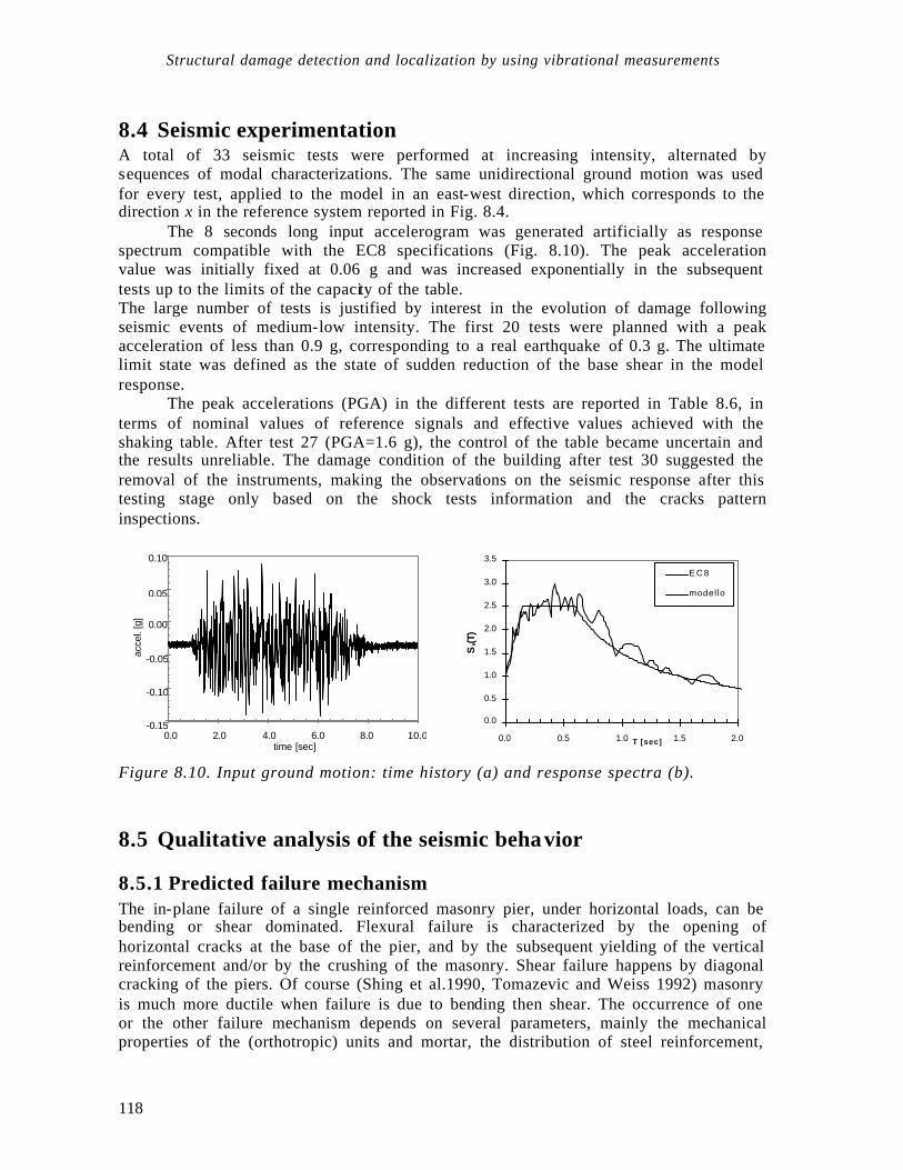
Structural damage detection and localization by using vibrational measurements
118
8.4 Seismic experimentation A total of 33 seismic tests were performed at increasing intensity, alternated by sequences of modal characterizations. The same unidirectional ground motion was used for every test, applied to the model in an east-west direction, which corresponds to the direction x in the reference system reported in Fig. 8.4.
The 8 seconds long input accelerogram was generated artificially as response spectrum compatible with the EC8 specifications (Fig. 8.10). The peak acceleration value was initially fixed at 0.06 g and was increased exponentially in the subsequent tests up to the limits of the capacity of the table. The large number of tests is justified by interest in the evolution of damage following seismic events of medium-low intensity. The first 20 tests were planned with a peak acceleration of less than 0.9 g, corresponding to a real earthquake of 0.3 g. The ultimate limit state was defined as the state of sudden reduction of the base shear in the model response.
The peak accelerations (PGA) in the different tests are reported in Table 8.6, in terms of nominal values of reference signals and effective values achieved with the shaking table. After test 27 (PGA=1.6 g), the control of the table became uncertain and the results unreliable. The damage condition of the building after test 30 suggested the removal of the instruments, making the observations on the seismic response after this testing stage only based on the shock tests information and the cracks pattern inspections.
-0.15
-0.10
-0.05
0.00
0.05
0.10
0.0 2.0 4.0 6.0 8.0 10.0time [sec]
acce
l. [g
]
0.0
0.5
1.0
1.5
2.0
2.5
3.0
3.5
0.0 0.5 1.0 1.5 2.0T [sec]
Se(T
)
E C 8
modello
Figure 8.10. Input ground motion: time history (a) and response spectra (b).
8.5 Qualitative analysis of the seismic behavior
8.5.1 Predicted failure mechanism The in-plane failure of a single reinforced masonry pier, under horizontal loads, can be bending or shear dominated. Flexural failure is characterized by the opening of horizontal cracks at the base of the pier, and by the subsequent yielding of the vertical reinforcement and/or by the crushing of the masonry. Shear failure happens by diagonal cracking of the piers. Of course (Shing et al.1990, Tomazevic and Weiss 1992) masonry is much more ductile when failure is due to bending then shear. The occurrence of one or the other failure mechanism depends on several parameters, mainly the mechanical properties of the (orthotropic) units and mortar, the distribution of steel reinforcement,
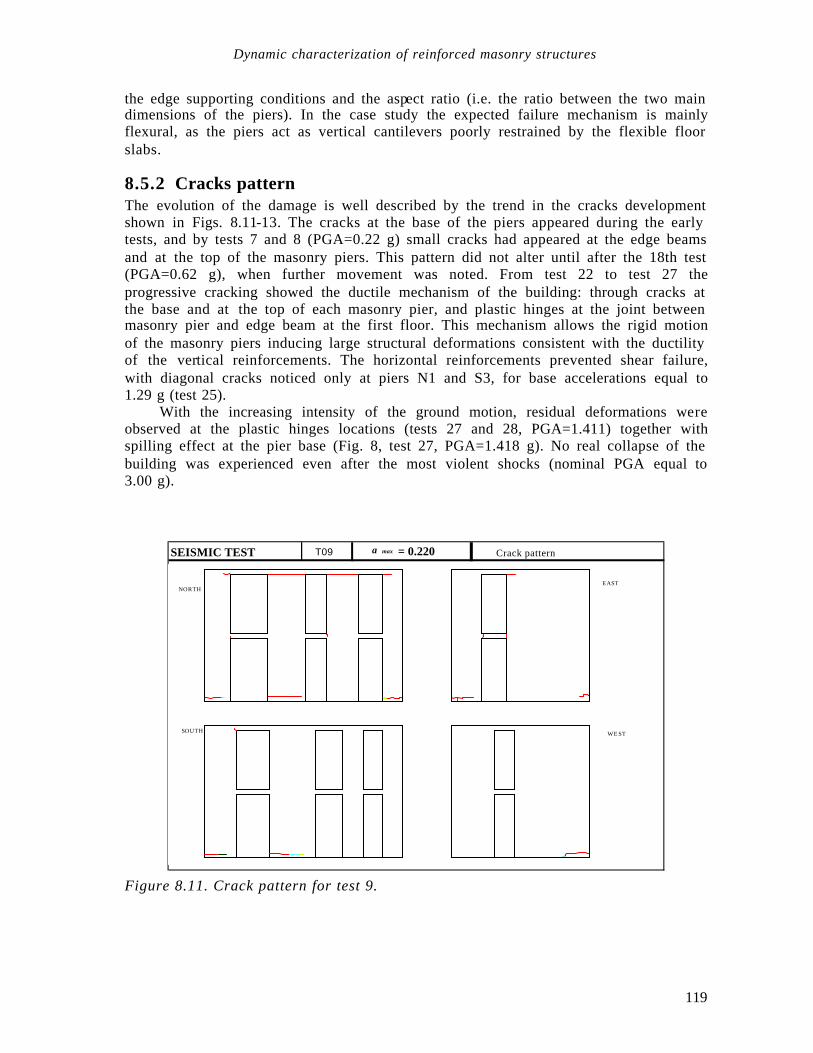
Dynamic characterization of reinforced masonry structures
119
the edge supporting conditions and the aspect ratio (i.e. the ratio between the two main dimensions of the piers). In the case study the expected failure mechanism is mainly flexural, as the piers act as vertical cantilevers poorly restrained by the flexible floor slabs.
8.5.2 Cracks pattern The evolution of the damage is well described by the trend in the cracks development shown in Figs. 8.11-13. The cracks at the base of the piers appeared during the early tests, and by tests 7 and 8 (PGA=0.22 g) small cracks had appeared at the edge beams and at the top of the masonry piers. This pattern did not alter until after the 18th test (PGA=0.62 g), when further movement was noted. From test 22 to test 27 the progressive cracking showed the ductile mechanism of the building: through cracks at the base and at the top of each masonry pier, and plastic hinges at the joint between masonry pier and edge beam at the first floor. This mechanism allows the rigid motion of the masonry piers inducing large structural deformations consistent with the ductility of the vertical reinforcements. The horizontal reinforcements prevented shear failure, with diagonal cracks noticed only at piers N1 and S3, for base accelerations equal to 1.29 g (test 25).
With the increasing intensity of the ground motion, residual deformations were observed at the plastic hinges locations (tests 27 and 28, PGA=1.411) together with spilling effect at the pier base (Fig. 8, test 27, PGA=1.418 g). No real collapse of the building was experienced even after the most violent shocks (nominal PGA equal to 3.00 g).
SEISMIC TEST T09 a max = 0.220 g
Crack pattern
WEST
EAST NORTH
SOUTH
Figure 8.11. Crack pattern for test 9.

Structural damage detection and localization by using vibrational measurements
120
SEISMIC TEST T27 a max = 1.418g
Crack pattern
WEST
EASTNORTH
South
Figure 8.12: Crack pattern for test 27.
SEISMIC TEST T31 a max = 3.00 g Crack patternFESSURATIVO
west
EastNorth
South
Figure 8.13. Crack pattern for test 31.

Dynamic characterization of reinforced masonry structures
121
8.6 Hypothesis for the structural response interpretation
8.6.1 Modeling as a single degree of freedom system When the system is non-linear, the hypothesis of modal superposition is no longer valid and the “exact” response can be found only by integrating the equations of motion over time. The use of modal decomposition technique provides an optional approach for the analysis of non linear system as well (Iwan and Yang, 1972). In the case of multi-story buildings that presents a regularity in plan (so allowing analysis of the system on a vertical plane) and in elevation, this non-rigorous approach is particularly justified as the system mainly responds according to one of its modal shapes. The system can then be represented as a non-linear SDOF oscillator, where absolute acceleration and relative motion are measured at a reference position (usually the top of the building). Even if the studied model is not geometrically symmetrical, the distribution of masses and stiffness is so that the first and second modal shapes show displacement components almost exclusively in the major directions x and y, respectively. The structure were therefore modeled as a SDOF oscillator, where the input is the ground motion and the output corresponds to the displacement in direction x of the centre of mass of the second storey, calculated as the average of the response of accelerometers 1 and 9.
8.6.2 Response of a non-linear SDOF system For non-linear SDOF systems, the equation of the motion is expressed in the general form:
( ) ( )mx F x x mz t&& , & &&+ = − (8.4)
where x&& is the relative acceleration of the oscillator, z&& is the input acceleration and ),( xxf & is the generic restoring force. It is useful to express the equation normalised to
the mass:
( ) ( )&& , & &&x f x x z t+ = − (8.5)
where:
( ) ( )f x x
F x xm
, &, &
= (8.6)
so that:
( ) ( )( ) ( )f x x x z t a t, & && &&= − + = − (8.7)
being ( )a t the absolute acceleration. The simplest type of non-linear vibrator is the elastic-plastic perfect oscillator (EPP), that is characterised by initial stiffness k0 and maximum restoring force intensity Fmax ,
i.e., in normalised form, by the natural frequency ω 02 and by the maximum absolute
acceleration. The required ductility is the expression of the maximum displacement in adimensional terms that occurs during the loading history:
µ = xx y
max (8.8)
Structural damage detection and localization by using vibrational measurements
122
where x y represents the yielding displacement. A well know technique for the response assessment of a non-linear oscillator is the Substitute Structure Method (Gulkan and Sozen 1974). This approximates the response of a generic non-linear system with that of a linear system with equivalent (effective) stiffness and viscous damping. The effective stiffness is the secant stiffness evaluated at the maximum displacement:
( )k
F x xxeff = max
max
, & (8.8)
Normalized with respect to the mass, it is also possible to define the natural effective frequency, as:
k meff eff= ω 2 (8.9)
The effective viscous damping is such that the energy dissipated by hysteresis in a cycle in the non-linear system corresponds to the energy dissipated by the viscous restoring force in the equivalent oscillator:
( )f x x x x xeq eff, & maxd d∫ ∫= 2ξ ω (8.10)
therefore, for a sinusoidal response of the equivalent oscillator:
ξπωeq
eff
f x
x= ∫ d
2 2 2max
(8.11)
In the case of the EPP oscillator, the energy dissipated in a cycle is:
( )F x F x x F xy y yr
d∫ = − = −
4 4 1 1
max max µ (8.12)
and the effective viscous damping results as being directly linked to the required ductility:
ξπ µeq EPP
r, = −
21
1 (8.13)
Being the energy dissipated in a cycle always lower than that of the elasto-plastic model, this equivalent damping value represents an upper limit. The effective load can be calculated in general terms with the equation:
m mV
= ∫ φd (8.14)
where φ represents the deflection of the structure, normalized with respect to the position of the reference measurement. In practice, for a multi-storey building this reference measurement is the displacement at the top, and the equation becomes:
m mi ii= ∑φ (8.15)
Where φi is the normalised displacement and mi the mass, concentrated at the ith storey. The maximum intensity of the total seismic action measured at the base (base shear) therefore can be expressed as:
BS a m a mi ii= = ∑max max φ (8.16)
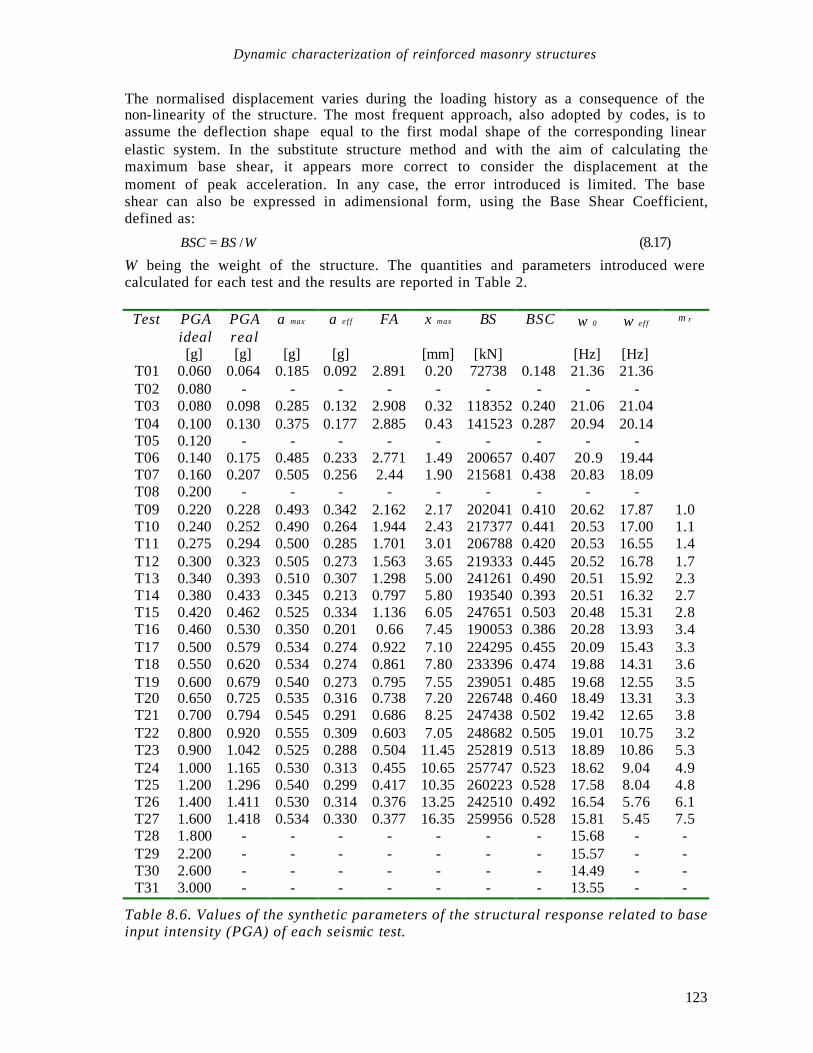
Dynamic characterization of reinforced masonry structures
123
The normalised displacement varies during the loading history as a consequence of the non-linearity of the structure. The most frequent approach, also adopted by codes, is to assume the deflection shape equal to the first modal shape of the corresponding linear elastic system. In the substitute structure method and with the aim of calculating the maximum base shear, it appears more correct to consider the displacement at the moment of peak acceleration. In any case, the error introduced is limited. The base shear can also be expressed in adimensional form, using the Base Shear Coefficient, defined as:
WBSBSC /= (8.17)
W being the weight of the structure. The quantities and parameters introduced were calculated for each test and the results are reported in Table 2.
Test PGA ideal
PGA real
a max a e f f FA x max BS BSC ω 0 ω e f f µ r
[g] [g] [g] [g] [mm] [kN] [Hz] [Hz] T01 0.060 0.064 0.185 0.092 2.891 0.20 72738 0.148 21.36 21.36 T02 0.080 - - - - - - - - - T03 0.080 0.098 0.285 0.132 2.908 0.32 118352 0.240 21.06 21.04 T04 0.100 0.130 0.375 0.177 2.885 0.43 141523 0.287 20.94 20.14 T05 0.120 - - - - - - - - - T06 0.140 0.175 0.485 0.233 2.771 1.49 200657 0.407 20.9 19.44 T07 0.160 0.207 0.505 0.256 2.44 1.90 215681 0.438 20.83 18.09 T08 0.200 - - - - - - - - - T09 0.220 0.228 0.493 0.342 2.162 2.17 202041 0.410 20.62 17.87 1.0 T10 0.240 0.252 0.490 0.264 1.944 2.43 217377 0.441 20.53 17.00 1.1 T11 0.275 0.294 0.500 0.285 1.701 3.01 206788 0.420 20.53 16.55 1.4 T12 0.300 0.323 0.505 0.273 1.563 3.65 219333 0.445 20.52 16.78 1.7 T13 0.340 0.393 0.510 0.307 1.298 5.00 241261 0.490 20.51 15.92 2.3 T14 0.380 0.433 0.345 0.213 0.797 5.80 193540 0.393 20.51 16.32 2.7 T15 0.420 0.462 0.525 0.334 1.136 6.05 247651 0.503 20.48 15.31 2.8 T16 0.460 0.530 0.350 0.201 0.66 7.45 190053 0.386 20.28 13.93 3.4 T17 0.500 0.579 0.534 0.274 0.922 7.10 224295 0.455 20.09 15.43 3.3 T18 0.550 0.620 0.534 0.274 0.861 7.80 233396 0.474 19.88 14.31 3.6 T19 0.600 0.679 0.540 0.273 0.795 7.55 239051 0.485 19.68 12.55 3.5 T20 0.650 0.725 0.535 0.316 0.738 7.20 226748 0.460 18.49 13.31 3.3 T21 0.700 0.794 0.545 0.291 0.686 8.25 247438 0.502 19.42 12.65 3.8 T22 0.800 0.920 0.555 0.309 0.603 7.05 248682 0.505 19.01 10.75 3.2 T23 0.900 1.042 0.525 0.288 0.504 11.45 252819 0.513 18.89 10.86 5.3 T24 1.000 1.165 0.530 0.313 0.455 10.65 257747 0.523 18.62 9.04 4.9 T25 1.200 1.296 0.540 0.299 0.417 10.35 260223 0.528 17.58 8.04 4.8 T26 1.400 1.411 0.530 0.314 0.376 13.25 242510 0.492 16.54 5.76 6.1 T27 1.600 1.418 0.534 0.330 0.377 16.35 259956 0.528 15.81 5.45 7.5 T28 1.800 - - - - - - - 15.68 - - T29 2.200 - - - - - - - 15.57 - - T30 2.600 - - - - - - - 14.49 - - T31 3.000 - - - - - - - 13.55 - -
Table 8.6. Values of the synthetic parameters of the structural response related to base input intensity (PGA) of each seismic test.

Structural damage detection and localization by using vibrational measurements
124
a max
0.0
0.2
0.4
0.6
0.8
1.0
0.00 0.50 1.00 1.50g
g
a eff
0.0
0.2
0.4
0.6
0.8
1.0
0.00 0.50 1.00 1.50g
g
FA
0.0
1.0
2.0
3.0
4.0
0.00 0.50 1.00 1.50g
adim
x max
0.0
2.5
5.0
7.5
10.0
12.5
15.0
17.5
0.00 0.50 1.00 1.50g
mm
ωω0
0.0
5.0
10.0
15.0
20.0
25.0
0.00 0.50 1.00 1.50g
Hz
ωωeff
0.0
5.0
10.0
15.0
20.0
25.0
0.00 0.50 1.00 1.50g
Hz
µ µ r
1.0
2.0
3.0
4.0
5.0
6.0
7.0
8.0
0.00 0.50 1.00 1.50g
adim
BSC
0.0
0.1
0.2
0.3
0.4
0.5
0.6
0.00 0.50 1.00 1.50g
adim
Figure 8.14. Trend of seismic response related to the base input intensity.
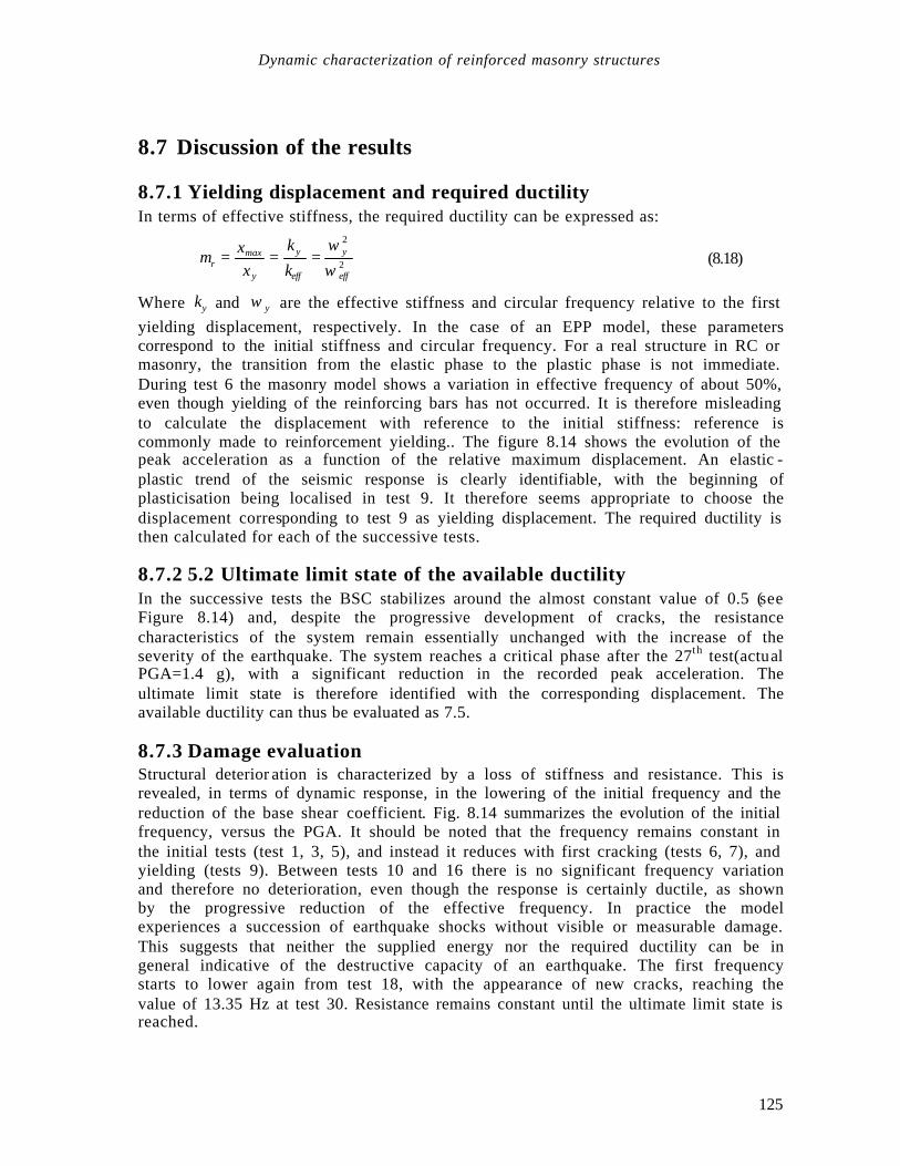
Dynamic characterization of reinforced masonry structures
125
8.7 Discussion of the results
8.7.1 Yielding displacement and required ductility In terms of effective stiffness, the required ductility can be expressed as:
µω
ωry
y
eff
y
eff
xx
k
k= = =max
2
2 (8.18)
Where ky and ω y are the effective stiffness and circular frequency relative to the first yielding displacement, respectively. In the case of an EPP model, these parameters correspond to the initial stiffness and circular frequency. For a real structure in RC or masonry, the transition from the elastic phase to the plastic phase is not immediate. During test 6 the masonry model shows a variation in effective frequency of about 50%, even though yielding of the reinforcing bars has not occurred. It is therefore misleading to calculate the displacement with reference to the initial stiffness: reference is commonly made to reinforcement yielding.. The figure 8.14 shows the evolution of the peak acceleration as a function of the relative maximum displacement. An elastic -plastic trend of the seismic response is clearly identifiable, with the beginning of plasticisation being localised in test 9. It therefore seems appropriate to choose the displacement corresponding to test 9 as yielding displacement. The required ductility is then calculated for each of the successive tests.
8.7.2 5.2 Ultimate limit state of the available ductility In the successive tests the BSC stabilizes around the almost constant value of 0.5 (see Figure 8.14) and, despite the progressive development of cracks, the resistance characteristics of the system remain essentially unchanged with the increase of the severity of the earthquake. The system reaches a critical phase after the 27th test(actual PGA=1.4 g), with a significant reduction in the recorded peak acceleration. The ultimate limit state is therefore identified with the corresponding displacement. The available ductility can thus be evaluated as 7.5.
8.7.3 Damage evaluation Structural deterior ation is characterized by a loss of stiffness and resistance. This is revealed, in terms of dynamic response, in the lowering of the initial frequency and the reduction of the base shear coefficient. Fig. 8.14 summarizes the evolution of the initial frequency, versus the PGA. It should be noted that the frequency remains constant in the initial tests (test 1, 3, 5), and instead it reduces with first cracking (tests 6, 7), and yielding (tests 9). Between tests 10 and 16 there is no significant frequency variation and therefore no deterioration, even though the response is certainly ductile, as shown by the progressive reduction of the effective frequency. In practice the model experiences a succession of earthquake shocks without visible or measurable damage. This suggests that neither the supplied energy nor the required ductility can be in general indicative of the destructive capacity of an earthquake. The first frequency starts to lower again from test 18, with the appearance of new cracks, reaching the value of 13.35 Hz at test 30. Resistance remains constant until the ultimate limit state is reached.
Structural damage detection and localization by using vibrational measurements
126
8.7.4 Calculation of the behavior factor The force-based design procedure is based on a check on a linear elastic model with a conventional resistance. The ductile behavior of the structure is token into account by reducing the seismic action by a given q-factor or behavior factor. This is defined as the ratio between the seismic forces Fe that the structure should elastically resist to, and the lowest design seismic forces Fy:
y
e
FF
q = (8.19)
and can also be expressed in the form:
( ) ( )q T
Te
u
* ,* ,
*ξ
β ξ
β= (8.20)
where β e and β u represent the amplification factors for the linear elastic response and for the non linear response at the ultimate limit state, respectively.
The q factor depends on a conventional design earthquake or a reference linear elastic model (characterized by natural period and viscous damping): despite the name, it is therefore not a characteristic coefficient of the structural behavior only. The definition of the period and damping of the equivalent linear elastic model is ambiguous as well, particularly for a masonry structure that does not show linear behavior even for minor deformations. At yielding point, the model presents a frequency ω = 20.62 Hz (that corresponds to a period of the real structure T=0.1455 s) and a damping ξ=15% Based on these values, the behaviour factor is equal to q=5.68. If we instead refer to the initial stiffness and damping (ξ =7.55%) we obtain q=7.60.
According to Eurocode 8, the q factor is defined as in (8.19) only in correspondence to the constant acceleration spectral branch, i.e. for typical vibration periods between TB and TC . In this case the amplification factors are:
β ηβe S= 0 (8.21)
ββ
u Sq
= 0 (8.22)
Where S is the soil parameter, ηξ
=+
72 100
is the damping correction factor and
β 0 =2.5 is the amplification factor for 5% viscous damping. Assuming equal the two ratios between the amplification factors we obtain:
( ) ( ) ( )q TT
q Te
u
e
u
* ,* ,
*ξ
β ξ
βββ
η= = = (8.23)
( )( ) ( )
q Tq T q T
= =
+
* , * ,ξ
η
ξ
ξ7
2 100
(8.24)
For T TB< (equal to 0.15 s) we obtain:

Dynamic characterization of reinforced masonry structures
127
( )β ηβeB
STT
= + −
1 10 (8.25)
β βu
B
STT q
= + −
1 10 (8.26)
( )
( )
−−+
+
−
=
T
T
TqT
TTq
BB 110027
,*11 0
0
βξξ
β (8.27)
Assuming the fundamental period of the structure as the one at yielding, a q equal to 3.6 can be deduced from (8.24). Assuming the period as the initial one, q=5.9 is instead obtained through (8.27). These are anyway values above the q=2.5 suggested by the code.
8.8 Conclusions The experimental study presented highlights a very satisfactory seismic behavior of the tested r. m. construction technique, both in terms of the response to low/medium intensity earthquake, and of behavior at the ultimate limit state. Specifically: 1. The building could sustain a consistent sequence of medium earthquake shocks,
without showing apparent damage or significant loss of stiffness or resistance; a consistent stiffness deterioration was observed at PGA values higher than 1g.
2. The achieved ductility m=7.5, evaluated at the ultimate limit state, was definitively satisfactory.
3. According to EC8 design requirements, a behavior factor q>=3.6 could be adopted, significantly higher than the value q=2.5 proposed by the code in absence of more precise information.

Structural damage detection and localization by using vibrational measurements
128

129
9 Non Destructive Evaluation on the PRESSS building model
Abstract A dynamic NDT shaking test was carried out on the UCSD 5-story PRESSS (Precast Seismic Structural Systems) building in the Powell laboratory. The intact structure was teste d before load application. Much data was collected during: 1) A large instrumented hammer test, and 2) A large 5000 lb couter-rotating mass shaker test. The building was instrumented in 4 different configurations (each comprised of 15 recording accelerometers). The first configuration (A) included 3 accelerometers on every floor. Each additional configuration focused on the dynamic response of an individual beam-column connection, with instruments closely clustered along the beam and column. Five resonances are readily apparent in the recorded data. Sommario Una sperimentazione non distruttiva è stata svolta presso sull'edificio a sperimentale del progettoPRESSS (sistema strutturale antisismico in precompresso) presso i Powell Laboratories dell'UCSD. La struttura integra è stata testata prima dell'applicazione del carico. I segnali sono stati acquisiti durante: 1)prove con il martello strumentato e 2)prove con una vibrodina a masse rotanti in grado di generare una forza di 5000 lb. L'edificio è stato strumentato in 4 diverse posizioni, ognuna comprendente 15 posizioni accelerometriche. La prima configurazione prevede 3 accelerometri per ciascun piano. Le successive configurazioni si sono concentrate sulla risposta di 3 diverse connessioni trave-colonna, con gli strumenti raggruppati in corrispondenza del nodo. Fra i dati acquisiti, sono state identificate chiaramente 5 risonanze.
Structural damage detection and localization by using vibrational measurements
130
9.1 Introduction
9.1.1 Seismic design philosophy of building As an understanding developed in the 1960s and 1970s of the importance of inelastic structural response to large scale earthquakes, the research community became increasingly involved in attempts to quantify the inelastic deformation capacity of structural component. Generally, it is expressed in terms of displacement ductility capacity Dµ , which is chosen as an useful indicator because of its apparent relationship to the force reduction factor R, commonly used to reduce expected elastic levels of base shear strength to acceptable design levels.
Modern seismic analysis is based on the concept of ductility, rather than strength. As it is well-known, the design philosophy founded on the concept that the distribution of strength through a building is more important than the absolute value of the design base shear for earthquake resistance, is known as capacity design (Park and Paulay, 1975).
In the capacity design of structures, distinct elements, we use to refer to as plastic hinges, are chosen and suitably designed and detailed for energy dissipation under severe imposed deformation (Paulay and Priestley 1991). For instance, capacity design philosophy applied to a frame -resistant multistory building requires that, under seismic action, plastic hinges should occur in beams rather than in columns (weak beam/strong column mechanism), and that the shear strength of members should exceed the shear corresponding to flexural strength. These are in fact the seismic-resistant design criteria of the PRESSS building.
Seismic design codes of many country, including EC8 and US standards, acknowledge the principles of capacity design, allowing very high design ductility capacity.
9.1.2 Post earthquake damage assessment As a consequence, in recent year many buildings have been constructed assuming high force reduction factors (these are the behaviour factors of the EC8), up to 6 and more, particularly in United States and New Zealand. Even if the guidelines of capacity design are strongly supported by a lot of experimental data, nevertheless these data mainly refer to pseudo-dynamic tests of local connections. This is justified by the consideration for the seismic performances of an high ductility buildings is supposed to be based on the inelastic behaviour of the connections. Anyway, information on the actual in field behaviour of the overall structures are scarce. It is reasonable that in the occurrence of a strong earthquake, the problem will be posed, of the evaluation of the damage occurred to these building, mainly for two different purposes: • to asses that the structure actually responded to the seismic action according to the
predicted design mechanism, then giving indication for future design guidelines; • to estimate the actual remaining carrying capacity of the structure, in order to plan
eventual repairing or retrofitting interventions. In absence of direct measures of the response of the building during the earthquake (eventually provided by a dynamic monitoring system), non destructive dynamic testing joint to damage detection techniques represent a practicable way to give an answer to these questions.

NDE on the PRESSS building model
131
Dynamic testing allow to obtain lots of information on the mechanical behavior of a structure with a relatively limited effort. They are easy to made, quite inexpensive, completely non destructive. On the other side, results are not readily interpretable, but require a significant signal processing, and sometimes a suitable modeling. Anyway, the potentialities of vibrational measurements in diagnostic problem have still to be completely highlight, and deserve much more attention.
9.1.3 Overview of the experimentation conducted The Precast Seismic Structural Systems (PRESSS) program, jointly sponsored by American institutions and companies, has coordinated the effors of over a dozen of different research team across the United States to improve the seismic performances of precast/prestressed concrete buildings (Nakaki et al., 1999). The PRESSS test program includes the construction of a 60% model (Figure 9.1) at the Powell laboratory of the University of California, San Diego: it represent a part of a prototype 5-story precast office building, which use frames to resist lateral loads in the longitudinal direction, and shear walls to resist lateral loads in the transverse direction. Main laboratory experimentation on the model consists of pseudo-dynamic load tests, first in the wall resistant direction, and then in the frame resistant direction. Loads applied simulate the action of moderate and severe earthquakes, according to US Standards specifications. This experimental work was completed during summer 1999: some results was published in Pampanin et al. 1999.
In coincidence with the pseudo-dynamic tests, a dynamic NDT investigation was conducted on the 5-story PRESSS building with the following aims: • To give additional information on the seismic performance of the innovative joints
investigated in the PRESSS program and of the overall building itself (therefore on the reliability of design hypothesis adopted);
• To carry out a diagnostic methodology based on dynamic testing/data analysis, to be adopted in practice in after-earthquake assessment of civil engineering structures, particularly in the case of multi-story building.
The intact structure was tested in two phases: 1. after the application of loads in the wall direction and before the
application of loads in the frames direction; 2. after the application of loads in the frames direction.
Much data was collected during large instrumented hammer test, and large 5000 lb couter-rotating mass shaker test, by instrumented the building in 4 different configurations, each comprised of 15 recording accelerometers. The first configuration included 3 accelerometers on every floor. Each additional configuration focused on the dynamic response of an individual beam-column connection, with instruments closely clustered along the beam and column. Many condition make, together, this experiment particularly significant for the development of a modal based NDT methodology for after earthquake assessment of civil engineering structures. An these are: • The PRESSS buildin g is not actually a full scale building, but its limited scale rate
(60%) assures a mechanical behavior very close to a full scale structure; • The dynamic testing has been made before the pseudo-dynamic testing in the frame
resistant, and has been repeated after: therefore, a direct comparison is possible between the data achieved in these two phases;
• The fact that the building have tested in laboratory, made possible a lot of experimental work, and in the most adequate testing conditions;
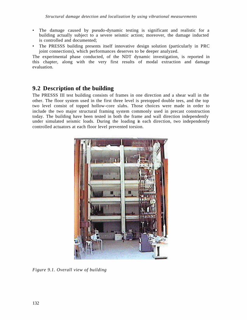
Structural damage detection and localization by using vibrational measurements
132
• The damage caused by pseudo-dynamic testing is significant and realistic for a building actually subject to a severe seismic action; moreover, the damage inducted is controlled and documented;
• The PRESSS building presents itself innovative design solution (particularly in PRC joint connections), which performances deserves to be deeper analyzed.
The experimental phase conducted, of the NDT dynamic investigation, is reported in this chapter, along with the very first results of modal extraction and damage evaluation.
9.2 Description of the building The PRESSS III test building consists of frames in one direction and a shear wall in the other. The floor system used in the first three level is pretopped double tees, and the top two level consist of topped hollow-core slabs. Those choices were made in order to include the two major structural framing system commonly used in precast construction today. The building have been tested in both the frame and wall direction independently under simulated seismic loads. During the loading in each direction, two independently controlled actuators at each floor level prevented torsion.
Figure 9.1. Overall view of building

NDE on the PRESSS building model
133
9.2.1 Frame connection system Four different types of ductile connection were used in the PRESSS III test building frames. They are: • Tension-compression Yielding (TCY) gap connection • TCY connection • Hybrid connection • Pretensioned connection The first three types of connections consist of multistory columns and single -bay beams, and are appropiate for floor-by-floor construction. The pretensioned connection uses multibay beams and single-story columns and is appropiate for "up-and-out" construction. The hybrid connection and pretensioned connection are used in one seismic frame, referred to as the Pretensioned Frame, and the remaining two connections are adopted in the other seismic frame, know as the Tension-Compression Yielding Frame. These two frame elevations are shown in Figures 6 and 7 respectively. The ammount of energy dissipation and residual displacement vary among the four connections, allowing a designer to control seismic behaviour of the structure with an appropiate choice of connection system.
9.2.1.1 Hybrid frame The hybrid was recently developed at the National Institute of Standards and Technology (NIST) (Stanton et al., 1997). The beams are connected to multistory columns by unbonded multistory columns by unbounded post-tensioning strands that run through the columns. Mild steel reinforcement is placed in ducts at the top and bottom of the beam through the column, and is grouted. it yields alternately in tension and compression and provides energy dissipation. The amount of mild steel reinforcement and post tensioning steel are balanced so that the frame re-centers after a major seismic event. The exterior joint of the Hybrid Frame uses a "stub" beam that contains the multistrand anchor. This is only required due to the scale of the test building
9.2.1.2 Pre Tensioned Frame The PreTensioned frame, named so as to differentiate it from just any frame constructed with pretensioned members, is intended to be used for construction where the most economical method consists of using one-story columns with multi-span beams. Long, multi-span beams are cast in normal pretensioned casting beds, with specified lengths of the pretensioning strand debonded. These beams are then set on one -story columns with the column reinforcing steel extending through sleeves in the beam. As the frame displaces laterally, the debonded strand remains elastic. While the system dissipates relatively less energy than other systems, it re-centers the structure after a major seismic event.
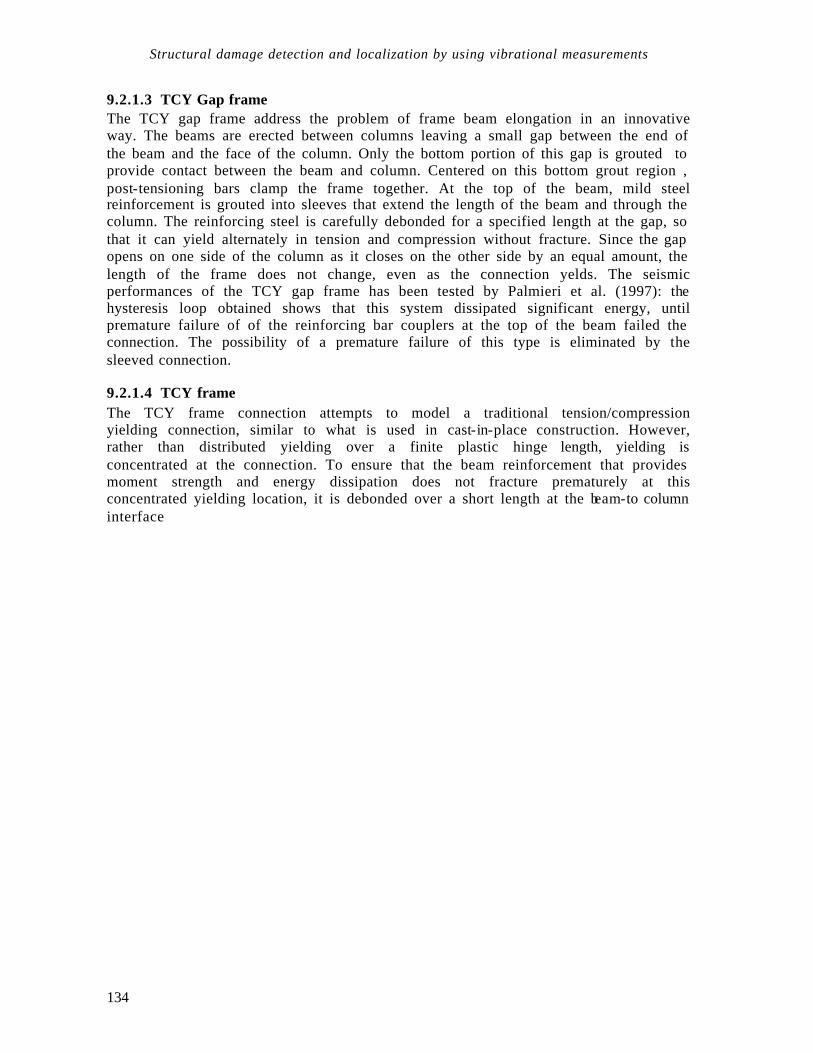
Structural damage detection and localization by using vibrational measurements
134
9.2.1.3 TCY Gap frame The TCY gap frame address the problem of frame beam elongation in an innovative way. The beams are erected between columns leaving a small gap between the end of the beam and the face of the column. Only the bottom portion of this gap is grouted to provide contact between the beam and column. Centered on this bottom grout region , post-tensioning bars clamp the frame together. At the top of the beam, mild steel reinforcement is grouted into sleeves that extend the length of the beam and through the column. The reinforcing steel is carefully debonded for a specified length at the gap, so that it can yield alternately in tension and compression without fracture. Since the gap opens on one side of the column as it closes on the other side by an equal amount, the length of the frame does not change, even as the connection yelds. The seismic performances of the TCY gap frame has been tested by Palmieri et al. (1997): the hysteresis loop obtained shows that this system dissipated significant energy, until premature failure of of the reinforcing bar couplers at the top of the beam failed the connection. The possibility of a premature failure of this type is eliminated by the sleeved connection.
9.2.1.4 TCY frame The TCY frame connection attempts to model a traditional tension/compression yielding connection, similar to what is used in cast-in-place construction. However, rather than distributed yielding over a finite plastic hinge length, yielding is concentrated at the connection. To ensure that the beam reinforcement that provides moment strength and energy dissipation does not fracture prematurely at this concentrated yielding location, it is debonded over a short length at the beam-to column interface

NDE on the PRESSS building model
135
9.3 Testing A complete dynamic characterization of the building has been made in two different phases: Phase 1: after pseudo-dynamic testing in X direction (shear wall resistant direction) and before pseudo-dynamic testing in Y direction. Phase 2: after pseudo-dynamic testing in X direction (frame resistant direction), i. e. at the end of pseudo-dynamic testing. Each phase includes modal testing of the whole structures (transducers in position A) and a local testing of three different joint (transducers in position B). Ambient vibration test, stepped sine test and shock test will be repeated for each instruments position.
9.3.1 Transducers position The building was instrumented in 4 different configurations (each comprised of 15 recording accelerometers). The first configuration (A) included 3 accelerometers on every floor (Figures 9.2 9.5). Each additional configuration (B, C and D) focused on the dynamic response of an individual beam-column connection, with instruments closely clustered along the beam and column (Figure 9.6). Three different innovative typology of joints have been investigated: B. Hybrid connection C. Tension-Compression Yielding (TCY) gap connection D. TCY connection
15’ - 0” 15’ - 0”
Gra
vity
Fra
me
15’
- 0”
15’
- 0”
Join
ted
Wal
l Sys
tem
TCY Frame
PreTensioned Frame
Gra
vity
Fra
me
Topped Hollow Core
Actuator Connection Panel
Topped Hollow Core
Actuator Connection Panel
Actuator Connection Panel
Shaker
1 (4,7,10,13)
3 (6,9,12,15)
2 (5,8,11,14)
accelerometer
Figures 9.2. Plan view of the building with transducers A position.
N
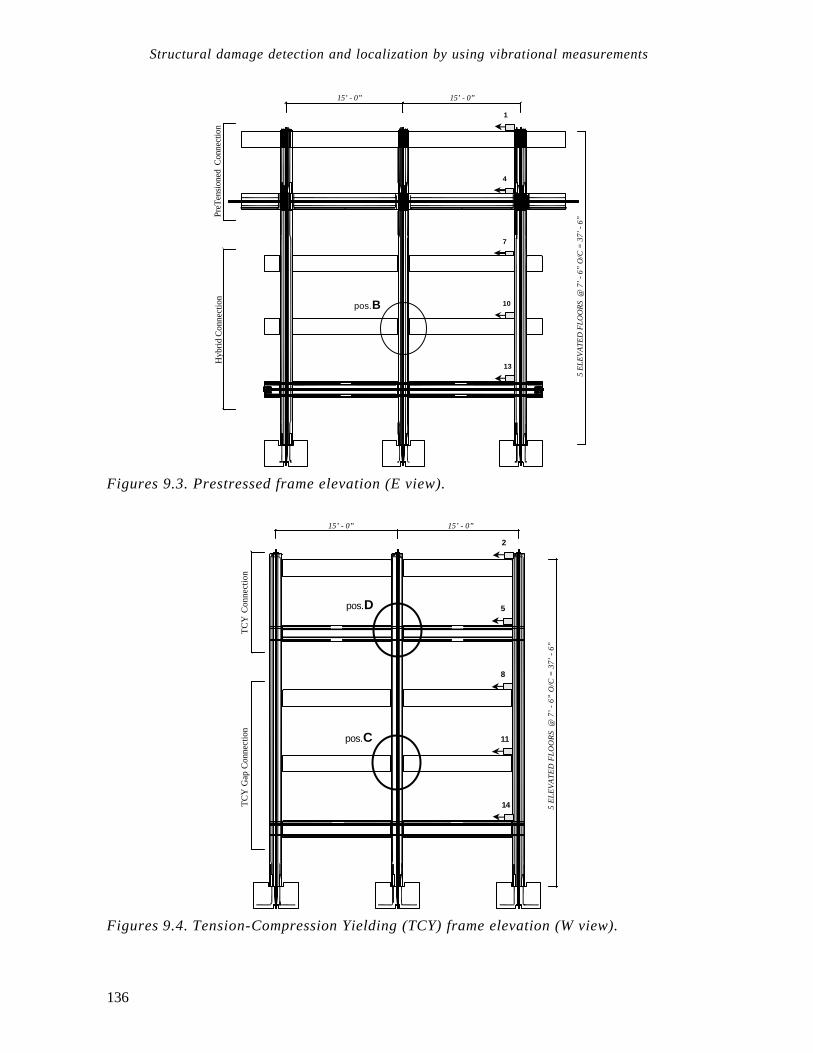
Structural damage detection and localization by using vibrational measurements
136
15’ - 0” 15’ - 0”
5 E
LEV
ATE
D F
LOO
RS
@ 7
’ -
6” O
/C =
37’
- 6
”
Hyb
rid C
onne
ctio
nPr
eTen
sion
ed C
onne
ctio
n
10
13
7
4
1
pos.B
Figures 9.3. Prestressed frame elevation (E view).
TC
Y G
ap C
onne
ctio
nT
CY
Con
nect
ion
15’ - 0” 15’ - 0”
5 E
LEV
ATE
D F
LOO
RS
@ 7
’ -
6” O
/C =
37’
- 6
”
11
14
8
5
2
pos.C
pos.D
Figures 9.4. Tension-Compression Yielding (TCY) frame elevation (W view).
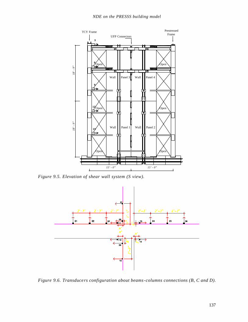
NDE on the PRESSS building model
137
PrestressedFrame
TCY FrameUFP Connectors
Wall Panel 1 Wall Panel 2
Wall Panel 3 Wall Panel 4
Open Open
Open Open
Open Open
15’ - 0” 15’ - 0”
18’
- 9”
18’
- 9”
12
15
9
6
3
Figure 9.5. Elevation of shear wall system (S view).
Figure 9.6. Transducers configuration about beams-columns connections (B, C and D).

Structural damage detection and localization by using vibrational measurements
138
Figure 9.7. Top view of the 5000 lb force shaker.
9.3.2 Testing techniques Tests include for each transducer configuration: • Ambient Vibration Tests (AVT); • Shock Tests (SHT), consisting in forcing the structures with an instrumented sledge
hammer; • Stepped Sinusoidal Tests (SST), consisting in forcing the structure with the shaker,
and measuring the steady-state response for a series of frequency values; • Free Vibration Tests (FVT), consisting in measuring the free vibration of the
structure following a sudden stop of the shaker. Details on the testing procedures are resumed in the following tables.
Figure 9.8. Shock test execution.

NDE on the PRESSS building model
139
Test: AVT (Ambient Vibration Test)
Forcing: Ambient vibration
Objective: To identify the main natural frequencies and the frequency range to
be investigated. To achieve PSD.
Description: A set of 32 signal is acquired and DSP is calculated.
Test: SST (Stepped-Sine Test)
Forcing: Shaker
Objective: To achieve FRF in a 0.1-4 frequency range
To extract main modal shapes
Description: The test consists in a sequence of steps. For each step, the shaker is drive at a fixed frequency, until the structural response is stationary. Hence, frequency and response amplitude are acquired. Steps should be repeated with a 0.1 Hz frequency interval for lowest frequency range, and 0.2 Hz for higher one. The whole frequency range to be investigated should be defined through AVT (approximately 0.4 to 4 Hz).
Test: SHT (Shock Test)
Forcing: Sledgehammer
Objective: To achieve FRF in a 0.1-30 Hz frequency range
To acquire free response
Description: The structure will be exited with the pulse sledgehammer in correspondence of some significant point (nn), basically A01, A02, A03. At less 8 free response time histories should be acquired for each excitation position. FRF will be calculated as an average of the 8 acquired signals. FRFs data and some significant time histories should be acquired.
Structural damage detection and localization by using vibrational measurements
140
Test: FVT (Free Vibration Test)
Forcing: Shaker
Objective: To acquire high amplitude free response of the structure.
Description: The shaker is driven at the most significant resonance frequencies,
then suddenly stopped. The free vibration is therefore acquired.
9.3.3 Test identification A code identifies each test as follows:
A1AVT01
Where: the first character identifies the accelerometers position A, B, C or D; the second character identifies the phase (p):
1 for the undamaged structures 2 for the damaged structures
The following three characters identify the type of excitation AVT for Ambient Vibration Test SST for Stepped Sinusoidal Test SHT for Shock Test FVT for Free Vibration Test For shock tests only, the following two characters identify the forcing position.
9.3.4 Signal processing Frequency Response Functions (FRFs) was calculated starting from the time history data acquired, both in the case of shock tests and of harmonic vibration tests. Some sample results are reported in the following pages, limited to channels that refer to the accelerometers on the top floor (A1 A2 and A3).
Five resonances are readily apparent in the recorded data, and change in frequencies appear definitively significant in a qualitative comparison between the before and after condition.
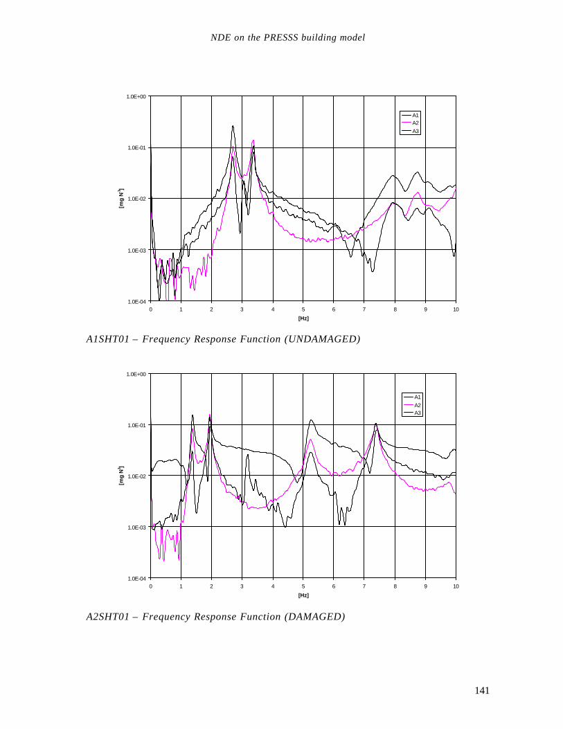
NDE on the PRESSS building model
141
1.0E-04
1.0E-03
1.0E-02
1.0E-01
1.0E+00
0 1 2 3 4 5 6 7 8 9 10
[Hz]
[mg
N-1]
A1A2A3
A1SHT01 – Frequency Response Function (UNDAMAGED)
1.0E-04
1.0E-03
1.0E-02
1.0E-01
1.0E+00
0 1 2 3 4 5 6 7 8 9 10
[Hz]
[mg
N-1]
A1A2A3
A2SHT01 – Frequency Response Function (DAMAGED)

Structural damage detection and localization by using vibrational measurements
142
1.0E-04
1.0E-03
1.0E-02
1.0E-01
1.0E+00
0 5 10 15 20 25 30 35 40
[Hz]
[mg
N-1]
A1A2A3
A1SHT01 – Frequency Response Function (UNDAMAGED)
1.0E-04
1.0E-03
1.0E-02
1.0E-01
1.0E+00
0 5 10 15 20 25 30 35 40
[Hz]
[mg
N-1]
A1A2A3
A2SHT03 – Frequency Response Function (UNDAMAGED)

NDE on the PRESSS building model
143
1.0E-04
1.0E-03
1.0E-02
1.0E-01
1.0E+00
0 1 2 3 4 5 6 7 8 9 10
[Hz]
[mg
N-1]
A1A2A3
A2SHT03 – Frequency Response Function (UNDAMAGED)
1.0E-04
1.0E-03
1.0E-02
1.0E-01
1.0E+00
0 1 2 3 4 5 6 7 8 9 10
[Hz]
[mg
N-1]
A1A2A3
A2SHT03 – Frequency Response Function (DAMAGED)

Structural damage detection and localization by using vibrational measurements
144
-1.5E-02
-1.0E-02
-5.0E-03
0.0E+00
5.0E-03
1.0E-02
1.5E-02
0.00 0.50 1.00 1.50 2.00 2.50 3.00
[sec]
[mg]
A1A2A3
A1SHT01 – Time History.
-5.0E-02
-4.0E-02
-3.0E-02
-2.0E-02
-1.0E-02
0.0E+00
1.0E-02
2.0E-02
3.0E-02
4.0E-02
0.00 0.50 1.00 1.50 2.00 2.50 3.00
[sec]
[mg]
A1A2A3
A1SHT03 – Time History.

NDE on the PRESSS building model
145
9.4 Modal extraction
9.4.1 Frequencies The direct Multi Degree Of Freedom (MDOF) curve fitting applied to FRFs, in the low frequencies range, and the direct resonance peak estimation, lead to the identification of five natural frequencies in the 1-15Hz range, as reported in Table 9.1.
frequency [Hz] mode
before after
2.69 1.38 I X-displacement mode 3.13 3.13 I Y-displaceme nt mode 3.38 1.94 I torsional mode 8.75 5.31 I X-displacement mode 11.20 7.38 II torsional mode 13.10 13.10 I Y-displacement mode
Table 9.1. Natural frequencies and modal recognition.
Frequencies associated to Y -direction modes remained unchanged, following the frame direction pseudo dynamic test: this is an expected outcome, as this is actually the wall resistant direction. Instead, significant changes in frequency were measured, in the case of X-direction and torsional mode, which mean signific ant loss in stiffness of the seismic resistant frames.
9.4.2 Mode shapes A deeper estimation of the 3 fundamental mode shapes of the whole building (configuration A) was subsequently carried out, through the MDOF curve fitting method, of shock tests based FRFs. Modal components relative to each channel have been processed making reference to a 15 dof simplified model of the building: each floor is supposed to be rigid in its plane, thus its motion can be described by three dof: x displacement, y displacement and rotation zϑ respect to the geometrical center. Results are reported in the following monographic tables, where the before and after conditions are compared. Different from frequencies, changes in mode shape appear quite insignificant
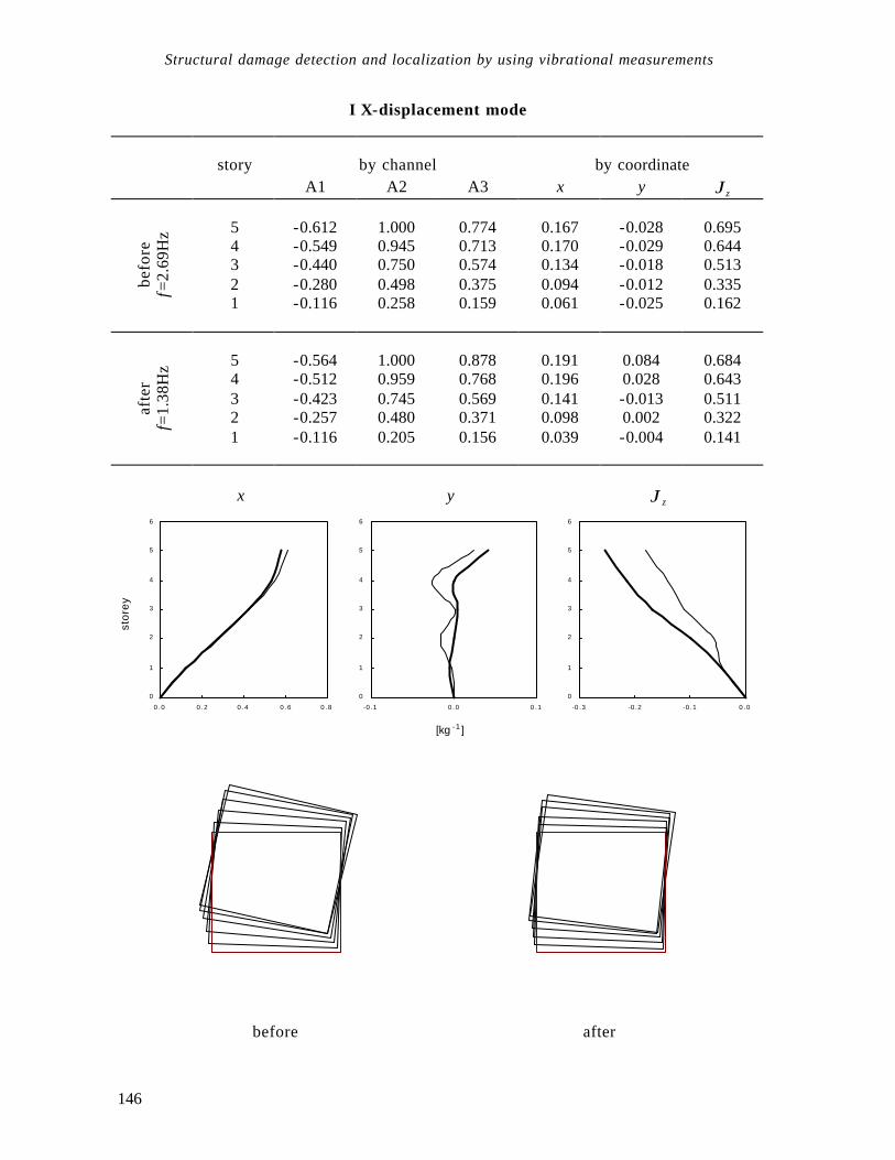
Structural damage detection and localization by using vibrational measurements
146
I X-displacement mode
story by channel by coordinate A1 A2 A3 x y zϑ
5 -0.612 1.000 0.774 0.167 -0.028 0.695 4 -0.549 0.945 0.713 0.170 -0.029 0.644 3 -0.440 0.750 0.574 0.134 -0.018 0.513 2 -0.280 0.498 0.375 0.094 -0.012 0.335 1 -0.116 0.258 0.159 0.061 -0.025 0.162
befo
re
f=2.
69H
z
5 -0.564 1.000 0.878 0.191 0.084 0.684 4 -0.512 0.959 0.768 0.196 0.028 0.643 3 -0.423 0.745 0.569 0.141 -0.013 0.511 2 -0.257 0.480 0.371 0.098 0.002 0.322 1 -0.116 0.205 0.156 0.039 -0.004 0.141
afte
r f=
1.38
Hz
x y zϑ
stor
ey
0
1
2
3
4
5
6
0.0 0.2 0.4 0.6 0.8
0
1
2
3
4
5
6
-0.1 0.0 0.1
0
1
2
3
4
5
6
-0.3 -0.2 -0.1 0.0
[kg -1 ]
before after

NDE on the PRESSS building model
147
I Y-displacement mode
storey by channel by coordinate x y zϑ
5 1.000 0.391 -0.255 0.578 0.041 -0.253 4 0.899 0.385 -0.257 0.533 0.000 -0.214 3 0.713 0.311 -0.195 0.425 0.005 -0.167 2 0.460 0.222 -0.118 0.283 0.001 -0.099 1 0.199 0.097 -0.055 0.123 -0.004 -0.042
befo
re
f=3.
13H
z
5 0.597 0.327 -0.116 0.615 0.025 -0.180 4 0.515 0.306 -0.125 0.546 -0.027 -0.139 3 0.402 0.237 -0.081 0.425 0.001 -0.109 2 0.252 0.166 -0.054 0.278 -0.015 -0.057 1 0.125 0.065 -0.032 0.127 -0.002 -0.040
afte
r f=
3.13
Hz
x y zϑ
stor
ey
0
1
2
3
4
5
6
0.0 0.1
0
1
2
3
4
5
6
0.0 0.1 0.2 0.3 0.4 0.5 0.6 0.7 0.8
0
1
2
3
4
5
6
-0.1 0.0 0.1
[kg -1 ]
before after
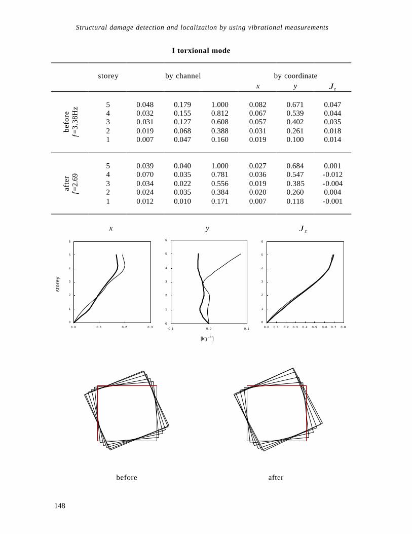
Structural damage detection and localization by using vibrational measurements
148
I torxional mode
storey by channel by coordinate x y zϑ
5 0.048 0.179 1.000 0.082 0.671 0.047 4 0.032 0.155 0.812 0.067 0.539 0.044 3 0.031 0.127 0.608 0.057 0.402 0.035 2 0.019 0.068 0.388 0.031 0.261 0.018 1 0.007 0.047 0.160 0.019 0.100 0.014
befo
re
f=3.
38H
z
5 0.039 0.040 1.000 0.027 0.684 0.001 4 0.070 0.035 0.781 0.036 0.547 -0.012 3 0.034 0.022 0.556 0.019 0.385 -0.004 2 0.024 0.035 0.384 0.020 0.260 0.004 1 0.012 0.010 0.171 0.007 0.118 -0.001
afte
r f=
2.69
x y zϑ
stor
ey
0
1
2
3
4
5
6
0.0 0.1 0.2 0.3
0
1
2
3
4
5
6
-0.1 0.0 0.1
0
1
2
3
4
5
6
0.0 0.1 0.2 0.3 0.4 0.5 0.6 0.7 0.8
[kg -1 ]
before after

NDE on the PRESSS building model
149
9.5 Damage assessment At now, damage assessment both of the whole structure and of the joints is a work still in process. Therefore, the scope of this paragraph is to provide some guidelines for using the dynamic investigation results in this sense.
9.5.1 NDE of the whole structures
9.5.1.1 Damage location/distribution assessment According to principles adopted in the PRESSS building design, a quite uniform damaging (identified by loss in stiffness, increment of damping capacity and occurrence of other phenomena) thorough the building is expected. The assessment and the quantification of this condition will give important indication on the effectiveness of the structural system. For this propose, different techniques for damage localization can be adopted,
Change in modal curvature/strain -mode-shape method represents the most suitable one. Figures 9.10 and 9.10 shows the strain -shapes of those modes associated with significanta changes in frequency, for the most significant generalized directions. A localized anomalies is visible, in correspondence of the first floor. The 15 d.o.f. is suitable to be further refined with a single -story based detailed model, in order to evaluate the damage distribution in each column or plastic hinge.
x zϑ
stor
ey
-0 .02 -0 .01 0.00 0.01 0.02
5
4
3
2
1
-0 .04 -0 .02 0.00 0.02 0.04 0.06
5
4
3
2
1
Figure 9.9. Strain-shape for the X-direction mode: x and zϑ components.
x zϑ
stor
ey
-0 .04 -0 .02 0.00 0.02 0.04 0.06
5
4
3
2
1
-0 .04 -0 .02 0.00 0.02 0.04
5
4
3
2
1
Figure 9.10. Strain-shape for the torsional mode: x and zϑ components.
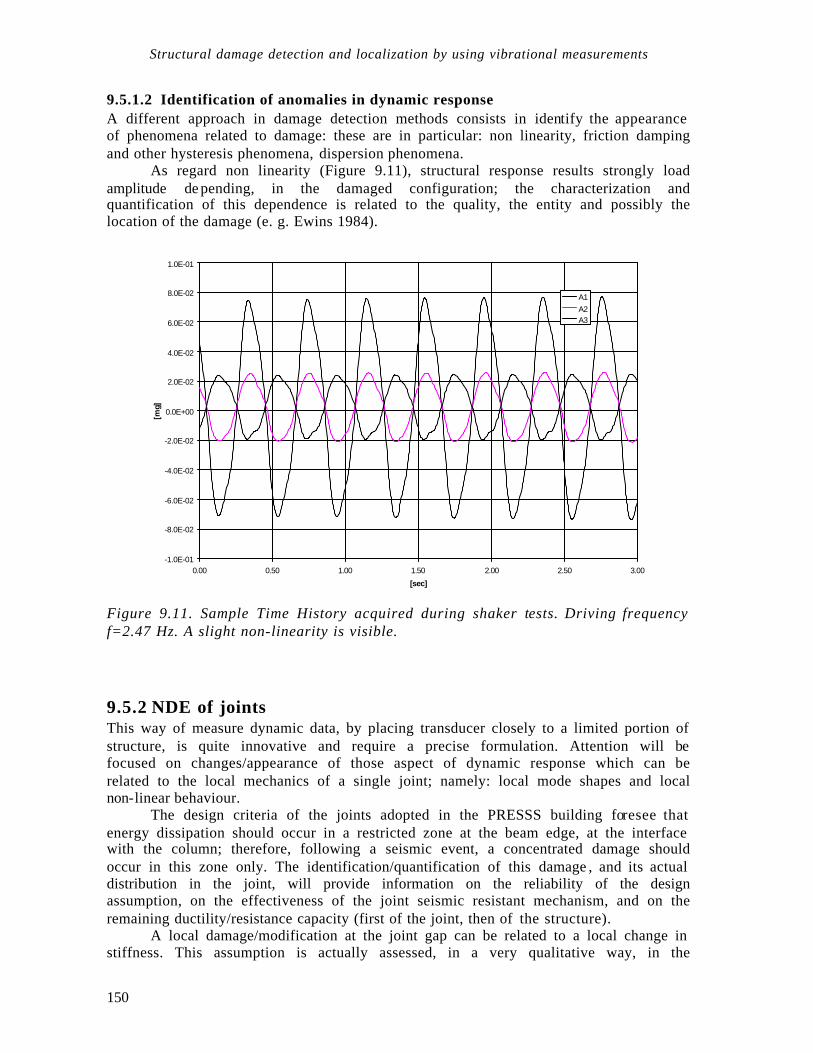
Structural damage detection and localization by using vibrational measurements
150
9.5.1.2 Identification of anomalies in dynamic response A different approach in damage detection methods consists in identify the appearance of phenomena related to damage: these are in particular: non linearity, friction damping and other hysteresis phenomena, dispersion phenomena.
As regard non linearity (Figure 9.11), structural response results strongly load amplitude de pending, in the damaged configuration; the characterization and quantification of this dependence is related to the quality, the entity and possibly the location of the damage (e. g. Ewins 1984).
-1.0E-01
-8.0E-02
-6.0E-02
-4.0E-02
-2.0E-02
0.0E+00
2.0E-02
4.0E-02
6.0E-02
8.0E-02
1.0E-01
0.00 0.50 1.00 1.50 2.00 2.50 3.00
[sec]
[mg]
A1A2A3
Figure 9.11. Sample Time History acquired during shaker tests. Driving frequency f=2.47 Hz. A slight non-linearity is visible.
9.5.2 NDE of joints This way of measure dynamic data, by placing transducer closely to a limited portion of structure, is quite innovative and require a precise formulation. Attention will be focused on changes/appearance of those aspect of dynamic response which can be related to the local mechanics of a single joint; namely: local mode shapes and local non-linear behaviour.
The design criteria of the joints adopted in the PRESSS building foresee that energy dissipation should occur in a restricted zone at the beam edge, at the interface with the column; therefore, following a seismic event, a concentrated damage should occur in this zone only. The identification/quantification of this damage , and its actual distribution in the joint, will provide information on the reliability of the design assumption, on the effectiveness of the joint seismic resistant mechanism, and on the remaining ductility/resistance capacity (first of the joint, then of the structure).
A local damage/modification at the joint gap can be related to a local change in stiffness. This assumption is actually assessed, in a very qualitative way, in the
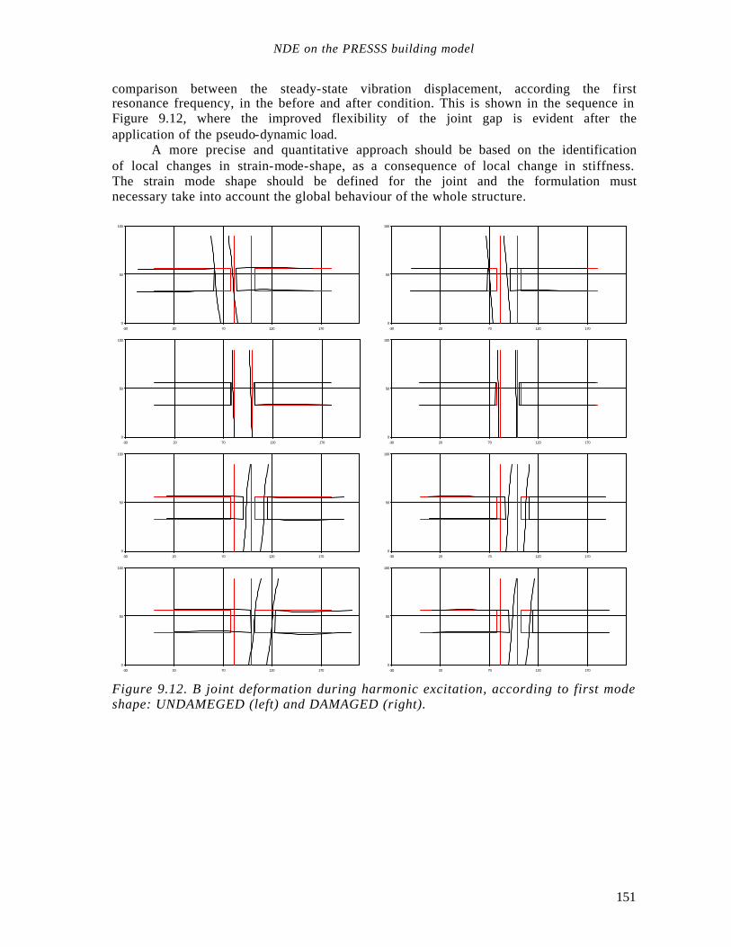
NDE on the PRESSS building model
151
comparison between the steady-state vibration displacement, according the first resonance frequency, in the before and after condition. This is shown in the sequence in Figure 9.12, where the improved flexibility of the joint gap is evident after the application of the pseudo-dynamic load.
A more precise and quantitative approach should be based on the identification of local changes in strain-mode-shape, as a consequence of local change in stiffness. The strain mode shape should be defined for the joint and the formulation must necessary take into account the global behaviour of the whole structure.
0
50
100
-30 20 70 120 170 0
50
100
-30 20 70 120 170
0
50
100
-30 20 70 120 170 0
50
100
-30 20 70 120 170
0
50
100
-30 20 70 120 170 0
50
100
-30 20 70 120 170
0
50
100
-30 20 70 120 170 0
50
100
-30 20 70 120 170 Figure 9.12. B joint deformation during harmonic excitation, according to first mode shape: UNDAMEGED (left) and DAMAGED (right).

Structural damage detection and localization by using vibrational measurements
152
153
References Allemang, R. J., and Brown D. L. (1982). "A correlation coefficient for modal vector analysis.", Proc., 1th Int. Modal Analysis Conf., Union College, Shenetady, NY, 110-115. Bachmann, H., and Dieterle, R. (1981) "Experiments and models for the damping behaviour of vibrating reinforced concrete beams in the uncracked and cracked conditions", Institut fur Baustatic und Konstruktion ETH, Zurich, Switzerland, Bericht Nr.119. Beolchini, S., Modena, C., and Sonda, D. (1996). "Influenza del danno e di difetti costruttivi sulle caratteristiche dinamiche di pannelli in c.a.p.", Proc.,11th CTE, Napoli, Italy 65-71 Casas, J., R. (1994) "An experimental study on the use of dynamic tests for surveillance of concrete structures", Mater. Struct., France, 27, 588 - 595 Casas, J., R., and Aparicio, A., C., (1994) "Structural damage ide ntification from dynamic -test data", J. Struct. Engrg., ASCE, 120 (8), 2437 - 2450 Cawley, P., and Adam, R., D., (1979). "The location of defects in structures from measurements of natural frequencies, J. Strain Analysis, 14 (2), 49-57. Ewin, D. J. 1984 Modal Testing: theory and practice : 24-25. Taunton: Research Studies Press Ltd. Farrar, C. R., and Doebling, S. C. (1998). "Damage detection II. Field application to a large structure." Proc., Modal Analysis & Testing Conf., NATO Advanced Study Institute, Sesimbra, Portugal, 427-443. Feldamn, M. (1997). "Non-linear vibration identification via the Hilbert Transform" J. of Sound and Vibration, 208 (3), 475-489. Gèradin, M. & Rixen, D. 1994. Mechanical Vibrations. New York: John Wiley & Sons, Inc. Geurts, C.P.W., Rutten, H.S., Wisse, J.A., 1993, Sensitivity of dynamic response to wind loading, proceedings of the first European and African conference on Wind Engineering. Geurts, C.P.W., 1994, Wind induced pressures on the main building of Eindhoven University of Technology.

Structural damage detection and localization by using vibrational measurements
154
Geurts, C.P.W., Rutten, H.S., Wisse, J.A., (1995). "Spatial distribution of wind induced pressure on buildings in complex terrain", Proceedings of 9ICWE, New Delhi, India. Geurts, C.P.W.(1996), "Wind tunnel modelling of the wind field over Eindhoven" , BKO report, Eindhoven University of Technology, 95-04. Gulkan, P. and Sozen, M.A (1974). "Inelastic response to of reinforced concrete structures to earthquake motions", ACI J. 71 (12), 604-610. Inaudi, J. A., and Makris, N.: Time-domain analysis of linear hysteretic damping, Earthquake Engineering and Structural Dynamics Vol. 25 (1996), pp. 529-545. Inman, D. J. (1989). "Engineering vibration." Prentince Hall, NJ. Iwan, W. D., Yang, I. M, (1972). "Application of Statistical Linearization Techniques to Nonlinear Multidegree-of-Freedom Systems", Journal of Applied Mechanics, trans. ASME 39 (2,) 545-550. Lieven, N. A. J.,and Ewins, D. J. (1988). "Spatial correlation of mode shapes, the coordinate modal assurance criterion." Proc., 8th Int. Modal Analysis Conf., Society for Experimental Mechanics, Bethel, Conn., 690-695. Mahrenholtz, O., and Bachmann, H. (1991) “Damping - Appendix C” Comite Euro-International du Beton, Lausanne, Switzerland, Bulletin n. 209, 169-180. Meirovitch, L. (1970). "Methods of analytical dynamics." McGraw Hill, NewYork. Modena, C., Sonda, D. and Zonta, D. (1998). "Sulla localizzazione del danno strutturale in elementi di c. a. p." Proc. XII congresso CTE, 293-302. Modena, C., Sonda, D. and Zonta, D. (1999). "Damage localisation in reinforced concrete structures by using damping measurements. Proc. DAMAS99 Conf. Uetikon-Zuerich: Trans Tech Publications Ltd. Nakaki, D. N., Stanton, J. F., and Sritharan, S. 1999, "An overview of the PRESSS five-story precast test building, PCI J., 2 (42), 26-39. Palmieri, L., Sagan, E., French, C., and Kreger, M. (1997). "Ductile connections for precast concrete frame systems", Proc. Mete A. Sozen Symposium, American Concrete Institute, Farmington Hills, MI, Paper No. SP162-13, 313-355. Pandy, A. K., Biswas, M., and Sammam, M. (1991). "Damage detection from changes in curvature mode shapes", J. of Sound & Vibration, 145 (2), 321-332. Pandey, A. K., and Biswas, M. (1994)."Damage detection in structures using changes in flexibility", J. of Sound & Vibration, 169 (1), 3-17. Simiu Scanlan, R.H. (1996), "Wind effects on structures", third edition, Wiley International.

References
155
Spina, D., Valente, C., and Tomlinson, G.,R. (1996). "A New Pocedure for Detecting Nonlinearity from Transient Data Using the Gabor Transform", Nonlinear Dynamics, Dordrecht, Kluver Academic, NL, 11, 235-244. Stanton, J. F., Stone, W. C., and Cheok, G. S. (1997). "A Hybrid reinforced precast frame for seismic regions", PCI J., 2 (42), 20-32. Swamidas, C. (1995) “Monit oring crack growth through change of modal parameters”, J. of Sound & Vibration, 186 (2), 325-343. Hop T. (1991). “The effect of degree of prestressing and age of concrete beams on frequency and damping of their free vibration”, Mater. Struct., France, 24, 210-220. Salawu, O. S. (1997). "Detection of structural damage through changes in frequency: a review", Engrg. Struct., Great Britain, 19 (9), 718 - 723. Tomlinson, G. R., and Hibbert, J. H., (1979). "Identification of the dynamic characteristics of a structure with coulomb friction", J. of Sound and Vibration Vol. 64 (2), 233-242. Yao, G. C., Chang, K. C., and Lee, G. C. (1992). "Damage diagnosis of steel frames using vibrational signature analysis", J. Engrg. Mech., ASCE, 118(9), 1949-1961. Vestroni, F., and Capecchi, D. (1996). "Damage evaluation in crecked vibrating beams using experimental frequencies and finite element models", J. of Vibration and Control, 2, 69-86. Wake, R. N., Burdess J. S. & Evans J. T. 1998. "Change in the natural frequencie s of repeated mode pairs induced by cracks in a vibrating ring. Journal of Sound and Vibration 214(4): 761-770. Whitham, G. B. (1974). "Linear and nonlinear waves". New York: John Wiley & Sons, Inc.

Structural damage detection and localization by using vibrational measurements
156

157
Notation A = inertance matrix (M -1) C = damping matrix D = sensitivity matrix (EJ) = bending stiffness ED = energy dissipated in a cycle EP = maximum potential energy of the system F = general relation that connects global measures to local damage parameters g, h = generic function l = distance between two successive measurement points I = identity matrix K = stiffness matrix k = constant M = mass matrix m = element of mass matrix S = change variable matrix s = element of change variable matrix z = global dynamic measure x = displacement vector α = flexibility matrix (K-1) χ = curvature ∆K = change in stiffness ∆φ = change in mode shape ∆χ = change in curvature ∆ω = change in frequency δ = local damage parameter δ = local damage parameter relative to torsional mode shapes φ = mode shape ϕ = rotation ϑ = relative rotation ω = frequency ξ = damping ratio ξ( ) = specific damping ratio ψ = distribution of forces Subscripts: i,j,n,m = positive integer indices; s = sth frequency.

Structural damage detection and localization by using vibrational measurements
158
Abbreviations: COMAC = Coordinate Modal Assurance Criterion FRF = Frequency Response Function HT = Hilbert Transform MAC = Modal Assurance Criterion MDOF = Multi Degree of Freedom STFT = Short Time Fourier Transform