Stratospheric temperature measurement with scanning Fabry...

Stratospheric temperature measurement with scanning Fabry-Perot interferometer for wind retrieval from mobile Rayleigh Doppler lidar Haiyun Xia, Xiankang Dou,* Mingjia Shangguan, Ruocan Zhao, Dongsong Sun, Chong Wang, Jiawei Qiu, Zhifeng Shu, Xianghui Xue, Yuli Han, and Yan Han

CAS Key Laboratory of Geospace Environment, School of Earth and Space Sciences, University of Science and Technology of China, 96 Jinzhai road, Hefei, Anhui, 230026, China

*[email protected]

Abstract: Temperature detection remains challenging in the low stratosphere, where the Rayleigh integration lidar is perturbed by aerosol contamination and ozone absorption while the rotational Raman lidar is suffered from its low scattering cross section. To correct the impacts of temperature on the Rayleigh Doppler lidar, a high spectral resolution lidar (HSRL) based on cavity scanning Fabry-Perot Interferometer (FPI) is developed. By considering the effect of the laser spectral width, Doppler broadening of the molecular backscatter, divergence of the light beam and mirror defects of the FPI, a well-behaved transmission function is proved to show the principle of HSRL in detail. Analysis of the statistical error of the HSRL is carried out in the data processing. A temperature lidar using both HSRL and Rayleigh integration techniques is incorporated into the Rayleigh Doppler wind lidar. Simultaneous wind and temperature detection is carried out based on the combined system at Delhi (37.371°N, 97.374°E; 2850 m above the sea level) in Qinghai province, China. Lower Stratosphere temperature has been measured using HSRL between 18 and 50 km with temporal resolution of 2000 seconds. The statistical error of the derived temperatures is between 0.2 and 9.2 K. The temperature profile retrieved from the HSRL and wind profile from the Rayleigh Doppler lidar show good agreement with the radiosonde data. Specifically, the max temperature deviation between the HSRL and radiosonde is 4.7 K from 18 km to 36 km, and it is 2.7 K between the HSRL and Rayleigh integration lidar from 27 km to 34 km.

©2014 Optical Society of America

OCIS codes: (010.0010) Atmospheric and oceanic optics; (120.0280) Remote sensing and sensors; (280.3340) Laser Doppler velocimetry; (280.3640) Lidar.

References and links

1. J. W. Meriwether and A. J. Gerrard, “Mesosphere inversion layers and stratosphere temperature enhancements,” Rev. Geophys. 42, RG3003 (2004).

2. A. Gettelman, P. Hoor, L. L. Pan, W. J. Randel, M. I. Hegglin, and T. Birner, “The extratropical upper troposphere and lower stratosphere,” Rev. Geophys. 49(3), RG3003 (2011).

3. M. P. Baldwin, L. J. Gray, T. J. Dunkerton, K. Hamilton, P. H. Haynes, W. J. Randel, J. R. Holton, M. J. Alexander, I. Hirota, T. Horinouchi, D. B. A. Jones, J. S. Kinnersley, C. Marquardt, K. Sato, and M. Takahashi, “The quasi-biennial oscillation,” Rev. Geophys. 39(2), 179–229 (2001).

4. A. J. Gerrard, Y. Bhattacharya, and J. P. Thayer, “Observations of in-situ generated gravity waves during a stratospheric temperature enhancement (STE) event,” Atmos. Chem. Phys. 11(22), 11913–11917 (2011).

5. M. P. Baldwin and T. J. Dunkerton, “Stratospheric harbingers of anomalous weather regimes,” Science 294(5542), 581–584 (2001).

6. M. P. Baldwin, D. W. J. Thompson, E. F. Shuckburgh, W. A. Norton, and N. P. Gillett, “Weather from the stratosphere?” Science 301(5631), 317–319 (2003).

7. V. Ramaswamy, M. L. Chanin, J. Angell, J. Barnett, D. Gaffen, M. Gelman, P. Keckhut, Y. Koshelkov, K. Labitzke, J. J. R. Lin, A. O’Neill, J. Nash, W. Randel, R. Rood, K. Shine, M. Shiotani, and R. Swinbank, “Stratospheric temperature trends: Observations and model simulations,” Rev. Geophys. 39(1), 71–122 (2001).

#215139 - $15.00 USD Received 1 Jul 2014; revised 19 Aug 2014; accepted 20 Aug 2014; published 2 Sep 2014(C) 2014 OSA 8 September 2014 | Vol. 22, No. 18 | DOI:10.1364/OE.22.021775 | OPTICS EXPRESS 21775

8. A. Behrendt, “Temperature measurements with lidar,” in Lidar: Range-Resolved Optical Remote Sensing of the Atmosphere, C. Weitkamp, ed (Springer, 2005).

9. M. Alpers, R. Eixmann, C. Fricke-Begemann, M. Gerding, and J. Höffner, “Temperature lidar measurements from 1 to 105 km altitude using resonance, Rayleigh, and Rotational Raman scattering,” Atmos. Chem. Phys. 4(3), 793–800 (2004).

10. X. Chu and G. C. Papen, “Resonance fluorescence lidar,” in Laser Remote Sensing, T. Fujii and T. Fukuchi, eds. (CRC, 2005).

11. M. L. Chanin and A. Hauchecorne, “Lidar studies of temperature and density using Rayleigh scattering,” in International Council of Scientific Unions Middle Atmosphere Handbook (National Aeronautics and Space Administration, 1984).

12. M. Gerding, J. Höffner, J. Lautenbach, M. Rauthe, and F.-J. Lübken, “Seasonal variation of nocturnal temperatures between 1 and 105 km altitude at 54° N observed by lidar,” Atmos. Chem. Phys. 8(24), 7465–7482 (2008).

13. W. N. Chen, C. C. Tsao, and J. B. Nee, “Rayleigh lidar temperature measurements in the upper troposphere and lower stratosphere,” J. Atmos. Sol.-Terr. Phys. 66(1), 39–49 (2004).

14. J. P. Vernier, L. W. Thomason, J. P. Pommereau, A. Bourassa, J. Pelon, A. Garnier, A. Hauchecorne, L. Blanot, C. Trepte, D. Degenstein, and F. Vargas, “Major influence of tropical volcanic eruptions on the stratospheric aerosol layer during the last decade,” Geophys. Res. Lett. 38, L12807 (2011).

15. O. E. Bazhenov, V. D. Burlakov, S. I. Dolgii, and A. V. Nevzorov, “Lidar observations of aerosol disturbances of the stratosphere over Tomsk (56.5° N; 85.0° E) in volcanic activity period 2006-2011,” Int. J. Opt. 2012, 1–10 (2012).

16. T. Shibata, M. Kobuchi, and M. Maeda, “Measurements of density and temperature profiles in the middle atmosphere with a XeF lidar,” Appl. Opt. 25(5), 685–688 (1986).

17. J. P. Burrows, A. Richter, A. Dehn, B. Deters, S. Himmelmann, S. Voigt, and J. Orphal, “Atmospheric remote sensing reference data from GOME: Part 2. Temperature-dependent absorption cross-sections of O3 in the 231 −794 nm range,” J. Quant. Spectrosc. Radiat. Transfer 61(4), 509–517 (1999).

18. A. Behrendt and J. Reichardt, “Atmospheric temperature profiling in the presence of clouds with a pure rotational Raman lidar by use of an interference-filter-based polychromator,” Appl. Opt. 39(9), 1372–1378 (2000).

19. A. Behrendt, T. Nakamura, M. Onishi, R. Baumgart, and T. Tsuda, “Combined Raman lidar for the measurement of atmospheric temperature, water vapor, particle extinction coefficient, and particle backscatter coefficient,” Appl. Opt. 41(36), 7657–7666 (2002).

20. A. Behrendt, T. Nakamura, and T. Tsuda, “Combined temperature lidar for measurements in the troposphere, stratosphere, and mesosphere,” Appl. Opt. 43(14), 2930–2939 (2004).

21. Y. Arshinov, S. Bobrovnikov, I. Serikov, A. Ansmann, U. Wandinger, D. Althausen, I. Mattis, and D. Müller, “Daytime operation of a pure rotational Raman lidar by use of a Fabry-Perot interferometer,” Appl. Opt. 44(17), 3593–3603 (2005).

22. E. Eloranta, “High spectral resolution lidar,” In Range-Resolved Optical Remote Sensing of the Atmosphere. C. Weitkamp, ed. (Springer, 2005).

23. G. G. Fiocco, G. Beneditti-Michelangeli, K. Maischberger, and E. Madonna, “Measurement of temperature and aerosol to molecule ratio in the troposphere by optical radar,” Nature 229, 78–79 (1971).

24. B. Witschas, C. Lemmerz, and O. Reitebuch, “Daytime measurements of atmospheric temperature profiles (2-15 km) by lidar utilizing Rayleigh-Brillouin scattering,” Opt. Lett. 39(7), 1972–1975 (2014).

25. R. L. Schwiesow and L. Lading, “Temperature profiling by Rayleigh-scattering lidar,” Appl. Opt. 20(11), 1972–1979 (1981).

26. H. Shimizu, S. A. Lee, and C. Y. She, “High spectral resolution lidar system with atomic blocking filters for measuring atmospheric parameters,” Appl. Opt. 22(9), 1373–1381 (1983).

27. H. Shimizu, K. Noguchi, and C. Y. She, “Atmospheric temperature measurement by a high spectral resolution lidar,” Appl. Opt. 25(9), 1460–1466 (1986).

28. C C. Y. She, R. J. Alvarez II, L. M. Caldwell, and D. A. Krueger, “High-spectral-resolution Rayleigh-Mie lidar measurement of aerosol and atmospheric profiles,” Opt. Lett. 17(7), 541–543 (1992).

29. P. Piironen and E. W. Eloranta, “Demonstration of a high-spectral-resolution lidar based on an iodine absorption filter,” Opt. Lett. 19(3), 234–236 (1994).

30. Z. Liu, I. Matsui, and N. Sugimoto, “High-spectral-resolution lidar using an iodine absorption filter for atmospheric measurements,” Opt. Eng. 38(10), 1661–1670 (1999).

31. J. W. Hair, L. M. Caldwell, D. A. Krueger, and C. Y. She, “High-spectral-resolution lidar with iodine-vapor filters: measurement of atmospheric-state and aerosol profiles,” Appl. Opt. 40(30), 5280–5294 (2001).

32. D. Hua, M. Uchida, and T. Kobayashi, “Ultraviolet Rayleigh-Mie lidar with Mie-scattering correction by Fabry-Perot etalons for temperature profiling of the troposphere,” Appl. Opt. 44(7), 1305–1314 (2005).

33. D. Hua, M. Uchida, and T. Kobayashi, “Ultraviolet Rayleigh-Mie lidar for daytime-temperature profiling of the troposphere,” Appl. Opt. 44(7), 1315–1322 (2005).

34. W. Huang, X. Chu, J. Wiig, B. Tan, C. Yamashita, T. Yuan, J. Yue, S. D. Harrell, C. Y. She, B. P. Williams, J. S. Friedman, and R. M. Hardesty, “Field demonstration of simultaneous wind and temperature measurements from 5 to 50 km with a Na double-edge magneto-optic filter in a multi-frequency Doppler lidar,” Opt. Lett. 34(10), 1552–1554 (2009).

35. Z. S. Liu, D. C. Bi, X. Q. Song, J. B. Xia, R. Z. Li, Z. J. Wang, and C. Y. She, “Iodine-filter-based high spectral resolution lidar for atmospheric temperature measurements,” Opt. Lett. 34(18), 2712–2714 (2009).


36. Z. Cheng, D. Liu, Y. Yang, L. Yang, and H. Huang, “Interferometric filters for spectral discrimination in high-spectral-resolution lidar: performance comparisons between Fabry-Perot interferometer and field-widened Michelson interferometer,” Appl. Opt. 52(32), 7838–7850 (2013).

37. D. Liu, Y. Yang, Z. Cheng, H. Huang, B. Zhang, T. Ling, and Y. Shen, “Retrieval and analysis of a polarized high-spectral-resolution lidar for profiling aerosol optical properties,” Opt. Express 21(11), 13084–13093 (2013).

38. Z. Cheng, D. Liu, J. Luo, Y. Yang, L. Su, L. Yang, H. Huang, and Y. Shen, “Effects of spectral discrimination in high-spectral-resolution lidar on the retrieval errors for atmospheric aerosol optical properties,” Appl. Opt. 53(20), 4386–4397 (2014).

39. A. Dabas, M. Denneulin, P. Flamant, C. Loth, A. Garnier, and A. Dolfi-Bouteyre, “Correcting winds measured with a Rayleigh Doppler lidar from pressure and temperature effects,” Tellus, Ser. A, Dyn. Meterol. Oceanogr. 60(2), 206–215 (2008).

40. J. M. Vaughan, The Fabry-Perot Interferometer: History, Theory, Practice and Applications (Adam Hilger, 1989), Appendix 6.

41. R. H. Eather and D. L. Reasoner, “Spectrophotometry of faint light sources with a tilting-filter photometer,” Appl. Opt. 8(2), 227–242 (1969).

42. H. Xia, X. Dou, D. Sun, Z. Shu, X. Xue, Y. Han, D. Hu, Y. Han, and T. Cheng, “Mid-altitude wind measurements with mobile Rayleigh Doppler lidar incorporating system-level optical frequency control method,” Opt. Express 20(14), 15286–15300 (2012).

43. H. Xia, D. Sun, Y. Yang, F. Shen, J. Dong, and T. Kobayashi, “Fabry-Perot interferometer based Mie Doppler lidar for low tropospheric wind observation,” Appl. Opt. 46(29), 7120–7131 (2007).

44. B. Witschas, C. Lemmerz, and O. Reitebuch, “Horizontal lidar measurements for the proof of spontaneous Rayleigh-Brillouin scattering in the atmosphere,” Appl. Opt. 51(25), 6207–6219 (2012).

45. I. S. Gradshteyn and I. M. Ryzhik, Table of Integrals, Series, and Products, 7th ed. (Academic, 2007). 46. E. Giannakaki, D. S. Balis, V. Amiridis, and S. Kazadzis, “Optical and geometrical characteristics of cirrus

clouds over a Southern European lidar station,” Atmos. Chem. Phys. 7(21), 5519–5530 (2007). 47. N. Hagen, M. Kupinski, and E. L. Dereniak, “Gaussian profile estimation in one dimension,” Appl. Opt. 46(22),

5374–5383 (2007). 48. Y. Dikmelik and F. M. Davidson, “Fiber-coupling efficiency for free-space optical communication through

atmospheric turbulence,” Appl. Opt. 44(23), 4946–4952 (2005).

1. Introduction

The middle atmosphere is that portion of the Earth’s atmosphere between two temperature minima at about 12 km altitude (the tropopause) and at about 85 km (the mesopause), comprising the stratosphere and mesosphere. In spite of intensive research activities over the past decades, the underlying mechanisms for some phenomena in the region, for instance, the stratosphere temperature enhancement and the mesosphere inversion layer, remain poorly understood [1–4]. The troposphere influences the stratosphere mainly through atmospheric waves propagating upward. Recent researches show that the stratosphere organizes the chaotic wave forcing from below to create long-lived changes in its circulation, and exerts impact on the tropospheric weather and climate. Thus, understanding the middle atmosphere is also essential for tropospheric weather prediction [5, 6]. Rocketsonde data are available through the early 1960s. However, such results are sporadic because the means for exploring the middle atmosphere are expensive. Even decades of rocket launches, radiosonde observations, satellite and aircraft measurements, provide only pieces of the whole picture [7].

Today, as one of the most promising remote sensing techniques, lidar for atmospheric researches has shown its inherited superiorities: including high spatial and temporal resolution, the potential of covering the height region from the boundary layer to the mesosphere, and allowing the detection of variable atmospheric parameters, such as temperature, pressure, density, wind, as well as the trace constituents. Particularly, temperature lidar techniques are approaching the maturity for routine observations [8]. Specifically, the resonance fluorescence technique, the Rayleigh integration technique and the rotational Raman technique are combined to cover the height region from the lower thermosphere to ground [9].

The resonance fluorescence technique is restricted to the altitude range between 80 and 105 km, where exist layers of metallic species, such as Fe, Ca, Na, and K atoms or ions [10].

The Rayleigh integration lidar has been proved to be the simplest tool for temperature detection in the mesosphere and stratosphere. Temperature is calculated from the molecular number density by assuming hydrostatic equilibrium. In addition, the top-to-bottom integration retrieval needs a reference point with known temperature at the beginning [11].


However, in the lower stratosphere, the aerosol contamination and ozone absorption makes the lidar backscatter no longer proportional to the molecular number density [12, 13]. So the Rayleigh backscatter must be corrected carefully for temperature detection. Unfortunately, in the lower stratosphere, recent volcanic eruptions aggravate the aerosol disturbances, which cannot be treated as low and stable background anymore [14, 15]. The ozone layer, which absorbs ultraviolet energy from the sun, is located primarily in the stratosphere, at altitudes of 15 to 35 km. The impact of O3 above 30 km on the Rayleigh temperature lidar can be ignored at working wavelength about 350 nm, with an error smaller than 1% [16]. And one should note that, the absorption cross section of O3 varies with wavelength. It is about 30 times lager at 532 nm than that at 355 nm [17].

Generally, to extend the detection altitude downward below 30 km, the rotational Raman technique is used for direct temperature detection, where two portions of pure-rotational Raman signals having opposite dependence on temperature are extracted by using filters with narrow bandwidth. The quite low rotational Raman scattering cross section requires sophisticated filters to suppress the disturbances from Rayleigh scattering and solar radiation. Nowadays, state-of-the-art rotational Raman lidars can be used to retrieve temperature up to 25 km. However, above this altitude, the statistical error usually exceeds 10 K [18–21].

The overview above comes to a conclusion that the temperature detection remains challenging in the low stratosphere, where the Rayleigh integration lidar is perturbed by aerosol contamination and ozone absorption while the rotational Raman lidar is suffered from its low scattering cross section. Fortunately, we demonstrate in this work that this dilemma can be resolved by using the so-called high spectral resolution lidar (HSRL). According to different implementations, the HSRL techniques fall into two categories [22]. On the one hand, the entire Cabannes line (more precisely, the sum of the Laudau-Placzek line and the Brillouin doublet) is obtained by scanning either the Fabry-Perot interferometer (FPI) or the laser. Then the temperature is calculated from the fitted linewidth of the Cabannes line [23, 24]. On the other hand, the lidar signal is measured before and passing through a static filter, for instance, a fixed FPI, Michelson interferometers, atomic or molecular absorption cells. It resolves the temperature dependent transmission of the Cabannes line through the filters [25–35]. In comparison, the former method is less efficient due to the fact that the ultra-narrow optical filter rejects most energy of the Cabannes scattering at each step of the scanning procedure. However, it shows immunity against the sunlight and Mie contamination [24]. Of course, HSRL is also a multi-function technique except for temperature detection [36–38]

The atmospheric temperature profile is necessary as an input parameter to the Rayleigh Doppler lidar. For example, a 1 K error on the actual temperature inside the sensing volume leads to a relative error of 0.2% of the true LOS wind for ADM-Aeolus [39]. In this paper, a HSRL using scanning FPI is incorporated into a mobile Rayleigh Doppler lidar for temperature detection from 18 to 35 km, and the Rayleigh integration lidar is used to retrieve temperature from 30 to 65 km. The combined system permits atmospheric temperature and wind detection simultaneously.

2. Principle

The key instrument inside the optical receiver of the HSRL used in this work is a cavity tunable FPI. Three piezo-electric actuators are used to tune the cavity while the capacitance sensors fabricated onto the mirror surfaces are used to sense changes in parallelism and cavity length. The FPI is mounted in a sealed cell with high efficiency anti-reflection coated windows and heater assembly around. This eliminates the impact of changes in environmental pressure, temperature and humidity on both the capacitance micrometers and on the optical cavity length.

The transmission function of a perfect parallel plane FPI is

( ) ( )( )

2

2

1,

1 2 cos 2 cosp e

e e FSR

T Rh

R Rν

πμν θ ν−

=+ − Δ

(1)


where eR is the effective surface reflectance, ν is the optical frequency relative to the center

frequency of the laser, θ is the angle of incidence of the light beams on the surfaces from within the interface, μ is the effective refractive index of the interspace, FSRνΔ is the free

spectral range. pT is the peak transmittance given by

( ) 21 1 ,p eT A R= − − (2)

where A is the surface absorptance. For an air-gapped FPI used in this paper, where 1μ ≈ , the transmission function can be written as

( ) ( )( )

( ) ( )( )

( )

2

2

2

2

cos 2 cos11 2

1 1 2 cos 2 cos

cos 2 cos sin 2 cos1 2

1 2 cos 2 cos

exp 2 cos1 2

1

e FSR eep

e e e FSR

e FSR e e FSRM

e e FSR

e FSRM

R RRh T

R R R

R R iRT e

R R

R iT e

πν θ νν

πν θ ν

πν θ ν πν θ νπν θ ν

πν θ ν

⋅ Δ − −= + + + − ⋅ Δ

⋅ Δ − + ⋅ Δ = + ℜ + − ⋅ Δ

⋅ ⋅ Δ= + ℜ

− ( )( )( )

( )( )

1 exp 2 cos

exp 2 cos 1 exp 2 cos

exp 2 cos1 2 ,

1 exp 2 cos

e FSR

e FSR e FSR

e FSRM

e FSR

R i

R i R i

R iT e

R i

πν θ νπν θ ν πν θ ν

πν θ νπν θ ν

− − ⋅ ⋅ Δ ⋅ ⋅ ⋅ Δ − − ⋅ ⋅ Δ ⋅ ⋅ Δ = + ℜ − ⋅ ⋅ Δ

(3)

where ( ) ( )1 1M p e eT T R R= − + , eℜ denotes the real part of a complex number. Utilizing

( ) ( )1

1 , 1n

n

x x x x+∞

=

→ − < and ( )exp 2 cos 1e FSRR i πν θ ν⋅ ⋅ Δ < , a periodic function in form

of Fourier series can be derived from Eq. (3) to describe the FPI transmission:

( ) ( )( )

( )

1

1

1 2 exp 2 cos

1 2 cos 2 cos .

n

M e FSRn

nM e FSR

n

h T e R i

T R n

ν πν θ ν

π ν θ ν

+∞

=

+∞

=

= + ℜ ⋅ ⋅ Δ

= + ⋅ Δ

(4)

This Fourier-series-type formulation above has been found particularly useful for further evaluation and computation of experimental profiles mainly because it permits simple convolution with other common functions, notably Gaussian and Lorentzian functions [40].

In our lidar system, a multimode fiber delivers the atmospheric backscatter from telescope to receiver. This configuration provides mechanical decoupling and remote placement of the lidar components. Furthermore, the fiber reduces the field of view of the telescope at the input end and defines the divergence of the collimated beam normal to the FPI at the output end. Suppose the incident illumination is uniformly distributed under the function of a mode-scrambler [41, 42], the actual transmission function is simply the sum of all rays from the normal to the half-maximum divergence 0θ :

( ) ( )

( ) ( )

( )

( ) ( )

0

0

2 00

2 010

0

210

0 0210

2sin

21 2 cos 2 cos cos

2cos 2 sin 2 cos

02

21 cos 2 sin 2 cos sin 2

2

nM e FSR

n

n FSRM e FSR

n

n FSRM e FSR FSR

n

H h d

T R n d

T R nn

T R n nn

θ

θ

ν ν θ θθ

π ν θ ν θθ

θνθ π ν θ νπ νθ

νθ π ν θ ν π ν νπ νθ

+∞

=

+∞

=

+∞

=

= ⋅

= + ⋅ Δ ⋅ −

Δ = − − ⋅ Δ

Δ= − − ⋅ Δ − Δ

.

(5)


Substituting the following power-reduction and sum-to-product formulas into Eq. (5)

( )2 2sin = 1 cos 2 / 2, 1,ϕ ϕ ϕ ϕ≈ − (6)

sin sin 2cos sin ,2 2

α β α βα β + −− = (7)

yields:

( )20 0 0

210

0 0

1

1 cos 1 cos2 2 22 2cos sin

2 2 2 2

1 cos 1 cos2 21 2 cos sin c .

2 2

n FSRM e

n FSR FSR

nM e

n FSR FSR

n nH T R

n

n nT R

θ ν θ θπ ν π ννπ ν ν νθ

θ θπ ν νν ν

+∞

=

+∞

=

Δ + − ≈ + ⋅ ⋅ Δ Δ + − = + ⋅ ⋅ Δ Δ

(8)

During the scanning procedure of the FPI, if the frequency ν shifts a range about FSRνΔ , the

cosine phase term will change 2nπ rapidly. On the contrary, the variation of the sinc term according to the same change of ν is small enough to be neglected. Therefore, Eq. (8) can be approximated as:

( )

( ) ( )

0 0 0

1

01

1 cos 2 1 cos21 2 cos sin c

2 2

1 2 cos sin c ,

nM e

n FSR FSR

nM e

n

nnH T R

T R nk n

θ ν θπ ννν ν

ν ϕ

+∞

=

+∞

=

+ − = + ⋅ ⋅ Δ Δ = +

(9)

where, for simplicity, let ( )01 cos FSRk π θ ν= + Δ and ( )0 0 01 cos FSRϕ ν θ ν= − Δ . To evaluate

the effect of the beam divergence to the transmission function, let n = 30, ( )0sin c 30ϕ =

0.98 is calculated using the system parameters listed in Table 1. The spectrum of the backscatter is broadened due to the random thermal motions of the air

particles. The aerosol backscatter spectrum ( )MieI ν can be replaced by the spectrum of the

outgoing laser ( )LaserI ν since the Brownian motion of aerosol particles does not broaden the

spectrum significantly [43]. In the low pressure altitude, the inelastic Brillouin scattering is negligible and the

molecular motion is thermally dominated. Thus the scattering lineshape takes the form of a thermally broadened Gaussian profile [39, 44].

The normalized spectra of aerosol backscatter ( )MI ν and molecule backscatter (Laudau-

Placzek line) ( )RI ν are approximated by Gaussian functions normalized to unit area:

( ) ( ) ( ) ( )12 2exp ,M L L LI Iν ν π ν ν ν

−≈ = Δ − Δ (10)

( ) ( ) ( )12 2exp .R R RI ν π ν ν ν

−= Δ − Δ (11)

Note that, LνΔ and 2 1 2(8 / )R akT mν λΔ = are the half-width at the 1/e intensity level of the

spectra of the outgoing laser and the Rayleigh backscatter, respectively. Where, k is the Boltzmann’s constant, aT is the atmosphere temperature, m is the average mass of the

atmospheric molecules, and λ is the laser wavelength. The transmission of the aerosol backscatter is a convolution of the transmission function of the FPI and the spectrum of aerosol backscatter:

( ) ( ) ( ) ( ) ( )

( ) ( ) ( )01

1 2 cos sin c .

M M L

nM e L

n

T H I H I

T R nk I n

ν ν ν ν ν

ν ν ϕ+∞

=

= ⊗ ≈ ⊗

≈ + ⊗

(12)


Using the integration formula ( ) ( ) ( )2 2 2 2exp exp 4p x qx dx p q pπ+∞

−∞

− ± = ⋅ , the

convolution in Eq. (12) can be expressed analytically [45]:

( ) ( ) ( )

( ) ( )

( )

2

021

2

021

2

11 2 exp cos sin c

11 2 exp exp sin c

11 2 exp exp

nM M e

n LL

nM e

n LL

nM e

L

xT T R nk x dx n

xT R e ink x dx n

xT R e ink

ν ν ϕνπ ν

ν ϕνπ ν

νπ ν

+∞+∞

= −∞

+∞+∞

= −∞

= + − ⋅ − ΔΔ = + ⋅ℜ − ⋅ − ΔΔ

= + ⋅ℜ −ΔΔ

( )

( ) ( )

( ) ( )

021

2 2 2

01

2 2 2

01

sin c

1 2 exp exp sin c4

1 2 cos exp sin c .4

n L

n LM e

n

n LM e

n

inkx dx n

n kT R e ink n

n kT R nk n

ϕν

νν ϕ

νν ϕ

+∞+∞

= −∞

+∞

=

+∞

=

−

− Δ = + ⋅ℜ

− Δ = + ⋅

(13)

Comparison of Eq. (4), (9) and (13) shows that, even considering the divergence of the incident light, the convolution is derived by concise multiplication of each successive term by

( )0sin c nϕ and ( )2 2exp 4Lk ν− Δ . Furthermore, the surface defect of the parallel mirrors can

also approximated as a Gaussian distribution

( ) ( ) ( )12 2exp ,D D DI ν π ν ν ν

−= Δ − Δ (14)

where DνΔ is the global parameter for all kinds of mirror defects [40]. Since the convolution of two Gaussian functions yields still a Gaussian function. Finally, the transmission function of aerosol backscatter can be written as

( ) ( ) ( ) ( )2 2 2 20

1

1 2 cos exp 4 sin c .nM M e L D

n

T T R nk n k nν ν ν ν ϕ+∞

=

= + ⋅ − Δ + Δ ⋅ (15)

Similarly, the transmission of the Rayleigh backscatter is

( ) ( ) ( ) ( )2 2 2 2 20

1

1 2 cos exp 4 sin c .nR M e L D R

n

T T R nk n k nν ν ν ν ν ϕ+∞

=

= + ⋅ − Δ + Δ + Δ ⋅ (16)

If aerosols are exist, the photon number corresponding to the mixed backscatter collected by the telescope is described as follow:

( ) ( ) ( ) ( ) ( )02 0

, exp 2 , ,2

Rq dT L o R R M M

A cN R E R T T R dR

h R

η τν η ξ β ν β ν κ νν

= + − (17)

where LE is the energy of the laser pulse, oη accounts for the optical efficiency of the

transmitted signal, qη is the quantum efficiency, h is the Planck constant, 0A is the area of

the telescope, ( )Rξ is the geometrical overlap factor at range R , Rβ and Mβ are the

Rayleigh and Mie volume backscatter coefficients, dτ is the detector’s response time

( ), Rκ ν is the atmospheric attenuation coefficient.


Considering the power fluctuation of the transmitter and variation of the round-trip atmospheric transmission during the scanning process, the backscatter energy is monitored for the same time at each scanning step:

( ) ( )[ ] ( )02 0

, exp 2 , .2

Rq dE L o R M

A cN R E R R dR

h R

η τν η ξ β β κ νν

= + − (18)

For atmospheric temperature profiling using HSRL technique, a ratio is defined as

( ) ( )( ) ( ) ( ) ( ),

, 1 .,

TR M

E

N RQ R T T

N R

νν ζ ν ζ ν

ν= = + − (19)

where ( )R R Mζ β β β= + denotes the percentage of the Rayleigh component in the total

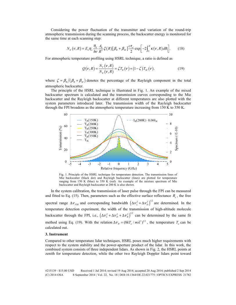
atmospheric backscatter. The principle of the HSRL technique is illustrated in Fig. 1. An example of the mixed

backscatter spectrum is calculated and the transmission curves corresponding to the Mie backscatter and the Rayleigh backscatter at different temperatures are also plotted with the system parameters introduced later. The transmission width of the Rayleigh backscatter through the FPI broadens as the atmospheric temperature increasing from 150 K to 350 K.

Fig. 1. Principle of the HSRL technique for temperature detection. The transmission lines of Mie backscatter (black dot) and Rayleigh backscatter (lines) are plotted for temperature ranging from 150 K (blue) to 350 K (red). An example of the mixture spectrum of Mie backscatter and Rayleigh backscatter at 200 K is also shown.

In the system calibration, the transmission of laser pulse through the FPI can be measured and fitted to Eq. (15). Then, parameters such as the effective surface reflectance eR , the free

spectral range FSRνΔ and corresponding bandwidth ( )1 22 2L Dν νΔ + Δ are determined. In the

temperature detection experiment, the width of the transmission of high-altitude molecule

backscatter through the FPI, i.e., ( )1 22 2 2L D Rν ν νΔ + Δ + Δ can be determined by the same fit

method using Eq. (19). With the relation 2 1 2(8 / )R akT mν λΔ = , the temperature aT can be calculated out.

3. Instrument

Compared to other temperature lidar techniques, HSRL poses much higher requirements with respect to the system stability and the power-aperture product of the lidar. In this work, the combined system consists of three independent lidars. As shown in Fig. 2, the HSRL points at zenith for temperature detection, while the other two Rayleigh Doppler lidars point toward


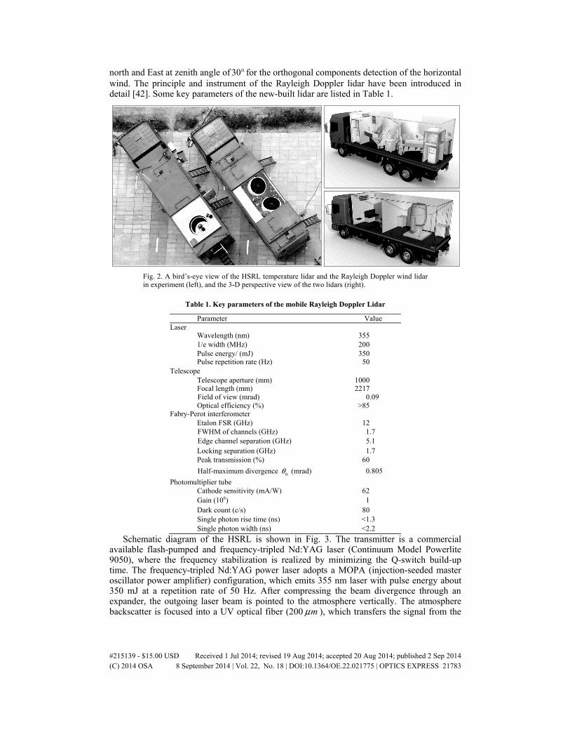
north and East at zenith angle of 30° for the orthogonal components detection of the horizontal wind. The principle and instrument of the Rayleigh Doppler lidar have been introduced in detail [42]. Some key parameters of the new-built lidar are listed in Table 1.

Fig. 2. A bird’s-eye view of the HSRL temperature lidar and the Rayleigh Doppler wind lidar in experiment (left), and the 3-D perspective view of the two lidars (right).

Table 1. Key parameters of the mobile Rayleigh Doppler Lidar

Parameter ValueLaser

Wavelength (nm) 3551/e width (MHz) 200 Pulse energy/ (mJ) 350Pulse repetition rate (Hz) 50

Telescope Telescope aperture (mm) 1000Focal length (mm) 2217Field of view (mrad) 0.09 Optical efficiency (%) >85

Fabry-Perot interferometerEtalon FSR (GHz) 12 FWHM of channels (GHz) 1.7Edge channel separation (GHz) 5.1 Locking separation (GHz) 1.7 Peak transmission (%) 60

Half-maximum divergence 0θ (mrad) 0.805

Photomultiplier tubeCathode sensitivity (mA/W) 62 Gain (106) 1 Dark count (c/s) 80 Single photon rise time (ns) <1.3 Single photon width (ns) <2.2

Schematic diagram of the HSRL is shown in Fig. 3. The transmitter is a commercial available flash-pumped and frequency-tripled Nd:YAG laser (Continuum Model Powerlite 9050), where the frequency stabilization is realized by minimizing the Q-switch build-up time. The frequency-tripled Nd:YAG power laser adopts a MOPA (injection-seeded master oscillator power amplifier) configuration, which emits 355 nm laser with pulse energy about 350 mJ at a repetition rate of 50 Hz. After compressing the beam divergence through an expander, the outgoing laser beam is pointed to the atmosphere vertically. The atmosphere backscatter is focused into a UV optical fiber (200 mμ ), which transfers the signal from the


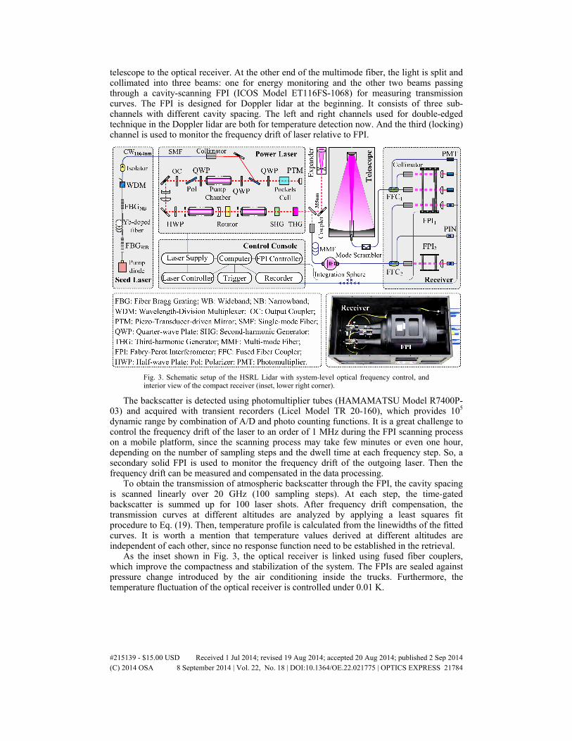
telescope to the optical receiver. At the other end of the multimode fiber, the light is split and collimated into three beams: one for energy monitoring and the other two beams passing through a cavity-scanning FPI (ICOS Model ET116FS-1068) for measuring transmission curves. The FPI is designed for Doppler lidar at the beginning. It consists of three sub-channels with different cavity spacing. The left and right channels used for double-edged technique in the Doppler lidar are both for temperature detection now. And the third (locking) channel is used to monitor the frequency drift of laser relative to FPI.

Fig. 3. Schematic setup of the HSRL Lidar with system-level optical frequency control, and interior view of the compact receiver (inset, lower right corner).

The backscatter is detected using photomultiplier tubes (HAMAMATSU Model R7400P-03) and acquired with transient recorders (Licel Model TR 20-160), which provides 105 dynamic range by combination of A/D and photo counting functions. It is a great challenge to control the frequency drift of the laser to an order of 1 MHz during the FPI scanning process on a mobile platform, since the scanning process may take few minutes or even one hour, depending on the number of sampling steps and the dwell time at each frequency step. So, a secondary solid FPI is used to monitor the frequency drift of the outgoing laser. Then the frequency drift can be measured and compensated in the data processing.

To obtain the transmission of atmospheric backscatter through the FPI, the cavity spacing is scanned linearly over 20 GHz (100 sampling steps). At each step, the time-gated backscatter is summed up for 100 laser shots. After frequency drift compensation, the transmission curves at different altitudes are analyzed by applying a least squares fit procedure to Eq. (19). Then, temperature profile is calculated from the linewidths of the fitted curves. It is worth a mention that temperature values derived at different altitudes are independent of each other, since no response function need to be established in the retrieval.

As the inset shown in Fig. 3, the optical receiver is linked using fused fiber couplers, which improve the compactness and stabilization of the system. The FPIs are sealed against pressure change introduced by the air conditioning inside the trucks. Furthermore, the temperature fluctuation of the optical receiver is controlled under 0.01 K.


4. Experiments

Simultaneous wind and temperature detection is carried out at Delhi (37.371°N, 97.374°E) in Qinghai province, China. The location is 2850 m above the sea level.

In the experiment, the transmission of Rayleigh backscatter through the FPI is achieved by scanning its cavity spacing [42, 43]. A step change of the cavity lΔ is related to the frequency sampling interval νΔ as

,l lν νΔ = − Δ (20)

where 12.5l mm= is the cavity spacing. As an example, if one needs to increase the FPI over 20 GHz, the cavity spacing should be shrink 295.83 nm. One should note that, after the spacing change, the FSR of the FPI also increases 0.284 MHz, which is negligible in this work.

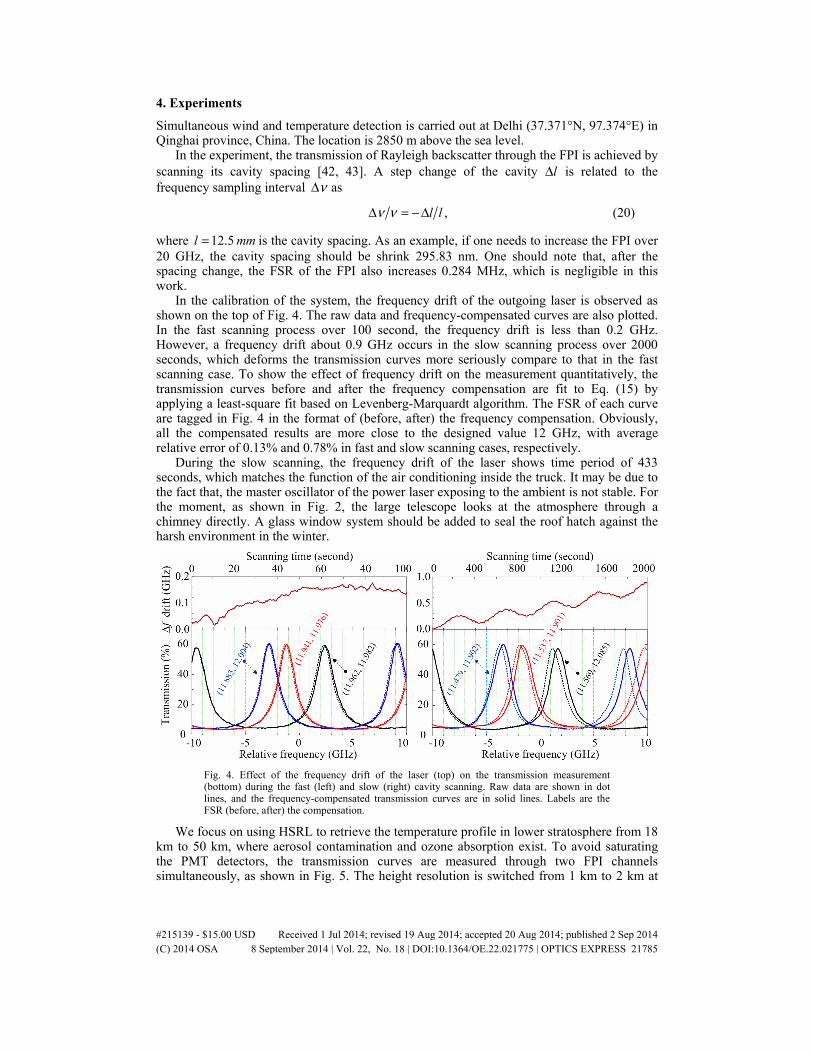
In the calibration of the system, the frequency drift of the outgoing laser is observed as shown on the top of Fig. 4. The raw data and frequency-compensated curves are also plotted. In the fast scanning process over 100 second, the frequency drift is less than 0.2 GHz. However, a frequency drift about 0.9 GHz occurs in the slow scanning process over 2000 seconds, which deforms the transmission curves more seriously compare to that in the fast scanning case. To show the effect of frequency drift on the measurement quantitatively, the transmission curves before and after the frequency compensation are fit to Eq. (15) by applying a least-square fit based on Levenberg-Marquardt algorithm. The FSR of each curve are tagged in Fig. 4 in the format of (before, after) the frequency compensation. Obviously, all the compensated results are more close to the designed value 12 GHz, with average relative error of 0.13% and 0.78% in fast and slow scanning cases, respectively.

During the slow scanning, the frequency drift of the laser shows time period of 433 seconds, which matches the function of the air conditioning inside the truck. It may be due to the fact that, the master oscillator of the power laser exposing to the ambient is not stable. For the moment, as shown in Fig. 2, the large telescope looks at the atmosphere through a chimney directly. A glass window system should be added to seal the roof hatch against the harsh environment in the winter.

Fig. 4. Effect of the frequency drift of the laser (top) on the transmission measurement (bottom) during the fast (left) and slow (right) cavity scanning. Raw data are shown in dot lines, and the frequency-compensated transmission curves are in solid lines. Labels are the FSR (before, after) the compensation.

We focus on using HSRL to retrieve the temperature profile in lower stratosphere from 18 km to 50 km, where aerosol contamination and ozone absorption exist. To avoid saturating the PMT detectors, the transmission curves are measured through two FPI channels simultaneously, as shown in Fig. 5. The height resolution is switched from 1 km to 2 km at


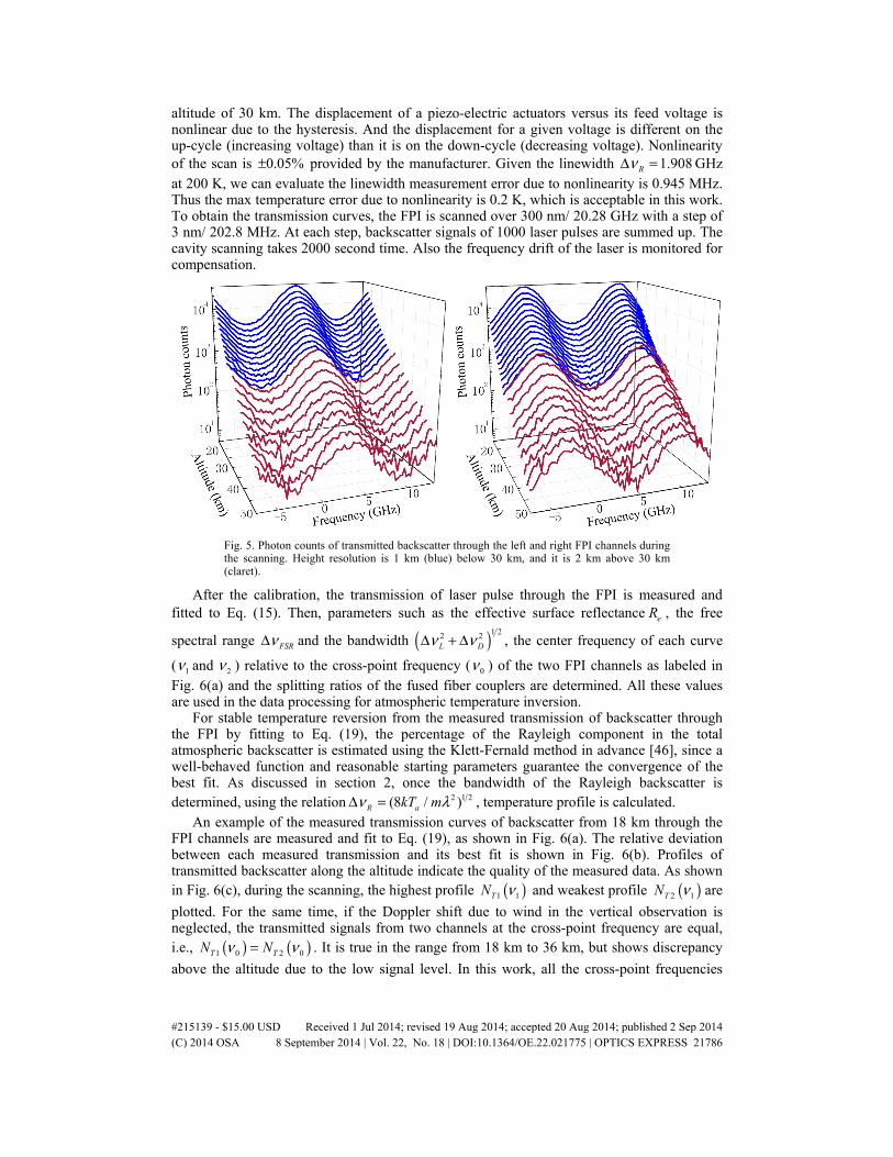
altitude of 30 km. The displacement of a piezo-electric actuators versus its feed voltage is nonlinear due to the hysteresis. And the displacement for a given voltage is different on the up-cycle (increasing voltage) than it is on the down-cycle (decreasing voltage). Nonlinearity of the scan is 0.05%± provided by the manufacturer. Given the linewidth 1.908RνΔ = GHz at 200 K, we can evaluate the linewidth measurement error due to nonlinearity is 0.945 MHz. Thus the max temperature error due to nonlinearity is 0.2 K, which is acceptable in this work. To obtain the transmission curves, the FPI is scanned over 300 nm/ 20.28 GHz with a step of 3 nm/ 202.8 MHz. At each step, backscatter signals of 1000 laser pulses are summed up. The cavity scanning takes 2000 second time. Also the frequency drift of the laser is monitored for compensation.

Fig. 5. Photon counts of transmitted backscatter through the left and right FPI channels during the scanning. Height resolution is 1 km (blue) below 30 km, and it is 2 km above 30 km (claret).

After the calibration, the transmission of laser pulse through the FPI is measured and fitted to Eq. (15). Then, parameters such as the effective surface reflectance eR , the free

spectral range FSRνΔ and the bandwidth ( )1 22 2L Dν νΔ + Δ , the center frequency of each curve

( 1ν and 2ν ) relative to the cross-point frequency ( 0ν ) of the two FPI channels as labeled in Fig. 6(a) and the splitting ratios of the fused fiber couplers are determined. All these values are used in the data processing for atmospheric temperature inversion.

For stable temperature reversion from the measured transmission of backscatter through the FPI by fitting to Eq. (19), the percentage of the Rayleigh component in the total atmospheric backscatter is estimated using the Klett-Fernald method in advance [46], since a well-behaved function and reasonable starting parameters guarantee the convergence of the best fit. As discussed in section 2, once the bandwidth of the Rayleigh backscatter is determined, using the relation 2 1 2(8 / )R akT mν λΔ = , temperature profile is calculated.

An example of the measured transmission curves of backscatter from 18 km through the FPI channels are measured and fit to Eq. (19), as shown in Fig. 6(a). The relative deviation between each measured transmission and its best fit is shown in Fig. 6(b). Profiles of transmitted backscatter along the altitude indicate the quality of the measured data. As shown in Fig. 6(c), during the scanning, the highest profile ( )1 1TN ν and weakest profile ( )2 1TN ν are

plotted. For the same time, if the Doppler shift due to wind in the vertical observation is neglected, the transmitted signals from two channels at the cross-point frequency are equal, i.e., ( ) ( )1 0 2 0T TN Nν ν= . It is true in the range from 18 km to 36 km, but shows discrepancy

above the altitude due to the low signal level. In this work, all the cross-point frequencies


from 18 km to 36 km are found and averaged. Center frequencies of the left and the right channels can be calculated using the parameters ( 0ν , 1ν and 2ν ) decided in advance.

Fig. 6. (a): Measured transmission curves of the backscatter (from 18 km) through the two channels (circle) and their best fit results (dash line), (b): Residual between the measured transmissions and the fit results, (c): Profiles of transmitted backscatter along altitude at given frequencies labeled in (a).

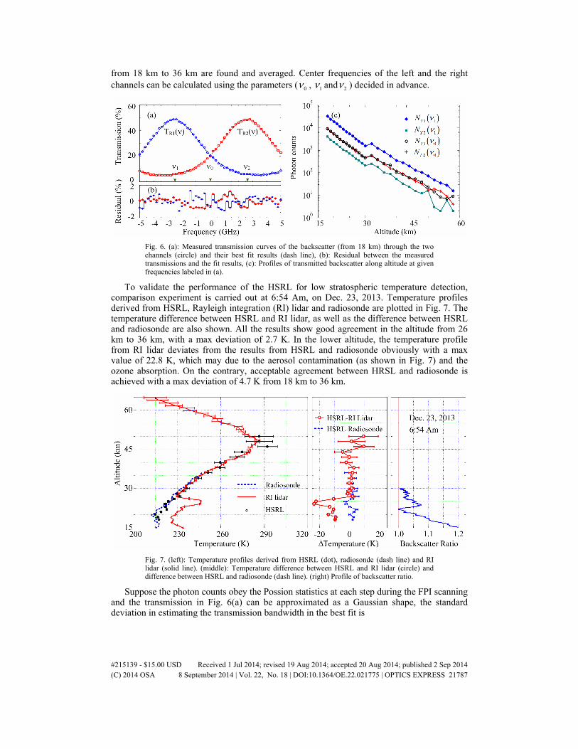
To validate the performance of the HSRL for low stratospheric temperature detection, comparison experiment is carried out at 6:54 Am, on Dec. 23, 2013. Temperature profiles derived from HSRL, Rayleigh integration (RI) lidar and radiosonde are plotted in Fig. 7. The temperature difference between HSRL and RI lidar, as well as the difference between HSRL and radiosonde are also shown. All the results show good agreement in the altitude from 26 km to 36 km, with a max deviation of 2.7 K. In the lower altitude, the temperature profile from RI lidar deviates from the results from HSRL and radiosonde obviously with a max value of 22.8 K, which may due to the aerosol contamination (as shown in Fig. 7) and the ozone absorption. On the contrary, acceptable agreement between HRSL and radiosonde is achieved with a max deviation of 4.7 K from 18 km to 36 km.

Fig. 7. (left): Temperature profiles derived from HSRL (dot), radiosonde (dash line) and RI lidar (solid line). (middle): Temperature difference between HSRL and RI lidar (circle) and difference between HSRL and radiosonde (dash line). (right) Profile of backscatter ratio.

Suppose the photon counts obey the Possion statistics at each step during the FPI scanning and the transmission in Fig. 6(a) can be approximated as a Gaussian shape, the standard deviation in estimating the transmission bandwidth in the best fit is


( ) / 2 ,F F Nσ ν νΔ = Δ (21)

where FνΔ is the half-width at the 1/e intensity level of the transmission curve under

estimation in Fig. 6(a). N is the total photon counts at a given altitude [47]. In the calibration, transmission of the laser pulse through the FPI is measured dozens of

times and averaged, allowing us ignore the error in estimating the bandwidth of the curves in Fig. 4. Comparing Eq. (15) with Eq. (16), one can approximate that ( ) ( )R Fσ ν σ νΔ ≈ Δ . So the statistical error of the obtained temperature profile from each FPI is calculated as

( ) 2 4 .a R FT m k Nσ λ ν ν= Δ Δ (22)

The measurement on the two FPI channels is uncorrelated, reducing the final statistical

uncertainty by a factor of 2 . The error bar of the temperature profile derived from HSRL is shown in Fig. 7.

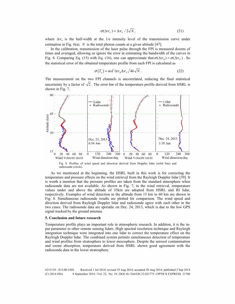
Fig. 8. Profiles of wind speed and direction derived from Doppler lidar (solid line) and radiosonde (circle).

As we mentioned at the beginning, the HSRL built in this work is for correcting the temperature and pressure effects on the wind retrieval from the Rayleigh Doppler lidar [39]. It is worth a mention that the pressure profiles are taken from the standard atmosphere when radiosonde data are not available. As shown in Fig. 7, in the wind retrieval, temperature values under and above the altitude of 35km are adopted from HSRL and RI lidar, respectively. Examples of wind detection in the altitude from 15 km to 60 km are shown in Fig. 8. Simultaneous radiosonde results are plotted for comparison. The wind speed and direction derived from Rayleigh Doppler lidar and radiosonde agree with each other in the two cases. The radiosonde data are sporadic on Dec. 24, 2013, which is due to the low GPS signal tracked by the ground antenna.

5. Conclusion and future research

Temperature profile plays an important role in atmospheric research. In addition, it is the in-put parameter to other remote sensing lidars. High spectral resolution technique and Rayleigh integration technique were integrated into one lidar to correct the temperature effect on the Rayleigh Doppler lidar. The combined system permits simultaneous detection of temperature and wind profiles from stratosphere to lower mesosphere. Despite the aerosol contamination and ozone absorption, temperature derived from HSRL shown good agreement with the radiosonde data in the lower stratosphere.


We noticed that the pulse duration decreases from 6.8 ns to 5.0 ns as the pulse energy decaying from 350 mJ to 150 mJ, so the spectral width of the outgoing laser pulse should be monitored. For future research, one channel of the FPI will be used to extend the temperature detection to the troposphere, where the spectrum of the molecular backscatter cannot be approximated as a simple Gaussian function, the Brilliouin doublet must be considered.

This work is on the assumption that atmospheric temperature is stable during the scanning of the FPI and the vertical component of the atmosphere wind is neglected. In the future, we need to shorten the scanning time without sacrificing the signal-to-noise ratio. Since high power laser and large telescope are adopted, we are going to use adaptive optics to improve the fiber-coupling efficiency [48].

Acknowledgments

The Institute of Atmospheric Physics, Chinese Academy of Sciences is gratefully acknowledged for providing the radiosonde instrument in the experiment. The authors are grateful to the editors and three anonymous reviewers for their constructive comments. This work was supported by the Chinese Academy of Sciences (KZZD-EW-01-1) and National Natural Science Foundation of China (41174131, 41274151). Haiyun Xia’s email is [email protected].


Stratospheric temperature measurement with scanning Fabry...

Documents

Transcript of Stratospheric temperature measurement with scanning Fabry...