
Sommario - arts.units.it · comune manifestazione della correlazione elettronica è la comparsa di...
190
Transcript of Sommario - arts.units.it · comune manifestazione della correlazione elettronica è la comparsa di...


Sommario
Questa tesi raccoglie i risultati del mio dottorato di ricerca che ha riguardato lo
studio teorico di processi di fotoionizzazione. In particolare, nel corso dei tre anni,
sono stati implementati diversi algoritmi, basati sull’uso di funzioni note con il
nome di B-spline, allo scopo di aumentare il numero di casi trattabili in questo
tipo di processi, come gli effetti di correlazione elettronica e i fenomeni non-
perturbativi associati alla fotoionizzazione.
La prima parte di questa tesi è dedicata agli effetti di correlazione che interessano
gli stati legati. Poiché il metodo Density Functional Theory (DFT) non permette
di studiare alcun effetto di correlazione, è stato usato un approccio a canale
singolo che sfrutta la così detta Configurazione di Interazione (CI) per descrivere
sia lo stato iniziale che lo stato finale. In particolare, al fine di trattare tali effetti di
correlazione, è stato utilizzato un approccio basato sul metodo Complete Active
Space Self-Consistent Field (CASSCF), accoppiato a un approccio n-electron
Valence State Perturbation Theory (NEVPT2) per ottenere valori più accurati di
potenziale di ionizzazione. In questo contesto, sono stati usati i così detti orbitali
di Dyson con cui sono stati poi calcolati i momenti di dipolo di transizione. La più
comune manifestazione della correlazione elettronica è la comparsa di bande
addizionali, chiamate bande satelliti, negli spettri di fotoelettrone. La struttura e la
posizione delle bande satelliti è stata studiata nel caso di alcune molecole
biatomiche. Sono state quindi calcolate le osservabili dinamiche di
fotoionizzazione dei primi stati ionici di tutte le molecole considerate,
confrontando tra loro i risultati ottenuti con i diversi approcci (Dyson, DFT e
Hartree-Fock). In collaborazione con altri gruppi di ricerca, questo studio è stato
applicato anche alla molecola di ozono, allo scopo di ottenere lo spettro di
fotoelettrone risolto nel tempo.
Al fine di trattare tutti gli effetti multi-elettronici, nella seconda parte di questa
tesi viene illustrata l’implementazione di un algoritmo per il calcolo degli integrali
bielettronici nella base Linear Combination of Atomic Orbitals (LCAO) B-splines

usata. L’obiettivo è quello di esprimere la funzione d’onda dello stato finale
mediante un formalismo Close-Coupling che, potenzialmente, permette di
descrivere tutti gli effetti di correlazione, compresi quelli che coinvolgono gli stati
del continuo. Gli integrali bielettronici sono stati calcolati risolvendo l’equazione
di Poisson relativa alla prima particella e integrando il potenziale risultante dalla
seconda particella. I risultati sono stati poi confrontati con quelli ottenuti dal
programma di chimica quantistica MOLPRO.
La terza parte della tesi si occupa della trattazione di fenomeni non perturbativi
sulla base della risoluzione dell’equazione di Schrödinger dipendente dal tempo
(TDSE). Nel metodo presentato, l’evoluzione temporale è discretizzata in sotto-
intervalli sufficientemente piccoli da poter considerare l’Hamiltoniano
indipendente dal tempo. Il pacchetto d’onda ottenuto dalla propagazione
temporale viene proiettato sugli stati del continuo ottenuti con il metodo DFT. Gli
spettri di fotoelettrone e i Molecular Frame Photoelectron Angular Distributions
(MFPADs) sono stati calcolati per diversi sistemi, quali 𝐻2+, 𝑁𝐻3 and 𝐻2𝑂.
Abstract
Photoionization processes have been examined from a theoretical perspective with
the aim of increasing the number of the describable phenomena involved in such
processes. This aim has been achieved by the implementation of several
algorithms based on the use of B-splines as basis functions to treat both
correlation effects and non-perturbative photoionization regime.
The first part of the thesis is dedicated to correlation effects within the bound
states. Since a standard DFT method does not permit to study any correlation
effect, we present a single channel approach that uses Configuration Interaction
(CI) to describe both the neutral initial state and ionic final state. More
specifically, this method applies a Complete Active Space Self-Consistent Field
(CASSCF) procedure to treat such correlation effects. Ionization potentials are
further improved by n-electron valence state perturbation theory (NEVPT2).
Dyson orbitals are used in this context to calculate the dipole transition moments.
The most frequent evidence of electron correlation is the presence of additional
bands, called satellite bands, in the photoelectron spectra. The structure and the
position of satellite bands in some diatomic molecules has been studied. For all
the considered molecules, dynamical photoionization observables have been
calculated for the first ionization states, by comparing the results so obtained to
those ones got by standard DFT method, Dyson orbital approach and HF method.
The formalism has been also applied to the 𝑂3 molecule within a collaboration
that aimed to obtain the time-resolved photoelectron spectrum of this molecule.
In the second part of the thesis, the implementation of an algorithm to calculate
two-electron integrals in the LCAO B-spline basis with the aim to treat all the
many-electron effects is illustrated. This has been done to fully express the final
wavefunction within the so called Close-Coupling (CC) formalism that permits to
also describe correlation effects involving continuum states. In particular, two-
electron integrals have been calculated by solving the Poisson equation relative to
the first charge density and integrating the resulting potential with the second

charge density. The results are compared to the corresponding integrals obtained
by using MOLPRO quantum chemistry package.
The third part of the thesis presents a method to treat the non-perturbative
phenomena by solving Time-Dependent Schrödinger Equation (TDSE). In this
method, time-evolution is discretized in subintervals sufficiently small so that the
Hamiltonian approximately becomes time-independent. The final wavepacket,
derived by time propagation, is then projected onto the continuum states
calculated with the DFT method. Photoelectron spectra and MFPADs are obtained
for several systems, such as hydrogen atom, 𝐻2+, 𝑁𝐻3 and 𝐻2𝑂.

Contents
1. Introduction ....................................................................................................... 1
1.1. Photoionization Spectroscopy ...................................................................... 1
1.2. Experimental aspects .................................................................................... 2
1.3. Photoelectron Spectra ................................................................................... 6
1.4. Basic Observables ........................................................................................ 8
1.5. Aim and outline .......................................................................................... 10
1.6. Computational tools ................................................................................... 11
2. Theory .............................................................................................................. 12
2.1. Photoionization processes .......................................................................... 12
2.1.1. Nature of the photoionization .............................................................. 13
2.1.2. Perturbative Few-Photon Ionization .................................................... 15
2.1.3. Non-Perturbative (Tunnel) Ionization ................................................. 16
2.2. Photoionization cross section ..................................................................... 17
2.2.1. Cross section in the molecular frame (MF) ......................................... 19
2.2.2. Cross section in the laboratory frame .................................................. 20
2.3. Final state wavefunction ............................................................................. 22
2.3.1. Boundary conditions for ionization processes ..................................... 22
2.3.2. The multichannel continuum wavefunction ........................................ 26
2.3.3 Convergence of the partial wave expansion ......................................... 28
2.4. The basis set ............................................................................................... 29
2.4.1. B-splines .............................................................................................. 29
2.4.2. Application of B-splines ...................................................................... 35
2.4.3 Complex and real spherical harmonics ................................................. 38
2.4.4. Construction of the LCAO basis set .................................................... 39
2.5. Expression of the wavefunction: different approximations ....................... 42
2.5.1. Correlation effects................................................................................ 42
2.5.2. General expression of the wavefunction .............................................. 44
2.5.3. Single particle approximation .............................................................. 45

2.5.4. Coupling of single excitation (TDDFT) .............................................. 47
2.5.5. Correlated single channel approach (Dyson orbitals) .......................... 48
2.5.6. Complete Close-Coupling wavefunction (Two-electron integrals in the
B-spline basis)................................................................................................ 50
2.5.7. Non-perturbative phenomena (TDSE) ................................................. 51
2.6. DFT calculation .......................................................................................... 53
2.6.1. Computational detail ............................................................................ 56
2.6.2. Initial guess .......................................................................................... 56
2.6.3. Construction of the Hamiltonian matrix and its diagonalization ......... 57
3. Correlation within the bound states .............................................................. 61
3.1. Methods ...................................................................................................... 61
3.1.1. Configuration Interaction ..................................................................... 61
3.1.2. MCSCF and CASSCF ......................................................................... 62
3.1.3. NEVPT2............................................................................................... 63
3.2. Transition moment from the Dyson orbitals .............................................. 63
3.3. Dyson orbital calculation ............................................................................ 65
3.3.1. Bound states and Dyson orbital calculation ......................................... 66
3.3.2. Projection onto the B-spline basis ....................................................... 66
3.4. Correlation in the outer valence region (CO, CSe, SiO and CS) .............. 68
3.4.1. Introduction .......................................................................................... 68
3.4.2. Computational details .......................................................................... 70
3.4.3. Results .................................................................................................. 72
3.5. Time resolved photoelectron spectra of O3 ................................................ 85
4. Calculation of two-electron integrals using B-spline ................................... 90
4.1 Introduction ................................................................................................. 90
4.2. Calculation of 2-electron integrals via solution of the Poisson’s equation 91
4.2.1. Calculation of (𝜑𝑖𝜒𝜇|𝜑𝑗𝜒𝜈) and (𝜑𝑖𝜑𝑗|𝜒𝜇𝜒𝜈) integrals ........................ 92
4.2.2. Testing the Poisson algorithm for two-electron integrals .................... 94
4.3. Testing the truncation errors ....................................................................... 95
4.3.1. I case: 𝑓(𝑟) = 𝐵𝑖𝐵𝑗 ............................................................................... 97

4.3.2. II case: 𝑓(𝑟) = 𝐵𝑖𝜑𝑗 ............................................................................ 101
4.3.3. III case: 𝑓(𝑟) = 𝜑𝑖𝜑𝑗 .......................................................................... 104
4.4. Potential from the Poisson equation ........................................................ 106
4.5. LCAO algorithm for the calculation of (𝜒𝜇|𝑓(𝒓)|𝜒𝜈) type integrals ........ 111
4.5.1. Calculation of the 00 block ................................................................ 113
4.5.2. Calculation of the 0𝑝, 𝑝0, and 𝑝𝑝 blocks .......................................... 115
4.6. Preliminary checks ................................................................................... 117
5. Non-perturbative regime .............................................................................. 119
5.1. Introduction .............................................................................................. 119
5.1.1. Electromagnetic field gauges ............................................................. 122
5.1.2. Influences on the photoionization spectrum ...................................... 126
5.2. TDSE theory ............................................................................................. 131
5.2.1. Exponential 𝑒−𝑖𝐻(𝑡)𝑡 .......................................................................... 133
5.2.2. Krylov subspaces ............................................................................... 134
5.2.3. Lanczos base and algorithm ............................................................... 135
5.2.4. Arnoldi base and algorithm................................................................ 137
5.2.5. Magnus expansion ............................................................................. 139
5.2.6. Final Wavepacket analysis................................................................. 142
5.3. Computational details ............................................................................... 145
5.4. Results ...................................................................................................... 146
5.4.1. Hydrogen atom .................................................................................. 146
5.4.2. 𝐻2+ and 𝐻𝑒𝐻++ .................................................................................. 156
5.4.3. 𝑁𝐻3 .................................................................................................... 162
5.4.4. 𝐻2𝑂 .................................................................................................... 163
6. Conclusions .................................................................................................... 173
7. Bibliography .................................................................................................. 177
1
1. Introduction
1.1. Photoionization Spectroscopy
Interaction between light and matter can lead to electron excitation and ionization
processes. The present thesis is focused on the study of the physical process,
known as photoionization, due to the interaction between electromagnetic
radiation and atoms or molecules where one or more electrons can be ejected.
Although photoionization generally occurs from excitation of valence electrons to
the continuum, inner-shell electrons can be also excited in case the photon energy
is sufficiently high.
Photoionization is exploited by Photoelectron spectroscopy (PE) to measure the
kinetic energies of ejected electrons and to collect, from the study of the
corresponding spectra, complex and detailed information on the target systems.
Unlike traditional forms of spectroscopy based on the measure of absorbance or
transmittance of photons, PE spectroscopy employs electrons as primary source of
information.
Studying molecules in gas phase through PE spectroscopy has permitted to shed
light on electronic structures of molecular systems together with the possibility to
examine the nature of chemical bonding and mechanism of chemical reactions.
PE spectroscopy, at the beginning of its development, was limited to the study of
simple systems and only spectral main lines in a very narrow energy range. As a
result, a spectrum which can be interpreted by using molecular orbitals is
obtained. Indeed, associating a spectral band to an electronic state of the
molecular ion and individuating orbitals from which electrons are ejected
constitute the analysis of a spectrum.
We are now able to examine a wide variety of systems and complex phenomena
such as appearing of further lines in the spectra, multiple-electron ejections and
ionization of excited states.
2
Such as analysis highlights the fact that a spectrum, where the position of a line is
associated to energy differences between the levels of a neutral and ionic systems,
represents a signature of the examined molecule.
It also a very deep probe into electron correlation, both in the bound states and the
final continuum. Much more information can be gained by the study of the
associated cross section, angular distribution and there energy dependence. The
development of new laser sources, including free electron lasers, opens a window
on new processes beyond the single one-photon absorption, and in the ultrafast
domain, down to few femtosecond or even in the attosecond regime.
All these experimental advances pose a renewed challenge to the theoretical
description, to match and interpret the experimental results.
Thus far we have highlighted the reasons that make PE spectroscopy a
fundamental technique in physical chemistry. This work is focused on the
photoionization process applied to samples in gas phase and on the specific effects
related to this process. Theoretical predictions are crucial to understand and
interpret results of experimental investigations.
1.2. Experimental aspects
In PE spectroscopy, the target system is exposed to an incident radiation with a
suitable energy hν, and the resulting emission of photoelectrons is observed. The
physical quantities that can be measured following a photoemission experiment
are, for each photoelectron emitted, kinetic energy, intensity as a function of
photon energy and angular distributions. These quantities allows insight into the
electronic structure of the target molecules.
The main components of a photoelectron spectrometer are the source of
electromagnetic radiation, a sample chamber, an energy analyzer, a photoelectron
detector and a recorder. Different sources of radiation can be chosen, depending
on the properties that are to be measured; for example, light-matter interaction
leads to two different kind of ionization: perturbative and non-perturbative. The
perturbative regime occurs when the intensity of the light radiation is low and the
mechanism is governed by a multiphoton (or few-photon) absorption that ionizes
3
the system. The non-perturbative regime occurs with high intensity and ultra-short
pulses and one electron can be ejected by tunnelling effect.
The most common types of radiation used in PES are vacuum UV radiation and
X-rays that allow, respectively, to probe valence levels with high resolution and to
eject electrons from both valence and inner orbitals. The VUV (Vacuum Ultra
Violet) usually corresponds to the He(I) emission line [1] at 21.2 eV or the He(II)
line [2] at 40.8 eV. These are generated by means of induced discharges through
helium gas. In the case of the monochromatic X-rays, some of the most common
sources used are the Mg Kα radiation, as well as the Al Kα radiation, generated in
an X-ray anode (upon which some incident electron generated in a tungsten
filament collide, provoking the emission of radiation), with energies of,
respectively, 1253.6 eV and 1486.6 eV. These traditional light sources can reach
high intensity, although just at certain characteristic energies, but they cannot be
used to study the photon energy dependence of PE spectra. Synchrotron radiation
(SR), observed for the first time in 1947 in the General Electric Research
Laboratory in Schenectady, New York, has offered the possibility to extend the
knowledge of the electronic structure of atomic and molecular systems, by filling
the gap between the low energy (VUV) and high-energy (X-ray) sources. SR
represents a challenging tool to probe outer and inner-shell excitations and
ionization processes in the molecules.
In particular, the new generation of synchrotron radiation sources (such as
ELETTRA in Italy) exploit ondulators that force the electrons through sinusoidal
or spiral trajectories.
SR turns out to be a very useful source of incident radiation for the PE
spectroscopy technique. Its usefulness is due to its versatility, since its spectrum is
a smooth continuum, and therefore the wavelength of interest can be tuned. Thus,
by definition, the SR is radiation emitted by charged particles moving at
relativistic speed forced by magnetic fields to follow curved trajectories. These
trajectories are covered by the electrons within a storage ring where the generated
electrons are injected. The magnetic fields are perpendicular with respect to the
direction of the electron motion in order to centripetally accelerate the electrons,
4
rendering them sources of electromagnetic radiation which is conveyed in suitable
ramifications (called beamlines) that run off tangentially to the storage ring [3].
The resulting emitted radiation possesses particular features that make SR a
unique tool for PE spectroscopy, such as: (1) wide hν spectral distribution from
infrared to X-rays, which provides the tunability of monochromatized photons in a
wide hν region, that enables the user to select a wavelength appropriate for the
experiment, (2) linear polarization in the orbital plane and elliptical polarization
slightly above or below this plane, (3) divergence of the radiation is 1/γ radian
[where the Lorentz factor γ is equal to 1957E, when the energy of the electrons
accelerated in the storage ring is E(GeV)]. Therefore the divergence is of the order
of 6.49 x 10⁻⁵
radian in the case of 8 GeV storage ring (SPring-8), (4) not a
continuous wave (cw) light source but a pulsed light source with a quite accurate
repetition (pulses typically 10 to 100 picoseconds in length separated by 10 to 100
nanoseconds) [4].
Furthermore, nowadays there are lasers with sub-femtosecond pulses [5], which
can be used to study time-resolved physical and chemical processes. Several
articles and reviews focussed on the ionization processes have been published.
Pump-probe approaches are really suitable to study the time evolution [6] of the
examined processes. Time-resolved studies are based on chains of snapshots
which are already available within subfemtosecond resolution [7]. Most of the
attosecond pump-probe experiments use pulses within two regions: NIR (near-
infrared) and UV (ultraviolet). The first one employs strong-field pulses in the
femtosecond time scale. It usually provides non-perturbative tunnel ionization.
The second one leads to perturbative multiphoton ionization. However, there are
further pump-probe methods, which allow us to study several proprieties in the
ultrafast time scale.
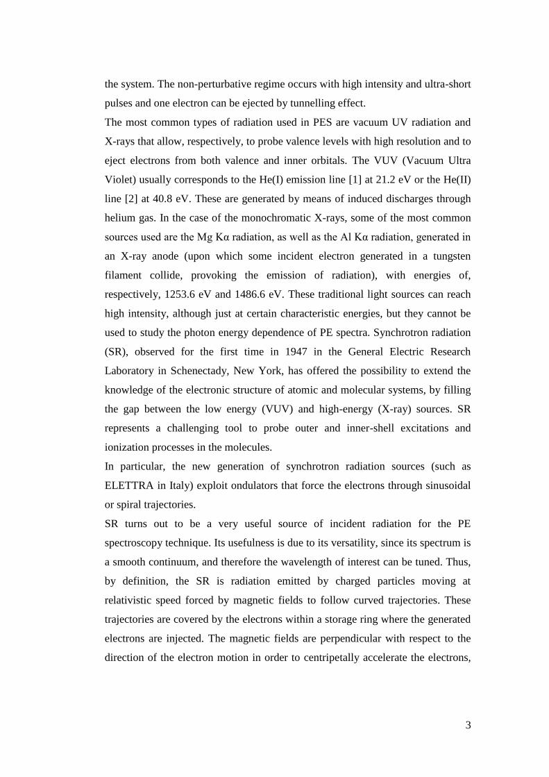
Regarding the components of a PE spectrometer, the energy analyzer (also called
electron density analyzer) accomplishes the task of dispersing the photoelectrons
as a function of their kinetic energies and counting them in order to obtain an
intensity distribution which represents the PE spectrum with a high resolution and
5
sensitivity. The electron density analyzer uses either electric or magnetic fields to
deflect electrons having different kinetic energies.
Following the analysis of the different kinetic energies of the electrons, these
come out from the energy analyzer and reach an electron multiplier, which is a
special kind of detector for the electron flux that operates on the basis of a cascade
effect, namely secondary electrons are produced by the primary ejected electrons
which strike the surface of the multiplier. A current pulse produced during this
process is detected and registered, thus providing the PE spectroscopy signal.
Spectrometers can be classified according to the number of electrons that are
detected simultaneously: in a differential spectrometer, electrons of only one
energy at a time are able to reach the detector; instead, in an integral
spectrometer, the whole set of photoelectrons having more than one energy value
are able to reach the spectrometer at the same time.
Figure 1.1: PES spectrometer setup.
6
1.3. Photoelectron Spectra
A photoelectron spectrum is the result of a PE spectroscopy experiment, and
contains information about the energy distribution of the emitted photoelectrons.
It is represented by the number of emitted electrons detected at each energy. The
characterization of a PE spectrum relies on three main sources of information
regarding the energy distribution of the photoelectrons, namely the line energies,
their corresponding intensities and the lineshape of each spectral signal
(particularly its width). During the photoexcitation process, electrons coming
from different energy levels could be ejected, giving rise to different molecular
ionic states. The observable quantity that is measured when the photoelectrons are
detected is the ionization energy of the electron of interest, which is given by the
energy difference between the electronic state of the molecular ion and the ground
state (GS) of the molecule under study.
The previously described photoexcitation phenomenon corresponds to purely
electronic transitions, nevertheless in practice the PE spectrum reports several
vibrational lines for each type of electron ionized, thus several vibronic transitions
are associated with a single electron photoionization and widen the signal that
would derive from a purely electronic transition in the PE spectrum. The
collection of lines that are associated with the ionization of a specific electron
constitute a band, and the corresponding energies describe the energy differences
between the molecular GS and the ionic state as described above.
As a starting point for the characterization of a PE spectrum, each spectral band is
assigned to a specific electronic state of the molecular ion, identifying the orbital
from which the electron has been ejected. The first approach that could be used
for characterizing the number and type of ionic states accessible during the
ionization process is considering an N-electronic state described by Molecular
Orbitals (MOs), each of which is occupied by at most two electrons. The binding
energy of each electron occupying a specific MO can be associated with its
ionization energy by means of the Koopmans’ theorem (KT), which states that the
7
negative of the binding energy of an electron in the N-electron wave function that
describes the molecular GS equals the vertical ionization energy necessary for
removing the electron from that MO. Within this approximation, the PE spectrum
could be interpreted as a direct molecular orbital energy diagram.
The Koopmans’ theorem along with these two approximations works well when
using them as a first approach towards the characterization of a PE spectrum,
nevertheless their inadequacy becomes evident when a spectrum shows a larger
number of bands with respect to the number of valence orbitals in the electronic
configuration of the molecule. This fact is due to the presence of several
mechanisms that give rise to additional bands, some of which stem from the
ionization of one electron with simultaneous excitation of a second electron
towards an unoccupied virtual orbital. This phenomenon is referred to as a two-
electron process.
As described above, PE band intensities provide information regarding the
electronic structure of the molecules studied. SR sources, which provide tunable
radiation energies, nowadays allow for obtaining high resolution spectra and thus
permit to carry out more extensive studies of PE band intensities. In a PES
experiment, the relative intensities of the spectral bands are of higher importance
with respect to the absolute band intensities. Indeed, on the one hand, the latter are
very difficult to obtain because they depend on several experimental parameters
(e.g. the intensity of incident radiation, the type of analyzer, the sensitivity of the
detector and so on); on the other hand, the relative intensities represent the
probabilities of photoionization towards different states of the ion, which are also
known as partial ionization cross sections. PE relative band intensities depend on
the nature of the molecular orbitals as well, thus information regarding the
variations in the geometry of the molecule following the photoionization event
can be extracted from a detailed analysis of the shape of the bands. The geometry
changes provide information about the nature of the molecular orbitals, such as
whether they are of bonding, anti-bonding or non-bonding character.
8
The physical quantity measured during a PE spectroscopy experiment is the
ionization energy, also known as Ionization Potential (IP). The IP is defined as the
energy required for extracting an electron from the electronic configuration of an
atom or molecule in its ground electronic state in free space. As stated at the
beginning of this section, the IP is associated with the energy difference between
the ionized molecule and the molecule in its GS. For an accurate description of
the experimental spectrum, a prior knowledge of the electronic structure of the
molecule and the ionization energies, obtained by means of theoretical
calculations, is necessary. The IPs are obtained, as a first approximation, by
calculating total energies within the Hartree-Fock framework [8] [9] [10], or
employing more accurate methods such as the Configuration-Interaction scheme
[11].
1.4. Basic Observables
In a PE experiment, some of the main physical quantities that can be obtained
from each ionized state generated, and which can also be determined theoretically,
are the cross sections, the asymmetry parameters and the Molecular Frame
Photoelectron Angular Distributions (MFPADs).
Partial cross section [12] is a measure of the probability of photoionization to an
ionic state [13] and gives information on the electronic structure of the considered
system. It is expressed by the following formula:
𝜎𝑖𝑓(ℎ𝜈) =
4𝜋2𝛼𝑎02
3ℎ𝜈∑|�̅�𝑖𝑓𝑙𝑚|
2
𝑙𝑚
(1.1)
where 𝛼 is the fine-structure constant, 𝑎0 is the Bohr radius, and �̅�𝑖𝑓𝑙𝑚 is the
dipole transition between the initial state and the final state.
In general, the emission pattern of photoelectrons is not isotropic in space, but
possesses a characteristic angular distribution. Indeed, if the spectrometer is set at
different positions in space, the detection of electrons emitted towards the
entrance slit of the spectrometer gives an angle-resolved signal and yields
9
information regarding the spatial distribution of the photoelectrons. Thus, by
studying the angular distribution, which is characteristic of the sample under study
being the pattern of photoelectrons not isotropic, a more detailed knowledge of
the photoionization process and the nature of the states involved in
photoexcitation can be attained. One of the main physical quantities that can be
determined from these measurements over a wide range of energies is the angular
distribution asymmetry parameter 𝛽, which represents the angular distribution of
photoelectrons. It appears in the expression of the differential partial cross section,
which for linearly polarized light is [14]
𝑑𝜎𝑖𝑓(ℎ𝜈)
𝑑𝛺=𝜎𝑖𝑓(ℎ𝜈)
4𝜋[1 + 𝛽𝑖𝑓(ℎ𝜈)𝑃2(𝑐𝑜𝑠𝜗)] (1.2)
where 𝜗represents the angle between the electric field vector of the photon beam
and the direction of the outgoing electron, and 𝑃2(𝑐𝑜𝑠𝜗) resents a Legendre
polynomial of second degree. Assuming a 100% linear polarization, the
differential partial cross section becomes proportional to the integral partial cross
section at the so called “magic angle” 𝜗 = 54.7°. The numerical value of 𝛽
actually determines the shape of the angular distribution pattern; for example, in
the case of photoionization of an electron from an s orbital and for negligible spin-
orbit coupling, the 𝛽 parameter has the energy-independent value of 2. In the
general case, the 𝛽 parameter varies between -1 and 2, since different amplitudes
contribute to the photoexcitation process.
This anisotropy parameter is useful for achieving an accurate description of the
photoelectron distribution when considering the measurement of PE spectra of
gas-phase free molecules, which are randomly oriented in space, in the laboratory
frame of reference. Nevertheless, from a theoretical point of view, the most
natural reference frame for considering molecular photoionization is the molecular
frame itself. Molecular frame photoelectron angular distributions (MFPADs) are
the richest observables of the photoionization. These three observables will be
described in more detail in Chapter 2.
10
1.5. Aim and outline
Aim of this thesis is to improve the theoretical description of photoionization
processes. In particular, the project consists in applying already available methods
[15] [16] [17] [18] and in implementing new algorithms in order to include more
complexes many-electron effects and to treat non-perturbative phenomena.
Chapter 2 introduces the underlying theory of photoionization processes, with a
particular attention to the main observables involved in this process, such as cross
sections and asymmetry parameters, together with the expression of the
wavefunctions and the quantum chemistry approaches used in the calculations. A
special attention will be given to the correlation effects and to the perturbative or
non-perturbative nature of the photoionization. Chapter 3 will present a correlated
single channel approach based on a CASSCF procedure coupled with Dyson
orbitals to describe the correlation effects within the bound states. In order to
describe all the correlation effects, including those involving continuum states,
and interaction among different channels, Chapter 4 will present an
implementation of the calculation of two-electron integrals, which are needed to
expand the solution in the Close-Coupling form. Finally, in Chapter 5, non-
perturbative phenomena with the numerical solution of the Time-Dependent
Schrödinger Equation (TDSE) will be treated.

11
1.6. Computational tools
Fortran90 is used to implement the algorithms. All the calculations performed for
this thesis have been executed on supercomputers at CINECA (Casalecchio di
Reno, Bologna, Italy). The one most used in this project is Marconi, which is one
of the fastest supercomputers available today within the community of Italian
industrial and public researchers. It is ranked at the 14th position in the top500 (as
june 2017), the list of the most powerful supercomputers in the world. Specifically
we worked on A1 partition, some technical references are reported below:
Model: Lenovo NeXtScale.
Architecture: Intel OmniPath Cluster
Nodes: 1512
Processors: 2 x 18-cores Intel Xeon E5-2697 v4 (Broadwell) at 2.30 GHz
Cores: 36 cores/node, 54432 cores in total
RAM: 128 GB/node, 3.5 GB/core
Internal Network: Intel OmniPath
Disk Space: 17 PB (raw) of local storage
Peak Performance: 2 PFlop/s
Available compilers: Fortran F90, C, C++
Parallel libraries: IntelMPI and OpenMPI
12
2. Theory
2.1. Photoionization processes
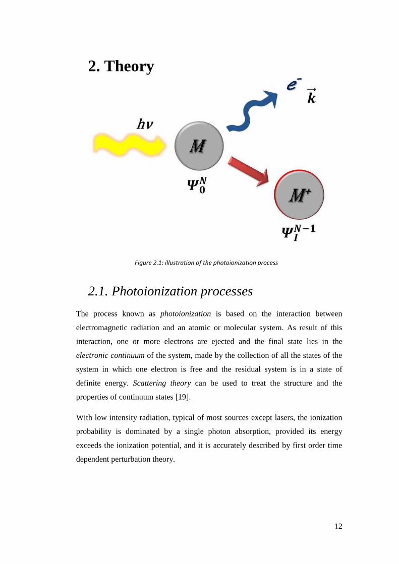
The process known as photoionization is based on the interaction between
electromagnetic radiation and an atomic or molecular system. As result of this
interaction, one or more electrons are ejected and the final state lies in the
electronic continuum of the system, made by the collection of all the states of the
system in which one electron is free and the residual system is in a state of
definite energy. Scattering theory can be used to treat the structure and the
properties of continuum states [19].
With low intensity radiation, typical of most sources except lasers, the ionization
probability is dominated by a single photon absorption, provided its energy
exceeds the ionization potential, and it is accurately described by first order time
dependent perturbation theory.
Figure 2.1: illustration of the photoionization process
13
In this regime, within scattering theory, the probability that a collision event
occurs is measured by an observable called cross section (𝜎). Cross section can be
viewed as the number of ejected electrons detected in a given solid angle ∆𝛺
divided by the number of incoming photons. By taking into account a small solid
angle 𝑑𝛺, one can express 𝜎 as:
𝜎(𝑑𝛺) =
𝑑𝜎(𝛺)
𝑑𝛺𝑑𝛺 (2.1)
where 𝑑𝜎(𝛺)
𝑑𝛺 is the differential cross section which represents the observable in
scattering experiments.
2.1.1. Nature of the photoionization
More generally, other processes become allowed with high intensity radiation.
Increasing intensity, light-matter interaction leads generally to two different kind
of ionization: perturbative and non-perturbative. Let us introduce the Keldysh
parameter 𝛾 to distinguish the two type of ionization [20]:
𝛾 = √𝐼𝑝
2𝑈𝑝 (2.2)
where 𝐼𝑝 represents the ionization potential of the considered electronic state and
𝑈𝑝 is the ponderomotive force, which is the energy that a free electron acquires in
the field, averaged over a cycle. It is related both to the amplitude 𝐸 and to the
frequency (or photon energy) ω of the electric field by
𝑈𝑝 = (
𝐸
2𝜔)2
(2.3)
The Keldysh parameter characterizes the regime of the ionization: if 𝛾 ≫ 1 the
ionization is perturbative, otherwise, if 𝛾 ≪ 1, it occurs a non-perturbative
multiphoton ionization.
14
Alternatively a more accurate criterion for the validity of the perturbation theory
is that 𝑈𝑝 is much smaller than the photon energy, i.e.
𝑍 =
𝑈𝑝
𝜔≪ 1 (2.4)
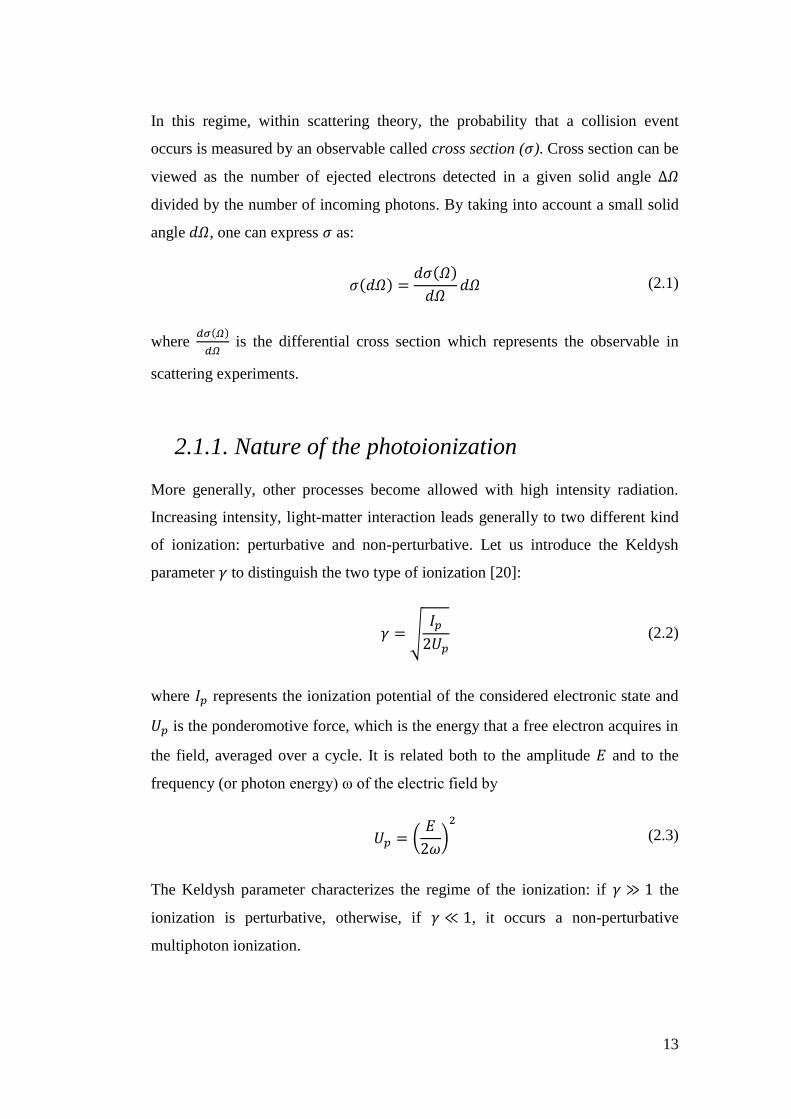
In Figure 2.2 [21], the differences between the two regimes are shown:
Of course there is a continuous transition between the two behaviours around
𝛾 = 1. Actually Keldysh parameter is not always a perfect index of the nature of
the ionization, in fact for 𝛾 < 1 with 𝜔 > ~ 𝐼𝑝 the ionization acquires perturbative
nature [22].
The perturbative regime is governed by a multiphoton (or few-photon) absorption
that ionizes the system. Therefore the final state is a consequence of a discrete
number 𝑛 of interaction between light and the considered system (Fig 2.2a). This
process can be accurately described by the lowest order in perturbation theory
(LOPT) in which the process is allowed.
In the non-perturbative (or tunnelling) regime the Coulomb potential is seen as the
perturbation. Thus, the interaction between light and matter can be described by a
Figure 2.2: physical illustration of multiphoton regimes: perturbative (a) and non-perturbative (b)
15
local potential that highly affect the Coulomb potential building a potential
barrier. In this way, the electron motion is dominated by the field-induced
potential (Fig 2.2b) and can escape the potential barrier by tunnelling through it
and lies in the continuum (tunnelling regime), or directly if the barrier is lowered
below its energy (over the barrier regime). In this regime one also refers to strong
field (SF) processes.
Once the electron is far from the ion, the Coulomb potential become negligible.
The non-perturbative ionization makes not possible to exactly define the number
of photon absorbed.
An observable that helps to distinguish the two regimes is the photoelectron
spectrum. A perturbative ionization furnishes a discrete photoelectron spectrum
where the peak positions are related to the number of photons absorbed; whereas
in non-perturbative ionization no characteristic peaks can be observed.
2.1.2. Perturbative Few-Photon Ionization
If allowed, the one-photon ionization is the most probable photoionization event,
but, increasing the intensity, one can observe an absorption of more photons. For
example, recently has been illustrated how in x-ray regime neon atom can absorb
up to 8 photons furnishing Ne8+
[23]. Using x-ray, in fact, the ionization is
governed by sequential absorption of one photon at time. This is explained by the
high value of Keldysh parameter (Equation 2.2): x-ray correspond to high energy,
thus, to very small ponderomotive potentials. These kind of processes are named
multiple one-photon ionizations.
The simplest multiphoton process is the absorption of two photon at the same
time. Generally, the simultaneous absorption of more than one photon is call non-
sequential multiphoton ionization. These kind of processes are favoured by value
of photon energy near to the resonance. For example, a non-sequential
multiphoton process has been showed in an experiment, also performed on Ne,
16
that produces Ne9+
. Which can be obtained only by combining sequential and non-
sequential two-photon ionization [24].
2.1.3. Non-Perturbative (Tunnel) Ionization
Let us consider a system under a high field strengths. The investigation of this
system using the perturbative approach for describing multiphoton ionization
could provide bad result. Using UV or X-ray current light sources, the non-
perturbative regime is difficult to achieve (very high intensities are needed).
Seeing Equation (2.2), the non-perturbative regime is easier to reach using optical
frequencies.
As already mentioned, the multiphoton non-perturbative ionization can be seen as
the distortion of the electronic system that deform enough the Coulomb potential
to cause a tunnel out of an electron. This process is also named as tunnel
ionization.
A typical current source is the Titanium sapphire laser, which provides pulses at
the fundamental wavelength of 800 nm (𝜔 = 1.57 𝑒𝑉), and its lowest harmonics.
Ultrashort pulses of few femtosecond or even attosecond length are provided by
the so called high harmonic generation (HHG) obtained by focussing the high
energy pulse on noble gases. HHG is extensively used either as a tool to
investigate ultrafast molecular process, or as a secondary source of ultrashort
pulses in the XUV region.
17
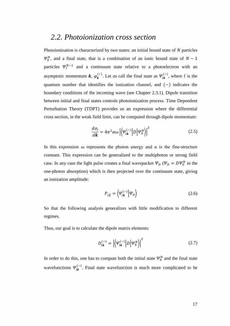
2.2. Photoionization cross section
Photoionization is characterized by two states: an initial bound state of 𝑁 particles
𝛹0𝑁, and a final state, that is a combination of an ionic bound state of 𝑁 − 1
particles 𝛹𝐼𝑁−1 and a continuum state relative to a photoelectron with an
asymptotic momentum 𝒌, 𝜑𝒌(−)
. Let us call the final state as 𝛹𝐼𝒌(−)
, where 𝐼 is the
quantum number that identifies the ionization channel, and (−) indicates the
boundary conditions of the incoming wave (see Chapter 2.3.1). Dipole transition
between initial and final states controls photoionization process. Time Dependent
Perturbation Theory (TDPT) provides us an expression where the differential
cross section, in the weak field limit, can be computed through dipole momentum:
𝑑𝜎𝐼𝑑𝒌
= 4𝜋2𝛼ω |⟨𝛹𝐼𝒌(−)|𝐷|𝛹0
𝑁⟩|2
(2.5)
In this expression ω represents the photon energy and α is the fine-structure
constant. This expression can be generalized to the multiphoton or strong field
case. In any case the light pulse creates a final wavepacket 𝛹𝐷 (𝛹𝐷 = 𝐷𝛹0𝑁 in the
one-photon absorption) which is then projected over the continuum state, giving
an ionization amplitude:
𝑃𝐼�⃗� = ⟨𝛹𝐼𝒌(−)|𝛹𝐷⟩ (2.6)
So that the following analysis generalizes with little modification to different
regimes.
Thus, our goal is to calculate the dipole matrix elements:
𝐷𝐼𝒌(−)= |⟨𝛹𝐼𝒌
(−)|𝐷|𝛹0
𝑁⟩|2
(2.7)
In order to do this, one has to compute both the initial state 𝛹0𝑁 and the final state
wavefunctions 𝛹𝐼𝒌(−)
. Final state wavefunction is much more complicated to be
18
evaluated with respect to the initial state wavefunction and has to satisfy definite
boundary conditions.
Before describing wavefunctions associated to the initial and final states, let us
consider how the cross section can be calculated. From the experimental point of
view, there are two frames regarding the orientation of a molecule: molecules can
be randomly oriented within the sample (gas phase experiment) or can be all
oriented in a specific direction. The first case is treated by averaging over all the
possible orientations, while the second case provides cross sections related to a
single orientation. In the latter case the angular distribution of the emitted
electrons is much richer, and is called MPFAD (Molecular Frame Photoelectron
Angular Distribution).
To compare theory and experiment, the reference system has to be the same. In
fact, experimental results are commonly reported in Laboratory Frame (LF) with
coordinates (x’, y’, z’). Coordinates are usually set up so that z’ axes corresponds
to the polarization or the direction of the incident radiation. Theoretical results are
reported in molecular frame (MF) with coordinates (x, y, z), where z is assumed to
be the main axes of the molecule. In order to transform one frame into the other
one, one can introduce the Euler angles 𝛺 = (𝛼, 𝛽, 𝛾), where 𝛼 and 𝛽 are the polar
angles that describe the incident radiation in the molecular frame.
The differential cross section can be expanded in terms of angular momentum
eigenfunctions 𝑌𝐿𝑀(휃, 𝜑) with coefficients 𝐴𝐿𝑀(𝑘, 𝛺) which depend on the
orientation of the electromagnetic radiation in the molecular frame:
𝑑𝜎𝐼
𝑑�̂�=∑𝐴𝐿𝑀𝑌𝐿𝑀
𝐿𝑀
(2.8)
At this point, the cross section can be expressed in terms of MF and LF.
19
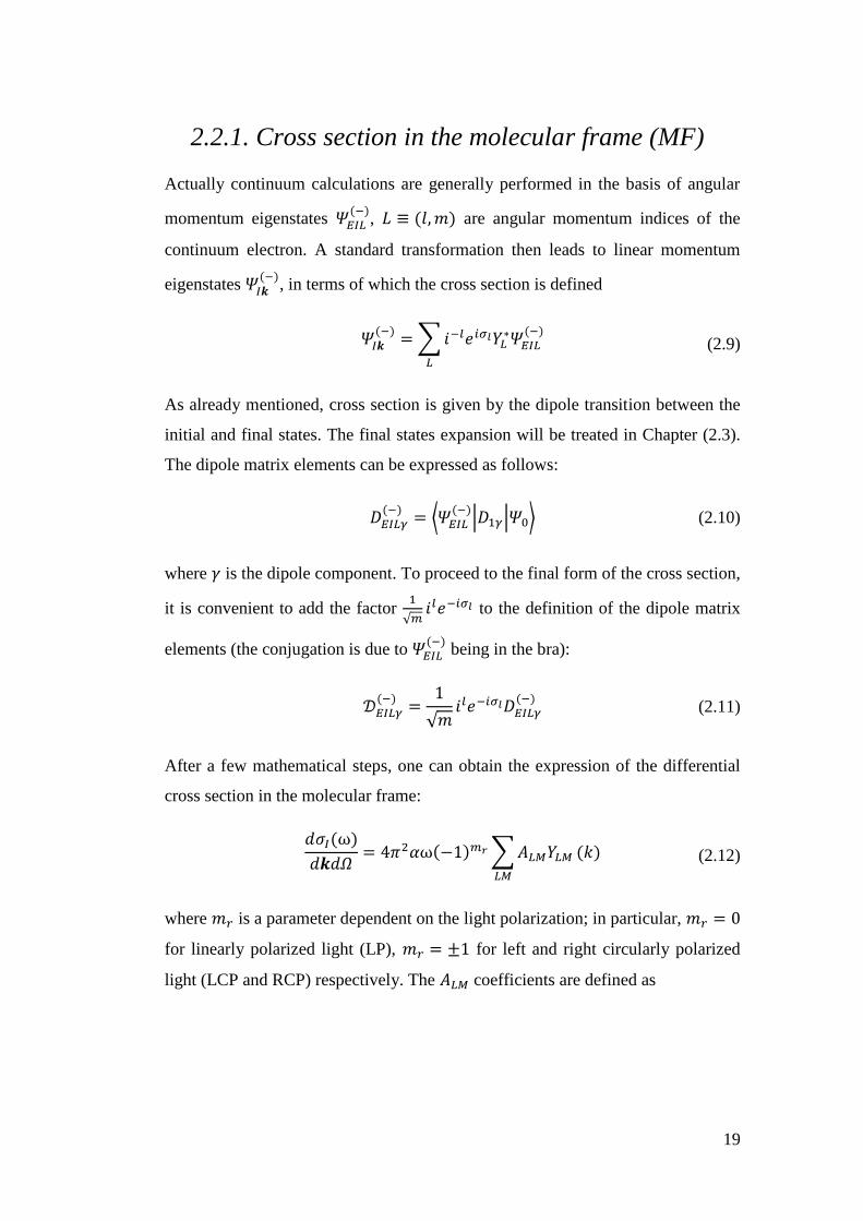
2.2.1. Cross section in the molecular frame (MF)
Actually continuum calculations are generally performed in the basis of angular
momentum eigenstates 𝛹𝐸𝐼𝐿(−)
, 𝐿 ≡ (𝑙,𝑚) are angular momentum indices of the
continuum electron. A standard transformation then leads to linear momentum
eigenstates 𝛹𝐼𝒌(−)
, in terms of which the cross section is defined
𝛹𝐼𝒌(−)=∑𝑖−𝑙𝑒𝑖𝜎𝑙𝑌𝐿
∗𝛹𝐸𝐼𝐿(−)
𝐿
(2.9)
As already mentioned, cross section is given by the dipole transition between the
initial and final states. The final states expansion will be treated in Chapter (2.3).
The dipole matrix elements can be expressed as follows:
𝐷𝐸𝐼𝐿𝛾(−)
= ⟨𝛹𝐸𝐼𝐿(−)|𝐷1𝛾|𝛹0⟩ (2.10)
where 𝛾 is the dipole component. To proceed to the final form of the cross section,
it is convenient to add the factor 1
√𝑚𝑖𝑙𝑒−𝑖𝜎𝑙 to the definition of the dipole matrix
elements (the conjugation is due to 𝛹𝐸𝐼𝐿(−)
being in the bra):
𝒟𝐸𝐼𝐿𝛾(−)
=1
√𝑚𝑖𝑙𝑒−𝑖𝜎𝑙𝐷𝐸𝐼𝐿𝛾
(−) (2.11)
After a few mathematical steps, one can obtain the expression of the differential
cross section in the molecular frame:
𝑑𝜎𝐼(ω)
𝑑𝒌𝑑𝛺= 4𝜋2𝛼ω(−1)𝑚𝑟∑𝐴𝐿𝑀𝑌𝐿𝑀
𝐿𝑀
(𝑘) (2.12)
where 𝑚𝑟 is a parameter dependent on the light polarization; in particular, 𝑚𝑟 = 0
for linearly polarized light (LP), 𝑚𝑟 = ±1 for left and right circularly polarized
light (LCP and RCP) respectively. The 𝐴𝐿𝑀 coefficients are defined as
20
𝐴𝐿𝑀
= ∑ (−1)𝑚+𝛾′𝑙𝑙′�̂� (
𝑙′ 𝑙 𝐿𝑚′ −𝑚 𝑀
)(𝑙′ 𝑙 𝐿0 0 0
)𝒟𝑙𝑚𝛾(−)𝒟
𝑙′𝑚′𝛾′(−) ∗
∙
𝑙𝑚𝛾,𝑙′𝑚′𝛾′
∙∑𝐽 (1 1 𝐽𝛾′ −𝛾 𝛾 − 𝛾′
) (1 1 𝐽𝑚𝑟 −𝑚𝑟 0
) 𝑌𝐽𝛾′−𝛾(𝛽, 𝛼)
𝐽
(2.13)
with 𝑙 = √2𝑙 + 1 and J an index of sum that goes from 0 to 2.
Thus, we have now defined an experiment with oriented molecules on the MF by
considering both direction of the emitted electrons and polarization of the incident
light. The angle-integrated cross section is obtained by:
∫𝑌𝐿𝑀(�̂�)𝑑�̂� = 𝛿𝐿0𝛿𝑀0√4𝜋 (2.14)
In this way, all the emission directions �̂� are taken into account. Finally, total
cross section in the MF is given by:
𝜎(𝛺) = ∫
𝑑𝜎𝐼𝑑𝒌𝑑𝒌 = 4𝜋2𝛼ω(−1)𝑚𝑟√4𝜋𝐴00 (2.15)
2.2.2. Cross section in the laboratory frame
In order to obtain an expression for the cross section in the laboratory frame, let us
start from Equation (2.12) calculated for the molecular frame. For this purpose,
rotation matrices are used to transform vector �̂� into the new coordinates. After a
few mathematical steps, one can obtain the equation for the differential cross
section in the laboratory frame, by averaging over all the molecular orientations:
𝑑𝜎
𝑑𝒌= 𝜋𝛼ω(−1)𝑚𝑟∑𝐴𝐿𝑃𝐿
𝐿
(𝑐𝑜𝑠휃′) (2.16)
where 휃 is the angle between 𝒌 and 𝑧 (light polarization or propagation axes) in
LF. In this case, the coefficients 𝐴𝐿 are:
21
𝐴𝐿(𝑘) = (2𝐿 + 1) (1 1 𝐿𝑚𝑟 −𝑚𝑟 0
) ∙
∙ ∑ (−1)𝑚+𝛾′√(2𝑙 + 1)(2𝑙′ + 1) (
𝑙′ 𝑙 𝐿0 0 0
) (𝑙′ 𝑙 𝐿−𝑚 𝑚′ 𝑚 −𝑚′
)
𝑙𝑚𝛾,𝑙′𝑚′𝛾′
∙ (1 1 𝐿𝛾′ −𝛾 𝛾 − 𝛾′
) (1 1 𝐿𝑚𝑟 −𝑚𝑟 0
)𝒟𝑙𝑚𝛾(−) 𝒟
𝑙′𝑚′𝛾′(−) ∗
(2.17)
and 𝑃𝐿(𝑐𝑜𝑠휃′) are the Legendre polynomials.
𝑌𝑙0(휃, 𝜑) = √2𝑙 + 1
4𝜋𝑃𝐿(𝑐𝑜𝑠휃
′) (2.18)
Here 𝐴𝐿 ≠ 0 only for 𝐿 = 0,1,2, and moreover 𝐴1 ≠ 0 only for chiral molecules
and circular polarized light. In this way one recovers the well-known formula
𝑑𝜎
𝑑𝒌=𝜎04𝜋[1 + 𝛽𝑃2(𝑐𝑜𝑠휃
′)] (2.19)
for ionization of unoriented molecules with linearly polarized light.
22
2.3. Final state wavefunction
2.3.1. Boundary conditions for ionization processes
In order to define the wavefunction for the final state, let us treat, first of all, the
boundary conditions that control the ejected electron. We will start by taking into
account different kinds of potentials, ranging from a spherically symmetric
potential to a non-spherically symmetric potential.
Spherically symmetric potential
In photodetachment process (where an electron is ejected from an anion), electron
is under the action of a short-range potential due to the neutral final system. This
situation can be described by an asymptotic behaviour with a spherically
symmetric potential. Using scattering theory, one can express the boundary
conditions that affect the wavefunction of the final state in the following form:
𝜑𝒌(−)(𝒓)
𝑟→∞→
1
(2𝜋)32
[𝑒𝑖𝒌∙𝒓 + 𝑓(−)(𝑘, �̂�, �̂�)𝑒−𝑖𝑘𝑟
𝑟] (2.20)
where 𝑓(−)(𝑘, �̂�, �̂�) is the scattering amplitude. This expression satisfies the
asymptotic behaviour of the final state by considering as open only one ionic state
and a photoelectron with energy
𝐸𝑘 =
𝑘2
2 (2.21)
Thus, the wavefunction is assumed to be a plane wave far from the origin of the
initial state, in addition to incoming spherical waves. This asymptotic form
corresponds to the physical situation when an electron with momentum 𝒌 is
detected at long distance.
In order to express the wavefunction 𝜑𝒌(−)(𝒓), let us introduce the representation
of a general function in polar coordinates, where it is expanded in partial waves:
23
𝛹(𝑥, 𝑦, 𝑧) ≡ 𝛹(𝑟, 휃, 𝜑) ≡∑𝑅𝑙𝑚(𝑟)𝑌𝑙𝑚(휃, 𝜑)
𝑙𝑚
(2.22)
In this expression spherical harmonics 𝑌𝑙𝑚 are used.
The exact solution of the wavefunction associated to an electron in a spherically
symmetric short-range potential can be expressed in terms of partial waves
𝑅𝑙𝑚(𝑟)𝑌𝑙𝑚(휃, 𝜑):
𝜑𝒌(−)(𝒓) =∑𝐶𝑙𝑚𝑅𝐸𝑙(𝑟)𝑌𝑙𝑚(휃, 𝜑)
𝑙𝑚
(2.23)
where 𝑅𝐸𝑙(𝑟) (now independent on 𝑚) is obtained from the solution of the
Schrödinger equation in the continuum:
𝐻𝜑𝐸𝑙𝑚 = 𝐸𝜑𝐸𝑙𝑚 (2.24)
𝐸 =
𝑘2
2𝑚
(2.25)
and can be expressed asymptotically as a linear combination of normalized 𝑓𝑙(𝑘𝑟)
regular and irregular 𝑔𝑙(𝑘𝑟) Bessel functions.
𝑅𝐸𝑙(𝑟) = 𝐴𝑙𝑓𝑙(𝑘𝑟) + 𝐵𝑙𝑔𝑙(𝑘𝑟) (2.26)
Let us divide by the coefficient 𝐴𝑙 to obtain the final form of the radial part
𝑅𝐸𝑙(𝑟), which is called “K-matrix normalized”:
𝑅𝐸𝑙(𝑟) = 𝑓𝑙(𝑘𝑟) + 𝐾𝑙𝑔𝑙(𝑘𝑟) (2.27)
where
𝐾𝑙 = 𝐵𝑙𝐴𝑙−1 (2.28)
It can be further transformed to so called incoming wave, or 𝑆+ matrix
normalization, as
24
𝑅𝐸𝑙(−) = 𝑅𝐸𝑙(1 + 𝑖𝐾𝑙)
−1 (2.29)
from which a standard transformation leads to the required asymptotic form
describing the free electron in this potential:
𝜑𝒌(−)(𝒓) =
1
√𝑚∑𝑖𝑙𝑅𝐸𝑙
(−)(𝑟)𝑌𝑙𝑚∗ (�̂�)𝑌𝑙𝑚(�̂�)
𝑙𝑚
(2.30)
expressed in partial waves. where 𝑅𝐸𝑙(−)
is the radial function to which the
asymptotic behaviour has been applied.
Regarding this wavefunction form, some considerations can be done. First,
product 𝑅𝐸𝑙(−)(𝑟)𝑌𝑙𝑚(�̂�) is a partial wave describing the single-electron
wavefunction in a state with angular momentum (𝑙,𝑚). The probability to find an
electron with direction �̂� in this state is given by 𝑌𝑙𝑚∗ (�̂�).
Coulomb potential
Photoionization process from an anionic state has been considered so far. Our
goal is now to generalize the previous considerations for treating photoionization
process which starts from a neutral or a cationic state. In this case, Coulomb
potential has to be considered:
𝑉(𝑟)
𝑟→∞→ −
𝑍𝑖𝑜𝑛𝑟
(2.31)
The previous development remains unaltered except that now 𝑓𝑙(𝑘𝑟) and 𝑔𝑙(𝑘𝑟)
are the regular and irregular Coulomb functions, well known analytically.
After a few steps, one can obtain the equation of the photoelectron wavefunction
(solution of the scattering Schrödinger equation) in a Coulomb potential:
𝜑𝒌(−)(𝒓) =
1
√𝑚∑𝑖𝑙𝑒−𝑖𝜎𝑙𝑅𝑬𝒍
(−)(𝑟)𝑌𝑙𝑚∗ (�̂�)𝑌𝑙𝑚(�̂�)
𝑙,𝑚
(2.32)
25
This equation is similar to that one calculated by not considering a Coulomb
potential (see Equation 2.30). The main difference lies in the form of the radial
function. A further difference is represented by the presence, in the normalization
factor, of the Coulomb phase-shift, 𝜎𝑙, which is equal to zero in the case of
spherically-symmetric potential.
Non-spherically symmetric potential
In order to further generalize the approach described so far, let us consider a non-
spherically symmetric potential. Under the action of this potential, the
wavefunction can be expressed in terms of partial waves as follows:
𝜑𝐸𝑙𝑚 = ∑ 𝑅𝐸𝑙′𝑚′𝑙𝑚𝑌𝑙′𝑚′
𝑙′𝑚′
(2.33)
By applying boundary conditions (K-matrix normalization) to this wavefunction,
one obtains a wavefunction indicated by 𝜑𝐸𝐿(𝐾)
, where 𝐿 ≡ (𝑙, 𝑚). After a few
steps, equation describing the free electron in the considered potential is obtained:
𝜑𝐿𝑀(−) =∑𝜑
𝐿′′(𝐾)(1 + 𝑖𝐾)𝐿′′𝐿
−1
𝐿′′
(2.34)
𝐾 is the K-matrix (see Equation 2.28). Although from the computational point of
view, it is generally more convenient to express wavefunctions on the basis of
angular momentum, it is sometimes useful to express them in terms of asymptotic
momentum 𝑘. Thus, this wavefunction can be transformed as follows:
𝜑𝒌(−) =∑𝐶𝐿𝜑𝐸𝐿
(−)
𝐿
(2.35)
where
𝐶𝐿 =
1
√𝑚𝑖𝑙𝑒−𝑖𝜎𝑙𝑌𝐿
∗(�̂�) (2.36)
𝜑𝒌(−)
satisfies both asymptotic boundary conditions and normalization, and
represents a suitable wavefunction for computing photoionization cross sections.
26
Moreover, molecular symmetry can be exploited within the wavefunction
expansion. In fact, Hamiltonian matrix is diagonal over different symmetry
irreducible representations (𝜆, 𝜇). Thus, implementation of a symmetry adapted
angular basis is really useful. This can be done by transforming the spherical
harmonic basis
𝑋𝑙ℎ𝜆𝜇 =∑𝑌𝑙𝑚𝑏𝑚𝑙ℎ𝜆𝜇𝑚
(2.37)
where ℎ counts each 𝑋𝑙ℎ𝜆𝜇 for each 𝑙. The coefficients satisfy the relation
𝑏+ = 𝑏−1, therefore
𝑌𝑙𝑚 =∑𝑋𝑙ℎ𝜆𝜇𝑏𝑚𝑙ℎ𝜆𝜇∗
ℎ𝜆𝜇
(2.38)
Use of the symmetry reduces the size of the Hamiltonian and overlap matrices,
which are block-diagonal in the symmetry indexes, so that the computational cost
dramatically decreases.
2.3.2. The multichannel continuum wavefunction
Up to here we have considered a single electron in a given potential. In a many-
electron system, once the electron is ejected, there are several final ionic states
that the system may reach by considering a photon energy ω, those whose
ionization potential is lower than ω. They are called open channels, 𝛹𝐼𝑁−1, and
𝐸𝐼𝑁−1 are the corresponding energies:
𝐼𝑃𝐼 = 𝐸𝐼𝑁−1 − 𝐸0
𝑁 < ħ𝜔, 𝐸 = 𝐸0𝑁 + ħ𝜔
𝑘𝐼 = √2(𝐸 − 𝐸𝐼𝑁−1) = √2(𝜔 − 𝐼𝑃𝐼
(2.39)
and 𝑘𝐼 are the corresponding electron kinetic energy. We have considered only
one open channel so far; however, our goal is to include all the open channels to
27
the previous wavefunction approach. To do this, the final state wavefunction,
including both photoelectron and ionic states, is expanded in terms of partial
waves:
𝛹𝐸𝐼𝐿 =∑𝛹𝐼′𝑁−1𝑅𝐸𝐼′𝐿′𝐼𝐿(𝑟)𝑌𝐿′(�̂�)
𝐼′𝐿′
(2.40)
where 𝐼 counts the open channels. The boundary conditions are
𝑅𝐸𝐼′𝐿′𝐼𝐿(𝑟) 𝑟→∞→ 𝑓𝑙′(𝑘𝐼𝑟)𝐴𝐼′𝐿′𝐼𝐿 + 𝑔𝑙′(𝑘𝐼𝑟)𝐵𝐼′𝐿′𝐼𝐿 (2.41)
They can be normalized by multiplying for 𝑨−1, providing the expansion with K-
matrix normalization
𝛹𝐸𝐼𝐿(𝐾)=∑𝛹𝐸𝐼′𝐿′𝐴𝐼′𝐿′𝐼𝐿
−1
𝐼′𝐿′
(2.42)
𝑲 = 𝑩𝑨−1 (2.43)
and applying the boundary condition of the incoming wave
𝛹𝐸𝐼𝐿(−)=∑𝛹𝐸𝐼𝐿
(𝐾)(1 + 𝑖𝐾)𝐼′𝐿′𝐼𝐿
−1
𝐼′𝐿′
(2.44)
As already mentioned, it can be useful to express the wavefunction in terms of
linear momentum:
𝛹𝐼𝒌(−)=∑𝐶𝐿𝑘𝛹𝐸𝐼𝐿
(−)
𝐿
(2.45)
where
𝐶𝐿𝑘 =
1
√𝑚𝑖𝑙𝑒−𝑖𝜎𝑙𝑌𝐿
∗(�̂�) (2.46)

28
2.3.3 Convergence of the partial wave expansion
The expansion in terms of partial waves can be considered as exact if an infinite
number of them is used. However, even with a truncated series, convergence of
this expansion is fast at low energies and becomes slower at high energies. This
can be explained by classical scattering, which provides us a hint about the
maximum value of 𝑙 to be used; in fact:
𝐿 = 𝑎𝑘 ~ 𝑙 (2.47)
where 𝑎 is the maximum impact parameter. Thus, the value of 𝑙 to be used is
proportional to the value of the electron momentum 𝑘. Increasing the value of
𝑙𝑚𝑎𝑥 implicates to increase the computational cost as well; therefore, the study at
high energies implicates a huge computational cost.
29
2.4. The basis set
Results of any quantum chemistry calculation dramatically depend on the choice
of the basis set. The present method works by using spherical coordinates, and
with a symmetry adapted basis which is a product of radial and angular functions:
𝜒𝑛𝑙ℎ𝜆𝜇(𝑟, 휃, 𝜙) = 𝑅𝑛(𝑟) ∙ 𝑋𝑙ℎ𝜆𝜇(휃, 𝜙) (2.48)
The angular part 𝑋𝑙ℎ𝜆𝜇(휃, 𝜙) is expanded in terms of real spherical harmonics
[15] which will be described in more detail in Chapter (2.4.3).
𝑋𝑙ℎ𝜆𝜇(휃, 𝜙) =∑𝑌𝑙𝑚𝑅 (휃, 𝜙)𝑏𝑙𝑚ℎ𝜆𝜇
𝑚
(2.49)
where 𝑛 is the index of the radial part; 𝑙 and 𝑚 are the angular momentum
quantum numbers; 𝜆 is the index that represents the irreducible representation (IR)
of the molecular point group; 𝜇 indicates the subspecies in case of degenerate IR;
finally, ℎ distinguishes between different elements with the same {𝑙, 𝜆, 𝜇} set. Note
that the transformation from spherical harmonics to the symmetry adapted angular
functions is unitary.
The radial part is expanded in terms of B-splines, which will be illustrated in the
following Chapter.
𝑅𝑛(𝑟) =
1
𝑟𝐵𝑛(𝑟) (2.50)
2.4.1. B-splines
B-splines [25] (B stands for basis) are functions designed for generalizing
polynomials in order to approximate arbitrary functions. Although they were
introduced by Schoenberg in 1946 [26], it was only with De Boor [27] that their
application to atomic physics started to be relevant. Indeed, De Boor published
FORTRAN subroutines that make it possible to define and manipulate B-splines
of arbitrary order and knot point distribution. It has been in the 1990s, with the
30
advent of powerful computers, that the number of applications has exponentially
grown up. Indeed, they have had one of the most significant development in the
field of computational atomic and molecular physics for the calculation of atomic
and molecular structure and dynamics. Different types of splines have been used,
particularly for fitting purposes; in addition to their application in numerical
analysis, they represent a standard part of fitting routines in commercial program
packages.
B-splines have the property of becoming rapidly complete with a relatively small
number of basis functions; this allows one to obtain an arbitrary large part of the
spectrum of the Schrödinger equation, including the continuum with a low
computational cost. This approach transforms the solution of a differential
equation into an algebraic eigenvalue problem and, together with the introduction
of electronic computers, it has become popular since linear algebra is one of the
best developed branches of numerical computation. Indeed, thanks to the
computational growth, large matrices can be routinely diagonalized with high
accuracy in short times.
To solve the single-particle equation, it is needed to briefly describe the
mathematical properties of B-splines; as previously highlighted, they are
piecewise polynomial positive functions used to approximate functions and
calculate the associated derivatives and integrals.
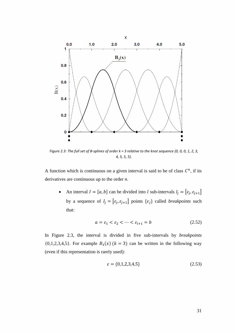
A complete B-splines set in the interval [0,5] is shown in Figure 2.3.
To better understand this concept, let us introduce some definitions:
a polynomial of order k has maximum degree k – 1:
𝑝(𝑥) = 𝑎0 + 𝑎1𝑥 + 𝑎2𝑥2 +⋯+ 𝑎𝑘−1𝑥
𝑘−1 (2.51)
31
A function which is continuous on a given interval is said to be of class 𝐶𝑛, if its
derivatives are continuous up to the order n.
An interval 𝐼 = [𝑎, 𝑏] can be divided into 𝑙 sub-intervals 𝐼𝑗 = [휀𝑗, 휀𝑗+1]
by a sequence of 𝐼𝑗 = [휀𝑗, 휀𝑗+1] points {휀𝑗} called breakpoints such
that:
𝑎 = 휀1 < 휀2 < ⋯ < 휀𝑙+1 = 𝑏 (2.52)
In Figure 2.3, the interval is divided in five sub-intervals by breakpoints
{0,1,2,3,4,5}. For example 𝐵3(𝑥) (𝑘 = 3) can be written in the following way
(even if this representation is rarely used):
휀 = {0,1,2,3,4,5} (2.53)
Figure 2.3: The full set of B-splines of order k = 3 relative to the knot sequence {0, 0, 0, 1, 2, 3,
4, 5, 5, 5}.
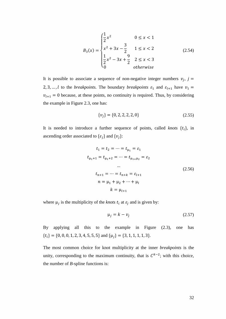
32
𝐵3(𝑥) =
{
1
2𝑥2 0 ≤ 𝑥 < 1
𝑥2 + 3𝑥 −3
2 1 ≤ 𝑥 < 2
1
2𝑥2 − 3𝑥 +
9
2 2 ≤ 𝑥 < 3
0 𝑜𝑡ℎ𝑒𝑟𝑤𝑖𝑠𝑒
(2.54)
It is possible to associate a sequence of non-negative integer numbers 𝑣𝑗 , 𝑗 =
2, 3, … , 𝑙 to the breakpoints. The boundary breakpoints 휀1 and 휀𝑙+1 have 𝑣1 =
𝑣𝑙+1 = 0 because, at these points, no continuity is required. Thus, by considering
the example in Figure 2.3, one has:
{𝑣𝑗} = {0, 2, 2, 2, 2, 0} (2.55)
It is needed to introduce a further sequence of points, called knots {𝑡𝑖}, in
ascending order associated to {휀𝑗} and {𝑣𝑗}:
𝑡1 = 𝑡2 = ⋯ = 𝑡µ1 = 휀1
𝑡µ1+1 = 𝑡µ1+2 = ⋯ = 𝑡µ1+µ2 = 휀2
…
𝑡𝑛+1 = ⋯ = 𝑡𝑛+𝑘 = 휀𝑙+1
𝑛 = µ1 + µ2 +⋯+ µ𝑙
𝑘 = µ𝑙+1
(2.56)
where µ𝑗 is the multiplicity of the knots 𝑡𝑖 at 휀𝑗 and is given by:
µ𝑗 = 𝑘 − 𝑣𝑗 (2.57)
By applying all this to the example in Figure (2.3), one has
{𝑡𝑖} = {0, 0, 0, 1, 2, 3, 4, 5, 5, 5} and {µ𝑗} = {3, 1, 1, 1, 1, 3}.
The most common choice for knot multiplicity at the inner breakpoints is the
unity, corresponding to the maximum continuity, that is 𝐶𝑘−2; with this choice,
the number of B-spline functions is:
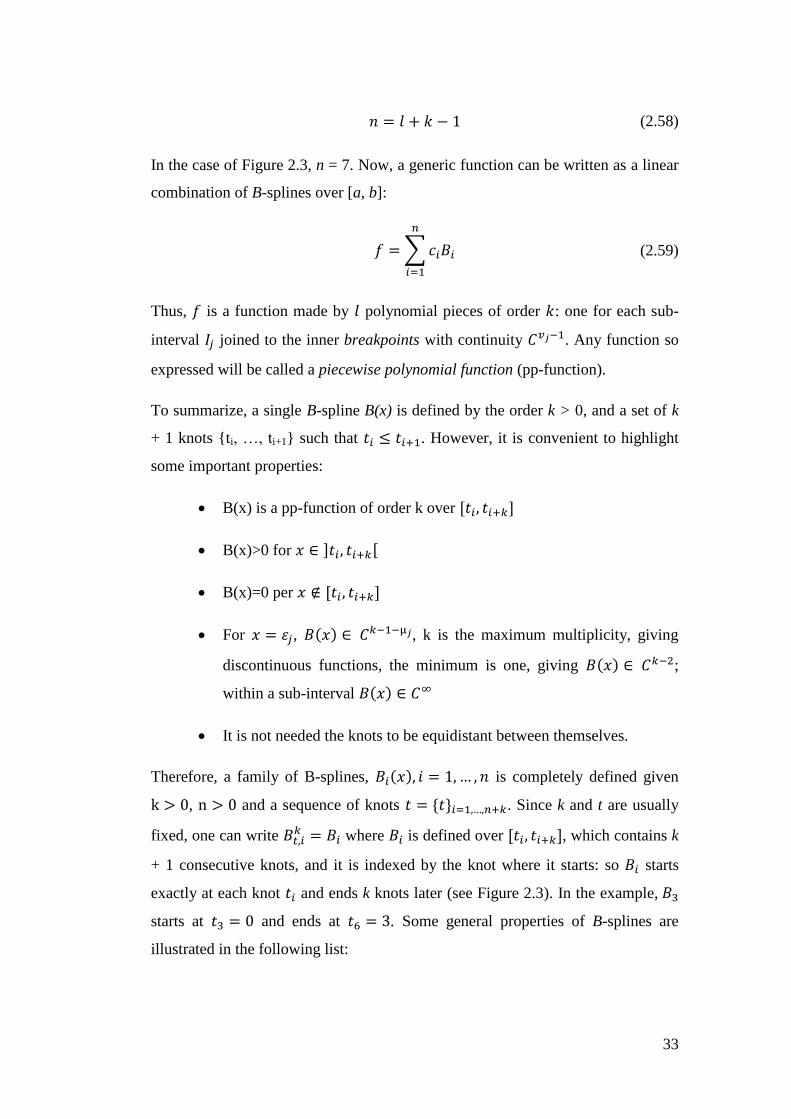
33
𝑛 = 𝑙 + 𝑘 − 1 (2.58)
In the case of Figure 2.3, n = 7. Now, a generic function can be written as a linear
combination of B-splines over [a, b]:
𝑓 =∑𝑐𝑖𝐵𝑖
𝑛
𝑖=1
(2.59)
Thus, 𝑓 is a function made by 𝑙 polynomial pieces of order 𝑘: one for each sub-
interval 𝐼𝑗 joined to the inner breakpoints with continuity 𝐶𝑣𝑗−1. Any function so
expressed will be called a piecewise polynomial function (pp-function).
To summarize, a single B-spline B(x) is defined by the order k > 0, and a set of k
+ 1 knots {ti, …, ti+1} such that 𝑡𝑖 ≤ 𝑡𝑖+1. However, it is convenient to highlight
some important properties:
B(x) is a pp-function of order k over [𝑡𝑖, 𝑡𝑖+𝑘]
B(x)>0 for 𝑥 ∈ ]𝑡𝑖 , 𝑡𝑖+𝑘[
B(x)=0 per 𝑥 ∉ [𝑡𝑖 , 𝑡𝑖+𝑘]
For 𝑥 = 휀𝑗, 𝐵(𝑥) ∈ 𝐶𝑘−1−µ𝑗, k is the maximum multiplicity, giving
discontinuous functions, the minimum is one, giving 𝐵(𝑥) ∈ 𝐶𝑘−2;
within a sub-interval 𝐵(𝑥) ∈ 𝐶∞
It is not needed the knots to be equidistant between themselves.
Therefore, a family of B-splines, 𝐵𝑖(𝑥), 𝑖 = 1,… , 𝑛 is completely defined given
k > 0, n > 0 and a sequence of knots 𝑡 = {𝑡}𝑖=1,…,𝑛+𝑘. Since k and t are usually
fixed, one can write 𝐵𝑡,𝑖𝑘 = 𝐵𝑖 where 𝐵𝑖 is defined over [𝑡𝑖 , 𝑡𝑖+𝑘], which contains k
+ 1 consecutive knots, and it is indexed by the knot where it starts: so 𝐵𝑖 starts
exactly at each knot 𝑡𝑖 and ends k knots later (see Figure 2.3). In the example, 𝐵3
starts at 𝑡3 = 0 and ends at 𝑡6 = 3. Some general properties of B-splines are
illustrated in the following list:
34
Into interval ]𝑡𝑖, 𝑡𝑖+𝑘[ there are exactly k nonzero B-splines
𝐵𝑗(𝑥) ≠ 0 𝑓𝑜𝑟 𝑗 = 𝑖 − 𝑘 + 1,… , 𝑖 (2.60)
𝐵𝑖(𝑥) ∙ 𝐵𝑗(𝑥) = 0 𝑓𝑜𝑟 |𝑖 − 𝑗| ≥ 𝑘 (2.61)
So, if |𝑖 − 𝑗| ≥ 𝑘:
∫ 𝐵𝑖(𝑥)𝐵𝑗(𝑥)𝑓(𝑥)𝑑𝑥 = 0𝑥𝑚𝑎𝑥
0
(2.62)
the expansion of an arbitrary function becomes:
𝑓(𝑥) = ∑𝑐𝑗𝐵𝑗(𝑥) = ∑ 𝑐𝑗𝐵𝑗(𝑥) 𝑓𝑜𝑟 𝑥 ∈ [𝑡𝑖 , 𝑡𝑖+𝑘]
𝑖
𝑗=𝑖−𝑘+1
𝑛
𝑗=1
(2.63)
B-splines are normalized so that:
∑𝐵𝑖(𝑥)𝑖
= 1 in [𝑡𝑘, 𝑡𝑛] (2.64)
They satisfy the recursion relation
𝐵𝑖𝑘(𝑥) =
𝑥 − 𝑡𝑖𝑡𝑖+𝑘−1 − 𝑡𝑖
𝐵𝑖𝑘−1(𝑥) −
𝑡𝑖+𝑘 − 𝑥
𝑡𝑖+𝑘 − 𝑡𝑖+1𝐵𝑖+1𝑘−1(𝑥) (2.65)
also giving an equation for the derivative:
𝐷𝐵𝑖
𝑘(𝑥) =𝑘 − 1
𝑡𝑖+𝑘−1 − 𝑡𝑖𝐵𝑖𝑘−1(𝑥) −
𝑘 − 1
𝑡𝑖+𝑘 − 𝑡𝑖+1𝐵𝑖+1𝑘−1(𝑥) (2.66)
A knot sequence has to be defined within a given interval; this has to be done to
ensure that the knots sequence suits the particular problem. This represents a
further important advantage of the use of B-splines. Because of the ease of
implementing boundary conditions at the endpoints, the standard choice 𝑡1 = ⋯ =
𝑡𝑘 = 휀1 and 𝑡𝑛+1 = ⋯ = 𝑡𝑛+𝑘 = 휀𝑙+1 is particularly convenient. For instance,
𝑓(𝑎) = 0 is satisfied by deleting 𝐵1 from the set (it is the only one that is
discontinuous in 𝑎), while 𝑓(𝑏) = 0 is satisfied by deleting the last B-spline. In
35
general, when analytic functions have to be approximated, the best choice is
employing splines of high-order, compatible with the numerical stability and
round off errors, typically in the range k = 7 – 10. Note that the error will be close
to:
휀~ℎ𝑗𝑘
𝑘!|𝐷𝑘𝑓(휂𝑗)| (2.67)
where ℎ𝑗 is the width of the interval 𝐼𝑗 and 휂𝑗 ∈ 𝐼𝑗 . This is the main advantage of
B-splines basis with respect to global basis, where the error can be controlled by
step size, in the same way as in the finite-difference approaches, but keeping all
the advantages of a basis set expansion.
2.4.2. Application of B-splines
From a computational point of view, value of the splines is given by an algorithm,
more precisely by a specific subroutine that implements the Formula 2.65. The
subroutine needs spline’s degree, knots sequence, abscissa value and left knot
index 𝑡𝑖 (that gives the index of 𝐵𝑖) as input data; it returns the values of k non
zero B-splines:
𝐵𝑖−𝑘+1(𝑥),… , 𝐵𝑖(𝑥) (2.68)
In case that also the derivatives are needed, these can be obtained by the
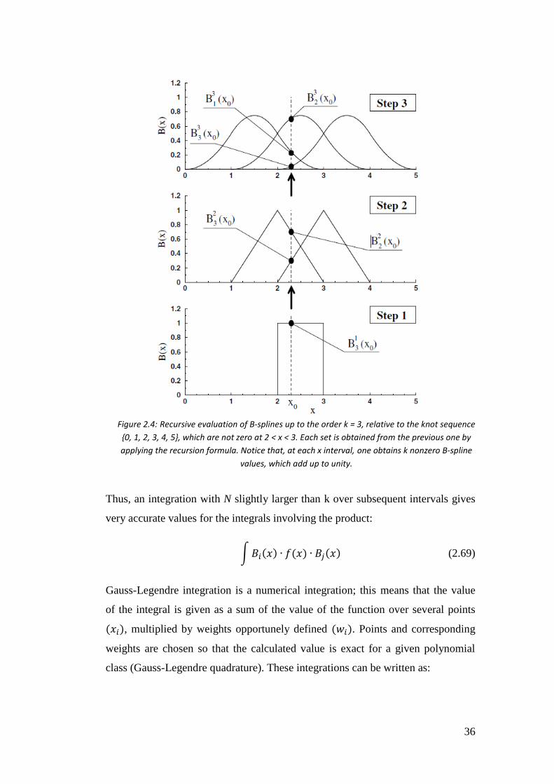
combination of B-splines of lower order through the Expression 2.66. Figure 2.4
shows how the subroutine works to generate the B-splines.
Gauss-Legendre integration [28] of suitable order over each interval is used to
compute integrals. Suitable order means order N (N points), it is exact for
polynomial of order 2N.
36
Thus, an integration with N slightly larger than k over subsequent intervals gives
very accurate values for the integrals involving the product:
∫𝐵𝑖(𝑥) ∙ 𝑓(𝑥) ∙ 𝐵𝑗(𝑥) (2.69)
Gauss-Legendre integration is a numerical integration; this means that the value
of the integral is given as a sum of the value of the function over several points
(𝑥𝑖), multiplied by weights opportunely defined (𝑤𝑖). Points and corresponding
weights are chosen so that the calculated value is exact for a given polynomial
class (Gauss-Legendre quadrature). These integrations can be written as:
Figure 2.4: Recursive evaluation of B-splines up to the order k = 3, relative to the knot sequence
{0, 1, 2, 3, 4, 5}, which are not zero at 2 < x < 3. Each set is obtained from the previous one by
applying the recursion formula. Notice that, at each x interval, one obtains k nonzero B-spline
values, which add up to unity.
37
∫ 𝑓(𝑥)𝑑𝑥 ≅∑𝑤𝑖𝑓(𝑥𝑖)
𝑁
𝑖=1
1
−1
(2.70)
To convert the integration interval from [-1, 1] to [a, b], a change of variables is
done:
𝑥 = [
𝑏 − 𝑎
2𝑡 +
𝑏 + 𝑎
2] (2.71)
∫ 𝑓(𝑥)𝑑𝑥 =
𝑏 − 𝑎
2∫ 𝑓 [
𝑏 − 𝑎
2𝑡 +
𝑏 + 𝑎
2] 𝑑𝑡
1
−1
𝑏
𝑎
≅𝑏 − 𝑎
2∑𝑤𝑖𝑓 [
𝑏 − 𝑎
2𝑡𝑖 +
𝑏 + 𝑎
2]
𝑁
𝑖=1
(2.72)
Thus, to calculate the exact integral value of an N order polynomial, one only has
to calculate the values of the functions at N/2 points. All the needed parameters
are calculated through the subroutine GAULEG [29]. By considering the B-
splines, the following integral has to be solved:
∫ 𝐵𝑖(𝑥)𝑓(𝑥)𝐵𝑗(𝑥)𝑑𝑥𝑏
𝑎
(2.73)
By assuming that the product 𝐵𝑖(𝑥) ∙ 𝐵𝑗(𝑥) is nonzero over k intervals, the
calculation of this product over each interval is easy:
∫ 𝐵𝑖(𝑥)𝑓(𝑥)𝐵𝑗(𝑥)𝑑𝑥𝑏
𝑎
=∑∫ 𝐵𝑖(𝑥)𝑓(𝑥)𝐵𝑗(𝑥)𝑑𝑥𝑥𝑚+1
𝑥𝑚𝑚
(2.74)
thereby only the intervals between adjacent knots are considered and the
discontinuity at knots is avoided.
38
2.4.3 Complex and real spherical harmonics
Using the following phase convention for the spherical harmonics
𝑌𝑙𝑚(휃, 𝜙) = (−)(𝑚+|𝑚|2
)√2𝑙 + 1
4𝜋 (𝑙 − |𝑚|)!
(𝑙 + |𝑚|)!𝑃𝑙|𝑚|(𝑐𝑜𝑠휃)𝑒𝑖𝑚𝜙. (2.75)
we define real spherical Harmonics (for |𝑚| > 0) in the following way:
𝑌𝑙|𝑚|𝑅 (휃, 𝜙) =
(−)|𝑚|𝑌𝑙|𝑚|(휃, 𝜙) + 𝑌𝑙−|𝑚|(휃, 𝜙)
√2 (2.76)
𝑌𝑙−|𝑚|𝑅 (휃, 𝜙) =
(−)|𝑚|𝑌𝑙|𝑚|(휃, 𝜙) − 𝑌𝑙−|𝑚|(휃, 𝜙)
𝑖√2
(2.77)
For 𝑚 = 0 we have 𝑌𝑙0𝑅(휃, 𝜙) = 𝑌𝑙0(휃, 𝜙). In general we have:
𝑌𝑙𝑚𝑅 = √
2𝑙 + 1
4𝜋 (𝑙 − |𝑚|)!
(𝑙 + |𝑚|)!𝑃𝑙|𝑚|(𝑐𝑜𝑠휃)
{
1
√𝜋𝑐𝑜𝑠 𝑚𝜙 𝑚 > 0
1
√2𝜋 𝑚 = 0
1
√𝜋𝑠𝑖𝑛 𝑚𝜙 𝑚 < 0
= Θ𝑙|𝑚|(휃)Φ𝑚(𝜙).
(2.78)
39
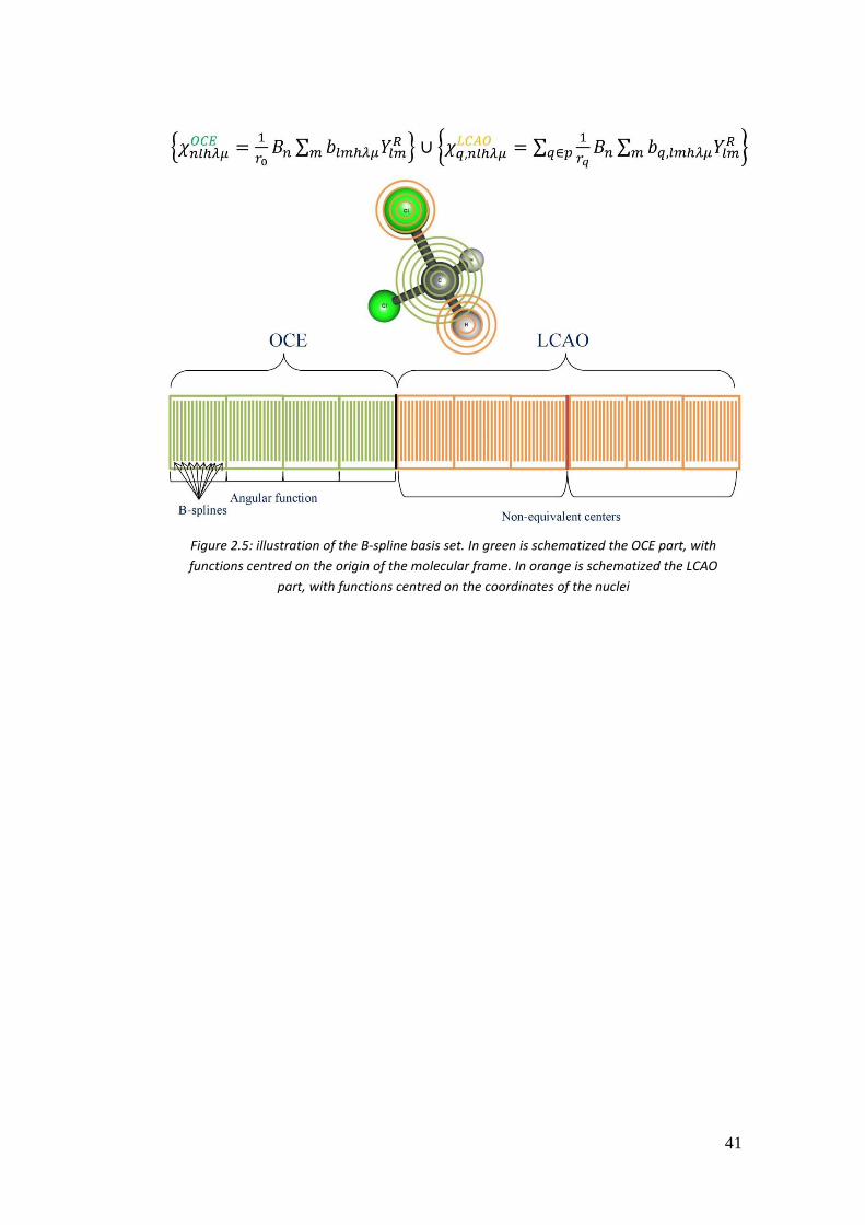
2.4.4. Construction of the LCAO basis set
As mentioned before, our method expands the wavefunction in a symmetry
adapted basis set composed by B-splines radial functions [27] and a linear
combination of real spherical harmonics. The whole basis set is made up of two
parts: the first one composed of functions centred on the origin of the molecular
frame, called One Centre Expansion (OCE); the second one characterized by
functions centred on the coordinates of the nuclei, called Linear Combination of
Atomic Orbitals (LCAO) since this basis has many centres. This multicentre
approach allows to dramatically improve the convergence of the calculation for
large molecules [15]. One of the advantages of using spherical B-spline functions
lies on the fact that their local nature allows not only to control the overlap
between functions but also to avoid numerical linear dependence problems [25],
which become unavoidable with global basis functions, such as STOs or GTOs
when enlarging the basis. Implementation of the LCAO basis set, in addition to
that one of the OCE, permits us to accurately treat both bound and continuum
states. From now on, the subscript 𝑂 indicates the OCE basis, whereas the
subscript 𝑞 indicates the basis relative to the non-equivalent centres considered.
The OCE basis is expressed as a product by B-splines radial functions and a
symmetry adapted linear combination of real spherical harmonics:
𝜒𝑛𝑙ℎ𝜆𝜇𝑂 (𝑟0, 휃0, 𝜙0) =
1
𝑟0𝐵𝑛(𝑟0)∑𝑏𝑙𝑚ℎ𝜆𝜇𝑌𝑙𝑚
𝑅 (휃0, 𝜙0)
𝑚
(2.79)
It is usually centred on the origin of the axes with large both radial (𝑅𝑚𝑎𝑥𝑂 ) and
angular grids (𝐿𝑚𝑎𝑥). This allows to describe the long range behaviour of the
continuum wavefunctions.
The LCAO part is expressed as a product of B-splines radial functions and a
symmetry adapted linear combination of real spherical harmonics as well. Each
LCAO subset, which refers to the 𝑝-th set of equivalent nuclei, can be written in
the form
40
𝜒𝑖𝑗𝜆𝜇𝑝 (𝒓) =∑휂𝑖𝑗𝜆𝜇
𝑞
𝑞∈𝑝
(2.80)
where
휂𝑖𝑗𝜆𝜇𝑞 =
1
𝑟𝑞𝐵𝑖(𝑟𝑞)∑𝑏𝑚𝑗𝜆𝜇,𝑞𝑌𝑙(𝑗)𝑚
𝑅 (휃𝑞 , 𝜙𝑞)
𝑚
(2.81)
and 𝑞 is any center of the equivalent set. Any molecular orbital, 𝜑𝑖𝜆𝜇(𝒓), is
expanded in this basis as follows:
𝜑𝑖𝜆𝜇(𝒓) =∑𝑐𝑖𝑗𝜆 𝜒𝑖𝑗𝜆𝜇𝑂 (𝒓)
𝑖𝑗⏟ 𝑂𝐶𝐸 𝑝𝑎𝑟𝑡
+∑𝑑𝑝𝑖𝑗𝜆,𝑘 𝜒𝑖𝑗𝜆𝜇𝑝 (𝒓)
𝑝𝑖𝑗⏟ 𝐿𝐶𝐴𝑂 𝑝𝑎𝑟𝑡
(2.82)
The LCAO basis just outlined above will be called symmetry-adapted, and it is
obtained (through the projection-operator method) by the symmetry adaptation of
the LCAO primitive basis
{휂𝑖𝑙𝑚 ≡
1
𝑟𝐵𝑖(𝑟)𝑌𝑙𝑚
𝑅 (휃, 𝜙)} ∪ {휂𝑖𝑙𝑚𝑞 ≡
1
𝑟𝑞𝐵𝑖(𝑟𝑞)𝑌𝑙𝑚
𝑅 (휃𝑞 , 𝜙𝑞)} (2.83)
centred on the 𝑞-th off-centre sphere. The LCAO radial grid is usually small
(𝑅𝑚𝑎𝑥𝑝 ≈ 1 𝑎. 𝑢. ) so as to avoid overlap with expansion performed on
neighbouring centres, and maintain good linear independence.
The complete basis set (illustrated in Figure 2.5) is completely defined by:
point group of the considered molecule.
OCE B-spline radial grid: 𝑅𝑚𝑎𝑥𝑂 , knots set, splines order (usually 10).
OCE maximum angular momentum 𝐿𝑚𝑎𝑥.
LCAO B-spline radial grid: 𝑅𝑚𝑎𝑥𝑝
, knots set, splines order (usually 10).
OCE maximum angular momentum 𝐿𝑚𝑎𝑥𝑝
.
41
Figure 2.5: illustration of the B-spline basis set. In green is schematized the OCE part, with
functions centred on the origin of the molecular frame. In orange is schematized the LCAO
part, with functions centred on the coordinates of the nuclei
42
2.5. Expression of the wavefunction: different
approximations
In order to obtain the cross section of the considered system, dipole transition
between initial and final states has to be computed (see Equation 2.5). To do this,
one has to accurately express both the wavefunctions of the initial and final states.
Calculating the wavefunctions relative to the initial state is not a complicated
issue, whereas the calculation of the wavefunction associated to the final state is a
really complex task. In this work, wavefunction of the final state is expressed
through some approximations that will be discussed later. Each approximation is
able to treat different properties. One of the main features of the photoionization
processes that we want to study is represented by the correlation effects and by the
perturbative and non-perturbative nature of the photoionization.
2.5.1. Correlation effects
The main problem to solve the Schrödinger Equation (SE) with a complete
Hamiltonian operator consists in describing the interaction between different
electrons given by the Coulomb potential, which makes the problem not
separable. Several approximations can be applied; among these, the most common
is the mean-field approximation where the considered particle is affected by the
mean field created by the other particles. Correlation effects are all the effects not
included in this approximation.
The mean-field approximation provides a first solution of the ionic states obtained
by photoionization process. One-particle method applied on a closed shell atom
furnishes an univocal correspondence between one orbital and a definite line of
the photoelectron spectrum. By taking into account a molecule, there are
rotational and vibrational excitations that provides more complex bands. Thus,
peaks in the PE spectra are associated to definite ionic states which, within this
approximation, can only be described by single hole configurations (1h) in the
case of a closed shell ground state.

43
By taking into account correlation between electrons, it is possible to describe
other peaks in a photoelectron spectrum. Additional peaks can also be due to the
relaxation effects, which derive from the modification of the orbitals caused by
the creation of a hole. These extra structures are called shake-up or satellite bands
and, in photoionization, are related to excitation during the ionization process. The
bands relative to these processes usually present lower intensities with respect to
the one relative to single photoionization. The experimental evidence of these
structures has been named as the breakdown of the independent-particle picture of
electronic structure [30].
From the theoretical point of view, these observed extra peaks are related to the
strong interaction between single-hole configurations and two-hole, one-particle
configurations. In addition to this, a redistribution of the intensity between states
of the same symmetry can be observed even for peaks relative to the main primary
ionization. This makes it really important to include the correlation effects in a
theoretical description.
There are three kind of correlation effects in photoionization processes [31]. One
describes correlation in bound initial state, called ISCI (initial state configuration
interaction) and refers to 𝑁 electrons. The other one is related to the correlation
within bound final states, called FISCI (final ionic state configuration interaction)
and refers to 𝑁 − 1 electrons. The third one is more complicated to be described
since it includes two classes of interaction in the continuum: correlation between
two continuum states (interchannel coupling, IC) and correlation between a
continuum state and a discrete state (autoionization resonances, also resonant
Auger). The interaction within bound states is responsible for most of the extra
structures that one can find in a PE spectrum; it can be described by several
methods, such as Configuration Interaction (CI), Perturbation Theory (PT) and
Green’s function (GF) [32].
44
2.5.2. General expression of the wavefunction
As already mentioned, in photoionization processes the final state can lie in
several possible states 𝛹𝐼, called open channels:
𝐼𝑃𝐼 = 𝐸𝐼𝑁−1 − 𝐸0
𝑁 < ℎ𝜈 (2.84)
Therefore, the final system is composed by an ionic bound state of 𝑁 − 1 particles
and a continuum state of one particle. Continuum eigenstates have to be the
solution of the following Schrödinger equation:
𝐻𝑁𝛹𝐸𝛼𝑁 = 𝐸𝛹𝐸𝛼
𝑁 (2.85)
where 𝛼 ≡ 𝐼𝑙𝑚 considers all the indeces that uniquely describe the wavefunction
(neglecting the symmetry of the system), which can be formally expressed using
the Close-Coupling form
𝛹𝐸𝛼𝑁 =∑𝛹𝐼′
𝑁−1
𝛼′
𝜑𝐸𝛼′𝛼 +∑𝛹𝐾𝑁𝐶𝐸𝛼𝐾
𝐾
(2.86)
The first part of this equation is, for each angular momentum and open channel,
the (antisymmetrized) product between the bound states of the ionic state 𝛹𝐼′𝑁−1
and the continuum state of the photoelectron with the proper boundary conditions
𝜑𝐸𝛼′𝛼 (Equation 2.20). This part accurately describes the function at long range
for all the considered open channels 𝐼′.
𝛹𝐸𝛼𝑁
𝑟→∞→ ∑𝛹𝐼′
𝑁−1
𝐼′
𝜑𝐸𝛼𝐼′ (2.87)
The second part of Equation (2.86) describes all the effects that are not taken into
account by the first sum. In particular, it involves the effects that are degenerate
with the ionization, such as correlation effect in the bound states. These effects are
expanded in terms of the bound state function 𝛹𝐾𝑁 that decays at long range.
45
∑𝛹𝐾𝑁𝐶𝐸𝛼𝐾
𝐾𝑟→∞→ 0 (2.88)
The expansion above is square integrable and it is analogous to the expansion
used in the Configuration Interaction (CI) method. In fact, functions 𝛹𝐾𝑁 can be
obtained through the common Quantum Chemistry approaches.
Close Coupling wavefunction ensures the asymptotic condition and, in principle,
it is correct if the second sum goes to infinity. Computationally speaking, since
this condition is impossible to be implemented, a truncation of the sum is needed.
Implementing the fully Close Coupling form is a demanding task. In fact, two-
electron integrals are needed to build each part of the equation (2.86). One can
apply some approximations for avoiding the calculation of two-electron integrals.
Although these approximations properly work and are able to describe the major
part of the observables, implementation of the two-electron integrals is of great
interest. This implementation allows the complete expansion of the wavefunction
through Equation (2.86), permitting us to fully describe the photoionization
process.
2.5.3. Single particle approximation
The simplest approximation is to consider only one open channel, so that the
Equation (2.86) becomes the antisymmetrized product between the wavefunctions
related to the final ionic state relative to open channel 𝐼 and that one describing
the photoelectron in the continuum state with energy 휀:
𝛹𝐸𝐼𝐿𝑁 = 𝐴𝛹𝐼
𝑁−1𝜑𝜀𝐼𝐿 (2.89)
where the continuum wavefunction satisfies the K-matrix boundary conditions.
Within this approximation, the initial state is defined as a single Slater
determinant:
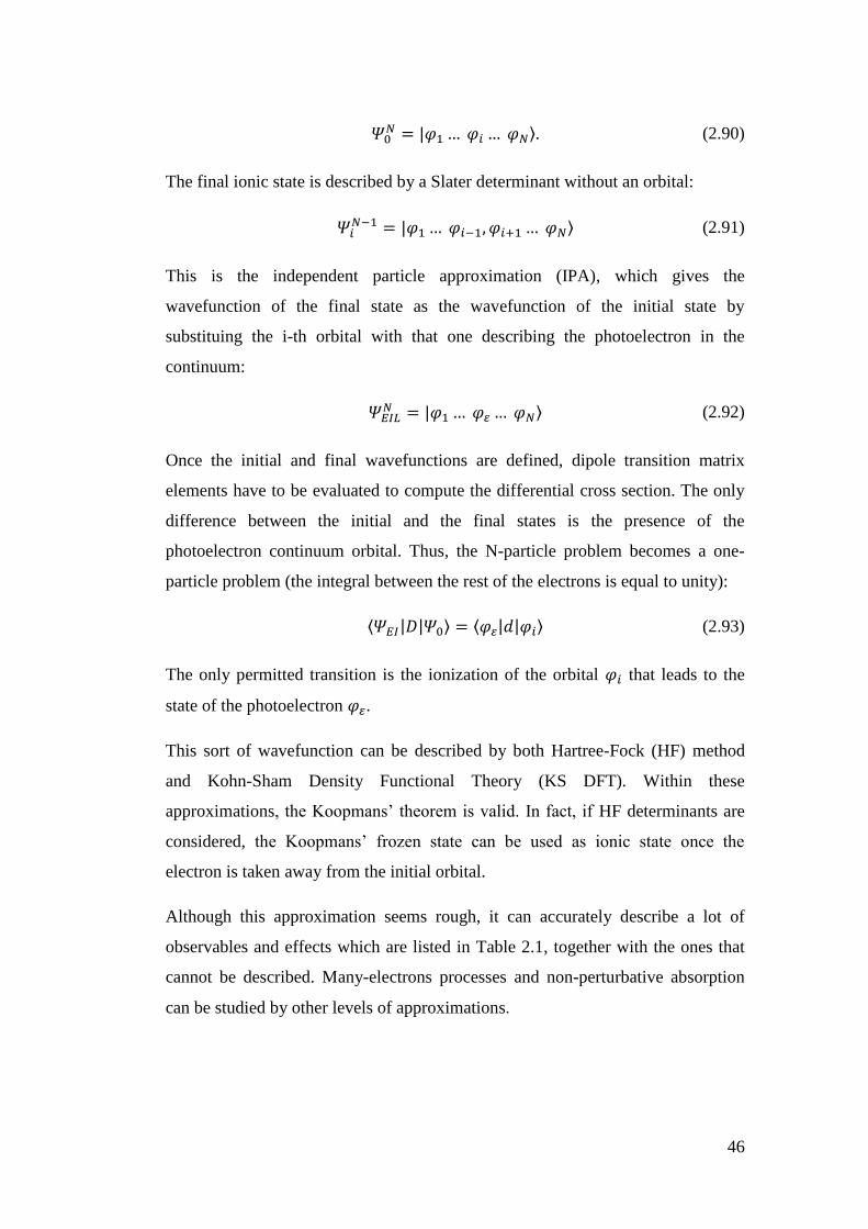
46
𝛹0𝑁 = |𝜑1… 𝜑𝑖 … 𝜑𝑁⟩. (2.90)
The final ionic state is described by a Slater determinant without an orbital:
𝛹𝑖𝑁−1 = |𝜑1… 𝜑𝑖−1, 𝜑𝑖+1… 𝜑𝑁⟩ (2.91)
This is the independent particle approximation (IPA), which gives the
wavefunction of the final state as the wavefunction of the initial state by
substituing the i-th orbital with that one describing the photoelectron in the
continuum:
𝛹𝐸𝐼𝐿𝑁 = |𝜑1… 𝜑𝜀… 𝜑𝑁⟩ (2.92)
Once the initial and final wavefunctions are defined, dipole transition matrix
elements have to be evaluated to compute the differential cross section. The only
difference between the initial and the final states is the presence of the
photoelectron continuum orbital. Thus, the N-particle problem becomes a one-
particle problem (the integral between the rest of the electrons is equal to unity):
⟨𝛹𝐸𝐼|𝐷|𝛹0⟩ = ⟨𝜑𝜀|𝑑|𝜑𝑖⟩ (2.93)
The only permitted transition is the ionization of the orbital 𝜑𝑖 that leads to the
state of the photoelectron 𝜑𝜀.
This sort of wavefunction can be described by both Hartree-Fock (HF) method
and Kohn-Sham Density Functional Theory (KS DFT). Within these
approximations, the Koopmans’ theorem is valid. In fact, if HF determinants are
considered, the Koopmans’ frozen state can be used as ionic state once the
electron is taken away from the initial orbital.
Although this approximation seems rough, it can accurately describe a lot of
observables and effects which are listed in Table 2.1, together with the ones that
cannot be described. Many-electrons processes and non-perturbative absorption
can be studied by other levels of approximations.
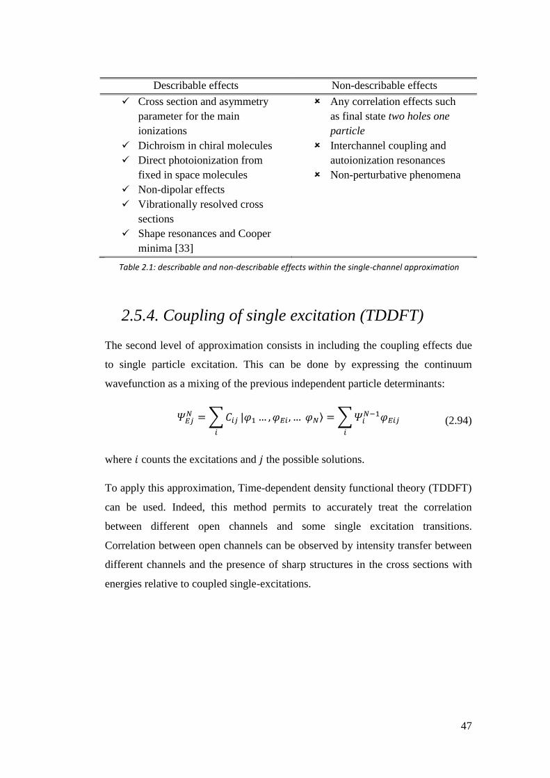
47
Describable effects Non-describable effects
Cross section and asymmetry
parameter for the main
ionizations
Dichroism in chiral molecules
Direct photoionization from
fixed in space molecules
Non-dipolar effects
Vibrationally resolved cross
sections
Shape resonances and Cooper
minima [33]
Any correlation effects such
as final state two holes one
particle
Interchannel coupling and
autoionization resonances
Non-perturbative phenomena
2.5.4. Coupling of single excitation (TDDFT)
The second level of approximation consists in including the coupling effects due
to single particle excitation. This can be done by expressing the continuum
wavefunction as a mixing of the previous independent particle determinants:
𝛹𝐸𝑗𝑁 =∑𝐶𝑖𝑗
𝑖
|𝜑1… ,𝜑𝐸𝑖 , … 𝜑𝑁⟩ =∑𝛹𝑖𝑁−1𝜑𝐸𝑖𝑗
𝑖
(2.94)
where 𝑖 counts the excitations and 𝑗 the possible solutions.
To apply this approximation, Time-dependent density functional theory (TDDFT)
can be used. Indeed, this method permits to accurately treat the correlation
between different open channels and some single excitation transitions.
Correlation between open channels can be observed by intensity transfer between
different channels and the presence of sharp structures in the cross sections with
energies relative to coupled single-excitations.
Table 2.1: describable and non-describable effects within the single-channel approximation
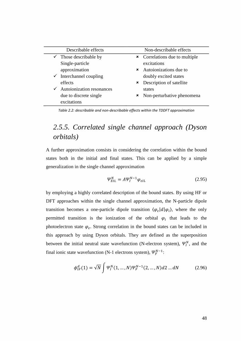
48
Describable effects Non-describable effects
Those describable by
Single-particle
approximation
Interchannel coupling
effects
Autoionization resonances
due to discrete single
excitations
Correlations due to multiple
excitations
Autoionizations due to
doubly excited states
Description of satellite
states
Non-perturbative phenomena
2.5.5. Correlated single channel approach (Dyson
orbitals)
A further approximation consists in considering the correlation within the bound
states both in the initial and final states. This can be applied by a simple
generalization in the single channel approximation
𝛹𝐸𝐼𝐿𝑁 = 𝐴𝛹𝐼
𝑁−1𝜑𝜀𝐼𝐿 (2.95)
by employing a highly correlated description of the bound states. By using HF or
DFT approaches within the single channel approximation, the N-particle dipole
transition becomes a one-particle dipole transition ⟨𝜑𝜀|𝑑|𝜑𝑖⟩, where the only
permitted transition is the ionization of the orbital 𝜑𝑖 that leads to the
photoelectron state 𝜑𝜀. Strong correlation in the bound states can be included in
this approach by using Dyson orbitals. They are defined as the superposition
between the initial neutral state wavefunction (N-electron system), 𝛹𝐼𝑁, and the
final ionic state wavefunction (N-1 electrons system), 𝛹𝐹𝑁−1:
𝜙𝐼𝐹𝑑 (1) = √𝑁∫𝛹𝐼
𝑁(1, … ,𝑁)𝛹𝐹𝑁−1(2,… ,𝑁)𝑑2…𝑑𝑁 (2.96)
Table 2.2: describable and non-describable effects within the TDDFT approximation
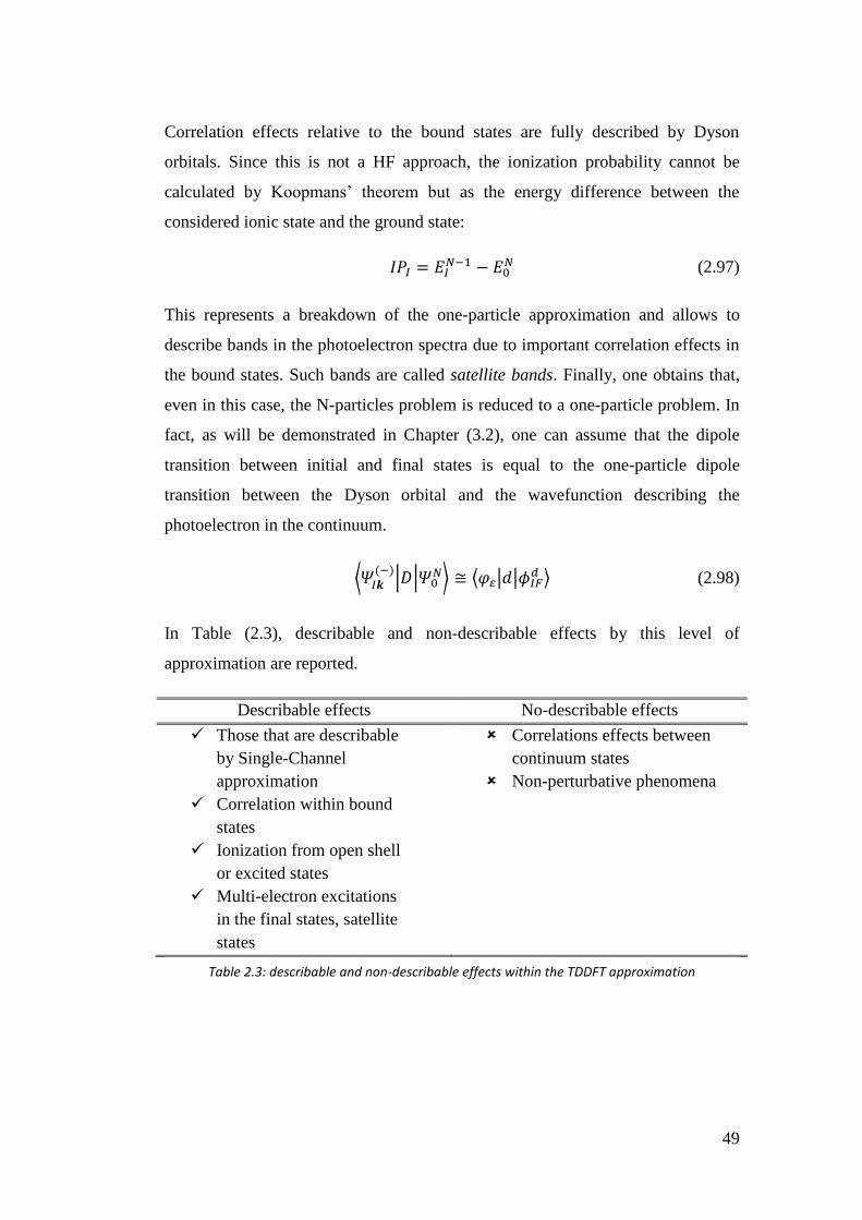
49
Correlation effects relative to the bound states are fully described by Dyson
orbitals. Since this is not a HF approach, the ionization probability cannot be
calculated by Koopmans’ theorem but as the energy difference between the
considered ionic state and the ground state:
𝐼𝑃𝐼 = 𝐸𝐼𝑁−1 − 𝐸0
𝑁 (2.97)
This represents a breakdown of the one-particle approximation and allows to
describe bands in the photoelectron spectra due to important correlation effects in
the bound states. Such bands are called satellite bands. Finally, one obtains that,
even in this case, the N-particles problem is reduced to a one-particle problem. In
fact, as will be demonstrated in Chapter (3.2), one can assume that the dipole
transition between initial and final states is equal to the one-particle dipole
transition between the Dyson orbital and the wavefunction describing the
photoelectron in the continuum.
⟨𝛹𝐼𝒌(−)|𝐷|𝛹0
𝑁⟩ ≅ ⟨𝜑𝜀|𝑑|𝜙𝐼𝐹𝑑 ⟩ (2.98)
In Table (2.3), describable and non-describable effects by this level of
approximation are reported.
Describable effects No-describable effects
Those that are describable
by Single-Channel
approximation
Correlation within bound
states
Ionization from open shell
or excited states
Multi-electron excitations
in the final states, satellite
states
Correlations effects between
continuum states
Non-perturbative phenomena
Table 2.3: describable and non-describable effects within the TDDFT approximation
50
2.5.6. Complete Close-Coupling wavefunction
(Two-electron integrals in the B-spline basis)
The previous methods drastically approximate the Close Coupling wavefunction;
in fact, they do not consider the second sum of Equation (2.86). Furthermore, the
continuum wavefunction is calculated by a one-particle DFT approach and then it
is added to the N-1 particles (calculated with ab-inito method). These
approximations are really distant from the complete expansion in the Close
Coupling form, and they are not able to describe all the correlation effects, as
those ones involving also continuum states. In case one wants to treat all the
correlation effects, one has to expand the solution in CC form. In order to do this,
two-electron integrals are needed to be computed. In fact, the complete ab-initio
Hamiltonian includes two-electron operator:
𝐻𝛹 = 𝐸𝛹 (2.99)
𝐻 = ∑ℎ(𝑖)
𝑖
+ ∑ 1
𝑟𝑖𝑗𝑖<𝑗
(2.100)
and matrix elements between basis functions:
⟨𝜒𝜇𝜒𝜈|𝑟𝑖𝑗−1|𝜒𝜌𝜒𝜎⟩ (2.101)
are required to compute the full N-particle matrix elements of the Hamiltonian.
The method used to solve these integrals is illustrated in details in Chapter 4.
Although implementing two-electron integrals is a demanding task, it permits to
completely build all the coefficients and matrices necessary to build the CC
wavefunction. In principle this allows the description of all the correlation effects
both in the bound and continuum states, and all couplings.
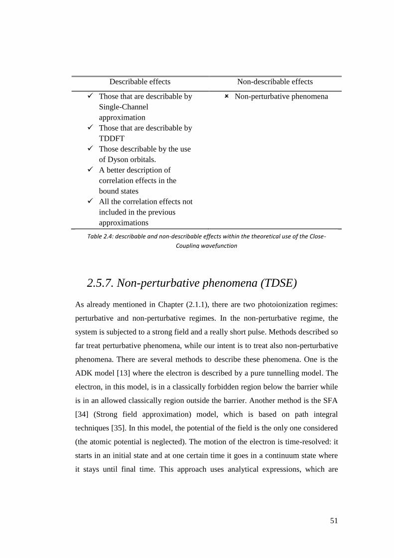
51
Describable effects Non-describable effects
Those that are describable by
Single-Channel
approximation
Those that are describable by
TDDFT
Those describable by the use
of Dyson orbitals.
A better description of
correlation effects in the
bound states
All the correlation effects not
included in the previous
approximations
Non-perturbative phenomena
2.5.7. Non-perturbative phenomena (TDSE)
As already mentioned in Chapter (2.1.1), there are two photoionization regimes:
perturbative and non-perturbative regimes. In the non-perturbative regime, the
system is subjected to a strong field and a really short pulse. Methods described so
far treat perturbative phenomena, while our intent is to treat also non-perturbative
phenomena. There are several methods to describe these phenomena. One is the
ADK model [13] where the electron is described by a pure tunnelling model. The
electron, in this model, is in a classically forbidden region below the barrier while
is in an allowed classically region outside the barrier. Another method is the SFA
[34] (Strong field approximation) model, which is based on path integral
techniques [35]. In this model, the potential of the field is the only one considered
(the atomic potential is neglected). The motion of the electron is time-resolved: it
starts in an initial state and at one certain time it goes in a continuum state where
it stays until final time. This approach uses analytical expressions, which are
Table 2.4: describable and non-describable effects within the theoretical use of the Close-
Coupling wavefunction

52
obtained applying several approximation that limits its applicability. Although it
is commonly employed to describe current experiments with success.
One of the best method to describe non-perturbative multiphoton ionization is the
numerical solution of the time-dependent Schrödinger equation (TDSE) as will be
discussed in Chapter 5. This requires a discretization capable to describe a large
part of the spectrum of the Hamiltonian, up to rather high energies and angular
momenta. For large systems, several approximations are needed to limit the
computational cost, but a wide range of continuum state is necessary to furnish
good results. Another really important parameter is the length grid because a too
short grid can provide artificial reflection of the emitted electron. Long enough
grids often lead huge computational costs, which are, in some case, unsustainable.
For this reason one can implement a complex absorbing potential (CAP) [36]
which has the task to absorb the electron at the end of the grid.
As will be illustrated in Chapter 5, although the solution of the time-dependent
Schrödinger equation allows to describe also the perturbative region, it is an
expensive computational method to be used for this purpose. We have
implemented TDSE in the spectral basis given by the full spectrum of the Khon-
Sham Hamiltonian obtained from the B-spline basis.
Since this method uses DFT, it is not able to treat any correlation effects.
Describable effects Non-describable effects
Those that are describable by
Single-Channel
approximation
Perturbative regime
Non-perturbative regime
Any Correlation effects
Table 2.5: describable and non-describable effects within the TDSE approximation
53
2.6. DFT calculation
Using Density Functional Theory (DFT) in many-body problems provides an
enormous simplification because the basic variational object is represented by the
electron density instead of a many-particle wavefunction. Indeed, the many-body
wavefunction is a very complex function in a 3N-dimensional space, on the
contrary the density is a simple function that depends solely on 3 variables, x, y
and z.
The many-body Hamiltonian operator within the Born-Oppenheimer
approximation [37] is given by:
�̂� = �̂� + �̂� + �̂� = [−1
2∑∇𝑖
2
𝑖
+∑𝑉𝑖(𝒓𝑖)
𝑖
+1
2∑𝑈(𝒓𝑖𝒓𝑗)
𝑖<𝑗
] (2.102)
where �̂� , �̂� and �̂� are, respectively, the kinetic energy, the external potential, i.e.
the attraction potential created by the nuclei, and the electron-electron interaction
operators. The solution of this 3N-dimensional differential equation is
complicated by the presence of the interelectronic potential in the Hamiltonian.
The expectation value of the energy can be reformulate as function of the electron
density 𝜌(𝒓):
𝐸 = ⟨𝛹|�̂�|𝛹⟩ = ⟨𝛹|�̂� + �̂� + �̂�|𝛹⟩
= −1
2∫𝑑𝒓𝑑𝒓′∇2𝜌(𝒓, 𝒓′) + ∫𝑑𝒓𝑣(𝒓)𝜌(𝒓)
+∬𝑑𝒓1𝑑𝒓2𝜌(𝒓1, 𝒓2)
𝑟12
(2.103)
where
𝜌(𝒓, 𝒓′) = 𝑁∫𝑑𝒓2…𝑑𝒓𝑁𝛹
∗(𝒓,… , 𝒓𝑁)𝛹(𝒓′,… , 𝒓𝑁) (2.104)
is the reduced one-particle density matrix, and the density is
54
𝜌(𝒓) = 𝜌(𝒓, 𝒓) (2.105)
and 𝜌(𝒓1, 𝒓2) is the two-particle density function given by
𝜌(𝒓1, 𝒓2) = 𝑁(𝑁 − 1)∫𝑑𝒓3…𝑑𝒓𝑁𝛹
∗(𝒓1, … , 𝒓𝑁)𝛹(𝒓1, … , 𝒓𝑁) (2.106)
Let us introduce a pair correlation function ℎ𝑥𝑐(𝒓1, 𝒓2) that includes non-classical
effects. The expectation value of �̂� then becomes:
⟨𝛹|�̂�|𝛹⟩ = 𝐽[𝜌] +
1
2∬𝑑𝒓1𝑑𝒓2𝜌(𝒓1)𝜌(𝒓2)
ℎ𝑥𝑐(𝒓1, 𝒓2)
𝑟12
= 𝐽[𝜌] +1
2∫𝑑𝒓1𝜌(𝒓1)𝑣𝑥𝑐(𝒓1)
(2.107)
where 𝐽[𝜌] is the classical Coulombian selfinteraction of a charge distribution and
𝑣𝑥𝑐(𝒓1) is a local potential that takes into account correlation and exchange
effects, defined as
𝑣𝑥𝑐(𝒓1) = ∫𝑑𝒓2𝜌(𝒓𝟐)
ℎ𝑥𝑐(𝒓1, 𝒓2)
𝑟12 (2.108)
The foundation for the use of DFT methods in computational chemistry is the
introduction of orbitals as suggested by Kohn and Sham. They made use of a
fictitious non-interacting system where its ground-state density was exactly the
same as that of some interacting system of interest.
The ground-state wavefunction associated with this non-interacting system can be
represented with a single Slater determinant of orthonormal orbitals, 𝜓𝑖. Thus, the
expression of the electronic density becomes
𝜌(𝒓) =∑|𝜓𝑖(𝒓)|2
𝑖
(2.109)
Separating the kinetic energy contribution as
55
𝑇 = −
1
2∑∫𝑑𝒓𝜓𝑖
∗(𝒓)∇2𝜓𝑖(𝒓)
𝑖
+ 𝑇𝑋𝐶(𝜌) (2.110)
and including the XC contribution to the kinetic energy in the 𝑣𝑋𝐶 potential,
finally, one obtains the Khon-Sham differential equation [38]:
−1
2𝛻2𝜓𝑖 + 𝑣𝐾𝑆𝜓𝑖 = 휀𝑖𝜓𝑖 (2.111)
where 𝑣𝐾𝑆 is given by:
𝑣𝐾𝑆 = 𝑣𝑒𝑥𝑡 + 𝑣𝑒𝑒 + 𝑣𝑥𝑐 (2.112)
The accuracy of DFT is determined by the accuracy of the description of 𝑣𝑥𝑐(𝒓1).
In order to implement the Kohn-Sham approach the exchange-correlation
functional must to be approximated. There exist different classes of functionals,
depending on the kind of the approximation. The two most important classes of
these functionals are LDA (Local Density approximantion) and GGA
(Generalized Gradient Approximation). The first one is based on the assumption
that the exchange-correlation potential depends only on the value of the charge
density at the same point. The second one includes the dependence also on
gradients of the density.
56
2.6.1. Computational detail
Let us introduce a typical DFT calculation based on B-spline functions associated
to a particularly simple least-squares formulation for the determination of
eigenvectors in the continuum spectrum. The computational procedure is made by
three steps:
I. Calculation of the ground state DFT electron energy with ADF program
[39]
II. Construction of the Hamiltonian matrix and its diagonalization in the
OCE-LCAO B-splines basis set. Bound states and continuum states are
obtained in this step.
III. Calculation of the dipole transition moment. This provides photoionization
cross sections, asymmetry parameters and further observables.
2.6.2. Initial guess
Calculation of the molecular ground state electron density represents the starting
point of the present method. There are several quantum chemistry programs able
to compute electronic density. Among these, we use ADF (Amsterdam Density
Functional [39]). For all the calculations in this work, a DZP (double zeta plus
polarization) basis set and a LB94 or LDA functional have been chosen. The
program expands the ground state Kohn-Sham atomic orbitals in terms of Slater-
type Orbitals (STOs):
𝜙𝑛𝑙𝑚𝜁𝑆𝑇𝑂 (𝒓) = 𝑅𝑛𝜁
𝑆𝑇𝑂(𝑟)𝑌𝑙𝑚(휃, 𝜙) (2.113)
where 𝑌𝑙𝑚𝑆𝑇𝑂(휃, 𝜙) are the spherical harmonics. The radial part is expressed as
follows:
𝑅𝑛𝜁𝑆𝑇𝑂(𝑟) = 𝑁𝑟𝑛−1𝑒−𝜁𝑟 (2.114)
where 𝑛 indicates the principal quantum number, 𝑙 and 𝑚 define the angular
momentum and 휁 is the nuclear effective charge.
57
Thus, Kohn-Sham molecular orbitals can be expressed as a linear combination of
atomic orbitals:
𝜑𝑖(𝒓) = ∑ ∑𝑎𝑗,𝑛𝑙𝑚𝜙𝑗,𝑛𝑙𝑚𝜁𝑆𝑇𝑂 (𝒓𝑗)
𝑛𝑙𝑚
𝑁 𝑎𝑡𝑜𝑚𝑠
𝑗
(2.115)
Obtained by the usual SCF algorithm. This permits to compute the ground state
electron density 𝜌0(𝒓) that will used to to construct the Hamiltonian matrix.
𝜌0(𝒓) = ∑ 𝜑𝑖∗(𝒓)𝜑𝑖(𝒓)
𝑜𝑟𝑏𝑖𝑡𝑎𝑙𝑠
𝑖
(2.116)
2.6.3. Construction of the Hamiltonian matrix and
its diagonalization
The ADF program furnishes us the electron density of the ground state that can be
used to obtain the one-electron orbitals in the B-spline basis through the Kohn-
Sham equation:
𝐻𝐾𝑆𝜑𝑖 = 휀𝑖𝜑𝑖 𝑖 = 1,… , 𝑛 (2.117)
where the Hamiltonian is defined as:
𝐻𝐾𝑆 = −
1
2∇2 −∑
𝑍𝑁|𝑟 − 𝑅𝑁|
𝑁
+∫𝜌0(𝒓
′)𝑑𝒓′
|𝒓 − 𝒓′|+ 𝑉𝑋𝐶[𝜌0(𝒓)] (2.118)
This Hamiltonian can be divided in four terms. First term (kinetic energy) and
second term (Coulomb attraction) are easily implemented in the algorithm.
Third term represents the classical electrostatic Hartree potential 𝑉𝐻. It uses the
electron density obtained by ADF and is obtained, expressed in the same B-spline
basis, by the solution of the Poisson equation:
58
∇2𝑉𝐻 = −4𝜋𝜌0(𝒓) (2.119)
Finally, fourth term is the exchange-correlation potential that can be chosen
according to the considered system. LB94 and LDA(VWN) functionals usually
produce accurate photoelectron spectra [40].
The Hamiltonian matrix has to be built by the expansion in the OCE-LCAO basis
set. Thus, each matrix element can be expressed as:
𝑯𝑖𝑗𝑚𝑛ℎℎ′𝑙𝑙′𝜆 = ∫𝐵𝑚
𝑖 (𝑟𝑖)𝑋𝑙ℎ𝜆𝜇𝑖 (휃𝑖, 𝜙𝑖)ℎ̂𝐾𝑆𝐵𝑚
𝑗(𝑟𝑗)𝑋𝑙ℎ𝜆𝜇
𝑗(휃𝑗, 𝜙𝑗) (2.120)
As already mentioned, this represents a symmetry adapted Hamiltonian. Thus, the
Hamiltonian is block-diagonal in each quantum number 𝜆 and it is independent of
𝜇. Within this DFT approximation, the problem is reduced to a one-particle
problem controlled by the one-particle Hamiltonian ℎ̂𝐾𝑆. The superscripts 𝑖 and 𝑗
define the nature of the OCE-LCAO basis set: “𝑂” indicates the OCE part and
𝑗 ∈ 𝑄𝑖 indicates the specific non-equivalent shell (see Chapter 2.4.4). Therefore,
the Hamiltonian matrix presents three kind of non-zero integrals: those combining
two OCE functions 𝑯00, those combining one OCE function with a LCAO
function 𝑯0𝑖, and, finally, those combining LCAO functions of the same set 𝑯𝑖𝑖.
Overlap between functions of different LCAO set is avoided, so that 𝑯𝑖𝑗 = 0. In
light of this, let us define the Hamiltonian matrix as follows:
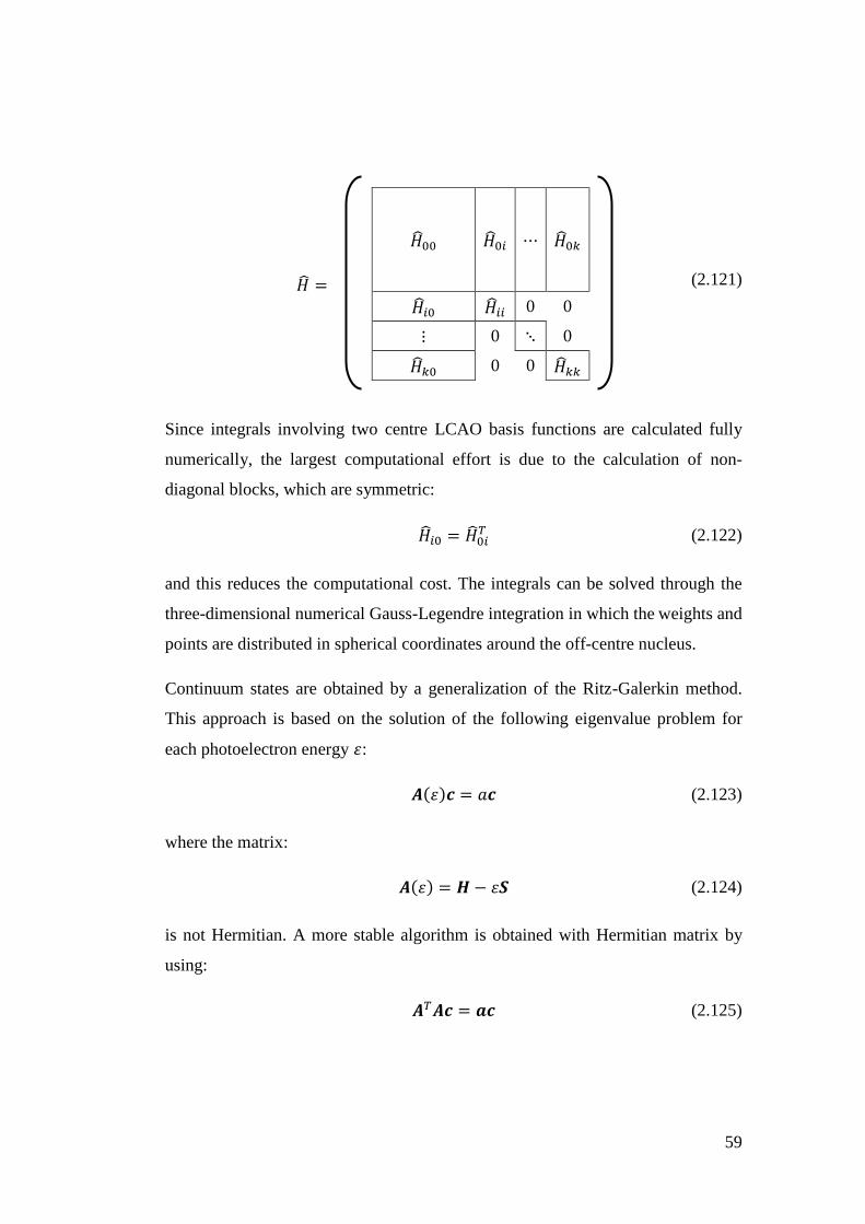
59
�̂� =
�̂�00 �̂�0𝑖 ⋯ �̂�0𝑘
�̂�𝑖0 �̂�𝑖𝑖 0 0
⋮ 0 ⋱ 0
�̂�𝑘0 0 0 �̂�𝑘𝑘
(2.121)
Since integrals involving two centre LCAO basis functions are calculated fully
numerically, the largest computational effort is due to the calculation of non-
diagonal blocks, which are symmetric:
�̂�𝑖0 = �̂�0𝑖𝑇 (2.122)
and this reduces the computational cost. The integrals can be solved through the
three-dimensional numerical Gauss-Legendre integration in which the weights and
points are distributed in spherical coordinates around the off-centre nucleus.
Continuum states are obtained by a generalization of the Ritz-Galerkin method.
This approach is based on the solution of the following eigenvalue problem for
each photoelectron energy 휀:
𝑨(휀)𝒄 = 𝑎𝒄 (2.123)
where the matrix:
𝑨(휀) = 𝑯 − 휀𝑺 (2.124)
is not Hermitian. A more stable algorithm is obtained with Hermitian matrix by
using:
𝑨𝑇𝑨𝒄 = 𝒂𝒄 (2.125)

60
Since the eigenvalues, very close to zero, relative to the full set of continuum
eigenvectors, are very well separated from the rest, the solution can be easily
obtained by block inverse iteration [41]. The eigenvectors so obtained constitute a
complete and independent set of stationary solutions. From these states, one can
build continuum states that are normalized and which satisfy suitable boundary
conditions.
Bound and continuum states are obtained by diagonalizing the fixed Kohn-Sham
Hamiltonian matrix. This method is called static-exchange DFT.
From the computational point of view, a dense knot grid around the nuclei is
needed to accurately obtain both bound and continuum states. A detailed basis is
needed to accurately describe both kind of states (continuum and bounds). A big
box size is really important because provide better results both on high bound
states and on the variation of the continuum states. The latter requires a larger
box. A dense knot grid is also required far from the origin to describe higher
continuum state. This is due to the asymptotic period of the radial oscillations of
the continuum wavefunctions.
In comparison with the typical AO basis employed in bound state calculations, the
OCE-LCAO basis set is much bigger. This allows an accurate description of the
continuum states, and a complete representation of the spectrum of the
Hamiltonian within the spherical box defined by 𝑅𝑚𝑎𝑥, up to very large energies.
As an example in 𝑂3 the DZP basis comprises 48 basis functions, while the OCE-
LCAO basis employed has 22844 functions.
Once bound and continuum states are obtained, dipole transition moment can be
calculated. This provides the photoionization observables, such as cross sections
and asymmetry parameters.
61
3. Correlation within the bound
states
This section will present some results obtained by using both single channel
approximation and Dyson orbitals (see sections 2.5.3 and 2.5.5). This is done with
the aim to compare the results obtained without considering correlation effects
(DFT and HF approaches) with those ones obtained by including highly
correlation within the bound states (Dyson orbital). Before continuing with the
description of the calculation, let us briefly summarize the main quantum
chemistry methods used in these kind of calculations that include correlation
effects.
3.1. Methods
3.1.1. Configuration Interaction
Correlation effects can be calculated by using the variational method with a
wavefunction that is a linear combination of Slater determinants. These
determinants correspond to electronic configurations in which electrons are
promoted into virtual orbitals. Hence, they represent excited states whose
contribution to the total wavefunction of the ground state generally decreases with
the order of excitation. This is the Configuration Interaction (CI) approach [11]
and the corresponding wavefunction can be written as
𝛹𝐶𝐼 = 𝑎0𝛷𝐻𝐹 +∑𝑎𝑆𝛷𝑆𝑆
+∑𝑎𝐷𝛷𝐷𝐷
+∑𝑎𝑇𝛷𝑇𝑇
+⋯ =∑𝑎𝑖𝛷𝑖𝑖
(3.1)
where subscripts S, D, T, etc. indicate determinants that are singly, doubly, triply,
etc., excited relative to the HF configuration.
Exploiting the symmetry properties of the system, a basis of states with
appropriate spatial and spin symmetry can be used to reduce the length of the CI
vector. Such linear combinations of determinants are called Configurational State

62
Functions (CSFs). If the expansion includes all possible CSFs of the appropriate
symmetry, it represents a full CI procedure which exactly solves the electronic
Schrödinger equation in the given basis.
3.1.2. MCSCF and CASSCF
The Multi-Configuration Self-Consistent Field (MCSCF) methods represent a
series of computational methods which include only a reduced number of
determinants in Eq. 3.1. In this method both the coefficients and the MOs used for
constructing the determinants are variationally optimized [42]. This is distinct
from the regular CI case where only the coefficients are optimized. MCSCF
treatments are generally designed to correct the HF energy by including the static
part of the correlation. This contribution, known as the neardegeneracy effect, is
mainly due to the existence of strongly interacting, quasi-degenerate
configurations.
The main problem in MCSCF methods is in choosing the most important
configurations to describe the property of interest. There exist several
implementations, one of these is the Complete Active Space Self-Consistent Field
(CASSCF) [43]. In this approach, the initial molecular orbital space, which may
be taken from a HF calculation, is partitioned into inactive and active spaces. The
inactive space is composed of the doubly occupied orbitals in all CSFs that are
used to build the multi-configurational wavefunction. Meanwhile, the active space
includes both occupied and virtual orbitals. These orbitals will typically include
some of the highest occupied and some of the lowest unoccupied MOs from a HF
calculation. The choice of the correct active space represents the chief difficulty in
the CASSCF method. In fact, the subdivision between active and inactive orbitals
depends on the target system and on its properties of interest.
63
3.1.3. NEVPT2
MCSCF and CASSCF consider the static part of the correlation, the remaining
dynamical contribution is associated with the instantaneous correlation between
electrons. Besides configuration interaction, typically single and double
excitations from the MCSCF ones (MRCI) it can be included by a perturbative
treatment, for example with CAS-PT2, or n-electron valence state perturbation
theory (NEVPT), which has been used in the present study. This method can be
applied to a multireference CASSCF wavefunction.
Roughly, in the NEVPT2 method, the orbital space is divided into three orbital
subspaces of inactive orbitals with occupations of 2, active orbitals with variable
occupations, and virtual orbitals with zero occupation. A certain number of
classes of spaces are generated by the action of excitation operators. These classes
are characterized by a different number of electrons promoted to and from the
CAS space. Different numbers of perturbing functions are chosen for these spaces
by further subdividing them into various categories: strongly contracted spaces
and partially contracted spaces [44] [45] [46].
3.2. Transition moment from the Dyson
orbitals
As already mentioned, Dyson orbital is defined as:
𝜙𝐼𝐹𝑑 (1) = √𝑁∫𝛹𝐼
𝑁(1, … ,𝑁)𝛹𝐹𝑁−1(2,… ,𝑁)𝑑2…𝑑𝑁 (3.2)
namely, as the superposition between the initial neutral state 𝛹𝐼𝑁 and the final
ionic state 𝛹𝐹𝑁−1.
Dyson orbital can be expanded as:
𝜙𝑑 =∑𝛾𝑝𝜙𝑝𝑝
(3.3)
64
where 𝜙𝑝 is an orthonormal basis, and the amplitude 𝛾𝑝 is:
𝛾𝑝 = ⟨𝛹𝐹𝑁−1|𝑎𝑝|𝛹𝐼
𝑁⟩ (3.4)
with the annihilation operator 𝑎𝑝.
After a few steps, dipole transition moment between initial and final states can be
expressed as follows [32]:
𝐷𝐹𝐼 =∑⟨𝜙𝜀|𝑡|𝜙𝑝⟩𝛾𝑝𝑝
+∑⟨𝜙𝜀|𝜙𝑝⟩휂𝑝𝑝
(3.5)
where 𝜙𝜀 is the photoelectron wavefunction, 𝑡 is the one-particle dipole transition
operator, and the amplitude 휂𝑝 is:
휂𝑝 = ⟨𝛹𝐹𝑁−1|𝑇𝑎𝑝|𝛹𝐼
𝑁⟩ (3.6)
where 𝑇 is the many particle dipole operator.
The first and the second terms of Equation (3.5) are called direct term and
conjugate term, respectively. Note that by considering the photoelectron
wavefunction orthogonal to all the occupied orbitals, conjugate terms can be
assumed equal to zero. This approximation is especially valid at high energies,
where the conjugate term is negligible. In light of this, the Equation (3.5) can be
expressed as follows:
𝐷𝐹𝐼 =∑⟨𝜙𝜀|𝑡|𝜙𝑝⟩𝛾𝑝𝑝
= ⟨𝜙𝜀|𝑡|𝜙𝑑⟩ (3.7)
namely as the transition moment between Dyson orbital and photoelectron
wavefunction.
The spectral strength (or pole strength) of the considered final state 𝛹𝐹𝑁−1 is
defined by the norm of the Dyson orbital:
65
‖𝜙𝑑‖2 =∑|𝛾𝑝|2
𝑝
= 𝑅𝐹 (3.8)
As already mentioned, Dyson orbital permits to treat correlation in bound states.
Correlation effects can be responsible for additional states and, as a consequence,
additional bands in the spectra. A measure of the intensity of these additional
bands is given by the pole strength. Furthermore, correlation produces a reduction
of the pole strengths associated to primary ionic states.
Thus, pole strength can give a hint of the nature of the final state: values included
in the 0.8 – 1.0 range can be associated to an outer valence state. Correlation
effects can be observed in particular in the inner valence region, where, for
example, a mixing with 2h−1p configurations relative to outer excitations can
occur. A further effect that can be observed is the mixing of the occupied
molecular orbitals during the photoionization.
3.3. Dyson orbital calculation
In this work, the correlated single channel calculation is made by five steps:
1. Calculation of ground and ionic states by using MOLPRO [47].
2. Evaluation of Dyson orbital coefficients.
3. Projection of the Dyson orbitals on the OCE-LCAO B-splines basis set.
4. Calculation of the continuum states.
5. Calculation of the dipole transition moments to obtain photoionization
observables.
66
3.3.1. Bound states and Dyson orbital calculation
In such a calculation, bound states relative to the ground and the ionic final states
are calculated by using the Molpro package [47]. In particular, both of them are
calculated through a CASSCF procedure. In order to take into account part of the
dynamic correlation, NEVPT2 treatment is also applied.
Once both the wavefunctions are obtained, one can calculate the Dyson orbitals as
the overlap between them. This is done by using a code built in collaboration with
the theoretical chemistry group of the University of Ferrara.
3.3.2. Projection onto the B-spline basis
Most of the quantum chemistry programs, including Molpro, expand molecular
orbitals 𝜙𝑘 as a linear combination of Contracted Gaussian Type Orbitals (CGTO)
𝜑𝑗:
𝜙𝑘 =∑𝑐𝑗𝑘𝜑𝑗
𝑛
𝑗=1
(3.9)
Dyson orbitals can be, in turn, expanded in terms of MOs:
𝜙𝑖,𝜆𝜇𝑑 =∑𝜙𝑘,𝜆𝜇𝐶𝑘,𝑖,𝜆
𝑑
𝑘
(3.10)
which are symmetrized as indicated by the subscript 𝜆𝜇. The coefficients are:
𝐶𝑘,𝑖,𝜆𝑑 = ⟨𝛹𝐼
𝑁|𝑎𝑘,𝜆𝜇+ |𝛹𝐹
𝑁−1⟩ (3.11)
that correspond to the amplitude 𝛾𝑝 (see Equation 3.4). Our aim is to express both
MOs and Dyson orbital in terms of our OCE-LCAO basis set. In order to do this,
one can apply the following projection
𝑏𝑛𝑘𝜆 = ⟨𝜒𝑛𝜆𝜇|𝜙𝑘,𝜆𝜇⟩ (3.12)

67
where 𝜒𝑛𝜆𝜇 is the OCE-LCAO B-spline basis set. The relative integrals are
evaluated numerically with high accuracy. By solving the linear system
∑𝑆𝑚𝑛𝜆 𝑎𝑛𝑘𝜆
𝑛
= 𝑏𝑛𝑘𝜆 (3.13)
one can obtain the expansion coefficients of the MOs in our basis set:
𝜙𝑘,𝜆𝜇 =∑𝑎𝑛𝑘𝜆𝜒𝑛𝜆𝜇𝑛
(3.14)
From the computational point of view, molecular orbitals of both the ground and
the ionic states are computed with a CASSCF calculation. The coefficients that
express MOs as linear combination of CGTO can be written in a Molden file, that
is a file used to display molecular density. This file is editable and can be used as
input for the projection onto the B-spline basis.
The same procedure is valid for Dyson orbitals, which are expressed in terms of
CASSCF orbitals and then projected onto our basis.
The accuracy of the projection is controlled by the norms of the projected orbitals,
which have to be very close to the that of the initial orbitals.
Once the Dyson orbitals are projected, one can calculate the continuum states and
the dipole transition matrices to obtain the photoionization observables. Of course
also projected MOs from HF or CASSCF calculations can be employed as initial
orbitals
68
3.4. Correlation in the outer valence region
(CO, CSe, SiO and CS)
3.4.1. Introduction
As already mentioned, the most frequent exhibition of the electron correlation is
the presence of additional bands, called satellite bands, in the photoelectron
spectra. Since these bands are due to many-electron excitations, they cannot be
described through the mean-field approximation. The study of these phenomena is
quite interesting from both theoretical and experimental point of view.
The main effect that determines the appearance of satellite bands in the
photoelectron spectra is the strong correlation between primary (1h) and (2h-1p)
configurations in the final ionic states. This effect is usually particularly strong in
the inner valence shell. Thus, ionization does not lead to the formation of a single
band in the spectrum but to several bands with lower intensities. This effect is
known as breakdown of the one particle approximation [30]. On the other hand,
the presence of satellite bands can be described by an accurate calculation,
coupled with the Dyson orbital approach, able to treat all the correlation effects in
the bound states.
Since the intensity of the satellite bands tends to be quite weak, the observation of
these bands is demanding also for experimental measurements [48]. In addition to
this, several satellite bands are often close together, making it even more difficult
to observe individual states [49] [50].
In this thesis, the correlated dipole matrix elements are obtained by using Dyson
orbitals, which are computed as an overlap between initial and final ionic states
obtained with a CASSCF procedure. The dynamical contribution to the energies
has been considered by the NEVPT2 multi-reference perturbation [44] [45] at the
Partially Contracted (PC(2)) level. The pole strength 𝑅𝐹 = ‖𝜙
𝑑‖2 can be used to
estimate the intensity ratio between a satellite band and the corresponding primary
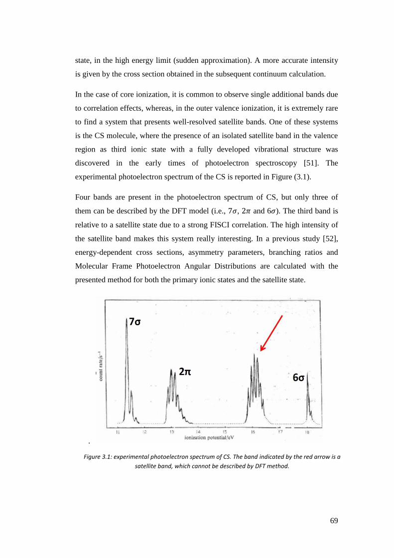
69
state, in the high energy limit (sudden approximation). A more accurate intensity
is given by the cross section obtained in the subsequent continuum calculation.
In the case of core ionization, it is common to observe single additional bands due
to correlation effects, whereas, in the outer valence ionization, it is extremely rare
to find a system that presents well-resolved satellite bands. One of these systems
is the CS molecule, where the presence of an isolated satellite band in the valence
region as third ionic state with a fully developed vibrational structure was
discovered in the early times of photoelectron spectroscopy [51]. The
experimental photoelectron spectrum of the CS is reported in Figure (3.1).
Four bands are present in the photoelectron spectrum of CS, but only three of
them can be described by the DFT model (i.e., 7𝜎, 2𝜋 and 6𝜎). The third band is
relative to a satellite state due to a strong FISCI correlation. The high intensity of
the satellite band makes this system really interesting. In a previous study [52],
energy-dependent cross sections, asymmetry parameters, branching ratios and
Molecular Frame Photoelectron Angular Distributions are calculated with the
presented method for both the primary ionic states and the satellite state.
.
Figure 3.1: experimental photoelectron spectrum of CS. The band indicated by the red arrow is a
satellite band, which cannot be described by DFT method.
70
A similar satellite is known to be present also in the spectrum of CO, but at higher
energy, beyond the second Σ primary ionization, and with a reduced intensity. It is
interesting to study the evolution of the satellite in isoelectronic molecules, and its
relation to the primary ionizations, as probed by photoionization observables, to
shed light on the changes in the electronic structure brought about by chemical
substitution. With this aim the same study has been made on CO, CSe and SiO.
3.4.2. Computational details
HF, CASSCF and NEVPT2 calculations on CO, CSe and SiO have been
performed using Molpro package with aug-cc-pVTZ as basis set. Ground state
electronic densities are obtained by ADF program using the LB94 exchange-
correlation potential and a DZP basis set. The B-spline basis has been built by
using a maximum value of the radial grid equal to 25 a.u. with a step equal to 0.2
a.u. and maximum value of the angular momentum 𝑙𝑚𝑎𝑥 = 20. The LCAO part
has been constructed using a maximum value of the radial grid for each off-centre
atom equal to 0.5 a.u. with a 𝑙𝑚𝑎𝑥 = 2. The equilibrium distance between the
atoms used are: 𝑅𝑒𝑞(𝐶𝑂) = 1.1228 Å [53], 𝑅𝑒𝑞(𝐶𝑆𝑒) = 1.6762 Å [54],
𝑅𝑒𝑞(𝑆𝑖𝑂) = 1.5097 Å [55].
The active spaces in CASSCF calculations are chosen in order to consider 10
electrons in 5 occupied orbitals (3𝜎, 1𝜋) and 3 virtual orbitals (2𝜎, 1𝜋). In
particular:
Occupied Virtual
CO 3𝜎, 4𝜎, 5𝜎, 1𝜋 6𝜎, 7𝜎, 2𝜋
CSe 9𝜎, 10𝜎, 11𝜎, 4𝜋 12𝜎, 13𝜎, 5𝜋
SiO 5𝜎, 6𝜎, 7𝜎, 2𝜋 8𝜎, 9𝜎, 3𝜋
The same scheme has been employed in the previous study on the CS molecule;
additional computational details can be found on ref 52.
Table 3.1: active spaces in the CASSCF calculations for both the ground state and the ionic
states for the CO, CSe and SiO molecules.
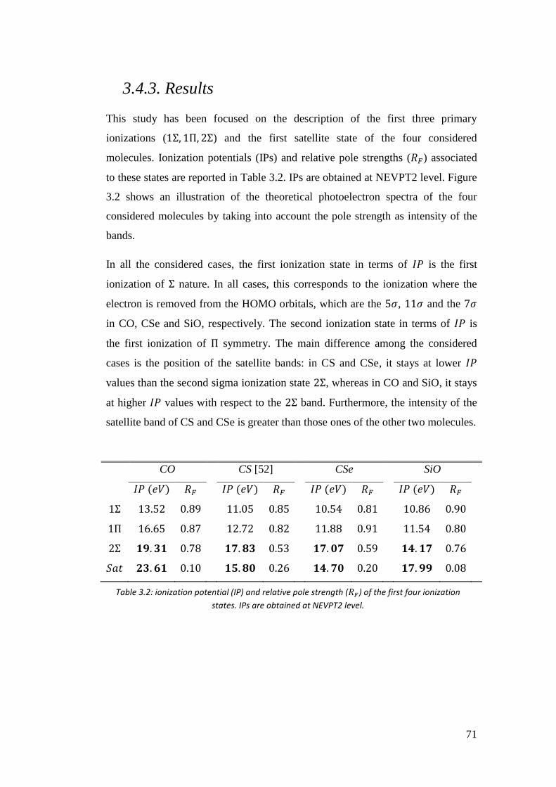
71
3.4.3. Results
This study has been focused on the description of the first three primary
ionizations (1Σ, 1Π, 2Σ) and the first satellite state of the four considered
molecules. Ionization potentials (IPs) and relative pole strengths (𝑅𝐹) associated
to these states are reported in Table 3.2. IPs are obtained at NEVPT2 level. Figure
3.2 shows an illustration of the theoretical photoelectron spectra of the four
considered molecules by taking into account the pole strength as intensity of the
bands.
In all the considered cases, the first ionization state in terms of 𝐼𝑃 is the first
ionization of Σ nature. In all cases, this corresponds to the ionization where the
electron is removed from the HOMO orbitals, which are the 5𝜎, 11𝜎 and the 7𝜎
in CO, CSe and SiO, respectively. The second ionization state in terms of 𝐼𝑃 is
the first ionization of Π symmetry. The main difference among the considered
cases is the position of the satellite bands: in CS and CSe, it stays at lower 𝐼𝑃
values than the second sigma ionization state 2Σ, whereas in CO and SiO, it stays
at higher 𝐼𝑃 values with respect to the 2Σ band. Furthermore, the intensity of the
satellite band of CS and CSe is greater than those ones of the other two molecules.
CO CS [52]
CSe SiO
𝐼𝑃 (𝑒𝑉) 𝑅𝐹 𝐼𝑃 (𝑒𝑉) 𝑅𝐹 𝐼𝑃 (𝑒𝑉) 𝑅𝐹 𝐼𝑃 (𝑒𝑉) 𝑅𝐹
1Σ 13.52 0.89 11.05 0.85 10.54 0.81 10.86 0.90
1Π 16.65 0.87 12.72 0.82 11.88 0.91 11.54 0.80
2Σ 𝟏𝟗. 𝟑𝟏 0.78 𝟏𝟕. 𝟖𝟑 0.53 𝟏𝟕. 𝟎𝟕 0.59 𝟏𝟒. 𝟏𝟕 0.76
𝑆𝑎𝑡 𝟐𝟑. 𝟔𝟏 0.10 𝟏𝟓. 𝟖𝟎 0.26 𝟏𝟒. 𝟕𝟎 0.20 𝟏𝟕. 𝟗𝟗 0.08
Table 3.2: ionization potential (IP) and relative pole strength (𝑅𝐹) of the first four ionization
states. IPs are obtained at NEVPT2 level.
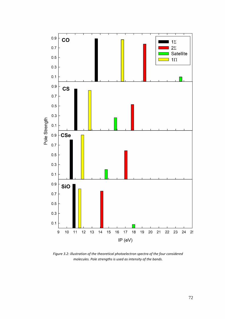
72
Figure 3.2: illustration of the theoretical photoelectron spectra of the four considered
molecules. Pole strengths is used as intensity of the bands.
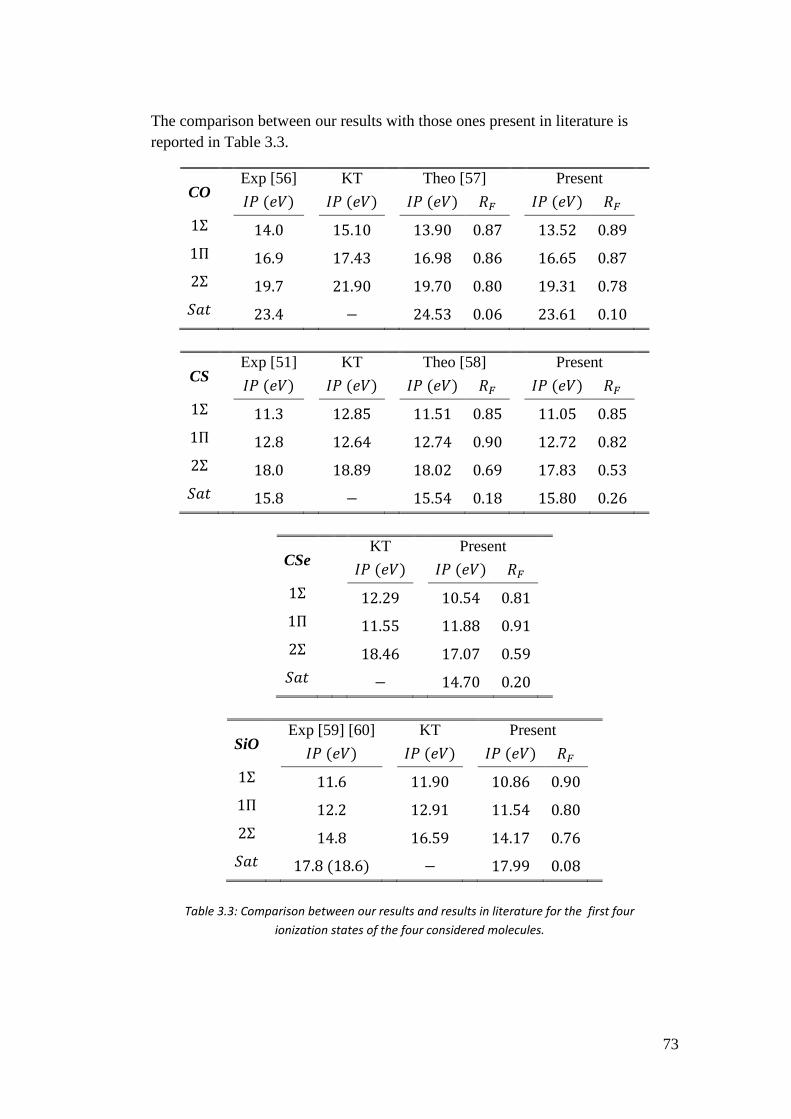
73
The comparison between our results with those ones present in literature is
reported in Table 3.3.
CO Exp [56] KT Theo [57] Present
𝐼𝑃 (𝑒𝑉) 𝐼𝑃 (𝑒𝑉) 𝐼𝑃 (𝑒𝑉) 𝑅𝐹 𝐼𝑃 (𝑒𝑉) 𝑅𝐹
1Σ 14.0 15.10 13.90 0.87 13.52 0.89
1Π 16.9 17.43 16.98 0.86 16.65 0.87
2Σ 19.7 21.90 19.70 0.80 19.31 0.78
𝑆𝑎𝑡 23.4 − 24.53 0.06 23.61 0.10
CS Exp [51] KT Theo [58] Present
𝐼𝑃 (𝑒𝑉) 𝐼𝑃 (𝑒𝑉) 𝐼𝑃 (𝑒𝑉) 𝑅𝐹 𝐼𝑃 (𝑒𝑉) 𝑅𝐹
1Σ 11.3 12.85 11.51 0.85 11.05 0.85
1Π 12.8 12.64 12.74 0.90 12.72 0.82
2Σ 18.0 18.89 18.02 0.69 17.83 0.53
𝑆𝑎𝑡 15.8 − 15.54 0.18 15.80 0.26
CSe KT Present
𝐼𝑃 (𝑒𝑉) 𝐼𝑃 (𝑒𝑉) 𝑅𝐹
1Σ 12.29 10.54 0.81
1Π 11.55 11.88 0.91
2Σ 18.46 17.07 0.59
𝑆𝑎𝑡 − 14.70 0.20
SiO Exp [59] [60] KT Present
𝐼𝑃 (𝑒𝑉) 𝐼𝑃 (𝑒𝑉) 𝐼𝑃 (𝑒𝑉) 𝑅𝐹
1Σ 11.6 11.90 10.86 0.90
1Π 12.2 12.91 11.54 0.80
2Σ 14.8 16.59 14.17 0.76
𝑆𝑎𝑡 17.8 (18.6) − 17.99 0.08
Table 3.3: Comparison between our results and results in literature for the first four
ionization states of the four considered molecules.
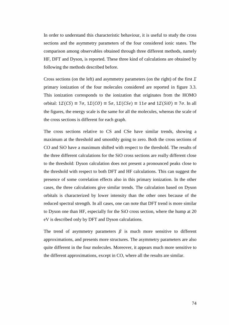
74
In order to understand this characteristic behaviour, it is useful to study the cross
sections and the asymmetry parameters of the four considered ionic states. The
comparison among observables obtained through three different methods, namely
HF, DFT and Dyson, is reported. These three kind of calculations are obtained by
following the methods described before.
Cross sections (on the left) and asymmetry parameters (on the right) of the first 𝛴
primary ionization of the four molecules considered are reported in figure 3.3.
This ionization corresponds to the ionization that originates from the HOMO
orbital: 1𝛴(𝐶𝑆) ≡ 7𝜎, 1𝛴(𝐶𝑂) ≡ 5𝜎, 1𝛴(𝐶𝑆𝑒) ≡ 11𝜎 and 1𝛴(𝑆𝑖𝑂) ≡ 7𝜎. In all
the figures, the energy scale is the same for all the molecules, whereas the scale of
the cross sections is different for each graph.
The cross sections relative to CS and CSe have similar trends, showing a
maximum at the threshold and smoothly going to zero. Both the cross sections of
CO and SiO have a maximum shifted with respect to the threshold. The results of
the three different calculations for the SiO cross sections are really different close
to the threshold: Dyson calculation does not present a pronounced peaks close to
the threshold with respect to both DFT and HF calculations. This can suggest the
presence of some correlation effects also in this primary ionization. In the other
cases, the three calculations give similar trends. The calculation based on Dyson
orbitals is characterized by lower intensity than the other ones because of the
reduced spectral strength. In all cases, one can note that DFT trend is more similar
to Dyson one than HF, especially for the SiO cross section, where the hump at 20
eV is described only by DFT and Dyson calculations.
The trend of asymmetry parameters 𝛽 is much more sensitive to different
approximations, and presents more structures. The asymmetry parameters are also
quite different in the four molecules. Moreover, it appears much more sensitive to
the different approximations, except in CO, where all the results are similar.
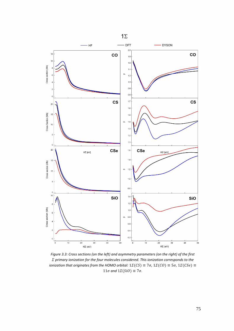
75
Figure 3.3: Cross sections (on the left) and asymmetry parameters (on the right) of the first
𝛴 primary ionization for the four molecules considered. This ionization corresponds to the
ionization that originates from the HOMO orbital: 1𝛴(𝐶𝑆) ≡ 7𝜎, 1𝛴(𝐶𝑂) ≡ 5𝜎, 1𝛴(𝐶𝑆𝑒) ≡
11𝜎 and 1𝛴(𝑆𝑖𝑂) ≡ 7𝜎.

76
This underlies the sensitivity of 𝛽 both to the electronic structure, that is the
variation in orbital composition brought about by chemical change, and the
amount of correlation effects, as evidenced by the change moving from the HF to
CASSCF results. From this point of view, weak correlation effects seem to affect
the HOMO ionization in CO, while they appear much more pronounced in the
other molecules, attributed to the presence of a heavier (third or fourth row) atom.
The second primary ionization of all the considered molecules is the first one of Π
symmetry. Cross sections (on the left) and asymmetry parameters (on the right) of
this ionization of the four molecules considered are reported in Figure 3.4. This
ionization corresponds to the ionization that originates from the highest occupied
𝜋-orbital: 1Π(𝐶𝑆) ≡ 2𝜋, 1Π(𝐶𝑂) ≡ 1𝜋, 1Π(𝐶𝑆𝑒) ≡ 4𝜋 and 1Π(𝑆𝑖𝑂) ≡ 2𝜋.
All the cross sections decay pretty fast, but, even in this case, the trends of the
cross sections of CS and CSe are similar. They present a maximum at the
threshold and a monotonic decrease. In these two cases, the three calculations
almost provide the same results, whereas in the CO and SiO cases, the differences
among the three calculations are significant. Unlike the previous examined
ionization state, cross section relative to the SiO obtained by the Dyson
calculation is quite similar to that one calculated with the other two methods: this
can suggest that correlation effects are less important in this state. Note that, also
in this case, the DFT results are quite similar to those obtained with Dyson
orbitals, especially for CO.
Regarding the asymmetry parameters, even in this case, trends are really different
for the considered molecules (except for CO and SiO that present a similar trend
with a minimum close to the threshold). At low energies, the three kind of
calculations provide similar results, with differences between each other
increasing at higher energies.
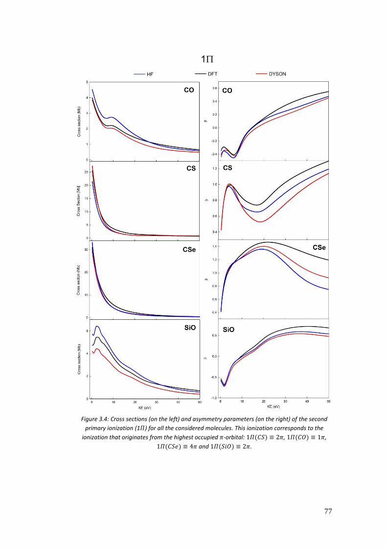
77
Figure 3.4: Cross sections (on the left) and asymmetry parameters (on the right) of the second
primary ionization (1𝛱) for all the considered molecules. This ionization corresponds to the
ionization that originates from the highest occupied 𝜋-orbital: 1𝛱(𝐶𝑆) ≡ 2𝜋, 1𝛱(𝐶𝑂) ≡ 1𝜋,
1𝛱(𝐶𝑆𝑒) ≡ 4𝜋 and 1𝛱(𝑆𝑖𝑂) ≡ 2𝜋.
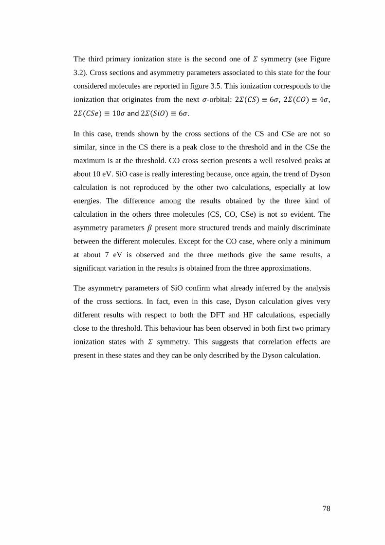
78
The third primary ionization state is the second one of 𝛴 symmetry (see Figure
3.2). Cross sections and asymmetry parameters associated to this state for the four
considered molecules are reported in figure 3.5. This ionization corresponds to the
ionization that originates from the next 𝜎-orbital: 2𝛴(𝐶𝑆) ≡ 6𝜎, 2𝛴(𝐶𝑂) ≡ 4𝜎,
2𝛴(𝐶𝑆𝑒) ≡ 10𝜎 and 2𝛴(𝑆𝑖𝑂) ≡ 6𝜎.
In this case, trends shown by the cross sections of the CS and CSe are not so
similar, since in the CS there is a peak close to the threshold and in the CSe the
maximum is at the threshold. CO cross section presents a well resolved peaks at
about 10 eV. SiO case is really interesting because, once again, the trend of Dyson
calculation is not reproduced by the other two calculations, especially at low
energies. The difference among the results obtained by the three kind of
calculation in the others three molecules (CS, CO, CSe) is not so evident. The
asymmetry parameters 𝛽 present more structured trends and mainly discriminate
between the different molecules. Except for the CO case, where only a minimum
at about 7 eV is observed and the three methods give the same results, a
significant variation in the results is obtained from the three approximations.
The asymmetry parameters of SiO confirm what already inferred by the analysis
of the cross sections. In fact, even in this case, Dyson calculation gives very
different results with respect to both the DFT and HF calculations, especially
close to the threshold. This behaviour has been observed in both first two primary
ionization states with 𝛴 symmetry. This suggests that correlation effects are
present in these states and they can be only described by the Dyson calculation.
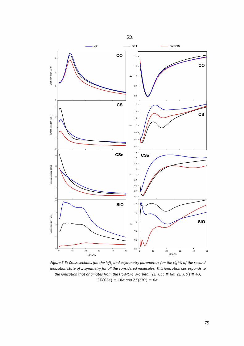
79
Figure 3.5: Cross sections (on the left) and asymmetry parameters (on the right) of the second
ionization state of 𝛴 symmetry for all the considered molecules. This ionization corresponds to
the ionization that originates from the HOMO-1 𝜎-orbital: 2𝛴(𝐶𝑆) ≡ 6𝜎, 2𝛴(𝐶𝑂) ≡ 4𝜎,
2𝛴(𝐶𝑆𝑒) ≡ 10𝜎 and 2𝛴(𝑆𝑖𝑂) ≡ 6𝜎.

80
The main feature of the photoionization of these four molecule is the presence of
the well resolved satellite bands of 𝛴 symmetry. As already mentioned, these can
be studied only by means of the Dyson approach. Cross sections (on the left) and
asymmetry parameters (on the right) of the satellite bands of the four considered
molecules are reported in Figure 3.6.
Cross sections relative to CS and CSe are really similar: both of them present a
maximum at the threshold and go to zero at higher energies. The trend of the cross
section of the CO is also similar, but it more slowly goes to zero. The SiO cross
section is more structured with the appearance of two bands: one close to the
threshold and one at about 20 eV. The faster decay is associated (by Fourier
transform) to the spatial extent of the ionized orbital. In this case, it indicates a
strong contribution of the heavier atom AOs in the Dyson orbital relative to
satellite ionization. 𝛽 parameters show a distinct individual behaviour for the four
molecules, although a broad trend, characterized by a large dip at intermediate
energy, is calculated for CS, CSe and SiO. The case of CO is remarkably
different, with 𝛽 rapidly increasing from threshold, and quickly reaching a high
asymptotic value, interrupted by a small dip around 10 eV (kinetic energy).
The cross section profiles appear to be smooth with a maximum at the threshold
and a trend going to zero. Further information can be achieved by considering
individual cross section ratios, which can also be easily obtained from the
experiment. From these ratios, it is possible to better characterize the satellite state
by understanding if the intensity of the satellite is mainly borrowed by a primary
state or is more complex due to contributions of several initial orbitals. The first
situation is described by a constant ratio.
On the left of Figure 3.7, ratios between satellite and first primary 𝛴 ionization of
the four considered molecules are reported; on the right, ratios between satellite
and second primary 𝛴 ionization are reported.
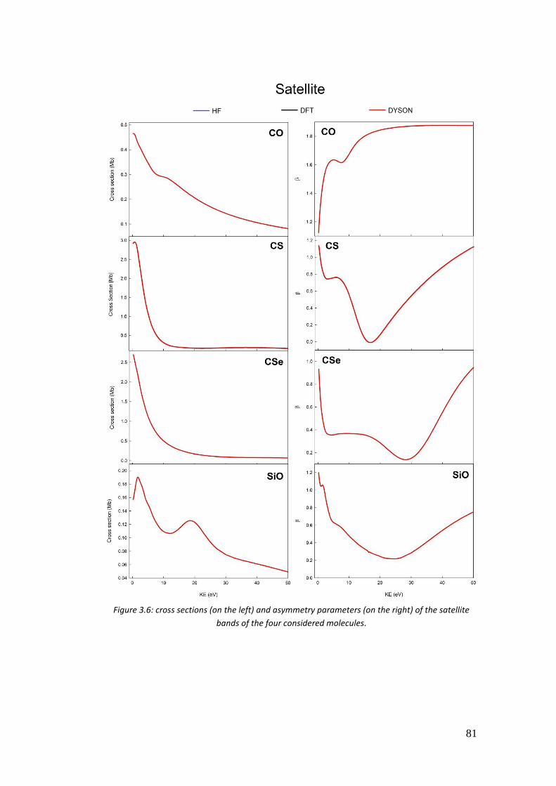
81
Figure 3.6: cross sections (on the left) and asymmetry parameters (on the right) of the satellite
bands of the four considered molecules.
82
None of the reported ratio is constant at low energies, proving the inadequacy of
the simple borrowing mechanism. At higher energies, some of the ratios approach
a constant value. By considering CS, CO and CSe, the ratio between cross
sections of satellite and first primary ionization state is not constant at all, so that
one can affirm that the intensity of the satellite band is not due to the first primary
ionization state. Indeed, the ratio between the cross sections of the satellite and the
second primary ionization state become constant at higher energies. This can
suggest that, at high energies, the second primary ionization state mainly
contributes to the intensity of the satellite state. The two ratios relative to SiO are
quite interesting since both of them approach constant value at higher energies.
Thus, both the primary ionizations contribute to the intensity of the satellite states
at higher energies.
To conclude, this study has shown the sensitivity of photoionization observables,
and, in particular, of the asymmetry parameter 𝛽, with respect to the changes in
the electronic structure of isoelectronic molecules. Moreover, it gives evidence of
strong correlation effects in the systems with a heavier atom. In particular, the
satellite band reaches the maximum intensity in the case of CS, and slightly
declines in the spectrum of CSe. On the contrary, it remains weak and positioned
at higher energy above the second 𝛴 primary ionization for CO and SiO, despite
of the different character it has in the two molecules, as can be seen from the
photoionization observables.
The comparison among the three kind of calculations has shown that the DFT
results are much more similar to the Dyson results with respect to HF results. This
is an indication that, even though the DFT method is a one-particle calculation, it
is able to treat a small part of the correlation but remaining unfit to treat strong
correlation effects. In fact, regarding SiO, the Dyson calculations for the first two
primary ionization states of 𝛴 symmetry have provided different results with
respect to the calculations performed with HF and DFT methods. This is a clear
indication of the presence of strong correlation effects even in the primary 𝛴
ionization states that are not visible in the primary Π ionization state.
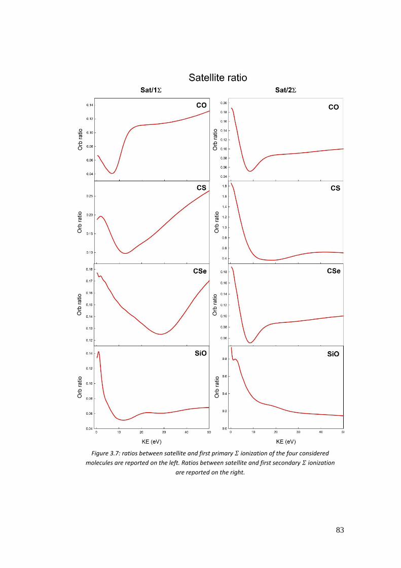
83
Figure 3.7: ratios between satellite and first primary 𝛴 ionization of the four considered
molecules are reported on the left. Ratios between satellite and first secondary 𝛴 ionization
are reported on the right.
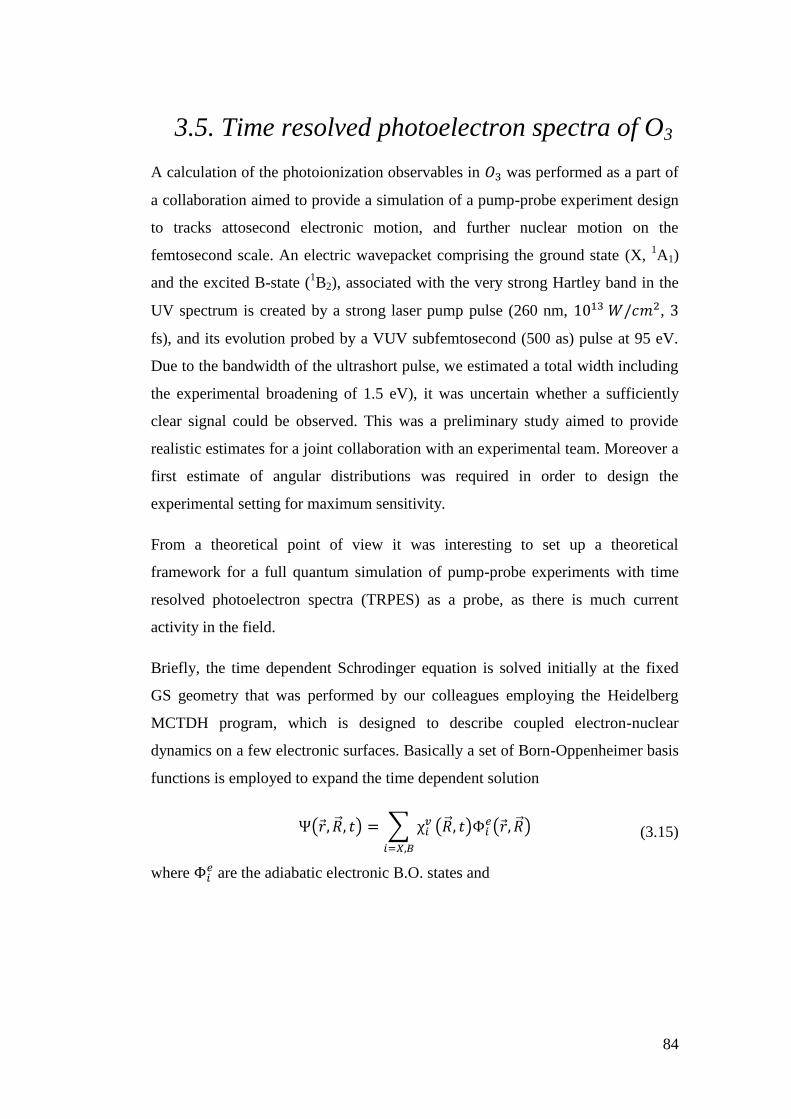
84
3.5. Time resolved photoelectron spectra of O3
A calculation of the photoionization observables in 𝑂3 was performed as a part of
a collaboration aimed to provide a simulation of a pump-probe experiment design
to tracks attosecond electronic motion, and further nuclear motion on the
femtosecond scale. An electric wavepacket comprising the ground state (X, 1A1)
and the excited B-state (1B2), associated with the very strong Hartley band in the
UV spectrum is created by a strong laser pump pulse (260 nm, 1013 𝑊/𝑐𝑚2, 3
fs), and its evolution probed by a VUV subfemtosecond (500 as) pulse at 95 eV.
Due to the bandwidth of the ultrashort pulse, we estimated a total width including
the experimental broadening of 1.5 eV), it was uncertain whether a sufficiently
clear signal could be observed. This was a preliminary study aimed to provide
realistic estimates for a joint collaboration with an experimental team. Moreover a
first estimate of angular distributions was required in order to design the
experimental setting for maximum sensitivity.
From a theoretical point of view it was interesting to set up a theoretical
framework for a full quantum simulation of pump-probe experiments with time
resolved photoelectron spectra (TRPES) as a probe, as there is much current
activity in the field.
Briefly, the time dependent Schrodinger equation is solved initially at the fixed
GS geometry that was performed by our colleagues employing the Heidelberg
MCTDH program, which is designed to describe coupled electron-nuclear
dynamics on a few electronic surfaces. Basically a set of Born-Oppenheimer basis
functions is employed to expand the time dependent solution
Ψ(𝑟 , �⃗� , 𝑡) = ∑ χ𝑖𝑣
𝑖=𝑋,𝐵
(�⃗� , 𝑡)Φ𝑖𝑒(𝑟 , �⃗� ) (3.15)
where Φ𝑖𝑒 are the adiabatic electronic B.O. states and
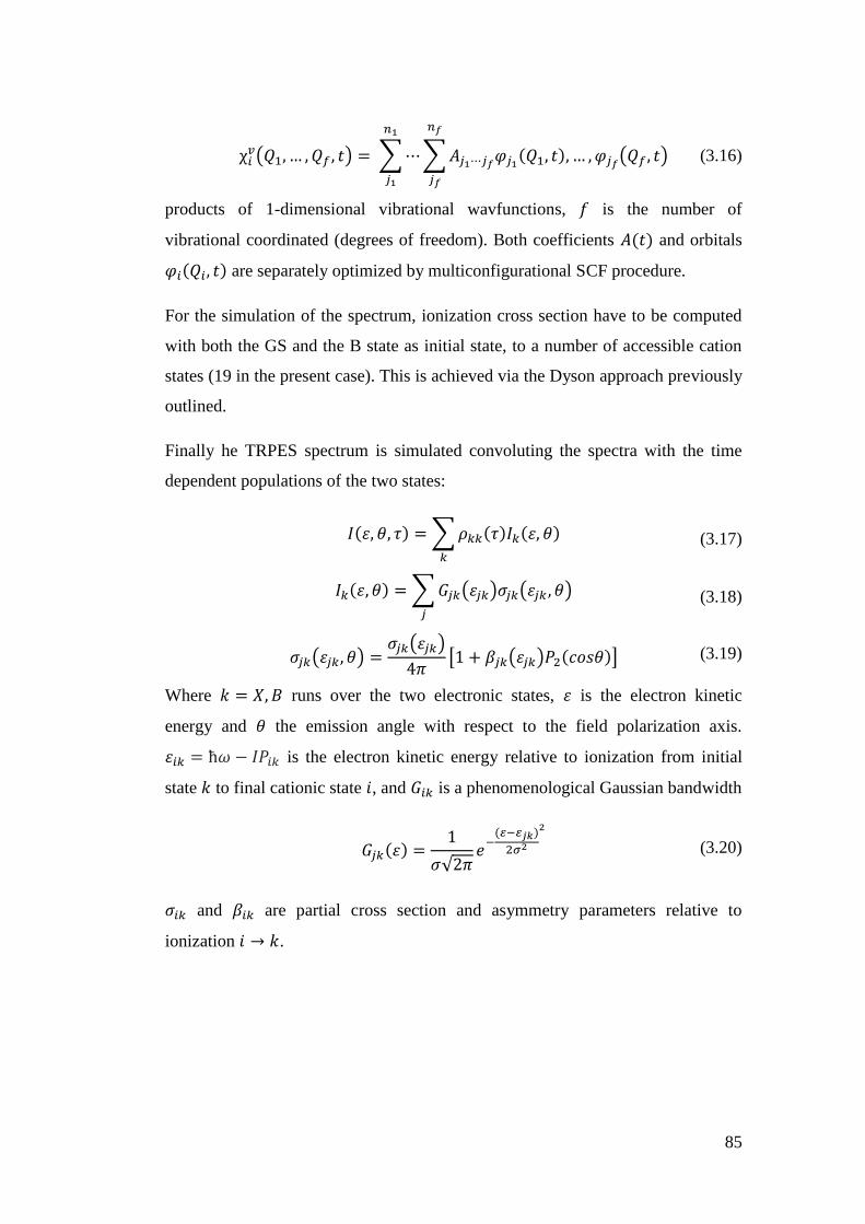
85
χ𝑖𝑣(𝑄1, … , 𝑄𝑓 , 𝑡) = ∑⋯∑𝐴𝑗1⋯𝑗𝑓𝜑𝑗1(𝑄1, 𝑡), … ,
𝑛𝑓
𝑗𝑓
𝑛1
𝑗1
𝜑𝑗𝑓(𝑄𝑓 , 𝑡) (3.16)
products of 1-dimensional vibrational wavfunctions, 𝑓 is the number of
vibrational coordinated (degrees of freedom). Both coefficients 𝐴(𝑡) and orbitals
𝜑𝑖(𝑄𝑖, 𝑡) are separately optimized by multiconfigurational SCF procedure.
For the simulation of the spectrum, ionization cross section have to be computed
with both the GS and the B state as initial state, to a number of accessible cation
states (19 in the present case). This is achieved via the Dyson approach previously
outlined.
Finally he TRPES spectrum is simulated convoluting the spectra with the time
dependent populations of the two states:
𝐼(휀, 휃, 𝜏) =∑𝜌𝑘𝑘(𝜏)𝐼𝑘(휀, 휃)
𝑘
(3.17)
𝐼𝑘(휀, 휃) =∑𝐺𝑗𝑘(휀𝑗𝑘)𝜎𝑗𝑘(휀𝑗𝑘 , 휃)
𝑗
(3.18)
𝜎𝑗𝑘(휀𝑗𝑘, 휃) =
𝜎𝑗𝑘(휀𝑗𝑘)
4𝜋[1 + 𝛽𝑗𝑘(휀𝑗𝑘)𝑃2(𝑐𝑜𝑠휃)] (3.19)
Where 𝑘 = 𝑋, 𝐵 runs over the two electronic states, 휀 is the electron kinetic
energy and 휃 the emission angle with respect to the field polarization axis.
휀𝑖𝑘 = ħ𝜔 − 𝐼𝑃𝑖𝑘 is the electron kinetic energy relative to ionization from initial
state 𝑘 to final cationic state 𝑖, and 𝐺𝑖𝑘 is a phenomenological Gaussian bandwidth
𝐺𝑗𝑘(휀) =
1
𝜎√2𝜋𝑒−(𝜀−𝜀𝑗𝑘)
2𝜎2
2
(3.20)
𝜎𝑖𝑘 and 𝛽𝑖𝑘 are partial cross section and asymmetry parameters relative to
ionization 𝑖 → 𝑘.
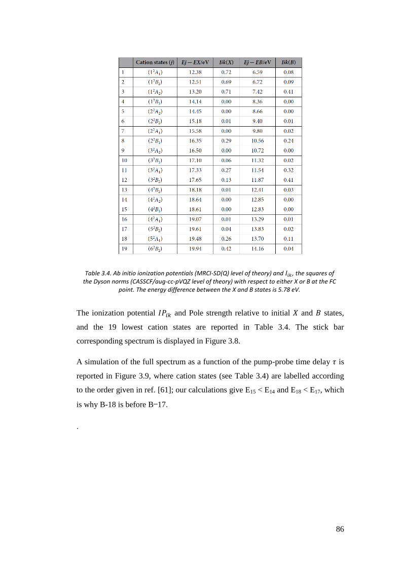
86
The ionization potential 𝐼𝑃𝑖𝑘 and Pole strength relative to initial 𝑋 and 𝐵 states,
and the 19 lowest cation states are reported in Table 3.4. The stick bar
corresponding spectrum is displayed in Figure 3.8.
A simulation of the full spectrum as a function of the pump-probe time delay 𝜏 is
reported in Figure 3.9, where cation states (see Table 3.4) are labelled according
to the order given in ref. [61]; our calculations give E15 < E14 and E18 < E17, which
is why B-18 is before B−17.
.
Table 3.4. Ab initio ionization potentials (MRCI-SD(Q) level of theory) and 𝐼𝑖𝑘 , the squares of the Dyson norms (CASSCF/aug-cc-pVQZ level of theory) with respect to either X or B at the FC
point. The energy difference between the X and B states is 5.78 eV.
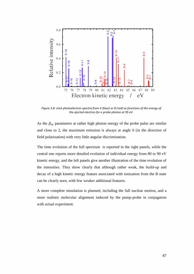
87
As the 𝛽𝑖𝑘 parameters at rather high photon energy of the probe pulse are similar
and close to 2, the maximum emission is always at angle 0 (in the direction of
field polarization) with very little angular discrimination.
The time evolution of the full spectrum is reported in the right panels, while the
central one reports more detailed evolution of individual energy from 80 to 90 eV
kinetic energy, and the left panels give another illustration of the time evolution of
the intensities. They show clearly that although rather weak, the build-up and
decay of a high kinetic energy feature associated with ionization from the B state
can be clearly seen, with few weaker additional features.
A more complete simulation is planned, including the full nuclear motion, and a
more realistic molecular alignment induced by the pump-probe in conjugation
with actual experiment.
Figure 3.8: stick photoelectron spectra from X (blue) or B (red) as functions of the energy of the ejected electron for a probe photon at 95 eV.
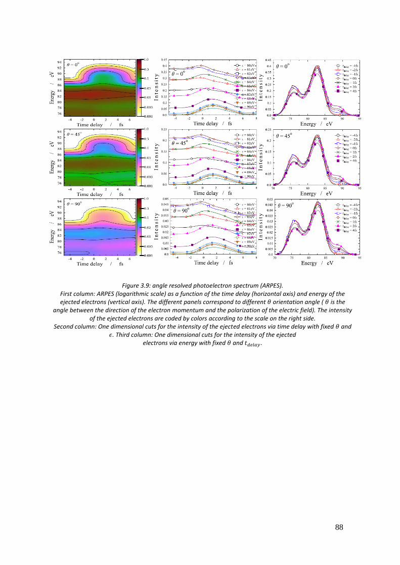
88
Figure 3.9: angle resolved photoelectron spectrum (ARPES). First column: ARPES (logarithmic scale) as a function of the time delay (horizontal axis) and energy of the ejected electrons (vertical axis). The different panels correspond to different 휃 orientation angle ( 휃 is the
angle between the direction of the electron momentum and the polarization of the electric field). The intensity of the ejected electrons are coded by colors according to the scale on the right side.
Second column: One dimensional cuts for the intensity of the ejected electrons via time delay with fixed 휃 and 𝜖. Third column: One dimensional cuts for the intensity of the ejected
electrons via energy with fixed 휃 and 𝑡𝑑𝑒𝑙𝑎𝑦 .
89
4. Calculation of two-electron
integrals using B-spline
4.1 Introduction
The DFT approach, described in Chapter (2.6), is extremely efficient but it has the
intrinsic limits typical of a single-particle treatment. Indeed, multi-electron
phenomena as well as subtle effects due to the electronic correlation cannot be
described through this method.
Our goal is implementing an algorithm that makes it possible to study all these
phenomena. In order to do this, it is needed to solve the Schrödinger equation. Let
us start by considering the complete Hamiltonian:
𝐻𝛹 = 𝐸𝛹 (4.1)
𝐻 = ∑ℎ(𝑖)
𝑖
+ ∑ 1
𝑟𝑖𝑗𝑖<𝑗
(4.2)
Since Hamiltonian contains both one-particle and two-particle operators, one-
electron and two-electrons integrals have to be solved. Calculation of two-
electrons integrals is particularly demanding. Let us also introduce the Chemist’s
notation for the Coulomb integrals:
∫𝑓𝑖(1)𝑓𝑗(2)
1
𝑟12𝑓𝑘(1)𝑓𝑙(2)𝑑𝑟1𝑑𝑟2 = ⟨𝑓𝑖𝑓𝑗|𝑓𝑘𝑓𝑙⟩ = (𝑓𝑖𝑓𝑘|𝑓𝑗𝑓𝑙) (4.3)
where, in the latter notation, with normal brackets, the left member is the charge
distribution 𝑓𝑖(1)𝑓𝑘(1) relative to particle one, and the right member is the charge
density relative to particle two. They can be further abbreviated as
⟨𝑖𝑗|𝑘𝑙⟩ = (𝑖𝑘|𝑗𝑙) (4.4)
90
4.2. Calculation of 2-electron integrals via
solution of the Poisson’s equation
We consider a mixed-basis approach. A basis of molecular orbitals (MOs) which
are obtained from a standard quantum chemistry package and expanded in a basis
of gaussian functions, {𝜑𝑖𝜆𝜇(𝒓)}, and a basis of B-spline functions, described in
Chapter (2.4.1), {𝜒𝑖𝑗𝜆𝜇𝑝 (𝒓)} which is actually used expand both the MOs basis and
the photoelectron continuum orbital.
In principle, a general close-coupling program which uses a mixed gaussian/B-
spline basis and a single electron in the continuum, needs three different types of
2-electron integrals. We use the Chemist's notation in the following, and denote a
generic LCAO basis function as follows 𝜒𝑖𝑗𝜆𝜇𝑝 (𝒓) ≡ 𝜒𝜈:
1. (𝜑𝑖𝜑𝑗|𝜑𝑘𝜒𝜈)
2. (𝜑𝑖𝜑𝑗|𝜒𝜇𝜒𝜈)
3. (𝜑𝑖𝜒𝜇|𝜑𝑗𝜒𝜈)
and clearly (𝜑𝑖𝜑𝑗|𝜑𝑘𝜒𝜈) can be readily obtained from either of the last two types
of integrals by a simple matrix-vector multiplication with the MOs expansion
coefficients in the LCAO basis. Alternatively, it can also be obtained from
quantities that are used in the computation of the other two types of integrals. A
sketch of the general procedure is given below while more details of the actual
implementation will follow.
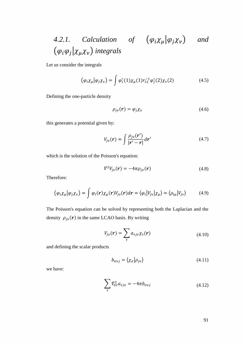
91
4.2.1. Calculation of (𝜑𝑖𝜒𝜇|𝜑𝑗𝜒𝜈) and
(𝜑𝑖𝜑𝑗|𝜒𝜇𝜒𝜈) integrals
Let us consider the integrals
(𝜑𝑖𝜒𝜇|𝜑𝑗𝜒𝜈) = ∫𝜑𝑖
∗(1)𝜒𝜇(1)𝑟12−1𝜑𝑗
∗(2)𝜒𝜈(2) (4.5)
Defining the one-particle density
𝜌𝑗𝜈(𝒓) = 𝜑𝑗𝜒𝜈 (4.6)
this generates a potential given by:
𝑉𝑗𝜈(𝒓) = ∫
𝜌𝑗𝜈(𝒓′)
|𝒓′ − 𝒓|𝑑𝒓′ (4.7)
which is the solution of the Poisson's equation:
𝛻2𝑉𝑗𝜈(𝒓) = −4𝜋𝜌𝑗𝜈(𝒓) (4.8)
Therefore:
(𝜑𝑖𝜒𝜇|𝜑𝑗𝜒𝜈) = ∫𝜑𝑖(𝒓)𝜒𝜇(𝒓)𝑉𝑗𝜈(𝒓)𝑑𝒓 = ⟨𝜑𝑖|𝑉𝑗𝜈|𝜒𝜇⟩ = ⟨𝜌𝑖𝜇|𝑉𝑗𝜈⟩ (4.9)
The Poisson's equation can be solved by representing both the Laplacian and the
density 𝜌𝑗𝜈(𝒓) in the same LCAO basis. By writing
𝑉𝑗𝜈(𝒓) =∑𝑎𝜏𝑗𝜈𝜒𝜏(𝒓)
𝜏
(4.10)
and defining the scalar products
𝑏𝜎𝜈𝑗 = ⟨𝜒𝜎|𝜌𝑗𝜈⟩ (4.11)
we have:
∑𝛻𝜎𝜏2 𝑎𝜏𝑗𝜈
𝜏
= −4𝜋𝑏𝜎𝜈𝑗 (4.12)
92
Once the expansion coefficients of the 𝑉𝑗𝜈(𝒓) potential, 𝑎𝜏𝑗𝜈, are obtained, it then
follows that the (𝜑𝑖𝜒𝜇|𝜑𝑗𝜒𝜈) integrals can be simply obtained by:
(𝜑𝑖𝜒𝜇|𝜑𝑗𝜒𝜈) =∑𝑎𝜏𝑗𝜈𝜏
𝑏𝜎𝜈𝑗 (4.13)
i.e. as a product of two matrices. The calculation of the (𝜑𝑖𝜑𝑗|𝜒𝜇𝜒𝜈) integrals is
best done by first solving the Poisson's equation relative to the
𝜌𝑖𝑗(𝒓) = 𝜑𝑖(𝒓)𝜑𝑗(𝒓) one-particle density:
𝛻2𝑉𝑖𝑗(𝒓) = −4𝜋𝜌𝑖𝑗(𝒓), (4.14)
and then by integrating the 𝑉𝑖𝑗(𝒓) over the product of two LCAO basis functions:
(𝜑𝑖𝜑𝑗|𝜒𝜇𝜒𝜈) = ∫𝜒𝜇(𝒓)𝑉𝑖𝑗(𝒓)𝜒𝜈(𝒓)𝑑𝒓 (4.15)
Finally, integrals are obtained as:
(𝜑𝑖𝜑𝑗|𝜑𝑘𝜒𝜈) =∑𝑎𝜏𝑖𝑗𝜏
𝑏𝜏𝜈𝑘 (4.16)
The core of the algorithm is therefore the computation of the matrix elements 𝑏𝜎𝜈𝑗
and 𝑏𝜏𝜈𝑘 which are then used in the solution of the corresponding Poisson's
equation, Eq.(4.14), In more detail, these matrix elements read:
𝑏𝜎𝜈𝑗 = ⟨𝜒𝑖𝑗𝜆𝜇𝑝 |𝜑𝑘𝜆𝑘𝜇𝑘𝜒𝑖′𝑗′𝜆′𝜇′
𝑝′⟩ (4.17)
and
𝑏𝜏𝜈𝑘 = ⟨𝜒𝑖𝑗𝜆𝜇𝑝 |𝜑𝑘𝜆𝑘𝜇𝑘𝜑𝑙𝜆𝑙𝜇𝑙⟩ (4.18)
At this point symmetry considerations can be invoked so that only non-zero
matrices are calculated. Presently, only abelian symmetry has been implemented
throughout, although some parts have been coded for all molecular point groups
that have real representations. For abelian point groups, all IRs are
monodimensional and therefore only matrices for which the direct products satisfy
93
the conditions 𝜆 ⊗ 𝜆𝑘 = 𝜆′ or 𝜆 ⊗ 𝜆𝑘 = 𝜆𝑙 need to be computed. We would also
like to remark that the generalization to non-abelian point groups requires in
principle only minor modifications to the algorithm outlined here. This issue is
postponed to a future work. At the outset, well-known and trivial symmetry
properties of the 2-electron integrals are used to lower the number of 𝑏 matrices
that need to be computed and the number of times the solution of a Poisson's
equation is required. Thus only 𝑏𝜎𝑖𝑗 matrices for which 𝑖 ≥ 𝑗 (or 𝑗 ≥ 𝑖) are
calculated and stored on disk, while in the calculation of the (𝜑𝑖𝜒𝜇|𝜑𝑗𝜒𝜈)
matrices only 𝑖 ≥ 𝑗 need to be considered.
For the purpose of an outline of the algorithm, we spell out the steps that are
required to integrate a totally-symmetric function, and only describe the
modifications that are required in the general case.
4.2.2. Testing the Poisson algorithm for two-
electron integrals
In the development of a product density
𝜌𝑗𝜈 = 𝜑𝑗𝜒𝜈 𝑜𝑟 𝜌𝑖𝑗 = 𝜑𝑖𝜑𝑗 (4.19)
as a linear combination of basis functions
𝜌𝑗𝜈 =∑𝜒𝜎𝑐𝜎𝑗𝜈𝜎
(4.20)
by using the same {𝜒𝜇} basis, one can incur a truncation error, both in the radial
expansion and in the angular expansion. Basically, the product of two splines of
order 𝑖𝑜𝑟𝑑 gives polynomials of order 2 ∙ 𝑖𝑜𝑟𝑑 − 1, higher than the original basis.
Moreover, the product of two spherical harmonics 𝑌𝑙1𝑚1 ∙ 𝑌𝑙2𝑚2 gives a linear
combination of harmonics with maximum 𝐿 = 𝑙1 + 𝑙2, some of them missing in
the original basis. In principle, to get an exact expansion (neglecting numerical
errors), one should employ an auxiliary expansion basis with spline order
2 ∙ 𝑖𝑜𝑟𝑑 − 1 and 𝐿𝑚𝑎𝑥1 = 2𝐿𝑚𝑎𝑥, where 𝑖𝑜𝑟𝑑 and 𝐿𝑚𝑎𝑥 refer to the original basis.
94
The situation with the LCAO basis is more complex and cannot be simply
analysed. Thus, to avoid numerical inaccuracies, one should thoroughly test both
spline order convergence and 𝐿𝑚𝑎𝑥 convergence.
4.3. Testing the truncation errors
As already mentioned, our method is based on defining the one-particle density as
a product of two functions. By taking into account two types of functions, it
follows that there are three possibilities to express the one-particle density:
I. 𝑓(𝑟) = 𝐵𝑖𝐵𝑗
(4.21) II. 𝑓(𝑟) = 𝐵𝑖𝜑𝑗
III. 𝑓(𝑟) = 𝜑𝑖𝜑𝑗
One condition which is required to be satisfied by 𝑓(𝑟) is that it can be accurately
expanded in a B-spline basis:
𝑓(𝑟) =∑𝐵𝑘′ 𝑐𝑘
𝑘
(4.22)
By using this expansion, truncation errors may occur [62]. Thus, three different
situations can be analysed: i) product of two B-splines, ii) product of a B-spline
and an orbital, iii) product of two orbitals. Note that orbitals are expanded in terms
of B-splines as well, namely:
𝜑𝑖=∑𝑐𝛾,𝑖𝐵𝛾
𝛾
(4.23)
Let us now introduce two basis characterized by the same set of knots {𝐵𝑖} and
{𝐵𝑘′ }, with orders 𝑖𝑜𝑟𝑑 and 𝑖𝑜𝑟𝑑′, respectively. Once fixed the spline order, the
degree of the basis functions under consideration are 𝑛 = 𝑖𝑜𝑟𝑑 − 1 and 𝑛′ =
𝑖𝑜𝑟𝑑′ − 1, so that the product 𝐵𝑖 ∙ 𝐵𝑗 has degree 2𝑛 corresponding to an order
equal to 2𝑛 + 1 = 2𝑖𝑜𝑟𝑑 − 1. Therefore, the order of the B-splines basis {𝐵𝑘′ } in
the expansion
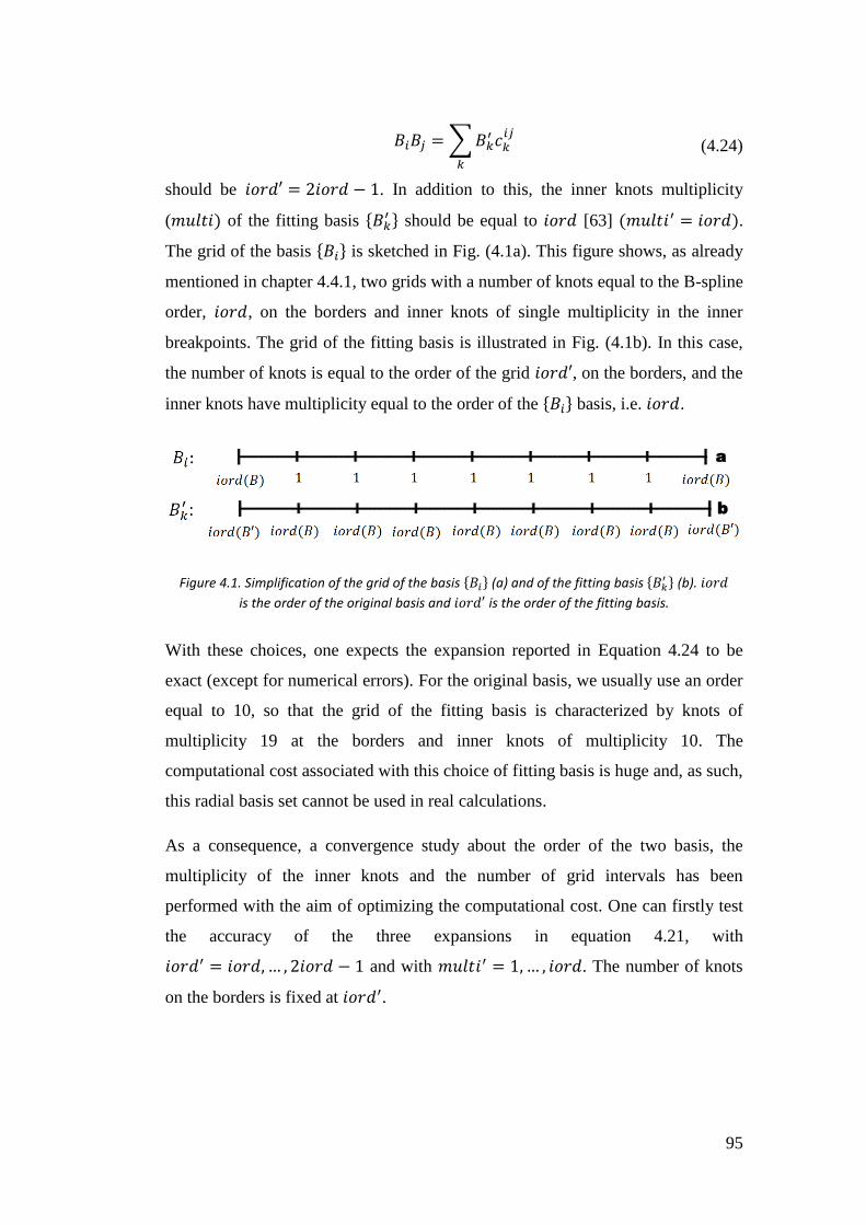
95
𝐵𝑖𝐵𝑗 =∑𝐵𝑘′ 𝑐𝑘𝑖𝑗
𝑘
(4.24)
should be 𝑖𝑜𝑟𝑑′ = 2𝑖𝑜𝑟𝑑 − 1. In addition to this, the inner knots multiplicity
(𝑚𝑢𝑙𝑡𝑖) of the fitting basis {𝐵𝑘′ } should be equal to 𝑖𝑜𝑟𝑑 [63] (𝑚𝑢𝑙𝑡𝑖′ = 𝑖𝑜𝑟𝑑).
The grid of the basis {𝐵𝑖} is sketched in Fig. (4.1a). This figure shows, as already
mentioned in chapter 4.4.1, two grids with a number of knots equal to the B-spline
order, 𝑖𝑜𝑟𝑑, on the borders and inner knots of single multiplicity in the inner
breakpoints. The grid of the fitting basis is illustrated in Fig. (4.1b). In this case,
the number of knots is equal to the order of the grid 𝑖𝑜𝑟𝑑′, on the borders, and the
inner knots have multiplicity equal to the order of the {𝐵𝑖} basis, i.e. 𝑖𝑜𝑟𝑑.
With these choices, one expects the expansion reported in Equation 4.24 to be
exact (except for numerical errors). For the original basis, we usually use an order
equal to 10, so that the grid of the fitting basis is characterized by knots of
multiplicity 19 at the borders and inner knots of multiplicity 10. The
computational cost associated with this choice of fitting basis is huge and, as such,
this radial basis set cannot be used in real calculations.
As a consequence, a convergence study about the order of the two basis, the
multiplicity of the inner knots and the number of grid intervals has been
performed with the aim of optimizing the computational cost. One can firstly test
the accuracy of the three expansions in equation 4.21, with
𝑖𝑜𝑟𝑑′ = 𝑖𝑜𝑟𝑑,… , 2𝑖𝑜𝑟𝑑 − 1 and with 𝑚𝑢𝑙𝑡𝑖′ = 1,… , 𝑖𝑜𝑟𝑑. The number of knots
on the borders is fixed at 𝑖𝑜𝑟𝑑′.
Figure 4.1. Simplification of the grid of the basis {𝐵𝑖} (a) and of the fitting basis {𝐵𝑘′ } (b). 𝑖𝑜𝑟𝑑
is the order of the original basis and 𝑖𝑜𝑟𝑑′ is the order of the fitting basis.
a
b
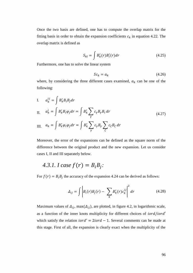
96
Once the two basis are defined, one has to compute the overlap matrix for the
fitting basis in order to obtain the expansion coefficients 𝑐𝑘 in equation 4.22. The
overlap matrix is defined as
𝑆𝑘𝑙 = ∫𝐵𝑘
′ (𝑟)𝐵𝑙′(𝑟)𝑑𝑟 (4.25)
Furthermore, one has to solve the linear system
𝑆𝑐𝑘 = 𝑎𝑘 (4.26)
where, by considering the three different cases examined, 𝑎𝑘 can be one of the
following:
I. 𝑎𝑘𝑖𝑗= ∫𝐵𝑘
′𝐵𝑖𝐵𝑗𝑑𝑟
(4.27) II. 𝑎𝑘𝑖 = ∫𝐵𝑘
′𝐵𝑖𝜑𝑗𝑑𝑟 = ∫𝐵𝑘′∑𝑐𝛾𝐵𝛾𝐵𝑖𝛾
𝑑𝑟
III. 𝑎𝑘 = ∫𝐵𝑘′𝜑𝑖𝜑𝑗𝑑𝑟 = ∫𝐵𝑘
′∑𝑐𝛾𝐵𝛾∑𝑐𝜁𝐵𝜁𝜁𝛾
𝑑𝑟
Moreover, the error of the expansions can be defined as the square norm of the
difference between the original product and the new expansion. Let us consider
cases I, II and III separately below.
4.3.1. I case 𝑓(𝑟) = 𝐵𝑖𝐵𝑗:
For 𝑓(𝑟) = 𝐵𝑖𝐵𝑗 the accuracy of the expansion 4.24 can be derived as follows:
𝛥𝑖𝑗 = ∫|𝐵𝑖(𝑟)𝐵𝑗(𝑟) − ∑𝐵𝑘′ (𝑟)𝑐𝑘
𝑖𝑗
𝑘
|
2
𝑑𝑟 (4.28)
Maximum values of 𝛥𝑖𝑗, max (𝛥𝑖𝑗), are plotted, in figure 4.2, in logarithmic scale,
as a function of the inner knots multiplicity for different choices of 𝑖𝑜𝑟𝑑/𝑖𝑜𝑟𝑑′
which satisfy the relation 𝑖𝑜𝑟𝑑′ = 2𝑖𝑜𝑟𝑑 − 1. Several comments can be made at
this stage. First of all, the expansion is clearly exact when the multiplicity of the
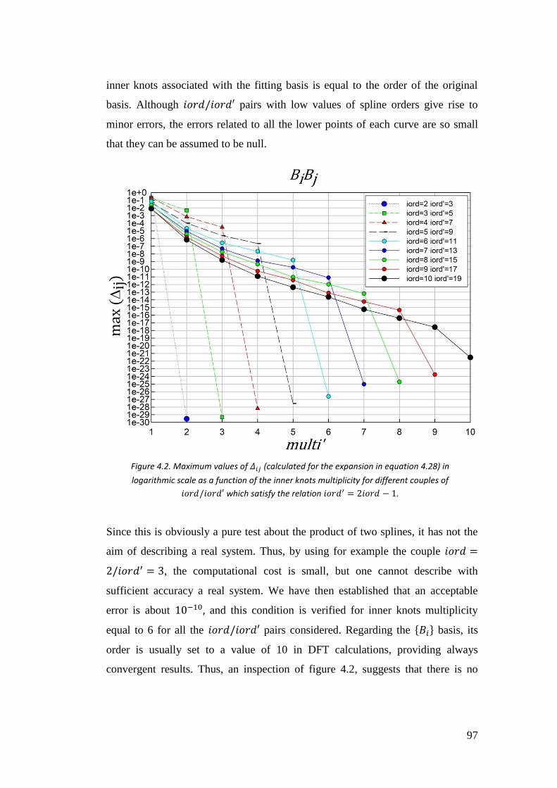
97
inner knots associated with the fitting basis is equal to the order of the original
basis. Although 𝑖𝑜𝑟𝑑/𝑖𝑜𝑟𝑑′ pairs with low values of spline orders give rise to
minor errors, the errors related to all the lower points of each curve are so small
that they can be assumed to be null.
Since this is obviously a pure test about the product of two splines, it has not the
aim of describing a real system. Thus, by using for example the couple 𝑖𝑜𝑟𝑑 =
2/𝑖𝑜𝑟𝑑′ = 3, the computational cost is small, but one cannot describe with
sufficient accuracy a real system. We have then established that an acceptable
error is about 10−10, and this condition is verified for inner knots multiplicity
equal to 6 for all the 𝑖𝑜𝑟𝑑/𝑖𝑜𝑟𝑑′ pairs considered. Regarding the {𝐵𝑖} basis, its
order is usually set to a value of 10 in DFT calculations, providing always
convergent results. Thus, an inspection of figure 4.2, suggests that there is no
Figure 4.2. Maximum values of 𝛥𝑖𝑗 (calculated for the expansion in equation 4.28) in
logarithmic scale as a function of the inner knots multiplicity for different couples of
𝑖𝑜𝑟𝑑/𝑖𝑜𝑟𝑑′ which satisfy the relation 𝑖𝑜𝑟𝑑′ = 2𝑖𝑜𝑟𝑑 − 1.
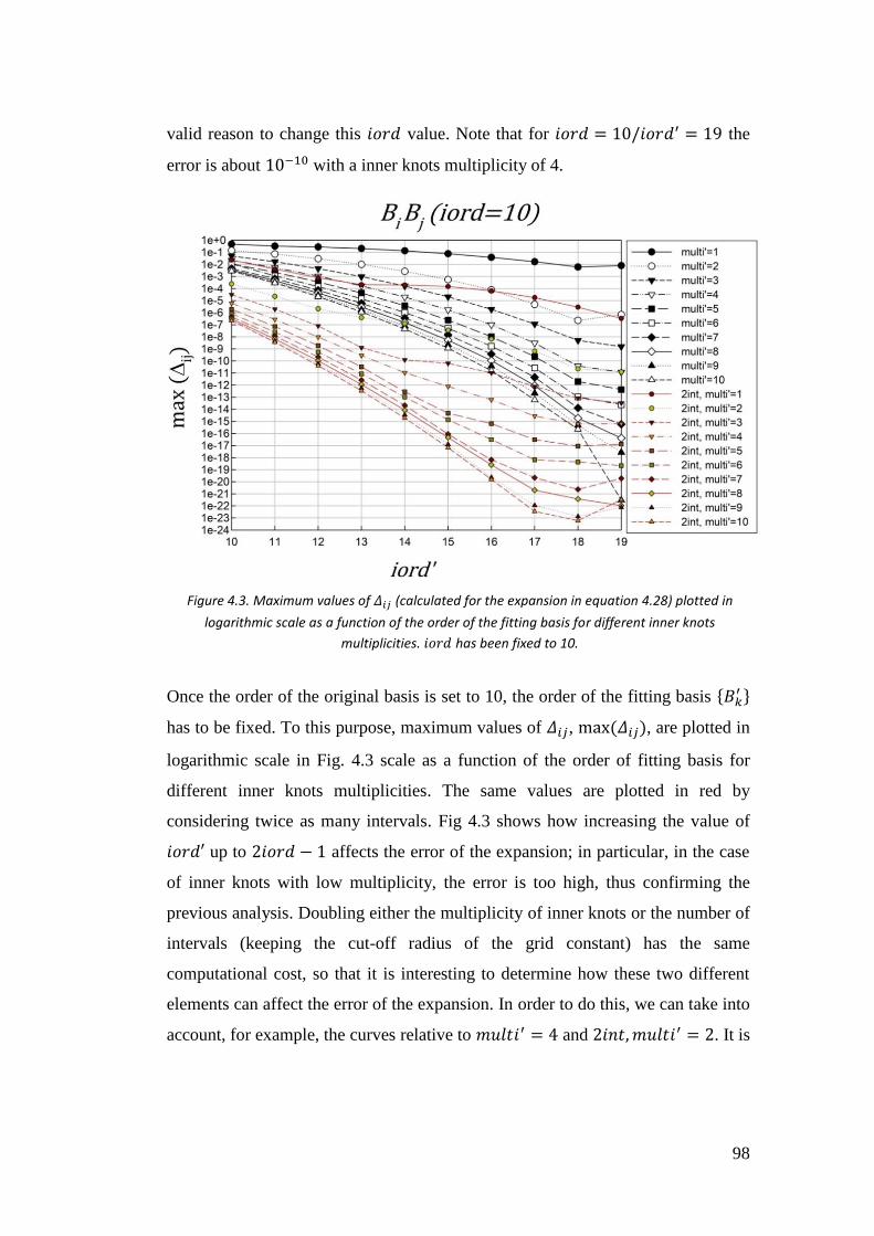
98
valid reason to change this 𝑖𝑜𝑟𝑑 value. Note that for 𝑖𝑜𝑟𝑑 = 10/𝑖𝑜𝑟𝑑′ = 19 the
error is about 10−10 with a inner knots multiplicity of 4.
Once the order of the original basis is set to 10, the order of the fitting basis {𝐵𝑘′ }
has to be fixed. To this purpose, maximum values of 𝛥𝑖𝑗, max (𝛥𝑖𝑗), are plotted in
logarithmic scale in Fig. 4.3 scale as a function of the order of fitting basis for
different inner knots multiplicities. The same values are plotted in red by
considering twice as many intervals. Fig 4.3 shows how increasing the value of
𝑖𝑜𝑟𝑑′ up to 2𝑖𝑜𝑟𝑑 − 1 affects the error of the expansion; in particular, in the case
of inner knots with low multiplicity, the error is too high, thus confirming the
previous analysis. Doubling either the multiplicity of inner knots or the number of
intervals (keeping the cut-off radius of the grid constant) has the same
computational cost, so that it is interesting to determine how these two different
elements can affect the error of the expansion. In order to do this, we can take into
account, for example, the curves relative to 𝑚𝑢𝑙𝑡𝑖′ = 4 and 2𝑖𝑛𝑡,𝑚𝑢𝑙𝑡𝑖′ = 2. It is
Figure 4.3. Maximum values of 𝛥𝑖𝑗 (calculated for the expansion in equation 4.28) plotted in
logarithmic scale as a function of the order of the fitting basis for different inner knots
multiplicities. 𝑖𝑜𝑟𝑑 has been fixed to 10.

99
easy to see how doubling the intervals provide better results at lower 𝑖𝑜𝑟𝑑′, but
furnishes almost the same accuracy with a value of 𝑖𝑜𝑟𝑑′ = 19. This trend is
observed for each pair (i.e., 𝑚𝑢𝑙𝑡𝑖′ = 6 and 2𝑖𝑛𝑡,𝑚𝑢𝑙𝑡𝑖′ = 3, 𝑚𝑢𝑙𝑡𝑖′ = 8 and
2𝑖𝑛𝑡, 𝑚𝑢𝑙𝑡𝑖′ = 4, or 𝑚𝑢𝑙𝑡𝑖′ = 10 and 2𝑖𝑛𝑡,𝑚𝑢𝑙𝑡𝑖′ = 5).
From a computational point of view, increasing the order of {𝐵𝑘′ } leads to an
increase in the knots only on the borders of the grid (see Fig. 4.1). Thus, it is
convenient to work such as the relation 𝑖𝑜𝑟𝑑′ = 2𝑖𝑜𝑟𝑑 − 1 is satisfied. In our
case, this means setting 𝑖𝑜𝑟𝑑 = 10 and 𝑖𝑜𝑟𝑑′ = 19. From the analysis of the last
points of the curves in Figure 4.3, we conclude that either doubling the intervals
or the multiplicity provide similar accuracy. Furthermore, an increase of the inner
knots multiplicity (or of the number of intervals) heavily affects the computational
cost. In fact, by doubling the inner knots multiplicity, the computational cost
doubles. An acceptable accuracy can be obtained with a inner knots multiplicity
equal to 4, so that by using this value of multiplicity together with 𝑖𝑜𝑟𝑑′ = 19, the
computational cost quadruples compared to the use of basis {𝐵𝑖}.
100
4.3.2. II case: 𝑓(𝑟) = 𝐵𝑖𝜑𝑗
The function to be expanded is a product of a B-spline function and an atomic
orbital. In this case, the error in the expansion is a vector defined as
𝛥𝑖 = ∫ |𝐵𝑖(𝑟)𝜑𝑗(𝑟) − ∑𝐵𝑘′ (𝑟)𝑐𝑘
𝑖
𝑘
|
2
𝑑𝑟
= ∫ |𝐵𝑖(𝑟)∑𝑐𝛾𝐵𝛾(𝑟)
𝛾
− ∑𝐵𝑘′ (𝑟)𝑐𝑘
𝑖
𝑘
|
2
𝑑𝑟
(4.29)
Thus, by considering all the error values for each spline index, 𝑖, one can get a
trend of the error as a function of the distance from the origin. A test has been
performed by taking into account the first six orbitals of Neon. On the left side of
figure 4.4 and figure 4.5, the error 𝛥𝑖, is plotted, in a logarithmic scale, as a
function of the related B-spline index for different values of inner knots
multiplicity (in black for single multiplicity, in red for double multiplicity and in
blue for triple multiplicity). On the right side of figure 4.4 and figure 4.5, the
radial part of Ne AOs has been plotted. In figure 4.4, the errors calculated for the
1𝑠, 2𝑠 and 3𝑠 orbitals of Ne are shown, while the corresponding for the 2𝑝, 3𝑝
and 3𝑑 AOs are reported in figure 4.5. All the calculations have been carried out
by using 𝑖𝑜𝑟𝑑 = 10 and 𝑖𝑜𝑟𝑑′ = 19.
Note that the curve relative to single multiplicity is rarely below an error of
10−10, so that, even in this case, although single multiplicity leads to a low
computational cost, it does not ensure good accuracy. Double and triple
multiplicity provide good results in almost every case. Only in the 1s and 2s cases,
errors are greater than 10−10 near the origin. This suggests that a non-linear grid
could be more suited for the case at hand. In fact, from the analysis of the shape of
the reported orbitals, one can observe a greater amplitude near the origin, while
the contribution decreases far from it.
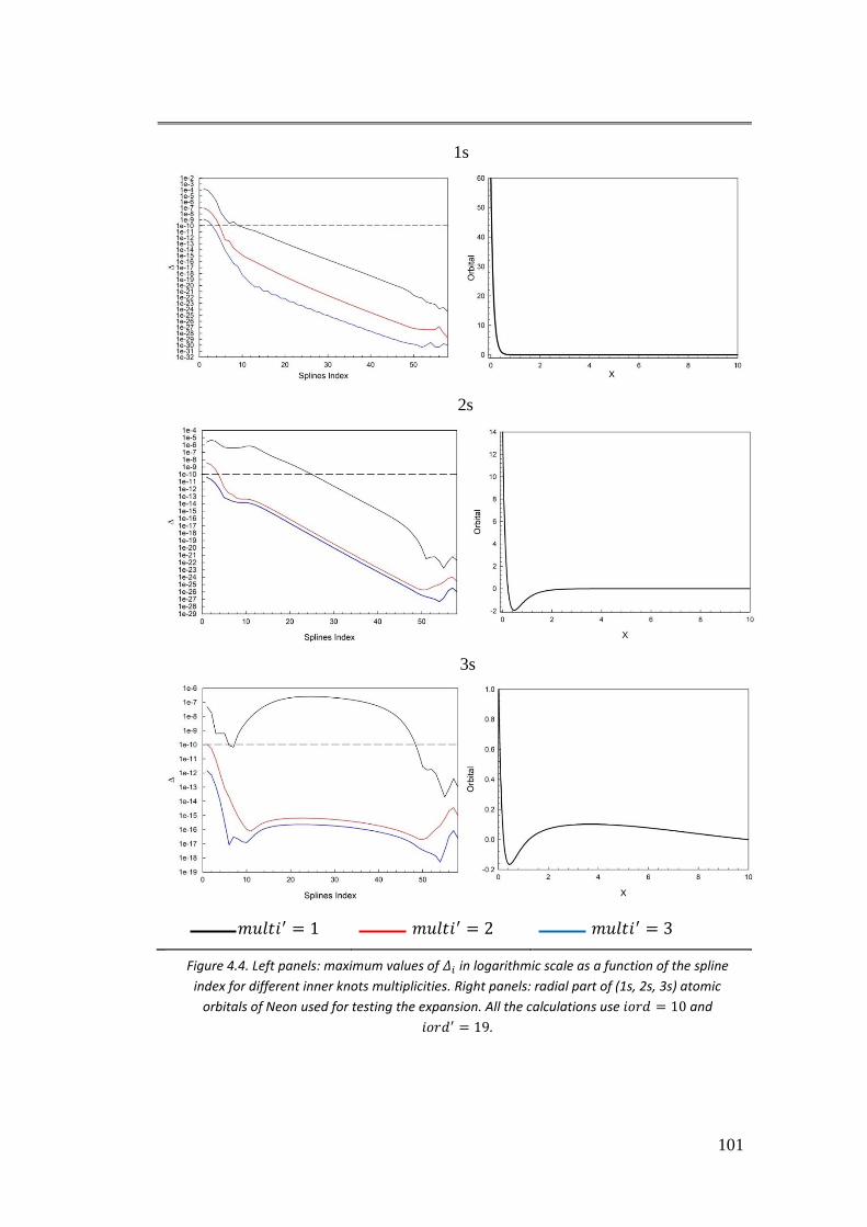
101
1s
2s
3s
𝑚𝑢𝑙𝑡𝑖′ = 1 𝑚𝑢𝑙𝑡𝑖′ = 2 𝑚𝑢𝑙𝑡𝑖′ = 3
Figure 4.4. Left panels: maximum values of 𝛥𝑖 in logarithmic scale as a function of the spline
index for different inner knots multiplicities. Right panels: radial part of (1s, 2s, 3s) atomic
orbitals of Neon used for testing the expansion. All the calculations use 𝑖𝑜𝑟𝑑 = 10 and
𝑖𝑜𝑟𝑑′ = 19.
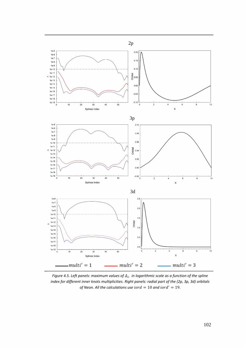
102
2p
3p
3d
𝑚𝑢𝑙𝑡𝑖′ = 1 𝑚𝑢𝑙𝑡𝑖′ = 2 𝑚𝑢𝑙𝑡𝑖′ = 3
Figure 4.5. Left panels: maximum values of 𝛥𝑖, in logarithmic scale as a function of the spline
index for different inner knots multiplicities. Right panels: radial part of the (2p, 3p, 3d) orbitals
of Neon. All the calculations use 𝑖𝑜𝑟𝑑 = 10 and 𝑖𝑜𝑟𝑑′ = 19.
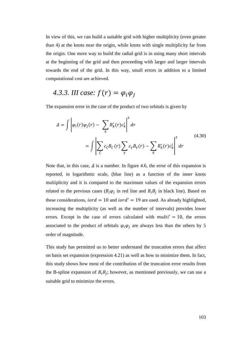
103
In view of this, we can build a suitable grid with higher multiplicity (even greater
than 4) at the knots near the origin, while knots with single multiplicity far from
the origin. One more way to build the radial grid is in using many short intervals
at the beginning of the grid and then proceeding with larger and larger intervals
towards the end of the grid. In this way, small errors in addition to a limited
computational cost are achieved.
4.3.3. III case: 𝑓(𝑟) = 𝜑𝑖𝜑𝑗
The expansion error in the case of the product of two orbitals is given by
𝛥 = ∫ |𝜑𝑖(𝑟)𝜑𝑗(𝑟) − ∑𝐵𝑘′ (𝑟)𝑐𝑘
𝑖
𝑘
|
2
𝑑𝑟
= ∫ |∑𝑐𝜁𝐵𝜁𝜁
(𝑟)∑𝑐𝛾𝐵𝛾(𝑟)
𝛾
−∑𝐵𝑘′ (𝑟)𝑐𝑘
𝑖
𝑘
|
2
𝑑𝑟
(4.30)
Note that, in this case, 𝛥 is a number. In figure 4.6, the error of this expansion is
reported, in logarithmic scale, (blue line) as a function of the inner knots
multiplicity and it is compared to the maximum values of the expansion errors
related to the previous cases (𝐵𝑖𝜑𝑗 in red line and 𝐵𝑖𝐵𝑗 in black line). Based on
these considerations, 𝑖𝑜𝑟𝑑 = 10 and 𝑖𝑜𝑟𝑑′ = 19 are used. As already highlighted,
increasing the multiplicity (as well as the number of intervals) provides lower
errors. Except in the case of errors calculated with 𝑚𝑢𝑙𝑡𝑖′ = 10, the errors
associated to the product of orbitals 𝜑𝑖𝜑𝑗 are always less than the others by 5
order of magnitude.
This study has permitted us to better understand the truncation errors that affect
on basis set expansion (expression 4.21) as well as how to minimize them. In fact,
this study shows how most of the contribution of the truncation error results from
the B-spline expansion of 𝐵𝑖𝐵𝑗; however, as mentioned previously, we can use a
suitable grid to minimize the errors.
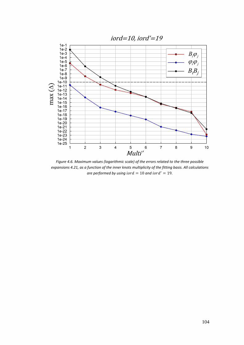
104
Figure 4.6. Maximum values (logarithmic scale) of the errors related to the three possible
expansions 4.21, as a function of the inner knots multiplicity of the fitting basis. All calculations
are performed by using 𝑖𝑜𝑟𝑑 = 10 and 𝑖𝑜𝑟𝑑′ = 19.
105
4.4. Potential from the Poisson equation
Let us expand a charge density 𝜌(𝒓) and the corresponding potential 𝑉(𝒓) in
spherical harmonics
𝜌(𝒓) =∑𝜌𝐿𝑀(𝑟)𝑌𝐿𝑀(휃, 𝜙)
𝐿𝑀
𝜌𝐿𝑀(𝑟) = ∫𝑌𝐿𝑀(𝜔)𝜌(𝒓)𝑑𝜔 (4.31)
𝑉(𝒓) =∑𝑉𝐿𝑀(𝑟)𝑌𝐿𝑀(휃, 𝜙)
𝐿𝑀
(4.32)
and using the multipole expansion
1
𝑟12=∑
4𝜋
2𝑙 + 1𝑙𝑚
𝑟<𝑙
𝑟>𝑙+1 𝑌𝑙𝑚(𝜔1)𝑌𝑙𝑚(𝜔2) (4.33)
the potential becomes
𝑉(𝒓𝟐) = ∫
𝜌(𝒓𝟏)
𝑟12𝑑𝒓𝟏 =∑
4𝜋
2𝑙 + 1𝑙𝑚
∫𝑟<𝑙
𝑟>𝑙+1 𝑌𝑙𝑚(𝜔1)𝜌(𝒓𝟏)𝑑𝒓𝟏 𝑌𝑙𝑚(𝜔2)
=∑∑4𝜋
2𝑙 + 1∫𝑟<𝑙
𝑟>𝑙+1 𝜌𝐿𝑀(𝑟1)𝑟1
2𝑑𝑟1∫𝑌𝑙𝑚(𝜔1) 𝑌𝐿𝑀(𝜔1)𝑑𝜔1 𝑌𝑙𝑚(𝜔2)
𝑙𝑚𝐿𝑀
=∑4𝜋
2𝑙 + 1∫𝑟<𝑙
𝑟>𝑙+1 𝜌𝐿𝑀(𝑟1)𝑟1
2𝑑𝑟1 𝑌𝐿𝑀(𝜔2)
𝐿𝑀
(4.34)
Now
∫
𝑟<𝑙
𝑟>𝑙+1 𝜌𝐿𝑀(𝑟1)𝑟1
2𝑑𝑟1
∞
0
=1
𝑟𝐿+1∫ 𝑡𝐿+2𝑟
0
𝜌𝐿𝑀(𝑡)𝑑𝑡 + 𝑟𝐿∫ 𝑡−𝐿+1
∞
0
𝜌𝐿𝑀(𝑡)𝑑𝑡
(4.35)
and finally
𝑉𝐿𝑀(𝑟) =
4𝜋
2𝑙 + 1[𝑄𝐿𝑀(𝑟)
𝑟𝐿+1+ 𝑟𝐿𝐼𝐿𝑀(𝑟)] (4.36)
where
106
𝑄𝐿𝑀(𝑟) = ∫ 𝑡𝐿+2
𝑟
0
𝜌𝐿𝑀(𝑡)𝑑𝑡 𝐼𝐿𝑀(𝑟) = ∫ 𝑡−𝐿+1𝑅𝑚𝑎𝑥
𝑟
𝜌𝐿𝑀(𝑡)𝑑𝑡 (4.37)
𝑅𝑚𝑎𝑥 is the range of 𝜌(𝒓), i.e. the minimum radius beyond which 𝜌 = 0
identically.
For 𝑟 ≥ 𝑅𝑚𝑎𝑥
𝑄𝐿𝑀(𝑟) = 𝑄𝐿𝑀, 𝐼𝐿𝑀 = 0 𝑉𝐿𝑀(𝑟) =
4𝜋
2𝑙 + 1
𝑄𝐿𝑀𝑟𝐿+1
(4.38)
For 𝜌(�̅�) finite at the origin,
𝑟 → 0 𝑄𝐿𝑀(𝑟)~ 𝑟𝐿+3 → 0 𝐼𝐿𝑀(𝑟) → 𝐼𝐿𝑀 𝑐𝑜𝑛𝑠𝑡 (4.39)
so that
𝑟 → 0 𝑉𝐿𝑀(𝑟) → 𝑐𝑜𝑛𝑠𝑡 (4.40)
𝑟 → ∞ 𝑉𝐿𝑀(𝑟) ~
4𝜋
2𝑙 + 1
𝑄𝐿𝑀𝑟𝐿+1
→ 0 (4.41)
One can get the potential relative to a charge density 𝜌 by solving the Poisson
equation (see Equation 4.14). Let us recall the form of the Laplacian in spherical
coordinates
∇2=
1
𝑟
𝜕2
𝜕𝑟2𝑟 +
𝐿2
𝑟2 (4.42)
Now defining �̃�𝐿𝑀(𝑟) = 𝑟𝑉𝐿𝑀(𝑟)
�̃�𝐿𝑀(𝑟) =
4𝜋
2𝑙 + 1[𝑄𝐿𝑀(𝑟)
𝑟𝐿+ 𝑟𝐿+1𝐼𝐿𝑀(𝑟)] (4.43)
and substituting the Equation 4.32 in the Poisson equation one obtains:
∑[
1
𝑟
𝑑2
𝑑𝑟2�̃�𝐿𝑀 +
𝐿(𝐿 + 1)
𝑟2�̃�𝐿𝑀𝑟] 𝑌𝐿𝑀
𝐿𝑀
= −4𝜋∑𝜌𝐿𝑀(𝑟)𝑌𝐿𝑀𝐿𝑀
(4.44)
that reduces to the radial equation
107
𝑑2
𝑑𝑟2�̃�𝐿𝑀 +
𝐿(𝐿 + 1)
𝑟2�̃�𝐿𝑀 = −4𝜋𝑟𝜌𝐿𝑀 (4.45)
Expanding �̃�𝐿𝑀(𝑟) in the B-spline basis
�̃�𝐿𝑀 =∑𝐵𝑗𝑣𝑗𝐿𝑀𝑗
(4.46)
and taking the scalar product with 𝐵𝑖 of the equation
∑[⟨𝐵𝑖|
𝑑2
𝑑𝑟2|𝐵𝑗⟩ − 𝐿(𝐿 + 1) ⟨𝐵𝑖|
1
𝑟2|𝐵𝑗⟩]
𝑗
𝑣𝑗𝐿𝑀 = −4𝜋⟨𝐵𝑖|𝑟𝜌𝐿𝑀⟩ (4.47)
4.4.1. Boundary Conditions
For 𝑟 → 0:
𝑟𝑉(𝒓) → 0 �̃�𝐿𝑀(𝑟) → 0 (4.48)
which is easily implemented as usual deleting the first spline.
For 𝑟 → ∞
𝑉𝐿𝑀(𝑟) →
4𝜋
2𝑙 + 1
𝑄𝐿𝑀𝑟𝐿+1
�̃�𝐿𝑀(𝑟) →4𝜋
2𝑙 + 1
𝑄𝐿𝑀𝑟𝐿
(4.49)
Notably, for 𝑟 → 𝑅𝑚𝑎𝑥
�̃�𝐿𝑀(𝑟) →
4𝜋
2𝑙 + 1
𝑄𝐿𝑀𝑅𝑚𝑎𝑥𝐿
(4.50)
Alternatively one can consider the limit for 𝑟 → 𝑅𝑚𝑎𝑥 of the derivative �̃�𝐿𝑀′ (𝑟).
The derivative of the first part of Equation 4.43 becomes:
108
𝑑
𝑑𝑟[𝑄𝐿𝑀(𝑟)
𝑟𝐿] =
𝑑
𝑑𝑟
1
𝑟𝐿∫ 𝑡𝐿+2𝜌𝐿𝑀(𝑡)𝑑𝑡𝑟
0
= −𝐿1
𝑟𝐿+1 ∫ 𝑡𝐿+2𝜌𝐿𝑀(𝑡)𝑑𝑡 +
𝑟
0
1
𝑟𝐿𝑟𝐿+2𝜌𝐿𝑀(𝑟)
= −𝐿𝑄𝐿𝑀𝑟𝐿+1
+ 𝑟2𝜌𝐿𝑀(𝑟)
(4.51)
the derivative of the second part of Equation 4.43 becomes:
𝑑
𝑑𝑟[𝑟𝐿+1𝐼𝐿𝑀(𝑟)] =
𝑑
𝑑𝑟𝑟𝐿+1∫ 𝑡−𝐿+1𝜌𝐿𝑀(𝑡)𝑑𝑡
𝑅𝑚𝑎𝑥
𝑟
= (𝐿 + 1)𝑟𝐿∫ 𝑡−𝐿+1𝜌𝐿𝑀(𝑡)𝑑𝑡𝑅𝑚𝑎𝑥
𝑟
+ 𝑟𝐿[𝑅𝑚𝑎𝑥−𝐿+1𝜌𝐿𝑀(𝑅𝑚𝑎𝑥) − 𝑟
−𝐿+1𝜌𝐿𝑀(𝑟)]
(4.52)
for 𝑟 → 𝑅𝑚𝑎𝑥 the second part is 0, thus
�̃�𝐿𝑀′ (𝑟) =
4𝜋
2𝑙 + 1[−𝐿
𝑄𝐿𝑀𝑟𝐿+1
+ 𝑟2𝜌𝐿𝑀(𝑟)]
= −𝐿
𝑟�̃�𝐿𝑀(𝑟) +
4𝜋
2𝑙 + 1𝑟2𝜌𝐿𝑀(𝑟)
(4.53)
for 𝑟 > 𝑅𝑚𝑎𝑥
�̃�𝐿𝑀′
�̃�𝐿𝑀= −
𝐿
𝑟 (4.54)
since 𝜌𝐿𝑀(𝑟) = 0.
If 𝜌(𝒓) = 0 for 𝑟 = 𝑅𝑚𝑎𝑥, then the homogeneous boundary condition
�̃�𝐿𝑀′
�̃�𝐿𝑀= −
𝐿
𝑅𝑚𝑎𝑥 (4.55)
can be implemented by substituting the last spline with the linear combination
�̂�𝑛−1 = 𝑎𝐵𝑛−1 + 𝐵𝑛 (4.56)
with coefficients determined by the condition

109
�̂�𝑛−1′ (𝑅𝑚𝑎𝑥) = −
𝐿
𝑅𝑚𝑎𝑥�̂�𝑛−1(𝑅𝑚𝑎𝑥) (4.57)
𝑎𝐵𝑛−1
′ (𝑅𝑚𝑎𝑥) + 𝐵𝑛′ (𝑅𝑚𝑎𝑥) = −
𝐿
𝑅𝑚𝑎𝑥[𝑎𝐵𝑛−1(𝑅𝑚𝑎𝑥) + 𝐵𝑛(𝑅𝑚𝑎𝑥)]
= −𝐿
𝑅𝑚𝑎𝑥
(4.58)
since 𝐵𝑛−1(𝑅𝑚𝑎𝑥) = 0 and 𝐵𝑛(𝑅𝑚𝑎𝑥) = 1, finally
𝑎 = −
𝐿𝑅𝑚𝑎𝑥
+ 𝐵𝑛′ (𝑅𝑚𝑎𝑥)
𝐵𝑛−1′ (𝑅𝑚𝑎𝑥)
(4.59)
So it is advantageous to work with densities that vanish at the outer boundary, as
is exactly verified when bound state orbitals are expanded with bound B-spline
only (i.e. excluding the last one), and product densities always include a bound
orbital factor.
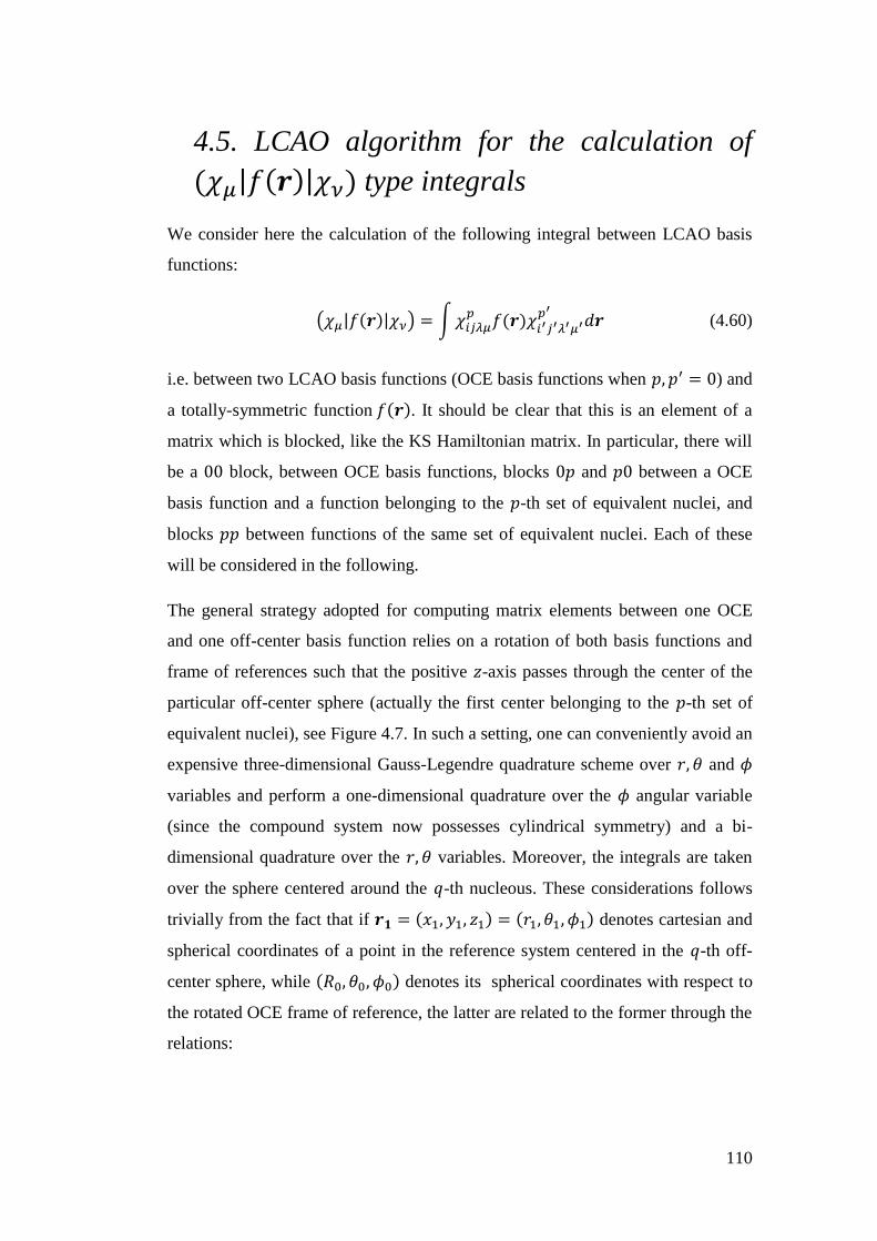
110
4.5. LCAO algorithm for the calculation of
(𝜒𝜇|𝑓(𝒓)|𝜒𝜈) type integrals
We consider here the calculation of the following integral between LCAO basis
functions:
(𝜒𝜇|𝑓(𝒓)|𝜒𝜈) = ∫𝜒𝑖𝑗𝜆𝜇
𝑝 𝑓(𝒓)𝜒𝑖′𝑗′𝜆′𝜇′𝑝′
𝑑𝒓 (4.60)
i.e. between two LCAO basis functions (OCE basis functions when 𝑝, 𝑝′ = 0) and
a totally-symmetric function 𝑓(𝒓). It should be clear that this is an element of a
matrix which is blocked, like the KS Hamiltonian matrix. In particular, there will
be a 00 block, between OCE basis functions, blocks 0𝑝 and 𝑝0 between a OCE
basis function and a function belonging to the 𝑝-th set of equivalent nuclei, and
blocks 𝑝𝑝 between functions of the same set of equivalent nuclei. Each of these
will be considered in the following.
The general strategy adopted for computing matrix elements between one OCE
and one off-center basis function relies on a rotation of both basis functions and
frame of references such that the positive 𝑧-axis passes through the center of the
particular off-center sphere (actually the first center belonging to the 𝑝-th set of
equivalent nuclei), see Figure 4.7. In such a setting, one can conveniently avoid an
expensive three-dimensional Gauss-Legendre quadrature scheme over 𝑟, 휃 and 𝜙
variables and perform a one-dimensional quadrature over the 𝜙 angular variable
(since the compound system now possesses cylindrical symmetry) and a bi-
dimensional quadrature over the 𝑟, 휃 variables. Moreover, the integrals are taken
over the sphere centered around the 𝑞-th nucleous. These considerations follows
trivially from the fact that if 𝒓𝟏 = (𝑥1, 𝑦1, 𝑧1) = (𝑟1, 휃1, 𝜙1) denotes cartesian and
spherical coordinates of a point in the reference system centered in the 𝑞-th off-
center sphere, while (𝑅0, 휃0, 𝜙0) denotes its spherical coordinates with respect to
the rotated OCE frame of reference, the latter are related to the former through the
relations:
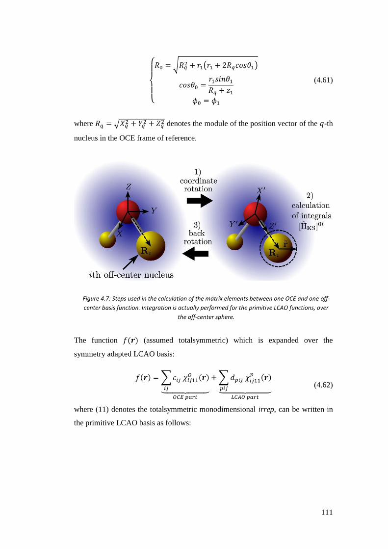
111
{
𝑅0 = √𝑅𝑞2 + 𝑟1(𝑟1 + 2𝑅𝑞𝑐𝑜𝑠휃1)
𝑐𝑜𝑠휃0 =𝑟1𝑠𝑖𝑛휃1𝑅𝑞 + 𝑧1
𝜙0 = 𝜙1
(4.61)
where 𝑅𝑞 = √𝑋𝑞2 + 𝑌𝑞2 + 𝑍𝑞2 denotes the module of the position vector of the 𝑞-th
nucleus in the OCE frame of reference.
The function 𝑓(𝒓) (assumed totalsymmetric) which is expanded over the
symmetry adapted LCAO basis:
𝑓(𝒓) =∑𝑐𝑖𝑗 𝜒𝑖𝑗11𝑂 (𝒓)
𝑖𝑗⏟ 𝑂𝐶𝐸 𝑝𝑎𝑟𝑡
+∑𝑑𝑝𝑖𝑗 𝜒𝑖𝑗11𝑝 (𝒓)
𝑝𝑖𝑗⏟ 𝐿𝐶𝐴𝑂 𝑝𝑎𝑟𝑡
(4.62)
where (11) denotes the totalsymmetric monodimensional irrep, can be written in
the primitive LCAO basis as follows:
Figure 4.7: Steps used in the calculation of the matrix elements between one OCE and one off-
center basis function. Integration is actually performed for the primitive LCAO functions, over
the off-center sphere.
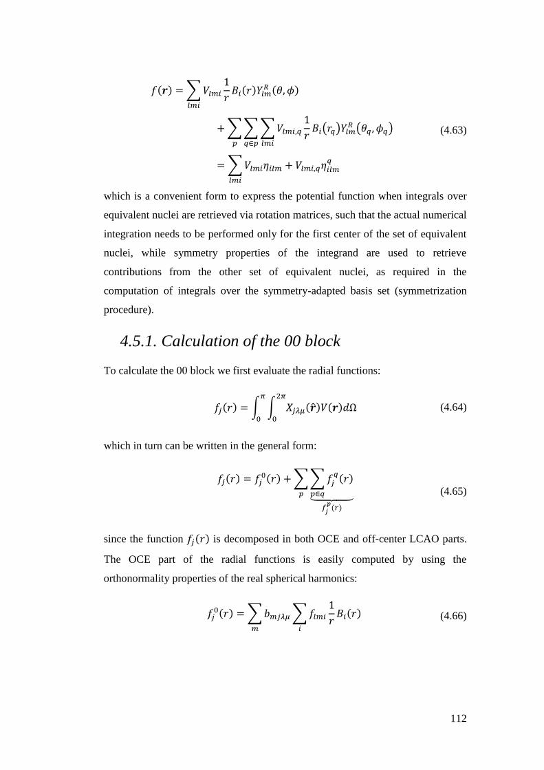
112
𝑓(𝒓) =∑𝑉𝑙𝑚𝑖
1
𝑟𝐵𝑖(𝑟)𝑌𝑙𝑚
𝑅 (휃, 𝜙)
𝑙𝑚𝑖
+∑∑∑𝑉𝑙𝑚𝑖,𝑞1
𝑟𝐵𝑖(𝑟𝑞)𝑌𝑙𝑚
𝑅 (휃𝑞 , 𝜙𝑞)
𝑙𝑚𝑖𝑞∈𝑝𝑝
=∑𝑉𝑙𝑚𝑖휂𝑖𝑙𝑚 + 𝑉𝑙𝑚𝑖,𝑞휂𝑖𝑙𝑚𝑞
𝑙𝑚𝑖
(4.63)
which is a convenient form to express the potential function when integrals over
equivalent nuclei are retrieved via rotation matrices, such that the actual numerical
integration needs to be performed only for the first center of the set of equivalent
nuclei, while symmetry properties of the integrand are used to retrieve
contributions from the other set of equivalent nuclei, as required in the
computation of integrals over the symmetry-adapted basis set (symmetrization
procedure).
4.5.1. Calculation of the 00 block
To calculate the 00 block we first evaluate the radial functions:
𝑓𝑗(𝑟) = ∫ ∫ 𝑋𝑗𝜆𝜇(�̂�)𝑉(𝒓)𝑑Ω
2𝜋
0
𝜋
0
(4.64)
which in turn can be written in the general form:
𝑓𝑗(𝑟) = 𝑓𝑗0(𝑟) +∑∑𝑓𝑗
𝑞(𝑟)
𝑝∈𝑞⏟ 𝑓𝑗𝑝(𝑟)
𝑝
(4.65)
since the function 𝑓𝑗(𝑟) is decomposed in both OCE and off-center LCAO parts.
The OCE part of the radial functions is easily computed by using the
orthonormality properties of the real spherical harmonics:
𝑓𝑗0(𝑟) =∑𝑏𝑚𝑗𝜆𝜇∑𝑓𝑙𝑚𝑖
1
𝑟𝐵𝑖(𝑟)
𝑖𝑚
(4.66)
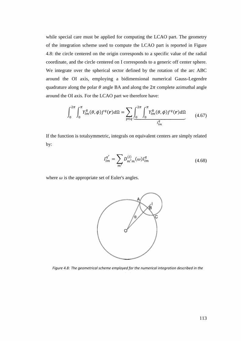
113
while special care must be applied for computing the LCAO part. The geometry
of the integration scheme used to compute the LCAO part is reported in Figure
4.8: the circle centered on the origin corresponds to a specific value of the radial
coordinate, and the circle centered on I corresponds to a generic off center sphere.
We integrate over the spherical sector defined by the rotation of the arc ABC
around the OI axis, employing a bidimensional numerical Gauss-Legendre
quadrature along the polar 휃 angle BA and along the 2𝜋 complete azimuthal angle
around the OI axis. For the LCAO part we therefore have:
∫ ∫ 𝑌𝑙𝑚
𝑅 (휃, 𝜙)𝑓𝑞(𝒓)𝑑Ω𝜋
0
2𝜋
0
=∑∫ ∫ 𝑌𝑙𝑚𝑅 (휃, 𝜙)𝑓𝑞(𝒓)𝑑Ω
𝜋
0
2𝜋
0⏟ 𝐼𝑙𝑚𝑞
𝑝∈𝑞
(4.67)
If the function is totalsymmetric, integrals on equivalent centers are simply related
by:
𝐼𝑙𝑚𝑞′ =∑𝐷
𝑚′𝑚
(𝑙) (𝜔)𝐼𝑙𝑚𝑞
𝑚′
(4.68)
where 𝜔 is the appropriate set of Euler's angles.
Figure 4.8: The geometrical scheme employed for the numerical integration described in the
text
114
Once the angular decomposition over the OCE basis has been performed, the 00
block can be calculated as:
⟨𝜒𝑖𝑗𝜆𝜇0 |𝑓(𝒓)|𝜒𝑖′𝑗′𝜆′𝜇′
0 ⟩
= ∑∫ 𝐵𝑖(𝑟)𝑓𝑗𝜅(𝑟)𝐵𝑖′(𝑟)𝑑𝑟 × ⟨𝑋𝑗𝜆𝜇|𝑋𝑗𝜅11|𝑋𝑗′𝜆′𝜇′⟩𝑅𝑚𝑎𝑥
0𝑗𝜅
(4.69)
i.e. as a sum of products of radial integrals times angular integrals that can be
evaluated analytically.
4.5.2. Calculation of the 0𝑝, 𝑝0, and 𝑝𝑝 blocks
Integrals of this type are numerically evaluated in the primitive LCAO basis
functions, while integrals over the symmetry-adapted basis are obtained with a
simple symmetrization procedure. Coefficients 𝑓𝑙𝑚𝑖 and 𝑓𝑙𝑚𝑖,𝑞′ of Eq. (4.63) refer
to the original iso-oriented reference systems and are related to the 𝑓𝑙𝑚𝑖 and 𝑓𝑙𝑚𝑖,𝑞′
referred to the rotated reference systems:
𝑓𝑙𝑚𝑖,𝑞′ =∑𝑉𝑙𝑚′𝑖𝐷𝑚𝑚′
(𝑙)(𝑅)
𝑚′
(4.70)
𝑓𝑞𝑙𝑚𝑖′ =∑𝑉𝑙𝑚′𝑖,𝑞𝐷𝑚𝑚′
(𝑙)(𝑅)
𝑚′
(4.71)
where 𝑅 denotes the set of Euler angles that specify the rotation that brings the
rotated reference systems into the original one. Then, on the sphere centered on
the first atom of the equivalent set, the following integrals (in the rotated reference
system) are numerically computed:
{⟨휂𝑖𝑙𝑚|𝑓(𝒓)|휂𝑖′𝑙′𝑚′
𝑞⟩ 01𝑏𝑙𝑜𝑐𝑘𝑠
⟨휂𝑖𝑙𝑚𝑞 |𝑓(𝒓)|휂
𝑖′𝑙′𝑚′𝑞
⟩ 11𝑏𝑙𝑜𝑐𝑘𝑠 (4.72)
As mentioned above, the rotation of the coordinate systems permits to avoid an
expensive three-dimensional Gauss-Legendre quadrature scheme over 𝑟, 휃 and 𝜙
115
variables and perform a one-dimensional quadrature over the 𝜙 angular variable
and a bi-dimensional quadrature over the 𝑟, 휃 variables.
In the computation of the matrix elements over the laplacian operators (∇2), as
required in the solution of the Poisson's equation in the LCAO basis set, the
integration over 𝜙 is analytical. Furthermore, the short-hand notation 01 and 11 is
used to remind us that the integration is numerically done only for the first center
of set of equivalent centers belonging to the 𝑝-th set. Integrals among LCAO
primitive basis functions for the other (𝑞 ≠ 1) centers of the equivalent set are
simply related by symmetry, by using the well-know rotational properties of the
real spherical harmonics, and using the symmetry properties of 𝑓(𝒓) (numerically
the same for a totalsymmetric function). Note that integrals over all primitive
basis functions are needed in the subsequent symmetrization procedure which is
performed to retrieve the integrals over the symmetry adapted LCAO basis.
For the case of a non totalsymmetric potential, integrals over the LCAO primitive
functions centered in the 𝑞 ≠ 1 sphere are related to those calculated in the first
sphere as follows: suppose that the function to be integrated belongs to the 𝜇-th
component of the 𝜆’s IR, i.e. 𝑉(𝒓) ≡ 𝑓𝑘𝜆𝑘𝜇𝑘(𝒓). Then we have:
𝑓𝑘𝜆𝑘𝜇𝑘(𝒓′) = 𝑓𝑘𝜆𝑘𝜇𝑘(𝑅𝒓) = (𝑅
−1𝑓𝑘𝜆𝑘𝜇𝑘)(𝒓) (4.73)
where
𝑅𝑓𝑘𝜆𝑘𝜇𝑘 =∑𝑓𝑘𝜆𝑘𝜇𝑘′𝐷𝜇𝑘𝜇𝑘
′𝜆 (𝑅)
𝜇𝑘′
(4.74)
In our case, the function 𝑓 can be either a MO (𝑓 = 𝜑𝑘𝜆𝑘𝜇𝑘) or a potential term,
solution of the corresponding Poisson's equation. In the algorithm, the procedure
outline above is used to evaluate the following integrals:
matrices 𝑏𝜎𝜈𝑗 = ⟨𝜒𝑖𝑗𝜆𝜇𝑝 |𝜑𝑘𝜆𝑘𝜇𝑘𝜒𝑖′𝑗′𝜆′𝜇′
𝑝′⟩
integrals of the 𝑉𝑖𝑗potential terms over LCAO basis functions, i.e.
⟨𝜒𝑖𝑗𝜆𝜇𝑝 |𝑉𝑖𝑗𝜆𝑖𝑗𝜇𝑖𝑗|𝜒𝑖′𝑗′𝜆′𝜇′
𝑝′⟩

116
while integrals 𝑏𝜎𝑘𝑙 = ⟨𝜒𝑖𝑗𝜆𝜇𝑝 |𝜑𝑘𝜆𝑘𝜇𝑘𝜑𝑙𝜆𝑙𝜇𝑙⟩ are evaluated with the same module
used to project a given MO obtained from a quantum chemistry package on the
LCAO basis.
4.6. Preliminary checks
So far the program has been tested in the following cases: integrals (𝜑𝑖𝜑𝑗|𝜒𝜇𝜒𝜈)
and (𝜑𝑖𝜒𝜇|𝜑𝑗𝜒𝜈) calculated at the OCE level have been compared with the
analogous calculated by using two-electron integrals over B-splines; (𝜑𝑖𝜑𝑗|𝜑𝑘𝜑𝑙)
have been calculated and compared with those obtained by using a quantum-
chemistry package like MOLPRO [47]. We have verified that accurate values for
(𝜑𝑖𝜑𝑗|𝜒𝜇𝜒𝜈) and (𝜑𝑖𝜒𝜇|𝜑𝑗𝜒𝜈) integrals are obtained in agreement with the
general requirements for the auxiliary basis set that emerge from the analysis
reported in the previous section. Accurate values for (𝜑𝑖𝜑𝑗|𝜑𝑘𝜑𝑙) can instead be
obtained by using the same LCAO basis set in the expansion of the potential
terms, as evidenced in Table 4.1 which report a comparison between two-electron
integrals for selected MOs calculated by using the MOLPRO quantum chemistry
package and the corresponding integrals calculated with the present algorithm.
Note that the implementation requires a preliminary step where MOs output from
MOLPRO are first expanded in the LCAO basis. The LCAO basis used in the
projection step has the following characteristics: the order of the radial B-spline
basis set is of order 10 for both the OCE expansion and the LCAO basis on the
off-center spheres; B-splines of the OCE expansions are defined in a radial grid of
knots extending up to 20.0 a.u. and with a linear step size of 0.25 a.u. while the
radial grid on the N atoms extends up to 0.6 a.u. The truncation of the OCE
expansion has been set to 𝑙𝑚𝑎𝑥𝑂𝐶𝐸 = 15, while the maximum angular momentum in
the off-center spheres is 𝑙𝑚𝑎𝑥𝑁 = 2.

117
int. MOLPRO
(HF/aug-ccPVTZ)
B-splines
(𝑙𝑚𝑎𝑥0 = 15, 𝑙𝑚𝑎𝑥
𝑁 = 2)
(1𝑎𝑔1𝑎𝑔|1𝑎𝑔1𝑎𝑔) 2.3015840737 2.3015822015
(2𝑎𝑔1𝑎𝑔|1𝑎𝑔1𝑎𝑔) -0.1980272759 -0.1980267754
(1𝑏2𝑢1𝑏2𝑢|1𝑏3𝑢1𝑏3𝑢) 0.5298663224 0.5298661084
(1𝑏2𝑢1𝑏2𝑢|1𝑏2𝑢1𝑏2𝑢) 0.5762867089 0.5762864532
Table 4.1: Two-electron integrals over MOs obtained at the HF/aug-ccpVTZ model chemistry
for 𝑁2. The experimental 𝑁-𝑁 bond distance has been used.
118
5. Non-perturbative regime
5.1. Introduction
The availability of very strong, ultra-short pulses of electromagnetic radiation, due
continual advancement in laser sources, including free electron lasers (FEL) has
generated an intense research activity in their interaction with matter, and
molecules in particular. Several new phenomena have been uncovered, giving rise
to the so called strong-field physics, in parallel with investigation of ultra-short
dynamics in pump-probe experiments, moving from nuclear dynamics in the
femto/picosecond regime [64] to the purely electronic motion triggered by broad
attosecond pulses. The description of strong field phenomena has been dominated
by the strong field model, starting with the so called three-step [65], or simpleman
model [66] with successive sophistication.
In principle a complete description is afforded by solution of the TDSE in the
external field, which is however very expensive, and has been applied only
simplest system, often in reduced dimensionality. We have undertaken an
extension, based on the availability of the very flexible and complete basis offered
by the LCAO B-spline approach. The obvious prerequisite is the set up and
validation of an efficient numerical TDSE solver, in conjunction with the B-spline
basis. A quick tour of interesting phenomena is as follow.
The prediction of the above-threshold ionization (ATI) photoelectron energy
spectrum is a challenging theoretical issue, mainly under conditions of ultrashort
and high-intensity pulses with several peaks. The comparison of the theoretical
results with the experimental data shows how difficult is to describe the sudden
appearance of side lobes or slope changes in the photoelectron spectra. In fact, it
is really demanding to establish convergence in this kind of calculations, which
involve the same requirements posed by the high-intensity non-perturbative
phenomenon, namely the high-order harmonic generation (HOHG). Thus, a non-
perturbative calculation in the presence of a strong field is required and it has to
119
be followed by the analysis of the photoelectron energy and, in some cases, by the
analysis of the angle-resolved spectrum.
The wavefunction can be expanded in terms of the eigenstates of the atom [67] or,
as in this work, in terms of a B-splines basis. Each method has advantages and
disadvantages, but they are complementary to other techniques.
Initially, the attention has been focused on the hydrogen atom because it can be
described by an exact potential, so direct calculations can be obtained. In addition
to this, the results can be compared to the experimental data [68]. In this way we
can obtain a benchmark calculation useful to compare different methods [69].
It is also of great interest for physics and chemistry trying to obtain time-resolved
imaging of chemical reactions or other structural changes with sub-femtosecond
resolution. In literature there are several examples of near-infrared ultrashort laser
experiments [70] [71] which can furnish information about the valence electrons
extracted by the radiation and the time resolution.
Time-resolved spectra at the atomic/molecular time scales are now accessible
thanks to studies of intense ultrashort fs and XUV laser pulses [72] [73] [74].
Furthermore, some experiments demonstrate that more than one orbital affects the
molecular strong-field response [75] [76] [77]. Although these multi-orbital
effects can furnish a lot of information, they complicate simple imaging schemes.
For example, by analysing the high-harmonic radiation [78], one can observe the
electron-hole in the ion generated by laser.
So far, it doesn’t seem possible yet to make direct imaging of the valence
electrons and of their field-free dynamics during, for example, a more complicated
chemical reaction.
Moreover, nuclear motion plays a crucial role in the competition of the different
molecular photoionization processes, such as autoionization (AI), dissociative
ionization (DI) and non dissociative ionization (NDI) [79] [80]. A temporal
picture of these competing processes can be obtained through calculations that
solve time-dependent Schrödinger equation by adding information to the
stationary pictures.
120
F. Martin et al [81] have shown how to analyze both the short- and the long-time
response of the H2 molecule after the absorption of one or several photons, using a
method based on the expansion of the time-dependent wavefunction in a basis of
discrete stationary states.
For example, one- and multi-photon ionization processes in the hydrogen
molecule are:
H2 + nħω H + H+ + e
- (DI)
H2 + nħω H2+ + e
- (NDI)
H2 + nħω H + H (D)
There are two regimes of photon energy: the multiphoton regime, where two or
more photons can be absorbed, and the one-photon regime. In the H2 case, the
first regime occurs from 2.7 to 13.7 eV, while the second one occurs from 25 to
40 eV, a range in which we can observe the autoionization process.
In the multiphoton regime, when the photon energy is in resonance with a bound
intermediate state, the multiphoton ionization probability is led by the proper
inclusion of the nuclear motion.
In the other case, the time-dependent Schrödinger equation affords to study the
interference phenomena appearing in the dissociative ionization, due both to the
autoionization and dissociation processes that arise from doubly excited states.
In this contest, the gauge of the electromagnetic field represents an important
formalism. It will be discuss in the next chapter.
121
5.1.1. Electromagnetic field gauges
According to a fundamental law of electromagnetic theory, the interaction of the
electromagnetic (EM) radiation with matter should be independent with respect to
the gauge of the electromagnetic field employed in the formulation of the
problem.
In perturbation theory and the dipole approximation, three gauges (length,
velocity and acceleration) are commonly employed in the non-relativistic theory
of the interaction of optical or UV frequencies with atoms or molecules, within
the dipole approximation.
Thus, when the transition amplitudes calculated within perturbation theory and
exact atomic wavefunctions are used, the result are the same in all three gauges.
Since it is not possible to get exact wavefunctions (except for the case of the
hydrogen atom), the agreement of the calculations in the different gauges is used
as criterion to probe the quality of the wavefunctions used in the calculation.
The situation is more complicated for the interaction of strong radiation with
atoms in the non-perturbative theory. The demands for the convergence of the
calculation are now more severe.
Convergence depends on many parameters (as well as the quality of the
wavefunctions), such as the number of the angular momenta, the spatial extent of
the total wavefunction, the time step in the integration of the time-dependent
Schrödinger equation (TDSE). Since one cannot know a priori their best
combination, each parameter is differently set during the calculation and may
differ from method to method.
In some cases, even within the same set of parameters and with the exact
wavefunctions, a time-dependent calculation converges much faster in one gauge
than in the other one.
Furthermore, the demands for convergence for one quantity could be different
from case to case, for example from the photoelectron spectrum of above-
threshold ionization (ATI) to ion yield.
122
An interesting case is represented by the number of angular momenta required for
convergence: in fact, when the problem is solved in the velocity gauge, the
number of angular momenta required for convergence dramatically decreases with
respect to the length gauge [82].
In this section, the main steps that lead to the expression of the Schrödinger
equation describing the behaviour of an atom in the presence of a strong
electromagnetic field, represented in the so-called ‘velocity’ and ‘length gauge’,
will be summarized. This issue is clearly discussed in Cohen-Tannoudji et al
(1989).
Let us consider an electron in a potential under the action of an external
electromagnetic field. Within the non-relativistic theory, the field can be
expressed in terms of vector and scalar potentials, A(r,t) and U(r,t), respectively,
as
𝐸 = −∇𝑈 −
𝑑𝐴
𝑑𝑡 𝑎𝑛𝑑 𝐵 = ∇ × 𝐴 (5.1)
and a gauge transformation generates new potentials 𝐴′, 𝑈′ that leave the fields
unchanged.
Using the Lagrangian formalism, we can express the Hamiltonian in the so called
minimal coupling form, as:
𝐻𝑣 =
1
2𝑚[𝒑𝑣 − 𝑞𝑨𝑣(𝒓, 𝑡)]
2 + 𝑉(𝑟) + 𝑞𝑈𝑣(𝒓, 𝑡) (5.2)
where q is the electron charge and m is the electron mass The gauge freedom
allows one to choose arbitrarily the value of ∇ ∙ 𝑨. The most common form to
describe radiation field is the coulomb gauge
∇ ∙ 𝑨 = 0 (5.3)
For a radiation field (𝜌 = 0, 𝑗 = 0) this requires also 𝑈 = 0. In Equation 5.2, 𝑝𝑣 is
the conjugate of 𝑟𝑣. They can be expressed as follows:
𝑟𝑣 = 𝑟 → 𝑟 (5.4)
123
𝑝𝑣 = 𝑚�̇� − (− 𝑞𝑨𝑣(𝒓, 𝑡)) → −𝑖ħ𝛻
𝑟 has no more any subscripts being gauge-indipendent because of the mechanical
momentum of the particle 𝜋 = 𝑚�̇� that is gauge-independent as well. Since the
two conjugate variables are substituted with the operators by the quantization
principle in the Equation 5.4, it is not relevant what they represent. The
Hamiltonian then becomes:
𝐻 =
1
2𝑚𝑝2 +
1
𝑚𝑨 ∙ 𝒑 +
1
2𝑚𝐴2 + 𝑉(𝑟) (5.5)
Thus, TDSE equation is satisfied by the total wavefunction of the system:
𝑖ħ𝜕
𝜕𝑡𝛹𝑣(𝒓, 𝑡) = 𝐻𝑣(𝒓, 𝑡)𝛹𝑣(𝒓, 𝑡) (5.6)
In order to obtain the Hamiltonian in the length gauge, one needs to express the
potentials and the operators in the new gauge. This can be done by using some
transformation formulas. In the case of potentials, they are:
𝑨𝑙(𝒓, 𝑡) = 𝑨𝑣(𝒓, 𝑡) + ∇𝜒(𝒓, 𝑡)
𝑼𝑙(𝒓, 𝑡) = 𝑼𝑣(𝒓, 𝑡) −𝜕
𝜕𝑡𝜒(𝒓, 𝑡)
(5.7)
and for the wavefunction it is:
𝛹𝑙(𝑟, 𝑡) = 𝑇𝛹𝑣(𝑟, 𝑡) = 𝑒(𝑖/ħ)𝑞𝜒(𝑟,𝑡)𝛹𝑣(𝑟, 𝑡) (5.8)
where 𝜒(𝒓, 𝑡) refers to gauge function that might be dependent on 𝒓 and 𝑡.
Göppert-Mayer [83] transformation can be used to obtain the equation expressed
in the ‘length gauge’. This transformation is based on the following gauge
function:
𝜒(𝒓, 𝑡) = −𝒓𝑨𝑣(0, 𝑡) (5.9)
The Hamiltonian in length gauge can be obtained by using Equations 5.7 and 5.9
and applying the electric dipole approximation:
124
𝐻𝑙 =
1
2𝑚𝒑𝑙2 + 𝑉(𝑟) + 𝑞𝒓𝑬(0, 𝑡) (5.10)
where 𝑬(0, 𝑡) is:
𝑬(0, 𝑡) = −
𝜕
𝜕𝑡𝐴(0, 𝑡) − 𝛻𝑈(0, 𝑡) (5.11)
This is the gauge-independent electric field within the dipole approximation. The
conjugate operators become:
𝑟𝑙 = 𝑟 → 𝑟
𝑝𝑙 = 𝑚�̇� → −𝑖ħ∇ (5.12)
Thus, the total wavefunction is now the solution of the TDSE equation in the
length gauge:
𝑖ħ𝜕
𝜕𝑡𝛹𝑙(𝒓, 𝑡) = 𝐻𝑙(𝒓, 𝑡)𝛹𝑙(𝒓, 𝑡) (5.13)
By summarizing, the Hamiltonian (in a.u. and in the dipole approximation,
neglecting the spatial dependence of the fields) is
𝐻(𝑡) = 𝐻0 − 𝑖�̅�(𝑡) ∙ ∇ 𝛹𝑉(𝑟, 𝑡) 𝑉 − 𝑔𝑎𝑢𝑔𝑒
𝐻(𝑡) = 𝐻0 − �̅�(𝑡) ∙ r̅ 𝛹𝐿(𝑟, 𝑡) 𝐿 − 𝑔𝑎𝑢𝑔𝑒
(5.14)
with
𝐸(𝑡) = −
𝜕𝐴(𝑡)
𝜕𝑡 𝐴(𝑡) = −∫ 𝐸(𝑠)𝑑𝑠
𝑡
0
(5.15)
At the end of the pulse of length T (with 𝑡 > 𝑇), E is equal to 0. We also impose
the condition A(t) = 0 to avoid a global additional time-dependent phase factor.
We employ a pulse of the form
𝐴(𝑡) = 𝐴0𝑓(𝑡)𝑠𝑖𝑛 (𝜔𝑡 + 𝜙) (5.16)
where 𝑓(𝑡) is a slowly varying function which defines the shape of the pulse, and
𝜙 is called the carrier envelope phase (CEP). 𝐴0 is the peak value related to the
peak of 𝐸 by 𝐴0 = 𝜔𝐸0.
125
5.1.2. Influences on the photoionization spectrum
Ionization is a physical process (multiphoton transition) from an initial state to a
final state lying in the electronic continuum through virtual intermediate states.
This process is influenced by both the pulse parameters and the level structure of
the system. The TDSE numerical solution provides photoelectron energy
spectrum, which is difficult to obtain, even for the case of the hydrogen atom.
Since this represents the simplest quantum system, it is the most used system to
understand the basic behaviour of the ionization processes. The hydrogen atom
makes possible accurate ab-initio numerical calculations and allows a complete
control of the convergence.
In the literature, a big number of hydrogen ionization studies has been published.
However, most of them use additional approximations, such as reducing the
dimensionality of the problem or employing a restricted basis set. Only a few of
these provide results which can be used for an exact comparison.
Besides the direct integration of TDSE the strong field problem in the non-
perturbative regime can be treated by ab-initio Floquet theory [84], variably
implemented such as Sturmian-Floquet [85] and R-matrix-Floquet (RMF) theory
[86].This treatment is exact for an infinite pulse duration (periodic field) but can
be used also for slowly variable envelopes. It has been used for multiphoton
ionization and high-order harmonic generation for atoms under electromagnetic
fields characterized by constant or slightly variable intensity.
Almost all approaches to the numerical solution of the TDSE employ a spatial
discretization of the wavefunction, either as amplitudes on a selected grid of
points: 𝑎𝑖(𝑡) = Ψ(𝑟𝑖, 𝑡), or as an expansion in a fixed basis set {𝜙𝑖},
Ψ(𝑡) =∑𝑎𝑖(𝑡)𝜙𝑖𝑖
. (5.17)
In any case the partial differential equation is transformed into a large system of
coupled ordinary differential equations (ODE) in the coefficients 𝑎𝑖(𝑡).
126
𝑖𝑑
𝑑𝑡𝑎𝑖(𝑡) =∑𝑀𝑖𝑗(𝑡)𝑎𝑗(𝑡)
𝑗
(5.18)
where 𝑀𝑖𝑗 is the corresponding discretization of the Hamiltonian.
There are several methods to solve ODE problems. Among them, Runge-Kutta
[87] [88] is the most used since it represents a good compromise between
efficiency and accuracy. This method is commonly used for a general system,
which does not require specific conditions. In our case, the Schrödinger equation
satisfies special conditions, such as unitary evolution (which is not satisfied by the
Runge-Kutta method) and temporal reversibility. One can expect that the use of a
method which satisfies these conditions can provide more accurate results than
methods which do not satisfy them.
A special choice used to solve the TDSE problem consists in expanding the
wavefunction on a suitable orthonormal basis. In the case of the hydrogen atom,
one can expand the wavefunction on the basis of his eigenstates:
𝛹(𝒓, 𝑡) =∑𝐶𝑛𝑙(𝑡)𝜓𝑛𝑙(𝒓)
𝑛𝑙
(5.19)
This provides the time-dependent basis state population:
𝑃𝑛𝑙 = |𝐶𝑛𝑙(𝑡)|2 (5.20)
The ionization probabilities and other final observables at 𝑡 = 𝑡𝑓 do not change;
as a consequence, for example the ground state final population is:
𝑃1𝑆 = |𝐶1𝑆(𝑡𝑓)|2 (5.21)
while the total ionization yield is expressed as
𝑌𝑖𝑜𝑛 = ∑ |𝐶𝑛𝑙(𝑡𝑓)|2
𝑛𝑙(𝐸>0)
(5.22)
By projecting over the continuum states, one can obtain the photoelectron
spectrum for any angle emission and over all angles of electric field polarization.
127
The calculations are usually done by considering light linearly polarized along the
z-axis with respect to which the angle is defined. This is done for two reasons: the
first one concerns the experimental data, which are very often obtained around
zero angle simply because of the practical difficulty in collecting angle-integrated
data; the second one is related to the fact that the prominence of a plateau is quite
different in an angle-integrated spectrum with respect to the case of an angle-
resolved spectrum.
The photoelectron spectrum contains characteristic features which depend on the
laser parameters. In fact, the spectrum may show pronounced peaks or a
continuum-like shape. Moreover, it is possible that the pronounced peaks are
distorted by some substructures. The main parameters that affect photoelectron
spectra are: laser intensity, laser frequency and pulse duration. The dependence of
these parameters can be examined by passing from one regime to the other.
laser intensity
The presence of single peaks or continuum-like shape in photoelectron spectrum
changes by varying the laser intensity: the lower is the intensity, the more
pronounced are the peaks. This is a consequence of the ionization process that
takes place by the absorption of the minimum (threshold) number of photons
required to overcome the ionization potential, the so-called threshold ionization.
As the intensity increases, we can observe a growth of the number of the visible
peaks at higher energy separated by the value of the photon energy. This is a
multiphoton above-threshold ionization (ATI)2. A shift of the position of the peak
to lower energies may be also observed: this is due to the increasing intensity-
dependent on the ionization potential. In fact, the latter produces an effect called
multiphoton channel closing. When the laser intensity exceeds a threshold value,
the multi-photon ionization becomes energetically forbidden, so that the channel
of the N-photon ionization becomes closed.
128
The photoelectron spectrum can also exhibit substructures nearby the peaks,
named Freeman resonances [89]. This can happen both at weak and high laser
intensities.
Furthermore, the transition from the multiphoton regime to the tunnelling one can
provide an increase of the peak intensity.
Laser frequency
By increasing the laser wavelength, the photoelectron spectra can show a growth
of the number of the peaks and a shift to lower energies which is due to the
channel closing. Furthermore, this shift rises both from a decrease of the photon
energy and from an increase of the dynamic energy. Obviously, increasing the
photon energy, the space between the peaks increases as well.
Finally, the transition from the multiphoton regime to the tunnelling regime can
also be observed by changing the laser frequency.
Pulse duration
Last but not least, pulse duration provides a change in the photoelectron spectra.
In particular, a transition from continuous to multipeaked is observed by
increasing it. These changes are evidently due to the peaks widths, which are
linked to the Fourier width of the pulse. The relation between these two aspect is
not trivial, and it can depend on the order of the multiphoton process [90].
The multiphoton ionization process is strongly nonlinear. This can lead to
situations where greater photoelectron yields are given by the less probable
photons absorption with energies that are below or above the incident photon.
A more detailed description of these effects, studied on the hydrogen atom, can be
found on ref [91].
129
Plateau
One of the common features that one can find in a photoelectron spectra is a kind
of plateau due to the high-order ATI peaks. In fact, photoelectron spectra exhibit a
typical exponential decay followed by a plateau ending with a cut-off. This
characteristic shape is explained by the rescattering processes and by the direct
ionization.
By using the simpleman model [92] [93], the electron starts without velocity, so
that the final kinetic energy is:
𝑇𝑓 =
𝐴(𝑡0)2
2 (5.23)
where 𝑡0 is the initial time when the electron is released and 𝐴 is the vector
potential.
Nevertheless, the plateau in the photoelectron spectra are not always similar, but it
changes in different situations and its shape depends on the laser intensity. A more
detailed study needs a quantitative rescattering theory [94].
All these effects are accurately described by the analysis of the wavepacket
generated by the solution of the TDSE with the appropriate pulse.
130
5.2. TDSE theory
The goal of this project is to solve the TDSE equation:
𝑖𝜕𝛹
𝜕𝑡= 𝐻(𝑡)𝛹(𝑡) (5.24)
with the initial condition:
𝛹(0) = 𝛹0 (5.25)
In this work an orthonormal base {𝜙𝑖} is employed, so that 𝐻(𝑡) is represented by
the matrix elements:
𝐻𝑖𝑗(𝑡) = ⟨𝜙𝑖|𝐻(𝑡)|𝜙𝑗⟩ (5.26)
The time-dependent wavefunction is expressed by the expansion on the chosen
orthonormal basis
𝛹(𝑡) =∑𝑎𝑖(𝑡)𝜙𝑖𝑖
(5.27)
In this way, the original equation is approximated by the ODE system:
𝑖𝜕𝑎𝑖(𝑡)
𝜕𝑡=∑𝐻𝑖𝑗(𝑡)𝑎𝑗(𝑡)
𝑗
(5.28)
If the Hamiltonian is time-independent, the solution is easily expressed in terms of
its eigenvectors:
𝐻𝜙𝑖 = 휀𝑖𝜙𝑖
𝑎𝑖(𝑡) = 𝑒−𝑖 𝜀𝑖𝑡𝑎𝑖(0)
(5.29)
which can be written in terms of the exponential of the Hamiltonian
Ψ(𝑡) = 𝑒𝑖𝐻𝑡Ψ(0) (5.30)
In the case of the time-dependent Hamiltonian 𝐻(𝑡), one can discretize the time
evolution in subintervals sufficiently small that the Hamiltonian is approximately
constant (an evenly spaced grid is not needed)
131
𝑡𝑛 = 𝑛∆𝑡 𝑡𝑛+1
2=1
2(𝑡𝑛+1 + 𝑡𝑛) 𝛹𝑛 = 𝛹(𝑡𝑛) (5.31)
so that one can propagate Ψ(𝑡) over the interval [𝑡𝑛+1, 𝑡] as
𝛹𝑛+1 = 𝑒−𝑖∆𝑡𝐻(𝑡𝑛+1/2)𝛹𝑛 (5.32)
This so called exponential midpoint rule (the Hamiltonian is evaluated at the
centre of the time interval) ensures an accuracy 0(∆𝑡2), which converges
quadratically with the time step.
It is possible to diagonalize 𝐻(𝑡𝑛+
1
2
) given a basis {𝜉𝑖} to calculate the exponential
value:
𝐻𝜒𝑘 = 𝐸𝜒𝑘 𝜒𝑘 =∑𝜉𝑗𝑐𝑗𝑘𝑗
𝑐𝑗𝑘 = ⟨𝜉𝑗|𝜒𝑘⟩ 𝑐𝑘𝑗−1 = ⟨𝜒𝑘|𝜉𝑗⟩ = 𝑐𝑗𝑘
∗ = 𝑐𝑘𝑗+
(5.33)
therefore, the expansion of 𝜉𝑗 is obtained:
𝜉𝑗 =∑𝜒𝑘𝑐𝑗𝑘∗
𝑘
(5.34)
Thus, it is evident that:
𝑒−𝑖𝐻𝑡𝜒𝑘 = 𝑒−𝑖𝐸𝑘𝑡𝜒𝑘
𝑒−𝑖𝐻𝑡𝜉𝑗 =∑𝑒−𝑖𝐸𝑘𝑡𝜒𝑘𝑐𝑗𝑘∗
𝑘
=∑𝑒−𝑖𝐸𝑘𝑡𝑐𝑗𝑘∗
𝑘
∑𝜉𝑙𝑐𝑙𝑘𝑙
=∑𝜉𝑙𝑑𝑙𝑗𝑙
(5.35)
where 𝑑𝑙𝑗 is:
𝑑𝑙𝑗 =∑𝑐𝑙𝑘𝑒−𝑖𝐸𝑘𝑡𝑐𝑗𝑘
∗
𝑘
(5.36)
therefore,
𝑒−𝑖𝐻𝑡𝜓 = 𝑒−𝑖𝐻𝑡∑𝑎𝑖𝜉𝑖𝑖
=∑𝑎𝑖𝑖
∑𝜉𝑙𝑑𝑙𝑖𝑙
=∑�̅�𝑙𝜉𝑙𝑙
(5.37)
where 𝑎�̅� is:
132
𝑎�̅� =∑𝑑𝑙𝑖𝑎𝑖𝑖
(5.38)
The fundamental equation can briefly be expressed as follows:
𝐻𝐶 = 𝐶𝐸 𝐻 = 𝐶𝐸𝐶+ 𝑒−𝑖𝐻𝑡 = 𝐶𝑒−𝑖𝐸𝑡𝐶+ = 𝐷. (5.39)
By summarizing, from the practical point of view, there are a few steps to
accomplish:
1) diagonalize 𝐻𝑖𝑗(𝑡) obtaining energies {𝐸𝐾} and coefficients {𝑐𝑗𝑘}.
2) Compute the coefficients 𝑑𝑙𝑗.
3) Calculate the transformed wavepacket coefficients 𝑎�̅�.
If the Hamiltonian is real, coefficients 𝑐𝑗𝑘 are real as well, so:
𝑑𝑙𝑗𝑅 =∑𝑐𝑙𝑘𝑐𝑗𝑘cos (𝐸𝑘𝑡)
𝑘
𝑑𝑙𝑗𝐼 = −∑𝑐𝑙𝑘𝑐𝑗𝑘sin (𝐸𝑘𝑡)
𝑘
�̅�𝑖𝑅 =∑𝑑𝑖𝑗
𝑅𝑎𝑗𝑅 − 𝑑𝑖𝑗
𝐼 𝑎𝑗𝐼
𝑗
�̅�𝑖𝐼 =∑𝑑𝑖𝑗
𝐼 𝑎𝑗𝑅 + 𝑑𝑖𝑗
𝑅𝑎𝑗𝐼
𝑗
(5.40)
5.2.1. Exponential 𝑒−𝑖𝐻(𝑡)𝑡
Since the Hamiltonian is different in each time interval, it is impractical to
diagonalize it completely at each time step. The complete Hamiltonian
diagonalization is possible only using small matrices and a few time steps; this is
computationally expensive but it can be useful as benchmark. An efficient
algorithm can be obtained by defining an appropriate small local basis, as
provided by approximate methods, such as Arnoldi [95] and Lanczos [96]
algorithms [97] [98] that are actually quite similar between each other.
133
5.2.2. Krylov subspaces
Let us introduce a matrix A and a vector b on a space V with dimension n (i.e.
dimV = n). The Krylov subspace with dimension m is defined as follows:
𝐾𝑚(𝐴, 𝑏) = {𝑏, 𝐴𝑏,… , 𝐴
𝑚−1𝑏} = {𝑥1, 𝑥2, … , 𝑥𝑚: 𝑥𝑖 = 𝐴𝑖−1𝑏}
(5.41)
Let us also introduce a polynomial:
𝑃𝑚(𝐴) = 𝑎0 + 𝑎1𝐴 +⋯+ 𝑎𝑚𝐴𝑚 (5.42)
The product 𝑃𝑚(𝐴)𝑏 is obtained building the 𝐾𝑚+1(𝐴, 𝑏) space: it is not needed to
build the corresponding matrix 𝑃𝑚(𝐴). In this way, only m matrix-vector product
will be executed:
𝑃𝑚(𝐴)𝑏 = 𝑎0𝑏 + 𝑎1𝐴𝑏 +⋯+ 𝑎𝑚𝐴
𝑚𝑏 = 𝑎0𝑥1 + 𝑎1𝑥2 +⋯+ 𝑎𝑚𝑥𝑚+1 (5.43)
Thus, 𝐾𝑚 represents the subspace of all the vector of V, that can be expressed as:
𝑥 = 𝑃(𝐴)𝑏 (5.44)
where P is any polynomial with degree not greater than 𝑚− 1.
This can be also employed to approximate functions 𝑓(𝐴) which can be expanded
by a power series truncated at a given order (polynomial 𝑃𝑚). For example, let us
assume that one wants to solve the following problem:
(𝐼 − 𝜆𝐴)𝑦 = 𝑏 (5.45)
with 𝜆 constant. If 𝜆 is sufficiently small, 𝑦 becomes:
𝑦 = (𝐼 + 𝜆𝐴 + 𝜆2𝐴2 +⋯+ 𝜆𝑚𝐴𝑚)𝑏 (5.46)
This expression indicates that the solution is included in the subspace 𝐾𝑚 (this is
true for an appropriate m). A further approximation to obtain 𝑓(𝐴)𝑏 might be
achieved by diagonalizing A on 𝐾𝑚:
134
𝐴(𝑚)𝜙𝑖(𝑚)
= 𝑎𝑖(𝑚)𝜙𝑖(𝑚)
(5.47)
where 𝐴(𝑚) is the A matrix restricted on 𝐾𝑚 space. In this way, 𝑓(𝐴)𝑏 can be
written as:
𝑓(𝐴)𝑏 =∑𝑓(𝑎𝑖(𝑚))𝜙𝑖
(𝑚)⟨𝜙𝑖(𝑚)|𝑏⟩
𝑖
(5.48)
Krylov subspaces are mostly used for taking into account large systems,
eigenvalue equations and iterative methods since this treatment allows to perform
matrix-vector products instead of matrix-matrix products.
One can build an orthonormal basis for 𝐾𝑚(𝐴, 𝑏) using Lanczos algorithm (if
𝐴+ = 𝐴) or using Arnoldi algorithm (with any 𝐴).
5.2.3. Lanczos base and algorithm
Lanczos algorithm is a simplification of the Arnoldi approach with the 𝐴+ = 𝐴
condition. Krylov vectors are orthonormalized by using the Gram–Schmidt
process:
𝑥𝑖 = 𝐴𝑖−1𝑏
𝑥𝑖 → 𝑦1 =𝑥𝑖 − ∑ ⟨𝑦𝑗|𝑥𝑖⟩𝑦𝑗
𝑖−1𝑗=1
‖ ∙ ‖
(5.49)
As a consequence, ⟨𝑦𝑖|𝑦𝑗⟩ = 𝛿𝑖𝑗.
𝑦𝑖 =∑𝑥𝑗𝑐𝑗
𝑖
𝑗=1
𝐴𝑦𝑖 =∑𝑥𝑗𝑐𝑗𝑖
𝑖+1
𝑗=1
=∑𝑎𝑗𝑦𝑗
𝑖+1
𝑗=1
(5.50)
Thus one obtains:
⟨𝑦𝑘|𝐴𝑦𝑗⟩ = 0 if 𝑘 > 𝑗 + 1 (5.51)
135
By applying the condition 𝐴+ = 𝐴 it follows also
⟨𝑦𝑗|𝐴𝑦𝑘⟩ = 0 if 𝑗 < 𝑘 − 1 (5.52)
therefore, using {𝑦𝑖} as basis, the 𝐴 matrix has to be tridiagonal, so that the only
non-zero elements 𝐴𝑖𝑗 are:
⟨𝑦𝑖−1|𝐴𝑦𝑖⟩, ⟨𝑦𝑖|𝐴𝑦𝑖⟩, ⟨𝑦𝑖+1|𝐴𝑦𝑖⟩ (5.53)
i.e., 𝐴 has this structure:
(5.54)
where,
𝛼𝑖 = ⟨𝑦𝑖|𝐴𝑦𝑖⟩, 𝛽𝑖+1 = ⟨𝑦𝑖|𝐴𝑦𝑖+1⟩ = ⟨𝑦𝑖+1|𝐴𝑦𝑖⟩
(5.55)
𝐴𝑦𝑖 =∑𝑦𝑗𝐴𝑗𝑖𝑗
= 𝐴𝑖+1,𝑖𝑦𝑖+1 + 𝐴𝑖𝑖𝑦𝑖 + 𝐴𝑖−1,𝑖𝑦𝑖−1
= 𝛽𝑖𝑦𝑖+1 + 𝛼𝑖𝑦𝑖 + 𝛽𝑖−1𝑦𝑖−1
(5.56)
and
𝛽𝑖+1𝑦𝑖+1 = 𝐴𝑦𝑖 − 𝛼𝑖𝑦𝑖 − 𝛽𝑖𝑦𝑖−1 𝛽1 ≡ 0 (5.57)
Defining 𝑢 as follows:
𝑢 = 𝐴𝑦𝑖 − 𝛼𝑖𝑦𝑖 − 𝛽𝑖𝑦𝑖−1 (5.58)
we finally have:
𝛽𝑖+1𝑦𝑖+1 = 𝑢
𝛽𝑖+1 = ‖𝑢‖, 𝑦𝑖+1 =𝑢
𝛽𝑖+1
(5.59)
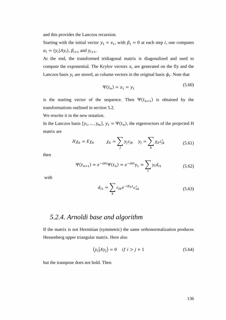
136
and this provides the Lanczos recursion.
Starting with the initial vector 𝑦1 = 𝑥1, with 𝛽1 = 0 at each step 𝑖, one computes
𝛼𝑖 = ⟨𝑦𝑖|𝐴𝑦𝑖⟩, 𝛽𝑖+1 and 𝑦𝑖+1.
At the end, the transformed tridiagonal matrix is diagonalized and used to
compute the exponential. The Krylov vectors 𝑥𝑖 are generated on the fly and the
Lanczos basis 𝑦𝑖 are stored, as column vectors in the original basis 𝜙𝑖. Note that
Ψ(𝑡𝑛) = 𝑥1 = 𝑦1
(5.60)
is the starting vector of the sequence. Then Ψ(𝑡𝑛+1) is obtained by the
transformations outlined in section 5.2.
We rewrite it in the new notation.
In the Lanczos basis {𝑦1, … , 𝑦𝑚}, 𝑦1 = Ψ(tn), the eigenvectors of the projected H
matrix are
𝐻𝜒𝑘 = 𝐸𝜒𝑘 𝜒𝑘 =∑𝑦𝑗𝑐𝑗𝑘𝑗
𝑦𝑗 =∑𝜒𝑘𝑐𝑗𝑘∗
𝑘
(5.61)
then
Ψ(𝑡𝑛+1) = 𝑒−𝑖𝐻𝑡Ψ(𝑡𝑛) = 𝑒
−𝑖𝐻𝑡y1 =∑𝑦𝑙𝑑𝑙1𝑙
(5.62)
with
𝑑𝑙1 =∑𝑐𝑙𝑘𝑒−𝑖𝐸𝑘𝑡𝑐1𝑘
∗
𝑘
(5.63)
5.2.4. Arnoldi base and algorithm
If the matrix is not Hermitian (symmetric) the same orthonormalization produces
Hessenberg upper triangular matrix. Here also
⟨𝑦𝑖|𝐴𝑦𝑗⟩ = 0 𝑖𝑓 𝑖 > 𝑗 + 1 (5.64)
but the transpose does not hold. Then
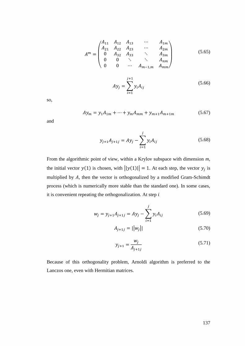
137
𝐴𝑚 =
(
𝐴11 𝐴12 𝐴13 ⋯ 𝐴1𝑚𝐴21 𝐴22 𝐴23 ⋯ 𝐴2𝑚0 𝐴32 𝐴33 ⋱ 𝐴3𝑚0 0 ⋱ ⋱ 𝐴𝑛𝑚0 0 ⋯ 𝐴𝑚−1,𝑚 𝐴𝑚𝑚)
(5.65)
𝐴𝑦𝑗 =∑𝑦𝑖𝐴𝑖𝑗
𝑗+1
𝑖=1
(5.66)
so,
𝐴𝑦𝑚 = 𝑦1𝐴1𝑚 +⋯+ 𝑦𝑚𝐴𝑚𝑚 + 𝑦𝑚+1𝐴𝑚+1𝑚 (5.67)
and
𝑦𝑗+1𝐴𝑗+1𝑗 = 𝐴𝑦𝑗 −∑𝑦𝑖𝐴𝑖𝑗
𝑗
𝑖=1
(5.68)
From the algorithmic point of view, within a Krylov subspace with dimension m,
the initial vector 𝑦(1) is chosen, with ||𝑦(1)|| = 1. At each step, the vector 𝑦𝑗 is
multiplied by 𝐴, then the vector is orthogonalized by a modified Gram-Schimdt
process (which is numerically more stable than the standard one). In some cases,
it is convenient repeating the orthogonalization. At step 𝑖
𝑤𝑗 = 𝑦𝑗+1𝐴𝑗+1𝑗 = 𝐴𝑦𝑗 −∑𝑦𝑖𝐴𝑖𝑗
𝑗
𝑖=1
(5.69)
𝐴𝑗+1𝑗 = ||𝑤𝑗|| (5.70)
𝑦𝑗+1 =𝑤𝑗
𝐴𝑗+1𝑗 (5.71)
Because of this orthogonality problem, Arnoldi algorithm is preferred to the
Lanczos one, even with Hermitian matrices.
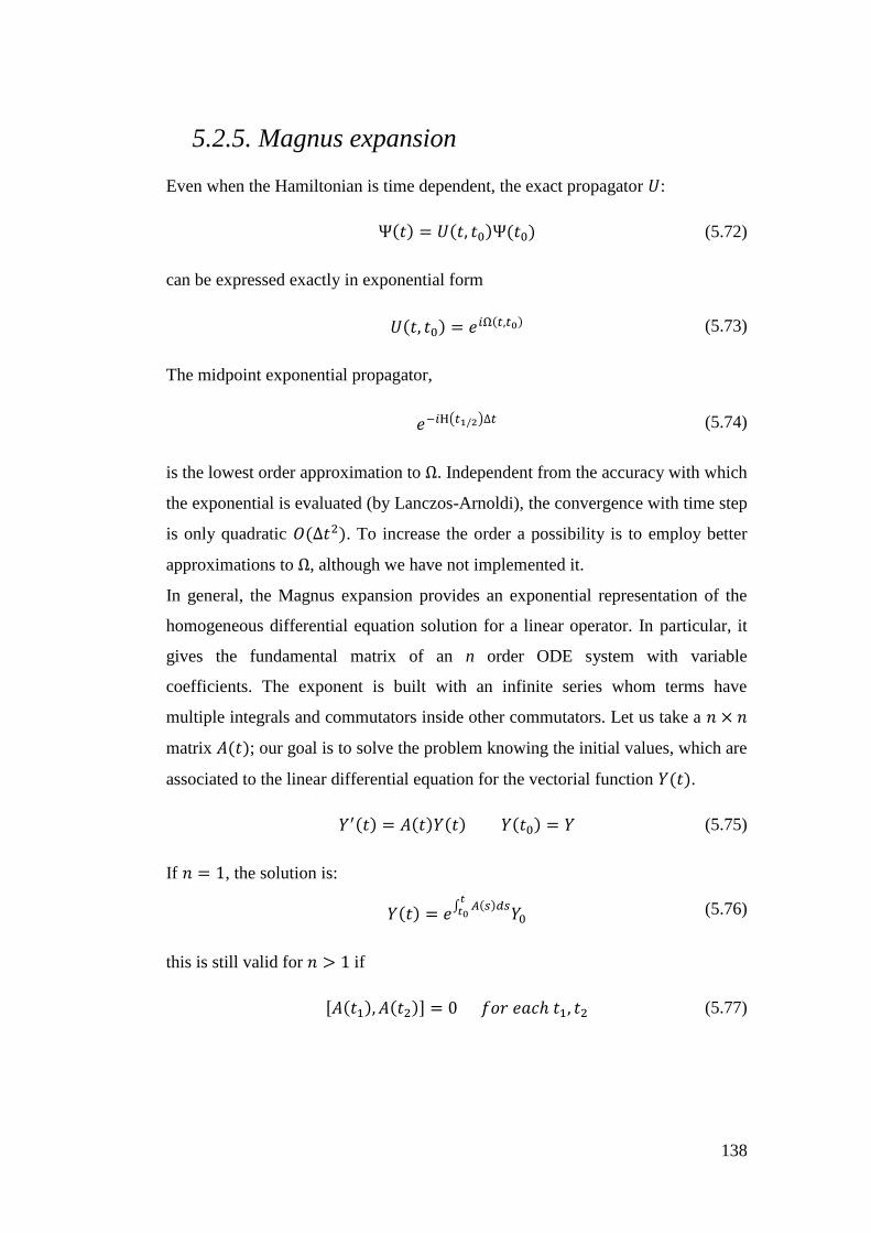
138
5.2.5. Magnus expansion
Even when the Hamiltonian is time dependent, the exact propagator 𝑈:
Ψ(𝑡) = 𝑈(𝑡, 𝑡0)Ψ(𝑡0) (5.72)
can be expressed exactly in exponential form
𝑈(𝑡, 𝑡0) = 𝑒𝑖Ω(𝑡,𝑡0) (5.73)
The midpoint exponential propagator,
𝑒−𝑖H(𝑡1/2)∆𝑡 (5.74)
is the lowest order approximation to Ω. Independent from the accuracy with which
the exponential is evaluated (by Lanczos-Arnoldi), the convergence with time step
is only quadratic 𝑂(Δ𝑡2). To increase the order a possibility is to employ better
approximations to Ω, although we have not implemented it.
In general, the Magnus expansion provides an exponential representation of the
homogeneous differential equation solution for a linear operator. In particular, it
gives the fundamental matrix of an n order ODE system with variable
coefficients. The exponent is built with an infinite series whom terms have
multiple integrals and commutators inside other commutators. Let us take a 𝑛 × 𝑛
matrix 𝐴(𝑡); our goal is to solve the problem knowing the initial values, which are
associated to the linear differential equation for the vectorial function 𝑌(𝑡).
𝑌′(𝑡) = 𝐴(𝑡)𝑌(𝑡) 𝑌(𝑡0) = 𝑌 (5.75)
If 𝑛 = 1, the solution is:
𝑌(𝑡) = 𝑒
∫ 𝐴(𝑠)𝑑𝑠𝑡𝑡0 𝑌0 (5.76)
this is still valid for 𝑛 > 1 if
[𝐴(𝑡1), 𝐴(𝑡2)] = 0 𝑓𝑜𝑟 𝑒𝑎𝑐ℎ 𝑡1, 𝑡2 (5.77)
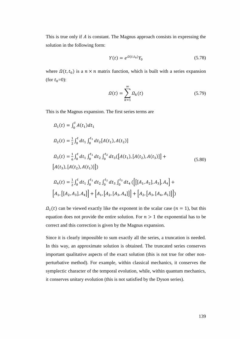
139
This is true only if 𝐴 is constant. The Magnus approach consists in expressing the
solution in the following form:
𝑌(𝑡) = 𝑒𝛺(𝑡,𝑡0)𝑌0 (5.78)
where 𝛺(𝑡, 𝑡0) is a 𝑛 × 𝑛 matrix function, which is built with a series expansion
(for 𝑡0=0):
𝛺(𝑡) = ∑𝛺𝑘(𝑡)
∞
𝑘=1
(5.79)
This is the Magnus expansion. The first series terms are
𝛺1(𝑡) = ∫ 𝐴(𝑡1)𝑑𝑡1𝑡
0
𝛺2(𝑡) =1
2∫ 𝑑𝑡1 ∫ 𝑑𝑡2[𝐴(𝑡1), 𝐴(𝑡2)]
𝑡1
0
𝑡
0
𝛺3(𝑡) =1
6∫ 𝑑𝑡1 ∫ 𝑑𝑡2 ∫ 𝑑𝑡3([𝐴(𝑡1), [𝐴(𝑡2), 𝐴(𝑡3)]] +
𝑡2
0
𝑡1
0
𝑡
0
[𝐴(𝑡3), [𝐴(𝑡2), 𝐴(𝑡1)]])
𝛺4(𝑡) =1
2∫ 𝑑𝑡1 ∫ 𝑑𝑡2 ∫ 𝑑𝑡3 ∫ 𝑑𝑡4
𝑡3
0([[[𝐴1, 𝐴2], 𝐴3], 𝐴4] +
𝑡2
0
𝑡1
0
𝑡
0
[𝐴1, [[𝐴2, 𝐴3], 𝐴4]] + [𝐴1, [𝐴2, [𝐴3, 𝐴4]]] + [𝐴2, [𝐴3, [𝐴4, 𝐴1]]])
(5.80)
𝛺1(𝑡) can be viewed exactly like the exponent in the scalar case (𝑛 = 1), but this
equation does not provide the entire solution. For 𝑛 > 1 the exponential has to be
correct and this correction is given by the Magnus expansion.
Since it is clearly impossible to sum exactly all the series, a truncation is needed.
In this way, an approximate solution is obtained. The truncated series conserves
important qualitative aspects of the exact solution (this is not true for other non-
perturbative method). For example, within classical mechanics, it conserves the
symplectic character of the temporal evolution, while, within quantum mechanics,
it conserves unitary evolution (this is not satisfied by the Dyson series).
140
From a mathematical point of view, the series converges when this condition is
satisfied:
∫ ‖𝐴(𝑠)‖𝑑𝑠𝑇
0
< 𝜋 (5.81)
where || ∙ || is a matrix norm.
All the expansion terms can be generated with a recursive method. Let us define
𝑆𝑛(𝑘)
as follows:
𝑆𝑛(𝑗)= ∑[𝛺𝑚, 𝑆𝑛−𝑚
(𝑗−1)]
𝑛−𝑗
𝑚=1
2 ≤ 𝑗 ≤ 𝑛 − 1 (5.82)
𝑆𝑛(1)= [𝛺𝑛−1, 𝐴]
𝑆𝑛(𝑛−1)
= 𝑎𝑑𝛺1𝑛−1(𝐴)
𝑎𝑑𝛺0𝐴 = 𝐴 𝑎𝑑𝛺
𝑘+1𝐴 = [𝛺, 𝑎𝑑𝛺𝑘𝐴]
(5.83)
thus
𝛺1 = ∫ 𝐴(𝑠)𝑑𝑠𝑡
0
𝛺𝑛 =∑𝐵𝑗
𝑗∫ 𝑆𝑛
(𝑗)(𝑠)𝑑𝑠𝑡
0
𝑛−1
𝑗=1
𝑛 ≥ 2
(5.84)
where 𝐵𝑗 is Bernoulli’s number. 𝛺𝑛 can be expressed as linear combination of
𝑛𝑡ℎintegral of 𝑛 − 1 nested commutator which contains 𝑛 matrices A.
𝛺𝑛(𝑡) = ∑𝐵𝑗
𝑗∑ ∫ 𝑎𝑑𝛺𝑘1
(𝑠)𝑎𝑑𝛺𝑘2(𝑠)⋯𝑎𝑑𝛺𝑘𝑗
(𝑠)𝑑𝑠𝑡
0𝑘1+⋯+𝑘𝑗=𝑛−1,𝑘𝑖≥1
𝑛−1
𝑗=1
(5.85)
This expression becomes more complicated at higher values of 𝑛. Approximate
formula of consistent order have been proposed in the literature [97].
141
5.2.6. Final Wavepacket analysis
Given a wavefunction (which we will generally call "wavepacket") properly
normalized, the probability of observing another quantum state 𝛹𝑖 is given by the
square of the amplitude
𝑃𝑖 = |⟨𝛹𝑖|𝜙⟩|2 (5.86)
This is true in particular for the eigenstates of the Hamiltonian of the system
𝐻𝛹𝑖 = 𝐸𝑖𝛹𝑖 (5.87)
which we shall call "free states".
For transitions in the continuous spectrum, such transition probabilities can be
converted into (generalized) cross sections, which depend on the angle of the
emitted electrons, or developed in an angular expansion, giving rise to angular
dependence parameters. Moreover, if the initial molecule is not prepared in a pure
state, by measuring all initial quantum numbers, one has also to average over the
statistical distribution of the sample. In particular, this is true for the rotational
motion, which is rarely controlled, so that a rotational average over random
molecular orientations is required. In other cases, the molecule can be partially
aligned, up to the ideal situation in which the orientation in space is fully
determined. This gives rise to molecular frame photoelectron angular
distributions (MFPADs). The same applies if final quantum numbers are not fully
resolved, which requires then a sum over those not observed.
To make things more precise, let us consider the fixed nuclei approximation and
the electrons only. Given a molecule with a point group symmetry and irreducible
representations (𝜆𝜇), and considering a single electron (independent particle
approximation), one can write the eigenstates of the Hamiltonian
𝐻𝛹𝑖𝜆𝜇 = 𝐸𝑖𝜆𝛹𝑖𝜆𝜇 (5.88)
in the discrete spectrum, and
𝐻𝛹𝐸𝑗𝜆𝜇 = 𝐸𝛹𝐸𝑗𝜆𝜇 (5.89)
142
in the continuum spectrum (notice the index j that counts independent channels
(angular momenta) within each symmetry (𝜆𝜇)). Alternatively the continuum state
may be characterized by the electron asymptotic momentum �̅�. Note moreover
that because of the infinite degeneracy of the continuum, different asymptotic
conditions may be employed, to uniquely fix the solution. Since calculations are
more easily carried out with wavefunctions in real form, employing the molecular
symmetry, the so called K-Matrix normalized solutions 𝛹𝐸𝑗𝜆𝜇 will be obtained. It
will then be necessary to transform from one boundary condition to another, and
between the angular and the momentum eigenstates, which amount to linear
transformations between different sets, as explained before.
Thus, the time propagation provides a final wavepacket:
𝜙𝐼 ≡∑𝜙𝐼𝜆𝜇𝜆𝜇
(5.90)
which we represent expanded on symmetry adapted components 𝜙𝐼𝜆𝜇 (in general,
external interaction will produce a mixing of different symmetries). On the other
hand, the continuum states have to be computed:
𝛹𝐸𝑗𝜆𝜇 →∑[𝑓𝑙𝑗′(𝑘𝑟)𝛿𝑗′𝑗 + 𝑔𝑙𝑗′
(𝑘𝑟)𝐾𝑗′𝑗𝜆 ]𝑋𝑗′𝜆𝜇
𝑗′
(5.91)
(or equally 𝜓𝐸𝑗𝜆𝜇− or 𝜓�̅�
−). To compute the transition probablity, it is necessary to
calculate the projection of the final wavepacket on these free field eigenstates.
𝑃𝐸𝑗𝜆𝜇,𝐼 = ⟨𝛹𝐸𝑗𝜆𝜇|𝜙𝐼⟩ = ⟨𝛹𝐸𝑗𝜆𝜇|𝜙𝐼𝜆𝜇⟩ (5.92)
Now, let us define the primitive basis:
{𝜒𝑛𝜆𝜇} = {𝜒𝑝𝑖𝑗𝜆𝜇}
(5.93)
where 𝑝 is the index of a shell of equivalent centers (atoms), 𝑗 is the index of
angular functions 𝑋𝑗𝜆𝜇in symmetry (λμ), and 𝑖 is the index of the radial B-spline
𝐵𝑖.
143
The overlap matrix 𝑆𝑚𝑛𝜆 is diagonal in λμ and independent of μ:
𝑆𝑚𝑛𝜆 = ⟨𝜒𝑚𝜆𝜇|𝜒𝑛𝜆𝜇⟩ (5.94)
The final wavepacket at 𝑡 (end of the pulse) is expanded as a linear combination
of the bound basis functions (which are zero at the outer boundary):
𝜙(𝑡0) =∑∑𝑐𝑛𝜆𝜇𝜒𝑛𝜆𝜇𝑛𝜆𝜇
(5.95)
K-matrix normalized continuum states are also expanded in the primitive spline
basis where now the {𝜒𝑝𝑖𝑗𝜆𝜇} basis includes the asymptotic ones (i.e. those
nonzero at the outer boundary).
𝛹𝐸𝑗𝜆𝜇 =∑𝑑𝐸𝑗𝜆𝜇𝜒𝑛𝜆𝜇𝑛
(5.96)
Note also that the 𝑑 coefficients are independent of 𝜇. Then the projection is
simply:
𝑃𝐸𝑗𝜆𝜇(𝑡0) =∑𝑑𝐸𝑗𝜆𝜇∗ 𝑆𝑚𝑛
𝜆 𝑐𝑛𝜆𝜇𝑚𝑛
(5.97)
Now it is possible to evaluate the probability 𝑃�̅�, after transforming the
amplitudes to incoming wave boundary conditions.
𝑑𝑃
𝑑�̅�= 𝑐𝑜𝑛𝑠𝑡 |⟨𝛹
�̅�
(−)|𝜙𝐼⟩|
2
=∑𝐴𝐿𝑀(𝛺)𝑌𝐿𝑀(�̅�)
𝐿𝑀
(5.98)
and the total cross section 𝜎, the angular distribution parameters 𝛽 or 𝐴𝐿𝑀, the
averages over molecular orientations, energy distribution of electrons, angular
distributions (𝛺 specifies orientation of �⃗� with respect to the molecule). The
latter, in particular, is obtained by computing 𝐴𝐿𝑀(𝛺) for all the energies and then
applying it by using the interested angles.

144
5.3. Computational details
From the computational point of view, a typical calculation requires:
diagonalize the Hamiltonian for the initial state. The input file needs: the
coordinates of the atoms, the symmetry group and the basis (radial grid and
angular grid).
Compute the dipole matrices starting from eigenvectors obtained by the
previous step.
Choose both the gauge of the electromagnetic field and the energy cut off
threshold.
Time propagation, giving in input: intensity of the electromagnetic field,
photon energy, duration of the pulse, Krylov dimension and time step.
Analysis of the wavepacket obtained by the time propagation projecting it
on the continuum. Thus probability density (photoelectron spectrum) and
angular distribution can be obtained.
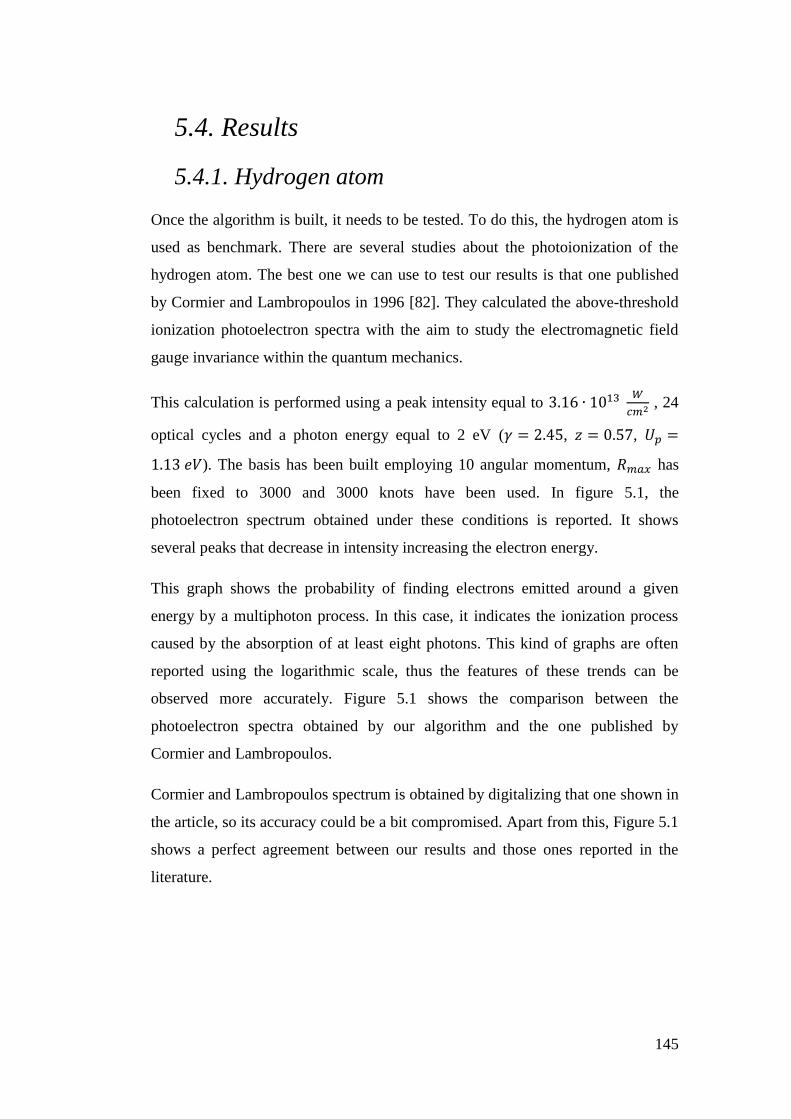
145
5.4. Results
5.4.1. Hydrogen atom
Once the algorithm is built, it needs to be tested. To do this, the hydrogen atom is
used as benchmark. There are several studies about the photoionization of the
hydrogen atom. The best one we can use to test our results is that one published
by Cormier and Lambropoulos in 1996 [82]. They calculated the above-threshold
ionization photoelectron spectra with the aim to study the electromagnetic field
gauge invariance within the quantum mechanics.
This calculation is performed using a peak intensity equal to 3.16 ∙ 1013 𝑊
𝑐𝑚2 , 24
optical cycles and a photon energy equal to 2 eV (𝛾 = 2.45, 𝑧 = 0.57, 𝑈𝑝 =
1.13 𝑒𝑉). The basis has been built employing 10 angular momentum, 𝑅𝑚𝑎𝑥 has
been fixed to 3000 and 3000 knots have been used. In figure 5.1, the
photoelectron spectrum obtained under these conditions is reported. It shows
several peaks that decrease in intensity increasing the electron energy.
This graph shows the probability of finding electrons emitted around a given
energy by a multiphoton process. In this case, it indicates the ionization process
caused by the absorption of at least eight photons. This kind of graphs are often
reported using the logarithmic scale, thus the features of these trends can be
observed more accurately. Figure 5.1 shows the comparison between the
photoelectron spectra obtained by our algorithm and the one published by
Cormier and Lambropoulos.
Cormier and Lambropoulos spectrum is obtained by digitalizing that one shown in
the article, so its accuracy could be a bit compromised. Apart from this, Figure 5.1
shows a perfect agreement between our results and those ones reported in the
literature.
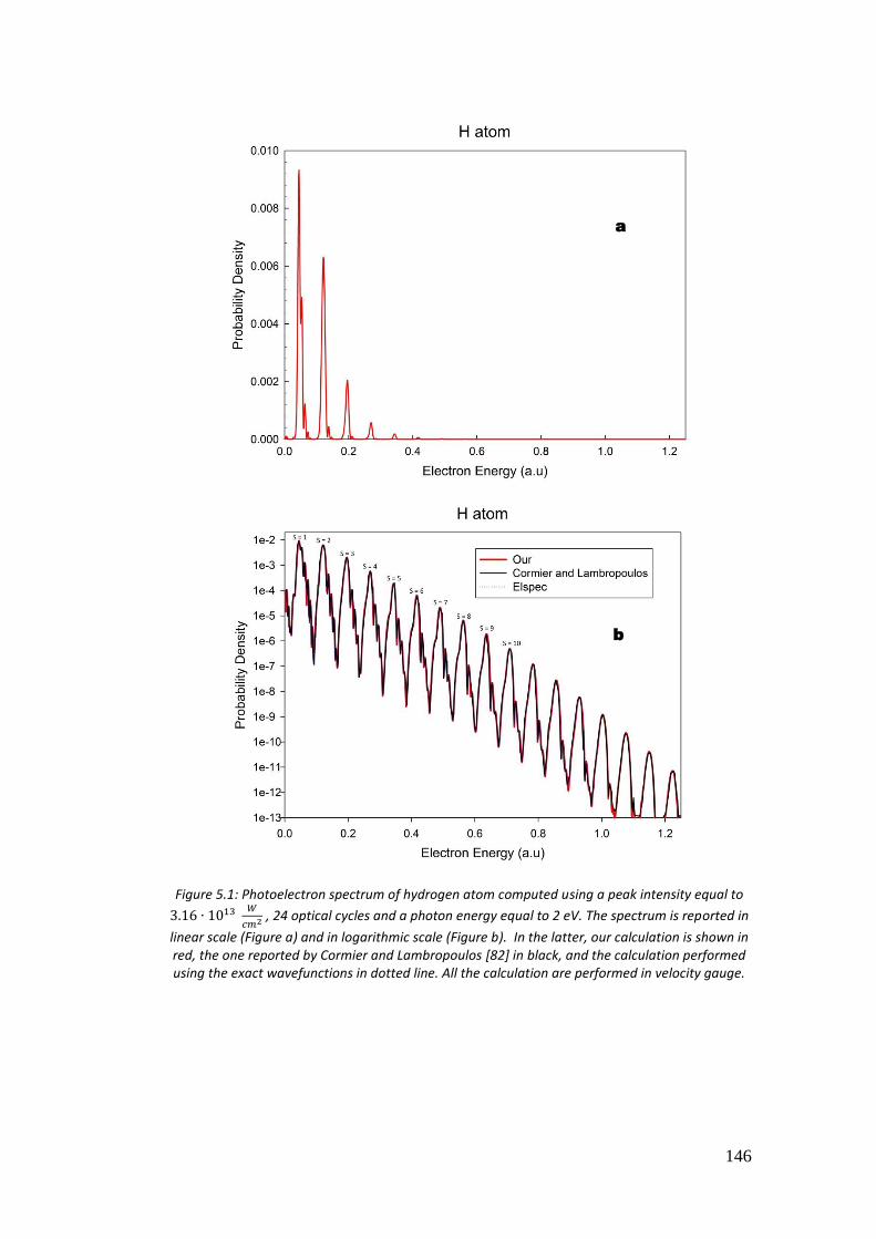
146
Figure 5.1: Photoelectron spectrum of hydrogen atom computed using a peak intensity equal to
3.16 ∙ 1013 𝑊
𝑐𝑚2 , 24 optical cycles and a photon energy equal to 2 eV. The spectrum is reported in
linear scale (Figure a) and in logarithmic scale (Figure b). In the latter, our calculation is shown in red, the one reported by Cormier and Lambropoulos [82] in black, and the calculation performed using the exact wavefunctions in dotted line. All the calculation are performed in velocity gauge.
a
b
147
An interesting property is the presence of substructures on the right side of the
lowest peaks which can be explained by intermediate resonances. The absorption
of at least eight photons when the field is at its maximum value leads to excitation
of high-lying Rydberg states and can enhance ionization at exact resonance.
In Figure 5.1, a further calculation is reported. This kind of calculation, called
“Elspec”, is performed using the exact wavefunction of the system. This is
obviously possible only for the hydrogen atom. This demonstrates that our method
properly works and can accurately describe at least the time-dependent
photoionization of the simplest quantum system.
This algorithm is not only capable of computing the photoelectron spectrum, but it
can also provide angular distributions. In fact, through photoionization, one can
follow the evolution of the system, and angular distributions related to an oriented
molecule provide more information than any other observable. In the case of the
hydrogen atom, there is obviously no orientation. So, standard one-photon
photoionization furnish angular distributions that show two symmetric lobes
(𝛽 = 2). Whereas with these condition, different energies produce different
angular distributions, which can provide a lot of information on the considered
system.
Cormier and Lambropoulos have also computed the angular distributions at some
energies; in particular, they have reported to those ones relative to the first 10
peaks of the photoelectron spectrum. In the Figure 5.2, the comparison between
our angular distributions (in red) and those ones calculated by Cormier and
Lambropoulos (in black) is reported. One can observe that there is a full
agreement between the results.
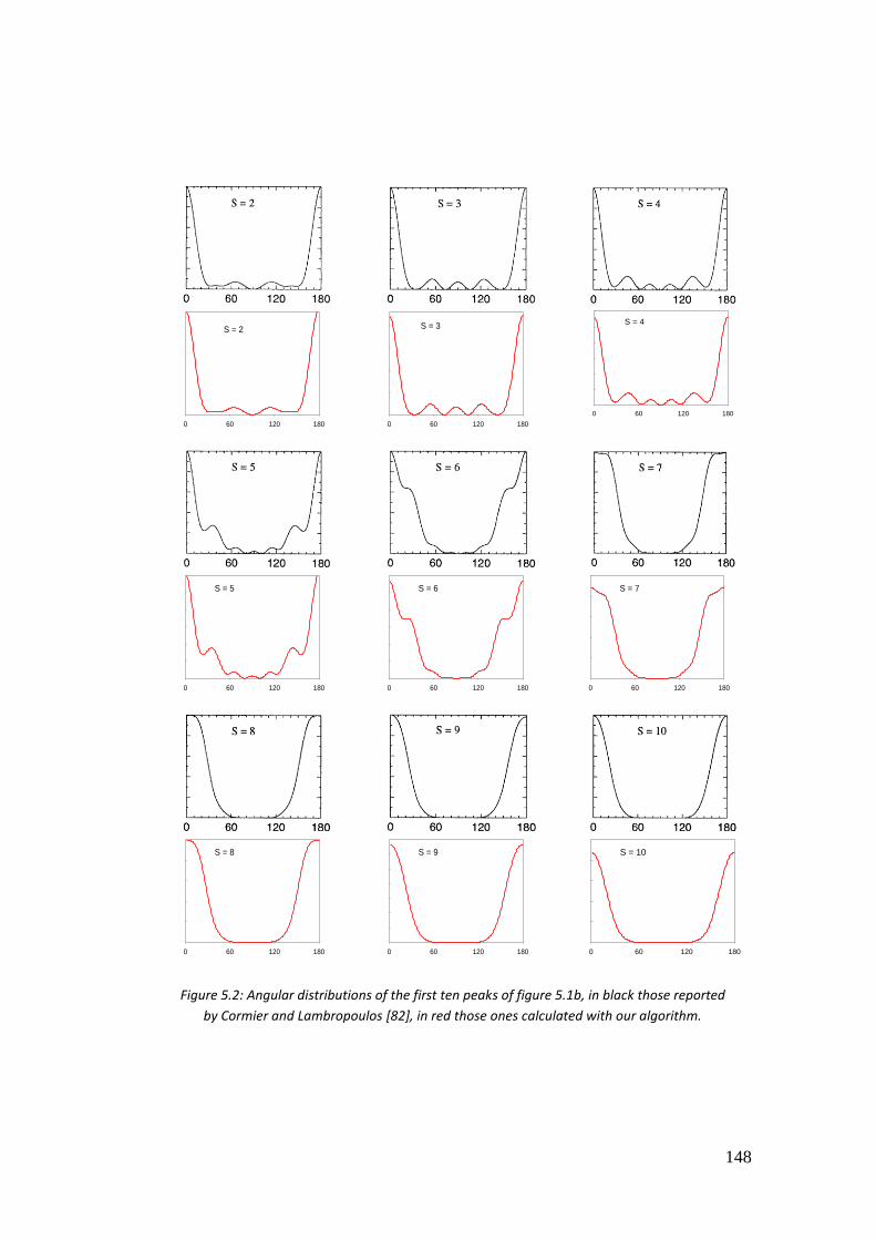
148
S = 2
0 60 120 180
S = 3
0 60 120 180
S = 4
0 60 120 180
S = 5
0 60 120 180
S = 6
0 60 120 180
S = 7
0 60 120 180
S = 8
0 60 120 180
S = 9
0 60 120 180
S = 10
0 60 120 180
Figure 5.2: Angular distributions of the first ten peaks of figure 5.1b, in black those reported
by Cormier and Lambropoulos [82], in red those ones calculated with our algorithm.
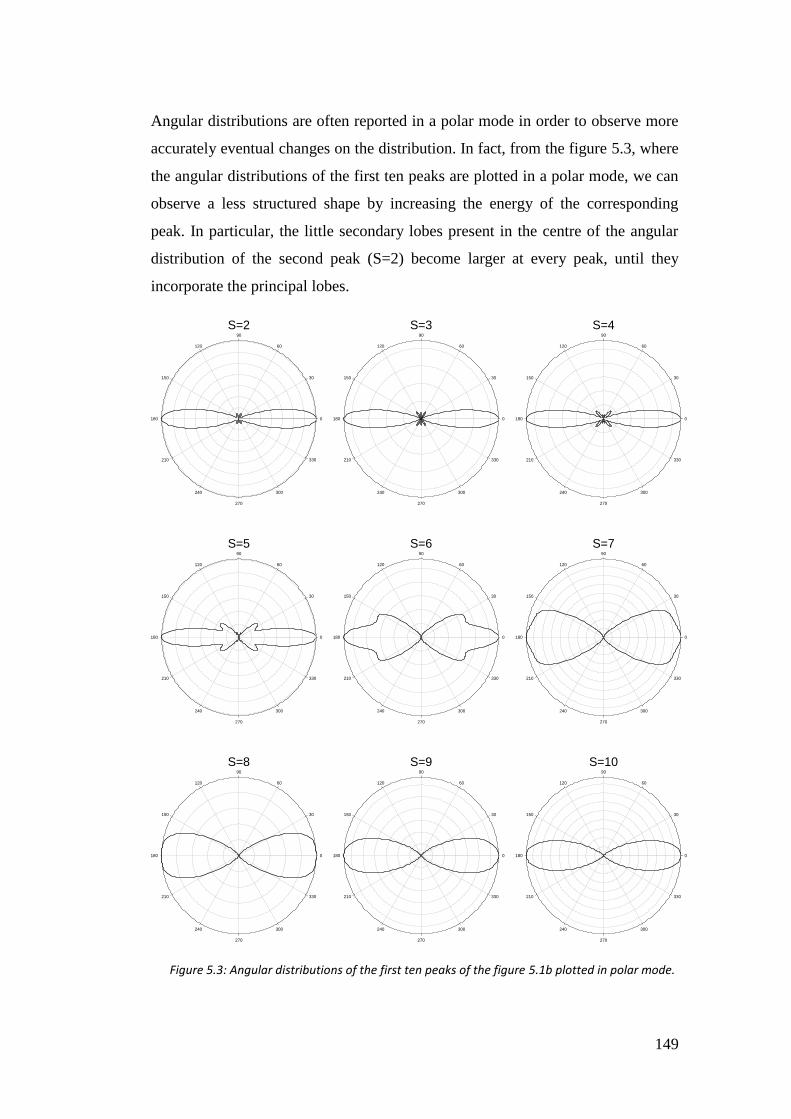
149
Angular distributions are often reported in a polar mode in order to observe more
accurately eventual changes on the distribution. In fact, from the figure 5.3, where
the angular distributions of the first ten peaks are plotted in a polar mode, we can
observe a less structured shape by increasing the energy of the corresponding
peak. In particular, the little secondary lobes present in the centre of the angular
distribution of the second peak (S=2) become larger at every peak, until they
incorporate the principal lobes.
S=2
0
30
60
90
120
150
180
210
240
270
300
330
S=3
0
30
60
90
120
150
180
210
240
270
300
330
S=4
0
30
60
90
120
150
180
210
240
270
300
330
S=5
0
30
60
90
120
150
180
210
240
270
300
330
S=6
0
30
60
90
120
150
180
210
240
270
300
330
S=7
0
30
60
90
120
150
180
210
240
270
300
330
S=8
0
30
60
90
120
150
180
210
240
270
300
330
S=9
0
30
60
90
120
150
180
210
240
270
300
330
S=10
0
30
60
90
120
150
180
210
240
270
300
330
Figure 5.3: Angular distributions of the first ten peaks of the figure 5.1b plotted in polar mode.
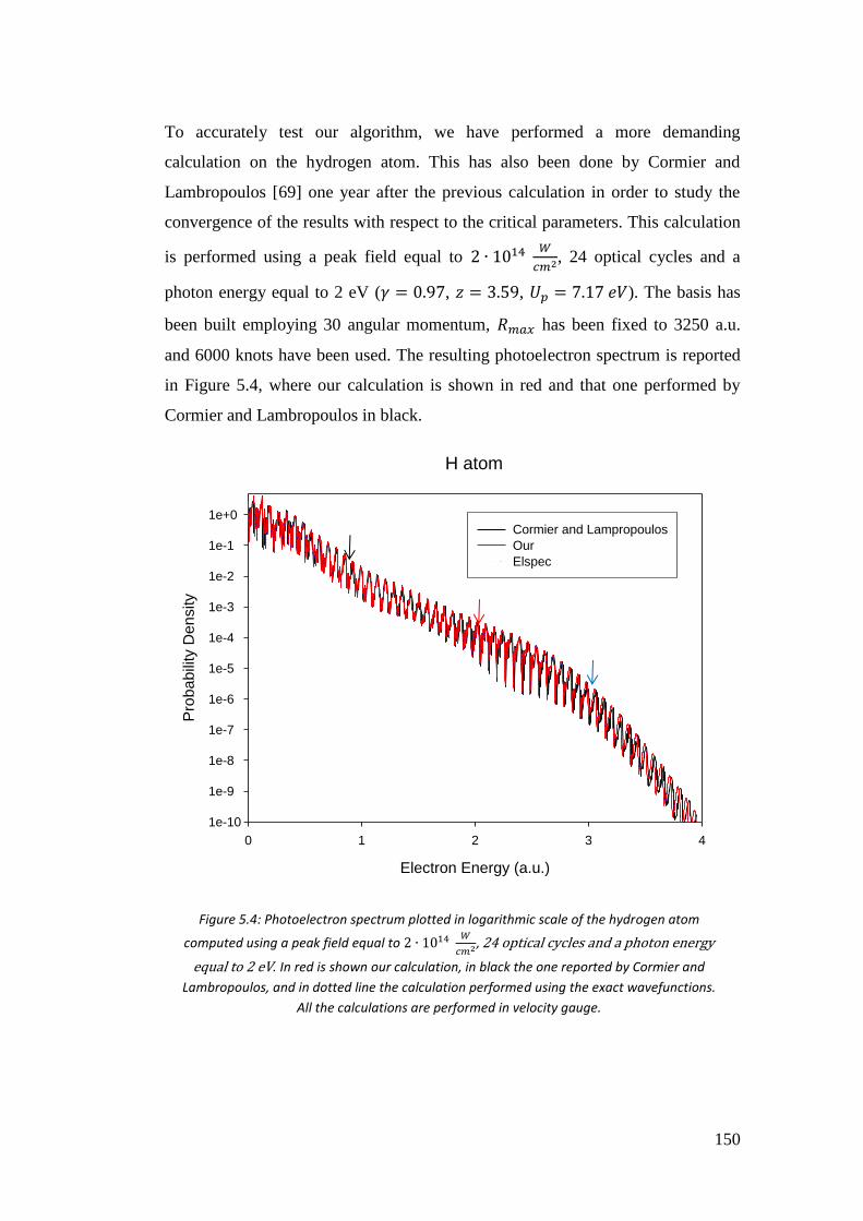
150
To accurately test our algorithm, we have performed a more demanding
calculation on the hydrogen atom. This has also been done by Cormier and
Lambropoulos [69] one year after the previous calculation in order to study the
convergence of the results with respect to the critical parameters. This calculation
is performed using a peak field equal to 2 ∙ 1014 𝑊
𝑐𝑚2, 24 optical cycles and a
photon energy equal to 2 eV (𝛾 = 0.97, 𝑧 = 3.59, 𝑈𝑝 = 7.17 𝑒𝑉). The basis has
been built employing 30 angular momentum, 𝑅𝑚𝑎𝑥 has been fixed to 3250 a.u.
and 6000 knots have been used. The resulting photoelectron spectrum is reported
in Figure 5.4, where our calculation is shown in red and that one performed by
Cormier and Lambropoulos in black.
H atom
Electron Energy (a.u.)
0 1 2 3 4
Pro
ba
bili
ty D
en
sity
1e-10
1e-9
1e-8
1e-7
1e-6
1e-5
1e-4
1e-3
1e-2
1e-1
1e+0Cormier and Lampropoulos
Our
Elspec
Figure 5.4: Photoelectron spectrum plotted in logarithmic scale of the hydrogen atom
computed using a peak field equal to 2 ∙ 1014 𝑊
𝑐𝑚2, 24 optical cycles and a photon energy
equal to 2 eV. In red is shown our calculation, in black the one reported by Cormier and
Lambropoulos, and in dotted line the calculation performed using the exact wavefunctions.
All the calculations are performed in velocity gauge.
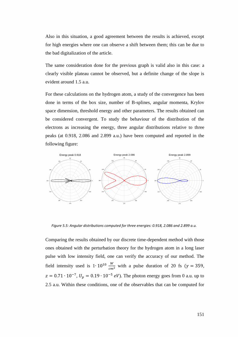
151
Also in this situation, a good agreement between the results is achieved, except
for high energies where one can observe a shift between them; this can be due to
the bad digitalization of the article.
The same consideration done for the previous graph is valid also in this case: a
clearly visible plateau cannot be observed, but a definite change of the slope is
evident around 1.5 a.u.
For these calculations on the hydrogen atom, a study of the convergence has been
done in terms of the box size, number of B-splines, angular momenta, Krylov
space dimension, threshold energy and other parameters. The results obtained can
be considered convergent. To study the behaviour of the distribution of the
electrons as increasing the energy, three angular distributions relative to three
peaks (at 0.918, 2.086 and 2.899 a.u.) have been computed and reported in the
following figure:
Energy peak 0.918
0
30
60
90
120
150
180
210
240
270
300
330
Energy peak 2.086
0
30
60
90
120
150
180
210
240
270
300
330
Energy peak 2.899
0
30
60
90
120
150
180
210
240
270
300
330
Comparing the results obtained by our discrete time-dependent method with those
ones obtained with the perturbation theory for the hydrogen atom in a long laser
pulse with low intensity field, one can verify the accuracy of our method. The
field intensity used is 1∙ 1010 𝑊
𝑐𝑚2 with a pulse duration of 20 fs (𝛾 = 359,
𝑧 = 0.71 ∙ 10−7, 𝑈𝑝 = 0.19 ∙ 10−5 𝑒𝑉). The photon energy goes from 0 a.u. up to
2.5 a.u. Within these conditions, one of the observables that can be computed for
Figure 5.5: Angular distributions computed for three energies: 0.918, 2.086 and 2.899 a.u.
152
the one-photon (N=1) and two-photon (N=2) ionization is the cross section, which
could be calculated by the TDSE ionization probabilities with the following
expression [81]:
𝜎(𝑐𝑚2𝑁𝑠𝑁−1) = (
𝜔
𝐼)𝑁 𝐶(𝑁)
𝑇𝑃𝑖𝑜𝑛𝑇𝐷𝑆𝐸
𝐶(1) =8
3 𝐶(2) =
128
35
(5.99)
where 𝜔 is the photon energy in Joules, 𝐼 is the laser intensity in W/cm2, 𝑇 is the
laser duration in seconds and 𝐶(𝑁) is a dimensionless factor that considers the
time dependence of the pulse envelope.
In Figure 5.6, the one-photon ionization cross section obtained by the time-
dependent propagation (in red) and that one obtained by the perturbation theory
(in black) are reported [99].
The figure shows the full agreement between the perturbative and the TDSE
results in the photon energy range considered. The cross section obtained by the
time-dependent propagation gets closer to the perturbative propagation by
increasing the pulse duration.
This can be done for the two-photon process as well. In Fig. 5.7, cross section
obtained with the TDSE method (in red) and the accurate perturbative result
obtained by Karule [100] (in black) for the two-photon ionization are compared.
Figure 5.7 shows that there is a perfect agreement for values of energy higher than
0.5 a.u. unlike at lower energies where the agreement is not so accurate. This is
due to the finite duration of the pulse: in fact, the singularities of the energies
below the threshold ionization are smoothed by the pulse bandwidth.
These results exhibit a good functionality of our algorithm, which is capable to
describe the above-threshold ionization in condition of a short pulse duration. The
latter has to be shorter than the time that the wavepacket needs to reach the
boundary of the box, where the system is confined.

153
Figure 5.6: One-photon cross section calculations as function of photon energy. In red dots the
cross section calculated through the TDSE ionization theory and in black that one calculated by
the perturbation theory.
Figure 5.7: Two-photon cross section calculations as function of photon energy. In red the
cross section calculated through the TDSE ionization theory and in black that one calculated
by Karule [100]
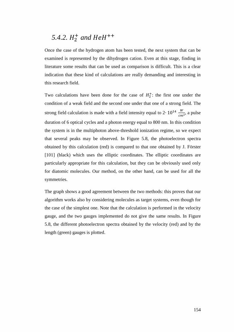
154
5.4.2. 𝐻2+ and 𝐻𝑒𝐻++
Once the case of the hydrogen atom has been tested, the next system that can be
examined is represented by the dihydrogen cation. Even at this stage, finding in
literature some results that can be used as comparison is difficult. This is a clear
indication that these kind of calculations are really demanding and interesting in
this research field.
Two calculations have been done for the case of 𝐻2+: the first one under the
condition of a weak field and the second one under that one of a strong field. The
strong field calculation is made with a field intensity equal to 2∙ 1014 𝑊
𝑐𝑚2, a pulse
duration of 6 optical cycles and a photon energy equal to 800 nm. In this condition
the system is in the multiphoton above-threshold ionization regime, so we expect
that several peaks may be observed. In Figure 5.8, the photoelectron spectra
obtained by this calculation (red) is compared to that one obtained by J. Förster
[101] (black) which uses the elliptic coordinates. The elliptic coordinates are
particularly appropriate for this calculation, but they can be obviously used only
for diatomic molecules. Our method, on the other hand, can be used for all the
symmetries.
The graph shows a good agreement between the two methods: this proves that our
algorithm works also by considering molecules as target systems, even though for
the case of the simplest one. Note that the calculation is performed in the velocity
gauge, and the two gauges implemented do not give the same results. In Figure
5.8, the different photoelectron spectra obtained by the velocity (red) and by the
length (green) gauges is plotted.
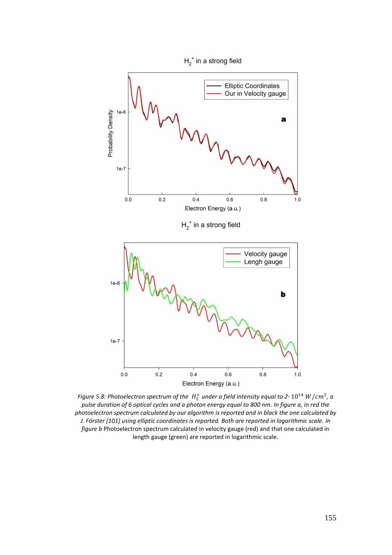
155
Figure 5.8: Photoelectron spectrum of the 𝐻2+ under a field intensity equal to 2∙ 1014 𝑊/𝑐𝑚2, a
pulse duration of 6 optical cycles and a photon energy equal to 800 nm. In figure a, in red the photoelectron spectrum calculated by our algorithm is reported and in black the one calculated by
J. Förster [101] using elliptic coordinates is reported. Both are reported in logarithmic scale. In figure b Photoelectron spectrum calculated in velocity gauge (red) and that one calculated in
length gauge (green) are reported in logarithmic scale.
a
b
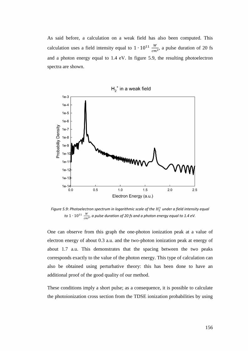
156
As said before, a calculation on a weak field has also been computed. This
calculation uses a field intensity equal to 1 ∙ 1011 𝑊
𝑐𝑚2, a pulse duration of 20 fs
and a photon energy equal to 1.4 eV. In figure 5.9, the resulting photoelectron
spectra are shown.
One can observe from this graph the one-photon ionization peak at a value of
electron energy of about 0.3 a.u. and the two-photon ionization peak at energy of
about 1.7 a.u. This demonstrates that the spacing between the two peaks
corresponds exactly to the value of the photon energy. This type of calculation can
also be obtained using perturbative theory: this has been done to have an
additional proof of the good quality of our method.
These conditions imply a short pulse; as a consequence, it is possible to calculate
the photoionization cross section from the TDSE ionization probabilities by using
Figure 5.9: Photoelectron spectrum in logarithmic scale of the 𝐻2+ under a field intensity equal
to 1 ∙ 1011 𝑊
𝑐𝑚2, a pulse duration of 20 fs and a photon energy equal to 1.4 eV.
157
the Expression 5.9. In this case, only the cross section relative to the one-photon
𝑘𝜎𝑢 transition can be computed. The latter is plotted in red in Figure 5.10 versus
the cross section calculated with the stationary method.
There is a good agreement between the two methods also in this case; this
demonstrates, once more, the capability of our algorithm to describe both
ionization regimes in condition of a short pulse duration.
Figure 5.10: Cross section related to the one-photon 𝜎𝑢 transition of the 𝐻2+ as function of
the photon energy. In red dots the cross section calculated through the TDSE ionization
theory and in black that one obtained by the perturbation theory.

158
In order to assess whether the time-propagation algorithm is well behaved, it has
been decided to test the final wavepacket through the coefficients that describe it.
This has been done starting with 𝐻𝑒𝐻++ which is a system more complicated
with respect to the 𝐻2+ molecule.
Two studies have been made: the first one (parallel) with carrier envelope phase
(CEP) equal to zero and the second one (antiparallel) with CEP=1. In Figure 5.11,
the coefficients of the final wavepackets obtained through a time propagation that
uses a peak field equal to 2∙ 1016 𝑊
𝑐𝑚2, a pulse duration of 2 optical cycles and a
photon energy equal to 800 nm are shown. These two results are compared to
those ones obtained by J. Förster [101]; differences between the two results are
difficult to find, even by analysing more accurately the figures.
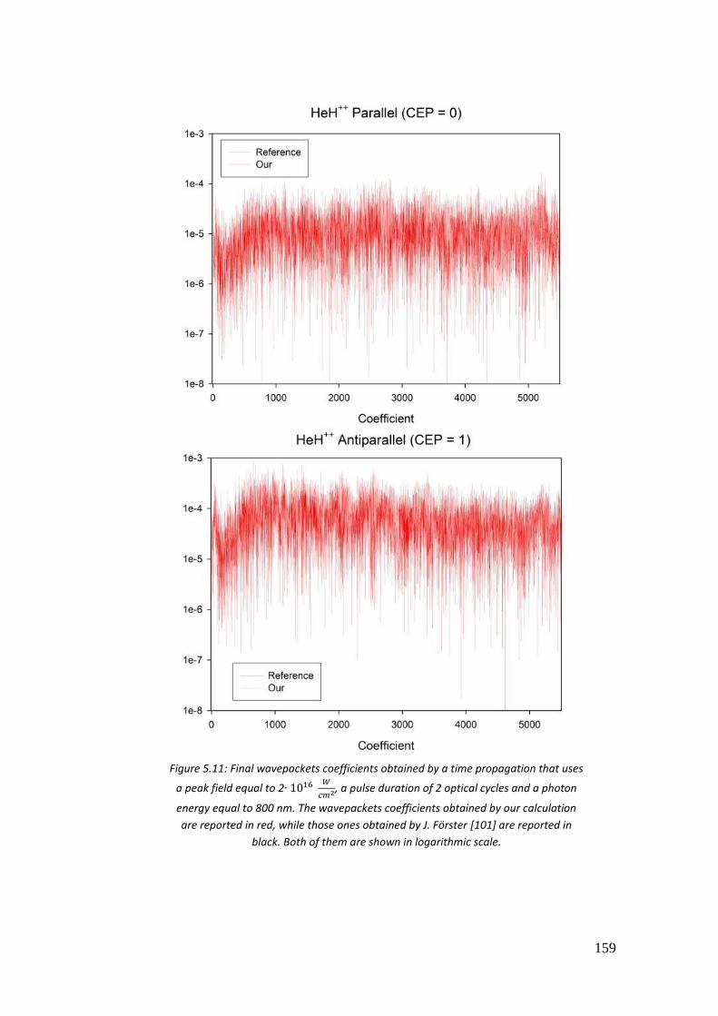
159
Figure 5.11: Final wavepackets coefficients obtained by a time propagation that uses
a peak field equal to 2∙ 1016 𝑊
𝑐𝑚2, a pulse duration of 2 optical cycles and a photon
energy equal to 800 nm. The wavepackets coefficients obtained by our calculation
are reported in red, while those ones obtained by J. Förster [101] are reported in
black. Both of them are shown in logarithmic scale.
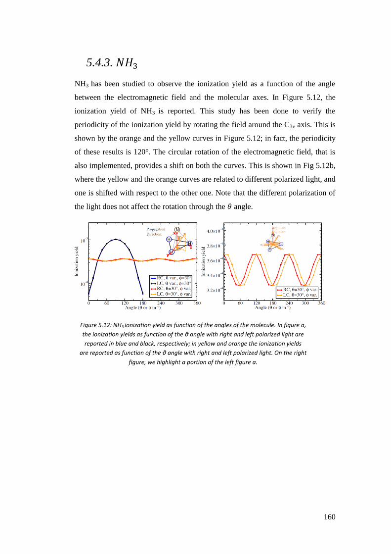
160
5.4.3. 𝑁𝐻3
NH3 has been studied to observe the ionization yield as a function of the angle
between the electromagnetic field and the molecular axes. In Figure 5.12, the
ionization yield of NH3 is reported. This study has been done to verify the
periodicity of the ionization yield by rotating the field around the C3v axis. This is
shown by the orange and the yellow curves in Figure 5.12; in fact, the periodicity
of these results is 120°. The circular rotation of the electromagnetic field, that is
also implemented, provides a shift on both the curves. This is shown in Fig 5.12b,
where the yellow and the orange curves are related to different polarized light, and
one is shifted with respect to the other one. Note that the different polarization of
the light does not affect the rotation through the 휃 angle.
Figure 5.12: NH3 ionization yield as function of the angles of the molecule. In figure a,
the ionization yields as function of the θ angle with right and left polarized light are
reported in blue and black, respectively; in yellow and orange the ionization yields
are reported as function of the θ angle with right and left polarized light. On the right
figure, we highlight a portion of the left figure a.
Both of them are shown in logarithmic scale.
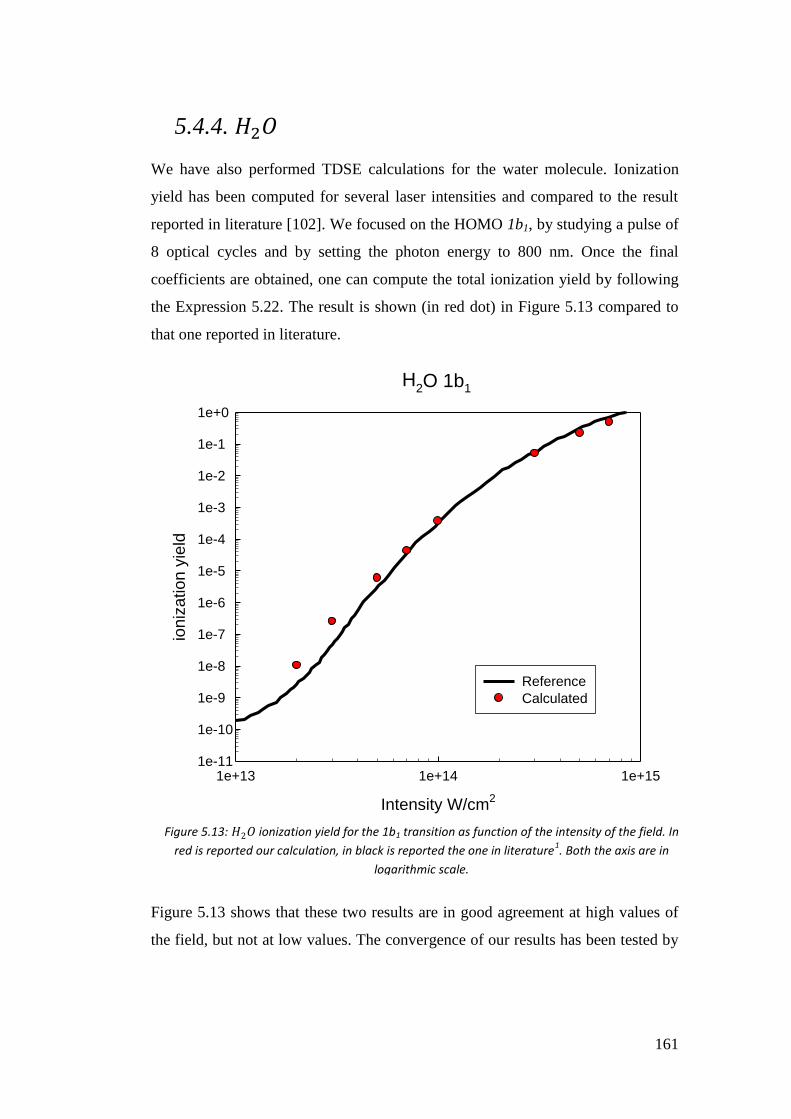
161
5.4.4. 𝐻2𝑂
We have also performed TDSE calculations for the water molecule. Ionization
yield has been computed for several laser intensities and compared to the result
reported in literature [102]. We focused on the HOMO 1b1, by studying a pulse of
8 optical cycles and by setting the photon energy to 800 nm. Once the final
coefficients are obtained, one can compute the total ionization yield by following
the Expression 5.22. The result is shown (in red dot) in Figure 5.13 compared to
that one reported in literature.
H2O 1b1
Intensity W/cm2
1e+13 1e+14 1e+15
ion
iza
tio
n y
ield
1e-11
1e-10
1e-9
1e-8
1e-7
1e-6
1e-5
1e-4
1e-3
1e-2
1e-1
1e+0
Reference
Calculated
Figure 5.13 shows that these two results are in good agreement at high values of
the field, but not at low values. The convergence of our results has been tested by
Figure 5.13: 𝐻2𝑂 ionization yield for the 1b1 transition as function of the intensity of the field. In
red is reported our calculation, in black is reported the one in literature1. Both the axis are in
logarithmic scale.
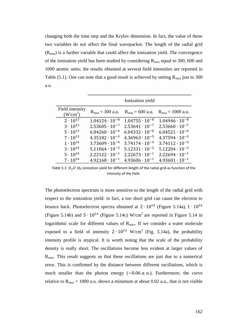
162
changing both the time step and the Krylov dimension. In fact, the value of these
two variables do not affect the final wavepacket. The length of the radial grid
(Rmax) is a further variable that could affect the ionization yield. The convergence
of the ionization yield has been studied by considering Rmax equal to 300, 600 and
1000 atomic units; the results obtained at several field intensities are reported in
Table (5.1). One can note that a good result is achieved by setting Rmax just to 300
a.u.
Ionization yield
Field intensity
(W/cm2)
Rmax = 300 a.u. Rmax = 600 a.u. Rmax = 1000 a.u.
2 ∙ 1013 1.04124 ∙ 10−8 1.04755 ∙ 10−8 1.04946 ∙ 10−8 3 ∙ 1013 2.53605 ∙ 10−7 2.53641 ∙ 10−7 2.53660 ∙ 10−7 5 ∙ 1013 6.04260 ∙ 10−6 6.04332 ∙ 10−6 6.04521 ∙ 10−6 7 ∙ 1013 4.35182 ∙ 10−5 4.36963 ∙ 10−5 4.37594 ∙ 10−5 1 ∙ 1014 3.73609 ∙ 10−4 3.74174 ∙ 10−4 3.74112 ∙ 10−4 3 ∙ 1014 5.11064 ∙ 10−2 5.12331 ∙ 10−2 5.12204 ∙ 10−2 5 ∙ 1014 2.22122 ∙ 10−1 2.22673 ∙ 10−1 2.22694 ∙ 10−1 7 ∙ 1014 4.92168 ∙ 10−1 4.93606 ∙ 10−1 4.93601 ∙ 10−1
The photoelectron spectrum is more sensitive to the length of the radial grid with
respect to the ionization yield: in fact, a too short grid can cause the electron to
bounce back. Photoelectron spectra obtained at 2 ∙ 1013 (Figure 5.14a), 1 ∙ 1014
(Figure 5.14b) and 5 ∙ 1014 (Figure 5.14c) W/cm2
are reported in Figure 5.14 in
logarithmic scale for different values of Rmax. If we consider a water molecule
exposed to a field of intensity 2 ∙ 1013 W/cm2
(Fig. 5.14a), the probability
intensity profile is atypical. It is worth noting that the scale of the probability
density is really short. The oscillations become less evident at larger values of
Rmax. This result suggests us that these oscillations are just due to a numerical
error. This is confirmed by the distance between different oscillations, which is
much smaller than the photon energy (~0.06 𝑎. 𝑢.). Furthermore, the curve
relative to Rmax = 1000 a.u. shows a minimum at about 0.02 a.u., that is not visible
Table 5.1: 𝐻2𝑂 1b1 ionization yield for different length of the radial grid as function of the
intensity of the field.

163
in the other curves. As a consequence, it is possible to argue that the structures
that should be visible in all the curves are hidden by numerical errors. The
oscillations become less evident at larger values of Rmax also for field of intensity
1 ∙ 1014 W/cm2. Convergence is reached at Rmax = 600 a.u. In fact, the difference
between the values calculated at Rmax = 600 a.u. and Rmax = 1000 a.u. is not so
evident. Figure (5.14b) with Rmax = 600 a.u. or Rmax = 1000 a.u. shows a typical
trend of the photoionization spectra: the spacing between different peaks is of the
order of the photon energy and the profile is decreasing. In this case, the scale of
the electron energy starts from 0 a.u. up to 1 a.u.
The last spectrum we have considered is that one with a value of field intensity of
5 ∙ 1014 W/cm2 (figure 5.14c). In this case, it is evident how increasing the value
of Rmax causes much smoother oscillations. In the smaller box inside the figure,
we consider the same profile just at low energy and we can observe oscillations
even for Rmax = 600 a.u. The profile calculated at Rmax = 1000 a.u. does not
exhibit any oscillations. The profile at Rmax = 300 a.u. shows a similar trend only
at low energies, while the profile at Rmax = 600 a.u. follows that one at Rmax =
1000 a.u. up to 0.8 a.u. Judging from the absence of fast oscillation and the
smoothness of the profile, one can expect the result reported to be fully
converged. In this case, although it should be interesting to use a larger value for
the length of the radial grid in order to ensure the convergence at higher energies,
the computational cost is huge: 256 processors, 500 GB and 24 h are in fact
needed to perform one calculation with Rmax = 1000 a.u.
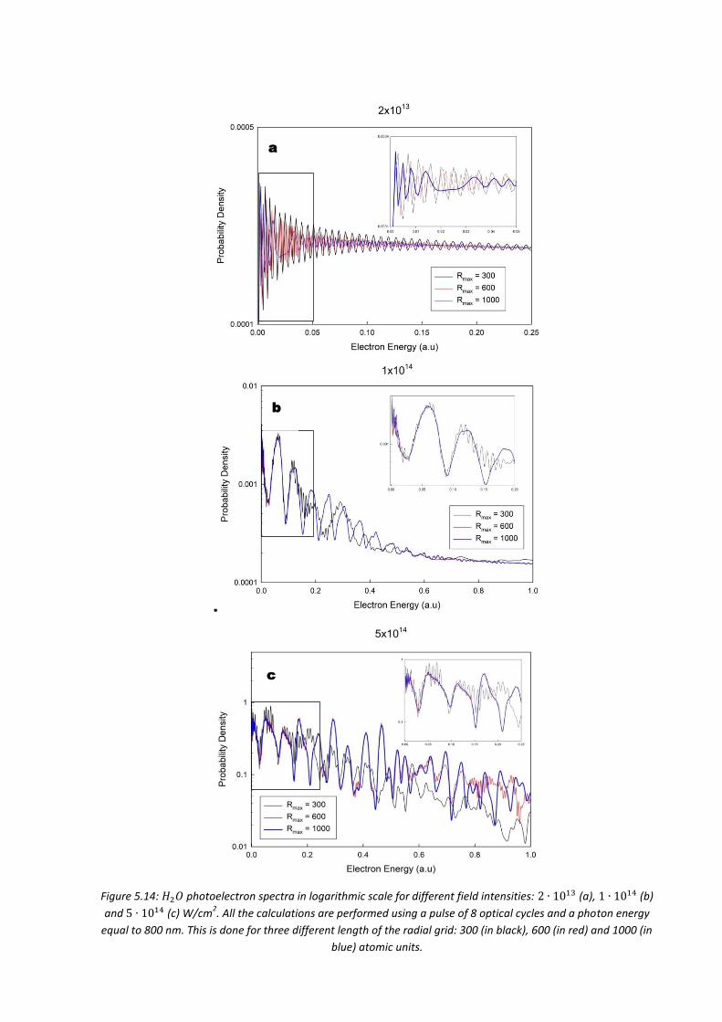
164
.
a
b
c
Figure 5.14: 𝐻2𝑂 photoelectron spectra in logarithmic scale for different field intensities: 2 ∙ 1013 (a), 1 ∙ 1014 (b)
and 5 ∙ 1014 (c) W/cm2. All the calculations are performed using a pulse of 8 optical cycles and a photon energy
equal to 800 nm. This is done for three different length of the radial grid: 300 (in black), 600 (in red) and 1000 (in
blue) atomic units.
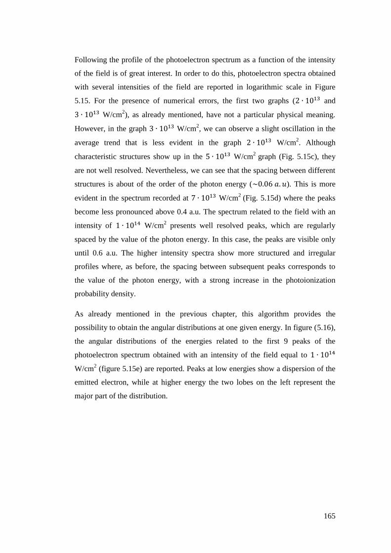
165
Following the profile of the photoelectron spectrum as a function of the intensity
of the field is of great interest. In order to do this, photoelectron spectra obtained
with several intensities of the field are reported in logarithmic scale in Figure
5.15. For the presence of numerical errors, the first two graphs (2 ∙ 1013 and
3 ∙ 1013 W/cm2), as already mentioned, have not a particular physical meaning.
However, in the graph 3 ∙ 1013 W/cm2, we can observe a slight oscillation in the
average trend that is less evident in the graph 2 ∙ 1013 W/cm2. Although
characteristic structures show up in the 5 ∙ 1013 W/cm2
graph (Fig. 5.15c), they
are not well resolved. Nevertheless, we can see that the spacing between different
structures is about of the order of the photon energy (~0.06 𝑎. 𝑢). This is more
evident in the spectrum recorded at 7 ∙ 1013 W/cm2
(Fig. 5.15d) where the peaks
become less pronounced above 0.4 a.u. The spectrum related to the field with an
intensity of 1 ∙ 1014 W/cm2 presents well resolved peaks, which are regularly
spaced by the value of the photon energy. In this case, the peaks are visible only
until 0.6 a.u. The higher intensity spectra show more structured and irregular
profiles where, as before, the spacing between subsequent peaks corresponds to
the value of the photon energy, with a strong increase in the photoionization
probability density.
As already mentioned in the previous chapter, this algorithm provides the
possibility to obtain the angular distributions at one given energy. In figure (5.16),
the angular distributions of the energies related to the first 9 peaks of the
photoelectron spectrum obtained with an intensity of the field equal to 1 ∙ 1014
W/cm2 (figure 5.15e) are reported. Peaks at low energies show a dispersion of the
emitted electron, while at higher energy the two lobes on the left represent the
major part of the distribution.
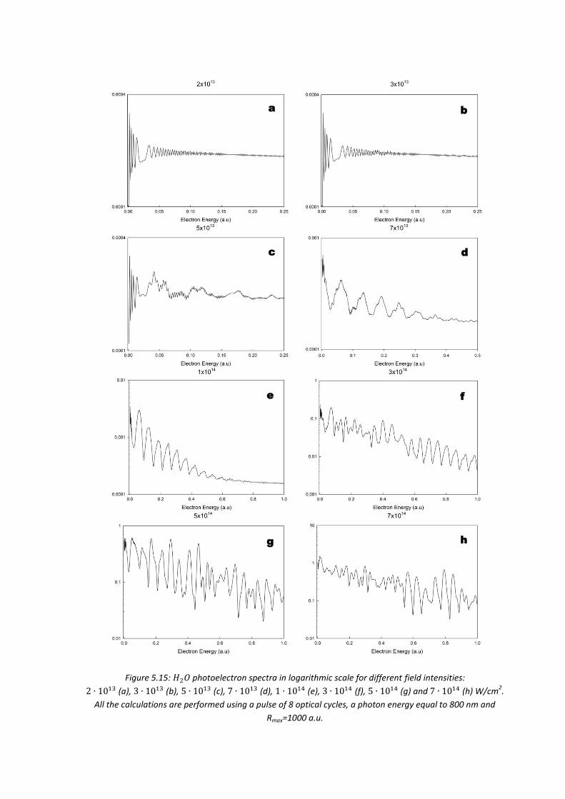
166
a b
c d
e f
g h
Figure 5.15: 𝐻2𝑂 photoelectron spectra in logarithmic scale for different field intensities:
2 ∙ 1013 (a), 3 ∙ 1013 (b), 5 ∙ 1013 (c), 7 ∙ 1013 (d), 1 ∙ 1014 (e), 3 ∙ 1014 (f), 5 ∙ 1014 (g) and 7 ∙ 1014 (h) W/cm2.
All the calculations are performed using a pulse of 8 optical cycles, a photon energy equal to 800 nm and
Rmax=1000 a.u.
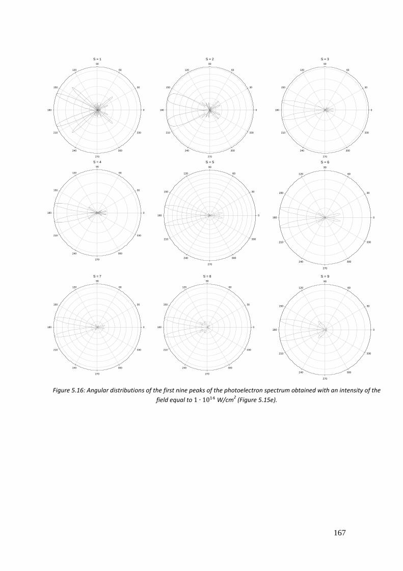
167
S = 1
0
30
60
90
120
150
180
210
240
270
300
330
S = 2
0
30
60
90
120
150
180
210
240
270
300
330
S = 3
0
30
60
90
120
150
180
210
240
270
300
330
S = 4
0
30
60
90
120
150
180
210
240
270
300
330
S = 5
0
30
60
90
120
150
180
210
240
270
300
330
S = 6
0
30
60
90
120
150
180
210
240
270
300
330
S = 7
0
30
60
90
120
150
180
210
240
270
300
330
S = 8
0
30
60
90
120
150
180
210
240
270
300
330
S = 9
0
30
60
90
120
150
180
210
240
270
300
330
Figure 5.16: Angular distributions of the first nine peaks of the photoelectron spectrum obtained with an intensity of the
field equal to 1 ∙ 1014 W/cm2 (Figure 5.15e).
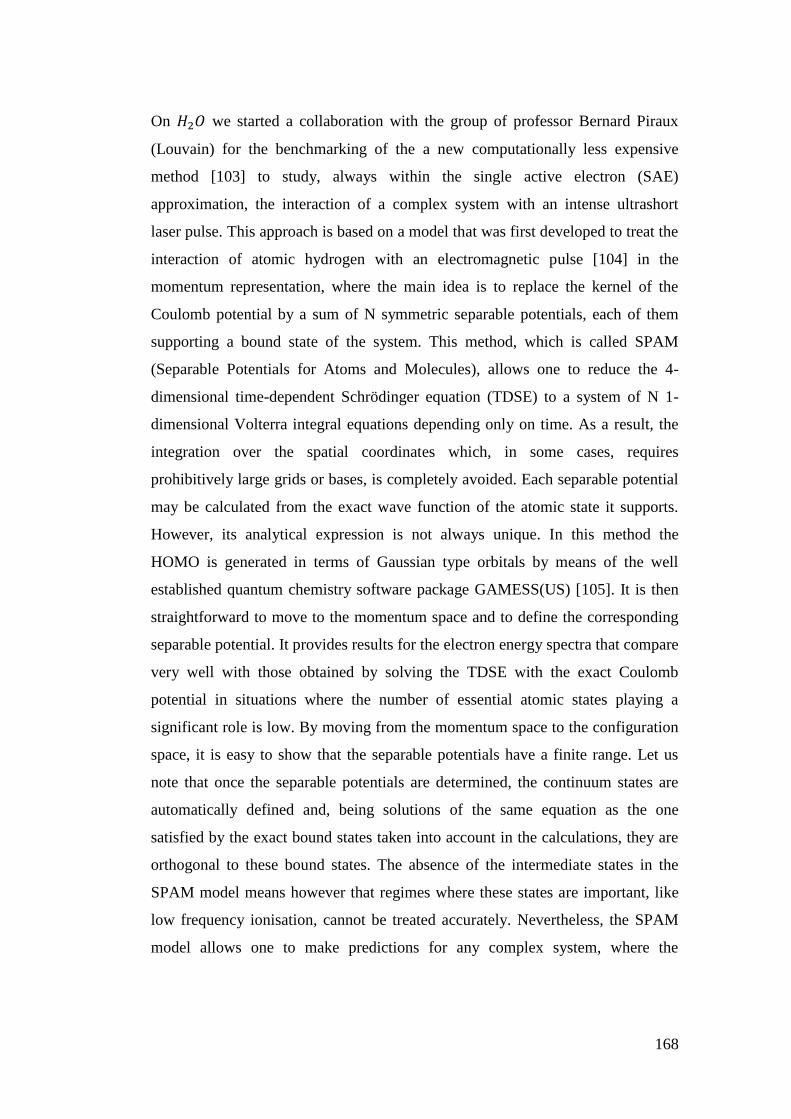
168
On 𝐻2𝑂 we started a collaboration with the group of professor Bernard Piraux
(Louvain) for the benchmarking of the a new computationally less expensive
method [103] to study, always within the single active electron (SAE)
approximation, the interaction of a complex system with an intense ultrashort
laser pulse. This approach is based on a model that was first developed to treat the
interaction of atomic hydrogen with an electromagnetic pulse [104] in the
momentum representation, where the main idea is to replace the kernel of the
Coulomb potential by a sum of N symmetric separable potentials, each of them
supporting a bound state of the system. This method, which is called SPAM
(Separable Potentials for Atoms and Molecules), allows one to reduce the 4-
dimensional time-dependent Schrödinger equation (TDSE) to a system of N 1-
dimensional Volterra integral equations depending only on time. As a result, the
integration over the spatial coordinates which, in some cases, requires
prohibitively large grids or bases, is completely avoided. Each separable potential
may be calculated from the exact wave function of the atomic state it supports.
However, its analytical expression is not always unique. In this method the
HOMO is generated in terms of Gaussian type orbitals by means of the well
established quantum chemistry software package GAMESS(US) [105]. It is then
straightforward to move to the momentum space and to define the corresponding
separable potential. It provides results for the electron energy spectra that compare
very well with those obtained by solving the TDSE with the exact Coulomb
potential in situations where the number of essential atomic states playing a
significant role is low. By moving from the momentum space to the configuration
space, it is easy to show that the separable potentials have a finite range. Let us
note that once the separable potentials are determined, the continuum states are
automatically defined and, being solutions of the same equation as the one
satisfied by the exact bound states taken into account in the calculations, they are
orthogonal to these bound states. The absence of the intermediate states in the
SPAM model means however that regimes where these states are important, like
low frequency ionisation, cannot be treated accurately. Nevertheless, the SPAM
model allows one to make predictions for any complex system, where the

169
aforementioned approximations are adequate, in the single photon regime. The
model is very scalable, so the limits on the size of the system are given by the
hardware resources.
In order to have some idea about how accurate is the prediction of the SPAM
model for high frequencies, we ran the SAE-TDSE code shown in this thesis in
different photoionization regimes and compared the ionisation yield prediction of
these two SAE models (see Figure 5.17). A significant difference between these
models is the fact that for SAE-TDSE the full coulomb potential has been taken
into account in generating the orbital basis, thus the SPAM result has been
corrected with a constant factor. In fact, for high frequencies we can approximate
a Coulomb wave with a plane wave. It turns out that using plane wave instead of
Coulomb wave is equivalent to introducing a constant factor. This factor is not "ad
hoc" as it can be derived from the dipole matrix elements in the case of a
Coulomb wave and a plane wave final state of the ionising system.
Both ionisation yields are normalised to 1. In fact, we have perfect agreement
between these models for high frequencies, and poor agreement for the photon
energies near the ionisation threshold. This can be explained by the fact that SAE-
TDSE uses 6000 Kohn-Sham orbitals to propagate the wavefunction, while in
SPAM there are no any intermediate state at all. This discrepancy could be
reduced by including the lowest unoccupied orbital in the SPAM calculation.
Note that, in Figure 5.18, the corrected SPAM coincides with SAE-TDSE in a
wide intensity range as well. This agreement of the corrected SPAM model and
SAE-TDSE approach in a wide intensity and frequency range indicates that the
SPAM correction factor does not depend on intensity and on frequency.
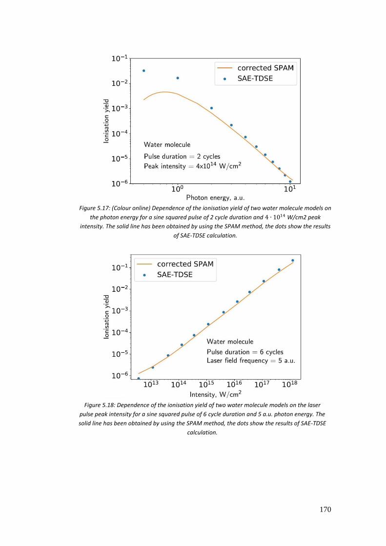
170
Figure 5.17: (Colour online) Dependence of the ionisation yield of two water molecule models on
the photon energy for a sine squared pulse of 2 cycle duration and 4 ∙ 1014 W/cm2 peak
intensity. The solid line has been obtained by using the SPAM method, the dots show the results
of SAE-TDSE calculation.
Figure 5.18: Dependence of the ionisation yield of two water molecule models on the laser
pulse peak intensity for a sine squared pulse of 6 cycle duration and 5 a.u. photon energy. The
solid line has been obtained by using the SPAM method, the dots show the results of SAE-TDSE
calculation.
171
6. Conclusions
This thesis has studied photoionization processes from a theoretical perspective
with the aim of increasing the number of the describable phenomena involving in
such processes. This aim has been achieved by using and implementing methods
focussed on the treatment of correlation effects and non-perturbative
photoionization regime.
The first part of the thesis has been dedicated to correlation effects within the
bound states. Since a standard DFT method does not permit to study any
correlation effect, it is necessary to use Configuration Interaction (CI) method to
describe both the neutral initial state and ionic final state. More specifically,
Complete Active Space Self-Consistent Field (CASSCF) procedure coupled to a n-
electron valence state perturbation theory (NEVPT2) procedure has been applied.
By the superposition between final and initial wavefunctions, one can define
Dyson orbitals. The most frequent evidence of electron correlation is the presence
of additional bands, called satellite bands, in the photoelectron spectra. It is
known that photoelectron spectrum of both CO and CS presents well-resolved
satellite bands. Thus, the structure of satellite bands in these molecules as in
further isoelectronic molecules (CSe and SiO) has been studied. The position of
the satellite bands in CS and CSe stays at lower 𝐼𝑃 values compared to the second
sigma primary ionization state 2𝛴, whereas in CO and SiO it stays at higher 𝐼𝑃
values with respect to the 2𝛴 band. For all the four considered molecules,
dynamical photoionization observables (i.e., cross sections and asymmetry
parameters) have been calculated for the first four ionization states, by comparing
the results so obtained to those ones got by standard DFT method, Dyson orbital
approach and HF method. Satellite bands can be taken into account only by the
Dyson approach, which has proved to be able to properly describe also the other
ionization states. A further significant result refers to DFT method, which, despite
its mono-determinantal nature, is able to treat a small part of correlation although
not to treat strong correlation effects, such as those ones present in the first two Σ
172
primary ionization states of the SiO molecule. The formalism has also been
applied to the 𝑂3 molecule in a collaboration aimed to study ultra short electron
motion after coherent excitation of the GS and the B excited state by an
appropriate laser pulse. As a probe we have considered time resolved
photoelectron spectra obtained by a subfemtosecond UV pulse, in preparation for
a further collaboration with an experimental group. A clear signature of the
wavepacket evolution is predicted, and its angular dependence has been
investigated, as reported in a joint publication [106].
In the second part of the thesis, the implementation of an algorithm to calculate
two-electron integrals in the LCAO B-spline basis with the aim to treat all the
many-electron effects has been illustrated. This has been done to fully express the
final wavefunction within the Close-Coupling (CC) formalism that permits to also
describe correlation effects involving continuum states. In particular, the integrals
have been calculated by solving the Poisson equation. A test on the product
between B-splines and orbitals has been carried out to ensure that the electron
density can be expanded in the B-splines basis set providing the best possible
compromise between truncation errors and computational cost. The program has
been tested by comparing two-electron integrals for selected MOs obtained by the
presented algorithm to the corresponding integrals calculated by using the
MOLPRO quantum chemistry package. The comparison, reported in Table 4.1,
has shown a good agreement between the two results. This represents a first but
extremely relevant step to completely describe the wavefunction with the Close-
Coupling formalism.
The third part of the thesis has been focused on the non-perturbative phenomena.
To study these phenomena, the implementation of an algorithm to solve Time-
Dependent Schrödinger Equation (TDSE) has been carried out. In the method that
will be presented, time-evolution is discretized in subintervals sufficiently small
so that the Hamiltonian approximately becomes time-independent. Since the
diagonalization at each step is not computationally feasible, an appropriate small
local basis is provided by Lanczos-Arnoldi method. The final wavepacket, derived
173
by time propagation, is then projected onto the continuum states calculated with
the DFT method. In this way, photoelectron spectrum and MFPADs can be
obtained. The program has been accurately tested by comparing our results to
those ones reported in literature. An intensive study has been done on the
hydrogen atom: photoelectron spectra calculated with different pulse parameters
have been compared to those ones reported by Cormier and Lambropoulos. All
the spectra, in addition to the angular distributions, have proved to be correct. This
method can intrinsically treat also the perturbative phenomena. An evidence of
this has been made by studying both one-photon and two-photon ionizations of
the hydrogen atom. This method has also been tested on some molecular systems.
The final wavepacket of 𝐻𝑒𝐻++ has been successfully compared to the one
calculated by another research group. Photoelectron spectra relative to molecules
under strong field and short pulse are really difficult to be found in literature, even
in the case of 𝐻2+: this demonstrates the rarity and then the importance of this kind
of calculations. Two different studies on 𝐻2+ have been done: the first by
employing a strong field and the second with a weak field. Strong field
photoelectron spectrum has been compared to that one obtained by using elliptical
coordinates, which are appropriate just for such systems. The calculation with a
weak field has been applied in the case of one-photon ionization. The resulting
cross section has been compared to that one obtained by the perturbative method.
NH3 has been studied to observe ionization yield as a function of the angle
between the electromagnetic field and the molecular axes, verifying that the
periodicity of the ionization yield by rotating the field around the C3v axes
amounts to 120°. Ionization yield of the 𝐻2𝑂 HOMO 1b1 has been calculated as a
function of the intensity of the field and it has been used as benchmark for a new
computationally less expensive method implemented by another research group
we started a collaboration with. Several photoelectron spectra of this molecule
have been calculated at different intensity of the field, with particular attention to
the convergence of the results by varying the length of the radial grid. Several
angular distributions have also been reported.

174
To conclude, this thesis collects the implementation of several algorithms based
on the use of B-splines as basis functions; these efficient functions have
contributed to the improvement of the theoretical knowledge about
photoionization processes, making possible the description of both many-electron
phenomena due to correlation effects and non-perturbative phenomena due to
strong field radiations. Moreover, the algorithms built can be efficiently used in
parallel computing. As a consequence, this study has improved the amount of
cases that can be treated and that can be compared to experimental data.

175
7. Bibliography
[1] D. W. Turner and M. I. Al-Jobory. J. Chem. Phys. 37, 3007 (1962).
URL https://doi.org/10.1063/1.1733134
[2] A. W. Potts, H. J. Lempka, D. G. Streets, and W. C. Price. Phil. Trans. R. Soc. Lond. 268, 59
(1970). URL http://rsta.royalsocietypublishing.org/content/268/1184/59.
[3] Philip Willmot, An introduction to Synchrotron Radiation: Techniques and Applications.
John Wiley & Sons, (2011).
[4] S. Suga, A. Sekiyama, Photoelectron Spectroscopy, Bulk and Surface Electronic Structures.
Springer-Verlag Berlin, (2014).
[5] T. Brabec and F. Krausz, Rev. Mod. Phys. 72, 545 (2000). URL https://journals.aps.org/rmp/abstract/10.1103/RevModPhys.72.545.
[6] F. J. Wuilleumier and M. Meyer, J. Phys. B 39, R425 (2006). URL http://iopscience.iop.org/article/10.1088/0953-4075/39/23/R01.
[7] J. Köhler, M. Wollenhaupt, T. Bayer, C. Sarpe, and T. Baumert, Opt. Express 19, 11638
(2011). URL https://www.osapublishing.org/oe/abstract.cfm?uri=oe-19-12-11638.
[8] D. R. Hartree. Proc. Cambridge Phil. Soc., 24, 89, (1927).
[9] V. Fock. Z. Physik, 61, 126 (1930). URL http://dx.doi.org/10.1007/BF01340294.
[10] J. C. Slater. Phys. Rev. 35, 210 (1930). URL http://link.aps.org/doi/10.1103/PhysRev.35.210.2
[11] C. D. Sherrill and H. F. Schaefer. Science Direct, 34, 143 (1999). URL http://www.sciencedirect.com/science/article/pii/S0065327608605328.
[12] U. Becker and D. A. Shirley. VUV and Soft X-Ray Photoionization.Plenum Press, (1996). [13] J. C. Green and P. Decleva. Coord. Chem. Rev. 249, 209 (2005).
URL http://www.sciencedirect.com/science/article/pii/S0010854504000396.
[14] B. H. Bransden and C. J. Joachain. Physics of Atoms and Molecules. Prentice Hall, (2003). [15] D. Toffoli, M. Stener, G. Fronzoni, and P. Decleva. Chem. Phys. 276, 25, (2002).
URL http://www.sciencedirect.com/science/article/pii/S0301010401005493.
[16] S. Petretti, Y.V. Vanne, A. Saenz, A. Castro and P. Decleva. Phys. Rev. Letters 104, 223001,
(2010). URL https://journals.aps.org/prl/abstract/10.1103/PhysRevLett.104.223001.

176
[17] T. Mizuno, J. Adachi, M. Kazama, M. Stener, P. Decleva, and A. Yagishita. Phys. Rev.
Letters 110, 043001 (2013). URL https://journals.aps.org/prl/abstract/10.1103/PhysRevLett.110.043001.
[18] R. K. Kushawaha, M. Patanen, R. Guillemin, L. Journel, C. Miron, M. Simon, M. N.
Piancastelli and P. Decleva PNAS, 110, 15201 (2013). URL http://www.pnas.org/content/110/38/15201.abstract.
[19] J. R. Taylor. Scattering Theory: The Quantum Theory of Nonrelativistic Collisions. Dover
Publications, (1983).
[20] L. Keldysh. Sov. Phys. JETP 20, 1307 (1965).
URL http://www.jetp.ac.ru/cgi-bin/e/index/e/20/5/p1307?a=list
[21] http://www.desy.de. Copyright c 2007 DESY.
[22] T. Topcu and F. Robicheaux, Phys. Rev. A 86, 053407 (2012).
URL https://journals.aps.org/pra/abstract/10.1103/PhysRevA.86.053407
[23] L. Young, E. P. Kanter, B. Krässig, et al. Nature 466, 56 (2010). URL
http://www.nature.com/nature/journal/v466/n7302/abs/nature09177.html?foxtrotcallback=tru
e
[24] G. Doumy, C. Roedig, S.-K. Son, et al. Phys. Rev. Lett. 106, 083002 (2011).
URL https://journals.aps.org/prl/issues/106/8
[25] H. Bachau, E. Cormier, P. Decleva, J. E. Hansen and F. Martın. Applications of B-splines in
atomic and molecular physics. Rep. Prog. Phys. 64, 1815–1942 (2001).
[26] I. J. Schoenberg. Quart. Appl. Math. 4, 45 (1946).
[27] C. De Boor. A Practical Guide to Splines. New York: Springer (1978).
[28] J. Stoer and R. Bulirsch. Introduction to Numerical Analysis. New York: Springer (1983).
[29] W.H. Press, S. A. Teukolsky, W. T. Vetterling, B. P. Flannery. The art of scientific
computing, Numerical Recipes in Fortran 77, Fortran numerical recipes, volume 1 (1992).
[30] L. S. Cederbaum, W. Domcke, J. Schirmer, and W. von Niessen. Adv. Chem. Phys. 65, 115,
(1986).
URL http://dx.doi.org/10.1002/9780470142899.ch3
[31] M. Martins, K. Godehusen, T. Richter, P. Wernet, and P. Zimmermann. J. Phys. B: At. Mol.
Opt. Phys. 39, R79 (2006).
URL http://stacks.iop.org/0953-4075/39/i=5/a=R01.
[32] R. L. Martin and D. A. Shirley. Phys. Rev. A, 13, 1475 (1976).
URL http://link.aps.org/doi/10.1103/PhysRevA.13.1475.
[33] J. C. Green and P. Decleva. Coord. Chem. Rev., 249, 209, (2005).
URL http://www.sciencedirect.com/science/article/pii/S0010854504000396.
[34] S. Popruzhenko and D. Bauer, J. Mod. Opt. 55, 2573 (2008).
URL http://www.tandfonline.com/doi/abs/10.1080/09500340802161881.

177
[35] A. Becker and F. H. M. Faisal, J. Phys. B 38, R1 (2005).
URL http://iopscience.iop.org/article/10.1088/0953-4075/38/3/R01/meta.
[36] U. V. Riss and H. D. Meyer. J. Phys. B 26, 4503 (1993).
URL http://iopscience.iop.org/article/10.1088/0953-4075/26/23/021/pdf.
[37] M. Born and J. R. Oppenheimer. Ann. Physik, 389, 457 (1927).
URL http://dx.doi.org/10.1002/andp.19273892002.
[38] W. Kohn and L. J. Sham. Phys. Rev., 140, A1133 (1965).
URL http://dx.doi.org/10.1007/BF01322090.
[39] G. te Velde, F. M. Bickelhaupt, E. J. Baerends, C. Fonseca Guerra, S. J. A. van Gisbergen, J.
G. Snijders, and T. Ziegler. J. Comput. Chem., 22:931 (2001).
URL http://dx.doi.org/10.1002/jcc.1056.
[40] M. Stener, A. Lisini, and P. Decleva. Int. J. Quantum Chem., 53, 229 (1995).
URL http://dx.doi.org/10.1002/qua.560530208.
[41] G. H. Golub and C. F. van Loan. Matrix computations. The Johns Hopkins University Press,
third edition, p.374 (1996).
[42] M. W. Schmidt and M. S. Gordon. Ann. Rev. Phys. Chem., 49, 233 (1998).
URL http://dx.doi.org/10.1146/annurev.physchem.49.1.233.
[43] B. O. Roos, P. R. Taylor, and P. E. M. Siegbahn. Chem. Phys., 48, 157, (1980).
URL http://www.sciencedirect.com/science/article/pii/0301010480800450.
[44] C. Angeli, R. Cimiraglia, S. Evangelisti, T. Leininger, and J.-P. Malrieu. J. Chem. Phys., 114,
10252, (2001).
URL http://scitation.aip.org/content/aip/journal/jcp/114/23/10.1063/1.1361246.
[45] C. Angeli, R. Cimiraglia, and J. P. Malrieu. J. Chem. Phys. 117, 9138 (2002).
URL http://scitation.aip.org/content/aip/journal/jcp/117/20/10.1063/1.1515317.
[46] C. Angeli, R. Cimiraglia, and J-P. Malrieu. Chem. Phys. Lett., 350, 297 (2001).
URL http://www.sciencedirect.com/science/article/pii/S0009261401013033.
[47] H.-J. Werner, P. J. Knowles, G. Knizia, F. R. Manby, M. Schütz, P. Celani, T. Korona, R.
Lindh, A. Mitrushenkov, G. Rauhut, K. R. Shamasundar, T. B. Adler, R. D. Amos, A.
Bernhardsson, A. Berning, D. L. Cooper, M. J. O. Deegan, A. J. Dobbyn, F. Eckert, E. Goll,
C. Hampel, A. Hesselmann, G. Hetzer, T. Hrenar, G. Jansen, C. Köppl, Y. Liu, A. W. Lloyd,
R. A. Mata, A. J. May, S. J. McNicholas, W. Meyer, M. E. Mura, A. Nicklass, D. P. O’Neill,
P. Palmieri, D. Peng, K. Pflüger, R. Pitzer, M. Reiher, T. Shiozaki, H. Stoll, A. J. Stone, R.
Tarroni, T. Thorsteinsson, and M. Wang. Molpro, version 2012.1, a package of ab initio
programs, (2012).
URL http://www.molpro.net.
[48] A. D. O. Bagawan and E. R. Davidson. Adv. Chem. Phys. 110, 215, (1999).
URL https://doi.org/ADCPAA.

178
[49] X. J. Liu, H. Fukuzawa, T. Teranishi, A. De Fanis, M. Takahashi, H. Yoshida, A. Cassimi, A.
Czasch, L. Schmidt, R. Doerner, I. Koyano, N. Saito, and K. Ueda. Phys. Rev. Lett. 101,
023001 (2008).
URL http://link.aps.org/doi/10.1103/PhysRevLett.101.023001.
[50] T. Jahnke, J. Titze, L. Foucar, R. Wallauer, T. Osipov, E. P. Benis, O. Jagutzki, W. Arnold,
A. Czasch, A. Staudte, M. Schöffler, A. Alnaser, T. Weber, M. H. Prior, H. Schmidt-
Böcking, and R. Dörner. J. Electron. Spectrosc. Relat. Phenom. 183, 48 (2011).
URL http://www.sciencedirect.com/science/article/pii/S0368204810000885.
[51] N.Jonathan, A.Morris, M.Okuda, K.J. Ross and D.J. Smith. Faraday Discuss 54, 48 (1972).
URL http://pubs.rsc.org/en/Content/ArticleLanding/1972/DC/DC9725400048#!divAbstract
[52] A. Ponzi, C. Angeli, R. Cimiraglia, S. Coriani and P. Decleva, J. Chem Phys. 140, 204304
(2014).
URL https://www.ncbi.nlm.nih.gov/pubmed/24880277.
[53] K.P. Huber, G. Herzberg, Molecular Spectra and Molecular Structure. IV. Constants of
Diatomic Molecules, Van Nostrand Reinhold Co. (1979).
URL http://webbook.nist.gov/cgi/cbook.cgi?Source=1979HUB%2FHER716B&Mask=1000.
[54] M. Springborg Phys, Rev. B 39, 5327, 8 (1989).
URL https://journals.aps.org/prb/abstract/10.1103/PhysRevB.39.5327.
[55] N. Varambhia, M. Gupta, A. Faure, K. L. Baluja and J. Tennyson. J. Phys. B: At. Mol. Opt.
Phys. 42, 095204 (2009).
URL http://iopscience.iop.org/article/10.1088/0953-4075/42/9/095204/meta.
[56] A. W. Potts and T. A. Williams J. Electron spectroscopy. 3, 3 (1974).
YRL http://www.sciencedirect.com/science/article/pii/0368204874800708?via%3Dihub.
[57] M. Ehara, M. Ishida, and H. Nakatsuji, Collect. Czech. Chem. Commun. 70, 881 (2005).
URL https://doi.org/CCCCAK
[58] A.B. Trofimov and W. Schirmer J. Chem. Phys. 123, 144115 (2005).
URL http://aip.scitation.org/doi/10.1063/1.2047550.
[59] E. A. Coulbourne, J. M. Dyke, E.P.F. Lee, A. Morris and I. R. Trickle, Mol. Phys. 35, 873
(1978).
URL https://doi.org/MOPHAM.
[60] N. Honjou. Mol. Phys. 101, 131 (2003).
URL http://www.tandfonline.com/doi/abs/10.1080/00268970310001617793.
[61] Y. Ohtsuka, J. Hasegawa & H. Nakatsuji. Chem. Phys. 332, 262 (2007).
URL https://doi.org/10.1016/j.chemphys.2006.12.008.
[62] X. Che, G. Farin , Z. Gao, D. Hansford. Advanced Materials Research, 186, 445 (2011).
URL https://www.scientific.net/AMR.186.445.
[63] K. Morken. Constr. Approx. 7, 195 (1991).
URL https://link.springer.com/article/10.1007/BF01888153.
[64] H. Zewail, J. Phys. Chem. A, 24, 104 (2000).

179
URL http://pubs.acs.org/doi/abs/10.1021/jp001460h.
[65] P. B. Corkum. Physical Review Letters. 71, 1994, (1997).
URL 10.1103/physrevlett.71.1994.
[66] O. Smirnova and M. Ivanov, Multielectron High Harmonic Generation: Simple Man on a
Complex Plane. Schultz and Vrakking. (2014)
URL http://onlinelibrary.wiley.com/doi/10.1002/9783527677689.ch7/summary.
[67] J. Zhang and P. Lambropoulos. J. Nonlinear Opt. Phys. Mater 4, 633 (1995).
URL http://www.worldscientific.com/doi/abs/10.1142/S0218863595000276.
[68] G. G. Paulus, W. Nicklich, F. Zacher, P. Lambropoulos and H. Walther. J. Phys. B: At. Mol.
Opt. Phys. 29, L249 (1996).
URL http://iopscience.iop.org/article/10.1088/0953-4075/29/7/002/meta
[69] E. Cormier and P. Lambropoulos, J. Phys. B: At. Mol. Opt. Phys. 30 77–91 (1997).
URL http://iopscience.iop.org/article/10.1088/0953-4075/30/1/010/meta.
[70] J. Itatani, J. Levesque, D. Zeidler, H. Niikura, H. Pepin, J.C. Kieffer, P.B. Corkum, D.M.
Villeneuve, Nature 432, 867 (2004).
URL http://www.nature.com/nature/journal/v432/n7019/abs/nature03183.html.
[71] M. Meckel, D. Comtois, D. Zeidler, A. Staudte, D. Pavičić, H. C. Bandulet, H. Pepin, J. C.
Kieffer, R. Dorner, D. M. Villeneuve, P. B. Corkum, Science 320, 1478 (2008).
URL http://dionne.stanford.edu/MatSci202_2011/Science-2008-Meckel-1478-82.pdf.
[72] P. Agostini, L.F. DiMauro, Rep. Prog. Phys. 67, 813 (2004).
URL http://iopscience.iop.org/article/10.1088/0034-4885/67/6/R01/meta.
[73] J. H. Posthumus, Rep. Prog. Phys. 67, 813 (2004).
URL http://iopscience.iop.org/article/10.1088/0034-4885/67/5/R01/meta.
[74] M. Drescher, F. Krausz, J. Phys. B 38, 727 (2005).
URL http://iopscience.iop.org/article/10.1088/0953-4075/38/9/019/meta.
[75] B. K. McFarland, J. P. Farrell, P. H. Bucksbaum, M. Guhr. Science 322, 1232 (2008).
URL http://science.sciencemag.org/content/322/5905/1232.
[76] H. Akagi, T. Otobe, A. Staudte, A. Shiner, F. Turner, R. Dorner, D.M. Villeneuve, P.B.
Corkum, Science 325, 1364 (2009).
URL https://www.ncbi.nlm.nih.gov/pubmed/19745145.
[77] J. P. Farrell, S. Petretti, J. Forster, B. K. McFarland, L. S. Spector, Y. V. Vanne, P. Decleva,
P. H. Bucksbaum, A. Saenz, M. Guhr, Phys. Rev. Lett. 107, 083001 (2011).
URL https://doi.org/10.1103/PhysRevLett.107.083001.
[78] O. Smirnova, Y. Mairesse, S. Patchkovskii, N. Dudovich, D. Villeneuve, P. Corkum, M.Y.
Ivanov, Nature 460, 972 (2009).
URL https://www.nature.com/nature/journal/v460/n7258/full/nature08253.html.
[79] I. Sánchez, F. Martín, Phys. Rev. Lett. 79, 1654 (1997).
URL https://journals.aps.org/prl/abstract/10.1103/PhysRevLett.79.1654.

180
[80] I. Sánchez, F. Martín, Phys. Rev. Lett. 82, 3775 (1999).
URL https://journals.aps.org/prl/abstract/10.1103/PhysRevLett.82.3775.
[81] J.L. Sanz-Vicario, A. Palacios, J.C. Cardona, H. Bachau, F. Martín. J. of Electron
Spectroscopy and Related Phenomena 161, 182–187 (2007).
URL http://www.sciencedirect.com/science/article/pii/S0368204807000679.
[82] E. Cormier and P. Lambropoulos. J. Phys. B: At. Mol. Opt. Phys. 29 1667–1680 (1996).
URL http://iopscience.iop.org/article/10.1088/0953-4075/29/9/013/meta.
[83] M. Göppert-Mayer, Über Elementarakte mit zwei Quantensprüngen J. A. Barth, (1931)
[84] M. G. Floquet: Équations différentielles linéires a coefficients périodiques. Ann. de l‘École
Normale Supérieure 12, 47 (1883).
[85] R. M. Potvliege and R. Shakeshaft: Nonperturbative treatment of multiphoton ionization
within the Floquet framework, in Atoms in Intense Laser Fields. Edited by M. Gavrila, p. 373
Academic Press (1992).
[86] P. G. Burke, P. Francken, and C. J. Joachain. Phys. B 24, 761 (1991).
URL http://iopscience.iop.org/article/10.1088/0953-4075/24/4/005/meta.
[87] C. Runge. Ueber die numerische Auflösung von Differentialgleichungen Math.
Ann., 46, 167–178 (1895).
URL https://link.springer.com/article/10.1007%2FBF01446807.
[88] W. Kutta, Beitrag zur naherungsweisen Integration von Differentialgleichungen. Z. Math.
und Phys. 46, 435–453 (1901).
[89] R. Wiehle, B. Witzel, H. Helm, and E. Cormier. Phys. Rev. A 67, 063405 (2003).
URL https://journals.aps.org/pra/abstract/10.1103/PhysRevA.67.063405.
[90] L. A. A. Nikolopoulos and P. Maragakis. Phys.Rev. A 64, 053407 (2001).
URL https://journals.aps.org/pra/abstract/10.1103/PhysRevA.64.053407.
[91] Ionization of Molecular Hydrogen in Ultrashort Intense Laser Pulses Dipl.-Phys. Yulian V.
Vanne (2010).
URL https://edoc.hu-berlin.de/handle/18452/16759.
[92] H. B. van Linden, van den Heuvell and H. G. Muller: Limiting cases of excessphoton
ionization, in Multiphoton Processes, edited by S. J. Smith and P. L. Knight, p. 25,
Cambridge Univ. Press, (1988).
[93] T. F. Gallagher. Phys.Rev. Lett. 61, 2304 (1988).
URL https://journals.aps.org/prl/abstract/10.1103/PhysRevLett.61.2304.
[94] Z. Chen, A.-T. Le, T. Morishita, and C. D. Lin. Phys.Rev. A 79, 033409 (2009).
URL https://journals.aps.org/pra/abstract/10.1103/PhysRevA.79.033409.
[95] W. E. Arnoldi, The principle of minimized iterations in the solution of the matrix eigenvalue
problem, Quarterly of Applied Mathematics, 9, 17–29, (1951).
[96] C. Lanczos. An iteration method for the solution of the eigenvalue problem of linear
differential and integral operators, J. Res. Nat’l Bur. Std. 45, 255-282 (1950).

181
[97] C. Lubich. From Quantum to Classical Molecular Dynamics: Reduced Models and
Numerical Analysis, Zurich lectures in advanced mathematics. (2008).
[98] Y. Saad. Numerical Methods for large eigenvalue problems. Algorithm and architectures for
advanced scientific computing (1992)
[99] The one-photon ionization cross section in a.u. reads 𝜎(𝜔) =25𝜋2
3𝑐𝜔4
𝑒−4𝛾𝑡𝑎𝑛−1(
1𝛾)
1−𝑒−2𝜋𝛾 where
𝛾 = 1/𝑘, 𝑘 = [2𝜇(𝜔 − 0.5)]1/2 and μ is the reduced mass. A treatment of the photoeffect in
Hydrogen is found in: “H. A. Bethe, E. E. Salpeter. Quantum Mechanics of One- and Two-
Electron Atoms, Springer-Verlags, New York, (1957)”.
[100]E. Karule. J. Phys. B, 11, 441 (1978).
URL http://iopscience.iop.org/article/10.1088/0022-3700/11/3/015/pdf.
[101]Johann Förster, Humboldt-Universität zu Berlin, Department of Physics, Berlin, private
communication.
[102]S. Petretti, A. Saenz, A. Castro, P. Decleva, Chem. Phys. 414, 45-52 (2013).
URL http://www.sciencedirect.com/science/article/pii/S0301010412000237?via%3Dihub.
[103]A. Galstyan, Y. V. Popov, N. Janssens, F. Mota-Furtado, P. F. O’Mahony, P. Decleva, N.
Quadri and B. Piraux. Ionisation of H2O by a strong ultrashort XUV pulse: a model within
the single active electron approximation. (2017)
URL https://arxiv.org/abs/1703.05517.
[104]T. Nganso, H. M. Popov, Y. V. Piraux, B. Madroñero, J. Njock, M. G. K. Physical Review A,
83, 013401, (2011).
URL https://journals.aps.org/pra/abstract/10.1103/PhysRevA.83.013401.
[105]M. W. Schmidt, K. K. Baldridge, J. A. Boatz, S. T. Elbert, M. S. Gordon, J. H. Jensen, S.
Koseki, N. Matsunaga, K. A. Nguyen, S. Su, T. L. Windus, M. Dupuis, J. A. Montgomery.
Journal of Computational Chemistry, 14, 1347–1363 (1993).
URL http://www.msg.ameslab.gov/gamess/.
[106]P. Decleva, N. Quadri, A. Perveaux, D. Lauvergnat, F. Gatti, B. Lasorne, G. J. Halász and Á.
Vibók. Scientific Reports. 6, 36613 (2016).
URL http://dx.doi.org/10.1038/srep36613.