SCUOLA DI INGEGNERIA E ARCHITETTURA Sede di Forlì … MAGISTRALE ANTONELLO... · Terminata la fase...

ALMA MATER STUDIORUM UNIVERSITA’ DI BOLOGNA

SCUOLA DI INGEGNERIA E ARCHITETTURA Sede di Forlì

Corso di Laurea in

INGEGNERIA MECCANICA

Classe LM-33

TESI DI LAUREA in Costruzione di macchine LM

DESIGN AND DEVELOPMENT OF A QUARTER

CAR TEST RIG

Anno Accademico 2015/2016

CANDIDATO

RELATORE Antonello Dambrosio Prof. Ing. Giangiacomo

Minak

CORRELATORE

Prof. Ing. Roberto Lot

ABSTRACT

Il presente lavoro di tesi, svolto presso l’università di Southampton, ha come obiettivo

la progettazione di un banco prova per un quarto di veicolo e la realizzazione di un

generatore di segnale che sia in grado di inviare segnali di ingresso ad un attuatore

idraulico il quale sarà utilizzato per eccitare la ruota in modo da simulare il profilo

stradale. La fase di progettazione è stata svolta utilizzando il software di disegno

Solidworks che ha permesso di delineare i disegni del banco prova. In seguito sono state

eseguite simulazioni per l’analisi strutturale e di frequenza di alcune parti del banco

tramite l’utilizzo del software Ansys.

Prima dello sviluppo del progetto sono state visionate diverse recensioni di Quarter-car

test rig, analizzando e valutando i punti forti e le carenze riscontrate. Sulla base di questa

ricerca è stata definita una lista di requisiti che dovrà soddisfare il banco.

Terminata la fase di progetto, il modello Solidworks è stato importato in ambiente

Simulink utilizzando i blocchi di modellazione della piattaforma

Simscape/SimMechanics, in modo da effettuarne un analisi dinamica del modello.

Tramite il software Matlab è stato realizzato uno script in grado di generare un segnale

che replica un profilo stradale secondo la classificazione ISO 8608. Successivamente è

stata eseguita una simulazione per valutare la risposta della massa sospesa per effetto

dell’eccitazione derivante dal profilo stradale.

L’ultima parte dello studio riguarda la realizzazione di un generatore di segnale, che allo

stesso tempo fosse in grado di ricevere il segnale di feedback proveniente dal servo

controller dell’attuatore. Il servo controller possiede un ingresso analogico a cui è

possibile applicare segnali esterni per il controllo di posizione dello shaker e un uscita

analogica per leggere il segnale proveniente dal trasduttore di spostamento posto nello

shaker. Il generatore è stato realizzato utilizzando il micro controllore Arduino Uno. Tale

dispositivo grazie alle sue potenzialità ha permesso la generazione di un segnale

sinusoidale a diverse ampiezza e frequenze in modo da coprirne un certo campo di valori

in base alla richiesta. Inoltre tale sistema è in grado di ricevere il segnale di feedback dal

servo controller dello shaker in modo tale da leggerne il valore e monitorarlo in tempo

reale sul PC. I risultati di questo studio mostrano che il Quarter car test rig progettato è

una piattaforma in grado di studiare il comportamento dinamico dei sistemi sospensivi,

la cui struttura si rende capace di poter testare diverse tipologie di sospensioni e pesi di

veicolo, rappresentando un solido punto di partenza per una futura realizzazione fisica

del banco.

In qualità di relatore autorizzo la redazione della tesi in lingua straniera e mi faccio garante della qualità linguistica dell’elaborato

Prof Ing. Giangiacomo Minak

Alla mia Famiglia

i

INDEX

List of figures .................................................................................................................. iii

1 - Introduction ................................................................................................................. 1

1.1 Motivation and objectives ..................................................................................... 1

1.2 Approach and outline............................................................................................. 2

2 - Literature review ......................................................................................................... 3

2.1 Automotive test methods ............................................................................................ 3

2.2 Quarter-car test rigs .................................................................................................... 4

2.3 Functional requirements of Quarter-car test rig ......................................................... 7

3 - Parts Design ................................................................................................................ 9

3.1 Quarter car test rig description ................................................................................... 9

3.2 Base plate .................................................................................................................. 11

3.3 Load frame ................................................................................................................ 13

3.3 Sprung mass frame ................................................................................................... 17

3.4 Linear Guides ........................................................................................................... 19

3.5 Hydraulic Shaker ...................................................................................................... 20

4 - Vehicle suspension modelling ................................................................................... 23

4.1 Vibration theory ........................................................................................................ 23

4.2 System Modelling ..................................................................................................... 24

4.2.1 Discrete and continuous models ............................................................................ 25

4.3 Vehicle model ........................................................................................................... 27

4.4 Quarter-car model ..................................................................................................... 31

5 - Simulation of a McPherson suspension on the test rig ............................................. 35

5.1 Vehicle suspension ................................................................................................... 35

5.2 Implementation of a McPherson suspension on the rig ............................................ 37

ii

5.3 Configuration of system parameters ......................................................................... 45

5.4 Simulation of a Quarter car test rig model in Simulink ............................................ 47

6 - Signal generator powered by Arduino Uno .............................................................. 57

6.1 Arduino Uno description .......................................................................................... 57

6.2 Objectives and Component used ......................................................................... 59

6.3 Development of the project ................................................................................. 59

7 - Conclusion and future development .......................................................................... 75

APPENDIX .................................................................................................................... 77

REFERENCES ............................................................................................................... 83

iii

List of figures

Figure 2. 1 – Four-post rig ................................................................................................ 4

Figure 2. 2 – Quarter car test rig developed by the University of Istanbul ...................... 5

Figure 2. 3 – Quarter-car test rig designed by University of Munchen ............................ 6

Figure 2. 4 – Quarter-car test rig of Pravara Rural Engineering College Loni ................ 7

Figure 3. 1 – Scheme of quarter-car test rig ................................................................... 10

Figure 3. 2 – Solidworks model of Quarter-car test rig .................................................. 11

Figure 3. 3 – Base plate .................................................................................................. 12

Figure 3. 4 – Fixing system on the base plate ................................................................ 13

Figure 3. 5 – Load frame ................................................................................................ 14

Figure 3. 6 – Finite element beam model ....................................................................... 15

Figure 3. 7 – Finite element model of load frame .......................................................... 16

Figure 3. 8 – Table of the first five resonance frequencies ............................................ 17

Figure 3. 9 – Sprung mass frame .................................................................................... 18

Figure 3. 10 – Ansys simulation results, a) Von Mises stress b) Deformation .............. 19

Figure 3. 11 - Linear guide ............................................................................................. 20

Figure 3. 12 – Hydraulic shaker ..................................................................................... 21

Figure 4. 1 – Quarter car model ...................................................................................... 28

Figure 4. 2 - Half-car model ........................................................................................... 29

Figure 4. 3 – Full-car model ........................................................................................... 29

Figure 4. 4 – Quarter car model ...................................................................................... 31

Figure 5. 1 – Double wishbones suspension................................................................... 36

Figure 5. 2 – McPherson suspension .............................................................................. 37

Figure 5. 3 – McPherson suspension Solidworks model ................................................ 38

Figure 5. 4 – Supports for absorber assembly and lower arm ........................................ 38

Figure 5. 5 – CAD assembly conversion process ........................................................... 39

Figure 5. 6 – Quarter-car test rig Simulink model .......................................................... 41

Figure 5. 7 – Load Frame_Base plate mask ................................................................... 42

Figure 5. 8 – MechanismConfiguration block ................................................................ 43

Figure 5. 9 – Quarter car mask ....................................................................................... 44

iv

Figure 5. 10 – Spring and Damper Force Block to simulate the stiffness and damping of

the tyre ............................................................................................................................ 44

Figure 5. 11 – Hydraulic_Shaker mask .......................................................................... 45

Figure 5. 12 – Solid block of sprung mass ..................................................................... 46

Figure 5. 13 – System suspension parameters ................................................................ 46

Figure 5. 14 –Chirp signal .............................................................................................. 47

Figure 5. 15 – Chirp input signal to the Hydraulic_Shaker block .................................. 48

Figure 5. 16 - Time domain response of the sprung mass and unsprung mass .............. 49

Figure 5. 17 – ISO 8608 values of 𝐺𝑑𝑛 and 𝐺𝑑𝛺 .......................................................... 51

Figure 5. 18 – ISO 8608 road roughness classification .................................................. 52

Figure 5. 19 – Values of the coefficient k for the generation of profile through ISO

classification ................................................................................................................... 53

Figure 5. 20 – Road elevation ......................................................................................... 53

Figure 5. 21 – Road Profile block................................................................................... 54

Figure 5. 22 – Mechanism Explorer window of SimMechanic/Simscape ..................... 54

Figure 5. 23 – Sprung mass response in time domain .................................................... 55

Figure 6. 1 – Arduino Uno Board ................................................................................... 57

Figure 6. 2 – Summary table of Arduino features .......................................................... 58

Figure 6. 3 – Sinewave generator with Arduino Uno, DAC MP4725 and Op-

AmpTL072CN ................................................................................................................ 60

Figure 6. 4 – DAC MCP4725 connected with Arduino Uno ......................................... 61

Figure 6. 5 - Example of DAC Output ........................................................................... 61

Figure 6. 6 – Differential amplifier configuration and pin connections of TL072 ......... 62

Figure 6. 7 - From unipolar signal (0 to 5V) to bipolar signal (-5V to +5V) ................. 63

Figure 6. 8 – Configuration of signal generator realized ................................................ 63

Figure 6. 9 – Hydraulic Servo Controller ....................................................................... 64

Figure 6. 10 – Summing amplifier configuration and Pin connections of TL071 ......... 65

Figure 6. 11 – Displacement signals from DISP (blue line) and from Summing amplifier

(red line) ......................................................................................................................... 66

Figure 6. 12 – Scheme to receive bipolar signal with Arduino Uno using TL071 in

summing amplifier configuration ................................................................................... 67

Figure 6. 13 – Signal generator powered by Arduino .................................................... 68

v

Figure 6. 14 – Scheme of signal generator powered by Arduino Uno ........................... 69

Figure 6. 15 – Layout of the system .............................................................................. 69

Figure 6. 16 - Code to program Arduino ........................................................................ 71

Figure 6. 17 - Matching between the displacement value on graduate scale and voltage

value on the oscilloscope ................................................................................................ 73

Figure 6. 18 - Matching Volt-cm .................................................................................... 73

Figure 6. 19 – Serial plotter to visualize the shaker displacement ................................. 74

Figure 7. 1 – Positions of the accelerometers ................................................................. 76

Figure 7. 2 – Layout of the system ................................................................................. 76

1

Chapter 1 Introduction

This chapter describes the motivations of the project presented in this thesis,

observing and evaluating the problems related with the development of a quarter car test

rig. Following, the objectives and the approach to realize this project are explained.

Finally, an outline of the thesis closes the chapter.

1.1 Motivation and objectives

The automotive industries use many indoor test platform for evaluation of vehicle

performance obtaining many advantages [1]. Specifically, the simulation tests can be

performed in about ¼ of the time required for road testing, offers more control and

repeatable testing environment and the simulation allows to measure dynamic operating

data for specific vehicle with costs relatively low. These advantages have involved

additional simulator control channels, allowing more vehicle road and operator inputs to

be reproduced as part of the test. Additionally, mechanical design enhancements have

expanded simulator frequency performance and dynamic range capabilities, allowing

more complete simulation of the operating environment. Improvements in modelling

system dynamics and more powerful computational hardware have also considerably

reduced the time required to develop the simulation control signals. In addition to the

automotive industries, a quarter car test rig can be used for educational purpose so that

the students improve the comprehension of the vehicle dynamic.

The thesis purpose is to set the start base for the construction of a Quarter-car test rig

at University of Southampton, developing the rig design and evaluating the technology

that allows to reach specific platform requirements. The desired functions of the quarter

car test rig consists in to allow the study of the vertical dynamic vehicle using several

suspension system configuration without adopt excessive change, perform a wide range

2

of test with several body loads on the sprung mass, flexibility for future upgrade and

reasonable cost.

1.2 Approach and outline

To achieve the thesis objectives, the first project approach is investigate on the

previous studies realized on the quarter car test rig in order to use the strengths and

improve the shortage observed. After evaluating the methods and technology, the design

of the rig is developed using Solidworks on the base of the desired function that the

platform must perform. The simulations are carried out with Solidworks and

Matlab/Simulink. In order to simulate the road profile, the wheel attached to the

suspension system will be excited using a hydraulic shaker of the Fairey industry present

in the dynamic laboratory of the University of Southampton. It has a servo controller with

an analog input to which is possible apply an external signal to control the shaker position

and an analog output to read the signal from the displacement transducer place within the

shaker. For the external signal generation has been developed a sinusoidal signal

generator using the Arduino Uno micro controller.

3

Chapter 2

Literature review

The chapter begins describing the methods used and the goals to reach of the

automotive industries during vehicle tests. Following, the quarter car test rigs are

evaluated for define the requirements that the platform designed must satisfy. The

difference between the rigs mentioned will showed and discussed.

2.1 Automotive test methods

The automotive industries realize tests concerning the evaluation of noise,

vibration and harshness (NVH), perform durability tests in order to improve the vehicle

performance [2, 3]. These tests can be carried out with several type of vehicle test rigs.

The purpose of each test rig regardless of its complexity is to excite and load the test in

known and repeatable boundary conditions. The equipment plays an important role on

the test accuracy such as data acquisition system, sensors and boundary condition

simulation. Component tests level are quick and generally require a shaker table for

simple modal tests without the need to access in the full vehicle. The full vehicle allows

to evaluate the interactions between elements and the vehicle structure such as four-post

rig (figure 2.1) constituted by four servo hydraulic actuators simultaneously controlled in

position. These are driven by an signal in a wide range of frequency with the aim of to

simulate the road profile [4]. To improve the performance test as seven-post rig is used.

It has three actuators more than previous rig described that they are placed between

ground and the sprung mass of the vehicle. This allows to reach a high level of capability

simulating events such as breaking, acceleration and cornering. However, they are very

expensive to realize and manage. Furthermore, the multi-post rigs are very complex and

require a high degree of control knowledge and understanding to use properly. The

documentations of these rigs are not available without permission, hence is been very

difficult to find detailed information.

4

Figure 2. 1 – Four-post rig

2.2 Quarter-car test rigs

The high cost and complexity of the system described in the previous paragraph

can be avoided using test benches such as the quarter-car test rigs. These addresses the

study on one corner of the vehicle. This characteristic decreases considerably the

complexity reducing computational time, equipment and the comprehension of the

problem and the results. However, in some cases the simulation response has not high

degree of accuracy. Often, to have an analysis more simple, the suspension parts are

simplified or omitted introducing correlation problems between simulation data and real

data. Usually, the sprung mass is constrained to move vertically along a load structure by

linear bearing. The choice of the linear bearings play an important role because if they

have a highly non-linear friction can be verify an incorrect dynamic response. The figure

2.2 show a quarter car developed by the Faculty of Mechanical Engineering of Istanbul

University [5]. This quarter-car test rig is based on a conventional quarter-car model, a

two degree of freedom (2 DOF) system. The suspension system consists of spring and

dumper that links sprung mass and unsprung mass. A shaker is on the ground and

5

connected to excitation plate on which the wheel is placed, in this way the sinusoidal road

input excites the system. The dynamic response is obtained by using two accelerometers

placed on the sprung mass and unsprung mass. These last are represented with moving

plates guided on columns by linear sliding bearings.

Figure 2. 2 – Quarter car test rig developed by the University of Istanbul

The other platform evaluated in this study is the quarter-car test rig (figure 2.3) designed

by University of Munchen [6]. This rig has first been realized for the passive suspension

and then for active suspension. The quarter car vehicle mass is represented with a steel

plate and the elements attached to it. To allow the vertical motion of the plate are used

the steel rolls on roller bearings. The left front suspension is mounted on the steel plate at

the double wishbones struts. The wheel is excited by an electrical linear motor to simulate

the road profile and the static load is supported by four springs to compensate the

6

gravitational force of the moving parts of the rig. For the active suspension system, a

second linear motor is implemented between the tire and the wheel.

Figure 2. 3 – Quarter-car test rig designed by University of Munchen

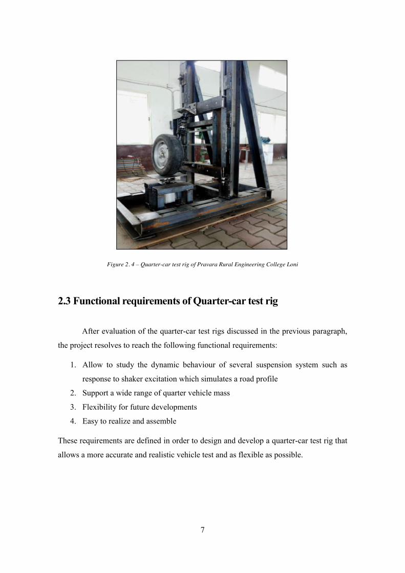
The shortcomings observed in the test rigs viewed so far consist in the inability to support

a wideband of load to simulate the quarter vehicle mass and also it can test only specific

suspension configuration. The figure 2.3 shows a quarter-car test rig with a load frame

that allows a high capacity of load and the sprung mass frame can accommodate several

configuration of suspensions [7]. In this way future study of expansion and flexibility of

testing are ensured. An actuator cylinder and tire pan are placed in proper position below

wheel. The sprung mass frame moves along load frame by using bearings properly

lubricated with oil.

7

Figure 2. 4 – Quarter-car test rig of Pravara Rural Engineering College Loni

2.3 Functional requirements of Quarter-car test rig

After evaluation of the quarter-car test rigs discussed in the previous paragraph,

the project resolves to reach the following functional requirements:

1. Allow to study the dynamic behaviour of several suspension system such as

response to shaker excitation which simulates a road profile

2. Support a wide range of quarter vehicle mass

3. Flexibility for future developments

4. Easy to realize and assemble

These requirements are defined in order to design and develop a quarter-car test rig that

allows a more accurate and realistic vehicle test and as flexible as possible.

9

Chapter 3 Parts Design

The chapter 3 describes the solutions adopted during the design phase of the test

rig, giving the reason of the choices. It begins with a short description of the quarter-car

test rig. Following, the major components of the platform are explained in details and the

results of the components analysis are shown.

3.1 Quarter car test rig description

A quarter-car test rig is realized to represent a vehicle’s corner, in order to study

the dynamic behaviour associated to it during several road profile excitations. The typical

scheme of a quarter-car test rig is shown in the figure 3.1.

10

Figure 3. 1 – Scheme of quarter-car test rig

The major components of the test rig are the sprung mass, load frame, suspension system,

tyre, wheel plate, shaker and base plate. The suspension system links the sprung mass and

unsprung mass. The sprung mass travels along the load frame through four carriages

constrained to move in vertical direction on the linear guides. The linear guides are fixed

vertically on the load frame by bolts. The unsprung mass consists in the set formed by

tyre, upright, break system and arm. The tyre is placed on the wheel plate fixed on the top

of the shaker. In this way, only the vertical dynamic response of the system can be tested.

Since the shaker excitation (road input) is known, using two accelerometers placed each

one on the sprung mass and unsprung mass, the system response as a result of the specific

input can be known.

In the following paragraphs are described in detail the components of the quarter-car test

rig designed in Solidworks (figure 3.2).

11

Figure 3. 2 – Solidworks model of Quarter-car test rig

The main components of the platform are:

1. Base plate

2. Load frame

3. Sprung mass frame

4. Linear guides

5. Quarter-car

6. Wheel plate

7. Hydraulic shaker

3.2 Base plate

In the control tests and in the study of vibrations, the fixing system used during

the tests must be designed in order to not influence the dynamic of the component tested.

12

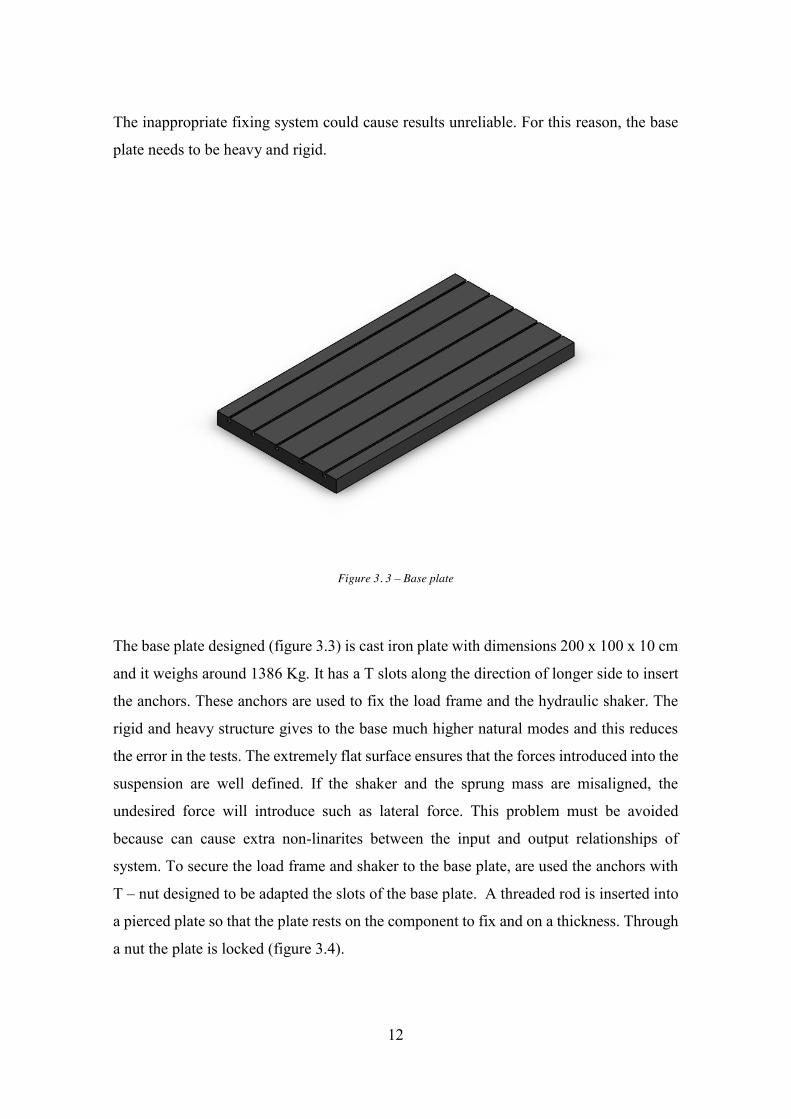
The inappropriate fixing system could cause results unreliable. For this reason, the base

plate needs to be heavy and rigid.

Figure 3. 3 – Base plate

The base plate designed (figure 3.3) is cast iron plate with dimensions 200 x 100 x 10 cm

and it weighs around 1386 Kg. It has a T slots along the direction of longer side to insert

the anchors. These anchors are used to fix the load frame and the hydraulic shaker. The

rigid and heavy structure gives to the base much higher natural modes and this reduces

the error in the tests. The extremely flat surface ensures that the forces introduced into the

suspension are well defined. If the shaker and the sprung mass are misaligned, the

undesired force will introduce such as lateral force. This problem must be avoided

because can cause extra non-linarites between the input and output relationships of

system. To secure the load frame and shaker to the base plate, are used the anchors with

T – nut designed to be adapted the slots of the base plate. A threaded rod is inserted into

a pierced plate so that the plate rests on the component to fix and on a thickness. Through

a nut the plate is locked (figure 3.4).

13

Figure 3. 4 – Fixing system on the base plate

This type of fixing allows a wide adjustment such as the precise positioning of the shaker

under the tyre. In this way, the rig could test several range of suspensions.

Summing, the functionality of the base plate fins in its rigid design to decrease the

undesired effects on the signals during the tests and its capacity to be adapted to the large

variety of suspension configuration.

3.3 Load frame

For the same reasons of the base plate, the load frame must be extremely strong

and rigid. In the design phase, the objective was to reduce the excitation of the sensors

such as accelerometers from external source including the rig’s structure. After the

evaluation of the test rigs discussed in the previous chapter, the structure choice is

triangular frame 170 x 80 x 70 cm as shown in the figure 3.5, it is assembled by welding

a steel square tubes 10 x10 cm with 1 cm of thickness. Completed, the load frame weighs

around 450 kg and is anchored to the base plate. Together, load frame and base plate have

the purpose to ensure an excellent rigid environment for study of vibration.

14

Figure 3. 5 – Load frame

To optimize the load frame, a Finite Element beam model is obtained in Ansys as shown

in the figure 3.6.

15

Figure 3. 6 – Finite element beam model

The first simulation concerns the load applied on the frame. The load is not directly acting

on it, but it occurs on the linear guides and it is of lateral type. Based on the viewed article

[7], for avoiding the complexity of loading is considered that the load is equal to the

corner weight of vehicle. This load acts transversely along the height of frame on the

beams that support the guides. It been asserted that during extreme situations such as

braking and cornering events, the corner weight of vehicle changes get to around the half

weight of entire vehicle. The half weight considered supposing extreme event is 1400 kg

corresponding about 13730 N.

16

Figure 3. 7 – Finite element model of load frame

For the analysis, the structure is constrained at the base and the load is applied in the in

the lateral direction. As shown in the figure 3.7, the results obtained with the simulation,

it can be observed that the Von Misess stress is much less than the yield strength of the

material and the maximum deflection is only 0.07 mm. On the base of the maximum

distortion energy criterion, the yielding will not occur [9].

The second analysis concerns the modal natural frequencies of the load frame. The

resonant frequencies must be very far above those of interest. In many tests of vehicle

dynamics, the frequency range of interest goes from 1 to 25 Hz [6]. The results of

frequency analysis carried out in Ansys are shown in the table of figure 3.8. In the table

you can see that the first resonance frequency is 131.84 Hz and the other resonance

frequencies are much higher than those interest.

17

The results obtained by analysis of the load frame indicate that it is very rigid and this

minimizes sensors noise from excitation of the load frame. To anchor the load frame to

base plate, a steel pads 15 x 15 x 2 cm will welded to bottom of each corner.

Figure 3. 8 – Table of the first five resonance frequencies

3.3 Sprung mass frame

The sprung mass frame is the component that allows to reproduce the sprung mass

of vehicle, including the body and chassis. In the phase of design, the objective was to

realize a flexible element that it accommodates a wide range of suspension configuration

without the need exaggerated modifications on the rig. The idea is been to use a modular

design.

18

Figure 3. 9 – Sprung mass frame

As it can see in the figure 3.9, it has holes to fix the adapters related at the several

suspensions system to test. The sprung mass frame has thickness 3 cm and size 90 x 80

cm, with longer dimension in the direction of motion. The surface defined by these

dimension allows a large working area to use for the suspension system. Other functional

wanted requirement in the sprung mass frame, was the capacity to host large corner

weight of vehicle. This is allowed thanks to the housing realized by the L-profile of the

sprung mass frame, on which can be placed a load in order to satisfy a large range of

quarter car weight.

The material chosen is Aluminium 6061–T6. An analysis in Solidworks Simulation is

carried out applying the lateral force of 13730 N in order to find the maximum deflection

and stress in the sprung mass frame. Figure 3.10 shows the results of simulation, where

it can see that the sprung mass frame would have a maximum deflection of 0.06 mm,

corresponding to a Von Mises stress of 34.48 MPa. This is much less than the yield

strength of the material, 235 MPa. This establish that the design of the sprung mass frame

is more than sufficient in strength and rigidity.

19

Figure 3. 10 – Ansys simulation results, a) Von Mises stress b) Deformation

The other component of the modular sprung mass frame are the adapter fixtures that allow

the interfacing between suspension system and the sprung mass frame. These fixings will

realized in according to the type of suspension to test.

3.4 Linear Guides

The elements that allows the vertical translation of the sprung mass along the load

frame are the linear guides (figure3.11). The functions found in the linear guides are high

accuracy, high load and low friction design. In the linear guides on profiled rails are used

rolling elements that thanks to their load capacity and high stiffness they are suitable in

many applications where the accuracy and low friction play an important role [10]. The

linear guides mainly consist in a carrier and a rail. The carrier is composed of one or more

circuit of rolling elements in recirculation between one load zone and one recirculation

zone. In the load zone, the rolling elements transmit the load from the carrier to the rail

and vice versa. In the recirculation channel, the rolling elements are not exposed to the

load but only drove to the load zone. Usually the rolling elements are realized in steel for

bearing and the rails as the carriers, are equipped of rolling tracks hardened. The number

of the recirculations of the rolling elements influences the load capacity, the stiffness and

the friction behaviour of the linear guides. A high recirculation number matches a high

load capacity and stiffness, but the complexity and the cost increase.

20

Figure 3. 11 - Linear guide

The linear guides on the profiled rails have to support the load from all directions.

Therefore, the rolling track or the contact points are placed second a characteristic contact

angle. The linear guides with contact angle of 45° have the same load capacity in all four

main stress directions. The load capacity is described by the static load factor and the

dynamic load factor. In the cases of compression load, tensile and lateral the force is

transmitted on two line of rolling elements and two rolling tracks. The worse situation

with contact angle of 45° occurs when the load acts with an angle of 45°. In this case, the

load is supported by only one line of rolling elements and one rolling track. In order to

increase the stiffness of linear guides, the carriers can be preloaded.

In this project are considered two rails of 150 cm each having two carriages. This gives a

high range of motion of sprung mass in order to allow various applications. The choice

of linear guides can be carried out by the software of the Scheaffler Industry that is based

on load type, type of bearing and dimensions.

3.5 Hydraulic Shaker

In this project the road profile will be simulated by a Hydraulic shaker of Fairey

Industry as shown in the figure 3.11.

21

Figure 3. 12 – Hydraulic shaker

This hydraulic actuator is basically a position controlled servo system, with very fast

response. It comprises three units:

1. Hydraulic power unit

2. Servo controller

3. Hydraulic shaker

The hydraulic power unit supplies oil, usually at 20 MPa, to provide the necessary

movement and thrust. This supply is controlled by servo valve attached to the shaker,

which is in turn driven by electrical signal received from the servo controller. In the next

chapter of this thesis will be treated how the shaker receive the signal using Arduino

board. The servo valve is a flow controller and since the shaker is a linear actuator, it will

move at a velocity proportional to the signal applied to the valve. In order to control the

position of the shaker, a displacement transducer is attached between the body and the

piston shaft, which continually feeds back information about generator, is applied to the

input of the servo control unit, it is compared with the feedback signal. If an error exists

between the two, it is amplified and fed to the servo valve in such a way as to reduce the

error. The maximum stroke of the shaker is 15 cm with wide range of frequency. On the

top of the shaker is place a base plate to support the tyre of the quarter car.

23

Chapter 4 Vehicle suspension modelling

This chapter begins with a brief comment of the vibration theory in order to

understand the dynamic systems behaviour and the principles that are at base. Following,

the more important models for the study the vehicle dynamic are described and evaluated

focusing on the quarter car model, of which the equation of motion are explaned and

analysed.

4.1 Vibration theory

The study of vibration is in charge of oscillatory motion of bodies and the relative forces.

All vibration systems have a mass and elasticity and can be characterized as linear or

nonlinear. The principles and mathematical techniques available to treat the linear

systems are well developed. In contrast, for the nonlinear systems, the techniques of

analysis are less known and not simple to apply. However, the knowledge of nonlinear

systems is important because all systems tend to become nonlinear with increasing

amplitude of oscillation [11].

The vibrations can be subdivided of two type: free vibrations and forced vibrations. The

first ones occuring when the system oscillates under force action inherent in the system

itself and the external forces are absent. In the case of the free vibration, the system

vibrates at one of more of its natural frequency and these are characteristics of the

dynamic system established by its mass and distribution of stiffness. The forced

vibrations occurring due to a external force, that excites the system. When the excitation

is oscillatory, the system is forced to vibrate at frequency of excitation. If the frequency

of excitation is equal to one of the natural frequency of the system, occurs the resonance

condition characterized by large oscillation of the system that can cause dangerous

24

situation. For this reason, the calculation of the natural frequencies is fundamental in the

study of vibrations.

All vibration system are subjected at damping because the energy is dissipated trough

friction and other form of resistance. If the damping is low, it has few influence on the

natural frequency of the system and for this, usually the calculations of natural frequency

are carried out without damping. Other side, the damping is very important to limit the

oscillation amplitude in resonance condition. The number of independent variables

needed to describe a system motion is called degrees of freedom (DOF). A body free to

move in the space have six degree of freedom, of which three to define the position and

three to define the orientation.

4.2 System Modelling

A system is an ensemble of elements interconnected that interact between them.

This leads to determine the influence that the behaviour of single elements have and the

connection between them on the entire system. For the treatment of the problem, the

modelling of mechanical system provides the fundamental means for the study of

machine dynamic [12]. First of all, for the study of any mechanical system, have to define

a physic model and following derive from its the relative mathematical model represented

by equation that describe the behaviour. When talking about to physic model we refer to

imaginary physic system equivalent to the real system within prefixed approximations

and respect at the characteristics of the interested system. The important factor of the

physic system is the possibility to study its by mathematical tools. The transition from the

real system to its physic model imply determined approximations, the most important of

which consist in neglect anything that causes effects believed negligible in the system

behaviour. However the physic model need to include a sufficient number of effects and

details in order to describe in the best way the system with equation and without become

too complex. The physic model can be linear or nonlinear, in base of the behaviour of the

system components. Linear models allow a quick solution and are simple to treat.

Sometimes, nonlinear models prove system characteristics that can not be predicted

correctly using linear system. After individuation of a physic model equivalent to the real

25

system, it proceeds with the determination of the relative mathematical model, that is an

ensemble of mathematical relationships that describe the behaviour of the physic model.

The writing of these equations is carried out by employing the principles of the dynamic

following different approaches among which the principle of d'Alembert, the principle of

virtual work, the principle of conservation of energy and the Lagrange equations. Usullay

the equations of motion are ordinary differential equations for a discrete system, and

partial differential equation for a continuous system. The equations can be linear or non-

linear in base of the type of the system components. Finally it passes to the realization of

an algorithm of resolution of the equations of the mathematical model. Only in simple

cases the solution can be obtained in closed form: usually the solution is obtained

numerically by the use of a computer. Depending on the nature of the problem it can use

one of the following techniques to find the solution: standard methods for the solution of

differential equations, methods based on the Laplace transform, matrix methods,

numerical methods. If the equations are nonlinear, hardly they can be solved in closed

form. The solution of the equations of motion provides the model of the behaviour system.

Then the model must be validated verifying the assumptions adopted during the

modelling of the real system. This verification can be performed through experimental

tests and it is fundamental for a proper design.

4.2.1 Discrete and continuous models

The mechanical systems which have high elasticity and low mass, and at the same

time, elements of considerable mass and high stiffness can be described using a finite

number of degrees of freedom. Instead, for systems that have an infinite number of mass

points and have not concentrations zones or deformable members, it is necessary an

infinite number of coordinates to specify its deformed configuration. The models with a

finite number of degrees of freedom are called discrete models or models with parameters

concentrated, while those with an infinite number of degrees of freedom are said

continuous models. Treating the system as continuous leads to accurate results but the

methods of analysis are limited to a much reduced type of systems, such as beams with

uniform sections, thin plates, membranes, etc. For this reason, often discrete models

26

approximate the continuous systems and for improve the accuracy of the results can be

increase the number of degrees of freedom. Among the automatic techniques of

discretization there is the finite element method (FEM). It considers a continuous system

consisting of finite elements through the creation of a mesh composed of finite elements

with definite shape (such as triangles, wishbones).

Generally, the discrete models present:

x Masses or inertias

x Elastic elements

x Damping elements

The elastic elements represent the parts of system that have a certain elasticity or stiffness

compared to the other system elements. They are considered devoid of mass and in these

elements we can find linear spring or nonlinear spring. When the liner spring deforms,

the force F developed is proportional to deformation itself. The relationship is the

following:

F = kx

where:

k is the stiffness,

x is the relative displacement of the ends.

The work is stored in the form potential energy:

𝑉 =12𝑘𝑥2

The nonlinear springs have a linear behaviour within certain limit of deformation,

beyond which the relationship between the force and deformation become

nonlinear. In many practical applications, it is assumed that the deformations are

small and therefore it considers that the springs have linear behaviour. In other

cases, is used a linearization process that approximates to linear spring.

27

In many mechanical systems, the vibration energy is gradually converted into

thermal energy or acoustic energy. The mechanism that causes the reduction of

energy, leading to a gradual decrease of the vibrational response of the system is

called damping. Usually it considers that a damping elements are free of mass and

elasticity.

A damper exerts a force only in the presence of relative speed between the two

extremes of the damper itself. Usually damping is modelled as a combination of the

following:

x viscous damping

x Coulomb friction

x Hysteretic damping (or structural)

Viscous damping is the most used in the study of vibrations. The force F exerted by

the viscous damping is expressed by the equation:

F = cx

where:

c is coefficient of dumping

x is the relative velocity of the two ends

4.3 Vehicle model

There are several mathematical models of vehicle suspensions and the choice of the

particular model depends of the purpose and from the information that we want extract.

The models most used and common are:

x Quarter car model

x Half car model

x Full car model

These three models are distinguished on base of the number of parts in which is divided

the vehicle. The Quarter-car model describes the vertical dynamic of vehicle

concentrating the study on the single tyre and the relative suspension system. Basically

the vehicle is subdivided in four section modelled separately ignoring the mutual

28

interaction. This simplify the real system allowing to have a system easy to resolve and

with dimensions contained. On the other hand this limits the simulation and the accuracy

because it is possible to study only the vertical translation (heave), the angular motions

such as roll, pitch cannot be analysed. In the figure 4.1 is shown a quarter car model for

passive suspension.

Figure 4. 1 – Quarter car model

This model presents a sprung mass (Ms) and the unsprung mass (Mu). The system

suspension is modelled by linear spring with stiffness Ks and a dumper with damping

coefficient Cs. The stiffness and damping of tyre is represented with Ku and Cu. The

coordinates associated to the sprung mass translation and unsprung mass translation are

called respectively Xm and Xu. The coordinate Xr is the coordinate of road profile.

The Half-car model shown in the figure 4.2 represents the side of vehicle in order to

model only the front and rear tyre with the relative system suspension. This allows to

describe in addition to the vertical motion of vehicle also the pitch movement.

The Full-car model shown in the figure 4.3 describes the entire vehicle dynamic through

the combination of four Quarter-car test rig linked by one rigid body. In this model is

possible to study the vertical motion, pitch and roll.

In this study we will focus more on the Quarter-car model.

29

Figure 4. 2 - Half-car model

Figure 4. 3 – Full-car model

31

4.4 Quarter-car model

The Quarter-car model, as said in previous paragraph, describes the dynamic of vehicle

concentrating exclusively on the vertical motion (heave). This model is a two degree of

freedom system and we can apply the principle of d’Alambert at model shown in the

figure 4.4 in order to obtain the motion equations.

Figure 4. 4 – Quarter car model

For the sprung mass 𝑚𝑠 results:

𝑚𝑠��𝑠 + 𝑐𝑠(��𝑠 − ��𝑢) + 𝑘𝑠(𝑥𝑠 − 𝑥𝑢) = 0

and for the unsprung mass 𝑚𝑢 results:

𝑚𝑢��𝑢 + 𝑐𝑠(��𝑢 − ��𝑠) + 𝑘𝑠(𝑥𝑢 − 𝑥𝑠) + 𝑐𝑢 ∙ ��𝑢 + 𝑘𝑠 ∙ 𝑥𝑢 = 𝐹(𝑡) = 𝑐𝑢 ∙ ��𝑟 + 𝑘𝑢 ∙ 𝑥𝑟

Where F(t) is the force induced by the irregularity of road surface that acts on the tyres.

From the knowledge of the road profile and then from the forcing, we can determinate

the vibrations of the two masses resolving the equation of motion in matrix form:

32

[𝑚𝑠 00 𝑚𝑢

] (��𝑠��𝑢) + [

𝑐𝑠 −𝑐𝑠−𝑐𝑠 𝑐𝑠 + 𝑐𝑢] (

��𝑠��𝑢) + [ 𝑘𝑠 −𝑘𝑠

−𝑘𝑠 𝑘𝑠 + 𝑘𝑢] (𝑥𝑠𝑥𝑢) = [ 0

𝑐𝑢 ∙ ��𝑟 + 𝑘𝑢 ∙ 𝑥𝑟]

The compact form is:

[𝑀](��) + [𝐶](��) + [𝐾](𝑋) = [𝐹]

with:

[𝑀]= mass matrix

[𝐶]= dumping matrix

[𝐾]= stiffness matrix

(��)= acceleration vector

(��)= velocity vector

(𝑋)= displacement vector

[𝐹]= force vector

For the calculation of the natural frequency of the system are considered the free

vibrations. Thus, putting 𝐹(𝑡) = 0 and the damping 𝑐𝑠 = 𝑐𝑢 = 0 the motion equations

become:

𝑚𝑠��𝑠 + 𝑘𝑠(𝑥𝑠 − 𝑥𝑢) = 0

𝑚𝑢��𝑢 + 𝑘𝑠𝑥𝑢 − 𝑘𝑠𝑥𝑠 + 𝑘𝑠 ∙ 𝑥𝑢 = 0

If we assume that the motion of the sprung mass 𝑚𝑠 and motion of the unsprung mass

𝑚𝑢 is the harmonic oscillation with pulsation 𝜔𝑛 and phase ф, but different amplitudes,

the solution of the previous equations will be of the type:

𝑥𝑠(𝑡) = 𝑋𝑠cos(𝜔𝑛 + ф)

𝑥𝑢(𝑡) = 𝑋𝑢cos(𝜔𝑛 + ф)

33

where 𝑋𝑠 and 𝑋𝑢 are respectively the amplitudes of oscillations of the sprung mass and

unsprung mass. Substituting in the motion equation, results:

([−𝑚𝑠𝜔𝑛2 + 𝑘𝑠]𝑋𝑠 − 𝑘𝑠𝑋𝑢)cos(𝜔𝑛 + ф) = 0

(−𝑘𝑢𝑋𝑠 + [−𝑚𝑢𝜔𝑛2 + (𝑘𝑠 + 𝑘𝑢]𝑋𝑢) cos(𝜔𝑛 + ф) = 0

Therefore results:

[−𝑚𝑠𝜔𝑛2 + 𝑘𝑠]𝑋𝑠 − 𝑘𝑠𝑋𝑢 = 0

−𝑘𝑢𝑋𝑠 + [−𝑚𝑢𝜔𝑛2 + (𝑘𝑠 + 𝑘𝑢)]𝑋𝑢 = 0

This is a homogenous system in the unknowns 𝑋𝑠 and 𝑋𝑢. The matrix form results:

[−𝑚𝑠𝜔𝑛2 + 𝑘𝑠 −𝑘𝑠

−𝑘𝑢𝑋𝑠 −𝑚𝑢𝜔𝑛2 + (𝑘𝑠 + 𝑘𝑢)

] [𝑋𝑠𝑋𝑢] = 0

A first solution of system is banal, 𝑋𝑠 = 𝑋𝑢 = 0, because implies the absence of

vibrations. A solution not banal is obtained putting equal to zero the matrix determinant

of the coefficients 𝑋𝑠 and 𝑋𝑢.

𝑑𝑒𝑡 [−𝑚𝑠𝜔𝑛2 + 𝑘𝑠 −𝑘𝑠

−𝑘𝑢𝑋𝑠 −𝑚𝑢𝜔𝑛2 + (𝑘𝑠 + 𝑘𝑢)

] = 0

(𝑚𝑠𝑚𝑢) ∙ 𝜔𝑛4 + (−𝑚𝑠𝑘𝑠−𝑚𝑠𝑘𝑢−𝑚𝑢𝑘𝑠) ∙ 𝜔𝑛

2 + 𝑘𝑠𝑘𝑢 = 0

The equation is called characteristic equation or equation of the frequencies because the

its solution leads at the natural frequencies of the system. The solutions are:

𝜔𝑛12 =

−𝐵 − √𝐵2 − 4𝐴𝐶2𝐴

34

𝜔𝑛22 =

−𝐵 + √𝐵2 − 4𝐴𝐶2𝐴

where:

𝐴 = 𝑚𝑠𝑚𝑢

𝐵 = −𝑚𝑠𝑘𝑠−𝑚𝑠𝑘𝑢−𝑚𝑢𝑘𝑠

𝐶 = 𝑘𝑠𝑘𝑢

Although the two equations have solution the natural pulsations ±𝜔𝑛12 𝑒±𝜔𝑛2

2 , the

negative values are discarded because they have not physic meaning. From the natural

pulsations 𝜔𝑛1 and 𝜔𝑛2 usually expressed in rad/s, it can calculate the natural frequencies

of the system in Hertz with the following relationship:

𝑓𝑛1 =𝜔𝑛1

2𝜋

𝑓𝑛2 =𝜔𝑛2

2𝜋

It is important to define that for the vehicle, the sprung mass 𝑚𝑠 is one order greater than

the unsprung mass 𝑚𝑢, while the stiffness of suspension 𝑘𝑠 is one order lower than the

stiffness equivalent of the tyre 𝑘𝑢.

On the base of this, it is possible to use a approximated method to determinate the two

natural frequencies of the 2 DOF system. The approximate values of the natural

frequencies of the sprung and unsprung mass expressed in Hertz, are calculated

respectively:

𝑓𝑛−𝑠 =12𝜋

√𝑘𝑠𝑘𝑢/(𝑘𝑠+𝑘𝑢)

𝑚𝑠

𝑓𝑛−𝑢 =12𝜋

√𝑘𝑠+𝑘𝑢𝑚𝑢

Where 𝑓𝑛−𝑠 is the natural frequency of sprung mass and 𝑓𝑛−𝑢 is the natural frequency of

unsprung mass.

35

Chapter 5

Simulation of a McPherson suspension on the test rig

This chapter describes the main suspensions used in the vehicle explaining the

configurations and characteristics. Following a McPherson suspension strut is

implemented in the test rig and a simulation is carried out in Matlab/Simulink

environment in order to demonstrate that the quarter car test rig designed can analyse the

dynamic behaviour of suspension tested. Finally, the chapter ends with the analysis of

results.

5.1 Vehicle suspension

The suspensions are essential in the vehicle because they ensure the comfort and the road

holding [13]. The suspension is a system consisting of springs, damper and linkages that

isolate the sprung mass (vehicle body) from the unsprung mass (wheel assembly). The

vehicle interacts with the road via the direct contact between tyres and the road. The

fundamental objective of a system suspension is to isolate the driver and the passengers

from the road noise while keeping good road contact [14]. The suspension systems used

on the vehicles can be subdivided in three macro types: independent, dependent and semi-

independent suspensions. The first type is characterized in that the force acting on one

tyre does not effect on the other tyre, because the two hubs of the same axle are not linked

by mechanical linkages. In the dependent suspensions is present a rigid mechanical

linkages between the two wheels of the same axle. This type of suspension system is used

mainly in industrial vehicle and off road vehicles. The semi-independent suspensions

have intermediate characteristics between the previous types. In this paragraph we will

36

focus mainly on the independent suspension. In the independent type the mechanical

linkages constrain five out of the six degrees of freedom of the wheel hub. The alone

degree of freedom is the vertical translation along the perpendicular direction to the road.

The common independent suspensions are double wishbone type and McPherson type.

Double wishbone suspension shown in the figure 5.1 is characterized by two A-arms

(wishbones), linked to the top and bottom of the wheel hub through a ball and socket

joint. This type is an optimum compromise between handling and comfort thanks to the

elasto-kinematic parameters, for this reason they are used mainly in the luxury sedans and

sports cars.

Figure 5. 1 – Double wishbones suspension

37

Figure 5. 2 – McPherson suspension

The McPherson suspension shown in the figure 5.2 is a common solution for front axels

of the small vehicles. Usually the basic configuration the suspension consists in a

triangular lower arm and a vertical element called upright at which is connected rigidly

the absorber assembly, this ensures the vertical motion of the wheel excited by the road

profile.

5.2 Implementation of a McPherson suspension on the rig

For the first application on the Quarter-car test rig, a McPherson suspension model shown

in the figure 5.3 is realized in Solidworks. Following the supports to fix the suspension

to the sprung mass is designed in order to carry out the simulation of the Quarter-car test

rig in Matlb/Simulink environment. The support of the suspension and the fixture of the

triangular lower arm to constrain them to the sprung mass are as shown as in figure 5.4

38

Figure 5. 3 – McPherson suspension Solidworks model

Figure 5. 4 – Supports for absorber assembly and lower arm

After the design of the test rig and the system suspension to test, the entire project realized

in Solidworks is exported in Simscape/SimMechanics, one block library of

39

Matlab/Simulink. The software allows to convert the CAD model in Simulink model (slx

format) in order to carry out dynamic simulations using blocks of SimMechanics.

Simscape Multibody platform allows to model and simulate physical systems in all

domains. The Simscape Multibody plug-in provides the interface to export CAD

assembly, generating a XML file containing in details the structure and the proprieties of

the assembly and 3D parts designed in Solidworks. Following, Simscape Multibody

analyses the XML data and it generates automatically an equivalent multibody model.

Simscape uses a block library for the modelling of physic systems in Simulink. All this

allows a conversion of a CAD model in multibody Simscape model which is based on a

file XML specially formatted to transfer a detailed description from CAD software to the

Simscape software multibody. The model description allows to recreate the CAD

assembly in the form of block diagram. The conversion of the CAD assembly occurs in

two steps:

x Export step

x Import step

In the export step happen the conversion of the CAD assembly in description file

multibody XML and in a set of STEP file for the geometry of the parts. The import step

converts the previous file of description and geometry in a Simscape multibody SLX

model and a data file M. The block parameters are obtained from data file M (figure 5.5).

Figure 5. 5 – CAD assembly conversion process

The model obtained in Simulink environment coherent with the CAD assembly designed

in Solidworks, for the modelling of the system uses mainly blocks of the SimMechanics

library such as Solid blocks, Rigid Transform Blocks, Joint blocks. The Solid blocks add

40

a solid element with the geometry, inertia and colour to the attached part. Geometry

parameters are shape and size and they are imported from external file in STEP format,

so that the block automatically computes the solid inertia from the specified mass and

geometry. The Rigid Transform blocks apply the transformation in terms of position of

parts through rotations and/or translations. The Joint blocks apply the constrain between

two parts. The Simulink model of the Quarter-car test rig is shown in the figure 5.6.

The Simulink model of the Quarter-car test rig designed is structured in three main masks

linked between them:

1. Load frame_Base plate

2. Quarter_car

3. Hydraulic_Shaker

41

Figure 5. 6 – Quarter-car test rig Simulink model

42

The Load frame_Base plate mask includes the solid blocks to model the load frame and

the base plate as shown in the figure 5.7. Load frame block and Base plate block are

rigidly connected because in the physic system the load frame is fixed on the base plate.

The “Load frame_Base plate” mask presents five connection ports, of which four are

dedicated for the connection between the Load frame and Quarter-car mask and one for

the connection between the Base_plate block and Hydraulic Shaker mask. The World

block represents the reference system of the model, a default right-handed. The

Base_plate block contains the frame data of the respective part and it is connected to

World block.

Figure 5. 7 – Load Frame_Base plate mask

The mechanical and simulation parameters to apply to the entire model, are set through

the MechanismConfiguration block. As shown in the figure 5.8, in this block we can

define the gravity and set the linearization delta that specifies the perturbation value that

is used to compute numerical partial derivatives for linearization. The gravity is chosen

through a row vector 1 x 3 that has, as elements, the axis directions of the reference

system. The Guide_Dx and Guide_Sx blocks containing the frame data of the guides, are

linked rigidly to the Load_frame block.

43

Figure 5. 8 – MechanismConfiguration block

The Quarter car mask shown in the figure 5.9, presents the Sprung_Mass block connected

to the Load frame through four prismatic joint blocks that physically represent the

coupling between the linear bearings and the guides. Because these types of joint block

allows one transitional degree of freedom, in this way the sprung mass frame can move

in Y vertical direction along the load frame. Furthermore, the prismatic joint block has a

sensing function that allow to know the displacement, velocity and acceleration of the

sprung mass connecting. The two remaining connections are dedicated for the constraint

of the lower arm and suspension system through a revolute joint block that allows one

rotational degree of freedom. The sprung mass block contain inside it a Solid blocks with

the frame data of suspension and lower arm fixtures. In the Simulink model, the

suspension system is modelled with the Suspension block. This block models the

suspension using a prismatic joint block between two solid blocks representing

respectively the cylinder and the plunger of dumper. The parameters requested by block

are the internal mechanics such as equilibrium position, spring stiffness and damping

coefficient in order to simulate the suspension system.

44

Figure 5. 9 – Quarter car mask

The Unsprung_mass block models the wheel assembly. The upright is connected to the

lower arm via spherical joint block that has three rotational degree of freedom, while the

connection with the suspension is rigid in order that the diagram block of the Simulink

model is coherent with McPherson type.

The Hydraulic shaker mask includes the blocks that model the shaker used to simulate

the excitation of the wheel. Mainly it presents one input to receive signal that simulates

the road profile and two connections. One of these connections connects rigidly the base

of shaker with the base plate. For the purpose of to simulate the stiffness and damping of

the tyre, the Spring and damper block is used between the tyre block and wheel_plate

block as shown in the figure 5.10.

Figure 5. 10 – Spring and Damper Force Block to simulate the stiffness and damping of the tyre

45

This block applies a linear damped spring force between the two frames and it can be

configured inserting the parameters such as natural length, spring stiffness and damping

coefficient. The Transform Sensor block measures time-dependent relationship between

two frames. Connecting to it the Scope blocks is possible to measure translation, velocity

and the acceleration of wheel. As shown the figure 5.11, the Hydraulic_Shaker mask

present a prismatic joint to simulate the shaker motion. The motion of shaker is controlled

in position using an input signal.

Figure 5. 11 – Hydraulic_Shaker mask

5.3 Configuration of system parameters

Before to carry out the vibration analysis of the Quarter-car test rig model in Simulink

environment, the blocks used to model the system are configured. The assigned weight

of the body of vehicle is 1000 kg, thus the sprung mass value is 250 Kg. This value is set

in the Solid block representing the sprung mass entire of the Quarter_car mask as shown

in the figure 5.12. This allows to choice the value of sprung mass desired for the system.

The parameters of suspension system are set in the Suspension block of the Quarter_car

mask. Precisely, a Matlab script sets the internal mechanics properties (figure 5.13) of the

Prismatic block of suspension. The values used to characterize the suspension system are:

x Equilibrium position (ep): 11 cm

x Spring Stiffness (ks): 25000 N/m

46

x Damping Coefficient (cs): 2200 s*N/m

Figure 5. 12 – Solid block of sprung mass

Figure 5. 13 – System suspension parameters

47

The wheel assembly consisting of upright, wheel and tyre weights 30 kg. Finally, the

Spring and Damper force block that represents the stiffness and damping of tyre is set

with the following values:

x Natural length: 0 cm

x Spring stiffness (ku): 180000 N/m

x Damping Coefficient (cu): 150 s*N/m

5.4 Simulation of a Quarter car test rig model in Simulink

After the assignment of the parameters in the Simulink model, the simulations are carried

out in order to verify that the rig has the dynamic behaviour coherent with a two degree

of freedom system. The first simulation is performed in time domain using the chirp signal

as an excitation signal input to the system. The frequency of the signal increases linearly

from 0 to 25 Hz in time range of 100 seconds. The time history of the excitation signal

used in the simulation is shown in the figure 5.12.

Figure 5. 14 –Chirp signal

This frequency range is chosen because the vehicle body (sprung mass) vibrations are

characterized by a range between 1 and 5 Hz and the wheel (unsprung mass) vibration

are concentrated between 12 and 18 Hz [15]. In Simulink model is used a chirp block in

48

input of the Hydraulic_Shaker block as shown in the figure 5.13 in order that the shaker

can move following the input signal.

Figure 5. 15 – Chirp input signal to the Hydraulic_Shaker block

The Simulink-PS converter block is used to convert the unit less Simulink input signal to

a physical signal. The configuration of this block is obtained assigning the unit of signal

and provides to derivate the signal.

The result obtained from the simulation is shown in the figure 5.16. The graphs represent

the velocity of the vehicle body (sprung mass) and the unsprung mass in the time domain

when the system is subject to the chirp signal. Both graphs present two peaks that

correspond to two resonances of the system. This proves that the Quarter-car test rig

designed is a two degree of freedom.

49

Figure 5. 16 - Time domain response of the sprung mass and unsprung mass

The second simulation concerns the study of the dynamic behaviour of the system when

it is subject to the road profile using ISO 8608 road surface roughness classification [16].

The response of the sprung mass following the excitation caused by the road profile is

evaluated. The road profile signal to excite the system is realized in accordance with ISO

8608. This road surface roughness classification allows a uniform method of reporting

measured vertical surface profile data from road [17]. A range of Power Spectral Density

(PSD) as shown in the figure 5.17 defines each class. The road profile can be described

through the PSD function of the vertical displacement of the road profile that it is obtained

by the Fourier Function Transform (FFT) of the auto-correlation of the stochastic process

describing the road profile [18].

Starting from a continuous road profile, for a defined value of spatial frequency n, centred

within a band of frequency Δn, the PSD function for the assigned frequency n is defined

by this equation:

𝐺𝑑(𝑛) = lim𝛥𝑛⟶0

𝜓𝑥2 (𝑛, 𝛥𝑛)𝛥𝑛

with 𝜓𝑛2 the mean square value of the component of the signal for the spatial frequency

n, within the ban of frequency Δn.

50

Considering a road profile with length L and the sampling interval is B, the maximum

theoretical sampling spatial frequency is 𝑛𝑚𝑎𝑥 = 1/𝐵, the effective sampling spatial

frequency, for the Nyquist theory, is 𝑛𝑒𝑓𝑓 = 𝑛𝑚𝑎𝑥/2 and the discretised spatial

frequency values 𝑛𝑖 are equally spaced with an interval of Δn = 1/L. The generic spatial

frequency value 𝑛𝑖 can be regarded as i⋅Δn and the PSD can be written in discrete form:

𝐺𝑑(𝑛𝑖) = lim𝛥𝑛⟶0

𝜓𝑥2 (𝑛𝑖, 𝛥𝑛)𝛥𝑛

=𝜓𝑥2 (𝑖 ∙ 𝛥𝑛, 𝛥𝑛)

𝛥𝑛

where:

x i varying from 0 to N

x 𝑁 = 𝑛𝑚𝑎𝑥𝛥𝑛

If the road profile is represented through a harmonic sampling function with equation:

𝑦(𝑥) = 𝐴𝑖 cos(2𝜋 ∙ 𝑛𝑖 ∙ 𝑥 + 𝜑) = 𝐴𝑖 cos(2𝜋 ∙ 𝑖 ∙ 𝛥𝑛 ∙ 𝑥 + 𝜑)

where:

x 𝐴𝑖 is the amplitude

x 𝑛𝑖 is the spatial frequency

x 𝜑 is the phase angle

It is possible to affirm that the mean square value of this harmonic signal is:

𝜓𝑥2 =

𝐴𝑖2

2

Thus:

𝐺𝑑(𝑛𝑖) =𝜓𝑥2 (𝑛𝑖)𝛥𝑛

=𝐴𝑖2

2 ∙ 𝛥𝑛

If the PSD function of vertical displacement is known, an artificial road profile can be

generated using the previous equation and assuming a random phase angle 𝜑𝑖 following

51

an uniform probabilistic distribution within the 0-2𝜋. In these hypotheses, the road profile

can be described with the equation:

𝑦(𝑥) =∑𝐴𝑖cos(2𝜋 ∙ 𝑛𝑖 ∙ 𝑥 + 𝜑𝑖)𝑁

𝑖=0 𝑖

= ∑√2 ∙ 𝛥𝑛 ∙ 𝐺𝑑(𝑖 ∙ 𝛥𝑛)cos(2𝜋 ∙ 𝑛𝑖 ∙ 𝑥 + 𝜑𝑖)𝑁

𝑖=0

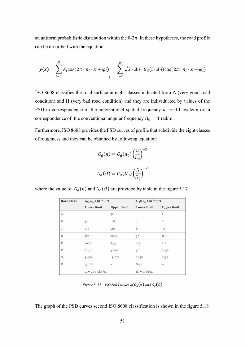
ISO 8608 classifies the road surface in eight classes indicated from A (very good road

condition) and H (very bad road condition) and they are individuated by values of the

PSD in correspondence of the conventional spatial frequency 𝑛0 = 0.1 cycle/m or in

correspondence of the conventional angular frequency 𝛺0 = 1 rad/m.

Furthermore, ISO 8608 provides the PSD curves of profile that subdivide the eight classes

of roughness and they can be obtained by following equation:

𝐺𝑑(𝑛) = 𝐺𝑑(𝑛0) (𝑛𝑛0)−2

𝐺𝑑(𝛺) = 𝐺𝑑(𝛺0) (𝛺𝛺0)−2

where the value of 𝐺𝑑(𝑛) and 𝐺𝑑(𝛺) are provided by table in the figure 5.17

Figure 5. 17 – ISO 8608 values of 𝐺𝑑(𝑛) and 𝐺𝑑(𝛺)

The graph of the PSD curves second ISO 8608 classification is shown in the figure 5.18

52

Figure 5. 18 – ISO 8608 road roughness classification

Substituting the previous equation in y(x), the artificial profile through the ISO

classification can be generated with following equation:

𝑦(𝑥) =∑√𝛥𝑛 ∙ 2𝑘 ∙ 10−3 ∙ (𝑛0

2 ∙ 𝛥𝑛) ∙ cos(2𝜋 ∙ 𝑛𝑖 ∙ 𝑥 + 𝜑𝑖)

𝑁

𝑖=0

where:

x x is the abscissa variable from 0 to L

x 𝛥𝑛 = 1/𝐿 = 𝐿/𝐵

x k is a constant value depending from ISO classification and is reported in table of

the figure 5.19.

53

Figure 5. 19 – Values of the coefficient k for the generation of profile through ISO classification

In Matlab is realized a script for the generation of signal that simulates the road profile

second the ISO 8608 classification in order to send it in input to the Shaker. For the

simulation, the parameters that must be insert to generate the signal corresponding to the

elevation of road are:

x Length of road profile L [m]

x Sampling interval B [m]

x Coefficient k of classification ISO 8608

x Velocity v [m/s]

The figure 5.20 shows the graph of the road elevation in the time domain of profile

realized using the script developed in Matlab.

Figure 5. 20 – Road elevation

54

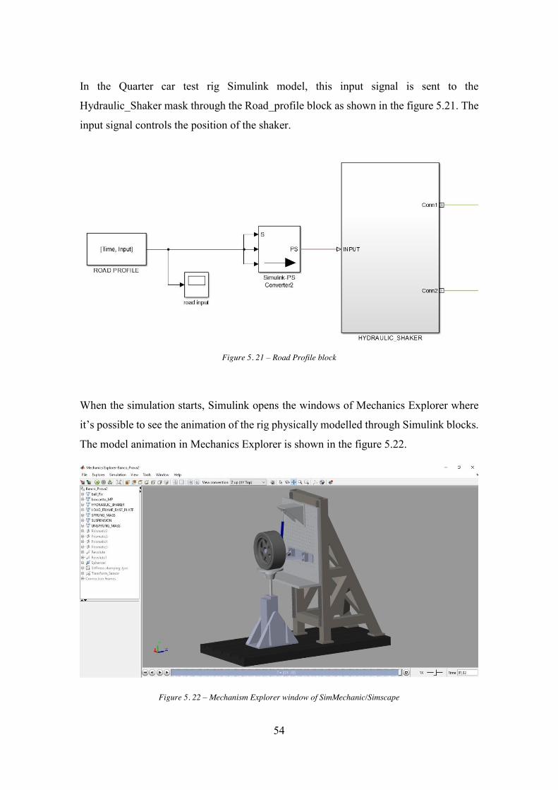
In the Quarter car test rig Simulink model, this input signal is sent to the

Hydraulic_Shaker mask through the Road_profile block as shown in the figure 5.21. The

input signal controls the position of the shaker.

Figure 5. 21 – Road Profile block

When the simulation starts, Simulink opens the windows of Mechanics Explorer where

it’s possible to see the animation of the rig physically modelled through Simulink blocks.

The model animation in Mechanics Explorer is shown in the figure 5.22.

Figure 5. 22 – Mechanism Explorer window of SimMechanic/Simscape

55

Through the scope blocks it’s possible to visualize the displacement, velocity and

acceleration response of the sprung mass after excitation of road profile. In the figure 5.23

are shown the response of the sprung mass subject to an excitation of the road profile with

ISO 8608 coefficient k = 4 and cruise speed v= 20 m/s.

Figure 5. 23 – Sprung mass response in time domain

57

Chapter 6

Signal generator powered by Arduino Uno

This chapter explains the realization of the signal generator powered by Arduino Uno

micro controller. In order to facilitate the understanding of this device, the chapter starts

with a brief description of the board. The results of this project and the methodology used

will be discussed.

6.1 Arduino Uno description

The main component of the project is Arduino Uno shown in figure 1. It is a

microcontroller board based on the ATmega328P. It has 14 digital input/output pins (of

which 6 can be used as PWM outputs), 6 analog inputs, a 16 MHz quartz crystal, a USB

connection, a power jack, an ICSP header and a reset button.

Figure 6. 1 – Arduino Uno Board

Firstly, it is possible to see the USB connector that allows the connection between

Arduino and Computer to perform the operations exposed below:

58

x Upload a new program on the Arduino

x Allow the communication between Arduino and PC

x Supply the power to Arduino (5V)

The Arduino Uno can be powered via the USB connection or with an external power

supply. The power source is selected automatically.

External (non-USB) power can come either from an AC-to-DC adapter (wall-wart) or

battery. The adapter can be connected by plugging a 2.1mm center-positive plug into the

board's power jack. Leads from a battery can be inserted in the Gnd and Vin pin headers

of the POWER connector [19].

The board can operate on an external supply of 6 to 20 volts. If supplied with less than

7V, however, the 5V pin may supply less than five volts and the board may be unstable.

If using more than 12V, the voltage regulator may overheat and damage the board. The

recommended range is 7 to 12 volts.

The features of Arduino Uno board are summarized in table of the figure 6.1

Figure 6. 2 – Summary table of Arduino features

59

6.2 Objectives and Component used

The project objectives are to generate and send sinewave signals with amplitude ±5 V

and with several frequencies between 1 and 20 Hz using Arduino Uno microcontroller.

Furthermore, Arduino will be able to read analog signals from the Hydraulic Servo

Controller in order to know the shaker position. The components used in the project are:

x Arduino Uno board

x DAC Adafruit MCP4725

x Op Amps Dual Low noise STMicroelectronics TL072CN

x Op Amp TL071 Texas Instruments

x 2 x 100 KΩ resistors



x 2 x PWR Supply

x 2 x BNC connection cables

x 2 x Breadboard

x Wires

x Arduino software

6.3 Development of the project

As said before, the project powered by Arduino will send sinusoidal analog signals with

several amplitudes (range ±5 V) and frequencies. Given that, Arduino board has not

analog outputs (as we can see also in the summary) a Digital Analog Converter is used.

To convert the digital signals to sinusoidal analog signals the MCP4725 DAC 12-bit by

Adafruit is implemented.

The Hydraulic Servo Controller need to receive an analog input between -5V to +5V, but

the DAC MCP4725 work on with the analog signals in the range 0-5V. For this reason,

afterwards, it is realized the unipolar to bipolar converter using a differential amplifier,

precisely the Op-Amp TL072CN, in order to obtain a voltage value between -5V to 5V.

In the figure 6.3 is shown the connections among Arduino board, DAC and Op Amp.

60

Figure 6. 3 – Sinewave generator with Arduino Uno, DAC MP4725 and Op-AmpTL072CN

The components used are:

1. Arduino Uno 2. DAC Adafruit MCP4725 3. Op Amps Dual Low noise STMicroelectronics TL072CN 4. 2 x 100 KΩ resistors 5. 2 x 200 KΩ resistors 6. Breadboard

The first step has been to connect the DAC with Arduino Uno as shown in figure 6.4, in

this way the digital signal from Arduino is converted to analog signal. The DAC output

voltage (Vout) is rail-to-rail and proportional to the power pin, so if run it from 5V the

output range is 0-5V.

The MCP4725 shows six pin (figure 6.4):

x VDD (Power): is the power pin and it is connected to 5V supply of Arduino x GND: connected to ground x SDA: connected to I2 Data of Arduino Uno, corresponding at pin A4 x SDL: connected to I2 Clock of Arduino Uno, corresponding at pin A5 x A0: allows to modify the I2C address, but no connected. By default (nothing

attached to A0) the address is hex 0x62. x VOUT: is the output voltage from DAC and the voltage range will be from 0 V to

VDD (5V)

61

Figure 6. 4 – DAC MCP4725 connected with Arduino Uno

The DAC MCP4725 has a resolution at 12 bit, this means that it maps integer values

between 0 and 4096 (2^12 bit) into voltages between 0 and 5 volts.

The DAC output (Vout) is a sinewave with Amplitude values included between 0 and 5V

and frequencies from 1 to 20 Hz (figure 6.5), both can be chosen by user.

Figure 6. 5 - Example of DAC Output

To convert the Unipolar Vout from DAC in Bipolar Voltage is used Op Amps Dual Low

noise STMicroelectronics TL072CN in differential amplifier configuration. For a correct

62

understanding, in figure 6.6 is shown the Op-Amp in differential Amplifier configuration

and Pin connections of Op-Amp TL072CN.

Figure 6. 6 – Differential amplifier configuration and pin connections of TL072

As we can see for this project is necessary only the first Op-amp. Any linear circuit has a

transfer function defined by gain and offset as in the following equation.

𝑉𝑜𝑢𝑡 = 𝑉𝑖𝑛 ∙ 𝐺𝑎𝑖𝑛 − 𝑉𝑜𝑓𝑓𝑠𝑒𝑡

Since we know the gain and offset, we can write down the transfer function of the unipolar

to bipolar converter.

𝑉𝑜𝑢𝑡 = 5𝑉 − 𝑉𝑖𝑛 ∙ 2

The transfer function is as follows:

𝑉𝑜𝑢𝑡 = 𝑉2𝑅4

𝑅3 + 𝑅4(1 +

𝑅2𝑅1) − 𝑉𝑖𝑛

𝑅2𝑅1

𝑉𝑜𝑢𝑡 = 5100

200 + 100(1 +

200100

) − 𝑉𝑖𝑛200100

𝑉𝑜𝑢𝑡 = 5 − 𝑉𝑖𝑛 ∙ 2

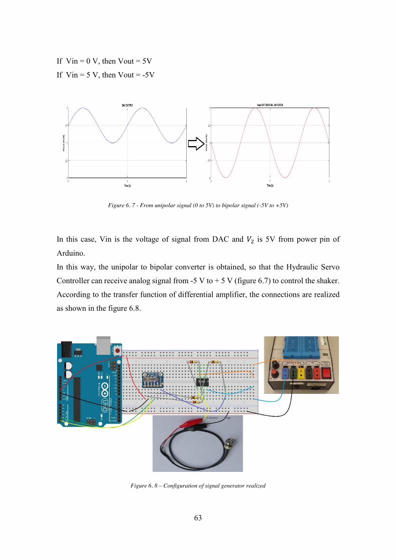
63

If Vin = 0 V, then Vout = 5V

If Vin = 5 V, then Vout = -5V

Figure 6. 7 - From unipolar signal (0 to 5V) to bipolar signal (-5V to +5V)

In this case, Vin is the voltage of signal from DAC and 𝑉2 is 5V from power pin of

Arduino.

In this way, the unipolar to bipolar converter is obtained, so that the Hydraulic Servo

Controller can receive analog signal from -5 V to + 5 V (figure 6.7) to control the shaker.

According to the transfer function of differential amplifier, the connections are realized

as shown in the figure 6.8.

Figure 6. 8 – Configuration of signal generator realized

64

The pins –Vcc and +Vcc are connected to the power supply with -7 volt and +7 volt

respectively.

Now, the signal generator is ready to be connected by BNC cable to the Hydraulic Servo

controller of the shaker shown in the figure 6.9.

Figure 6. 9 – Hydraulic Servo Controller

The Hydraulic Servo Controller shows:

x The Switch ON/OFF

x Transducer selector for the position

x INPUT connector to receive external analog signals in volt from a signal generator

x Displacement connector (DISP) to send in output the voltage value of

displacement transducer. This Output allows to know the Shaker position.

x GAIN knob set to 5.

x POSITION knob to adjust the shaker positon manually. The Position Value is set

to 4.90, so that the DISP value at start, without external inputs, is 0V.

To receive the displacement signal from the Servo Controller (DISP) and visualize it on

the computer, is realized a bipolar to unipolar converter. Given that Arduino Uno can

65

receive only analog signals between 0 to 5 V and the displacement transducer sends

bipolar signals between – 5 V to + 5V, a summing amplifier is used.

The summing amplifier configuration and Pin connections of Op-Amp TL071 Texas

Instruments are shown in the figure 6.10:

Figure 6. 10 – Summing amplifier configuration and Pin connections of TL071

The general equations is as follows:

𝑉𝑜𝑢𝑡 = 𝑉𝑖𝑛 ∙ 𝐺𝑎𝑖𝑛 + 𝑉𝑜𝑓𝑓𝑠𝑒𝑡

There are two unknown here, Gain and Voffset. But, since the output swing is half the

input range, the gain has to be 0.5.

To determinate the circuit offset, we can replace in the general equation one of the

input/output condition, say Vin = - 5 V and Vout = 0 V and determinate Voffset (2.5 V).

With the gain and offset Known, we can write the equation as:

𝑉𝑜𝑢𝑡 = 𝑉𝑖𝑛 ∙12+ 2.5

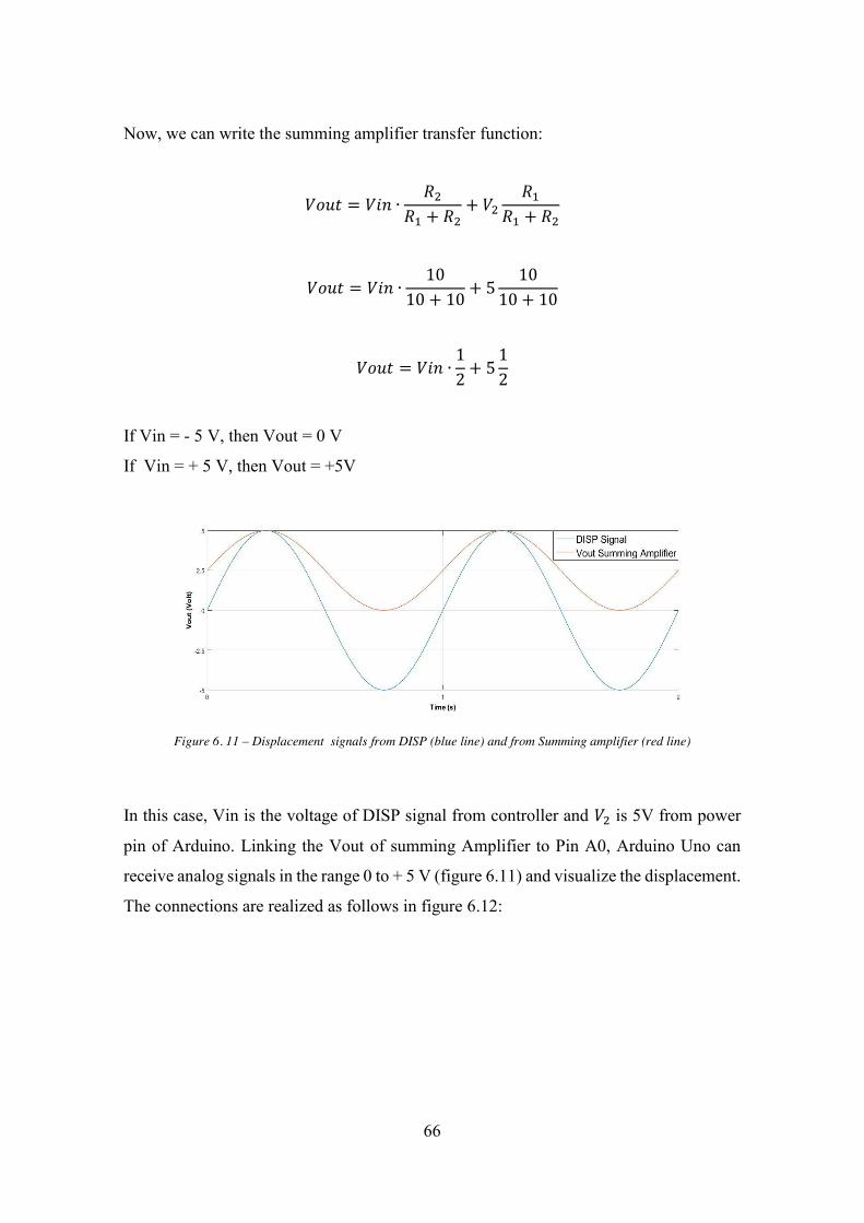
66

Now, we can write the summing amplifier transfer function:

𝑉𝑜𝑢𝑡 = 𝑉𝑖𝑛 ∙𝑅2

𝑅1 + 𝑅2+ 𝑉2

𝑅1𝑅1 + 𝑅2

𝑉𝑜𝑢𝑡 = 𝑉𝑖𝑛 ∙10

10 + 10+ 5

1010 + 10

𝑉𝑜𝑢𝑡 = 𝑉𝑖𝑛 ∙12+ 5

12

If Vin = - 5 V, then Vout = 0 V

If Vin = + 5 V, then Vout = +5V

Figure 6. 11 – Displacement signals from DISP (blue line) and from Summing amplifier (red line)

In this case, Vin is the voltage of DISP signal from controller and 𝑉2 is 5V from power

pin of Arduino. Linking the Vout of summing Amplifier to Pin A0, Arduino Uno can

receive analog signals in the range 0 to + 5 V (figure 6.11) and visualize the displacement.

The connections are realized as follows in figure 6.12:

67

Figure 6. 12 – Scheme to receive bipolar signal with Arduino Uno using TL071 in summing amplifier configuration

The pins –Vcc and +Vcc are connected at the power supply with -7 volt and +7 volt

respectively.

The components used are:

1. Arduino Uno 2. Op Amp TL071 Texas Instruments 3. 2 x 10 KΩ resistors 4. Power supply

By plugging the BNC with DISP output on the controller, is possible to receive analog

signals from the displacement transducer and know the shaker position.

The entire project powered by Arduino is shown the figure 6.13.

68

Figure 6. 13 – Signal generator powered by Arduino

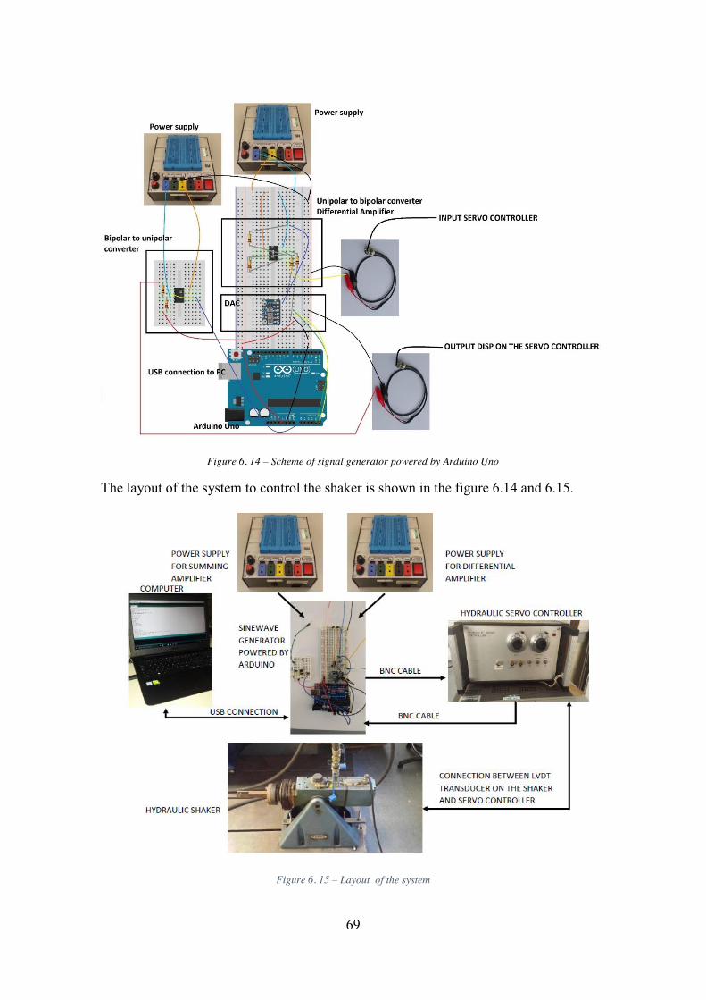
69

Figure 6. 14 – Scheme of signal generator powered by Arduino Uno

The layout of the system to control the shaker is shown in the figure 6.14 and 6.15.

Figure 6. 15 – Layout of the system

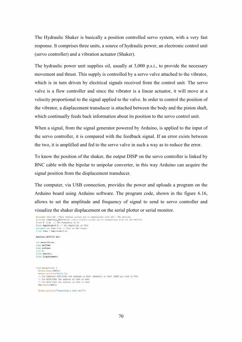
70

The Hydraulic Shaker is basically a position controlled servo system, with a very fast

response. It comprises three units, a source of hydraulic power, an electronic control unit

(servo controller) and a vibration actuator (Shaker).

The hydraulic power unit supplies oil, usually at 3,000 p.s.i., to provide the necessary

movement and thrust. This supply is controlled by a servo valve attached to the vibrator,

which is in turn driven by electrical signals received from the control unit. The servo

valve is a flow controller and since the vibrator is a linear actuator, it will move at a

velocity proportional to the signal applied to the valve. In order to control the position of

the vibrator, a displacement transducer is attached between the body and the piston shaft,

which continually feeds back information about its position to the servo control unit.

When a signal, from the signal generator powered by Arduino, is applied to the input of

the servo controller, it is compared with the feedback signal. If an error exists between

the two, it is amplified and fed to the servo valve in such a way as to reduce the error.

To know the position of the shaker, the output DISP on the servo controller is linked by

BNC cable with the bipolar to unipolar converter, in this way Arduino can acquire the

signal position from the displacement transducer.

The computer, via USB connection, provides the power and uploads a program on the

Arduino board using Arduino software. The program code, shown in the figure 6.16,

allows to set the amplitude and frequency of signal to send to servo controller and

visualize the shaker displacement on the serial plotter or serial monitor.

71

Figure 6. 16 - Code to program Arduino

Setting the frequency (range 1-20 Hz) and the amplitude (range 0-5V), it acts on the DAC

output (Vout), generating a sinewave signal in the range 0-5V that has equation:

𝑉𝑜𝑢𝑡 = 2.5 + (𝐴𝑚𝑝𝑙𝑖𝑡𝑢𝑑𝑒

2) sin(2𝜋𝑓𝑡)

In the code, the equation of Vout is wrote in the range of integer values between 0 and

4096, because the DAC having resolution 12 bit must receive in input a digital signal with

values between 0 and 4096 and will convert it to voltage value between 0 and 5 V.

The relationship between digital value in the range 0-4096 and analog value in the range

0-5V is the following:

𝐴𝑛𝑎𝑙𝑜𝑔𝑣𝑎𝑙𝑢𝑒 =5

4096∙ 𝐷𝑖𝑔𝑖𝑡𝑎𝑙𝑣𝑎𝑙𝑢𝑒

The equation of Vout in the code is:

𝑉𝑜𝑢𝑡 = 𝑉𝑜𝑓𝑓𝑠𝑒𝑡 + (𝑉𝑚𝑎𝑥 ∗ 2047) ∗ sin(2𝜋𝑓𝑇 ∗ 0.000001)

where:

Voffset is 2047 (≅ 5V) allows to center the sinewave in the range 0-5V;

Vmax is the peak deviation coefficient of the function from Voffset and has equation:

72

𝑉𝑚𝑎𝑥 =𝐴𝑚𝑝𝑙𝑖𝑡𝑢𝑑𝑒

5.0

f is the frequency chose in Hz;

T is the time in µs;

For example, if the Amplitude chose is 5.0 and f is 1 Hz, Vmax is 1.0 and Vout will

became:

𝑉𝑜𝑢𝑡 = 2047 + (1.0 ∗ 2047) ∗ sin(2𝜋𝑓𝑇 ∗ 0.000001)

𝑉𝑜𝑢𝑡 = 2047 + 2047 ∗ sin(2𝜋𝑓𝑇 ∗ 0.000001)

The DAC output will be a sinewave with amplitude around 2.5 V and frequency 1 Hz

shifted by 2.5V. In this way the signal is between 0 to 5V.

As explained previously, the DAC output will be the input of differential amplifier that

converts the signal from unipolar (0-5V) to bipolar (±5V).

In the second part of the code by means of the function analogRead() is acquired on the

pin A0 of Arduino the signal from the displacement transducer. The signal is unipolar

given that passed through the bipolar to unipolar converter.

Arduino reads the analog signal and converts it in digital signal at 10 bit, a integer values

between 0 and 1023. The equation used to convert these values in volt is:

voltage = sensorValue ∗ (5.0/1023.0)

Where:

sensorValue is the signal value in the range 0 – 1023;

voltage is the signal value in the range 0 - 5V.

To know the real value bipolar from the displacement transducer is used the following

equation:

𝑅𝑒𝑎𝑙𝑉𝑎𝑙 = 2 ∗ 𝑣𝑜𝑙𝑡𝑎𝑔𝑒 − 5

𝑅𝑒𝑎𝑙𝑉𝑎𝑙 = 𝑔𝑎𝑖𝑛 ∗ 𝑣𝑜𝑙𝑡𝑎𝑔𝑒 − 𝑜𝑓𝑓𝑠𝑒𝑡

73

In this way is obtained the bipolar signal in the range ±5 of the output DISP on the

controller.

The matching between volt and shaker position is measured positioning a graduate scale

in centimetre (from -10 cm to 10 cm) under the shaker as shown in figure 6.17.

Figure 6. 17 - Matching between the displacement value on graduate scale and voltage value on the oscilloscope

The start position is 0 cm and the signal of transducer visualized on the oscilloscope is 0

V. By moving the shaker using the position knob, the transducer response in volt changes

visualizing the corresponding voltage value on the oscilloscope. The measure matching

in centimetres is obtained reading the displacement on the graduate scale.

The matching volt-cm is 2V=1 cm and is represented with a graph in the figure 16.18:

Figure 6. 18 - Matching Volt-cm

The shaker displacement can be visualized using the Serial.println() function that allows

to plot in real time the shaker state on the graph as shown in the figure 6.19.

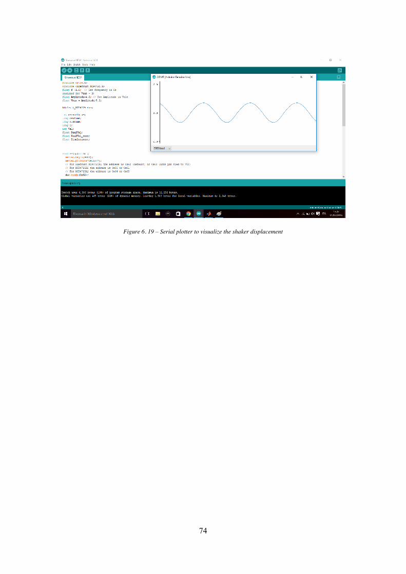
74

Figure 6. 19 – Serial plotter to visualize the shaker displacement

75

Chapter 7

Conclusion and future development

The Quarter-car test rig designed in this study, thanks to its modular structure, it proves

able to accommodate several configuration of suspension system and a wide range of

vehicle mass. The heavy and rigid structure of the main components reduces the

excitation from external source of the future sensors implemented such as accelerometers.

This is very important in the study of vibration systems in order to not influence the

dynamic behaviour of the component tested. The simulations carried out in Ansys show

that the resonance frequency of the load frame are very far above those of interest. The

first frequency of the load frame is 131,84 Hz. The implementation of the rig in Simulink

environment has allowed to verify that the Quarter car test rig designed is suitable to test

the suspension systems because the joints used between the components are coherent with

a two degree of freedom system. From the simulation, results that the system have two

resonance frequency. The signal generator powered by Arduino Uno is able to send

sinusoidal signal with amplitude ± 5 V and several frequencies between 1 and 20 Hz. This

allows to drive the shaker to excite the tyre of quarter car system. Furthermore, the

position of the shaker can be received and visualized on the computer through the script

realized in Arduino software.

The future developments, after the physic realization of the parts and the choice of the

suspension system to test, concern the implementation of a sensors and a data acquisition

system [20]. Two accelerometers can be used to measure the accelerations of the sprung

mass and unsprung mass. It is important that the accelerometers are positioned in order

that they are exposed to as little transverse vibration as possible. These vibrations could

cause a non-linearity error in the measurement. The good position on which to install the

accelerometers can be those shown in the figure 7.1.

76

Figure 7. 1 – Positions of the accelerometers

The displacement transducer of the hydraulic shaker can be used in feedback control of

the actuation system. Through the signal generator powered by Arduino the analog signal

can be send to servo controller of the shaker. A data acquisition equipment, real time

control box, oscilloscope and a computer are necessary to control the system and the

acquisition of signals. An example of the possible layout of the system is shown in the

figure 7.2.

Figure 7. 2 – Layout of the system

77

APPENDIX INITIAL START-UP PROCEDURE

1. Open the Arduino Software

2. Open the program code: File > Open > Sinewave_Generator

3. In the code, set Frequency 1 HZ and Amplitude 0 V

4. On the servo controller, set:

x Mains power switch OFF x Displacement switch ON x Divide by 10 switch OFF x Gain Dial: 5 x Position Dial around 4.90 x (ADVICE: Connect the oscilloscope to DISP and turn on the shaker

without external input signal. Rotate the knob position until the oscilloscope shows 0 V. Now the shaker is at half stroke. Turn off the shaker)

78

5. Connect the BNC cable 1 to the input of controller and the BNC cable 2 to DISP on the controller. It’s possible to use a BNC T connector (with double female splitter) to connect

the BNC from Arduino and BNC from the oscilloscope to DISP, in order to check

the displacement signal also on the oscilloscope.

6. Switch on Servo Controller and connect Arduino to computer via USB cable.

7. Switch on the two power supplies, checking that the two knobs are set around 7V

79

8. Switch on Hydraulic Unit.

9. In Arduino software open Tools > Serial Plotter.

10. In the code of Arduino software adjust Amplitude and Frequency (f) as desired and click upload. Amplitude range is 0 -5 V

Frequency range is 1-20 Hz

Hydraulic shaker should oscillate

SHUT-DOWN PRCEDURE

Essentially to return the Hydraulic Shaker to its start up position.

1. Adjust Amplitude to 0 V and Frequency to 1 Hz.

2. Switch off Hydraulic Pump Unit.

80

3. Plug off the USB cable from computer and switch off Hydraulic Controller

4. Switch off the Power Supplies.

SINEWAVE GENERATOR CODE

#include <Wire.h> //This library allows you to communicate with I2C / TWI devices

#include <Adafruit_MCP4725.h> //This library allows you to communicate with the

DAC MCP4725

float f =1.0; // Set frequency in Hz

float Amplitude=0.0; // Set Amplitude in Volt

unsigned int Vout = 0; // Vout is DAC Output

float Vmax = Amplitude/5.0;

Adafruit_MCP4725 dac;

int sensorValue;

long newTime;

long oldTime;

long T;

float RealVal;

float Displacement;

void setup(void) {

Serial.begin(9600);

Serial.println("Hello!");

// For Adafruit MCP4725A1 the address is 0x62 (default) or 0x63 (ADDR pin tied to

VCC)

// For MCP4725A0 the address is 0x60 or 0x61

81

// For MCP4725A2 the address is 0x64 or 0x65

dac.begin(0x62);

Serial.println("Generating a sine wave");

oldTime = micros();

}

void loop(void) {

newTime=micros();

if (newTime << oldTime)

{ oldTime = newTime;}

T = newTime - oldTime;

Vout = 2047 + (Vmax*2047)*(sin(2 * PI * f * T * 0.000001)); // Moves the DAC output

in the range 0-5V

dac.setVoltage(Vout, false); // To set the DAC output

// Serial.println(Vout);

int sensorValue=analogRead(A0); //Reads the value on the pin A0 connected with DISP

Of The controller

float voltage= sensorValue * (5.0/1023.0); // Trsforms the Value in scale from 0 to

2^10bit=1024, in scale from 0 to 5V

float RealVal=(2*voltage)-5; // Real Value of displacement transducer between -5V to

+5V

float Displacement=(RealVal)/2; // Matching Voltage/Displacement (2V=1cm)

82

Serial.println(Displacement); // Open Tools, than Serial Plotter or Serial Monitor to

visualize the Desplacement in cm

}

83

REFERENCES

[1] Larry Mianzo, David Fricke, and Rakan Chabaan, Road Profile Control Methods for

Laboratory Vehicle Road Simulators, Body and Chassis Test Deprtment Advanced

Vehicle Technology Ford Motor Compny

[2] M. French, M. Jay (1998), Automotive test Methods, Automotive NVH Series: Part 2”

[3] Y. Hayama, T. Nozaki, M. Nakakouji, S. Fujikawa, K. Fukushima, NVH Analysis

Using Full Vehicle Multi Body Dynamic Model, NTN Technical review No.73 (2005)

[4] D. Vetturi, A. Magalini, Road Profile excitation on a vehicle measurements and

indoor testing using a four-post rig, Dipartimento di Ingegneria Meccanica –

Università degli studi di Brescia

[5] Y. Taskin, N. Ygiz and I. Yuksek, Lamped parameter identification of a quarter car

test rig, Department of Mechanical Engineering, Faculty of Engineering, Istanbul

University,

[6] Guido Koch, E. Pellegrini, Sebastian Spirk and Boris Lohamann, Design and

Modeling of a Quarter- Vehicle test rig fo active suspension control, Initsitute of

Automatic Contol, Technische Univeristat Munchen Boltzmannstr

[7] Yogesh Sanjay Pathare, Nimbalkar Sachin R., Design and Development of Quarter

car suspension Test rig model and It’s Simulation, International Journal of innovative

Research & Development (2014)

[8] William F. Milliken, Douglas L. Milliken, Race car vehicle dynamics

[9] G. Petrucci, Lezione di costruzione di machine

[10] Bosch Rexroth Group (2011), Manuale di tecnica lineare

[11] William T. Thomson, Theory of Vibration with Applications Fourth Edition

[12] A. Rivola, Meccanica e Dinamica delle machine LM, Università degli studi di

Bologna

[13] Gianpaolo Riva, Le sospensioni

84

[14] Olugbenga Moses Anubi, Variable Stiffness Suspension System, University of

Florida

[15] Janusz Kowal, Jack Snamina, Tomasz Wzorek, Design of the laboratory stand for

testing vehicle suspensions, Mechanics and control Vol. 30 No. 1 2011

[16] Andrea Aldegheri, Studio in ambiente Matlab/Simulink di un Sistema di controllo

per sospensioni attive, Università degli studi di Padova

[17] Ye Hong, An investigation of band-limited fluid damper configuration using lumped

parameter modelling, The University of Texas at Arlington (2015)

[18] M. Agostinacchio, D. Ciampa, S. Olita, The vibrations induced by surface

irregularities in road pavements

[19] Maik Schmidt, Il Manuale di Arduino, Apogeo

[20] Justin D. Langdon, Design and Adaptive Control of a Lab-based , Tire-coupled,

Quarter-car Suspension Test Rig for Accurate Re-creation of Vehicle Response

SCUOLA DI INGEGNERIA E ARCHITETTURA Sede di Forlì … MAGISTRALE ANTONELLO... · Terminata la fase...

Documents

Transcript of SCUOLA DI INGEGNERIA E ARCHITETTURA Sede di Forlì … MAGISTRALE ANTONELLO... · Terminata la fase...