Robotica - home.deib.polimi.ithome.deib.polimi.it/restelli/Lezione7.pdf15/12/2006 Corso di Robotica...
74
Transcript of Robotica - home.deib.polimi.ithome.deib.polimi.it/restelli/Lezione7.pdf15/12/2006 Corso di Robotica...
15/12/200615/12/2006 Corso di Robotica 06/07Corso di Robotica 06/07Davide Migliore - [email protected] Migliore - [email protected]
22/69/69
TodayToday
● Bayes Filters Review:– Bayes Filter– Gaussian Filters
● Nonparametric Filters:– Particle Filter– Fast SLAM 1.0– Fast SLAM 2.0

15/12/200615/12/2006 Corso di Robotica 06/07Corso di Robotica 06/07Davide Migliore - [email protected] Migliore - [email protected]
33/69/69
Previous lessonsPrevious lessons

15/12/200615/12/2006 Corso di Robotica 06/07Corso di Robotica 06/07Davide Migliore - [email protected] Migliore - [email protected]
44/69/69
Bayes Filters: FrameworkBayes Filters: Framework● Given:
– Stream of observations z and action data u:
– Sensor model P(z|x).– Action model P(x|u,x’).– Prior probability of the system state P(x).
● Wanted: – Estimate of the state X of a dynamical system.– The posterior of the state is also called Belief:
),,,|()( 11 tttt zuzuxPxBel =
},,,{ 11 ttt zuzud =
15/12/200615/12/2006 Corso di Robotica 06/07Corso di Robotica 06/07Davide Migliore - [email protected] Migliore - [email protected]
55/69/69
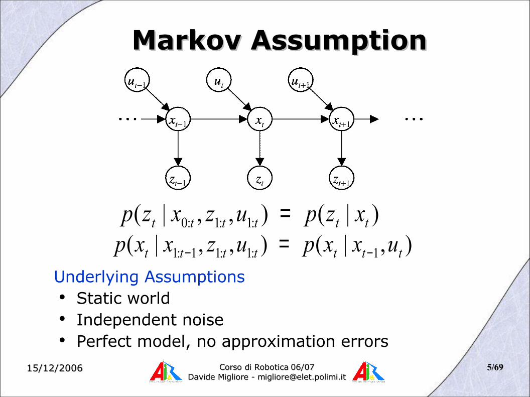
Markov AssumptionMarkov Assumption
Underlying Assumptions● Static world● Independent noise● Perfect model, no approximation errors
),|(),,|( 1:1:11:1 ttttttt uxxpuzxxp −− =)|(),,|( :1:1:0 tttttt xzpuzxzp =
15/12/200615/12/2006 Corso di Robotica 06/07Corso di Robotica 06/07Davide Migliore - [email protected] Migliore - [email protected]
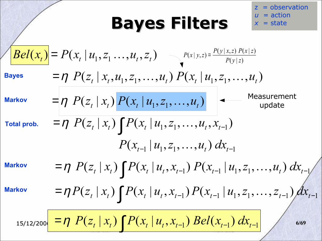
66/69/69111 )(),|()|( −−−∫= ttttttt dxxBelxuxPxzPη
Bayes FiltersBayes Filters
),,,|(),,,,|( 1111 ttttt uzuxPuzuxzP η=Bayes
z = observationu = actionx = state
),,,|()( 11 tttt zuzuxPxBel =
Markov ),,,|()|( 11 tttt uzuxPxzP η=
Markov11111 ),,,|(),|()|( −−−∫= tttttttt dxuzuxPxuxPxzP η
1111
111
),,,|(
),,,,|()|(
−−
−∫=
ttt
ttttt
dxuzuxP
xuzuxPxzP
ηTotal prob.
Markov111111 ),,,|(),|()|( −−−−∫= tttttttt dxzzuxPxuxPxzP η
Measurement update
)|(
)|(),|(),|(
zyP
zxPzxyPzyxP =

15/12/200615/12/2006 Corso di Robotica 06/07Corso di Robotica 06/07Davide Migliore - [email protected] Migliore - [email protected]
77/69/69
● Prediction
● Correction
Bayes Filter SummaryBayes Filter Summary
111 )(),|()( −−−∫= tttttt dxxbelxuxpxbel
)()|()( tttt xbelxzpxbel η=

15/12/200615/12/2006 Corso di Robotica 06/07Corso di Robotica 06/07Davide Migliore - [email protected] Migliore - [email protected]
88/69/69
Discrete Kalman FilterDiscrete Kalman Filter
tttttt uBxAx ε++= −1
tttt xCz δ+=
Estimates the state x of a discrete-time controlled process that is governed by the linear stochastic difference equation
with a measurement

15/12/200615/12/2006 Corso di Robotica 06/07Corso di Robotica 06/07Davide Migliore - [email protected] Migliore - [email protected]
99/69/69
( )0000 ,;)( Σ= µxNxbel
Linear Gaussian Systems: InitializationLinear Gaussian Systems: Initialization
● Initial belief is normally distributed:

15/12/200615/12/2006 Corso di Robotica 06/07Corso di Robotica 06/07Davide Migliore - [email protected] Migliore - [email protected]
1010/69/69
● Dynamics are linear function of state and control plus additive noise:
tttttt uBxAx ε++= −1
Linear Gaussian Systems: DynamicsLinear Gaussian Systems: Dynamics
( )ttttttttt RuBxAxNxuxp ,;),|( 11 += −−
( ) ( )1111
111
,;~,;~
)(),|()(
−−−−
−−−
Σ+⇓⇓
= ∫
ttttttttt
tttttt
xNRuBxAxN
dxxbelxuxpxbel
µ

15/12/200615/12/2006 Corso di Robotica 06/07Corso di Robotica 06/07Davide Migliore - [email protected] Migliore - [email protected]
1111/69/69
Linear Gaussian Systems: DynamicsLinear Gaussian Systems: Dynamics
( ) ( )
+Σ=Σ+=
=
−Σ−−
−−−−−=
⇓
Σ+⇓⇓
=
−
−
−−−−−−−
−−
−
−−−−
−−−
∫
∫
tTtttt
tttttt
ttttT
tt
ttttttT
tttttt
ttttttttt
tttttt
RAA
uBAxbel
dxxx
uBxAxRuBxAxxbel
xNRuBxAxN
dxxbelxuxpxbel
1
1
1111111
11
1
1111
111
)(
)()(2
1exp
)()(2
1exp)(
,;~,;~
)(),|()(
µµ
µµ
η
µ

15/12/200615/12/2006 Corso di Robotica 06/07Corso di Robotica 06/07Davide Migliore - [email protected] Migliore - [email protected]
1212/69/69
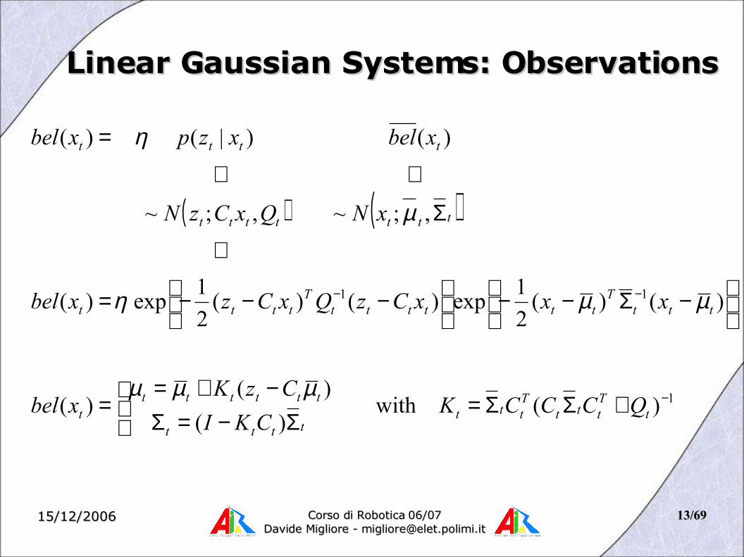
● Observations are linear function of state plus additive noise:
tttt xCz δ+=
Linear Gaussian Systems: ObservationsLinear Gaussian Systems: Observations
( )tttttt QxCzNxzp ,;)|( =
( ) ( )ttttttt
tttt
xNQxCzN
xbelxzpxbel
Σ
⇓⇓
=
,;~,;~
)()|()(
µ
η
15/12/200615/12/2006 Corso di Robotica 06/07Corso di Robotica 06/07Davide Migliore - [email protected] Migliore - [email protected]
1313/69/69
Linear Gaussian Systems: ObservationsLinear Gaussian Systems: Observations
( ) ( )
1
11
)(with )(
)()(
)()(2
1exp)()(
2
1exp)(
,;~,;~
)()|()(
−
−−
+ΣΣ=
Σ−=Σ−+=
=
−Σ−−
−−−=
⇓
Σ
⇓⇓
=
tTttt
Tttt
tttt
ttttttt
tttT
ttttttT
tttt
ttttttt
tttt
QCCCKCKI
CzKxbel
xxxCzQxCzxbel
xNQxCzN
xbelxzpxbel
µµµ
µµη
µ
η

15/12/200615/12/2006 Corso di Robotica 06/07Corso di Robotica 06/07Davide Migliore - [email protected] Migliore - [email protected]
1414/69/69
Kalman Filter Algorithm Kalman Filter Algorithm
1. Algorithm Kalman_filter( µt-1, Σt-1, ut, zt):
3. Prediction:4. 5.
6. Correction:7. 8. 9.
10. Return µt, Σt
ttttt uBA += −1µµ
tTtttt RAA +Σ=Σ −1
1)( −+ΣΣ= tTttt
Tttt QCCCK
)( tttttt CzK µµµ −+=tttt CKI Σ−=Σ )(
15/12/200615/12/2006 Corso di Robotica 06/07Corso di Robotica 06/07Davide Migliore - [email protected] Migliore - [email protected]
1515/69/69
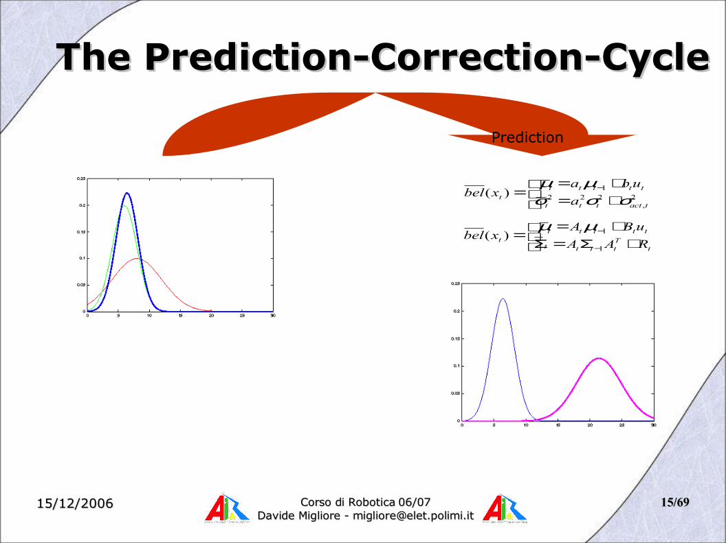
The Prediction-Correction-CycleThe Prediction-Correction-Cycle
+Σ=Σ+=
=−
−
tTtttt
tttttt RAA
uBAxbel
1
1)(µµ
+=+=
= −2
,2221)(
tactttt
tttttt a
ubaxbel σσσ
µµ
Prediction

15/12/200615/12/2006 Corso di Robotica 06/07Corso di Robotica 06/07Davide Migliore - [email protected] Migliore - [email protected]
1616/69/69
The Prediction-Correction-CycleThe Prediction-Correction-Cycle
1)(,)(
)()( −+ΣΣ=
Σ−=Σ−+=
= tTttt
Tttt
tttt
ttttttt QCCCK
CKI
CzKxbel
µµµ
2,
2
2
22 ,)1(
)()(
tobst
tt
ttt
tttttt K
K
zKxbel
σσσ
σσµµµ
+=
−=−+=
=
Correction
15/12/200615/12/2006 Corso di Robotica 06/07Corso di Robotica 06/07Davide Migliore - [email protected] Migliore - [email protected]
1717/69/69
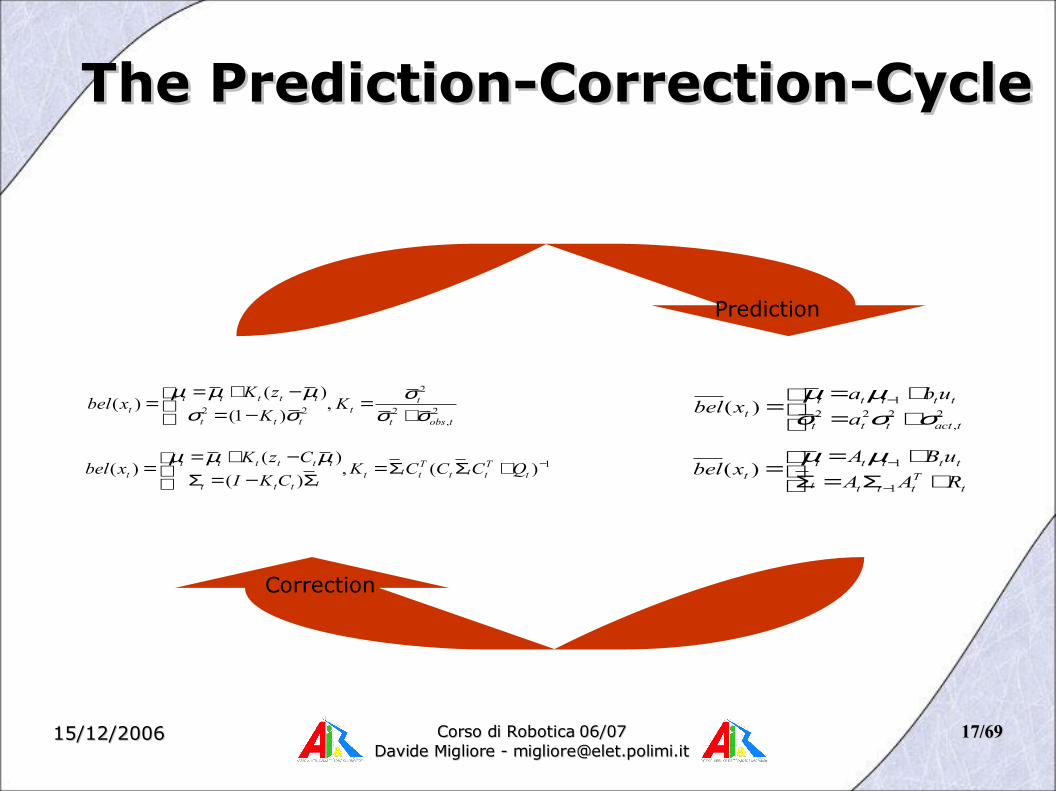
The Prediction-Correction-CycleThe Prediction-Correction-Cycle
1)(,)(
)()( −+ΣΣ=
Σ−=Σ−+=
= tTttt
Tttt
tttt
ttttttt QCCCK
CKI
CzKxbel
µµµ
2,
2
2
22 ,)1(
)()(
tobst
tt
ttt
tttttt K
K
zKxbel
σσσ
σσµµµ
+=
−=−+=
=
+Σ=Σ+=
=−
−
tTtttt
tttttt RAA
uBAxbel
1
1)(µµ
+=+=
= −2
,2221)(
tactttt
tttttt a
ubaxbel σσσ
µµ
Correction
Prediction

15/12/200615/12/2006 Corso di Robotica 06/07Corso di Robotica 06/07Davide Migliore - [email protected] Migliore - [email protected]
1818/69/69
Kalman Filter SummaryKalman Filter Summary
● Highly efficient: Polynomial in measurement dimensionality k and state dimensionality n: O(k2.376 + n2)
● Optimal for linear Gaussian systems!
● Most robotics systems are nonlinear!
15/12/200615/12/2006 Corso di Robotica 06/07Corso di Robotica 06/07Davide Migliore - [email protected] Migliore - [email protected]
1919/69/69
Nonlinear Dynamic SystemsNonlinear Dynamic Systems
● Most realistic robotic problems involve nonlinear functions
),( 1−= ttt xugx
)( tt xhz =
15/12/200615/12/2006 Corso di Robotica 06/07Corso di Robotica 06/07Davide Migliore - [email protected] Migliore - [email protected]
2020/69/69
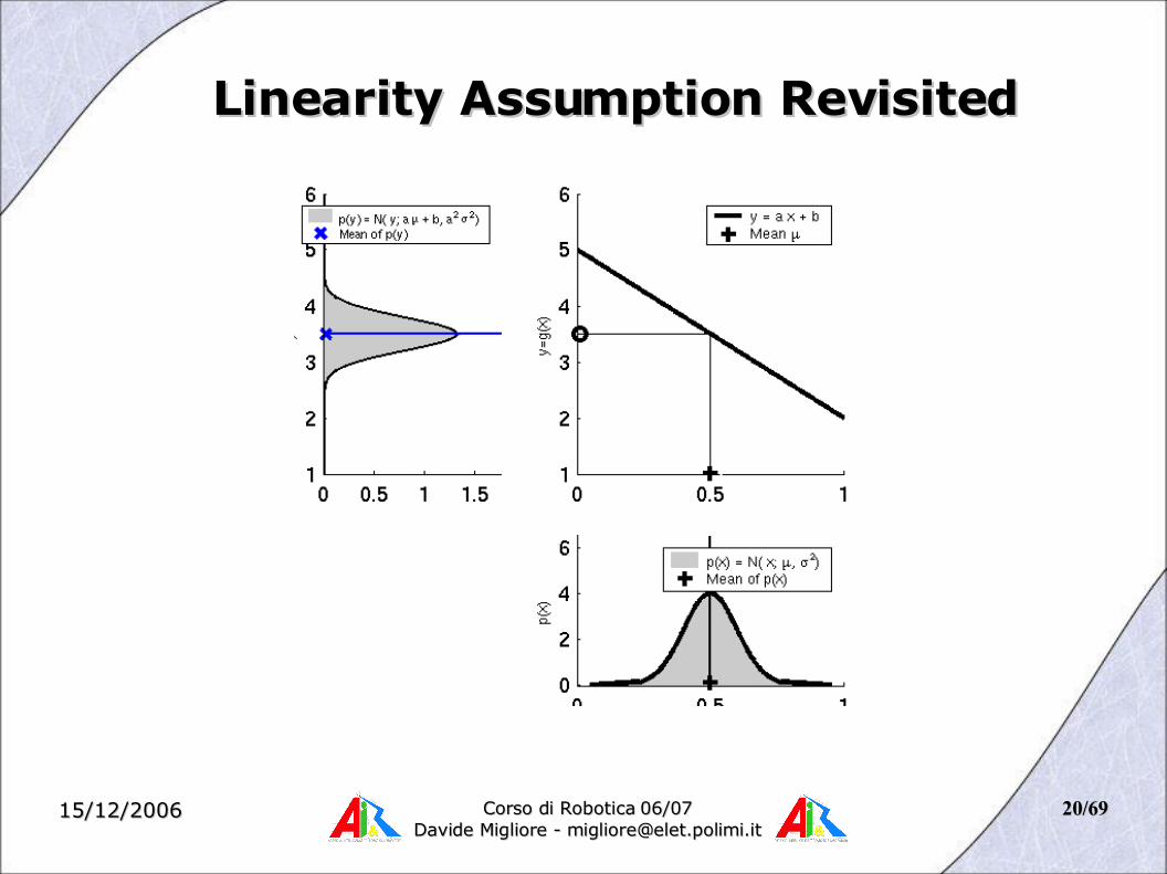
Linearity Assumption RevisitedLinearity Assumption Revisited

15/12/200615/12/2006 Corso di Robotica 06/07Corso di Robotica 06/07Davide Migliore - [email protected] Migliore - [email protected]
2121/69/69
Non-linear FunctionNon-linear Function
15/12/200615/12/2006 Corso di Robotica 06/07Corso di Robotica 06/07Davide Migliore - [email protected] Migliore - [email protected]
2222/69/69
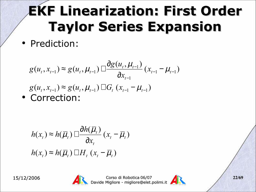
● Prediction:
● Correction:
EKF Linearization: First Order EKF Linearization: First Order Taylor Series ExpansionTaylor Series Expansion
)(),(),(
)(),(
),(),(
1111
111
111
−−−−
−−−
−−−
−+≈
−∂
∂+≈
ttttttt
ttt
tttttt
xGugxug
xx
ugugxug
µµ
µµµ
)()()(
)()(
)()(
ttttt
ttt
ttt
xHhxh
xx
hhxh
µµ
µµµ
−+≈
−∂
∂+≈
15/12/200615/12/2006 Corso di Robotica 06/07Corso di Robotica 06/07Davide Migliore - [email protected] Migliore - [email protected]
2323/69/69
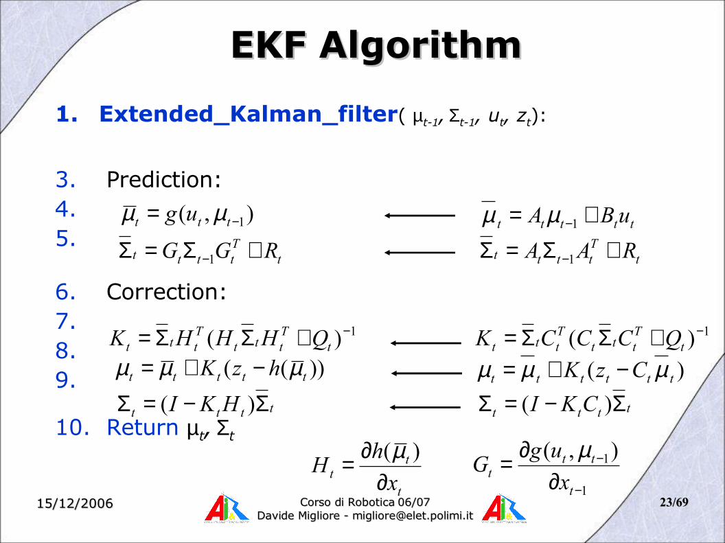
EKF Algorithm EKF Algorithm
1. Extended_Kalman_filter( µt-1, Σt-1, ut, zt):
3. Prediction:4. 5.
6. Correction:7. 8. 9.
10. Return µt, Σt
),( 1−= ttt ug µµ
tTtttt RGG +Σ=Σ −1
1)( −+ΣΣ= tTttt
Tttt QHHHK
))(( ttttt hzK µµµ −+=
tttt HKI Σ−=Σ )(
1
1),(
−
−
∂∂=
t
ttt x
ugG
µ
t
tt x
hH
∂∂= )(µ
ttttt uBA += −1µµ
tTtttt RAA +Σ=Σ −1
1)( −+ΣΣ= tTttt
Tttt QCCCK
)( tttttt CzK µµµ −+=tttt CKI Σ−=Σ )(
15/12/200615/12/2006 Corso di Robotica 06/07Corso di Robotica 06/07Davide Migliore - [email protected] Migliore - [email protected]
2424/69/69
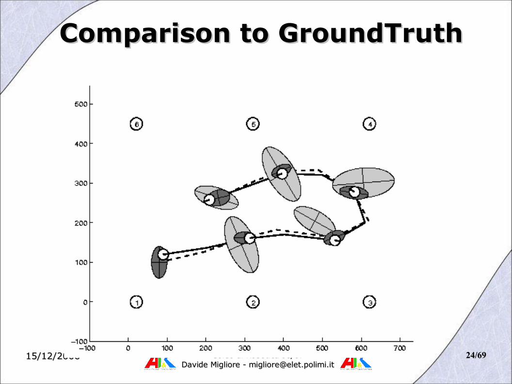
Comparison to GroundTruthComparison to GroundTruth
15/12/200615/12/2006 Corso di Robotica 06/07Corso di Robotica 06/07Davide Migliore - [email protected] Migliore - [email protected]
2525/69/69
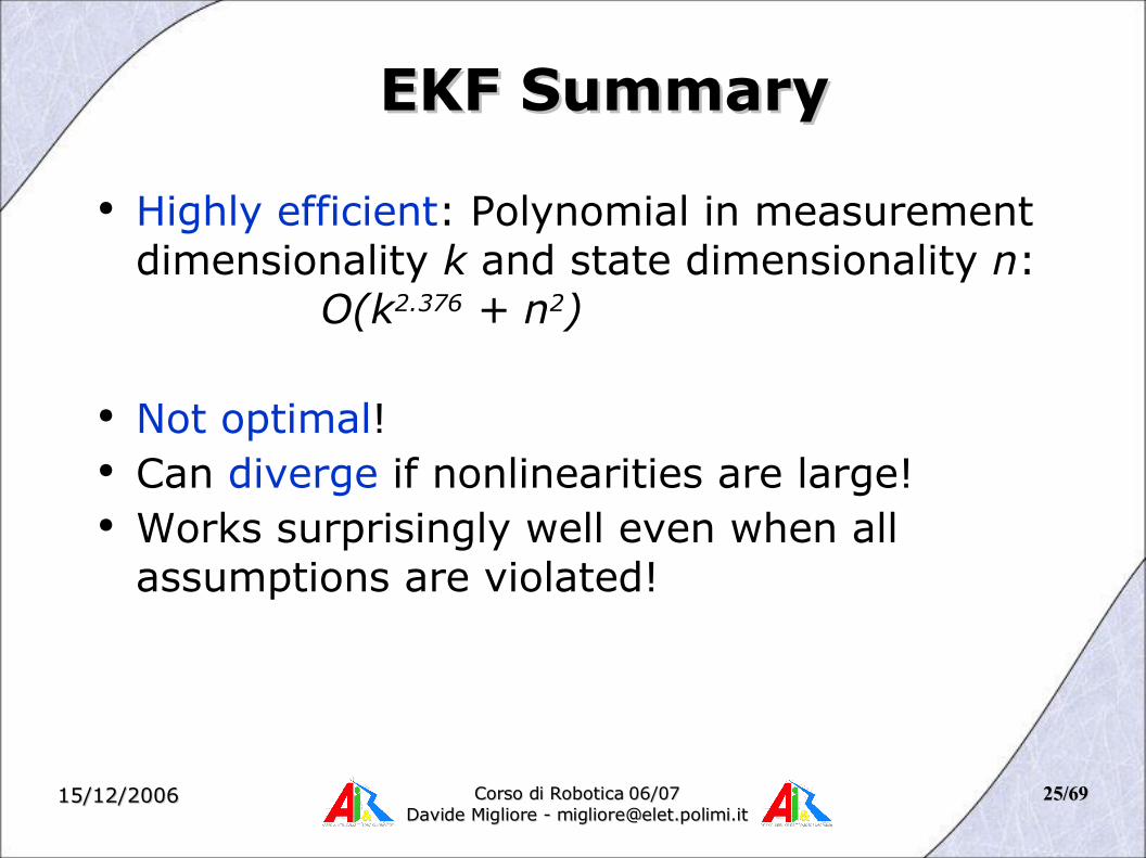
EKF SummaryEKF Summary
● Highly efficient: Polynomial in measurement dimensionality k and state dimensionality n: O(k2.376 + n2)
● Not optimal!● Can diverge if nonlinearities are large!● Works surprisingly well even when all
assumptions are violated!

15/12/200615/12/2006 Corso di Robotica 06/07Corso di Robotica 06/07Davide Migliore - [email protected] Migliore - [email protected]
2626/69/69
Linearization via Unscented Linearization via Unscented TransformTransform
EKF UKF
15/12/200615/12/2006 Corso di Robotica 06/07Corso di Robotica 06/07Davide Migliore - [email protected] Migliore - [email protected]
2727/69/69
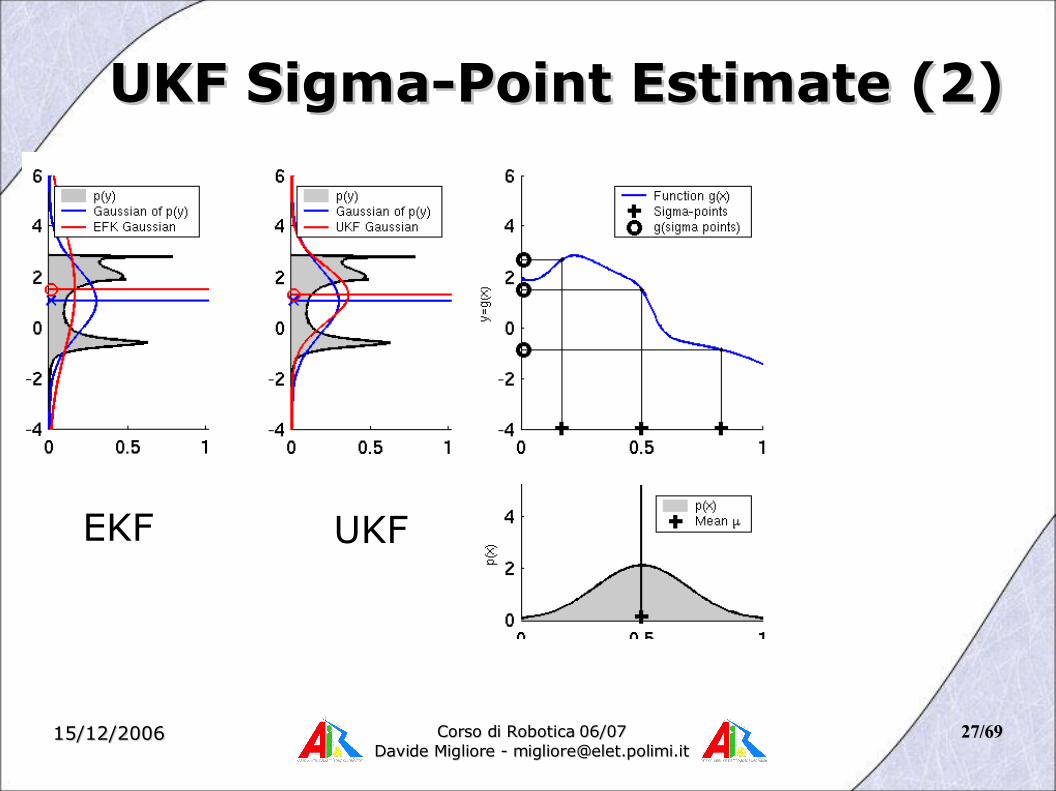
UKF Sigma-Point Estimate (2)UKF Sigma-Point Estimate (2)
EKF UKF

15/12/200615/12/2006 Corso di Robotica 06/07Corso di Robotica 06/07Davide Migliore - [email protected] Migliore - [email protected]
2828/69/69
Unscented TransformUnscented Transform
( ) nin
wwn
nw
nw
ic
imi
i
cm
2,...,1for )(2
1 )(
)1( 2000
=+
==Σ+±=
+−++
=+
==
λλµχ
βαλ
λλ
λµχ
Sigma points Weights
)( ii g χψ =
∑
∑
=
=
−−=Σ
=
n
i
Tiiic
n
i
iim
w
w
2
0
2
0
))(('
'
µψµψ
ψµ
Pass sigma points through nonlinear function
Recover mean and covariance
15/12/200615/12/2006 Corso di Robotica 06/07Corso di Robotica 06/07Davide Migliore - [email protected] Migliore - [email protected]
2929/69/69
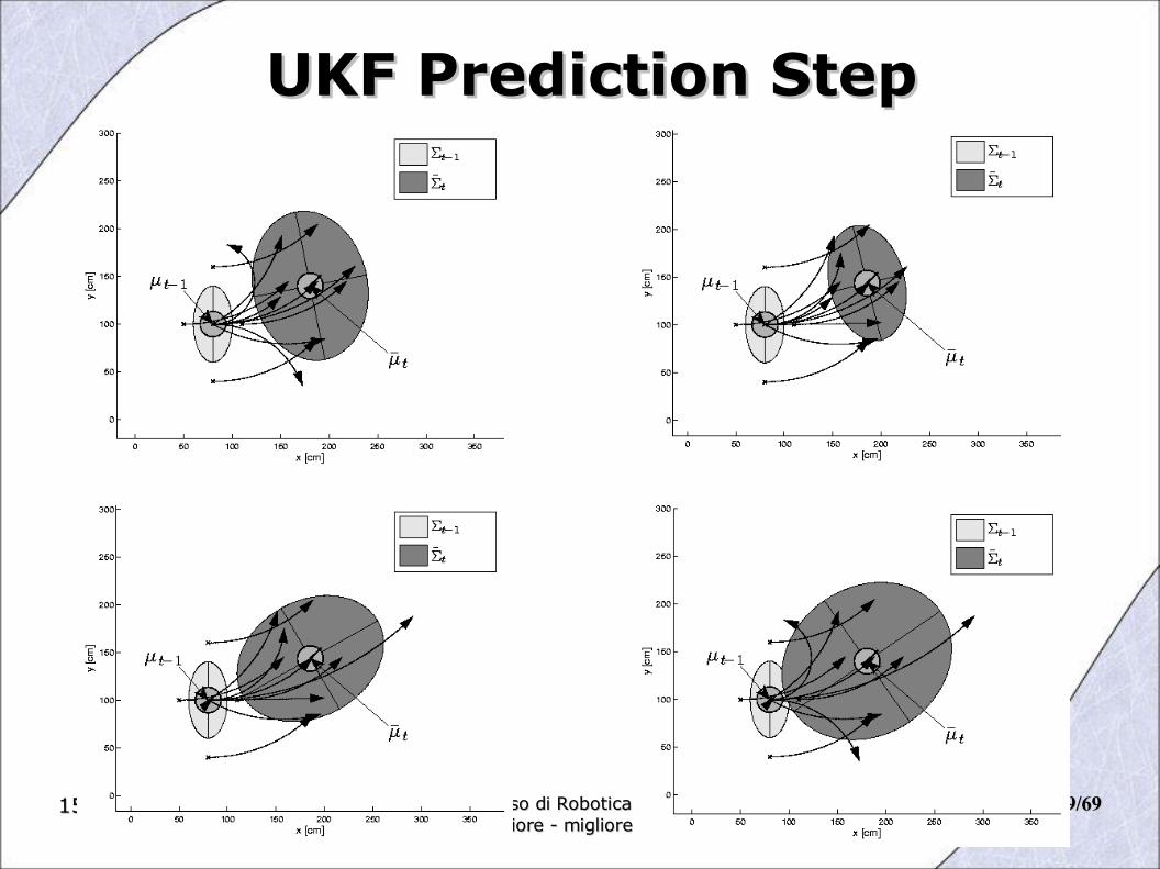
UKF Prediction StepUKF Prediction Step

15/12/200615/12/2006 Corso di Robotica 06/07Corso di Robotica 06/07Davide Migliore - [email protected] Migliore - [email protected]
3030/69/69
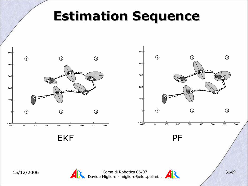
Estimation SequenceEstimation Sequence
EKF PF UKF
15/12/200615/12/2006 Corso di Robotica 06/07Corso di Robotica 06/07Davide Migliore - [email protected] Migliore - [email protected]
3131/69/69
Estimation SequenceEstimation Sequence
UKF PF EKF PF

15/12/200615/12/2006 Corso di Robotica 06/07Corso di Robotica 06/07Davide Migliore - [email protected] Migliore - [email protected]
3232/69/69
Estimation SequenceEstimation Sequence
UKF PF UKF PF
15/12/200615/12/2006 Corso di Robotica 06/07Corso di Robotica 06/07Davide Migliore - [email protected] Migliore - [email protected]
3333/69/69
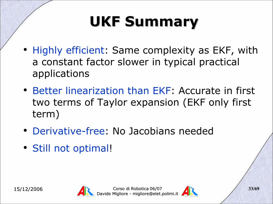
UKF SummaryUKF Summary
● Highly efficient: Same complexity as EKF, with a constant factor slower in typical practical applications
● Better linearization than EKF: Accurate in first two terms of Taylor expansion (EKF only first term)
● Derivative-free: No Jacobians needed
● Still not optimal!
15/12/200615/12/2006 Corso di Robotica 06/07Corso di Robotica 06/07Davide Migliore - [email protected] Migliore - [email protected]
3434/69/69
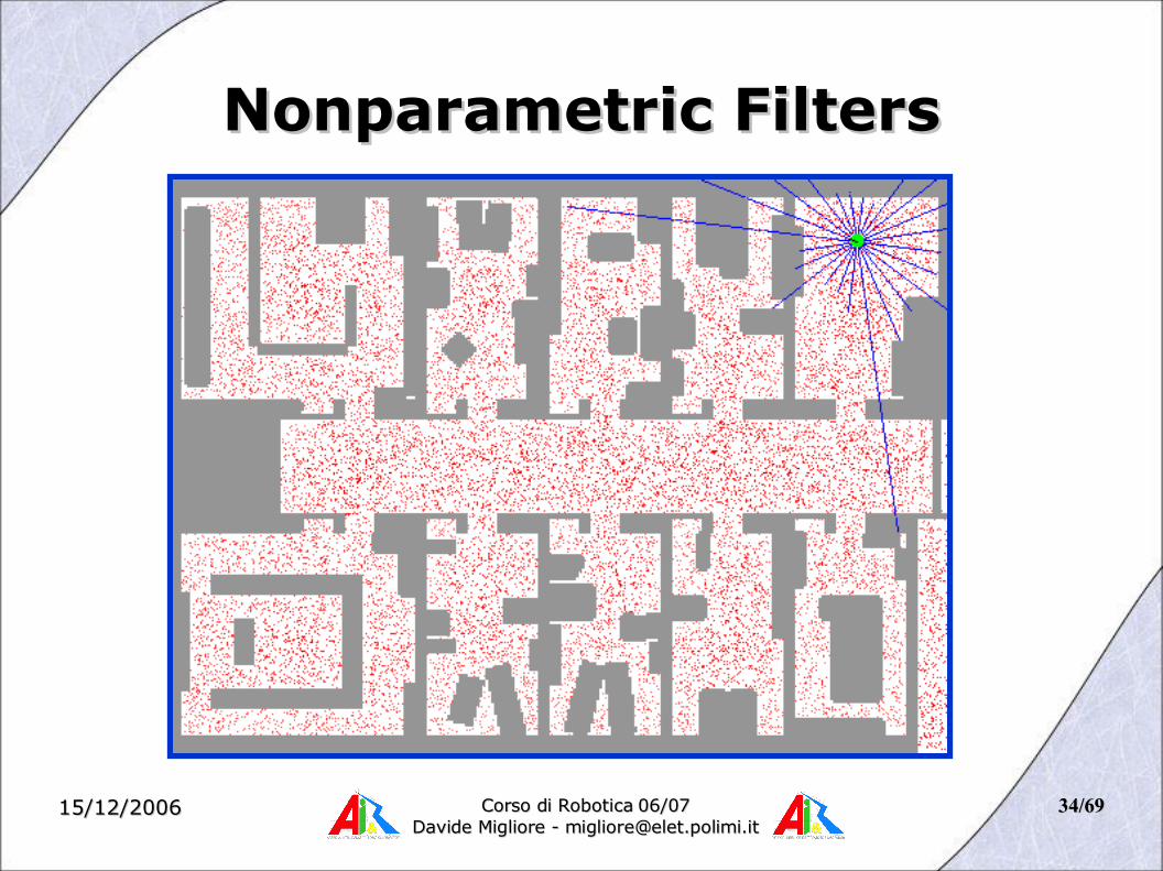
Nonparametric FiltersNonparametric Filters

15/12/200615/12/2006 Corso di Robotica 06/07Corso di Robotica 06/07Davide Migliore - [email protected] Migliore - [email protected]
3535/69/69
Particle FiltersParticle Filters
Represent belief by random samples
Estimation of non-Gaussian, nonlinear processes
Monte Carlo filter, Survival of the fittest, Condensation, Bootstrap filter, Particle filter:
•Filtering: [Rubin, 88], [Gordon et al., 93], [Kitagawa 96]
•Computer vision: [Isard and Blake 96, 98]
•Dynamic Bayesian Networks: [Kanazawa et al., 95]d
15/12/200615/12/2006 Corso di Robotica 06/07Corso di Robotica 06/07Davide Migliore - [email protected] Migliore - [email protected]
3636/69/69
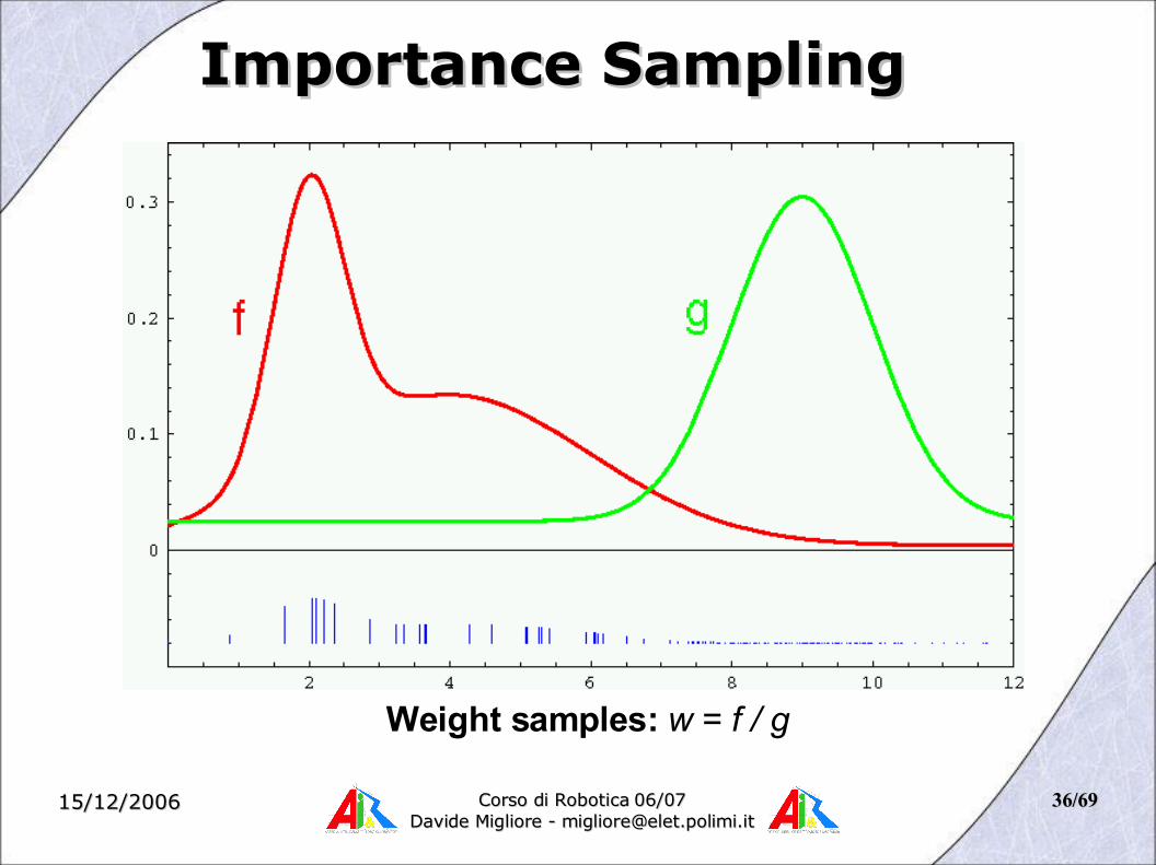
Weight samples: w = f / g
Importance SamplingImportance Sampling
15/12/200615/12/2006 Corso di Robotica 06/07Corso di Robotica 06/07Davide Migliore - [email protected] Migliore - [email protected]
3737/69/69
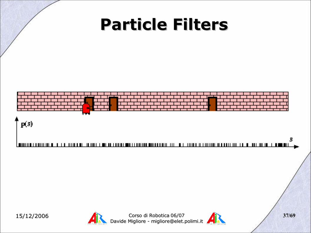
Particle FiltersParticle Filters
15/12/200615/12/2006 Corso di Robotica 06/07Corso di Robotica 06/07Davide Migliore - [email protected] Migliore - [email protected]
3838/69/69
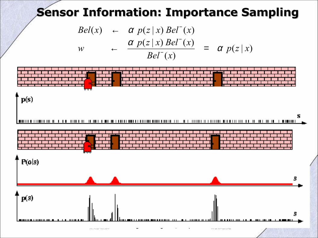
)|()(
)()|()()|()(
xzpxBel
xBelxzpw
xBelxzpxBel
ααα
=←
←
−
−
−
Sensor Information: Importance SamplingSensor Information: Importance Sampling
15/12/200615/12/2006 Corso di Robotica 06/07Corso di Robotica 06/07Davide Migliore - [email protected] Migliore - [email protected]
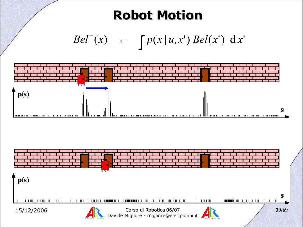
3939/69/69
∫←− 'd)'()'|()( , xxBelxuxpxBel
Robot MotionRobot MotionRobot Motion

15/12/200615/12/2006 Corso di Robotica 06/07Corso di Robotica 06/07Davide Migliore - [email protected] Migliore - [email protected]
4040/69/69
)|()(
)()|()()|()(
xzpxBel
xBelxzpw
xBelxzpxBel
ααα
=←
←
−
−
−
Sensor Information: Importance SamplingSensor Information: Importance Sampling

15/12/200615/12/2006 Corso di Robotica 06/07Corso di Robotica 06/07Davide Migliore - [email protected] Migliore - [email protected]
4141/69/69
Robot MotionRobot Motion
∫←− 'd)'()'|()( , xxBelxuxpxBel
4242/69/69
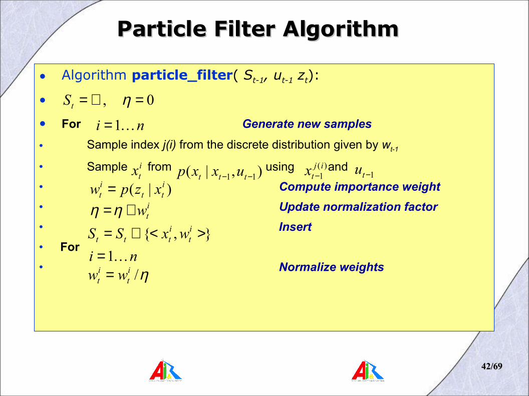
Particle Filter AlgorithmParticle Filter Algorithm
• Algorithm particle_filter( St-1, ut-1 zt):
•
• For Generate new samples
• Sample index j(i) from the discrete distribution given by wt-1
• Sample from using and
• Compute importance weight
• Update normalization factor
• Insert
• For
• Normalize weights
0, =∅= ηtS
ni 1=
},{ ><∪= it
ittt wxSS
itw+=ηη
itx ),|( 11 −− ttt uxxp )(
1ij
tx − 1−tu)|( itt
it xzpw =
ni 1=η/it
it ww =

4343/69/69
draw xit−1 from Bel(xt−1)
draw xit from p(xt | xi
t−1,ut−1)
Importance factor for xit:
)|()(),|(
)(),|()|(ondistributi proposal
ondistributitarget
111
111
tt
tttt
tttttt
it
xzpxBeluxxp
xBeluxxpxzp
w
∝
=
=
−−−
−−−η
1111 )(),|()|()( −−−−∫= tttttttt dxxBeluxxpxzpxBel η
Particle Filter AlgorithmParticle Filter Algorithm
4444/69/69
ResamplingResampling● Given: Set S of weighted samples.
● Wanted : Random sample, where the probability of drawing xi is given by wi.
● Typically done n times with replacement to generate new sample set S’.

4545/69/69
w2
w3
w1wn
Wn-1
ResamplingResampling
w2
w3
w1wn
Wn-1
• Roulette wheel
• Binary search, n log n
• Stochastic universal sampling
• Systematic resampling
• Linear time complexity
• Easy to implement, low variance
4646/69/69
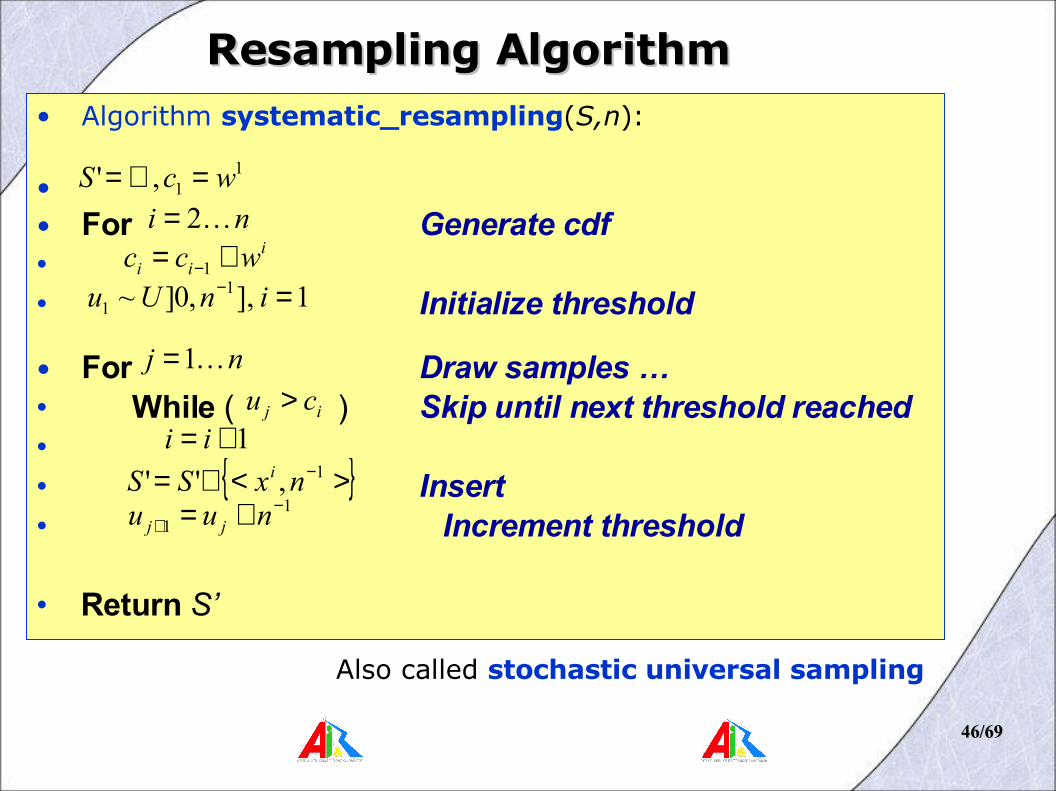
• Algorithm systematic_resampling(S,n):
• • For Generate cdf• • Initialize threshold
• For Draw samples …• While ( ) Skip until next threshold reached• • Insert• Increment threshold
• Return S’
Resampling AlgorithmResampling Algorithm
11,' wcS =∅=
ni 2=i
ii wcc += −1
1],,0]~ 11 =− inUu
nj 1=
11
−+ += nuu jj
ij cu >
{ }><∪= −1,'' nxSS i
1+= ii
Also called stochastic universal sampling

4747/69/69

4848/69/69

4949/69/69
5050/69/69

5151/69/69
5252/69/69

5353/69/69

5454/69/69
5555/69/69
5656/69/69

5757/69/69

5858/69/69

5959/69/69
6060/69/69
6161/69/69

6262/69/69

6363/69/69
6464/69/69

6565/69/69
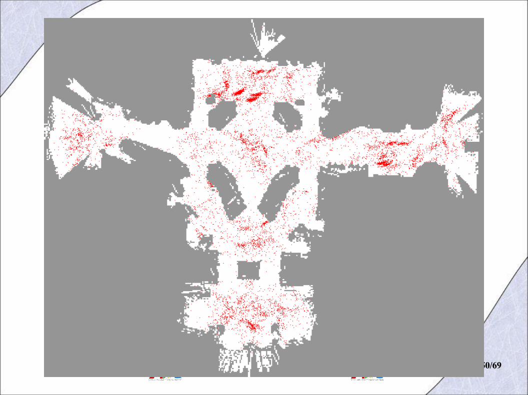
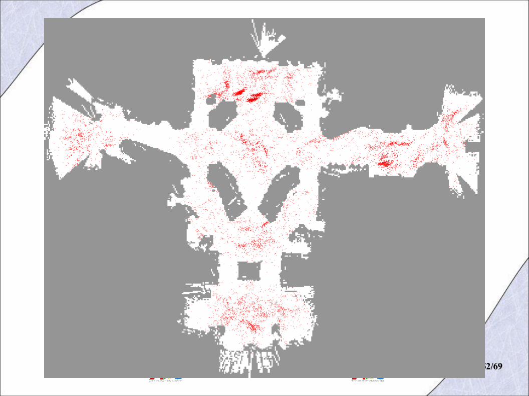
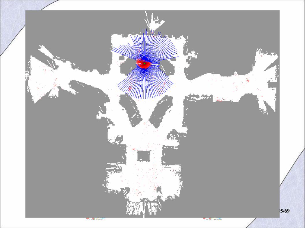
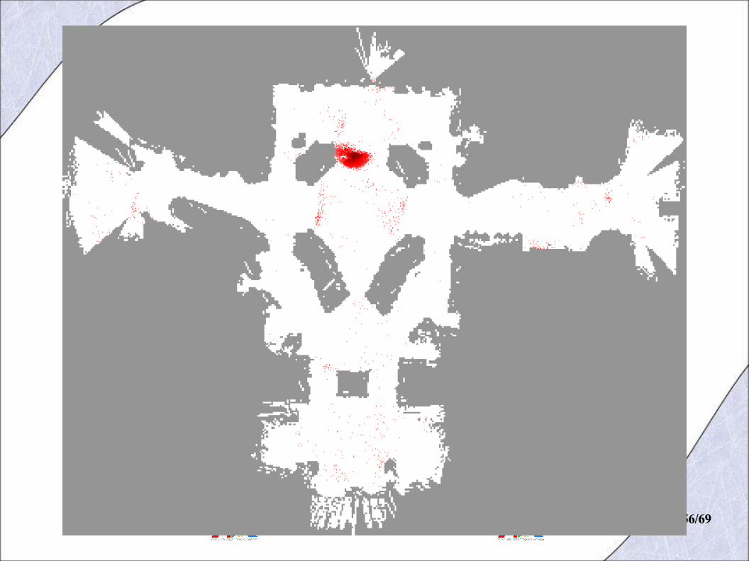
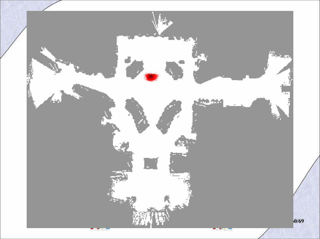
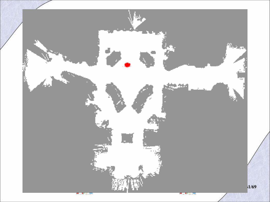
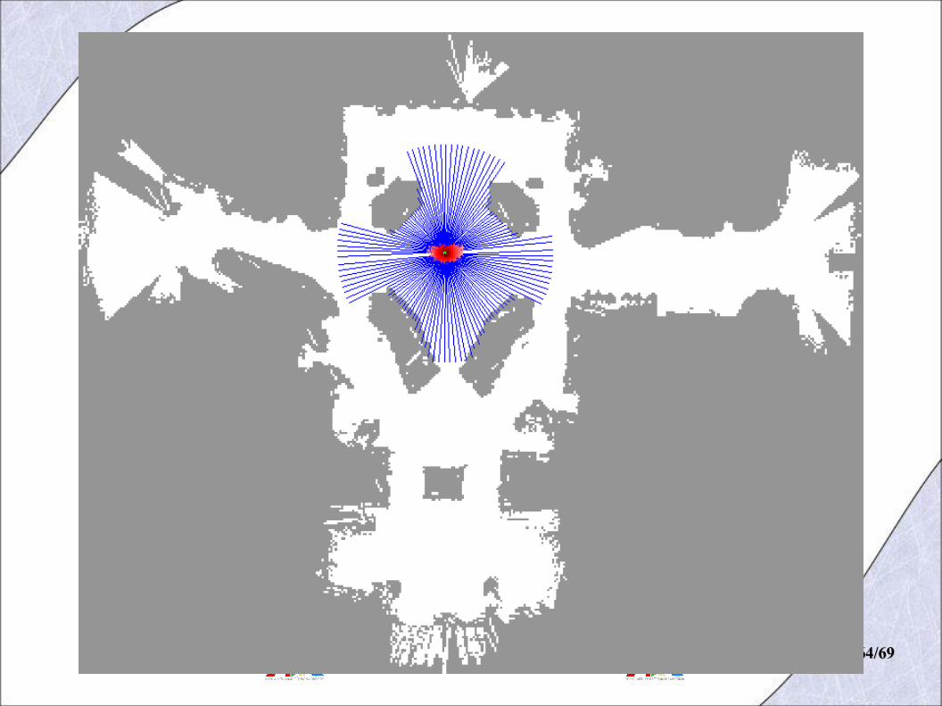
SummarySummary
• Particle filters are an implementation of recursive Bayesian filtering
• They represent the posterior by a set of weighted samples.
• In the context of localization, the particles are propagated according to the motion model.
• They are then weighted according to the likelihood of the observations.
• In a re-sampling step, new particles are drawn with a probability proportional to the likelihood of the observation.
12/10/0612/10/06 Corso di Robotica 06/07Corso di Robotica 06/07Davide Migliore - [email protected] Migliore - [email protected]
6666/69/69
Rao-Blackwellized (FastSLAM)Rao-Blackwellized (FastSLAM)
● Introduced by Montemerlo, Thrun et al. '92● A Monte Carlo sampling inspired approach ● Directly represents the nonlinear process model
and non-Gaussian pose distribution● FastSLAM still linearizes the observation model, but
this is typically a reasonable approximation for range-bearing measurements when the vehicle pose is known.
● High space dimensional state-space of SLAM – Particle filters computationally infeasible
12/10/0612/10/06 Corso di Robotica 06/07Corso di Robotica 06/07Davide Migliore - [email protected] Migliore - [email protected]
6767/69/69
Rao-Blackwellized (FastSLAM)Rao-Blackwellized (FastSLAM)
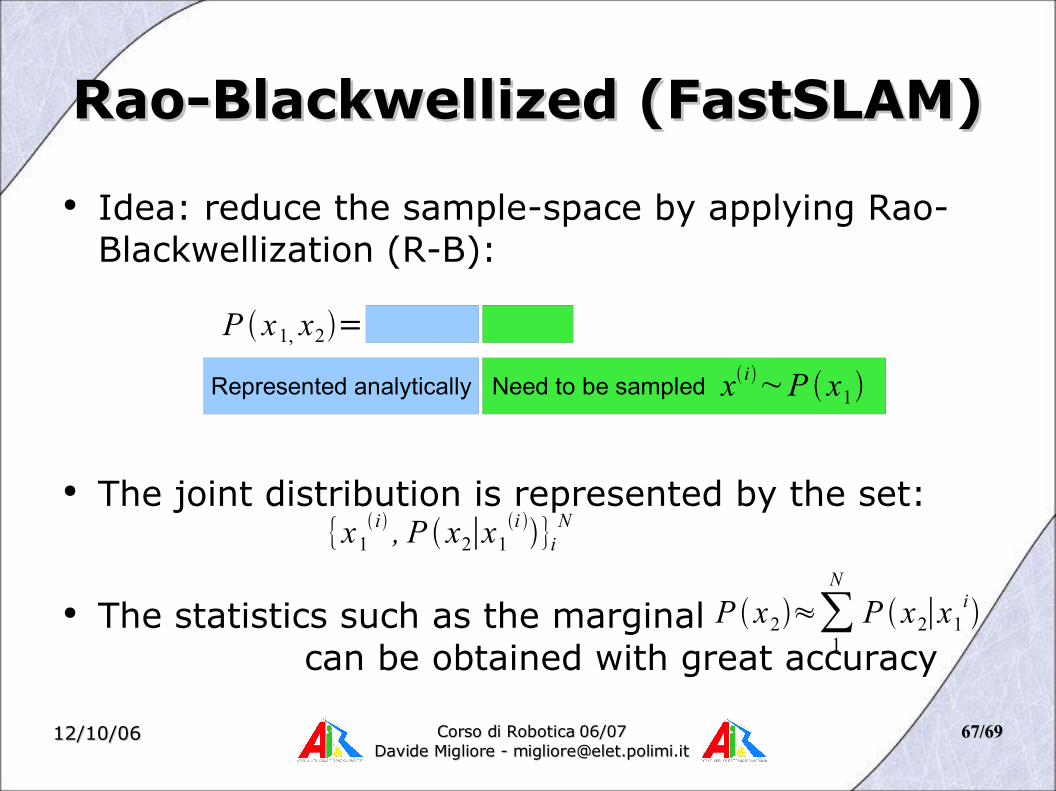
● Idea: reduce the sample-space by applying Rao-Blackwellization (R-B):
● The joint distribution is represented by the set:
● The statistics such as the marginal can be obtained with great accuracy
{x1 i , P x2∣x1
i }iN
P x2≈∑1
N
P x2∣x1i
P x1, x2=P x2∣x1P x1
Represented analytically Need to be sampled x i~P x1

12/10/0612/10/06 Corso di Robotica 06/07Corso di Robotica 06/07Davide Migliore - [email protected] Migliore - [email protected]
6868/69/69
Rao-Blackwellized (FastSLAM)Rao-Blackwellized (FastSLAM)
● The joint SLAM state may be factored into a vehicle component and a conditional map component:
–
P X 0 : k ,m∣X 0 : k ,U 0 : k , x0=P m∣X 0 : k , Z 0 : kP X 0 : k∣Z 0 : k ,U 0 : k , x0
Key property of FastSLAM:When conditioned on the trajectory the map landmarks becomes independent

12/10/0612/10/06 Corso di Robotica 06/07Corso di Robotica 06/07Davide Migliore - [email protected] Migliore - [email protected]
6969/69/69
Rao-Blackwellized (FastSLAM)Rao-Blackwellized (FastSLAM)
● The structure is a Rao-Blackwellized state:– The trajectory is represented by weighted samples
– The map is computed analytically
● The joint distribution (at time k) is represented by the set
And the map is composed by independent Gaussian distribution:
● Recursive estimation performed by particle filter for the pose states and the EKF for the map states
{wki , X 0: k
i , P m∣X 0: k i , Z 0: k }i
N
P m∣X 0 : ki , Z 0 : k =∏
j
M
P m j∣X 0 : k i , Z 0 : k

12/10/0612/10/06 Corso di Robotica 06/07Corso di Robotica 06/07Davide Migliore - [email protected] Migliore - [email protected]
7070/69/69
Particle Filter in FastSLAMParticle Filter in FastSLAM
● Sequential Importance Sampling (SIS) form● Sample from a joint state history “telescoped”
into a recursion via the product rule:
● At each time-step k particle are drawn from a proposal distribution which approximates the true distribution
● The samples are given importance weights to compensate any discrepancy
P x0 , x1 , ... , xT∣Z 0:T =P x0∣Z 0 :T P x1∣x0 , Z 0:T ...P xT∣X 0:T−1 , Z 0 :T
xk∣X 0 : k−1Z 0 :k P x k∣X 0 : k−1 , Z 0:T

12/10/0612/10/06 Corso di Robotica 06/07Corso di Robotica 06/07Davide Migliore - [email protected] Migliore - [email protected]
7171/69/69
Particle Filter in FastSLAMParticle Filter in FastSLAM
● At time k-1 the joint state is represented by
1 For each particle, compute a proposal distribution, conditioned on the specific particle history, and draw a sample from it
2 Weight samples according to the importance function
{wk−1i , X 0 :k−1
i , P m∣X 0 : k−1i , Z 0: k−1}i
N
xk i~ xk∣X 0 : k−1Z 0 : k , uk X 0 :k
i ={X 0 : k−1i , x k
i}
w k i=
P zk∣X 0 : ki , Z 0: k−1P xk
i∣xk−1i ,uk
xki∣X 0: k−1
i , Z 0 : k , uk
P z k∣X 0 : k i , Z 0: k−1=∫ P zk∣xk ,mP m∣X 0: k−1 , Z 0 : k−1dm
12/10/0612/10/06 Corso di Robotica 06/07Corso di Robotica 06/07Davide Migliore - [email protected] Migliore - [email protected]
7272/69/69
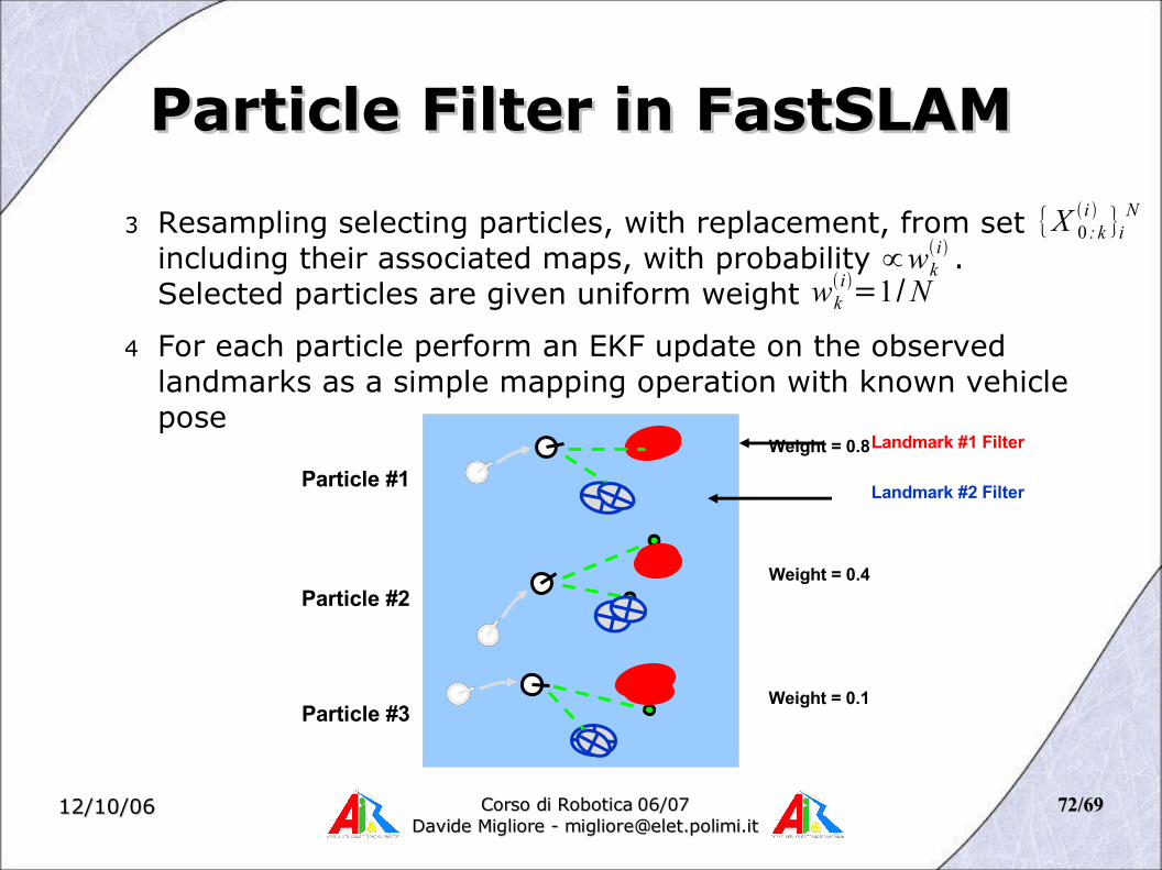
3 Resampling selecting particles, with replacement, from set including their associated maps, with probability . Selected particles are given uniform weight
4 For each particle perform an EKF update on the observed landmarks as a simple mapping operation with known vehicle pose
Particle Filter in FastSLAMParticle Filter in FastSLAM
{X 0 : ki }i
N
∝wk i
wk i=1/N
Particle #1
Particle #2
Particle #3
Landmark #1 Filter
Landmark #2 Filter
Weight = 0.8
Weight = 0.4
Weight = 0.1

12/10/0612/10/06 Corso di Robotica 06/07Corso di Robotica 06/07Davide Migliore - [email protected] Migliore - [email protected]
7373/69/69
FastSLAM 1.0 & 2.0FastSLAM 1.0 & 2.0
● Differ only in term of the form of their proposal distribution (step 1) and their importance weight (step 2)
● FastSLAM 1.0
● FastSLAM 2.0
locally optimal
xk i~P xk∣x k−1
i , uk
w k i=w k−1
i P z k∣X 0: ki , Z 0 :k−1w k
i=w k−1 i P z k∣X 0 : k
i , Z 0 :k−1
xk i~P xk∣X 0 :k
i , Z 0: k ,uk
P x k∣X 0 : k−1i , Z 0: k ,uk =
1CP z k∣x k , X 0 : k−1
i , Z 0 :k−1P xk∣xk−1i , uk
w k i=w k−1
i C

12/10/0612/10/06 Corso di Robotica 06/07Corso di Robotica 06/07Davide Migliore - [email protected] Migliore - [email protected]
7474/69/69
FastSLAM 1.0 & 2.0FastSLAM 1.0 & 2.0
● Statistically FastSLAM suffers degeneration due to its inability to forget past
● Marginalizing the map (step 4) introduces dependence on the pose and measurement history– When resampling depletes this history, statistical
accuracy is lost
● Nevertheless empirical results of FastSLAM 2.0 in real outdoor environments show that the algorithm is capable of generating an accurate map in practice