POLITECNICO DI MILANOSimulink, NI VeriStand e Simulink Desktop Real-Time. Il tipo di test dipende...
139
POLITECNICO DI MILANO Facoltà di Ingegneria Scuola di Ingegneria Industriale e dell’Informazione Dipartimento di Elettronica, Informazione e Bioingegneria Corso di Laurea Magistrale In Ingegneria Elettrica ADVANCED TECHNIQUES FOR HIL SIMULATION OF RENEWABLE ENERGY: THE CASE OF PV SYSTEM Supervisor: Prof. Giambattista Gruosso Master Graduation Thesis by: Harshavardhan Palahalli Mallikarjun Person Code: 10543042 Academic Year: 2017-2018
Transcript of POLITECNICO DI MILANOSimulink, NI VeriStand e Simulink Desktop Real-Time. Il tipo di test dipende...
P O L I T E C N I C O D I M I L A N OFacoltà di Ingegneria
Scuola di Ingegneria Industriale e dell’InformazioneDipartimento di Elettronica, Informazione e Bioingegneria
Corso di Laurea Magistrale In Ingegneria Elettrica
A D VA N C E D T E C H N I Q U E S F O R H I L S I M U L AT I O NO F R E N E WA B L E E N E R G Y: T H E C A S E O F P V S Y S T E M
Supervisor:Prof. Giambattista Gruosso
Master Graduation Thesis by:Harshavardhan Palahalli Mallikarjun
Person Code: 10543042
Academic Year: 2017-2018

Harshavardhan Palahalli MallikarjunCorso di Laurea Magistrale In Ingegneria ElettricaAdvanced Techniques For HIL Simulation of Renewable Energy: TheCase Of PV System

Dedicated toProfessors and all the staff of Politecnico Di Milano

A B S T R A C T
The need of alternative energy is pushing PV to be more pre-dominant to supply energy. Conducting real-time simulationsbefore commissioning the PV plant is much observed to vali-date the project proposals. As PV mathematical model dependson the temperature and the irradiation level of the atmosphere,there is a need of real-time simulation to study the dynamiccharacteristics of PV system.
The idea of this work is to present Real-time simulation frame-work, coupling modeling environments such as Matlab Simulinkto a real-time hardware like National Instruments myRIO. Theidea is to draft an implementation of Hardware-in-the-loop sim-ulation for renewable energy systems by taking a case of PVincluding control strategy and interaction with the rest of thesystem like micro-grid. They have to cope with different con-straints, the former is the solution of the differential algebraicequation (DAE) system required by the PV which is stronglynon-linear. The latter is the fast simulation of the dynamic con-trol strategy of PV such as Maximum power point tracking al-gorithm and the micro-grid with frequency regulation. In themiddle several other requirements, including Hardware-in-theloop simulation having interface algorithm of the models overEthernet and actual measurement is discussed.
This work proposes two kinds of test bench using tools likeSimulink, NI VeriStand and Simulink Desktop Real-Time. Thechoice of kind of simulation depends on the complexity of themodel that has to be simulated in real-time. The test benches 1
and 2 uses Simulink, for the model design and C code genera-tion for execution in myRIO hardware. Co-Simulation platformis presented in the case of test bench 3, where the model isdesigned in Simulink and they are compiled to execute in In-tel’s processor of the desktop, and the PV model built usingLabVIEW VI is made to run as standalone system in myRIO,later both the systems are synchronized through Ethernet forthe execution in real-time.
This thesis contains 11 Chapters, in which all the phenomenaof Hardware-in-the-loop simulation in the case of PV, havingdifferent interface algorithms are being presented.
v

E S T R AT O
La necessità di introdurre energia alternativa, nel nostro studioè l’introduzione del sistema fotovoltaico(PV) per fornire ener-gia al sistema elettrico. Prima di poter realizzare fisicamenteil sistema fotovoltaico dobbiamo simularlo in modo da poterprevedere e capire il comportamento del sistema il modellomatematico del sistema fotovoltaico dipende dalla temperaturae dal livello di irraggiamento dell’atmosfera, inoltre dobbiamostudiare la caratteristica dinamica del sistema fotovoltaico at-traverso la simulazione in tempo reale (real-time-simulation).
In questo lavoro proponiamo l’uso di Real-time simulationframework usando Matlab Simulink per la modellizzazione deicomponenti della rete e National Instruments myRIO per real-time hardware. L’idea è di implementare una bozza di Hardware-in-loop simulation per i sistemi di energia rinnovabile, pren-dendo come caso il sistema fotovoltaico con il suo corrispettivosistema di controllo e l’interazione che il PV ha con la micro-grid.
Per realizzare la modellizzazione del PV dobbiamo gestire iseguenti vincoli:
1. Risoluzione della equazione differenziale del sistema richi-esta dal PV, la quale è una equazione non lineare.
2. Realizzazione di Hardware-in-loop-simulation collegandoi modelli precedentemente citati attraverso il cavo ether-net e le misure attuali .
3. Realizzazione della simulazione delle dinamiche di con-trollo del PV attraverso l’algoritmo del Maximum pointtracking e la regolazione in frequenza della micro-gird.
Questo lavoro propone due tipi di test usando strumenti comeSimulink, NI VeriStand e Simulink Desktop Real-Time. Il tipodi test dipende dalla complessità del modello che vogliamo sim-ulare in real-time, inoltre in questo lavoro abbiamo fatto tre test.Sia il test 1 che il test 2 usano Simulink, per modellizzazione eil codice C è generato per essere eseguito in myRIO hardware.Il test 3 utilizza la piattaforma di Co-simulation, dove il mod-ello è disegnato in Simulink ed è compilato per essere eseguitoda Intel’s processor del Desktop, mentre il modello del sistema
vii

fotovoltaico è costruito utilizzando LabVIEW VI ed è stato fattoeseguire come sistema autonomo in myRIO, dopo di che i sis-temi vengono sincronizzati grazie all’ethernet per eseguirlo inreal-time.
Questa tesi contiene 11 capitoli, nei quali tutti i fenomenidi Hardware-in-the-loop simulation nel caso del sistema foto-voltaico, avendo diverse interfacce.
viii

A C K N O W L E D G E M E N T S
I would like to tribute my deepest gratitude to the following in-dividuals, for helping me in the development of the this work.
To Professor Giambattista Gruosso, for providing me an oppor-tunity to work under his supervision, for the development ofthis thesis and also for introducing me to the field of research.His guidance and ideas intrigue me to work on this topic andto gain more knowledge in the subject matter of interest.
To Yujia Huo, Phd Student of Politecnico Di Milano who helpedme to solve the complex modeling problems and also for pro-viding the key insights, during the development of this workand the research paper.
To Bhavya Ponna, for helping me to solve the errors encoun-tered while typesetting this document.
To Srikanth Kadiga and Mahanta Raju Penmatsa, my fellowbatch mates who provided me all kind of support, when I wasin need of it.
To Repubblica italiana, for allowing me to study in it’s pres-tigious institution with scholarship and for providing all thebasic needs to nurture my career.
To my parents, for their support from long distances whom Iowe all of my achievements to.
ix

C O N T E N T S
1 introduction 1
1.1 Motivation . . . . . . . . . . . . . . . . . . . . . . . 1
1.2 Need of Real-time PV simulations . . . . . . . . . 2
1.3 Problem Formulation . . . . . . . . . . . . . . . . . 3
1.4 Research Objectives . . . . . . . . . . . . . . . . . . 3
1.5 Thesis Outline . . . . . . . . . . . . . . . . . . . . . 4
i theoretical aspects of hil 5
2 hardware-in-the-loop for power electrical
systems 7
2.1 Simulation . . . . . . . . . . . . . . . . . . . . . . . 7
2.1.1 Real-time Simulation . . . . . . . . . . . . . 8
2.2 Hardware-in-the-loop . . . . . . . . . . . . . . . . . 12
2.2.1 Different HIL methodologies for Electricdrive system . . . . . . . . . . . . . . . . . . 16
2.3 Power-hardware-in-the-loop . . . . . . . . . . . . . 22
2.3.1 Basic architecture of P-HIL simulation . . . 23
2.3.2 Real-time digital simulator and Interfacein P-HIL simulation . . . . . . . . . . . . . 24
2.3.3 Interface Algorithm . . . . . . . . . . . . . . 27
2.3.4 Pros and Cons of Interface Algorithms . . 32
2.3.5 Open issues in P-HIL simulation . . . . . . 32
2.3.6 Accuracy issue of P-HIL . . . . . . . . . . . 36
2.3.7 Procedure to conduct P-HIL simulation . . 37
ii application of p-hil in renewable energy
simulation 39
3 proposed real-time simulation architecture 41
3.1 Real-time Digital Simulator . . . . . . . . . . . . . 41
3.1.1 NI VeriStand . . . . . . . . . . . . . . . . . . 42
3.1.2 FPGA target . . . . . . . . . . . . . . . . . . 44
3.2 Interface algorithm using actual Measurement sys-tem . . . . . . . . . . . . . . . . . . . . . . . . . . . 45
4 modeling of pv and other systems under study 49
4.0.1 Solar cell characteristics . . . . . . . . . . . 49
4.0.2 Mathematical Modeling of PV in MATLAB-Simulink . . . . . . . . . . . . . . . . . . . . 52
4.1 MPPT System . . . . . . . . . . . . . . . . . . . . . 55
4.1.1 Perturbation and Observation Technique . 57
xi
xii contents
4.1.2 Boost Converter . . . . . . . . . . . . . . . . 58
4.1.3 Storage System . . . . . . . . . . . . . . . . 59
5 real-time simulation and results of pv us-ing fpga 61
5.1 Test-bench 1: PV and MPPT with the fixed Resis-tive load . . . . . . . . . . . . . . . . . . . . . . . . 61
5.2 Test-bench 2: PV with storage connected to DC Bus 66
5.2.1 Experiment . . . . . . . . . . . . . . . . . . 66
iii pv and micro-grid hil co-simulation hav-ing interface algorithm over ethernet 71
6 ethernet protocol for rt simulations 73
6.1 Need of interface algorithm over Ethernet . . . . . 73
6.2 Characteristics of the Real-time Ethernet . . . . . . 75
6.2.1 Real-time response . . . . . . . . . . . . . . 75
6.2.2 Synchronization . . . . . . . . . . . . . . . . 75
6.3 Real-time UDP Communication Protocol . . . . . 75
6.3.1 User Datagram Header format . . . . . . . 76
7 architecture of co-simulation platform 79
7.1 Real-time Digital Simulator . . . . . . . . . . . . . 79
7.1.1 Simulink Desktop Real-Time . . . . . . . . 79
7.2 LabVIEW RIO architecture . . . . . . . . . . . . . . 81
7.2.1 Architecture of the proposed test-bench . . 82
7.2.2 Model simulated in the test-bench . . . . . 83
7.3 Modeling of micro Grid and VSC converter . . . . 83
7.3.1 Non Linear model of hydraulic turbine sys-tem . . . . . . . . . . . . . . . . . . . . . . . 85
7.3.2 Governor system of Turbine . . . . . . . . . 88
7.3.3 Synchronous Machine . . . . . . . . . . . . 89
7.3.4 Turbine and generator relationship . . . . . 92
7.3.5 Excitation system model of synchronousgenerator . . . . . . . . . . . . . . . . . . . . 93
7.3.6 Control of 3φ Voltage Source Converter . . 95
8 pv and micro-grid hil co-simulation and re-sults 99
8.1 Real-time co-simulation test-bench . . . . . . . . . 99
8.2 Experiment and Results . . . . . . . . . . . . . . . 101
9 conclusion 107
9.1 Contributions to the Engineering Community . . 107
9.2 Recommendations and Future Research . . . . . . 108
10 appendix a 111
10.1 How to Create Custom FPGA bit file . . . . . . . . 111

contents xiii
10.1.1 Making a copy of the sample FPGA VIand project . . . . . . . . . . . . . . . . . . . 111
10.1.2 Customizing the FPGA VI . . . . . . . . . . 112
10.1.3 Compiling the Custom FPGA VI into aBitfile . . . . . . . . . . . . . . . . . . . . . . 113
11 appendix b 115
11.1 SLDRT Kernel Installation . . . . . . . . . . . . . . 115
11.2 Configuring Model . . . . . . . . . . . . . . . . . . 115
11.3 Code generation Parameters . . . . . . . . . . . . . 116
11.4 Signal logging to Workspace . . . . . . . . . . . . . 116
bibliography 117
L I S T O F F I G U R E S
Figure 1 Categories of Simulation based on the speedof execution . . . . . . . . . . . . . . . . . 8
Figure 2 Execution of steps in real-time and in nonreal-time simulation . . . . . . . . . . . . . 9
Figure 3 Simulation category according to the in-teraction among different modules un-der study . . . . . . . . . . . . . . . . . . . 10
Figure 4 Components of Hardware-in-the-loop sim-ulation . . . . . . . . . . . . . . . . . . . . . 13
Figure 5 Architecture of C-HIL simulation . . . . . 14
Figure 6 Architecture of P-HIL simulation . . . . . 15
Figure 7 Electrical drive framework . . . . . . . . . 16
Figure 8 DC Drive having a vehicle wheel as amechanical load . . . . . . . . . . . . . . . 17
Figure 9 Signal level HIL Simulation block diagram 19
Figure 10 Signal level HIL Simulation of DC drive . 19
Figure 11 Power level HIL Simulation block diagram 20
Figure 12 Power level HIL Simulation of Electricaldrive . . . . . . . . . . . . . . . . . . . . . . 20
Figure 13 Mechanical level HIL Simulation blockdiagram . . . . . . . . . . . . . . . . . . . . 21
Figure 14 Mechanical level HIL Simulation of Elec-trical drive . . . . . . . . . . . . . . . . . . 22
Figure 15 Voltage divider circuit . . . . . . . . . . . . 23
Figure 16 Architecture of P-HIL simulation consid-ering a voltage divider circuit . . . . . . . 24
Figure 17 P-HIL simulation interface done by cur-rent amplification . . . . . . . . . . . . . . 28
Figure 18 Ideal-transformer model method of in-terface algorithm . . . . . . . . . . . . . . 29
Figure 19 Scheme of TLM interface algorithm . . . . 29
Figure 20 TLM interface algorithm . . . . . . . . . . 30
Figure 21 PCD interface algorithm . . . . . . . . . . 31
Figure 22 DIM interface algorithm . . . . . . . . . . 31
Figure 23 Interface of Voltage divider circuit for sta-bility studies . . . . . . . . . . . . . . . . . 35
Figure 24 Architecture of VeriStand Engine deployedin RT Target . . . . . . . . . . . . . . . . . 43
xiv

List of Figures xv
Figure 25 VeriStand interface between PC and theRT Target . . . . . . . . . . . . . . . . . . . 44
Figure 26 Sequential procedure that is followed inReal-time execution . . . . . . . . . . . . . 45
Figure 27 Analog input ports of myRIO with ADC . 46
Figure 28 Solar cell equivalent electric circuit . . . . 49
Figure 29 Equivalent PV cell circuit used for mod-eling . . . . . . . . . . . . . . . . . . . . . . 52
Figure 30 Simulink model of the PV cell . . . . . . . 53
Figure 31 Current Characteristics of modeled PVmodule . . . . . . . . . . . . . . . . . . . . 54
Figure 32 Power of modeled PV array for differentirradiation and @ constant temperatureof 298.15K . . . . . . . . . . . . . . . . . . . 54
Figure 33 Power of modeled PV array for differenttemperature and constant irradiation . . . 55
Figure 34 PV with MPPT system connecting to load 56
Figure 35 Perturbation and Observation Techniqueflowchart . . . . . . . . . . . . . . . . . . . 58
Figure 36 Schematic diagram of Boost Converter . . 59
Figure 37 Generic battery model . . . . . . . . . . . 59
Figure 38 PV with MPPT system in myRIO . . . . . 61
Figure 39 Input and output voltage of the boost con-verter for change in irradiation from 1000W/m2
to 800W/m2 at 0.5s . . . . . . . . . . . . . 62
Figure 40 PV system model compiled for RT simu-lation . . . . . . . . . . . . . . . . . . . . . 63
Figure 41 Simulink model to be compiled for RTsimulation . . . . . . . . . . . . . . . . . . 64
Figure 42 Input and output Voltage of the boostconverter in RT Simulation for change inirradiation from 1000W/m2 to 800W/m2
at 0.5s . . . . . . . . . . . . . . . . . . . . . 64
Figure 43 Maximum Power tracked in real-time withthe output voltage maintained by MPPTsystem across the PV array terminals . . . 65
Figure 44 Simulation results comparison . . . . . . . 65
Figure 45 Block diagram of the test bench created . 66
Figure 46 Test-bench used for HIL simulation . . . . 67
Figure 47 Irradiation and temperature measured inreal-time . . . . . . . . . . . . . . . . . . . 68
Figure 48 Voltage measured across DC bus in real-time . . . . . . . . . . . . . . . . . . . . . . 68
xvi List of Figures
Figure 49 Voltage measured across DC bus usingoscilloscope . . . . . . . . . . . . . . . . . . 69
Figure 50 Power delivered by PV and consumed byload . . . . . . . . . . . . . . . . . . . . . . 69
Figure 51 SOC and the battery current . . . . . . . . 70
Figure 52 Battery terminal voltage . . . . . . . . . . 70
Figure 53 UDP Header format . . . . . . . . . . . . . 77
Figure 54 UDP Pseudo header format . . . . . . . . 77
Figure 55 Simulink desktop Real-time architecture . 81
Figure 56 LabVIEW RIO Architecture . . . . . . . . 81
Figure 57 Co-Simulation architecture used for HILsimulation . . . . . . . . . . . . . . . . . . 82
Figure 58 Block diagram of the simulated model . . 83
Figure 59 Block diagram of Hydroelectric power plantsystem . . . . . . . . . . . . . . . . . . . . . 85
Figure 60 Block diagram of Hydraulic turbine system 88
Figure 61 Block diagram of Hydraulic turbine gov-ernor . . . . . . . . . . . . . . . . . . . . . . 89
Figure 62 Block diagram of DC Exciter type 1 . . . . 94
Figure 63 Block diagram of Control of VSC . . . . . 97
Figure 64 Test-bench created for co-simulation . . . 99
Figure 65 LabVIEW VI for UDP transmission andreception in myRIO . . . . . . . . . . . . . 100
Figure 66 MATLAB-Simulink model compiled foruse in SLDRT . . . . . . . . . . . . . . . . . 101
Figure 67 Power delivered by PV system in boththe simulations . . . . . . . . . . . . . . . . 102
Figure 68 Power of PV system at 18th s . . . . . . . . 103
Figure 69 Frequency of the grid in per unit . . . . . 104
Figure 70 Voltage at PCC in per unit . . . . . . . . . 105
Figure 71 Power delivered by Synchronous gener-ator to grid . . . . . . . . . . . . . . . . . . 105
Figure 72 Reactive power delivered by PV systemto grid . . . . . . . . . . . . . . . . . . . . . 106

L I S T O F TA B L E S
Table 1 Pros and Cons of Interface algorithm . . . 34
Table 2 Available communication protocols . . . . 74
Table 3 Excitation System . . . . . . . . . . . . . . 97
Table 4 Parameters of Synchronous Machine . . . 98
Table 5 Mechanical Driving System . . . . . . . . 98
xvii
A C R O N Y M S
ADC Analog To Digital Converter
C-HIL Controller Hardware In The Loop
DAC Digital To Analog Converter
etc Et Cetera
FIFO First In First Out
FPGA Filed Programmable Gate Array
GUI Graphical User Interface
HIL Hardware In The Loop
HUT Hardware Under Test
HMI Human Machine Interface
MPPT Maximum Power Point Tracking
P-HIL Power Hardware In The Loop
PCC Point of Common Connection
RIO Re-configurable Input Output
ROS Rest of The System
RT Real-time
RTDS Real-time Digital Simulator
SG Synchronous Generator
SLDRT Simulink Desktop Real-Time
SOC State of The Charge
UDP Unigram Data Protocol
VSC Voltage Source Converter
VSS Virtually Simulated System
V2G Vehicle To Grid
xviii
1I N T R O D U C T I O N
In this chapter I have taken an opportunity to convey my ideasand motivation for thesis work being done on Hardware In theLoop (HIL) simulation studies of renewable energy, by takingcase of photovoltaic (PV) system, to demonstrate the platformand to solve the problems of simulating complex mathematicalmodels in real-time.
1.1 motivation
Entire human population of this era, is in the quest of ’Se-cure, Clean and Efficient Energy’. It is one of the big societalchallenge that is being addressed by most of the world orga-nizations and the governments. To name one, Horizon 2020 isthe biggest EU Research and Innovation programme ever withnearly €80 billion of funding available over 7 years (2014 to2020) [1], in which the above mentioned problem of energy isone of the societal challenge addressed through this project byEuropean Union.
Increase in energy demand, the constraint of the present in-frastructure to fully exploit the conventional energy source andalso environmental concern has made us look at PV cell to har-ness solar energy.
A PV system is mainly used for,
1. Bulk production of electrical energy to meet the existingenergy demand as an alternative supply.
2. Satellites, space crafts and in other aero-space applica-tions to harness solar energy in space.
3. Electric vehicles as an hybrid configuration, but not sopopular and useful.
A great number of research work is being conducted to bringdown PV unit cost and to increase the efficiency of the PV mod-ules. As a result, today we are able to get upto 27% efficientsolar cells [43] which are remarkable.
1
2 introduction
PV delivers lot of energy in the afternoon, while the peakenergy demand is in the morning and evening, hence storagesystem is very important. But the storage system takes much ofthe investment and requires maintenance [17]. Instead of hav-ing PV on top of electric vehicles, batteries designed for electricvehicles are used for storing excess energy from the grid, and itis exchanged back when it’s in need. This technology is calledas Vehicle to grid (V2G) [20], a ground breaking concept that isin much of interest by the research community.
These upcoming technologies are very promising for mankindto live in a sustainable world. Simulation studies of PV for gridinteraction, storage and V2G brings faster implementation oftechnology from paper to people. As many of the countries areproposing solar power projects, especially developing countrieslike China and India, a low cost platform to conduct these stud-ies are much appreciated.
1.2 need of real-time pv simulations
As penetration of PV generation increases, it’s impact on stabil-ity and and security of the power system will become more andmore significant, due to the characteristic of randomness andvolatility [31]. Modeling and simulation are the basic technolo-gies to study the impact for the power grid in which, large-scalePV generation systems are integrated.
Simulations in usual platform may give good results but theyare not able to deliver results for dynamic change in input aspresent in real-world in run-time, the model may not respondfor such a change. When we try to simulate to know the longterm performance of a system, the normal simulation requires avery long time to deliver results and the accuracy of the resultsmay also get compromised. Hence it is necessary to conductreal-time simulation with the models that can respond for fasterinput dynamics [32].
The power generation capability of the PV depends on theever-changing environmental conditions like temperature andsolar irradiation, hence real-time simulation of PV system to-gether with its controller is recommended to validate the con-trol aspects and also to study the behavioral aspects of the sys-tem under different circumstances resulting from external orinternal dynamic influence.
’Hardware In the Loop’ is the state of the art simulation thatprovides the solution for the above requirement, where a sys-
1.3 problem formulation 3
tem behaviour is emulated in a hardware and tested in real-time according to the requirement.
1.3 problem formulation
While simulating the complex model like PV system interactionwith the grid in real-time, we may encounter many problems.The important ones to mention are,
1. The need of a PV mathematical model that can deliverresults faster to keep the real-time simulation propertiesduring execution. Solving the algebraic loop in the PVmodel is an important task as algebraic loops are not sup-ported in the real-time hardwares.
2. There is a need of cost-effective test bench/platform forsimulating PV systems in real-time that can be used forcontrol validation, studies of storage system and integra-tion of PV system to the power drive train or grid.
3. Model based design of process and systems are very pop-ular, there are tools available for automatic code genera-tion for the developed model, it’s required to use thesetools, that can deliver C code from the model, which canbe used for cost effective target hardwares.
4. The memory of the real-time digital Simulator (RTDS) isa main constraint while simulating a complex model likegrid, this memory is used for storing and executing thecomplied C code in real-time. It may be necessary to splitthe model into two or more separate systems and bridgethem using an appropriate interface.
5. Interfacing the two models using respective interfacing al-gorithm introduces some errors in the execution, that re-sults in, instability of the system during run time and alsoaccuracy of the results varies according to the interfacingalgorithm used.
1.4 research objectives
As explained earlier the main objective of this work is to pro-pose the low-cost real-time simulation platforms, that can be
4 introduction
used for real-time simulations, incorporating HIL testing method-ologies using hardware. The following objectives are framed tomeet in this research work.
1. To create a Mathematical model of PV system that can beused for real-time simulation, which has faster convergingbehaviour that keeps the execution in real-time.
2. To create a test bench for validating the control or theprocess validation of the PV system.
3. To use the real world data in run-time of the simulation.
4. To create a co-simulation platform for emulating PV ina hardware and complex model like grid as rest of thesystem in the Simulink Desktop real-time.
1.5 thesis outline
The thesis is being divided into three parts, Part I containsChapter 2, which presents the detailed study of HIL simula-tion by presenting examples and case studies. The need andtypes of interface algorithms are studied. Also about maintain-ing stability and accuracy during the execution in run-time arediscussed.
Part II contains three Chapters, in Chapter 3 the proposedarchitecture for real-time simulation using VeriStand as real-time digital simulator and myRIO as hardware is presented.Chapter 4 presents the detailed modelling of PV, MPPT, DC-DCConverter, etc. Later in Chapter 5 the results of HIL real-timesimulation is illustrated with the test bench created.
Part III has four chapters, in Chapter 6 the Ethernet pro-tocol that are being used for data communications are men-tioned and detailed explanation is given on UDP protocol, inChapter 7 the architecture of proposed test bench for HIL co-simulation having interface algorithm over Ethernet is beingpresented. The Chapter 8 deals with the created test-bench andthe execution of real-time experiment along with the discussionof results. Finally the conclusion of this work is drawn in Chap-ter 9.
Part I
T H E O R E T I C A L A S P E C T S O F H I L
In this part the detailed study of Hardware-in-the-loop simulation is presented. It is very essential tounderstand the basic ideology of this type of simu-lation methods for the development of the PV testbench for different test case scenarios. The majorproblem in executing HIL simulation is, having thesystem states stable throughout the simulation andalso to maintain accuracy without affecting the char-acteristics of the emulated system. In my case theemulated system is PV array whose characteristicsdepends on the series and parallel resistances, whichcan be affected by introducing the interfacing algo-rithm of HIL simulation. The key points that has tobe understood for successful execution of HIL simu-lation is given in this part.

2H A R D WA R E - I N - T H E - L O O P F O R P O W E RE L E C T R I C A L S Y S T E M S
This chapter will light on the facts of simulation, its categoriesand need of different kind of simulation techniques. It alsonarrates, state of the art real-time simulation, Hardware-in-the-loop, Power-hardware-in-the-loop, their methods and issues. Mymain goal in this work is,
1. To present a real-time simulation framework coupling mod-elling environment such as MATLAB Simulink to a real-time hardware, in this work National Instruments myRIOis chosen as the real-time hardware which is being ex-plained in the later section.
2. To conduct Co-simulation in real-time, incorporating Hard-ware in the Loop simulation strategy for simulating PVsystem and grid whose mathematical models are inter-faced through Ethernet.
HIL is widely used for testing in automotive industries, ma-rine and aerospace applications etc., but nowadays it is gain-ing much popularity in real-time testing in Electrical powerdomain, especially in renewable energy planning, testing andcommissioning. Though HIL has much benefits, it is still aemerging topic in the field of research, hence the detailed studyof HIL simulation is given in this chapter.
2.1 simulation
The development of many products and the process is charac-terized by the integration with digital control systems. The in-tegration is performed by the hardware and the software com-ponents. Because of the expanding multifaceted nature and themutual relationship between the design of the process and con-trol system, computer aided techniques for modeling, simula-tion and furthermore the design methods are required. Thereare many tools available in the market to address these needs.
Thus, a faster way to validate research proposals pertainingto the above-mentioned characteristics is by adopting simula-
7
8 hardware-in-the-loop for power electrical systems
tion techniques. With respect to the required speed of the com-putation, the simulation can be grouped into three categories[19].
1. Simulation without time limitation
2. Real-time Simulation
3. Simulation faster than real-time
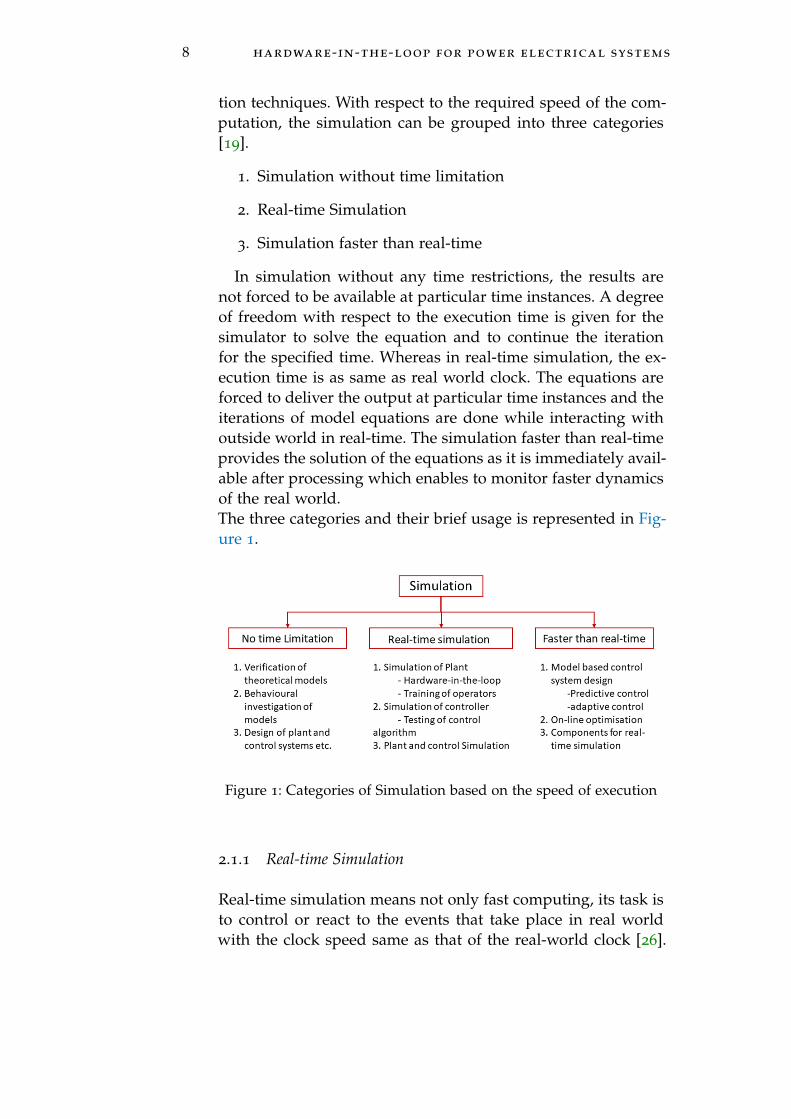
In simulation without any time restrictions, the results arenot forced to be available at particular time instances. A degreeof freedom with respect to the execution time is given for thesimulator to solve the equation and to continue the iterationfor the specified time. Whereas in real-time simulation, the ex-ecution time is as same as real world clock. The equations areforced to deliver the output at particular time instances and theiterations of model equations are done while interacting withoutside world in real-time. The simulation faster than real-timeprovides the solution of the equations as it is immediately avail-able after processing which enables to monitor faster dynamicsof the real world.The three categories and their brief usage is represented in Fig-ure 1.
Figure 1: Categories of Simulation based on the speed of execution
2.1.1 Real-time Simulation
Real-time simulation means not only fast computing, its task isto control or react to the events that take place in real worldwith the clock speed same as that of the real-world clock [26].
2.1 simulation 9
Digital real-time simulation (DRTS) of the electric power sys-tem is the reproduction of voltage or current waveforms withthe desired accuracy, that are representative of the behavior ofthe real power system being modeled.
To achieve such a goal, a digital real-time simulator needs tosolve the model equations for one time-step within the sametime in real-world clock [15]. Therefore, it produces outputs atdiscrete time intervals, where the system states are computedat certain discrete times using a fixed time-step.
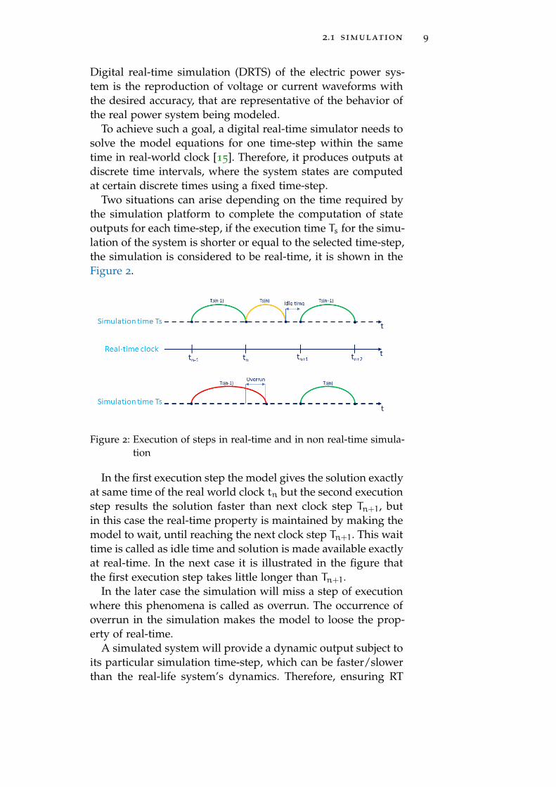
Two situations can arise depending on the time required bythe simulation platform to complete the computation of stateoutputs for each time-step, if the execution time Ts for the simu-lation of the system is shorter or equal to the selected time-step,the simulation is considered to be real-time, it is shown in theFigure 2.
Figure 2: Execution of steps in real-time and in non real-time simula-tion
In the first execution step the model gives the solution exactlyat same time of the real world clock tn but the second executionstep results the solution faster than next clock step Tn+1, butin this case the real-time property is maintained by making themodel to wait, until reaching the next clock step Tn+1. This waittime is called as idle time and solution is made available exactlyat real-time. In the next case it is illustrated in the figure thatthe first execution step takes little longer than Tn+1.
In the later case the simulation will miss a step of executionwhere this phenomena is called as overrun. The occurrence ofoverrun in the simulation makes the model to loose the prop-erty of real-time.
A simulated system will provide a dynamic output subject toits particular simulation time-step, which can be faster/slowerthan the real-life system’s dynamics. Therefore, ensuring RT
10 hardware-in-the-loop for power electrical systems
is not a matter of accelerating or slowing the simulation, butproviding valid outputs at precise (reality-consistent) instants.Having an early or a delayed result makes the simulation failas it no longer captures the real dynamics of the system.
2.1.1.1 On-line and Off-line Simulation
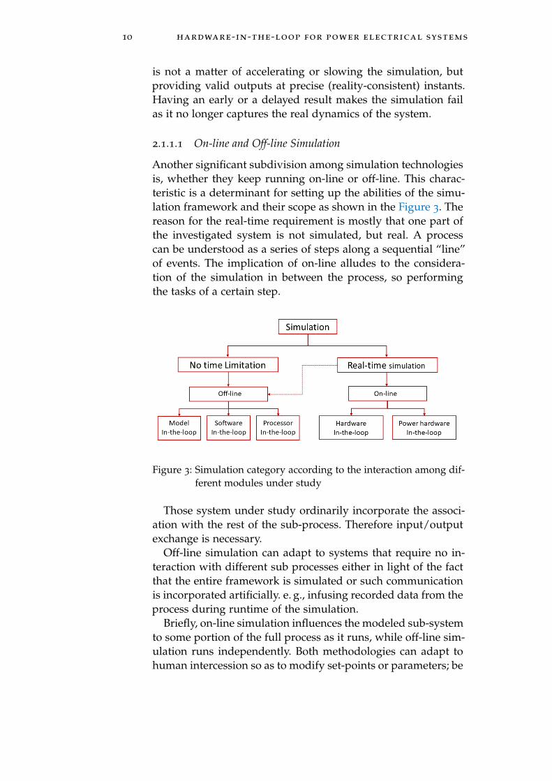
Another significant subdivision among simulation technologiesis, whether they keep running on-line or off-line. This charac-teristic is a determinant for setting up the abilities of the simu-lation framework and their scope as shown in the Figure 3. Thereason for the real-time requirement is mostly that one part ofthe investigated system is not simulated, but real. A processcan be understood as a series of steps along a sequential “line”of events. The implication of on-line alludes to the considera-tion of the simulation in between the process, so performingthe tasks of a certain step.
Figure 3: Simulation category according to the interaction among dif-ferent modules under study
Those system under study ordinarily incorporate the associ-ation with the rest of the sub-process. Therefore input/outputexchange is necessary.
Off-line simulation can adapt to systems that require no in-teraction with different sub processes either in light of the factthat the entire framework is simulated or such communicationis incorporated artificially. e. g., infusing recorded data from theprocess during runtime of the simulation.
Briefly, on-line simulation influences the modeled sub-systemto some portion of the full process as it runs, while off-line sim-ulation runs independently. Both methodologies can adapt tohuman intercession so as to modify set-points or parameters; be

2.1 simulation 11
that as it may, such human interaction yields on-line behavioronly if it is an actual sub-process in the previously mentionedline of events i. e., when it can’t be infused by programmedinfusion of the data.
On-line simulations can only be run if real-time propertiesare ensured, as the surrounding events react under real worldclock timing. In this way, the simulation copes with the dy-namic behavior and the input/output characteristics of the sim-ulated sub-process. Effective on-line simulation will be usefulfor detailed analyses as the collected data will depict close-to-real process behavior. In this way, bandwidth, precision, gainsand limits, as well as stability, sensitivity, noise rejection, out-put effort, etc., can be studied due to dynamical consistencyand minimized assumptions.
It is worth mentioning that real-time off-line simulations arepossible. As long as the deterministic simulation deadlines aremet effectively, hence in the Figure 3 the real-time simulation isconnected to off-line simulation methodology in a dotted line.The RT simulation can be guaranteed on an independent envi-ronment. However, it has no input/output interaction with thereal world exists in this case.
2.1.1.2 In-the-loop Simulation
Whenever a process is cyclical, a “loop” instead of a line definesthe system’s flow. Having any in-the-loop sub-process impliesthe same on-line integration with the surrounding system. TheIn-the-Loop (IL) notation is used to denote such an interactiontogether with the specific system being added to the main pro-cess. Numerous simulation strategies are accessible to addressthe issues of the framework outlined [28]. They are, model-in-the-loop (MIL), software-in-the-loop (SIL), processor- in-the-loop (PIL), hardware- in-the-loop (HIL) and power-hardware-in-the-loop (P-HIL). They directly refer to the specific technolo-gies used and their supported interactions. Brief narration oneach of the In-the-loop simulation techniques are as follows.
1. Model-in-the-loop: Controller and the plant are simulatedin the host computer without any real hardware compo-nents.
2. Software-in-the-loop: Simulated plant is run with the sim-ulated control in the host computer
12 hardware-in-the-loop for power electrical systems
3. Processor-in-the-loop: Plant/control runs in a digital plat-form (Micro-controller/DSP/FPGA) and the controller orplant runs in the host computer.
4. Hardware- in-the-loop: Process in which a plant, synthe-sized in a compiled code, runs in digital platform and in-teracts in real-time with a physical controller. In this tech-nique the simulated process in the external digital plat-form and is operated with the real control hardware.
As shown in Figure 3 HIL and simulation techniques based onHIL require real-time conditions to be met, as actual real worldsignals or power interactions are used as the interface.
Summarizing, a simple non-real-time simulation will wait forall results to be ready after performing the required ordinarydifferential equation (ODE) solver operations. This will gener-ally take a long time to be processed and will give "ideal" dis-crete results. Real-time simulation powers the process to fit intoa deterministic time-step, so showing the real-time qualities ofthe system. Real-time results are closer to reality since all pro-cessing modules are demanded to react for changes at the rele-vant time scale.
Finally, HIL incorporates the actual hardware solution to beimplemented. Consequently, the real-time model accounts forthose cases at the appropriate time scale to which the Hardware-under-Test (HUT) is to be subjected.
2.2 hardware-in-the-loop
The hardware- in-the-loop simulation (HIL) is characterized byoperating real components in connection with real-time emu-lated components. Usually, the control system hardware andsoftware are the real system, as they are used in production.The controlled process consists of actuators, where as plant/-physical process and sensors are emulated or some parts of itare real. Consider this example of ‘Soyuz Simulator’ to train as-tronauts. In this case the astronaut is subject under test whereas the flight behaviors are emulated, the controllers and the ac-tuators are real. A HIL framework composed of three crucialparts, a hardware under test (HUT), a virtually simulated sys-tem (VSS) and an interface that connects both HUT and VSS.
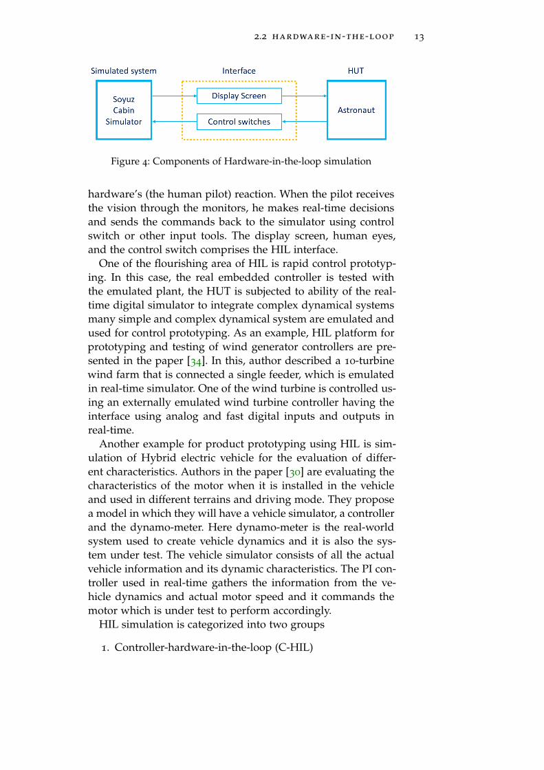
Figure 4 gives practical example of HIL simulation. In thiscase, the simulator mimics a virtual environment of dockingand re-entry that is continuously changing according to the
2.2 hardware-in-the-loop 13
Figure 4: Components of Hardware-in-the-loop simulation
hardware’s (the human pilot) reaction. When the pilot receivesthe vision through the monitors, he makes real-time decisionsand sends the commands back to the simulator using controlswitch or other input tools. The display screen, human eyes,and the control switch comprises the HIL interface.
One of the flourishing area of HIL is rapid control prototyp-ing. In this case, the real embedded controller is tested withthe emulated plant, the HUT is subjected to ability of the real-time digital simulator to integrate complex dynamical systemsmany simple and complex dynamical system are emulated andused for control prototyping. As an example, HIL platform forprototyping and testing of wind generator controllers are pre-sented in the paper [34]. In this, author described a 10-turbinewind farm that is connected a single feeder, which is emulatedin real-time simulator. One of the wind turbine is controlled us-ing an externally emulated wind turbine controller having theinterface using analog and fast digital inputs and outputs inreal-time.
Another example for product prototyping using HIL is sim-ulation of Hybrid electric vehicle for the evaluation of differ-ent characteristics. Authors in the paper [30] are evaluating thecharacteristics of the motor when it is installed in the vehicleand used in different terrains and driving mode. They proposea model in which they will have a vehicle simulator, a controllerand the dynamo-meter. Here dynamo-meter is the real-worldsystem used to create vehicle dynamics and it is also the sys-tem under test. The vehicle simulator consists of all the actualvehicle information and its dynamic characteristics. The PI con-troller used in real-time gathers the information from the ve-hicle dynamics and actual motor speed and it commands themotor which is under test to perform accordingly.
HIL simulation is categorized into two groups
1. Controller-hardware-in-the-loop (C-HIL)

14 hardware-in-the-loop for power electrical systems
2. Power-hardware-in the-loop (P-HIL)
2.2.0.1 Controller-HIL and Power-HIL
Most of the rapid control prototyping HIL applications exchangethe signals between the simulator and the HUT are at lowpower levels typically in the voltage range of ±12V and theycan easily interact with the real world using analog to digitalconverter or vice versa with good accuracy and no power ex-change takes place between the simulator and the HUT, thistype of HIL testing is called as C-HIL.
Figure 5 shows the basic architecture of Controller-hardware-in-the-loop. In this type of simulation only signals are exchangedbetween the real-time digital simulator (RTDS) and the hard-ware under test. Usually the electronic control unit is subjectedto the hardware under test which receives the forward signalsof the process/plant emulated in RTDS. The forward signal-s/feedback signals generated in the RTDS will undergo digi-tal to analog conversion to feed the pseudo measurements ofprocess/plant to the controller. The controller interprets thispseudo measurement signals as real world signals. After it pro-cessing the information, it generates the control signal that isfed to RTDS through a analog to digital converter to behaveaccording to the instructions obtained by HUT.
Figure 5: Architecture of C-HIL simulation
Whereas in many cases, there is a need of exchanging powerbetween the simulator and the HUT (example Electric vehiclemotor as HUT) and the simulator should be able to address
2.2 hardware-in-the-loop 15
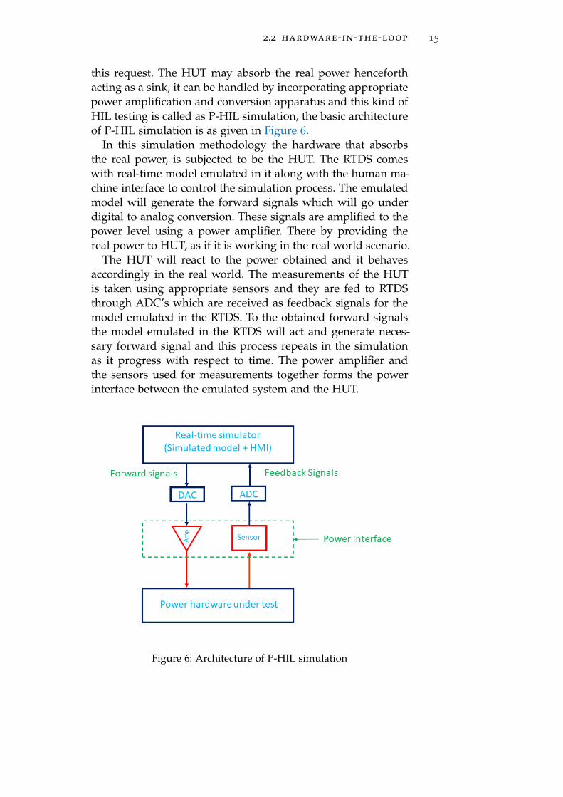
this request. The HUT may absorb the real power henceforthacting as a sink, it can be handled by incorporating appropriatepower amplification and conversion apparatus and this kind ofHIL testing is called as P-HIL simulation, the basic architectureof P-HIL simulation is as given in Figure 6.
In this simulation methodology the hardware that absorbsthe real power, is subjected to be the HUT. The RTDS comeswith real-time model emulated in it along with the human ma-chine interface to control the simulation process. The emulatedmodel will generate the forward signals which will go underdigital to analog conversion. These signals are amplified to thepower level using a power amplifier. There by providing thereal power to HUT, as if it is working in the real world scenario.
The HUT will react to the power obtained and it behavesaccordingly in the real world. The measurements of the HUTis taken using appropriate sensors and they are fed to RTDSthrough ADC’s which are received as feedback signals for themodel emulated in the RTDS. To the obtained forward signalsthe model emulated in the RTDS will act and generate neces-sary forward signal and this process repeats in the simulationas it progress with respect to time. The power amplifier andthe sensors used for measurements together forms the powerinterface between the emulated system and the HUT.
Figure 6: Architecture of P-HIL simulation
16 hardware-in-the-loop for power electrical systems
2.2.1 Different HIL methodologies for Electric drive system
To know the different HIL methodologies that can be imple-mented in electrical domain, I introduce an example of Electricdrive system given in the paper [10], the author has given thedistinctive techniques for directing HIL simulation for electricdrives. In which he clarifies the interfaces and the strategies togo from signal level to mechanical level of integration.
An electrical drive can be defined as an electro-mechanicaldevice for converting electrical energy into mechanical energyto impart motion to different machines and mechanisms forvarious kinds of process control [27].
Figure 7: Electrical drive framework
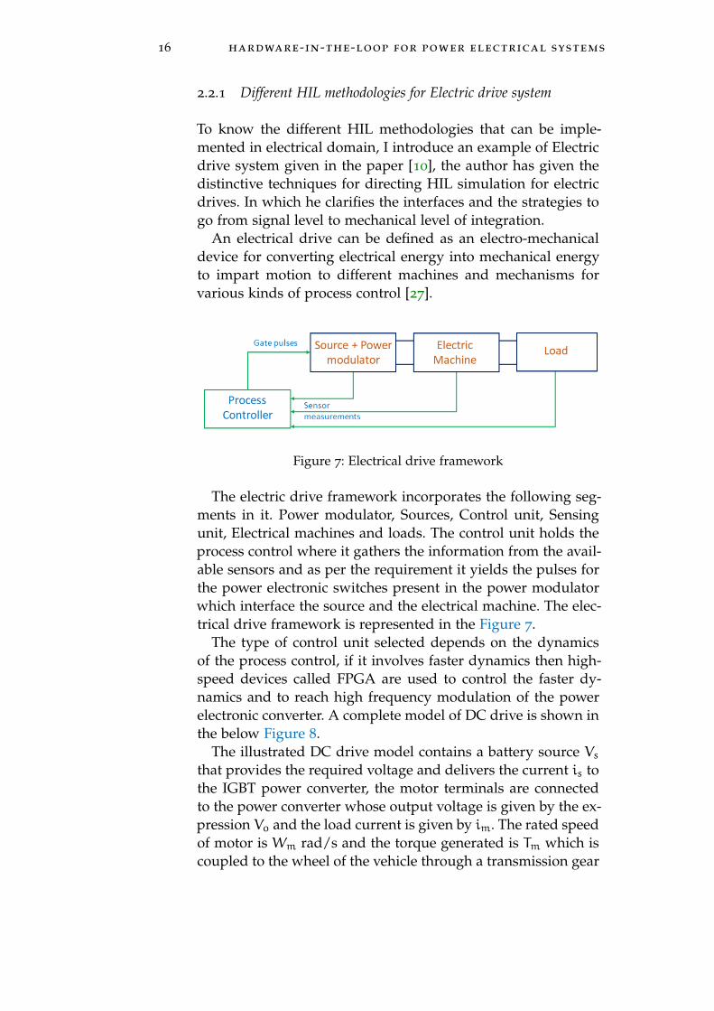
The electric drive framework incorporates the following seg-ments in it. Power modulator, Sources, Control unit, Sensingunit, Electrical machines and loads. The control unit holds theprocess control where it gathers the information from the avail-able sensors and as per the requirement it yields the pulses forthe power electronic switches present in the power modulatorwhich interface the source and the electrical machine. The elec-trical drive framework is represented in the Figure 7.
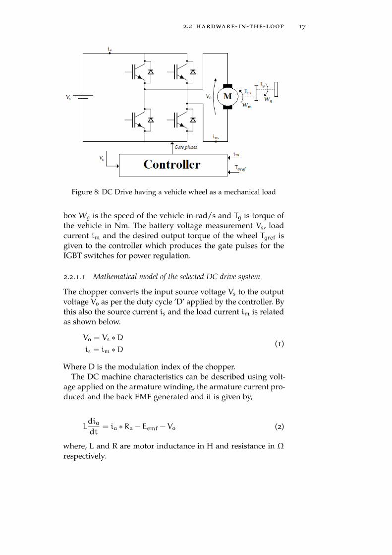
The type of control unit selected depends on the dynamicsof the process control, if it involves faster dynamics then high-speed devices called FPGA are used to control the faster dy-namics and to reach high frequency modulation of the powerelectronic converter. A complete model of DC drive is shown inthe below Figure 8.
The illustrated DC drive model contains a battery source Vsthat provides the required voltage and delivers the current is tothe IGBT power converter, the motor terminals are connectedto the power converter whose output voltage is given by the ex-pression Vo and the load current is given by im. The rated speedof motor is Wm rad/s and the torque generated is Tm which iscoupled to the wheel of the vehicle through a transmission gear
2.2 hardware-in-the-loop 17
Figure 8: DC Drive having a vehicle wheel as a mechanical load
box Wg is the speed of the vehicle in rad/s and Tg is torque ofthe vehicle in Nm. The battery voltage measurement Vs, loadcurrent im and the desired output torque of the wheel Tgref isgiven to the controller which produces the gate pulses for theIGBT switches for power regulation.
2.2.1.1 Mathematical model of the selected DC drive system
The chopper converts the input source voltage Vs to the outputvoltage Vo as per the duty cycle ’D’ applied by the controller. Bythis also the source current is and the load current im is relatedas shown below.
Vo = Vs ∗Dis = im ∗D
(1)
Where D is the modulation index of the chopper.The DC machine characteristics can be described using volt-
age applied on the armature winding, the armature current pro-duced and the back EMF generated and it is given by,
Ldiadt
= ia ∗ Ra − Eemf − Vo (2)
where, L and R are motor inductance in H and resistance in Ωrespectively.
18 hardware-in-the-loop for power electrical systems
The torque of the DC machine is is proportional to the arma-ture current ia and the EMF generated if proportional to thespeed of the machine Wm.
Tm = ka ∗ iaEemf = ka ∗Wm
(3)
where, Ka is the torque co-efficient.Gearbox gives the torque Tg and the speed of the wheel Wg
from the machine torque and the machine speed using the gearratio kg.
Tg = kg ∗ TmWm = kg ∗Wg
(4)
The wheel converts the rotational motion Wg to the linearmotion Vspeed and also the obtain torque Tg to the traction forceFtract using the wheel radius Rwheel.
Ftract =Tg
Rwheel
Wg =Vspeed
Rwheel
(5)
Vehicle speed is obtained by equation of vehicle dynamicsrelation with traction force Ft and resistant force Fres.
MdVspeed
dt= Ftract − Fres (6)
where, M is the mass of the vehicle including the rotating mass.The resistant force Fres is calculated using the relation,
Fres = Fo +αVspeed + bV2speed +M ∗ g ∗ sin(θ) (7)
where, Fo is the frictional force, α is the friction co-efficient, bis the drag co-efficient,θ is the slope angle to the horizontalsurface and g is acceleration due to gravity.
2.2.1.2 Signal level HIL Simulation
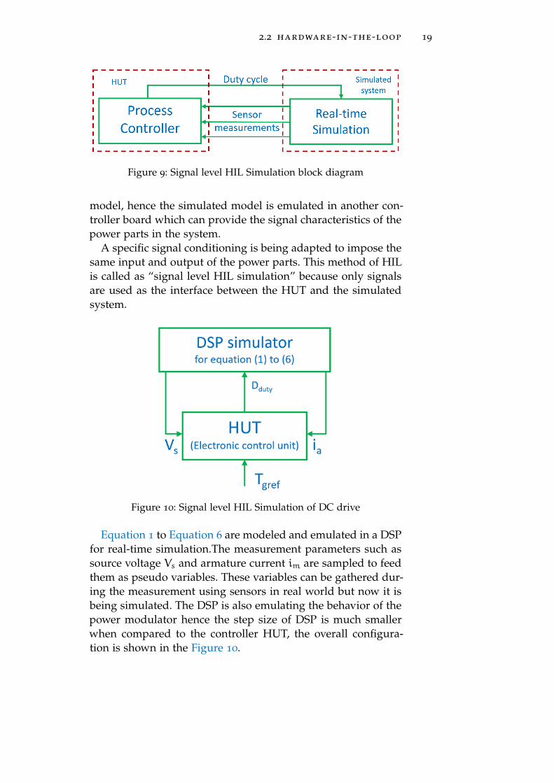
In signal level of HIL simulation, only the control hardwarethat holds the process control is tested. The other parts such aspower modulator, electrical machine and the mechanical loadare simulated in real-time. The simulation should be able to ex-change the signals between the controller (HUT) and simulated
2.2 hardware-in-the-loop 19
Figure 9: Signal level HIL Simulation block diagram
model, hence the simulated model is emulated in another con-troller board which can provide the signal characteristics of thepower parts in the system.
A specific signal conditioning is being adapted to impose thesame input and output of the power parts. This method of HILis called as “signal level HIL simulation” because only signalsare used as the interface between the HUT and the simulatedsystem.
Figure 10: Signal level HIL Simulation of DC drive
Equation 1 to Equation 6 are modeled and emulated in a DSPfor real-time simulation.The measurement parameters such assource voltage Vs and armature current im are sampled to feedthem as pseudo variables. These variables can be gathered dur-ing the measurement using sensors in real world but now it isbeing simulated. The DSP is also emulating the behavior of thepower modulator hence the step size of DSP is much smallerwhen compared to the controller HUT, the overall configura-tion is shown in the Figure 10.
20 hardware-in-the-loop for power electrical systems
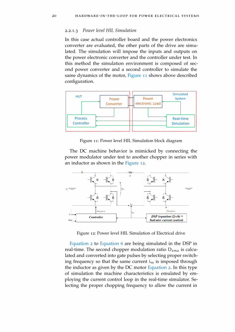
2.2.1.3 Power level HIL Simulation
In this case actual controller board and the power electronicsconverter are evaluated, the other parts of the drive are simu-lated. The simulation will impose the inputs and outputs onthe power electronic converter and the controller under test. Inthis method the simulation environment is composed of sec-ond power converter and a second controller to simulate thesame dynamics of the motor, Figure 11 shows above describedconfiguration.
Figure 11: Power level HIL Simulation block diagram
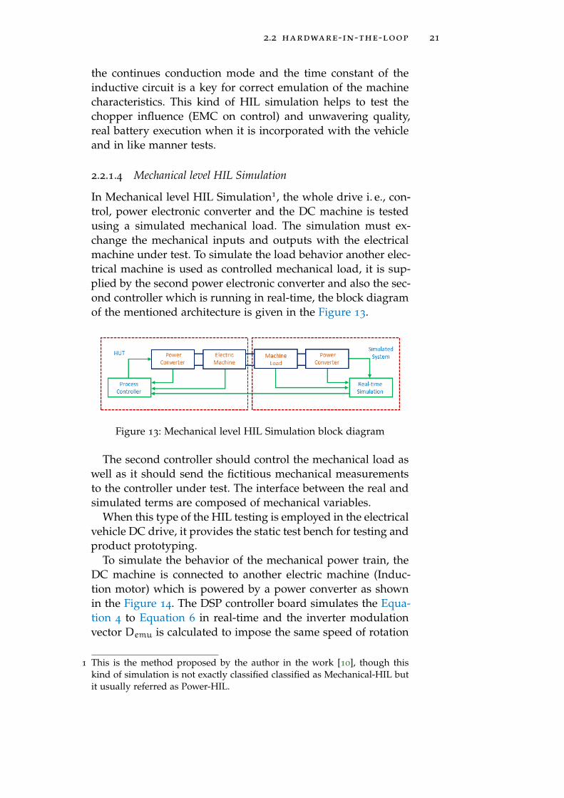
The DC machine behavior is mimicked by connecting thepower modulator under test to another chopper in series withan inductor as shown in the Figure 12.
Figure 12: Power level HIL Simulation of Electrical drive
Equation 2 to Equation 6 are being simulated in the DSP inreal-time. The second chopper modulation ratio Demu is calcu-lated and converted into gate pulses by selecting proper switch-ing frequency so that the same current im is imposed throughthe inductor as given by the DC motor Equation 2. In this typeof simulation the machine characteristics is emulated by em-ploying the current control loop in the real-time simulator. Se-lecting the proper chopping frequency to allow the current in
2.2 hardware-in-the-loop 21
the continues conduction mode and the time constant of theinductive circuit is a key for correct emulation of the machinecharacteristics. This kind of HIL simulation helps to test thechopper influence (EMC on control) and unwavering quality,real battery execution when it is incorporated with the vehicleand in like manner tests.
2.2.1.4 Mechanical level HIL Simulation
In Mechanical level HIL Simulation1, the whole drive i. e., con-trol, power electronic converter and the DC machine is testedusing a simulated mechanical load. The simulation must ex-change the mechanical inputs and outputs with the electricalmachine under test. To simulate the load behavior another elec-trical machine is used as controlled mechanical load, it is sup-plied by the second power electronic converter and also the sec-ond controller which is running in real-time, the block diagramof the mentioned architecture is given in the Figure 13.
Figure 13: Mechanical level HIL Simulation block diagram
The second controller should control the mechanical load aswell as it should send the fictitious mechanical measurementsto the controller under test. The interface between the real andsimulated terms are composed of mechanical variables.
When this type of the HIL testing is employed in the electricalvehicle DC drive, it provides the static test bench for testing andproduct prototyping.
To simulate the behavior of the mechanical power train, theDC machine is connected to another electric machine (Induc-tion motor) which is powered by a power converter as shownin the Figure 14. The DSP controller board simulates the Equa-tion 4 to Equation 6 in real-time and the inverter modulationvector Demu is calculated to impose the same speed of rotation
1 This is the method proposed by the author in the work [10], though thiskind of simulation is not exactly classified classified as Mechanical-HIL butit usually referred as Power-HIL.
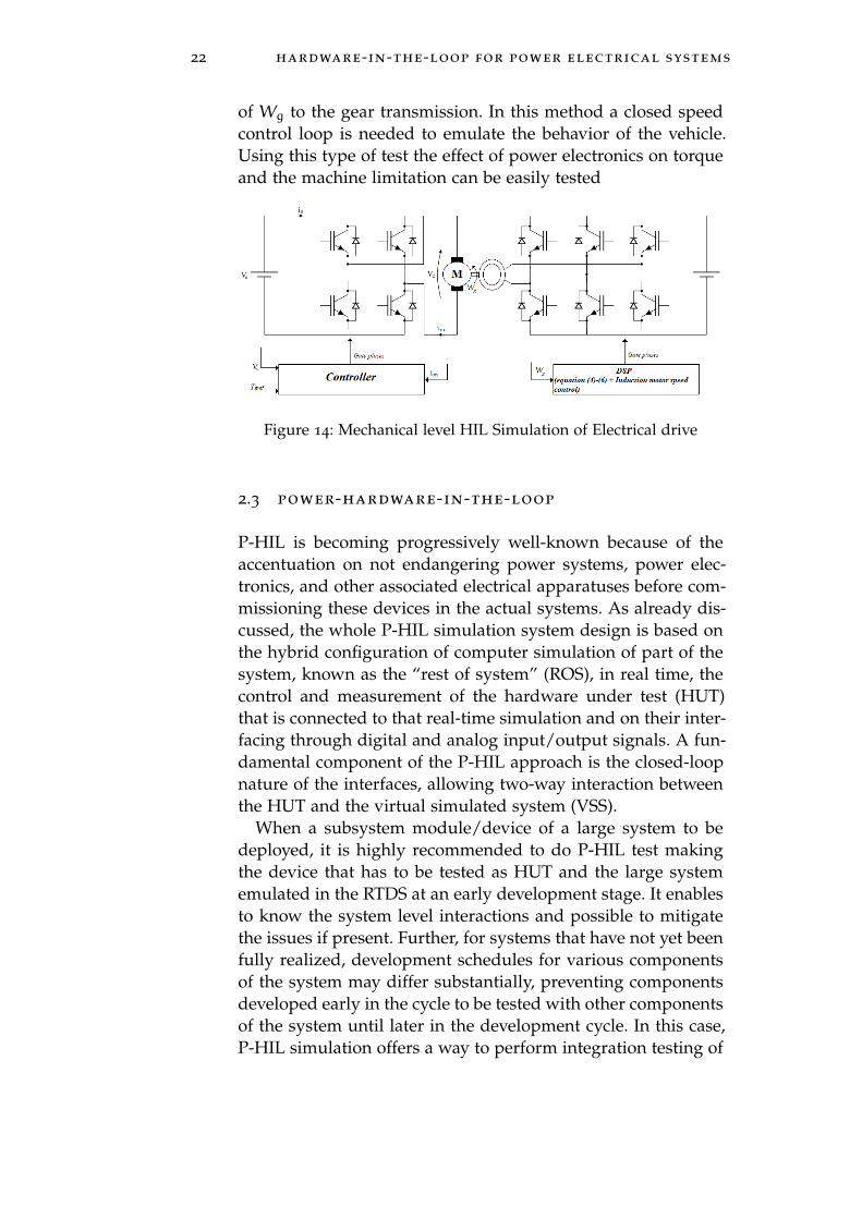
22 hardware-in-the-loop for power electrical systems
of Wg to the gear transmission. In this method a closed speedcontrol loop is needed to emulate the behavior of the vehicle.Using this type of test the effect of power electronics on torqueand the machine limitation can be easily tested
Figure 14: Mechanical level HIL Simulation of Electrical drive
2.3 power-hardware-in-the-loop
P-HIL is becoming progressively well-known because of theaccentuation on not endangering power systems, power elec-tronics, and other associated electrical apparatuses before com-missioning these devices in the actual systems. As already dis-cussed, the whole P-HIL simulation system design is based onthe hybrid configuration of computer simulation of part of thesystem, known as the “rest of system” (ROS), in real time, thecontrol and measurement of the hardware under test (HUT)that is connected to that real-time simulation and on their inter-facing through digital and analog input/output signals. A fun-damental component of the P-HIL approach is the closed-loopnature of the interfaces, allowing two-way interaction betweenthe HUT and the virtual simulated system (VSS).
When a subsystem module/device of a large system to bedeployed, it is highly recommended to do P-HIL test makingthe device that has to be tested as HUT and the large systememulated in the RTDS at an early development stage. It enablesto know the system level interactions and possible to mitigatethe issues if present. Further, for systems that have not yet beenfully realized, development schedules for various componentsof the system may differ substantially, preventing componentsdeveloped early in the cycle to be tested with other componentsof the system until later in the development cycle. In this case,P-HIL simulation offers a way to perform integration testing of
2.3 power-hardware-in-the-loop 23
the HUT at an early stage, making use of models of the othercomponents in the system.
P-HIL experiments can be conducted in a tightly controlledlab environment in which experiments can be quickly and grace-fully terminated, P-HIL simulation provides a means to test theHUT for extreme or dangerous conditions that would not be at-tempted with a fully hardware-based test bed of the surround-ing system.
Though it has so much advantages, this methodology is oftenforgotten in the scientific community, hence a less number of re-search work is being carried in this area. Due to advancementin digital dives like FPGA and immediate need of addressingenergy issues using renewable sources. P-HIL tests are gainingmore emphasis in this regard for design, project evaluation andtesting of integration of renewable energy source with the gridsimulation for worst case scenarios. P-HIL is a safe risk reduc-ing method that is extremely applicable because it provides amore realistic environment than software simulation alone.
2.3.1 Basic architecture of P-HIL simulation
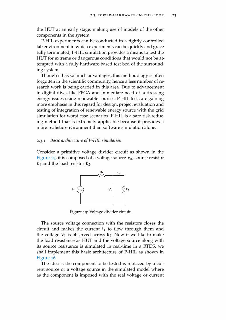
Consider a primitive voltage divider circuit as shown in theFigure 15, it is composed of a voltage source Vo, source resistorR1 and the load resistor R2.
Figure 15: Voltage divider circuit
The source voltage connection with the resistors closes thecircuit and makes the current i1 to flow through them andthe voltage V1 is observed across R2. Now if we like to makethe load resistance as HUT and the voltage source along withits source resistance is simulated in real-time in a RTDS, weshall implement this basic architecture of P-HIL as shown inFigure 16.
The idea is the component to be tested is replaced by a cur-rent source or a voltage source in the simulated model whereas the component is imposed with the real voltage or current
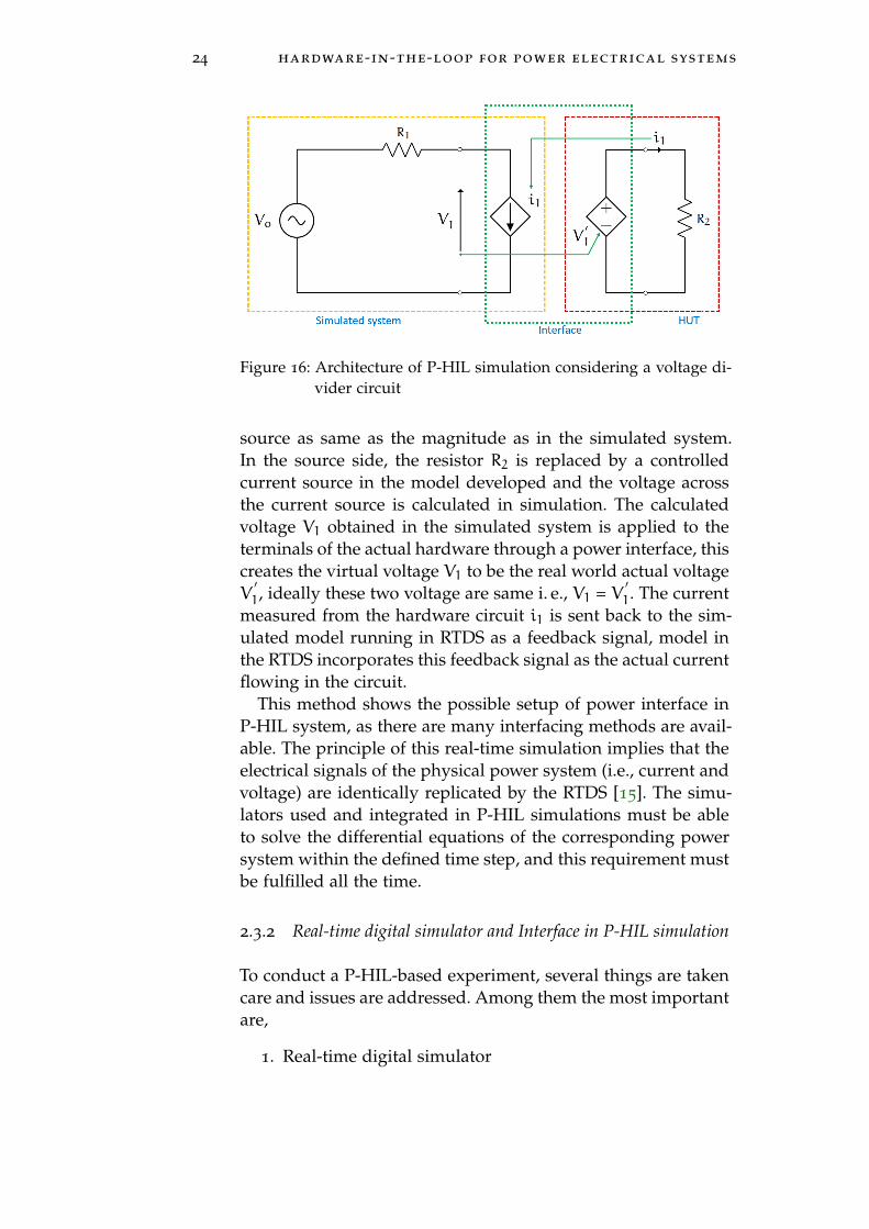
24 hardware-in-the-loop for power electrical systems
Figure 16: Architecture of P-HIL simulation considering a voltage di-vider circuit
source as same as the magnitude as in the simulated system.In the source side, the resistor R2 is replaced by a controlledcurrent source in the model developed and the voltage acrossthe current source is calculated in simulation. The calculatedvoltage V1 obtained in the simulated system is applied to theterminals of the actual hardware through a power interface, thiscreates the virtual voltage V1 to be the real world actual voltageV
′1, ideally these two voltage are same i. e., V1 = V
′1. The current
measured from the hardware circuit i1 is sent back to the sim-ulated model running in RTDS as a feedback signal, model inthe RTDS incorporates this feedback signal as the actual currentflowing in the circuit.
This method shows the possible setup of power interface inP-HIL system, as there are many interfacing methods are avail-able. The principle of this real-time simulation implies that theelectrical signals of the physical power system (i.e., current andvoltage) are identically replicated by the RTDS [15]. The simu-lators used and integrated in P-HIL simulations must be ableto solve the differential equations of the corresponding powersystem within the defined time step, and this requirement mustbe fulfilled all the time.
2.3.2 Real-time digital simulator and Interface in P-HIL simulation
To conduct a P-HIL-based experiment, several things are takencare and issues are addressed. Among them the most importantare,
1. Real-time digital simulator
2.3 power-hardware-in-the-loop 25
2. Power amplifier
3. Interface
2.3.2.1 Real-time digital simulator
RTDS plays a major role in entire P-HIL simulation because ofthe model emulated is controlled by RTDS and it is only respon-sible for keeping the simulation in real-time. A wide variety ofreal-time digital simulators are available in the market. Somereal-time engines cater more toward bulk power applicationsand thus, form a P-HIL standpoint. It is also a software bridgebetween the emulated model in the target device and human,it provides the HMI between the tester and the real-time target.
The selection of the target device is based on many factors,but one importantly is the computing capability of it. To modelthe high switching characteristics of converters, a fast processoris needed to reach the minimum step size as low as 1µs. A real-time simulator needs to solve a grid-scale model by roughly50µs or a smaller time-step, a simulation of such a system mayrequire more computing capability and the ability to simulatewith a very small time-step. From a hard ware architecturalpoint of view, the RTDS can be grouped into the following cat-egories.
• PC based
• Custom processor based
• Supercomputer based
• FPGA based
The PC-based RTDS uses general-purpose multi core proces-sors that run on RT-Linux and execute real-time code gener-ated from the system model with optimized solvers. Custom-processor-based RTDS are based on RISC processors runningon VxWorks RT-OS and its user interface. Supercomputer-basedRTDSs are based on machines with large computational plat-form and the last one uses FPGAs as the main computationalhardware that is used for both large-scale and small-scale sim-ulation activities. Simulation on FPGA is a good solution toachieve the custom performance. However, the coding of com-plex solvers for FPGA is still very complex and often requireslow-level FPGA programming expertise.
26 hardware-in-the-loop for power electrical systems
Most of the RTDS comes with the application software wherean inbuilt library providing GUI to do build model by dragand drop, also they provide a platform to build custom modelusing C code or any other tool. The application software holdsthe solver methodology to solve the model as well. Most promi-nently usage of MATLAB model gives an easy development en-vironment. As, a well-defined libraries enables user to cut thedevelopment time, but very less RTDS support this facility.
2.3.2.2 Power amplifiers
As P-HIL experiments involve the transfer of power throughthe interface, an amplifier is needed to reproduce simulatedconditions at the point of common coupling with the HUT.In P-HIL-based experiments, it is typically desired to test theelectrical apparatus at its intended power rating and dynamicevents may further require voltages and currents more thanthe rated values for limited duration. Thus, it is required toutilize an amplifier that is sized appropriately for the task andthat additionally has a bandwidth that can conduct the planneddynamic tests. Also, considerations that must be taken care in-cludes slew rate limiting due to bandwidth limitations as wellas quantization error in voltage/current synthesis.
It’s the task of the engineer who is testing to select appropri-ate power amplifier according to his testing needs. The guideto select proper power amplifier is given in [24] in this paperthey suggest three types of power amplifiers addressing differ-ent needs. They are,
1. Switched mode power amplifier: Switched-mode ampli-fiers are commonly used for P-HIL simulation rangingfrom small-scale power applications up to the megawattrange. Typical AC/DC/AC converter typologies consist-ing of front-end rectifier and back-end inverter is used inthis method. Based on type of P-HIL experiment, controlstrategy of the amplifier, switching frequency and the out-put filters are selected.
2. Linear power amplifiers: They are most suitable for P-HILapplications in the small to medium power scale.
3. Generator-type power amplifiers: This type of amplifica-tion employs a three-phase synchronous generator drivenby a DC or AC motor and separate exciter systems.
2.3 power-hardware-in-the-loop 27
The following characteristics must also be carefully consid-ered to select the amplifier for the P-HIL application.
• Power ratings of the device under test
• Amplifier interface connections
• Source and sink power ratings of the amplifier
• Amplifier response times
• Amplifier slew rate
• Amplifier harmonic distortion and frequency resolution
• Amplifier input and output voltage/current range
• Amplifier input and output impudence
2.3.2.3 Interface
Interfacing the RTDS with the HUT holds an important task inP-HIL simulation. Type of interface will decide the stability andaccuracy of the simulation, selecting the proper interfacing al-gorithm is the key to get accurate results and meeting the goalsof the P-HIL simulation. Many types of interface algorithms areavailable and it’s being explained in detail in the next section.
2.3.3 Interface Algorithm
Interface algorithms provide the means of relating simulatedvoltage and currents at the PCC between the ROS and theHUT to the measured voltage and current of the P-HIL am-plifier. This element is critical as it has a profound influenceon the accuracy and stability of the P-HIL-based experiment.Few commonly known methods of interface algorithm are pre-sented here [36]. Dual forms of each method, referred to asvoltage type and current type, are generally available to accom-modate operation with an amplifier accepting either a voltagereference or a current reference, respectively.
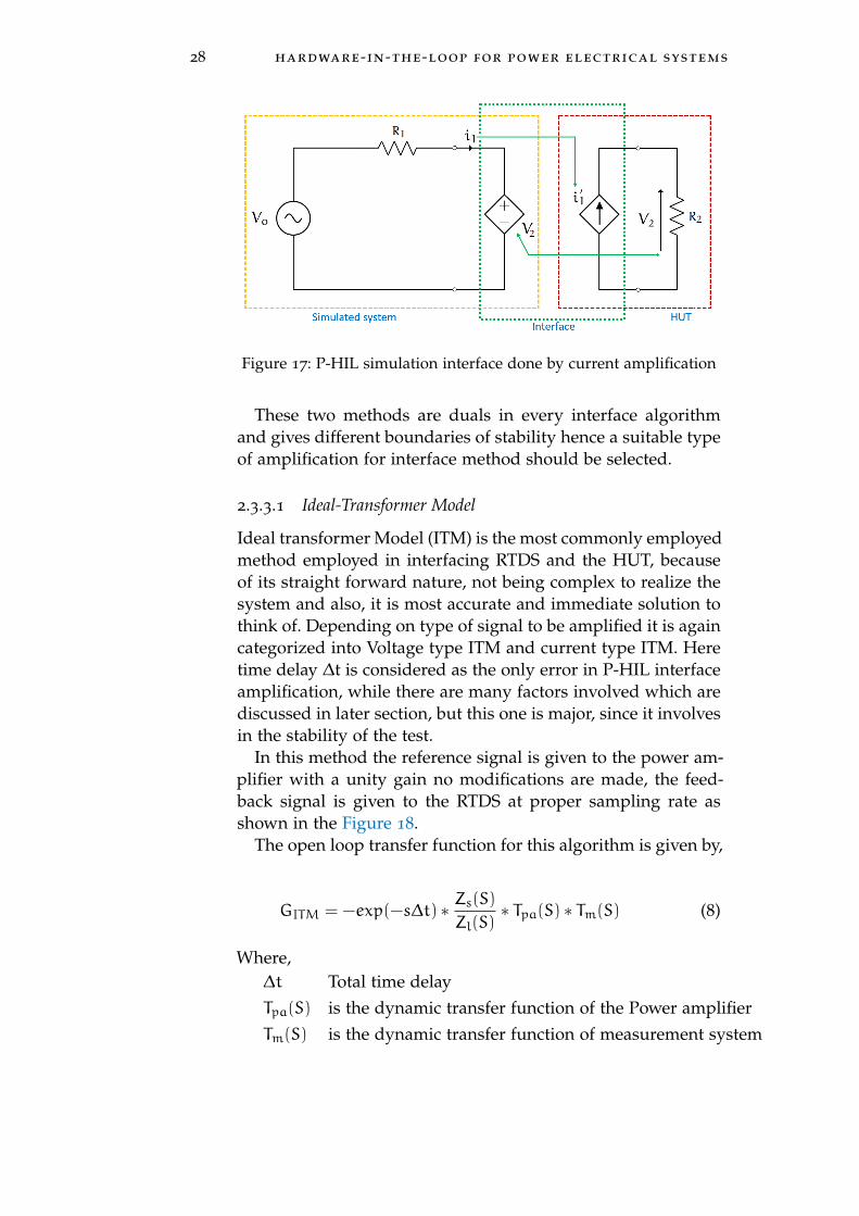
Figure 16 shows the interfacing method, where the voltageV1 is amplified for the same kind of P-HIL application it can beinterfaced by amplifying current instead of voltage and the volt-age across the HUT is sent as feedback to the RTDS as shownin the Figure 17.
28 hardware-in-the-loop for power electrical systems
Figure 17: P-HIL simulation interface done by current amplification
These two methods are duals in every interface algorithmand gives different boundaries of stability hence a suitable typeof amplification for interface method should be selected.
2.3.3.1 Ideal-Transformer Model
Ideal transformer Model (ITM) is the most commonly employedmethod employed in interfacing RTDS and the HUT, becauseof its straight forward nature, not being complex to realize thesystem and also, it is most accurate and immediate solution tothink of. Depending on type of signal to be amplified it is againcategorized into Voltage type ITM and current type ITM. Heretime delay ∆t is considered as the only error in P-HIL interfaceamplification, while there are many factors involved which arediscussed in later section, but this one is major, since it involvesin the stability of the test.
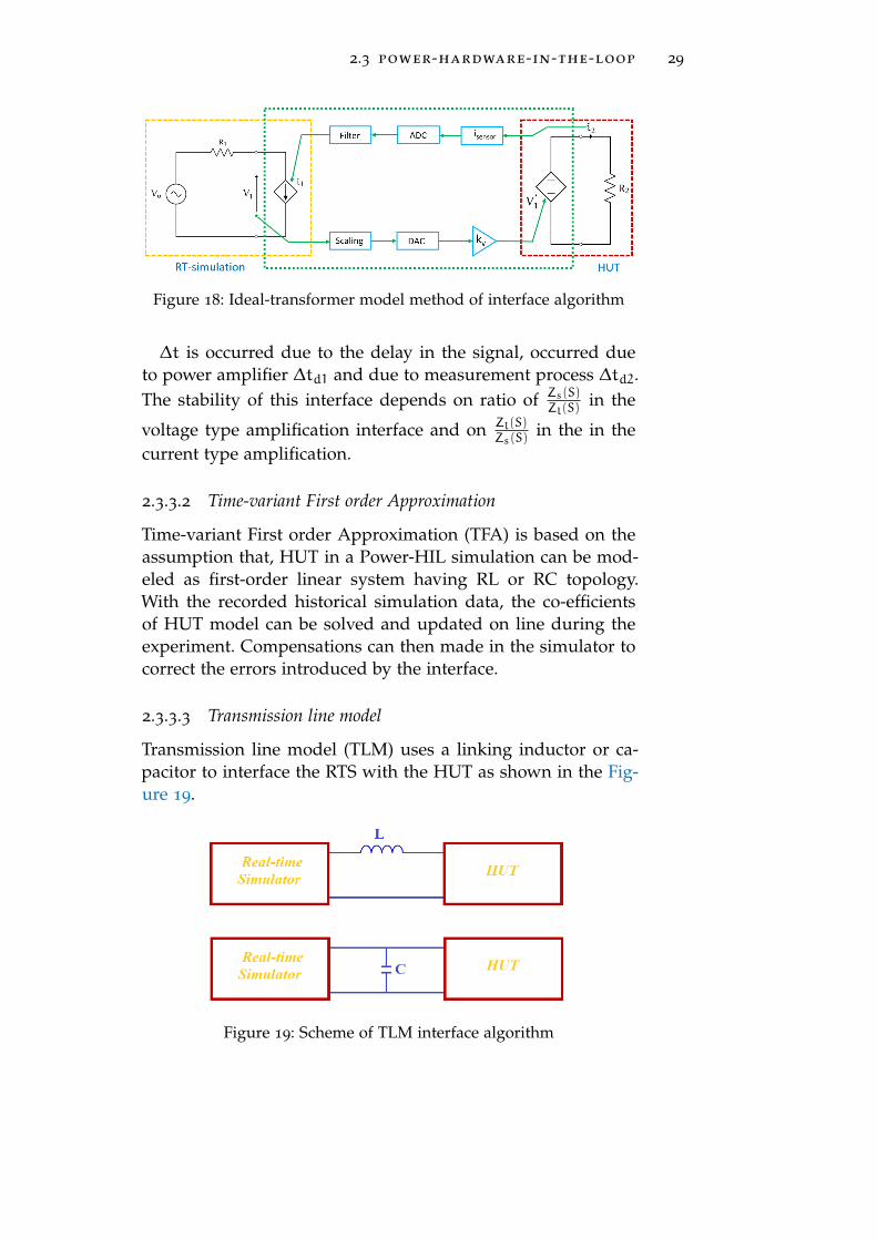
In this method the reference signal is given to the power am-plifier with a unity gain no modifications are made, the feed-back signal is given to the RTDS at proper sampling rate asshown in the Figure 18.
The open loop transfer function for this algorithm is given by,
GITM = −exp(−s∆t) ∗ Zs(S)Zl(S)
∗ Tpa(S) ∗ Tm(S) (8)
Where,∆t Total time delayTpa(S) is the dynamic transfer function of the Power amplifierTm(S) is the dynamic transfer function of measurement system
2.3 power-hardware-in-the-loop 29
Figure 18: Ideal-transformer model method of interface algorithm
∆t is occurred due to the delay in the signal, occurred dueto power amplifier ∆td1 and due to measurement process ∆td2.The stability of this interface depends on ratio of Zs(S)
Zl(S)in the
voltage type amplification interface and on Zl(S)Zs(S)
in the in thecurrent type amplification.
2.3.3.2 Time-variant First order Approximation
Time-variant First order Approximation (TFA) is based on theassumption that, HUT in a Power-HIL simulation can be mod-eled as first-order linear system having RL or RC topology.With the recorded historical simulation data, the co-efficientsof HUT model can be solved and updated on line during theexperiment. Compensations can then made in the simulator tocorrect the errors introduced by the interface.
2.3.3.3 Transmission line model
Transmission line model (TLM) uses a linking inductor or ca-pacitor to interface the RTS with the HUT as shown in the Fig-ure 19.
Figure 19: Scheme of TLM interface algorithm
30 hardware-in-the-loop for power electrical systems
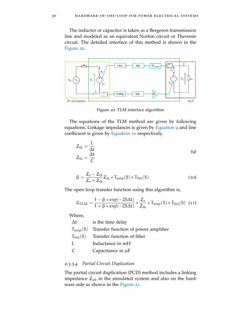
The inductor or capacitor is taken as a Bergeron transmissionline and modeled as an equivalent Norton circuit or Thevenincircuit. The detailed interface of this method is shown in theFigure 20.
Figure 20: TLM interface algorithm
The equations of the TLM method are given by followingequations, Linkage impedances is given by Equation 9 and linecoefficient is given by Equation 10 respectively.
Zlk =L
∆t
Zlk =∆t
C
(9)
β =Zs −ZlkZs +Zlk
Zlk ∗ Tamp(S) ∗ Tflit(S) (10)
The open loop transfer function using this algorithm is,
GTLM =1−β ∗ exp(−2S∆t)1+β ∗ exp(−2S∆t)
∗ ZsZlk∗ Tamp(S) ∗ Tflit(S) (11)
Where,∆t is the time delayTamp(S) Transfer function of power amplifierTflit(S) Transfer function of filterL Inductance in mHC Capacitance in µF
2.3.3.4 Partial Circuit Duplication
The partial circuit duplication (PCD) method includes a linkingimpedance Zab in the simulated system and also on the hard-ware side as shown in the Figure 21.

2.3 power-hardware-in-the-loop 31
Figure 21: PCD interface algorithm
Large values of the linking impedance improves the stabil-ity of the interface but introduces inaccuracies due to increasedpower losses. The open loop transfer function of the PCD methodis given by
Gpcd =ZsZhut
(Zs +Zab)(Zhut +Zab)∗ exp(−s∆t) ∗ Tamp(S) ∗ Tfilt(S)
(12)
Where,∆t is the time delayTamp(S) Transfer function of power amplifierTflit(S) Transfer function of filterZab Impedance linked
2.3.3.5 Damping Impedance Method
The damping impedance method(DIM) is a composite of theideal transformer and PCD methods. It has a linking impedanceZab similar to the PCD and includes a damping impedanceZdamp as shown in Figure 22. The DIM method has very high
Figure 22: DIM interface algorithm
32 hardware-in-the-loop for power electrical systems
stability when the value of Zdamp is equal to Zhut. The openloop transfer function of the DIM method is given by Equa-tion 13.
Gdim =Zs(Zhut −Zdamp)
(Zs +Zab +Zdamp)(Zhut +Zab)∗exp(−s∆t)∗Tamp(S)∗Tfilt(S)
(13)
Where,
∆t is the time delayTamp(S) Transfer function of power amplifierTflit(S) Transfer function of filterZab Impedance linkedZdamp Damping Impedance
There are many interface algorithms are coming up accord-ing to the needs and to address the issues, but the above men-tioned are the basic types that can be incorporated easily.
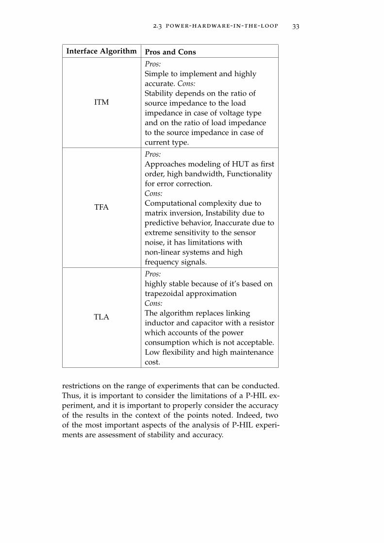
2.3.4 Pros and Cons of Interface Algorithms
Several advantages and disadvantages of using different inter-face algorithms are briefly presented in the Table 1 [14, 36].
2.3.5 Open issues in P-HIL simulation
As with any modeling and simulation work, the accuracy ofthe virtual surrounding system is limited by the accuracy ofthe models employed in that system. Second, the restrictionsimposed by the real-time simulation requirement may imposeadditional limitations on the size and level of detail that can beincluded in the models. Real-time simulators typically employfixed time-step solvers with some minimum achievable time-step sizes. This restriction can have implications on the timeconstants that can be represented, switching frequencies thatcan be employed for switching power electronics models, andgenerally on the frequency band over which the models canappropriately represent reality.
Additionally, the amplifiers, actuators, sensors and ADC orDAC cards comprising the P-HIL interfaces introduce time de-lays, distortion, and their own bandwidth limitations which canaffect the experiments and, in some cases, lead to instabilities.
Capability limitations in terms of voltage, current, torque,speed, etc. of the amplifiers and actuators also impose further
2.3 power-hardware-in-the-loop 33
Interface Algorithm Pros and Cons
ITM
Pros:Simple to implement and highlyaccurate. Cons:Stability depends on the ratio ofsource impedance to the loadimpedance in case of voltage typeand on the ratio of load impedanceto the source impedance in case ofcurrent type.
TFA
Pros:Approaches modeling of HUT as firstorder, high bandwidth, Functionalityfor error correction.Cons:Computational complexity due tomatrix inversion, Instability due topredictive behavior, Inaccurate due toextreme sensitivity to the sensornoise, it has limitations withnon-linear systems and highfrequency signals.
TLA
Pros:highly stable because of it’s based ontrapezoidal approximationCons:The algorithm replaces linkinginductor and capacitor with a resistorwhich accounts of the powerconsumption which is not acceptable.Low flexibility and high maintenancecost.
restrictions on the range of experiments that can be conducted.Thus, it is important to consider the limitations of a P-HIL ex-periment, and it is important to properly consider the accuracyof the results in the context of the points noted. Indeed, twoof the most important aspects of the analysis of P-HIL experi-ments are assessment of stability and accuracy.

34 hardware-in-the-loop for power electrical systems
Interface Algorithm Pros and Cons
PCD
Pros:Highly stable, it is a promisingmethod to implement for large scalecircuits and systems.Cons:Value of linking component ratio tosource or load impedance affectsaccuracy. Accuracy is often low dueto stability requirements on Zab, poorconvergence limits the applicabilityof the relaxation technique.
DIM
Pros:high stability and accuracy when thedamping impedance is equal to theload impedance of HUT, this methodhas the ability to adapt.Cons:High fidelity impedance basedmodel of the HUT is required,though it may often not available.
Table 1: Pros and Cons of Interface algorithm
2.3.5.1 Stability issue of P-HIL
the closed-loop system in real-time simulation platform con-sists of DAC converters, power amplifier, HUT, measurementprobes, sample-and hold circuit and ADC converters shouldnot exhibit unstable/oscillatory behavior. Stability is a neces-sary criterion for the accuracy of the simulation and for theequipment safety, HUT devices may be damaged when the sys-tem becomes unstable. Hence, appropriate counter measuresshould be implemented to detect undesired modes of opera-tion and return to a safe state.
One of the main sources of instability in P-HIL simulationsis the computation time and data acquisition time of the RTDSsystem [36]. Even if the time step is very short as small as microseconds, for certain parameter values of the hardware part to besimulated and the hardware part attached as real HUT device,the P-HIL simulation may become unstable. Additionally, de-pending on the equipment used and its realization, the poweramplifier may be far from ideal by introducing additional de-
2.3 power-hardware-in-the-loop 35
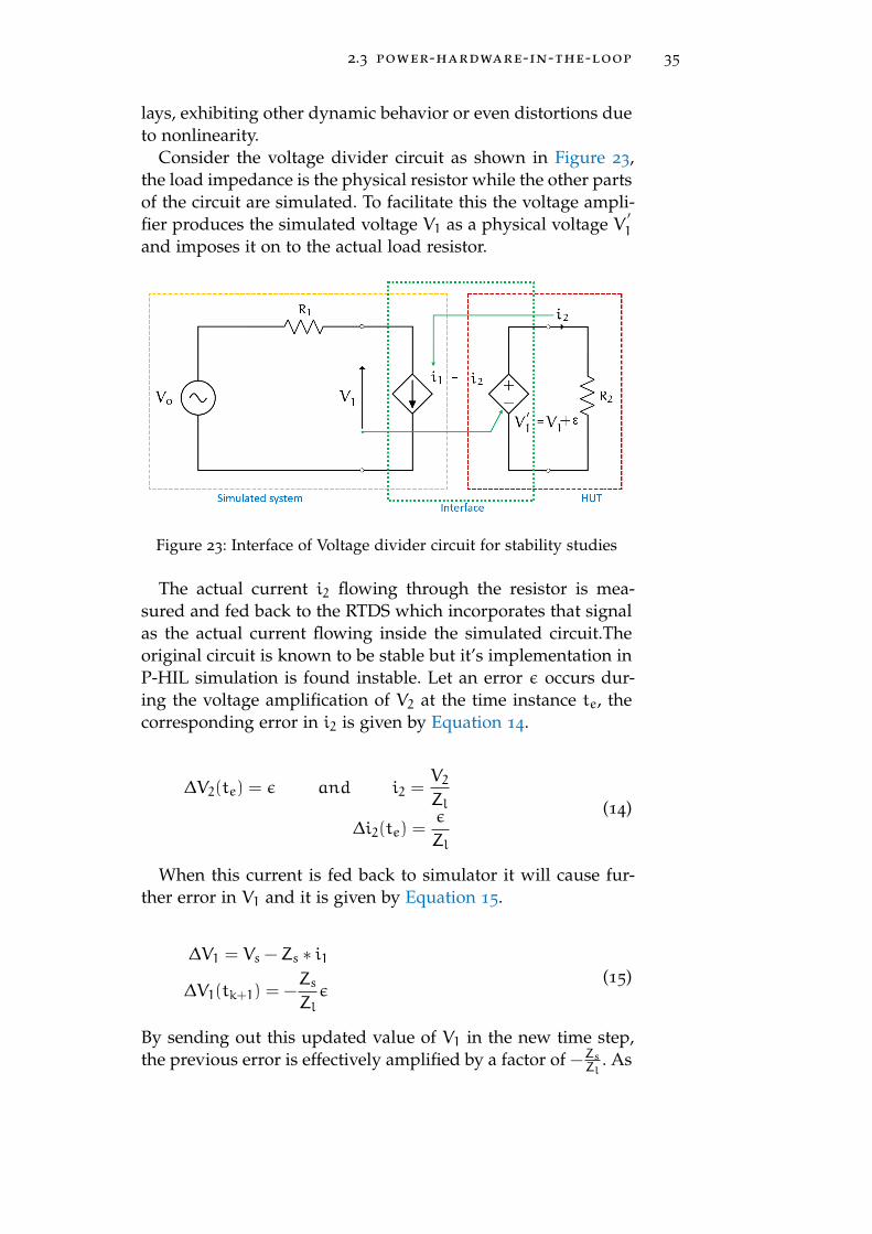
lays, exhibiting other dynamic behavior or even distortions dueto nonlinearity.
Consider the voltage divider circuit as shown in Figure 23,the load impedance is the physical resistor while the other partsof the circuit are simulated. To facilitate this the voltage ampli-fier produces the simulated voltage V1 as a physical voltage V
′1
and imposes it on to the actual load resistor.
Figure 23: Interface of Voltage divider circuit for stability studies
The actual current i2 flowing through the resistor is mea-sured and fed back to the RTDS which incorporates that signalas the actual current flowing inside the simulated circuit.Theoriginal circuit is known to be stable but it’s implementation inP-HIL simulation is found instable. Let an error ε occurs dur-ing the voltage amplification of V2 at the time instance te, thecorresponding error in i2 is given by Equation 14.
∆V2(te) = ε and i2 =V2Zl
∆i2(te) =ε
Zl
(14)
When this current is fed back to simulator it will cause fur-ther error in V1 and it is given by Equation 15.
∆V1 = Vs −Zs ∗ i1
∆V1(tk+1) = −Zs
Zlε
(15)
By sending out this updated value of V1 in the new time step,the previous error is effectively amplified by a factor of −Zs
Zl. As
36 hardware-in-the-loop for power electrical systems
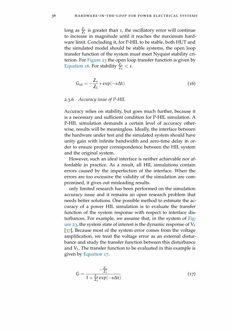
long as ZsZl
is greater than 1, the oscillatory error will continueto increase in magnitude until it reaches the maximum hard-ware limit. Concluding it, for P-HIL to be stable, both HUT andthe simulated model should be stable systems, the open looptransfer function of the system must meet Nyquist stability cri-terion. For Figure 23 the open loop transfer function is given byEquation 16. For stability Zs
Zl< 1.
Gol = −Zs
Zl∗ exp(−s∆t) (16)
2.3.6 Accuracy issue of P-HIL
Accuracy relies on stability, but goes much further, because itis a necessary and sufficient condition for P-HIL simulation. AP-HIL simulation demands a certain level of accuracy other-wise, results will be meaningless. Ideally, the interface betweenthe hardware under test and the simulated system should haveunity gain with infinite bandwidth and zero-time delay in or-der to ensure proper correspondence between the HIL systemand the original system.
However, such an ideal interface is neither achievable nor af-fordable in practice. As a result, all HIL simulations containerrors caused by the imperfection of the interface. When theerrors are too excessive the validity of the simulation are com-promised, it gives out misleading results.
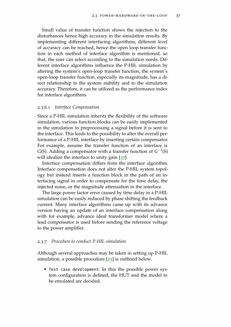
only limited research has been performed on the simulationaccuracy issue and it remains an open research problem thatneeds better solutions. One possible method to estimate the ac-curacy of a power HIL simulation is to evaluate the transferfunction of the system response with respect to interface dis-turbances. For example, we assume that, in the system of Fig-ure 23, the system state of interest is the dynamic response of V1[37], Because most of the system error comes from the voltageamplification, we treat the voltage error as an external distur-bance and study the transfer function between this disturbanceand V1. The transfer function to be evaluated in this example isgiven by Equation 17.
G =−ZsZl
1+ ZsZlexp(−s∆t)
(17)
2.3 power-hardware-in-the-loop 37
Small value of transfer function shows the rejection to thedisturbances hence high accuracy in the simulation results. Byimplementing different interfacing algorithms, different levelof accuracy can be reached, hence the open loop transfer func-tion in each method of interface algorithm is mentioned, sothat, the user can select according to the simulation needs. Dif-ferent interface algorithms influence the P-HIL simulation byaltering the system’s open-loop transfer function, the system’sopen-loop transfer function, especially its magnitude, has a di-rect relationship to the system stability and to the simulationaccuracy. Therefore, it can be utilized as the performance indexfor interface algorithms.
2.3.6.1 Interface Compensation
Since a P-HIL simulation inherits the flexibility of the softwaresimulation, various function blocks can be easily implementedin the simulation to preprocessing a signal before it is sent tothe interface. This leads to the possibility to alter the overall per-formance of a P-HIL interface by inserting certain compensator.For example, assume the transfer function of an interface isG(S). Adding a compensator with a transfer function of G−1(S)will idealize the interface to unity gain [37].
Interface compensation differs from the interface algorithm.Interface compensation does not alter the P-HIL system topol-ogy but instead inserts a function block in the path of an in-terfacing signal in order to compensate for the time delay, theinjected noise, or the magnitude attenuation in the interface.
The large power factor error caused by time delay in a P-HILsimulation can be easily reduced by phase shifting the feedbackcurrent. Many interface algorithms came up with its advanceversion having an update of an interface compensation alongwith for example, advance ideal transformer model where alead compensator is used before sending the reference voltageto the power amplifier.
2.3.7 Procedure to conduct P-HIL simulation
Although several approaches may be taken in setting up P-HILsimulation, a possible procedure [23] is outlined below.
• Test case development: In this the possible power sys-tem configuration is defined, the HUT and the model tobe emulated are decided.
38 hardware-in-the-loop for power electrical systems
• Selection and analysis of equipment: Selection of theRTDS, power amplifiers, measuring devices, filters IO’sare done in this phase.
• Modeling phase: Detailed model is built according to in-teraction of model with the real world.
• Execution of off-line simulation: Off-line simulationis conducted to check the feasibility of the model in openloop conditions without any feedback loops or the inputparameters from the outside real world.
• Verification of off-line system stability: Verificationof simulation system errors and signal accuracy etc.
• Stability evaluation: The open loop or closed loop trans-fer function is studied and appropriate measures are takento make system to be ensured to have stability criteria.
• I/O signal verification: The IO ports of the RTDS, HUTand ADC/DAC are verified and scaled according to theneeds of the simulation.
• integration and verification of hardware and software
safety: Alarm signals, trip signal initiations are designedfor the critical parameters to ensure the safety of the equip-ment and to the test.
• execution of online P-HIL simulation: Closed loop op-eration along with the interaction of the emulated systemwith the HUT considered in the real world in real-timeand gathering the generated results for further analysis.
Part II
A P P L I C AT I O N O F P - H I L I NR E N E WA B L E E N E R G Y S I M U L AT I O N
In this part in Chapter 3, I have presented the archi-tecture of the real-time digital simulator to conductHIL simulation of PV using the actual measurementtechnique with the use of a test bench. Afterwardsin Chapter 4, the detail explanation of modelling fol-lowing systems to conduct HIL experiment is pre-sented.
1. PV
2. MPPT control
3. Boost converter
4. storage
5. bi-directional DC-DC converter
The following tools are used to create the mathemat-ical model and to execute the real-time simulation.
1. MATLAB-Simulink
2. NI VeriStand
3. Model Interface tool-kit by NI
4. Simulink Coder
The main advantage of these tools are, they allow tocreate the mathematical model in model based de-sign environment like MATLAB-Simulink and thenby the use of Simulink coder, the code for the appro-priate targets can be generated automatically. Modelinterface tool-kit adds on Simulink and helps to gen-erate automatic code for NI hardware targets. NIVeriStand is used for execution of the real-time sim-ulation whose advantages are explained later. Thecreated test bench is being illustrated with the dis-cussion of results in Chapter 5.

3P R O P O S E D R E A L - T I M E S I M U L AT I O NA R C H I T E C T U R E
This chapter will brief about the employed architecture to con-duct real-time simulation, also the integration of mathematicalmodel to real-time target using VeriStand, a real-time digitalsimulator.
3.1 real-time digital simulator
As already seen in the previous chapter, RTDS plays a majorrole in HIL simulation, because of the model emulated is con-trolled by RTDS and it is only responsible for keeping the sim-ulation in real-time. It is also a software bridge between theemulated model in the target device and human, it providesthe HMI between the tester and the real-time target.
There are many types of RTDS present in the market by dif-ferent hardware manufacturers and the service providers. Toname few dSPACE, RT-LAB from Opal-RT, Simulink real-time,TestStand, VeriStand from National Instruments etc. Many ofthese RTDS are very costly and hardware proprietary. Theywork with only the recommended hardware.
For example Simulink real-time is a very good platform forreal-time simulation, it decreases the complexity of dependen-cies while generating the code but it works only with the speed-goat family of hardware. The hardware solution provided byOpal technologies are very bulky and should be installed atfixed place which makes it student un-friendly and Cost in-effective. Much flexible RTDS I found is VeriStand, it can workwith the numerous hardware suggested by National Instruments,also it allows the user to add custom hardware by followingsimple procedures. It’s architecture is designed by keeping inmind to support many of the communication protocol that arebeing used in recent days.
The model interface tool kit of VeriStand allows to importthe mathematical model using many model based design plat-forms and also with C coder. The hardware I have chosen towork with VeriStand is myRIO-1900 manufactured by NationalInstruments, it is very light and student friendly to use, it is
41
42 proposed real-time simulation architecture
widely used as Engineering teaching platform by most of thescholars across the world.
3.1.1 NI VeriStand
In this study ’NI VeriStand’ is used as RTDS where an FPGAcan be added as a target device [2]. It is a configuration-basedtesting software, specifically designed to run the real-time test-ing application, thus allowing us to develop and test controlsystem using hardware I/O and simulation models. It comeswith multi-core-ready real-time engine to execute tasks such asreal-time stimulus generation, data acquisition for high-speedand conditioned measurements. It can also import control al-gorithms, simulation models, and other tasks from LabVIEW,MATLAB and other third-party environments.
3.1.1.1 NI VeriStand Engine architecture
The NI VeriStand Engine is the execution mechanism that isresponsible for executing hardware I/O, models, procedures,alarms, and other test system tasks that are specified in thesystem definition file1.
The architecture of VeriStand engine consists of multiple timedloops, and its execution timing is controlled by hardware eventswith micro second resolution, the Figure 24 shows it’s architec-ture, it consists of four major loops.
• Primary control loop
• Model execution loops
• Data management loop
• Model interface loop
1. Primary control loop: The default execution rate is of 100
Hz and can be varied according to the requirement, itcontrols the timing for VeriStand Engine and maintainsthe most recent channel values. Per iteration, it reads andwrites the FPGA I/O, analog I/O, It speaks to all otherloops with the first in and first out (FIFO) channel andalso, it is only responsible for the creation of mappingconnections among various elements.
1 folder consisting of all the information of the test test setup including FPGAtarget and the models to be simulated in real-time
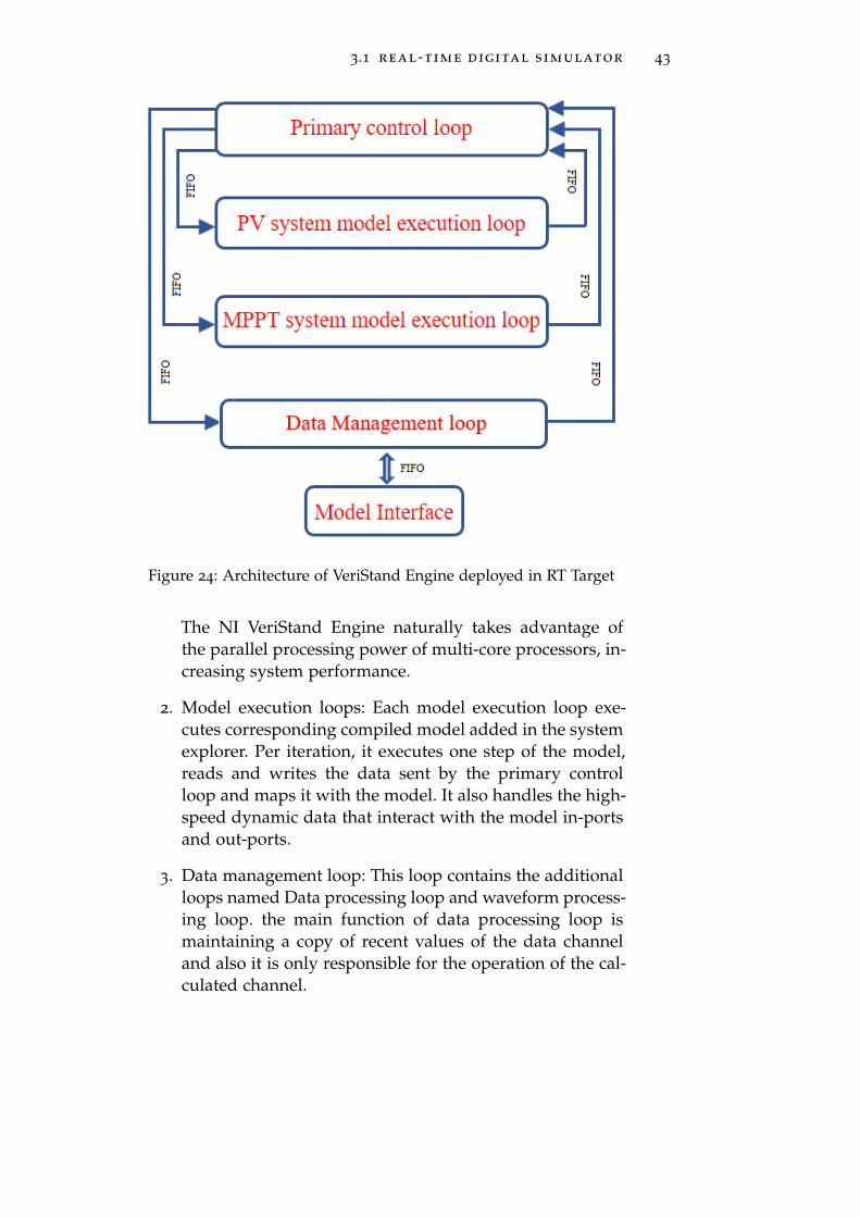
3.1 real-time digital simulator 43
Figure 24: Architecture of VeriStand Engine deployed in RT Target
The NI VeriStand Engine naturally takes advantage ofthe parallel processing power of multi-core processors, in-creasing system performance.
2. Model execution loops: Each model execution loop exe-cutes corresponding compiled model added in the systemexplorer. Per iteration, it executes one step of the model,reads and writes the data sent by the primary controlloop and maps it with the model. It also handles the high-speed dynamic data that interact with the model in-portsand out-ports.
3. Data management loop: This loop contains the additionalloops named Data processing loop and waveform process-ing loop. the main function of data processing loop ismaintaining a copy of recent values of the data channeland also it is only responsible for the operation of the cal-culated channel.
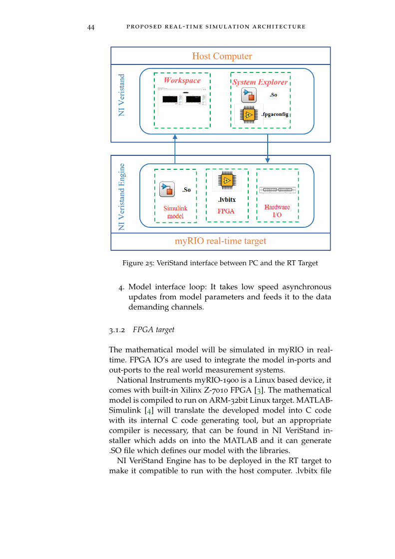
44 proposed real-time simulation architecture
Figure 25: VeriStand interface between PC and the RT Target
4. Model interface loop: It takes low speed asynchronousupdates from model parameters and feeds it to the datademanding channels.
3.1.2 FPGA target
The mathematical model will be simulated in myRIO in real-time. FPGA IO’s are used to integrate the model in-ports andout-ports to the real world measurement systems.
National Instruments myRIO-1900 is a Linux based device, itcomes with built-in Xilinx Z-7010 FPGA [3]. The mathematicalmodel is compiled to run on ARM-32bit Linux target. MATLAB-Simulink [4] will translate the developed model into C codewith its internal C code generating tool, but an appropriatecompiler is necessary, that can be found in NI VeriStand in-staller which adds on into the MATLAB and it can generate.SO file which defines our model with the libraries.
NI VeriStand Engine has to be deployed in the RT target tomake it compatible to run with the host computer. .lvbitx file
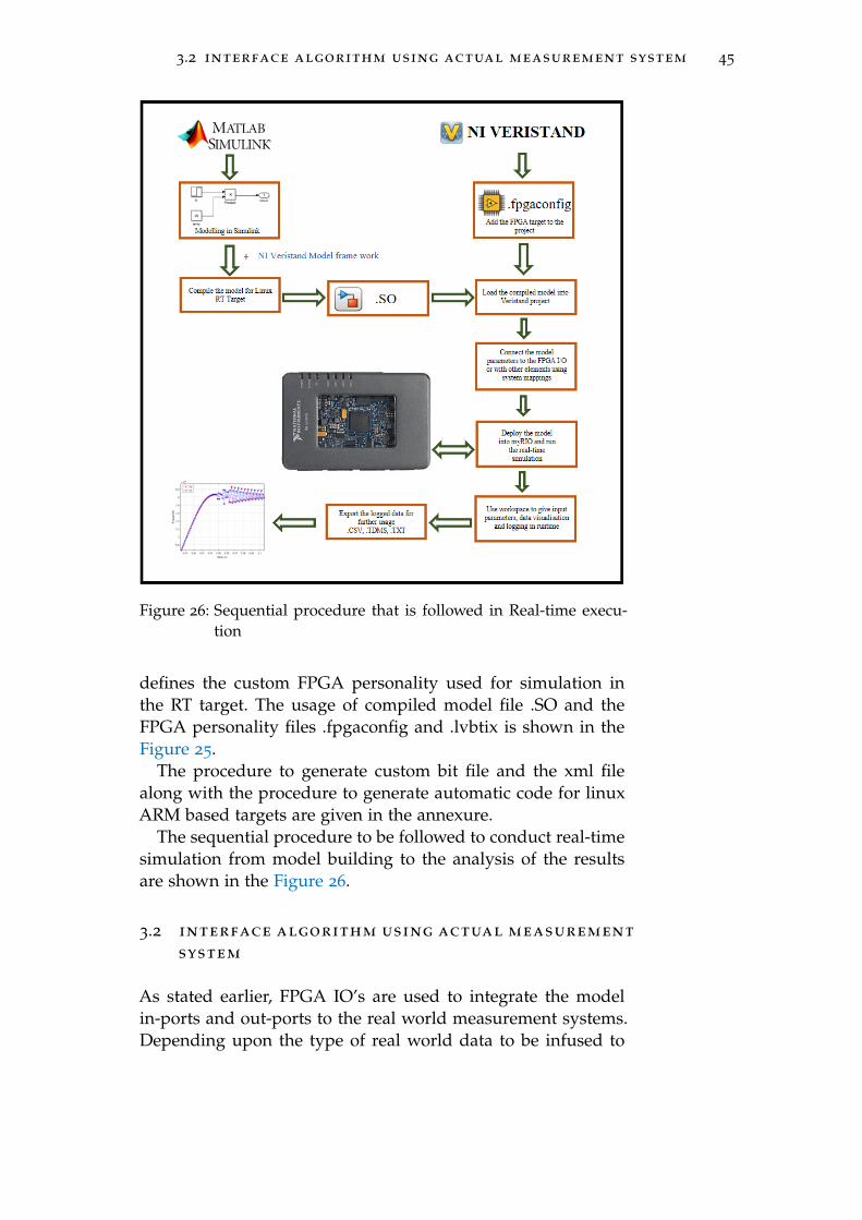
3.2 interface algorithm using actual measurement system 45
Figure 26: Sequential procedure that is followed in Real-time execu-tion
defines the custom FPGA personality used for simulation inthe RT target. The usage of compiled model file .SO and theFPGA personality files .fpgaconfig and .lvbtix is shown in theFigure 25.
The procedure to generate custom bit file and the xml filealong with the procedure to generate automatic code for linuxARM based targets are given in the annexure.
The sequential procedure to be followed to conduct real-timesimulation from model building to the analysis of the resultsare shown in the Figure 26.
3.2 interface algorithm using actual measurement
system
As stated earlier, FPGA IO’s are used to integrate the modelin-ports and out-ports to the real world measurement systems.Depending upon the type of real world data to be infused to
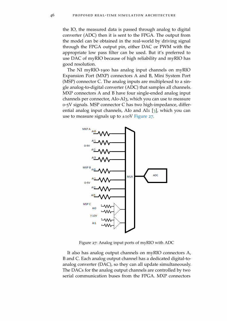
46 proposed real-time simulation architecture
the IO, the measured data is passed through analog to digitalconverter (ADC) then it is sent to the FPGA. The output fromthe model can be obtained in the real-world by driving signalthrough the FPGA output pin, either DAC or PWM with theappropriate low pass filter can be used. But it’s preferred touse DAC of myRIO because of high reliability and myRIO hasgood resolution.
The NI myRIO-1900 has analog input channels on myRIOExpansion Port (MXP) connectors A and B, Mini System Port(MSP) connector C. The analog inputs are multiplexed to a sin-gle analog-to-digital converter (ADC) that samples all channels.MXP connectors A and B have four single-ended analog inputchannels per connector, AI0-AI3, which you can use to measure0-5V signals. MSP connector C has two high-impedance, differ-ential analog input channels, AI0 and AI1 [3], which you canuse to measure signals up to ±10V Figure 27.
Figure 27: Analog input ports of myRIO with ADC
It also has analog output channels on myRIO connectors A,B and C. Each analog output channel has a dedicated digital-to-analog converter (DAC), so they can all update simultaneously.The DACs for the analog output channels are controlled by twoserial communication buses from the FPGA. MXP connectors
3.2 interface algorithm using actual measurement system 47
A and B share one bus, and MSP connector C and the audiooutputs share a second bus. MXP connectors A and B have twoanalog output channels per connector, AO0 and AO1, whichyou can use to generate 0-5 V signals. MSP connector C hastwo analog output channels, AO0 and AO1, which you can useto generate signals up to ±10 V.
Converting raw data values to voltage is done by incorporat-ing appropriate mathematical relation. For AI and AO channelson the MXP connectors, the ADC resolution in bits is 12.
LSBweight =5V
212= 1.221mV (18)
Maxreading = 4095 ∗ 1.221mV = 4.999V (19)
For AI and AO channels on the MSP connectors,
LSBweight =20V
212= 4.833mV (20)
Max+reading = +2047 ∗ 4.833mV = +9.995V (21)
Max−reading = −2048 ∗ 4.833mV = −10.000V (22)

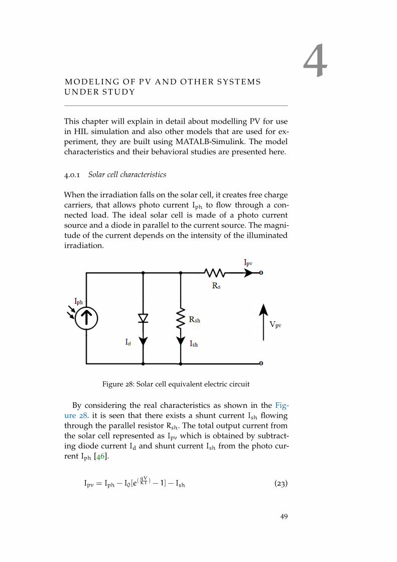
4M O D E L I N G O F P V A N D O T H E R S Y S T E M SU N D E R S T U D Y
This chapter will explain in detail about modelling PV for usein HIL simulation and also other models that are used for ex-periment, they are built using MATALB-Simulink. The modelcharacteristics and their behavioral studies are presented here.
4.0.1 Solar cell characteristics
When the irradiation falls on the solar cell, it creates free chargecarriers, that allows photo current Iph to flow through a con-nected load. The ideal solar cell is made of a photo currentsource and a diode in parallel to the current source. The magni-tude of the current depends on the intensity of the illuminatedirradiation.
Figure 28: Solar cell equivalent electric circuit
By considering the real characteristics as shown in the Fig-ure 28. it is seen that there exists a shunt current Ish flowingthrough the parallel resistor Rsh. The total output current fromthe solar cell represented as Ipv which is obtained by subtract-ing diode current Id and shunt current Ish from the photo cur-rent Iph [46].
Ipv = Iph − I0[e(qVKT ) − 1] − Ish (23)
49
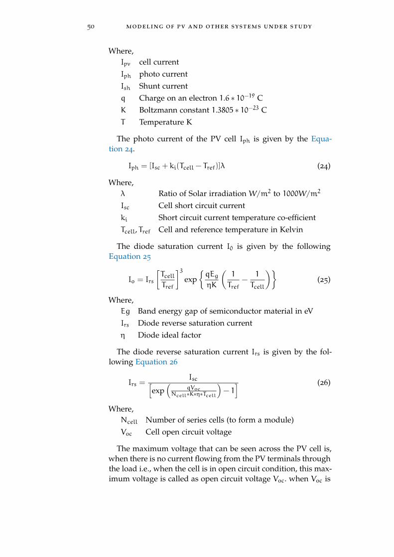
50 modeling of pv and other systems under study
Where,Ipv cell currentIph photo currentIsh Shunt currentq Charge on an electron 1.6 ∗ 10−19 CK Boltzmann constant 1.3805 ∗ 10−23 CT Temperature K
The photo current of the PV cell Iph is given by the Equa-tion 24.
Iph = [Isc + ki(Tcell − Tref)]λ (24)
Where,λ Ratio of Solar irradiation W/m2 to 1000W/m2
Isc Cell short circuit currentki Short circuit current temperature co-efficientTcell, Tref Cell and reference temperature in Kelvin
The diode saturation current I0 is given by the followingEquation 25
Io = Irs
[TcellTref
]3expqEg
ηK
(1
Tref−
1
Tcell
)(25)
Where,Eg Band energy gap of semiconductor material in eVIrs Diode reverse saturation currentη Diode ideal factor
The diode reverse saturation current Irs is given by the fol-lowing Equation 26
Irs =Isc[
exp(
qVocNcell∗K∗η∗Tcell
)− 1] (26)
Where,Ncell Number of series cells (to form a module)Voc Cell open circuit voltage
The maximum voltage that can be seen across the PV cell is,when there is no current flowing from the PV terminals throughthe load i.e., when the cell is in open circuit condition, this max-imum voltage is called as open circuit voltage Voc. when Voc is
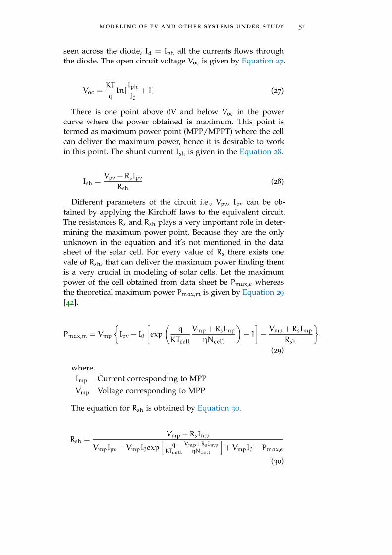
modeling of pv and other systems under study 51
seen across the diode, Id = Iph all the currents flows throughthe diode. The open circuit voltage Voc is given by Equation 27.
Voc =KT
qln[Iph
I0+ 1] (27)
There is one point above 0V and below Voc in the powercurve where the power obtained is maximum. This point istermed as maximum power point (MPP/MPPT) where the cellcan deliver the maximum power, hence it is desirable to workin this point. The shunt current Ish is given in the Equation 28.
Ish =Vpv − RsIpv
Rsh(28)
Different parameters of the circuit i.e., Vpv, Ipv can be ob-tained by applying the Kirchoff laws to the equivalent circuit.The resistances Rs and Rsh plays a very important role in deter-mining the maximum power point. Because they are the onlyunknown in the equation and it’s not mentioned in the datasheet of the solar cell. For every value of Rs there exists onevale of Rsh, that can deliver the maximum power finding themis a very crucial in modeling of solar cells. Let the maximumpower of the cell obtained from data sheet be Pmax,e whereasthe theoretical maximum power Pmax,m is given by Equation 29
[42].
Pmax,m = Vmp
Ipv − I0
[exp
(q
KTcell
Vmp + RsImpηNcell
)− 1
]−Vmp + RsImp
Rsh
(29)
where,Imp Current corresponding to MPPVmp Voltage corresponding to MPP
The equation for Rsh is obtained by Equation 30.
Rsh =Vmp + RsImp
VmpIpv − VmpI0exp[
qKTcell
Vmp+RsImp
ηNcell
]+ VmpI0 − Pmax,e
(30)
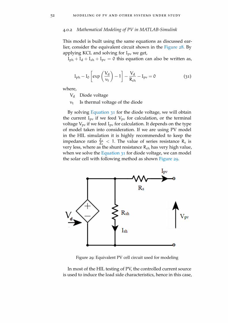
52 modeling of pv and other systems under study
4.0.2 Mathematical Modeling of PV in MATLAB-Simulink
This model is built using the same equations as discussed ear-lier, consider the equivalent circuit shown in the Figure 28. Byapplying KCL and solving for Ipv we get,Iph + Id + Ish + Ipv = 0 this equation can also be written as,
Iph − I0
[exp
(Vdvt
)− 1
]−VdRsh
− Ipv = 0 (31)
where,Vd Diode voltagevt Is thermal voltage of the diode
By solving Equation 31 for the diode voltage, we will obtainthe current Ipv if we feed Vpv for calculation, or the terminalvoltage Vpv if we feed Ipv for calculation. It depends on the typeof model taken into consideration. If we are using PV modelin the HIL simulation it is highly recommended to keep theimpedance ratio Zs
Zl< 1. The value of series resistance Rs is
very less, where as the shunt resistance Rsh has very high value,when we solve the Equation 31 for diode voltage, we can modelthe solar cell with following method as shown Figure 29.
Figure 29: Equivalent PV cell circuit used for modeling
In most of the HIL testing of PV, the controlled current sourceis used to induce the load side characteristics, hence in this case,
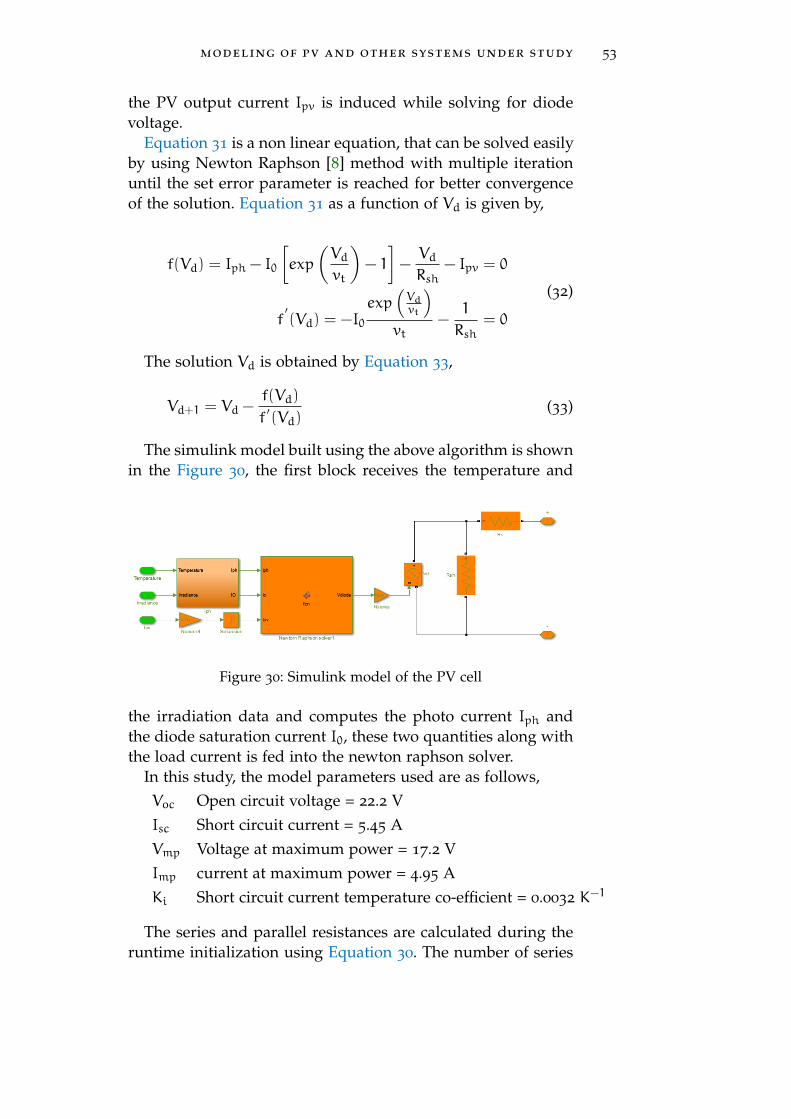
modeling of pv and other systems under study 53
the PV output current Ipv is induced while solving for diodevoltage.
Equation 31 is a non linear equation, that can be solved easilyby using Newton Raphson [8] method with multiple iterationuntil the set error parameter is reached for better convergenceof the solution. Equation 31 as a function of Vd is given by,
f(Vd) = Iph − I0
[exp
(Vdvt
)− 1
]−VdRsh
− Ipv = 0
f′(Vd) = −I0
exp(Vdvt
)vt
−1
Rsh= 0
(32)
The solution Vd is obtained by Equation 33,
Vd+1 = Vd −f(Vd)
f′(Vd)
(33)
The simulink model built using the above algorithm is shownin the Figure 30, the first block receives the temperature and
Figure 30: Simulink model of the PV cell
the irradiation data and computes the photo current Iph andthe diode saturation current I0, these two quantities along withthe load current is fed into the newton raphson solver.
In this study, the model parameters used are as follows,Voc Open circuit voltage = 22.2 VIsc Short circuit current = 5.45 AVmp Voltage at maximum power = 17.2 VImp current at maximum power = 4.95 AKi Short circuit current temperature co-efficient = 0.0032 K−1
The series and parallel resistances are calculated during theruntime initialization using Equation 30. The number of series
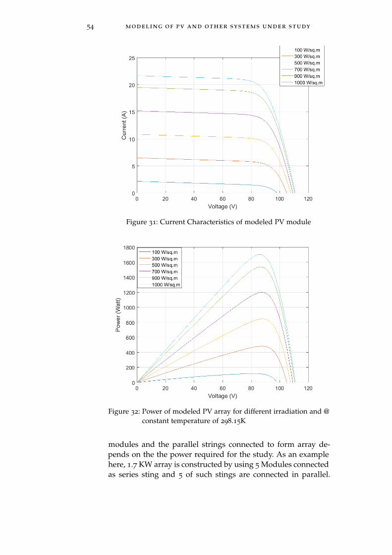
54 modeling of pv and other systems under study
Figure 31: Current Characteristics of modeled PV module
Figure 32: Power of modeled PV array for different irradiation and @constant temperature of 298.15K
modules and the parallel strings connected to form array de-pends on the the power required for the study. As an examplehere, 1.7 KW array is constructed by using 5 Modules connectedas series sting and 5 of such stings are connected in parallel.
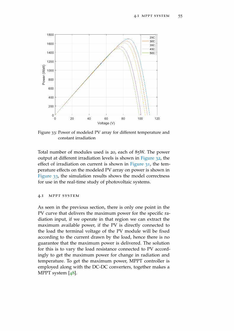
4.1 mppt system 55
Figure 33: Power of modeled PV array for different temperature andconstant irradiation
Total number of modules used is 20, each of 85W. The poweroutput at different irradiation levels is shown in Figure 32, theeffect of irradiation on current is shown in Figure 31, the tem-perature effects on the modeled PV array on power is shown inFigure 33, the simulation results shows the model correctnessfor use in the real-time study of photovoltaic systems.
4.1 mppt system
As seen in the previous section, there is only one point in thePV curve that delivers the maximum power for the specific ra-diation input, if we operate in that region we can extract themaximum available power, if the PV is directly connected tothe load the terminal voltage of the PV module will be fixedaccording to the current drawn by the load, hence there is noguarantee that the maximum power is delivered. The solutionfor this is to vary the load resistance connected to PV accord-ingly to get the maximum power for change in radiation andtemperature. To get the maximum power, MPPT controller isemployed along with the DC-DC converters, together makes aMPPT system [48].
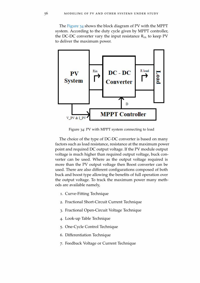
56 modeling of pv and other systems under study
The Figure 34 shows the block diagram of PV with the MPPTsystem. According to the duty cycle given by MPPT controller,the DC-DC converter vary the input resistance Rin to keep PVto deliver the maximum power.
Figure 34: PV with MPPT system connecting to load
The choice of the type of DC-DC converter is based on manyfactors such as load resistance, resistance at the maximum powerpoint and required DC output voltage. If the PV module outputvoltage is much higher than required output voltage, buck con-verter can be used. Where as the output voltage required ismore than the PV output voltage then Boost converter can beused. There are also different configurations composed of bothbuck and boost type allowing the benefits of full operation overthe output voltage. To track the maximum power many meth-ods are available namely,
1. Curve-Fitting Technique
2. Fractional Short-Circuit Current Technique
3. Fractional Open-Circuit Voltage Technique
4. Look-up Table Technique
5. One-Cycle Control Technique
6. Differentiation Technique
7. Feedback Voltage or Current Technique
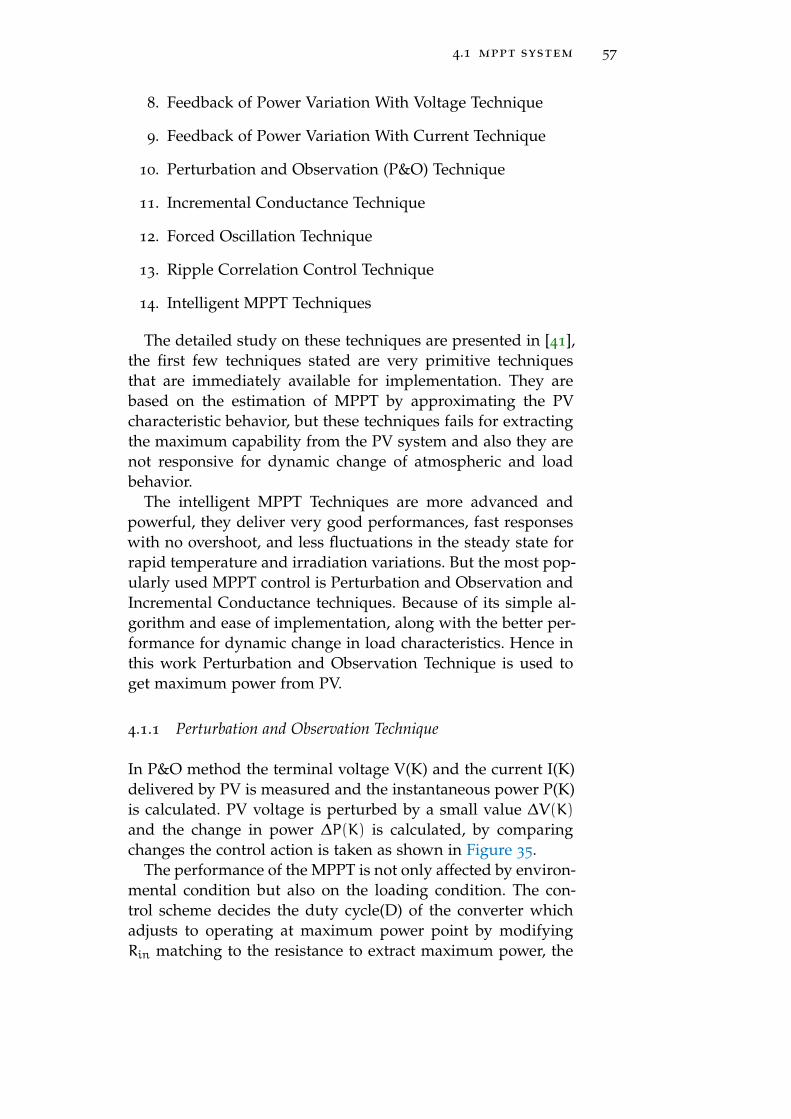
4.1 mppt system 57
8. Feedback of Power Variation With Voltage Technique
9. Feedback of Power Variation With Current Technique
10. Perturbation and Observation (P&O) Technique
11. Incremental Conductance Technique
12. Forced Oscillation Technique
13. Ripple Correlation Control Technique
14. Intelligent MPPT Techniques
The detailed study on these techniques are presented in [41],the first few techniques stated are very primitive techniquesthat are immediately available for implementation. They arebased on the estimation of MPPT by approximating the PVcharacteristic behavior, but these techniques fails for extractingthe maximum capability from the PV system and also they arenot responsive for dynamic change of atmospheric and loadbehavior.
The intelligent MPPT Techniques are more advanced andpowerful, they deliver very good performances, fast responseswith no overshoot, and less fluctuations in the steady state forrapid temperature and irradiation variations. But the most pop-ularly used MPPT control is Perturbation and Observation andIncremental Conductance techniques. Because of its simple al-gorithm and ease of implementation, along with the better per-formance for dynamic change in load characteristics. Hence inthis work Perturbation and Observation Technique is used toget maximum power from PV.
4.1.1 Perturbation and Observation Technique
In P&O method the terminal voltage V(K) and the current I(K)delivered by PV is measured and the instantaneous power P(K)is calculated. PV voltage is perturbed by a small value ∆V(K)and the change in power ∆P(K) is calculated, by comparingchanges the control action is taken as shown in Figure 35.
The performance of the MPPT is not only affected by environ-mental condition but also on the loading condition. The con-trol scheme decides the duty cycle(D) of the converter whichadjusts to operating at maximum power point by modifyingRin matching to the resistance to extract maximum power, the
58 modeling of pv and other systems under study
Figure 35: Perturbation and Observation Technique flowchart
Simulink model is built using math script block, based on theabove algorithm.
4.1.2 Boost Converter
In this work it’s likely to operate with Boost converter, as out-put voltage required is more than the PV terminal voltage [11],the output voltage of the converter Vo is given by Equation 34,The schematic diagram of boost converter is shown in the Fig-ure 36, an average model is built in Simulink for the same.
Vo =Vpv
1−D(34)
where,

4.1 mppt system 59
Vo Converter output voltageVpv PV terminal voltageD Duty cycle issued by the MPPT controller
Figure 36: Schematic diagram of Boost Converter
4.1.3 Storage System
The generic battery model is used in this work, it consists ofa controlled voltage source connected to a resistance [45], themodel of the battery is as shown in the Figure 37. The stateof the charge of the battery is implemented as state variable toavoid the algebraic loop.
Figure 37: Generic battery model
The open circuit voltage is given as Equation 35,
Voc = E0 −KQ
Q−∫i ∗ dt
i− R0i (35)
where,
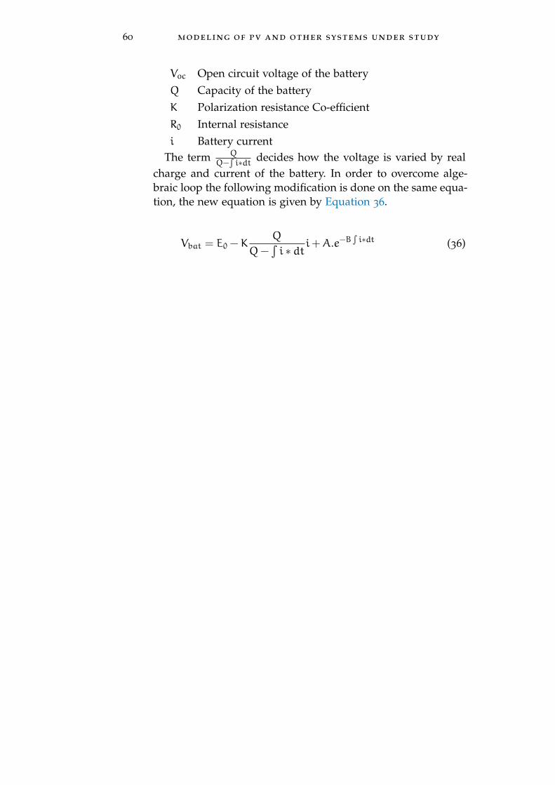
60 modeling of pv and other systems under study
Voc Open circuit voltage of the batteryQ Capacity of the batteryK Polarization resistance Co-efficientR0 Internal resistancei Battery current
The term QQ−∫i∗dt decides how the voltage is varied by real
charge and current of the battery. In order to overcome alge-braic loop the following modification is done on the same equa-tion, the new equation is given by Equation 36.
Vbat = E0 −KQ
Q−∫i ∗ dt
i+A.e−B∫i∗dt (36)
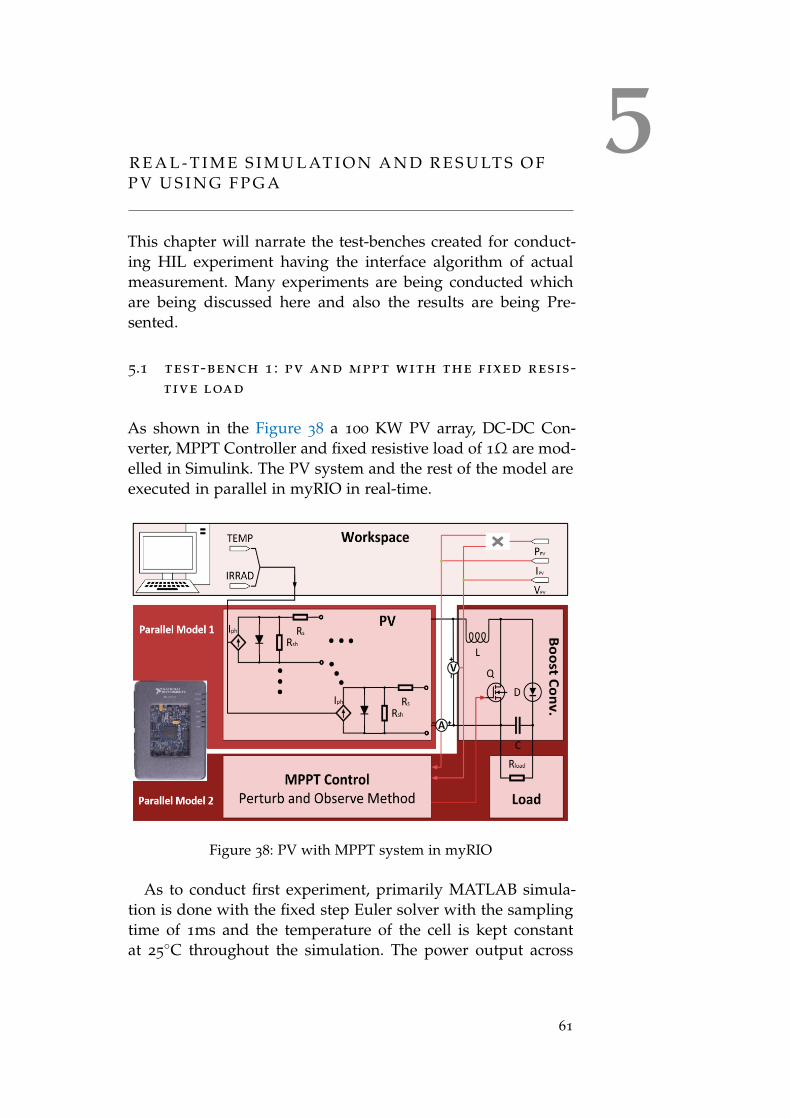
5R E A L - T I M E S I M U L AT I O N A N D R E S U LT S O FP V U S I N G F P G A
This chapter will narrate the test-benches created for conduct-ing HIL experiment having the interface algorithm of actualmeasurement. Many experiments are being conducted whichare being discussed here and also the results are being Pre-sented.
5.1 test-bench 1 : pv and mppt with the fixed resis-tive load
As shown in the Figure 38 a 100 KW PV array, DC-DC Con-verter, MPPT Controller and fixed resistive load of 1Ω are mod-elled in Simulink. The PV system and the rest of the model areexecuted in parallel in myRIO in real-time.
Figure 38: PV with MPPT system in myRIO
As to conduct first experiment, primarily MATLAB simula-tion is done with the fixed step Euler solver with the samplingtime of 1ms and the temperature of the cell is kept constantat 25
C throughout the simulation. The power output across
61
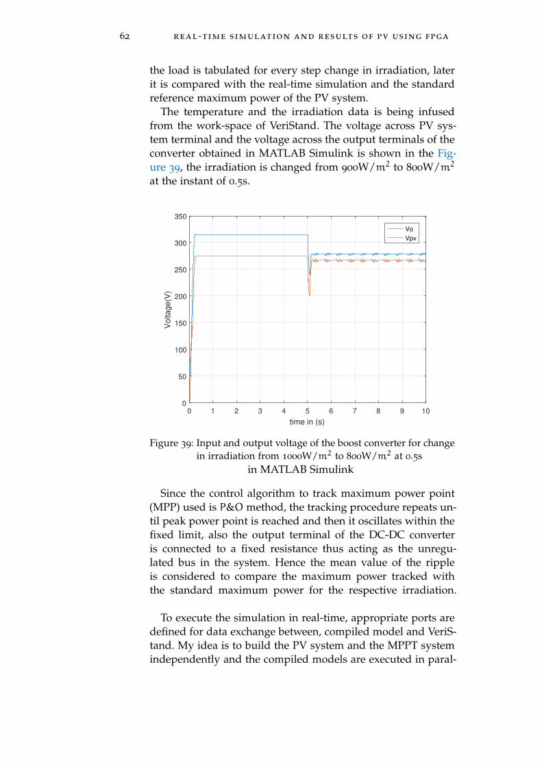
62 real-time simulation and results of pv using fpga
the load is tabulated for every step change in irradiation, laterit is compared with the real-time simulation and the standardreference maximum power of the PV system.
The temperature and the irradiation data is being infusedfrom the work-space of VeriStand. The voltage across PV sys-tem terminal and the voltage across the output terminals of theconverter obtained in MATLAB Simulink is shown in the Fig-ure 39, the irradiation is changed from 900W/m2 to 800W/m2
at the instant of 0.5s.
0 1 2 3 4 5 6 7 8 9 10
time in (s)
0
50
100
150
200
250
300
350
Voltage(V
)
Vo
Vpv
Figure 39: Input and output voltage of the boost converter for changein irradiation from 1000W/m2 to 800W/m2 at 0.5s
in MATLAB Simulink
Since the control algorithm to track maximum power point(MPP) used is P&O method, the tracking procedure repeats un-til peak power point is reached and then it oscillates within thefixed limit, also the output terminal of the DC-DC converteris connected to a fixed resistance thus acting as the unregu-lated bus in the system. Hence the mean value of the rippleis considered to compare the maximum power tracked withthe standard maximum power for the respective irradiation.
To execute the simulation in real-time, appropriate ports aredefined for data exchange between, compiled model and VeriS-tand. My idea is to build the PV system and the MPPT systemindependently and the compiled models are executed in paral-
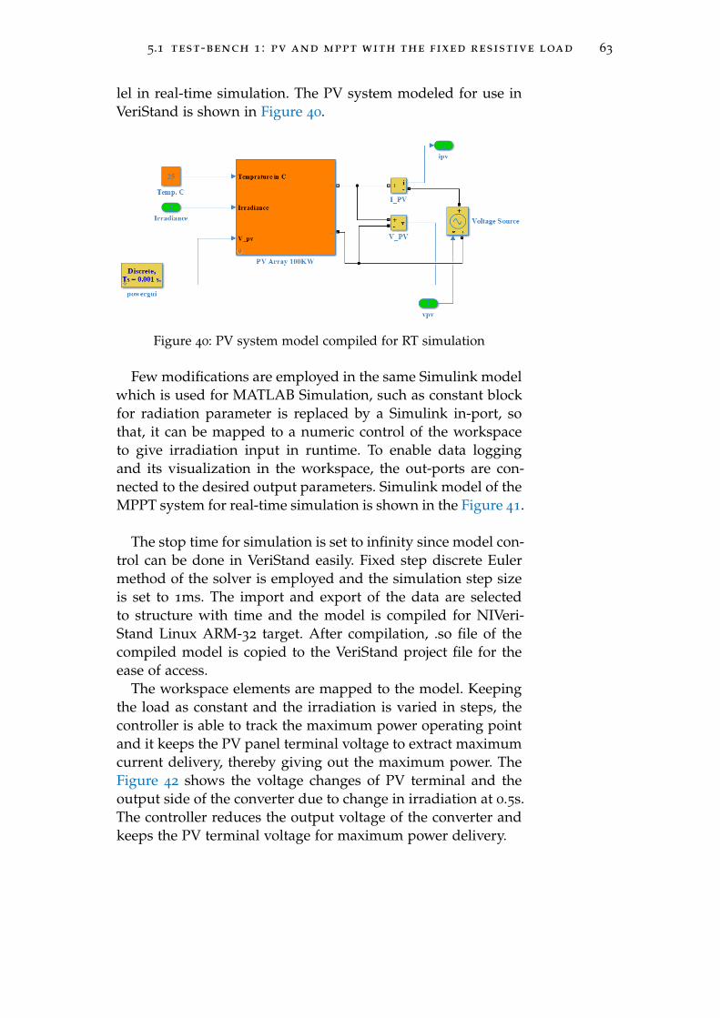
5.1 test-bench 1 : pv and mppt with the fixed resistive load 63
lel in real-time simulation. The PV system modeled for use inVeriStand is shown in Figure 40.
Figure 40: PV system model compiled for RT simulation
Few modifications are employed in the same Simulink modelwhich is used for MATLAB Simulation, such as constant blockfor radiation parameter is replaced by a Simulink in-port, sothat, it can be mapped to a numeric control of the workspaceto give irradiation input in runtime. To enable data loggingand its visualization in the workspace, the out-ports are con-nected to the desired output parameters. Simulink model of theMPPT system for real-time simulation is shown in the Figure 41.
The stop time for simulation is set to infinity since model con-trol can be done in VeriStand easily. Fixed step discrete Eulermethod of the solver is employed and the simulation step sizeis set to 1ms. The import and export of the data are selectedto structure with time and the model is compiled for NIVeri-Stand Linux ARM-32 target. After compilation, .so file of thecompiled model is copied to the VeriStand project file for theease of access.
The workspace elements are mapped to the model. Keepingthe load as constant and the irradiation is varied in steps, thecontroller is able to track the maximum power operating pointand it keeps the PV panel terminal voltage to extract maximumcurrent delivery, thereby giving out the maximum power. TheFigure 42 shows the voltage changes of PV terminal and theoutput side of the converter due to change in irradiation at 0.5s.The controller reduces the output voltage of the converter andkeeps the PV terminal voltage for maximum power delivery.
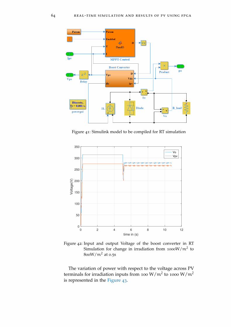
64 real-time simulation and results of pv using fpga
Figure 41: Simulink model to be compiled for RT simulation
0 2 4 6 8 10 12
time in (s)
0
50
100
150
200
250
300
350
Voltage(V
)
Vo
Vpv
Figure 42: Input and output Voltage of the boost converter in RTSimulation for change in irradiation from 1000W/m2 to800W/m2 at 0.5s
The variation of power with respect to the voltage across PVterminals for irradiation inputs from 100 W/m2 to 1000 W/m2
is represented in the Figure 43.
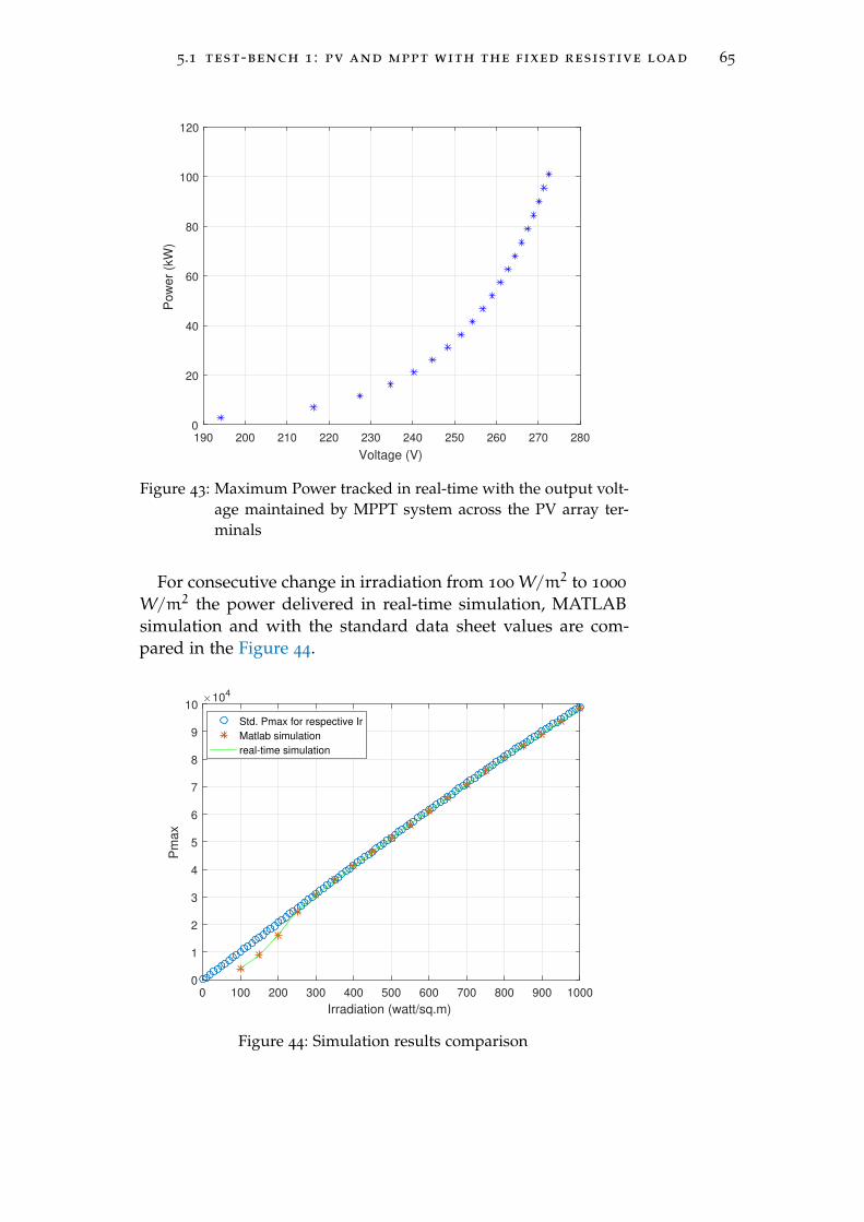
5.1 test-bench 1 : pv and mppt with the fixed resistive load 65
190 200 210 220 230 240 250 260 270 280
Voltage (V)
0
20
40
60
80
100
120
Pow
er
(kW
)
Figure 43: Maximum Power tracked in real-time with the output volt-age maintained by MPPT system across the PV array ter-minals
For consecutive change in irradiation from 100 W/m2 to 1000
W/m2 the power delivered in real-time simulation, MATLABsimulation and with the standard data sheet values are com-pared in the Figure 44.
0 100 200 300 400 500 600 700 800 900 1000
Irradiation (watt/sq.m)
0
1
2
3
4
5
6
7
8
9
10
Pm
ax
×104
Std. Pmax for respective Ir
Matlab simulation
real-time simulation
Figure 44: Simulation results comparison
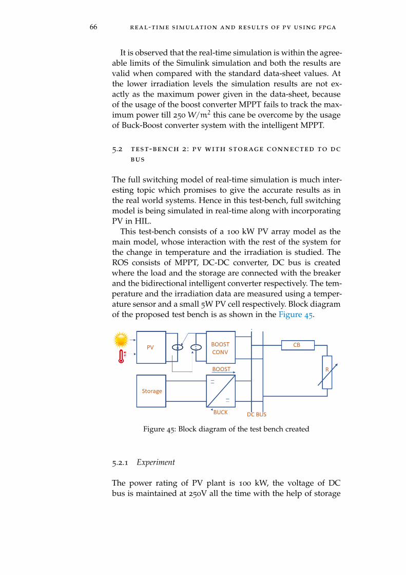
66 real-time simulation and results of pv using fpga
It is observed that the real-time simulation is within the agree-able limits of the Simulink simulation and both the results arevalid when compared with the standard data-sheet values. Atthe lower irradiation levels the simulation results are not ex-actly as the maximum power given in the data-sheet, becauseof the usage of the boost converter MPPT fails to track the max-imum power till 250 W/m2 this cane be overcome by the usageof Buck-Boost converter system with the intelligent MPPT.
5.2 test-bench 2 : pv with storage connected to dc
bus
The full switching model of real-time simulation is much inter-esting topic which promises to give the accurate results as inthe real world systems. Hence in this test-bench, full switchingmodel is being simulated in real-time along with incorporatingPV in HIL.
This test-bench consists of a 100 kW PV array model as themain model, whose interaction with the rest of the system forthe change in temperature and the irradiation is studied. TheROS consists of MPPT, DC-DC converter, DC bus is createdwhere the load and the storage are connected with the breakerand the bidirectional intelligent converter respectively. The tem-perature and the irradiation data are measured using a temper-ature sensor and a small 5W PV cell respectively. Block diagramof the proposed test bench is as shown in the Figure 45.
Figure 45: Block diagram of the test bench created
5.2.1 Experiment
The power rating of PV plant is 100 kW, the voltage of DCbus is maintained at 250V all the time with the help of storage
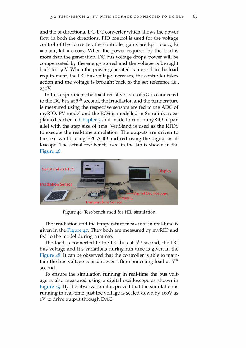
5.2 test-bench 2 : pv with storage connected to dc bus 67
and the bi-directional DC-DC converter which allows the powerflow in both the directions. PID control is used for the voltagecontrol of the converter, the controller gains are kp = 0.055, ki= 0.001, kd = 0.0003. When the power required by the load ismore than the generation, DC bus voltage drops, power will becompensated by the energy stored and the voltage is broughtback to 250V. When the power generated is more than the loadrequirement, the DC bus voltage increases, the controller takesaction and the voltage is brought back to the set reference i.e.,250V.
In this experiment the fixed resistive load of 1Ω is connectedto the DC bus at 5th second, the irradiation and the temperatureis measured using the respective sensors are fed to the ADC ofmyRIO. PV model and the ROS is modelled in Simulink as ex-plained earlier in Chapter 3 and made to run in myRIO in par-allel with the step size of 1ms, VeriStand is used as the RTDSto execute the real-time simulation. The outputs are driven tothe real world using FPGA IO and red using the digital oscil-loscope. The actual test bench used in the lab is shown in theFigure 46.
Figure 46: Test-bench used for HIL simulation
The irradiation and the temperature measured in real-time isgiven in the Figure 47. They both are measured by myRIO andfed to the model during runtime.
The load is connected to the DC bus at 5th second, the DCbus voltage and it’s variations during run-time is given in theFigure 48. It can be observed that the controller is able to main-tain the bus voltage constant even after connecting load at 5th
second.To ensure the simulation running in real-time the bus volt-
age is also measured using a digital oscilloscope as shown inFigure 49. By the observation it is proved that the simulation isrunning in real-time, just the voltage is scaled down by 100V as1V to drive output through DAC.
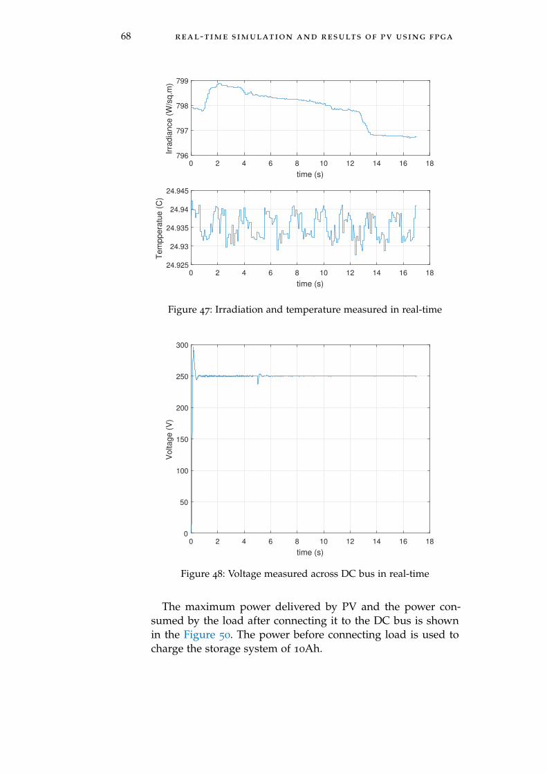
68 real-time simulation and results of pv using fpga
0 2 4 6 8 10 12 14 16 18
time (s)
796
797
798
799
Irra
dia
nce (
W/s
q.m
)
0 2 4 6 8 10 12 14 16 18
time (s)
24.925
24.93
24.935
24.94
24.945
Tem
ppera
tue (
C)
Figure 47: Irradiation and temperature measured in real-time
0 2 4 6 8 10 12 14 16 18
time (s)
0
50
100
150
200
250
300
Voltage (
V)
Figure 48: Voltage measured across DC bus in real-time
The maximum power delivered by PV and the power con-sumed by the load after connecting it to the DC bus is shownin the Figure 50. The power before connecting load is used tocharge the storage system of 10Ah.
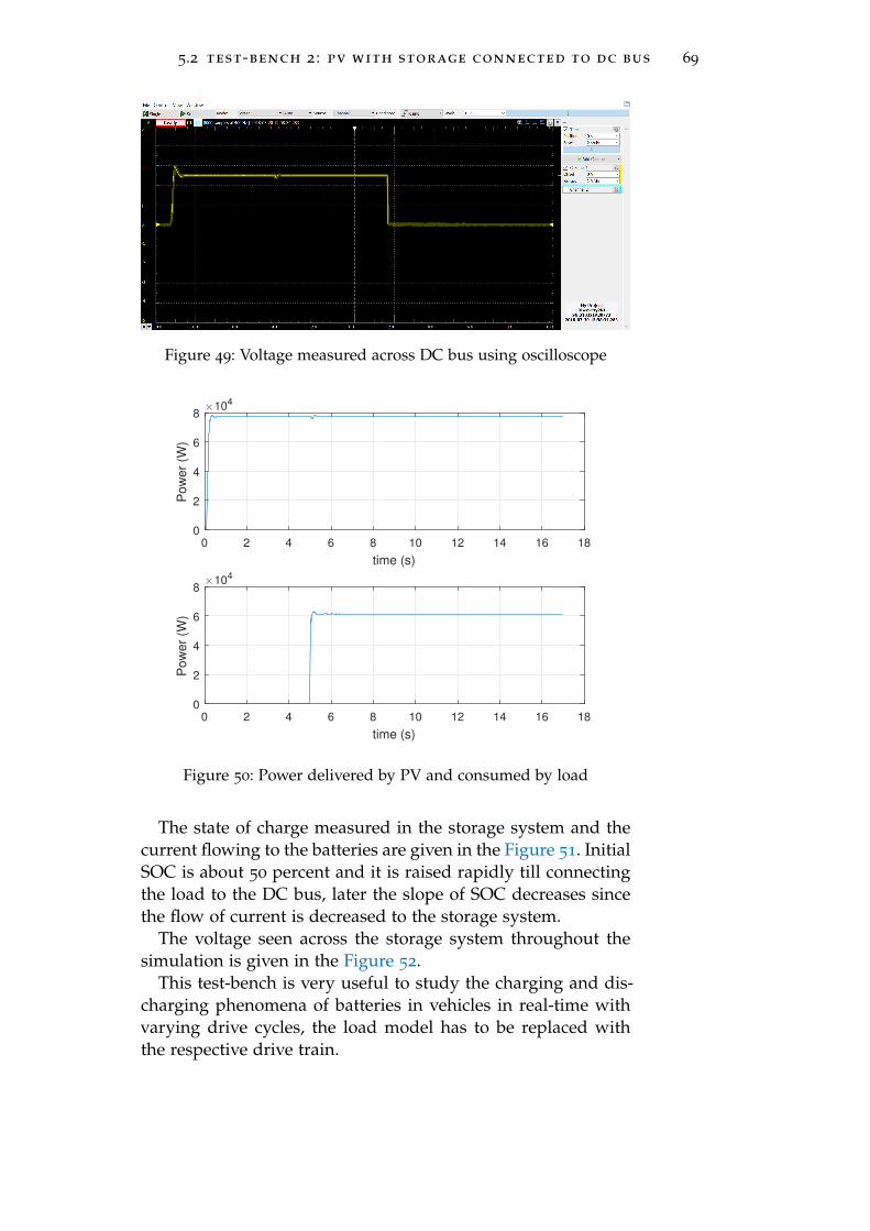
5.2 test-bench 2 : pv with storage connected to dc bus 69
Figure 49: Voltage measured across DC bus using oscilloscope
0 2 4 6 8 10 12 14 16 18
time (s)
0
2
4
6
8
Pow
er
(W)
104
0 2 4 6 8 10 12 14 16 18
time (s)
0
2
4
6
8
Pow
er
(W)
104
Figure 50: Power delivered by PV and consumed by load
The state of charge measured in the storage system and thecurrent flowing to the batteries are given in the Figure 51. InitialSOC is about 50 percent and it is raised rapidly till connectingthe load to the DC bus, later the slope of SOC decreases sincethe flow of current is decreased to the storage system.
The voltage seen across the storage system throughout thesimulation is given in the Figure 52.
This test-bench is very useful to study the charging and dis-charging phenomena of batteries in vehicles in real-time withvarying drive cycles, the load model has to be replaced withthe respective drive train.
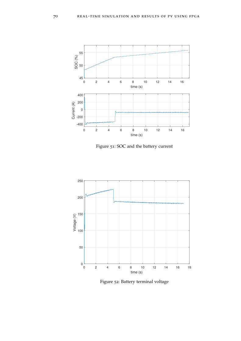
70 real-time simulation and results of pv using fpga
0 2 4 6 8 10 12 14 16
time (s)
45
50
55
SO
C (
%)
0 2 4 6 8 10 12 14 16
time (s)
-400
-200
0
200
400
Curr
ent (A
)
Figure 51: SOC and the battery current
0 2 4 6 8 10 12 14 16 18
time (s)
0
50
100
150
200
250
Voltage (
V)
Figure 52: Battery terminal voltage
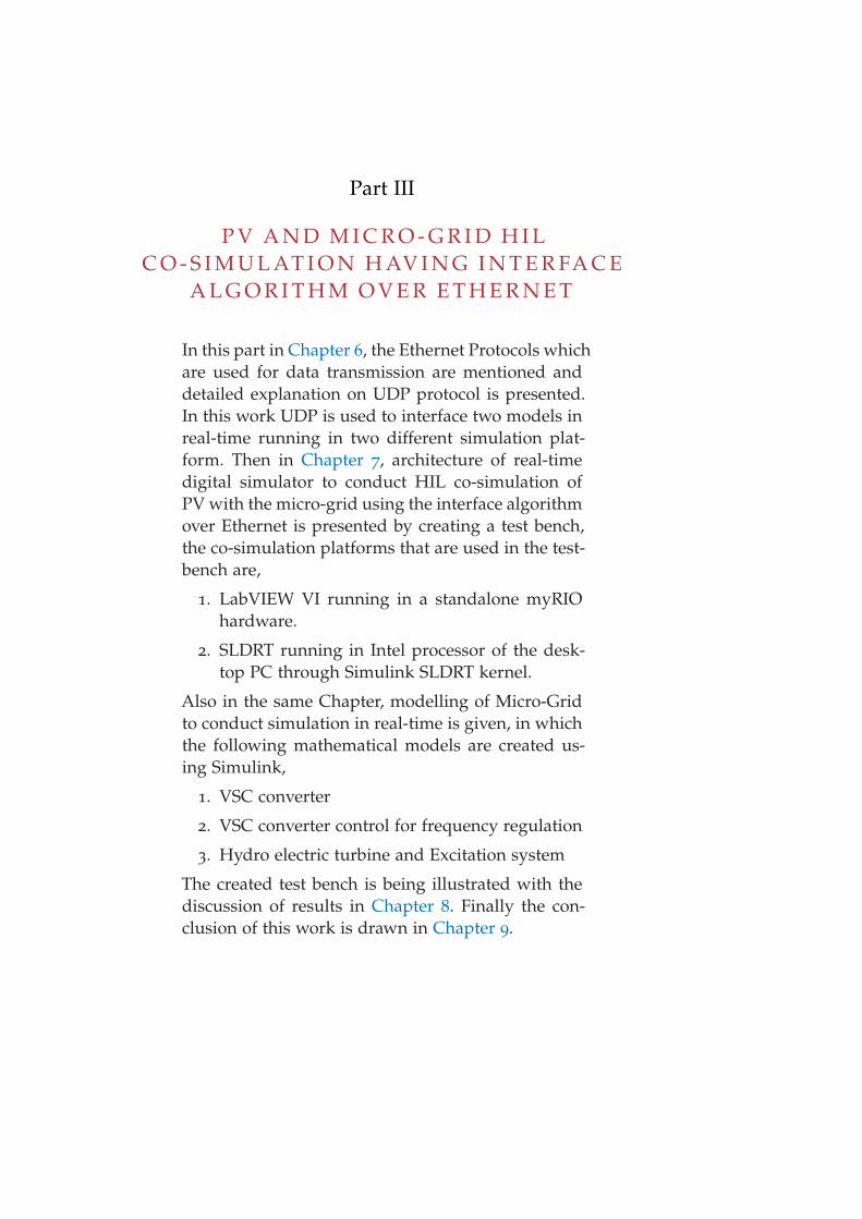
Part III
P V A N D M I C R O - G R I D H I LC O - S I M U L AT I O N H AV I N G I N T E R FA C E
A L G O R I T H M O V E R E T H E R N E T
In this part in Chapter 6, the Ethernet Protocols whichare used for data transmission are mentioned anddetailed explanation on UDP protocol is presented.In this work UDP is used to interface two models inreal-time running in two different simulation plat-form. Then in Chapter 7, architecture of real-timedigital simulator to conduct HIL co-simulation ofPV with the micro-grid using the interface algorithmover Ethernet is presented by creating a test bench,the co-simulation platforms that are used in the test-bench are,
1. LabVIEW VI running in a standalone myRIOhardware.
2. SLDRT running in Intel processor of the desk-top PC through Simulink SLDRT kernel.
Also in the same Chapter, modelling of Micro-Gridto conduct simulation in real-time is given, in whichthe following mathematical models are created us-ing Simulink,
1. VSC converter
2. VSC converter control for frequency regulation
3. Hydro electric turbine and Excitation system
The created test bench is being illustrated with thediscussion of results in Chapter 8. Finally the con-clusion of this work is drawn in Chapter 9.

6E T H E R N E T P R O T O C O L F O R RT S I M U L AT I O N S
This chapter will narrate the need of Ethernet Protocols for RTsimulation, available methods of data communication and thebest suited method to conduct HIL experiment using interfac-ing algorithm over Ethernet.
6.1 need of interface algorithm over ethernet
There are numerous products available providing solutions todifferent kind of problems, the creation of a system to solvea particular problem may involve different products. Depend-ing on the need and the expertise service given by the compa-nies/products in the filed of interest makes the system morecomplex and it need to be followed a standard protocol forcommunication among different components of the same sys-tem. The designer has the responsibility to verify the feasibil-ity of the solution proposed by him for the problem hence, co-simulation plays an important role in these aspects.
In co-simulation the different subsystems which form a cou-pled problem are modeled and simulated in a distributed man-ner. Hence, the modeling is done on the subsystem level with-out having the coupled problem in mind. Furthermore, the cou-pled simulation is carried out by running the subsystems in ablack-box manner. During the simulation the subsystems willexchange data. Co-simulation can be considered as the jointsimulation of the already well-established tools and semantics;when they are simulated with their suitable solvers.
Co-simulation proves its advantage in validation of multi-domain and cyber physical system by offering a flexible solu-tion which allows consideration of multiple domains with dif-ferent time steps, at the same time. As the calculation load isshared among simulators, co-simulation also enables the possi-bility of large scale system assessment.
In the previous test-benches real-time simulation was doneusing NI VeriStand as RTDS and NI myRIO as target devicewhich are custom solutions given by National Instruments. Veri-Stand fails to have real-time characteristics with myRIO withthe step size less than 1ms, though myRIO has ability to reach
73
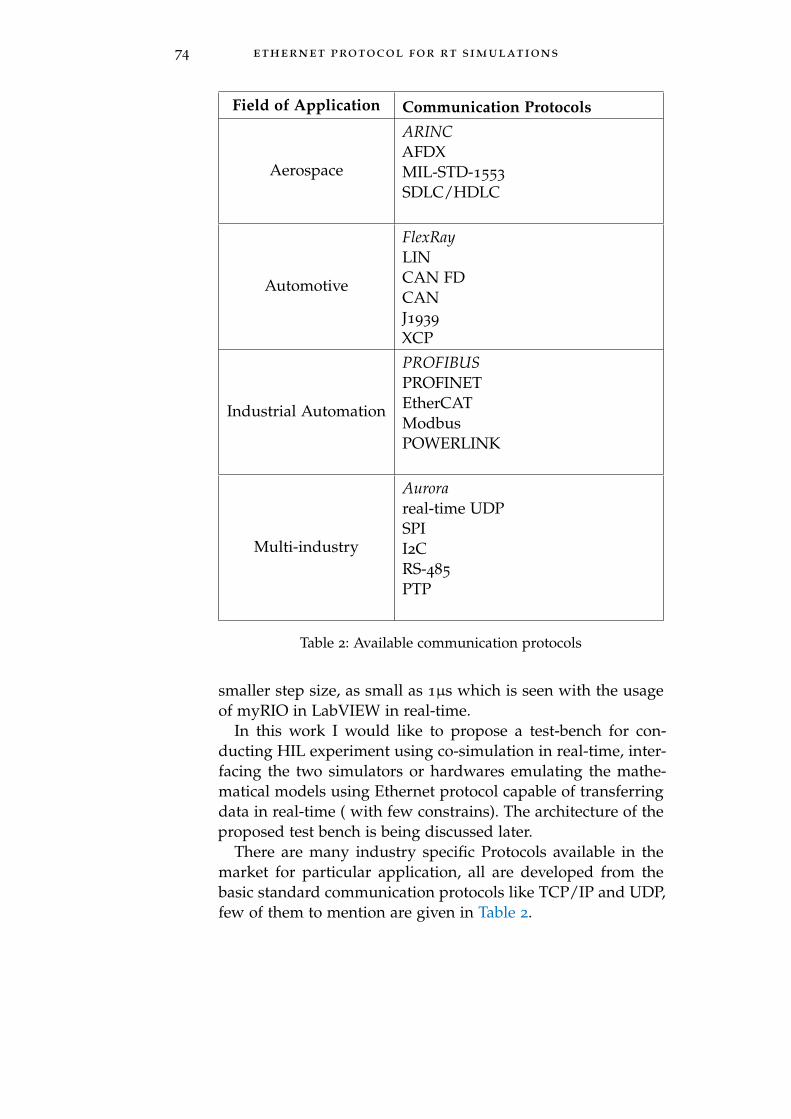
74 ethernet protocol for rt simulations
Field of Application Communication Protocols
Aerospace
ARINCAFDXMIL-STD-1553
SDLC/HDLC
Automotive
FlexRayLINCAN FDCANJ1939
XCP
Industrial Automation
PROFIBUSPROFINETEtherCATModbusPOWERLINK
Multi-industry
Aurorareal-time UDPSPII2CRS-485
PTP
Table 2: Available communication protocols
smaller step size, as small as 1µs which is seen with the usageof myRIO in LabVIEW in real-time.
In this work I would like to propose a test-bench for con-ducting HIL experiment using co-simulation in real-time, inter-facing the two simulators or hardwares emulating the mathe-matical models using Ethernet protocol capable of transferringdata in real-time ( with few constrains). The architecture of theproposed test bench is being discussed later.
There are many industry specific Protocols available in themarket for particular application, all are developed from thebasic standard communication protocols like TCP/IP and UDP,few of them to mention are given in Table 2.
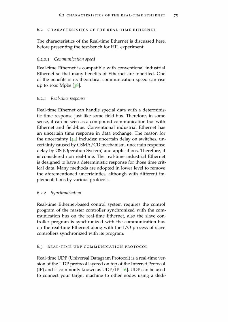
6.2 characteristics of the real-time ethernet 75
6.2 characteristics of the real-time ethernet
The characteristics of the Real-time Ethernet is discussed here,before presenting the test-bench for HIL experiment.
6.2.0.1 Communication speed
Real-time Ethernet is compatible with conventional industrialEthernet so that many benefits of Ethernet are inherited. Oneof the benefits is its theoretical communication speed can riseup to 1000 Mpbs [38].
6.2.1 Real-time response
Real-time Ethernet can handle special data with a determinis-tic time response just like some field-bus. Therefore, in somesense, it can be seen as a compound communication bus withEthernet and field-bus. Conventional industrial Ethernet hasan uncertain time response in data exchange. The reason forthe uncertainty [44] includes: uncertain delay on switches, un-certainty caused by CSMA/CD mechanism, uncertain responsedelay by OS (Operation System) and applications. Therefore, itis considered non real-time. The real-time industrial Ethernetis designed to have a deterministic response for those time crit-ical data. Many methods are adopted in lower level to removethe aforementioned uncertainties, although with different im-plementations by various protocols.
6.2.2 Synchronization
Real-time Ethernet-based control system requires the controlprogram of the master controller synchronized with the com-munication bus on the real-time Ethernet, also the slave con-troller program is synchronized with the communication buson the real-time Ethernet along with the I/O process of slavecontrollers synchronized with its program.
6.3 real-time udp communication protocol
Real-time UDP (Universal Datagram Protocol) is a real-time ver-sion of the UDP protocol layered on top of the Internet Protocol(IP) and is commonly known as UDP/IP [16]. UDP can be usedto connect your target machine to other nodes using a dedi-
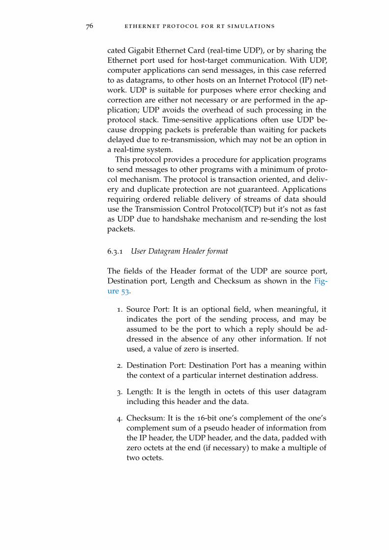
76 ethernet protocol for rt simulations
cated Gigabit Ethernet Card (real-time UDP), or by sharing theEthernet port used for host-target communication. With UDP,computer applications can send messages, in this case referredto as datagrams, to other hosts on an Internet Protocol (IP) net-work. UDP is suitable for purposes where error checking andcorrection are either not necessary or are performed in the ap-plication; UDP avoids the overhead of such processing in theprotocol stack. Time-sensitive applications often use UDP be-cause dropping packets is preferable than waiting for packetsdelayed due to re-transmission, which may not be an option ina real-time system.
This protocol provides a procedure for application programsto send messages to other programs with a minimum of proto-col mechanism. The protocol is transaction oriented, and deliv-ery and duplicate protection are not guaranteed. Applicationsrequiring ordered reliable delivery of streams of data shoulduse the Transmission Control Protocol(TCP) but it’s not as fastas UDP due to handshake mechanism and re-sending the lostpackets.
6.3.1 User Datagram Header format
The fields of the Header format of the UDP are source port,Destination port, Length and Checksum as shown in the Fig-ure 53.
1. Source Port: It is an optional field, when meaningful, itindicates the port of the sending process, and may beassumed to be the port to which a reply should be ad-dressed in the absence of any other information. If notused, a value of zero is inserted.
2. Destination Port: Destination Port has a meaning withinthe context of a particular internet destination address.
3. Length: It is the length in octets of this user datagramincluding this header and the data.
4. Checksum: It is the 16-bit one’s complement of the one’scomplement sum of a pseudo header of information fromthe IP header, the UDP header, and the data, padded withzero octets at the end (if necessary) to make a multiple oftwo octets.
6.3 real-time udp communication protocol 77
Figure 53: UDP Header format
The pseudo header is prefixed to the UDP header containsthe source address, the destination address, the protocol, andthe UDP length. This information gives protection against mis-routed datagrams. This is being shown in the Figure 54.
Figure 54: UDP Pseudo header format
If the computed checksum is zero, it is transmitted as all ones(the equivalent in one’s complement arithmetic).
78 ethernet protocol for rt simulations
6.3.1.1 Advantages of UDP Protocol
• UDP protocol is not connection based algorithm, The re-sponsibility of the sender is to just bundle the data accord-ing to the format and to transmit. It doesn’t care aboutwho is receiving and did receiver obtained all the data.Hence It can broadcast multicast the data over Ethernetfor multiple destinations.
• It doesn’t restrict to a connection based communicationmodel, so startup latency in distributed applications ismuch lower, as is operating system overhead FAST.
• The recipient of UDP packets gets them unmangled, in-cluding block boundaries.
• Much faster than TCP. Due to low latency, it is much bet-ter for real-time communications hence it is also used forvoice over IP and many upcoming real-time communica-tions.
6.3.1.2 Disadvantages of UDP Protocol
• There are no guarantees with UDP, A packet may not bedelivered, or delivered out of order.
• UDP has no flow control, Control implementation is theduty of user programs.
• Receiver program should manually break the data intopackets.
• UDP most of the time suffers from data packet loss whichhas to be taken care during the experimentation.
7A R C H I T E C T U R E O F C O - S I M U L AT I O NP L AT F O R M
In this chapter the architecture of the Co-simulation platform toconduct HIL simulation of PV with the grid interaction havingthe interfacing algorithm over Ethernet is presented along withthe discussion of simulation model that has to be simulated inreal-time.
7.1 real-time digital simulator
As already discussed RTDS plays a major role in HIL simula-tions, it enables tester to control the emulated model and alsothe sole responsible to keep the HIL simulation in real-time.Simulink desktop Real-time and LabVIEW are used as RTDS,co-simulating in real-time.
7.1.1 Simulink Desktop Real-Time
Simulink Desktop Real-Time is a real-time digital simulatorprovided by MATWORKS. As we are well familiar with theSimulink, the same Simulink model is compiled to run in theIntel’s processor turning the desktop as a real-time target [5].Simulink Desktop Real-Time provides a real-time kernel for ex-ecuting Simulink models externally out of Simulink. It includeslibrary blocks that connect to a range of I/O devices that en-ables to create and tune a real-time system for rapid prototyp-ing and hardware-in-the-loop simulation without using any ex-tra hardware.
With the help of Simulink coder an extra package in Simulink,enables us to conduct real-time performance upto sample rateof 20 kHz. The Simulink Desktop Real-Time software uses asmall real-time kernel that runs in operating system kernelmode using the built-in CPU clock as primary time source. Inexternal mode, both the application and the I/O drivers run inthe kernel.
79

80 architecture of co-simulation platform
7.1.1.1 Real-time Application
The real-time application runs in real time on host computerand has the following characteristics.
1. Compiled code: Created from the generated C-code usinga bundled C compiler shipped with the Simulink DesktopReal-Time software.
2. Relation to Simulink model: The executable contains a bi-nary form of Simulink model components, connectionsbetween blocks, time dependencies, and variables in theSimulink blocks.
3. Relation to the kernel: The executable must be loaded andexecuted directly by the Simulink Desktop Real-Time ker-nel. It cannot be executed without the kernel. The ker-nel runs as an operating system kernel-mode driver, in-tercepts timer interrupts from the CPU clock, maintainsclock signals for the operating system, and runs the ap-plication in real-time. As a result, both the kernel and thereal-time application run in kernel mode.
4. Checksum: The Simulink model and the executable con-tain a checksum value. The kernel uses this checksumvalue to determine if the Simulink model structure, atthe time of code generation, is consistent with the real-time application structure during execution. This verifiesthat when you change parameters during an execution,the Simulink model parameters map to the memory loca-tions in the real-time application.
7.1.1.2 Real-time Execution
In external mode, the real-time application runs in the kernelmode process. Using I/O drivers running in that process tocommunicate with the hardware, it stores contiguous responsedata in memory accessible to Simulink until a data buffer isfilled. When the buffer is filled, the real-time application con-tinues to run while Simulink transfers the data to the MATLABenvironment through Simulink external mode. The architectureof this method is given in the Figure 55.
Transfer of data is less critical than maintaining determinis-tic real-time updates at the selected sample interval. Therefore,data transfer runs at a lower priority in the remaining CPU time
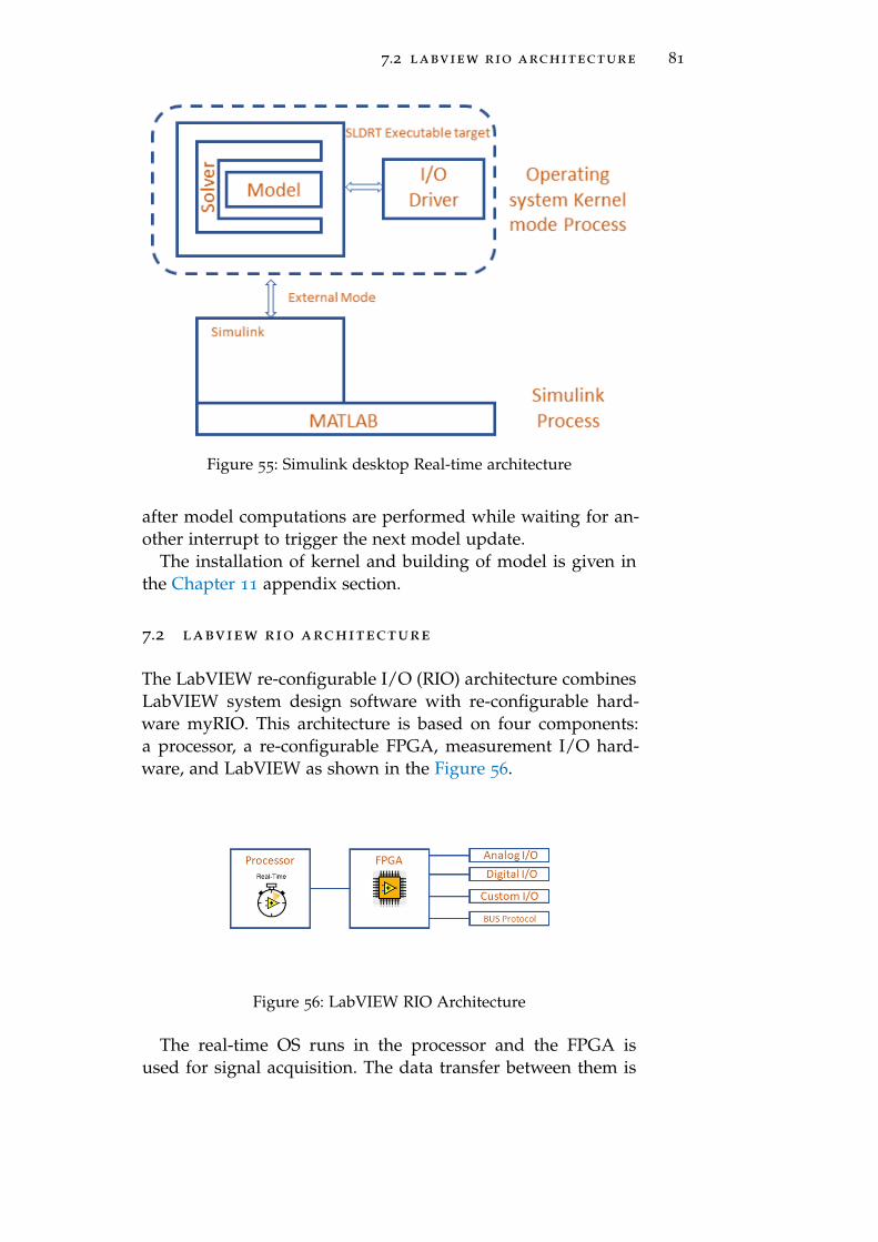
7.2 labview rio architecture 81
Figure 55: Simulink desktop Real-time architecture
after model computations are performed while waiting for an-other interrupt to trigger the next model update.
The installation of kernel and building of model is given inthe Chapter 11 appendix section.
7.2 labview rio architecture
The LabVIEW re-configurable I/O (RIO) architecture combinesLabVIEW system design software with re-configurable hard-ware myRIO. This architecture is based on four components:a processor, a re-configurable FPGA, measurement I/O hard-ware, and LabVIEW as shown in the Figure 56.
Figure 56: LabVIEW RIO Architecture
The real-time OS runs in the processor and the FPGA isused for signal acquisition. The data transfer between them is
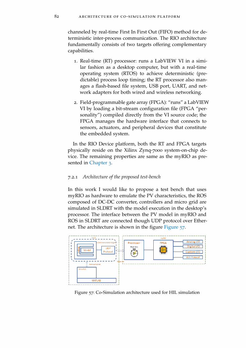
82 architecture of co-simulation platform
channeled by real-time First In First Out (FIFO) method for de-terministic inter-process communication. The RIO architecturefundamentally consists of two targets offering complementarycapabilities.
1. Real-time (RT) processor: runs a LabVIEW VI in a simi-lar fashion as a desktop computer, but with a real-timeoperating system (RTOS) to achieve deterministic (pre-dictable) process loop timing; the RT processor also man-ages a flash-based file system, USB port, UART, and net-work adapters for both wired and wireless networking.
2. Field-programmable gate array (FPGA): “runs” a LabVIEWVI by loading a bit-stream configuration file (FPGA “per-sonality”) compiled directly from the VI source code; theFPGA manages the hardware interface that connects tosensors, actuators, and peripheral devices that constitutethe embedded system.
In the RIO Device platform, both the RT and FPGA targetsphysically reside on the Xilinx Zynq-7000 system-on-chip de-vice. The remaining properties are same as the myRIO as pre-sented in Chapter 3.
7.2.1 Architecture of the proposed test-bench
In this work I would like to propose a test bench that usesmyRIO as hardware to emulate the PV characteristics, the ROScomposed of DC-DC converter, controllers and micro grid aresimulated in SLDRT with the model execution in the desktop’sprocessor. The interface between the PV model in myRIO andROS in SLDRT are connected though UDP protocol over Ether-net. The architecture is shown in the figure Figure 57.
Figure 57: Co-Simulation architecture used for HIL simulation

7.3 modeling of micro grid and vsc converter 83
7.2.2 Model simulated in the test-bench
A simplified micro-grid with only one Synchronous Generatorand one PV system will be taken as an example to explain thecontrol strategy and to demonstrate the effectiveness of the pro-posed interface algorithm in real-time simulation. The PV sys-tem is made to work at the maximum power point, so it will notbe able to inject extra active power during the transient. Withthe frequency control strategy of the VSC converter, it is madeto exchange reactive power during frequency transients. There-fore, in addition to the maximum power point tracking, the PVpower converter will perform a reactive power regulation.
The testing micro-grid is composed of a 250 kVA/400 V syn-chronous generator and a 100 kVA/400 V PV system. SG isdriven by a hydraulic turbine controlled by a PID governor sys-tem and is excited by an exciter with voltage regulator imple-menting an excitation system realized according with type 1 ofIEEE standard 421.5, the block diagram of the simulation modelis shown Figure 58.
Figure 58: Block diagram of the simulated model
7.3 modeling of micro grid and vsc converter
A 100 kW PV is emulated using the equations discussed inChapter 4 and deployed to myRIO using LabVIEW to run as anindependent executable project. in the following sections mod-elling of ROS except PV and MPPT is being discussed withits theoretical studies where as the modeling of PV MPPT andDC-DC converters are given in Chapter 4.
Hydroelectric power is a domestic source of energy, allowingeach country/state to produce their own energy without be-ing reliant on international fuel sources. The energy generated
84 architecture of co-simulation platform
through hydro power relies on the water cycle, which is drivenby the sun, making it a renewable power source, making it amore reliable and affordable source than fossil fuels that arerapidly being depleted. hydro power facilities can quickly gofrom zero power to maximum output [47]. Because of hydropower plants can generate power to the grid immediately, theyprovide essential back-up power during major electricity out-ages or disruptions. In addition to a sustainable fuel source, hy-dro power efforts produce a number of benefits, such as floodcontrol, irrigation, and water supply.
The hydro power potential is a combination between headand water flow as given in Equation 37.
Pmax = ρgQHη (37)
where,ρ Density of water kg/m2
g acceleration due to gravity m/s2
Q water flow m3/s
H Net head mη Hydraulic efficiency of the turbine
Turbines convert the energy of flowing water into rotationalenergy of the shaft. Generally, turbines are classified into im-pulse or reaction turbines. Reaction turbines are submerged inwater where the pressure rotates the runner blades. Impulseturbines on the other hand work by an impulse jet that rotatesthe runner blades [29].
The selection of the turbine depends on the site. The mostimportant characteristics are the head and the flow available.In addition to these key parameters, it is also important to con-sider the running speed of the generator and whether the tur-bine is expected to run in various flow conditions. All of thesecharacteristics affect the efficiency of the turbine and each tur-bine has an efficiency maximum at a certain head, flow androtation speed.
The generator efficiency is usually considered constant overa wide operating range. However, the hydraulic efficiency de-pends significantly on both the water discharge and the nethead. These relationships are generally represented using Tur-bine Hill Chart [6].
An ideal modeling of Hydro power plant (HPP) componentssuch as synchronous machine, turbine and its governing sys-tem is necessary to analysis the power system response during
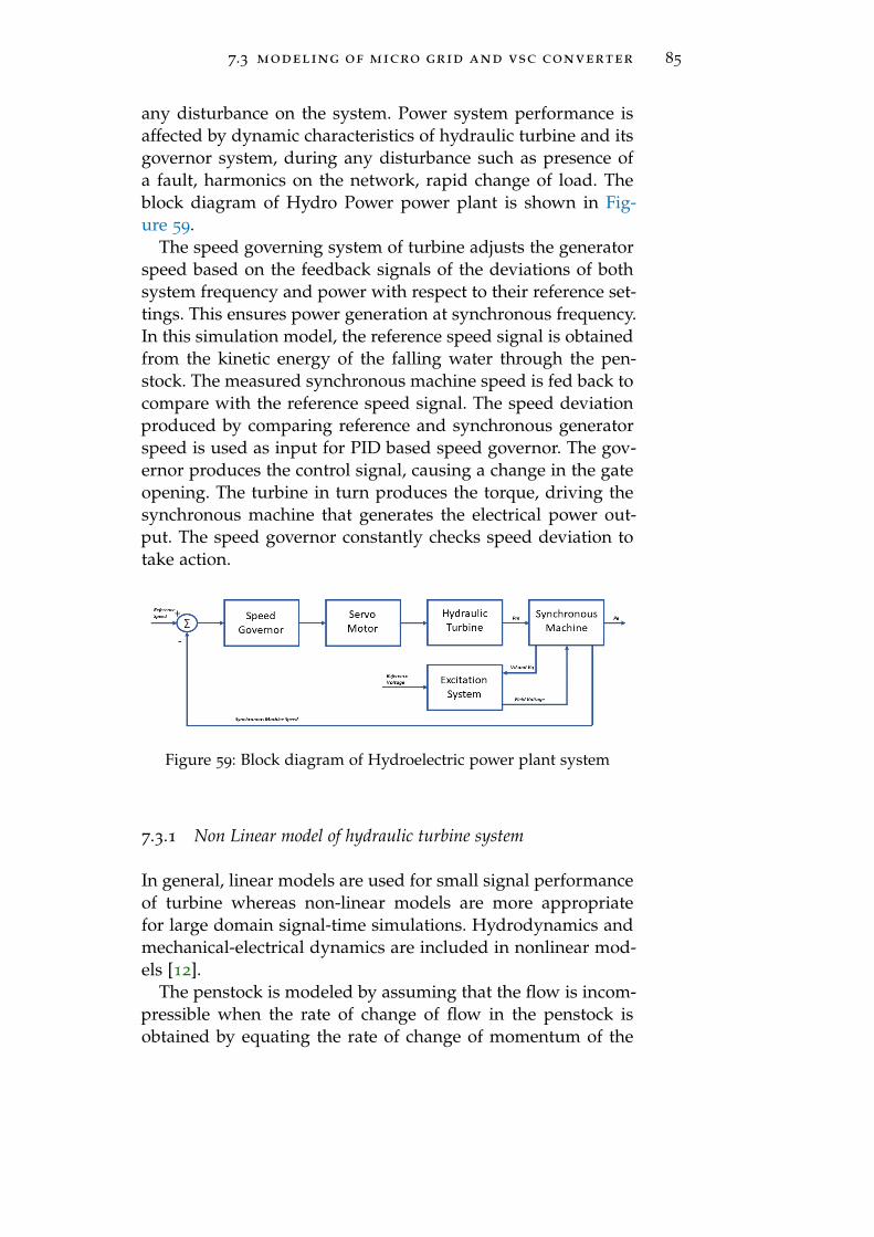
7.3 modeling of micro grid and vsc converter 85
any disturbance on the system. Power system performance isaffected by dynamic characteristics of hydraulic turbine and itsgovernor system, during any disturbance such as presence ofa fault, harmonics on the network, rapid change of load. Theblock diagram of Hydro Power power plant is shown in Fig-ure 59.
The speed governing system of turbine adjusts the generatorspeed based on the feedback signals of the deviations of bothsystem frequency and power with respect to their reference set-tings. This ensures power generation at synchronous frequency.In this simulation model, the reference speed signal is obtainedfrom the kinetic energy of the falling water through the pen-stock. The measured synchronous machine speed is fed back tocompare with the reference speed signal. The speed deviationproduced by comparing reference and synchronous generatorspeed is used as input for PID based speed governor. The gov-ernor produces the control signal, causing a change in the gateopening. The turbine in turn produces the torque, driving thesynchronous machine that generates the electrical power out-put. The speed governor constantly checks speed deviation totake action.
Figure 59: Block diagram of Hydroelectric power plant system
7.3.1 Non Linear model of hydraulic turbine system
In general, linear models are used for small signal performanceof turbine whereas non-linear models are more appropriatefor large domain signal-time simulations. Hydrodynamics andmechanical-electrical dynamics are included in nonlinear mod-els [12].
The penstock is modeled by assuming that the flow is incom-pressible when the rate of change of flow in the penstock isobtained by equating the rate of change of momentum of the
86 architecture of co-simulation platform
water in the penstock to the net force on the water in the pen-stock as given in Equation 38.
Fnet = ρLdq
dt(38)
where,L Penstock length
The net force on the water can be obtained by consideringthe pressure head at the conduit. On entry to the penstock theforce on the water is proportional to the static head Hs. whileat the wicket gate it is proportional to the head H across theturbine. Due to friction effects in the conduit, there is also afriction force on the water represented by the head loss so thatthe net force on the water in the penstock is Equation 39.
Fnet = (Hs −Hl −H)Aρg (39)
where,A Penstock Cross-sectional area
By equating Equation 38 and Equation 39 we get Equation 40.
ρLdq
dt= (Hs −Hl −H)Aρg (40)
It is usual to normalize this equation to a convenient base.The base flow rate qbase is taken as the flow rate through theturbine with the gates fully open and the head at the turbineequal to hbase. Dividing Equation 40 by qbase ∗ hbase we getEquation 41.
dq
dt= (1− hl − h)
1
Tw(41)
where,q normalized flow q = Q
qbase
h normalized head q = Hhbase
Tw is water starting timehl is normalized head loss
The water starting time Tw is theoretically defined as the timetaken for the flow rate in the penstock to change by a value
7.3 modeling of micro grid and vsc converter 87
equal to qbase when the head term in brackets changes by avalue equal to hbase it is given by Equation 42.
Tw =LqbaseAghbase
(42)
The head loss is proportional to the flow rate squared and de-pends on the conduit dimensions and friction factor, it is givenby hl = kfq2 which is often neglected.
In turbine modeling, its hydraulic characteristics and mechan-ical power output must be modeled. Pressure head across theturbine is related to the flow rate by assuming that the turbinecan be represented by the valve characteristic as given in Equa-tion 43 and it is normalized by dividing both sides by base.
Q = kG√Hq = G
√H (43)
where,G Gate position from 0 to 1 (fully open)
the power developed by the turbine is proportional to theproduct of the flow rate and the head and depends on the effi-ciency. To account for the turbine not being 100% efficient theno-load flow qnl is subtracted from the actual flow, in normal-ized parameters its given by Equation 44.
pm = h(q− qnl) (44)
for the generator whose parameters are normalized to thegenerator MVA base so that last equation is written as in Equa-tion 45.
pm = Ath(q− qnl) (45)
where, At is introduced to account for the difference in thebases. A damping effect is also present that is dependent ongate opening so that at any load condition the turbine powercan be expressed as in Equation 46.
pm = Ath(q− qnl) −DG∆W (46)
The turbine model is shown in the block diagram Figure 60
same is being modeled in simulink.
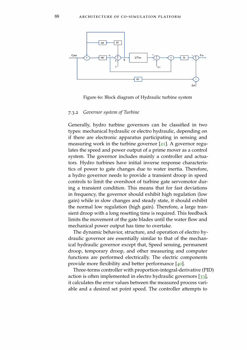
88 architecture of co-simulation platform
Figure 60: Block diagram of Hydraulic turbine system
7.3.2 Governor system of Turbine
Generally, hydro turbine governors can be classified in twotypes: mechanical hydraulic or electro hydraulic, depending onif there are electronic apparatus participating in sensing andmeasuring work in the turbine governor [21]. A governor regu-lates the speed and power output of a prime mover as a controlsystem. The governor includes mainly a controller and actua-tors. Hydro turbines have initial inverse response characteris-tics of power to gate changes due to water inertia. Therefore,a hydro governor needs to provide a transient droop in speedcontrols to limit the overshoot of turbine gate servomotor dur-ing a transient condition. This means that for fast deviationsin frequency, the governor should exhibit high regulation (lowgain) while in slow changes and steady state, it should exhibitthe normal low regulation (high gain). Therefore, a large tran-sient droop with a long resetting time is required. This feedbacklimits the movement of the gate blades until the water flow andmechanical power output has time to overtake.
The dynamic behavior, structure, and operation of electro hy-draulic governor are essentially similar to that of the mechan-ical hydraulic governor except that, Speed sensing, permanentdroop, temporary droop, and other measuring and computerfunctions are performed electrically. The electric componentsprovide more flexibility and better performance [40].
Three-terms controller with proportion-integral-derivative (PID)action is often implemented in electro hydraulic governors [33],it calculates the error values between the measured process vari-able and a desired set point speed. The controller attempts to
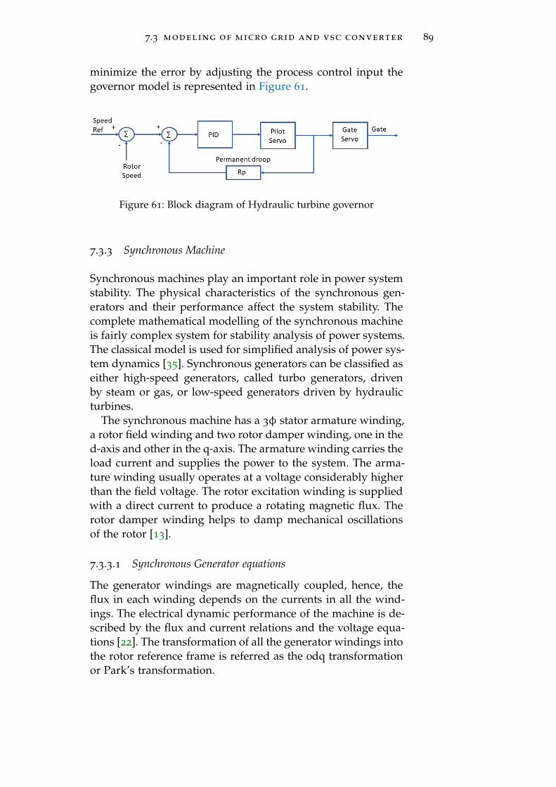
7.3 modeling of micro grid and vsc converter 89
minimize the error by adjusting the process control input thegovernor model is represented in Figure 61.
Figure 61: Block diagram of Hydraulic turbine governor
7.3.3 Synchronous Machine
Synchronous machines play an important role in power systemstability. The physical characteristics of the synchronous gen-erators and their performance affect the system stability. Thecomplete mathematical modelling of the synchronous machineis fairly complex system for stability analysis of power systems.The classical model is used for simplified analysis of power sys-tem dynamics [35]. Synchronous generators can be classified aseither high-speed generators, called turbo generators, drivenby steam or gas, or low-speed generators driven by hydraulicturbines.
The synchronous machine has a 3φ stator armature winding,a rotor field winding and two rotor damper winding, one in thed-axis and other in the q-axis. The armature winding carries theload current and supplies the power to the system. The arma-ture winding usually operates at a voltage considerably higherthan the field voltage. The rotor excitation winding is suppliedwith a direct current to produce a rotating magnetic flux. Therotor damper winding helps to damp mechanical oscillationsof the rotor [13].
7.3.3.1 Synchronous Generator equations
The generator windings are magnetically coupled, hence, theflux in each winding depends on the currents in all the wind-ings. The electrical dynamic performance of the machine is de-scribed by the flux and current relations and the voltage equa-tions [22]. The transformation of all the generator windings intothe rotor reference frame is referred as the 0dq transformationor Park’s transformation.
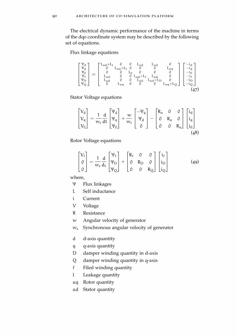
90 architecture of co-simulation platform
The electrical dynamic performance of the machine in termsof the dq0 coordinate system may be described by the followingset of equations.
Flux linkage equations
ΨdΨq
Ψ0ΨfΨDΨQ
=
Lad+Ll 0 0 Lad Lad 00 Laq+Ll 0 0 0 Laq0 0 L0 0 0 0Lad 0 0 Lad+Lf Lad 0Lad 0 0 Lad Lad+LD 00 Laq 0 0 0 Laq+LQ
−id−iq−i0−if−iD−iQ
(47)
Stator Voltage equations
VdVqV0
=1
ws
d
dt
ΨdΨqΨ0
+w
ws
−ΨqΨd0
−
Ra 0 0
0 Ra 0
0 0 Ra
idiqi0
(48)
Rotor Voltage equations
Vf00
=1
ws
d
dt
ΨfΨDΨQ
+
Rf 0 0
0 RD 0
0 0 RQ
ifiDiQ
(49)
where,Ψ Flux linkagesL Self inductancei CurrentV VoltageR Resistancew Angular velocity of generatorws Synchronous angular velocity of generator
d d-axis quantityq q-axis quantityD damper winding quantity in d-axisQ damper winding quantity in q-axisf Filed winding quantityl Leakage quantityaq Rotor quantityad Stator quantity
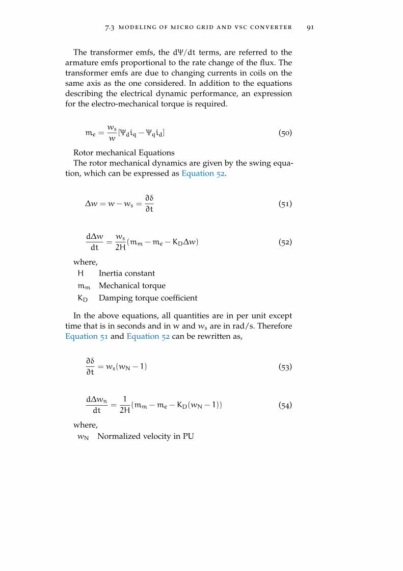
7.3 modeling of micro grid and vsc converter 91
The transformer emfs, the dΨ/dt terms, are referred to thearmature emfs proportional to the rate change of the flux. Thetransformer emfs are due to changing currents in coils on thesame axis as the one considered. In addition to the equationsdescribing the electrical dynamic performance, an expressionfor the electro-mechanical torque is required.
me =ws
w[Ψdiq −Ψqid] (50)
Rotor mechanical EquationsThe rotor mechanical dynamics are given by the swing equa-
tion, which can be expressed as Equation 52.
∆w = w−ws =∂δ
∂t(51)
d∆w
dt=ws
2H(mm −me −KD∆w) (52)
where,H Inertia constantmm Mechanical torqueKD Damping torque coefficient
In the above equations, all quantities are in per unit excepttime that is in seconds and in w and ws are in rad/s. ThereforeEquation 51 and Equation 52 can be rewritten as,
∂δ
∂t= ws(wN − 1) (53)
d∆wn
dt=
1
2H(mm −me −KD(wN − 1)) (54)
where,wN Normalized velocity in PU
92 architecture of co-simulation platform
7.3.4 Turbine and generator relationship
The generator needs to generate an alternating voltage with afrequency specified by grid-users [50], usually a small intervalaround 50HZ or 60HZ, In order to achieve this, the generatorrotor needs to have the correct amount of rotor poles with re-gards to the turbine optimal rotational speed. For a 2-pole gen-erator, the voltage completes one period per revolution of therotor. The voltage angular frequency for steady-state operationis given by Equation 55.
wgrid = wgenerator =P
2wt (55)
where,wt Turbine angular frequencywgrid Grid angular frequencywgenerator Generator angular frequencyP Generator poles
This means that the generator must yield a variable poweroutput at a constant rotational speed. It must also operate withina reasonably constant voltage. The output power (and torque)is then a function of the output current.
Pelectric = wgridT = EI (56)
The output is increased by adjusting the rotor magnetizationcurrent. When the generator is producing power at a steady-state condition, the rotor will rotate at an angular displacementlocated in front of the synchronous reference frame of the sta-tor. This can be viewed as the rotor "pulling" the magnetic fieldalong with the rotation. This angle is a function of the gener-ator output, the larger the output, the larger the displacement.Should either the output power or grid frequency change, sowill the magnetic displacement angle, thus allowing the turbineto accelerate the rotor slightly despite being grid-connected.Shifting the synchronous machine power angle requires torque.This will act as a magnetic spring that resists sudden changesin rotational speed, hence acting in the direction opposite ofrotational acceleration. All of these factors are accounted in thesimulation model.
7.3 modeling of micro grid and vsc converter 93
7.3.5 Excitation system model of synchronous generator
Type DC1A excitation system model of IEEE RecommendedPractice for Excitation System Models for Power System Stabil-ity Studies [18] is used. Excitation system provides the currentrequired for the field winding of a synchronous generator toproduce the rated terminal voltage at the generator terminals.In this type of exciter a separately or self excited DC generatordriven by a motor is connected to the same shaft as that of themain generator rotor is used. In case of separately excited DCgenerator the field winding of the DC generator is energizedthrough a permanent magnet AC generator, the three-phaseoutput of which is converted to DC through rectifiers.
IEEE type DC1A exciter dynamics can be expressed by thefollowing three equations.
TEdEfddt
= VR − (KE + SE(Efd))Efd (57)
TAdVRdt
= −VR +KARF −KAKFTF
Efd +KA(Vref − Vt) (58)
dRfdt
= −RF +KFTFEfd (59)
where,KE Gain of the DC exciterTE Time constant of the DC exciterEfd DC generator output armature voltageKA Gain of the Voltage regulatorTA Time constant of the voltage regulatorVt voltage of transducer of load compensatorVR voltage regulator output for error vinSE(Efd) Saturation functionKF stabilizing transformer gainRF Rate feedback of stabilizing transformerTF Time constant of the stabilizing system
using Equation 57, Equation 58 and Equation 59 the Simulinkmodel is built, the block diagram approach of the exciter sys-tem is shown in the Figure 62.
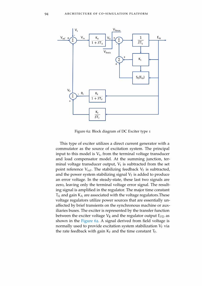
94 architecture of co-simulation platform
Figure 62: Block diagram of DC Exciter type 1
This type of exciter utilizes a direct current generator with acommutator as the source of excitation system. The principalinput to this model is Vt, from the terminal voltage transducerand load compensator model. At the summing junction, ter-minal voltage transducer output, Vt is subtracted from the setpoint reference Vref. The stabilizing feedback VF is subtracted,and the power system stabilizing signal VF is added to producean error voltage. In the steady-state, these last two signals arezero, leaving only the terminal voltage error signal. The result-ing signal is amplified in the regulator. The major time constantTA and gain KA are associated with the voltage regulators.Thesevoltage regulators utilize power sources that are essentially un-affected by brief transients on the synchronous machine or aux-iliaries buses. The exciter is represented by the transfer functionbetween the exciter voltage VR and the regulator output EFD asshown in the Figure 62. A signal derived from field voltage isnormally used to provide excitation system stabilization VF viathe rate feedback with gain KF and the time constant TF.
7.3 modeling of micro grid and vsc converter 95
7.3.6 Control of 3φ Voltage Source Converter
3φ Voltage Source Converter (VSC) is used to connect the PVsystem to the Point of coupling (PCC) of the micro grid. Sincethe study is on transient response and frequency regulation dueto disturbances in the system, in real-time. We are not inter-ested in the harmonics due to the use of power electronic con-verters, hence the average model of the converter is used in thiswork. But more emphasis is given on the control strategy. Thecontroller designed is responsible for fixing the DC bus voltageand also for the regulation of various parameters at PCC.
7.3.6.1 Synchronous reference frame
In the designed model, the control takes place in synchronousreference frame, this can be achieved by converting the 3φ natu-ral frame [7] to d-axis and q-axis (dq) reference frame as shownin Equation 60.
[vd
vq
]=
√2
3
[sin(wt) sin(wt− 2π
3 ) sin(wt+ 2π3 )
cos(wt) cos(wt− 2π3 ) cos(wt+ 2π
3 )
]vavbvc
(60)
The same equation is valid for the currents, it is given byEquation 61.
[id
iq
]=
√2
3
[sin(wt) sin(wt− 2π
3 ) sin(wt+ 2π3 )
cos(wt) cos(wt− 2π3 ) cos(wt+ 2π
3 )
]iaibic
(61)
Control action is taken in this frame and later these quantitiesare converted to three phase actual quantities by taking inverseor reverse transformation on the same set of equations.
7.3.6.2 Phase locked loops
To supply unity power factor current and to maintain synchro-nism with the micro grid, PV system needs grid angle,voltageand frequency which can be obtained by the Phase locked loop
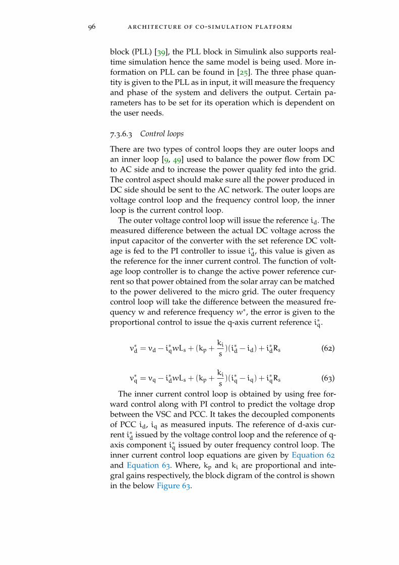
96 architecture of co-simulation platform
block (PLL) [39], the PLL block in Simulink also supports real-time simulation hence the same model is being used. More in-formation on PLL can be found in [25]. The three phase quan-tity is given to the PLL as in input, it will measure the frequencyand phase of the system and delivers the output. Certain pa-rameters has to be set for its operation which is dependent onthe user needs.
7.3.6.3 Control loops
There are two types of control loops they are outer loops andan inner loop [9, 49] used to balance the power flow from DCto AC side and to increase the power quality fed into the grid.The control aspect should make sure all the power produced inDC side should be sent to the AC network. The outer loops arevoltage control loop and the frequency control loop, the innerloop is the current control loop.
The outer voltage control loop will issue the reference id. Themeasured difference between the actual DC voltage across theinput capacitor of the converter with the set reference DC volt-age is fed to the PI controller to issue i∗d, this value is given asthe reference for the inner current control. The function of volt-age loop controller is to change the active power reference cur-rent so that power obtained from the solar array can be matchedto the power delivered to the micro grid. The outer frequencycontrol loop will take the difference between the measured fre-quency w and reference frequency w∗, the error is given to theproportional control to issue the q-axis current reference i∗q.
v∗d = vd − i∗qwLs + (kp +
kis)(i∗d − id) + i
∗dRs (62)
v∗q = vq − i∗dwLs + (kp +
kis)(i∗q − iq) + i
∗qRs (63)
The inner current control loop is obtained by using free for-ward control along with PI control to predict the voltage dropbetween the VSC and PCC. It takes the decoupled componentsof PCC id, iq as measured inputs. The reference of d-axis cur-rent i∗d issued by the voltage control loop and the reference of q-axis component i∗q issued by outer frequency control loop. Theinner current control loop equations are given by Equation 62
and Equation 63. Where, kp and ki are proportional and inte-gral gains respectively, the block digram of the control is shownin the below Figure 63.
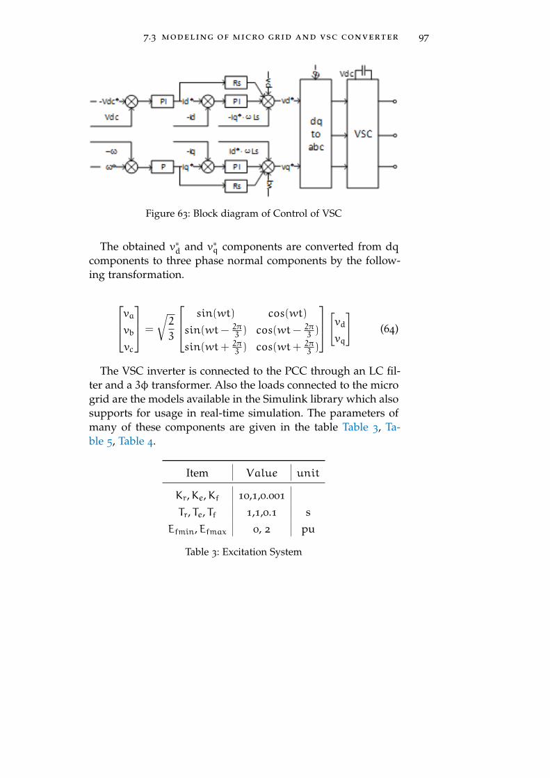
7.3 modeling of micro grid and vsc converter 97
Figure 63: Block diagram of Control of VSC
The obtained v∗d and v∗q components are converted from dqcomponents to three phase normal components by the follow-ing transformation.
vavbvc
=
√2
3
sin(wt) cos(wt)
sin(wt− 2π3 ) cos(wt− 2π
3 )
sin(wt+ 2π3 ) cos(wt+ 2π
3 )
[vdvq
](64)
The VSC inverter is connected to the PCC through an LC fil-ter and a 3φ transformer. Also the loads connected to the microgrid are the models available in the Simulink library which alsosupports for usage in real-time simulation. The parameters ofmany of these components are given in the table Table 3, Ta-ble 5, Table 4.
Item Value unit
Kr,Ke,Kf 10,1,0.001
Tr, Te, Tf 1,1,0.1 sEfmin,Efmax 0, 2 pu
Table 3: Excitation System
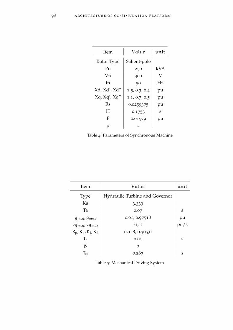
98 architecture of co-simulation platform
Item Value unit
Rotor Type Salient-polePn 250 kVAVn 400 Vfn 50 Hz
Xd, Xd’, Xd” 1.5, 0.3, 0.4 puXq, Xq’, Xq” 1.1, 0.7, 0.5 pu
Rs 0.0259375 puH 0.1753 sF 0.01579 pup 2
Table 4: Parameters of Synchronous Machine
Item Value unit
Type Hydraulic Turbine and GovernorKa 3.333
Ta 0.07 sgmin,gmax 0.01, 0.97518 puvgmin, vgmax -1, 1 pu/sRp,Kp,Ki,Kd 0, 0.8, 0.305,0
Td 0.01 sβ 0
Tw 0.267 s
Table 5: Mechanical Driving System
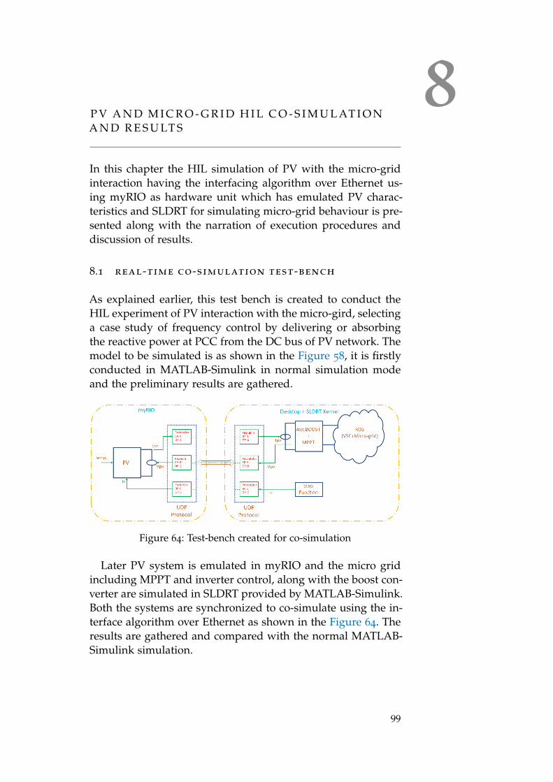
8P V A N D M I C R O - G R I D H I L C O - S I M U L AT I O NA N D R E S U LT S
In this chapter the HIL simulation of PV with the micro-gridinteraction having the interfacing algorithm over Ethernet us-ing myRIO as hardware unit which has emulated PV charac-teristics and SLDRT for simulating micro-grid behaviour is pre-sented along with the narration of execution procedures anddiscussion of results.
8.1 real-time co-simulation test-bench
As explained earlier, this test bench is created to conduct theHIL experiment of PV interaction with the micro-gird, selectinga case study of frequency control by delivering or absorbingthe reactive power at PCC from the DC bus of PV network. Themodel to be simulated is as shown in the Figure 58, it is firstlyconducted in MATLAB-Simulink in normal simulation modeand the preliminary results are gathered.
Figure 64: Test-bench created for co-simulation
Later PV system is emulated in myRIO and the micro gridincluding MPPT and inverter control, along with the boost con-verter are simulated in SLDRT provided by MATLAB-Simulink.Both the systems are synchronized to co-simulate using the in-terface algorithm over Ethernet as shown in the Figure 64. Theresults are gathered and compared with the normal MATLAB-Simulink simulation.
99
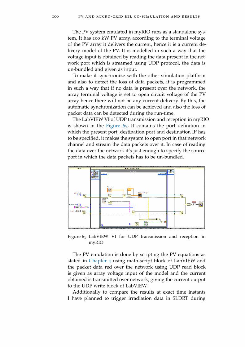
100 pv and micro-grid hil co-simulation and results
The PV system emulated in myRIO runs as a standalone sys-tem, It has 100 kW PV array, according to the terminal voltageof the PV array it delivers the current, hence it is a current de-livery model of the PV. It is modelled in such a way that thevoltage input is obtained by reading the data present in the net-work port which is streamed using UDP protocol, the data isun-bundled and given as input.
To make it synchronize with the other simulation platformand also to detect the loss of data packets, it is programmedin such a way that if no data is present over the network, thearray terminal voltage is set to open circuit voltage of the PVarray hence there will not be any current delivery. By this, theautomatic synchronization can be achieved and also the loss ofpacket data can be detected during the run-time.
The LabVIEW VI of UDP transmission and reception in myRIOis shown in the Figure 65, It contains the port definition inwhich the present port, destination port and destination IP hasto be specified, it makes the system to open port in that networkchannel and stream the data packets over it. In case of readingthe data over the network it’s just enough to specify the sourceport in which the data packets has to be un-bundled.
Figure 65: LabVIEW VI for UDP transmission and reception inmyRIO
The PV emulation is done by scripting the PV equations asstated in Chapter 4 using math-script block of LabVIEW andthe packet data red over the network using UDP read blockis given as array voltage input of the model and the currentobtained is transmitted over network, giving the current outputto the UDP write block of LabVIEW.
Additionally to compare the results at exact time instantsI have planned to trigger irradiation data in SLDRT during
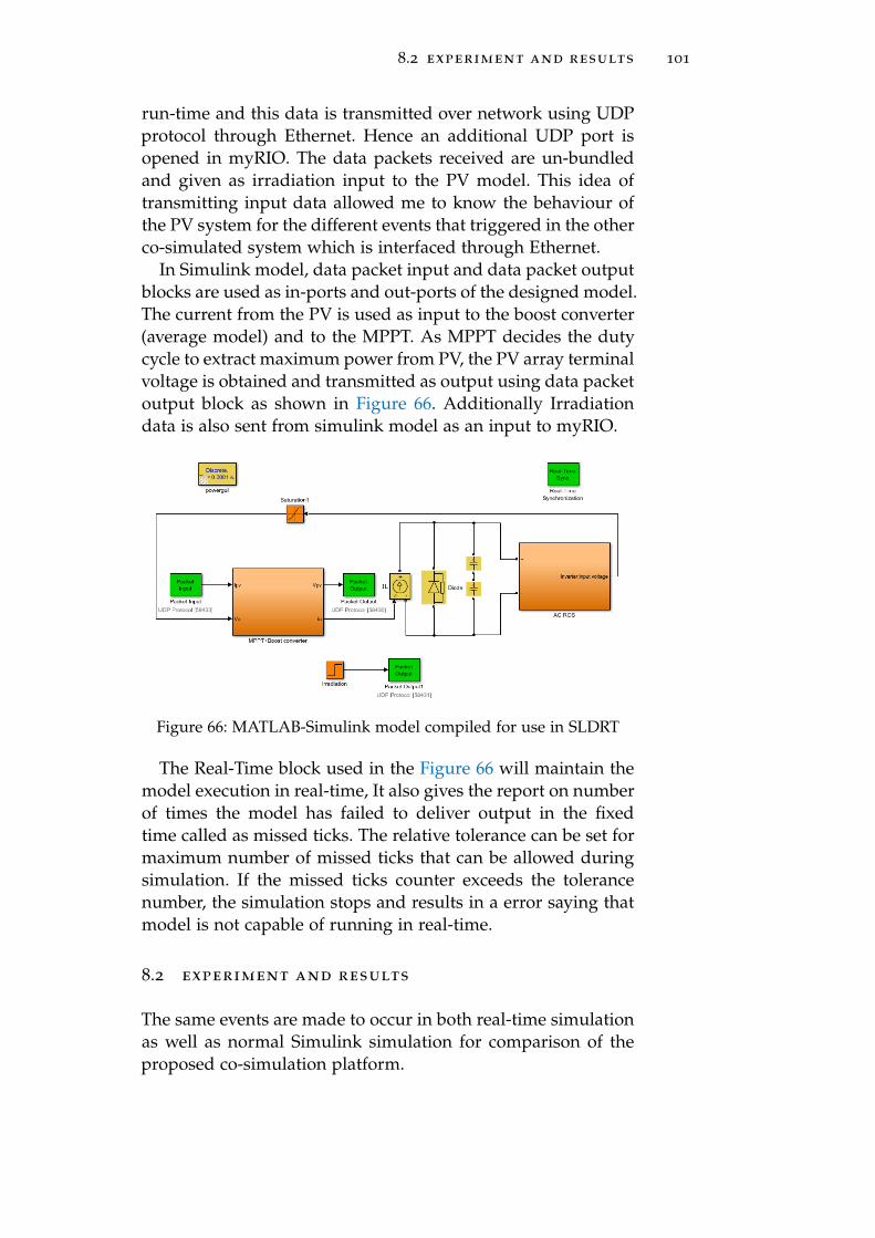
8.2 experiment and results 101
run-time and this data is transmitted over network using UDPprotocol through Ethernet. Hence an additional UDP port isopened in myRIO. The data packets received are un-bundledand given as irradiation input to the PV model. This idea oftransmitting input data allowed me to know the behaviour ofthe PV system for the different events that triggered in the otherco-simulated system which is interfaced through Ethernet.
In Simulink model, data packet input and data packet outputblocks are used as in-ports and out-ports of the designed model.The current from the PV is used as input to the boost converter(average model) and to the MPPT. As MPPT decides the dutycycle to extract maximum power from PV, the PV array terminalvoltage is obtained and transmitted as output using data packetoutput block as shown in Figure 66. Additionally Irradiationdata is also sent from simulink model as an input to myRIO.
Figure 66: MATLAB-Simulink model compiled for use in SLDRT
The Real-Time block used in the Figure 66 will maintain themodel execution in real-time, It also gives the report on numberof times the model has failed to deliver output in the fixedtime called as missed ticks. The relative tolerance can be set formaximum number of missed ticks that can be allowed duringsimulation. If the missed ticks counter exceeds the tolerancenumber, the simulation stops and results in a error saying thatmodel is not capable of running in real-time.
8.2 experiment and results
The same events are made to occur in both real-time simulationas well as normal Simulink simulation for comparison of theproposed co-simulation platform.
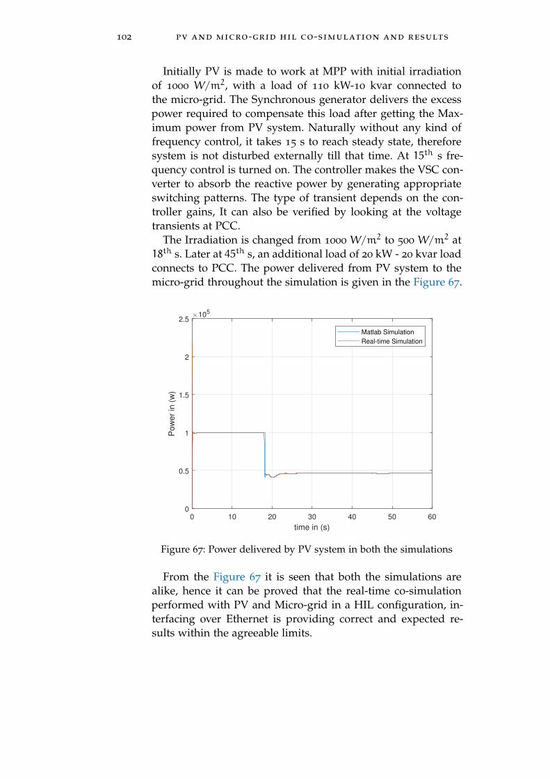
102 pv and micro-grid hil co-simulation and results
Initially PV is made to work at MPP with initial irradiationof 1000 W/m2, with a load of 110 kW-10 kvar connected tothe micro-grid. The Synchronous generator delivers the excesspower required to compensate this load after getting the Max-imum power from PV system. Naturally without any kind offrequency control, it takes 15 s to reach steady state, thereforesystem is not disturbed externally till that time. At 15th s fre-quency control is turned on. The controller makes the VSC con-verter to absorb the reactive power by generating appropriateswitching patterns. The type of transient depends on the con-troller gains, It can also be verified by looking at the voltagetransients at PCC.
The Irradiation is changed from 1000 W/m2 to 500 W/m2 at18th s. Later at 45th s, an additional load of 20 kW - 20 kvar loadconnects to PCC. The power delivered from PV system to themicro-grid throughout the simulation is given in the Figure 67.
0 10 20 30 40 50 60
time in (s)
0
0.5
1
1.5
2
2.5
Pow
er
in (
w)
105
Matlab Simulation
Real-time Simulation
Figure 67: Power delivered by PV system in both the simulations
From the Figure 67 it is seen that both the simulations arealike, hence it can be proved that the real-time co-simulationperformed with PV and Micro-grid in a HIL configuration, in-terfacing over Ethernet is providing correct and expected re-sults within the agreeable limits.
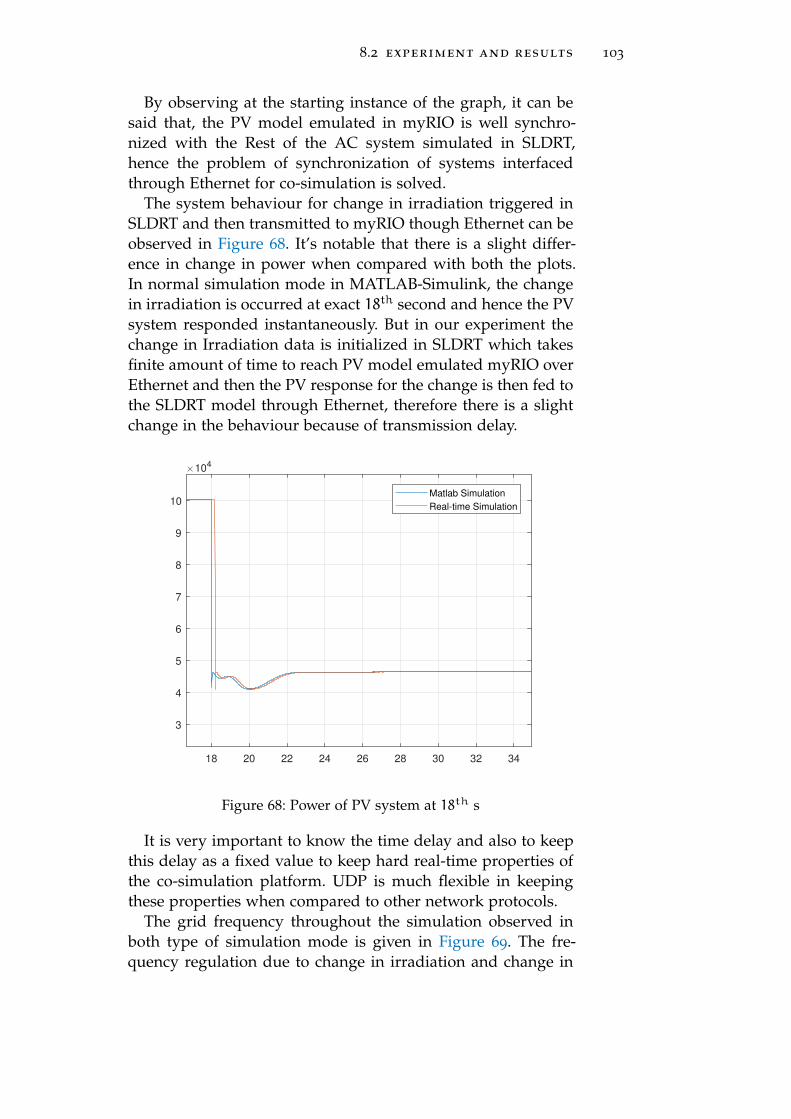
8.2 experiment and results 103
By observing at the starting instance of the graph, it can besaid that, the PV model emulated in myRIO is well synchro-nized with the Rest of the AC system simulated in SLDRT,hence the problem of synchronization of systems interfacedthrough Ethernet for co-simulation is solved.
The system behaviour for change in irradiation triggered inSLDRT and then transmitted to myRIO though Ethernet can beobserved in Figure 68. It’s notable that there is a slight differ-ence in change in power when compared with both the plots.In normal simulation mode in MATLAB-Simulink, the changein irradiation is occurred at exact 18th second and hence the PVsystem responded instantaneously. But in our experiment thechange in Irradiation data is initialized in SLDRT which takesfinite amount of time to reach PV model emulated myRIO overEthernet and then the PV response for the change is then fed tothe SLDRT model through Ethernet, therefore there is a slightchange in the behaviour because of transmission delay.
18 20 22 24 26 28 30 32 34
3
4
5
6
7
8
9
10
104
Matlab Simulation
Real-time Simulation
Figure 68: Power of PV system at 18th s
It is very important to know the time delay and also to keepthis delay as a fixed value to keep hard real-time properties ofthe co-simulation platform. UDP is much flexible in keepingthese properties when compared to other network protocols.
The grid frequency throughout the simulation observed inboth type of simulation mode is given in Figure 69. The fre-quency regulation due to change in irradiation and change in
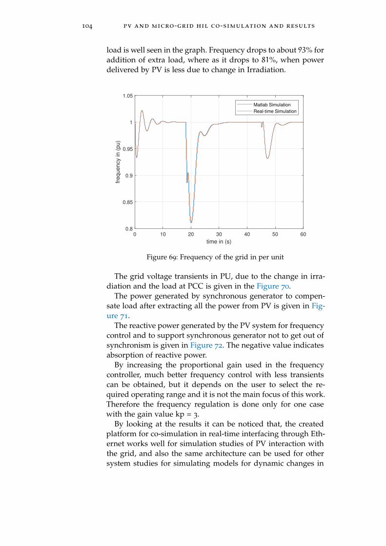
104 pv and micro-grid hil co-simulation and results
load is well seen in the graph. Frequency drops to about 93% foraddition of extra load, where as it drops to 81%, when powerdelivered by PV is less due to change in Irradiation.
0 10 20 30 40 50 60
time in (s)
0.8
0.85
0.9
0.95
1
1.05
frequency in (
pu)
Matlab Simulation
Real-time Simulation
Figure 69: Frequency of the grid in per unit
The grid voltage transients in PU, due to the change in irra-diation and the load at PCC is given in the Figure 70.
The power generated by synchronous generator to compen-sate load after extracting all the power from PV is given in Fig-ure 71.
The reactive power generated by the PV system for frequencycontrol and to support synchronous generator not to get out ofsynchronism is given in Figure 72. The negative value indicatesabsorption of reactive power.
By increasing the proportional gain used in the frequencycontroller, much better frequency control with less transientscan be obtained, but it depends on the user to select the re-quired operating range and it is not the main focus of this work.Therefore the frequency regulation is done only for one casewith the gain value kp = 3.
By looking at the results it can be noticed that, the createdplatform for co-simulation in real-time interfacing through Eth-ernet works well for simulation studies of PV interaction withthe grid, and also the same architecture can be used for othersystem studies for simulating models for dynamic changes in
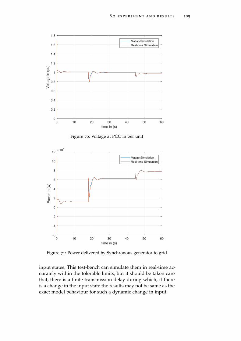
8.2 experiment and results 105
0 10 20 30 40 50 60
time in (s)
0
0.2
0.4
0.6
0.8
1
1.2
1.4
1.6
1.8
Voltage in (
pu)
Matlab Simulation
Real-time Simulation
Figure 70: Voltage at PCC in per unit
0 10 20 30 40 50 60
time in (s)
-6
-4
-2
0
2
4
6
8
10
12
Pow
er
in (
w)
104
Matlab Simulation
Real-time Simulation
Figure 71: Power delivered by Synchronous generator to grid
input states. This test-bench can simulate them in real-time ac-curately within the tolerable limits, but it should be taken carethat, there is a finite transmission delay during which, if thereis a change in the input state the results may not be same as theexact model behaviour for such a dynamic change in input.
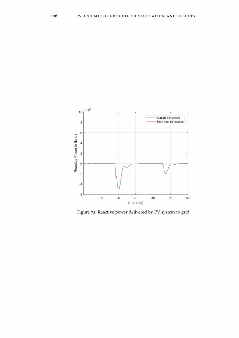
106 pv and micro-grid hil co-simulation and results
0 10 20 30 40 50 60
time in (s)
-6
-4
-2
0
2
4
6
8
10
Reactive P
ow
er
in (
kvar)
104
Matlab Simulation
Real-time Simulation
Figure 72: Reactive power delivered by PV system to grid
9C O N C L U S I O N
In this thesis work an overview of Hardware-in-the-loop sim-ulation studies, that can be used to investigate PV system in-teraction with the other systems under study are presented. Ahigh performance PV model which can deliver accurate resultsupto 5 decimals with good convergence is created and used forreal-time simulation to validate the control used for MPPT andalso to study the system behaviour with the grid using P-HILtechniques.
9.1 contributions to the engineering community
A suite of general purpose analytic tools and mathematicalmodels have been developed to facilitate the detailed studyof PV systems implemented, on a state-of-the-art Hardware-in-the-loop system, Specifically,
1. A platform for real-time simulation of PV is proposedwith the architecture that enables simulation of multiplemodels in parallel and has model integration over theactual measurement system, allowing to implement HILtechniques in data level, signal level and power level.
Data level integration is implemented by model integra-tion through the software which bridges the model run-ning in the hardware internally, signal level is done bydriving the inputs and outputs through the FPGA IO,present in myRIO hardware. Power level integration canbe done with the present architecture, where as it’s notpresented in this work. Two test benches are created tomeet the goals of this thesis using proposed architecture,
a) Test-bench 1: PV and MPPT with the fixed resistiveload; in this test-bench the ability of MPPT controlto operate the PV system to deliver the maximumpower is investigated in real-time. The results ob-tained for change in irradiation is compared with theMATLAB-Simulink results and the standards men-tioned in data sheet.
107
108 conclusion
From the results mentioned in Chapter 5, I can con-clude that the developed model is delivering accu-rate results and the test bench can be used for furtherstudies of PV and validation of controller.
b) Test-bench 2: PV with Storage connected to a DC bus;This test-bench is created to study the PV systemmodel upto DC bus level with the switching charac-teristics of the converter, a DC bus regulated at con-stant voltage to which, multiple loads, PV source andstorage systems are connected. The real world tem-perature and irradiation are given to the emulatedPV model in run-time using respective sensors andFPFA IO. The storage interaction for maintaining thegrid voltage constant for power variation in load andsource are studied.
2. The procedural methods to bring the mathematical modelfrom model based design environment to the hardwareintegration of the model using tools like Simulink coder,Model interface tool kit etc., that generate automatic Ccode for respective hardware targets.
3. While simulating a complex model like grid, memory isa main problem that is encountered to emulate the modelin a real-time hardware, hence another frame work is pro-posed to reduce the complications of grid emulation.
a) In this work I emulate the PV model in myRIO hard-ware using LabVIEW VI and executed as a standalonesystem, the grid model along with the DC-DC con-verter and the MPPT control is modeled in MATLAB-Simulink and co-Simulated with myRIO making SL-DRT as RTDS and using Intel processor of desktopas a target hardware.
b) Both the systems are interfaced over Ethernet usingUDP protocol for data transmission. This test-benchis also useful to study the hard real-time propertiesof data transmission used in power system commu-nication network.
9.2 recommendations and future research
1. Acausal approach of modelling PV is a very interestingtopic that can be used for HIL testing. It reduces the com-
9.2 recommendations and future research 109
plexity of modelling PV for current type delivery or volt-age type delivery as required by system present in theROS. Unfortunately automatic code generator like Simulinkcoder doesn’t support for code conversion of acausal mod-els.
2. myRIO is capable of reaching higher frequencies upto 4
Mhz in LabVIEW, but with VeriStand it is seen that upto 1
khz it is able to work with the real-time capabilities, afterthat overrun occurs. I suggest, it is a good topic to inves-tigate and solve this problem to have better performanceof myRIO to simulate complex models with higher fre-quency in real-time using VeriStand.
3. The test-bench one, is having the controller in the ROSmodel, instead a real hardware can be used as controllerand connect to the model using FPGA IO, so it can beused for testing the prototype and quality check in caseof bulk manufacturing.
4. myRIO can also be used as an input and output device togather the real world data and feed them to SLDRT or todeliver the simulated output to the real world system inrun-time.
5. Though it’s declared by Mathworks that, the UDP proto-col used in SLDRT is hard-realtime, it is observed thatthere is no fixed delay in the transmission. Hence it is bet-ter to investigate the problem that, is the problem is frommyRIO or SLDRT and to have hard-realtime characteris-tics in the simulation.

10A P P E N D I X A
This chapter will explain about few factors that has to be con-sidered for preparation of myRIO for usage in VeriStand.
10.1 how to create custom fpga bit file
The following procedures will guide you regarding how to cre-ate a custom FPGA bit file for myRIO. Bit file for myRIO isnot officially present in VeriStand, as it is present for cRIO orother hardware targets of National Instruments, this is because,myRIO is not officially supported for use in VeriStanad thoughit gas all capabilities of doing so. Here in this work i have madeconscious effort to guide the reader to successfully create bitfile and the xml file for FPGA that has to added in VeriStand todefine the FPGA hardware target present in the myRIO chassis.
Creation of FPGA bitfile requires these platforms installedin the PC. they are, LabVIEW, LabVIEW FPGA, myRIO add-on on LabVIEW, LabVIEW RT and VeriStand. This procedureinvolves 3 stages they are,
1. Making a copy of the sample FPGA VI and project.
2. Customizing the FPGA VI.
3. Compiling the FPGA VI into a bitfile.
10.1.1 Making a copy of the sample FPGA VI and project
1. Browse to the following folder C:/Users/Public/Documents/NationalInstruments/NIVeriStand2017/FPGA/Templates,in the templates folder you can find the LabVIEW VI andprojects.
2. Copy ’NI VeriStand FPGA IO cRIO’ project in the samedirectory and open the copy in LabVIEW.
3. Expand the RT CompactRIO Target item under My Com-puter in the Project Explorer window. Complete the fol-lowing steps to add a new device to the project.
a) Connect myRIO to PC with the appropriate IP adress.
111
112 appendix a
b) Right-click My Computer and select New then Tar-gets and Devices from the shortcut menu.
c) Select the New target or device option in the Targetsand Devices dialog box.
d) Select the device type from the list and click the OKbutton to close the dialog box and add the device.
e) In the Project Explorer window, drag NI VeriStandFPGA DMA IO.vi from the FPGA Target (cRIO-9103)to the myRIO FPGA target. Also drag the DMA WRITEand DMA READ FIFOs, and the FPGA I/O foldersfrom the original target to the new target. The FPGAVI shows broken wires from any FPGA I/O Nodeswith undefined channels.
f) Double-click NI VeriStand FPGA DMA IO.vi in theProject Explorer window to open the VI. Save Asfrom the pull-down menu of the NI VeriStand FPGADMA IO VI window. Ensure the Substitute copy fororiginal option is selected and click the Continue but-ton.
g) Rename the VI and save it in the same folder andalso save the project.
10.1.2 Customizing the FPGA VI
Modify the FPGA VI, paying attention to the following guide-lines:
1. Do not modify, remove, or rename any block diagram ob-jects in the gray areas of the sample FPGA VI.
2. Do not modify the read and write code except to changethe number of read and write packets or to change thesize of the array constant for the DMA read operation ofthe DMA WRITE FIFO.
3. As you create controls that represent parameters, ensurethat the name of each control is unique within the VI.
4. Do not use the following control/indicator names: LoopRate (usec), Use External Timing, Reset, Start.
5. Replace cRIO unrecognized IO, PWM etc., blocks with thesame myRIO blocks and save the VI.

10.1 how to create custom fpga bit file 113
10.1.3 Compiling the Custom FPGA VI into a Bitfile
Complete the following steps to compile the custom FPGA VIand create the bitfile.
1. Display the Project Explorer window.
2. Right-click the FPGA VI in the tree and select Compilefrom the shortcut menu to compile the FPGA VI. Lab-VIEW then creates a bitfile for this VI.
3. The compiler places the bitfile in a sub directory, FPGABit files, relative to the project file directory. By default,the bitfile name is name of project name of FPGA VI.lvbitx.
To create the xml file that can be used, open the present xmlfile already given in the folder C:/Users/Public/Documents/
NationalInstruments/NIVeriStand2017/FPGA, open the file named’cRIO-9103 Analog, PWM, Digital Lines’ in text format and thenreplace the name of the bit file to the file name of the newly gen-erated bit file, and save it.
It should be noted that the bit file .LVBTIX, xml file , NI Veri-Stand FPGA DMA.xsd and NI VeriStand FPGA DMA shouldbe in the same folder. Now you can add the generated bit filein VeriStand.

11A P P E N D I X B
This Chapter will brief about how to prepare the model andthe PC for real-time execution in desktop using Simulink Desk-top Real-Time and it’s kernel. The Simulink Desktop Real-Timekernel assigns the highest priority of execution to the real-timeexecutable, which allows it to run without interference at theselected sample rate
11.1 sldrt kernel installation
Installing the kernel configures it to start running in the back-ground each time the computer is turned on. The procedure forinstallation is,
1. Type sldrtkernel -install and execute in the MATLABCommand Window.
The MATLAB Command Window displays one of thesemessages: You are going to install the Simulink DesktopReal-Time kernel. Do you want to proceed? [y] :
2. Type y to continue installing the kernel.
3. If a message appears asking you to restart your computer,do so before attempting to use the kernel, or your SimulinkDesktop Real-Time model will not run.
4. After installing the kernel, verify that it was installed bytyping: rtwho.
11.2 configuring model
1. In the Simulink window, and from the Simulation menu,click Model Configuration Parameters. In the Configura-tion Parameters dialog box, click the Solver tab.
2. In the Start time field, enter 0.0. In the Stop time field,enter the amount of time to run the model.
3. From the Type list, choose Fixed-step. Simulink Codercode generation software does not support variable stepsolvers. From the Solver list, choose a solver.
115
116 appendix b
4. In the Fixed step size field, enter a sample time.
11.3 code generation parameters
After you creating the Simulink model, we have to enter sim-ulation parameters for use by Simulink Coder code generationsoftware for creating C code and building a real-time applica-tion.
1. In the Simulink window, and from the Simulation menu,click large Model Configuration Parameters. Then clickCode generation node.
2. In the Target selection section, click the Browse button atthe System target file list.
3. Select the system target file for building a Simulink Desk-top Real-Time application, rtwin.tlc, and click OK.
4. Click the Hardware Implementation node. The defaultvalues are derived from the architecture of the host com-puter. Then verify the data and click Apply and then OK.
5. Click on build model symbol to generate code and buildthe model for execution in real-time.
11.4 signal logging to workspace
Data is saved to the MATLAB workspace through a SimulinkScope block, After creating Simulink model and adding a Scopeblock, enter the signal and triggering properties for logging tothe MATLAB workspace by following procedure.
1. In the Simulation window, click Code then External ModeControl Panel.
2. Click Signal and Triggering button.
3. Click the Select all button. From the Source list, choosemanual. From the Mode list, choose normal.
4. In the Duration field, enter the number of sample pointsin a data buffer. It depends on your sample rate and thestop time. Click apply and close it. Restart MATLAB aftermodel building and then select external mode and thenclick run by connecting to the hardware target.
B I B L I O G R A P H Y
[1] url: https://ec.europa.eu/programmes/horizon2020/what-horizon-2020.
[2] url: http://www.ni.com/veristand/.
[3] url: http://www.ni.com/pdf/manuals/376047c.pdf.
[4] url: https://mathworks.com.
[5] url: https://it.mathworks.com/products/simulink-desktop-real-time.html.
[6] George A Aggidis and Audrius Židonis. “Hydro turbineprototype testing and generation of performance curves:Fully automated approach.” In: Renewable Energy 71 (2014),pp. 433–441.
[7] KN Areerak, SV Bozhko, GM Asher, and DWP Thomas.“DQ-transformation approach for modelling and stabilityanalysis of AC-DC power system with controlled PWMrectifier and constant power loads.” In: Power electronicsand motion control conference, 2008. EPE-PEMC 2008. 13th.IEEE. 2008, pp. 2049–2054.
[8] Adi Ben-Israel. “A Newton-Raphson method for the solu-tion of systems of equations.” In: J. Math. Anal. Appl 15.2(1966), pp. 243–252.
[9] Upama Bose, Sumit K Chattopadhyay, Chandan Chakraborty,and Bikash Pal. “A novel method of frequency regulationin microgrid.” In: Power India International Conference (PI-ICON), 2016 IEEE 7th. IEEE. 2016, pp. 1–6.
[10] Alain Bouscayrol. “Different types of hardware-in-the-loopsimulation for electric drives.” In: Industrial Electronics,2008. ISIE 2008. IEEE International Symposium on. IEEE.2008, pp. 2146–2151.
[11] Komkrit Chomsuwan, Prapart Prisuwanna, and VeerapolMonyakul. “Photovoltaic grid-connected inverter usingtwo-switch buck-boost converter.” In: Photovoltaic Special-ists Conference, 2002. Conference Record of the Twenty-NinthIEEE. IEEE. 2002, pp. 1527–1530.
117

118 Bibliography
[12] E De Jaeger, N Janssens, B Malfliet, and F Van De Meule-broeke. “Hydro turbine model for system dynamic stud-ies.” In: IEEE Transactions on Power Systems 9.4 (1994), pp. 1709–1715.
[13] Francisco P Demello and Charles Concordia. “Conceptsof synchronous machine stability as affected by excitationcontrol.” In: IEEE Transactions on power apparatus and sys-tems 88.4 (1969), pp. 316–329.
[14] Chris S Edrington, Michael Steurer, James Langston, TouriaEl-Mezyani, and Karl Schoder. “Role of power hardwarein the loop in modeling and simulation for experimenta-tion in power and energy systems.” In: Proceedings of theIEEE 103.12 (2015), pp. 2401–2409.
[15] MD Omar Faruque, Thomas Strasser, Georg Lauss, VahidJalili-Marandi, Paul Forsyth, Christian Dufour, VenkataDinavahi, Antonello Monti, Panos Kotsampopoulos, JuanA Martinez, et al. “Real-time simulation technologies forpower systems design, testing, and analysis.” In: IEEEPower and Energy Technology Systems Journal 2.2 (2015), pp. 63–73.
[16] Max Felser. “Real-time ethernet-industry prospective.” In:Proceedings of the IEEE 93.6 (2005), pp. 1118–1129.
[17] Charles Hanley, Georgianne Peek, John Boyes, Geoff Klise,Joshua Stein, Dan Ton, and Tien Duong. “Technology de-velopment needs for integrated grid-connected PV sys-tems and electric energy storage.” In: Photovoltaic Special-ists Conference (PVSC), 2009 34th IEEE. IEEE. 2009, pp. 001832–001837.
[18] “’IEEE Standard Definitions for Excitation Systems forSynchronous Machines’.” In: ().
[19] Rolf Isermann, Jochen Schaffnit, and Stefan Sinsel. “Hardware-in-the-loop simulation for the design and testing of engine-control systems.” In: Control Engineering Practice 7.5 (1999),pp. 643–653.
[20] Willett Kempton, Victor Udo, Ken Huber, Kevin Komara,Steve Letendre, Scott Baker, Doug Brunner, and Nat Pearre.“A test of vehicle-to-grid (V2G) for energy storage and fre-quency regulation in the PJM system.” In: Results from anIndustry-University Research Partnership 32 (2008).
Bibliography 119
[21] Nand Kishor, RP Saini, and SP Singh. “A review on hy-dropower plant models and control.” In: Renewable andSustainable Energy Reviews 11.5 (2007), pp. 776–796.
[22] Prabha Kundur, Neal J Balu, and Mark G Lauby. Powersystem stability and control. Vol. 7. McGraw-hill New York,1994.
[23] Georg F Lauss, M Omar Faruque, Karl Schoder, Chris-tian Dufour, Alexander Viehweider, and James Langston.“Characteristics and design of power hardware-in-the-loopsimulations for electrical power systems.” In: IEEE Trans-actions on Industrial Electronics 63.1 (2016), pp. 406–417.
[24] Felix Lehfuss, Georg Lauss, Panos Kotsampopoulos, NikosHatziargyriou, Paul Crolla, and Andrew Roscoe. “Com-parison of multiple power amplification types for powerHardware-in-the-Loop applications.” In: Complexity in En-gineering (COMPENG), 2012. IEEE. 2012, pp. 1–6.
[25] Wen Li and Jason Meiners. “Introduction to phase-lockedloop system modeling.” In: Analog Applications (2000).
[26] PM Menghal and A Jaya Laxmi. “Real time control of elec-trical machine drives: A review.” In: Power, Control andEmbedded Systems (ICPCES), 2010 International Conferenceon. IEEE. 2010, pp. 1–6.
[27] Ned Mohan and Tore M Mohan. Power electronics. Vol. 3.John wiley & sons New York, 1995.
[28] Saad Motahhir, Abdelaziz El Ghzizal, Souad Sebti, andAziz Derouich. “MIL and SIL and PIL tests for MPPTalgorithm.” In: Cogent Engineering 4.1 (2017), p. 1378475.
[29] Sabar Nababan, E Muljadi, and Frede Blaabjerg. “An overviewof power topologies for micro-hydro turbines.” In: PowerElectronics for Distributed Generation Systems (PEDG), 20123rd IEEE International Symposium on. IEEE. 2012, pp. 737–744.
[30] Sung Chul Oh. “Evaluation of motor characteristics forhybrid electric vehicles using the hardware-in-the-loopconcept.” In: IEEE transactions on vehicular technology 54.3(2005), pp. 817–824.
[31] Jukka V Paatero and Peter D Lund. “Effects of large-scalephotovoltaic power integration on electricity distributionnetworks.” In: Renewable Energy 32.2 (2007), pp. 216–234.
120 Bibliography
[32] H Palahalli, Y Huo, and G Gruosso. “Real Time Simula-tion of Photovoltaic System using FPGA.” In: 2018 Inter-national Symposium on Power Electronics, Electrical Drives,Automation and Motion (SPEEDAM). IEEE. 2018, pp. 865–870.
[33] KOU Pan-Gao, ZHOU Jian-zhong, HE Yao-Yao, XIANGXiu-qiao, and LI Chao-shun. “Optimal PID governor tun-ing of hydraulic turbine generators with bacterial forag-ing particle swarm optimization algorithm.” In: Proceed-ings of the CSEE 29.26 (2009), pp. 101–106.
[34] Jean-Nicolas Paquin, Christian Dufour, and Jean Bélanger.“A hardware-in-the-loop simulation platform for proto-typing and testing of wind generator controllers.” In: CIGRÉCanada Conference on Power Systems Winnipeg. 2008.
[35] BR Prentice. “Fundamental concepts of synchronous ma-chine reactances.” In: Transactions of the American Instituteof Electrical Engineers 56.12 (1937), pp. 1–21.
[36] Wei Ren, Michael Steurer, and Thomas L Baldwin. “Im-prove the stability and the accuracy of power hardware-in-the-loop simulation by selecting appropriate interfacealgorithms.” In: IEEE Transactions on Industry Applications44.4 (2008), pp. 1286–1294.
[37] Wei Ren, Michael Steurer, and Steve Woodruff. “Accuracyevaluation in power hardware-in-the-loop (PHIL) simu-lation center for advanced power systems.” In: Proceed-ings of the 2007 summer computer simulation conference. Soci-ety for Computer Simulation International. 2007, pp. 489–493.
[38] Pedro Reviriego, Jose-Alberto Hernadez, David Larrabeiti,and Juan Antonio Maestro. “Burst transmission for energy-efficient ethernet.” In: IEEE Internet Computing 14.4 (2010),pp. 50–57.
[39] David Ruffieux. Phase-locked loop. US Patent 8,040,190. 2011.
[40] Bruno Strah, Ognjen Kuljaca, and Zoran Vukic. “Speedand active power control of hydro turbine unit.” In: IEEETransactions on energy conversion 20.2 (2005), pp. 424–434.
[41] Bidyadhar Subudhi and Raseswari Pradhan. “A compara-tive study on maximum power point tracking techniquesfor photovoltaic power systems.” In: IEEE transactions onSustainable Energy 4.1 (2013), pp. 89–98.
Bibliography 121
[42] S Sumathi, L Ashok Kumar, and P Surekha. Solar PVand wind energy conversion systems: an introduction to the-ory, modeling with MATLAB/SIMULINK, and the role of softcomputing techniques. Springer, 2015.
[43] Mikio Taguchi, Ayumu Yano, Satoshi Tohoda, Kenta Mat-suyama, Yuya Nakamura, Takeshi Nishiwaki, KazunoriFujita, and Eiji Maruyama. “24.7% record efficiency HITsolar cell on thin silicon wafer.” In: IEEE Journal of Photo-voltaics 4.1 (2014), pp. 96–99.
[44] Poi Loon Tang and Clarence W de Silva. “Compensa-tion for transmission delays in an ethernet-based controlnetwork using variable-horizon predictive control.” In:IEEE Transactions on Control Systems Technology 14.4 (2006),pp. 707–718.
[45] Olivier Tremblay, Louis-A Dessaint, and Abdel-Illah Dek-kiche. “A generic battery model for the dynamic simu-lation of hybrid electric vehicles.” In: Vehicle Power andPropulsion Conference, 2007. VPPC 2007. IEEE. Ieee. 2007,pp. 284–289.
[46] Huan-Liang Tsai, Ci-Siang Tu, Yi-Jie Su, et al. “Devel-opment of generalized photovoltaic model using MAT-LAB/SIMULINK.” In: Proceedings of the world congress onEngineering and computer science. Vol. 2008. San Francisco,USA. 2008, pp. 1–6.
[47] H Vu, P Pruvot, C Launay, and Y Harmand. “An im-proved voltage control on large-scale power system.” In:IEEE transactions on power systems 11.3 (1996), pp. 1295–1303.
[48] Geoff Walker et al. “Evaluating MPPT converter topolo-gies using a MATLAB PV model.” In: Journal of Electrical& Electronics Engineering, Australia 21.1 (2001), p. 49.
[49] Bin Wu, Yongqiang Lang, Navid Zargari, and Samir Kouro.“Power converters in wind energy conversion systems.”In: Power Conversion and Control of Wind Energy Systems(2011), pp. 87–152.
[50] Hao Zhang, Diyi Chen, Beibei Xu, and Feifei Wang. “Non-linear modeling and dynamic analysis of hydro-turbinegoverning system in the process of load rejection tran-sient.” In: Energy Conversion and Management 90 (2015),pp. 128–137.