
Optimization of an ejector refrigeration cycle
153
DOTTORATO DI RICERCA IN "Energetica a Tecnologie industriali innovative" CICLO XXV COORDINATORE Prof. Maurizio De Lucia Optimization of an ejector refrigeration cycle Settore Scientifico Disciplinare ING/IND10 Dottorando Tutore Dott. Dario Paganini Prof. Giuseppe Grazzini ___________________ ____________________ (firma) (firma) Anni 2010/2012
Transcript of Optimization of an ejector refrigeration cycle
DOTTORATO DI RICERCA IN "Energetica a Tecnologie industriali
innovative"
CICLO XXV
COORDINATORE Prof. Maurizio De Lucia
Optimization of an ejector refrigeration cycle
Settore Scientifico Disciplinare ING/IND10 Dottorando Tutore Dott. Dario Paganini Prof. Giuseppe Grazzini ___________________ ____________________ (firma) (firma)
Anni 2010/2012
Contents
List of Figures 3
List of Tables 5
1 Introduction 8
2 Ejector refrigeration 10
2.1 Historical background . . . . . . . . . . . . . . . . . 11
2.2 State of the art . . . . . . . . . . . . . . . . . . . . . 12
2.2.1 Modelling techniques . . . . . . . . . . . . . . 12
2.3 Working fluid analysis . . . . . . . . . . . . . . . . . 15
2.4 Ejector refrigeration cycle . . . . . . . . . . . . . . . 17
2.5 Working fluid selection . . . . . . . . . . . . . . . . . 19
3 Cycle optimization 23
3.1 Optimization concept . . . . . . . . . . . . . . . . . 24
3.1.1 Optimization algorithm . . . . . . . . . . . . 25
3.2 Plant modelling . . . . . . . . . . . . . . . . . . . . . 27
3.2.1 Working fluids properties . . . . . . . . . . . 28
3.2.2 Heat exchangers . . . . . . . . . . . . . . . . 28
3.3 Optimization program description . . . . . . . . . . 39
3.4 Optimization results . . . . . . . . . . . . . . . . . . 42
4 Plant design 44
4.1 Model description . . . . . . . . . . . . . . . . . . . . 44
1
CONTENTS 2
4.2 Design program description . . . . . . . . . . . . . . 47
4.3 Suction line heat exchanger . . . . . . . . . . . . . . 52
4.4 Pump . . . . . . . . . . . . . . . . . . . . . . . . . . 53
4.5 Secondary expansion . . . . . . . . . . . . . . . . . . 53
4.5.1 Secondary expansion efficiency . . . . . . . . 54
4.6 Primary expansion . . . . . . . . . . . . . . . . . . . 59
4.6.1 Primary expansion efficiency . . . . . . . . . 59
4.7 Mixing . . . . . . . . . . . . . . . . . . . . . . . . . . 62
4.8 Diffuser design: the CRMC method . . . . . . . . . 66
4.8.1 CRMC stretch . . . . . . . . . . . . . . . . . 70
4.8.2 Conical stretch . . . . . . . . . . . . . . . . . 71
4.8.3 Diffuser design results . . . . . . . . . . . . . 71
4.9 Design program results . . . . . . . . . . . . . . . . . 73
4.10 Sensitivity analysis . . . . . . . . . . . . . . . . . . . 74
5 Experimental results 78
5.1 Experimental apparatus . . . . . . . . . . . . . . . . 78
5.1.1 Plant layout . . . . . . . . . . . . . . . . . . . 79
5.1.2 Ejector description . . . . . . . . . . . . . . . 80
5.1.3 Plate heat exchangers selection . . . . . . . . 85
5.1.4 Measurement equipment . . . . . . . . . . . . 86
5.2 Experimental results . . . . . . . . . . . . . . . . . . 87
5.2.1 Positioning of NXP . . . . . . . . . . . . . . . 87
5.2.2 Condenser pressure variation . . . . . . . . . 88
5.2.3 Pressure profiles along ejector . . . . . . . . . 92
5.2.4 Error analysis . . . . . . . . . . . . . . . . . . 94
5.2.5 Results analysis . . . . . . . . . . . . . . . . . 95
6 Conclusions 97
Acknowledgements 99
Bibliography 100
A Optimization program code 107

CONTENTS 3
B Design program code 120
C Nozzle efficiency code 141
List of Figures
2.1 Scheme of operating cycle of ejector refrigerator . . . 18
2.2 Typical ejector refrigeration cycle on Ts diagram . . 19
2.3 Typical Ts diagram for wet and dry fluid . . . . . . 20
3.1 System considered for plant optimization . . . . . . 27
3.2 Optimization program block diagram . . . . . . . . . 40
3.3 CRMC diffuser design obtained by optimization pro-
gram . . . . . . . . . . . . . . . . . . . . . . . . . . . 43
4.1 Ts diagram for the ejector cycle with R245fa . . . . 45
4.2 Ph diagram for the ejector cycle with R245fa . . . . 46
4.3 Scheme of ejector refrigeration system . . . . . . . . 46
4.4 Flow chart of the design program . . . . . . . . . . . 48
4.5 Secondary nozzle profile . . . . . . . . . . . . . . . . 56
4.6 Pressure profile along secondary nozzle . . . . . . . . 58
4.7 Primary nozzle profile . . . . . . . . . . . . . . . . . 61
4.8 Pressure profile along the primary nozzle . . . . . . . 63
4.9 Mixing chamber geometry . . . . . . . . . . . . . . . 63
4.10 Velocity derivative profile along supersonic diffuser . 70
4.11 Radius and Mach of supersonic diffuser . . . . . . . 72
4.12 Pressure and entropy of supersonic diffuser . . . . . 72
4.13 Ejector geometry . . . . . . . . . . . . . . . . . . . . 74
4.14 Ts diagram for the ejector cycle with R245fa and SLHX 77
5.1 Experimental prototype plant scheme . . . . . . . . 80
4
LIST OF FIGURES 5
5.2 Experimental prototype plant . . . . . . . . . . . . . 81
5.3 Complete ejector design . . . . . . . . . . . . . . . . 82
5.4 Diffuser solution A . . . . . . . . . . . . . . . . . . . 84
5.5 Diffuser solution B . . . . . . . . . . . . . . . . . . . 85
5.6 Water heating system for generator supply circuit . . 86
5.7 COPs as function of different NXP positions . . . . . 88
5.8 COPs as function of condenser pressure - solution A 90
5.9 COPs as function of condenser pressure - solution B 91
5.10 Comparison of COP as function of critical temperature 92
5.11 Wall pressure values along diffuser - solution A . . . 93
5.12 Wall pressure values along diffuser for different con-
denser pressure - solution B . . . . . . . . . . . . . . 93
5.13 Wall pressure values along diffuser for different evap-
orator temperatures - solution B . . . . . . . . . . . 94
List of Tables
2.1 Relevant features of possible refrigerants . . . . . . . 22
3.1 Thermodynamic input data for plate heat exchangers 30
3.2 Geometric input data for plate heat exchangers . . . 31
3.3 Correlations references for generator and evaporator
plate heat exchangers . . . . . . . . . . . . . . . . . 33
3.4 Coefficients used for plate heat exchangers correlations 34
3.5 Correlations references for condenser plate heat ex-
changer . . . . . . . . . . . . . . . . . . . . . . . . . 36
3.6 Input data table for plate heat exchangers . . . . . . 39
3.7 Optimization program input data . . . . . . . . . . . 41
3.8 Range of variable parameters of optimization program 41
3.9 Optimization program main results . . . . . . . . . . 43
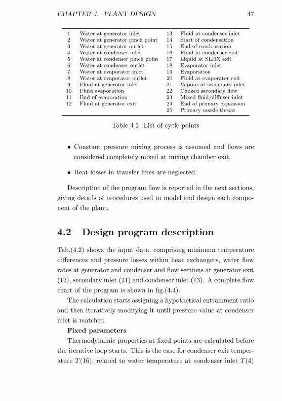
4.1 List of cycle points . . . . . . . . . . . . . . . . . . . 47
4.2 Design program input data . . . . . . . . . . . . . . 49
4.3 Secondary nozzle efficiency determination results . . 58
4.4 Primary nozzle efficiency determination results . . . 62
4.5 Design program input data . . . . . . . . . . . . . . 73
4.6 Design program output data . . . . . . . . . . . . . . 74
4.7 Design program output for different ∆T . . . . . . . 75
4.8 Design program output for different ηmix . . . . . . 76
4.9 Design program output for different CRMC length . 76
4.10 Design program output for different CRMC length . 77
6

LIST OF TABLES 7
5.1 Different diffuser solution comparison . . . . . . . . 83
5.2 Simulation results used for ejector B design . . . . . 84
5.3 Characteristics of selected plate heat exchangers . . 85
Chapter 1
Introduction
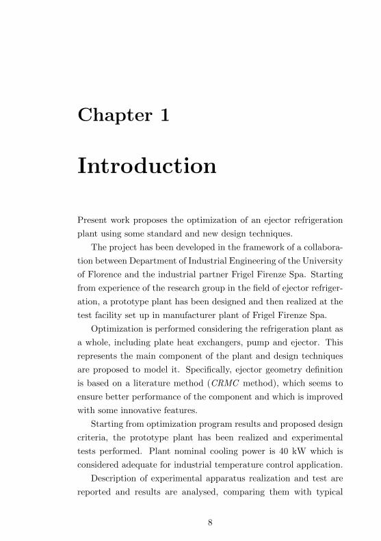
Present work proposes the optimization of an ejector refrigeration
plant using some standard and new design techniques.
The project has been developed in the framework of a collabora-
tion between Department of Industrial Engineering of the University
of Florence and the industrial partner Frigel Firenze Spa. Starting
from experience of the research group in the field of ejector refriger-
ation, a prototype plant has been designed and then realized at the
test facility set up in manufacturer plant of Frigel Firenze Spa.
Optimization is performed considering the refrigeration plant as
a whole, including plate heat exchangers, pump and ejector. This
represents the main component of the plant and design techniques
are proposed to model it. Specifically, ejector geometry definition
is based on a literature method (CRMC method), which seems to
ensure better performance of the component and which is improved
with some innovative features.
Starting from optimization program results and proposed design
criteria, the prototype plant has been realized and experimental
tests performed. Plant nominal cooling power is 40 kW which is
considered adequate for industrial temperature control application.
Description of experimental apparatus realization and test are
reported and results are analysed, comparing them with typical
8

CHAPTER 1. INTRODUCTION 9
ejector refrigeration system behaviour and design choices. Based
on experimental results, reliability of proposed models and design
techniques is verified.
Chapter 2
Ejector refrigeration
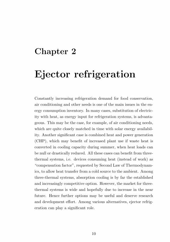
Constantly increasing refrigeration demand for food conservation,
air conditioning and other needs is one of the main issues in the en-
ergy consumption inventory. In many cases, substitution of electric-
ity with heat, as energy input for refrigeration systems, is advanta-
geous. This may be the case, for example, of air conditioning needs,
which are quite closely matched in time with solar energy availabil-
ity. Another significant case is combined heat and power generation
(CHP), which may benefit of increased plant use if waste heat is
converted in cooling capacity during summer, when heat loads can
be null or drastically reduced. All these cases can benefit from three-
thermal systems, i.e. devices consuming heat (instead of work) as
“compensation factor”, requested by Second Law of Thermodynam-
ics, to allow heat transfer from a cold source to the ambient. Among
three-thermal systems, absorption cooling is by far the established
and increasingly competitive option. However, the market for three-
thermal systems is wide and hopefully due to increase in the near
future. Hence further options may be useful and deserve research
and development effort. Among various alternatives, ejector refrig-
eration can play a significant role.
10
CHAPTER 2. EJECTOR REFRIGERATION 11
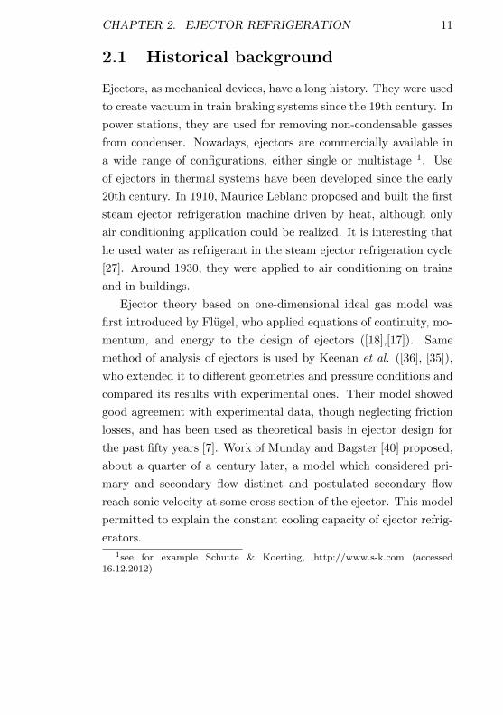
2.1 Historical background
Ejectors, as mechanical devices, have a long history. They were used
to create vacuum in train braking systems since the 19th century. In
power stations, they are used for removing non-condensable gasses
from condenser. Nowadays, ejectors are commercially available in
a wide range of configurations, either single or multistage 1. Use
of ejectors in thermal systems have been developed since the early
20th century. In 1910, Maurice Leblanc proposed and built the first
steam ejector refrigeration machine driven by heat, although only
air conditioning application could be realized. It is interesting that
he used water as refrigerant in the steam ejector refrigeration cycle
[27]. Around 1930, they were applied to air conditioning on trains
and in buildings.
Ejector theory based on one-dimensional ideal gas model was
first introduced by Flugel, who applied equations of continuity, mo-
mentum, and energy to the design of ejectors ([18],[17]). Same
method of analysis of ejectors is used by Keenan et al. ([36], [35]),
who extended it to different geometries and pressure conditions and
compared its results with experimental ones. Their model showed
good agreement with experimental data, though neglecting friction
losses, and has been used as theoretical basis in ejector design for
the past fifty years [7]. Work of Munday and Bagster [40] proposed,
about a quarter of a century later, a model which considered pri-
mary and secondary flow distinct and postulated secondary flow
reach sonic velocity at some cross section of the ejector. This model
permitted to explain the constant cooling capacity of ejector refrig-
erators.
1see for example Schutte & Koerting, http://www.s-k.com (accessed16.12.2012)
CHAPTER 2. EJECTOR REFRIGERATION 12
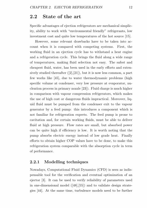
2.2 State of the art
Specific advantages of ejection refrigerators are mechanical simplic-
ity, ability to work with “environmental friendly” refrigerants, low
investment cost and quite low temperatures of the hot source [15].
However, some relevant drawbacks have to be taken into ac-
count when it is compared with competing systems. First, the
working fluid in an ejection cycle has to withstand a heat engine
and a refrigeration cycle. This brings the fluid along a wide range
of temperatures, making fluid selection not easy. The safest and
cheapest fluid, water, has been used in the early efforts and exten-
sively studied thereafter ([2],[21]), but it is now less common, a part
few works like [45], due to water thermodynamic problems (high
specific volume at condenser, very low pressure at evaporator, nu-
cleation process in primary nozzle [23]). Fluid charge is much higher
in comparison with vapour compression refrigerators, which makes
the use of high cost or dangerous fluids impractical. Moreover, liq-
uid fluid must be pumped from the condenser exit to the vapour
generator by a feed pump: this introduces a component which is
not familiar for refrigeration experts. The feed pump is prone to
cavitation and, for certain working fluids, must be able to deliver
fluid at high pressure. Flow rates are small, but absorbed power
can be quite high if efficiency is low. It is worth noting that the
pump absorbs electric energy instead of low grade heat. Finally
efforts to obtain higher COP values have to be done, to make this
refrigeration system comparable with the absorption cycle in term
of performance.
2.2.1 Modelling techniques
Nowadays, Computational Fluid Dynamics (CFD) is seen as indis-
pensable tool for the verification and eventual optimization of an
ejector [3]. It can be used to verify reliability of parameters used
in one-dimensional model ([48],[55]) and to validate design strate-
gies [44]. At the same time, turbulence models need to be further
CHAPTER 2. EJECTOR REFRIGERATION 13
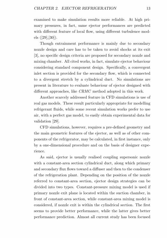
examined to make simulation results more reliable. At high pri-
mary pressures, in fact, same ejector performances are predicted
with different feature of local flow, using different turbulence mod-
els ([29],[30]).
Though entrainment performance is mainly due to secondary
nozzle design and care has to be taken to avoid shocks at its exit
[3], no specific design criteria are proposed for secondary nozzle and
mixing chamber. All cited works, in fact, simulate ejector behaviour
considering standard component design. Specifically, a convergent
inlet section is provided for the secondary flow, which is connected
to a divergent stretch by a cylindrical duct. No simulations are
present in literature to evaluate behaviour of ejector designed with
different approaches, like CRMC method adopted in this work.
Another scarcely addressed feature in CFD simulations is use of
real gas models. These result particularly appropriate for modelling
refrigerant fluids, while some recent simulation works prefer to use
air, with a perfect gas model, to easily obtain experimental data for
validation [29].
CFD simulations, however, requires a pre-defined geometry and
the main geometric features of the ejector, as well as of other com-
ponents of the refrigerator, may be calculated, in first instance, only
by a one-dimensional procedure and on the basis of designer expe-
rience.
As said, ejector is usually realised coupling supersonic nozzle
with a constant-area section cylindrical duct, along which primary
and secondary flux flows toward a diffuser and then to the condenser
of the refrigeration plant. Depending on the position of the nozzle
referred to constant-area section, ejector design strategies can be
divided into two types. Constant-pressure mixing model is used if
primary nozzle exit plane is located within the suction chamber, in
front of constant-area section, while constant-area mixing model is
considered, if nozzle exit is within the cylindrical section. The first
seems to provide better performance, while the latter gives better
performance prediction. Almost all current study has been focused
CHAPTER 2. EJECTOR REFRIGERATION 14
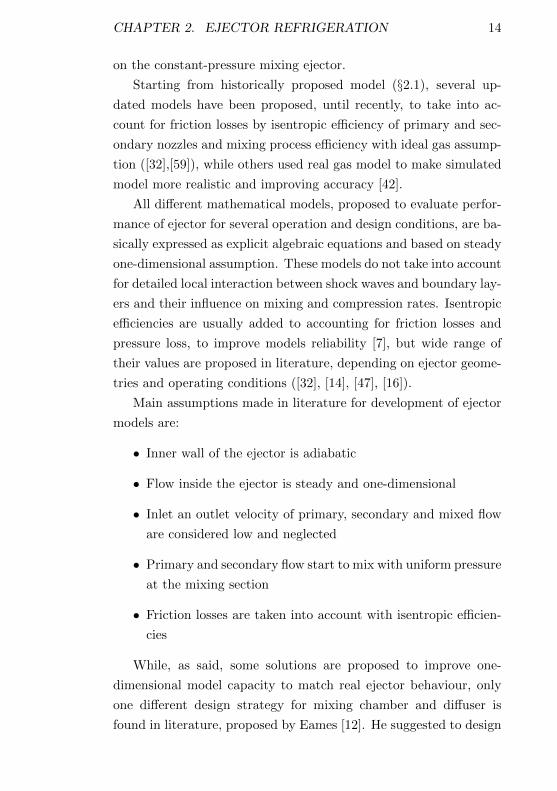
on the constant-pressure mixing ejector.
Starting from historically proposed model (§2.1), several up-
dated models have been proposed, until recently, to take into ac-
count for friction losses by isentropic efficiency of primary and sec-
ondary nozzles and mixing process efficiency with ideal gas assump-
tion ([32],[59]), while others used real gas model to make simulated
model more realistic and improving accuracy [42].
All different mathematical models, proposed to evaluate perfor-
mance of ejector for several operation and design conditions, are ba-
sically expressed as explicit algebraic equations and based on steady
one-dimensional assumption. These models do not take into account
for detailed local interaction between shock waves and boundary lay-
ers and their influence on mixing and compression rates. Isentropic
efficiencies are usually added to accounting for friction losses and
pressure loss, to improve models reliability [7], but wide range of
their values are proposed in literature, depending on ejector geome-
tries and operating conditions ([32], [14], [47], [16]).
Main assumptions made in literature for development of ejector
models are:
• Inner wall of the ejector is adiabatic
• Flow inside the ejector is steady and one-dimensional
• Inlet an outlet velocity of primary, secondary and mixed flow
are considered low and neglected
• Primary and secondary flow start to mix with uniform pressure
at the mixing section
• Friction losses are taken into account with isentropic efficien-
cies
While, as said, some solutions are proposed to improve one-
dimensional model capacity to match real ejector behaviour, only
one different design strategy for mixing chamber and diffuser is
found in literature, proposed by Eames [12]. He suggested to design
CHAPTER 2. EJECTOR REFRIGERATION 15
mixing chamber and diffuser using a new criterion, defined Constant
Rate of Momentum Change (CRMC), which imposes a constant rate
of variation of velocity along diffuser profile to obtain its geometric
description. This method ensures better performance, in term of
ejector entrainment ratio, compared to standard design approaches,
as results from experimental analysis performed on small scale pro-
totype [13].
Though a quite large amount of works have been done on mod-
elling and analysing ejector behaviour, further efforts seems to be
still necessary [28]
1. to study the influence of isentropic coefficients which are taken
as constant in the models and their impact on ejector perfor-
mance
2. to develop a simulation and design procedure, for the whole re-
frigeration system, which blends ejector models with the other
component of the system
3. to improve, for numerical simulation approach, accuracy of
turbulence models
By previous analysis, it can be pointed out that there are still
some efforts to make to obtain a funded modelling framework for
ejectors applied in refrigeration plants, specially for evaluation of
impact of ejector design on plant performance and its interaction
with other plant components.
2.3 Working fluid analysis
Starting from the fundamental work [11], which used R11, R22,
R114, R123, R133a, R134a, R141b, R142b, R152a, RC318, R141b
e RC318, many authors considered pure fluids as well as azeotropic
or non-azeotropic mixtures as candidate fluids for ejector refrigera-
tors. Sun [53] compare performances of ejector refrigeration systems
CHAPTER 2. EJECTOR REFRIGERATION 16
operating with eleven different refrigerants used as working fluids in-
cluding water, halocarbon compounds (R11, R12, R113, R21, R123,
R142b, R134a, R152a), a cyclic organic compound (RC318) and an
azeotrope (R500). For given operating conditions, optimum ejec-
tor area ratios and COPs are computed for each fluid, concluding
that ejectors using environment-friendly HFC refrigerants R134a
abd R152a perform very well and pattern of performance variation
for different refrigerants is almost independent of chosen operating
conditions. Cizungu et al. [9] simulate a vapour jet refrigeration sys-
tem using one-dimensional ideal gas model based on mass, momen-
tum and energy balances for different environment-friendly refriger-
ants. Theoretical model validation is carried out by using R11 and
then COPs are obtained for four fluids (R123, R134a, R152a, R717),
given different operating conditions and area ratios. By comparing
results, all fluids show similar performance characteristics, depend-
ing on the ejector area ratios and operating conditions and refriger-
ants R134a and R152a should be used with high area ratios for low
grade heat source to achieve better COP. Five refrigerants (R134a,
R152a, R290, R600a, R717) are considered by Selvaraju and Mani
[49] and performance of the ejector refrigeration system are achieved
by a computer simulation, based on one-dimensional ejector theory
and mass, momentum and energy balances, while thermodynamic
properties of fluids are obtained using REFPROP libraries. Pattern
of variation of critical ejector area ratio, critical entrainment ratio
and critical COP are similar and better performance are found for
R134a. Using empirical correlation from literature [11], comparison
of COPs for solar powered ejector refrigeration system, operating
with eight different working fluids, is done by Nehdi et al. [41],
mainly focusing on system overall efficiency and obtaining best per-
formance for R717 as refrigerant. Two fluids (R142b, R600a) are
considered by Boumaraf and Lallemand [5] to analyse refrigeration
system operating in design and off-design conditions, using ideal
gas and constant-area mixing models and including two-phase heat
exchangers. They conclude that ejector refrigerating system operat-
CHAPTER 2. EJECTOR REFRIGERATION 17
ing with R142b gives better performance due to its higher molecular
weight compared to R600a.
Abdulateef et al. [1] use R11, R12, R113, R123, R141b, R134a
and R718 (water). Unfortunately many fluids are no longer usable
(or will be phased out soon) within the current regulatory frame-
work. Petrenko [43] asserts that refrigerants offering low environ-
mental impact, good performance and moderate generator pressure,
are R245fa, R245ca, R600 e R600a. The last feature makes feed
pump selection easier.
2.4 Ejector refrigeration cycle
Ejector refrigeration system is based on three heat source refriger-
ation cycle, which uses high pressure vapour, generated supplying
thermal power to the fluid in the generator, and then accelerated
through a supersonic nozzle, to extract secondary fluid from evap-
orator. Primary and secondary flow mix and gain pressure in the
diffuser until condenser is reached, where vapour condenses. Liq-
uid is then partly pumped to the generator and partly returned
to the evaporator through an expansion valve. Cooling power is
obtained by using quite low temperature hot source, usually from
300C down to 100C, and only electrical power needed by a feed
pump, generally two orders of magnitude lower than thermal power.
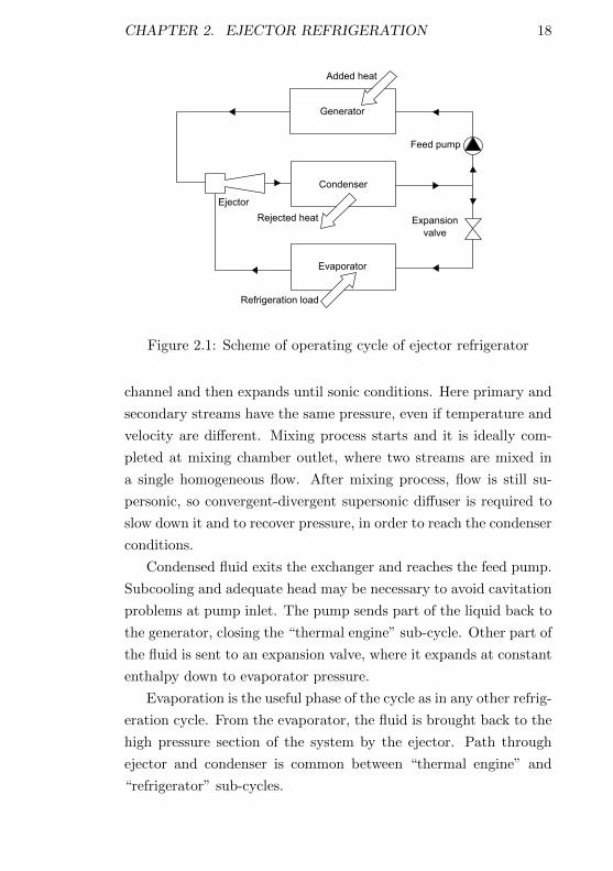
A general scheme of ejector refrigeration system is shown in
fig.(2.1).
The hot fluid may come from various kinds of thermal source
having temperature lower than 300C, like waste heat from internal
combustion engines and turbines or solar energy. Generator, evapo-
rator and condenser may be any kind of heat exchanger. Refrigerant
vapour exits generator at maximum cycle temperature and expands
in the primary nozzle until supersonic condition. Supersonic expan-
sion establishes low pressure condition at primary nozzle exit, which
permits secondary flow to be evaporated and drawn toward mixing
chamber. Cold fluid at evaporator pressure enters the secondary
CHAPTER 2. EJECTOR REFRIGERATION 18
Generator
Condenser
Evaporator
Feed pump
Expansionvalve
Ejector
Refrigeration load
Rejected heat
Added heat
Figure 2.1: Scheme of operating cycle of ejector refrigerator
channel and then expands until sonic conditions. Here primary and
secondary streams have the same pressure, even if temperature and
velocity are different. Mixing process starts and it is ideally com-
pleted at mixing chamber outlet, where two streams are mixed in
a single homogeneous flow. After mixing process, flow is still su-
personic, so convergent-divergent supersonic diffuser is required to
slow down it and to recover pressure, in order to reach the condenser
conditions.
Condensed fluid exits the exchanger and reaches the feed pump.
Subcooling and adequate head may be necessary to avoid cavitation
problems at pump inlet. The pump sends part of the liquid back to
the generator, closing the “thermal engine” sub-cycle. Other part of
the fluid is sent to an expansion valve, where it expands at constant
enthalpy down to evaporator pressure.
Evaporation is the useful phase of the cycle as in any other refrig-
eration cycle. From the evaporator, the fluid is brought back to the
high pressure section of the system by the ejector. Path through
ejector and condenser is common between “thermal engine” and
“refrigerator” sub-cycles.
CHAPTER 2. EJECTOR REFRIGERATION 19
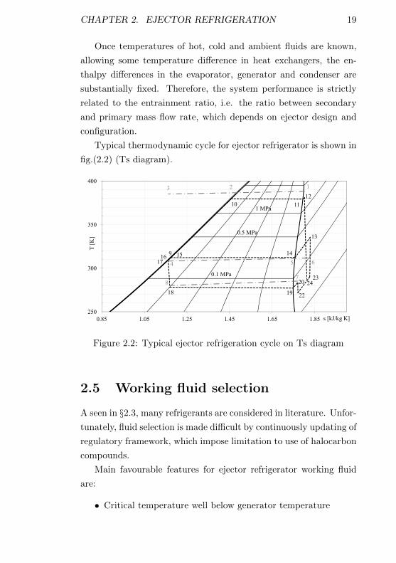
Once temperatures of hot, cold and ambient fluids are known,
allowing some temperature difference in heat exchangers, the en-
thalpy differences in the evaporator, generator and condenser are
substantially fixed. Therefore, the system performance is strictly
related to the entrainment ratio, i.e. the ratio between secondary
and primary mass flow rate, which depends on ejector design and
configuration.
Typical thermodynamic cycle for ejector refrigerator is shown in
fig.(2.2) (Ts diagram).
0.5 MPa
1 MPa10 11
12
151617
9 14
4 5 6
123
13
300
350
400
T [
K]
0.1 MPa
18 19
20
22
24
4
78
23
250
300
0.85 1.05 1.25 1.45 1.65 1.85 s [kJ/kg K]
Figure 2.2: Typical ejector refrigeration cycle on Ts diagram
2.5 Working fluid selection
A seen in §2.3, many refrigerants are considered in literature. Unfor-
tunately, fluid selection is made difficult by continuously updating of
regulatory framework, which impose limitation to use of halocarbon
compounds.
Main favourable features for ejector refrigerator working fluid
are:
• Critical temperature well below generator temperature
CHAPTER 2. EJECTOR REFRIGERATION 20
• High latent heat at evaporator temperature, to increase spe-
cific cooling capacity
• Normal boiling pressure close to ambient pressure, to avoid
vacuum condenser
• Moderate generator pressure, to make feed pump selection
easier and to reduce safety costs
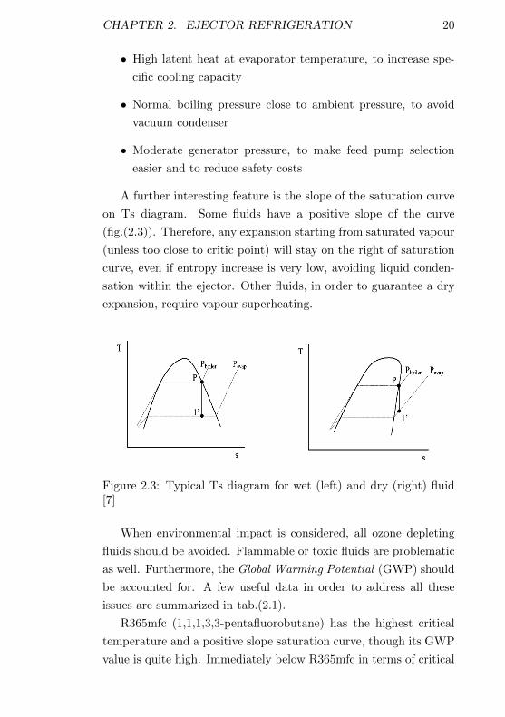
A further interesting feature is the slope of the saturation curve
on Ts diagram. Some fluids have a positive slope of the curve
(fig.(2.3)). Therefore, any expansion starting from saturated vapour
(unless too close to critic point) will stay on the right of saturation
curve, even if entropy increase is very low, avoiding liquid conden-
sation within the ejector. Other fluids, in order to guarantee a dry
expansion, require vapour superheating.
Figure 2.3: Typical Ts diagram for wet (left) and dry (right) fluid[7]
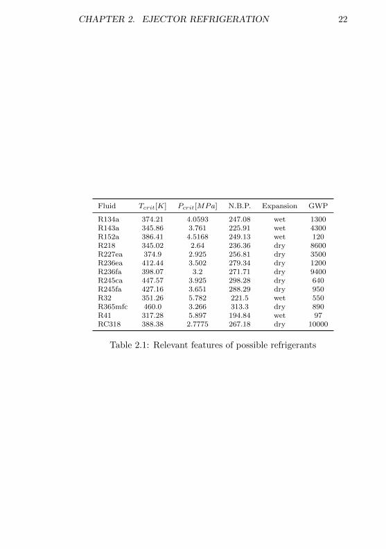
When environmental impact is considered, all ozone depleting
fluids should be avoided. Flammable or toxic fluids are problematic
as well. Furthermore, the Global Warming Potential (GWP) should
be accounted for. A few useful data in order to address all these
issues are summarized in tab.(2.1).
R365mfc (1,1,1,3,3-pentafluorobutane) has the highest critical
temperature and a positive slope saturation curve, though its GWP
value is quite high. Immediately below R365mfc in terms of critical
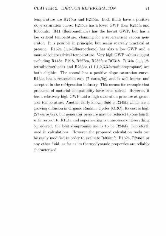
CHAPTER 2. EJECTOR REFRIGERATION 21
temperature are R245ca and R245fa. Both fluids have a positive
slope saturation curve. R245ca has a lower GWP then R245fa and
R365mfc. R41 (fluoromethane) has the lowest GWP, but has a
low critical temperature, claiming for a supercritical vapour gen-
erator. It is possible in principle, but seems scarcely practical at
present. R152a (1,1-difluoroethane) has also a low GWP and a
more adequate critical temperature. Very high GWP values suggest
excluding R143a, R218, R227ea, R236fa e RC318. R134a (1,1,1,2-
tetrafluoroethane) and R236ea (1,1,1,2,3,3-hexafluoropropane) are
both eligible. The second has a positive slope saturation curve.
R134a has a reasonable cost (7 euros/kg) and is well known and
accepted in the refrigeration industry. This means for example that
problems of material compatibility have been solved. However, it
has a relatively high GWP and a high saturation pressure at gener-
ator temperature. Another fairly known fluid is R245fa which has a
growing diffusion in Organic Rankine Cycles (ORC). Its cost is high
(27 euros/kg), but generator pressure may be reduced to one fourth
with respect to R134a and superheating is unnecessary. Everything
considered, the best compromise seems to be R245fa, henceforth
used in calculations. However the proposed calculation tools can
be easily modified in order to evaluate R365mfc, R152a, R236ea or
any other fluid, as far as its thermodynamic properties are reliably
characterized.
CHAPTER 2. EJECTOR REFRIGERATION 22
Fluid Tcrit[K] Pcrit[MPa] N.B.P. Expansion GWP
R134a 374.21 4.0593 247.08 wet 1300R143a 345.86 3.761 225.91 wet 4300R152a 386.41 4.5168 249.13 wet 120R218 345.02 2.64 236.36 dry 8600R227ea 374.9 2.925 256.81 dry 3500R236ea 412.44 3.502 279.34 dry 1200R236fa 398.07 3.2 271.71 dry 9400R245ca 447.57 3.925 298.28 dry 640R245fa 427.16 3.651 288.29 dry 950R32 351.26 5.782 221.5 wet 550R365mfc 460.0 3.266 313.3 dry 890R41 317.28 5.897 194.84 wet 97RC318 388.38 2.7775 267.18 dry 10000
Table 2.1: Relevant features of possible refrigerants
Chapter 3
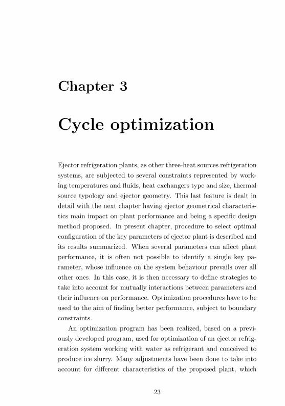
Cycle optimization
Ejector refrigeration plants, as other three-heat sources refrigeration
systems, are subjected to several constraints represented by work-
ing temperatures and fluids, heat exchangers type and size, thermal
source typology and ejector geometry. This last feature is dealt in
detail with the next chapter having ejector geometrical characteris-
tics main impact on plant performance and being a specific design
method proposed. In present chapter, procedure to select optimal
configuration of the key parameters of ejector plant is described and
its results summarized. When several parameters can affect plant
performance, it is often not possible to identify a single key pa-
rameter, whose influence on the system behaviour prevails over all
other ones. In this case, it is then necessary to define strategies to
take into account for mutually interactions between parameters and
their influence on performance. Optimization procedures have to be
used to the aim of finding better performance, subject to boundary
constraints.
An optimization program has been realized, based on a previ-
ously developed program, used for optimization of an ejector refrig-
eration system working with water as refrigerant and conceived to
produce ice slurry. Many adjustments have been done to take into
account for different characteristics of the proposed plant, which
23
CHAPTER 3. CYCLE OPTIMIZATION 24
is designed to supply refrigerated water for industrial application,
working with halocarbon compounds. Main differences concern with
• use of three plate heat exchangers to take into account for the
necessity of distinct circuits for the refrigerant fluid and water
used to heat and condense fluid itself
• use of specific functions to compute thermodynamic properties
of refrigerant along the cycle
First aspect has to be taken into account modelling exchangers be-
haviour or characterizing them, and evaluating their heat transfer
coefficients and pressure drops for specified working temperatures
and mass flow rates of fluid and water. Refrigerant properties have
been computed using REFPROP libraries [38], developed by NIST,
which ensure high accuracy and wide fluids database.
3.1 Optimization concept
Many complex decision or allocation problems can be approached
using optimization. In this way, it is in fact possible to define crite-
rion to guide complex decision problem, involving choose of values
for several correlated parameters, by identifying a single objective
function, which quantify performance [39]. This objective function
can then be maximized or minimized depending on problem for-
mulation, using specific mathematical algorithms and eventually
subject to some constraints. Of course, like all other field where
modelling is required, choose appropriate and accurate description
of constraints and objective in terms of physical and mathemat-
ical model is necessary to obtain reliable results. On the other
hand, it is however useful to reduce model complexity, avoiding
time-consuming computer applications, as possible as reliability is
preserved. As a consequence of models and parameters use, op-
timization results have to be considered as approximation of real
behaviour, being the goodness of the results themselves dependent
of skill in modelling essential features of a problem.
CHAPTER 3. CYCLE OPTIMIZATION 25
Non linear relations between parameters imply that changing
one variable at time (OVAT method) to find optimal solution in-
volves loose of information about variables interactions and correla-
tions [19]. Multivariate optimization method, described in following
section, is used in present analysis to better identify optimal solu-
tion over a wide range of variables values. To apply optimization
approach to ejector refrigeration plant design, this last feature of
the method is particularly suitable, permitting it to explore a wide
range of possible design solutions in a field where standardization is
not yet reached.
Finally, it must be considered that objective function choice
strongly influences optimization results [26], representing its value
the base on which all other parameters are modified. Any choice
is admissible for objective function, as long as its computational
complexity remains reasonable, but it has to remember that results
meaning is strictly connected to its definition.
3.1.1 Optimization algorithm
Main element of the program is the numerical optimization subrou-
tine based on Complex (Constrained simplex) method proposed by
Box [6] starting from Simplex method proposed by Spendley et al.
[52]. Its aim is to search constrained maxima and minima of an
objective function which, in our case, is represented by COP of the
ejector refrigeration plant. The method ensures good performance
and quite rapid convergence, when studied function presents several
local maxima and minima in the region of interest. In particular it
is conceived to find global maximum of functions when local ex-
trema are present. Unlike other methods, Complex method searches
for the maximum not only in the neighbour of starting point, but
analysing a wide area of the region of interest, then guaranteeing
the location of the global maximum is as independent as possible of
the set of initial values.
CHAPTER 3. CYCLE OPTIMIZATION 26
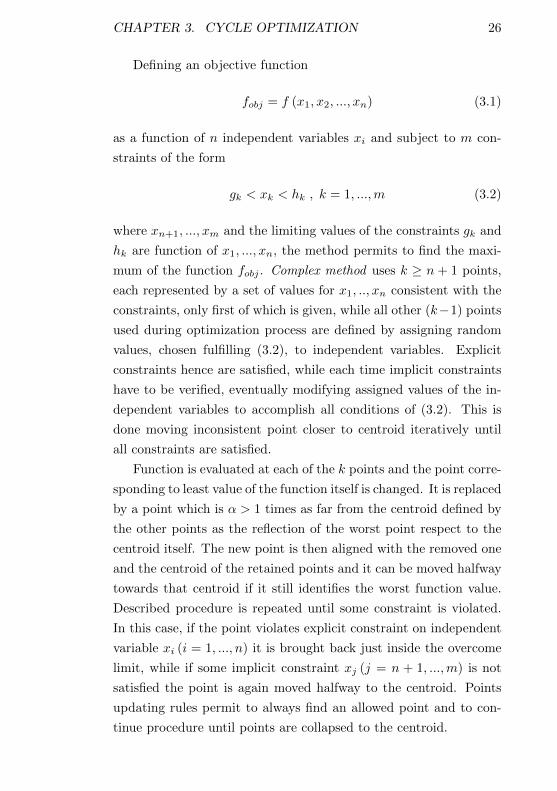
Defining an objective function
fobj = f (x1, x2, ..., xn) (3.1)
as a function of n independent variables xi and subject to m con-
straints of the form
gk < xk < hk , k = 1, ...,m (3.2)
where xn+1, ..., xm and the limiting values of the constraints gk and
hk are function of x1, ..., xn, the method permits to find the maxi-
mum of the function fobj . Complex method uses k ≥ n + 1 points,
each represented by a set of values for x1, .., xn consistent with the
constraints, only first of which is given, while all other (k−1) points
used during optimization process are defined by assigning random
values, chosen fulfilling (3.2), to independent variables. Explicit
constraints hence are satisfied, while each time implicit constraints
have to be verified, eventually modifying assigned values of the in-
dependent variables to accomplish all conditions of (3.2). This is
done moving inconsistent point closer to centroid iteratively until
all constraints are satisfied.
Function is evaluated at each of the k points and the point corre-
sponding to least value of the function itself is changed. It is replaced
by a point which is α > 1 times as far from the centroid defined by
the other points as the reflection of the worst point respect to the
centroid itself. The new point is then aligned with the removed one
and the centroid of the retained points and it can be moved halfway
towards that centroid if it still identifies the worst function value.
Described procedure is repeated until some constraint is violated.
In this case, if the point violates explicit constraint on independent
variable xi (i = 1, ..., n) it is brought back just inside the overcome
limit, while if some implicit constraint xj (j = n + 1, ...,m) is not
satisfied the point is again moved halfway to the centroid. Points
updating rules permit to always find an allowed point and to con-
tinue procedure until points are collapsed to the centroid.
CHAPTER 3. CYCLE OPTIMIZATION 27
Stopping criterion for the method is that the computed values
of fobj are identical (within defined tolerance) for a fixed number
of procedure iteration, so permitting the program to proceed until
there is any possibility to improve function value. Global maximum,
instead a local one, is found if multiple repeats of the program with
different initial points converge to the same solution.
Advantage of the method is its reliability to search maxima of
functions, which present multiple local maximum in the region of
interest thanks to randomly assigned initial points and repeated
over-reflection.
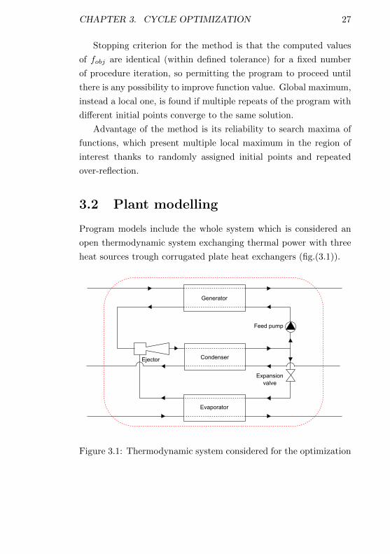
3.2 Plant modelling
Program models include the whole system which is considered an
open thermodynamic system exchanging thermal power with three
heat sources trough corrugated plate heat exchangers (fig.(3.1)).
Generator
Condenser
Evaporator
Feed pump
Expansionvalve
Ejector
Figure 3.1: Thermodynamic system considered for the optimization
CHAPTER 3. CYCLE OPTIMIZATION 28
3.2.1 Working fluids properties
Use of refrigerants as working fluids for ejector refrigeration plant
requires to find libraries able to determine their properties, which
can be integrated in optimization program. NIST REFPROP li-
braries [38] are chosen to this aim. They supply subroutine to
compute thermodynamic and transport properties of industrially
significant fluids and their mixtures, with particular attention on
refrigerants and hydrocarbons, based on most accurate and mixture
models available in literature.
NIST REFPROP libraries are conceived to guarantee flexible
use, being possible to explicitly call Fortran subroutines in devel-
oped program or use external calls to libraries. During this work,
they are used first in the optimization program directly, including
Fortran code in the program, and then though their interface with
Visual Basic for Application in Excel.
Original optimization program consider water as working fluid
and as thermal vector in the exchangers, without necessity to dis-
tinguish external circuits from refrigerant ones from the point of
view of modelling techniques. This is instead necessary in the new
version of optimization program, so water and refrigerant properties
computing is modified to access NIST REFPROP libraries for the
latter, while maintaining previous formulation for water.
All fluids considered in selection (§2.5) are present in NIST REF-
PROP libraries database, so their use permits great flexibility in
refrigeration plant analysis.
Finally NIST REFPROP is constantly updated to include new
fluids and models and this guarantees future improvement of the
analysis.
3.2.2 Heat exchangers
Original program models steam generator as tube and shell heat ex-
changer, evaporator as flash evaporator and condenser as corrugated
plate heat exchanger, according to steam ejector plant considered
CHAPTER 3. CYCLE OPTIMIZATION 29
[25]. New program is conceived to project optimized ejector refriger-
ation system working with halocarbon compounds for refrigeration
cycle and water in external channels. It is then necessary to dif-
ferentiate refrigerant circuit from water one and it is done by using
three plate heat exchanger.
Two different approaches can be used to treat heat exchangers
depending on what data are at disposal about their building and
geometric characteristics and on which type of models are present
in literature. If geometry and size of plate are known with an ade-
quate level of accuracy, correlations can be found in literature which
permits to compute heat transfer coefficient and pressure drops of
the exchangers for some fluids. This method is very sensitive to
geometry variation and fluid type and its main drawback is scarce
flexibility to refrigerant changes, though it ensures finest setting ca-
pacity for mass flow rates, number of plates and temperature levels,
whose values can be varied virtually continuously.
Unfortunately geometry of corrugated plate heat exchanger and
plate characteristics is often patent pending and it is difficult to
obtain all necessary information, with enough level of accuracy to
model exchanger behaviour from the point of view of its heat trans-
fer performance. In this case it is however possible to extract heat
transfer coefficients and pressure drops estimated with software,
that manufacturers make usually available, varying boundary con-
ditions in the range of interest for the values of mass flow rates and
temperatures. Moreover same type of heat exchanger is suitable for
different fluids so allowing to simulate use of different refrigerants.
Results can be finally summarized in tables read by the optimization
program to vary working point at discrete steps.
Both described methods are implemented in the optimization
program. Correlations are initially used to determine heat exchang-
ers behaviour, while program has then been modified to read tables,
obtained by manufacturer software, with the aim to overcome mis-
matching between computed results and tabulated data and the lack
of literature correlations for less common fluids.
CHAPTER 3. CYCLE OPTIMIZATION 30
Heat exchangers correlations
Models to describe plate heat exchangers are yet quite limited, par-
ticularly for what concern phase change zones, and they are fur-
ther strongly dependent of exchanger geometry (Chevron angle and
plate corrugation) and fluid type. Even if models with general va-
lidity are not present, some detailed formulation for specific fluids
and exchanger geometries can be found in literature. In particular,
for R134a, initially selected as suitable for ejector plant application,
correlations are presented in literature related to its behaviour dur-
ing evaporation and condensation phases in corrugated plate heat
exchangers, so it is possible to include them in the optimization
program.
When these correlations are used to compute heat transfer co-
efficients and pressure drops, input data are represented by water
mass flow rate, water inlet temperature and nominal pressure and
number of plates as summarized in tab.(3.1). Superheating at gen-
erator outlet and evaporation temperature are further defined for
generator and evaporator respectively.
Geometric characteristics of plates and exchangers are moreover
provided to the program to complete information (tab.(3.2)).
Input data for plate heat exchangers
mw Water side mass flow rate [kg/s]Pw,nom Water side nominal pressure [Pa]Tw,in Water side inlet temperature [K]hp Plates height [m]
Table 3.1: Thermodynamic input parameters for plate heat ex-changer when correlations are used
Global heat transfer coefficient U can be obtained by
1
U=
1
hr+
1
hw+
s
kp(3.3)
where hr and hw represent refrigerant and water side heat transfer
coefficients respectively, while kp and s thermal conductivity ans
CHAPTER 3. CYCLE OPTIMIZATION 31
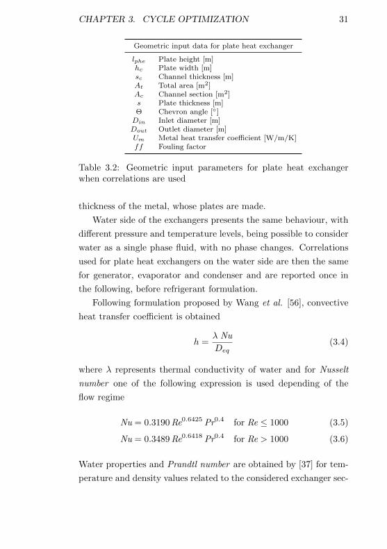
Geometric input data for plate heat exchanger
lphe Plate height [m]hc Plate width [m]sc Channel thickness [m]At Total area [m2]Ac Channel section [m2]s Plate thickness [m]Θ Chevron angle []Din Inlet diameter [m]Dout Outlet diameter [m]Um Metal heat transfer coefficient [W/m/K]ff Fouling factor
Table 3.2: Geometric input parameters for plate heat exchangerwhen correlations are used
thickness of the metal, whose plates are made.
Water side of the exchangers presents the same behaviour, with
different pressure and temperature levels, being possible to consider
water as a single phase fluid, with no phase changes. Correlations
used for plate heat exchangers on the water side are then the same
for generator, evaporator and condenser and are reported once in
the following, before refrigerant formulation.
Following formulation proposed by Wang et al. [56], convective
heat transfer coefficient is obtained
h =λ Nu
Deq(3.4)
where λ represents thermal conductivity of water and for Nusselt
number one of the following expression is used depending of the
flow regime
Nu = 0.3190 Re0.6425 Pr0.4 for Re ≤ 1000 (3.5)
Nu = 0.3489 Re0.6418 Pr0.4 for Re > 1000 (3.6)
Water properties and Prandtl number are obtained by [37] for tem-
perature and density values related to the considered exchanger sec-
CHAPTER 3. CYCLE OPTIMIZATION 32
tion and Reynolds number by the formula
Re =ρ cDeq
µ(3.7)
where dynamic viscosity µ again is computed by [37].
Pressure losses on water side of the exchanger are computed
starting from relation
∆P =fG2L
2Deqρ(3.8)
where G represents specific mass flow rate, L the length of the con-
sidered section of the exchanger, Deq hydraulic diameter which is
assumed to be twice the channel spacing and friction factor f is
obtained by
f = 94.41 Re−0.9125 for Re < 200 (3.9)
f = 2.31 Re−0.2122 for Re ≥ 200 (3.10)
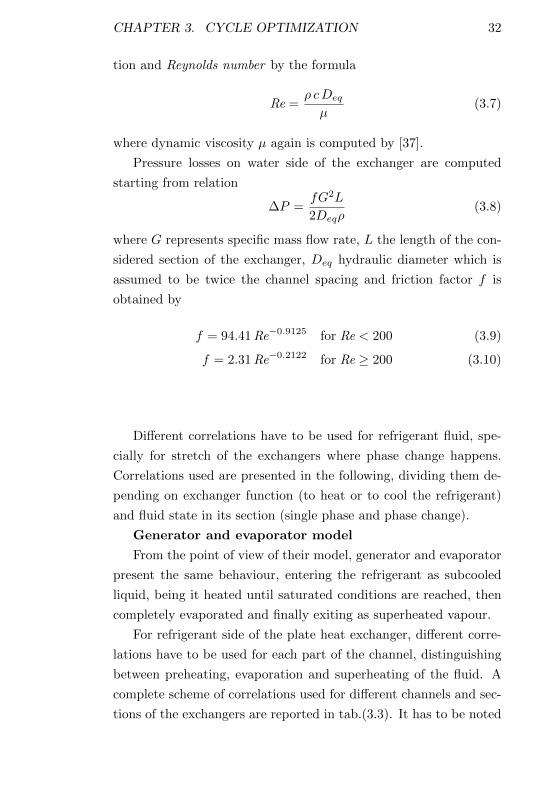
Different correlations have to be used for refrigerant fluid, spe-
cially for stretch of the exchangers where phase change happens.
Correlations used are presented in the following, dividing them de-
pending on exchanger function (to heat or to cool the refrigerant)
and fluid state in its section (single phase and phase change).
Generator and evaporator model
From the point of view of their model, generator and evaporator
present the same behaviour, entering the refrigerant as subcooled
liquid, being it heated until saturated conditions are reached, then
completely evaporated and finally exiting as superheated vapour.
For refrigerant side of the plate heat exchanger, different corre-
lations have to be used for each part of the channel, distinguishing
between preheating, evaporation and superheating of the fluid. A
complete scheme of correlations used for different channels and sec-
tions of the exchangers are reported in tab.(3.3). It has to be noted
CHAPTER 3. CYCLE OPTIMIZATION 33
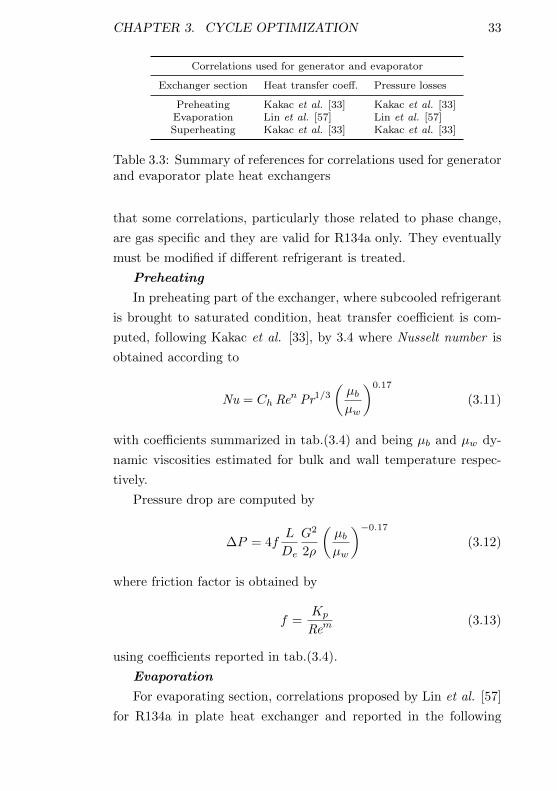
Correlations used for generator and evaporator
Exchanger section Heat transfer coeff. Pressure losses
Preheating Kakac et al. [33] Kakac et al. [33]Evaporation Lin et al. [57] Lin et al. [57]Superheating Kakac et al. [33] Kakac et al. [33]
Table 3.3: Summary of references for correlations used for generatorand evaporator plate heat exchangers
that some correlations, particularly those related to phase change,
are gas specific and they are valid for R134a only. They eventually
must be modified if different refrigerant is treated.
Preheating
In preheating part of the exchanger, where subcooled refrigerant
is brought to saturated condition, heat transfer coefficient is com-
puted, following Kakac et al. [33], by 3.4 where Nusselt number is
obtained according to
Nu = Ch Ren Pr1/3(µbµw
)0.17
(3.11)
with coefficients summarized in tab.(3.4) and being µb and µw dy-
namic viscosities estimated for bulk and wall temperature respec-
tively.
Pressure drop are computed by
∆P = 4fL
De
G2
2ρ
(µbµw
)−0.17(3.12)
where friction factor is obtained by
f =Kp
Rem(3.13)
using coefficients reported in tab.(3.4).
Evaporation
For evaporating section, correlations proposed by Lin et al. [57]
for R134a in plate heat exchanger and reported in the following
CHAPTER 3. CYCLE OPTIMIZATION 34
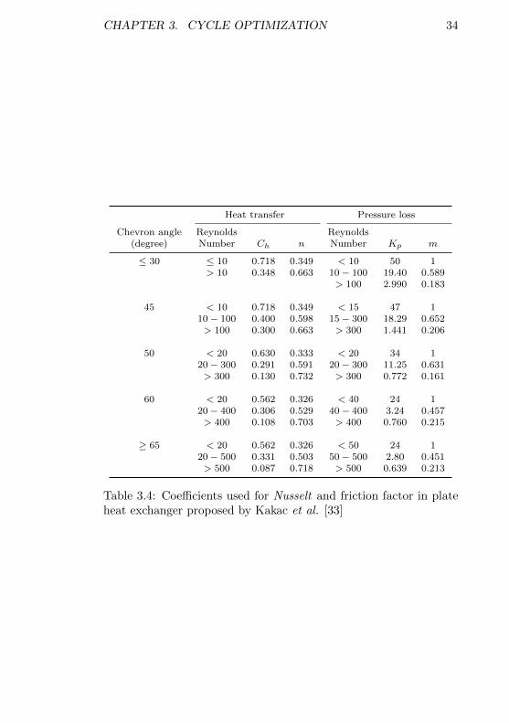
Heat transfer Pressure loss
Chevron angle Reynolds Reynolds(degree) Number Ch n Number Kp m
≤ 30 ≤ 10 0.718 0.349 < 10 50 1> 10 0.348 0.663 10 − 100 19.40 0.589
> 100 2.990 0.183
45 < 10 0.718 0.349 < 15 47 110 − 100 0.400 0.598 15 − 300 18.29 0.652> 100 0.300 0.663 > 300 1.441 0.206
50 < 20 0.630 0.333 < 20 34 120 − 300 0.291 0.591 20 − 300 11.25 0.631> 300 0.130 0.732 > 300 0.772 0.161
60 < 20 0.562 0.326 < 40 24 120 − 400 0.306 0.529 40 − 400 3.24 0.457> 400 0.108 0.703 > 400 0.760 0.215
≥ 65 < 20 0.562 0.326 < 50 24 120 − 500 0.331 0.503 50 − 500 2.80 0.451> 500 0.087 0.718 > 500 0.639 0.213
Table 3.4: Coefficients used for Nusselt and friction factor in plateheat exchanger proposed by Kakac et al. [33]
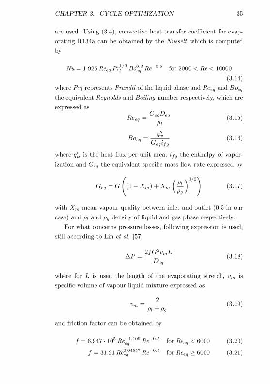
CHAPTER 3. CYCLE OPTIMIZATION 35
are used. Using (3.4), convective heat transfer coefficient for evap-
orating R134a can be obtained by the Nusselt which is computed
by
Nu = 1.926 Reeq Pr1/3l Bo0.3
eq Re−0.5 for 2000 < Re < 10000
(3.14)
where Prl represents Prandtl of the liquid phase and Reeq and Boeq
the equivalent Reynolds and Boiling number respectively, which are
expressed as
Reeq =GeqDeq
µl(3.15)
Boeq =q′′w
Geqifg(3.16)
where q′′w is the heat flux per unit area, ifg the enthalpy of vapor-
ization and Geq the equivalent specific mass flow rate expressed by
Geq = G
((1−Xm) +Xm
(ρlρg
)1/2)
(3.17)
with Xm mean vapour quality between inlet and outlet (0.5 in our
case) and ρl and ρg density of liquid and gas phase respectively.
For what concerns pressure losses, following expression is used,
still according to Lin et al. [57]
∆P =2fG2vmL
Deq(3.18)
where for L is used the length of the evaporating stretch, vm is
specific volume of vapour-liquid mixture expressed as
vm =2
ρl + ρg(3.19)
and friction factor can be obtained by
f = 6.947 · 105 Re−1.109eq Re−0.5 for Reeq < 6000 (3.20)
f = 31.21 Re0.04557eq Re−0.5 for Reeq ≥ 6000 (3.21)
CHAPTER 3. CYCLE OPTIMIZATION 36
Superheating
After evaporation is completed, vapour is superheated in the
last stretch of the exchanger and heat transfer coefficient again is
obtained by computing Nusselt with (3.11) and pressure loss by
(3.12).
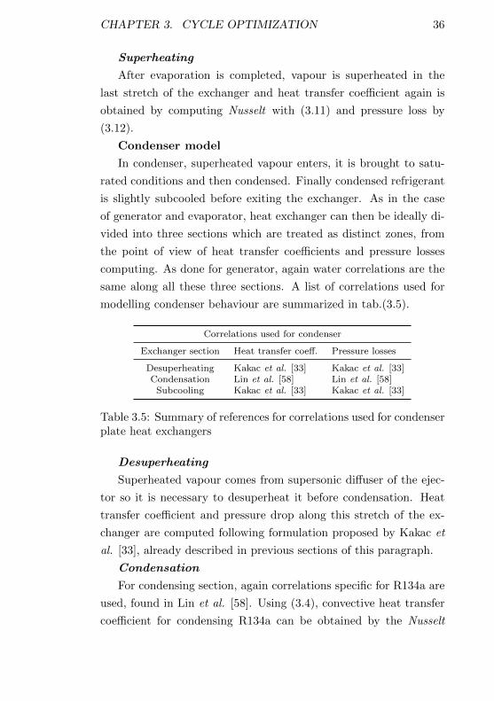
Condenser model
In condenser, superheated vapour enters, it is brought to satu-
rated conditions and then condensed. Finally condensed refrigerant
is slightly subcooled before exiting the exchanger. As in the case
of generator and evaporator, heat exchanger can then be ideally di-
vided into three sections which are treated as distinct zones, from
the point of view of heat transfer coefficients and pressure losses
computing. As done for generator, again water correlations are the
same along all these three sections. A list of correlations used for
modelling condenser behaviour are summarized in tab.(3.5).
Correlations used for condenser
Exchanger section Heat transfer coeff. Pressure losses
Desuperheating Kakac et al. [33] Kakac et al. [33]Condensation Lin et al. [58] Lin et al. [58]
Subcooling Kakac et al. [33] Kakac et al. [33]
Table 3.5: Summary of references for correlations used for condenserplate heat exchangers
Desuperheating
Superheated vapour comes from supersonic diffuser of the ejec-
tor so it is necessary to desuperheat it before condensation. Heat
transfer coefficient and pressure drop along this stretch of the ex-
changer are computed following formulation proposed by Kakac et
al. [33], already described in previous sections of this paragraph.
Condensation
For condensing section, again correlations specific for R134a are
used, found in Lin et al. [58]. Using (3.4), convective heat transfer
coefficient for condensing R134a can be obtained by the Nusselt
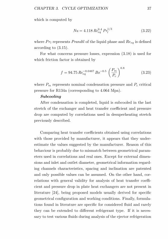
CHAPTER 3. CYCLE OPTIMIZATION 37
which is computed by
Nu = 4.118 Re0.4eq Pr1/3l (3.22)
where Prl represents Prandtl of the liquid phase and Reeq is defined
according to (3.15).
For what concerns pressure losses, expression (3.18) is used for
which friction factor is obtained by
f = 94.75 Re−0.0467eq Bo−0.5(PmPc
)0.8
(3.23)
where Pm represents nominal condensation pressure and Pc critical
pressure for R134a (corresponding to 4.064 Mpa).
Subcooling
After condensation is completed, liquid is subcooled in the last
stretch of the exchanger and heat transfer coefficient and pressure
drop are computed by correlations used in desuperheating stretch
previously described.
Comparing heat transfer coefficients obtained using correlations
with those provided by manufacturer, it appears that they under-
estimate the values suggested by the manufacturer. Reason of this
behaviour is probably due to mismatch between geometrical param-
eters used in correlations and real ones. Except for external dimen-
sions and inlet and outlet diameter, geometrical information regard-
ing channels characteristics, spacing and inclination are patented
and only possible values can be assumed. On the other hand, cor-
relations with general validity for analysis of heat transfer coeffi-
cient and pressure drop in plate heat exchangers are not present in
literature [24], being proposed models usually derived for specific
geometrical configuration and working conditions. Finally, formula-
tions found in literature are specific for considered fluid and rarely
they can be extended to different refrigerant type. If it is neces-
sary to test various fluids during analysis of the ejector refrigeration
CHAPTER 3. CYCLE OPTIMIZATION 38
plant, literature correlations have to be found and difficulties arise
to gather them, particularly for recently developed refrigerants.
Based on these considerations, a further method to treat plate
heat exchangers is implemented in the program which overcomes
almost all limitations of correlations use, though it however implies
some drawbacks. This approach is described in the following section.
Plate heat exchangers tables
During plant project different feature can affect fluid choice as previ-
ously described (§2.5). It is then often necessary to change refriger-
ant fluid type and verify working conditions of the plant for the new
one. Using correlations to characterize plate heat exchangers shows
some limitations connected to literature availability of formulation
to describe fluid behaviour, specially during phase changes. In this
case, different strategy can be implemented using data provided by
heat exchangers manufacturers. In fact, it is usually available soft-
ware which gets all characteristics of the exchanger starting from
some known input parameter (generally user defined). It is possi-
ble to summarize these data in formatted tables which in turn can
be read from the optimization program. Differently from correla-
tions use, input parameters assigned to define exchanger represent
now discrete values instead continuous ones, but on the other hand
they better match specific exchanger behaviour. Moreover, man-
ufacturers usually update quite rapidly their software to take into
account for new refrigerant fluids, generally supplying them in ad-
vance of literature correlations. Example of optimization program
input data for heat exchangers is reported in tab.(3.6). Different
values for nominal temperatures, powers, water mass flow rates and
inlet temperatures and superheating for generator and evaporator
are chosen, over which optimization is performed.
CHAPTER 3. CYCLE OPTIMIZATION 39
Plate heat exchangers input table
Generator Evaporator Condenser
Tnom [C] 85, 95, 105 2, 4, 6 30, 35, 40Inlet quality - 0.2, 0.22, 0.25 -Power [kW] 150 40, 50, 60 190, 200, 210mwat [kg/s] 2.6, 3.6, 5 - 5, 10, 15Tin,wat [C] 110, 115, 120 - 25, 30
Overheat [C] 6, 8, 10 1, 3, 5 -Number 81 81 34
Table 3.6: Input data table for plate heat exchangers
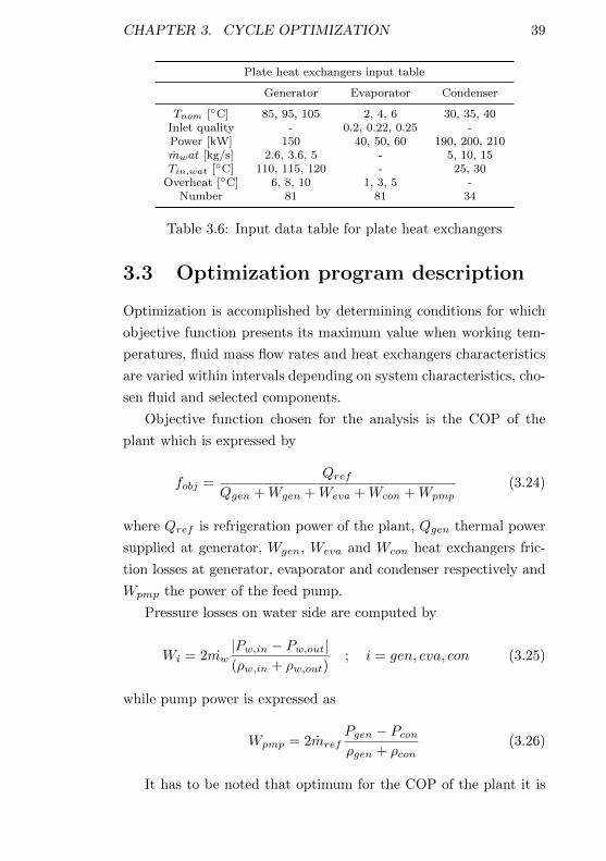
3.3 Optimization program description
Optimization is accomplished by determining conditions for which
objective function presents its maximum value when working tem-
peratures, fluid mass flow rates and heat exchangers characteristics
are varied within intervals depending on system characteristics, cho-
sen fluid and selected components.
Objective function chosen for the analysis is the COP of the
plant which is expressed by
fobj =Qref
Qgen +Wgen +Weva +Wcon +Wpmp(3.24)
where Qref is refrigeration power of the plant, Qgen thermal power
supplied at generator, Wgen, Weva and Wcon heat exchangers fric-
tion losses at generator, evaporator and condenser respectively and
Wpmp the power of the feed pump.
Pressure losses on water side are computed by
Wi = 2mw|Pw,in − Pw,out|(ρw,in + ρw,out)
; i = gen, eva, con (3.25)
while pump power is expressed as
Wpmp = 2mrefPgen − Pconρgen + ρcon
(3.26)
It has to be noted that optimum for the COP of the plant it is
CHAPTER 3. CYCLE OPTIMIZATION 40
not necessarily obtained by optimization of single components, being
system optimization more relevant than that of single components to
obtain better performance [20]. Multivariate optimization method is
then used, as said, to consider the several possibilities of parameters
combinations for all key components of the plant as a whole.
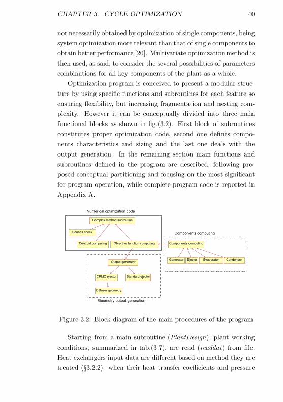
Optimization program is conceived to present a modular struc-
ture by using specific functions and subroutines for each feature so
ensuring flexibility, but increasing fragmentation and nesting com-
plexity. However it can be conceptually divided into three main
functional blocks as shown in fig.(3.2). First block of subroutines
constitutes proper optimization code, second one defines compo-
nents characteristics and sizing and the last one deals with the
output generation. In the remaining section main functions and
subroutines defined in the program are described, following pro-
posed conceptual partitioning and focusing on the most significant
for program operation, while complete program code is reported in
Appendix A.
Complex method subroutine
Bounds check
Centroid computing Objective function computing Components computing
EvaporatorGenerator Ejector CondenserOutput generator
Standard ejectorCRMC ejector
Diffuser geometry
Numerical optimization code
Components computing
Geometry output generation
Figure 3.2: Block diagram of the main procedures of the program
Starting from a main subroutine (PlantDesign), plant working
conditions, summarized in tab.(3.7), are read (readdat) from file.
Heat exchangers input data are different based on method they are
treated (§3.2.2): when their heat transfer coefficients and pressure
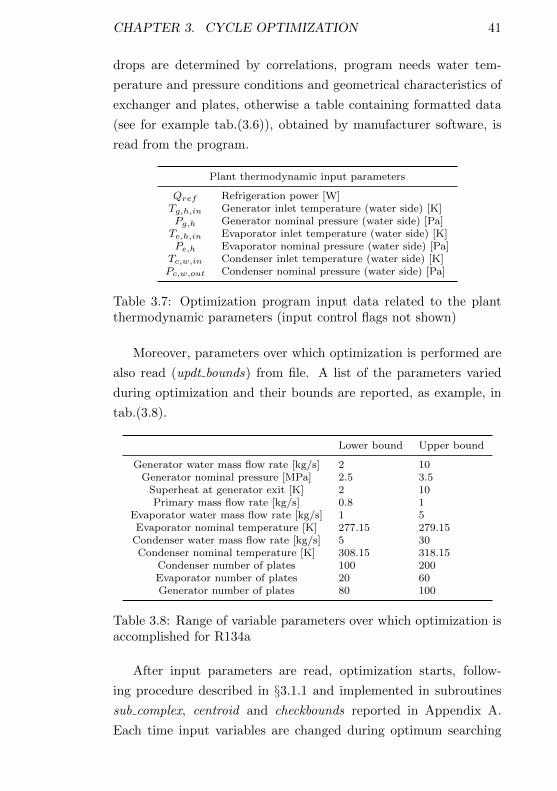
CHAPTER 3. CYCLE OPTIMIZATION 41
drops are determined by correlations, program needs water tem-
perature and pressure conditions and geometrical characteristics of
exchanger and plates, otherwise a table containing formatted data
(see for example tab.(3.6)), obtained by manufacturer software, is
read from the program.
Plant thermodynamic input parameters
Qref Refrigeration power [W]Tg,h,in Generator inlet temperature (water side) [K]Pg,h Generator nominal pressure (water side) [Pa]Te,h,in Evaporator inlet temperature (water side) [K]Pe,h Evaporator nominal pressure (water side) [Pa]Tc,w,in Condenser inlet temperature (water side) [K]Pc,w,out Condenser nominal pressure (water side) [Pa]
Table 3.7: Optimization program input data related to the plantthermodynamic parameters (input control flags not shown)
Moreover, parameters over which optimization is performed are
also read (updt bounds) from file. A list of the parameters varied
during optimization and their bounds are reported, as example, in
tab.(3.8).
Lower bound Upper bound
Generator water mass flow rate [kg/s] 2 10Generator nominal pressure [MPa] 2.5 3.5
Superheat at generator exit [K] 2 10Primary mass flow rate [kg/s] 0.8 1
Evaporator water mass flow rate [kg/s] 1 5Evaporator nominal temperature [K] 277.15 279.15
Condenser water mass flow rate [kg/s] 5 30Condenser nominal temperature [K] 308.15 318.15
Condenser number of plates 100 200Evaporator number of plates 20 60Generator number of plates 80 100
Table 3.8: Range of variable parameters over which optimization isaccomplished for R134a
After input parameters are read, optimization starts, follow-
ing procedure described in §3.1.1 and implemented in subroutines
sub complex, centroid and checkbounds reported in Appendix A.
Each time input variables are changed during optimum searching
CHAPTER 3. CYCLE OPTIMIZATION 42
procedure, objective function has to be updated according to ex-
changers characteristics assigned by tables or iteratively computed
starting from input data and using correlations. Ejector design is
done, with subroutine Eje design Eames, based on Constant Rate
of Momentum Change proposed by Eames [12], which is deeply de-
scribed in §4.8.1. Differently from new CRMC design procedure
proposed in following chapter, no friction losses are explicitly com-
puted in optimization program and they are considered applying an
overall isentropic efficiency. Moreover, according to calorically per-
fect gas model ([51],[31]), constant specific heat ratio is considered
along mixing chamber and diffuser.
Many iterations are necessary to the optimization program to
converge for each single run, mainly because starting from ran-
domly selected input values, which guarantees to widely explore
input ranges, causes that even incoherent configurations are con-
sidered and then discarded if convergence is not reached for any
components. All these trials are saved in specific output file for
following check.
3.4 Optimization results
Optimization program outputs are plate heat exchangers selected
or their characteristics for the optimum configuration and main ge-
ometrical information about ejector. In particular, throat sections
of the nozzles and the diffuser is reported which are obtained as-
suming isentropic efficiencies. Moreover, a profile of the section of
the supersonic diffuser is computed at optimum conditions applying
Constant Rate of Momentum Change method.
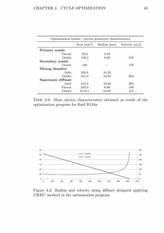
Results of optimization program are summarized, as example, in
tab.(3.9) and profile of the diffuser is shown in fig.(3.3).
CHAPTER 3. CYCLE OPTIMIZATION 43
Optimization results - ejector geometric characteristics
Area [mm2] Radius [mm] Velocity [m/s]
Primary nozzleThroat 50.8 4.02 -Outlet 140.4 6.69 319
Secondary nozzleOutlet 188 - 176
Mixing chamberInlet 328.8 10.23 -
Outlet 315.4 10.02 264Supersonic diffuser
Inlet 315.4 10.02 264Throat 243.3 8.80 188Outlet 9110.1 53.85 2.8
Table 3.9: Main ejector characteristics obtained as result of theoptimization program for fluid R134a
100
150
200
250
300
20
30
40
50
60
R [mm]
u [m/s]
0
50
100
0
10
20
0 100 200 300 400 500 600 700 800 900 1000
Figure 3.3: Radius and velocity along diffuser designed applyingCRMC method in the optimization program
Chapter 4
Plant design
Starting from optimization program results, a design program is
developed whose purpose is to define ejector geometry based on
a one-dimensional fluid flow model [22]. Design program permits
to evaluate plant COP varying heat exchangers characteristics and
temperature levels and to find geometric design of ejector. Program
description follows code structure, analysing, component by compo-
nent, used model and assumptions made. Finally program results
and sensitivity analysis are reported.
4.1 Model description
Fixed working conditions of plate heat exchangers used as input,
program defines sections of mixing chamber and supersonic diffuser
along flow direction. Inlet conditions for mixing chamber are de-
termined by characteristics of primary and secondary nozzle, whose
geometry is defined outside the design program and whose efficiency
is found by applying ideal gas model implemented in specific simu-
lation code. Starting from some hypothesises about flow behaviour,
program finds area of the duct with a step by step procedure moving
forward along x coordinate.
Real gas model is adopted, over the whole ejector, to compute
44
CHAPTER 4. PLANT DESIGN 45
thermodynamic properties of fluid by using NIST REFPROP li-
braries [38].
Generator, condenser and evaporator are represented by three
counterflow corrugated plate heat exchangers, through which water
gives or receive thermal power by refrigerant depending of the func-
tion of the exchanger. Design program considers heat exchangers
by their temperature levels and pressure drops and by the mass flow
rates of water and refrigerant. Their characteristics are found out-
side the design code using a selection program provided by the man-
ufacturer. Some hypothesis are made on pressure drops distribution
internal to exchangers itself, which are described and analysed in the
following.
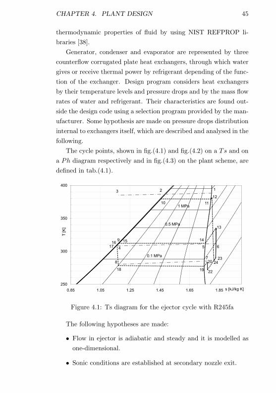
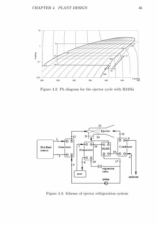
The cycle points, shown in fig.(4.1) and fig.(4.2) on a Ts and on
a Ph diagram respectively and in fig.(4.3) on the plant scheme, are
defined in tab.(4.1).
0.5 MPa
1 MPa10 11
12
123
13
350
400
T [K
]
0.1 MPa
151617
18 19
20
9
22
24
14
4 5 6
78
23
250
300
0.85 1.05 1.25 1.45 1.65 1.85
T [K
]
s [kJ/kg K]
Figure 4.1: Ts diagram for the ejector cycle with R245fa
The following hypotheses are made:
• Flow in ejector is adiabatic and steady and it is modelled as
one-dimensional.
• Sonic conditions are established at secondary nozzle exit.
CHAPTER 4. PLANT DESIGN 46
350
1293751
10
250
275
300
325
18
2224
23
1317
21
0.01
0.1
200 250 300 350 400 450 500
P [M
Pa
]
h [kJ/kg]
Figure 4.2: Ph diagram for the ejector cycle with R245fa
Figure 4.3: Scheme of ejector refrigeration system
CHAPTER 4. PLANT DESIGN 47
1 Water at generator inlet 13 Fluid at condenser inlet2 Water at generator pinch point 14 Start of condensation3 Water at generator outlet 15 End of condensation4 Water at condenser inlet 16 Fluid at condenser exit5 Water at condenser pinch point 17 Liquid at SLHX exit6 Water at condenser outlet 18 Evaporator inlet7 Water at evaporator inlet 19 Evaporation8 Water at evaporator outlet 20 Fluid at evaporator exit9 Fluid at generator inlet 21 Vapour at secondary inlet10 Fluid evaporation 22 Choked secondary flow11 End of evaporation 23 Mixed fluid/diffuser inlet12 Fluid at generator exit 24 End of primary expansion
25 Primary nozzle throat
Table 4.1: List of cycle points
• Constant pressure mixing process is assumed and flows are
considered completely mixed at mixing chamber exit.
• Heat losses in transfer lines are neglected.
Description of the program flow is reported in the next sections,
giving details of procedures used to model and design each compo-
nent of the plant.
4.2 Design program description
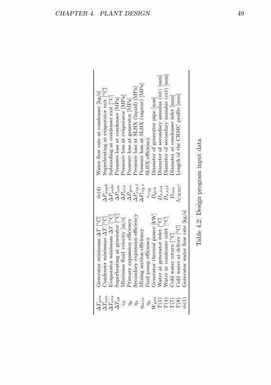
Tab.(4.2) shows the input data, comprising minimum temperature
differences and pressure losses within heat exchangers, water flow
rates at generator and condenser and flow sections at generator exit
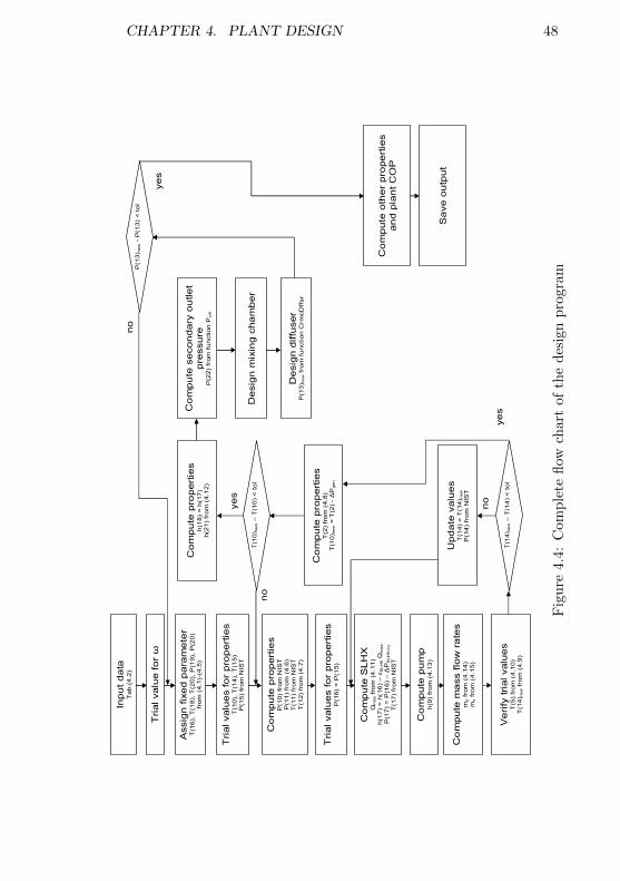
(12), secondary inlet (21) and condenser inlet (13). A complete flow
chart of the program is shown in fig.(4.4).
The calculation starts assigning a hypothetical entrainment ratio
and then iteratively modifying it until pressure value at condenser
inlet is matched.
Fixed parameters
Thermodynamic properties at fixed points are calculated before
the iterative loop starts. This is the case for condenser exit temper-
ature T (16), related to water temperature at condenser inlet T (4)
CHAPTER 4. PLANT DESIGN 48
Tri
al valu
e f
or
ω
Assig
n fix
ed
pa
ram
ete
rT
(16),
T(1
8),
T(2
0),
P(1
9),
P(2
0)
from
(4.1
)-(4
.5)
Tri
al valu
es f
or
pro
pert
ies
T(1
0),
T(1
4),
T(1
5)
P(1
5)
from
NIS
T
Co
mp
ute
pro
pert
ies
P(1
0)
from
NIS
TP
(11)
from
(4
.6)
T(1
1)
from
NIS
TT
(12)
from
(4
.7)
Tri
al valu
es f
or
pro
pert
ies
P(1
6)
= P
(15)
Inp
ut
da
taT
ab
.(4
.2)
Co
mp
ute
SL
HX
Qm
ax
from
(4.1
1)
h(1
7)
= h
(16
)–
ε SL
HX
Qm
ax
P(1
7)
= P
(16)
–Δ
PS
LH
X,liq
T(1
7)
from
NIS
T
Co
mp
ute
pu
mp
h(9
)fr
om
(4.1
3)
Co
mp
ute
ma
ss f
low
ra
tes
mp
from
(4.1
4)
ms
from
(4.1
5)
Ve
rify
tri
al valu
es
T(5
)fr
om
(4.1
0)
T(1
4) n
ew
from
(4.9
)
T(1
4) n
ew
–T
(14
) <
tol
Up
da
te v
alu
es
T(1
4)
= T
(14) n
ew
P(1
4)
from
NIS
T
Co
mp
ute
pro
pert
ies
T(2
)fr
om
(4.8
)T
(10) n
ew
= T
(2)
-Δ
Pge
n
T(1
0) n
ew
–T
(10
) <
tol
Co
mp
ute
pro
pert
ies
h(1
8)
= h
(17
)h(2
1)
from
(4.1
2)
Co
mp
ute
se
co
nd
ary
ou
tle
tp
ressu
reP
(22)
from
function
Pcri
t
De
sig
nm
ixin
g c
ha
mb
er
De
sig
n d
iffu
ser
P(1
3) n
ew
from
function C
rmcD
ffsr
P(1
3) n
ew
-P
(13)
< t
ol
Co
mp
ute
oth
er
pro
pe
rtie
sa
nd
pla
nt
CO
P
Sa
ve
ou
tpu
t
no
ye
s
no
ye
s
no
ye
s
Fig
ure
4.4:
Com
ple
tefl
owch
art
of
the
des
ign
pro
gra
m
CHAPTER 4. PLANT DESIGN 49
∆Tgen
Gen
erato
rm
inim
um
∆T
[C
]m
(4)
Wate
rfl
ow
rate
at
con
den
ser
[kg/s]
∆Tcon
Con
den
ser
min
imu
m∆T
[C
]∆Psuph
Su
per
hea
tin
gat
evap
ora
tor
exit
[C
]∆Teva
Evap
ora
tor
min
imu
m∆T
[C
]∆Psubc
Su
bco
olin
gat
con
den
ser
exit
[C
]∆Tsh
Su
per
hea
tin
gat
gen
erato
r[
C]
∆Pcon
Pre
ssu
relo
ssat
con
den
ser
[MP
a]
c 0M
inim
um
flu
idvel
oci
ty[m
/s]
∆Peva
Pre
ssu
relo
ssat
evap
ora
tor
[MP
a]
ηp
Pri
mary
exp
an
sion
effici
ency
∆Pgen
Pre
ssu
relo
ssat
gen
erato
r[M
Pa]
ηs
Sec
on
dary
exp
an
sion
effici
ency
∆Prig
,lP
ress
ure
loss
at
SL
HX
(liq
uid
)[M
Pa]
ηm
ixM
ixin
gse
ctio
neffi
cien
cy∆Prig
,vP
ress
ure
loss
at
SL
HX
(vap
ou
r)[M
Pa]
ηp
Fee
dp
um
peffi
cien
cyε r
igS
LH
Xeffi
cien
cyW
gen
Gen
erato
rth
erm
al
pow
er[k
W]
Dgen
Dia
met
erof
gen
erato
rp
ipe
[mm
]T
(1)
Wate
rat
gen
erato
rin
let
[C
]D
s,int
Dia
met
erof
seco
nd
ary
an
nu
lus
(int)
[mm
]T
(4)
Wate
rat
con
den
ser
inle
t[
C]
Ds,ext
Dia
met
erof
seco
nd
ary
an
nu
lus
(ext)
[mm
]T
(7)
Cold
wate
rre
turn
[C
]D
con
Dia
met
erat
con
den
ser
inle
t[m
m]
T(8
)C
old
wate
rat
del
iver
[C
]l C
RM
CL
ength
of
the
CR
MC
pro
file
[mm
]m
(1)
Gen
erato
rw
ate
rfl
ow
rate
[kg/s]
Tab
le4.
2:D
esig
np
rogr
amin
pu
td
ata
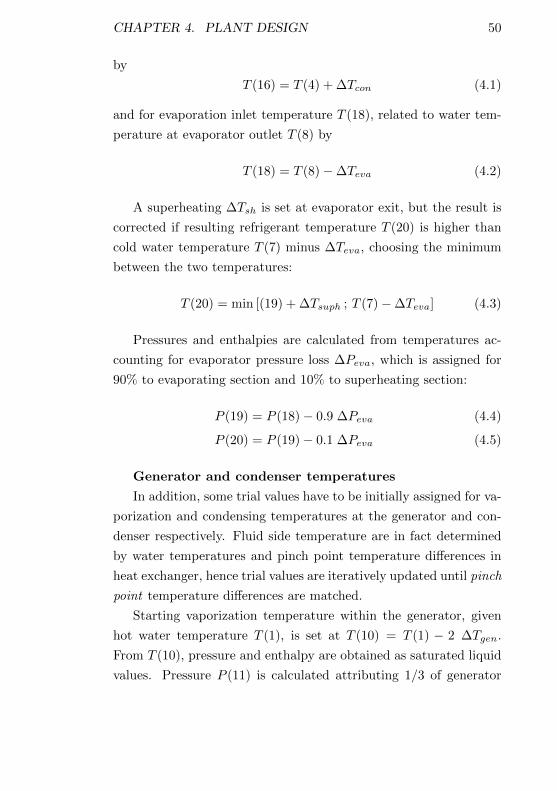
CHAPTER 4. PLANT DESIGN 50
by
T (16) = T (4) + ∆Tcon (4.1)
and for evaporation inlet temperature T (18), related to water tem-
perature at evaporator outlet T (8) by
T (18) = T (8)−∆Teva (4.2)
A superheating ∆Tsh is set at evaporator exit, but the result is
corrected if resulting refrigerant temperature T (20) is higher than
cold water temperature T (7) minus ∆Teva, choosing the minimum
between the two temperatures:
T (20) = min [(19) + ∆Tsuph ; T (7)−∆Teva] (4.3)
Pressures and enthalpies are calculated from temperatures ac-
counting for evaporator pressure loss ∆Peva, which is assigned for
90% to evaporating section and 10% to superheating section:
P (19) = P (18)− 0.9 ∆Peva (4.4)
P (20) = P (19)− 0.1 ∆Peva (4.5)
Generator and condenser temperatures
In addition, some trial values have to be initially assigned for va-
porization and condensing temperatures at the generator and con-
denser respectively. Fluid side temperature are in fact determined
by water temperatures and pinch point temperature differences in
heat exchanger, hence trial values are iteratively updated until pinch
point temperature differences are matched.
Starting vaporization temperature within the generator, given
hot water temperature T (1), is set at T (10) = T (1) − 2 ∆Tgen.
From T (10), pressure and enthalpy are obtained as saturated liquid
values. Pressure P (11) is calculated attributing 1/3 of generator
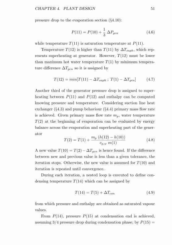
CHAPTER 4. PLANT DESIGN 51
pressure drop to the evaporation section (§4.10):
P (11) = P (10) +1
3∆Pgen (4.6)
while temperature T (11) is saturation temperature at P (11).
Temperature T (12) is higher than T (11) by ∆Tsuph, which rep-
resents superheating at generator. However, T (12) must be lower
than maximum hot water temperature T (1) by minimum tempera-
ture difference ∆Tgen so it is assigned by
T (12) = min[T (11)−∆Tsuph ; T (1)−∆Tgen] (4.7)
Another third of the generator pressure drop is assigned to super-
heating between P (11) and P (12) and enthalpy can be computed
knowing pressure and temperature. Considering suction line heat
exchanger (§4.3) and pump behaviour (§4.4) primary mass flow rate
is achieved. Given primary mass flow rate mp, water temperature
T (2) at the beginning of evaporation can be evaluated by energy
balance across the evaporation and superheating part of the gener-
ator
T (2) = T (1) +mp (h(12)− h(10))
cp,w m(1)(4.8)
A new value T (10) = T (2)−∆Tgen is hence found. If the difference
between new and previous value is less than a given tolerance, the
iteration stops. Otherwise, the new value is assumed for T (10) and
iteration is repeated until convergence.
During each iteration, a nested loop is executed to define con-
densing temperature T (14) which can be assigned by
T (14) = T (5) + ∆Tcon (4.9)
from which pressure and enthalpy are obtained as saturated vapour
values.
From P (14), pressure P (15) at condensation end is achieved,
assuming 3/4 pressure drop during condensation phase, by P (15) =
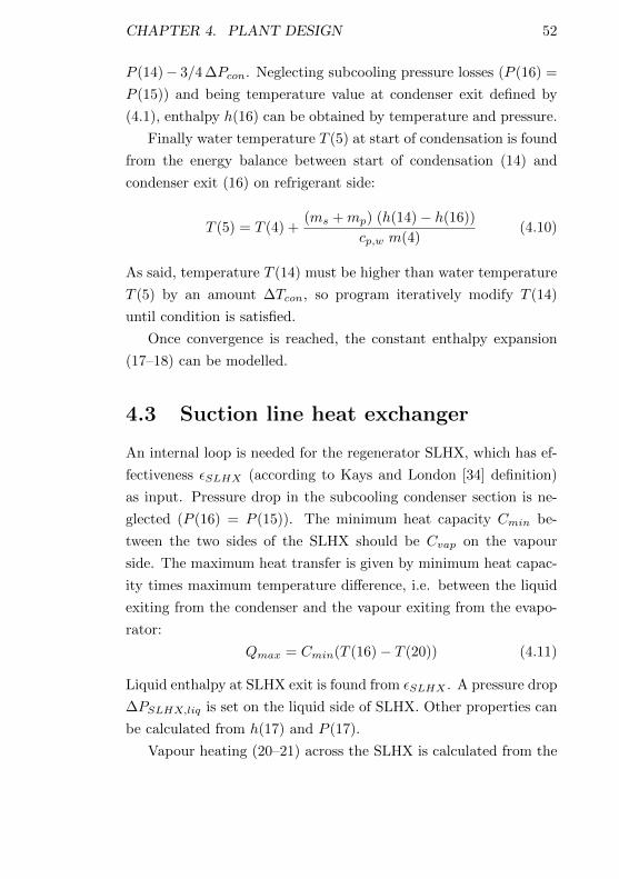
CHAPTER 4. PLANT DESIGN 52
P (14)− 3/4 ∆Pcon. Neglecting subcooling pressure losses (P (16) =
P (15)) and being temperature value at condenser exit defined by
(4.1), enthalpy h(16) can be obtained by temperature and pressure.
Finally water temperature T (5) at start of condensation is found
from the energy balance between start of condensation (14) and
condenser exit (16) on refrigerant side:
T (5) = T (4) +(ms +mp) (h(14)− h(16))
cp,w m(4)(4.10)
As said, temperature T (14) must be higher than water temperature
T (5) by an amount ∆Tcon, so program iteratively modify T (14)
until condition is satisfied.
Once convergence is reached, the constant enthalpy expansion
(17–18) can be modelled.
4.3 Suction line heat exchanger
An internal loop is needed for the regenerator SLHX, which has ef-
fectiveness εSLHX (according to Kays and London [34] definition)
as input. Pressure drop in the subcooling condenser section is ne-
glected (P (16) = P (15)). The minimum heat capacity Cmin be-
tween the two sides of the SLHX should be Cvap on the vapour
side. The maximum heat transfer is given by minimum heat capac-
ity times maximum temperature difference, i.e. between the liquid
exiting from the condenser and the vapour exiting from the evapo-
rator:
Qmax = Cmin(T (16)− T (20)) (4.11)
Liquid enthalpy at SLHX exit is found from εSLHX . A pressure drop
∆PSLHX,liq is set on the liquid side of SLHX. Other properties can
be calculated from h(17) and P (17).
Vapour heating (20–21) across the SLHX is calculated from the

CHAPTER 4. PLANT DESIGN 53
previously found maximum heat transfer and from effectiveness
h(21) = h(20) +εSLHX QSLHX,max
ω(4.12)
Pressure at SLHX exit is found taking into account for pressure
drop ∆PSHLX,vap on the vapour side and then all properties at
secondary inlet (21) are evaluated. If the SLHX is absent, point 16
is equivalent to 17 and also points 20 and 21 coincide.
4.4 Pump
Pressure at generator inlet P (9) is determined assuming another 1/3
of pressure drop ∆Pgen on the liquid heating part of the generator.
If the pump had no losses, the enthalpy at point 9 would be hrev,
i.e. the enthalpy at P (9) and s(17). Applying pump efficiency ηp
enthalpy h(9) can be obtained by
h(9) = h(7) +hrev − h(17)
ηp(4.13)
T (9) and s(9) are found from pressure and enthalpy. The primary
mass flow rate is calculated from generator powerWgen and enthalpy
difference
mp =Wgen
h(12)− h(9)(4.14)
The value of the entrainment ratio ω gives the secondary mass flow
rate ms
ms = ω mp (4.15)
4.5 Secondary expansion
Starting from properties at SLHX exit, the assigned flow area Ω(21)
yields the velocity.
c(21) =ms
ρ(21) Ω(21)(4.16)
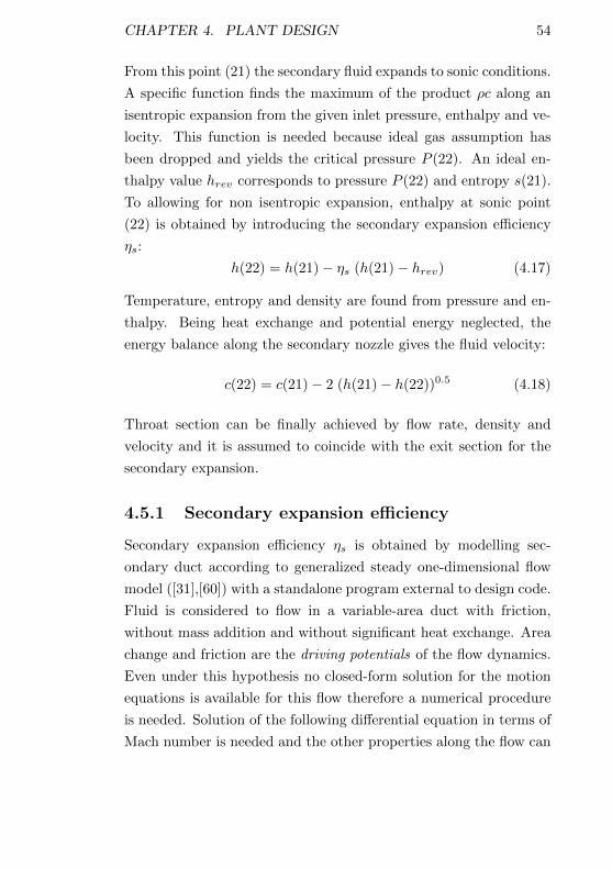
CHAPTER 4. PLANT DESIGN 54
From this point (21) the secondary fluid expands to sonic conditions.
A specific function finds the maximum of the product ρc along an
isentropic expansion from the given inlet pressure, enthalpy and ve-
locity. This function is needed because ideal gas assumption has
been dropped and yields the critical pressure P (22). An ideal en-
thalpy value hrev corresponds to pressure P (22) and entropy s(21).
To allowing for non isentropic expansion, enthalpy at sonic point
(22) is obtained by introducing the secondary expansion efficiency
ηs:
h(22) = h(21)− ηs (h(21)− hrev) (4.17)
Temperature, entropy and density are found from pressure and en-
thalpy. Being heat exchange and potential energy neglected, the
energy balance along the secondary nozzle gives the fluid velocity:
c(22) = c(21)− 2 (h(21)− h(22))0.5 (4.18)
Throat section can be finally achieved by flow rate, density and
velocity and it is assumed to coincide with the exit section for the
secondary expansion.
4.5.1 Secondary expansion efficiency
Secondary expansion efficiency ηs is obtained by modelling sec-
ondary duct according to generalized steady one-dimensional flow
model ([31],[60]) with a standalone program external to design code.
Fluid is considered to flow in a variable-area duct with friction,
without mass addition and without significant heat exchange. Area
change and friction are the driving potentials of the flow dynamics.
Even under this hypothesis no closed-form solution for the motion
equations is available for this flow therefore a numerical procedure
is needed. Solution of the following differential equation in terms of
Mach number is needed and the other properties along the flow can
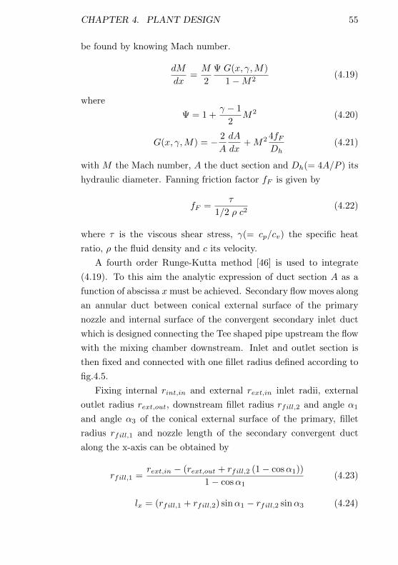
CHAPTER 4. PLANT DESIGN 55
be found by knowing Mach number.
dM
dx=M
2
Ψ G(x, γ,M)
1−M2(4.19)
where
Ψ = 1 +γ − 1
2M2 (4.20)
G(x, γ,M) = − 2
A
dA
dx+M2 4fF
Dh(4.21)
with M the Mach number, A the duct section and Dh(= 4A/P ) its
hydraulic diameter. Fanning friction factor fF is given by
fF =τ
1/2 ρ c2(4.22)
where τ is the viscous shear stress, γ(= cp/cv) the specific heat
ratio, ρ the fluid density and c its velocity.
A fourth order Runge-Kutta method [46] is used to integrate
(4.19). To this aim the analytic expression of duct section A as a
function of abscissa x must be achieved. Secondary flow moves along
an annular duct between conical external surface of the primary
nozzle and internal surface of the convergent secondary inlet duct
which is designed connecting the Tee shaped pipe upstream the flow
with the mixing chamber downstream. Inlet and outlet section is
then fixed and connected with one fillet radius defined according to
fig.4.5.
Fixing internal rint,in and external rext,in inlet radii, external
outlet radius rext,out, downstream fillet radius rfill,2 and angle α1
and angle α3 of the conical external surface of the primary, fillet
radius rfill,1 and nozzle length of the secondary convergent duct
along the x-axis can be obtained by
rfill,1 =rext,in − (rext,out + rfill,2 (1− cosα1))
1− cosα1(4.23)
lx = (rfill,1 + rfill,2) sinα1 − rfill,2 sinα3 (4.24)
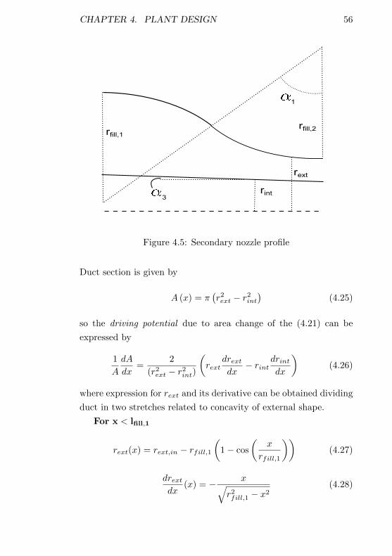
CHAPTER 4. PLANT DESIGN 56
rint
rext
1
rfill,2
3
rfill,1
Figure 4.5: Secondary nozzle profile
Duct section is given by
A (x) = π(r2ext − r2int
)(4.25)
so the driving potential due to area change of the (4.21) can be
expressed by
1
A
dA
dx=
2
(r2ext − r2int)
(rext
drextdx− rint
drintdx
)(4.26)
where expression for rext and its derivative can be obtained dividing
duct in two stretches related to concavity of external shape.
For x < lfill,1
rext(x) = rext,in − rfill,1(
1− cos
(x
rfill,1
))(4.27)
drextdx
(x) = − x√r2fill,1 − x2
(4.28)
CHAPTER 4. PLANT DESIGN 57
For x > lfill,1
rext(x) = rext,out + rfill,2
(1− cos
(lx − xrfill,2
))(4.29)
drextdx
(x) = − lx − x√r2fill,2 − (lx − x)
2(4.30)
A single expression is used for the internal surface radius rint
and its derivative along the whole secondary duct length
rint(x) = rint,out + tanα3 (lx − x) (4.31)
drintdx
= − tanα3 (4.32)
Solving (4.19) for M expression for thermodynamic properties
along the duct can be obtained starting from inlet conditions ac-
cording to ideal gas hypothesis. Being expansion adiabatic, static
temperature can be expressed by
T
Tin=
1 + γ−12 M2
in
1 + γ−12 M2
(4.33)
and starting from mass flow rate definition following expression can
be derived for static pressure
P
Pin=mAinMin
minAM
√T
Tin(4.34)
Under hypothesis of adiabatic expansion stagnation temperature
stays unchanged and stagnation pressure is obtained by
P0
P0,in=
P
Pin
(1 + γ−1
2 M2
1 + γ−12 M2
in
) γγ−1
(4.35)
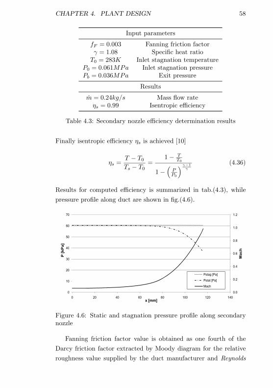
CHAPTER 4. PLANT DESIGN 58
Input parameters
fF = 0.003 Fanning friction factorγ = 1.08 Specific heat ratioT0 = 283K Inlet stagnation temperature
P0 = 0.061MPa Inlet stagnation pressurePb = 0.036MPa Exit pressure
Results
m = 0.24kg/s Mass flow rateηs = 0.99 Isentropic efficiency
Table 4.3: Secondary nozzle efficiency determination results
Finally isentropic efficiency ηs is achieved [10]
ηs =T − T0Ts − T0
=1− T
T0
1−(PP0
) γ−1γ
(4.36)
Results for computed efficiency is summarized in tab.(4.3), while
pressure profile along duct are shown in fig.(4.6).
0.8
1.0
1.2
40
50
60
70
P [
kP
a]
0.0
0.2
0.4
0.6
0
10
20
30
40
0 20 40 60 80 100 120 140
Ma
ch
P [
kP
a]
x [mm]
Pstag [Pa]
Pstat [Pa]
Mach
Figure 4.6: Static and stagnation pressure profile along secondarynozzle
Fanning friction factor value is obtained as one fourth of the
Darcy friction factor extracted by Moody diagram for the relative
roughness value supplied by the duct manufacturer and Reynolds
CHAPTER 4. PLANT DESIGN 59
number of the flow. Model assumes constant value for γ while it
actually changes slightly along the duct according to gas properties
changes. Influence of this behaviour on the value of efficiency is
however negligible.
4.6 Primary expansion
Once the pressure at the end of secondary expansion is known, given
the hypothesis of constant pressure mixing, the same pressure is
assumed for the primary flow at nozzle exit. Hence, from generator
exit (12), the fluid expands to pressure P (24) = P (22). Entropy
and density can be found from pressure and temperature calculated
above. Initial velocity c(12) is found as done for c(21) in (4.16)
applying mass flow rate definition.
Ideal enthalpy hrev is found at P (24) and s(12). The real value
h(24) comes from the primary nozzle efficiency ηp:
h(24) = h(12)− ηp (h(12)− hrev) (4.37)
Exit velocity c(24) is found as done for c(22) in (4.18).
4.6.1 Primary expansion efficiency
Like for secondary expansion, primary expansion efficiency is ob-
tained modelling primary nozzle by 1D generalized flow equations
and solving them by fourth-order Runge-Kutta method. Sonic point
is a singular point of the (4.19) because denominator becomes un-
bounded while M approaches 1. Following procedure proposed by
Beans [4] it is possible to transit sonic point location and overcome
discontinuity. Rearranging (4.19) as
1−M2
M2
dM2
dx= Ψ G(x, γ,M) (4.38)
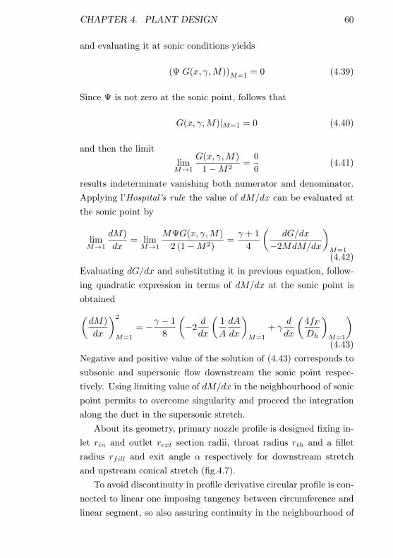
CHAPTER 4. PLANT DESIGN 60
and evaluating it at sonic conditions yields
(Ψ G(x, γ,M))M=1 = 0 (4.39)
Since Ψ is not zero at the sonic point, follows that
G(x, γ,M)|M=1 = 0 (4.40)
and then the limit
limM→1
G(x, γ,M)
1−M2=
0
0(4.41)
results indeterminate vanishing both numerator and denominator.
Applying l’Hospital’s rule the value of dM/dx can be evaluated at
the sonic point by
limM→1
dM)
dx= limM→1
MΨG(x, γ,M)
2 (1−M2)=γ + 1
4
(dG/dx
−2MdM/dx
)M=1(4.42)
Evaluating dG/dx and substituting it in previous equation, follow-
ing quadratic expression in terms of dM/dx at the sonic point is
obtained(dM)
dx
)2
M=1
= −γ − 1
8
(−2
d
dx
(1
A
dA
dx
)M=1
+ γd
dx
(4fFDh
)M=1
)(4.43)
Negative and positive value of the solution of (4.43) corresponds to
subsonic and supersonic flow downstream the sonic point respec-
tively. Using limiting value of dM/dx in the neighbourhood of sonic
point permits to overcome singularity and proceed the integration
along the duct in the supersonic stretch.
About its geometry, primary nozzle profile is designed fixing in-
let rin and outlet rext section radii, throat radius rth and a fillet
radius rfill and exit angle α respectively for downstream stretch
and upstream conical stretch (fig.4.7).
To avoid discontinuity in profile derivative circular profile is con-
nected to linear one imposing tangency between circumference and
linear segment, so also assuring continuity in the neighbourhood of
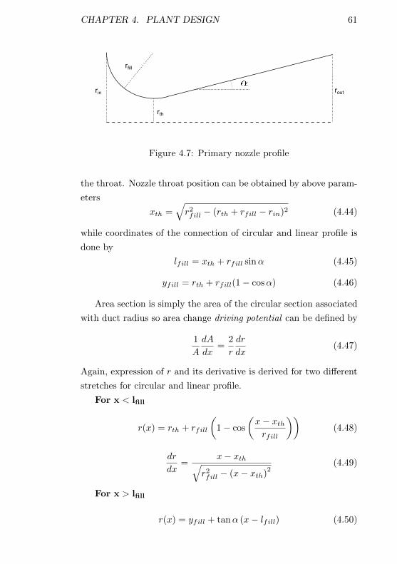
CHAPTER 4. PLANT DESIGN 61
routrin
rth
rfill
Figure 4.7: Primary nozzle profile
the throat. Nozzle throat position can be obtained by above param-
eters
xth =√r2fill − (rth + rfill − rin)2 (4.44)
while coordinates of the connection of circular and linear profile is
done by
lfill = xth + rfill sinα (4.45)
yfill = rth + rfill(1− cosα) (4.46)
Area section is simply the area of the circular section associated
with duct radius so area change driving potential can be defined by
1
A
dA
dx=
2
r
dr
dx(4.47)
Again, expression of r and its derivative is derived for two different
stretches for circular and linear profile.
For x < lfill
r(x) = rth + rfill
(1− cos
(x− xthrfill
))(4.48)
dr
dx=
x− xth√r2fill − (x− xth)
2(4.49)
For x > lfill
r(x) = yfill + tanα (x− lfill) (4.50)
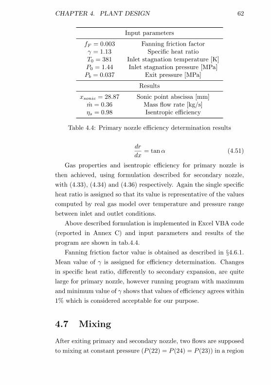
CHAPTER 4. PLANT DESIGN 62
Input parameters
fF = 0.003 Fanning friction factorγ = 1.13 Specific heat ratioT0 = 381 Inlet stagnation temperature [K]P0 = 1.44 Inlet stagnation pressure [MPa]Pb = 0.037 Exit pressure [MPa]
Results
xsonic = 28.87 Sonic point abscissa [mm]m = 0.36 Mass flow rate [kg/s]ηs = 0.98 Isentropic efficiency
Table 4.4: Primary nozzle efficiency determination results
dr
dx= tanα (4.51)
Gas properties and isentropic efficiency for primary nozzle is
then achieved, using formulation described for secondary nozzle,
with (4.33), (4.34) and (4.36) respectively. Again the single specific
heat ratio is assigned so that its value is representative of the values
computed by real gas model over temperature and pressure range
between inlet and outlet conditions.
Above described formulation is implemented in Excel VBA code
(reported in Annex C) and input parameters and results of the
program are shown in tab.4.4.
Fanning friction factor value is obtained as described in §4.6.1.
Mean value of γ is assigned for efficiency determination. Changes
in specific heat ratio, differently to secondary expansion, are quite
large for primary nozzle, however running program with maximum
and minimum value of γ shows that values of efficiency agrees within
1% which is considered acceptable for our purpose.
4.7 Mixing
After exiting primary and secondary nozzle, two flows are supposed
to mixing at constant pressure (P (22) = P (24) = P (23)) in a region
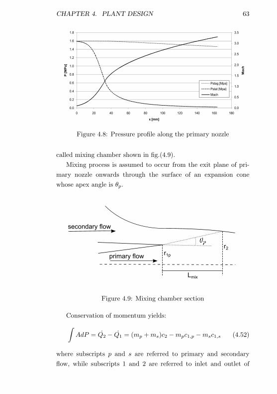
CHAPTER 4. PLANT DESIGN 63
0.0
0.5
1.0
1.5
2.0
2.5
3.0
3.5
0.0
0.2
0.4
0.6
0.8
1.0
1.2
1.4
1.6
1.8
0 20 40 60 80 100 120 140 160 180
Mach
P [
MP
a]
x [mm]
Pstag [Mpa]
Pstat [Mpa]
Mach
Figure 4.8: Pressure profile along the primary nozzle
called mixing chamber shown in fig.(4.9).
Mixing process is assumed to occur from the exit plane of pri-
mary nozzle onwards through the surface of an expansion cone
whose apex angle is θp.
primary flow
secondary flow
Lmix
r1p
r2
Figure 4.9: Mixing chamber section
Conservation of momentum yields:∫AdP = Q2 − Q1 = (mp +ms)c2 −mpc1,p −msc1,s (4.52)
where subscripts p and s are referred to primary and secondary
flow, while subscripts 1 and 2 are referred to inlet and outlet of
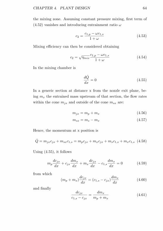
CHAPTER 4. PLANT DESIGN 64
the mixing zone. Assuming constant pressure mixing, first term of
(4.52) vanishes and introducing entrainment ratio ω
c2 =c1,p − ωc1,s
1 + ω(4.53)
Mixing efficiency can then be considered obtaining
c2 =√ηmix
c1,p − ωc1,s1 + ω
(4.54)
In the mixing chamber is
dQ
dx= 0 (4.55)
In a generic section at distance x from the nozzle exit plane, be-
ing mx the entrained mass upstream of that section, the flow rates
within the cone mjx and outside of the cone msx are:
mjx = mp +mx (4.56)
msx = ms −mx (4.57)
Hence, the momentum at x position is
Q = mjxcjx +msxc1,s = mpcjx +mxcjx +msc1,s +mxc1,s (4.58)
Using (4.55), it follows
mpdcjxdx
+ cjxdmx
dx+mx
dcjxdx− c1,s
dmx
dx= 0 (4.59)
from which
(mp +mx)dcjxdx
= (c1,s − cjx)dmx
dx(4.60)
and finallydcjx
c1,s − cjx=
dmx
mp +mx(4.61)
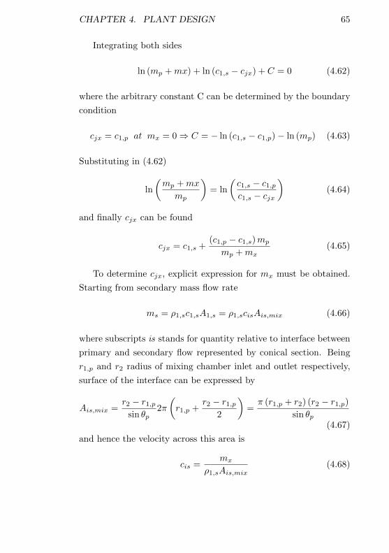
CHAPTER 4. PLANT DESIGN 65
Integrating both sides
ln (mp +mx) + ln (c1,s − cjx) + C = 0 (4.62)
where the arbitrary constant C can be determined by the boundary
condition
cjx = c1,p at mx = 0⇒ C = − ln (c1,s − c1,p)− ln (mp) (4.63)
Substituting in (4.62)
ln
(mp +mx
mp
)= ln
(c1,s − c1,pc1,s − cjx
)(4.64)
and finally cjx can be found
cjx = c1,s +(c1,p − c1,s)mp
mp +mx(4.65)
To determine cjx, explicit expression for mx must be obtained.
Starting from secondary mass flow rate
ms = ρ1,sc1,sA1,s = ρ1,scisAis,mix (4.66)
where subscripts is stands for quantity relative to interface between
primary and secondary flow represented by conical section. Being
r1,p and r2 radius of mixing chamber inlet and outlet respectively,
surface of the interface can be expressed by
Ais,mix =r2 − r1,p
sin θp2π
(r1,p +
r2 − r1,p2
)=π (r1,p + r2) (r2 − r1,p)
sin θp(4.67)
and hence the velocity across this area is
cis =mx
ρ1,sAis,mix(4.68)
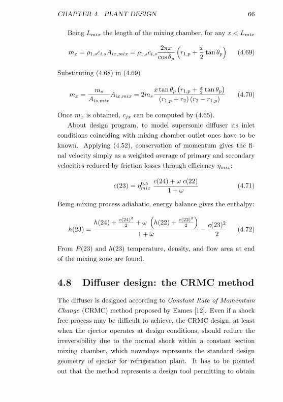
CHAPTER 4. PLANT DESIGN 66
Being Lmix the length of the mixing chamber, for any x < Lmix
mx = ρ1,sci,sAix,mix = ρ1,sci,s2πx
cos θp
(r1,p +
x
2tan θp
)(4.69)
Substituting (4.68) in (4.69)
mx =ms
Ais,mixAix,mix = 2ms
x tan θp(r1,p + x
2 tan θp)
(r1,p + r2) (r2 − r1,p)(4.70)
Once mx is obtained, cjx can be computed by (4.65).
About design program, to model supersonic diffuser its inlet
conditions coinciding with mixing chamber outlet ones have to be
known. Applying (4.52), conservation of momentum gives the fi-
nal velocity simply as a weighted average of primary and secondary
velocities reduced by friction losses through efficiency ηmix:
c(23) = η0.5mixc(24) + ω c(22)
1 + ω(4.71)
Being mixing process adiabatic, energy balance gives the enthalpy:
h(23) =h(24) + c(24)2
2 + ω(h(22) + c(22)2
2
)1 + ω
− c(23)2
2(4.72)
From P (23) and h(23) temperature, density, and flow area at end
of the mixing zone are found.
4.8 Diffuser design: the CRMC method
The diffuser is designed according to Constant Rate of Momemtum
Change (CRMC) method proposed by Eames [12]. Even if a shock
free process may be difficult to achieve, the CRMC design, at least
when the ejector operates at design conditions, should reduce the
irreversibility due to the normal shock within a constant section
mixing chamber, which nowadays represents the standard design
geometry of ejector for refrigeration plant. It has to be pointed
out that the method represents a design tool permitting to obtain
CHAPTER 4. PLANT DESIGN 67
geometry description of supersonic diffuser imposing rate of momen-
tum change. It is hence the central element of the design program
whose aim it to obtain geometric definition of the ejector starting
from its operating conditions. CRMC method, as proposed in lit-
erature, does not provide a specific design for the mixing chamber,
it is based on isentropic assumption and does not limit the angle of
the divergent stretch of the diffuser. In this work, a specific criterion
to design mixing chamber is adopted (§4.7) and friction loss term is
included in flow equations. Moreover, diffuser exit angle has been
limited to avoid flow separation.
Complete mixing is assumed at diffuser inlet (23). The mixed
flow, still supersonic, claims for a converging–diverging profile to
complete pressure recovery. Specific function is developed to shape
supersonic diffuser, whose purpose is to give pressure and enthalpy
at diffuser exit as a function of initial conditions, relative roughness,
maximum angle of the divergent duct and condenser inlet diameter.
The diffuser is divided in two stretches: the first is modelled fix-
ing the rate of momentum change and deriving the section profile,
while the second is a conical divergent section duct. Distinguishing
two stretches, permits to contain apex angle of conical duct limiting
flow detachment phenomena. In fact conical section for the second
part of the diffuser is introduced to avoid too much rapidly diverg-
ing profile at the end of the diffuser itself, and it starts when the
diverging angle exceeds a threshold passed to the function as input
parameter.
The function gives the diffuser outlet pressure Pnew and enthalpy
h(13) for the initial conditions P (23), c(23), h(23) and radius rin
at the inlet section. Relative roughness is used to find the friction
factor value. Maximum angle of the divergent duct and final diam-
eter (i.e. condenser inlet diameter) determine the conical stretch
geometry. Both the stretches are solved as variable section ducts
with friction, but no heat transfer, work or mass addiction. The
First and Second Law of Thermodynamics for an infinitesimal open
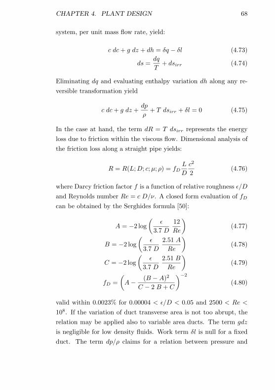
CHAPTER 4. PLANT DESIGN 68
system, per unit mass flow rate, yield:
c dc+ g dz + dh = δq − δl (4.73)
ds =dq
T+ dsirr (4.74)
Eliminating dq and evaluating enthalpy variation dh along any re-
versible transformation yield
c dc+ g dz +dp
ρ+ T dsirr + δl = 0 (4.75)
In the case at hand, the term dR = T dsirr represents the energy
loss due to friction within the viscous flow. Dimensional analysis of
the friction loss along a straight pipe yields:
R = R(L;D; c;µ; ρ) = fDL
D
c2
2(4.76)
where Darcy friction factor f is a function of relative roughness ε/D
and Reynolds number Re = c D/ν. A closed form evaluation of fD
can be obtained by the Serghides formula [50]:
A = −2 log
(ε
3.7 D
12
Re
)(4.77)
B = −2 log
(ε
3.7 D
2.51 A
Re
)(4.78)
C = −2 log
(ε
3.7 D
2.51 B
Re
)(4.79)
fD =
(A− (B −A)2
C − 2 B + C
)−2(4.80)
valid within 0.0023% for 0.00004 < ε/D < 0.05 and 2500 < Re <
108. If the variation of duct transverse area is not too abrupt, the
relation may be applied also to variable area ducts. The term gdz
is negligible for low density fluids. Work term δl is null for a fixed
duct. The term dp/ρ claims for a relation between pressure and
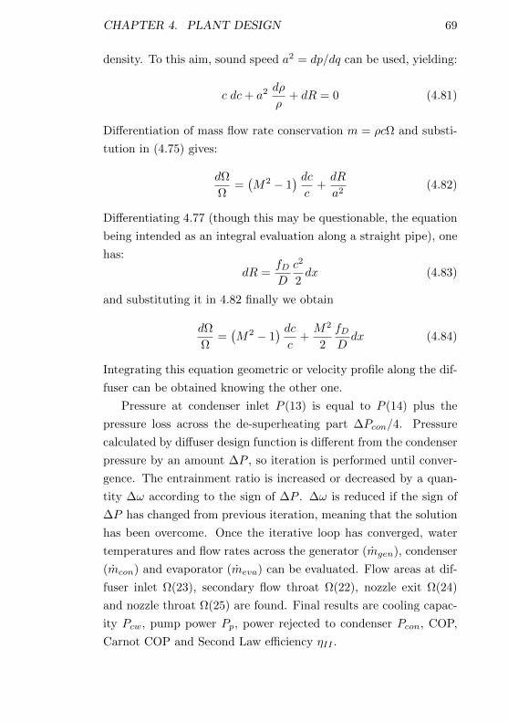
CHAPTER 4. PLANT DESIGN 69
density. To this aim, sound speed a2 = dp/dq can be used, yielding:
c dc+ a2dρ
ρ+ dR = 0 (4.81)
Differentiation of mass flow rate conservation m = ρcΩ and substi-
tution in (4.75) gives:
dΩ
Ω=(M2 − 1
) dcc
+dR
a2(4.82)
Differentiating 4.77 (though this may be questionable, the equation
being intended as an integral evaluation along a straight pipe), one
has:
dR =fDD
c2
2dx (4.83)
and substituting it in 4.82 finally we obtain
dΩ
Ω=(M2 − 1
) dcc
+M2
2
fDDdx (4.84)
Integrating this equation geometric or velocity profile along the dif-
fuser can be obtained knowing the other one.
Pressure at condenser inlet P (13) is equal to P (14) plus the
pressure loss across the de-superheating part ∆Pcon/4. Pressure
calculated by diffuser design function is different from the condenser
pressure by an amount ∆P , so iteration is performed until conver-
gence. The entrainment ratio is increased or decreased by a quan-
tity ∆ω according to the sign of ∆P . ∆ω is reduced if the sign of
∆P has changed from previous iteration, meaning that the solution
has been overcome. Once the iterative loop has converged, water
temperatures and flow rates across the generator (mgen), condenser
(mcon) and evaporator (meva) can be evaluated. Flow areas at dif-
fuser inlet Ω(23), secondary flow throat Ω(22), nozzle exit Ω(24)
and nozzle throat Ω(25) are found. Final results are cooling capac-
ity Pcw, pump power Pp, power rejected to condenser Pcon, COP,
Carnot COP and Second Law efficiency ηII .
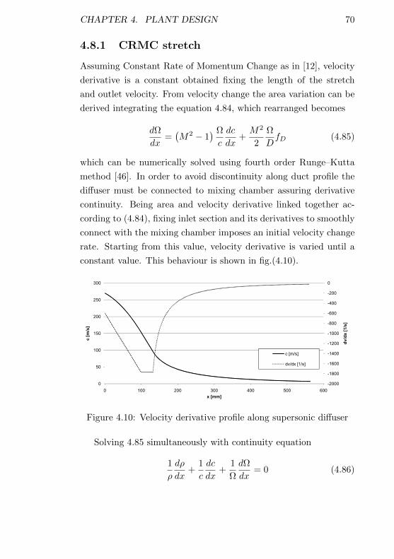
CHAPTER 4. PLANT DESIGN 70
4.8.1 CRMC stretch
Assuming Constant Rate of Momentum Change as in [12], velocity
derivative is a constant obtained fixing the length of the stretch
and outlet velocity. From velocity change the area variation can be
derived integrating the equation 4.84, which rearranged becomes
dΩ
dx=(M2 − 1
) Ω
c
dc
dx+M2
2
Ω
DfD (4.85)
which can be numerically solved using fourth order Runge–Kutta
method [46]. In order to avoid discontinuity along duct profile the
diffuser must be connected to mixing chamber assuring derivative
continuity. Being area and velocity derivative linked together ac-
cording to (4.84), fixing inlet section and its derivatives to smoothly
connect with the mixing chamber imposes an initial velocity change
rate. Starting from this value, velocity derivative is varied until a
constant value. This behaviour is shown in fig.(4.10).
-800
-600
-400
-200
0
200
250
300
1/s
]
c [m
/s]
-2000
-1800
-1600
-1400
-1200
-1000
0
50
100
150
0 100 200 300 400 500 600
dv
/dx
[1
c [m
/s]
x [mm]
c [m/s]
dv/dx [1/s]
Figure 4.10: Velocity derivative profile along supersonic diffuser
Solving 4.85 simultaneously with continuity equation
1
ρ
dρ
dx+
1
c
dc
dx+
1
Ω
dΩ
dx= 0 (4.86)
CHAPTER 4. PLANT DESIGN 71
and energy conservation
dh
dx+ c
dc
dx= 0 (4.87)
density and enthalpy along the supersonic diffuser can be obtained.
From them, NIST Refprop functions give the other thermodynamic
properties (pressure, temperature, entropy, gas specific heat and
fluid viscosity).
4.8.2 Conical stretch
If a threshold is set on the aperture angle of the diverging part
of the diffuser, the above described procedure must be modified.
As soon as the threshold angle is exceeded, the geometry will be
imposed, for example by setting a constant value of the diverging
angle. Rearranging (4.84), fluid velocity derivative can be expressed
as function of area change
dc
dx=
1
M2 − 1
c
Ω
dΩ
dx+
M2
2 (M2 − 1)
c
DfD (4.88)
Fluid density and enthalpy are hence obtained simultaneously solv-
ing (4.88) together wiht (4.86) and (4.87). Other thermodynamic
properties (pressure, temperature, entropy, gas specific heat and
fluid viscosity) are computed by NIST Refprop functions. Finally,
isentropic efficiency of the diffuser can be obtained dividing the
static enthalpy difference along isentropic flow by the same differ-
ence computed with friction. No arbitrary assumption, like those
done for the efficiency of primary/secondary expansion and mixing,
is needed.
4.8.3 Diffuser design results
Main results of previously described procedure are the definition of
the internal shape of supersonic diffuser and the computation of gas
properties along the duct. Graphical presentation of the results can
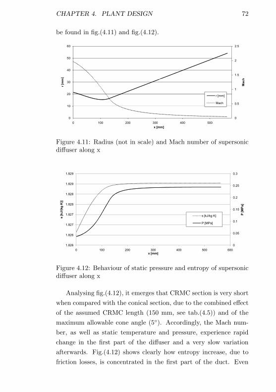
CHAPTER 4. PLANT DESIGN 72
be found in fig.(4.11) and fig.(4.12).
1.5
2
2.5
40
50
60
Mac
h
r [m
m]
0
0.5
1
0
10
20
30
0 100 200 300 400 500
Mac
h
r [m
m]
x [mm]
r [mm]
Mach
Figure 4.11: Radius (not in scale) and Mach number of supersonicdiffuser along x
0
0.05
0.1
0.15
0.2
0.25
0.3
1.826
1.826
1.827
1.827
1.828
1.828
1.829
1.829
0 100 200 300 400 500 600
P [
MP
a]
s [
kJ/
(kg
K)]
x [mm]
s [kJ/kg K]
P [MPa]
Figure 4.12: Behaviour of static pressure and entropy of supersonicdiffuser along x
Analysing fig.(4.12), it emerges that CRMC section is very short
when compared with the conical section, due to the combined effect
of the assumed CRMC length (150 mm, see tab.(4.5)) and of the
maximum allowable cone angle (5). Accordingly, the Mach num-
ber, as well as static temperature and pressure, experience rapid
change in the first part of the diffuser and a very slow variation
afterwards. Fig.(4.12) shows clearly how entropy increase, due to
friction losses, is concentrated in the first part of the duct. Even
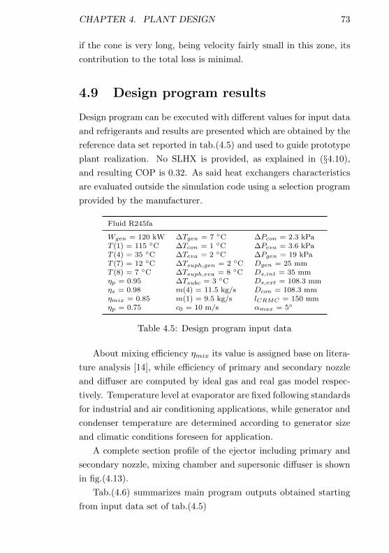
CHAPTER 4. PLANT DESIGN 73
if the cone is very long, being velocity fairly small in this zone, its
contribution to the total loss is minimal.
4.9 Design program results
Design program can be executed with different values for input data
and refrigerants and results are presented which are obtained by the
reference data set reported in tab.(4.5) and used to guide prototype
plant realization. No SLHX is provided, as explained in (§4.10),
and resulting COP is 0.32. As said heat exchangers characteristics
are evaluated outside the simulation code using a selection program
provided by the manufacturer.
Fluid R245fa
Wgen = 120 kW ∆Tgen = 7 C ∆Pcon = 2.3 kPaT (1) = 115 C ∆Tcon = 1 C ∆Peva = 3.6 kPaT (4) = 35 C ∆Teva = 2 C ∆Pgen = 19 kPaT (7) = 12 C ∆Tsuph,gen = 2 C Dgen = 25 mmT (8) = 7 C ∆Tsuph,eva = 8 C Ds,int = 35 mmηp = 0.95 ∆Tsubc = 3 C Ds,ext = 108.3 mmηs = 0.98 m(4) = 11.5 kg/s Dcon = 108.3 mmηmix = 0.85 m(1) = 9.5 kg/s lCRMC = 150 mmηp = 0.75 c0 = 10 m/s αmax = 5
Table 4.5: Design program input data
About mixing efficiency ηmix its value is assigned base on litera-
ture analysis [14], while efficiency of primary and secondary nozzle
and diffuser are computed by ideal gas and real gas model respec-
tively. Temperature level at evaporator are fixed following standards
for industrial and air conditioning applications, while generator and
condenser temperature are determined according to generator size
and climatic conditions foreseen for application.
A complete section profile of the ejector including primary and
secondary nozzle, mixing chamber and supersonic diffuser is shown
in fig.(4.13).
Tab.(4.6) summarizes main program outputs obtained starting
from input data set of tab.(4.5)
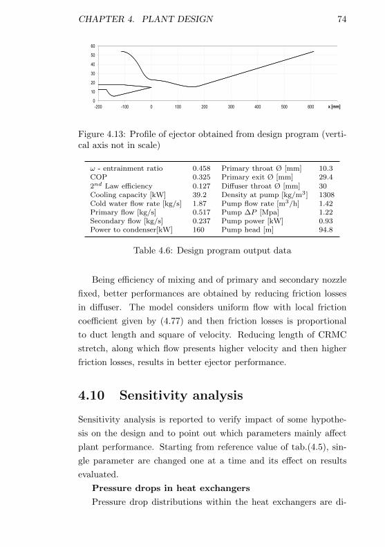
CHAPTER 4. PLANT DESIGN 74
40
50
60
10
20
30
40
0-200 -100 0 100 200 300 400 500 600 700x [mm]
Figure 4.13: Profile of ejector obtained from design program (verti-cal axis not in scale)
ω - entrainment ratio 0.458 Primary throat Ø [mm] 10.3COP 0.325 Primary exit Ø [mm] 29.42nd Law efficiency 0.127 Diffuser throat Ø [mm] 30Cooling capacity [kW] 39.2 Density at pump [kg/m3] 1308Cold water flow rate [kg/s] 1.87 Pump flow rate [m3/h] 1.42Primary flow [kg/s] 0.517 Pump ∆P [Mpa] 1.22Secondary flow [kg/s] 0.237 Pump power [kW] 0.93Power to condenser[kW] 160 Pump head [m] 94.8
Table 4.6: Design program output data
Being efficiency of mixing and of primary and secondary nozzle
fixed, better performances are obtained by reducing friction losses
in diffuser. The model considers uniform flow with local friction
coefficient given by (4.77) and then friction losses is proportional
to duct length and square of velocity. Reducing length of CRMC
stretch, along which flow presents higher velocity and then higher
friction losses, results in better ejector performance.
4.10 Sensitivity analysis
Sensitivity analysis is reported to verify impact of some hypothe-
sis on the design and to point out which parameters mainly affect
plant performance. Starting from reference value of tab.(4.5), sin-
gle parameter are changed one at a time and its effect on results
evaluated.
Pressure drops in heat exchangers
Pressure drop distributions within the heat exchangers are di-
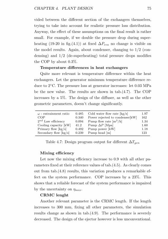
CHAPTER 4. PLANT DESIGN 75
vided between the different section of the exchangers themselves,
trying to take into account for realistic pressure loss distribution.
Anyway, the effect of these assumptions on the final result is rather
small. For example, if we double the pressure drop during super-
heating (19-20 in fig.(4.1)) at fixed ∆Peva no change is visible on
the model results. Again, about condenser, changing to 1/2 (con-
densing) and 1/2 (de-superheating) total pressure drops modifies
the COP by about 0.3%.
Temperature differences in heat exchangers
Quite more relevant is temperature difference within the heat
exchangers. Let the generator minimum temperature difference re-
duce to 2C. The pressure loss at generator increases: let 0.03 MPa
be the new value. The results are shown in tab.(4.7). The COP
increases by a 5%. The design of the diffuser, as well as the other
geometric parameters, doesn’t change significantly.
ω - entrainment ratio 0.485 Cold water flow rate [kg/s] 1.97COP 0.340 Power rejected to condenser[kW] 1622nd Law efficiency 0.094 Pump flow rate [m3/h] 1.34Cooling capacity [kW] 41.2 Pump ∆P [Mpa] 1.60Primary flow [kg/s] 0.492 Pump power [kW] 1.18Secondary flow [kg/s] 0.239 Pump head [m] 123
Table 4.7: Design program output for different ∆Tgen
Mixing efficiency
Let now the mixing efficiency increase to 0.9 with all other pa-
rameters fixed at their reference values of tab.(4.5). As clearly comes
out from tab.(4.8) results, this variation produces a remarkable ef-
fect on the system performance. COP increases by a 23%. This
shows that a reliable forecast of the system performance is impaired
by the uncertainty on ηmix.
CRMC lenght
Another relevant parameter is the CRMC length. If the length
increases to 300 mm, fixing all other parameters, the simulation
results change as shown in tab.(4.9). The performance is severely
decreased. The design of the ejector however is less unconventional.
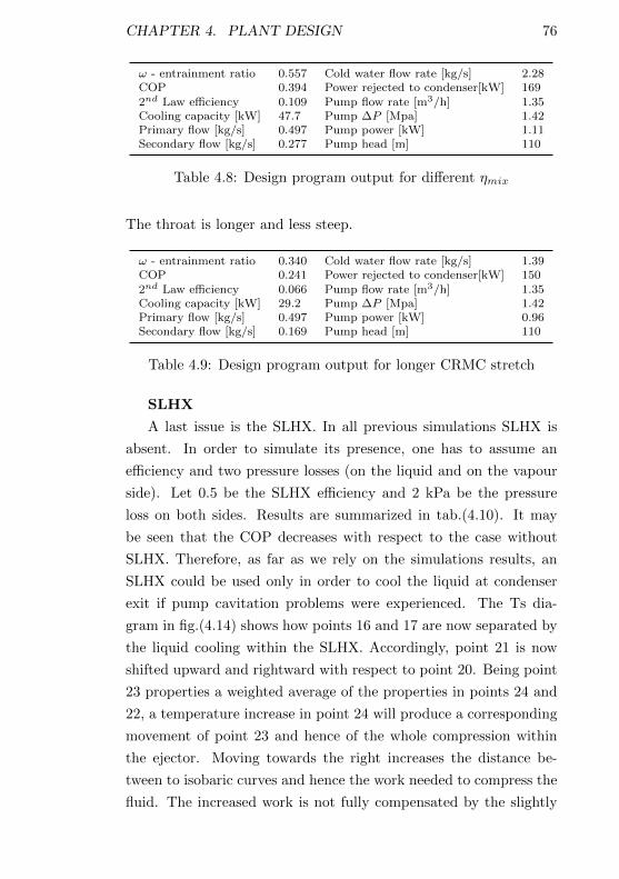
CHAPTER 4. PLANT DESIGN 76
ω - entrainment ratio 0.557 Cold water flow rate [kg/s] 2.28COP 0.394 Power rejected to condenser[kW] 1692nd Law efficiency 0.109 Pump flow rate [m3/h] 1.35Cooling capacity [kW] 47.7 Pump ∆P [Mpa] 1.42Primary flow [kg/s] 0.497 Pump power [kW] 1.11Secondary flow [kg/s] 0.277 Pump head [m] 110
Table 4.8: Design program output for different ηmix
The throat is longer and less steep.
ω - entrainment ratio 0.340 Cold water flow rate [kg/s] 1.39COP 0.241 Power rejected to condenser[kW] 1502nd Law efficiency 0.066 Pump flow rate [m3/h] 1.35Cooling capacity [kW] 29.2 Pump ∆P [Mpa] 1.42Primary flow [kg/s] 0.497 Pump power [kW] 0.96Secondary flow [kg/s] 0.169 Pump head [m] 110
Table 4.9: Design program output for longer CRMC stretch
SLHX
A last issue is the SLHX. In all previous simulations SLHX is
absent. In order to simulate its presence, one has to assume an
efficiency and two pressure losses (on the liquid and on the vapour
side). Let 0.5 be the SLHX efficiency and 2 kPa be the pressure
loss on both sides. Results are summarized in tab.(4.10). It may
be seen that the COP decreases with respect to the case without
SLHX. Therefore, as far as we rely on the simulations results, an
SLHX could be used only in order to cool the liquid at condenser
exit if pump cavitation problems were experienced. The Ts dia-
gram in fig.(4.14) shows how points 16 and 17 are now separated by
the liquid cooling within the SLHX. Accordingly, point 21 is now
shifted upward and rightward with respect to point 20. Being point
23 properties a weighted average of the properties in points 24 and
22, a temperature increase in point 24 will produce a corresponding
movement of point 23 and hence of the whole compression within
the ejector. Moving towards the right increases the distance be-
tween to isobaric curves and hence the work needed to compress the
fluid. The increased work is not fully compensated by the slightly
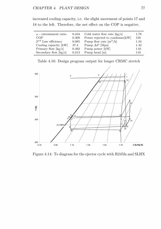
CHAPTER 4. PLANT DESIGN 77
increased cooling capacity, i.e. the slight movement of points 17 and
18 to the left. Therefore, the net effect on the COP is negative.
ω - entrainment ratio 0.434 Cold water flow rate [kg/s] 1.78COP 0.309 Power rejected to condenser[kW] 1582nd Law efficiency 0.085 Pump flow rate [m3/h] 1.34Cooling capacity [kW] 37.4 Pump ∆P [Mpa] 1.42Primary flow [kg/s] 0.492 Pump power [kW] 1.01Secondary flow [kg/s] 0.213 Pump head [m] 110
Table 4.10: Design program output for longer CRMC stretch
0.2 MPa
10 1112
151617
18 19
20
9
2224
14
4 5 6
123
78
23
13
21
250
300
350
400
0.75 0.95 1.15 1.35 1.55 1.75 1.95s [kJ/kg K]
T [
K]
Figure 4.14: Ts diagram for the ejector cycle with R245fa and SLHX
Chapter 5
Experimental results
In this chapter experimental results, obtained by prototype plant
realized at the test facility, set up in manufacturer plant of Frigel
Firenze Spa, are presented.
Ejector refrigeration apparatus is described focusing on main
building feature and measurement equipment in the first part of the
chapter and then data analysis is presented and results evaluated.
5.1 Experimental apparatus
The results of a study of potential working fluids lead to R245fa
being selected as the most suitable fluid, because of its relatively
high critical temperature, moderate system pressure ratio, posi-
tively sloped saturated vapour curve, (that gives a dry expansion
even starting with saturated vapour) and a reasonable GWP. The
saturation temperatures at the generator, condenser and evapora-
tor selected are 106C, 39C and 4C respectively at design point.
From design program results (§4), it is estimated that the jet-pump
entrainment ratio would be approximately 0.44 and this give a sys-
tem COP value of about 0.31. Therefore, for an evaporator cooling
capacity of about 40 kW the vapour generator would require ap-
proximately 130 kW of heat input.
78
CHAPTER 5. EXPERIMENTAL RESULTS 79
Starting from these data, plant components have been selected
and found under a collaboration with Frigel Firenze Spa, at whose
test facility assembly has been made and experimental tests per-
formed.
According to research interest, plant is equipped with measure-
ment instrumentation, which permits to obtain pressure trend along
the ejector and working conditions of plate heat exchangers. A de-
tailed description of used instrumentation and probes, and their
placement over the plant are reported in §5.1.4.
Moreover, prototype plant is designed to permit substitution of
primary nozzle and diffuser, to test different ejector solution. All
other parts of the plant are unchanged and it is then possible to
compare some geometric solution for ejector on the same configura-
tion. Actually, two different diffuser profile are tested, obtained by
two different building process and materials (§5.1.2).
5.1.1 Plant layout
Main components of the prototype plant are the three heat exchang-
ers, ejector and feed pump (fig.(5.1)). An electronic expansion valve
(EEV) is used to control liquid level in the evaporator. During com-
ponents placing, several features have to be taken into account like
to avoid feed pump cavitation and heat exchangers thermal losses,
to position measurement probes, to permit easy connection with
external water circuits and to allow access to diffuser for assembly
and disassembly operations.
Vertical arrangement is chosen for heat exchangers placement,
partly to reduce floor space occupied by the plant, but mainly to
mitigate any flow cavitation problems at pump inlet, being in this
way possible to place condenser in the upper part of the structure
and pump at the bottom, increasing condensed refrigerant head.
Consequently, main axis of ejector also has to be vertically aligned.
The main drawback of described configuration is the elbow con-
necting the end of the diffuser to the condenser inlet. This elbow
should have an adequate radius and a suitable straight connecting
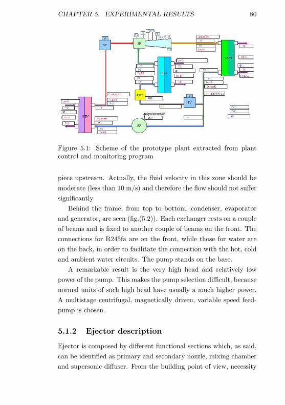
CHAPTER 5. EXPERIMENTAL RESULTS 80
Figure 5.1: Scheme of the prototype plant extracted from plantcontrol and monitoring program
piece upstream. Actually, the fluid velocity in this zone should be
moderate (less than 10 m/s) and therefore the flow should not suffer
significantly.
Behind the frame, from top to bottom, condenser, evaporator
and generator, are seen (fig.(5.2)). Each exchanger rests on a couple
of beams and is fixed to another couple of beams on the front. The
connections for R245fa are on the front, while those for water are
on the back, in order to facilitate the connection with the hot, cold
and ambient water circuits. The pump stands on the base.
A remarkable result is the very high head and relatively low
power of the pump. This makes the pump selection difficult, because
normal units of such high head have usually a much higher power.
A multistage centrifugal, magnetically driven, variable speed feed-
pump is chosen.
5.1.2 Ejector description
Ejector is composed by different functional sections which, as said,
can be identified as primary and secondary nozzle, mixing chamber
and supersonic diffuser. From the building point of view, necessity
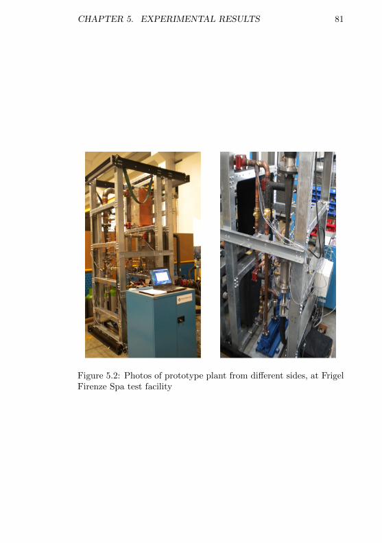
CHAPTER 5. EXPERIMENTAL RESULTS 81
Figure 5.2: Photos of prototype plant from different sides, at FrigelFirenze Spa test facility
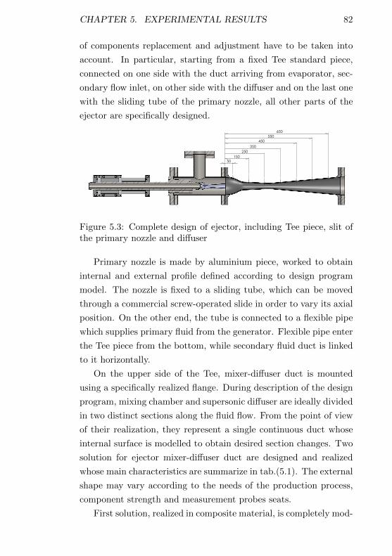
CHAPTER 5. EXPERIMENTAL RESULTS 82
of components replacement and adjustment have to be taken into
account. In particular, starting from a fixed Tee standard piece,
connected on one side with the duct arriving from evaporator, sec-
ondary flow inlet, on other side with the diffuser and on the last one
with the sliding tube of the primary nozzle, all other parts of the
ejector are specifically designed.
50150
250350
450550
650
Figure 5.3: Complete design of ejector, including Tee piece, slit ofthe primary nozzle and diffuser
Primary nozzle is made by aluminium piece, worked to obtain
internal and external profile defined according to design program
model. The nozzle is fixed to a sliding tube, which can be moved
through a commercial screw-operated slide in order to vary its axial
position. On the other end, the tube is connected to a flexible pipe
which supplies primary fluid from the generator. Flexible pipe enter
the Tee piece from the bottom, while secondary fluid duct is linked
to it horizontally.
On the upper side of the Tee, mixer-diffuser duct is mounted
using a specifically realized flange. During description of the design
program, mixing chamber and supersonic diffuser are ideally divided
in two distinct sections along the fluid flow. From the point of view
of their realization, they represent a single continuous duct whose
internal surface is modelled to obtain desired section changes. Two
solution for ejector mixer-diffuser duct are designed and realized
whose main characteristics are summarize in tab.(5.1). The external
shape may vary according to the needs of the production process,
component strength and measurement probes seats.
First solution, realized in composite material, is completely mod-
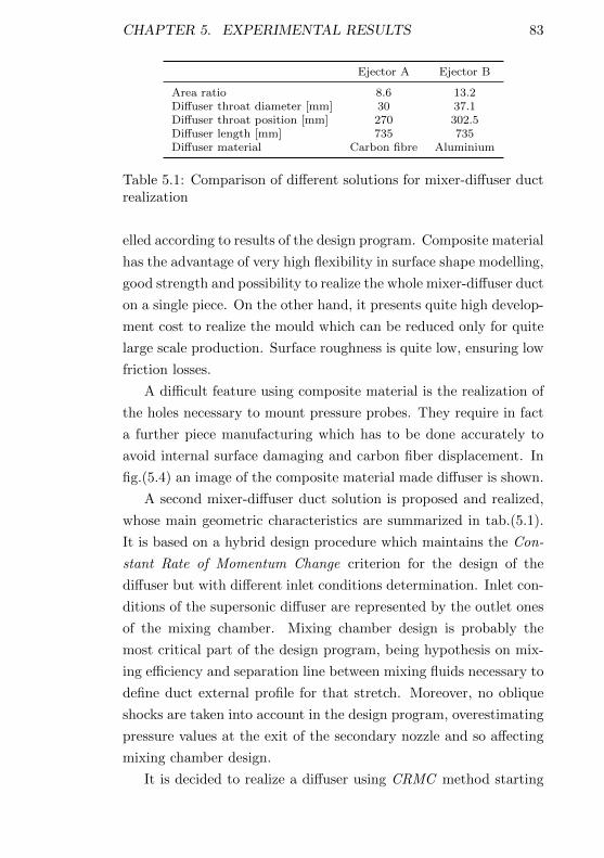
CHAPTER 5. EXPERIMENTAL RESULTS 83
Ejector A Ejector B
Area ratio 8.6 13.2Diffuser throat diameter [mm] 30 37.1Diffuser throat position [mm] 270 302.5Diffuser length [mm] 735 735Diffuser material Carbon fibre Aluminium
Table 5.1: Comparison of different solutions for mixer-diffuser ductrealization
elled according to results of the design program. Composite material
has the advantage of very high flexibility in surface shape modelling,
good strength and possibility to realize the whole mixer-diffuser duct
on a single piece. On the other hand, it presents quite high develop-
ment cost to realize the mould which can be reduced only for quite
large scale production. Surface roughness is quite low, ensuring low
friction losses.
A difficult feature using composite material is the realization of
the holes necessary to mount pressure probes. They require in fact
a further piece manufacturing which has to be done accurately to
avoid internal surface damaging and carbon fiber displacement. In
fig.(5.4) an image of the composite material made diffuser is shown.
A second mixer-diffuser duct solution is proposed and realized,
whose main geometric characteristics are summarized in tab.(5.1).
It is based on a hybrid design procedure which maintains the Con-
stant Rate of Momentum Change criterion for the design of the
diffuser but with different inlet conditions determination. Inlet con-
ditions of the supersonic diffuser are represented by the outlet ones
of the mixing chamber. Mixing chamber design is probably the
most critical part of the design program, being hypothesis on mix-
ing efficiency and separation line between mixing fluids necessary to
define duct external profile for that stretch. Moreover, no oblique
shocks are taken into account in the design program, overestimating
pressure values at the exit of the secondary nozzle and so affecting
mixing chamber design.
It is decided to realize a diffuser using CRMC method starting
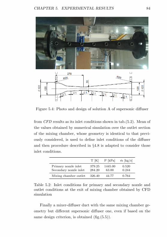
CHAPTER 5. EXPERIMENTAL RESULTS 84
Figure 5.4: Photo and design of solution A of supersonic diffuser
from CFD results as its inlet conditions shown in tab.(5.2). Mean of
the values obtained by numerical simulation over the outlet section
of the mixing chamber, whose geometry is identical to that previ-
ously considered, is used to define inlet conditions of the diffuser
and then procedure described in §4.8 is adapted to consider those
inlet conditions.
T [K] P [kPa] m [kg/s]
Primary nozzle inlet 379.25 1445.00 0.520Secondary nozzle inlet 284.20 63.00 0.244
Mixing chamber outlet 326.40 44.77 0.764
Table 5.2: Inlet conditions for primary and secondary nozzle andoutlet conditions at the exit of mixing chamber obtained by CFDsimulation
Finally a mixer-diffuser duct with the same mixing chamber ge-
ometry but different supersonic diffuser one, even if based on the
same design criterion, is obtained (fig.(5.5)).
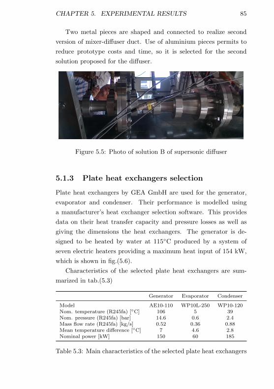
CHAPTER 5. EXPERIMENTAL RESULTS 85
Two metal pieces are shaped and connected to realize second
version of mixer-diffuser duct. Use of aluminium pieces permits to
reduce prototype costs and time, so it is selected for the second
solution proposed for the diffuser.
Figure 5.5: Photo of solution B of supersonic diffuser
5.1.3 Plate heat exchangers selection
Plate heat exchangers by GEA GmbH are used for the generator,
evaporator and condenser. Their performance is modelled using
a manufacturer’s heat exchanger selection software. This provides
data on their heat transfer capacity and pressure losses as well as
giving the dimensions the heat exchangers. The generator is de-
signed to be heated by water at 115C produced by a system of
seven electric heaters providing a maximum heat input of 154 kW,
which is shown in fig.(5.6).
Characteristics of the selected plate heat exchangers are sum-
marized in tab.(5.3)
Generator Evaporator Condenser
Model AE10-110 WP10L-250 WP10-120Nom. temperature (R245fa) [C] 106 5 39Nom. pressure (R245fa) [bar] 14.6 0.6 2.4Mass flow rate (R245fa) [kg/s] 0.52 0.36 0.88Mean temperature difference [C] 7 4.6 2.8Nominal power [kW] 150 60 185
Table 5.3: Main characteristics of the selected plate heat exchangers
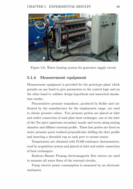
CHAPTER 5. EXPERIMENTAL RESULTS 86
Figure 5.6: Water heating system for generator supply circuit
5.1.4 Measurement equipment
Measurement equipment is provided for the prototype plant which
permits on one hand to give parameters to the control logic and on
the other hand to validate design hypothesis and numerical simula-
tion results.
Piezoresistive pressure transducer, produced by Keller and cal-
ibrated by the manufacturer for the employment range, are used
to obtain pressure values. Two pressure probes are placed at inlet
and outlet connection of each plate heat exchanger, one at the inlet
of the Tee piece upstream secondary nozzle and seven along mixing
chamber and diffuser external profile. These last probes are fixed on
static pressure ports realized perpendicular drilling the duct profile
and inserting a threaded cup at each port to mount sensor.
Temperature are obtained with Pt100 resistance thermometers,
read by acquisition system and placed at inlet and outlet connection
of heat exchangers.
Endress+Hauser Promag electromagnetic flow meters are used
to measure all water flows of the external circuits.
Pump electric power consumption is measured by an electronic
wattmeter.
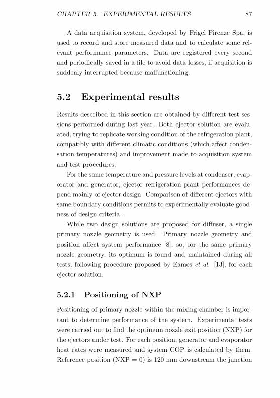
CHAPTER 5. EXPERIMENTAL RESULTS 87
A data acquisition system, developed by Frigel Firenze Spa, is
used to record and store measured data and to calculate some rel-
evant performance parameters. Data are registered every second
and periodically saved in a file to avoid data losses, if acquisition is
suddenly interrupted because malfunctioning.
5.2 Experimental results
Results described in this section are obtained by different test ses-
sions performed during last year. Both ejector solution are evalu-
ated, trying to replicate working condition of the refrigeration plant,
compatibly with different climatic conditions (which affect conden-
sation temperatures) and improvement made to acquisition system
and test procedures.
For the same temperature and pressure levels at condenser, evap-
orator and generator, ejector refrigeration plant performances de-
pend mainly of ejector design. Comparison of different ejectors with
same boundary conditions permits to experimentally evaluate good-
ness of design criteria.
While two design solutions are proposed for diffuser, a single
primary nozzle geometry is used. Primary nozzle geometry and
position affect system performance [8], so, for the same primary
nozzle geometry, its optimum is found and maintained during all
tests, following procedure proposed by Eames et al. [13], for each
ejector solution.
5.2.1 Positioning of NXP
Positioning of primary nozzle within the mixing chamber is impor-
tant to determine performance of the system. Experimental tests
were carried out to find the optimum nozzle exit position (NXP) for
the ejectors under test. For each position, generator and evaporator
heat rates were measured and system COP is calculated by them.
Reference position (NXP = 0) is 120 mm downstream the junction
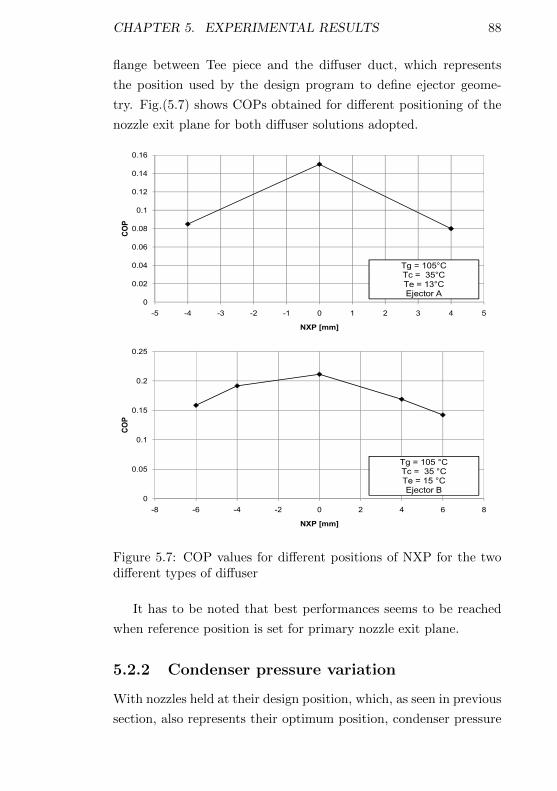
CHAPTER 5. EXPERIMENTAL RESULTS 88
flange between Tee piece and the diffuser duct, which represents
the position used by the design program to define ejector geome-
try. Fig.(5.7) shows COPs obtained for different positioning of the
nozzle exit plane for both diffuser solutions adopted.
0.08
0.1
0.12
0.14
0.16
CO
P
0
0.02
0.04
0.06
0.08
-5 -4 -3 -2 -1 0 1 2 3 4 5
CO
P
NXP [mm]
Tg = 105°CTc = 35°CTe = 13°CEjector A
0.15
0.2
0.25
CO
P
0
0.05
0.1
-8 -6 -4 -2 0 2 4 6 8
CO
P
NXP [mm]
Tg = 105 °CTc = 35 °CTe = 15 °CEjector B
Figure 5.7: COP values for different positions of NXP for the twodifferent types of diffuser
It has to be noted that best performances seems to be reached
when reference position is set for primary nozzle exit plane.
5.2.2 Condenser pressure variation
With nozzles held at their design position, which, as seen in previous
section, also represents their optimum position, condenser pressure
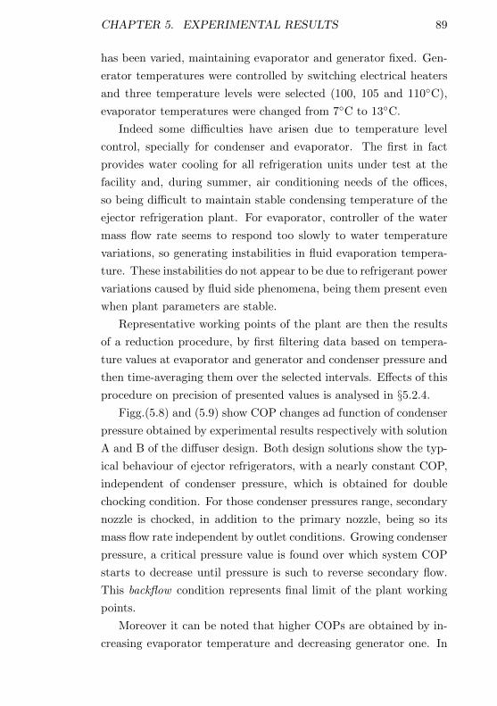
CHAPTER 5. EXPERIMENTAL RESULTS 89
has been varied, maintaining evaporator and generator fixed. Gen-
erator temperatures were controlled by switching electrical heaters
and three temperature levels were selected (100, 105 and 110C),
evaporator temperatures were changed from 7C to 13C.
Indeed some difficulties have arisen due to temperature level
control, specially for condenser and evaporator. The first in fact
provides water cooling for all refrigeration units under test at the
facility and, during summer, air conditioning needs of the offices,
so being difficult to maintain stable condensing temperature of the
ejector refrigeration plant. For evaporator, controller of the water
mass flow rate seems to respond too slowly to water temperature
variations, so generating instabilities in fluid evaporation tempera-
ture. These instabilities do not appear to be due to refrigerant power
variations caused by fluid side phenomena, being them present even
when plant parameters are stable.
Representative working points of the plant are then the results
of a reduction procedure, by first filtering data based on tempera-
ture values at evaporator and generator and condenser pressure and
then time-averaging them over the selected intervals. Effects of this
procedure on precision of presented values is analysed in §5.2.4.
Figg.(5.8) and (5.9) show COP changes ad function of condenser
pressure obtained by experimental results respectively with solution
A and B of the diffuser design. Both design solutions show the typ-
ical behaviour of ejector refrigerators, with a nearly constant COP,
independent of condenser pressure, which is obtained for double
chocking condition. For those condenser pressures range, secondary
nozzle is chocked, in addition to the primary nozzle, being so its
mass flow rate independent by outlet conditions. Growing condenser
pressure, a critical pressure value is found over which system COP
starts to decrease until pressure is such to reverse secondary flow.
This backflow condition represents final limit of the plant working
points.
Moreover it can be noted that higher COPs are obtained by in-
creasing evaporator temperature and decreasing generator one. In
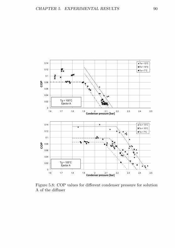
CHAPTER 5. EXPERIMENTAL RESULTS 90
0.1
0.12
0.14 Te = 13°C
Te = 10°C
Te = 7°C
0
0.02
0.04
0.06
0.08
1.6 1.7 1.8 1.9 2 2.1 2.2 2.3 2.4 2.5
COP
Condenser pressure [bar]
Tg = 100°CEjector A
0.1
0.12
0.14 Te = 13°C
Te = 10°C
Te = 7°C
0
0.02
0.04
0.06
0.08
1.6 1.7 1.8 1.9 2 2.1 2.2 2.3 2.4 2.5
COP
Condenser pressure [bar]
Tg = 105°CEjector A
Figure 5.8: COP values for different condenser pressure for solutionA of the diffuser
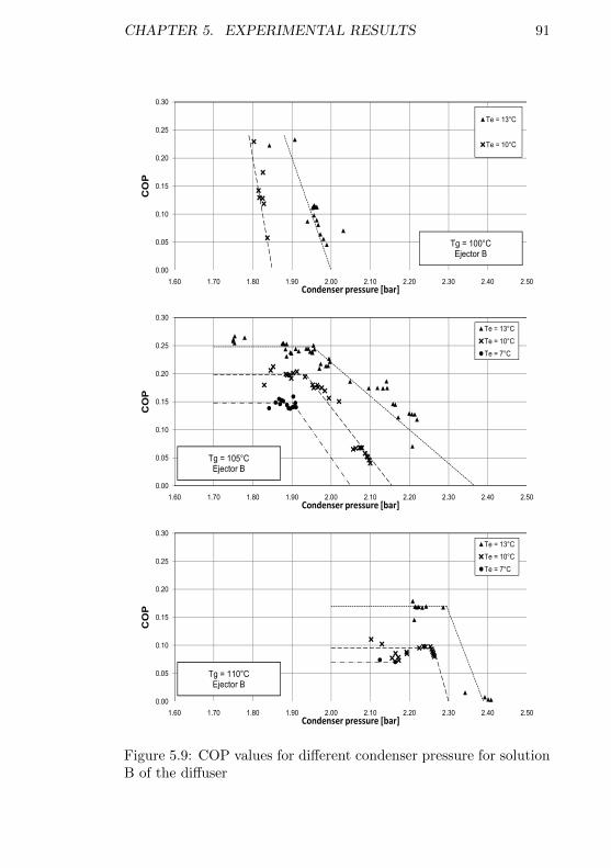
CHAPTER 5. EXPERIMENTAL RESULTS 91
0.20
0.25
0.30
Te = 13°C
Te = 10°C
0.00
0.05
0.10
0.15
1.60 1.70 1.80 1.90 2.00 2.10 2.20 2.30 2.40 2.50
COP
Condenser pressure [bar]
Tg = 100°CEjector B
0.20
0.25
0.30
Te = 13°C
Te = 10°C
Te = 7°C
0.00
0.05
0.10
0.15
1.60 1.70 1.80 1.90 2.00 2.10 2.20 2.30 2.40 2.50
COP
Condenser pressure [bar]
Tg = 105°CEjector B
0.20
0.25
0.30
Te = 13°C
Te = 10°C
Te = 7°C
0.00
0.05
0.10
0.15
1.60 1.70 1.80 1.90 2.00 2.10 2.20 2.30 2.40 2.50
COP
Condenser pressure [bar]
Tg = 110°CEjector B
Figure 5.9: COP values for different condenser pressure for solutionB of the diffuser
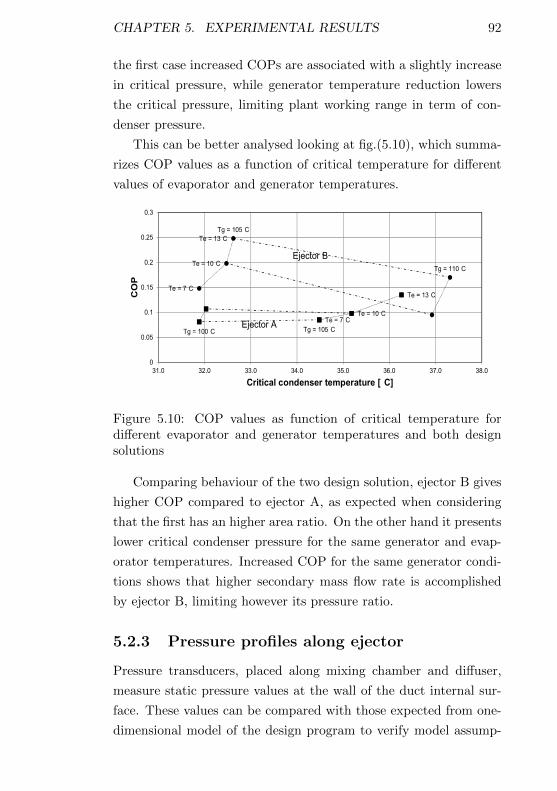
CHAPTER 5. EXPERIMENTAL RESULTS 92
the first case increased COPs are associated with a slightly increase
in critical pressure, while generator temperature reduction lowers
the critical pressure, limiting plant working range in term of con-
denser pressure.
This can be better analysed looking at fig.(5.10), which summa-
rizes COP values as a function of critical temperature for different
values of evaporator and generator temperatures.
Tg = 110 C
Tg = 105 CTe = 13 C
Te = 10 C
Te = 7 C
Tg = 100 C Tg = 105 C
Te = 13 C
Te = 10 CTe = 7 C
0
0.05
0.1
0.15
0.2
0.25
0.3
31.0 32.0 33.0 34.0 35.0 36.0 37.0 38.0
CO
P
Critical condenser temperature [ C]
Ejector A
Ejector B
Figure 5.10: COP values as function of critical temperature fordifferent evaporator and generator temperatures and both designsolutions
Comparing behaviour of the two design solution, ejector B gives
higher COP compared to ejector A, as expected when considering
that the first has an higher area ratio. On the other hand it presents
lower critical condenser pressure for the same generator and evap-
orator temperatures. Increased COP for the same generator condi-
tions shows that higher secondary mass flow rate is accomplished
by ejector B, limiting however its pressure ratio.
5.2.3 Pressure profiles along ejector
Pressure transducers, placed along mixing chamber and diffuser,
measure static pressure values at the wall of the duct internal sur-
face. These values can be compared with those expected from one-
dimensional model of the design program to verify model assump-
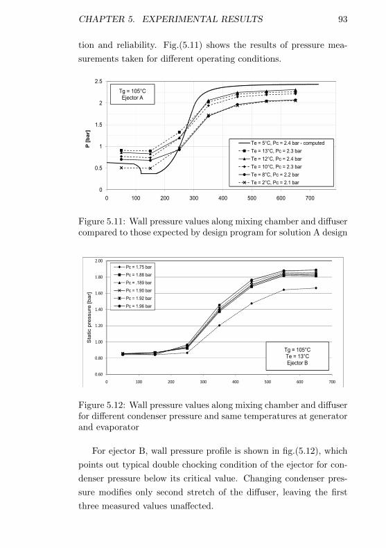
CHAPTER 5. EXPERIMENTAL RESULTS 93
tion and reliability. Fig.(5.11) shows the results of pressure mea-
surements taken for different operating conditions.
1.5
2
2.5
Tg = 105°CEjector A
0
0.5
1
1.5
0 100 200 300 400 500 600 700
P [
ba
r]
Te = 5°C, Pc = 2.4 bar - computed
Te = 13°C, Pc = 2.3 bar
Te = 12°C, Pc = 2.4 bar
Te = 10°C, Pc = 2.3 bar
Te = 8°C, Pc = 2.2 bar
Te = 2°C, Pc = 2.1 bar
Figure 5.11: Wall pressure values along mixing chamber and diffusercompared to those expected by design program for solution A design
1.40
1.60
1.80
2.00
Sta
tic p
ress
ure
[b
ar]
Pc = 1.75 bar
Pc = 1.88 bar
Pc = .189 bar
Pc = 1.90 bar
Pc = 1.92 bar
Pc = 1.96 bar
0.60
0.80
1.00
1.20
1.40
0 100 200 300 400 500 600 700
Sta
tic p
ress
ure
[b
ar]
Pc = 1.96 bar
Tg = 105°CTe = 13°CEjector B
Figure 5.12: Wall pressure values along mixing chamber and diffuserfor different condenser pressure and same temperatures at generatorand evaporator
For ejector B, wall pressure profile is shown in fig.(5.12), which
points out typical double chocking condition of the ejector for con-
denser pressure below its critical value. Changing condenser pres-
sure modifies only second stretch of the diffuser, leaving the first
three measured values unaffected.
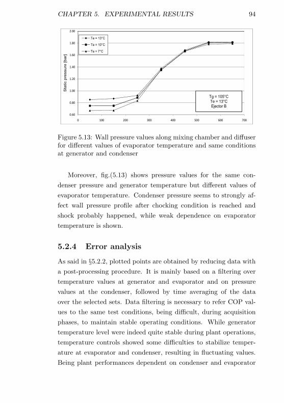
CHAPTER 5. EXPERIMENTAL RESULTS 94
1.40
1.60
1.80
2.00
Sta
tic p
ress
ure
[b
ar]
Te = 13°C
Te = 10°C
Te = 7°C
0.60
0.80
1.00
1.20
1.40
0 100 200 300 400 500 600 700
Sta
tic p
ress
ure
[b
ar]
Tg = 105°CPc = 1.88 bar
Ejector B
Tg = 105°CTe = 13°CEjector B
Figure 5.13: Wall pressure values along mixing chamber and diffuserfor different values of evaporator temperature and same conditionsat generator and condenser
Moreover, fig.(5.13) shows pressure values for the same con-
denser pressure and generator temperature but different values of
evaporator temperature. Condenser pressure seems to strongly af-
fect wall pressure profile after chocking condition is reached and
shock probably happened, while weak dependence on evaporator
temperature is shown.
5.2.4 Error analysis
As said in §5.2.2, plotted points are obtained by reducing data with
a post-processing procedure. It is mainly based on a filtering over
temperature values at generator and evaporator and on pressure
values at the condenser, followed by time averaging of the data
over the selected sets. Data filtering is necessary to refer COP val-
ues to the same test conditions, being difficult, during acquisition
phases, to maintain stable operating conditions. While generator
temperature level were indeed quite stable during plant operations,
temperature controls showed some difficulties to stabilize temper-
ature at evaporator and condenser, resulting in fluctuating values.
Being plant performances dependent on condenser and evaporator
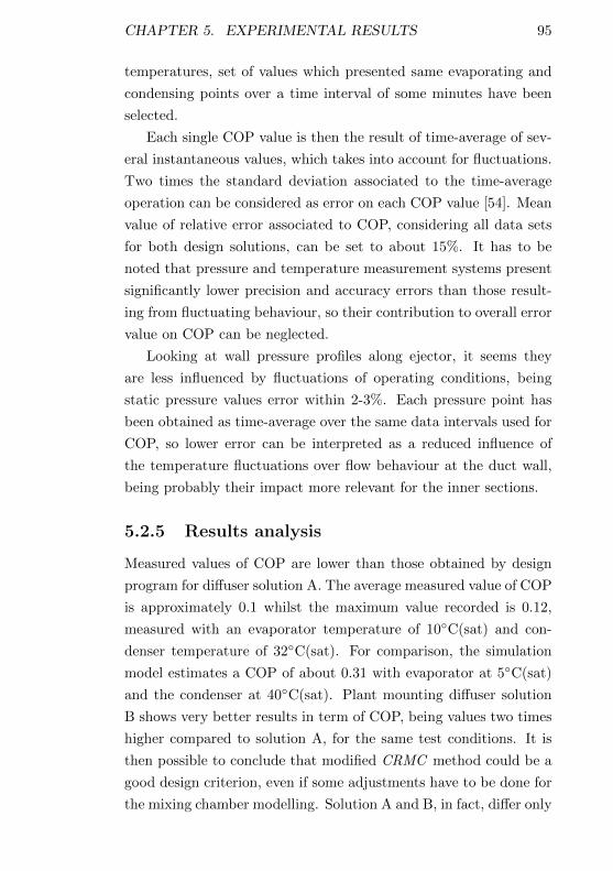
CHAPTER 5. EXPERIMENTAL RESULTS 95
temperatures, set of values which presented same evaporating and
condensing points over a time interval of some minutes have been
selected.
Each single COP value is then the result of time-average of sev-
eral instantaneous values, which takes into account for fluctuations.
Two times the standard deviation associated to the time-average
operation can be considered as error on each COP value [54]. Mean
value of relative error associated to COP, considering all data sets
for both design solutions, can be set to about 15%. It has to be
noted that pressure and temperature measurement systems present
significantly lower precision and accuracy errors than those result-
ing from fluctuating behaviour, so their contribution to overall error
value on COP can be neglected.
Looking at wall pressure profiles along ejector, it seems they
are less influenced by fluctuations of operating conditions, being
static pressure values error within 2-3%. Each pressure point has
been obtained as time-average over the same data intervals used for
COP, so lower error can be interpreted as a reduced influence of
the temperature fluctuations over flow behaviour at the duct wall,
being probably their impact more relevant for the inner sections.
5.2.5 Results analysis
Measured values of COP are lower than those obtained by design
program for diffuser solution A. The average measured value of COP
is approximately 0.1 whilst the maximum value recorded is 0.12,
measured with an evaporator temperature of 10C(sat) and con-
denser temperature of 32C(sat). For comparison, the simulation
model estimates a COP of about 0.31 with evaporator at 5C(sat)
and the condenser at 40C(sat). Plant mounting diffuser solution
B shows very better results in term of COP, being values two times
higher compared to solution A, for the same test conditions. It is
then possible to conclude that modified CRMC method could be a
good design criterion, even if some adjustments have to be done for
the mixing chamber modelling. Solution A and B, in fact, differ only
CHAPTER 5. EXPERIMENTAL RESULTS 96
for diffuser inlet conditions that are obtained as outlet conditions
of the mixing stretch by one-dimensional model and CFD results
respectively.
Looking at fig.(5.11), it seems that model used in design pro-
gram gives too rapid pressure increase. Moreover pressure in mix-
ing chamber is assumed to reach lower values than measured ones,
being not considered oblique shocks starting from primary nozzle
exit plane. Probably more complex modelling technique may be
required to better match measured pressures and to obtain better
agreement with COP values.
Because of the rapid variation in the chilled water temperature
difference across the evaporator, precise evaluation of COP is dif-
ficult. This problem is thought to result from the large thermal
inertia of the evaporator and the responsiveness of the chilled water
flow control system. Although time-averaged measurements helped
to smooth the data and gave more stable results COP data are still
quite scattered.
The prototype refrigerator was shown to operate stably over a
range of operating conditions. The minimum suction and maximum
condenser pressures and temperatures achieved are acceptable to the
proposed application. Feed pump behaviour is satisfactory, justify-
ing vertical arrangement.
Chapter 6
Conclusions
During present work, an optimization program based on a multivari-
ate approach is developed, which permits to define configuration of
a whole ejector refrigeration system including heat exchangers and
ejector. Program is capable to easily adapt to run with different
working fluids, being properties computed with NIST REFPROP
libraries included in the code.
Ejector models are proposed to design mixing chamber with a
specific criterion and supersonic diffuser with a literature method
(CRMC ) modified introducing some innovative feature. Specifically,
friction is included in flow equations contributing to define diffuser
geometry itself.
Starting from program results and design models, two different
solutions for ejector have been developed and experimentally tested
in a prototype plant. An experimental ejector refrigeration system
has been, in fact, realized at the test facility set up in manufacturer
plant of Frigel Firenze Spa, which collaborates to system building
and measurement instrumentation placement and calibration. Sys-
tem nominal refrigerant power is 40 kW, which is considered ade-
quate for industrial temperature control application, but maximum
of about 30 kW has been achieved with one of the two ejector so-
lution mounted. The minimum suction and maximum condenser
97
CHAPTER 6. CONCLUSIONS 98
pressures and temperatures achieved are however acceptable to the
proposed application. The prototype refrigerator was shown to op-
erate stably over a range of operating conditions.
One-dimensional models seems to be promising instrument for
optimized development of ejection refrigeration plant. Many itera-
tions required by multivariate optimization algorithms need in fact
quite fast, but reliable ways to describe fluid behaviour through
ejector.
Possibility to realize an ejector refrigeration plant, whose size
is adequate to industrial application with a reasonable COP has
been pointed out. Based on results obtained by this prototype, the
development of a pilot plant can start and numerical simulation of
the component validated.
Finally, some limits of the proposed models have been identified
from the point of view of foreseen, compared to real behaviour of
the ejector and of the evaluation of system performance. Starting
from those limits some strategies have been recognized to improve
models themselves.
Acknowledgements
Author wishes to thank Prof. Ian Eames of the University of Not-
tingham for his suggestions during ejector model definition and ex-
perimental tests organization.
Frigel Firenze Spa made prototype realization possible provid-
ing components, skills in plant assembly and control and test facility
availability. Moreover, collaboration of Ing. Michele Livi and Ing.
Filippo Malvolti was valuable during plant development and exper-
imental data collection.
Author wishes to thank, for collaboration and results of CFD
analysis produced, Ing. Simone Salvadori and Prof. Francesco
Martelli.
Finally special thanks go to Prof. Giuseppe Grazzini and Ing.
Adriano Milazzo for their suggestions and fruitful collaboration.
The prototype has been partly funded by Regione Toscana.
99
Bibliography
[1] J.M. Abdulateef, K. Sopian, M.A. Alghoul, and M.Y. Su-
laiman. Review on solar-driven ejector refrigeration technolo-
gies. Renewable and Sustainable Energy Reviews, 13(6–7):1338–
1349, 2009.
[2] S. Aphornratana and I.W. Eames. A small capacity steam-
ejector refrigerator: experimental investigation of a system us-
ing ejector with movable primary nozzle. International Journal
of Refrigeration, 20(5):352–358, 1997.
[3] Y. Bartosiewicz, Z. Aidoun, and Y. Mercadier. Numerical
assessment of ejector operation for refrigeration applications
based on cfd. Applied Thermal Engineering, 26(5–6):604–612,
2006.
[4] E. W. Beans. Computer solution to generalized one-
dimensional flow. Journal of Spacecraft and Rockets,
7(12):1460–1464, 2009.
[5] L. Boumaraf and A. Lallemand. Modeling of an ejector refrig-
erating system operating in dimensioning and off-dimensioning
conditions with the working fluids r142b and r600a. Applied
Thermal Engineering, 29(2–3):265–274, 2009.
[6] M.J. Box. A new method of constrained optimization and
a comparison with other methods. The Computer Journal,
8(1):42–52, 1965.
100

BIBLIOGRAPHY 101
[7] K. Chunnanond and S. Aphornratana. Ejectors: applications
in refrigeration technology. Renewable and Sustainable Energy
Reviews, 8(2):129–155, 2004.
[8] K. Chunnanond and S. Aphornratana. An experimental in-
vestigation of a steam ejector refrigerator: the analysis of the
pressure profile along the ejector. Applied Thermal Engineer-
ing, 24(2-3):311–322, 2004.
[9] K. Cizungu, A. Mani, and M. Groll. Performance comparison
of vapour jet refrigeration system with environment friendly
working fluids. Applied Thermal Engineering, 21(5):585–598,
2001.
[10] S. L. Dixon. Fluid mechanics and thermodynamics of turboma-
chinery. Butterworth-Heinemann, 1998.
[11] R. Dorantes and A. Lallemand. Prediction of performance of
a jet cooling system operating with pure refrigerants or non-
azeotropic mixtures. International Journal of Refrigeration,
18(1):21–30, 1995.
[12] I.W. Eames. A new prescription for the design of supersonic
jet-pumps: the constant rate of momentum change method.
Applied Thermal Engineering, 22(2):121–131, 2002.
[13] I.W. Eames, A.E. Ablwaifa, and V. Petrenko. Results of an ex-
perimental study of an advanced jet-pump refrigerator operat-
ing with r245fa. Applied Thermal Engineering, 27(17-18):2833–
2840, 2007.
[14] I.W. Eames, S. Aphornratana, and H. Haider. A theoretical
and experimental study of a small-scale steam jet refrigerator.
International Journal of Refrigeration, 18(6):378–386, 1995.
[15] I.W. Eames, S. Aphornratana, and D.-W. Sun. The jet-pump
cycle — a low cost refrigerator option powered by waste heat.
Heat Recovery Systems and CHP, 15(8):711–721, 1995.
BIBLIOGRAPHY 102
[16] Hisham El-Dessouky, Hisham Ettouney, Imad Alatiqi, and
Ghada Al-Nuwaibit. Evaluation of steam jet ejectors. Chem-
ical Engineering and Processing: Process Intensification,
41(6):551–561, 2002.
[17] J. Fischer. On ejector technology. International Journal of
Refrigeration, (In press).
[18] G. Flugel. The design of jet pumps. NACA Technical Memo-
randum 982, 1941.
[19] I.E. Frank and R. Todeschini. The data analysis handbook.
Elsiever, 1994.
[20] G. Grazzini. Ottimizzazione termodinamica di frigoriferi.
Pitagora Editrice Bologna, 1999.
[21] G. Grazzini and A. Mariani. A simple program to design a
multi-stage jet-pump for refrigeration cycles. Energy Conver-
sion and Management, 39(16–18):1827–1834, 1998.
[22] G. Grazzini, A. Milazzo, and D. Paganini. Design of an ejector
cycle refrigeration system. Energy Conversion and Manage-
ment, 54(1):38–46, 2012.
[23] G. Grazzini, A. Milazzo, and S. Piazzini. Prediction of conden-
sation in steam ejector for a refrigeration system. International
Journal of Refrigeration, 34(7):1641–1648, 2011.
[24] G. Grazzini, S. Piazzini, and A. Rocchetti. Confronto e verifica
di correlazioni per il dimensionamento di uno scambiatore a
piastre. In XXV Congresso Nazionale UIT sulla Trasmissione
del Calore, Trieste, 2007.
[25] G. Grazzini, S. Piazzini, and A. Rocchetti. Progetto ottimiz-
zato di un impianto frigorifero ad eiezione. In XXV Congresso
Nazionale UIT sulla Trasmissione del Calore, Trieste, 2007.
BIBLIOGRAPHY 103
[26] G. Grazzini and A. Rocchetti. Influence of the objective func-
tion on the optimisation of a steam ejector cycle. International
Journal of Refrigeration, 31(3):510–515, 2008.
[27] E.A. Groll. Ejector technology. International Journal of Re-
frigeration, 34(7):1543–1544, 2011.
[28] S. He, Y. Li, and R.Z. Wang. Progress of mathematical mod-
eling on ejectors. Renewable and Sustainable Energy Reviews,
13(8):1760–1780, 2009.
[29] A. Hemidi, F. Henry, S. Leclaire, J.-M. Seynhaeve, and Y. Bar-
tosiewicz. Cfd analysis of a supersonic air ejector. part i: Ex-
perimental validation of single-phase and two-phase operation.
Applied Thermal Engineering, 29(8–9):1523–1531, 2009.
[30] A. Hemidi, F. Henry, S. Leclaire, J.-M. Seynhaeve, and Y. Bar-
tosiewicz. Cfd analysis of a supersonic air ejector. part ii: Rela-
tion between global operation and local flow features. Applied
Thermal Engineering, 29(14–15):2990–2998, 2009.
[31] B. K. Hodge and K. Koenig. Compressible fluid dynamics with
personal computer applications. Prentice Hall, 1995.
[32] B.J. Huang, J.M. Chang, C.P. Wang, and V.A. Petrenko. A
1-d analysis of ejector performance. International Journal of
Refrigeration, 22(5):354–364, 1999.
[33] S. Kakac and H liu. Heat exchangers : selection, rating, and
thermal design. CRC Press, 1998.
[34] W. M. Kays and A. L. London. Compact heat exchangers.
McGraw-Hill, 1984.
[35] J.H. Keenan and E.P. Neumann. A simple air ejector. ASME
Journal of Applied Mechanics Translation, 64:A75–84, 1942.
[36] J.H. Keenan, E.P. Neumann, and F. Lustwerk. An investigation
of ejector design by analysis and experiment. ASME Journal
of Applied Mechanics Translation, 72:299–309, 1950.
BIBLIOGRAPHY 104
[37] S.A. Klein and A.H. Harvey. NIST Standard Reference
Database 10: NIST/ASME Steam Properties. National Insti-
tute of Standards and Technology, Standard Reference Data
Program, 2.0 edition, 1996.
[38] E.W. Lemmon, M.L. Huber, and M.O. McLinden. NIST Stan-
dard Reference Database 23: Reference Fluid Thermodynamic
and Transport Properties - REFPROP. National Institute of
Standards and Technology, Standard Reference Data Program,
8.0 edition, 2008.
[39] D.G. Luenberger. Linear and nonlinear programming. Addison-
Wesley Publishing Company, 1984.
[40] J. T. Munday and D. F. Bagster. A new ejector theory applied
to steam jet refrigeration. Industrial and Engineering Chem-
istry Process Design and Development, 16(4):442–449, 1977.
[41] E. Nehdi, L. Kairouani, and M. Elakhdar. A solar ejector air-
conditioning system using environment-friendly working fluids.
International Journal of Energy Research, 32(13):1194–1201,
2008.
[42] M. Ouzzane and Z. Aidoun. Model development and numeri-
cal procedure for detailed ejector analysis and design. Applied
Thermal Engineering, 23(18):2337–2351, 2003.
[43] V. O. Petrenko. Application of innovative ejector chillers
and air conditioners operating with low boiling refrigerants in
trigeneration systems. International Seminar on ejector/jet-
pump technology and application, Louvain-la-Neuve, Belgium,
September 7–9, 2009.
[44] K. Pianthong, W. Seehanam, M. Behnia, T. Sriveerakul, and
S. Aphornratana. Investigation and improvement of ejector
refrigeration system using computational fluid dynamics tech-
nique. Energy Conversion and Management, 48(9):2556–2564,
2007.
BIBLIOGRAPHY 105
[45] C. Pollerberg, A.H.H. Ali, and C. Dotsch. Experimental study
on the performance of a solar driven steam jet ejector chiller.
Energy Conversion and Management, 49(11):3318–3325, 2008.
[46] W. H. Press, B. P. Flanney, S. A. Teukolsky, and W. T. Vet-
terling. Numerical recipes - The art of scientific computing.
Cambridge University Press, 1986.
[47] E.D. Rogdakis and G.K. Alexis. Investigation of ejector de-
sign at optimum operating condition. Energy Conversion and
Management, 41(17):1841–1849, 2000.
[48] E. Rusly, L. Aye, W.W.S. Charters, and A. Ooi. Cfd analysis
of ejector in a combined ejector cooling system. International
Journal of Refrigeration, 28(7):1092–1101, 2005.
[49] A. Selvaraju and A. Mani. Analysis of an ejector with envi-
ronment friendly refrigerants. Applied Thermal Engineering,
24(5–6):827–838, 2004.
[50] T. K. Serghides. Estimate friction factor accurately. Chemical
Engineer Journal, 91:63–64, 1984.
[51] A.H. Shapiro. The dynamics and thermodynamics of compress-
ible fluid flow. John Wiley and Sons, 1953.
[52] W. Spendley, G.R. Hext, and F.R. Himsworth. Sequential ap-
plication of simplex designs in optimisation and evolutionary
operation. Technometrics, 4(4):441–461, 1962.
[53] Da-Wen Sun. Comparative study of the performance of an
ejector refrigeration cycle operating with various refrigerants.
Energy Conversion and Management, 40(8):873–884, 1999.
[54] J. R. Taylor. An Introduction to Error Analysis: The Study
of Uncertainties in Physical Measurements. University Science
Books, 1997.
BIBLIOGRAPHY 106
[55] S. Varga, A. C. Oliveira, and B. Diaconu. Numerical assessment
of steam ejector efficiencies using cfd. International Journal of
Refrigeration, 32(6):1203–1211, 2009.
[56] Z.-Z. Wang and Z.-N. Zhao. Analysis of performance of steam
condensation heat transfer and pressure drop in plate con-
densers. International Journal of Heat and Mass Transfer,
14(4):32–41, 1993.
[57] Y.-Y. Yan and T.-F. Lin. Evaporation heat transfer and pres-
sure drop of refrigerant r-134a in a plate heat exchanger. Jour-
nal of Heat Transfer, 121(1):118–127, 1999.
[58] Y.-Y. Yan, H.-C. Lio, and T.-F. Lin. Condensation heat trans-
fer and pressure drop of refrigerant r-134a in a plate heat ex-
changer. International Journal of Heat and Mass Transfer,
42(6):993–1006, 1999.
[59] Y. Zhu, W. Cai, C. Wen, and Y. Li. Simplified ejector model
for control and optimization. Energy Conversion and Manage-
ment, 49(6):1424–1432, 2008.
[60] M. J. Zucrow and J. D. Hoffman. Gas dynamics. John Wiley
and Sons, 1976.
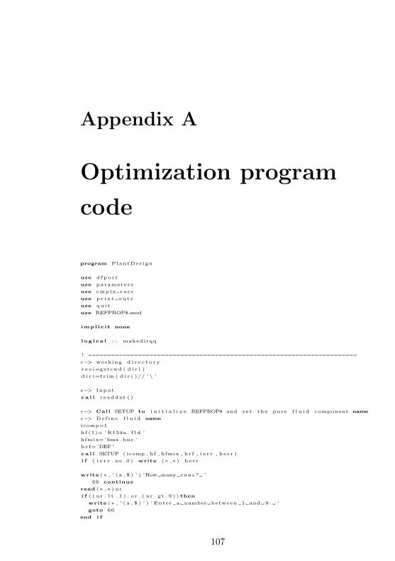
Appendix A
Optimization program
code
program PlantDesign
use dfport
use parameters
use cmplx vars
use p r i n t ou t s
use qu i t
use REFPROP8 mod
implic it none
log ica l : : makedirqq
! ======================================================================
c−> working d i r e c t o r y
r e s i=getcwd ( d i r i )
d i r i=trim ( d i r i )// ’\ ’
c−> Input
ca l l readdat ( )
c−> Call SETUP to i n i t i a l i z e REFPROP8 and se t the pure f l u i d component name
c−> Def ine f l u i d name
icomp=1
hf (1)= ’R134a . f l d ’
hfmix=’hmx. bnc ’
h r f=’DEF ’
ca l l SETUP ( icomp , hf , hfmix , hrf , i e r r , herr )
i f ( i e r r . ne . 0 ) write (∗ ,∗) herr
write (∗ , ’ ( a , $ ) ’ ) ’How many runs ? ’
66 continue
read (∗ ,∗) nr
i f ( ( nr . l t . 1 ) . or . ( nr . gt . 9 ) ) then
write (∗ , ’ ( a , $ ) ’ ) ’ Enter a number between 1 and 9 : ’
goto 66
end i f
107
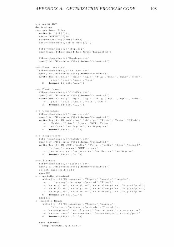
APPENDIX A. OPTIMIZATION PROGRAM CODE 108
c−> multi−RUN
do i r =1,nr
c−> ge s t i one f i l e s
write ( ic , ’ ( i 1 ) ’ ) i r
d i ro=’OUTPUT ’ // i c
r e s l=makedirqq ( trim ( d i ro ) )
d i ro=trim ( d i r i )// trim ( d i ro )// ’\ ’
f i l e=trim ( d i ro )// ’ sk ip . log ’
open ( logu , f i l e=trim ( f i l e ) , form=’ formatted ’ )
f i l e=trim ( d i ro )// ’Randoms . dat ’
open ( lrd , f i l e=trim ( f i l e ) , form=’ formatted ’ )
c−> Punti s c a r t a t i
f i l e=trim ( d i ro )// ’ Fa i lu r e . dat ’
open ( lko , f i l e=trim ( f i l e ) , form=’ formatted ’ )
write ( lko , 2 ) ’ nt g ’ , ’mg h ’ , ’ pg c ’ , ’ dt g ’ , ’mp 1 ’ , ’mp 2 ’ , ’ meis ’ ,
− ’ pe n ’ , ’ np c ’ , ’mc c ’ , ’ t c n ’
2 format (11( a10 , ’ ’ ) )
c−> Punti buoni
f i l e=trim ( d i ro )// ’ CplxPts . dat ’
open ( lok , f i l e=trim ( f i l e ) , form=’ formatted ’ )
write ( lok , 3 ) ’ nt g ’ , ’mg h ’ , ’ pg c ’ , ’ dt g ’ , ’mp 1 ’ , ’mp 2 ’ , ’ meis ’ ,
− ’ pe n ’ , ’ np c ’ , ’mc c ’ , ’ t c n ’ , ’C.O.P. ’
3 format (12( a10 , ’ ’ ) )
c−> Generatore
f i l e=trim ( d i ro )// ’ Generat . dat ’
open ( l sg , f i l e=trim ( f i l e ) , form=’ formatted ’ )
write ( l sg , 4 ) ’ IN : mh ’ , ’mc ’ , ’ ph ’ , ’ pc ’ , ’ Th in ’ , ’ Tc in ’ , ’DT sh ’ ,
− ’ Ntubi ’ , ’ D int ’ , ’ Spess ’ , ’OUT: Tc ou ’ ,
− ’∗∗ Q ∗∗ ’ , ’∗∗ D p ∗∗ ’ , ’∗∗ W pmp ∗∗ ’
4 format (14( a11 , ’ ’ ) )
c−> Evaporatore
f i l e=trim ( d i ro )// ’ FlashEv . dat ’
open ( lev , f i l e=trim ( f i l e ) , form=’ formatted ’ )
write ( lev , 5 ) ’ IN : Wf ’ , ’ m l in ’ , ’ T l in ’ , ’ p l i n ’ , ’ Loss ’ , ’ h cond ’ ,
− ’ p cond ’ , ’ p eva ’ , ’OUT: m eva ’ ,
− ’∗∗ m s v ∗∗ ’ , ’∗∗ m ev ∗∗ ’ , ’∗∗ Sup ∗∗ ’ , ’∗∗ W p ∗∗ ’
5 format (13( a11 , ’ ’ ) )
c−> Eie t t o r e
f i l e=trim ( d i ro )// ’ E jec tor . dat ’
open ( l e j , f i l e=trim ( f i l e ) , form=’ formatted ’ )
se lect case ( e j f l a g 1 )
case (0)
c − modello standard
write ( l e j , 6 ) ’ IN : p gen ’ , ’ T gen ’ , ’ m g 1 ’ , ’ m g 2 ’ ,
− ’ p evap ’ , ’m evap ’ , ’ p cond ’ , ’ T cond ’ ,
− ’∗∗ m p1 ∗∗ ’ , ’∗∗ A g1 ∗∗ ’ , ’∗∗ m s1/m p1 ∗∗ ’ , ’∗ p o1/ p s1 ’ ,
− ’∗∗ m p2 ∗∗ ’ , ’∗∗ A g2 ∗∗ ’ , ’∗∗ m s2/m p2 ∗∗ ’ , ’∗ p o2/ p s2 ’ ,
− ’∗∗ m p ∗∗ ’ , ’∗∗ A ex ∗∗ ’ , ’∗∗ m ev/m p ∗∗ ’ , ’∗ p ex /p ev ’
6 format (20( a11 , ’ ’ ) )
case (1)
c− modello Eames
write ( l e j , 8 ) ’ IN : p gen ’ , ’ T gen ’ , ’m gen ’ ,
− ’ p evap ’ , ’m evap ’ , ’ p cond ’ , ’ T cond ’ ,
− ’∗∗ m p ∗∗ ’ , ’∗∗ A g ∗∗ ’ , ’∗∗ m s ∗∗ ’ , ’∗ p ex ∗ ’ ,
− ’∗∗ m t ∗∗ ’ , ’∗∗ A ex ∗∗ ’ , ’∗ m s/m p ∗ ’ , ’∗ p ex / p i ’
8 format (15( a11 , ’ ’ ) )
case default
stop ’ERROR: e j f l a g 1 . ’
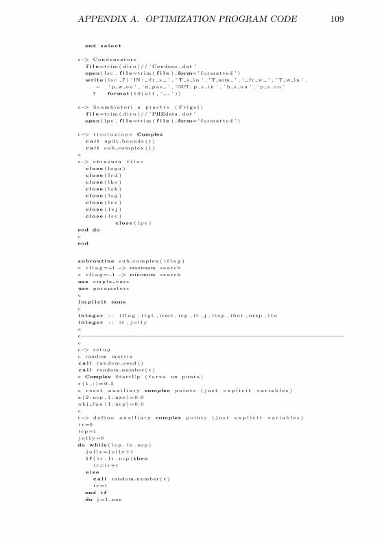
APPENDIX A. OPTIMIZATION PROGRAM CODE 109
end se lect
c−> Condensatore
f i l e=trim ( d i ro )// ’Condens . dat ’
open ( l s c , f i l e=trim ( f i l e ) , form=’ formatted ’ )
write ( l s c , 7 ) ’ IN : f r s ’ , ’ T s in ’ , ’T nom ’ , ’ f r w ’ , ’ T w in ’ ,
− ’ p w ou ’ , ’ n pas ’ , ’OUT: p s i n ’ , ’ h s ou ’ , ’ p s ou ’
7 format (10( a11 , ’ ’ ) )
c−> Scambiator i a p i a s t r e ( F r i g e l )
f i l e=trim ( d i ro )// ’PHEdata . dat ’
open ( lpe , f i l e=trim ( f i l e ) , form=’ formatted ’ )
c−> r i s o l u z i o n e Complex
ca l l updt bounds (1)
ca l l sub complex (1)
c
c−> ch iusura f i l e s
close ( logu )
close ( l r d )
close ( lko )
close ( lok )
close ( l s g )
close ( l ev )
close ( l e j )
close ( l s c )
close ( lpe )
end do
c
end
subroutine sub complex ( i f l a g )
c i f l a g=+1 −> maximum search
c i f l a g=−1 −> minimum search
use cmplx vars
use parameters
c
implic it none
c
integer : : i f l a g , i t g t , irmv , icp , i t , j , i top , ibot , nrep , i t e
integer : : i r , j o l l y
c
c−−−−−−−−−−−−−−−−−−−−−−−−−−−−−−−−−−−−−−−−−−−−−−−−−−−−−−−−−−−−−−−−−−−−−−−c
c−> setup
c random matrix
ca l l random seed ( )
ca l l random number ( r )
c Complex StartUp ( f o r zo un punto )
r (1 , : )=0 .5
c r e s e t aux i l i a r y complex po int s ( j u s t e x p l i c i t v a r i a b l e s )
x ( 2 : ncp , 1 : nxe )=0.0
ob j fun ( 1 : ncp )=0.0
c
c−> de f i n e aux i l i a r y complex po int s ( j u s t e x p l i c i t v a r i a b l e s )
i r=0
icp=1
j o l l y=0
do while ( i cp . l e . ncp )
j o l l y=j o l l y+1
i f ( i r . l t . ncp ) then
i r=i r+1
else
ca l l random number ( r )
i r=1
end i f
do j =1,nxe
APPENDIX A. OPTIMIZATION PROGRAM CODE 110
x( icp , j )=bound l ( j )+r ( i r , j )∗( bound u ( j )−bound l ( j ) )
end do
ca l l updt obj fun ( i cp )
i f ( ob j fun ( i cp ) . gt . 0 . 0 ) i cp=icp+1
end do
c
c
c−> main complex loop
c =================
i t=1
nrep=1
do while ( ( i t . l t . itmax ) . and . ( nrep . l e . mrep ) )
c f i nd point with h ighes t function value
i top=locmax ( ob j fun ( : ) , ncp )
c f i nd point with lowest function value
ibot=locmin ( ob j fun ( : ) , ncp )
c f i r s t convergency c r i t e r i o n
i f ( ob j fun ( i top)−ob j fun ( ibot ) . ge . eps ln ) nrep=0
nrep=nrep+1
c
i f ( nrep . l e . mrep ) then
c switch max/min search ( accord ing to i f l a g )
i t g t =((1+ i f l a g )∗ i t op+(1− i f l a g )∗ i bo t )/2
irmv=((1+ i f l a g )∗ i bo t+(1− i f l a g )∗ i t op )/2
c r ep l a c e the point with worst function value while i t i s worst
ca l l cent ro id ( irmv , ncp )
x ( irmv , 1 : nxe )=(1.0+ alpha )∗ xc ( 1 : nxe)−alpha∗x( irmv , 1 : nxe )
ca l l checkbounds ( irmv , ncp )
ca l l updt obj fun ( irmv )
i t e=1
do while ( ( l ocwors t ( i f l a g ) . eq . irmv ) . and . ( i t e . l e . 1 0 ) )
x ( irmv , 1 : nxe )=0.5∗( x ( irmv , 1 : nxe)+xc ( 1 : nxe ) )
ca l l checkbounds ( irmv , ncp )
ca l l updt obj fun ( irmv )
i t e=i t e+1
end do
i f ( l ocwors t ( i f l a g ) . eq . irmv ) then
x( irmv , 1 : nxe)=x( i t g t , 1 : nxe )
ob j fun ( irmv)=obj fun ( i t g t )−0.5∗ eps ln∗ f l o a t ( i f l a g )
end i f
end i f
i t=i t+1
end do
c
i t g t=locwors t (− i f l a g )
ca l l updt obj fun ( i t g t )
ca l l best output ( i t g t )
c
write (∗ ,∗)write (∗ ,∗)write (∗ ,∗) ’Done ! ’
c
return
end
subroutine cent ro id ( i sk ip , ipmax )
use cmplx vars
c
implic it none
c
integer : : i s k ip , ipmax
integer : : i , j
real div
c
c−−−−−−−−−−−−−−−−−−−−−−−−−−−−−−−−−−−−−−−−−−−−−−−−−−−−−−−−−−−−−−−−−−−−−−−c
div=1.0/ f l o a t ( ipmax−1)
APPENDIX A. OPTIMIZATION PROGRAM CODE 111
do j =1,nxe
xc ( j )=0.0
do i =1,ipmax
xc ( j )=xc ( j )+x( i , j )
end do
xc ( j )=(xc ( j )−x( i sk ip , j ) )∗ div
end do
c
return
end
subroutine updt obj fun ( i cp )
c
use d f l i b
use cmplx vars
use c y c l e v a r s
use parameters
use pt data s e t
use p r i n t ou t s
c
implic it none
c
integer : : i cp
l og ica l : : s c a r ta
c
! ======================================================================
c
c− setup
ob j fun ( i cp )=0.0
mg h= x( icp , 1)
pg c= x( icp , 2)
dt g= x( icp , 3)
mp 1= x( icp , 4)
meis= x( icp , 5)
te n= x( icp , 6)
mc c= x( icp , 7)
tc n= x( icp , 8)
np c=in t (x ( icp , 9 ) )
np e=in t (x ( icp , 1 0 ) )
np g=in t (x ( icp , 1 1 ) )
c
c− pr in tout s ( per debug )
cread ( lrd , 1 ) nt g , mg h , pg c , dt g , mp 1 ,mp 2 , meis , pe n , np c , mc c , t c n
write ( lrd , 1 ) nt g , mg h , pg c , dt g , mp 1 ,mp 2 , meis , pe n , np c , mc c , t c n
1 format ( i9 , ’ ’ , 7 ( e15 . 7 ) , i9 , ’ ’ , 2 ( e15 . 7 ) )
c
c− c a l c o l o componenti impianto completo
ca l l componenti ( s ca r ta )
i f ( s ca r ta ) then
c
write ( lko , 2 ) nt g , mg h , pg c , dt g , mp 1 ,mp 2 , meis , pe n , np c , mc c ,
− t c n
2 format ( i10 , ’ ’ , e13 . 3 , f13 . 1 , f13 . 2 , 3 e13 . 3 , f13 . 1 , i10 , ’ ’ ,
− e13 . 2 , f13 . 2 )
else
ob j fun ( i cp )=q f r g /( q gen+w gen+w eva+w phe+w pmp)
i f ( ob j fun ( i cp ) . eq . 0 . 0 ) then
pause
end i f
c
write ( lok , 3 ) nt g , mg h , pg c , dt g , mp 1 ,mp 2 , meis , pe n , np c , mc c ,
− tc n , ob j fun ( i cp )
3 format ( i10 , ’ ’ , e13 . 3 , f13 . 1 , f13 . 2 , 3 e13 . 3 , f13 . 1 , i10 , ’ ’ ,
− e13 . 2 , f13 . 2 , e13 . 3 )
c ca l l good output ( i cp )
c
APPENDIX A. OPTIMIZATION PROGRAM CODE 112
ca l l best output ( i cp ) ! o u t p u t c om p l e t o p e r i l b e s t−p t
end i f
c
return
end
subroutine checkbounds ( icp , icm )
use cmplx vars
c
implic it none
c
integer : : icp , icm , j
l og ica l : : r epeat
c
! ======================================================================
c
repeat=. true .
do while ( repeat )
do j =1,nxe
i f (x ( icp , j ) . l t . bound l ( j ) ) then
x( icp , j )=bound l ( j )+de l ta
else i f (x ( icp , j ) . gt . bound u ( j ) ) then
x( icp , j )=bound u ( j )−de l ta
end i f
end do
repeat=. f a l s e .
c
do j=nxe+1,nxt
i f ( ( x ( icp , j ) . l t . bound l ( j ) ) . or . ( x ( icp , j ) . gt . bound u ( j ) ) ) then
ca l l cent ro id ( icp , icm )
x ( icp , 1 : nxe )=0.5∗( x ( icp , 1 : nxe)+xc ( 1 : nxe ) )
repeat=. true .
end i f
end do
end do
c
return
end
subroutine componenti ( s ca r ta )
! ===============================================
c
use c y c l e v a r s
use parameters
use pt data s e t
use Gdat
use SCdat
use qu i t
use WSCall
use REFPROP8Call
use GEA mod
c
implic it none
c
real , parameter : : t o l l =1.0e−3
integer , parameter : : n i t=50
c
l og ica l : : s c a r ta
c
real : : mg c , hg ic
real : : tcou , dcou
real : : teou
c
real : : me ,mex , em
integer : : i t
c
real : : dum, dlth , dum2
APPENDIX A. OPTIMIZATION PROGRAM CODE 113
real : : tgam , pgam
c
c================================================
c
c−> s tar tup
sca r ta =. f a l s e .
sk ip=. f a l s e .
write (∗ ,∗)write ( logu ,∗ ) ’ ’
c
mg c=mp 1+mp 2
t g i c=tc n
c
tcou=tc n
ca l l REFRsatur t ( tcou , pcou , dcou ,dum)
hcou=REFRenth td ( tcou , dcou )
c
pcin=pcou
c
me=2.0e−3
em=1.0
i t=1
ca l l REFRsatur t ( te n , pe n ,dum,dum2)
c cod i ce di l e t t u r a de i dat i d a l l e t a b e l l e GEA ( l ’ equ iva l en t e cod i ce
c di l e t t u r a d e l l e v a r i a b i l i i nd ipendent i po s i z i ona to in sub complex )
c−> l e t t u r a dat i generatore
i f (GEAInputEna ( 3 ) . eq . 1 ) then
c a l l GenReadGEAPHE
wr i te (∗ , ’ ( a , $ ) ’ ) ’SG ’ // trim (GeaGen%PHEname)
w gen=(GeaGen%WaterTotPdrop ∗1.0 e+3)∗GeaGen%WaterFlowRate /1 .0 e+3
pg c=GeaGen%RefrPout ∗1.0 e+5 ! bar −> Pa
tgoc=GeaGen%RefrTout+273.15 ! degC −> K
mg c=GeaGen%RefrFlowRate
q gen=GeaGen%PHEpower∗1.0 e+3 ! kW −> W
i f ( sk ip ) then
s ca r ta =. true .
wr i te (∗ ,∗)return
end i f
wr i te (∗ , ’ ( a , $ ) ’ ) ’ . ’
end i f
c−> l e t t u r a dat i evaporatore
i f (GEAInputEna ( 1 ) . eq . 1 ) then
c a l l EvaReadGEAPHE
wr i te (∗ , ’ ( a , $ ) ’ ) ’EV ’ // trim (GeaEva%PHEname)
w eva=(GeaEva%WaterTotPdrop ∗1.0 e+3)∗GeaEva%WaterFlowRate /1 .0 e+3
pe n=GeaEva%RefrPout ∗1.0 e+5 ! bar −> Pa
me=GeaEva%RefrFlowRate
i f ( sk ip ) then
s ca r ta =. true .
wr i te (∗ ,∗)return
end i f
wr i te (∗ , ’ ( a , $ ) ’ ) ’ . ’
end i f
c−> l e t t u r a dat i condensatore
i f (GEAInputEna ( 3 ) . eq . 1 ) then
c a l l ConReadGEAPHE
wr i te (∗ , ’ ( a , $ ) ’ ) ’SC ’ // trim (GeaCon%PHEname)
w phe=(GeaCon%WaterTotPdrop ∗1.0 e+3)∗GeaCon%WaterFlowRate /1 .0 e+3
pcou=GeaCon%RefrPout ∗1.0 e+5 ! bar −> Pa
tcou=GeaCon%RefrTout+273.15 ! degC −> K
dcou=REFRdens tp ( tcou , pcou )
hcou=REFRenth td ( tcou , dcou )
i f (GeaCon%RefrTotPdrop . gt . 0 . 0 ) then
pcin=(GeaCon%RefrPout ∗1.0 e+5)+(GeaCon%RefrTotPdrop ∗1.0 e+3)
APPENDIX A. OPTIMIZATION PROGRAM CODE 114
e l s e
pcin=(GeaCon%RefrPout ∗1.0 e+5)
end i f
t c i n=GeaCon%RefrTin+273.15 ! degC −> K
i f ( sk ip ) then
s ca r ta =. true .
wr i te (∗ ,∗)return
end i f
wr i te (∗ , ’ ( a , $ ) ’ ) ’ . ’
end i f
c−> c a l c o l o di gamma e d e g l i a l t r i e sponent i i s e n t r o p i c i
tgam=(tgoc+tc i n )/2 . 0
pgam=(pg c+pcin )/2 . 0
REFRgam=REFRgamma tp( tgoc , pg c )
REFRgm1 g=(REFRgam−1.0)/REFRgam
REFRg gm1=REFRgam/(REFRgam−1.0)
c====> LOOP su l l a portata proven iente d a l l ’ evaporatore (me)
do while ( (em. gt . t o l l ) . and . ( i t . l e . n i t ) . and . ( . not . sk ip ) )
mex=me
i f ( i t . eq . 1 )mex=1.0
i f (GEAInputEna ( 3 ) . eq . 0 ) then
write (∗ , ’ ( a , $ ) ’ ) ’SG ’
! c a l l g e n e r a t o r e ( mg h , mg c , p g h , p g c , t g h i n , t g i c , d t g , n t g ,
! − d i n t , s p e s , t g o c )
ca l l GenPHE(mg h , mg c , p g h , pg c , tghin , tg i c , dt g , np g , ! hp , smp ,
& tgoc )
i f ( sk ip ) then
s ca r ta =. true .
write (∗ ,∗)return
end i f
write (∗ , ’ ( a , $ ) ’ ) ’ . ’
end i f
c
i f (GEAInputEna ( 1 ) . eq . 0 ) then
write (∗ , ’ ( a , $ ) ’ ) ’EV ’
! c a l l e v a p f ( q f r g , me i s , t e h i n , p e h , d p e i s , hcou , pcou , p e n , me )
ca l l EvaPHE(meis ,me , p e h , pe n , tehin , te n , hcou , 0 . 0 , np e , ! hp , smp ,
& teou )
i f ( sk ip ) then
s ca r ta =. true .
write (∗ ,∗)return
end i f
write (∗ , ’ ( a , $ ) ’ ) ’ . ’
end i f
c
c−> e i e t t o r e
write (∗ , ’ ( a , $ ) ’ ) ’EJ ’
se lect case ( e j f l a g 1 )
case (0)
ca l l e j 2 d e s i gn ( pg c , tgoc , mp 1 ,mp 2 , pe n ,me , pcin , t c i n )
case (1)
ca l l e j e de s i gn eames ( pg c , tgoc , mg c , pe n ,me , pcin , t c i n )
case default
stop ’ERROR: e j f l a g 1 ’
end se lect
i f ( sk ip ) then
s ca r ta =. true .
write (∗ ,∗)return
end i f
write (∗ , ’ ( a , $ ) ’ ) ’ . ’
APPENDIX A. OPTIMIZATION PROGRAM CODE 115
c
c =========================
i f (GEAInputEna ( 3 ) . eq . 0 ) then
mc h=mg c+me
write (∗ , ’ ( a , $ ) ’ ) ’SC ’
ca l l phe (mc h , tc in , tc n , mc c , tcwi , pcwo , np c , pcin , hcou , pcou )
i f ( sk ip ) then
s ca r ta =. true .
write (∗ ,∗)return
end i f
write (∗ , ’ ( a , $ ) ’ ) ’ . ’
end i f
c
dcou=REFRdens ph ( pcou , hcou )
d l th=(pg c−pcou )/ dcou
hgic=hcou+dlth
t g i c=REFRtemp ph( pg c , hg ic )
w pmp=mg c∗dlth
em=abs (1.0−me/mex)
i t=i t+1
end do
c
write (∗ ,∗) ’ OK. ’
c
return
end
subroutine Eje design Eames ( pgen , tgen ,mgen , peva ,meva , pcon , tcon )
c
use qu i t
use TFData
use REFPROP8Call
c
implic it none
c
integer , parameter : : i f l g =0
real , parameter : : p to l =0.5
c
real : : pgen , tgen ,mgen , peva ,meva , pcon , tcon
c
real : : px , rhux
real : : d0p , d0s ,dum
real : : dp , sp , ep , pl , pr ,pm
c
integer : : t e s t
c−> setup
p0p=pgen
t0p=tgen
mp1=mgen
mp2=0.0
p0s=peva
ms1=meva
c
d0p=REFRdens tp ( t0p , p0p )
h0 g=REFRenth td ( t0p , d0p )
ca l l REFRsatur p ( t0s , p0s ,dum, d0s )
h0 e=REFRenth td ( t0s , d0s )
c
c−> dimensionamento go la
ca l l chock (p0p , t0p , eta1 , i f l g , px , rhux )
ag1=mp1/rhux
ag2=0.0
c
c−> f l u s s o secondar io
c − cond iz ione di chocking
ca l l chock ( p0s , t0s , 1 . 0 , i f l g , px , rhux )
APPENDIX A. OPTIMIZATION PROGRAM CODE 116
c
pl=px
pr=p0s
dp=0.5∗( pr−pl ) ! a l i a s : −(pr−p l ) / 2 0 −−p2=pr !
ep=−1.0 !
do while ( ( ep . l t . 0 . 0 ) . and . ( dp . gt . 0 . 0 1 ) ) !
dp=−0.1∗dp !<−−−−−−−−−−−−−−−−−−−−−−do while ( ( ep . l t . 0 . 0 ) . and . ( p2 . gt . p l ) )
pr=p2
p2=p2+dp
ca l l solvEames ( )
i f ( sk ip ) return
ep=p5−pcon
end do
dp=−0.1∗dp
do while ( ( ep . gt . p to l ) . and . ( p2 . l t . pr ) )
p l=p2
p2=p2+dp
ca l l solvEames ( )
i f ( sk ip ) return
ep=p5−pcon
end do
end do
c
c−> c on t r o l l o convergenza
i f ( ( ep . gt . p to l ) . or . ( ep . l t . 0 . 0 ) ) then
sk ip=. true .
write ( logu ,∗ ) ’EJ−Eje des ign eames : c on t r o l l o f i n a l e . ’
return
end i f
c
tcon=t5
ca l l CRMCdffsr ( )
return
end
subroutine solvEames ( )
c
use qu i t
use TFData
c
implic it none
c
integer , parameter : : i f l g =4
c
real : : rhux
integer : : t e s t
c
c================================================
c
c−> dimensionamento s e z i one di u s c i t a pr imar io
ca l l xpans (p0p , t0p , p2 , eta1 , i f l g , t21 , d21 , u21 ,m21 , rhux , h21 )
i f ( sk ip ) return
a21=mp1/rhux
c−> dimensionamento s e z i one di u s c i t a secondar io
ca l l xpans ( p0s , t0s , p2 , 1 . 0 , i f l g , t22 , d22 , u22 ,m22 , rhux , h22 )
i f ( sk ip ) return
a22=ms1/rhux
c−> d i f f u s o r e−mixer
ca l l mixexpand (p2 ,mp1 , h21 , a21 , u21 ,
− ms1 , h22 , a22 , u22 ,
− p5 , mtt , h0m1 , a5 , u5 , t5 , d5 ,m5, t e s t )
i f ( sk ip ) return
return
end
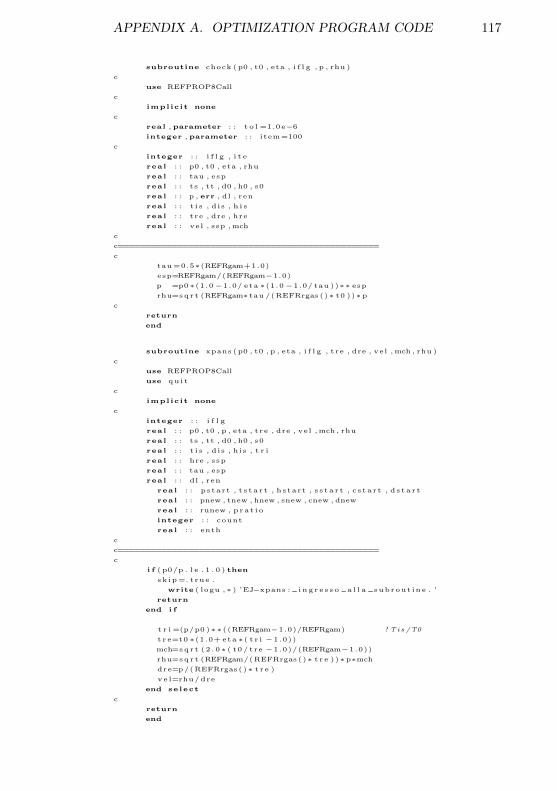
APPENDIX A. OPTIMIZATION PROGRAM CODE 117
subroutine chock (p0 , t0 , eta , i f l g , p , rhu )
c
use REFPROP8Call
c
implic it none
c
real , parameter : : t o l =1.0e−6
integer , parameter : : item=100
c
integer : : i f l g , i t e
real : : p0 , t0 , eta , rhu
real : : tau , esp
real : : ts , tt , d0 , h0 , s0
real : : p , err , dl , ren
real : : t i s , dis , h i s
real : : tre , dre , hre
real : : vel , ssp ,mch
c
c================================================
c
tau=0.5∗(REFRgam+1.0)
esp=REFRgam/(REFRgam−1.0)
p =p0∗(1.0−1.0/ eta ∗(1.0−1.0/ tau ))∗∗ esp
rhu=sqr t (REFRgam∗tau /(REFRrgas ()∗ t0 ))∗pc
return
end
subroutine xpans (p0 , t0 , p , eta , i f l g , tre , dre , vel ,mch , rhu )
c
use REFPROP8Call
use qu i t
c
implic it none
c
integer : : i f l g
real : : p0 , t0 , p , eta , tre , dre , vel ,mch , rhu
real : : ts , tt , d0 , h0 , s0
real : : t i s , dis , his , t r i
real : : hre , ssp
real : : tau , esp
real : : dl , ren
real : : pstart , t s t a r t , hstart , s s t a r t , c s ta r t , d s ta r t
real : : pnew , tnew , hnew , snew , cnew , dnew
real : : runew , p ra t i o
integer : : count
real : : enth
c
c================================================
c
i f ( p0/p . l e . 1 . 0 ) then
sk ip=. true .
write ( logu ,∗ ) ’EJ−xpans : i n g r e s s o a l l a subrout ine . ’
return
end i f
t r i =(p/p0 )∗∗ ( (REFRgam−1.0)/REFRgam) ! T i s /T0
t r e=t0 ∗(1.0+ eta ∗( t r i −1.0))
mch=sqr t ( 2 . 0∗ ( t0 / tre −1.0)/(REFRgam−1.0))
rhu=sqr t (REFRgam/(REFRrgas ()∗ t r e ))∗p∗mch
dre=p/(REFRrgas ()∗ t r e )
ve l=rhu/dre
end se lect
c
return
end
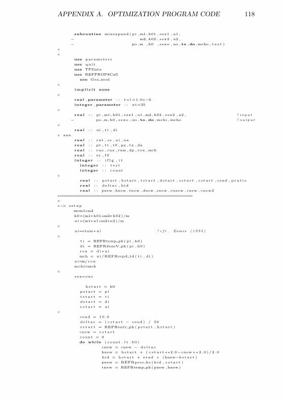
APPENDIX A. OPTIMIZATION PROGRAM CODE 118
subroutine mixexpand ( pi ,m1, h01 , sez1 , u1 ,
− m2, h02 , sez2 , u2 ,
− po ,m , h0 , sezo , uo , to ,do , mcho , t e s t )
c
c
use parameters
use qu i t
use TFData
use REFPROP8Call
use Gea mod
c
implic it none
c
real , parameter : : t o l =1.0e−6
integer , parameter : : nt=35
c
real : : pi ,m1, h01 , sez1 , u1 ,m2, h02 , sez2 , u2 , ! i n p u t
− po ,m, h0 , sezo , uo , to ,do , mchi ,mcho ! o u t p u t
c
real : : ui , t i , d i
c aux
real : : rut , ss , xi , xa
real : : pt , tt , t0 , px , tx , dx
real : : ruo , rux , rum , dp , rou ,mch
real : : er , f 0
integer : : i f l g , i t
integer : : t e s t
integer : : count
c
real : : pstart , hstart , t s t a r t , dstart , s s t a r t , c s ta r t , cend , p ra t i o
real : : de l tac , hid
real : : pnew , hnew , tnew , dnew , snew , runew , cnew , cnew2
c================================================
c
c−> setup
m=m1+m2
h0=(m1∗h01+m2∗h02 )/m
ui=(m1∗u1+m2∗u2 )/m
c
ui=etam∗ui ! c f r . Eames ( 1 9 9 5 )
c
t i = REFRtemp ph( pi , h0 )
di = REFRdensV ph( pi , h0 )
rou = di∗ui
mch = ui /REFRsspd td ( t i , d i )
a i=m/rou
mchi=mch
c
sezo=ao
hs ta r t = h0
ps ta r t = pi
t s t a r t = t i
d s ta r t = di
c s t a r t = ui
c
cend = 10.0
de l t a c = ( c s t a r t − cend ) / 50
s s t a r t = REFRentr ph ( pstart , h s ta r t )
cnew = c s t a r t
count = 0
do while ( count . l t . 5 0 )
cnew = cnew − de l t a c
hnew = hs ta r t + ( c s t a r t ∗∗2.0−cnew ∗∗2 .0 )/2 .0
hid = hs ta r t + etad ∗ (hnew−hs ta r t )
pnew = REFRpres hs ( hid , s s t a r t )
tnew = REFRtemp ph(pnew , hnew)
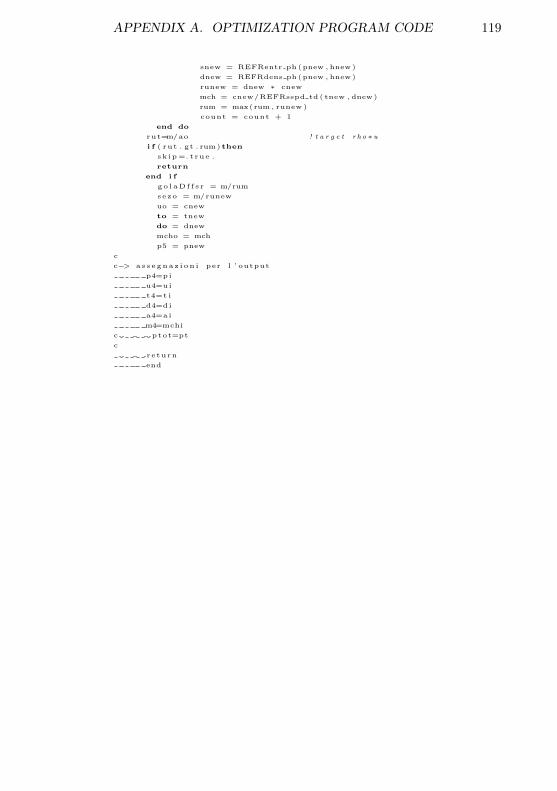
APPENDIX A. OPTIMIZATION PROGRAM CODE 119
snew = REFRentr ph (pnew , hnew)
dnew = REFRdens ph(pnew , hnew)
runew = dnew ∗ cnew
mch = cnew/REFRsspd td ( tnew , dnew)
rum = max(rum , runew )
count = count + 1
end do
rut=m/ao ! t a r g e t r h o ∗ui f ( rut . gt . rum) then
sk ip=. true .
return
end i f
go l aD f f s r = m/rum
sezo = m/runew
uo = cnew
to = tnew
do = dnew
mcho = mch
p5 = pnew
c
c−> a s s egnaz i on i per l ’ output
p4=pi
u4=ui
t4=t i
d4=di
a4=a i
m4=mchi
c ptot=pt
c
return
end
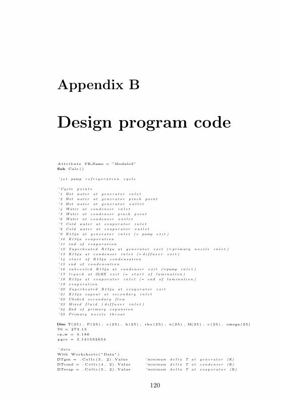
Appendix B
Design program code
Attr ibute VB Name = ”Modulo3”
Sub Calc ( )
’ j e t pump r e f r i g e r a t i o n c y c l e
’ C y c l e p o i n t s
’ 1 Hot w a t e r a t g e n e r a t o r i n l e t
’ 2 Hot w a t e r a t g e n e r a t o r p i n c h p o i n t
’ 3 Hot w a t e r a t g e n e r a t o r o u t l e t
’ 4 Water a t c o n d e n s e r i n l e t
’ 5 Water a t c o n d e n s e r p i n c h p o i n t
’ 6 Water a t c o n d e n s e r o u t l e t
’ 7 Co l d w a t e r a t e v a p o r a t o r i n l e t
’ 8 Co l d w a t e r a t e v a p o r a t o r o u t l e t
’ 9 R134a a t g e n e r a t o r i n l e t (= pump e x i t )
’ 10 R134a e v a p o r a t i o n
’ 11 end o f e v a p o r a t i o n
’ 12 S u p e r h e a t e d R134a a t g e n e r a t o r e x i t (= p r im a r y n o z z l e i n l e t )
’ 13 R134a a t c o n d e n s e r i n l e t (= d i f f u s e r e x i t )
’ 14 s t a r t o f R134a c o n d e n s a t i o n
’ 15 end o f c o n d e n s a t i o n
’ 16 s u b c o o l e d R134a a t c o n d e n s e r e x i t (=pump i n l e t )
’ 17 l i q u i d a t SLHX e x i t (= s t a r t o f l a m i n a t i o n )
’ 18 R134a a t e v a p o r a t o r i n l e t (= end o f l a m i n a t i o n )
’ 19 e v a p o r a t i o n
’ 20 S u p e r h e a t e d R134a a t e v a p o r a t o r e x i t
’ 21 R134a v a p o u r a t s e c o n d a r y i n l e t
’ 22 Choked s e c o n d a r y f l o w
’ 23 Mixed f l u i d ( d i f f u s e r i n l e t )
’ 24 End o f p r im a r y e x p a n s i o n
’ 25 Pr ima r y n o z z l e t h r o a t
Dim T(25) , P(25) , s (25) , h (25) , rho (25) , x (25) , M(25) , c (25) , omega (25)
T0 = 273.15
cp w = 4.186
pgre = 3.141592654
’ d a t a
With Worksheets ( ”Data” )
DTgen = . Ce l l s (3 , 2) . Value ’ minimum d e l t a T a t g e n e r a t o r (K)
DTcond = . Ce l l s (4 , 2) . Value ’ minimum d e l t a T a t c o n d e n s e r (K)
DTevap = . Ce l l s (5 , 2) . Value ’ minimum d e l t a T a t e v a p o r a t o r (K)
120
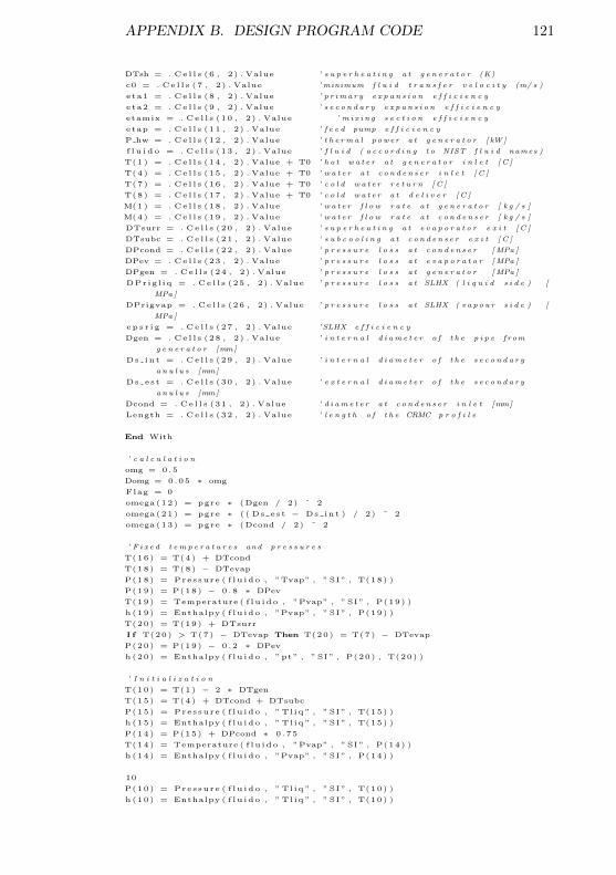
APPENDIX B. DESIGN PROGRAM CODE 121
DTsh = . Ce l l s (6 , 2) . Value ’ s u p e r h e a t i n g a t g e n e r a t o r (K)
c0 = . Ce l l s (7 , 2) . Value ’ minimum f l u i d t r a n s f e r v e l o c i t y (m/ s )
eta1 = . Ce l l s (8 , 2) . Value ’ p r im a r y e x p a n s i o n e f f i c i e n c y
eta2 = . Ce l l s (9 , 2) . Value ’ s e c o n d a r y e x p a n s i o n e f f i c i e n c y
etamix = . Ce l l s (10 , 2) . Value ’ m i x i n g s e c t i o n e f f i c i e n c y
etap = . Ce l l s (11 , 2) . Value ’ f e e d pump e f f i c i e n c y
P hw = . Ce l l s (12 , 2) . Value ’ t h e r m a l p owe r a t g e n e r a t o r [ kW ]
f l u i d o = . Ce l l s (13 , 2) . Value ’ f l u i d ( a c c o r d i n g t o NIST f l u i d names )
T(1) = . Ce l l s (14 , 2) . Value + T0 ’ h o t w a t e r a t g e n e r a t o r i n l e t [ C ]
T(4) = . Ce l l s (15 , 2) . Value + T0 ’ w a t e r a t c o n d e n s e r i n l e t [ C ]
T(7) = . Ce l l s (16 , 2) . Value + T0 ’ c o l d w a t e r r e t u r n [ C ]
T(8) = . Ce l l s (17 , 2) . Value + T0 ’ c o l d w a t e r a t d e l i v e r [ C ]
M(1) = . Ce l l s (18 , 2) . Value ’ w a t e r f l o w r a t e a t g e n e r a t o r [ k g / s ]
M(4) = . Ce l l s (19 , 2) . Value ’ w a t e r f l o w r a t e a t c o n d e n s e r [ k g / s ]
DTsurr = . Ce l l s (20 , 2) . Value ’ s u p e r h e a t i n g a t e v a p o r a t o r e x i t [ C ]
DTsubc = . Ce l l s (21 , 2) . Value ’ s u b c o o l i n g a t c o n d e n s e r e x i t [ C ]
DPcond = . Ce l l s (22 , 2) . Value ’ p r e s s u r e l o s s a t c o n d e n s e r [ MPa ]
DPev = . Ce l l s (23 , 2) . Value ’ p r e s s u r e l o s s a t e v a p o r a t o r [ MPa ]
DPgen = . Ce l l s (24 , 2) . Value ’ p r e s s u r e l o s s a t g e n e r a t o r [ MPa ]
DPrig l iq = . Ce l l s (25 , 2) . Value ’ p r e s s u r e l o s s a t SLHX ( l i q u i d s i d e ) [
MPa ]
DPrigvap = . Ce l l s (26 , 2) . Value ’ p r e s s u r e l o s s a t SLHX ( v a p o u r s i d e ) [
MPa ]
ep s r i g = . Ce l l s (27 , 2) . Value ’ SLHX e f f i c i e n c y
Dgen = . Ce l l s (28 , 2) . Value ’ i n t e r n a l d i a m e t e r o f t h e p i p e f r om
g e n e r a t o r [mm]
Ds int = . Ce l l s (29 , 2) . Value ’ i n t e r n a l d i a m e t e r o f t h e s e c o n d a r y
a n u l u s [mm]
Ds est = . Ce l l s (30 , 2) . Value ’ e x t e r n a l d i a m e t e r o f t h e s e c o n d a r y
a n u l u s [mm]
Dcond = . Ce l l s (31 , 2) . Value ’ d i a m e t e r a t c o n d e n s e r i n l e t [mm]
Length = . Ce l l s (32 , 2) . Value ’ l e n g t h o f t h e CRMC p r o f i l e
End With
’ c a l c u l a t i o n
omg = 0.5
Domg = 0.05 ∗ omg
Flag = 0
omega (12) = pgre ∗ (Dgen / 2) ˆ 2
omega (21) = pgre ∗ ( ( Ds est − Ds int ) / 2) ˆ 2
omega (13) = pgre ∗ (Dcond / 2) ˆ 2
’ F i x e d t e m p e r a t u r e s and p r e s s u r e s
T(16) = T(4) + DTcond
T(18) = T(8) − DTevap
P(18) = Pressure ( f l u ido , ”Tvap” , ”SI ” , T(18) )
P(19) = P(18) − 0 .8 ∗ DPev
T(19) = Temperature ( f l u ido , ”Pvap” , ”SI ” , P(19) )
h (19) = Enthalpy ( f l u ido , ”Pvap” , ”SI ” , P(19) )
T(20) = T(19) + DTsurr
I f T(20) > T(7) − DTevap Then T(20) = T(7) − DTevap
P(20) = P(19) − 0 .2 ∗ DPev
h (20) = Enthalpy ( f l u ido , ”pt” , ”SI ” , P(20) , T(20) )
’ I n i t i a l i z a t i o n
T(10) = T(1) − 2 ∗ DTgen
T(15) = T(4) + DTcond + DTsubc
P(15) = Pressure ( f l u ido , ”Tl iq ” , ”SI ” , T(15) )
h (15) = Enthalpy ( f l u ido , ”Tl iq ” , ”SI ” , T(15) )
P(14) = P(15) + DPcond ∗ 0 .75
T(14) = Temperature ( f l u ido , ”Pvap” , ”SI ” , P(14) )
h (14) = Enthalpy ( f l u ido , ”Pvap” , ”SI ” , P(14) )
10
P(10) = Pressure ( f l u ido , ”Tl iq ” , ”SI ” , T(10) )
h (10) = Enthalpy ( f l u ido , ”Tl iq ” , ”SI ” , T(10) )
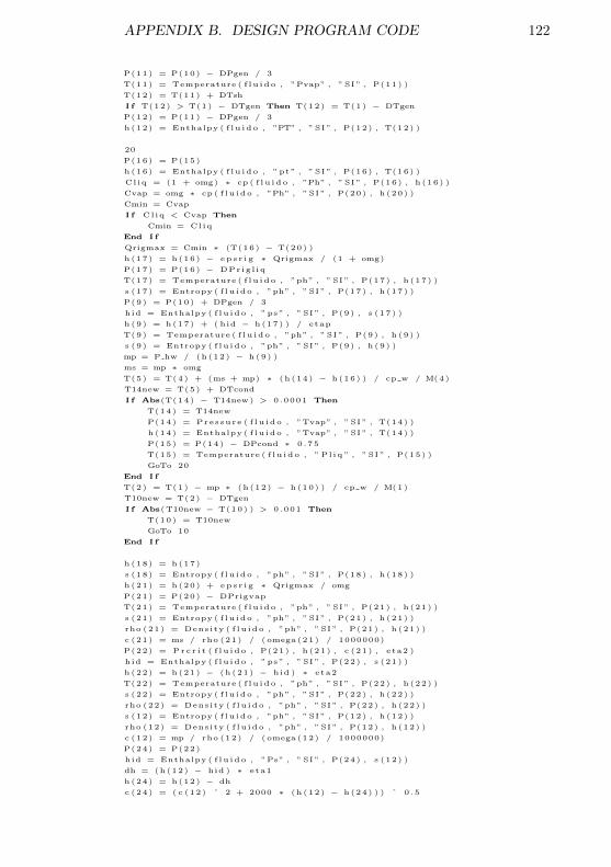
APPENDIX B. DESIGN PROGRAM CODE 122
P(11) = P(10) − DPgen / 3
T(11) = Temperature ( f l u ido , ”Pvap” , ”SI ” , P(11) )
T(12) = T(11) + DTsh
I f T(12) > T(1) − DTgen Then T(12) = T(1) − DTgen
P(12) = P(11) − DPgen / 3
h (12) = Enthalpy ( f l u ido , ”PT” , ”SI ” , P(12) , T(12) )
20
P(16) = P(15)
h (16) = Enthalpy ( f l u ido , ”pt” , ”SI ” , P(16) , T(16) )
Cl iq = (1 + omg) ∗ cp ( f l u ido , ”Ph” , ”SI ” , P(16) , h (16) )
Cvap = omg ∗ cp ( f l u ido , ”Ph” , ”SI ” , P(20) , h (20) )
Cmin = Cvap
I f Cliq < Cvap Then
Cmin = Cliq
End I f
Qrigmax = Cmin ∗ (T(16) − T(20) )
h (17) = h(16) − ep s r i g ∗ Qrigmax / (1 + omg)
P(17) = P(16) − DPrig l iq
T(17) = Temperature ( f l u ido , ”ph” , ”SI ” , P(17) , h (17) )
s (17) = Entropy ( f l u ido , ”ph” , ”SI ” , P(17) , h (17) )
P(9) = P(10) + DPgen / 3
hid = Enthalpy ( f l u ido , ”ps” , ”SI ” , P(9) , s (17) )
h (9) = h(17) + ( hid − h (17) ) / etap
T(9) = Temperature ( f l u ido , ”ph” , ”SI ” , P(9) , h (9) )
s (9) = Entropy ( f l u ido , ”ph” , ”SI ” , P(9) , h (9) )
mp = P hw / (h (12) − h (9) )
ms = mp ∗ omg
T(5) = T(4) + (ms + mp) ∗ (h (14) − h (16) ) / cp w / M(4)
T14new = T(5) + DTcond
I f Abs(T(14) − T14new) > 0.0001 Then
T(14) = T14new
P(14) = Pressure ( f l u ido , ”Tvap” , ”SI ” , T(14) )
h (14) = Enthalpy ( f l u ido , ”Tvap” , ”SI ” , T(14) )
P(15) = P(14) − DPcond ∗ 0 .75
T(15) = Temperature ( f l u ido , ” Pl iq ” , ”SI ” , P(15) )
GoTo 20
End I f
T(2) = T(1) − mp ∗ (h (12) − h (10) ) / cp w / M(1)
T10new = T(2) − DTgen
I f Abs(T10new − T(10) ) > 0.001 Then
T(10) = T10new
GoTo 10
End I f
h (18) = h(17)
s (18) = Entropy ( f l u ido , ”ph” , ”SI ” , P(18) , h (18) )
h (21) = h(20) + ep s r i g ∗ Qrigmax / omg
P(21) = P(20) − DPrigvap
T(21) = Temperature ( f l u ido , ”ph” , ”SI ” , P(21) , h (21) )
s (21) = Entropy ( f l u ido , ”ph” , ”SI ” , P(21) , h (21) )
rho (21) = Density ( f l u ido , ”ph” , ”SI ” , P(21) , h (21) )
c (21) = ms / rho (21) / ( omega (21) / 1000000)
P(22) = Prc r i t ( f l u ido , P(21) , h (21) , c (21) , eta2 )
hid = Enthalpy ( f l u ido , ”ps” , ”SI ” , P(22) , s (21) )
h (22) = h(21) − (h (21) − hid ) ∗ eta2
T(22) = Temperature ( f l u ido , ”ph” , ”SI ” , P(22) , h (22) )
s (22) = Entropy ( f l u ido , ”ph” , ”SI ” , P(22) , h (22) )
rho (22) = Density ( f l u ido , ”ph” , ”SI ” , P(22) , h (22) )
s (12) = Entropy ( f l u ido , ”ph” , ”SI ” , P(12) , h (12) )
rho (12) = Density ( f l u ido , ”ph” , ”SI ” , P(12) , h (12) )
c (12) = mp / rho (12) / ( omega (12) / 1000000)
P(24) = P(22)
hid = Enthalpy ( f l u ido , ”Ps” , ”SI ” , P(24) , s (12) )
dh = (h (12) − hid ) ∗ eta1
h (24) = h(12) − dh
c (24) = ( c (12) ˆ 2 + 2000 ∗ (h (12) − h (24) ) ) ˆ 0 .5
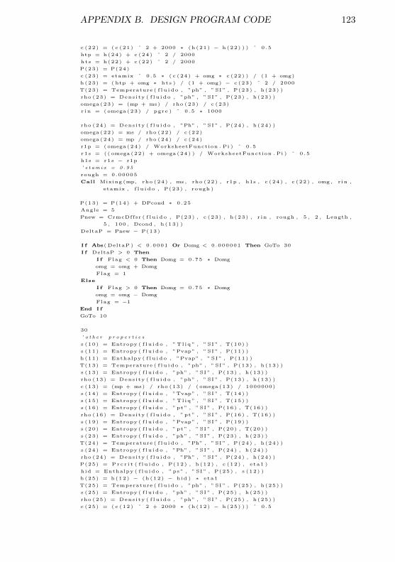
APPENDIX B. DESIGN PROGRAM CODE 123
c (22) = ( c (21) ˆ 2 + 2000 ∗ (h (21) − h (22) ) ) ˆ 0 .5
htp = h(24) + c (24) ˆ 2 / 2000
hts = h(22) + c (22) ˆ 2 / 2000
P(23) = P(24)
c (23) = etamix ˆ 0 .5 ∗ ( c (24) + omg ∗ c (22) ) / (1 + omg)
h (23) = ( htp + omg ∗ hts ) / (1 + omg) − c (23) ˆ 2 / 2000
T(23) = Temperature ( f l u ido , ”ph” , ”SI ” , P(23) , h (23) )
rho (23) = Density ( f l u ido , ”ph” , ”SI ” , P(23) , h (23) )
omega (23) = (mp + ms) / rho (23) / c (23)
r i n = (omega (23) / pgre ) ˆ 0 .5 ∗ 1000
rho (24) = Density ( f l u ido , ”Ph” , ”SI ” , P(24) , h (24) )
omega (22) = ms / rho (22) / c (22)
omega (24) = mp / rho (24) / c (24)
r1p = (omega (24) / WorksheetFunction . Pi ) ˆ 0 .5
r1s = ( ( omega (22) + omega (24) ) / WorksheetFunction . Pi ) ˆ 0 .5
h1s = r1s − r1p
’ e t am i x = 0 . 9 5
rough = 0.00005
Call Mixing (mp, rho (24) , ms , rho (22) , r1p , h1s , c (24) , c (22) , omg , r in ,
etamix , f l u ido , P(23) , rough )
P(13) = P(14) + DPcond ∗ 0 .25
Angle = 5
Pnew = CrmcDffsr ( f l u ido , P(23) , c (23) , h (23) , r in , rough , 5 , 2 , Length ,
5 , 100 , Dcond , h (13) )
DeltaP = Pnew − P(13)
I f Abs( DeltaP ) < 0.0001 Or Domg < 0.000001 Then GoTo 30
I f DeltaP > 0 Then
I f Flag < 0 Then Domg = 0.75 ∗ Domg
omg = omg + Domg
Flag = 1
Else
I f Flag > 0 Then Domg = 0.75 ∗ Domg
omg = omg − Domg
Flag = −1
End I f
GoTo 10
30
’ o t h e r p r o p e r t i e s
s (10) = Entropy ( f l u ido , ”Tl iq ” , ”SI ” , T(10) )
s (11) = Entropy ( f l u ido , ”Pvap” , ”SI ” , P(11) )
h (11) = Enthalpy ( f l u ido , ”Pvap” , ”SI ” , P(11) )
T(13) = Temperature ( f l u ido , ”ph” , ”SI ” , P(13) , h (13) )
s (13) = Entropy ( f l u ido , ”ph” , ”SI ” , P(13) , h (13) )
rho (13) = Density ( f l u ido , ”ph” , ”SI ” , P(13) , h (13) )
c (13) = (mp + ms) / rho (13) / ( omega (13) / 1000000)
s (14) = Entropy ( f l u ido , ”Tvap” , ”SI ” , T(14) )
s (15) = Entropy ( f l u ido , ”Tl iq ” , ”SI ” , T(15) )
s (16) = Entropy ( f l u ido , ”pt” , ”SI ” , P(16) , T(16) )
rho (16) = Density ( f l u ido , ”pt” , ”SI ” , P(16) , T(16) )
s (19) = Entropy ( f l u ido , ”Pvap” , ”SI ” , P(19) )
s (20) = Entropy ( f l u ido , ”pt” , ”SI ” , P(20) , T(20) )
s (23) = Entropy ( f l u ido , ”ph” , ”SI ” , P(23) , h (23) )
T(24) = Temperature ( f l u ido , ”Ph” , ”SI ” , P(24) , h (24) )
s (24) = Entropy ( f l u ido , ”Ph” , ”SI ” , P(24) , h (24) )
rho (24) = Density ( f l u ido , ”Ph” , ”SI ” , P(24) , h (24) )
P(25) = Prc r i t ( f l u ido , P(12) , h (12) , c (12) , eta1 )
hid = Enthalpy ( f l u ido , ”ps” , ”SI ” , P(25) , s (12) )
h (25) = h(12) − (h (12) − hid ) ∗ eta1
T(25) = Temperature ( f l u ido , ”ph” , ”SI ” , P(25) , h (25) )
s (25) = Entropy ( f l u ido , ”ph” , ”SI ” , P(25) , h (25) )
rho (25) = Density ( f l u ido , ”ph” , ”SI ” , P(25) , h (25) )
c (25) = ( c (12) ˆ 2 + 2000 ∗ (h (12) − h (25) ) ) ˆ 0 .5
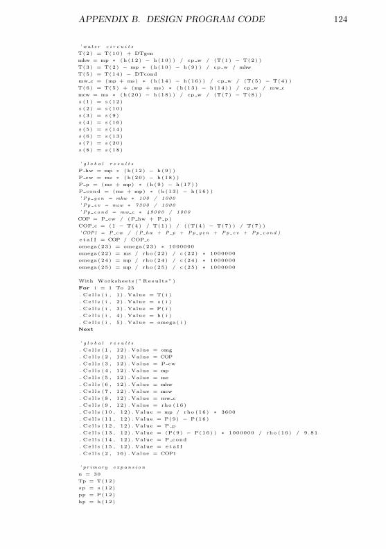
APPENDIX B. DESIGN PROGRAM CODE 124
’ w a t e r c i r c u i t s
T(2) = T(10) + DTgen
mhw = mp ∗ (h (12) − h (10) ) / cp w / (T(1) − T(2) )
T(3) = T(2) − mp ∗ (h (10) − h (9) ) / cp w / mhw
T(5) = T(14) − DTcond
mw c = (mp + ms) ∗ (h (14) − h (16) ) / cp w / (T(5) − T(4) )
T(6) = T(5) + (mp + ms) ∗ (h (13) − h (14) ) / cp w / mw c
mcw = ms ∗ (h (20) − h (18) ) / cp w / (T(7) − T(8) )
s (1) = s (12)
s (2) = s (10)
s (3) = s (9)
s (4) = s (16)
s (5) = s (14)
s (6) = s (13)
s (7) = s (20)
s (8) = s (18)
’ g l o b a l r e s u l t s
P hw = mp ∗ (h (12) − h (9) )
P cw = ms ∗ (h (20) − h (18) )
P p = (ms + mp) ∗ (h (9) − h (17) )
P cond = (ms + mp) ∗ (h (13) − h (16) )
’ P p g e n = mhw ∗ 100 / 1000
’ P p e v = mcw ∗ 7300 / 1000
’ Pp c ond = mw c ∗ 49000 / 1000
COP = P cw / (P hw + P p )
COP c = (1 − T(4) / T(1) ) / ( (T(4) − T(7) ) / T(7) )
’COP1 = P cw / ( P hw + P p + Pp g e n + Pp e v + Pp c ond )
e t a I I = COP / COP c
omega (23) = omega (23) ∗ 1000000
omega (22) = ms / rho (22) / c (22) ∗ 1000000
omega (24) = mp / rho (24) / c (24) ∗ 1000000
omega (25) = mp / rho (25) / c (25) ∗ 1000000
With Worksheets ( ”Resu l t s ” )
For i = 1 To 25
. Ce l l s ( i , 1) . Value = T( i )
. Ce l l s ( i , 2) . Value = s ( i )
. Ce l l s ( i , 3) . Value = P( i )
. Ce l l s ( i , 4) . Value = h( i )
. Ce l l s ( i , 5) . Value = omega ( i )
Next
’ g l o b a l r e s u l t s
. C e l l s (1 , 12) . Value = omg
. Ce l l s (2 , 12) . Value = COP
. Ce l l s (3 , 12) . Value = P cw
. Ce l l s (4 , 12) . Value = mp
. Ce l l s (5 , 12) . Value = ms
. Ce l l s (6 , 12) . Value = mhw
. Ce l l s (7 , 12) . Value = mcw
. Ce l l s (8 , 12) . Value = mw c
. Ce l l s (9 , 12) . Value = rho (16)
. Ce l l s (10 , 12) . Value = mp / rho (16) ∗ 3600
. Ce l l s (11 , 12) . Value = P(9) − P(16)
. Ce l l s (12 , 12) . Value = P p
. Ce l l s (13 , 12) . Value = (P(9) − P(16) ) ∗ 1000000 / rho (16) / 9 .81
. Ce l l s (14 , 12) . Value = P cond
. Ce l l s (15 , 12) . Value = e t a I I
. Ce l l s (2 , 16) . Value = COP1
’ p r im a r y e x p a n s i o n
n = 30
Tp = T(12)
sp = s (12)
pp = P(12)
hp = h(12)
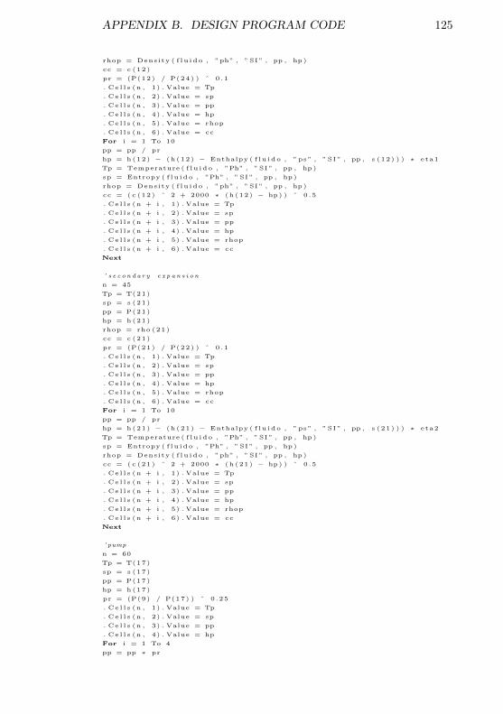
APPENDIX B. DESIGN PROGRAM CODE 125
rhop = Density ( f l u ido , ”ph” , ”SI ” , pp , hp)
cc = c (12)
pr = (P(12) / P(24) ) ˆ 0 .1
. Ce l l s (n , 1) . Value = Tp
. Ce l l s (n , 2) . Value = sp
. Ce l l s (n , 3) . Value = pp
. Ce l l s (n , 4) . Value = hp
. Ce l l s (n , 5) . Value = rhop
. Ce l l s (n , 6) . Value = cc
For i = 1 To 10
pp = pp / pr
hp = h(12) − (h (12) − Enthalpy ( f l u ido , ”ps” , ”SI ” , pp , s (12) ) ) ∗ eta1
Tp = Temperature ( f l u ido , ”Ph” , ”SI ” , pp , hp)
sp = Entropy ( f l u ido , ”Ph” , ”SI ” , pp , hp)
rhop = Density ( f l u ido , ”ph” , ”SI ” , pp , hp)
cc = ( c (12) ˆ 2 + 2000 ∗ (h (12) − hp) ) ˆ 0 .5
. Ce l l s (n + i , 1) . Value = Tp
. Ce l l s (n + i , 2) . Value = sp
. Ce l l s (n + i , 3) . Value = pp
. Ce l l s (n + i , 4) . Value = hp
. Ce l l s (n + i , 5) . Value = rhop
. Ce l l s (n + i , 6) . Value = cc
Next
’ s e c o n d a r y e x p a n s i o n
n = 45
Tp = T(21)
sp = s (21)
pp = P(21)
hp = h(21)
rhop = rho (21)
cc = c (21)
pr = (P(21) / P(22) ) ˆ 0 .1
. Ce l l s (n , 1) . Value = Tp
. Ce l l s (n , 2) . Value = sp
. Ce l l s (n , 3) . Value = pp
. Ce l l s (n , 4) . Value = hp
. Ce l l s (n , 5) . Value = rhop
. Ce l l s (n , 6) . Value = cc
For i = 1 To 10
pp = pp / pr
hp = h(21) − (h (21) − Enthalpy ( f l u ido , ”ps” , ”SI ” , pp , s (21) ) ) ∗ eta2
Tp = Temperature ( f l u ido , ”Ph” , ”SI ” , pp , hp)
sp = Entropy ( f l u ido , ”Ph” , ”SI ” , pp , hp)
rhop = Density ( f l u ido , ”ph” , ”SI ” , pp , hp)
cc = ( c (21) ˆ 2 + 2000 ∗ (h (21) − hp) ) ˆ 0 .5
. Ce l l s (n + i , 1) . Value = Tp
. Ce l l s (n + i , 2) . Value = sp
. Ce l l s (n + i , 3) . Value = pp
. Ce l l s (n + i , 4) . Value = hp
. Ce l l s (n + i , 5) . Value = rhop
. Ce l l s (n + i , 6) . Value = cc
Next
’ pump
n = 60
Tp = T(17)
sp = s (17)
pp = P(17)
hp = h(17)
pr = (P(9) / P(17) ) ˆ 0 .25
. Ce l l s (n , 1) . Value = Tp
. Ce l l s (n , 2) . Value = sp
. Ce l l s (n , 3) . Value = pp
. Ce l l s (n , 4) . Value = hp
For i = 1 To 4
pp = pp ∗ pr
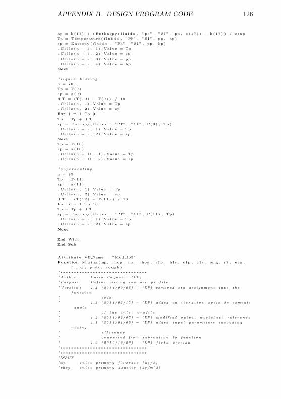
APPENDIX B. DESIGN PROGRAM CODE 126
hp = h(17) + ( Enthalpy ( f l u ido , ”ps” , ”SI ” , pp , s (17) ) − h (17) ) / etap
Tp = Temperature ( f l u ido , ”Ph” , ”SI ” , pp , hp)
sp = Entropy ( f l u ido , ”Ph” , ”SI ” , pp , hp)
. Ce l l s (n + i , 1) . Value = Tp
. Ce l l s (n + i , 2) . Value = sp
. Ce l l s (n + i , 3) . Value = pp
. Ce l l s (n + i , 4) . Value = hp
Next
’ l i q u i d h e a t i n g
n = 70
Tp = T(9)
sp = s (9)
diT = (T(10) − T(9) ) / 10
. Ce l l s (n , 1) . Value = Tp
. Ce l l s (n , 2) . Value = sp
For i = 1 To 9
Tp = Tp + diT
sp = Entropy ( f l u ido , ”PT” , ”SI ” , P(9) , Tp)
. Ce l l s (n + i , 1) . Value = Tp
. Ce l l s (n + i , 2) . Value = sp
Next
Tp = T(10)
sp = s (10)
. Ce l l s (n + 10 , 1) . Value = Tp
. Ce l l s (n + 10 , 2) . Value = sp
’ s u p e r h e a t i n g
n = 85
Tp = T(11)
sp = s (11)
. Ce l l s (n , 1) . Value = Tp
. Ce l l s (n , 2) . Value = sp
diT = (T(12) − T(11) ) / 10
For i = 1 To 10
Tp = Tp + diT
sp = Entropy ( f l u ido , ”PT” , ”SI ” , P(11) , Tp)
. Ce l l s (n + i , 1) . Value = Tp
. Ce l l s (n + i , 2) . Value = sp
Next
End With
End Sub
Attr ibute VB Name = ”Modulo5”
Function Mixing (mp, rhop , ms , rhos , r1p , h1s , c1p , c1s , omg , r2 , eta ,
f l u i d , pmix , rough )
’ ∗∗∗∗∗∗∗∗∗∗∗∗∗∗∗∗∗∗∗∗∗∗∗∗∗∗∗∗∗∗∗∗’ Au t h o r : Da r i o P a g a n i n i (DP)
’ P u r p o s e : D e f i n e m i x i n g c h ambe r p r o f i l e
’ V e r s i o n : 1 . 4 ( 2 0 1 1 / 0 9 / 0 5 ) − (DP) r emov ed e t a a s s i g nm e n t i n t o t h e
f u n c t i o n
’ c o d e
’ 1 . 3 ( 2 0 1 1 / 0 2 / 1 7 ) − (DP) a d d e d an i t e r a t i v e c y c l e t o c ompu t e
a n g l e
’ o f t h e i n l e t p r o f i l e
’ 1 . 2 ( 2 0 1 1 / 0 2 / 0 7 ) − (DP) m o d i f i e d o u t p u t w o r k s h e e t r e f e r e n c e
’ 1 . 1 ( 2 0 1 1 / 0 1 / 0 5 ) − (DP) a d d e d i n p u t p a r am e t e r s i n c l u d i n g
m i x i n g
’ e f f c i e n c y
’ c o n v e r t e d f r om s u b r o u t i n e t o f u n c t i o n
’ 1 . 0 ( 2 0 1 0 / 1 2 / 0 3 ) − (DP) f i r t s v e r s i o n
’ ∗∗∗∗∗∗∗∗∗∗∗∗∗∗∗∗∗∗∗∗∗∗∗∗∗∗∗∗∗∗∗∗’ ∗∗∗∗∗∗∗∗∗∗∗∗∗∗∗∗∗∗∗∗∗∗∗∗∗∗∗∗∗∗∗∗’ INPUT
’mp i n l e t p r im a r y f l o w r a t e [ k g / s ]
’ r h o p i n l e t p r im a r y d e n s i t y [ k g /mˆ 3 ]
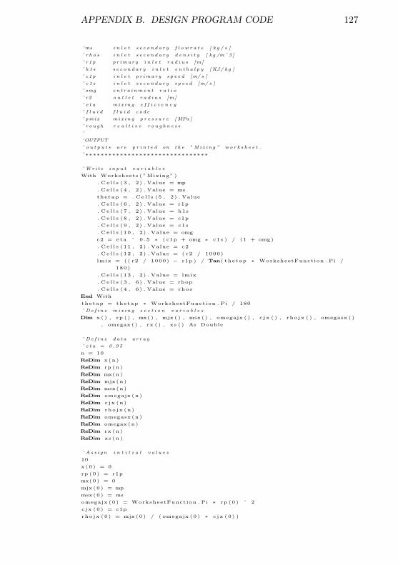
APPENDIX B. DESIGN PROGRAM CODE 127
’ ms i n l e t s e c o n d a r y f l o w r a t e [ k g / s ]
’ r h o s i n l e t s e c o n d a r y d e n s i t y [ k g /mˆ 3 ]
’ r 1 p p r im a r y i n l e t r a d i u s [m]
’ h 1 s s e c o n d a r y i n l e t e n t h a l p y [ KJ/ k g ]
’ c 1 p i n l e t p r im a r y s p e e d [m/ s ]
’ c 1 s i n l e t s e c o n d a r y s p e e d [m/ s ]
’ omg e n t r a i nm e n t r a t i o
’ r 2 o u t l e t r a d i u s [m]
’ e t a m i x i n g e f f i c i e n c y
’ f l u i d f l u i d c o d e
’ pmix m i x i n g p r e s s u r e [ MPa ]
’ r o u g h r e a l t i v e r o u g h n e s s
’
’OUTPUT
’ o u t p u t s a r e p r i n t e d on t h e ” M i x i n g ” w o r k s h e e t .
’ ∗∗∗∗∗∗∗∗∗∗∗∗∗∗∗∗∗∗∗∗∗∗∗∗∗∗∗∗∗∗∗∗
’ Wr i t e i n p u t v a r i a b l e s
With Worksheets ( ”Mixing” )
. Ce l l s (3 , 2) . Value = mp
. Ce l l s (4 , 2) . Value = ms
thetap = . Ce l l s (5 , 2) . Value
. Ce l l s (6 , 2) . Value = r1p
. Ce l l s (7 , 2) . Value = h1s
. Ce l l s (8 , 2) . Value = c1p
. Ce l l s (9 , 2) . Value = c1s
. Ce l l s (10 , 2) . Value = omg
c2 = eta ˆ 0 .5 ∗ ( c1p + omg ∗ c1s ) / (1 + omg)
. Ce l l s (11 , 2) . Value = c2
. Ce l l s (12 , 2) . Value = ( r2 / 1000)
lmix = (( r2 / 1000) − r1p ) / Tan( thetap ∗ WorksheetFunction . Pi /
180)
. Ce l l s (13 , 2) . Value = lmix
. Ce l l s (3 , 6) . Value = rhop
. Ce l l s (4 , 6) . Value = rhos
End With
thetap = thetap ∗ WorksheetFunction . Pi / 180
’ D e f i n e m i x i n g s e c t i o n v a r i a b l e s
Dim x ( ) , rp ( ) , mx( ) , mjx ( ) , msx ( ) , omegajx ( ) , c jx ( ) , rhojx ( ) , omegasx ( )
, omegax ( ) , rx ( ) , xs ( ) As Double
’ D e f i n e d a t a a r r a y
’ e t a = 0 . 9 5
n = 10
ReDim x(n)
ReDim rp (n)
ReDim mx(n)
ReDim mjx(n)
ReDim msx(n)
ReDim omegajx (n)
ReDim c jx (n)
ReDim rhojx (n)
ReDim omegasx (n)
ReDim omegax (n)
ReDim rx (n)
ReDim xs (n)
’ A s s i g n i n t i t i a l v a l u e s
10
x (0) = 0
rp (0) = r1p
mx(0) = 0
mjx (0) = mp
msx (0) = ms
omegajx (0) = WorksheetFunction . Pi ∗ rp (0) ˆ 2
c jx (0) = c1p
rhojx (0) = mjx (0) / ( omegajx (0) ∗ c jx (0) )
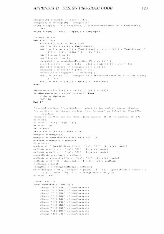
APPENDIX B. DESIGN PROGRAM CODE 128
omegasx (0) = msx (0) / ( rhos ∗ c1s )
omegax (0) = omegajx (0) + omegasx (0)
rx (0) = ( rp (0) ˆ 2 + omegasx (0) / WorksheetFunction . Pi ∗ Cos( alpha ) ) ˆ
0 .5
xs (0) = x (0) + ( rx (0) − rp (0) ) ∗ Tan( alpha )
’ A s s i g n v a l u e s
For i = 1 To n
x( i ) = x( i − 1) + ( lmix / n)
rp ( i ) = r1p + (x ( i ) ∗ Tan( thetap ) )
mx( i ) = 2 ∗ ms ∗ x( i ) ∗ Tan( thetap ) ∗ ( r1p + (x ( i ) ∗ Tan( thetap ) /
2) ) / ( ( r2 / 1000) ˆ 2 − r1p ˆ 2)
mjx ( i ) = mp + mx( i )
msx( i ) = ms − mx( i )
omegajx ( i ) = WorksheetFunction . Pi ∗ rp ( i ) ˆ 2
c jx ( i ) = ( c1s + (mp ∗ ( c1p − c1s ) / (mjx ( i ) ) ) ) ∗ eta ˆ 0 .5
rhojx ( i ) = mjx ( i ) / ( omegajx ( i ) ∗ c jx ( i ) )
omegasx ( i ) = msx( i ) / ( rhos ∗ c1s )
omegax ( i ) = omegajx ( i ) + omegasx ( i )
rx ( i ) = ( rp ( i ) ˆ 2 + omegasx ( i ) / WorksheetFunction . Pi ∗ Cos( alpha )
) ˆ 0 .5
xs ( i ) = x( i ) + ( rx ( i ) − rp ( i ) ) ∗ Tan( alpha )
Next
alphanew = −Atn( ( rx (1) − rx (0) ) / (x (1) − x (0) ) )
I f Abs( alphanew − alpha ) > 0.0001 Then
alpha = alphanew
GoTo 10
End I f
’ C o n i c a l s e c t i o n ( f r c i t i o n l e s s ) a d d e d t o t h e end o f m i x i n g c h ambe r
’ t o a c t i v a t e t h e c h a n g e r e a d i n g f r om ” M i x i n g ” w o r k s h e e t i n C rmcD f f s r
f u n c t i o n
’ mus t b e s h i f t e d one row down ( f r om i n d e x e s 25−26 t o i n d e x e s 26−27)
x1 = x(n)
x2 = x1 + (x(n) − x(n − 1) )
dx = x2 − x1
rr1 = rx (n)
r r2 = rr1 + ( rx (n) − rx (n − 1) )
omegax1 = omegax (n)
omegax2 = WorksheetFunction . Pi ∗ r r2 ˆ 2
domegax = omegax2 − omegax1
v1 = cjx (n)
mach = v1 / SpeedOfSound ( f l u i d , ”dp” , ”SI ” , rhojx (n) , pmix )
cpConic = cp ( f l u i d , ”dp” , ”SI ” , rhojx (n) , pmix )
cvConic = cv ( f l u i d , ”dp” , ”SI ” , rhojx (n) , pmix )
gammaConic = cpConic / cvConic
muConic = Vi s co s i t y ( f l u i d , ”dp” , ”SI ” , rhojx (n) , pmix )
ReConic = 10 ˆ 6 ∗ rhojx (n) ∗ v1 ∗ 2 ∗ r r1 / muConic
RelRough = rough
fSergConic = fSerg (RelRough , ReConic )
Dv = domegax ∗ v1 / ( omegax1 ∗ (mach ˆ 2 − 1) ) + gammaConic ∗ (mach ˆ 2
/ (1 − mach ˆ 2) ) ∗ v1 ∗ fSergConic ∗ dx / rr1
v2 = v1 + Dv
’ P r i n t r e s u l t s
With Worksheets ( ”Mixing” )
. Range ( ”A16 : A26” ) . ClearContents
. Range ( ”B16 : B26” ) . ClearContents
. Range ( ”C16 : C26” ) . ClearContents
. Range ( ”D16 :D26” ) . ClearContents
. Range ( ”E16 : E26” ) . ClearContents
. Range ( ”F16 : F26” ) . ClearContents
. Range ( ”G16 :G26” ) . ClearContents
. Range ( ”H16 : H26” ) . ClearContents
. Range ( ” I16 : I26 ” ) . ClearContents
. Range ( ”J16 : J26” ) . ClearContents
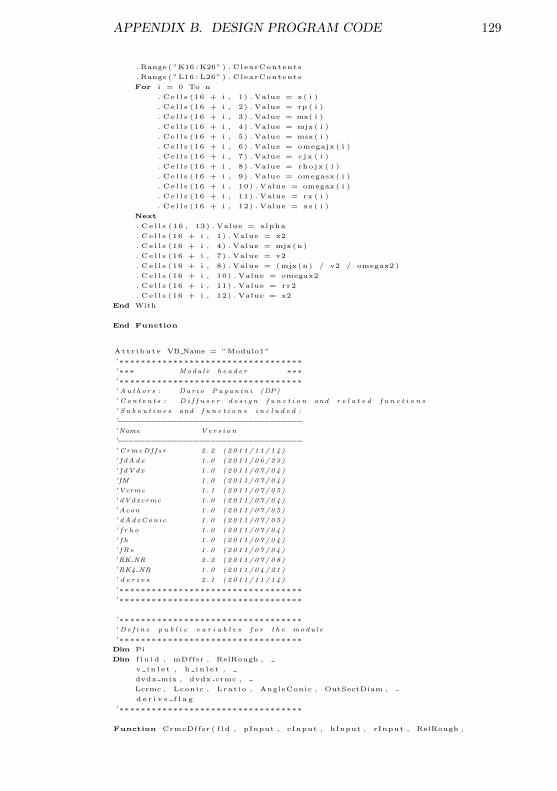
APPENDIX B. DESIGN PROGRAM CODE 129
. Range ( ”K16 :K26” ) . ClearContents
. Range ( ”L16 : L26” ) . ClearContents
For i = 0 To n
. Ce l l s (16 + i , 1) . Value = x( i )
. Ce l l s (16 + i , 2) . Value = rp ( i )
. Ce l l s (16 + i , 3) . Value = mx( i )
. Ce l l s (16 + i , 4) . Value = mjx ( i )
. Ce l l s (16 + i , 5) . Value = msx( i )
. Ce l l s (16 + i , 6) . Value = omegajx ( i )
. Ce l l s (16 + i , 7) . Value = cjx ( i )
. Ce l l s (16 + i , 8) . Value = rhojx ( i )
. Ce l l s (16 + i , 9) . Value = omegasx ( i )
. Ce l l s (16 + i , 10) . Value = omegax ( i )
. Ce l l s (16 + i , 11) . Value = rx ( i )
. Ce l l s (16 + i , 12) . Value = xs ( i )
Next
. C e l l s (16 , 13) . Value = alpha
. Ce l l s (16 + i , 1) . Value = x2
. Ce l l s (16 + i , 4) . Value = mjx (n)
. Ce l l s (16 + i , 7) . Value = v2
. Ce l l s (16 + i , 8) . Value = (mjx (n) / v2 / omegax2 )
. Ce l l s (16 + i , 10) . Value = omegax2
. Ce l l s (16 + i , 11) . Value = rr2
. Ce l l s (16 + i , 12) . Value = x2
End With
End Function
Attr ibute VB Name = ”Modulo1”
’ ∗∗∗∗∗∗∗∗∗∗∗∗∗∗∗∗∗∗∗∗∗∗∗∗∗∗∗∗∗∗∗∗∗∗’∗∗∗ Modu l e h e a d e r ∗∗∗’ ∗∗∗∗∗∗∗∗∗∗∗∗∗∗∗∗∗∗∗∗∗∗∗∗∗∗∗∗∗∗∗∗∗∗’ A u t h o r s : Da r i o P a g a n i n i (DP)
’ C o n t e n t s : D i f f u s e r d e s i g n f u n c t i o n and r e l a t e d f u n c t i o n s
’ S u b o u t i n e s and f u n c t i o n s i n c l u d e d :
’−−−−−−−−−−−−−−−−−−−−−−−−−−−−−−−−−−’ Name V e r s i o n
’−−−−−−−−−−−−−−−−−−−−−−−−−−−−−−−−−−’ C rmcD f f s r 2 . 2 ( 2 0 1 1 / 1 1 / 1 4 )
’ f dAd x 1 . 0 ( 2 0 1 1 / 0 6 / 2 3 )
’ f dVd x 1 . 0 ( 2 0 1 1 / 0 7 / 0 4 )
’ fM 1 . 0 ( 2 0 1 1 / 0 7 / 0 4 )
’ Vcrmc 1 . 1 ( 2 0 1 1 / 0 7 / 0 5 )
’ dVdxcrmc 1 . 0 ( 2 0 1 1 / 0 7 / 0 4 )
’ Acon 1 . 0 ( 2 0 1 1 / 0 7 / 0 5 )
’ dAdxCon i c 1 . 0 ( 2 0 1 1 / 0 7 / 0 5 )
’ f r h o 1 . 0 ( 2 0 1 1 / 0 7 / 0 4 )
’ f h 1 . 0 ( 2 0 1 1 / 0 7 / 0 4 )
’ fRe 1 . 0 ( 2 0 1 1 / 0 7 / 0 4 )
’RK NR 2 . 2 ( 2 0 1 1 / 0 7 / 0 8 )
’ RK4 NR 1 . 0 ( 2 0 1 1 / 0 4 / 2 1 )
’ d e r i v s 2 . 1 ( 2 0 1 1 / 1 1 / 1 4 )
’ ∗∗∗∗∗∗∗∗∗∗∗∗∗∗∗∗∗∗∗∗∗∗∗∗∗∗∗∗∗∗∗∗∗∗’ ∗∗∗∗∗∗∗∗∗∗∗∗∗∗∗∗∗∗∗∗∗∗∗∗∗∗∗∗∗∗∗∗∗∗
’ ∗∗∗∗∗∗∗∗∗∗∗∗∗∗∗∗∗∗∗∗∗∗∗∗∗∗∗∗∗∗∗∗∗∗’ D e f i n e p u b l i c v a r i a b l e s f o r t h e modu l e
’ ∗∗∗∗∗∗∗∗∗∗∗∗∗∗∗∗∗∗∗∗∗∗∗∗∗∗∗∗∗∗∗∗∗∗Dim Pi
Dim f l u i d , mDffsr , RelRough ,
v i n l e t , h i n l e t ,
dvdx mix , dvdx crmc ,
Lcrmc , Lconic , Lrat io , AngleConic , OutSectDiam ,
d e r i v s f l a g
’ ∗∗∗∗∗∗∗∗∗∗∗∗∗∗∗∗∗∗∗∗∗∗∗∗∗∗∗∗∗∗∗∗∗∗
Function CrmcDffsr ( f ld , pInput , cInput , hInput , rInput , RelRough ,
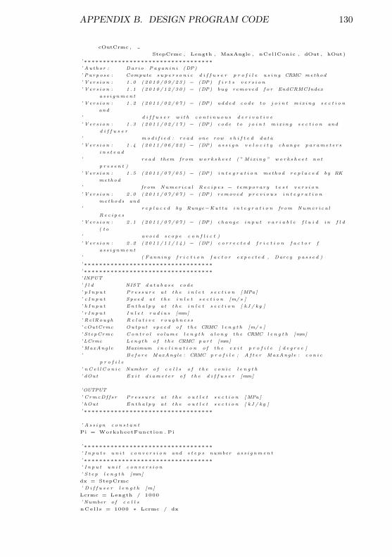
APPENDIX B. DESIGN PROGRAM CODE 130
cOutCrmc ,
StepCrmc , Length , MaxAngle , nCellConic , dOut , hOut)
’ ∗∗∗∗∗∗∗∗∗∗∗∗∗∗∗∗∗∗∗∗∗∗∗∗∗∗∗∗∗∗∗∗∗∗’ Au t h o r : Da r i o P a g a n i n i (DP)
’ P u r p o s e : Compute s u p e r s o n i c d i f f u s e r p r o f i l e u s i n g CRMC me thod
’ V e r s i o n : 1 . 0 ( 2 0 1 0 / 0 9 / 2 3 ) − (DP) f i r t s v e r s i o n
’ V e r s i o n : 1 . 1 ( 2 0 1 0 / 1 2 / 3 0 ) − (DP) b u g r emov ed f o r EndCRMCIndex
a s s i g nm e n t
’ V e r s i o n : 1 . 2 ( 2 0 1 1 / 0 2 / 0 7 ) − (DP) a d d e d c o d e t o j o i n t m i x i n g s e c t i o n
and
’ d i f f u s e r w i t h c o n t i n u o u s d e r i v a t i v e
’ V e r s i o n : 1 . 3 ( 2 0 1 1 / 0 2 / 1 7 ) − (DP) c o d e t o j o i n t m i x i n g s e c t i o n and
d i f f u s e r
’ m o d i f i e d : r e a d one row s h i f t e d d a t a
’ V e r s i o n : 1 . 4 ( 2 0 1 1 / 0 6 / 2 2 ) − (DP) a s s i g n v e l o c i t y c h a n g e p a r am e t e r s
i n s t e a d
’ r e a d them f rom w o r k s h e e t ( ” M i x i n g ” w o r k s h e e t n o t
p r e s e n t )
’ V e r s i o n : 1 . 5 ( 2 0 1 1 / 0 7 / 0 5 ) − (DP) i n t e g r a t i o n me t hod r e p l a c e d b y RK
me thod
’ f r om Nume r i c a l R e c i p e s − t em p o r a r y t e s t v e r s i o n
’ V e r s i o n : 2 . 0 ( 2 0 1 1 / 0 7 / 0 7 ) − (DP) r emov ed p r e v i o u s i n t e g r a t i o n
me t h o d s and
’ r e p l a c e d b y Runge−Ku t t a i n t e g r a t i o n f r om Nume r i c a l
R e c i p e s
’ V e r s i o n : 2 . 1 ( 2 0 1 1 / 0 7 / 0 7 ) − (DP) c h a n g e i n p u t v a r i a b l e f l u i d i n f l d
( t o
’ a v o i d s c o p e c o n f l i c t )
’ V e r s i o n : 2 . 2 ( 2 0 1 1 / 1 1 / 1 4 ) − (DP) c o r r e c t e d f r i c t i o n f a c t o r f
a s s i g nm e n t
’ ( Fann i n g f r i c t i o n f a c t o r e x p e c t e d , Darcy p a s s e d )
’ ∗∗∗∗∗∗∗∗∗∗∗∗∗∗∗∗∗∗∗∗∗∗∗∗∗∗∗∗∗∗∗∗∗∗’ ∗∗∗∗∗∗∗∗∗∗∗∗∗∗∗∗∗∗∗∗∗∗∗∗∗∗∗∗∗∗∗∗∗∗’ INPUT
’ f l d NIST d a t a b a s e c o d e
’ p I n p u t P r e s s u r e a t t h e i n l e t s e c t i o n [MPa ]
’ c I n p u t S p e e d a t t h e i n l e t s e c t i o n [m/ s ]
’ h I n p u t E n t h a l p y a t t h e i n l e t s e c t i o n [ kJ / k g ]
’ r I n p u t I n l e t r a d i u s [mm]
’ Re lRou gh R e l a t i v e r o u g h n e s s
’ cOutCrmc Ou t p u t s p e e d o f t h e CRMC l e n g t h [m/ s ]
’ S t epCrmc C o n t r o l v o l ume l e n g t h a l o n g t h e CRMC l e n g t h [mm]
’ LCrmc L e n g t h o f t h e CRMC p a r t [mm]
’ MaxAng l e Maximum i n c l i n a t i o n o f t h e e x i t p r o f i l e [ d e g r e e ]
’ B e f o r e MaxAng l e : CRMC p r o f i l e ; A f t e r MaxAng l e : c o n i c
p r o f i l e
’ n C e l l C o n i c Number o f c e l l s o f t h e c o n i c l e n g t h
’ dOut E x i t d i a m e t e r o f t h e d i f f u s e r [mm]
’OUTPUT
’ C rmcD f f s r P r e s s u r e a t t h e o u t l e t s e c t i o n [MPa ]
’ hOut E n t h a l p y a t t h e o u t l e t s e c t i o n [ kJ / k g ]
’ ∗∗∗∗∗∗∗∗∗∗∗∗∗∗∗∗∗∗∗∗∗∗∗∗∗∗∗∗∗∗∗∗∗∗
’ A s s i g n c o n s t a n t
Pi = WorksheetFunction . Pi
’ ∗∗∗∗∗∗∗∗∗∗∗∗∗∗∗∗∗∗∗∗∗∗∗∗∗∗∗∗∗∗∗∗∗∗’ I n p u t s u n i t c o n v e r s i o n and s t e p s number a s s i g nm e n t
’ ∗∗∗∗∗∗∗∗∗∗∗∗∗∗∗∗∗∗∗∗∗∗∗∗∗∗∗∗∗∗∗∗∗∗’ I n p u t u n i t c o n v e r s i o n
’ S t e p l e n g t h [mm]
dx = StepCrmc
’ D i f f u s e r l e n g t h [m]
Lcrmc = Length / 1000
’ Number o f c e l l s
nCe l l s = 1000 ∗ Lcrmc / dx
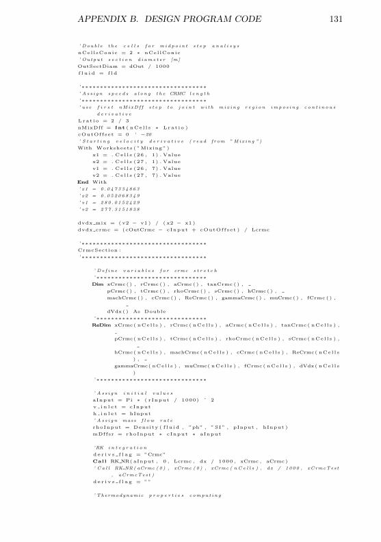
APPENDIX B. DESIGN PROGRAM CODE 131
’ D o u b l e t h e c e l l s f o r m i d p o i n t s t e p a n a l i s y s
nCel l sConic = 2 ∗ nCel lConic
’ O u t p u t s e c t i o n d i am e t e r [m]
OutSectDiam = dOut / 1000
f l u i d = f l d
’ ∗∗∗∗∗∗∗∗∗∗∗∗∗∗∗∗∗∗∗∗∗∗∗∗∗∗∗∗∗∗∗∗∗∗’ A s s i g n s p e e d s a l o n g t h e CRMC l e n g t h
’ ∗∗∗∗∗∗∗∗∗∗∗∗∗∗∗∗∗∗∗∗∗∗∗∗∗∗∗∗∗∗∗∗∗∗’ u s e f i r s t nM i xD f f s t e p t o j o i n t w i t h m i x i n g r e g i o n i m p o s i n g c o n t i n o u s
d e r i v a t i v e
Lrat io = 2 / 3
nMixDff = Int ( nCe l l s ∗ Lrat io )
cOutOffset = 0 ’ −20
’ S t a r t i n g v e l o c i t y d e r i v a t i v e ( r e a d f r om ” M i x i n g ” )
With Worksheets ( ”Mixing” )
x1 = . Ce l l s (26 , 1) . Value
x2 = . Ce l l s (27 , 1) . Value
v1 = . Ce l l s (26 , 7) . Value
v2 = . Ce l l s (27 , 7) . Value
End With
’ x 1 = 0 . 0 4 7 3 3 4 8 6 3
’ x2 = 0 . 0 5 2 0 6 8 3 4 9
’ v1 = 2 8 0 . 0 1 5 2 4 2 9
’ v2 = 2 7 7 . 3 1 5 1 8 3 8
dvdx mix = ( v2 − v1 ) / ( x2 − x1 )
dvdx crmc = (cOutCrmc − cInput + cOutOffset ) / Lcrmc
’ ∗∗∗∗∗∗∗∗∗∗∗∗∗∗∗∗∗∗∗∗∗∗∗∗∗∗∗∗∗∗∗∗∗∗CrmcSection :
’ ∗∗∗∗∗∗∗∗∗∗∗∗∗∗∗∗∗∗∗∗∗∗∗∗∗∗∗∗∗∗∗∗∗∗
’ D e f i n e v a r i a b l e s f o r crmc s t r e t c h
’ ∗∗∗∗∗∗∗∗∗∗∗∗∗∗∗∗∗∗∗∗∗∗∗∗∗∗∗∗∗∗Dim xCrmc ( ) , rCrmc ( ) , aCrmc ( ) , tanCrmc ( ) ,
pCrmc ( ) , tCrmc ( ) , rhoCrmc ( ) , sCrmc ( ) , hCrmc ( ) ,
machCrmc ( ) , cCrmc ( ) , ReCrmc ( ) , gammaCrmc( ) , muCrmc( ) , fCrmc ( ) ,
dVdx ( ) As Double
’ ∗∗∗∗∗∗∗∗∗∗∗∗∗∗∗∗∗∗∗∗∗∗∗∗∗∗∗∗∗∗ReDim xCrmc( nCe l l s ) , rCrmc ( nCe l l s ) , aCrmc( nCe l l s ) , tanCrmc ( nCe l l s ) ,
pCrmc( nCe l l s ) , tCrmc ( nCe l l s ) , rhoCrmc ( nCe l l s ) , sCrmc( nCe l l s ) ,
hCrmc( nCe l l s ) , machCrmc( nCe l l s ) , cCrmc( nCe l l s ) , ReCrmc( nCe l l s
) ,
gammaCrmc( nCe l l s ) , muCrmc( nCe l l s ) , fCrmc ( nCe l l s ) , dVdx( nCe l l s
)
’ ∗∗∗∗∗∗∗∗∗∗∗∗∗∗∗∗∗∗∗∗∗∗∗∗∗∗∗∗∗∗
’ A s s i g n i n i t i a l v a l u e s
aInput = Pi ∗ ( rInput / 1000) ˆ 2
v i n l e t = cInput
h i n l e t = hInput
’ A s s i g n mass f l o w r a t e
rhoInput = Density ( f l u i d , ”ph” , ”SI ” , pInput , hInput )
mDffsr = rhoInput ∗ cInput ∗ aInput
’RK i n t e g r a t i o n
d e r i v s f l a g = ”Crmc”
Call RK NR( aInput , 0 , Lcrmc , dx / 1000 , xCrmc , aCrmc)
’ C a l l RK NR( aCrmc ( 0 ) , xCrmc ( 0 ) , xCrmc ( n C e l l s ) , d x / 1 0 0 0 , xCrmcTes t
, aCrmcTes t )
d e r i v s f l a g = ””
’ The rmodynamic p r o p e r t i e s c omp u t i n g
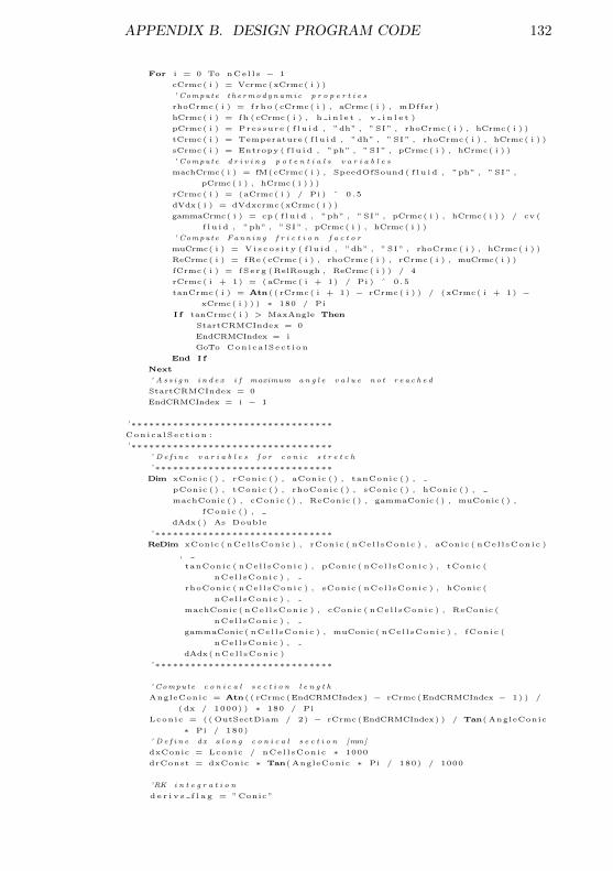
APPENDIX B. DESIGN PROGRAM CODE 132
For i = 0 To nCe l l s − 1
cCrmc( i ) = Vcrmc(xCrmc( i ) )
’ Compute t h e rmo d y n am i c p r o p e r t i e s
rhoCrmc ( i ) = frho (cCrmc( i ) , aCrmc( i ) , mDffsr )
hCrmc( i ) = fh (cCrmc( i ) , h i n l e t , v i n l e t )
pCrmc( i ) = Pressure ( f l u i d , ”dh” , ”SI ” , rhoCrmc ( i ) , hCrmc( i ) )
tCrmc ( i ) = Temperature ( f l u i d , ”dh” , ”SI ” , rhoCrmc ( i ) , hCrmc( i ) )
sCrmc( i ) = Entropy ( f l u i d , ”ph” , ”SI ” , pCrmc( i ) , hCrmc( i ) )
’ Compute d r i v i n g p o t e n t i a l s v a r i a b l e s
machCrmc( i ) = fM(cCrmc( i ) , SpeedOfSound ( f l u i d , ”ph” , ”SI ” ,
pCrmc( i ) , hCrmc( i ) ) )
rCrmc ( i ) = (aCrmc( i ) / Pi ) ˆ 0 .5
dVdx( i ) = dVdxcrmc(xCrmc( i ) )
gammaCrmc( i ) = cp ( f l u i d , ”ph” , ”SI ” , pCrmc( i ) , hCrmc( i ) ) / cv (
f l u i d , ”ph” , ”SI ” , pCrmc( i ) , hCrmc( i ) )
’ Compute Fann i n g f r i c t i o n f a c t o r
muCrmc( i ) = Vi s co s i t y ( f l u i d , ”dh” , ”SI ” , rhoCrmc ( i ) , hCrmc( i ) )
ReCrmc( i ) = fRe (cCrmc( i ) , rhoCrmc ( i ) , rCrmc ( i ) , muCrmc( i ) )
fCrmc ( i ) = fSerg (RelRough , ReCrmc( i ) ) / 4
rCrmc ( i + 1) = (aCrmc( i + 1) / Pi ) ˆ 0 .5
tanCrmc ( i ) = Atn( ( rCrmc ( i + 1) − rCrmc ( i ) ) / (xCrmc( i + 1) −xCrmc( i ) ) ) ∗ 180 / Pi
I f tanCrmc ( i ) > MaxAngle Then
StartCRMCIndex = 0
EndCRMCIndex = i
GoTo Conica lSect ion
End I f
Next
’ A s s i g n i n d e x i f maximum a n g l e v a l u e n o t r e a c h e d
StartCRMCIndex = 0
EndCRMCIndex = i − 1
’ ∗∗∗∗∗∗∗∗∗∗∗∗∗∗∗∗∗∗∗∗∗∗∗∗∗∗∗∗∗∗∗∗∗∗Conica lSect ion :
’ ∗∗∗∗∗∗∗∗∗∗∗∗∗∗∗∗∗∗∗∗∗∗∗∗∗∗∗∗∗∗∗∗∗∗’ D e f i n e v a r i a b l e s f o r c o n i c s t r e t c h
’ ∗∗∗∗∗∗∗∗∗∗∗∗∗∗∗∗∗∗∗∗∗∗∗∗∗∗∗∗∗∗Dim xConic ( ) , rConic ( ) , aConic ( ) , tanConic ( ) ,
pConic ( ) , tConic ( ) , rhoConic ( ) , sConic ( ) , hConic ( ) ,
machConic ( ) , cConic ( ) , ReConic ( ) , gammaConic ( ) , muConic ( ) ,
fConic ( ) ,
dAdx ( ) As Double
’ ∗∗∗∗∗∗∗∗∗∗∗∗∗∗∗∗∗∗∗∗∗∗∗∗∗∗∗∗∗∗ReDim xConic ( nCel l sConic ) , rConic ( nCel l sConic ) , aConic ( nCel l sConic )
,
tanConic ( nCel l sConic ) , pConic ( nCel l sConic ) , tConic (
nCel l sConic ) ,
rhoConic ( nCel l sConic ) , sConic ( nCel l sConic ) , hConic (
nCel l sConic ) ,
machConic ( nCel l sConic ) , cConic ( nCel l sConic ) , ReConic (
nCel l sConic ) ,
gammaConic ( nCel l sConic ) , muConic ( nCel l sConic ) , fConic (
nCel l sConic ) ,
dAdx( nCel l sConic )
’ ∗∗∗∗∗∗∗∗∗∗∗∗∗∗∗∗∗∗∗∗∗∗∗∗∗∗∗∗∗∗
’ Compute c o n i c a l s e c t i o n l e n g t h
AngleConic = Atn( ( rCrmc (EndCRMCIndex) − rCrmc (EndCRMCIndex − 1) ) /
(dx / 1000) ) ∗ 180 / Pi
Lconic = ( ( OutSectDiam / 2) − rCrmc (EndCRMCIndex) ) / Tan( AngleConic
∗ Pi / 180)
’ D e f i n e dx a l o n g c o n i c a l s e c t i o n [mm]
dxConic = Lconic / nCel l sConic ∗ 1000
drConst = dxConic ∗ Tan( AngleConic ∗ Pi / 180) / 1000
’RK i n t e g r a t i o n
d e r i v s f l a g = ”Conic”
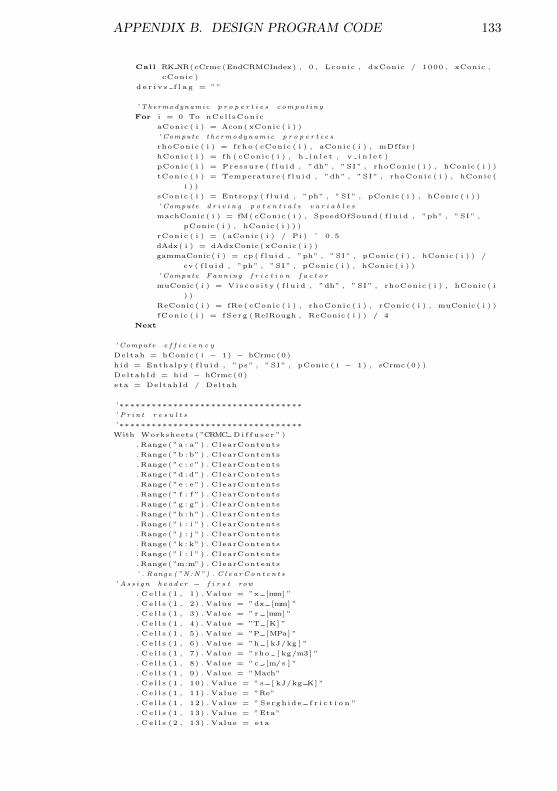
APPENDIX B. DESIGN PROGRAM CODE 133
Call RK NR(cCrmc(EndCRMCIndex) , 0 , Lconic , dxConic / 1000 , xConic ,
cConic )
d e r i v s f l a g = ””
’ The rmodynamic p r o p e r t i e s c omp u t i n g
For i = 0 To nCel l sConic
aConic ( i ) = Acon( xConic ( i ) )
’ Compute t h e rmo d y n am i c p r o p e r t i e s
rhoConic ( i ) = f rho ( cConic ( i ) , aConic ( i ) , mDffsr )
hConic ( i ) = fh ( cConic ( i ) , h i n l e t , v i n l e t )
pConic ( i ) = Pressure ( f l u i d , ”dh” , ”SI ” , rhoConic ( i ) , hConic ( i ) )
tConic ( i ) = Temperature ( f l u i d , ”dh” , ”SI ” , rhoConic ( i ) , hConic (
i ) )
sConic ( i ) = Entropy ( f l u i d , ”ph” , ”SI ” , pConic ( i ) , hConic ( i ) )
’ Compute d r i v i n g p o t e n t i a l s v a r i a b l e s
machConic ( i ) = fM( cConic ( i ) , SpeedOfSound ( f l u i d , ”ph” , ”SI ” ,
pConic ( i ) , hConic ( i ) ) )
rConic ( i ) = ( aConic ( i ) / Pi ) ˆ 0 .5
dAdx( i ) = dAdxConic ( xConic ( i ) )
gammaConic ( i ) = cp ( f l u i d , ”ph” , ”SI ” , pConic ( i ) , hConic ( i ) ) /
cv ( f l u i d , ”ph” , ”SI ” , pConic ( i ) , hConic ( i ) )
’ Compute Fann i n g f r i c t i o n f a c t o r
muConic ( i ) = V i s co s i t y ( f l u i d , ”dh” , ”SI ” , rhoConic ( i ) , hConic ( i
) )
ReConic ( i ) = fRe ( cConic ( i ) , rhoConic ( i ) , rConic ( i ) , muConic ( i ) )
fConic ( i ) = fSerg (RelRough , ReConic ( i ) ) / 4
Next
’ Compute e f f i c i e n c y
Deltah = hConic ( i − 1) − hCrmc(0)
hid = Enthalpy ( f l u i d , ”ps” , ”SI ” , pConic ( i − 1) , sCrmc (0) )
DeltahId = hid − hCrmc(0)
eta = DeltahId / Deltah
’ ∗∗∗∗∗∗∗∗∗∗∗∗∗∗∗∗∗∗∗∗∗∗∗∗∗∗∗∗∗∗∗∗∗∗’ P r i n t r e s u l t s
’ ∗∗∗∗∗∗∗∗∗∗∗∗∗∗∗∗∗∗∗∗∗∗∗∗∗∗∗∗∗∗∗∗∗∗With Worksheets ( ”CRMC Di f f u s e r ” )
. Range ( ”a : a” ) . ClearContents
. Range ( ”b : b” ) . ClearContents
. Range ( ”c : c” ) . ClearContents
. Range ( ”d : d” ) . ClearContents
. Range ( ”e : e” ) . ClearContents
. Range ( ” f : f ” ) . ClearContents
. Range ( ”g : g” ) . ClearContents
. Range ( ”h : h” ) . ClearContents
. Range ( ” i : i ” ) . ClearContents
. Range ( ” j : j ” ) . ClearContents
. Range ( ”k : k” ) . ClearContents
. Range ( ” l : l ” ) . ClearContents
. Range ( ”m:m” ) . ClearContents
’ . Range ( ”N :N” ) . C l e a r C o n t e n t s
’ A s s i g n h e a d e r − f i r s t row
. C e l l s (1 , 1) . Value = ”x [mm] ”
. Ce l l s (1 , 2) . Value = ”dx [mm] ”
. Ce l l s (1 , 3) . Value = ” r [mm] ”
. Ce l l s (1 , 4) . Value = ”T [K] ”
. Ce l l s (1 , 5) . Value = ”P [MPa] ”
. Ce l l s (1 , 6) . Value = ”h [ kJ/kg ] ”
. Ce l l s (1 , 7) . Value = ”rho [ kg/m3] ”
. Ce l l s (1 , 8) . Value = ”c [m/ s ] ”
. Ce l l s (1 , 9) . Value = ”Mach”
. Ce l l s (1 , 10) . Value = ” s [ kJ/kg K] ”
. Ce l l s (1 , 11) . Value = ”Re”
. Ce l l s (1 , 12) . Value = ” Serghide f r i c t i o n ”
. Ce l l s (1 , 13) . Value = ”Eta”
. Ce l l s (2 , 13) . Value = eta
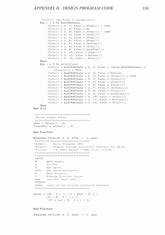
APPENDIX B. DESIGN PROGRAM CODE 134
. C e l l s (1 , 14) . Value = ”dv/dx [1/ s ] ”
For i = 0 To EndCRMCIndex
. Ce l l s ( i + 2 , 1) . Value = xCrmc( i ) ∗ 1000
. Ce l l s ( i + 2 , 2) . Value = dx
. Ce l l s ( i + 2 , 3) . Value = rCrmc( i ) ∗ 1000
. Ce l l s ( i + 2 , 4) . Value = tCrmc( i )
. Ce l l s ( i + 2 , 5) . Value = pCrmc( i )
. Ce l l s ( i + 2 , 6) . Value = hCrmc( i )
. Ce l l s ( i + 2 , 7) . Value = rhoCrmc ( i )
. Ce l l s ( i + 2 , 8) . Value = cCrmc( i )
. Ce l l s ( i + 2 , 9) . Value = machCrmc( i )
. Ce l l s ( i + 2 , 10) . Value = sCrmc( i )
. Ce l l s ( i + 2 , 11) . Value = ReCrmc( i )
. Ce l l s ( i + 2 , 12) . Value = fCrmc ( i )
Next
For i = 0 To nCel l sConic
. Ce l l s ( i + EndCRMCIndex + 2 , 1) . Value = (xCrmc(EndCRMCIndex) +
xConic ( i ) ) ∗ 1000
. Ce l l s ( i + EndCRMCIndex + 2 , 2) . Value = dxConic
. Ce l l s ( i + EndCRMCIndex + 2 , 3) . Value = rConic ( i ) ∗ 1000
. Ce l l s ( i + EndCRMCIndex + 2 , 4) . Value = tConic ( i )
. Ce l l s ( i + EndCRMCIndex + 2 , 5) . Value = pConic ( i )
. Ce l l s ( i + EndCRMCIndex + 2 , 6) . Value = hConic ( i )
. Ce l l s ( i + EndCRMCIndex + 2 , 7) . Value = rhoConic ( i )
. Ce l l s ( i + EndCRMCIndex + 2 , 8) . Value = cConic ( i )
. Ce l l s ( i + EndCRMCIndex + 2 , 9) . Value = machConic ( i )
. Ce l l s ( i + EndCRMCIndex + 2 , 10) . Value = sConic ( i )
. Ce l l s ( i + EndCRMCIndex + 2 , 11) . Value = ReConic ( i )
. Ce l l s ( i + EndCRMCIndex + 2 , 12) . Value = fConic ( i )
Next
End With
’ ∗∗∗∗∗∗∗∗∗∗∗∗∗∗∗∗∗∗∗∗∗∗∗∗∗∗∗∗∗∗∗∗∗∗’ A s s i g n o u t p u t v a l u e s
’ ∗∗∗∗∗∗∗∗∗∗∗∗∗∗∗∗∗∗∗∗∗∗∗∗∗∗∗∗∗∗∗∗∗∗hOut = hConic ( i − 2)
CrmcDffsr = pConic ( i − 2)
End Function
Function fdAdx (M, A, V, dVdx , r , f , gam)
’ ∗∗∗∗∗∗∗∗∗∗∗∗∗∗∗∗∗∗∗∗∗∗∗∗∗∗∗∗∗∗∗∗∗∗’ Au t h o r : Da r i o P a g a n i n i (DP)
’ P u r p o s e : Compute d r i v i n g p o t e n t i a l s f u n c t i o n f o r dA/ dx
’ V e r s i o n : 1 . 0 ( 2 0 1 1 / 0 6 / 2 3 ) − (DP) f i r t s v e r s i o n
’ ∗∗∗∗∗∗∗∗∗∗∗∗∗∗∗∗∗∗∗∗∗∗∗∗∗∗∗∗∗∗∗∗∗∗’ ∗∗∗∗∗∗∗∗∗∗∗∗∗∗∗∗∗∗∗∗∗∗∗∗∗∗∗∗∗∗∗∗∗∗’ INPUT
’M Mach number
’A S e c t i o n
’V Gas s p e e d
’ dVdx Gas s p e e d d e r i v a t i v e
’D Duc t d i a m e t e r
’ f F ann i n g f r i c t i o n f a c t o r
’ gam s p e c i f i c h e a t r a t i o
’OUTPUT
’ f dAd x v a l u e o f t h e d r i v i n g p o t e n t i a l f u n c t i o n
’ ∗∗∗∗∗∗∗∗∗∗∗∗∗∗∗∗∗∗∗∗∗∗∗∗∗∗∗∗∗∗∗∗∗∗
fdAdx = ((M ˆ 2 − 1) ∗ A ∗ dVdx / V) +
( Pi ∗ M ˆ 2 ∗ r ∗ f )
’ ( P i ∗ gam ∗ M ˆ 2 ∗ r ∗ f )
End Function
Function fdVdx (M, A, V, dAdx , r , f , gam)
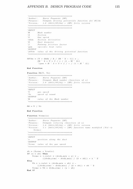
APPENDIX B. DESIGN PROGRAM CODE 135
’ ∗∗∗∗∗∗∗∗∗∗∗∗∗∗∗∗∗∗∗∗∗∗∗∗∗∗∗∗∗∗∗∗∗∗’ Au t h o r : Da r i o P a g a n i n i (DP)
’ P u r p o s e : Compute d r i v i n g p o t e n t i a l s f u n c t i o n f o r dV/ dx
’ V e r s i o n : 1 . 0 ( 2 0 1 1 / 0 7 / 0 4 ) − (DP) f i r t s v e r s i o n
’ ∗∗∗∗∗∗∗∗∗∗∗∗∗∗∗∗∗∗∗∗∗∗∗∗∗∗∗∗∗∗∗∗∗∗’ ∗∗∗∗∗∗∗∗∗∗∗∗∗∗∗∗∗∗∗∗∗∗∗∗∗∗∗∗∗∗∗∗∗∗’ INPUT
’M Mach number
’A S e c t i o n
’V Gas s p e e d
’ dAdx S e c t i o n d e r i v a t i v e
’D Duc t d i a m e t e r
’ f F ann i n g f r i c t i o n f a c t o r
’ gam s p e c i f i c h e a t r a t i o
’OUTPUT
’ f dVd x v a l u e o f t h e d r i v i n g p o t e n t i a l f u n c t i o n
’ ∗∗∗∗∗∗∗∗∗∗∗∗∗∗∗∗∗∗∗∗∗∗∗∗∗∗∗∗∗∗∗∗∗∗
fdVdx = (V ∗ dAdx / A / (M ˆ 2 − 1) ) +
(M ˆ 2 ∗ V ∗ f / r / (1 − M ˆ 2) )
’ ( gam ∗ M ˆ 2 ∗ V ∗ f / r / ( 1 − M ˆ 2 ) )
End Function
Function fM(V, Vs)
’ ∗∗∗∗∗∗∗∗∗∗∗∗∗∗∗∗∗∗∗∗∗∗∗∗∗∗∗∗∗∗∗∗∗∗’ Au t h o r : Da r i o P a g a n i n i (DP)
’ P u r p o s e : Compute Mach number ( f u n c t i o n o f x )
’ V e r s i o n : 1 . 0 ( 2 0 1 1 / 0 7 / 0 4 ) − (DP) f i r t s v e r s i o n
’ ∗∗∗∗∗∗∗∗∗∗∗∗∗∗∗∗∗∗∗∗∗∗∗∗∗∗∗∗∗∗∗∗∗∗’ ∗∗∗∗∗∗∗∗∗∗∗∗∗∗∗∗∗∗∗∗∗∗∗∗∗∗∗∗∗∗∗∗∗∗’ INPUT
’V g a s s p e e d
’ Vs s p e e d o f s o und
’OUTPUT
’M v a l u e o f t h e Mach number
’ ∗∗∗∗∗∗∗∗∗∗∗∗∗∗∗∗∗∗∗∗∗∗∗∗∗∗∗∗∗∗∗∗∗∗
fM = V / Vs
End Function
Function Vcrmc(x )
’ ∗∗∗∗∗∗∗∗∗∗∗∗∗∗∗∗∗∗∗∗∗∗∗∗∗∗∗∗∗∗∗∗∗∗’ Au t h o r : Da r i o P a g a n i n i (DP)
’ P u r p o s e : Compute v e l o c i t y ( f u n c t i o n o f x )
’ V e r s i o n : 1 . 0 ( 2 0 1 1 / 0 7 / 0 4 ) − (DP) f i r t s v e r s i o n
’ V e r s i o n : 1 . 1 ( 2 0 1 1 / 0 7 / 0 5 ) − (DP) f u n c t i o n name m o d i f i e d ( Ve l −>Vcrmc )
’ ∗∗∗∗∗∗∗∗∗∗∗∗∗∗∗∗∗∗∗∗∗∗∗∗∗∗∗∗∗∗∗∗∗∗’ ∗∗∗∗∗∗∗∗∗∗∗∗∗∗∗∗∗∗∗∗∗∗∗∗∗∗∗∗∗∗∗∗∗∗’ INPUT
’ x p o s i t i o n a l o n g t h e d u c t
’OUTPUT
’ Vcrmc v a l u e o f t h e g a s s p e e d
’ ∗∗∗∗∗∗∗∗∗∗∗∗∗∗∗∗∗∗∗∗∗∗∗∗∗∗∗∗∗∗∗∗∗∗
xb = (Lcrmc ∗ Lrat io )
I f (x < xb ) Then
Vcrmc = v i n l e t + ( dvdx mix ∗ x) +
(( dvdx crmc − dvdx mix ) / (2 ∗ xb ) ) ∗ x ˆ 2
Else
Vb = v i n l e t + ( dvdx mix ∗ xb ) +
(( dvdx crmc − dvdx mix ) / (2 ∗ xb ) ) ∗ xb ˆ 2
Vcrmc = Vb + dvdx crmc ∗ (x − xb )
End I f
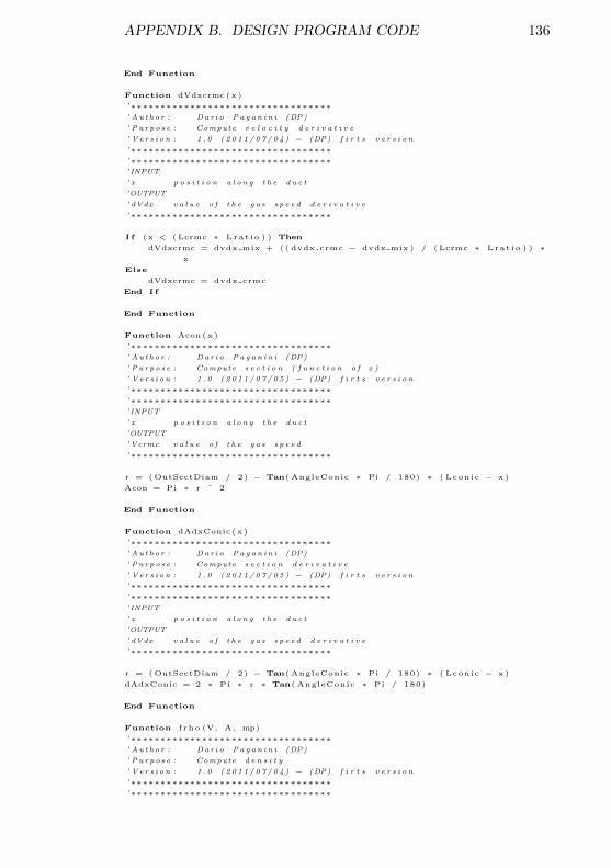
APPENDIX B. DESIGN PROGRAM CODE 136
End Function
Function dVdxcrmc(x )
’ ∗∗∗∗∗∗∗∗∗∗∗∗∗∗∗∗∗∗∗∗∗∗∗∗∗∗∗∗∗∗∗∗∗∗’ Au t h o r : Da r i o P a g a n i n i (DP)
’ P u r p o s e : Compute v e l o c i t y d e r i v a t i v e
’ V e r s i o n : 1 . 0 ( 2 0 1 1 / 0 7 / 0 4 ) − (DP) f i r t s v e r s i o n
’ ∗∗∗∗∗∗∗∗∗∗∗∗∗∗∗∗∗∗∗∗∗∗∗∗∗∗∗∗∗∗∗∗∗∗’ ∗∗∗∗∗∗∗∗∗∗∗∗∗∗∗∗∗∗∗∗∗∗∗∗∗∗∗∗∗∗∗∗∗∗’ INPUT
’ x p o s i t i o n a l o n g t h e d u c t
’OUTPUT
’ dVdx v a l u e o f t h e g a s s p e e d d e r i v a t i v e
’ ∗∗∗∗∗∗∗∗∗∗∗∗∗∗∗∗∗∗∗∗∗∗∗∗∗∗∗∗∗∗∗∗∗∗
I f (x < (Lcrmc ∗ Lrat io ) ) Then
dVdxcrmc = dvdx mix + (( dvdx crmc − dvdx mix ) / (Lcrmc ∗ Lrat io ) ) ∗x
Else
dVdxcrmc = dvdx crmc
End I f
End Function
Function Acon(x )
’ ∗∗∗∗∗∗∗∗∗∗∗∗∗∗∗∗∗∗∗∗∗∗∗∗∗∗∗∗∗∗∗∗∗∗’ Au t h o r : Da r i o P a g a n i n i (DP)
’ P u r p o s e : Compute s e c t i o n ( f u n c t i o n o f x )
’ V e r s i o n : 1 . 0 ( 2 0 1 1 / 0 7 / 0 5 ) − (DP) f i r t s v e r s i o n
’ ∗∗∗∗∗∗∗∗∗∗∗∗∗∗∗∗∗∗∗∗∗∗∗∗∗∗∗∗∗∗∗∗∗∗’ ∗∗∗∗∗∗∗∗∗∗∗∗∗∗∗∗∗∗∗∗∗∗∗∗∗∗∗∗∗∗∗∗∗∗’ INPUT
’ x p o s i t i o n a l o n g t h e d u c t
’OUTPUT
’ Vcrmc v a l u e o f t h e g a s s p e e d
’ ∗∗∗∗∗∗∗∗∗∗∗∗∗∗∗∗∗∗∗∗∗∗∗∗∗∗∗∗∗∗∗∗∗∗
r = (OutSectDiam / 2) − Tan( AngleConic ∗ Pi / 180) ∗ ( Lconic − x)
Acon = Pi ∗ r ˆ 2
End Function
Function dAdxConic (x )
’ ∗∗∗∗∗∗∗∗∗∗∗∗∗∗∗∗∗∗∗∗∗∗∗∗∗∗∗∗∗∗∗∗∗∗’ Au t h o r : Da r i o P a g a n i n i (DP)
’ P u r p o s e : Compute s e c t i o n d e r i v a t i v e
’ V e r s i o n : 1 . 0 ( 2 0 1 1 / 0 7 / 0 5 ) − (DP) f i r t s v e r s i o n
’ ∗∗∗∗∗∗∗∗∗∗∗∗∗∗∗∗∗∗∗∗∗∗∗∗∗∗∗∗∗∗∗∗∗∗’ ∗∗∗∗∗∗∗∗∗∗∗∗∗∗∗∗∗∗∗∗∗∗∗∗∗∗∗∗∗∗∗∗∗∗’ INPUT
’ x p o s i t i o n a l o n g t h e d u c t
’OUTPUT
’ dVdx v a l u e o f t h e g a s s p e e d d e r i v a t i v e
’ ∗∗∗∗∗∗∗∗∗∗∗∗∗∗∗∗∗∗∗∗∗∗∗∗∗∗∗∗∗∗∗∗∗∗
r = (OutSectDiam / 2) − Tan( AngleConic ∗ Pi / 180) ∗ ( Lconic − x)
dAdxConic = 2 ∗ Pi ∗ r ∗ Tan( AngleConic ∗ Pi / 180)
End Function
Function f rho (V, A, mp)
’ ∗∗∗∗∗∗∗∗∗∗∗∗∗∗∗∗∗∗∗∗∗∗∗∗∗∗∗∗∗∗∗∗∗∗’ Au t h o r : Da r i o P a g a n i n i (DP)
’ P u r p o s e : Compute d e n s i t y
’ V e r s i o n : 1 . 0 ( 2 0 1 1 / 0 7 / 0 4 ) − (DP) f i r t s v e r s i o n
’ ∗∗∗∗∗∗∗∗∗∗∗∗∗∗∗∗∗∗∗∗∗∗∗∗∗∗∗∗∗∗∗∗∗∗’ ∗∗∗∗∗∗∗∗∗∗∗∗∗∗∗∗∗∗∗∗∗∗∗∗∗∗∗∗∗∗∗∗∗∗
APPENDIX B. DESIGN PROGRAM CODE 137
’ INPUT
’V g a s s p e e d
’A s e c t i o n
’mp mass f l o w r a t e
’OUTPUT
’ r h o g a s d e n s i t y
’ ∗∗∗∗∗∗∗∗∗∗∗∗∗∗∗∗∗∗∗∗∗∗∗∗∗∗∗∗∗∗∗∗∗∗
f rho = mp / V / A
End Function
Function fh (V, h i n l e t , v i n l e t )
’ ∗∗∗∗∗∗∗∗∗∗∗∗∗∗∗∗∗∗∗∗∗∗∗∗∗∗∗∗∗∗∗∗∗∗’ Au t h o r : Da r i o P a g a n i n i (DP)
’ P u r p o s e : Compute t o t a l e n t h a l p y
’ V e r s i o n : 1 . 0 ( 2 0 1 1 / 0 7 / 0 4 ) − (DP) f i r t s v e r s i o n
’ ∗∗∗∗∗∗∗∗∗∗∗∗∗∗∗∗∗∗∗∗∗∗∗∗∗∗∗∗∗∗∗∗∗∗’ ∗∗∗∗∗∗∗∗∗∗∗∗∗∗∗∗∗∗∗∗∗∗∗∗∗∗∗∗∗∗∗∗∗∗’ INPUT
’V g a s s p e e d
’ h i n i t d u c t i n l e t t o t a l e n t h a l p y
’ v i n l e t d u c t g a s s p e e d a t i n l e t s e c t i o n
’OUTPUT
’ h g a s t o t a l e n t h a l p y
’ ∗∗∗∗∗∗∗∗∗∗∗∗∗∗∗∗∗∗∗∗∗∗∗∗∗∗∗∗∗∗∗∗∗∗
fh = h i n l e t + ( v i n l e t ˆ 2 − V ˆ 2) / 2000
End Function
Function fRe (V, rho , r , mu)
’ ∗∗∗∗∗∗∗∗∗∗∗∗∗∗∗∗∗∗∗∗∗∗∗∗∗∗∗∗∗∗∗∗∗∗’ Au t h o r : Da r i o P a g a n i n i (DP)
’ P u r p o s e : Compute R e y n o l d s
’ V e r s i o n : 1 . 0 ( 2 0 1 1 / 0 7 / 0 4 ) − (DP) f i r t s v e r s i o n
’ ∗∗∗∗∗∗∗∗∗∗∗∗∗∗∗∗∗∗∗∗∗∗∗∗∗∗∗∗∗∗∗∗∗∗’ ∗∗∗∗∗∗∗∗∗∗∗∗∗∗∗∗∗∗∗∗∗∗∗∗∗∗∗∗∗∗∗∗∗∗’ INPUT
’V g a s s p e e d
’ r h o d e n s i t y
’D d u c t d i a m e t e r
’mu v i s c o s i t y
’OUTPUT
’ Re R e y n o l d s number
’ ∗∗∗∗∗∗∗∗∗∗∗∗∗∗∗∗∗∗∗∗∗∗∗∗∗∗∗∗∗∗∗∗∗∗
fRe = 10 ˆ 6 ∗ rho ∗ V ∗ 2 ∗ r / mu
End Function
’ ∗∗∗∗∗∗∗∗∗∗∗∗∗∗∗∗∗∗∗∗∗∗∗∗∗∗∗∗∗∗∗∗∗∗’∗∗∗ Modu l e h e a d e r ∗∗∗’ ∗∗∗∗∗∗∗∗∗∗∗∗∗∗∗∗∗∗∗∗∗∗∗∗∗∗∗∗∗∗∗∗∗∗’ A u t h o r s : A d r i a n o M i l a z z o (AM) , Da r i o P a g a n i n i (DP)
’ C o n t e n t s : Runge−Ku t t a i n t e g r a t i o n s u b r o u t i n e s
’ S u b o u t i n e s and f u n c t i o n s i n c l u d e d :
’−−−−−−−−−−−−−−−−−−−−−−−−−−−−−−−−−−’ Name V e r s i o n
’−−−−−−−−−−−−−−−−−−−−−−−−−−−−−−−−−−’RK NR 2 . 1 ( 2 0 1 1 / 0 7 / 0 4 )
’ RK4 NR 1 . 0 ( 2 0 1 1 / 0 4 / 2 1 )
’ d e r i v s 2 . 0 ( 2 0 1 1 / 0 7 / 0 5 )
’ ∗∗∗∗∗∗∗∗∗∗∗∗∗∗∗∗∗∗∗∗∗∗∗∗∗∗∗∗∗∗∗∗∗∗’ ∗∗∗∗∗∗∗∗∗∗∗∗∗∗∗∗∗∗∗∗∗∗∗∗∗∗∗∗∗∗∗∗∗∗
Sub RK NR( vstart , x1 , x2 , h , xx , y )
APPENDIX B. DESIGN PROGRAM CODE 138
’ ∗∗∗∗∗∗∗∗∗∗∗∗∗∗∗∗∗∗∗∗∗∗∗∗∗∗∗∗∗∗∗∗∗∗’ Au t h o r : Da r i o P a g a n i n i (DP)
’ P u r p o s e : Runge−Ku t t a i n t e g r a t i o n d r i v e r
’ V e r s i o n : 1 . 0 ( 2 0 1 1 / 0 4 / 2 3 ) − (DP) f i r s t v e r s i o n
’ V e r s i o n : 2 . 0 ( 2 0 1 1 / 0 5 / 1 2 ) − (DP) i n p u t p a r am e t e r c h a n g e : h i n s t e a d
o f n s t e p ,
’ n s t e p i s c ompu t e d u s i n g h
’ V e r s i o n : 2 . 1 ( 2 0 1 1 / 0 7 / 0 4 ) − (DP) c h a n g e V v a r i a b l e i n RK V
’ V e r s i o n : 2 . 2 ( 2 0 1 1 / 0 7 / 0 8 ) − (DP) n s t e p c ompu t e d u s i n g r o und f u n c t i o n
i n s e a d
’ i n t f u n c t i o n
’ ∗∗∗∗∗∗∗∗∗∗∗∗∗∗∗∗∗∗∗∗∗∗∗∗∗∗∗∗∗∗∗∗∗∗’ ∗∗∗∗∗∗∗∗∗∗∗∗∗∗∗∗∗∗∗∗∗∗∗∗∗∗∗∗∗∗∗∗∗∗’ Runge−Ku t t a i n t e g r a t i o n f r om ” Nume r i c a l R e c i p e s ” W i l l i am H . P r e s s e t
a l .
’ ∗∗∗∗∗∗∗∗∗∗∗∗∗∗∗∗∗∗∗∗∗∗∗∗∗∗∗∗∗∗∗∗∗∗’ ∗∗∗∗∗∗∗∗∗∗∗∗∗∗∗∗∗∗∗∗∗∗∗∗∗∗∗∗∗∗∗∗∗∗’ INPUT
’ v s t a r t
’ x1 s t a r t p o s i t i o n
’ x2 end p o s i t i o n
’ h i n t e g r a t i o n s t e p l e n g t h
’OUTPUT
’ x x a r r a y o f t h e o u t p u t a b s c i s s a s
’ y a r r a y o f t h e i n t e g r a t e d v a l u e s
’ ∗∗∗∗∗∗∗∗∗∗∗∗∗∗∗∗∗∗∗∗∗∗∗∗∗∗∗∗∗∗∗∗∗∗
RK V = vs ta r t
y (0) = RK V
xx (0) = x1
x = x1
nstep = Round(Abs( ( x2 − x1 ) / h) )
For k = 1 To nstep
Call de r i v s (x , RK V, Dv)
Call RK4 NR(RK V, Dv, x , h , RK V)
I f (x + h = x) Then MsgBox ( ”Error in s t e p s i z e ” )
x = x + h
xx (k ) = x
y(k ) = RK V
Next
End Sub
Sub RK4 NR(y , dydx , x , h , yout )
’ ∗∗∗∗∗∗∗∗∗∗∗∗∗∗∗∗∗∗∗∗∗∗∗∗∗∗∗∗∗∗∗∗∗∗’ Au t h o r : Da r i o P a g a n i n i (DP)
’ P u r p o s e : Runge−Ku t t a i n t e g r a t i o n s t e p
’ V e r s i o n : 1 . 0 ( 2 0 1 1 / 0 4 / 2 1 ) − (DP) f i r s t v e r s i o n
’ ∗∗∗∗∗∗∗∗∗∗∗∗∗∗∗∗∗∗∗∗∗∗∗∗∗∗∗∗∗∗∗∗∗∗’ ∗∗∗∗∗∗∗∗∗∗∗∗∗∗∗∗∗∗∗∗∗∗∗∗∗∗∗∗∗∗∗∗∗∗’ Runge−Ku t t a i n t e g r a t i o n f r om ” Nume r i c a l R e c i p e s ” W i l l i am H . P r e s s e t
a l .
’ ∗∗∗∗∗∗∗∗∗∗∗∗∗∗∗∗∗∗∗∗∗∗∗∗∗∗∗∗∗∗∗∗∗∗’ ∗∗∗∗∗∗∗∗∗∗∗∗∗∗∗∗∗∗∗∗∗∗∗∗∗∗∗∗∗∗∗∗∗∗’ INPUT
’ y f u n c t i o n v a l u e a t x
’ d y d x d e r i v a t i v e s v a l u e a t x
’ x p o s i t i o n
’ h s t e p d im e n s i o n
’ y o u t f u n c t i o n v a l u e a t x+h
’ i a l em e n t i n d e x o f t h e i n t e g r a t e d a r r a y
’OUTPUT
’ ∗∗∗∗∗∗∗∗∗∗∗∗∗∗∗∗∗∗∗∗∗∗∗∗∗∗∗∗∗∗∗∗∗∗
Dim dym, dyt , yt As Double
APPENDIX B. DESIGN PROGRAM CODE 139
hh = h ∗ 0 .5
h6 = h / 6
xh = x + hh
’ F i r s t s t e p
yt = y + hh ∗ dydx
’ S e c on d s t e p
Call de r i v s (xh , yt , dyt )
yt = y + hh ∗ dyt
’ T h i r d s t e p
Call de r i v s (xh , yt , dym)
yt = y + h ∗ dym
dym = dym + dyt
’ F o u r t h s t e p
Call de r i v s (x + h , yt , dyt )
yout = y + h6 ∗ ( dydx + dyt + 2# ∗ dym)
End Sub
Sub de r i v s (x , y , dydx )
’ ∗∗∗∗∗∗∗∗∗∗∗∗∗∗∗∗∗∗∗∗∗∗∗∗∗∗∗∗∗∗∗∗∗∗’ Au t h o r : Da r i o P a g a n i n i (DP)
’ P u r p o s e : Compute d e r i v a t i v e s d y d x a t x
’ V e r s i o n : 1 . 0 ( 2 0 1 1 / 0 4 / 2 1 ) − (DP) f i r s t v e r s i o n
’ V e r s i o n : 2 . 0 ( 2 0 1 1 / 0 7 / 0 5 ) − (DP) m o d i f i e d f o r C rmcD f f s r f u n c t i o n
’ a d d e d f l a g t o s e l e c t d e r i v a t i v e ( u s e d a s p u b l i c
v a r i a b l e )
’ V e r s i o n : 2 . 1 ( 2 0 1 1 / 1 1 / 1 4 ) − (DP) c o r r e c t e d f r i c t i o n f a c t o r f
a s s i g nm e n t
’ ( Fann i n g f r i c t i o n f a c t o r e x p e c t e d , Darcy p a s s e d )
’ ∗∗∗∗∗∗∗∗∗∗∗∗∗∗∗∗∗∗∗∗∗∗∗∗∗∗∗∗∗∗∗∗∗∗’ ∗∗∗∗∗∗∗∗∗∗∗∗∗∗∗∗∗∗∗∗∗∗∗∗∗∗∗∗∗∗∗∗∗∗’ INPUT
’
’OUTPUT
’ ∗∗∗∗∗∗∗∗∗∗∗∗∗∗∗∗∗∗∗∗∗∗∗∗∗∗∗∗∗∗∗∗∗∗
Select Case d e r i v s f l a g
Case ”Crmc”
’ A s s i g n s p e e d and s e c t i o n
A = y
V = Vcrmc(x )
dVdx = dVdxcrmc(x )
’ Compute t h e rmo d y n am i c p r o p e r t i e s
rho = frho (V, A, mDffsr )
h = fh (V, h i n l e t , v i n l e t )
P = Pressure ( f l u i d , ”dh” , ”SI ” , rho , h)
’ Copmpute d r i v i n g p o t e n t i a l s v a r i a b l e s
M = fM(V, SpeedOfSound ( f l u i d , ”ph” , ”SI ” , P, h) )
r = (A / Pi ) ˆ 0 .5
gam = cp ( f l u i d , ”ph” , ”SI ” , P, h) / cv ( f l u i d , ”ph” , ”SI ” , P, h)
’ Compute Fann i n g f r i c t i o n f a c t o r
mu = Vi s co s i t y ( f l u i d , ”dh” , ”SI ” , rho , h)
Re = fRe (V, rho , r , mu)
f = fSerg (RelRough , Re) / 4
’ Compute d r i v i n g p o t e n t i a l s f u n c t i o n
dydx = fdAdx (M, A, V, dVdx , r , f , gam)
Case ”Conic”
’ A s s i g n s p e e d and s e c t i o n
V = y
A = Acon(x )
dAdx = dAdxConic (x )
’ Compute t h e rmo d y n am i c p r o p e r t i e s
rho = frho (V, A, mDffsr )
h = fh (V, h i n l e t , v i n l e t )
APPENDIX B. DESIGN PROGRAM CODE 140
P = Pressure ( f l u i d , ”dh” , ”SI ” , rho , h)
’ Copmpute d r i v i n g p o t e n t i a l s v a r i a b l e s
M = fM(V, SpeedOfSound ( f l u i d , ”ph” , ”SI ” , P, h) )
r = (A / Pi ) ˆ 0 .5
gam = cp ( f l u i d , ”ph” , ”SI ” , P, h) / cv ( f l u i d , ”ph” , ”SI ” , P, h)
’ Compute Fann i n g f r i c t i o n f a c t o r
mu = Vi s co s i t y ( f l u i d , ”dh” , ”SI ” , rho , h)
Re = fRe (V, rho , r , mu)
f = fSerg (RelRough , Re) / 4
’ Compute d r i v i n g p o t e n t i a l s f u n c t i o n
dydx = fdVdx (M, A, V, dAdx , r , f , gam)
Case Else
d e r i v s e r r = 1
der ivs msg = ”Error in d e r i v a t i v e s e l e c t i o n opt ion ”
End Select
End Sub
Function fSe rg (RelRough , ReynoldsNum)
’ F r i c t i o n F a c t o r c a l u l a t e d b y T .K . S e r g h i d e ’ s i m p l e m e n t a t i o n o f
S t e f f e n s o n
’ R e f e r e n c e C h em i c a l E n g i n e e r i n g March 5 , 1984
Dim A As S ing l e
Dim B As S ing l e
Dim c As S ing l e
’ No t e t h a t i n V i s u a l B a s i c ” Log ” s t a n d s f o r N a t u r a l Log
A = −0.86858896 ∗ Log(RelRough / 3 .7 + 12 / ReynoldsNum)
B = −0.86858896 ∗ Log(RelRough / 3 .7 + (2 .51 ∗ A / ReynoldsNum) )
c = −0.86858896 ∗ Log(RelRough / 3 .7 + (2 .51 ∗ B / ReynoldsNum) )
fSe rg = (A − ( (B − A) ˆ 2) / ( c − (2 ∗ B) + A) ) ˆ −2
End Function
Appendix C
Nozzle efficiency code
Attr ibute VB Name = ”Modulo1”
’ ∗∗∗∗∗∗∗∗∗∗∗∗∗∗∗∗∗∗∗∗∗∗∗∗∗∗∗∗∗∗∗∗∗∗’ A u t h o r s : A d r i a n o M i l a z z o (AM) , Da r i o P a g a n i n i (DP)
’ C o n t e n t s : S u b r o u t i n e s t o c ompu t e s u p e r s o n i c n o z z l e ( e v e n t u a l l y w i t h
n o rma l
’ s h o c k wave ) s t a r t i n g a s s i g n i n g i n l e t t o o u t l e t p r e s s u r e
r a t i o
’ S u b o u t i n e s and f u n c t i o n s i n c l u d e d :
’−−−−−−−−−−−−−−−−−−−−−−−−−−−−−−−−−−’ Name V e r s i o n
’−−−−−−−−−−−−−−−−−−−−−−−−−−−−−−−−−−’ NozSim 1 . 6 ( 2 0 1 2 / 1 1 / 1 6 )
’ n o z z l e 3 . 0 ( 2 0 1 1 / 0 5 / 1 2 )
’ n o z z l e P r o p 1 . 1 ( 2 0 1 1 / 0 5 / 1 6 )
’ ShockJump 1 . 1 ( 2 0 1 1 / 0 4 / 0 7 )
’ DmdxSon ic n o t d e f i n e d
’ NozGeoDe f 1 . 0 ( 2 0 1 1 / 0 4 / 2 1 )
’ ∗∗∗∗∗∗∗∗∗∗∗∗∗∗∗∗∗∗∗∗∗∗∗∗∗∗∗∗∗∗∗∗∗∗’ ∗∗∗∗∗∗∗∗∗∗∗∗∗∗∗∗∗∗∗∗∗∗∗∗∗∗∗∗∗∗∗∗∗∗
Public Pi , GAM, PEX, f , ISHOCK, X arr ( ) , XM arr ( ) , PSTAG arr ( ) , PS arr
( ) ,
TSTAG arr ( ) , TS arr ( ) , XMINAREA, NozRin , NozRout , NozRth , NozAlpha ,
NozRf i l l e t , xchange , ychange , dmdxmax , xsp , DXSAVE
Sub NozSim ()
’ ∗∗∗∗∗∗∗∗∗∗∗∗∗∗∗∗∗∗∗∗∗∗∗∗∗∗∗∗∗∗∗∗∗∗’ Au t h o r : Da r i o P a g a n i n i (DP)
’ P u r p o s e : S o l v e n o z z l e f o r d i f f e r e n t b a c k p r e s s u r e v a l u e s
’ V e r s i o n : 1 . 0 ( 2 0 1 1 / 0 4 / 0 6 ) − (DP) f i r s t v e r s i o n
’ V e r s i o n : 1 . 1 ( 2 0 1 1 / 0 4 / 2 1 ) − (DP) a d d e d n o z z l e g e om e t r y d e f i n i t i o n
’ V e r s i o n : 1 . 2 ( 2 0 1 1 / 0 5 / 1 1 ) − (DP) r emov ed X s o n i c s u b r o u t i n e c a l l ( XSP
’ c ompu t e d a n a l i t i c a l l y )
’ V e r s i o n : 1 . 3 ( 2 0 1 1 / 0 5 / 2 0 ) − (DP) r emov ed b u g i n P b s t a r c omp u t i n g
’ V e r s i o n : 1 . 4 ( 2 0 1 1 / 0 6 / 1 6 ) − (DP) a d d e d t h r e s h o l d t o t r e a t a s
i s e n t r o p i c i f
’ f < 0 . 0 0 0 5
’ a d d e d a u t om a t i c v e r s i o n p r i n t i n g on w o r k s h e e t
’ r emov e d u n u s e d c o d e
’ V e r s i o n : 1 . 5 ( 2 0 1 1 / 0 9 / 1 5 ) − (DP) D im e n s i o n a l p r o p e r t i e s i n t r o d u c e d
’ m o d i f i e d NozProp w o r k s h e e t and d a t a r e a d i n g f r om i t
141
APPENDIX C. NOZZLE EFFICIENCY CODE 142
’ V e r s i o n : 1 . 6 ( 2 0 1 2 / 1 1 / 1 6 ) − (DP) Added d e c i m a t i o n on p r i n t e d o u t p u t
d a t a
’ t o r e d u c e e x e c t u i o n t im e
’ ∗∗∗∗∗∗∗∗∗∗∗∗∗∗∗∗∗∗∗∗∗∗∗∗∗∗∗∗∗∗∗∗∗∗’ ∗∗∗∗∗∗∗∗∗∗∗∗∗∗∗∗∗∗∗∗∗∗∗∗∗∗∗∗∗∗∗∗∗∗’ A l g o r i t h m s and r e l a t i o n s a r e g o t f r om B .K . Hodge and K . Ko en i g ”
C om p r e s s i b l e
’ f l u i d d y n am i c s w i t h p e r s o n a l c ompu t e r a p p l i c a t i o n s ”
’ ∗∗∗∗∗∗∗∗∗∗∗∗∗∗∗∗∗∗∗∗∗∗∗∗∗∗∗∗∗∗∗∗∗∗’ ∗∗∗∗∗∗∗∗∗∗∗∗∗∗∗∗∗∗∗∗∗∗∗∗∗∗∗∗∗∗∗∗∗∗’ INPUT
’ no i n p u t s
’
’OUTPUT
’ o u t p u t a r e p r i n t e d on w o r k s h e e t s .
’ ∗∗∗∗∗∗∗∗∗∗∗∗∗∗∗∗∗∗∗∗∗∗∗∗∗∗∗∗∗∗∗∗∗∗’ D e f i n e p r o g r am v e r s i o n
NozSimVer = ” 1 .6 (2012/11/16) ”
’ C o n s t a n t s d e f i n i t i o n
Pi = 3.1415926
’ D e f i n e n o z z l e g e om e t r y
Call NozGeoDef (XMINAREA, XMAX)
’ Da ta r e a d f r om w o r k s h e e t
With Worksheets ( ”NozProp” )
GAM = . Ce l l s (3 , 2) . Value
cp = . Ce l l s (4 , 2) . Value
f = . Ce l l s (5 , 2) . Value
’ Read i n i t i a l s t a g n a t i o n p r o p e r t i e s
Tstag0 = . Ce l l s (3 , 4) . Value
Pstag0 = . Ce l l s (4 , 4) . Value
’ Read b a c k p r e s s u r e
Pb = . Ce l l s (5 , 4) . Value
’ C l e a r p r e v i o u s l y c ompu t e d d a t a
. Range ( ”A10 : A65000” ) . ClearContents
. Range ( ”B10 : B65000” ) . ClearContents
. Range ( ”C10 : C65000” ) . ClearContents
. Range ( ”D10 : D65000” ) . ClearContents
. Range ( ”E10 : E65000” ) . ClearContents
. Range ( ”F10 : F65000” ) . ClearContents
. Range ( ”G10 : G65000” ) . ClearContents
. Range ( ”H10 : H65000” ) . ClearContents
. Range ( ” I10 : I65000 ” ) . ClearContents
. Range ( ”J10 : J65000” ) . ClearContents
End With
’ P r e s s u r e r a t i o
PREF = Pb / Pstag0
’ Compute s o n i c p o i n t l o c a t i o n
I f ( f < 0 .0005) Then
’ Number o f i n t e g r a t i o n s t e p s b e t w e e n m in a r e a and i n l e t s e c t i o n
DXnum = 100
xsp = XMINAREA
dx = XMINAREA / DXnum
f = 0
Else
’ Number o f i n t e g r a t i o n s t e p s b e t w e e n m in a r e a and t h r o a t s e c t i o n
DXnum = 2
xsp = XMINAREA + NozR f i l l e t ∗ (1 / ( (4 / GAM / GAM / f / f ) −1) ) ˆ 0 .5
dx = ( xsp − XMINAREA) / DXnum
End I f
I f ( xsp > xchange ) Then Stop ’ S o n i c p o i n t i n t h e c o n i c a l s e c t i o n
APPENDIX C. NOZZLE EFFICIENCY CODE 143
’ Wr i t e i n t e g r a t i o n s t e p on w o r k s h e e t
With Worksheets ( ”NozProp” )
. Ce l l s (6 , 2) . Value = dx
End With
’ C a l l f u n c t i o n t o d e t e r m i n e dM/ dx a t s o n i c p o i n t (M=1)
dmdxmax = DmdxSonic ( xsp , dx )
’ Bac kward i n t e g r a t i o n f r om s o n i c p o i n t t o f i n d i n i t i a l Mach number
Call nozz l e (−1, xsp , dmdxmax , −dx , xsp , 0 , 1 , xback , mback)
’ A s s i g n p r o p e r t i e s i n i t i a l v a l u e s
nback = UBound( xback )
x i = xback ( nback )
XMI = mback( nback )
Tstagi = TSTAGFN(0#)
Tstat i = TSTAGFN(0#) / ET(XMI)
Pstag i = 1#
Psta t i = Pstag i / (ET(XMI) ˆ (GAM / (GAM − 1) ) )
Call nozzleProp ( xi , XMI, Tstat i , Tstagi , Pstat i , Pstagi , xback ,
mback , Tstatback , Tstagback , Pstatback , Pstagback )
’ C a l l t h r e e t i m e s t h e n o z z l e s u b r o u t i n e t o d e f i n e b a c k p r e s s u r e
i n t e r v a l s
’ f o r w h i c h d i f f e r e n t s h o c k wa v e s b e h a v i o u r i s p r e s e n t
’ F i nd Pbd v a l u e ( s h o c k− f r e e f l o w )
xshock = −1
Call nozz l e ( xshock , xsp , dmdxmax , dx , xsp , XMAX, 1 , xfor , mfor )
Call nozzleProp ( xi , XMI, Tstat i , Tstagi , Pstat i , Pstagi , xfor , mfor
, Tstat , Tstag , Pstat , Pstag )
Pbd = Pstat (UBound( Pstat ) )
’ F i nd P b s t a r v a l u e ( n o rma l s h o c k i mm e d i a t e l y a f t e r t h e t h r o a t )
xshock = xsp + dx ∗ (1 + 0 .01 ) ’ Add 1% t o dx t o a v o i d r o u n d i n g
e r r o r
Call nozz l e ( xshock , xsp , dmdxmax , dx , xsp , XMAX, 1 , xfor , mfor )
Call nozzleProp ( xi , XMI, Tstat i , Tstagi , Pstat i , Pstagi , xfor , mfor
, Tstat , Tstag , Pstat , Pstag )
Pbstar = Pstat (UBound( Pstat ) )
’ F i nd Pbc v a l u e ( n o rma l s h o c k a t t h e e x i t p l a n e )
xshock = XMAX
Call nozz l e ( xshock , xsp , dmdxmax , dx , xsp , XMAX, 1 , xfor , mfor )
Call nozzleProp ( xi , XMI, Tstat i , Tstagi , Pstat i , Pstagi , xfor , mfor
, Tstat , Tstag , Pstat , Pstag )
Pbc = Pstat (UBound( Pstat ) )
’ S t o p
’ I d e n t i f y s h o c k wave c o n f i g u r a t i o n
I f (PREF <= 1) And (PREF >= Pbstar ) Then
ShockWaveString = ”SUBSONIC FLOW”
End I f
I f (PREF < Pbstar ) And (PREF >= Pbc) Then
ShockWaveString = ”SHOCK IN NOZZLE”
End I f
I f (PREF < Pbc) And (PREF > Pbd) Then
ShockWaveString = ”OBLIQUE SHOCK AT EXIT”
End I f
I f (PREF = Pbd) Then
ShockWaveString = ”SHOCK−FREE FLOW”
End I f
I f (PREF < Pbd) Then
ShockWaveString = ”OUTSIDE EXPANSION WAVE”
End I f
APPENDIX C. NOZZLE EFFICIENCY CODE 144
Select Case ShockWaveString
Case ”SUBSONIC FLOW”
’ C a l l n o z z l e (−1 , −1, dmdxmax , dx , 0 , XMAX, XMI / 100 , x s u b ,
msub )
’ C a l l n o z z l e P r o p ( x i , XMI , T s t a t i , T s t a g i , P s t a t i , P s t a g i ,
x s u b , msub , T s t a t s u b , T s t a g s u b , P s t a t s u b , P s t a g s u b )
’ n s u b = UBound ( x s u b )
ISHOCK = −1
Case ”SHOCK IN NOZZLE”
xshock = xsp + dx ∗ (1 + 0 .01 ) ’ Add 1% t o dx t o a v o i d
r o u n d i n g e r r o r
DELTAX = (XMAX − xsp ) / 10
f l a g = 0
Call nozz l e ( xshock , xsp , dmdxmax , dx , xsp , XMAX, 1 , xfor ,
mfor )
Call nozzleProp ( xi , XMI, Tstat i , Tstagi , Pstat i , Pstagi ,
xfor , mfor , Tstat , Tstag , Pstat , Pstag )
1000
DELTAP = Pstat (UBound( Pstat ) ) − PREF
I f Abs(DELTAP) < 0.0001 Or DELTAX < dx Then GoTo 1001
I f DELTAP > 0 Then
I f f l a g < 0 Then DELTAX = 0.5 ∗ DELTAX
xshock = xshock + DELTAX
Call nozz l e ( xshock , xsp , dmdxmax , dx , xsp , XMAX, 1 ,
xfor , mfor )
Call nozzleProp ( xi , XMI, Tstat i , Tstagi , Pstat i , Pstagi
, xfor , mfor , Tstat , Tstag , Pstat , Pstag )
f l a g = 1
Else
I f f l a g > 0 Then DELTAX = 0.5 ∗ DELTAX
xshock = xshock − DELTAX
Call nozz l e ( xshock , xsp , dmdxmax , dx , xsp , XMAX, 1 ,
xfor , mfor )
Call nozzleProp ( xi , XMI, Tstat i , Tstagi , Pstat i , Pstagi
, xfor , mfor , Tstat , Tstag , Pstat , Pstag )
f l a g = −1
End I f
GoTo 1000
1001
nfor = UBound( x fo r )
Case ”OBLIQUE SHOCK AT EXIT”
xshock = −1
Call nozz l e ( xshock , xsp , dmdxmax , dx , xsp , XMAX, 1 , xfor ,
mfor )
Call nozzleProp ( xi , XMI, Tstat i , Tstagi , Pstat i , Pstagi ,
xfor , mfor , Tstat , Tstag , Pstat , Pstag )
n for = UBound( x fo r )
ISHOCK = −1
Case ”SHOCK−FREE FLOW”
xshock = −1
Call nozz l e ( xshock , xsp , dmdxmax , dx , xsp , XMAX, 1 , xfor ,
mfor )
Call nozzleProp ( xi , XMI, Tstat i , Tstagi , Pstat i , Pstagi ,
xfor , mfor , Tstat , Tstag , Pstat , Pstag )
n for = UBound( x fo r )
ISHOCK = −1
Case ”OUTSIDE EXPANSION WAVE”
xshock = −1
Call nozz l e ( xshock , xsp , dmdxmax , dx , xsp , XMAX, 1 , xfor ,
mfor )
APPENDIX C. NOZZLE EFFICIENCY CODE 145
Call nozzleProp ( xi , XMI, Tstat i , Tstagi , Pstat i , Pstagi ,
xfor , mfor , Tstat , Tstag , Pstat , Pstag )
n for = UBound( x fo r )
ISHOCK = −1
Case Else
ERFLAG = 1
ERMSG = ”ERROR IN PRESSURE RANGE”
End Select
I f ( ShockWaveString <> ”SUBSONIC FLOW”) Then
ntot = nback + nfor
’ P r o p e r t i e s a r r a y d e f i n i t i o n
ReDim X arr ( ntot )
ReDim XM arr ( ntot )
ReDim PSTAG arr ( ntot )
ReDim PS arr ( ntot )
ReDim TSTAG arr ( ntot )
ReDim TS arr ( ntot )
For k = 0 To ntot
I f (k > nback ) Then
X arr (k ) = xfo r (k − nback )
XM arr (k ) = mfor (k − nback )
PSTAG arr (k ) = Pstag (k − nback )
PS arr (k ) = Pstat (k − nback )
TSTAG arr (k ) = Tstag (k − nback )
TS arr (k ) = Tstat (k − nback )
Else
X arr (k ) = xback ( nback − k)
XM arr (k ) = mback( nback − k)
PSTAG arr (k ) = Pstagback ( nback − k)
PS arr (k ) = Pstatback ( nback − k)
TSTAG arr (k ) = Tstagback ( nback − k)
TS arr (k ) = Tstatback ( nback − k)
End I f
Next
’ Compute i s e n t r o p i c e f f c i e n c y
eta = (1 − TS arr ( ntot ) ) / (1 − ( PS arr ( ntot ) ˆ ( (GAM − 1) /
GAM) ) )
With Worksheets ( ”NozProp” )
. Ce l l s (1 , 4) . Value = NozSimVer
. Ce l l s (4 , 6) . Value = xsp
. Ce l l s (4 , 7) . Value = dmdxmax
. Ce l l s (4 , 8) . Value = XM arr (0)
. Ce l l s (4 , 9) . Value = xshock
. Ce l l s (4 , 10) . Value = eta
. Ce l l s (7 , 1) . Value = ShockWaveString
For I = 0 To ntot
I f ( ( I Mod 100) = 0) Then
. C e l l s (10 + I / 100 , 1) . Value = I + 1
. Ce l l s (10 + I / 100 , 2) . Value = X arr ( I )
. Ce l l s (10 + I / 100 , 3) . Value = XM arr ( I )
. Ce l l s (10 + I / 100 , 4) . Value = PSTAG arr ( I ) ∗ Pstag0
. Ce l l s (10 + I / 100 , 5) . Value = PS arr ( I ) ∗ Pstag0
. Ce l l s (10 + I / 100 , 6) . Value = TSTAG arr ( I ) ∗ Tstag0
. Ce l l s (10 + I / 100 , 7) . Value = TS arr ( I ) ∗ Tstag0
End I f
I f ( I = ISHOCK) And (ISHOCK > 0) Then
. C e l l s (10 + I , 8) . Value = ”NORMAL SHOCK WAVE”
End I f
Next
End With
Else
’ n t o t = n s u b
’ ReDim X a r r ( n s u b )
’ ReDim XM arr ( n s u b )
’ ReDim PSTAG arr ( n s u b )
APPENDIX C. NOZZLE EFFICIENCY CODE 146
’ ReDim PS a r r ( n s u b )
’ ReDim TSTAG arr ( n s u b )
’ ReDim TS a r r ( n s u b )
’ For k = 0 To n s u b
’ X a r r ( k ) = x s u b ( k )
’ XM arr ( k ) = msub ( k )
’ PSTAG arr ( k ) = P s t a g s u b ( k )
’ P S a r r ( k ) = P s t a t s u b ( k )
’ TSTAG arr ( k ) = T s t a g s u b ( k )
’ TS a r r ( k ) = T s t a t s u b ( k )
’ N e x t
’ Wi th Wo r k s h e e t s ( ” NozProp ” )
’ For I = 0 To n t o t
’ . C e l l s ( 1 0 + I , 1 ) . Va l u e = I + 1
’ . C e l l s ( 1 0 + I , 2 ) . Va l u e = X a r r ( I )
’ . C e l l s ( 1 0 + I , 3 ) . Va l u e = XM arr ( I )
’ . C e l l s ( 1 0 + I , 4 ) . Va l u e = PSTAG arr ( I )
’ . C e l l s ( 1 0 + I , 5 ) . Va l u e = PS a r r ( I )
’ . C e l l s ( 1 0 + I , 6 ) . Va l u e = TSTAG arr ( I )
’ . C e l l s ( 1 0 + I , 7 ) . Va l u e = TS a r r ( I )
’ N e x t
’ End With
End I f
’ S t o p
End Sub
Sub nozz l e ( xshock , xsp , dmdxmax , h , xstart , xend , ystart , xout , yout )
’ ∗∗∗∗∗∗∗∗∗∗∗∗∗∗∗∗∗∗∗∗∗∗∗∗∗∗∗∗∗∗∗∗∗∗’ Au t h o r : Ad r i a n o M i l a z z o (AM) , Da r i o P a g a n i n i (DP)
’ P u r p o s e : S i m u l a t e f l u i d f l o w t h r o u g h c o n v e r g i n g−d i v e r g i n g n o z z l e
’ V e r s i o n : 1 . 0 ( 2 0 1 1 / 0 3 / 2 2 ) − (AM,DP) f i r s t v e r s i o n
’ V e r s i o n : 2 . 0 ( 2 0 1 1 / 0 4 / 0 5 ) − (DP) a d d e d XSHOCK as i n p u t
’ p r e s s u r e and t e m p e r a t u r e v a l u e s p a s s e d a s P u b l i c a r r a y
i n s t e a d
’ o f p r i n t e d on w o r k s h e e t
’ V e r s i o n : 2 . 1 ( 2 0 1 1 / 0 4 / 0 7 ) − (DP) XSP and DMDXMAX p a s s e d a s
p a r am e t e r s
’ r emov e d c a l l t o s u b r o u t i n e X s o n i c and DmdxSon ic
’ V e r s i o n : 3 . 0 ( 2 0 1 1 / 0 5 / 1 2 ) − (DP) i n t e g r a t i o n s u b r o u t i n e c a l l e d
c h a n g e
’ I /O p a r am e t e r s m o d i f i e d
’ ∗∗∗∗∗∗∗∗∗∗∗∗∗∗∗∗∗∗∗∗∗∗∗∗∗∗∗∗∗∗∗∗∗∗’ ∗∗∗∗∗∗∗∗∗∗∗∗∗∗∗∗∗∗∗∗∗∗∗∗∗∗∗∗∗∗∗∗∗∗’ A l g o r i t h m s and r e l a t i o n s a r e g o t f r om B .K . Hodge and K . Ko en i g ”
C om p r e s s i b l e
’ f l u i d d y n am i c s w i t h p e r s o n a l c ompu t e r a p p l i c a t i o n s ”
’ ∗∗∗∗∗∗∗∗∗∗∗∗∗∗∗∗∗∗∗∗∗∗∗∗∗∗∗∗∗∗∗∗∗∗’ ∗∗∗∗∗∗∗∗∗∗∗∗∗∗∗∗∗∗∗∗∗∗∗∗∗∗∗∗∗∗∗∗∗∗’ INPUT
’ x s h o c k no rma l s h o c k p o s i t i o n ( n e g a t i v e v a l u e i f no s h o c k p r e s e n t )
’ x s p s o n i c p o i n t p o s i t i o n ( n e g a t i v e v a l u e i f s u b s o n i c f l o w )
’ dmdxmax dM/ dx v a l u e a t s o n i c p o i n t
’ h i n t e g r a t i o n s t e p
’ x s t a r t i n t e g r a t i o n s t a r t i n g p o i n t
’ x e n d i n t e g r a t i o n e n d i n g p o i n t
’ y s t a r t f u n c t i o n s t a r t i n g v a l u e
’
’OUTPUT
’ x o u t p o s i t i o n s a r r a y
’ y o u t f u n c t i o n v a l u e s a r r a y
’ ∗∗∗∗∗∗∗∗∗∗∗∗∗∗∗∗∗∗∗∗∗∗∗∗∗∗∗∗∗∗∗∗∗∗I f ( ( xshock < 0) Or ( xshock > xend ) ) Then ’ W i t h o u t s h o c k
nstep = Int (Abs( ( xend − x s ta r t ) / h) )
ReDim xout ( nstep ) , yout ( nstep )
Call RK NR( ystart , xstart , xend , h , xout , yout )
APPENDIX C. NOZZLE EFFICIENCY CODE 147
Else ’ Wi th s h o c k
’ Fo rwa rd i n t e g r a t i o n f r om t h r o a t t o s h o c k
nstep1 = Int (Abs( ( xshock − x s ta r t ) / h) )
Dim x1 ( ) , y1 ( ) As Double
ReDim x1 ( nstep1 ) , y1 ( nstep1 )
Call RK NR( ystart , xstart , xshock , h , x1 , y1 )
’ Fo rwa rd i n t e g r a t i o n f r om s h o c k t o end
yshock = y1 ( nstep1 )
Call ShockJump( IIS , I , yshock , xshock , TS, PS , TSI , PSI )
nstep2 = Int (Abs( ( xend − xshock ) / h) )
Dim x2 ( ) , y2 ( ) As Double
ReDim x2 ( nstep2 ) , y2 ( nstep2 )
Call RK NR( yshock , xshock , xend , h , x2 , y2 )
nstep = nstep1 + nstep2
ReDim xout ( nstep ) , yout ( nstep )
For k = 0 To nstep
I f k < nstep1 Then
xout (k ) = x1 (k )
yout (k ) = y1 (k )
Else
xout (k ) = x2 (k − nstep1 )
yout (k ) = y2 (k − nstep1 )
End I f
Next
End I f
End Sub
Sub nozzleProp ( xi , mi , Tstat i , Tstagi , Pstat i , Pstagi , x , m, Tstat ,
Tstag , Pstat , Pstag )
’ ∗∗∗∗∗∗∗∗∗∗∗∗∗∗∗∗∗∗∗∗∗∗∗∗∗∗∗∗∗∗∗∗∗∗’ Au t h o r : Ad r i a n o M i l a z z o (AM) , Da r i o P a g a n i n i (DP)
’ P u r p o s e : Compute p r o p e r t i e s i n t h e n o z z l e s t a r t i n g f r om Mach numbe r s
’ V e r s i o n : 1 . 0 ( 2 0 1 1 / 0 5 / 1 3 ) − (DP) f i r s t v e r s i o n
’ V e r s i o n : 1 . 1 ( 2 0 1 1 / 0 5 / 1 6 ) − (DP) r emov e d x s h o c k and x s p a s i n p u t
p a r am e t e r s
’ ∗∗∗∗∗∗∗∗∗∗∗∗∗∗∗∗∗∗∗∗∗∗∗∗∗∗∗∗∗∗∗∗∗∗’ ∗∗∗∗∗∗∗∗∗∗∗∗∗∗∗∗∗∗∗∗∗∗∗∗∗∗∗∗∗∗∗∗∗∗’ A l g o r i t h m s and r e l a t i o n s a r e g o t f r om B .K . Hodge and K . Ko en i g ”
C om p r e s s i b l e
’ f l u i d d y n am i c s w i t h p e r s o n a l c ompu t e r a p p l i c a t i o n s ”
’ ∗∗∗∗∗∗∗∗∗∗∗∗∗∗∗∗∗∗∗∗∗∗∗∗∗∗∗∗∗∗∗∗∗∗’ ∗∗∗∗∗∗∗∗∗∗∗∗∗∗∗∗∗∗∗∗∗∗∗∗∗∗∗∗∗∗∗∗∗∗’ INPUT
’ x i i n i t i a l p o s i t i o n
’ mi i n i t i a l Mach number
’
’OUTPUT
’ T s t a t S t a t i c t e m p e r a t u r e
’ T s t a g S t a g n a t i o n t e m p e r a t u r e
’ P s t a t S t a t i c p r e s s u r e
’ P s t a g S t a g n a t i o n p r e s s u r e
’ ∗∗∗∗∗∗∗∗∗∗∗∗∗∗∗∗∗∗∗∗∗∗∗∗∗∗∗∗∗∗∗∗∗∗nstep = UBound(x )
ReDim Tstat ( nstep ) , Tstag ( nstep ) , Pstat ( nstep ) , Pstag ( nstep )
For k = 0 To nstep
T2OT1 = TSTAGFN(x(k ) ) ∗ ET(mi ) / TSTAGFN( x i ) / ET(m(k) )
Tstat (k ) = T2OT1 ∗ Tstat i
Tstag (k ) = TSTAGFN(x(k ) )
P2OP1 = MDOT(x(k ) ) ∗ AREA( x i ) ∗ mi ∗ Sqr (T2OT1) / (MDOT( x i ) ∗AREA(x(k ) ) ∗ m(k) )
Pstat (k ) = P2OP1 ∗ Psta t i
Pstag (k ) = P2OP1 ∗ Pstag i ∗ (ET(m(k) ) / ET(mi ) ) ˆ (GAM / (GAM −1) )
Next
APPENDIX C. NOZZLE EFFICIENCY CODE 148
End Sub
Function DmdxSonic ( xsp , dx )
’EVALUATION OF DMDXMAX FOR SONIC POINT EVALUATION
XSPP = xsp + dx / 10
XSPM = xsp − dx / 10
DGDX = (G(AREADP(XSPP) , FRICDP(XSPP, f ) , HEATDP(XSPP) , MASSDP(XSPP)
, XSPP, 1 ! , GAM) − G(AREADP(XSPM) , FRICDP(XSPM, f ) , HEATDP(
XSPM) , MASSDP(XSPM) , XSPM, 1 ! , GAM) ) / (XSPP − XSPM)
CTERM = (GAM + 1 ! ) ∗ DGDX / 8 !
BTERM = (GAM + 1 ! ) ∗ ( 2 ! ∗ GAM / 8 ! ) ∗ (FRICDP( xsp , f ) + HEATDP( xsp
) + 2 ! ∗ MASSDP( xsp ) )
DMDX1 = −0.5 ∗ BTERM + 0.5 ∗ Sqr (BTERM ∗ BTERM − 4 ! ∗ CTERM) : DMDX2
= −0.5 ∗ BTERM − Sqr (BTERM ∗ BTERM − 4 ! ∗ CTERM)
dmdxmax = DMDX1 ’DMDXMAX FOR SUPERSONIC FLOW CHOSEN
DmdxSonic = dmdxmax
End Function
Sub ShockJump( IIS , I , XM, x , TS, PS , TSI , PSI )
’ ∗∗∗∗∗∗∗∗∗∗∗∗∗∗∗∗∗∗∗∗∗∗∗∗∗∗∗∗∗∗∗∗∗∗’ Au t h o r : Ad r i a n o M i l a z z o (AM) , Da r i o P a g a n i n i (DP)
’ P u r p o s e : Compute p r o p e r t i e s t h r o u g h s h o c k wave
’ V e r s i o n : 1 . 0 ( 2 0 1 1 / 0 3 / 2 2 ) − (AM,DP) f i r s t v e r s i o n
’ V e r s i o n : 1 . 1 ( 2 0 1 1 / 0 4 / 0 7 ) − (DP) p r o p e r t i e s s a v e d on a r r a y s i n s t e a d
o f
’ p r i n t e d on w o r k s h e e t
’ ∗∗∗∗∗∗∗∗∗∗∗∗∗∗∗∗∗∗∗∗∗∗∗∗∗∗∗∗∗∗∗∗∗∗’ ∗∗∗∗∗∗∗∗∗∗∗∗∗∗∗∗∗∗∗∗∗∗∗∗∗∗∗∗∗∗∗∗∗∗’ A l g o r i t h m s and r e l a t i o n s a r e g o t f r om B .K . Hodge and K . Ko en i g ”
C om p r e s s i b l e
’ f l u i d d y n am i c s w i t h p e r s o n a l c ompu t e r a p p l i c a t i o n s ”
’ ∗∗∗∗∗∗∗∗∗∗∗∗∗∗∗∗∗∗∗∗∗∗∗∗∗∗∗∗∗∗∗∗∗∗’ ∗∗∗∗∗∗∗∗∗∗∗∗∗∗∗∗∗∗∗∗∗∗∗∗∗∗∗∗∗∗∗∗∗∗’ INPUT
’ I I S s h o c k wave f l a g
’ I i t e r a t i o n i n d e x
’XM Mach number b e f o r e s h o c k
’X s h o c k p o s i t i o n
’TS S t a t i c t e m p e r a t u r e a f t e r s h o c k
’ PS S t a t i c p r e s s u r e a f t e r s h o c k
’ TSI S t a t i c t e m p e r a t u r e b e f o r e s h o c k
’ PSI S t a t i c t e m p e r a t u r e b e f o r e s h o c k
’
’OUTPUT
’ p r o p e r t i e s a r e s a v e d on P u b l i c p r o p e r t i e s a r r a y s
’ ∗∗∗∗∗∗∗∗∗∗∗∗∗∗∗∗∗∗∗∗∗∗∗∗∗∗∗∗∗∗∗∗∗∗’SHOCK WAVE JUMP CONDITIONS
I IS = 1
MO = XM
te s t = ( (XM ∗ XM + 2! / (GAM − 1 ! ) ) / ( 2 ! ∗ GAM / (GAM − 1 ! ) ∗ XM ∗XM − 1 ! ) )
XM = Sqr ( (XM ∗ XM + 2! / (GAM − 1 ! ) ) / ( 2 ! ∗ GAM / (GAM − 1 ! ) ∗ XM
∗ XM − 1 ! ) )
’ PS = PS ∗ ( 2 ! ∗ GAM / (GAM + 1 ! ) ∗ MO ∗ MO − (GAM − 1 ! ) / (GAM +
1 ! ) )
’ TS = TS ∗ ET(MO) / ET(XM)
’PSTAG = PS ∗ ET(XM) ˆ PEX
’DELS = Log ( TS / TSI ) − (GAM − 1 ! ) ∗ Log ( PS / PSI ) / GAM
’ X a r r ( I − 1 + I I S ) = x
’ xM a r r ( I − 1 + I I S ) = XM
’ PSTAG arr ( I − 1 + I I S ) = PSTAG
’ PS a r r ( I − 1 + I I S ) = PS
’ TSTAG arr ( I − 1 + I I S ) = TSTAG
’ TS a r r ( I − 1 + I I S ) = TS
End Sub
APPENDIX C. NOZZLE EFFICIENCY CODE 149
Sub NozGeoDef (xTh , xout )
’ ∗∗∗∗∗∗∗∗∗∗∗∗∗∗∗∗∗∗∗∗∗∗∗∗∗∗∗∗∗∗∗∗∗∗’ Au t h o r : Da r i o P a g a n i n i (DP)
’ P u r p o s e : N o z z l e g e om e t r y d e f i n i t i o n
’ V e r s i o n : 1 . 0 ( 2 0 1 1 / 0 4 / 2 1 ) − (DP) f i r s t v e r s i o n
’ ∗∗∗∗∗∗∗∗∗∗∗∗∗∗∗∗∗∗∗∗∗∗∗∗∗∗∗∗∗∗∗∗∗∗’ ∗∗∗∗∗∗∗∗∗∗∗∗∗∗∗∗∗∗∗∗∗∗∗∗∗∗∗∗∗∗∗∗∗∗’ F r i g e l n o z z l e g e om e t r y
’ ∗∗∗∗∗∗∗∗∗∗∗∗∗∗∗∗∗∗∗∗∗∗∗∗∗∗∗∗∗∗∗∗∗∗’ ∗∗∗∗∗∗∗∗∗∗∗∗∗∗∗∗∗∗∗∗∗∗∗∗∗∗∗∗∗∗∗∗∗∗’ INPUT
’
’OUTPUT
’ xTh P o s i t i o n o f t h e minimum a r e a s e c t i o n
’ xOu t N o z z l e l e n g t h ( x−a x i s o r i g i n i n 0 )
’ ∗∗∗∗∗∗∗∗∗∗∗∗∗∗∗∗∗∗∗∗∗∗∗∗∗∗∗∗∗∗∗∗∗∗
With Worksheets ( ”NozGeo” )
NozRin = . Ce l l s (3 , 1) . Value
NozRth = . Ce l l s (3 , 2) . Value
NozRout = . Ce l l s (3 , 3) . Value
NozR f i l l e t = . Ce l l s (3 , 4) . Value
NozAlpha = . Ce l l s (3 , 5) . Value
End With
’ F i nd t h r o a t p o s i t i o n
xTh = ( NozR f i l l e t ˆ 2# − (NozRth + NozR f i l l e t − NozRin ) ˆ 2#) ˆ 0 .5
’ F i nd s t a r t p o s i t i o n f o r l i n e a r p r o f i l e
xchange = xTh + NozR f i l l e t ∗ Sin (NozAlpha ∗ Pi / 180)
ychange = NozRth + NozR f i l l e t ∗ (1 − Cos(NozAlpha ∗ Pi / 180) )
’ F i nd n o z z l e l e n g t h
xout = Round( xchange + (( NozRout − ychange ) / Tan(NozAlpha ∗ Pi / 180) )
)
’ P r i n t n o z z l e p r o f i l e v a l u e s
NozStepLen = 0.5
NozStepNum = Int ( xout / NozStepLen )
xtemp = 0
With Worksheets ( ”NozGeo” )
. Range ( ”G2 : G10000” ) . ClearContents
. Range ( ”H2 : H10000” ) . ClearContents
For I = 0 To NozStepNum
xtemp = ( I ∗ NozStepLen )
. Ce l l s (2 + I , 7) . Value = xtemp
I f ( xtemp < xchange ) Then
theta = WorksheetFunction . Asin ( ( xtemp − xTh) / NozR f i l l e t )
. Ce l l s (2 + I , 7) . Value = xtemp
. Ce l l s (2 + I , 8) . Value = NozRth + NozR f i l l e t ∗ (1 − Cos(
theta ) )
Else
. C e l l s (2 + I , 7) . Value = xtemp
. Ce l l s (2 + I , 8) . Value = ychange + Tan(NozAlpha ∗ Pi / 180)
∗ ( xtemp − xchange )
End I f
Next
End With
End Sub
Attr ibute VB Name = ”Modulo2”
’ ∗∗∗∗∗∗∗∗∗∗∗∗∗∗∗∗∗∗∗∗∗∗∗∗∗∗∗∗∗∗∗∗∗∗’ A u t h o r s : A d r i a n o M i l a z z o (AM) , Da r i o P a g a n i n i (DP)
’ C o n t e n t s : D r i v i n g p o t e n t i a l f u n c t i o n and u s e f u l f u n c t i o n s d e f i n i t i o n s
’ S u b o u t i n e s and f u n c t i o n s i n c l u d e d :
’−−−−−−−−−−−−−−−−−−−−−−−−−−−−−−−−−−’ Name V e r s i o n
’−−−−−−−−−−−−−−−−−−−−−−−−−−−−−−−−−−’AREADP 1 . 0 ( 2 0 1 1 / 0 4 / 2 1 )
APPENDIX C. NOZZLE EFFICIENCY CODE 150
’HEATDP no t d e f i n e d
’ DIA1 1 . 0 ( 2 0 1 1 / 0 4 / 2 1 )
’MASSDP no t d e f i n e d
’ FRICDP 1 . 0 ( 2 0 1 1 / 0 4 / 2 1 )
’TSTAGFN no t d e f i n e d
’AREA 1 . 0 ( 2 0 1 1 / 0 4 / 2 1 )
’MDOT no t d e f i n e d
’G n o t d e f i n e d
’FM no t d e f i n e d
’MT no t d e f i n e d
’ET n o t d e f i n e d
’ ∗∗∗∗∗∗∗∗∗∗∗∗∗∗∗∗∗∗∗∗∗∗∗∗∗∗∗∗∗∗∗∗∗∗’ ∗∗∗∗∗∗∗∗∗∗∗∗∗∗∗∗∗∗∗∗∗∗∗∗∗∗∗∗∗∗∗∗∗∗
Function AREADP(a )
’ ∗∗∗∗∗∗∗∗∗∗∗∗∗∗∗∗∗∗∗∗∗∗∗∗∗∗∗∗∗∗∗∗∗∗’ Au t h o r : Da r i o P a g a n i n i (DP)
’ P u r p o s e : Compute a r e a d r i v i n g p o t e n t i a l
’ V e r s i o n : 1 . 0 ( 2 0 1 1 / 0 4 / 2 1 ) − (DP) f i r s t v e r s i o n
’ ∗∗∗∗∗∗∗∗∗∗∗∗∗∗∗∗∗∗∗∗∗∗∗∗∗∗∗∗∗∗∗∗∗∗’ ∗∗∗∗∗∗∗∗∗∗∗∗∗∗∗∗∗∗∗∗∗∗∗∗∗∗∗∗∗∗∗∗∗∗’ INPUT
’ a a b s c i s s a
’OUTPUT
’ ∗∗∗∗∗∗∗∗∗∗∗∗∗∗∗∗∗∗∗∗∗∗∗∗∗∗∗∗∗∗∗∗∗∗I f ( a < xchange ) Then
theta = WorksheetFunction . Asin ( ( a − XMINAREA) / NozR f i l l e t )
r = NozRth + NozR f i l l e t ∗ (1 − Cos( theta ) )
AREADP = (2 / r ) ∗( ( a − XMINAREA) / ( NozR f i l l e t ˆ 2# − ( a − XMINAREA) ˆ 2#) ˆ
0 . 5 )
Else
r = ychange + Tan(NozAlpha ∗ Pi / 180) ∗ ( a − xchange )
AREADP = (2 / r ) ∗ Tan(NozAlpha ∗ Pi / 180)
End I f
’AREADP = −Pi ∗ S i n ( P i ∗ a ) / ( 1 ! + 0 . 5 ∗ Cos ( P i ∗ a ) )
End Function
Function HEATDP(a )
HEATDP = 0!
End Function
Function DIA1( a )
’ ∗∗∗∗∗∗∗∗∗∗∗∗∗∗∗∗∗∗∗∗∗∗∗∗∗∗∗∗∗∗∗∗∗∗’ Au t h o r : Da r i o P a g a n i n i (DP)
’ P u r p o s e : Compute s e c t i o n d i am e t e r
’ V e r s i o n : 1 . 0 ( 2 0 1 1 / 0 4 / 2 1 ) − (DP) f i r s t v e r s i o n
’ ∗∗∗∗∗∗∗∗∗∗∗∗∗∗∗∗∗∗∗∗∗∗∗∗∗∗∗∗∗∗∗∗∗∗’ ∗∗∗∗∗∗∗∗∗∗∗∗∗∗∗∗∗∗∗∗∗∗∗∗∗∗∗∗∗∗∗∗∗∗’ INPUT
’ a a b s c i s s a
’OUTPUT
’ ∗∗∗∗∗∗∗∗∗∗∗∗∗∗∗∗∗∗∗∗∗∗∗∗∗∗∗∗∗∗∗∗∗∗I f ( a < xchange ) Then
theta = WorksheetFunction . Asin ( ( a − XMINAREA) / NozR f i l l e t )
r = NozRth + NozR f i l l e t ∗ (1 − Cos( theta ) )
DIA1 = 2 ∗ r
Else
r = ychange + Tan(NozAlpha ∗ Pi / 180) ∗ ( a − xchange )
DIA1 = 2 ∗ r
End I f
’ S t o p
’ DIA1 = 1 ! + 0 . 5 ∗ Cos ( P i ∗ a )
End Function
Function MASSDP(a )
MASSDP = 0 ! :
End Function
APPENDIX C. NOZZLE EFFICIENCY CODE 151
Function FRICDP(a , f )
’ ∗∗∗∗∗∗∗∗∗∗∗∗∗∗∗∗∗∗∗∗∗∗∗∗∗∗∗∗∗∗∗∗∗∗’ Au t h o r : Da r i o P a g a n i n i (DP)
’ P u r p o s e : Compute f r i c t i o n d r i v i n g p o t e n t i a l
’ V e r s i o n : 1 . 0 ( 2 0 1 1 / 0 4 / 2 1 ) − (DP) f i r s t v e r s i o n
’ ∗∗∗∗∗∗∗∗∗∗∗∗∗∗∗∗∗∗∗∗∗∗∗∗∗∗∗∗∗∗∗∗∗∗’ ∗∗∗∗∗∗∗∗∗∗∗∗∗∗∗∗∗∗∗∗∗∗∗∗∗∗∗∗∗∗∗∗∗∗’ INPUT
’ a a b s c i s s a
’OUTPUT
’ ∗∗∗∗∗∗∗∗∗∗∗∗∗∗∗∗∗∗∗∗∗∗∗∗∗∗∗∗∗∗∗∗∗∗I f ( a < xchange ) Then
theta = WorksheetFunction . Asin ( ( a − XMINAREA) / NozR f i l l e t )
r = NozRth + NozR f i l l e t ∗ (1 − Cos( theta ) )
FRICDP = 4! ∗ f / (2 ∗ r )
Else
r = ychange + Tan(NozAlpha ∗ Pi / 180) ∗ ( a − xchange )
FRICDP = 4! ∗ f / (2 ∗ r )
End I f
’ S t o p
’ FRICDP = 4 ! ∗ f / ( 1 ! + 0 . 5 ∗ Cos ( P i ∗ a ) )
End Function
Function TSTAGFN(a )
TSTAGFN = 1!
End Function
Function AREA(a )
’ ∗∗∗∗∗∗∗∗∗∗∗∗∗∗∗∗∗∗∗∗∗∗∗∗∗∗∗∗∗∗∗∗∗∗’ Au t h o r : Da r i o P a g a n i n i (DP)
’ P u r p o s e : Compute f r i c t i o n f a c t o r
’ V e r s i o n : 1 . 0 ( 2 0 1 1 / 0 4 / 2 1 ) − (DP) f i r s t v e r s i o n
’ ∗∗∗∗∗∗∗∗∗∗∗∗∗∗∗∗∗∗∗∗∗∗∗∗∗∗∗∗∗∗∗∗∗∗’ ∗∗∗∗∗∗∗∗∗∗∗∗∗∗∗∗∗∗∗∗∗∗∗∗∗∗∗∗∗∗∗∗∗∗’ INPUT
’ a a b s c i s s a
’OUTPUT
’ ∗∗∗∗∗∗∗∗∗∗∗∗∗∗∗∗∗∗∗∗∗∗∗∗∗∗∗∗∗∗∗∗∗∗I f ( a < xchange ) Then
theta = WorksheetFunction . Asin ( ( a − XMINAREA) / NozR f i l l e t )
r = NozRth + NozR f i l l e t ∗ (1 − Cos( theta ) )
AREA = Pi ∗ r ˆ 2
Else
r = ychange + Tan(NozAlpha ∗ Pi / 180) ∗ ( a − xchange )
AREA = Pi ∗ r ˆ 2
End I f
’ S t o p
’AREA = 0 . 2 5 ∗ Pi ∗ ( 1 ! + 0 . 5 ∗ Cos ( P i ∗ a ) ) ˆ 2
End Function
Function MDOT(a )
MDOT = 1!
End Function
Function G(DPA, DPF, DPH, DPM, a , CM, GAM)
G = 2! ∗ (−DPA + 0.5 ∗ GAM ∗ CM ∗ CM ∗ DPF + 0.5 ∗ ( 1 ! + GAM ∗ CM ∗CM) ∗ DPH + (1 ! + GAM ∗ CM ∗ CM) ∗ DPM)
End Function
’ DIFFERENTIAL EQUATION DEFINITION
Function FM(AET, AMT, DPA, DPF, DPH, DPM, a , CM, GAM)
FM = CM ∗ AET / AMT ∗ (−DPA + 0.5 ∗ GAM ∗ CM ∗ CM ∗ DPF + 0.5 ∗ ( 1 !
+ GAM ∗ CM ∗ CM) ∗ DPH + (1 ! + GAM ∗ CM ∗ CM) ∗ DPM)
End Function
’USEFUL FUNCTION DEFINITIONS
Function MT(CM)
MT = 1! − CM ∗ CM
End Function
Function ET(CM)

APPENDIX C. NOZZLE EFFICIENCY CODE 152
ET = 1! + 0.5 ∗ (GAM − 1 ! ) ∗ CM ∗ CM
End Function