Sede amministrativa: Universita degli Studi di Padova

Dipartimento di Biologia

SCUOLA DI DOTTORATO: BIOSCIENZE E BIOTECNOLOGIEINDIRIZZO: GENETICA E BIOLOGIA MOLECOLARE DELLO SVILUPPOCICLO: XVIII

INTEGRATING GENE EXPRESSION DATA TOINFER HOW BIOLOGICAL CHANGES DRIVE

TRANSCRIPTIONAL RESPONSES

Direttore della scuola: Ch.mo Prof. Paolo Bernardi

Coordinatore d’indirizzo: Ch.mo Prof. Rodolfo Costa

Supervisore: Ch.ma Prof.ssa Chiara Romualdi

Co-supervisore: Ch.mo Dott. Kristof Engelen

Dottorando: Marco Moretto

2

A Sara, Alice e Francesco

Acknowledgements

Arrivati alla fine di un lungo percorso, come e quello di dottorato, generalmentela lista di persone verso cui si ha un debito di riconoscenza e considerevolmentelunga. Il mio caso non fa eccezione. In primo luogo ringrazio la mia tutordi dottorato, Chiara Romualdi per i consigli, il supporto e i momenti di sanagoliardia che non sono mancati. Un grazie particolare anche ai loschi figuri di cuiil gruppo di Chiara e composto, ovvero: Gabriele Sales, Enrica Calura, PaoloMartini e Valentina Cappelletti con cui ho condiviso dal primo giorno questaavventura. I colleghi (ed ex-colleghi) dell’Unita di Biologia Computazionalein Fondazione. Paolo Sonego, Davide Albanese, Samantha Riccadonna, PietroFranceschi, Federico Vaggi, Luca Bianco, Paolo Fontana, Andrea Cattani, PaoloFrancesco Lenti e Claudio Donati, che rendono FEM un luogo di lavoro piacevolee stimolante a cui devo un numero x di piaceri e da cui, in generale, ho imparatomolto (quando presto attenzione :-P). Alessandro Cestaro che, assieme a PaoloFontana, e stato il mio primo vero tutor e che tutt’ora tutoreggia (ti devouna doccia Ale). Tutti i colleghi del Dipartimento di Genomica e Biologiadella piante da frutto, tra cui Fabrizio Costa ed in particolare Mirko Moser,con cui si condivide volentieri oltre al grande ufficio anche una birra e qualchepartita a Descent. Mario Di Guardo verso cui nutro sentimenti altalenanti mache correlano con la preparazione della granatina siciliana ed il suo ostinatotalento per il genere neo-melodico. Un grazie ai miei genitori, mia sorella,Andrea, Edoardo e Lorenzo. Distanti ma sempre presenti. Un ringraziamentoparticolare va a Carla e Valerio. Senza di voi non so davvero dove saremmoe, soprattutto, se questa tesi avrebbe mai visto la luce. Un enorme grazieovviamente va a Sara, che ogni giorno mi onora della sua compagnia e da cuitraggo (sfinendola) la forza necessaria per ogni progetto, grande o piccolo chesia. Con te accanto, tutto diventa possimpibile1. Infine un sentito grazie al mioco-supervisore Kristof Engelen per il costante supporto, la pazienza e la mole

1https://www.youtube.com/watch?v=GuLcxg5VGuo

3

4

di tempo che mi ha dedicato per (tentare di) insegnarmi qualcosa. Senza il tuoaiuto difficilmente sarei riuscito a terminare (e probabilmente iniziare) questolavoro di dottorato. Grazie davvero.

Contents

1 Introduction 111.1 Background . . . . . . . . . . . . . . . . . . . . . . . . . . . . 11

1.1.1 Transcriptomics and data integration . . . . . . . . . . . 121.1.2 The COLOMBOS approach to gene expression data in-

tegration . . . . . . . . . . . . . . . . . . . . . . . . . . 141.2 An integrated and flexible environment for data acquisition . . . 141.3 Mathematical models for gene expression compendia . . . . . . 16

1.3.1 A Bayesian noise model . . . . . . . . . . . . . . . . . . 171.3.2 Modeling contrasts with Boolean networks . . . . . . . . 18

Part one 19

2 Creating gene expression compendia 212.1 Compendium creation workflow . . . . . . . . . . . . . . . . . . 212.2 Implementation of a workbench for compendia creation . . . . . 222.3 COMMAND: revisited . . . . . . . . . . . . . . . . . . . . . . . 242.4 Gene expression data collection workflow . . . . . . . . . . . . . 25

3 COLOMBOS v3.0: leveraging gene expression compendia forcross-species analyses 31

Abstract . . . . . . . . . . . . . . . . . . . . . . . . . . . . . . 31Introduction . . . . . . . . . . . . . . . . . . . . . . . . . . . . 32Data content update . . . . . . . . . . . . . . . . . . . . . . . 33

Complete sample annotation . . . . . . . . . . . . . . . 33Functionality update . . . . . . . . . . . . . . . . . . . . . . . . 35

Cross-species analysis . . . . . . . . . . . . . . . . . . . 35Analysis tools . . . . . . . . . . . . . . . . . . . . . . . 35

Discussion and future plans . . . . . . . . . . . . . . . . . . . . 36

4 VESPUCCI: exploring patterns of gene expression in grapevine 37Abstract . . . . . . . . . . . . . . . . . . . . . . . . . . . . . . 37Introduction . . . . . . . . . . . . . . . . . . . . . . . . . . . . 38Materials and methods . . . . . . . . . . . . . . . . . . . . . . 39

Data sources . . . . . . . . . . . . . . . . . . . . . . . . 39

5

CONTENTS 6

Gene annotation . . . . . . . . . . . . . . . . . . . . . . 40Sample annotation . . . . . . . . . . . . . . . . . . . . 40Compendium creation . . . . . . . . . . . . . . . . . . . 40

Results . . . . . . . . . . . . . . . . . . . . . . . . . . . . . . . 41Vitis vinifera gene expression compendium . . . . . . . . 41Defining measurable gene transcripts . . . . . . . . . . . 41Probe-to-gene remapping . . . . . . . . . . . . . . . . . 43Sample annotation . . . . . . . . . . . . . . . . . . . . 45Vitis Expression Studies Platform Using COLOMBOSCompendia Instances (VESPUCCI) . . . . . . . . . . . . 45

Discussion . . . . . . . . . . . . . . . . . . . . . . . . . . . . . 49

Part two 53

5 Modelling changes in gene expression 555.1 A Bayesian approach . . . . . . . . . . . . . . . . . . . . . . . 56

5.1.1 Bayesian statistics . . . . . . . . . . . . . . . . . . . . . 565.1.2 A Bayesian noise model . . . . . . . . . . . . . . . . . . 575.1.3 Analytical form of the posterior . . . . . . . . . . . . . . 595.1.4 Fitting unknown parameters . . . . . . . . . . . . . . . 605.1.5 Implementation . . . . . . . . . . . . . . . . . . . . . . 62

5.2 A Boolean approach . . . . . . . . . . . . . . . . . . . . . . . . 645.2.1 Boolean networks . . . . . . . . . . . . . . . . . . . . . 645.2.2 The model . . . . . . . . . . . . . . . . . . . . . . . . . 645.2.3 Implementation . . . . . . . . . . . . . . . . . . . . . . 65

6 Conclusion, discussion and future perspectives 69

Appendices 73

A Proofs 75

References 87

Riassunto

Questa tesi di dottorato tratta principalmente di due argomenti tra loro inter-connessi: il primo e lo sviluppo di una serie di tool per l’integrazione di datidi espressione genica. Il secondo e lo sviluppo di metodologie per la model-lazione matematica di tali dati. Nella prima parte, quindi, viene descritta lametodologia utilizzata per integrare dati di espressione genica disponibili neiprincipali database pubblici, la creazione di una serie di strumenti software cheimplementano tali metodologie e l’applicazione di quest’ultimi al fine di realiz-zare collezioni di dati di espressione (compendia) per diversi procarioti ed unaspecie eucariote di interesse agrario (Vitis vinifera). Tali compendia sono par-ticolarmente rilevanti applicate alla systems biology in quanto forniscono unaricca fonte di informazione. Essi sono delle matrici di espressione in cui ogniriga rappresenta un gene della specie di interesse, mentre le colonne rappre-sentano le diverse condizioni in cui l’espressione genica e stata misurata. Oltread essere il risultato della prima parte di questo lavoro di dottorato, i compen-dia di espressione sono anche il punto di partenza per la seconda parte che halo scopo di facilitare l’interpretazione biologica dei dati attraverso inferenza sumodelli matematici creati a partire da essi. In particolare vengono discussi esviluppati due modelli tra loro complementari. Il primo utilizza un approccioBayesiano modellando una distribuzione di probabilita sul vero cambiamentodell’espressione di un particolare gene in risposta ad una particolare condizione.Il secondo modello sfrutta le reti Booleane per modellare l’informazione strut-turale dei meccanismi genetici noti di risposta agli stimoli. Le reti Booleanevengono utilizzate per la creazione di una distribuzione di probabilita sui possi-bili stati stazionari delle cellule presenti nel campione effettivamente misurato.Utilizzando questi modelli e possibile, ad esempio, formulare ipotesi statisti-camente valide sugli stimoli/segnali maggiormente responsabili dell’espressionedi alcuni geni, sulla innata variabilita di un determinato gene (indipendente-mente dalle condizioni in cui esso e misurato) oppure trovare complessi schemidi co-espressione genica.

7

CONTENTS 8

Abstract

The work presented in this Ph.D. thesis is two sided. The first part describes aseries of tools to integrate gene expression data, while the second one describeshow to mathematically model them. The first part explains the methodologyused to integrate publicly available transcriptomic data, the creation of a se-ries of software tools that implement this methodology, and their applicationto create collections of gene expression data (compendia) for several prokaryotespecies and one eukaryote (the crop plant Vitis vinifera). Compendia are geneexpression matrices in which every row is a gene of the species of interest whilecolumns represent the different conditions in which genes have been measured.They provide a rich source of information for systems biology applications. Be-sides being the result of the first part of this Ph.D. project, gene expressioncompendia are the starting point for the second part, with the purpose of fa-cilitating biological knowledge discovery drawing inference from mathematicalmodels. We develop and discuss two complementary models. The first oneuses a Bayesian approach, in which we model a probability distribution over anunderlying true change in expression for a given gene in response to a givencondition. The second one uses Boolean networks to model structural infor-mation about the known genetic mechanisms of response to stimuli. Booleannetworks are used to fit a distribution over steady-states of cells in measuredsamples. These models may be used for various types of statistical inferenceand decision making. They can serve to formulate statistically sound hypothesisabout stimuli/signals that better explain observed changes in gene expression,or about the inherent variability of a gene (independently from the conditionsin which it is measured), or to find complex patterns of co-expression.

9

CONTENTS 10

CHAPTER 1

Introduction

The “-ome, -omics” serves wellthe “low input, high throughput,no output” modern, nowadaysscience.

Michael I. Lerman,Sydney Brenner

1.1 Background

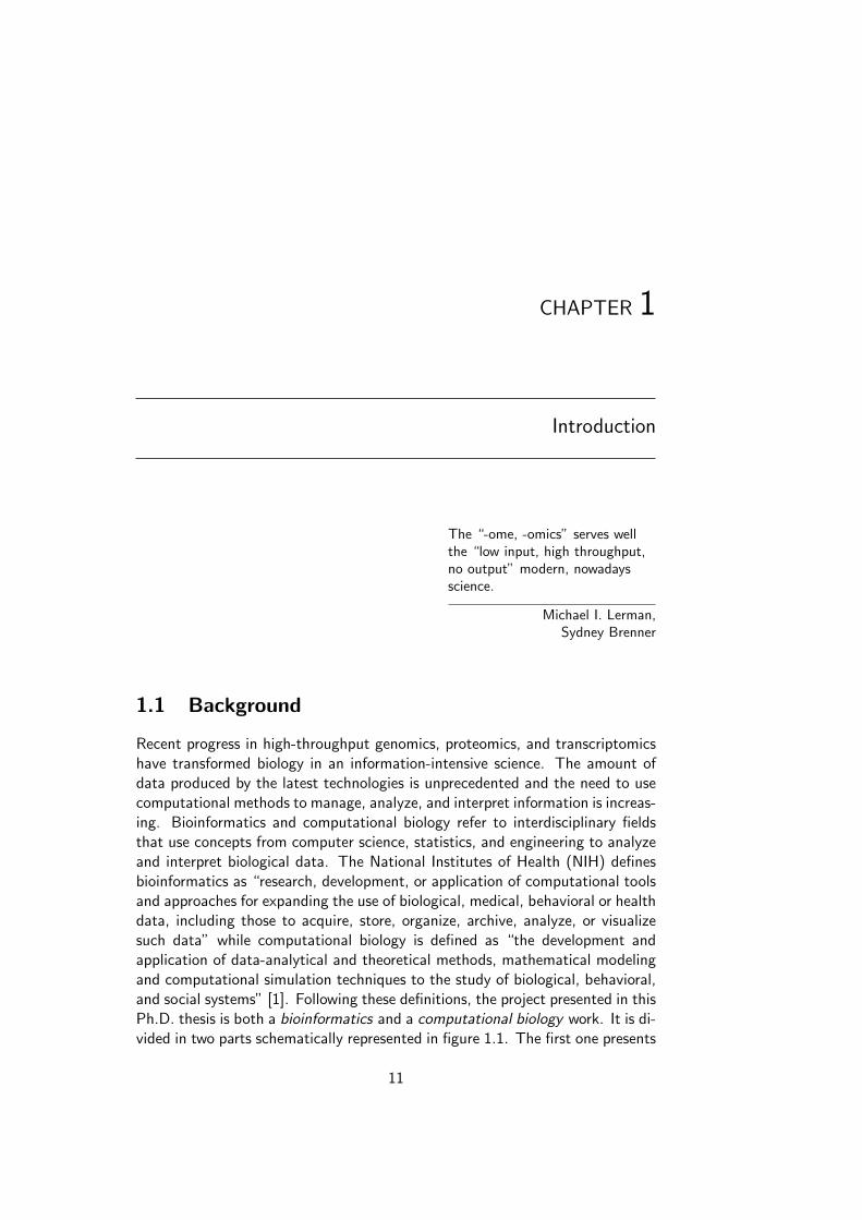
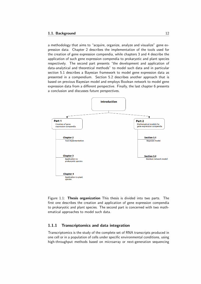
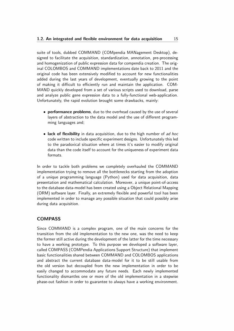
Recent progress in high-throughput genomics, proteomics, and transcriptomicshave transformed biology in an information-intensive science. The amount ofdata produced by the latest technologies is unprecedented and the need to usecomputational methods to manage, analyze, and interpret information is increas-ing. Bioinformatics and computational biology refer to interdisciplinary fieldsthat use concepts from computer science, statistics, and engineering to analyzeand interpret biological data. The National Institutes of Health (NIH) definesbioinformatics as “research, development, or application of computational toolsand approaches for expanding the use of biological, medical, behavioral or healthdata, including those to acquire, store, organize, archive, analyze, or visualizesuch data” while computational biology is defined as “the development andapplication of data-analytical and theoretical methods, mathematical modelingand computational simulation techniques to the study of biological, behavioral,and social systems” [1]. Following these definitions, the project presented in thisPh.D. thesis is both a bioinformatics and a computational biology work. It is di-vided in two parts schematically represented in figure 1.1. The first one presents

11

1.1. Background 12

a methodology that aims to “acquire, organize, analyze and visualize” gene ex-pression data. Chapter 2 describes the implementation of the tools used forthe creation of gene expression compendia, while chapters 3 and 4 describe theapplication of such gene expression compendia to prokaryotic and plant speciesrespectively. The second part presents “the development and application ofdata-analytical and theoretical methods” to model such data and in particularsection 5.1 describes a Bayesian framework to model gene expression data aspresented in a compendium. Section 5.2 describes another approach that isbased on previous Bayesian model and employs Boolean network to model geneexpression data from a different perspective. Finally, the last chapter 6 presentsa conclusion and discusses future perspectives.

Figure 1.1: Thesis organization This thesis is divided into two parts. Thefirst one describes the creation and application of gene expression compendiato prokaryotic and plant species. The second part is concerned with two math-ematical approaches to model such data.

1.1.1 Transcriptomics and data integration

Transcriptomics is the study of the complete set of RNA transcripts produced inone cell or in a population of cells under specific environmental conditions, usinghigh-throughput methods based on microarray or next-generation sequencing

1.1. Background 13

technologies. The widespread use of these tools has resulted in a rapid accu-mulation of gene expression data in public repositories such as NCBI GEO [2],ArrayExpress [3] and NCBI SRA1. Such repositories have the enormous poten-tial to provide an holistic view of how different experimental conditions leadsto gene expression changes, by comparing transcriptome fluctuations across allpossible measured conditions. Unfortunately, this is not a task easily achiev-able due to differences among laboratories and technology platforms that makedirect comparisons difficult. Nonetheless, in recent years there have been sev-eral efforts to fulfill data integration of gene expression studies. One issue indata integration is technical variability due to different laboratories’ workingmethods. To assess the agreement on experimental results, several initiatives[4], [5], [6] compared data obtained from different laboratories using microarrayand RNA-seq platforms with identical RNA samples. Since there are severalbiological and technical sources of variability to be considered, and the em-ployment of an advanced technology does not eliminate either, only a carefulexperimental design is effective in order to keep bias and batch effects undercontrol. Proposed approaches to integrate gene expression analysis usually canbe categorized as direct integration or meta-analysis: they can either directlyconsider the sample-level measurements within each study[7], and merge theseinto a single data set or select only some features assumed to be related acrossstudies, such as parameters that capture the relationship between genes andphenotypes [8]. Direct integration tries to overcome the limits of meta-analysiswith model-based approaches[12], that can directly integrate gene expressiondata and better account for confounding effects. This is generally done on ex-periments of the same platform, using e.g. the Robust Multi-Array averaging(RMA) [13], [14] normalization, because for direct integration of experimentsfrom different experimental platforms one needs to adjust the data for batcheffects (which are usually confounded with true biological changes) by e.g. aBayesian framework. Meta-analysis integrates gene expression analysis com-bining information from primary statistics [9] (such as p-value) or secondarystatistics [10] (such as gene list) resulting from single studies. Those studiesmanually combine the information from several data sources defining confidencelevels subjectively for each individual study without a general scheme. Meta-analysis is a common method to integrate conclusions from different studies.Goldstein et al. [11] analyze several meta-analysis approaches used for com-bining results of independent studies discussing general pros and cons of themeta-analysis approach.

1http://www.ncbi.nlm.nih.gov/sra

1.2. An integrated and flexible environment for data acquisition 14

1.1.2 The COLOMBOS approach to gene expression data inte-gration

One of the efforts towards data integration in gene expression studies is COLOM-BOS [15], originally COLlection Of Microarrays for Bacterial OrganismS, devel-oped for three bacterial species (Escherichia coli, Bacillus subtilis, and Salmonellaenterica serovar Typhimurium) and recently updated with sixteen others prokary-otic species [16], [17] and including also RNA-seq technology. COLOMBOS isa comprehensive organism-specific cross-platform expression database that pro-vides a suite of tools for the exploration, analysis and visualization of geneexpression data. COLOMBOS’ approach to data integration is unique in thesense of directly combining gene expression information from different techno-logical platforms and experiments. Data and experiment-related information(meta-data) are gathered and curated starting from raw intensities or sequencereads for microarrays and RNA-Seq respectively. A robust normalization andquality control procedure is performed to permit direct comparison of gene ex-pression values across different experiments and platforms. This results in asingle expression matrix in which each row represents a gene and each columnrepresents a ‘sample contrast’. Sample contrasts measure the difference be-tween a test and a reference condition, both of which are extensively annotatedwith various sorts of meta-data. The expression data itself are log-ratios (base2), so that positive values represent up-regulation, and negative values representdown-regulation of a gene in the test sample compared to the reference sam-ple. COLOMBOS falls under the direct integration methodology, but withoutthe need for batch-normalization as calculating logratios, for contrasts that aredefined by samples that come from the same experiment and platform combi-nation (a ‘batch’), ensures that a lot of batch related variation is removed [18].COLOMBOS principal goal is to gather together as many expression data aspossible for a given organism to explore patterns of co-expression across severalexperimental conditions. The creation of a co-expressed genes cluster (knownas module) is performed similarly to a BLAST [19] search in which COLOMBOSlooks for expression values for a given set of conditions, but using expressioncorrelation instead of sequence similarity to score the best matches. Modulescan be modified in several ways in order to highlight their genes’ behavior andto analyze (anti)co-expression patterns. COLOMBOS has shown to be a validresource both as an exploratory tool and as a gene expression database used fordownstream analysis [20], [21], [22],[23],[24],[25],[26],[27],[28],[29],[30].

1.2 An integrated and flexible environment for dataacquisition

COLOMBOS technologies are composed by a front-end web application used toaccess and analyze gene expression data in the compendia and by a back-end

1.2. An integrated and flexible environment for data acquisition 15

suite of tools, dubbed COMMAND (COMpendia MANagement Desktop), de-signed to facilitate the acquisition, standardization, annotation, pre-processingand homogenization of public expression data for compendia creation. The orig-inal COLOMBOS and COMMAND implementations date back to 2011 and theoriginal code has been extensively modified to account for new functionalitiesadded during the last years of development, eventually growing to the pointof making it difficult to efficiently run and maintain the application. COM-MAND quickly developed from a set of various scripts used to download, parseand analyze public gene expression data to a fully-functional web-application.Unfortunately, the rapid evolution brought some drawbacks, mainly:

• performance problems, due to the overhead caused by the use of severallayers of abstraction to the data model and the use of different program-ming languages and;

• lack of flexibility in data acquisition, due to the high number of ad hoccode written to include specific experiment designs. Unfortunately this ledto the paradoxical situation where at times it’s easier to modify originaldata than the code itself to account for the uniqueness of experiment dataformats.

In order to tackle both problems we completely overhauled the COMMANDimplementation trying to remove all the bottlenecks starting from the adoptionof a unique programming language (Python) used for data acquisition, datapresentation and mathematical calculation. Moreover, a unique point-of-accessto the database data-model has been created using a Object Relational Mapping(ORM) software layer. Finally, an extremely flexible and powerful tool has beenimplemented in order to manage any possible situation that could possibly ariseduring data acquisition.

COMPASS

Since COMMAND is a complex program, one of the main concerns for thetransition from the old implementation to the new one, was the need to keepthe former still active during the development of the latter for the time necessaryto have a working prototype. To this purpose we developed a software layer,called COMPASS (COMPendia Applications Support Structure) that implementbasic functionalities shared between COMMAND and COLOMBOS applicationsand abstract the current database data-model for it to be still usable fromthe old version but decoupled from the new implementation in order to beeasily changed to accommodate any future needs. Each newly implementedfunctionality dismantles one or more of the old implementation in a stepwisephase-out fashion in order to guarantee to always have a working environment.

1.3. Mathematical models for gene expression compendia 16

COMMAND

The new implementation of the back end program for data acquisition is basedon the assumption that it would be worthless to try to manage every possible wayin which public expression data are deposited. Instead, we provide a powerfultool to manage experiment uniqueness shaping the experiment structure andinjecting user-defined Python scripts to mine for experiment primary informationand raw data. Moreover, the new implementation provides several tools tocreate an expression compendia from scratch and to manage both raw andannotation data.

COLOMBOS application to plant species

COLOMBOS had been originally developed to collect microarray data for prokary-otes. Over the years it evolved allowing both the integration of different tran-scriptomics technologies, like RNA-seq, and the creation of compendia forarcheae and eukaryotes. While collecting a large amount of data for modelorganisms, like Escherichia coli, is facilitated due to the great number of exper-iments performed, for non-model species the situation is usually pretty differentas only few experiments are available. The importance of expression data in-tegration in this case is even more significant given the need for an adequatemagnitude of data to be able to draw valid and general conclusions. The appli-cation of COLOMBOS technology to grapevine species led to the developmentof VESPUCCI (Vitis Expression Studies Platform Using COLOMBOS Compen-dia Instances)[31], a gene expression compendium that include most of publiclyavailable expression data for grapevine. Working with a non-model plant specieshighlighted the need to significantly rethink some aspects of the data acquisitionand annotation process. The creation of a gene expression compendium usingCOLOMBOS technology is made easier thanks to the aid provided by the COM-MAND tool but it is still mainly a manual effort. The peculiarity and complexityof both plant transcriptome and experiment design required the possibility toflexibly manage how micorarray probes and RNA-Seq short read sequences aremapped and thus assigned to a measurable gene. The same concept of ‘measur-able transcipt’ was also used to account for some technical limitations, like theimpossibility to distinguish among some genes given the high sequence similaritythey share.

1.3 Mathematical models for gene expression com-pendia

COLOMBOS first and foremost goal is to bring together as much data as pos-sible, and opening this comprehensive data up for exploration and search forcomplex (co)expression patterns. While COLOMBOS provides a rich resourcefor top-down systems biology or for complementing more focused molecular

1.3. Mathematical models for gene expression compendia 17

biology research, one of the drawbacks is that the potential for rigorous statis-tical inference is not used. Simply relying on existing tools is unfeasible, dueto the cross-experiment/cross-platform nature of the data, the complicationsassociated with varying number of replicate sample contrasts, the existence ofself-self contrasts (measuring only biological variability), and the issue of de-pendence through a shared reference sample. To overcome this limitation andfurther extend the range of usage of COLOMBOS, we developed a statisticalframework that can be employed for various types of inference and decision mak-ing, explicitly taking into account dependencies between contrasts and workingirrespective of the number of replicate sample contrasts available. It serves as abasis for ‘interrogating’ the data in a statistically sound way to answer diversequestions such as: identifying differentially expressed genes for one (or more)contrast(s), finding complex patterns of co-expression, classification/predictionand ‘biomarker’ discovery. While the purpose of statistical framework is to pro-vide a sound statistical model to deal with data in the compendia, a differentapproach, that exploits the statistical model, was developed to describe howour knowledge of the ‘system’ (i.e. which genetic entities have the potential tointeract or be involved in related biological processes) can explain the observedgenome-wide expression responses to a ‘stimulus’ or a shift in biological condi-tions. This second approach extrapolates a single-cell model to population levelin order to account for how gene expression measurements have been collectedduring experiments and relationships among genes.

1.3.1 A Bayesian noise model

Using a Bayesian approach we developed a statistical framework that modela probability distribution over the underlying true change in expression for agene in response to a shift in biological conditions. We defined the probabilitydistribution:

p(µx|X,G,C)

where µx is the underlying true change in gene expression for the given geneG, in response to a given contrast C, with X = (x1, . . . , xn)T being the nreplicate expression log-ratios. Such an approach has several advantages thatare particularly relevant given the requirements:

• inferring the complete posterior p(µx|X,G,C) distribution, instead ofusing point estimators, gives more flexibility with respect to the kind ofquestions we would like to answer;

• the inherent sequential nature of Bayesian learning makes it well-suitedfor the disparateness in the number of replicates present in the compendia;

• the Bayesian formulation provides a convenient way for introducing priorknowledge, such as the dependence that exists between contrasts shar-

1.3. Mathematical models for gene expression compendia 18

ing the same references as well as general properties of the data and itsdistribution for gene G and contrast C that we know empirically.

1.3.2 Modeling contrasts with Boolean networks

Genes known to be involved in a biological process are represented as nodes(that can be either on or off ) in a Boolean network, while the relationshipamong those genes are represented as Boolean functions. Expression data inthe compendia are used to fit a model that uses Boolean network attractorstates to simulate the different steady-states in which sub-populations of cellswere at the time measurements were taken. The fitted estimated weights ofeach possible attractor state represent the proportion of cells in a particularsteady-state during the shift in biological conditions.

Part one

19

CHAPTER 2

Creating gene expression compendia

2.1 Compendium creation workflow

The typical workflow for compendia creation via COMMAND is described inthe original COLOMBOS paper [15] (here we report and briefly describe it forthe sake of completeness). There are three main steps toward the creation ofa gene expression compendium using COLOMBOS technology. Each of themrequires a set of dedicated tools and they have to be done sequentially.

Collection of gene expression data

Public repositories such as NCBI GEO ([2]) and ArrayExpress ([3]) are accessedthrough the available Application Programming Interface (API). All the mi-croarray experiment information together with the related platform informationare downloaded. Raw data (or normalized data when raw aren’t available) arestored in a unified format. Microarray probe sequences are also stored andmapped in a platform-specific way to a unique list of genes that is composedby the organism’s RefSeq file available at NCBI. These genes correspond to therows in the final expression matrix. If probes aren’t available, it’s gene target isidentified by other information such as the locus tags or common gene names.Regarding RNA-Seq experiments, pre-processing such as quality control, clean-ing of raw reads and alignment on a reference genome (or transcriptome) isdone separately. Raw counts associated with the organism specific gene list arestored together with the related platform information.

21

2.2. Implementation of a workbench for compendia creation 22

Annotation of samples and experiments

After raw intensities and platform-related information have been stored in thedatabase, the next phase constitutes the definition and annotation of conditioncontrasts. As stated in the introduction (section 1.1.2) a ‘condition contrast’does not represent a single experimental condition, but rather the difference(in log-ratios) between a test and a reference condition . Samples are taggedas ‘test’ or ‘reference’ for single channel microarray experiments and RNA-Seqexperiments, while for dual channel microarray experiments, usually one of ev-ery two array hybridizations serves as a reference to the other. If a sampledoes not represent a unique and distinctive biological condition (such as sam-ples of genomic DNA or a pool of different samples) it is not considered andgets discarded. This choice ensures the biological interpretability of every de-fined contrast, as the associated log-ratios measure a change in expression inresponse to quantifiable stimuli that have been altered from the reference tothe test sample. After contrasts are defined, they are annotated using termsfrom a controlled vocabulary created to ensure both computational tractabilityand human readability. The creation of the controlled vocabulary is a manualprocess, in which new terms are neatly added to the vocabulary tree as neededduring the importing of experiment samples.

Homogenization of gene expression data

The last step in the creation of the compendium is the homogenization of geneexpression data. Various pre-processing techniques are carried on in order torender experiments from different platforms comparable. The following ‘generalrules’ are applied whenever possible during this step:

• raw intensities/reads are preferred over already pre-processed data as datasource;

• no local background correction or mismatch probe correction are per-formed;

• non-linear normalization techniques are performed;

• variance dispersion stabilization is performed on RNA-seq data.

2.2 Implementation of a workbench for compendiacreation

COLOMBOS is an extensive program. It’s main characteristic is given by thepossibility of exploring a huge database of gene expression data scanning forpatterns of (anti)co-expression. In spite of his apparent complexity it ‘only’has to deal with one well-defined data-model providing a user-friendly interface

2.2. Implementation of a workbench for compendia creation 23

to easily browse the expression matrix. The real complexity lies in the cre-ation of such expression matrix, i.e. in the back-end program used to collect,annotate, and manage gene expression data. The COMpendia MANagementDesktop (COMMAND) has been created with the purpose of simplifying thethree necessary steps to create a compendia (as explained above in section 2).The original COMMAND code was composed by several scripts, mainly writ-ten in the Matlab and Ruby programming languages that have grown in time,up to the point of being considered a fully functional application. The steptowards the creation of a web-application had been completed by adding PHPand JavaScript code to glue together all those scripts. Its evolution from a‘bunch of scripts’ to a fully-featured application that ‘just works’ has been fastand more time had been dedicated to adding new features instead of correctingold mistakes. Because of that, the COMMAND source code had grown to thepoint of being hard to be further developed and maintained. The main problemswith the old implementation of COMMAND are:

• The use of several programming languages: Ruby, PHP and Matlabhave been used to code the server side part of the application. Thishas lead to redundancy (especially between some Ruby and PHP parts),a general lack of performance, and difficulty in debugging, maintainingand deploying the code given the need to install all code dependencies asexternal packages.

• More points of access to the database: all languages independentlyaccess to the database. This leads once again to redundancy (in savingcredentials for accessing the database) and general difficulty in under-standing which part of the code accesses the database to retrieve (orstore) data and passes it to another part of the code.

• Unused functionalities: some features have been developed but neverfully exploited. Such design choices have to be taken into account whendealing with the data-model weighing down the typical workflow.

• Some persistent data are stored in files: not all critical data arestored in the database, some of them are organized in files and direc-tories. This has several drawbacks such as the lack of control for integritywith database data, the difficulty in retrieving them since the location issometimes hidden in the file-system, and the general lack of security giventhe possibility to accidentally delete them.

• Data-model abstraction using XML files: this is linked with ‘unusedfunctionalities’ as extra code has been developed with the purpose ofensuring enough abstraction and scalability in case of changes in the data-model. Unfortunately, the drawbacks overpower the advantages as theoverhead given by the intermediate creation of XML files slows down thewhole execution.

2.3. COMMAND: revisited 24

• Lack of flexibility: a lot of code has been developed to account for theuniqueness and heterogeneity of specific data-formats and experimentaldesigns. This created several problems during data acquisition as newexperiments not always match previously developed code used for other,similar experiments. This sometimes leads to the contra-productive sit-uation in which modifying original data formats, instead of the code tohandle them, was the easiest strategy to import data.

2.3 COMMAND: revisited

Thanks to the newly available technologies, measuring the complete transcrip-tome is an easily achievable task nowadays. New experiments and data becomespublicly available on a daily basis and thus a tool like COMMAND is partic-ularly useful in order not only to build gene expression compendia but alsoto keep them up-to-date. Unfortunately, updating compendia using the oldCOMMAND implementation soon became unfeasible given the lack of flexi-bility needed to correctly manage and import gene expression experiments aseach of them requires a specific way to be correctly handled and imported. Thedecision to re-implement COMMAND has been made focusing on some majorimprovements that had to be carried out, such as:

1. overhaul the way in which experiments are imported;

2. update the database structure;

3. create a coherent server-side programming interface;

4. use less programming languages (possibly one);

5. update the client-side software libraries (ExtJS);

In order to successfully fulfill both the need for a coherent server-side program-ming interface and the usage of possibly only one programming language tobe used as server-side web-application, general business logic programming andnumerical calculation, the choice naturally fell on Python. Python is a versa-tile programming language thanks to the plethora of freely available modulesand libraries developed from the community. There’s also several working en-vironments for Python that greatly simplify and speed up the development anddebugging of Python applications.

COMMAND implementation

Figure 2.1 shows the old and the new COMMAND implementation. They areboth centered around the database structure that holds the data-model usedfrom both COMMAND and COLOMBOS applications. Each application (likeCOMMAND and COLOMBOS) are composed by a client-side, that is the GUI

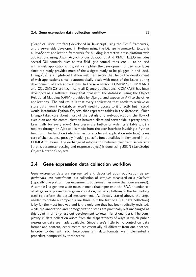
2.4. Gene expression data collection workflow 25

(Graphical User Interface) developed in Javascript using the ExtJS framework,and a server-side developed in Python using the Django Framework. ExtJS isa JavaScript application framework for building interactive cross-platform webapplications using Ajax (Asynchronous JavaScript And XML). ExtJS includesseveral GUI controls, such as text field, grid control, tabs, etc. . . , to be usedwithin web applications. It greatly simplifies the development of user interfacessince it already provides most of the widgets ready to be plugged-in and used.Django[32] is a high-level Python web framework that helps the developmentof web applications since it automatically deals with most of the issues duringdevelopment of such applications. In the new version COMPASS, COMMANDand COLOMBOS are technically all Django applications. COMPASS has beendeveloped as a software library that deal with the database, using the ObjectRelational Mapping (ORM) provided by Django, and expose an API to the otherapplications. The end result is that every application that needs to retrieve orstore data from the database, won’t need to access to it directly but insteadwould instantiate Python Objects that represent tables in the database. SinceDjango takes care about most of the details of a web-application, the flow ofexecution and the communication between client and server-side is pretty basic.Essentially for every event (like pressing a button or ordering a table grid) arequest through an Ajax call is made from the user interface invoking a Pythonfunction. The function (which is part of a coherent application interface) takescare of the response possibly invoking specific functionalities implemented in theCOMPASS library. The exchange of information between client and server side(that is parameter passing and response object) is done using JSON (JavaScriptObject Notation) objects.

2.4 Gene expression data collection workflow

Gene expression data are represented and deposited upon publication as ex-periments. An experiment is a collection of samples measured on a platform(typically one platform per experiment, but sometimes more than one are used).A sample is a genome-wide measurement that represents the RNA abundancesof all genes expressed in a given condition, while a platform is the technologyused to perform the actual measurement. As already stated above, the stepsneeded to create a compendia are three, but the first one (i.e. data collection)is by far the most involved and is the only one that has been radically revisited,while the annotation and homogenization steps are practically left unchanged atthis point in time (phase-out development to retain functionalities). The com-plexity in data collection arises from the disparateness of ways in which publicexpression data are made available. Since there’s little to no control on dataformat and content, experiments are essentially all different from one another.In order to deal with such heterogeneity in data formats, we implemented aprocedure composed by three steps:

2.4. Gene expression data collection workflow 26

Figure 2.1: Past and future software layer implementation The upper partof the figure shows the old implementation with several point of access to thedatabase and all the different programming languages used. The lower partshows the new implementation with COMPASS as the only software layer thatdeal with the database and implements the data-model while each of the appli-cations have one coherent Python interface to manage all server-side function-alities.

2.4. Gene expression data collection workflow 27

• experiment selection and raw-data download;

• experiment structure definition;

• experiment parsing and data extraction.

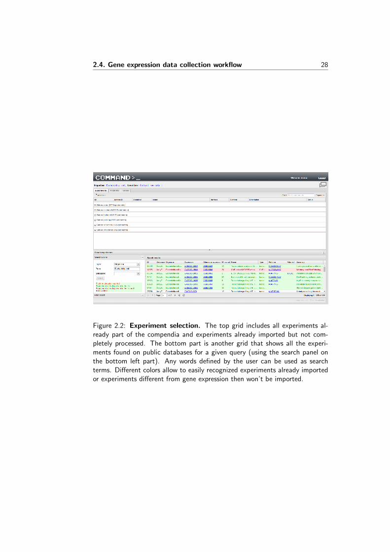
Figure 2.2 shows the interface for the first step. This first part allow to see allpublic gene expression experiments from GEO and ArrayExpress. From here ispossible to select and download data for the new experiments we wish to import,or specify which experiments we explicitly want to exclude. From this sameinterface it is also possible to manage already imported or partially importedexperiments, together with platform information (description, probe sequence,etc. . . ) and gene information (sequence and functional annotation). Accordingto the different steps of the import process in which an experiment can be, itis labelled with a different status:

• searched: the experiment has been added to the list of experiments tobe imported from the search result (first part of the import process);

• structured: the experiment structure has been defined (second part ofthe import process);

• parsing: parsing scripts have been assigned to experiment files (third partof the import process);

• included: the experiment is imported in the database;

• annotated: the experiment is annotated;

• excluded: the experiment is of no interest and won’t be imported.

The second part of the import process (see Figure 2.3) is done definingthe experiment structure, i.e. the platforms and the samples the experiment iscomposed of, as a hierarchy tree. In this context, a platform is defined as thespecific technological platform used to measure RNA abundance (for example anAffymetrix chip), with all the associated information and meta-information likeprobes sequences or name and description of the platform. A sample is intendedas all the information and meta-information, such as raw measurements, nameand description, related to a single biological RNA sample measured with aspecific platform. (Note that a single biological RNA sample is not limited toa single gene, but consists of all transcripts of the genes that are expressedin that sample.) Once this is done, files that contains meta-information, dataand measurements are associated with the respective experiment, platform andsample in the hierarchy. This approach is completely different from the originalone and it provides great flexibility because of the way in which we can assignany file to any entity in the hierarchical structure of the experiment in order toget out the relevant information.

2.4. Gene expression data collection workflow 28

Figure 2.2: Experiment selection. The top grid includes all experiments al-ready part of the compendia and experiments already imported but not com-pletely processed. The bottom part is another grid that shows all the experi-ments found on public databases for a given query (using the search panel onthe bottom left part). Any words defined by the user can be used as searchterms. Different colors allow to easily recognized experiments already importedor experiments different from gene expression then won’t be imported.

2.4. Gene expression data collection workflow 29

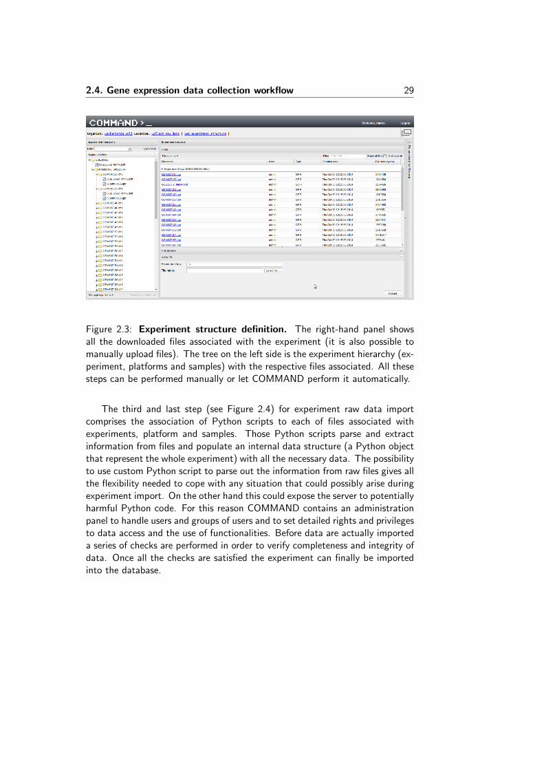
Figure 2.3: Experiment structure definition. The right-hand panel showsall the downloaded files associated with the experiment (it is also possible tomanually upload files). The tree on the left side is the experiment hierarchy (ex-periment, platforms and samples) with the respective files associated. All thesesteps can be performed manually or let COMMAND perform it automatically.

The third and last step (see Figure 2.4) for experiment raw data importcomprises the association of Python scripts to each of files associated withexperiments, platform and samples. Those Python scripts parse and extractinformation from files and populate an internal data structure (a Python objectthat represent the whole experiment) with all the necessary data. The possibilityto use custom Python script to parse out the information from raw files gives allthe flexibility needed to cope with any situation that could possibly arise duringexperiment import. On the other hand this could expose the server to potentiallyharmful Python code. For this reason COMMAND contains an administrationpanel to handle users and groups of users and to set detailed rights and privilegesto data access and the use of functionalities. Before data are actually importeda series of checks are performed in order to verify completeness and integrity ofdata. Once all the checks are satisfied the experiment can finally be importedinto the database.

2.4. Gene expression data collection workflow 30

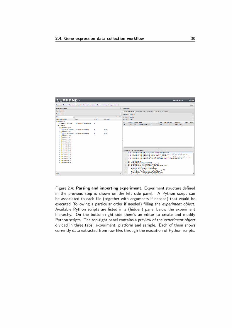
Figure 2.4: Parsing and importing experiment. Experiment structure definedin the previous step is shown on the left side panel. A Python script canbe associated to each file (together with arguments if needed) that would beexecuted (following a particular order if needed) filling the experiment object.Available Python scripts are listed in a (hidden) panel below the experimenthierarchy. On the bottom-right side there’s an editor to create and modifyPython scripts. The top-right panel contains a preview of the experiment objectdivided in three tabs: experiment, platform and sample. Each of them showscurrently data extracted from raw files through the execution of Python scripts.

CHAPTER 3

COLOMBOS v3.0: leveraging gene expression compendia forcross-species analyses

Marco Moretto, Paolo Sonego, Nicolas Dierckxsens, Mat-

teo Brilli, Luca Bianco, Daniela Ledezma-Tejeida, Socorro

Gama-Castro, Marco Galardini, Chiara Romualdi, Kris

Laukens, Julio Collado-Vides, Pieter Meysman and Kristof

Engelen[17]

Abstract

COLOMBOS is a database that integrates publicly available transcriptomicsdata for several prokaryotic model organisms. Compared to the previous versionit has more than doubled in size, both in terms of species and data avail-able. The manually curated condition annotation has been overhauled as well,giving more complete information about samples’ experimental conditions andtheir differences. Functionality-wise cross-species analyses now enable users toanalyse expression data for all species simultaneously, and identify candidategenes with evolutionary conserved expression behaviour. All the expression-based query tools have undergone a substantial improvement, overcoming thelimit of enforced co-expression data retrieval and instead enabling the return ofmore complex patterns of expression behaviour. COLOMBOS is freely availablethrough a web application at http://colombos.net/. The complete databaseis also accessible via REST API or downloadable as tab-delimited text files.

31

32

Introduction

COLOMBOS is a collection of expression data from both microarray and RNA-Seq experiments for several prokaryotic species, taken from publicly availabledatabase such as the Gene Expression Omnibus (GEO) [2] and ArrayExpress[3]. Its uniqueness resides in the ability to cope with data heterogeneity anddirectly integrate data coming from different platforms and technologies. Othergene expression compendia are usually built either from data for a single tran-scriptomics platform or they rely on the integration of expression analysis results,rather than the integration of the actual measurements. In COLOMBOS how-ever, data are collected and curated starting from the original raw intensitiesfor microarrays and sequence reads for RNA-Seq, and then processed with arobust normalization and quality control pipeline to allow direct comparison ofgene expression behaviour across different experiments and platforms [15]. Thisresults in a single expression matrix for every species, its rows representing themeasured genes and its columns representing condition contrasts, comparisonsbetween test and reference samples of different biological conditions. Attentionis also given to the acquisition of metadata related to the description of thebiological conditions surveyed in an experiment, so that all the included sam-ples and condition contrasts are formally annotated by means of a controlledvocabulary of condition properties. This annotation is a manual effort withthe purpose of making the data comparable from a biological viewpoint and toyield reliable interpretations of expression patterns. COLOMBOS compendiaare accessible using the web interface, through a set of REST API calls, or viathe R [33] package Rcolombos; they are also available for download in theirentirety for use of COLOMBOS data in third-party stand-alone applications.Different types of analyses can be done using the COLOMBOS web interfaceitself; typical operations include starting from a set of known genes to find theconditions where they are (co)-expressed or to identify additional co-expressedgenes. COLOMBOS’ tools are designed for users to ‘play around’ with thecompendia, exploring the data with respect to the biological question they areinterested in. They are encouraged to try different types of search queries basedon genes or conditions, the available annotations or by relying on the actualexpression values in a way reminiscent of a BLAST functionality with gene ex-pression behaviour instead of sequence similarity. They can then visualize theirresults, use them as a basis for new queries to find additional (anti-)co-expressedgenes, generate clusters to separate disjoint expression profiles, explore the over-lap between multiple query results and potentially combine them, etc. Thereare several detailed use case tutorials on the website, illustrating step-by-stephow concrete examples of conceptually different biological questions could behandled through the COLOMBOS interface. The previous v2.0, with all of itsoriginal databases and tools, will be kept available for future reference along sideCOLOMBOS v3.0; how to access it is explained in the website’s Help section.

33

Data content update

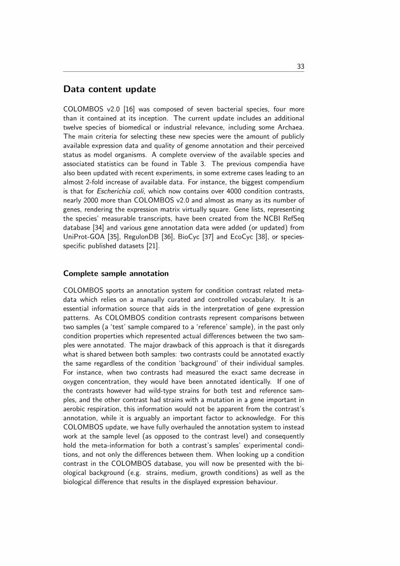
COLOMBOS v2.0 [16] was composed of seven bacterial species, four morethan it contained at its inception. The current update includes an additionaltwelve species of biomedical or industrial relevance, including some Archaea.The main criteria for selecting these new species were the amount of publiclyavailable expression data and quality of genome annotation and their perceivedstatus as model organisms. A complete overview of the available species andassociated statistics can be found in Table 3. The previous compendia havealso been updated with recent experiments, in some extreme cases leading to analmost 2-fold increase of available data. For instance, the biggest compendiumis that for Escherichia coli, which now contains over 4000 condition contrasts,nearly 2000 more than COLOMBOS v2.0 and almost as many as its number ofgenes, rendering the expression matrix virtually square. Gene lists, representingthe species’ measurable transcripts, have been created from the NCBI RefSeqdatabase [34] and various gene annotation data were added (or updated) fromUniProt-GOA [35], RegulonDB [36], BioCyc [37] and EcoCyc [38], or species-specific published datasets [21].

Complete sample annotation

COLOMBOS sports an annotation system for condition contrast related meta-data which relies on a manually curated and controlled vocabulary. It is anessential information source that aids in the interpretation of gene expressionpatterns. As COLOMBOS condition contrasts represent comparisons betweentwo samples (a ‘test’ sample compared to a ‘reference’ sample), in the past onlycondition properties which represented actual differences between the two sam-ples were annotated. The major drawback of this approach is that it disregardswhat is shared between both samples: two contrasts could be annotated exactlythe same regardless of the condition ‘background’ of their individual samples.For instance, when two contrasts had measured the exact same decrease inoxygen concentration, they would have been annotated identically. If one ofthe contrasts however had wild-type strains for both test and reference sam-ples, and the other contrast had strains with a mutation in a gene important inaerobic respiration, this information would not be apparent from the contrast’sannotation, while it is arguably an important factor to acknowledge. For thisCOLOMBOS update, we have fully overhauled the annotation system to insteadwork at the sample level (as opposed to the contrast level) and consequentlyhold the meta-information for both a contrast’s samples’ experimental condi-tions, and not only the differences between them. When looking up a conditioncontrast in the COLOMBOS database, you will now be presented with the bi-ological background (e.g. strains, medium, growth conditions) as well as thebiological difference that results in the displayed expression behaviour.

34

Str

ain

Nu

mb

erof

gen

esN

um

ber

ofco

ntr

asts

Mis

sin

gva

lues

(%)

Fir

stin

clu

sion

Sam

ple

sE

xper

imen

tsP

latf

orm

s

Esc

her

ich

iaco

liM

G16

5543

2140

773.

6v1

.055

1025

4[1

5]73

Bac

illu

ssu

bti

lis16

841

7612

593.

7v1

.018

1445

35S

alm

onel

laen

teri

case

rova

rT

yph

imu

riu

mcr

oss-

stra

in62

6110

6641

.6v1

.018

5636

22

Str

epto

myc

esco

elic

olor

LT2

4556

172

6.4

v2.0

316

810

Pse

ud

omon

asae

rugi

nos

a14

028S

5416

681

22.7

v2.0

1252

177

Hel

icob

acte

rpy

lori

SL

1344

4655

213

9.8

v2.0

288

119

Bac

illu

san

thra

cis

A3(

2)82

3937

17.

3v2

.054

67

[2]

7B

acill

us

cere

us

PA

O1

5647

559

1.6

v2.0

592

332

Bac

tero

ides

thet

aiot

aom

icro

n26

695

1616

133

3.1

v2.0

256

85

Cam

pylo

bac

ter

jeju

ni

Am

es50

3966

3.0

v3.0

754

4C

lost

rid

ium

acet

obu

tylic

um

AT

CC

1457

952

3128

32.

4v3

.039

216

10L

acto

bac

illu

srh

amn

osu

sV

PI-

5482

4816

333

1.9

v3.0

353

194

Met

han

oco

ccu

sm

arip

alu

dis

NC

TC

1116

815

7215

212

.5v3

.026

014

11S

hig

ella

flex

ner

iA

TC

C82

437

7837

72.

4v3

.041

912

11S

inor

hiz

obiu

mm

elilo

tiG

G28

3479

3.6

v3.0

158

32

Str

epto

cocc

us

pn

eum

onia

eS

217

2236

41.

5v3

.072

819

3T

her

mu

sth

erm

oph

ilus

301

4315

3517

.0v3

.038

33

Yer

sin

iap

esti

s10

2162

1842

42.

7v3

.071

320

[19]

10

Tab

le3.

1:R

ows

ofth

eta

ble

repr

esen

tal

lth

esp

ecie

san

dst

rain

sfo

rw

hic

ha

gen

eex

pres

sion

com

pen

diu

mis

hos

ted

.C

olu

mn

sre

pres

ent

(fro

mle

ftto

righ

t):

the

spec

ies

nam

e,th

est

rain

use

das

refe

ren

cege

nom

efo

rm

icro

arra

ypr

obe

toge

ne

map

pin

gan

dR

NA

-Seq

read

alig

nm

ent,

the

tota

ln

um

ber

ofge

nes

inth

eco

mp

end

ium

,th

eto

tal

nu

mb

erof

con

tras

tsin

the

com

pen

diu

m,

the

per

cen

tage

ofm

issi

ng

valu

es,

the

CO

LO

MB

OS

vers

ion

ofth

efi

rst

incl

usi

onof

the

resp

ecti

vesp

ecie

sor

stra

in,

the

tota

ln

um

ber

ofsa

mp

les

from

wh

ich

the

com

pen

diu

m’s

con

tras

tsar

eb

uilt

,th

eto

taln

um

ber

ofco

rres

pon

din

gex

per

imen

tson

GE

Oan

dA

rray

Exp

ress

(th

ela

tter

ind

icat

edb

etw

een

squ

are

brac

kets

)an

dth

eto

tal

nu

mb

erof

pla

tfor

ms

repr

esen

ted

.

35

Functionality update

Cross-species analysis

A completely new functionality in COLOMBOS v3.0 is the ability to work with allspecies simultaneously. The data from different organisms have been integratedon a higher level based on clusters of homologous genes (CHG) constructedwith OrthoMCL v2.0.9 [39] using the default settings as applied to the proteinsequences for the strains included in COLOMBOS v3.0. These CHGs can bethought of as the rows of an overarching expression matrix obtained by stitch-ing together the individual compendia. Expression data for orthologous genes,i.e. genes assigned to the same CHG, are aligned across the respective species;species without a representative gene in a CHG can be thought of as havingmissing values. In case a CHG contains paralogous genes (multiple genes fromthe same species), their expression values are averaged. All data analysis toolsincluded in COLOMBOS have been adapted to deal with these new cross-speciescompendia, so that this complex expression matrix can be queried and exploredwith the same flexibility as any single species. The cross-species comparison isnot only a novelty for the identification of co-expressed gene sets across severalspecies for e.g. evolutionary studies, but also has several advantages for theway compendia can be constructed. We can now build compendia for differentstrains and integrate them at the species level using homologue mappings. Thishas a clear advantage as, instead of using a single reference strain’s genome torepresent the species as was done before, we can now explicitly recognize ge-nomic differences between strains and thus improve read alignment (RNA-seq)or probe to gene mapping (microarrays) to generate higher quality expressiondata. This concept has been used to improve our Salmonella enterica sp. Ty-phimurium compendium, where the original consisted of more or less equal partsof three different strains with minor differences in their genomic content.

Analysis tools

Several changes have been made to web portal’s suite of analysis tools and theRESTful web service and R API. These are mainly related to the query function-alities that actually make use of the expression values themselves (‘BLASTingwith expression data’). While these previously looked solely for consistent co-expression, they are now capable of returning complex patterns of expressionbehaviour across sets of query genes (or conditions). For instance, in v2.0 theQuicksearch functionality would return, for a set of user defined genes, the con-trasts where those genes behave in a similar and coherent way. These are notnecessarily the most informative, or relevant, contrasts for the user, especiallyfor larger gene sets for which co-expression behaviour might be rare and unrep-resentative. By default the Quicksearch in v3.0 will visualize complex patternsof co-expression by running a biclustering on the returned module data, and

36

will not necessarily return contrasts where the query input genes behave in thesame way (although this functionality is still available in the Advanced search).Other improvements include various export functionalities so that COLOMBOSresults can be easily imported in other widely used tools or databases (such asCytoscape [40], BioCyc) for further downstream analysis.

Discussion and future plans

COLOMBOS’ growths over the years have been a continuous effort towards bet-ter gene expression data integration and easier exploration and interpretation.Not only has the data more than doubled, but this last major update is anotherstep in the direction of improving the strengths and eliminating the weaknessesof the previous version(s). The redesigned condition annotation system providesa more reliable interpretation of expression patterns with respect to the biolog-ical stimuli that are causing them. The new cross-species capabilities have theobvious advantage over the old system to be able to perform gene expressionanalyses on all species simultaneously, but also enable more accurate measure-ments mapping by separating different strains within the same species. Keepingthe compendia up-to-date, as well as expanding the scope by adding new or-ganisms, is naturally our first priority. We generally select new species or strainsbased on data availability, but are always open to suggestions or requests fromusers who are interested in access to a gene expression compendium for a partic-ular species. Further improvements and new functionalities that revolve aroundcross-species capabilities are planned for future versions. Flexibility regardingCHGs selection and composition, as well as new tools to empower users whendealing with complex CHGs are amongst the priorities. For instance, insteadof being limited to pre-calculated, fixed CHGs for which homologues cannotbe re-defined and that encompass all species in the compendia as is the casenow, users will be able to define the settings to create CHGs for the speciesof their choice and consequently more dynamically integrate the data from thecorresponding compendia. Updated tools will likewise enable a finer manage-ment of CHGs, unlike e.g. the current paralogues’ expression calculation that isaveraged across all paralogues without the possibility for a different evaluationconsidering the variability amongst those paralogues, as well as give users theability to compare expression derived measures, such as co-expression scores ornetworks, across species.

CHAPTER 4

VESPUCCI: exploring patterns of gene expression ingrapevine

Marco Moretto, Paolo Sonego, Stefania Pilati, Giulia

Malacarne, Laura Costantini, Lukasz Grzeskowiak, Gior-

gia Bagagli, Maria Stella Grando, Claudio Moser and

Kristof Engelen[31]

Abstract

Large-scale transcriptional studies aim to decipher the dynamic cellular re-sponses to a stimulus, like different environmental conditions. In the era of high-throughput omics biology, the most used technologies for these purposes are mi-croarray and RNA-Seq, whose data are usually required to be deposited in publicrepositories upon publication. Such repositories have the enormous potential toprovide a comprehensive view of how different experimental conditions lead toexpression changes, by comparing gene expression across all possible measuredconditions. Unfortunately, this task is greatly impaired by differences amongexperimental platforms that make direct comparisons difficult. In this paper, wepresent the Vitis Expression Studies Platform Using COLOMBOS CompendiaInstances (VESPUCCI), a gene expression compendium for grapevine which wasbuilt by adapting an approach originally developed for bacteria, and show howit can be used to investigate complex gene expression patterns. We integratednearly all publicly available microarray and RNA-Seq expression data: 1608 geneexpression samples from 10 different technological platforms. Each sample hasbeen manually annotated using a controlled vocabulary developed ad hoc toensure both human readability and computational tractability. Expression datain the compendium can be visually explored using several tools provided by the

37

38

web interface or can be programmatically accessed using the REST interface.VESPUCCI is freely accessible at http://vespucci.colombos.fmach.it.

Introduction

Grapevine (Vitis spp.) is an economically important fruit crop and one of themost cultivated crops worldwide [41]. Grape berries are consumed as freshfruit or used for high-valued commodities as wine or spirits. Grapevine tran-scriptomics studies started over a decade ago, initially using microarrays butlater, exploiting the sequenced genomes [42], [43] and the availability of high-throughput sequencing, also using RNA-Seq approaches. As system biologybecomes more prevailing in everyday analysis, one of the pressing aspect ofanalysis is how to integrate different sources of information into one coherentframework that can be interrogated in order to gain knowledge about the sys-tem as a whole [44]. Prior to biological information integration across severallevels (such as proteomics, transcriptomics, and metabolomics), it is importantto acquire and combine all the possible available information within each spe-cific field. Together with the methodological problem of combining differentsources of information, there’s the more practical issue of having sufficient datato justify data integration in the first place, because in order to draw generaland valid conclusions a large amount of data is a desirable feature. While formodel species this is hardly an issue, for non-model crop species the numberof performed experiments might be limited, the technological platforms less es-tablished, and heterogeneous data a further complicating factor. Nevertheless,as biology is turning into a data-driven science the prospect of large datasetavailability becomes more and more feasible even for non-model species, andin terms of gene expression and functional analysis there have been several ef-forts to fulfill data integration in different organisms including grapevine [45],[46], strawberry [47], and citrus [48]. In this paper, we present an expansivegrapevine gene expression compendium that can be used to analyze grapevinegene expression at a broad level. It was created based on an approach for deal-ing with the large heterogeneity of data formats present in public databases,and to integrate cross-platform gene expression experiments in one dedicated,coherent database. The proof-of-concept of this approach was presented in [15]as a web-application for exploring and analyzing specific expression data of sev-eral bacterial species. This original technology platform has already been usedas a basic framework for creating a gene expression compendium for a morecomplex case as the multicellular, higher eukaryote Zea mays [49]. Here, weused the most updated version of the COLOMBOS technology [17] to showhow this approach can be further extended for the creation of gene expressioncompendia on other important crop species, focusing our attention on grapevinegene expression studies. Regardless of the available tools, most of the steps to-ward the creation of such a compendium, require a massive amount of manual

39

Platform namePlatformtype

Numberof samples

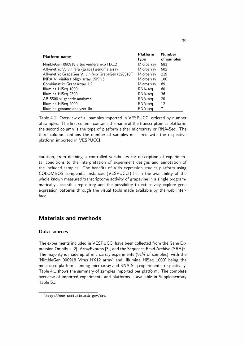
NimbleGen 090918 vitus vinifera exp HX12 Microarray 583Affymetrix V. vinifera (grape) genome array Microarray 502Affymetrix GrapeGen V. vinifera GrapeGena520510F Microarray 219INRA V. vinifera oligo array 15K v3 Microarray 100Combimatrix GrapeArray 1.2 Microarray 69Illumina HiSeq 1000 RNA-seq 60Illumina HiSeq 2500 RNA-seq 36AB 5500 xl genetic analyzer RNA-seq 20Illumina HiSeq 2000 RNA-seq 12Illumina genome analyzer IIx RNA-seq 7

Table 4.1: Overview of all samples imported in VESPUCCI ordered by numberof samples. The first column contains the name of the transcriptomics platform,the second column is the type of platform either microarray or RNA-Seq. Thethird column contains the number of samples measured with the respectiveplatform imported in VESPUCCI.

curation, from defining a controlled vocabulary for description of experimen-tal conditions to the interpretation of experiment designs and annotation ofthe included samples. The benefits of Vitis expression studies platform usingCOLOMBOS compendia instances (VESPUCCI) lie in the availability of thewhole known measured transcriptome activity of grapevine in a single program-matically accessible repository and the possibility to extensively explore geneexpression patterns through the visual tools made available by the web inter-face.

Materials and methods

Data sources

The experiments included in VESPUCCI have been collected from the Gene Ex-pression Omnibus [2], ArrayExpress [3], and the Sequence Read Archive (SRA)1.The majority is made up of microarray experiments (91% of samples), with the‘NimbleGen 090918 Vitus HX12 array’ and ‘Illumina HiSeq 1000’ being themost used platforms among microarray and RNA-Seq experiments, respectively.Table 4.1 shows the summary of samples imported per platform. The completeoverview of imported experiments and platforms is available in SupplementaryTable S1.

1http://www.ncbi.nlm.nih.gov/sra

40

Gene annotation

The CRIBI V1 gene prediction2 and associated sequences for Vitis viniferaPN40024 (cv. Pinot Noir) have been used as the base gene transcript list.Corresponding gene functional annotations have also been added. Togetherwith the original CRIBI annotation, which comprises GO [50], KEGG [51], Pfam[52], ProSite [53], and Smart [54], the VitisNet [55] molecular network was alsoincluded.

Sample annotation

Samples in VESPUCCI have been manually curated using a controlled vocab-ulary to precisely describe which parameters have changed across different ex-perimental conditions. The creation of the controlled vocabulary is an ongoingadaptive manual process, in which curators add or modify new terms as neededduring the acquisition of new experiment samples, keeping the vocabulary asconcise and organized as possible. Terms in the vocabulary have largely beenintroduced ex novo following the original experimental designs, but on occasionhave also been borrowed from other annotation systems like the Plant Ontol-ogy3 [56] for describing the plant anatomical structures or the modified Eich-horn–Lorenz scale [57] for describing grapevine-specific developmental stages.The complete vocabulary, along with its hierarchical structure, is available inthe Supplementary Table S2.

Compendium creation

The compendium creation process can be divided in three major steps: data col-lection and parsing, sample annotation, and data homogenization. To facilitatethese three steps and to deal with the complexity of maintaining big amounts ofdata and meta-data, we have relied mostly on the COLOMBOS v2.0 [16] andv3.0 [17] backend managing applications. For this V. vinifera expression com-pendium, new tools were added to the COLOMBOS backend software, mainlyrelated to the probe-to-gene (re)mapping. Specifically, microarray probes arenow aligned by a two-step filtering procedure using the BLAST+ program [19].The two filtering steps are done to ensure that probes not only map to genes withhigh similarity (restrictive alignment threshold), but also that they map uniquely(unambiguously) to a single location and be less prone to cross-hybridization(less restrictive alignment threshold). Probes of different microarray platformsgenerally vary in terms of length, species/cultivar of origin, and sequence quality.To always obtain the reasonably best possible alignment according to each plat-form’s specific characteristics, parameters, and cutoff thresholds were employedon a platform-specific basis.

2http://genomes.cribi.unipd.it/DATA/V1/3http://www.plantontology.org/

41

Results

Vitis vinifera gene expression compendium

At the core of the VESPUCCI V. vinifera compendium is a gene expression ma-trix that combines publicly available transcriptome experiments from the mostcommon microarray and RNA-Seq platforms (an overview is given in Table 4.1and Supplementary Table S1). VESPUCCI’s distinctive characteristics are itsdata integration strategy and the way in which it handles information com-ing from different platforms and technologies, which is based on COLOMBOStechnology. Data and meta-data are gathered and curated starting from raw in-tensities or sequence reads for microarrays and RNA-Seq, respectively. A robustnormalization and quality control procedure is performed to permit direct com-parison of gene expression values across different experiments and platforms.This results in a single expression matrix in which each row represents a geneand each column represents a ‘sample contrast’. Sample contrasts measure thedifference between a ‘test’ and a ‘reference’ sample from the same experiment.The decision as to which samples are paired to form contrasts, is made in partbased on technical considerations as explained in [15], and in part on the desireto deviate as little as possible from the original intent of the experiment. Bothsamples, and the differences between them, are then extensively annotated withvarious sorts of meta-data. The expression data itself are log-ratios (in base 2),so that positive values represent up-regulation, and negative values representdown-regulation of a gene in the test sample compared to the reference sample.VESPUCCI’s compendium was built with specific modifications and additionsfor V. vinifera to the COLOMBOS technology, and these are described in thefollowing sections.

Defining measurable gene transcripts

The list of measurable gene transcripts, representing the rows of the expressionmatrix, is based on the CRIBI V1 gene annotation, with some modifications tooptimize probe-to-gene remapping (see next section), and read alignment. Animportant consideration for this remapping is that the CRIBI V1 gene predic-tions can show (regions of) high similarity, which is not uncommon for plantcrop species. As a result, probes can end up matching perfectly, or near per-fectly, to more than one gene. According to the way in which, we built thecompendium, such shared, ambiguous probes would usually be discarded be-cause of their inability to reliably measure one single gene. Instead of removingthese probes, with consequent loss of information, we decided to keep themas a measurement of a whole cluster of genes, implying those genes expressionchanges can only be assessed as a whole but not individually. The decisionis a trade-off between losing probes (measurements) and losing the possibilityto distinctively measure each gene as a single entity. We used the Nimblegen

42

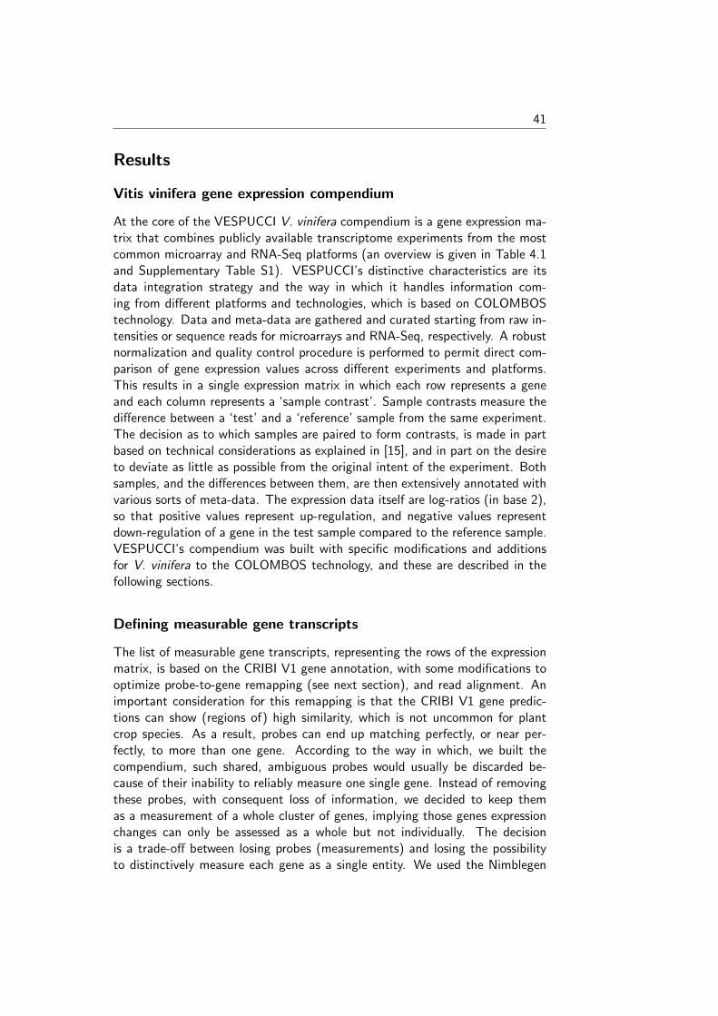
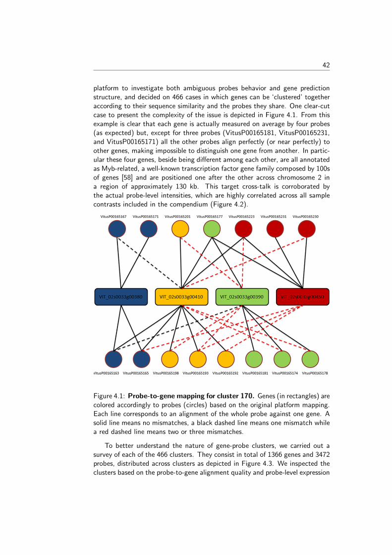
platform to investigate both ambiguous probes behavior and gene predictionstructure, and decided on 466 cases in which genes can be ‘clustered’ togetheraccording to their sequence similarity and the probes they share. One clear-cutcase to present the complexity of the issue is depicted in Figure 4.1. From thisexample is clear that each gene is actually measured on average by four probes(as expected) but, except for three probes (VitusP00165181, VitusP00165231,and VitusP00165171) all the other probes align perfectly (or near perfectly) toother genes, making impossible to distinguish one gene from another. In partic-ular these four genes, beside being different among each other, are all annotatedas Myb-related, a well-known transcription factor gene family composed by 100sof genes [58] and are positioned one after the other across chromosome 2 ina region of approximately 130 kb. This target cross-talk is corroborated bythe actual probe-level intensities, which are highly correlated across all samplecontrasts included in the compendium (Figure 4.2).

Figure 4.1: Probe-to-gene mapping for cluster 170. Genes (in rectangles) arecolored accordingly to probes (circles) based on the original platform mapping.Each line corresponds to an alignment of the whole probe against one gene. Asolid line means no mismatches, a black dashed line means one mismatch whilea red dashed line means two or three mismatches.

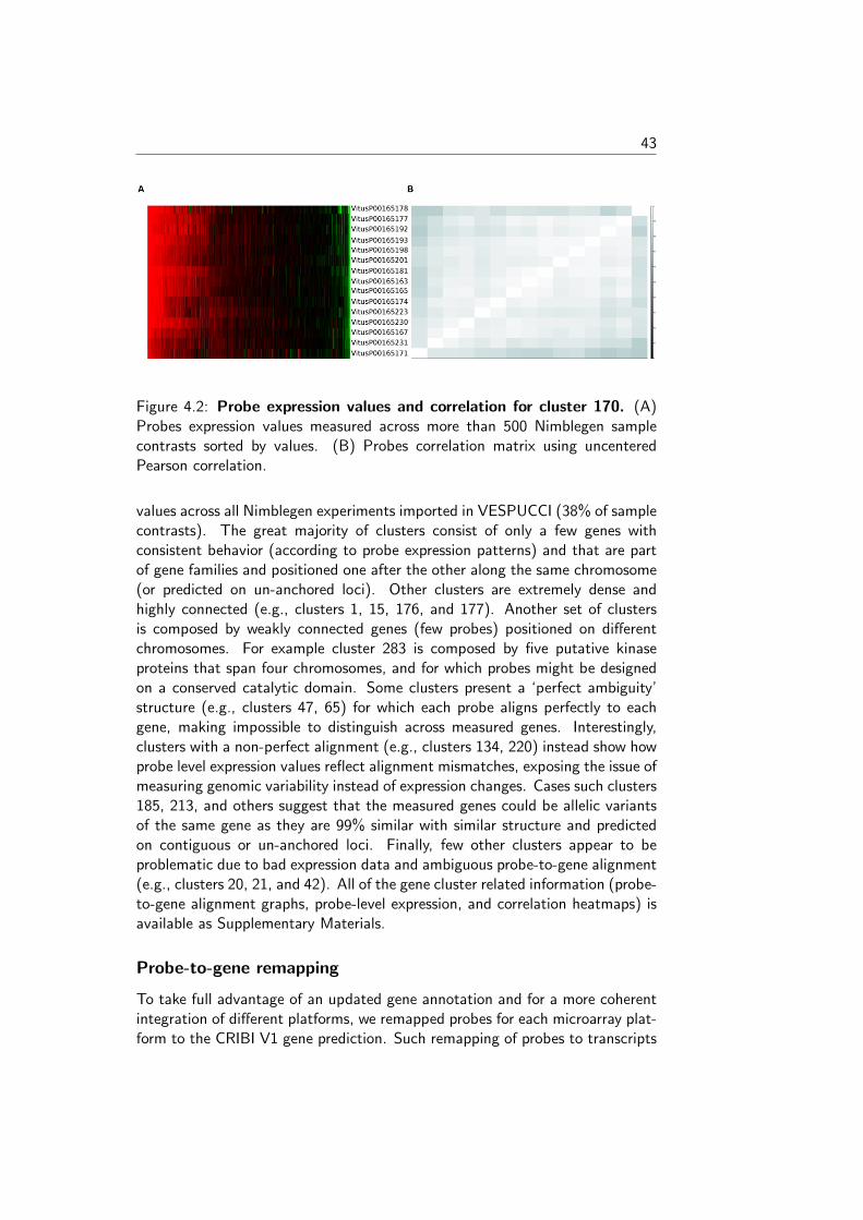
To better understand the nature of gene-probe clusters, we carried out asurvey of each of the 466 clusters. They consist in total of 1366 genes and 3472probes, distributed across clusters as depicted in Figure 4.3. We inspected theclusters based on the probe-to-gene alignment quality and probe-level expression

43

Figure 4.2: Probe expression values and correlation for cluster 170. (A)Probes expression values measured across more than 500 Nimblegen samplecontrasts sorted by values. (B) Probes correlation matrix using uncenteredPearson correlation.

values across all Nimblegen experiments imported in VESPUCCI (38% of samplecontrasts). The great majority of clusters consist of only a few genes withconsistent behavior (according to probe expression patterns) and that are partof gene families and positioned one after the other along the same chromosome(or predicted on un-anchored loci). Other clusters are extremely dense andhighly connected (e.g., clusters 1, 15, 176, and 177). Another set of clustersis composed by weakly connected genes (few probes) positioned on differentchromosomes. For example cluster 283 is composed by five putative kinaseproteins that span four chromosomes, and for which probes might be designedon a conserved catalytic domain. Some clusters present a ‘perfect ambiguity’structure (e.g., clusters 47, 65) for which each probe aligns perfectly to eachgene, making impossible to distinguish across measured genes. Interestingly,clusters with a non-perfect alignment (e.g., clusters 134, 220) instead show howprobe level expression values reflect alignment mismatches, exposing the issue ofmeasuring genomic variability instead of expression changes. Cases such clusters185, 213, and others suggest that the measured genes could be allelic variantsof the same gene as they are 99% similar with similar structure and predictedon contiguous or un-anchored loci. Finally, few other clusters appear to beproblematic due to bad expression data and ambiguous probe-to-gene alignment(e.g., clusters 20, 21, and 42). All of the gene cluster related information (probe-to-gene alignment graphs, probe-level expression, and correlation heatmaps) isavailable as Supplementary Materials.

Probe-to-gene remapping

To take full advantage of an updated gene annotation and for a more coherentintegration of different platforms, we remapped probes for each microarray plat-form to the CRIBI V1 gene prediction. Such remapping of probes to transcripts

44

Figure 4.3: Overview of gene clusters. Both the size and color of the spheresare proportional to the number of clusters that is made up of a given numberof genes and probes. It is clear that the great majority of clusters are composedby just few genes and probes.

has advantages over original annotations [59]. Different microarray platformshave different probe-to-gene alignment qualities. Given the disparateness interms of number of samples, number of measured transcripts, and probe-to-genemapping quality not all the available microarray platforms have been imported.The top performing platform is the Nimblegen microarray that shows a nearlyperfect correspondence to the one in VESPUCCI. This is easily explained bythe fact that it contains 118015 probes of 60 nucleotides with an average offour probes per gene and was specifically designed to match the CRIBI V1 geneprediction. It measures the expression of 29549 (out of 29971) gene predictionsrepresenting ∼98.6% of the genes of the CRIBI V1 gene prediction and 19091random probes as negative controls [60], [61]. On the other hand, platforms likethe ‘University of Arizona Vitis buds spotted DNA/cDNA array’ exhibit quitepoor performance in terms of number of measured transcripts, probe-to-genemapping, and probe signal (data not shown), which made us decide to excludeit from the compendium. The low quality can be ascribed to the fact that its10369 probes have been designed from ESTs of two V. vinifera cultivars (Per-lette and Superior) as well as the V. riparia species, and have an average lengthof nearly 1 kb. We compared our probe-to-gene mapping results to the origi-nal mappings for the microarray platforms using the complete gene annotation4

4http://www.sdstate.edu/ps/research/vitis/pathways.cfm

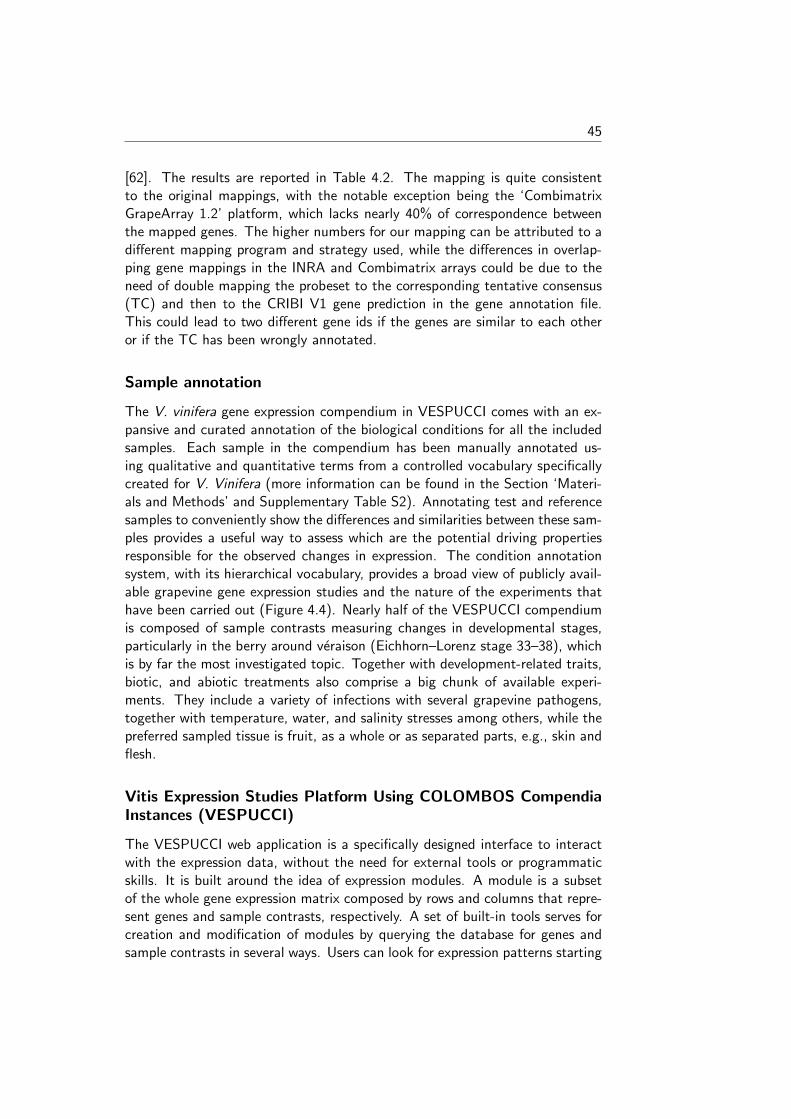
45

[62]. The results are reported in Table 4.2. The mapping is quite consistentto the original mappings, with the notable exception being the ‘CombimatrixGrapeArray 1.2’ platform, which lacks nearly 40% of correspondence betweenthe mapped genes. The higher numbers for our mapping can be attributed to adifferent mapping program and strategy used, while the differences in overlap-ping gene mappings in the INRA and Combimatrix arrays could be due to theneed of double mapping the probeset to the corresponding tentative consensus(TC) and then to the CRIBI V1 gene prediction in the gene annotation file.This could lead to two different gene ids if the genes are similar to each otheror if the TC has been wrongly annotated.

Sample annotation

The V. vinifera gene expression compendium in VESPUCCI comes with an ex-pansive and curated annotation of the biological conditions for all the includedsamples. Each sample in the compendium has been manually annotated us-ing qualitative and quantitative terms from a controlled vocabulary specificallycreated for V. Vinifera (more information can be found in the Section ‘Materi-als and Methods’ and Supplementary Table S2). Annotating test and referencesamples to conveniently show the differences and similarities between these sam-ples provides a useful way to assess which are the potential driving propertiesresponsible for the observed changes in expression. The condition annotationsystem, with its hierarchical vocabulary, provides a broad view of publicly avail-able grapevine gene expression studies and the nature of the experiments thathave been carried out (Figure 4.4). Nearly half of the VESPUCCI compendiumis composed of sample contrasts measuring changes in developmental stages,particularly in the berry around veraison (Eichhorn–Lorenz stage 33–38), whichis by far the most investigated topic. Together with development-related traits,biotic, and abiotic treatments also comprise a big chunk of available experi-ments. They include a variety of infections with several grapevine pathogens,together with temperature, water, and salinity stresses among others, while thepreferred sampled tissue is fruit, as a whole or as separated parts, e.g., skin andflesh.

Vitis Expression Studies Platform Using COLOMBOS CompendiaInstances (VESPUCCI)

The VESPUCCI web application is a specifically designed interface to interactwith the expression data, without the need for external tools or programmaticskills. It is built around the idea of expression modules. A module is a subsetof the whole gene expression matrix composed by rows and columns that repre-sent genes and sample contrasts, respectively. A set of built-in tools serves forcreation and modification of modules by querying the database for genes andsample contrasts in several ways. Users can look for expression patterns starting

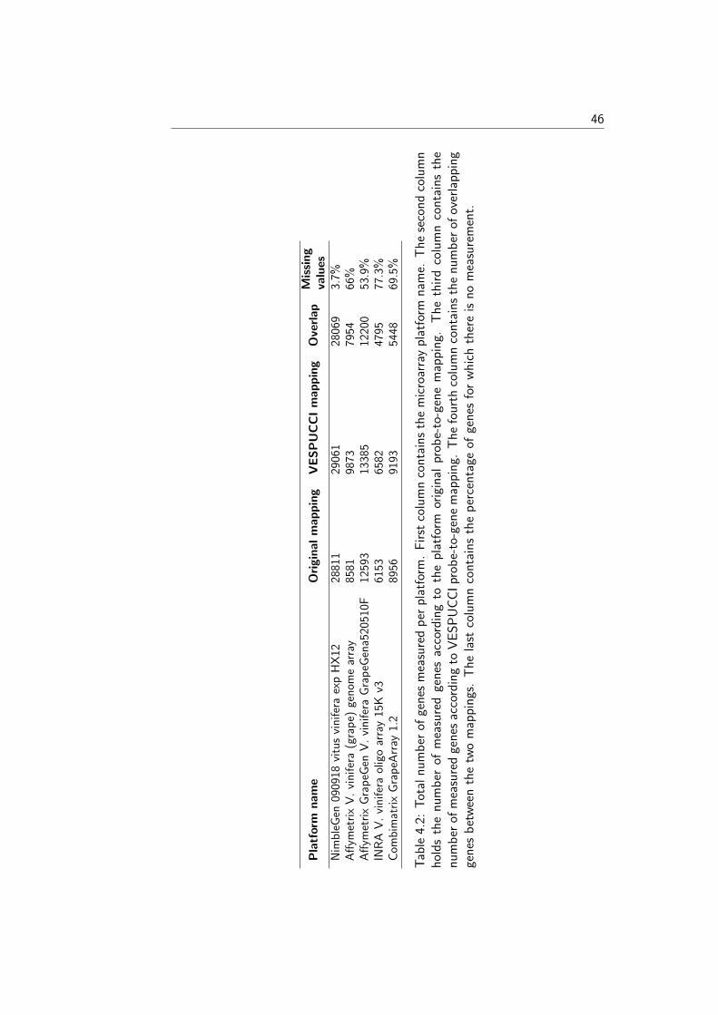
46

Pla

tfo

rmn

am

eO

rig

ina

lm

ap

pin

gV

ES

PU

CC

Im

ap

pin

gO

verl

ap

Mis

sin

gva

lues

Nim

ble

Gen

0909

18vi

tus

vin

ifer

aex

pH

X12

2881

129

061

2806

93.

7%A

ffym

etri

xV

.vi

nif

era

(gra

pe)

gen

ome

arra

y85

8198

7379

5466

%A

ffym

etri

xG

rap

eGen

V.

vin

ifer

aG

rap

eGen

a520

510F

1259

313

385

1220

053

.9%

INR

AV

.vi

nif

era

olig

oar

ray

15K

v361

5365

8247

9577

.3%

Com

bim

atri

xG

rap

eArr

ay1.

289

5691

9354

4869

.5%

Tab

le4.

2:T

otal

nu

mb

erof

gen

esm

easu

red

per

pla

tfor

m.

Fir

stco

lum

nco

nta

ins

the

mic

roar

ray

pla

tfor

mn

ame.

Th

ese

con

dco

lum

nh

old

sth

en

um

ber

ofm

easu

red

gen

esac

cord

ing

toth

ep

latf

orm

orig

inal

prob

e-to

-gen

em

app

ing.

Th

eth

ird

colu

mn

con

tain

sth

en

um

ber

ofm

easu

red

gen

esac

cord

ing

toV

ES

PU

CC

Ipr

obe-

to-g

ene

map

pin

g.T

he

fou

rth

colu

mn

con

tain

sth

en

um

ber

ofov

erla

pp

ing

gen

esb

etw

een

the

two

map

pin

gs.

Th

ela

stco

lum

nco

nta

ins

the

per

cen

tage

ofge

nes

for

wh

ich

ther

eis

no

mea

sure

men

t.

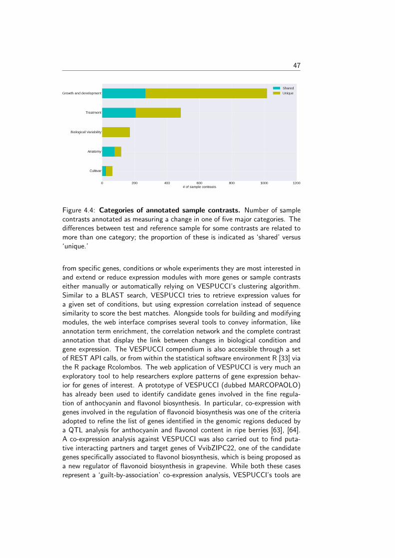
47

Figure 4.4: Categories of annotated sample contrasts. Number of samplecontrasts annotated as measuring a change in one of five major categories. Thedifferences between test and reference sample for some contrasts are related tomore than one category; the proportion of these is indicated as ‘shared’ versus‘unique.’

from specific genes, conditions or whole experiments they are most interested inand extend or reduce expression modules with more genes or sample contrastseither manually or automatically relying on VESPUCCI’s clustering algorithm.Similar to a BLAST search, VESPUCCI tries to retrieve expression values fora given set of conditions, but using expression correlation instead of sequencesimilarity to score the best matches. Alongside tools for building and modifyingmodules, the web interface comprises several tools to convey information, likeannotation term enrichment, the correlation network and the complete contrastannotation that display the link between changes in biological condition andgene expression. The VESPUCCI compendium is also accessible through a setof REST API calls, or from within the statistical software environment R [33] viathe R package Rcolombos. The web application of VESPUCCI is very much anexploratory tool to help researchers explore patterns of gene expression behav-ior for genes of interest. A prototype of VESPUCCI (dubbed MARCOPAOLO)has already been used to identify candidate genes involved in the fine regula-tion of anthocyanin and flavonol biosynthesis. In particular, co-expression withgenes involved in the regulation of flavonoid biosynthesis was one of the criteriaadopted to refine the list of genes identified in the genomic regions deduced bya QTL analysis for anthocyanin and flavonol content in ripe berries [63], [64].A co-expression analysis against VESPUCCI was also carried out to find puta-tive interacting partners and target genes of VvibZIPC22, one of the candidategenes specifically associated to flavonol biosynthesis, which is being proposed asa new regulator of flavonoid biosynthesis in grapevine. While both these casesrepresent a ‘guilt-by-association’ co-expression analysis, VESPUCCI’s tools are

48

not limited to that and are designed to encourage users to play around withdata in the compendium given the biological process they are interested in.One could also query for experiments of interest instead of genes, or simplystudy the behavior of (a set of) genes of interest across the different biolog-ical conditions without necessarily looking for other co-expressed genes. Forinstance, the top part of Figure 4.5 shows the results of a default Quicksearchfor the 11 genes of the carotenoid cleavage dioxygenases (CCD/NCED) genefamily, part of the grape carotenoid pathway [65]. The results of such a defaultsearch do not show all condition contrasts in the compendium, but only thetop most relevant for the query genes, and can already provide insights intotheir behavior. First and foremost, it appears that the genes of this small genefamily are not at all expressed in the same manner, and that for this particularfamily similarities in expression profiles are correlated up to a certain extent withthe phylogenetic relationships between its genes [the superimposed tree in thebottom part of the figure is adapted from the phylogeny presented in Figure6 of [66]]. A deeper inspection of that behavior not only confirms previouslyreported results, such as up-regulation at berry ripening of CCD4a and CCD4b,but not CCD4c [67], but it also provides some novel, potentially interesting leadsfor further exploration. For instance, there is a prominent -but not consistent-anti-correlation of NCED2 and NCED3 with CCD4a and CCD4b. There arealso strong changes in expression of some gene family members in response toEutypa lata infection. These sort of observations generally only represent theinitial starting point of further VESPUCCI analyses, such as investigating thesegenes’ behavior in other infection processes contained in the compendium, ormaybe looking for co-expressed genes with NCED2/NCED3 or CCD4a/CCD4b.For an in-depth illustration of these concepts, we have included another casestudy in the website as well, which is presented there as a detailed step-by-steptutorial with the ability to load associated data directly in the interface. Thisparticular case study is meant to show off VESPUCCI’s most common featuresand capabilities in a hands-on manner. It focuses on a set of genes found tobe modulated by the phytohormone abscisic acid (ABA) in pre-veraison berries(Stefania Pilati, personal communication); this list of genes was used as in-put to query the database. After performing any database query, VESPUCCIcreates an expression ‘module’, a subset of the whole expression compendiumdetermined by a set of genes and a set of sample contrasts and the correspond-ing expression values. The returned gene expression module indicated that the55 ABA genes appear highly modulated in 353 experimental conditions in theVESPUCCI compendium. The default visualization of this module (‘by expres-sion’; Figure 4.6) emphasizes the interesting patterns of condition-dependent(anti-)co-expression behavior among this set of ABA genes. The gene anno-tation enrichment in turn reports their involvement in the response to stressand ABA, as well as in galactose metabolism. The main biological processesrepresented in our module, correspond to different biological contexts in whichABA affects gene expression: fruit and berry development, bud development,

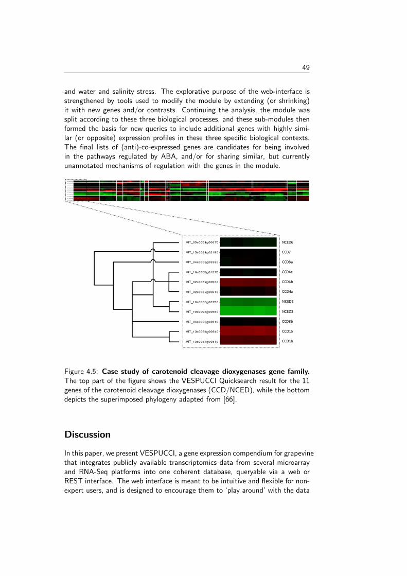
49

and water and salinity stress. The explorative purpose of the web-interface isstrengthened by tools used to modify the module by extending (or shrinking)it with new genes and/or contrasts. Continuing the analysis, the module wassplit according to these three biological processes, and these sub-modules thenformed the basis for new queries to include additional genes with highly simi-lar (or opposite) expression profiles in these three specific biological contexts.The final lists of (anti)-co-expressed genes are candidates for being involvedin the pathways regulated by ABA, and/or for sharing similar, but currentlyunannotated mechanisms of regulation with the genes in the module.

Figure 4.5: Case study of carotenoid cleavage dioxygenases gene family.The top part of the figure shows the VESPUCCI Quicksearch result for the 11genes of the carotenoid cleavage dioxygenases (CCD/NCED), while the bottomdepicts the superimposed phylogeny adapted from [66].

Discussion

In this paper, we present VESPUCCI, a gene expression compendium for grapevinethat integrates publicly available transcriptomics data from several microarrayand RNA-Seq platforms into one coherent database, queryable via a web orREST interface. The web interface is meant to be intuitive and flexible for non-expert users, and is designed to encourage them to ‘play around’ with the data

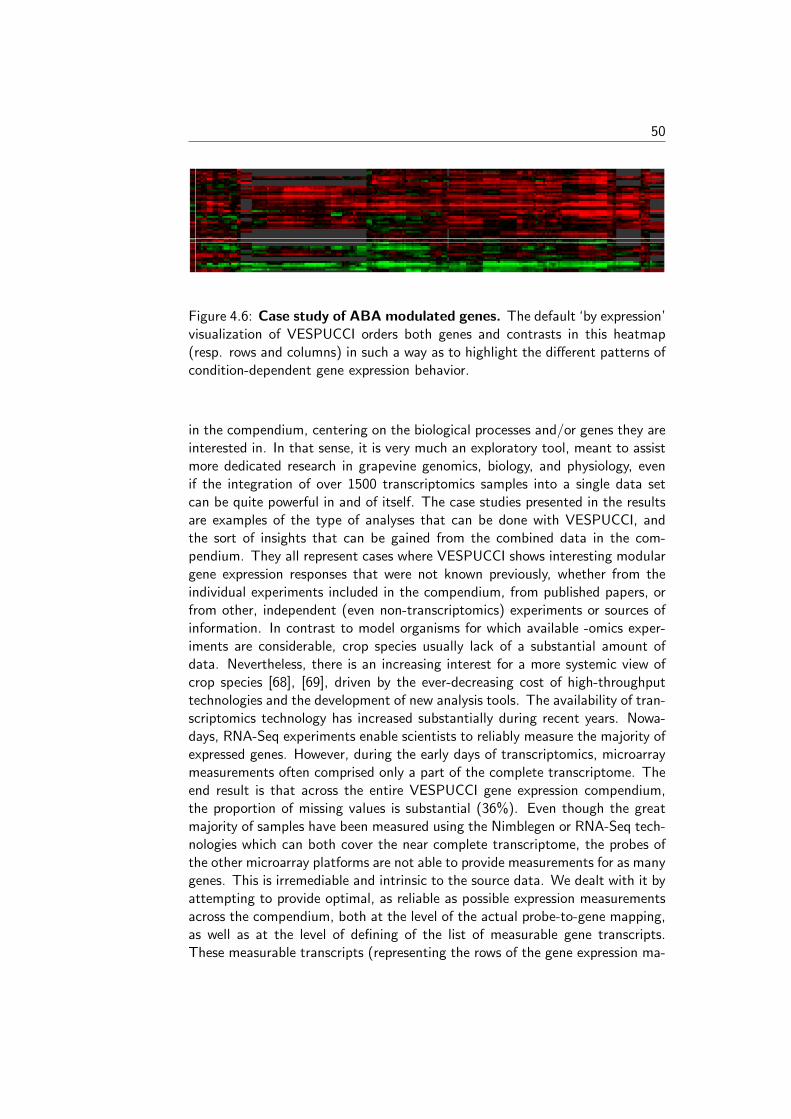
50

Figure 4.6: Case study of ABA modulated genes. The default ‘by expression’visualization of VESPUCCI orders both genes and contrasts in this heatmap(resp. rows and columns) in such a way as to highlight the different patterns ofcondition-dependent gene expression behavior.

in the compendium, centering on the biological processes and/or genes they areinterested in. In that sense, it is very much an exploratory tool, meant to assistmore dedicated research in grapevine genomics, biology, and physiology, evenif the integration of over 1500 transcriptomics samples into a single data setcan be quite powerful in and of itself. The case studies presented in the resultsare examples of the type of analyses that can be done with VESPUCCI, andthe sort of insights that can be gained from the combined data in the com-pendium. They all represent cases where VESPUCCI shows interesting modulargene expression responses that were not known previously, whether from theindividual experiments included in the compendium, from published papers, orfrom other, independent (even non-transcriptomics) experiments or sources ofinformation. In contrast to model organisms for which available -omics exper-iments are considerable, crop species usually lack of a substantial amount ofdata. Nevertheless, there is an increasing interest for a more systemic view ofcrop species [68], [69], driven by the ever-decreasing cost of high-throughputtechnologies and the development of new analysis tools. The availability of tran-scriptomics technology has increased substantially during recent years. Nowa-days, RNA-Seq experiments enable scientists to reliably measure the majority ofexpressed genes. However, during the early days of transcriptomics, microarraymeasurements often comprised only a part of the complete transcriptome. Theend result is that across the entire VESPUCCI gene expression compendium,the proportion of missing values is substantial (36%). Even though the greatmajority of samples have been measured using the Nimblegen or RNA-Seq tech-nologies which can both cover the near complete transcriptome, the probes ofthe other microarray platforms are not able to provide measurements for as manygenes. This is irremediable and intrinsic to the source data. We dealt with it byattempting to provide optimal, as reliable as possible expression measurementsacross the compendium, both at the level of the actual probe-to-gene mapping,as well as at the level of defining of the list of measurable gene transcripts.These measurable transcripts (representing the rows of the gene expression ma-

51

trix) incur some limitations in and of themselves as they are entirely based onthe gene predictions for V. vinifera cv. Pinot Noir, with implications for exper-iments done on other cultivars. When microarray experiments are performedto measure expression for a specific cultivar with platforms containing probesdesigned from different cultivars, this generally leads to poorer signals, giventhe impossibility to distinguish expression variability from genomic differencesamong those cultivars. The reason is the lack of available high-quality genepredictions for each cultivar. While RNA-Seq has the advantage of enhanc-ing its value over time with better genomes and gene annotations by re-doingthe transcriptome mapping on the appropriate cultivar, the situation is morecomplicated for microarray data. The solution is never ideal as nothing can bedone to increase the quality of intensity signals if there is a mismatch betweenthe cultivar used to design the probes, and the one used to do the experi-ment. Nevertheless, remapping the microarray probes on the cultivar-specificgenes of the experiment would improve the gene annotation of the array plat-form and ensure only the reliable probes are considered to generate the finalexpression values. A novelty in the latest release of COLOMBOS is the optionto explicitly recognize genomic differences between strains or cultivars insteadof using a single reference genome to represent a species. This improves readalignment (RNA-Seq) or probe-to-gene mapping (microarrays) and generateshigher quality expression data. In the long term, as more grapevine cultivargenomes become available, we can rely on these COLOMBOS innovations tobuild compendia for different cultivars and integrate them at the species levelusing homolog mappings, creating a proper ‘meta-compendium’ for grapevinevarieties. Currently VESPUCCI is limited to our knowledge of the V. vinifera cv.Pinot Noir genome, and despite the existence of a more recent version of theCRIBI gene prediction [70], we decided to keep V1 as the basis for this first re-lease. From a practical perspective, by the time V2 was made publicly available,most of the compendium was already built and the switch to the newer versiondidn’t show a significant increase quality-wise. The great majority of genes doesnot change in terms of gene structure, and as such for our purposes the endresult was largely unaffected by the enhancements of the newer version over V1.Nevertheless, as the number of experiments (especially RNA-Seq) increases, thebenefits of relying on V2 will become more prominent; for future VESPUCCIreleases, we will most likely shift toward V2 (or more recent versions) to takeadvantage of the extended UTR regions for which NGS technologies providebetter measurements. The measurable gene transcripts that, we defined do notcorrespond one-to-one to the CRIBI gene predictions, but instead contain some‘gene clusters’. Expression data for these gene clusters are a compromise be-tween our ability to measure each and every single gene individually, and howmany genes can be reliably measured in total. While not absolute proof thatthese probes are unable to adequately distinguish the intended target genes, ourresults (Figures 4.1 and 4.2, and Supplementary Materials) showed that it isalmost impossible to measure differences between each single gene in the clus-

52

ters. This supports our decision to throw them together: even if these probeswere capable of capturing different transcripts, the results do not indicate thatthis was the case for the more than 500 Nimblegen sample contrasts in thecompendium. Therefore, instead of discarding the shared probes and lose po-tentially valuable information, we accepted the impossibility to unambiguouslydiscriminate each and every single gene, gaining the opportunity to have a singlemeasurement for those gene transcripts as a whole. Note that while the issueitself is (microarray) platform specific, the proposed ‘gene clusters’ are not. Wechose to define them based on the platform with the highest data representa-tion: the Nimblegen platform holds the largest number of samples as well asthe highest quality of probe-to-gene mapping. This has no detrimental effect ondata from the other microarray platforms, but RNA-Seq technology can provideindividual gene measurements for at least some of our defined clusters (giventhat the corresponding gene sequences show enough dissimilarity). Due to thecurrent low number of RNA-Seq experiments compared to the Nimblegen ones,we decided on clustering genes together in measurable sets to get the best outof all the data as a whole. As soon as RNA-Seq experiments will be more preva-lent, we will revise the gene clusters to gain the ability to measure more genesseparately for RNA-Seq, at the expense of losing the corresponding probes onthe Nimblegen platform. VESPUCCI includes nearly all of the gene expressiondata that is publicly available for grapevine at the moment; it provides a snap-shot of the current situation of transcriptomics experiments performed. We’replanning to keep it up to date by releasing yearly content updates. In the cur-rent release, berry development studies are the most represented experiments(especially during veraison) and this comes with no surprise given the impor-tance of fruit quality in wine and spirits’ production. This will be all the moreobvious when mining for genes related to fruit ripening. Given the complexity ofthis developmental process, in which the fruit undergoes radical phenotypic andbiochemical modifications (related to shape, size, color, sugar and aroma con-tent, etc.), the number of modulated genes is quite big. VESPUCCI is meantas an exploratory tool to help researcher not only in finding patterns of geneexpression for genes of interest, but also to aid the design of new experimentsproviding the most complete transcriptomics information currently available.

Part two

53

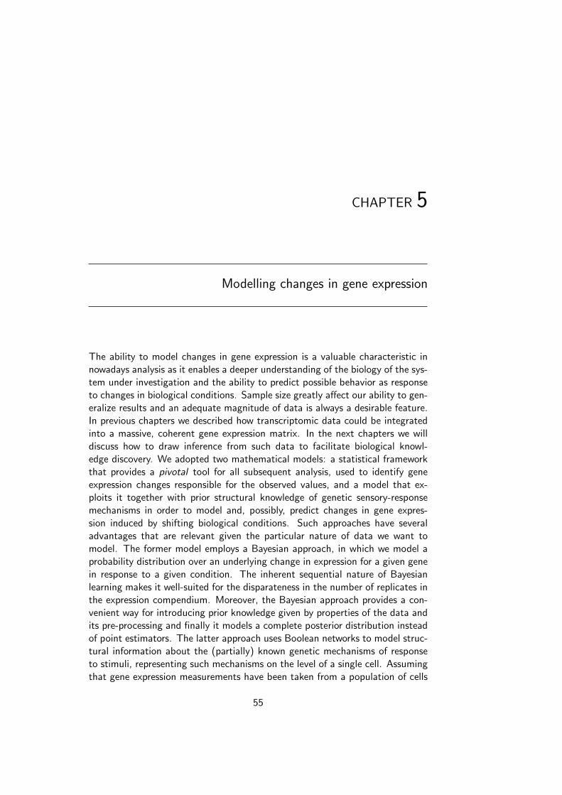
CHAPTER 5

Modelling changes in gene expression

The ability to model changes in gene expression is a valuable characteristic innowadays analysis as it enables a deeper understanding of the biology of the sys-tem under investigation and the ability to predict possible behavior as responseto changes in biological conditions. Sample size greatly affect our ability to gen-eralize results and an adequate magnitude of data is always a desirable feature.In previous chapters we described how transcriptomic data could be integratedinto a massive, coherent gene expression matrix. In the next chapters we willdiscuss how to draw inference from such data to facilitate biological knowl-edge discovery. We adopted two mathematical models: a statistical frameworkthat provides a pivotal tool for all subsequent analysis, used to identify geneexpression changes responsible for the observed values, and a model that ex-ploits it together with prior structural knowledge of genetic sensory-responsemechanisms in order to model and, possibly, predict changes in gene expres-sion induced by shifting biological conditions. Such approaches have severaladvantages that are relevant given the particular nature of data we want tomodel. The former model employs a Bayesian approach, in which we model aprobability distribution over an underlying change in expression for a given genein response to a given condition. The inherent sequential nature of Bayesianlearning makes it well-suited for the disparateness in the number of replicates inthe expression compendium. Moreover, the Bayesian approach provides a con-venient way for introducing prior knowledge given by properties of the data andits pre-processing and finally it models a complete posterior distribution insteadof point estimators. The latter approach uses Boolean networks to model struc-tural information about the (partially) known genetic mechanisms of responseto stimuli, representing such mechanisms on the level of a single cell. Assumingthat gene expression measurements have been taken from a population of cells

55

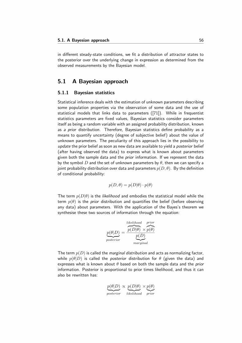
5.1. A Bayesian approach 56

in different steady-state conditions, we fit a distribution of attractor states tothe posterior over the underlying change in expression as determined from theobserved measurements by the Bayesian model.

5.1 A Bayesian approach

5.1.1 Bayesian statistics

Statistical inference deals with the estimation of unknown parameters describingsome population properties via the observation of some data and the use ofstatistical models that links data to parameters ([71]). While in frequentiststatistics parameters are fixed values, Bayesian statistics consider parametersitself as being a random variable with an assigned probability distribution, knownas a prior distribution. Therefore, Bayesian statistics define probability as ameans to quantify uncertainty (degree of subjective belief) about the value ofunknown parameters. The peculiarity of this approach lies in the possibility toupdate the prior belief as soon as new data are available to yield a posterior belief(after having observed the data) to express what is known about parametersgiven both the sample data and the prior information. If we represent the databy the symbol D and the set of unknown parameters by θ, then we can specify ajoint probability distribution over data and parameters p(D, θ). By the definitionof conditional probability:

p(D, θ) = p(D|θ) · p(θ)

The term p(D|θ) is the likelihood and embodies the statistical model while theterm p(θ) is the prior distribution and quantifies the belief (before observingany data) about parameters. With the application of the Bayes’s theorem wesynthesise these two sources of information through the equation:

p(θ|D)︸ ︷︷ ︸posterior

=

likelihood︷ ︸︸ ︷p(D|θ) ×

prior︷︸︸︷p(θ)

p(D)︸ ︷︷ ︸marginal

The term p(D) is called the marginal distribution and acts as normalizing factor,while p(θ|D) is called the posterior distribution for θ (given the data) andexpresses what is known about θ based on both the sample data and the priorinformation. Posterior is proportional to prior times likelihood, and thus it canalso be rewritten has:

p(θ|D)︸ ︷︷ ︸posterior

∝ p(D|θ)︸ ︷︷ ︸likelihood

× p(θ)︸︷︷︸prior

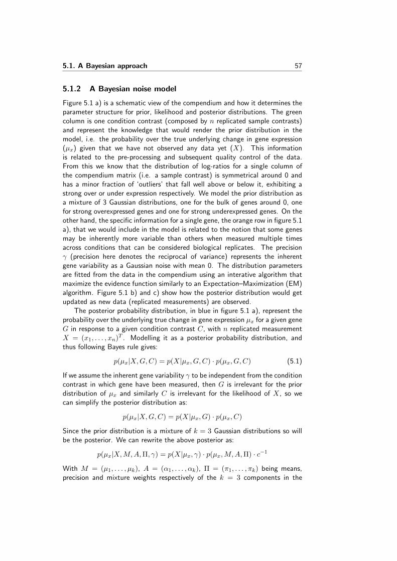
5.1. A Bayesian approach 57

5.1.2 A Bayesian noise model

Figure 5.1 a) is a schematic view of the compendium and how it determines theparameter structure for prior, likelihood and posterior distributions. The greencolumn is one condition contrast (composed by n replicated sample contrasts)and represent the knowledge that would render the prior distribution in themodel, i.e. the probability over the true underlying change in gene expression(µx) given that we have not observed any data yet (X). This informationis related to the pre-processing and subsequent quality control of the data.From this we know that the distribution of log-ratios for a single column ofthe compendium matrix (i.e. a sample contrast) is symmetrical around 0 andhas a minor fraction of ‘outliers’ that fall well above or below it, exhibiting astrong over or under expression respectively. We model the prior distribution asa mixture of 3 Gaussian distributions, one for the bulk of genes around 0, onefor strong overexpressed genes and one for strong underexpressed genes. On theother hand, the specific information for a single gene, the orange row in figure 5.1a), that we would include in the model is related to the notion that some genesmay be inherently more variable than others when measured multiple timesacross conditions that can be considered biological replicates. The precisionγ (precision here denotes the reciprocal of variance) represents the inherentgene variability as a Gaussian noise with mean 0. The distribution parametersare fitted from the data in the compendium using an interative algorithm thatmaximize the evidence function similarly to an Expectation–Maximization (EM)algorithm. Figure 5.1 b) and c) show how the posterior distribution would getupdated as new data (replicated measurements) are observed.

The posterior probability distribution, in blue in figure 5.1 a), represent theprobability over the underlying true change in gene expression µx for a given geneG in response to a given condition contrast C, with n replicated measurementX = (x1, . . . , xn)T . Modelling it as a posterior probability distribution, andthus following Bayes rule gives:

p(µx|X,G,C) = p(X|µx, G,C) · p(µx, G,C) (5.1)

If we assume the inherent gene variability γ to be independent from the conditioncontrast in which gene have been measured, then G is irrelevant for the priordistribution of µx and similarly C is irrelevant for the likelihood of X, so wecan simplify the posterior distribution as:

p(µx|X,G,C) = p(X|µx, G) · p(µx, C)

Since the prior distribution is a mixture of k = 3 Gaussian distributions so willbe the posterior. We can rewrite the above posterior as:

p(µx|X,M,A,Π, γ) = p(X|µx, γ) · p(µx,M,A,Π) · c−1

With M = (µ1, . . . , µk), A = (α1, . . . , αk), Π = (π1, . . . , πk) being means,precision and mixture weights respectively of the k = 3 components in the

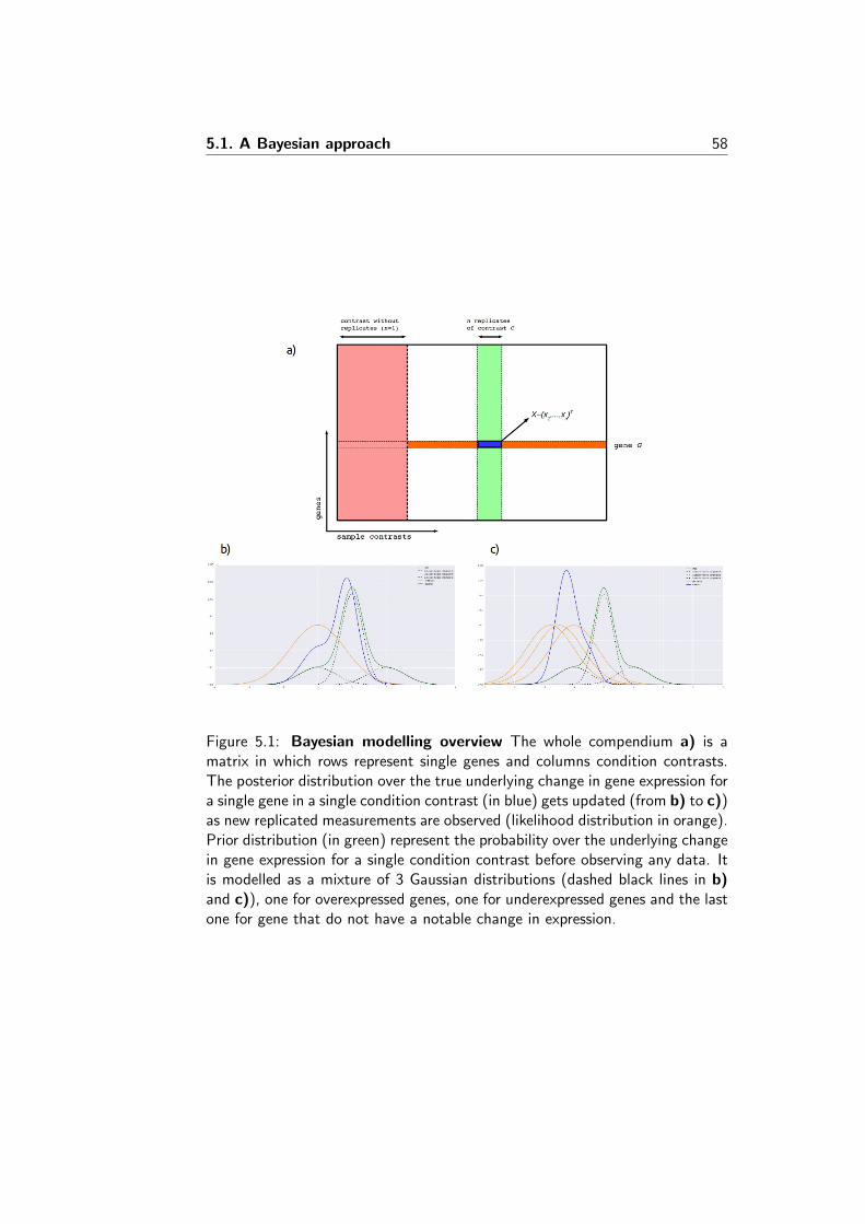
5.1. A Bayesian approach 58

Figure 5.1: Bayesian modelling overview The whole compendium a) is amatrix in which rows represent single genes and columns condition contrasts.The posterior distribution over the true underlying change in gene expression fora single gene in a single condition contrast (in blue) gets updated (from b) to c))as new replicated measurements are observed (likelihood distribution in orange).Prior distribution (in green) represent the probability over the underlying changein gene expression for a single condition contrast before observing any data. Itis modelled as a mixture of 3 Gaussian distributions (dashed black lines in b)and c)), one for overexpressed genes, one for underexpressed genes and the lastone for gene that do not have a notable change in expression.

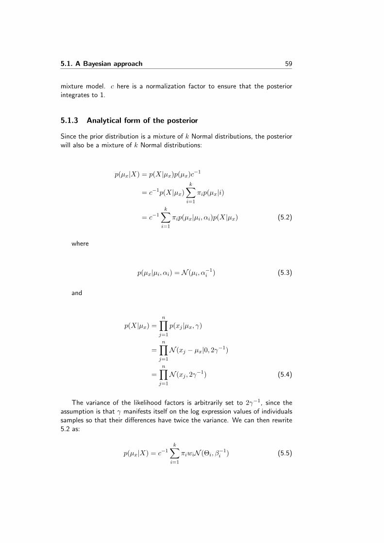
5.1. A Bayesian approach 59

mixture model. c here is a normalization factor to ensure that the posteriorintegrates to 1.

5.1.3 Analytical form of the posterior

Since the prior distribution is a mixture of k Normal distributions, the posteriorwill also be a mixture of k Normal distributions:

p(µx|X) = p(X|µx)p(µx)c−1

= c−1p(X|µx)k∑i=1

πip(µx|i)

= c−1k∑i=1

πip(µx|µi, αi)p(X|µx) (5.2)

where

p(µx|µi, αi) = N (µi, α−1i ) (5.3)

and

p(X|µx) =n∏j=1

p(xj |µx, γ)

=

n∏j=1

N (xj − µx|0, 2γ−1)

=

n∏j=1

N (xj , 2γ−1) (5.4)

The variance of the likelihood factors is arbitrarily set to 2γ−1, since theassumption is that γ manifests itself on the log expression values of individualssamples so that their differences have twice the variance. We can then rewrite5.2 as:

p(µx|X) = c−1k∑i=1

πiwiN (Θi, β−1i ) (5.5)

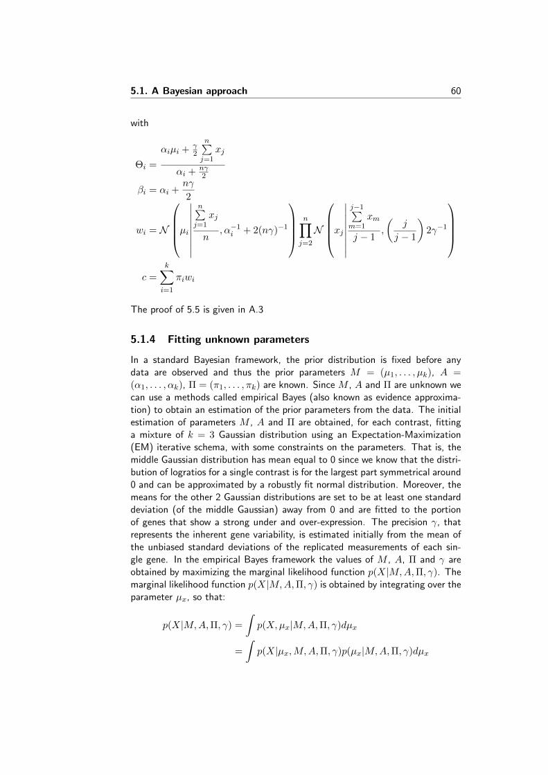
5.1. A Bayesian approach 60

with

Θi =

αiµi + γ2

n∑j=1

xj

αi + nγ2

βi = αi +nγ

2

wi = N

µi∣∣∣∣∣∣∣∣∣n∑j=1

xj

n, α−1i + 2(nγ)−1

n∏j=2

N

xj∣∣∣∣∣∣∣∣∣j−1∑m=1

xm

j − 1,

(j

j − 1

)2γ−1

c =

k∑i=1

πiwi

The proof of 5.5 is given in A.3

5.1.4 Fitting unknown parameters

In a standard Bayesian framework, the prior distribution is fixed before anydata are observed and thus the prior parameters M = (µ1, . . . , µk), A =(α1, . . . , αk), Π = (π1, . . . , πk) are known. Since M , A and Π are unknown wecan use a methods called empirical Bayes (also known as evidence approxima-tion) to obtain an estimation of the prior parameters from the data. The initialestimation of parameters M , A and Π are obtained, for each contrast, fittinga mixture of k = 3 Gaussian distribution using an Expectation-Maximization(EM) iterative schema, with some constraints on the parameters. That is, themiddle Gaussian distribution has mean equal to 0 since we know that the distri-bution of logratios for a single contrast is for the largest part symmetrical around0 and can be approximated by a robustly fit normal distribution. Moreover, themeans for the other 2 Gaussian distributions are set to be at least one standarddeviation (of the middle Gaussian) away from 0 and are fitted to the portionof genes that show a strong under and over-expression. The precision γ, thatrepresents the inherent gene variability, is estimated initially from the mean ofthe unbiased standard deviations of the replicated measurements of each sin-gle gene. In the empirical Bayes framework the values of M , A, Π and γ areobtained by maximizing the marginal likelihood function p(X|M,A,Π, γ). Themarginal likelihood function p(X|M,A,Π, γ) is obtained by integrating over theparameter µx, so that:

p(X|M,A,Π, γ) =

∫p(X,µx|M,A,Π, γ)dµx

=

∫p(X|µx,M,A,Π, γ)p(µx|M,A,Π, γ)dµx

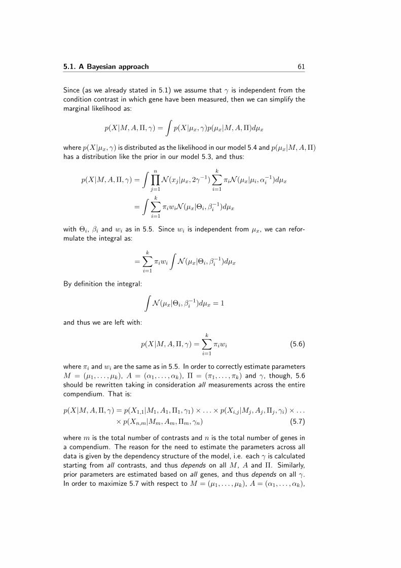
5.1. A Bayesian approach 61

Since (as we already stated in 5.1) we assume that γ is independent from thecondition contrast in which gene have been measured, then we can simplify themarginal likelihood as:

p(X|M,A,Π, γ) =

∫p(X|µx, γ)p(µx|M,A,Π)dµx

where p(X|µx, γ) is distributed as the likelihood in our model 5.4 and p(µx|M,A,Π)has a distribution like the prior in our model 5.3, and thus:

p(X|M,A,Π, γ) =

∫ n∏j=1

N (xj |µx, 2γ−1)k∑i=1

πiN (µx|µi, α−1i )dµx

=

∫ k∑i=1

πiwiN (µx|Θi, β−1i )dµx

with Θi, βi and wi as in 5.5. Since wi is independent from µx, we can refor-mulate the integral as:

=k∑i=1

πiwi

∫N (µx|Θi, β

−1i )dµx

By definition the integral: ∫N (µx|Θi, β

−1i )dµx = 1

and thus we are left with:

p(X|M,A,Π, γ) =

k∑i=1

πiwi (5.6)

where πi and wi are the same as in 5.5. In order to correctly estimate parametersM = (µ1, . . . , µk), A = (α1, . . . , αk), Π = (π1, . . . , πk) and γ, though, 5.6should be rewritten taking in consideration all measurements across the entirecompendium. That is:

p(X|M,A,Π, γ) = p(X1,1|M1, A1,Π1, γ1)× . . .× p(Xi,j |Mj , Aj ,Πj , γi)× . . .× p(Xn,m|Mm, Am,Πm, γn) (5.7)

where m is the total number of contrasts and n is the total number of genes ina compendium. The reason for the need to estimate the parameters across alldata is given by the dependency structure of the model, i.e. each γ is calculatedstarting from all contrasts, and thus depends on all M , A and Π. Similarly,prior parameters are estimated based on all genes, and thus depends on all γ.In order to maximize 5.7 with respect to M = (µ1, . . . , µk), A = (α1, . . . , αk),

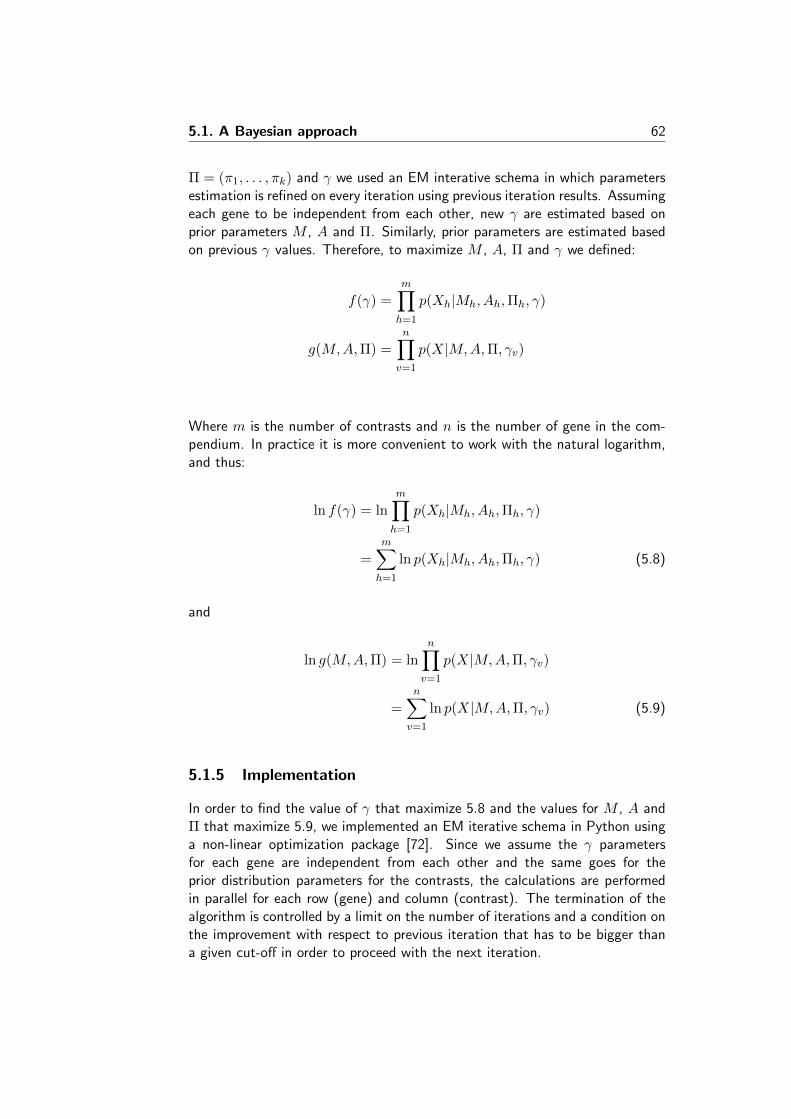
5.1. A Bayesian approach 62

Π = (π1, . . . , πk) and γ we used an EM interative schema in which parametersestimation is refined on every iteration using previous iteration results. Assumingeach gene to be independent from each other, new γ are estimated based onprior parameters M , A and Π. Similarly, prior parameters are estimated basedon previous γ values. Therefore, to maximize M , A, Π and γ we defined:

f(γ) =

m∏h=1

p(Xh|Mh, Ah,Πh, γ)

g(M,A,Π) =

n∏v=1

p(X|M,A,Π, γv)

Where m is the number of contrasts and n is the number of gene in the com-pendium. In practice it is more convenient to work with the natural logarithm,and thus:

ln f(γ) = lnm∏h=1

p(Xh|Mh, Ah,Πh, γ)

=

m∑h=1

ln p(Xh|Mh, Ah,Πh, γ) (5.8)

and

ln g(M,A,Π) = ln

n∏v=1

p(X|M,A,Π, γv)

=n∑v=1

ln p(X|M,A,Π, γv) (5.9)

5.1.5 Implementation

In order to find the value of γ that maximize 5.8 and the values for M , A andΠ that maximize 5.9, we implemented an EM iterative schema in Python usinga non-linear optimization package [72]. Since we assume the γ parametersfor each gene are independent from each other and the same goes for theprior distribution parameters for the contrasts, the calculations are performedin parallel for each row (gene) and column (contrast). The termination of thealgorithm is controlled by a limit on the number of iterations and a condition onthe improvement with respect to previous iteration that has to be bigger thana given cut-off in order to proceed with the next iteration.

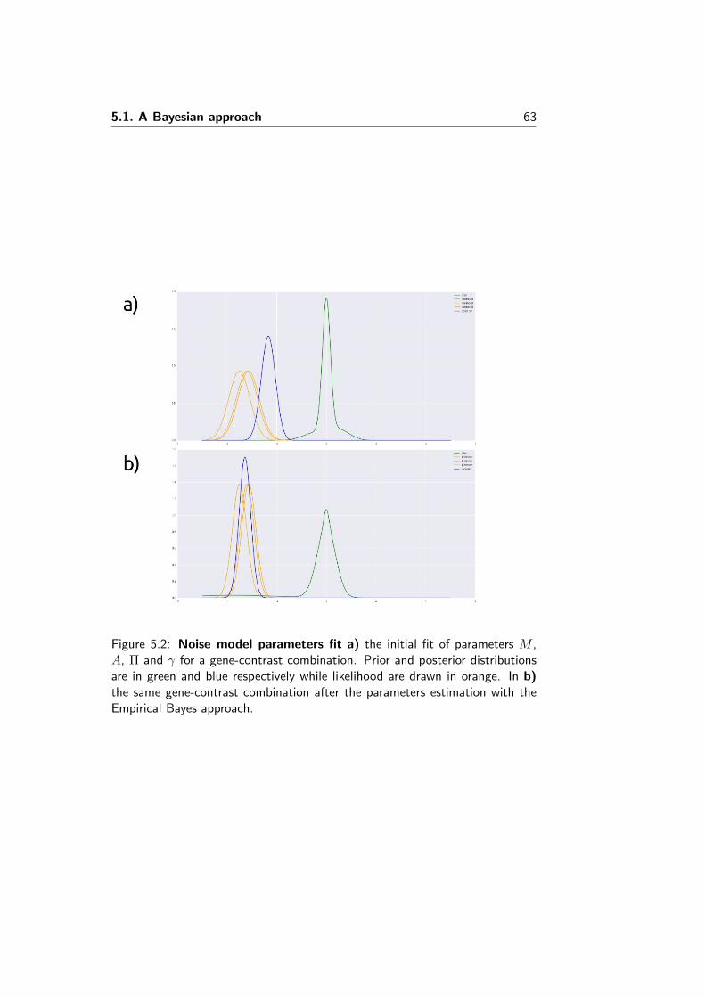
5.1. A Bayesian approach 63

Figure 5.2: Noise model parameters fit a) the initial fit of parameters M ,A, Π and γ for a gene-contrast combination. Prior and posterior distributionsare in green and blue respectively while likelihood are drawn in orange. In b)the same gene-contrast combination after the parameters estimation with theEmpirical Bayes approach.

5.2. A Boolean approach 64

5.2 A Boolean approach

5.2.1 Boolean networks

Boolean networks[73] are sets of Boolean variables (i.e. variables having just twovalues, usually denoted true and false), and Boolean function (i.e. a functionwith the form f : Bk → B, where B = true, false are connected by logicaloperators and, or, not and k ∈ N). Each variable (a node in the network)has associated a function, with inputs the states of the nodes connected to it.Boolean networks have a fixed topology that doesn’t change with time, butthey are dynamic in the sense that states of nodes (values of Boolean variables)change synchronously and discreetly with time. If the state of a node vi attime t is denoted as xi(t), then the state of that same node at time t + 1 isgiven by: xi(t + 1) = bi(xi1, . . . , xik) where xij are the states of the nodesconnected to vi and bi is a Boolean function. Since a Boolean network has only2n possible states (with n being the number of nodes) and their dynamics aredeterministic a trajectory will, sooner or later, reach a previously visited state.Once this will happen once, the trajectory will be stuck to repeatedly visit thesame nodes forever. These cycles of states into which the Boolean networks‘falls’ are called attractor states. Attractors are particularly interesting as theycapture the intuition of steady-states for living systems, i.e. a situation in whichall state variables are constant in spite of ongoing processes that strive to changethem.

5.2.2 The model

Every measurement in the compendia is a difference in expression (in logarithmicscale) between two conditions. Since we assume that:

1. every sample is composed by a population of cells;

2. every sample have been measured during cells steady-state;

the actual measurements in the compendia for a single gene in a given conditioncontrast do not represent one single ‘behavior’ coming from that gene in a singlecell, but (more precisely) represent an ‘average behavior’ for that gene measuredin the entire population of cells the sample is composed of. Even though ex-pression data in the COLOMBOS compendia are not well suited for being usedas-is with Boolean networks (since they usually don’t represent time-series andso it’s impossible to model the time-dependency of expression changes), theystill provide both a simple model for describing interactions of how a single cellresponds to stimuli, and a convenient way to describe each possible steady-statein which a system (a living cell in our case) can be at any given time, throughthe concept of attractor states. Since we cannot assume all cells in the sampleto be in the same steady-state, we are left with the problem of estimating howmany cells (in proportion) are in a specific steady-state in order to explain the

5.2. A Boolean approach 65

expression, or better the ‘mixture‘ of expressions, we observe. Thus, given ashift in biological conditions, expression data in the compendia for those samegenes (known to be involved) are used to fit a model that uses Boolean networkattractor states to simulate the different steady-states in which sub-populationsof cells were during the time of measurements. Estimated weights for eachpossible attractor state represent then the proportion of cells in that particularsteady-state. Since we don’t directly fit, but rather simulate, a Boolean net-work, prior knowledge on its topology is required in order to take advantage ofcompendia gene expression data. Boolean networks are manually built start-ing from the concept of ‘genetic sensory response units’ (Gensor Units) [75].Gensor Units (see figure 5.3) are relatively small modules that encapsulate theconcept of a signal sensed by the cell, the transduction of the signal and thetranscriptional regulation that modifies expression of genes responsible for theresponse. Gensor Units have several advantages since they are:

1. highly characterized;

2. manually curated;

3. modular;

4. relatively small;

5. heterogeneous.

Their specificity for a single condition input signal, highly characterization andmodularity provide an ideal framework for the methodology in degrees of in-creasing complexity. However, even if Boolean network simplicity permits towork with relatively large networks, the complexity of the problem, once severalof such units are combined, is combinatorial. Thus initially we limited simulatedcondition contrasts to be just four per GU in order to keep the computationtractable: the combination of the activation (or inactivation) of signal and tran-scription factor.

5.2.3 Implementation

The complete procedure as it is currently implemented starts from one (or more)given Gensor Units converted into a Boolean network, then it:

1. simulates test and reference conditions: setting nodes correspondingto signal and transcription factor to all the 4 combinations of true andfalse (to simulate the presence/absence) in the Boolean network;

2. calculate all possible attractor states for the two networks: to defineBoolean networks and calculate all possible attractor state we used the Rpackage BoolNet [76];

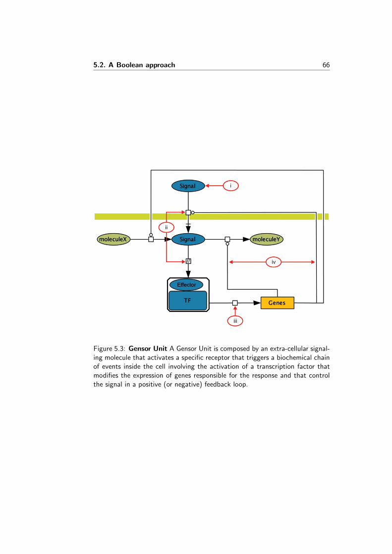
5.2. A Boolean approach 66

Figure 5.3: Gensor Unit A Gensor Unit is composed by an extra-cellular signal-ing molecule that activates a specific receptor that triggers a biochemical chainof events inside the cell involving the activation of a transcription factor thatmodifies the expression of genes responsible for the response and that controlthe signal in a positive (or negative) feedback loop.

5.2. A Boolean approach 67

3. calculate expression level for each network: as the relative value ofexpressed genes over all attractor states. That is, the ratio between thenumber of time a gene node value is true over the total number of at-tractor states;

4. calculate the simulated contrasts expression values: as the differencebetween test and reference expression values;

5. find the best weight for the attractor states: currently implementedas an optimization problem:

maxx,y∈Rn,w∈Rm

fw(x,y) (5.10)

with

m∑i=1

wi = 1

where f is the cosine similarity function, x is a simulated contrast calcu-lated in the previous step, y is a real contrast 1 in the compendia withthe same test and reference conditions, w is the vector of weights forthe attractor states, n is the number of genes and m is the number ofattractors.

The need to fit the weights to real contrasts is justified by the fact that otherwiseall attractor states would be considered equally important. Namely, all sub-population of cells in different steady-state in the measured sample would beequally numerous. Once the model is fit, it would be possible, given an unknowncontrast to understand which signal (if any) has been sensed by the cells in thesample. The real benefit, however, would rise combining more Gensor Units atthe same time to model signal interactions.

1Actually it is a vector of point-estimator like maximum a posteriori (MAP) from theposterior over the underlying true change in gene expression as determined from the observedmeasurements by the Bayesian model.

5.2. A Boolean approach 68

CHAPTER 6

Conclusion, discussion and future perspectives

The technological possibilities that arose during last few decades have givemodern biologists a lot of opportunities in terms of system-wide experimentsmeasuring a lot of features at the same time. Unfortunately, this comes with theproduction of a considerable amount of data for which at least basic skills ondata-management are required. The charm of new high-throughput technolo-gies urges scientists to adopt them, sometimes without having a clear idea aboutlimits and possibilities, or the new sources of noise that accompany them andof which little may be known. Moreover, the sole adoption of new technologiestends to be considered adequate by scientific journals to justify a publication.This tendency has led to the situation in which data production is often con-sidered the goal of a scientific effort instead of being considered just a tooltowards answering a scientific question. Since data alone aren’t sufficient tocreate knowledge, the adoption of statistical methods is fundamental to extractvaluable information and attempt to give valid biological interpretations of data.In this context data integration is a valuable approach since:

• it ease the issues about data and noise management and allow a broadview on existing experiments;

• and an adequate magnitude of data is a necessary characteristic to beable to draw strong and valid conclusions.

This Ph.D. thesis tries to tackles both issues showing the implementation andthe application of a methodology for gene expression data integration, and thedevelopment of statistical tools to analyze them.

The first part of the thesis focused on the work that was done related to theCOLOMBOS gene expression compendia technology. The integration of tran-scriptomic, and in general different -omics data, is an inherent part of biology

69

70

nowadays. The shift towards a data-driven science started with the advent ofhigh-throughput technologies that are able to produce an impressive amountof data measuring several layers of information at a broad level. Currently thequantity of data produced outweighs our ability to analyze them [77],[78] andoften not all the information a dataset can provide is used (for example RNA-seqexperiment used only for quantification, ignoring the actual sequence informa-tion, or sequencing the whole genome to extract only mitochondria informationfor phylogeny reconstruction). Bioinformatics and computational biology areessential tools for life-sciences because of it, and is testified to by the numberof publications that use bioinformatics tools and databases [79]. In this con-text of need for data integration, the COLOMBOS approach to transcriptomicintegration proved to be useful [23],[24],[25]. The entire expression compendiahave been used as well, for transcriptional regulatory network inference [26], forthe creation of co-expression networks [27],[28], and to study the evolution ofregulatory networks [21]. They also served to study Mutation Rate Plasticity(MRP) allowing a fast analysis of all published studies in gene expression [20], orprovided essential data for a multi-omics data integration using network analy-sis and flux balance analysis [22]. The COLOMBOS controlled vocabulary usedto formally annotate condition contrasts has provided a way to link changes ingene expression to causal factors like genomic mutations [29], or the activationof transcription regulation [30].

The maintenance and development of COLOMBOS (and COMMAND, thecompendia build tools) has been an ongoing process and in chapter 2 we dis-cussed how we initialized a radical change. The stepwise phase-out strategyadopted here to gradually disband the old implementation, has permitted touse the newer version as soon as it became a working prototype while preserv-ing the old implementation for all the features not yet implemented in the newerversion. The development of COLOMBOS old code will stop and the whole ap-plication will be moved to the new framework, implementing a new paradigm formeta-compendia allowing a more natural and powerful implementation of cross-species analysis that is now bound to the limit of the current version. Moreover,the noise model (described in section 5.1), or a future version thereof, will beincluded to provide a statistical layer on which several statistical tools wouldbe developed (like identification of differentially expressed genes, mining com-plex patterns of co-expression and the use of the Boolean network frameworkdescribed in section 5.2).

COLOMBOS was originally conceived for three prokaryotes model organ-isms, Escherichia coli, Bacillus subtilis and Salmonella enterica serovar Ty-phimurium and got extended over the years including several non-model bac-terial species. The latest version of COLOMBOS has been applied also to theplant crop Vitis vinifera [31] creating a comprehensive tool for gene expressiondata exploration for the grapevine community. The issue of data integrationfor non-model organisms is even more important given the lesser amount ofavailable data, that instead would provide more insight when gathered together

71

[64]. Alongside the creation of a grapevine gene expression compendium, westarted the creation of a compendium for apple (Malus x domestica). In thiscase, however, there was little to no publicly available gene expression data anda reliable list of genes was lacking. Thus, our effort has been devoted more tothe creation of such a list of genes to be used as starting point for measuringgene expression. An iterative process of transcriptome sequence assembly thatstarts from short and reliable sequences from various sources of data (Roche454 and Illumina sequences) was developed to refine and elongate transcriptsequences by exploiting the genome sequence to correctly group together se-quence reads potentially coming from the same transcript. Although the finallist has already been used in different projects, the number of gene expressionexperiments from public databases, as well as those produced inside the Fon-dazione Edmund Mach, does not yet justify the creation of a gene expressioncompendium and so this work was not included as part of this thesis.

COLOMBOS primary objective is first and foremost to bring together asmuch data as possible allowing the exploration and research for complex pat-terns of (co)expression. The second part of this thesis was focused on thesort of biological knowledge we could gain from such expansive expression datasets. One of the disadvantage of its current implementations however, is theimpossibility to perform rigorous statistical inference, because of the peculiarnature of the data, like the varying number of replicates, the existence of con-trasts that measure only biological variability and the dependency of referencesamples. In chapter 5 we developed a statistical framework with the purposeto overcome some of such limitations. The Bayesian noise model developed insection 5.1 serves as a basis for ‘interrogating’ the data in a statistically soundway. Notwithstanding the possibility to perform statistical analysis, there is stillroom for improvements together with issues to be addressed. The likelihood in5.4 is a particular case and represents the most straightforward situation whereall the logratios in X are independent. This is only partially true. In reality a lotof measurements for a condition contrast are dependent by sharing a referencesample. If that reference sample is also replicated, this will generally result in anadditional self-self contrast which measures at most biological variability. Onepossible solution would be to reformulate the original data in the compendia inorder to make them represent logratios of single test samples against the aver-age of the reference samples, and thus removing self-self contrasts. Expressionlogaratios X of this type (defined against the same average reference sample)are still dependent, and as such suffer from an unknown bias δ that then shouldbe incorporated in the likelihood expression to be marginalized out and repre-senting the difference between the average reference sample expression over rreplicates and the true underlying expression of that reference condition. Theimplementation of the EM schema to fit M , A, Π and γ can be improved aswell by using gradients to help the search algorithm to converge faster, since atthe moment it uses a derivative-free method.

While the Bayesian noise model provides a basic statistical framework to deal

72

with the inherent variability of genes, the Boolean network approach (describedin section 5.2) exploit the prior knowledge about relationships among genes (asgiven by Gensor Units) to provide new information about the possible stimuliand conditions that lead to observed gene expression measurements. Despitethe potential of such approach, the benefits are bound to be untapped since thelack of appropriate data to be used to fit the model.

Appendices

73

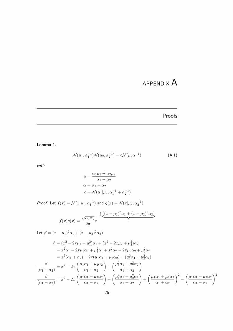
APPENDIX A

Proofs

Lemma 1.

N (µ1, α−11 )N (µ2, α

−12 ) = cN (µ, α−1) (A.1)

with

µ =α1µ1 + α2µ2α1 + α2

α = α1 + α2

c = N (µ1|µ2, α−11 + α−12 )

Proof. Let f(x) = N (x|µ1, α−11 ) and g(x) = N (x|µ2, α−12 )

f(x)g(x) =

√α1α2

2πe

− 12

((x− µ1)2α1 + (x− µ2)2α2)︸ ︷︷ ︸β

Let β = (x− µ1)2α1 + (x− µ2)2α2)

β = (x2 − 2xµ1 + µ21)α1 + (x2 − 2xµ2 + µ22)α2

= x2α1 − 2xµ1α1 + µ21α1 + x2α2 − 2xµ2α2 + µ22α2

= x2(α1 + α2)− 2x(µ1α1 + µ2α2) + (µ21α1 + µ22α2)

β

(α1 + α2)= x2 − 2x

(µ1α1 + µ2α2

α1 + α2

)+

(µ21α1 + µ22α2

α1 + α2

)β

(α1 + α2)= x2 − 2x

(µ1α1 + µ2α2

α1 + α2

)+

(µ21α1 + µ22α2

α1 + α2

)+

(µ1α1 + µ2α2

α1 + α2

)2

−(µ1α1 + µ2α2

α1 + α2

)2

75

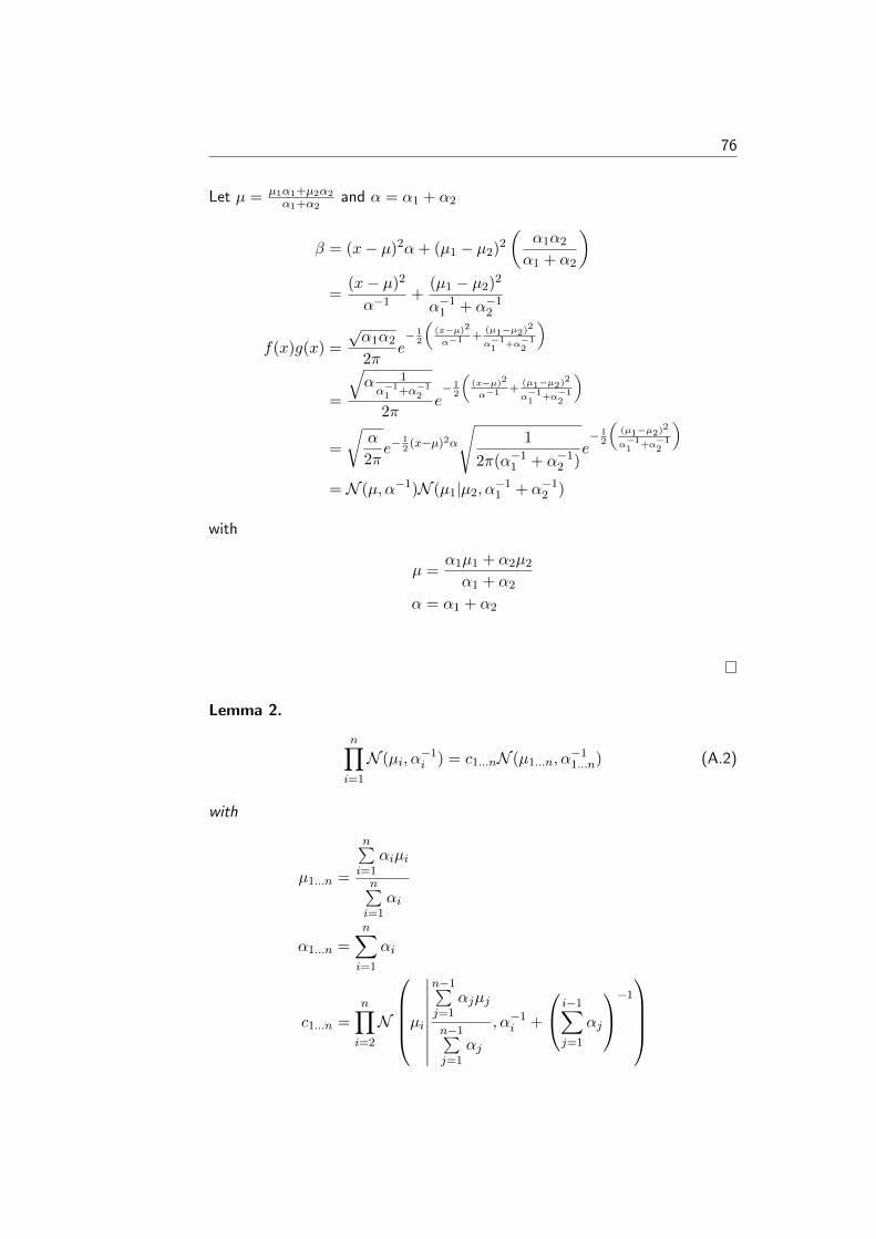
76

Let µ = µ1α1+µ2α2

α1+α2and α = α1 + α2

β = (x− µ)2α+ (µ1 − µ2)2(

α1α2

α1 + α2

)=

(x− µ)2

α−1+

(µ1 − µ2)2

α−11 + α−12

f(x)g(x) =

√α1α2

2πe− 1

2

((x−µ)2

α−1 +(µ1−µ2)

2

α−11 +α−1

2

)

=

√α 1α−11 +α−1

2

2πe− 1

2

((x−µ)2

α−1 +(µ1−µ2)

2

α−11 +α−1

2

)

=

√α

2πe−

12(x−µ)2α

√1

2π(α−11 + α−12 )e− 1

2

((µ1−µ2)

2

α−11 +α−1

2

)

= N (µ, α−1)N (µ1|µ2, α−11 + α−12 )

with

µ =α1µ1 + α2µ2α1 + α2

α = α1 + α2

Lemma 2.

n∏i=1

N (µi, α−1i ) = c1...nN (µ1...n, α

−11...n) (A.2)

with

µ1...n =

n∑i=1

αiµi

n∑i=1

αi

α1...n =n∑i=1

αi

c1...n =

n∏i=2

N

µi∣∣∣∣∣∣∣∣∣n−1∑j=1

αjµj

n−1∑j=1

αj

, α−1i +

i−1∑j=1

αj

−1

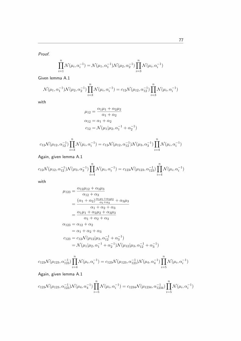
77

Proof.

n∏i=1

N (µi, α−1i ) = N (µ1, α

−11 )N (µ2, α

−12 )

n∏i=3

N (µi, α−1i )

Given lemma A.1

N (µ1, α−11 )N (µ2, α

−12 )

n∏i=3

N (µi, α−1i ) = c12N (µ12, α

−112 )

n∏i=3

N (µi, α−1i )

with

µ12 =α1µ1 + α2µ2α1 + α2

α12 = α1 + α2

c12 = N (µ1|µ2, α−11 + α−12 )

c12N (µ12, α−112 )

n∏i=3

N (µi, α−1i ) = c12N (µ12, α

−112 )N (µ3, α

−13 )

n∏i=4

N (µi, α−1i )

Again, given lemma A.1

c12N (µ12, α−112 )N (µ3, α

−13 )

n∏i=4

N (µi, α−1i ) = c123N (µ123, α

−1123)

n∏i=4

N (µi, α−1i )

with

µ123 =α12µ12 + α3µ3α12 + α3

=(α1 + α2)

α1µ1+α2µ2α1+α2

+ α3µ3

α1 + α2 + α3

=α1µ1 + α2µ2 + α3µ3

α1 + α2 + α3

α123 = α12 + α2

= α1 + α2 + α3

c123 = c12N (µ12|µ3, α−112 + α−13 )

= N (µ1|µ2, α−11 + α−12 )N (µ12|µ3, α−112 + α−13 )

c123N (µ123, α−1123)

n∏i=4

N (µi, α−1i ) = c123N (µ123, α

−1123)N (µ4, α

−14 )

n∏i=5

N (µi, α−1i )

Again, given lemma A.1

c123N (µ123, α−1123)N (µ4, α

−14 )

n∏i=5

N (µi, α−1i ) = c1234N (µ1234, α

−11234)

n∏i=5

N (µi, α−1i )

78

with

µ1234 =α123µ123 + α4µ4

α123 + α4

=(α1 + α2 + α3)

α1µ1+α2µ2+α3µ3α1+α2+α3

+ α4µ4

α1 + α2 + α3 + α4

=α1µ1 + α2µ2 + α3µ3 + α4µ4

α1 + α2 + α3 + α4

α1234 = α123 + α4

= α1 + α2 + α3 + α4

c1234 = c123N (µ123|µ4, α−1123 + α−14 )

= N (µ1|µ2, α−11 + α−12 )N (µ12|µ3, α−112 + α−13 )N (µ123|µ4, α−1123 + α−14 )

and thus

n∏i=1

N (µi, α−1i ) = c1...nN (µ1...n, α

−11...n)

with

µ1...n =

n∑i=1

αiµi

n∑i=1

αi

α1...n =

n∑i=1

αi

c1...n =n∏i=2

N

µi∣∣∣∣∣∣∣∣∣n−1∑j=1

αjµj

n−1∑j=1

αj

, α−1i +

i−1∑j=1

αj

−1

Lemma 3.

p(µx|X) = c−1k∑i=1

πiwiN (Θi, β−1i ) (A.3)

79

with

Θi =

αiµi + γ2

n∑j=1

xj

αi + nγ2

βi = αi +nγ

2

wi = N

µi∣∣∣∣∣∣∣∣∣n∑j=1

xj

n, α−1i + 2(nγ)−1

n∏j=2

N

xj∣∣∣∣∣∣∣∣∣j−1∑m=1

xm

j − 1,

(j

j − 1

)2γ−1

c =

k∑i=1

πiwi

Proof. By definition of 5.2

p(µx|X) = p(X|µx)p(µx)c−1

= c−1k∑i=1

πiN (µi, α−1i )

n∏j=1

N (xj , 2γ−1)

Given lemma 2, we can rewrite the product:

n∏j=1

N (xj , 2γ−1) = c1...nN (µ1...n, α

−11...n)

80

with

µ1...n =

n∑j=1

γ2xj

n∑j=1

γ2

=

γ2

n∑j=1

xj

nγ2

=

n∑j=1

xj

n

α1...n =n∑j=1

γ

2

=nγ

2

c1...n =n∏j=2

N

xj∣∣∣∣∣∣∣∣∣j−1∑m=1

γ2xm

j−1∑m=1

γ2

,2

γ+

(j−1∑m=1

γ

2

)−1And thus

p(µx|X) = c−1k∑i=1

πiN (µi, α−1i )c1...nN (µ1...n, α

−11...n)

Given lemma A.1:

N (µi, α−1i )N (µ1...n, α

−11...n) = wiN (Θi, β

−1i )

with

Θi =αiµi + nγ

2

n∑j=1

xj

n

αi + nγ2

=

αiµi + γ2

n∑j=1

xj

αi + nγ2

βi = αi +nγ

2

wi = N

µi∣∣∣∣∣∣∣∣∣n∑j=1

xj

n, α−1i + 2(nγ)−1

n∏j=2

N

xj∣∣∣∣∣∣∣∣∣j−1∑m=1

xm

j − 1,

(j

j − 1

)2γ−1

81

And thus,

p(µx|X) = c−1k∑i=1

πiwiN (Θi, β−1i )

82

List of Figures

1.1 Thesis organization This thesis is divided into two parts. Thefirst one describes the creation and application of gene expressioncompendia to prokaryotic and plant species. The second part isconcerned with two mathematical approaches to model such data. 12

2.1 Past and future software layer implementation The upperpart of the figure shows the old implementation with severalpoint of access to the database and all the different program-ming languages used. The lower part shows the new implemen-tation with COMPASS as the only software layer that deal withthe database and implements the data-model while each of theapplications have one coherent Python interface to manage allserver-side functionalities. . . . . . . . . . . . . . . . . . . . . . 26

2.2 Experiment selection. The top grid includes all experimentsalready part of the compendia and experiments already importedbut not completely processed. The bottom part is another gridthat shows all the experiments found on public databases for agiven query (using the search panel on the bottom left part). Anywords defined by the user can be used as search terms. Differentcolors allow to easily recognized experiments already imported orexperiments different from gene expression then won’t be imported. 28

2.3 Experiment structure definition. The right-hand panel showsall the downloaded files associated with the experiment (it is alsopossible to manually upload files). The tree on the left side is theexperiment hierarchy (experiment, platforms and samples) withthe respective files associated. All these steps can be performedmanually or let COMMAND perform it automatically. . . . . . . 29

83

LIST OF FIGURES 84

2.4 Parsing and importing experiment. Experiment structure de-fined in the previous step is shown on the left side panel. APython script can be associated to each file (together with argu-ments if needed) that would be executed (following a particularorder if needed) filling the experiment object. Available Pythonscripts are listed in a (hidden) panel below the experiment hier-archy. On the bottom-right side there’s an editor to create andmodify Python scripts. The top-right panel contains a previewof the experiment object divided in three tabs: experiment, plat-form and sample. Each of them shows currently data extractedfrom raw files through the execution of Python scripts. . . . . . 30

4.1 Probe-to-gene mapping for cluster 170. Genes (in rectan-gles) are colored accordingly to probes (circles) based on theoriginal platform mapping. Each line corresponds to an align-ment of the whole probe against one gene. A solid line meansno mismatches, a black dashed line means one mismatch whilea red dashed line means two or three mismatches. . . . . . . . . 42

4.2 Probe expression values and correlation for cluster 170. (A)Probes expression values measured across more than 500 Nim-blegen sample contrasts sorted by values. (B) Probes correlationmatrix using uncentered Pearson correlation. . . . . . . . . . . . 43

4.3 Overview of gene clusters. Both the size and color of thespheres are proportional to the number of clusters that is madeup of a given number of genes and probes. It is clear that thegreat majority of clusters are composed by just few genes andprobes. . . . . . . . . . . . . . . . . . . . . . . . . . . . . . . . 44

4.4 Categories of annotated sample contrasts. Number of sam-ple contrasts annotated as measuring a change in one of fivemajor categories. The differences between test and referencesample for some contrasts are related to more than one category;the proportion of these is indicated as ‘shared’ versus ‘unique.’ . 47

4.5 Case study of carotenoid cleavage dioxygenases gene fam-ily. The top part of the figure shows the VESPUCCI Quicksearchresult for the 11 genes of the carotenoid cleavage dioxygenases(CCD/NCED), while the bottom depicts the superimposed phy-logeny adapted from [66]. . . . . . . . . . . . . . . . . . . . . . 49

4.6 Case study of ABA modulated genes. The default ‘by expres-sion’ visualization of VESPUCCI orders both genes and contrastsin this heatmap (resp. rows and columns) in such a way as tohighlight the different patterns of condition-dependent gene ex-pression behavior. . . . . . . . . . . . . . . . . . . . . . . . . . 50

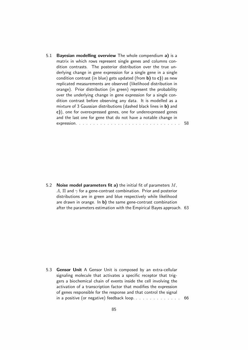
5.1 Bayesian modelling overview The whole compendium a) is amatrix in which rows represent single genes and columns con-dition contrasts. The posterior distribution over the true un-derlying change in gene expression for a single gene in a singlecondition contrast (in blue) gets updated (from b) to c)) as newreplicated measurements are observed (likelihood distribution inorange). Prior distribution (in green) represent the probabilityover the underlying change in gene expression for a single con-dition contrast before observing any data. It is modelled as amixture of 3 Gaussian distributions (dashed black lines in b) andc)), one for overexpressed genes, one for underexpressed genesand the last one for gene that do not have a notable change inexpression. . . . . . . . . . . . . . . . . . . . . . . . . . . . . . 58

5.2 Noise model parameters fit a) the initial fit of parameters M ,A, Π and γ for a gene-contrast combination. Prior and posteriordistributions are in green and blue respectively while likelihoodare drawn in orange. In b) the same gene-contrast combinationafter the parameters estimation with the Empirical Bayes approach. 63

5.3 Gensor Unit A Gensor Unit is composed by an extra-cellularsignaling molecule that activates a specific receptor that trig-gers a biochemical chain of events inside the cell involving theactivation of a transcription factor that modifies the expressionof genes responsible for the response and that control the signalin a positive (or negative) feedback loop. . . . . . . . . . . . . . 66

85

LIST OF TABLES 86

List of Tables

3.1 Rows of the table represent all the species and strains for which agene expression compendium is hosted. Columns represent (fromleft to right): the species name, the strain used as referencegenome for microarray probe to gene mapping and RNA-Seq readalignment, the total number of genes in the compendium, thetotal number of contrasts in the compendium, the percentage ofmissing values, the COLOMBOS version of the first inclusion ofthe respective species or strain, the total number of samples fromwhich the compendium’s contrasts are built, the total numberof corresponding experiments on GEO and ArrayExpress (thelatter indicated between square brackets) and the total numberof platforms represented. . . . . . . . . . . . . . . . . . . . . . 34

4.1 Overview of all samples imported in VESPUCCI ordered by num-ber of samples. The first column contains the name of the tran-scriptomics platform, the second column is the type of platformeither microarray or RNA-Seq. The third column contains thenumber of samples measured with the respective platform im-ported in VESPUCCI. . . . . . . . . . . . . . . . . . . . . . . . 39

4.2 Total number of genes measured per platform. First column con-tains the microarray platform name. The second column holdsthe number of measured genes according to the platform originalprobe-to-gene mapping. The third column contains the numberof measured genes according to VESPUCCI probe-to-gene map-ping. The fourth column contains the number of overlappinggenes between the two mappings. The last column contains thepercentage of genes for which there is no measurement. . . . . . 46

Bibliography

[1] M. Huerta, G. Downing, F. Haseltine, B. Seto, and Y. Liu, “Nih work-ing definition of bioinformatics and computational biology,” US NationalInstitute of Health, 2000.

[2] T. Barrett, S. E. Wilhite, P. Ledoux, C. Evangelista, I. F. Kim, M. Toma-shevsky, K. A. Marshall, K. H. Phillippy, P. M. Sherman, M. Holko, et al.,“Ncbi geo: archive for functional genomics data sets—update,” Nucleicacids research, vol. 41, no. D1, pp. D991–D995, 2013.

[3] N. Kolesnikov, E. Hastings, M. Keays, O. Melnichuk, Y. A. Tang,E. Williams, M. Dylag, N. Kurbatova, M. Brandizi, T. Burdett, et al., “Ar-rayexpress update—simplifying data submissions,” Nucleic acids research,p. gku1057, 2014.

[4] R. A. Irizarry, D. Warren, F. Spencer, I. F. Kim, S. Biswal, B. C. Frank,E. Gabrielson, J. G. Garcia, J. Geoghegan, G. Germino, et al., “Multiple-laboratory comparison of microarray platforms,” Nature methods, vol. 2,no. 5, pp. 345–350, 2005.

[5] M. A. Taub, H. C. Bravo, and R. A. Irizarry, “Overcoming bias and system-atic errors in next generation sequencing data,” Genome medicine, vol. 2,no. 12, p. 1, 2010.

[6] K. D. Hansen, Z. Wu, R. A. Irizarry, and J. T. Leek, “Sequencing technol-ogy does not eliminate biological variability,” Nature biotechnology, vol. 29,no. 7, pp. 572–573, 2011.

[7] W. E. Johnson, C. Li, and A. Rabinovic, “Adjusting batch effects in mi-croarray expression data using empirical bayes methods,” Biostatistics,vol. 8, no. 1, pp. 118–127, 2007.

87

BIBLIOGRAPHY 88

[8] R. B. Scharpf, H. Tjelmeland, G. Parmigiani, and A. B. Nobel, “A bayesianmodel for cross-study differential gene expression,” Journal of the AmericanStatistical Association, 2012.

[9] E. Garrett-Mayer, G. Parmigiani, X. Zhong, L. Cope, and E. Gabrielson,“Cross-study validation and combined analysis of gene expression microar-ray data,” Biostatistics, vol. 9, no. 2, pp. 333–354, 2008.

[10] J. K. Choi, U. Yu, S. Kim, and O. J. Yoo, “Combining multiple microar-ray studies and modeling interstudy variation,” Bioinformatics, vol. 19,no. suppl 1, pp. i84–i90, 2003.

[11] D. R. Goldstein, M. Delorenzi, R. Luthi-Carter, and T. Sengstag, “Com-parison of meta-analysis to combined analysis of a replicated microarraystudy,” Meta-Analysis and Combining Information in Genetics and Ge-nomics, vol. 1, pp. 135–156, 2005.

[12] A. A. Shabalin, H. Tjelmeland, C. Fan, C. M. Perou, and A. B. Nobel,“Merging two gene-expression studies via cross-platform normalization,”Bioinformatics, vol. 24, no. 9, pp. 1154–1160, 2008.

[13] R. A. Irizarry, B. M. Bolstad, F. Collin, L. M. Cope, B. Hobbs, and T. P.Speed, “Summaries of affymetrix genechip probe level data,” Nucleic acidsresearch, vol. 31, no. 4, pp. e15–e15, 2003.

[14] J. Kim, K. Patel, H. Jung, W. P. Kuo, and L. Ohno-Machado, “Anyexpress:integrated toolkit for analysis of cross-platform gene expression data usinga fast interval matching algorithm,” BMC bioinformatics, vol. 12, no. 1,p. 1, 2011.

[15] K. Engelen, Q. Fu, P. Meysman, A. Sanchez-Rodrıguez, R. De Smet,K. Lemmens, A. C. Fierro, and K. Marchal, “Colombos: access port forcross-platform bacterial expression compendia,” PLoS One, vol. 6, no. 7,p. e20938, 2011.

[16] P. Meysman, P. Sonego, L. Bianco, Q. Fu, D. Ledezma-Tejeida, S. Gama-Castro, V. Liebens, J. Michiels, K. Laukens, K. Marchal, et al., “Colombosv2. 0: an ever expanding collection of bacterial expression compendia,”Nucleic acids research, p. gkt1086, 2013.

[17] M. Moretto, P. Sonego, N. Dierckxsens, M. Brilli, L. Bianco, D. Ledezma-Tejeida, S. Gama-Castro, M. Galardini, C. Romualdi, K. Laukens, et al.,“Colombos v3. 0: leveraging gene expression compendia for cross-speciesanalyses,” Nucleic acids research, vol. 44, no. D1, pp. D620–D623, 2016.

[18] J. Luo, M. Schumacher, A. Scherer, D. Sanoudou, D. Megherbi, T. Davi-son, T. Shi, W. Tong, L. Shi, H. Hong, et al., “A comparison of batch

BIBLIOGRAPHY 89

effect removal methods for enhancement of prediction performance usingmaqc-ii microarray gene expression data,” The pharmacogenomics journal,vol. 10, no. 4, pp. 278–291, 2010.

[19] C. Camacho, G. Coulouris, V. Avagyan, N. Ma, J. Papadopoulos, K. Bealer,and T. L. Madden, “Blast+: architecture and applications,” BMC bioin-formatics, vol. 10, no. 1, p. 1, 2009.

[20] R. V. Belavkin, J. A. Aston, A. Channon, E. Aston, B. M. Rash,M. Kadirvel, S. Forbes, C. G. Knight, et al., “Mutation rate plasticityin rifampicin resistance depends on escherichia coli cell–cell interactions,”Nature communications, vol. 5, 2014.

[21] M. Galardini, M. Brilli, G. Spini, M. Rossi, B. Roncaglia, A. Bani, M. Chi-ancianesi, M. Moretto, K. Engelen, G. Bacci, et al., “Evolution of intra-specific regulatory networks in a multipartite bacterial genome,” PLoSComput Biol, vol. 11, no. 9, p. e1004478, 2015.

[22] C. Angione, M. Conway, and P. Lio, “Multiplex methods provide effectiveintegration of multi-omic data in genome-scale models,” BMC bioinfor-matics, vol. 17, no. 4, p. 257, 2016.

[23] K. Lemmens, T. De Bie, T. Dhollander, S. C. De Keersmaecker, I. M. Thijs,G. Schoofs, A. De Weerdt, B. De Moor, J. Vanderleyden, J. Collado-Vides,et al., “Distiller: a data integration framework to reveal condition depen-dency of complex regulons in escherichia coli,” Genome biology, vol. 10,no. 3, p. 1, 2009.

[24] T. Michoel, R. De Smet, A. Joshi, Y. Van de Peer, and K. Marchal,“Comparative analysis of module-based versus direct methods for reverse-engineering transcriptional regulatory networks,” BMC systems biology,vol. 3, no. 1, p. 1, 2009.

[25] H. Zhao, L. Cloots, T. Van den Bulcke, Y. Wu, R. De Smet, V. Storms,P. Meysman, K. Engelen, and K. Marchal, “Query-based biclustering ofgene expression data using probabilistic relational models,” BMC bioinfor-matics, vol. 12, no. Suppl 1, p. S37, 2011.

[26] J. P. Faria, R. Overbeek, F. Xia, M. Rocha, I. Rocha, and C. S. Henry,“Genome-scale bacterial transcriptional regulatory networks: reconstruc-tion and integrated analysis with metabolic models,” Briefings in bioinfor-matics, vol. 15, no. 4, pp. 592–611, 2014.

[27] L. Cloots and K. Marchal, “Network-based functional modeling of ge-nomics, transcriptomics and metabolism in bacteria,” Current opinion inmicrobiology, vol. 14, no. 5, pp. 599–607, 2011.

BIBLIOGRAPHY 90

[28] M. Kolar, J. Meier, V. Mustonen, M. Lassig, and J. Berg, “Graphalignment:Bayesian pairwise alignment of biological networks,” BMC systems biology,vol. 6, no. 1, p. 1, 2012.

[29] D. De Maeyer, J. Renkens, L. Cloots, L. De Raedt, and K. Marchal, “Phe-netic: network-based interpretation of unstructured gene lists in e. coli,”Molecular BioSystems, vol. 9, no. 7, pp. 1594–1603, 2013.

[30] Y. I. Balderas-Martınez, M. Savageau, H. Salgado, E. Perez-Rueda,E. Morett, and J. Collado-Vides, “Transcription factors in escherichia coliprefer the holo conformation,” PloS one, vol. 8, no. 6, p. e65723, 2013.

[31] M. Moretto, P. Sonego, S. Pilati, G. Malacarne, L. Costantini,L. Grzeskowiak, G. Bagagli, M. S. Grando, C. Moser, and K. Engelen,“Vespucci: Exploring patterns of gene expression in grapevine,” Frontiersin Plant Science, vol. 7, p. 633, 2016.

[32] “Django web framework.” https://www.djangoproject.com/. Ac-cessed: 2016-05-30.

[33] R. C. Team, “R: A language and environment for statistical computing. rfoundation for statistical computing, vienna, austria. 2013,” 2014.

[34] T. Tatusova, S. Ciufo, B. Fedorov, K. O’Neill, and I. Tolstoy, “Refseqmicrobial genomes database: new representation and annotation strategy,”Nucleic acids research, vol. 43, no. 7, p. 3872, 2015.

[35] R. P. Huntley, T. Sawford, P. Mutowo-Meullenet, A. Shypitsyna, C. Bonilla,M. J. Martin, and C. O’Donovan, “The goa database: gene ontologyannotation updates for 2015,” Nucleic acids research, vol. 43, no. D1,pp. D1057–D1063, 2015.

[36] H. Salgado, M. Peralta-Gil, S. Gama-Castro, A. Santos-Zavaleta, L. Muniz-Rascado, J. S. Garcıa-Sotelo, V. Weiss, H. Solano-Lira, I. Martınez-Flores,A. Medina-Rivera, et al., “Regulondb v8. 0: omics data sets, evolutionaryconservation, regulatory phrases, cross-validated gold standards and more,”Nucleic acids research, vol. 41, no. D1, pp. D203–D213, 2013.

[37] R. Caspi, T. Altman, R. Billington, K. Dreher, H. Foerster, C. A. Fulcher,T. A. Holland, I. M. Keseler, A. Kothari, A. Kubo, et al., “The metacycdatabase of metabolic pathways and enzymes and the biocyc collectionof pathway/genome databases,” Nucleic acids research, vol. 42, no. D1,pp. D459–D471, 2014.

[38] I. M. Keseler, A. Mackie, M. Peralta-Gil, A. Santos-Zavaleta, S. Gama-Castro, C. Bonavides-Martınez, C. Fulcher, A. M. Huerta, A. Kothari,M. Krummenacker, et al., “Ecocyc: fusing model organism databases with

BIBLIOGRAPHY 91

systems biology,” Nucleic acids research, vol. 41, no. D1, pp. D605–D612,2013.

[39] L. Li, C. J. Stoeckert, and D. S. Roos, “Orthomcl: identification of orthologgroups for eukaryotic genomes,” Genome research, vol. 13, no. 9, pp. 2178–2189, 2003.

[40] P. Shannon, A. Markiel, O. Ozier, N. S. Baliga, J. T. Wang, D. Ramage,N. Amin, B. Schwikowski, and T. Ideker, “Cytoscape: a software environ-ment for integrated models of biomolecular interaction networks,” Genomeresearch, vol. 13, no. 11, pp. 2498–2504, 2003.

[41] M. A. Vivier and I. S. Pretorius, “Genetically tailored grapevines for thewine industry,” Trends in biotechnology, vol. 20, no. 11, pp. 472–478,2002.

[42] O. Jaillon, J.-M. Aury, B. Noel, A. Policriti, C. Clepet, A. Casagrande,N. Choisne, S. Aubourg, N. Vitulo, C. Jubin, et al., “The grapevine genomesequence suggests ancestral hexaploidization in major angiosperm phyla,”Nature, vol. 449, no. 7161, pp. 463–467, 2007.

[43] R. Velasco, A. Zharkikh, M. Troggio, D. A. Cartwright, A. Cestaro,D. Pruss, M. Pindo, L. M. FitzGerald, S. Vezzulli, J. Reid, et al., “Ahigh quality draft consensus sequence of the genome of a heterozygousgrapevine variety,” PloS one, vol. 2, no. 12, p. e1326, 2007.

[44] S. Y. Rhee, J. Dickerson, and D. Xu, “Bioinformatics and its applicationsin plant biology,” Annu. Rev. Plant Biol., vol. 57, pp. 335–360, 2006.

[45] D. C. Wong, C. Sweetman, D. P. Drew, and C. M. Ford, “Vtcdb: a geneco-expression database for the crop species vitis vinifera (grapevine),” BMCgenomics, vol. 14, no. 1, p. 882, 2013.

[46] A. Pulvirenti, R. Giugno, R. Distefano, G. Pigola, M. Mongiovi, G. Giudice,V. Vendramin, A. Lombardo, F. Cattonaro, and A. Ferro, “A knowledgebase for vitis vinifera functional analysis,” BMC systems biology, vol. 9,no. Suppl 3, p. S5, 2015.

[47] J. Yue, X. Ma, R. Ban, Q. Huang, W. Wang, J. Liu, and Y. Liu, “Frdatabase 1.0: a resource focused on fruit development and ripening,”Database, vol. 2015, p. bav002, 2015.

[48] D. C. Wong, C. Sweetman, and C. M. Ford, “Annotation of gene functionin citrus using gene expression information and co-expression networks,”BMC plant biology, vol. 14, no. 1, p. 1, 2014.

[49] Q. Fu, A. C. Fierro, P. Meysman, A. Sanchez-Rodriguez, K. Vandepoele,K. Marchal, and K. Engelen, “Magic: access portal to a cross-platform

BIBLIOGRAPHY 92

gene expression compendium for maize,” Bioinformatics, vol. 30, no. 9,pp. 1316–1318, 2014.

[50] G. O. Consortium et al., “Gene ontology consortium: going forward,” Nu-cleic acids research, vol. 43, no. D1, pp. D1049–D1056, 2015.

[51] M. Kanehisa, Y. Sato, M. Kawashima, M. Furumichi, and M. Tanabe,“Kegg as a reference resource for gene and protein annotation,” Nucleicacids research, vol. 44, no. D1, pp. D457–D462, 2016.

[52] R. D. Finn, P. Coggill, R. Y. Eberhardt, S. R. Eddy, J. Mistry, A. L.Mitchell, S. C. Potter, M. Punta, M. Qureshi, A. Sangrador-Vegas, et al.,“The pfam protein families database: towards a more sustainable future,”Nucleic acids research, p. gkv1344, 2015.

[53] C. J. Sigrist, E. De Castro, L. Cerutti, B. A. Cuche, N. Hulo, A. Bridge,L. Bougueleret, and I. Xenarios, “New and continuing developments atprosite,” Nucleic acids research, p. gks1067, 2012.

[54] I. Letunic, T. Doerks, and P. Bork, “Smart: recent updates, new devel-opments and status in 2015,” Nucleic acids research, vol. 43, no. D1,pp. D257–D260, 2015.

[55] J. Grimplet, G. R. Cramer, J. A. Dickerson, K. Mathiason, J. Van Hemert,and A. Y. Fennell, “Vitisnet:“omics” integration through grapevine molec-ular networks,” PloS one, vol. 4, no. 12, p. e8365, 2009.

[56] L. Cooper, R. L. Walls, J. Elser, M. A. Gandolfo, D. W. Stevenson,B. Smith, J. Preece, B. Athreya, C. J. Mungall, S. Rensing, et al., “Theplant ontology as a tool for comparative plant anatomy and genomic anal-yses,” Plant and Cell Physiology, vol. 54, no. 2, pp. e1–e1, 2013.

[57] B. Coombe, “Grapevine growth stages. the modified el system,” Aust. J.Grape Wine Res, vol. 1, pp. 100–110, 1995.

[58] J. T. Matus, F. Aquea, and P. Arce-Johnson, “Analysis of the grape mybr2r3 subfamily reveals expanded wine quality-related clades and conservedgene structure organization across vitis and arabidopsis genomes,” BMCPlant Biology, vol. 8, no. 1, p. 83, 2008.

[59] J. Yin, S. McLoughlin, I. B. Jeffery, A. Glaviano, B. Kennedy, and D. G.Higgins, “Integrating multiple genome annotation databases improves theinterpretation of microarray gene expression data,” BMC genomics, vol. 11,no. 1, p. 1, 2010.

[60] M. Fasoli, S. Dal Santo, S. Zenoni, G. B. Tornielli, L. Farina, A. Zamboni,A. Porceddu, L. Venturini, M. Bicego, V. Murino, et al., “The grapevineexpression atlas reveals a deep transcriptome shift driving the entire plant

BIBLIOGRAPHY 93

into a maturation program,” The Plant Cell, vol. 24, no. 9, pp. 3489–3505,2012.

[61] S. J. Cookson and N. Ollat, “Grafting with rootstocks induces extensivetranscriptional re-programming in the shoot apical meristem of grapevine,”BMC plant biology, vol. 13, no. 1, p. 1, 2013.

[62] J. Grimplet, J. Van Hemert, P. Carbonell-Bejerano, J. Dıaz-Riquelme,J. Dickerson, A. Fennell, M. Pezzotti, and J. M. Martınez-Zapater,“Comparative analysis of grapevine whole-genome gene predictions, func-tional annotation, categorization and integration of the predicted gene se-quences,” BMC Research notes, vol. 5, no. 1, p. 213, 2012.

[63] L. Costantini, G. Malacarne, S. Lorenzi, M. Troggio, F. Mattivi, C. Moser,and M. S. Grando, “New candidate genes for the fine regulation of thecolour of grapes,” Journal of experimental botany, p. erv159, 2015.

[64] G. Malacarne, L. Costantini, E. Coller, J. Battilana, R. Velasco,U. Vrhovsek, M. S. Grando, and C. Moser, “Regulation of flavonol con-tent and composition in (syrah× pinot noir) mature grapes: integration oftranscriptional profiling and metabolic quantitative trait locus analyses,”Journal of experimental botany, vol. 66, no. 15, pp. 4441–4453, 2015.

[65] P. R. Young, J. G. Lashbrooke, E. Alexandersson, D. Jacobson, C. Moser,R. Velasco, and M. A. Vivier, “The genes and enzymes of the carotenoidmetabolic pathway in vitis vinifera l.,” BMC genomics, vol. 13, no. 1, p. 1,2012.

[66] J. Grimplet, A.-F. Adam-Blondon, P.-F. Bert, O. Bitz, D. Cantu, C. Davies,S. Delrot, M. Pezzotti, S. Rombauts, and G. R. Cramer, “The grapevinegene nomenclature system,” BMC genomics, vol. 15, no. 1, p. 1, 2014.

[67] J. G. Lashbrooke, P. R. Young, S. J. Dockrall, K. Vasanth, and M. A.Vivier, “Functional characterisation of three members of the vitis vinifera l.carotenoid cleavage dioxygenase gene family,” BMC plant biology, vol. 13,no. 1, p. 156, 2013.

[68] X. Yin and P. C. Struik, “Modelling the crop: from system dynamics tosystems biology,” Journal of Experimental Botany, vol. 61, no. 8, pp. 2171–2183, 2010.

[69] B. P. Sheth and V. S. Thaker, “Plant systems biology: insights, advancesand challenges,” Planta, vol. 240, no. 1, pp. 33–54, 2014.

[70] N. Vitulo, C. Forcato, E. C. Carpinelli, A. Telatin, D. Campagna,M. D’Angelo, R. Zimbello, M. Corso, A. Vannozzi, C. Bonghi, et al., “Adeep survey of alternative splicing in grape reveals changes in the splicing

BIBLIOGRAPHY 94

machinery related to tissue, stress condition and genotype,” BMC plantbiology, vol. 14, no. 1, p. 1, 2014.

[71] P. M. Lee, Bayesian statistics: an introduction. John Wiley & Sons, 2012.

[72] S. G. Johnson, “The nlopt nonlinear-optimization package.” http://

ab-initio.mit.edu/nlopt. Accessed: 2016-05-30.

[73] S. Kauffman, “Homeostasis and differentiation in random genetic controlnetworks,” Nature, vol. 224, pp. 177–178, 1969.

[74] “Boolean network.” https://en.wikipedia.org/wiki/Boolean_

network. Accessed: 2016-05-30.

[75] S. Gama-Castro, H. Salgado, M. Peralta-Gil, A. Santos-Zavaleta, L. Muniz-Rascado, H. Solano-Lira, V. Jimenez-Jacinto, V. Weiss, J. S. Garcia-Sotelo,A. Lopez-Fuentes, et al., “Regulondb version 7.0: transcriptional regulationof escherichia coli k-12 integrated within genetic sensory response units(gensor units),” Nucleic acids research, vol. 39, no. suppl 1, pp. D98–D105, 2011.

[76] C. Mussel, M. Hopfensitz, and H. A. Kestler, “Boolnet—an r package forgeneration, reconstruction and analysis of boolean networks,” Bioinformat-ics, vol. 26, no. 10, pp. 1378–1380, 2010.

[77] R. Van Noorden, “Global scientific output doubles every nine years,” Na-ture, 2014.

[78] V. Marx, “Biology: The big challenges of big data,” Nature, vol. 498,no. 7453, pp. 255–260, 2013.

[79] G. Duck, G. Nenadic, M. Filannino, A. Brass, D. L. Robertson, andR. Stevens, “A survey of bioinformatics database and software usagethrough mining the literature,” PloS one, vol. 11, no. 6, p. e0157989,2016.