
Il progetto COKA · - PILLOLE di CALCOLO PARALLELO ... strutturano uno stile di programmazione un...
33
Il progetto COKA programmazione parallela su MIC F. Di Renzo Università di Parma e I.N.F.N. Parma Genova, 29 Maggio 2013 Workshop CCR 2013 mercoledì 29 maggio 13
Transcript of Il progetto COKA · - PILLOLE di CALCOLO PARALLELO ... strutturano uno stile di programmazione un...

Il progettoCOKA
programmazione parallela su MIC
F. Di RenzoUniversità di Parma e I.N.F.N. Parma
Genova, 29 Maggio 2013
Workshop CCR 2013
mercoledì 29 maggio 13

Segnatamente parleremo di ...
- PILLOLE di CALCOLO PARALLELO
- La filosofia della architettura MIC
- PILLOLE di STRATEGIA per il CALCOLO PARALLELO Non entreremo nei dettagli di approcci “aggressivi”: guarderemo a volo d’uccello alcune linee per uno stile di programmazione
- STRUMENTI per PROGRAMMARE in modo sostanzialmente semplice Un benchmark elementare (operazioni matriciali)
Il progetto Coka si propone di indagare le capacità di calcolo di architetture innovative, in particolare la architettura many-core Intel MIC. Ci chiederemo quali attenzioni siano da prestare per una programmazione ragionevolmente efficiente di simili dispositivi.
Mentre sono possibili approcci che, mirando alla ricerca della massima efficienza, richiedono una completa ristrutturazione di codici eventualmente già esistenti e consolidati nel tempo, evidenzieremo come questa non sia l'unica soluzione possibile.
Sono praticabili metodologie di programmazione che cerchino un accettabile compromesso fra efficienza di calcolo e portabilità di codice esistente.
Anche per un simile approccio è comunque necessario avere presenti alcune linee guida ineludibili, che strutturano uno stile di programmazione un poco diverso da quello cui siamo abitutati su architetture non parallele.
mercoledì 29 maggio 13
PILLOLE di CALCOLO PARALLELO
mercoledì 29 maggio 13
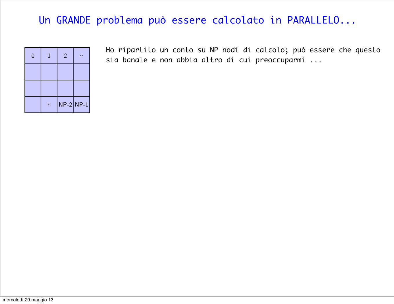
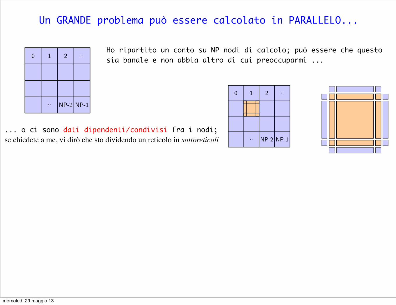
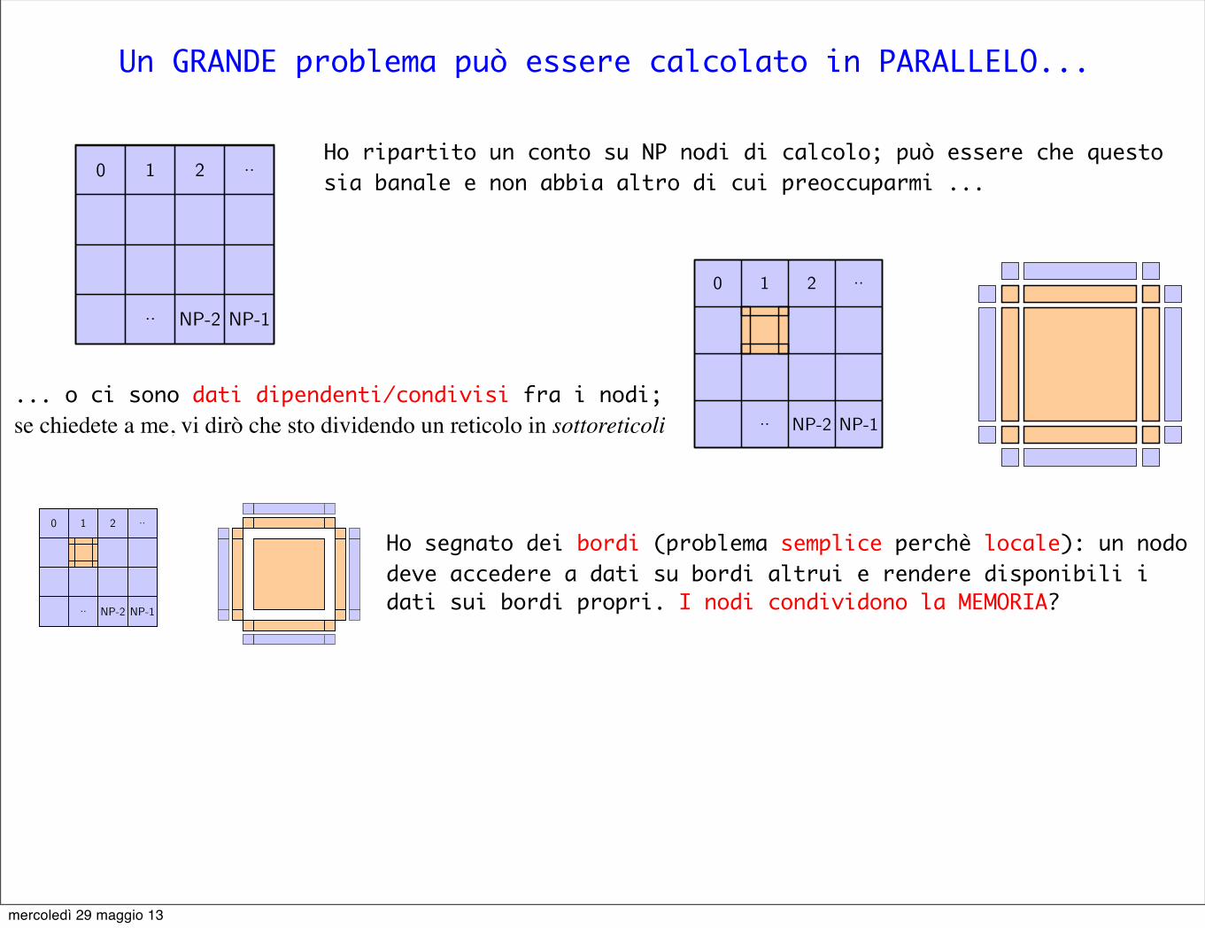
Un GRANDE problema può essere calcolato in PARALLELO...
Parallelizzazione di una Simulazione Monte Carlo del Modello XY Bidimensionale
Implementazione
Implementazione
0 1 2 ..
.. NP-2 NP-1
Viene suddiviso in tantisottoreticoli quanti nodi dicalcolo si ha a disposizione.
Ogni sottoreticolo “evolve”secondo l’HMC “in parallelo”.
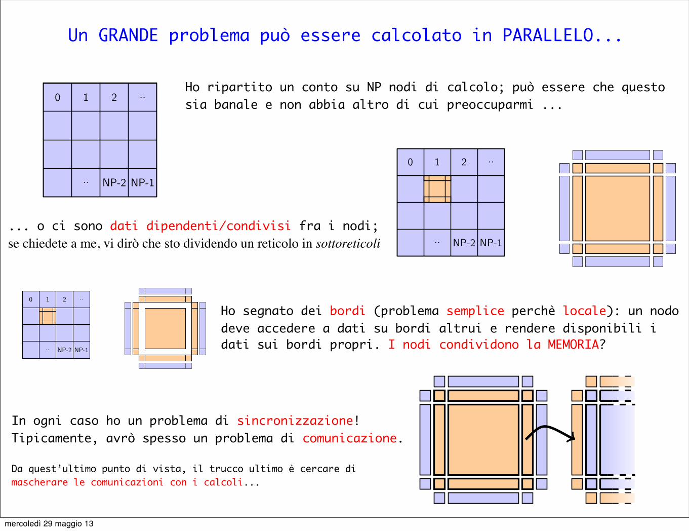
Ho ripartito un conto su NP nodi di calcolo; può essere che questo sia banale e non abbia altro di cui preoccuparmi ...
mercoledì 29 maggio 13
Un GRANDE problema può essere calcolato in PARALLELO...
Parallelizzazione di una Simulazione Monte Carlo del Modello XY Bidimensionale
Implementazione
Implementazione
0 1 2 ..
.. NP-2 NP-1
Viene suddiviso in tantisottoreticoli quanti nodi dicalcolo si ha a disposizione.
Ogni sottoreticolo “evolve”secondo l’HMC “in parallelo”.
Parallelizzazione di una Simulazione Monte Carlo del Modello XY Bidimensionale
Implementazione
Implementazione
0 1 2 ..
.. NP-2 NP-1
Ho ripartito un conto su NP nodi di calcolo; può essere che questo sia banale e non abbia altro di cui preoccuparmi ...
... o ci sono dati dipendenti/condivisi fra i nodi; se chiedete a me, vi dirò che sto dividendo un reticolo in sottoreticoli
mercoledì 29 maggio 13
Un GRANDE problema può essere calcolato in PARALLELO...
Parallelizzazione di una Simulazione Monte Carlo del Modello XY Bidimensionale
Implementazione
Implementazione
0 1 2 ..
.. NP-2 NP-1
Viene suddiviso in tantisottoreticoli quanti nodi dicalcolo si ha a disposizione.
Ogni sottoreticolo “evolve”secondo l’HMC “in parallelo”.
Parallelizzazione di una Simulazione Monte Carlo del Modello XY Bidimensionale
Implementazione
Implementazione
0 1 2 ..
.. NP-2 NP-1Parallelizzazione di una Simulazione Monte Carlo del Modello XY Bidimensionale
Implementazione
Implementazione
0 1 2 ..
.. NP-2 NP-1
Ho ripartito un conto su NP nodi di calcolo; può essere che questo sia banale e non abbia altro di cui preoccuparmi ...
... o ci sono dati dipendenti/condivisi fra i nodi; se chiedete a me, vi dirò che sto dividendo un reticolo in sottoreticoli
Ho segnato dei bordi (problema semplice perchè locale): un nodo deve accedere a dati su bordi altrui e rendere disponibili i dati sui bordi propri. I nodi condividono la MEMORIA?
mercoledì 29 maggio 13
Un GRANDE problema può essere calcolato in PARALLELO...Parallelizzazione di una Simulazione Monte Carlo del Modello XY Bidimensionale
Implementazione
Mascheramento delle comunicazioni
Mascheramento delle comunicazioni
In MPI le comunicazioni sono di due tipi: bloccanti o nonbloccanti.
Utilizzando quelle non bloccanti e possibile avanzare di un passodel Leapfrog, durante lo scambio.
⇥i (n + 1) = ⇥i (n) + �⇤i (n),
⇤i (n + 1) = ⇤i (n)� �⌅S [⇥]
⌅⇥i (n + 1),
⇤i (n) = ⇤i (n)� �
2
⌅S [⇥]
⌅⇥i (n).
Parallelizzazione di una Simulazione Monte Carlo del Modello XY Bidimensionale
Implementazione
Implementazione
0 1 2 ..
.. NP-2 NP-1
Viene suddiviso in tantisottoreticoli quanti nodi dicalcolo si ha a disposizione.
Ogni sottoreticolo “evolve”secondo l’HMC “in parallelo”.
Parallelizzazione di una Simulazione Monte Carlo del Modello XY Bidimensionale
Implementazione
Implementazione
0 1 2 ..
.. NP-2 NP-1Parallelizzazione di una Simulazione Monte Carlo del Modello XY Bidimensionale
Implementazione
Implementazione
0 1 2 ..
.. NP-2 NP-1
Ho ripartito un conto su NP nodi di calcolo; può essere che questo sia banale e non abbia altro di cui preoccuparmi ...
... o ci sono dati dipendenti/condivisi fra i nodi; se chiedete a me, vi dirò che sto dividendo un reticolo in sottoreticoli
Ho segnato dei bordi (problema semplice perchè locale): un nodo deve accedere a dati su bordi altrui e rendere disponibili i dati sui bordi propri. I nodi condividono la MEMORIA?
In ogni caso ho un problema di sincronizzazione! Tipicamente, avrò spesso un problema di comunicazione.
Da quest’ultimo punto di vista, il trucco ultimo è cercare di mascherare le comunicazioni con i calcoli...
mercoledì 29 maggio 13
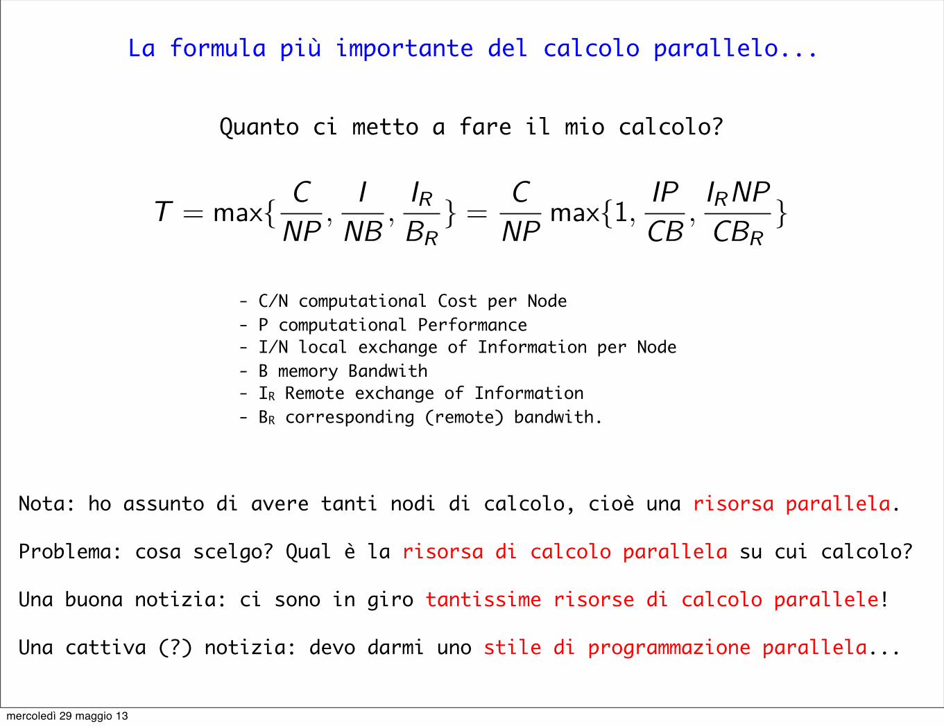
La formula più importante del calcolo parallelo...
Nota: ho assunto di avere tanti nodi di calcolo, cioè una risorsa parallela.
Problema: cosa scelgo? Qual è la risorsa di calcolo parallela su cui calcolo?
Una buona notizia: ci sono in giro tantissime risorse di calcolo parallele!
Una cattiva (?) notizia: devo darmi uno stile di programmazione parallela...
The game we have been playing for a while: our basicformula
Now: LQCD dates back to 1974; in the mid of the 80’s, the LQCD communitystarted thinking of going parallel. What to look for?
In the end, since then we have been kept on looking at the same formula
T = max{ C
NP
,I
NB
,IR
BR} =
C
NP
max{1,IP
CB
,IRNP
CBR}
being C/N the computational cost per node, P the computational performance,I/N the local exchange of information per node, B the memory bandwith, IR theremote exchange of information and BR the corresponding bandwith.
Maybe strange to say, but for a very long time the best way to fulfill therequirements coming from the above has been: DO IT YOURSELF, i.e. if nocomputer matches your computational requirements, build your own.
At the Istituto Nazionale di Fisica Nucleare (INFN) this program was made real
hw in the APE (Array Processors Experiment) machines. Everything was custom!
F. Di Renzo (UNIPR, INFN, AuroraScience Coll.) AuroraScience ScalPerf10, Sept 23rd 2010 9 / 19
- C/N computational Cost per Node - P computational Performance- I/N local exchange of Information per Node - B memory Bandwith- IR Remote exchange of Information - BR corresponding (remote) bandwith.
Quanto ci metto a fare il mio calcolo?
mercoledì 29 maggio 13

La filosofia della architettura MIC
mercoledì 29 maggio 13
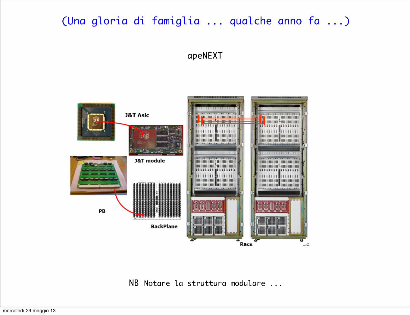
(Una gloria di famiglia ... qualche anno fa ...)
apeNEXT A spasso per TOP500
Ecco la generazione attuale di APE (apeNEXT)
NB Notare la struttura modulare ...
mercoledì 29 maggio 13
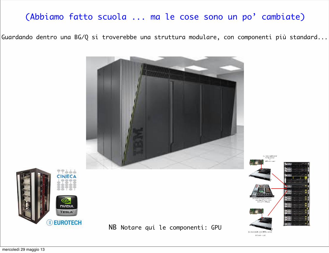
(Abbiamo fatto scuola ... ma le cose sono un po’ cambiate)
Guardando dentro una BG/Q si troverebbe una struttura modulare, con componenti più standard...
NB Notare qui le componenti: GPU
mercoledì 29 maggio 13
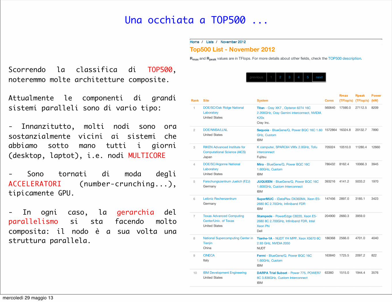
Una occhiata a TOP500 ...
Scorrendo la classifica di TOP500, noteremmo molte architetture composite.
Attualmente le componenti di grandi sistemi paralleli sono di vario tipo:
- Innanzitutto, molti nodi sono ora sostanzialmente vicini ai sistemi che abbiamo sotto mano tutti i giorni (desktop, laptot), i.e. nodi MULTICORE
- Sono tornati di moda degli ACCELERATORI (number-crunching...), tipicamente GPU.
- In ogni caso, la gerarchia del parallelismo si sta facendo molto composita: il nodo è a sua volta una struttura parallela.
09/05/13 Top500 List - November 2012 | TOP500 Supercomputer Sites
www.top500.org/list/2012/11/ 1/6
HomeHome // ListsLists // November 2012November 2012
Top500 List - November 2012R and R values are in TFlops. For more details about other fields, check the TOP500 description.
previous 1 2 3 4 5 next
Rank Site System CoresRmax(TFlop/s)
Rpeak(TFlop/s)
Power(kW)
1 DOE/SC/Oak Ridge NationalLaboratoryUnited States
Titan - Cray XK7 , Opteron 6274 16C2.200GHz, Cray Gemini interconnect, NVIDIAK20xCray Inc.
560640 17590.0 27112.5 8209
2 DOE/NNSA/LLNLUnited States
Sequoia - BlueGene/Q, Power BQC 16C 1.60GHz, CustomIBM
1572864 16324.8 20132.7 7890
3 RIKEN Advanced Institute forComputational Science (AICS)Japan
K computer, SPARC64 VIIIfx 2.0GHz, TofuinterconnectFujitsu
705024 10510.0 11280.4 12660
4 DOE/SC/Argonne NationalLaboratoryUnited States
Mira - BlueGene/Q, Power BQC 16C1.60GHz, CustomIBM
786432 8162.4 10066.3 3945
5 Forschungszentrum Juelich (FZJ)Germany
JUQUEEN - BlueGene/Q, Power BQC 16C1.600GHz, Custom InterconnectIBM
393216 4141.2 5033.2 1970
6 Leibniz RechenzentrumGermany
SuperMUC - iDataPlex DX360M4, Xeon E5-2680 8C 2.70GHz, Infiniband FDRIBM
147456 2897.0 3185.1 3423
7 Texas Advanced ComputingCenter/Univ. of TexasUnited States
Stampede - PowerEdge C8220, Xeon E5-2680 8C 2.700GHz, Infiniband FDR, IntelXeon PhiDell
204900 2660.3 3959.0
8 National Supercomputing Center inTianjinChina
Tianhe-1A - NUDT YH MPP, Xeon X5670 6C2.93 GHz, NVIDIA 2050NUDT
186368 2566.0 4701.0 4040
9 CINECAItaly
Fermi - BlueGene/Q, Power BQC 16C1.60GHz, CustomIBM
163840 1725.5 2097.2 822
10 IBM Development EngineeringUnited States
DARPA Trial Subset - Power 775, POWER78C 3.836GHz, Custom InterconnectIBM
63360 1515.0 1944.4 3576
11 CEA/TGCC-GENCIFrance
Curie thin nodes - Bullx B510, Xeon E5-2680 8C 2.700GHz, Infiniband QDRBull SA
77184 1359.0 1667.2 2251
12 National Supercomputing Centre inShenzhen (NSCS)China
Nebulae - Dawning TC3600 Blade System,Xeon X5650 6C 2.66GHz, Infiniband QDR,NVIDIA 2050Dawning
120640 1271.0 2984.3 2580
13 NCAR (National Center forAtmospheric Research)United States
Yellowstone - iDataPlex DX360M4, Xeon E5-2670 8C 2.600GHz, Infiniband FDRIBM
72288 1257.6 1503.6 1437
14 NASA/Ames Research Center/NASUnited States
Pleiades - SGI ICE X/8200EX/8400EX, Xeon54xx 3.0/5570/5670/E5-26702.93/2.6/3.06/3.0 Ghz, Infiniband QDR/FDRSGI
125980 1243.0 1731.8 3987
15 International Fusion EnergyResearch Centre (IFERC), EU(F4E) -Japan Broader Approach
Helios - Bullx B510, Xeon E5-2680 8C2.700GHz, Infiniband QDRBull SA
70560 1237.0 1524.1 2200
Mi piace Piace a 2.374 persone.
TOP10 November 2012
1 Titan - Cray XK7 , Opteron 627416C 2.200GHz, Cray Geminiinterconnect, NVIDIA K20x
2 Sequoia - BlueGene/Q, PowerBQC 16C 1.60 GHz, Custom
3 K computer, SPARC64 VIIIfx2.0GHz, Tofu interconnect
4 Mira - BlueGene/Q, Power BQC
16C 1.60GHz, Custom
5 JUQUEEN - BlueGene/Q, PowerBQC 16C 1.600GHz, CustomInterconnect
6 SuperMUC - iDataPlexDX360M4, Xeon E5-2680 8C2.70GHz, Infiniband FDR
7 Stampede - PowerEdge C8220,Xeon E5-2680 8C 2.700GHz,Infiniband FDR, Intel Xeon Phi
8 Tianhe-1A - NUDT YH MPP, XeonX5670 6C 2.93 GHz, NVIDIA 2050
9 Fermi - BlueGene/Q, Power BQC16C 1.60GHz, Custom
10 DARPA Trial Subset - Power 775,POWER7 8C 3.836GHz, CustomInterconnect
Not logged inLog inLog in or Sign upSign up
SearchHomeHome Project Project Features Features Lists Lists Statistics Statistics Contact Contact
max peak
mercoledì 29 maggio 13
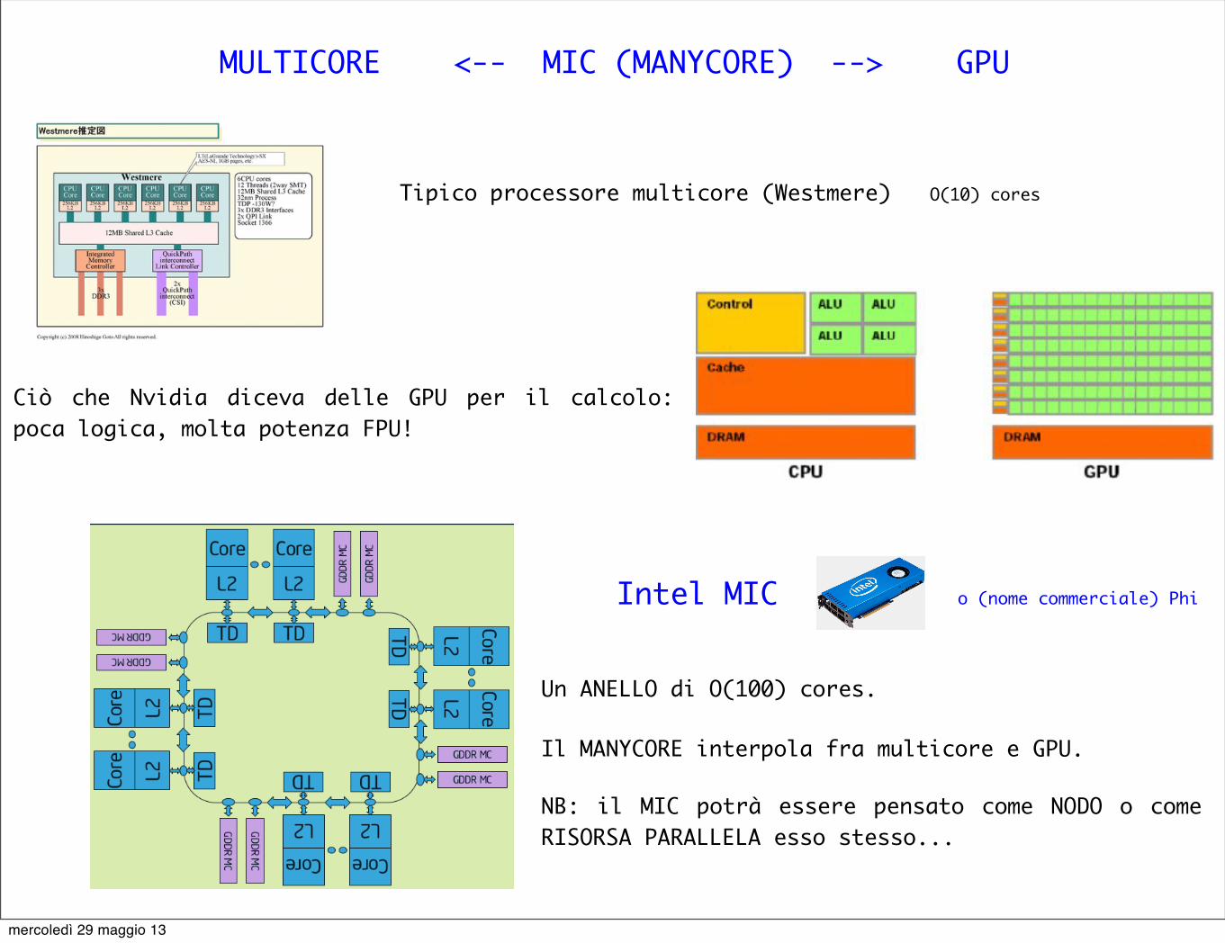
MULTICORE <-- MIC (MANYCORE) --> GPU
Tipico processore multicore (Westmere) O(10) cores
Ciò che Nvidia diceva delle GPU per il calcolo: poca logica, molta potenza FPU!
Intel MIC o (nome commerciale) Phi
Un ANELLO di O(100) cores.
Il MANYCORE interpola fra multicore e GPU.
NB: il MIC potrà essere pensato come NODO o come RISORSA PARALLELA esso stesso...
mercoledì 29 maggio 13
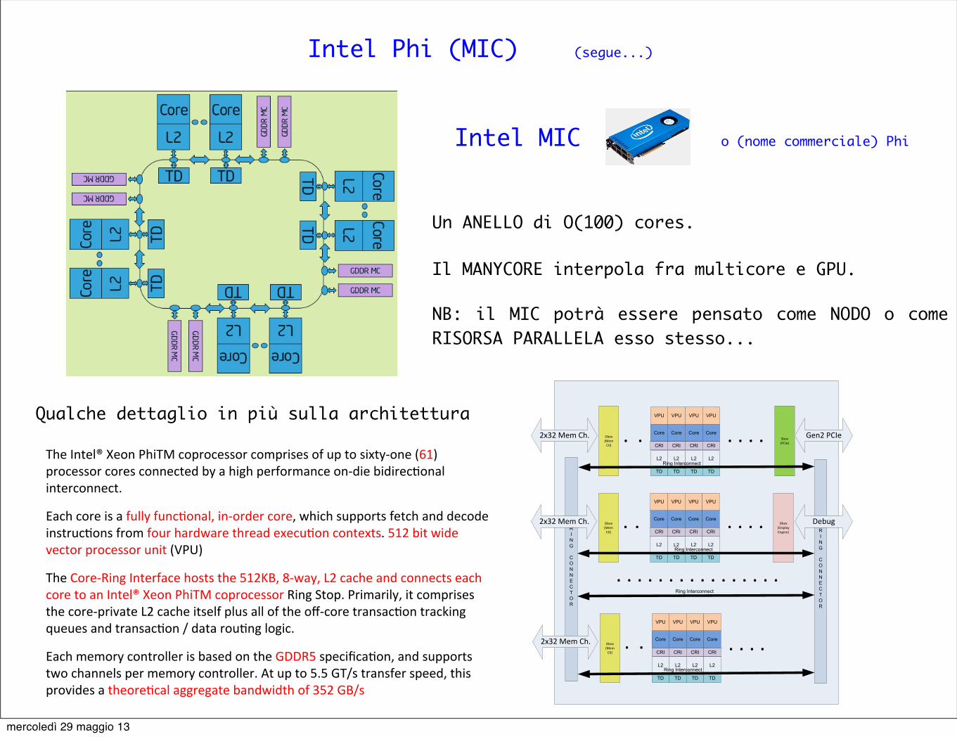
Intel Phi (MIC) (segue...)
Intel MIC o (nome commerciale) Phi
Un ANELLO di O(100) cores.
Il MANYCORE interpola fra multicore e GPU.
NB: il MIC potrà essere pensato come NODO o come RISORSA PARALLELA esso stesso...
Page 14
Sbox(PCIe)
Core
VPU
CRI
L2
Core
VPU
CRI
L2
Core
VPU
CRI
L2
Core
VPU
CRI
L2Ring Interconnect
TD TD TD TD
. . . .
Dbox(DisplayEngine)
. . . . . . . . . . . . . . . .
Gbox(Mem
Ctl)
RING
CONN E C T O R
RING
CONN E C T O R
Gen2 PCIe
Debug
2x32 Mem Ch. .
Core
VPU
CRI
L2
Core
VPU
CRI
L2
Core
VPU
CRI
L2
Core
VPU
CRI
L2Ring Interconnect
TD TD TD TD
. . . .Gbox(Mem
Ctl)
2x32 Mem Ch. .
Core
VPU
CRI
L2
Core
VPU
CRI
L2
Core
VPU
CRI
L2
Core
VPU
CRI
L2
TD TD
Ring Interconnect
TD TD
. . . .Gbox(Mem
Ctl)
2x32 Mem Ch. .
Ring Interconnect
.
.
.
Figure 2-1. Basic building blocks of the Intel® Xeon Phi™ Coprocessor
Qualche dettaglio in più sulla architettura
The Intel® Xeon PhiTM coprocessor comprises of up to sixty-‐one (61) processor cores connected by a high performance on-‐die bidirecAonal interconnect.
Each core is a fully funcAonal, in-‐order core, which supports fetch and decode instrucAons from four hardware thread execuAon contexts. 512 bit wide vector processor unit (VPU)
The Core-‐Ring Interface hosts the 512KB, 8-‐way, L2 cache and connects each core to an Intel® Xeon PhiTM coprocessor Ring Stop. Primarily, it comprises the core-‐private L2 cache itself plus all of the off-‐core transacAon tracking queues and transacAon / data rouAng logic.
Each memory controller is based on the GDDR5 specificaAon, and supports two channels per memory controller. At up to 5.5 GT/s transfer speed, this provides a theoreAcal aggregate bandwidth of 352 GB/s
mercoledì 29 maggio 13

PILLOLE di STRATEGIA per il CALCOLO PARALLELOquello che abbiamo imparato sui multicore
e che vorremmo mettere a frutto in generale (anche sul MIC)
mercoledì 29 maggio 13
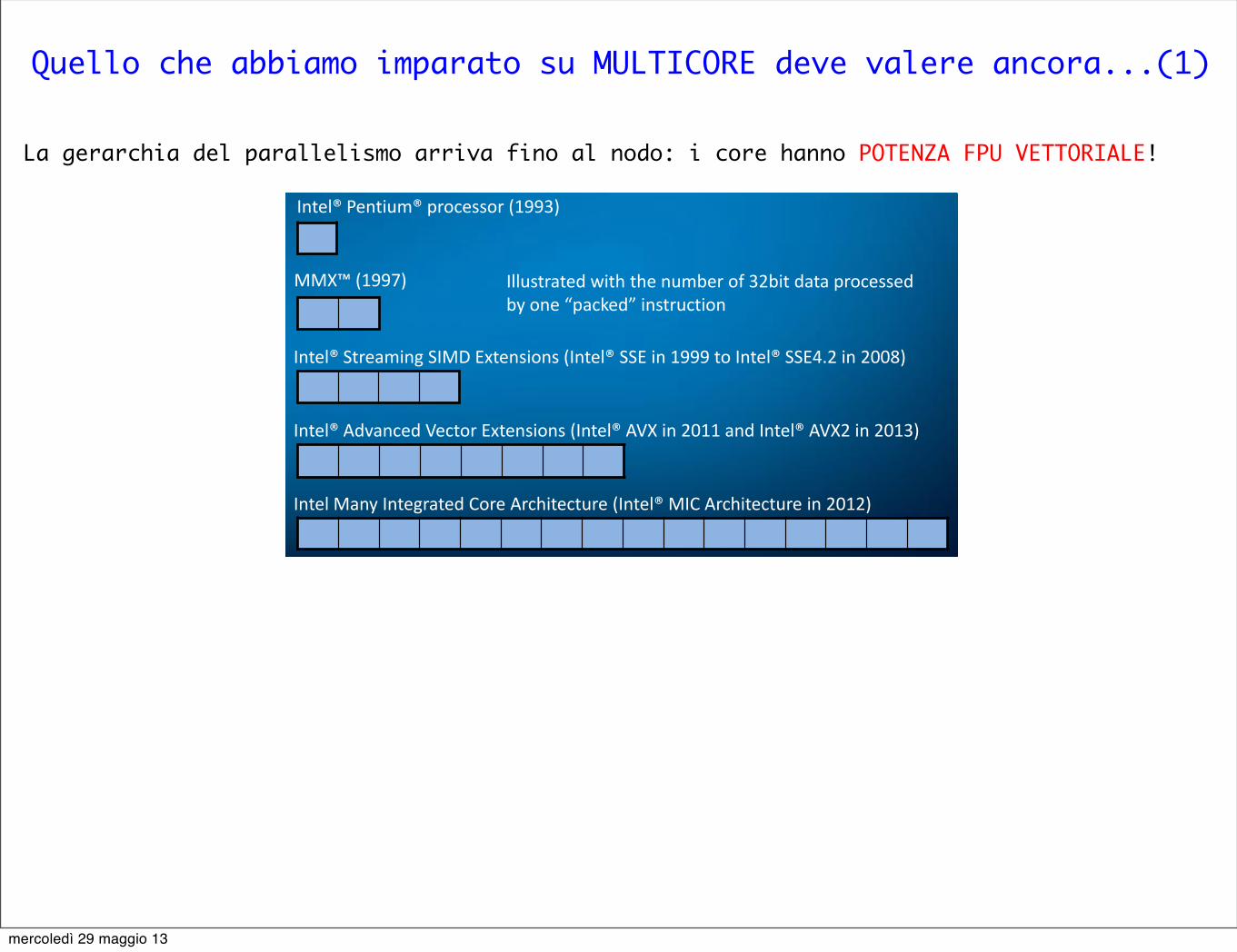
Quello che abbiamo imparato su MULTICORE deve valere ancora...(1)
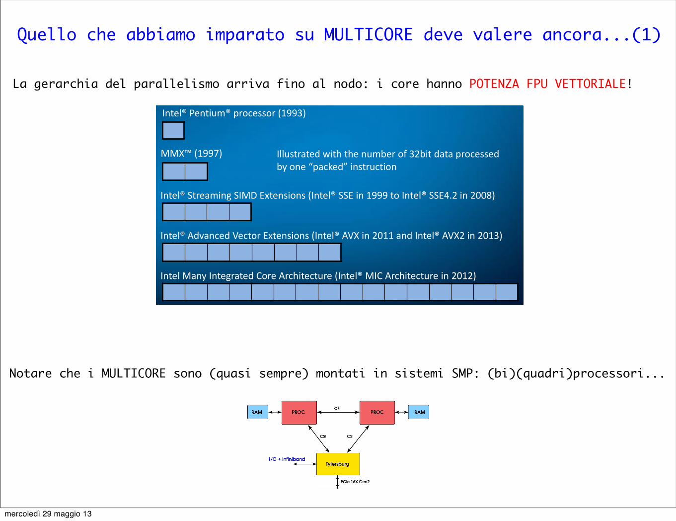
La gerarchia del parallelismo arriva fino al nodo: i core hanno POTENZA FPU VETTORIALE!
History of SIMD ISA extensions
7 6/15/2012
MMX™ (1997)
Intel® Streaming SIMD Extensions (Intel® SSE in 1999 to Intel® SSE4.2 in 2008)
Intel® Advanced Vector Extensions (Intel® AVX in 2011 and Intel® AVX2 in 2013)
Intel Many Integrated Core Architecture (Intel® MIC Architecture in 2012)
Intel® Pentium® processor (1993)
Illustrated with the number of 32bit data processed by one “packed” instruction
Intel Confidential – NDA Presentation
mercoledì 29 maggio 13
Quello che abbiamo imparato su MULTICORE deve valere ancora...(1)
La gerarchia del parallelismo arriva fino al nodo: i core hanno POTENZA FPU VETTORIALE!
History of SIMD ISA extensions
7 6/15/2012
MMX™ (1997)
Intel® Streaming SIMD Extensions (Intel® SSE in 1999 to Intel® SSE4.2 in 2008)
Intel® Advanced Vector Extensions (Intel® AVX in 2011 and Intel® AVX2 in 2013)
Intel Many Integrated Core Architecture (Intel® MIC Architecture in 2012)
Intel® Pentium® processor (1993)
Illustrated with the number of 32bit data processed by one “packed” instruction
Intel Confidential – NDA Presentation
Notare che i MULTICORE sono (quasi sempre) montati in sistemi SMP: (bi)(quadri)processori...
mercoledì 29 maggio 13
Quello che abbiamo imparato su MULTICORE deve valere ancora...(2)
Efficiency on multi-core CPUs: the Wilson Dirac operator on Aurora Michele Brambilla
3. Wilson Dirac operator
Our study refers to the Wilson Dirac operator
φ !x = (m0+4r)φx"
12
4
∑µ=1
!
Ux,µ (1" γµ)φx+µ +U†x"µ,µ(1" γµ)φx"µ
"
(3.1)
The computational effort required by the Dirac operator can be reduced observing [4] thatP±µ = 1± γµ is a spin projector; this reduces the effective number of spin components from 4to 2. Only two components have to be multiplied by the corresponding U matrix; the other twocomponents are then reconstructed. To update each lattice site one has to collect the 8 neighbourspinors (each made of 24 double). All in all, the algorithm performs 1396 flops operating on# 1.5 KB (double precision) data for each site.
Data layout is SIMD friendly: space-time indices run slower while spin, color and real/imaginaryrun faster. Such a layout allows to keep data required for the update of a site in contiguous memoryregions.
We exploited SIMD programming via SSE intrinsics, which appear more natural to implementthan assembly code. The resulting code reads something like
__m128d x2 = _mm_mul_pd(R2,(v+i)->whr[0].m);
v2 = _mm_addsub_pd(_mm_shuffle_pd(x2,x2,1), ...
Westmere processors introduce the new standard SSE4.2. In particular a new instruction turnsout to be very useful for our purposes: _mm_dp_pd computes the dot product between two SSEregisters. Exploiting this feature the dot product of two double precision complex numbers is oneinstruction cheaper. However, the results presented in this proceeding does not exploit this feature:if not carefully tuned it can give rise to bottlenecks in the pipeline.
4. Single board optimization
In the case of a single board we consider multithread parallelization via pthread. We madeour tests on different lattice sizes and considered different approaches, which we will describelater in this section. We make use of the hyperthreading feature of Westmere processors: in thisway it is natural to accomodate up to 24 computing threads. Since not all the physical resourcesof the CPU are doubled in the core, the expected speedup is less than 2: the measured value is#1.2.
The most relevant issue in multithreading is to find out how to split the lattice between threadsin order to achieve the best performances. Partitioning is enforced taking care of core affinity andmemory binding. One makes sure that each thread will be executed on a precise core (physicalor virtual) and that all the memory resources will be allocated on the proper socket (inter-socketcommunications are quite slow).
3
Efficiency on multi-core CPUs: the Wilson Dirac operator on Aurora Michele Brambilla
S2
S1
x2,x3,x4
x1
Figure 1: Along the slowest di-rection the lattice is sliced intotwo big chunks across the twosockets: this reduces the numberof inter-socket communications.
All in all, we want to reduce the number of timesone core has to retrieve data accessing memory resi-dent on the other socket. In order to do that, weslice the lattice into two large blocks along the slow-est direction (x1) and bind each block to a differentsocket. All the threads resident on socket 0 will takecare of one slice, while the threads resident on socket1 will take care of the second slice (see the figure).Only at the boundaries (with respect to the slowest direc-tion) one needs to access memory resident on the othersocket.
To further improve efficiency, one also needs to take into account accesses to different cachelevels (even though L3 and L2 latency is low and bandwidth high). Our approach is to fit the fastestrunning direction (x4) inside L2 cache. To perform this we tried two different approaches: a firstcase named “interleaved”, the latter named “traditional”. Refer to Fig. 2:
• in the “interleaved” approach a thread takes many chunks, each of the minimum (1) sizealong the second fastest direction (x3); in the figure (where 4 threads are at work) the resultingstride is 4.
• in the “traditional” case each thread takes care of a single chunk, resulting in a non-trivialsize along the second fastest direction (x3).
x4
x3
t0
t0
t1
t1
t2
t2
t3
t3
(a)
x4
x3
t0
t1
t2
t3
(b)
Figure 2: Different approaches to parallelization in the x3 direction: either one thread con work on manysmaller chunks or on a single bigger one.
Using hyperthreading, each couple of real+virtual cores take care of contiguous sublattices:this is expected to improve cache efficiency since L1 and L2 caches are shared between the realand virtual core (only registers are duplicated). The “traditional” approach shows the best perfor-mances, with a peak of 52.6GFlops/board.
In both approaches the intra-node parallelization was along x1 (the slowest) and x3 (the secondfastest) directions. We have already commented on the choice of x1 (this optimizes accesses to
4
T = max{ C
NP
, I
NB
, IR
BR}: carefully balancing the bandwiths
Examples of di↵erent performances for di↵erent node (sub-)lattice data layout andsizes: Wilson Dirac operator application
Single node performances (Parma group)
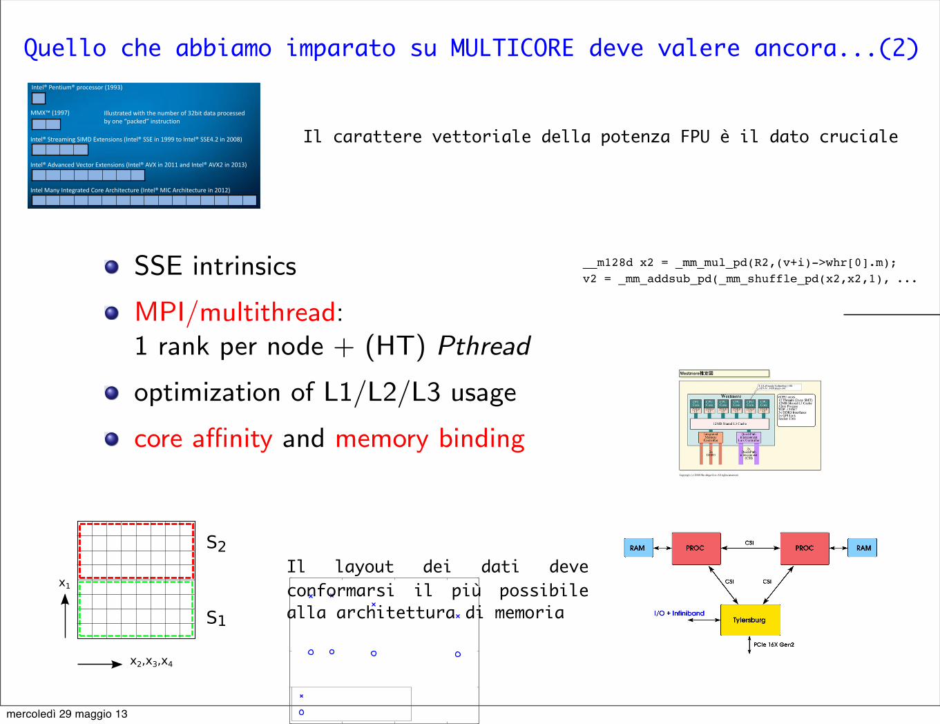
SSE intrinsics
MPI/multithread:1 rank per node + (HT) Pthread
optimization of L1/L2/L3 usage
core a�nity and memory binding
Efficiency on multi-core CPUs: the Wilson Dirac operator on Aurora Michele Brambilla
3. Wilson Dirac operator
Our study refers to the Wilson Dirac operator
φ �x = (m0+4r)φx�12
4
∑µ=1
�Ux,µ (1� γµ)φx+µ +U†
x�µ,µ(1� γµ)φx�µ�
(3.1)
The computational effort required by the Dirac operator can be reduced observing [4] thatP±µ = 1± γµ is a spin projector; this reduces the effective number of spin components from 4to 2. Only two components have to be multiplied by the corresponding U matrix; the other twocomponents are then reconstructed. To update each lattice site one has to collect the 8 neighbourspinors (each made of 24 double). All in all, the algorithm performs 1396 flops operating on� 1.5 KB (double precision) data for each site.
Data layout is SIMD friendly: space-time indices run slower while spin, color and real/imaginaryrun faster. Such a layout allows to keep data required for the update of a site in contiguous memoryregions.
We exploited SIMD programming via SSE intrinsics, which appear more natural to implementthan assembly code. The resulting code reads something like
__m128d x2 = _mm_mul_pd(R2,(v+i)->whr[0].m);
v2 = _mm_addsub_pd(_mm_shuffle_pd(x2,x2,1), ...
Westmere processors introduce the new standard SSE4.2. In particular a new instruction turnsout to be very useful for our purposes: _mm_dp_pd computes the dot product between two SSEregisters. Exploiting this feature the dot product of two double precision complex numbers is oneinstruction cheaper. However, the results presented in this proceeding does not exploit this feature:if not carefully tuned it can give rise to bottlenecks in the pipeline.
4. Single board optimization
In the case of a single board we consider multithread parallelization via pthread. We madeour tests on different lattice sizes and considered different approaches, which we will describelater in this section. We make use of the hyperthreading feature of Westmere processors: in thisway it is natural to accomodate up to 24 computing threads. Since not all the physical resourcesof the CPU are doubled in the core, the expected speedup is less than 2: the measured value is�1.2.
The most relevant issue in multithreading is to find out how to split the lattice between threadsin order to achieve the best performances. Partitioning is enforced taking care of core affinity andmemory binding. One makes sure that each thread will be executed on a precise core (physicalor virtual) and that all the memory resources will be allocated on the proper socket (inter-socketcommunications are quite slow).
3
Efficiency on multi-core CPUs: the Wilson Dirac operator on Aurora Michele Brambilla
S2
S1
x2,x3,x4
x1
Figure 1: Along the slowest di-rection the lattice is sliced intotwo big chunks across the twosockets: this reduces the numberof inter-socket communications.
All in all, we want to reduce the number of timesone core has to retrieve data accessing memory resi-dent on the other socket. In order to do that, weslice the lattice into two large blocks along the slow-est direction (x1) and bind each block to a differentsocket. All the threads resident on socket 0 will takecare of one slice, while the threads resident on socket1 will take care of the second slice (see the figure).Only at the boundaries (with respect to the slowest direc-tion) one needs to access memory resident on the othersocket.
To further improve efficiency, one also needs to take into account accesses to different cachelevels (even though L3 and L2 latency is low and bandwidth high). Our approach is to fit the fastestrunning direction (x4) inside L2 cache. To perform this we tried two different approaches: a firstcase named “interleaved”, the latter named “traditional”. Refer to Fig. 2:
• in the “interleaved” approach a thread takes many chunks, each of the minimum (1) sizealong the second fastest direction (x3); in the figure (where 4 threads are at work) the resultingstride is 4.
• in the “traditional” case each thread takes care of a single chunk, resulting in a non-trivialsize along the second fastest direction (x3).
x4
x3
t0
t0
t1
t1
t2
t2
t3
t3
(a)
x4
x3
t0
t1
t2
t3
(b)
Figure 2: Different approaches to parallelization in the x3 direction: either one thread con work on manysmaller chunks or on a single bigger one.
Using hyperthreading, each couple of real+virtual cores take care of contiguous sublattices:this is expected to improve cache efficiency since L1 and L2 caches are shared between the realand virtual core (only registers are duplicated). The “traditional” approach shows the best perfor-mances, with a peak of 52.6GFlops/board.
In both approaches the intra-node parallelization was along x1 (the slowest) and x3 (the secondfastest) directions. We have already commented on the choice of x1 (this optimizes accesses to
4
lattice size Gflops8 �4� 242 52.68 �12� 482 37.7122 � 482 30.4
12 �24� 482 26.812 �482 � 96 22.5
Strong scaling of di↵erent variants of ETMC code: remote communications viaMPI on IB. (L. Scorzato)
0 10 20 300
5
10
15
20
Nr. of node cards
Perf.
/nod
e ca
rd [G
Flop
s]
483 x 96323 x 64
0 10 20 300
5
10
15
20
Nr. of node cards
Perf.
/nod
e ca
rd [G
Flop
s]
483 x 96323 x 64
Figure 3.1.2. Example of strong scaling (left) and weak scaling (right). In the case of weak scaling, the lattice sizes in the legend refer to 32 nodes.
With the new algorithm we obtained up to 12% of the peak performance (which is 150 Gflops / node-card). In Figure 3.1.2 (left) we show an example of strong scaling, in which the problem size is kept fixed and distributed across an increasing number of nodes. In the right panel of the same figure we show an example of weak scaling, in which the size of the problem in a single node is kept fixed while the full problem size grows proportionally to the number of nodes. Weak scaling is nearly ideal, which means that the Infiniband network is still very efficient up to the size that we considered. Strong scaling is sensitive to more effects, but it appears to be still quite good up to 32 nodes. The code can also use the 3D-network, but the present size of the Aurora prototype is too small to see the advantage. More details can be found in Ref. [4]
3.1.2 Production of Dynamical Nf=4 Gauge Configurations for the Computation of the Renormalization Factors
The computation of the renormalization factors (RF) is an essential ingredient for the precise computation of many physical quantities with Lattice QCD techniques. Since the RF are defined in the chiral limit, the best way to compute them non perturbatively is via
0 10 20 300
5
10
15
20
Nr. of node cards
Perf.
/nod
e ca
rd [G
Flop
s]
483 x 96, time�split483 x 96, half�spinor
Figure 3.1.1 Performance gain of the time-split algorithm.
Playing around with data layout, i.e.
lattice vs sublattices
data ordering
one can gain quite a lot.
F. Di Renzo (UNIPR) Lattice QCD on current architectures New Frontiers in LGT 7 / 15
History of SIMD ISA extensions
7 6/15/2012
MMX™ (1997)
Intel® Streaming SIMD Extensions (Intel® SSE in 1999 to Intel® SSE4.2 in 2008)
Intel® Advanced Vector Extensions (Intel® AVX in 2011 and Intel® AVX2 in 2013)
Intel Many Integrated Core Architecture (Intel® MIC Architecture in 2012)
Intel® Pentium® processor (1993)
Illustrated with the number of 32bit data processed by one “packed” instruction
Intel Confidential – NDA Presentation
Il carattere vettoriale della potenza FPU è il dato cruciale
Il layout dei dati deve conformarsi il più possibile alla architettura di memoria
mercoledì 29 maggio 13
STRUMENTI per PROGRAMMARE in modo sostanzialmente semplice
Un benchmark elementare (operazioni matriciali)
mercoledì 29 maggio 13
La domanda ultima...
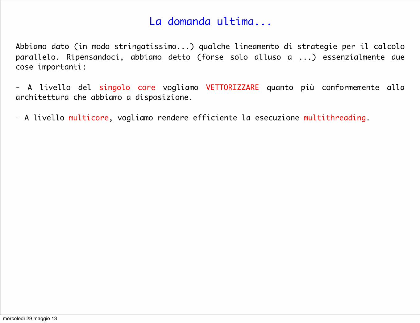
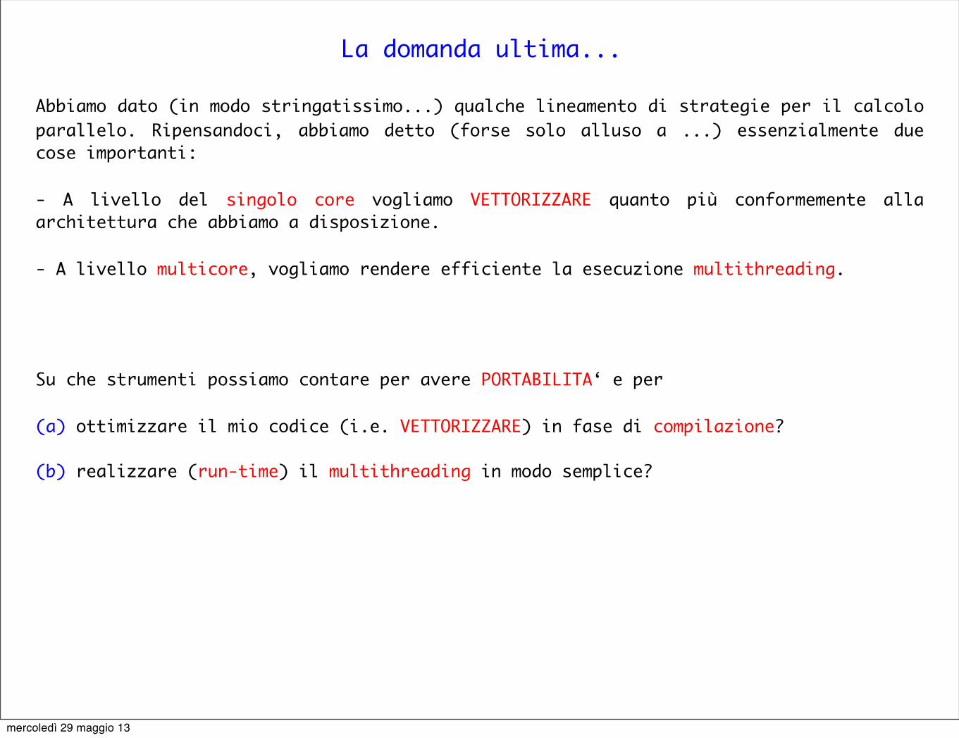
Abbiamo dato (in modo stringatissimo...) qualche lineamento di strategie per il calcolo parallelo. Ripensandoci, abbiamo detto (forse solo alluso a ...) essenzialmente due cose importanti:
- A livello del singolo core vogliamo VETTORIZZARE quanto più conformemente alla architettura che abbiamo a disposizione.
- A livello multicore, vogliamo rendere efficiente la esecuzione multithreading.
mercoledì 29 maggio 13
La domanda ultima...
Abbiamo dato (in modo stringatissimo...) qualche lineamento di strategie per il calcolo parallelo. Ripensandoci, abbiamo detto (forse solo alluso a ...) essenzialmente due cose importanti:
- A livello del singolo core vogliamo VETTORIZZARE quanto più conformemente alla architettura che abbiamo a disposizione.
- A livello multicore, vogliamo rendere efficiente la esecuzione multithreading.
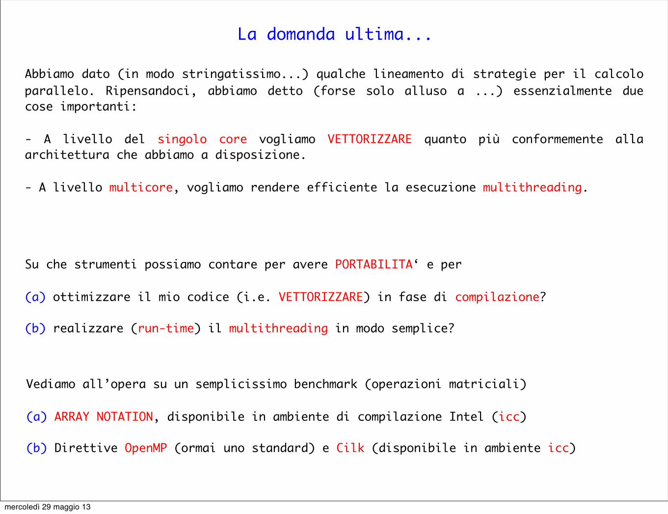
Su che strumenti possiamo contare per avere PORTABILITA‘ e per
(a) ottimizzare il mio codice (i.e. VETTORIZZARE) in fase di compilazione?
(b) realizzare (run-time) il multithreading in modo semplice?
mercoledì 29 maggio 13
La domanda ultima...
Abbiamo dato (in modo stringatissimo...) qualche lineamento di strategie per il calcolo parallelo. Ripensandoci, abbiamo detto (forse solo alluso a ...) essenzialmente due cose importanti:
- A livello del singolo core vogliamo VETTORIZZARE quanto più conformemente alla architettura che abbiamo a disposizione.
- A livello multicore, vogliamo rendere efficiente la esecuzione multithreading.
Su che strumenti possiamo contare per avere PORTABILITA‘ e per
(a) ottimizzare il mio codice (i.e. VETTORIZZARE) in fase di compilazione?
(b) realizzare (run-time) il multithreading in modo semplice?
Vediamo all’opera su un semplicissimo benchmark (operazioni matriciali)
(a) ARRAY NOTATION, disponibile in ambiente di compilazione Intel (icc)
(b) Direttive OpenMP (ormai uno standard) e Cilk (disponibile in ambiente icc)
mercoledì 29 maggio 13
Risorse compilation-time e run-time
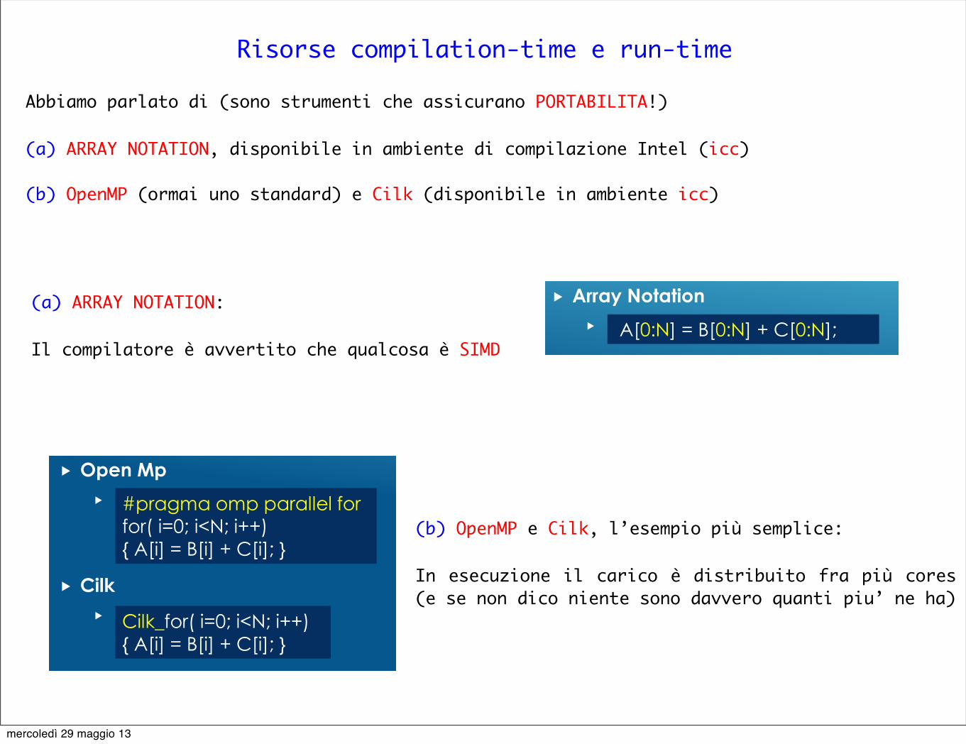
Abbiamo parlato di (sono strumenti che assicurano PORTABILITA!)
(a) ARRAY NOTATION, disponibile in ambiente di compilazione Intel (icc)
(b) OpenMP (ormai uno standard) e Cilk (disponibile in ambiente icc)
BENCHMARK: ATTUAZIONE DEL PARALLELISMO
Ottimizzazione in fase di compilazione: vettorizzazione con istruzioni SIMD
Array Notation
Ottimizzazione Run Time: Creazione del Multi thread
Open Mp
Cilk
for( i=0; i<N; i++){ A[i] = B[i] + C[i]; }
A[0:N] = B[0:N] + C[0:N];
Cilk_for( i=0; i<N; i++){ A[i] = B[i] + C[i]; }
#pragma omp parallel forfor( i=0; i<N; i++){ A[i] = B[i] + C[i]; }
Versione seriale
(a) ARRAY NOTATION:
Il compilatore è avvertito che qualcosa è SIMD
(b) OpenMP e Cilk, l’esempio più semplice:
In esecuzione il carico è distribuito fra più cores (e se non dico niente sono davvero quanti piu’ ne ha)
mercoledì 29 maggio 13
Qualcosa di più su ARRAY NOTATION (facciamolo dire ad Intel)
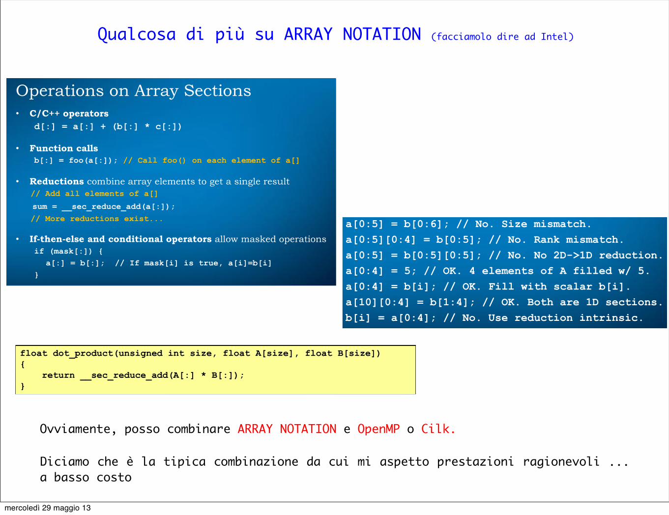
Operations on Array Sections • C/C++ operators
d[:] = a[:] + (b[:] * c[:])
• Function calls b[:] = foo(a[:]); // Call foo() on each element of a[]
• Reductions combine array elements to get a single result // Add all elements of a[] sum = __sec_reduce_add(a[:]); // More reductions exist...
• If-then-else and conditional operators allow masked operations if (mask[:]) { a[:] = b[:]; // If mask[i] is true, a[i]=b[i] }
24 6/15/2012 Intel Confidential – NDA Presentation
“The Fine Print” • If array size is not known, both start-index and length must be
specified • A loop will be generated if vectorization is not possible • Unaligned data, and lengths not divisible by 4, are vectorized as
much as possible, with loops to handle leftovers • Section ranks and lengths (“shapes”) must match. Scalars are OK.
a[0:5] = b[0:6]; // No. Size mismatch. a[0:5][0:4] = b[0:5]; // No. Rank mismatch. a[0:5] = b[0:5][0:5]; // No. No 2D->1D reduction. a[0:4] = 5; // OK. 4 elements of A filled w/ 5. a[0:4] = b[i]; // OK. Fill with scalar b[i]. a[10][0:4] = b[1:4]; // OK. Both are 1D sections. b[i] = a[0:4]; // No. Use reduction intrinsic.
25 6/15/2012 Intel Confidential – NDA Presentation
Simple example: Dot product
• Serial version
• Array Notation Version
30 6/15/2012
float dot_product(unsigned int size, float A[size], float B[size]) { int i; float dp=0.0f; for (i=0; i<size; i++) { dp += A[i] * B[i]; } return dp; }
float dot_product(unsigned int size, float A[size], float B[size]) { return __sec_reduce_add(A[:] * B[:]); }
Intel Confidential – NDA Presentation
Ovviamente, posso combinare ARRAY NOTATION e OpenMP o Cilk.
Diciamo che è la tipica combinazione da cui mi aspetto prestazioni ragionevoli ... a basso costo
mercoledì 29 maggio 13
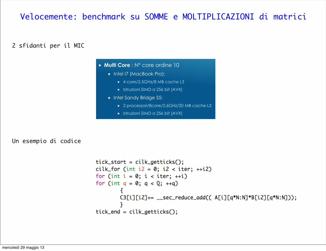
Velocemente: benchmark su SOMME e MOLTIPLICAZIONI di matrici
2 sfidanti per il MIC
CORE: USO MULTIPLO
Many Core : N° core ordine 100
Intel MIC:
60 core/1,053 GHz/240 thread
Istruzioni SIMD a 512 bit (MIC)
8 GB di memoria e larghezza di banda di 320 GB/s
L’Intel si è avviata verso un ulteriore step rappresentato dal passaggio dal multi al manycore
Multi Core : N° core ordine 10
Intel I7 (MacBook Pro):
4 core/2.5GHz/8 MB cache L3
Istruzioni SIMD a 256 bit (AVX)
Intel Sandy Bridge S5:
2 processori/8core/2.6GHz/20 MB cache L3
Istruzioni SIMD a 256 bit (AVX)
Architettura
Un esempio di codice
mercoledì 29 maggio 13
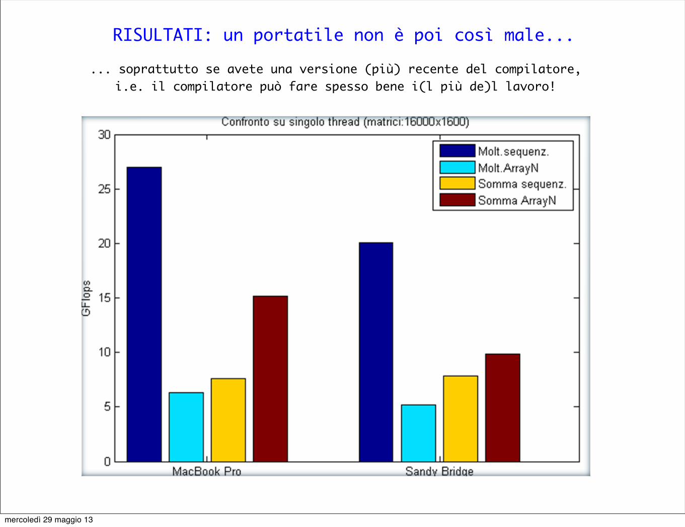
RISULTATI: un portatile non è poi così male...RISULTATI: ESECUZIONE SU SINGOLO THREAD
Tralasciamo l’esecuzione sul singolo core del MIC
Uso dell’Array Notation:• Nel caso della moltiplicazione il
compilatore attua da solo la miglior vettorizzazione
• Per le somme l’uso della Notazione Array incrementa la prestazioni
... soprattutto se avete una versione (più) recente del compilatore, i.e. il compilatore può fare spesso bene i(l più de)l lavoro!
mercoledì 29 maggio 13
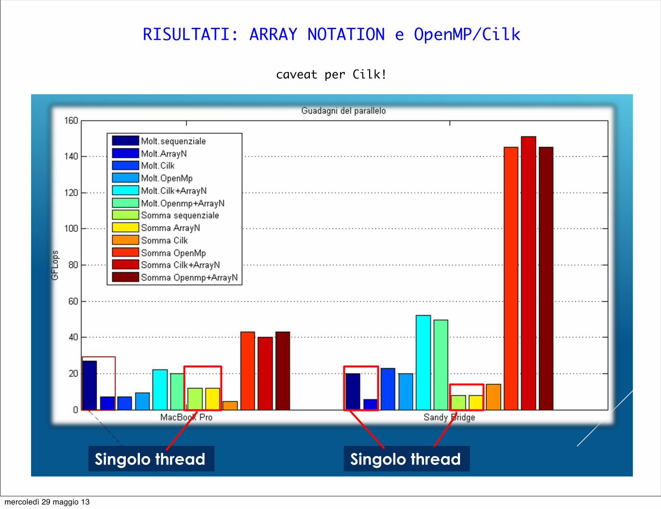
RISULTATI: GUADAGNI IN PARALLELO
Singolo thread Singolo thread
RISULTATI: ARRAY NOTATION e OpenMP/Cilk
caveat per Cilk!
mercoledì 29 maggio 13
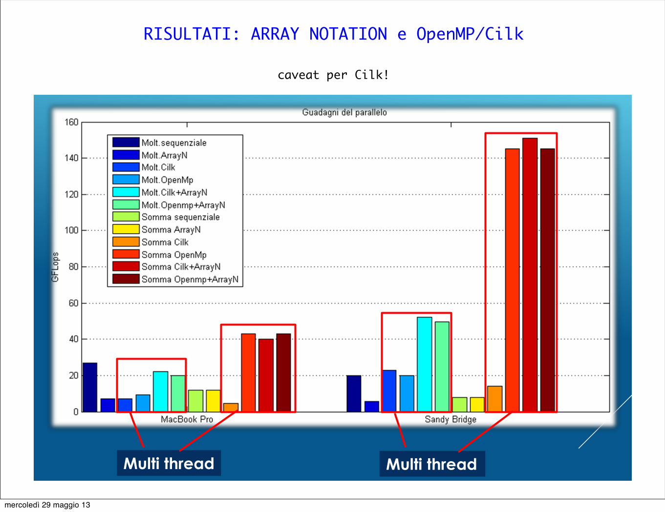
RISULTATI: ARRAY NOTATION e OpenMP/Cilk
RISULTATI: GUADAGNI IN PARALLELO
Multi thread Multi thread
caveat per Cilk!
mercoledì 29 maggio 13
RISULTATI MIC
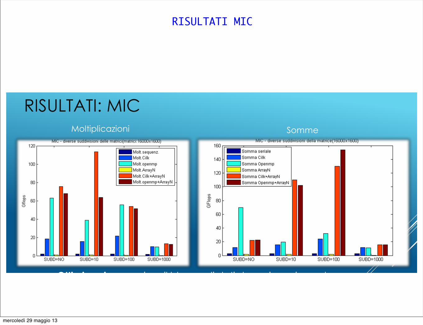
RISULTATI: MIC
Ottimizzazione: variare il blocco di dati da caricare in cache
for( i=0; i<N; i++){ A[i] = B[i] + C[i]; }
for( j=0; j<10; j++)for( i=0; i<N/10; i++){ A[i+j*N] = B[i+j*N] + C[i]; }
Moltiplicazioni Somme
mercoledì 29 maggio 13
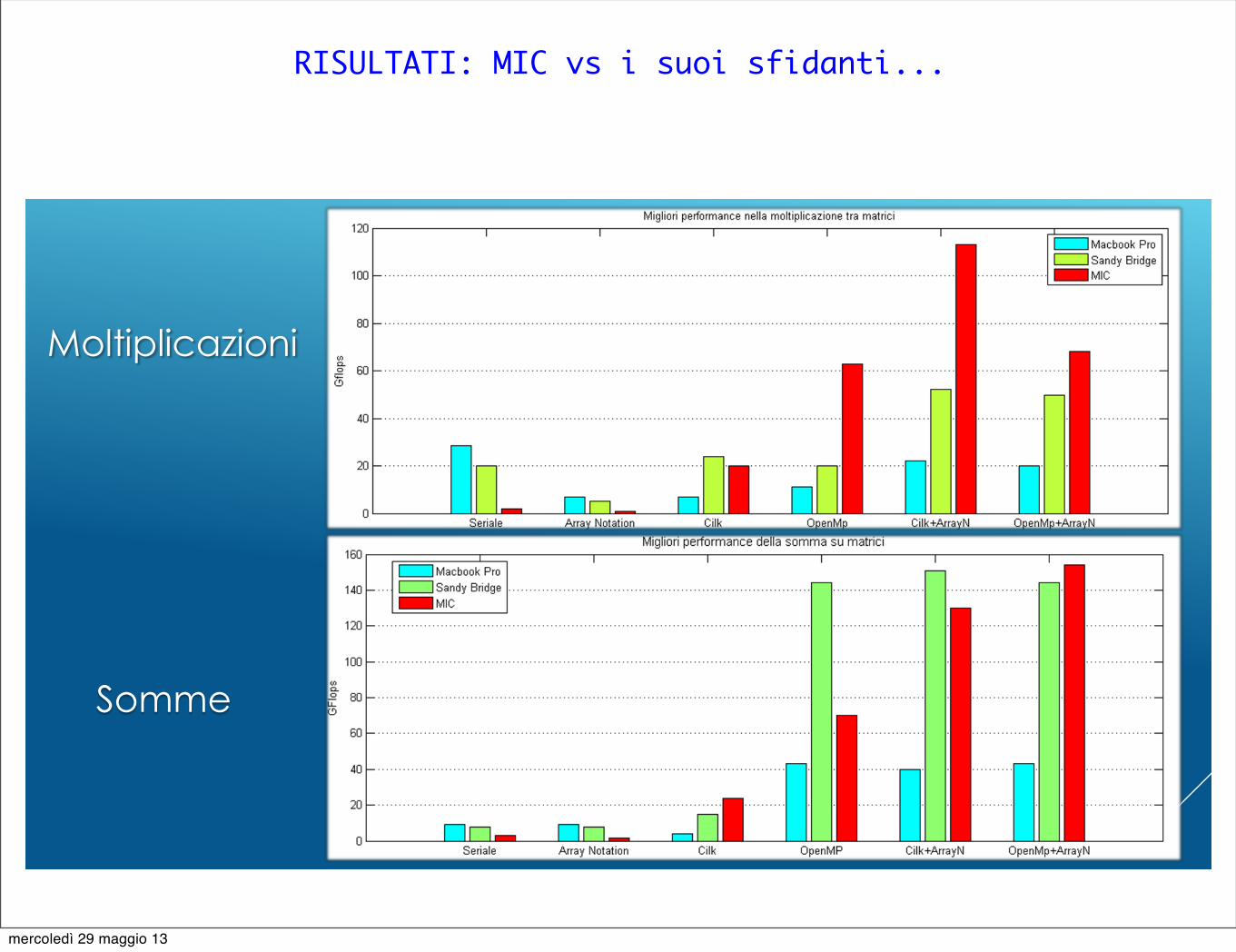
RISULTATI: MIC vs i suoi sfidanti...
RISULTATI: CONFRONTO TRA LE MACCHINE
Moltiplicazioni
Somme
MacBook Pro
Sandy Bridge
MIC
mercoledì 29 maggio 13
Qualche conclusione
Le strategie di parallelizzazione possono essere sottili e il lavoro da loro richiesto pesante (riscrivere codice...). E’ però vero che in generale possiamo pensare di ottenere risultati ragionevoli se ricordiamo sempre che:
- A livello del singolo core vogliamo VETTORIZZARE quanto più conformemente alla architettura che abbiamo a disposizione.
- A livello multicore, vogliamo rendere efficiente la esecuzione multithreading.
Abbiamo visto all’opera su un semplicissimo benchmark (operazioni matriciali)
(a) ARRAY NOTATION, disponibile in ambiente di compilazione Intel (icc)
(b) Direttive OpenMP (ormai uno standard) e Cilk (disponibile in ambiente icc)
mercoledì 29 maggio 13
Qualche conclusione
Le strategie di parallelizzazione possono essere sottili e il lavoro da loro richiesto pesante (riscrivere codice...). E’ però vero che in generale possiamo pensare di ottenere risultati ragionevoli se ricordiamo sempre che:
- A livello del singolo core vogliamo VETTORIZZARE quanto più conformemente alla architettura che abbiamo a disposizione.
- A livello multicore, vogliamo rendere efficiente la esecuzione multithreading.
Abbiamo visto all’opera su un semplicissimo benchmark (operazioni matriciali)
(a) ARRAY NOTATION, disponibile in ambiente di compilazione Intel (icc)
(b) Direttive OpenMP (ormai uno standard) e Cilk (disponibile in ambiente icc)
Un paio di notizie
(una buona) ARRAY NOTATION, OpenMP, Cilk sono strumenti semplici e abbastanza buoni
(una meno buona) Il MIC di suo non ha prestazioni confrontabili al guadagno teorico
mercoledì 29 maggio 13