Università di Napoli “Federico II” Polo delle Scienze e delle Tecnologie

Dottorato di Ricerca in Rischio Sismico

XVIII Ciclo Attenuation and velocity structure in the area of

Pozzuoli-Solfatara (Campi Flegrei, Italy)

for the estimate of local site response

Candidate: Simona Petrosino

Tutor: Prof. Edoardo Del Pezzo

Co-Tutor: Prof. Leopoldo Milano

Coordinator: Prof. Paolo Gasparini

1

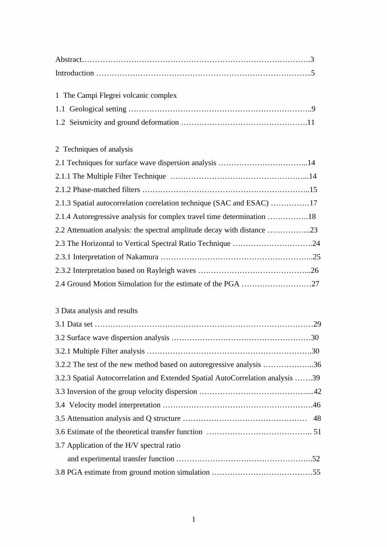
Abstract…………………………………………………………………………….3

Introduction ………………………………………………………………………..5

1 The Campi Flegrei volcanic complex

1.1 Geological setting ……………………………………………………………..9

1.2 Seismicity and ground deformation ………………………………………….11

2 Techniques of analysis

2.1 Techniques for surface wave dispersion analysis ……………………………..14

2.1.1 The Multiple Filter Technique ……………………………………………...14

2.1.2 Phase-matched filters ………………………………………………………..15

2.1.3 Spatial autocorrelation correlation technique (SAC and ESAC) ……………17

2.1.4 Autoregressive analysis for complex travel time determination …………….18

2.2 Attenuation analysis: the spectral amplitude decay with distance ……………..23

2.3 The Horizontal to Vertical Spectral Ratio Technique ………………………….24

2.3.1 Interpretation of Nakamura …………………………………………………..25

2.3.2 Interpretation based on Rayleigh waves ……………………………………..26

2.4 Ground Motion Simulation for the estimate of the PGA ………………………27

3 Data analysis and results

3.1 Data set …………………………………………………………………………29

3.2 Surface wave dispersion analysis ………………………………………………30

3.2.1 Multiple Filter analysis ……………………………………………………….30

3.2.2 The test of the new method based on autoregressive analysis ………………..36

3.2.3 Spatial Autocorrelation and Extended Spatial AutoCorrelation analysis …….39

3.3 Inversion of the group velocity dispersion ……………………………………...42

3.4 Velocity model interpretation ………………………………………………….46

3.5 Attenuation analysis and Q structure ………………………………………… 48

3.6 Estimate of the theoretical transfer function ………………………………….. 51

3.7 Application of the H/V spectral ratio

and experimental transfer function ……………………………………………..52

3.8 PGA estimate from ground motion simulation …………………………………55

2

Discussion ……………………………………………………………………………59

Conclusions ………………………………………………………………………….61

Acknowledgments ……………………………………………………………………62

Appendix A - Demonstration of relation (2.2) ……………………………………….63

Appendix B -A Mathcad worksheet for AR analysis ……………………………… 66

Appendix C - Resolution kernels …………………………………………………….72

Appendix D - A Mathcad worksheet for the attenuation analysis ……………………74

Appendix E - A Mathcad worksheet for the computation of the theoretical

transfer function ……………………………………………………….80

Appendix F - A Mathcad worksheet for the PGA estimate ………………………… 85

References ……………………………………………………………………………95

3

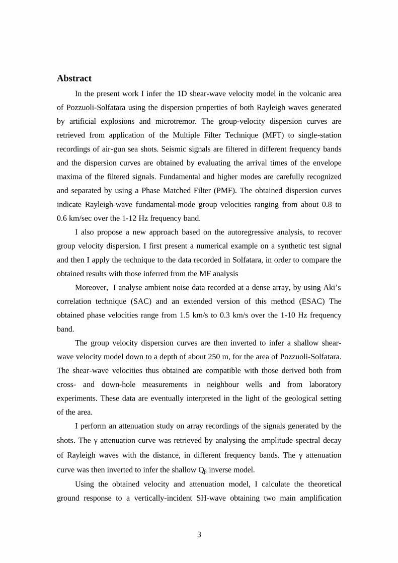
Abstract

In the present work I infer the 1D shear-wave velocity model in the volcanic area

of Pozzuoli-Solfatara using the dispersion properties of both Rayleigh waves generated

by artificial explosions and microtremor. The group-velocity dispersion curves are

retrieved from application of the Multiple Filter Technique (MFT) to single-station

recordings of air-gun sea shots. Seismic signals are filtered in different frequency bands

and the dispersion curves are obtained by evaluating the arrival times of the envelope

maxima of the filtered signals. Fundamental and higher modes are carefully recognized

and separated by using a Phase Matched Filter (PMF). The obtained dispersion curves

indicate Rayleigh-wave fundamental-mode group velocities ranging from about 0.8 to

0.6 km/sec over the 1-12 Hz frequency band.

I also propose a new approach based on the autoregressive analysis, to recover

group velocity dispersion. I first present a numerical example on a synthetic test signal

and then I apply the technique to the data recorded in Solfatara, in order to compare the

obtained results with those inferred from the MF analysis

Moreover, I analyse ambient noise data recorded at a dense array, by using Aki’s

correlation technique (SAC) and an extended version of this method (ESAC) The

obtained phase velocities range from 1.5 km/s to 0.3 km/s over the 1-10 Hz frequency

band.

The group velocity dispersion curves are then inverted to infer a shallow shear-

wave velocity model down to a depth of about 250 m, for the area of Pozzuoli-Solfatara.

The shear-wave velocities thus obtained are compatible with those derived both from

cross- and down-hole measurements in neighbour wells and from laboratory

experiments. These data are eventually interpreted in the light of the geological setting

of the area.

I perform an attenuation study on array recordings of the signals generated by the

shots. The γ attenuation curve was retrieved by analysing the amplitude spectral decay

of Rayleigh waves with the distance, in different frequency bands. The γ attenuation

curve was then inverted to infer the shallow Qβ inverse model.

Using the obtained velocity and attenuation model, I calculate the theoretical

ground response to a vertically-incident SH-wave obtaining two main amplification

4

peaks centered at frequencies of 2.1 and 5.4 Hz. The transfer function was compared

with that obtained experimentally from the application of Nakamura’s technique to

microtremor data, artificial explosions and local earthquakes. Agreement between the

two transfer functions is observed only for the amplification peak of frequency 5.4 Hz.

Finally, as a complementary contribution that might be used to the assessment of

seismic risk in the investigated area, I evaluate the peak ground acceleration (PGA) for

the whole Campi Flegrei caldera and locally for the Pozzuoli-Solfatara area, by

performing stochastic simulation of ground motion partially constrained by the

previously described results. Two different methods (Random Vibration Theory (RVT)

and ground motion generated from a Gaussian distribution (GMG)) are used, providing

the PGA values of 0.04 g and 0.097 g for Campi Flegrei and Pozzuoli-Solfatara,

respectively.

5

Introduction

It is well known that shallow layers with high impedance contrasts affects the

ground motion, causing strong amplifications (Bard and Bouchon, 1980; Hough et al.,

1990). Therefore the detailed knowledge of the velocity and attenuation structure at

shallow depths is of great relevance for the quantitative estimate of the theoretical

ground response to a seismic input. Such determinations are crucial especially in

densely urbanized areas, where a quantitative assessment of the amplification factors is

necessary for a correct evaluation of seismic hazard.

The determination of the subsoil structure often requires expensive drilling. An

alternative and more economic approaches to investigate the shallow velocity structure

are based on the analysis of surface waves. In the last years, the determination of the

seismic velocities at shallow depths from the dispersion of surface waves has got an

increasing popularity and recent results in seismic engineering (Liu et al., 2000; Louie,

2001; Bettig et al. 2001) have demonstrated that inversions of dispersion data can

provide very fine resolution of the velocity structure and constrain shallow shear wave

velocity structures with a minimum level of uncertainty. Single-station methods (MFT;

Herrmann, 1973, 1987) were widely used the aim of obtaining the group velocity

dispersion curves of short period Rayleigh waves and inferring the shallow velocity

structure in sedimentary and tectonic areas (Malagnini et al., 1995, 1997; De Lorenzo

et al., 2003). These techniques were also adapted and successfully applied to retrieve the

dispersive properties of the seismic signals generated by the volcanic activity, in order

to to infer shallow velocity structure in volcanic areas (Petrosino et al., 1999, 2002). The

multichannel (MASW, SAC; Louie, 2001; Aki, 1957; Bettig et al., 2001) techniques

also represent a very attractive tool for the phase velocity determination because they

can be applied to ambient noise and do not require any particular energizing source.

These methods have been also used on microtremor data recordeded on active

volcanoes such as the Puu Oo crater, Hawaii (Saccorotti et al., 2003), Stromboli

(Chouet et al., 1998) and Vesuvius (Saccorotti et al., 2001)

The ground motion amplitude is strongly affected not only by the impedance

contrasts, but also by the damping of soils and (hence by the quality factor Q). Studies

of seismic attenuation are helpful in delineating the dissipative properties of rocks. In

6

particular, the attenuation of surface waves attenuation can be analyzed to obtain local

Qβ models (Malagnini et al., 1995; Malagnini, 1996; Petrosino et al. 2002).

The informations coming from velocity and attenuation structures are useful for

the estimate of the theoretical transfer function (Malagnini et al., 1996, Margheriti et al.,

2000). In this way, the resonance frequencies that could cause the amplification of the

ground shaking can be determined. This parameters should be taken into account in the

assessment of seismic hazard.

In the recent years, experimentally measurements of the site transfer function have

been obtained by Nakamura’s spectral ratio technique (Nakamura, 1989). In particular,

the maxima of the horizontal to vertical (H/V) function, under certain assumption,

correctly indicates the resonance frequencies of soft shallow sediments overlying the

bedrock. Many authors have proved the validity of the techniques by empirical,

theoretical, and numerical results (Field and Jacob, 1993; Lermo and Chavez-Garcia,

1993; Lachet and Bard, 1994; Lermo and Chavez-Garcia, 1994; Field and Jacob, 1995;

Castro et al., 1997). However other authors (Luzon et al., 2001; Malischewsky and

Scherbaum, 2004) found that in the case of low impedance contrast, the method does

not predict accurately the resonance frequencies and the amplification level. Moreover

is still not clear the techniques can be applied only to the ambient noise or also to

earthquakes and artificial explosions. Actually some authors found a discrepancy in the

H/V functions for noise and earthquakes (Malagnini et al, 1996), while others observed

a good agreement (at least in certain frequency range) between H/V ratio of

microtremor and S-waves (Seekins at al., 1996, Satoh, 2001). In this framework, further

investigation and more tests on data are still needed to establish the range of

applicability of Nakamura’s technique.

Whether using experimental or theoretical approaches, the site transfer function is

extremely useful to put constraints for the evaluation of the peak ground acceleration

(PGA), that is an important parameter to be considered in seismic hazard studies, as it

allows to predict the maximum expected ground shaking (Kramer, 1996).

In the present work I will focus on the volcanic area of Pozzuoli-Solfatara and

carry on a complete study according to the following tasks:

7

1) Analysis of Rayleigh wave dispersion and inversion for the velocity structure

2) Analysis of Rayleigh wave attenuation and inversion for the Qβ model

3) Estimate of the theoretical transfer function

4) Determination of the experimental transfer function

5) Peak ground acceleration (PGA) estimate

For task 1) I use the Multiple Filter (MFT), the Spatial AutoCorrelation (SAC) and

the Extended Spatial AutoCorrelation (ESAC) techniques. Moreover, I propose a new

alternative approach based on the autoregressive signal analysis to recover group

velocity dispersion. I first present some numerical examples on synthetics and then I

apply the technique to the data recorded in Solfatara, to compare the obtained results

with those inferred from the MFT analysis.

With task 1) and 2) I want to contribute to the knowledge of the very shallow

structure of the area of Pozzuoli-Solfatara and provide some complementary

information to those given by the available velocity and attenuation tomography, that

has greater depths of investigation but cannot resolve the finer structure (first 250 m) of

the subsoil.

Task 3) is carried on by using the results obtained from task 1) and 2). Velocity and

attenuation structures are used to calculate the ground response to a vertically

propagating SH wave in a multiple layered medium. The obtained transfer function

might be considered for assessing seismic hazard in the densely-populated Pozzuoli-

Solfatara volcanic area.

For task 4) I will use Nakamura’s spectral ratio technique applied to both

microtremor data, explosions and local earthquakes and compare it with the theoretical

ground response obtained in task 3). At the present there is a great scientific debate

about the validity, the range of applicability of Nakamura method and if it suitable only

for ambient noise or can be applied to earthquakes too. I want to give my contribution

by proposing some example of application to different kind of data recorded in an area

with low-impedance contrast.

8

Finally, as complementary result in task 5) I provide an estimate of the expected

peak ground acceleration for the Campi Flegrei area, by simulating the ground motion

produced by local earthquakes. Moreover for the area of Pozzuoli-Solfatara, I estimate

the PGA taking into account the local site effects evidenced by the resonance

frequencies in the transfer function derived in 3). These evaluations refine the present

PGA values for the Phlegraen area reported in the hazard maps (www.mi.ingv.it; Slejko

et al., 1998), which have been calculated considering the ground motion produced by

strong tectonic earthquakes occurring in the Apennines.

In the next chapters I first illustrate the geological setting of the Campi Fegrei area

(Chapter I), I describe the techniques used for this study (Chapter II) and then I present

the obtained results (Chapter III) with the relative discussion.

9

Chapter I

The Campi Flegrei volcanic complex

1.1 Geological setting

The Campi Flegrei is a nested caldera originated by two large collapses occurred

during the Campanian Ignimbrite (39 ka) and the Neapolitan Yellow Tuff (NYT, 15 ka)

eruptions (Orsi et al., 1996, Di Vito et al., 1999, Orsi et. al., 2003).

The Campanian Ignimbrite is one of the major explosive eruption occurred in the

Mediterranean area in the last 200,000 years and its deposits buried a large part of the

Campania region. The Campanian Ignimbrite caldera, which formed after the collapse

includes the present area of the Campi Flegrei, the city of Naples, the western part of the

bay of Naples and the bay of Pozzuoli.

During the Neapolitan Yellow Tuff eruption several tens of km3 of magma were

emitted and an area of approximately 1,000 km2 was covered by pyroclastic deposits.

These deposits have been found in Neapolitan-Phlegraean area and the Campanian Plain

as far as in the Appennines. The NYT caldera is nested inside the Campanian Ignimbrite

caldera, it includes part of the present Campi Flegrei area and the bay of Pozzuoli. The

caldera floor is affected by brittle deformation, being its continental north-eastern sector

crossed by faults oriented NW-SE and NE-SW, which are the same directions as those

of the faults affecting the Campanian Plain and the inner sectors of the Apennine belt.

Since 15 ka the volcanic activity concentrated inside the NYT caldera and many

eruptions took place during three distinct epochs of activity, alternated to two periods of

quiescence. In particular, volcanism of the I epoch (15-9.5 ka) includes 34 variable

magnitude explosive eruptions. During this epoch several tuff-cones were formed near

the present coast of Pozzuoli (Rione Terra, La Pietra).

During the II epoch (8.6-8.2 ka), the volcanic activity occurred along the north-

eastern structural boundary of the NYT caldera, whereas vents (Solfatara, Accademia,

Monte Olibano) of the III epoch (4.8–3.8 ka) were mainly located in the north-eastern

sector of the caldera floor, near the present town Pozzuoli.

The last eruption (Monte Nuovo) occurred in 1538, after a period of quiescence

which lasted approximately 3,000 years.

10

Since the NYT collapse, the whole Campi Flegrei caldera is affected by

subsidence, while the younger central part of the caldera floor is characterized by

resurgence. In particular, during the three epochs of volcanic activity, the La Starza

marine terrace (the most uplifted part of the resurgent block) alternated periods of

emersion and submersion and after the onset of the III epoch it definitely emerged.

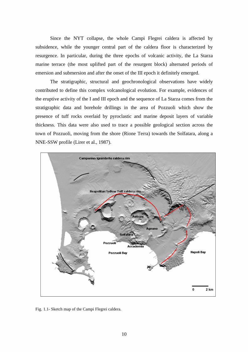
The stratigraphic, structural and geochronological observations have widely

contributed to define this complex volcanological evolution. For example, evidences of

the eruptive activity of the I and III epoch and the sequence of La Starza comes from the

stratigraphic data and borehole drillings in the area of Pozzuoli which show the

presence of tuff rocks overlaid by pyroclastic and marine deposit layers of variable

thickness. This data were also used to trace a possible geological section across the

town of Pozzuoli, moving from the shore (Rione Terra) towards the Solfatara, along a

NNE-SSW profile (Lirer et al., 1987).

Fig. 1.1- Sketch map of the Campi Flegrei caldera.

0 2 km

11

1.2 Seismicity and ground deformation

Seismicity in the Campi Flegrei area generally occurs during the phases of ground

uplift, while it is absent during the periods of subsidence.

The major uplift episodes occurred in 1969-1972 and in 1982-1984 (Orsi et al.,

1999). During the bradyseismic crisis of 1969-1972, the ground lifted by approximately

1.5 m. The seismic activity began with some low-energy events which preceded a 1.8

magnitude earthquake occurred on 1970, March 26th. Other seismic swarms followed on

1970, April 2nd, July 21st and November 26th. The strongest earthquake was recorded on

1972, March 2nd. In the summer of 1972 the ground stopped to rise and, at the same

time, the seismic activity ended. Between 1973 and 1981 the Campi Flegrei area was

subjected to a slow process of subsidence, interrupted by a small uplift episode (less

than 10 cm) in the month of September 1976 which was accompanied by about 12

earthquakes located in the Solfatara area.

During the 1982-1984 crisis a ground uplift of 1.79 m took place. This was

accompanied by intense seismic activity: swarms of earthquakes were recorded with a

magnitude between 0.6 and 4.2, generally at a depth of 1.5 to 5 Km. The most

significant swarm (513 earthquakes in about 6 hours) was detected on 1984, April 1st.

The strongest earthquake (magnitude 4.2) occurred on 1983, December 8th. During this

seismic crisis, over 10,000 earthquakes were recorded. Most of the seismicity

concentrated in the area of Pozzuoli-Solfatara. In Pozzuoli, the seismic activity was

characterized by low-energy swarms, while the Solfatara area was the epicentral zone

for the most energetic earthquakes (Vilardo et al., 1991).

After the 1982-1984 episode, no further seismic activity was recorded in the

Phlegrean area until 1987, when on April 10th and November 4th two seismic swarms

consisting of 50 and 26 earthquakes respectively, were recorded and located in the

Solfatara area. Between April and June 1989, at the time of an episode of renewed

ground uplift (about 7.5 cm), there were 316 earthquakes, located SE of the Solfatara

crater. In particular on April 3rd a seismic swarm was recorded, consisting of 82 events,

while the severest earthquake of this period happened June on 6th. After the 1989

episode, no further significant events were recorded until July 2000.

In the period July-August 2000 a net uplift of 4 cm centered on Pozzuoli occurred.

This phase was accompanied by two low-energy seismic swarms on July 2nd and August

12

22nd (Bianco et al., 2004). Seismic activity started between July 2nd and 10th, when

about ten low-energy low-frequency events were recorded. On August 22nd there was a

seismic swarm of about sixty volcano-tectonic earthquakes, some of them were felt by

the population living in the area of the Solfatara. The high frequency pattern of this

swarm is similar to that shown by the volcano-tectonic events recorded during the 1983-

84 uplifting episode. The strongest earthquake had magnitude 2.2. The seismic swarm

was located in the Solfatara area, at a depth of about 2 Km.

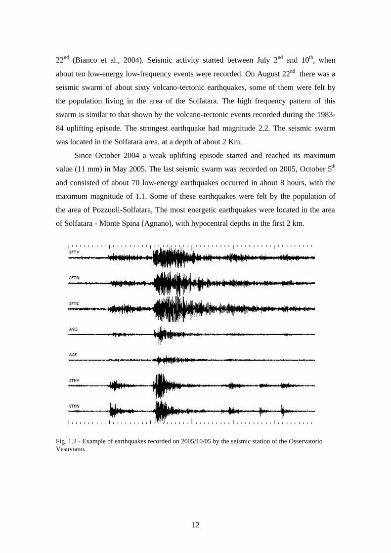
Since October 2004 a weak uplifting episode started and reached its maximum

value (11 mm) in May 2005. The last seismic swarm was recorded on 2005, October 5th

and consisted of about 70 low-energy earthquakes occurred in about 8 hours, with the

maximum magnitude of 1.1. Some of these earthquakes were felt by the population of

the area of Pozzuoli-Solfatara, The most energetic earthquakes were located in the area

of Solfatara - Monte Spina (Agnano), with hypocentral depths in the first 2 km.

Fig. 1.2 - Example of earthquakes recorded on 2005/10/05 by the seismic station of the Osservatorio Vesuviano.

13

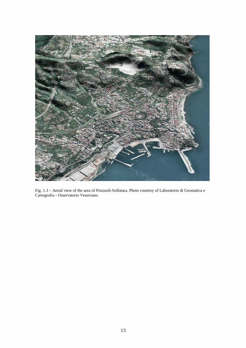
Fig. 1.3 – Aerial view of the area of Pozzuoli-Solfatara. Photo courtesy of Laboratorio di Geomatica e Cartografia - Osservatorio Vesuviano.

14

Chapter II

Techniques of analysis

2.1 Techniques for surface wave dispersion analysis

A brief review of the techniques that I used for the analysis of surface wave

dispersion is reported in the following section.

2.1.1 The Multiple Filter Technique

The Multiple Filter Technique (MFT; Dziewonski et al.,1969; Herrmann, 1987) is

a single station method based on the evidence that for dispersive signals, different wave

packets arrive at different times, depending on the frequency. The method consists in

the application of gaussian band-pass filters to multi-modal dispersive signals associated

to the propagation of surface waves. Then, the arrival times of the maxima of the

envelope of the filtered signal are estimated and used to calculate group velocity.

Repeating the procedure for different frequencies, the group velocity dispersion curve

can be inferred.

The technique is based on the following theory. The displacement caused by a

dispersive wave packet at time t and distance r from the source is represented as

superposition of the M+1 modes present in the signal (Aki and Richards, 1980):

( ) [ ] ωωωπ

ωωωπ

drktirAdtirFrtf jj

M

j

)(exp),(21

exp),(21

),(0

−== ∫∑∫∞

∞− =

∞

∞−

where ω is the angular frequency, jk and jA are the wave number and the complex

amplitude of the j-th mode, respectively. First consider the application of a gaussian

band-pass filter to a single-mode signal. If ( )0

ωω −H is a gaussian filter centered at

0ωω = with cutoff frequency at cωωω ±=0

:

( ) ( ) −

=0

exp0

2 ωωαωH

c

c

ωωωω

>≤

the expression of the filtered signal will be:

( ) ( ) ( )[ ] ωωωωωπ

ωω

ωω

dkrtirAHtrgc

c

−−= ∫+

−

exp,21

),(0

0

0

15

After changing variable, the integral becomes:

( ) ( ) ( ) ( )[ ] ωωωωωωωωπ

ω

ω

drktirAHtrgc

c

000exp,

21

),( +−++= ∫−

(2.1)

After an expansion in Taylor series of ( )rA ,ω and of ( )ωk around 0

ω , Herrmann

(1973) demonstrated that equation (2.1) can be written as (see appendix A):

( ) ( )[ ]

−−−=

2

04expexp

2,

2

000

0

Ur

trktiA

rtgα

ωω

απ

πω

(2.2)

where U0 is the group velocity. From (2.2) one can easily see that the envelope (or

magnitude) of the function ( )rtg , has the maximum at the time 0Urt = .

In case of multi-modal signals, the equation (2.2) assumes the form:

( ) ( ) ( )[ ]

−−−= ∑

=

2

00 4expexp,

2,

2

0

000

0

j

M

jj U

rtrktirArtg j α

ωωω

απ

πω

(2.3)

where the index j represents the value of U and A for the j-th mode. Taking the envelope

of (2.3), the individual maxima correspond to the arrivals jUrt 0= relative to the

different modes, each of them propagating with group velocity jU 0 . If the individual

maxima are well separated and the source-to-receiver distance r is known, the group

velocities jU 0 can be calculated.

2.1.2 Phase-matched filters

The phase-matched filters (PMF; Herrin and Goforth, 1977) are defined as the

class of linear filters for which the Fourier phase is equal to that of a given signal.

Considering the convolution and the cross-correlation of a signal ( )ts with the filter

( )tf and taking the Fourier transform, one obtains:

( ) ( ) ( ) ( ) ( ) ( )[ ]ωφωσωω +⇒∗ iFStfts exp (2.4)

( ) ( ) ⇒⊗ tfts ( ) ( ) ( ) ( )[ ]ωφωσωω −iFS exp (2.5)

where the symbol ⇒ denotes the Fourier transform operation. If )(tf is a phase-

matched filter, then ( ) ( )ωφωσ = . With this choice, the Fourier transform of equation

(2.5) will be ( ) ( )ωω FS . The same result can be obtained from (2.4) if we consider the

16

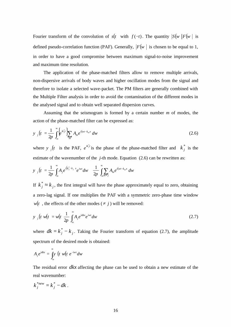
Fourier transform of the convolution of ( )ts with )( tf − . The quantity ( ) ( )ωω FS is

defined pseudo-correlation function (PAF). Generally, ( )ωF is chosen to be equal to 1,

in order to have a good compromise between maximum signal-to-noise improvement

and maximum time resolution.

The application of the phase-matched filters allow to remove multiple arrivals,

non-dispersive arrivals of body waves and higher oscillation modes from the signal and

therefore to isolate a selected wave-packet. The PM filters are generally combined with

the Multiple Filter analysis in order to avoid the contamination of the different modes in

the analysed signal and to obtain well separated dispersion curves.

Assuming that the seismogram is formed by a certain number m of modes, the

action of the phase-matched filter can be expressed as:

( ) ( )∫ ∑∞

∞−

−=m

xktim

tikj deAet mj ω

πψ ω*

21

(2.6)

where ( )tjψ is the PAF, tik je*

is the phase of the phase-matched filter and k j* is the

estimate of the wavenumber of the j-th mode. Equation (2.6) can be rewritten as:

( ) ( ) ( )∫ ∑∫∞

∞− ≠

−∞

∞−

− +=jm

xktim

tixkkijj deAdeeAt mjj ω

πω

πψ ωω

21

21 *

If k kj j* ≈ , the first integral will have the phase approximately equal to zero, obtaining

a zero-lag signal. If one multiplies the PAF with a symmetric zero-phase time window

( )tw , the effects of the other modes ( j≠ ) will be removed:

( ) ( ) ( ) ∫+∞

∞−

= ωπ

ψ ωδ deeAtwtwt tikxijj 2

1 (2.7)

where δk k kj j= −* . Taking the Fourier transform of equation (2.7), the amplitude

spectrum of the desired mode is obtained:

( ) ( )∫∞

∞−

−= ωψ ωδ detwteA tikxij

The residual error δkx affecting the phase can be used to obtain a new estimate of the

real wavenumber:

k k kjnew

j* *= − δ .

17

The procedure can be iterated to obtain a precise estimate of the wavenumber (and

hence of the group velocity) for the mode of interest.

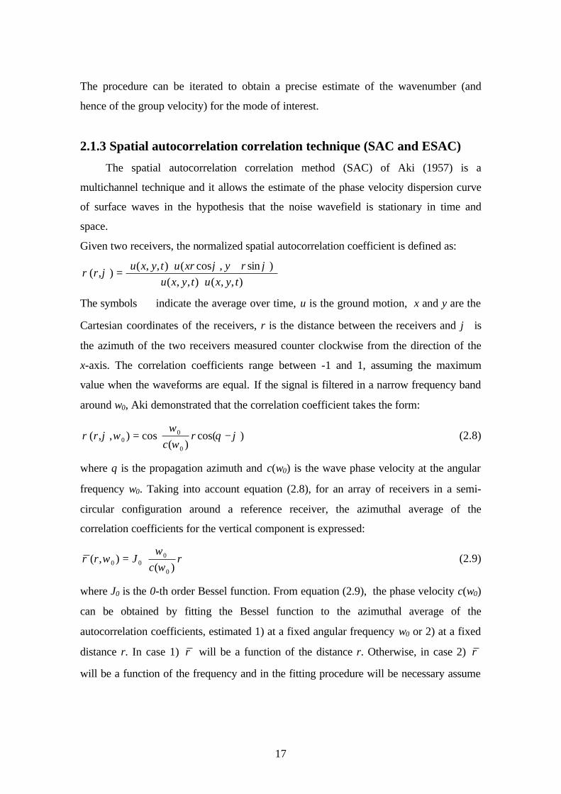
2.1.3 Spatial autocorrelation correlation technique (SAC and ESAC)

The spatial autocorrelation correlation method (SAC) of Aki (1957) is a

multichannel technique and it allows the estimate of the phase velocity dispersion curve

of surface waves in the hypothesis that the noise wavefield is stationary in time and

space.

Given two receivers, the normalized spatial autocorrelation coefficient is defined as:

⟩⋅⟨⟩+⋅⟨

=),,(),,(

)sin,cos(),,(),(

tyxutyxuryxrutyxu

rϕϕ

ϕρ

The symbols ⟨⟩ indicate the average over time, u is the ground motion, x and y are the

Cartesian coordinates of the receivers, r is the distance between the receivers and ϕ is

the azimuth of the two receivers measured counter clockwise from the direction of the

x-axis. The correlation coefficients range between -1 and 1, assuming the maximum

value when the waveforms are equal. If the signal is filtered in a narrow frequency band

around ω0, Aki demonstrated that the correlation coefficient takes the form:

−= )cos(

)(cos),,(

0

00 ϕθ

ωω

ωϕρ rc

r (2.8)

where θ is the propagation azimuth and c(ω0) is the wave phase velocity at the angular

frequency ω0. Taking into account equation (2.8), for an array of receivers in a semi-

circular configuration around a reference receiver, the azimuthal average of the

correlation coefficients for the vertical component is expressed:

= r

cJr

)(),(

0

000 ω

ωωρ (2.9)

where J0 is the 0-th order Bessel function. From equation (2.9), the phase velocity c(ω0)

can be obtained by fitting the Bessel function to the azimuthal average of the

autocorrelation coefficients, estimated 1) at a fixed angular frequency ω0 or 2) at a fixed

distance r. In case 1) ρ will be a function of the distance r. Otherwise, in case 2) ρ

will be a function of the frequency and in the fitting procedure will be necessary assume

18

an a-priori dispersion law c(ω0). In this case, the phase velocity is usually assumed to

have a frequency dependence described by a power-law function: bAffc −=)(

The choice 1), which is the best because no a priori dispersion should be assumed, is

generally possible when the array is formed by a large number of sensors and the

correlation coefficients can be evaluated for a relatively high number of inter-station

distances. This requires a particular geometry of the seismic array, with the sensors

deployed along many semicircles with different radius.

Extension of Aki’s SAC method (ESAC) to non-semicircular arrays was proposed

by Bettig (2001) and consists in averaging, for each individual target frequency, the

correlation coefficients evaluated at subsets of M station pairs whose distances range

between r-dr and r+dr. This procedure allows a robust assessment of the azimuthally-

averaged correlation coefficients, once the relative position vectors of the selected

station pairs depict an uniform and tight sampling of the 0-180° azimuthal range. In this

case the condition of having a large number of available inter-station distances can be

achieved without the constrain of adopting a particular geometry for the array

deployment. For this reason, the advantage of ESAC compared to the conventional SAC

is that the evaluation of (2.9) at a fixed frequency can be easily carried on, and the

estimates of phase velocities may be retrieved at any individual frequency without the

need of assuming any a-priori dispersion relationship.

2.1.4 Autoregressive analysis for complex travel time determination

In this section I discuss a new approach to recover the group velocity dispersion

curve of surface waves.

Consider a pulse occurring at a certain point at time t = 0. As an effect of the

propagation, the signal observed at the given point can be represented by the

superposition of a certain number j of pulses that may have been propagating along

different paths, with different phase velocities, c (Aki and Richards, 1980) :

[ ]∑∑ −=−=j

jjj

jj

j qtiAxk

tiAtf )(exp)(exp()( ωω

ω (2.10)

19

where Aj is the amplitude of the j-th pulse and ω is the angular frequency. In case of

dissipative medium, k is the complex wavenumber and the quantity q is defined as the

complex travel-time:

−=

Qi

ck

jj 2

1ω

jjj ivq += τ

The real part of q represents the arrival time τ = x/c = kx/ω and the imaginary part is

expressed as:

cQx

v2

−=

with c phase velocity and Q quality factor.

In the frequency domain, the sequence of pulses is represented by the Fourier transform

of (2.10):

∑∑ −=−=j

jjjj

jj xikAiqAF )exp()exp()( ωω (2.11)

The real and imaginary part of (2.11) correspond to oscillating signals in the frequency

domain. Hasada et al. (2001) proposed an impulse model corresponding to equation

(2.11). Actually it can be demonstrated that the inverse Fourier transform of the

function F(ω) corresponds to the real part of the complex Lorentzian function L(t):

∑∑ =

−=

jj

j j

j tLqt

iAth ))(Re(

1Re

1)(

ππ

As the amplitude A can be expressed as )exp(0 ωφiAA = , for φ =0 the real part of the

function L(t) is a Lorentzian function centered at τ, with a width of wj=-2vj and the

imaginary part is asymmetric respect t = τ. In general, for different values of φ, Re(L(t))

is a linear combination of a symmetric and asymmetric components.

For dispersive wave packets, the complex wavenumber k is a function of frequency and

can be expanded in a Taylor series around the point ω0:

)()(

1)()()()( 0

0000

0

ωωω

ωωωω

ωωωω

−+=−∂

∂+=

= j

jj u

kk

kk

where u is the group velocity. Substituting this expression in the equation (2.11) we

obtain:

20

[ ][ ] =−−−= ∑ ))((exp())(exp()( 000 ωωωωω gj

jjjj iqxikAF

[ ][ ]))((exp()(exp( 000 ωωωωω −−−= ∑ gj

jjj iqiqA

gjq is the complex group delay that is related to the complex group velocity:

)()(

00 ω

ωj

jgl u

xq =

Consider now the function F(ω) in a narrow frequency band centered around ω0; it will

assume the following form:

[ ][ ]=−−−= ∑ ))(exp()))()((exp(),( 00000 ωωωωωωω gj

j

gjjj iqqqiAH

))(exp()( 00 ωωω gj

jj iqB −= ∑ (2.12)

Comparing this expression with (2.11), we note that the two transfer functions have the

same form with the difference that in the case of dispersive media the amplitude Aj and

the phase delay jq in equation (2.11) have been replaced by Bj and the group delay

gjq at the frequency ω0. Therefore, the impulse sequence model corresponding to the

complex Lorentzian function can also be applied to the case of dispersive media if one

considers a narrow frequency band. In this case the real part of the complex travel time

corresponds to the travel time of the group velocity at the frequency f0. Taking this into

account, a dispersion curve can be obtained by estimating the real part of complex travel

time for a set of center frequencies.

The problem of providing a reliable estimate of the complex travel time (and

therefore of the group arrivals) can be carried on by using an autoregressive (AR)

approach. In the following I will describe some general concepts of the autoregressive

method applied to complex frequency series, then in appendix B I will show an

application to a synthetic signal to demonstrate the ability of the technique in

discriminating closely spaced pulses and hence in reliably determining the travel times.

The complex frequency series corresponding to expression (2.11) can be

considered as the superposition of two independent components, the signal H and

Gaussian white noise E:

iii EHY += i = 0…N-1

21

where N is the number of points of the complex frequency series. The signal H consists

of decaying oscillations and satisfies an m order AR equation:

∑=

−==m

kj

kkj HzaHzA

0

0)( (2.13)

A(z) is a complex AR operator of order m, ak are the AR coefficients and z is the unit-

frequency-shift operator:

1+= jj HzH

)2exp( fqiz ∆−= π

with ∆f the unit of frequency discretization. To estimate the unknown parameters (the

complex travel time q which are related to the z operator) in the given complex

frequency series, several approaches exists. I will follow that proposed by Hori et al.

(1989) based on the minimization of the prediction error that leads to the determination

of the AR ak coefficients by solving an eigenvalue problem. Taking into account (2.13),

the prediction error is:

∑ ∑∑−

= =−

=−

−

=1

00

1 N

mj

m

kkjk

m

kkjk YaYa

mNF

The prediction error can be minimized by using the method of the Lagrange multiplier

with the constraint 12

=aρ

, in order to exclude trivial solutions:

010

=

−−

∂∂ ∑

=

m

kkk

l

aaFa

λ

If one introduces the non-Toeplitz Hermitian autocovariance matrix of Yi whose

elements are given by:

∑−

=−−−

==1

,,1 N

mjljkjkllk YY

mNPP mlk ≤≤ ,0

the problem of the prediction error minimization reduces to the eigenvalue problem:

µµµ λ aaPρρρ

= m....1,0=µ

=

µ

µ

µ

µ

ma

aa

a...

1

0

ρ

where λµ and aµ are the eigenvalues and eigenvectors of Pρ

. The eigenvalues problem is

solved through the diagonalization of the matrix Pρ

, obtaining a set of m+1 eigenvalues.

22

From this set one chooses the minimum eigenvalue λ0 which corresponds to minimum

noise power, and determines the m+1 eigenvectors 0ka . In terms of the eigenvalue λ0,

one can quantify the Akaike Information Criterion (Matsuura et al. 1990) as:

)1(2log 0 ++= mNAIC λ

This quantity can be used to determine the minimum AR filer order required to resolve

the wave elements in the complex frequency series.

Once the eigenvectors ak have been determined, the next step is to calculate z and hence

the complex travel times q. The AR equation (2.13) can be satisfied (excluding the

trivial condition Hj=0) if one requires:

00

0 =∑=

−m

k

kk za (2.14)

where 0ka are the eigenvectors corresponding to the minimum eigenvalue λ0. This

characteristic equation is an m-th algebraic equation for z-1 whose solutions are:

)2exp( fqiz kk ∆−= π

Therefore, from the characteristic roots of (2.14) one can calculate the complex travel

times:

fzi

ivq kkkk ∆

=+=π

τ2ln

The quantity τk is the group-velocity travel time. In the analysis of complex frequency

series a Nyquist travel time tN exists: 0 and 2tN represent the lower and upper limits of

the time band in which the travel times can be resolved. The Nyquist travel time is

defined in terms of the unit of frequency discretization ∆f:

fN ∆=

21

τ

The travel times τk corresponding to the solutions of the characteristic equation will be

distributed in the 0-2 tN Nyquist time band. As suggested by Kumazawa et al. (1990), an

empirical way to select the solutions corresponding to the signal and discard those

representing noise, is to construct the so-called cumulative “τ-v plot”. If one reports in a

2D plane the τ values versus the v values for all the AR filter orders, a clustering of the

data points will be observed for the true arrival times τ, while scattered points

correspond to the noise.

23

Once the travel times have been obtained, the group velocity can be calculated by

simply dividing the source-to-receiver distance D to the tk:

kk

Du τ=

To obtain the group velocity dispersion curves, the whole procedure should be applied

to a windowed complex frequency series. In this way a particular frequency band

centered on a certain value f0 is chosen and the application of the AR filter will provide

the group velocity values relative to that selected frequency. The dispersion curve will

be obtained by repeating the analysis for different segments of the complex frequency

series corresponding to a the selected center frequencies.

Although AR techniques are well known in spectral analysis, until now this

approach has never been applied to real data for the estimate of dispersion curves. The

unique application of the AR method for complex travel time determination for in

surface waves dispersion studies is that proposed by Hasada et al. (2001). However in

their work, the authors test the method only on synthetic frequency series

(corresponding to pulses in the time domain) and do not use real data. In this thesis I

first applied the technique to synthetic data simulating a dispersive wave packet,

confirming the ability of the method in resolving closely time-spaced pulses (appendix

B), and then in section 3.2.2 I present a completely new application to a real data set.

2.2 Attenuation analysis: the spectral amplitude decay with distance

The study of the attenuation of seismic waves can be carried out analysing the

decay of the spectral amplitude with the distance. The amplitude spectrum of the j-th

signal recorded at the i-th station is expressed as (Aki and Richards, 1980):

( ) ( )( )

( )ini

jiij R

R

ARA γ

ωω −= exp, 0 (2.15)

where

vQπω

γ2

=

and A0 is the source spectral amplitude at the angular frequency ω, Ri is the source-to-

station distance, n is the geometrical spreading coefficient (1 for body waves and 0.5 for

24

surface waves), v is the wave velocity, and Q is the quality factor assumed as frequency-

independent.Taking the logarithm of equation (2.15) we obtain:

ijiij RARnA γ−=+ 0lnlnln i =1…N, j = 1…M (2.16)

where N is the number of stations and M is the number of signals to be analysed.

Extending relation (2.16) to N stations and M signals, we obtain an overdetermined

system of NxM equations with unknowns A0j and γ which can be rewritten in the matrix

form:

d = Gm (2.17)

where d is a vector of NxM rows that contains the observational data, G is the

(M+1)x(NxM) coefficient matrix and m is the vector of length (M+1) that contains the

unknown model parameters. The explicit form of equation (2.17) is:

−

⋅

=

+

++

++

γM

N

N

NNM

NN

A

AA

R

RR

RR

RnA

RnARnA

RnARnA

0

02

01

1

2

1

112

1

221

111

...

...

...

1...000..................

.........10

.........01..................

.........01

.........01

lnln...

lnlnlnln

...lnlnlnln

This problem can be solved by using a least square inversion technique to find the best

solution for m (and hence for γ), according to the generalized inverse formulation:

(GTG)-1 GT d = m

When this analysis is applied to surface waves in different frequency bands, the γ

attenuation curve (that is the trend of the attenuation coefficient as a function of

frequency) can be recovered.

2.3 The Horizontal to Vertical Spectral Ratio Technique

The idea that the horizontal to vertical (H/V) spectral ratio of microtremor was

representative of the site transfer function was initially proposed Nogoshi and Igarashi

(1971). These authors justified their assumption suggesting that the observed peak of

the H/V ratio was related to the ellipticity curve of fundamental mode Rayleigh waves

and it was indicative of the shallow soil structure.

25

In 1989 Nakamura revisited method proposing a new semi-qualitative theoretical

explanation in terms of multiple refraction of SH waves. He claimed that peak in the

H/V spectral ratio cannot be explained in terms of Rayleigh waves, but it is due to

vertical incident SH wave, therefore it represents a reliable estimates for the site transfer

function of the S waves.

Both the interpretations are based on some strong assumptions and for this reason

at the present there is still a great scientific debate about the correct definition of the

theoretical background of the technique and about the validity of the results (see for

example Bard, 1999). The present efforts of the scientific community, mainly addressed

to provide more robust theoretical basis, essentially follows two aprroaches: 1) the use

of numerical simulations aimed at understanding both if the H/V are related to Rayleigh

or S waves (Fäh et al., 2001; Malischewsky and Scherbaum, 2004) and if it can be

representative of a site true transfer function (Luzon, et al., 2001) and 2) the application

to real data in order to compare the experimental results with the theory (Lermo and

Chavez-Garcia, 1994; Konno and Omachi, 1998).

In the next sections, I report a brief review about the two interpretations (Bard,

1999).

2.3.1 Interpretation of Nakamura

Nakamura (1989, 1996) provides only a semi-qualitative theoretical explanation

that is based on some strong assumptions. The noise can be separated into body and

surface waves: Hs

HbT

Hs

Hb

H SfRfHfSfSfS +=+= )()()()()(

Vs

VbT

Vs

Vb

V SfRfVfSfSfS +=+= )()()()()(

where the subscripts and superscripts H and V stand for horizontal and vertical

component respectively, b and s stand for body and surface waves, S is the Fourier

spectrum of the noise, R is the spectrum of the body-wave part of the noise at the

reference site and HT and VT represent the true site amplification function for the

horizontal and vertical component respectively. The H/V spectral ratio between the

amplitude spectra of the noise can be expressed as:

ββ

++

=T

sHVrTHV

VAAH

A

26

where HVrA is the H/V noise spectral ratio at a rock site, V

bVs SS=β is the relative part

of surface waves in the noise wavefield and Vs

Hss SSA = is the horizontal to vertical

spectral ratio due only to surface waves. Nakamura claims that the ratio between the

horizontal and vertical noise spectra is equal to the true site amplification function for

the horizontal component:

THV HA =

Consider first the previous relation evaluated at the fundamental resonance frequency f0:

)()( 00 fHfA THV = (2.18)

This equality requires the following assumptions:

1) the vertical component is not amplified at f0

2) The H/V spectral ratio on the rock site is equal to 1 at f0

3) β is much smaller than 1 at f0

4) )( 0fAsβ is much smaller than )( 0fH T

The point 1) and 2) can be justified on the basis of the experimental evidences. However

1) and 2) are not obviously extended to the case that equation (2.18) should hold for all

the frequencies. The other two points are very controversial and seems to be in

contradiction, as the assumption in 3) can be valid in the presence of a high-impedance

contrast, since VsS vanishes around f0. On the contrary point 4) cannot be accepted since

the second term of the product )( 0fAs is very large. The whole quantity )( 0fAsβ is

equal to )()( 00 fRfS Vb

Hs that is the ratio of the horizontal amplitude of surface waves

compared to the vertical amplitude of body waves at the rock; there is no obvious

reason that this ratio is small compared to the S wave amplification.

2.3.2 Interpretation based on Rayleigh waves

The basic assumption of this interpretation is that the noise wavefield mainly

consists of surface waves. In particular one assumes that the H/V ratio is related to the

Rayleigh wave ellipticity, due to the predominance of Rayleigh waves in the vertical

component. In this hypothesis, introducing the Rayleigh wave eigenfunctions evaluated

at the free surface Ui(0) (i=1,2,3 where 1 is the direction of motion and 3 is the vertical

direction), it follows:

27

)0()0(

3

1

UU

VH

=

The ellipticity depends on the frequency and shows a sharp peak around the

fundamental frequency for site characterized by a high impedance contrasts. This peak

is related with the vanishing of the vertical component, due to the inversion of the

elliptical motion of Rayleigh wave fundamental mode from counter clockwise to

clockwise.

Recently, the H/V method has been extended to other kinds of signals such as

earthquakes and artificial explosions (see for example the analyses reported in

Malagnini et al.1996; Satoh et al., 2001; Seekins et al. 1996). Also in these applications,

the results are controversial and at present it is still not clear if the method yields

unambiguous results when it is applied to different types of signals.

2.4 Ground Motion Simulation for the estimate of the Peak Ground

Acceleration (PGA)

The determination of ground motion parameters like peak ground acceleration

(PGA) can be carried on by numerically simulating the time history related to the

maximum expected earthquake in a given area. Among the techniques used for such

estimate, the stochastic method (Boore, 2003) is widely applied to predict the ground

motion due to a seismic input, which can be modelled taking into account source, path

and site effects. The method is particularly useful to simulate the ground motion for the

frequency range usually investigated by earthquake engineering. The basis of the

stochastic method is the knowledge of the spectrum of the ground motion A, that can be

considered as the contribution of source S, path P ad site G:

)(),(),(),,( 00 fGfRPfMSfRMA = (2.19)

where M0 is the seismic moment, R is the distance from the source and f is the

frequency. Once the spectrum of ground motion has been defined in terms of the source,

site and path contribution, the PGA estimate can be obtained by using the random

vibration theory (RVT) and Parseval’s theorem. The RVT provides the estimate of the

ratio of the peak motion (amax) to rms motion (arms), while Parseval’s theorem is applied

to calculate arms, therefore the combined use of the two results allows for the PGA

28

estimate. The ratio of peak to rms motion can be calculated by using the Cartwrigth and

Longuet-Higgins equation (1956):

( )[ ]∫∞

−−−=0

2max )exp(112 dzzaa Ne

rms

ξ (2.20)

with NeNz=ξ

Nz and Ne are the number of zero crossings and extrema of the time series. If N is large:

[ ][ ])ln(2

5772.0ln(2max

NzNz

aa

rms

+=

In the above equations the number of zero crossing Nz and extrema Ne are related to the

frequencies of zero crossings fz and extrema fe, respectively, and to the duration T

according to:

zfTNz~

2= π2

)(~ 02 mmf z =

efTNe~

2= π2

)(~ 24 mmf e =

The quantities mk are the moments of the squared spectral amplitude, defined as:

∫∞

=0

2)()2(2 dffAfm k

k π

where A(f) is the spectrum of the motion, defined in (2.19).

From Parseval’s theorem, arms can be estimated:

TmdffAfarms

0

0

2)(2 =⋅= ∫∞

(2.21)

Combining equation (2.20) and (2.21), the value of the PGA can be calculated:

( )[ ]

⋅

−−−= ∫

∞

Tmdzza

Ne0

0

2max )exp(112 ξ

Besides this methodology, in the present thesis I also apply another method

(GMG) which can be considered a slight modification to the RVT. The details of the

modified technique will be given in the section 3.8 dedicated to the PGA estimate for

the Campi Flegrei area, together with the definition of the spectrum of ground motion

A(M0,R,f) in terms of source, site and path for the investigated site.

29

Chapter III

Data analysis and results

3.1 Data set

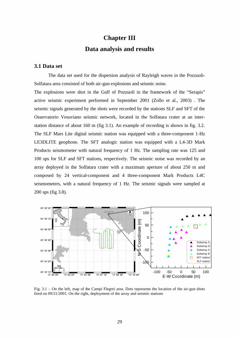
The data set used for the dispersion analysis of Rayleigh waves in the Pozzuoli-

Solfatara area consisted of both air-gun explosions and seismic noise.

The explosions were shot in the Gulf of Pozzuoli in the framework of the “Serapis”

active seismic experiment performed in September 2001 (Zollo et al., 2003) . The

seismic signals generated by the shots were recorded by the stations SLF and SFT of the

Osservatorio Vesuviano seismic network, located in the Solfatara crater at an inter-

station distance of about 160 m (fig 3.1). An example of recording is shown in fig. 3.2.

The SLF Mars Lite digital seismic station was equipped with a three-component 1-Hz

LE3DLITE geophone. The SFT analogic station was equipped with a L4-3D Mark

Products seismometer with natural frequency of 1 Hz. The sampling rate was 125 and

100 sps for SLF and SFT stations, respectively. The seismic noise was recorded by an

array deployed in the Solfatara crater with a maximum aperture of about 250 m and

composed by 24 vertical-component and 4 three-component Mark Products L4C

seismometers, with a natural frequency of 1 Hz. The seismic signals were sampled at

200 sps (fig 3.8).

Fig. 3.1 – On the left, map of the Campi Flegrei area. Dots represents the location of the air-gun shots fired on 09/21/2001. On the right, deployment of the array and seismic stations

-100 -50 0 50 100E-W Coordinate (m)

-100

-50

0

50

100

N-S

Coo

rdin

ate

(m)

Subarray CSubarray DSubarray ASubarray BSFT stationSLF station

30

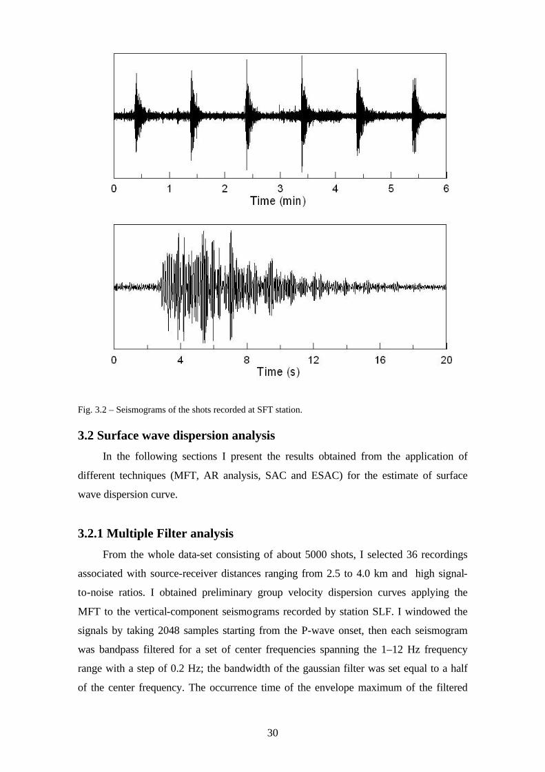
Fig. 3.2 – Seismograms of the shots recorded at SFT station. 3.2 Surface wave dispersion analysis

In the following sections I present the results obtained from the application of

different techniques (MFT, AR analysis, SAC and ESAC) for the estimate of surface

wave dispersion curve.

3.2.1 Multiple Filter analysis

From the whole data-set consisting of about 5000 shots, I selected 36 recordings

associated with source-receiver distances ranging from 2.5 to 4.0 km and high signal-

to-noise ratios. I obtained preliminary group velocity dispersion curves applying the

MFT to the vertical-component seismograms recorded by station SLF. I windowed the

signals by taking 2048 samples starting from the P-wave onset, then each seismogram

was bandpass filtered for a set of center frequencies spanning the 1–12 Hz frequency

range with a step of 0.2 Hz; the bandwidth of the gaussian filter was set equal to a half

of the center frequency. The occurrence time of the envelope maximum of the filtered

31

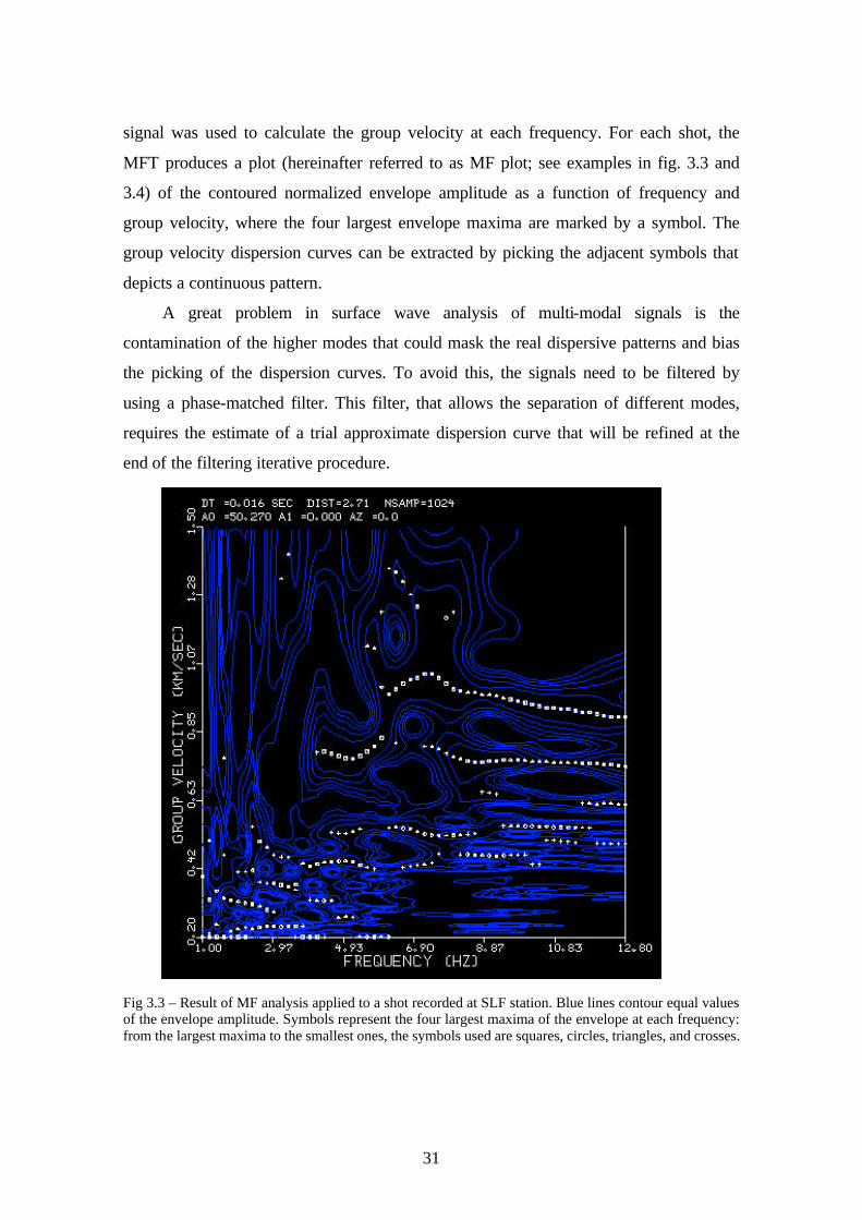
signal was used to calculate the group velocity at each frequency. For each shot, the

MFT produces a plot (hereinafter referred to as MF plot; see examples in fig. 3.3 and

3.4) of the contoured normalized envelope amplitude as a function of frequency and

group velocity, where the four largest envelope maxima are marked by a symbol. The

group velocity dispersion curves can be extracted by picking the adjacent symbols that

depicts a continuous pattern.

A great problem in surface wave analysis of multi-modal signals is the

contamination of the higher modes that could mask the real dispersive patterns and bias

the picking of the dispersion curves. To avoid this, the signals need to be filtered by

using a phase-matched filter. This filter, that allows the separation of different modes,

requires the estimate of a trial approximate dispersion curve that will be refined at the

end of the filtering iterative procedure.

Fig 3.3 – Result of MF analysis applied to a shot recorded at SLF station. Blue lines contour equal values of the envelope amplitude. Symbols represent the four largest maxima of the envelope at each frequency: from the largest maxima to the smallest ones, the symbols used are squares, circles, triangles, and crosses.

32

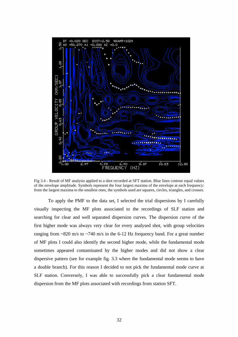
Fig 3.4 - Result of MF analysis applied to a shot recorded at SFT station. Blue lines contour equal values of the envelope amplitude. Symbols represent the four largest maxima of the envelope at each frequency: from the largest maxima to the smallest ones, the symbols used are squares, circles, triangles, and crosses.

To apply the PMF to the data set, I selected the trial dispersions by I carefully

visually inspecting the MF plots associated to the recordings of SLF station and

searching for clear and well separated dispersion curves. The dispersion curve of the

first higher mode was always very clear for every analysed shot, with group velocities

ranging from ~820 m/s to ~740 m/s in the 6-12 Hz frequency band. For a great number

of MF plots I could also identify the second higher mode, while the fundamental mode

sometimes appeared contaminated by the higher modes and did not show a clear

dispersive pattern (see for example fig. 3.3 where the fundamental mode seems to have

a double branch). For this reason I decided to not pick the fundamental mode curve at

SLF station. Conversely, I was able to successfully pick a clear fundamental mode

dispersion from the MF plots associated with recordings from station SFT.

33

The fundamental mode and two higher-mode dispersions previously derived,

were used as trial curves for the PMF, which I first applied to the signals from station

SLF. This procedure is summarized in the following steps:

1) The 36 waveforms were filtered by using the trial curve of the first higher mode to

allow the separation of the first mode wave packet from the residual seismograms.

2) The residual seismograms were filtered by using the trial curve of the second higher

mode, to separate the second mode wave packet from the new residual seismograms.

3) The new residual waveforms were filtered by using the trial curve of the

fundamental mode, to extract the fundamental mode wave packet.

To validate the results obtained for the fundamental mode at station SLF, a further

phase-matched filtering was performed by using the trial fundamental dispersion on the

seismograms recorded by the station SFT, in order to extract the fundamental mode

wave packet.

The MFT was applied once again to all the filtered signals (both for stations SLF

and SFT). As the filtered signal contains single mode wave packet, the MFT produces a

plot in which the dispersion curve relative to that mode is greatly enhanced respect to

the non-filtered signal. Finally, a more robust and reliable estimate of the final

dispersion relations is achieved by performing the stacking of a certain number of

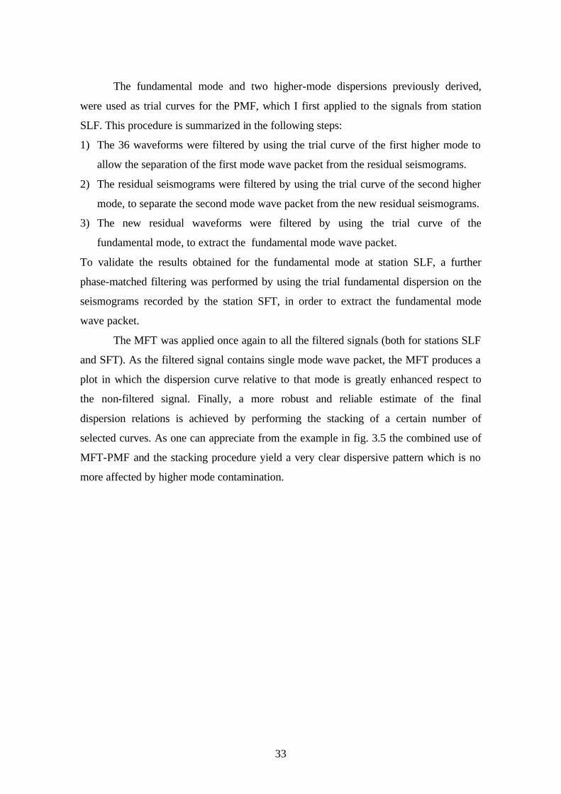
selected curves. As one can appreciate from the example in fig. 3.5 the combined use of

MFT-PMF and the stacking procedure yield a very clear dispersive pattern which is no

more affected by higher mode contamination.

34

Fig. 3.5 – Stacked dispersion curve of the fundamental mode obtained after the application of PMF and MFT to data recorded at station SLF.

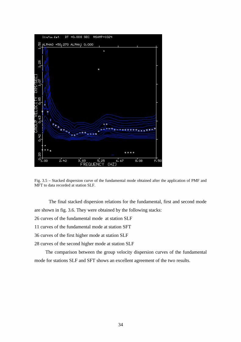
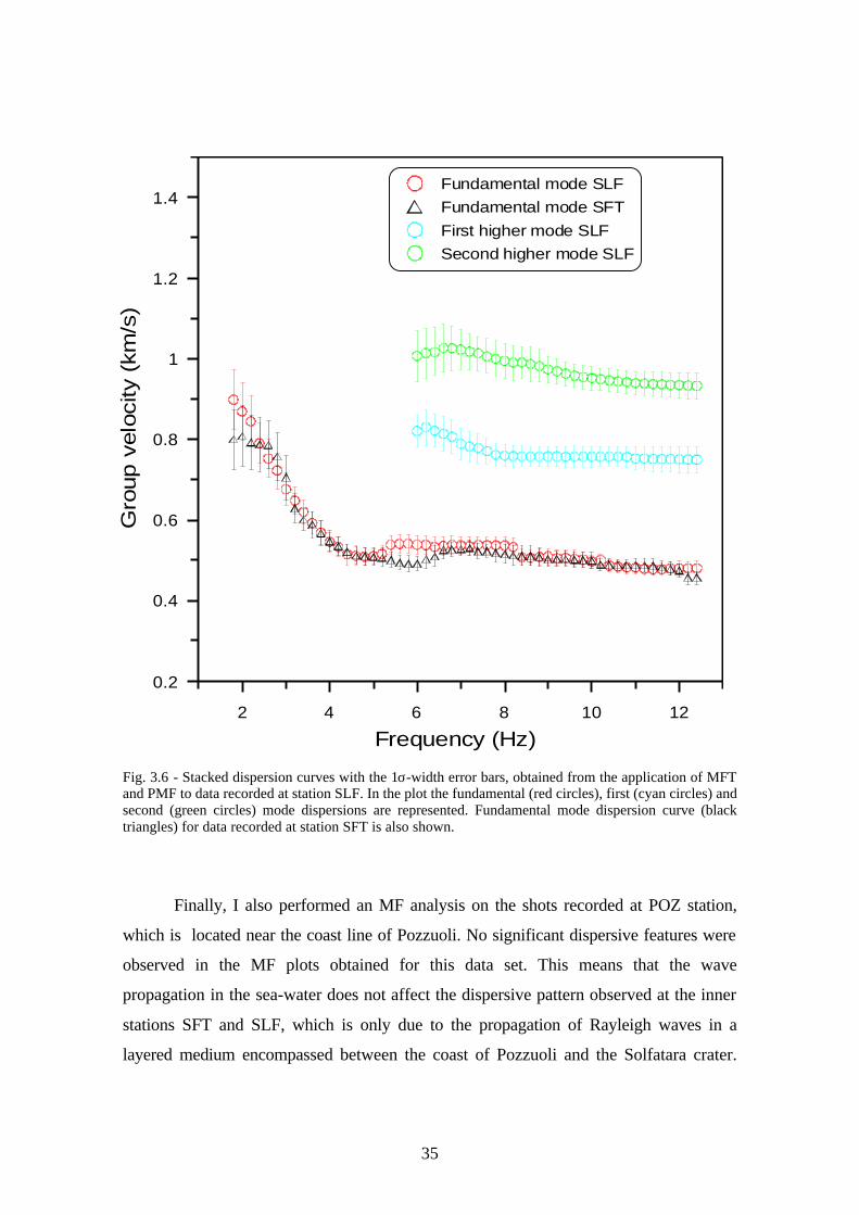
The final stacked dispersion relations for the fundamental, first and second mode

are shown in fig. 3.6. They were obtained by the following stacks:

26 curves of the fundamental mode at station SLF

11 curves of the fundamental mode at station SFT

36 curves of the first higher mode at station SLF

28 curves of the second higher mode at station SLF

The comparison between the group velocity dispersion curves of the fundamental

mode for stations SLF and SFT shows an excellent agreement of the two results.

35

Fig. 3.6 - Stacked dispersion curves with the 1σ-width error bars, obtained from the application of MFT and PMF to data recorded at station SLF. In the plot the fundamental (red circles), first (cyan circles) and second (green circles) mode dispersions are represented. Fundamental mode dispersion curve (black triangles) for data recorded at station SFT is also shown.

Finally, I also performed an MF analysis on the shots recorded at POZ station,

which is located near the coast line of Pozzuoli. No significant dispersive features were

observed in the MF plots obtained for this data set. This means that the wave

propagation in the sea-water does not affect the dispersive pattern observed at the inner

stations SFT and SLF, which is only due to the propagation of Rayleigh waves in a

layered medium encompassed between the coast of Pozzuoli and the Solfatara crater.

2 4 6 8 10 12

Frequency (Hz)

0.2

0.4

0.6

0.8

1

1.2

1.4

Gro

up v

eloc

ity (

km/s

)

Fundamental mode SLFFundamental mode SFTFirst higher mode SLFSecond higher mode SLF

36

This fact ensures that the obtained group velocity dispersions of fig. 3.6 are to be

considered representative of the average properties of the medium along this path.

3.2.2 The test of the new method based on autoregressive analysis

I apply the method described in section 2.1.4, to 4 seismic signals associated to the

shots fired during the Serapis experiment and recorded at the stations SLF, SFT and 8A

(that is the station of the sub-array A closest to SLF). As the application of the AR

technique for the determination of group arrivals of dispersive wave packets of real

seismic signals is completely new, I will describe in details the whole procedure. First,

by integration, I transformed 14 seconds (starting from the P-wave onset) of the vertical

component velocity-seismogram in the equivalent displacement time history, then I

obtained the pulse time series by using the Hilbert transform h(t) of the displacement

u(t):

22 ))(())(()( thtutx +=

I calculated the FFT of the pulse sequence x(t) to obtain the complex frequency series

x(f). The Nyquist travel time is determined from length T of the time series according to:

fN ∆=

21

τ T

f1

=∆

therefore group arrivals comprised in the Nyquist time band 0-14 s can be resolved.

Once obtained the complex frequency series x(f), I windowed it by using a boxcar in

order to select the frequency band in which perform the autoregressive analysis. I

performed the segmentation of the complex series using frequency windows of 1 Hz

width, with an overlapping of 25%. The center frequencies were selected in the 2-12 Hz

frequency range. The segmentation of the complex series in the frequency domain can

be seen as equivalent to the band-pass filtering performed in applying the Multiple

Filter Technique. However, the advantage in handling complex frequency series is that

the filtering procedure in this case reduces to a simple segmentation of the signal. At

this point, each segment of the complex frequency series can be analysed by using the

autoregressive technique. On the basis of the Akaike criterion, I chose the filter order m

from 2 to 14 and solved the eigenvalue problem (section 2.1.4) for each value of m. The

roots z of the characteristic equation, that corresponds to the group arrival τ and v factor

(or equivalently w = - 2v) are therefore obtained for each filter order and represented in

37

a cumulative τ-w plot. In this plot, the group arrival times relative to the different wave

packets are represented by clustered points, while the noise corresponds to the scattered

points. As the distance between the source of the shot and the receiver is known, the

clustered points corresponding to the group travel times are transformed in group

velocity. Finally, plotting the group velocity clusters calculated for each segment of the

complex series as a function of frequency, I obtained the final group velocity dispersion

curve. I implemented the whole procedure in a Mathcad worksheet, similar to that I set

up for the analysis of the synthetic signal. In fact, for the dispersion analysis I slightly

modified the worksheet reported in appendix B by simply adding a routine that

performs the complex series segmentation and allows to reiterate the analysis in

different frequency bands.

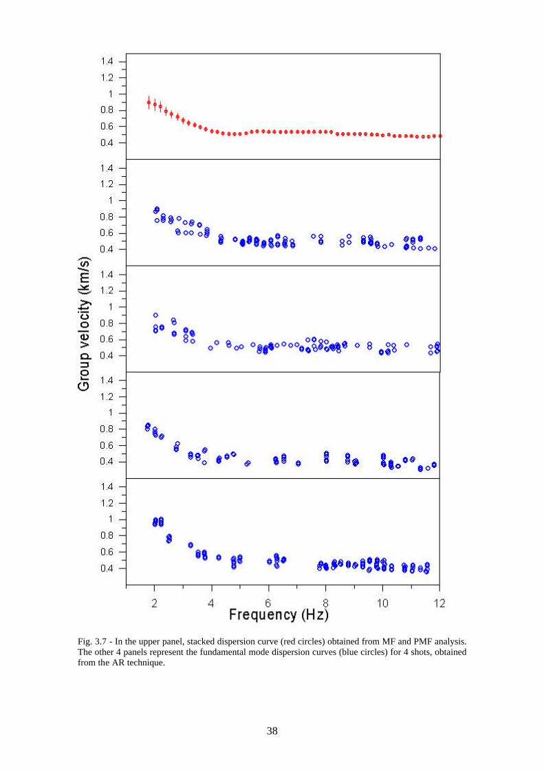
In fig. 3.7 I report the fundamental mode dispersion curves obtained from the

autoregressive analysis applied to 4 selected shots. The curves are in agreement with

that derived from MF and PMF analysis (also reported in the same figure). It is

important to remark that although the curves obtained from the AR technique seem to

have a quite large scatter around the group velocity values, they are relative to the

analysis of single events. On the other hand, the curve obtained from the combined use

of MFT and PMF is the result of a stacking procedure over a certain number of events

and therefore it is affected by lower uncertainties. Surely, in the future, it will be very

useful to introduce a stacking procedure in the AR analysis too, in order to reduce the

spreading in the group velocity values.

38

Fig. 3.7 - In the upper panel, stacked dispersion curve (red circles) obtained from MF and PMF analysis. The other 4 panels represent the fundamental mode dispersion curves (blue circles) for 4 shots, obtained from the AR technique.

39

3.2.3 Spatial Autocorrelation and Extended Spatial AutoCorrelation

analysis

In this section I describe the application of ESAC and SAC techniques to ambient

noise recorded at Solfatara array.

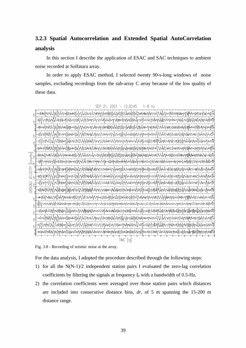
In order to apply ESAC method, I selected twenty 90-s-long windows of noise

samples, excluding recordings from the sub-array C array because of the low quality of

these data.

Fig. 3.8 - Recording of seismic noise at the array. For the data analysis, I adopted the procedure described through the following steps:

1) for all the N(N-1)/2 independent station pairs I evaluated the zero-lag correlation

coefficients by filtering the signals at frequency f0 with a bandwidth of 0.5-Hz.

2) the correlation coefficients were averaged over those station pairs which distances

are included into consecutive distance bins, dr, of 5 m spanning the 15-200 m

distance range.

40

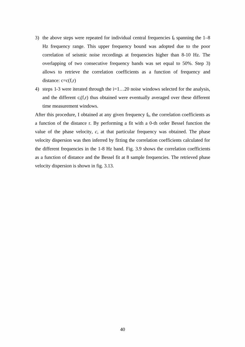
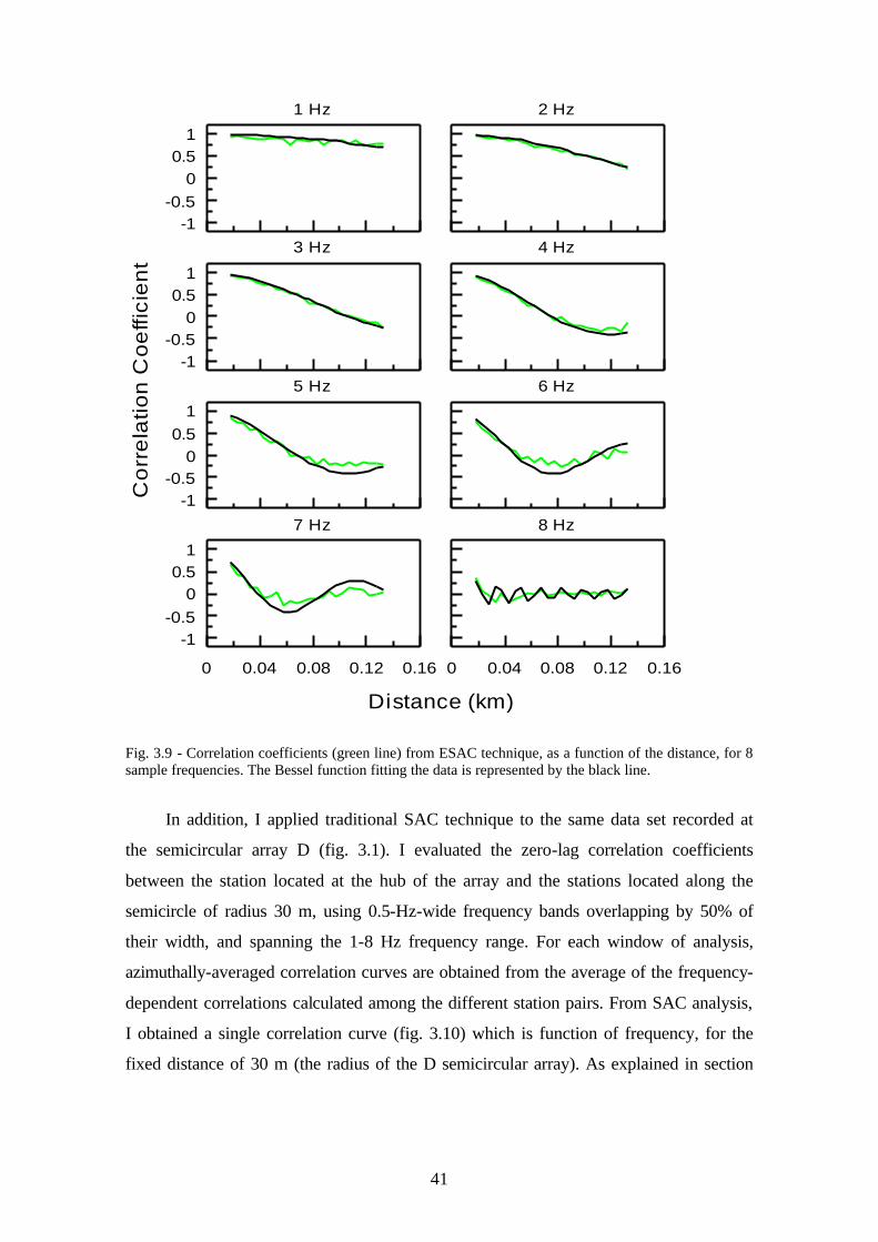
3) the above steps were repeated for individual central frequencies f0 spanning the 1–8

Hz frequency range. This upper frequency bound was adopted due to the poor

correlation of seismic noise recordings at frequencies higher than 8-10 Hz. The

overlapping of two consecutive frequency bands was set equal to 50%. Step 3)

allows to retrieve the correlation coefficients as a function of frequency and

distance: c=c(f,r)

4) steps 1-3 were iterated through the i=1…20 noise windows selected for the analysis,

and the different ci(f,r) thus obtained were eventually averaged over these different

time measurement windows.

After this procedure, I obtained at any given frequency f0, the correlation coefficients as

a function of the distance r. By performing a fit with a 0-th order Bessel function the

value of the phase velocity, c, at that particular frequency was obtained. The phase

velocity dispersion was then inferred by fitting the correlation coefficients calculated for

the different frequencies in the 1-8 Hz band. Fig. 3.9 shows the correlation coefficients

as a function of distance and the Bessel fit at 8 sample frequencies. The retrieved phase

velocity dispersion is shown in fig. 3.13.

41

Fig. 3.9 - Correlation coefficients (green line) from ESAC technique, as a function of the distance, for 8 sample frequencies. The Bessel function fitting the data is represented by the black line.

In addition, I applied traditional SAC technique to the same data set recorded at

the semicircular array D (fig. 3.1). I evaluated the zero-lag correlation coefficients

between the station located at the hub of the array and the stations located along the

semicircle of radius 30 m, using 0.5-Hz-wide frequency bands overlapping by 50% of

their width, and spanning the 1-8 Hz frequency range. For each window of analysis,

azimuthally-averaged correlation curves are obtained from the average of the frequency-

dependent correlations calculated among the different station pairs. From SAC analysis,

I obtained a single correlation curve (fig. 3.10) which is function of frequency, for the

fixed distance of 30 m (the radius of the D semicircular array). As explained in section

-1-0.5

00.5

1

1 Hz 2 Hz

-1-0.5

00.5

1

3 Hz 4 Hz

-1-0.5

00.5

1

Co

rre

latio

n C

oe

ffici

en

t

5 Hz 6 Hz

0 0.04 0.08 0.12 0.16

Distance (km)

-1-0.5

00.5

1

7 Hz

0 0.04 0.08 0.12 0.16

8 Hz

42

2.1.3, in this case the Bessel fit over the azimuthal-averaged correlation coefficients can

be performed assuming a priori a dispersion law of the form: bAffc −=)(

The best-fit coefficients A and b took the values 0.8 and 0.12, respectively.

The resulting phase velocity dispersion function is shown in fig. 3.13. For both SAC

and ESAC method the relative uncertainties on the phase velocity estimates are of the

order of 20%.

Fig. 3.10 - Correlation curve (orange line) obtained from application of SAC method to microtremors data from semicircular array D. The black line is the Bessel function fitting the correlation data.

3.3 Inversion of the group velocity dispersion

The group velocity dispersion curves obtained from the Multiple Filter analysis

were inverted for a plane-layered earth structure to infer the shallow shear-wave

velocity model for the area of Pozzuoli-Solfatara. Basing on the available geological

and geophysical observations, I build up a set of possible starting models with a variable

number of layers (from the simple single-layer-models to 5-layer-models) and different

shear-wave velocities (chosen in the range 200-1500 m/s, which is compatible with the

S-velocities typically observed for shallow soils and rocks in volcanic areas).

Constraints for the minimum and maximum resolvable layer thickness and depths were

imposed on the basis of the empirical relationships (Midzi, 2001). For the frequency

range I investigated, the minimum resolvable layer thickness is on the order of 20 m,

and the maximum resolvable depth is on the order of 250 m. I performed a first

selection of the velocity structure by using a trial and error procedure to look for models

which produced theoretical dispersion curves compatible with those experimentally

0 2 4 6 8 10Frequency (Hz)

-1

-0.5

0

0.5

1

Cor

r. C

oef

f.

43

observed. On this basis, some of the initial starting models with large misfit between

observed and predicted data where rejected, while others were modified, adjusting layer

thicknesses and velocities to better reproduce the dispersive pattern. The new subset of

starting models was then inverted both for velocities and layer thicknesses by using an

iterative procedure (Herrmann, 1987). After the iterative inversion of the whole new

subset I selected the 3-layer-model because it yields the lowest rms value between

observed and theoretical data and it fitted the greatest number of observations.

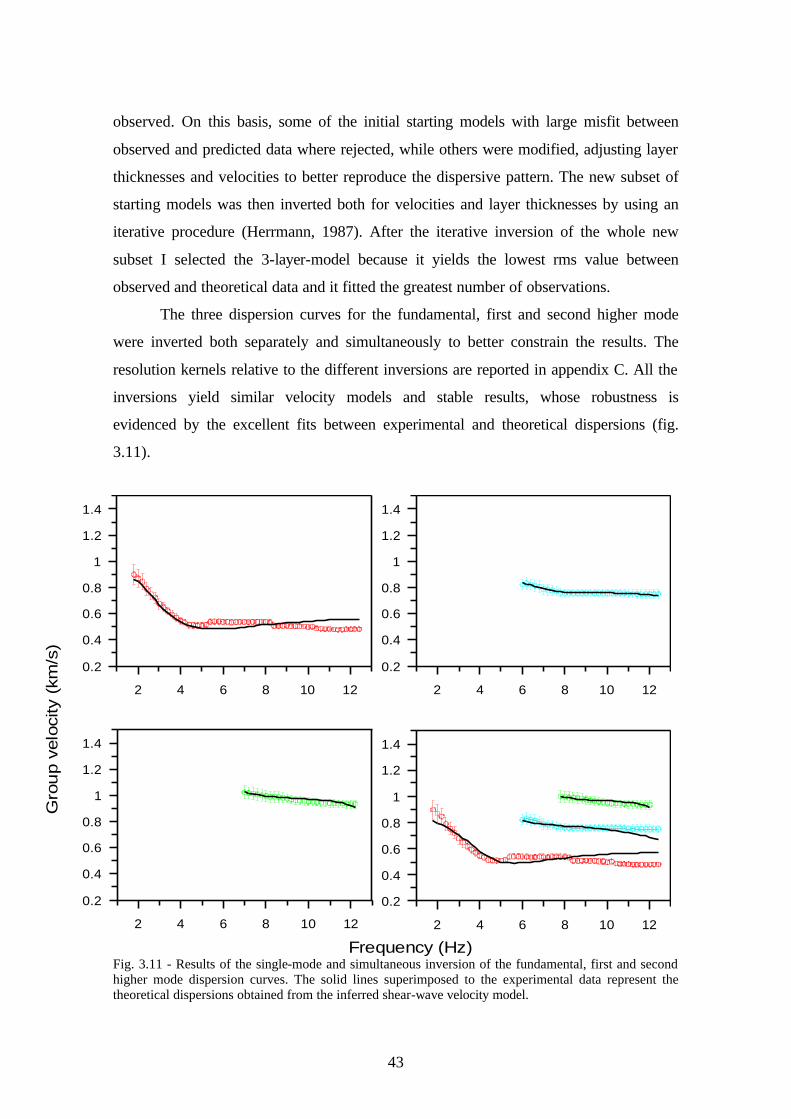
The three dispersion curves for the fundamental, first and second higher mode

were inverted both separately and simultaneously to better constrain the results. The

resolution kernels relative to the different inversions are reported in appendix C. All the

inversions yield similar velocity models and stable results, whose robustness is

evidenced by the excellent fits between experimental and theoretical dispersions (fig.

3.11).

Fig. 3.11 - Results of the single-mode and simultaneous inversion of the fundamental, first and second higher mode dispersion curves. The solid lines superimposed to the experimental data represent the theoretical dispersions obtained from the inferred shear-wave velocity model.

2 4 6 8 10 12

0.2

0.4

0.6

0.8

1

1.2

1.4

2 4 6 8 10 12

0.2

0.4

0.6

0.8

1

1.2

1.4

2 4 6 8 10 12

Frequency (Hz)

0.2

0.4

0.6

0.8

1

1.2

1.4

Gro

up

velo

city

(km

/s)

2 4 6 8 10 12

0.2

0.4

0.6

0.8

1

1.2

1.4

44

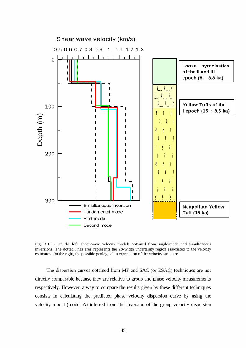
The inferred velocity models (fig. 3.12) show a marked discontinuity at a depth

of about 50 m where the shear-wave velocity abruptly changes from about 650 m/s to

900 m/s. Another slight increase of the S-velocity (from 900 m/s to 1000 m/s) is

observed at a depth of about 100 m.

To verify how well this two discontinuities are constrained and to check the

stability of the obtained results I perturbed the starting 3-layer model by changing both

velocities and layer thicknesses and repeating the inversion procedure. In all the cases

the inversion converged to the final model previously described.

The simultaneous inversion provides the best constrained velocity structure

because it yields the maximum resolution at the different depths, and therefore I used

this model (hereinafter referred to as model A) for the error analysis. The uncertainties

that affect this model are estimated by determining the range of shear-wave velocities

obtained by the inversion procedure, when one considers the errors associated to the

group velocity measurements. In fact, the stacked group velocity values calculated by

the Multiple Filter analysis are affected by uncertainties which are quantified in terms of

the standard deviation σ. By subtracting and adding 2σ to the group velocity values, I

generated the two extreme dispersion curves corresponding to the 95% error limits.

These curves were then inverted to infer two extreme velocity models which actually

represent the upper and lower bound for the model A. As one can note from fig. 3.12,

all the velocity models relative to both single-mode and simultaneous inversion are

bounded by the 2σ error bars.

45

Fig. 3.12 - On the left, shear-wave velocity models obtained from single-mode and simultaneous inversions. The dotted lines area represents the 2σ-width uncertainty region associated to the velocity estimates. On the right, the possible geological interpretation of the velocity structure.

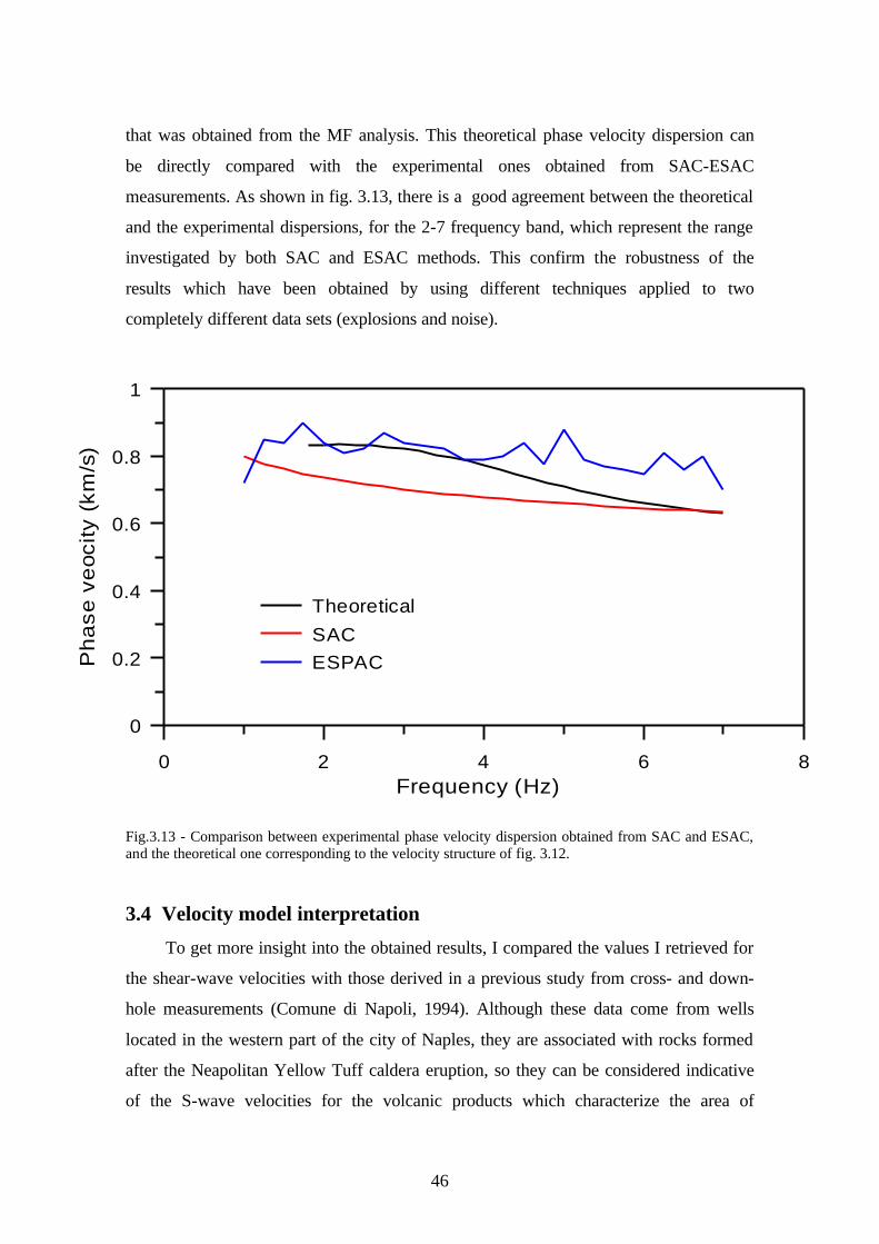
The dispersion curves obtained from MF and SAC (or ESAC) techniques are not

directly comparable because they are relative to group and phase velocity measurements

respectively. However, a way to compare the results given by these different techniques

consists in calculating the predicted phase velocity dispersion curve by using the

velocity model (model A) inferred from the inversion of the group velocity dispersion

300

200

100

0

Depth

(m

)0.5 0.6 0.7 0.8 0.9 1 1.1 1.2 1.3

Shear wave velocity (km/s)

Simultaneous inversion

Fundamental mode

First mode

Second mode

Loose pyroclasticsof the II and IIIepoch (8 ÷ 3.8 ka)

Yellow Tuffs of theI epoch (15 ÷ 9.5 ka)

Neapolitan YellowTuff (15 ka)

46

that was obtained from the MF analysis. This theoretical phase velocity dispersion can

be directly compared with the experimental ones obtained from SAC-ESAC

measurements. As shown in fig. 3.13, there is a good agreement between the theoretical

and the experimental dispersions, for the 2-7 frequency band, which represent the range

investigated by both SAC and ESAC methods. This confirm the robustness of the

results which have been obtained by using different techniques applied to two

completely different data sets (explosions and noise).

Fig.3.13 - Comparison between experimental phase velocity dispersion obtained from SAC and ESAC, and the theoretical one corresponding to the velocity structure of fig. 3.12.

3.4 Velocity model interpretation

To get more insight into the obtained results, I compared the values I retrieved for

the shear-wave velocities with those derived in a previous study from cross- and down-

hole measurements (Comune di Napoli, 1994). Although these data come from wells

located in the western part of the city of Naples, they are associated with rocks formed

after the Neapolitan Yellow Tuff caldera eruption, so they can be considered indicative

of the S-wave velocities for the volcanic products which characterize the area of

0 2 4 6 8Frequency (Hz)

0

0.2

0.4

0.6

0.8

1

Ph

ase

ve

ocity

(km

/s)

Theoretical

SACESPAC

47

Pozzuoli-Solfatara. The authors observed, for loose and unconsolidated ash deposits,

shear-wave velocities strongly depending on the depth and ranging from 180 m/s at

depths of about 5 m to 800 m/s at depth of 85 m, with a value of 550 m/s at a depth of

about 50 m. For the compact tuff rocks (lithoid facies of NYT) typical Vs values are

about 800-1000 m/s, with a weak dependence on depth.

From field and laboratory measurements Nunziata et al. (1999) evaluated the

shear-wave velocities of the Phlegraean soils and tuffs obtaining results in agreement

with those reported above. Nunziata et al. found that for pyroclastic products and

coastal deposits Vs is influenced by the increasing lithostatic pressure and ranges from

100 to 600 m/s over the 0-20 m depth range, while the compact NYT is characterized by

Vs values ranging from 800 to 1100 m/s and weakly depending on the lithostatic load.

Slightly lower shear-wave velocities are observed for fractured NYT but those values,

unlike for the compact NYT, rapidly increase with pressure due to the closing of the

fractures.

Taking into account the volcanological history of the Campi Flegrei area (see

section 1.1), the geological constraints and comparison with literature data, I finally

give a possible interpretation (fig. 3.12) of the velocity model inferred from surface

wave dispersion analysis. The first 50-m-thick layer could be composed of loose

pyroclastic rocks emitted during the III epoch of activity and marine deposits of the La

Starza terrace. The Vs value found for this layer is in fact compatible with those

reported in Comune di Napoli (1994) and Nunziata et al. (1999) for the same types of

rocks. The seismic velocity discontinuity at 50 m can likely mark the transition to the

yellow tuffs (which have analogous mechanical characteristics of NYT and hence

similar shear-wave velocities) produced during the tuff-cone activity of the I epoch. The

second discontinuity at 100-m-depth, which is less marked with respect to the shallower

one, has two possible interpretations. It could be due to an effect of the lithostatic

pressure which closes cracks and fractures in the tuff rock, with a consequent increase

of seismic velocity. An other possible explanation is that this discontinuity marks the

contact between the products emitted by two distinct tuff cones which erupted during

the I epoch. These units probably overlay the NYT bedrock. The interface with NYT is

not resolved by the presented velocity model, whose maximum resolvable depth is of

48

about 250 m. However geological observations suggest a depth of about 300 m for the

top of this unit (M. Di Vito, personal communication).

The velocity structure presented in this thesis is in agreement with that recently

obtained at larger scale from a 3D seismic tomography by Vanorio et al. (2005), who

observe low Vs values (1000-1200 m/s for the first 2 km) in the central part of the

caldera. The present results are also compatible with the shallow velocity structure

proposed for the Solfatara crater by Bruno et al. (2004). Although the model of Bruno et

al. is limited to a depth of about 30 m, a rapid increase of Vs up to 540 m/s is reported

for the lower bound of the structure.

3.5 Attenuation analysis and Qβ structure

For the attenuation analysis I selected 9 artificial explosions (vertical component)

recorded by the 6 stations composing linear sub-array A (fig. 3.1) and I applied the

methodology reported in section 2.2 to study the spectral decay with distance of

Rayleigh wave amplitude, in different frequency bands. I used a 9-s-long time window

starting 1 second after the P-wave onset, in order to exclude the body-wave

contribution. The data were band-pass filtered around a series of center frequencies

spanning the 2.5-8.5 Hz frequency range, with a bandwidth of 1 Hz. I chose this upper

limit because for frequencies greater than 8 Hz the noise contribution begins to be

strong and hence could mask the attenuation pattern of the Rayleigh waves composing

the wavefield associated to the shots. For each frequency band, the matrix equation

(2.17) of section 2.2 was solved in order to determine the γ factor. The geometrical

spreading coefficient in (2.17) was set equal to 0.5 because the analysis concerns

Rayleigh waves. By solving the (2.17) analysis in the different frequency bands, I

recovered the γ attenuation curve shown in fig. 3.14.

To quantify the uncertainties that affect the estimate of the attenuation factor, I

calculated the covariance matrix. In terms of the quantities defined in equation (2.17) of

chapter II, the expression of the covariance matrix is (Menke, 1984):

( )[ ] [ ][ ] [ ][ ] [ ] 1T2T

T1T2T1T cov−−−

== GGGGGIGGGm dd σσ

I is the identity matrix and σd is the uncertainty affecting the data d. As the error on the

distances R is negligible respect the uncertainty σA that affects the spectral amplitudes

A, the quantity σd can be expressed in terms of σA:

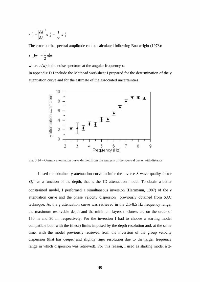
49

22

22

2 1A

iAd AA

dσσσ =

∂∂

=

The error on the spectral amplitude can be calculated following Boatwright (1978):

( ) ( )ωωσ nA 21

=

where n(ω) is the noise spectrum at the angular frequency ω.

In appendix D I include the Mathcad worksheet I prepared for the determination of the γ

attenuation curve and for the estimate of the associated uncertainties.

Fig. 3.14 – Gamma attenuation curve derived from the analysis of the spectral decay with distance.

I used the obtained γ attenuation curve to infer the inverse S-wave quality factor 1−

βQ as a function of the depth, that is the 1D attenuation model. To obtain a better

constrained model, I performed a simultaneous inversion (Herrmann, 1987) of the γ

attenuation curve and the phase velocity dispersion previously obtained from SAC

technique. As the γ attenuation curve was retrieved in the 2.5-8.5 Hz frequency range,

the maximum resolvable depth and the minimum layers thickness are on the order of

150 m and 30 m, respectively. For the inversion I had to choose a starting model

compatible both with the (these) limits imposed by the depth resolution and, at the same

time, with the model previously retrieved from the inversion of the group velocity

dispersion (that has deeper and slightly finer resolution due to the larger frequency

range in which dispersion was retrieved). For this reason, I used as starting model a 2-

50

layered structure whose thicknesses (50 m for both the layers) and S-wave velocities are

constrained by the (corresponding) values of the velocity model derived in section 3.3

and I assigned to the different layers some trial values of Qβ, compatible with those

usually observed in shallow subsoils of volcanic areas. Several inversions were

performed by perturbing the trial values of Qβ, but in any case the inversion procedure

always yields stable results, converging to the same final solution despite the

differences in the starting Qβ values. The obtained attenuation model presents low Qβ

value, being Qβ = 4 in the first 50-m-thick layer and Qβ = 12 in the second 50-m-thick

layer. The value of the quality factor in the halfspace is not resolved. In the next figures

I show the result of the inversion (fig. 3.15), the attenuation model and the resolution

kernels (fig. 3.16).

Fig. 3.15 - Results of the inversion of the γ attenuation curve. The solid lines superimposed to the experimental data represent the theoretical dispersions obtained from the inferred attenuation model.

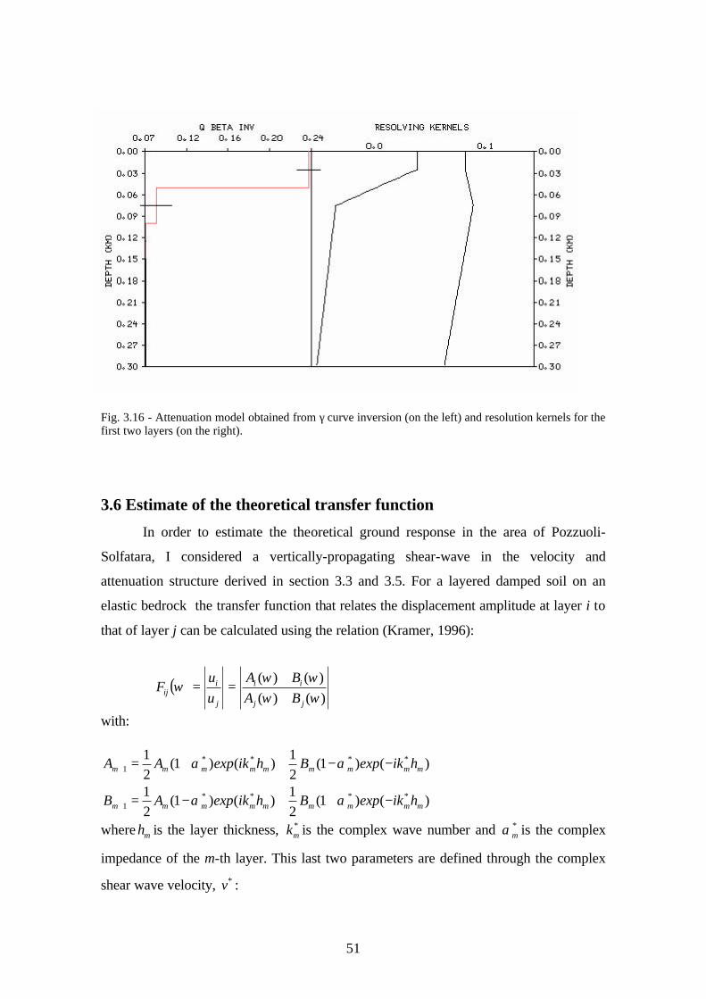
51

Fig. 3.16 - Attenuation model obtained from γ curve inversion (on the left) and resolution kernels for the first two layers (on the right).

3.6 Estimate of the theoretical transfer function

In order to estimate the theoretical ground response in the area of Pozzuoli-

Solfatara, I considered a vertically-propagating shear-wave in the velocity and

attenuation structure derived in section 3.3 and 3.5. For a layered damped soil on an

elastic bedrock the transfer function that relates the displacement amplitude at layer i to

that of layer j can be calculated using the relation (Kramer, 1996):

( ))()()()(

ωωωω

ωjj

ii

j

iij BA

BAuu

F++

==

with:

)()1(21

)()1(21 ****

1 mmmmmmmmm hikexpBhikexpAA −−++=+ αα

)()1(21

)()1(21 ****

1 mmmmmmmmm hikexpBhikexpAB −++−=+ αα

where mh is the layer thickness, *mk is the complex wave number and *

mα is the complex

impedance of the m-th layer. This last two parameters are defined through the complex

shear wave velocity, *v :

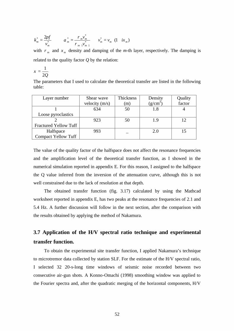
52

** 2

mm v

fk

π= *

11

**

++

=mm

mmm v

vρ

ρα )1(*

mmm ivv ξ+⋅=

with mρ and mξ density and damping of the m-th layer, respectively. The damping is

related to the quality factor Q by the relation:

Q21

=ξ

The parameters that I used to calculate the theoretical transfer are listed in the following table:

Layer number Shear wave velocity (m/s)

Thickness (m)

Density (g/cm3)

Quality factor

1 Loose pyroclastics

634 50 1.8 4

2 Fractured Yellow Tuff

923 50 1.9 12

Halfspace Compact Yellow Tuff

993 _ 2.0 15

The value of the quality factor of the halfspace does not affect the resonance frequencies

and the amplification level of the theoretical transfer function, as I showed in the

numerical simulation reported in appendix E. For this reason, I assigned to the halfspace

the Q value inferred from the inversion of the attenuation curve, although this is not

well constrained due to the lack of resolution at that depth.

The obtained transfer function (fig. 3.17) calculated by using the Mathcad

worksheet reported in appendix E, has two peaks at the resonance frequencies of 2.1 and

5.4 Hz. A further discussion will follow in the next section, after the comparison with

the results obtained by applying the method of Nakamura.

3.7 Application of the H/V spectral ratio technique and experimental

transfer function.

To obtain the experimental site transfer function, I applied Nakamura’s technique

to microtremor data collected by station SLF. For the estimate of the H/V spectral ratio,

I selected 32 20-s-long time windows of seismic noise recorded between two

consecutive air-gun shots. A Konno-Omachi (1998) smoothing window was applied to

the Fourier spectra and, after the quadratic merging of the horizontal components, H/V

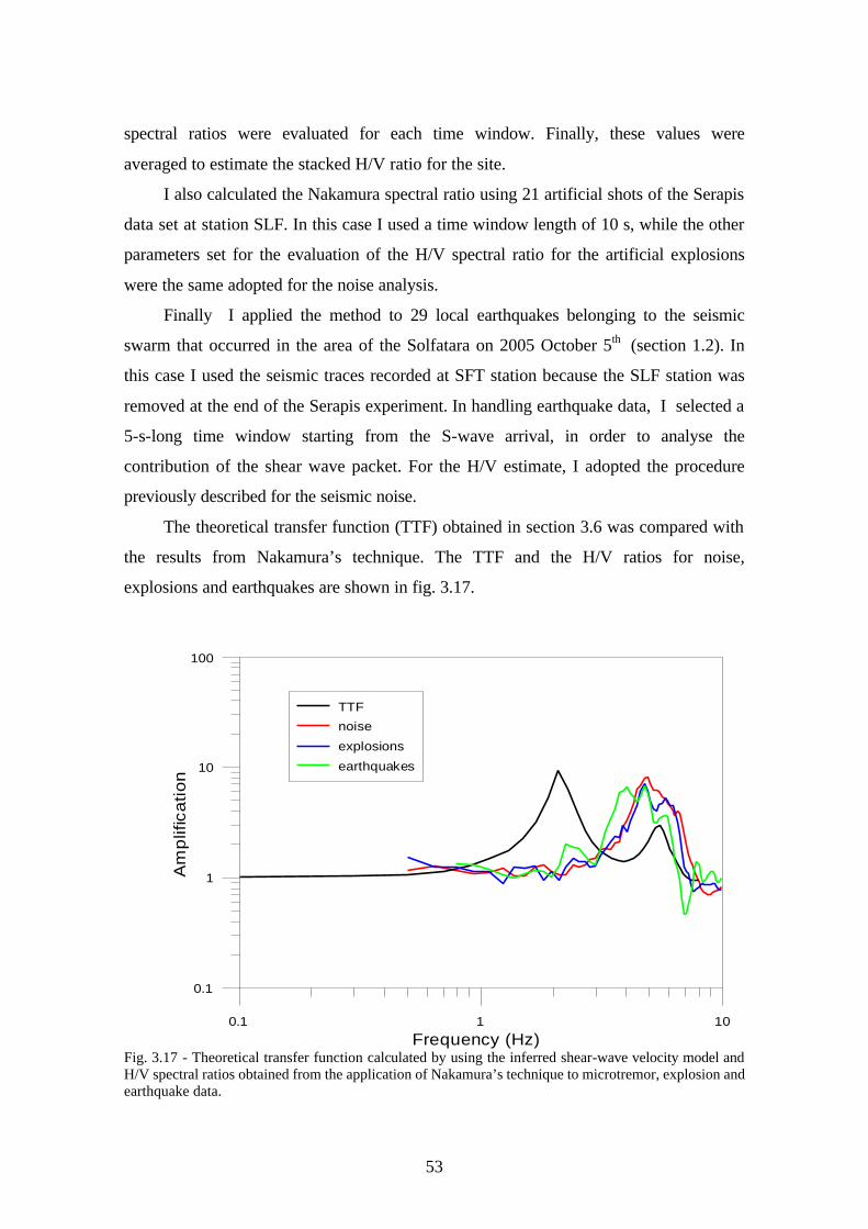
53

spectral ratios were evaluated for each time window. Finally, these values were

averaged to estimate the stacked H/V ratio for the site.

I also calculated the Nakamura spectral ratio using 21 artificial shots of the Serapis

data set at station SLF. In this case I used a time window length of 10 s, while the other

parameters set for the evaluation of the H/V spectral ratio for the artificial explosions

were the same adopted for the noise analysis.

Finally I applied the method to 29 local earthquakes belonging to the seismic

swarm that occurred in the area of the Solfatara on 2005 October 5th (section 1.2). In

this case I used the seismic traces recorded at SFT station because the SLF station was

removed at the end of the Serapis experiment. In handling earthquake data, I selected a

5-s-long time window starting from the S-wave arrival, in order to analyse the

contribution of the shear wave packet. For the H/V estimate, I adopted the procedure

previously described for the seismic noise.

The theoretical transfer function (TTF) obtained in section 3.6 was compared with

the results from Nakamura’s technique. The TTF and the H/V ratios for noise,

explosions and earthquakes are shown in fig. 3.17.

Fig. 3.17 - Theoretical transfer function calculated by using the inferred shear-wave velocity model and H/V spectral ratios obtained from the application of Nakamura’s technique to microtremor, explosion and earthquake data.

0.1 1 10

Frequency (Hz)

0.1

1

10

100

Am

plif

ica

tion

TTF

noise

explosions

earthquakes

54

The first result to note is the good agreement among the three experimental H/V

ratios, that evidenced the resonance frequency at:

f = 4.9 ± 0.3 for microtremor

f = 4.9 ± 0.4 for explosions

f = 4.5 ± 0.6 for earthquakes

This resonance frequency, as one can note in fig. 3.17, partially agrees with the

second resonance frequency of the theoretical transfer function, although this last is

slightly higher (5.4 Hz). On the contrary, there is a quite large discrepancy in the

amplification level at this frequency, being the amplification provided by the TTF lower

respect to that estimated by from the H/V ratio. Above all, the most evident discrepancy

is the complete disagreement between the curves for the fundamental resonance

frequency of 2.1 Hz which is observed only in the theoretical transfer function. Three

possible reasons could explain this discrepancy:

1) The H/V ratio is sensitive to the velocity structure just beneath the station,

while the 1D velocity model obtained from the inversion of Rayleigh wave dispersion

represents an average model for the medium between the source and the receiver. So I

expect that the H/V is compatible with the TTF only if the local structure beneath the

station located in the Solfatara crater is exactly the same represented by the average

velocity model. However it is possible that in the Solfatara crater a very local thickening

or thinning of the shallow layers could produce a shift in the amplification frequencies.

In this case the H/V is to be considered indicative of the very local transfer function just

for the Solfatara crater, while the transfer function derived from Rayleigh wave

dispersion is valid for the area that goes from the shore of Pozzuoli to the external rim

of the Solfatara crater.

2) A very local destructive interference occurring in the Solfatara crater, whose

basin-like structure is expected to cause significant wave-trapping phenomena, could

prevent to observe the 2.1 resonance frequency.

3) Finally, as confirmed by many studies (Luzon et al., 2001; Malischewsky and

Scherbaum, 2004) Nakamura’s technique gives a good estimate of the fundamental

frequency only in the case of large impedance contrast (generally > 2.5), while it often

fails once dealing with low impedance contrast. For the Solfatara I estimate an

impedance contrast of about 0.6, which is probably too low for considering reliable the

55

results obtained from the application of Nakamura’s technique. In this case, the H/V

spectral ratio cannot be considered indicative of the site transfer function.

3.8 PGA estimate from ground motion simulation

I calculated the peak ground acceleration (PGA) due to the expected largest

magnitude local earthquake, both for the whole caldera of the Campi Flegrei and locally

for the area of Pozzuoli-Solfatara. The first method I used is based on the random

vibration theory (RVT). The procedure that I followed is summarized in the following

steps:

1) the shape of acceleration spectrum A(f) is defined as function of source

parameters (fc, M0(Mmax)), path (Q), radiation pattern (Yθφ), geometrical

spreading (R), free surface operator (F) and medium parameters (Vs ρ0);

hereinafter all these parameters are defined as the ensemble Ki;

2) the moments mk of the squared spectral amplitude of acceleration are evaluated

in order to calculate the numbers Nz,e of zero crossing and extrema of time

series;

3) the ratio (PGA/arms) of PGA to the root mean square acceleration (arms) is

calculated by using Cartwrigth and Longuet-Higgins equation;

4) Parseval’s theorem is used to obtain the estimate of the rms acceleration arms in

terms of the squared amplitude spectrum of ground motion |A(f,Ki)|2;

5) PGA value is calculated by considering the product between the values of

(PGA/arms) evaluated at point 3) and arms.

The second method that I used for the estimate of PGA estimate can be considered

as a slight modification of the first. I describe this method (hereinafter referred to as

GMG) in the following steps:

1) the shape of acceleration spectrum A(f, Ki) is defined;

2) Parseval’s theorem is used to calculate arms;

3) Ground motion acceleration A(t) is generated using a gaussian distribution with

σ equal to arms;

4) PGA is evaluated by considering the maximum amplitude of A(t);

56

5) the averaged value of PGA is calculated by performing a great number of

simulations (N > 50) (the iterative procedure is repeated from point 1) to point

4)).

The definition of spectral ground acceleration A(f,Ki) and the setting of the

parameters Ki are the most important aspects of the three above described methods.

The shape of the acceleration spectrum A(f,Ki) is defined following Boatwright

(1980):

−

+

⋅Ω=

⋅ QfT

ff

fKfA

C

i

πγ

exp

1

),(2

20 (3.1)

For the area of Pozzuoli-Solfatara I took into account the local site effects considering

in equation (3.1) the site contribution too:

)(),(),( fGKfAKfA iiPS ⋅=

where G(f) represents the theoretical amplification function derived in section 3.6.

In the following, I describe how I chose all the parameters of equation (3.1), both

for the Campi Flegrei caldera and for the area of Pozzuoli-Solfatara.

I estimated the spectral ground acceleration A(f, Ki) for the maximum expected

magnitude Mmax in the investigated areas, for a given recurrence time period. As well

known, the number of earthquakes that occurred in a time period τ can be represented

by Gutenberg-Richter relation (Lay and Wallace, 1985):

bMaMN −=)(log (3.2)

where N is the number of earthquakes with magnitudes in a fixed range around

magnitude M, a and b are parameters respectively related to seismicity level and earth

heterogeneity (Scholz, 1968). Equation (3.2) can be used to calculate the expected

maximum magnitude Mmax. If a and b are estimated for data in a time period τ, the ratio

a/b gives the value of Mmax expected in that period. For the Campi Flegrei area a and b

parameters of Gutenberg-Richter distribution were calculated by De Natale and Zollo

(1986). The seismic catalogue used in that work starts form 1975 and ends in 2000, it

contains more than 10,000 seismic events (0 < MD < 4.2) mainly related to the

bradyseism episode of 1983-84. The completeness threshold of this catalogue is MD =

0.6. The parameters a and b were obtained using a least square evaluation on the

57

selected data. Using these values I estimated the value of Mmax equal to 4.35 ± 0.30 for

the Campi Flegrei area, for a recurrence period of 25 years.

After the determination of the expected maximum magnitude, I used the empirical

formula derived in Galluzzo et al. (2004) that relates seismic moment to magnitude, in

order to calculate the expected maximum moment:

DMM 9.09.9log 0 +=

By using this relation, it resulted that M0(Mmax) is equal to 6.5⋅1013 Nm.

I evaluated the corner frequency fc associated to the maximum expected

magnitude Mmax by using the Brune formula (Brune, 1970) where the value of the

source radius rc corresponding to M0(Mmax) is estimated extrapolating the scaling

relationships (Galluzzo et al., 2004).

As concerns the attenuation parameters, for the Campi Flegrei caldera I fixed the

shear-wave velocity and quality factor Q equal to 3 km/s and 110, respectively, as these

values represents an average estimate for the whole area (Del Pezzo et al., 1987). For

the local estimate in the area of Pozzuoli-Solfatara, I took into account the velocity and

quality factor values derived in this thesis, by considering in equation (3.1) three

contributions related to the propagation in the layered structure of section 3.6. Only for

the halfspace, I still used the average quality factor Q = 110, as the attenuation structure

derived in section 3.5 could not resolve the Q value in the halfspace.

The medium density ρ0 was considered equal to 2.2 gm/cm3 in the caldera and 2.1

gm/cm3 for Pozzuoli-Solfatara. Geometrical spreading factor 1/R was obtained by

evaluating the average hypocentral distance between the mean of source locations and

the nearest station site. I fixed R equal to 2 km being this value the minimum possible

hypocentral distance.

Finally, I fixed the radiation pattern term YSθϕ equal to 1 in order to take into

account the effects due to the maximum radiated energy, while a value of 2 was chosen

for the free surface operator F.

Using the above defined parameters, I applied the two techniques (RVT and GMG; see

the Mathcad worksheet reported in appendix F) obtaining the following PGA values:

0.04 g RVT method Campi Flegrei area

0.04 ± 0.01 g GMG method Campi Flegrei area

0.097 g RVT method Pozzuoli-Solfatara area

58

0.096 ± 0.004 g GMG method Pozzuoli-Solfatara area

59

Discussion

In this thesis I contribute to the characterization of the shallow velocity and

attenuation structure for the area of Pozzuoli-Solfatara. For this aim, I apply different

techniques (combined MFT and PMF, SAC, ESAC) to different kind of data

(explosions, seismic noise), providing robust and stable results, which I successfully

validated against the available constraints given by the direct and indirect geophysical

and geological measurements. In addition, the techniques adopted for this study

represent a cheap manner to obtain fast and reliable measurements of local elastic

properties of the earth. These measurements constitute a good observational set to be

used in all the studies on the seismic source in the area.

I also introduce a new approach based on the autoregressive analysis, for

recovering the dispersion curve of surface waves. This method offers some advantages

respect to the combined use of MFT and PMF; one is that there is no need to filter the

data because this operation is equivalent to the segmentation of the complex frequency

series. In addition the computer time required for the elaboration is very small. As I

have shown in this thesis, the AR technique applied to real signals generated by the

artificial explosions has provided reliable results. The ability of the method in

discriminating closely spaced arrival times implies an accurate determination of the

dispersion curves. The results presented in this thesis are very promising, although a

little effort is now required for the quantification of the uncertainties related to the travel

time estimates and their propagation on the group velocity dispersion values. However,

in my opinion, this technique could be extensively applied for future studies of surface

wave dispersion.

I used the velocity and attenuation structure presented in this thesis to estimate

the theoretical transfer function and assess the local site response, that I took into

account to better constrain the PGA value for the area of Pozzuoli-Solfatara. Such

estimates are very important in an area that is periodically subjected to seismic crises

and where the most part of the seismicity related to the bradysesimic crisis is located.

Although this local seismicity is characterised by relatively low energy earthquakes,

local amplification occurring at the resonance frequencies can produce great damages to

60

building and infrastructures. All these aspects should be taken into account for the

assessment of the seismic hazard in this densely-populated volcanic area.

The comparison between the amplification peak frequencies obtained from the

theoretical transfer function and the ones retrieved from the application of Nakamura’s

technique opens several points for discussion. In section 3.7 I gave some 3 possible

interpretations that could explain the observed discrepancy. Here I just would like to

add that, as remarked in point 1) of section 3.7, that local deviations from the average

velocity model can produce differences in the transfer function; although the very

shallow crustal structure going from Pozzuoli coast to the Solfatara crater rim is not so

heterogeneous (as it is inside the flat part of a collapsed caldera), some local variations

in the layer thicknesses just beneath the Solfatara crater are possible. I further

investigated this aspect by looking at the experimental phase velocity dispersion curve

deduced from SAC technique, which is representative of the velocity structure just

beneath the array. As shown in fig. 3.13, this curve is quite compatible with the

theoretical phase velocity dispersion associated to the velocity model I have found.

However, after some numerical simulation, I found that the experimental phase velocity

dispersion could also be compatible with a crustal structure formed by a 30-m thick

layer of pyroclastic materials on an elastic halfspace composed by fractured yellow tuff.

This crustal structure (that would be valid just beneath the array site and that only

slightly differs from that of section 3.4) would produce a theoretical transfer function

with the fundamental resonance frequency at about 5 Hz. This would agree with

Nakamura’s spectral ratio.

On these premises, it would be very useful to plan an experiment aimed at the

sampling of microtremor in the nodes of a grid densely covering the area which goes

from the coast of Pozzuoli to the rim Solfatara crater, as well as the bottom of the

whole crater itself. In this way a more punctual evaluation of the H/V Nakamura’s

spectral ratio would be possible, thus allowing the comparison both with the

experimental transfer functions for different sites and with the theoretical transfer

function estimated for the average velocity and attenuation structure presented in this

thesis.

61

Conclusions

• A remarkable result is the robustness of the retrieved dispersion curves, which

have been obtained applying different techniques to both natural and artificial

sources. The present techniques represent a cheap manner to obtain fast and

reliable measurements of local elastic properties of the earth.

• The new approach based on AR analysis and proposed for the determination of

surface wave dispersion curves has provided encouraging results. In the future this

technique could be successfully applied for such kind of studies.

• The obtained seismic velocity and attenuation models contribute to the definition

of the surface geology at small-scale in the area of Pozzuoli-Solfatara. These

models have been used to determine the local site response, in order to contribute

to the seismic hazard assessment for that area.

• The present study adds new observations that contribute to the present scientific

debate about the applicability of the method of Nakamura.

• The PGA value for the Campi Flegrei and for the area of Pozzuoli-Solfatara was

calculated by simulating the ground motion produced by local earthquakes and

taking into account the estimated local site response.

62

Acknowledgments

I am grateful to all the colleagues who helped me in my research activity with

their useful suggestions: Edoardo Del Pezzo, Gilberto Saccorotti, Paola Cusano (not

only a seismologist but also a good friend), Francesca Bianco, Mario Castellano and

Rosalba Maresca. Danilo Galluzzo, Mario La Rocca and Vincenzo Nisii are fully

acknowledged both for the interesting scientific discussions and for their contribution to

the field work and data management. I wish to thank Mauro Di Vito who provided

useful information about the volcanological history of the Campi Flegrei caldera and

Vincenzo Torello and Giuseppe Borriello, two nice special supporters. Finally, a special

thank to Pierpaolo who, sharing my the passion for volcanoes, encouraged me to carry

on my studies.

This thesis is dedicated to all the people who strongly persist in reaching their

goals.

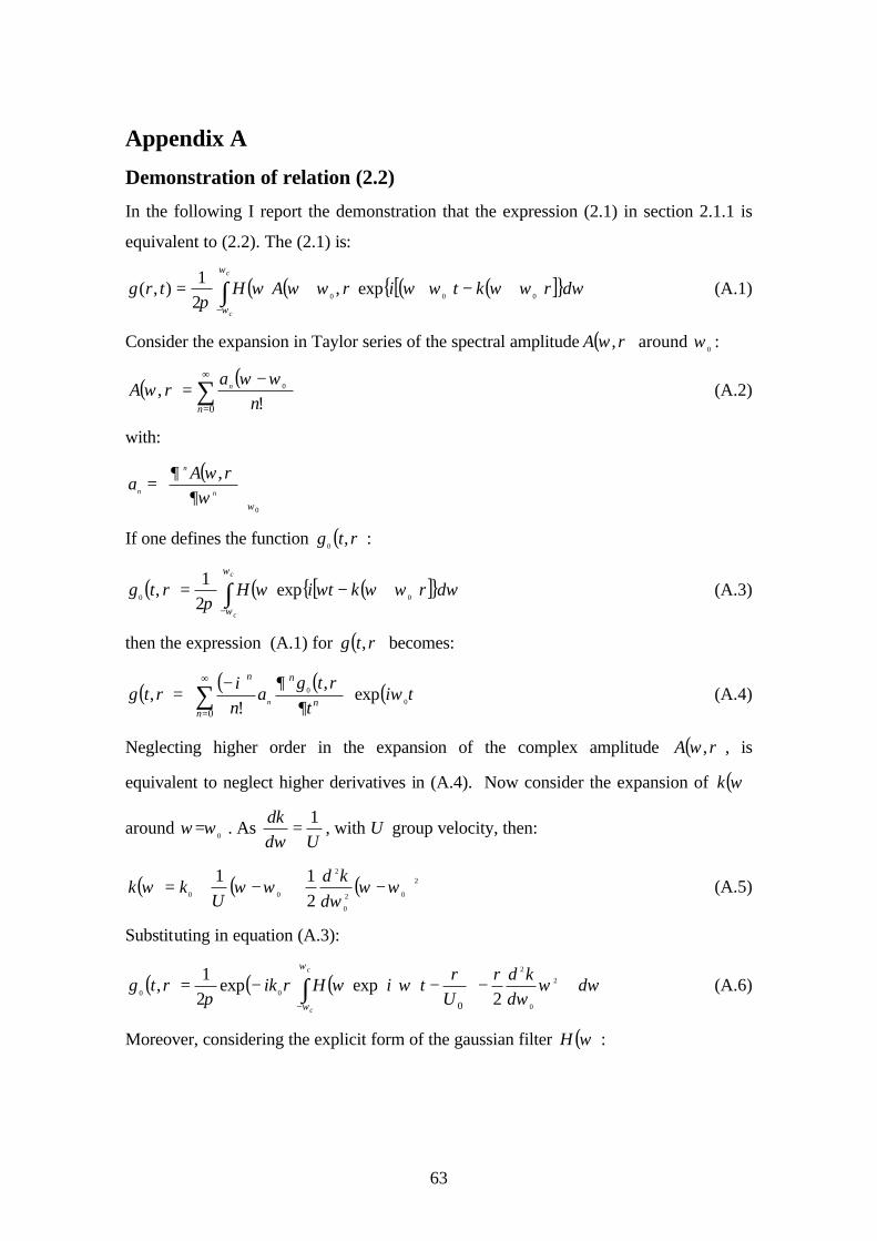
63

Appendix A

Demonstration of relation (2.2)

In the following I report the demonstration that the expression (2.1) in section 2.1.1 is

equivalent to (2.2). The (2.1) is:

( ) ( ) ( ) ( )[ ] ωωωωωωωωπ

ω

ω

drktirAHtrgc

c

000exp,

21

),( +−++= ∫−

(A.1)

Consider the expansion in Taylor series of the spectral amplitude ( )rA ,ω around 0

ω :

( ) ( )∑∞

=

−=

0 !, 0

n na

rA n ωωω (A.2)

with:

( )0

,

ω∂ω

ω∂

=

n

n

n

rAa

If one defines the function ( )rtg ,0

:

( ) ( ) ( )[ ] ωωωωωπ

ω

ω

drktiHrtgc

c

00exp

21

, +−= ∫−

(A.3)

then the expression (A.1) for ( )rtg , becomes:

( ) ( ) ( ) ( )tit

rtga

ni

rtgn

n

nn

n 0

0 exp,

!,

0

ω∂

∂

−

= ∑∞

=

(A.4)

Neglecting higher order in the expansion of the complex amplitude ( )rA ,ω , is

equivalent to neglect higher derivatives in (A.4). Now consider the expansion of ( )ωk

around 0

ωω = . As Ud

dk 1=

ω, with U group velocity, then:

( ) ( ) ( )2

02

0

2

00 211

ωωω

ωωω −+−+=d

kdU

kk (A.5)

Substituting in equation (A.3):

( ) ( ) ( ) ωωω

ωωπ

ω

ω

dd

kdrUr

tiHrikrtgc

c

−

−−= ∫

−

2

0

2

00 2expexp

21

,0

(A.6)

Moreover, considering the explicit form of the gaussian filter ( )ωH :

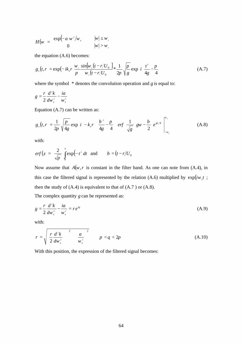
64

( ) ( ) −

=0

exp0

2 ωωαωH

c

c

ωωωω

>≤

the equation (A.6) becomes:

( ) ( ) ( )[ ]( )

−

−−

−=44

exp21

*exp,2

00

0

0 πγγ

ππω

ωπω t

iUrt

Urtsinrikrtg

c

cc (A.7)

where the symbol * denotes the convolution operation and γ is equal to:

2

0

2

0

2

2 ωα

ωγ

id

kdr−=

Equation (A.7) can be written as:

( )c

c

ieerfrkirtg

ω

ω

πβγω

γπ

γβ

γπ

π−

−

−+−= 4

21

44exp

421

,2

00 (A.8)

with:

( ) ( )dttzerfz

∫ −

=

0

2exp2π

and ( )0Urt −=β

Now assume that ( )rA ,ω is constant in the filter band. As one can note from (A.4), in

this case the filtered signal is represented by the relation (A.6) multiplied by ( )ti0

exp ω ;

then the study of (A.4) is equivalent to that of (A.7 ) or (A.8).

The complex quantity γ can be represented as:

2

0

2

0

2

2 ωα

ωγ

id

kdr−= θρ ie= (A.9)

with:

22

2

0

2

0

2

2

+

+=

ωα

ωρ

dkdr

πθπ 2<< (A.10)

With this position, the expression of the filtered signal becomes:

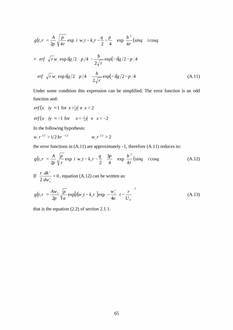
65

( ) ( )

+

−−−= θθ

ρβπθ

ωρ

ππ

cos4

exp42

exp42

,2

00 isinrktiA

rtg

( ) ( )( )

−−−+× 42exp

242exp πθ

ρβ

πθωρ iierf c

( ) ( )( )

−−+++ 42exp

242exp πθ

ρβ

πθωρ iierf c (A.11)

Under some condition this expression can be simplified. The error function is an odd

function and:

( ) 1≈+ iyxerf for yx > e 2>x

( ) 1−≈+ iyxerf for yx −< e 2−<x

In the following hypothesis: 2121 21 −> βρρω

c 221 >ρω

c

the error functions in (A.11) are approximately -1, therefore (A.11) reduces to:

( ) ( )

+

+−−= θθ

ρβπθ

ωρπ

πcos

4exp

43

2exp

2,

2

00 isinrktiA

rtg (A.12)

If 02 2

0

2

=ωd

dkr, equation (A.12) can be written as:

( ) ( )[ ]

−−−=

2

04expexp

2,

2

0

00

0

Ur

trktiA

rtgα

ωω

απ

πω

(A.13)

that is the equation (2.2) of section 2.1.1.

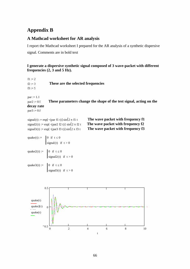
66

Appendix B

A Mathcad worksheet for AR analysis

I report the Mathcad worksheet I prepared for the AR analysis of a synthetic dispersive

signal. Comments are in bold text

I generate a dispersive synthetic signal composed of 3 wave-packet with different frequencies (2, 3 and 5 Hz). f1 2:= f2 3:= These are the selected frequencies f3 5:= par 1.1:= par2 0.9:= These parameters change the shape of the test signal, acting on the decay rate par3 0.8:= signal t( ) exp par f1⋅ t⋅( )−[ ] sin 2 π⋅ f1⋅ t⋅( ):= The wave packet with frequency f1 signal2 t( ) exp par2 f2⋅ t⋅( )−[ ] sin 2 π⋅ f2⋅ t⋅( )⋅:= The wave packet with frequency f2 signal3 t( ) exp par3 f3⋅ t⋅( )−[ ] sin 2 π⋅ f3⋅ t⋅( ):= The wave packet with frequency f3 quake t( ) 0 t 0≤if

signal t( ) t 0>if

:=

quake2 t( ) 0 t 0≤if

signal2 t( ) t 0>if

:=

quake3 t( ) 0 t 0≤if

signal3 t( ) t 0>if

:=

0 2 4 6 8 100.5

0

0.5

quake t( )

quake2 t( )

quake t( )

t

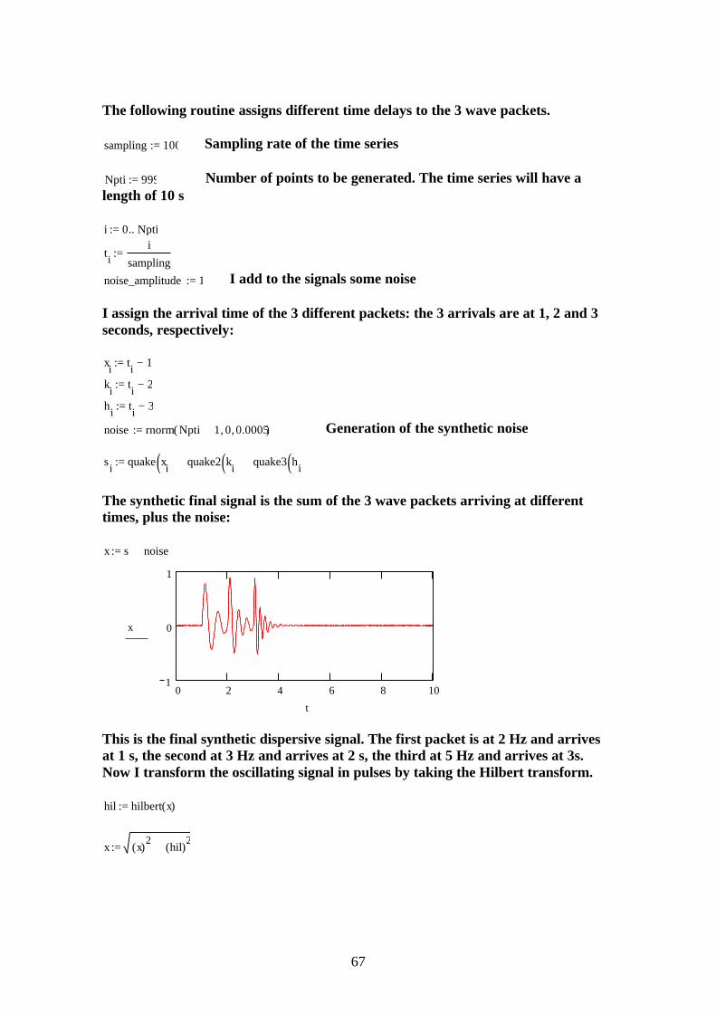
67

The following routine assigns different time delays to the 3 wave packets. sampling 100:= Sampling rate of the time series Npti 999:= Number of points to be generated. The time series will have a length of 10 s i 0 Npti..:=

tii

sampling:=

noise_amplitude 1:= I add to the signals some noise I assign the arrival time of the 3 different packets: the 3 arrivals are at 1, 2 and 3 seconds, respectively: xi ti 1−:=

ki ti 2−:=

hi ti 3−:=

noise rnorm Npti 1+ 0, 0.0005,( ):= Generation of the synthetic noise s i quake xi( ) quake2 ki( )+ quake3 hi( )+:=

The synthetic final signal is the sum of the 3 wave packets arriving at different times, plus the noise: x s noise+:=

0 2 4 6 8 101

0

1

x

t This is the final synthetic dispersive signal. The first packet is at 2 Hz and arrives at 1 s, the second at 3 Hz and arrives at 2 s, the third at 5 Hz and arrives at 3s. Now I transform the oscillating signal in pulses by taking the Hilbert transform. hil hilbert x( ):=

x x( )2

hil( )2

+:=

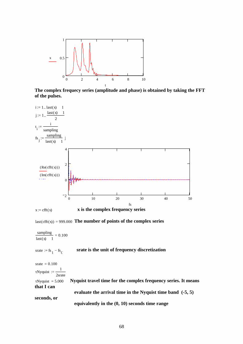
68

0 2 4 6 8 100

0.5

1

x

t

The complex frequecy series (amplitude and phase) is obtained by taking the FFT of the pulses. i 1 last x( ) 1+..:=

j 1last x( ) 1+

2..:=

tii

sampling:=

fs jsampling

last x( ) 1+j⋅:=

0 10 20 30 40 502

0

2

4

Re cfft x( )( )( )

Im cfft x( )( )( )

fs

x cfft x( ):= x is the complex frequency series last cfft x( )( ) 999.000= The number of points of the complex series

sampling

last x( ) 1+0.100=

srate fs1 fs0−:=

srate is the unit of frequency discretization

srate 0.100=

τNyquist1

2srate:=

τNyquist 5.000= Nyquist travel time for the complex frequency series. It means that I can evaluate the arrival time in the Nyquist time band (-5, 5) seconds, or equivalently in the (0, 10) seconds time range

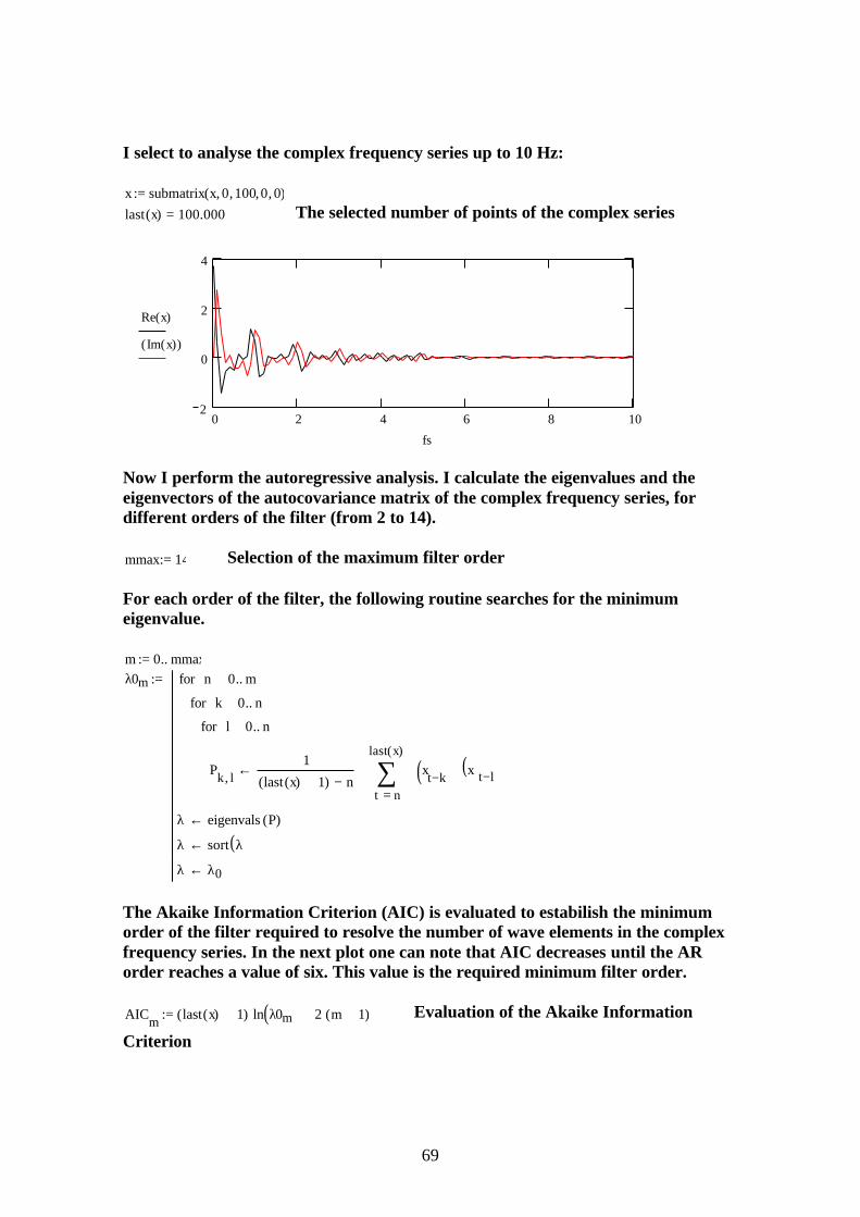
69

I select to analyse the complex frequency series up to 10 Hz: x submatrix x 0, 100, 0, 0,( ):= last x( ) 100.000= The selected number of points of the complex series

0 2 4 6 8 102

0

2

4

Re x( )

Im x( )( )

fs

Now I perform the autoregressive analysis. I calculate the eigenvalues and the eigenvectors of the autocovariance matrix of the complex frequency series, for different orders of the filter (from 2 to 14). mmax 14:= Selection of the maximum filter order For each order of the filter, the following routine searches for the minimum eigenvalue. m 0 mmax..:= λ0m

Pk l,1

last x( ) 1+( ) n−n

last x( )

t

xt k−( ) x( )

t l− ⋅

∑

=

⋅←

l 0 n..∈for

k 0 n..∈for

n 0 m..∈for

λ eigenvals P( )←

λ sort λ( )←

λ λ0←

:=

The Akaike Information Criterion (AIC) is evaluated to estabilish the minimum order of the filter required to resolve the number of wave elements in the complex frequency series. In the next plot one can note that AIC decreases until the AR order reaches a value of six. This value is the required minimum filter order. AICm last x( ) 1+( ) ln λ0m( )⋅ 2 m 1+( )⋅+:=

Evaluation of the Akaike Information

Criterion

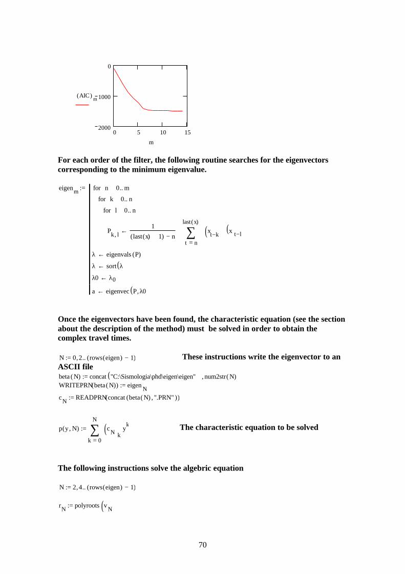
70

0 5 10 152000

1000

0

AIC( ) m

m

For each order of the filter, the following routine searches for the eigenvectors corresponding to the minimum eigenvalue. eigenm

Pk l,1

last x( ) 1+( ) n−n

last x( )

t

xt k−( ) x( )

t l− ⋅

∑

=

⋅←

l 0 n..∈for

k 0 n..∈for

n 0 m..∈for

λ eigenvals P( )←

λ sort λ( )←

λ0 λ0←

a eigenvec P λ0,( )←

:=

Once the eigenvectors have been found, the characteristic equation (see the section about the description of the method) must be solved in order to obtain the complex travel times. N 0 2, rows eigen( ) 1−( )..:= These instructions write the eigenvector to an ASCII file beta N( ) concat "C:\Sismologia\phd\eigen\eigen" num2str N( ),( ):= WRITEPRN beta N( )( ) eigen N:=

cN READPRN concat beta N( ) ".PRN",( )( ):=

p y N,( )

0

N

k

cN( )k

yk

⋅∑=

:=

The characteristic equation to be solved

The following instructions solve the algebric equation N 2 4, rows eigen( ) 1−( )..:= rN polyroots vN( ):=

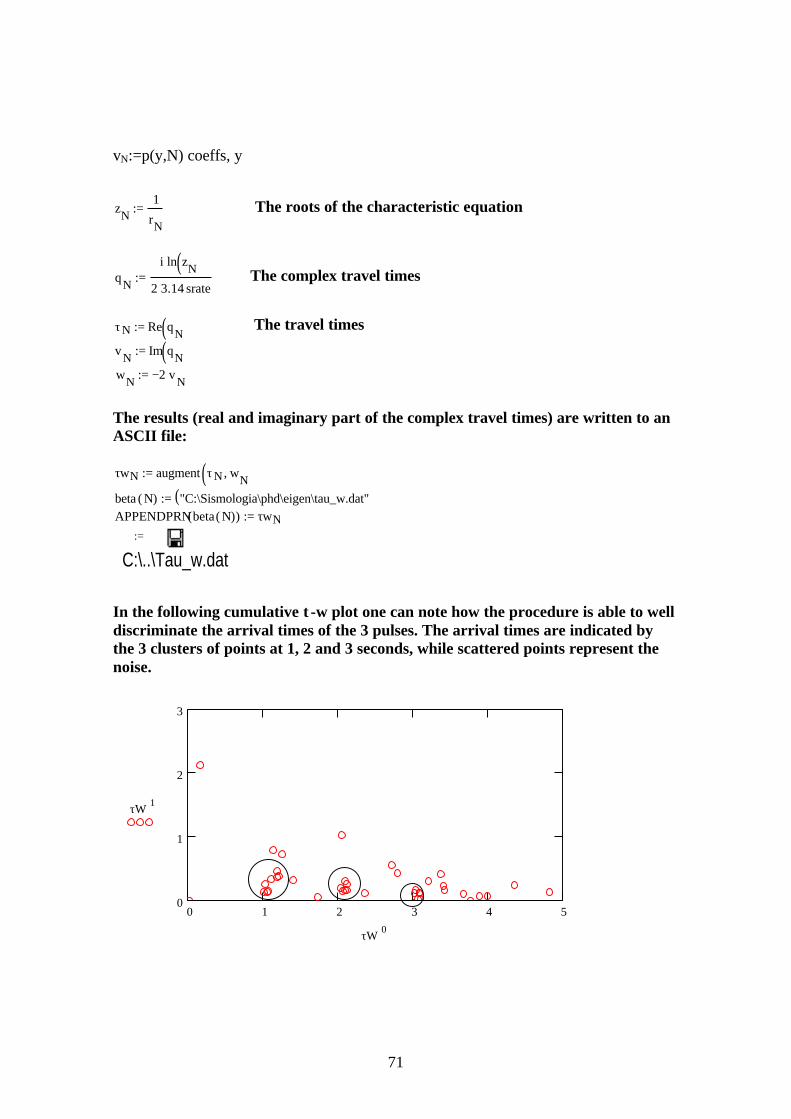
71

vN:=p(y,N) coeffs, y

zN1

rN:=

The roots of the characteristic equation

qN

i ln zN( )⋅

2 3.14⋅ srate⋅:= The complex travel times

τN Re qN( ):=

The travel times

vN Im qN( ):=

wN 2− vN⋅:=

The results (real and imaginary part of the complex travel times) are written to an ASCII file: τwN augment τN wN,( ):=

beta N( ) "C:\Sismologia\phd\eigen\tau_w.dat"( ):= APPENDPRNbeta N( )( ) τwN:= τW

C:\..\Tau_w.dat:=

In the following cumulative τ-w plot one can note how the procedure is able to well discriminate the arrival times of the 3 pulses. The arrival times are indicated by the 3 clusters of points at 1, 2 and 3 seconds, while scattered points represent the noise.

0 1 2 3 4 50

1

2

3

τW 1⟨ ⟩

τW 0⟨ ⟩

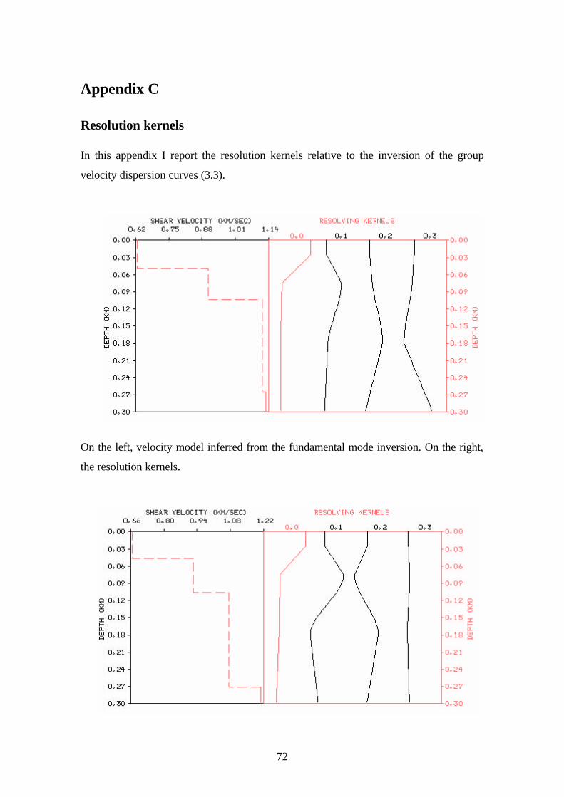
72

Appendix C

Resolution kernels In this appendix I report the resolution kernels relative to the inversion of the group

velocity dispersion curves (3.3).

On the left, velocity model inferred from the fundamental mode inversion. On the right,

the resolution kernels.

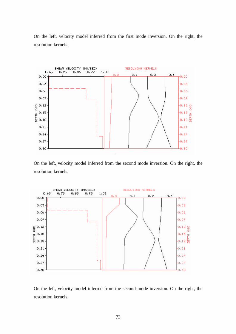
73

On the left, velocity model inferred from the first mode inversion. On the right, the

resolution kernels.

On the left, velocity model inferred from the second mode inversion. On the right, the

resolution kernels.

On the left, velocity model inferred from the second mode inversion. On the right, the

resolution kernels.

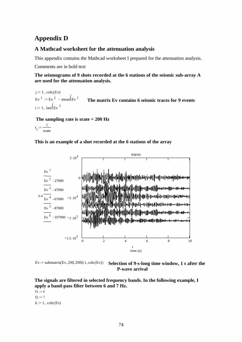
74

Appendix D

A Mathcad worksheet for the attenuation analysis

This appendix contains the Mathcad worksheet I prepared for the attenuation analysis.

Comments are in bold text

The seismograms of 9 shots recorded at the 6 stations of the seismic sub-array A are used for the attenuation analysis. j 1 cols Ev( )..:=

Ev j⟨ ⟩Ev j⟨ ⟩

mean Ev j⟨ ⟩( )−:= The matrix Ev contains 6 seismic traces for 9 events

i 1 last Ev 1⟨ ⟩( )..:= The sampling rate is srate = 200 Hz

tii

srate:=

This is an example of a shot recorded at the 6 stations of the array

0 2 4 6 8 101.5 .105

1 .105

5 .104

0

5 .104 traces

time (s)

a.u.

Ev 1⟨ ⟩

Ev 2⟨ ⟩27000−

Ev 3⟨ ⟩47000−

Ev 4⟨ ⟩67000−

Ev 5⟨ ⟩87000−

Ev 6⟨ ⟩107000−

t

Ev submatrix Ev 200, 2000, 1, cols Ev( ),( ):= Selection of 9-s-long time window, 1 s after the P-wave arrival The signals are filtered in selected frequency bands. In the following example, I apply a band-pass filter between 6 and 7 Hz. f1 6:= f2 7:= k 1 cols Ev( )..:=

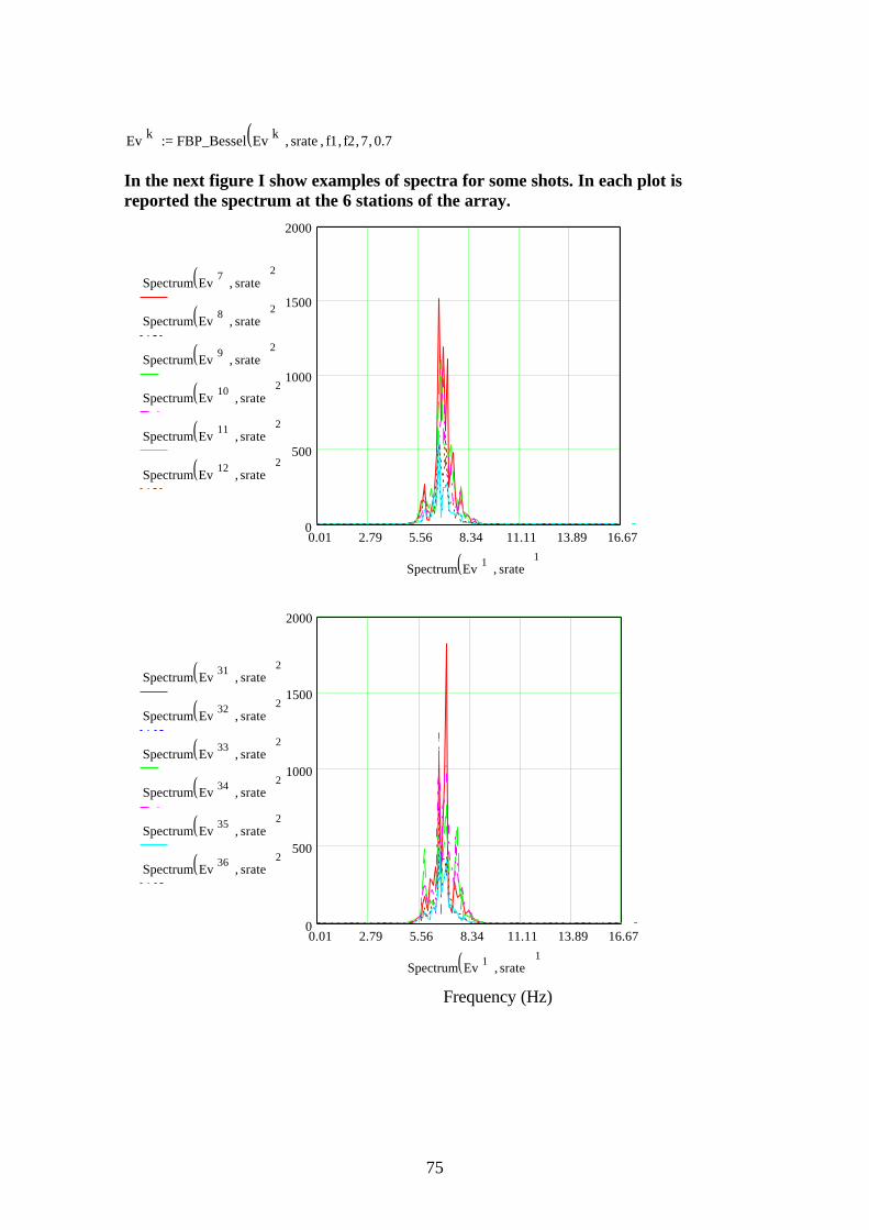
75

Ev k⟨ ⟩FBP_Bessel Ev k⟨ ⟩

srate, f1, f2, 7, 0.7,( ):= In the next figure I show examples of spectra for some shots. In each plot is reported the spectrum at the 6 stations of the array.

0.01 2.79 5.56 8.34 11.11 13.89 16.670

500

1000

1500

2000

Spectrum Ev 7⟨ ⟩srate,( ) 2⟨ ⟩

Spectrum Ev 8⟨ ⟩srate,( ) 2⟨ ⟩

Spectrum Ev 9⟨ ⟩srate,( ) 2⟨ ⟩

Spectrum Ev 10⟨ ⟩srate,( ) 2⟨ ⟩

Spectrum Ev 11⟨ ⟩srate,( ) 2⟨ ⟩

Spectrum Ev 12⟨ ⟩srate,( ) 2⟨ ⟩

Spectrum Ev 1⟨ ⟩srate,( ) 1⟨ ⟩

Frequency (Hz)

0.01 2.79 5.56 8.34 11.11 13.89 16.670

500

1000

1500

2000

Spectrum Ev 31⟨ ⟩srate,( ) 2⟨ ⟩

Spectrum Ev 32⟨ ⟩srate,( ) 2⟨ ⟩

Spectrum Ev 33⟨ ⟩srate,( ) 2⟨ ⟩

Spectrum Ev 34⟨ ⟩srate,( ) 2⟨ ⟩

Spectrum Ev 35⟨ ⟩srate,( ) 2⟨ ⟩

Spectrum Ev 36⟨ ⟩srate,( ) 2⟨ ⟩

Spectrum Ev 1⟨ ⟩srate,( ) 1⟨ ⟩

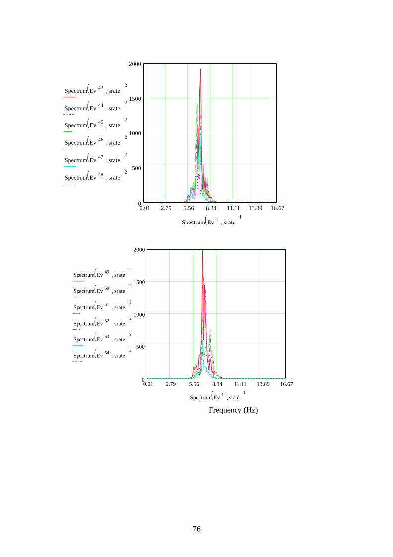
76

0.01 2.79 5.56 8.34 11.11 13.89 16.670

500

1000

1500

2000

Spectrum Ev 43⟨ ⟩srate,( ) 2⟨ ⟩

Spectrum Ev 44⟨ ⟩srate,( ) 2⟨ ⟩

Spectrum Ev 45⟨ ⟩srate,( ) 2⟨ ⟩

Spectrum Ev 46⟨ ⟩srate,( ) 2⟨ ⟩

Spectrum Ev 47⟨ ⟩srate,( ) 2⟨ ⟩

Spectrum Ev 48⟨ ⟩srate,( ) 2⟨ ⟩

Spectrum Ev 1⟨ ⟩srate,( ) 1⟨ ⟩

Frequency (Hz)

0.01 2.79 5.56 8.34 11.11 13.89 16.670

500

1000

1500

2000

Spectrum Ev 49⟨ ⟩srate,( ) 2⟨ ⟩

Spectrum Ev 50⟨ ⟩srate,( ) 2⟨ ⟩

Spectrum Ev 51⟨ ⟩srate,( ) 2⟨ ⟩

Spectrum Ev 52⟨ ⟩srate,( ) 2⟨ ⟩

Spectrum Ev 53⟨ ⟩srate,( ) 2⟨ ⟩

Spectrum Ev 54⟨ ⟩srate,( ) 2⟨ ⟩

Spectrum Ev 1⟨ ⟩srate,( ) 1⟨ ⟩

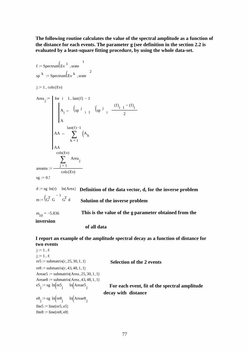
77

The following routine calculates the value of the spectral amplitude as a function of the distance for each events. The parameter γ (see definition in the section 2.2 is evaluated by a least-square fitting procedure, by using the whole data-set.

f Spectrum Ev 1⟨ ⟩srate,( ) 1⟨ ⟩

:=

sp k⟨ ⟩Spectrum Ev k⟨ ⟩

srate,( ) 2⟨ ⟩:=

j 1 cols Ev( )..:= Area j

Ai sp j⟨ ⟩( )i 1+ sp j⟨ ⟩( )

i+

f( )i 1+ f( )i− 2

⋅←

A

i 1 last f( ) 1−..∈for

AA

1

last f( ) 1−

h

Ah( )∑=

←

AA

:=

areams1

cols Ev( )

j

Area j∑=

cols Ev( ):=

sg 0.5:= d sg ln r( )⋅ ln Area( )+:= Definition of the data vector, d, for the inverse problem

m GT G⋅( ) 1−GT⋅ d⋅:= Solution of the inverse problem

m10 5.836−= This is the value of the γ parameter obtained from the

inversion of all data I report an example of the amplitude spectral decay as a function of distance for two events j 1 6..:= j 1 6..:= re5 submatrix r 25, 30, 1, 1,( ):= Selection of the 2 events re8 submatrix r 43, 48, 1, 1,( ):= Areae5 submatrix Area 25, 30, 1, 1,( ):= Areae8 submatrix Area 43, 48, 1, 1,( ):= e5j sg ln re5j( )⋅ ln Areae5 j( )+:=

For each event, fit of the spectral amplitude decay with distance e8j sg ln re8j( )⋅ ln Areae8 j( )+:=

fite5 line re5 e5,( ):= fite8 line re8 e8,( ):=

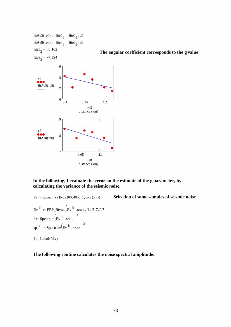
78

fitAe5 re5( ) fite51 fite52 re5⋅+:=

fitAe8 re8( ) fite81 fite82 re8⋅+:=

fite52 8.162−= The angular coefficient corresponds to the γ value

fite82 7.524−=

3.1 3.15 3.26

7

8

9

distance (km)

e5

fitAe5 re5( )

re5

4.05 4.17

8

9

distance (km)

e8

fitAe8 re8( )

re8

In the following, I evaluate the error on the estimate of the γ parameter, by calculating the variance of the seismic noise. Ev submatrix Ev 2200, 4000, 1, cols Ev( ),( ):= Selection of some samples of seismic noise Ev k⟨ ⟩

FBP_Bessel Ev k⟨ ⟩srate, f1, f2, 7, 0.7,( ):=

f Spectrum Ev 1⟨ ⟩srate,( ) 1⟨ ⟩

:=

sp k⟨ ⟩Spectrum Ev k⟨ ⟩

srate,( ) 2⟨ ⟩:=

j 1 cols Ev( )..:= The following routine calculates the noise spectral amplitude:

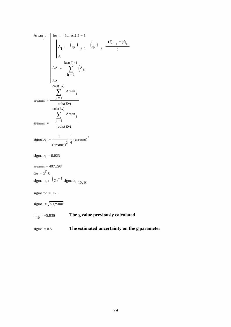
79

Arean j

Ai sp j⟨ ⟩( )i 1+ sp j⟨ ⟩( )

i+

f( )i 1+ f( )i− 2

⋅←

A

i 1 last f( ) 1−..∈for

AA

1

last f( ) 1−

h

Ah( )∑=

←

AA

:=

areamn1

cols Ev( )

j

Arean j∑=

cols Ev( ):=

areamn1

cols Ev( )

j

Arean j∑=

cols Ev( ):=

sigmadq1

areams( )2

1

4⋅ areamn( )

2⋅:=

sigmadq 0.023= areamn 407.298=

Ge GT G⋅:=

sigmamq Ge1−

sigmadq⋅( )10 10,:=

sigmamq 0.25= sigma sigmamq:= m10 5.836−=

The γ value previously calculated

sigma 0.5= The estimated uncertainty on the γ parameter

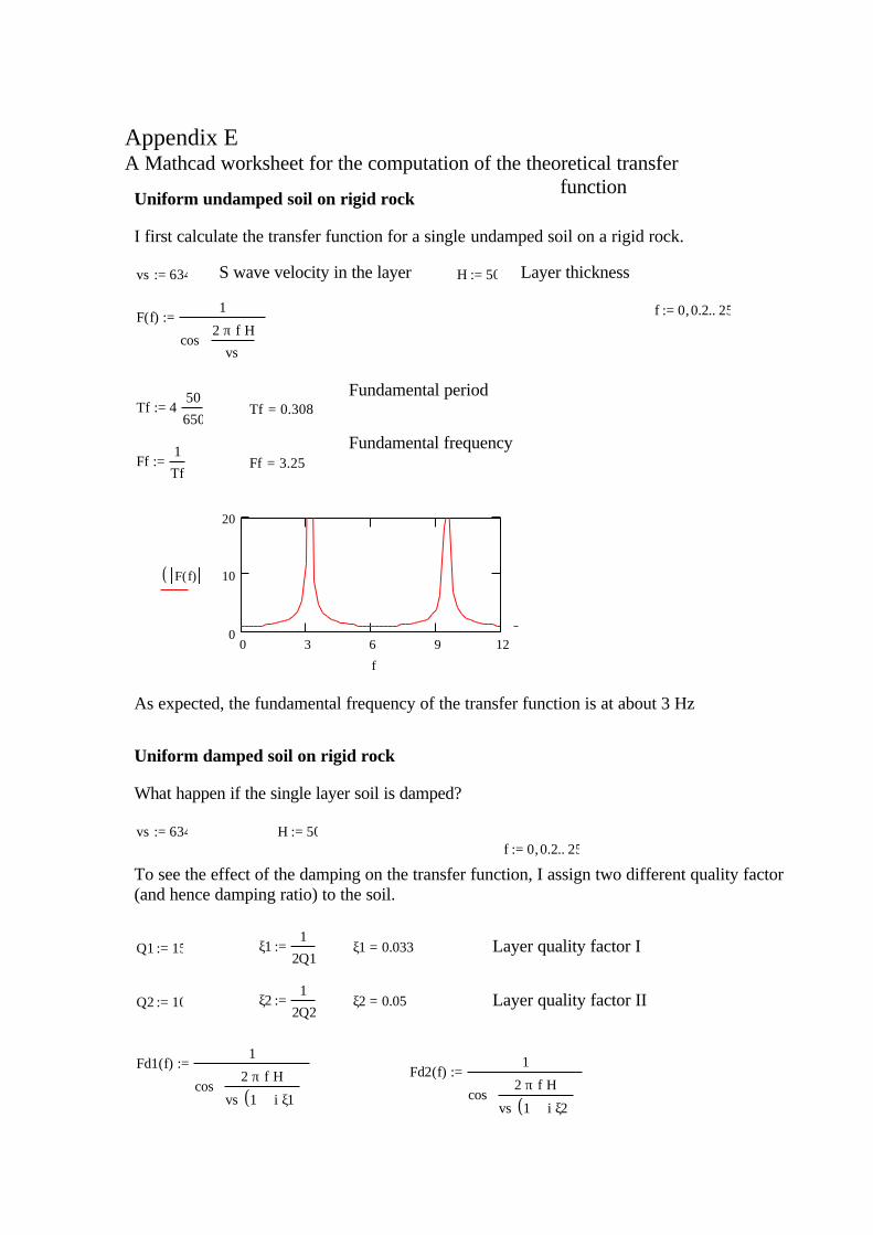
Appendix E A Mathcad worksheet for the computation of the theoretical transfer

functionUniform undamped soil on rigid rock

I first calculate the transfer function for a single undamped soil on a rigid rock.

vs 634:= S wave velocity in the layer H 50:= Layer thickness

f 0 0.2, 25..:= F f( )1

cos2 π⋅ f⋅ H⋅

vs

:=

Tf 450

650⋅:= Tf 0.308=

Fundamental period

Fundamental frequency Ff

1

Tf:= Ff 3.25=

0 3 6 9 120

10

20

F f( )( )

f

As expected, the fundamental frequency of the transfer function is at about 3 Hz

Uniform damped soil on rigid rock

What happen if the single layer soil is damped?

vs 634:= H 50:= f 0 0.2, 25..:=

To see the effect of the damping on the transfer function, I assign two different quality factor (and hence damping ratio) to the soil.

Q1 15:= ξ11

2Q1:= ξ1 0.033= Layer quality factor I

Q2 10:= ξ21

2Q2:= ξ2 0.05= Layer quality factor II

Fd1 f( )1

cos2 π⋅ f⋅ H⋅

vs 1 i ξ1⋅+( )⋅

:= Fd2 f( )

1

cos2 π⋅ f⋅ H⋅

vs 1 i ξ2⋅+( )⋅

:=

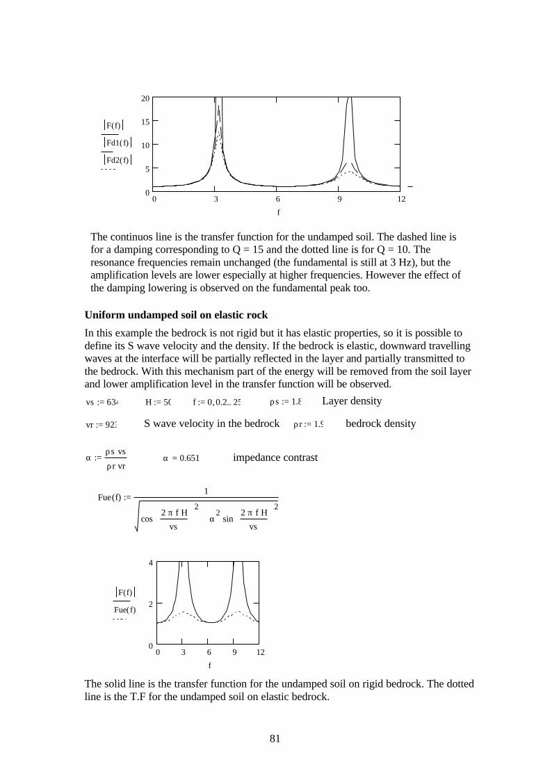
81

0 3 6 9 120

5

10

15

20

F f( )

Fd1 f( )

Fd2 f( )

f

The continuos line is the transfer function for the undamped soil. The dashed line is for a damping corresponding to Q = 15 and the dotted line is for Q = 10. The resonance frequencies remain unchanged (the fundamental is still at 3 Hz), but the amplification levels are lower especially at higher frequencies. However the effect of the damping lowering is observed on the fundamental peak too.

Uniform undamped soil on elastic rock

In this example the bedrock is not rigid but it has elastic properties, so it is possible to define its S wave velocity and the density. If the bedrock is elastic, downward travelling waves at the interface will be partially reflected in the layer and partially transmitted to the bedrock. With this mechanism part of the energy will be removed from the soil layer and lower amplification level in the transfer function will be observed.

vs 634:= H 50:= f 0 0.2, 25..:= ρs 1.8:= Layer density

vr 923:= S wave velocity in the bedrock ρr 1.9:= bedrock density

αρs vs⋅

ρr vr⋅:= α 0.651= impedance contrast

Fue f( )1

cos2 π⋅ f⋅ H⋅

vs

2α

2sin

2 π⋅ f⋅ H⋅

vs

2⋅+

:=

0 3 6 9 120

2

4

F f( )

Fue f( )

f

The solid line is the transfer function for the undamped soil on rigid bedrock. The dotted line is the T.F for the undamped soil on elastic bedrock.

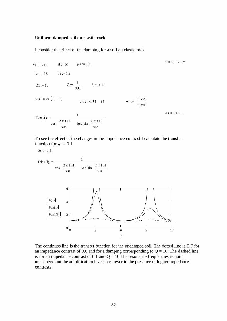
82

Uniform damped soil on elastic rock

I consider the effect of the damping for a soil on elastic rock

f 0 0.2, 25..:= vs 634:= H 50:= ρs 1.8:=

vr 923:= ρr 1.9:=

Q1 10:= ξ1

2Q1:= ξ 0.05=

vss vs 1 i ξ⋅+( )⋅:= vrr vr 1 i ξ⋅+( )⋅:= αs

ρs vss⋅

ρr vrr⋅:=

αs 0.651= Fde f( )

1

cos2 π⋅ f⋅ H⋅

vss

iαs sin2 π⋅ f⋅ H⋅

vss

⋅+

:=

To see the effect of the changes in the impedance contrast I calculate the transfer function for αs = 0.1

αs 0.1:=

Fde1 f( )1

cos2 π⋅ f⋅ H⋅

vss

iαs sin2 π⋅ f⋅ H⋅

vss

⋅+

:=

0 3 6 9 120

2

4

6

F f( )

Fde f( )

Fde1 f( )

f

The continuos line is the transfer function for the undamped soil. The dotted line is T.F for an impedance contrast of 0.6 and for a damping corresponding to Q = 10. The dashed line is for an impedance contrast of 0.1 and Q = 10.The resonance frequencies remain unchanged but the amplification levels are lower in the presence of higher impedance contrasts.

83

Multiple layer models

The case of Pozzuoli-Solfatara: layered damped soil on elastic bedrock

First layer (50 m): poorly unconsolidated pyroclastics and marine deposits

f 0 0.2, 25..:= v1 634:= h1 50:= ρ1 1.8:=

Q1 4:= ξ11

2Q1:= ξ1 0.05=

Second layer (50 m): fractured yellow tuff

v2 923:= h2 50:= ρ2 1.9:=

Q2 12:= ξ21

2Q2:= ξ2 0.025= impedance contrast v1 ρ1⋅

v2 ρ2⋅0.651=

The compact yellow tuff unit is considered as bedrock with the following parameters:

v3 993:= ρ3 2.0:=

Q3 15:= ξ31

2Q3:= ξ3 0.02=

v1s v1 1 i ξ1⋅+( )⋅:= v3s v3 1 i ξ3⋅+( )⋅:= v2s v2 1 i ξ2⋅+( )⋅:=

α1ρ1 v1s⋅

ρ2 v2s⋅:= α2

ρ2 v2s⋅

ρ3 v3s⋅:=

If there were only a single layer on a halfspace, the transfer function would be:

A1 1:=

A2 f( ) A11

21 α1+( )⋅ exp i

2 π⋅ f⋅

v1s⋅ h1⋅

⋅1

21 α1−( )⋅ exp i−

2 π⋅ f⋅

v1s⋅ h1⋅

⋅+

⋅:=

B2 f( ) A11

21 α1−( )⋅ exp i

2 π⋅ f⋅

v1s⋅ h1⋅

⋅1

21 α1+( )⋅ exp i−

2 π⋅ f⋅

v1s⋅ h1⋅

⋅+

⋅:=

Fl f( )2

A2 f( ) B2 f( )+:=

0 3 6 9 120

2

4

6

Fl f( )

f

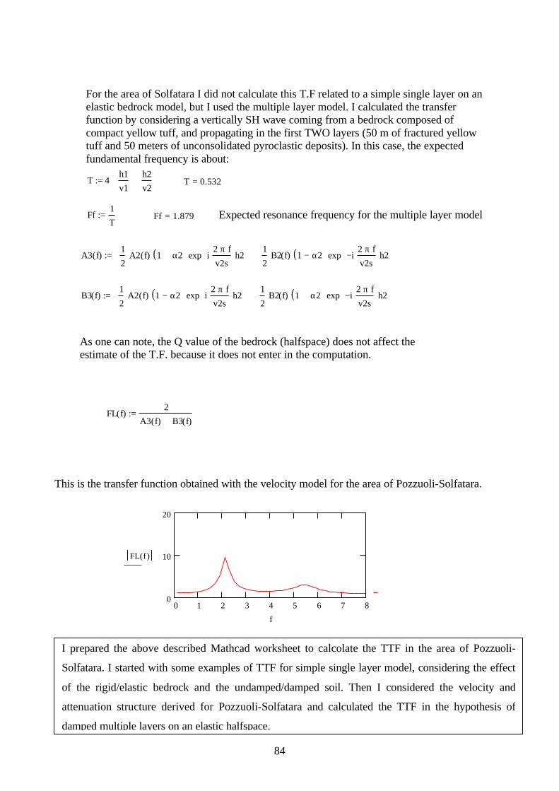
84

For the area of Solfatara I did not calculate this T.F related to a simple single layer on an elastic bedrock model, but I used the multiple layer model. I calculated the transfer function by considering a vertically SH wave coming from a bedrock composed of compact yellow tuff, and propagating in the first TWO layers (50 m of fractured yellow tuff and 50 meters of unconsolidated pyroclastic deposits). In this case, the expected fundamental frequency is about:

T 4h1

v1

h2

v2+

⋅:= T 0.532=

Ff1

T:= Ff 1.879= Expected resonance frequency for the multiple layer model

A3 f( )1

2A2 f( )⋅ 1 α2+( )⋅ exp i

2 π⋅ f⋅

v2s⋅ h2⋅

⋅1

2B2 f( )⋅ 1 α2−( )⋅ exp i−

2 π⋅ f⋅

v2s⋅ h2⋅

⋅+

:=

B3 f( )1

2A2 f( )⋅ 1 α2−( )⋅ exp i

2 π⋅ f⋅

v2s⋅ h2⋅

⋅1

2B2 f( )⋅ 1 α2+( )⋅ exp i−

2 π⋅ f⋅

v2s⋅ h2⋅

⋅+

:=

As one can note, the Q value of the bedrock (halfspace) does not affect the estimate of the T.F. because it does not enter in the computation.

FL f( )2

A3 f( ) B3 f( )+:=

This is the transfer function obtained with the velocity model for the area of Pozzuoli-Solfatara.

0 1 2 3 4 5 6 7 80

10

20

FL f( )

f

I prepared the above described Mathcad worksheet to calcolate the TTF in the area of Pozzuoli-

Solfatara. I started with some examples of TTF for simple single layer model, considering the effect

of the rigid/elastic bedrock and the undamped/damped soil. Then I considered the velocity and

attenuation structure derived for Pozzuoli-Solfatara and calculated the TTF in the hypothesis of

damped multiple layers on an elastic halfspace.

85

Appendix F

A Mathcad worksheet for the PGA estimate

For the estimate of the PGA in the area of Pozzuoli-Solfatara, I prepared the following

Mathcad worksheet that uses the mathematical formulation derived for both GMG and

RVT methods.

Definition of the source and propagation parameters a 4.00:= a and b values from the Gutenberg-Richter (De Natale et al., 1986) b 0.92:= δa 0.10:= Uncertainties on a and b values δb 0.04:= Md 4.35:= Expected maximum magnitude maxima at Campi Flegrei c 9.9:= Parameters of the empirical formula that relates seismic moment and magnitude d 0.9:= δc 0.1:= Uncertainties on c and d values δd 0.01:= δc

c0.01=

δd

d0.011=

M 109.9 0.9Md+( ) N⋅ m⋅:= Relation between seismic moment and magnitude

(Galluzzo et al., 2004) Now I estimate the seismic moment and the uncertainty:

M 6.531 1013

× J= Mdyne 107 M

J:=

Mdyne 6.531 10

20×= The value of the seismic

moment

δMd δa( )2 1

b

2⋅ δb( )2 a

b2

2⋅+:=

δMd 0.218= δMd

Md0.05=

δM δc( )210

c d Md⋅+( )log 10( )

2⋅ δd( )2

10c d Md⋅+( )

log 10( )⋅ Md⋅ 2

⋅+ δMd( )210

c d Md⋅+( )log 10( )⋅ d⋅

2⋅+

N m⋅:=

δM 1.466 1013

× J=

86

δM

M0.225=

Relative error on the seismic moment estimate

kk 4:= Stress drop value in bar (Galluzzo et al., 2004)

∆σkk kk 105

⋅N

m2

⋅:=

Uncertainty on the stress drop

r0.44 M⋅( )

1 ∆σkk⋅

1

3:=

Relation between source radius and seismic moment (Keilis -

Borok, 1959) r 415.717m= The value of the source radius

δr0.44

∆σkk

1

3⋅

M0.44

∆σkk⋅

2−

3⋅

2

δM( )2⋅:=

Uncertainty on the source radius

δr 31.112 m= δr

r0.075=

Relative error on the source radius estimate

F 2:= Free surface operator (Del Pezzo et al., 1987) R 2:= Hypocentral distance in km (insert adimensional values)

Thickness of the first layer in km (this thesis). Insert adimensional values

Thickness of the second layer in km (this thesis). Insert adimensional values

Average density (this thesis)

Shear wave velocity of the first layer (this thesis) Shear wave velocity of the second layer (this thesis) Average shear wave velocity of the halfspace (this thesis)

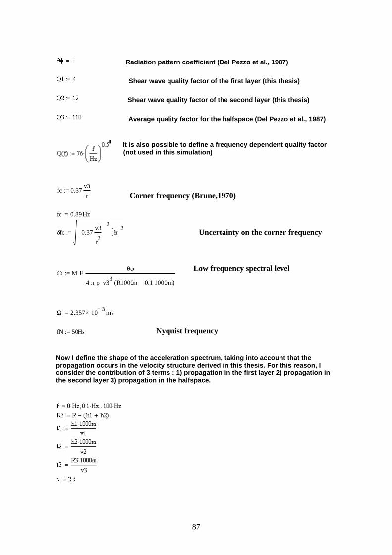
87

Radiation pattern coefficient (Del Pezzo et al., 1987)

Shear wave quality factor of the first layer (this thesis)

Shear wave quality factor of the second layer (this thesis)

Average quality factor for the halfspace (Del Pezzo et al., 1987)

It is also possible to define a frequency dependent quality factor (not used in this simulation)

Corner frequency (Brune,1970)

fc 0.89Hz= Uncertainty on the corner frequency

Low frequency spectral level

Ω 2.357 103−

× ms= fN 50Hz:= Nyquist frequency Now I define the shape of the acceleration spectrum, taking into account that the propagation occurs in the velocity structure derived in this thesis. For this reason, I consider the contribution of 3 terms : 1) propagation in the first layer 2) propagation in the second layer 3) propagation in the halfspace.

fc 0.37v3

r⋅:=

δfc 0.37v3

r2

⋅

2δr( )2

⋅:=

Ω M F⋅θφ

4 π⋅ ρ⋅ v33

⋅ R1000m 0.1 1000⋅ m⋅+( )⋅⋅:=

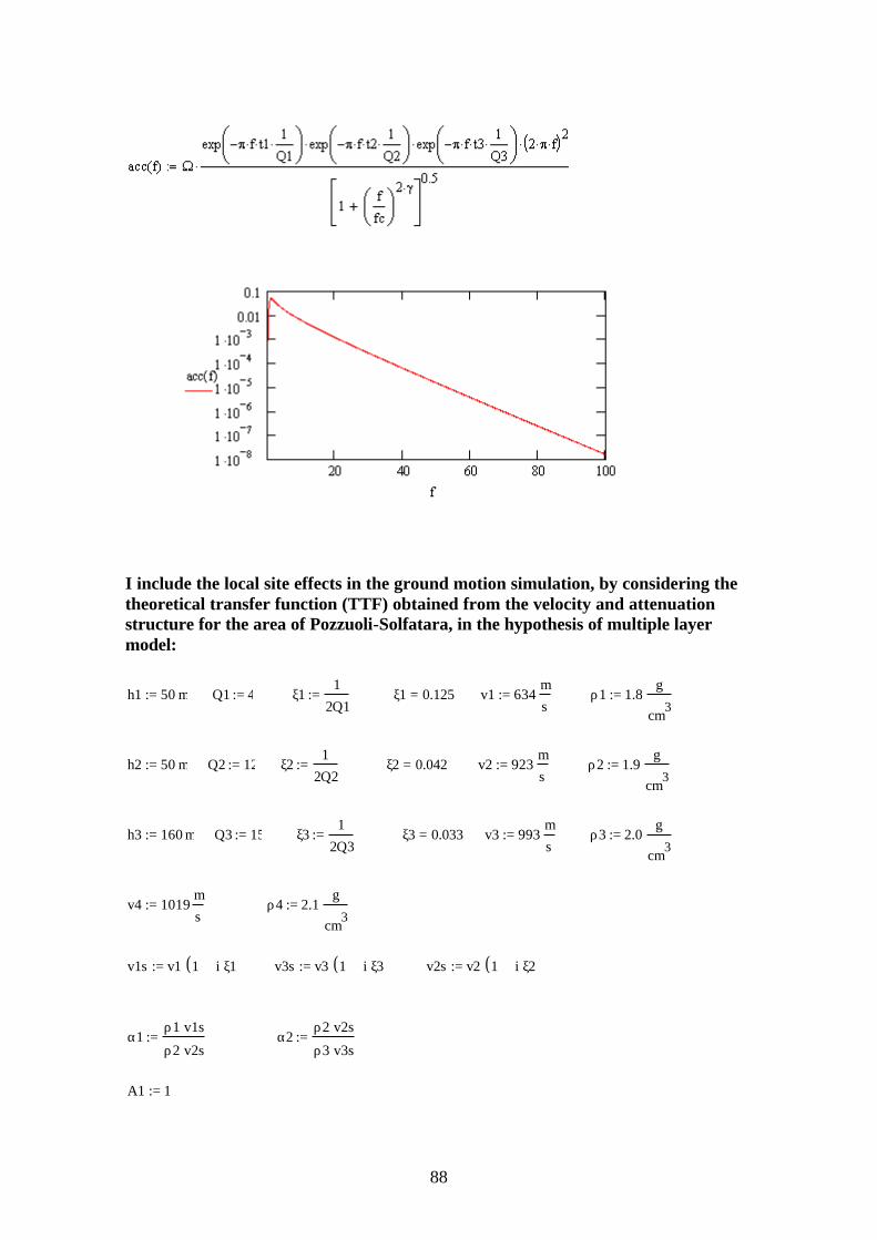
88

I include the local site effects in the ground motion simulation, by considering the theoretical transfer function (TTF) obtained from the velocity and attenuation structure for the area of Pozzuoli-Solfatara, in the hypothesis of multiple layer model:

h1 50 m⋅:= Q1 4:= ξ11

2Q1:=

ξ1 0.125= v1 634

m

s⋅:=

ρ1 1.8

g

cm3

⋅:=

h2 50 m⋅:= Q2 12:= ξ21

2Q2:=

ξ2 0.042= v2 923

m

s⋅:=

ρ2 1.9

g

cm3

⋅:=

h3 160 m⋅:= Q3 15:= ξ31

2Q3:=

ξ3 0.033= v3 993

m

s⋅:=

ρ3 2.0

g

cm3

⋅:=

v4 1019m

s⋅:=

ρ4 2.1

g

cm3

⋅:=

v1s v1 1 i ξ1⋅+( )⋅:= v3s v3 1 i ξ3⋅+( )⋅:= v2s v2 1 i ξ2⋅+( )⋅:=

α1ρ1 v1s⋅

ρ2 v2s⋅:=

α2

ρ2 v2s⋅

ρ3 v3s⋅:=

A1 1:=

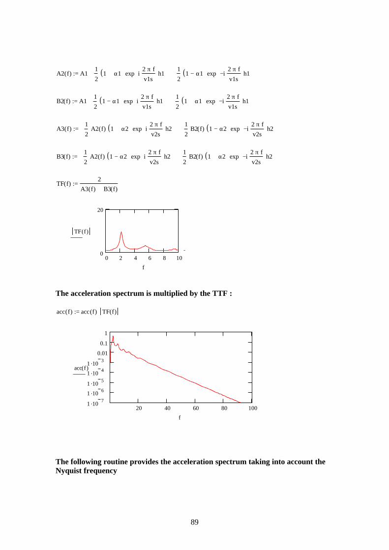
89

A2 f( ) A11

21 α1+( )⋅ exp i

2 π⋅ f⋅

v1s⋅ h1⋅

⋅1

21 α1−( )⋅ exp i−

2 π⋅ f⋅

v1s⋅ h1⋅

⋅+

⋅:=

B2 f( ) A11

21 α1−( )⋅ exp i

2 π⋅ f⋅

v1s⋅ h1⋅

⋅1

21 α1+( )⋅ exp i−

2 π⋅ f⋅

v1s⋅ h1⋅

⋅+

⋅:=

A3 f( )1

2A2 f( )⋅ 1 α2+( )⋅ exp i

2 π⋅ f⋅

v2s⋅ h2⋅

⋅1

2B2 f( )⋅ 1 α2−( )⋅ exp i−

2 π⋅ f⋅

v2s⋅ h2⋅

⋅+

:=

B3 f( )1

2A2 f( )⋅ 1 α2−( )⋅ exp i

2 π⋅ f⋅

v2s⋅ h2⋅

⋅1

2B2 f( )⋅ 1 α2+( )⋅ exp i−

2 π⋅ f⋅

v2s⋅ h2⋅

⋅+

:=

TF f( )2

A3 f( ) B3 f( )+:=

0 2 4 6 8 100

20

TF f( )

f The acceleration spectrum is multiplied by the TTF : acc f( ) acc f( ) TF f( )⋅:=

20 40 60 80 1001 .10 71 .10 61 .10 51 .10 41 .10 3

0.01

0.1

1

acc f( )

f The following routine provides the acceleration spectrum taking into account the Nyquist frequency

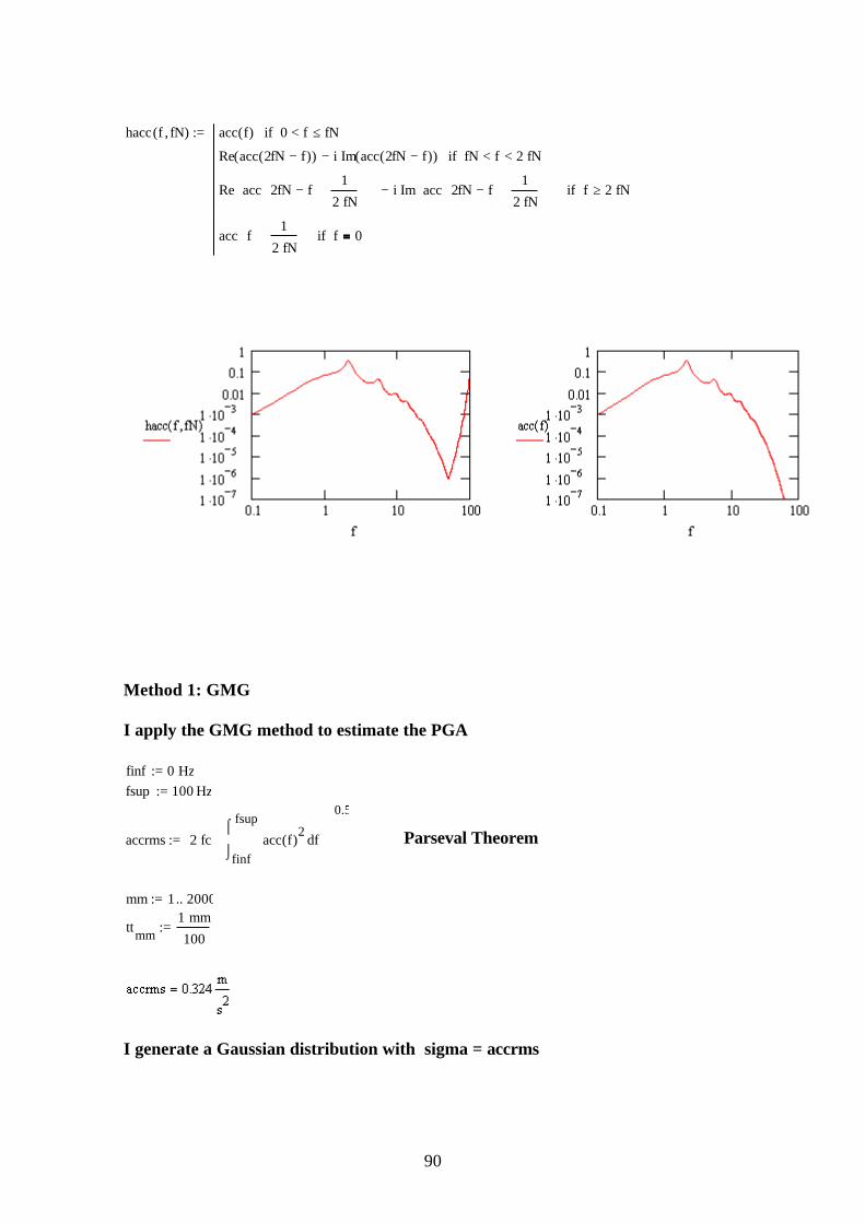
90

hacc f fN,( ) acc f( ) 0 f< fN≤if

Re acc 2fN f−( )( ) i Im acc 2fN f−( )( )⋅− fN f< 2 fN⋅<if

Re acc 2fN f−1

2 fN⋅+

i Im acc 2fN f−1

2 fN⋅+

⋅− f 2 fN⋅≥if

acc f1

2 fN⋅+

f 0if

:=

Method 1: GMG I apply the GMG method to estimate the PGA finf 0 Hz⋅:= fsup 100 Hz⋅:=

accrms 2 fc⋅finf

fsup

facc f( )2⌠

⌡

d

⋅

0.5

:=

Parseval Theorem

mm 1 2000..:=

ttmm1 mm⋅100

:=

I generate a Gaussian distribution with sigma = accrms

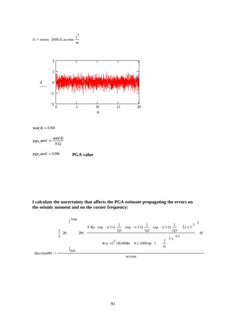
91

d rnorm 2000 0, accrmss

2

m⋅,

:=

PGA value I calculate the uncertainty that affects the PGA estimate propagating the errors on the seismic moment and on the corner frequency:

daccrmsdM

1

22fc

finf

fsup

f2M

F θφ⋅ exp π− f⋅ t1⋅1

Q1⋅

exp π− f⋅ t2⋅1

Q2⋅

⋅ exp π− f⋅ t3⋅1

Q3⋅

⋅

⋅ 2 π⋅ f⋅( )2⋅

4π ρ v33

⋅ R1000m 0.1 1000⋅ m⋅+( )⋅ 1f

fc

2 γ⋅+

0.5

2

⋅

⌠⌡

d⋅

accrms:=

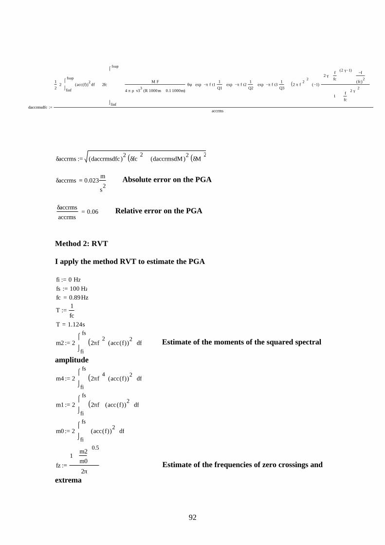
92

δaccrms daccrmsdfc( )2 δfc( )2⋅ daccrmsdM( )

2 δM( )2⋅+:=

δaccrms 0.023m

s2

=

Absolute error on the PGA

δaccrms

accrms0.06=

Relative error on the PGA

Method 2: RVT I apply the method RVT to estimate the PGA fi 0 Hz⋅:= fs 100 Hz⋅:= fc 0.89Hz=

T1

fc:=

T 1.124s=

m2 2fi

fs

f2πf( )2acc f( )( )

2 ⌠⌡

d⋅:=

Estimate of the moments of the squared spectral

amplitude

m4 2fi

fs

f2πf( )4acc f( )( )

2 ⌠⌡

d⋅:=

m1 2fi

fs

f2πf( ) acc f( )( )2

⌠⌡

d⋅:=

m0 2fi

fs

facc f( )( )2

⌠⌡

d⋅:=

fz

1m2

m0

0.5⋅

2π:=

Estimate of the frequencies of zero crossings and

extrema

daccrmsdfc

1

22

finf

fsup

facc f( )( )2⌠

⌡

d

2fc

finf

fsup

M F⋅

4 π⋅ ρ⋅ v33

⋅ R 1000⋅ m⋅ 0.1 1000⋅ m⋅+( )⋅θφ⋅ exp π− f⋅ t1⋅

1

Q1⋅

exp π− f⋅ t2⋅

1

Q2⋅

⋅ exp π− f⋅ t3⋅

1

Q3⋅

⋅

⋅ 2 π⋅ f⋅( )2

⋅

21−( )

2 γ⋅f

fc

2 γ⋅ 1−( )⋅

f−

fc( )2

⋅

1f

fc

2 γ⋅+

2⋅

⋅

⌠⌡

⋅+

accrms:=

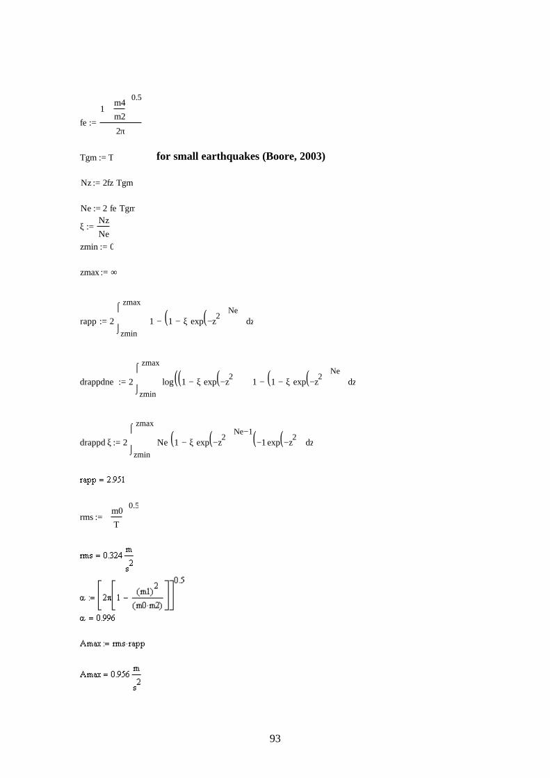
93

fe

1m4

m2

0.5⋅

2π:=

Tgm T:= for small earthquakes (Boore, 2003) Nz 2fz Tgm⋅:= Ne 2 fe⋅ Tgm⋅:=

ξNz

Ne:=

zmin 0:= zmax ∞:=

rapp 2zmin

zmax

z1 1 ξ exp z2

−( )⋅−( )Ne−

⌠⌡

d:=

drappdne 2zmin

zmax

zlog 1 ξ exp z2

−( )⋅−( )( ) 1 1 ξ exp z2

−( )⋅−( )Ne−

⋅

⌠⌡

d:=

drappd ξ 2zmin

zmax

zNe 1 ξ exp z2

−( )⋅−( ) Ne 1−1− exp z

2−( )( )⋅

⌠⌡

d:=

rmsm0

T

0.5:=

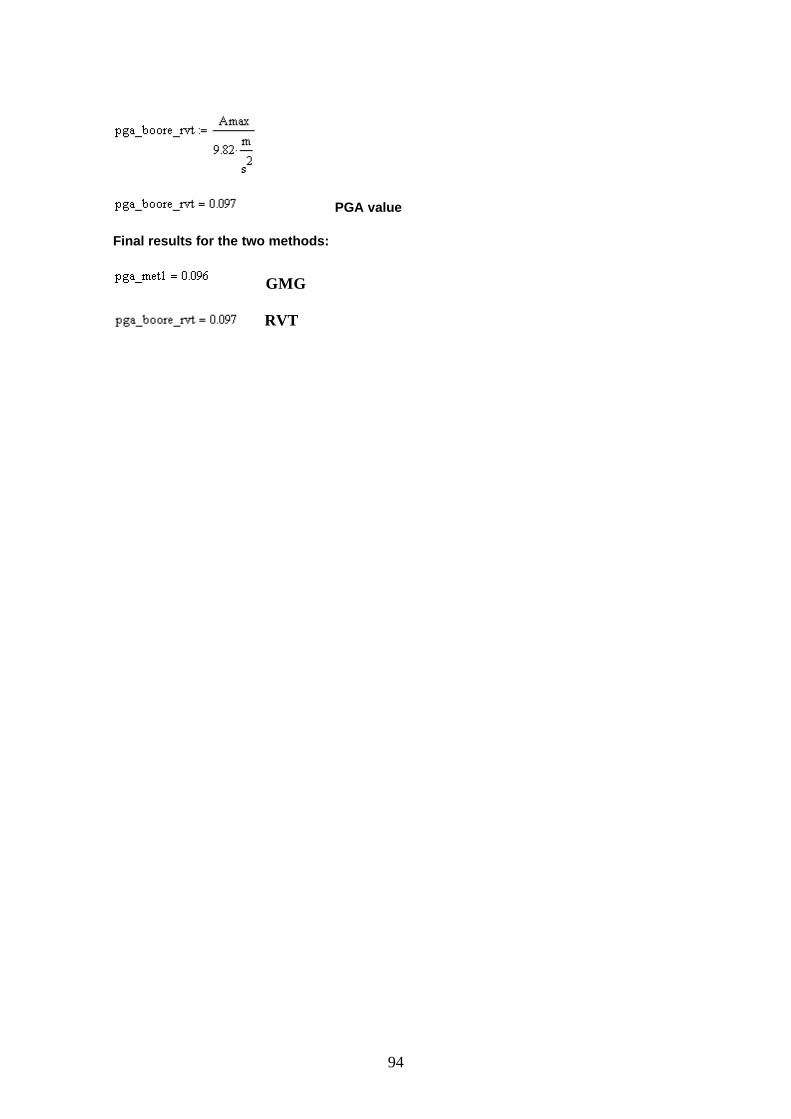
94

PGA value Final results for the two methods:

GMG RVT

95

References

Aki K., 1957. Space and Time Spectra of Stationary Stochastic Waves, with special

reference to microtremors. Bull. Earthq. Res. Inst. Tokio Univ., 25: 415-457.

Aki K and P.G Richards, 1980. Quantitative Seismology – Theory and Methods. W.H.

Freeman and company, San Francisco.

Bard, P.-Y., and M. Bouchon, 1980. The seismic response of sediment-filled valleys.

Part 1: The case of incident SH waves. Bull. seism. Soc. Am., 70, 1263-1286.

Bard, P.-Y., 1999. Microtremor measurements: a tool for site effect estimation?. In The

Effects of Surface Geology on Seismic Motion (Irikura, Kudo, Okada and Satasani eds.)

Balkerna, Rotterdam, 1999), 1251–1279.

Bettig B., Bard P.Y., Scherbaum F., Riepl J., Cotton F., Cornou C., Hatzfeld D, 2001.

Analysis of dense array noise measurements using the modified spatial autocorrelation

method (SPAC). Application to the Grenoble area. Boll. Geof. Teor. Appl., 42: 15-27.

Bianco F., Del Pezzo E., Saccorotti G., Ventura G., 2004. The role of hydrothermal

fluids in triggering the July-August 2000 seismic swarm at Campi Flegrei, Italy:

evidence from seismological and mesostructural data. Journal of Volcanology and

Geothermal Research 133, 229-246

Boatwright J., 1978. Detailed spectral analysis of two small New-York state

earthquakes. Bull. seism. Soc. Am., 68, 1117-1131.

Boatwright J., 1980. A spectral theory for circular seismic sources: simple estimates of

source dimension, dynamic stress drop and radiated energy. Bull. Seism. Soc. Am. 71,

69–94.

Boore, D.M., 2003. Simulation of Ground Motion using the Stochastic Method, Pure

Appl. Geophys., 160, 635-676.

Brune, J.N., 1970. Tectonic stress and seismic shear waves from earthquakes. J.

Geophys. Res., 75, 4997-5009.

Bruno P.P., Bais G., Chiodini G., Godio A., Costi F., 2004. Geophysical study of the

shallow hydrothermal system at Solfatara (Campi Flegrei; Italy). J. Geophys. Res.,

(submitted).

Cartwright, D.E. and Longuet-Higgins M.S.,1956. The statistical distribution of the

maxima of a random function, Proc. R. Soc. London, 237, 212-232.

96

Castro, R., M. Mucciarelli, F. Pacor, and C. Petrungaro, 1997. S-wave site response

estimates using horizontal to vertical spectral ratios. Bull. Seism. Soc. Am. 87, no. 1,

256–260.

Comune di Napoli, 1994. Indagini geologiche per l’adeguamento del P.R.G. alla legge

regionale 07.01.1983 n. 9 in difesa del territorio dal rischio sismico.

Indagini per l’applicazione della L.R. n. 9/83.

Del Pezzo E., De Nartale G., Martini M., Zollo A., 1987: Source parameters of

microearthquakes at Campi Flegrei (Southern Italy) volcanic area, Phys.Earth Planet.

Inter., 47, 25-42.

De Natale G. and Zollo A., 1986. Statistical analysis and clustering features of the

Phlegrean Fields earthquake sequence (May 1983-May 1984), Bull. Seismol. Soc. Am.,

76 (3), 801-814.

Di Vito M.A., Isaia R., Orsi G., Southon J., de Vita S., D’Antonio M., Pappalardo L.,

Piochi M., 1999. Volcanism and deformation since 12,000 years at the Campi Flegr ei

caldera (Italy). J. Volcanol. Geotherm. Res., 91: 221-246.

Dziewonski A., Bloch S., Landisman M., 1969. A technique for the analysis of transient

seismic signanals. Bull. Seism. Soc. Am., 59: 427-444.

Fäh D., Kind F., Giardini D., 2001. A theoretical investigation of average H/V ratios

Geophys. J. Int., 145, 535–549

Field, E. H., and K. H. Jacob (1993). The theoretical response of sedimentary layers to

ambient seismic noise. Geophys. Res. Lett. 20, 2925–2928.

Field, E. H., and K. H. Jacob,1995. A comparison and test of various site response

estimation techniques including three that are not reference site dependent. Bull. Seism.

Soc. Am. 85, 1127–1143.

Galluzzo D., Del Pezzo E., La Rocca M., Petrosino S., 2004. Peak ground acceleration

produced by local earthquakes in volcanic areas of Campi Flegrei and Mt. Vesuvius.

Annals of Geophysics, Vol. 47, N.4: 1377-1389.

Hasada Y, Kumagai H., Kumazawa M., 2001. Autoregressive modeling of transfer

functions in frequency domain to determine complex travel times. Earth Planets Space,

53, 3–11.

Herrin, E. and Goforth, T., 1977. Phase-matched filters: application to the study of

Rayleigh waves. Bull. Seism. Soc Am., 67: 1259-1275.

97

Herrmann R. B., 1973. Some aspects of band-pass filtering of surface waves. Bull.

Seism. Soc. Am., 63: 663-671.

Herrmann, R. B., 1987. Computer Programs in Seismology. User's manual Vol. II-IV.

St. Louis University, Missouri.

Hori, S., Y. Fukao, M. Kumazawa, M. Furumoto, Yamamoto A., 1989. A new method

of spectral analysis and its application to the Earth’s free oscillations: The “Sompi”

method, J. Geophys. Res., 94(B6), 7535–7553.

Hough S. E., Borcherdt R. D., Friberg P. A., Busby R., Field E., Jacobs K.H., 1990. The

role of sediment-induced amplification in the collapse of the Nimitz freeway during the

October 17, 1989 Loma Prieta earthquake. Nature, 344: 853-855.

Keilis-Borok V.I., 1959. On estimation of the displacement in an earthquake source

dimension, Ann. Geofis., 12, 205-214.

Konno, K. and Ohmachi, T., 1998. Ground-Motion Characteristics Estimated from

Spectral Ratio between Horizontal and Vertical Components of Microtremor. Bull.

Seism. Soc. Am., Vol. 88, No.1, 228-241.

Kramer, S.L. (1996). Geotechnical Earthquake Engineering, Prentice Hall, Inc., Upper

Saddle River, New Jersey.

Kumazawa, M., Y. Imanishi, Y. Fukao, M. Furumoto, and A. Yamamoto, 1990. A

theory of spectral analysis based on the characteristic property of a linear dynamic

system, Geophys. J. Int., 101, 613–630.

Lachet, C. and P.-Y. Bard, 1994. Numerical and theoretical investigations on the

possibilities and limitations of Nakamura’s technique. J. Phys. Earth. 42, 377–397.

Lay T. and WALLACE T.C, 1995. Modern Global Seismology. (Academic Press,

London).

Lermo, J., and F. J. Chavez-Garcia,1993. Site effects evaluation using spectral ratios

with only one station. Bull. Seism. Soc. Am. 83, no. 5, 1574–1594.

Lermo, J., and F. J. Chavez-Garcia, 1994. Are microtremors useful in site response

evaluation?. Bull. Seism. Soc. Am. 84, no. 5, 1350–1364.

Lirer L., Pescatore T.S., Corbelli V., Di Vito M., Gattullo V., Romano A., 1987.

Geologia delle aree di Monteruscello e del centro storico di Pozzuoli. Quaderno di

documentazione n.1, ed. Ministero della Protezione Civile, Napoli.

98

Louie J. N., 2001. Faster, better: Shear–wave velocity to 100 meters depth from

refraction microtremor arrays. Bull. Seism. Soc. Am., 91: 347-364.

Luzon F., Al Yuncha Z., Sanchez-Sesma F.J., Ortiz-Aleman C., 2001. A Numerical

Experiment on the Horizontal to Vertical Spectral Ratio in Flat Sedimentary Basins.

Pure Appl. Geophys., 158: 2451-2461.

Malagnini L., Herrmann R.B., Biella G., de Franco R., 1995. Rayleigh waves in

Quaternary alluvium from esplosive sources: determination of shear-wave velocity and

Q structure. Bull. Seism. Soc. Am., 85: 900-922.

Malagnini L., 1996. Velocity and attenuation structure of very shallow soils: evidence

for a frequency dependent Q. Bull. Seism. Soc. Am., 86, 1471-1486.

Malagnini L., Tricarico P., Rovelli A., Herrmann R.B., Opice S., Biella G., de Franco

R., 1996. Explosion, Earthquake, and Ambient Noise Recordings in a Pliocene

Sediment-Filled Valley: Inferences on Seismic Response Properties by Reference- and

Non-Reference-Site Techniques. Bull. Seism. Soc. Am., 86: 670-682.

Malagnini, L., R. B. Herman, A. Mercuri, S. Opice, G. Biella, and R. de Franco, 1997.

Shear-wave velocity structure of sediments from the inversion of explosion-induced

Rayleigh waves: comparison with cross hole measurements, Bull. Seism. Soc. Am. 87,

1413–1421.

Malischewsky P. G. and Scherbaum F., 2004. Love’s formula and H/V-ratio (ellipticity)

of Rayleigh waves). Wave Motion, 40: 57-67.

Matsuura, T., Y. Imanishi, M. Imanari, and M. Kumazawa, 1990. Application of a new

method of high-resolution spectral analysis, “Sompi,” for free induction decay of

nuclear magnetic resonance, Appl. Spectrosc., 44, 618–626.

Margheriti L., Azzara R. M., Cocco M., Delladio A., and Nardi A., 2000. Analysis of

Borehole Broadband Recordings: Test Site in the Po Basin, Northern Italy. Bull. Seism.

Soc. Am. 90, 1454–1463.

Menke W., 1984. Geophysical data analysis: discrete inverse theory. Academic Press,

inc., USA.

Midzi V., 2001. 3-D surface wave group velocity distribution in Central-Southern

Africa. J. Seismology, 5: 559-574.

99

Nakamura Y., 1989. A Method for Dynamic Characteristics Estimation of Subsurface

Using Microtremor on the Ground Surface. Q. Rept. Railway Tech. Res. Inst., 30,1: 25-

33.

Nakamura, Y., 1996. Real Time Information Systems for Seismic Hazards Mitigation

UrEDAS, HERAS and PIC. Quarterly Report of RTRI, Vol. 37, No. 3, 112-127.

Nogoshi, M. and Igarashi, T., 1971. On the Amplitude Characteristics of Microtremor

(Part 2) (in Japanese with English abstract). Jour. Seism. Soc. Japan, 24, 26-40.

Nunziata C., Mele R., Natale M., 1999. Shear wave velocities and primary influencing

factors of Campi Flegrei-Neapolitan deposits. Engineering Geology, 54: 299-312.

Orsi G., De Vita S., Di Vito M.A., 1996. The restless resurgent Campi Flegrei nested

caldera (Italy): constraints on its evolution and configuration. J. Volcanol. Geotherm.

Res., 74: 179-214.

Orsi, G., Civetta, L., Del Gaudio, C., De Vita, S., Di Vito, M., Isaia, R., Petrazzuoli,

S.M., Ricciardi, G.P., Ricco, C., 1999. Short term ground deformations and seismicity

in

the resurgent Campi Flegrei caldera (Italy): An example of active block-resurgence in a

densely populated area. J. Volcanol. Geotherm. Res. 91, 415-451.

Orsi G., de Vita S., Di Vito M., Isaia R., Nave R., Heiken G., 2003. Facing volcanic and

related hazards in the Neapolitan area. In: Heiken G., Fakundiny R, Sutter J. (Eds)

“Earth Sciences in Cities”, American Geophysical Union book, Washington, 56, 121-

170.

Petrosino S., Cusano P., Saccorotti G., Del Pezzo E.; 2002. Seismic attenuation and

shallow velocity structures at Stromboli Volcano, Italy; Bulletin of the Seismological

Society of America, Vol 92, N. 3: 1102-1116.

Satoh T., Kawase H., Matsushima S, 2001. Differences Between Site Characteristics

Obtained From Microtremors, S-waves, P-waves, and Codas.Bull. Seism. Soc. Am., 91:

313-334.

Sholz C., 1968. The frequency-magnitude relation of microfracturingin rock and its

relation to earthquakes.Bull. Seismol. Soc. Am., 58, 399-415.

Seekins L.C., Wennerberg L., Margheriti L., Liu H.-P., 1996. Site Amplification at Five

Locations in San Francisco, California: A Comparison of S Waves, Codas and

Microtremors. Bull. Seism. Soc. Am., 86: 627-635.

100

Slejko D., Peruzza L., Rebez A., 1998. Seismic hazard maps of Italy. Ann. Geofis.,

41(2), 183-214

Vanorio T., Virieux J., Zollo A., Capuano P., Russo G., 2005. 3-D Seismic Tomography

from P- and S- Microearthquake Traveltimes and Rock Physics Characterization in the

Campi Flegrei Caldera. J. Geophys. Res., 110, B03201, doi:10.1029/2004JB003102

Vilardo, G., Alessio, G., Luongo, G., 1991. Analysis of the magnitude-frequency

distribution for the 1983-1984 earthquake activity of Campi Flegrei, Italy. J. Volcanol.

Geotherm.

Res. 48, 115-125.

Zollo A., Judenherc S., Auger E., D’Auria L., Virieux J., Capuano P., Chiarabba C., de

Franco R., Makris J., Michelini A., Musacchio G., 2003. Evidence for the bouried rim

of Campi Flegrei caldera from 3-d active seismic imaging. Geophys. Res. Lett., 30(19),

2002, doi:10.1029/2003GL018173.